www.elsevier.com/locate/ynimg

NeuroImage 37 (2007) 1227–1236

Signal and noise characteristics of SSFP FMRI: A comparisonwith GRE at multiple field strengths

Karla L. Miller,a,⁎ Stephen M. Smith,a Peter Jezzard,a

Graham C. Wiggins,b and Christopher J. Wigginsb

aCentre for Functional MRI of the Brain (FMRIB), University of Oxford, Oxford, UKbA.A. Martinos Center, Massachusetts General Hospital, Charlestown, MA, USA

Received 22 April 2007; revised 4 June 2007; accepted 6 June 2007Available online 10 July 2007

Recent work has proposed the use of steady-state free precession(SSFP) as an alternative to the conventional methods for obtainingfunctional MRI (FMRI) data. The contrast mechanism in SSFP is likelyto be related to conventional FMRI signals, but the details of the signalchanges may differ in important ways. Functional contrast in SSFP hasbeen proposed to result from several different mechanisms, which arelikely to contribute in varying degrees depending on the specificparameters used in the experiment. In particular, the signal dynamicsare likely to differ depending on whether the sequence is configured toscan in the SSFP transition band or passband. This work describesexperiments that explore the source of SSFP FMRI signal changes bycomparing SSFP data to conventional gradient-recalled echo (GRE)data. Data were acquired at a range of magnetic field strengths andrepetition times, for both transition band and passband methods. Thesignal properties of SSFP and GRE differ significantly, confirming adifferent source of functional contrast in SSFP. In addition, thetemporal noise properties are significantly different, with importantimplications for SSFP FMRI sequence optimisation.© 2007 Elsevier Inc. All rights reserved.

Introduction

Most functional MRI (FMRI) data are acquired using gradient-recalled echo (GRE) pulse sequences with single-shot echo planarimaging (EPI) acquisitions. This method uses a long echo time (TE)to sensitise the sequence to blood oxygenation level dependent(BOLD) signal changes and single-shot EPI to obtain reasonabletemporal resolution. While highly efficient, GRE-EPI suffers fromsignal dropout due to long TE and heavy image distortion due tothe long, single-shot readout. These artefacts limit the achievableresolution and effectively preclude imaging in certain regions ofthe brain (e.g., prefrontal lobe).

⁎ Corresponding author. FMRIB Centre, John Radcliffe Hospital,Headington, Oxford, OX3 9DU, UK. Fax: +44 1865 222717.

E-mail address: karla@fmrib.ox.ac.uk (K.L. Miller).Available online on ScienceDirect (www.sciencedirect.com).

1053-8119/$ - see front matter © 2007 Elsevier Inc. All rights reserved.doi:10.1016/j.neuroimage.2007.06.024

Balanced steady-state free precession (SSFP) is a pulsesequence that combines short readout durations with fast andefficient imaging, properties that are desirable in FMRI. Severalrecent studies have demonstrated the ability to obtain functionalcontrast with SSFP (Scheffler et al., 2001; Miller et al., 2003;Bowen et al., 2005). These methods are able to obtain BOLD-likefunctional contrast at short TE and use rapid multi-shot readoutswith a short repetition time (TR). These methods should thereforebe relatively immune to the image distortion and signal dropoutfound in single-shot GRE-EPI.

Although previous work has demonstrated the ability to acquireFMRI contrast with SSFP, the signal characteristics, including thesource of contrast, have not been carefully studied. Several sourcesof contrast have been proposed depending on the details of theSSFP acquisition, including direct detection of the BOLDfrequency modulations (Scheffler et al., 2001; Miller et al., 2003),diffusion in the extravascular space (Bowen et al., 2006) and T2

*

effects at long TR (Zhong et al., 2007). Because the SSFP signal hasa fairly complicated dependence on all these effects, they are alllikely to contribute to varying degrees depending on the details ofthe SSFP acquisition; however, no detailed characterisation haspreviously been performed to study these affects.

In addition to potential sources of functional contrast in SSFP,noise characteristics are also important for pragmatic reasons. It haspreviously been established that sources of temporal frequency drift(e.g., from respiration (Lee et al., 2006) or gradient heating (Miller etal., 2006; Wu et al., 2007)) can introduce significant temporalinstability. Although methods for reducing these drifts using real-time feedback have been suggested (Lee et al., 2006;Wu et al.,2007), no detailed characterisation of the noise has previously beenreported.

In this work, we attempt to clarify some of these issues bycharacterising the functional contrast and temporal noise in SSFPFMRI. This characterisation is primarily based on matched SSFPand GRE experiments, which use the well-studied GRE signal as areference for T2

* BOLD signal. We also compare the noise sensi-tivity of the different methods by fitting a model for physiologicalnoise in FMRI (Krüger and Glover, 2001) to the experimental data.

1228 K.L. Miller et al. / NeuroImage 37 (2007) 1227–1236

Theory

FMRI with Balanced SSFP

Balanced SSFP has two defining characteristics. First, use of ashort TR (TRbT2) causes the transverse magnetisation to persist overmultiple repetition periods. Second, all gradient waveforms havezero total area over the TR, such that any phase accumulated duringthe TR is purely due to off-resonance precession. The combinedeffect of these properties is that the resultant steady-state signal has astrong dependence on the relationship between the signal phase (dueto off-resonance precession) and the RF excitation phase (which istypically incremented from one excitation to the next).

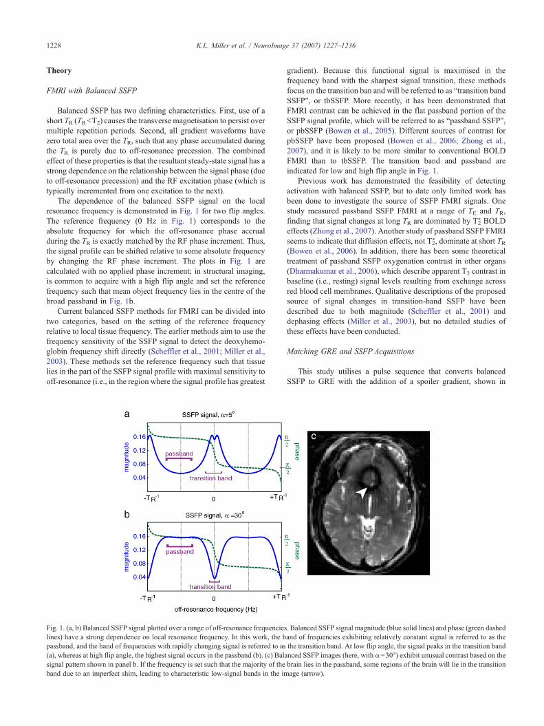
The dependence of the balanced SSFP signal on the localresonance frequency is demonstrated in Fig. 1 for two flip angles.The reference frequency (0 Hz in Fig. 1) corresponds to theabsolute frequency for which the off-resonance phase accrualduring the TR is exactly matched by the RF phase increment. Thus,the signal profile can be shifted relative to some absolute frequencyby changing the RF phase increment. The plots in Fig. 1 arecalculated with no applied phase increment; in structural imaging,is common to acquire with a high flip angle and set the referencefrequency such that mean object frequency lies in the centre of thebroad passband in Fig. 1b.

Current balanced SSFP methods for FMRI can be divided intotwo categories, based on the setting of the reference frequencyrelative to local tissue frequency. The earlier methods aim to use thefrequency sensitivity of the SSFP signal to detect the deoxyhemo-globin frequency shift directly (Scheffler et al., 2001; Miller et al.,2003). These methods set the reference frequency such that tissuelies in the part of the SSFP signal profile with maximal sensitivity tooff-resonance (i.e., in the region where the signal profile has greatest

Fig. 1. (a, b) Balanced SSFP signal plotted over a range of off-resonance frequencieslines) have a strong dependence on local resonance frequency. In this work, the bpassband, and the band of frequencies with rapidly changing signal is referred to as(a), whereas at high flip angle, the highest signal occurs in the passband (b). (c) Balasignal pattern shown in panel b. If the frequency is set such that the majority of theband due to an imperfect shim, leading to characteristic low-signal bands in the im

gradient). Because this functional signal is maximised in thefrequency band with the sharpest signal transition, these methodsfocus on the transition ban and will be referred to as “transition bandSSFP”, or tbSSFP. More recently, it has been demonstrated thatFMRI contrast can be achieved in the flat passband portion of theSSFP signal profile, which will be referred to as “passband SSFP”,or pbSSFP (Bowen et al., 2005). Different sources of contrast forpbSSFP have been proposed (Bowen et al., 2006; Zhong et al.,2007), and it is likely to be more similar to conventional BOLDFMRI than to tbSSFP. The transition band and passband areindicated for low and high flip angle in Fig. 1.

Previous work has demonstrated the feasibility of detectingactivation with balanced SSFP, but to date only limited work hasbeen done to investigate the source of SSFP FMRI signals. Onestudy measured passband SSFP FMRI at a range of TE and TR,finding that signal changes at long TR are dominated by T2

* BOLDeffects (Zhong et al., 2007). Another study of passband SSFP FMRIseems to indicate that diffusion effects, not T2

*, dominate at short TR(Bowen et al., 2006). In addition, there has been some theoreticaltreatment of passband SSFP oxygenation contrast in other organs(Dharmakumar et al., 2006), which describe apparent T2 contrast inbaseline (i.e., resting) signal levels resulting from exchange acrossred blood cell membranes. Qualitative descriptions of the proposedsource of signal changes in transition-band SSFP have beendescribed due to both magnitude (Scheffler et al., 2001) anddephasing effects (Miller et al., 2003), but no detailed studies ofthese effects have been conducted.

Matching GRE and SSFP Acquisitions

This study utilises a pulse sequence that converts balancedSSFP to GRE with the addition of a spoiler gradient, shown in

. Balanced SSFP signal magnitude (blue solid lines) and phase (green dashedand of frequencies exhibiting relatively constant signal is referred to as thethe transition band. At low flip angle, the signal peaks in the transition bandnced SSFP images (here, with α=30°) exhibit unusual contrast based on thebrain lies in the passband, some regions of the brain will lie in the transitionage (arrow).

1229K.L. Miller et al. / NeuroImage 37 (2007) 1227–1236

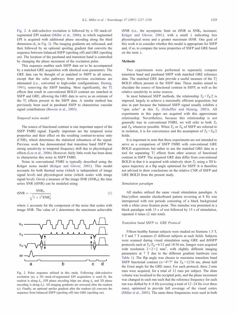
Fig. 2. A slab-selective excitation is followed by a 3D stack-of-segmented EPI readout (Miller et al., 2006), in which segmentedEPI is acquired with additional phase encoding along the thirddimension (kz in Fig. 2). The imaging gradients are refocused, andthen followed by an optional spoiling gradient that converts thesequence between balanced SSFP (spoiling off) and GRE (spoilingon). The location of the passband and transition band is controlledby changing the phase increment of the excitation pulse.

This sequence enables each SSFP data set to be accompaniedby a matched GRE acquisition with identical scan parameters. TheGRE data can be thought of as matched to SSFP in all senses,except that the echo pathways from previous excitations areattenuated (i.e., converted to high-order configurations; Hennig,1991), removing the SSFP banding. Most significantly, the T2

*

effects that result in conventional BOLD contrast are matched inSSFP and GRE, allowing the GRE data to serve as an estimate ofthe T2

* effects present in the SSFP data. A similar method haspreviously been used in passband SSFP to characterise vascularsignal contributions (Bowen et al., 2005).

Temporal noise model

The source of functional contrast is one important aspect of theSSFP FMRI signal. Equally important are the temporal noiseproperties and their effect on the resulting contrast-to-noise ratio(CNR), which determines the statistical robustness of the signal.Previous work has demonstrated that transition band SSFP hasstrong sensitivity to temporal frequency drift due to physiologicaleffects (Lee et al., 2006). However, fairly little work has been doneto characterise this noise in SSFP FMRI.

Noise in conventional FMRI is typically described using theKrüger noise model (Krüger and Glover, 2001). This modelaccounts for both thermal noise (which is independent of imagesignal level) and physiological noise (which scales with imagesignal level). Given a measure of the image SNR (SNR0), the timeseries SNR (tSNR) can be modeled using:

tSNR ¼ SNR0ffiffiffiffiffiffiffiffiffiffiffiffiffiffiffiffiffiffiffiffiffiffiffiffi1þ k2SNR2

0

q ð1Þ

where λ accounts for the component of the noise that scales withimage SNR. The value of λ determines the maximum achievable

Fig. 2. Pulse sequence utilised in this study. Following slab-selectiveexcitation (a), a 3D stack-of-segmented EPI acquisition is used (b, thereadout is along kx, EPI phase encoding blips are along ky and 3D phaseencoding is along kz). All imaging gradients are rewound after the readout(c). Finally, an optional spoiler gradient after the readout (d) converts thesequence from balanced SSFP (spoiling off) into GRE (spoiling on).

tSNR (i.e., the asymptotic limit on tSNR as SNR0 increases;Krüger and Glover, 2001), with a small λ indicating lessphysiological noise and a greater maximum tSNR. One goal ofthis work is to consider whether this model is appropriate for SSFPand, if so, to compare the noise properties of SSFP and GRE basedon the term λ.

Methods

Two experiments were performed to separately comparetransition band and passband SSFP with matched GRE referencedata. The matched GRE data provide a useful measure of the T2

*

BOLD effects present in the SSFP data. These studies aimed toelucidate the source of functional contrast in SSFP, as well as therelative sensitivity to noise sources.

In most balanced SSFP methods, the relationship TE=TR/2 isimposed, largely to achieve a maximally efficient acquisition, butalso in part because the balanced SSFP signal usually exhibits a“spin echo” at this TE (Scheffler and Hennig, 2003). Allexperiments in this paper are acquired with this approximaterelationship. Nevertheless, because this relationship is notgenerally true in conventional FMRI, we will refer to both TEand TR whenever possible. When TE or TR of SSFP are referred toin isolation, it is for convenience and the assumption of TE=TR/2holds.

It is important to note that these experiments are not intended toserve as a comparison of SSFP FMRI with conventional GREBOLD acquisitions but rather to use the matched GRE data as atool for separating T2

* effects from other sources of functionalcontrast in SSFP. The acquired GRE data differ from conventionalBOLD in that it is acquired with relatively short TE using a 3D k-space trajectory at a flip angle optimised for SSFP. It is thereforenot advised to draw conclusions on the relative CNR of SSFP andGRE BOLD from the present study.

Stimulation paradigm

All studies utilised the same visual stimulation paradigm. Ablue/yellow annular checkerboard pattern reversing at 8 Hz wasinterspersed with rest periods consisting of a black backgroundwith a white cross fixation point. This stimulus was presented in ablock paradigm with 15 s of rest followed by 15 s of stimulation,repeated 4 times (2 min total).

Transition band SSFP vs. GRE Protocol

Fifteen healthy human subjects were studied on Siemens 1.5 T,3 T and 7 T scanners (5 different subjects at each field). Subjectswere scanned during visual stimulation using GRE and tbSSFPprotocols each at TE/TR=6/12 and 18/36 ms. Images were acquiredwith resolution 2×2×2 mm3, with slightly different imagingparameters at 7 T due to the different gradient hardware (seeTable 1). The flip angle was chosen to maximise transition bandSSFP functional contrast (α=4°/7° for TR=12/36 ms, about halfthe Ernst angle for the GRE runs). For each protocol, three 2-minruns were acquired, for a total of 12 runs per subject. The shimvolume was localised to the occipital pole, and the phase incrementwas changed in each run such that the reference frequency for eachrun was shifted by 4–6 Hz (covering a total of 12–24 Hz over threeruns), optimised to provide full coverage of the visual cortex(Miller et al., 2003). The same three frequencies were used in both

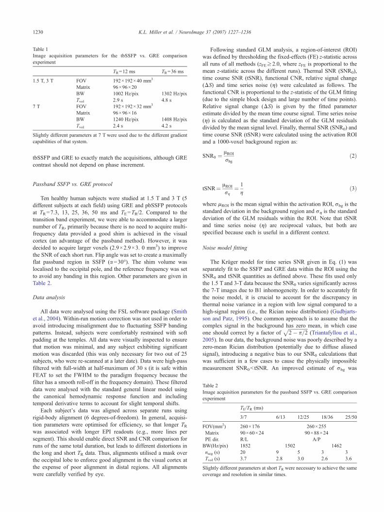
Table 1Image acquisition parameters for the tbSSFP vs. GRE comparisonexperiment

TR=12 ms TR=36 ms

1.5 T, 3 T FOV 192×192×40 mm3

Matrix 96×96×20BW 1002 Hz/pix 1302 Hz/pixTvol 2.9 s 4.8 s

7 T FOV 192×192×32 mm3

Matrix 96×96×16BW 1240 Hz/pix 1408 Hz/pixTvol 2.4 s 4.2 s

Slightly different parameters at 7 T were used due to the different gradientcapabilities of that system.

1230 K.L. Miller et al. / NeuroImage 37 (2007) 1227–1236

tbSSFP and GRE to exactly match the acquisitions, although GREcontrast should not depend on phase increment.

Table 2Image acquisition parameters for the passband SSFP vs. GRE comparisonexperiment

TE/TR (ms)

3/7 6/13 12/25 18/36 25/50

FOV(mm2) 260×176 260×255Matrix 90×60×24 90×88×24PE dir. R/L A/P

BW(Hz/pix) 1852 1502 1462nseg (s) 20 9 5 3 3Tvol (s) 3.7 2.8 3.0 2.6 3.6

Slightly different parameters at short TR were necessary to achieve the samecoverage and resolution in similar times.

Passband SSFP vs. GRE protocol

Ten healthy human subjects were studied at 1.5 T and 3 T (5different subjects at each field) using GRE and pbSSFP protocolsat TR=7.3, 13, 25, 36, 50 ms and TE=TR/2. Compared to thetransition band experiment, we were able to accommodate a largernumber of TR, primarily because there is no need to acquire multi-frequency data provided a good shim is achieved in the visualcortex (an advantage of the passband method). However, it wasdecided to acquire larger voxels (2.9×2.9×3. 0 mm3) to improvethe SNR of each short run. Flip angle was set to create a maximallyflat passband region in SSFP (α=30°). The shim volume waslocalised to the occipital pole, and the reference frequency was setto avoid any banding in this region. Other parameters are given inTable 2.

Data analysis

All data were analysed using the FSL software package (Smithet al., 2004). Within-run motion correction was not used in order toavoid introducing misalignment due to fluctuating SSFP bandingpatterns. Instead, subjects were comfortably restrained with softpadding at the temples. All data were visually inspected to ensurethat motion was minimal, and any subject exhibiting significantmotion was discarded (this was only necessary for two out of 25subjects, who were re-scanned at a later date). Data were high-passfiltered with full-width at half-maximum of 30 s (it is safe withinFEAT to set the FWHM to the paradigm frequency because thefilter has a smooth roll-off in the frequency domain). These filtereddata were analysed with the standard general linear model usingthe canonical hemodynamic response function and includingtemporal derivative terms to account for slight temporal shifts.

Each subject's data was aligned across separate runs usingrigid-body alignment (6 degrees-of-freedom). In general, acquisi-tion parameters were optimised for efficiency, so that longer TRwas associated with longer EPI readouts (e.g., more lines persegment). This should enable direct SNR and CNR comparison forruns of the same total duration, but leads to different distortions inthe long and short TR data. Thus, alignments utilised a mask overthe occipital lobe to enforce good alignment in the visual cortex atthe expense of poor alignment in distal regions. All alignmentswere carefully verified by eye.

Following standard GLM analysis, a region-of-interest (ROI)was defined by thresholding the fixed-effects (FE) z-statistic acrossall runs of all methods (zFE≥2.0, where zFE is proportional to themean z-statistic across the different runs). Thermal SNR (SNR0),time course SNR (tSNR), functional CNR, relative signal change(ΔS) and time series noise (η) were calculated as follows. Thefunctional CNR is proportional to the z-statistic of the GLM fitting(due to the simple block design and large number of time points).Relative signal change (ΔS) is given by the fitted parameterestimate divided by the mean time course signal. Time series noise(η) is calculated as the standard deviation of the GLM residualsdivided by the mean signal level. Finally, thermal SNR (SNR0) andtime course SNR (tSNR) were calculated using the activation ROIand a 1000-voxel background region as:

SNR0 ¼ AROIrbg

ð2Þ

tSNR¼ AROIrg

¼ 1g

ð3Þ

where μROI is the mean signal within the activation ROI, σbg is thestandard deviation in the background region and ση is the standarddeviation of the GLM residuals within the ROI. Note that tSNRand time series noise (η) are reciprocal values, but both arespecified because each is useful in a different context.

Noise model fitting

The Krüger model for time series SNR given in Eq. (1) wasseparately fit to the SSFP and GRE data within the ROI using theSNR0 and tSNR quantities as defined above. These fits used onlythe 1.5 T and 3-T data because the SNR0 varies significantly acrossthe 7-T images due to B1 inhomogeneity. In order to accurately fitthe noise model, it is crucial to account for the discrepancy inthermal noise variance in a region with low signal compared to ahigh-signal region (i.e., the Rician noise distribution) (Gudbjarts-son and Patz, 1995). One common approach is to assume that thecomplex signal in the background has zero mean, in which caseone should correct by a factor of

ffiffiffiffiffiffiffiffiffiffiffiffiffiffiffiffi2� p=2

p(Triantafyllou et al.,

2005). In our data, the background noise was poorly described by azero-mean Rician distribution (potentially due to diffuse aliasedsignal), introducing a negative bias to our SNR0 calculations thatwas sufficient in a few cases to cause the physically impossiblemeasurement SNR0b tSNR. An improved estimate of σbg was

1231K.L. Miller et al. / NeuroImage 37 (2007) 1227–1236

obtained by fitting the background noise histogram to a Riciandistribution with non-zero mean. Non-linear fits were performed inMatlab (using the nlinfit function) and were found to have anacceptable confidence interval (typically 5–10%, although occa-sionally as high as 30%).

Results

Transition band SSFP vs. GRE

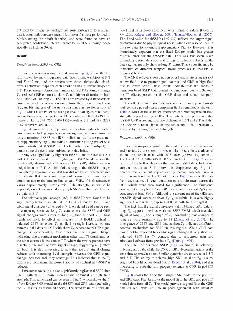
Example activation maps are shown in Fig. 3, where the toprow shows the multi-frequency data from a single subject at 3 Tand TR=12 ms, and the bottom row shows thresholded fixed-effects activation maps for each condition in a different subject at3 T. These images demonstrate increased SSFP banding at longerTR, reduced GRE contrast at short TR and higher distortion in bothSSFP and GRE at long TR. The ROIs are created by a fixed-effectscombination of the activation maps from the different conditions(i.e., an FE analysis of the activation maps in the lower row ofFig. 3, which is equivalent to a single-level FE analysis of all data).Across the different subjects, the ROIs contained 18–134 (39±37)voxels at 1.5 T, 294–767 (560±183) voxels at 3 T and 436–2233(1183±659) voxels at 7 T.

Fig. 4 presents a group analysis pooling subjects withinconditions including significance testing (subject-wise paired t-tests comparing tbSSFP vs. GRE). Individual results are presentedas Supplementary Fig. 9, including significance testing (voxel-wisepaired t-tests of tbSSFP vs. GRE within each subject) todemonstrate the good inter-subject reproducibility.

SNR0 was significantly higher in tbSSFP than in GRE at 1.5 Tand 3 T, as expected in the high-signal SSFP bands where thefunctionally determined ROI occurs. This SNR0 difference wasinsignificant at 7 T. At this field strength, the tbSSFP imagesqualitatively appeared to exhibit less-distinct bands, which seemedto indicate that the signal was not forming a robust SSFPcondition due to the broader line spread. SNR0 of both sequencesvaries approximately linearly with field strength, as would beexpected, except for anomalously high SNR0 in the tbSSFP shortTR data at 3 T.

The relative signal change (ΔS) in tbSSFP was found to besignificantly higher than GRE at 1.5 T and 3 T, but the tbSSFP andGRE signal changes converged at 7 T. A related trend can be seenin comparing short vs. long TR data, where the SSFP and GREsignal changes were closer at long TR than at short TR. Thesetrends are likely to reflect an increase in T2

* BOLD contrast inbalanced SSFP as either TE or field strength increase. At oneextreme is the data at 1.5 T with short TR, where the tbSSFP signalchange is approximately four times the GRE signal change,indicating that a contrast mechanism other than T2

* dominates. Atthe other extreme is the data at 7 T, where the two sequences haveessentially the same relative signal change, suggesting a T2

* effectfor both. It is also interesting to note that tbSSFP signal changereduces with increasing field strength, whereas the GRE signalchange increases until they converge. This indicates that as the T2

*

effects are increasing, the non-T2* source of contrast in tbSSFP is

reduced.Time series noise (η) is also significantly higher in tbSSFP than

GRE, with tbSSFP noise increasingly dominant at high fieldstrength. This same trend can be seen in Fig. 5, which shows the fitof the Krüger SNR model to the tbSSFP and GRE data (excludingthe 7-T results, as discussed above). The fitted value of λ for GRE

(λ=1.1%) is in good agreement with literature values (typicallyλ=1.2%; Krüger and Glover, 2001; Triantafyllou et al., 2005).The fitted value for tbSSFP (λ=2.4%) reflects the larger signalfluctuations due to physiological noise (which can also be seen inthe raw data, for example Supplementary Fig. 9). However, it isimmediately apparent that the fitted Krüger model has greaterresidual error for the tbSSFP data. This was true even whendiscarding outlier data sets and fitting to reduced subsets of thedata (e.g., using only short or long TR data). These poor fits may beindicative of different temporal noise processes in tbSSFP, asdiscussed below.

The CNR reflects a combination of ΔS and η, favoring tbSSFPat low field due to greater signal contrast and GRE at high fielddue to lower noise. These results indicate that the bands intransition band SSFP both contribute functional contrast (beyondthe T2

* effects present in the GRE data) and reduce temporalstability.

The effect of field strength was assessed using paired t-tests(subject-wise paired t-tests comparing field strengths), as shown inTable 3. Most of the statistical measures exhibited significant fieldstrength dependence (pb0.05). The notable exceptions are thattbSSFP CNR is not significantly different at 1.5 T and 3 T, and thatthe tbSSFP percent signal change tends not to be significantlyaffected by a change in field strength.

Passband SSFP vs. GRE

Example images acquired with passband SSFP at the longestand shortest TR are shown in Fig. 6. The fixed-effects analysis ofall data resulted in ROIs with 1628–3603 (2559±943) voxels at1.5 T and 3710–5404 (4504±890) voxels at 3 T. Fig. 7 showsresults of the ROI analysis on the passband SSFP data. Individualsubject results at 3 T, shown in Supplementary Fig. 10,demonstrate excellent reproducibility across subjects (similarresults were found at 1.5 T, not shown). Fig. 7 reduces the datafrom each subject in each condition to a single mean across theROI, which were then tested for significance. The functionalcontrast (ΔS) for pbSSFP and GRE is different for short TE/TR andconverges at long TE/TR. Although the divergence of the GRE andpbSSFP signal curves at short TE/TR is subtle, it is also highlysignificant across the group (pb0.001 at both field strengths).

The fact that the signal converges with T2*-based GRE data at

long TR supports previous work on SSFP FMRI which modeledsignal at long TR and a range of TE, concluding that changes atlong TR were primarily due to T2

* (Zhong et al., 2007). Thedivergence of SSFP and GRE data at short TR indicates a differentcontrast mechanism for SSFP in this regime. While GRE datawould not be expected to exhibit signal changes at very short TE,balanced SSFP has T2 contrast due to refocused spin andstimulated echoes from previous TR (Hennig, 1991).

The CNR of passband SSFP (Figs. 7a and c) is relativelyindependent of TE, while the CNR of GRE decreases rapidly as theecho time approaches zero. Similar dynamics are observed at 1.5 Tand 3 T. The ability to achieve high SNR at short TR is a re-cognised benefit of passband SSFP (Reeder et al., 2004), and it isinteresting to note that this property extends to CNR in pbSSFPFMRI.

Fig. 8 shows the fit of the Krüger SNR model to the pbSSFPand GRE data. Fig. 8a shows the model fit to the GRE and pbSSFPpooled data from all TR. The model provides a good fit to the GREdata (in red), with λ=1.0% in good agreement with literature

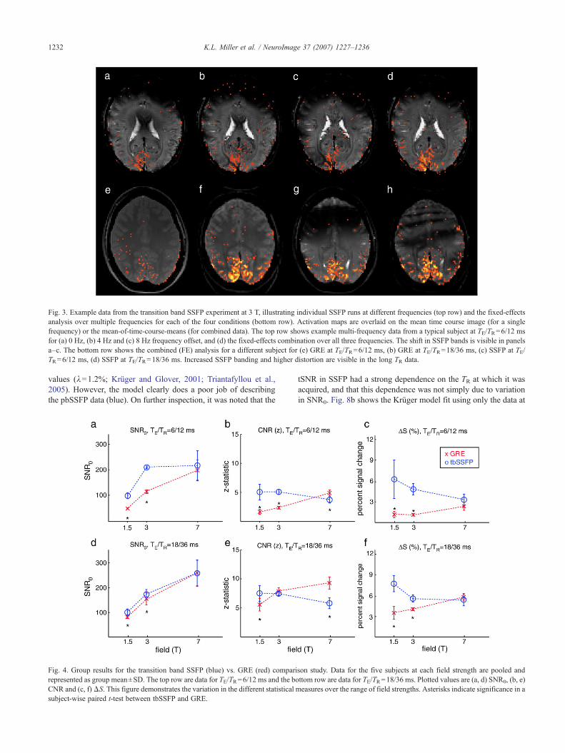
Fig. 3. Example data from the transition band SSFP experiment at 3 T, illustrating individual SSFP runs at different frequencies (top row) and the fixed-effectsanalysis over multiple frequencies for each of the four conditions (bottom row). Activation maps are overlaid on the mean time course image (for a singlefrequency) or the mean-of-time-course-means (for combined data). The top row shows example multi-frequency data from a typical subject at TE/TR=6/12 msfor (a) 0 Hz, (b) 4 Hz and (c) 8 Hz frequency offset, and (d) the fixed-effects combination over all three frequencies. The shift in SSFP bands is visible in panelsa–c. The bottom row shows the combined (FE) analysis for a different subject for (e) GRE at TE/TR=6/12 ms, (b) GRE at TE/TR=18/36 ms, (c) SSFP at TE/TR=6/12 ms, (d) SSFP at TE/TR=18/36 ms. Increased SSFP banding and higher distortion are visible in the long TR data.

1232 K.L. Miller et al. / NeuroImage 37 (2007) 1227–1236

values (λ=1.2%; Krüger and Glover, 2001; Triantafyllou et al.,2005). However, the model clearly does a poor job of describingthe pbSSFP data (blue). On further inspection, it was noted that the

Fig. 4. Group results for the transition band SSFP (blue) vs. GRE (red) comparirepresented as group mean±SD. The top row are data for TE/TR=6/12 ms and the boCNR and (c, f)ΔS. This figure demonstrates the variation in the different statisticalsubject-wise paired t-test between tbSSFP and GRE.

tSNR in SSFP had a strong dependence on the TR at which it wasacquired, and that this dependence was not simply due to variationin SNR0. Fig. 8b shows the Krüger model fit using only the data at

son study. Data for the five subjects at each field strength are pooled andttom row are data for TE/TR=18/36 ms. Plotted values are (a, d) SNR0, (b, e)measures over the range of field strengths. Asterisks indicate significance in a

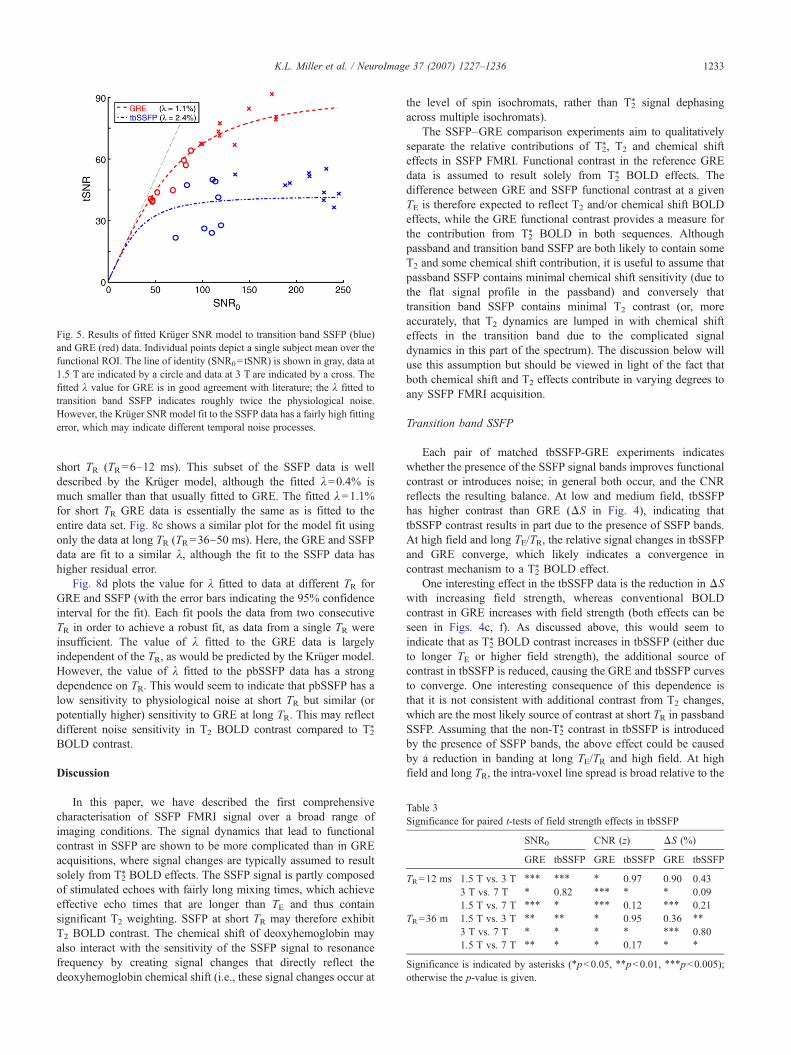
Fig. 5. Results of fitted Krüger SNR model to transition band SSFP (blue)and GRE (red) data. Individual points depict a single subject mean over thefunctional ROI. The line of identity (SNR0= tSNR) is shown in gray, data at1.5 T are indicated by a circle and data at 3 T are indicated by a cross. Thefitted λ value for GRE is in good agreement with literature; the λ fitted totransition band SSFP indicates roughly twice the physiological noise.However, the Krüger SNR model fit to the SSFP data has a fairly high fittingerror, which may indicate different temporal noise processes.

Table 3Significance for paired t-tests of field strength effects in tbSSFP

SNR0 CNR (z) ΔS (%)

GRE tbSSFP GRE tbSSFP GRE tbSSFP

TR=12 ms 1.5 T vs. 3 T ⁎⁎⁎ ⁎⁎⁎ ⁎ 0.97 0.90 0.433 T vs. 7 T ⁎ 0.82 ⁎⁎⁎ ⁎ ⁎ 0.091.5 T vs. 7 T ⁎⁎⁎ ⁎ ⁎⁎⁎ 0.12 ⁎⁎⁎ 0.21

TR=36 m 1.5 T vs. 3 T ⁎⁎ ⁎⁎ ⁎ 0.95 0.36 ⁎⁎

3 T vs. 7 T ⁎ ⁎ ⁎ ⁎ ⁎⁎⁎ 0.801.5 T vs. 7 T ⁎⁎ ⁎ ⁎ 0.17 ⁎ ⁎

Significance is indicated by asterisks (⁎pb0.05, ⁎⁎pb0.01, ⁎⁎⁎pb0.005);otherwise the p-value is given.

1233K.L. Miller et al. / NeuroImage 37 (2007) 1227–1236

short TR (TR=6–12 ms). This subset of the SSFP data is welldescribed by the Krüger model, although the fitted λ=0.4% ismuch smaller than that usually fitted to GRE. The fitted λ=1.1%for short TR GRE data is essentially the same as is fitted to theentire data set. Fig. 8c shows a similar plot for the model fit usingonly the data at long TR (TR=36–50 ms). Here, the GRE and SSFPdata are fit to a similar λ, although the fit to the SSFP data hashigher residual error.

Fig. 8d plots the value for λ fitted to data at different TR forGRE and SSFP (with the error bars indicating the 95% confidenceinterval for the fit). Each fit pools the data from two consecutiveTR in order to achieve a robust fit, as data from a single TR wereinsufficient. The value of λ fitted to the GRE data is largelyindependent of the TR, as would be predicted by the Krüger model.However, the value of λ fitted to the pbSSFP data has a strongdependence on TR. This would seem to indicate that pbSSFP has alow sensitivity to physiological noise at short TR but similar (orpotentially higher) sensitivity to GRE at long TR. This may reflectdifferent noise sensitivity in T2 BOLD contrast compared to T2

*

BOLD contrast.

Discussion

In this paper, we have described the first comprehensivecharacterisation of SSFP FMRI signal over a broad range ofimaging conditions. The signal dynamics that lead to functionalcontrast in SSFP are shown to be more complicated than in GREacquisitions, where signal changes are typically assumed to resultsolely from T2

* BOLD effects. The SSFP signal is partly composedof stimulated echoes with fairly long mixing times, which achieveeffective echo times that are longer than TE and thus containsignificant T2 weighting. SSFP at short TR may therefore exhibitT2 BOLD contrast. The chemical shift of deoxyhemoglobin mayalso interact with the sensitivity of the SSFP signal to resonancefrequency by creating signal changes that directly reflect thedeoxyhemoglobin chemical shift (i.e., these signal changes occur at

the level of spin isochromats, rather than T2* signal dephasing

across multiple isochromats).The SSFP–GRE comparison experiments aim to qualitatively

separate the relative contributions of T2*, T2 and chemical shift

effects in SSFP FMRI. Functional contrast in the reference GREdata is assumed to result solely from T2

* BOLD effects. Thedifference between GRE and SSFP functional contrast at a givenTE is therefore expected to reflect T2 and/or chemical shift BOLDeffects, while the GRE functional contrast provides a measure forthe contribution from T2

* BOLD in both sequences. Althoughpassband and transition band SSFP are both likely to contain someT2 and some chemical shift contribution, it is useful to assume thatpassband SSFP contains minimal chemical shift sensitivity (due tothe flat signal profile in the passband) and conversely thattransition band SSFP contains minimal T2 contrast (or, moreaccurately, that T2 dynamics are lumped in with chemical shifteffects in the transition band due to the complicated signaldynamics in this part of the spectrum). The discussion below willuse this assumption but should be viewed in light of the fact thatboth chemical shift and T2 effects contribute in varying degrees toany SSFP FMRI acquisition.

Transition band SSFP

Each pair of matched tbSSFP-GRE experiments indicateswhether the presence of the SSFP signal bands improves functionalcontrast or introduces noise; in general both occur, and the CNRreflects the resulting balance. At low and medium field, tbSSFPhas higher contrast than GRE (ΔS in Fig. 4), indicating thattbSSFP contrast results in part due to the presence of SSFP bands.At high field and long TE/TR, the relative signal changes in tbSSFPand GRE converge, which likely indicates a convergence incontrast mechanism to a T2

* BOLD effect.One interesting effect in the tbSSFP data is the reduction in ΔS

with increasing field strength, whereas conventional BOLDcontrast in GRE increases with field strength (both effects can beseen in Figs. 4c, f). As discussed above, this would seem toindicate that as T2

* BOLD contrast increases in tbSSFP (either dueto longer TE or higher field strength), the additional source ofcontrast in tbSSFP is reduced, causing the GRE and tbSSFP curvesto converge. One interesting consequence of this dependence isthat it is not consistent with additional contrast from T2 changes,which are the most likely source of contrast at short TR in passbandSSFP. Assuming that the non-T2

* contrast in tbSSFP is introducedby the presence of SSFP bands, the above effect could be causedby a reduction in banding at long TE/TR and high field. At highfield and long TR, the intra-voxel line spread is broad relative to the

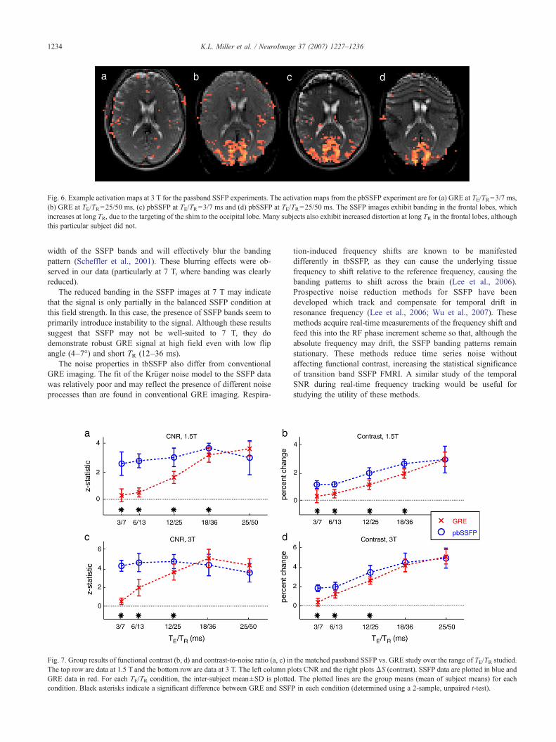
Fig. 6. Example activation maps at 3 T for the passband SSFP experiments. The activation maps from the pbSSFP experiment are for (a) GRE at TE/TR=3/7 ms,(b) GRE at TE/TR=25/50 ms, (c) pbSSFP at TE/TR=3/7 ms and (d) pbSSFP at TE/TR=25/50 ms. The SSFP images exhibit banding in the frontal lobes, whichincreases at long TR, due to the targeting of the shim to the occipital lobe. Many subjects also exhibit increased distortion at long TR in the frontal lobes, althoughthis particular subject did not.

1234 K.L. Miller et al. / NeuroImage 37 (2007) 1227–1236

width of the SSFP bands and will effectively blur the bandingpattern (Scheffler et al., 2001). These blurring effects were ob-served in our data (particularly at 7 T, where banding was clearlyreduced).

The reduced banding in the SSFP images at 7 T may indicatethat the signal is only partially in the balanced SSFP condition atthis field strength. In this case, the presence of SSFP bands seem toprimarily introduce instability to the signal. Although these resultssuggest that SSFP may not be well-suited to 7 T, they dodemonstrate robust GRE signal at high field even with low flipangle (4–7°) and short TR (12–36 ms).

The noise properties in tbSSFP also differ from conventionalGRE imaging. The fit of the Krüger noise model to the SSFP datawas relatively poor and may reflect the presence of different noiseprocesses than are found in conventional GRE imaging. Respira-

Fig. 7. Group results of functional contrast (b, d) and contrast-to-noise ratio (a, c) inThe top row are data at 1.5 T and the bottom row are data at 3 T. The left column pGRE data in red. For each TE/TR condition, the inter-subject mean±SD is plottedcondition. Black asterisks indicate a significant difference between GRE and SSF

tion-induced frequency shifts are known to be manifesteddifferently in tbSSFP, as they can cause the underlying tissuefrequency to shift relative to the reference frequency, causing thebanding patterns to shift across the brain (Lee et al., 2006).Prospective noise reduction methods for SSFP have beendeveloped which track and compensate for temporal drift inresonance frequency (Lee et al., 2006; Wu et al., 2007). Thesemethods acquire real-time measurements of the frequency shift andfeed this into the RF phase increment scheme so that, although theabsolute frequency may drift, the SSFP banding patterns remainstationary. These methods reduce time series noise withoutaffecting functional contrast, increasing the statistical significanceof transition band SSFP FMRI. A similar study of the temporalSNR during real-time frequency tracking would be useful forstudying the utility of these methods.

the matched passband SSFP vs. GRE study over the range of TE/TR studied.lots CNR and the right plots ΔS (contrast). SSFP data are plotted in blue and. The plotted lines are the group means (mean of subject means) for eachP in each condition (determined using a 2-sample, unpaired t-test).

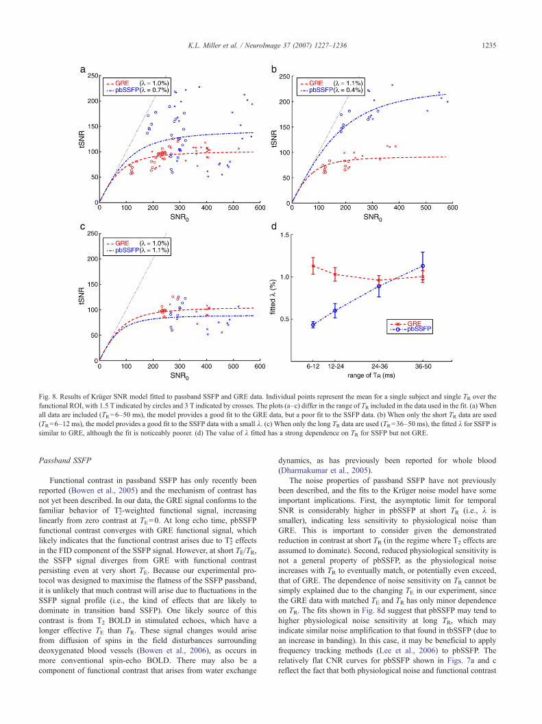
Fig. 8. Results of Krüger SNR model fitted to passband SSFP and GRE data. Individual points represent the mean for a single subject and single TR over thefunctional ROI, with 1.5 T indicated by circles and 3 T indicated by crosses. The plots (a–c) differ in the range of TR included in the data used in the fit. (a) Whenall data are included (TR=6–50 ms), the model provides a good fit to the GRE data, but a poor fit to the SSFP data. (b) When only the short TR data are used(TR=6–12 ms), the model provides a good fit to the SSFP data with a small λ. (c) When only the long TR data are used (TR=36–50 ms), the fitted λ for SSFP issimilar to GRE, although the fit is noticeably poorer. (d) The value of λ fitted has a strong dependence on TR for SSFP but not GRE.

1235K.L. Miller et al. / NeuroImage 37 (2007) 1227–1236

Passband SSFP

Functional contrast in passband SSFP has only recently beenreported (Bowen et al., 2005) and the mechanism of contrast hasnot yet been described. In our data, the GRE signal conforms to thefamiliar behavior of T2

*-weighted functional signal, increasinglinearly from zero contrast at TE=0. At long echo time, pbSSFPfunctional contrast converges with GRE functional signal, whichlikely indicates that the functional contrast arises due to T2

* effectsin the FID component of the SSFP signal. However, at short TE/TR,the SSFP signal diverges from GRE with functional contrastpersisting even at very short TE. Because our experimental pro-tocol was designed to maximise the flatness of the SSFP passband,it is unlikely that much contrast will arise due to fluctuations in theSSFP signal profile (i.e., the kind of effects that are likely todominate in transition band SSFP). One likely source of thiscontrast is from T2 BOLD in stimulated echoes, which have alonger effective TE than TR. These signal changes would arisefrom diffusion of spins in the field disturbances surroundingdeoxygenated blood vessels (Bowen et al., 2006), as occurs inmore conventional spin-echo BOLD. There may also be acomponent of functional contrast that arises from water exchange

dynamics, as has previously been reported for whole blood(Dharmakumar et al., 2005).

The noise properties of passband SSFP have not previouslybeen described, and the fits to the Krüger noise model have someimportant implications. First, the asymptotic limit for temporalSNR is considerably higher in pbSSFP at short TR (i.e., λ issmaller), indicating less sensitivity to physiological noise thanGRE. This is important to consider given the demonstratedreduction in contrast at short TR (in the regime where T2 effects areassumed to dominate). Second, reduced physiological sensitivity isnot a general property of pbSSFP, as the physiological noiseincreases with TR to eventually match, or potentially even exceed,that of GRE. The dependence of noise sensitivity on TR cannot besimply explained due to the changing TE in our experiment, sincethe GRE data with matched TE and TR has only minor dependenceon TR. The fits shown in Fig. 8d suggest that pbSSFP may tend tohigher physiological noise sensitivity at long TR, which mayindicate similar noise amplification to that found in tbSSFP (due toan increase in banding). In this case, it may be beneficial to applyfrequency tracking methods (Lee et al., 2006) to pbSSFP. Therelatively flat CNR curves for pbSSFP shown in Figs. 7a and creflect the fact that both physiological noise and functional contrast

1236 K.L. Miller et al. / NeuroImage 37 (2007) 1227–1236

increase with TR. This property may be useful for optimisingpbSSFP since short TR acquisitions will both reduce bandingartifacts and image distortion.

Conclusions

The passband SSFP technique has been shown to be consistentwith contrast that changes from T2 BOLD at short TE/TR to T2

*

BOLD at long TE/TR. The transition band SSFP technique alsoappears to exhibit significant T2

* BOLD contrast at long TE/TR, butat short times exhibits high contrast that is more consistent withsensitivity of transition band SSFP to the deoxyhemoglobin fre-quency shift. SSFP has also been shown to exhibit different sen-sitivity to physiological noise. The physiological noise in passbandSSFP is lower than GRE at low TR and comparable to GRE at longTR, which is likely related to the passband contrast mechanism.The physiological noise in transition band SSFP is considerablyhigher than GRE, presumably due to the known sensitivity of thetransition band signal to respiratory-induced frequency drift.

Acknowledgments

Dr. Miller is funded a Royal Academy of Engineering/EPSRCResearch Fellowship.

Appendix A. Supplementary data

Supplementary data associated with this article can be found, inthe online version, at doi:10.1016/j.neuroimage.2007.06.024.

References

Bowen, C., Menon, R., and Gati, J. (2005). High field balanced-SSFPFMRI: A BOLD technique with excellent tissue sensitivity and superiorlarge vessel suppression. In Proc 13th ISMRM, page 119, Miami.

Bowen, C., Mason, J., Menon, R., and Gati, J. (2006). High field balanced-SSFP FMRI: Examining a diffusion contrast mechanism using variedflip angles. In Proc 14th ISMRM, page 665, Seattle.

Dharmakumar, R., Hong, J., Brittain, J.H., Plewes, D.B., Wright, G.A.,2005. Oxygen-sensitive contrast in blood for steady-state free precessionimaging. Magn. Reson. Med. 53 (3), 574–583.

Dharmakumar, R., Hong, J., Wright, G.A., 2006. Detecting microcirculatorychanges in blood oxygen state with steady-state precession imaging.Magn. Reson. Med. 55 (6), 1372–1380.

Gudbjartsson, H., Patz, S., 1995. The Rician distribution of noisy MRI data.Magn. Reson. Med. 34, 910–914.

Hennig, J., 1991. Echoes: How to generate, recognize, use or avoid them inMR-imaging sequences. Concepts Magn. Reson. 3, 125–143.

Krüger, G., Glover, G.H., 2001. Physiological noise in oxygenation-sensitive magnetic resonance imaging. Magn. Reson. Med. 46 (4),631–637.

Lee, J., Santos, J.M., Conolly, S.M., Miller, K.L., Hargreaves, B.A., Pauly,J.M., 2006. Respiratory-induced B0 field fluctuation compensation inbalanced SSFP: Real-time approach for transition-band SSFP FMRI.Magn. Reson. Med. 55, 1197–1201.

Miller, K.L., Hargreaves, B.A., Lee, J., Ress, D., deCharms, R.C., Pauly,J.M., 2003. Functional MRI using a blood oxygenation sensitive steadystate. Magn. Reson. Med. 50, 675–683.

Miller, K.L., Smith, S.M., Jezzard, P., Pauly, J.M., 2006. High-resolutionFMRI at 1.5 T using balanced SSFP. Magn. Reson. Med. 55, 161–170.

Reeder, S.B., Herzka, D.A., McVeigh, E.R., 2004. Signal-to-noise ratiobehavior of steady-state free precession. Magn. Reson. Med. 42,123–130.

Scheffler, K., Hennig, J., 2003. Is trueFISP a gradient-echo or spin-echosequence? Magn. Reson. Med. 49, 395–397.

Scheffler, K., Seifritz, E., Bilecen, D., Venkatesan, R., Hennig, J., Deimling,M., Haacke, E.M., 2001. Detection of BOLD changes by means of afrequency-sensitive TrueFISP technique: Preliminary results. NMRBiomed. 14, 490–496.

Smith, S.M., Jenkinson, M., Woolrich, M.W., Beckmann, C.F., Behrens, T.E.J., Johansen-Berg, H., Bannister, P.R., Luca, M.D., Drobnjak, I.,Flitney, D.E., Niazy, R.K., Saunders, J., Vickers, J., Zhang, Y., Stefano,N.D., Brady, J.M., Matthews, P.M., 2004. Advances in functional andstructural MR image analysis and implementation as FSL. NeuroImage23, S208–S219.

Triantafyllou, C., Hoge, R.D., Krueger, G., Wiggins, C.J., Potthast, A.,Wiggins, G.C., Wald, L.L., 2005. Comparison of physiological noise at1.5 T, 3 T and 7 T and optimization of fMRI acquisition parameters.NeuroImage 26, 243–250.

Wu, M.L., Wu, P.H., Huang, T.Y., Shih, Y.Y., Chou, M.C., Liu, H.S., Chung,H.W., Chen, C.Y., 2007. Frequency stabilization using infinite impulseresponse filtering for SSFP FMRI at 3 T. Magn. Reson. Med. 57,369–379.

Zhong, K., Leupold, J., Hennig, J., Speck, O., 2007. Systematicinvestigation of balanced steady-state free precession for functionalMRI in the human visual cortex at 3 Tesla. Magn. Reson. Med. 57 (1),67–73.