Signal and background separationW. von der Linden, V. DoseMax-Planck-Institut f�ur Plasmaphysik, EURATOM AssociationD-85740 Garching b. M�unchen, Germanye-mail: wvl@ipp.mpg.deJ. Padayachee, V. ProzeskyVan de Graa� Group National Accelerator CentreP.O.Box 72, FAURE 7131, South Africae-mail: padayachee@nac.ac.za(26.8.98)

AbstractIn many areas of research the measured spectra consist of a collection of`peaks' { the sought-for signals { which sit on top of an unknown background.The subtraction of the background in a spectrum has been the subject ofmany investigations and di�erent techniques, varying from �ltering to �ttingpolynomial functions, have been developed. These techniques yield resultswhich are not always satisfactory and often even misleading. Based upon therules of probability theory, we derive a formalism to separate the background-from the signal-part of a spectrum in a rigorous and self-consistent manner.We compare the results of the probabilistic approach to those obtained by twocommonly used methods in an analysis of Particle Induced X-ray Emission(PIXE) spectra.02.50.-r,02.50.Rj,07.60.-j,29.30.Kv

Typeset using REVTEX1

I. INTRODUCTIONThe analysis of spectra is generally hampered by the presence of noise and an unknownbackground. This is especially true for particle induced X-ray emission (PIXE) spectrawhere projectile and secondary electron bremsstrahlung leads to a signi�cant background.We will therefore use PIXE spectra as real-world test examples.The central problem to be tackled in this paper is best explained using the PIXE spec-trum depicted in Fig.1. It consists of a fairly smooth background plus signal with bothvery large as well as small peaks which are comparable in height to the background. Thegoal is to determine the background part of the spectrum and by eliminating it from thedata-points to infer the desired signal. The problem falls into the realm of inductive logicwhich tells us how to deal with partial truth: We have experimental data, a vague theoret-ical conception and additional prior knowledge. The information is, however, not stringentenough for a unique result. (Bayesian) probability theory (BPT) [8,9], as E.T. Jaynes [10]appropriately called it 'The Logic of Science', provides the consistent frame to exploitall bits of information rigorously. A nice tutorial type of introduction to BPT is given byD.S. Sivia in his book 'Data Analysis - A Bayesian Tutorial' [11].Before discussing the details of the probabilistic approach, we want to mention thatseveral techniques are available for determining the background in a spectrum. The tradi-tional method is to estimate the background by �tting a set of 'semi-empirical' polynomialfunctions [1,2] to the data while limiting the expansion order to keep the �t from beingin uenced by sharp peaks in the spectrum. These techniques have been optimized [3] bythe use of orthonormal basis sets for the �tting functions, with initialization routines thatimprove initial guesses of the functions and their coe�cients for the �nal �tting during thefull non-linear least squares �tting process. Modern methods tend towards the elimination ofthe background by digital �ltering [4,5] or stripping [6], avoiding any assumption regardingthe functional form of the background.In basic polynomial �tting routines the biggest problems were the unstable nature of the

2

�ts, mainly due to the addition of more degrees of freedom to the non-linear �tting program.These problems were alleviated by using polynomials with some physical basis, as well asby empirical improvements to the functions. Non-linear �tting programs simultaneouslydetermine the signal peaks and the coe�cients of the background polynomials based oniterative least squares methods. The expansion order of these polynomials were typicallyless than 10, increasing the number of degrees of freedom by that number. This often ledto unstable �ts, with a resulting increase in analysis time with human input to correct theprocedure.Digital �ltering is based on the convolution of the spectrum with a top-hat �lter, as inthe GUPIX program [4], or a frequency di�erentiated non-linear digital �lter ("rolling ball"),as in the program used at the Schonland Research Centre (SRC) in Johannesburg [5]. Thetop-hat �lter has a central upper lobe consisting of a number of positive coe�cients, and twonegative outer lobes each having a number of negative coe�cients. The convolution replacesthe data content of every channel by this convolving �lter. The width of the �lter is basedon the energy resolution of the measurement, and therefore is e�ective in areas where thebackground changes linearly over any region of around 400 eV, which is generally a goodapproximation.In the "rolling ball" method [5] the di�erentiated non-linear digital �lter is the equivalentof rolling a ball below the data points and marking out the background as the locus of theball at each point. To account for the varying peak width of the energy spectra, the diameterof the ball gradually increases as a function of energy. The mathematical functions involvedare relatively simple arithmetic functions that can be e�ciently computed. There is somedistortion of the peaks, but this does not adversely a�ect the results.The stripping of the peaks in GeoPIXE [6] is based on estimating the background by it-erative suppression of the counts in channels containing peak information. These techniquesare less e�cient in areas where the background shape changes relatively quickly, leadingto over-�ltering or stripping in that case. The advantage of �ltering and stripping is theelimination of extra free parameters in the non-linear �t routine in the analysis program,3

and the relative robustness of these techniques.II. THE BAYESIAN APPROACH

All techniques discussed so far are ad-hoc and yield results of unpredictable reliability.A �rst consistent probabilistic approach had been suggested by us [7] to separate the signalfrom the noise and the background and at the same time deconvolve the apparatus functionwithin quanti�ed maximum entropy (QME). The main goal there was to derive a formalismwhich still allows the use of standard (commercial) QME packages with merely modi�edinput. In return we had to put up with a couple of approximations. Here we will present thefull probabilistic approach leaving the framework of QME. The basic idea is best explainedguided by the PIXE spectrum mentioned before in Fig.1. Intuitively, one has a fairly clearconception on the essence of the background. What our intuition does is the following: Findthe regions of the spectrum that have no signal contribution and �t a smooth function tothe so-determined background data points. How can this idea by quanti�ed? The answer isprovided by BPT [8,9,11]. Here, we are seeking the probability for the background having avalue bi at point xi, i.e. p(bijd;�;�; I) in the light of all data points di (summaries in d), therespective experimental noise �, a yet unspeci�ed set of parameters � and all backgroundinformation I that uniquely de�nes the problem. The latter plays a crucial role since itprovides the information which we need to discriminate the signal from the background. Ithas to do with correlations either in the signal or the background and is strongly problemdependent. To cover a wide range of applications, we identify the background by the factthat it is smoother then the signal. More restrictive speci�cations are certainly possible fora restricted class of problems and can be dealt with in a similar fashion. The smoothness ofthe background is ensured by expanding it in an appropriate set of basis functions ��(x)bi = EX�=1 ��(xi)c� = EX�=1 �i;�c� (1)or in vector notation b = �c. Here E is the expansion order, which is part of the parameterlist �. The basis set which we will employ in the examples are either Legendre polynomials4

or cubic splines. The formalism is, however, valid for any basis set and for other applicationsa di�erent basis might be more appropriate. The probability for the background vector b isp(bjd;�;�; I) = Z dEc p(bjc;d;�;�; I) p(cjd;�;�; I)

= Z dEc �(b� �c)p(cjd;�;�; I) ; (2)where we have used the probabilistic marginalization rule [11]. According to Bayes theorem[12,11] the desired probability p(cjd;�;�; I) can be expressed as

p(cjd;�;�; I) = 1Zp(djc;�;�; I) p(cj�;�; I) : (3)Bayes theorem splits the problem into the likelihood p(djc;�;�; I), i.e. the error statisticsof the experiment and the prior p(cj�;�; I). The latter is the place to feed in all we knowabout the solution irrespective of the experimental data. The normalization Z can mosteasily be derived in the end by making sure that R dEc p(cjd;�;�; I) = 1.

A. The prior probabilityWe assumed, that the discriminating feature of the background is its smoothness. Con-sequently, the global �rst derivative is a characteristic quantity appropriate as testable in-formation [13,14]. Hence, the prior probability according to the Maximum Entropy principle[13,14] becomes

p(bj�; I) = 1Z e��Pi(b0(xi))2 ; (4)where b0(xi) stands for the slope of the background at point xi. The hyper-parameter � willbe marginalized later on. The expansion in Eq. (1) yields

p(cj�; I) = ��E=2�E=2(detD)1=2e��cTDcDl1;l2 = NXi �0l1(xi)�0l2(xi) ; (5)where we have included the normalization factor. Obviously, �0l(x) � 0 for a constantfunction, i.e. D has one eigenvector 0 with eigenvalue zero. In order to deal with a5

normalizable prior we modify D ! D + � 0 T0 and let � tend to zero in the �nal results. Itcan be shown that this is equivalent to replacing det(D) in Eq. (5) by det(D0)det(D0) := Yi�i>0�i ; (6)

where �i are the eigenvalues of D. The regularization parameter � is a hyperparameter to beintegrated out according to the rules of probability p(cjI)=R d�p(cj�; I)p(�jI). The priorfor the scale parameter � is Je�reys' prior p(�jI) = 1=� and we obtain the multivariatestudent-t distributionp(cjI) = ��E=2(detD0)1=2�(E=2)(cTDc)�E=2 ; (7)

It should be pointed out, that Je�reys' prior is not normalizable. It can, however, be con-sidered as limiting distribution of a sequence proper priors. Since the posterior probabilitywill be proper, the missing normalization constant of Je�reys' prior drops out.B. The Marginal Likelihood

The term p(djc;�;�; I) in Eq. (3) is actually a marginal likelihood since the experi-mental data consist of signal plus background plus noise d = s+ b+ � and the signal-partis not speci�ed in p(djc;�;�; I). Hence, the signal has been integrated by the marginal-ization means of BPT [15]. The idea we put forth is an extension of a suggestion made bySivia and Press [16,17] on how to deal with du� data, a collection of data-points which areinconsistent in the sense that they lay far outside each other's error bars. Recalling the ideaexposed in the beginning, the spectrum consists of regions which have no signal contributionand those which have a signal contribution and can be identi�ed with the du� data in theSivia-Press approach. We introduce the propositions Bi: `data point i is purely background'and the complement Bi: `data point i contains a signal contribution'. In the �rst case thelikelihood is simply the statistics of the experiment. We allow for two common situations:6

uncorrelated Gaussian or Poisson distribution. For data point i the likelihood readsp(dijBi; bi;�;�; I) =

8>>><>>>:1p2��2i e�(di�bi)2=2�2i ; Gaussian

e�bi bdiidi! ; Poisson ; (8)In the second case, the data point contains a signal contribution si which easily predominatesthe background part. In this case the likelihood is again given by

p(dijsi; bi;�;�; I) =8>>><>>>:

1p2�2i e�(di�bi�si)2=2�2i ; Gaussiane�(bi+si) (bi+si)didi! ; Poisson : (9)

So far so good, but what is the value si for the signal? Here the marginalization rule [15]saves the day:p(dijBi; c;�;�; I) = Z 10 dsi p(dijsi; c;�; I) p(sij�; I) : (10)

We omitted all irrelevant entries in the conditional part of the probabilities. Again employingthe maximum entropy principle along with the least committal testable information, namelythe �rst moment, we havep(sij�; I) = 1� e� si� (11)

In other words we introduce a scale � for the signal. This quantity is part of the parameterlist �. There are as usual two possibilities, either the scale is known due to prior knowledgeabout the experimental setup or it is not and has to be inferred by the rules of probabilitytheory. Now the marginal likelihood for the case `an unspeci�ed signal is included in thedata' can be evaluated analytically yieldingp(dijBi; c;�;�; I) =

8>>>>><>>>>>:12� (1 + erf(di�bi��2i =�p2�2i )) ; Gaussiane bi� Q(di + 1; bi(1 + 1=�))�(1 + 1=�)di+1 ; Poisson ; (12)

7

where Q(a; x) is the regularized incomplete gamma-function �(a; x)=�(a). The entire mar-ginal likelihood of Eq. (3) constitutes a mixture model [18] of the two cases Eq. (8) andEq. (12) with respective weights � = p(Bij�; I) and (1� �) = p(Bij�; I). The parameter� completes the list � = fE; �; �g.p(djc;�;�; I) =Yi �(1� �) p(dijBi; c;�;�; I) + � p(dijBi; c;�;�; I)� : (13)

The two likelihood functions of the mixture model are plotted in Fig.2. For each data pointdi there are two typical scales in the likelihood terms: the individual error �i and the globalsignal scale �. In both models, the smaller scale �i prevents the background from risingsigni�cantly above the data points. As far as deviations to lower values are concerned, thetwo likelihood functions behave di�erently: In the the �rst case Eq. (8) the background istightly bound to the data points on a scale set by �i. Whereas the second likelihood Eq. (12)decays merely exponentially on a much larger scale set by �. So in the peak regions of thespectrum the second likelihood takes over since it penalizes only weakly the large discrepancybetween the data and the background. As desired, the approach almost entirely ignores thesignal-regions of the spectrum in the determination of the background parameters c. Thispart of the spectrum is, however, important as far as inference of the parameters � areconcerned. An integral part of the probabilistic approach is the so-called Ockham's razor[19,20], which tries to keep the model as simple as possible. The �rst likelihood function,the one for the background-only cas, is simpler since it is less exible. The measure ofcomplexity that enters the formalism is the Ockham factor, the ratio of the amplitudesof the two likelihood functions, i.e. p�2 �i� , which is a very small quantity. This factorpenalizes individually those data points which are described by the more complex model,the one containing a signal contribution. The complex model wins only if there is no decentchance to interpret the data as background-only points. Qualitatively, the behavior is asfollows: for � = 1 the entire spectrum is assumed to be background and the approach wouldminimize the mis�t between the data and the background model. The resulting backgroundwould be much too large. In the opposite case (� = 0) it is assumed that all data points8

contain a signal contribution and therefore the resulting background estimate would be toosmall. In the intermediate case (0 < � < 1) Ockham's factor is active and tries to treat asmany points as consistent with the data as background-only.Given the posterior probability for the background we can easily compute the expectationvalue and con�dence interval bi = Z bip(bjd;�;�; I)db�2bi = Z (bi � bi)2p(bjd;�;�; I)db : (14)These quantities will be given for several PIXE spectra in a later section of the paper.

C. Probabilities for � and BiThe posterior probability still depends on yet unknown parameters�. Since the marginallikelihood and the prior are given, it is an easy matter of applying BPT to determine thejoint probability for the parameters in the list �, namely E, � and �:

p(�jd;�; I) = 1Zp(�jI)Z dEc p(djc;�;�; I) p(cj�; I)| {z }exp(� ) : (15)Unnecessary conditions have been omitted. We will employ the standard Laplace approxi-mation to evaluate the integral analytically. To this end we expand to second order aroundthe maximum value c yielding a Gaussian. In addition, since the Gaussian is restricted to avery narrow region, we can ignore the positivity constraint imposed on the background andthe integral Eq. (15) can be evaluated analyticallyp(�jd;�; I) � 1Zp(�jI)p(djc;�;�; I) p(cj�; I) (2�)E=2 det(rrT jc)�1=2 : (16)

The argument of the determinant is the Hessian. The prior for the parameters factors intop(�jI) = p(EjI) p(�jI) p(�jI) since expansion order E, prior background probability � andthe signal scale � are logically independent. The expansion order is certainly restricted to amoderate upper limit E� yielding a at prior p(EjI) = �(E � E�)=(E�). The uninformative9

prior for � is p(�jI) = �(0 � � � 1) while for the scale parameter � it is Je�reys' [8,9] priorp(�jI) = 1=�. For the expansion order E it is again Ockham's razor that implicitly tendsto keep the model as simple as possible, i.e. it favors small expansion orders. The drivingforce for the Ockham factor is in the prior for c Eq. (7).An interesting quantity is the `background probability' i.e. the probability for propositionBi, p(Bijd;�; I). In order to determine the `background probability' we employ the sum-rule to introduce the missing bits of information, i.e. parameter set � and backgroundcoe�cients cp(Bijd;�; I) = Z d�Z dEc p(Bijd; c;�;�; I) p(cjd;�;�; I) p(�jd;�; I): (17)

The probabilities for c and �, respectively, are sharply peaked at c and �. Sincethe background probability is just a diagnostic tool, it su�ces to replace Eq. (17) byp(Bijd;�; I) = p(Bijd; c;�; �; I). The next step uses Bayes' theoremp(Bijd; c;�; �; I) = 1Zp(djBi; c;�; �; I) p(Bij�; I)| {z }1��= (1� �)Z Yj 6=i p(dj jBi; c;�; �; I) p(dijBi; c;�; �; I)

= (1� �) p(dijBi; c;�; �; I)� p(dijBi; c;�; �; I) + (1� �) p(dijBi; c;�; �; I) (18)In the last line we inserted the normalization which is the sum over the two cases of Bi beingtrue or false. We de�ne an average background probability

p(Bijd;�; I) = 1N NXi=1 p(Bijd;�; I) : (19)It is expedient to express the signal scale � in units of the average data value

d = 1N NXi=1 di : (20)This completes the formalism needed to determine all quantities of interest. The remainingtask is the numerical evaluation of the formalism, i.e. �rst the determination of the mostprobable values for the parameters E, �, � and the computation of the expectation valuesfor the background b and the respective con�dence intervals.10

III. RESULTSWe begin the discussion of the results with the ivory PIXE spectrum depicted in Fig.1.The afore-mentioned intuitive approach would �rst identify 'background-only' points andthen �t a smooth function to these data points. The Bayesian analysis allows to quan-tify the detection of background-only points. In Fig.3 those data points are marked bysolid circles for which the background probability p(Bijd;�; I) as determined in Eq. (18)is greater then 90%. The latter value for the threshold in Fig.3 is arbitrary and servesmerely a diagnostic purpose. For the present example the average background probabilityp(Bijd;�; I) = 0:9, which agrees fairly well with our intuitive conception. The expectationvalue for the background bi as de�ned in Eq. (14) is depicted in Fig.4 and it is comparedwith the results obtained by the rolling-ball and the GeoPIXE method, respectively. Weobserve that both, the Bayesian as well as the GeoPIXE result are reasonable and in closeagreement, while the rolling ball result is somewhat disappointing. The signal contribution,which is de�ned here as simply the di�erence between PIXE spectrum and background isshown in Fig.5. The computed con�dence intervalls are comparable to the original errorbarsand the �ve small peaksof approximately 50 counts amplitude are all signi�cant. We haveomitted the errorbars in Fig.5 in order not to overload the �gure. In the present examplethe Bayesian approach and the GeoPIXE method yield comparably good results, while therolling ball result is somewhat disappointing. The most probable value for the signal scale is� = 1:9d. A few additional remarks are in order. The abscissa values of the support-pointsof the cubic splines have been chosen equidistantly with a spacing set by twice the widthof the narrowest signal peak. This is part of our prior-information I, which allows us todistinguish signal from background.Next we turn to a geological grain sample where the detector had a dip between 8 and10keV. The PIXE spectrum in Fig.6 is again decomposed into background-only and signal-carrying data points. The average background-probability is again p(Bijd;�; I) = 0:9. Thesignal scale is here � = 1:0 d. It is noteworthy that we generally found fairly good results for

11

the background if we use � �= d and � � 0:5 instead of the correct most probable values.The inferred background is shown in Fig.7. It is again compared with the results obtainedby the rolling-ball and the GeoPIXE method, respectively. In this example the Bayesianapproach yields again a satisfactory result, while the outcome of the other methods is reallydisappointing. This is particularly obvious in the extracted signal which is shown in Fig.8.Apart from the main peaks, all other structures are zero within the con�dence intervals.We have compared our method with GeoPIXE and rolling ball for a variety of PIXEspectra. We have seen in the presented examples that the Bayesian approach furnishes goodresults. The same quality was observed in all analized spectra and the Bayesian results areused as standards to measure the quality of the other approaches. Instead of presenting alarge collection of graphs we introduce a �gure of merit �m =Pi(bmi � bbayesi )=Pi jbbayesi j, toassess the quality of the two common methods, GeoPIXE and rolling balls. The sum extendsover all data points and bmi stands for the background at data point i obtained with methodm. As pointed out before, the Bayesian result serves as standard. The results are listedin Table I. The samples are identi�ed by there �lenames. The table contains two PIXEspectrum of the ivory tusk (ivo) of an African elephant, the study was to determine whetheryou can localize the tusks from the trace element signature, this has implications in poachingcontrol. 'Oto' stands for geological grains. This sample is particularly interesting for us,since the detector used for the measurement was showing a strange e�ciency behaviour,which makes the background separation more challenging. The 'Geop' is the spectrum of ageopolymer.Neither of the standard methods is clearly preferable over the other. In both methodsit happens that the background goes far into the signal part or is much too small, which isindicated by large positive or negative �1-values. The �rst row corresponds to the spectrumof Fig.3 and the second row to the spectrum of Fig.6.Finally, we consider an example for which the spline basis is disadvantageous and whichis best treated in the Legendre basis. It is the mock spectrum depicted in Fig.9 which12

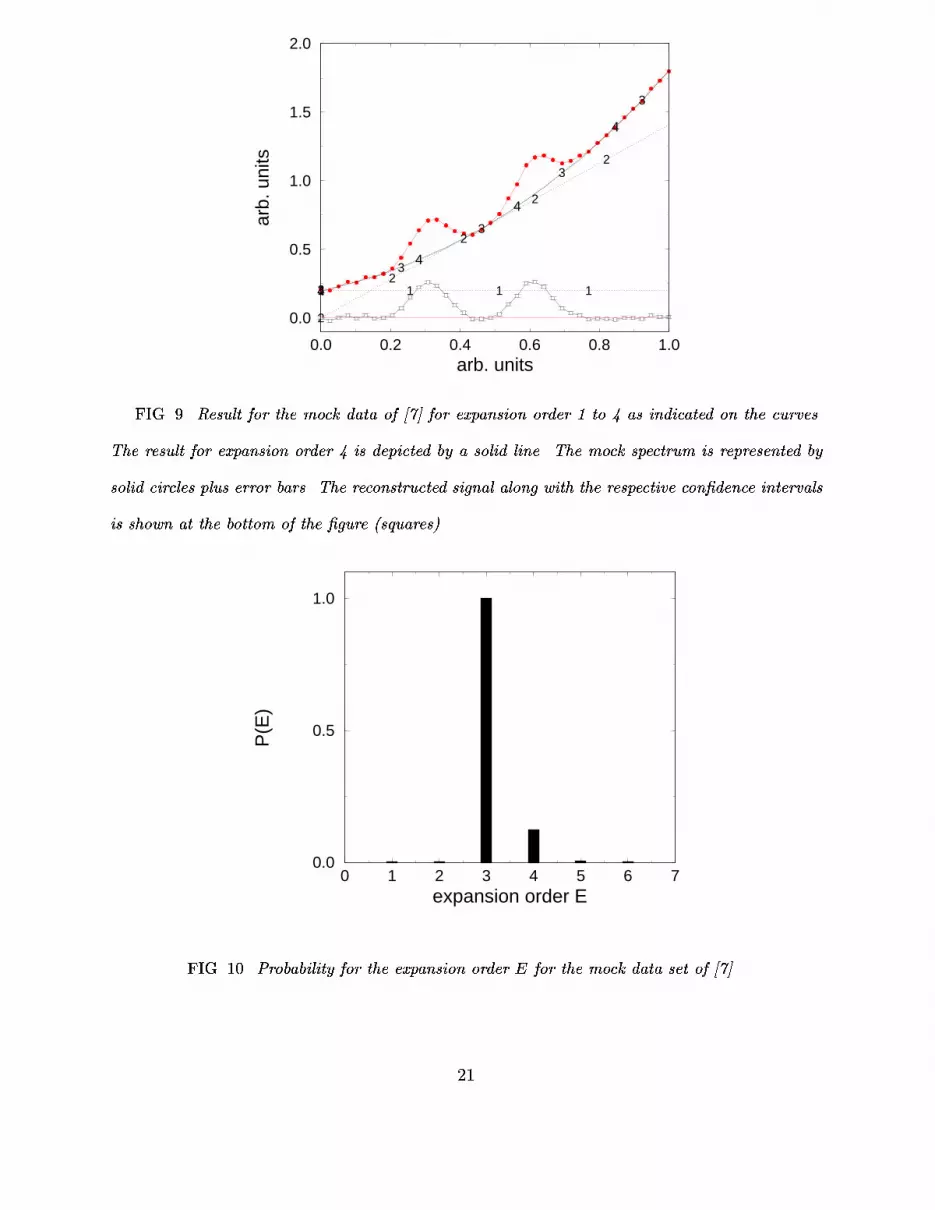
consists of two signal peaks, broadened by a rather broad apparatus function. The signalsits on a parabolic background. This example had been introduced in ref. [7] to illustrate theimportance of background elimination in the quanti�ed maximum entropy scheme. In Fig.9the inferred background is given for expansion order 1-4, which corresponds to polynomialsof degree 0-3. We see that we need expansion order 3 to describe the background. Expansionto higher orders does, however, not improve the quality of the �t through the background-only data points. The probability for the expansion order, which is depicted in Fig.10, isindeed sharply peaked at E = 3. We again encounter the interplay of data-constraint andsimplicity. An expansion order less than 3 is not su�cient to �t the data while an expansionorder beyond 3 does not pay o� �t-wise and is therefore penalized by Ockham's factor.Fig.10 also shows the typical asymmetry in this probability. The left ank is described by aGaussian due to the likelihood while the right ank follows a power-law decay dictated byOckham's razor. For the optimal expansion order (3) the background is subtracted from themock data furnishing the desired bare signal also shown in Fig.9. The signal still containsthe experimental broadening which can now easily be deconvoluted by standard QME, sincethere is no background left which could give rise to ringing or other arti�cial structures.IV. SUMMARY

We have demonstrated how the rules of probability theory can be used to separate thesignal- from the background-part of a spectrum. The probabilistic approach has been testedin a variety of cases and it appeared that the results were in all cases satisfactory. Ofcourse, the probabilistic approach is superior to any other ad-hoc method, since it providesthe frame to consistently and rigorously exploit all bits of information available for a givenproblem [8,9]. If, contrary to expectation, another approach leads to 'better' results thatwould merely mean that this method employs information which has been withheld fromthe probabilistic approach. The probabilistic approach has only one drawback, it is slightlymore laborious than ad-hoc methods, which are usually geared to be computationally simple13

and fast. The reader, who is mainly interested in a quick and dirty approach, can, however,simplify the formalism by setting � � :5 and � � 1N PNi=1 di. The remaining task is merelythe maximization of the marginal likelihood Eq. (13) with respect to the background-expansion coe�cients ci, which can be accomplished by standard library packages. Thecomputational e�ort is then comparable to that of non-linear least-squares problems. Ingeneral, the parameters � have to be optimized according to their posterior probability.But even for a data-set comprising 2000 data points the entire analysis takes approximatelyone minute on a medium-sized workstation.

14

REFERENCES[1] P. V. Espen, K. Janssens, and J. Nobels Cheamom. Int. Lab. Syst., 1, p. 109, 1986.[2] G. Johannsson X-ray Spectrom., 11, p. 194, 1982.[3] B. Vekemans, K. Jannssens, L. Vincze, F. Adams, and P. V. Espen Spectrochimica Acta,50B(2), p. 149, 1995.[4] J. Maxwell, J. Campbell, and W. Teesdale Nucl. Instr. and Meth., B43, p. 218, 1989.[5] M. Kneen and H. Annegarn Nucl. Instr. and Meth., B109/110, p. 209, 1996.[6] C. Ryan, D. Cousens, S. Sie, W. Gri�n, G. Suter, and E. Clayton Nucl. Instr. andMeth., B47, p. 55, 1990.[7] W. von der Linden, V. Dose, and R. Fischer, \How to separate the signal from thebackground," in MAXENT96 - Proceedings of the Maximum Entropy Conference 1996,M. Sears, V. Nedeljkovic, N. E. Pendock, and S. Sibisi, eds., p. 146, NMB Printers, PortElizabeth, South Africa, 1996.[8] H. Je�reys, Theory of Probability, Oxford University Press, London, 1939.[9] M. Tribus, Rational Descriptions, Decisions and Design, Pergamon, New York, 1969.[10] E. Jaynes, Probability Theory: The Logic of Science.http://omega.albany.edu:8008/JaynesBook.html.[11] D. Sivia, Data Analysis - A Bayesian Tutorial, Clarendon Press, Oxford, 1996.[12] R. T. Bayes, \Essay toward solving a problem in the doctrine of chances," Philos. Trans.R. Soc. London, 53, pp. 370{418, 1763.[13] E. Jaynes, \Prior probabilities," in E. T. Jaynes: Papers on Probability, Statistics andStatistical Physics, R. Rosenkrantz, ed., p. 114, Reidel, Dordrecht, 1983.[14] J. Kapur and H. Kesavan, eds., Entropy Optimization Principles with Applications,

15

Academic Press, Inc., San Diego, 1992.[15] E. Jaynes, \Marginalization and prior probabilities," in E. T. Jaynes: Papers on Proba-bility, Statistics and Statistical Physics, R. Rosenkrantz, ed., p. 337, Reidel, Dordrecht,1983.[16] D. Sivia, \Dealing with du� data," in MAXENT96 - Proceedings of the MaximumEntropy Conference 1996, M. Sears, V. Nedeljkovic, N. E. Pendock, and S. Sibisi, eds.,p. 131, NMB Printers, Port Elizabeth, South Africa, 1996.[17] W. H. Press, \Understanding data better with bayesian and global statistical methods,"in Unsolved Problems in Astrophysics, Proceedings of Conference in Honor of JohnBahcall, J. P. Ostriker, ed., Princeton University Press, Princeton, 1996. preprint inastro-ph/9604126.[18] A. O'Hagan in Kendall's advanced theory of statistics, Bayesian Inference, John Wiley& Sons, New York, 1st ed., 1994.[19] A. Garrett, \Ockham's razor," Physics World, Mai, p. 39, 1991.[20] A. Garrett, \Ockham's razor," inMaximum Entropy and Bayesian Methods, W. Grandy,Jr. and L. Schick, eds., p. 357, Kluwer Academic Publishers, Dordrecht, 1991.

16

FIGURES

0.0 0.1 0.2 0.3energy (arb. units)

0

500

1000

1500

2000

coun

ts

FIG. 1. Illustrative PIXE spectrum of ivory.

−100 −50 0(bi−di)/σi

10−8

10−6

10−4

10−2

100

p(d i/σ

i|bi s

0 I)

FIG. 2. The two contributions to the marginal likelihood Eq. (13) terms for the cases barebackground (solid line) and background plus marginalized signal (dashed line) for � = 100�. Hereonly the Gaussian likelihood is shown, the curves for for the Poisson likelihood look qualitativelythe same. 17

0.0 0.1 0.2 0.3energy (arb. units)

0

500

1000

1500

2000

coun

ts

FIG. 3. Same ivory PIXE spectrum as in Fig.1. Data points which are identi�ed to carry asignal contribution are marked by open circles while the 'background-only' points are marked bysolid circles.

0.0 0.1 0.2 0.3 0.4 0.5energy (arb. units)

0

100

200

300

400

500

coun

ts

FIG. 4. Comparison of the reconstructed background part of the ivory PIXE spectrum of Fig.1.Solid line: bayes, Dashed line: rolling ball, diamonds: G eoPIXE.

18

0.0 0.1 0.2 0.3 0.4 0.5energy (arb. units)

0

500

coun

ts0.0 0.1 0.2 0.3 0.4 0.5

0

500

coun

ts

0.0 0.1 0.2 0.3 0.4 0.5

0

500

coun

ts

FIG. 5. Signal contribution of the ivory PIXE spectrum of Fig.1. From top to bottom: Bayes,GeoPIXE, and rolling ball.

0.0 0.1 0.2 0.3energy (arb. units)

0

1000

2000

3000

4000

5000

coun

ts

FIG. 6. Geological-PIXE spectrum. Data points which are identi�ed to carry a signal contribu-tion are marked by open circles while the 'background-only' points are depicted as solid circles.19

0.0 0.1 0.2 0.3energy (arb. units)

0

100

200

300

400

500

coun

ts

FIG. 7. Comparison of the reconstructed background part of the PIXE spectrum of Fig.6. Solidline: bayes, dashed line: rolling ball, diamonds: G eoPIXE.

0.0 0.1 0.2 0.3energy (arb. units)

0

500

coun

ts

0.0 0.1 0.2 0.3

0

500

coun

ts

0.0 0.1 0.2 0.3

0

500

coun

ts

FIG. 8. Signal contribution of the PIXE spectrum of Fig.6. From top to bottom: Bayes,GeoPIXE, and rolling ball.20

0.0 0.2 0.4 0.6 0.8 1.0arb. units

0.0

0.5

1.0

1.5

2.0

arb.

uni

ts1 1 1 1

2

2

2

2

2

3

3

3

3

3

4

4

4

4

FIG. 9. Result for the mock data of [7] for expansion order 1 to 4 as indicated on the curves.The result for expansion order 4 is depicted by a solid line. The mock spectrum is represented bysolid circles plus error bars. The reconstructed signal along with the respective con�dence intervalsis shown at the bottom of the �gure (squares).

0 1 2 3 4 5 6 7expansion order E

0.0

0.5

1.0

P(E

)

FIG. 10. Probability for the expansion order E for the mock data set of [7].21

TABLESTABLE I. Figure of merit � for the GeoPIXE (gp) and rolling ball (rb) method computed forvarious spectra.name �gp �rbIvo212 -0.02 -0.19Oto100 -0.39 -0.22Oto01 -0.37 0.00Ivo100 1.56 0.03Geop17 0.58 -0.11AgZn18 0.74 3.65

22