service design for six sigma
TRANSCRIPT


SERVICE DESIGNFOR SIX SIGMA
A Road Map for Excellence
BASEM EL-HAIKDAVID M. ROY
A WILEY-INTERSCIENCE PUBLICATION
ffirs.qxd 5/11/2005 12:05 PM Page iii

SERVICE DESIGNFOR SIX SIGMA
ffirs.qxd 5/11/2005 12:05 PM Page i

ffirs.qxd 5/11/2005 12:05 PM Page ii

SERVICE DESIGNFOR SIX SIGMA
A Road Map for Excellence
BASEM EL-HAIKDAVID M. ROY
A WILEY-INTERSCIENCE PUBLICATION
ffirs.qxd 5/11/2005 12:05 PM Page iii

Copyright © 2005 by John Wiley & Sons, Inc. All rights reserved.
Published by John Wiley & Sons, Inc., Hoboken, New JerseyPublished simultaneously in Canada.
No part of this publication may be reproduced, stored in a retrieval system or transmitted in any form orby any means, electronic, mechanical, photocopying, recording, scanning or otherwise, except aspermitted under Section 107 or 108 of the 1976 United States Copyright Act, without either the priorwritten permission of the Publisher, or authorization through payment of the appropriate per-copy fee tothe Copyright Clearance Center, Inc., 222 Rosewood Drive, Danvers, MA 01923, 978-750-8400, fax
be addressed to the Permissions Department, John Wiley & Sons, Inc., 111 River Street, Hoboken, NJ07030, (201) 748-6011, fax (201) 748-6008.
Limit of Liability/Disclaimer of Warranty: While the publisher and author have used their best efforts inpreparing this book, they make no representation or warranties with respect to the accuracy orcompleteness of the contents of this book and specifically disclaim any implied warranties ofmerchantability or fitness for a particular purpose. No warranty may be created or extended by salesrepresentatives or written sales materials. The advice and strategies contained herein may not besuitable for your situation. You should consult with a professional where appropriate. Neither thepublisher nor author shall be liable for any loss of profit or any other commercial damages, includingbut not limited to special, incidental, consequential, or other damages.
For general information on our other products and services please contact our Customer CareDepartment within the U.S. at 877-762-2974, outside the U.S. at 317-572-3993 or fax 317-572-4002.
Wiley also publishes its books in a variety of electronic formats. Some content that appears in print,however, may not be available in electronic format.
Library of Congress Cataloging-in-Publication Data is available.
ISBN-13 978-0-471-68291-2ISBN-10 0-471-68291-8
Printed in the United States of America.
10 9 8 7 6 5 4 3 2 1
ffirs.qxd 5/11/2005 12:05 PM Page iv
978-646-8600, or on the web at www.copyright.com. Requests to the Publisher for permission should

To our parents, families and friendsfor their continuous support
ffirs.qxd 5/11/2005 12:05 PM Page v

ffirs.qxd 5/11/2005 12:05 PM Page vi
1. Service Design 11.1 Introduction 11.2 What is Quality? 21.3 Quality Operating System and Service Life Cycle 4
1.3.1 Stage 1: Idea Creation 41.3.2 Stage 2: Voice of the Customer and Business 41.3.3 Stage 3: Concept Development 51.3.4 Stage 4: Preliminary Design 61.3.5 Stage 5: Design Optimization 71.3.6 Stage 6: Verification 71.3.7 Stage 7: Launch Readiness 71.3.8 Stage 8: Production 81.3.9 Stage 9: Service Consumption 81.3.10 Stage 10: Phase-Out 81.3.11 Service Life Cycle and Quality Operating System 8
1.4 Developments of Quality in Service 81.4.1 Statistical Analysis and Control 111.4.2 Root Cause Analysis 111.4.3 Total Quality Management/Control Analysis 121.4.4 Design Quality 121.4.5 Process Simplification 131.4.6 Six Sigma and Design For Six Sigma (DFSS) 13
1.5 Business Excellence: A Value Proposition? 141.5.1 Business Operation Model 141.5.2 Quality and Cost 151.5.3 Quality and Time to Market 16
1.6 Introduction to the Supply Chain 161.7 Summary 17
vii
CONTENTS
ftoc.qxd 5/11/2005 12:09 PM Page vii
2. What Is Six Sigma 192.1 Introduction 192.2 What Is Six Sigma? 192.3 Introduction to Process Modeling 20
2.3.1 Process Mapping 202.3.2 Value Stream Mapping 21
2.4 Introduction to Business Process Management 222.5 Measurement Systems Analysis 242.6 Process Capability and Six Sigma Process Performance 252.6.1 Motorola’s Six Sigma Quality 262.7 Overview of Six Sigma Improvement (DMAIC) 28
2.7.1 Phase 1: Define 292.7.2 Phase 2: Measure 292.7.3 Phase 3: Analyze 292.7.4 Phase 4: Improve 302.7.5 Phase 5: Control 30
2.8 Six Sigma Goes Upstream—Design For Six Sigma 302.9 Summary 31
3. Introduction to Service Design for Six Sigma (DFSS) 333.1 Introduction 333.2 Why Use Service Design for Six Sigma? 343.3 What Is Service Design For Six Sigma? 373.4 Service DFSS: The ICOV Process 393.5 Service DFSS: The ICOV Process In Service Development 413.6 Other DFSS Approaches 423.7 Summary 43
4. Service Design for Six Sigma Deployment 454.1 Introduction 454.2 Service Six Sigma Deployment 454.3 Service Six Sigma Deployment Phases 46
4.3.1 Predeployment 464.3.2 Predeployment considerations 484.3.3 Deployment 66
4.3.3.1 Training 674.3.3.2 Six Sigma Project Financial Aspects 68
4.3.4 Postdeployment Phase 694.3.4.1 DFSS Sustainability Factors 70
4.4 Black Belt and DFSS Team: Cultural Change 72
5. Service DFSS Project Road Map 775.1 Introduction 775.2 The Service Design For Six Sigma Team 795.3 Service Design For Six Sigma Road Map 81
viii CONTENTS
ftoc.qxd 5/11/2005 12:09 PM Page viii
5.3.1 Service DFSS Phase I: Identify Requirements 835.3.1.1 Identify Phase Road Map 845.3.1.2 Service Company Growth & Innovation 85
Strategy: Multigeneration Planning5.3.1.3 Research Customer Activities 86
5.3.2 Service DFSS Phase 2: Characterize Design 865.3.3 Service DFSS Phase 3: Optimize Phase 895.3.4 Service DFSS Phase 4: Validate Phase 90
5.4 Summary 92
6. Service DFSS Transfer Function and Scorecards 936.1 Introduction 936.2 Design mappings 94
6.2.1 Functional Mapping 956.2.2 Process Mapping 966.2.3 Design Mapping Steps 96
6.3 Design Scorecards and Transfer Function 976.3.1 DFSS Scorecard Development 986.3.2 Transfer Function Life Cycle 99
6.4 Transfer Function 1026.5 Transfer Functions and Optimization 1056.6 Monte Carlo Simulation 1076.7 Summary 109
7. Quality Function Deployment (QFD) 1117.1 Introduction 1117.2 History of QFD 1127.3 QFD Overview 1137.4 QFD Methodology 1137.5 HOQ Evaluation 1167.6 HOQ 1—“The Customer’s House” 1177.7 Kano Model 1187.8 QFD HOQ 2—“Translation House” 1217.9 QFD HOQ 3—“Design House” 1227.10 QFD HOQ 4—“Process House” 1227.11 QFD Example 122
7.11.1 HOQ 1 1237.11.2 HOQ 2 1267.11.3 HOQ 3 1277.11.4 HOQ 4 134
7.12 Summary 140
8. Process Modeling and Process Management 1418.1 Introduction 1418.2 Process Modeling Techniques 142
CONTENTS ix
ftoc.qxd 5/11/2005 12:09 PM Page ix
8.2.1 SIPOC 1428.2.2 Process Mapping 1428.2.3 Value Stream Mapping 148
8.2.3.1 Value Stream Mapping Process Steps 1508.3 Business Process Management System (BPMS) 155
8.3.1 What is BPMS? 1558.3.2 How is BPMS Implemented? 156
8.4 Relationship of Process Modeling to Discrete Event Simulation 1568.5 Functional Mapping 158
8.5.1 Value Analysis/Engineering FAST Technique 1598.5.2 Axiomatic Method 164
8.5.2.1 Axiomatic Design Software (ftp://ftp-wiley. 170com/public/sci_tech_med/six_sigma)
8.5.2.2 Axiomatic Design Mapping Example 1718.6 Pugh Concept Selection 1778.7 Summary 181Appendix 8.A: IDEF Mapping Technique 181
8.A.1 IDEF0 Technique 183Appendix 8.B: Matrix Review 187
9. Theory of Inventive Problem Solving (TRIZ) for Service 1899.1 Introduction 1899.2 TRIZ History 1899.3 TRIZ Foundations 191
9.3.1 Overview 1919.3.2 Analytical Tools 1959.3.3 Knowledge-Base Tools 195
9.4 TRIZ Problem Solving Flowchart 2009.5 Ideal Final Result 201
9.5.1 Itself 2029.5.2 Ideality Checklist 2029.5.3 Ideality Equation 203
9.6 Build Sufficient Functions 2039.7 Harmful Function Elimination 2039.8 Inventive Principles 2059.9 Detection and Measurement 2119.10 TRIZ Root Cause Analysis 2119.11 Evolutionary Trends of Technological Systems 2129.12 Transitions from TRIZ Examples 2159.13 Summary 216Appendix 9.A 218
10. Introduction to Design For Transactional DFX 22310.1 Introduction 22310.2 History and Evolution 224
x CONTENTS
ftoc.qxd 5/11/2005 12:09 PM Page x
10.3 Design for X for Transactional Processes 22710.3.1 Design for Product Service (DFPS) 227
10.4 Design for Processability and Assembly 23010.4.1 The DFMA Approach 233
10.5 Design for Testability and Inspectability 23610.6 Summary 240
11. Failure Mode and Effect Analysis (FMEA) 24111.1 Introduction 24111.2 FMEA Fundamentals 24311.3 Service Design FMEA (DFMEA) 24911.4 Process FMEA (PFMEA) 25711.5 FMEA Interfaces with Other Tools 258
11.5.1 Cause-and-Effect Tools 25911.5.2 Quality Systems and Control Plans 259
12 Fundamentals of Experimental Design 26312.1 Introduction 26312.2 Hypothesis Testing 26612.3 Classical DOE Basics 269
12.3.1 DOE Study Definition 27012.3.2 Selection of the Response 27112.3.3 Choice of DOE Factors, Levels, and Ranges 27212.3.4 Select DOE Strategy 27312.3.5 Develop a Measurement Strategy for DOE 27412.3.6 Experimental Design Selection 27512.3.7 Conduct the Experiment 27612.3.8 Analysis of DOE Raw Data 27712.3.9 Conclusions and Recommendations 278
12.4 Factorial Experiment 27912.5 Mathematical Transfer Function Models 28012.6 What is Interaction? 28012.7 ANalysis Of VAriance (ANOVA) 283
12.7.1 ANOVA Steps For Two factors Completely 284Randomized Experiment
12.8 Full 2k Factorial Designs 28912.8.1 Full 2k Factorial Design Layout 29012.8.2 2k Data Analysis 29112.8.3 The 23 Design 29712.8.4 The 23 Design with Center Points 299
12.9 Fractional Factorial Designs 30012.9.1. The 23–1 Design 30112.9.2 Half Factional 2k Design 30212.9.3. Design Resolution 30312.9.4 Quarter Fraction of 2k Design 304
CONTENTS xi
ftoc.qxd 5/11/2005 12:09 PM Page xi
12.10 Other Factorial Designs 30912.10.1 Three-Level Factorial design 30912.10.2 Box–Behnken Designs 310
12.11 Summary 310Appendix 311
13 Service Design Robustness 31313.1 Introduction 31313.2 Robustness Overview 31413.3 Robustness Concept #1: Quality Loss Function 315
13.3.1 Larger-the-Better Loss Function 31713.3.2 Smaller-the-Better Loss Function 318
13.4 Robustness Concept #2: Signal, Noise and Control Factors 31913.5 Robustness Concept #3: Signal-to-Noise Ratios 31913.6 Robustness Concept #4: The Accumulation Analysis 321
13.6.1 Accumulation Analysis Example 32113.7 Robustness Concept #5: Orthogonal Arrays 32513.8 Robustness Concept #6: Parameter Design Analysis 32713.9 Summary 329
14 Discrete Event Simulation 33114.1 Introduction 33114.2 System Modeling 332
14.2.1 System Concept 33214.2.2 Modeling Concept 33414.2.3 Types of Models 335
14.3 System Modeling With Discrete Event Simulation (DES) 33714.3.1 System Structure 33814.3.2 System Layout 33914.3.3 System Data 33914.3.4 System Logic 34114.3.5 System Statistics 341
14.4 Elements of Discrete Event Simulation 34214.4.1 System Entities 34214.4.2 System State 34314.4.3 State Variables 34314.4.4 System Events 34414.4.5 System Activities 34514.4.6 System Resources 34614.4.7 System Delay 34814.4.8 System Logic 348
14.5 DES Mechanisms 34814.5.1 Discrete-Event Mechanism 35014.5.2 Time-Advancement Mechanism 35114.5.3 Random Sampling Mechanism 352
xii CONTENTS
ftoc.qxd 5/11/2005 12:09 PM Page xii
14.5.4 Statistical Accumulation Mechanism 35314.5.5 Animation Mechanism 354
14.6 Manual Simulation Example 35514.7 Variability in Simulation Outputs 360
14.7.1. Variance Reduction Techniques 36114.8 Service Processes Simulation Implications 36314.9 Summary 364
15 Design Validation 36515.1 Introduction 36515.2 Design Validation Steps 36515.3 Prototype Building 36715.4 Testing 36815.5 Confidence Interval of Small Sample Validation 37015.6 Control Plans and Statistical Process Control 37015.7 Statistical Process Control 371
15.7.1 Choosing the Control Chart 37315.7.2 Interpreting the Control Chart 37515.7.3 Taking Action 376
15.8 Process Capability 37615.9 Summary 377
16 Supply Chain Process 37916.1 Introduction 37916.2 Supply Chain Definition 379
16.2.1 Demand Forecasting 38016.2.2 Planning and Scheduling 38016.2.3 Strategic Sourcing 38016.2.4 Processing 38016.2.5 Asset and Inventory Management 38116.2.6 Distribution and Logistics 38116.2.7 Postservice Support 381
16.3 Summary 381
17 DFSS in the Supply Chain 38317.1 Introduction 38317.2 The Process 38317.3 Stage 1—Idea Creation 38317.4 Stage 2—Voice of the Customer and the Business 385
17.4.1 Voices 38517.4.2 Risk Assessment 386
17.5 Stage 3—Concept Design 38917.5.1 Concept Development 395
CONTENTS xiii
ftoc.qxd 5/11/2005 12:09 PM Page xiii

17.6 Stage 4—Preliminary Design 39917.7 Stage 5—Design Optimization 40317.8 Stage 6—Verification 40517.9 Stage 7—Launch Readiness 40617.10 Production 40617.11 Summary 407
References 409
Index 419
xiv CONTENTS
ftoc.qxd 5/11/2005 12:09 PM Page xiv
Today’s service design solutions of current development practices in many indus-tries are generally suffering from deficiencies or vulnerabilities such as modestquality levels, ignorance of customer wants and desires, and too much complexity.These are caused by a lack of a systematic design methodology to address these is-sues. Such vulnerabilities are common and generate hidden and unnecessary devel-opmental effort, in terms of non-value-added elements, and, later, operational costsas experienced by the customer. Design vulnerabilities manifest themselves in ahigh degree of customer dissatisfaction, low market share, a rigid organizationalstructure, and high complexity of operations. Complexity in design creates opera-tional bureaucracies that can be attributed to the lack of adherence to sound designprocesses. This root cause is coupled with several sources of variation in the servicedelivery processes, inducing variability in customer attributes, which are commonlyknown as critical-to-satisfaction characteristics (CTSs).
The success of Six Sigma deployments in many industries has generated enor-mous interest in the business world. In demonstrating such successes, Six Sigmacombines the power of teams and process. The power of teams implies organiza-tional support and trained teams tackling objectives. The power of process meanseffective Six Sigma methodology deployment, risk mitigation, project manage-ment, and an array of statistical and system-based methods. Six Sigma focuses onthe whole quality of a business. Whole quality includes product or service quality toexternal customers and also the operation quality of all internal processes, such asaccounting, billing and so on. A whole-quality business with whole-quality per-spectives will not only provide high-quality products or services, but will also oper-ate at lower cost and higher efficiency because all of its business processes are opti-mized.
Compared with the defect-correction Six Sigma methodology that is character-ized by “DMAIC” processes (define, measure, analyze, improve, control), servicedesign for six sigma (identify, characterize, optimize, verify) is proactive. TheDMAIC Six Sigma objective is to improve a process without redesigning it.
xv
PREFACE
fpref.qxd 5/11/2005 4:56 PM Page xv
Design for Six Sigma focuses on design by doing things right the first time—aproactive approach. The ultimate goal of service DFSS is whole quality, that is, dothe right things, and do things right all the time. This means achieving absoluteexcellence in design, whether it is a service process facing the customer or an in-ternal business process facing the employee. Superior service design will deliversuperior functions to generate high customer satisfaction. A design for Six Sigma(DFSS) entity will generate a process that delivers the service in a most efficient,economic, and flexible manner. Superior service process design will generate aservice process that exceeds customer wants, and delivers with quality and lowcost. Superior business process design will generate the most efficient, effective,economical, and flexible business process. This is what we mean by whole quali-ty. That is, not only should we provide superior service, the service design andsupporting processes should always deliver what they were intended to do and atSix Sigma quality levels. A company will not survive if it develops some very su-perior service products, but also develops some poor products as well, leading toinconsistent performance. It is difficult to establish a service business based on ahighly defective product.
Service design for Six Sigma (DFSS), as described in this book, proactively pro-duces highly consistent processes with extremely low variation in service perfor-mance. The term “Six Sigma” indicates low variation; it means no greater than 3.4defective (parts) per million opportunities (DPMO1) as defined by the distance be-tween the specification limits and the mean, in standard deviation units. We careabout variation because customers notice inconsistency and variation, not the aver-ages. Can you recall the last time you experienced the average wait time? Nowa-days, high consistency is not only necessary for a sound reputation, it is also a mat-ter of survival. For example, the dispute between Ford and Firestone over tires onlyinvolved an extremely small fraction of tires, but the negative publicity and litiga-tion impacted a giant company like Ford significantly.
Going beyond Six Sigma DMAIC, this book will introduce many new methodsthat add to the effectiveness of service DFSS. For example, key methodologies formanaging innovativeness and complexity in design will be introduced. Axiomaticdesign, design for X, theory of inventive problem solving (TRIZ), transfer function,and scorecards are really powerful methods to create superior service designs; thatis, to do the right things within our whole quality perspective.
This book also adds another powerful methodology, the Taguchi method (robustdesign), to its toolbox. A fundamental objective of the Taguchi method is to create asuperior entity that can perform consistently in light of many external disturbancesand uncertainties called noise factors, thus performing robustly all the time.
Because of the sophistication of DFSS tools, DFSS operative training (BlackBelts, Green Belts, and the like) is quite involved. However, this incremental in-vestment is rewarded by dramatically improved results. A main objective of thisbook is to provide a complete picture of service DFSS to readers, with a focus onsupply chain applications.
xvi PREFACE
1See Chapter 2 for more details on this terminology.
fpref.qxd 5/11/2005 4:56 PM Page xvi
OBJECTIVES OF THIS BOOK
This book aims to
1. Provide in-depth and clear coverage of philosophical, organizational, andtechnical aspects of service DFSS to readers.
2. Illustrate very clearly all the service DFSS deployment and executionprocesses—the DFSS road map.
3. Present the know-how of all the key methods used in service DFSS, dis-cussing the theory and background of each method clearly. Examples are pro-vided, with detailed step-by-step implementation processes for each method.
4. Assist in developing the readers’ practical skills in applying DFSS in serviceenvironments.
BACKGROUND REQUIRED
The background required to read this book includes some familiarity with simplestatistics, such as normal distribution, mean, variance, and simple data analysistechniques.
SUMMARY OF CHAPTER CONTENTS
In Chapter 1, we introduce service design. We highlight how customers experienceservice, the process through which the service is delivered, and the roles that peopleand other resources play in this context. We discuss the relationship between differ-ent quality tasks and tools and at various stages of service development. This chap-ter presents the Six Sigma quality concept, the whole quality, business excellence,quality assurance, and service life cycle. It provides a detailed chronology of theevolution of quality, the key pioneers in the field, and supply chain applications.
In Chapter 2, we explain what Six Sigma is and how it has evolved over time.We explain that it is a process-based methodology and introduce the reader toprocess modeling, with a high-level overview of process mapping, value streammapping, and value analysis, as well as the business process management system(BPMS). The criticality and application of measurement systems analysis (MSA)is introduced. The DMAIC methodology and how it incorporates these conceptsinto a road map method is also explained, and a design for Six Sigma (DFSS)briefing is presented.
Chapter 3 offers a high-level DFSS process. The DFSS approach as introducedhelps design teams frame their project with financial, cultural, and strategic impli-cations to the business. In this chapter, we formed and integrated several strategic,tactical, and synergistic methodologies to enhance service DFSS capabilities and todeliver a broad set of optimized solutions. It highlights and presents the service
PREFACE xvii
fpref.qxd 5/11/2005 4:56 PM Page xvii
DFSS phases: identify, characterize, optimize, and verify, or ICOV for short. In thisbook, the ICOV and DFSS acronyms will be used interchangeably.
In Chapter 4, we discuss the deployment of a service DFSS initiative startingfrom a white paper. We present the deployment plan, roles, and responsibilities ofdeployment operatives, project sources, and other aspects of sound deploymentstrategy in three phases: predeployment, initial deployment, and steady-state de-ployment. We also discuss certain desirable characteristics of design teams and of-fer several perspectives on cultural transformation and initiative sustainability.
In Chapter 5, we present the service design for a Six Sigma project road map.The road map highlights at a high-level the identify, charcaterize, optimize, and val-idate phases over the seven development stages (idea creation, voice of the cus-tomer and business, concept development, preliminary design, design optimization,verification, launch readiness). In this chapter, the concept of the tollgate is intro-duced. We also highlight the most appropriate DFSS tools and methods for eachDFSS phase, indicating where it is most appropriate to start tool usage. The meth-ods are presented in the subsequent chapters.
In Chapter 6, the transfer function and design scorecard tools are introduced. Theuse of these DFSS tools parallels the design mappings. A transfer function is amathematical relationship relating a design response to design elements. A designscorecard is used to document the transfer function as well the performance.
In Chapter 7, quality function deployment (QFD) is presented. It is used to trans-late customer needs and wants into focused design actions, and parallels designmapping as well. QFD is key to preventing problems from occurring once the de-sign is operational. The linkage to the DFSS road map allows for rapid design cy-cles and effective utilization of resources while achieving Six Sigma levels of per-formance.
Design mapping is a design activity that is presented in Chapter 8. The serviceDFSS project road map recognizes two different mappings: the functional mappingand the process mapping. In this chapter, we present the functional mapping as alogical model, depicting the logical and cause–effect relationships between designelements through techniques such as axiomatic design and value engineering. Aprocess map is a visual aid for picturing work processes; it shows how inputs, out-puts, and tasks are linked. In this chapter, we feature the business process manage-ment system (BPMS), an effective tool for improving overall business performancewithin the design context. The Pugh concept selection method is used after designmapping to select a winning concept for further DFSS road map processing.
The use of creativity methods such as the theory of problem solving (TIPS,also known as TRIZ) in service DFSS is presented in Chapter 9. TRIZ, based onthe discovery that there are only 40 unique innovative principles, provides designteams a priceless toolbox for innovation so they can focus on the true design op-portunity and provide principles to resolve, improve, and optimize concepts. TRIZis a useful innovative problem solving method that, when applied successfully, re-places the trial-and-error method in the search for vulnerability-free concepts. It isthe ultimate library of lessons learned. TRIZ-based thinking for management taskshelps to identify the technology tools that come into play, such as innovation prin-
xviii PREFACE
fpref.qxd 5/11/2005 4:56 PM Page xviii
ciples for business and management, separation principles for resolving organiza-tional contradictions and conflicts, operators for revealing and utilizing system re-sources, and patterns of evolution of technical systems to support conceptual opti-mization.
In Chapter 10, we introduce the concept of design for X (DFX) as it relates toservice transactions and builds from the work performed for product design. In thiscontext, we show that DFX for service requires that the process content be evaluat-ed, much the same as in assembly processes, to minimize complexity and maximizecommonality. The end result will be a robust design that meets the customer’sneeds profitably, through implementation of methods such as design for service-ability, processability, and inspectability.
Chapter 11 discusses failure mode and effect analysis (FMEA). FMEA is a veryimportant design review method to remove potential failures in the various designstages. We discuss all aspects of FMEA, as well as the difference between designFMEA and process FMEA and the linkages to service DFSS road maps.
In Chapter 12, we present the service DFSS approach to the design of experi-ments (DOE), a prime optimization tool, with many service-related examples. DOEis a structured method for determining the transfer function relationship betweenfactors affecting a process and the output of that process. DOE refers to experimen-tal methods used to quantify indeterminate measurements of factors and interac-tions between factors statistically through observance of forced changes made me-thodically, as directed by systematic tables called design arrays. The main DOEdata analysis tools include analysis of variance (ANOVA), empirical transfer func-tion model building, and main effects and interaction charts.
Chapter 13 presents the employment of robust design methodology in servicedesign environments. Thinking about robustness helps the DFSS team classify de-sign parameters and process variables mapped into the design as controlled and un-controlled. The objective is to desensitize the design to the uncontrolled disturbancefactors, also called noise factors, thus producing a consistently performing, on-tar-get design with minimal variation.
The Discrete event simulation (DES) technique presented in Chapter 14 is apowerful method for business process simulation of a transactional nature withinDFSS and Six Sigma projects. A DES provides modeling of service entity flowswith capabilities that allow the design team to see how flow objects are routedthrough the process. DES leads to growing capabilities, software tools, and a widespectrum of real-world applications in DFSS.
In Chapter 15, we present validation as a critical step in the DFSS road map anddiscuss the need for it to be addressed well in advance of production of a new de-sign. The best validation occurs when it is done as near to production configurationand operation as possible. Service design validation often requires prototypes thatneed to be near “final design” but are often subject to trade-offs in scope and com-pleteness due to cost or availability. Once prototypes are available, a comprehen-sive test plan should be followed in order to capture any special event and to popu-late the design scorecard, and should be based on statistically significant criteria.This chapter concludes the DFSS deployment and core methods that were presented
PREFACE xix
fpref.qxd 5/11/2005 4:56 PM Page xix

in Chapters 1 through 15. The last two chapters present the supply chain threadthrough a design case study.
Chapter 16 discusses the supply chain process that covers the life cycle of under-standing customer needs to producing, distributing, and servicing the value chainsfrom customers to suppliers. We describe how supply chains apply to all contexts ofacquiring resources to be transformed into value for customers. Because of its broadapplicability to all aspects of consumption and fulfillment, the supply chain is theultimate “service” for design consideration. A case study is presented in Chapter17.
In Chapter 17, we apply the DFSS road map to accelerate the introduction ofnew processes and align the benefits for customers and stakeholders. In this supplychain case study, we describe how service DFSS tools and tollgates allow for riskmanagement, creativity, and a logical documented flow that is superior to the“launch and learn” mode that many new organizations, processes, or services aredeployed with. Not all projects will use all of the complete toolkit of DFSS toolsand methodologies, and some will use some to a greater extent than others. In thesupply chain case study, the design scorecard, quality function deployment, and ax-iomatic design applications are discussed, among others.
WHAT DISTINGUISH THIS BOOK FROM OTHERS IN THE AREA?
This book is the first to address service design for Six Sigma and to present an ap-proach to applications via a supply chain design case study. Its main distinguishingfeature is its completeness and comprehensiveness, starting from a high-leveloverview of deployment aspects and the service design toolbox. Most of the impor-tant topics in DFSS are discussed clearly and in depth. The organizational, imple-mentation, theoretical, and practical aspects of both the DFSS road map and DFSStoolbox methods are covered very carefully and in complete detail. Many of thebooks in this subject area give only superficial descriptions of DFSS without anydetails. This is the only book that discusses all service DFSS perspectives, such astransfer functions, axiomatic design,2 and TRIZ and Taguchi methods in great de-tail. The book can be used either as a complete reference book on DFSS, or as acomplete training manual for DFSS teams. We remind readers that not every pro-ject requires full use of every tool.
With each copy of this book, purchasers can access a copy of Acclaro DFSSLight® by downloading it from the Wiley ftp site. This is a training version of theAcclaro DFSS software toolkit from Axiomatic Design Solutions, Inc. (ADSI3) ofBrighton, MA. Under license from MIT, ADSI is the only company dedicated tosupporting axiomatic design methods with services and software solutions. Acclaro
xx PREFACE
2Axiomatic design is a methodology used by individuals as well as Fortune 100 design organizations.The axiomatic design process aids design and development organizations in diverse industries includingautomotive, aerospace, semiconductor, medical, government, and consumer products. 3Browse their site at http://www.axiomaticdesign.com/default.asp.
fpref.qxd 5/11/2005 4:56 PM Page xx

software, a Microsoft Windows-based solution implementing DFSS quality frame-works around axiomatic design processes, won Industry Week’s Technology of theYear award. Acclaro DFSS Light® is a JAVA-based software package that imple-ments axiomatic design processes as presented in Chapter 8.
John Wiley & Sons maintains an ftp site at: ftp://ftp.wiley.com/public/sci_tech_med/six_sigma
ACKNOWLEDGMENTS
In preparing this book, we received advice and encouragement from several people.We are thankful to Peter Pereira, Sheila Bernhard, Sherly Vogt, Eric Richardson,Jeff Graham, and Mike Considine. We are also thankful to Dr. Raid Al-Aomar ofJordan University of Science and Technology (JUST) for his contribution to Chap-ter 14. The authors are appreciative of the help of many individuals, includingGeorge Telecki and Rachel Witmer of John Wiley & Sons, Inc. We are very thank-ful to Invention Machine Inc. for their permission to use TechOptimizer™ softwareand to Generator.com for many excellent examples in Chapter 9.
CONTACTING THE AUTHORS
Your comments and suggestions about this book are greatly appreciated. We willgive serious considerations to your suggestions for future editions. We also conductpublic and in-house Six Sigma and DFSS workshops and provide consulting ser-vices. Dr. Basem El-Haik can be reached via e-mail at [email protected] Roy can be reached via e-mail at [email protected].
PREFACE xxi
fpref.qxd 5/11/2005 4:56 PM Page xxi

fpref.qxd 5/11/2005 4:56 PM Page xxii

1.1 INTRODUCTION
Throughout the evolution of quality control processes, the focus has mainly been onmanufacturing (parts). In recent years, there has been greater focus on process ingeneral; however, the application of a full suite of tools to service design is rare andstill considered risky or challenging. Only companies that have mature Six Sigmadeployment programs see the application of design for Six Sigma (DFSS) toprocesses as an investment rather than a needless expense. Even those companiesthat embark on DFSS for processes seem to struggle with confusion over the DFSS“process” and the process being designed.
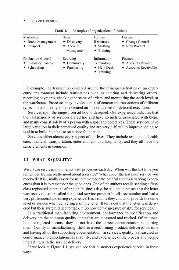
There are multiple business processes that can benefit from DFSS. A sample ofthese are listed in Table 1.1.
If properly measured, we would find that few if any of these processes performat Six Sigma performance levels. The cost per transaction, timeliness, or quality(accuracy, completeness) are never where they should be and hardly world class.
We could have chosen any one of the processes listed in Table 1.1 for the com-mon threaded service DFSS book example but we have selected a full supply chainprocess because it either supports each of the other processes or is analogous in itsconstruct. Parts, services, people, or customers are all in need of being sourced atsome time.
A service is typically something that we create to serve a paying customer.Customers may be internal or external; if external, the term consumer (or end user)will be used for clarification purposes. Some services, for example dry cleaning, con-sist of a single process, whereas many services consist of several processes linked to-gether. At each process, transactions occur. A transaction is the simplest process stepand typically consists of an input, procedures, resources and a resulting output. Theresources can be people or machines and the procedures can be written, learned oreven digitized in software code. It is important to understand that some services areenablers to other services, whereas some provide their output to the end customer.
Service Design for Six Sigma. By Basem El-Haik and David M. Roy 1© 2005 by John Wiley & Sons.
1SERVICE DESIGN
c01.qxd 4/22/2005 7:31 AM Page 1
For example, the transaction centered around the principal activities of an order-entry environment include transactions such as entering and delivering orders,recording payments, checking the status of orders, and monitoring the stock levels atthe warehouse. Processes may involve a mix of concurrent transactions of differenttypes and complexity either executed on-line or queued for deferred execution.
Services span the range from ad hoc to designed. Our experience indicates thatthe vast majority of services are ad hoc and have no metrics associated with them,and many consist solely of a person with a goal and objectives. These services havelarge variation in their perceived quality and are very difficult to improve; doing sois akin to building a house on a poor foundation.
Services affect almost every aspect of our lives. They include restaurants, healthcare, financial, transportation, entertainment, and hospitality, and they all have thesame elements in common.
1.2 WHAT IS QUALITY?
We all use services and interact with processes each day. When was the last time youremember feeling really good about a service? What about the last poor service youreceived? It is usually easier for us to remember the painful and dissatisfying experi-ences than it is to remember the good ones. One of the authors recalls sending a first-class registered letter and after eight business days he still could not see that the letterwas received, so he called the postal service provider’s toll-free number and had avery professional and caring experience. It is a shame they could not provide the samelevel of service when delivering a simple letter. It turns out that the letter was deliv-ered but their system failed to track it. So how do we measure quality for services?
In a traditional manufacturing environment, conformance to specification anddelivery are the common quality items that are measured and tracked. Often times,lots are rejected because they do not have the correct documentation supportingthem. Quality in manufacturing, then, is a conforming product, delivered on timeand having all of the supporting documentation. In services, quality is measured asconformance to expectations, availability, and experience of the process and peopleinteracting with the service delivery.
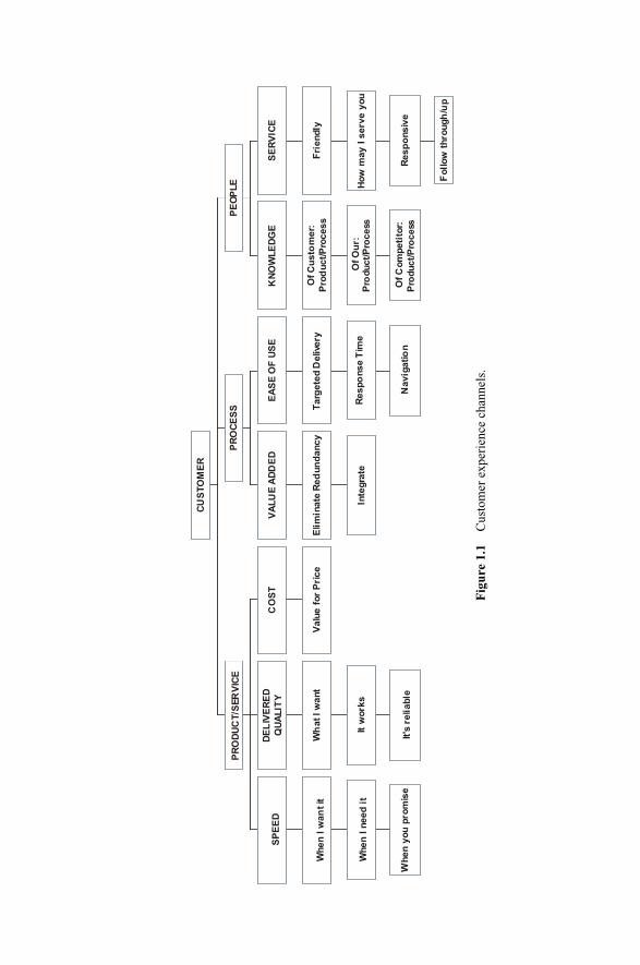
If we look at Figure 1.1, we can see that customers experience service in threeways:
2 SERVICE DESIGN
Table 1.1 Examples of organizational functions
Marketing Sales Human Design� Brand Management � Discovery Resources � Change Control� Prospect � Account � Staffing � New Product
Management � Training
Production Control Sourcing Information Finance� Inventory Control � Commodity Technology � Accounts Payable� Scheduling � Purchasing � Help Desk � Accounts Receivable
� Training
c01.qxd 4/22/2005 7:31 AM Page 2
Wh
en
yo
u p
rom
ise
When
I n
eed
it
When
I w
an
t it
SP
EE
D
It's
reliable
It w
ork
s
Wh
at I
want
DE
LIV
ER
ED
QU
ALIT
Y
Valu
e f
or
Pri
ce
CO
ST
PR
OD
UC
T/S
ER
VIC
E
Inte
gra
te
Elim
inate
Red
un
dancy
VA
LU
E A
DD
ED
Navig
atio
n
Resp
onse T
ime
Targ
ete
d D
elive
ry
EA
SE
OF U
SE
PR
OC
ES
S
Of C
om
peti
tor:
Pro
duct/P
rocess
Of O
ur:
Pro
duct/P
rocess
Of C
usto
mer:
Pro
duct/P
rocess
KN
OW
LE
DG
E
Foll
ow
th
rough
/up
Resp
onsiv
e
How
may I s
erv
e y
ou
Fri
endly
SE
RV
ICE
PE
OP
LE
CU
STO
ME
R
Fig
ure
1.1
Cus
tom
er e
xper
ienc
e ch
anne
ls.
c01.qxd 4/22/2005 7:31 AM Page 3
1. The specific service or product has attributes such as availability, it’s what Iwanted, and it works.
2. The process through which the service is delivered can be ease of use or val-ue added.
3. The people (or system) should be knowledgeable and friendly.
To fulfill these needs, there is a service life cycle to which we apply a quality op-erating system.
1.3 QUALITY OPERATING SYSTEM AND SERVICE LIFE CYCLE
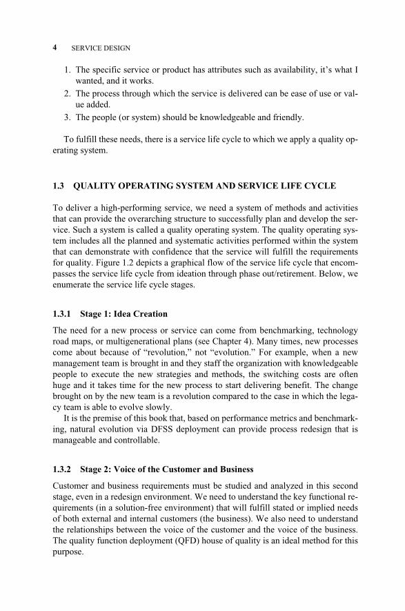
To deliver a high-performing service, we need a system of methods and activitiesthat can provide the overarching structure to successfully plan and develop the ser-vice. Such a system is called a quality operating system. The quality operating sys-tem includes all the planned and systematic activities performed within the systemthat can demonstrate with confidence that the service will fulfill the requirementsfor quality. Figure 1.2 depicts a graphical flow of the service life cycle that encom-passes the service life cycle from ideation through phase out/retirement. Below, weenumerate the service life cycle stages.
1.3.1 Stage 1: Idea Creation
The need for a new process or service can come from benchmarking, technologyroad maps, or multigenerational plans (see Chapter 4). Many times, new processescome about because of “revolution,” not “evolution.” For example, when a newmanagement team is brought in and they staff the organization with knowledgeablepeople to execute the new strategies and methods, the switching costs are oftenhuge and it takes time for the new process to start delivering benefit. The changebrought on by the new team is a revolution compared to the case in which the lega-cy team is able to evolve slowly.
It is the premise of this book that, based on performance metrics and benchmark-ing, natural evolution via DFSS deployment can provide process redesign that ismanageable and controllable.
1.3.2 Stage 2: Voice of the Customer and Business
Customer and business requirements must be studied and analyzed in this secondstage, even in a redesign environment. We need to understand the key functional re-quirements (in a solution-free environment) that will fulfill stated or implied needsof both external and internal customers (the business). We also need to understandthe relationships between the voice of the customer and the voice of the business.The quality function deployment (QFD) house of quality is an ideal method for thispurpose.
4 SERVICE DESIGN
c01.qxd 4/22/2005 7:31 AM Page 4

1.3.3 Stage 3: Concept Development
Concept development is the third stage in the service life cycle. In this stage, con-cepts are developed that fulfill the functional requirements obtained from the previ-ous stage. This stage of the life cycle process is still at a high level and remains so-lution free; that is, the design team is able to specify “what needs to beaccomplished to satisfy the customer wants” and not “how to accomplish thesewants.” The strategy of the design team is to create several innovative concepts anduse selection methodologies to narrow down the choices. At this stage, we canhighlight the Pugh concept selection method (Pugh, 1996) as summarized in Figure1.3.
The method of “controlled convergence” was developed by Dr. Stuart Pugh(Pugh, 1991) as part of his solution selection process. Controlled convergence is asolution-iterative selection process that allows alternate convergent (analytic) anddivergent (synthetic) thinking to be experienced by the service design team. Themethod alternates between generation and convergence selection activities.
1.3 QUALITY OPERATING SYSTEM AND SERVICE LIFE CYCLE 5
Figure 1.2 Service life cycle. (See Yang and El-Haik (2003) for the product life cycleequivalent.)
Stage 1: Idea Creation
Stage 2: Voice of the Customer &
Business
Stage 3: Concept Development
Stage 4: Preliminary Design
Stage 5: Design Optimization
Stage 6: Verification
Stage 7: Launch Readiness
Stage 8: Production
Stage 9: Service Consumption
Stage 10: Phase Out
c01.qxd 4/22/2005 7:31 AM Page 5
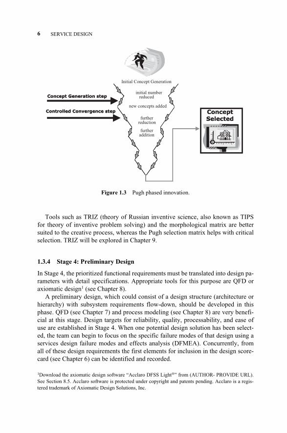
Tools such as TRIZ (theory of Russian inventive science, also known as TIPSfor theory of inventive problem solving) and the morphological matrix are bettersuited to the creative process, whereas the Pugh selection matrix helps with criticalselection. TRIZ will be explored in Chapter 9.
1.3.4 Stage 4: Preliminary Design
In Stage 4, the prioritized functional requirements must be translated into design pa-rameters with detail specifications. Appropriate tools for this purpose are QFD oraxiomatic design1 (see Chapter 8).
A preliminary design, which could consist of a design structure (architecture orhierarchy) with subsystem requirements flow-down, should be developed in thisphase. QFD (see Chapter 7) and process modeling (see Chapter 8) are very benefi-cial at this stage. Design targets for reliability, quality, processability, and ease ofuse are established in Stage 4. When one potential design solution has been select-ed, the team can begin to focus on the specific failure modes of that design using aservices design failure modes and effects analysis (DFMEA). Concurrently, fromall of these design requirements the first elements for inclusion in the design score-card (see Chapter 6) can be identified and recorded.
6 SERVICE DESIGN
Figure 1.3 Pugh phased innovation.
Concept Generation step
Controlled Convergence step ConceptSelected
Initial Concept Generation
initial number
reduced
new concepts added
further
reduction
further
addition
Concept Generation step
Controlled Convergence step ConceptSelected
1Download the axiomatic design software “Acclaro DFSS Light®” from (AUTHOR- PROVIDE URL).See Section 8.5. Acclaro software is protected under copyright and patents pending. Acclaro is a regis-tered trademark of Axiomatic Design Solutions, Inc.
c01.qxd 4/22/2005 7:31 AM Page 6
1.3.5 Stage 5: Design Optimization
In stage 5, the design team will make sure the final design matches the customer re-quirements that were originally identified in Stage 2 (capability flow-up to meet thevoice of the customer). There are techniques [DFx (see Chapter 10), Poka Yoke(see Chapter 10), FMEA (see Chapter 11)] that can be used at this point to ensurethat the design cannot be used in a way that was not intended, processed or main-tained incorrectly, or that if there is a mistake it will be immediately obvious.
A final test plan is generated in order to assure that all requirements are met atthe Six Sigma level by the pilot or prototype that is implemented or built in the nextstage.
In Stage 5, detail designs are formulated and tested either physically or throughsimulation. Functional requirements are flowed down from the system level intosubsystem design parameters using transfer functions (see Chapter 6), process mod-eling (see Chapter 8), and design of experiments (see Chapter 12). Designs aremade robust to withstand the “noise” introduced by external uncontrollable factors(see Chapter 13). All of the activities in Stage 5 should result in a design that can beproduced in a pilot or prototype form.
1.3.6 Stage 6: Verification
Test requirements and procedures are developed and the pilot is implementedand/or the prototype is built in this stage. The pilot is run in as realistic a setting aspossible with multiple iterations and subjected to as much “noise” as possible in anenvironment that is as close to its final usage conditions as possible. The same phi-losophy applies to the testing of a prototype. The prototype should be tested at theextremes of its intended envelope and sometimes beyond. To the extent possible orallowed by regulation, simulation should replace as much testing as is feasible inorder to reduce cost and risk.
The results of pilot or prototype testing allow the design team the opportunity tomake final adjustments or changes in the design to ensure that product, service, orbusiness process performance is optimized to match customer expectations.
In some cases, only real-life testing can be performed. In this situation, design ofexperiments is an efficient way to determine if the desired impact is created andconfirmed.
1.3.7 Stage 7: Launch Readiness
Based on successful verification in a production environment, the team will assessthe readiness of all of the process infrastructure and resources. For instance, haveall standard operating procedures been documented and people been trained in theprocedures? What is the plan for process switch-over or ramp-up? What contingen-cies are in place? What special measures will be in place to ensure rapid discovery?Careful planning and understanding the desired behavior is paramount to successfultransition from the design world into the production environment.
1.3 QUALITY OPERATING SYSTEM AND SERVICE LIFE CYCLE 7
c01.qxd 4/22/2005 7:31 AM Page 7
1.3.8 Stage 8: Production
In this stage, if the team has not already begun implementation of the design solu-tion in the production or service environment, the team should do so now. Valida-tion of some services or business processes may involve approval by regulatoryagencies (e.g., approval of quality systems) in addition to your own rigorous assess-ment of the design capability. Appropriate controls are implemented to ensure thatthe design continues to perform as expected and anomalies are addressed as soon asthey are identified (update the FMEA) in order to eliminate waste, reduce variation,and further error-proof the design and any associated processes.
1.3.9 Stage 9: Service Consumption
Whether supporting the customers of the service with help lines or the productionprocesses, which themselves need periodic maintenance (e.g., toner cartridges in aprinter or money in an ATM), the support that will be required and how to provideit are critical in maintaining Six Sigma performance levels. Understanding the totallife cycle of the service consumption and support are paramount to planning ade-quate infrastructure and procedures.
1.3.10 Stage 10: Phase-Out
Eventually, all products and services become obsolete and are either replaced bynew technologies or new methods. Also, the dynamic and cyclical nature of cus-tomer attributes dictates continuous improvement to maintain adequate marketshare. Usually, it is difficult to turn off the switch, as many customers have differentdependencies on services and processes. Just look at the bank teller and the ATMmachine. One cannot just convert to a single new process. There must be a coordi-nated effort, and often change management is required to provide incentives forcustomers to shift to the new process. In terms of electronic invoicing, a discountmay be offered for use of the electronic means or an extra charge imposed for thenonstandard method.
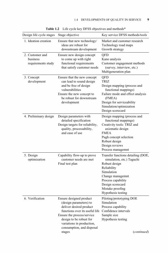
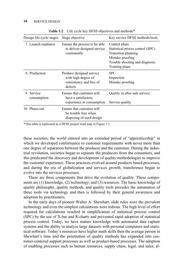
1.3.11 Service Life Cycle and Quality Operating System
The service life cycle is depicted in Figure 1.2. In addition, Table 1.2 highlights thekey DFSS tools and objectives of service life cycle stages. The DFSS topics in thisbook span the first seven phases of the life cycle. Opportunities still exist for appli-cation in the remainder of the stages; however, the first seven have the highest po-tential life cycle impact.
1.4 DEVELOPMENTS OF QUALITY IN SERVICE
The earliest societies—Egyptians, Mayans, and Aztecs—provide archeological evi-dence of precision and accuracy nearly unmatched today. Following the example of
8 SERVICE DESIGN
c01.qxd 4/22/2005 7:31 AM Page 8
1.4 DEVELOPMENTS OF QUALITY IN SERVICE 9
Table 1.2 Life cycle key DFSS objectives and methods*
Design life cycle stages Stage objective Key service DFSS methods/tools
1. Ideation creation Ensure that new technology/ Market and customer researchideas are robust for Technology road mapsdownstream development Growth strategy
2. Customer and Ensure new design concept QFDbusiness to come up with right Kano analysisrequirements study functional requirements Customer engagement methods
that satisfy customer needs (survey, interview, etc.)Multigeneration plan
3. Concept Ensure that the new concept QFDdevelopment can lead to sound design TRIZ
and be free of design Design mapping (process andvulnerabilities functional mappings)
Ensure the new concept to Failure mode and effect analysis be robust for downstream (FMEA)development Design for serviceability
Simulation/optimizationDesign scorecard
4. Preliminary design Design parameters with Design mapping (process and detailed specification functional mappings)
Design targets for reliability, Creativity tools: TRIZ and quality, processability, axiomatic designand ease of use FMEA
Pugh concept selectionRobust designDesign reviewsProcess managemnt
5. Design Capability flow-up to prove Transfer functions detailing (DOE,optimization customer needs are met simulation, etc.) Taguchi
Final test plan Robust designReliabilitySimulationChange managemntProcess capabilityDesign scorecardMistake proofingHypothesis testing
6. Verification Ensure designed product Piloting/prototyping DOE(design parameters) to Simulationdeliver desired product Process capabilityfunctions over its useful life Confidence intervals
Ensure the process/service Sample sizedesign to be robust for Hypothesis testingvariations in production,consumption, and disposalstages (continued)
c01.qxd 4/22/2005 7:31 AM Page 9
these societies, the world entered into an extended period of “apprenticeship” inwhich we developed conformance to customer requirements with never more thanone degree of separation between the producer and the customer. During the indus-trial revolution, societies began to separate the producers from the consumers, andthis predicated the discovery and development of quality methodologies to improvethe customer experience. These practices evolved around products based processes,and during the era of globalization and services growth, transference began toevolve into the services processes.
There are three components that drive the evolution of quality. These compo-nents are (1) knowledge, (2) technology, and (3) resources. The basic knowledge ofquality philosophy, quality methods, and quality tools precedes the automation ofthese tools via technology and then is followed by their general awareness andadoption by practitioners.
In the early days of pioneer Walter A. Shewhart, slide rules were the prevalenttechnology and even the simplest calculations were tedious. The high level of effortrequired for calculations resulted in simplification of statistical process control(SPC) by the use of X-bar and R-charts and prevented rapid adoption of statisticalprocess control. Today, we have mature knowledge with automated data capturesystems and the ability to analyze large datasets with personal computers and statis-tical software. Today’s resources have higher math skills then the average person inShewhart’s time and the penetration of quality methods has expanded into cus-tomer-centered support processes as well as product-based processes. The adoptionof enabling processes such as human resources, supply chain, legal, and sales, al-
10 SERVICE DESIGN
Table 1.2 Life cycle key DFSS objectives and methods*
Design life cycle stages Stage objective Key service DFSS methods/tools
7. Launch readiness Ensure the process to be able Control plansto deliver designed service Statistical proces control (SPC)consistently Transition planning
Mistake proofingTrouble shooting and diagnosisTraining plans
8. Production Produce designed service SPCwith high degree of Inspectionconsistency and free of Mistake proofingdefects
9. Service Ensure that customer will Quality in after-sale serviceconsumption have a satisfactory
experience in consumption Service quality
10 Phase-out Ensure that customer will be trouble free whendisposing of used design
*This table is replicated as a DFSS project road map in Figure 5.1.
c01.qxd 4/22/2005 7:31 AM Page 10
though analogous to customer-centered processes, is weak due to a perceived costbenefit deficit and a lack of process-focused metrics in these processes.
Let us look at an abbreviated chronological review of some of the pioneers whoadded much to our knowledge of quality. Much of the evolution of quality has oc-curred in the following five disciplines:
1. Statistical analysis and control
2. Root cause analysis
3. Total quality management
4. Design quality
5. Process simplification
The earliest evolution began with statistical analysis and control, so we start ourchronology there.
1.4.1 Statistical Analysis and Control
In 1924, Walter A. Shewhart introduced the first application of control charting tomonitor and control important production variables in a manufacturing process.This charting method introduced the concepts of special cause and common causevariation. He developed his concepts and published Economic Control of Quality ofManufactured Product in 1931, which successfully brought together the disciplinesof statistics, engineering, and economics, and with this book, Shewhart becameknown as the father of modern quality control. Shewhart also introduce the plan-do-study-act cycle (Shewhart cycle) later made popular by Deming as the PDCA cycle.
In 1925, Sir Ronald Fisher published the book, Statistical Methods for ResearchWorkers (Fisher, 1925), and introduced the concepts of randomization and theanalysis of variance (ANOVA). Later in 1925 he wrote Design of Experiments(DOE). Frank Yates was an associate of Fisher and contributed the Yates standardorder for ANOVA calculations. In 1950, Gertrude Cox and William Cochran coau-thored Experimental Design, which became the standard of the time. In Japan, Dr.Genechi Taguchi introduced orthogonal arrays as an efficient method for conduct-ing experimentation within the context of robust design. He followed this up in1957 with his book, Design of Experiments. Taguchi robustness methods have beenused in product development since the 1980s. In 1976, Dr. Douglas Montgomerypublished Design and Analysis of Experiments. This was followed by George Box,William Hunter, and Stuart Hunter’s Statistics for Experimenters in 1978.
1.4.2 Root Cause Analysis
In 1937, Joseph Juran introduced the Pareto principle as a means of narrowing in onthe vital few. In 1943, Kaoru Ishikawa developed the cause and effect diagram, alsoknown as the fishbone diagram. In 1949, the use of multivari charts was promotedfirst by Len Seder of Gillette Razors and then service marked by Dorian Shainin,
1.4 DEVELOPMENTS OF QUALITY IN SERVICE 11
c01.qxd 4/22/2005 7:31 AM Page 11

who added it to his Red X toolbox, which became the Shainin techniques from 1951through 1975. Root cause analysis as known today relies on seven basic tools: thecause and effect diagram, check sheet, control chart (special cause verses commoncause), flowchart, histogram, Pareto chart, and scatter diagram.
1.4.3 Total Quality Management/Control
The integrated philosophy and organizational alignment for pursuing the deploy-ment of quality methodologies is often referred to as total quality management. Thelevel of adoption has often been directly related to the tools and methodologies ref-erenced by the thought leaders who created the method and tools as well as the per-ceived value of adopting these methods and tools. Dr. Armand V. Feigenbaum pub-lished Total Quality Control while still at MIT pursuing his doctorate in 1951. Helater became the head of quality for General Electric and interacted with Hitachiand Toshiba. His pioneering effort was associated with the translation into Japaneseof his 1951 book, Quality Control: Principles, Practices and Administration, andhis articles on total quality control.
Joseph Juran followed closely in 1951 with the Quality Control Handbook, themost comprehensive “how-to” book on quality ever published. At this time, Dr W.Edwards Deming was gaining fame in Japan following his work for the U.S. gov-ernment in the Census Bureau developing survey statistics, and published his mostfamous work, Out of the Crisis, in 1968. Dr. Deming was associated with WalterShewhart and Sir Ronald Fisher and has become the most notable TQM proponent.Deming’s basic quality philosophy is that productivity improves as variability de-creases, and that statistical methods are needed to control quality. He advocated theuse of statistics to measure performance in all areas, not just conformance to designspecifications. Furthermore, he thought that it is not enough to meet specifications;one has to keep working to reduce the variations as well. Deming was extremelycritical of the U.S. approach to business management and was an advocate of work-er participation in decision making. Later, Kaoru Ishikawa gained notice for his de-velopment of “quality circles” in Japan and published the Guide to Quality Controlin 1968. The last major pioneer is Philip Crosby, who published Quality is Free in1979, in which he focused on the “absolutes” of quality, the basic elements of im-provement, and the pursuit of “Zero Defects.”
1.4.4 Design Quality
Design quality includes philosophy and methodology. The earliest contributor inthis field was the Russian Genrich Altshuller, who provided us with the theory ofinventive problem sSolving (TIPS or TRIZ) in 1950. TRIZ is based on inventiveprinciples derived from the study of over 3.5 million of the world’s most innovativepatents and inventions. TRIZ provides a revolutionary new way of systematicallysolving problems based on science and technology. TRIZ helps organizations usethe knowledge embodied in the world’s inventions to quickly, efficiently, and cre-atively develop “elegant” solutions to their most difficult design and engineering
12 SERVICE DESIGN
c01.qxd 4/22/2005 7:31 AM Page 12
problems. The next major development was the quality function deployment (QFD)concept, promoted in Japan by Dr. Yoji Akao and Shigeru Mizuno in 1966 but notwesternized until the 1980s. Their purpose was to develop a quality assurancemethod that would design customer satisfaction into a product before it was manu-factured. Prior quality control methods were primarily aimed at fixing a problemduring or after manufacturing. QFD is a structured approach to defining customerneeds or requirements and translating them into specific plans to produce productsor services to meet those needs. The “voice of the customer” is the term used to de-scribe these stated and unstated customer needs or requirements.
In the 1970s Dr. Taguchi promoted the concept of the quality loss function,which stated that any deviation from nominal was costly and that designing with thenoise of the system the product would operate within, one could optimize designs.Taguchi packaged his concepts in the methods named after him, also called robustdesign or quality engineering.
The last major development in design quality was by Dr. Nam P. Suh, who for-mulated the approach of axiomatic design. Axiomatic design is a principle-basedmethod that provides the designer with a structured approach to design tasks. In theaxiomatic design approach, the design is modeled as mapping between different do-mains. For example, in the concept design stage, it could be a mapping betweencustomer attribute domains to design the function domain; in the product designstage, it is a mapping from function domain to design parameter domain. There aremany possible design solutions for the same design task. However, based on its twofundamental axioms, the axiomatic design method developed many design princi-ples to evaluate and analyze design solutions and give designers directions to im-prove designs. The axiomatic design approach not only can be applied in engineer-ing design, but also in other design tasks such as organization systems.
1.4.5 Process Simplification
Lately, “lean” is the topic of interest. The pursuit of the elimination of waste has ledto several quality improvements. The earliest development in this area was “pokayoke” (mistake proofing), developed by Shigeo Shingo in Japan in 1961. The es-sential idea of poka-yoke is to design processes in a way that mistakes are impossi-ble to make or at least easily detected and corrected. Poka-yoke devices fall intotwo major categories: prevention and detection. A prevention device affects theprocess in such a way that it is impossible to make a mistake. A detection devicesignals the user when a mistake has been made, so that the user can quickly correctthe problem. Shingo later developed the single minute exchange of die (SMED) in1970. This trend has also seen more of a system-wide process mapping and valueanalysis, which has evolved into value stream maps.
1.4.6 Six Sigma and Design For Six Sigma (DFSS)
The initiative known as Six Sigma follows in the footstep of all of the above. SixSigma was conceptualized and introduced by Motorola in the early 1980s. It spread
1.4 DEVELOPMENTS OF QUALITY IN SERVICE 13
c01.qxd 4/22/2005 7:31 AM Page 13
to Texas Instruments and Asea Brown Boveri before Allied Signal and then to GEin 1995. It was enabled by the emergence of the personal computer and statisticalsoftware packages such as Minitab™, SAS™, BMDP™, and SPSS™. It combineseach of the elements of process management and design. The define-measure-ana-lyze-improve-control (DMAIC) and design for six sigma (DFSS) processes will bediscussed in detail in Chapter 2 and Chapter 3, respectively.
1.5 BUSINESS EXCELLENCE: A VALUE PROPOSITION?
At the highest level, business excellence is characterized by good profitability,business viability, and growth in sales and market share, based on quality (Peters,1982). Achieving business excellence is the common goal for all business leadersand their employees. To achieve business excellence, design quality by itself is notsufficient; quality has to be replaced by “whole quality,” which includes quality inbusiness operations such as those in Table 1.1. We will see this in our explorationof supply chain design throughout the book. To understand business excellence, weneed to understand business operations and other metrics in business operations,which we cover in the next section.
1.5.1 Business Operation Model
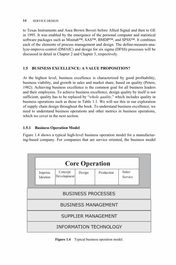
Figure 1.4 shows a typical high-level business operation model for a manufactur-ing-based company. For companies that are service oriented, the business model
14 SERVICE DESIGN
Figure 1.4 Typical business operation model.
BUSINESS PROCESSES
BUSINESS MANAGEMENT
SUPPLIER MANAGEMENT
INFORMATION TECHNOLOGY
Core Operation
Impetus
Ideation
Concept
Development
Design Production Sales/
Service
c01.qxd 4/22/2005 7:31 AM Page 14
could look somewhat different. However, for every company, there is always a“core operation” and a number of other enabling business elements. The core oper-ation is the collection of all activities (processes and actions) used to provide ser-vice designs to customers. For example, the core operation of Federal Express is todeliver packages around the world, and the core operation of Starbucks is to providecoffee service all over the world. Core operations extend across all activities in theservice design life cycle.
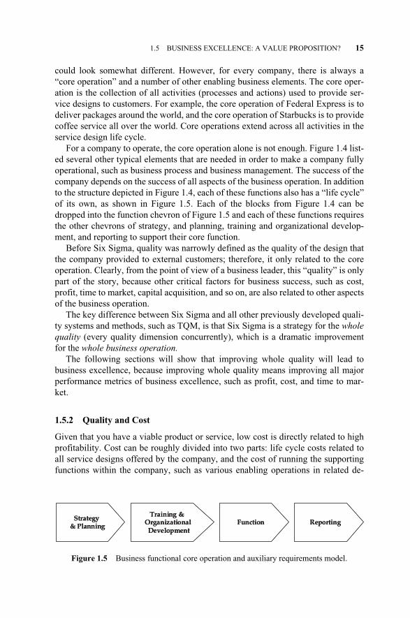
For a company to operate, the core operation alone is not enough. Figure 1.4 list-ed several other typical elements that are needed in order to make a company fullyoperational, such as business process and business management. The success of thecompany depends on the success of all aspects of the business operation. In additionto the structure depicted in Figure 1.4, each of these functions also has a “life cycle”of its own, as shown in Figure 1.5. Each of the blocks from Figure 1.4 can bedropped into the function chevron of Figure 1.5 and each of these functions requiresthe other chevrons of strategy, and planning, training and organizational develop-ment, and reporting to support their core function.
Before Six Sigma, quality was narrowly defined as the quality of the design thatthe company provided to external customers; therefore, it only related to the coreoperation. Clearly, from the point of view of a business leader, this “quality” is onlypart of the story, because other critical factors for business success, such as cost,profit, time to market, capital acquisition, and so on, are also related to other aspectsof the business operation.
The key difference between Six Sigma and all other previously developed quali-ty systems and methods, such as TQM, is that Six Sigma is a strategy for the wholequality (every quality dimension concurrently), which is a dramatic improvementfor the whole business operation.
The following sections will show that improving whole quality will lead tobusiness excellence, because improving whole quality means improving all majorperformance metrics of business excellence, such as profit, cost, and time to mar-ket.
1.5.2 Quality and Cost
Given that you have a viable product or service, low cost is directly related to highprofitability. Cost can be roughly divided into two parts: life cycle costs related toall service designs offered by the company, and the cost of running the supportingfunctions within the company, such as various enabling operations in related de-
1.5 BUSINESS EXCELLENCE: A VALUE PROPOSITION? 15
Figure 1.5 Business functional core operation and auxiliary requirements model.
Strategy& Planning
Training & OrganizationalDevelopment
Function ReportingStrategy
& Planning
Training & OrganizationalDevelopment
Function Reporting
c01.qxd 4/22/2005 7:31 AM Page 15
partments. For a particular product or service, life cycle cost includes production/service cost plus the cost for design development.
The relationship between quality and cost is rather complex; the “quality” in thiscontext is referred to as the design quality, not the whole quality. This relationshipis very much dependent on what kind of quality strategy is adopted by a particularcompany. If a company adopted a quality strategy heavily focused on the down-stream part of the design life cycle, that is, fire fighting, rework, and error correc-tions, then that “quality” is going to be very costly. If a company adopted a strategyemphasizing upstream improvement and problem prevention, then improving qual-ity could actually reduce the life cycle cost because there will be less rework, lessrecall, less fire fighting, and, therefore, less design development cost. In the service-based company, it may also mean fewer complaints, higher throughput, and higherproductivity. For more discussion on this topic, see Chapter 3 of Yang & El-Haik(2003).
If we define quality as the “whole quality,” then higher whole quality will defi-nitely mean lower total cost. Because whole quality means higher performance lev-els of all aspects of the business operation, it means high performance of all sup-porting functions, high performance of the production system, less waste, andhigher efficiency. Therefore, it will definitely reduce business operation cost, pro-duction cost, and service cost without diminishing the service level to the customer.
1.5.3 Quality and Time to Market
Time to market is the time required to introduce new or improved products and ser-vices to the market. It is a very important measure for competitiveness in today’smarketplace. If two companies provide similar designs with comparable functionsand price, the company with the faster time to market will have a tremendous com-petitive position. The first company to reach the market benefits from a psychologi-cal effect that will be very difficult to be matched by latecomers.
There are many techniques to reduce time to market, such as:
� Concurrency: encouraging multitasking and parallel working
� Complexity reduction (see Suh (2001) and El-Haik (2005))
� Project management: tuned for design development and life cycle manage-ment
In the Six Sigma approach and whole quality concept, improving the quality ofmanaging the design development cycle is a part of the strategy. Therefore, improv-ing whole quality will certainly help to reduce time to market.
1.6 INTRODUCTION TO THE SUPPLY CHAIN
Supply chain can mean many things to many different businesses and may be calledsourcing, full supply chain, or integrated supply chain. The function of the supply
16 SERVICE DESIGN
c01.qxd 4/22/2005 7:31 AM Page 16
chain is integral to every organization and process, as resource planning and acqui-sition are pertinent whether applied to people, materials, information, or infrastruc-ture. How often do we find ourselves asking, should I buy or make whatever weneed or provide? Even in staffing and recruiting activities, we question whether topurchase the services of an outside recruiter or hire our own staff. What type ofworkload will there be? Where will we store the resumes and interview results? Dowe source the applicant screening?
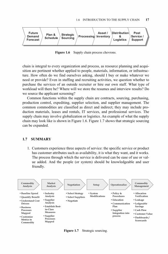
Common functions within the supply chain are contracts, sourcing, purchasing,production control, expediting, supplier selection, and supplier management. Thecommon commodities are classified as direct and indirect; they may include pro-duction materials, leases and rentals, IT services, and professional services. Thesupply chain may involve globalization or logistics. An example of what the supplychain may look like is shown in Figure 1.6. Figure 1.7 shows that strategic sourcingcan be expanded.
1.7 SUMMARY
1. Customers experience three aspects of service: the specific service or producthas customer attributes such as availability, it is what they want, and it works.The process through which the service is delivered can be ease of use or val-ue added. And the people (or system) should be knowledgeable and userfriendly.
1.6 INTRODUCTION TO THE SUPPLY CHAIN 17
Figure 1.6 Supply chain process chevrons.
FutureDemandForecast
Plan & Schedule
StrategicSourcing
ProcessingAsset /
InventoryMgmt
Distribution&
Logistics
Post Service /Support
FutureDemandForecast
Plan & Schedule
StrategicSourcing
ProcessingAsset /
InventoryMgmt
Distribution&
Logistics
Post Service /Support
Figure 1.7 Strategic sourcing.
CommodityCommodityAnalysisAnalysis
MarketMarketAnalysisAnalysis
NegotiationNegotiation SetupSetupCommodityCommodityManagementManagement
OperationalizeOperationalize
• Industry Analysis
• Supplier Analysis
• Establish Best-
in-Class Measures
• Supplier Processes Mapped
• Baseline Spend
• Quantify Benefit
• Understand Cost Drivers
• Business Processes
Mapped
• Customize Metrics to Commodity
• Select Strategy
• Select Suppliers
• Negotiate
• System Modifications
• Policy & Procedures
• Education
• Communication Plan
• Supplier
Integration into process
• Allocation Verification
• Leakage
• Ledgerable Savings
• Cash Flow
• Customer Value
• Dashboards /
Scorecards
c01.qxd 4/22/2005 7:31 AM Page 17

2. Quality assurance and service life cycle are not the result of happenstance,and the best way to ensure customer satisfaction is to adhere to a process thatis enabled by tools and methodologies aimed at preventing defects rather thancorrecting them.
3. Quality has evolved over time from the early 1920s, when Shewhart intro-duced the first control chart, through the transformation of Japan in the1950s, to the late 1980s when Six Sigma first came on the scene. Six Sigmaand “lean” have now been merged and enabled by personal computers andstatistical software to provide easy-to-use and high-value methodologies toeliminate waste and reduce variation, both on new designs as well as existingprocesses, in order to fulfill customer requirements.
4. The supply chain is applicable to every business function, so using it as anexample for design for Six Sigma (as an objective) should allow every practi-tioner to leverage the application of design for Six Sigma (DFSS as aprocess).
We will next explore Six Sigma fundamentals in Chapter 2.
18 SERVICE DESIGN
c01.qxd 4/22/2005 7:31 AM Page 18
2.1 INTRODUCTION
In this chapter, we will provide an overview of Six Sigma and its development, aswell as the traditional deployment for process/product improvement called DMA-IC, and three components of the methodology. We will also introduce the designapplication, which will be detailed in Chapter 3 and beyond.
2.2 WHAT IS SIX SIGMA?
Six Sigma is a philosophy, a measure, and a methodology that provides businesseswith the perspective and tools to achieve new levels of performance both in servicesand products. In Six Sigma, the focus is on process improvement to increase capa-bility and reduce variation. The vital few inputs are chosen from the entire systemof controllable and noise variables and the focus of improvement is on controllingthese vital few inputs.
Six Sigma as a philosophy helps companies believe that very low defects permillion opportunities over long-term exposure is achievable. Six Sigma gives us astatistical scale to measure our progress and benchmark other companies, process-es, or products. The defect per million opportunities measurement scale rangesfrom zero to one million, whereas the sigma scale ranges from 0 to 6. The method-ologies used in Six Sigma, which will be discussed in more detail in the followingchapters, build upon all of the tools that have evolved to date but puts them into adata-driven framework. This framework of tools allows companies to achieve thelowest defects per million opportunities possible.
Six Sigma evolved from the early TQM efforts mentioned in Chapter 1. Motoro-la initiated the movement and then it spread to Asea Brown Boveri, Texas Instru-
Service Design for Six Sigma. By Basem El-Haik and David M. Roy 19© 2005 by John Wiley & Sons.
2WHAT IS SIX SIGMA?
c02.qxd 4/22/2005 7:33 AM Page 19
ments Missile Division, and Allied Signal. It was at this juncture that Jack Welchlearned from Larry Bossidy of the power of Six Sigma and with a convert’s zealcommitted GE to embracing the movement. It was GE that bridged the gap betweenjust a manufacturing process and product focus and took it to what was first calledtransactional processes and later commercial processes. One of the reasons thatWelch was so interested in this program was that an employee survey had just beencompleted and it revealed that the top-level managers of the company believed thatGE had invented quality. After all, Armand Feigenbaum worked at GE. However,the vast majority of employees did not think GE could spell quality. Six Sigma hasturned out to be the methodology to accomplish Crosby’s goal of zero defects. Un-derstanding what the key process input variables are and that variation and shift canoccur, we can create controls that maintain Six Sigma, or 6� for short, performanceon any product or service and in any process. The Greek letter � is used by statisti-cians to indicate standard deviation, a statistical parameter, of the population of in-terest. Before we can clearly understand the process inputs and outputs, we need tounderstand process modeling.
2.3 INTRODUCTION TO PROCESS MODELING
Six Sigma is a process-focused approach to achieving new levels of performancethroughout any business or organization. We need to focus on a process as a systemof inputs, activities, and output(s) in order to provide a holistic approach to all thefactors and the way they interact together to create value or waste. Many productsand services, when used in a productive manner, are also processes. An ATM ma-chine takes your account information, personal identification number, energy, andmoney and processes a transaction that dispenses funds or an account rebalance. Acomputer can take keystroke inputs, energy, and software to process bits into aWord document. At the simplest level, the process model can be represented by aprocess diagram, often called an IPO diagram, for input–process–output (Figure2.1).
If we take the IPO concept and extend the ends to include the suppliers of the in-puts and the customers of the outputs, then we have the SIPOC, which stands forsupplier-input–process–output–customer (Figure 2.2). This is a very effective toolfor gathering information and modeling any process. A SIPOC tool can take theform of a table, with a column per each category.
2.3.1 Process Mapping
Whereas the SIPOC is a linear flow of steps, process mapping is a means of dis-playing the relationship between process steps, and allows for the display of variousaspects of the process including delays, decisions, measurements, and rework anddecision loops. Process mapping builds upon the SIPOC information by using stan-dard symbols to depict varying aspects of the processes flow linked together withlines and arrows demonstrating the direction of flow.
20 WHAT IS SIX SIGMA?
c02.qxd 4/22/2005 7:33 AM Page 20
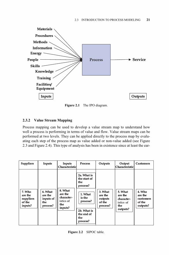
2.3.2 Value Stream Mapping
Process mapping can be used to develop a value stream map to understand howwell a process is performing in terms of value and flow. Value stream maps can beperformed at two levels. They can be applied directly to the process map by evalu-ating each step of the process map as value added or non-value added (see Figure2.3 and Figure 2.4). This type of analysis has been in existence since at least the ear-
2.3 INTRODUCTION TO PROCESS MODELING 21
Process
Inputs Outputs
Materials
Procedures
Methods
Information
Energy
People
Skills
Knowledge
Training
Facilities/Equipment
ServiceProcess
Inputs Outputs
Materials
Procedures
Methods
Information
Energy
People
Skills
Knowledge
Training
Facilities/Equipment
Service
Figure 2.1 The IPO diagram.
Inputs InputsCharacteristic
Process Outputs OutputCharacteristic
Suppliers Customers
1. What is the process?
2a. What is the start of the process?
2b. What is the end of the process?
3. What are the outputs of the process?
4. Who are the customers of the outputs?
5. What are the
the outputs?
7. Who are the suppliers of the inputs?
8. What are the character-
the inputs?
6. What are the inputs of the process?
Inputs InputsCharacteristic
Process Outputs OutputCharacteristic
Suppliers Customers
1. What is the process?
2a. What is the start of the process?
2b. What is the end of the process?
3. What are the outputs of the process?
4. Who are the customers of the outputs?
5. What are the
the outputs?
7. Who are the suppliers of the inputs?
8. What are the characteisticsthe inputs?
6. What are the inputs of the process?
character-characteistics of
of
Figure 2.2 SIPOC table.
c02.qxd 4/22/2005 7:33 AM Page 21
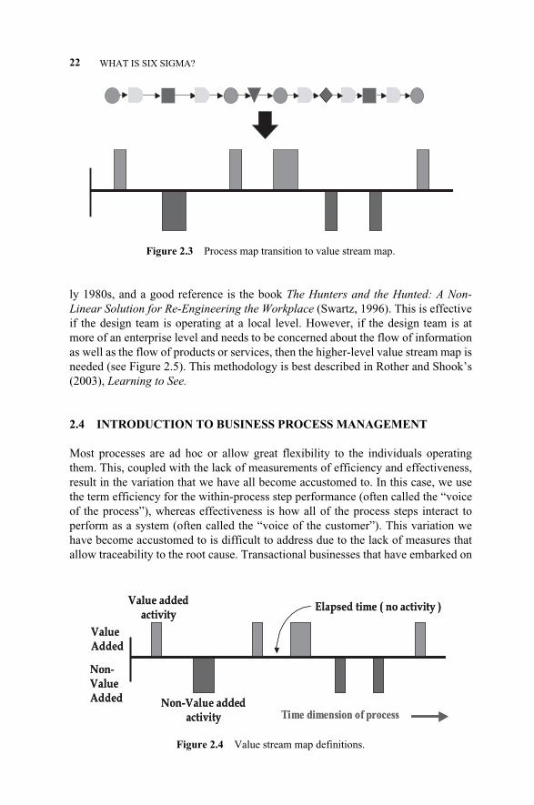
ly 1980s, and a good reference is the book The Hunters and the Hunted: A Non-Linear Solution for Re-Engineering the Workplace (Swartz, 1996). This is effectiveif the design team is operating at a local level. However, if the design team is atmore of an enterprise level and needs to be concerned about the flow of informationas well as the flow of products or services, then the higher-level value stream map isneeded (see Figure 2.5). This methodology is best described in Rother and Shook’s(2003), Learning to See.
2.4 INTRODUCTION TO BUSINESS PROCESS MANAGEMENT
Most processes are ad hoc or allow great flexibility to the individuals operatingthem. This, coupled with the lack of measurements of efficiency and effectiveness,result in the variation that we have all become accustomed to. In this case, we usethe term efficiency for the within-process step performance (often called the “voiceof the process”), whereas effectiveness is how all of the process steps interact toperform as a system (often called the “voice of the customer”). This variation wehave become accustomed to is difficult to address due to the lack of measures thatallow traceability to the root cause. Transactional businesses that have embarked on
22 WHAT IS SIX SIGMA?
Figure 2.3 Process map transition to value stream map.
Value added activity
Non-Value added activity
Elapsed time ( no activity )
Time dimension of process
Value Added
Non Value Added
Value added activity
Non-Value added activity
Elapsed time ( no activity )
Time dimension of process
Value Added
Non- Value Added
Figure 2.4 Value stream map definitions.
c02.qxd 4/22/2005 7:34 AM Page 22
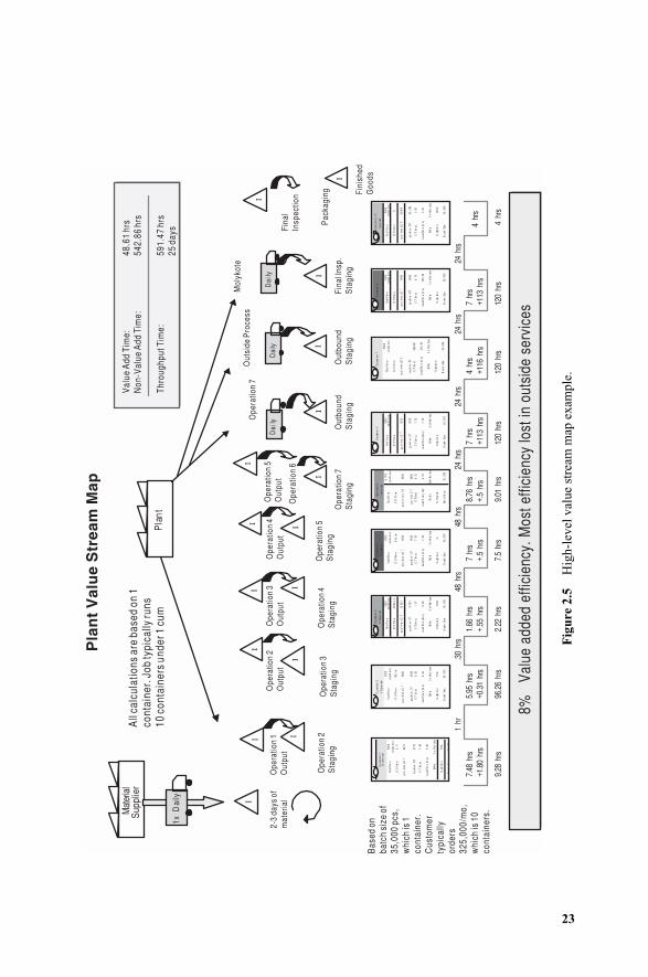
23
% Up
time
Ba
tch S
ize35
,00 0
Shifts
7.00
Lead
Time
(hrs)
3 s
hifts/
day
pcs/
hr w/
o DT
5000
C/T
(hr
s)7.
00
pcs/h
r w
/ DT
5000
Op
erat
ion 6
Takt
Tim
e5.3
32
sec/ p
iece
C/O
Tim
eDai
ly
Ope
ratio
n 5
1 op
erato
r
Takt
Time
5.33
2
sec/p
iece
C/O
Tim e
pcs/
hr w
/o D
T39
96
C/T (
hrs)
8.76
pcs/
hr w/
DT
3885
Shift
s
9.01
Lead
Time
(hrs
)
3 sh
ifts/d
ay
% U
ptime
Batc
h Siz
e35
,000
% Up
time
%
Ba
tch S
ize35
,000
Shifts
7.00
Lead
Time
(hrs)
3 s
hifts/
day
pcs/
hr w/
o DT
5000
C/T
(hr
s)7.
00
pcs/h
r w
/ DT
5000
Op
erat
ion 4
1 Op
erat
or
Takt
Tim
e5.3
32
sec/ p
iece
C/O
Tim
e.5
hours
% U
ptim
e10
0%
Ba
tch S
ize35
,000
Shifts
2.22
Lead
Time
(hrs)
3 s
hifts/
day
pcs/
hr w/
o DT
2100
0
C/T
(hrs
)1.
67
pcs/h
r w
/ DT
1575
0
Op
erat
ion 3
1/3 o
per
ator
Takt
Tim
e5.3
32
sec/ p
iece
C/O
Time
.25 h
our
s
Op
eratio
n 1
1/2 O
pera
tor
Takt
Tim
e5.3
32
sec/ p
iece
C/O
Tim
e2.
71
pcs/
hr w/
o DT
4677
C/T
(hr
s)7.
48
pcs/h
r w
/ DT
3772
Shifts
9.28
Lead
Time
(hrs)
3 s
hifts/
day
% Up
time
70%
Ba
tchSiz
e35
000
Pla
nt
Va l
ue
Str
e am
Ma p
8%
Va
lue
ad
de
d E
ffic
ien
cy –
mo
st
eff
icie
ncy
ls
t in
Ou
t S
ide
Se
rvic
es
8%Va
lue
adde
d ef
ficie
ncy.
Mos
t effi
cien
cy lo
st in
out
side
ser
vice
s
Pla
nt
Op
erat
ion 7
Takt
Tim
e5.3
32
sec/ p
iece
C/O
Tim
e
pcs/
hr w/
o DT
C/T
(hr
s)#D
IV/0!
pcs/h
r w
/ DT
Shifts
120.
00Le
ad Tim
e (hr
s )
3 s
hifts/
day
% Up
time
Ba
tch S
ize35
,000
% Up
time
Ba
tch S
ize35
,00 0
Shifts
120.
00Le
ad Tim
e (hr
s)
3 s
hifts/
day
pcs/
hr w/
o DT
3996
C/T
(hr
s)8.
76
pcs/h
r w
/ DT
3886
Op
erat
ion 8
Takt
Tim
e5.3
32
sec/ p
iece
C/O
Tim
e
Mat
eria
lSu
ppl i e
r
I
2-3
days
of
mat
eria
l
1x D
aily
% Up
time
74%
Ba
tch S
ize3 5
,000
Shifts
6.26
Lead
Time
(hrs)
3 s
hifts/
day
pcs/
hr w/
o DT
5880
C/T
(hr
s)5.
95
pcs/h
r w
/ DT
5594
Op
eratio
n 2
1/3 o
per
ator
Takt
Tim
e5.3
32
sec/ p
iece
C/O
Tim
e1.3
8 h
rs
Dai
lyD
aily
Ope
ratio
n 9 &
10
1 op
erato
r
Takt
Tim
e5.3
32
sec/ p
iece
C/O
Tim
e0
pcs/
hr w/
o DT
3500
0
C/T
(hr
s)1.
00
pcs/h
r w
/ DT
35,0
00
Shifts
1.00
Lead
Time
(hrs)
3 s
hifts/
day
% U
ptim
e10
0%
Ba
tch S
ize35
,000
I I
I
I
I I
I I
I
II
I
I
I
I
Ope
ratio
n 1
Out
put
Ope
ratio
n 2
Out
put
Ope
ratio
n 3
Out
put
Ope
ratio
n 4
Out
put
Ope
ratio
n 5
Out
put
Ope
ratio
n 2
Sta
ging
Ope
ratio
n 3
Sta
ging
Ope
ratio
n 4
Sta
ging
Ope
ratio
n 5
Sta
ging
Ope
ratio
n 6
Ope
ratio
n 7
Sta
ging
Out
boun
dS
tagi
ngO
utbo
und
Sta
ging
Fina
l Ins
p.S
tagi
ng
Fina
lIn
spec
tion
Pac
kagi
ng Fini
shed
Goo
ds
Mol
ykot
eO
utsi
de P
roce
ssO
pera
tion
7
Al l
cal c
ulat
i ons
are
bas
ed o
n 1
cont
aine
r. J
ob ty
pica
lly ru
ns10
con
tain
ers
unde
r 1 c
um
Val
ue A
dd T
i me:
48
.61
hrs
Non
-Val
ue A
dd T
i me:
54
2.86
hrs
Thro
ughp
ut T
ime:
59
1.47
hrs
25 d
ays
Bas
ed o
nba
tch
size
of
35,0
00 p
cs,
whi
ch is
1co
ntai
ner.
Cus
tom
erty
pica
llyor
ders
325,
000/
mo,
whi
ch is
10
cont
aine
rs.
9.28
hrs
7.48
hrs
+1.8
0 hr
s
96.2
6 hr
s
5.95
hrs
+0.3
1 hr
s
2.22
hrs
1.66
hrs
+.55
hrs
7.5
hrs
7 hr
s+.
5 hr
s
9.01
hrs
8.76
hrs
+.5
hrs
120
hrs
7 hr
s+1
13 h
rs
120
hrs
4 hr
s+1
16 h
rs
120
hrs
7 hr
s+1
13 h
rs
4 hr
s
4 hr
s
24 h
rs24
hrs
24 h
rs24
hrs
48 h
rs48
hrs
.30
hrs
1 hr
Fig
ure
2.5
Hig
h-le
vel v
alue
str
eam
map
exa
mpl
e.
c02.qxd 4/22/2005 7:34 AM Page 23
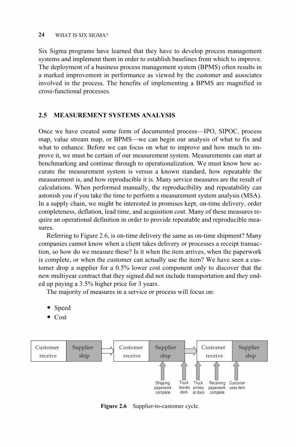
Six Sigma programs have learned that they have to develop process managementsystems and implement them in order to establish baselines from which to improve.The deployment of a business process management system (BPMS) often results ina marked improvement in performance as viewed by the customer and associatesinvolved in the process. The benefits of implementing a BPMS are magnified incross-functional processes.
2.5 MEASUREMENT SYSTEMS ANALYSIS
Once we have created some form of documented process—IPO, SIPOC, processmap, value stream map, or BPMS—we can begin our analysis of what to fix andwhat to enhance. Before we can focus on what to improve and how much to im-prove it, we must be certain of our measurement system. Measurements can start atbenchmarking and continue through to operationalization. We must know how ac-curate the measurement system is versus a known standard, how repeatable themeasurement is, and how reproducible it is. Many service measures are the result ofcalculations. When performed manually, the reproducibility and repeatability canastonish you if you take the time to perform a measurement system analysis (MSA).In a supply chain, we might be interested in promises kept, on-time delivery, ordercompleteness, deflation, lead time, and acquisition cost. Many of these measures re-quire an operational definition in order to provide repeatable and reproducible mea-sures.
Referring to Figure 2.6, is on-time delivery the same as on-time shipment? Manycompanies cannot know when a client takes delivery or processes a receipt transac-tion, so how do we measure these? Is it when the item arrives, when the paperworkis complete, or when the customer can actually use the item? We have seen a cus-tomer drop a supplier for a 0.5% lower cost component only to discover that thenew multiyear contract that they signed did not include transportation and they end-ed up paying a 3.5% higher price for 3 years.
The majority of measures in a service or process will focus on:
� Speed
� Cost
24 WHAT IS SIX SIGMA?
Suppliership
Customer
receive
Customer
receive
Suppliership
Customer
receive
Suppliership
Supplier
ship
Supplier
ship
Supplier
ship
Shipping paperwork complete
Truck leaves dock
Truck arrives at dock
Receiving paperwork complete
Customeruses item
Figure 2.6 Supplier-to-customer cycle.
c02.qxd 4/22/2005 7:34 AM Page 24
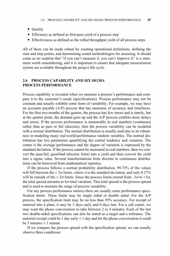
� Quality
� Efficiency as defined as first-pass yield of a process step
� Effectiveness as defined as the rolled throughput yield of all process steps
All of these can be made robust by creating operational definitions, defining thestart and stop points, and determining sound methodologies for assessing. It shouldcome as no surprise that “if you can’t measure it, you can’t improve it” is a state-ment worth remembering, and it is important to ensure that adequate measurementsytems are available throughout the project life cycle.
2.6 PROCESS CAPABILITY AND SIX SIGMA PROCESS PERFORMANCE
Process capability is revealed when we measure a process’s performance and com-pare it to the customer’s needs (specifications). Process performance may not beconstant and usually exhibits some form of variability. For example, we may havean accounts payable (A/P) process that has measures of accuracy and timeliness.For the first two months of the quarter, the process has few errors and is timely, butat the quarter point, the demand goes up and the A/P process exhibits more delaysand errors. If the process performance is measurable in real numbers (continous)rather than as pass or fail (discrete), then the process variability can be modeledwith a normal distribution. The normal distribution is usually used due to its robust-ness in modeling many real-world-performance random variables. The normal dis-tribution has two parameters quantifying the central tendency and variation. Thecenter is the average performance and the degree of variation is expressed by thestandard deviation. If the process cannot be measured in real numbers, then we con-vert the pass/fail, good/bad (discrete form) into a yield and then convert the yieldinto a sigma value. Several transformations from discrete to continuous distribu-tions can be borrowed from mathematical statistics.
If the process follows a normal probability distribution, 99.73% of the valueswill fall between the ± 3� limits, where � is the standard deviation, and only 0.27%will be outside of the ± 3� limits. Since the process limits extend from –3� to +3�,the total spread amounts to 6� total variation. This total spread is the process spreadand is used to measure the range of process variability.
For any process performance metrics there are usually some performance speci-fication limits. These limits may be single sided or double sided. For the A/Pprocess, the specification limit may be no less than 95% accuracy. For receipt ofmaterial into a plant, it may be 2 days early and 0 days late. For a call center, wemay want the phone conversation to take between 2 to 4 minutes. Each of the lasttwo double-sided specifications can also be stated as a target and a tolerance. Thematerial receipt could be 1 day early ± 1 day and for the phone conversation it couldbe 3 minutes ± 1 minute.
If we compare the process spread with the specification spread, we can usuallyobserve three conditions:
2.6 PROCESS CAPABILITY AND SIX SIGMA PROCESS PERFORMANCE 25
c02.qxd 4/22/2005 7:34 AM Page 25

1. Condition I: Highly Capable Process (see Figure 2.7). The process spread iswell within the specification spread:
6� < (USL – LSL)
The process is capable because it is extremely unlikely that it will yield unac-ceptable performance.
2. Condition II: Marginally Capable Process (see Figure 2.8). The processspread is approximately equal to the specification spread:
6� = (USL – LSL)
When a process spread is nearly equal to the specification spread, the processis capable of meeting the specifications. If we remember that the process cen-ter is likely to shift from one side to the other, then a significant amount of theoutput will fall outside of the specification limit and will yield unacceptableperformance.
3. Condition III: Incapable Process (see Figure 2.9). The process spread isgreater than the specification spread:
6� > (USL – LSL)
When a process spread is greater than the specification spread, the process is in-capable of meeting the specifications and a significant amount of the output willfall outside of the specification limit and will yield unacceptable performance.
2.6.1 Motorola’s Six Sigma Quality
In 1986, the Motorola Corporation won the Malcolm Baldrige National QualityAward. Motorola based its success in quality on its Six Sigma program. The goal of
26 WHAT IS SIX SIGMA?
LSL USL
-6 -4 -2 0 2 4 6
LSL USL+6σ-6σ
Figure 2.7 Highly capable process.
c02.qxd 4/22/2005 7:34 AM Page 26
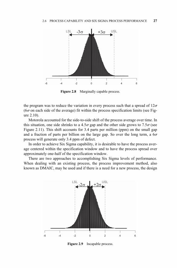
the program was to reduce the variation in every process such that a spread of 12�(6� on each side of the average) fit within the process specification limits (see Fig-ure 2.10).
Motorola accounted for the side-to-side shift of the process average over time. Inthis situation, one side shrinks to a 4.5� gap and the other side grows to 7.5� (seeFigure 2.11). This shift accounts for 3.4 parts per million (ppm) on the small gapand a fraction of parts per billion on the large gap. So over the long term, a 6�process will generate only 3.4 ppm of defect.
In order to achieve Six Sigma capability, it is desirable to have the process aver-age centered within the specification window and to have the process spread overapproximately one-half of the specification window.
There are two approaches to accomplishing Six Sigma levels of performance.When dealing with an existing process, the process improvement method, alsoknown as DMAIC, may be used and if there is a need for a new process, the design
2.6 PROCESS CAPABILITY AND SIX SIGMA PROCESS PERFORMANCE 27
USLLSL
6420-2-4-6
USLLSL +3σ-3σ
Figure 2.8 Marginally capable process.
LSL USL
+2-2
-6 -4 -2 0 2 4 6
LSL USL+2σ-2σ
Figure 2.9 Incapable process.
c02.qxd 4/22/2005 7:34 AM Page 27
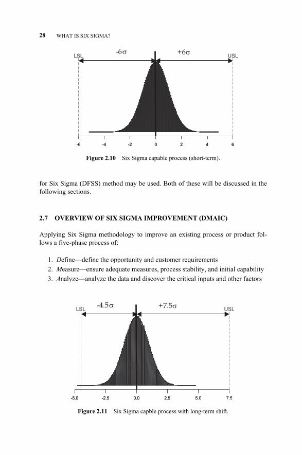
for Six Sigma (DFSS) method may be used. Both of these will be discussed in thefollowing sections.
2.7 OVERVIEW OF SIX SIGMA IMPROVEMENT (DMAIC)
Applying Six Sigma methodology to improve an existing process or product fol-lows a five-phase process of:
1. Define—define the opportunity and customer requirements
2. Measure—ensure adequate measures, process stability, and initial capability
3. Analyze—analyze the data and discover the critical inputs and other factors
28 WHAT IS SIX SIGMA?
-6 -4 -2 0 2 4 6
LSL USL
-6 -4 -2 0 2 4 6
LSL USL+6σ-6σ
Figure 2.10 Six Sigma capable process (short-term).
-5.0 -2.5 0.0 2.5 5.0 7.5
LSL USL
-
-5.0 -2.5 0.0 2.5 5.0 7.5
LSL USL+7.5σ-4.5σ
Figure 2.11 Six Sigma capble process with long-term shift.
c02.qxd 4/22/2005 7:34 AM Page 28
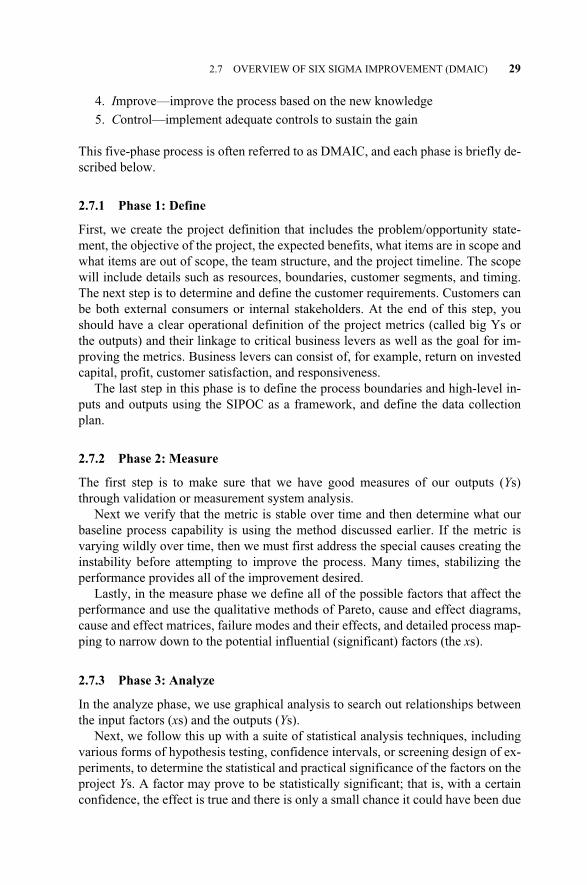
4. Improve—improve the process based on the new knowledge
5. Control—implement adequate controls to sustain the gain
This five-phase process is often referred to as DMAIC, and each phase is briefly de-scribed below.
2.7.1 Phase 1: Define
First, we create the project definition that includes the problem/opportunity state-ment, the objective of the project, the expected benefits, what items are in scope andwhat items are out of scope, the team structure, and the project timeline. The scopewill include details such as resources, boundaries, customer segments, and timing.The next step is to determine and define the customer requirements. Customers canbe both external consumers or internal stakeholders. At the end of this step, youshould have a clear operational definition of the project metrics (called big Ys orthe outputs) and their linkage to critical business levers as well as the goal for im-proving the metrics. Business levers can consist of, for example, return on investedcapital, profit, customer satisfaction, and responsiveness.
The last step in this phase is to define the process boundaries and high-level in-puts and outputs using the SIPOC as a framework, and define the data collectionplan.
2.7.2 Phase 2: Measure
The first step is to make sure that we have good measures of our outputs (Ys)through validation or measurement system analysis.
Next we verify that the metric is stable over time and then determine what ourbaseline process capability is using the method discussed earlier. If the metric isvarying wildly over time, then we must first address the special causes creating theinstability before attempting to improve the process. Many times, stabilizing theperformance provides all of the improvement desired.
Lastly, in the measure phase we define all of the possible factors that affect theperformance and use the qualitative methods of Pareto, cause and effect diagrams,cause and effect matrices, failure modes and their effects, and detailed process map-ping to narrow down to the potential influential (significant) factors (the xs).
2.7.3 Phase 3: Analyze
In the analyze phase, we use graphical analysis to search out relationships betweenthe input factors (xs) and the outputs (Ys).
Next, we follow this up with a suite of statistical analysis techniques, includingvarious forms of hypothesis testing, confidence intervals, or screening design of ex-periments, to determine the statistical and practical significance of the factors on theproject Ys. A factor may prove to be statistically significant; that is, with a certainconfidence, the effect is true and there is only a small chance it could have been due
2.7 OVERVIEW OF SIX SIGMA IMPROVEMENT (DMAIC) 29
c02.qxd 4/22/2005 7:34 AM Page 29
to a mistake. The statistically significant factor is not always practical, in that it mayonly account for a small percentage of the effect on the Ys, in which case control-ling this factor would not provide much improvement. The transfer function Y = f(x)for every Y measure usually represents the regression of several influential factorson the project outputs. There may be more than one project metric (output), hencethe Ys.
2.7.4 Phase 4: Improve
In the improve phase, we first identify potential solutions through team meetingsand brainstorming or the use of TRIZ (covered in Chapter 9). It is important at thispoint to have completed a measurement system analysis on the key factors (xs) andpossibly to have performed some confirmation design of experiments.
The next step is to validate the solution(s) identified through a pilot run orthrough optimization design of experiments. Following confirmation of the im-provement, a detailed project plan and cost benefit analysis should be completed.
The last step in this phase is to implement the improvement. This is a point atwhich change management tools can prove to be beneficial.
2.7.5 Phase 5: Control
The control phase consists of four steps. In the first step we determine the controlstrategy based on the new process map, failure mode and effects, and a detailedcontrol plan. The control plan should balance between the output metric and thecritical few input variables.
The second step involves implementing the controls identified in the controlplan. This is typically a blend of poka yoke’s, control charts, clear roles and respon-sibilities, and operator instructions depicted in operational method sheets.
Third, we determine what the final capability of the process is with all of the im-provements and controls in place.
The final step is to perform the ongoing monitoring of the process based on thefrequency defined in the control plan. The DMAIC methodology has allowed busi-nesses to achieve lasting breakthrough improvements that break the paradigm of re-acting to the symptoms rather than the causes. This method allows design teams tomake fact-based decisions using statistics as a compass and implement lasting im-provements that satisfy the external and internal customers.
2.8 SIX SIGMA GOES UPSTREAM—DESIGN FOR SIX SIGMA
The DMAIC methodology is excellent when dealing with an existing process inwhich reaching the entitled level of performance will provide all of the benefit re-quired. Entitlement is the best the process or product is capable of performing at ad-equate control. Reviewing historical data, it is often seen to be the best performancepoint. But what do we do if reaching entitlement is not enough or there is a need for
30 WHAT IS SIX SIGMA?
c02.qxd 4/22/2005 7:34 AM Page 30
an innovative solution never before deployment? We could continue with the typi-cal build it and fix it process or we can utilize the most powerful tools and methodsavailable for developing an optimized, robust, risk-free design. These tools andmethods can be aligned with an existing new product/process development processor used in a stand-alone manner. The rest of this book is devoted to explaining anddemonstrating the design for Six Sigma (DFSS) tools and methodology. Chapter 3is the introductory chapter for DFSS, giving overviews for DFSS theory, DFSS gat-ed processes, and DFSS applications. Chapter 4 gives a detailed description abouthow to deploy DFSS in a company, covering the training, organization support, fi-nancial management, and deployment strategy. Chapter 5 gives a very detailed“road map” of the whole DFSS project execution, which includes very detailed de-scriptions of the DFSS stages, task management, scorecards, and how to integrateall DFSS methods in developmental stages. Chapters 6 through 17 give detailed de-scriptions with examples of all of the major methods used in DFSS.
2.9 SUMMARY
In this chapter, we have explained what Six Sigma is and how it has evolved overtime. We explained that it is a process-based methodology and introduced the read-er to process modeling with a high-level overview of IPO, process mapping, valuestream mapping, and value analysis, as well as business process management sys-tems (BPMSs). We have explained the criticality of understanding the measure-ments of the process or system and how this is accomplished with masurement sys-tems analysis (MSA). Once we understand the goodness of our measures, we canevaluate the capability of the process to meet customer requirements and demon-strate what Six Sigma capability is. Next, we moved to an explanation of theDMAIC methodology and how it incorporates these concepts into a road-mapmethod. Finally, we covered how Six Sigma moves upstream to the design environ-ment with the application of DFSS. In the next chapter, we will introduce the readerto the service design for Six Sigma (DFSS) process.
2.9 SUMMARY 31
c02.qxd 4/22/2005 7:34 AM Page 31

c02.qxd 4/22/2005 7:34 AM Page 32
3.1 INTRODUCTION
The objective of this chapter is to introduce the service design for Six Sigma(DFSS) process theory and to lay the foundation for the next chapters of the book.DFSS combines design analysis (e.g., requirements cascading) with design synthe-sis (e.g., process engineering) within the framework of the deploying company’sservice- (product-) development systems. Emphasis is placed on CTSs (critical-to-satisfaction requirements, also known as big Ys), identification, optimization, andverification using the transfer function and scorecard vehicles. A transfer functionin its simplest form is a mathematical relationship between the CTSs and/or theircascaded functional requirements (FRs) and the critical influential factors (calledthe xs). Scorecards help predict risks to the achievement of CTSs or FRs by moni-toring and recording their mean shifts and variability performance.
DFSS is a disciplined and rigorous approach to service, process, and product de-sign that ensures that new designs meet customer requirements at launch. It is a de-sign approach that ensures complete understanding of process steps, capabilities,and performance measurements by using scorecards, transfer functions, and tollgatereviews to ensure the accountability of all the design team members (black belts,project champions, and deployment champions1) and the rest of the organization.
The service DFSS objective is to attack the design vulnerabilities in both theconceptual and operational phases by deriving and integrating tools and methodsfor their elimination and reduction. Unlike the DMAIC methodology, the phases orsteps of DFSS are not universally defined, as evidenced by the many customizedtraining curriculums available in the market. Many times, the deploying companieswill implement the version of DFSS used by their vendor, thus assisting in the de-ployment. On the other hand, a company may implement DFSS to suit their busi-ness, industry, and culture by creating their own version. However, all approachesshare common themes, objectives, and tools.
Service Design for Six Sigma. By Basem El-Haik and David M. Roy 33© 2005 by John Wiley & Sons.
3INTRODUCTION TO SERVICE DESIGNFOR SIX SIGMA (DFSS)
1We will explore the roles and responsibilities of these Six Sigma operatives and others in Chapter 4.
c03.qxd 4/22/2005 7:36 AM Page 33
DFSS is used to design or redesign a product or service. The expected processsigma level for a DFSS product or service is at least 4.52, but can be 6� or higherdepending on the designed entity. The achievement of such a low defect level fromproduct or service launch means that customer expectations and needs must becompletely understood before a design can be operationalized. That is quality as de-fined by the customer.
The material presented here is intended to give the reader a high-level under-standing of service DFSS, its uses, and benefits. After reading this chapter, readersshould be able to assess how it can be used in relation to their jobs and identify theirneeds for further learning.
DFSS as defined in this book has a two-track deployment and application. Bydeployment, we mean the strategy adopted by the deploying company to launch theSix Sigma initiative. It includes putting into play the deployment infrastructure,strategy, and plan for initiative execution (see Chapter 4). Six Sigma deploymentwill be covered in Chapter 4. In what follows, we are assuming that the deploymentstrategy is in place as a prerequisite for application and project execution. TheDFSS tools are laid on top of four phases, as detailed in Chapter 5, in what we willcall the service DFSS project road map.
There are two distinct tracks within the Six Sigma initiative, as discussed in theprevious chapters: the retroactive Six Sigma DMAIC3 approach that takes existingprocess improvement as an objective, and the proactive design for Six Sigma(DFSS) that targets redesign and new service introduction in both the developmentand production (process) arenas. DFSS is different from the Six Sigma DMAIC ap-proach in that it is a proactive prevention approach to design.
The service DFSS approach can be broken down into identify, characterize, opti-mize, and verify, or ICOV for short. These are defined below:
Identify customer and design requirements. Prescribe the CTSs, design parame-ters, and corresponding process variables.
Characterize the concepts, specifications, and technical and project risks.
Optimize the design transfer functions and mitigate risks.
Verify that the optimized design meets the intent (customer, regulatory, and de-ploying service functions).
In this book, both ICOV and DFSS acronyms will be used interchangeably.
3.2 WHY USE SERVICE DESIGN FOR SIX SIGMA?
Generally, customer-oriented design is a development process of transforming cus-tomers’ wants into design service solutions that are useful to the customer. This
34 INTRODUCTION TO SERVICE DESIGN FOR SIX SIGMA (DFSS)
2No more than approximately 1 defect per thousand opportunities.3Define project goals and customer deliverables; Measure the process and determine baseline; Analyze—determine root causes; Improve the process by optimization (i.e., eliminating/reducing defects); andControl—sustain the optimized solution.
c03.qxd 4/22/2005 7:36 AM Page 34
process is carried out over several development stages, starting at the conceptualstage. In this stage, conceiving, evaluating, and selecting good design solutions aredifficult tasks with enormous consequences. It is usually the case that organizationsoperate in two modes: “proactive,” that is, conceiving feasible and healthy concep-tual entities; and “retroactive,” that is, problem solving such that the design entitycan live up to its committed potentials. Unfortunately, the latter mode consumes thelargest portion of an organization’s human and nonhuman resources. The design forSix Sigma approach highlighted in this book is designed to target both modes of op-eration.
DFSS is the premier approach to process design that is able to embrace and im-prove developed homegrown supportive processes (e.g., sales and marketing) with-in its development system. This advantage will enable the deploying company tobuild on current foundations while enabling them to reach unprecedented levels ofachievement that exceed the set targets.
The linking of the Six Sigma initiative and DFSS to the company vision and an-nual objectives should be direct, clear, and crisp. DFSS has to be the crucial mecha-nism to develop and improve business performance and increase customer satisfac-tion and quality metrics. Significant improvements in all health metrics are thefundamental source of DMAIC and DFSS projects that will, in turn, transform thecompany’s culture one project at a time. Achieving a Six Sigma culture is very es-sential for the future well-being of the deploying company and represents thebiggest return on investment beyond the obvious financial benefits. Six Sigma ini-tiatives must apply to all elements of the company’s strategy in all areas of the busi-ness if massive impact is the objective.
The objective of this book is to present the service design for Six Sigma ap-proach, concepts, and tools that eliminate or reduce both the conceptual and opera-tional types of vulnerabilities of service entities and enables such entities to operateat Six Sigma quality levels in meeting all of their requirements.
Reducing operational vulnerability means adjustment of the critical-to-quality,critical-to-cost, and critical-to-delivery requirements (the CTSs). This objective hasbeen the subject of many knowledge fields such as parameter design, DMAIC SixSigma, and tolerance design/tolerancing techniques. On the contrary, the conceptu-al vulnerabilities are usually overlooked due to the lack of a compatible systemicapproach to finding ideal solutions, ignorance of the designer, pressure of dead-lines, and budget limitations. This can be partly attributed to the fact that traditionalquality methods can be characterized as after-the-fact practices since they use lag-ging information for developmental activities, such as bench tests and field data.Unfortunately, this practice drives design toward endless cycles ofdesign–test–fix–retest, creating what is broadly known as the “fire fighting” modeof the design process, that is, the creation of design-hidden factories. Companiesthat follow these practices usually suffer from high development costs, longer timeto market, lower quality levels, and marginal competitive edge. In addition, correc-tive actions to improve their conceptual vulnerabilities via operational vulnerabili-ties improvement means are marginally effective if at all useful. Typically, thesecorrections are costly and hard to implement as the service project progresses in the
3.2 WHY USE SERVICE DESIGN FOR SIX SIGMA? 35
c03.qxd 4/22/2005 7:36 AM Page 35
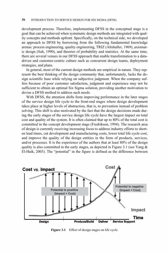
development process. Therefore, implementing DFSS in the conceptual stage is agoal that can be achieved when systematic design methods are integrated with qual-ity concepts and methods upfront. Specifically, on the technical side, we developedan approach to DFSS by borrowing from the following fundamental knowledgearenas: process engineering, quality engineering, TRIZ (Altshuller, 1969), axiomat-ic design (Suh, 1990), and theories of probability and statistics. At the same time,there are several venues in our DFSS approach that enable transformation to a data-driven and customer-centric culture such as concurrent design teams, deploymentstrategies, and plans.
In general, most of the current design methods are empirical in nature. They rep-resent the best thinking of the design community that, unfortunately, lacks the de-sign scientific base while relying on subjective judgment. When the company suf-fers because of poor customer satisfaction, judgment and experience may not besufficient to obtain an optimal Six Sigma solution, providing another motivation todevise a DFSS method to address such needs.
With DFSS, the attention shifts from improving performance in the later stagesof the service design life cycle to the front-end stages where design developmenttakes place at higher levels of abstraction, that is, to prevention instead of problemsolving. This shift is also motivated by the fact that the design decisions made dur-ing the early stages of the service design life cycle have the largest impact on totalcost and quality of the system. It is often claimed that up to 80% of the total cost iscommitted in the concept development stage (Fredrikson, 1994). The research areaof design is currently receiving increasing focus to address industry efforts to short-en lead times, cut development and manufacturing costs, lower total life cycle cost,and improve the quality of the design entities in the form of products, services,and/or processes. It is the experience of the authors that at least 80% of the designquality is also committed in the early stages, as depicted in Figure 3.1 (see Yang &El-Haik, 2003). The “potential” in the figure is defined as the difference between
36 INTRODUCTION TO SERVICE DESIGN FOR SIX SIGMA (DFSS)
Figure 3.1 Effect of design stages on life cycle.
Design Service SupportProduce/Build Deliver
Cost
Impact
Cost vs. Impact
Potential is positivePotential is positive
(Impact > Cost)(Impact > Cost)
Potential is negativePotential is negative
(Impact < Cost)(Impact < Cost)
TimeDesign Service SupportProduce/Build Deliver
Cost
Impact
Cost vs. Impact
Potential is positivePotential is positive
(Impact > Cost)(Impact > Cost)
Potential is negativePotential is negative
(Impact < Cost)(Impact < Cost)
TimeDesign Service SupportProduce/Build Deliver
Cost
Impact
Cost vs. Impact
Potential is positivePotential is positive
(Impact > Cost)(Impact > Cost)
Potential is negativePotential is negative
(Impact < Cost)(Impact < Cost)
TimeDesign Service SupportProduce/Build Deliver
Cost
Impact
Cost vs. Impact
Potential is positivePotential is positive
(Impact > Cost)(Impact > Cost)
Potential is negativePotential is negative
(Impact < Cost)(Impact < Cost)
Time
c03.qxd 4/22/2005 7:36 AM Page 36
the impact (influence), of the design activity at a certain design stage and the totaldevelopment cost up to that stage. The potential is positive but decreases as designprogresses, implying reduced design freedom over time. As financial resources arecommitted (e.g., buying process equipment and facilities, hiring staff) the potentialstarts changing sign, going from positive to negative. For the consumer, the poten-tial is negative and the cost overcomes the impact tremendously. At this stage, de-sign changes for corrective actions can only be achieved at high cost, including cus-tomer dissatisfaction, warranty problems, and marketing promotions, in many casesunder the scrutiny of the government (e.g., recall costs).
3.3 WHAT IS SERVICE DESIGN FOR SIX SIGMA?
Service DFSS is a structured, data-driven approach to design in all aspects of ser-vice functions (e.g., human resources, marketing, sales, IT) where deployment islaunched, to eliminate the defects induced by the design process and to improvecustomer satisfaction, sales, and revenue. To deliver these benefits, DFSS appliesdesign methods like axiomatic design,4 creativity methods like TRIZ,5 and statisti-cal techniques to all levels of design decision making in every corner of the busi-ness, identifies and optimizes the critical design factors (the xs), and validates alldesign decisions in the use (or surrogate) environment of the end user.
DFSS is not an add-on but represents a cultural change within different functionsand organizations in which deployment is launched. It provides the means to tackleweak or new processes, driving customer and employee satisfaction. DFSS and SixSigma should be linked to the deploying company’s annual objectives, vision, andmission statements. They should not be viewed as another short-lived initiative.They are vital, permanent components to achieve leadership in design, customersatisfaction, and cultural transformation. From marketing and sales to development,operations, and finance, each business function needs to be headed by a deploymentleader or a deployment champion. This local deployment team will be responsiblefor delivering dramatic change, thereby removing a number of customer issues andinternal problems and expediting growth. The deployment team can deliver on theirobjective through Six Sigma operatives called black belts and green belts, who willbe executing scoped projects that are in alignment with the objectives of the compa-ny. Project champions are responsible for scoping projects from within their realmof control and handing project charters (contracts) over to the Six Sigma resourcesgroup. The project champion will select projects consistent with corporate goalsand remove barriers. The Six Sigma resources will complete successful projects us-ing Six Sigma methodology and will train and mentor the local organization on SixSigma. The deployment leader, the highest initiative operative, sets meaningful
3.3 WHAT IS SERVICE DESIGN FOR SIX SIGMA? 37
4A perspective design method that employs two design axioms: the independence axiom and the infor-mation axiom. See Chapter 8 for more details.5TRIZ is the Russian acronym for theory of inventive problem solving, also known as TIPS. It is a sys-tematic method to conceive creative, innovative, and predictable design solutions. See Chapter 9 formore details.
c03.qxd 4/22/2005 7:36 AM Page 37
goals and objectives for the deployment in his or her function area and drives theimplementation of Six Sigma publicly.
The Six Sigma black belt resources group consists of full-time Six Sigma opera-tives as opposed to green belts, who should be completing smaller projects of theirown as well as assisting black belts. The black belts play a key role in raising thecompetency of the company as they drive the initiative into day-to-day operations.
Black belts are the driving force of service DFSS deployment. They are projectleaders who are removed from day-to-day assignments for a period of time (usuallytwo years) to focus exclusively on design and improvement projects. They have in-tensive training in Six Sigma tools, design techniques, problem solving, and teamleadership. The black belts are trained by master black belts, who are initially hiredif not available homegrown.
A black belt should have process and organizational knowledge, know some basicdesign theory, have statistical skills, and be eager to learn new tools. A black belt is a“change agent” who carries the initiative to his or her team, the staff, and the entirecompany. In doing so, communication and leadership skills are vital. Black belts needeffective intervention skills. They must understand why some team members may re-sist the Six Sigma cultural transformation. Some soft training on leadership should beembedded in their training curriculum. Soft-skills training may target deploymentmaturity analysis, team development, business acumen, and individual leadership. Intraining, it is wise to share several maturity initiative indicators that are being trackedin the deployment scorecard, for example, alignment of the project to company ob-jectives in its own scorecard (the big Ys), readiness of the project’s mentoring struc-ture, preliminary budget, team member identification, and scoped project charter.
DFSS black belt training is intended to be delivered in tandem with a trainingproject for hands-on application. The training project should be well scoped withample opportunity for tool application and should have cleared tollgate “0” prior toclass. Usually, project presentations will be weaved into each training session.More details are given Chapter 4.
While handling projects, the role of the black belts spans several functions suchas learning, mentoring, teaching, and coaching. As a mentor, the black belt culti-vates a network of experts in the project on hand, working with the process opera-tors; process owners, and all levels of management. To become self-sustained, thedeployment team may need to task their black belts with providing formal trainingto green belts and team members.
Service design for Six Sigma (DFSS) is a disciplined methodology that appliesthe transfer function [CTSs = ƒ(x)] to ensure that customer expectations are met andembedded into the design, design performance is predicted prior to the pilot, perfor-mance measurement systems (scorecards) are built into the design to ensure effec-tive ongoing process management, and a common language for design is leveragedwithin the design tollgate process.
DFSS projects can be categorized as design or redesign of an entity, whetherproduct, process, or service. “Creative design” is the term that we will be using toindicate new design, design from scratch, and “incremental design,” to indicate theredesign case or design from a datum. In the later case, some data can be used to
38 INTRODUCTION TO SERVICE DESIGN FOR SIX SIGMA (DFSS)
c03.qxd 4/22/2005 7:36 AM Page 38
baseline current performance. The degree of deviation of the redesign from the da-tum is the key factor in deciding on the usefulness of relative existing data. ServiceDFSS projects can come from historical sources (e.g., service redesign due to cus-tomer issues) or from proactive sources like growth and innovation (new service in-troduction). In either case, the service DFSS project requires greater emphasis on:
� Voice of the customer collection scheme
� Addressing all (multiple) CTSs as cascaded by the customer
� Assessing and mitigating technical failure modes and project risks in theirown environment as they are linked to the tollgate process reviews
� Project management with some communication plan to all affected partiesand budget management
� Detailed project change management process
3.4 SERVICE DFSS: THE ICOV PROCESS
As mentioned in Section 3.1, design for Six Sigma has four phases spread over sev-en development stages. They are identify, characterize, optimize, and verify. Theacronym ICOV is used to denote these four phases. The service life cycle is depict-ed in Figure 3.2. Notice the position of service ICOV phases of a design project.
Naturally, the process of service design begins when there is a need (an impetus).People create the need, whether it is a problem to be solved (e.g., if waiting time at acall center becomes very long, then the customer satisfaction deteriorates and theprocess needs to be redesigned) or a new invention. Design objective and scope arecritical in the impetus stage. A design project charter should describe simply andclearly what is to be designed. It cannot be vague. Writing a clearly stated designcharter is just one step. In stage 2, the design team must write down all the informa-tion they may need, in particular, the voice of the customer (VOC) and the voice ofthe business (VOB). With the help of the quality function deployment (QFD)process, such consideration will lead to the definition of the service design function-al requirements that will be later grouped into processes (systems and subsystems)and subprocesses (components). A functional requirement must contribute to an in-novation or to a solution of the objective described in the design charter. Anotherquestion that should be on the minds of the team members relates to how the end re-sult will look. The simplicity, comprehensiveness, and interfaces should make theservice attractive. What options are available to the team? And at what cost? Do theyhave the right physical properties, such as bandwidth, completeness, language, andreliability? Will the service be difficult to operate and maintain? Consider whatmethods you will need to employ to process, store, and deliver the service.
In stage 3, the design team should produce a number of solutions. It is very im-portant that they write or draw every idea on paper as it occurs to them. This will helpthem remember and describe them more clearly. It is also easier to discuss them withother people if drawings are available. These first drawings do not have to be very de-tailed or accurate. Sketches will suffice and should be made quickly. The important
3.4 SERVICE DFSS: THE ICOV PROCESS 39
c03.qxd 4/22/2005 7:36 AM Page 39
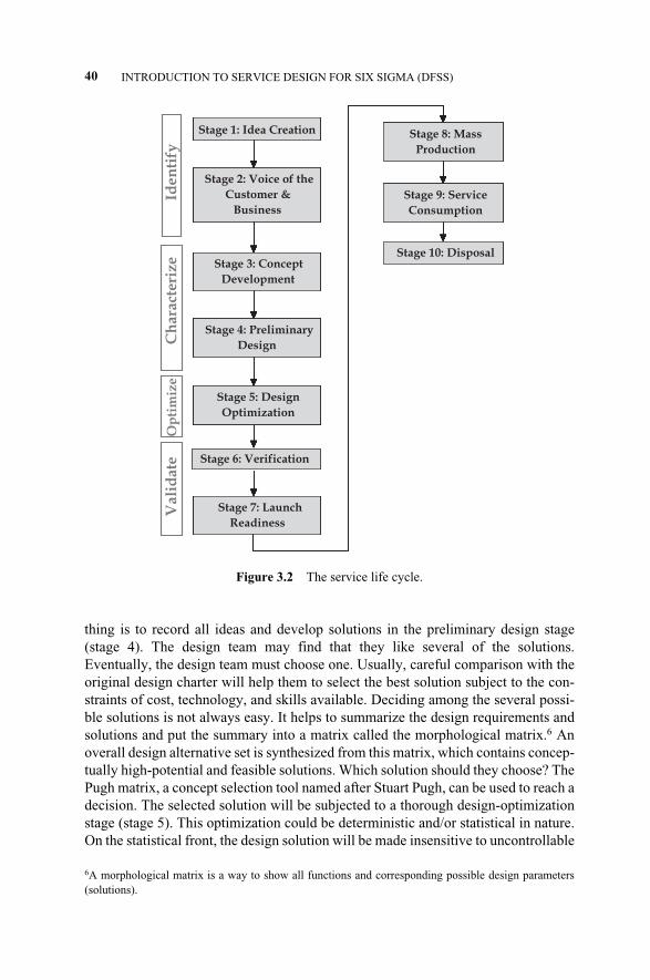
thing is to record all ideas and develop solutions in the preliminary design stage(stage 4). The design team may find that they like several of the solutions.Eventually, the design team must choose one. Usually, careful comparison with theoriginal design charter will help them to select the best solution subject to the con-straints of cost, technology, and skills available. Deciding among the several possi-ble solutions is not always easy. It helps to summarize the design requirements andsolutions and put the summary into a matrix called the morphological matrix.6 Anoverall design alternative set is synthesized from this matrix, which contains concep-tually high-potential and feasible solutions. Which solution should they choose? ThePugh matrix, a concept selection tool named after Stuart Pugh, can be used to reach adecision. The selected solution will be subjected to a thorough design-optimizationstage (stage 5). This optimization could be deterministic and/or statistical in nature.On the statistical front, the design solution will be made insensitive to uncontrollable
40 INTRODUCTION TO SERVICE DESIGN FOR SIX SIGMA (DFSS)
Figure 3.2 The service life cycle.
Iden
tify
Ch
ara
cteri
ze
Op
tim
ize
Vali
date
Stage 1: Impetus
Stage 2: Voice of the
Customer &
Business
Stage 3: Concept
Development
Stage 4: Preliminary
Design
Stage 5: Design
Optimization
Stage 7: launch
Readiness
Stage 8: Mass
Production
Stage 9: Service
Consumption
Stage 10: Disposal
Stage 1: Idea Creation
Stage 2: Voice of the
Customer &
Business
Stage 3: Concept
Development
Stage 4: Preliminary
Design
Stage 5: Design
Optimization
Stage 6: Verification
Stage 7: launch
Readiness
Stage 8: Mass
Production
Stage 9: Service
Consumption
Stage 10: Disposal
Stage 1: Impetus
Stage 2: Voice of the
Customer &
Business
Stage 3: Concept
Development
Stage 4: Preliminary
Design
Stage 5: Design
Optimization
Stage 7: launch
Readiness
Stage 8: Mass
Production
Stage 9: Service
Consumption
Stage 10: Disposal
Stage 1: Idea Creation
Stage 2: Voice of the
Customer &
Business
Stage 3: Concept
Development
Stage 4: Preliminary
Design
Stage 5: Design
Optimization
Stage 6: Verification
Stage 7: Launch
Readiness
Stage 8: Mass
Production
Stage 9: Service
Consumption
Stage 10: Disposal
6A morphological matrix is a way to show all functions and corresponding possible design parameters(solutions).
c03.qxd 4/22/2005 7:36 AM Page 40
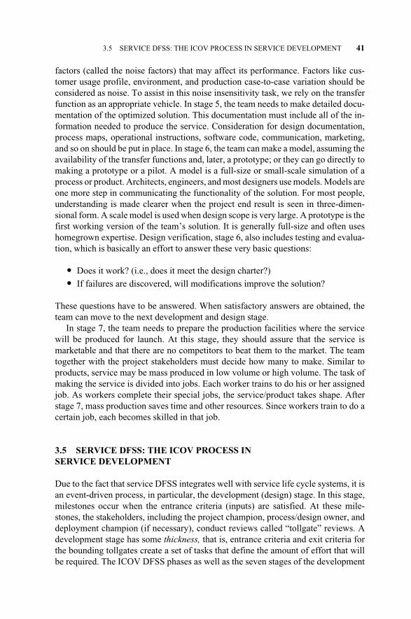
factors (called the noise factors) that may affect its performance. Factors like cus-tomer usage profile, environment, and production case-to-case variation should beconsidered as noise. To assist in this noise insensitivity task, we rely on the transferfunction as an appropriate vehicle. In stage 5, the team needs to make detailed docu-mentation of the optimized solution. This documentation must include all of the in-formation needed to produce the service. Consideration for design documentation,process maps, operational instructions, software code, communication, marketing,and so on should be put in place. In stage 6, the team can make a model, assuming theavailability of the transfer functions and, later, a prototype; or they can go directly tomaking a prototype or a pilot. A model is a full-size or small-scale simulation of aprocess or product. Architects, engineers, and most designers use models. Models areone more step in communicating the functionality of the solution. For most people,understanding is made clearer when the project end result is seen in three-dimen-sional form. A scale model is used when design scope is very large. A prototype is thefirst working version of the team’s solution. It is generally full-size and often useshomegrown expertise. Design verification, stage 6, also includes testing and evalua-tion, which is basically an effort to answer these very basic questions:
� Does it work? (i.e., does it meet the design charter?)
� If failures are discovered, will modifications improve the solution?
These questions have to be answered. When satisfactory answers are obtained, theteam can move to the next development and design stage.
In stage 7, the team needs to prepare the production facilities where the servicewill be produced for launch. At this stage, they should assure that the service ismarketable and that there are no competitors to beat them to the market. The teamtogether with the project stakeholders must decide how many to make. Similar toproducts, service may be mass produced in low volume or high volume. The task ofmaking the service is divided into jobs. Each worker trains to do his or her assignedjob. As workers complete their special jobs, the service/product takes shape. Afterstage 7, mass production saves time and other resources. Since workers train to do acertain job, each becomes skilled in that job.
3.5 SERVICE DFSS: THE ICOV PROCESS IN SERVICE DEVELOPMENT
Due to the fact that service DFSS integrates well with service life cycle systems, it isan event-driven process, in particular, the development (design) stage. In this stage,milestones occur when the entrance criteria (inputs) are satisfied. At these mile-stones, the stakeholders, including the project champion, process/design owner, anddeployment champion (if necessary), conduct reviews called “tollgate” reviews. Adevelopment stage has some thickness, that is, entrance criteria and exit criteria forthe bounding tollgates create a set of tasks that define the amount of effort that willbe required. The ICOV DFSS phases as well as the seven stages of the development
3.5 SERVICE DFSS: THE ICOV PROCESS IN SERVICE DEVELOPMENT 41
c03.qxd 4/22/2005 7:36 AM Page 41
process are depicted in Figure 3.3. In these reviews, a decision should be made as towhether to proceed to the next phase of development, recycle back for further clari-fication on certain decisions, or cancel the project altogether. Cancellation of prob-lematic projects, as early as possible, is a good thing. It stops nonconforming projectsfrom progressing further while consuming resources and frustrating people. In anycase, the black belt should quantify the size of the benefits of the design project inlanguage that will have impact on upper management, identify major opportunitiesfor improving customer dissatisfaction and associated threats to salability, and stim-ulate improvements through publication of the DFSS approach.
In tollgate reviews, work proceeds when the exit criteria (required decisions) aremade. As a DFSS deployment side bonus, a standard measure of developmentprogress across the deploying company, using a common development terminolo-gy, is achieved. Consistent exit criteria are obtained in each tollgate from the fol-lowing: (1) DFSS ICOV process deliverables, (2) deploying business company-wide deliverables, and (3) a select subset of deliverables specific to certain businessfunctions (for example, sales or human resources) within the deploying company.The detailed entrance and exit criteria by stage are presented in Chapter 5.
3.6 OTHER DFSS APPROACHES
Design for Six Sigma (DFSS) can be accomplished using any one of many othermethodologies besides the one presented in this book. IDOV7 is one popularmethodology for designing products and services to meet six sigma standards. It is afour-phase process that consists of identify, design, optimize, and verify. These fourphases parallel the four phases of the ICOV process presented in this book:
� Identify Phase. It begins the process by formally tying the design to the voiceof the customer (VOC). This phase involves developing a team and teamcharter, gathering the VOC, performing competitive analysis, and developingCTSs.
� Design Phase. This phase emphasizes CTSs and consists of identifying func-tional requirements, developing alternative concepts, evaluating alternatives,
42 INTRODUCTION TO SERVICE DESIGN FOR SIX SIGMA (DFSS)
Figure 3.3 The ICOV DFSS process.
Identify Conceptualize Optimize Validate
Stag
e 1:
Id
ea C
reat
ion
Stag
e 2:
Voi
ce o
f the
Cust
omer
&Bu
sine
ss
Stag
e 3:
Co
ncep
t De
velo
pmen
t
Stag
e 4:
Pr
elim
inar
y De
sign
To
llg
ate
1T
oll
gat
e 1
To
llg
ate
2T
oll
gat
e 2
To
llg
ate
3T
oll
gat
e 3
To
llg
ate
4T
oll
gat
e 4
Stag
e 5:
De
sign
Opt
imiz
atio
n
To
llg
ate
5T
oll
gat
e 5
Stag
e 6:
Ve
rific
atio
n
To
llg
ate
6T
oll
gat
e 6
Stag
e 7:
La
unch
Rea
dine
ss
To
llg
ate
7T
oll
gat
e 7
Prod
uctio
n
7See Dr. David Woodford’s article at http://www.isixsigma.com/library/content/c020819a.asp.
c03.qxd 4/22/2005 7:36 AM Page 42
selecting a best-fit concept, deploying CTSs, and predicting sigma capability.
� Optimize Phase. The optimize phase requires use of process capability infor-mation and a statistical approach to tolerancing. Developing detailed designelements, predicting performance, and optimizing design take place withinthis phase.
� Validate Phase. The Validate phase consists of testing and validating the de-sign. As increased testing using formal tools occurs, feedback of require-ments should be shared with production operations and sourcing, and futureoperations and design improvements should be noted.
Another popular design for Six Sigma methodology is called DMADV. It retainsthe same number of letters, number of phases, and general feel as the DMAICacronym. The five phases of DMADV are:
� Define: Define the project goals and customer (internal and external) require-ments.
� Measure: Measure and determine customer needs and specifications; bench-mark competitors and industry.
� Analyze: Analyze the process options to meet the customer needs.
� Design: Design (in detail) the process to meet the customer needs.
� Verify: Verify the design performance and ability to meet customer needs.
Another flavor of the DMADV methodology is DMADOV—design, measure,analyze, design, optimize, and verify. Other modified versions include DCCDI andDMEDI. DCCDI is being promoted by Geoff Tennant and is defined as define, cus-tomer concept, design, and implement, a replica of the DMADV phases. DMEDI isbeing promoted by PriceWaterhouseCoopers and stands for define, measure, ex-plore, develop, and implement. The fact is that all of these DFSS methodologies usealmost the same tools (quality function deployment, failure modes and effectsanalysis, benchmarking, design of experiments, simulation, statistical optimization,error proofing, robust design, etc.), presenting little difficulty to their alternate use.In addition to these common elements, the ICOV offers a thread-through road mapwith overlaid tools that are based on nontraditional tools such as design mappings,design axioms, creativity tools such as TRIZ, as well as cultural treatments.
3.7 SUMMARY
Service DFSS offers a robust set of tools and processes that address many of to-day’s complex business design problems. The DFSS approach helps design teamsframe their project based on a process with financial, cultural, and strategic implica-tions to the business. The service DFSS comprehensive tools and methods de-scribed in this book allow teams to quickly assess service issues and identify finan-cial and operational improvements that reduce costs, optimize investments, andmaximize returns. Service DFSS leverages a flexible and nimble organization and
3.7 SUMMARY 43
c03.qxd 4/22/2005 7:36 AM Page 43
maintains low development costs, allowing deploying companies to pass these ben-efits on to their customers. Service DFSS employs a unique gated process that al-lows teams to build tailor-made approaches—not all the tools need to be used ineach project. Therefore, designs can accommodate the specific needs of the projectcharter. Project by project, the competency level of the design teams will be en-hanced, leading to deeper knowledge and broader experience.
In this book, we form and integrate several strategic and tactical methodologiesthat produce synergies to enhance service DFSS capabilities to deliver a broad setof optimized solutions. The methods presented in this book can have wide-spreadapplication to help design teams and the “belt” population in different project areas(e.g., staffing and other human resources functions, finance, operations and supplychain functions, organizational development, financial services, training, technolo-gy and software tools and methods, etc.)
Service DFSS provides a unique commitment to the project customers by guar-anteeing agreed upon financial and other results. Each project must have measur-able outcomes and the design team must be responsible for defining and achievingthose outcomes. The service DFSS approach ensures these outcomes through riskidentification and mitigation plans, variable (DFSS tools that are used over manystages) and fixed (DFSS tools that are used once) tool structures, and advanced con-ceptual tools. The DFSS principles and structure should motivate design teams toprovide businesses and customers with a substantial return on their design invest-ment.
44 INTRODUCTION TO SERVICE DESIGN FOR SIX SIGMA (DFSS)
c03.qxd 4/22/2005 7:36 AM Page 44
4.1 INTRODUCTION
Service design for Six Sigma (DFSS) is a disciplined methodology that embedscustomer expectations into the design, applies the transfer function approach to en-sure that customer expectations are met, predicts design performance prior to the pi-lot, builds performance measurement systems (scorecards) into the design to ensureeffective ongoing process management, leverages a common language for design,and uses tollgate reviews to ensure accountability
This chapter examines the service DFSS deployment team, which launches the SixSigma program. A deployment team includes different levels of the deploying compa-ny’s leadership, including initiative senior leaders, project champions, and other de-ployment sponsors. As such, the material of this chapter should be used as a deploy-ment guideline with ample room for customization. It provides the considerations andgeneral aspects required for a smooth and successful initial deployment experience.
The extent to which service DFSS produces the desired results is a function ofthe adopted deployment plan. Historically, we can observe that many sound initia-tives became successful when commitment was secured from involved people at alllevels. An initiative is successful when it is adopted as the new norm. Service SixSigma and DFSS are no exception. A successful DFSS deployment depends onpeople, so almost every level, function, and division involved with the designprocess should participate in it, including the customer.
4.2 SERVICE SIX SIGMA DEPLOYMENT
The extent to which a service Six Sigma program produces results is directly affect-ed by the plan with which it is deployed. This section presents a high-level perspec-tive of a sound plan by outlining the critical elements of successful deployment. Wemust point out up front that a successful Six Sigma initiative is the result of key
Service Design for Six Sigma. By Basem El-Haik and David M. Roy 45© 2005 by John Wiley & Sons.
4SERVICE DESIGN FOR SIX SIGMA DEPLOYMENT
c04.qxd 4/22/2005 7:38 AM Page 45
contributions from people at all levels and functions of the company. In short, suc-cessful Six Sigma initiatives require buy-in, commitment, and support from offi-cers, executives, and management staff before and during execution of improve-ment projects by operational and process-level employees.
This top-down approach is critical to the success of a service Six Sigma pro-gram. Although black belts are the focal point for executing projects and generatingcash from process improvements, their success is inextricably linked to the wayleaders and managers establish the Six Sigma culture, create motivation, allocategoals, institute plans, set procedures, initialize systems, select projects, control re-sources, and provide recognition and rewards.
Several scales of deployment may be used; however, maximum benefit can onlybe achieved when all affected functions are engaged. A full-scale, company-widedeployment program requires that senior leadership install the proper culture ofchange before embarking on their support for training, logistics, and other resourcesrequired. People empowerment is key, as is leadership by example.
Benchmarking the DMAIC Six Sigma program in several successful deploy-ments, we can conclude that a top-down deployment approach will work for serviceDFSS deployment as well. This conclusion reflects the critical importance of secur-ing and cascading the buy-in from the top leadership level. The black belts and thegreen belts are the focused force of deployment under the guidance of the masterblack belts and champions. Success is measured by increase in revenue, customersatisfaction, and generated cash, one project at a time. Belted projects should bediligently scoped and aligned to company’s objectives with some prioritizationscheme. Six Sigma program benefits cannot be harvested without a sound strategyand the long-term vision of establishing the Six Sigma culture. In the short term, de-ployment success is dependent on motivation, management commitment, projectselection and scoping, institutionalized reward and recognition systems, and opti-mized resources allocation. This chapter is organized into several sections contain-ing the information for use by the deployment team.
4.3 SERVICE DFSS DEPLOYMENT PHASES
We categorize the deployment process, in term of evolution time, into three phases:
1. The predeployment phase to build the infrastructure
2. The deployment phase, where most activities will take place
3. The postdeployment phase, where effort needs to be sustained
4.3.1 Predeployment
Predeployment is a phase representing the period of time in which a leadershipteam lays the groundwork and prepares the company for service Six Sigma designimplementation, ensures the alignment of their individual deployment plans, andcreates synergy and heightened performance.
46 SERVICE DESIGN FOR SIX SIGMA DEPLOYMENT
c04.qxd 4/22/2005 7:38 AM Page 46
The first step in an effective service DFSS deployment starts with the top leader-ship of the deployment company. It is at this level that the team tasked with deploy-ment works with the senior executives to develop a strategy and plan for deploy-ment that is designed for success. The “marketing” and “selling” of the Six Sigmainitiative culture should come from the top. Our observation is that senior leader-ship benchmark themselves across corporate America in terms of results, manage-ment style, and company aspirations. Six Sigma, and in particular DFSS, is no ex-ception. The process usually starts with a senior leader or a pioneer who learnsabout Six Sigma and the benefits it brings to the culture and results. The pioneerstarts the deployment one step at a time and begins challenging old paradigms. Theold paradigms’ guards come to its defense and try to block the deployment. Defensemechanisms fall one after the other in the face of the undisputable results achievedby several benchmarked deploying companies (GE, 3M, Motorola, Textron, AlliedSignal, Bank of America, etc.). Momentum builds up and a team is formed to betasked with deployment. As a first step, it is advisable that select senior leadershipmeet jointly as a team with the assigned deployment team in an off-site location(with limited distractions). This entails a balanced mix of strategic thinking, SixSigma high-level education, interaction, and hands-on planning. On the educationside, overviews of Six Sigma concepts, presentations of successful deployments,and demonstrations of Six Sigma statistical methods, improvement measures, andmanagement controls will be very useful. Specifically, the following should be theminimum set of objectives of this launch meeting:
� Understand the philosophy and techniques of service DFSS and Six Sigma ingeneral.
� Experience the application of some of the tools during the meeting.
� Brainstorm a deployment strategy and a corresponding deployment plan withhigh first-time capability.
� Understand the organizational infrastructure requirements for deployment.
� Set financial and cultural goals, targets, and limits for the initiative.
� Discuss the project pipeline and black belt resources in all phases of deploy-ment.
� Put a mechanism in place to mitigate deployment risks and failure modes; forexample, failure mode and effect analysis (FMEA) of a typical service DFSSdeployment. Failure modes like the following are indicative of problematicstrategies: training black belts before champions; deploying DFSS withoutmultigenerational service and process plans and, if possible, technology roadmaps; and lack of valid data and measurement systems, leadership develop-ment, compensation plan, or change management process.
� Design a mechanism for tracking the progress of the initiative. Establish a ro-bust “financial” management and reporting system for the initiative.
Once this initial joint meeting has been held, the deployment team could bereplicated in other tiers of leadership whose buy-in is deemed necessary to push the
4.3 SERVICE DFSS DEPLOYMENT PHASES 47
c04.qxd 4/22/2005 7:38 AM Page 47
initiative through the different functions of the company. A service Six Sigma pullsystem needs to be created and sustained in deployment and postdeployment phas-es. Sustainment indicates the establishment of bottom-up pulling power.
Service Six Sigma, including DFSS, has revolutionized many companies in thelast 20 years. On the service side, companies in various industries can be found im-plementing service DFSS as a vehicle to plan growth, improve product/processquality and delivery performance, and reduce cost. Similarly, many deploying com-panies also find themselves reaping the benefits of increased employee satisfactionthrough the true empowerment Six Sigma provides. Factual studies of several suc-cessful deployments indicate that push and pull strategies need to be adopted basedon needs and that they differ strategically by objective and phase of deployment. Apush strategy is needed in the predeployment and deployment phases to jump startand operationalize deployment efforts. A pull system is needed in the postdeploy-ment phase once sustainment is accomplished, to improve deployment process per-formance on a continuous basis. In any case, top and medium management shouldbe on board at deployment, otherwise, the DFSS initiative will fade away eventual-ly.
4.3.2 Predeployment Considerations
The impact of a DFSS initiative depends on the effectiveness of deployment, that is,how well the Six Sigma design principles and tools are practiced by the DFSS pro-ject teams. Intensity and constancy of purpose beyond the norm are required to con-stantly improve deployment. Rapid deployment of DFSS plus commitment, train-ing, and practice characterize winning deploying companies.
In the predeployment phase, the deployment leadership should create a com-pelling business case for initiating, deploying, and sustaining DFSS as an effort.They need to raise general awareness about what DFSS is, why the company is pur-suing it, what is expected of various people, and how it will benefit the company.Building the commitment and alignment among executives and deployment cham-pions to aggressively support and drive deployment throughout the designatedfunctions of the company is a continuous activity. Empowerment of leaders andDFSS operatives to effectively carry out their respective roles and responsibilities iskey to success. A successful DFSS deployment requires the following prerequisitesin addition to senior leadership commitment previously discussed
Establish Deployment Structure.1 The first step taken by the senior deploymentleader is to establish a deployment team to develop strategies and oversee deploy-ment. With the help of the deployment team, the leader is responsible for designing,managing, and delivering the successful deployment of the initiative throughout thecompany, locally and globally. He or she needs to work with the human resourcesdepartment to develop policy to ensure that the initiative becomes integrated intothe culture, which may include integration with internal leadership development
48 SERVICE DESIGN FOR SIX SIGMA DEPLOYMENT
1See Yang & El-Haik (2003) for product DFSS perspectives.
c04.qxd 4/22/2005 7:38 AM Page 48
programs, career planning for black belts and deployment champions, a reward andrecognition program, and progress reporting to the senior leadership team. In addi-tion, the deployment leader needs to provide training, communication (as a singlepoint of contact to the initiative), and infrastructure support to ensure consistent de-ployment.
The critical importance of the team overseeing the deployment to ensure smoothand efficient rollout cannot be overemphasized. This team puts the DFSS deploy-ment effort in the path to success, whereby the proper individuals are positionedand support infrastructures are established. The deployment team is on the deploy-ment forward edge, assuming the responsibility for implementation. In this role,team members perform a company assessment of deployment maturity, conduct adetailed gap analysis, create an operational vision, and develop a cross-functionalSix Sigma deployment plan that spans human resources, information technology(IT), finance, and other key functions. Conviction about the initiative must be ex-pressed at all times, even though in the early stages there is no physical proof of thecompany’s specifics. They also accept and embody the following deployment as-pects:
� Visibility of the top-down leadership commitment to the initiative (indicatinga push system).
� Development and qualification of a measurement system with defined metricsto track the deployment progress. The objective here is to provide a tangiblepicture of deployment efforts. Later, a new set of metrics that target effective-ness and sustainment needs to be developed in maturity stages (end-of-de-ployment phase).
� Establish a goal-setting process in order to focus the culture on changing theprocess by which work gets done rather than adjusting current processes,leading to quantum rates of improvement.
� Strict adherence to the devised strategy and deployment plan.
� Clear communication of success stories that demonstrate how DFSS methods,technologies, and tools have been applied to achieve dramatic operational andfinancial improvements.
� Provide a system that will recognize and reward those who achieve success.
Deployment structure is not limited to the deployment team overseeing deploy-ment both strategically and tactically, but also includes project champions, func-tional area deployment champions, owners of processes and designs for which solu-tions will be implemented, and master black belts (MBBs) who mentor and coachthe black belts. All should have clearly defined roles and responsibilities with de-fined objectives. A premier deployment objective can be that the black belts areused as a task force to improve customer satisfaction, company image, and otherstrategic long-term objectives of the deploying company. To achieve such objec-tives, the deploying division should establish a deployment structure formed fromthe deployment directors, the centralized deployment team overseeing deployment,
4.3 SERVICE DFSS DEPLOYMENT PHASES 49
c04.qxd 4/22/2005 7:38 AM Page 49
and master black belts (MBBs) with defined roles and responsibilities for long-termand short-term planning. The structure can take the form of a council meeting atdefinite, recurring times. We suggest using service DFSS to design the DFSS de-ployment process and strategy. The deployment team should:
� Develop a green belt structure of support to the black belts in every depart-ment.
� Cluster the green belts (GBs) as a network around the black belts for synergyand to increase the velocity of deployment.
� Ensure that the scopes of the projects are within control, that the project selec-tion criteria are focused on the company’s objectives, like quality, cost, cus-tomer satisfaction, delivery drivers, and so on.
� Hand off (match) the right scoped projects to black belts.
� Support projects with key up-front documentation like charters or contractswith financial analysis, highlighting savings and other benefits, efficiency im-provements, customer impact, project rationale, and so on. Such documenta-tion will be reviewed and agreed upon by primary stakeholders (deploymentchampions, design owners, black belts, and finance).
� Allocate the black belt resources optimally across many divisions of the com-pany, targeting high-impact projects first, and create a long-term allocationmechanism to target a mix of DMAIC versus DFSS projects to be revisitedperiodically. In a healthy deployment, the number of DFSS projects shouldgrow while the number of DMAIC projects should decrease over time. How-ever, this growth in the number of DFSS projects should be managed. Agrowth model, such as an S-curve, can be modeled over time to depict this de-ployment performance. The initiating condition of how many and whereDFSS projects will be targeted is a significant growth control factor. This isvery critical aspect of deployment, in particular when the deploying companychooses not to separate the DMAIC and DFSS training tracks of the blackbelts and train the black belts in both methodologies.
� Available external resources will be used as leverage, when advantageous, toobtain and provide the required technical support.
� Promote and foster work synergy through the different departments involvedin the DFSS projects.
� Maximize the utilization of the continually growing DFSS community bysuccessfully closing most of the matured projects approaching the targetedcompletion dates.
� Keep leveraging significant projects that address company’s objectives, inparticular, the customer satisfaction targets.
� Maximize black belt certification turnover (set targets based on maturity).
� Achieve and maintain working relationships with all parties involved inDFSS projects, promoting an atmosphere of cooperation, trust, and confi-dence between them.
50 SERVICE DESIGN FOR SIX SIGMA DEPLOYMENT
c04.qxd 4/22/2005 7:38 AM Page 50
Other Deployment Operatives. A number of key people in the company are re-sponsible for jump starting engagement in the company for successful deployment.The same people are also responsible for creating the momentum, establishing theculture, and driving DFSS through the company during the predeployment and de-ployment phases. This section describes who these people are in terms of their rolesand responsibilities. The purpose is to establish clarity about what is expected ofeach deployment team member and to minimize the ambiguity that so often charac-terizes change initiatives that might otherwise be known as “the flavor-of-themonth.”
Deployment Champions. In the deployment structure, the deployment championrole is key. This position is usually given to an executive-ranked vice president as-signed to various functions within the company (e.g., marketing, IT, communica-tions, sales). Their tasks as part of the deployment team are to remove barriers with-in their functional area and to make things happen, review DFSS projectsperiodically to ensure that project champions are supporting their black belts’progress toward goals, assist with project selection, and serve as “change agents.”
Deployment champions work full time at this assignment and should be at a lev-el high enough to execute the top-down approach and the push system in the prede-ployment and deployment phases. They are key individuals with the managerial andtechnical knowledge required to create the focus and facilitate the leadership, im-plementation, and deployment of DFSS in designated areas of their respective orga-nizations. In service DFSS deployment, they are tasked with recruiting, coaching,developing, and mentoring (but not training) black belts; identifying and prioritiz-ing projects; leading product and process owners; removing barriers; providing thedrumbeat for results; and expanding project benefits across boundaries via a mech-anism of replication. Champions should develop a big-picture understanding ofDFSS, deliverables, and tools to the appropriate level, and understand how DFSSfits within the service life cycle.
The deployment champion will lead his or her respective function’s total qualityefforts toward improving growth opportunities, quality of operations, and operatingmargins, among other functions, using service DFSS. This leader will have a blendof business acumen and management experience, and have a passion for processimprovement. The deployment champions need to develop and grow a master blackbelt training program for the purpose of certifying and deploying homegrown futuremaster back belts throughout deployment.
In summary, the deployment champion is responsible for broad-based deploy-ment, establishing a common language, and effecting culture transformation byweaving Six Sigma into the company DNA, making it their own consistent, teach-able point of view.
Project Champions. The project champions are accountable for the performance ofblack belts and the selection, scoping, and successful completion of black belt pro-jects. The project champions remove roadblocks for black belts within their area ofcontrol and ensure timely completion of projects. The following considerations
4.3 SERVICE DFSS DEPLOYMENT PHASES 51
c04.qxd 4/22/2005 7:38 AM Page 51
should be the focus of the deployment team project champions as they lay downtheir strategy:
� What does a DFSS champion need to know to be effective?
� How does one monitor impact and progress in projects?
� What are the expectations of senior leadership, the black belt population, andothers?
� What are the expectations relative to the timeline for full adoption of DFSSinto the development process?
� The playbook (reference) for the project champions.
� “Must have” versus “nice to have” tools. Learn DFSS project application.
� How does one use champions as “change agents”?
� Complete a FMEA exercise in their area, identifying deployment failuremodes, ranking, and corrective actions. The FMEA will focus on potentialfailure modes in project execution.
� Plan for DFSS implementation: develop a timely deployment plan withintheir area of control, carry out project selection, select project resources andproject pipeline.
� Develop guidelines, reference, and checklist (cheat sheet) for champions tohelp them understand (and force) compliance with service DFSS project de-liverables.
The roles and responsibilities of a champion in project execution are a vital di-mension of successful deployment that needs to be iterated in the deployment com-munication plan. Champions should develop their teachable point of view or reso-nant message.
A suggested deployment structure is presented in Figure 4.1.
Design/Process Owner. This operative is the owner of the process or design inwhich the DFSS project results and conclusions will be implemented. As owner ofthe design entity and resources, his or her buy-in is critical and he or she must beengaged early on. In predeployment, the design/process owners may be over-whelmed with the initiative and wondering why a black belt was assigned to fixtheir process. They need to be educated, consulted on project selection, and maderesponsible for the implementation of project findings. They should be tasked withthe sustainment of project gains by tracking project success metrics after full imple-mentation. Typically, they should serve as team members on the project, participatein reviews, and push the team to find permanent innovative solutions. In the deploy-ment and postdeployment phases, process owners should be the first in line to stafftheir projects with “belts.”
Master Black Belt (MBB). A master black belt should possess expert knowledge ofthe full Six Sigma tool kit and have proven experience with DFSS. As this is a full-
52 SERVICE DESIGN FOR SIX SIGMA DEPLOYMENT
c04.qxd 4/22/2005 7:38 AM Page 52
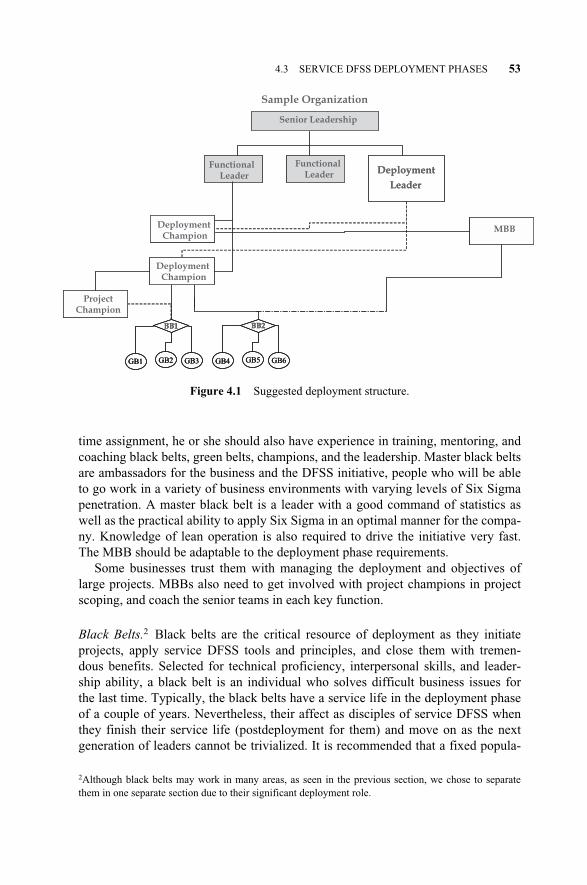
time assignment, he or she should also have experience in training, mentoring, andcoaching black belts, green belts, champions, and the leadership. Master black beltsare ambassadors for the business and the DFSS initiative, people who will be ableto go work in a variety of business environments with varying levels of Six Sigmapenetration. A master black belt is a leader with a good command of statistics aswell as the practical ability to apply Six Sigma in an optimal manner for the compa-ny. Knowledge of lean operation is also required to drive the initiative very fast.The MBB should be adaptable to the deployment phase requirements.
Some businesses trust them with managing the deployment and objectives oflarge projects. MBBs also need to get involved with project champions in projectscoping, and coach the senior teams in each key function.
Black Belts.2 Black belts are the critical resource of deployment as they initiateprojects, apply service DFSS tools and principles, and close them with tremen-dous benefits. Selected for technical proficiency, interpersonal skills, and leader-ship ability, a black belt is an individual who solves difficult business issues forthe last time. Typically, the black belts have a service life in the deployment phaseof a couple of years. Nevertheless, their affect as disciples of service DFSS whenthey finish their service life (postdeployment for them) and move on as the nextgeneration of leaders cannot be trivialized. It is recommended that a fixed popula-
4.3 SERVICE DFSS DEPLOYMENT PHASES 53
Senior Leadership
FunctionalLeader
Functionalleader
Deployment
Leader
BB1
GB1 GB2 GB3
BB2
GB4 GB5 GB6
Deployment
Deployment
Project
MBB
Sample Organization
Senior Leadership
FunctionalLeader
FunctionalLeader
Deployment
Leader
BB1
GB1 GB2 GB3
BB1
GB1 GB2 GB3
BB2
GB4 GB5 GB6
BB2
GB4 GB5 GB6
Deployment Champion
Deployment Deployment Champion
ProjectProjectChampion
MBBMBB
Figure 4.1 Suggested deployment structure.
2Although black belts may work in many areas, as seen in the previous section, we chose to separatethem in one separate section due to their significant deployment role.
c04.qxd 4/22/2005 7:38 AM Page 53
tion of black belts (usually computed as a percentage of affected functions whereservice DFSS is deployed) be kept in the pool during the designated service life.This population is not static, however. It is replenished every year by new blood.Repatriated black belts, in turn, replenish the disciple population, and the cyclecontinues until sustainment is achieved and service DFSS becomes the way of do-ing design business.
Black belts will learn and understand service methodologies and principles andfind application opportunities within the project, cultivate a network of experts,train and assist others (e.g., green belts) in new strategies and tools, leverage sur-face business opportunities through partnerships, and drive concepts and methodol-ogy into the way of doing work.
The deployment of black belts is a subprocess within the deployment process it-self with the following steps: (1) black belt identification, (2) black belt projectscoping, (3) black belt training, (4) black belt deployment during the service life,and (5) black belt repatriation into the mainstream.
The deployment team prepares designated training waves or classes of serviceblack belts to apply DFSS and associated technologies, methods, and tools onscoped projects. Black belts are developed by project execution, training in statis-tics and design principles with on-the-project application, and mentored reviews.Typically, with a targeted quick cycle time, a black belt should be able to close atleast three projects a year. Our observations indicate that black belt productivity, onthe average, increases after his/her training projects. Following their training fo-cused, descoped project, black belt projects can get more complex and evolve intocross-function, supply chain, and customer projects.
The black belts are the leaders of the future. Their visibility should be apparentto the rest of the organization and they should be cherry-picked to join the serviceDFSS program with “leader of the future” statue. Armed with the right tools,processes, and DFSS principles, black belts are the change agents the deployingcompany should utilize to achieve its vision and mission statements. They need tobe motivated and recognized for their good efforts while mentored at both the tech-nical and leadership fronts by the master black belt and the project champions. Oraland written presentation skills are crucial for their success. To increase the effec-tiveness of the black belts, we suggest building a black belt collaboration mecha-nism for the purpose of maintaining structures and environments to foster individ-ual and collective learning of initiative and DFSS knowledge, including initiativedirection, vision, and prior history. In addition, the collaboration mechanism,whether virtual or physical, could serve as a focus for black belt activities to fosterteam building, growth, and inter- and intrafunction communication and collabora-tion. Another important reason for establishing such a mechanism is to ensure thatthe deployment team gets its information in an accurate and timely fashion to pre-vent and mitigate failure modes downstream of deployment and postdeploymentphases. Historical knowledge might include lessons learned, best practices sharing,and deployment benchmarking data.
Table 4.1 summarizes the roles and responsibilities of the deployment operativespresented in this section. Figure 4.2 depicts the growth curve of the Six Sigma de-
54 SERVICE DESIGN FOR SIX SIGMA DEPLOYMENT
c04.qxd 4/22/2005 7:38 AM Page 54
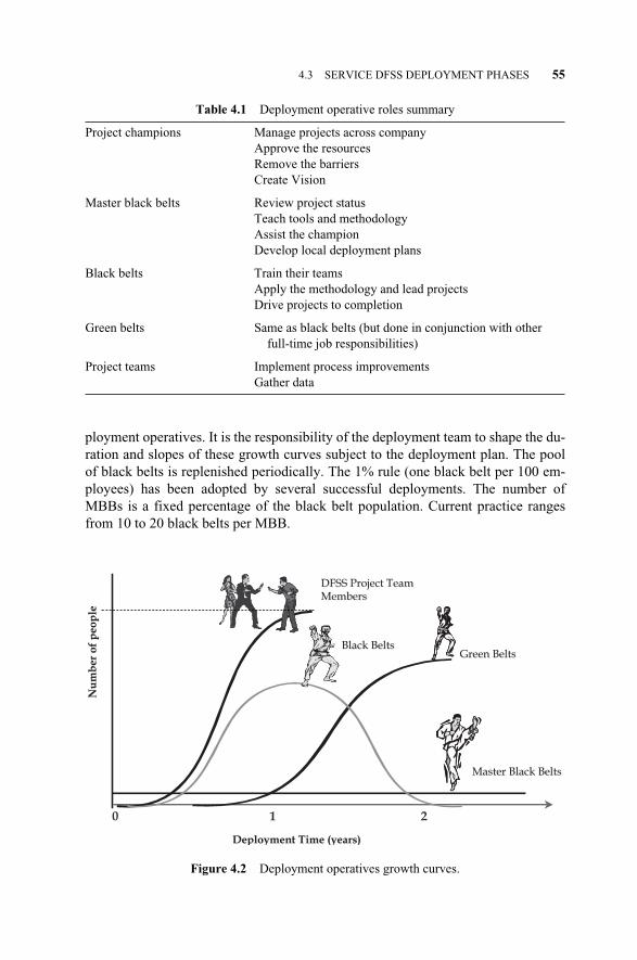
ployment operatives. It is the responsibility of the deployment team to shape the du-ration and slopes of these growth curves subject to the deployment plan. The poolof black belts is replenished periodically. The 1% rule (one black belt per 100 em-ployees) has been adopted by several successful deployments. The number ofMBBs is a fixed percentage of the black belt population. Current practice rangesfrom 10 to 20 black belts per MBB.
4.3 SERVICE DFSS DEPLOYMENT PHASES 55
Table 4.1 Deployment operative roles summary
Project champions Manage projects across companyApprove the resourcesRemove the barriersCreate Vision
Master black belts Review project statusTeach tools and methodologyAssist the championDevelop local deployment plans
Black belts Train their teamsApply the methodology and lead projectsDrive projects to completion
Green belts Same as black belts (but done in conjunction with other full-time job responsibilities)
Project teams Implement process improvementsGather data
Figure 4.2 Deployment operatives growth curves.
0 1 2
Deployment Time (years)Deployment Time (years)
Nu
mb
er
of
peo
ple
Nu
mb
er
of
peo
ple
Master Black BeltsMaster Black Belts
Green BeltsGreen Belts
DFSS Project Team DFSS Project Team MembersMembers
Black BeltsBlack Belts
c04.qxd 4/22/2005 7:38 AM Page 55
Green Belt. A green belt is an employee of the deploying company who has beentrained in Six Sigma and will participate on project teams as part of their full-timejob. The green belt’s knowledge of Six Sigma is less than a black belt’s. Thegreen belt’s business knowledge of his or her company is a necessity to ensuresuccess of the process improvement task. The green belt employee plays an im-portant role in executing the Six Sigma process in day-to-day operations by com-pleting smaller-scope projects. Black belts should be networked around greenbelts to support and coach them. Green belt training is not for awareness. The de-ployment plan should enforce certification while tracking their project status ascontrol mechanisms for deployment. Green belts, like black belts, should be clos-ing projects as well.
In summary, green belts are employees trained in Six Sigma methodologies whoconduct or contribute to projects that require Six Sigma application. Following suc-cessful completion of training, green belts will be able to participate in larger pro-jects being conducted by black belts, lead small projects, and apply Six Sigma toolsand concepts to daily work.
Communication Plan. To ensure the success of service DFSS, the deploymentteam should develop a communication plan that highlights the key steps as serviceDFSS is being deployed. In doing so, they should target the audience that will re-ceive necessary communication at various points in the deployment process withidentifiable possible media of communication deemed most effective by the compa-ny. The deployment team should outline the overriding communication objectivesat each major phase of service DFSS deployment and provide a high-level, recom-mended communication plan for each of the identified communicators during com-pany DFSS initialization.
As service DFSS is deployed in a company, we recommend that various peoplecommunicate certain messages at certain times. For example, at the outset of de-ployment, the CEO should send a strong message to the executive population thatthe corporation is adopting service DFSS, why it is necessary, who will be leadingthe effort both at leadership and deployment team levels, why their commitmentand involvement is absolutely required, and other important items. The CEO alsosends, among other communiqués to other audiences, a message to the deploymentchampions, explaining why they have been chosen, what is expected of them, andhow they are empowered to enact their respective roles and responsibilities.
Several key people will need to communicate key messages to key audiences asDFSS is initiated, deployed, and sustained; for example, the training and develop-ment leader, finance leader, HR leader, IT leader, project champions, deploymentchampions (functional leaders), mangers and supervisors, black belts, and greenbelts to name a few. Every leader involved in DFSS processes must be totally com-mitted to the cause to avoid derailment of cultural evolution driven by DFSS. Everyleader must seek out information from the deployment team to validate their con-viction to the process.
To further assist in effective communications, the leader and others responsiblefor communicating DFSS deployment should delineate who delivers messages to
56 SERVICE DESIGN FOR SIX SIGMA DEPLOYMENT
c04.qxd 4/22/2005 7:38 AM Page 56
whom during the predeployment phase. It is obvious that certain people have pri-mary communication responsibility during the initial stages of Six Sigma deploy-ment, including the CEO, Service DFSS deployment leader, and deployment cham-pions. The company communications leader plays a role in supporting the CEO,deployment leader, and others leaders as they formulate and deliver their commu-niqués in support of predeployment. The communication plan should include thefollowing minimum communiqués:
� Why the company is deploying DFSS, along with several key points abouthow Six Sigma supports and is integrated with company’s vision, includingother business initiatives.
� Set of financial targets, operational goals, and metrics that will be providingstructure and guidance to the DFSS deployment effort, to be done with con-sideration of the targeted audience.
� A breakdown of where DFSS will be focused in the company; a roll-out se-quence by function, geography, product or other scheme; a general timeframe for how quickly and aggressively DFSS will be deployed.
� A firmly established and supported long-term commitment to the DFSS phi-losophy, methodology and anticipated results.
� Specific managerial guidelines to control the scope and depth of deploymentfor a corporation or function.
� Review and examine key performance metrics to ensure the progressive uti-lization and deployment of DFSS.
� Commitment of part-time and full-time deployment champions, projectchampion, and full-time black belt resources.
Service DFSS Project Sources. The successful deployment of the DFSS initiativewithin a company is tied to projects derived from the company’s breakthrough ob-jectives, multigeneration planning, growth and innovation strategy, and chronic,pressing redesign issues. Such service DFSS project sources can be categorized asretroactive or proactive sources. In either case, an active measurement systemshould be in place for both internal and external critical-to-satisfaction (CTS’s)metrics, sometimes called the “big Ys.” The measurement system should pass aGauge R&R study in all big Y metrics.
How should big Ys be defined? This question underscores why we need to de-cide early who is the primary customer (internal and external) of our potentialDFSS project. What is the big Y (CTS) in customer terms? It does us no good, forexample, to develop a delivery system to shorten flow processes if the customer ismainly upset with quality and reliability. Likewise, it does us little good to developa project to reduce tool breakage if the customer is actually upset with inventory cy-cle losses. It pays dividends to later project success to know the big Y. No big Y(CTS) simply means no project! Potential projects with hazy big Y definitions aresetups for black belt failure. Again, it is unacceptable to not know the big Ys of topproblems (retroactive project sources) or those of proactive project sources aligned
4.3 SERVICE DFSS DEPLOYMENT PHASES 57
c04.qxd 4/22/2005 7:38 AM Page 57
with the annual objectives, growth and innovation strategy, benchmarking, multi-generation process and product planning, and technology road maps.
On the proactive side, black belts will be claiming projects from a multigenera-tional service/process plan or from the big Ys replenished, prioritized projectpipeline. Green belts should be clustered around these key projects for the deploy-ing function or business operations and tasked with assisting the black belts, as sug-gested by Figure 4.3.
We need some useful measure of big Ys, in variable terms,3 to establish thetransfer function, Y = f (x). The transfer function is the means for determining cus-tomer satisfaction, or other big Ys, and can be identified by a combination of designmapping and design of experiment (if transfer functions are not available or cannotbe derived). A transfer function is a mathematical relationship in the associatedmapping, linking controllable and uncontrollable factors. Transfer functions can bederived, empirically obtained from a DOE, or regressed using historical data. Insome cases, no closed mathematical formula can be obtained and the DFSS teamcan resort to modeling. In the DFSS project road map, there is a transfer functionfor every functional requirement, for every design parameter, for every processvariable, and, ultimately, for every big Y.
Sometimes, we find that measurement of the big Y opens windows to the mindwith insights powerful enough to solve the problem immediately. It is not rare tofind customer complaints that are very subjective and unmeasured. The black beltneeds to find the best measure available to his/her project big Y to help describe thevariation faced and to support Y = f(x) analysis. The black belt may have to developa measuring system for the project to be true to the customer and big Y definition!
We need measurements of the big Y that we can trust. Studying problems withfalse measurements leads to frustration and defeat. With variable measurements,the issue is handled as a straightforward Gauge R&R question. With attribute orother subjective measures, it is an attribute Measurement system analysis (MSA)issue. It is tempting to ignore MSA of the big Y, but this is not a safe practice.More that 50% of the black belts we coached encounter MSA problems in theirprojects. This issue in the big Y measurement is probably worse because littlethought is conventionally given to MSA at the customer level. The black beltsshould make every effort to assure themselves that their big Y measurement is er-ror minimized. We need to be able to establish a distribution of Y from which tomodel or draw samples for Y = f(x) study. The better the measurement of the bigY, the better the black belt can see the distribution contrasts needed to yield orconfirm Y = f(x).
What is the value to the customer? This should be a moot point if the project is atop issue. The value decisions have already been made. Value is a relative term withnumerous meanings. It may be cost, appearance, status, but the currency of valuemust be decided on. In Six Sigma, it is a common practice to ask that each projectgenerate average benefits greater than $250,000. This is seldom a problem in topprojects that are aligned to business issues and opportunities.
58 SERVICE DESIGN FOR SIX SIGMA DEPLOYMENT
3The transfer function will be weak and questionable without it.
c04.qxd 4/22/2005 7:38 AM Page 58

The black belt together with the finance individual assigned to the project shoulddecide on a value standard and do a final check to ascertain that the potential projectvalue is greater than the minimum. High-value projects are not necessarily harderthan low-value projects. Projects usually hide their level of complexity until solved.Many low-value projects are just as difficult to complete as high-value projects, sothe deployment champions should leverage their effort by value. Deployment man-agement, including the local master black belt, has the lead in identifying redesignproblems and opportunities as good potential projects. The task, however, of goingfrom a potential to an assigned Six Sigma project belongs to the project champion.The deployment champion selects a project champion, who then carries out the nextphases. The champion is responsible for the project scope, black belt assignment,ongoing project review, and, ultimately, the success of the project. This is an impor-tant and responsible position and must be taken very seriously. A suggested projectinitiation process is depicted in Figure 4.4.
It is a significant piece of work to develop a good project but black belts, partic-ularly those already certified, have a unique perspective that can be of great assis-tance to the project champions. Green belts, as well, should be taught fundamentalskills useful in developing a project scope. Black belt and green belt engagement iskey to helping champions fill the project pipeline, investigate potential projects, pri-oritize them, and develop achievable project scopes. It is the observation of manyskilled problem solvers that adequately defining the problem and setting up a solu-tion strategy consumes the most time on the path to a successful project. The betterwe define and scope a project, the faster the deploying company and its customerbase will benefit from the solution. That is the primary Six Sigma objective.
4.3 SERVICE DFSS DEPLOYMENT PHASES 59
Figure 4.3 Green belt (GB) and black belt (BB) clustering scheme.
Big Y
BB1
GB1
GB3
GBn
BB
43
GB
GB
GB
BB
2G
B
GB
GB
GB2
Big Y
BB1
GB1
GB3
GBn
BB
43
GB
GB
GB
BB
43
GB
GB
GB
BB
2G
B
GB
GB
BB
2G
B
GB
GB
GB2
c04.qxd 4/22/2005 7:38 AM Page 59
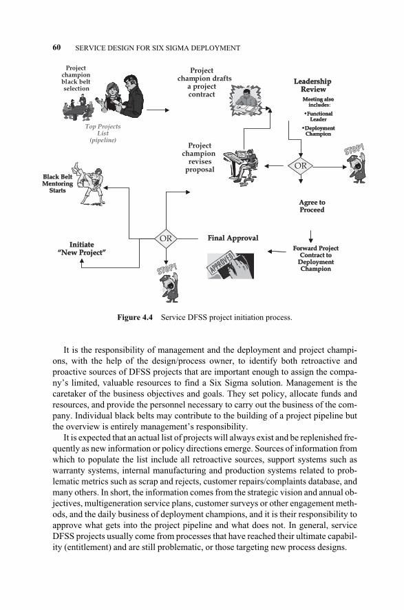
It is the responsibility of management and the deployment and project champi-ons, with the help of the design/process owner, to identify both retroactive andproactive sources of DFSS projects that are important enough to assign the compa-ny’s limited, valuable resources to find a Six Sigma solution. Management is thecaretaker of the business objectives and goals. They set policy, allocate funds andresources, and provide the personnel necessary to carry out the business of the com-pany. Individual black belts may contribute to the building of a project pipeline butthe overview is entirely management’s responsibility.
It is expected that an actual list of projects will always exist and be replenished fre-quently as new information or policy directions emerge. Sources of information fromwhich to populate the list include all retroactive sources, support systems such aswarranty systems, internal manufacturing and production systems related to prob-lematic metrics such as scrap and rejects, customer repairs/complaints database, andmany others. In short, the information comes from the strategic vision and annual ob-jectives, multigeneration service plans, customer surveys or other engagement meth-ods, and the daily business of deployment champions, and it is their responsibility toapprove what gets into the project pipeline and what does not. In general, serviceDFSS projects usually come from processes that have reached their ultimate capabil-ity (entitlement) and are still problematic, or those targeting new process designs.
60 SERVICE DESIGN FOR SIX SIGMA DEPLOYMENT
Figure 4.4 Service DFSS project initiation process.
l ct a l a projectproject
Agree to Agree to ProceedProceed
OROR
Forward Project Forward Project Contract to Contract to
Deployment Deployment ChampionChampion
Final ApprovalFinal ApprovalORORInitiate Initiate
“New Project”“New Project”
LeadershipLeadershipReviewReview
Meeting also Meeting also include:include:
••Functional Functional LeaderLeader
••Deployment Deployment ChampionChampion
Black BeltBlack BeltMentoring Mentoring
StartsStarts
Project championblack belt
l a
sel
l
ection
a projectproject
Top ProjectsList
(pipeline)
Agree to Agree to ProceedProceed
Project champion
revisesproposal OROR
Forward Project Forward Project Contract to Contract to
Deployment Deployment ChampionChampion
Final ApprovalFinal ApprovalORORInitiate Initiate
“New Project”“New Project”
Project champion drafts
a projectcontract
LeadershipLeadershipReviewReview
Meeting also Meeting also include:include:
••Functional Functional LeaderLeader
••Deployment Deployment ChampionChampion
LeadershipLeadershipReviewReview
Meeting also Meeting also include:includes:
••Functional Functional LeaderLeader
••Deployment Deployment ChampionChampion
Black BeltBlack BeltMentoring Mentoring
StartsStarts
c04.qxd 4/22/2005 7:38 AM Page 60
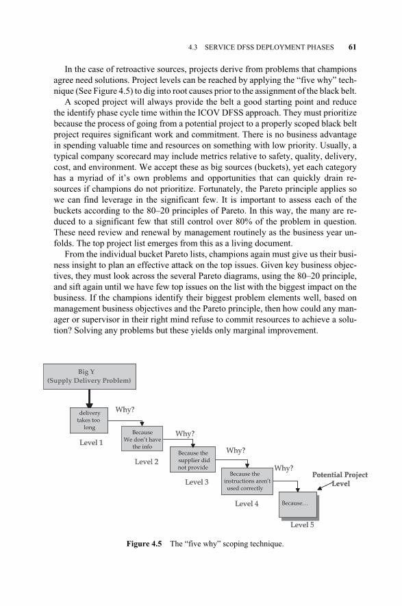
In the case of retroactive sources, projects derive from problems that championsagree need solutions. Project levels can be reached by applying the “five why” tech-nique (See Figure 4.5) to dig into root causes prior to the assignment of the black belt.
A scoped project will always provide the belt a good starting point and reducethe identify phase cycle time within the ICOV DFSS approach. They must prioritizebecause the process of going from a potential project to a properly scoped black beltproject requires significant work and commitment. There is no business advantagein spending valuable time and resources on something with low priority. Usually, atypical company scorecard may include metrics relative to safety, quality, delivery,cost, and environment. We accept these as big sources (buckets), yet each categoryhas a myriad of it’s own problems and opportunities that can quickly drain re-sources if champions do not prioritize. Fortunately, the Pareto principle applies sowe can find leverage in the significant few. It is important to assess each of thebuckets according to the 80–20 principles of Pareto. In this way, the many are re-duced to a significant few that still control over 80% of the problem in question.These need review and renewal by management routinely as the business year un-folds. The top project list emerges from this as a living document.
From the individual bucket Pareto lists, champions again must give us their busi-ness insight to plan an effective attack on the top issues. Given key business objec-tives, they must look across the several Pareto diagrams, using the 80–20 principle,and sift again until we have few top issues on the list with the biggest impact on thebusiness. If the champions identify their biggest problem elements well, based onmanagement business objectives and the Pareto principle, then how could any man-ager or supervisor in their right mind refuse to commit resources to achieve a solu-tion? Solving any problems but these yields only marginal improvement.
4.3 SERVICE DFSS DEPLOYMENT PHASES 61
Figure 4.5 The “five why” scoping technique.
Why?
Why?
Why?Level 1
Level 2
Level 3
Level 4 Because…
Why?
deliverytake too
longBecause
We don’t have the info
Because thesupplier did not provide
Because theinstructions aren’tused correctly
Potential ProjectLevel
Level 5
Big Y (Supply D DeDeliver y Pr oblem)
Why?
Why?
Why?Level 1
Level 2
Level 3
Level 4 Because…
Why?
deliverytakes too
longBecause
We don’t havethe info
Because thesupplier didnot provide
Because theinstructions aren’tused correctly
Potential ProjectLevel
Level 5
Big Y(Supply Delivery Problem)
c04.qxd 4/22/2005 7:38 AM Page 61
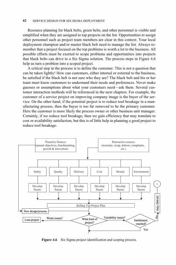
Resource planning for black belts, green belts, and other personnel is visible andsimplified when they are assigned to top projects on the list. Opportunities to assignother personnel such as project team members are clear in this context. Your localdeployment champion and/or master black belt need to manage the list. Always re-member that a project focused on the top problems is worth a lot to the business. Allpossible efforts must be exerted to scope problems and opportunities into projectsthat black belts can drive to a Six Sigma solution. The process steps in Figure 4.6help us turn a problem into a scoped project.
A critical step in the process is to define the customer. This is not a question thatcan be taken lightly! How can customers, either internal or external to the business,be satisfied if the black belt is not sure who they are? The black belt and his or herteam must know customers to understand their needs and preferences. Never makeguesses or assumptions about what your customers need—ask them. Several cus-tomer interaction methods will be referenced in the next chapters. For example, thecustomer of a service project on improving company image is the buyer of the ser-vice. On the other hand, if the potential project is to reduce tool breakage in a man-ufacturing process, then the buyer is too far removed to be the primary customer.Here the customer is more likely the process owner or other business unit manager.Certainly, if we reduce tool breakage, then we gain efficiency that may translate tocost or availability satisfaction, but this is of little help in planning a good project toreduce tool breakage.
62 SERVICE DESIGN FOR SIX SIGMA DEPLOYMENT
Figure 4.6 Six Sigma project identification and scoping process.
Retroactive sources
(warranty, scrap, defects, complaints,
etc.)
Safety Quality Delivery Cost Morale Environment
Develop
Pareto
Develop
Pareto
Develop
Pareto
Develop
Pareto
Develop
Pareto
Develop
Pareto
Rolling Top Project Plan
What kind of
project?
Variability issues?
Proactive Sources
(annual objectives, benchmarking,
growth & innovation)
Entitlement
reached?
No
Yes
Lean projectWaste issues?
New design/process
1
On
ly D
MA
IC
Retroactive sources
(warranty, scrap, defects, complaints,
etc.)
Safety Quality Delivery Cost Morale EnvironmentSafety Quality Delivery Cost Morale Environment
Develop
Pareto
Develop
Pareto
Develop
Pareto
Develop
Pareto
Develop
Pareto
Develop
Pareto
Rolling Top Project Plan
What kind of
project?
Variability issues?
Proactive Sources
(annual objectives, benchmarking,
growth & innovation)
Entitlement
reached?
No
Yes
Lean projectWaste issues?
New design/process
11
On
ly D
MA
IC
c04.qxd 4/22/2005 7:38 AM Page 62
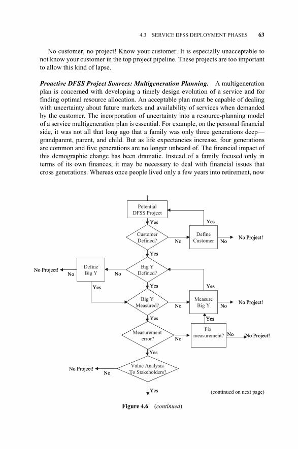
No customer, no project! Know your customer. It is especially unacceptable tonot know your customer in the top project pipeline. These projects are too importantto allow this kind of lapse.
Proactive DFSS Project Sources: Multigeneration Planning. A multigenerationplan is concerned with developing a timely design evolution of a service and forfinding optimal resource allocation. An acceptable plan must be capable of dealingwith uncertainty about future markets and availability of services when demandedby the customer. The incorporation of uncertainty into a resource-planning modelof a service multigeneration plan is essential. For example, on the personal financialside, it was not all that long ago that a family was only three generations deep—grandparent, parent, and child. But as life expectancies increase, four generationsare common and five generations are no longer unheard of. The financial impact ofthis demographic change has been dramatic. Instead of a family focused only interms of its own finances, it may be necessary to deal with financial issues thatcross generations. Whereas once people lived only a few years into retirement, now
4.3 SERVICE DFSS DEPLOYMENT PHASES 63
Figure 4.6 (continued)
Customer
Defined?
Big Y
Defined?
Big Y
Measured?
Value Analysis
To Stakeholders?
Potential
DFSS Project
No
Define
Customer No
Yes
No Project!
Define
Big YNo No
Yes
No Project!
No
Measure
Big Y No
Yes
No Project!
Yes
Yes
Yes
Yes
Yes
NoNo Project!
Yes
Measurement
error? No
Fix
measurement? No No Project!
Yes
Yes
(continued on next page)
c04.qxd 4/22/2005 7:38 AM Page 63
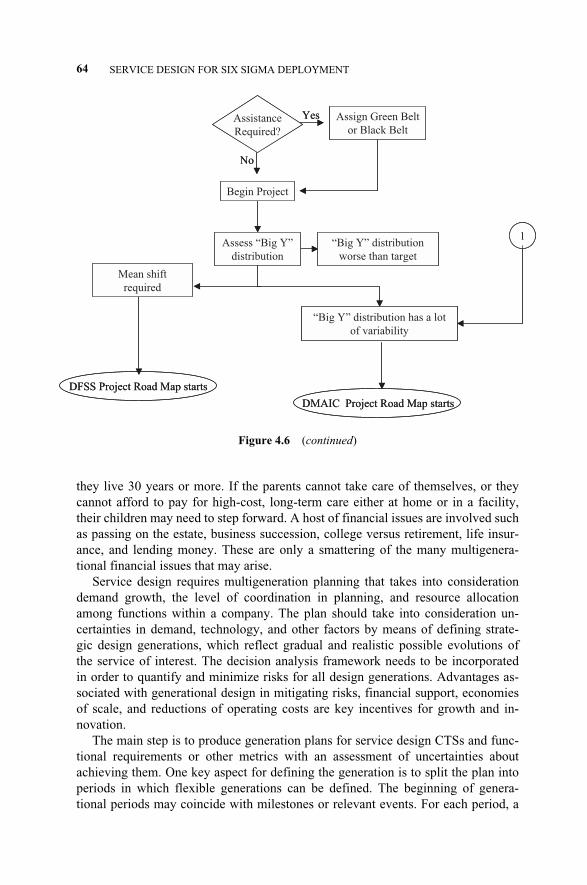
they live 30 years or more. If the parents cannot take care of themselves, or theycannot afford to pay for high-cost, long-term care either at home or in a facility,their children may need to step forward. A host of financial issues are involved suchas passing on the estate, business succession, college versus retirement, life insur-ance, and lending money. These are only a smattering of the many multigenera-tional financial issues that may arise.
Service design requires multigeneration planning that takes into considerationdemand growth, the level of coordination in planning, and resource allocationamong functions within a company. The plan should take into consideration un-certainties in demand, technology, and other factors by means of defining strate-gic design generations, which reflect gradual and realistic possible evolutions ofthe service of interest. The decision analysis framework needs to be incorporatedin order to quantify and minimize risks for all design generations. Advantages as-sociated with generational design in mitigating risks, financial support, economiesof scale, and reductions of operating costs are key incentives for growth and in-novation.
The main step is to produce generation plans for service design CTSs and func-tional requirements or other metrics with an assessment of uncertainties aboutachieving them. One key aspect for defining the generation is to split the plan intoperiods in which flexible generations can be defined. The beginning of genera-tional periods may coincide with milestones or relevant events. For each period, a
64 SERVICE DESIGN FOR SIX SIGMA DEPLOYMENT
Figure 4.6 (continued)
Assistance
Required?
No
Yes Assign Green Belt
or Black Belt
Begin Project
Assess “Big Y”
distribution
“Big Y” distribution
worse than target
Mean shift
required
“Big Y” distribution has a lot
of variability
DFSS Project Road Map starts
DMAIC Project Road Map starts
1
Assistance
Required?
No
Yes Assign Green Belt
or Black Belt
Begin Project
Assess “Big Y”
distribution
“Big Y” distribution
worse than target
Mean shift
required
“Big Y” distribution has a lot
of variability
DFSS Project Road Map starts
DMAIC Project Road Map starts
11
c04.qxd 4/22/2005 7:38 AM Page 64
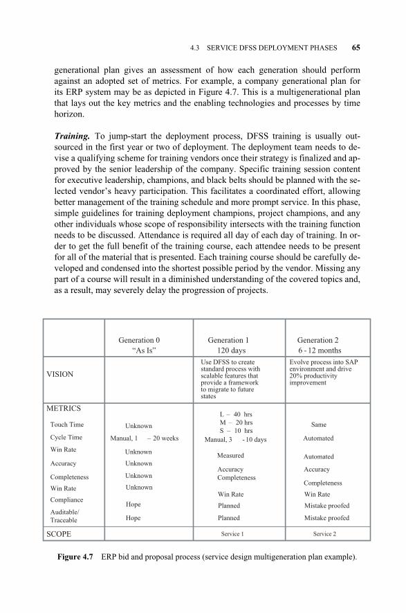
generational plan gives an assessment of how each generation should performagainst an adopted set of metrics. For example, a company generational plan forits ERP system may be as depicted in Figure 4.7. This is a multigenerational planthat lays out the key metrics and the enabling technologies and processes by timehorizon.
Training. To jump-start the deployment process, DFSS training is usually out-sourced in the first year or two of deployment. The deployment team needs to de-vise a qualifying scheme for training vendors once their strategy is finalized and ap-proved by the senior leadership of the company. Specific training session contentfor executive leadership, champions, and black belts should be planned with the se-lected vendor’s heavy participation. This facilitates a coordinated effort, allowingbetter management of the training schedule and more prompt service. In this phase,simple guidelines for training deployment champions, project champions, and anyother individuals whose scope of responsibility intersects with the training functionneeds to be discussed. Attendance is required all day of each day of training. In or-der to get the full benefit of the training course, each attendee needs to be presentfor all of the material that is presented. Each training course should be carefully de-veloped and condensed into the shortest possible period by the vendor. Missing anypart of a course will result in a diminished understanding of the covered topics and,as a result, may severely delay the progression of projects.
4.3 SERVICE DFSS DEPLOYMENT PHASES 65
Figure 4.7 ERP bid and proposal process (service design multigeneration plan example).
Generation 0 Generation 1 Generation 2
“As Is” 120 days 6 - 12 months
VISION
Use DFSS to create
standard process with
scalable features that
provide a framework
to migrate to future
states
Evolve process into SAP
environment and drive
20% productivity
improvement
METRICS
Touch Time
Cycle Time
Win Rate
Accuracy
Completeness
Win Rate
Compliance
Auditable/
Traceable
SCOPE Service 1 Service 2
Unknown
Manual, 1 – 20 weeks
Unknown
Unknown
Unknown
Unknown
Hope
Hope
L – 40 hrs
M – 20 hrs
S – 10 hrs
Manual, 3 - 10 days
Measured
Accuracy
Completeness
Win Rate
Planned
Planned
Same
Automated
Automated
Accuracy
Completeness
Win Rate
Mistake proofed
Mistake proofed
c04.qxd 4/22/2005 7:38 AM Page 65
Existence of a Service Program Development Management System. Our experi-ence is that a project road map is required for successful DFSS deployment. Theroad map works as a compass, leading black belts to closure by laying out the fullpicture of the DFSS project. We would like to think of this road map as a recipe thatcan be further tailored to the customized application within the company’s manage-ment system that spans the design life cycle (see Chapter 1). Usually, the serviceDFSS deployment team has two choices at this point:
1. Develop a new business process management system (BPMS; see Chapter 8)to include the proposed DFSS roadmap. Examples are advanced productquality planning (APQP) in the automotive industry, integrated product andprocess design (IPPD) in the aerospace industry, the Project Management In-stitute (PMI) process, and James Martin in software industry. It is the experi-ence of the authors that many companies lack such universal discipline in apractical sense. This choice is suitable for companies practicing a variety ofBPMS and hoping that alignment will evolve. The BPMS should span theservice life cycle presented in Chapter 1
2. Integrate with the current BPMS by laying this roadmap over it and synchro-nizing when and where needed.
In either case, the DFSS project will be paced at the speed of the leading pro-gram from which the project was derived in the BPMS. Initially, highly leverageprojects should target subsystems that the business and the customer are sensitiveto. A sort of requirement flowdown or cascading method should be adopted to iden-tify these subsystems. Later, when DFSS becomes the way of doing business, sys-tem-level DFSS deployment becomes the norm and the issue of synchronizationwith the BPMS will diminish eventually. Actually, the BPMS will be crafted to re-flect the DFSS learning experience that the company gained over years of experi-ence.
4.3.3 Deployment
This phase is the period of time in which champions are trained and select initialblack belt projects, as well as when the initial wave of black belts are trained andprojects are completed that yield significant soft and hard operational benefits. Thetraining encompasses most of the deployment activities in this phase and is dis-cussed in the following section. Additionally, this phase includes the following as-signments of the deployment team:
� Reiterate to key personnel their responsibilities at critical points in the de-ployment process.
� Reinforce the commitment of project champions and black belts to aggres-sively execute selected improvement projects. Mobilize and empower bothpopulations to effectively carry out their respective roles and responsibilities.
66 SERVICE DESIGN FOR SIX SIGMA DEPLOYMENT
c04.qxd 4/22/2005 7:38 AM Page 66

� Recognize exemplary performance in execution and in culture at the projectchampion and black belt levels.
� Inform the general employee population about the tenets of Six Sigma and thedeployment process.
� Build information packets for project champions and black belts that containadministrative, logistical, and other information they need to execute their re-sponsibilities at given points in time.
� Document and publicize successful projects and the positive consequencesfor the company and its employees.
� Document and distribute project savings data by business unit, product, orother appropriate areas of focus.
� Hold Six Sigma events or meetings with all employees at given locationswhere leadership is present and involved and where such topics are covered.
4.3.3.1 Training. The critical steps in DFSS training are (1) determining the con-tent and outline, (2) developing the materials, and (3) deploying training classes. Indoing so, the deployment team and their training vendor of choice should be verycautious about cultural aspects and weave the culture change into the soft side ofthe initiative training. Training is the significant mechanism within deploymentthat, in addition to equipping trainees with the right tools, concepts and methods,will expedite deployment and help shape a data-driven culture. This section willpresent a high-level perspective of the training recipients and what type of trainingthey should receive. The training recipients are arranged below by level of com-plexity.
Senior Leadership. Training for senior leadership should include an overview ofbusiness and financial benefits of implementation, benchmarking of successful de-ployments, and specific training on tools to ensure successful implementation.
Deployment Champions. Training for deployment champions is more detailed thanthat provided to senior leadership. Topics would include the DFSS concept,methodology, and “must-have” tools and processes to ensure successful deploy-ment within their function. A class focused on how to be an effective champion aswell as their roles and responsibilities is often beneficial.
Master Black Belts. Initially, experienced master black belts are hired from the out-side to jump-start the system. Additional homegrown MBBs may need to have ad-ditional training beyond their black belt training. Training for master black beltsmust be rigorous about the concept, methodology, and tools, as well as include de-tailed statistics training, computer analysis, and other tool application. Their train-ing should include soft and hard skills to get them to a level of proficiency compat-ible with their roles. On the soft side, topics like strategy, deployment lessonslearned, their roles and responsibilities, presentation and writing skills, leadershipand resource management, and critical success factors benchmarking history and
4.3 SERVICE DFSS DEPLOYMENT PHASES 67
c04.qxd 4/22/2005 7:38 AM Page 67

outside deployment are included. On the hard side, typical training may go into thetheory of topics like DOE, ANOVA, axiomatic design, theory of inventive problemsolving (TRIZ), hypothesis testing of discrete random variables, and lean tools.
Black Belts. As project leaders, the black belts will implement the DFSS methodol-ogy and tools within a function on projects aligned with the business objectives.They lead projects, institutionalize a timely project plan, determine appropriate tooluse, perform analyses, and act as the central point of contact for their projects.Training for black belts includes detailed information about the concept, methodol-ogy and tools. Depending on the curriculum, the duration is usually between threeto six weeks on a monthly schedule. Black belts will be assigned a training-focused,descoped project that has ample opportunities for tool application to foster learningwhile delivering deployment objectives. The weeks between the training sessionswill be spent on gathering data, forming and training their teams, and applying con-cepts and tools where necessary. DFSS concepts and tools flavored by some softskills are the core of the curriculum. Of course, DFSS training and deployment willbe synchronized with the service development process already adopted by the de-ploying company. We provide in Chapter 5 of this book a suggested service DFSSproject road map to serve as a design algorithm for the Six Sigma team. The roadmap will work as a compass, leading black belts to closure by laying out the fullpicture of a typical DFSS project.
Green Belts. The green belts may also take training courses developed specificallyfor black belts where there needs to be more focus. Short-circuiting theory andcomplex tools to meet the allocated short training time (usually less than 50% ofblack belt training period) may dilute many subjects. Green belts can resort to theirblack belt network for help on complex subjects and for coaching and mentoring.
4.3.3.2 Six Sigma Project Financial Aspects. In general, DFSS project finan-cials can be categorized as hard or soft savings and are mutually calculated or as-sessed by the black belt and the assigned financial analyst to the project. The finan-cial analyst assigned to a DFSS team should act as the lead in quantifying thefinancials related to the project “actions” at the initiation and closure phases, assistin identification of “hidden factory” savings, support the black belt on an ongoingbasis, and if financial information is required from areas outside his/her area of ex-pertise, he/she needs to direct the black belt to the appropriate contacts, follow up,and ensure that the black belt receives the appropriate data. The analyst, at projectclosure, should ensure that the appropriate stakeholders concur with the savings.This primarily affects processing costs, design expense, and nonrevenue items forrejects not directly led by black belts from those organizations. In essence, the ana-lyst needs to provide more than an audit function.
“Hard savings” are defined as measurable savings associated with improvementsin repairs, rework, absorptions, writeoffs, concessions, inspections, material costs,warranty, labor savings (will be achieved/collectable through work rebalances),revenue associated with reductions in customer dissatisfaction, cash flow savings
68 SERVICE DESIGN FOR SIX SIGMA DEPLOYMENT
c04.qxd 4/22/2005 7:38 AM Page 68
(i.e., inventory), and other values of lost customer satisfaction. Hard savings arecalculated against present operating levels, not against a budget or a plan. They rep-resent the bottom-line savings that directly affect the company’s income statementand cash flow and are the result of measurable product, service, and process im-provements. The effect on company financial statements will be determined off-lineby the appropriate company office. “Soft” savings are less direct in nature and in-clude projects that open floor space (as a side benefit), may allow for the location offuture operations, reduce vehicle weight, may enable other design actions to deleteexpensive light weight materials, and lead to cost avoidance. Cost avoidance is usu-ally confused with cost savings. For example, employing an ATM instead a teller toreduce operating cost is avoidance rather than saving.
The financial analyst should work with the black belt to assess the projected an-nual financial savings based on the information available at that time (e.g., scope,expected outcome). This is not a detailed review, but a rough order-of-magnitudeapproval. These estimates are expected to be revised as the project progresses andmore accurate data become available. The project should have the potential toachieve the annual target, usually $250,000. The analyst confirms the business ra-tionale for the project where necessary.
Yang and El-Haik (2003) developed a scenario of black belt target cascadingthat can be customized to different applications. It is based on project cycle time,number of projects handled simultaneously by the black belt, and their importanceto the organization.
4.3.4 Postdeployment Phase
This phase spans the period of time during which subsequent waves of black beltsare trained, when the synergy and scale of Six Sigma builds to a critical mass, andwhen additional elements of DFSS deployment are implemented and integrated.
In what follows, we present some thoughts and observations that were gainedthrough our deployment experience of Six Sigma and, in particular, DFSS. The pur-pose is to determine factors that lead to maintaining and expanding the momentumof DFSS deployment so that it becomes sustainable.
This book presents the service DFSS methodology that exhibits the merging ofmany tools at both the conceptual and analytical levels and penetrates dimensionslike characterization, optimization, and validation by integrating tools, principles,and concepts. This vision of DFSS is a core competency in a company’s overalltechnology strategy to accomplish its goals. An evolutionary strategy that movesthe deployment of the DFSS method toward the ideal culture is discussed. In thestrategy, we have identified the critical elements, needed decisions, and deploymentconcerns.
The literature suggests that more innovative methods fail immediately after ini-tial deployment than at any other stage. Useful innovation attempts that are chal-lenged by cultural change are not directly terminated, but are allowed to fade slow-ly and silently. A major reason for the failure of technically viable innovations isthe inability of leadership to commit to an integrated, effective, cost-justified, and
4.3 SERVICE DFSS DEPLOYMENT PHASES 69
c04.qxd 4/22/2005 7:38 AM Page 69
evolutionary program for sustainability that is consistent with company’s mission.The DFSS deployment parallels in many aspects the technical innovation chal-lenges from the cultural perspective. The DFSS initiatives are particularly vulnera-ble if they are too narrowly conceived, built upon only one major success mecha-nism, do not fit the larger organizational objectives. The tentative top-downdeployment approach works where the top leadership support is the significant dri-ver. However, this approach can be strengthened when built around superior mech-anisms like DFSS as a design approach and the methodologies are attractive to de-signers who want to become more proficient in their jobs.
Although there is a need to customize the deployment strategy, it should not berigid. The strategy should be flexible enough to meet expected improvements. Thedeployment strategy itself should be DFSS driven and responsive to anticipatedchanges. It should be insensitive to expected swings in the financial health of com-pany and should be attuned to the company’s objectives on a continuous basis.
The strategy should consistently build coherent linkages between DFSS and dai-ly design business. For example, engineers and architects need to see how all of theprinciples and tools fit together, complement one another, and build toward a coher-ent whole process. DFSS needs to be seen, initially, as an important part, if not thecentral core, of an overall effort to increase technical flexibility.
4.3.4.1 DFSS Sustainability Factors. In our view, DFSS possesses many inher-ent sustaining characteristics that are not offered by other current design practices.Many deign methods, some called best practices, are effective if the design is at alow level and needs to satisfy minimum number of functional requirements, for ex-ample, a component or a process. As the number of the requirements increases (thedesign becomes more complex), the efficiency of these methods decreases. In addi-tion, these methods are hinged on heuristics and developed algorithms (e.g., designfor processability; see Chapter 10), limiting their application across the different de-velopment phases.
The process of design can be improved by constant deployment of DFSS, whichbegins from a different premise, namely, the principle of design. The design axiomsand principles are central to the conception part of DFSS. As will be defined inChapter 8, axioms are general principles or truths that cannot be derived, exceptwhen there are no counterexamples or exceptions. Axioms are fundamental to manyengineering disciplines; examples are thermodynamics laws, Newton’s laws, andthe concepts of force and energy. Axiomatic design provides the principles to de-velop a good design systematically and can overcome the need for customized ap-proaches.
In a sustainability strategy, the following attributes would be persistent and per-vasive features:
� A deployment measurement system that tracks the critical-to-deployment re-quirements and failure modes, and implements corrective actions.
� Continued improvement in the effectiveness of DFSS deployment by bench-marking other successful deployment elsewhere.
70 SERVICE DESIGN FOR SIX SIGMA DEPLOYMENT
c04.qxd 4/22/2005 7:38 AM Page 70
� Enhanced control (over time) over the company’s objectives via selectedDFSS projects that lead to rapid improvement.
� Extended involvement of all levels and functions.
� Embedding DFSS into the everyday operations of the company.
The prospectus for sustaining success will improve if the strategy yields a con-sistent day-to-day emphasis of recognizing that DFSS represent a cultural changeand a paradigm shift, and allows the necessary time for projects success. Severaldeployments found it very useful to extend their DFSS initiative to key suppliersand extending these beyond the component level to subsystem- and system-levelprojects. Some call these projects intraprojects when they span different areas,functions, and business domains. This ultimately will lead to integrating the DFSSphilosophy as a superior design approach within the BPMS and align the issues offunding, timing, and reviews to the embedded philosophy. As a side bonus of thedeployment, conformance to narrow design protocols will start fading away. In allcases, sustaining leadership and managerial commitment to adopting appropriate,consistent, relevant, and continuing reward and recognition mechanisms for blackbelts and green belts is critical to the overall sustainment of the initiative.
The vision is that DFSS as a consistent, complete, fully justified, and usableprocess should be expanded to other areas. The deployment team should keep aneye on the changes that are needed to accommodate altering a black belt’s tasksfrom individualized projects to broader-scope, intrateam assignments. A prioritiz-ing mechanism for future projects that targets the location, size, complexity, in-volvement of other units, type of knowledge to be gained, and potential for fit with-in the strategic plan should be developed.
Another sustaining factor lies in providing relevant on-time training and oppor-tunities for competency enhancement of black belts and green belts. The capacity tocontinue learning and the alignment of rewards with competency and experiencemust be fostered. Instituting an accompanying accounting and financial evaluationthat enlarges the scope of consideration of the impact of the project on bothfronts—hard and soft savings—is a lesson learned. Finance and other resourcesshould be moved upfront toward the beginning of the design cycle in order to ac-commodate the DFSS methodology.
If the DFSS approach is to become pervasive as a central culture underlying adevelopment strategy, it must be linked to larger company objectives. In general,the DFSS methodology should be linked to:
1. The societal contribution of the company in terms of developing more reli-able, efficient, and environmentally friendly products, processes, and ser-vices.
2. The goals of the company including profitability and sustainability in localand global markets.
3. The explicit goals of management embodied in company mission statements,including such characteristics as greater design effectiveness, efficiency, cy-cle time reduction, responsiveness to customers and the like.
4.3 SERVICE DFSS DEPLOYMENT PHASES 71
c04.qxd 4/22/2005 7:38 AM Page 71
4. A greater capacity for the deploying company to adjust and respond to cus-tomers and competitive conditions.
5. The satisfaction of mangers, supervisors, and designers.
A deployment strategy is needed to sustain the momentum achieved in the de-ployment phase. The strategy should show how DFSS allows black belts and theirteams to respond to a wide variety of externally induced challenges and how com-plete deployment of DFSS will fundamentally increase the yield of company opera-tions and its ability to provide a wide variety of design responses. DFSS deploy-ment should be a core competence of a company. DFSS will enhance the varietyand quality of design entities and design processes. These two themes should becontinuously stressed in strategy presentations to more senior leadership. As de-ployment proceeds, the structures and processes used to support deployment willalso need to evolve. Several factors need to be considered and built into the overallsustainability strategy. For example, the future strategy and plan for sustainingDFSS needs to incorporate more modern learning theory on the usefulness of thetechnique for green belts and other members at the time they need the information.Once DFSS deployment has been achieved, we suggest that the DFSS community(black belts, green belts, master black belts, champions, and deployment directors)commit to the following:
� Support their company image and mission as a highly motivated producer ofworld class, innovative products, processes, or services that lead in qualityand technology and exceed customer expectations in satisfaction and value.
� Take pride in their work and in the contribution they make internally and ex-ternally.
� Constantly pursue “do it right the first time” as a means of reducing the costto their customers and company.
� Strive to be recognized as a resource vital to both current and future develop-ment programs and management of operations.
� Establish and foster a partnership with subject-matter experts and the techni-cal community in their company.
� Treat DFSS lessons learned as a corporate source of returns and savings byreplicating solutions and processes in other relevant areas.
� Promote the use of DFSS principles, tools, and concepts where possible inboth project and day-to-day operations and promote the data-driven decisionculture, the crest of Six Sigma culture.
4.4 BLACK BELT AND DFSS TEAM: CULTURAL CHANGE
The first step in DFSS is to create an environment of teamwork. One thing the blackbelt will eventually learn is that team members have very different abilities, motiva-tions, and personalities. For example, there will be some team members who are pi-
72 SERVICE DESIGN FOR SIX SIGMA DEPLOYMENT
c04.qxd 4/22/2005 7:38 AM Page 72
oneers and others want to vanish. If black belts allow the latter behavior, those teammembers become dead weight and a source of frustration. The black belt must notlet this happen. When team members vanish, it may not be entirely their fault. Takesomeone who is introverted and finds it stressful to talk in a group. They like tothink things through before they start talking. They consider others’ feelings and doseek a way to participate. It is the extroverts’ responsibility to consciously includethe introvert, to not talk over their heads or take the floor away from them. If theblack belt wants the team to succeed, he or she has to accept that they must activelymanage others. One of the first things the black belt should do as a team member ismake sure every member knows every other member beyond name introduction. Itis important to get an idea about what each person is good at, and what resourcesthey can bring to the project.
One thing to realize is that when teams are new, each individual is wonderingabout their identity within the team. Identity is a combination of personality, com-petencies, behavior, and position in the organization chart. The black belt needs topush for another dimension of identity, that of belonging to the same team with theDFSS project as the task on hand. Vision is, of course, key. Besides the explicitDFSS project-phased activities, what are the real project goals? A useful team exer-cise, which is also a deliverable, is to create a project charter, with a vision state-ment, among themselves and with the project stakeholders. The charter is basicallya contract that says what the team is about, what their objectives are, what they areultimately trying to accomplish, where they will get resources, and what kinds ofbenefits will be gained as a return on their investment on closing the project. Thebest charters are usually those that gain from each member’s input. A vision state-ment may also be useful. Each member should separately figure out what they thinkthe team should accomplish, then get together see if there are any common elementsout of which they can build a single, coherent vision statement that each person cancommit to. The reason why it is helpful to use common elements of members’ inputis that this capitalizes on the common direction and motivates the team going for-ward.
It is a critical step in the DFSS project endeavor to establish and maintain aDFSS project team that has a shared vision. Teamwork fosters the Six Sigma trans-formation and instills the culture of execution and pride. It is difficult for teams tosucceed without a leader, the black belt, who should be equipped with several lead-ership qualities acquired by experience and through training. It is a fact that therewill be team functions that need to be performed, and he or she could do all of them,or split up the job among pioneer thinkers within the team. One key function is thatof facilitator. The black belt will call meetings, keep members on track, and pay at-tention to team dynamics. As a facilitator, the black belt makes sure that the teamfocuses on the project, encourages the participation of all members, prevents per-sonal attacks, suggests alternative procedures when the team is stalled, and summa-rizes and clarifies the team’s decisions. In doing so, the black belt should stay neu-tral until the data starts speaking, and stop meetings from running too long, even ifthey are going well, or people will try to avoid coming next time. Another key func-tion is that of liaison. The black belt will serve as liaison between the team and the
4.4 BLACK BELT AND DFSS TEAM: CULTURAL CHANGE 73
c04.qxd 4/22/2005 7:38 AM Page 73
project stakeholders for most of the work in progress. Finally, there is the projectmanagement function. As a manger of the DFSS project, the black belt organizesthe project plan and sees to it that it is implemented. He or she needs to be able totake a whole project task and break it down into scoped and bounded activities withclearly defined deliverables to be handed out to team members as assignments. Theblack belt has to be able to budget time and resources and get members to executetheir assignments at the right time.
Team meetings can be very useful if done right. One simple thing that helps a lotis having an updated agenda. Having a written agenda, the black belt will make itpossible for the team to steer things back to the project activities and assignments.The written agenda serves as a compass.
There will be many situations in which the black belt needs to provide feedbackto other team members. It is extremely important to avoid any negative commentsthat would seem to be about the member personally, rather than their work or theirbehavior. It is very important that teams assess their own performance from time totime. Most teams have good starts, and then drift away from their original goals andeventually collapse. This is much less likely to happen if from time to time theblack belt asks everyone how they are feeling about the team, and takes the perfor-mance pulse of the team and compares it to the project charter. It is just as importantthat the black belt to maintain the team to continuously improve its performance.This function, therefore, is an ongoing effort throughout the project’s full life cycle.
The DFSS teams emerge and grow through systematic efforts to foster continu-ous learning, shared direction, interrelationships, and a balance between intrinsicmotivators (a desire that comes from within) and extrinsic motivators (a desirestimulated by external actions). Winning is usually contagious. Successful DFSSteams foster other teams. Growing synergy arises from ever-increasing numbers ofmotivated teams and accelerates improvement throughout the deploying company.The payback for the small, up-front investment in team performance can be enor-mous.
DFSS deployment will shake up many guarded and old paradigms. People’s re-action to change varies from denial to pioneering, passing through many stages inbetween. In this area, the objective of the black belt is to develop alliances for his orher efforts as he or she progresses. Yang and El-Haik (2003) defined the differentstages of change (Figure 4.8). The Six Sigma change stages are linked by what iscalled the “frustration curves.” We suggest that the black belt draw such a curve pe-riodically for each team member and use some or all of the strategies listed below tomove his team members to the positive side, the “recommitting” phase. What aboutSix Sigma culture? What we are finding to be powerful in cultural transformation isthe premise that the company results wanted equals the culture wanted. Leadershipmust first identify objectives that the company must achieve. These objectives mustbe carefully defined so that the other elements such as employees’ beliefs, behav-iors, and actions support them. A company has certain initiatives and actions thatthey must maintain in order to achieve the new results, but to achieve Six Sigma re-sults, certain things must be stopped while others must be started (e.g., deploy-ment). These changes will require a behavioral shift that people must make in order
74 SERVICE DESIGN FOR SIX SIGMA DEPLOYMENT
c04.qxd 4/22/2005 7:38 AM Page 74
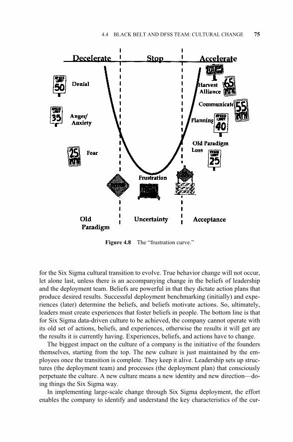
for the Six Sigma cultural transition to evolve. True behavior change will not occur,let alone last, unless there is an accompanying change in the beliefs of leadershipand the deployment team. Beliefs are powerful in that they dictate action plans thatproduce desired results. Successful deployment benchmarking (initially) and expe-riences (later) determine the beliefs, and beliefs motivate actions. So, ultimately,leaders must create experiences that foster beliefs in people. The bottom line is thatfor Six Sigma data-driven culture to be achieved, the company cannot operate withits old set of actions, beliefs, and experiences, otherwise the results it will get arethe results it is currently having. Experiences, beliefs, and actions have to change.
The biggest impact on the culture of a company is the initiative of the foundersthemselves, starting from the top. The new culture is just maintained by the em-ployees once the transition is complete. They keep it alive. Leadership sets up struc-tures (the deployment team) and processes (the deployment plan) that consciouslyperpetuate the culture. A new culture means a new identity and new direction—do-ing things the Six Sigma way.
In implementing large-scale change through Six Sigma deployment, the effortenables the company to identify and understand the key characteristics of the cur-
4.4 BLACK BELT AND DFSS TEAM: CULTURAL CHANGE 75
Figure 4.8 The “frustration curve.”
c04.qxd 4/22/2005 7:38 AM Page 75

rent culture. Leadership together with the deployment team then develop the SixSigma culture characteristics and the deployment plan of “how to get there.” Com-panies with major internal conflicts or those faced with accelerated changes in busi-ness strategy are advised to move with more caution in their deployment.
Several topics that are vital to deployment success should be considered fromcultural standpoint. These include:
� Elements of cultural change in the deployment plan
� Assessing resistance
� Ways to handle resistance to change relative to culture
� Types of leaders and leadership needed at different points in the deploymenteffort
� How to communicate effectively when very little is certain initially
� Change readiness and maturity measurement or assessment
A common agreement between the senior leadership and deployment teamshould be reached on major deployment priorities and timing relative to culturaltransformation and those areas where further work is needed.
At the team level, there are several strategies a black belt could use to his or heradvantage in order to deal with team change in the context of Figure 4.8. To helpreconcile differences, the black belt needs to listen with empathy, acknowledge dif-ficulties, and define what is out of scope and what is not. To help stop the old para-digm and reorient the team to the DFSS paradigm, the black belt should encourageredefinition, utilize management to provide structure and strength, rebuild a senseof identity, gain a sense of control and influence, and encourage opportunities forcreativity. To help recommit the team to the new paradigm, he or she should rein-force the new beginning, provide clear purpose, develop a detailed plan, be consis-tent in the spirit of Six Sigma, and celebrate success.
76 SERVICE DESIGN FOR SIX SIGMA DEPLOYMENT
c04.qxd 4/22/2005 7:38 AM Page 76
5.1 INTRODUCTION
This chapter is written primarily to present the service DFSS project road map inorder to support the service black belt and green belt and his or her team and thefunctional champion in the project execution mode of deployment. The design pro-ject is the core of the DFSS deployment and has to be executed consistently using aroad map that lays out the DFSS principles, tools, and methods within an adoptedgated design process (see Chapter 3, Section 3.5). From a high-level perspective,this road map provides the immediate details required for a smooth and successfulDFSS deployment experience.
The chart presented in Figure 5.1 depicts the road map proposed. The road mapobjective is to develop Six Sigma service solutions entities with unprecedented lev-els of fulfillment of customer wants, needs, and delight over its total life cycle (seeChapter 1, Section 1.3). The service DFSS road map has four phases identify, charc-terize, optimize, and validate, (ICOV) in seven developmental stages. Stages are sep-arated by milestones called the tollgates. Coupled with design principles and tools,the objective of this chapter is to combine all of these factors into a comprehensive,implementable sequence in a manner that enables deployment companies to system-atically achieve desired benefits by executing projects. In Figure 5.1, a design stageconstitutes a collection of design activities and can be bounded by entrance and exittollgates. A tollgate, denoted as TG, represents a milestone in the service design cy-cle and has some formal meaning defined by the company’s own service develop-ment coupled with management recognition. The ICOV stages are averages of theauthors’ studies of several deployments. They need not be adopted blindly, but maybe customized to reflect the deployment of interest. For example, in industry, serviceproduction cycles and volume are factors that can contribute to the shrinkage or elon-gation of some of the phases. Generally, the life cycle of a service or a process startswith some form of idea generation, whether in a freely invented format or in a moredisciplined format such as multigeneration service planning and growth strategy.
Service Design for Six Sigma. By Basem El-Haik and David M. Roy 77© 2005 by John Wiley & Sons.
5SERVICE DFSS PROJECT ROAD MAP
c05.qxd 4/22/2005 7:42 AM Page 77
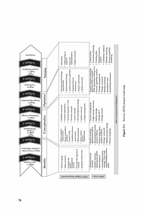
78
•M
ark
et/
cust
om
er
rese
arc
h
•Q
uali
ty f
un
ctio
n
dep
loy
men
t (Q
FD
)
•K
an
o A
na
lysi
s
•G
row
th/i
nn
ov
ati
on
st
rate
gy
: T
ech
. ro
ad
m
ap
s/m
ult
igen
era
tio
n
pla
ns
Iden
tify
Co
nce
ptu
ali
ze
Op
tim
ize
Vali
date
Stage 1: Idea Creation
Stage 2: Voice of theCustomer &Business
Stage 3: Concept
Development
Stage 4: Preliminary Design
Tollgate 1 Tollgate 1
Tollgate 2 Tollgate 2
Tollgate 3 Tollgate 3
Tollgate 4 Tollgate 4
Stage 5: Design Optimization
Tollgate 5 Tollgate 5
Stage 6: Verification
Tollgate 6 Tollgate 6
Stage 7: Launch Readiness
Tollgate 7 Tollgate 7
Production
DFSS ToolsDFSS Tollgate Requirements
•P
roje
ct s
cop
ing
•A
lig
n r
eso
urc
es
•E
sta
bli
sh t
he
p
roje
ctm
an
ag
em
en
tp
roce
ss
•D
esc
rib
e t
he
hig
h-l
ev
el
con
cep
t
•E
sta
bli
sh V
OB
& V
OC
•K
no
w c
ust
om
er
req
uir
em
en
ts
•K
no
w c
om
pe
titi
ve
po
siti
on
•D
efi
ne
CT
Qs
•E
sta
bli
sh m
ea
sure
-
me
nt
syst
em
•R
isk
ass
ess
me
nt
•K
no
w c
riti
cal
pro
cess
req
uir
em
en
ts
•D
ev
elo
p d
eta
ile
d d
esi
gn
re
qu
ire
me
nts
•B
uil
d d
eta
ile
d d
esi
gn
•A
na
lyz
e p
roce
ss c
ap
ab
ilit
y
•S
imu
late
Pro
cess
Pe
rfo
rma
nce
•P
rep
are
co
ntr
ol
pla
n
•U
pd
ate
sco
reca
rd
•P
ilo
t p
lan
s
•A
dju
st d
esi
gn
as
req
uir
ed
•F
ull
-sca
leim
ple
me
nta
tio
n
•U
pd
ate
sco
reca
rd
•E
sta
bli
sh s
core
card
•E
va
lua
te a
lte
rna
tiv
es
•T
ran
sfe
r fu
nct
ion
Y =
f(Y
)
•D
ev
elo
p c
on
cep
ts
•A
sse
ss c
on
cep
ts
•D
ev
elo
p h
igh
-le
ve
l d
esi
gn
•U
pd
ate
sco
reca
rd
•C
ha
ng
e m
an
ag
em
en
t
Ris
k A
sse
ssm
en
t &
Mit
iga
tio
n
•Q
ua
lity
fu
nct
ion
d
ep
loy
men
t (Q
FD
)
•M
ea
sure
me
nt
syst
em
an
aly
sis
(MS
A)
•F
ail
ure
mo
de
eff
ect
an
aly
sis
(FM
EA
)
•D
esi
gn
sc
ore
card
•T
RIZ
/Ax
iom
ati
c d
esi
gn
•P
roce
ss m
ap
pin
g
•P
roce
ss m
an
ag
em
en
t
•P
ug
h c
on
cep
t se
lect
ion
•R
ob
ust
desi
gn
•D
esi
gn
fo
r Y
•D
esi
gn
rev
iew
•T
ran
sfer
fun
ctio
n d
eta
ilin
g
(ph
ysi
cal
DO
E, co
mp
ute
r D
OE
, h
yp
oth
esi
s te
stin
g, etc
.)
•P
roce
ss c
ap
ab
ilit
y a
na
lysi
s
•C
han
ge m
an
ag
em
en
t
•D
esi
gn
sc
ore
card
•M
ista
ke p
roo
fin
g
•S
imu
lati
on
to
ols
•R
eli
ab
ilit
y/r
ob
ust
ne
ss
•C
on
tro
l p
lan
s
•T
ran
siti
on
pla
nn
ing
•T
rain
ing
pla
n
•S
tati
stic
al
pro
cess
co
ntr
ol
•C
on
fid
en
ce a
naly
sis
•M
ista
ke
-p
roo
fin
g
•P
roce
ss c
ap
ab
ilit
y
mo
de
lin
g
Fig
ure
5.1
Ser
vice
DF
SS
pro
ject
roa
d m
ap.
c05.qxd 4/22/2005 7:42 AM Page 78
Prior to starting on the DFSS road map, the black belt team needs to understandthe rationale of the project. We advise they assure the feasibility of continuing theproject by validating the project scope, the project charter, and the project resourceplan (see Chapter 4, Section 4.3.2, Service DFSS Project Sources). A session withthe champion should take place once the matching between the black belt and pro-ject charter is done. The objective is to make sure that everyone is aligned with theobjectives and to discuss the next steps.
In service DFSS deployment, we will emphasize the synergistic service DFSScrossfunctional team. A well-developed team has the potential to design winningSix Sigma solutions. The growing synergy, which arises from ever-increasing num-bers of successful teams, accelerates deployment throughout the company. Thepayback for up-front investments in team performance can be enormous. Continu-ous vigilance on the part of the black belt at improving and measuring team perfor-mance throughout the project life cycle will be rewarded with ever-increasing capa-bility and commitment to deliver winning design solutions. Given time, there willbe a transition from resistance to embracing the methodology, and the company cul-ture will be transformed.
5.2 THE SERVICE DESIGN FOR SIX SIGMA TEAM1
It is well known that services intended to serve the same purpose in the same marketmay be designed and produced in radically different varieties. For example, compareyour lodging experience at different hotel chains or your mortgage experience whenshopping for a home. Why is it that two services function and feel so different? Fromthe perspective of the design process, the obvious answer is that the design entity de-rives from a series of decisions, and that different decisions made at the tollgates inthe process result in such differentiation. This is common sense; however, it has sig-nificant consequences. It suggests that a design can be understood, not only in termsof the design process adopted, but also in terms of the decision-making process usedto arrive at it. Measures to address both sources of design variation need to be insti-tutionalized. We believe that the adoption of the ICOV DFSS process presented inthis chapter will address one issue—the consistency of development activities. Forservice design teams, this means that the company structures used to facilitate coor-dination during the project execution have an effect on the core of the design process.In addition to coordination, the primary intent of an organizational design structure isto control the decision-making process. It is logical to conclude, then, that we mustconsider the design implications of the types of organizational structures we deploythe ICOV process in to manage design practice. When flat organizational structuresare adopted by design teams, members must negotiate design decisions among them-selves, because a top-down approach to decision making may not be available.
5.2 THE SERVICE DESIGN FOR SIX SIGMA TEAM 79
1Adapted from David A. Owens, http://216.239.57.104/search?q=cache:mG3a-1wdz4sJ:mba.vander-bilt.edu/david.owens/Papers/2000%2520Owens%2520Status%2520in%2520Design%2520Teams%2520DMJ.pdf+motivating+design+teams&hl=en
c05.qxd 4/22/2005 7:42 AM Page 79
Members of a service design team negotiating decisions with each other during de-sign projects is obviously such a practice. A common assumption seems to be thatthese decision-making negotiations proceed in a reasonable manner, this being a ba-sic premise of concurrent service design. Patterns and outcomes of decision makingare best explained as a dynamic behavior of the teams. Even if two teams developsimilar services using the same process, members of the otherwise comparable de-sign teams may have varying levels of influence as decisions are made. The rank ofdifferent members of a design team can play a substantial role in team dynamics fromthe perspective of day-to-day decisions. It is the responsibility of the black belt to bal-ance such dynamics in his or her team. As team leaders, black belts and master blackbelts need to understand that design teams must make decisions and that, invariably,some set of values must drive those decisions.
Decision making and team structure in companies that use hierarchical structuresfollow known patterns. Although day-to-day decision making is subject to team dy-namics, the milestone decisions are not. In the latter, decisions are made based on for-mal rank. That is, decisions made by higher-ranking individuals override those madeby lower-ranking individuals. Such authoritative decision-making patterns makesense as long as the rank of the decision maker is matched with expertise and appre-ciation of company goals. This pattern will also assure that those higher in rank cancoordinate and align the actions of others with the goals of the company. We adopt-ed this model for DFSS deployment in Chapter 4. Despite these clear benefits, a num-ber of factors make this traditional form of hierarchical structure less attractive, par-ticularly in the context of the design team. For example, risk caused by increasedtechnological complexity of the services being designed, market volatility, and otherfactors make it difficult to create a decision-making structure for day-to-day designactivities. To address this problem, we suggest a flatter, looser structure that empow-ers team members, black belts, and master black belts to use their own expertise whenneeded in day-to-day activities. In our view, an ideal design team should consist ofteam members who represent every phase of a service life cycle. This concurrentstructure combined with the road map will assure a company-consistent, minimal de-sign process variation, and successful DFSS deployment. This approach allows in-formation to flow freely across the bounds of time and distance, in particular for ge-ographically wide-spread companies. It also ensures that representatives of laterstages of the life cycle have the same influence in making design decisions as dothose representatives of earlier stages (e.g., customer service, maintenance, vendors,aftermarket). While benefits such as these can result from a flattened structure, itneed not be taken to the extreme. It is apparent that having no structure means the ab-sence of a sound decision-making process. Current practice indicates that a designproject is far from a rational process of simply identifying day-to-day activities andthen assigning the expertise required to handle them. Rather, the truly important de-sign decisions are more likely to be subjective decisions made based on judgments,incomplete information, or personally biased values, even though we strive to mini-mize these gaps in VOC and technology roadmapping. In milestones, the final sayover decisions in a flat design team remains with the champions or tollgate (TG) ap-provers. It must not happen at random but, rather, in a mapped fashion.
80 SERVICE DFSS PROJECT ROAD MAP
c05.qxd 4/22/2005 7:42 AM Page 80
Our recommendation is twofold. First, a deployment company should adopt acommon design process that is customized with their design needs and has the flex-ibility to adapt the DFSS process to obtain design consistency and to assure success.Second, choose flatter, looser design team structures that empower team membersto use their own expertise when needed. This practice works best in companies ser-vicing advanced development work in high-technology domains.
A cross-functional synergistic design team is one of the ultimate objectives ofany deployment effort. The black belt needs to be aware of the fact that full partici-pation in design is not guaranteed simply because members are assigned into ateam. The structural barriers and interests of others on the team are likely to be fartoo formidable as the team travels down the ICOV DFSS process.
The success of service development activities depends on the performance of theteam that is fully integrated, that is, one having members internal and external (sup-pliers and customers) groups. Special efforts may be necessary to create a multi-functional DFSS team that collaborates to achieve a shared project vision. Roles,responsibilities, membership, and resources are best defined up front, collaborative-ly, by the teams. Once the team is established, however, it is just as important tomaintain the team to continuously improve its performance. This first step, there-fore, is an ongoing effort throughout the service DFSS ICOV cycle of planning, for-mulation, and production.
The primary challenge for a design organization is to learn and improve fasterthan their competitors. Lagging competitors must go faster to catch up. Leadingcompetitors must go faster to stay in front. A service DFSS team should learn rapid-ly, not only about what needs to be done, but about how to do it—how to pervasive-ly implement DFSS process.
Learning without application is really just gathering information, not learning.No company becomes premier by simply knowing what is required, but rather bypracticing, by training day in and day out, and by using the best contemporaryDFSS methods. The team needs to monitor competitive performance using bench-marking of services and processes to help guide directions of change and employlessons learned to help identify areas for improvement. In addition, they will benefitfrom deploying program and risk management best practices throughout the projectlife cycle (Figure 5.1). This activity is key to achieving a winning rate of improve-ment by avoiding or eliminating risks. The team is advised to continuously practicedesign principles and systems thinking, that is, thinking in terms profound knowl-edge of the total service.
5.3 SERVICE DESIGN FOR SIX SIGMA ROAD MAP
In Chapter 3, we learned about the ICOV process and the seven developmentalstages spaced by bounding tollgates indicating a formal transition between entranceand exit. As depicted in Figure 5.2, tollgates or design milestone events include re-views to assess what has been accomplished in the current developmental stage andpreparation for the next stage. The service design stakeholders, including the pro-
5.3 SERVICE DESIGN FOR SIX SIGMA ROAD MAP 81
c05.qxd 4/22/2005 7:42 AM Page 81
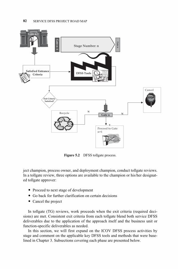
ject champion, process owner, and deployment champion, conduct tollgate reviews.In a tollgate review, three options are available to the champion or his/her designat-ed tollgate approver:
� Proceed to next stage of development
� Go back for further clarification on certain decisions
� Cancel the project
In tollgate (TG) reviews, work proceeds when the exit criteria (required deci-sions) are met. Consistent exit criteria from each tollgate blend both service DFSSdeliverables due to the application of the approach itself and the business unit orfunction-specific deliverables as needed.
In this section, we will first expand on the ICOV DFSS process activities bystage and comment on the applicable key DFSS tools and methods that were base-lined in Chapter 3. Subsections covering each phase are presented below.
82 SERVICE DFSS PROJECT ROAD MAP
Stage Number: n
Gate
n
Gate
n-
1
Y
Exit Criteria Satisfied?
N
Gate n
Proceed to Gate n+1
Recycle
Cancel
N
Satisfied Entrance Criteria
Satisfied Entrance Criteria DFSS Tools
Gate n-1
Gate n-1
Figure 5.2 DFSS tollgate process.
c05.qxd 4/22/2005 7:42 AM Page 82
5.3.1 Service DFSS Phase I: Identify Requirements
This phase includes two stages: idea creation (Stage 1) and voice of the customerand business (Stage 2).
Stage 1: Idea Creation
Stage 1 Entrance Criteria. Entrance criteria may be tailored by the deploying func-tion for the particular program/project, provided that the modified entrance criteria,in the opinion of the function, are adequate to the support the exit criteria for thisstage. They may include:
� A target customer or market
� A market vision, with an assessment of marketplace advantages
� An estimate of development cost
� Risk assessment
Tollgate “1”—Stage 1 Exit Criteria
� Decision to collect the voice of the customer to define customer needs, wants,and satisfaction
� Verification that adequate funding is available to define customer needs
� Identification of the tollgate keepers’2 leader and the appropriate staff
Stage 2: Customer and Business Requirements Study
Stage 2 Entrance Criteria
� Closure of Tollgate 1: Approval of the gatekeeper is obtained
� A service DFSS project charter that includes project objectives, service de-sign statement, big Y and other business levers, metrics, resources, and teammembers
These are almost the same criteria required for DMAIC projects. However,project duration is usually longer and initial cost is probably higher. The DFSSteam, relative to DMAIC, typically experiences longer project cycle times. Thegoal here is either designing or redesigning a different entity, not just patching upthe holes in an existing one. Higher initial cost is due to the fact that the valuechain is being energized by process/service development and not by manufactur-ing or production arenas. There may be new customer requirements to be satisfiedadding more cost to the developmental effort. For DMAIC projects, we may only
5.3 SERVICE DESIGN FOR SIX SIGMA ROAD MAP 83
2A tollgate keeper is an individual or group who will assess the quality of work done by the design teamand initiate a decision to approve, reject, cancel, or recycle the project to an earlier gate. Usually, the pro-ject champion(s) is tasked with this mission.
c05.qxd 4/22/2005 7:42 AM Page 83

work on improving a very limited subset of the critical-to-satisfaction characteris-tics, the CTSs or big Ys.
� Completion of a market survey to determine customer needs critical to satis-faction (CTS) or the voice of the customer (VOC)
In this step, customers are fully identified and their needs collected and analyzedwith the help of quality function deployment (QFD) and Kano analysis (see Chapter7). Then, the most appropriate set of CTSs or big Y metrics are determined in orderto measure and evaluate the design. Again, with the help of QFD and Kano analy-sis, the numerical limits and targets for each CTS are established. The list of tasksin this step follows. A detailed explanation is provided in later chapters.
� Determine methods of obtaining customer needs and wants
� Obtain customer needs and wants and transform them into a list of the voiceof customer (VOC)
� Finalize requirements
� Establish minimum requirement definitions
� Identify and fill gaps in customer-provided requirements
� Validate application and usage environments
� Translate the VOC to CTSs as critical-to-quality, critical-to-delivery, critical-to-cost, and so on
� Quantify CTSs or big Ys
� Establish metrics for CTSs
� Establish acceptable performance levels and operating windows
� Start flow-down of CTSs
� Make an assessment of required technologies
� Make a project development plan (through TG2)
� Conduct risk assessment
� Align with business objectives—voice of the business (VOB) relative togrowth and innovation strategy
Tollgate “2”—Stage 2 Exit Criteria
� Assess of market opportunity
� Command a reasonable price or be affordable
� Commit to development of the conceptual designs
� Verify that adequate funding is available to develop the conceptual design
� Identify the gatekeepers’ leader (gate approver) and the appropriate staff
� Continue flow-down of CTSs to functional requirements
5.3.1.1 Identify Phase Road Map. DFSS tools used in this phase include (seeFigure 5.1):
84 SERVICE DFSS PROJECT ROAD MAP
c05.qxd 4/22/2005 7:42 AM Page 84
� Market/customer research
� Quality function deployment (QFD): Phase I
� Kano analysis
� Growth/innovation strategy
5.3.1.2 Service Company Growth and Innovation Strategy: MultigenerationPlanning.3 Even within best-in-class companies, there is the need and opportunityto strengthen and accelerate progress. The first step is to establish a set of clear andunambiguous guiding growth principles as a means to characterize company posi-tion and focus. For example, growth in emerging markets might be the focusabroad, whereas effectiveness and efficiency of resource usage within the contextof enterprise productivity and sustainability may be the local position. Growth prin-ciples and vision at a high level are adequate to find agreement, focus debate withinthe zone of interest, and exclude or diminish nonrealistic targets. The second keystep is to assess the current know-how and solutions of the services portfolio in thecontext of these growth principles. An inventory is made of what the senior leader-ship team knows they have, and how they integrate that into the set of guidinggrowth principles. The third step is to establish a vision of the ultimate state for thecompany. The final step is to develop a multigeneration plan to focus the research,product development, and integration efforts in planned steps to move toward thatvision. The multigeneration plan is key because it helps the deploying companystage progress in realistic developmental stages, one DFSS project at a time, but al-ways with an eye on the ultimate vision.
In today’s business climate, successful companies must be efficient and mar-ket-sensitive to beat their competitors. By focusing on new services, companiescan create custom solutions to meet customer needs, enabling customers to keepin step with new service trends and changes that affect them. As the design teamengages the customers (through surveys, interviews, focus groups, etc.) and startsthe QFD, they gather competitive intelligence. This information helps increase de-sign team awareness of competing services or how they stack up competitivelywith a particular key customer. By doing this homework, the team identifies po-tential gaps in their development maturity. Several in-house tools to manage thelife cycle of each service product from the cradle to the grave need to be devel-oped, including the multigeneration plan and a customized version of the ICOVDFSS process, if required. The multigeneration plan evaluates the market size andtrends, service position, competition, and technology requirements. This tool pro-vides a means to easily identify any gaps in the portfolio while directing the DFSSproject road map. The multigeneration plan needs to be supplemented with a de-cision-analysis tool used to determine the financial and strategic value of potentialnew applications over a medium time horizon. If the project passes this decision-making step, it can be lined up with others in the Six Sigma project portfolio forstart of schedule.
5.3 SERVICE DESIGN FOR SIX SIGMA ROAD MAP 85
3Scott H. Hutchins, http://216.239.57.104/search?q=cache:WTPP0iD4WTAJ:cipm.ncsu.edu/sympo-sium/docs/Hutchins_text.doc+product+multi-generation+plan&hl=en
c05.qxd 4/22/2005 7:42 AM Page 85
5.3.1.3 Research Customer Activities. This is usually done by the service plan-ning departments (service and process) or market research experts, who should beon the DFSS team. The black belt and his team start by brainstorming all possiblecustomer groups of the product. Using the affinity diagram method to group thebrainstormed potential customer groups, categories of markets, user types, or ser-vice and process applications types will emerge. From these categories, the DFSSteam should work toward a list of clearly defined customer groups from which indi-viduals can be selected.
External customers might be drawn from customer centers, independent sales or-ganizations, regulatory agencies, societies, and special interest groups. Merchantsand, most importantly, the end user, should be included. The selection of externalcustomers should include both existing and loyal customers, recently lost cus-tomers, and newly acquired customers within the market segments. Internal cus-tomers might be drawn from production, functional groups, facilities, finance, em-ployee relations, design groups, and distribution organizations. Internal researchmight assist in selecting internal customer groups that would be most instrumentalin identifying wants and needs in operations and service operations.
The ideal service definition, in the eye of the customer, may be extracted fromcustomer engagement activities. This will help turn the knowledge gained fromcontinuous monitoring of consumer trends, competitive benchmarking, and cus-tomer likes and dislikes into a preliminary definition of an ideal service. In addition,it will help identify areas for further research and dedicated efforts. The designshould be described from a customer’s viewpoint (external and internal) and shouldprovide the first insight into what a good service should look like. Concept modelsand design studies using TRIZ (see Chapter 9) and Axiomatic Design4 (see Chapter8) are good sources for evaluating consumer appeal and areas of likes or dislikes.
The array of customer attributes should include all customer and regulatory re-quirements and social and environmental expectations. It is necessary to understandrequirement and prioritization similarities and differences in order to understandwhat can be standardized and what needs to be tailored.
5.3.2 Service DFSS Phase 2: Characterize Design
This phase spans the following two stages: concept development (Stage 3) and pre-liminary design (Stage 4).
Stage 3: Concept Development
Stage 3 Entrance Criteria
� Closure of Tollgate 2: Approval of the gatekeeper is obtained.
� Define system technical and operational requirements. Translate customer re-quirements (CTSs or big Ys) to service/process functional requirements. Cus-
86 SERVICE DFSS PROJECT ROAD MAP
4Download the Axiomatic Design Software “Acclaro DFSS Light®” from ftp://ftp.wiley.com/public/sci_tech_med/six_sigma. See Section 8.5. Acclaro software is protected under copyright andpatents pending. Acclaro is a registered trademark of Axiomatic Design Solutions, Inc.
c05.qxd 4/22/2005 7:42 AM Page 86
tomer requirements (CTSs) give us ideas about what will satisfy the customerbut they usually cannot be used directly as the requirements for product orprocess design. We need to translate customer requirements to service andprocess functional requirements. Another phase of QFD can be used to devel-op this transformation. Axiomatic design principles will be also very helpfulfor this step.
� Select a process or service conceptual design.
� Trade off alternate conceptual designs with the following steps. (1) Generatedesign alternatives. After the determination of the functional requirementsfor the new design entity (service or process), we need to characterize (de-velop) design entities that are able to deliver those functional requirements.In general, there are two possibilities. The first is that if the existing tech-nology or known design concept is able to deliver all the requirements sat-isfactorily, then this step becomes almost a trivial exercise. The second pos-sibility is that if the existing technology or known design is not able todeliver all requirements satisfactorily, then a new design concept has to bedeveloped. This new design should be “creative” or “incremental,” reflect-ing the degree of deviation from the baseline design, if any. The TRIZmethod (see Chapter 9) and axiomatic design (see Chapter 8) will be help-ful in generating many innovative design concepts in this step. (2) Evaluatedesign alternatives. Several design alternatives might be generated in the laststep. We need to evaluate them and make a final determination as to whichconcept will be used. Many methods can be used in design evaluation, in-cluding the Pugh concept selection technique, design reviews, and FMEA.After design evaluation, a winning concept will be selected. During theevaluation, many weaknesses of the initial set of design concepts will be ex-posed and the concepts will be revised and improved. If we are designing aprocess, process management techniques will also be used as an evaluationtool.
� Functional, performance, and operating requirements are allocated to servicedesign components (subprocesses).
� Do development cost estimate (tollgates 2 through 5).
� Do target product/service unit production cost assessment.
� With regard to the market,
Determine profitability and growth rate
Do supply chain assessment
Do time-to-market assessment
Do share assessment
� Do overall risk assessment.
� Create a project management plan (tollgates 2 through 5) with schedule andtest plan.
� Create a team member staffing plan.
5.3 SERVICE DESIGN FOR SIX SIGMA ROAD MAP 87
c05.qxd 4/22/2005 7:42 AM Page 87
Tollgate “3”—Stage 3 Exit Criteria
� Assess that the conceptual development plan and cost will satisfy the cus-tomer base.
� Decide whether the service design represents an economic opportunity (if ap-propriate).
� Verify that adequate funding will be available to perform preliminary design.
� Identify the tollgate keeper and the appropriate staff.
� Write an action plan to continue flow-down of the design functional require-ments.
Stage 4: Preliminary Design
Stage 4 Entrance Criteria
� Closure of tollgate 3: approval of the gatekeeper is obtained.
� Flow-down of system functional, performance, and operating requirements tosubprocesses and steps (components).
� Document design data package with configuration management5 at the lowestlevel of control.
� Development-to-production operations transition plan published and in ef-fect.
� Subprocesses (steps) functionality, performance, and operating requirementsverified.
� Development testing objectives complete under nominal operating condi-tions.
� Test with design parametric variations under critical operating conditions.Tests might not utilize the intended operational production processes.
� Perform design, performance, and operating transfer functions.
� Do reports documenting the design analyses, as appropriate.
� Create a procurement strategy (if applicable).
� Decide whether to make or buy.
� Arrange for sourcing (if applicable).
� Perform risk assessment.
Tollgate “4”—Stage 4 Exit Criteria:
� Acceptance of the selected service solution/design.
� Agreement that the design is likely to satisfy all design requirements.
� Agreement to proceed with the next stage of the selected service solution/de-sign.
88 SERVICE DFSS PROJECT ROAD MAP
5A systematic approach to defining design configurations and managing the change process.
c05.qxd 4/22/2005 7:42 AM Page 88
� An action plan to finish the flow-down of the design functional requirementsto design parameters and process variables.
DFSS tools used in this phase:
� QFD
� TRIZ/axiomatic design
� Measurement system analysis (MSA)
� Failure mode effect analysis (FMEA)
� Design scorecard
� Process mapping
� Process management
� Pugh concept selection
� Robust design
� Design for X
� Design reviews
5.5.3 Service DFSS Phase 3: Optimize the Design
This phase spans the Stage 5 only, the “Design Optimization” stage.
Stage 5: Design Optimization
Stage 5 Entrance Criteria
� Closure of tollgate 4: approval of the gatekeeper is obtained.
� Design documentation defined: the design is complete and includes the infor-mation specific to the operations processes (in the opinion of the operatingfunctions).
� Design documents are under the highest level of control.
� Formal change configuration is in effect.
� Operations are validated by the operating function to preliminary documenta-tion.
� Demonstration test plan put together that must demonstrate functionality andperformance under operational environments
� Risk assessment performed.
Tollgate “5”—Stage 5 Exit Criteria
� Reach agreement that functionality and performance meet the customers’ andbusiness requirements under the intended operating conditions.
� Decide to proceed with verification test of a pilot built to preliminary opera-tional process documentation.
5.3 SERVICE DESIGN FOR SIX SIGMA ROAD MAP 89
c05.qxd 4/22/2005 7:42 AM Page 89
� Perform analyses to document that the design optimization meets or exceedsfunctional, performance, and operating requirements.
� Optimized transfer functions. DOE (design of experiments) is the backbone ofprocess design and redesign improvement. It represents the most common ap-proach to quantify the transfer functions between the set of CTSs and/or re-quirements and the set of critical factors, the Xs, at different levels of design hi-erarchy. DOE can be conducted by hardware or software (e.g., simulation).From the subset of vital few Xs, experiments are designed to actively manipu-late the inputs to determine their effect on the outputs (big Ys or small ys). Thisphase is characterized by a sequence of experiments, each based on the resultsto the previous study. “Critical” variables are identified during this process.Usually, a small number of Xs account for most of the variation in the outputs.
The result of this phase is an optimized service entity with all functional require-ments released at Six Sigma performance level. As the concept design is finalized,there are still a lot of design parameters that can be adjusted and changed. With thehelp of computer simulation and/or hardware testing, DOE modeling, Taguchi’s ro-bust design methods, and response surface methodology, the optimal parameter set-tings will be determined. Usually, this parameter optimization phase will be fol-lowed by a tolerance-optimization step. The objective is to provide a logical andobjective basis for setting requirements and process tolerances. If the design para-meters are not controllable, we may need to repeat Stages 1–3 of service DFSS.
The DFSS tools used in this phase are:
� Transfer function detailing (physical DOE, computer DOE, hypothesis test-ing, etc.)
� Process capability analysis
� Design scorecard
� Simulation tools
� Mistake-proofing plan
� Robustness assessment (Taguchi methods: parameter and tolerance design)
5.3.4 Service DFSS Phase 4: Validate the Design
This phase spans the following two stages: verification (Stage 6) and launch readi-ness (Stage 7).
Stage 6: Verification
Stage 6 Entrance Criteria
� Closure of tollgate 5: Approval of the gatekeeper is obtained
� Risk assessment
Tollgate (TG) “6”—Stage 6 Exit Criteria. After the parameter and tolerance design
90 SERVICE DFSS PROJECT ROAD MAP
c05.qxd 4/22/2005 7:42 AM Page 90
is finished, we will move to the final verification and validation activities, includingtesting. The key actions are:
� The pilot tests are audited for conformance with design and operationalprocess documentation.
� Pilot test and refining: No service should go directly to market without firstbeing subjected to piloting and refining. Here we can use design failure modeeffect analysis (DFMEA, see Chapter 11) as well as pilot and small-scale im-plementations to test and evaluate real-life performance.
� Validation and process control: In this step we will validate the new entitymake sure that the service, as designed, meets the requirements, and establishprocess controls in operations to ensure that critical characteristics are alwaysproduced to the specifications of the Optimize phase.
Stage 7: launch Readiness
Stage 7 Entrance Criteria
� Closure of tollgate 6: approval of the gatekeeper is obtained
� The operational processes have been demonstrated
� Risk assessment has been performed
� All control plans are in place.
� Final design and operational process documentation has been published
� The process is achieving or exceeding all operating metrics
� Operations have demonstrated continuous operation without the support ofthe design development personnel
� Planned sustaining development personnel are transferred to operations:
Optimize, eliminate, automate, and/or control the vital few inputs defined inthe previous phase
Document and implement the control plan
Sustain the gains identified
Reestablish and monitor long-term delivered capability
� A transition plan is in place for the design development personnel
� Risk assessment is performed
Tollgate (TG) “7” Exit Criteria
� The decision is made to reassign the DFSS black belt
� Full commercial rollout and handover to new process owner: As the designentity is validated and process control is established, we will launch full-scalecommercial rollout and the new designed service together with the supporting
5.3 SERVICE DESIGN FOR SIX SIGMA ROAD MAP 91
c05.qxd 4/22/2005 7:42 AM Page 91
operations processes can be handed over to design and process owners, com-plete with requirements settings and control and monitoring systems.
� Closure of tollgate 7: Approval of the gatekeeper is obtained
DFSS tools used in this phase are:
� Process control plan
� Control plans
� Transition planning
� Training plan
� Statistical process control
� Confidence analysis
� Mistake-proofing
� Process capability modeling
5.4 SUMMARY
In this chapter, we presented the service design for Six Sigma road map. The roadmap is depicted in Figure 5.1, which highlights at a high level the identify, charca-terize, optimize, and validate phases, and the seven service development stages(idea creation, voice of the customer and business, concept development, prelimi-nary design, design optimization, verification, and launch readiness). The road mapalso recognizes the tollgates, design milestones at which DFSS teams update thestakeholders on development status and ask for decisions to be made whether to ap-prove going to the next stage, going back to an earlier stage or cancelling the projectaltogether.
The road map also highlights the most appropriate DFSS tools by ICOV phase.It indicates where it is most appropriate to start tool usage. These tools are present-ed in Chapters 6 and 7.
92 SERVICE DFSS PROJECT ROAD MAP
c05.qxd 4/22/2005 7:42 AM Page 92
6.1 INTRODUCTION
In its simplest form, a transfer function is a mathematical representation of the rela-tionship between the input and output of a system or a process. For example,putting a speaker in a room will make the speaker sound different than it does in anonenclosed space. This is caused by reflection, absorption, and resonance of theroom. This change is called the transfer function.
Speed of answering in a call center is dependent on call volume, number of ser-vice representatives, and time spent on each call. The speed of answering is a func-tion of these three factors and their relationship is called a transfer function.
All systems have a transfer function or a set of transfer functions. Typically, themost noticeable change in artificial (man-made) systems is caused by excitation byan energy source. An output response or a design functional requirement is inherentbecause the system is like a box, an enclosed entity that promotes reaction to energyexcitement. But the transfer function is more than just a change in a system’s orprocess’s status; it also can cause major changes in the system’s physical embodi-ment. As designers, DFSS teams usually determine the transfer function(s) of theirdesigned service entity through their design activities. They can map the activitiesand optimize the output functional requirements, and then build the system orprocess and take advantage of their knowledge of the transfer function. So what is atransfer function?
A transfer function describes the relationship between design parameters orprocess variables (x1, x2, . . . , xn) and a functional requirement (y), denoted by the re-lationship y = f(x1, x2, . . . , xn). The variable y is the dependent output variable of aprocess or a system of interest to the customer. In service design, the transfer func-tion is used to design and monitor a process to detect if it is out of control, or if symp-toms are developing within a process. Once derived or quantified through design ofexperiment (DOE, see Chapters 12 and 13), a transfer function y = f(x1, x2, . . . , xn)can be developed to define the relationship of process variables that can lead to a plan
Service Design for Six Sigma. By Basem El-Haik and David M. Roy 93© 2005 by John Wiley & Sons.
6SERVICE DFSS TRANSFER FUNCTION AND SCORECARDS
c06.qxd 4/22/2005 9:00 AM Page 93
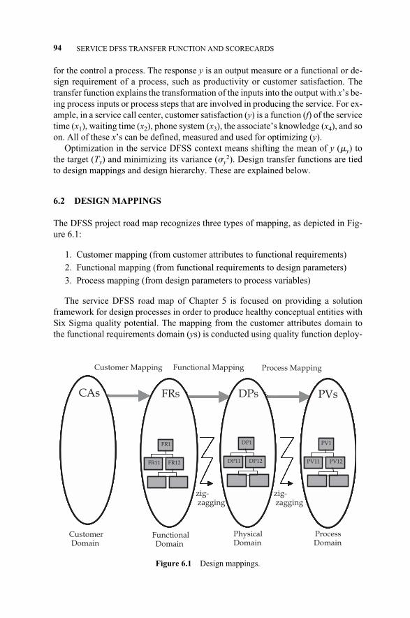
for the control a process. The response y is an output measure or a functional or de-sign requirement of a process, such as productivity or customer satisfaction. Thetransfer function explains the transformation of the inputs into the output with x’s be-ing process inputs or process steps that are involved in producing the service. For ex-ample, in a service call center, customer satisfaction (y) is a function (f) of the servicetime (x1), waiting time (x2), phone system (x3), the associate’s knowledge (x4), and soon. All of these x’s can be defined, measured and used for optimizing (y).
Optimization in the service DFSS context means shifting the mean of y (�y) tothe target (Ty) and minimizing its variance (�y
2). Design transfer functions are tiedto design mappings and design hierarchy. These are explained below.
6.2 DESIGN MAPPINGS
The DFSS project road map recognizes three types of mapping, as depicted in Fig-ure 6.1:
1. Customer mapping (from customer attributes to functional requirements)
2. Functional mapping (from functional requirements to design parameters)
3. Process mapping (from design parameters to process variables)
The service DFSS road map of Chapter 5 is focused on providing a solutionframework for design processes in order to produce healthy conceptual entities withSix Sigma quality potential. The mapping from the customer attributes domain tothe functional requirements domain (ys) is conducted using quality function deploy-
94 SERVICE DFSS TRANSFER FUNCTION AND SCORECARDS
Figure 6.1 Design mappings.
CAs FRs
FR1
FR11 FR12
FR1
FR11 FR12
DPs
DP1
DP11 DP12
DP1
DP11 DP12
PVs
PV1
PV11 PV12
PV1
PV11 PV12
PV1
PV11 PV12
CAs FRs
FR1
FR11 FR12
FR1
FR11 FR12
DPs
DP1
DP11 DP12
DP1
DP11 DP12
PV1
PV11 PV12
PV1
PV11 PV12
P
PV1
PV11 PV12
PV1
PV11 PV12
CAs FRs
FR1
FR11 FR12
FR1
FR11 FR12
DPs
DP1
DP11 DP12
DP1
DP11 DP12
PV1
PV11 PV12
PV1
PV11 PV12
PV1
PV11 PV12
PV1
PV11 PV12
CAs FRs
FR1
FR11 FR12
FR1
FR11 FR12
DPs
DP1
DP11 DP12
DP1
DP11 DP12
PV1
PV11 PV12
PV1
PV11 PV12
PV1
PV11 PV12
PV1
PV11 PV12
CAs FRs
FR1
FR11 FR12
FR1
FR11 FR12
DPs
DP1
DP11 DP12
DP1
DP11 DP12
PV1
PV11 PV12
PV1
PV11 PV12
PV1
PV11 PV12
PV1
PV11 PV12
Customer Mapping Functional Mapping Process Mapping
zig-zagging
CustomerD i
FunctionalD i
PhysicalD i
ProcessD i
CAs FRs
FR1
FR11 FR12
DPs
DP1
DP11 DP12
PV1
PV11 PV12
PV1
PV11 PV12
PVs
PV1
PV11 PV12
zig-zagging
CustomerDomain
FunctionalDomain
PhysicalDomain
ProcessDomain
c06.qxd 4/22/2005 9:00 AM Page 94
ment (QFD) as described in Chapter 7. QFD represents a mapping from the rawcustomer attributes to the functional requirements.
Functional mapping is done in the following phase, where the Six Sigma con-ceptual potential of the functional requirements, the ys, are set. This mapping phasepresents a systematic approach for establishing the capability at the conceptual lev-el in the service entity by cascading requirements into a hierarchy while deployingdesign best practices such as design principles. The application of design principles,in particular those promoted to axioms, is the team’s insurance against repeating al-ready known vulnerabilities. The axiomatic design1 method and FAST techniques(see Chapter 8) are two prime tools for functional mapping and analysis. A call cen-ter design-mapping example is depicted in Figure 6.2.
Process mapping is a mapping from the design parameters domain to the processvariables domain. Process variables are parameters that can be dialed (adjusted orchanged) to deliver design parameters that in turn satisfy a functional requirement.Graphical process mapping, IDEF2 family, and value stream mapping (Chapter 8)are techniques used to map a design process.
In addition to design mapping, Figure 6.1 also conveys the concept of design hi-erarchy such as process, subprocess, step, and so on. At a given level of design hier-archy, there exists a set of requirements defined as the minimum set of needed re-quirements at that level. Defining acceptable functional requirements may involveseveral iterations when a limited number of logical questions in the mappingprocess are employed.
6.2.1 Functional Mapping
Functional mapping is design mapping between functional requirements and designparameters. Functional mapping can be represented graphically or mathematically,depicting the input–output or cause-and-effect relationships of functional elements.In its graphical form, block diagrams are used to capture the mapping and are com-posed of nodes connected by arrows depicting such relationships. A block diagramshould capture all design elements within the DFSS project scope and ensure correctflow-down to critical parameters. Functional mapping represented mathematicallyusing mapping matrices; matrices belonging to the same hierarchical level are clus-tered together. Design hierarchy is built by decomposing a design into a number ofsimpler design matrices that collectively meet the high-level functional requirementsidentified in the first mapping. The collection of design matrices or blocks forms theconceptual design blueprint and provides a means to track the chain of effects for de-sign changes as they propagate across the design. The decomposition starts by theidentification of a minimum set of functional requirements that deliver the design
6.2 DESIGN MAPPINGS 95
1Download the Axiomatic Design Software “Acclaro DFSS Light®” from ftp://ftp.wiley.com/public/sci_tech_med/six_sigma. See Section 8.5. Acclaro software is protected under copyright andpatents pending. Acclaro is a registered trademark of Axiomatic Design Solutions, Inc.2IDEF is a family of mapping techniques that were developed by the U.S. Air Force. They are discussedin Chapter 8. IDEF stands for Integrated computer aided manufacturing (ICAM) DEFinition (ICAM de-finition).
c06.qxd 4/22/2005 9:00 AM Page 95
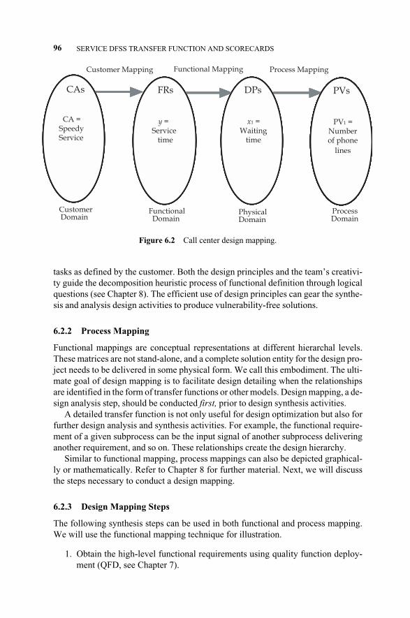
tasks as defined by the customer. Both the design principles and the team’s creativi-ty guide the decomposition heuristic process of functional definition through logicalquestions (see Chapter 8). The efficient use of design principles can gear the synthe-sis and analysis design activities to produce vulnerability-free solutions.
6.2.2 Process Mapping
Functional mappings are conceptual representations at different hierarchal levels.These matrices are not stand-alone, and a complete solution entity for the design pro-ject needs to be delivered in some physical form. We call this embodiment. The ulti-mate goal of design mapping is to facilitate design detailing when the relationshipsare identified in the form of transfer functions or other models. Design mapping, a de-sign analysis step, should be conducted first, prior to design synthesis activities.
A detailed transfer function is not only useful for design optimization but also forfurther design analysis and synthesis activities. For example, the functional require-ment of a given subprocess can be the input signal of another subprocess deliveringanother requirement, and so on. These relationships create the design hierarchy.
Similar to functional mapping, process mappings can also be depicted graphical-ly or mathematically. Refer to Chapter 8 for further material. Next, we will discussthe steps necessary to conduct a design mapping.
6.2.3 Design Mapping Steps
The following synthesis steps can be used in both functional and process mapping.We will use the functional mapping technique for illustration.
1. Obtain the high-level functional requirements using quality function deploy-ment (QFD, see Chapter 7).
96 SERVICE DFSS TRANSFER FUNCTION AND SCORECARDS
Figure 6.2 Call center design mapping.
CAs FRs DPs PVs
PV1
PV11 PV12
PVs
PV1
PV11 PV12
PV1
PV11 PV12
CAs FRs DPs PVsPVs
Process Mapping
CA = Speedy Service
CAs
Y=Service time
FRs
X1=Waiting
time
DPs PVs
PV1=Number of phone
lines
PVsCAs FRs DPs PVs
PV1
PV11 PV12
PV1
PV11 PV12
PVs
PV1
PV11 PV12
PV1
PV11 PV12
Process
CAs FRs DPs PVsPVs
Functional Mapping
Customer Functional Physical
CA = Speedy Service
CAs
y =Service
time
FRs
x1 = Waiting
time
DPs PVs
PV1 =Number of phone
lines
PVs
Customer Mapping
ProcessDomain
CustomerDomain
FunctionalDomain
PhysicalDomain
c06.qxd 4/22/2005 9:00 AM Page 96

2. Define boundaries from the project scope.
3. Conduct the mapping, using the techniques from Chapter 8, to the lowestpossible level and identify the transfer functions at every level. The lowestlevel represents the standard design parameters or process variables. For ex-ample, in service DFSS projects, forms, standards, and procedures are at thelowest level.
4. Define the respective hierarchical levels of design mapping.
5. Within a level, for each mapping, and for each requirement (y), determine thepotential mapped-to-design parameters and process variables.
6. Select and use a consistent mapping technique (see Chapter 8) for both func-tional and process mappings for compatible analysis.
7. Aggregate the chains of mappings in every hierarchical level into an overallmapping. You will produce something that resembles Figure 6.1 for yourproject.
6.3 DESIGN SCORECARDS AND TRANSFER FUNCTION3
In a world in which data is plentiful and data storage is relatively inexpensive, it is apainful irony that most design companies are unable to use that data to make betterdecisions. They are rich in data but poor in knowledge. Hidden within thosemegabytes of information is useful knowledge about customers, services, andprocesses that, if uncovered, could result in significant cost savings or revenue en-hancement. Transfer function models uncover hidden relationships and improve de-sign decision making. DFSS teams can use transfer function models effectively tocleanse, augment, and enhance historical knowledge.
A transfer function is a means of optimization and design detailing and is usual-ly documented in a scorecard. A transfer function should be treated as a living enti-ty within the DFSS road map that passes through its own life cycle stages. A trans-fer function is first identified using functional mapping and then detailed byderivation, modeling, or experimentation. Design transfer functions belonging tothe same hierarchical level in the design should be recorded in the scorecard of thathierarchical level. A scorecard is used to record and optimize the transfer functions.The transfer functions are integrated with other DFSS concepts and tools likeprocess mapping, DOE, and DFMEA. Functional mapping and process mappingare the premier activities performed in the characterize phase of the DFSS road map(see Chapter 5). Both types of design activities as well their corresponding tech-niques are covered in Chapter 8.
Through several transfer function detailing options such as DOE, transfer func-tions can be approximated by an algebraic equation of a polynomial additive model
6.3 DESIGN SCORECARDS AND TRANSFER FUNCTION 97
3Usually, transfer function models refer to a statistical technique used in forecasting a variable over time.The technique is similar to regression analysis and is often referred to as dynamic regression analysis.Transfer function models are most often used as a relatively simple and effective time-series forecastingtechnique and is useful in forecasting demand and capacity in logistic problems.
c06.qxd 4/22/2005 9:00 AM Page 97
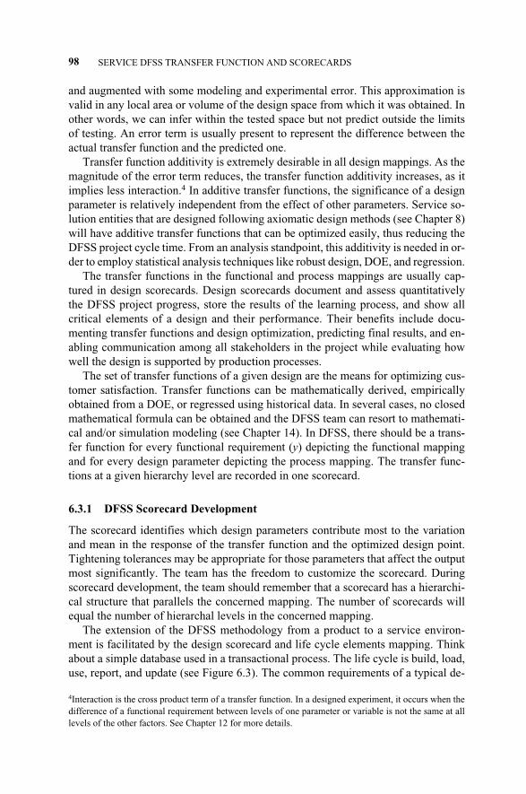
and augmented with some modeling and experimental error. This approximation isvalid in any local area or volume of the design space from which it was obtained. Inother words, we can infer within the tested space but not predict outside the limitsof testing. An error term is usually present to represent the difference between theactual transfer function and the predicted one.
Transfer function additivity is extremely desirable in all design mappings. As themagnitude of the error term reduces, the transfer function additivity increases, as itimplies less interaction.4 In additive transfer functions, the significance of a designparameter is relatively independent from the effect of other parameters. Service so-lution entities that are designed following axiomatic design methods (see Chapter 8)will have additive transfer functions that can be optimized easily, thus reducing theDFSS project cycle time. From an analysis standpoint, this additivity is needed in or-der to employ statistical analysis techniques like robust design, DOE, and regression.
The transfer functions in the functional and process mappings are usually cap-tured in design scorecards. Design scorecards document and assess quantitativelythe DFSS project progress, store the results of the learning process, and show allcritical elements of a design and their performance. Their benefits include docu-menting transfer functions and design optimization, predicting final results, and en-abling communication among all stakeholders in the project while evaluating howwell the design is supported by production processes.
The set of transfer functions of a given design are the means for optimizing cus-tomer satisfaction. Transfer functions can be mathematically derived, empiricallyobtained from a DOE, or regressed using historical data. In several cases, no closedmathematical formula can be obtained and the DFSS team can resort to mathemati-cal and/or simulation modeling (see Chapter 14). In DFSS, there should be a trans-fer function for every functional requirement (y) depicting the functional mappingand for every design parameter depicting the process mapping. The transfer func-tions at a given hierarchy level are recorded in one scorecard.
6.3.1 DFSS Scorecard Development
The scorecard identifies which design parameters contribute most to the variationand mean in the response of the transfer function and the optimized design point.Tightening tolerances may be appropriate for those parameters that affect the outputmost significantly. The team has the freedom to customize the scorecard. Duringscorecard development, the team should remember that a scorecard has a hierarchi-cal structure that parallels the concerned mapping. The number of scorecards willequal the number of hierarchal levels in the concerned mapping.
The extension of the DFSS methodology from a product to a service environ-ment is facilitated by the design scorecard and life cycle elements mapping. Thinkabout a simple database used in a transactional process. The life cycle is build, load,use, report, and update (see Figure 6.3). The common requirements of a typical de-
98 SERVICE DFSS TRANSFER FUNCTION AND SCORECARDS
4Interaction is the cross product term of a transfer function. In a designed experiment, it occurs when thedifference of a functional requirement between levels of one parameter or variable is not the same at alllevels of the other factors. See Chapter 12 for more details.
c06.qxd 4/22/2005 9:00 AM Page 98
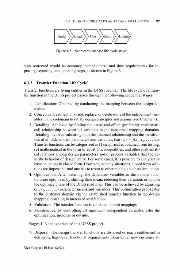
sign scorecard would be accuracy, completeness, and time requirements for in-putting, reporting, and updating steps, as shown in Figure 6.4.
6.3.2 Transfer Function Life Cycle5
Transfer functions are living entities in the DFSS roadmap. The life cycle of a trans-fer function in the DFSS project passes through the following sequential stages:
1. Identification: Obtained by conducting the mapping between the design do-mains.
2. Conceptual treatment: Fix, add, replace, or delete some of the independent vari-ables in the codomain to satisfy design principles and axioms (see Chapter 8).
3. Detailing: Achieved by finding the cause-and-effect (preferably mathemati-cal) relationship between all variables in the concerned mapping domains.Detailing involves validating both the assumed relationship and the sensitivi-ties of all independent parameters and variables, that is, y = f(x1, x2, . . . , xn).Transfer functions can be categorized as (1) empirical as obtained from testing,(2) mathematical in the form of equations, inequalities, and other mathemati-cal relations among design parameters and/or process variables that the de-scribe behavior of design entity. For some cases, it is possible to analyticallyhave equations in closed form. However, in many situations, closed form solu-tions are impossible and one has to resort to other methods such as simulation.
4. Optimization: After detailing, the dependent variables in the transfer func-tions are optimized by shifting their mean, reducing their variation, or both inthe optimize phase of the DFSS road map. This can be achieved by adjusting(x1, x2, . . . , xn) parameter means and variances. This optimization propagatesto the customer domain via the established transfer function in the designmapping, resulting in increased satisfaction.
5. Validation: The transfer function is validated in both mappings.
6. Maintenance, by controlling all significant independent variables, after theoptimization, in-house or outside.
Stages 1–6 are experienced in a DFSS project.
7. Disposal. The design transfer functions are disposed or reach entitlement indelivering high-level functional requirements when either new customer at-
6.3 DESIGN SCORECARDS AND TRANSFER FUNCTION 99
Figure 6.3 Scorecard database life cycle stages.
Build Load Use Report Update
5See Yang and El-Haik (2003).
c06.qxd 4/22/2005 9:00 AM Page 99
tributes that cannot be satisfied with the current design emerge or when themean or controlled variance of the requirements are no longer acceptable bythe customer. This stage is usually followed by the evolution of new transferfunctions to satisfy the needs that have emerged.
8. Evolution of a new transfer function. Per TRIZ (see Chapter 9), an evolutionusually follows certain basic patterns of development. Evolutionary trends ofthe functional performance of a certain design can be plotted over time andhave been found to evolve in a manner that resembles an S curve (Figure6.5).
The following are some possible sources of “detailed” transfer functions:
1. Direct documented knowledge like equations derived from laws of business(e.g., profit = price – cost, interest formulas) Transfer function variability op-timization and statistical inference can be done using simulation, usually viathe Monte Carlo method or Taylor series expansions. The transfer functionsobtained this way are very much dependent on the team’s understanding of andcompetency with their design and the discipline of knowledge it represents.
100 SERVICE DFSS TRANSFER FUNCTION AND SCORECARDS
Figure 6.4 Design scorecard for database.
Quantity Defects DPU RTY Zlt Zst
Top Level
Input 100 6 0.06 0.941765 1.569761 3.069761
Report 2 3 1.5 0.22313 -0.76166 0.738336
Maintain 5 6 1.2 0.67032 0.440798 1.940798
TOTAL 0.140858 -1.07647 0.423529
Quantity Defects DPU RTY Zlt Zst
Input Level
Accuracy 100 3 0.03 0.970446 1.887383 3.387383
Completeness 100 1 0.01 0.99005 2.328215 3.828215
Time to input 100 2 0.02 0.980199 2.057868 3.557868
100 6 0.941765 1.569761 3.069761
Quantity Defects DPU RTY Zlt Zst
Report Level
Accuracy 2 1 0.5 0.606531 0.270288 1.770288
Completeness 2 1 0.5 0.606531 0.270288 1.770288
Process Time 2 1 0.5 0.606531 0.270288 1.770288
2 3 0.22313 -0.76166 0.738336
Quantity Defects DPU RTY Zlt Zst
Maintain Level
Completeness 5 0 0 1 6 7.5
Accuracy 5 0 0 1 6 7.5
Time to Perform 5 2 0.4 0.67032 0.440798 1.940798
5 6 0.67032 0.440798 1.940798
c06.qxd 4/22/2005 9:00 AM Page 100
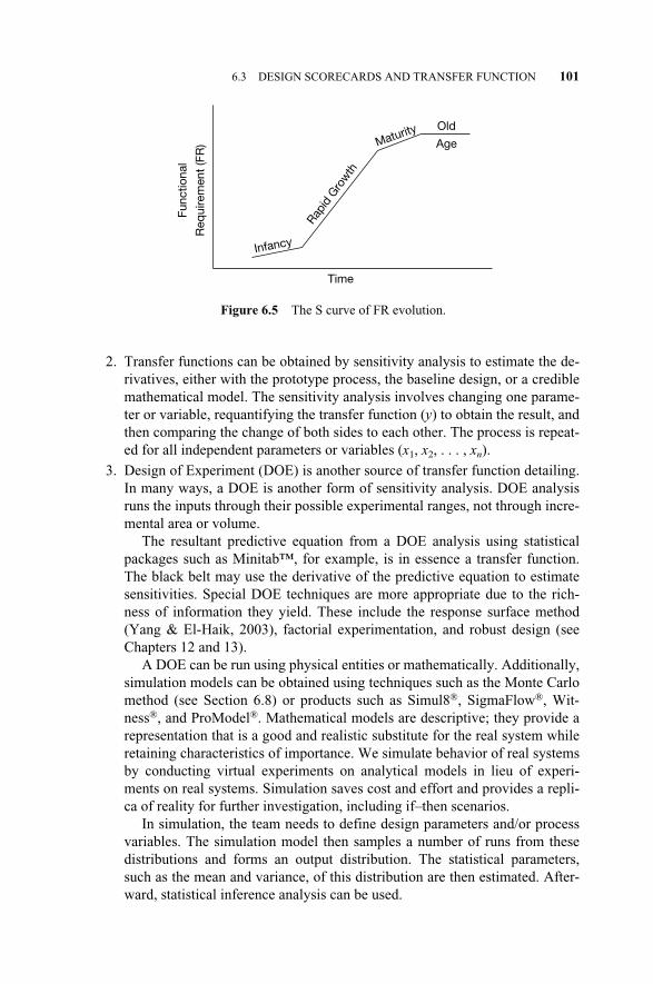
2. Transfer functions can be obtained by sensitivity analysis to estimate the de-rivatives, either with the prototype process, the baseline design, or a crediblemathematical model. The sensitivity analysis involves changing one parame-ter or variable, requantifying the transfer function (y) to obtain the result, andthen comparing the change of both sides to each other. The process is repeat-ed for all independent parameters or variables (x1, x2, . . . , xn).
3. Design of Experiment (DOE) is another source of transfer function detailing.In many ways, a DOE is another form of sensitivity analysis. DOE analysisruns the inputs through their possible experimental ranges, not through incre-mental area or volume.
The resultant predictive equation from a DOE analysis using statisticalpackages such as Minitab™, for example, is in essence a transfer function.The black belt may use the derivative of the predictive equation to estimatesensitivities. Special DOE techniques are more appropriate due to the rich-ness of information they yield. These include the response surface method(Yang & El-Haik, 2003), factorial experimentation, and robust design (seeChapters 12 and 13).
A DOE can be run using physical entities or mathematically. Additionally,simulation models can be obtained using techniques such as the Monte Carlomethod (see Section 6.8) or products such as Simul8®, SigmaFlow®, Wit-ness®, and ProModel®. Mathematical models are descriptive; they provide arepresentation that is a good and realistic substitute for the real system whileretaining characteristics of importance. We simulate behavior of real systemsby conducting virtual experiments on analytical models in lieu of experi-ments on real systems. Simulation saves cost and effort and provides a repli-ca of reality for further investigation, including if–then scenarios.
In simulation, the team needs to define design parameters and/or processvariables. The simulation model then samples a number of runs from thesedistributions and forms an output distribution. The statistical parameters,such as the mean and variance, of this distribution are then estimated. After-ward, statistical inference analysis can be used.
6.3 DESIGN SCORECARDS AND TRANSFER FUNCTION 101
Figure 6.5 The S curve of FR evolution.
Time
Func
tiona
l
Req
uire
men
t (F
R) Maturity
Rapid
Gro
wth
Infancy
Old
Age
c06.qxd 4/22/2005 9:00 AM Page 101
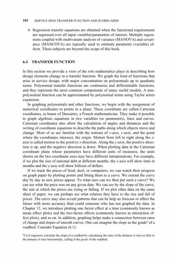
4. Regression transfer equations are obtained when the functional requirementsare regressed over all input variables/parameters of interest. Multiple regres-sions coupled with multivariate analysis of variance (MANOVA) and covari-ance (MANCOVA) are typically used to estimate parameter (variable) ef-fects. These subjects are beyond the scope of this book.
6.4 TRANSFER FUNCTION
In this section we provide a view of the role mathematics plays in describing howdesign elements change in a transfer function. We graph the kind of functions thatarise in service design, with major concentration on polynomials up to quadraticterms. Polynomial transfer functions are continuous and differentiable functions,and they represent the most common components of many useful models. A non-polynomial function can be approximated by polynomial terms using Taylor seriesexpansion.
In graphing polynomials and other functions, we begin with the assignment ofnumerical coordinates to points in a plane. These coordinate are called Cartesiancoordinates, in honor of Descartes, a French mathematician. They make it possibleto graph algebraic equations in two variables (or parameters), lines and curves.Cartesian coordinates also allow the calculation of angles and distances and thewriting of coordinate equations to describe the paths along which objects move andchange. Most of us are familiar with the notions of x-axis, y-axis, and the pointwhere the coordinates intersect, the origin. Motion from left to right along the x-axis is called motion in the positive x-direction. Along the y-axis, the positive direc-tion is up, and the negative direction is down. When plotting data in the Cartesiancoordinate plane whose parameters have different units of measures, the unitsshown on the two coordinate axes may have different interpretations. For example,if we plot the size of national debt at different months, the x-axis will show time inmonths and the y-axis will show billions of dollars.
If we track the prices of food, steel, or computers, we can watch their progresson graph paper by plotting points and fitting them to a curve. We extend the curveday by day as new prices appear. To what uses can we then put such a curve? Wecan see what the price was on any given date. We can see by the slope of the curve,the rate at which the prices are rising or falling. If we plot other data on the samesheet of paper, we can perhaps see what relation they have to the rise and fall ofprices. The curve may also reveal patterns that can be help us forecast or affect thefuture with more accuracy than could someone who has not graphed the data. InChapter 12, we introduce plotting one factor effect at a time (commonly known asmean effect plots) and the two-factor effects (commonly known as interaction ef-fect plots), and so on. In addition, graphing helps make a connection between ratesof change and slopes of smooth curves. One can imagine the slope as the grade6 of aroadbed. Consider Equation (6.1):
102 SERVICE DFSS TRANSFER FUNCTION AND SCORECARDS
6Civil engineers calculate the slope of a roadbed by calculating the ratio of the distance it rises or falls tothe distance it runs horizontally, calling it the grade of the roadbed.
c06.qxd 4/22/2005 9:00 AM Page 102

y = f(x1) = a0 + a1x1 (6.1)
Where a1x1 is a linear term. This is an equation of a liner transfer function in whicha0 and a1 are the y-intercept and slope, respectively. It is a polynomial of the firstdegree or a linear polynomial. In this case, the output y is called the dependent vari-able, whereas x is called the independent variable. This relationship can be exempli-fied by the inventory cost of an item that is replenished at a constant rate a1, with aninitial stocking cost of a0. In this case, the y output is the cost of total units in the in-ventory since acquisitions, and x1 is the stocked units (quantity) variable. The termsy, a0, and a1x1 are in units of cost. Therefore, the unit of a1, the slope, is the unit ofinventory cost per unit of the item. Another example is revenue (y) as a function ofsales. This function is graphed in Figure 6.6.
Suppose there is another item denoted by x2 that is also stocked in the same in-ventory space, and we are interested in the overall inventory cost of both items. Inthis case, the cost can be given as
y = f(x1, x2) = a0 + a1x1 + a2x2 (6.2)
where a1x1 + a2x2 are linear terms. The plot of such a transfer function is given inFigure 6.7. As you may conclude, it is a plane. Note that this transfer function maybe enhanced by cross product terms reflecting the interaction between parametersor factors x1 and x2. In Chapter 12, we will call this cross product term interaction.This may occur when the there is a limited inventory space and competing itemstocks. Equation (6.2) then becomes
y = f(x1, x2) = a0 + a1x1 + a2x2 + a12x1x2 (6.3)
where a1x1 + a2x2 are linear terms and a12x1x2 is an interaction term.
6.4 TRANSFER FUNCTION 103
Figure 6.6 Linear transfer function.
0a
x1
y
Slope = a1 = y/x
�y
�x
c06.qxd 4/22/2005 9:00 AM Page 103
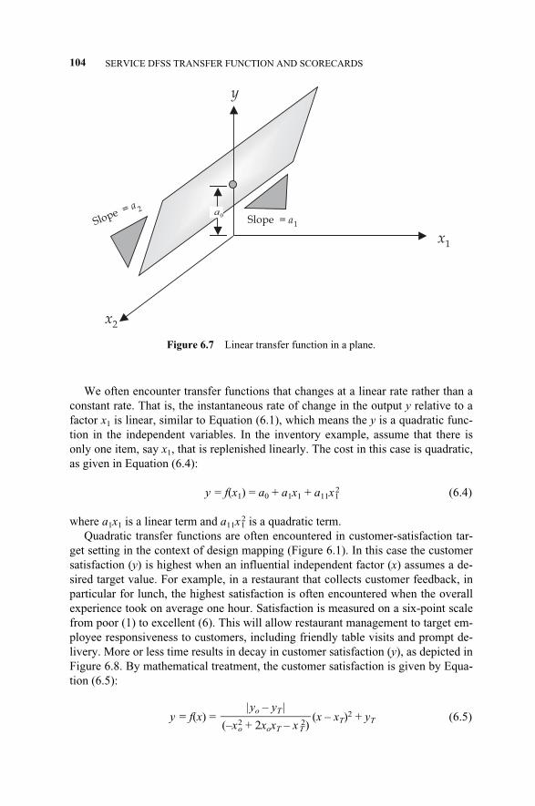
We often encounter transfer functions that changes at a linear rate rather than aconstant rate. That is, the instantaneous rate of change in the output y relative to afactor x1 is linear, similar to Equation (6.1), which means the y is a quadratic func-tion in the independent variables. In the inventory example, assume that there isonly one item, say x1, that is replenished linearly. The cost in this case is quadratic,as given in Equation (6.4):
y = f(x1) = a0 + a1x1 + a11x12 (6.4)
where a1x1 is a linear term and a11x12 is a quadratic term.
Quadratic transfer functions are often encountered in customer-satisfaction tar-get setting in the context of design mapping (Figure 6.1). In this case the customersatisfaction (y) is highest when an influential independent factor (x) assumes a de-sired target value. For example, in a restaurant that collects customer feedback, inparticular for lunch, the highest satisfaction is often encountered when the overallexperience took on average one hour. Satisfaction is measured on a six-point scalefrom poor (1) to excellent (6). This will allow restaurant management to target em-ployee responsiveness to customers, including friendly table visits and prompt de-livery. More or less time results in decay in customer satisfaction (y), as depicted inFigure 6.8. By mathematical treatment, the customer satisfaction is given by Equa-tion (6.5):
y = f(x) = (x – xT)2 + yT (6.5)|yo – yT |
��(–xo
2 + 2xoxT – xT2)
104 SERVICE DFSS TRANSFER FUNCTION AND SCORECARDS
Figure 6.7 Linear transfer function in a plane.
0a
0a
x1
y
Slope = a1
x2
Slope = a 2
c06.qxd 4/22/2005 9:00 AM Page 104
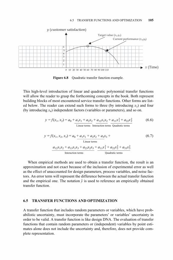
This high-level introduction of linear and quadratic polynomial transfer functionswill allow the reader to grasp the forthcoming concepts in the book. Both representbuilding blocks of most encountered service transfer functions. Other forms are list-ed below. The reader can extend such forms to three (by introducing x3) and four(by introducing x4) independent factors (variables or parameters), and so on.
y = f (x1, x2) = a0 + a1x1 + a2x2 + a12x1x2 + a11x12 + a22x2
2 (6.6)_________ ______ ___________Linear terms Interaction terms Quadratic terms
y = f (x1, x2, x3) = a0 + a1x1 + a2x2 + a3x3 + (6.7)____________________
Linear terms
a12x1x2 + a13x1x3 + a23x2x3 + a11x12 + a22x2
2 + a33x32
_______________________________ ________________________Interaction terms Quadratic terms
When empirical methods are used to obtain a transfer function, the result is anapproximation and not exact because of the inclusion of experimental error as wellas the effect of unaccounted for design parameters, process variables, and noise fac-tors. An error term will represent the difference between the actual transfer functionand the empirical one. The notation �y is used to reference an empirically obtainedtransfer function.
6.5 TRANSFER FUNCTIONS AND OPTIMIZATION
A transfer function that includes random parameters or variables, which have prob-abilistic uncertainty, must incorporate the parameters’ or variables’ uncertainty inorder to be valid. A transfer function is like design DNA. The evaluation of transferfunctions that contain random parameters or (independent) variables by point esti-mates alone does not include the uncertainty and, therefore, does not provide com-plete representation.
6.5 TRANSFER FUNCTIONS AND OPTIMIZATION 105
Figure 6.8 Quadratic transfer function example.
0 10 20 30 40 50 60 70 80 90 100 110
y (customer satisfaction)
Target value (xT,yT)
x (Time)1
2
345
6
Current performance (x0,y0)
c06.qxd 4/22/2005 9:00 AM Page 105
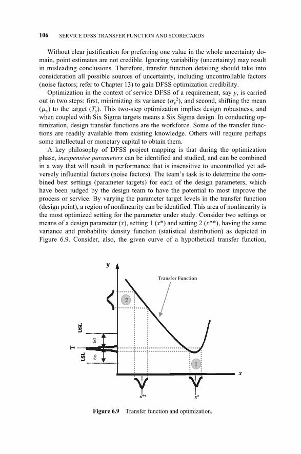
Without clear justification for preferring one value in the whole uncertainty do-main, point estimates are not credible. Ignoring variability (uncertainty) may resultin misleading conclusions. Therefore, transfer function detailing should take intoconsideration all possible sources of uncertainty, including uncontrollable factors(noise factors; refer to Chapter 13) to gain DFSS optimization credibility.
Optimization in the context of service DFSS of a requirement, say y, is carriedout in two steps: first, minimizing its variance (�y
2), and second, shifting the mean(�y) to the target (Ty). This two-step optimization implies design robustness, andwhen coupled with Six Sigma targets means a Six Sigma design. In conducting op-timization, design transfer functions are the workforce. Some of the transfer func-tions are readily available from existing knowledge. Others will require perhapssome intellectual or monetary capital to obtain them.
A key philosophy of DFSS project mapping is that during the optimizationphase, inexpensive parameters can be identified and studied, and can be combinedin a way that will result in performance that is insensitive to uncontrolled yet ad-versely influential factors (noise factors). The team’s task is to determine the com-bined best settings (parameter targets) for each of the design parameters, whichhave been judged by the design team to have the potential to most improve theprocess or service. By varying the parameter target levels in the transfer function(design point), a region of nonlinearity can be identified. This area of nonlinearity isthe most optimized setting for the parameter under study. Consider two settings ormeans of a design parameter (x), setting 1 (x*) and setting 2 (x**), having the samevariance and probability density function (statistical distribution) as depicted inFigure 6.9. Consider, also, the given curve of a hypothetical transfer function,
106 SERVICE DFSS TRANSFER FUNCTION AND SCORECARDS
Figure 6.9 Transfer function and optimization.
x**
LS
LU
SL
T
2
1
y
x*
x
LS
LL
SL
US
L
Transfer Function
x**
LS
LL
SL
US
L
6σ
T
2
1
y
x*
x
LS
LL
SL
US
L
6σ
c06.qxd 4/22/2005 9:00 AM Page 106
which is in this case a nonlinear function in the design parameter, x. It is obviousthat setting 1 produces less variation in the functional requirement (y) than setting 2by capitalizing on nonlinearity.7 Setting 1 (x*) will also produce a lower qualityloss, a concept that is entertained in Chapter 13. In other words, the design pro-duced by setting 1 (x*) is more robust (optimized) than that produced by setting 2.Setting 1 (x*) robustness is evident in the amount of transferred variation throughthe transfer function to the y response in Figure 6.9.8 When the distance between thespecification limits is six times the standard deviation (6�y), a Six Sigma level opti-mized y is achieved. When all design functional requirements are released at thislevel, a Six Sigma design is obtained.
The black belt and the rest of the DFSS team need to detail the transfer functionsin the context of the DFSS algorithm if they want to optimize, validate, and predictthe exact performance of their project in the intended environment. However, theteam should be cautious about the predictability of some of the transfer functionsdue to the stochastic effects of noise factors in the intended environment, which areparticularly hard to predict. The team should explore all knowledge to obtain thetransfer functions desired. For example, stack-up based on tolerances may containdescriptions of functionality that are based on a lumped-mass model and geometry.Transfer functions that are obtained by means other than direct documented knowl-edge are approximate and, for the purposes of the DFSS roadmap, are valid untilproven wrong or disposed due to the evolution of other adopted concepts.
6.6 MONTE CARLO SIMULATION
Monte Carlo simulation is named for Monte Carlo, Monaco, where the primary at-traction is gambling. Gambling implies the use of chance and probability, similar tothe simulation mechanism of employing randomness. Games of chance, such asroulette wheels, dice, and slot machines, exhibit random behavior. When we use theword simulation, we refer to any analytical method meant to replicate a real-lifeprocess, especially when other transfer functions are too mathematically complexor too difficult to reproduce. Without the aid of simulation, a developed model willgenerally reveal a single outcome, the most likely or average scenario. Analysisuses simulation to automatically analyze the effect of varying inputs on outputs ofthe modeled process. One type of spreadsheet simulation is Monte Carlo simula-tion, which randomly generates values for variables over and over to simulate aprocess.
The random behavior in gambling games is similar to how Monte Carlo simula-tion selects variable values at random to simulate a model. When a die is rolled, youknow that a 1, 2, 3, 4, 5, or 6 will come up, but you don’t know which will come upfor any particular trial. It’s the same with the process variables that have a known
6.8 MONTE CARLO SIMULATION 107
7In addition to nonlinearity, leveraging interactions between the noise factors and the design parametersis another popular empirical parameter design approach.8Also the flatter quadratic quality loss function in Figure 13.3.
c06.qxd 4/22/2005 9:00 AM Page 107
range of values but an uncertain value for any particular time or event (e.g., staffingneeds, stock prices, inventory, phone calls per minute).
For each process variable (one that has a range of possible values), the DFSSteam defines the possible values with a probability distribution. The type of distrib-ution you select is based on the conditions surrounding that variable. Distributiontypes include normal, uniform, exponential, and triangular. To add this sort of func-tion to an Excel spreadsheet, you would need to know the equation that representsthis distribution. In commercially available software packages such as CrystalBall®, these equations are automatically calculated for you. They can even fit a dis-tribution to any historical data available.
A simulation calculates multiple scenarios of a model by repeatedly samplingvalues from the probability distributions for the process variables and use those val-ues for the advancement of transactions in the process. Simulations can consist ofhundreds or even thousands of trials in just a few seconds. During a single MontoCarlo trial, a simulation model randomly selects a value from the defined possibili-ties (the range and shape of the distribution) for each process variable and then re-calculates the spreadsheet.
Monte Carlo simulation is a popular simulation method to evaluate the uncer-tainty of a functional requirement (y). It involves some sampling from the indepen-dent parameters or variables, and probability distributions to provide their values. Arandom-number generator is used to obtain the parameter value based on the proba-bility density function. When all independent parameters or variables are quanti-fied, the functional requirement is quantified to produce the numerical result. Thisprocess is repeated for a desired number of iterations. A histogram of the results isthen built from the answer and can be used for statistical inference. The black beltneeds to:
� Determine the applicable distribution of y.
� Estimate the parameters of that distribution.
� Use the distribution for optimization and inference. For example, assumingnormality y, we can use the following upper z value, zy = (USL – �y)/�y, tocalculate the defects per million.
The drawbacks of this method are:
� Simulation time may be an issue, in particular for some complex mathemati-cal forms of transfer functions and large numbers of iterations.
� Identifying the proper probability distribution functions for the independentparameters and variables may be difficult due to lack of data or not under-standing the underlying process.
� Randomness of the random-number generator may be an issue.
Tables of ready-to-use generated random numbers are available, especially inMonte Carlo simulations, where random sampling is used to estimate certain re-
108 SERVICE DFSS TRANSFER FUNCTION AND SCORECARDS
c06.qxd 4/22/2005 9:00 AM Page 108
quirements. Also, most simulation software packages have the capability of auto-matic random number generation. The detail of sampling from probability distribu-tions is not within the scope of this chapter.
Monte Carlo simulation models are time-independent (static) models that dealwith a process of fixed state. In such spreadsheet-like models, certain variable val-ues are changed by random generation and a certain measure or more are evaluatedper such changes without considering the timing and the dynamics of such changes,a prime disadvantage that is handled by discrete event simulation models (seeChapter 14). In discrete event simulation, the time dimension is live.
6.7 SUMMARY
Design can be defined by a series of mappings between four domains. The DFSSproject road map recognizes three types of mapping:
1. Customer mapping (from customer attributes to functional requirements)
2. Functional mapping (from functional requirements to design parameters)
3. Process mapping (from design parameters to process variables)
Transfer functions are mathematical relationships relating a design response,usually a functional requirement, with design parameters and/or process variables.Transfer functions are DFSS optimization vehicles. They facilitate the DFSS opti-mization of process outputs related to the service entity of interest by defining thetrue relationship between input variables and the output. Optimization in this con-text means minimizing the requirement variability and shifting its mean to some de-sired target value desired by the customer. Design scorecards are used to documentthe transfer function as well as the optimization calculations.
6.7 SUMMARY 109
c06.qxd 4/22/2005 9:00 AM Page 109

c06.qxd 4/22/2005 9:00 AM Page 110

7.1 INTRODUCTION
In this chapter, we will cover the history of quality function deployment (QFD), de-scribe the methodology of applying the QFD within the DFSS project road map(see Chapter 5), and apply the QFD to our supply chain example.
QFD is a planning tool that allows the flow-down of high-level customer needsand wants through to design parameters and then to process variables critical to ful-filling the high-level needs. By following the QFD methodology, relationships areexplored between quality characteristics expressed by customers and substitutequality requirements expressed in engineering terms (Cohen 1988, 1995). In thecontext of DFSS, we call these requirements “critical-to” characteristics. Thesecritical-to characteristics can be expanded along the dimensions of speed (critical todelivery, CTD), quality (CTQ), cost (CTC), as well as the other dimensions intro-duced in Figure 1.1. In the QFD methodology, customers define their wants andneeds using their own expressions, which rarely carry any actionable technical ter-minology. The voice of the customer can be refined into a list of needs and wantsthat can be used as input to a relationship matrix called QFD’s house of quality(HOQ) using the affinity diagram.
Knowledge of the customer’s needs and wants is paramount in designing effec-tive products and services by innovative and rapid means. Utilizing the QFDmethodology allows the developer to attain the shortest development cycle whileensuring the fulfillment of the customer’s needs and wants.
Figure 7.1 shows that teams that use QFD place more emphasis on responding toproblems early in the design cycle. Intuitively, it incurs more effort, time, resources,and energy to implement a design change at production launch than at the conceptphase because more resources are required to resolve problems than to prevent theiroccurrence in the first place.
With QFD, quality is defined by the customer. Customers want products and ser-
Service Design for Six Sigma. By Basem El-Haik and David M. Roy 111© 2005 by John Wiley & Sons.
7QUALITY FUNCTION DEPLOYMENT (QFD)
c07.qxd 4/22/2005 9:02 AM Page 111

vices that throughout their lifetimes meet their needs and expectations at a valuethat exceeds cost.
QFD methodology links these needs through design and into process control.The QFD’s ability to link and prioritize at the same time guides the design team infocussing its energy and resources with amazing focus.
In this chapter, we will provide the detailed methodology to create the four QFD“houses” and evaluate them for completeness and goodness, introduce the Kanomodel for the voice of the customer, and relate QFD with the DFSS road map intro-duced in Chapter 5.
7.2 HISTORY OF QFD
As we mentioned in Chapter 1, QFD was developed in Japan by Yoji Akao andShigeru Mizuno in 1966 but not westernized until the 1980s. Their purpose was todevelop a quality assurance method that would design customer satisfaction into aproduct before it was manufactured. For six years, the methodology was developedfrom the initial concept of Kiyotaka Oshiumi of Bridgestone Tire Corporation. Fol-lowing the first publication of an article on quality deployment by Dr. Yoji Akao in1972 (Akao, 1972) the pivotal development work was conducted at Kobe Shipyardsfor Mitsubishi Heavy Industry. The stringent government regulations for militaryvessels coupled with the large capital outlay forced the management at the shipyardto seek a method of ensuring upstream quality that would cascade down throughoutall activities. The team developed a matrix that related all the government regula-tions, critical design requirements, and customer requirements to technical charac-teristics of how the company would achieve them. Within the matrix, the team de-picted the importance of each requirement, which allowed for prioritization.
112 QUALITY FUNCTION DEPLOYMENT (QFD)
TraditionalPlanned Resource Level
Res
ou
rce
Le
vel
ExpectedResource Level
with QFD
ExpectedResource Level
with QFD
Time
Figure 7.1 The time-phased effort for DFSS versus traditional design.
c07.qxd 4/22/2005 9:02 AM Page 112
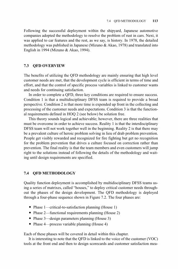
Following the successful deployment within the shipyard, Japanese automotivecompanies adopted the methodology to resolve the problem of rust in cars. Next, itwas applied to car features and the rest, as we say, is history. In 1978, the detailedmethodology was published in Japanese (Mizuno & Akao, 1978) and translated intoEnglish in 1994 (Mizuno & Akao, 1994).
7.3 QFD OVERVIEW
The benefits of utilizing the QFD methodology are mainly ensuring that high levelcustomer needs are met, that the development cycle is efficient in terms of time andeffort, and that the control of specific process variables is linked to customer wantsand needs for continuing satisfaction.
In order to complete a QFD, three key conditions are required to ensure success.Condition 1 is that a multidisciplinary DFSS team is required to provide a broadperspective. Condition 2 is that more time is expended up front in the collecting andprocessing of the customer needs and expectations. Condition 3 is that the function-al requirements defined in HOQ 2 (see below) be solution free.
This theory sounds logical and achievable; however, there are three realities thatmust be overcome in order to achieve success. Reality 1 is that the interdisciplinaryDFSS team will not work together well in the beginning. Reality 2 is that there maybe a prevalent culture of heroic problem solving in lieu of drab problem prevention.People get visibly rewarded and recognized for fire fighting but get no recognitionfor the problem prevention that drives a culture focused on correction rather thanprevention. The final reality is that the team members and even customers will jumpright to the solutions instead of following the details of the methodology and wait-ing until design requirements are specified.
7.4 QFD METHODOLOGY
Quality function deployment is accomplished by multidisciplinary DFSS teams us-ing a series of matrixes, called “houses,” to deploy critical customer needs through-out the phases of the design development. The QFD methodology is deployedthrough a four-phase sequence shown in Figure 7.2. The four phases are:
� Phase 1—critical-to-satisfaction planning (House 1)
� Phase 2—functional requirements planning (House 2)
� Phase 3—design parameters planning (House 3)
� Phase 4—process variable planning (House 4)
Each of these phases will be covered in detail within this chapter.It is interesting to note that the QFD is linked to the voice of the customer (VOC)
tools at the front end and then to design scorecards and customer satisfaction mea-
7.4 QFD METHODOLOGY 113
c07.qxd 4/22/2005 9:02 AM Page 113
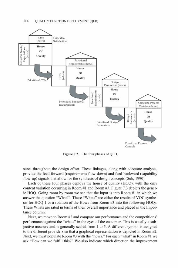
sures throughout the design effort. These linkages, along with adequate analysis,provide the feed-forward (requirements flow-down) and feed-backward (capabilityflow-up) signals that allow for the synthesis of design concepts (Suh, 1990).
Each of these four phases deploys the house of quality (HOQ), with the onlycontent variation occurring in Room #1 and Room #3. Figure 7.3 depicts the gener-ic HOQ. Going room by room we see that the input is into Room #1 in which weanswer the question “What?”. These “Whats” are either the results of VOC synthe-sis for HOQ 1 or a rotation of the Hows from Room #3 into the following HOQs.These Whats are rated in terms of their overall importance and placed in the Impor-tance column.
Next, we move to Room #2 and compare our performance and the competitions’performance against the “whats” in the eyes of the customer. This is usually a sub-jective measure and is generally scaled from 1 to 5. A different symbol is assignedto the different providers so that a graphical representation is depicted in Room #2.Next, we must populate Room #3 with the “hows.” For each “what” in Room #1 weask “How can we fulfill this?” We also indicate which direction the improvement
114 QUALITY FUNCTION DEPLOYMENT (QFD)
House
Of
Quality
House
Of
Quality
House
Of
Quality
House
Of
Quality
CTSs (hows)
Functional
Requirements (hows)
DesignParameters (hows)
Critical to Process
Variables (hows)
Cu
sto
mer
Nee
ds/
E
xp
ecta
tio
ns
(w
hat
s)
CT
Ss
(wh
ats)
Fu
nct
ion
al
Req
uir
em
ents
(wh
ats)
Des
ign
P
ara
met
ers
(wh
ats)
Prioritized Process Controls
Prioritized FunctionalRequirements
Critical to Satisfaction
Prioritized CTSs
Prioritized Design Parameters
Figure 7.2 The four phases of QFD.
c07.qxd 4/22/2005 9:02 AM Page 114
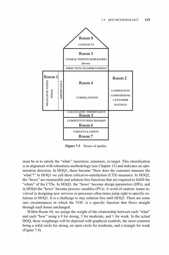
must be in to satisfy the “what:” maximize, minimize, or target. This classificationis in alignment with robustness methodology (see Chapter 13) and indicates an opti-mization direction. In HOQ1, these become “How does the customer measure the‘what’?” In HOQ1 we call these critical-to-satisfaction (CTS) measures. In HOQ2,the “hows” are measurable and solution-free functions that are required to fulfill the“whats” of the CTSs. In HOQ3, the “hows” become design parameters (DPs), andin HOQ4 the “hows” become process variables (PVs). A word of caution: teams in-volved in designing new services or processes often times jump right to specific so-lutions in HOQ1. It is a challenge to stay solution free until HOQ3. There are somerare circumstances in which the VOC is a specific function that flows straightthrough each house unchanged.
Within Room #4, we assign the weight of the relationship between each “what”and each “how” using a 9 for strong, 3 for moderate, and 1 for weak. In the actualHOQ, these weightings will be depicted with graphical symbols, the most commonbeing a solid circle for strong, an open circle for moderate, and a triangle for weak(Figure 7.4).
7.4 QFD METHODOLOGY 115
Room 7
Room 3
Room 5
Room 4
Room 1
Room 6
Room 2
Room 8
IMP
OR
TA
NC
E
DIRECTION OF IMPROVEMENT
CALCULATED IMPORTANCE
COMPETITIVE
COMPARISON/
CUSTOMER
RATINGS
CONFLICTSH
IGH
-LE
VE
L N
EE
DS
(Wh
ats
)
CORRELATIONS
COMPETITIVE BENCHMARKS
TARGETS & LIMITS
CHARACTERISTICS/MEASURES
(Hows)
Figure 7.3 House of quality.
c07.qxd 4/22/2005 9:02 AM Page 115
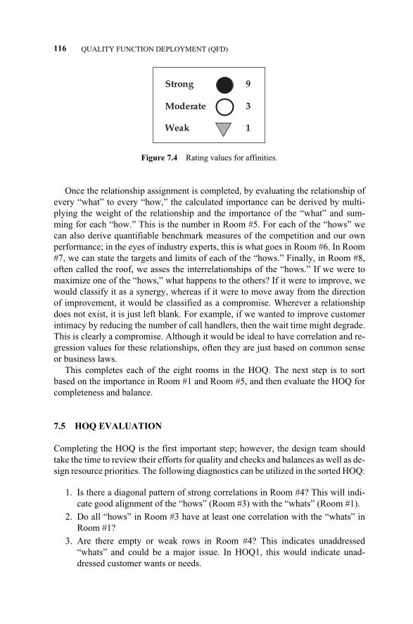
Once the relationship assignment is completed, by evaluating the relationship ofevery “what” to every “how,” the calculated importance can be derived by multi-plying the weight of the relationship and the importance of the “what” and sum-ming for each “how.” This is the number in Room #5. For each of the “hows” wecan also derive quantifiable benchmark measures of the competition and our ownperformance; in the eyes of industry experts, this is what goes in Room #6. In Room#7, we can state the targets and limits of each of the “hows.” Finally, in Room #8,often called the roof, we asses the interrelationships of the “hows.” If we were tomaximize one of the “hows,” what happens to the others? If it were to improve, wewould classify it as a synergy, whereas if it were to move away from the directionof improvement, it would be classified as a compromise. Wherever a relationshipdoes not exist, it is just left blank. For example, if we wanted to improve customerintimacy by reducing the number of call handlers, then the wait time might degrade.This is clearly a compromise. Although it would be ideal to have correlation and re-gression values for these relationships, often they are just based on common senseor business laws.
This completes each of the eight rooms in the HOQ. The next step is to sortbased on the importance in Room #1 and Room #5, and then evaluate the HOQ forcompleteness and balance.
7.5 HOQ EVALUATION
Completing the HOQ is the first important step; however, the design team shouldtake the time to review their efforts for quality and checks and balances as well as de-sign resource priorities. The following diagnostics can be utilized in the sorted HOQ:
1. Is there a diagonal pattern of strong correlations in Room #4? This will indi-cate good alignment of the “hows” (Room #3) with the “whats” (Room #1).
2. Do all “hows” in Room #3 have at least one correlation with the “whats” inRoom #1?
3. Are there empty or weak rows in Room #4? This indicates unaddressed“whats” and could be a major issue. In HOQ1, this would indicate unad-dressed customer wants or needs.
116 QUALITY FUNCTION DEPLOYMENT (QFD)
Strong 9
Moderate 3
Weak 1
Figure 7.4 Rating values for affinities.
c07.qxd 4/22/2005 9:03 AM Page 116
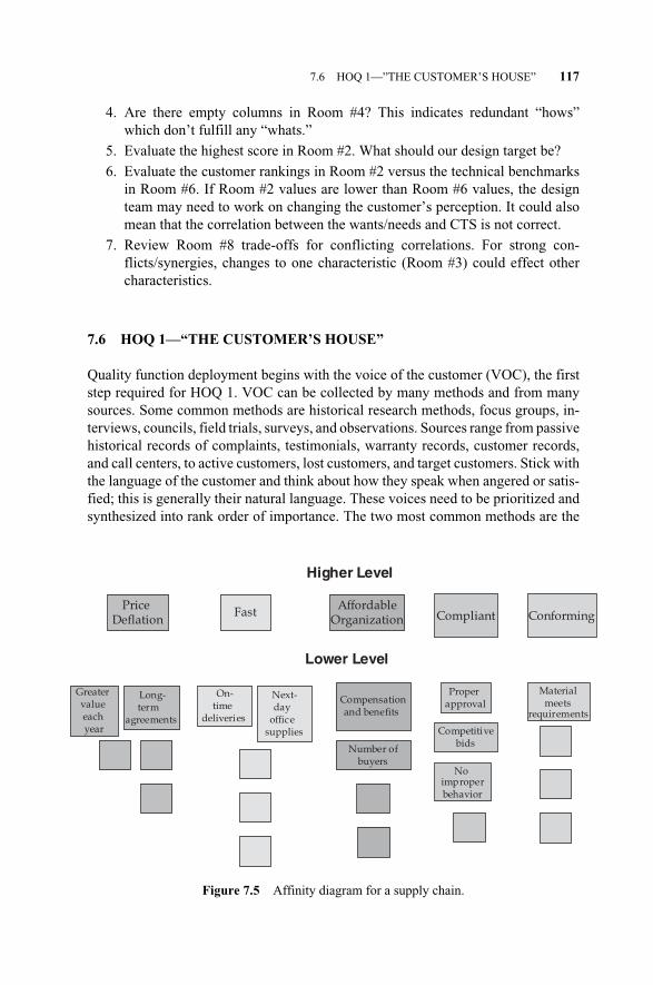
4. Are there empty columns in Room #4? This indicates redundant “hows”which don’t fulfill any “whats.”
5. Evaluate the highest score in Room #2. What should our design target be?
6. Evaluate the customer rankings in Room #2 versus the technical benchmarksin Room #6. If Room #2 values are lower than Room #6 values, the designteam may need to work on changing the customer’s perception. It could alsomean that the correlation between the wants/needs and CTS is not correct.
7. Review Room #8 trade-offs for conflicting correlations. For strong con-flicts/synergies, changes to one characteristic (Room #3) could effect othercharacteristics.
7.6 HOQ 1—“THE CUSTOMER’S HOUSE”
Quality function deployment begins with the voice of the customer (VOC), the firststep required for HOQ 1. VOC can be collected by many methods and from manysources. Some common methods are historical research methods, focus groups, in-terviews, councils, field trials, surveys, and observations. Sources range from passivehistorical records of complaints, testimonials, warranty records, customer records,and call centers, to active customers, lost customers, and target customers. Stick withthe language of the customer and think about how they speak when angered or satis-fied; this is generally their natural language. These voices need to be prioritized andsynthesized into rank order of importance. The two most common methods are the
7.6 HOQ 1—”THE CUSTOMER’S HOUSE” 117
Number ofbuyers
Greater value each year
On- time
deliveries
Compensationand benefits
Proper approval
Materialmeets
requirements
Long-term
agreements
Price Deflation
FastAffordable
Organization Compliant Conforming
Higher Level
Lower Level
Next- day
office supplies Competitive
bids
No improperbehavior
Figure 7.5 Affinity diagram for a supply chain.
c07.qxd 4/22/2005 9:03 AM Page 117
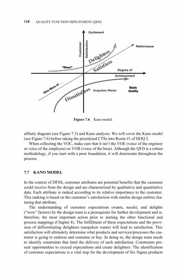
affinity diagram (see Figure 7.5) and Kano analysis. We will cover the Kano model(see Figure 7.6) before taking the prioritized CTSs into Room #1 of HOQ 2.
When collecting the VOC, make sure that it isn’t the VOE (voice of the engineeror voice of the employee) or VOB (voice of the boss). Although the QFD is a robustmethodology, if you start with a poor foundation, it will deteriorate throughout theprocess.
7.7 KANO MODEL
In the context of DFSS, customer attributes are potential benefits that the customercould receive from the design and are characterized by qualitative and quantitativedata. Each attribute is ranked according to its relative importance to the customer.This ranking is based on the customer’s satisfaction with similar design entities fea-turing that attribute.
The understanding of customer expectations (wants, needs), and delights(“wow” factors) by the design team is a prerequisite for further development and is,therefore, the most important action prior to starting the other functional andprocess mappings (Chapter 8). The fulfillment of these expectations and the provi-sion of differentiating delighters (unspoken wants) will lead to satisfaction. Thissatisfaction will ultimately determine what products and services/processes the cus-tomer is going to endorse and consume or buy. In doing so, the design team needsto identify constraints that limit the delivery of such satisfaction. Constraints pre-sent opportunities to exceed expectations and create delighters. The identificationof customer expectations is a vital step for the development of Six Sigma products
118 QUALITY FUNCTION DEPLOYMENT (QFD)
Performance
Quality
Give More
of . . .
Give More
of
“Wow!”“Wow!”
Excitement
Quality
Basic
Quality
Performance
Quality
Give More
of
Give More
of
“Wow!”“Wow!”
Excitement
Quality
“Wow!”“Wow!”
Excitement
Basic
Quality
Performance
Degree of
Performance
Quality
Give More
of
Give More
of
“Wow!”“Wow!”
Excitement
Quality
Basic
Quality
Achievement
Cu
sto
me
r
Sati
sfa
cti
on
Performance
Quality
Give More
of
Give More
of
“Wow!”“Wow!”
Excitement
Quality
“Wow!”“Wow!”
Excitement
Basic
QualityUnspoken Wants
Performance
Dissatisfiers
Satisfie
rsDelighters
Figure 7.6 Kano model.
c07.qxd 4/22/2005 9:03 AM Page 118

and services the customer will buy in preference to those of the competitors. Noria-ki Kano, a Japanese consultant, has developed a model relating design characteris-tics to customer satisfaction (Cohen, 1995). This model (see Figure 7.6) dividescharacteristics into categories—dissatifiers, satisfiers, and delighters—each ofwhich affects customers differently.
“Dissatisfiers” are also known as basic, “must-be,” or expected attributes, andcan be defined as a characteristic that a customer takes for granted and that causesdissatisfaction when it is missing. “Satisfiers” are performance, one-dimensional, orstraight-line characteristics, and are defined as something the customer wants andexpects; the more, the better. “Delighters” are features that exceed competitive of-ferings in creating unexpected, pleasant surprises. Not all customer satisfaction at-tributes are equal from an importance standpoint. Some are more important to cus-tomers than others in subtly different ways. For example, dissatisfiers may notmatter when they are met, but subtract from overall design satisfaction when theyare not delivered.
When customers interact with the design team, delighters often surface that havenot been independently conceived. Another source of delighters may emerge fromteam creativity, as some features have the unintended result of becoming delightersin the eyes of customers. Any design feature that fills a latent or hidden need is a de-lighter and, with time, becomes a want. A good example of this is the remote con-trols first introduced in televisions. Early on, these were differentiating delighters;today, they are common features in televisions, radios, and even automobile igni-tions and door locks. Today, if you received a television without a remote control itwould be a dissatisfier. Delighters can be sought in areas of weakness, competitorbenchmarking, technical, social, and strategic innovation. Social aspects are be-coming more important as educated buyers want to preserve the environment andhuman rights.
The design team should conduct a customer evaluation study. This is hard todo in creative design situations. Customer evaluation is conducted to assess howwell the current or proposed design delivers on the needs and desires of the enduser. The most frequently used method for this evaluation is to ask the customer(e.g., via a focus group or a survey) how well the design project is meeting eachcustomer’s expectations. In order to leap ahead of the competition, the team mustalso understand the evaluation and performance of their toughest competition. Inthe HOQ 1, the team has the opportunity to grasp and compare, side by side, howwell the current, proposed, or competitive design solutions are delivering on cus-tomer needs.
The objective of the HOQ 1 Room 2 evaluation is to broaden the team’s strategicchoices for setting targets for the customer performance goals. For example, armedwith meaningful customer desires, the team could aim their efforts at either thestrengths or weaknesses of best-in-class competitors, if any. In another choice, theteam might explore other innovative avenues to gain competitive advantages.
The list of customer wants and needs should include all from the customer aswell as regulatory requirements and social and environmental expectations. It isnecessary to understand requirements and prioritization similarities and differ-
7.7 KANO MODEL 119
c07.qxd 4/22/2005 9:03 AM Page 119
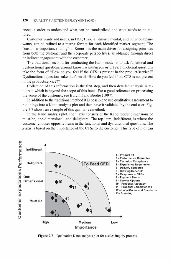
ences in order to understand what can be standardized and what needs to be tai-lored.
Customer wants and needs, in HOQ1, social, environmental, and other companywants, can be refined to a matrix format for each identified market segment. The“customer importance rating” in Room 1 is the main driver for assigning prioritiesfrom both the customer and the corporate perspectives, as obtained through director indirect engagement with the customer.
The traditional method for conducting the Kano model is to ask functional anddysfunctional questions around known wants/needs or CTSs. Functional questionstake the form of “How do you feel if the CTS is present in the product/service?”Dysfunctional questions take the form of “How do you feel if the CTS is not presentin the product/service?”
Collection of this information is the first step, and then detailed analysis is re-quired, which is beyond the scope of this book. For a good reference on processingthe voice of the customer, see Burchill and Brodie (1997).
In addition to the traditional method it is possible to use qualitative assessment toput things into a Kano analysis plot and then have it validated by the end user. Fig-ure 7.7 shows an example of this qualitative method.
In the Kano analysis plot, the y axis consists of the Kano model dimensions ofmust be, one-dimensional, and delighters. The top item, indefferent, is where thecustomer chooses opposite items in the functional and dysfunctional questions. Thex axis is based on the importance of the CTSs to the customer. This type of plot can
120 QUALITY FUNCTION DEPLOYMENT (QFD)
9
18
42
3
10
11
5
6 12
To Feed QFD
7
13
High LowMedium
1 – Product Fit
2 – Performance Guarantee
3 – Technical Compliance
4 – Experience Requirement
5 – Delivery Schedule
6 – Drawing Schedule
7 – Response to CTSs
8 – Payment Terms
9 – Service Options
10 – Proposal Accuracy
11 – Proposal Completeness
12 – Local Codes and Standards
13 - Sourcing
Cu
sto
mer
Exp
ecta
tio
ns
Perf
orm
an
ce
Delighters
One-
Dimensional
Must Be
Importance
Indifferent
Figure 7.7 Qualitative Kano analysis plot for a sales inquiry process.
c07.qxd 4/22/2005 9:03 AM Page 120
be completed from the Kano model or can be arranged qualitatively by the designteam, but it must be validated by the customer or we will fall into the trap of voiceof the engineer again.
7.8 QFD HOQ 2—“TRANSLATION HOUSE”
The critical-to-satisfaction (CTS) list is the set of metrics derived by the designteam from the customer to answer the customer attributes list. The CTS list rotatesinto HOQ 2 Room #1 in this QFD phase. The objective is to determine a set of func-tional requirements (FRs) with which the critical-to-satisfaction requirements canbe materialized. The answering activity translates customer expectations into re-quirements such as waiting time and number of mouse clicks for on-line purchasingservice. For each CTS, there should be one or more FRs that describe a means of at-taining customer satisfaction.
At this stage, only overall CTSs that can be measured and controlled need to beused. We will call these CTSs “Technical CTSs.” As explained in Section 7.1,CTSs are traditionally known as substitute quality characteristics. Relationshipsbetween technical CTSs and FRs are often used to prioritize CTSs filling the rela-tionship matrix of HOQ 2 rooms. For each CTS, the design team has to assign avalue that reflects the extent to which the defined FRs contribute to meeting it.This value, along with the calculated importance index of the CTS, establishes thecontribution of the FRs to the overall satisfaction and can be used for prioritiza-tion.
The analysis of the relationships of FRs and CTSs allows a comparison to otherindirect information, which needs to be understood before prioritization can be fi-nalized. The new information from Room 2 in the QFD HOQ needs to be contrast-ed with the available design information (if any) to ensure that reasons for modifi-cation are understood.
The purpose of the QFD HOQ 2 activity is to define the design functions interms of customer expectations, benchmark projections, institutional knowledge,and interface management with other systems, and to translate this information intoservice technical functional requirement targets and specifications. This will facili-tate the design mappings (see Chapter 8). Since the FRs are solution free, their tar-gets and the specifications for them are flowed down from the CTs. For example, aCTS is for “speed of order” and the measure is hours to process, and we want orderprocessing to occur within four hours. The functional requirements for this CTS,the “hows,” could include process design, in which the number of process steps andthe speed of each step would be the flow-down requirements to achieve “speed oforder.” Obviously, the greater the number of process steps, the shorter each stepwill need to be. Since at this stage we do not know what the process will be andhow many steps will be required, we can allocate the sum of all process steps multi-plied by their process time, not to exceed 4 hours. A major reason for customer dis-satisfaction is that the service design specifications do not adequately link to cus-tomer use of the product or service. Often, the specification is written after the
7.8 QFD HOQ 2—”TRANSLATION HOUSE” 121
c07.qxd 4/22/2005 9:03 AM Page 121
design is completed. It may also be a copy of outdated specifications. This realitymay be attributed to the current planned design practices that do not allocate activi-ties and resources in areas of importance to customers, and waste resources byspending too much time in activities that provide marginal value, a gap that is nice-ly filled by the QFD activities. The targets and tolerance setting activity in QFDPhase 2 should also be stressed.
7.9 QFD HOQ 3—“DESIGN HOUSE”
The functional requirements (FRs) are the list of solution-free requirements derivedby the design team to answer the CTS array. The FRs list is rotated into HOQ 3Room #1 in this QFD phase. The objective is to determine a set of design parame-ters which will fulfill the FRs. Again, the FRs are the “whats,” and we decomposethis into the “hows.” This is the phase that most design teams want to jump rightinto so, hopefully, they will have completed the prior phases of HOQ 1 and HOQ 2before arriving here. The design requirements must be tangible solutions
7.10 QFD HOQ 4—“PROCESS HOUSE”
The design parameters (DPs) are a list of tangible functions derived by the designteam to answer the FRs array. The DPs list is rotated into HOQ 4 Room #1 in thisQFD phase. The objective is to determine a set of process variables that, when con-trolled, ensure the DRs. Again, the DRs are the “whats,” and we decompose thisinto the “hows.”
7.11 QFD EXAMPLE
There was a business that purchased $3 billion of direct materials (materials that aresold to customers) and $113 million of indirect materials and services (materialsand services that are consumed internally in order to support the customer-facingprocesses) and yet had no formal supply chain organization. The procurement func-tion existed in each functional group, so Operations purchased what they needed asdid Human Resources, Legal, and Information Systems. This distributed functionresulted in a lack of power in dealing with suppliers, mostly supplier-favorable con-tracts, and some incestuous relationships (lavish trips and gifts given to the decisionmakers).
The corporate parent required that all procurement be consolidated into a formalsupply chain organization with sound legal contracts, high integrity, and year-over-year deflation on the total spend. The design team was a small set of certified blackbelts and a master black belt who were being repatriated into a clean-sheet supplychain organization.
122 QUALITY FUNCTION DEPLOYMENT (QFD)
c07.qxd 4/22/2005 9:03 AM Page 122
7.11.1 HOQ 1
The DFSS team will identify the customers and establish their wants, needs, de-lights, and usage profiles. In order to complete the HOQ, the team also needs to un-derstand the competing performance and the environmental aspects the design willoperate within. The design team realized that the actual customer base would in-clude the corporate parent looking for results, a local management team that wantedno increased organizational cost, and the operational people who needed materialsand services. Through interviews laced with a dose of common sense, the followingcustomer wants and needs were derived:
� Price deflation
� Conforming materials
� Fast process
� Affordable process
� Compliant process
� Ease of use
The next step was to determine how these would be measured by the customer.The critical-to-satisfaction measures were determined to be:
� Percentage year-over-year price deflation
� Percentage defective deliveries
� Percentage late deliveries
� Cost per transaction
� Cost of organization/Cost of orders
� Speed of order (hours)
� Number of compliance violations
� Number of process steps
Next, the team used the QFD application, Decision Capture,1 to assign the directionof improvement and importance of the wants/needs and the relationship betweenthese and the CTSs. Figure 7.8 shows the results. We can see that price deflation ismoderately related to percentage of defective deliveries and number of complianceviolations, weakly related to percentage of late deliveries, and strongly related toyear-over-year price deflation. We see that price deflation is extremely importantand the direction of improvement is to maximize it.
In Figure 7.8 we can see that the importance of the CTSs has been calculated.The method of calculation is as follows for the top sorted CTS:
7.11 QFD EXAMPLE 123
1Decision capture is a software application from International TechneGroup Inc. (www.decisioncap-ture.com).
c07.qxd 4/22/2005 9:03 AM Page 123
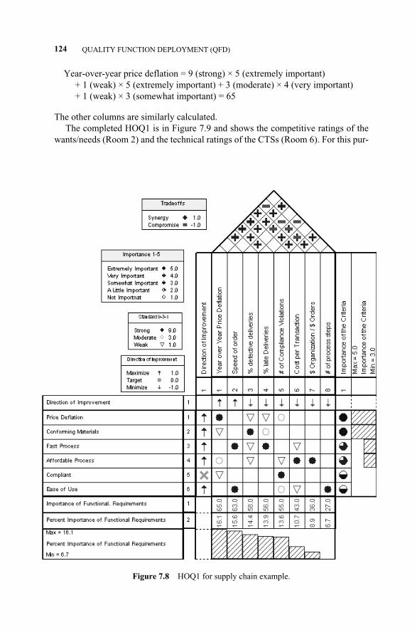
124 QUALITY FUNCTION DEPLOYMENT (QFD)
Figure 7.8 HOQ1 for supply chain example.
Year-over-year price deflation = 9 (strong) × 5 (extremely important)+ 1 (weak) × 5 (extremely important) + 3 (moderate) × 4 (very important) + 1 (weak) × 3 (somewhat important) = 65
The other columns are similarly calculated.The completed HOQ1 is in Figure 7.9 and shows the competitive ratings of the
wants/needs (Room 2) and the technical ratings of the CTSs (Room 6). For this pur-
c07.qxd 4/22/2005 9:03 AM Page 124
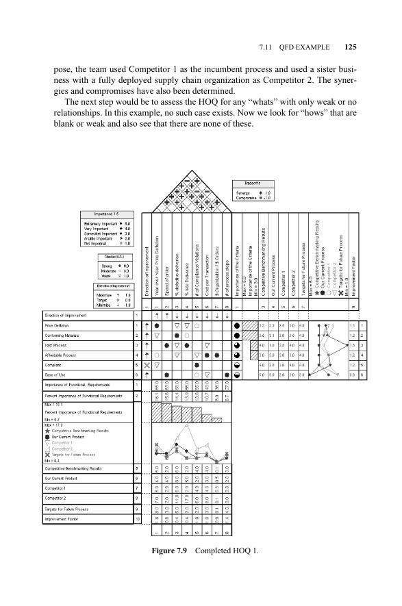
pose, the team used Competitor 1 as the incumbent process and used a sister busi-ness with a fully deployed supply chain organization as Competitor 2. The syner-gies and compromises have also been determined.
The next step would be to assess the HOQ for any “whats” with only weak or norelationships. In this example, no such case exists. Now we look for “hows” that areblank or weak and also see that there are none of these.
7.11 QFD EXAMPLE 125
Figure 7.9 Completed HOQ 1.
c07.qxd 4/22/2005 9:03 AM Page 125
7.11.2 HOQ 2
Now that the team feels confident about HOQ 1, they move on to HOQ 2. We willfollow the seven-step process:
1. Define functional requirements (FRs) (Room 3)
2. Define direction of improvement (Room 3)
3. Define relationship between CTSs and FRs (Room 4)
4. Calculate the importance value (Room 5)
5. Sort importance values in descending order
6. Define the trade-offs (Room 8)
7. Evaluate the matrix for strengths and weaknesses
The first step is to decompose the CTSs into “solution-free” functional require-ments. The first CTS is “percentage year-over-year price deflation.” This is the“what,” and we ask, “How can we do this?” First we need measures of deflation.Notice that this does not specify any specific means of measurement, and surely weneed a measure if we are to convince the stakeholders of what we want to accom-plish. In addition to this measure, we need methods for achieving deflation and re-sources to achieve deflation. So the first CTS can be fulfilled by:
� Measures of deflation
� Cost-reduction methods
� Resources to achieve deflation
Similarly, the other CTSs are decomposed into their functional requirements:
� Percentage of defective deliveries:
Measures of delivery quality
Delivered quality improvement methods
Resources to achieve delivery quality
� Percentage of late deliveries:
Measures of on-time delivery
Methods for improving on-time delivery
Resources to achieve on-time delivery
� Number of compliance violations:
Measures of compliance
Compliance training
Staffing methods
Compliance audits
� Cost per transaction:
Organizational cost
Systems process cost
126 QUALITY FUNCTION DEPLOYMENT (QFD)
c07.qxd 4/22/2005 9:03 AM Page 126

� Purchased material and services cost divided by organizational cost:
Organizational design
Amount of spending controlled
Supplier support
� Speed of order:
Approval speed
Process speed
System availability
� Number of process steps:
Process design
Approval levels
We place these in the matrix (Room 3), define the direction of improvement, andthen define the relationship between each CTS and FR (Room 4). We calculate thematrix and sort on the prioritized FRs, and then define the trade-offs on the roof(Room 8). Last, we evaluate the HOQ 2 for completeness and logic. Figure 7.10shows the completed HOQ 2.
7.11.3 HOQ 3
Now that the team feels confident about HOQ 2, they move on to HOQ 3. We willagain follow the seven-step process:
1. Define design parameters (DPs) (Room 3)
2. Define direction of improvement (Room 3)
3. Define relationship between FRs and DPs (Room 4)
4. Calculate the importance value (Room 5)
5. Sort importance values in descending order
6. Define the trade-offs (Room 8)
7. Evaluate the matrix for strengths and weaknesses
The first step is to decompose the FRs into the corresponding design parameters.The first FR is “resources,” which are required for supplier development in deliv-ery, quality and productivity. This is the “what,” and we ask, “How can we dothis?” First, we need to know the type of resources. In addition to this we need toknow the quantity of resources. So the first FR can be fulfilled by:
� Type of resources
� Number of resources
Similarly, the other FRs are decomposed into their design parameters:
� Organizational design
Type of resources
7.11 QFD EXAMPLE 127
c07.qxd 4/22/2005 9:03 AM Page 127
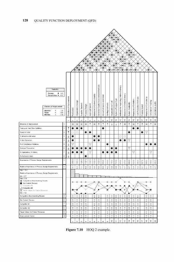
128 QUALITY FUNCTION DEPLOYMENT (QFD)
Figure 7.10 HOQ 2 example.
c07.qxd 4/22/2005 9:03 AM Page 128

7.11 QFD EXAMPLE 129
Figure 7.10 (continued)
c07.qxd 4/22/2005 9:03 AM Page 129
Quantity of resources
Location of resources
� Supplier support
Type of support
Frequency of support
Magnitude of support
� Process design
Intuitive
Workflow
� Approval speed
Approval levels
Speed of approval levels
� Measures of delivery quality
By supplier
By commodity
By part
By buyer
� Methods for improving delivery quality
Lean methods
Variation reduction methods
Contract delivery quality terms
� Amount of spend controlled
Consolidated purchase amount
� Staffing methods
Background checks
Screening methods
� Organizational cost
Compensation and benefits
Travel and living
� Systems process cost
Depreciation cost
Telecommunication cost
Mail cost
� Methods for improving on-time delivery
Lean methods
Variation reduction methods
Contract on-time delivery terms
� Measures of on-time delivery
By supplier
130 QUALITY FUNCTION DEPLOYMENT (QFD)
c07.qxd 4/22/2005 9:03 AM Page 130

By commodity
By part
By buyer
� System availability
Uptime
Bandwidth
� Measures of deflation
By supplier
By commodity
By part
By buyer
� Cost reduction methods
Leveraged spend
Supplier deflation performance
Lean methods
Variation reduction methods
Contract cost-reduction terms
� Process speed
Number of process steps
Speed of each process step
Resource quantity
Resource skill
� Measures of compliance
By compliance category
By buyer
By process
� Compliance training
Target audience
Content
Frequency
� Compliance audits
Auditors
Audit method
We place these in the matrix (Room 3), define the direction of improvement, andthen define the relationship between each FR and DP (Room 4). We calculate thematrix (Room 5), sort on the prioritized DPs, and then define the trade-offs on theroof (Room 8). Figure 7.11 shows the completed HOQ 3. Last, we evaluate theHOQ 3 for completeness and logic.
7.11 QFD EXAMPLE 131
c07.qxd 4/22/2005 9:03 AM Page 131
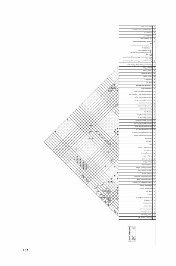
132
Direction of Improvement 1
Type of Resources
Number of Resources
Location of resources
Type of Support
Contract Terms
Lean Methods
Variation Reduction Methods
Intuitive
Work Flow
Frequency of Support
Magnitude of Support
Quality performance by Commodity
Quality performance by Part
Quality performance by Supplier
Levels of approval
Speed of approval levels
Quality performance by Buyer
Consolidated Buy
System Uptime
System Bandwidth
Background Checks
Screening Methods
Travel & Living
Compensation & Benefits
Telecomm
Depreciation
Delivery performance by Supplier
Delivery performance by Commodity
Delivery performance by Part
Delivery performance by Buyer
Deflation Measure by Commodity
Deflation Measure by Supplier
Deflation Measure by Part
Deflation Measure by Buyer
Leverage Buy
Resource Knowledge
Number of process steps
Speed of process steps
Compliance Measure by Process
Compliance Measure by Buyer
Compliance Measure by Compliance item
Compliance Training Frequency
Compliance Topics
Compliance Target Audience
Audit Staff
Audit Method
Office Expense
Number of Policies
Type of Policies
Defined Policies
1
2
3
4
5
6
7
8
9
10
11
12
13
14
15
16
17
18
19
20
21
22
23
24
25
26
27
28
29
30
31
32
33
34
35
36
37
38
39
40
41
42
43
44
45
46
47
48
49
50
51
Importance of Process Design Requirements 1
Relative Importance of Process Design Requirements 2
Max = 13.7
Relative Importance of Process Design Requirements
Min = 2.6Max = 5.0
Competitive Benchmarking Results
Our Current Process
Competitor #1
Competitor #2
Target Values for Future Processes
Min = 1.0
Competitive Benchmarking Results 5
Our Current Process 6
Competitor #1 7
Competitor #2 8
Target Values for Future Processes 9
Improvement Factor 10
Directio
n o
f Im
prov
em
ent
Maxi
miz
e1.0
Targ
et
0.0
Min
imiz
e-1
.0
c07.qxd 4/22/2005 9:03 AM Page 132

133
Fig
ure
7.11
HO
Q 3
exa
mpl
e.
621.0
585.0
1026.0
1026.0
678.0
678.0
558.0
531.0
819.0
711.0
711.0
1197.0
1296.0
2566.0
666.0
1485.0
1045.0
495.0
567.0
909.0
3.3
3.1
5.5
5.5
3.6
3.6
3.0
2.8
4.4
3.8
3.8
6.4
6.9
13.7
3.6
7.9
5.6
2.6
3.0
4.9
3.0
3.0
4.0
4.0
2.0
2.0
2.0
3.0
3.0
2.0
3.0
3.0
2.0
4.0
3.0
2.0
1.0
1.0
2.0
1.0
1.0
3.0
2.0
3.0
2.0
3.0
2.0
1.0
2.0
2.0
1.0
2.0
2.0
3.0
3.0
4.0
2.0
2.0
2.0
3.0
3.0
2.0
3.0
3.0
2.0
3.0
3.0
2.0
3.0
3.0
4.0
2.0
2.0
2.0
2.0
3.0
2.0
1.0
2.0
3.0
2.0
4.0
2.0
2.0
4.0
4.0
4.0
4.0
4.0
4.0
4.0
4.0
4.0
4.0
5.0
4.0
3.0
4.0
4.0
4.0
1.6
1.6
1.4
1.6
1.6
1.2
1.4
1.2
1.4
1.2
1.6
1.6
1.2
1.4
1.6
1.4
1 2 3 4 5 6 7 8 9 10
11
12
13
14
15
16
17
18
19
20
Directio
n o
f Im
provem
ent
1
Resour
ces
Org
ani
zation
Desi
gn
Sup
plie
r S
upp
ort
Pro
cess
Desig
n
Appr
ova
l Speed
Measur
es
of D
eliv
ery
Qualit
y
Deliv
ere
d Q
ualit
y Im
pro
vem
ent
Met
hods
Am
ount
of spe
nd
controlle
d
Sta
ffin
g M
eth
ods
Org
ani
zationa
l Cost
Sys
tem
s P
roce
ss C
ost
Meth
ods
for Im
pro
ving
Ont
ime D
eliv
ery
Measur
es
of O
ntim
e D
eliv
ery
Sys
tem
Availa
bility
Measur
es
of D
efla
tion
Cost R
educ
tion M
eth
ods
Pro
cess
Spe
ed
Measur
es
of C
om
plia
nce
Com
plia
nce
Tra
inin
g
Com
plia
nce
Aud
its
1 2 3 4 5 6 7 8 9 10
11
12
13
14
15
16
17
18
19
20
Im
port
anc
e o
f C
TP
Variable
s
1
56.6
62.3
58.7
221.9
215.1
221.9
107.7
62.3
155.6
107.3
50.2
58.7
58.7
43.7
27.2
27.2
27.2
49.3
110.0
110.0
110.0
32.6
32.6
32.6
32.6
25.5
25.5
25.5
23.8
23.8
28.1
29.8
29.8
29.8
29.8
43.4
43.4
26.8
26.8
26.8
34.2
34.2
34.2
34.2
34.2
11.4
0.0
0.0
0.0
39.4
39.4
Rela
tive
Im
portanc
e o
f C
TP
Variab
les
2
2.0
2.2
2.1
8.0
7.8
8.0
3.9
2.2
5.6
3.9
1.8
2.1
2.1
1.6
1.0
1.0
1.0
1.8
4.0
4.0
4.0
1.2
1.2
1.2
1.2
0.9
0.9
0.9
0.9
0.9
1.0
1.1
1.1
1.1
1.1
1.6
1.6
1.0
1.0
1.0
1.2
1.2
1.2
1.2
1.2
0.4
0.0
0.0
0.0
1.4
1.4
Max
= 8
.0
Rela
tive
Im
portanc
e o
f C
TP
Variabl
es
Min
= 0
.0M
ax
= 1
0.0
Com
petit
ive B
ench
mark
ing
Resu
lts
Our
Curr
ent
Pro
duct
Com
petit
or
#1
Com
petit
or
#2
Targ
et Valu
es
for Targ
et P
roce
ss
Min
= 4
.0
Com
petit
ive B
enc
hmark
ing
Resu
lts
5
8.3
5.0
6.4
4.5
7.0
6.1
5.8
4.0
7.5
7.3
8.5
7.5
5.1
Our
Curr
ent
Pro
duct
6
5.8
5.6
5.8
5.0
10.0
5.2
5.0
5.5
5.8
5.0
6.1
6.3
Com
petit
or
#1
7
8.3
5.0
6.4
4.5
7.0
6.1
5.8
4.0
7.5
7.3
8.5
7.5
5.1
Com
petit
or
#2
8
Targ
et Valu
es
for Targ
et P
roce
ss
9
5.0
5.0
5.0
5.0
5.0
5.0
5.0
5.0
5.0
5.0
5.0
5.0
5.0
Im
prove
ment Fact
or
1
0
-0.7
0.0
-0.3
0.1
-0.4
-0.2
-0.2
0.2
-0.5
-0.5
-0.7
-0.5
0.0
11
1
2
3
4
5
6
7
8
9
10
11
12
13
14
15
16
17
18
19
20
21
22
23
24
25
26
27
28
29
30
31
32
33
34
35
36
37
38
39
40
41
42
43
44
45
46
47
48
49
50
51
Sta
ndard
9-3
-1
Strong
9.0
Modera
te3.0
Weak
1.0
Tra
deoffs
Syn
erg
y1.0
Com
pro
mis
e-1
.0
c07.qxd 4/22/2005 9:03 AM Page 133
7.11.4 HOQ 4
Now that the team feels confident about HOQ 3, they move on to HOQ 4. We willfollow the seven-step process one last time:
1. Define process variables (PVs) (Room 3)
2. Define direction of improvement (Room 3)
3. Define relationship between DPs and PVs (Room 4)
4. Calculate the importance value (Room 5)
5. Sort importance values in descending order
6. Define the trade-offs (Room 8)
7. Evaluate the matrix for strengths and weaknesses
The first step is to decompose the DPs into the corresponding process variables.The first DP is “type of resources.” This is the “what,” and we ask, “How can we dothis?” First, we need commodity leaders. In addition to this we need buyers andclerical support. All of these positions need to be scaled by opportunity, so theprocess variables that we need in order to make these choices are dynamic and varyby activity and resource type. The first DP can be fulfilled by:
� Capacity model
� Volume per person
Similarly, the other DPs are decomposed into their process variables:
� Number of resources
Volume per person
Capacity model
� Location of resources
Travel cost per person
� Type of support
Problem resolution support
Productivity support
� Contract terms
Delivery performance terms
Quality performance terms
Productivity performance terms
� Lean methods
Lean material content
Number of persons trained in lean methods
Number of lean projects
� Variation-reduction methods
134 QUALITY FUNCTION DEPLOYMENT (QFD)
c07.qxd 4/22/2005 9:03 AM Page 134

Variation-reduction materials content
Number of persons trained in variation-reduction methods
Number of variation-reduction projects
� Intuitive
Templates
Self-help
� Workflow
Percentage of workflow
� Frequency of support
Date of activity
Count of activity
� Magnitude of support
Hours per supplier per year
� Quality performance by commodity
Commodity class
Quality measure
� Quality performance by part
Part ID
Quality measure
� Quality performance by supplier
Supplier ID
Quality measure
� Levels of approval
Approval policies
� Speed of approval levels
Time to approve by level
� Quality performance by buyer
Buyer ID
Quality measure
� Consolidated purchasing
Supplier ID
Annual spend by supplier
Dollar amount of spend actively managed
Number of suppliers
� System uptime
Minutes available per schedule
� System bandwidth
Transaction per minute
� Background checks
7.11 QFD EXAMPLE 135
c07.qxd 4/22/2005 9:03 AM Page 135
Backgrounds performed
Backgrounds with defects
� Screening methods
Interview questions
� Travel and living expense
Buyer ID
Supplier ID
Commodity class
Trip approval
Reason for travel
Expense per month
� Compensation and benefits
Buyer ID
Expense per month
� Mail expense
Cost per month
� Telecommunication expense
Expense per month
Number of telephones
� Depreciation expense
Expense per month
� Delivery performance by supplier
Supplier ID
Delivery performance
� Delivery performance by commodity
Commodity class
Delivery performance
� Delivery performance by part
Part ID
Delivery performance
� Delivery performance by buyer
Buyer ID
Delivery performance
� Deflation measure by commodity
Commodity class
Deflation measure
� Deflation measure by supplier
Supplier ID
Deflation measure
136 QUALITY FUNCTION DEPLOYMENT (QFD)
c07.qxd 4/22/2005 9:03 AM Page 136
� Deflation measure by part
Part ID
Deflation measure
� Deflation measure by buyer
Buyer ID
Deflation measure
� Leveraged purchases
Annual spend by supplier
Volume by part
� Resource knowledge
Date of training
Hours of training
Type of training
Defects per buyer
� Number of process steps
Count of steps
� Speed of process steps
Time to process per step
� Compliance measure by process
Process step classification
Count of compliance defects
� Compliance measure by buyer
Buyer ID
Count of compliance defects
� Compliance measure by compliance item
Compliance category
Count of compliance defects
� Compliance training frequency
Compliance requirements by position
� Compliance items
Compliance category
Compliance requirements by position
� Compliance target audience
Buyer ID
Compliance requirements by position
� Audit staff
Quantity
Source
� Audit method
7.11 QFD EXAMPLE 137
c07.qxd 4/22/2005 9:03 AM Page 137
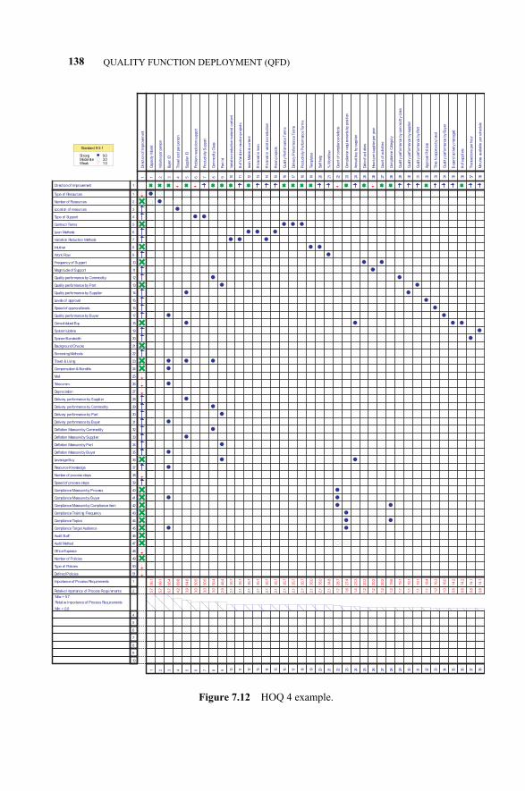
138 QUALITY FUNCTION DEPLOYMENT (QFD)
Dir
ection o
f Im
pro
vem
ent
1
Capacity
Model
Volu
me
per pers
on
Buye
r ID
Tra
vel co
st per pers
on
Supplie
r ID
Pro
ble
m r
eso
lution s
uppo
rt
Pro
duct
ivity
Suppor
t
Com
modity
Cla
ss
Par t I
d
Variation reduct
ion m
ate
rial con
tent
# o
f V
aria
tion r
ecution
pro
ject
s
Lean M
ate
rial
conte
nt
# t
rain
ed in lean
# t
rain
ed in v
ariation reduct
ion
# lean p
roje
cts
Qual
ity
Perf
orm
anc
e T
erm
s
Delive
ry P
erform
ance
Term
s
Pro
duct
ivity
Perform
ance T
erm
s
Tem
pla
tes
Self h
elp
% W
ork
flow
Count of com
plia
nce d
efe
cts
Com
plia
nce
requ
irem
ent
s b
y p
osi
tion
Annual b
uy b
y s
upp
lier
Date
of activities
Hours
per suppl
ier per
year
Count of activ
itie
s
Com
plia
nce
Cat
egory
Qual
ity
per
form
ance
by
com
modity
clas
s
Qual
ity
per
form
ance
by
supplie
r
Qual
ity
per
form
ance
by
Part
Appro
val Polici
es
Tim
e t
o appro
ve b
y lev
el
Qual
ity
per
form
ance
by
Buyer
$ s
pend a
ctive
ly m
anaged
# o
f sup
pliers
Tra
nsact
ions
per hour
Min
ute
s a
vaila
ble
per sch
edule
1 2 3 4 5 6 7 8 9 10
11
12
13
14
15
16
17
18
19
20
21
22
23
24
25
26
27
28
29
30
31
32
33
34
35
36
37
38
Di rection of Improvement 1
Type of Resources
Number of Resources
Location of resources
Type of Support
Contract Terms
Lean Methods
Variation Reduction Methods
Intuitive
Work Flow
Frequency of Support
Magni tude of Support
Quality performance by Commodity
Quality performance by Part
Quality performance by Supplier
Levels of approval
Speed of approval levels
Quality performance by Buyer
Consolidated Buy
System Uptime
System Bandwidth
Background Checks
Screening Methods
Travel & Living
Compensation & Benefits
Telecomm
Depreciation
Delivery performance by Supplier
Delivery performance by Commodity
Delivery performance by Part
Delivery performance by Buyer
Deflation Measure by Commodity
Deflation Measure by Supplier
Deflation Measure by Part
Deflation Measure by Buyer
Leverage Buy
Resource Knowledge
Number of process steps
Speed of process steps
Compliance Measure by Process
Compliance Measure by Buyer
Compliance Measure by Compliance i tem
Compliance Training Frequency
Compliance Topics
Compliance Target Audience
Audit Staff
Audit Method
Office Expense
Number of Policies
Type of Policies
Defined Policies
1
2
3
4
5
6
7
8
9
10
11
12
13
14
15
16
17
18
19
20
21
22
23
24
25
26
27
28
29
30
31
32
33
34
35
36
37
38
39
40
41
42
43
44
45
46
47
48
49
50
51
Importance of Process Requirements 1
96.1
96.1
69.8
50.5
50.5
35.7
35.7
35.7
35.7
35.7
35.7
35.0
35.0
34.8
20.2
20.2
20.2
50.4
19.1
48.4
19.1
64.6
19.1
18.4
16.3
95.4
16.0
14.2
14.2
14.1
14.1
23.3
28.7
19.6
27.4
35.7
35.7
35.7
Relative Importance of Process Requi rements 2 5.7
5.7
4.2
3.0
3.0
2.1
2.1
2.1
2.1
2.1
2.1
2.1
2.1
2.1
1.2
1.2
1.2
3.0
1.1
2.9
1.1
3.9
1.1
1.1
1.0
5.7
1.0
0.8
0.8
0.8
0.8
1.4
1.7
1.2
1.6
2.1
2.1
2.1
Max = 5.7
Relative Importance of Process Requirements
Min = 0.0
4
5
6
7
8
9
10
1 2 3 4 5 6 7 8 9 10
11
12
13
14
15
16
17
18
19
20
21
22
23
24
25
26
27
28
29
30
31
32
33
34
35
36
37
38
Standard 9-3-1
Strong 9.0Moderate 3.0Weak 1.0
Figure 7.12 HOQ 4 example.
c07.qxd 4/22/2005 9:03 AM Page 138
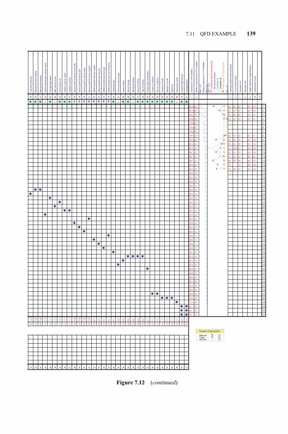
7.11 QFD EXAMPLE 139 Inte
rvie
w Q
uestions
Back
gro
und
check
meth
od
Back
gro
und
checke
rs
Syst
em
Depre
ciatio
n c
ost per m
onth
Trip a
ppro
val/re
aso
n
cos
t per m
onth
Com
p &
Ben
cos
t
Tele
com
cost
per
month
Tele
pho
ne n
um
ber
Delive
ry p
erform
anc
e b
y c
om
modi
ty
Delive
ry p
erform
anc
e b
y p
art
Delive
ry p
erform
anc
e b
y b
uyer
Delive
ry p
erform
anc
e b
y s
uppl
ier
Deflation p
erform
ance b
y s
uppl
ier
Deflation p
erform
ance b
y p
art
Deflation p
erform
ance b
y b
uyer
Deflation p
erform
ance b
y c
om
mod
ity
Volu
me
by
part
Tim
e t
o pro
cess
by
step
Count of ste
ps
Date
of tr
ain
ing
Defe
cts
per pers
on
Hours
of tr
ain
ing
Typ
e o
f train
ing
Pro
cess
Ste
p c
lassificatio
n
Quan
tity
of audi
tors
Sourc
e o
f aud
itors
Fre
quncy
of Audit
Sele
ctio
n o
f audi
t
Reportin
g
Expe
nse b
y m
onth
Indust
ry R
equ
irem
ents
Com
pan
y P
olic
y
39
40
41
42
43
44
45
46
47
48
49
50
51
52
53
54
55
56
57
58
59
60
61
62
63
64
65
66
67
68
69
70
71
Im
port
ance
of
CT
P V
ariable
s
1
56.6
62.3
58.7
221.9
215.1
221.9
107.7
62.3
155.6
107.3
50.2
58.7
58.7
43.7
27.2
27.2
27.2
49.3
110.0
110.0
110.0
32.6
32.6
32.6
32.6
25.5
25.5
25.5
23.8
23.8
28.1
29.8
29.8
29.8
29.8
43.4
43.4
26.8
26.8
26.8
34.2
34.2
34.2
34.2
34.2
11.4
0.0
0.0
0.0
39.4
39.4 R
ela
tive Im
portance o
f C
TP
Variable
s
2
2.0
2.2
2.1
8.0
7.8
8.0
3.9
2.2
5.6
3.9
1.8
2.1
2.1
1.6
1.0
1.0
1.0
1.8
4.0
4.0
4.0
1.2
1.2
1.2
1.2
0.9
0.9
0.9
0.9
0.9
1.0
1.1
1.1
1.1
1.1
1.6
1.6
1.0
1.0
1.0
1.2
1.2
1.2
1.2
1.2
0.4
0.0
0.0
0.0
1.4
1.4
Max =
8.0
Rela
tive
Im
por
tance
of
CT
P V
ariable
s
Min
= 0
.0M
ax =
10.0
Com
petitive
Bench
mar
kin
g R
esults
Our C
urr
ent Pro
duct
Com
petito
r #1
Com
petito
r #2
Targ
et Valu
es for Targ
et P
rocess
Min
= 4
.0
Com
pet
itiv
e B
enchm
ark
ing
Resu
lts
5
8.3
5.0
6.4
4.5
7.0
6.1
5.8
4.0
7.5
7.3
8.5
7.5
5.1
Our C
urr
ent P
roduc
t
6
5.8
5.6
5.8
5.0
10.0
5.2
5.0
5.5
5.8
5.0
6.1
6.3
Com
pet
itor #1
7
8.3
5.0
6.4
4.5
7.0
6.1
5.8
4.0
7.5
7.3
8.5
7.5
5.1
Com
pet
itor #2
8
Targ
et V
alu
es
for
Targ
et P
roce
ss
9
5.0
5.0
5.0
5.0
5.0
5.0
5.0
5.0
5.0
5.0
5.0
5.0
5.0
Im
provem
ent Facto
r
10
-0.7
0.0
-0.3
0.1
-0.4
-0.2
-0.2
0.2
-0.5
-0.5
-0.7
-0.5
0.0
11
1
2
3
4
5
6
7
8
9
10
11
12
13
14
15
16
17
18
19
20
21
22
23
24
25
26
27
28
29
30
31
32
33
34
35
36
37
38
39
40
41
42
43
44
45
46
47
48
49
50
51
10.6
10.6
10.6
10.6
9.7
9.7
9.7
9.7
12.8
12.8
12.8
11.1
11.1
11.1
11.1
11.1
11.1
9.1
8.8
8.8
8.8
8.8
8.8
8.8
8.7
7.7
7.7
7.7
7.7
7.7
0.0
0.0
3.7
0.6
0.6
0.6
0.6
0.6
0.6
0.6
0.6
0.8
0.8
0.8
0.7
0.7
0.7
0.7
0.7
0.7
0.5
0.5
0.5
0.5
0.5
0.5
0.5
0.5
0.5
0.5
0.5
0.5
0.5
0.0
0.0
0.2
39
40
41
42
43
44
45
46
47
48
49
50
51
52
53
54
55
56
57
58
59
60
61
62
63
64
65
66
67
68
69
70
71
Direction of Improvement
Maximize 1.0Target 0.0Minimize -1.0
Figure 7.12 (continued)
c07.qxd 4/22/2005 9:03 AM Page 139
Frequency of audit
Selection of audit target
Reporting
� Office expense
Expense by month
Expense category
� Number of policies
Industry requirements
Company policy
� Type of policies
Industry requirements
Company policy
� Defined policies
Industry requirements
Company policy
We place these in the matrix, define the direction of improvement, and then de-fine the relationship between each DP and PV. We calculate the matrix and sort onthe prioritized PVs. There is no need to define the trade-offs since these measuresare independent of each other (or uncoupled in the context of Chapter 8). Last, weevaluate the HOQ 3 for completeness and logic.
7.12 SUMMARY
QFD is a planning tool used to translate customer needs and wants into focused de-sign actions. This tool is best accomplished with cross-functional teams and is keyin preventing problems from occurring once the design is operationalized. Thestructured linkage allows for rapid design cycles and effective utilization of re-sources while achieving Six Sigma levels of performance.
To be successful with the QFD, the team needs to avoid “jumping” right to solu-tions, and should process HOQ1 and HOQ2 thoroughly and properly before per-forming a detailed design. The team will also be challenged to keep the functionalrequirements solution neutral in HOQ2.
It is important to have the correct voice of customer and the appropriate bench-mark information. Also, a strong cross-functional team willing to think outside thebox is required in order to truly obtain Six-Sigma-capable products or processes.From this point on, the QFD is process driven but it is not the charts that we are try-ing to complete, it is the total concept of listening to the voice of the customerthroughout the design effort.
140 QUALITY FUNCTION DEPLOYMENT (QFD)
c07.qxd 4/22/2005 9:03 AM Page 140
8.1 INTRODUCTION1
In this chapter, we will cover process modeling from the simplest SIPOC (seeChapter 2) to functional modeling and demonstrate the available evaluation tech-niques. By the end of this chapter, the DFSS green belt or black belt should be ableto prepare a detailed process map. Process mapping and functional modeling tech-niques are key for service DFSS projects in the context of the road map depicted inFigure 5.1. The objective of this chapter is to present the case for process mapping,review the different types of process maps, and discuss techniques and tools used tomap a process.
Process mapping can be used when designing or improving processes or parts ofprocesses within the DFSS project scope. By breaking the process down into itssmaller elements and making its value and nonvalue portions apparent, process map-ping helps teams to visualize the process. In a DFSS project, processes are usuallyidentified via tools such as SIPOC, flow planning studies, and simulation analysis (ifany). Once the processes are identified, tools such as process mapping are recom-mended to enable the identification of non-value-added steps of a process for furthertreatment, transfer function detailing, defect locations, and pinpointing where im-provement can be sought. In addition to documenting the process, process maps canbe used to communicate information and train employees in the process aspects.
Design teams usually think they have a pretty good understanding of how theirproject processes work. But, oftentimes, the actual process works somewhat or sig-nificantly differently. Within the process, different steps may be taken or performedin different order. Some of these variations may happen for legitimate or illegiti-mate reasons. To complete a process map, the team should walk through the actual
Service Design for Six Sigma. By Basem El-Haik and David M. Roy 141© 2005 by John Wiley & Sons.
8PROCESS MODELING AND PROCESS MANAGEMENT
1It is recommended that the reader familiarize him or herself with the concepts of Chapter 2 prior toreading this chapter, in particular Sections 2.2, 2.5, and 2.6. These sections discuss the concepts of valuein service, lean processes, yield, and service metrics.
c08.qxd 4/22/2005 9:04 AM Page 141
process and talk with all those involved in the process to understand it. This willhelp highlight opportunities for improving the process using quick-hit, actionableitems and pave the way for the redesign effort leading to the map of “how the teamwould like it to be.” When working with multilocation or cross-functional processflows, the process map enables the graphical representation that allows everyone inthe process to see the entire flow rather than their isolated portions.
In this chapter, we will cover several mapping tools. Some are graphical in na-ture, whereas the rest are logical and prescriptive. The premier attribute of thegraphical method is simplicity and ease of communication to different audienceswith different levels of involvement. The tools are handy and easy to use in re-design projects. On the other hand, the major advantage of logical and prescriptivetools is their logical enforcing functions when applied to new and creative designsituations. The penetration of these tools is very immature in the service industry to-day. However, their power is really remarkable. This book is an attempt to exposethem to service Six Sigma populations. In addition, this chapter features the busi-ness process management system (BPMS, see Chapter 2), which directs the ongo-ing accountability and performance of a process.
8.2 PROCESS MODELING TECHNIQUES
8.2.1 SIPOC
There are two approaches possible with the SIPOC tool. The first approach is to gath-er all of the items within each of the columns without regard to the order in whichthey are applied in the actual process. This is a brainstorming tool for use with teamsat the macro process level. The other method is to take each subprocess step, one at atime, and apply the SIPOC at the micro level. The order of approach is the same forboth methods. The design team starts at the “process “column, ask what “inputs” arerequired, and asks then who the “suppliers” are for these inputs. At this time, theyalso assess what input characteristics the process requires. These are usually in theframework of speed, quality or cost. The next step is to assess what is the “output” ofthe process, who is the “customer,” and what characteristics are required of the out-put by the customer. Figure 8.1 illustrates a generic SIPOC methodology. Figure 8.2shows an application of the tool in BPMS (see Chapter 2 and Section 8.3).
8.2.2 Process Mapping
Like most of the DFSS tools, process mapping requires a cross-functional team ef-fort with involvement from process owners, process members, customers, and sup-pliers. Brainstorming, operation manuals, specifications, operator’s experience, andprocess walkthroughs are very critical inputs to the mapping activity. A detailedprocess map provides input to other tools such as FMEA, transfer function DOEs,capability studies, and control plans.
Process maps can be created for many different levels, zooming in and out of thetargeted process and delivering the service under consideration in the DFSS project.
142 PROCESS MODELING AND PROCESS MANAGEMENT
c08.qxd 4/22/2005 9:04 AM Page 142
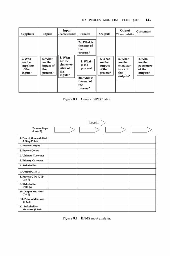
8.2 PROCESS MODELING TECHNIQUES 143
Figure 8.1 Generic SIPOC table.
Input Output
1. What is the process?
2a. What is the start of the process?
2b. What is the end of the process?
3. What are the outputs of the process?
4. Who are the customers of the outputs?
5. What are the
the outputs?
7. Who are the suppliers of the inputs?
8. What are the character-stics of
the inputs?
6. What are the inputs of the process?
InputsInpu
Characteristics Process OutputsOutput
SuppliersCustomers
1. What is the process?
2a. What is the start of the process?
2b. What is the end of the process?
3. What are the outputs of the process?
4. Who are the customers of the outputs?
5. What are the
the outputs?
7. Who are the suppliers of the inputs?
8. What are the charistics of the inputs?
6. What are the inputs of the process?
Characteristics
character-istics of
Figure 8.2 BPMS input analysis.
Level 1
1. Description and Start & Stop Points
2. Process Output
3. Process Owner
4. Ultimate Customer
Process Steps:(Level 2)
5. Primary Customer
6. Stakeholder
7. Output CTQ (2)
8. Process CTQ (CTP) (2 & 7)
9. Stakeholder CTQ (6)
10. Output Measures (7 & 2)
11. Process Measures(8 & 3)
12. StakeholderMeasures (9 & 6)
c08.qxd 4/22/2005 9:04 AM Page 143
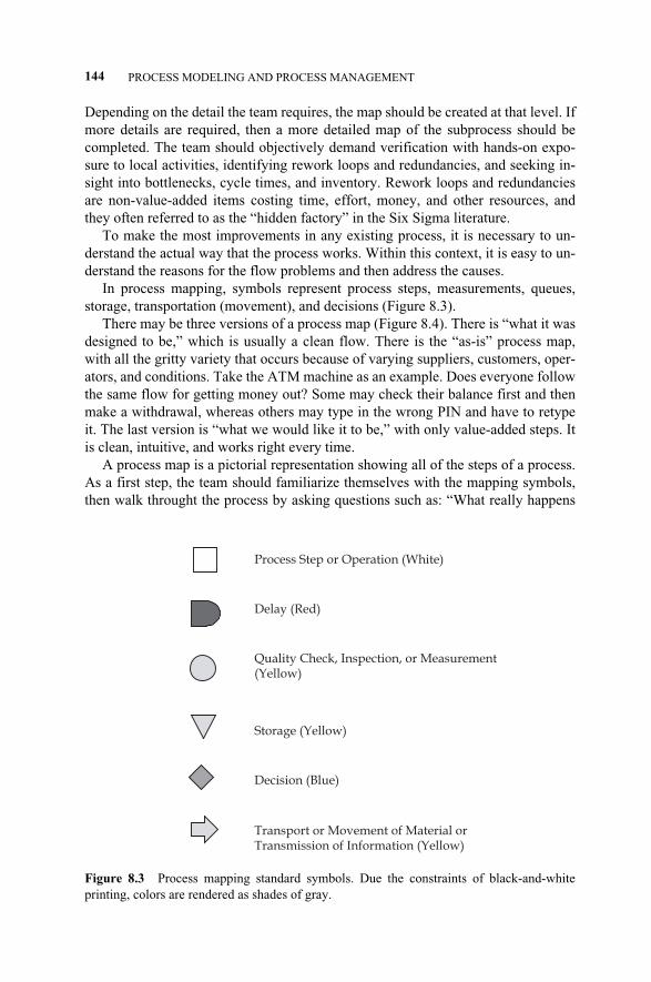
Depending on the detail the team requires, the map should be created at that level. Ifmore details are required, then a more detailed map of the subprocess should becompleted. The team should objectively demand verification with hands-on expo-sure to local activities, identifying rework loops and redundancies, and seeking in-sight into bottlenecks, cycle times, and inventory. Rework loops and redundanciesare non-value-added items costing time, effort, money, and other resources, andthey often referred to as the “hidden factory” in the Six Sigma literature.
To make the most improvements in any existing process, it is necessary to un-derstand the actual way that the process works. Within this context, it is easy to un-derstand the reasons for the flow problems and then address the causes.
In process mapping, symbols represent process steps, measurements, queues,storage, transportation (movement), and decisions (Figure 8.3).
There may be three versions of a process map (Figure 8.4). There is “what it wasdesigned to be,” which is usually a clean flow. There is the “as-is” process map,with all the gritty variety that occurs because of varying suppliers, customers, oper-ators, and conditions. Take the ATM machine as an example. Does everyone followthe same flow for getting money out? Some may check their balance first and thenmake a withdrawal, whereas others may type in the wrong PIN and have to retypeit. The last version is “what we would like it to be,” with only value-added steps. Itis clean, intuitive, and works right every time.
A process map is a pictorial representation showing all of the steps of a process.As a first step, the team should familiarize themselves with the mapping symbols,then walk throught the process by asking questions such as: “What really happens
144 PROCESS MODELING AND PROCESS MANAGEMENT
Figure 8.3 Process mapping standard symbols. Due the constraints of black-and-whiteprinting, colors are rendered as shades of gray.
Process Step or Operation (White)
Delay (Red)
Quality Check, Inspection, or Measurement(Yellow)
Storage (Yellow)
Decision (Blue)
Transport or Movement of Material orTransmission of Information (Yellow)
c08.qxd 4/22/2005 9:04 AM Page 144
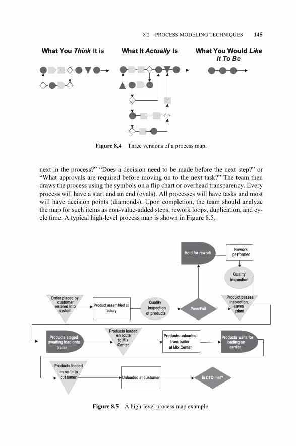
next in the process?” “Does a decision need to be made before the next step?” or“What approvals are required before moving on to the next task?” The team thendraws the process using the symbols on a flip chart or overhead transparency. Everyprocess will have a start and an end (ovals). All processes will have tasks and mostwill have decision points (diamonds). Upon completion, the team should analyzethe map for such items as non-value-added steps, rework loops, duplication, and cy-cle time. A typical high-level process map is shown in Figure 8.5.
8.2 PROCESS MODELING TECHNIQUES 145
Figure 8.4 Three versions of a process map.
What You Think What You Would Like What It ActuallyWhat You Think What You Would Like
It To Be
What It Actually It is Is
Figure 8.5 A high-level process map example.
Order placed bycustomer
entered intosystem
Product assembled at factory
Product passesinspection,
leavesplant
Products staged awaiting load onto
trailer
Products loaded en routeto MixCenter
Products unloaded
at Mix Center
Products waits forloading on
carrier
Products loaded en route tocustomer Unloaded at customer Is CTQ met?
Quality inspection
of products
Rework performed
Quality inspection
Hold for rework
Pass/Fail
from trailer
c08.qxd 4/22/2005 9:04 AM Page 145
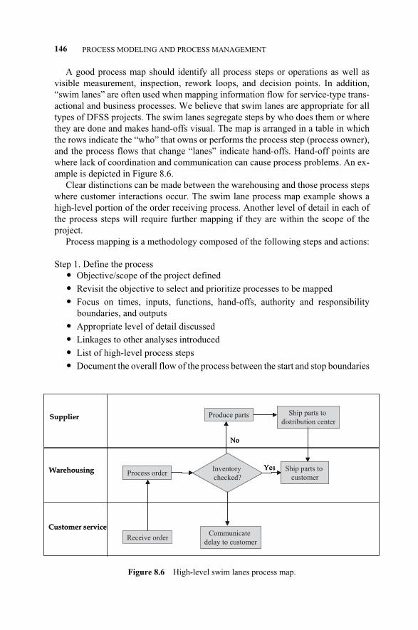
A good process map should identify all process steps or operations as well asvisible measurement, inspection, rework loops, and decision points. In addition,“swim lanes” are often used when mapping information flow for service-type trans-actional and business processes. We believe that swim lanes are appropriate for alltypes of DFSS projects. The swim lanes segregate steps by who does them or wherethey are done and makes hand-offs visual. The map is arranged in a table in whichthe rows indicate the “who” that owns or performs the process step (process owner),and the process flows that change “lanes” indicate hand-offs. Hand-off points arewhere lack of coordination and communication can cause process problems. An ex-ample is depicted in Figure 8.6.
Clear distinctions can be made between the warehousing and those process stepswhere customer interactions occur. The swim lane process map example shows ahigh-level portion of the order receiving process. Another level of detail in each ofthe process steps will require further mapping if they are within the scope of theproject.
Process mapping is a methodology composed of the following steps and actions:
Step 1. Define the process� Objective/scope of the project defined
� Revisit the objective to select and prioritize processes to be mapped
� Focus on times, inputs, functions, hand-offs, authority and responsibilityboundaries, and outputs
� Appropriate level of detail discussed
� Linkages to other analyses introduced
� List of high-level process steps
� Document the overall flow of the process between the start and stop boundaries
146 PROCESS MODELING AND PROCESS MANAGEMENT
Figure 8.6 High-level swim lanes process map.
Produce parts Ship parts to
distribution center
Process orderInventory
checked?
Ship parts to
customer
Communicate
delay to customer
Yes
No
Receive order
Customer service
Warehousing
Supplier Produce parts Ship parts to
distribution center
Process orderInventory
checked?
Ship parts to
customer
Communicate
delay to customer
Yes
No
Receive order
Produce parts Ship parts to
distribution center
Process orderInventory
checked?
Ship parts to
customer
Communicate
delay to customer
Yes
No
Receive order
Customer service
Warehousing
Supplier
c08.qxd 4/22/2005 9:04 AM Page 146
Step 2. Collect information� Data required. Use sampling and collection techniques (focus groups, inter-
views, observations)
� Resources required in this mapping step and the mapping exercise in general
� Process walk-through schedule based on shifts, days, and weeks whereunique work occurs
� When do we zoom in to map every process step?
� Continuous flow
� Process stops (when flow is disrupted or disconnected)
� Have process inputs and output variables (PIV, the xs, and POV, the ys) beenidentified. Remember that we are after a transfer function that fully describeswhat is happening/should be happening to confirm that the solution is reallyoptimal.
� Consider merging of multiple steps
� Add operating specifications
� Be clear about terminology and nomenclature so that everyone is speaking thesame language. Avoid biased, nontechnical language. Be consistent.
� Accumulate a list of quick-hits items and develop an action plan for their im-plementation.
Step 3. Validate and verify � Ensure the use of common terms and nomenclature
� Consolidate, compile, and reconcile information
� Summarize findings
� Validate information
� Confirm controversial data
Step 4. Build the process maps � Sequence of activities and work steps based on the previous steps
� Swim lanes (if necessary)
� Beginning and end of process
� Work steps assigned to participants
� Parcel out times for each work step
� Initial assessment of control plan
� Start an initial assessment after process map is complete
� Add measurement techniques
� Define operating specifications
� Determine targets
� Know the context of the process mapping within the project
� Does process mapping fit with previous, parallel, and proceeding analyses?
� Conduct benchmarking
8.2 PROCESS MODELING TECHNIQUES 147
c08.qxd 4/22/2005 9:04 AM Page 147
� Baseline current performance
� Document comments
Step 5. Analyze and draw conclusions � Identfy characteristics of the process steps
� Define hypotheses about how the process steps inputs link to output variablesrelative to targets/historical means and variances
� Plan follow-up work if any (e.g., new measurement systems, SPC charting)
� View improvement or redesign opportunities
� Apply “if–then” simulation scenarios for any layout changes (see Chapter13)
Step 6. Communicate recommendations, findings, and conclusions� Customize the presentation to the audience with insights into change implica-
tions
� Update specifications, control plans, procedures, training, and so on.
8.2.3 Value Stream Mapping
Value stream mapping (VSM) was initially used to document manufacturingprocesses that are to be improved using lean manufacturing methods. VMS isequally applicable to service processes as well. They are most useful with higher-frequency processes, even mixed-model processes. In this section, we will definevalue stream mapping and its value, and present the different steps for its construc-tion. Usually, whenever there is a product/service for a customer, there is a valuestream. Therefore, value stream mapping is applicable whenever the design team istrying to make waste in a process visible to eliminate non-value-added steps, ac-tions, and activities. A value-added activity or step is any activity or thing the cus-tomer is willing to pay for. Non-value-added activities are the activities that do notadd market form or function or are not necessary. They should be eliminated, sim-plified, reduced, or integrated.
Visibility to waste can be assured via a scorecard documenting performance ofvariables (metrics) such as non-value-added cycle time, inventory, rework, and de-fects. Such measurement should be taken within a broader scope of a value streammanagement process. Value stream management is the process of increasing the ra-tio of value to nonvalue by identifying and eliminating sources of waste. Waste andnon-value-added activities exhibit themselves in several formats:
� Unnecessary movement of people
� Overproduction ahead of demand
� Unnecessary movement of materials
� Waiting for the next step (idle time)
� Overprocessing
148 PROCESS MODELING AND PROCESS MANAGEMENT
c08.qxd 4/22/2005 9:04 AM Page 148
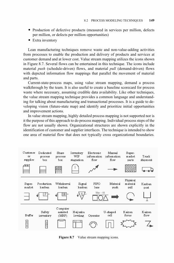
� Production of defective products (measured in services per million, defectsper million, or defects per million opportunities)
� Extra inventory
Lean manufacturing techniques remove waste and non-value-adding activitiesfrom processes to enable the production and delivery of products and services atcustomer demand and at lower cost. Value stream mapping utilizes the icons shownin Figure 8.7. Several flows can be entertained in this technique. The icons includematerial push (schedule-driven) flows, and material pull (demand-driven) flowswith depicted information flow mappings that parallel the movement of materialand parts.
Current-state-process maps, using value stream mapping, demand a processwalkthrough by the team. It is also useful to create a baseline scorecard for processwaste where necessary, assuming credible data availability. Like other techniques,the value stream mapping technique provides a common language and understand-ing for talking about manufacturing and transactional processes. It is a guide to de-veloping vision (future-state map) and identify and prioritize initial opportunitiesand improvement actions.
In value stream mapping, highly detailed process mapping is not supported nor isit the purpose of this approach to do process mapping. Individual process steps of theflow are not usually shown. Organizational structures are shown explicitly in theidentification of customer and supplier interfaces. The technique is intended to showone area of material flow that does not typically cross organizational boundaries.
8.2 PROCESS MODELING TECHNIQUES 149
Figure 8.7 Value stream mapping icons.
c08.qxd 4/22/2005 9:04 AM Page 149
Decisions loops, traditional logical operators, and if–then statements are explicitlyprovided. Typically, they are implied in lean concepts such as kanban, supermarket,and work-in-process inventory points. Most of the logic will occur within theprocesses themselves (box icons) and will not be specifically identified by the map.Value stream mapping is a great tool that helps tremendously in visualizing the ser-vice operation. It helps us visualize more than just the single-process level by expos-ing the flow of material, information, and sources of waste. In addition, this tech-nique provides an organized, visual structure that includes certain data to the DFSSteam and their management. It represents a gateway to institutionalize lean thinkingby linking to lean concepts and techniques that avoid “cherry picking” or “KamikazeKaizen.” It forms the basis for a lean implementation plan. In this regard, valuestream mapping enables a whole door-to-door flow, a blueprint for lean implementa-tion. The technique provides a current baseline by obtaining current operating andmeasurable information that will enable teams to identify waste and develop a vision(future state) with defined actions needed to reach such a state. Several time metricsare used to gauge improvement of the future state from the current state. They are:
� Lead-time. The time it takes for one unit to complete the process, includingnon-value-added time that the unit or product waits between operations.
� Total cycle time. Cumulative time it takes for unit or product to complete alloperations, not including wait time between operations. Also known as sum-mation of touch time but not process time.
� Throughput time. How often a unit or product is completed by the operationfrom start to finish.
� Changeover time. Time to switch from producing one product type to anoth-er.
� Uptime. Calculated by dividing the actual machine time available to run bythe time scheduled to run.
� Working time. Time per period minus breaks and cleanup.
� Queue time. Time in which work is waiting for an operation.
8.2.3.1 Value Stream Mapping Process Steps (see Figure 8.8)
Step 1. Define and Select VSM Resources � Identify the product/process families that pass through similar processing
steps and/or over common equipment in the downstream processes.
� Write down clearly what the product/process family is, how many differentfinished products and services there are, what the demand quantity is, andwith what frequency.
� Process operators and line management are the ideal cross-functional teamand are a requirement in order to gain proper insight.
Step 2. Set up a “war room” with all logistics (e.g., paper, markers, sticky notes)and computer resources needed.
150 PROCESS MODELING AND PROCESS MANAGEMENT
c08.qxd 4/22/2005 9:04 AM Page 150
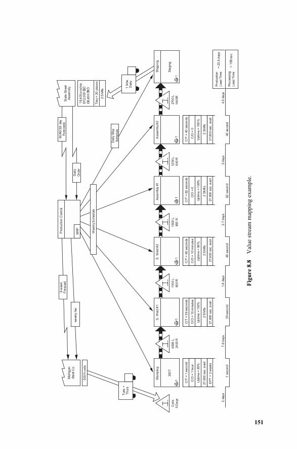
151
Fig
ure
8.8
Val
ue s
trea
m m
appi
ng e
xam
ple.
Sta
gin
g
= 2
3.6
days
= 1
88 s
ec.
Pro
duction
Lead
Tim
e
Pro
cessin
g
Lead
Tim
e
270
0 L
144
0R
C/T
= 4
0 s
econ
ds
C/O
= 0
Uptim
e =
100
%
12
00 L
640 R
C/T
= 6
2 s
econ
ds
C/O
= 0
Up
time =
100%
1600
L
850 R
C/T
= 4
6 s
econ
ds
C/O
= 1
0 m
inute
s
Uptim
e =
80
%
110
0 L
60
0 R
500 f
t coils
Pro
duction
Contr
ol
MR
P
Tues +
Thurs
Mic
hig
an
Ste
el C
o
6-w
ee
k
we
ekly
fax
Fore
cast
Coils
5 D
ays
Sta
te S
treet
Assem
bly
90
/60/3
0/
day
Fo
recasts
Daily
Ord
er
18,4
00 p
cs/m
oÐ
12,0
00
ÒLÓ
Ð6,4
00
ÒRÓ
Tr a
y =
20
pie
ce
s
2 S
hifts
1 t
ime
Daily
2 S
hifts
27,6
00
sec. a
vail
2 S
hifts
27,6
00 s
ec. ava
il
2 S
hift
s
27,6
00
sec. a
vail
2 S
hifts
27,6
00 s
ec.
avail
C/T
= 3
9 s
eco
nds
C/O
= 1
0 m
inute
s
Up
tim
e =
100%
S.
Weld
#1
S.
Weld
#2
Asse
mb
ly #
1A
ssem
bly
#2
Ship
pin
g
4600
L
24
00 R
27,6
00
sec. a
vail
EP
T =
2 w
eeks
C/T
= 1
seco
nd
C/O
= 1
ho
ur
Uptim
e =
85%
Sta
mp
ing
200
T
5 d
ays
1 s
econ
d
7.6
days
39 s
eco
nd
1.8
days
46
secon
d
2.7
days
62
secon
d
2 d
ays
4.5
da
ys
40 s
econd
Wee
kly
Sched
ule
Daily
Ship
Sched
ule
11
11
11
c08.qxd 4/22/2005 9:04 AM Page 151
Step 3. Draw the current state map� Collect current-state information while walking through the actual pathways
of material/content and information flows. Begin with a quick walkthrough ofthe entire door-to-door value stream to get a sense of the flow sequence of theprocesses. Instead of starting at the receiving dock and walking downstream,begin at the shipping end and walk upstream to begin with the processes thatare linked most directly to the customer. Start with the concept of what thecustomer values, and as you move upstream, challenge each process step forhow it adds to or creates customer value.
� Every team member draws a map when walking through the process.
� Develop a specific set of questions before going to the work area.
� While walking through the process talk to the employees.
� Map the “current condition,” using the standard icons to convey key informa-tion (material/content and information flow). Emphasize the importance ofdata collection involved in the VSM effort.
� Start with the customer on the upper-right corner, and draw a factory icon, asshown if the example in Figure 8.8. Underneath this icon, draw data boxes,with the customer name in the top box. Make a record of other informationsuch as services ordered per day, week or month required, packaging require-ments, and number of shifts the customer runs. Process boxes (rectangles),cycle times, shifts operated, and changeover time and information such asnumber of people, cycle time, changeover time, uptime, shifts, and availableworking time must be noted and mapped. Add inventory locations (triangles),including material/content type and quantity stored at each location, and ma-terial/content flow (fat arrows), including indication of whether a “push” or“pull” discipline is followed.
� Insert a truck icon and the broad arrow to indicate movement of finishedgoods to the customer.
� At the other end of the map, insert a factory icon and a data box for the sup-plier.
� Populate the supplier and the trucks data boxes with appropriate data.
� Draw the information flow lines as appropriate. Add the information flow byadding narrow lines. A small box icon is used to describe the different infor-mation-flow arrows.
� A process box indicates the production control department.
� Add “push” and pull” arrows.
� Draw triangles to indicate inventory and populate the boxes with appropriateinformation. Other icons and information indicate external suppliers’ deliveryfrequency and so on. Significant problems (e.g., frequent machine break-downs) are represented by “bad clouds” or starbursts as depicted in Figure8.9.
� Identifying the lead-time ladder along the bottom is the next step. To get thetotal production lead time, the team needs to take the inventory number and
152 PROCESS MODELING AND PROCESS MANAGEMENT
c08.qxd 4/22/2005 9:04 AM Page 152

153
Fig
ure
8.9
Val
ue s
trea
m m
ap o
f F
igur
e 8.
8 w
ith
loop
s an
d st
arbu
rsts
add
ed.
Sta
gin
g
= 2
3.6
days
= 1
88 s
ec.
Pro
duction
Lead T
ime
Pro
cessin
g
Lead T
ime
2700 L
1440R
C/T
= 4
0 s
econds
C/O
= 0
Uptim
e =
100%
1200 L
640 R
C/T
= 6
2 s
econds
C/O
= 0
Uptim
e =
100%
1600 L
850 R
C/T
= 4
6 s
econds
C/O
= 1
0 m
inute
s
Uptim
e =
80%
1100 L
600 R
500 ft coils
Pro
duction C
ontr
ol
MR
P
Tues +
Thurs
Mic
hig
an
Ste
el C
o
6-w
eek
weekly
fax
Fore
cast
Coils
5 D
ays
Sta
te S
treet
Assem
bly
90/6
0/3
0/ day
Fore
casts
Daily
Ord
er
18,4
00 p
cs/m
o
Ð12,0
00
ÒLÓ
Ð6,4
00
ÒRÓ
Tra
y =
20 p
ieces
2 S
hifts
1 tim
e
Daily
2 S
hifts
27,6
00 s
ec. avail
2 S
hifts
27,6
00 s
ec. avail
2 S
hifts
27,6
00 s
ec. avail
2 S
hifts
27,6
00 s
ec. avail
C/T
= 3
9 s
econds
C/O
= 1
0 m
inute
s
Uptim
e =
100%
S. W
eld
#1
S. W
eld
#2
Assem
bly
#1
Assem
bly
#2
Ship
pin
g
4600 L
2400 R
27,6
00 s
ec. avail
EP
T =
2 w
eeks
C/T
= 1
second
C/O
= 1
hour
Uptim
e =
85%
Sta
mpin
g
200T
5 d
ays
1 s
econd
7.6
days
39 s
econd
1.8
days
46 s
econd
2.7
days
62 s
econd
2 d
ays
4.5
days
40 s
econd
Weekly
Schedule
Daily
Ship
Schedule
11
11
11
Ch
an
geo
ver
bu
rst
Ch
an
geo
ver
bu
rst
Loop
1
Loop
3L
oop
2
c08.qxd 4/22/2005 9:04 AM Page 153
divide it by the daily customer requirements. To get the cycle time (or value-added time), you need to add up all the cycle time numbers. For maps withmultiple upstream flows, use the ratio of longest lead time to total the leadtime. When it is all added up, it usually indicates astonishing numbers.
� When done walking through the process the team goes back to the “warroom”1 and, as a team, integrates and develops one current state map. Themost important reason, though, for establishing a team war room is to ensurethat the team gets its information right, up front, to prevent expensive changesdownstream.
� Conduct formal brainstorming of all issues based on the observations madeduring the walkthrough and questions to the employees. The brainstorm itemsshould be recorded.
� On the value stream map, the team needs to draw loops around parts of themap where improvements can be sought. Examples include combiningprocesses to create a better flow and eliminate batching of inventory betweenthose processes. Cell loops, pacemaker loops, and constraints are typical. Apull-system “supermarket” usually corresponds to a loop. Within each loop,the team should use lightening bursts to highlight improvement ideas, startingwith loop that has the biggest issue and and will require the most fixing. Fig-ure 8.9 replicates Figure 8.8 with added loops.
Step 4. Draw and implement the future-state map. The power behind value streammapping is always the future-state map. To develop a future-state map and imple-mentation plan, the team needs a well-defined map with loops identified (Figure8.9). The team needs to be exposed to flow concepts, setup reduction, cellular con-cepts, and total preventive maintenance. The design team keeps updating the cur-rent-state map with material/content flows. They look for waste and creative ideaslike moving processes closer together, combining operations, and eliminating trans-portation. Basically, the steps are:
� Utilizing the map with loops identified, map a future-state proposal reflectingwhat the situation will be after improvements are made.
� Develop implementation plans to achieve the future-state map.
� Present the future-state map and the implementation to management for theirbuy-in.
� Execute actions to achieve the future-state condition, then stabilize the newcondition.
� Repeat current-state mapping, analysis, looping, and future-state mappingsteps to achieve the next future-state target.
154 PROCESS MODELING AND PROCESS MANAGEMENT
1The war room is the service DFSS team information center. The value in having a dedicated team roomis in creating and maintaining facilities and environments to foster individual and collective learning ofservice and process knowledge, including project direction/vision and prior history. The war room couldserve as a focus for team activities to foster team building/growth and inter- and intradisciplinary com-munication and collaboration.
c08.qxd 4/22/2005 9:04 AM Page 154
Step 5: Develop and implement a communication plan. Develop a communicationplan that supports the project and communicates objectives, accomplishments, andteam efforts. The communication plan must be synchronized with the tollgate re-view schedule (making it timely) and continue after project closure, if needed. Con-duct a value stream mapping overview for workshop participants
An example of a value stream map for typical manufacturing operations isshown in Figure 8.8 (see Rother and Shook, 2000). Take special note of the rulerrunning along the bottom of the map that shows the flow time at each step in theplant. Notice how the high-level processes, process level, and plant levels aredrawn with very little detail. The value stream map is a good overview, helps theteam focus on specific processes, and shows both informational and material/con-tent flows.
After creating the current-state map in the charcaterize phase of the DFSS roadmap, the next step is to conduct analysis and determine the team thinking for the fu-ture-state map. The future-state map is part of the optimize phase. The future-statemapping may include future-state cell design, implementation plan (with who?,what?, and when?), and FMEA of the future-state implementation plan.
The purpose of the future-state map is to reflect the looped map in identifyingwaste and determining what can become a reality within a short period of time. Theimplementation is time bounded. After improvements in the value stream have beenimplemented, the future-state map becomes the current-state map, and a new fu-ture-state map is developed.
8.3 BUSINESS PROCESS MANAGEMENT SYSTEM (BPMS)
BPMS is used to establish ongoing integrated ownership, accountability, and per-formance of a process. Oftentimes, the results of transactions in one function are theinputs to transactions in a different functional process. A good example of this iswhen sales creates a sales order that determines the quantity and desired deliverydate as well as the price. This information meanders through various processes andends up with a build order and associated purchase order at a supplier. Commonsense tells us that accuracy and timeliness of the information flow is paramount inorder to fulfill the customer need, but how is this related to the infrastructures andprocedures that exist today in non-Six Sigma processes?
8.3.1 What is BPMS?
BPMS is a system composed of teams organized around a process with a clear mis-sion, process objectives, roles and responsibilities, and performance expectations.There are process management charts that document the procedures, measurements,monitoring, and reaction plans for the process. The teams hold formal reviews fo-cused around the process metrics displayed in a dashboard manner. The teams shareaccountability and, through effective communication and feedback, they drive com-mitment, reenforcing practices and process improvements.
8.3 BUSINESS PROCESS MANAGEMENT SYSTEM (BPMS) 155
c08.qxd 4/22/2005 9:04 AM Page 155
8.3.2 How Is BPMS Implemented?
The deployment of BPMS can follow a DMAIC framework (see Chapter 2). Thedefine phase consists of defining the purpose, boundaries, and goals. The measurephase consists of process mapping the “as is” state and determining the inputs, out-puts, and internal process measures, as well as the suppliers and customers of eachof these. Measures of effectiveness, efficiency, and cycle time are determined. Theanalyze phase consists of evaluating the capability of the process to meet theprocess goals and determining which set of measures and control indicators are theminimum number that will appear on the process dashboard. The improve phaseconsists of deployment of the defined process, with clearly defined roles and re-sponsibilities documented in procedures. In this phase, active data collection beginsto feed the control phase. The final phase is the control phase, which consists of en-suring that the process is performing as expected and the structures and proceduresare being adhered to. This final phase of the BPMS deployment is an ideal buildingblock for either DMAIC or DFSS process improvements.
8.4 RELATIONSHIP OF PROCESS MODELING TO DISCRETE EVENT SIMULATION
There is a strong link between process modeling and discrete event simulation,which will be further explored in Chapter 14. Simulation employs a set of theoreti-cal concepts and computational methods that describe, represent, and simulate thefunctioning of real processes. Computer simulations are becoming popular in per-forming research, and are expanding traditional experimental and theoretical ap-proaches. Simulation can be regarded as a numerical experiment, but it often re-quires advanced theories. It can provide information that is impossible or tooexpensive to measure, as well as insights that are not amenable to or are too compli-cated for analytical methods.
Simulation models are simplified abstractions of reality representing or describ-ing its most important and driving elements and their interactions. Simulation canbe used for a multitude of purposes such as analysis and understanding of design,redesign and problem solving projects, testing of if–then hypotheses and theories,prediction of process behavior under various conditions and scenarios in support ofdecision making, and analysis with visualization of results.
Real processes are sometimes complex and often include nonlinear behavior aswell as stochastic components and loops (e.g., rework) over spatial and time scales;therefore, models can represent the processes only at a certain level of simplifica-tion. Empirical knowledge is based on statistical analysis of observed data, and theyare usually applicable only to the same conditions under which the observationswere made. Process mapping is based on understanding the processes within thescope and their input–output relationships and logical linkages. Discrete event sim-ulation models of complex systems often use a combination of empirical knowl-edge and process-based approaches. Process simulation software enables the fol-lowing outcomes:
156 PROCESS MODELING AND PROCESS MANAGEMENT
c08.qxd 4/22/2005 9:04 AM Page 156
� Design and redesign of new processes to optimize them
� Increase service productivity
� Reduce total process cycle time
� Increase throughput
� Reduce waiting time
� Reduce activity cost
� Reduce inventory costs
� Troubleshooting of existing processes
� What–if studies
In a DFSS project, the primary emphasis is on using discrete system models toanalyze administrative, decision-making, service development, manufacturing, andservice delivery processes. Discrete system models characterize the system as aflow of entities that enter and move through various processes and queues accord-ing to probability functions specified by the modeler. Some processes may also ex-hibit continuous characteristics, in which case continuous model constructs may beapplied. Continuous system models utilize the numerical integration of differentialequations to simulate behavior over time. Such models are often used for studyingthe systems containing feedback loops, in which the outputs are fed back and com-pared with control inputs. In this book, discrete event simulation and its uniquechallenges will be covered in some detail. Discrete event simulation is best suitedfor business and service-type processes due to its transactional and event-driven be-havior.
Business processes are often too complex and dynamic to be understood and an-alyzed by flowcharting and spreadsheets alone. Herein lies the opportunity for SixSigma deployment to institutionalize simulation as the standard tool. Simulation isthe only tool that can provide both accurate analysis and visualization of the processand alternatives. Process simulation is the technique that allows representation andinteraction of processes, people, and technology. There are essentially four steps indoing it: (1) building a model, (2) validating and running a model, (3) analyzing theperformance measures, and (4) evaluating alternative scenarios.2
A model mimics the operations of a business. This is accomplished by steppingthrough the events in compressed time while displaying an animated picture of theflow. Because simulation software keeps track of statistics about model elements,performance of a process can be evaluated by analyzing the model output data.
By modifying decision variables in the model, without the cost and risk of dis-rupting existing operations or building a new system, the team can accurately pre-dict, compare, or optimize the performance of the reengineered process. Simulationmodels can provide the most accurate and insightful means to analyze and predictthe performance measures of business processes in these scenarios. Discrete-event-based simulation is the most capable and powerful tool for business process simula-
8.4 RELATIONSHIP OF PROCESS MODELING TO DISCRETE EVENT SIMULATION 157
2See Kerim Tumay, http://www.reengineering.com/articles/janfeb96/sptprochr.htm, Business ProcessSimulation: Matching Processes with Modeling Characteristics, ER SPOTLIGHT.
c08.qxd 4/22/2005 9:04 AM Page 157
tion that are discrete-event-driven in nature. These tools provide modeling of entityflows, with animation capabilities that allow the user to see how flow objects arerouted through the system. Some of these tools even provide object-oriented and hi-erarchical modeling, which simplifies development of large business process mod-els. Simulation process modeling is aimed at improving our understanding and pre-dicting the impact of processes and their interactions. It provides supporting toolsfor modeling, especially data management, analysis, and visualization. Processmapping models describe the behavior of phenomena represented by a set of indi-vidual processes with various types of value-added and non-value-added step inter-actions at local, regional, or global value streams. Simulation models can be fullyintegrated or linked through data and interfaces.
8.5 FUNCTIONAL MAPPING
A functional map can be defined as the functional elements and the set of logicaland cause–effect relationships amongst them. Mathematically, design mapping,transfer functions, and simulation models can be defined as functional mappings.Graphically, functional mapping is depicted in a block diagram that is composed ofnodes connected by arrows depicting the relationships. Both functional and processmodels should capture all design elements and ensure correct relationships betweenprocess variables (xs or PVs) and functional requirements (ys or FRs). A functionalmodel is captured mathematically using transfer functions with matrices belongingto a design hierarchical level. Hierarchy is built by breaking down the design into anumber of simpler functional design mappings that collectively meet the high-levelfunctional requirements of the design. There are two recognized mappings in theservice DFSS road map of Chapter 5:
� The functional mapping between the functional requirements (FRs) and thedesign parameters (DPs), the subject of this section
� The process mapping between the DPs and the process variables (PVs), thesubject of Section 8.2
The functional mapping is usually developed first to define the design concept.Preliminary concepts are best selected using the Pugh selection method (Section8.6). The preliminary work to verify mapping choices should help the DFSS teamto get started on concept generation. The team needs to select the best solution enti-ty in terms of design parameters (DPs) to meet or exceed functional requirements.New technologies (DPs) can enable new process mappings. The pursuit of linkedtechnology and mapping options may reveal new opportunities for customer satis-faction (see Section 7.7). Process mappings need to be robust against customer use,misuse, and abuse; errors in requirements and specifications; unanticipated interac-tions with other portions of the solution entity; or process variations. The functionalrequirements that are derived from VOC should be verified over a range of opera-tional parameters that exceed known requirements and specifications. This may re-
158 PROCESS MODELING AND PROCESS MANAGEMENT
c08.qxd 4/22/2005 9:04 AM Page 158
quire sensitivity studies in the form of a classical DOE or Taguchi’s parameter de-sign. Determining sensitivity of design performance due to changes in operatingconditions (including local environment and solution entity interactions) over theexpected operating range is an essential task for transfer function optimizationwithin the DFSS road map.
8.5.1 Value Analysis/Engineering FAST Technique
The Society of American Value Engineering defines value engineering as “the sys-tematic application of recognized techniques which identify the functions of a prod-uct or service, establish a monetary value for that function and provide the neces-sary function at the lowest overall cost.” Value engineering (VE) or value analysis(VA) is the application of a wide variety of skills to reduce cost for the manufactur-ing or service industries. These skills range from statistics, engineering, and psy-chology to accounting and selling. Value engineering relates the worth of a productor service to its cost.
It is very well known that VE is obsessed with definitions. Defining the designproblem is the milestone in this type of expertise. Defining a system (problem un-der study) in terms of its functional structure is synonymous to understanding it.A key technique used to define and decompose the functional structure is thefunction analysis system technique (FAST). In service design, FAST is capable ofidentifying the functionality of processes and steps, and isolating their basic func-tions together with the primary logical paths by using a complete set of logicalquestions. Basic functions are the principal functions that need to be delivered tosatisfy customer needs. Primary paths are the functional paths that evolve fromthe basic functions. Their root, the basic functions, uniquely characterizes them. Inthe primary path, many other supporting functions called secondary functions willfollow the basic function. Secondary functions in the primary path are there be-cause of the logical thinking that a design team’s collective experiences uses tofulfill the basic function. Their development is governed by the design team’s cre-ativity and knowledge. In a dynamic service environment, basic functions arework functions (e.g., transmit information). Secondary functions, on the otherhand, are subjective in nature (e.g., create style) and constitute a high percentageof total cost. Another factor in practicing FAST is decomposition, that is, break-ing down the design project into well-defined smaller and manageable processesand subprocesses. This is achieved through the set of logical questions listed be-low:
� HOW is the function accomplished?
� WHY is the function performed?
� WHEN is the function performed?
� WHAT mechanism (process step, hardware, software) performs it?
Value engineering lays the design problem out in a series of steps, each of whichis progress toward a possible solution. A subdivision can be created so that the facts
8.5 FUNCTIONAL MAPPING 159
c08.qxd 4/22/2005 9:04 AM Page 159
are capable of having a direct or indirect bearing on the system. A VE project mustbe done over six consecutive phases called the job plan (Park 1992).
In value engineering, the functional mapping is a starting point. The service isviewed as a set of steps and subprocesses acting in harmony to deliver desired fea-tures and analyzed from the functionality point of view. The value engineeringFAST technique produces a logical functional map for the design. There may bemany different mechanisms to provide the same process function, out of which alimited and creative subset of options deserves careful consideration. Functionanalysis makes it possible for us to set up aggressive cost reduction goals while sat-isfying customer requirements (Park, 1992). Function definition is a very criticalstep and may lead to unfortunate consequences if conducted arbitrarily. For exam-ple, in a simple business office, the task of filing may be defined as “store files.”Such a functional definition has operational limitations and may constrain opportu-nities for improvement and creativity. It may be better to describe it as “store data,”since there are many ways to achieve this function and “filing” is only one of them.Data may be stored in computers (software, hardware), microfiches, transparencies,notes, tags, CPU memory, and so on. Thus, defining the function in the broadestterms allows greater freedom to creatively develop alternatives (Park, 1992). Thistype of naming nomenclature is very similar to the QFD process when defining so-lution free functional requirements (see Chapter 7). In order to facilitate conductingthis task, some guidelines were developed to help steer the definition activity andkeep it on the right track. However, these guidelines are not rules, and their success-ful implementation is contingent on the design team qualities and experience. Theof guidelines are:
� Define functions using the broadest possible viewpoint in order to unlock cre-ative possibilities for improvement (make the process solution free).
� Try to limit an expression of the function to two words only, a verb and anoun. Using this constraint, we avoid hidden or multiple functions whendefining a functional map of a service entity. The use of abstraction can facil-itate this descriptive activity. Avoid using names in the noun part; that is, gen-erality in the noun part (a type of fuzzy uncertainty, nonspecific) is desired infunction definition in the concept stage. The functional requirements (FRs)represent the noun part of the function definition.
8.5.1.1 The Generation of FAST. FAST which was developed by Charles W.Bytheway in 1963, is a primary tool with the appealing feature of defining a func-tional logical map by employing logical questions. It is not a flow chart, althoughits appearance is similar to a flow chart. FAST is a logical diagram that utilizesfour logical questions: how, why, when, and what. When a service design is phys-ically stated, levels of hierarchy prevail through physical connections. Dynamicinformation and energy flow as shown in Figure 8.10. These physical relationsare not reflected in FAST, which is mainly a functional diagram. The FAST stepsare:
160 PROCESS MODELING AND PROCESS MANAGEMENT
c08.qxd 4/22/2005 9:04 AM Page 160
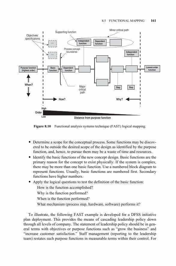
� Determine a scope for the conceptual process. Some functions may be discov-ered to be outside the desired scope of the design as identified by the purposefunction, and, hence, to pursue them may be a waste of time and resources.
� Identify the basic functions of the new concept design. Basic functions are theprimary reason for the concept to exist physically. If the system is complex,there may be more than one basic function. Use a numbered block diagram torepresent functions. Usually, basic functions are numbered first. Secondaryfunctions have higher numbers.
� Apply the logical questions to test the definition of the basic function:
How is the function accomplished?
Why is the function performed?
When is the function performed?
What mechanism (process step, hardware, software) performs it?
To illustrate, the following FAST example is developed for a DFSS initiativeplan deployment. This provides the means of cascading leadership policy downthrough all levels of company. The statement of leadership policy should be in gen-eral terms with objectives or purpose functions such as “grow the business” and“increase customer satisfaction.” Staff management (reporting to the leadershipteam) restates such purpose functions in measurable terms within their control. For
8.5 FUNCTIONAL MAPPING 161
Figure 8.10 Functional analysis systems technique (FAST) logical mapping.
Purpose function(highest order)
…..
…..
Basicfunction
Dependentfunction
Independentfunction
Dependentfunction
Objectives/specifications
Supporting function
Process conceptboundaries
Step Step
Independentfunction
Minor critical path
Major critical path
Lowest-order function
How? Why?
When?
Distance from purpose function
OrderHigh
Low
c08.qxd 4/22/2005 9:04 AM Page 161
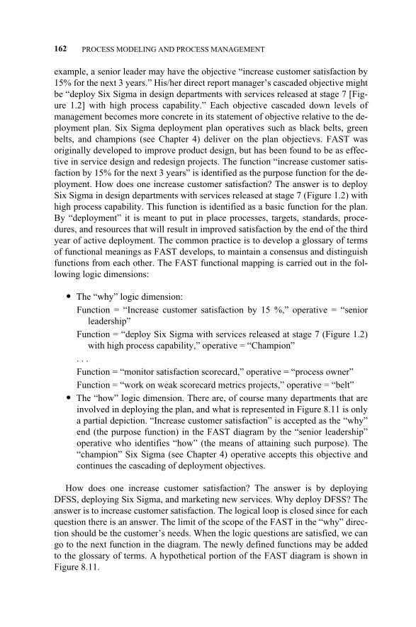
example, a senior leader may have the objective “increase customer satisfaction by15% for the next 3 years.” His/her direct report manager’s cascaded objective mightbe “deploy Six Sigma in design departments with services released at stage 7 [Fig-ure 1.2] with high process capability.” Each objective cascaded down levels ofmanagement becomes more concrete in its statement of objective relative to the de-ployment plan. Six Sigma deployment plan operatives such as black belts, greenbelts, and champions (see Chapter 4) deliver on the plan objectievs. FAST wasoriginally developed to improve product design, but has been found to be as effec-tive in service design and redesign projects. The function “increase customer satis-faction by 15% for the next 3 years” is identified as the purpose function for the de-ployment. How does one increase customer satisfaction? The answer is to deploySix Sigma in design departments with services released at stage 7 (Figure 1.2) withhigh process capability. This function is identified as a basic function for the plan.By “deployment” it is meant to put in place processes, targets, standards, proce-dures, and resources that will result in improved satisfaction by the end of the thirdyear of active deployment. The common practice is to develop a glossary of termsof functional meanings as FAST develops, to maintain a consensus and distinguishfunctions from each other. The FAST functional mapping is carried out in the fol-lowing logic dimensions:
� The “why” logic dimension:
Function = “Increase customer satisfaction by 15 %,” operative = “seniorleadership”
Function = “deploy Six Sigma with services released at stage 7 (Figure 1.2)with high process capability,” operative = “Champion”
. . .
Function = “monitor satisfaction scorecard,” operative = “process owner”
Function = “work on weak scorecard metrics projects,” operative = “belt”
� The “how” logic dimension. There are, of course many departments that areinvolved in deploying the plan, and what is represented in Figure 8.11 is onlya partial depiction. “Increase customer satisfaction” is accepted as the “why”end (the purpose function) in the FAST diagram by the “senior leadership”operative who identifies “how” (the means of attaining such purpose). The“champion” Six Sigma (see Chapter 4) operative accepts this objective andcontinues the cascading of deployment objectives.
How does one increase customer satisfaction? The answer is by deployingDFSS, deploying Six Sigma, and marketing new services. Why deploy DFSS? Theanswer is to increase customer satisfaction. The logical loop is closed since for eachquestion there is an answer. The limit of the scope of the FAST in the “why” direc-tion should be the customer’s needs. When the logic questions are satisfied, we cango to the next function in the diagram. The newly defined functions may be addedto the glossary of terms. A hypothetical portion of the FAST diagram is shown inFigure 8.11.
162 PROCESS MODELING AND PROCESS MANAGEMENT
c08.qxd 4/22/2005 9:04 AM Page 162
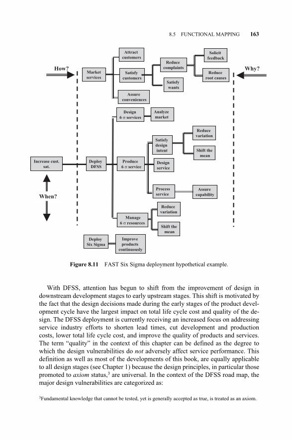
With DFSS, attention has begun to shift from the improvement of design indownstream development stages to early upstream stages. This shift is motivated bythe fact that the design decisions made during the early stages of the product devel-opment cycle have the largest impact on total life cycle cost and quality of the de-sign. The DFSS deployment is currently receiving an increased focus on addressingservice industry efforts to shorten lead times, cut development and productioncosts, lower total life cycle cost, and improve the quality of products and services.The term “quality” in the context of this chapter can be defined as the degree towhich the design vulnerabilities do not adversely affect service performance. Thisdefinition as well as most of the developments of this book, are equally applicableto all design stages (see Chapter 1) because the design principles, in particular thosepromoted to axiom status,3 are universal. In the context of the DFSS road map, themajor design vulnerabilities are categorized as:
8.5 FUNCTIONAL MAPPING 163
Figure 8.11 FAST Six Sigma deployment hypothetical example.
Increase cust.
sat.
Deploy
DFSS
Produce
6 σ service
Analyze
market
Process
service
Satisfy
design
intent Shift the
mean
Reduce
variation
How? Why?
When?
Design
6 σ services
Design
service
Assure
capability
Shift the
mean
Reduce
variation
Deploy
Six Sigma
Improve
products
continuously
Market
servicesSatisfy
customers
Attract
customers
Assure
conveniences
Satisfy
wants
Reduce
complaints
Reduce
root causes
Solicit
feedback
Manage
6 σ resources
3Fundamental knowledge that cannot be tested, yet is generally accepted as true, is treated as an axiom.
c08.qxd 4/22/2005 9:04 AM Page 163
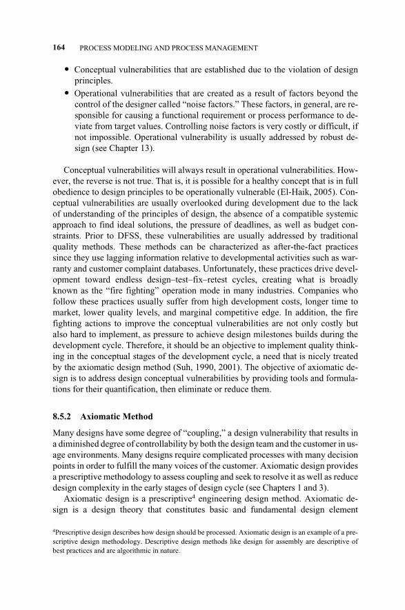
� Conceptual vulnerabilities that are established due to the violation of designprinciples.
� Operational vulnerabilities that are created as a result of factors beyond thecontrol of the designer called “noise factors.” These factors, in general, are re-sponsible for causing a functional requirement or process performance to de-viate from target values. Controlling noise factors is very costly or difficult, ifnot impossible. Operational vulnerability is usually addressed by robust de-sign (see Chapter 13).
Conceptual vulnerabilities will always result in operational vulnerabilities. How-ever, the reverse is not true. That is, it is possible for a healthy concept that is in fullobedience to design principles to be operationally vulnerable (El-Haik, 2005). Con-ceptual vulnerabilities are usually overlooked during development due to the lackof understanding of the principles of design, the absence of a compatible systemicapproach to find ideal solutions, the pressure of deadlines, as well as budget con-straints. Prior to DFSS, these vulnerabilities are usually addressed by traditionalquality methods. These methods can be characterized as after-the-fact practicessince they use lagging information relative to developmental activities such as war-ranty and customer complaint databases. Unfortunately, these practices drive devel-opment toward endless design–test–fix–retest cycles, creating what is broadlyknown as the “fire fighting” operation mode in many industries. Companies whofollow these practices usually suffer from high development costs, longer time tomarket, lower quality levels, and marginal competitive edge. In addition, the firefighting actions to improve the conceptual vulnerabilities are not only costly butalso hard to implement, as pressure to achieve design milestones builds during thedevelopment cycle. Therefore, it should be an objective to implement quality think-ing in the conceptual stages of the development cycle, a need that is nicely treatedby the axiomatic design method (Suh, 1990, 2001). The objective of axiomatic de-sign is to address design conceptual vulnerabilities by providing tools and formula-tions for their quantification, then eliminate or reduce them.
8.5.2 Axiomatic Method
Many designs have some degree of “coupling,” a design vulnerability that results ina diminished degree of controllability by both the design team and the customer in us-age environments. Many designs require complicated processes with many decisionpoints in order to fulfill the many voices of the customer. Axiomatic design providesa prescriptive methodology to assess coupling and seek to resolve it as well as reducedesign complexity in the early stages of design cycle (see Chapters 1 and 3).
Axiomatic design is a prescriptive4 engineering design method. Axiomatic de-sign is a design theory that constitutes basic and fundamental design element
164 PROCESS MODELING AND PROCESS MANAGEMENT
4Prescriptive design describes how design should be processed. Axiomatic design is an example of a pre-scriptive design methodology. Descriptive design methods like design for assembly are descriptive ofbest practices and are algorithmic in nature.
c08.qxd 4/22/2005 9:04 AM Page 164
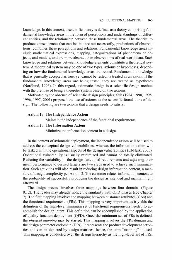
knowledge. In this context, a scientific theory is defined as a theory comprising fun-damental knowledge areas in the form of perceptions and understandings of differ-ent entities, and the relationship between these fundamental areas. The theorist, toproduce consequences that can be, but are not necessarily, predictions of observa-tions, combines these perceptions and relations. Fundamental knowledge areas in-clude mathematical expressions, mapping, categorizations of phenomena or ob-jects, and models, and are more abstract than observations of real-world data. Suchknowledge and relations between knowledge elements constitute a theoretical sys-tem. A theoretical system may be one of two types, axioms or hypotheses, depend-ing on how the fundamental knowledge areas are treated. Fundamental knowledgethat is generally accepted as true, yet cannot be tested, is treated as an axiom. If thefundamental knowledge areas are being tested, they are treated as hypotheses(Nordlund, 1996). In this regard, axiomatic design is a scientific design methodwith the premise of being a theoretic system based on two axioms.
Motivated by the absence of scientific design principles, Suh (1984, 1990, 1995,1996, 1997, 2001) proposed the use of axioms as the scientific foundations of de-sign. The following are two axioms that a design needs to satisfy:
Axiom 1: The Independence Axiom
Maintain the independence of the functional requirements
Axiom 2: The Information Axiom
Minimize the information content in a design
In the context of axiomatic deployment, the independence axiom will be used toaddress the conceptual design vulnerabilities, whereas the information axiom willbe tasked with the operational aspects of the design vulnerabilities (El-Haik, 2005).Operational vulnerability is usually minimized and cannot be totally eliminated.Reducing the variability of the design functional requirements and adjusting theirmean performance to desired targets are two steps used to achieve such minimiza-tion. Such activities will also result in reducing design information content, a mea-sure of design complexity per Axiom 2. The customer relates information content tothe probability of successfully producing the design as intended and maintaining itafterward.
The design process involves three mappings between four domains (Figure8.12). The reader may already notice the similarity with QFD phases (see Chapter7). The first mapping involves the mapping between customer attributes (CAs) andthe functional requirements (FRs). This mapping is very important as it yields thedefinition of the high-level minimum set of functional requirements needed to ac-complish the design intent. This definition can be accomplished by the applicationof quality function deployment (QFD). Once the minimum set of FRs is defined,the physical mapping may be started. This mapping involves the FRs domain andthe design parameter codomain (DPs). It represents the product development activi-ties and can be depicted by design matrices; hence, the term “mapping” is used.This mapping is conducted over the design hierarchy as the high-level set of FRs,
8.5 FUNCTIONAL MAPPING 165
c08.qxd 4/22/2005 9:04 AM Page 165
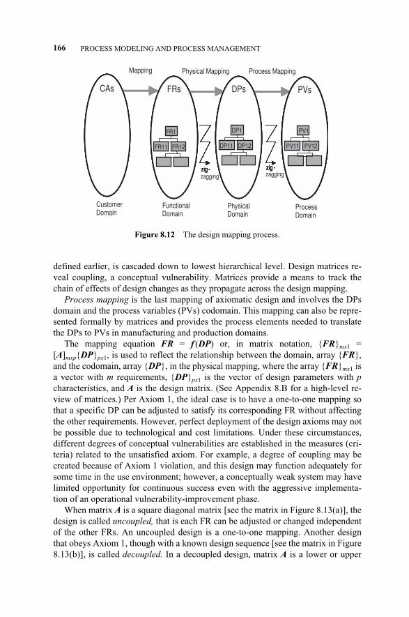
defined earlier, is cascaded down to lowest hierarchical level. Design matrices re-veal coupling, a conceptual vulnerability. Matrices provide a means to track thechain of effects of design changes as they propagate across the design mapping.
Process mapping is the last mapping of axiomatic design and involves the DPsdomain and the process variables (PVs) codomain. This mapping can also be repre-sented formally by matrices and provides the process elements needed to translatethe DPs to PVs in manufacturing and production domains.
The mapping equation FR = f (DP) or, in matrix notation, {FR}mx1 =[A]mxp{DP}px1, is used to reflect the relationship between the domain, array {FR},and the codomain, array {DP}, in the physical mapping, where the array {FR}mx1 isa vector with m requirements, {DP}px1 is the vector of design parameters with pcharacteristics, and A is the design matrix. (See Appendix 8.B for a high-level re-view of matrices.) Per Axiom 1, the ideal case is to have a one-to-one mapping sothat a specific DP can be adjusted to satisfy its corresponding FR without affectingthe other requirements. However, perfect deployment of the design axioms may notbe possible due to technological and cost limitations. Under these circumstances,different degrees of conceptual vulnerabilities are established in the measures (cri-teria) related to the unsatisfied axiom. For example, a degree of coupling may becreated because of Axiom 1 violation, and this design may function adequately forsome time in the use environment; however, a conceptually weak system may havelimited opportunity for continuous success even with the aggressive implementa-tion of an operational vulnerability-improvement phase.
When matrix A is a square diagonal matrix [see the matrix in Figure 8.13(a)], thedesign is called uncoupled, that is each FR can be adjusted or changed independentof the other FRs. An uncoupled design is a one-to-one mapping. Another designthat obeys Axiom 1, though with a known design sequence [see the matrix in Figure8.13(b)], is called decoupled. In a decoupled design, matrix A is a lower or upper
166 PROCESS MODELING AND PROCESS MANAGEMENT
Figure 8.12 The design mapping process.
CAs FRs
FR1
FR11 FR12
DPs
DP1
DP11 DP12
PVs
PV1
PV11 PV12
zig - zig -
CAs FRs
FR1
FR11 FR12
FR1
FR11 FR12
DPs
DP1
DP11 DP12
DP1
DP11 DP12
PVs
PV1
PV11 PV12
PVs
PV1
PV11 PV12
PV1
PV11 PV12
zig - zig -
CAs FRs
FR1
FR11 FR12
FR1
FR11 FR12
DPs
DP1
DP11 DP12
DP1
DP11 DP12
PVs
PV1
PV11 PV12
PVs
PV1
PV11 PV12
PV1
PV11 PV12
CAs FRs
FR1
FR11 FR12
FR1
FR11 FR12
DPs
DP1
DP11 DP12
DP1
DP11 DP12
PVs
PV1
PV11 PV12
PVs
PV1
PV11 PV12
PV1
PV11 PV12
zig - zig -
CAs FRs
FR1
FR11 FR12
FR1
FR11 FR12
DPs
DP1
DP11 DP12
DP1
DP11 DP12
PVs
PV1
PV11 PV12
PV1
PV11 PV12
PVs
PV1
PV11 PV12
PV1
PV11 PV12
Physical Mapping Process Mapping
zig -zagging
zig -zagging
ProcessDomain
CAs FRs
FR1
FR11 FR12
DPs
DP1
DP11 DP12
PVs
PV1
PV11 PV12
PV1
PV11 PV12
PVs
PV1
PV11 PV12
Mapping
PhysicalDomain
FunctionalDomain
CustomerDomain
c08.qxd 4/22/2005 9:04 AM Page 166
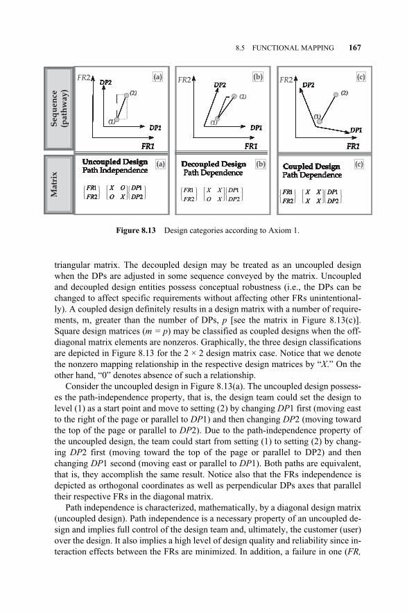
triangular matrix. The decoupled design may be treated as an uncoupled designwhen the DPs are adjusted in some sequence conveyed by the matrix. Uncoupledand decoupled design entities possess conceptual robustness (i.e., the DPs can bechanged to affect specific requirements without affecting other FRs unintentional-ly). A coupled design definitely results in a design matrix with a number of require-ments, m, greater than the number of DPs, p [see the matrix in Figure 8.13(c)].Square design matrices (m = p) may be classified as coupled designs when the off-diagonal matrix elements are nonzeros. Graphically, the three design classificationsare depicted in Figure 8.13 for the 2 × 2 design matrix case. Notice that we denotethe nonzero mapping relationship in the respective design matrices by “X.” On theother hand, “0” denotes absence of such a relationship.
Consider the uncoupled design in Figure 8.13(a). The uncoupled design possess-es the path-independence property, that is, the design team could set the design tolevel (1) as a start point and move to setting (2) by changing DP1 first (moving eastto the right of the page or parallel to DP1) and then changing DP2 (moving towardthe top of the page or parallel to DP2). Due to the path-independence property ofthe uncoupled design, the team could start from setting (1) to setting (2) by chang-ing DP2 first (moving toward the top of the page or parallel to DP2) and thenchanging DP1 second (moving east or parallel to DP1). Both paths are equivalent,that is, they accomplish the same result. Notice also that the FRs independence isdepicted as orthogonal coordinates as well as perpendicular DPs axes that paralleltheir respective FRs in the diagonal matrix.
Path independence is characterized, mathematically, by a diagonal design matrix(uncoupled design). Path independence is a necessary property of an uncoupled de-sign and implies full control of the design team and, ultimately, the customer (user)over the design. It also implies a high level of design quality and reliability since in-teraction effects between the FRs are minimized. In addition, a failure in one (FR,
8.5 FUNCTIONAL MAPPING 167
Figure 8.13 Design categories according to Axiom 1.
FR1
DP1
DP2
Uncoupled DesignPath Independence
FR1
DP1
DP2
FR1
DP1
DP2
(1)
Uncoupled DesignPath Independence
FR1
DP1
DP2
Uncoupled DesignPath Independence
2
1
2
1
DP
DP
XO
OX
FR
FR
(2)
FR1
DP1
DP2
Uncoupled DesignPath Independence
FR1
DP1
DP2
FR1
DP1
DP2
(1)
Uncoupled DesignPath Independence
FR1
DP1
DP2
Uncoupled DesignPath Independence
2
1
2
1
DP
DP
XO
OX
FR
FR
(2)
FR1
DP1
DP2
Coupled DesignPath Dependence
FR1
DP1
DP2
FR1
DP1
DP2
Coupled DesignPath Dependence
FR1
DP1
DP2
Coupled DesignPath Dependence
2
1
2
1
DP
DP
XX
XX
FR
FR
(1)
(2)
FR1
DP1
DP2
Coupled DesignPath Dependence
FR1
DP1
DP2
FR1
DP1
DP2
Coupled DesignPath Dependence
FR1
DP1
DP2
Coupled DesignPath Dependence
2
1
2
1
DP
DP
XX
XX
FR
FR
(1)
(2)
(c)
FR1
DP1
DP2
Decoupled DesignPath Dependence
FR1
DP1
DP2
FR1
DP1
DP2
Decoupled DesignPath Dependence
FR1
DP1
DP2
Decoupled DesignPath Dependence
2
1
2
1
DP
DP
XO
XX
FR
FR
(1)
(2)
(b)
FR1
DP1
DP2
Decoupled DesignPath Dependence
FR1
DP1
DP2
Matr
ixS
eq
ue
nce
(pa
thw
ay
)
(a)
(a)
(b) (c)
FR1
DP1
DP2
Uncoupled DesignPath Independence
FR1
DP1
DP2
FR1
DP1
DP2
(1)
Uncoupled DesignPath Independence
FR1
DP1
DP2
Uncoupled DesignPath Independence
2
1
2
1
DP
DP
XO
OX
FR
FR
(2)
FR1
DP1
DP2
Uncoupled DesignPath Independence
FR1
FR2
DP1
DP2
FR1
DP1
DP2
(1)
Uncoupled DesignPath Independence
FR1
DP1
DP2
Uncoupled DesignPath Independence
2
1
2
1
DP
DP
XO
OX
FR
FR
(2)
FR1
DP1
DP2
Coupled DesignPath Dependence
FR1
DP1
DP2
FR1
DP1
DP2
Coupled DesignPath Dependence
FR1
DP1
DP2
Coupled DesignPath Dependence
�2
1
2
1
DP
DP
XX
XX
FR
FR
(1)
(2)
FR1
FR2
DP1
DP2
Coupled DesignPath Dependence
FR1
DP1
DP2
FR1
DP1
DP2
Coupled DesignPath Dependence
FR1
DP1
DP2
Coupled DesignPath Dependence
2
1
2
1
DP
DP
XX
XX
FR
FR
(1)
(2)
(c)
FR1
DP1
DP2
Decoupled DesignPath Dependence
FR1
DP1
DP2
FR1
DP1
DP2
Decoupled DesignPath Dependence
FR1
DP1
DP2
Decoupled DesignPath Dependence
2
1
2
1
DP
DP
XO
XX
FR
FR
(1)
(2)
(b)
FR1
FR2
DP1
DP2
Decoupled DesignPath Dependence
FR1
DP1
DP2
Matr
ixS
eq
ue
nce
(pa
thw
ay
)
(a)
(a)
(b) (c)
�� ���� �� ���� �� ���
c08.qxd 4/22/2005 9:04 AM Page 167
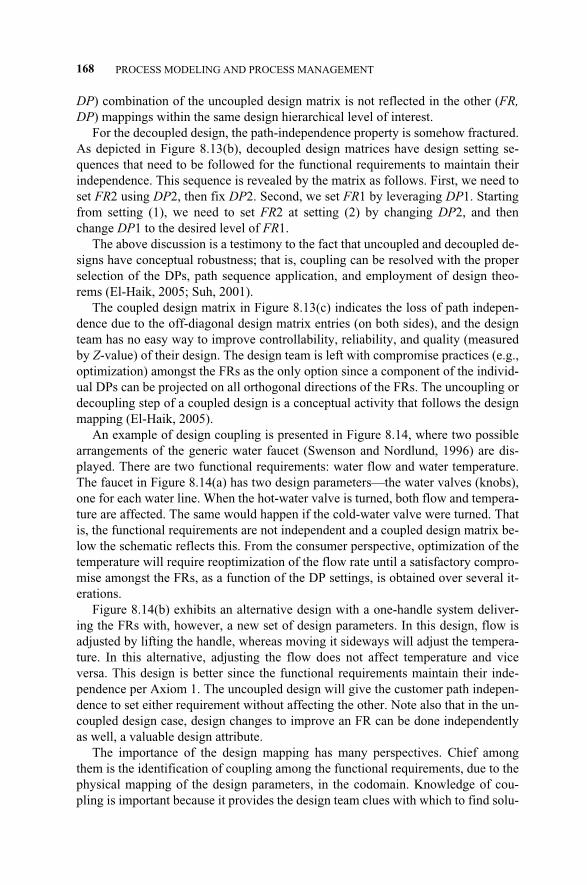
DP) combination of the uncoupled design matrix is not reflected in the other (FR,DP) mappings within the same design hierarchical level of interest.
For the decoupled design, the path-independence property is somehow fractured.As depicted in Figure 8.13(b), decoupled design matrices have design setting se-quences that need to be followed for the functional requirements to maintain theirindependence. This sequence is revealed by the matrix as follows. First, we need toset FR2 using DP2, then fix DP2. Second, we set FR1 by leveraging DP1. Startingfrom setting (1), we need to set FR2 at setting (2) by changing DP2, and thenchange DP1 to the desired level of FR1.
The above discussion is a testimony to the fact that uncoupled and decoupled de-signs have conceptual robustness; that is, coupling can be resolved with the properselection of the DPs, path sequence application, and employment of design theo-rems (El-Haik, 2005; Suh, 2001).
The coupled design matrix in Figure 8.13(c) indicates the loss of path indepen-dence due to the off-diagonal design matrix entries (on both sides), and the designteam has no easy way to improve controllability, reliability, and quality (measuredby Z-value) of their design. The design team is left with compromise practices (e.g.,optimization) amongst the FRs as the only option since a component of the individ-ual DPs can be projected on all orthogonal directions of the FRs. The uncoupling ordecoupling step of a coupled design is a conceptual activity that follows the designmapping (El-Haik, 2005).
An example of design coupling is presented in Figure 8.14, where two possiblearrangements of the generic water faucet (Swenson and Nordlund, 1996) are dis-played. There are two functional requirements: water flow and water temperature.The faucet in Figure 8.14(a) has two design parameters—the water valves (knobs),one for each water line. When the hot-water valve is turned, both flow and tempera-ture are affected. The same would happen if the cold-water valve were turned. Thatis, the functional requirements are not independent and a coupled design matrix be-low the schematic reflects this. From the consumer perspective, optimization of thetemperature will require reoptimization of the flow rate until a satisfactory compro-mise amongst the FRs, as a function of the DP settings, is obtained over several it-erations.
Figure 8.14(b) exhibits an alternative design with a one-handle system deliver-ing the FRs with, however, a new set of design parameters. In this design, flow isadjusted by lifting the handle, whereas moving it sideways will adjust the tempera-ture. In this alternative, adjusting the flow does not affect temperature and viceversa. This design is better since the functional requirements maintain their inde-pendence per Axiom 1. The uncoupled design will give the customer path indepen-dence to set either requirement without affecting the other. Note also that in the un-coupled design case, design changes to improve an FR can be done independentlyas well, a valuable design attribute.
The importance of the design mapping has many perspectives. Chief amongthem is the identification of coupling among the functional requirements, due to thephysical mapping of the design parameters, in the codomain. Knowledge of cou-pling is important because it provides the design team clues with which to find solu-
168 PROCESS MODELING AND PROCESS MANAGEMENT
c08.qxd 4/22/2005 9:04 AM Page 168
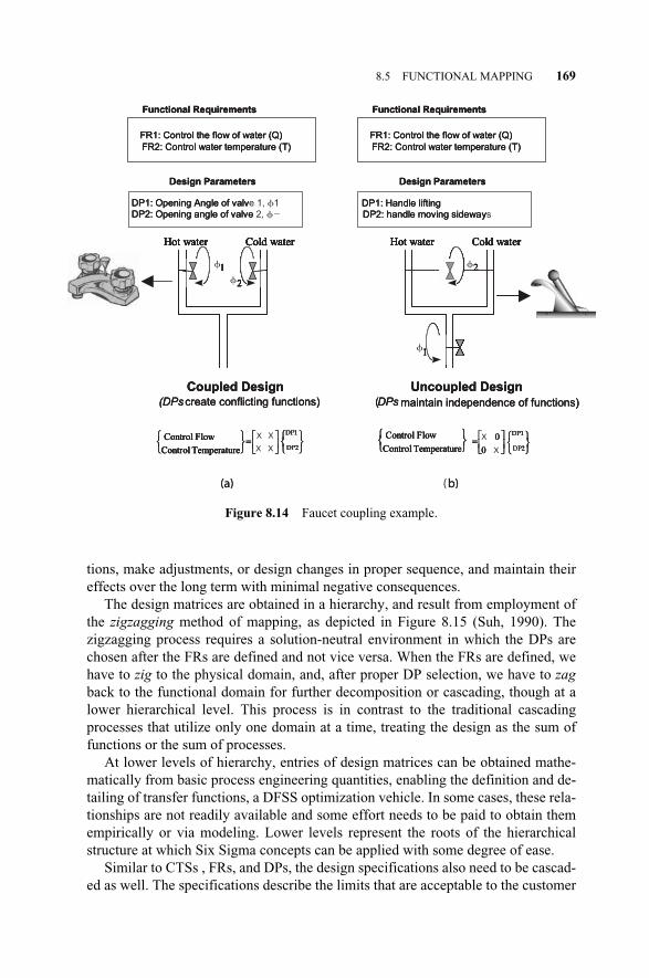
tions, make adjustments, or design changes in proper sequence, and maintain theireffects over the long term with minimal negative consequences.
The design matrices are obtained in a hierarchy, and result from employment ofthe zigzagging method of mapping, as depicted in Figure 8.15 (Suh, 1990). Thezigzagging process requires a solution-neutral environment in which the DPs arechosen after the FRs are defined and not vice versa. When the FRs are defined, wehave to zig to the physical domain, and, after proper DP selection, we have to zagback to the functional domain for further decomposition or cascading, though at alower hierarchical level. This process is in contrast to the traditional cascadingprocesses that utilize only one domain at a time, treating the design as the sum offunctions or the sum of processes.
At lower levels of hierarchy, entries of design matrices can be obtained mathe-matically from basic process engineering quantities, enabling the definition and de-tailing of transfer functions, a DFSS optimization vehicle. In some cases, these rela-tionships are not readily available and some effort needs to be paid to obtain themempirically or via modeling. Lower levels represent the roots of the hierarchicalstructure at which Six Sigma concepts can be applied with some degree of ease.
Similar to CTSs , FRs, and DPs, the design specifications also need to be cascad-ed as well. The specifications describe the limits that are acceptable to the customer
8.5 FUNCTIONAL MAPPING 169
Figure 8.14 Faucet coupling example.
Functional Requirements
2
1
Hot water Cold water
1
2
Hot water Cold water
Control Flow
Control Temperature
=
Coupled Design(DPscreate conflicting functions)
= X
0
0
Uncoupled Design(DPsmaintain independence of functions)
FR1: Control the flow of water (Q)
FR2: Control water temperature (T)
DP2: Opening angle of valve
DP1: Opening Angle of valv
Design Parameters
2
1
Hot water Cold water
1
2
Hot water Cold water
Control Flow
Control Temperature
Functional Requirements
FR1: Control the flow of water (Q)
FR2: Control water temperature (T)
DP2: handle moving sideway
DP1: Handle lifting
Design Parameters
DP1
DP2
DP1
DP2
(a) b)
Functional Requirements
2
1
Hot water Cold water
1
2
Hot water Cold water
Control Flow
Control Temperature
=
Coupled Design(DPscreate conflicting functions)
=
0
0
Uncoupled Design(DPsmaintain independence of functions)
FR1: Control the flow of water (Q)
FR2: Control water temperature (T)
DP2: Opening angle of valve
DP1: Opening Angle of valv
Design Parameters
2
1
Hot water Cold water
1
2
Hot water Cold water
Control Flow
Control Temperature
Functional Requirements
FR1: Control the flow of water (Q)
FR2: Control water temperature (T)
DP2: handle moving sideway
DP1: Handle lifting
Design Parameters
DP1
DP2
DP1
DP2
Functional Requirements
2
1
Hot water Cold water
1
2
Hot water Cold water
Control Flow
Control Temperature
Control Flow
Control Temperature
=
Coupled Design(DPscreate conflicting functions)
=
0
0
Uncoupled Design(DPsmaintain independence of functions)
FR1: Control the flow of water (Q)
FR2: Control water temperature (T)
DP2: Opening angle of valve 2, ��DP1: Opening Angle of valve 1, �1
Design Parameters
2
�1
Hot water Cold water
1
2
Hot water Cold water
Control Flow
Control Temperature
Control Flow
Control Temperature
Functional Requirements
FR1: Control the flow of water (Q)
FR2: Control water temperature (T)
DP2: handle moving sideways
DP1: Handle lifting
Design Parameters
DP1
DP2
DP1
DP2
DP1
DP2
DP1
DP2
(a) (b)
� �
�
X
X X
X X
c08.qxd 4/22/2005 9:04 AM Page 169
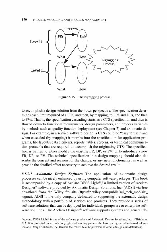
to accomplish a design solution from their own perspective. The specification deter-mines each limit required of a CTS and then, by mapping, to FRs and DPs, and thento PVs. That is, the specification cascading starts as a CTS specification and then isflowed down to functional requirements, design parameters, and process variablesby methods such as quality function deployment (see Chapter 7) and axiomatic de-sign. For example, in a service software design, a CTS could be “easy to use,” andwhen cascaded (by mapping) it morphs into the specification for application pro-grams, file layouts, data elements, reports, tables, screens, or technical communica-tion protocols that are required to accomplish the originating CTS. The specifica-tion is written to either modify the existing FR, DP, or PV, or to introduce a newFR, DP, or PV. The technical specification in a design mapping should also de-scribe the concept and reasons for the change, or any new functionality, as well asprovide the detailed effort necessary to achieve the desired result.
8.5.2.1 Axiomatic Design Software. The application of axiomatic designprocesses can be nicely enhanced by using computer software packages. This bookis accompanied by a copy of Acclaro DFSS Light®,5 a limited version of AcclaroDesigner® software provided by Axiomatic Design Solutions, Inc. (ADSI) via freedownload from the Wiley ftp site (ftp://ftp.wiley.com/public/sci_tech_med/six_sigma). ADSI is the only company dedicated to supporting the axiomatic designmethodology with a portfolio of services and products. They provide a series ofsoftware solutions that can be deployed for individual, groupware or enterprise soft-ware solutions. The Acclaro Designer® software supports systems and general de-
170 PROCESS MODELING AND PROCESS MANAGEMENT
Figure 8.15 The zigzagging process.
.FRs
.
.
What
.
.
.
How
.
.
.
What
.
.
.
How
ZigzaggingProcess
DPs
Level 1
Level 1.1
.FRs
.
.
What
.
.
.
How
.
.
.
What
.
.
.
How
Zigzagging
DPs
Level 1
Level 1.1
.FRs
.
.
What
.
.
.
How
.
.
.
What
.
.
.
How
ZigzaggingProcess
DPs
Level 1
Level 1.1
.FRs
.
.
What
.
.
.
How
mapping
.
.
.
What
.
.
.
How
Zigzagging
DPs
Level 1
Level 1.1
5Acclaro DFSS Light® is one of the software products of Axiomatic Design Solutions, Inc. of Brighton,MA. It is protected under both copyright and pending patents. Acclaro is a registered trademark of Ax-iomatic Design Solutions, Inc. Browse their website at http://www.axiomaticdesign.com/default.asp.
c08.qxd 4/22/2005 9:04 AM Page 170
sign problems. The Acclaro Scheduler® software supports software design opti-mization working with IBM’s Rational Rose software development toolsets. TheAcclaro Sync® software is a package that runs with Microsoft Project, permittingthe effective project scheduling and synchronization of design projects usingAcclaro Designer® and Acclaro Scheduler®.
Acclaro DFSS Light® is a JAVA-based software package that implements ax-iomatic design processes. It is about a 30 megabyte download installation file. It re-quires Windows 95, 2000, NT, XP, or later revisions with 256K of memory.Acclaro® software suite was Industry Week’s Technology of the Year and a winnerof the International Institution for Production Research (CIRP) award.
Acclaro DFSS Light® enables the design team to meet the following needs inmanaging the DFSS ICOV process:
� Creates a process for requirements cascading (hierarchy) and analysis by im-plement zigzagging and decomposition trees to capture and track design logic.
� Permits design teams to collaborate at the earliest possible time with visualiza-tion and graphical representations. Geographically supports separate teams.
� Introduces a systematic process for design synthesis before document–build–test cycles.
� Analyzes design quality before committing to any cost by applying axioms.
� Enables design team to completely track the process from customer needs torequirements to design mappings to final designs.
� Visualizes and quantifies impact assessments when requirements change.
� Provides features to capture and track the design and development processeschanges and instantly assess the ripple effect through the design. It is alsoequipped with model flow diagrams, providing capability to understand opti-mal design task sequencing.
� Keeps a running list of changes to the design at FR, DP, PV, or CN levels.
� Contains features to plan, estimate, and control conceptual design with cou-pling analysis to identify suboptimal designs with single- and full-level de-sign matrix dependency analysis.
8.5.2.2 Axiomatic Design Mapping Example. Here we examine an implementa-tion methodology for transition from traditional manufacturing to cellular manufac-turing using axiomatic design (Bulent et al., 2002; El-Haik, 2005). In this casestudy, a framework to transform a traditional production system from process orien-tation to cellular orientation based on axiomatic design principles is introduced. Afeedback mechanism for continuous improvement is also suggested for evaluatingand improving the cellular design against preselected performance criteria (see Fig-ure 8.16). The criteria, which are developed based on the independence axiom, pro-vide the necessary steps in transforming an existing process-oriented system into acellular manufacturing system.
Transition to cellular manufacturing follows after all cellular manufacturing
8.5 FUNCTIONAL MAPPING 171
c08.qxd 4/22/2005 9:04 AM Page 171
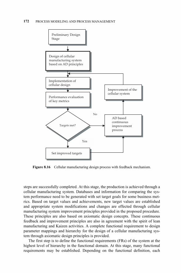
steps are successfully completed. At this stage, the production is achieved through acellular manufacturing system. Databases and information for comparing the sys-tem performance need to be generated with set target goals for some business met-rics. Based on target values and achievements, new target values are establishedand appropriate system modifications and changes are effected through cellularmanufacturing system improvement principles provided in the proposed procedure.These principles are also based on axiomatic design concepts. These continuousfeedback and improvement principles are also in agreement with the spirit of leanmanufacturing and Kaizen activities. A complete functional requirement to designparameter mappings and hierarchy for the design of a cellular manufacturing sys-tem through axiomatic design principles is provided.
The first step is to define the functional requirements (FRs) of the system at thehighest level of hierarchy in the functional domain. At this stage, many functionalrequirements may be established. Depending on the functional definition, each
172 PROCESS MODELING AND PROCESS MANAGEMENT
Figure 8.16 Cellular manufacturing design process with feedback mechanism.
Design of cellular manufacturing system based on AD principles
Design of cellular manufacturing system based on AD principles
Implementation of cellular design
Implementation of cellular design
Performance evaluation of key metrics
Performance evaluation of key metrics
Targets met?
AD based continuous improvement process
AD based continuous improvement process
Improvement of the cellular system
Improvement of the cellular system
Set improved targetsSet improved targets
No
Yes
Preliminary Design Stage
Preliminary Design Stage
Design of cellular manufacturing system based on AD principles
Design of cellular manufacturing system based on AD principles
Implementation of cellular design
Implementation of cellular design
Performance evaluation of key metrics
Performance evaluation of key metrics
Targets met?
AD based continuous improvement process
AD based continuous improvement process
Improvement of the cellular system
Improvement of the cellular system
Set improved targetsSet improved targets
No
Yes
Preliminary Design Stage
Preliminary Design Stage
c08.qxd 4/22/2005 9:04 AM Page 172
functional requirement established at this stage may lead to a completely differentcellular manufacturing design. The authors have selected the following as the high-est functional requirements:
Hierarchical Level 1 Analysis
FR = Provide flexible production in line with customer needs
Customer needs are summarized as more product variety, smaller batch sizes withhigher quality, and more frequent deliveries at lower costs. These requirements areforcing companies to reevaluate their classical production systems to obtain moreflexibility in response to these customer needs. The flexibility of a production sys-tem is measured by its speed and agility to respond to rapidly changing customerneeds.
In step 2, the mapping to the design parameters domain is accomplished usingthe zigzagging approach. At this step, design parameters (DPs), which satisfy theFRs established in the previous step, are defined by zigging. In order to make thecorrect DP selection, the DPs corresponding to the FRs established before must beexhaustively generated. The following DP has been selected to satisfy the FR pro-vided above:
DP = Cellular production system design
The production system, which can meet customer’s needs in an efficient waythrough elimination of waste, reduction of lead time, and improved quality, is a cel-lular production system designed with lean principles in mind.
Hierarchical Level 2 Analysis. In step 3, the zigzagging process is continued forfurther hierarchical level prescription of the design and to obtain further clarifica-tion. If the DPs proposed for satisfying the FRs defined earlier cannot be imple-mented without further clarification, the axiomatic design principles recommend re-turning to the functional domain (in a zagging step) for decomposing the FRs intotheir lower functional requirement set as follows:
FR1 = Classify and group products/components for simple material flow
FR2 = Define production strategy based on product specifications
FR3 = Rearrange resources to minimize waste
FR4 = Provide means to control production based on customer demand
In step 4, we need to find the corresponding DPs by mapping FRs in the physicaldomain (a zigging step). In satisfying the four FRs defined above, we move to thephysical domain from the functional domain (a zigging step) and obtain:
DP1 = Procedure for defining product families
DP2 = Procedure for selecting production strategy
8.5 FUNCTIONAL MAPPING 173
c08.qxd 4/22/2005 9:04 AM Page 173
DP3 = Product oriented layout
DP4 = Pull production control system
The next logical step (step 5) is to determine the design matrix (DM), which pro-vides the relationships between the FR and DP mapping elements. It is critical to in-sure that the DM, as established, satisfies the independence axiom. The DM is
� � = � �� � (8.1)
A quick look reveals that the design is decoupled and, thus, satisfies Axiom 1. Inthe DM above, X represents a strong relationship between the correspondingFR–DP pair. The 0 indicates the absence of such relationship.
Hierarchical Level 3 Analysis. In step 6, the zigzagging process continues withFR1, FR2, FR3, and FR4 by going from the physical to the functional domain againand determining the corresponding DPs.
Step 6a. FR1—Products/Components Branch. The functional requirement FR1as defined above may be broken down with DP1 (procedure for defining productfamilies) in mind as:
FR11 = Determine high-volume products/components to be grouped
FR12 = Determine operations and machine types for producing each productfamily
FR13 = Form product families
FR14 = Determine final number of machine groups
The corresponding DPs may be stated as:
DP11 = Product–quantity Pareto analysis
DP12 = Machine–component incidence matrix
DP13 = Product grouping techniques
DP14 = Cost analysis and economic justification techniques
In this step, product families that will be economically manufactured throughcellular manufacturing and their corresponding machine groups are determined byusing Pareto analysis, followed by product family assignment techniques. The DMfor the above vectors of FRs and DPs is
� � = � �� � (8.2)
DP11DP12DP13DP14
000X
00XX
0XXX
XX00
FR11FR12FR13FR14
DP1DP2DP3DP4
000X
00XX
0XXX
XXXX
FR1FR2FR3FR4
174 PROCESS MODELING AND PROCESS MANAGEMENT
c08.qxd 4/22/2005 9:04 AM Page 174
Once again, this is a decoupled design satisfying the independence axiom.Step 6b. FR2—Production Strategy Branch. The functional requirement FR2 as
defined above (define production strategy based on product specifications) may bedecomposed with DP2 (procedure for selecting production strategy) in mind as:
FR21 = Determine the master process
FR22 = Select most appropriate process elements
FR23 = Determine required training/education needs
FR24 = Motivate labor participation
The corresponding DPs may be stated as:
DP21 = Master Process selection
DP22 = Production resources selection procedure
DP23 = Multipurpose labor training programs
DP24 = Profit sharing program
At this stage, production resources are determined following the establishmentof the master process based on product specifications. Once the resource selectionis complete, the education and training requirements of the workers can be estab-lished. For ensuring the full participation of workers, appropriate profit sharing pro-grams must be established and announced to the workers to seek their dedicationand involvement. The design-decoupled DM for this requirement is
� � = � �� � (8.3)
Step 6c. FR3—Resource Rearrangement Branch. The functional requirementFR3 as defined above as “rearrange resources to minimize waste” may be brokendown with DP3, defined as “product-oriented layout,” in mind as:
FR31 = Minimize material handling
FR32 = Eliminate wasted motion of operators
FR33 = Minimize waste due to imbalance in the system
The corresponding DPs may be stated as:
DP31 = Material-flow-oriented layout
DP32 = Arrangement of stations to facilitate operator tasks
DP33 = Balanced resources in response to Takt time (Takt time = available time/demand)
DP21DP22DP23DP24
000X
00XX
0XXX
XX00
FR21FR22FR23FR24
8.5 FUNCTIONAL MAPPING 175
c08.qxd 4/22/2005 9:04 AM Page 175
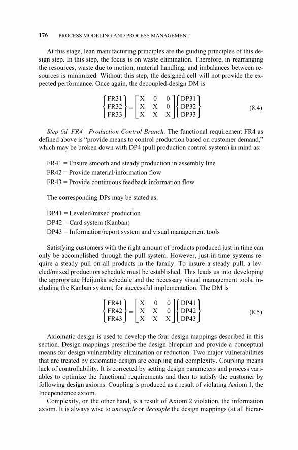
At this stage, lean manufacturing principles are the guiding principles of this de-sign step. In this step, the focus is on waste elimination. Therefore, in rearrangingthe resources, waste due to motion, material handling, and imbalances between re-sources is minimized. Without this step, the designed cell will not provide the ex-pected performance. Once again, the decoupled-design DM is
� � = � �� � (8.4)
Step 6d. FR4—Production Control Branch. The functional requirement FR4 asdefined above is “provide means to control production based on customer demand,”which may be broken down with DP4 (pull production control system) in mind as:
FR41 = Ensure smooth and steady production in assembly line
FR42 = Provide material/information flow
FR43 = Provide continuous feedback information flow
The corresponding DPs may be stated as:
DP41 = Leveled/mixed production
DP42 = Card system (Kanban)
DP43 = Information/report system and visual management tools
Satisfying customers with the right amount of products produced just in time canonly be accomplished through the pull system. However, just-in-time systems re-quire a steady pull on all products in the family. To insure a steady pull, a lev-eled/mixed production schedule must be established. This leads us into developingthe appropriate Heijunka schedule and the necessary visual management tools, in-cluding the Kanban system, for successful implementation. The DM is
� � = � �� � (8.5)
Axiomatic design is used to develop the four design mappings described in thissection. Design mappings prescribe the design blueprint and provide a conceptualmeans for design vulnerability elimination or reduction. Two major vulnerabilitiesthat are treated by axiomatic design are coupling and complexity. Coupling meanslack of controllability. It is corrected by setting design parameters and process vari-ables to optimize the functional requirements and then to satisfy the customer byfollowing design axioms. Coupling is produced as a result of violating Axiom 1, theIndependence axiom.
Complexity, on the other hand, is a result of Axiom 2 violation, the informationaxiom. It is always wise to uncouple or decouple the design mappings (at all hierar-
DP41DP42DP43
00X
0XX
XXX
FR41FR42FR43
DP31DP32DP33
00X
0XX
XXX
FR31FR32FR33
176 PROCESS MODELING AND PROCESS MANAGEMENT
c08.qxd 4/22/2005 9:04 AM Page 176
chical levels) before the DFSS team proceeds to the next stages of service develop-ment. The theory of inventive problem solving (TRIZ) provides a road map for cou-pling elimination or reduction by following certain principles such as Altshuler’strade-off or contradiction matrix (see Chapter 9). Complexity can be reduced byvariability reduction and means shifting of the functional requirements to deliverthe CTSs. This is the essence of DFSS optimization practices. Chapters 12 and 13are dedicated to such design treatments.
Axiomatic design can be used to design improvement and to select concepts ofconceptual robustness (in obedience to design axioms) while probing the necessarysequence of design development within a prescribed design hierarchy. It can bemorphed to a tool to assess technical risk and opportunities while complementingin-house current design best practices (El-Haik, 2005). As a conceptual approach, itprovides the team greater flexibility to conduct trade-offs (if–then scenarios) at anyhierarchical level by substituting different design parameters or process variables ina given mapping. In doing so, it highlights necessary organization communicationchannels amongst the different team satellite members, stakeholders, and the rest ofDFSS project core team.
8.6 PUGH CONCEPT SELECTION
The key mechanisms for selecting the best possible design or process solution is themethod of “controlled convergence,” which was developed by Stuart Pugh (Pugh,1991) as part of his concept selection process. Controlled convergence is a solution-iterative selection process that allows alternate convergent (analytic) and divergent(synthetic) thinking to be experienced by the team. The method alternates betweengeneration and selection activities (Figure 8.17). El-Haik and Yang (2003) suggest-ed the following enhancements to the controlled convergence method:
1. The “generation” activity can be enriched by the deployment of design Ax-iom 1 and its entire derived theoretical framework, which calls for functionalrequirements independence. This deployment will be further enhanced bymany TRIZ methodology concepts to resolve design vulnerabilities whereapplicable.
2. The “selection” activity can be enhanced by the deployment of Axiom 2,which calls for design simplicity.
The controlled convergence uses comparison of each alternative solution entityto a reference datum. Evaluation of a concept is more subjective than objective.However, the method discourages promotion of ideas based upon opinions and,thus, promotes objectivity. The controlled convergence method allows for elimina-tion of bad features and weak concepts and, thereby, facilitates the emergence ofnew concepts. It illuminates the best concept as the one most likely to meet the con-straints and requirements of the customer (CTSs) as expressed by the specification,and the one least vulnerable to immediate project competition.
8.6 PUGH CONCEPT SELECTION 177
c08.qxd 4/22/2005 9:04 AM Page 177

The development of the concepts through the combination of solution alterna-tives and functional requirement can be identified by a matrix called the morpho-logical or synthesis matrix. In this matrix, the functional requirements (FRs) arelisted in the rows and the solution alternatives (the design parameters and/orprocess variables) are laid down in the columns. At this point, process steps (sub-processes) are usually defined as the design parameters at a hierarchal level if thedesign mapping was conducted similar to the example in Subsection 8.5.2.1. How-ever, this knowledge is not detailed at this stage. The functional requirements needto be listed in the order of their hierarchy by the team, to the best of their knowledgeat this step, and should be grouped according to their type of DP/PV (proceduretype, policy type, training type, communication type, etc.).
The concepts are synthesized and generated from all possible feasible combina-tions of all possible design parameters (DPs) per functional requirement (FR) in thematrix. Connecting all possible solutions using arrows between the design parame-ters identifies a feasible design concept. The arrows can only be connected whenthe team is technically confident about the functional and production feasibility (El-Haik, 2003, 2005).
In conducting this exercise, the team will identify all possible feasible design so-lutions. In the next step, guided by their knowledge and the DFSS road map, theteam should concentrate only on promising solutions. The challenge here is to en-sure that the physical and functional compatibility and other constraints are met andthe appropriate flow of DPs such as procedures, policies, communication, and so onis properly identified. Normally, each functional requirement can be delivered byseveral possible DPs in a given hierarchical level within a concept. Therefore, thesynthesis matrix exercise should be conducted at all levels of design structure. The
178 PROCESS MODELING AND PROCESS MANAGEMENT
Figure 8.17 Controlled convergence method.
Concept Generation step
Controlled Convergence step ConceptSelected
Initial Concept Generation
initial number
reduced
new concepts added
further
reduction
further
addition
Concept Generation step
Controlled Convergence step ConceptSelected
c08.qxd 4/22/2005 9:04 AM Page 178

identification of all possible alternative solutions (DPs) per functional requirementmay be facilitated by the use of the morphological approaches of Zwicky (1984)and TRIZ methodology (see Chapter 9).
Several feasible high-level and undetailed concepts are usually generated usingthe synthesis matrix. This generation of multiple concepts poses a selection prob-lem. Which concept should be selected for further detailing in the DFSS roadmap?The DFSS team must select the best concept using the Pugh concept selectionmethod.6
In this step, the DFSS team produces the convergence to the best concept in iter-ative steps that are performed with DFSS discipline and rigor. The following se-quence may be used to facilitate the convergence to the best concept by the DFSSteam:
1. Develop a set of criteria based on the customer’s wants and needs, theCTSs. Determine CTS importance weights. Do not forget regulatory and le-gal requirements in design mapping. These criteria should be measurable,defined, and understood by all members of the team.
2. Develop a way to sketch concepts developed so far.
3. Choose a datum (baseline) with which all other concepts are to be com-pared. The datum could be an existing baseline, as in the case of redesignsituations. In new design situations, the datum could be any concept that theteam may generate from the synthesis matrix.
4. Develop a group of design concepts that are aimed at satisfying the CTSsand FRs.
5. Using a simple matrix, list the criteria from step 1 above on the left and theconcepts across the top. List concepts in the columns of the Pugh matrix asobtained from the synthesis matrix.
6. Compare the new concepts with the datum. Evaluate concepts versus the de-fined criteria. Use the traditional evaluation of plus (+), minus, or the same(s). The datum will be the neutral element(s) of the numbering system cho-sen. Comparing each solution entity against the datum, rate them either asplus (better than), minus (worse than), or same as the datum. (See Figure8.18 for a Pugh matrix of a European vacation.)
7. Identify the top best new concepts, having scored them relative to the datum,and sum the ranks across all criteria to get the scores. These scores must notbe treated as absolute as they are for guidance only and, as such, must not besummed algebraically. Certain concepts will exhibit relative strengths,whereas others will demonstrate relative weakness. Select the best conceptwith maximum number of pluses and the minimum number of minuses.
8. Make hybrids. Combine best concepts to make a new datum. Incorporatestrong ideas from other concepts. Perform trade-off studies to generate al-ternatives using design axioms and TRIZ. Look at the negatives. What isneeded in the design to reverse the negative (relative to the datum)? Will the
8.6 PUGH CONCEPT SELECTION 179
6The concept selection problem was formulated by El-Haik (2005) as an optimization problem.
c08.qxd 4/22/2005 9:04 AM Page 179
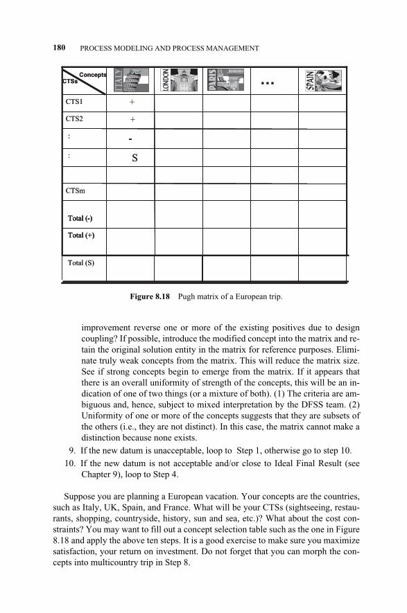
improvement reverse one or more of the existing positives due to designcoupling? If possible, introduce the modified concept into the matrix and re-tain the original solution entity in the matrix for reference purposes. Elimi-nate truly weak concepts from the matrix. This will reduce the matrix size.See if strong concepts begin to emerge from the matrix. If it appears thatthere is an overall uniformity of strength of the concepts, this will be an in-dication of one of two things (or a mixture of both). (1) The criteria are am-biguous and, hence, subject to mixed interpretation by the DFSS team. (2)Uniformity of one or more of the concepts suggests that they are subsets ofthe others (i.e., they are not distinct). In this case, the matrix cannot make adistinction because none exists.
9. If the new datum is unacceptable, loop to Step 1, otherwise go to step 10.
10. If the new datum is not acceptable and/or close to Ideal Final Result (seeChapter 9), loop to Step 4.
Suppose you are planning a European vacation. Your concepts are the countries,such as Italy, UK, Spain, and France. What will be your CTSs (sightseeing, restau-rants, shopping, countryside, history, sun and sea, etc.)? What about the cost con-straints? You may want to fill out a concept selection table such as the one in Figure8.18 and apply the above ten steps. It is a good exercise to make sure you maximizesatisfaction, your return on investment. Do not forget that you can morph the con-cepts into multicountry trip in Step 8.
180 PROCESS MODELING AND PROCESS MANAGEMENT
Figure 8.18 Pugh matrix of a European trip.
Total (-)
CTSm
Total (+)
S:
-:
+CTS2
1CTS1
Total (-)
Total (+)
:
-:
+
…Concepts
CTSs
Total (S)
Total (-)
CTSm
Total (+)
S:
-:
+CTS2
1CTS1
Total (-)
Total (+)
:
-:
+
…Concepts
CTSs
Total (S)
+
+
c08.qxd 4/22/2005 9:04 AM Page 180
8.7 SUMMARY
In the service DFSS project road map, there are two different mappings that are re-quired—the functional mapping and the process mapping. A functional mapping isa logical model depicting the logical and cause–effect relationships between designfunctional elements. There are several techniques used to produce functional map-pings, such as the axiomatic design zigzagging method, value engineering, theFAST approach, and IDEF methodologies.
A process map is a schematic model for a process. A process map is considered tobe a visual aid for picturing work processes, which show how inputs, outputs, andtasks are linked. There are a number of different methods of process mapping, suchas graphical process mapping and value stream mapping. A process is the basic unitfor service Six Sigma design projects. The business process management system(BPMS) is an effective tool for improving overall performance. Simulation is a toolthat can be used within the DFSS map for redesign of projects at Six Sigma levels.
Pugh concept selection method is used after design mapping to select a winningconcept that will be detailed, optimized, piloted, and validated in the following de-sign stages.
APPENDIX 8.A: IDEF MAPPING TECHNIQUE
During the 1970s, the U.S. Air Force Program for Integrated Computer Aided Man-ufacturing (ICAM) sought to increase manufacturing productivity through system-atic application of computer technology. The ICAM program identified the need forbetter analysis and communication techniques for people involved in improvingmanufacturing productivity. As a result, the ICAM program developed a series oftechniques known as the Integration Definition For Function Modeling (IDEF)techniques, which include those discussed in this section.
In 1983, the U.S. Air Force Integrated Information Support System program en-hanced the IDEF1 information modeling technique to produce IDEF1x (IDEF1 Ex-tended), a semantic data-modeling technique. The IDEF family of techniques iswidely used in the government, industrial, and commercial sectors, supportingmodeling efforts for a wide range of enterprises and application domains. In 1991,the National Institute of Standards and Technology (NIST) received support fromthe U.S. Department of Defense, Office of Corporate Information Management(DoD/CIM), to develop one or more Federal Information Processing Standards(FIPS) for modeling techniques. The techniques selected were IDEF0 for functionmodeling and IDEF1x for information modeling. These FIPS documents are basedon the IDEF manuals published by the U.S. Air Force in the early 1980s.
Today, IDEF is a family of mapping techniques with different objectives. Forexample, IDEF0 is a technique used to model a wide variety of systems that usehardware, software, and people to perform activities. IDEF1x semantically modelsthe relationships between various pieces of data, and IDEF2 captures the dynamicbehavior of a system. IDEF3 was created specifically to model the sequence of ac-tivities in manufacturing systems. IDEF5 models domain ontologies, and IDEF6
APPENDIX 8.A: IDEF MAPPING TECHNIQUE 181
c08.qxd 4/22/2005 9:04 AM Page 181

defines the motives that drive the decision-making process. In this section, we willonly examine IDEF0 and IDEF3 due to their application to service mapping.
In IDEF0 and IDEF3, multiple flows are shown by how the arrows enter processboxes (Figure 8A.1). Each side of the function box has a standard meaning in termsof box–arrow relationships. The side of the box with which an arrow interfaces re-flects the arrow’s role. Arrows entering the left side of the box are inputs (I). Inputsare transformed or consumed by the function to produce outputs. Arrows enteringthe box on the top are controls (C). Controls specify the conditions required for thefunction to produce correct outputs, usually interpreted as information. Arrows leav-ing a box on the right side are outputs (O). Outputs are the data or objects producedby the function, as shown in Figure 8A.1. Mechanisms are the means (design para-meters or process variables) by which functions are delivered, and they enter the boxfrom the bottom.
Function boxes are linked together to map the process. Some boxes are complexenough that the task within the box can have its own child process map diagram.These parent–child diagrams are linked together in a context diagram, which can berepresented as a tree or as an indented list, as shown in Figure 8A.2.
An IDEF3 map typically contains four to six process boxes per map. Additionaldetail will force the mapping to continue onto another map at a lower level in the hi-
182 PROCESS MODELING AND PROCESS MANAGEMENT
Figure 8A.1 (a) IDEF3 function box and interface arrows. (b) IDEF0 function box and in-terface arrows.
(a)
ACTIVITYInput (I)
Control (C)
ACTIVITY
Output (O)Input (I)
Control (C)
FUNCTION
Output (O)Input (I)
Control (C)
Mechanism (M)
(b)
c08.qxd 4/22/2005 9:04 AM Page 182
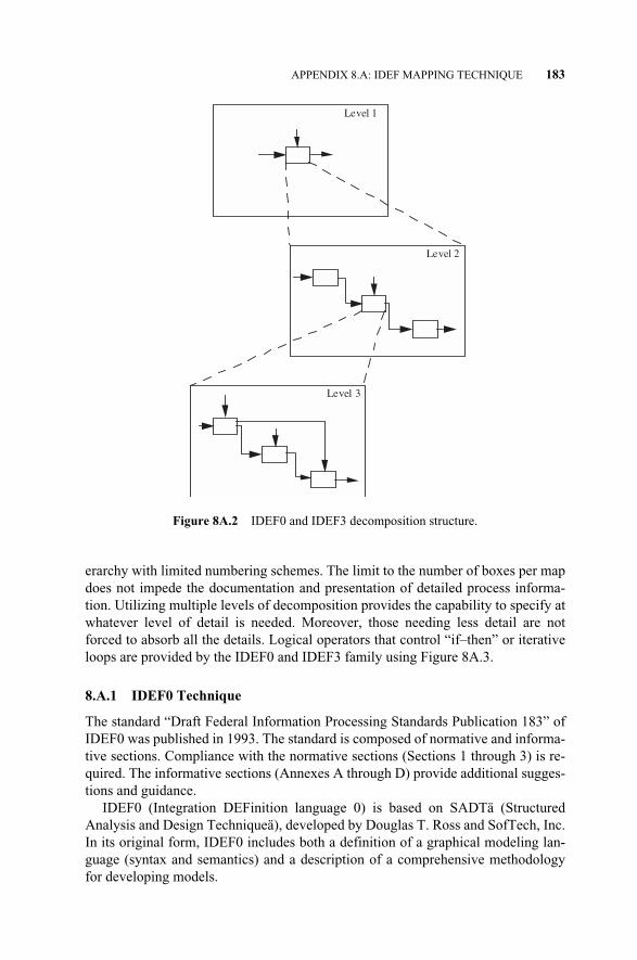
erarchy with limited numbering schemes. The limit to the number of boxes per mapdoes not impede the documentation and presentation of detailed process informa-tion. Utilizing multiple levels of decomposition provides the capability to specify atwhatever level of detail is needed. Moreover, those needing less detail are notforced to absorb all the details. Logical operators that control “if–then” or iterativeloops are provided by the IDEF0 and IDEF3 family using Figure 8A.3.
8.A.1 IDEF0 Technique
The standard “Draft Federal Information Processing Standards Publication 183” ofIDEF0 was published in 1993. The standard is composed of normative and informa-tive sections. Compliance with the normative sections (Sections 1 through 3) is re-quired. The informative sections (Annexes A through D) provide additional sugges-tions and guidance.
IDEF0 (Integration DEFinition language 0) is based on SADTä (StructuredAnalysis and Design Techniqueä), developed by Douglas T. Ross and SofTech, Inc.In its original form, IDEF0 includes both a definition of a graphical modeling lan-guage (syntax and semantics) and a description of a comprehensive methodologyfor developing models.
APPENDIX 8.A: IDEF MAPPING TECHNIQUE 183
Figure 8A.2 IDEF0 and IDEF3 decomposition structure.
Level 2
Level 3
Level 1
c08.qxd 4/22/2005 9:04 AM Page 183
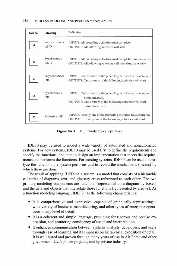
IDEF0 may be used to model a wide variety of automated and nonautomatedsystems. For new systems, IDEF0 may be used first to define the requirements andspecify the functions, and then to design an implementation that meets the require-ments and performs the functions. For existing systems, IDEF0 can be used to ana-lyze the functions the system performs and to record the mechanisms (means) bywhich these are done.
The result of applying IDEF0 to a system is a model that consists of a hierarchi-cal series of diagrams, text, and glossary cross-referenced to each other. The twoprimary modeling components are functions (represented on a diagram by boxes)and the data and objects that interrelate those functions (represented by arrows). Asa function modeling language, IDEF0 has the following characteristics:
� It is comprehensive and expressive, capable of graphically representing awide variety of business, manufacturing, and other types of enterprise opera-tions to any level of detail.
� It is a coherent and simple language, providing for rigorous and precise ex-pression, and promoting consistency of usage and interpretation.
� It enhances communication between systems analysts, developers, and usersthrough ease of learning and its emphasis on hierarchical exposition of detail.It is well tested and proven through many years of use in Air Force and othergovernment development projects, and by private industry.
184 PROCESS MODELING AND PROCESS MANAGEMENT
Figure 8A.3 IDEF family logical operators.
&Asynchronous
AND
INPUTS: All preceding activities must complete
OUTPUTS: All following activities will start
Synchronous
AND
INPUTS: All preceding activities must complete simultaneously
OUTPUTS: All following activities will start simultaneously&
OAsynchronous
OR
INPUTS: One or more of the preceding activities must complete
OUTPUTS: One or more of the following activities will start
Synchronous
OR
INPUTS: One or more of the preceding activities must complete
simultaneously
OUTPUTS: One or more of the following activities will start
simultaneously
O
Y Exclusive ORINPUTS: Exactly one of the preceding activities must complete
OUTPUTS: Exactly one of the following activities will start
Symbol Meaning
&&
&&
OO
OO
YX
Symbol Meaning Definition
c08.qxd 4/22/2005 9:04 AM Page 184
� It can be generated by a variety of computer graphics tools; numerous com-mercial products specifically support development and analysis of IDEF0 di-agrams and models.
In addition to definition of the IDEF0 language, the IDEF0 methodology alsoprescribes procedures and techniques for developing and interpreting models, in-cluding ones for data gathering, diagram construction, review cycles, and documen-tation. Materials related solely to modeling procedures are presented in the informa-tive annexes of the standard. In this section, we will limit the exposure to the IDEF0algorithmic steps and follow with an illustrative example.
Step 1. Define the mapping scope. IDEF0 process experts are identified and addedto the DFSS team. Team members are to be provided with basic training in themethodology. Team meets regularly to perform tasks related to the processmodeling effort, that is, information collection and model construction.
Step 2. Define appropriate activities
Step 3. Arrange activities in phased sequence
Step 4. Identify and define input and output objects in all stages of the processlife cycle stages
Step 5. Determine decision points and flow junctions
Step 6. Identify and define activity controls and mechanisms
Step 7. Define notifications and messages
Example: Buying a house (Figure 8.A.4)
Glossary of activities at level 1:
Obtain Loan Amount—Determine maximum amount that can be loanedSelect a house—Find a house that suits the buyer’s needsNegotiate Price—Determine a mutually agreed upon priceComplete Paperwork—Sign loan and legal closing documents
Glossary of inputs and outputs at level 1:
Loan Application—The bank’s loan applicationLoan Amount—The amount the bank will loanSelected house—The house the buyer choseAgreed-Upon Price—Mutually agreed-upon priceNew house—The newly purchased house
Glossary of controls and mechanisms at level 1):
Credit History—Past history of the buyer’s ability to pay back loansLoan officer—Person who determines the buyer’s fitness for a loanBank regulations—Rules regarding bank applicationsMarket analysis—Analysis providing purchasing information for house with
similar attributes in the area of interestReal estate agent—An individual who assists in house purchase
APPENDIX 8.A: IDEF MAPPING TECHNIQUE 185
c08.qxd 4/22/2005 9:04 AM Page 185
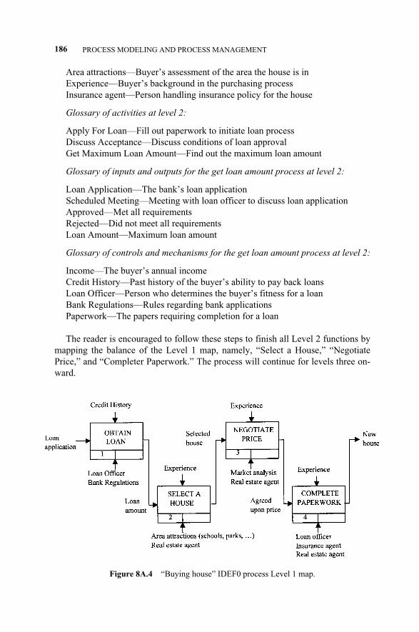
Area attractions—Buyer’s assessment of the area the house is inExperience—Buyer’s background in the purchasing processInsurance agent—Person handling insurance policy for the house
Glossary of activities at level 2:
Apply For Loan—Fill out paperwork to initiate loan processDiscuss Acceptance—Discuss conditions of loan approvalGet Maximum Loan Amount—Find out the maximum loan amount
Glossary of inputs and outputs for the get loan amount process at level 2:
Loan Application—The bank’s loan applicationScheduled Meeting—Meeting with loan officer to discuss loan applicationApproved—Met all requirementsRejected—Did not meet all requirementsLoan Amount—Maximum loan amount
Glossary of controls and mechanisms for the get loan amount process at level 2:
Income—The buyer’s annual incomeCredit History—Past history of the buyer’s ability to pay back loansLoan Officer—Person who determines the buyer’s fitness for a loanBank Regulations—Rules regarding bank applicationsPaperwork—The papers requiring completion for a loan
The reader is encouraged to follow these steps to finish all Level 2 functions bymapping the balance of the Level 1 map, namely, “Select a House,” “NegotiatePrice,” and “Completer Paperwork.” The process will continue for levels three on-ward.
186 PROCESS MODELING AND PROCESS MANAGEMENT
Figure 8A.4 “Buying house” IDEF0 process Level 1 map.
c08.qxd 4/22/2005 9:04 AM Page 186
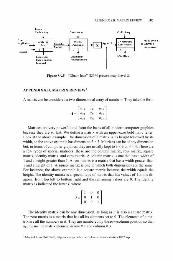
APPENDIX 8.B: MATRIX REVIEW7
A matrix can be considered a two-dimensional array of numbers. They take the form
A = � �Matrices are very powerful and form the basis of all modern computer graphics
because they are so fast. We define a matrix with an upper-case bold italic letter.Look at the above example. The dimension of a matrix is its height followed by itswidth, so the above example has dimension 3 × 3. Matrices can be of any dimensionbut, in terms of computer graphics, they are usually kept to 3 × 3 or 4 × 4. There area few types of special matrices; these are the column matrix, row matrix, squarematrix, identity matrix, and zero matrix. A column matrix is one that has a width of1 and a height greater than 1. A row matrix is a matrix that has a width greater than1 and a height of 1. A square matrix is one in which both dimensions are the same.For instance, the above example is a square matrix because the width equals theheight. The identity matrix is a special type of matrix that has values of 1 in the di-agonal from top left to bottom right and the remaining values are 0. The identitymatrix is indicated the letter I, where
I = � �The identity matrix can be any dimension, as long as it is also a square matrix.
The zero matrix is a matrix that has all its elements set to 0. The elements of a ma-trix are all the numbers in it. They are numbered by the row/column position so thata13 means the matrix element in row # 1 and column # 3.
001
010
100
a13
a23
a33
a13
a23
a33
a11
a21
a31
APPENDIX 8.B: MATRIX REVIEW 187
Figure 8A.5 “Obtain loan” IDEF0 process map, Level 2.
7Adopted from Phil Dadd, http://www.gamedev.net/reference/articles/article1832.asp.
c08.qxd 4/22/2005 9:04 AM Page 187

c08.qxd 4/22/2005 9:04 AM Page 188
9.1 INTRODUCTION
As we design services, there are many contradictions or trade-offs that must be re-solved. Often we discover, when the design is operationalized, that the design willnot achieve the desired level of performance because of the unresolved or subopti-mized resolution of contradictions or because of coupling (see Chapter 8). What if atool existed that allowed for effective resolution of these contradictions, expandedthe design teams knowledge, and allowed for safe and effective innovation? Would-n’t you be interested in such a tool?
Well, there is such a tool, the theory of inventive problem solving (TRIZ, alsoknow as TIPS) that was introduced in the United States circa 1991 and is the culmi-nation of efforts by Genrich S. Altshuller of Russia. The purpose of this chapter isto familiarize the reader with the basics of TRIZ, and provide some practical appli-cations and references for further reading. TRIZ is a tool that can be used heavily inthe DFSS road map conceptualize phase (see Figure 5.1). Opportunities for TRIZapplications are vital in other phases moving forward.
9.2 TRIZ HISTORY
The history of TRIZ is interesting and mirrors the life of its inventor, Genrich S.Altshuller. Altshuller was born on October 15, 1926 in Tashkent, Uzbekistan.While in the ninth grade, he obtained his first patent (Author’s Certificate) for anunderwater diving apparatus. In the tenth grade, he developed a boat propelled by acarbide-fueled rocket engine. In 1946, he invented a method for escaping from animmobilized submarine, and this led to employment in the patent office of theCaspian Sea Military Navy. The head of this department challenged Altshuller tosolve a difficult problem and he was successful, but a series of events, meetings,and letters led to imprisonment four years later. He was driven to invent and assist
Service Design for Six Sigma. By Basem El-Haik and David M. Roy 189© 2005 by John Wiley & Sons.
9THEORY OF INVENTIVE PROBLEMSOLVING (TRIZ) FOR SERVICE
c09.qxd 4/22/2005 9:06 AM Page 189

others to invent. He was troubled by the common misconception that invention wasthe result of accidental enlightenment or genealogy, so he sought to discover amethodology for inventing.
He called upon a former schoolmate, Rafael Shapiro, also a passionate inventor,to work with him to discover the methodology of invention. By now, Altshuller be-lieved that invention was no more than the removal of technical contradictions withthe help of certain principles. Shapiro was excited about the discovery and they re-searched all the existing patents and took part in inventing competitions in theirsearch for new methods of invention. They received a National Competition Awardfor the design of a flame- and heat-resistant suit. In recognition of that, they wereinvited to Tbilisi, a town in Georgia, where upon arrival they were arrested, interro-gated and sentenced to 25 years in Siberia. It turns out that all of the letters that Al-shuller had written to Stalin had him pegged as an intellectual and there was onlyone place for intellectuals in the USSR.
Altshuller used his TRIZ model to survive, minimizing harmful function and op-timizing useful function. In Siberia, he worked 12 hours per day logging and decid-ed it was better to be put in solitary confinement. Later, he was transferred to theVarkuta coal mines where he had to toil for 8–10 hours per day. In 1954, a year anda half after Stalin’s death, Altshuller was released from prison.
In 1956, the first paper by Altshuller and Shapiro “Psychology of Inventive Cre-ativity,” was published. In 1961, his first book, How to Learn to Invent, was pub-lished, and 50,000 readers paid around 25 cents to read about the First 20 InventivePrinciples. In 1959, he wrote his first letter to the highest patent organization in theformer Soviet Union, VOIR, requesting a chance to prove his theory. After writinghundreds of letters, 9 years later they promised a meeting no later than December1968. When the meeting was held, he met for the first time many people who con-sidered themselves his students. In 1969, he wrote a new book, Algorithm for In-venting, in which he delivered the mature 40 Principles and the first algorithm tosolve complex inventive problems.
For a period from 1970 through 1980, many TRIZ schools were opened through-out the USSR and hundreds of students were trained. During this period, Altshullertraveled to conduct seminars. This stage ended in 1980 when the first TRIZ special-ist conference took place in Petrozavodsk, Russia. During the next period, from 1980through 1985, TRIZ received much publicity in the USSR. Many people becamedevotees of TRIZ and of Altshuller, and the first TRIZ professionals and semiprofes-sionals appeared. Altshuller was highly efficient at developing his TRIZ model dueto the large number of seminars he conducted, the various TRIZ schools that were es-tablished, and the individual followers who joined the ranks, allowing for the rapidtesting of ideas and tools. TRIZ schools in St. Petersburg, Kishinev, Minsk,Novosibirsk, and other cities became very active under Altshuller’s leadership.
In 1986, the situation changed dramatically. Altshuller’s illness limited his abili-ty to work on TRIZ and control its development. Also, for the first time in the histo-ry of TRIZ, perestroika allowed it to be applied commercially. The Russian TRIZAssociation was founded in 1989 with Altshuller as president. The period from1991 on saw the rapid deterioration of economic conditions in the former USSR,
190 THEORY OF INVENTIVE PROBLEM SOLVING (TRIZ) FOR SERVICE
c09.qxd 4/22/2005 9:06 AM Page 190
and many capable TRIZ specialists, most of whom who had established their ownbusinesses, had to move abroad. Many of the TRIZ specialists immigrated to theUnited States and started promoting TRIZ individually. Others found internationalpartners and established TRIZ companies. Today, there are many consultants andfirms offering training, consultation, and software tools. Trizjournal.com has be-come a force in disseminating knowledge and information on the development andapplication of TRIZ worldwide.
9.3 TRIZ FOUNDATIONS
Contradictions and trade-offs are constraints that often create design issues forwhich neither QFD nor other tools in the DFSS toolkit provide a means for resolu-tion. Contradiction is a conflict, the result of opposing interests. For this reason,TRIZ is a welcome improvement on past innovation tools.
9.3.1 Overview
When Genrich Altshuller completed his research of the world patent base, he madefour key observations:
1. There are five levels of invention:
Level 5: Discovery of new phenomena
Level 4: Invention outside a design paradigm requiring new technology froma different field of science
Level 3: Invention inside a design paradigm that requires the resolution of aphysical contradiction
Level 2: Improvement by invention that requires the resolution of a technicalcontradiction
Level 1: Apparent solution (no innovation) results in simple improvement
2. Inventive problems contain at least one contradiction. Altshuller recognizedthat the same design problem that includes contradiction had been addressedby a number of inventions in different areas of industries. He also observedthe repetition of using the same fundamental solutions, often separated byseveral years. Altshuller concluded that if the later designer had the knowl-edge of the earlier solution, his/her task would have been simpler. He soughtto extract, compile, and organize such information, leading him to observa-tion (3) and observation (4) below.
3. The same principles are used in many inventive designs and can therefore beconsidered solution patterns. An inventive principle is a best practice that hasbeen used in many applications and has been extracted from several indus-tries. For example, the “nested doll principle” offers the most efficient use ofinternal cavities of objects like holes and dents to store material. These hol-low spaces may enclose objects of interest to the design, a packaging benefit.
9.3 TRIZ FOUNDATIONS 191
c09.qxd 4/22/2005 9:06 AM Page 191

Helen Richare, footwear designer from Great Britain, invented a method tohelp women following a youthful fashion (platform shoes) eliminate carryinga purse. Richard designed a number of models in which the cavity in the shoeis used as a depository for necessary little things (Figure 9.1). The cavity isaccessed through a special door in the shoe’s heel.
4. There are standard patterns of evolution. To create a product or service, it is nec-essary to forecast and make analogies to future situations for similar concepts interms of design functionality. The past evolution of a design is examined andthen an analogy is applied to predict the future of the design of interest. For ex-ample, when searching for variants of attaching a detachable soap dish to a wall,one may use an analogy with a load-handling crane, as in Figure 9.2.
Exhaustive study of the world’s patents reveals that the same principles have beenused in innovative solutions to problems in different industries and fields, sometimeswith many years elapsing between applications. Access to this information is one ofthe contributions of TRIZ. For example, Figure 9.3 shows the multiple applicationsof radio transmission. In 1897, Marconi obtained a patent for radio transmission. In1901, he transmitted a message across the Atlantic. In 1922, the British BroadcastingCorporation (BBC) was founded. In 1989, 200 patents were issued with radio in theirabstract, increasing to 1194 in 2002. Radio waves have been applied to televisionbroadcasting and to the remote controls for televisions (noninfrared types). Wirelesstelephones, wireless speakers, wireless internet connections, magnetic resonanceimaging, and RF ID tags on products for inventory control all demonstrate how oneinvention can be applied to multiple industries to enable unique solutions.
Defining function is the very basis of the TRIZ methodology. In fact, TRIZ isobsessed with functional definition. For example, the main useful function of a ve-hicle is “to transport people or load.” The vehicle is a technical system that con-
192 THEORY OF INVENTIVE PROBLEM SOLVING (TRIZ) FOR SERVICE
Figure 9.1 Nested doll TRIZ principle applied to shoe design. (From Shpakovsky, N. andNovitskaya, E., 2002, “Multifunctional Heel,” downloaded from Generator Website athttp://www.gnrtr.com/solutions/en/s040.html.)
c09.qxd 4/22/2005 9:06 AM Page 192
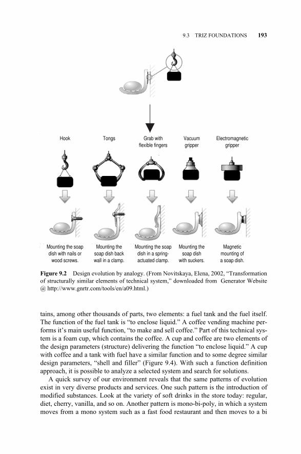
tains, among other thousands of parts, two elements: a fuel tank and the fuel itself.The function of the fuel tank is “to enclose liquid.” A coffee vending machine per-forms it’s main useful function, “to make and sell coffee.” Part of this technical sys-tem is a foam cup, which contains the coffee. A cup and coffee are two elements ofthe design parameters (structure) delivering the function “to enclose liquid.” A cupwith coffee and a tank with fuel have a similar function and to some degree similardesign parameters, “shell and filler” (Figure 9.4). With such a function definitionapproach, it is possible to analyze a selected system and search for solutions.
A quick survey of our environment reveals that the same patterns of evolutionexist in very diverse products and services. One such pattern is the introduction ofmodified substances. Look at the variety of soft drinks in the store today: regular,diet, cherry, vanilla, and so on. Another pattern is mono-bi-poly, in which a systemmoves from a mono system such as a fast food restaurant and then moves to a bi
9.3 TRIZ FOUNDATIONS 193
Figure 9.2 Design evolution by analogy. (From Novitskaya, Elena, 2002, “Transformationof structurally similar elements of technical system,” downloaded from Generator Website@ http://www.gnrtr.com/tools/en/a09.html.)
�
Mounting the soap Mounting the Mounting the soap Mounting the Magneticdish with nails or soap dish back dish in a spring- soap dish mounting of
wood screws. wall in a clamp. actuated clamp. with suckers. a soap dish.
Hook Tongs Grab with Vacuum Electromagneticflexible fingers gripper gripper
c09.qxd 4/22/2005 9:06 AM Page 193
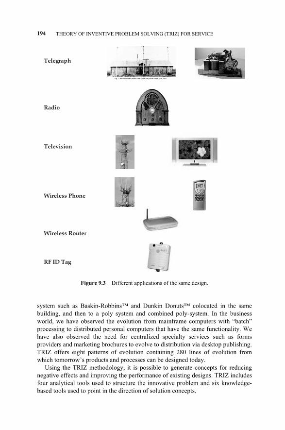
system such as Baskin-Robbins™ and Dunkin Donuts™ colocated in the samebuilding, and then to a poly system and combined poly-system. In the businessworld, we have observed the evolution from mainframe computers with “batch”processing to distributed personal computers that have the same functionality. Wehave also observed the need for centralized specialty services such as formsproviders and marketing brochures to evolve to distribution via desktop publishing.TRIZ offers eight patterns of evolution containing 280 lines of evolution fromwhich tomorrow’s products and processes can be designed today.
Using the TRIZ methodology, it is possible to generate concepts for reducingnegative effects and improving the performance of existing designs. TRIZ includesfour analytical tools used to structure the innovative problem and six knowledge-based tools used to point in the direction of solution concepts.
194 THEORY OF INVENTIVE PROBLEM SOLVING (TRIZ) FOR SERVICE
Figure 9.3 Different applications of the same design.
Television
Wireless Phone
Wireless Router
RF ID Tag
Radio
Telegraph
c09.qxd 4/22/2005 9:06 AM Page 194
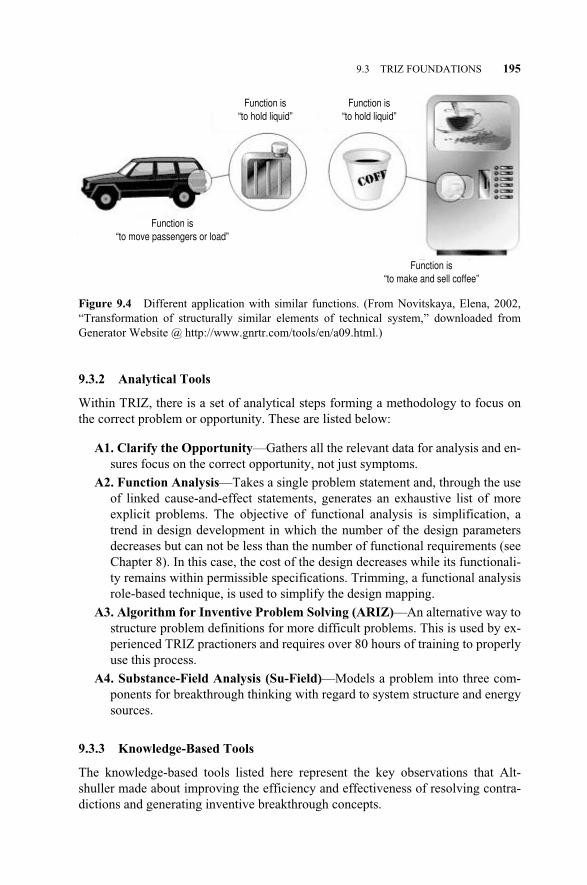
9.3.2 Analytical Tools
Within TRIZ, there is a set of analytical steps forming a methodology to focus onthe correct problem or opportunity. These are listed below:
A1. Clarify the Opportunity—Gathers all the relevant data for analysis and en-sures focus on the correct opportunity, not just symptoms.
A2. Function Analysis—Takes a single problem statement and, through the useof linked cause-and-effect statements, generates an exhaustive list of moreexplicit problems. The objective of functional analysis is simplification, atrend in design development in which the number of the design parametersdecreases but can not be less than the number of functional requirements (seeChapter 8). In this case, the cost of the design decreases while its functionali-ty remains within permissible specifications. Trimming, a functional analysisrole-based technique, is used to simplify the design mapping.
A3. Algorithm for Inventive Problem Solving (ARIZ)—An alternative way tostructure problem definitions for more difficult problems. This is used by ex-perienced TRIZ practioners and requires over 80 hours of training to properlyuse this process.
A4. Substance-Field Analysis (Su-Field)—Models a problem into three com-ponents for breakthrough thinking with regard to system structure and energysources.
9.3.3 Knowledge-Based Tools
The knowledge-based tools listed here represent the key observations that Alt-shuller made about improving the efficiency and effectiveness of resolving contra-dictions and generating inventive breakthrough concepts.
9.3 TRIZ FOUNDATIONS 195
Figure 9.4 Different application with similar functions. (From Novitskaya, Elena, 2002,“Transformation of structurally similar elements of technical system,” downloaded fromGenerator Website @ http://www.gnrtr.com/tools/en/a09.html.)
Function is“to make and sell coffee”
Function is“to move passengers or load”
Function is“to hold liquid”
Function is“to hold liquid”
c09.qxd 4/22/2005 9:06 AM Page 195
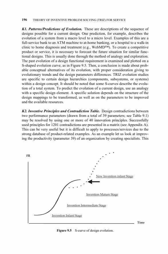
K1. Patterns/Predictions of Evolution. These are descriptions of the sequence ofdesigns possible for a current design. One prediction, for example, describes theevolution of a system from a macro level to a micro level. Examples of this are afull-service bank to an ATM machine to at-home banking, or a hospital to a walk-inclinic to home diagnosis and treatment (e.g., WebMD™). To create a competitiveproduct or service, it is necessary to forecast the future situation for similar func-tional designs. This is usually done through the method of analogy and exploration.The past evolution of a design functional requirement is examined and plotted on aS-shaped evolution curve, as in Figure 9.5. Then, a conclusion is made about prob-able conceptual alternatives of its evolution, with proper consideration giving toevolutionary trends and the design parameters differences. TRIZ evolution studiesare specific to certain design hierarchies (components, subsystems, or systems)within a design concept. It should be noted that some S-curves describe the evolu-tion of a total system. To predict the evolution of a current design, use an analogywith a specific design element. A specific solution depends on the structure of thedesign mappings to be transformed, as well as on the parameters to be improvedand the available resources.
K2. Inventive Principles and Contradiction Table. Design contradictions betweentwo performance parameters (drawn from a total of 39 parameters; see Table 9.1)may be resolved by using one or more of 40 innovation principles. Successfullyused principles for 1201 contradictions are presented in a matrix (see Appendix A).This can be very useful but it is difficult to apply to processes/services due to thestrong database of product-related examples. As an example let us look at improv-ing the productivity (parameter 39) of an organization by creating specialists. This
196 THEORY OF INVENTIVE PROBLEM SOLVING (TRIZ) FOR SERVICE
Figure 9.5 S-curve of design evolution.
Time
FR
Invention Infant Stage
Invention Intermediate Stage
Invention Mature Stage
New Invention infant Stage
c09.qxd 4/22/2005 9:06 AM Page 196
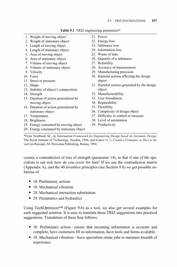
creates a contradiction of loss of strength (parameter 14), in that if one of the spe-cialists is out sick how do you cover for him? If we use the contradiction matrix(Appendix A), and the 40 inventive principles (see Section 9.8) we get possible so-lutions of
� 10. Preliminary actions
� 18. Mechanical vibration
� 28. Mechanical interaction substitution
� 29. Pneumatics and hydraulics
Using TechOptimizer™ (Figure 9.6) as a tool, we also get several examples foreach suggested solution. It is easy to translate these TRIZ suggestions into practicalsuggestions. Translation of these four follows:
� 10. Preliminary action—ensure that incoming information is accurate andcomplete, have customers fill in information, have tools and forms available.
� 18. Mechanical vibration—have specialists rotate jobs to maintain breadth ofexperience.
9.3 TRIZ FOUNDATIONS 197
Table 9.1 TRIZ engineering parameters*
1. Weight of moving object2. Weight of stationary object3. Length of moving object4. Length of stationary object5. Area of moving object6. Area of stationary object7. Volume of moving object8. Volume of stationary object9. Velocity
10. Force11. Stress or pressure12. Shape13. Stability of object’s composition14. Strength15. Duration of action generalized by
moving object16. Duration of action generalized by
stationary object17. Temperature18. Brightness19. Energy consumed by moving object20. Energy consumed by stationary object
21. Power22. Energy loss23. Substance loss24. Information loss25. Waste of time26. Quantity of a substance27. Reliability28. Accuracy of measurement29. Manufacturing precision30. Harmful actions affecting the design
object31. Harmful actions generated by the design
object32. Manufacturability33. User friendliness34. Repairability35. Flexibility36. Complexity of design object37. Difficulty to control or measure38. Level of automation39. Productivity
*From Nordlund, M., An Information Framework for Engineering Design based on Axiomatic Design,The Royal Institute of Technology, Sweden, 1996; and Ivanov G. I., Creative Formulas, or How to In-vent (in Russian), M. Prosvenia Publishing, Russia, 1994.
c09.qxd 4/22/2005 9:06 AM Page 197
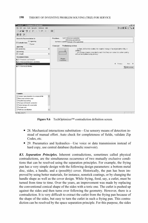
� 28. Mechanical interactions substitution—Use sensory means of detection in-stead of manual effort. Auto check for completeness of fields, validate ZipCodes, etc.
� 29. Pneumatics and hydraulics—Use voice or data transmission instead ofhard copy, use central database (hydraulic reservoir).
K3. Separation Principles. Inherent contradictions, sometimes called physicalcontradictions, are the simultaneous occurrence of two mutually exclusive condi-tions that can be resolved using the separation principles. For example, the fryingpan has a very simple design with the following design parameters: a bottom metaldisc, sides, a handle, and a (possibly) cover. Historically, the pan has been im-proved by using better materials, for instance, nonstick coatings, or by changing thehandle shape as well as the cover design. While frying, food, say, a cutlet, must beturned from time to time. Over the years, an improvement was made by replacingthe conventional conical shape of the sides with a toric one. The cutlet is pushed upagainst the sides and then turns over following the geometry. However, there is acontradiction. It is very difficult to extract the cutlet from the frying pan because ofthe shape of the sides, but easy to turn the cutlet in such a frying pan. This contra-diction can be resolved by the space separation principle. For this purpose, the sides
198 THEORY OF INVENTIVE PROBLEM SOLVING (TRIZ) FOR SERVICE
Figure 9.6 TechOptimizer™ contradiction definition screen.
c09.qxd 4/22/2005 9:06 AM Page 198

are made traditionally (conical) on one side of the frying pan and toric on the otherside, as in Figure 9.7.
K4. 76 Standard Solutions. These are generic system modifications for the modeldeveloped using Su-Field Analysis. These solutions can be grouped into five majorcategories:
1. Improving the systems with no or little change—13 standard solutions
2. Improving the system by changing the system—23 standard solutions
3. System transitions—6 standard solutions
4. Detection and measurement—17 standard solutions
5. Strategies for simplification and improvements—17 standard solutions
For example, in recycling household wastes we used to place all recyclablewaste (paper, metal, plastic, and other waste) into a single trash container. Today,many municipalities require separation of waste into specialized categories. This isone of the standard solutions suggested—segmentation of flow into many parts.
K5. Effects. An effect is a physical action of an object that produces a field or an-other action as a consequence. As a general rule, these are phenomena related toproduct design. Physical, chemical, geometric, and other effects offer “free” re-sources commonly forgotten and sometimes even incompatible with the system asdesigned:
� Material resources
System elements
Inexpensive materials
Modified materials
Waste
Raw materials
9.3 TRIZ FOUNDATIONS 199
Figure 9.7 TRIZ separation example for frying pan. Left, traditional pan. Right, pan withboth conical and toroidal sides. (From Shpakovsky, N. and Novitskaya, E., 2002, “FryingPan,” downloaded from Generator Website at http://www.gnrtr.com/solutions/en/s054.html.)
c09.qxd 4/22/2005 9:06 AM Page 199
� Time resources
Parallel operations
Pre/post work
� Information resources
� Field resources
Energy in system
Energy in environment
� Space resources
Empty space
Another dimension
Nesting
� Function resources
Harmful functions that can be converted to good ones
Enhance secondary effects of functions
K6. System of Operators. When analyzing a function model after the clarify theopportunity step, we can approach the model from three perspectives or strategies.These strategies are (1) eliminate harmful effects, (2) eliminate excessive actions,and (3) enhance useful actions. Universal operators are recommendations thatare potentially applicable to any situation, such as excessive action (e.g., e-mail-ing every employee or customer when the message is only relevant to a smallsubgroup). General operators are recommendations applicable to improving func-tionality and eliminating undesired effects, such as elimination of a harmful action(e.g., separation or transfer to a subsystem). Specialized operators are used toimprove specific parameters or features of a product or process, that is, they en-hance useful actions (examples include those for increasing speed, accuracy, andreliability). All of the TRIZ knowledge-based tools yield concepts that requireconversion to practical solutions in order to satisfy the needs of the current prob-lem.
9.4 TRIZ PROBLEM SOLVING FLOWCHART
The application of TRIZ needs to follow a logical flow since the methodology cansolve many different problems or provide many enhancements within your designproject. Figure 9.8 shows one such flow. This flow emulates the structure of theTechOptimizer™ software.
The flow begins with your practical issue and must end with a practical solutionor set of solutions. Once you enter the realm of TRIZ, the first step is to clarify theopportunity. In this step, the model is created with true functions, covered in Sec-tion 9.6, and the supersystem that interacts with the model. The ideal final resultshould be formulated at this point to assist in the last step of determining the ideali-ty of any solution arrived at.
200 THEORY OF INVENTIVE PROBLEM SOLVING (TRIZ) FOR SERVICE
c09.qxd 4/22/2005 9:06 AM Page 200
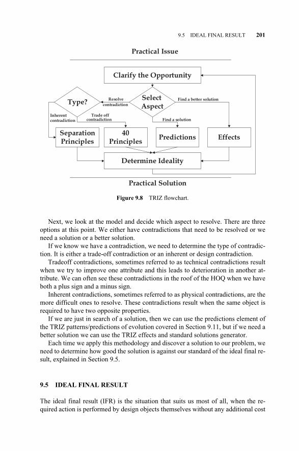
Next, we look at the model and decide which aspect to resolve. There are threeoptions at this point. We either have contradictions that need to be resolved or weneed a solution or a better solution.
If we know we have a contradiction, we need to determine the type of contradic-tion. It is either a trade-off contradiction or an inherent or design contradiction.
Tradeoff contradictions, sometimes referred to as technical contradictions resultwhen we try to improve one attribute and this leads to deterioration in another at-tribute. We can often see these contradictions in the roof of the HOQ when we haveboth a plus sign and a minus sign.
Inherent contradictions, sometimes referred to as physical contradictions, are themore difficult ones to resolve. These contradictions result when the same object isrequired to have two opposite properties.
If we are just in search of a solution, then we can use the predictions element ofthe TRIZ patterns/predictions of evolution covered in Section 9.11, but if we need abetter solution we can use the TRIZ effects and standard solutions generator.
Each time we apply this methodology and discover a solution to our problem, weneed to determine how good the solution is against our standard of the ideal final re-sult, explained in Section 9.5.
9.5 IDEAL FINAL RESULT
The ideal final result (IFR) is the situation that suits us most of all, when the re-quired action is performed by design objects themselves without any additional cost
9.5 IDEAL FINAL RESULT 201
Figure 9.8 TRIZ flowchart.
Practical Issue
Clarify the Opportunity
Select Aspect
SeparationPrinciples
40Principles
Predictions Effects
Determine Ideality
Practical Solution
Type?Resolve
contradiction
Find a better solution
Trade offcontradiction
Inherentcontradiction Find a solution
c09.qxd 4/22/2005 9:06 AM Page 201
or effort. In solving an inventive problem, the notion of IFR creates a solution ideal-ity that the design team should target. An IFR describes (defines) an ideal systemthat delivers benefit without harm. It should
� Occupy no space
� Have no weight
� Require no labor
� Take no time
� Require no maintenance, and so on
There are three methods for defining the IFR: itself, ideality checklist, and theideality equation.
9.5.1 Itself
Using the itself method, teams can look at functions and define them in an idealstate for use in developing concept solutions. In order to use this method, expressthe IFR as itself, then reexpress it in terms of actual circumstances of the problem.For example, an ideal computer is one that performs its functions without actuallyexisting. There is no such computer, or course, but we can try to approach the ideal.This concept is explored in the following examples.
Example 1. “Grass mows itself” can be reexpressed as “grass keeps itself at an at-tractive height.” How can grass do that? How do other biological systems do it? Inthe southern parts of the United States, landscapers use grasses such as Zoysia,Bermuda, and St. Augistine, which are slow-growing, creeping-type grasses. Theymay also spray the grass with a growth inhibitor that slows down the growth rate.So there are two elements used to achieve the close-to-ideal result of “grass keepsitself at an attractive height.”
Example 2. “Data enters itself” can be reexpressed as “data stays accurate, current,and in correct form.” This example is the basis of many Web-enabled, self-servicesolutions.
9.5.2 Ideality Checklist
When any concept is created, the design team can test the concept against the fol-lowing checklist:
1. Eliminates deficiencies of original system
2. Preserves advantages of original system
3. Does not make system more complicated (uses free or available resources)
4. Does not introduce new disadvantages
202 THEORY OF INVENTIVE PROBLEM SOLVING (TRIZ) FOR SERVICE
c09.qxd 4/22/2005 9:06 AM Page 202
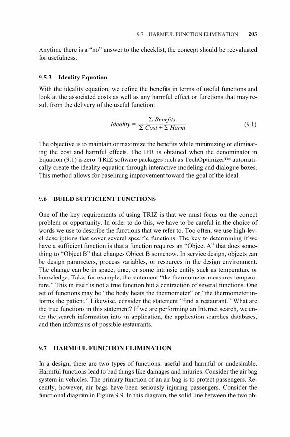
Anytime there is a “no” answer to the checklist, the concept should be reevaluatedfor usefulness.
9.5.3 Ideality Equation
With the ideality equation, we define the benefits in terms of useful functions andlook at the associated costs as well as any harmful effect or functions that may re-sult from the delivery of the useful function:
Ideality = (9.1)
The objective is to maintain or maximize the benefits while minimizing or eliminat-ing the cost and harmful effects. The IFR is obtained when the denominator inEquation (9.1) is zero. TRIZ software packages such as TechOptimizer™ automati-cally create the ideality equation through interactive modeling and dialogue boxes.This method allows for baselining improvement toward the goal of the ideal.
9.6 BUILD SUFFICIENT FUNCTIONS
One of the key requirements of using TRIZ is that we must focus on the correctproblem or opportunity. In order to do this, we have to be careful in the choice ofwords we use to describe the functions that we refer to. Too often, we use high-lev-el descriptions that cover several specific functions. The key to determining if wehave a sufficient function is that a function requires an “Object A” that does some-thing to “Object B” that changes Object B somehow. In service design, objects canbe design parameters, process variables, or resources in the design environment.The change can be in space, time, or some intrinsic entity such as temperature orknowledge. Take, for example, the statement “the thermometer measures tempera-ture.” This in itself is not a true function but a contraction of several functions. Oneset of functions may be “the body heats the thermometer” or “the thermometer in-forms the patient.” Likewise, consider the statement “find a restaurant.” What arethe true functions in this statement? If we are performing an Internet search, we en-ter the search information into an application, the application searches databases,and then informs us of possible restaurants.
9.7 HARMFUL FUNCTION ELIMINATION
In a design, there are two types of functions: useful and harmful or undesirable.Harmful functions lead to bad things like damages and injuries. Consider the air bagsystem in vehicles. The primary function of an air bag is to protect passengers. Re-cently, however, air bags have been seriously injuring passengers. Consider thefunctional diagram in Figure 9.9. In this diagram, the solid line between the two ob-
� Benefits��� Cost + � Harm
9.7 HARMFUL FUNCTION ELIMINATION 203
c09.qxd 4/22/2005 9:06 AM Page 203
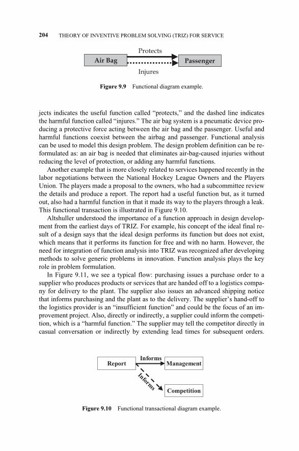
jects indicates the useful function called “protects,” and the dashed line indicatesthe harmful function called “injures.” The air bag system is a pneumatic device pro-ducing a protective force acting between the air bag and the passenger. Useful andharmful functions coexist between the airbag and passenger. Functional analysiscan be used to model this design problem. The design problem definition can be re-formulated as: an air bag is needed that eliminates air-bag-caused injuries withoutreducing the level of protection, or adding any harmful functions.
Another example that is more closely related to services happened recently in thelabor negotiations between the National Hockey League Owners and the PlayersUnion. The players made a proposal to the owners, who had a subcommittee reviewthe details and produce a report. The report had a useful function but, as it turnedout, also had a harmful function in that it made its way to the players through a leak.This functional transaction is illustrated in Figure 9.10.
Altshuller understood the importance of a function approach in design develop-ment from the earliest days of TRIZ. For example, his concept of the ideal final re-sult of a design says that the ideal design performs its function but does not exist,which means that it performs its function for free and with no harm. However, theneed for integration of function analysis into TRIZ was recognized after developingmethods to solve generic problems in innovation. Function analysis plays the keyrole in problem formulation.
In Figure 9.11, we see a typical flow: purchasing issues a purchase order to asupplier who produces products or services that are handed off to a logistics compa-ny for delivery to the plant. The supplier also issues an advanced shipping noticethat informs purchasing and the plant as to the delivery. The supplier’s hand-off tothe logistics provider is an “insufficient function” and could be the focus of an im-provement project. Also, directly or indirectly, a supplier could inform the competi-tion, which is a “harmful function.” The supplier may tell the competitor directly incasual conversation or indirectly by extending lead times for subsequent orders.
204 THEORY OF INVENTIVE PROBLEM SOLVING (TRIZ) FOR SERVICE
Figure 9.9 Functional diagram example.
Air Bag Passenger
Protects
Injures
Figure 9.10 Functional transactional diagram example.
Report ManagementInforms
Competition
Informs
c09.qxd 4/22/2005 9:06 AM Page 204
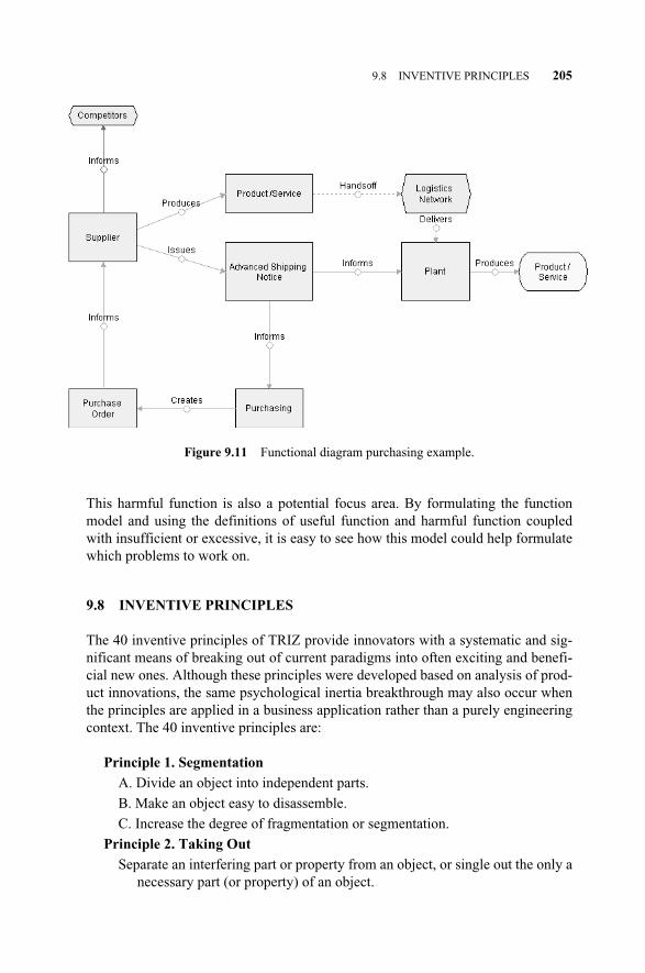
This harmful function is also a potential focus area. By formulating the functionmodel and using the definitions of useful function and harmful function coupledwith insufficient or excessive, it is easy to see how this model could help formulatewhich problems to work on.
9.8 INVENTIVE PRINCIPLES
The 40 inventive principles of TRIZ provide innovators with a systematic and sig-nificant means of breaking out of current paradigms into often exciting and benefi-cial new ones. Although these principles were developed based on analysis of prod-uct innovations, the same psychological inertia breakthrough may also occur whenthe principles are applied in a business application rather than a purely engineeringcontext. The 40 inventive principles are:
Principle 1. Segmentation
A. Divide an object into independent parts.
B. Make an object easy to disassemble.
C. Increase the degree of fragmentation or segmentation.
Principle 2. Taking Out
Separate an interfering part or property from an object, or single out the only anecessary part (or property) of an object.
9.8 INVENTIVE PRINCIPLES 205
Figure 9.11 Functional diagram purchasing example.
c09.qxd 4/22/2005 9:06 AM Page 205
Principle 3. Local Quality
A. Change an object’s structure from uniform to nonuniform; change an exter-nal environment (or external influence) from uniform to nonuniform.
B. Make each part of an object function in conditions most suitable for its op-eration.
C. Make each part of an object fulfill a different and useful function.
Principle 4. Asymmetry
A. Change the shape of an object from symmetrical to asymmetrical.
B. If an object is asymmetrical, change its degree of asymmetry.
Principle 5. Merging
A. Bring closer together (or merge) identical or similar objects; assembleidentical or similar parts to perform parallel operations.
B. Make operations contiguous or parallel; bring them together in time.
Principle 6. Universality
A. Make an object or structure perform multiple functions; eliminate the needfor other parts.
Principle 7. “Nested Doll”
A. Place one object inside another; place each object, in turn, inside the other.
B. Make one part pass through a cavity in the other.
Principle 8. Anti-Weight
A. To compensate for the weight (downward tendency) of an object, merge itwith other objects that provide lift.
B. To compensate for the weight (downward tendency) of an object, make itinteract with the environment (e.g., use global lift forces).
Principle 9. Preliminary Anti-Action
A. If it will be necessary to perform an action with both harmful and useful ef-fects, this action should be replaced with anti-actions to control harmful ef-fects.
B. Create beforehand stresses in an object that will oppose known undesirableworking stresses later on.
Principle 10. Preliminary Action
A. Perform, before it is needed, the required change of an object (either fullyor partially).
B. Prearrange objects such that they can come into action at the most conve-nient place and without losing time for their delivery.
Principle 11. Beforehand Cushioning
Prepare emergency means beforehand to compensate for the relatively low re-liability of an object.
Principle 12. Equipotentiality
In a potential field, limit position changes (e.g., change operating conditionsto eliminate the need to raise or lower objects in a gravity field).
206 THEORY OF INVENTIVE PROBLEM SOLVING (TRIZ) FOR SERVICE
c09.qxd 4/22/2005 9:06 AM Page 206
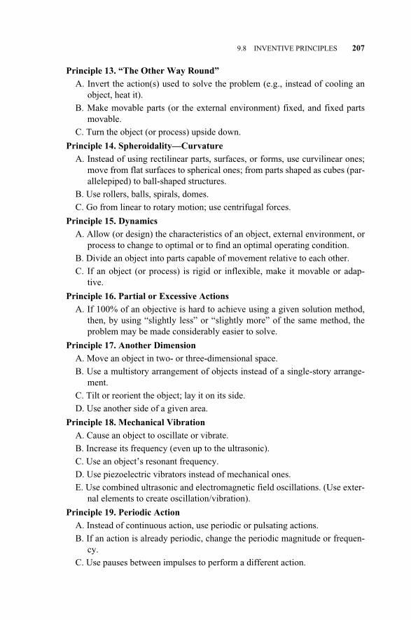
Principle 13. “The Other Way Round”
A. Invert the action(s) used to solve the problem (e.g., instead of cooling anobject, heat it).
B. Make movable parts (or the external environment) fixed, and fixed partsmovable.
C. Turn the object (or process) upside down.
Principle 14. Spheroidality—Curvature
A. Instead of using rectilinear parts, surfaces, or forms, use curvilinear ones;move from flat surfaces to spherical ones; from parts shaped as cubes (par-allelepiped) to ball-shaped structures.
B. Use rollers, balls, spirals, domes.
C. Go from linear to rotary motion; use centrifugal forces.
Principle 15. Dynamics
A. Allow (or design) the characteristics of an object, external environment, orprocess to change to optimal or to find an optimal operating condition.
B. Divide an object into parts capable of movement relative to each other.
C. If an object (or process) is rigid or inflexible, make it movable or adap-tive.
Principle 16. Partial or Excessive Actions
A. If 100% of an objective is hard to achieve using a given solution method,then, by using “slightly less” or “slightly more” of the same method, theproblem may be made considerably easier to solve.
Principle 17. Another Dimension
A. Move an object in two- or three-dimensional space.
B. Use a multistory arrangement of objects instead of a single-story arrange-ment.
C. Tilt or reorient the object; lay it on its side.
D. Use another side of a given area.
Principle 18. Mechanical Vibration
A. Cause an object to oscillate or vibrate.
B. Increase its frequency (even up to the ultrasonic).
C. Use an object’s resonant frequency.
D. Use piezoelectric vibrators instead of mechanical ones.
E. Use combined ultrasonic and electromagnetic field oscillations. (Use exter-nal elements to create oscillation/vibration).
Principle 19. Periodic Action
A. Instead of continuous action, use periodic or pulsating actions.
B. If an action is already periodic, change the periodic magnitude or frequen-cy.
C. Use pauses between impulses to perform a different action.
9.8 INVENTIVE PRINCIPLES 207
c09.qxd 4/22/2005 9:06 AM Page 207

Principle 20. Continuity of Useful Action
A. Carry on work continuously; make all parts of an object work at full load,all the time.
B. Eliminate all idle or intermittent actions or work.
Principle 21. Skipping
Conduct a process or certain stages (e.g., destructive, harmful, or hazardousoperations) at high speed.
Principle 22. “Blessing in Disguise” or “Turn Lemons into Lemonade”
A. Use harmful factors (particularly, harmful effects of the environment orsurroundings) to achieve a positive effect.
B. Eliminate the primary harmful action by adding it to another harmful actionto resolve the problem.
C. Amplify a harmful factor to such a degree that it is no longer harmful.
Principle 23. Feedback
A. Introduce feedback (referring back, cross-checking) to improve a processor action.
B. If feedback is already used, change its magnitude or influence.
Principle 24. “Intermediary”
A. Use an intermediary carrier article or intermediary process.
B. Merge one object temporarily with another (which can be easily removed).
Principle 25. Self-service
A. Make an object serve itself by performing auxiliary helpful functions
B. Use wasted (or lost) resources, energy, or substances.
Principle 26. Copying
A. Instead of an unavailable, expensive, fragile object, use simpler and inex-pensive copies.
B. Replace an object or process with optical copies.
C. If optical copies are used, move to IR or UV (use an appropriate out-of-the-ordinary illumination and viewing situation).
Principle 27. Cheap, Short-Lived Objects
A. Replace an expensive object with a multitude of inexpensive objects, com-promising certain qualities (such as service life, for instance).
Principle 28 Mechanical Substitution
A. Replace a mechanical means with a sensory (optical, acoustic, taste, orsmell) means.
B. Use electric, magnetic, and electromagnetic fields to interact with the ob-ject.
C. Change from static to movable fields, from unstructured fields to thosehaving structure.
D. Use fields in conjunction with field-activated (e.g., ferromagnetic) particles.
208 THEORY OF INVENTIVE PROBLEM SOLVING (TRIZ) FOR SERVICE
c09.qxd 4/22/2005 9:06 AM Page 208

Principle 29. Pneumatics and Hydraulics
A. Use gas and liquid parts of an object instead of solid parts (e.g., inflatable,filled with liquids, air cushion, hydrostatic, hydroreactive).
Principle 30. Flexible Shells and Thin Films
A. Use flexible shells and thin films instead of three-dimensional structures.
B. Isolate the object from the external environment using flexible shells andthin films.
Principle 31. Porous Materials
A. Make an object porous or add porous elements (inserts, coatings, etc.).
B. If an object is already porous, use the pores to introduce a useful substanceor function.
Principle 32. Color Changes
A. Change the color of an object or its external environment.
B. Change the transparency of an object or its external environment.
Principle 33. Homogeneity
A. Make objects interact with a given object of the same material (or materialwith identical properties).
Principle 34. Discarding and Recovering
A. Make portions of an object that have fulfilled their functions go away (discardby dissolving, evaporating, etc.) or modify them directly during an operation.
B. Conversely, restore consumable parts of an object directly in an operation.
Principle 35. Parameter Changes
A. Change an object’s physical state (e.g., to a gas, liquid, or solid).
B. Change the concentration or consistency.
C. Change the degree of flexibility.
D. Change the temperature.
Principle 36. Phase Transitions
Use phenomena occurring during phase transitions (awareness of macroscalebusiness phenomena).
Principle 37. Thermal Expansion
A. Use thermal expansion (or contraction) of materials.
B. If thermal expansion is being used, use multiple materials with different co-efficients of thermal expansion.
Principle 38. Strong Oxidants (“Boosted Interactions”)
A. Replace common air with oxygen-enriched air (enriched atmosphere).
B. Replace enriched air with pure oxygen (highly enriched atmosphere).
C. Expose air or oxygen to ionizing radiation.
D. Use ionized oxygen.
E. Replace ozonized (or ionized) oxygen with ozone (atmosphere enriched by“unstable” elements).
9.8 INVENTIVE PRINCIPLES 209
c09.qxd 4/22/2005 9:06 AM Page 209
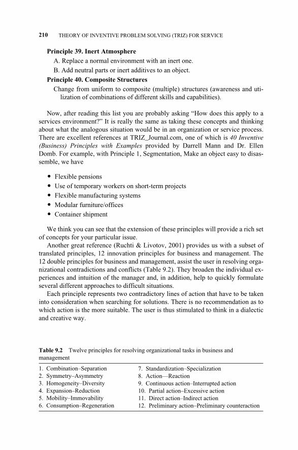
Principle 39. Inert Atmosphere
A. Replace a normal environment with an inert one.
B. Add neutral parts or inert additives to an object.
Principle 40. Composite Structures
Change from uniform to composite (multiple) structures (awareness and uti-lization of combinations of different skills and capabilities).
Now, after reading this list you are probably asking “How does this apply to aservices environment?” It is really the same as taking these concepts and thinkingabout what the analogous situation would be in an organization or service process.There are excellent references at TRIZ_Journal.com, one of which is 40 Inventive(Business) Principles with Examples provided by Darrell Mann and Dr. EllenDomb. For example, with Principle 1, Segmentation, Make an object easy to disas-semble, we have
� Flexible pensions
� Use of temporary workers on short-term projects
� Flexible manufacturing systems
� Modular furniture/offices
� Container shipment
We think you can see that the extension of these principles will provide a rich setof concepts for your particular issue.
Another great reference (Ruchti & Livotov, 2001) provides us with a subset oftranslated principles, 12 innovation principles for business and management. The12 double principles for business and management, assist the user in resolving orga-nizational contradictions and conflicts (Table 9.2). They broaden the individual ex-periences and intuition of the manager and, in addition, help to quickly formulateseveral different approaches to difficult situations.
Each principle represents two contradictory lines of action that have to be takeninto consideration when searching for solutions. There is no recommendation as towhich action is the more suitable. The user is thus stimulated to think in a dialecticand creative way.
210 THEORY OF INVENTIVE PROBLEM SOLVING (TRIZ) FOR SERVICE
Table 9.2 Twelve principles for resolving organizational tasks in business andmanagement
1. Combination–Separation2. Symmetry–Asymmetry3. Homogeneity–Diversity4. Expansion–Reduction5. Mobility–Immovability6. Consumption–Regeneration
7. Standardization–Specialization8. Action—Reaction9. Continuous action–Interrupted action10. Partial action–Excessive action11. Direct action–Indirect action12. Preliminary action–Preliminary counteraction
c09.qxd 4/22/2005 9:06 AM Page 210
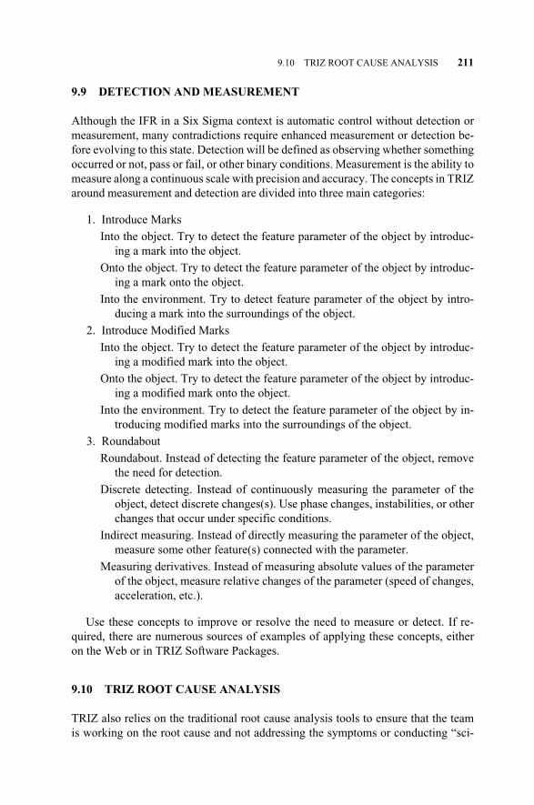
9.9 DETECTION AND MEASUREMENT
Although the IFR in a Six Sigma context is automatic control without detection ormeasurement, many contradictions require enhanced measurement or detection be-fore evolving to this state. Detection will be defined as observing whether somethingoccurred or not, pass or fail, or other binary conditions. Measurement is the ability tomeasure along a continuous scale with precision and accuracy. The concepts in TRIZaround measurement and detection are divided into three main categories:
1. Introduce Marks
Into the object. Try to detect the feature parameter of the object by introduc-ing a mark into the object.
Onto the object. Try to detect the feature parameter of the object by introduc-ing a mark onto the object.
Into the environment. Try to detect feature parameter of the object by intro-ducing a mark into the surroundings of the object.
2. Introduce Modified Marks
Into the object. Try to detect the feature parameter of the object by introduc-ing a modified mark into the object.
Onto the object. Try to detect the feature parameter of the object by introduc-ing a modified mark onto the object.
Into the environment. Try to detect the feature parameter of the object by in-troducing modified marks into the surroundings of the object.
3. Roundabout
Roundabout. Instead of detecting the feature parameter of the object, removethe need for detection.
Discrete detecting. Instead of continuously measuring the parameter of theobject, detect discrete changes(s). Use phase changes, instabilities, or otherchanges that occur under specific conditions.
Indirect measuring. Instead of directly measuring the parameter of the object,measure some other feature(s) connected with the parameter.
Measuring derivatives. Instead of measuring absolute values of the parameterof the object, measure relative changes of the parameter (speed of changes,acceleration, etc.).
Use these concepts to improve or resolve the need to measure or detect. If re-quired, there are numerous sources of examples of applying these concepts, eitheron the Web or in TRIZ Software Packages.
9.10 TRIZ ROOT CAUSE ANALYSIS
TRIZ also relies on the traditional root cause analysis tools to ensure that the teamis working on the root cause and not addressing the symptoms or conducting “sci-
9.10 TRIZ ROOT CAUSE ANALYSIS 211
c09.qxd 4/22/2005 9:06 AM Page 211
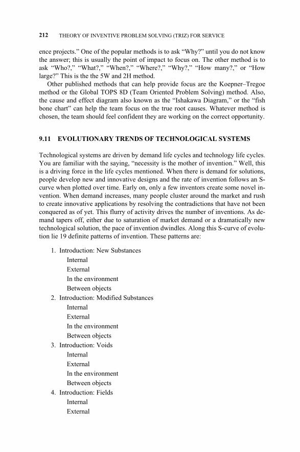
ence projects.” One of the popular methods is to ask “Why?” until you do not knowthe answer; this is usually the point of impact to focus on. The other method is toask “Who?,” “What?,” “When?,” “Where?,” “Why?,” “How many?,” or “Howlarge?” This is the the 5W and 2H method.
Other published methods that can help provide focus are the Koepner–Tregoemethod or the Global TOPS 8D (Team Oriented Problem Solving) method. Also,the cause and effect diagram also known as the “Ishakawa Diagram,” or the “fishbone chart” can help the team focus on the true root causes. Whatever method ischosen, the team should feel confident they are working on the correct opportunity.
9.11 EVOLUTIONARY TRENDS OF TECHNOLOGICAL SYSTEMS
Technological systems are driven by demand life cycles and technology life cycles.You are familiar with the saying, “necessity is the mother of invention.” Well, thisis a driving force in the life cycles mentioned. When there is demand for solutions,people develop new and innovative designs and the rate of invention follows an S-curve when plotted over time. Early on, only a few inventors create some novel in-vention. When demand increases, many people cluster around the market and rushto create innovative applications by resolving the contradictions that have not beenconquered as of yet. This flurry of activity drives the number of inventions. As de-mand tapers off, either due to saturation of market demand or a dramatically newtechnological solution, the pace of invention dwindles. Along this S-curve of evolu-tion lie 19 definite patterns of invention. These patterns are:
1. Introduction: New Substances
Internal
External
In the environment
Between objects
2. Introduction: Modified Substances
Internal
External
In the environment
Between objects
3. Introduction: Voids
Internal
External
In the environment
Between objects
4. Introduction: Fields
Internal
External
212 THEORY OF INVENTIVE PROBLEM SOLVING (TRIZ) FOR SERVICE
c09.qxd 4/22/2005 9:06 AM Page 212

In the environment
Between objects
5. Mono–bi–poly: Similar Objects
Introduction of similar objects
Introduction of several similar objects
Combining similar objects into a common system
6. Mono–bi–poly: Various Objects
Introduction of various objects
Introduction of several various objects
Combining various objects into a common system
7. Segmentation: Substances
Monolith
Segmented
Liquid/powder
Gas/plasma
Field
8. Segmentation: Space
Introduction of a void
Segmentation of a void
Creating pores and capillaries
Activating pores and capillaries
9. Segmentation: Surface
Flat surface
Protrusions
Roughness
Activating surface
10. Segmentation: Flow
Into to parts (paths)
Into several parts (paths)
Into many parts (paths)
11. Coordination: Dynamism
Immobile
Joint (partial mobility)
Many joints (degrees of freedom)
Elastic (flexible)
Liquid/gas (transition to molecular)
Field (transition to field)
12. Coordination: Rhythm
Continuous action
9.11 EVOLUTIONARY TRENDS OF TECHNOLOGICAL SYSTEMS 213
c09.qxd 4/22/2005 9:06 AM Page 213

Pulsating action
Pulsation in the resonance mode
Several actions
Traveling wave
13. Coordination: Action
None
Partial
Full
Interval
14. Coordination: Control
Manual
Semiautomatic
Automatic
15. Geometric Evolution: Dimensions
Point
Line
Surface
Volume
16. Geometric Evolution: Linear
Line
Two-dimensional curve
Three-dimensional curve
Compound three-dimensional
17. Geometric Evolution: Surface
Plane
Single curvature of plane
Double curvature of plane
Combined surface
18. Geometric Evolution: Volumetric
Prism
Cylindrical
Spheroidal
Combined object
19. Trimming
Complete system
System with eliminated objects
Partially trimmed system
Fully trimmed system
214 THEORY OF INVENTIVE PROBLEM SOLVING (TRIZ) FOR SERVICE
c09.qxd 4/22/2005 9:06 AM Page 214

It would be unusual to find a modern-day invention that relied on only one ofthese patterns. Consider cameras. They started out monolithic, with a single lens.Later, they became hinged and had two lenses, one for near focus and one for far.Today, the compact digital camera has an LCD (gas/plasma) display and a zoomlens (combined poly system), as well as jointed flash. Organizations and processesfollow similar patterns. Just think about the paper form, which has evolved to theelectronic form, a journey from immobile ink on paper to a field of electrons.
The important application of this topic is that you can actually tell where the so-lution you select lies along the S-curve. You do not want to be relying on a declin-ing technology, nor do you want to be at the “bleeding edge” of invention.
9.12 TRANSITIONS FROM TRIZ EXAMPLES
Many service-improvement teams trying to use TRIZ will have difficulty findingrelevant examples since the TRIZ methodology has evolved from a study of prod-uct-based patents and the ratio of product patents to service and process patents isstill overwhelming. In order to assist in finding useful knowledge and examples inthe TRIZ databases, a tool to transition from product-based examples to other appli-cations is required. In this section, we will introduce a transition tool that is basedon the substance-field model of TRIZ. Earlier, we discussed the function model inwhich Object A acts on Object B. In order for this model to function, Object A hasto change something in Object B, implying that energy has to be transferred be-tween the objects. To fulfill the transfer of energy, there are three elements re-quired: (1) source of energy (2) transmission of energy, and (3) guidance and con-trol. A simple transition worksheet (Figure 9.12) is used to create the full transition.
9.12 TRANSITIONS FROM TRIZ EXAMPLES 215
Figure 9.12 Transition worksheet.
Object
“A”
My Problem ImprovedMy Problem StartingExample ImprovedExample StartingElement
Guidance and
Transmission of
Source of energy
Object A (Acting)
Object B (acted on)
My Problem ImprovedMy Problem StartingExample ImprovedExample StartingElement
Object
“B”
Acts On
energy
control
c09.qxd 4/22/2005 9:06 AM Page 215
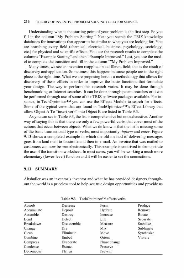
Understanding what is the starting point of your problem is the first step. So youfill in the column “My Problem Starting.” Next you search the TRIZ knowledgedatabases for innovations that appear to be similar to what you are looking for. Youare searching every field (chemical, electrical, business, psychology, sociology,etc.) for physical and scientific effects. You use the research results to complete thecolumns “Example Starting” and then “Example Improved.” Last, you use the mod-el to complete the transition and fill in the column “”My Problem Improved.”
Many times, we see an invention reapplied in a different field; this is the result ofdiscovery and application. Sometimes, this happens because people are in the rightplace at the right time. What we are proposing here is a methodology that allows fordiscovery of these effects in order to improve the basic functions that formulateyour design. The way to perform this research varies. It may be done throughbenchmarking or Internet searches. It can be done through patent searches or it canbe performed through use of some of the TRIZ software packages available. For in-stance, in TechOprimizer™ you can use the Effects Module to search for effects.Some of the typical verbs that are found in TechOptimizer™’s Effect Library thatallow Object A To “insert verb” into Object B are listed in Table 9.3.
As you can see in Table 9.3, the list is comprehensive but not exhaustive. Anotherway of saying this is that there are only a few powerful verbs that cover most of theactions that occur between objects. What we do know is that the list is missing someof the basic transactional type of verbs, most importantly, inform and enter. Figure9.13 shows a completed example in which the old method of delivering messagesgoes from land mail to facsimile and then to e-mail. An invoice that was mailed tocustomers can now be sent electronically. This example is contrived to demonstratethe use of the transition worksheet. In most cases, you will be working a much moreelementary (lower-level) function and it will be easier to see the connections.
9.13 SUMMARY
Altshuller was an inventor’s inventor and what he has provided designers through-out the world is a priceless tool to help see true design opportunities and provide us
216 THEORY OF INVENTIVE PROBLEM SOLVING (TRIZ) FOR SERVICE
Table 9.3 TechOptimizer™ effects verbs
Absorb Decrease Form Produce Accumulate Deposit Hydrate Remove Assemble Destroy Increase Rotate Bend Detect Lift Separate Breakdown Disassemble Measure Stabilize Change Dry Mix SublimateClean Eliminate Move Synthesize Combine Embed Orient Vibrate Compress Evaporate Phase changeCondense Extract PreserveDecompose Flatten Prevent
c09.qxd 4/22/2005 9:06 AM Page 216
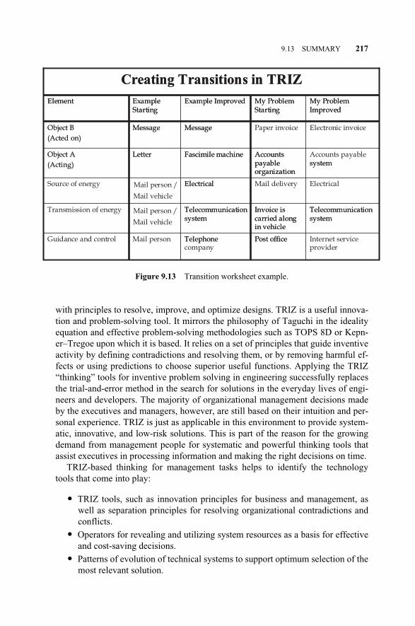
with principles to resolve, improve, and optimize designs. TRIZ is a useful innova-tion and problem-solving tool. It mirrors the philosophy of Taguchi in the idealityequation and effective problem-solving methodologies such as TOPS 8D or Kepn-er–Tregoe upon which it is based. It relies on a set of principles that guide inventiveactivity by defining contradictions and resolving them, or by removing harmful ef-fects or using predictions to choose superior useful functions. Applying the TRIZ“thinking” tools for inventive problem solving in engineering successfully replacesthe trial-and-error method in the search for solutions in the everyday lives of engi-neers and developers. The majority of organizational management decisions madeby the executives and managers, however, are still based on their intuition and per-sonal experience. TRIZ is just as applicable in this environment to provide system-atic, innovative, and low-risk solutions. This is part of the reason for the growingdemand from management people for systematic and powerful thinking tools thatassist executives in processing information and making the right decisions on time.
TRIZ-based thinking for management tasks helps to identify the technologytools that come into play:
� TRIZ tools, such as innovation principles for business and management, aswell as separation principles for resolving organizational contradictions andconflicts.
� Operators for revealing and utilizing system resources as a basis for effectiveand cost-saving decisions.
� Patterns of evolution of technical systems to support optimum selection of themost relevant solution.
9.13 SUMMARY 217
Figure 9.13 Transition worksheet example.
Internet service provider
Post officeTelephone company
Telecommunication system
Invoice is carried along in vehicle
Telecommunication system
Mail person /
Mail vehicle
ElectricalMail deliveryElectrical
Accounts payable system
Accounts payable organization
Fascimile machineLetterObject A
(Acting)
Electronic invoicePaper invoiceMessageMessageObject B
(Acted on)
My Problem Improved
My Problem Starting
Example ImprovedExample Starting
Element
Creating Transitions in TRIZ
Post officeTelephone Mail personGuidance and control
Telecommunication system
Invoice is carried along in vehicle
Telecommunication system
Transmission of energy
ElectricalSource of energy
systemAccounts payable organization
Fascimile machineLetterObject A
(Acting)
MessageMessageObject B
(Acted on)
My Problem Improved
My Problem Starting
Example ImprovedExample Starting
Element
Creating Transitions in TRIZ
Mail person /
Mail vehicle
c09.qxd 4/22/2005 9:06 AM Page 217
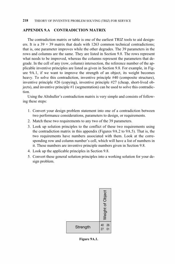
218 THEORY OF INVENTIVE PROBLEM SOLVING (TRIZ) FOR SERVICE
APPENDIX 9.A CONTRADICTION MATRIX
The contradiction matrix or table is one of the earliest TRIZ tools to aid design-ers. It is a 39 × 39 matrix that deals with 1263 common technical contradictions;that is, one parameter improves while the other degrades. The 39 parameters in therows and columns are the same. They are listed in Section 9.8. The rows representwhat needs to be improved, whereas the columns represent the parameters that de-grade. In the cell of any (row, column) intersection, the reference number of the ap-plicable inventive principles are listed as given in Section 9.8. For example, in Fig-ure 9A.1, if we want to improve the strength of an object, its weight becomesheavy. To solve this contradiction, inventive principle #40 (composite structure),inventive principle #26 (copying), inventive principle #27 (cheap, short-lived ob-jects), and inventive principle #1 (segmentation) can be used to solve this contradic-tion.
Using the Altshuller’s contradiction matrix is very simple and consists of follow-ing these steps:
1. Convert your design problem statement into one of a contradiction betweentwo performance considerations, parameters to design, or requirements.
2. Match these two requirements to any two of the 39 parameters.
3. Look up solution principles to the conflict of these two requirements usingthe contradiction matrix in this appendix (Figures 9A.2 to 9A.5). That is, thetwo requirements have numbers associated with them. Look at the corre-sponding row and column number’s cell, which will have a list of numbers init. These numbers are inventive principle numbers given in Section 9.8.
4. Look up the applicable principles in Section 9.8.
5. Convert these general solution principles into a working solution for your de-sign problem.
Figure 9A.1.
Strength
Wei
ght
of O
bje
ct
40 2627 01
c09.qxd 4/22/2005 9:06 AM Page 218

219
12
34
56
78
910
11
12
13
14
15
16
17
18
19
20
115. 8.
29. 34
29. 17.
38. 34
29. 2.
40. 28
2. 8. 15.
38
8. 10.
18. 37
10. 36.
37. 40
10. 14.
35. 40
1. 35.
19. 39
28. 27.
18. 40
5. 34.
31. 35
6. 29. 4.
38
19. 1.
32
35. 12.
34. 31
210. 1.
29. 35
35. 30.
13. 2
5. 35.
14. 2
8. 10.
19. 35
13. 29.
10. 18
13. 10.
29. 14
26. 39.
1. 40
28. 2.
10. 27
2. 27.
19. 6
28. 19.
32. 22
35. 19.
32
18. 19.
28. 1
315. 8.
29. 34
15. 17.
4
7. 17.
4. 35
13. 4. 8
17. 10.
41. 8. 35
1. 8. 10.
29
1. 8. 15.
34
8. 35.
29. 34
19
10. 15.
19
32
8. 35.
24
435. 28.
40. 29
17. 7.
10. 40
35. 8.
2. 14
28. 1
1. 14.
35
13. 14.
15. 7
39. 37.
35
15. 14.
28. 26
1. 40.
35
3. 35.
38. 18
3. 25
52. 17.
29. 4
14. 15.
18. 4
7. 14.
17. 4
29. 30.
4. 34
19. 30.
35. 2
10. 15.
36. 28
5. 34.
29. 4
11. 2.
13. 39
3. 15.
40. 14
6. 3
2. 15.
16
15. 32.
19. 13
19. 32
630. 2.
14. 18
26. 7.
9. 39
1. 18.
35. 36
10. 15.
36. 37
2. 38
40
2. 10.
19. 30
35. 39.
38
72. 26.
29. 40
1. 7.
35. 4
1. 7. 4
.
17
29. 4.
38. 34
15. 35.
36. 37
6. 35.
36. 37
1. 15.
29. 4
28. 10.
1. 39
9. 14.
15. 7
6. 35. 4
34. 39.
10. 18
10. 13.
235
835. 10.
19. 14
19. 14
35. 8.
2. 14
2. 18.
37
24. 35
7. 2. 35
34. 28.
35. 40
9. 14.
17. 15
35. 34.
38
35. 6. 4
92. 28.
13. 38
13. 14.
8
29. 30.
34
7. 29.
34
13. 28.
15. 19
6. 18.
38. 40
35. 15.
18. 34
28. 33.
1. 18
8. 3. 26.
14
3. 19.
35. 5
28. 30.
36. 2
10. 13.
19
8. 15.
35. 38
10
8. 1.
37. 18
18. 13.
1. 28
17. 19.
9. 36
28. 1
19. 10.
15
1. 18.
36. 37
15. 9.
12. 37
2. 36.
18. 37
13. 28.
15. 12
18. 21.
11
10. 35.
40. 34
35. 10.
21
35. 10.
14. 27
19. 2
35. 10.
21
19. 17.
10
1. 16.
36. 37
11
10. 36.
37. 40
13. 29.
10. 18
35. 10.
36
35. 1.
14. 16
10. 15.
36. 28
10. 15.
36. 37
6. 35.
10
35. 34
6. 35.
36
36. 35.
21
35. 4.
15. 10
35. 33.
2. 40
9. 18. 3.
40
19. 3.
27
35. 39.
19. 2
14. 24.
10. 37
12
8. 10.
29. 40
15. 10.
26. 3
29. 34.
5. 4
13. 14.
10. 7
5. 34.
4. 10
14. 4.
15. 22
7. 2. 3
535. 15.
34. 18
35. 10.
37. 40
34. 15.
10. 14
33. 1.
18. 4
30. 14.
10. 40
14. 26.
9. 25
22. 14.
19. 32
13. 15.
32
2. 6. 34.
14
13
21. 35.
2. 39
26. 39.
1. 40
13. 15.
1. 28
37
2. 11.
13
39
28. 10.
19. 39
34. 28.
35. 40
33. 15.
28. 18
10. 35.
21. 16
2. 35.
40
22. 1.
18. 4
17. 9.
15
13. 27.
10. 35
39. 3.
35. 23
35. 1.
32
32. 3.
27. 15
13. 19
27. 4.
29. 18
14
1. 8.
40. 15
40. 26.
27. 1
1. 15.
8. 35
15. 14.
28. 26
3. 34.
40. 29
9. 40.
28
10. 15.
14. 7
9. 14.
17. 15
8. 13.
26. 14
10. 18.
3. 14
10. 3.
18. 40
10. 30.
35. 40
13. 17.
35
27. 3.
26
30. 10.
40
35. 19
19. 35.
10
35
15
19. 5.
34. 31
2. 19. 9
3. 17.
19
10. 2.
19. 30
3. 35. 5
19. 2.
16
19. 3.
27
14. 26.
28. 25
13. 3.
35
27. 3.
10
19. 35.
39
2. 19. 4.
35
28. 6.
35. 18
16
6. 27.
19. 16
1. 40.
35
35. 34.
38
39. 3.
35. 23
19. 18.
36. 40
17
36. 22.
6. 38
22. 35.
32
15. 19.
9
15. 19.
9
3. 35.
39. 18
35. 38
34. 39.
40. 18
35. 6. 4
2. 28.
36. 30
35. 10.
3. 21
35. 39.
19. 2
14. 22.
19. 32
1. 35.
32
10. 30.
22. 40
19. 13.
39
19. 18.
36. 40
32. 30.
21. 16
19. 15.
3. 17
18
19. 1.
32
2. 35.
32
19. 32.
16
19. 32.
26
2. 13.
10
10. 13.
19
26. 19.
632. 30
32. 3.
27
35. 19
2. 19. 6
32. 35.
19
32. 1.
19
32. 35.
1. 15
19
12. 18.
28. 31
12. 28
15. 19.
25
35. 13.
18
8. 15.
35
16. 26.
21. 2
23. 14.
25
12. 2.
29
19. 13.
17. 24
5. 19. 9.
35
28. 35.
6. 18
19. 24.
3. 14
2. 15.
19
20
19. 9.
6. 27
36. 37
27. 4.
29. 18
35
19. 2.
35. 32
Fig
ure
9.A
.2C
ontr
adic
tion
mat
rix
1 th
roug
h 20
by
1 th
roug
h 20
.
c09.qxd 4/22/2005 9:06 AM Page 219

220
12
34
56
78
91
01
11
21
31
41
51
61
71
81
92
0
21
8. 36.
38. 31
19. 26.
17. 27
1. 10.
35. 37
19. 38
17. 32.
13. 38
35. 6.
38
30. 6.
25
15. 35.
2
26. 2.
36. 35
22. 10.
35
29. 14.
2. 40
35. 32.
15. 31
26. 10.
28
19
. 3
5.
10. 38
16
2. 14.
17. 25
16
. 6
.
19
16. 6.
19. 37
22
15. 6.
19. 28
19. 6.
18. 9
7.
2.
6.
13
6.
38
. 7
15. 26.
17. 30
17. 7.
30. 18
7. 18.
23
716. 35.
38
36. 38
14. 2.
39. 6
26
19. 38.
7
1.
13
.
32. 15
23
35. 6.
23. 40
35. 6.
22. 32
14. 29.
10. 39
10. 28.
24
35. 2.
10. 31
10. 18.
39. 31
1. 29.
30. 36
3. 39.
18. 31
10. 13.
28. 38
14. 15.
18. 40
3. 36.
37. 10
29. 35.
3.
5
2. 14.
30. 40
35. 28.
31
. 4
0
28
. 2
7.
3. 18
27. 16.
18. 38
21. 36.
39. 31
1. 6. 13
35
. 1
8.
24. 5
28
. 2
7.
12. 31
24
10. 24.
35
10. 35.
51. 26
26
30. 26
30. 16
2. 22
26. 32
10
10
19
25
10. 20.
37. 35
10. 20.
26. 5
15. 2.
29
30
. 2
4.
14. 5
26
. 4
. 5
.
16
10. 35.
17. 4
2.
5.
34
.
10
35. 16.
32. 18
10. 37.
36. 5
37. 36.
4
4. 10.
34. 17
35. 3.
22. 5
29. 3.
28. 18
20. 10.
28. 18
28
. 2
0.
10. 16
35. 29.
21
. 1
8
1.
19
.
21. 17
35. 38.
19. 18
1
26
35. 6.
18. 31
27. 26.
18. 35
29. 14.
35. 18
15. 14.
29
2. 18.
40. 4
15. 20.
29
35. 29.
34. 28
35. 14.
3
10. 36.
14. 3
35. 14
15. 2.
17. 40
14. 35.
34
. 1
0
3.
35
.
10. 40
3.
35
.
31
3. 17.
39
34
. 2
9.
16. 18
3. 35.
31
27
3. 8.
10. 40
3. 10.
8. 28
15. 9.
14. 4
15
. 2
9.
28
. 1
1
17. 10.
14. 16
32. 35.
40. 4
3. 10.
14. 24
2. 35.
24
21. 35.
11. 28
8. 28.
10. 3
10. 24.
35. 19
35. 1.
16. 11
11. 28
2.
35
. 3
.
25
34. 27.
6. 40
3.
35
.
10
11
. 3
2.
13
21
. 1
1.
27. 19
36. 23
28
32. 35.
26. 28
28. 35.
25. 26
28. 26.
5. 16
32. 28.
3. 16
26. 28.
32. 3
26. 28.
32. 3
32. 13.
6
28. 13.
32. 24
32. 2
6. 28.
32
6. 28.
32
32. 35.
13
28. 6.
32
28. 6.
32
10. 26.
24
6. 19.
28. 24
6.
1.
32
3.
6.
32
29
28. 32.
13. 18
28. 35.
27. 9
10. 28.
29. 37
2. 32.
10
28. 33.
29. 32
2. 29.
18. 36
32. 28.
2
25. 10.
35
10. 28.
32
28. 19.
34. 36
3. 35
32. 30.
40
30
. 1
83
. 2
73. 27.
40
19. 26
3. 32
32. 2
30
22. 21.
27. 39
2. 22.
13. 24
17. 1.
39. 4
1. 18
22. 1.
33. 28
27. 2.
39. 35
22. 23.
37. 35
34. 39.
19. 27
21. 22.
35. 28
13. 35.
39. 18
22. 2.
37
22
. 1
. 3
.
35
35. 24.
30. 18
18. 35.
37
. 1
22. 15.
33. 28
17. 1.
40. 33
22. 33.
35. 2
1. 19.
32. 13
1.
24
. 6
.
27
10. 2.
22
. 3
7
31
19. 22.
15. 39
35. 22.
1. 39
17. 15.
16. 22
17. 2.
18. 39
22. 1.
40
17. 2.
40
30. 18.
35. 4
35. 28.
3. 23
35. 28.
1. 40
2. 33.
27. 18
35. 1
35. 40.
27. 39
15. 35.
22. 2
15. 22.
33
. 3
1
21
. 3
9.
16. 22
22. 35.
2. 24
19
. 2
4.
39. 32
2.
35
. 6
19. 22.
18
32
28. 29.
15. 16
1. 27.
36. 13
1. 29.
13. 17
15. 17.
27
13. 1.
26. 12
16. 4
13. 29.
1. 40
35
35. 13.
8.
135. 12
35. 19.
1. 37
1. 28.
13. 27
11. 13.
1
1.
3.
10
.
32
27
. 1
. 4
35
. 1
627. 26.
18
28. 24.
27. 1
28
. 2
6.
27. 1
1.
4
33
25. 2.
13. 15
6. 13.
1. 25
1. 17.
13. 12
1. 17.
13. 16
18. 16.
15. 39
1. 16.
35. 15
4. 18.
31. 39
18. 13.
34
28. 13.
35
2. 32.
12
15. 34.
29. 28
32. 35.
30
32. 40.
3. 28
29. 3.
8.
25
1. 16.
25
26327.
13
13. 17.
1. 24
1.
13
.
24
34
2. 27.
35. 11
2. 27.
35. 11
1. 28.
10. 25
3. 18.
31
15. 32.
13
16. 25
25. 2.
35. 11
134. 9
1. 11.
10
13
1.
13
. 2
.
42. 35
1.
11
. 2
.
9
11. 29.
28
. 2
71
4.
10
15
. 1
.
13
15
. 1
.
28. 16
35
1. 6.
15. 8
19. 15.
29. 16
35. 1.
29. 2
1. 35.
16
35. 30.
29. 7
15. 16
15. 35.
29
35. 10.
14
15. 17.
20
35. 16
15. 37.
1.
8
35. 30.
14
35. 3.
32. 6
13. 1.
35
2. 16
27
. 2
. 3
.
35
6. 22.
26. 1
19
. 3
5.
29
. 1
3
36
26. 30.
34. 36
2. 26.
35. 39
1. 19.
26. 24
26
14. 1.
13. 16
6. 36
34. 26.
61. 16
34. 10.
28
26. 16
19. 1.
35
29. 13.
28. 15
2. 22.
17. 19
2. 13.
28
10. 4.
28
. 1
5
2.
17
.
13
24. 17.
13
27
. 2
.
29. 28
37
27. 26.
28. 13
6. 13.
28. 1
16. 17.
26. 24
26
2. 13.
18. 17
2. 39.
30. 16
29
. 1
. 4
.
16
2. 18.
26. 31
3.
4.
16
.
35
36. 28.
40. 19
35. 36.
37. 32
27. 13.
1. 39
11. 22.
39. 30
27. 3.
15. 28
19
. 2
9.
25. 39
25. 34.
6. 35
3.
27
.
35. 16
2. 24.
26
35
. 3
81
9.
35
.
16
38
28. 26.
18. 35
28. 26.
35. 10
14. 13.
28. 17
23
17. 14.
13
35. 13.
16
28. 10
2. 35
13. 35
15. 32.
1. 13
18. 1
25. 13
6. 9
26
. 2
.
19
8. 32.
19
2.
32
.
13
39
35. 26.
24. 37
28. 27.
15. 3
18. 4.
28. 38
30. 7.
14. 26
10. 26.
34. 31
10. 35.
17. 7
2.
6.
34
.
10
35. 37.
10. 2
28. 15.
10. 36
10. 37.
14
14. 10.
34. 40
35. 3.
22. 39
29
. 2
8.
10. 18
35. 10.
2. 18
20
. 1
0.
16. 38
35. 21.
28
. 1
0
26
. 1
7.
19. 1
35. 10.
38. 19
1
Fig
ure
9.A
.3C
ontr
adic
tion
mat
rix
21 th
roug
h 39
by
1 th
roug
h 20
.
c09.qxd 4/22/2005 9:06 AM Page 220

221
21
22
23
24
25
26
27
28
29
30
31
32
33
34
35
36
37
38
39
112. 36.
18. 31
6. 2. 34.
19
5. 35. 3.
31
10. 24.
35
10. 35.
20. 28
3. 26.
18. 31
3. 11. 1.
27
28. 27.
35. 26
28. 35.
26. 18
22. 21.
18. 27
22. 35.
31. 39
27. 28.
1. 36
35. 3. 2.
24
2. 27.
28. 11
29. 5.
15. 8
26. 30.
36. 34
28. 29.
26. 32
26. 35.
18. 19
35. 3.
24. 37
215. 19.
18. 22
18. 19.
28. 15
5. 8. 13.
30
10. 15.
35
10. 20.
35. 26
19. 6.
18. 26
10. 28.
8. 3
18. 26.
28
10. 1.
35. 17
2. 19.
22. 37
35. 22.
1. 39
28. 1. 9
6. 13. 1.
32
2. 27.
28. 11
19. 15.
29
1. 10.
26. 39
25. 28.
17. 15
2. 26.
35
1. 28.
15. 35
31. 35
7. 2. 35.
39
4. 29.
23. 10
1. 24
15. 2.
29
29. 35
10. 14.
29. 40
28. 32.
4
10. 28.
29. 37
1. 15.
17. 24
17. 15
1. 29.
17
15. 29.
35. 4
1. 28.
10
14. 15.
1. 16
1. 19.
26. 24
35. 1.
26. 24
17. 24.
26. 16
14. 4.
28. 29
412. 8
6. 28
10. 28.
24. 35
24. 26
30. 29.
14
15. 29.
28
32. 28.
3
2. 32.
10
1. 18
15. 17.
27
2. 25
31. 35
1. 26
26
30. 14.
7. 26
519. 10.
32. 18
15. 17.
30. 26
10. 35.
2. 39
30. 26
26. 4
29. 30.
6. 13
29. 9
26. 28.
32. 3
2. 32
22. 33.
28. 1
17. 2.
18. 39
13. 1.
26. 24
15. 17.
1316
15. 13.
10. 1
15. 30
14. 1.
13
2. 36.
26. 18
14. 30.
28. 23
10. 26.
34. 2
617. 32
17. 7.
30
10. 14.
18. 39
30. 16
10. 35.
4. 18
2. 18.
40. 4
32. 35.
40. 4
26. 28.
32. 3
2. 29.
18. 36
27. 2.
39. 35
22. 1.
40
40. 16
16. 4
16
15. 16
1. 18.
36
2. 35.
30. 18
23
10. 156.
17. 7
735. 6.
13. 18
7. 15.
13. 16
36. 39.
34. 10
2. 22
2. 6. 34.
10
29. 30.
7
14. 1.
40. 11
25. 26.
28
25. 28.
2. 16
22. 21.
27. 35
17. 2.
40. 1
29. 1.
40
15. 13.
30. 12
10
15. 29
26. 1
29. 26.
4
35. 34.
16. 24
10. 6. 2.
34
830. 6
10. 39.
35. 34
35. 16.
32. 18
35. 3
2. 35.
16
35. 10.
25
34. 39.
19. 27
30. 18.
35. 4
35
11. 31
2. 17.
26
35. 37.
10. 2
919. 35.
38. 2
14. 20.
19. 35
10. 13.
28. 38
13. 26
10. 19.
29. 38
11. 35.
27. 28
28. 32.
1. 24
10. 28.
32. 25
1. 28.
35. 23
2. 24.
32. 21
35. 13.
8. 1
32. 28.
13. 12
34. 2.
28. 27
15. 10.
26
10. 28.
4. 34
3. 34.
27. 16
10. 18
10
19. 35.
18. 37
14. 15
8. 35.
40. 5
10. 37.
36
14. 29.
18. 36
3. 35.
13. 21
35. 10.
23. 24
28. 29.
37. 36
1. 35.
40. 18
13. 3.
36. 24
15. 37.
18. 1
1. 28. 3.
25
15. 1.
11
15. 17.
18. 20
26. 35.
10. 18
36. 37.
10. 19
2. 35
3. 28.
35. 37
11
10. 35.
14
2. 36.
25
10. 36.
37
37. 36.
4
10. 14.
36
10. 13.
19. 35
6. 28.
25
3. 35
22. 2.
37
2. 33.
27. 18
1. 35.
16
11
235
19. 1.
35
2. 36.
37
35. 24
10. 14.
35. 37
12
4. 6. 2
14
35. 29.
3. 5
14. 10.
34. 17
36. 22
10. 40.
16
28. 32.
1
32. 30.
40
22. 1. 2.
35
35. 1
1. 32.
17. 28
32. 15.
26
2. 13. 1
1. 15.
29
16. 29.
1. 28
15. 13.
39
15. 1.
32
17. 26.
34. 10
13
32. 35.
27. 31
14. 2.
39. 6
2. 14.
30. 40
35. 27
15. 32.
35
13
18
35. 23.
18. 30
35. 40.
27. 39
35. 19
32. 35.
30
2. 35.
10. 16
35. 30.
34. 2
2. 35.
22. 26
35. 22.
39. 23
1. 8. 35
23. 35.
40. 3
14
10. 26.
35. 28
35
35. 28.
31. 40
29. 3.
28. 10
29. 10.
27
11. 3
3. 27.
16
3. 27
18. 35.
37. 1
15. 35.
22. 2
11. 3.
10. 32
32. 40.
28. 2
27. 11.
3
15. 3.
32
2. 13.
28
27. 3.
15. 40
15
29. 35.
10. 14
15
19. 10.
35. 38
28. 27.
3. 18
10
20. 10.
28. 18
3. 35.
10. 40
11. 2.
13
33. 27.
16. 40
22. 15.
33. 28
21. 39.
16. 22
27. 1. 4
12. 27
29. 10.
27
1. 35.
13
10. 4.
29. 15
19. 29.
39. 35
6. 10
35. 17.
14. 19
16
16
27. 16.
18. 38
10
28. 20.
10. 16
3. 35.
31
34. 27.
6. 40
10. 26.
24
17. 1.
40. 33
22
35. 10
11
225. 34.
6. 35
120. 10.
16. 38
17
2. 14.
17. 25
21. 17.
35. 38
21. 36.
29. 31
35. 28.
21. 18
3. 17.
30. 39
19. 35.
3. 10
32. 19.
24
24
22. 33.
35. 2
22. 35.
2. 24
26. 27
26. 27
4. 10.
16
2. 18.
27
2. 17.
16
3. 27.
35. 31
23. 2.
19. 16
15. 28.
35
18
32
19. 16.
1. 6
13. 1
1. 6
19. 1.
26. 17
1. 19
11. 15.
32
3. 32
15. 19
35. 19.
32. 39
19. 35.
28. 26
28. 26.
19
15. 17.
13. 16
15. 1.
19
6. 32.
13
32. 15
2. 26.
10
2. 25.
16
19
6. 19.
37. 18
12. 22.
15. 24
35. 24.
18. 5
35. 38.
19. 18
34. 23.
16. 18
19. 21.
11. 27
3. 1. 32
1. 35. 6.
27
2. 35. 6
28. 26.
30
19. 35
1. 15.
17. 28
15. 17.
13. 16
2. 29.
27. 28
35. 38
32. 2
12. 28.
35
20
28. 27.
18. 31
3. 35.
31
10. 36.
23
10. 2.
22. 37
19. 22.
18
1. 4
19. 35.
16. 25
1. 6
Fig
ure
9.A
.4C
ontr
adic
tion
mat
rix
1 th
roug
h 20
by
21 th
roug
h 39
.
c09.qxd 4/22/2005 9:06 AM Page 221

222
21
22
23
24
25
26
27
28
29
30
31
32
33
34
35
36
37
38
39
21
10. 35.
38
28. 27.
18. 38
10. 19
35. 20.
10. 6
4. 34.
19
19. 24.
26. 31
32. 15.
232. 2
19. 22.
31. 2
2. 35.
18
26. 10.
34
26. 35.
10
35. 2.
10. 34
19. 17.
34
20. 19.
30. 34
19. 35.
16
28. 2.
17
28. 35.
34
22
3. 38
35. 27.
2. 37
19. 10
10. 18.
32. 7
7. 18.
25
11. 10.
35
32
21. 22.
35. 2
21. 35.
2. 22
35. 32.
12. 19
7. 23
35. 3.
15. 23
228. 10.
29. 35
23
28. 27.
18. 38
35. 27.
2. 31
15. 18.
35. 10
6. 3. 10.
24
10. 29.
39. 35
16. 34.
31. 28
35. 10.
24. 31
33. 22.
30. 10
10. 1.
34. 29
15. 34.
33
32. 28.
2. 24
2. 35.
34. 27
15. 10.
2
35. 10.
28. 24
35. 18.
10. 13
35. 10.
18
28. 35.
10. 23
24
10. 19
19. 10
24. 26.
28. 32
24. 28.
35
10. 28.
23
22. 10.
1
10. 21.
22
32
27. 22
35. 33
35
13. 23.
15
25
35. 20.
10. 6
10. 5.
18. 32
35. 18.
10. 39
24. 26.
28. 32
35. 38.
18. 16
10. 30.
4
24. 34.
28. 32
24. 26.
28. 18
35. 18.
34
35. 22.
18. 39
35. 28.
34. 4
4. 28.
10. 34
32. 1.
10
35. 28
6. 29
18. 28.
32. 10
24. 28.
35. 30
26
35
7. 18.
25
6. 3. 10.
24
24. 28.
35
35. 38.
18316
18. 3.
28. 40
3. 2. 28
33. 30
35. 33.
29. 31
3. 35.
40. 39
29. 1.
35. 27
35. 29.
10. 25
2. 32.
10. 25
15. 3.
29
3. 13.
27. 10
3. 27.
29. 18
8. 35
13. 29.
3. 27
27
21. 11.
26. 31
10. 11.
35
10. 35.
29. 39
10. 28
10. 30.
4
21. 28.
40. 3
32. 3.
11. 23
11. 32.
1
27. 35.
2. 40
35. 2.
40. 26
27. 17.
40
1. 11
13. 35.
8. 24
13. 35.
1
27. 40.
28
11. 13.
27
1. 35.
29. 38
28
3. 6. 32
26. 32.
27
10. 16.
31. 28
24. 34.
28. 32
2. 6. 32
5. 11. 1.
23
28. 24.
22. 26
3. 33.
39. 10
6. 35.
25. 18
1. 13.
17. 34
1. 32.
13. 11
13. 35.
2
27. 35.
10. 34
26. 24.
32. 28
28. 2.
10. 34
10. 34.
28. 32
29
32. 2
13. 32.
2
35. 31.
10. 24
32. 26.
28. 18
32. 30
11. 32.
1
26. 28.
10. 36
4. 17.
34. 26
1. 32.
35. 23
25. 10
26. 2.
18
26. 28.
18. 23
10. 18.
32. 39
30
19. 22.
31. 2
21. 22.
35. 2
33. 22.
19. 40
22. 10.
2
35. 18.
34
35. 33.
29. 31
27. 24.
2. 40
28. 33.
23. 26
26. 28.
10. 18
24. 35.
2
2. 25.
28. 39
35. 10.
2
35. 11.
22. 31
22. 19.
29. 40
22. 19.
29. 40
33. 3.
34
22. 35.
13. 24
31
2. 35.
18
21. 35.
22. 2
10. 1.
34
10. 21.
29
1. 22
3. 24.
39. 1
24. 2.
40. 39
3. 33.
26
4. 17.
34. 26
19. 1.
31
2. 21.
27. 1
222. 35.
18. 39
32
27. 1.
12. 24
19. 35
15. 34.
33
32. 24.
18. 16
35. 28.
34. 4
35. 23.
1. 24
1. 35.
12. 18
24. 2
2. 5. 13.
16
35. 1.
11. 9
2. 13.
15
27. 26.
1
6. 28.
11. 1
8. 28. 1
35. 1.
10. 28
33
35. 34.
2. 10
2. 19.
13
28. 32.
2. 24
4. 10.
27. 22
4. 28.
10. 34
12. 35
17. 27.
8. 40
25. 13.
2. 34
1. 32.
35. 23
2. 25.
28. 39
2. 5. 12
12. 26.
1. 32
15. 34.
1. 16
32. 25.
12. 17
1. 34.
12. 3
15. 1.
28
34
15. 10.
32. 2
15. 1.
32. 19
2. 35.
34. 27
32. 1.
10. 25
2. 28.
10. 25
11. 10.
1. 16
10. 2.
13
25. 10
35. 102.
16
1. 35.
11. 10
1. 12.
26. 15
7. 1. 4.
16
35. 1.
13. 11
34. 35.
7. 13
1. 32.
10
35
19. 1.
29
18. 15.
1
15. 10.
2. 13
35. 28
3. 35.
15
35. 13.
8. 24
35. 5. 1.
10
35. 11.
32. 31
1. 13.
31
15. 34.
1. 16
1. 16. 7.
4
15. 29.
37. 28
127. 34.
35
35. 28.
6. 37
36
20. 19.
30. 34
10. 35.
13. 2
35. 10.
28. 29
6. 29
13. 3.
27. 10
13. 35.
1
2. 26.
10. 34
26. 24.
32
22. 19.
29. 40
19. 1
27. 26.
1. 13
27. 9.
26. 24
1. 13
29. 15.
28. 37
15. 10.
37. 28
15. 1.
24
12. 17.
28
37
19. 1.
16. 10
35. 3.
15. 19
1. 18.
10. 24
35. 33.
27. 22
18. 28.
32. 9
3. 27.
29. 18
27. 40.
28. 8
26. 24.
32. 28
22. 19.
29. 28
2. 21
5. 28.
11. 29
2. 5
12. 26
1. 15
15. 10.
37. 28
34. 21
35. 18
38
28. 2.
27
23. 28
35. 10.
18. 5
35. 33
24. 28.
35. 30
35. 13
11. 27.
32
28. 26.
10. 34
28. 26.
18. 23
2. 33
21. 26.
13
1. 12.
34. 3
1. 35.
13
27. 4. 1.
35
15. 24.
10
34. 27.
25
5. 12.
35. 26
39
35. 20.
10
28. 10.
29. 35
28. 10.
35. 23
13. 15.
23
35. 38
1. 35.
10. 38
1. 10.
34. 28
32. 1.
18. 10
22. 35.
13. 24
35. 22.
18. 39
35. 28.
2. 24
1. 28. 7.
19
1. 32.
10. 25
1. 35.
28. 37
12. 17.
28. 24
35. 18.
27. 2
5. 12.
35. 26
Fig
ure
9.A
.5C
ontr
adic
tion
mat
rix
21 th
roug
h 39
by
21 th
roug
h 39
.
c09.qxd 4/22/2005 9:06 AM Page 222
10.1 INTRODUCTION
As we realigned our design efforts to focus on the voice of the customer and stake-holder, and strive for innovative designs through concurrent efforts, it is inevitablethat some overlaps and gaps in total design quality will occur. Without strict designstandards and seamless sharing between separate subsystem design teams, there is aneed to step back and think about the solutions we have chosen and test themthrough a set of commonsense filters. These filters ask simple questions such as,“Have we maximized commonality?”, “How large a solution do I require for today?What about six months from now?”, “What will the reliability/availability of theprocess be?”
DFX or Design for X provides answers to questions such as these. Although thisconcept originated in the product environment, it has several useful applications ina process/service environment. In this chapter, we will introduce to you the historyof DFX and its common product solutions, and show you the relevant applicationsto services.
It is important to understand the subtle difference between services for productsand service DFX. A car requires service such as fueling, oil changes, and tune-ups.When designing the car, these service aspects should be taken into consideration toallow for “serviceability.” Consider fueling a car in which you have to open theback door and fold the back seat up to access the fuel tank. This is not a very logicaldesign, would you not agree? Think about the things that you have to service duringthe course of work: disk clean-up, pen refills, change ink/toner cartridges. Whattools or equipment do you use in the course of your job: telephones, computers,data storage. What would happen if your phone needed to be maintained after every10 phone calls? Service DFX, we will see, is dependent on these aspects of productDFX as well as some service process extensions of these applications.
The majority of service processes depend on some product infrastructure to sup-port their operation, much as a restaurant requires a building and kitchen equipment
Service Design for Six Sigma. By Basem El-Haik and David M. Roy 223© 2005 by John Wiley & Sons.
10INTRODUCTION TO DESIGN FOR TRANSACTIONAL DFX
c10.qxd 4/22/2005 9:07 AM Page 223
to enable its service provisioning. Many functional organizations require buildingsand office equipment such as a personal computers and telephones as well as com-puter applications to provide their services. These items are classified as infrastruc-ture in a service environment. The service itself is made up of roles and responsibil-ities, procedures, methods, training, and other “soft” items. It should be evident thatthe infrastructure elements are a direct link to the tangible product environment andall of the traditional DFX applications can be directly applied as relevant. The restof the service elements can benefit from a services extension of the DFX concepts.For additional clarification let us look at the evolution of a purchasing departmentin Table 10.1. We can see that in the days of only postal delivery, the infrastructurewas made up of manual elements such as typewriters and forms. As telecommuni-cations evolved, we began to rely on the facsimile machine and there was a slightchange in the infrastructure. Further evolution of enabling technologies has provid-ed a faster, highly automated infrastructure. As the design elements change over theevolution of the environment, the type of DFX application changes also.
Another aspect of a service environment is the continuum from purely product-related services, which we are most familiar with and interact with almost daily, ex-tending down to a purely transactional service. In between these extremes are theinternal process services that are often overlooked. Table 10.2 provides some exam-ples of each of these categories.
Design for X is a family of approaches generally denoted as Design for X orDFX1 for short. The letter “X” in DFX is made up of life cycle processes (x). Inproduct design, for example, one of the first members of the DFX family is DFA, orDesign for Assembly. DFSS teams with service projects can greatly benefit fromthis chapter by drawing analogies between their processes and/or services and thetopics presented here, in particular, Design for Processing and Design for Reliabili-ty (DFR).
DFX techniques are part of the conceptualize phase of the DFSS road map (seeChapter 5) and are ideal approaches to improve life cycle cost,2 quality, design flex-ibility, efficiency, and productivity using concurrent design concepts (Maskell,1991). Benefits are usually categorized as improved decision making with competi-tiveness measures and enhanced operational efficiency.
10.2 HISTORY AND EVOLUTION
The DFX family started with Design for Assembly (DFA) and keeps increasing innumber as fostered by the need for better decision making up front, in particular thoserelated to product processability. Early efforts started in the 1970s by a group of re-searchers at the University of Massachusetts and in the United Kingdom, and result-
224 INTRODUCTION TO DESIGN FOR TRANSACTIONAL DFX
1See Yang and El-Haik (2003) for more in-depth handling of DFX within the DFSS product design are-na.2Life cycle cost is the real cost of the design. It includes not only the original cost of manufacture, but theassociated costs of defects, litigation, buybacks, distribution support, warranty, and the implementationcost of all employed DFX methods.
c10.qxd 4/22/2005 9:07 AM Page 224
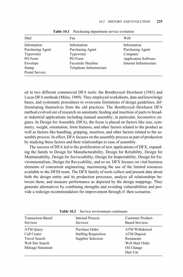
ed in two different commercial DFA tools: the Boothryoyd–Dewhurst (1983) andLucas DFA methods (Miles, 1989). They employed worksheets, data and knowledgebases, and systematic procedures to overcome limitations of design guidelines, dif-ferentiating themselves from the old practices. The Boothryoyd–Dewhurst DFAmethod evolved out of research on automatic feeding and insertion of parts to broad-er industrial applications including manual assembly, in particular, locomotive en-gines. In Design for Assembly (DFA), the focus is placed on factors like size, sym-metry, weight, orientation, form features, and other factors related to the product aswell as factors like handling, gripping, insertion, and other factors related to the as-sembly process. In effect, DFA focuses on the assembly process as part of productionby studying these factors and their relationships to ease of assembly.
The success of DFA led to the proliferation of new applications of DFX, expand-ing the family to Design for Manufacturability, Design for Reliability, Design forMaintainability, Design for Serviceability, Design for Inspectability, Design for En-vironmentalism, Design for Recycability, and so on. DFX focuses on vital businesselements of concurrent engineering, maximizing the use of the limited resourcesavailable to the DFSS team. The DFX family of tools collect and present data aboutboth the design entity and its production processes, analyze all relationships be-tween them, and measure performance as depicted by the design mappings. Theygenerate alternatives by combining strengths and avoiding vulnerabilities and pro-vide a redesign recommendation for improvement through if–then scenarios.
10.2 HISTORY AND EVOLUTION 225
Table 10.1 Purchasing department service evolution
Mail Fax Web
Information Information Information Purchasing Agent Purchasing Agent Purchasing AgentTypewriter Typewriter ComputerPO Form PO Form Application SoftwareEnvelope Facsimile Machine Internet InfrastructureStamp Telephone InfrastructurePostal Service
Table 10.2 Service environment continuum
Transaction-Based Internal Process Customer Product-Services Services Based Services
ATM Query Purchase Order ATM Withdrawal Call Center Staffing Requisition ATM Deposit Travel Search Supplier Selection Restaurant Web Site Search Web Mail Order Mileage Statement Oil Change
Hair Cut
c10.qxd 4/22/2005 9:07 AM Page 225
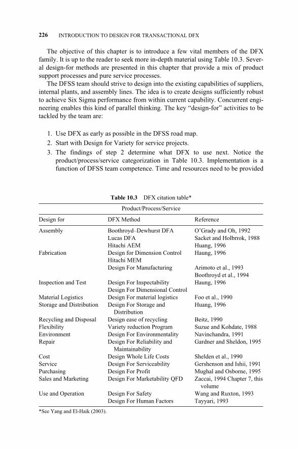
The objective of this chapter is to introduce a few vital members of the DFXfamily. It is up to the reader to seek more in-depth material using Table 10.3. Sever-al design-for methods are presented in this chapter that provide a mix of productsupport processes and pure service processes.
The DFSS team should strive to design into the existing capabilities of suppliers,internal plants, and assembly lines. The idea is to create designs sufficiently robustto achieve Six Sigma performance from within current capability. Concurrent engi-neering enables this kind of parallel thinking. The key “design-for” activities to betackled by the team are:
1. Use DFX as early as possible in the DFSS road map.
2. Start with Design for Variety for service projects.
3. The findings of step 2 determine what DFX to use next. Notice theproduct/process/service categorization in Table 10.3. Implementation is afunction of DFSS team competence. Time and resources need to be provided
226 INTRODUCTION TO DESIGN FOR TRANSACTIONAL DFX
Table 10.3 DFX citation table*
Product/Process/Service
Design for DFX Method Reference
Assembly Boothroyd–Dewhurst DFA O’Grady and Oh, 1992Lucas DFA Sacket and Holbrrok, 1988Hitachi AEM Huang, 1996
Fabrication Design for Dimension Control Haung, 1996Hitachi MEMDesign For Manufacturing Arimoto et al., 1993
Boothroyd et al., 1994Inspection and Test Design For Inspectability Haung, 1996
Design For Dimensional ControlMaterial Logistics Design For material logistics Foo et al., 1990Storage and Distribution Design For Storage and Huang, 1996
DistributionRecycling and Disposal Design ease of recycling Beitz, 1990Flexibility Variety reduction Program Suzue and Kohdate, 1988Environment Design For Environmentality Navinchandra, 1991Repair Design For Reliability and Gardner and Sheldon, 1995
MaintainabilityCost Design Whole Life Costs Shelden et al., 1990Service Design For Serviceability Gershenson and Ishii, 1991Purchasing Design For Profit Mughal and Osborne, 1995Sales and Marketing Design For Marketability QFD Zaccai, 1994 Chapter 7, this
volumeUse and Operation Design For Safety Wang and Ruxton, 1993
Design For Human Factors Tayyari, 1993
*See Yang and El-Haik (2003).
c10.qxd 4/22/2005 9:07 AM Page 226
to carry out the “design-for” activities. Service-specific options from Table10.1 include Design for Life Cycle Cost, Design for Serviceability, Designfor Profit, Design for Marketability, Design for Safety, Design for HumanFactors, Design for Reliability, and Design for Maintainability.
10.3 DESIGN FOR X IN TRANSACTIONAL PROCESSES
The best way to approach DFX for a transactional process is to think of the processand the content as two separate design activities that need to be optimized in unison.The content is normally the application that affects the customer or forms, as in aWeb page, key elements are of data structure and layout. The process is the infra-structure elements that support the content presentation or flow.
An automated teller machine (ATM) is a bank service process. It provides theend user with transactions that rely on a set of subservices, information flow, andhardware performance. The hardware is the ATM machine itself, the telephone sys-tem, the armored security vehicle, the building housing the ATM, and the power de-livery system. In fact if we revisit the IPO diagram introduced in Chapter 2, we candepict this system as shown in Figure 10.1.
The ATM machine and other hardware infrastructure should go through the for-mal DFX for Products process to make them affordable, reliable, and maintainable.Service maintenance for the ATM will include cleaning and restocking forms andmoney. What are some of the considerations for the elements of accessibility andmaterial choices that support the services of cleaning and restocking?
10.3.1 Design for Product Service (DFPS)
The following are the DFPS guidelines, which follow the Eliminate, consoli-date/standardize, and simplify hierarchy:
� Reduce service functional requirements (FRs) by minimizing the need for ser-vice. This can be easily done in companies that track their service warrantiesor activities. The DFSS team has the opportunity to make their DFPS proce-dure data driven by analyzing the possible failure rates of baseline designsand rank them using Pareto analysis to address service requirement in a prior-itized sequence. Use the appropriate DFX family tool such as axiomatic de-sign and robustness techniques to improve the reliability. For example, De-sign for Assembly improves reliability by reducing the number of parts, andAxiom 2 helps reduce design FRs’ variation (Chapter 8), which is a majorcause of failures.
� Identify customer service attributes and appropriate type of service. Type ofservice required by any customer segment is the determinant of the DFPStechnique to be used. There are three types:
Standard operations. Consist of normal wear and tear items like replenishingfunds in an ATM machine. For standard operations, service ease should be
10.3 DESIGN FOR X IN TRANSACTIONAL PROCESSES 227
c10.qxd 4/22/2005 9:07 AM Page 227
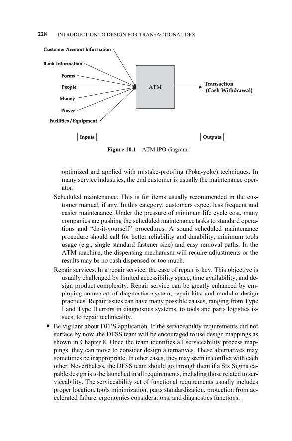
optimized and applied with mistake-proofing (Poka-yoke) techniques. Inmany service industries, the end customer is usually the maintenance oper-ator.
Scheduled maintenance. This is for items usually recommended in the cus-tomer manual, if any. In this category, customers expect less frequent andeasier maintenance. Under the pressure of minimum life cycle cost, manycompanies are pushing the scheduled maintenance tasks to standard opera-tions and “do-it-yourself” procedures. A sound scheduled maintenanceprocedure should call for better reliability and durability, minimum toolsusage (e.g., single standard fastener size) and easy removal paths. In theATM machine, the dispensing mechanism will require adjustments or theresults may be no cash dispensed or too much.
Repair services. In a repair service, the ease of repair is key. This objective isusually challenged by limited accessibility space, time availability, and de-sign product complexity. Repair service can be greatly enhanced by em-ploying some sort of diagnostics system, repair kits, and modular designpractices. Repair issues can have many possible causes, ranging from TypeI and Type II errors in diagnostics systems, to tools and parts logistics is-sues, to repair technicality.
� Be vigilant about DFPS application. If the serviceability requirements did notsurface by now, the DFSS team will be encouraged to use design mappings asshown in Chapter 8. Once the team identifies all serviceability process map-pings, they can move to consider design alternatives. These alternatives maysometimes be inappropriate. In other cases, they may seem in conflict with eachother. Nevertheless, the DFSS team should go through them if a Six Sigma ca-pable design is to be launched in all requirements, including those related to ser-viceability. The serviceability set of functional requirements usually includesproper location, tools minimization, parts standardization, protection from ac-celerated failure, ergonomics considerations, and diagnostics functions.
228 INTRODUCTION TO DESIGN FOR TRANSACTIONAL DFX
Figure 10.1 ATM IPO diagram.
ATM
Inputs Outputs
Customer Account Information
Bank Information
People
Forms
Money
Power
Facilities / Equipment
Transaction(Cash Withdrawal)
ATM
Inputs Outputs
Customer Account Information
Bank Information
People
Forms
Money
Power
Facilities / Equipment
Transaction(Cash Withdrawal)
c10.qxd 4/22/2005 9:07 AM Page 228
The DFSS team should more or less follow the following steps to devise a soundDFPS approach:
� Review assumptions, serviceability customer requirements from the QFD,serviceability types, customer segments, and FMEA and Six Sigma targets.
� Check baseline designs and use the data available as a way to predict their de-sign performance from the historical database. The team should also bench-mark a best-in-class competition to exceed customer satisfaction.
� Identify types of services needed (e.g., standard operation, scheduled mainte-nance, or repair) and map them to appropriate customer segments.
� Understand all applicable service procedures including steps, sequence, andpotential problems. Reference the company’s lessons-learned library and con-trolled documentation.
� Estimate time of labor. Labor time is considered the foundation of service-ability quantification for warranty assessment purposes. Labor time is thesum of repair recognition time, diagnostic time, logistic time, and actual re-pair time. The team should aim to beat the best-in-class labor time.
� Minimize all problematic service areas by reviewing the customer concerntracking system (if any), determining and eliminating root causes, addressingthe problem based on a prioritization scheme (e.g., Pareto analysis of warran-ty cost), searching for solutions in the literature (including core books), andpredicting future trends.
� Determine solution approaches. The extracted information from the gathereddata will lead to some formulation of a serviceability design strategy. Everyseparate component or critical part should be addressed for its unique service-ability requirements.
� Introduce Design for Serviceability parameters into the process mapping.These can be categorized based on the following categories:
Orientation
Do the components have easy removal paths (service process mapping)?
Do the service steps require reorientation?
Contamination
Can the contents, if any, be contained prior to or through service?
What is the possibility of contaminating units during service?
Access
Assembleability. Is it possible to group components for ease of service?Check the mapping.
Is disassembly/sorting intuitive?
Can asymmetrical components fit one way?
Reachability. Can the component be reached by hand? By tool? Can thepart be removed from the assembly?
10.3 DESIGN FOR X IN TRANSACTIONAL PROCESSES 229
c10.qxd 4/22/2005 9:07 AM Page 229
Layerability. Is the part in the assembly layer correlated to frequency ofservice?
“Real estate.” Possibility of moving or sizing parts for service space.
Efficiency. Unnecessary removal of parts that obstruct visibility or service.
Diagnostics. Can the part be accessed for diagnostics without disassembly?
Service reliability. Address potential damage of serviced or removed parts.Are all possibilities for parts minimization using DFMA exhausted?
Consider use of standard parts (e.g., fasteners).
Simplicity
Customer considerations
Tools. Design for generic tools.
Minimize special tools use.
Adjustment. Reduce customer intervention through tuning and adjust-ment. Use robustness techniques.
Mistake-proofing or Poka-yoke. Use color codes and very clear instruc-tions.
For DFS, the ideal final result from a TRIZ perspective is to design the prod-uct/process for serviceability without additional cost. In reality, an incremental costis usually needed. To decide on a budget allocation for service elements, some eco-nomic consideration is needed. If the defects per million is 10, it makes no sense toadd 2¢ to a $1 part as incremental repair cost. In addition to the economic matters,the cost of losing a customer and those potential customers that the lost customercan influence must be considered.
10.4 DESIGN FOR PROCESSABILITY3 AND ASSEMBLY
Design for Assembly (DFA) may be applied to an individual assembly or for awhole complex product like a vehicle (Sackett & Holbrook, 1990). In the lattercase, a number of distinct areas can be coordinated to reflect the functional andprocess mappings discussed in Chapter 8, leading to the optimization of the wholeproduct from the assembly and processability points of view. In doing so, interfacesand trade-off decisions are required if design conceptual vulnerabilities such ascoupling and complexity were not resolved earlier. Therefore, linkages betweenteams handling several assemblies must be defined in terms of design mapping toensure that everyone is operating in a coherent way.
Design for Processability (DFP) can be defined as designing a product to be pro-duced in the most efficient manner possible in terms of time, money, and resources,taking into consideration how the product or service will be processed and utilizingthe existing skill base to achieve the highest rolled-throughput yield possible. DFP
230 INTRODUCTION TO DESIGN FOR TRANSACTIONAL DFX
3Processability is used here in lieu of manufacturability. This section has strong linkages to product de-sign because it assumes that designing is a process for a product (as a service design) on one hand, aswell as highlighting overlaps where service is the ultimate end product.
c10.qxd 4/22/2005 9:07 AM Page 230
and DFA are proven design methodologies that work for any size company. Toshorten development cycle time, the early consideration of processability implica-tions minimizes development cost and ensures a smooth launch of production. DFPpromotes and ensures processability of product designs. By bridging the gap be-tween design and process, DFP can significantly reduce critical time to market.DFSS quality themes can be designed early on with optimal parts selection and prop-er integration of parts for minimum vulnerabilities. By considering the cumulativeeffect of part quality on overall product quality, designers are encouraged to careful-ly specify quality.
DFP and DFA are systematic approaches within the DFX family that the DFSSteam can use to carefully analyze each high-level design parameter that can be de-fined as a part or subassembly for manual or automated processability and assem-bly. The objective is to eliminate design waste. Waste, or “muda” in Japanese, maymean any of several things. It may mean features that have no function (are non-value added) and those that should have been trimmed using the mapping methodsof Chapter 8. But the most leverage of DFX in the DFSS road map is in attackingthe following waste sources: (1) assembly directions that need several additionaloperations and (2) design parameters with unnecessarily tight tolerances.
It is a golden rule of design that the DFSS team should minimize the number ofsetups and stages through which a part or subassembly must pass through before itbecomes a physical entity within a connected whole.
As a prerequisite for DFP, the team needs to understand through experience inproduction how services are manufactured. Specifically, the process design shouldparallel the product development in a concurrent engineering setup. Developing andfostering a multifunctional team with early and active participation from purchas-ing, process design, finance, industrial engineering, vendors, marketing, compli-ance specialists, and factory workers assures a good DFP output. One of the firstdecisions the team has to make concerns the optimal use of off-the-shelf parts. Inmany cases, the product may have to literally be designed around the off-the-shelfcomponents, but this can provide substantial benefits to the design.
Before using the DFA and DFP tools, the team should:
� Revisit the design mappings (Chapters 6 and 8) of the DFSS road map as wellas the marketing strategy. The team should be aware that the DFSS road mapas a design strategy is global and that the process strategy is usually local, de-pending on the already existing process facilities.
� Review market analysis, customer attributes, the critical-to-satisfaction char-acteristics (CTSs), and other requirements like packaging and maintenance.Where clarification is sought, the team may develop necessary prototypes,models, experiments, and simulations to minimize risks. In doing so, the teamshould take advantage of available specifications, testing, cost–benefit analy-sis, and modeling to build the design.
� Analyze existing processability and assembly functional requirements, opera-tions, and sequences concurrently, using simulation tools to examine assem-bly and subassembly definitions of the product and service and find the bestorganization and production methods.
10.4 DESIGN FOR PROCESSABILITY AND ASSEMBLY 231
c10.qxd 4/22/2005 9:07 AM Page 231
� Specify optimal tolerances (see Yang and El-Haik, 2003 and El-Haik, 2005)with the use of robust design. Understand tolerance step functions and specifytolerances wisely. Each process has its practical limit as to how tight a toler-ance could be specified for a given skill level in a production process. If thetolerance is tighter than the limit, the next most precise process must be used.Design within current process capabilities. Avoid unnecessarily tight toler-ances that are beyond the capability of the processes. Through design map-pings, determine when new production process capabilities are needed early,to allow sufficient time to determine optimal process variables and establish acontrolled process. For products, avoid tight tolerances on multiple stackedparts. Tolerances on such parts will “stack up,” making maintenance of over-all tolerance difficult.
� Use the most appropriate rather than the latest technology in the processesidentified in the process mappings (see Chapter 8).
� Design for the minimum number of parts by physical integration. Simplifythe design and reduce the number of parts because for each part, there are op-portunities for process defects and assembly errors. The total cost of fabricat-ing and assembling a product goes up with the increased number of parts. Au-tomation becomes more difficult and more expensive when more parts arehandled and processed. Costs related to purchasing, stocking, and servicingalso go down as the number of parts are reduced. Inventory and work-in-process levels will go down with fewer parts. The team should go through theassembly part by part and evaluate whether a part can be eliminated, com-bined with another part, or the function can be performed in another way. Todetermine the theoretical minimum number of parts, ask the following: Doesthe part move relative to all other moving parts? Must the part absolutely beof a different material from the other parts? Must the part be different to allowpossible disassembly? Avoid designing mirror image (right- or left-hand)parts. Design the product so the same part can function in both right- and left-hand modes. If identical parts cannot perform both functions, add features toboth right- and left-hand parts to make them the same.
� Create “modular” designs using standard parts to build components and sub-assemblies. Standard and off-the-shelf parts are less expensive, consideringthe cost of design, documentation, prototyping, testing, overhead, and non-core-competency processabilities. Standard parts save the time that would beneeded to design, document, administer, build, test, and fix prototype parts.
� Choose the appropriate materials for fabrication ease.
� Apply the layered assembly principles to parts handling and feeding, orienta-tion, identification, positioning, allowable tolerances, and mating.
� Minimize setups. For machined parts, ensure accuracy by designing parts andfixtures so that all key dimensions are cut in the same setup. Use less expen-sive single-setup machining.
� Fixture design considerations. The team needs to understand the processabili-ties well enough to be able to design parts and dimension them for fixtures.
232 INTRODUCTION TO DESIGN FOR TRANSACTIONAL DFX
c10.qxd 4/22/2005 9:07 AM Page 232
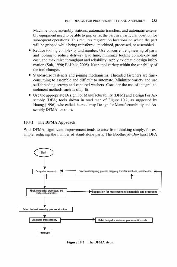
Machine tools, assembly stations, automatic transfers, and automatic assem-bly equipment need to be able to grip or fix the part in a particular position forsubsequent operations. This requires registration locations on which the partwill be gripped while being transferred, machined, processed, or assembled.
� Reduce tooling complexity and number. Use concurrent engineering of partsand tooling to reduce delivery lead time, minimize tooling complexity andcost, and maximize throughput and reliability. Apply axiomatic design infor-mation (Suh, 1990; El-Haik, 2005). Keep tool variety within the capability ofthe tool changer.
� Standardize fasteners and joining mechanisms. Threaded fasteners are time-consuming to assemble and difficult to automate. Minimize variety and useself-threading screws and captured washers. Consider the use of integral at-tachment methods such as snap-fit.
� Use the appropriate Design For Manufacturability (DFM) and Design For As-sembly (DFA) tools shown in road map of Figure 10.2, as suggested byHuang (1996), who called the road map Design for Manufacturability and As-sembly DFMA for short.
10.4.1 The DFMA Approach
With DFMA, significant improvement tends to arise from thinking simply, for ex-ample, reducing the number of stand-alone parts. The Boothroyd–Dewhurst DFA
10.4 DESIGN FOR PROCESSABILITY AND ASSEMBLY 233
Figure 10.2 The DFMA steps.
Start
Design for assembly
Finalize material, processes, andearly cost estimates
Select the best assembly process structure
Prototype
Detail design for minimum processability costs
Functional mapping, process mapping, transfer functions, specifi
Suggestion for more economic materials and processes
Design for processability
cation
c10.qxd 4/22/2005 9:07 AM Page 233
methodology provides the following three criteria against which each part must beexamined as it is added to the assembly (Huang, 1996):
1. During operation of the product, does the part move relative to all other partsalready assembled?
2. Must the part be of different material than, or be isolated from, all other partsalready assembled? Only fundamental reasons concerned with material prop-erties are acceptable.
3. Must the part be separate from all other parts already assembled because thenecessary assembly or disassembly of other separate parts would otherwisebe impossible?
A “yes” answer to any of these questions indicates that the part must be separateor is, using DFA terminology, a critical part. All other parts, those which are notcritical, can theoretically be removed or physically coupled with other critical parts.Therefore, theoretically, the number of critical parts is the minimum number of sep-arate assemblies of the design. Next, the DFSS team estimates the assembly timefor the design and establishes its efficiency rating in terms of assembly difficulty.This task can be done when each part is checked for how it will be grasped, orient-ed, and inserted into the product. From this exercise, the design is rated and fromthis rating standard times are determined for all operations necessary to assemblethe part. The DFA time standard is a classification of design features that affect theassembly process. The total assembly time can then be assessed and, using standardlabor rates, the assembly cost and efficiency can be estimated. At this stage,processability costs are not considered, but assembly time and efficiency providebenchmarks for new iterations. After all feasible simplification tasks are intro-duced, the next step is to analyze the manufacture of the individual parts. The ob-jective of DFM within the DFMA structured process is to enable the DFSS team toweigh alternatives, assess processability cost, and decide between physical integra-tion into assemblies and increased processability cost. The DFM approach providesexperimental data for estimating the cost of many processes. The team should de-sign for ease of assembly by utilizing simple patterns of movement and minimizingthe axes of assembly (Crew, 1998). To reduce defective parts, features such aschamfers and tapers may be provided. In addition, parts must be designed to consis-tently orient themselves when fed into a process. The product’s design should en-able assembly to begin with a base component with a large relative mass and a lowcenter of gravity upon which other parts are added. Assembly should proceed verti-cally, with other parts added on top and positioned with the aid of gravity. This willminimize the need for both reorientation and temporary fastening. Assembly that isautomated will be more uniform, more reliable, and of a higher quality. Crew(1998) lists the following basic principles to facilitate parts handling and orienta-tion:
� Product design must avoid parts that can become tangled, wedged, or disori-ented. Avoid holes and tabs and “closed” parts. This type of design will allow
234 INTRODUCTION TO DESIGN FOR TRANSACTIONAL DFX
c10.qxd 4/22/2005 9:07 AM Page 234
the use of automation devices in parts handling and assembly such as vibrato-ry bowls, tubes, magazines, etc.
� Part design should incorporate symmetry around both axes of insertion wher-ever possible. Where parts cannot be symmetrical, the asymmetry should beemphasized to assure correct insertion or easily identifiable features shouldbe provided.
� With hidden features that require a particular orientation, provide an externalfeature or guide surface to correctly orient the part.
� Guide surfaces should be provided to facilitate insertion.
� Parts should be designed with surfaces so that they can be easily grasped,placed, and fixed. Ideally this means flat, parallel surfaces that would allow apart to be picked up by a person or a gripper with a pick-and-place robot andthen easily fixed.
� Minimize thin, flat parts that are more difficult to pick up. Avoid very smallparts that are difficult to pick up or require a tool such as a tweezer to bepicked up, which would increase handling and orientation time.
� Avoid parts with sharp edges, burrs, or points. These parts can injure workersor customers, and they require more careful handling. They can damage prod-uct finishes and they may be more susceptible to damage themselves if thesharp edge is an intended feature.
� Avoid parts that can be easily damaged or broken.
� Avoid parts that are sticky or slippery (thin, oily plates, oily parts, adhesive-backed parts, small plastic parts with smooth surfaces, etc.).
� Avoid heavy parts that will increase worker fatigue, increase risk of workerinjury, and slow the assembly process.
� Design the workstation area to minimize the distance to access and move apart.
� When purchasing components, consider acquiring materials already orientedin magazines, bands, tape, or strips.
The DFMA approach usually benefits from Poka-yoke techniques, which maybe applied when components are taking form and processability and assembly is-sues are simultaneously considered. Poka-yoke is a technique for avoiding humanerror at work. The Japanese manufacturing engineer Shigeo Shingo developed thetechnique to achieve zero defects and came up with this term, which means, “mis-take proofing.” A defect exists in either one of two states: it has already occurred,calling for defect detection, or is about to occur, calling for defect prediction. Thethree basic functions of Poka-yoke used against defects are shutdown, control, andwarning. The technique consists of steps for analyzing the process for potentialproblems; identifying parts by the characteristics of dimension, shape, and weight;and detecting processes deviations from nominal procedure standards. Parts shouldbe designed so that they can be assembled by one method only. Asymmetricalholes, notches, and stops can be used to mistake-proof the assembly process.
10.4 DESIGN FOR PROCESSABILITY AND ASSEMBLY 235
c10.qxd 4/22/2005 9:07 AM Page 235
10.5 DESIGN FOR TESTABILITY AND INSPECTABILITY
Testability is the methodology of design, execution, and optimization of the actionsnecessary and sufficient for test and diagnosis so that those are financially mostprofitable in terms of cost and accuracy. The concept of testability can imply theability to change the means of a design functional requirement and the ability tomake visible the state of such functional requirement. Test and inspection processesusually consume a significant part of the effort and cost of development, in additionto the cost and time for the acquisition of test equipment, which may be consider-able. Inspectability and testability is a design requirement for continuous, rapid, andsafe functionality. Testability and inspectability provide control feedback for designprocesses for validation and corrective actions. Early participation of testing per-sonnel in the DFSS team will lead to design choices that can minimize the cost oftestability and inspectability at the various stages of life cycle. A common under-standing between team members is needed relative to the requirements for designverification and validation, acceptance after first time through production, as wellas field diagnosis for defect identification. Literature on testability in electroniccomponents exists and more common applications are now available (Drury, 1992).For example, a special color array is available for printers to ensure that all speci-fied colors are printed on a stamp for ease of Post Office automatic inspectability.As another example, fluid containers used in cars are made from transparent materi-als to show the fluid levels in the container (e.g., coolant and washer fluid). Today,all computers have testing capabilities booted using the Power-On Self-Test(POST) that conducts functional inspection of several functionalities and subsys-tems, informs the user of any failures, and provides suggestion for corrective ac-tions at the user’s disposal. Another example comes from aerospace. Built-in Test-ing Equipment (BITE) is a means for evaluating functional requirements withoutdisassembling parts, a concept similar to POST in computers. The BITE system im-proves accuracy and precision of the inspection function while saving time and,therefore, reducing cost.
The participation of testing personnel is required at Stage 1 of the DFSS roadmap to define test requirements and design the test procedures. The design, pur-chase or outsourcing of testing equipment and procedures can be done in parallelwith design developmental activities. The understanding of design requirementswill help the team in specifying the testing specification in terms of test require-ments, equipment cost and utilization, and standard testing operating procedures.Testability and inspectability are usually justified by higher production rates andstandardized test methods.
To deliver on testability and inspectability functions, several design rules may belisted in this context. The specification of design parameters and their tolerancesshould be within the natural capabilities of the production process, with process ca-pability indices that reflect Six Sigma capability. Like Design for Serviceability(DFS), sufficient “real estate” to support test points, connections, and built-in testcapabilities needs to be provided. Standard test equipment with automation compat-ibility to reduce setup effort, time, and cost is recommended. A built-in test and di-
236 INTRODUCTION TO DESIGN FOR TRANSACTIONAL DFX
c10.qxd 4/22/2005 9:07 AM Page 236
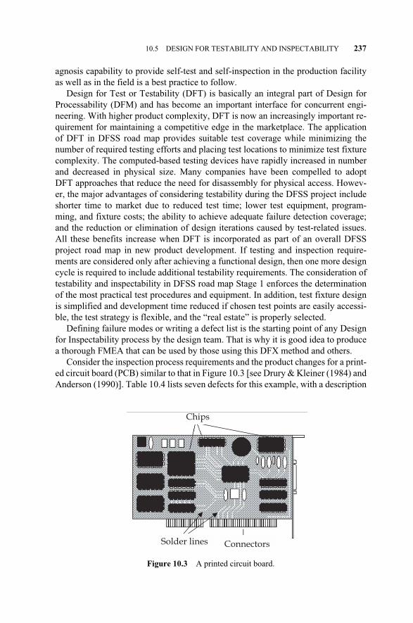
agnosis capability to provide self-test and self-inspection in the production facilityas well as in the field is a best practice to follow.
Design for Test or Testability (DFT) is basically an integral part of Design forProcessability (DFM) and has become an important interface for concurrent engi-neering. With higher product complexity, DFT is now an increasingly important re-quirement for maintaining a competitive edge in the marketplace. The applicationof DFT in DFSS road map provides suitable test coverage while minimizing thenumber of required testing efforts and placing test locations to minimize test fixturecomplexity. The computed-based testing devices have rapidly increased in numberand decreased in physical size. Many companies have been compelled to adoptDFT approaches that reduce the need for disassembly for physical access. Howev-er, the major advantages of considering testability during the DFSS project includeshorter time to market due to reduced test time; lower test equipment, program-ming, and fixture costs; the ability to achieve adequate failure detection coverage;and the reduction or elimination of design iterations caused by test-related issues.All these benefits increase when DFT is incorporated as part of an overall DFSSproject road map in new product development. If testing and inspection require-ments are considered only after achieving a functional design, then one more designcycle is required to include additional testability requirements. The consideration oftestability and inspectability in DFSS road map Stage 1 enforces the determinationof the most practical test procedures and equipment. In addition, test fixture designis simplified and development time reduced if chosen test points are easily accessi-ble, the test strategy is flexible, and the “real estate” is properly selected.
Defining failure modes or writing a defect list is the starting point of any Designfor Inspectability process by the design team. That is why it is good idea to producea thorough FMEA that can be used by those using this DFX method and others.
Consider the inspection process requirements and the product changes for a print-ed circuit board (PCB) similar to that in Figure 10.3 [see Drury & Kleiner (1984) andAnderson (1990)]. Table 10.4 lists seven defects for this example, with a description
10.5 DESIGN FOR TESTABILITY AND INSPECTABILITY 237
Figure 10.3 A printed circuit board.
Chips
ConnectorsSolder lines
c10.qxd 4/22/2005 9:07 AM Page 237
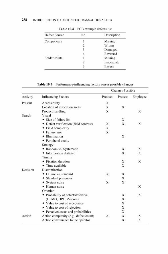
238 INTRODUCTION TO DESIGN FOR TRANSACTIONAL DFX
Table 10.4 PCB example defects list
Defect Source No. Description
Components 1 Missing2 Wrong3 Damaged4 Reversed
Solder Joints 1 Missing2 Inadequate3 Excess
Table 10.5 Performance-influencing factors versus possible changes
Changes Possible
Activity Influencing Factors Product Process Employee
Present Accessibility XLocation of inspection areas X XProduct handling X X
Search Visual� Size of failure list X� Defect verification (field contrast) X X X� Field complexity X� Failure size X� Illumination X� Peripheral acuityStrategy� Random vs. Systematic X X� Interfixation distance X XTiming� Fixation duration X X� Time available X
Decision Discrimination� Failure vs. standard X X� Standard presences X� System noise X X� Human noise XCriterion� Probability of defect/defective X X
(DPMO, DPO, Z-score) X� Value to cost of acceptance X� Value to cost of rejection X� Perceived costs and probabilities X
Action Action complexity (e.g., defect count) X X XAction convenience to the operator X X
c10.qxd 4/22/2005 9:07 AM Page 238
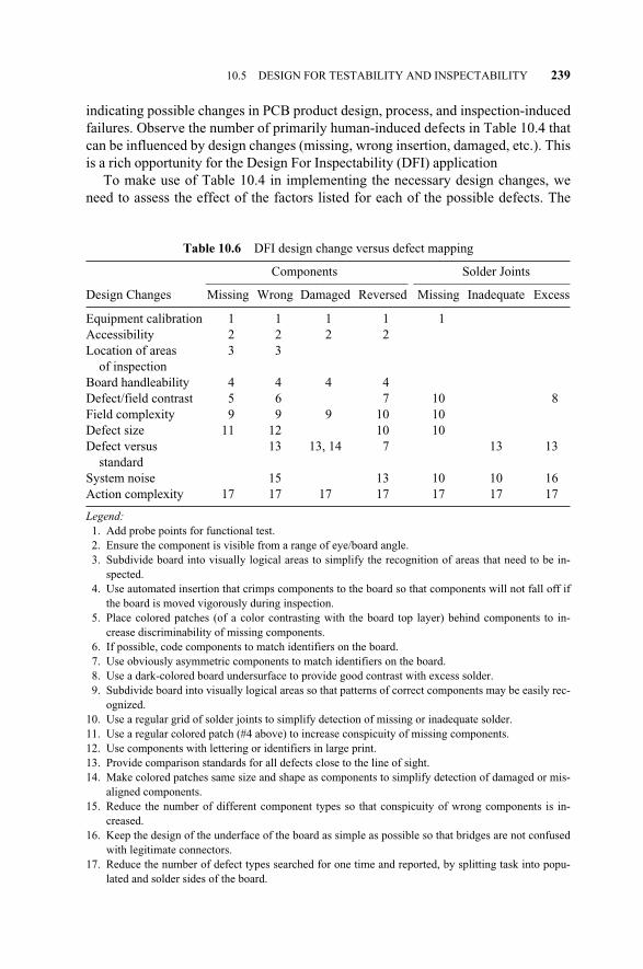
indicating possible changes in PCB product design, process, and inspection-inducedfailures. Observe the number of primarily human-induced defects in Table 10.4 thatcan be influenced by design changes (missing, wrong insertion, damaged, etc.). Thisis a rich opportunity for the Design For Inspectability (DFI) application
To make use of Table 10.4 in implementing the necessary design changes, weneed to assess the effect of the factors listed for each of the possible defects. The
10.5 DESIGN FOR TESTABILITY AND INSPECTABILITY 239
Table 10.6 DFI design change versus defect mapping
Components Solder Joints_______________________________ ________________________
Design Changes Missing Wrong Damaged Reversed Missing Inadequate Excess
Equipment calibration 1 1 1 1 1Accessibility 2 2 2 2Location of areas 3 3
of inspectionBoard handleability 4 4 4 4Defect/field contrast 5 6 7 10 8Field complexity 9 9 9 10 10Defect size 11 12 10 10Defect versus 13 13, 14 7 13 13
standardSystem noise 15 13 10 10 16Action complexity 17 17 17 17 17 17 17
Legend:1. Add probe points for functional test.2. Ensure the component is visible from a range of eye/board angle.3. Subdivide board into visually logical areas to simplify the recognition of areas that need to be in-
spected.4. Use automated insertion that crimps components to the board so that components will not fall off if
the board is moved vigorously during inspection.5. Place colored patches (of a color contrasting with the board top layer) behind components to in-
crease discriminability of missing components.6. If possible, code components to match identifiers on the board.7. Use obviously asymmetric components to match identifiers on the board.8. Use a dark-colored board undersurface to provide good contrast with excess solder.9. Subdivide board into visually logical areas so that patterns of correct components may be easily rec-
ognized.10. Use a regular grid of solder joints to simplify detection of missing or inadequate solder.11. Use a regular colored patch (#4 above) to increase conspicuity of missing components.12. Use components with lettering or identifiers in large print.13. Provide comparison standards for all defects close to the line of sight.14. Make colored patches same size and shape as components to simplify detection of damaged or mis-
aligned components.15. Reduce the number of different component types so that conspicuity of wrong components is in-
creased.16. Keep the design of the underface of the board as simple as possible so that bridges are not confused
with legitimate connectors.17. Reduce the number of defect types searched for one time and reported, by splitting task into popu-
lated and solder sides of the board.
c10.qxd 4/22/2005 9:07 AM Page 239
PCB design team needs to produce a mapping depicting the relationship betweenperformance-influencing factors and the list of failures and defects as given inTable 10.5. Notice that Table 10.5 includes both functional failures and potentialfailures found by visual inspection.
At this point, the team is ready to search for solutions to defects listed in Table10.5 by making changes to the design requirements, including inspection. An objec-tive is error-proof inspection (Drury and Kleiner, 1992). Product design changes arethe core of DFI. Using this fact allows the design team to produce a mapping relat-ing the design changes and the defects listed in Table 10.5. This is given in Table10.6.
A DFI change is numbered as in Table 10.6 and defined. For example, the De-sign for Inspectability change No. 1 in Table 10.5 is the change referring to addingprobe points for functional testing, whereas the change No. 7 refers to the use of ob-viously asymmetric parts for defect reversal. Notice that Table 10.6 lists inspectiondesign changes and includes both functional failures (design and testing) and poten-tial visual inspection defects. It also possible to add process and operator changeseven in this simple example. For example, lighting changes are part of inspectionprocess improvement (Drury, 1992), and employee selection (Thackray, 1994) , au-tomation (Drury, 1994), and training (Kleiner and Drury, 1993) are other improve-ments sources. A summary of this example can be found in Huang (1996).
10.6 SUMMARY
This chapter introduces the concept of DFX as it relates to service transactions andbuilds from the work performed for product environments. Regardless of the envi-ronment, product or service, the concurrent design team needs to step back and as-sess the solution chosen from the perspective of the voice of the customer for lifecycle performance. DFX for service transactions requires the process content to beevaluated much in the same light as assembly processes to minimize complexityand maximize commonality. The service process is also dependent on infrastructuresupport that should be processed through the DFX for products methodology. Theend result will be a robust design that meets customer’s needs profitably.
240 INTRODUCTION TO DESIGN FOR TRANSACTIONAL DFX
c10.qxd 4/22/2005 9:07 AM Page 240
11.1 INTRODUCTION
Failure made and effect analysis (FMEA) is a disciplined procedure that recognizesand evaluates the potential and actual effects of failure of a product or a process andidentifies actions that reduce the chance of a potential failure occurring (Yang & El-Haik, 2003). It helps the DFSS team members improve their design and its deliveryprocesses by asking “what can go wrong?” and “where can variation come from?”Service design and production, delivery, and other processes are then revised toprevent occurrence of failure modes and to reduce variation. Inputs to FMEA in-clude past warranty or process experience, if any; customer wants, needs, and de-lights; performance requirements; drawings and specifications; and process map-pings. For each service functional requirement and process the team needs to ask,“what can go wrong?” and determine possible design and process failure modes andsources of potential variation in all service processes under consideration, includingvariations in customer usage, potential causes of failure over useful life, and poten-tial process issues such as missed tags or steps, shipping concerns, and service mis-diagnosis. The team should modify the service design and processes to preventwrong things from happening and develop strategies to deal with different situa-tions, the redesign of processes to reduce variation, and mistake-proofing (Poka-yoke) of services and processes. Efforts to anticipate failure modes and sources ofvariation are iterative. This action continues as the team strives to further improvetheir service design and its processes.
FMEA is a team activity, with representation from project personnel involvedwith quality, reliability, and operations, and suppliers and customers if possible. ASix Sigma operative, typically a black or green belt, leads the team. The processowner should own the documentation.
The design team may experience several FMEA types in the DFSS road map(see Chapter 5). They are:
Service Design for Six Sigma. By Basem El-Haik and David M. Roy 241© 2005 by John Wiley & Sons.
11FAILURE MODE AND EFFECT ANALYSIS (FMEA)
c11.qxd 4/22/2005 9:08 AM Page 241
� Concept FMEA. Used to analyze systems and subsystems in the early conceptand design stages. Focuses on potential failure modes associated with thefunctions of a system caused by the design.
Design FMEA (DFMEA). Used to analyze product/service designs beforethey are released to production. A DFMEA should always be completedwell in advance of a prototype/pilot build. Focuses on design functionalrequirement. It has a hierarchy that parallels the modular structure interms of systems, subsystems, and components.
Process FMEA: It is used to analyze processing, assembly, or any otherprocesses. The focus is on process inputs. It has a hierarchy that paral-lels the modular structure in terms of systems, subsystems, and compo-nents.
� Project FMEA. Documents and addresses failures that could happen during amajor program.
� Software FMEA. Documents and addresses failure modes associated withsoftware functions.
We suggest using concept FMEA to analyze services and process designs in theearly concept and design stages (see Figure 5.1). It focuses on potential failuremodes associated with the functions of a system caused by the design. The conceptFMEA helps the DFSS team to review targets for the functional requirements(FRs), to select optimum physical maps with minimum vulnerabilities, to identifypreliminary testing requirements, and to determine if redundancy is required for re-liability target settings. The input to DFMEA is the array of functional requirementsthat is obtained from the quality function deployment phases presented in Chapter7. The outputs are (1) list of actions to prevent causes or to detect failure modes,and (2) history of actions taken and future activity. The DFMEA helps the DFSSteam in:
1. Estimating the effects on all customer segments,
2. Assessing and selecting design alternatives
3. Developing an efficient validation phase within the DFSS algorithm
4. Inputting the needed information for Design for X (e.g., Design for Manufac-turability, Design for Assembly, Design for Reliability, Design for Service-ability, Design for Environment)
5. Prioritizing the list of corrective action strategies that include mitigating,transferring, ignoring, or preventing the failure modes altogether,
6. Identifying the potential special design parameters from the failure stand-point, and documenting the findings for future reference
Software FMEA documents and addresses failure modes associated with soft-ware functions. On the other hand, process FMEA (PFMEA) is used to analyze ser-vice, manufacturing, assembly, or any other processes such as those encountered in
242 FAILURE MODE AND EFFECT ANALYSIS (FMEA)
c11.qxd 4/22/2005 9:08 AM Page 242
transactional business processes. The focus is on process inputs. The PFMEA is avaluable tool available to the concurrent DFSS team to help them in identifying po-tential manufacturing/assembly or production process causes in order to place con-trols for either increasing detection or reducing occurrence, or both, thus prioritiz-ing the list of corrective actions. Strategies include mitigating, transferring,ignoring, or preventing the failure modes, documenting the results of their process-es, and identifying the potential special process variables that need special controlsfrom the failure standpoint.
11.2 FMEA FUNDAMENTALS
FMEA can be described as being complementary to the process of defining what adesign or process must do to satisfy the customer (AIAG, 2001). In our case, theprocess of defining what a design or a process must do to satisfy the customer iswhat we do in the service DFSS project road map discussed in Chapter 5. TheDFSS team may use an existing FMEA, if applicable, for further enhancement andupdating. In all cases, the FMEA should be handled as a living document.
The fundamentals of FMEA inputs, regardless of their type, are depicted in Fig-ure 11.1 and the listed below:
1. Define scope, service functional requirements, and design parameters andprocess steps. For the DFSS team, this input column can be easily extractedfrom the functional and process mappings discussed in Chapter 8. However,we suggest doing the FMEA exercise for the revealed design hierarchy re-sulting from the employment of mapping techniques of their choice. At thispoint, it may be useful to revisit the project scope boundary as input to theFMEA of interest in terms of what is included and excluded. In DFMEA,for example, potential failure modes include the delivery of “No” FR, par-tial and degraded FR delivery over time, intermittent FR delivery, and unin-tended FR (not intended in the mapping).
2. Identify potential failure modes. Failure modes indicate the loss of at leastone FR. The DFSS team should identify all potential failure modes by ask-ing, “In what way will the design fail to deliver its FRs?” as identified in themapping. Failure modes are generally categorized as materials, environ-ment, people, equipment, methods, and so on, and have a hierarchy of theirown. That is, a potential failure mode can be cause or effect in a higher-lev-el subsystem causing failure in its FRs. A failure mode may occur but notnecessarily must occur. Potential failure modes may be studied from thebaseline of past and current data, tests, and current baseline FMEAs.
3. Potential failure effects(s). A potential effect is the consequence of the fail-ure of other physical entities as experienced by the customer.
4. Severity. Severity is a subjective measure of “how bad” or “serious” is theeffect of the failure mode. Usually, severity is rated on a discrete scale from
11.2 FMEA FUNDAMENTALS 243
c11.qxd 4/22/2005 9:08 AM Page 243
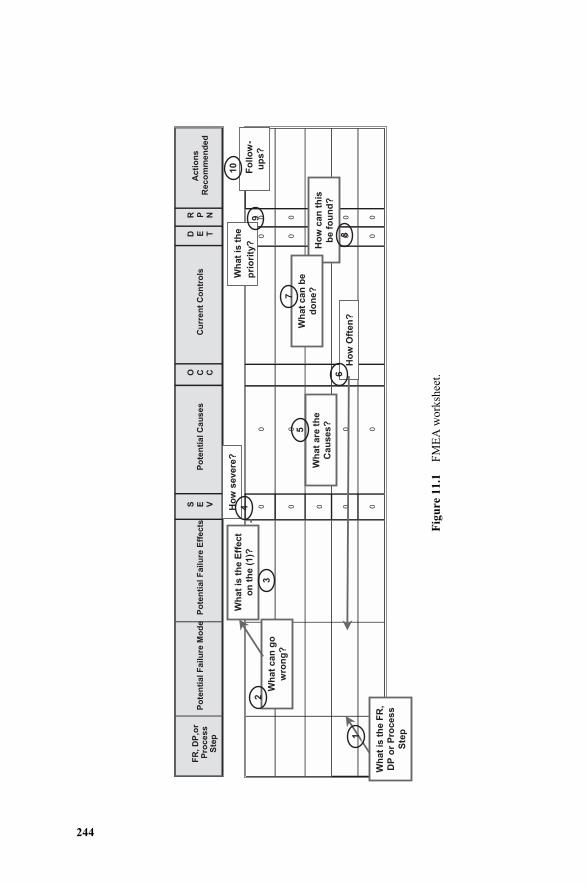
244
Fig
ure
11.1
FM
EA
wor
kshe
et.
FR
, D
P,o
r P
roc
ess
Ste
p
Po
ten
tial
Fa
ilu
re M
od
eP
ote
nti
al
Fail
ure
Eff
ects
S E VP
ote
nti
al C
au
se
sO C C
Cu
rre
nt
Co
ntr
ols
D E T
R P N
Ac
tio
ns
R
ec
om
me
nd
ed
FR
, D
P,o
r P
roc
ess
Ste
p
Po
ten
tial
Fa
ilu
re M
od
eP
ote
nti
al
Fail
ure
Eff
ects
S E VP
ote
nti
al C
au
se
sO C C
Cu
rre
nt
Co
ntr
ols
D E T
R P N
Ac
tio
ns
R
ec
om
me
nd
ed
00
00
00
00
00
00
00
00
00
00
Wh
at
is t
he F
R,
DP
or
Pro
cess
Ste
p
Wh
at
can
go
wro
ng
?
Wh
at
is t
he E
ffect
on
th
e (
1)?
Wh
at
are
th
e
Cau
ses?
Ho
w s
evere
?
Ho
w O
fte
n?
Ho
w c
an
th
is
be f
ou
nd
?
Fo
llo
w-
up
s?
Wh
at
can
be
do
ne
?
1
23
4
5
6
7
8
10
Wat
isth
e
pri
ori
ty?
h
9
c11.qxd 4/22/2005 9:08 AM Page 244
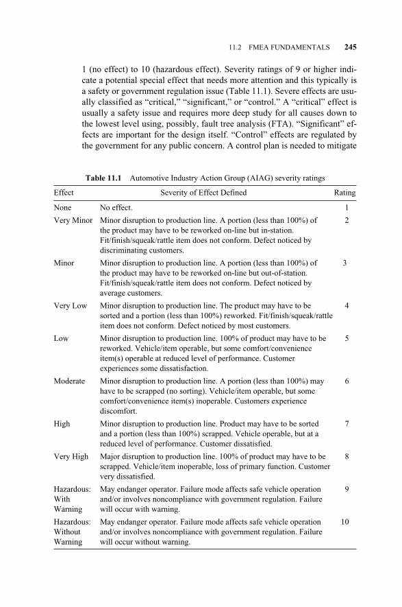
1 (no effect) to 10 (hazardous effect). Severity ratings of 9 or higher indi-cate a potential special effect that needs more attention and this typically isa safety or government regulation issue (Table 11.1). Severe effects are usu-ally classified as “critical,” “significant,” or “control.” A “critical” effect isusually a safety issue and requires more deep study for all causes down tothe lowest level using, possibly, fault tree analysis (FTA). “Significant” ef-fects are important for the design itself. “Control” effects are regulated bythe government for any public concern. A control plan is needed to mitigate
11.2 FMEA FUNDAMENTALS 245
Table 11.1 Automotive Industry Action Group (AIAG) severity ratings
Effect Severity of Effect Defined Rating
None No effect. 1
Very Minor Minor disruption to production line. A portion (less than 100%) of 2the product may have to be reworked on-line but in-station.Fit/finish/squeak/rattle item does not conform. Defect noticed by discriminating customers.
Minor Minor disruption to production line. A portion (less than 100%) of 3the product may have to be reworked on-line but out-of-station.Fit/finish/squeak/rattle item does not conform. Defect noticed by average customers.
Very Low Minor disruption to production line. The product may have to be 4sorted and a portion (less than 100%) reworked. Fit/finish/squeak/rattle item does not conform. Defect noticed by most customers.
Low Minor disruption to production line. 100% of product may have to be 5reworked. Vehicle/item operable, but some comfort/convenience item(s) operable at reduced level of performance. Customer experiences some dissatisfaction.
Moderate Minor disruption to production line. A portion (less than 100%) may 6have to be scrapped (no sorting). Vehicle/item operable, but somecomfort/convenience item(s) inoperable. Customers experience discomfort.
High Minor disruption to production line. Product may have to be sorted 7and a portion (less than 100%) scrapped. Vehicle operable, but at a reduced level of performance. Customer dissatisfied.
Very High Major disruption to production line. 100% of product may have to be 8scrapped. Vehicle/item inoperable, loss of primary function. Customer very dissatisfied.
Hazardous: May endanger operator. Failure mode affects safe vehicle operation 9With and/or involves noncompliance with government regulation. Failure Warning will occur with warning.
Hazardous: May endanger operator. Failure mode affects safe vehicle operation 10Without and/or involves noncompliance with government regulation. Failure Warning will occur without warning.
c11.qxd 4/22/2005 9:08 AM Page 245
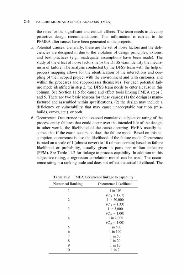
the risks for the significant and critical effects. The team needs to developproactive design recommendations. This information is carried to thePFMEA after causes have been generated in the projects.
5. Potential Causes. Generally, these are the set of noise factors and the defi-ciencies are designed in due to the violation of design principles, axioms,and best practices (e.g., inadequate assumptions have been made). Thestudy of the effect of noise factors helps the DFSS team identify the mecha-nism of failure. The analysis conducted by the DFSS team with the help ofprocess mapping allows for the identification of the interactions and cou-pling of their scoped project with the environment and with customer, andwithin the processes and subprocesses themselves. For each potential fail-ure mode identified in step 2, the DFSS team needs to enter a cause in thiscolumn. See Section 11.5 for cause and effect tools linking FMEA steps 3and 5. There are two basic reasons for these causes: (1) the design is manu-factured and assembled within specifications, (2) the design may include adeficiency or vulnerability that may cause unacceptable variation (mis-builds, errors, etc.), or both.
6. Occurrence. Occurrence is the assessed cumulative subjective rating of theprocess entity failures that could occur over the intended life of the design,in other words, the likelihood of the cause occuring. FMEA usually as-sumes that if the cause occurs, so does the failure mode. Based on this as-sumption, occurrence is also the likelihood of the failure mode. Occurrenceis rated on a scale of 1 (almost never) to 10 (almost certain) based on failurelikelihood or probability, usually given in parts per million defective(PPM). See Table 11.2 for linkage to process capability. In addition to thissubjective rating, a regression correlation model can be used. The occur-rence rating is a ranking scale and does not reflect the actual likelihood. The
246 FAILURE MODE AND EFFECT ANALYSIS (FMEA)
Table 11.2 FMEA Occurrence linkage to capability
Numerical Ranking Occurrence Likelihood
1 1 in 106
(Cpk > 1.67)2 1 in 20,000
(Cpk = 1.33)3 1 in 5,000
(Cpk ~ 1.00)4 1 in 2,000
(Cpk < 1.00)5 1 in 5006 1 in 1007 1 in 508 1 in 209 1 in 10
10 1 in 2
c11.qxd 4/22/2005 9:08 AM Page 246
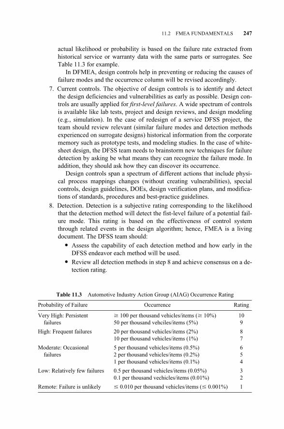
actual likelihood or probability is based on the failure rate extracted fromhistorical service or warranty data with the same parts or surrogates. SeeTable 11.3 for example.
In DFMEA, design controls help in preventing or reducing the causes offailure modes and the occurrence column will be revised accordingly.
7. Current controls. The objective of design controls is to identify and detectthe design deficiencies and vulnerabilities as early as possible. Design con-trols are usually applied for first-level failures. A wide spectrum of controlsis available like lab tests, project and design reviews, and design modeling(e.g., simulation). In the case of redesign of a service DFSS project, theteam should review relevant (similar failure modes and detection methodsexperienced on surrogate designs) historical information from the corporatememory such as prototype tests, and modeling studies. In the case of white-sheet design, the DFSS team needs to brainstorm new techniques for failuredetection by asking be what means they can recognize the failure mode. Inaddition, they should ask how they can discover its occurrence.
Design controls span a spectrum of different actions that include physi-cal process mappings changes (without creating vulnerabilities), specialcontrols, design guidelines, DOEs, design verification plans, and modifica-tions of standards, procedures and best-practice guidelines.
8. Detection. Detection is a subjective rating corresponding to the likelihoodthat the detection method will detect the fist-level failure of a potential fail-ure mode. This rating is based on the effectiveness of control systemthrough related events in the design algorithm; hence, FMEA is a livingdocument. The DFSS team should:
� Assess the capability of each detection method and how early in theDFSS endeavor each method will be used.
� Review all detection methods in step 8 and achieve consensus on a de-tection rating.
11.2 FMEA FUNDAMENTALS 247
Table 11.3 Automotive Industry Action Group (AIAG) Occurrence Rating
Probability of Failure Occurrence Rating
Very High: Persistent � 100 per thousand vehicles/items (� 10%) 10failures 50 per thousand vehciles/items (5%) 9
High: Frequent failures 20 per thousand vehicles/items (2%) 810 per thousand vehicles/items (1%) 7
Moderate: Occasional 5 per thousand vehicles/items (0.5%) 6failures 2 per thousand vehicles/items (0.2%) 5
1 per thousand vehicles/items (0.1%) 4
Low: Relatively few failures 0.5 per thousand vehicles/items (0.05%) 30.1 per thousand vechicles/items (0.01%) 2
Remote: Failure is unlikely 0.010 per thousand vehicles/items ( 0.001%) 1
c11.qxd 4/22/2005 9:08 AM Page 247
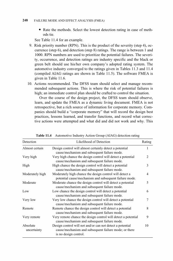
� Rate the methods. Select the lowest detection rating in case of meth-ods tie.
See Table 11.4 for an example.
9. Risk priority number (RPN). This is the product of the severity (step 4), oc-currence (step 6), and detection (step 8) ratings. The range is between 1 and1000. RPN numbers are used to prioritize the potential failures. The severi-ty, occurrence, and detection ratings are industry specific and the black orgreen belt should use his/her own company’s adopted rating system. Theautomotive industry converged to the ratings given in Tables 11.3 and 11.4(compiled AIAG ratings are shown in Table 11.5). The software FMEA isgiven in Table 11.6.
10. Actions recommended. The DFSS team should select and manage recom-mended subsequent actions. This is where the risk of potential failures ishigh; an immediate control plan should be crafted to control the situation.
Over the course of the design project, the DFSS team should observe,learn, and update the FMEA as a dynamic living document. FMEA is notretrospective, but a rich source of information for corporate memory. Com-panies should build a “corporate memory” that will record the design bestpractices, lessons learned, and transfer functions, and record what correc-tive actions were attempted and what did and did not work and why. This
248 FAILURE MODE AND EFFECT ANALYSIS (FMEA)
Table 11.4 Automotive Industry Action Group (AIAG) detection rating
Detection Likelihood of Detection Rating
Almost certain Design control will almost certainly detect a potential 1cause/mechanism and subsequent failure mode.
Very high Very high chance the design control will detect a potential 2cause/mechanism and subsequent failure mode.
High High chance the design control will detect a potential 3cause/mechanism and subsequent failure mode.
Moderately high Moderately high chance the design control will detect a 4potential cause/mechanism and subsequent failure mode.
Moderate Moderate chance the design control will detect a potential 5cause/mechanism and subsequent failure mode.
Low Low chance the design control will detect a potential 6cause/mechanism and subsequent failure mode.
Very low Very low chance the design control will detect a potential 7cause/mechanism and subsequent failure mode.
Remote Remote chance the design control will detect a potential 8cause/mechanism and subsequent failure mode.
Very remote Very remote chance the design control will detect a potential 9cause/mechanism and subsequent failure mode.
Absolute Design control will not and/or can not detect a potential 10uncertainty cause/mechanism and subsequent failure mode; or there
is no design control.
c11.qxd 4/22/2005 9:08 AM Page 248
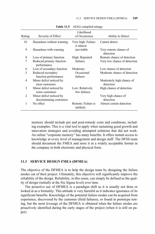
memory should include pre and post-remedy costs and conditions, includ-ing examples. This is a vital tool to apply when sustaining good growth andinnovation strategies and avoiding attempted solutions that did not work.An online “corporate memory” has many benefits. It offers instant access toknowledge at every level of management and design staff. The DFSS teamshould document the FMEA and store it in a widely acceptable format inthe company in both electronic and physical form.
11.3 SERVICE DESIGN FMEA (DFMEA)
The objective of the DFMEA is to help the design team by designing the failuremodes out of their project. Ultimately, this objective will significantly improve thereliability of the design. Reliability, in this sense, can simply be defined as the qual-ity of design (initially at the Six Sigma level) over time.
The proactive use of DFMEA is a paradigm shift as it is usually not done orlooked at as a formality. This attitude is very harmful as it indicates ignorance of itssignificant benefits. Knowledge of the potential failure modes can be acquired fromexperience, discovered by the customer (field failures), or found in prototype test-ing, but the most leverage of the DFMEA is obtained when the failure modes areproactively identified during the early stages of the project (when it is still on pa-per).
11.3 SERVICE DESIGN FMEA (DFMEA) 249
Table 11.5 AIAG compiled ratings
LikelihoodRating Severity of Effect of Occurrence Ability to Detect
10 Hazardous without warning Very high: Failure Cannot detectis almost
9 Hazardous with warning inevitable Very remote chance of detection
8 Loss of primary function High: Repeated Remote chance of detection7 Reduced primary function failures Very low chance of detection
performance6 Loss of secondary function Moderate: Low chance of detection5 Reduced secondary Occasional Moderate chance of detection
function performance failures4 Minor defect noticed by Moderately high chance of
most customers detection3 Minor defect noticed by Low: Relatively High chance of detection
some customers few failures2 Minor defect noticed by Very high chance of
discriminating customers detection1 No effect Remote: Failure is Almost certain detection
unlikely
c11.qxd 4/22/2005 9:08 AM Page 249
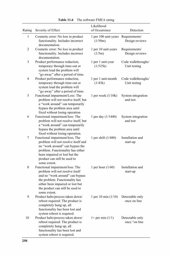
250
Table 11.6 The software FMEA rating
LikelihoodRating Severity of Effect of Occurrence Detection
1 Cosmetic error: No loss in product 1 per 100 unit-years Requirements/ functionality. Includes incorrect (1/50m) Design reviewsdocumentation.
2 Cosmetic error: No loss in product 1 per 10 unit-years Requirements/functionality. Includes incorrect (1/5m) Design reviewsdocumentation.
3 Product performance reduction, 1 per 1 unit-year Code walkthroughs/ temporary through time-out or (1/525k) Unit testingsystem load the problem will “go away” after a period of time.
4 Product performance reduction, 1 per 1 unit-month Code walkthroughs/temporary through time-out or (1/43k) Unit testingsystem load the problem will “go away” after a period of time.
5 Functional impairment/Loss: The 1 per week (1/10k) System integration problem will not resolve itself, but and testa “work around” can temporarily bypass the problem area until fixed without losing operation
6 Functional impairment/loss: The 1 per day (1/1440) System integration problem will not resolve itself, but and testa “work around” can temporarily bypass the problem area until fixed without losing operation.
7 Functional impairment/loss; The 1 per shift (1/480) Installation and problem will not resolve itself and start-upno “work around” can bypass the problem. Functionality has either been impaired or lost but the product can still be used to some extent.
8 Functional impairment/loss: The 1 per hour (1/60) Installation and problem will not resolve itself start-upand no “work around” can bypass the problem. Functionality has either been impaired or lost but the product can still be used to some extent.
9 Product halts/process taken down/ 1 per 10 min (1/10) Detectable only reboot required: The product is once on linecompletely hung up, allfunctionality has been lost andsystem reboot is required.
10 Product halts/process taken down/ 1+ per min (1/1) Detectable only reboot required: The product is once “on linecompletely hung up, all functionality has been lost and system reboot is required.
c11.qxd 4/22/2005 9:08 AM Page 250

The DFMEA exercise within the DFSS road map is a function of the hierarchyidentified in the service design mapping. First, the DFSS team will exercise theDFMEA at the lowest hierarchical level (e.g., a secondary requirement or subfunc-tion), then estimate the effect of each failure mode at the next hierarchal level (e.g.a primary-functional requirement), and so on. The FMEA is a bottom-up approachnot a top-down one and usually does not reveal all higher-levels potential failures.
Prior to embarking on any FMEA exercise, we advise the Six Sigma black orgreen belt to book a series of FMEA meetings in advance, circulate all relevant in-formation ahead of the FMEA meetings, clearly define objectives at the start ofeach meeting, adhere to effective roles, and communicate effectively.
A service DFMEA can be conducted by following the steps in Section 11.2.Here we highlight any peculiar steps for such an exercise. The fundamental steps inthe DFMEA to be taken by the DFSS team are:
1. Constructing the project boundary (scope) bounded by a functional mappingof the team’s choice. Steps or activities, subprocesses, and processes are atdifferent hierarchal levels. The team will start at the lowest hierarchical leveland proceed upward. The relative information from the lower levels is inputto the appropriate higher level in the respective steps. Here the IDEF3 exam-ple of Chapter 8 is used for illustration in Figures 11.2 and 11.3. Revisit thefunctional mapping, using a technique or a combination of techniques fromChapter 8 that fully describes interfaces at the all levels of the hierarchy with-in the scope. Interfaces will include controlled and uncontrolled inputs likeenvironmental factors, deterioration, and customer usage.
2. Identifying the potential failures for all functional requirements at all hierar-chical levels in the map. The team needs to identify all potential ways inwhich the design may fail. For each functional requirement in the map, theteam will brainstorm the design failure modes. Failure modes describe howeach functional entity in the map may initially fail prior to the end of its in-tended life or introduce unwanted side effects. The potential design failuremode is the way in which a service design entity in the functional map mayfail to deliver its array of functional requirements.
3. Studying the failure causes and effects. The causes are generally categorizedas conceptual weaknesses due to axiom violations (El-Haik, 2005). Anothertype is due to the mean effects of noise factors and their interaction with thedesign parameters, for example, unit-to-unit production deficiencies, such aswhen a step is not within specifications. Assembly errors, that is, steps thatare delivered to specifications but with assembly process errors, may propa-gate to the higher levels in the map. In addition, material variation, environ-ment, and operator usage are the premier noise factors for team’s considera-tion.
4. The direct consequence of a failure is the failure mode on the next higher hi-erarchical level, the customer and regulations. Potential failure causes can beanalyzed by tools like fault tree analysis (FTA), cause-and-effect diagrams,and cause-and-effect matrices. Two golden rules should be followed in cause
11.3 SERVICE DESIGN FMEA (DFMEA) 251
c11.qxd 4/22/2005 9:08 AM Page 251
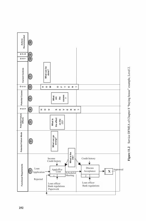
252
Fig
ure
11.2
Ser
vice
DF
ME
A o
f C
hapt
er 8
“bu
ying
hou
se”
exam
ple,
Lev
el 2
.
Fu
ncti
on
al R
eq
uir
em
en
tsP
ote
nti
al F
ailu
re M
od
eP
ote
nti
al F
ailu
re
Eff
ects
S E V
Po
ten
tial C
au
ses
O C CC
urr
en
t C
on
tro
lsD E T
R P N
Ac
tio
ns
Reco
mm
en
ded
12
34
56
78
10
9
Rejected
Scheduled
Meeting
Loan
Application
1
ApplyfFor Loan
Income
Credit history
Loan officer
Bank regulations
Paperwork
Approved
2
Discuss
Acceptance
Credit history
Loan officer
Bank regulations
X
Wh
at
is t
he
FR
?
Wh
at
can
go
wro
ng
?
Wh
at
is
the e
ffect
on
th
e
(1)?
Wh
at
are
the
cau
ses
?
H O w S E V E R E ?
H O W O F T E N ?
Wh
at
can
be
do
ne?
c11.qxd 4/22/2005 9:08 AM Page 252
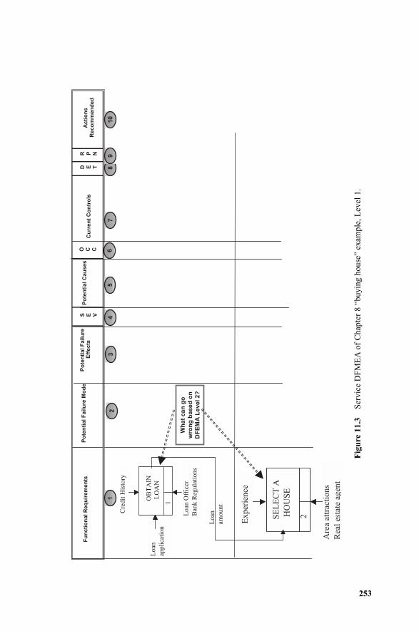
253
Fig
ure
11.3
Ser
vice
DF
ME
A o
f C
hapt
er 8
“bu
ying
hou
se”
exam
ple,
Lev
el 1
.
Fu
ncti
on
al R
eq
uir
em
en
ts
Po
ten
tial F
ailu
re M
od
eP
ote
nti
al F
ailu
re
Eff
ects
S E V
Po
ten
tial C
au
ses
O C CC
urr
en
t C
on
tro
lsD E T
R P N
Ac
tio
ns
Reco
mm
en
ded
12
34
56
78
10
9
Cre
dit
His
tory
Loan
appli
cati
on
Lo
an O
ffic
er
Bank R
egula
tions
1
Loan
am
ount
OB
TA
IN
LO
AN
Ex
peri
en
ce
Are
a a
ttra
cti
on
s
Real
esta
te a
gen
t
2SE
LE
CT
A
HO
US
E
Wh
at
can
go
wro
ng
based
on
DF
EM
A L
evel 2?
c11.qxd 4/22/2005 9:08 AM Page 253
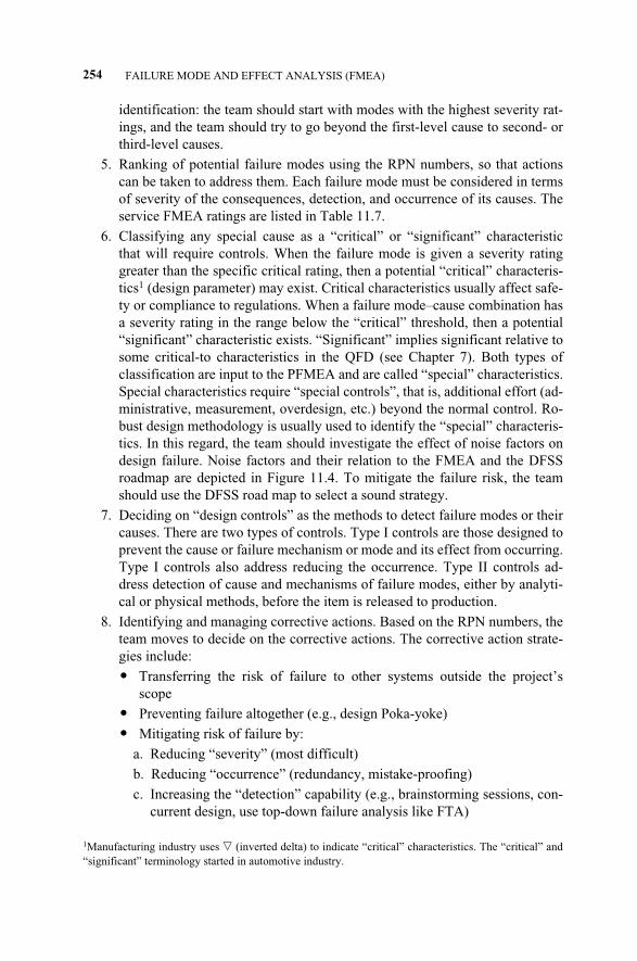
identification: the team should start with modes with the highest severity rat-ings, and the team should try to go beyond the first-level cause to second- orthird-level causes.
5. Ranking of potential failure modes using the RPN numbers, so that actionscan be taken to address them. Each failure mode must be considered in termsof severity of the consequences, detection, and occurrence of its causes. Theservice FMEA ratings are listed in Table 11.7.
6. Classifying any special cause as a “critical” or “significant” characteristicthat will require controls. When the failure mode is given a severity ratinggreater than the specific critical rating, then a potential “critical” characteris-tics1 (design parameter) may exist. Critical characteristics usually affect safe-ty or compliance to regulations. When a failure mode–cause combination hasa severity rating in the range below the “critical” threshold, then a potential“significant” characteristic exists. “Significant” implies significant relative tosome critical-to characteristics in the QFD (see Chapter 7). Both types ofclassification are input to the PFMEA and are called “special” characteristics.Special characteristics require “special controls”, that is, additional effort (ad-ministrative, measurement, overdesign, etc.) beyond the normal control. Ro-bust design methodology is usually used to identify the “special” characteris-tics. In this regard, the team should investigate the effect of noise factors ondesign failure. Noise factors and their relation to the FMEA and the DFSSroadmap are depicted in Figure 11.4. To mitigate the failure risk, the teamshould use the DFSS road map to select a sound strategy.
7. Deciding on “design controls” as the methods to detect failure modes or theircauses. There are two types of controls. Type I controls are those designed toprevent the cause or failure mechanism or mode and its effect from occurring.Type I controls also address reducing the occurrence. Type II controls ad-dress detection of cause and mechanisms of failure modes, either by analyti-cal or physical methods, before the item is released to production.
8. Identifying and managing corrective actions. Based on the RPN numbers, theteam moves to decide on the corrective actions. The corrective action strate-gies include:
� Transferring the risk of failure to other systems outside the project’sscope
� Preventing failure altogether (e.g., design Poka-yoke)
� Mitigating risk of failure by:
a. Reducing “severity” (most difficult)
b. Reducing “occurrence” (redundancy, mistake-proofing)
c. Increasing the “detection” capability (e.g., brainstorming sessions, con-current design, use top-down failure analysis like FTA)
254 FAILURE MODE AND EFFECT ANALYSIS (FMEA)
1Manufacturing industry uses � (inverted delta) to indicate “critical” characteristics. The “critical” and“significant” terminology started in automotive industry.
c11.qxd 4/22/2005 9:08 AM Page 254
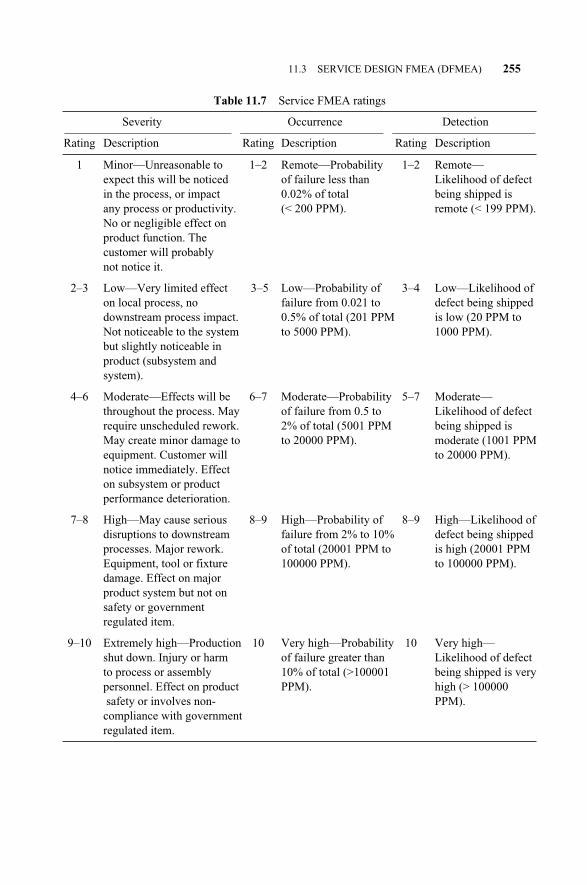
11.3 SERVICE DESIGN FMEA (DFMEA) 255
Table 11.7 Service FMEA ratings
Severity Occurrence Detection____________________________ ________________________ ________________________Rating Description Rating Description Rating Description
1 Minor—Unreasonable to 1–2 Remote—Probability 1–2 Remote— expect this will be noticed of failure less than Likelihood of defect in the process, or impact 0.02% of total being shipped is any process or productivity. (< 200 PPM). remote (< 199 PPM).No or negligible effect on product function. The customer will probably not notice it.
2–3 Low—Very limited effect 3–5 Low—Probability of 3–4 Low—Likelihood of on local process, no failure from 0.021 to defect being shipped downstream process impact. 0.5% of total (201 PPM is low (20 PPM to Not noticeable to the system to 5000 PPM). 1000 PPM).but slightly noticeable in product (subsystem and system).
4–6 Moderate—Effects will be 6–7 Moderate—Probability 5–7 Moderate—throughout the process. May of failure from 0.5 to Likelihood of defect require unscheduled rework. 2% of total (5001 PPM being shipped is May create minor damage to to 20000 PPM). moderate (1001 PPM equipment. Customer will to 20000 PPM).notice immediately. Effect on subsystem or product performance deterioration.
7–8 High—May cause serious 8–9 High—Probability of 8–9 High—Likelihood of disruptions to downstream failure from 2% to 10% defect being shipped processes. Major rework. of total (20001 PPM to is high (20001 PPM Equipment, tool or fixture 100000 PPM). to 100000 PPM).damage. Effect on major product system but not on safety or government regulated item.
9–10 Extremely high—Production 10 Very high—Probability 10 Very high—shut down. Injury or harm of failure greater than Likelihood of defect to process or assembly 10% of total (>100001 being shipped is very personnel. Effect on product PPM). high (> 100000 safety or involves non- PPM).
compliance with government regulated item.
c11.qxd 4/22/2005 9:08 AM Page 255
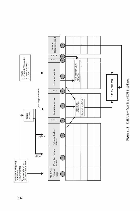
256
Fig
ure
11.4
FM
EA
inte
rfac
es in
the
DF
SS
roa
d m
ap.
FR
, D
P,o
r P
roce
ss
Ste
p
Po
ten
tia
l F
ailu
re M
od
eP
ote
ntia
l F
ailu
re E
ffe
cts
S E V
Po
ten
tia
l C
au
se
s
O C C
Cu
rre
nt C
on
tro
ls
D E T
R P N
Actio
ns
Re
co
mm
en
de
d
FR
, D
P,o
r
Pro
ce
ss
Ste
p
Po
ten
tia
l F
ailu
re
Mo
de
Po
ten
tia
l F
ailu
re
Effe
cts
S E V
Po
ten
tia
l C
au
se
s
O C C
Cu
rre
nt C
on
tro
ls
D E T
R P N
Actio
ns
Re
co
mm
en
de
d
12
34
56
78
10
9
P-
dia
gra
ms*
Nois
e
Facto
rs
Wear
variability
Couplin
g/Inte
raction
Functional M
appin
g(F
unctional
Requir
em
ents
)or
Pro
cess M
appin
g(P
rocess V
ari
able
s)
•T
ests
•A
naly
sis
/Sim
ula
tion
•P
eer
Revie
ws
•D
OE
,
Next-
Hig
her-
Level
DF
ME
AV
alid
ation
pri
oritization
(Severe
/Hig
h R
PN
)
•D
FS
S r
oad m
ap
c11.qxd 4/22/2005 9:08 AM Page 256
9. Review analysis, document and update the DFMEA. The DFMEA is a livingdocument and should be reviewed and managed on an ongoing basis. Steps1–8 should be documented in the appropriate media. The potential failuremodes at any level can be brainstormed by leveraging existing knowledgesuch as process engineering, mapping, and simulation analysis, historicalfailure databases of the baseline design, possible designed-in errors, andphysics of failures, if applicable. For comprehensiveness and as a good prac-tice, the black belt should instruct the DFSS team members to always main-tain and update their specific list of failures modes.
11.4 PROCESS FMEA (PFMEA)
The activities in the PFMEA are similar to the DFMEA; however, the focus here ison process failures. The fundamental steps in the PFMEA are the same as those of aDFMEA. Steps peculiar to PFMEA are presented in this section.
As a first step, the DFSS team should already have the project scope definedwith the constructed project process map. The team can maximize the design quali-ty by preventing all processes failures. Similar to DFMEA, the team should startwith the lowest hierarchical level, the step level, and utilize the process map to cov-er all processes. The team then proceeds to the next hierarchal level, the subprocesslevel, finishes all subprocess PFMEA, and proceeds upward.
The process map should fully describe the design interfaces at all levels of thehierarchy within its scope. Interfaces will include controlled inputs, the subprocessand process variables, uncontrolled inputs, and noise factors like processing, opera-tor, and assembly errors and variations. The macro-level process map is leveragedby the micromappings. Micromappings exhibit detailed operations like transporta-tion, inspection stations, and cycle times. The relative information from the lowerlevels is input to the next-higher hierarchical level PFMEA, where appropriate, inthe respective steps.
The team must revisit the process map at all hierarchical levels where defined.The task here is to make sure that all process variables in the process map end upbeing hosted by some process or subprocess domain (see Figure 6.1), setting thestage for addressing the potential failures for each hierarchical level in the processmap. Having gone through the corresponding hierarchical-level DFMEA, the teammust identify all potential ways in which the design may fail due to all processesfailures. For each requirement or design parameter in the map, the team will brain-storm the process failure modes. Failure modes describe how each hierarchical enti-ty in the structure may initially fail prior to the end of its intended life. The potentialprocess failure mode is the way in which a processed service entity in the structuremay fail to deliver its array of design parameters and functional requirements.
For proper failure treatment, the team should study the failure causes and effects.The causes are generally categorized as weaknesses due to inherent process weak-ness caused by conceptual vulnerability in the design functional and/or processmaps and failures due to the effect of noise factors. In this cause of failure, a service
11.4 PROCESS FMEA (PFMEA) 257
c11.qxd 4/22/2005 9:08 AM Page 257

is produced within the design specification. Nevertheless, it still cannot be deliv-ered or function as intended or requested by the customer. The other type of failuresmay be caused by noise factors such as variation and deficiencies due mainly to in-capable processes, material variation, machine deterioration, and environment andoperator error.
The effect of a failure is the direct consequence of the failure mode in the currentprocess step in terms of rework or inefficiency, the next upstream processes, and,ultimately, the customer. Potential failure causes can be analyzed at the process lev-el by tools like fault tree analysis (FTA), cause-and-effect diagrams, and cause-and-effect matrices. To address the causes, the team should start with modes with high-est severity ratings and try to go beyond the first-level cause to second- orthird-level causes. The team should ask the following process questions:
1. What incoming source of variations could cause this process to fail to deliverits mapped functional requirements?
2. What could cause the process to fail, assuming that the incoming inputs arecorrect and to specifications?
3. If the process fails, what are the consequences for operator health and safety,machinery, the component itself, the next downstream processes, the cus-tomer, and regulations?
The classification of any process variable as a “special” characteristic that willrequire controls like operator safety characteristics, indicates that it is a process pa-rameter that does not affect service but may have an impact on safety or govern-ment regulations applicable to process operation. Another category of process “spe-cial” characteristics is the “high-impact” characteristics. This type of processcharacteristic occurs when the condition of being outside of the specification toler-ance severely affects the operation of the process itself or subsequent operationsand does not affect service being processed. Both types of classification are input tothe PFMEA and are called “special” characteristics. The PFMEA handling of con-trols and corrective actions parallels the service DFMEA.
PFMEA should be conducted according to the process map. It is useful to addthe PFMEA and DFMEA processes to the design project-management charts. ThePERT or CPM approaches are both advisable. The black belt should schedule shortmeetings (less than two hours) with clearly defined objectives. Intermittent objec-tives of a FMEA may include tasks like measurement system evaluation, processcapability verification, and conducting exploratory DOEs or simulation studies.These activities consume resources and time, introducing sources of variability tothe DFSS project closure cycle time.
11.5 FMEA INTERFACES WITH OTHER TOOLS
Fault Tree Analysis (FTA), a top-down approach, can enhance the understanding ofsafety-related and catastrophic failures. FTA, like FMEA, helps the DFSS team an-
258 FAILURE MODE AND EFFECT ANALYSIS (FMEA)
c11.qxd 4/22/2005 9:08 AM Page 258
swer the “what if?” questions. This tool increases the design team’s understandingof their creation by identifying where and how failures may occur. In essence, FTAcan be viewed as a mathematical model that graphically uses deductive logic gates(e.g., AND, OR, etc.) to combine events that can produce the failure or the fault ofinterest. The objective is to emphasize the lower-level faults that directly or indi-rectly contribute to high-level failures in the DFSS project structures. Facilitated bythe mapping development, FTA must be performed as early as possible, particular-ly with regard to safety-related failures as well as Design for Serviceability.
11.5.1 Cause-and-Effect Tools
The cause-and-effect diagram, also know as the “fishbone” or “Ishikawa” diagram,and the cause–effect matrix are two commonly used tools that help the DFSS teamin their FMEA exercise. The cause-and-effect diagram classifies the various causesthought to affect the operation of the design, indicatiing the cause-and-effect rela-tions among them with arrows.
The diagram is formed from the causes that can result in the undesirable failuremode. The causes are the independent variables and the failure mode is the depen-dent variable. An example is depicted in Figure 11.5. In this example, a companythat manufactures consumer products suffers from warranty costs, measured as apercentage of sales. The current performance is above the budgeted upper specifica-tion limit. Customers tend to be very sensitive to warranty issues and equipmentdowntime, which results in a dissatisfaction. Figure 11.5 shows several causes forthe cost.
The cause-and-effect matrix is another technique that can be used to identifyfailure causes. In the columns, the DFSS team can list the failure modes. The teamthen proceeds to rank each failure mode numerically using the RPN numbers. Theteam uses brainstorming to identify all potential causes that can impact the failuremodes and lists these along the left hand side of the matrix. It is useful practice toclassify theses causes as design weaknesses or noise factor effects by type (e.g.variability and production environment). The team then rates, numerically, the ef-fect of cause of each failure mode within the body of the matrix. This is based onthe experience of the team and any available information. The team then cross-mul-tiplies the rate of the effect by the RPN to total each row (cause). These totals arethen used to analyze and determine where to focus the effort when creating theFMEA. By grouping the causes according to their classification (weakness, envi-ronmental effect, production unit-to-unit effect, wear effect, etc.), the team will de-velop several hypotheses about the strength of these types of causes to devise theirattack strategy.
11.5.2 Quality Systems and Control Plans
Control plans are the means to sustain any DFSS project findings. However, theseplans are not effective if not implemented within a comprehensive quality operatingsystem. A solid quality system can provide the means through which your project
11.5 FMEA INTERFACES WITH OTHER TOOLS 259
c11.qxd 4/22/2005 9:08 AM Page 259
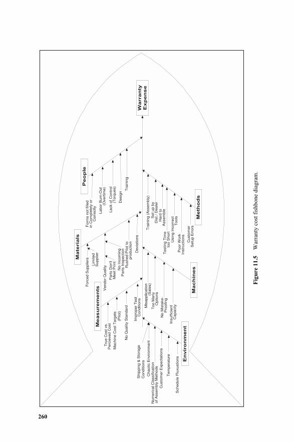
260
Fig
ure
11.5
War
rant
y co
st f
ishb
one
diag
ram
.
Wa
rra
nty
Ex
pe
ns
e
Me
as
ure
me
nts
Ma
teria
ls
Ma
ch
ine
sM
eth
od
s
Pe
op
le
En
vir
on
me
nt
Tru
e C
ost
vs.
Perc
ieve
d C
ost
Mach
ine C
ost
Targ
ets
(Pilo
t)
Forc
ed S
upplie
rs
Vendor
Qualit
y
Part
s D
on't
Meet
Devi
atio
ns
No I
nco
min
gP
art
s In
spect
ion
Form
s not
fille
din
Com
ple
tely
or
Corr
ect
lyLim
ited
Supplie
r
Tra
inin
g (
Ass
em
bly
)
Labor
Burn
-Out
(Ove
rtim
e)
Mis
applic
atio
n(S
ale
s)S
et
up b
yD
ist.
/ D
eale
r
Lack
of
Contr
ol
(Torq
ues)
Chaotic
Envi
ronm
ent
Test
ing T
ime
too S
hort
Num
erica
l Cla
ssifi
catio
nof A
ssem
bly
Meth
ods
Usi
ng I
nco
rrect
Tools
Rush
ed P
ilot
topro
duct
ion
Hard
to
Ass
em
ble
Desi
gn
Too M
any
Optio
ns
No Q
ualit
y S
tandard
Impro
per
Test
Conditi
ons
Tra
inin
g
Cust
om
er
Exp
ect
atio
ns
Tem
pera
ture
Sch
edule
Flu
xuatio
ns
Ship
pin
g &
Sto
rage
Conditi
ons
No M
ista
ke-
Pro
ofin
g
Poor
Work
Inst
ruct
ions
Cust
om
er
Setu
p E
rrors
Insu
ffic
ient
Capaci
ty
c11.qxd 4/22/2005 9:08 AM Page 260
will sustain its long-term gains. Quality system certifications are becoming a cus-tomer requirement and a trend in many industries. The validate phase of the ICOVDFSS algorithm requires that a solid quality system be employed in the DFSS pro-ject area.
The quality system objective is to achieve customer satisfaction by preventingnonconformity at all stages from design through service. A quality system is the SixSigma deploying company’s agreed-upon method of doing business. It is not to beconfused with a set of documents that are meant to satisfy an outside auditing orga-nization (i.e., ISO 900x). That is, a quality system represents the actions, not thewritten words of a company. The elements of an effective quality system includethe quality mission statement, management reviews, company structure, planning,design control, data control, purchasing-quality-related functions (e.g., supplierevaluation and incoming inspection), design of product and process structures fortraceability, process control, preventive maintenance, process monitoring and oper-ator training, capability studies, MSA, audit functions, inspection and testing, ser-vice, statistical analysis, and standards.
Automated or manual control methods are used for both design (service or prod-uct) as well as their processes. Control methods include tolerancing, mistake-proof-ing (Poka-yoke), statistical process control charting [SPC, like X-bar&R or X&MRcharts (manual or automatic), p&np charts (manual or automatic), c&u charts (man-ual or automatic), etc.], with or without warning, trend signals applied to control theprocess variables or monitor the design parameters, standard operating procedures(SOP) for detection purposes, and short-term inspection actions. In applying thesemethods, the DFSS team should revisit operator training to ensure proper controlfunctions and to extract historical long-term and short-term information.
Control plans are the living documents of the manufacturing, assembly, or pro-duction environment. They are used to document all process control methods, assuggested by the FMEA or other DFSS algorithm steps like optimization and robustdesign studies. The control plan is a written description of the systems for control-ling services, products, and processes. The control plan should be updated to reflectchanges of controls based on experience gained over time.
11.5 FMEA INTERFACES WITH OTHER TOOLS 261
c11.qxd 4/22/2005 9:08 AM Page 261

c11.qxd 4/22/2005 9:08 AM Page 262
12.1 INTRODUCTION
In the mid 1920s, a British statistician named Ronald Fisher put the finishing touch-es on a method for making breakthrough discoveries. Fisher’s method, now knownas design of experiments (DOE), has become a powerful tool for engineers, re-searchers, and Six Sigma practitioners.
Sir Ronald Fisher first used design of experiments as a research design tool toimprove farm yields in early 1930s. Fisher was a geneticist working on improvingcrop yields in England using supervised field trials, fertilizers, and seed varieties asexperimental factors. In his studies, Fisher encountered issues such as uncontrol-lable variation in the soil from plot to plot and the limited number of plots availablefor any given trial. Fisher solved these issues by varying the fertilizers or seed vari-eties used in the field. This action minimized the effects of soil variation in theanalysis of the plot yields. Fisher also developed the correct method for analyzingdesigned experiments called analysis of variance (ANOVA). This analysis methodbreaks up the total variation in the data into components from different sources.This analysis of variance delivers surprisingly precise results when applied to asmall, well-structured matrix. Today, these components are called signals andnoise, and the estimated effects are calculated as the sum of squares and the signal-to-noise ratio. There is a signal component for each controlled source (factor) in theexperiment and a noise component representing variations not attributable to any ofthe controlled variations. ANOVA using the signal-to-noise ratio provides preciseallocations of the effects of the factors and interactions. The ANOVA solutions de-veloped for these problems work just as well in today’s Six Sigma applications asthey did in 20th century agriculture.
Design of experiments provides a powerful tool within the DFSS road map toaccomplish breakthrough improvements in products, services, or process efficien-cy and effectiveness by optimizing the fulfillment of CTSs, FRs, and DPs. In each
Service Design for Six Sigma. By Basem El-Haik and David M. Roy 263© 2005 by John Wiley & Sons.
12FUNDAMENTALS OF EXPERIMENTAL DESIGN
c12.qxd 4/22/2005 9:12 AM Page 263

case, we create a response variable (y) and vary the factors that can cause achange in the performance of y. We can have CTS = f(FRs), or CTS = f(DPs), orFR = f(DPs), or DP = f(PVs) (see Section 8.5.2). It is important to note that mostexperimentation occurs in the relationships between DPs and PVs; if these do notyield breakthrough performance, then the design team should revisit the FRs andlook at options. The most proper utilization of DOE is in the optimize phase with-in the road map of Figure 5.1. Optimization in a DOE sense implies finding theproper settings of influential factors that enable the DFSS team to shift the meanand reduce the variation of their design requirements or responses. DOE has beenavailable for decades but its penetration in industry has been limited. Besides ig-norance and lack of proper training, implementation has been resisted because ofthe discipline required as well as the use of statistical techniques. Scientist, man-agers, and service designers usually fear employment of statistics. Six SigmaBlack and Green Belts play a big role in helping their teams and satellite membersovercome such emotional barriers.
Traditionally, the approach to experimentation in a process required changingonly one factor at a time (OFAT). Soon, it was found that the OFAT approach is in-capable of detecting interactions1 among the factors, which is a more probable andpossible event than most professionals think. Therefore, design of experiments isalso called statistically designed experiments. The purpose of the experiment anddata analysis is to establish and detail the transfer functions2 between outputs (e.g.,design parameters) and experimental factors (e.g., process variables and noise fac-tors) in a mapping that usually uses a P-diagram as illustrated in Figure 12.1.
A transfer function is the means of optimization and design detailing and is usual-ly documented in the scorecard. A transfer function is treated as a living entity with-in the DFSS methodology that passes through its own life cycle stages. A transferfunction is first identified using the proper mapping method (see Chapter 8) and thendetailed by derivation, modeling, or experimentation. The prime uses of the transferfunction are optimization and validation. Design transfer functions belonging to thesame hierarchical level in the design structures (system, subsystem, or component)should be recorded in that hierarchical-level scorecard (see Chapter 6). A scorecardis used to record and optimize the transfer functions. The transfer function concept isintegrated with other DFSS concepts and tools like mapping, robust design, and P-di-agrams within the rigor of design scorecards (Yang & El-Haik, 2003).
In Fischer’s experiments, the output, or response variable, y, was usually theyield of a certain farm crop. Controllable factors, x = (x1, x2, . . . , xn) were usuallythe “farm variables,” such as the amount of various fertilizers applied, watering pat-terns, selection of seeds, and so on. Uncontrollable factors, z = (z1, z2, . . . , zp) couldbe soil types, weather patterns, and so on (see Figure 12.1) . In early agricultural ex-periments, the experimenter wanted to find the cause-and-effect relationship be-tween the yield and controllable factors. That is, the experimenter wanted to know
264 FUNDAMENTALS OF EXPERIMENTAL DESIGN
1Interaction could be two level, three level, and so on. In a two-level interaction, a change in the response(output) of factor A occurs when factor B changes. 2Recall that DOE is a transfer-function-detailing method as presented in Chapter 6.
c12.qxd 4/22/2005 9:12 AM Page 264
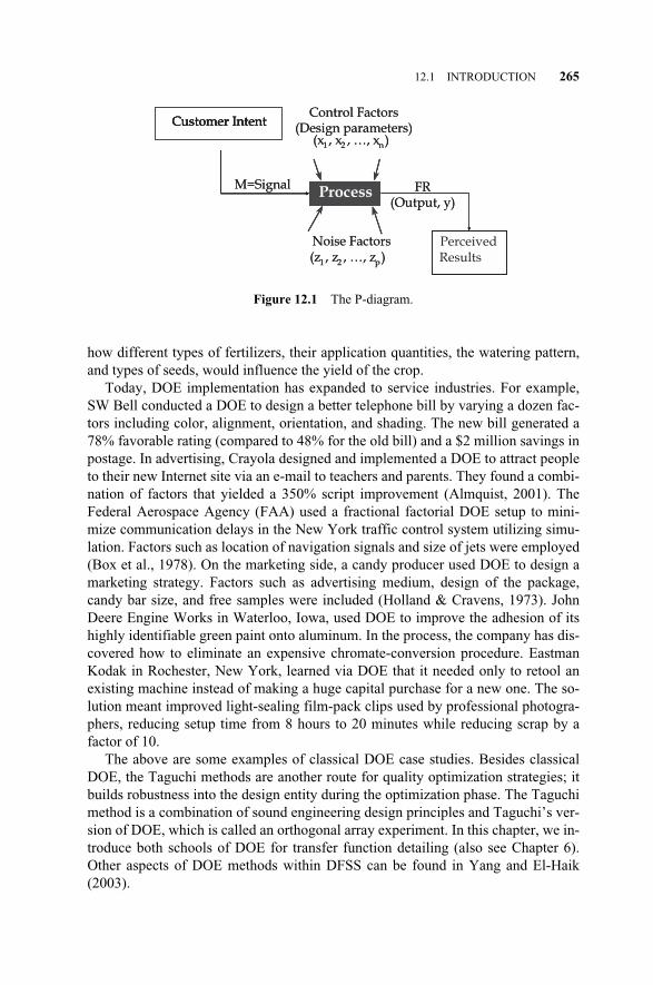
how different types of fertilizers, their application quantities, the watering pattern,and types of seeds, would influence the yield of the crop.
Today, DOE implementation has expanded to service industries. For example,SW Bell conducted a DOE to design a better telephone bill by varying a dozen fac-tors including color, alignment, orientation, and shading. The new bill generated a78% favorable rating (compared to 48% for the old bill) and a $2 million savings inpostage. In advertising, Crayola designed and implemented a DOE to attract peopleto their new Internet site via an e-mail to teachers and parents. They found a combi-nation of factors that yielded a 350% script improvement (Almquist, 2001). TheFederal Aerospace Agency (FAA) used a fractional factorial DOE setup to mini-mize communication delays in the New York traffic control system utilizing simu-lation. Factors such as location of navigation signals and size of jets were employed(Box et al., 1978). On the marketing side, a candy producer used DOE to design amarketing strategy. Factors such as advertising medium, design of the package,candy bar size, and free samples were included (Holland & Cravens, 1973). JohnDeere Engine Works in Waterloo, Iowa, used DOE to improve the adhesion of itshighly identifiable green paint onto aluminum. In the process, the company has dis-covered how to eliminate an expensive chromate-conversion procedure. EastmanKodak in Rochester, New York, learned via DOE that it needed only to retool anexisting machine instead of making a huge capital purchase for a new one. The so-lution meant improved light-sealing film-pack clips used by professional photogra-phers, reducing setup time from 8 hours to 20 minutes while reducing scrap by afactor of 10.
The above are some examples of classical DOE case studies. Besides classicalDOE, the Taguchi methods are another route for quality optimization strategies; itbuilds robustness into the design entity during the optimization phase. The Taguchimethod is a combination of sound engineering design principles and Taguchi’s ver-sion of DOE, which is called an orthogonal array experiment. In this chapter, we in-troduce both schools of DOE for transfer function detailing (also see Chapter 6).Other aspects of DOE methods within DFSS can be found in Yang and El-Haik(2003).
12.1 INTRODUCTION 265
Process
Customer IntentCustomer Intent
Perceived Results
M=Signal FR(Output, y)
Control Factors (Design parameters)
(x1 , x2 , …, xn)
Noise Factors(z1 , z2 , …, zp)
Process
Customer IntentCustomer Intent
Perceived Results
M=Signal FR(Output, y)
Control Factors (Design parameters)
(x1 , x2 , …, xn)
Noise Factors(z1 , z2 , …, zp)
Figure 12.1 The P-diagram.
c12.qxd 4/22/2005 9:12 AM Page 265
12.2 HYPOTHESIS TESTING
When testing and observing changes in processes, how does one know that the ob-served response was due to something that we controlled (changed) rather than arandom effect from a host of environmental noise factors? At what point are weconfident that the measured change is significant? These are some of the questionsthat hypothesis testing helps provide answers to.
Hypothesis testing is a method of inferential statistics that is aimed at testing theviability of a hypothesis about a certain population parameter in the light of experi-mental data. This hypothesis is usually called the null hypothesis. In the most com-mon use of hypothesis testing, the null hypothesis is put forward and it is deter-mined whether the available data are strong enough to reject it. If the data are verydifferent from what would be expected under the assumption that the null hypothe-sis is true, then the null hypothesis is rejected. If the data are not greatly at variancewith what would be expected under the assumption that the null hypothesis is true,then the null hypothesis is not rejected. Failure to reject the null hypothesis is notthe same thing as accepting the null hypothesis.
In DOE, hypothesis testing is essential for comparing if–then factorial settings(design parameter or process variables) and, therefore, design alternatives. Two ormore design alternatives can be compared with the goal of identifying the optimumdesign alternative relative to some requirements. For example, in the context of sim-ulation modeling (see Chapter 14), the null hypothesis is often the reverse of what thesimulation analyst actually believes about the model performance. Thus, the null hy-pothesis is put forward to allow the collected simulation data to contradict it and,hopefully, discredit it. If the Six Sigma Black or Green Belt has proposed a new de-sign alternative to a certain production process, he or she would be interested in test-ing experimentally whether the proposed design works better than the existing pro-duction process. To this end, the team would design an experiment comparing thetwo methods of production. The hourly throughput of the two processes could be col-lected and used as data for testing the viability of the null hypothesis. The null hy-pothesis would be that there is no difference between the two methods (the estimatedpopulation means of the throughput for the two production processes, �1 and �2, areidentical). In such case, the analyst would be hoping to reject the null hypothesis andconclude that the proposed method he or she developed is a better approach.
The symbol H0 is used to indicate the null hypothesis, where “null” refers to thehypothesis of no difference. For the example just given, the following would desig-nate the null hypothesis: H0: �1 = �2, or Ha: �1 �2. The alternative hypothesis(Ha) is simply that the mean throughput of the proposed method (�1) is higher thanthat of the current production process (�2), that is, Ha: �1 > �2.
It is possible for the null hypothesis to be that the difference (d) between popula-tion means is of a particular value (H0: �1 – �2 = d), or the null hypothesis could bethat the population mean is of a certain standard value (H0: � = �0).
The test of hypothesis implies defining a certain design parameter, process vari-ables, or functional requirement as a random variable with a valid measurement sys-tem, derived test statistics, and an associated distribution, as well as a determined re-
266 FUNDAMENTALS OF EXPERIMENTAL DESIGN
c12.qxd 4/22/2005 9:12 AM Page 266

jection area. Rejection area reflects a 100% (1 – �) confidence level in the hypothe-sis decision. The Greek symbol � represents the risk associated with the party affect-ed by rejecting the null hypothesis. Data is collected by random sampling techniques.Hypothesis testing requires normality as an assumption. In mean hypothesis testing,most tests involve comparisons of a mean performance with a certain value or withanother process mean of the same random variable. For more than two populations,DOE is used to test such hypotheses of means equality, that is, H0: �1 = �2 = . . . = �a,where a is the number of different populations (settings) of a random variable, say A,that will be tested. When the variance of the random variable (�2) is known, the Zscore, Z0, or the Z value under true H0, is used as a test statistic for the null hypothe-sis H0: � = �0, assuming that the observed population is normal or the sample size islarge enough so that the central limit theorem applies. Z0 is computed as follows:
Z0 = (12.1)
The 100% (1 – �) confidence interval on the true population mean is
X� – Z�/2�/�n� � X� + Z�/2�/�n� (12.2)
We use the absolute value of Z0 because the normal distribution is symmetricaland this is shown as |Z0|. Therefore, the null hypothesis H0: � = �0, would be reject-ed if |Z0| > Z�/2 when Ha: � �0, Z0 < –Z� when Ha: � < �0, and Z0 > Z� when Ha:� > �0. For the null hypothesis H0: �1 = �2, Z0 is computed as follows:
Z0 = (12.3)
The null hypothesis H0: �1 = �2 would be rejected if |Z0| > Z�/2 when Ha: �1 �2, Z0 < –Z� when Ha: �1 < �2, and Z0 > Z� when Ha: �1 > �2.
When the variance parameter (�2) is unknown, which is typically the case inreal-world applications, the t statistic, t0, is used as a test statistic for the null hy-pothesis H0: � = �0. The test statistic, t0, is computed as follows:
t0,n–1 = (12.5)
where n is the sample size. The 100% (1 – �) interval on the true population mean is
X�– t�/2,n–1s/�n� � X� + t�/2,n–1s/�n� (12.6)
The null hypothesis H0: � = �0 would be rejected if |t0| > t�/2,n–1 when Ha: � �0, t0 < –t�,n–1 when Ha: � < �0, and t0 > t�,n–1 when Ha: � > �0. For the null hy-pothesis H0: �1 = �2, t0 is computed as
X� – �0��s/�n�
X�1 – X�2��
���
n�1
12
�� +� ��
n�2
22
��
X� – �0���/�n�
12.2 HYPOTHESIS TESTING 267
c12.qxd 4/22/2005 9:12 AM Page 267
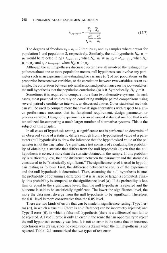
t0,n1–n2–2 = (12.7)
The degrees of freedom n1 – n2 – 2 implies n1 and n2 samples where drawn forpopulation 1 and population 2, respectively. Similarly, the null hypothesis H0: �1 =�2 would be rejected if |t0| > t�/2,n1–n2–2 when Ha: �1 �2, t0 < –t�,n1–n2–2 when Ha:�1 < �2, and t0 > t�,n1–n2–2 when Ha: �1 > �2.
Although the null hypotheses discussed so far have all involved the testing of hy-potheses about one or more population means, null hypotheses can involve any para-meter such as an experiment investigating the variance (�2) of two populations, or theproportion between two variables, or the correlation between two variables. As an ex-ample, the correlation between job satisfaction and performance on the job would testthe null hypothesis that the population correlation (�) is 0. Symbolically, H0: � = 0.
Sometimes it is required to compare more than two alternative systems. In suchcases, most practical studies rely on conducting multiple paired comparisons usingseveral paired-t confidence intervals, as discussed above. Other statistical methodscan still be used to compare more than two design alternatives with respect to a giv-en performance measure, that is, functional requirement, design parameter, orprocess variable. Design of experiments is an advanced statistical method that is of-ten utilized for comparing a much larger number of alternative systems. This is thesubject of this chapter.
In all cases of hypothesis testing, a significance test is performed to determine ifan observed value of a statistic differs enough from a hypothesized value of a para-meter (null hypothesis) to draw the inference that the hypothesized value of the pa-rameter is not the true value. A significance test consists of calculating the probabil-ity of obtaining a statistic that differs from the null hypothesis (given that the nullhypothesis is correct) more than the statistic obtained in the sample. If this probabil-ity is sufficiently low, then the difference between the parameter and the statistic isconsidered to be “statistically significant.” The significance level is used in hypoth-esis testing as follows. First, the difference between the results of the experimentand the null hypothesis is determined. Then, assuming the null hypothesis is true,the probability of obtaining a difference that is as large or larger is computed. Final-ly, this probability is compared to the significance level (�). If the probability is lessthan or equal to the significance level, then the null hypothesis is rejected and theoutcome is said to be statistically significant. The lower the significance level, themore the data must diverge from the null hypothesis to be significant. Therefore,the 0.01 level is more conservative than the 0.05 level.
There are two kinds of errors that can be made in significance testing: Type I er-ror (�), in which a true null (there is no difference) can be incorrectly rejected; andType II error ( ), in which a false null hypothesis (there is a difference) can fail tobe rejected. A Type II error is only an error in the sense that an opportunity to rejectthe null hypothesis correctly was lost. It is not an error in the sense that an incorrectconclusion was drawn, since no conclusion is drawn when the null hypothesis is notrejected. Table 12.1 summarized the two types of test error.
X�1 – X�2��
��n
s12
�1
��+� �n
s�2
22
��
268 FUNDAMENTALS OF EXPERIMENTAL DESIGN
c12.qxd 4/22/2005 9:12 AM Page 268
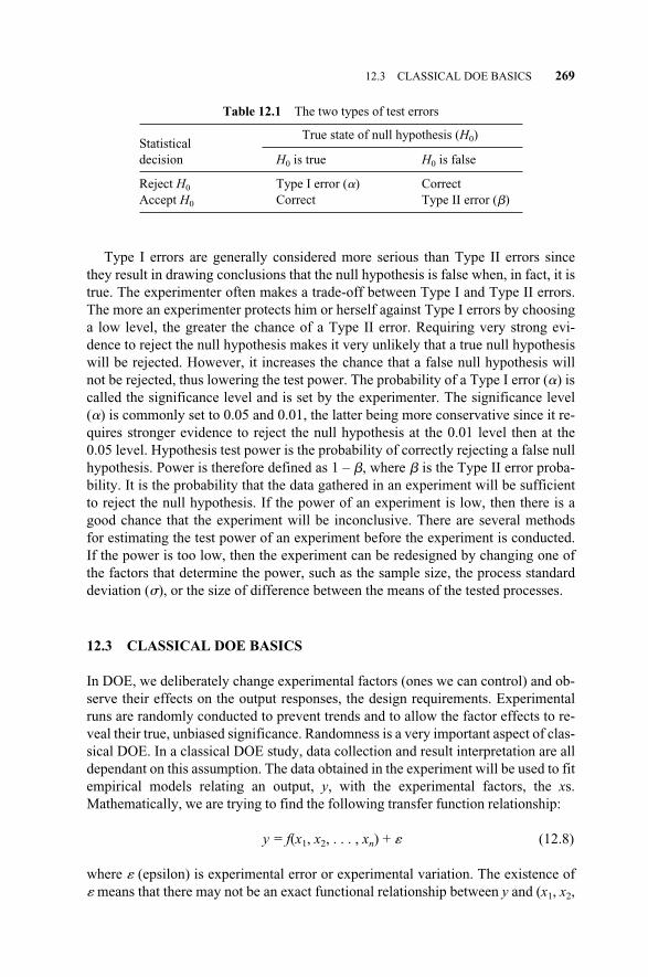
Type I errors are generally considered more serious than Type II errors sincethey result in drawing conclusions that the null hypothesis is false when, in fact, it istrue. The experimenter often makes a trade-off between Type I and Type II errors.The more an experimenter protects him or herself against Type I errors by choosinga low level, the greater the chance of a Type II error. Requiring very strong evi-dence to reject the null hypothesis makes it very unlikely that a true null hypothesiswill be rejected. However, it increases the chance that a false null hypothesis willnot be rejected, thus lowering the test power. The probability of a Type I error (�) iscalled the significance level and is set by the experimenter. The significance level(�) is commonly set to 0.05 and 0.01, the latter being more conservative since it re-quires stronger evidence to reject the null hypothesis at the 0.01 level then at the0.05 level. Hypothesis test power is the probability of correctly rejecting a false nullhypothesis. Power is therefore defined as 1 – , where is the Type II error proba-bility. It is the probability that the data gathered in an experiment will be sufficientto reject the null hypothesis. If the power of an experiment is low, then there is agood chance that the experiment will be inconclusive. There are several methodsfor estimating the test power of an experiment before the experiment is conducted.If the power is too low, then the experiment can be redesigned by changing one ofthe factors that determine the power, such as the sample size, the process standarddeviation (�), or the size of difference between the means of the tested processes.
12.3 CLASSICAL DOE BASICS
In DOE, we deliberately change experimental factors (ones we can control) and ob-serve their effects on the output responses, the design requirements. Experimentalruns are randomly conducted to prevent trends and to allow the factor effects to re-veal their true, unbiased significance. Randomness is a very important aspect of clas-sical DOE. In a classical DOE study, data collection and result interpretation are alldependant on this assumption. The data obtained in the experiment will be used to fitempirical models relating an output, y, with the experimental factors, the xs.Mathematically, we are trying to find the following transfer function relationship:
y = f(x1, x2, . . . , xn) + � (12.8)
where � (epsilon) is experimental error or experimental variation. The existence of� means that there may not be an exact functional relationship between y and (x1, x2,
12.3 CLASSICAL DOE BASICS 269
Table 12.1 The two types of test errors
True state of null hypothesis (H0)Statisticaldecision H0 is true H0 is false
Reject H0 Type I error (�) CorrectAccept H0 Correct Type II error ( )
c12.qxd 4/22/2005 9:12 AM Page 269
. . . , xn). This is because the uncontrollable factors (z1, z2, . . . , zp) will influence therequirement y but are not accounted for in Equation (12.1), and there are experi-mental and measurement errors on both y and (x1, x2, . . . , xn) in the experiment. ADOE study within a DFSS study road map will follow a multiple step methodology,described in the following subsections.
12.3.1 DOE Study Definition
DOE is used in research as well as in product and service optimization settings, al-though sometimes for very different objectives. The primary purpose in scientificresearch is usually to show the statistical significance of an effect that a particularfactor exerts on the dependent variable of interest (a design requirement denoted as“y”). In an optimization DOE, the primary objective is usually to extract the maxi-mum amount of unbiased information regarding the factors affecting a process orproduct from as few observations as possible to minimize cost. In the research ap-plication, DOE techniques are used to uncover the interactive nature of the applica-tion that is manifested in higher-order interactions (those involving three or morefactors). In a robust design variability experiment (see Chapter 13) , interaction ef-fects are often regarded as a “nuisance” as they only complicate the process of iden-tifying significant factors.
In either case, this is not trivial. The team needs to decide on the objective of theDOE study or studies within their DFSS project road map. Do they want to reducedefects? Is their purpose to improve current service performance? What is the studyscope within the mapping (see Chapter 8)? Do they work on a process or a sub-process? Is one DOE sufficient?
To develop an overall DOE, we suggest the following steps:
1. Define the problem and set the objectives
2. Select the responses
3. Select the factors and levels
4. Identify noise variables
5. Select the DOE design
6. Plan the experiment with regard to
Resources
Supplies
Schedule
Sample size
Risk assessment
The following process should be followed:
� Understand the current state of the DFSS project by reviewing and develop-ing an understanding of the technical domains that are active in the process or
270 FUNDAMENTALS OF EXPERIMENTAL DESIGN
c12.qxd 4/22/2005 9:12 AM Page 270

processes being optimized. A review of the physical laws, process and sys-tems behaviors, and underlying assumptions is appropriate at this stage.
� Develop a shared vision for optimizing service and process mappings. Theteam is advised to conduct a step-by-step review of the DOE methodology tounderstand and reinforce the importance of each strategic activity associatedwith experimentation and to facilitate consensus on the criteria for comple-tion of each activity.
� The DFSS team will need an appreciation for what elements of experimentalplan development will require the greatest time commitment. The team willalso need to discuss the potential impact associated with compromise of thekey DOE principles, if any.
� Plan time allocation. The team needs to develop a work plan that includestiming for several individual DOE sequences, if required.
� Plan time for measurement system(s) verification.
� Develop a P-diagram for preliminary experimentation to determine the mostimportant sources of variation, including the noise factors.
� Plan for selection of experimental factors and logistical considerations forbuilding test samples, and so on.
� Allocate a budget to perform the DOE plan. Develop cost estimation and seekresource approval to conduct the DOE test plan. Plan budgeting for multipleoptimization experiments.
� Add something about risk consideration. What effect will experimental con-ditions have on yield, scrap, rework, and safety? Will it affect the end user orwill it be contained internally? What will happen to the experimental units af-ter the experiment? Will they be scrapped or be reused?
12.3.2 Selection of the Response
The purpose of describing the process in terms of its inputs and outputs is to struc-ture the development of the DOE strategy. The description provided by processmapping provides an effective summary of what level of process optimization aretaking place, what measurement approach the DOE optimization will be based on,and what major sources of variation influence the process. As such, the followingactions are suggested:
� Revisit the definition of the responses in the DOE by developing a characteri-zation of boundary conditions and describe the process(es) delivering them interms of the inputs and outputs using a P-diagram. The description is also acharacterization of the basic function of the system, which has been identifiedin Chapter 8 using the mapping techniques of the team choice. The responsecan be generalized as a measurement characteristic related to the processmappings of a service process map (e.g., a functional requirement or a designparameter). It may be helpful to list various measurement characteristics,which can be viewed as alternative measurement approaches.
12.3 CLASSICAL DOE BASICS 271
c12.qxd 4/22/2005 9:12 AM Page 271
� After study definition, the team needs to select the requirements that will beoptimized. In this example, we will explore the case of a single requirement(y). In selecting a response variable, the DFSS team should select the left-hand side of a defined transfer function of their study as depicted in the pro-ject process and functional mappings. DOE will be used to detail their designand to provide other useful information about the design under study. It is de-sirable for the y to be a continuous variable characteristic of the design, mak-ing data analysis much easier and meaningful, a variable that can be easilyand accurately measured.
12.3.3 Choice of DOE Factors, Levels, and Ranges
In general, every step used in a process allows for the adjustment of various factorsaffecting the resultant quality of the service produced. Experimentation allows thedesign team to adjust the settings in a systematic manner and to learn which factorshave the greatest impact on the resultant functional requirement or design parame-ter. Using this information, the settings can be constantly improved until optimumquality is obtained.
Factors can be classified as control or noise. Control factors are design parame-ters or process variables that are freely specified by the design team using theirknowledge about the concept design and the technology that is being developed forthe purpose of DOE optimization.
There are two kinds of factors: continuous and discrete. A continuous factor canbe expressed over a defined real number interval with one continuous motion of thepencil. For example, weight, speed, and price are continuous factors. A discrete fac-tor is also called a categorical variable or attribute variable. For example, types ofmarketing strategy, types of delivery methods (face to face or via a third party), andtypes of operating system are discrete factors. Historic information and brainstorm-ing by the team will facilitate a P-diagram listing of potential factors belonging tothe categories (response, control, and noise)3 and aid in structuring the developmentof a strategy for DOE.
A key aspect of DFSS philosophy is that during the design stage, inexpensiveparameters can be identified and studied, and can be combined in a way that will re-sult in performance that is insensitive to uncontrollable sources of variation. Theteam’s task is to determine the combined best settings (parameter targets) for eachof the control parameters that have been judged by the design team to have the po-tential to improve the output(s) of interest. The selection of factors will be done in amanner that will enable target values to be varied during experimentation with nomajor impact on service cost. The greater the number of potential control factorsthat are identified, the greater the opportunity for optimization of the functional out-put in the presence of noise factors.
272 FUNDAMENTALS OF EXPERIMENTAL DESIGN
3In robust design classification, another category, not considered here, is the “signal” factor. A signal is aparameter that is controlled by the customer/user of the service (or by the output from another process el-ement) to express the intended value of the service or product response.
c12.qxd 4/22/2005 9:12 AM Page 272
Noise factors cause the functional requirement (response “y”) to deviate from theintended performance or target desired by the customer. Noise factors can be classi-fied into external sources (usage and environment), unit-to-unit sources (productionand supplier variation), and deterioration sources (wear-out or the general effects ofusage over time). The concept to account for noise factors was advanced byTaguchi within his robustness methodology and will be explored in chapter 13. Fora classical DOE setting, the subject of this chapter, it is important to have the designteam conduct such categorization of input factors (both control and noise) and doc-ument such classification in the P-diagram. Selected factors of both categoriesdeemed to be experimentation candidates by the team are considered as factorialvariables in the same array of DOE testing. The idea is to look for interaction be-tween the two categories in order to reduce the variation on the design functionalrequirements (DOE responses).
In a DOE study, each experimental factor will be changed at least once, that is,each factor will have at least two settings. Otherwise, that factor will not be a vari-able but rather a fixed factor in the experiment. The number of settings of a factor inthe experiment is called levels. For a continuous factor, the levels often correspondto different numerical values. For example, two levels of a product price could begiven as $190 and $195. For continuous factors, the range of a variable is also im-portant. If the range of variable is too small, then we may miss lots of useful infor-mation. If the range is too large, then those extreme values might yield infeasibleexperimental runs or defective or unuseable output. For a discrete variable, thenumber of levels is often equal to “the number of useful choices.” For example, ifthe color of the product in a marketing DOE is the factor, then the number of levelsdepends on how many preferred choices there are and which levels the team want totest in this experiment. For example, a retailer may use a designed experiment toquantify the effect of factors such as price, advertising cost, display space (in squarefootage), and location on profit and revenue. The first three factors are continuous,whereas the location is categorical. The choice of the number of levels in an experi-ment depends on time and cost considerations. The more levels we have in experi-mental factors, the more information we will get from the experiment, but there willbe more experimental runs, leading to higher cost and longer time to conclusion.
12.3.4 Select DOE Strategy
The choice of DOE objectives (recall Section 12.3.1) has a profound effect onwhether to conduct a research, optimization, or screening DOE. In science and re-search, the primary focus is on experimental designs with up to, perhaps, five fac-tors and more emphasis is focused on the significance of interactions. However, ex-perimentation in industry is broader in implementation, with many factors whoseinteraction effects cannot be evaluated. The primary focus of the discussion isplaced on the derivation of unbiased main effect (and, perhaps, two-way) estimateswith a minimum number of observations.
Although DOE is used primarily for optimization in the DFSS road map, thereare many situations in which the knowledge is not profound and the team may re-
12.3 CLASSICAL DOE BASICS 273
c12.qxd 4/22/2005 9:12 AM Page 273
sort to exploring factor relations via a screening-type DOE. In this type of DOE, theobjective is to segregate the vital few influential factors while withholding factorsknown to have little effect. It is not uncommon that there are very many differentfactors that may potentially be important. Special designs (e.g., Plackett–Burmandesigns and Taguchi orthogonal arrays) have been developed to screen such largenumbers of factors in an efficient manner, that is, with the least number of observa-tions necessary. For example, you can design and analyze an experiment with n fac-tors and only n + 1 runs; you will be able to estimate the main effects for each factorand, thus, you can quickly identify which ones are important and most likely toyield improvements in the process under study.
A confirmation-type DOE is used to prove the significance of what was found inthe screening DOE, and usually follows screening DOEs. In most service cases, theconfirmation type is used to detail design transfer functions as well as optimization.When a transfer surface rather than a transfer function is desired (see Chapter 6), aspecial optimization technique called response surface methodology is usually usedto find the optimum design in the design space. In these cases, a verification type ofDOE should be performed to confirm the predictability of the transfer function orsurface for all responses of interest and for which the process remains optimum orrobust under use conditions.
The purpose of DOE strategy is to coordinate all the knowledge about theprocess and/or service under development into a comprehensive experimentationand data-collection plan. The plan should be designed to maximize research and de-velopment efficiency through the application of a sound testing array, functional re-quirements (responses), and other statistical data analysis.
The DFSS team is encouraged to experimentally explore as many factors as fea-sible to investigate the functional performance potential of the design being adoptedfrom the characterize phase within the project map. Transferability of the improvedfunctional performance to the customer environment will be maximized as a resultof the application of a sound optimization strategy during data collection.
Data from the optimization experiment will be used to generate an analyticalmodel, which will aid in improving the design sigma level in the selected DOE re-sponse. The validity of this model and the resulting conclusions will be influencedby the experimental and statistical assumptions made by the team. For example,what assumptions can be made regarding the existence of interactions between fac-tor main effects? What assumptions can be made (if any) regarding the underlyingdistribution of the experimental data? What assumptions can be made regarding theeffect of nuisance factors on the variance of the response?
12.3.5 Develop a Measurement Strategy for DOE
The objective of developing a measurement strategy is to identify validated mea-surement system(s) in order to observe the output of the process that is being devel-oped or improved. The measurement strategy is the foundation of any experimenta-tion effort. In optimization DOE, the team should revisit the objective and express(in quantifiable terms) the level of functional performance that is to be expected
274 FUNDAMENTALS OF EXPERIMENTAL DESIGN
c12.qxd 4/22/2005 9:12 AM Page 274
from the DOE. An opportunity statement for optimized performance, translated interms of total cost or time-to-market effects, will help rationalize cost versus quali-ty trade-offs should they arise. Note that binary variables (pass/fail) or any discrete(attribute) data are symptoms of poor functional choices and are not experimentallyefficient for optimization.
The team needs to validate that the measurement approach has a high strength ofassociation to changing input conditions for the service under design. The way todetermine and quantify this association is to use a correlation analysis. The designrequirement (y) is measured over a range of input parameters values. The input vari-able can be any important design parameter, and the analysis can be repeated for ad-ditional parameters in an effort to determine the degree of correlation. In this con-text, measurement repeatability improves with increasing positive correlation.Interpretation of the quality of a measurement system can be accomplished by ap-plying confidence intervals to a plot of y data calculated using data statistics. Whenstatements about the data are bounded by confidence intervals, a much clearer pic-ture can be derived that influences conclusions about what the data are saying. Theability to make precise statements from the data increases with increasing samplesizes. A black belt can calculate the appropriate sample size for a desired confi-dence region using statistical methods reviewed in Chapter 2. The following formu-la can be used to approximate the number of replications4 (n) that are needed tobring the confidence interval half-width (hw) down to a certain specified erroramount at a certain significance level (�):
n = � �2(12.9)
where s is the sample standard deviation.In analyzing a measurement system, the team needs to assure its repeatability
and reproducibility (R&R). Refer to Chapter 2 for a discussion of measurement sys-tems. The team should analyze and verify that the repeatability error of the mea-surement system is orders of magnitude smaller than the tolerance of interest for thespecimens to be measured. Otherwise, it will become difficult to measure the actualeffect of design parameter changes during experimentation because the effect onthe system response will be masked by excessive measurement error. Taking re-peated samples and using the average for a response could reduce the effect of mea-surement error.
12.3.6 Experimental Design Selection
There are varying considerations that enter into the different types of designs. In themost general terms, the goal is always to allow the design team to evaluate in an un-biased (or least-biased) way the consequences of changing the levels of a particular
(Za/2)s�
hw
12.3 CLASSICAL DOE BASICS 275
4To replicate is to run each combination of factor levels in the design more than once. This allows the es-timation of the so-called pure error in the experiment.
c12.qxd 4/22/2005 9:12 AM Page 275
factor, that is, regardless of how other factors were set. In more technical terms, theteam attempts to generate designs in which main effects are unconfounded amongthemselves and, in some cases, even unconfounded with the interaction of factors.
Experimental methods are finding increasing use in the service industry to opti-mize processes. Specifically, the goal of these methods is to identify the optimumsettings for the different factors that affect a process.
The general representation of the number of experiments is lk where l is the num-ber of levels of decision variables and k is the number of factors. Using only twolevels of each control factor (low and high) often results in 2k factorial designs. Theeasiest experimental method is to change one design factor while the other factorsare kept fixed. Factorial design, therefore, looks at the combined effect of multiplefactors on system performance. Fractional and full factorial DOE are the two typesof factorial design. The major classes of designs that are typically used in experi-mentation are:
� 2k full factorial
� 2(k–p) (two-level, multifactor) designs screen designs for large numbers of fac-tors
� 3(k–p) (three-level, multifactor) designs (mixed designs with two- and three-level factors also supported)
� Central composite (or response surface) designs
� Latin square designs
� Taguchi robust design analysis (see Chapter 13)
� Mixture designs and special procedures for constructing experiments in con-strained experimental regions
Interestingly, many of these experimental techniques have “made their way”from the product arena into the service arena, and successful implementations havebeen reported in profit planning in business, cash-flow optimization in banking, andso on.
The type of experimental design to be selected will depend on the number of fac-tors, the number of levels in each factor, and total number of experimental runs thatcan be afforded. In this chapter, we are primarily considering full factorial designs(2k type) and fractional factorial designs (2k–p type) on the classical DOE side. If thenumber of factors and levels are given, then full factorial experiments will needmore experimental runs, and thus be more costly, but they also provide more infor-mation about the design under study. The fractional factorial experiments will needfewer runs, and thus be less costly, but they will also provide less information aboutthe design. This will be discussed in subsequent sections.
12.3.7 Conduct the Experiment
Classical DOE of random effects (the subject of this chapter) uses runs (observa-tions) that are created either by running trials of factor combinations or by using
276 FUNDAMENTALS OF EXPERIMENTAL DESIGN
c12.qxd 4/22/2005 9:12 AM Page 276
representative analytical modeling to simulate the desired DOE combinations. Theexperimental samples should be as representative of production as reasonable (asclose to the production pedigree as possible). The sample set utilization describedbelow suggests how many samples are required. The test sample combinations aredefined by the DOE methods in order to preserve orthogonality, so the factors areindependent of each other, and are prepared accordingly. Experimental conditionsshould be clearly labeled for identification and imposed noise factors considered. Adata collection form will help to organize data collection during experimentation. Inaddition, it is important to record and identify the specific experimental combina-tion for each sample. This information can be used to recreate the actual conditionsand to regenerate the data if necessary. The team should also record the actual runorder to assist in the recreation of conditions if this should become necessary laterin the analysis. To verify the level and precise combination of factor conditions dur-ing each experimental trial, a record is made of the actual conditions for each exper-imental sample at the time the response data were collected. When running the ex-periment, we must pay attention to the following (Yang & El-Haik, 2003):
1. Check the performance of measurement devices first.
2. Check that all planned runs are feasible.
3. Watch out for process drifts and shifts during the run.
4. Avoid unplanned changes (e.g., swap operators halfway through).
5. Allow some time (and back-up material) for unexpected events.
6. Obtain buy-in from all parties involved.
7. Preserve all the raw data
8. Record everything that happens.
9. Reset all factors to their original state after the experiment.
12.3.8 Analysis of DOE Raw Data
There are several statistical methods for analyzing designs with random effects. TheANOVA technique provides numerous options for estimating variance componentsfor random effects, and for performing approximate hypothesis tests using F-testsbased on synthesized error terms.
Statistical methods will be used. A large portion of this chapter is dedicated tohow to analyze the data from a statistically designed experiment. From the analysisof experimental data, we are able to identify the significant or insignificant effectsand interactions, the arguments of the transfer function. Not all the factors are thesame in terms of their effects on the output. When the DFSS team changes the levelof a factor, if its impact on the response is relatively small, in comparison with in-herited experimental variation due to uncontrollable noise factors and experimentalerror, then this factor might be an insignificant factor. Otherwise, if a factor has alarge impact on both the response mean and variance then it might be a significantfactor. Sometimes, two or more factors may have interactions; in this case, their ef-fects on the output will be complex. However, it is also possible that none of the ex-
12.3 CLASSICAL DOE BASICS 277
c12.qxd 4/22/2005 9:12 AM Page 277
perimental factors will be found to be significant. In this case, the experiment is in-conclusive in finding influential factors yet it leaves us with the knowledge of fac-tors that are not significant. This situation may indicate that we may have missedimportant factors in the experiment. DOE data analysis can identify significant andinsignificant factors by using ANOVA. In addition, the DFSS team will be able torank the relative importance of factor effects and their interactions using ANOVAwith a numerical score.
As a typical output, a DOE data analysis provides an empirical mathematicaltransfer function relating the output, y, to experimental factors. The form of thetransfer function could be linear or polynomial with significant interactions. DOEdata analysis can also provide graphical representations of the mathematical rela-tionship between experimental factors and output, in the form of main effect chartsand interaction charts.
Additionally, if there were an ideal direction of goodness for the output, for ex-ample, if y were the satisfaction of customers, then the direction of goodness for ywould be higher the better. By using the mathematical transfer function model,DOE data analysis identifies the best setting of experimental factors, which willachieve the best possible result for the output.
An advantage to using DOE for optimization includes the ability to use statisticalsoftware to develop the transfer function to make predictions about any combina-tion of the factors in between and slightly beyond the different levels, and to gener-ate types of informative two- and three-dimensional plots. In addition, the designteam needs to be aware of the fact that DOEs do not directly compare resultsagainst a control or standard. They evaluate all effects and interactions and deter-mine if there are statistically significant differences among them. Statistical confi-dence intervals can be calculated for each response optimized. A large effect mightresult, but if the statistical error for that measurement is high, then that effect is notbelievable. In other words, we get a large change in output but we cannot be certainthat it was due to anything that we did.
12.3.9 Conclusions and Recommendations
Once the data analysis is completed, the DFSS team can draw practical conclusionsabout their study. If the data analysis provides enough information, we might beable to make recommendations for some changes to the design to improve its ro-bustness and performance. Sometimes, the data analysis cannot provide enough in-formation and additional experiments may be needed to be run. When the analysisof the experiment is complete, one must verify whether the conclusions are good ornot. These are called validation or confirmation runs. The interpretation and conclu-sions from an experiment may include a “best” setting to use to meet the goals ofthe experiment. Even if this “best” setting were included in the experiment, itshould be run again as part of the confirmation runs to make sure nothing haschanged and that the response values are close to their predicted values. Typically,it is very desirable to have a stable process. Therefore, one should run more thanone test at the “best” settings. A minimum of three runs should be conducted. If the
278 FUNDAMENTALS OF EXPERIMENTAL DESIGN
c12.qxd 4/22/2005 9:12 AM Page 278
time between actually running the experiments and conducting the confirmationruns is more than the average time span between the experimental runs, the DFSSteam must be careful to ensure that nothing else has changed since the original datacollection. If the confirmation runs do not produce the results expected, then theyteam needs to verify that they have the correct settings for the confirmation runs, re-visit the transfer function model to verify the “best” settings from the analysis, andverify that they had the correct predicted value for the confirmation runs. Other-wise, the transfer function model may not predict very well in the defined designspace. Nevertheless, the team will still learn from the experiment and they shoulduse the information gained from this experiment to design another follow-up orsubstitute experiment.
12.4 FACTORIAL EXPERIMENT
In the DFSS project road map (see Chapter 5), experimental design is usually con-ducted for optimization, that is, to produce a credible transfer function or surfaceplot. This usually means determining how an output of a process responds to achange in some factors. In addition, a DOE is conducted following the optimizationphase to validate or confirm the obtained transfer function. In either case, carefulplanning (see Section 12.2) at the outset of the DOE will save a great deal of re-sources.
If the response (y) under consideration is dependant on one factor, the DOEstrategy is simple—conduct an experiment by varying the factor and measure thecorresponding response at these values. A transfer function is obtained by fitting aline or a curve to the experimental observations. In a classical DOE, the best factorlevels are used to obtain a certain level of information, the predictive equation, orthe transfer function. The proper choice of experimental conditions increases the in-formation obtained from the experiment. The recognition and measurement of in-teractions is of real value in the study of processes in which interaction is common.A DOE can also be used to reduce the resources needed in experimenting by elimi-nating redundant observations and ending up with approximately the same amountof information from fewer experimental runs.
Most experiments involve two or more experimental factors. In this case, factor-ial designs are the most frequently used designs. By a factorial design, we mean thatall combinations of factor levels will be tested in the experiment. For example, ifwe have two factors in the experiment, say factor A and B, each having multiplelevels, and if A has a levels and B has b levels, then in a factorial experiment we aregoing to test all ab combinations. In each combination, we may duplicate the exper-iment several times, say, n times. Then there are n replicates in the experiment. If n= 1, then the experiment is called single replicate. Therefore, for two factors, the to-tal number of experimental observations (runs) is equal to abn. For example, in anexperiment of two factors, factor A and factor B, with each factor at two levels, thenumber of runs equals 2 × 2 × n = 4n. In general, a two-factor factorial experiment(factors A and B) has the arrangement of Table 12.2. Each cell of Table 12.2 corre-
12.4 FACTORIAL EXPERIMENT 279
c12.qxd 4/22/2005 9:12 AM Page 279
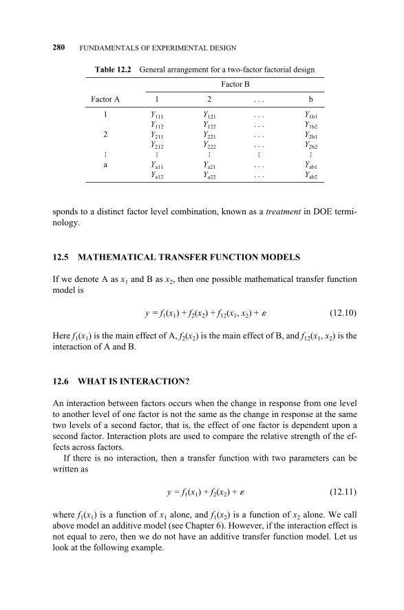
sponds to a distinct factor level combination, known as a treatment in DOE termi-nology.
12.5 MATHEMATICAL TRANSFER FUNCTION MODELS
If we denote A as x1 and B as x2, then one possible mathematical transfer functionmodel is
y = f1(x1) + f2(x2) + f12(x1, x2) + � (12.10)
Here f1(x1) is the main effect of A, f2(x2) is the main effect of B, and f12(x1, x2) is theinteraction of A and B.
12.6 WHAT IS INTERACTION?
An interaction between factors occurs when the change in response from one levelto another level of one factor is not the same as the change in response at the sametwo levels of a second factor, that is, the effect of one factor is dependent upon asecond factor. Interaction plots are used to compare the relative strength of the ef-fects across factors.
If there is no interaction, then a transfer function with two parameters can bewritten as
y = f1(x1) + f2(x2) + � (12.11)
where f1(x1) is a function of x1 alone, and f1(x2) is a function of x2 alone. We callabove model an additive model (see Chapter 6). However, if the interaction effect isnot equal to zero, then we do not have an additive transfer function model. Let uslook at the following example.
280 FUNDAMENTALS OF EXPERIMENTAL DESIGN
Table 12.2 General arrangement for a two-factor factorial design
Factor B
Factor A 1 2 . . . b
1 Y111 Y121 . . . Y1b1
Y112 Y122 . . . Y1b2
2 Y211 Y221 . . . Y2b1
Y212 Y222 . . . Y2b2
� � � � �
a Ya11 Ya21 . . . Yab1
Ya12 Ya22 . . . Yab2
c12.qxd 4/22/2005 9:12 AM Page 280
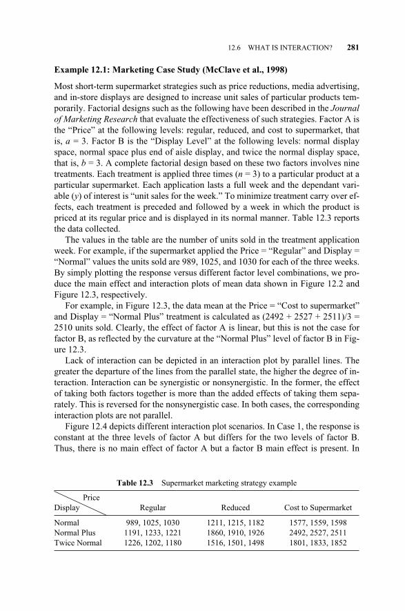
Example 12.1: Marketing Case Study (McClave et al., 1998)
Most short-term supermarket strategies such as price reductions, media advertising,and in-store displays are designed to increase unit sales of particular products tem-porarily. Factorial designs such as the following have been described in the Journalof Marketing Research that evaluate the effectiveness of such strategies. Factor A isthe “Price” at the following levels: regular, reduced, and cost to supermarket, thatis, a = 3. Factor B is the “Display Level” at the following levels: normal displayspace, normal space plus end of aisle display, and twice the normal display space,that is, b = 3. A complete factorial design based on these two factors involves ninetreatments. Each treatment is applied three times (n = 3) to a particular product at aparticular supermarket. Each application lasts a full week and the dependant vari-able (y) of interest is “unit sales for the week.” To minimize treatment carry over ef-fects, each treatment is preceded and followed by a week in which the product ispriced at its regular price and is displayed in its normal manner. Table 12.3 reportsthe data collected.
The values in the table are the number of units sold in the treatment applicationweek. For example, if the supermarket applied the Price = “Regular” and Display =“Normal” values the units sold are 989, 1025, and 1030 for each of the three weeks.By simply plotting the response versus different factor level combinations, we pro-duce the main effect and interaction plots of mean data shown in Figure 12.2 andFigure 12.3, respectively.
For example, in Figure 12.3, the data mean at the Price = “Cost to supermarket”and Display = “Normal Plus” treatment is calculated as (2492 + 2527 + 2511)/3 =2510 units sold. Clearly, the effect of factor A is linear, but this is not the case forfactor B, as reflected by the curvature at the “Normal Plus” level of factor B in Fig-ure 12.3.
Lack of interaction can be depicted in an interaction plot by parallel lines. Thegreater the departure of the lines from the parallel state, the higher the degree of in-teraction. Interaction can be synergistic or nonsynergistic. In the former, the effectof taking both factors together is more than the added effects of taking them sepa-rately. This is reversed for the nonsynergistic case. In both cases, the correspondinginteraction plots are not parallel.
Figure 12.4 depicts different interaction plot scenarios. In Case 1, the response isconstant at the three levels of factor A but differs for the two levels of factor B.Thus, there is no main effect of factor A but a factor B main effect is present. In
12.6 WHAT IS INTERACTION? 281
Table 12.3 Supermarket marketing strategy example
PriceDisplay Regular Reduced Cost to Supermarket
Normal 989, 1025, 1030 1211, 1215, 1182 1577, 1559, 1598Normal Plus 1191, 1233, 1221 1860, 1910, 1926 2492, 2527, 2511Twice Normal 1226, 1202, 1180 1516, 1501, 1498 1801, 1833, 1852
c12.qxd 4/22/2005 9:12 AM Page 281
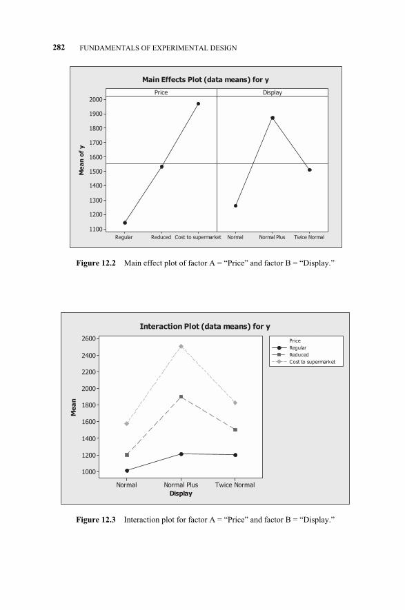
282 FUNDAMENTALS OF EXPERIMENTAL DESIGN
Figure 12.2 Main effect plot of factor A = “Price” and factor B = “Display.”
Me
an
of
y
Cost to supermarketReducedRegular
2000
1900
1800
1700
1600
1500
1400
1300
1200
1100
Twice NormalNormal PlusNormal
Price Display
Main Effects Plot (data means) for y
Figure 12.3 Interaction plot for factor A = “Price” and factor B = “Display.”
Display
Me
an
Twice NormalNormal PlusNormal
2600
2400
2200
2000
1800
1600
1400
1200
1000
Price
Cost to supermarket
Regular
Reduced
Interaction Plot (data means) for y
c12.qxd 4/22/2005 9:12 AM Page 282
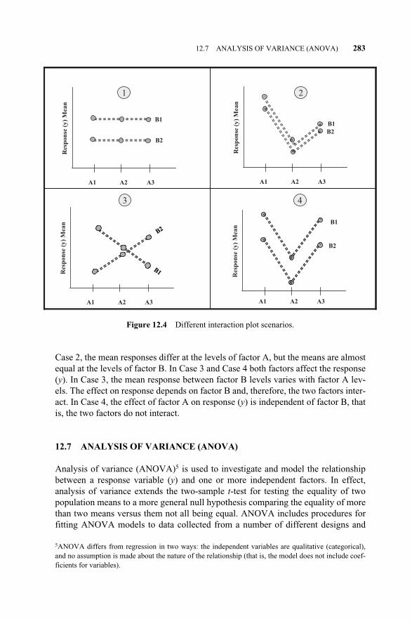
Case 2, the mean responses differ at the levels of factor A, but the means are almostequal at the levels of factor B. In Case 3 and Case 4 both factors affect the response(y). In Case 3, the mean response between factor B levels varies with factor A lev-els. The effect on response depends on factor B and, therefore, the two factors inter-act. In Case 4, the effect of factor A on response (y) is independent of factor B, thatis, the two factors do not interact.
12.7 ANALYSIS OF VARIANCE (ANOVA)
Analysis of variance (ANOVA)5 is used to investigate and model the relationshipbetween a response variable (y) and one or more independent factors. In effect,analysis of variance extends the two-sample t-test for testing the equality of twopopulation means to a more general null hypothesis comparing the equality of morethan two means versus them not all being equal. ANOVA includes procedures forfitting ANOVA models to data collected from a number of different designs and
12.7 ANALYSIS OF VARIANCE (ANOVA) 283
Figure 12.4 Different interaction plot scenarios.
A1 A2 A3
B1
B2
Resp
on
se (
y)
Mean
1
A1 A2 A3
B1
B2
Resp
on
se (
y)
Mean
2
A1 A2 A3
B1
B2
Resp
on
se (
y)
Mea
n
4
A1 A2 A3
B1B1
B2B2
Resp
on
se (
y)
Mea
n
3
5ANOVA differs from regression in two ways: the independent variables are qualitative (categorical),and no assumption is made about the nature of the relationship (that is, the model does not include coef-ficients for variables).
c12.qxd 4/22/2005 9:12 AM Page 283
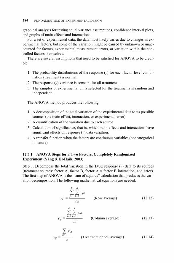
graphical analysis for testing equal variance assumptions, confidence interval plots,and graphs of main effects and interactions.
For a set of experimental data, the data most likely varies due to changes in ex-perimental factors, but some of the variation might be caused by unknown or unac-counted for factors, experimental measurement errors, or variation within the con-trolled factors themselves.
There are several assumptions that need to be satisfied for ANOVA to be credi-ble:
1. The probability distributions of the response (y) for each factor level combi-nation (treatment) is normal.
2. The response (y) variance is constant for all treatments.
3. The samples of experimental units selected for the treatments is random andindependent.
The ANOVA method produces the following:
1. A decomposition of the total variation of the experimental data to its possiblesources (the main effect, interaction, or experimental error)
2. A quantification of the variation due to each source
3. Calculation of significance, that is, which main effects and interactions havesignificant effects on response (y) data variation.
4. A transfer function when the factors are continuous variables (noncategoricalin nature)
12.7.1 ANOVA Steps for a Two Factors, Completely RandomizedExperiment (Yang & El-Haik, 2003)
Step 1. Decompose the total variation in the DOE response (y) data to its sources(treatment sources: factor A, factor B, factor A × factor B interaction, and error).The first step of ANOVA is the “sum of squares” calculation that produces the vari-ation decomposition. The following mathematical equations are needed:
y�i .. = (Row average) (12.12)
y�.j. = (Column average) (12.13)
y�ij. = (Treatment or cell average) (12.14)k=1
yijk
�n
a
i=1n
k=1
yijk
��an
b
j=1n
k=1
yijk
��bn
284 FUNDAMENTALS OF EXPERIMENTAL DESIGN
c12.qxd 4/22/2005 9:12 AM Page 284
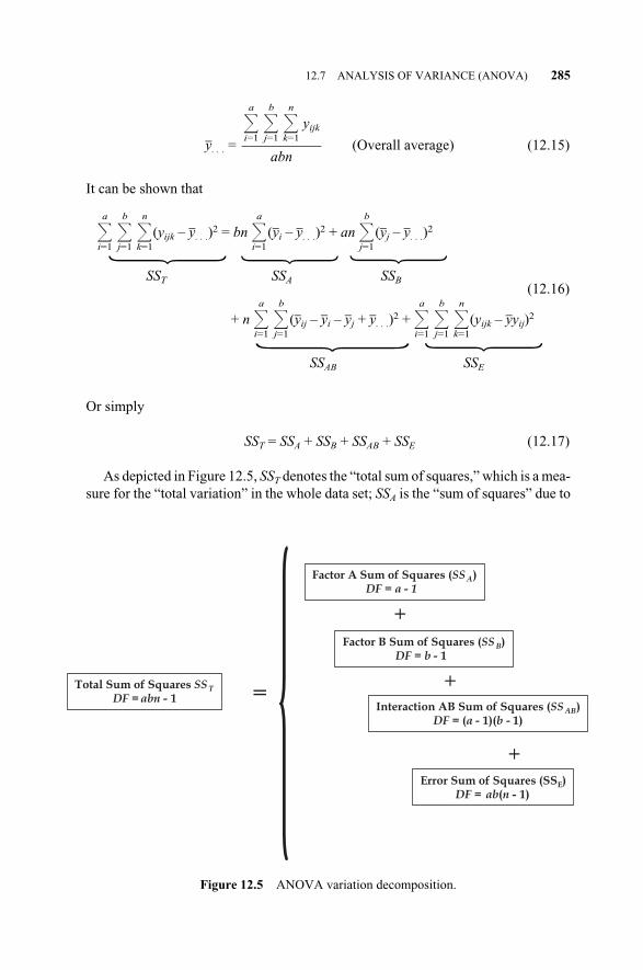
y�. . . = (Overall average) (12.15)
It can be shown that
a
i=1b
j=1n
k=1
(yijk – y�. . .)2 = bn a
i=1
(y�i – y�. . .)2 + an b
j=1
(y�j – y�. . .)2
SST SSA SSB(12.16)
+ n a
i=1b
j=1
(y�ij – y�i – y�j + y�. . .)2 + a
i=1b
j=1n
k=1
(yijk – y�yij)2
SSAB SSE
Or simply
SST = SSA + SSB + SSAB + SSE (12.17)
As depicted in Figure 12.5, SST denotes the “total sum of squares,” which is a mea-sure for the “total variation” in the whole data set; SSA is the “sum of squares” due to
a
i=1b
j=1n
k=1
yijk
��abn
12.7 ANALYSIS OF VARIANCE (ANOVA) 285
Figure 12.5 ANOVA variation decomposition.
Total Sum of Squares SS T
DF = abn - 1
Factor A Sum of Squares (SS A)DF = a - 1
Factor B Sum of Squares (SS B)DF = b - 1
Interaction AB Sum of Squares (SS AB)DF = (a - 1)(b - 1)
Error Sum of Squares (SSE)DF = ab(n - 1)
=
+
+
+
� � ���
c12.qxd 4/22/2005 9:12 AM Page 285

factor A, which is a measure of total variation caused by the main effect of A; SSB isthe sum of squares due to factor B, which is a measure of total variation caused by themain effect of B; SSAB is the sum of squares due to the interaction of factors A and B(denoted as AB), which is the measure of variation caused by interaction; and SSE isthe sum of squares due to error, which is the measure of total variation due to error.
Step 2. Test the null hypothesis with regard to the significance of the factor Amean effect and the factor B mean effect as well as their interaction. The test vehicleis the mean square calculation. The mean square of a source of variation is calculat-ed by dividing the source of variation sum of squares by its degrees of freedom.
The actual amount of variability in the response data depends on the data size. Aconvenient way of expressing this dependence is to say that the sum of squares hasdegrees of freedom (DF) equal to its corresponding variability source data size re-duced by one. Based on statistics, the number of degrees of freedom associated witheach sum of squares is shown in Table 12.4.
Test for Main Effect of Factor AH0: No difference among the a mean levels of factor A (�A1 = �A2 = . . . = �Aa)Ha: At least two factor A mean levels differ
Test for Main Effect of Factor BH0: No difference among the mean levels of factor B (�B1 = �B2 = . . . = �Ba)Ha: At least two factor B mean levels differ
Test for Main Effect of Factor A × Factor B InteractionH0: Factor A and factor B do not interact in the response meanHa: Factor A and factor B interact in the response mean
Step 3. Compare the F-test of the mean square of the experimental treatmentsources to the error to test the null hypothesis that the treatment means are equal. Ifthe test results in nonrejection of the null hypothesis, refine the experiment by in-creasing the number of replicates n or adding other factors. Otherwise, the responseis unrelated to the two factors.
In the F-test, the F0 will be compared, with F-critical defining the null hypothe-sis rejection region values with appropriate degree of freedom. If F0 is larger thanthe critical value, then the corresponding effect is statistically significant. Several
286 FUNDAMENTALS OF EXPERIMENTAL DESIGN
Table 12.4 Degrees of freedom for two-factor factorial design
Effect Degree of freedom (DF)
A a – 1B b – 1AB interaction (a – 1)(b – 1)Error ab(n – 1)
Total abn – 1
c12.qxd 4/22/2005 9:12 AM Page 286

statistical software packages, such as Minitab™, can be used to analyze DOE dataconveniently, or spreadsheet packages like Excel™ can also be used.
In ANOVA, a sum of squares is divided by its corresponding degree of freedomto produce a statistic called the “mean square” that is used in the F-test to see if thecorresponding effect is statistically significant. An ANOVA is often summarized ina table similar to Table 12.5.
Test for Main Effect of Factor ATest statistic: F0,a–1,ab(n–1) = MSA/MSE, with a numerator DF equal to (a – 1) and de-
nominator DF equal to ab(n – 1). H0 hypothesis rejection region: F0,a–1,ab(n–1) � F�,a–1,ab(n–1), with numerator DF
equal to (a – 1) and denominator DF equal to ab(n – 1).
Test for Main Effect of Factor BTest statistic: F0,b–1,ab(n–1) = MSB/MSE, with numerator DF equal to (b – 1) and de-
nominator DF equal to ab(n – 1). H0 hypothesis rejection region: F0,b–1,ab(n–1) � F�,b–1,ab(n–1), with numerator DF
equal to (b – 1) and denominator DF equal to ab(n – 1).
Test for Main Effect of Factor A x Factor B InteractionTest statistic: F0,(a–1)(b–1),ab(n–1) = MSAB/MSE, with a numerator DF equal to (a – 1)(b
– 1) and denominator DF equal to ab(n – 1). H0 hypothesis rejection region: F0,(a–1)(b–1),ab(n–1) � F�,(a–1)(b–1),ab(n–1), with numera-
tor DF equal to (a – 1)(b – 1) and denominator DF equal to ab(n – 1).
The interaction null hypothesis is tested first by computing the F-test of the meansquare for interaction versus the mean square for error. If the test results in nonre-jection of the null hypothesis, then proceed to test the main effects of the factors. Ifthe test results in rejection of the null hypothesis, we conclude that the two factorsinteract in the mean response (y). If the test of interaction is significant, a multiple
12.7 ANALYSIS OF VARIANCE (ANOVA) 287
Table 12.5 ANOVA table
Source of Sum of Degree of variation squares freedom Mean squares F0
A SSA a – 1 MSA = F0 =
B SSB b – 1 MSB = F0 =
AB SSAB (a – 1)(b – 1) MSAB = F0 =
Error SSE ab(n – 1)
Total SST abn – 1
MSAB�MSE
SSAB��(a – 1)(b – 1)
MSB�MSE
SSB�b – 1
MSA�MSE
SSA�a – 1
c12.qxd 4/22/2005 9:12 AM Page 287
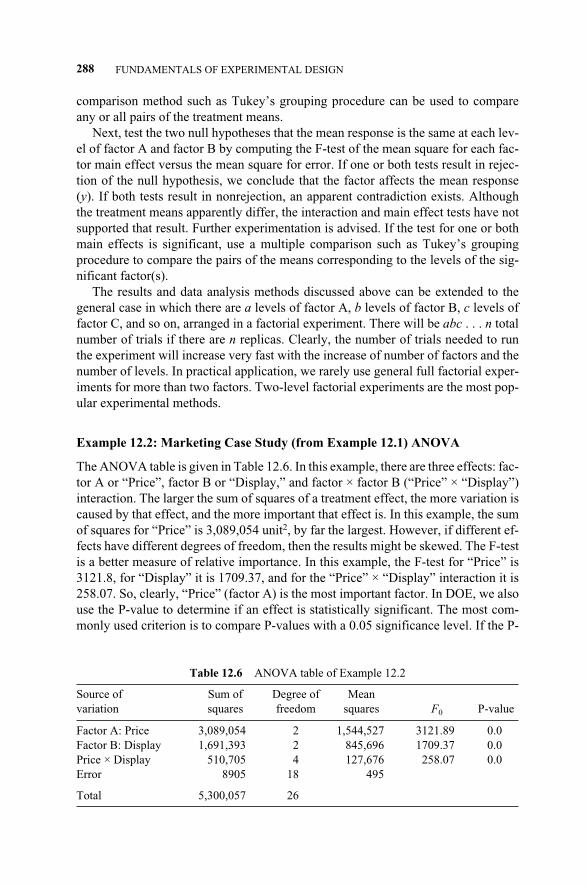
comparison method such as Tukey’s grouping procedure can be used to compareany or all pairs of the treatment means.
Next, test the two null hypotheses that the mean response is the same at each lev-el of factor A and factor B by computing the F-test of the mean square for each fac-tor main effect versus the mean square for error. If one or both tests result in rejec-tion of the null hypothesis, we conclude that the factor affects the mean response(y). If both tests result in nonrejection, an apparent contradiction exists. Althoughthe treatment means apparently differ, the interaction and main effect tests have notsupported that result. Further experimentation is advised. If the test for one or bothmain effects is significant, use a multiple comparison such as Tukey’s groupingprocedure to compare the pairs of the means corresponding to the levels of the sig-nificant factor(s).
The results and data analysis methods discussed above can be extended to thegeneral case in which there are a levels of factor A, b levels of factor B, c levels offactor C, and so on, arranged in a factorial experiment. There will be abc . . . n totalnumber of trials if there are n replicas. Clearly, the number of trials needed to runthe experiment will increase very fast with the increase of number of factors and thenumber of levels. In practical application, we rarely use general full factorial exper-iments for more than two factors. Two-level factorial experiments are the most pop-ular experimental methods.
Example 12.2: Marketing Case Study (from Example 12.1) ANOVA
The ANOVA table is given in Table 12.6. In this example, there are three effects: fac-tor A or “Price”, factor B or “Display,” and factor × factor B (“Price” × “Display”)interaction. The larger the sum of squares of a treatment effect, the more variation iscaused by that effect, and the more important that effect is. In this example, the sumof squares for “Price” is 3,089,054 unit2, by far the largest. However, if different ef-fects have different degrees of freedom, then the results might be skewed. The F-testis a better measure of relative importance. In this example, the F-test for “Price” is3121.8, for “Display” it is 1709.37, and for the “Price” × “Display” interaction it is258.07. So, clearly, “Price” (factor A) is the most important factor. In DOE, we alsouse the P-value to determine if an effect is statistically significant. The most com-monly used criterion is to compare P-values with a 0.05 significance level. If the P-
288 FUNDAMENTALS OF EXPERIMENTAL DESIGN
Table 12.6 ANOVA table of Example 12.2
Source of Sum of Degree of Mean variation squares freedom squares F0 P-value
Factor A: Price 3,089,054 2 1,544,527 3121.89 0.0Factor B: Display 1,691,393 2 845,696 1709.37 0.0Price × Display 510,705 4 127,676 258.07 0.0Error 8905 18 495
Total 5,300,057 26
c12.qxd 4/22/2005 9:12 AM Page 288

value is less than 0.05, then that treatment effect is significant. In this example, the P-values for “Price” and “Display” are 0.0, both smaller than 0.05, so the main effectsof both “Price” and “Display” are statistically significant. It is also the case for“Price” × “Display” interaction, with a 0.0 as a P-value indicating a significant effect.
This example was analyzed using Minitab™, which generated the interaction andmain effects of this example in Figure 12.2 and Figure 12.3. From the interaction plot(Figure 12.3), it is clear that the three line effects are not parallel, so there is an inter-action effect. In main effect chart, we can clearly see that “Price” at the “Cost to su-permarket” level gives much higher units sold. For “Display,” the “Normal Plus”level gives highest units sold. Overall, for achieving the highest product sold units,the supermarket needs to sell it at the cost and display it in a normal-plus space. The� (error) is 8905, which is 0.1% of the total, so we may conclude that the three factorsare statistically significant and provide practical leverage in the response.
12.8 2K FULL FACTORIAL DESIGNS
In many cases, it is sufficient to consider the factors affecting a process at two lev-els. For example, the shoppers for a product may be male or female, marketingstrategy may either be set the price a little higher or a little lower than a target, andso on. The black belt would like to determine whether any of these changes affectthe results of a process. The most intuitive approach to study these factors would beto vary the factors of interest in a full factorial design, that is, to try all possiblecombinations of levels. Such an experiment is called a 2k, an experiment with k fac-tors each with two levels, that is, the number of treatment combinations in a two-level full factorial of k factors is 2 × 2 . . . 2 = 2k. If there are n replicas of each treat-ment combination, then the total number of experimental trials is 2kn. Because thereare only two levels for each factor, we call them the “low” and “high” levels. Forexample, if a factor is “Price,” with two levels, “Regular” and “Regular Plus,” then“Regular” is the low level and “Regular Plus” is the high level.
The two-level factorial design is the most popular designs because it is a full fac-torial design with the least number of runs, an ideal situation for screening experi-ments. The two-level factorial design is the basis of the fractional factorial designthat will be discussed next.
The number of necessary runs in a full 2k experiment will increase geometrical-ly. For example, if the black belt wants to study seven factors, the necessary numberof runs in the experiment would be 27 = 128. To study 10 factors he or she wouldneed 210 = 1,024 runs in the experiment. Because each run may require time-con-suming and costly setting and resetting of the process, it is often not feasible to re-quire that many different runs for the experiment. Under these conditions, fraction-al factorials are used that sacrifice interaction effects so that main effects may stillbe computed correctly.
The standard layout for a two-level design uses a binary notation with +1 and –1denoting the “high level” and the “low level,” respectively, for each factor. For ex-ample, Table 12.7 describes an experiment in which four trials (or runs) were con-
12.8 2K FULL FACTORIAL DESIGNS 289
c12.qxd 4/22/2005 9:12 AM Page 289
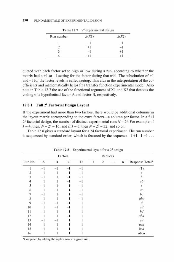
ducted with each factor set to high or low during a run, according to whether thematrix had a +1 or –1 setting for the factor during that trial. The substitution of +1and –1 for the factor levels is called coding. This aids in the interpretation of the co-efficients and mathematically helps fit a transfer function experimental model. Alsonote in Table 12.7 the use of the functional argument of X1 and X2 that denotes thecoding of a hypothetical factor A and factor B, respectively.
12.8.1 Full 2k Factorial Design Layout
If the experiment had more than two factors, there would be additional columns inthe layout matrix corresponding to the extra factors—a column per factor. In a full2k factorial design, the number of distinct experimental runs N = 2k. For example, ifk = 4, then, N = 24 = 16; and if k = 5, then N = 25 = 32; and so on.
Table 12.8 gives a standard layout for a 24 factorial experiment. The run numberis sequenced by standard order, which is featured by the sequence –1 +1 –1 +1 . . .
290 FUNDAMENTALS OF EXPERIMENTAL DESIGN
Table 12.7 24 experimental design
Run number A(X1) A(X2)
1 –1 –12 +1 –13 –1 +14 +1 +1
Table 12.8 Experimental layout for a 24 design
Factors Replicas__________________________ _____________________Run No. A B C D 1 2 . . . n Response Total*
1 –1 –1 –1 –1 (1)2 1 –1 –1 –1 a3 –1 1 –1 –1 b4 1 1 –1 –1 ab5 –1 –1 1 –1 c6 1 –1 1 –1 ac7 –1 1 1 –1 bc8 1 1 1 –1 abc9 –1 –1 –1 1 d
10 1 –1 –1 1 ad11 –1 1 –1 1 bd12 1 1 –1 1 abd13 –1 –1 1 1 cd14 1 –1 1 1 acd15 –1 1 1 1 bcd16 1 1 1 1 abcd
*Computed by adding the replica row in a given run.
c12.qxd 4/22/2005 9:12 AM Page 290
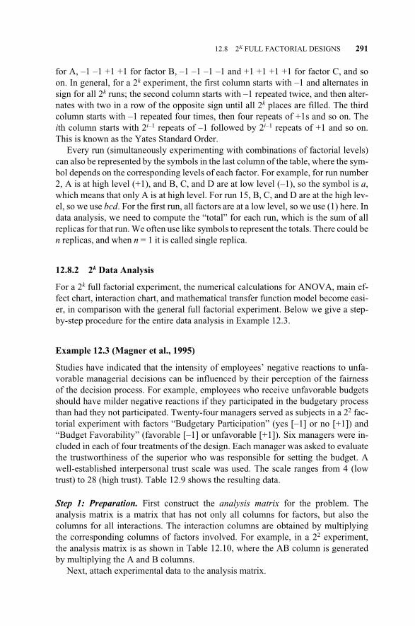
for A, –1 –1 +1 +1 for factor B, –1 –1 –1 –1 and +1 +1 +1 +1 for factor C, and soon. In general, for a 2k experiment, the first column starts with –1 and alternates insign for all 2k runs; the second column starts with –1 repeated twice, and then alter-nates with two in a row of the opposite sign until all 2k places are filled. The thirdcolumn starts with –1 repeated four times, then four repeats of +1s and so on. Theith column starts with 2i–1 repeats of –1 followed by 2i–1 repeats of +1 and so on.This is known as the Yates Standard Order.
Every run (simultaneously experimenting with combinations of factorial levels)can also be represented by the symbols in the last column of the table, where the sym-bol depends on the corresponding levels of each factor. For example, for run number2, A is at high level (+1), and B, C, and D are at low level (–1), so the symbol is a,which means that only A is at high level. For run 15, B, C, and D are at the high lev-el, so we use bcd. For the first run, all factors are at a low level, so we use (1) here. Indata analysis, we need to compute the “total” for each run, which is the sum of allreplicas for that run. We often use like symbols to represent the totals. There could ben replicas, and when n = 1 it is called single replica.
12.8.2 2k Data Analysis
For a 2k full factorial experiment, the numerical calculations for ANOVA, main ef-fect chart, interaction chart, and mathematical transfer function model become easi-er, in comparison with the general full factorial experiment. Below we give a step-by-step procedure for the entire data analysis in Example 12.3.
Example 12.3 (Magner et al., 1995)
Studies have indicated that the intensity of employees’ negative reactions to unfa-vorable managerial decisions can be influenced by their perception of the fairnessof the decision process. For example, employees who receive unfavorable budgetsshould have milder negative reactions if they participated in the budgetary processthan had they not participated. Twenty-four managers served as subjects in a 22 fac-torial experiment with factors “Budgetary Participation” (yes [–1] or no [+1]) and“Budget Favorability” (favorable [–1] or unfavorable [+1]). Six managers were in-cluded in each of four treatments of the design. Each manager was asked to evaluatethe trustworthiness of the superior who was responsible for setting the budget. Awell-established interpersonal trust scale was used. The scale ranges from 4 (lowtrust) to 28 (high trust). Table 12.9 shows the resulting data.
Step 1: Preparation. First construct the analysis matrix for the problem. Theanalysis matrix is a matrix that has not only all columns for factors, but also thecolumns for all interactions. The interaction columns are obtained by multiplyingthe corresponding columns of factors involved. For example, in a 22 experiment,the analysis matrix is as shown in Table 12.10, where the AB column is generatedby multiplying the A and B columns.
Next, attach experimental data to the analysis matrix.
12.8 2K FULL FACTORIAL DESIGNS 291
c12.qxd 4/22/2005 9:12 AM Page 291

Step 2: Compute Contrasts. The contrast of each factor is calculated by multiply-ing the factor column coefficient by the corresponding total and summing them. InTable 12.11, the column coefficients for A (first column) are (–1, +1, –1, +1), thetotal is [(1), a, b, ab] = (132, 121, 138, 90). Therefore,
ContrastA = –(1) + a – b + ab = –132 + 121 – 138 + 90 = –59
Similarly,
ContrastB = –(1) – a + b + ab = –132 – 121 + 138 + 90 = –25
ContrastAB = (1) – a – b + ab = 132 – 121 – 138 + 90 = –37
Contrasts are the basis for many subsequent calculations.
Step 3: Compute Effects. “Effects” include both main effects and interaction ef-fects. All effects are computed by the following formula:
Effect = (12.18)
where N is the total number of runs. The definition for any main effect, for example,the main effect of A, is
A = y�A+ – y�A– (12.19)
Contrast�
2k–1n
292 FUNDAMENTALS OF EXPERIMENTAL DESIGN
Table 12.9 Example 12.3 22 setup
Factor A: Participation
Factor B: Favorability Yes No
Favorable 19 22 25 17 16 2018 25 23 24 23 21
Unfavorable 23 28 20 16 12 1526 18 23 18 15 14
Table 12.10 Analysis Matrix
Run number A B AB
1 –1 –1 (–1) × (–1) = +12 +1 –1 (+1) × (–1) = –13 –1 +1 (–1) × (+1) = –14 +1 +1 (+1) × (+1) = +1
c12.qxd 4/22/2005 9:12 AM Page 292

that is, the average response for A at high level minus the average of response for Aat low level. By Equation (12.18),
A = = = –4.917
Similarly,
B = = = –2.083
AB = = = –3.083
Step 4: Compute SS (Sum of Squares). The sum of squares is the basis for theanalysis of variance computation. The formula for the sum of squares is
SS = = (12.20)
Therefore,
SSA = = = 145.042
SSB = = = 26.042
SSAB = = = 57.042
For completing ANOVA, we also need SST and SSE, in a 22 factorial design:
SST = 2
i=1k
j=1n
k=1
y2ijk – (12.21)
y2. . .
�Nn
(–37)2
�4 × 6
Contrast2AB��
22n
(–25)2
�4 × 6
Contrast2B��
22n
(–59)2
�4 × 6
Contrast2A��
22n
Contrast2�
Nn
Contrast2�
2kn
–37�22–1 6
ContrastAB��
2k–1n
–25�22–1 6
ContrastB��
2k–1n
–59�22–1 6
ContrastA��
2k–1n
12.8 2K FULL FACTORIAL DESIGNS 293
Table 12.11 Analysis matrix and data for Example 12.3
Response
Run No. A B AB 1 2 3 4 5 6 Total
1 –1 –1 1 19 22 25 18 25 23 (1) = 1322 1 –1 –1 17 16 20 24 23 21 a = 1213 –1 1 –1 23 28 20 26 18 23 b = 1384 1 1 1 16 12 15 18 15 14 ab = 90
c12.qxd 4/22/2005 9:12 AM Page 293
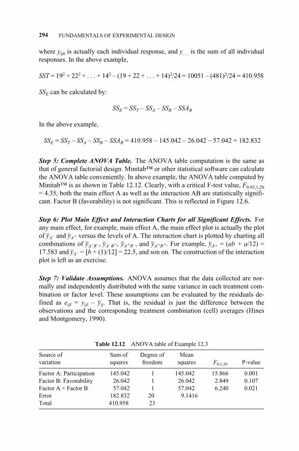
where yijk is actually each individual response, and y. . . is the sum of all individualresponses. In the above example,
SST = 192 + 222 + . . . + 142 – (19 + 22 + . . . + 14)2/24 = 10051 – (481)2/24 = 410.958
SSE can be calculated by:
SSE = SST – SSA – SSB – SSAB
In the above example,
SSE = SST – SSA – SSB – SSAB = 410.958 – 145.042 – 26.042 – 57.042 = 182.832
Step 5: Complete ANOVA Table. The ANOVA table computation is the same asthat of general factorial design. Minitab™ or other statistical software can calculatethe ANOVA table conveniently. In above example, the ANOVA table computed byMinitab™ is as shown in Table 12.12. Clearly, with a critical F-test value, F0.05,1,20
= 4.35, both the main effect A as well as the interaction AB are statistically signifi-cant. Factor B (favorability) is not significant. This is reflected in Figure 12.6.
Step 6: Plot Main Effect and Interaction Charts for all Significant Effects. Forany main effect, for example, main effect A, the main effect plot is actually the plotof y�A– and y�A+ versus the levels of A. The interaction chart is plotted by charting allcombinations of y�A–B–, y�A–B+, y�A+B–, and y�A+B+. For example, y�A+ = (ab + a/12) =17.583 and y�A– = [b + (1)/12] = 22.5, and son on. The construction of the interactionplot is left as an exercise.
Step 7: Validate Assumptions. ANOVA assumes that the data collected are nor-mally and independently distributed with the same variance in each treatment com-bination or factor level. These assumptions can be evaluated by the residuals de-fined as eijl = yijl – y�ij. That is, the residual is just the difference between theobservations and the corresponding treatment combination (cell) averages (Hinesand Montgomery, 1990).
294 FUNDAMENTALS OF EXPERIMENTAL DESIGN
Table 12.12 ANOVA table of Example 12.3
Source of Sum of Degree of Mean variation squares freedom squares F0,1,20 P-value
Factor A: Participation 145.042 1 145.042 15.866 0.001Factor B: Favorability 26.042 1 26.042 2.849 0.107Factor A × Factor B 57.042 1 57.042 6.240 0.021Error 182.832 20 9.1416Total 410.958 23
c12.qxd 4/22/2005 9:12 AM Page 294

Plotting the residuals on normal probability paper and looking for a straight-linefit can check the normality assumption. To check the assumption of equal varianceat each factor level, we plot the residual against the factor levels and compare thespread in the residuals. It is also useful to plot the residuals against fitted values ortreatment combination averages. The variability in the residuals should not in anyway depend on the value of cell averages. When a pattern appears in the plots, indi-cating nonnormality, it suggests the need for transformation, that is, analyzing thedata in a different metric or dimension. In some problems, the dependency of resid-uals scatter in fitted values is very important. We would like to select the level thatimproves y in the direction of goodness; however, this level may also cause morevariation in y from observation to observation.
Plotting the residuals against the time or run order in which the DOE was per-formed can check the independence assumption. A pattern in this plot, such as a se-quence of positive and negative residuals, may indicate that the observations are notindependent. This indicates that the time or run order is important or factors thatchange over time are important and have not been included in the DOE.
Figure 12.7 presents the residual analysis of Example 12.3. The normal probabil-ity plot of these residuals does not appear to deviate from normality. The graph ofresiduals versus fitted values does not reveal any unusual pattern.
Figure 12.8 depicts the Box plot of the response data. It reflects a variabilitydifference between the levels of factor A, the “Participation.” This warrants hy-
12.8 2K FULL FACTORIAL DESIGNS 295
Figure 12.6 Example 12.3 Pareto chart of effects.
Te
rm
Standardized Effect
B
AB
A
43210
2.086Factor Name
A Participation
B Fav orability
Pareto Chart of the Standardized Effects(response is C7, Alpha = .05)
c12.qxd 4/22/2005 9:12 AM Page 295
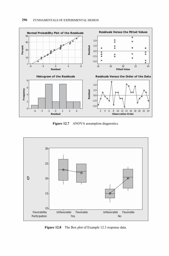
296 FUNDAMENTALS OF EXPERIMENTAL DESIGN
Figure 12.7 ANOVA assumption diagnostics.
Residual
Pe
rce
nt
840-4-8
99
90
50
10
1
Fitted Value
Re
sid
ua
l
2422201816
5.0
2.5
0.0
-2.5
-5.0
Residual
Fre
qu
en
cy
6420-2-4-6
8
6
4
2
0
Observation Order
Re
sid
ua
l
24222018161412108642
5.0
2.5
0.0
-2.5
-5.0
Normal Probability Plot of the Residuals Residuals Versus the Fitted Values
Histogram of the Residuals Residuals Versus the Order of the Data
Figure 12.8 The Box plot of Example 12.3 response data.
C7
Participation
Favorability
NoYes
FavorableUnfavorableFavorableUnfavorable
30
25
20
15
10
Boxplot of “Trustworthiness” by Participation, Favorability
C7
Participation
Favorability
NoYes
FavorableUnfavorableFavorableUnfavorable
30
25
20
15
10
c12.qxd 4/22/2005 9:12 AM Page 296
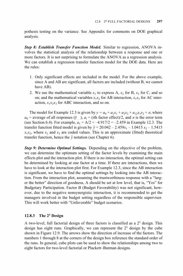
pothesis testing on the variance. See Appendix for comments on DOE graphicalanalysis.
Step 8: Establish Transfer Function Model. Similar to regression, ANOVA in-volves the statistical analysis of the relationship between a response and one ormore factors. It is not surprising to formulate the ANOVA as a regression analysis.We can establish a regression transfer function model for the DOE data. Here arethe rules:
1. Only significant effects are included in the model. For the above example,since A and AB are significant, all factors are included (without B, we cannothave AB).
2. We use the mathematical variable x1 to express A, x2 for B, x3 for C, and soon; and the mathematical variables x1x2 for AB interaction, x1x3 for AC inter-action, x1x2x3 for ABC interaction, and so on.
The model for Example 12.3 is given by y = a0 + a1x1 + a2x2 + a12x1x2 + �, wherea0 = average of all responses (y�. . .), ai = (ith factor effect)/2, and � is the error term(see Section 6.4). For example, a1 = A/2 = –4.917/2 = –2.459 in Example 12.3. Thetransfer function fitted model is given by y = 20.042 – 2.459x1 – 1.0415 x2 – 1.5415x1x2, where x1 and x2 are coded values. This is an approximate (fitted) theoreticaltransfer function, hence the y notation (see Chapter 6).
Step 9: Determine Optimal Settings. Depending on the objective of the problem,we can determine the optimum setting of the factor levels by examining the maineffects plot and the interaction plot. If there is no interaction, the optimal setting canbe determined by looking at one factor at a time. If there are interactions, then wehave to look at the interaction plot first. For Example 12.3, since the AB interactionis significant, we have to find the optimal settings by looking into the AB interac-tion. From the interaction plot, assuming the trustworthiness response with a “larg-er the better” direction of goodness, A should be set at low level, that is, “Yes” forBudgetary Participation. Factor B (Budget Favorability) was not significant, how-ever, due to the negative nonsynergistic interaction, it is recommended to get themanagers involved in the budget setting regardless of the responsible supervisor.This will work better with “Unfavorable” budget scenarios.
12.8.3 The 23 Design
A two-level, full factorial design of three factors is classified as a 23 design. Thisdesign has eight runs. Graphically, we can represent the 23 design by the cubeshown in Figure 12.9. The arrows show the direction of increase of the factors. Thenumbers 1 through 8 at the corners of the design box reference the standard order ofthe runs. In general, cube plots can be used to show the relationships among two toeight factors for two-level factorial or Plackett–Burman designs.
12.8 2K FULL FACTORIAL DESIGNS 297
c12.qxd 4/22/2005 9:12 AM Page 297
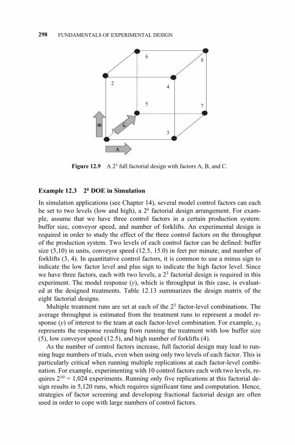
Example 12.3 2k DOE in Simulation
In simulation applications (see Chapter 14), several model control factors can eachbe set to two levels (low and high), a 2k factorial design arrangement. For exam-ple, assume that we have three control factors in a certain production system:buffer size, conveyor speed, and number of forklifts. An experimental design isrequired in order to study the effect of the three control factors on the throughputof the production system. Two levels of each control factor can be defined: buffersize (5,10) in units, conveyor speed (12.5, 15.0) in feet per minute, and number offorklifts (3, 4). In quantitative control factors, it is common to use a minus sign toindicate the low factor level and plus sign to indicate the high factor level. Sincewe have three factors, each with two levels, a 23 factorial design is required in thisexperiment. The model response (y), which is throughput in this case, is evaluat-ed at the designed treatments. Table 12.13 summarizes the design matrix of theeight factorial designs.
Multiple treatment runs are set at each of the 23 factor-level combinations. Theaverage throughput is estimated from the treatment runs to represent a model re-sponse (y) of interest to the team at each factor-level combination. For example, y5
represents the response resulting from running the treatment with low buffer size(5), low conveyor speed (12.5), and high number of forklifts (4).
As the number of control factors increase, full factorial design may lead to run-ning huge numbers of trials, even when using only two levels of each factor. This isparticularly critical when running multiple replications at each factor-level combi-nation. For example, experimenting with 10 control factors each with two levels, re-quires 210 = 1,024 experiments. Running only five replications at this factorial de-sign results in 5,120 runs, which requires significant time and computation. Hence,strategies of factor screening and developing fractional factorial design are oftenused in order to cope with large numbers of control factors.
298 FUNDAMENTALS OF EXPERIMENTAL DESIGN
Figure 12.9 A 23 full factorial design with factors A, B, and C.
1
24
3
5
68
7
A
B C
c12.qxd 4/22/2005 9:12 AM Page 298
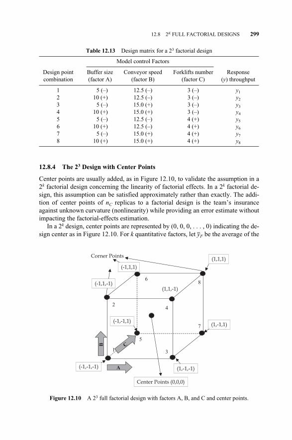
12.8.4 The 23 Design with Center Points
Center points are usually added, as in Figure 12.10, to validate the assumption in a2k factorial design concerning the linearity of factorial effects. In a 2k factorial de-sign, this assumption can be satisfied approximately rather than exactly. The addi-tion of center points of nC replicas to a factorial design is the team’s insuranceagainst unknown curvature (nonlinearity) while providing an error estimate withoutimpacting the factorial-effects estimation.
In a 2k design, center points are represented by (0, 0, 0, . . . , 0) indicating the de-sign center as in Figure 12.10. For k quantitative factors, let y�F be the average of the
12.8 2K FULL FACTORIAL DESIGNS 299
Table 12.13 Design matrix for a 23 factorial design
Model control Factors
Design point Buffer size Conveyor speed Forklifts number Response combination (factor A) (factor B) (factor C) (y) throughput
1 5 (–) 12.5 (–) 3 (–) y1
2 10 (+) 12.5 (–) 3 (–) y2
3 5 (–) 15.0 (+) 3 (–) y3
4 10 (+) 15.0 (+) 3 (–) y4
5 5 (–) 12.5 (–) 4 (+) y5
6 10 (+) 12.5 (–) 4 (+) y6
7 5 (–) 15.0 (+) 4 (+) y7
8 10 (+) 15.0 (+) 4 (+) y8
Figure 12.10 A 23 full factorial design with factors A, B, and C and center points.
1
24
3
5
68
7
A
B C
Center Points (0,0,0)
Corner Points
(1,-1,-1)
(-1,1,-1)(1,1,-1)
(-1,-1,-1)
(1,-1,1)
(-1,1,1)
(1,1,1)
(-1,-1,1)
c12.qxd 4/22/2005 9:12 AM Page 299

2k factorial points and let y�C be the average of the nC center points. When the differ-ence y�F – y�C is large, the center points lie far from the planes passing through thefactorial points, and curvature exists. A single degree of freedom is usually givenfor the sum of squares of nonlinearity or curvature that can be calculated using
SSCurvature = (12.22)
with nC – 1 degrees of freedom, and nF is the number of factorial design points. Fora 23 design, nF = 8. When center points are added to the 23 design, a potential trans-fer function is produced with quadratic terms such as
y = f (x1, x2, x3) = a0 + a1x1 + a2x2 + a3x3 + a12x1x2 + a13x1x3 + a23x2x3__________________ _____________________Linear terms Interaction terms
(12.23)+ a11x1
2 + a22x22 + a33x3
2 + �____________________Quadratic terms
where � is the error term. Each of the coefficients a11, a22, and a33, can be tested for curvature significance
using the hypothesis H0 = a11 + a22 +a33 = 0, versus Ha: at least one quadratic termcoefficient 0.
12.9 FRACTIONAL FACTORIAL DESIGNS6
As the number of factors k increases, the number of runs specified for a full factori-al design can quickly become very large. For example, when k = 6, 26 = 64. Howev-er, in this six-factor experiment, there are six main effects, say, A, B, C, D, E, andF; 15 two-factor interactions, AB, AC, AD, AE, AF, BC, BD, BE, BF, CD, CE, CF,DE, DF, and EF; 20 three-factor interactions, ABC, ABD, . . . ; 15 four-factor inter-actions, ABCD, . . . ; six five-factor interactions; and one six-factor interaction.
Fractional factorial design is a good solution for experimental design with limit-ed resources. The fractional factorial design procedure usually starts by selecting asubset of combinations to test. The subset is selected by focusing on the main ef-fects of control factors and some interactions of interest. The subset size represents2k–p of the 2k possible factorial designs. Determining the p subset, which can be 1,2, 3, and so on, depends on the level of confounding in 2k–p fractional factorial de-signs, where one effect is confounded with another if the two effects are determinedusing the same formula. Factor screening provides a smaller treatment subset byscreening out factors with little or no impact on process performance, using meth-ods such as Plackett–Burman designs, supersaturated design, group-screening de-signs, and frequency-domain methods.
nFnC (y�F – y�C)��
nFnC
300 FUNDAMENTALS OF EXPERIMENTAL DESIGN
6See Chapter 12 of Yang and El-Haik (2003).
c12.qxd 4/22/2005 9:12 AM Page 300
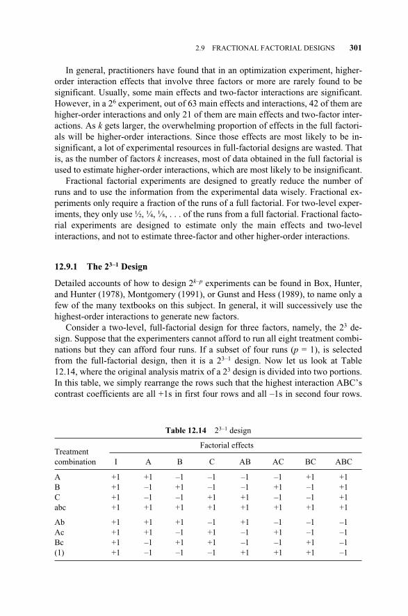
In general, practitioners have found that in an optimization experiment, higher-order interaction effects that involve three factors or more are rarely found to besignificant. Usually, some main effects and two-factor interactions are significant.However, in a 26 experiment, out of 63 main effects and interactions, 42 of them arehigher-order interactions and only 21 of them are main effects and two-factor inter-actions. As k gets larger, the overwhelming proportion of effects in the full factori-als will be higher-order interactions. Since those effects are most likely to be in-significant, a lot of experimental resources in full-factorial designs are wasted. Thatis, as the number of factors k increases, most of data obtained in the full factorial isused to estimate higher-order interactions, which are most likely to be insignificant.
Fractional factorial experiments are designed to greatly reduce the number ofruns and to use the information from the experimental data wisely. Fractional ex-periments only require a fraction of the runs of a full factorial. For two-level exper-iments, they only use ½, ¼, ⅛, . . . of the runs from a full factorial. Fractional facto-rial experiments are designed to estimate only the main effects and two-levelinteractions, and not to estimate three-factor and other higher-order interactions.
12.9.1 The 23–1 Design
Detailed accounts of how to design 2k–p experiments can be found in Box, Hunter,and Hunter (1978), Montgomery (1991), or Gunst and Hess (1989), to name only afew of the many textbooks on this subject. In general, it will successively use thehighest-order interactions to generate new factors.
Consider a two-level, full-factorial design for three factors, namely, the 23 de-sign. Suppose that the experimenters cannot afford to run all eight treatment combi-nations but they can afford four runs. If a subset of four runs (p = 1), is selectedfrom the full-factorial design, then it is a 23–1 design. Now let us look at Table12.14, where the original analysis matrix of a 23 design is divided into two portions.In this table, we simply rearrange the rows such that the highest interaction ABC’scontrast coefficients are all +1s in first four rows and all –1s in second four rows.
2.9 FRACTIONAL FACTORIAL DESIGNS 301
Table 12.14 23–1 design
Factorial effectsTreatmentcombination I A B C AB AC BC ABC
A +1 +1 –1 –1 –1 –1 +1 +1B +1 –1 +1 –1 –1 +1 –1 +1C +1 –1 –1 +1 +1 –1 –1 +1abc +1 +1 +1 +1 +1 +1 +1 +1
Ab +1 +1 +1 –1 +1 –1 –1 –1Ac +1 +1 –1 +1 –1 +1 –1 –1Bc +1 –1 +1 +1 –1 –1 +1 –1(1) +1 –1 –1 –1 +1 +1 +1 –1
c12.qxd 4/22/2005 9:12 AM Page 301
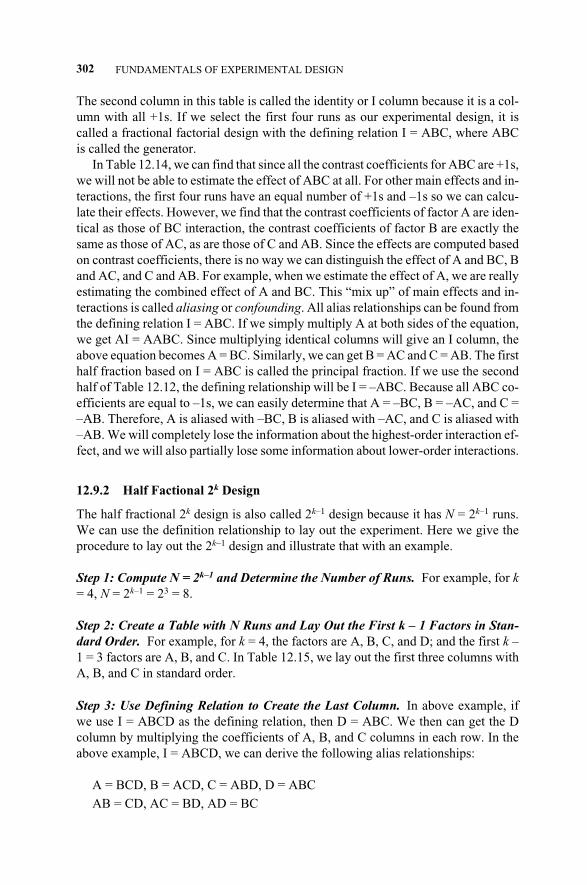
The second column in this table is called the identity or I column because it is a col-umn with all +1s. If we select the first four runs as our experimental design, it iscalled a fractional factorial design with the defining relation I = ABC, where ABCis called the generator.
In Table 12.14, we can find that since all the contrast coefficients for ABC are +1s,we will not be able to estimate the effect of ABC at all. For other main effects and in-teractions, the first four runs have an equal number of +1s and –1s so we can calcu-late their effects. However, we find that the contrast coefficients of factor A are iden-tical as those of BC interaction, the contrast coefficients of factor B are exactly thesame as those of AC, as are those of C and AB. Since the effects are computed basedon contrast coefficients, there is no way we can distinguish the effect of A and BC, Band AC, and C and AB. For example, when we estimate the effect of A, we are reallyestimating the combined effect of A and BC. This “mix up” of main effects and in-teractions is called aliasing or confounding. All alias relationships can be found fromthe defining relation I = ABC. If we simply multiply A at both sides of the equation,we get AI = AABC. Since multiplying identical columns will give an I column, theabove equation becomes A = BC. Similarly, we can get B = AC and C = AB. The firsthalf fraction based on I = ABC is called the principal fraction. If we use the secondhalf of Table 12.12, the defining relationship will be I = –ABC. Because all ABC co-efficients are equal to –1s, we can easily determine that A = –BC, B = –AC, and C =–AB. Therefore, A is aliased with –BC, B is aliased with –AC, and C is aliased with–AB. We will completely lose the information about the highest-order interaction ef-fect, and we will also partially lose some information about lower-order interactions.
12.9.2 Half Factional 2k Design
The half fractional 2k design is also called 2k–1 design because it has N = 2k–1 runs.We can use the definition relationship to lay out the experiment. Here we give theprocedure to lay out the 2k–1 design and illustrate that with an example.
Step 1: Compute N = 2k–1 and Determine the Number of Runs. For example, for k= 4, N = 2k–1 = 23 = 8.
Step 2: Create a Table with N Runs and Lay Out the First k – 1 Factors in Stan-dard Order. For example, for k = 4, the factors are A, B, C, and D; and the first k –1 = 3 factors are A, B, and C. In Table 12.15, we lay out the first three columns withA, B, and C in standard order.
Step 3: Use Defining Relation to Create the Last Column. In above example, ifwe use I = ABCD as the defining relation, then D = ABC. We then can get the Dcolumn by multiplying the coefficients of A, B, and C columns in each row. In theabove example, I = ABCD, we can derive the following alias relationships:
A = BCD, B = ACD, C = ABD, D = ABC
AB = CD, AC = BD, AD = BC
302 FUNDAMENTALS OF EXPERIMENTAL DESIGN
c12.qxd 4/22/2005 9:12 AM Page 302
Unlike 23–1 design, the main effects are not aliased with two-factor interactions, buttwo-factor interactions are aliased with each other. If we assume that three-factorinteractions are not significant, then main effects can be estimated free of aliases.Though both 23–1 and 24–1 are half fractional factorial designs, 24–1 has less con-founding than 23–1. This is because their resolutions are different.
12.9.3 Design Resolution
A 2k–p design means that we study overall k factors; however, p of those factorswere generated from the interactions of a full 2k–p factorial design. As a result, thedesign does not give full resolution; that is, there are certain interaction effects thatare confounded with other effects. In general, a design of resolution R is one inwhich no main effects are confounded with any other interaction of order less thanR – l. In a resolution III (R = III) design, no main effects are confounded with anyother interaction of order less than R – I = III – I = II. Thus, main effects in this de-sign are confounded with two-way interactions and, consequently, all higher-orderinteractions are equally confounded.
The resolution is defined as the length of the shortest “word” in a defining rela-tion. For example, the defining relation of a 23–1 design is I = ABC. There are threeletters in the defining relation (“word”), so it is a resolution III design. The definingrelation of a 24–1 design is I = ABCD. There are four letters in the defining relation,so it is a resolution IV design. Resolution describes the degree to which estimatedmain effects are aliased (or confounded) with estimated two-level interactions,three-level interactions, and so on. Higher-resolution designs have less severe con-founding, but require more runs.
A resolution IV design is “better” than a resolution III design because we have aless-severe confounding pattern in the resolution IV design than in the resolution IIIsituation, so higher-order interactions are less likely to be significant than lower-or-der interactions. A higher-resolution design for the same number of factors will,however, require more runs. In two-level fractional factorial experiments, the fol-lowing three resolutions are most frequently used:
2.9 FRACTIONAL FACTORIAL DESIGNS 303
Table 12.15 23–1 standard order table
Factors Replicas__________________________ _______________________
Run No. A B C D 1 2 . . . n Response total
1 –1 –1 –1 –1 (1)2 1 –1 –1 –1 a3 –1 1 –1 –1 b4 1 1 –1 –1 ab5 –1 –1 1 –1 c6 1 –1 1 –1 ac7 –1 1 1 –1 bc8 1 1 1 –1 abc
c12.qxd 4/22/2005 9:12 AM Page 303
� Resolution III Designs. Main effects are confounded (aliased) with two-factorinteractions.
� Resolution IV Designs. No main effects are aliased with two-factor interac-tions, but two-factor interactions are aliased with each other.
� Resolution V Designs. No main effect or two-factor interaction is aliased withany other main effect or two-factor interaction, but two-factor interactions arealiased with three-factor interactions.
12.9.4 Quarter Fraction of 2k Design
When the number of factors, k, gets larger, 2k–1 designs will also require many runs.Then, a smaller fraction factorial design is needed. A quarter fraction of factorialdesign is also called a 2k–2 design. For a 2k–1 design, there is one defining relation-ship. Each defining relationship is able to reduce the number of runs by half. For a2k–2 design, two defining relationships are needed. If P and Q represent the genera-tors chosen, then I = P and I = Q are called generating relations for the design. Also,because I = P and I = Q, I = PQ. I = P = Q = PQ is called the complete defining re-lation.
Consider a 26–2 design. In this design, there are six factors, say, A, B, C, D, E,and F. For a 26–1 design, the generator would be I = ABCDEF, and we would have aresolution VI design. For a 26–2 design, if we choose P and Q to have five letters, forexample, P = ABCDE, Q = ACDEF, then PQ = BF. From I = P = Q = PQ, the com-plete defining relation is I = ABCDE = ACDEF = BF. We will only have resolutionII! In this case, even the main effects are confounded so, clearly, it is not a good de-sign. If we choose P and Q to be four letters, for example P = ABCE, Q = BCDF,then PQ = ADEF and I = ABCE = BCDF = ADEF. This is a resolution IV design.Clearly, it is also the highest resolution that a 26–2 design can achieve. Now we candevelop a procedure to lay out the 2k–2 design, and illustrate that with an example.
Step 1: Compute N = 2k–2 and Determine the Number of Runs. For example, for k= 6, N = 2k–2 = 24 = 16.
Step 2: Create a Table with N Runs, and Lay Out the First k – 2 Factors in Stan-dard Order. For example, for k = 6, the factors are A, B, C, D, E, and F. The first k– 2 = 4 factors are A, B, C, and D. We will lay out the first four columns with A, B,C, and D in standard order (Table 12.16).
Step 3: Use Defining Relation to Create the Last Two Columns. In Table 12.16, ifwe use I = ABCE as the defining relation, then E = ABC and I = BCDF, then F =BCD.
Example 12.4 (See Yang and El-Haik, 2003)
The manager of a manufacturing company is concerned about the large number oferrors in invoices. An investigation is conducted to determine the major sources of
304 FUNDAMENTALS OF EXPERIMENTAL DESIGN
c12.qxd 4/22/2005 9:12 AM Page 304
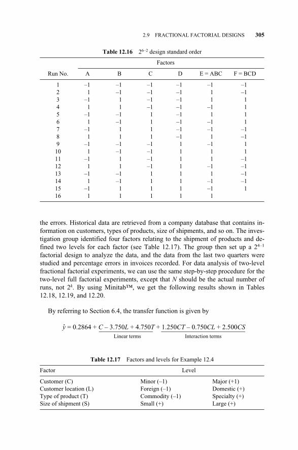
the errors. Historical data are retrieved from a company database that contains in-formation on customers, types of products, size of shipments, and so on. The inves-tigation group identified four factors relating to the shipment of products and de-fined two levels for each factor (see Table 12.17). The group then set up a 24–1
factorial design to analyze the data, and the data from the last two quarters werestudied and percentage errors in invoices recorded. For data analysis of two-levelfractional factorial experiments, we can use the same step-by-step procedure for thetwo-level full factorial experiments, except that N should be the actual number ofruns, not 2k. By using Minitab™, we get the following results shown in Tables12.18, 12.19, and 12.20.
By referring to Section 6.4, the transfer function is given by
y = 0.2864 + C – 3.750L + 4.750T + 1.250CT – 0.750CL + 2.500CS________________ _________________________Linear terms Interaction terms
2.9 FRACTIONAL FACTORIAL DESIGNS 305
Table 12.16 26–2 design standard order
Factors
Run No. A B C D E = ABC F = BCD
1 –1 –1 –1 –1 –1 –12 1 –1 –1 –1 1 –13 –1 1 –1 –1 1 14 1 1 –1 –1 –1 15 –1 –1 1 –1 1 16 1 –1 1 –1 –1 17 –1 1 1 –1 –1 –18 1 1 1 –1 1 –19 –1 –1 –1 1 –1 1
10 1 –1 –1 1 1 111 –1 1 –1 1 1 –112 1 1 –1 1 –1 –113 –1 –1 1 1 1 –114 1 –1 1 1 –1 –115 –1 1 1 1 –1 116 1 1 1 1 1
Table 12.17 Factors and levels for Example 12.4
Factor Level
Customer (C) Minor (–1) Major (+1)Customer location (L) Foreign (–1) Domestic (+)Type of product (T) Commodity (–1) Specialty (+)Size of shipment (S) Small (+) Large (+)
c12.qxd 4/22/2005 9:12 AM Page 305
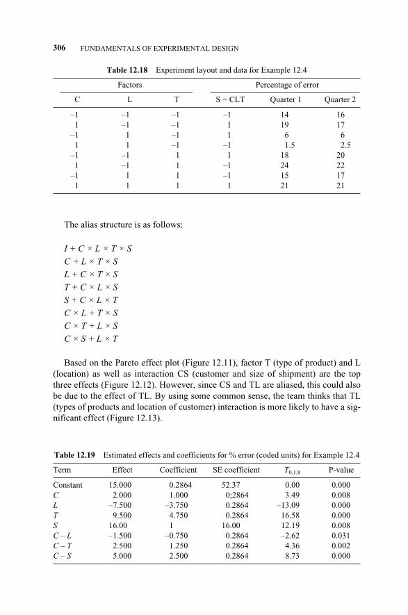
The alias structure is as follows:
I + C × L × T × S
C + L × T × S
L + C × T × S
T + C × L × S
S + C × L × T
C × L + T × S
C × T + L × S
C × S + L × T
Based on the Pareto effect plot (Figure 12.11), factor T (type of product) and L(location) as well as interaction CS (customer and size of shipment) are the topthree effects (Figure 12.12). However, since CS and TL are aliased, this could alsobe due to the effect of TL. By using some common sense, the team thinks that TL(types of products and location of customer) interaction is more likely to have a sig-nificant effect (Figure 12.13).
306 FUNDAMENTALS OF EXPERIMENTAL DESIGN
Table 12.18 Experiment layout and data for Example 12.4
Factors Percentage of error________________________________ ____________________________________
C L T S = CLT Quarter 1 Quarter 2
–1 –1 –1 –1 14 161 –1 –1 1 19 17
–1 1 –1 1 6 61 1 –1 –1 1.5 2.5
–1 –1 1 1 18 201 –1 1 –1 24 22
–1 1 1 –1 15 171 1 1 1 21 21
Table 12.19 Estimated effects and coefficients for % error (coded units) for Example 12.4
Term Effect Coefficient SE coefficient T0,1,8 P-value
Constant 15.000 0.2864 52.37 0.00 0.000C 2.000 1.000 0;2864 3.49 0.008L –7.500 –3.750 0.2864 –13.09 0.000T 9.500 4.750 0.2864 16.58 0.000S 16.00 1 16.00 12.19 0.008C – L –1.500 –0.750 0.2864 –2.62 0.031C – T 2.500 1.250 0.2864 4.36 0.002C – S 5.000 2.500 0.2864 8.73 0.000
c12.qxd 4/22/2005 9:12 AM Page 306
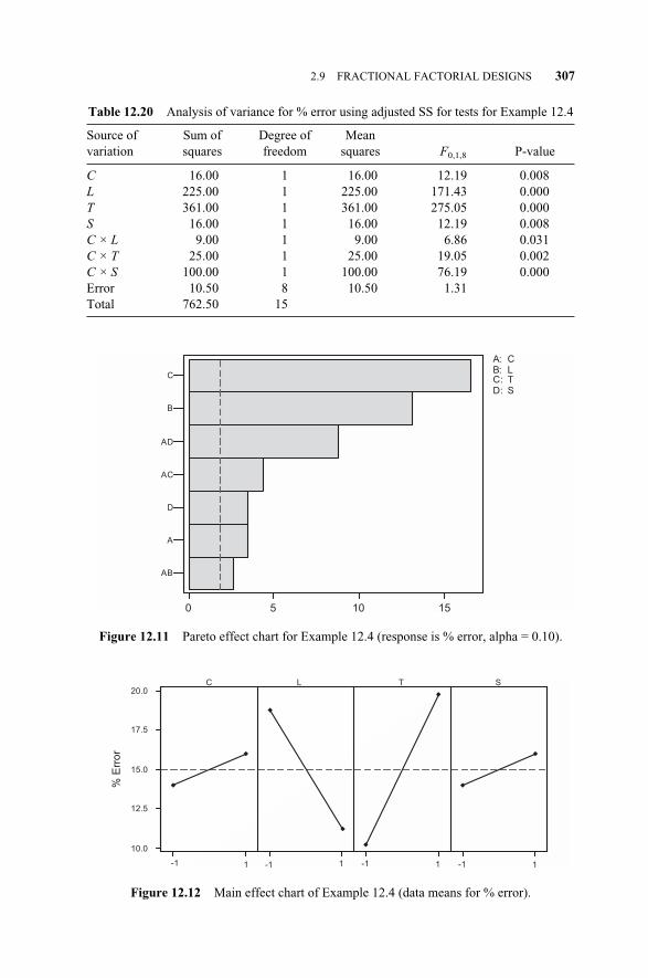
2.9 FRACTIONAL FACTORIAL DESIGNS 307
Table 12.20 Analysis of variance for % error using adjusted SS for tests for Example 12.4
Source of Sum of Degree of Mean variation squares freedom squares F0,1,8 P-value
C 16.00 1 16.00 12.19 0.008L 225.00 1 225.00 171.43 0.000T 361.00 1 361.00 275.05 0.000S 16.00 1 16.00 12.19 0.008C × L 9.00 1 9.00 6.86 0.031C × T 25.00 1 25.00 19.05 0.002C × S 100.00 1 100.00 76.19 0.000Error 10.50 8 10.50 1.31Total 762.50 15
Figure 12.11 Pareto effect chart for Example 12.4 (response is % error, alpha = 0.10).
0 5 10 15
AB
A
D
AC
AD
B
C
A: CB: LC: TD: S
Figure 12.12 Main effect chart of Example 12.4 (data means for % error).
C L T S
10.0
12.5
15.0
17.5
20.0
% E
rro
r
-1 1 -1 -1 -11 1 1
c12.qxd 4/22/2005 9:12 AM Page 307
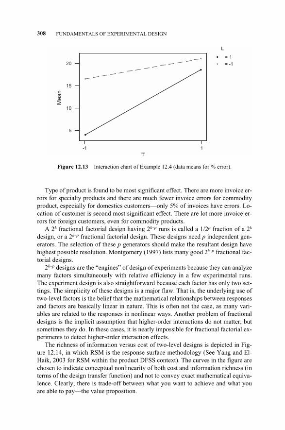
Type of product is found to be most significant effect. There are more invoice er-rors for specialty products and there are much fewer invoice errors for commodityproduct, especially for domestics customers—only 5% of invoices have errors. Lo-cation of customer is second most significant effect. There are lot more invoice er-rors for foreign customers, even for commodity products.
A 2k fractional factorial design having 2k–p runs is called a 1/2p fraction of a 2k
design, or a 2k–p fractional factorial design. These designs need p independent gen-erators. The selection of these p generators should make the resultant design havehighest possible resolution. Montgomery (1997) lists many good 2k–p fractional fac-torial designs.
2k–p designs are the “engines” of design of experiments because they can analyzemany factors simultaneously with relative efficiency in a few experimental runs.The experiment design is also straightforward because each factor has only two set-tings. The simplicity of these designs is a major flaw. That is, the underlying use oftwo-level factors is the belief that the mathematical relationships between responsesand factors are basically linear in nature. This is often not the case, as many vari-ables are related to the responses in nonlinear ways. Another problem of fractionaldesigns is the implicit assumption that higher-order interactions do not matter; butsometimes they do. In these cases, it is nearly impossible for fractional factorial ex-periments to detect higher-order interaction effects.
The richness of information versus cost of two-level designs is depicted in Fig-ure 12.14, in which RSM is the response surface methodology (See Yang and El-Haik, 2003 for RSM within the product DFSS context). The curves in the figure arechosen to indicate conceptual nonlinearity of both cost and information richness (interms of the design transfer function) and not to convey exact mathematical equiva-lence. Clearly, there is trade-off between what you want to achieve and what youare able to pay—the value proposition.
308 FUNDAMENTALS OF EXPERIMENTAL DESIGN
Figure 12.13 Interaction chart of Example 12.4 (data means for % error).
= 1
= -1
-1 1
5
10
15
20
T
L
Mean
c12.qxd 4/22/2005 9:12 AM Page 308
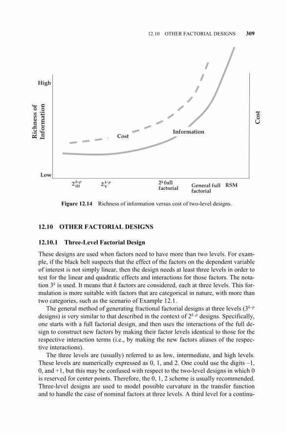
12.10 OTHER FACTORIAL DESIGNS
12.10.1 Three-Level Factorial Design
These designs are used when factors need to have more than two levels. For exam-ple, if the black belt suspects that the effect of the factors on the dependent variableof interest is not simply linear, then the design needs at least three levels in order totest for the linear and quadratic effects and interactions for those factors. The nota-tion 3k is used. It means that k factors are considered, each at three levels. This for-mulation is more suitable with factors that are categorical in nature, with more thantwo categories, such as the scenario of Example 12.1.
The general method of generating fractional factorial designs at three levels (3k–p
designs) is very similar to that described in the context of 2k–p designs. Specifically,one starts with a full factorial design, and then uses the interactions of the full de-sign to construct new factors by making their factor levels identical to those for therespective interaction terms (i.e., by making the new factors aliases of the respec-tive interactions).
The three levels are (usually) referred to as low, intermediate, and high levels.These levels are numerically expressed as 0, 1, and 2. One could use the digits –1,0, and +1, but this may be confused with respect to the two-level designs in which 0is reserved for center points. Therefore, the 0, 1, 2 scheme is usually recommended.Three-level designs are used to model possible curvature in the transfer functionand to handle the case of nominal factors at three levels. A third level for a continu-
12.10 OTHER FACTORIAL DESIGNS 309
Figure 12.14 Richness of information versus cost of two-level designs.
2 IIIk-p
High
Low
Ric
hn
ess
of
Info
rma
tio
n
2kfull factorial
2 Vk-p
General full factorial
RSM
CostInformation
Co
st
c12.qxd 4/22/2005 9:12 AM Page 309
ous factor facilitates investigation of a quadratic relationship between the responseand each of the factors. Unfortunately, the three-level design is prohibitive in termsof the number of runs and, thus, in terms of cost and effort.
12.10.2 Box–Behnken Designs
For 2k–p designs, Plackett and Burman (1946) developed highly fractionalized de-signs to screen the maximum number of (main) effects in the least number of exper-imental runs. Their equivalent for 3k–p designs are the so-called Box–Behnken de-signs (Box and Draper, 1987). These designs do not have simple design generators(they are constructed by combining two-level factorial designs with incompleteblock designs), and suffer from complex confounding of interaction. However, thedesigns are economical and, therefore, particularly useful when it is expensive toperform the necessary experimental runs. The analysis of these types of designsproceeds basically in the same way as was described in the context of 2k–p designs.However, for each effect, one can now test for the linear effect and the quadratic(nonlinear) effect. Nonlinearity often occurs when a process performs near its opti-mum.
12.11 SUMMARY
A design of experiment (DOE) is a structured method for determining the transferfunction relationship between factors affecting a process and the output of thatprocess (y). In essence, it is a methodology for conducting and analyzing controlledtests to evaluate the effects of factors that control the value of a variable or a groupof responses. DOE refers to experimental methods used to quantify indeterminatemeasurements of factors and interactions between factors statistically, through ob-servance of forced changes made methodically as directed by systematic tables.
There are two main bodies of knowledge in DOE: experimental design and ex-perimental data analysis. Two types of experimental design strategies are discussedin this chapter: full factorial and fractional factorial. Full factorial design is used toobtain more information when affordable, since the size of the experiment willgrow exponentially with the number of experimental factors and levels. Fractionalfactorial design obtains less information from an experiment but the experimentsize will grow much slower than that of a full factorial design. In addition, we canadjust the resolution of a fractional factorial design so it can obtain the needed in-formation while keeping the experiment to a manageable size. Therefore, fractionalfactorial design has become the “work horse” of DOE. DOE is critical in creatingorthogonal designs, those in which the factors are independent of each other.
The main DOE data analysis tools include analysis of variance (ANOVA), em-pirical transfer function model building, and main effects and interaction charts.ANOVA is able to identify the set of significant factors and interactions, and rankthe relative importance of each effect and interaction in terms of their effect on de-sign output. Empirical transfer function models, main effect plots, and interaction
310 FUNDAMENTALS OF EXPERIMENTAL DESIGN
c12.qxd 4/22/2005 9:12 AM Page 310
plots show the empirical relationship between design output and design factors.They can also be used to identify optimal factor level settings and correspondingoptimal design performance levels.
APPENDIX
Diagnostic Plots of Residuals
Before accepting a particular ANOVA result or a transfer function that includes aparticular number of effects, the black belt should always examine the distributionof the residual values. This is computed as the difference between the predicted val-ues (as predicted by the current model) and the observed values. He or she can com-pute the histogram for these residual values, as well as probability plots, or generatethem from a statistical package such as Minitab™.
The parameter estimates and ANOVA tables are based on the assumption thatthe residuals are normally distributed. The histogram provides one way to visuallycheck whether this assumption holds.
The normal probability plot is another common tool to assess how closely a setof observed values (residuals in this case) follows a theoretical distribution. In thisplot, the actual residual values are plotted along the horizontal X-axis; the verticalY-axis shows the expected normal values for the respective values, after they havebeen rank ordered. If all values fall onto a straight line, then one can be satisfiedthat the residuals follow the normal distribution.
Pareto Chart of Effects
The Pareto chart of effects is often an effective tool for communicating the resultsof an experiment, in particular to laymen. In this graph, the ANOVA effect esti-mates are sorted from the largest absolute value to the smallest absolute value. Acolumn represents the magnitude of each effect and, often, a line going across thecolumns indicates how large an effect has to be to be statistically significant.
Square and Cube Plots
These plots are often used to summarize predicted values for the response variable,given the respective high and low settings of the factors. The square plot will showthe predicted values for two factors at a time. The cube plot will show the predictedvalues for three factors at a time.
Interaction Plots
A general graph for showing the means is the standard interaction plot, in whichpoints connected by lines indicate the means. This plot is particularly useful whenthere are significant interaction effects in the analysis.
APPENDIX 311
c12.qxd 4/22/2005 9:12 AM Page 311

c12.qxd 4/22/2005 9:12 AM Page 312
13.1 INTRODUCTION
In the context of this book, the terms “quality” and “robustness” can be used inter-changeably. Robustness is defined as the method of reducing the variation of thefunctional requirements of a design and keeping them on target as defined by thecustomer (Taguchi, 1986; Taguchi and Wu, 1986; Phadke, 1989; Taguchi et al.,1989; Taguchi et al., 1999).
Variability reduction has been investigated in the context of robust design(Taguchi, 1986) through methods such as parameter design and tolerance design.The principal idea of robust design is that statistical testing of a product or processshould be carried out at the design stage, also referred to as the “off-line stage” verymuch in line with DFSS. In order to make the service robust against the effects ofvariation sources in the production and use environments, the design problem isviewed from the point of view of quality and cost (Taguchi, 1986; Taguchi and Wu,1989; Taguchi et al., 1989; Taguchi et al., 1999; Nair, 1992).
Quality is measured by quantifying statistical variability through measures suchas standard deviation or mean square error. The main performance criterion is toachieve the design parameter (DP) target on average, while simultaneously mini-mizing variability around this target.
Robustness means that a system performs its intended functions under all operat-ing conditions (different causes of variations) throughout its intended life. The un-desirable and uncontrollable factors that cause the DP under consideration to devi-ate from the target value are called “noise factors.” Noise factors adversely affectquality, and ignoring them will result in a system not optimized for conditions ofuse and, possibly, failure. Eliminating noise factors may be expensive. Instead, weseek to reduce the effect of the noise factors on the DP’s performance by choosingdesign parameters and their settings that are insensitive to noise.
Robust design is a disciplined process that seeks to find the best expression of asystem or process design. “Best” is carefully defined to mean that the design is the
Service Design for Six Sigma. By Basem El-Haik and David M. Roy 313© 2005 by John Wiley & Sons.
13SERVICE DESIGN ROBUSTNESS
c13.qxd 4/22/2005 9:16 AM Page 313
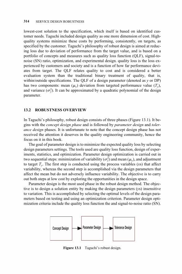
lowest-cost solution to the specification, which itself is based on identified cus-tomer needs. Taguchi included design quality as one more dimension of cost. High-quality systems minimize these costs by performing, consistently, on targets, asspecified by the customer. Taguchi’s philosophy of robust design is aimed at reduc-ing loss due to deviation of performance from the target value, and is based on aportfolio of concepts and measures such as quality loss function (QLF), signal-to-noise (SN) ratio, optimization, and experimental design. quality loss is the loss ex-perienced by customers and society and is a function of how far performance devi-ates from target. The QLF relates quality to cost and is considered a betterevaluation system than the traditional binary treatment of quality, that is,within/outside specifications. The QLF of a design parameter (denoted as y or DP)has two components: mean (�y) deviation from targeted performance value (Ty),and variance (� y
2). It can be approximated by a quadratic polynomial of the designparameter.
13.2 ROBUSTNESS OVERVIEW
In Taguchi’s philosophy, robust design consists of three phases (Figure 13.1). It be-gins with the concept design phase and is followed by parameter design and toler-ance design phases. It is unfortunate to note that the concept design phase has notreceived the attention it deserves in the quality engineering community, hence thefocus on it in this book.
The goal of parameter design is to minimize the expected quality loss by selectingdesign parameters settings. The tools used are quality loss function, design of exper-iments, statistics, and optimization. Parameter design optimization is carried out intwo sequential steps: minimization of variability (� y
2) and mean (�y), and adjustmentto target Ty. The first step is conducted using the process variables (xs) that affectvariability, whereas the second step is accomplished via the design parameters thataffect the mean but do not adversely influence variability. The objective is to carryout both steps at low cost by exploring the opportunities in the design space.
Parameter design is the most used phase in the robust design method. The objec-tive is to design a solution entity by making the design parameters (ys) insensitiveto variation. This is accomplished by selecting the optimal levels of the design para-meters based on testing and using an optimization criterion. Parameter design opti-mization criteria include the quality loss function the and signal-to-noise ratio (SN).
314 SERVICE DESIGN ROBUSTNESS
Concept Design Parameter Design Tolerance Design
Figure 13.1 Taguchi’s robust design.
c13.qxd 4/22/2005 9:16 AM Page 314
The optimum levels of the xs are the levels that maximize the SN and are deter-mined in an experimental setup from a pool of economical alternatives. These alter-natives assume the testing levels in searching for the optimum.
An output response of a process can be classified as static or dynamic from a ro-bustness perspective. A static entity has a fixed target value. The parameter designphase in the case of the static solution entity brings the response (y) and mean, �y,to the target, Ty. On the other hand, the dynamic response expresses a variable tar-get depending on customer intent. In this case, the optimization phase is carried outover a range of useful customer applications called the signal factor. The signal fac-tor can be used to set the y to an intended value. For example, in the loan process ofa mortgage, the signal factor is the amount requested.
Parameter design optimization requires the classification of the design parame-ters (output responses) as smaller the better (e.g., minimize customer complaints,reduce operating cost), larger the better (e.g., increase profit; maximize satisfac-tion), nominal the best (where keeping the process to a single performance objec-tive is the main concern, e.g., meet delivery commitment), and dynamic (where en-ergy related functional performance over a prescribed dynamic rage of usage isperspective, e.g., loan granted versus loan requested).
When robustness cannot be assured by parameter design, we resort to the toler-ance design phase. Tolerance design is the last phase of robust design. This in-volves upgrading or tightening tolerances of some design parameters so that qualityloss can be reduced. However, tightening tolerances will usually add cost to theprocess that controls the tolerance. El-Haik (2005) formulated the problem of find-ing the optimum tolerances of the design parameters that minimize both quality lossand tolerance control costs.
The important contribution of robust design is the systematic inclusion in the ex-perimental design of noise variables, that is, the variables over which the designerhas no or little control. A distinction is also made between internal noise, such asmaterial variability, and environmental noise, which the design team cannot control(e.g., culture, politics). Robust design’s objective is to suppress, as far as possible,the effect of noise by exploring the levels of the factors to determine their potentialfor making the system insensitive to these sources of variation.
Several robust design concepts that apply to service design are presented below.
13.3 ROBUSTNESS CONCEPT #1: QUALITY LOSS FUNCTION
Traditional inspection schemes represent the heart of on-line quality control. In-spection schemes depend on the binary characterization of design parameters, thatis, being within the specification limits or outside the specification limits. A processis called conforming if all of its inspected design parameters are within their respec-tive specification limits, otherwise it is nonconforming. This binary representationof the acceptance criteria per a design parameter is not realistic since it character-izes, equally, entities that are marginally off the specification limits and entities thatare marginally within these limits. In addition, this characterization does not distin-
13.3 ROBUSTNESS CONCEPT #1: QUALITY LOSS FUNCTION 315
c13.qxd 4/22/2005 9:16 AM Page 315
guish the marginally off entities from those that are significantly off. The point hereis that it is not realistic to assume that as we move away from the nominal specifica-tion in a process, the quality loss is zero as long as we stay within the set tolerancelimits. Rather, if the process is not exactly “on target,” then loss will result, for ex-ample, in terms of customer satisfaction. Moreover, this loss is probably not a linearfunction of the deviation from nominal specifications but, rather, a quadratic func-tion. Taguchi proposed a continuous and better representation than this dichoto-mous characterization—the quality loss function (Taguchi and Wu, 1989). The lossfunction provides a better estimate of how the monetary loss incurred by the pro-duction process and customers as an output response (a design parameter) leads todeviation from the targeted performance value, Ty. The determination of the targetTy implies the nominal-the-best and dynamic classifications.
A quality loss function can be interpreted as a method to translate variation andtarget adjustment to a monetary value. It allows the design teams to perform a de-tailed optimization of cost by relating technical terminology to economic measures.In its quadratic form, a quality loss is determined by first finding the functional lim-its,1 Ty ± �y, of the concerned response. The functional limits are the points atwhich the process would fail, that is, the design produces unacceptable performancein approximately half of the customer applications. In a sense, these represent per-formance levels that are equivalent to average customer tolerance. Kapur (1988)continued with this line of thinking and illustrated the derivation of specificationlimits using Taguchi’s quality loss function. Quality loss is incurred due to the devi-ation, caused by noise factors, in the response (y or FR) as from their intended tar-geted performance, Ty. Let L denote the quality loss function (QLF) by taking thenumerical value of the FR and the targeted value as arguments. By Taylor series ex-pansion2 at FR = T, and with some assumption about the significant of the expan-sion terms, we have
L(FR, T) K(FR – TFR)2 (13.1)
Let FR � Ty – �y, Ty + �y , where Ty is the target value and �y is the functionaldeviation from the target (see Figure 13.2). Let A� be the quality loss incurred dueto the symmetrical deviation, �y. Then, by substitution into Equation 13.1 and solv-ing for K,
K = (13.2)
In the Taguchi tolerance design method, the quality loss coefficient K can be de-termined on the basis of losses in monetary terms if the requirement fall outside the
A��(�y)2
316 SERVICE DESIGN ROBUSTNESS
1Functional limits or customer tolerance in robust design terminology is synonymous with design range,DR, in the axiomatic design approach terminology. See Section 2.4.2The assumption here that L is a higher-order continuous function such that derivatives exist and aresymmetrical around y = T.
c13.qxd 4/22/2005 9:16 AM Page 316
≈ ∆
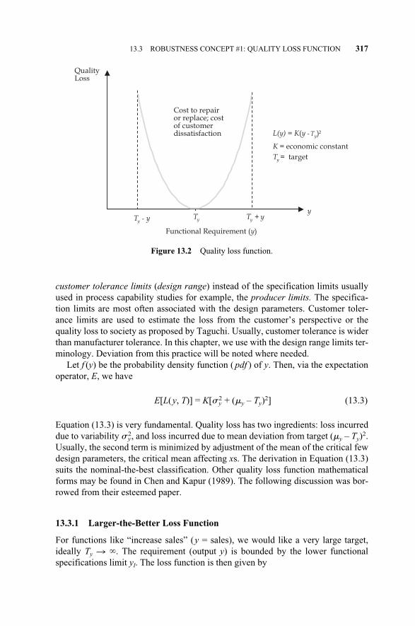
customer tolerance limits (design range) instead of the specification limits usuallyused in process capability studies for example, the producer limits. The specifica-tion limits are most often associated with the design parameters. Customer toler-ance limits are used to estimate the loss from the customer’s perspective or thequality loss to society as proposed by Taguchi. Usually, customer tolerance is widerthan manufacturer tolerance. In this chapter, we use with the design range limits ter-minology. Deviation from this practice will be noted where needed.
Let f (y) be the probability density function ( pdf ) of y. Then, via the expectationoperator, E, we have
E[L(y, T)] = K[� y2 + (�y – Ty)2] (13.3)
Equation (13.3) is very fundamental. Quality loss has two ingredients: loss incurreddue to variability � y
2, and loss incurred due to mean deviation from target (�y – Ty)2.Usually, the second term is minimized by adjustment of the mean of the critical fewdesign parameters, the critical mean affecting xs. The derivation in Equation (13.3)suits the nominal-the-best classification. Other quality loss function mathematicalforms may be found in Chen and Kapur (1989). The following discussion was bor-rowed from their esteemed paper.
13.3.1 Larger-the-Better Loss Function
For functions like “increase sales” (y = sales), we would like a very large target,ideally Ty � �. The requirement (output y) is bounded by the lower functionalspecifications limit yl. The loss function is then given by
13.3 ROBUSTNESS CONCEPT #1: QUALITY LOSS FUNCTION 317
L(y) = K(y - Ty)2
K = economic constant
Ty = target
Ty - yy
Quality Loss
Cost to repair or replace; cost of customer dissatisfaction
Ty
Functional Requirement (y)
Ty + y
Figure 13.2 Quality loss function.
c13.qxd 4/22/2005 9:16 AM Page 317
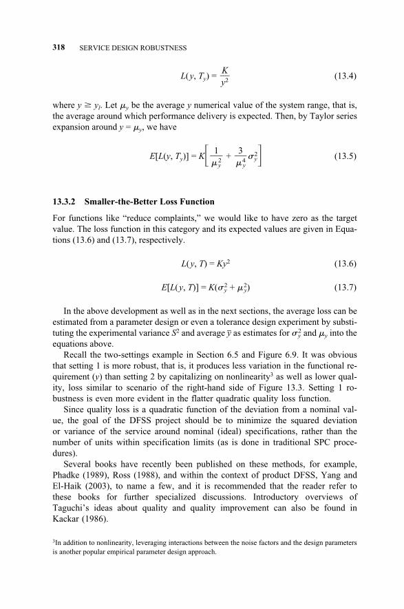
L(y, Ty) = (13.4)
where y � yl. Let �y be the average y numerical value of the system range, that is,the average around which performance delivery is expected. Then, by Taylor seriesexpansion around y = �y, we have
E[L(y, Ty)] = K� + � y2� (13.5)
13.3.2 Smaller-the-Better Loss Function
For functions like “reduce complaints,” we would like to have zero as the targetvalue. The loss function in this category and its expected values are given in Equa-tions (13.6) and (13.7), respectively.
L(y, T) = Ky2 (13.6)
E[L(y, T)] = K(� y2 + � y
2) (13.7)
In the above development as well as in the next sections, the average loss can beestimated from a parameter design or even a tolerance design experiment by substi-tuting the experimental variance S2 and average y� as estimates for � y
2 and �y into theequations above.
Recall the two-settings example in Section 6.5 and Figure 6.9. It was obviousthat setting 1 is more robust, that is, it produces less variation in the functional re-quirement (y) than setting 2 by capitalizing on nonlinearity3 as well as lower qual-ity, loss similar to scenario of the right-hand side of Figure 13.3. Setting 1 ro-bustness is even more evident in the flatter quadratic quality loss function.
Since quality loss is a quadratic function of the deviation from a nominal val-ue, the goal of the DFSS project should be to minimize the squared deviationor variance of the service around nominal (ideal) specifications, rather than thenumber of units within specification limits (as is done in traditional SPC proce-dures).
Several books have recently been published on these methods, for example,Phadke (1989), Ross (1988), and within the context of product DFSS, Yang andEl-Haik (2003), to name a few, and it is recommended that the reader refer tothese books for further specialized discussions. Introductory overviews ofTaguchi’s ideas about quality and quality improvement can also be found inKackar (1986).
3�� y
4
1�� y
2
K�y2
318 SERVICE DESIGN ROBUSTNESS
3In addition to nonlinearity, leveraging interactions between the noise factors and the design parametersis another popular empirical parameter design approach.
c13.qxd 4/22/2005 9:16 AM Page 318
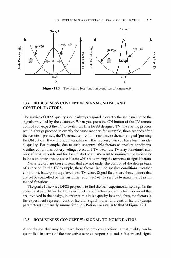
13.4 ROBUSTNESS CONCEPT #2: SIGNAL, NOISE, AND CONTROL FACTORS
The service of DFSS quality should always respond in exactly the same manner to thesignals provided by the customer. When you press the ON button of the TV remotecontrol you expect the TV to switch on. In a DFSS designed TV, the starting processwould always proceed in exactly the same manner; for example, three seconds afterthe remote is pressed, the TV comes to life. If, in response to the same signal (pressingthe ON button), there is random variability in this process, then you have less than ide-al quality. For example, due to such uncontrollable factors as speaker conditions,weather conditions, battery voltage level, and TV wear, the TV may sometimes startonly after 20 seconds and finally not start at all. We want to minimize the variabilityin the output response to noise factors while maximizing the response to signal factors.
Noise factors are those factors that are not under the control of the design teamof a service. In the TV example, these factors include speaker conditions, weatherconditions, battery voltage level, and TV wear. Signal factors are those factors thatare set or controlled by the customer (end user) of the service to make use of its in-tended functions.
The goal of a service DFSS project is to find the best experimental settings (in theabsence of an off-the-shelf transfer function) of factors under the team’s control thatare involved in the design, in order to minimize quality loss and, thus, the factors inthe experiment represent control factors. Signal, noise, and control factors (designparameters) are usually summarized in a P-diagram similar to that of Figure 12.1.
13.5 ROBUSTNESS CONCEPT #3: SIGNAL-TO-NOISE RATIOS
A conclusion that may be drawn from the previous sections is that quality can bequantified in terms of the respective service response to noise factors and signal
13.5 ROBUSTNESS CONCEPT #3: SIGNAL-TO-NOISE RATIOS 319
12
QLF(y)
QLF(y)
Target
Qu
alit
y L
oss
Target
Qu
alit
y L
oss
Target
Qu
alit
y L
oss
TargetTarget
Pro
b. D
ensi
ty,
f(y)
Qu
alit
y L
oss
Pro
b. D
ensi
ty,
f(y)
Target
Qu
alit
y L
oss
Target
Qu
alit
y L
oss
Target
Qu
alit
y L
oss
TargetTarget
Pro
b. D
ensi
ty,
=T=Ty
Qu
alit
y L
oss
=T=Ty
12
QLF(y)f(y), pdf
QLF(y)f(y), pdf
Target
Qu
alit
y L
oss
Target
Qu
alit
y L
oss
Target
Qu
alit
y L
oss
TargetTarget
Pro
b. D
ensi
ty,
f(y)
Qu
alit
y L
oss
Pro
b. D
ensi
ty,
f(y)
Target
Qu
alit
y L
oss
Target
Qu
alit
y L
oss
Target
Qu
alit
y L
oss
TargetTarget
Pro
b. D
ensi
ty,
=T=Ty
Qu
alit
y L
oss
��
=T=Ty
�
�
�
�
Figure 13.3 The quality loss function scenarios of Figure 6.9.
c13.qxd 4/22/2005 9:16 AM Page 319
factors. The ideal service will only respond to customer signals and be unaffectedby random noise factors. Therefore, the goal of the DFSS project can be stated asattempting to maximize the signal-to-noise (SN) ratio for the product. The SN ratiosdescribed in the following paragraphs were proposed by Taguchi (1986).
Smaller the better. In cases in which the DFSS team wants to minimize the oc-currences of some undesirable service responses, they would compute the followingSN ratio:
SN = –10 log10� N
n=1
y i2� (13.8)
The constant, N, represents the number of observations (that have yi as their de-sign parameter) measured in an experiment or in a sample. Experiments are con-ducted and the y measurements are collected. For example, the number of com-plaints with respect to a home mortgage process could be measured as the y variableand analyzed via this SN ratio. The effect of the signal factors is zero, since zerocomplaints is the only intended or desired state of the loan process. Note how thisSN ratio is an expression of the assumed quadratic nature of the loss function. Thefactor 10 ensures that this ratio measures the inverse of bad quality; the more com-plaints in the process, the greater is the sum of the squared number of complaints,and the smaller (i.e., more negative) the SN ratio. Thus, maximizing this ratio willincrease quality.
Nominal the best. Here, the DFSS team has a fixed signal value (nominal value),and the variance around this value can be considered the result of noise factors:
SN = –10 log10� � (13.9)
This signal-to-noise ratio could be used whenever ideal quality is equated with aparticular nominal value. For example, the time delay with respect to a target com-mitment in a home mortgage process could be measured as the y variable and ana-lyzed via this SN ratio. The effect of the signal factors is zero, since the target dateis the only intended or desired state of the loan process.
Larger the better. Examples of this type of service problem are sales, revenue,profit, and so on. The following SN ratio should be used:
SN = –10 log10� N
n=1� (13.10)
Fraction defective (p). This SN ratio is useful for minimizing scrap (servicesoutside the specification limits), for example, the percent of nonclosed mortgageloans. Note that this SN ratio is identical to the familiar logit transformation:
1�y i
2
1�N
�2
��2
1�N
320 SERVICE DESIGN ROBUSTNESS
c13.qxd 4/22/2005 9:16 AM Page 320
SN = 10 log10� � (13.11)
where p is the proportion defective.
13.6 ROBUSTNESS CONCEPT #4: ACCUMULATION ANALYSIS
Accumulation is the most appealing robust design technique to service due to itstreatment of categorical DOE data. In some cases, measurements on a service out-put response can only be obtained in terms of categorical judgments. For example,consumers may rate a service as excellent, good, average, or below average. In thatcase, the DFSS team would attempt to maximize the number of excellent or goodratings. Typically, the results of an accumulation analysis are summarized graphi-cally in a stacked bar plot or a line plot.
When analyzing ordered categorical data, ANOVA is not appropriate. Rather, acumulative plot is produced of the number of observations in a particular category.For each level of each factor, the design team plots the cumulative proportion of thenumber of categories. Thus, this graph provides valuable information concerningthe distribution of the categorical counts across the different factor settings.
13.6.1 Accumulation Analysis Example
Sixteen workers were randomly selected to participate in an experiment to deter-mine the effects of work scheduling and method of payment on attitude toward thejob. Two schedules were employed (Factor A), the standard 8:00 am–5:00 pmworkday and a modification whereby the worker could decide each day whether tostart at 7:00 am or 8:00 am (Level A1); in addition, the worker could choose be-tween a ½ hour and 1 hour lunch period every day (Level A2, current). The twomethods of payments (Factor B) were standard hourly rate (Level B1; current) anda reduced hourly rate with an added piece rate based on the worker’s production(Level B2). Four workers were randomly assigned to each of the four scheduling-payment treatments, and each competed an attitude test after one month on the job.The design team decided to record the attitude data in the following subjective cate-gories, listed progressively opposite to the direction of goodness:
Category I: Excellent
Category II: Good
Category III: Indifferent
Category IV: Bad
The test scores are shown in Table 13.1.
Step 1: Cumulative Accumulation. Among the four data points (worker attitude)in Experiment 1 three belong to category I, 1 belongs to category II, and none be-
p�1 – p
13.6 ROBUSTNESS CONCEPT #4: ACCUMULATION ANALYSIS 321
c13.qxd 4/22/2005 9:16 AM Page 321
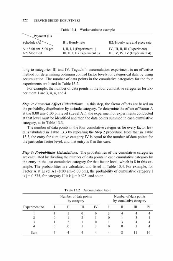
long to categories III and IV. Taguchi’s accumulation experiment is an effectivemethod for determining optimum control factor levels for categorical data by usingaccumulation. The number of data points in the cumulative categories for the fourexperiments are listed in Table 13.2.
For example, the number of data points in the four cumulative categories for Ex-periment 1 are 3, 4, 4, and 4.
Step 2: Factorial Effect Calculations. In this step, the factor effects are based onthe probability distribution by attitude category. To determine the effect of Factor Aat the 8:00 am–5:00 pm level (Level A1), the experiment or experiments conductedat that level must be identified and then the data points summed in each cumulativecategory, as in Table 13.3.
The number of data points in the four cumulative categories for every factor lev-el is tabulated in Table 13.3 by repeating the Step 2 procedure. Note that in Table13.3, the entry for cumulative category IV is equal to the number of data points forthe particular factor level, and that entry is 8 in this case.
Step 3: Probabilities Calculations. The probabilities of the cumulative categoriesare calculated by dividing the number of data points in each cumulative category bythe entry in the last cumulative category for that factor level, which is 8 in this ex-ample. The probabilities are calculated and listed in Table 13.4. For example, forFactor A at Level A1 (8:00 am–5:00 pm), the probability of cumulative category Iis 3–
8 = 0.375, for category II it is 5–8 = 0.625, and so on.
322 SERVICE DESIGN ROBUSTNESS
Table 13.1 Worker attitude example
Payment (B)
Schedule (A) B1: Hourly rate B2: Hourly rate and piece rate
A1: 8:00 am–5:00 pm I, II, I, I (Experiment 1) IV, III, II, III (Experiment)A2: Modified III, II, I, II (Experiment 3) III, IV, IV, IV (Experiment 4)
Table 13.2 Accumulation table
Number of data points Number of data points by category by cumulative category
___________________________ __________________________Experiment no. I II III IV I II III IV
1 3 1 0 0 3 4 4 42 0 1 2 1 0 1 3 43 1 2 1 0 1 3 4 44 0 0 1 3 0 0 1 4
Sum 4 4 4 4 4 8 11 16
c13.qxd 4/22/2005 9:16 AM Page 322
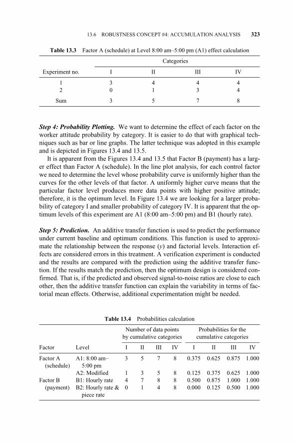
Step 4: Probability Plotting. We want to determine the effect of each factor on theworker attitude probability by category. It is easier to do that with graphical tech-niques such as bar or line graphs. The latter technique was adopted in this exampleand is depicted in Figures 13.4 and 13.5.
It is apparent from the Figures 13.4 and 13.5 that Factor B (payment) has a larg-er effect than Factor A (schedule). In the line plot analysis, for each control factorwe need to determine the level whose probability curve is uniformly higher than thecurves for the other levels of that factor. A uniformly higher curve means that theparticular factor level produces more data points with higher positive attitude;therefore, it is the optimum level. In Figure 13.4 we are looking for a larger proba-bility of category I and smaller probability of category IV. It is apparent that the op-timum levels of this experiment are A1 (8:00 am–5:00 pm) and B1 (hourly rate).
Step 5: Prediction. An additive transfer function is used to predict the performanceunder current baseline and optimum conditions. This function is used to approxi-mate the relationship between the response (y) and factorial levels. Interaction ef-fects are considered errors in this treatment. A verification experiment is conductedand the results are compared with the prediction using the additive transfer func-tion. If the results match the prediction, then the optimum design is considered con-firmed. That is, if the predicted and observed signal-to-noise ratios are close to eachother, then the additive transfer function can explain the variability in terms of fac-torial mean effects. Otherwise, additional experimentation might be needed.
13.6 ROBUSTNESS CONCEPT #4: ACCUMULATION ANALYSIS 323
Table 13.3 Factor A (schedule) at Level 8:00 am–5:00 pm (A1) effect calculation
Categories
Experiment no. I II III IV
1 3 4 4 42 0 1 3 4
Sum 3 5 7 8
Table 13.4 Probabilities calculation
Number of data points Probabilities for the by cumulative categories cumulative categories____________________ _________________________
Factor Level I II III IV I II III IV
Factor A A1: 8:00 am– 3 5 7 8 0.375 0.625 0.875 1.000(schedule) 5:00 pm
A2: Modified 1 3 5 8 0.125 0.375 0.625 1.000Factor B B1: Hourly rate 4 7 8 8 0.500 0.875 1.000 1.000
(payment) B2: Hourly rate & 0 1 4 8 0.000 0.125 0.500 1.000piece rate
c13.qxd 4/22/2005 9:16 AM Page 323
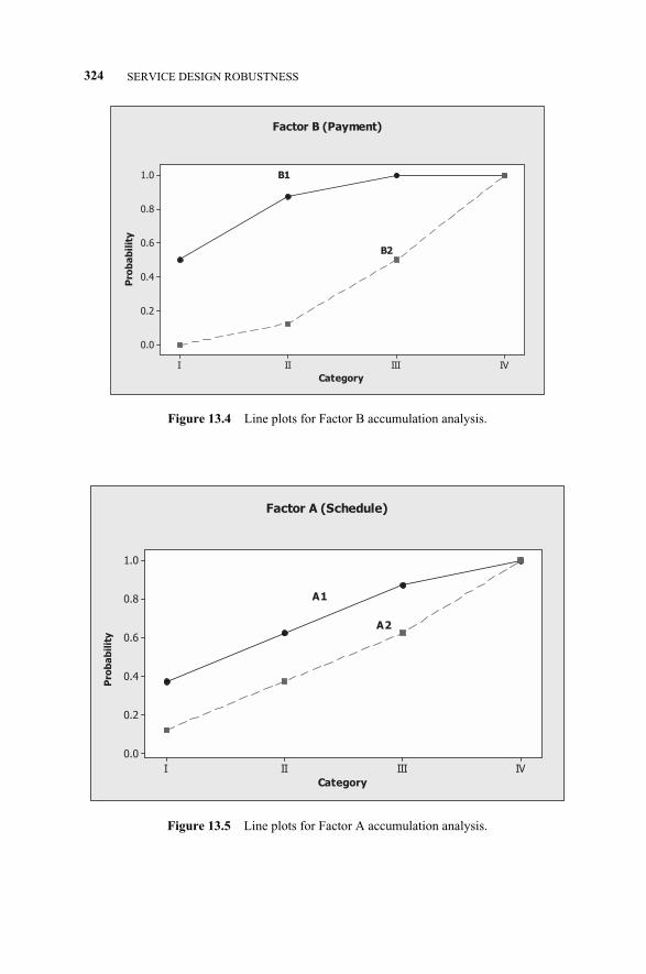
324 SERVICE DESIGN ROBUSTNESS
Category
Pro
ba
bil
ity
IVIIIIII
1.0
0.8
0.6
0.4
0.2
0.0
Factor B (Payment)
B1
B2
Figure 13.4 Line plots for Factor B accumulation analysis.
Category
IVIIIIII
1.0
0.8
0.6
0.4
0.2
0.0
Factor A (Schedule)
A1
A2
Pro
ba
bil
ity
Figure 13.5 Line plots for Factor A accumulation analysis.
c13.qxd 4/22/2005 9:16 AM Page 324
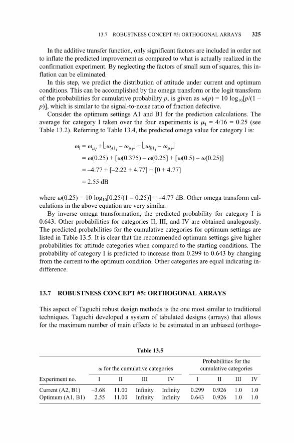
In the additive transfer function, only significant factors are included in order notto inflate the predicted improvement as compared to what is actually realized in theconfirmation experiment. By neglecting the factors of small sum of squares, this in-flation can be eliminated.
In this step, we predict the distribution of attitude under current and optimumconditions. This can be accomplished by the omega transform or the logit transformof the probabilities for cumulative probability p, is given as �(p) = 10 log10[p/(1 –p)], which is similar to the signal-to-noise ratio of fraction defective.
Consider the optimum settings A1 and B1 for the prediction calculations. Theaverage for category I taken over the four experiments is �I = 4/16 = 0.25 (seeTable 13.2). Referring to Table 13.4, the predicted omega value for category I is:
�I = ��I+ �A1I
– ��I+ �B1I
– ��I
= �(0.25) + [�(0.375) – �(0.25] + [�(0.5) – �(0.25)]
= –4.77 + [–2.22 + 4.77] + [0 + 4.77]
= 2.55 dB
where �(0.25) = 10 log10[0.25/(1 – 0.25)] = –4.77 dB. Other omega transform cal-culations in the above equation are very similar.
By inverse omega transformation, the predicted probability for category I is0.643. Other probabilities for categories II, III, and IV are obtained analogously.The predicted probabilities for the cumulative categories for optimum settings arelisted in Table 13.5. It is clear that the recommended optimum settings give higherprobabilities for attitude categories when compared to the starting conditions. Theprobability of category I is predicted to increase from 0.299 to 0.643 by changingfrom the current to the optimum condition. Other categories are equal indicating in-difference.
13.7 ROBUSTNESS CONCEPT #5: ORTHOGONAL ARRAYS
This aspect of Taguchi robust design methods is the one most similar to traditionaltechniques. Taguchi developed a system of tabulated designs (arrays) that allowsfor the maximum number of main effects to be estimated in an unbiased (orthogo-
13.7 ROBUSTNESS CONCEPT #5: ORTHOGONAL ARRAYS 325
Table 13.5
Probabilities for the � for the cumulative categories cumulative categories
_______________________________ ________________________Experiment no. I II III IV I II III IV
Current (A2, B1) –3.68 11.00 Infinity Infinity 0.299 0.926 1.0 1.0Optimum (A1, B1) 2.55 11.00 Infinity Infinity 0.643 0.926 1.0 1.0
c13.qxd 4/22/2005 9:16 AM Page 325
≈ ∆ ≈ ∆
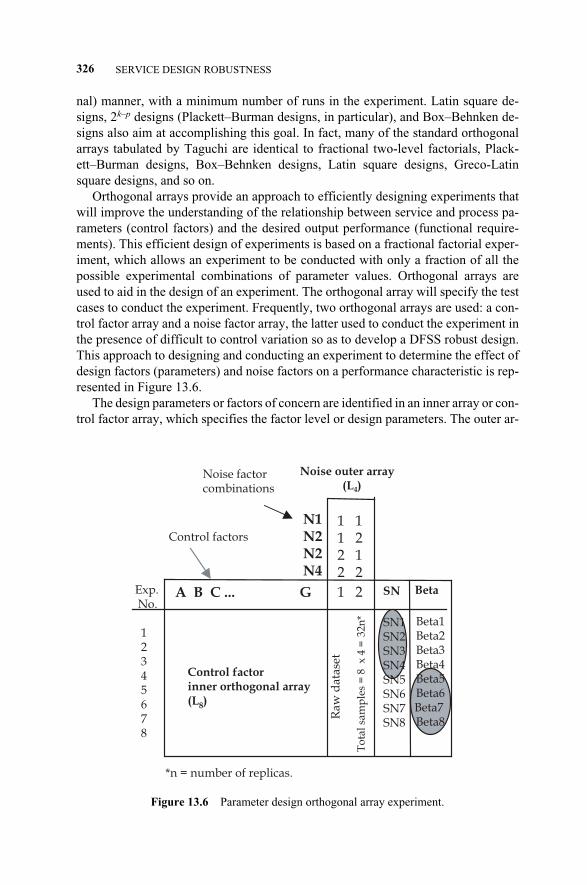
nal) manner, with a minimum number of runs in the experiment. Latin square de-signs, 2k–p designs (Plackett–Burman designs, in particular), and Box–Behnken de-signs also aim at accomplishing this goal. In fact, many of the standard orthogonalarrays tabulated by Taguchi are identical to fractional two-level factorials, Plack-ett–Burman designs, Box–Behnken designs, Latin square designs, Greco-Latinsquare designs, and so on.
Orthogonal arrays provide an approach to efficiently designing experiments thatwill improve the understanding of the relationship between service and process pa-rameters (control factors) and the desired output performance (functional require-ments). This efficient design of experiments is based on a fractional factorial exper-iment, which allows an experiment to be conducted with only a fraction of all thepossible experimental combinations of parameter values. Orthogonal arrays areused to aid in the design of an experiment. The orthogonal array will specify the testcases to conduct the experiment. Frequently, two orthogonal arrays are used: a con-trol factor array and a noise factor array, the latter used to conduct the experiment inthe presence of difficult to control variation so as to develop a DFSS robust design.This approach to designing and conducting an experiment to determine the effect ofdesign factors (parameters) and noise factors on a performance characteristic is rep-resented in Figure 13.6.
The design parameters or factors of concern are identified in an inner array or con-trol factor array, which specifies the factor level or design parameters. The outer ar-
326 SERVICE DESIGN ROBUSTNESS
1 11 22 12 2
1 2
N1N2N2N4
A B C ... G
Control factorinner orthogonal array(L8)
Raw
dat
aset
To
tal
sam
ple
s =
8 x
4 =
32n
*
No.
12345678
Control factors
Noise factorcombinations
Noise outer array (L4)
SN1SN2SN3SN4SN5SN6SN7SN8
SN Beta
Beta1Beta2Beta3Beta4Beta5Beta6Beta7Beta8
*n = number of replicas.
Exp.
Figure 13.6 Parameter design orthogonal array experiment.
c13.qxd 4/22/2005 9:16 AM Page 326
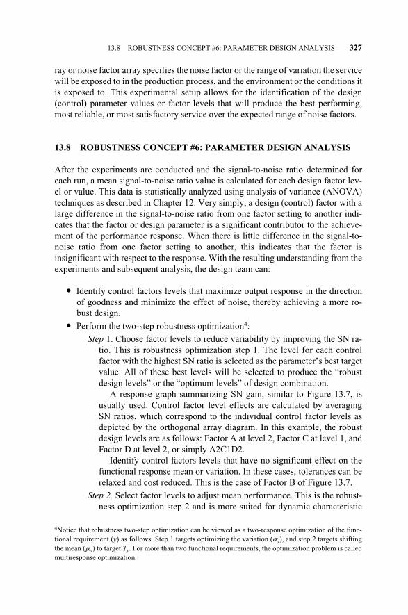
ray or noise factor array specifies the noise factor or the range of variation the servicewill be exposed to in the production process, and the environment or the conditions itis exposed to. This experimental setup allows for the identification of the design(control) parameter values or factor levels that will produce the best performing,most reliable, or most satisfactory service over the expected range of noise factors.
13.8 ROBUSTNESS CONCEPT #6: PARAMETER DESIGN ANALYSIS
After the experiments are conducted and the signal-to-noise ratio determined foreach run, a mean signal-to-noise ratio value is calculated for each design factor lev-el or value. This data is statistically analyzed using analysis of variance (ANOVA)techniques as described in Chapter 12. Very simply, a design (control) factor with alarge difference in the signal-to-noise ratio from one factor setting to another indi-cates that the factor or design parameter is a significant contributor to the achieve-ment of the performance response. When there is little difference in the signal-to-noise ratio from one factor setting to another, this indicates that the factor isinsignificant with respect to the response. With the resulting understanding from theexperiments and subsequent analysis, the design team can:
� Identify control factors levels that maximize output response in the directionof goodness and minimize the effect of noise, thereby achieving a more ro-bust design.
� Perform the two-step robustness optimization4:
Step 1. Choose factor levels to reduce variability by improving the SN ra-tio. This is robustness optimization step 1. The level for each controlfactor with the highest SN ratio is selected as the parameter’s best targetvalue. All of these best levels will be selected to produce the “robustdesign levels” or the “optimum levels” of design combination.
A response graph summarizing SN gain, similar to Figure 13.7, isusually used. Control factor level effects are calculated by averagingSN ratios, which correspond to the individual control factor levels asdepicted by the orthogonal array diagram. In this example, the robustdesign levels are as follows: Factor A at level 2, Factor C at level 1, andFactor D at level 2, or simply A2C1D2.
Identify control factors levels that have no significant effect on thefunctional response mean or variation. In these cases, tolerances can berelaxed and cost reduced. This is the case of Factor B of Figure 13.7.
Step 2. Select factor levels to adjust mean performance. This is the robust-ness optimization step 2 and is more suited for dynamic characteristic
13.8 ROBUSTNESS CONCEPT #6: PARAMETER DESIGN ANALYSIS 327
4Notice that robustness two-step optimization can be viewed as a two-response optimization of the func-tional requirement (y) as follows. Step 1 targets optimizing the variation (�y), and step 2 targets shiftingthe mean (�y) to target Ty. For more than two functional requirements, the optimization problem is calledmultiresponse optimization.
c13.qxd 4/22/2005 9:16 AM Page 327
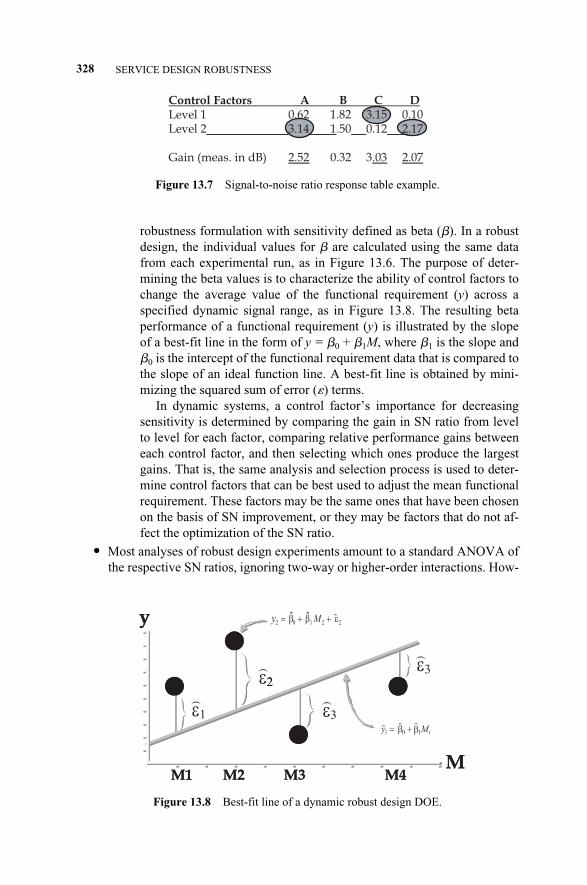
robustness formulation with sensitivity defined as beta ( ). In a robustdesign, the individual values for are calculated using the same datafrom each experimental run, as in Figure 13.6. The purpose of deter-mining the beta values is to characterize the ability of control factors tochange the average value of the functional requirement (y) across aspecified dynamic signal range, as in Figure 13.8. The resulting betaperformance of a functional requirement (y) is illustrated by the slopeof a best-fit line in the form of y = 0 + 1M, where 1 is the slope and 0 is the intercept of the functional requirement data that is compared tothe slope of an ideal function line. A best-fit line is obtained by mini-mizing the squared sum of error (�) terms.
In dynamic systems, a control factor’s importance for decreasingsensitivity is determined by comparing the gain in SN ratio from levelto level for each factor, comparing relative performance gains betweeneach control factor, and then selecting which ones produce the largestgains. That is, the same analysis and selection process is used to deter-mine control factors that can be best used to adjust the mean functionalrequirement. These factors may be the same ones that have been chosenon the basis of SN improvement, or they may be factors that do not af-fect the optimization of the SN ratio.
� Most analyses of robust design experiments amount to a standard ANOVA ofthe respective SN ratios, ignoring two-way or higher-order interactions. How-
328 SERVICE DESIGN ROBUSTNESS
Control Factors A B C DLevel 1 0.62 1.82 3.15 0.10Level 2 3.14 1.50 0.12 2.17
Gain (meas. in dB) 2.52 0.32 3.03 2.07
Figure 13.7 Signal-to-noise ratio response table example.
102ˆˆˆy
ii My10
)))
y
M
2
)
M1 M2 M3 M4
22
ˆˆ εββ ++= M
β)))
+=
y
M
2
M1 M2 M3 M4
ε
1
)ε 3
)ε
3
)ε
β
Figure 13.8 Best-fit line of a dynamic robust design DOE.
c13.qxd 4/22/2005 9:16 AM Page 328
ever, when estimating error variances, one customarily pools together maineffects of negligible size. It should be noted at this point that, of course, all ofthe designs discussed in Chapter 12 (e.g., 2k, 2k–p, 3k–p, etc.) can be used to an-alyze SN ratios. In fact, the many additional diagnostic plots and other op-tions available for those designs (e.g., estimation of quadratic components,etc.) may prove very useful when analyzing the variability (SN ratios) in thedesign. As a visual summary, a SN ratio plot is usually displayed using theexperimental average SN ratio by factor levels. In this plot, the optimum set-ting (largest SN ratio) for each factor can easily be identified.
For prediction purposes, the DFSS team can compute the expected SN ratio giv-en optimum settings of factors (ignoring factors that were pooled into the errorterm). These predicted SN ratios can then be used in a verification experiment inwhich the design team actually sets the process accordingly and compares the resul-tant observed SN ratio with the predicted SN ratio from the experiment. If major de-viations occur, one must conclude that the simple main effect model is not appropri-ate. In those cases, Taguchi (1986) recommends transforming the dependentvariable to accomplish additivity of factors, that is, to make the main effects modelfit. Phadke (1989, Chapter 6) also discusses in detail methods for achieving additiv-ity of factors.
13.9 SUMMARY
To briefly summarize, when using robustness methods, the DFSS team first needsto determine the design or control factors that can be controlled. These are the fac-tors in the experiment for which the team will try different levels. Next, they decideto select an appropriate orthogonal array for the experiment. Next, they need to de-cide on how to measure the quality characteristic of interest. Most SN ratios requirethat multiple measurements be taken in each run of the experiment, so the variabili-ty around the nominal value cannot otherwise be assessed. Finally, the team con-ducts the experiment and identifies the factors that most strongly affect the chosensignal-to-noise ratio, and they reset the process parameters accordingly.
13.9 SUMMARY 329
c13.qxd 4/22/2005 9:16 AM Page 329

c13.qxd 4/22/2005 9:16 AM Page 330

14.1 INTRODUCTION
Production and business systems are key building blocks in the structure of modernindustrial societies. Companies and industrial firms, through which production andbusiness operations are usually performed, represent the major sector of today’sglobal economy. In the last decade, companies have made continuous improvementof their production and business systems a driver in their strategic planning for thenew millennium. To remain competitive, companies have to maintain a high levelof performance by maintaining high quality, low cost, short lead times, and highcustomer satisfaction. Production and business operations have the potential tomake or break a company’s competitive ability. Therefore, efficient and robust pro-duction and business operations become a necessity for survival in the marketplace.These survival instincts are enforced by fierce competition and decreasing businesssafety margins.
Many industrial engineering (IE) subjects such as operations research and sys-tems modeling offer robust and efficient design and problem-solving tools with theultimate aim of performance enhancement. Examples of this performance includethe yield of a process or a factory, the quality of a product, or the profit of an orga-nization.
Simulation modeling, as a tool for process and system design and improvement,has undergone tremendous development in the last decade, in particular with thelaunch of Six Sigma methodology. In the DFSS project road map, simulation mod-eling combined with several statistical tools is most beneficial in the optimize phase(see Figure 5.1). This development can be seein in the growing capabilities of simu-lation software tools and the application of simulation solutions to a variety of real-world problems in different business arenas. With the aid of simulation, companiesare able to design efficient production and business systems, validate and trade offproposed design solution alternatives, solve potential problems, improve systemsperformance metrics, and, consequently, cut cost, meet targets, and boost sales and
Service Design for Six Sigma. By Basem El-Haik and David M. Roy 331© 2005 by John Wiley & Sons.
14DISCRETE EVENT SIMULATION
c14.qxd 4/22/2005 9:17 AM Page 331
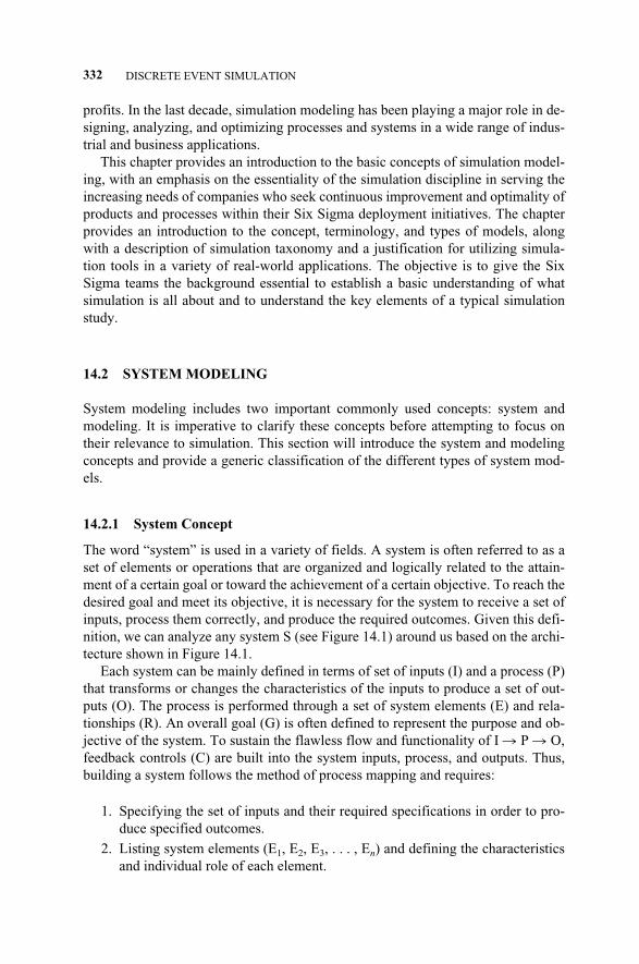
profits. In the last decade, simulation modeling has been playing a major role in de-signing, analyzing, and optimizing processes and systems in a wide range of indus-trial and business applications.
This chapter provides an introduction to the basic concepts of simulation model-ing, with an emphasis on the essentiality of the simulation discipline in serving theincreasing needs of companies who seek continuous improvement and optimality ofproducts and processes within their Six Sigma deployment initiatives. The chapterprovides an introduction to the concept, terminology, and types of models, alongwith a description of simulation taxonomy and a justification for utilizing simula-tion tools in a variety of real-world applications. The objective is to give the SixSigma teams the background essential to establish a basic understanding of whatsimulation is all about and to understand the key elements of a typical simulationstudy.
14.2 SYSTEM MODELING
System modeling includes two important commonly used concepts: system andmodeling. It is imperative to clarify these concepts before attempting to focus ontheir relevance to simulation. This section will introduce the system and modelingconcepts and provide a generic classification of the different types of system mod-els.
14.2.1 System Concept
The word “system” is used in a variety of fields. A system is often referred to as aset of elements or operations that are organized and logically related to the attain-ment of a certain goal or toward the achievement of a certain objective. To reach thedesired goal and meet its objective, it is necessary for the system to receive a set ofinputs, process them correctly, and produce the required outcomes. Given this defi-nition, we can analyze any system S (see Figure 14.1) around us based on the archi-tecture shown in Figure 14.1.
Each system can be mainly defined in terms of set of inputs (I) and a process (P)that transforms or changes the characteristics of the inputs to produce a set of out-puts (O). The process is performed through a set of system elements (E) and rela-tionships (R). An overall goal (G) is often defined to represent the purpose and ob-jective of the system. To sustain the flawless flow and functionality of I � P � O,feedback controls (C) are built into the system inputs, process, and outputs. Thus,building a system follows the method of process mapping and requires:
1. Specifying the set of inputs and their required specifications in order to pro-duce specified outcomes.
2. Listing system elements (E1, E2, E3, . . . , En) and defining the characteristicsand individual role of each element.
332 DISCRETE EVENT SIMULATION
c14.qxd 4/22/2005 9:17 AM Page 332
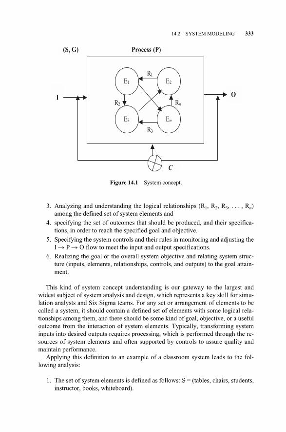
3. Analyzing and understanding the logical relationships (R1, R2, R3, . . . , Rn)among the defined set of system elements and
4. specifying the set of outcomes that should be produced, and their specifica-tions, in order to reach the specified goal and objective.
5. Specifying the system controls and their rules in monitoring and adjusting theI � P � O flow to meet the input and output specifications.
6. Realizing the goal or the overall system objective and relating system struc-ture (inputs, elements, relationships, controls, and outputs) to the goal attain-ment.
This kind of system concept understanding is our gateway to the largest andwidest subject of system analysis and design, which represents a key skill for simu-lation analysts and Six Sigma teams. For any set or arrangement of elements to becalled a system, it should contain a defined set of elements with some logical rela-tionships among them, and there should be some kind of goal, objective, or a usefuloutcome from the interaction of system elements. Typically, transforming systeminputs into desired outputs requires processing, which is performed through the re-sources of system elements and often supported by controls to assure quality andmaintain performance.
Applying this definition to an example of a classroom system leads to the fol-lowing analysis:
1. The set of system elements is defined as follows: S = (tables, chairs, students,instructor, books, whiteboard).
14.2 SYSTEM MODELING 333
Figure 14.1 System concept.
Rn
R3
R2
R1
E1 E2
E3 En
O
Process (P)(S, G)
I
C
c14.qxd 4/22/2005 9:17 AM Page 333
2. The defined elements in S are logically related. For example, chairs are locat-ed around the tables, tables face the instructor, students sit on chairs, booksare on tables in front of students, the instructor uses the whiteboard to explainthe concepts, and so on.
3. The interactions explained in the previous point lead to the goal (G) of learn-ing or educating students on a certain subject.
4. In order to achieve G, students should finish the class with certain qualifica-tions and skills as an outcome (O) of the system.
5. To educate students, learning resources and materials are required as an inputset (I) to the system.
6. Finally, the instructor applies regulations and rules of conduct in the class-room, attendance and grading policies, and so on as a sort of control on theeducation process.
Finally, it is worth mentioning that term “system” includes both products andprocesses. A product system can be an automobile, a cellular phone, a computer, acalculator, and so on. Any of those products involves the defined components of thesystem in terms of inputs, outputs, elements, relationships, controls, and goals. Tryto analyze all the abovementioned examples from this perspective. On the otherhand, a process system can be a manufacturing process, an assembly line, a powerplant, a business process such as banking operations, a logistic system, an educa-tional or academic system, and so on. Similarly, any of these processes involves thedefined components of the system in terms of inputs, outputs, elements, relation-ships, controls, and goals. Try to analyze all the abovementioned examples fromthis perspective too.
14.2.2 Modeling Concept
The word modeling refers to the process of representing a system (a product orprocess) with a selected replica model that is an easier to understand and less ex-pensive to build compared to the actual model. The system representation in themodel implies taking into account the components of the system discussed in theprevious section. This includes representing system elements, relationships, goal,inputs, controls, and outputs. Modeling a system, therefore, has two prerequisites:
1. Understanding the structure of the actual (real-world) system and the func-tionality and characteristics of each system component and relationship. It isimperative to be familiar with the system of interest before attempting tomodel it and to understand its purpose and functionality before establishing auseful representation of its behavior.
2. Being familiar with different modeling and system representation techniquesand methods. This skill is essential when choosing the most appropriate mod-el for representing the real-world system. Once the most appropriate modelhas been selected, it should also assessed for practicality and feasibility. As
334 DISCRETE EVENT SIMULATION
c14.qxd 4/22/2005 9:17 AM Page 334
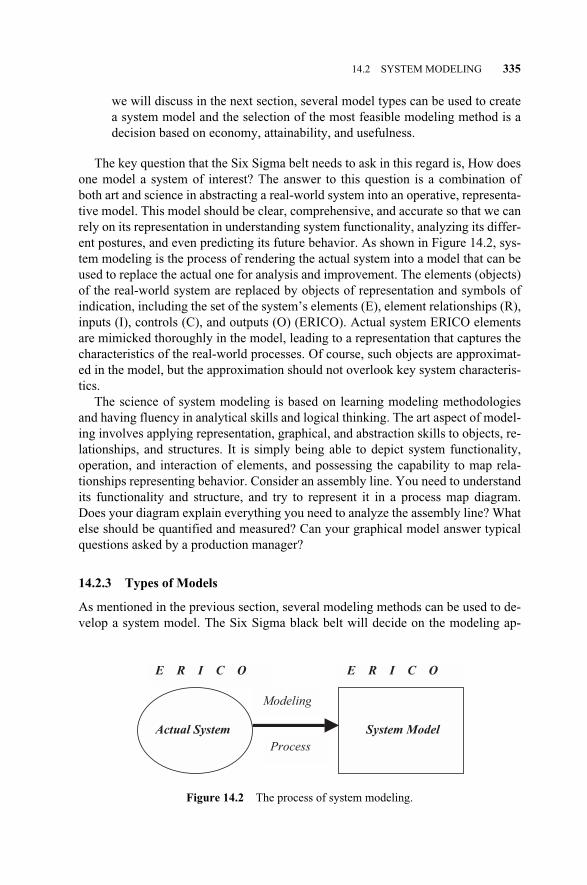
we will discuss in the next section, several model types can be used to createa system model and the selection of the most feasible modeling method is adecision based on economy, attainability, and usefulness.
The key question that the Six Sigma belt needs to ask in this regard is, How doesone model a system of interest? The answer to this question is a combination ofboth art and science in abstracting a real-world system into an operative, representa-tive model. This model should be clear, comprehensive, and accurate so that we canrely on its representation in understanding system functionality, analyzing its differ-ent postures, and even predicting its future behavior. As shown in Figure 14.2, sys-tem modeling is the process of rendering the actual system into a model that can beused to replace the actual one for analysis and improvement. The elements (objects)of the real-world system are replaced by objects of representation and symbols ofindication, including the set of the system’s elements (E), element relationships (R),inputs (I), controls (C), and outputs (O) (ERICO). Actual system ERICO elementsare mimicked thoroughly in the model, leading to a representation that captures thecharacteristics of the real-world processes. Of course, such objects are approximat-ed in the model, but the approximation should not overlook key system characteris-tics.
The science of system modeling is based on learning modeling methodologiesand having fluency in analytical skills and logical thinking. The art aspect of model-ing involves applying representation, graphical, and abstraction skills to objects, re-lationships, and structures. It is simply being able to depict system functionality,operation, and interaction of elements, and possessing the capability to map rela-tionships representing behavior. Consider an assembly line. You need to understandits functionality and structure, and try to represent it in a process map diagram.Does your diagram explain everything you need to analyze the assembly line? Whatelse should be quantified and measured? Can your graphical model answer typicalquestions asked by a production manager?
14.2.3 Types of Models
As mentioned in the previous section, several modeling methods can be used to de-velop a system model. The Six Sigma black belt will decide on the modeling ap-
14.2 SYSTEM MODELING 335
Figure 14.2 The process of system modeling.
Actual System
Modeling
System Model
Process
E R I C O E R I C O
c14.qxd 4/22/2005 9:17 AM Page 335

proach by choosing a certain type of model to represent the actual system. Theblack belt’s choice will be based on several criteria such as system complexity, theobjectives of system modeling, and the cost of modeling. As shown in Figure 14.3,we can classify different types of models into four major categories: physical mod-els, graphical models, mathematical models, and computer models. The followingis a summary of those types of models.
1. Physical models. Physical models are tangible prototypes of the actual prod-ucts or processes, created by using a one-to-one scale or any other feasiblescale of choice. Such models provide a close-to-reality, direct representationof the actual system and can be used for demonstrating the system’s structure,the role of each system element, and the actual functionality of system of in-terest in a physical manner. They help designers achieve a deeper understand-ing of system structure and details and allow them to try out different config-urations of design elements before the actual build of the product anddeployment of the process. They are used primarily in large-scale projects toexamine a limited set of behavioral characteristics in the system. For exam-ple, in the transactional world, an extra customer service clerk can be addedto check the reduction of waiting time.
2. Graphical models. Graphical models are abstracts of the actual products orprocesses created by using graphical tools. This type of modeling starts frompaper and pencil sketches, and proceeds to engineering drawings, pictures,and movies of the system of interest. Most common graphical representationsof systems include the process and functional mapping techniques presentedin Chapter 8.
3. Mathematical models. Mathematical modeling is the process of representingsystem behavior with formulas, mathematical equations, or transfer func-tions. Such models are symbolic representations of systems functionality, de-cision (control) variables, responses, and constraints. They assist in formulat-ing the system design problem in a form that is solvable using graphical andcalculus-based methods. Mathematical models use mathematical equations(transfer functions), probabilistic models, and statistical methods to representthe key relationships among system components. A transfer function equa-tion can be derived in a number of ways. Many of them come from DOE
336 DISCRETE EVENT SIMULATION
Figure 14.3 Types of models.
System Models
Physical
Models
Graphical
Models
Mathematical
Models
Computer
Models
c14.qxd 4/22/2005 9:17 AM Page 336
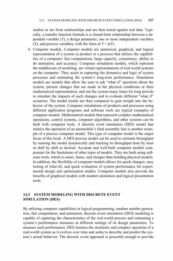
studies or are from relationships and are then tested against real data. Typi-cally, a transfer function formula is a closed-form relationship between a de-pendent variable (Y), a design parameter, one or more independent variables(X), and process variables, with the form of Y = f(X).
4. Computer models. Computer models are numerical, graphical, and logicalrepresentation of a system (a product or a process) that utilizes the capabili-ties of a computer: fast computations, large capacity, consistency, ability todo animation, and accuracy. Computer simulation models, which representthe middleware of modeling, are virtual representations of real-world systemson the computer. They assist in capturing the dynamics and logic of systemprocesses and estimating the system’s long-term performance. Simulationmodels are models that allow the user to ask “what if” questions about thesystem, present changes that are made in the physical conditions or theirmathematical representation, and run the system many times for long periodsto simulate the impacts of such changes and to evaluate different “what if”scenarios. The model results are then compared to gain insight into the be-havior of the system. Computer simulations of products and processes usingdifferent application programs and software tools are typical examples ofcomputer models. Mathematical models that represent complex mathematicaloperations, control systems, computer algorithms, and other systems can bebuilt with computer tools. A discrete event simulation (DES) model thatmimics the operation of an automobile’s final assembly line is another exam-ple of a process computer model. This type of computer model is the majorfocus of this book. A DES process model can be used to estimate throughputby running the model dynamically and tracking its throughput hour by houror shift by shift as desired. Accurate and well-built computer models com-pensate for the limitations of other types of models. They are built using soft-ware tools, which is easier, faster, and cheaper than building physical models.In addition, the flexibility of computer models allows for quick changes, easytesting of what-ifs, and quick evaluation of system performance for experi-mental design and optimization studies. Computer models also provide thebenefits of graphical models with modern animation and logical presentationtools.
14.3 SYSTEM MODELING WITH DISCRETE EVENT SIMULATION (DES)
By utilizing computer capabilities in logical programming, random number genera-tion, fast computation, and animation, discrete event simulation (DES) modeling iscapable of capturing the characteristics of the real-world process and estimating asystem’s performance measures at different settings of its design parameters. Tomeasure such performance, DES imitates the stochastic and complex operation of areal-world system as it evolves over time and seeks to describe and predict the sys-tem’s actual behavior. The discrete event approach is powerful enough to provide
14.3 SYSTEM MODELING WITH DISCRETE EVENT SIMULATION (DES) 337
c14.qxd 4/22/2005 9:17 AM Page 337
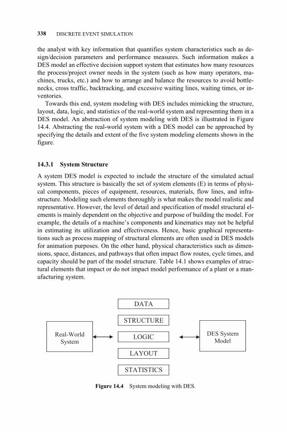
the analyst with key information that quantifies system characteristics such as de-sign/decision parameters and performance measures. Such information makes aDES model an effective decision support system that estimates how many resourcesthe process/project owner needs in the system (such as how many operators, ma-chines, trucks, etc.) and how to arrange and balance the resources to avoid bottle-necks, cross traffic, backtracking, and excessive waiting lines, waiting times, or in-ventories.
Towards this end, system modeling with DES includes mimicking the structure,layout, data, logic, and statistics of the real-world system and representing them in aDES model. An abstraction of system modeling with DES is illustrated in Figure14.4. Abstracting the real-world system with a DES model can be approached byspecifying the details and extent of the five system modeling elements shown in thefigure.
14.3.1 System Structure
A system DES model is expected to include the structure of the simulated actualsystem. This structure is basically the set of system elements (E) in terms of physi-cal components, pieces of equipment, resources, materials, flow lines, and infra-structure. Modeling such elements thoroughly is what makes the model realistic andrepresentative. However, the level of detail and specification of model structural el-ements is mainly dependent on the objective and purpose of building the model. Forexample, the details of a machine’s components and kinematics may not be helpfulin estimating its utilization and effectiveness. Hence, basic graphical representa-tions such as process mapping of structural elements are often used in DES modelsfor animation purposes. On the other hand, physical characteristics such as dimen-sions, space, distances, and pathways that often impact flow routes, cycle times, andcapacity should be part of the model structure. Table 14.1 shows examples of struc-tural elements that impact or do not impact model performance of a plant or a man-ufacturing system.
338 DISCRETE EVENT SIMULATION
Figure 14.4 System modeling with DES.
Real-World
System
DES System
Model
DATA
STRUCTURE
LOGIC
LAYOUT
STATISTICS
c14.qxd 4/22/2005 9:17 AM Page 338
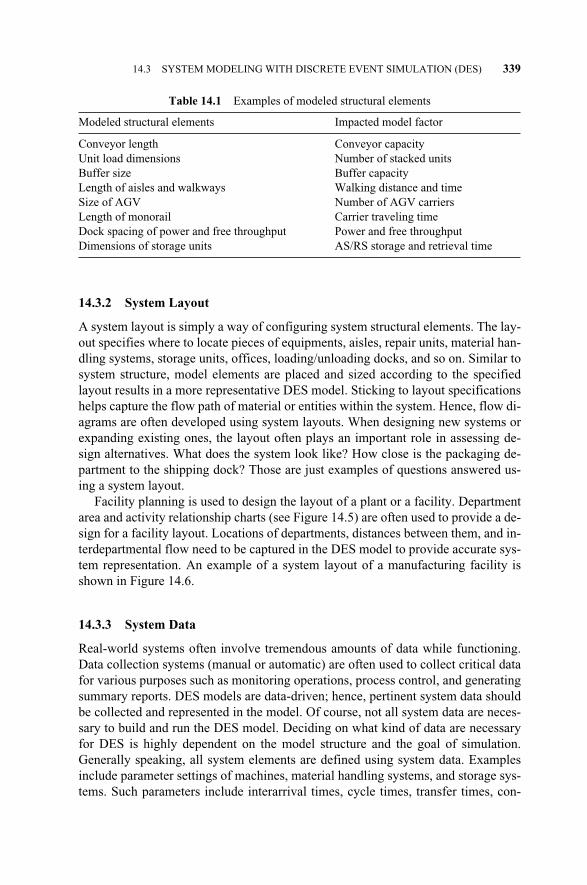
14.3.2 System Layout
A system layout is simply a way of configuring system structural elements. The lay-out specifies where to locate pieces of equipments, aisles, repair units, material han-dling systems, storage units, offices, loading/unloading docks, and so on. Similar tosystem structure, model elements are placed and sized according to the specifiedlayout results in a more representative DES model. Sticking to layout specificationshelps capture the flow path of material or entities within the system. Hence, flow di-agrams are often developed using system layouts. When designing new systems orexpanding existing ones, the layout often plays an important role in assessing de-sign alternatives. What does the system look like? How close is the packaging de-partment to the shipping dock? Those are just examples of questions answered us-ing a system layout.
Facility planning is used to design the layout of a plant or a facility. Departmentarea and activity relationship charts (see Figure 14.5) are often used to provide a de-sign for a facility layout. Locations of departments, distances between them, and in-terdepartmental flow need to be captured in the DES model to provide accurate sys-tem representation. An example of a system layout of a manufacturing facility isshown in Figure 14.6.
14.3.3 System Data
Real-world systems often involve tremendous amounts of data while functioning.Data collection systems (manual or automatic) are often used to collect critical datafor various purposes such as monitoring operations, process control, and generatingsummary reports. DES models are data-driven; hence, pertinent system data shouldbe collected and represented in the model. Of course, not all system data are neces-sary to build and run the DES model. Deciding on what kind of data are necessaryfor DES is highly dependent on the model structure and the goal of simulation.Generally speaking, all system elements are defined using system data. Examplesinclude parameter settings of machines, material handling systems, and storage sys-tems. Such parameters include interarrival times, cycle times, transfer times, con-
14.3 SYSTEM MODELING WITH DISCRETE EVENT SIMULATION (DES) 339
Table 14.1 Examples of modeled structural elements
Modeled structural elements Impacted model factor
Conveyor length Conveyor capacityUnit load dimensions Number of stacked unitsBuffer size Buffer capacityLength of aisles and walkways Walking distance and timeSize of AGV Number of AGV carriersLength of monorail Carrier traveling timeDock spacing of power and free throughput Power and free throughputDimensions of storage units AS/RS storage and retrieval time
c14.qxd 4/22/2005 9:17 AM Page 339
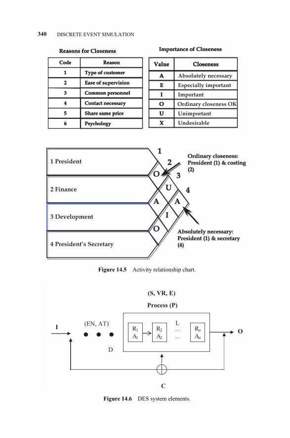
340 DISCRETE EVENT SIMULATION
Figure 14.5 Activity relationship chart.
Reasons for Closeness
Code
1
2
3
4
5
6
Reason
Type of customer
Ease of supervision
Common personnel
Contact necessary
Share same price
Psychology
Value
A
E
I
O
U
X
Closeness
Absolutely necessary
Especially important
Important
Ordinary closeness OK
Unimportant
Undesirable
Importance of Closeness
1 President
O
2 Finance U
A A
3 Development I
O
4 President’s Secretary
11
22
33
Ordinary closeness: Ordinary closeness: President (1) & costing President (1) & costing (2)(2)
Absolutely necessary: Absolutely necessary: President (1) & secretary President (1) & secretary (4)(4)
44
Reasons for Closeness
Code
1
2
3
4
5
6
Reason
Type of customer
Ease of supervision
Common personnel
Contact necessary
Share same price
Psychology
Value
A
E
I
O
U
X
Closeness
Importance of ClosenessReasons for Closeness
Code
1
2
3
4
5
6
Reason
Type of customer
Ease of supervision
Common personnel
Contact necessary
Share same price
Psychology
Value
A
E
I
O
U
X
ClosenessValue
A
E
I
O
U
X
Closeness
Importance of Closeness
O
U
A A
I
O
11
22
33
Ordinary closeness: Ordinary closeness: President (1) & costing President (1) & costing (2)(2)
Absolutely necessary: Absolutely necessary: President (1) & secretary President (1) & secretary (4)(4)
44
Figure 14.6 DES system elements.
O
C
I … R1
A1
R2
A2
Rn
An
...
...
D
L(EN, AT)
(S, VR, E)
Process (P)
c14.qxd 4/22/2005 9:17 AM Page 340
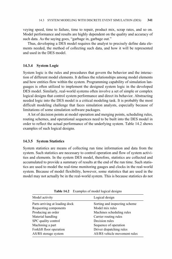
veying speed, time to failure, time to repair, product mix, scrap rates, and so on.Model performance and results are highly dependent on the quality and accuracy ofsuch data. As the saying goes, “garbage in, garbage out.”
Thus, developing a DES model requires the analyst to precisely define data ele-ments needed, the method of collecting such data, and how it will be representedand used in the DES model.
14.3.4 System Logic
System logic is the rules and procedures that govern the behavior and the interac-tion of different model elements. It defines the relationships among model elementsand how entities flow within the system. Programming capability of simulation lan-guages is often utilized to implement the designed system logic in the developedDES model. Similarly, real-world systems often involve a set of simple or complexlogical designs that control system performance and direct its behavior. Abstractingneeded logic into the DES model is a critical modeling task. It is probably the mostdifficult modeling challenge that faces simulation analysts, especially because oflimitations of some simulation software packages.
A lot of decision points at model operation and merging points, scheduling rules,routing schemes, and operational sequences need to be built into the DES model inorder to reflect the actual performance of the underlying system. Table 14.2 showsexamples of such logical designs.
14.3.5 System Statistics
System statistics are means of collecting run time information and data from thesystem. Such statistics are necessary to control operation and flow of system activi-ties and elements. In the system DES model, therefore, statistics are collected andaccumulated to provide a summary of results at the end of the run time. Such statis-tics are used to model the real-time monitoring gauges and clocks in the real-worldsystem. Because of model flexibility, however, some statistics that are used in themodel may not actually be in the real-world system. This is because statistics do not
14.3 SYSTEM MODELING WITH DISCRETE EVENT SIMULATION (DES) 341
Table 14.2 Examples of model logical designs
Model activity Logical design
Parts arriving at loading dock Sorting and inspecting schemeRequesting components Model mix rulesProducing an order Machines scheduling rulesMaterial handling Carrier routing rulesSPC quality control Decision rulesMachining a part Sequence of operationForklift floor operation Driver dispatching rulesAS/RS storage system AS/RS vehicle movement rules
c14.qxd 4/22/2005 9:17 AM Page 341
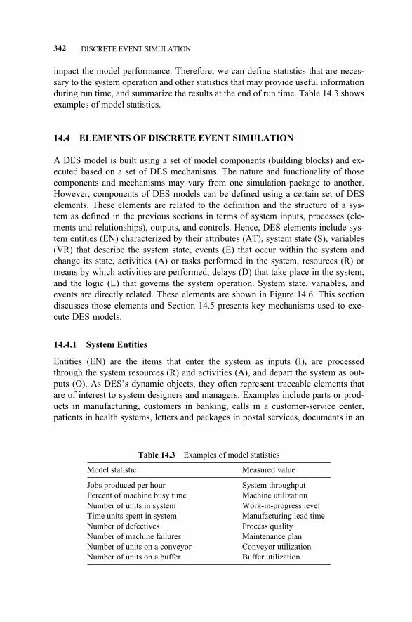
impact the model performance. Therefore, we can define statistics that are neces-sary to the system operation and other statistics that may provide useful informationduring run time, and summarize the results at the end of run time. Table 14.3 showsexamples of model statistics.
14.4 ELEMENTS OF DISCRETE EVENT SIMULATION
A DES model is built using a set of model components (building blocks) and ex-ecuted based on a set of DES mechanisms. The nature and functionality of thosecomponents and mechanisms may vary from one simulation package to another.However, components of DES models can be defined using a certain set of DESelements. These elements are related to the definition and the structure of a sys-tem as defined in the previous sections in terms of system inputs, processes (ele-ments and relationships), outputs, and controls. Hence, DES elements include sys-tem entities (EN) characterized by their attributes (AT), system state (S), variables(VR) that describe the system state, events (E) that occur within the system andchange its state, activities (A) or tasks performed in the system, resources (R) ormeans by which activities are performed, delays (D) that take place in the system,and the logic (L) that governs the system operation. System state, variables, andevents are directly related. These elements are shown in Figure 14.6. This sectiondiscusses those elements and Section 14.5 presents key mechanisms used to exe-cute DES models.
14.4.1 System Entities
Entities (EN) are the items that enter the system as inputs (I), are processedthrough the system resources (R) and activities (A), and depart the system as out-puts (O). As DES’s dynamic objects, they often represent traceable elements thatare of interest to system designers and managers. Examples include parts or prod-ucts in manufacturing, customers in banking, calls in a customer-service center,patients in health systems, letters and packages in postal services, documents in an
342 DISCRETE EVENT SIMULATION
Table 14.3 Examples of model statistics
Model statistic Measured value
Jobs produced per hour System throughputPercent of machine busy time Machine utilizationNumber of units in system Work-in-progress levelTime units spent in system Manufacturing lead timeNumber of defectives Process qualityNumber of machine failures Maintenance planNumber of units on a conveyor Conveyor utilizationNumber of units on a buffer Buffer utilization
c14.qxd 4/22/2005 9:17 AM Page 342
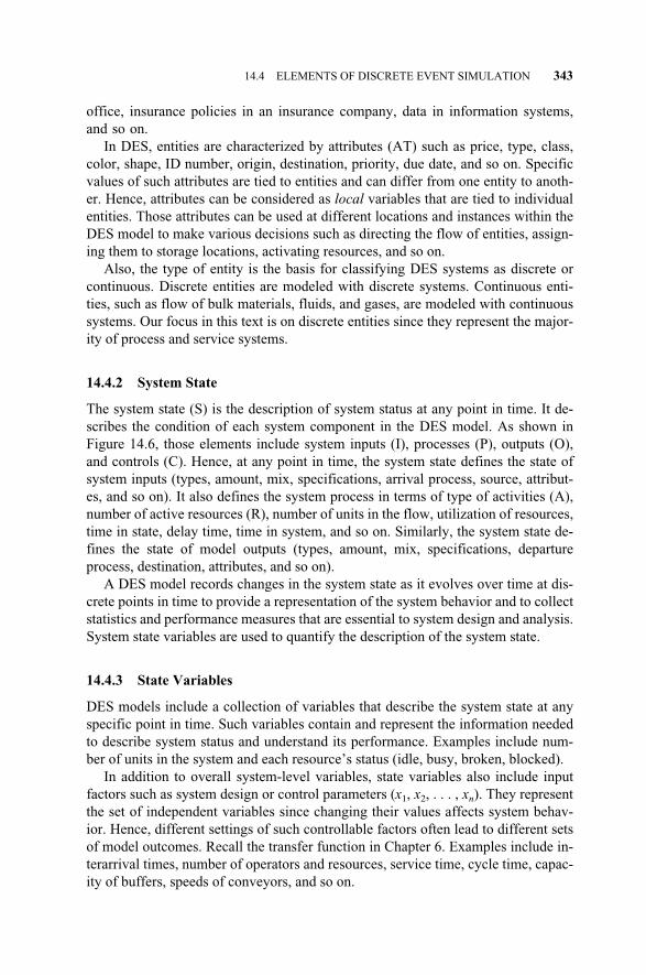
office, insurance policies in an insurance company, data in information systems,and so on.
In DES, entities are characterized by attributes (AT) such as price, type, class,color, shape, ID number, origin, destination, priority, due date, and so on. Specificvalues of such attributes are tied to entities and can differ from one entity to anoth-er. Hence, attributes can be considered as local variables that are tied to individualentities. Those attributes can be used at different locations and instances within theDES model to make various decisions such as directing the flow of entities, assign-ing them to storage locations, activating resources, and so on.
Also, the type of entity is the basis for classifying DES systems as discrete orcontinuous. Discrete entities are modeled with discrete systems. Continuous enti-ties, such as flow of bulk materials, fluids, and gases, are modeled with continuoussystems. Our focus in this text is on discrete entities since they represent the major-ity of process and service systems.
14.4.2 System State
The system state (S) is the description of system status at any point in time. It de-scribes the condition of each system component in the DES model. As shown inFigure 14.6, those elements include system inputs (I), processes (P), outputs (O),and controls (C). Hence, at any point in time, the system state defines the state ofsystem inputs (types, amount, mix, specifications, arrival process, source, attribut-es, and so on). It also defines the system process in terms of type of activities (A),number of active resources (R), number of units in the flow, utilization of resources,time in state, delay time, time in system, and so on. Similarly, the system state de-fines the state of model outputs (types, amount, mix, specifications, departureprocess, destination, attributes, and so on).
A DES model records changes in the system state as it evolves over time at dis-crete points in time to provide a representation of the system behavior and to collectstatistics and performance measures that are essential to system design and analysis.System state variables are used to quantify the description of the system state.
14.4.3 State Variables
DES models include a collection of variables that describe the system state at anyspecific point in time. Such variables contain and represent the information neededto describe system status and understand its performance. Examples include num-ber of units in the system and each resource’s status (idle, busy, broken, blocked).
In addition to overall system-level variables, state variables also include inputfactors such as system design or control parameters (x1, x2, . . . , xn). They representthe set of independent variables since changing their values affects system behav-ior. Hence, different settings of such controllable factors often lead to different setsof model outcomes. Recall the transfer function in Chapter 6. Examples include in-terarrival times, number of operators and resources, service time, cycle time, capac-ity of buffers, speeds of conveyors, and so on.
14.4 ELEMENTS OF DISCRETE EVENT SIMULATION 343
c14.qxd 4/22/2005 9:17 AM Page 343
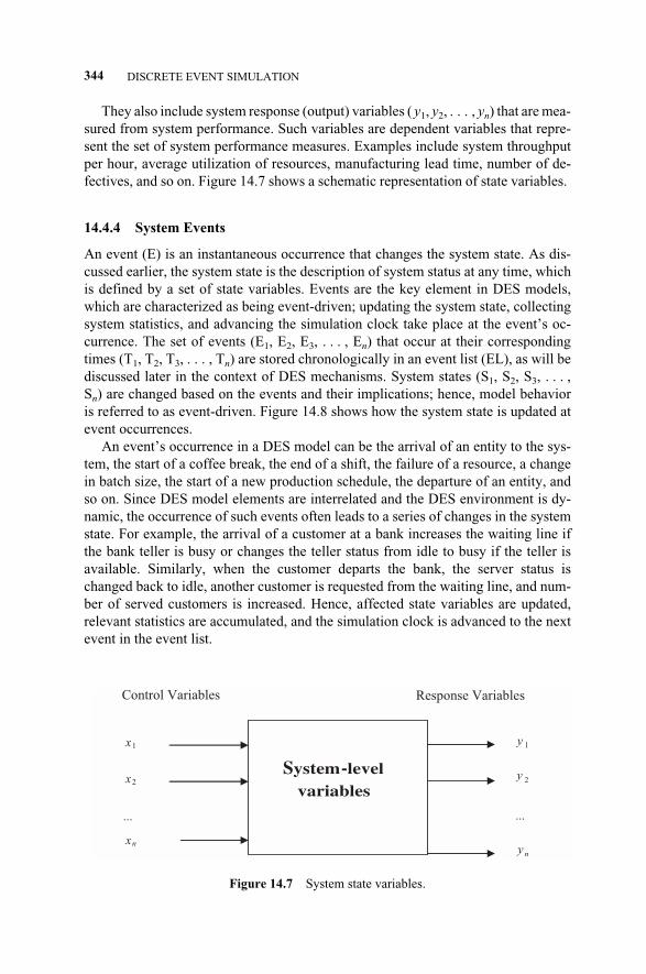
They also include system response (output) variables ( y1, y2, . . . , yn) that are mea-sured from system performance. Such variables are dependent variables that repre-sent the set of system performance measures. Examples include system throughputper hour, average utilization of resources, manufacturing lead time, number of de-fectives, and so on. Figure 14.7 shows a schematic representation of state variables.
14.4.4 System Events
An event (E) is an instantaneous occurrence that changes the system state. As dis-cussed earlier, the system state is the description of system status at any time, whichis defined by a set of state variables. Events are the key element in DES models,which are characterized as being event-driven; updating the system state, collectingsystem statistics, and advancing the simulation clock take place at the event’s oc-currence. The set of events (E1, E2, E3, . . . , En) that occur at their correspondingtimes (T1, T2, T3, . . . , Tn) are stored chronologically in an event list (EL), as will bediscussed later in the context of DES mechanisms. System states (S1, S2, S3, . . . ,Sn) are changed based on the events and their implications; hence, model behavioris referred to as event-driven. Figure 14.8 shows how the system state is updated atevent occurrences.
An event’s occurrence in a DES model can be the arrival of an entity to the sys-tem, the start of a coffee break, the end of a shift, the failure of a resource, a changein batch size, the start of a new production schedule, the departure of an entity, andso on. Since DES model elements are interrelated and the DES environment is dy-namic, the occurrence of such events often leads to a series of changes in the systemstate. For example, the arrival of a customer at a bank increases the waiting line ifthe bank teller is busy or changes the teller status from idle to busy if the teller isavailable. Similarly, when the customer departs the bank, the server status ischanged back to idle, another customer is requested from the waiting line, and num-ber of served customers is increased. Hence, affected state variables are updated,relevant statistics are accumulated, and the simulation clock is advanced to the nextevent in the event list.
344 DISCRETE EVENT SIMULATION
Figure 14.7 System state variables.
System-levelvariables
1x1
2
n
... ...
2
n
Response VariablesControl Variables
x
x
y
y
y
c14.qxd 4/22/2005 9:17 AM Page 344
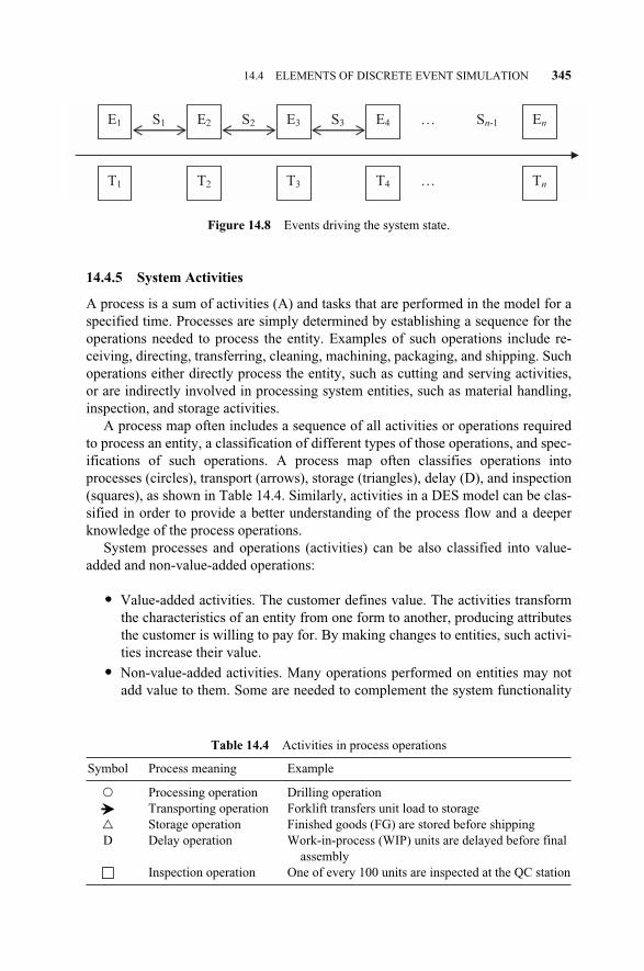
14.4.5 System Activities
A process is a sum of activities (A) and tasks that are performed in the model for aspecified time. Processes are simply determined by establishing a sequence for theoperations needed to process the entity. Examples of such operations include re-ceiving, directing, transferring, cleaning, machining, packaging, and shipping. Suchoperations either directly process the entity, such as cutting and serving activities,or are indirectly involved in processing system entities, such as material handling,inspection, and storage activities.
A process map often includes a sequence of all activities or operations requiredto process an entity, a classification of different types of those operations, and spec-ifications of such operations. A process map often classifies operations intoprocesses (circles), transport (arrows), storage (triangles), delay (D), and inspection(squares), as shown in Table 14.4. Similarly, activities in a DES model can be clas-sified in order to provide a better understanding of the process flow and a deeperknowledge of the process operations.
System processes and operations (activities) can be also classified into value-added and non-value-added operations:
� Value-added activities. The customer defines value. The activities transformthe characteristics of an entity from one form to another, producing attributesthe customer is willing to pay for. By making changes to entities, such activi-ties increase their value.
� Non-value-added activities. Many operations performed on entities may notadd value to them. Some are needed to complement the system functionality
14.4 ELEMENTS OF DISCRETE EVENT SIMULATION 345
Figure 14.8 Events driving the system state.
E1
T1
E2
T2
S1 S2 E3
T3
S3 E4
T4
… En
Tn
Sn-1
…
Table 14.4 Activities in process operations
Symbol Process meaning Example
� Processing operation Drilling operation� Transporting operation Forklift transfers unit load to storage� Storage operation Finished goods (FG) are stored before shippingD Delay operation Work-in-process (WIP) units are delayed before final
assembly� Inspection operation One of every 100 units are inspected at the QC station
c14.qxd 4/22/2005 9:17 AM Page 345
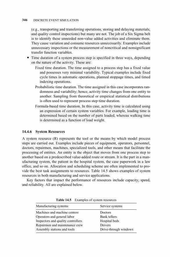
(e.g., transporting and transferring operations, storing and delaying materials,and quality control inspections) but many are not. The job of a Six Sigma beltis to identify these unneeded non-value added activities and eliminate them.They cause variation and consume resources unnecessarily. Examples includeunnecessary inspections or the measurement of noncritical and nonsignificanttransfer function variables.
� Time duration of a system process step is specified in three ways, dependingon the nature of the activity. These are:
Fixed time duration. The time assigned to a process step has a fixed valueand possesses very minimal variability. Typical examples include fixedcycle times in automatic operations, planned stoppage times, and timedindexing operations.
Probabilistic time duration. The time assigned in this case incorporates ran-domness and variability; hence, activity time changes from one entity toanother. Sampling from theoretical or empirical statistical distributionsis often used to represent process step time duration.
Formula-based time duration. In this case, activity time is calculated usingan expression of certain system variables. For example, loading time isdetermined based on the number of parts loaded, whereas walking timeis determined as a function of load weight.
14.4.6 System Resources
A system resource (R) represents the tool or the means by which model processsteps are carried out. Examples include pieces of equipment, operators, personnel,doctors, repairmen, machines, specialized tools, and other means that facilitate theprocessing of entities. An entity is the object that moves from one process step toanother based on a predescribed value-added route or stream. It is the part in a man-ufacturing system, the patient in the hospital system, the case paperwork in a lawoffice, and so on. Allocation and scheduling scheme are often implemented to pro-vide the best task assignments to resources. Table 14.5 shows examples of systemresources in both manufacturing and service applications.
Key factors that impact the performance of resources include capacity, speed,and reliability. All are explained below.
346 DISCRETE EVENT SIMULATION
Table 14.5 Examples of system resources
Manufacturing systems Service systems
Machines and machine centers DoctorsOperators and general labor Bank tellersInspectors and quality controllers Hospital bedsRepairmen and maintenance crew DriversAssembly stations and tools Drive-through windows
c14.qxd 4/22/2005 9:17 AM Page 346
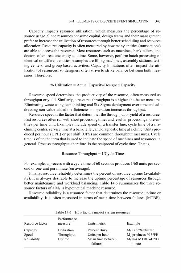
Capacity impacts resource utilization, which measures the percentage of re-source usage. Since resources consume capital, design teams and their managementprefer to increase the utilization of resources through better scheduling and resourceallocation. Resource capacity is often measured by how many entities (transactions)are able to access the resource. Most resources such as machines, bank tellers, anddoctors often treat one entity at a time. Some, however, perform batch processing ofidentical or different entities; examples are filling machines, assembly stations, test-ing centers, and group-based activities. Capacity limitations often impact the uti-lization of resources, so designers often strive to strike balance between both mea-sures. Therefore,
% Utilization = Actual Capacity/Designed Capacity
Resource speed determines the productivity of the resource, often measured asthroughput or yield. Similarly, a resource throughput is a higher-the-better measure.Eliminating waste using lean thinking and Six Sigma deployment over time and ad-dressing non-value-added inefficiencies in operation increases throughput.
Resource speed is the factor that determines the throughput or yield of a resource.Fast resources often run with short processing times and result in processing more en-tities per time unit. Examples include speed of a transfer line, cycle time of a ma-chining center, service time at a bank teller, and diagnostic time at a clinic. Units pro-duced per hour (UPH) or per shift (UPS) are common throughput measures. Cycletime is often the term that is used to indicate the speed of machines and resources ingeneral. Process throughput, therefore, is the reciprocal of cycle time. That is,
Resource Throughput = 1/Cycle Time
For example, a process with a cycle time of 60 seconds produces 1/60 units per sec-ond or one unit per minute (on average).
Finally, resource reliability determines the percent of resource uptime (availabil-ity). It is always desirable to increase the uptime percentage of resources throughbetter maintenance and workload balancing. Table 14.6 summarizes the three re-source factors of a M2, a hypothetical machine resource.
Resource reliability is a resource factor that determines the resource uptime oravailability. It is often measured in terms of mean time between failures (MTBF),
14.4 ELEMENTS OF DISCRETE EVENT SIMULATION 347
Table 14.6 How factors impact system resources
PerformanceResource factor measure Units metric Example
Capacity Utilization Percent Busy M2 is 85% utilizedSpeed Throughput Units per hour M2 produces 60 UPHReliability Uptime Mean time between M2 has MTBF of 200
failures minutes
c14.qxd 4/22/2005 9:17 AM Page 347
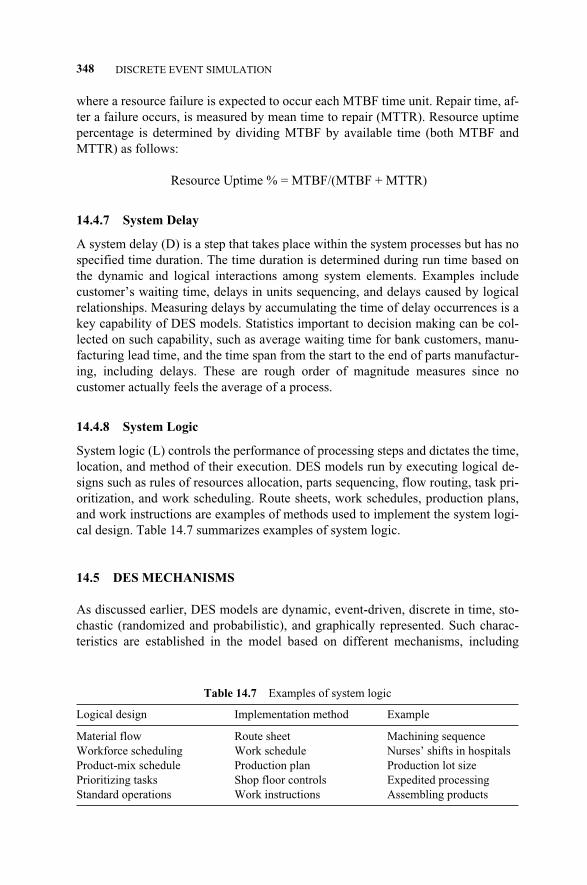
where a resource failure is expected to occur each MTBF time unit. Repair time, af-ter a failure occurs, is measured by mean time to repair (MTTR). Resource uptimepercentage is determined by dividing MTBF by available time (both MTBF andMTTR) as follows:
Resource Uptime % = MTBF/(MTBF + MTTR)
14.4.7 System Delay
A system delay (D) is a step that takes place within the system processes but has nospecified time duration. The time duration is determined during run time based onthe dynamic and logical interactions among system elements. Examples includecustomer’s waiting time, delays in units sequencing, and delays caused by logicalrelationships. Measuring delays by accumulating the time of delay occurrences is akey capability of DES models. Statistics important to decision making can be col-lected on such capability, such as average waiting time for bank customers, manu-facturing lead time, and the time span from the start to the end of parts manufactur-ing, including delays. These are rough order of magnitude measures since nocustomer actually feels the average of a process.
14.4.8 System Logic
System logic (L) controls the performance of processing steps and dictates the time,location, and method of their execution. DES models run by executing logical de-signs such as rules of resources allocation, parts sequencing, flow routing, task pri-oritization, and work scheduling. Route sheets, work schedules, production plans,and work instructions are examples of methods used to implement the system logi-cal design. Table 14.7 summarizes examples of system logic.
14.5 DES MECHANISMS
As discussed earlier, DES models are dynamic, event-driven, discrete in time, sto-chastic (randomized and probabilistic), and graphically represented. Such charac-teristics are established in the model based on different mechanisms, including
348 DISCRETE EVENT SIMULATION
Table 14.7 Examples of system logic
Logical design Implementation method Example
Material flow Route sheet Machining sequenceWorkforce scheduling Work schedule Nurses’ shifts in hospitalsProduct-mix schedule Production plan Production lot sizePrioritizing tasks Shop floor controls Expedited processingStandard operations Work instructions Assembling products
c14.qxd 4/22/2005 9:17 AM Page 348
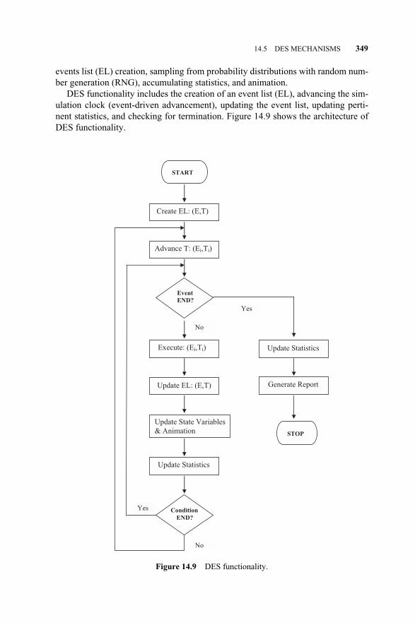
events list (EL) creation, sampling from probability distributions with random num-ber generation (RNG), accumulating statistics, and animation.
DES functionality includes the creation of an event list (EL), advancing the sim-ulation clock (event-driven advancement), updating the event list, updating perti-nent statistics, and checking for termination. Figure 14.9 shows the architecture ofDES functionality.
14.5 DES MECHANISMS 349
Figure 14.9 DES functionality.
START
Create EL: (E,T)
Advance T: (Ei,Ti)
Execute: (Ei,Ti)
Update EL: (E,T)
Update Statistics
Update Statistics
Update State Variables
& Animation
Generate Report
STOP
Yes
No
Yes
No
Event
END?
Condition
END?
c14.qxd 4/22/2005 9:17 AM Page 349
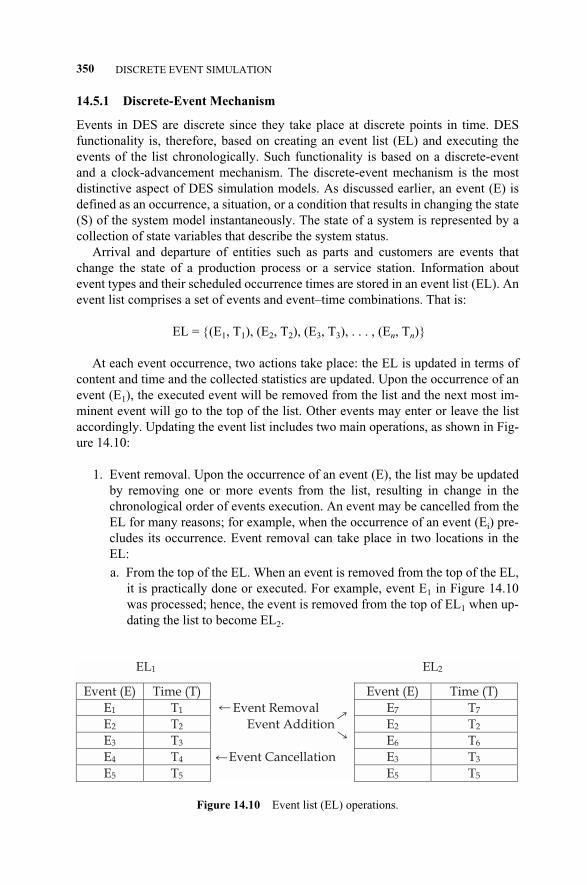
14.5.1 Discrete-Event Mechanism
Events in DES are discrete since they take place at discrete points in time. DESfunctionality is, therefore, based on creating an event list (EL) and executing theevents of the list chronologically. Such functionality is based on a discrete-eventand a clock-advancement mechanism. The discrete-event mechanism is the mostdistinctive aspect of DES simulation models. As discussed earlier, an event (E) isdefined as an occurrence, a situation, or a condition that results in changing the state(S) of the system model instantaneously. The state of a system is represented by acollection of state variables that describe the system status.
Arrival and departure of entities such as parts and customers are events thatchange the state of a production process or a service station. Information aboutevent types and their scheduled occurrence times are stored in an event list (EL). Anevent list comprises a set of events and event–time combinations. That is:
EL = {(E1, T1), (E2, T2), (E3, T3), . . . , (En, Tn)}
At each event occurrence, two actions take place: the EL is updated in terms ofcontent and time and the collected statistics are updated. Upon the occurrence of anevent (E1), the executed event will be removed from the list and the next most im-minent event will go to the top of the list. Other events may enter or leave the listaccordingly. Updating the event list includes two main operations, as shown in Fig-ure 14.10:
1. Event removal. Upon the occurrence of an event (E), the list may be updatedby removing one or more events from the list, resulting in change in thechronological order of events execution. An event may be cancelled from theEL for many reasons; for example, when the occurrence of an event (Ei) pre-cludes its occurrence. Event removal can take place in two locations in theEL:
a. From the top of the EL. When an event is removed from the top of the EL,it is practically done or executed. For example, event E1 in Figure 14.10was processed; hence, the event is removed from the top of EL1 when up-dating the list to become EL2.
350 DISCRETE EVENT SIMULATION
Figure 14.10 Event list (EL) operations.
EL1 EL2
Event (E) Time (T) Event (E) Time (T)
E1 T1 Event Removal E7 T7
E2 T2 Event Addition E2 T2
E3 T3 E6 T6
E4 T4 Event Cancellation E3 T3
E5 T5 E5 T5
�
�
��
c14.qxd 4/22/2005 9:17 AM Page 350

b. From any other location within the EL. When an event is removed fromany other location in the EL besides the top of the list, it is practically can-celled. For example, event E4 in Figure 14.10 was cancelled; hence, theevent is removed from EL1 and did not show up in EL2.
2. Event addition. Upon the occurrence of an event (E), the list may also be up-dated by adding one or more events to the list, resulting in changing thechronological order of event execution. Event additions can take place in twolocations in the EL:
a. To the top of EL. When an event is added to the top of the EL, it is consid-ered the most imminent event to take place. For example, Event E7 in Fig-ure 14.10 was added to top of EL2 and will be processed first. E7 was not amember of EL1 when the list was updated to become EL2.
b. To any other location within the EL. When an event is added to any otherlocation in the EL besides the top of the list, it is just being added as a fu-ture event. For example, Event E6 in Figure 14.10 was added to EL2 andwill be processed right after E2.
In a discrete-event mechanism, we view a system as progressing through timefrom one event to another, rather than changing continuously. Since many real sys-tems (plants, banks, hospitals, etc.) can be viewed as queuing networks, discreteevents occur in the simulation model in a manner similar to a queuing system (ar-rival and departure of events). For instance, a customer joins a queue at a discreteinstant of time and at a later discrete instant leaves the bank. There is no continu-ously varying quantity that says a customer is 65% in the queue. Time is accumulat-ed upon the occurrence of events at discrete points in time. The customer is either inor out the queue. This view results in a computationally efficient way of represent-ing time. The ability to represent time in an event-driven manner is the greateststrength of DES since it captures the dynamic behavior of real-world productionand business systems.
14.5.2 Time-Advancement Mechanism
The association of time with events (T1, T2, T3, . . . , Tn) in a simulation model ismaintained using a simulation clock time variable. This variable is updated throughthe next-event time-advancement mechanism that advances the simulation clock tothe time of the most imminent event in the event list. For example, Figure 14.11shows an event list of 10 events (E1, E2, E3, . . . , E10) that are chronologically or-dered as T1, T2, T3, . . . , T10. In DES, the time periods between events (E1 and E2,for example) are skipped when executing the model, resulting in a compressedcomputation time. Hence, the total time required to process the 10 events in a DEScomputer model is much shorter than the actual clock time. The mechanism simplystates that if no event is occurring in a time span, there is no need to observe themodel and update any statistics, so the time is simply skipped to the next eventscheduled in the EL. This event-driven time-advancement process continues untilsome specified stopping condition is satisfied.
14.5 DES MECHANISMS 351
c14.qxd 4/22/2005 9:17 AM Page 351
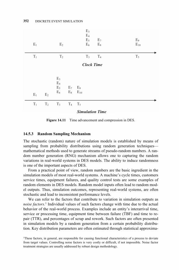
14.5.3 Random Sampling Mechanism
The stochastic (random) nature of simulation models is established by means ofsampling from probability distributions using random generation techniques—mathematical methods used to generate streams of pseudo-random numbers. A ran-dom number generation (RNG) mechanism allows one to capturing the randomvariations in real-world systems in DES models. The ability to induce randomnessis one of the important aspects of DES.
From a practical point of view, random numbers are the basic ingredient in thesimulation models of most real-world systems. A machine’s cycle times, customersservice times, equipment failures, and quality control tests are some examples ofrandom elements in DES models. Random model inputs often lead to random mod-el outputs. Thus, simulation outcomes, representing real-world systems, are oftenstochastic and lead to inconsistent performance levels.
We can refer to the factors that contribute to variation in simulation outputs asnoise factors.1 Individual values of such factors change with time due to the actualbehavior of the real-world process. Examples include an entity’s interarrival time,service or processing time, equipment time between failure (TBF) and time to re-pair (TTR), and percentages of scrap and rework. Such factors are often presentedin simulation models by a random generation from a certain probability distribu-tion. Key distribution parameters are often estimated through statistical approxima-
352 DISCRETE EVENT SIMULATION
Figure 14.11 Time advancement and compression in DES.
E1 E2
T1
E3
E4
E5
E6
T2 T3
E7
E8
E9
E10
T4 T5
E1 E2
E3
E4
E5
E6
E7
E8
E9
E10
T1 T2 T3 T4 T5
Simulation Time
Clock Time
1These factors, in general, are responsible for causing functional characteristics of a process to deviatefrom target values. Controlling noise factors is very costly or difficult, if not impossible. Noise factortreatment strategies are usually addressed by robust design methodology.
c14.qxd 4/22/2005 9:17 AM Page 352
tions based on fitting a collected set of empirical data to one of the commonly useddistributions.
The behavior of a DES model is, therefore, driven by the stochastic nature ofreal-world processes such as an entity’s arrival process, in-system service process,and output departure process. Such variability in model processes results in stochas-tic variability in model response (system performance measures). Therefore, thethroughput of a production system that is subject to variability in material delivery,tool failure, and operator efficiency is represented by the DES model in a stochasticmanner. Based on the inherent fluctuations, the throughput (yield) could be a lowvalue in one shift and then higher in another. The amount of variability in modeloutputs depends on the amount of variability in model inputs, along with the dy-namics caused by the logical interactions among different model elements andprocesses. Thus, simulation runs yield estimates of such performance measures interms of means and variances to assess such variability. Figure 14.12 presents ex-amples of variation factors in a DES model.
The probabilistic nature of the time period (T) that separates successive eventswhen executing a DES model represents the merit of randomness in simulationmodels. Events (such as customer arrival, machine failure, and product departure)can occur at any point in time, stimulating a stochastic simulation environment. Togenerate successive random time samples (T = T1, T2, . . .) between events, sam-pling from probability distributions is used. Hence, most simulation languages, aswell as generic programming languages, include a RNG engine to generate eventtimes and other modeled random variables. For example, interarrival times of cer-tain entities to the system are generated randomly by sampling from the exponentialdistribution, whereas the number of arriving entities per unit time is randomly gen-erated from the Poisson distribution.
14.5.4 Statistical Accumulation Mechanism
Statistics are the set of performance measures and monitoring variables that are de-fined within the DES model to quantify its performance and collect observationsabout its behavior. These statistics are defined in the model for various reasons,such as:
� Monitoring simulation progress. Values of the set of model statistics can bedefined to be part of model animation. Such values are updated discretelythroughout model run time. The simulation analyst can observe the progressof simulation by monitoring the changes that occur in the values of the de-fined statistics. For example, the Six Sigma team can continuously observethe changes that occur in the number of units/customers in the system.
� Conducting scheduled simulation reviews. It is often required to review thesystem state at certain points in the simulation run time. These could be theend of one week of operation, the completion of a certain order, or at a model-mix change. With model statistics defined, the Six Sigma team can halt simu-lation at any point in time, determined by the simulation clock, and review theprogress of the simulation by checking the values of such statistics. For exam-
14.5 DES MECHANISMS 353
c14.qxd 4/22/2005 9:17 AM Page 353
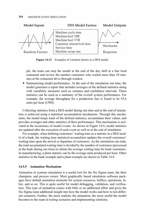
ple, the team can stop the model at the end of the day shift at a fast foodrestaurant and review the number customers who waited more than 10 min-utes at the restaurant drive-through window.
� Summarizing model performance. At the end of the simulation run time, themodel generates a report that includes averages of the defined statistics alongwith variability measures such as variance and confidence intervals. Thesestatistics can be used as a summary of the overall system performance. Forexample, the average throughput for a production line is found to be 55.6units per hour (UPH).
Collecting statistics from a DES model during run time and at the end of simula-tion is achieved using a statistical accumulation mechanism. Through this mecha-nism, the model keeps track of the defined statistics, accumulates their values, andprovides averages and other statistics of their performance. This mechanism is acti-vated at the occurrence of model events. As shown in Figure 14.9, model statisticsare updated after the execution of each event as well as at the end of simulation.
For example, when defining customers’ waiting time as a statistic in a DES mod-el of a bank, the waiting time statistical accumulator updates the overall customers’waiting time upon the arrival or departure of customers. As the simulation run ends,the total accumulated waiting time is divided by the number of customers (processedin the bank during run time) to obtain the average waiting time for bank customers.In manufacturing, a plant statistic can be the average units produced per hour. Otherstatistics in the bank example and a plant example are shown in Table 14.8.
14.5.5 Animation Mechanism
Animation in systems simulation is a useful tool for the Six Sigma team, the theirchampion, and process owner. Most graphically based simulation software pack-ages have default animation elements for system resources, buffers, operations, la-bor, and so on. This is quite useful for model debugging, validation, and verifica-tion. This type of animation comes with little or no additional effort and gives theSix Sigma team additional insight into how the model works and how to test differ-ent scenarios. Further, the more realistic the animation, the more useful the modelbecomes to the team in testing scenarios and implementing solutions.
354 DISCRETE EVENT SIMULATION
Figure 14.12 Examples of variation factors in a DES model.
Model Inputs DES Model Factors Model Outputs
Stochastic
Random Factors Response
Machine cycle time
Machine/tool TBF
Machine/tool TTR
Customer interarrival time
Service time
Machine scrap rate
c14.qxd 4/22/2005 9:17 AM Page 354
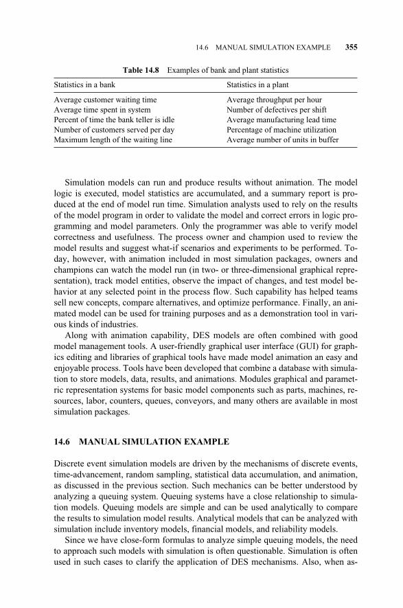
Simulation models can run and produce results without animation. The modellogic is executed, model statistics are accumulated, and a summary report is pro-duced at the end of model run time. Simulation analysts used to rely on the resultsof the model program in order to validate the model and correct errors in logic pro-gramming and model parameters. Only the programmer was able to verify modelcorrectness and usefulness. The process owner and champion used to review themodel results and suggest what-if scenarios and experiments to be performed. To-day, however, with animation included in most simulation packages, owners andchampions can watch the model run (in two- or three-dimensional graphical repre-sentation), track model entities, observe the impact of changes, and test model be-havior at any selected point in the process flow. Such capability has helped teamssell new concepts, compare alternatives, and optimize performance. Finally, an ani-mated model can be used for training purposes and as a demonstration tool in vari-ous kinds of industries.
Along with animation capability, DES models are often combined with goodmodel management tools. A user-friendly graphical user interface (GUI) for graph-ics editing and libraries of graphical tools have made model animation an easy andenjoyable process. Tools have been developed that combine a database with simula-tion to store models, data, results, and animations. Modules graphical and paramet-ric representation systems for basic model components such as parts, machines, re-sources, labor, counters, queues, conveyors, and many others are available in mostsimulation packages.
14.6 MANUAL SIMULATION EXAMPLE
Discrete event simulation models are driven by the mechanisms of discrete events,time-advancement, random sampling, statistical data accumulation, and animation,as discussed in the previous section. Such mechanics can be better understood byanalyzing a queuing system. Queuing systems have a close relationship to simula-tion models. Queuing models are simple and can be used analytically to comparethe results to simulation model results. Analytical models that can be analyzed withsimulation include inventory models, financial models, and reliability models.
Since we have close-form formulas to analyze simple queuing models, the needto approach such models with simulation is often questionable. Simulation is oftenused in such cases to clarify the application of DES mechanisms. Also, when as-
14.6 MANUAL SIMULATION EXAMPLE 355
Table 14.8 Examples of bank and plant statistics
Statistics in a bank Statistics in a plant
Average customer waiting time Average throughput per hourAverage time spent in system Number of defectives per shiftPercent of time the bank teller is idle Average manufacturing lead timeNumber of customers served per day Percentage of machine utilizationMaximum length of the waiting line Average number of units in buffer
c14.qxd 4/22/2005 9:17 AM Page 355
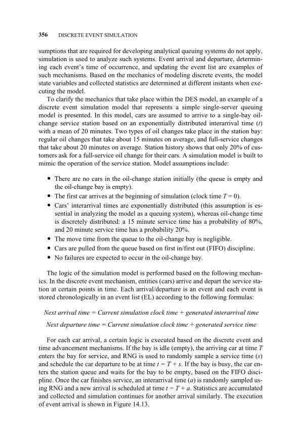
sumptions that are required for developing analytical queuing systems do not apply,simulation is used to analyze such systems. Event arrival and departure, determin-ing each event’s time of occurrence, and updating the event list are examples ofsuch mechanisms. Based on the mechanics of modeling discrete events, the modelstate variables and collected statistics are determined at different instants when exe-cuting the model.
To clarify the mechanics that take place within the DES model, an example of adiscrete event simulation model that represents a simple single-server queuingmodel is presented. In this model, cars are assumed to arrive to a single-bay oil-change service station based on an exponentially distributed interarrival time (t)with a mean of 20 minutes. Two types of oil changes take place in the station bay:regular oil changes that take about 15 minutes on average, and full-service changesthat take about 20 minutes on average. Station history shows that only 20% of cus-tomers ask for a full-service oil change for their cars. A simulation model is built tomimic the operation of the service station. Model assumptions include:
� There are no cars in the oil-change station initially (the queue is empty andthe oil-change bay is empty).
� The first car arrives at the beginning of simulation (clock time T = 0).
� Cars’ interarrival times are exponentially distributed (this assumption is es-sential in analyzing the model as a queuing system), whereas oil-change timeis discretely distributed: a 15 minute service time has a probability of 80%,and 20 minute service time has a probability 20%.
� The move time from the queue to the oil-change bay is negligible.
� Cars are pulled from the queue based on first in/first out (FIFO) discipline.
� No failures are expected to occur in the oil-change bay.
The logic of the simulation model is performed based on the following mechan-ics. In the discrete event mechanism, entities (cars) arrive and depart the service sta-tion at certain points in time. Each arrival/departure is an event and each event isstored chronologically in an event list (EL) according to the following formulas:
Next arrival time = Current simulation clock time + generated interarrival time
Next departure time = Current simulation clock time + generated service time
For each car arrival, a certain logic is executed based on the discrete event andtime advancement mechanisms. If the bay is idle (empty), the arriving car at time Tenters the bay for service, and RNG is used to randomly sample a service time (s)and schedule the car departure to be at time t = T + s. If the bay is busy, the car en-ters the station queue and waits for the bay to be empty, based on the FIFO disci-pline. Once the car finishes service, an interarrival time (a) is randomly sampled us-ing RNG and a new arrival is scheduled at time t = T + a. Statistics are accumulatedand collected and simulation continues for another arrival similarly. The executionof event arrival is shown in Figure 14.13.
356 DISCRETE EVENT SIMULATION
c14.qxd 4/22/2005 9:17 AM Page 356
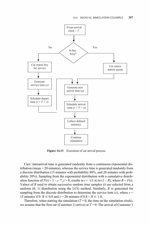
Cars’ interarrival time is generated randomly from a continuous exponential dis-tribution (mean = 20 minutes), whereas the service time is generated randomly froma discrete distribution (15 minutes with probability 80%, and 20 minutes with prob-ability 20%). Sampling from the exponential distribution with a cumulative distrib-ution function of F(t) = 1 – e–�t, t > 0, results in t = –(1/�) ln (1 – R), where R = F(t).Values of R used to obtain successive random time samples (t) are selected from auniform (0, 1) distribution using the LCG method. Similarly, R is generated forsampling from the discrete distribution to determine the service time (s), where s =15 minutes if 0 R 0.8 and s = 20 minutes if 0.8 < R 1.0.
Therefore, when starting the simulation (T = 0, the time on the simulation clock),we assume that the first car (Customer 1) arrives at T = 0. The arrival of Customer 1
14.6 MANUAL SIMULATION EXAMPLE 357
Figure 14.13 Execution of car arrival process.
Event arrival
clock = T
Is bay
busy?
Car enters bay
for service
Generate
service time (s)
Schedule depart
time (t = T + s)
Car enters
station queue
Generate new
arrival time (a)
Schedule arrival
time (t = T + a)
Collect defined
statistics
Continue
simulation
No Yes
c14.qxd 4/22/2005 9:17 AM Page 357

is the event that changes the state of the service station from idle to busy. The ser-vice time assigned for Customer 1, using R = 0.6574, is s = 15.00 minutes. Thus,Customer 1 departure time is scheduled as 0 + 15.00 = 15.00 minutes.
While the car of Customer 1 receives the service of regular oil change, anothercar (Customer 2) may drive into the service station. The arrival time of Customer 2is determined using R = 0.8523 as t = –(20) ln (1 – 0.8523) = 38.24 minutes. Hence,the arrival time for Customer 2 is scheduled as 0 + 38.24 = 38.24 minutes.
Based on this mechanism, the first event list (EL) is formed with two scheduledevents on the simulation clock:
(E1, t1): Departure of Customer 1. Departure time is T = 15.00 minutes.
(E2, t2): Arrival of Customer 2. Arrival time is T = 38.24 minutes.
Apparently, Customer 1 will depart the service station before Customer 2 ar-rives. E1 will be removed from top of the EL and the list will be reduced to E2 only.The simulation clock will be advanced to next event (E2) time (T = 15.00 minutes)in order to execute E2. The departure of Customer 1 is the event that changes thestate of the service station from busy to idle.
The service time assigned for Customer 2 using R = 0.8867 is s = 20.00 minutes.Hence, the departure time of Customer 2 is scheduled as 38.24 + 20.00 = 58.24minutes. After the arrival of Customer 2, another car (Customer 3) is scheduled toarrive at t = –(20) ln (1 – 0.2563) = 5.92 minutes, using R = 0.2563. The arrival ofCustomer 3 is scheduled as 38.24 + 5.92 = 44.16 minutes.
Based on this mechanism, the event list is updated with the two scheduled events(E3 = departure of Customer 2, and E4 = arrival of Customer 3). The two events arescheduled on the simulation clock as follows:
E3: T = 58.24 minutes
E4: T = 44.16 minutes
Apparently, Customer 3 will arrive at the service station before the departure ofCustomer 2, resulting in a waiting time of 58.24 – 44.16 = 14.08 minutes.
Simulation run time continues using the described mechanism until a certain ter-minating condition is met at a certain number of time units (for example, threeshifts of production, one year of service, 2000 units are produced, and so on). Asimulation table that summarizes the dynamics of the first 20 cars arriving at theservice station is shown in Table 14.9, in which the following variables are used:
A: Customer number (1, 2, . . . , 20)
B: Randomly generated interarrival time in minutes for each customer
C: Arrival time of each customer
D: Randomly generated service time in minutes for each customer
E: Time at which service (oil change) begins
F: Time each customer waits in the queue for service to begin
358 DISCRETE EVENT SIMULATION
c14.qxd 4/22/2005 9:17 AM Page 358
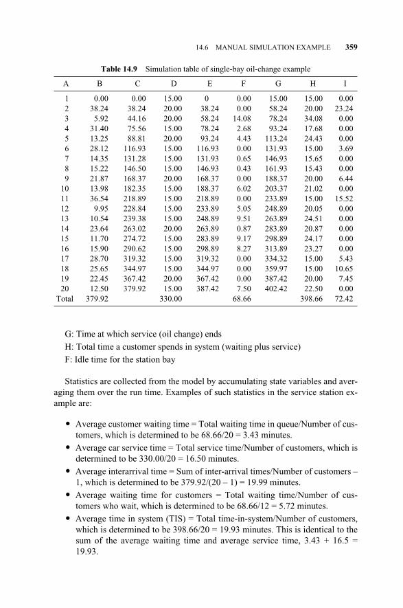
G: Time at which service (oil change) ends
H: Total time a customer spends in system (waiting plus service)
F: Idle time for the station bay
Statistics are collected from the model by accumulating state variables and aver-aging them over the run time. Examples of such statistics in the service station ex-ample are:
� Average customer waiting time = Total waiting time in queue/Number of cus-tomers, which is determined to be 68.66/20 = 3.43 minutes.
� Average car service time = Total service time/Number of customers, which isdetermined to be 330.00/20 = 16.50 minutes.
� Average interarrival time = Sum of inter-arrival times/Number of customers –1, which is determined to be 379.92/(20 – 1) = 19.99 minutes.
� Average waiting time for customers = Total waiting time/Number of cus-tomers who wait, which is determined to be 68.66/12 = 5.72 minutes.
� Average time in system (TIS) = Total time-in-system/Number of customers,which is determined to be 398.66/20 = 19.93 minutes. This is identical to thesum of the average waiting time and average service time, 3.43 + 16.5 =19.93.
14.6 MANUAL SIMULATION EXAMPLE 359
Table 14.9 Simulation table of single-bay oil-change example
A B C D E F G H I
1 0.00 0.00 15.00 0 0.00 15.00 15.00 0.002 38.24 38.24 20.00 38.24 0.00 58.24 20.00 23.243 5.92 44.16 20.00 58.24 14.08 78.24 34.08 0.004 31.40 75.56 15.00 78.24 2.68 93.24 17.68 0.005 13.25 88.81 20.00 93.24 4.43 113.24 24.43 0.006 28.12 116.93 15.00 116.93 0.00 131.93 15.00 3.697 14.35 131.28 15.00 131.93 0.65 146.93 15.65 0.008 15.22 146.50 15.00 146.93 0.43 161.93 15.43 0.009 21.87 168.37 20.00 168.37 0.00 188.37 20.00 6.44
10 13.98 182.35 15.00 188.37 6.02 203.37 21.02 0.0011 36.54 218.89 15.00 218.89 0.00 233.89 15.00 15.5212 9.95 228.84 15.00 233.89 5.05 248.89 20.05 0.0013 10.54 239.38 15.00 248.89 9.51 263.89 24.51 0.0014 23.64 263.02 20.00 263.89 0.87 283.89 20.87 0.0015 11.70 274.72 15.00 283.89 9.17 298.89 24.17 0.0016 15.90 290.62 15.00 298.89 8.27 313.89 23.27 0.0017 28.70 319.32 15.00 319.32 0.00 334.32 15.00 5.4318 25.65 344.97 15.00 344.97 0.00 359.97 15.00 10.6519 22.45 367.42 20.00 367.42 0.00 387.42 20.00 7.4520 12.50 379.92 15.00 387.42 7.50 402.42 22.50 0.00
Total 379.92 330.00 68.66 398.66 72.42
c14.qxd 4/22/2005 9:17 AM Page 359
� The probability that a customer has to wait = Number of customers whowait/Number of customers, which is determined to be 12/20 = 60%.
� The utilization of the station bay = [1.00 – (Total idle time/Total run time)] ×100%, which is determined to be 100% × [1.00 – (72.42/402.42)] = 82.00%
14.7 VARIABILITY IN SIMULATION OUTPUTS
In designing, analyzing, and operating complex production and business systemswith DES, one is interested not only in performance evaluation but also in sensitiv-ity analysis, experimentation, and optimization. However, simulation outcomes,representing real-world systems, are often stochastic and lead to inconsistent per-formance levels.
We can classify the factors that contribute to variation in simulation outputs ascontrollable and uncontrollable (noise) factors. Model design factors such as buffersizes, number of production resources, cycle times of automatic operations, andspeeds of conveyance systems are usually considered controllable factors. Differentsettings of system controllable factors may result in different sets of model outputs.However, design teams running a simulation study can control such factors andchange their parameters to the benefit of the process performance. Once set to theiroptimum levels, control factors do not change with time or changes in running con-ditions.
On the other hand, random factors are those uncontrollable factors whose indi-vidual values change over time due to the actual behavior of the real-world process;hence, they are often presented in simulation models by random generation from acertain probability distribution. Key distribution parameters are often estimatedthrough statistical approximations based on fitting a collected set of empirical datato one of the commonly used distributions (see Chapter 2). The behavior of DESmodels is, therefore, driven by the stochastic nature of real-world processes such asan entity’s arrival process, in-system service process, and output departure process.Variability in these processes is caused by random factors such as arrival rate, ser-vice/processing rate, equipment time between failure (TBF) and time to repair(TTR), percentages of scrap and rework (measured by defects per opportunity anddefects per million opportunities) and so on.
Such variability in model processes results in stochastic variability in model re-sponse (system performance measures). Therefore, the throughput of a productionsystem, for example, is subject to variability in material delivery, tool failure, andoperator efficiency and is represented in a DES model by stochastic behavior.Based on the inherent fluctuations, the throughput could be a low value in one shiftand a higher one in another. The amount of variability in model outputs depends onthe amount of variability in model inputs along with the dynamics caused by thelogical interactions among different model elements and processes. Thus, simula-tion runs yield estimates of such performance measures (throughput in this case) interms of means and variances to reflect such variability.
360 DISCRETE EVENT SIMULATION
c14.qxd 4/22/2005 9:17 AM Page 360
Noise factors can also arise from uncontrollable internal sources of variationwithin the simulated system. For example, in a plant, such factors can be the plantclimate, team dynamics, union relations, and worker strikes. They also representexternal factors such as the variation in the plant logistics, supply chain dynamics,and environmental changes. Such factors also cause variations in model outcomes.Although DES can include certain assumptions that represent model noise factors,most practical simulation studies are focused on modeling controllable and randomdesign factors. Hence, by determining optimum settings to model controllable fac-tors, statistical and simulation-based optimization methods aim at obtaining a sys-tem response that meets design expectations with minimal sensitivity to variations(it is robust) in modeling random factors.
In addition to controllable, random, and noise factors, artificial factors are asource of variation in simulation outputs. Artificial factors are those simulation-specific factors such as system initialization state, warm-up period,2 run length,3
termination condition, and random number streams. Changing the settings of suchfactors from one simulation run to another often results in changes in model out-comes. Hence, testing such factors in the model and providing proper settings fordifferent model run controls to obtain a steady-state response is basically a pre-requisite for applying statistical and simulation-based optimization methods.Figure 14.14 presents a summary of different sources of variation in simulationmodels.
14.7.1 Variance Reduction Techniques
It has been shown in the previous section that the stochastic nature of simulation of-ten produces random outputs. Random and probabilistic model inputs result in ran-dom model outputs. As the amount of input variability increases, the observed mod-el response tends to be more random, with high variance and wide confidenceintervals around the response mean. As a result, less precise performance estimatesare obtained from the simulation model. Thus, the objective of using variance re-duction techniques (VRTs) is primarily to make better decisions based on simula-tion results by reducing the variability in model outcomes. The response mean andconfidence interval are typically used to describe the performance measure of asimulation model. Hence, reducing the response variance results in reducing thewidth of the confidence interval around the mean, which increases the precision ofsimulation estimation.
14.7 VARIABILITY IN SIMULATION OUTPUTS 361
2Warm-up period is a transient simulation state. A steady-state or nonterminating simulation applies tosystems whose operation continues indefinitely or for a long time period with no statistical change in be-havior. Such periods include a relatively short transient (warm-up) period and a relatively long steady-state period. The warm-up period is excluded from results analysis and simulation statistics are collectedfrom the steady-state period. 3The simulation run length represents the time period in which model behavior is observed, statistics areaccumulated and collected, and performance measures are recorded. It is essential to set the model to runfor enough time past the warm-up period in order to collect representative data and arrive at correct con-clusions about the model behavior.
c14.qxd 4/22/2005 9:17 AM Page 361
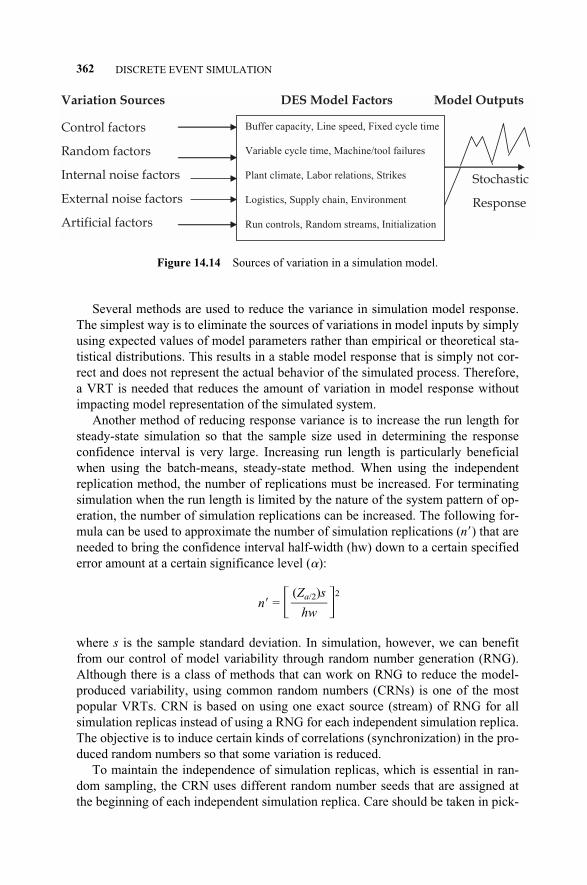
Several methods are used to reduce the variance in simulation model response.The simplest way is to eliminate the sources of variations in model inputs by simplyusing expected values of model parameters rather than empirical or theoretical sta-tistical distributions. This results in a stable model response that is simply not cor-rect and does not represent the actual behavior of the simulated process. Therefore,a VRT is needed that reduces the amount of variation in model response withoutimpacting model representation of the simulated system.
Another method of reducing response variance is to increase the run length forsteady-state simulation so that the sample size used in determining the responseconfidence interval is very large. Increasing run length is particularly beneficialwhen using the batch-means, steady-state method. When using the independentreplication method, the number of replications must be increased. For terminatingsimulation when the run length is limited by the nature of the system pattern of op-eration, the number of simulation replications can be increased. The following for-mula can be used to approximate the number of simulation replications (n�) that areneeded to bring the confidence interval half-width (hw) down to a certain specifiederror amount at a certain significance level (�):
n� = � �2
where s is the sample standard deviation. In simulation, however, we can benefitfrom our control of model variability through random number generation (RNG).Although there is a class of methods that can work on RNG to reduce the model-produced variability, using common random numbers (CRNs) is one of the mostpopular VRTs. CRN is based on using one exact source (stream) of RNG for allsimulation replicas instead of using a RNG for each independent simulation replica.The objective is to induce certain kinds of correlations (synchronization) in the pro-duced random numbers so that some variation is reduced.
To maintain the independence of simulation replicas, which is essential in ran-dom sampling, the CRN uses different random number seeds that are assigned atthe beginning of each independent simulation replica. Care should be taken in pick-
(Za/2)s�
hw
362 DISCRETE EVENT SIMULATION
Figure 14.14 Sources of variation in a simulation model.
Variation Sources DES Model Factors Model Outputs
Control factors
Random factors
Internal noise factors Stochastic
External noise factors Response
Artificial factors
Buffer capacity, Line speed, Fixed cycle time
Variable cycle time, Machine/tool failures
Plant climate, Labor relations, Strikes
Logistics, Supply chain, Environment
Run controls, Random streams, Initialization
c14.qxd 4/22/2005 9:17 AM Page 362
ing the seed so that the segments of the random stream are not shared between repli-cas. Simulation software tools provide the CRN option that automatically assignsseed values to each replica so that the possibility of sharing segments of the randomstream is minimized. Each stochastic element in the model, such as cycle times, ar-rival times, and failure times, can be assigned a different random number stream tokeep random numbers synchronized across the simulated system.
Using CRN is particularly useful when comparing the performance of two ormore simulated systems (strategies or design alternatives) because using the CRNresults in positive correlation among compared strategies, which actually reducesthe variance of sample differences collected from the model but does not reducethe variance of the simulation output. If no correlation is created between com-pared �2 systems or a negative correlation was created, using CRN will result ineither no impact or an increase in the variance obtained from comparing simulat-ed systems. The variance (�2) of two independent systems (x1 and x2) is expressedas follows:
�2x1–x2
= �2x1
+ �2x2
When using a synchronized CRN, however, a positive correlation is induced be-tween x1 and x2, which results in less variance (reduced by the covariance “COV”component) and is expressed as follows:
�2x1–x2
= �2x1
+ �2x2
– 2 cov(x1, x2)
Several other VRTs can be used in addition to the CRN method. Examples in-clude antithetic variates, control variates, indirect estimation, and conditioning.
14.8 SERVICE PROCESSES SIMULATION IMPLICATIONS
Several considerations should prepare the design team for planning a businessprocess simulation study and for addressing the suitability of their choice of simula-tion package. First, a clear classification of their project business process is needed.It could be product development; a production process;4 problem solving, includingdistribution5 processes; or a service-based process.6 A team usually designs theproduct development processes. These processes are analyzed using DFSS tools.However, process cycle times and resource requirements are usually handled bysimulation, which produces more accurate results. Many DES simulation packagesare capable of representing the highly variable steps in tightly coupled resources.Modeling shifts, downtime, overtime, and learning curves with multiple replicas of
14.8 SERVICE PROCESSES SIMULATION IMPLICATIONS 363
4Typical examples are order fulfillment, accounts payable, and claims processing activities.5Includes transportation and delivery processes, in which products or people are carried between loca-tions via a distribution network. 6Example of service processes are telephonic services (call centers), restaurants, copy centers, hospitals,and retail stores.
c14.qxd 4/22/2005 9:17 AM Page 363
resources are some of the important considerations in building a valid simulation ofa product development process.
In the context of Six Sigma, discrete event simulation is quite suitable for pro-duction process problem solving when outputs are produced in a batch or continu-ous flow mode in relatively high volumes. Tasks such as assembly, disassembly,setup, inspection, and rework are typical steps in production processes with queuingrules and downtime modeling. Such processes are usually modeled to obtainsteady-state behavior past the warm-up period. In modeling distribution processesin a production environment, it is important to define attributes for flow entities inorder to keep track of unique characteristics such as value-adds, cost, and distancetraveled. Due to the transient nature of distribution processes, the simulation modelwarm-up period is usually longer than other production processes.
In a service-based industry, processes present a major area for employment ofsimulation studies. These processes are typically characterized by a non-value-added time that exceeds the value-added (processing time). The simulation of ser-vice processes represents a challenge because both the entities and processing re-sources are typically people. Modeling human behavior is complex andunpredictable. For example, customers calling a service center may hold or hangup. Modeling adaptation is required to model such situations. Also, processingtimes are highly variable and customer arrivals are random and cyclical, adding tothe model complexity. Model accuracy demands representative probability distribu-tions. Otherwise, a steady state may not be reached.
14.9 SUMMARY
The discrete event simulation (DES) techniques presented in this chapter are mostcapable and powerful tools for business process simulation of transactional naturewithin DFSS and Six Sigma projects. DES provides modeling of entity flows withcapabilities that allow the design team to see how flow objects are routed throughthe system. DES capability is increasing due to new software tools and a wide spec-trum of real-world applications.
Basic concepts of simulation modeling include the system concept, model con-cept, and simulation concept. Systems include inputs, entities, relationships, con-trols, and outputs. System elements should be tuned toward attaining an overall sys-tem goal. A system model is a representation or an approximation of a real-worldsystem. Models can be physical, graphical, mathematical, or computer models. Thegoal of modeling is to provide a cheaper, faster, and easier-to-understand tool forprocess analysis, design, and improvement. Simulation is the art and science ofmimicking the operation of a real-world system on a computer. It is aimed at cap-turing complex, dynamic, and stochastic characteristics of real-world processes.Other types of models fall short in this regard. Based on type of state variables,computer simulation models can be discrete, continuous, or combined. They canalso be deterministic or stochastic based on randomness modeling. Finally, they canbe static or dynamic based on the changes of system state.
364 DISCRETE EVENT SIMULATION
c14.qxd 4/22/2005 9:17 AM Page 364
15.1 INTRODUCTION
The final aspect of DFSS methodology that differentiates it from the prevalent“launch and learn” method is design validation. This chapter covers in detail theverify phase of the DFSS (ICOV) project road map (see Figure 5.1). Design valida-tion helps identify unintended consequences and effects of design, aids in develop-ing plans, and helps reduce risk for full-scale commercialization.
At this final stage before the full-scale production stage (see Chapter 1, Section1.3.6), we want to verify that the design’s performance is capable of achieving theexpectations of customers and stakeholders at Six Sigma performance levels. Wewant to accomplish this assessment in a low-risk, cost-effective manner. This chap-ter will cover the service-relevant aspects of design validation, including prototyp-ing, testing, and assessment.
15.2 DESIGN VALIDATION STEPS
Design validation can take on many different forms depending on the magnitude ofthe design change and the complexity of the environment in which the design willoperate. Typically, it is desirable to understand the performance of the new designas early as possible in the design cycle with the highest confidence achievable. Inorder to accomplish this, we can rely on the design of experiments methods detailedin Chapters 12 and 13 but often these DOEs are specialized around a subset of in-put-significant factors and do not provide a full functional test. Product-specificvalidation often means building prototypes and testing them in a “beta” environ-ment. The beta environment is one in which real end users utilize the new design intheir actual application and provide feedback. In the context of writing this book,people proofread the draft (prototype) chapters in a beta environment and providedvaluable feedback. In the beta environment, end users are willing to test the new de-
Service Design for Six Sigma. By Basem El-Haik and David M. Roy 365© 2005 by John Wiley & Sons.
15DESIGN VALIDATION
c15.qxd 4/22/2005 9:18 AM Page 365
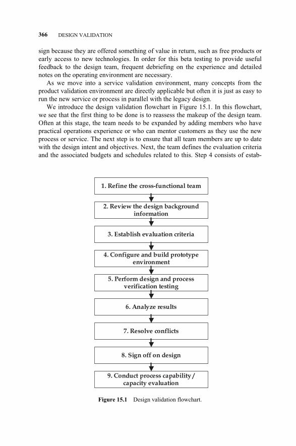
sign because they are offered something of value in return, such as free products orearly access to new technologies. In order for this beta testing to provide usefulfeedback to the design team, frequent debriefing on the experience and detailednotes on the operating environment are necessary.
As we move into a service validation environment, many concepts from theproduct validation environment are directly applicable but often it is just as easy torun the new service or process in parallel with the legacy design.
We introduce the design validation flowchart in Figure 15.1. In this flowchart,we see that the first thing to be done is to reassess the makeup of the design team.Often at this stage, the team needs to be expanded by adding members who havepractical operations experience or who can mentor customers as they use the newprocess or service. The next step is to ensure that all team members are up to datewith the design intent and objectives. Next, the team defines the evaluation criteriaand the associated budgets and schedules related to this. Step 4 consists of estab-
366 DESIGN VALIDATION
1. Refine the cross-functional team
2. Review the design background information
3. Establish evaluation criteria
4. Configure and build prototype environment
5. Perform design and process verification testing
6. Analyze results
7. Resolve conflicts
8. Sign off on design
9. Conduct process capability / capacity evaluation
Figure 15.1 Design validation flowchart.
c15.qxd 4/22/2005 9:18 AM Page 366

lishing the prototype environment so that is as close to the production environmentas possible, considering cost and risk factors. In step 5, the process/service is runand observed based on the evaluation criteria and environmental factors are deter-mined. Once the verification testing results are available, they are analyzed. It is im-portant to note that analysis should not be left until the end of the testing as the teamwill want to be sensitive to any initial defects as soon as possible and make go/no-go decisions after each completed cycle. After the results have been analyzed, theteam makes decisions as to whether conflicts exist that require design modifica-tions. If design modifications are made, a decision must be made whether to loopback to Step 4 again. Once the team is satisfied that the new design is correct, thedocumentation should be formally signed off. The last step is to conduct process ca-pability analysis and any capacity planning.
The key elements of validation, then, are to create a prototype, subject it to a re-alistic test environment, summarize the observed performance, and feed back anyrequired changes into the design. We will next cover the details of each of thesesteps as well as the need for statistical process control and control plans.
15.3 PROTOTYPE BUILDING
In order to produce a useful prototype of the new design that is sufficient to allowfor evaluation, consideration must be given to the completeness and stability of theelements that make up the design. These elements can be classified as design para-meters that are manifested as components and subsystems, and production processvariables with all steps and subprocesses. We can look at components, subsystems,and systems to determine the lack of knowledge of performance and the interactionof preexisting (carried over) subsystems in a new system. In order to assist in deter-mining if the prototype is complete enough and relevant for testing, it is helpful toassess the elements as being a:
� Current design
� Analogous design
� New design, low risk
� New design, high risk
Risk can be assessed from FMEA and technology road maps or other sources(e.g., history) and/or DFSS tools usage. If any of the elements are in the new design,high-risk category, they should not be compromised and must be included in theprototype.
The prototype in a product environment may not have been produced on actualproduction equipment or with the actual production process and people. The samecan happen in a service environment. New software or organization structures maybe months away and you still want to know if the new design will perform properly.In an enterprise resource planning (ERP) or customer relationship management
15.3 PROTOTYPE BUILDING 367
c15.qxd 4/22/2005 9:18 AM Page 367

(CRM) system deployment, the configured software is often built into a conferenceroom pilot (CRP) on nonproduction hardware and tested under test script scenarios.The built CRP is a prototype.
Prototypes usually involve some trade-off between the final completed designand some elements that will not be available until later. Prototype designs are testedoff-line under controlled conditions. Some examples are:
� Initial mock-up hardware that is created in a lab environment.
� New software to prioritize/route calls for a call center is tested off-line.
� A modified version of the current month-end close process in accounting istested in parallel with an actual system prior to pilot testing.
� An Excel model is used to conduct an off-line sensitivity analysis of salescommission by salesperson prior to real application of customers.
Prototypes should be evaluated using objective and robust analytical techniquesto objectively demonstrate design performance for a product/service pilot. The test-ing method is critical to accomplishing objective decision making and obtaining in-formation in the most cost-effective manner.
15.4 TESTING
When testing prototypes, it is vital to follow a rigorous process in order to assess theperformance and learn from any unusual observations. Many times, unexpected re-sults may occur, and without the correct approach these will have to be written offas unusual observations when, in fact, they may be significant events that can eitherdifferentiate your new design or plague it. The key elemets of a rigorous test planare:
� Assign individual names to each role.
� Confirm that the test environment has been established and is ready for use.
� Finalize/confirm testing estimates.
� Estimate hours to be spent by each individual.
� Plan calendar duration of all testing.
� Set testing milestones (target dates).
� Finalize test cases.
� Finalize test scenarios.
� Describe inputs and expected results.
� Implement defect tracking mechanisms.
� Confirm issue resolution procedures that should include decisions to defer,fix, or withdraw.
� Finalize acceptance test criteria/comparison tests.
368 DESIGN VALIDATION
c15.qxd 4/22/2005 9:18 AM Page 368
� Perform cycle tests.
� Do performance test.
� Do integration test.
� Do regression test.
Some of the specific types of testing include pilot tests and pre-production (low-rate production) tests. A pilot tests prototype design under limited real-world condi-tions to verify original design assumptions versus actual performance. Preproduc-tion testing takes a new product or process through concept and pilot evaluation tofull production or roll out.
In validation, the DFSS team conducts a progressive sequence of verificationtests to quantify the ability of the service to satisfy FRs under conditions that ap-proximate the conditions of actual use. The DFSS team needs to conduct specifica-tion and verification tests and make initial adjustments to testing and measurementequipment. Initial conditions are verified and recorded according to a test plan. Theteam then begins collecting data for those tests that are designed to analyze perfor-mance and records any abnormalities that may occur during test and may facilitatesubsequent concern resolution. This involves tiered testing (testing that parallels hi-erarchy) as part of the test strategy, to enable functional verification at progressivelevels of process mappings.
The first hierarchical level is associated with subprocess-step-level testing. Thesecond hierarchical level is associated with subprocesses. The third level of testingis for the process, which includes the functional subprocesses. Functional insensi-tivity to the testing environment (lack of reliability) will be most quantifiable at thestep and subprocess hierarchical levels. This is due in part to the number of teststhat can be effectively performed, and to the greater ability to measure functionalrequirements performance at lower levels of design complexity. The issue just not-ed is not a hard-and-fast rule but is certainly observable in the greater number oftests that are run (hence, the improved quantification) at the component and sub-process levels.
Testing costs at the subprocess level are typically one-tenth of those at the nextlevel. This also includes finalizing packaging, shipping, and delivery processes (ifany). In addition, the teams need to verify time studies and process capabilities. Thevalidation staff includes seasoned personnel with direct operating and regulatorycompliance experience in addition to the DFSS team. The extended DFSS teamshould identify critical process parameters and production limitations and managethe launch through process efficiency studies using simulation, design of experi-ments for prevalidation investigations, writing the process validation protocols, andoverseeing the work.
Validation planning should begin early in the design process, starting with thecharacterize DFSS phase. It is most important to integrate validation activities ear-ly in design rather than as an afterthought. Significant design issues must be re-viewed, understood, and accepted by the extended DFSS team before progressingtoo far into detailed design.
15.4 TESTING 369
c15.qxd 4/22/2005 9:18 AM Page 369
15.5 CONFIDENCE INTERVAL OF SMALL SAMPLE VALIDATION
When testing in a preproduction environment, the scope of the available samples orresources is often very small due to cost or time factors. Proof of concept is usuallydetermined after a single successful transaction but robust performance can only bedetermined after a significant number of cycles have been experienced. It is recom-mended that the legacy system be baselined for statistical parameters and the newdesign validated to a degree of statistical significance. Power and sample size calcu-lations can be made based on the underlying variation assumptions and the changein performance expected. If a process or service will only experience a single cyclein the period of a year, then it is very unlikely that you will be able to validate theprocess statistically. Many new processes or services experience many cycles perweek and it is reasonable to validate these with 95% confidence intervals for evalu-ating the results as statistically valid and different.
The statistical factors that affect the sample size are the confidence interval de-sired, the system noise (standard deviation), and the delta change between the sig-nals (averages). The sample size (n) is given by
n = � �2(15.1)
where � = error = |y� – �|. For example, take a legacy process that “approves” 25transactions per day with an average approval time of 98 hours and standard devia-tion of 13.7 hours. How many observations would be needed in order to have 95%confidence that there was a statistically significant difference? If we take the casesof differences in average approval time of 2, 12, and 94 hours, we find the follow-ing required sample sizes:
2 hour difference—612 samples
12 hour difference—19 samples
94 hour difference—3 samples.
The factors that affect the sample size are the confidence interval desired, the sys-tem noise (standard deviation), and the delta change between the signals (averages).
If in your validation process you are unable to achieve such a level of test confi-dence, it is recommended that you roll out your deployment gradually and incre-mentally. Start out with typical users who are less sensitive to any issues and pulsethem for performance. As you feel more comfortable with the performance, in-crease the scope and continue to ramp up the new process/service until the oldprocess/service is retired.
15.6 CONTROL PLANS AND STATISTICAL PROCESS CONTROL
As we build upon the DOE transfer functions, finalize the process capability, andupdate the design scorecard, we become cognizant of the key process input vari-
Z�/2��
�
370 DESIGN VALIDATION
c15.qxd 4/22/2005 9:18 AM Page 370
ables (KPIV) and the key process output characteristics (KPOC) that are critical formonitoring and controlling in the production environment. One of the best tools tostart the process of implementing process control is the control plan depicted in Fig-ure 15.2. In this control plan, take the KPIVs and the KPOCs and list them in thecolumn labeled Specification Characteristic. In the columns labeled Sub Processand Sub Process Step, input the corresponding labels.
The next required element is the Specification Requirement. In this cell, the up-per and lower specification limits (USL and LSL) are typically entered. In someprocesses, only one limit may be required or just the target value for attribute typerequirements.
The next cell is for the measurement method. How will the measurement be ac-quired? Many times this is the result of a calculation from several fields, as in thecase of processes and services. For instance, process time might be calculated fromthe field of start time and end time. Other times, the measurement may require sur-veys or audits.
The cell labeled Sample Size is for how many measurements will be required atthe specified frequency. This refers back to the underlying statistical significancethat is required to capture the variation.
In the frequency cell, enter the required frequency. This can be, for example,every cycle, every 20 cycles, quarterly, or annually, depending on the stability ofthe feeder process and the nature of the measured characteristic.
The column labeled Who is for the assigned person(s) who will collect the mea-surements. The Where Recorded is the location where the collected measurement isdocumented for referral or audit purposes. The Decision Rule/Corrective Action col-umn is for the rules for what action to take if the measurement is outside of the spec-ification requirement. This can either be a set of actions or reference to a policy orprocedure. The column labeled SOP Reference is for the document name or numberthat is the standard operating procedure for the subprocess or subprocess step.
It is important to note that if the design team has followed all of the optimizationand validation steps and the design is operating at a very low defect rate (approach-ing Six Sigma capability) then there should be relatively few KPIVs and theKPOCs should be the prioritized CTQs from the HOQ1.
15.7 STATISTICAL PROCESS CONTROL
Once the data measurements are collected as prescribed in the control plan, themethod for charting the data should be determined. Since statistical process control(SPC) is a well-developed subject and there are many textbooks on the subject, wewill not be covering the methodology in any detail in this book. We do feel, howev-er, that in the transactional world of services and business processes, there is littleevidence of the use of SPC, so brief coverage of the subject will be provided. Wewill cover the selection of the charting method and some of the basic rules of inter-pretation. For specific books on the subject, see Wheeler (1995) and Wheeler andChambers (1992).
15.7 STATISTICAL PROCESS CONTROL 371
c15.qxd 4/22/2005 9:18 AM Page 371
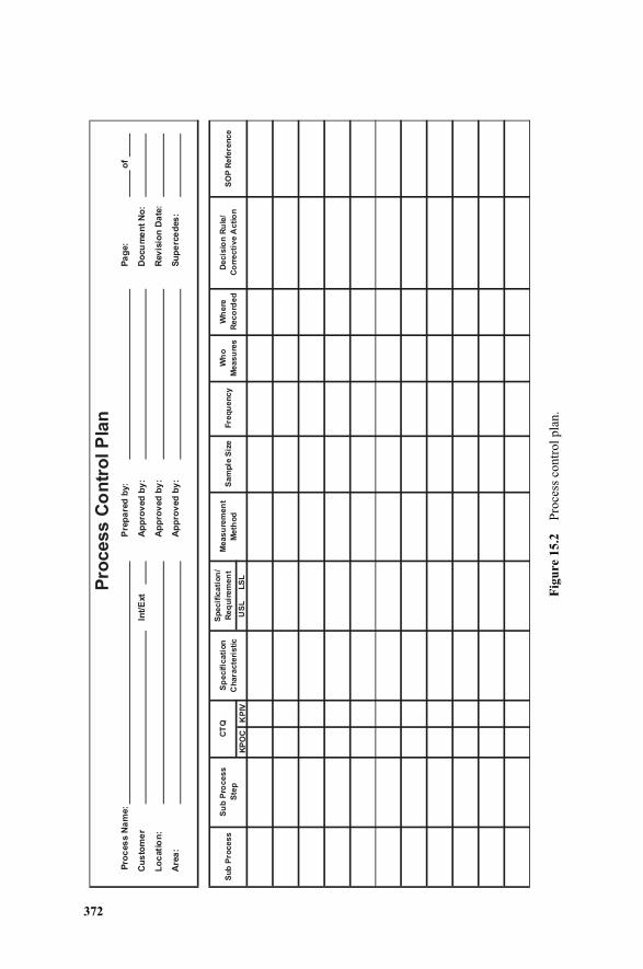
372
Pre
pa
red
by:
Pa
ge:
of
Ap
pro
ved
by
:D
ocu
me
nt
No
:
Lo
cati
on
:A
pp
rov
ed
by
:R
ev
isio
n D
ate
:
Are
a:
Ap
pro
ved
by
:S
up
erc
ed
es
:
KP
OC
KP
IV
Measu
rem
en
t
Meth
od
Wh
o
Measu
res
Sub
Pro
cess
Su
b P
rocess
Ste
p
Sp
ecific
ati
on
Chara
cte
ristic
Specif
icati
on
/
Req
uir
em
en
t
US
L L
SL
CT
QS
am
ple
Siz
eFre
qu
ency
Wh
ere
Reco
rded
SO
P R
efe
rence
Decis
ion
Ru
le/
Co
rrecti
ve A
ctio
n
Pro
cess C
on
tro
l P
lan
Cu
sto
me
r
Pro
ces
s N
am
e:
Int/
Ext F
igur
e 15
.2P
roce
ss c
ontr
ol p
lan.
c15.qxd 4/22/2005 9:18 AM Page 372
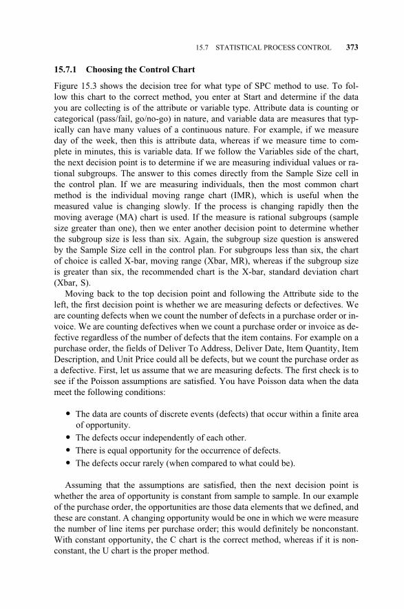
15.7.1 Choosing the Control Chart
Figure 15.3 shows the decision tree for what type of SPC method to use. To fol-low this chart to the correct method, you enter at Start and determine if the datayou are collecting is of the attribute or variable type. Attribute data is counting orcategorical (pass/fail, go/no-go) in nature, and variable data are measures that typ-ically can have many values of a continuous nature. For example, if we measureday of the week, then this is attribute data, whereas if we measure time to com-plete in minutes, this is variable data. If we follow the Variables side of the chart,the next decision point is to determine if we are measuring individual values or ra-tional subgroups. The answer to this comes directly from the Sample Size cell inthe control plan. If we are measuring individuals, then the most common chartmethod is the individual moving range chart (IMR), which is useful when themeasured value is changing slowly. If the process is changing rapidly then themoving average (MA) chart is used. If the measure is rational subgroups (samplesize greater than one), then we enter another decision point to determine whetherthe subgroup size is less than six. Again, the subgroup size question is answeredby the Sample Size cell in the control plan. For subgroups less than six, the chartof choice is called X-bar, moving range (Xbar, MR), whereas if the subgroup sizeis greater than six, the recommended chart is the X-bar, standard deviation chart(Xbar, S).
Moving back to the top decision point and following the Attribute side to theleft, the first decision point is whether we are measuring defects or defectives. Weare counting defects when we count the number of defects in a purchase order or in-voice. We are counting defectives when we count a purchase order or invoice as de-fective regardless of the number of defects that the item contains. For example on apurchase order, the fields of Deliver To Address, Deliver Date, Item Quantity, ItemDescription, and Unit Price could all be defects, but we count the purchase order asa defective. First, let us assume that we are measuring defects. The first check is tosee if the Poisson assumptions are satisfied. You have Poisson data when the datameet the following conditions:
� The data are counts of discrete events (defects) that occur within a finite areaof opportunity.
� The defects occur independently of each other.
� There is equal opportunity for the occurrence of defects.
� The defects occur rarely (when compared to what could be).
Assuming that the assumptions are satisfied, then the next decision point iswhether the area of opportunity is constant from sample to sample. In our exampleof the purchase order, the opportunities are those data elements that we defined, andthese are constant. A changing opportunity would be one in which we were measurethe number of line items per purchase order; this would definitely be nonconstant.With constant opportunity, the C chart is the correct method, whereas if it is non-constant, the U chart is the proper method.
15.7 STATISTICAL PROCESS CONTROL 373
c15.qxd 4/22/2005 9:18 AM Page 373
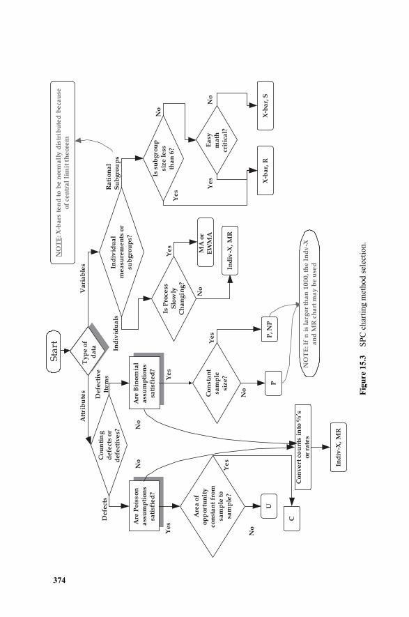
374
Ty
pe
of
da
ta
Ty
pe
of
da
ta
Att
rib
ute
sV
ari
ab
les
De
fect
ive
Ite
ms
De
fect
s
No
Ra
tio
na
lS
ub
gro
up
s
Ye
s
Ind
ivid
ua
ls
Ye
s
No
Ye
s
No
NO
TE
: If
n i
s la
rge
r th
an
10
00
, th
e I
nd
v-X
a
nd
MR
ch
art
ma
y b
e u
sed
NO
TE
: If
n i
s la
rge
r th
an
10
00
, th
e I
nd
v-X
a
nd
MR
ch
art
ma
y b
e u
sed
Are
Bin
om
ial
ass
um
pti
on
ssa
tisf
ied
?
Are
Bin
om
ial
ass
um
pti
on
ssa
tisf
ied
?
Are
Po
iss
on
ass
um
pti
on
ssa
tisf
ied
?
Are
Po
iss
on
ass
um
pti
on
ssa
tisf
ied
?
Ye
s
No
No
No
Ye
sY
es
Sta
rtS
tart
Is P
roce
ssS
low
lyC
ha
ng
ing
?
Ind
iv-X
, M
R
MA
or
EW
MA
Ind
ivid
ua
l m
ea
sure
me
nts
or
sub
gro
up
s?
X-b
ar,
RX
-ba
r, S
Ea
sy
ma
th
crit
ica
l?
Is s
ub
gro
up
si
ze
le
ss
tha
n 6
?
Ye
sN
o
NO
TE
: X-b
ars
te
nd
to
be
no
rma
lly
dis
trib
ute
d b
eca
use
o
f ce
ntr
al
lim
it t
he
ore
m
Co
un
tin
g
de
fect
s o
r d
efe
ctiv
es?
Are
a o
f o
pp
ort
un
ity
co
nst
an
t fr
om
sa
mp
le t
o
sam
ple
?
U
C
Co
ns
tan
t sa
mp
le
siz
e?
Ind
iv-X
, M
R
Co
nv
ert
co
un
ts i
nto
%’s
o
r ra
tes
P, N
PP
Fig
ure
15.3
SP
C c
hart
ing
met
hod
sele
ctio
n.
c15.qxd 4/22/2005 9:18 AM Page 374
Returning to the first decision point for attribute data, we move to the DefectiveItems path on the righthand side. The first check is to see if the binomial assump-tions are satisfied. You have binomial data when it meets the following conditions:
� Each item is the result of identical conditions.
� Each item results in one of two possible outcomes (pass/fail or go/no-go).
� The probability of success (or failure) is constant for each item.
� The outcomes of the items are independent.
Assuming that these assumptions are met, we then need to determine if the sam-ple size is constant or not. With a constant sample size, the P chart is the correctmethod, but for nonconstant sample size the NP chart or the P chart are the correctmethods. You may note from Figure 15.3 that the most robust chart is the I-MRchart, which can be used for individual variable measures and for the defects or de-fectives if the number of data points is large or the results are converted to percent-ages.
15.7.2 Interpreting the Control Chart
Once the proper charting method is selected, the data is plotted and the charts areinterpreted for stability. A process that is in control exhibits only random variation.In other words, the process is stable or consistent. There is no evidence of special-cause variation.
Control charts assess statistical control by determining whether the process out-put falls within statistically calculated control limits and exhibits only random vari-ation. A process is classified as in control if the data demonstrate stability on thecontrol chart. The typical indicators that a process is unstable or out of control iswhen there are definite trends upward or downward (usually seven consecutivepoints). This is evidence of cyclical behavior, either by shift, supplier, or even sea-son. The chart in Figure 15.4 depicts the distribution that occurs on most controlcharts. The diagram is symmetrical about the centerline which is the mean. Thezone defined by the two “C”s is called Zone C and is the ±1 standard deviationabout the mean. The area encompassed by the two “B”s (and the previous “C”s) iscalled Zone B and encompasses the ±2 standard deviations. The final Zone is calledZone A and encompasses the ±3 standard deviations.
The specific tests used are (Nelson tests):
� Any point outside the control limits (outside of Zone A)
� Nine points in a row on same side of the center line
� Six points in a row, all increasing or all decreasing
� Fourteen points in a row, alternating up and down
� Two out of three points in the same Zone A or beyond
� Four out of five in same Zone B or beyond
15.7 STATISTICAL PROCESS CONTROL 375
c15.qxd 4/22/2005 9:18 AM Page 375
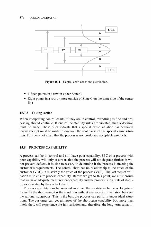
� Fifteen points in a row in either Zone C
� Eight points in a row or more outside of Zone C on the same side of the centerline
15.7.3 Taking Action
When interpreting control charts, if they are in control, everything is fine and pro-cessing should continue. If one of the stability rules are violated, then a decisionmust be made. These rules indicate that a special cause situation has occurred.Every attempt must be made to discover the root cause of the special cause situa-tion. This does not mean that the process is not producing acceptable products.
15.8 PROCESS CAPABILITY
A process can be in control and still have poor capability. SPC on a process withpoor capability will only assure us that the process will not degrade further; it willnot prevent defects. It is also necessary to determine if the process is meeting thecustomer’s requirements. The control chart has no relationship to the voice of thecustomer (VOC); it is strictly the voice of the process (VOP). The last step of vali-dation is to ensure process capability. Before we get to this point, we must ensurethat we have adequate measurement capability and the process is in a state of stabil-ity as indicated by the control chart.
Process capability can be assessed in either the short-term frame or long-termframe. In the short term, it is the condition without any sources of variation betweenthe rational subgroups. This is the best the process can perform under ideal situa-tions. The customer can get glimpses of the short-term capability but, more thanlikely they, will experience the full variation and, therefore, the long-term capabili-
376 DESIGN VALIDATION
±1±2±3
A
C
C
B
B
A
LCL
UCL
Figure 15.4 Control chart zones and distribution.
c15.qxd 4/22/2005 9:18 AM Page 376
ty is a better gauge of what the customer will experience. Capability can be mea-sured with several indices. There are the traditional methods defined by Cp and Cpkand there are the sigma values that correspond to the part per million defects. Eachof these methods utilizes specification limits as defined by the customer and can bedefined as the USL – LSL. We are interested in how many times the process varia-tions can fit with these limits. Obviously, the more times the process spread can fitin the specification limits, the less is the chance that a defect will be experienced.Simply put, the capability is (USL – LSL)/6�LT, where �LT can be calculated withthe following formula for an overall long-term sample of size n:
�LT =��We can use the Cp measure, which is, (USL – LSL)/6�LT, or the Cpk:
Cpk = min�� �, � ��
15.9 SUMMARY
Validation is a critical step in the DFSS road map (see Chapter 5) and needs to bethought out well in advance of final deployment of the new design. Validation oftenrequires prototypes that need to be near “final design” but are often subject to trade-offs in scope and completeness due to cost or availability. Assessing the compo-nents and subsystems of any new design against the type of design risk assists in de-termining when a prototype is required and what configuration must be available.Once prototypes are available, a comprehensive test plan should be followed in or-der to capture any special event and to populate the design scorecard. Any go/no-godecision should be based on statistically significant criteria and all lessons learnedshould be incorporated into the final design if appropriate.
Before hand-off to the production environment, the process stability and capabil-ity should be assured.
x� – LSL�
3�LT
USL – x��3�LT
n
i=1
(xi – x�)2
��n – 1
15.9 SUMMARY 377
c15.qxd 4/22/2005 9:18 AM Page 377

c15.qxd 4/22/2005 9:18 AM Page 378
16.1 INTRODUCTION
In order to appreciate the design activity that will be covered in Chapter 17, wemust first describe the aspects of the supply chain.
16.2 SUPPLY CHAIN DEFINITION
The supply chain has many definitions and covers many traditional functions aswell as life cycle aspects of acquiring resources for use in the production of valuefor end users. The traditional definition of the supply chain (Figure 16.1) is the col-lection of activities that connect suppliers to end users, forming a chain of events.Value-added operations supply end customers, and this relationship is repeated withsuppliers and their suppliers.
In the life cycle of acquiring resources, processing them into value-added solu-tions, and providing postdelivery support there are seven main process-focused re-quirements that must be met to varying degrees. These processes are:
1. Demand forecasting
2. Planning and scheduling
3. Strategic sourcing
4. Processing
5. Asset and inventory management
6. Distribution and logistics
7. Postservice support
We shall briefly describe what is performed in each of these process steps.
Service Design for Six Sigma. By Basem El-Haik and David M. Roy 379© 2005 by John Wiley & Sons.
16SUPPLY CHAIN PROCESS
c16.qxd 4/22/2005 9:18 AM Page 379
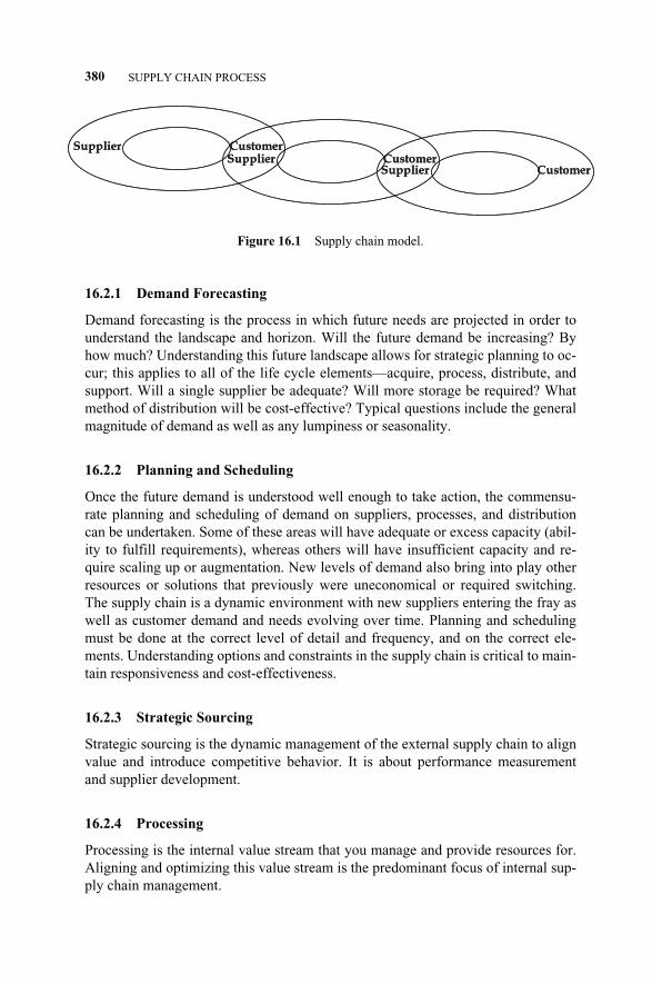
16.2.1 Demand Forecasting
Demand forecasting is the process in which future needs are projected in order tounderstand the landscape and horizon. Will the future demand be increasing? Byhow much? Understanding this future landscape allows for strategic planning to oc-cur; this applies to all of the life cycle elements—acquire, process, distribute, andsupport. Will a single supplier be adequate? Will more storage be required? Whatmethod of distribution will be cost-effective? Typical questions include the generalmagnitude of demand as well as any lumpiness or seasonality.
16.2.2 Planning and Scheduling
Once the future demand is understood well enough to take action, the commensu-rate planning and scheduling of demand on suppliers, processes, and distributioncan be undertaken. Some of these areas will have adequate or excess capacity (abil-ity to fulfill requirements), whereas others will have insufficient capacity and re-quire scaling up or augmentation. New levels of demand also bring into play otherresources or solutions that previously were uneconomical or required switching.The supply chain is a dynamic environment with new suppliers entering the fray aswell as customer demand and needs evolving over time. Planning and schedulingmust be done at the correct level of detail and frequency, and on the correct ele-ments. Understanding options and constraints in the supply chain is critical to main-tain responsiveness and cost-effectiveness.
16.2.3 Strategic Sourcing
Strategic sourcing is the dynamic management of the external supply chain to alignvalue and introduce competitive behavior. It is about performance measurementand supplier development.
16.2.4 Processing
Processing is the internal value stream that you manage and provide resources for.Aligning and optimizing this value stream is the predominant focus of internal sup-ply chain management.
380 SUPPLY CHAIN PROCESS
Supplier CustomerSupplier CustomerSupplier CustomerSupplier Customer
Supplier CustomerSupplier Customer
Figure 16.1 Supply chain model.
c16.qxd 4/22/2005 9:18 AM Page 380
16.2.5 Asset and Inventory Management
Assets are the capital resources that you apply to produce the value you deliver tocustomers. Minimizing the capital you have tied up while optimizing the fulfillmentof your customer’s needs is necessary for profitability and longevity. Inventory canbe supply chain resources or intellectual property (data-based information). Theseinventory items also need to be managed so that you have the minimum amount onhand to be responsive to the customer’s needs. If you have too little, you fail to sat-isfy customers, whereas if you have too much, you lose profitability.
16.2.6 Distribution and Logistics
Once you produce a solution for your customer, you need to determine how to get itto them. If you are providing information, then you need to decide if an electronicformat is sufficient or if hard copy is required. This may require delivery of the hardcopy by land mail, express mail, or courier. The same aspects can be explored withhardware. Do we ship form the plant or from regional warehouses?
16.2.7 Postservice Support
After a service or solution is provided, there will often be some type of service re-quired. This may be a field upgrade such as updating virus definition files, or it maybe postservice follow-up such as that performed after placing an employment can-didate and surveying what the level of satisfaction is from both parties. The activi-ties may range from standard maintenance items to standard wear-and-tear replace-ment activities. All of these elements have a bearing on the first two steps ofdemand forecasting and planning and scheduling, as well as on the process designand provisioning (resourcing) that are required to fulfill the postservice support.
16.3 SUMMARY
The supply chain process covers the life cycle of understanding needs, producing,distributing, and servicing the value chains from customers to suppliers. It appliesto all contexts of acquiring resources and transforming them into value for cus-tomers. This can be product based, information based, or even resource based, suchas capital equipment, employees, raw materials, components, information, expenseitems, or services. Because of its broad applicability to all aspects of consumptionand fulfillment, the supply chain is the ultimate “service” for design consideration.
16.3 SUMMARY 381
c16.qxd 4/22/2005 9:18 AM Page 381

c16.qxd 4/22/2005 9:18 AM Page 382
17.1 INTRODUCTION
In this chapter, we will cover specific elements of the DFSS road map (see Chapter5) that lead to the successful deployment of a full supply chain redesign in a legacyenvironment in which every function was performing its own sourcing and buyingand having incestuous relationships with the suppliers. This redesign is more than areorganization as it represents a major change in strategy and structures, withgreater active management of $4 billion spent in 12 countries, including $3.9 billionspent on materials resold to customers and $113 million in expense-related purchas-es, including consultants, information technology, travel-related services, and officesupplies.
17.2 THE PROCESS
In the context of Figure 3.2, we will demonstrate the progression from Stage 1—Idea Creation through Stage 7—Launch Readiness, that is, the implementation ofthe transformation from a decentralized, relation-based procurement model to a fullsupply chain model delivering double-digit productivity on the total purchase base.Figure 17.1 (a replica of Figure 5.1) will provide the road map that we will follow.
17.3 STAGE 1—IDEA CREATION
In this stage, we learn why the project was conceived and what its scope and re-sources are. Based on the existing model of sourcing and integrated supply chainmanagement in its manufacturing businesses, this company wanted to instill thesame rigor in its nonmanufacturing businesses to leverage and control spending onall purchased items, including office supplies, rent, information technology pur-chases and licenses, and travel.
Service Design for Six Sigma. By Basem El-Haik and David M. Roy 383© 2005 by John Wiley & Sons.
17DFSS IN THE SUPPLY CHAIN
c17.qxd 4/22/2005 9:19 AM Page 383
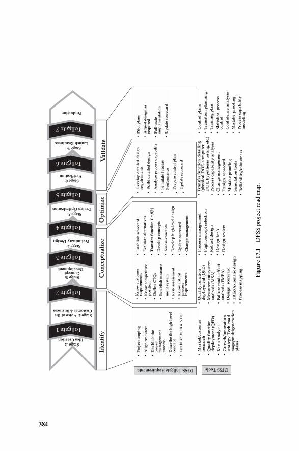
384
Fig
ure
17.1
DF
SS
pro
ject
roa
d m
ap.
•M
ark
et/
cust
om
er
rese
arc
h
•Q
uali
ty f
un
ctio
n
dep
loy
men
t (Q
FD
)
•K
an
o A
na
lysi
s
•G
row
th/i
nn
ov
ati
on
st
rate
gy
: T
ech
. ro
ad
m
ap
s/m
ult
igen
era
tio
n
pla
ns
Iden
tify
Co
nce
ptu
ali
ze
Op
tim
ize
Vali
date
Stage 1: Idea Creation
Stage 2: Voice of theCustomer &Business
Stage 3: Concept
Development
Stage 4: Preliminary Design
Tollgate 1 Tollgate 1
Tollgate 2 Tollgate 2
Tollgate 3 Tollgate 3
Tollgate 4 Tollgate 4
Stage 5: Design Optimization
Tollgate 5 Tollgate 5
Stage 6: Verification
Tollgate 6 Tollgate 6
Stage 7: Launch Readiness
Tollgate 7 Tollgate 7
Production
DFSS ToolsDFSS Tollgate Requirements
•P
roje
ct s
cop
ing
•A
lig
n r
eso
urc
es
•E
sta
bli
sh t
he
p
roje
ctm
an
ag
em
en
tp
roce
ss
•D
esc
rib
e t
he
hig
h-l
ev
el
con
cep
t
•E
sta
bli
sh V
OB
& V
OC
•K
no
w c
ust
om
er
req
uir
em
en
ts
•K
no
w c
om
pe
titi
ve
po
siti
on
•D
efi
ne
CT
Qs
•E
sta
bli
sh m
ea
sure
-
me
nt
syst
em
•R
isk
ass
ess
me
nt
•K
no
w c
riti
cal
pro
cess
req
uir
em
en
ts
•D
ev
elo
p d
eta
ile
d d
esi
gn
re
qu
ire
me
nts
•B
uil
d d
eta
ile
d d
esi
gn
•A
na
lyz
e p
roce
ss c
ap
ab
ilit
y
•S
imu
late
Pro
cess
Pe
rfo
rma
nce
•P
rep
are
co
ntr
ol
pla
n
•U
pd
ate
sco
reca
rd
•P
ilo
t p
lan
s
•A
dju
st d
esi
gn
as
req
uir
ed
•F
ull
-sca
leim
ple
me
nta
tio
n
•U
pd
ate
sco
reca
rd
•E
sta
bli
sh s
core
card
•E
va
lua
te a
lte
rna
tiv
es
•T
ran
sfe
r fu
nct
ion
Y =
f(Y
)
•D
ev
elo
p c
on
cep
ts
•A
sse
ss c
on
cep
ts
•D
ev
elo
p h
igh
-le
ve
l d
esi
gn
•U
pd
ate
sco
reca
rd
•C
ha
ng
e m
an
ag
em
en
t
•Q
ua
lity
fu
nct
ion
d
ep
loy
men
t (Q
FD
)
•M
ea
sure
me
nt
syst
em
an
aly
sis
(MS
A)
•F
ail
ure
mo
de e
ffect
an
aly
sis
(FM
EA
)
•D
esi
gn
sc
ore
card
•T
RIZ
/Ax
iom
ati
c d
esi
gn
•P
roce
ss m
ap
pin
g
•P
roce
ss m
an
ag
em
en
t
•P
ug
h c
on
cep
t se
lect
ion
•R
ob
ust
desi
gn
•D
esi
gn
fo
r Y
•D
esi
gn
rev
iew
•T
ran
sfer
fun
ctio
n d
eta
ilin
g
(ph
ysi
cal
DO
E, co
mp
ute
r D
OE
, h
yp
oth
esi
s te
stin
g, etc
.)
•P
roce
ss c
ap
ab
ilit
y a
na
lysi
s
•C
han
ge m
an
ag
em
en
t
•D
esi
gn
sc
ore
card
•M
ista
ke p
roo
fin
g
•S
imu
lati
on
to
ols
•R
eli
ab
ilit
y/r
ob
ust
ne
ss
•C
on
tro
l p
lan
s
•T
ran
siti
on
pla
nn
ing
•T
rain
ing
pla
n
•S
tati
stic
al
pro
cess
co
ntr
ol
•C
on
fid
en
ce a
naly
sis
•M
ista
ke
-p
roo
fin
g
•P
roce
ss c
ap
ab
ilit
y
mo
de
lin
g
c17.qxd 4/22/2005 9:19 AM Page 384
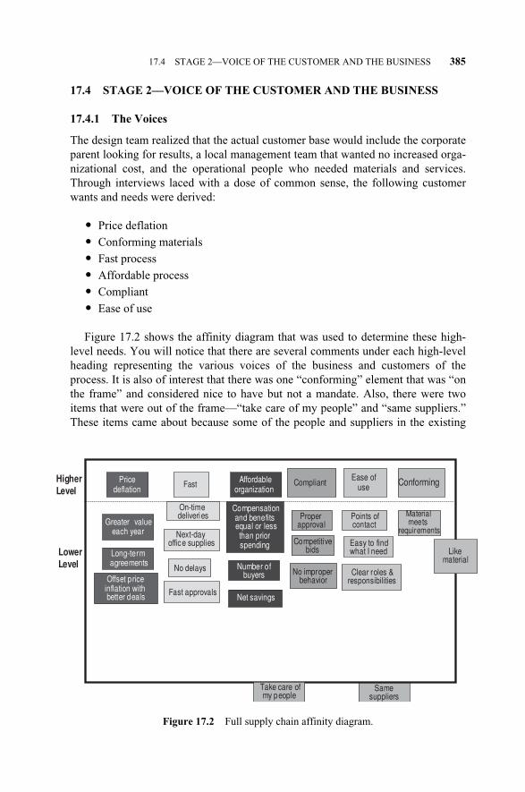
17.4 STAGE 2—VOICE OF THE CUSTOMER AND THE BUSINESS
17.4.1 The Voices
The design team realized that the actual customer base would include the corporateparent looking for results, a local management team that wanted no increased orga-nizational cost, and the operational people who needed materials and services.Through interviews laced with a dose of common sense, the following customerwants and needs were derived:
� Price deflation
� Conforming materials
� Fast process
� Affordable process
� Compliant
� Ease of use
Figure 17.2 shows the affinity diagram that was used to determine these high-level needs. You will notice that there are several comments under each high-levelheading representing the various voices of the business and customers of theprocess. It is also of interest that there was one “conforming” element that was “onthe frame” and considered nice to have but not a mandate. Also, there were twoitems that were out of the frame—“take care of my people” and “same suppliers.”These items came about because some of the people and suppliers in the existing
17.4 STAGE 2—VOICE OF THE CUSTOMER AND THE BUSINESS 385
Figure 17.2 Full supply chain affinity diagram.
Net savings
Number ofbuyers
Fast approvals
No delaysOffset price
inflation with better deals
Greater value each year
On-timedeliveries
Compensationand benefits equal or less than prior spending
Same suppliers
Proper approval
Materialmeets
requirements
Long-term agreements
Price deflation
Fast Affordableorganization
Compliant ConformingHigher Level
Lower Level
Next-day office supplies Competitive
bids
No improperbehavior
Take care of my people
Like material
Points of contact
Ease of use
Easy to find what I need
Clear roles & responsibilities
c17.qxd 4/22/2005 9:19 AM Page 385
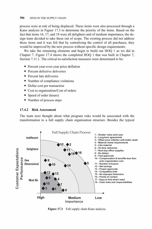
process were at risk of being displaced. These items were also processed through aKano analysis in Figure 17.3 to determine the priority of the items. Based on thefact that items 16, 17, and 18 were all delighters and of medium importance, the de-sign team decided to take these out of scope. The existing process did not addressthese items and it was felt that by centralizing the control of all purchases, theywould be improved by the new process without specific design requirements.
We take the remaining elements and begin to build our HOQ 1 as we did inChapter 7. Figure 17.4 shows the completed HOQ 1 that was built in Chapter 7,Section 7.11.1. The critical-to-satisfaction measures were determined to be:
� Percent year-over-year price deflation
� Percent defective deliveries
� Percent late deliveries
� Number of compliance violations
� Dollar cost per transaction
� Cost to organization/Cost of orders
� Speed of order (hours)
� Number of process steps
17.4.2 Risk Assessment
The team next thought about what program risks would be associated with thetransformation to a full supply chain organization structure. Besides the typical
386 DFSS IN THE SUPPLY CHAIN
Figure 17.3 Full supply chain Kano analysis.
9
8
4
2
3
10
11
6
12
7
High LowMedium
1 – Greater value each year
2 – Long-term agreements
3 – Offset price inflation with better deals
4 – Material meets requirements
5 – Like material
6 – On-time deliveries
7 – Next-day office supplies
8 – No delays
9 – Fast approvals
10 – Compensation & benefits less than
prior organization cost
11 – Number of buyers
12 – Net savings
13 – Proper approvals
14 – Competitive bids
15 – No improper behaviors
16 – Points of contact
17 – Easy to find what I need
18 – Clear roles and responsibilities
Cu
sto
mer
Exp
ecta
tio
ns
Perf
orm
an
ce
Delighters
One-
Dimensional
Must Be
Importance
Full Supply Chain Process
Indifferent
5
1
13
14
15
16
17
18
c17.qxd 4/22/2005 9:19 AM Page 386
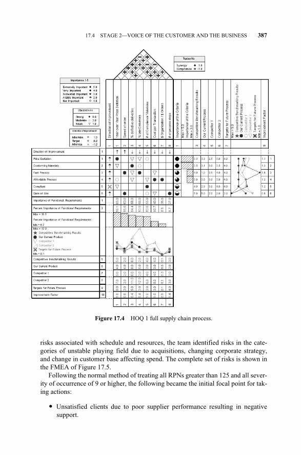
risks associated with schedule and resources, the team identified risks in the cate-gories of unstable playing field due to acquisitions, changing corporate strategy,and change in customer base affecting spend. The complete set of risks is shown inthe FMEA of Figure 17.5.
Following the normal method of treating all RPNs greater than 125 and all sever-ity of occurrence of 9 or higher, the following became the initial focal point for tak-ing actions:
� Unsatisfied clients due to poor supplier performance resulting in negativesupport.
17.4 STAGE 2—VOICE OF THE CUSTOMER AND THE BUSINESS 387
Figure 17.4 HOQ 1 full supply chain process.
c17.qxd 4/22/2005 9:19 AM Page 387

388
Fig
ure
17.5
Ful
l sup
ply
chai
n pr
ojec
t FM
EA
.
Ris
k C
ate
go
ryP
ote
nti
al
Fa
ilu
re M
od
eP
ote
nti
al
Fa
ilu
re E
ffec
tsS
EV
Po
ten
tia
l C
au
seO
CC
Cu
rre
nt
Co
ntr
ols
DE
TR
PN
Ma
nag
em
en
tU
nst
able
en
vir
onm
ent
Lac
k o
f sa
vin
gs
7C
orp
ora
te d
irec
tion
s6
Str
ong
lin
kag
e to
co
rpor
ate
284
Ma
na
ge
me
nt
Un
stab
le e
nv
iron
men
tL
ack
of
reso
urc
es9
Lo
ss o
f cu
stom
ers
2M
onth
ly o
per
atio
ns
rev
iew
236
Ma
nag
em
en
tU
nst
able
en
vir
onm
ent
Lac
k o
f sa
vin
gs
7A
cqu
isit
ion
8D
eal r
evie
w b
oar
d2
112
Ma
nag
em
en
tU
nst
able
en
vir
onm
ent
Lac
k o
f re
sou
rces
9A
cqu
isit
ion
8D
eal r
evie
w b
oar
d2
144
Cli
en
tL
ack
of
bu
y-i
nC
ont
inu
ed le
akag
e7
Un
wil
lin
g to
giv
e u
p c
ont
rol
8M
onth
ly A
/P
rep
ort
422
4
Cli
en
tU
nsa
tisf
ied
Ne g
ativ
e su
pp
ort
9P
oor
su
pp
lier
per
form
ance
8N
on
e8
576
Su
pp
lie
rsL
ack
of
qu
alif
ied
su
pp
lier
sL
ack
of
sav
ing
s 7
Un
abl e
to
qu
alif
y s
up
pli
ers
3N
on
e4
84
Su
pp
lie
rsL
ack
of
qu
alif
ied
su
pp
lier
sD
imin
shed
per
form
ance
6
To
o s
mal
l at
new
su
pp
lier
4D
etai
led
an
aly
sis
of
sup
pli
er2
48
Su
pp
lie
rsSw
itch
ing
cos
tsD
ilu
ted
net
sav
ing
s5
Lo
ng
-ter
m a
gre
emen
ts5
Su
pp
lier
not
ific
atio
n6
150
Te
ch
no
log
yA
vai
lab
ilit
yL
ack
of
mea
sure
men
ts5
IT R
eso
urc
es5
IT p
roje
ct p
ipel
ine
375
Tech
no
log
yA
ffor
dab
leD
ilu
ted
net
sav
ing
s5
Con
ver
sion
/im
ple
men
tati
on
2A
pp
rop
riat
ion
pro
cess
220
Pro
ject
Lac
k o
f q
ual
ifie
d r
eso
urc
esD
elay
ed b
enef
its
7U
nw
illi
ng
to r
elea
se i
nd
ivid
ual
s6
Man
pow
er r
evie
w3
126
Pro
ject
Lac
k o
f q
ual
ifie
d r
eso
urc
esC
ont
inu
ed le
gac
y b
ehav
ior
8U
nab
le t
o fi
nd
qu
alif
ied
3
Rec
ruit
ers
248
c17.qxd 4/22/2005 9:19 AM Page 388
� Lack of buy-in from clients due to their unwillingness to give up control thatresults in leakage in spending.
� High switching costs to change suppliers due to long-term contracts or uniquerequirements that results in diluted savings.
� Lack of critical resources due to a major acquisition, which deflects assignedresources from leveraging supplier performance.
� Lack of qualified resources for new competency model.
� Lack of resources due to change in customer base.
The team needed to ensure that any new suppliers or suppliers that lowered theirpricing maintained the level of performance that the business was accustomed to. Inregard to the leakage, the team needed to review the accounts payable data for sup-plier and cost centers to see if spending could be accounted for. The other itemswere deemed to require watching but no further action at this time.
17.5 STAGE 3—CONCEPT DESIGN
The current organizational structure had purchasing resources basically doing trans-actional work, with ad hoc reporting capability. This structure was replicated ineach country. When the team completed the activity of HOQ 2, the output depictedin Figure 17.6 was obtained.
The prioritized functional requirements with the corresponding CTS in parenthe-ses are:
� Resources to achieve deflation (percent year-over-year price deflation)
� Resources to achieve delivery quality (percent defective deliveries)
� Resources to achieve on time delivery (percent late deliveries)
� Organizational design (spend/organizational cost)
� Supplier support (spend/organizational cost)
� Process design (number of process steps)
� Approval speed (speed of order)
� Measures of delivery quality (percent defective deliveries)
� Delivered quality improvement methods (percent defective deliveries)
� Amount of spending controlled (spending/organizational cost)
� Staffing methods (number of compliance violations)
� Organizational cost (cost per transaction)
� Systems process cost (cost per transaction)
� Approval levels (number of process steps)
� Methods for improving on-time delivery (percent late deliveries)
� Measures of on-time delivery (percent late deliveries)
� System availability (speed of order)
17.5 STAGE 3—CONCEPT DESIGN 389
c17.qxd 4/22/2005 9:19 AM Page 389

390 DFSS IN THE SUPPLY CHAIN
Figure 17.6 Full supply chain HOQ2.
c17.qxd 4/22/2005 9:19 AM Page 390

17.5 STAGE 3—CONCEPT DESIGN 391
Figure 17.6 (continued).
c17.qxd 4/22/2005 9:19 AM Page 391
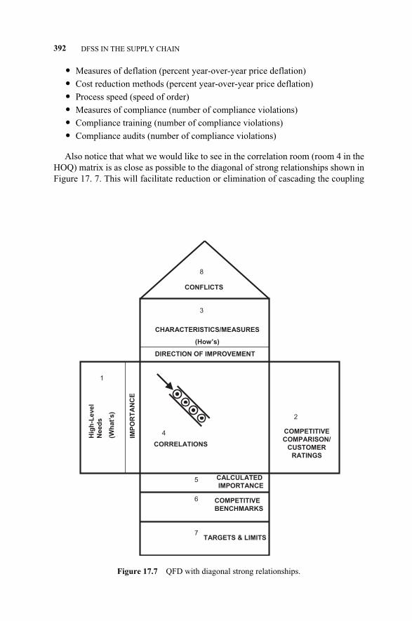
� Measures of deflation (percent year-over-year price deflation)
� Cost reduction methods (percent year-over-year price deflation)
� Process speed (speed of order)
� Measures of compliance (number of compliance violations)
� Compliance training (number of compliance violations)
� Compliance audits (number of compliance violations)
Also notice that what we would like to see in the correlation room (room 4 in theHOQ) matrix is as close as possible to the diagonal of strong relationships shown inFigure 17. 7. This will facilitate reduction or elimination of cascading the coupling
392 DFSS IN THE SUPPLY CHAIN
Figure 17.7 QFD with diagonal strong relationships.
7
3
5
1
6
2
8
IMP
OR
TA
NC
E
DIRECTION OF IMPROVEMENT
CALCULATED
IMPORTANCE
COMPETITIVE
COMPARISON/
CUSTOMER
RATINGS
CONFLICTS
Hig
h-L
evel
Need
s
(Wh
at’
s)
COMPETITIVE
BENCHMARKS
TARGETS & LIMITS
CHARACTERISTICS/MEASURES
(How’s)
4
CORRELATIONS
c17.qxd 4/22/2005 9:19 AM Page 392
vulnerability to HOQ 2 and beyond (recall Section 8.5.2 and Figure 8.13). At thispoint, we will highlight the following submatrices of room 4.
Case 1: Uncoupled CaseFR1 = “year-over-year price deflation” and FR2 = “speed of order” are both uncou-pled in DP3 = “supplier support” and DP4 = “process design.” The design matrix isgiven as
� � = � �� � (17.1)
That is, the design team is free to decide in which way they utilize the design para-meters to satisfy the functional requirements. There is no design sequence to followunder the assumption that only these two DPs will be used for the two FRs men-tioned above.
Case 2: Decoupled CaseA prime example is when FR6 = “cost per transaction” and FR7 = “$ organization/$order” are decoupled in DP2 = “organization design” and DP9 = “staffing meth-ods.” The design matrix is given as
� � = � �� � (17.2)
That, is the design team has to satisfy FR6 first, using DP2, fix DP2 when they sat-isfy FR7, and then use DP9 only to satisfy FR7, as was discussed in the context ofFigure 8.13.
Case 3: Coupled CaseIn this case, we find that FR3 = “percent defective deliveries” and FR4 = “percentlate deliveries” are coupled in DP7 = “delivered quality improvement methods” andDP6 = “measures of delivery quality.” The design matrix is given by
� � = � �� � (17.3)
That is, the best that the team can do is to compromise by satisfying the two FRs ifthey want to live with that. The other option is to use the TRIZ contradiction table(Appendix 9.A) to make either or both of the off-diagonal elements zero or approx-imately zero. Which TRIZ solution principle is applicable here? The answer is leftas an exercise.
The above three cases are just examples of what the team may face in resolvingdesign vulnerabilities. There are many other examples of the case of 2 × 2 matrices.Notice that we concentrate only on strong relationships and we did not examine 3 ×3, 4 × 4, or other size submatrices. For more details on such handling, see El-Haik(2005).
DP7DP6
X XX X
FR3FR4
DP2DP9
X 0X X
FR6FR7
DP3DP4
X 00 X
FR1FR2
17.5 STAGE 3—CONCEPT DESIGN 393
c17.qxd 4/22/2005 9:19 AM Page 393

17.5.1 Concept Development
From the list of functional requirements (FRs), concepts for the fulfillment of therequirements can be developed. We also have trade-off compromises for several ofthe FRs; for example, the number of resources is a trade-off with the organizationalcost. These trade-offs are couplings that are design vulnerabilities that will affectthe next HOQ. It is best if the team can solve them at this stage with some creativethinking. Because we are dealing with multiple countries, it was determined that afour-tier approach should be pursued. First, any commodity that could be controlledat the corporate level would be. The next tier would be the items that were businessspecific and could be controlled at the business unit level. The third tier would beby major geographical area. There were three major areas defined: North America,Europe, and the Far East. The fourth tier would be the country-specific spendingthat could not be consolidated.
Through benchmarking, it was determined that a commodity team approachwould provide the best solution for achieving the delivery, quality, and cost-reduc-tion objectives while staying close to the needs of the client and be able to competi-tively leverage the supply chain.
At the time this project was active, there were limited options for some of thetechnological solutions. The morphological matrix of possible solutions is summa-rized in Figure 17.8. For each functional requirement, possible solutions are brain-stormed and placed into the matrix.
The next step was to look at these options and choose the ones that seemed to bea best fit. Figure 17.9 depicts what will be labeled Concepts 1 and 2. The way to in-terpret this is that the functional requirement of organizational design will be ful-filled by a centralized commodity team, supplier support will be provided by inter-nal company resources, and so on. For concept 1 the team plans to rely on theexisting systems while for concept 2 they would rely on an Ariba Catalogue systemfor expense item management
Figure 17.10 depicts what will be called Concept 3. The major difference be-tween Concept 1 and Concept 2 is the use of contracted resources instead of compa-ny resources. This means that you can acquire experienced talent but at the cost ofaffordability and use of company personnel.
Once a set of concepts has been generated, they can be evaluated through thePugh selection method (see Chapter 8). The initial datum is generally the existingsystem. The legend on the right-hand side outlines what the other concepts are. TheCTSs are taken from the HOQ 1 and are used to evaluate how the concepts fulfillthe CTSs. When a concept provides more functionality to the CTS compared to thedatum, it is scored as “+”; if it is the same, it is scored as “S”; and if it offers dimin-ished functionality, it is scored as “–.” The team evaluated the four concepts andfound that Concept 1 provided the best solution (Figure 17.11).
Concept 2 provided a good solution, as evidenced by the number of +’s and S’s.However, it was not as strong as Concept 1, as there are five +’s in Concept 1, is 5versus three in Concept 2. Concept 3 was definitely inferior, as it contains five mi-nuses and only a single S.
394 DFSS IN THE SUPPLY CHAIN
c17.qxd 4/22/2005 9:19 AM Page 394
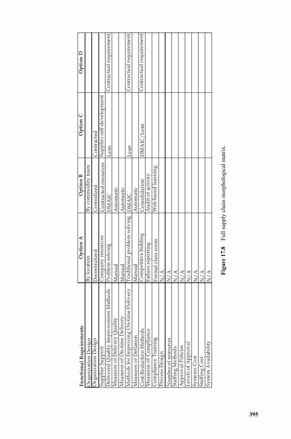
395
Fig
ure
17.8
Ful
l sup
ply
chai
n m
orph
olog
ical
mat
rix.
Fu
nct
ion
al
Req
uir
em
en
tsO
pti
on
AO
pti
on
BO
pti
on
CO
pti
on
D
Or g
an
izat
ion
De
sig
nB
y l
oca
tio
nB
y c
om
mo
dit
y t
eam
Org
an
izat
ion
De
sig
nD
ecen
tra
lize
dC
en
tra
liz
edC
on
trac
ted
Su
pp
lier
Su
pp
ort
Co
mp
an
y r
eso
urc
esC
on
tra
cte
d r
eso
urc
esS
up
pli
er
self
-de
ve
lop
me
nt
De
liv
ere
d Q
ual
ity
Im
pro
ve
men
t M
eth
od
sP
rob
lem
so
lvin
gD
MA
ICL
ean
Co
ntr
act
ua
l re
qu
ire
me
nt
Mea
sure
s o
f D
eliv
ery
Qu
ali
tyM
an
ual
Au
t om
at i
cM
easu
res
of
On
-tim
e D
eli
ve
ryM
an
ual
Au
t om
at i
cM
eth
od
s fo
r Im
pro
vin
g O
n-t
ime
Del
iver
yT
rad
itio
na
l p
rob
lem
so
lvin
gD
MA
ICL
ean
Co
ntr
act
ua
l re
qu
ire
me
nt
Mea
sure
s o
f D
efla
tio
nM
an
ual
Au
tom
ati
c
Co
st-R
ed
uct
ion
Met
ho
ds
Co
mp
eti
tiv
e b
idd
ing
Co
nso
lid
ati
on
DM
AIC
/L
ean
Co
ntr
act
ua
l re
qu
ire
me
nt
Mea
sure
s o
f C
om
pli
an
ceF
ailu
re r
epo
rtin
gA
ud
it o
f ac
tiv
ity
Co
mp
lia
nce
Tra
inin
gF
orm
al
cla
ss r
oo
mW
eb-b
ase
d l
earn
ing
Pro
cess
De
sig
nN
/A
Nu
mb
er
of
reso
urc
esN
/A
Sta
ffin
g M
eth
od
sN
/A
Ap
pro
va
l P
oli
cies
N/
AL
eve
ls o
f A
pp
rov
al
N/
AS
yst
em
s C
ost
N/
AS
taff
ing
Co
stN
/A
Sy
ste
m A
va
ilab
ilit
yN
/A
c17.qxd 4/22/2005 9:19 AM Page 395
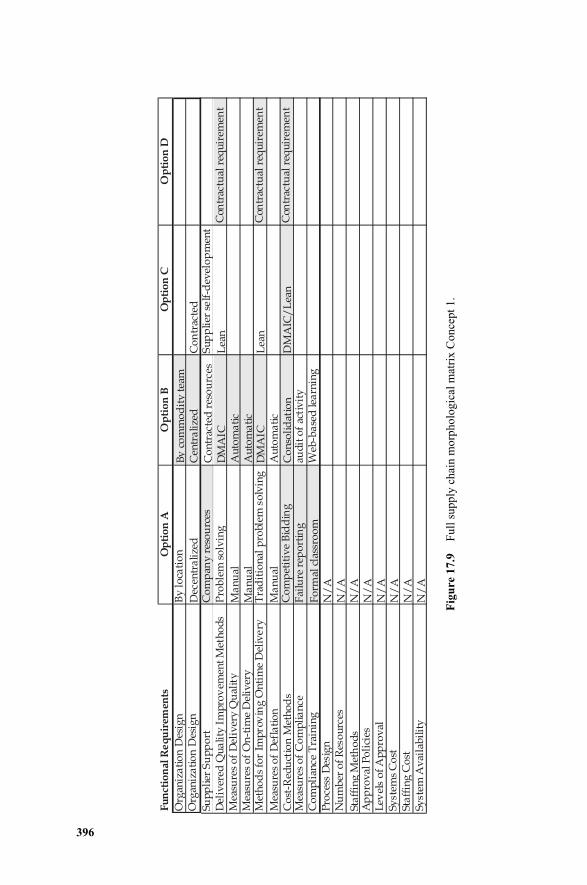
396
Fig
ure
17.9
Ful
l sup
ply
chai
n m
orph
olog
ical
mat
rix
Con
cept
1.
Fu
nct
ion
al R
eq
uir
emen
tsO
pti
on
AO
pti
on
BO
pti
on
CO
pti
on
D
Org
aniz
ati
on
Des
ign
B
y l
oca
tio
nB
y c
om
mo
dit
y t
eam
Org
aniz
ati
on
Des
ign
Dec
entr
ali
zed
Cen
tra
lize
dC
on
trac
ted
Sup
pli
er S
up
po
rtC
om
pan
y r
eso
urc
esC
on
trac
ted
res
ou
rces
Su
pp
lier
se
lf-d
evel
op
men
tD
eliv
ered
Qu
ali
t y I
mp
rov
emen
t M
eth
od
sP
rob
lem
so
lvin
gD
MA
ICL
ean
Con
trac
tual
req
uir
emen
tM
easu
res
of
Del
iver
y Q
ual
ity
Ma
nu
alA
uto
ma
tic
Mea
sure
s o
f O
n-t
ime
Del
iver
yM
an
ual
Au
tom
ati
cM
eth
od
s fo
r Im
pro
vin
g O
nti
me
Del
ive
ryT
rad
itio
nal
pro
blem
so
lvin
gD
MA
ICL
ean
Con
trac
tual
req
uir
emen
t
Mea
sure
s o
f D
efla
tio
nM
an
ual
Au
tom
ati
cC
ost
-Red
uct
ion
Met
ho
ds
Co
mp
etit
ive
Bid
din
gC
on
soli
dat
ion
DM
AIC
/L
ean
Con
trac
tual
req
uir
emen
tM
easu
res
of
Co
mp
lia
nce
Fai
lure
rep
ort
ing
aud
it o
f ac
tiv
ity
Co
mp
lian
ce T
rain
ing
Fo
rmal
cla
ssro
om
Web
-ba
sed
lea
rnin
gP
roce
ss D
esig
nN
/A
Nu
mb
er o
f R
eso
urc
esN
/A
Sta
ffin
g M
eth
od
sN
/A
Ap
pro
val
Po
lici
esN
/A
Lev
els
of
Ap
pro
val
N/
AS y
stem
s C
ost
N/
ASt
aff
ing
Co
stN
/A
S yst
em A
vai
lab
ilit
yN
/A
c17.qxd 4/22/2005 9:19 AM Page 396
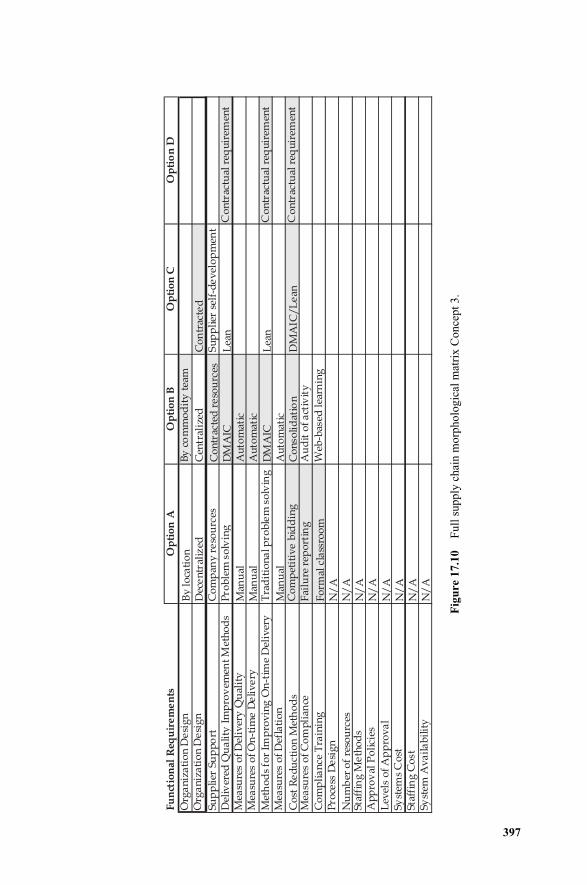
397
Fig
ure
17.1
0F
ull s
uppl
y ch
ain
mor
phol
ogic
al m
atri
x C
once
pt 3
.
Fu
nct
ion
al R
equ
ire
me
nts
Op
tio
n A
Op
tio
n B
Op
tio
n C
Op
tio
n D
Org
an
iza
tio
n D
esi
gn
B
y l
oca
tio
nB
y c
om
mo
dit
y t
eam
Org
an
iza
tio
n D
esi
gn
Dec
en
tral
ized
Cen
tral
ized
Co
ntr
acte
dSu
pp
lier
Su
pp
ort
Co
mp
any
re
sou
rces
Co
ntr
acte
d r
eso
urc
esS
up
pli
er s
elf-
de
vel
op
men
tD
eliv
ered
Qu
ali
ty I
mp
rov
emen
t M
eth
od
sP
rob
lem
so
lvin
gD
MA
ICL
ean
Co
ntr
actu
al r
equ
irem
ent
Mea
sure
s o
f D
eliv
ery
Qu
alit
yM
anu
alA
uto
mat
icM
easu
res
of
On
-tim
e D
eli
ve
ryM
anu
alA
uto
mat
icM
eth
od
s fo
r Im
pro
vin
g O
n-t
ime
Del
iver
yT
rad
itio
na
l pro
ble
m s
olv
ing
DM
AIC
Lea
nC
on
trac
tual
req
uir
emen
tM
easu
res
of
Def
lati
on
Man
ual
Au
tom
atic
Co
st R
ed
uct
ion
Met
ho
ds
Co
mp
etit
ive
bid
din
gC
on
soli
dat
ion
DM
AIC
/L
ean
Co
ntr
actu
al r
equ
irem
ent
Mea
sure
s o
f C
om
pli
ance
Fai
lure
rep
ort
ing
Au
dit
of
act
ivit
y
Co
mp
lia
nce
Tra
inin
gF
orm
al c
lass
roo
mW
eb-b
ased
lea
rnin
gP
roce
ss D
esi
gn
N/
AN
um
ber
of
reso
urc
esN
/A
Staf
fin
g M
eth
od
sN
/A
Ap
pro
val
Po
lici
esN
/A
Lev
els
of
Ap
pro
va
lN
/A
S yst
ems
Co
stN
/A
Staf
fin
g C
ost
N/
ASy
stem
Av
ail
ab
ilit
yN
/A
c17.qxd 4/22/2005 9:19 AM Page 397
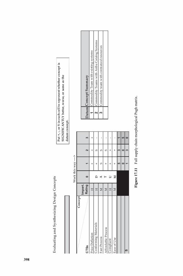
398
Fig
ure
17.1
1F
ull s
uppl
y ch
ain
mor
phol
ogic
al P
ugh
mat
rix.
Ev
alu
ati
ng
an
d S
yn
the
siz
ing
De
sig
n C
on
cep
tsP
ut
+,
-, o
r S
in
ea
ch c
ell
to
rep
rese
nt
wh
eth
er
con
cep
t is
SIG
NIF
ICA
NT
LY
bet
ter,
wo
rse,
or
sam
e a
s th
e
da
tum
co
nce
pt.
Wo
rk t
his
wa
y -
--->
Co
nce
pt
CT
Ss
Imp
ort
.
Rati
ng
01
23
Da
tum
Co
nce
pt
Su
mm
ary
Pri
ce D
efla
tio
nH
++
+1
Co
mm
od
ity
Te
am w
ith
exi
stin
g s
yst
ems
Co
nfo
rmin
g M
ate
ria
lsH
D+
S-
2C
om
mo
dit
y T
eam
s w
ith
Ari
ba
Ca
talo
g S
yst
ems
Fas
t P
roce
ssM
AS
S-
3C
om
mo
dit
y t
eam
wit
h c
on
tra
tce
d r
eso
urc
es
Aff
ord
ab
le P
roce
ssM
T+
S-
Co
mp
lia
nt
HU
++
-
Ea
se o
f U
seM
M+
+-
53
1
00
5S
13
0
c17.qxd 4/22/2005 9:19 AM Page 398
17.6 STAGE 4—PRELIMINARY DESIGN
Once the conceptual design is selected, the next phase entails detailed design to thelevel of design parameters that is done in HOQ 3.
The design parameters from HOQ 3 were developed in Chapter 7 and are repeat-ed here. The functional requirements are in parentheses:
� Type of resources (resources)
� Number of resources (resources)
� Type of resources (organization design)
� Quantity of resources (organization design)
� Location of resources (organization design)
� Type of support (supplier support)
� Frequency of support (supplier support)
� Magnitude of support (supplier support)
� Intuitive (process design)
� Workflow (process design)
� Approval levels (approval speed)
� Speed of approval levels (approval speed)
� By supplier (measures of delivery quality)
� By commodity (measures of delivery quality)
� By part (measures of delivery quality)
� By buyer (measures of delivery quality)
� Lean methods (methods for improving delivery quality)
� Variation reduction methods (methods for improving delivery quality)
� Contract delivery quality terms (methods for improving delivery quality)
� Consolidated buying (amount of spend controlled)
� Background checks (staffing methods)
� Screening methods (staffing methods)
� Compensation and benefits (organizational cost)
� Travel and living (organizational cost)
� Depreciation cost (systems process cost)
� Telecommunication cost (systems process cost)
� Mail cost (systems process cost)
� Lean methods (methods for improving on-time delivery)
� Variation reduction methods (methods for improving on-time delivery)
� Contract on time delivery terms (methods for improving on time delivery)
� By supplier (measures of on-time delivery)
� By commodity (measures of on-time delivery)
� By part (measures of on time delivery)
17.6 STAGE 4—PRELIMINARY DESIGN 399
c17.qxd 4/22/2005 9:19 AM Page 399
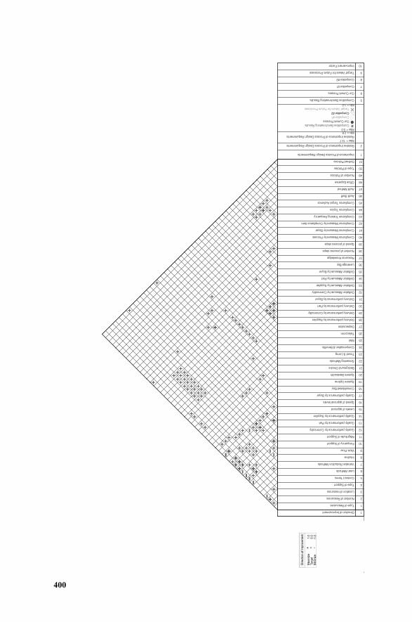
400
Direction of Improvement 1
Type of Resources
Number of Resources
Location of resources
Type of Support
Contract Terms
Lean Methods
Variation Reduction Methods
Intuitive
Work Flow
Frequency of Support
Magnitude of Support
Quality performance by Commodity
Quality performance by Part
Quality performance by Supplier
Levels of approval
Speed of approval levels
Quality performance by Buyer
Consolidated Buy
System Uptime
System Bandwidth
Background Checks
Screening Methods
Travel & Living
Compensation & Benefits
Telecomm
Depreciation
Delivery performance by Supplier
Delivery performance by Commodity
Delivery performance by Part
Delivery performance by Buyer
Deflation Measure by Commodity
Deflation Measure by Supplier
Deflation Measure by Part
Deflation Measure by Buyer
Leverage Buy
Resource Knowledge
Number of process steps
Speed of process steps
Compliance Measure by Process
Compliance Measure by Buyer
Compliance Measure by Compliance item
Compliance Training Frequency
Compliance Topics
Compliance Target Audience
Audit Staff
Audit Method
Office Expense
Number of Policies
Type of Policies
Defined Policies
1
2
3
4
5
6
7
8
9
10
11
12
13
14
15
16
17
18
19
20
21
22
23
24
25
26
27
28
29
30
31
32
33
34
35
36
37
38
39
40
41
42
43
44
45
46
47
48
49
50
51
Importance of Process Design Requirements 1
Relative Importance of Process Design Requirements 2
Max = 13.7
Relative Importance of Process Design Requirements
Min = 2.6Max = 5.0
Competitive Benchmarking Results
Our Current Process
Competitor #1
Competitor #2
Target Values for Future Processes
Min = 1.0
Competitive Benchmarking Results 5
Our Current Process 6
Competitor #1 7
Competitor #2 8
Target Values for Future Processes 9
Improvement Factor 10
Directio
n o
f Im
prov
em
ent
Maxi
miz
e1.0
Targ
et
0.0
Min
imiz
e-1
.0
c17.qxd 4/22/2005 9:19 AM Page 400
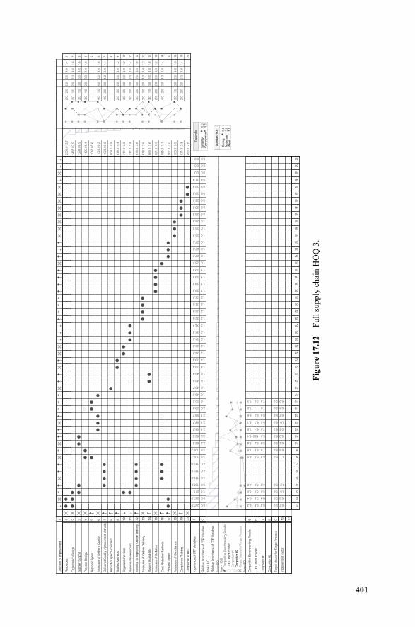
401
Fig
ure
17.1
2F
ull s
uppl
y ch
ain
HO
Q 3
.
621.0
585.0
1026.0
1026.0
678.0
678.0
558.0
531.0
819.0
711.0
711.0
1197.0
1296.0
2566.0
666.0
1485.0
1045.0
495.0
567.0
909.0
3.3
3.1
5.5
5.5
3.6
3.6
3.0
2.8
4.4
3.8
3.8
6.4
6.9
13.7
3.6
7.9
5.6
2.6
3.0
4.9
3.0
3.0
4.0
4.0
2.0
2.0
2.0
3.0
3.0
2.0
3.0
3.0
2.0
4.0
3.0
2.0
1.0
1.0
2.0
1.0
1.0
3.0
2.0
3.0
2.0
3.0
2.0
1.0
2.0
2.0
1.0
2.0
2.0
3.0
3.0
4.0
2.0
2.0
2.0
3.0
3.0
2.0
3.0
3.0
2.0
3.0
3.0
2.0
3.0
3.0
4.0
2.0
2.0
2.0
2.0
3.0
2.0
1.0
2.0
3.0
2.0
4.0
2.0
2.0
4.0
4.0
4.0
4.0
4.0
4.0
4.0
4.0
4.0
4.0
5.0
4.0
3.0
4.0
4.0
4.0
1.6
1.6
1.4
1.6
1.6
1.2
1.4
1.2
1.4
1.2
1.6
1.6
1.2
1.4
1.6
1.4
1 2 3 4 5 6 7 8 9 10
11
12
13
14
15
16
17
18
19
20
Directio
n o
f Im
provem
ent
1
Resour
ces
Org
ani
zation
Desi
gn
Sup
plie
r S
upp
ort
Pro
cess
Desig
n
Appr
ova
l Speed
Measur
es
of D
eliv
ery
Qualit
y
Deliv
ere
d Q
ualit
y Im
pro
vem
ent
Met
hods
Am
ount
of spe
nd
controlle
d
Sta
ffin
g M
eth
ods
Org
ani
zationa
l Cost
Sys
tem
s P
roce
ss C
ost
Meth
ods
for Im
pro
ving
Ont
ime D
eliv
ery
Measur
es
of O
ntim
e D
eliv
ery
Sys
tem
Availa
bility
Measur
es
of D
efla
tion
Cost R
educ
tion M
eth
ods
Pro
cess
Spe
ed
Measur
es
of C
om
plia
nce
Com
plia
nce
Tra
inin
g
Com
plia
nce
Aud
its
1 2 3 4 5 6 7 8 9 10
11
12
13
14
15
16
17
18
19
20
Im
port
anc
e o
f C
TP
Variable
s
1
56.6
62.3
58.7
221.9
215.1
221.9
107.7
62.3
155.6
107.3
50.2
58.7
58.7
43.7
27.2
27.2
27.2
49.3
110.0
110.0
110.0
32.6
32.6
32.6
32.6
25.5
25.5
25.5
23.8
23.8
28.1
29.8
29.8
29.8
29.8
43.4
43.4
26.8
26.8
26.8
34.2
34.2
34.2
34.2
34.2
11.4
0.0
0.0
0.0
39.4
39.4
Rela
tive
Im
portanc
e o
f C
TP
Variab
les
2
2.0
2.2
2.1
8.0
7.8
8.0
3.9
2.2
5.6
3.9
1.8
2.1
2.1
1.6
1.0
1.0
1.0
1.8
4.0
4.0
4.0
1.2
1.2
1.2
1.2
0.9
0.9
0.9
0.9
0.9
1.0
1.1
1.1
1.1
1.1
1.6
1.6
1.0
1.0
1.0
1.2
1.2
1.2
1.2
1.2
0.4
0.0
0.0
0.0
1.4
1.4
Max
= 8
.0
Rela
tive
Im
portanc
e o
f C
TP
Variabl
es
Min
= 0
.0M
ax
= 1
0.0
Com
petit
ive B
ench
mark
ing
Resu
lts
Our
Curr
ent
Pro
duct
Com
petit
or
#1
Com
petit
or
#2
Targ
et Valu
es
for Targ
et P
roce
ss
Min
= 4
.0
Com
petit
ive B
enc
hmark
ing
Resu
lts
5
8.3
5.0
6.4
4.5
7.0
6.1
5.8
4.0
7.5
7.3
8.5
7.5
5.1
Our
Curr
ent
Pro
duct
6
5.8
5.6
5.8
5.0
10.0
5.2
5.0
5.5
5.8
5.0
6.1
6.3
Com
petit
or
#1
7
8.3
5.0
6.4
4.5
7.0
6.1
5.8
4.0
7.5
7.3
8.5
7.5
5.1
Com
petit
or
#2
8
Targ
et Valu
es
for Targ
et P
roce
ss
9
5.0
5.0
5.0
5.0
5.0
5.0
5.0
5.0
5.0
5.0
5.0
5.0
5.0
Im
prove
ment Fact
or
1
0
-0.7
0.0
-0.3
0.1
-0.4
-0.2
-0.2
0.2
-0.5
-0.5
-0.7
-0.5
0.0
11
1
2
3
4
5
6
7
8
9
10
11
12
13
14
15
16
17
18
19
20
21
22
23
24
25
26
27
28
29
30
31
32
33
34
35
36
37
38
39
40
41
42
43
44
45
46
47
48
49
50
51
Sta
ndard
9-3
-1
Strong
9.0
Modera
te3.0
Weak
1.0
Tra
deoffs
Syn
erg
y1.0
Com
pro
mis
e-1
.0
c17.qxd 4/22/2005 9:19 AM Page 401
� By buyer (measures of on time delivery)
� Uptime (system availability)
� Bandwidth (system availability)
� By supplier (measures of deflation)
� By commodity (measures of deflation)
� By part (measures of deflation)
� By buyer (measures of deflation)
� Leverage buy (cost-reduction methods)
� Supplier deflation performance (cost-reduction methods)
� Lean methods (cost-reduction methods)
� Variation-reduction methods (cost-reduction methods)
� Contract cost-reduction terms (cost-reduction methods)
� Number of process steps (process speed)
� Speed of each process step (process speed)
� Resource quantity (process speed)
� Resource skill (process speed)
� By compliance category (measures of compliance)
� By buyer (measures of compliance)
� By process (measures of compliance)
� Target audience (compliance training)
� Content (compliance training)
� Frequency (compliance training)
� Auditors (compliance audits)
� Audit method (compliance audits)
Most of these parameters come directly from the morphological matrix; howev-er, the ones in the matrix that are denoted N/A require another level of decomposi-tion. For example, the sixth DP is “Type of Support,” aligned with the FR “Suppli-er Support.” The types of support that may be required are order status, invoicestatus, productivity support, ramp-up support, and so on. Ramp-up support refers tothe situation in which you are ordering a new part from an existing supplier or anew supplier ramps up to full production. The decomposition complexity of someof these can have a major impact on the type and quantity of resources that will berequired. In a Six Sigma deployment, the tactical support elements of order statusand invoice status should not be required, since all of the elements of the processwork the first time. This puts more focus on the strategic support items such as pro-ductivity support and ramp-up support. It is at this level that the design scorecardcould provide valuable guidance in terms of the capacity planning for the supportelements. Figure 17.13 shows a top-level design scorecard. If you look at the rolledthroughput yield (RTY) column, you can quickly see that the two items that are notperforming at high levels are productivity and the on-time delivery. These two
402 DFSS IN THE SUPPLY CHAIN
c17.qxd 4/22/2005 9:19 AM Page 402
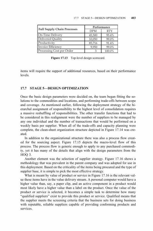
items will require the support of additional resources, based on their performancelevels.
17.7 STAGE 5—DESIGN OPTIMIZATION
Once the basic design parameters were decided on, the team began fitting the so-lutions to the commodities and locations, and performing trade-offs between scopeand coverage. As mentioned earlier, following the deployment strategy of the hi-erarchal assignment of responsibility to the highest level of consolidation requiresa massive reshuffling of responsibilities. The other transfer functions that had tobe considered in this realignment were the number of suppliers to be managed byany one individual and the number of transactions that would be performed on aweekly basis per supplier. When all of the trade-offs and capacity planning werecomplete, the clean-sheet organization structure depicted in Figure 17.14 was cre-ated.
In addition to the organizational structure there was also a process flow creat-ed for the sourcing aspect. Figure 17.15 depicts the macro-level flow of thisprocess. The process flow is generic enough to apply to any purchased commodi-ty, yet it has many of the details that align with the design parameters from theHOQ 3.
Another element was the selection of supplier strategy. Figure 17.16 shows amethodology that was prevalent in the parent company and was adopted for use inthis deployment. Based on the criticality of the items being procured and the type ofsupplier base, it is simple to pick the most effective strategy.
What is meant by value of product or service in Figure 17.16 is the relevant val-ue these items have in the value delivery stream. A personal computer would have ahigher value than, say, a paper clip, and an active component in a product wouldmost likely have a higher value than a label on the product. Once the value of theproduct or service is selected, it becomes a simple task to determine how many“qualified suppliers” exist to provide this product or service. Qualified means thatthe supplier meets the screening criteria that the business sets for doing businesswith reputable, reliable suppliers capable of providing conforming products andservices.
17.7 STAGE 5—DESIGN OPTIMIZATION 403
Figure 17.13 Top-level design scorecard.
DPM RTY
On-Time Delivery 45,500 95.4%Delivered Quality 10,050 99.0%Productivity 85,716 91.4%Invoice Efficiency 9,950 99.0%Processing Cost per Order 3 100.0%
PerformanceFull Supply Chain Processes
c17.qxd 4/22/2005 9:19 AM Page 403

404 DFSS IN THE SUPPLY CHAIN
Figure 17.15 Sourcing macro process.
CommodityCommodity
AnalysisAnalysis
MarketMarket
AnalysisAnalysisNegotiationNegotiation SetupSetup
CommodityCommodity
ManagementManagementOperationalizeOperationalize
• Industry Analysis
• Supplier Analysis
• Establish Best
in Class Measures
• Supplier Processes Mapped
• Baseline Spend
• Quantify Benefit
• Understand Cost Drivers
• Business Processes
Mapped
• Customize Metrics to Commodity
• Select Strategy
• Select Suppliers
• Negotiate
• System Modifications
• Policy & Procedures
• Education
• Communication Plan
• Supplier
Integration into process
• Allocation Verification
• Leakage
• Ledgerable Savings
• Cash Flow
• Customer Value
• Dashboards /
Scorecards
Training &
OrganizationalDevelopment
SourcingReporting
Strategy &
Planning
Figure 17.14 Full supply chain new organization structure.
SVP Global Sourcing
Director, North American Sourcing
Director, European Sourcing
Director, Japan Sourcing
Indirect Sourcing Commodity Leader
Direct SourcingCommodity Leader
Sourcing Manager,Europe C
Sourcing Manager,U.K.
Sourcing Manager,Iberia
Sourcing Manager,Italy
Direct Commodity Leader
Direct Commodity Leader
Indirect Commodity Leader
Facilities Management
Sourcing Manager,France
Sourcing Analyst
Direct Commodity Leader
Indirect Commodity Leader
Manager, Facilities Management
Direct Commodity Leader
Indirect Administrator
Office Services Manager
Office Service Planner
Maintenance & Construction
c17.qxd 4/22/2005 9:19 AM Page 404
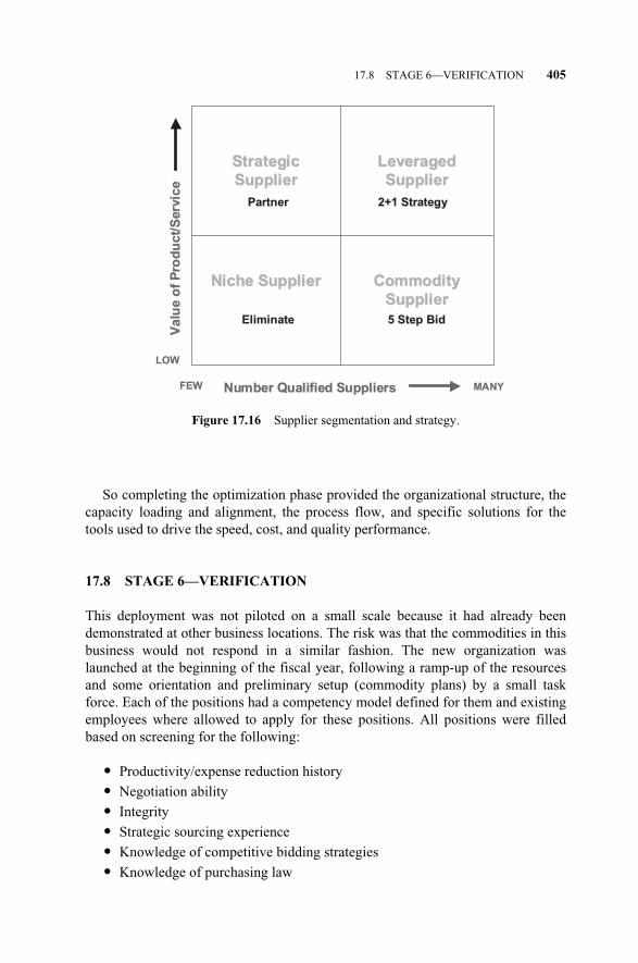
So completing the optimization phase provided the organizational structure, thecapacity loading and alignment, the process flow, and specific solutions for thetools used to drive the speed, cost, and quality performance.
17.8 STAGE 6—VERIFICATION
This deployment was not piloted on a small scale because it had already beendemonstrated at other business locations. The risk was that the commodities in thisbusiness would not respond in a similar fashion. The new organization waslaunched at the beginning of the fiscal year, following a ramp-up of the resourcesand some orientation and preliminary setup (commodity plans) by a small taskforce. Each of the positions had a competency model defined for them and existingemployees where allowed to apply for these positions. All positions were filledbased on screening for the following:
� Productivity/expense reduction history
� Negotiation ability
� Integrity
� Strategic sourcing experience
� Knowledge of competitive bidding strategies
� Knowledge of purchasing law
17.8 STAGE 6—VERIFICATION 405
Figure 17.16 Supplier segmentation and strategy.
Strategic Strategic
SupplierSupplierLeveraged Leveraged
SupplierSupplier
Niche SupplierNiche Supplier Commodity Commodity
SupplierSupplier
Number Qualified SuppliersNumber Qualified Suppliers
Valu
e o
f P
rod
uct/
Serv
ice
Valu
e o
f P
rod
uct/
Serv
ice
PartnerPartner
5 Step Bid5 Step BidEliminateEliminate
2+1 Strategy2+1 Strategy
LOWLOW
MANYMANYFEWFEW
c17.qxd 4/22/2005 9:19 AM Page 405
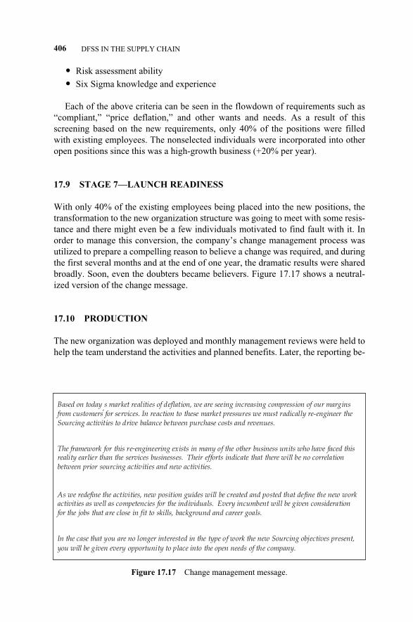
� Risk assessment ability
� Six Sigma knowledge and experience
Each of the above criteria can be seen in the flowdown of requirements such as“compliant,” “price deflation,” and other wants and needs. As a result of thisscreening based on the new requirements, only 40% of the positions were filledwith existing employees. The nonselected individuals were incorporated into otheropen positions since this was a high-growth business (+20% per year).
17.9 STAGE 7—LAUNCH READINESS
With only 40% of the existing employees being placed into the new positions, thetransformation to the new organization structure was going to meet with some resis-tance and there might even be a few individuals motivated to find fault with it. Inorder to manage this conversion, the company’s change management process wasutilized to prepare a compelling reason to believe a change was required, and duringthe first several months and at the end of one year, the dramatic results were sharedbroadly. Soon, even the doubters became believers. Figure 17.17 shows a neutral-ized version of the change message.
17.10 PRODUCTION
The new organization was deployed and monthly management reviews were held tohelp the team understand the activities and planned benefits. Later, the reporting be-
406 DFSS IN THE SUPPLY CHAIN
Figure 17.17 Change management message.
Based on today’s market realities of deflation, we are seeing increasing compression of our margins
from customers for services. In reaction to these market pressures we must radically re-engineer the Sourcing activities to drive balance between purchase costs and revenues.
The framework for this re-engineering exists in many of the other business units who have faced this reality earlier than the services businesses. Their efforts indicate that there will be no correlation between prior sourcing activities and new activities.
As we redefine the activities, new position guides will be created and posted that define the new work activities as well as competencies for the individuals. Every incumbent will be given consideration for the jobs that are close in fit to skills, background and career goals.
In the case that you are no longer interested in the type of work the new Sourcing objectives present,
you will be given every opportunity to place into the open needs of the company.
c17.qxd 4/22/2005 9:19 AM Page 406

came strictly report based, without any formal meetings. During the first year, thegroup costs were increased by 14%, even though the head count was reduced by19%, and the benefits exceeded $32,000,000 ($12,000,000 on the expense itemsand $20,000,000 on the rebilling), a 1000% increase in benefits. Another way oflooking at this is that savings per head went from $80,000 to over $1,000,000.
This increased performance also translated into improved customer loyalty, as per-formance from their perspective improved dramatically, and the company was betterable to maintain profit margins while being price sensitive to the paying customer.
17.11 SUMMARY
Following the DFSS road map presented in Chapter 5 helps accelerate a newprocess introduction and aligns the benefits for customers and stakeholders. Thetools and tollgates allow for risk management, creativity, and a logical documentedflow that is superior to the “launch and learn” mode that many new organizations,processes, or services are deployed with. Not all projects will use all of the DFSStools and methodology, and some will use some to a greater extent than others. Inthis case, the design scorecard was shown at only the highest level. In some serviceprocesses, it is required to show the process and infrastructure levels as well as thetop level. The transfer functions in this example were simple dollar savings perhead and dollar cost per head.
17.11 SUMMARY 407
c17.qxd 4/22/2005 9:19 AM Page 407

c17.qxd 4/22/2005 9:19 AM Page 408

Abbatiello, N. (1995), Development of Design for Service Strategy, MS Thesis, University ofRhode Island.
Akao, Y. (1972), “New Product Deployment and Quality Assurance—Quality DeploymentSystem” (in Japanese), Standardization and Quality Control, 25, 14, 7–14.
Akao, Y. (1997), “QFD: Past, Present, and Future,” www.qfdi.org/qfd_history.pdf, Proceed-ings of the the 3rd Annual International QFD Conference at Linkoping, October 1997.
Alexander, C. (1964), Notes on the Synthesis of Form, Harvard University Press, Cambridge,MA.
Al-Aomar, R. (2002), “A Methodology for Determining System and Process-level Manufac-turing Performance Metrics,” SAE 2002, Transactions Journal of Materials & Manufac-turing, V111-5, pp. 1043–1050.
Al-Aomar, Raid (2000), “Model-Mix Analyses with DES,” in Proceedings of the 2000 Win-ter Simulation Conference, pp. 1385–1392, Orlando, FL.
Almquist, W. (2001), “Boost Your Marketing ROI with Experimental Design,” HarvardBusiness Review, October.
Altshuler, G. S. (1988), Creativity as Exact Science, Gordon & Breach, New York.
Altshuler, G. S. (1990), “On the Theory of Solving Inventive Problems,” Design Methodsand Theories, 24, 2, 1216–1222.
Anderson, D. M. (1990), Design for Manufacturability, CIM Press, Lafayette, CA.
Arciszewsky, T. (1988), “ARIZ 77: An Innovative Design Method,” Design Methods andTheories, 22, 2, 796–820.
Arimoto, S., Ohashi, T., Ikeda, M., and Miyakawa, S. (1993), “Development of MachiningProductivity Evaluation Method (MEM),” Annals of CIRP, 42, 1, 119–1222.
Ashby, W. R. (1973), “Some Peculiarities of Complex Systems,” Cybernetic Medicine, 9,1–7.
Automotive Industry Action Group (AIAG) (2001), Potential Failure Mode and EffectsAnalysis (FMEA) Reference Manual, 3rd ed., AIAG, Southfield, MI.
Beitz, W. (1990), “Design for Ease of Recycling (Guidelines VDI 2243),” in ICED Proceed-ings 90, Dubrovnik, Heurista, Zurich.
Service Design for Six Sigma. By Basem El-Haik and David M. Roy 409© 2005 by John Wiley & Sons.
REFERENCES
bref.qxd 4/22/2005 9:20 AM Page 409

Boothroyd, G. and Dewhurst, P. (1983), Product Design for Assembly Handbook,Boothroyd-Dewhurst Inc., Wakefield, RI.
Boothroyd, G., Dewhurst, P., and Knight, W. (1994), Product Design of Manufacture andAssembly, Marcel Dekker, New York.
Bothe, D. R. (1997), Measuring Process Capabilities, McGraw-Hill, New York.
Box, G. E. P. and Draper, N. R. (1987), Empirical Building and Response Surfaces, Wiley,New York.
Box, G. E. P., Hunter, W. G., and Hunter, J. S. (1978), Statistics for Experimenters, Wiley,New York.
Brejcha, M. F. (1982), Automatic Transmission, 2nd ed., Prentice-Hall, Englewood Cliffs,NJ.
Bulent, D. M., Kulak, O. and Tufekci, S. (2002), “An Implementation Methodology forTransition from Traditional Manufacturing to Cellular Manufacturing Using AxiomaticDesign,” in Proceedings of the International Conference on Axiomatic Design, Cam-bridge, MA.
Burchill, G. and Brodie, C. H. (1997), Voices Into Choices: Acting on the Voice of the Cus-tomer, Joiner Associates, Inc., Madison WI.
Bussey, L. E. (1998), The Economic Analysis of Industrial Projects, Prentice-Hall, UpperSaddle River, NJ.
Carnap, R. (1977), Two Essays on Entropy, University of California Press, Berkeley.
Cha, J. Z. and Mayne, R. W. (1987), “Optimization with Discrete Variables via RecursiveQuadratic Programming,” in Advances in Design Automation—1987, American Societyof Mechanical Engineers, September, 1987.
Chase, K. W. and Greenwood, W. H. (1988), “Design Issues In Mechanical ToleranceAnalysis,” Manufacturing Review, 1, 1, 50–59.
Chen, E. (2002), “Potential Failure Mode and Effect Analysis: Enhancing Design and Manu-facturing Reliability,” A George Washington Center for Professional DevelopmentCourse.
Chen, G. and Kapur, K. C. (1989), “Quality Evaluation System Using Loss Function,” inProceedings of International Industrial Engineering Conference, Toronto, Canada, 1989.
Clausing, D. P. and Ragsdell, K. M. (1984), “The Efficient Design and Development ofMedium and Light Machinery Employing State-of-The-Art Technology,” in Internation-al Symposium on Design and Synthesis, Tokyo, July 11–13.
Clausing, D. P. (1994), Total Quality Development: A Step by Step Guide to World-ClassConcurrent Engineering, ASME Press, New York.
Cohen, L. (1988), “Quality Function Deployment and Application Perspective from DigitalEquipment Corporation,” National Productivity Review, 7, 3, 197–208.
Cohen, L. (1995), Quality Function Deployment: How to Make QFD Work for You, Addi-son-Wesley, Reading, MA.
Cochran, W. and Cox, G. (1957), Experimental Design, Wiley, New York.
Crew, K. (1998), “Design for Manufacturability—Assembly Guidelines,” DRM Associates,http://www/npd-solutions.com/dfmguidelines.html.
Crosby, P. (1979), Quality is Free, McGraw-Hill, New York.
Dadd, P. and Woodford, D., http://www.gamedev.net/reference/articles/article1832.asp.
Deming, W. E. (1986), Out of the Crisis, MIT Center for Advanced Engineering Studies,Cambridge, MA.
410 REFERENCES
bref.qxd 4/22/2005 9:20 AM Page 410
Dewhurst, P. (1989), “Cutting Assembly Costs with Molded Parts,” Machine Design, July.
Dewhurst, P. and Blum, C. (1989), Supporting Analyses for the Economic Assessment ofDie Casting in Product Design, Annals of CIRP, 28, 1, 161.
Dixon, J. R. (1966), Design Engineering: Inventiveness, Analysis, and Decision Making, Mc-Graw-Hill, New York.
Domb, E. and Dettner, W. (1999), “Breakthrough Innovation in Conflict Resolution: Marry-ing Triz and the Thinking Process,” www.triz-journal.com/archives/1999.
Domb, E. (1997), “Finding the Zones of Conflict: Tutorial,” www.triz-journal.com/archives/1997.
Dorf, R. C. and Bishop, R. H. (2000), Modern Control Systems, 9th ed., Prentice Hall, UpperSaddle River, NJ.
Dovoino, I. (1993), “Forecasting Additional Functions in Technical Systems,” in Proceedingof ICED—93, vol. 1, pp. 247–277, The Hague.
Drury, C. G. (1992), “Inspection Performance,” in Handbook of Industrial Engineers, 2nded., pp. 2282–2314, edited by G. Salvendy, Wiley, New York.
Drury, C. G. and Kleiner, B. M. (1984), “A Comparison of Blink Aided and Manual Inspec-tion Using Laboratory and Plant Subjects,” in Proceedings of International Conferenceon Occupational Ergonomics, Rexdale, Ontario, Human Factors Association of Canada,pp. 670–676.
Drury, C. G. and Kleiner, B. M. (1993), “Design and Evaluation of an Inspection TrainingProgram,” Applied Ergonomics, 24, 2, 75–82.
El-Haik, B. (1996), Vulnerability Reduction Techniques in Engineering Design, Ph.D. Dis-sertation, Wayne State University, 1996.
El-Haik, B. (2005), Axiomatic Quality: Integrating Axiomatic Design with Six Sigma Relia-bility and Quality Engineering, Wiley, Hoboken, NJ.
El-Haik, B. and Yang, K. (1999), “The Components of Complexity in Engineering Design,”IIE Transactions, 31, 10, 925–934.
El-Haik, B. and Yang, K. (2000a), “An Integer Programming Formulation for the ConceptSelection Problem with an Axiomatic Perspective (Part I): Crisp Formulation,” in Pro-ceedings of the 1st International Conference on Axiomatic Design, MIT, Cambridge,MA, pp. 56–61.
El-Haik, B. and Yang, K. (2000b), “An Integer Programming Formulation for the ConceptSelection Problem with an Axiomatic Perspective: Fuzzy Formulation,” Proceedings ofthe 1st international Conference on Axiomatic Design, MIT, Cambridge, MA, pp. 62–69.
Feigenbaum, A. (1983), Total Quality Control, 3rd ed., McGraw-Hill, New York.
Fisher, R. (1925), The Design of Experiments, Oliver & Boyd, London and Endinburgh.
Foo, G., Clancy, J. P., Kinney, L. E., and Lindemudler, C. R., “Design for Material Logis-tics,” AT&T Technical Journal, 69, 3, 61–67.
Fowlkes, W. Y. and Creveling, C. M. (1995), Engineering Methods for Robust Product De-sign, Addison-Wesley, Reading, MA.
Fredriksson, B. (1994), Holistic Systems Engineering in Product Development, Saab-ScaniaGriffin, Linkoping, Sweden.
Galbraith, J. R. (1973), Designing Complex Organizations, Addison-Wesley, Reading, MA.
Gardner, S., and Sheldon, D. F. (1995), “Maintainability as an Issue for Design,” Journal ofEngineering Design, 6, 2, 75–89.
REFERENCES 411
bref.qxd 4/22/2005 9:20 AM Page 411

Gershenson, J. and Ishii, K. (1991), “Life Cycle Serviceability Design,” in Proceedings ofASME Conference on Design Theory and Methodology, 1991.
Grossley, E. (1980), “Make Science a Partner,” Machine Design, April 24.
Handerson, R. and Clark, K. B. (1990), “Architectural Innovation: The Reconfiguration ofExisting Product Technologies and the Failure of Established Firms,” Administrative Sci-ence Quarterly, 35, 1, 9–30.
Harry, M. J. (1994), The Vision of 6-Sigma: A Roadmap for Breakthrough, Sigma PublishingCompany, Phoenix, AZ.
Harry, M. J. (1998), “Six Sigma: A Breakthrough Strategy for Profitability,” QualityProgress, May, 60–64.
Harry, M. and Schroeder, R. (2000). Six Sigma: The Breakthrough Management StrategyRevolutionizing the World’s Top Corporations. Doubleday, New York.
Hauser, J. R. and Clausing, D. (1988), “The House of Quality,” Harvard Business Review,66, 3, 63–73.
Hines, W. M. and Mongomery, D. C. (1990), Probability and Statistics in Engineering andManagement, 3rd ed., Wiley, New York.
Hintersteiner, J. D. (1999a), “A Fractal Representation for Systems,” in International CIRPDesign Seminar, Enschede, the Netherlands, March 24–26.
Hintersteiner, J. D. and Nain, A. S. (1999b), “Integrating Software into Systems: An Ax-iomatic design Approach,” in 3rd International Conference on Engineering Design andAutomation, Vancouver, B.C., Canada, August 1–4.
Holland, P. and Carvens, A. (1973), “Fractional Factorial Experimental Designs in Market-ing Research,” Journal of Marketing Research, 270–276.
Hornbeck, R. W. (1975), Numerical Methods, pp. 16–23, Quantum Publishers, New York.
Hubka, V. (1980), Principles of Engineering Design, Butterworth Scientific, London.
Hubka, V. and Eder, W. (1984), Theory of Technical Systems, Springer-Verlag, New York.
Kacker, R. N. (1985), “Off-line Quality Control, Parameter Design, and the TaguchiMethod,” Journal of Quality Technology, 17, 176–188.
Huang, G. Q. (Ed.) (1996), Design for X: Concurrent Engineering Imperatives, Chapman &Hall, London.
Hutchins, S. (2004), http://216.239.57.104/search?q=cache:WTPP0iD4WTAJ:cipm.ncsu.edu/symposium/docs/Hutchins_text.doc+product+multi-generation+plan&hl=en.
Ishikawa, K. (1968), Guide to Quality Control,
Johnson, R. A., and Wichern, D. W. (1982), Applied Multivariate Statistical Analysis, Pren-tice-Hall, Englwood Cliffs, NJ.
Juran, J. (1951), Quality Control Handbook, McGraw-Hill, New York.
Kacker, R. N. (1986), “Taguchi’s Quality Philosophy: Analysis and Comment,” QualityProgress, 19, 12, 21–29.
Kapur, K. C. (1988), “An Approach for the Development of Specifications for Quality Im-provement,” Quality Engineering, 1, 1, 63–77.
Kapur, K. C. (1991), “Quality Engineering and Tolerance Design,” Concurrent Engineering:Automation, Tools and Techniques, 287–306.
Kapur, K. C. and Lamberson, L. R. (1977), Reliability In Engineering Design, Wiley, NewYork.
Kim, S., J., Suh, N. P., and Kim, S. G. (1991), “Design of Software System Based on Ax-iomatic Design,” Annals of the CIRP, 40, 1, 165–70.
412 REFERENCES
bref.qxd 4/22/2005 9:20 AM Page 412

Knight, W. A. (1991), Design for Manufacture Analysis: Early Estimates of Tool Costs forSintered Parts,” Annals of CIRP, 40, 1, 131.
Kota, S. (1994), “Conceptual Design of Mechanisms Using Kinematics Building Blocks—AComputational Approach,” Final report, NSF Design Engineering Program, Grant #DDM 9103008, October, 1994.
Ku, H. H. (1966), “Notes on the Use of Propagation of Error Formulas,” Journal of Researchof The National Bureau of Standards: C. Engineering and Instrumentation, 70, 4,263–273.
Kusiak, A. and Szczerbicki, E. (1993), “Transformation from Conceptual to EmbodimentDesign,” IIE Transactions, 25, 4, 1993.
Lee, T. S. (1999), The System Architecture Concept in Axiomatic Design Theory: HypothesesGeneration and Case-Study Validation, M.S. Thesis, Department of Mechanical Engi-neering, MIT, Cambridge, MA.
Lerner, (1991), “Genrich Altshuller: Father of Triz,” Ogonek, (Russian magazine),www.aitriz.org/downloads/ga40p.pdf.
Magrab, E. B. (1997), Integrated Product and Process Design and Development, CRC Press.
Magner, N., Welker, R. and Campbell, T. (1995), “The Interactive Effect of Budgetary Par-ticipation and Budget Favorability on Attitudes Toward Budgetary Decision Makers: AResearch Note,” Accounting, Organization and Society, 20, 7/8, 611–618.
Mann, D. and Domb, E. (1999), “40 Inventive (Business ) Principles with Examples,”www.triz-journal.com/archives/1999.
Maskell, B. H. (1991), Performance Measurement for World Class Manufacturing, Produc-tivity Press.
Matousek, R. (1957), Engineering Design: A Systematic Approach, Lackie & Son, London.
McClave, J., Benson, P. G., and Sincich, T. (1998), Statistics for Business and Economics,7th ed., Prentice-Hall, Upper Saddle River, NJ.
McCord, K. R. and Eppinger, S. D. (1993), “Managing the Integration Problem in Concur-rent Engineering,” MIT Sloan School of Management working paper 359-93-MSA.
Miles, B. L. (1989), “Design for Assembly: A Key Element Within Design for Manufac-ture,” Proceedings of IMechE, Part D, Journal of Automobile Engineering, 203, 29–38.
Mizuno, S. and Akao, Y. (1978), Quality Function Deployment: A Company Wide Approach(in Japanese), JUSE Press.
Mizuno, S. and Akao, Y. (1994), QFD: The Customer-Driven Approach to Quality Planningand Deployment (trans. by G. H. Mazur), Asian Productivity Organization.
Montgomery, D. (1991), Design and Analysis of Experiments, 3rd ed., Wiley, New York.
Montgomery, D. (1997), Design and Analysis of Experiments, 4th ed., Wiley, New York.
Mostow, J. (1985), “Toward Better Models of the Design Process,” AI Magazine, 44–57.
Mughal, H., and Osborne, R. (1995), “Design for Profit,” World Class Design to Manufac-ture, 2, 5, 160–26.
Myres, J. D. (1984), Solar Applications In Industry and Commerce, Prentice-Hall, Engle-wood Cliffs, NJ.
Nair, V. N. (1992), “Taguchi’s Parameter Design: A Panel Discussion,” Technometrics, 34,127–161.
Navichandra, D. (1991), Design for Environmentality,” in Proceedings of ASME Conferenceon Design Theory and Methodology, New York.
Neibel, B. W. and Baldwin, E. N. (1957), Designing for Production, Irwin, Homewood, IL.
REFERENCES 413
bref.qxd 4/22/2005 9:20 AM Page 413

Nordlund, M. (1996), An Information Framework for Engineering Design Based on Ax-iomatic Design, Doctoral Thesis, The Royal Institute of Technology (KTH), Departmentof Manufacturing Systems, Stockholm, Sweden.
Nordlund, M., Tate, D., and Suh, N. P. (1996), “Growth of Axiomatic Design through Indus-trial Practice,” in 3rd CIRP Workshop on Design and Implementation of Intelligent Man-ufacturing Systems, Tokyo, Japan, June 19–21, pp. 77–84.
O’Grady, P. and Oh, J. (1991), “A Review of Approaches to Design for Assembly,” Concur-rent Engineering, 1, 5–11.
Owens, D. A. (2004), http://216.239.57.104/search?q=cache:mG3a-1wdz4sJ:mba.vander-bilt.edu/david.owens/Papers/2000%2520Owens%2520Status%2520in%2520De-sign%2520Teams%2520DMJ.pdf+motivating+design+teams&hl=en.
Papalambros, P. Y. and Wilde, D. J. (1988), Principles of Optimal Design, Cambridge Uni-versity Press, Cambridge, UK.
Park, R. J. (1992), Value Engineering, R.J. Park & Associates, Inc., Birmingham, MI.
Pech, H. (1973), Designing for Manufacture, Pitman & Sons, London.
Penny, R. K. (1970), “Principles of Engineering Design,” Postgraduate, 46, 344–349.
Phadke, M. S. (1989), Quality Engineering Using Robust Design, Prentice-Hall, EnglewoodCliffs, NJ.
Phal, G. and Beitz, W. (1988), Engineering Design: A Systematic Approach, Springier-Ver-lag, New York.
Pimmler, T. U. and Eppinger, S. D. (1994), “Integration Analysis of Product Decomposi-tion,” Design Theory and Methodology, 68, 343–351.
Plackett, R. L. and Burman, J. P. (1946), “The Design of Optimum Multifactorial Experi-ments,” Biometrika, 33, 305–325.
Pugh, S. (1991), Total Design: Integrated Methods for Successful Product Engineering, Ad-dison-Wesley, Reading, MA.
Pugh, S. (1996) in Creating Innovative Products Using Total Design, edited by Clausing andAndrade, Addison-Wesley, Reading, MA.
Ramachandran, et. al. (1992), “Initial Design Strategies for Iterative Design,” Research inEngineering Design, 4, 3.
Ross (1988)
Ruchti, B. and Livotov, P. (2001), “TRIZ-based Innovation Principles and a Process forProblem Solving in Business and Management,” in Proceedings of the European TRIZAssociation, November.
Rantanen, K. (1988), “Altshuler’s Methodology in Solving Inventive Problems,” in Proceed-ings of ICED—88, Budapest, 23–25 August.
Reinderle, J. R. (1982), Measures of Functional Coupling in Design, Ph.D. Dissertation,Massachusetts Institute of Technology, June, 1982.
Reklaitis, J. R., Ravindran, A., and Ragsdell, K. M. (1983), Engineering Design Optimiza-tion, Wiley, New York.
Rinderle, J. R. (1982), Measures of Functional Coupling in Design, Ph.D. Dissertation,Massachusetts Institute of Technology.
Rother M. and Shook, J. (2000), Learning to See: Value Stream Mapping to Create Valueand Eliminate Muda, The Lean Enterprise Institute.
Sackett, P. and Holbrook, A. (1988), “DFA as a Primary Process Decreases Design Deficien-cies,” Assembly Automation, 12, 2, 15–16.
414 REFERENCES
bref.qxd 4/22/2005 9:20 AM Page 414

Sackett, P. and Holbrook, A. (1990), “DFA as a Pimary Process Decreases Deficiencies,” inAllen, C. W. (Ed.), Simultaneous Engineering, pp. 152–155, SME, Detroit.
Shannon, C. E. (1948), “The Mathematical Theory of Communication,” Bell System Techni-cal Journal, 27, 379–423, 623–656.
Sheldon, D. F., Perks, R., Jackson, M., Miles, B. L., and Holland, J. (1990), “Designing forWhole-life Costs at the Concept Stage,” in Proceedings of ICED, Heurista, Zurich.
Shewhart, W. A. (1931), Economic Control of Manufactured Product,
Simon, H. A. (1981), The Science of the Artificial, 2nd ed., MIT Press, Cambridge, MA.
Smith, G. and Browne, G. J. (1993), “Conceptual Foundation of Design Problem Solving,”IEEE Transaction on Systems, Man, and Cybernetics, 23, 5, September/October.
Snee, R. D., Hare, L. B., Trout, S. B. (Eds.), (1985), “Experimenting with Large Number ofVariables,” in Experiments in Industry: Design, Analysis, and Interpretation of Results,ASQC Press.
Sohlenius, G., Kjellberg, A., and Holmstedt, P. (1999), “Productivity System Design andCompetence Management,” in Proceedings of World XIth Productivity Congress, Edin-burgh.
Spotts, M. F. (1973), “Allocation of Tolerance to Minimize Cost of Assembly,” Transactionsof the ASME, 762–764.
Srinivasan, R. S., and Wood, K. L. (1992), “A Computational Investigation into the Structureof Form and Size Errors Based on Machining Mechanics,” in Advances in Design Au-tomation, Phoenix, AZ, pp. 161–171.
Steinberg, L., Langrana, N. Mitchell, T., Mostow, J. and Tong, C. (1986), “A Domain Inde-pendent Model of Knowledge-Based Design,” Technical report AI/VLSI Project workingpaper no. 33, Rutgers University.
Steward, D. V. (1981), Systems Analysis and Management: Structure, Strategy, and Design,Petrocelli Books, New York.
Suh, N. P. (1984), “Development of the Science Base for the Manufacturing Field Throughthe Axiomatic Approach,” Robotics & Computer Integrated Manufacturing, 1.
Suh, N. P. (1990), The Principles of Design, Oxford University Press, New York.
Suh, N. (1995), “Design and Operation of Large Systems,” Journal of Manufacturing Sys-tems, 14, 3.
Suh, N. P. (1996), “Impact of Axiomatic Design,” in 3rd CIRP Workshop on Design and theImplementation of Intelligent Manufacturing Systems, Tokyo, Japan, pp. 8–17, June,19–22.
Suh, N. P. (1997), “Design of Systems,” Annals of CIRP, 46, 1, 75–80.
Suh, N. P. (2001), Axiomatic Design: Advances and Applications, Oxford University Press.
Sushkov, V. V. (1994), “Reuse of Physical Knowledge in Creative Design,” ECAI-94 Work-shop Notes, Amsterdam, August.
Suzue, T. and Kohdate, A. (1988), Variety Reduction Programs: A Production Strategy forProduct Diversification, Productivity Press, Cambridge, MA.
Swartz, J. B. (1996), Hunters and the Hunted,
Swenson, A. and Nordlund, M. of Saab (1996), “Axiomatic Design of Water Faucet,” unpub-lished report, Linkoping, Sweden.
Taguchi, G., (1957), Design of Experiments,
Taguchi, G. (1986), Introduction to Quality Engineering, UNIPUB/Kraus International Pub-lications, White Plains, NY.
REFERENCES 415
bref.qxd 4/22/2005 9:20 AM Page 415
Taguchi, G., and Wu, Y. (1989), Taguchi Method Case Studies from the U.S. and Europe,Quality Engineering Series, Vol. 6, ASI.
Taguchi, G., Elsayed, E., and Hsiang, T. (1989), Quality Engineering in Production Systems,McGraw-Hill, New York.
Tate, D., and Nordlund, M. (1998), “A Design Process Roadmap As a General Tool forStructuring and Supporting Design Activities,” SDPS Journal of Integrated Design andProcess Science, 2, 3, 11–19, 1998.
Tate, K. and Domb, E. (1997), “40 Inventive Principles with Examples,” www.triz-journal.com/archives/1997.
Tayyari, F. (1993), “Design for Human Factors,”in Concurrent Engineering, pp. 297–325,edited by H. R. Parsaei and W. G. Sullivan, Chapman & Hall, London.
Thackray, R. (1994), Correlations of Individual Differences in Non-destructive InspectionPerformance, Human Factors in Aviation Maintenance, Phase 4, Vol. 1, Program Report,DOT/FAA/Am-94/xx, National Technical Information Service, Springfield, VA.
Tsourikov, V. M. (1993), “Inventive Machine: Second Generation,” Artificial Intelligence &Society, 7, 62–77.
Tumay, K. http://www.reengineering.com/articles/janfeb96/sptprochr.htm, Business ProcessSimulation: Matching Processes with Modeling Characteristics, ER Spotlight.
Ullman, D. G. (1992), The Mechanical Design Process, McGraw-Hill, New York.
Ulrich, K. T. and Tung, K. (1994), “Fundamentals of Product Modularity,” in ASME WinterAnnual Meeting, DE Vol. 39, Atlanta, pp. 73–80.
Ulrich, K. T. and Eppinger, S. D. (1995), Product Design and Development, McGraw-Hill,New York.
Ulrich, K. T. and Seering, W. P. (1987), “Conceptual Design: Synthesis of Systems Compo-nents,” in Intelligent and Integrated Manufacturing Analysis and Synthesis, AmericanSociety of Mechanical Engineers, New York, pp. 57–66.
Ulrich, K. T. and Seering, W. P. (1988), “Function Sharing in Mechanical Design,” in 7thNational Conference on Artificial Intelligence, AAAI-88, Minneapolis, MN, August21–26.
Ulrich, K. T. and Seering, W. P. (1989), “Synthesis of Schematic Description in MechanicalDesign,” Research in Engineering Design, 1, 1.
Vasseur, H., Kurfess, T., and Cagan, J. (1993), “Optimal Tolerance Allocation For ImprovedProductivity,” in Proceedings of the 1993 NSF Design and Manufacturing Systems Con-ference, Charlotte, NC, pp. 715–719.
Verno, A., and Salminen (1993), “Systematic Shortening of The Product Development Cy-cle,” presented at the International Conference on Engineering Design, The Hague,Netherlands.
Wagner, T. C. and Papalambros, P. (1993), “A General Framework for DecompositionAnalysis in Optimal Design,” presented at the 23rd ASME Design Automation Confer-ence, Albuquerque, New Mexico, September.
Wang, J., and Ruxton, T. (1993), “Design for Safety of Make-to-Order Products,” in Nation-al Design Engineering Conference of ASME, 93-DE-1.
Warfield, J. and Hill, J. D. (1972), A United Systems Engineering Concept, Battle Mono-graph, No. 1, June.
Weaver, W. (1948), “Science and Complexity,” American Scientist, 36, 536–544.
416 REFERENCES
bref.qxd 4/22/2005 9:20 AM Page 416

Wheeler, D. (1995). Advanced Topics in Statistical Process Control: The Power of ShewhartCharts, SPC Press.
Wheeler, D., and Chambers, D. S. (1992), Understanding Statistical Process Control, 2nded., SPC Press.
Wei, C., Rosen, D., Allen, J. K., and Mistree, F. (1994), “Modularity and the Independenceof Functional Requirements in Designing Complex Systems,” DE-Vol. 74, ConcurrentProduct Design, ASME.
Wirth, N. (1971), “Program Development by Stepwise Refinement,” Communications of theACM, 14, 221–227.
Wood, G. W., Srinivasan, R.S., Tumer, I. Y., and Cavin, R. (1993), “Fractal-Based Toleranc-ing: Theory, Dynamic Process Modeling, Test Bed Development, and Experiment,” inProceedings of the 1993 NSF Design and Manufacturing Systems Conference, Charlotte,NC, pp. 731–740.
Woodford, D. (2004), http://www.isixsigma.com/library/content/c020819a.asp.
Yang, K. and El-Haik, B. (2003), Design for Six Sigma: A Roadmap for Produvct Excellem-ce, McGraw-Hill, New York.
Yang, K. and Trewn, J. (1999), “A Treatise on the Mathematical Relationship Between Sys-tem Reliability and Design Complexity,” Proceedings of IERC.
Zaccai, G. (1994), “The New DFM: Design for Marketability,” World-Class Manufacture toDesign, 1, 6, 5–11.
Zenger, D. and Dewhurst, P. (1988), Early Assessment of Tooling Costs in the Design ofSheet Metal Parts, Report 29, Department of Industrial and Manufacturing Engineering,University of Rhode Island.
Zakarian, A. (2002), Manufacturing Systems Course Material, University of Michigan, Dear-born.
Zhang, C. T. (2003), “40 Inventive Principles with Applications in Service Operations Man-agement,” www.triz-journal.com/archives/2003.
Zhang, H. C. and Huq, M. E. (1994), “Tolerancing Techniques: The State-of-the-Art,” Inter-national Journal of Production Research, 30, 9, 2111–2135.
Zwicky, F. (1984), Morphological Analysis and Construction, Wiley Interscience, NewYork.
REFERENCES 417
bref.qxd 4/22/2005 9:20 AM Page 417

bref.qxd 4/22/2005 9:20 AM Page 418

Control plans and statistical processControl, 370
Controlled convergence, 5Cost, 15Cox, Gertrude, 11Creative design, 38“Critical-to” characteristics, 111Critical-to-satisfaction requirements, 33Crosby, Philip, 12CTSs, 33, 35Cultural change, 72Customers, 1
DCCDI, 43Decision variables, 157Deming, W. Edwards, 11, 12Deployment champion, 51DES mechanisms, 348
animation mechanism, 354discrete-event mechanism, 350random sampling mechanism, 352statistical accumulation mechanism, 353time-advancement mechanism, 351
Design, 6Design coupling, 168Design failure modes and effects analysis
(DFMEA), 6Design for assembly (DFA), 224, 230Design for manufacturability and assembly
(DFMA), 233Design for processability (DFM), 237
Accumulation analysis, 321cumulative accumulation, 321factorial effect calculations, 322prediction, 323probability calculations, 322probability plotting, 323
Akao, Yoji, 13Altshuller, Genrich, 12, 189Analysis of variance (ANOVA), 263, 283
steps for a two factors, completelyrandomized experiment, 284
Axiomatic design, 6, 164, 176design software, 170mapping Example, 171
Axiomatic method, 164
Big Ys, 33Black belt, 38, 53Box, George, 11Box–Behnken Designs, 310Business excellence, 14Business operation model, 14Business process management, 22Business process management system
(BPMS), 155
Cause and effect diagram, 11Cochran, William, 11Concept development, 5Confidence interval of small sample
validation, 370
Service Design for Six Sigma. By Basem El-Haik and David M. Roy 419© 2005 by John Wiley & Sons.
INDEX
bindex.qxd 4/22/2005 9:21 AM Page 419
Design for processability (DFP), 230Design for product service (DFPS), 227Design for serviceability (DFS), 236Design for Six Sigma (DFSS), 1, 13, 30, 31,
33, 34, 35, 38, 41, 42Design for test or testability (DFT), 237Design for testability and inspectability, 236Design mapping, 94, 168
steps, 96Design milestone events, 81Design of experiments (DOE), 101, 263,
269analysis of raw data, 277choice of factors, levels, and ranges, 272classical, 269conducting the experiments, 276experimental design selection, 275measurement strategy, 274selection of the response, 271strategy, 273study definition, 270
Design optimization, 7Design quality, 12Design targets, 6Design validation, 365
steps, 365Design/process owner, 52DFSS in the supply chain, 383
concept development, 395process, 383production, 406Stage 1—Idea creation, 383Stage 2—Voice of the customer and the
business, 385Stage 3—Concept design, 389Stage 4—Preliminary design, 399Stage 5—Design optimization, 403Stage 6—Verification, 405tage 7—Launch readiness, 406
DFSS Phase 1: Identify requirements, 83identify phase road map, 84multigeneration planning, 85research customer activities, 86service company growth and innovation
strategy, 85Stage 1: Idea creation, 83Stage 2: Customer and business
requirements study, 83DFSS Phase 2: Characterize design, 86
420 INDEX
concept development, 86design optimization, 89launch readiness, 91preliminary design, 88verification, 90
DFX, 7in transactional processes, 227
Diagnostic plots of residuals, 311Discrete event simulation, 331, 342
state variables, 343system activities, 345system delay, 348system entities, 342system events, 344system logic, 348system resources, 346system state, 343
DMADOV, 43DMADV, 43
analyze, 43define, 43design, 43measure, 43verify, 43
DMAIC, 33, 35DMEDI, 43
Experimental design, 263Factorial experiment, 279Failure mode and effect analysis (FMEA),
241cause-and-Effect Tools, 259fundamentals, 243
actions recommended., 248current controls, 247define scope, service functional
requirements, and design parametersand process steps, 243
detection, 247identify potential failure modes, 243occurrence, 246potential Causes, 246potential failure effects, 243risk priority number (RPN), 248severity, 243
interfaces with Other Tools, 258quality Systems and Control Plans, 259
Fault tree analysis (FTA), 258
bindex.qxd 4/22/2005 9:21 AM Page 420

Feigenbaum, Armand V., 12“Fire fighting,” 35Fishbone diagram, 11Fisher, Ronald, 11, 12, 263Fractional factorial designs, 300
23–1 design, 301design resolution, 303half factional 2k Design, 302quarter Fraction of 2k Design, 304
Function analysis system technique(FAST), 159, 160
Functional mapping, 95, 158Functional requirements (FRs), 33
Green belt, 56
HOQ, 114evaluation, 116HOQ 1—“The Customer’s House”, 117HOQ 2—“Translation House”, 121HOQ 3—“Design House”, 122HOQ 4—“Process House”, 122
House of quality, 4, 111; see also HOQHunter, Stuart, 11Hunter, William, 11Hypothesis testing, 266
ICOV, 34, 41design phase, 42identify phase, 42optimize phase, 43process, 39validate phase, 43
Idea creation, 4IDEF mapping technique, 181IDEF0 technique, 183Incremental design, 38Interaction, 280Interaction plots, 311IPO diagram, 20Ishikawa, Kaoru, 11, 12
Juran, Joseph, 11, 12
Kano analysis, 117Kano model, 118
Larger-the-better loss function, 317Launch readiness, 7
INDEX 421
Manual simulation, 355Mapping equation, 166Master black belt, 38, 52Mathematical transfer function model,
280Matrices, 187Measurement system analysis (MSA), 24Mizuno, Mizuno, 13Monte Carlo simulation, 107Montgomery, Douglas, 11Motorola, 13, 19, 26
Noise factors, 273Null hypothesis, 267
Optimization, 106
Parameter design analysis, 327Pareto chart of effects, 311Pareto principle, 11Path independence, 167Phase-out, 8Poke yoke, 7Power-on self-test (POST), 236Preliminary design, 6Process, 1Process capability, 25, 376Process FMEA (PFMEA), 257Process management, 141Process map, 144Process mapping, 20, 21, 95, 96, 142, 166Process modeling, 20, 141
techniques, 142Process performance, 25
highly capable, 26incapable process, 26marginally capable, 26
Process simplification, 13Production, 8Project champion, 51Prototype building, 367Pugh concept selection, 177Pugh matrix, 40Pugh phased innovation, 6Pugh selection matrix, 6Pugh, Stuart, 5, 40
Quality, 2, 15Quality control processes, 1
bindex.qxd 4/22/2005 9:21 AM Page 421

Quality function deployment (QFD), 4, 6,13, 39, 111, 122
HOQ 1, 123HOQ 2, 126HOQ 3, 127HOQ 4, 134history, 112methodology, 113overview, 113
Quality in service, 8Quality loss function, 315Quality operating system, 4
Random behavior, 107Random numbers, 108Randomness, 107Red X toolbox, 12Regression transfer equations, 102Relationship of process modeling to
discrete event simulation, 156Road map, 77, 94Robustness, 314
accumulation analysis, 321orthogonal arrays, 325Overview, 314parameter design analysis, 327quality loss function, 315signal, noise, and control factors, 319signal-to-noise ratio, 319
Root cause analysis, 11, 12
Scorecard, 38, 97development, 98
Service consumption, 8Service design, 1Service design FMEA (DFMEA), 249Service design for Six Sigma (DFSS), 37,
45Service design for Six Sigma road map,
81Service design For Six Sigma team, 79Service design robustness, 313Service DFSS, 37, 39, 46Service DFSS deployment phases, 46
deployment, 66black belt, 68deployment champion, 67green belt, 68master black belt, 67
422 INDEX
project financial aspects, 68senior leadership, 67training, 67
phases, 46postdeployment, 69
sustainability factors, 70predeployment, 46
communication plan, 56considerations, 48deployment champions, 51deployment structure, 48multigeneration planning, 63operatives, 51proactive DFSS project sources, 63project champion, 51service DFSS project sources, 57service program development
management system, 66training, 65
Service life cycle, 4, 8concept development, 5design optimization, 7idea creation, 4launch readiness, 7phase-out, 8preliminary design, 6production, 8and quality operating system, 8service consumption, 8verification, 7voice of the customer and business, 4
Service processes simulation implications,363
Services, 1, 2Shainin technique, 12Shared vision, 73Shewhart, Walter A., 10, 11, 12Signal-to-noise ratio, 263, 319Simulation, 101Simulation models, 156SIPOC, 20, 142Six Sigma, 13, 19Six Sigma improvement (DMAIC), 28
Phase 1: Define, 29Phase 2: Measure, 29Phase 3: Analyze, 29Phase 4: Improve, 30Phase 5: Control, 30
Smaller-the-better loss function, 318
bindex.qxd 4/22/2005 9:21 AM Page 422

Square and cube plots, 311Statistical analysis and control, 11Statistical process control (SPC), 10, 371
choosing the control chart, 373interpreting the control chart, 375taking action, 376
Strategic sourcing, 380Suh, Nam P., 13Sum of squares, 263Supply chain, 16
asset and inventory management, 381definition, 379demand forecasting, 380distribution and logistics, 381planning and scheduling, 380postservice support, 381process, 379processing, 380strategic courcing, 380
System modeling, 332concept, 332modeling concept, 334types of models, 335
computer, 337graphical, 336mathematical, 336physical, 336
System modeling with discrete eventsimulation, 337
system data, 339system layout, 339system logic, 341system statistics, 341system structure, 338
Taguchi tolerance design method, 316Taguchi, Genechi, 11, 13Team meetings, 74Testing, 368Theory of inventive problem solving
(TRIZ), 6, 12, 36, 189analytical tools, 195build sufficient functions, 203design for transactional DFX, 223design for X, 223detection and measurement, 211
introduce marks, 211introduce modified marks, 211roundabout, 211
INDEX 423
DFX, 223effects, 199evolutionary trends of technological
systems, 212foundations, 191harmful function elimination, 203history, 189history and evolution, 224ideal final result, 201ideality checklist, 202ideality equation, 203inventive principles, 205
another dimension, 207anti-weight, 206asymmetry, 206beforehand cushioning, 206“blessing in disguise” or “turn lemons
into lemonade”, 208cheap, short-lived objects, 208color changes, 209composite structures, 210continuity of useful action, 208copying, 208discarding and recovering, 209dynamics, 207equipotentiality, 206feedback, 208flexible shells and thin films, 209homogeneity, 209inert atmosphere, 210“intermediary”, 208local quality, 206mechanical substitution, 208mechanical vibration, 207merging, 206“nested doll”, 206“the other way round,” 207parameter changes, 209partial or excessive actions, 207periodic action, 207phase transitions, 209pneumatics and hydraulics, 209porous caterials, 209preliminary action, 206preliminary anti-action, 206segmentation, 205self-service, 208skipping, 208spheroidality—curvature, 207
bindex.qxd 4/22/2005 9:21 AM Page 423

Theory of inventive problem solving(TRIZ), inventive principles(continued)
strong oxidants (“boostedinteractions”), 209
taking out, 205thermal expansion, 209universality, 206
inventive principles and contradictiontable, 196
itself method, 202knowledge-based tools, 195patterns/predictions of evolution, 196problem solving flowchart, 200root cause analysis, 211separation principles, 19876 standard solutions, 199system of operators, 200transitions from, 215
Three-level factorial design, 309Time to market, 16TIPS, 6, 12, 189Tollgate (TG) reviews, 82Tollgates, 81Total quality management/control, 12TQM, 19Transaction, 1Transfer function, 93, 100, 102, 104, 264
life cycle, 99
424 INDEX
linear, 104and optimization, 105quadratic, 104
Transfer function additivity, 9823 design, 297
in simulation, 298with center points, 299
2k full factorial designs, 289data analysis, 291layout, 290
Value analysis (VA), 159Value engineering (VE), 159Value stream mapping (VSM), 21, 148
process steps, 150Variability in simulation outputs, 360Variance reduction techniques, 361Verification, 7Voice of the business (VOB), 39Voice of the customer (VOC), 22, 39Voice of the customer and business, 4Voice of the process, 22
Welch, Jack, 20
Yates, Frank, 11
Zigzagging, 169
bindex.qxd 4/22/2005 9:21 AM Page 424