sequential pattern mining -- approaches and algorithms
TRANSCRIPT
Sequential Pattern Mining – Approaches andAlgorithms
CARL H. MOONEY and JOHN F. RODDICK
School of Computer Science, Engineering and Mathematics,
Flinders University,
P.O.Box 2100, Adelaide 5001, South Australia.
Sequences of events, items or tokens occurring in an ordered metric space appear often in data and
the requirement to detect and analyse frequent subsequences is a common problem. Sequential
Pattern Mining arose as a sub-field of data mining to focus on this field. This paper surveys theapproaches and algorithms proposed to date.
Categories and Subject Descriptors: H.2.8 [Database Applications]: Data mining
Additional Key Words and Phrases: sequential pattern mining
1. INTRODUCTION
1.1 Background and Previous Research
Sequences are common, occurring in any metric space that facilitates either totalor partial ordering. Events in time, codons or nucleotides in an amino acid, websitetraversal, computer networks and characters in a text string are examples of wherethe existence of sequences may be significant and where the detection of frequent(totally or partially ordered) subsequences might be useful. Sequential patternmining has arisen as a technology to discover such subsequences.
The sequential pattern mining problem was first addressed by Agrawal andSrikant [1995] and was defined as follows:
“Given a database of sequences, where each sequence consists of a list oftransactions ordered by transaction time and each transaction is a setof items, sequential pattern mining is to discover all sequential patternswith a user-specified minimum support, where the support of a patternis the number of data-sequences that contain the pattern.”
Since then there has been a growing number of researchers in the field, evidenced bythe volume of papers produced, and the problem definition has been reformulatedin a number of ways. For example, Garofalakis et al. [1999] described it as
“Given a set of data sequences, the problem is to discover sub-sequencesthat are frequent, i.e. the percentage of data sequences containing themexceeds a user-specified minimum support”,
while Masseglia et al. [2000] describe it as
“. . . the discovery of temporal relations between facts embedded in a database”,
and Zaki [2001b] as a process toACM Journal Name, Vol. V, No. N, M 20YY, Pages 1–46.

2 · C.H. Mooney, J.F. Roddick
“. . . discover a set of attributes, shared across time among a large numberof objects in a given database.”
Since there are varied forms of dataset (transactional, streams, time series, andso on) algorithmic development in this area has largely focused on the developmentand improvement for specific domain data. In the majority of cases the data hasbeen stored as transactional datasets and similar techniques such as those usedby association rule miners [Ceglar and Roddick 2006] have been employed in thediscovery process. However, the data used for sequence mining is not limited todata stored in overtly temporal or longitudinally maintained datasets – examplesinclude genome searching, web logs, alarm data in telecommunications networksand population health data. In such domains data can be viewed as a series ofordered or semi-ordered events, or episodes, occurring at specific times or in aspecific order and therefore the problem becomes a search for collections of eventsthat occur, perhaps according to some pattern, frequently together. Mannila et al.[1997] described the problem as follows:
“An episode is a collection of events that occur relatively close to eachother in a given partial order.”
Such episodes can be represented as acyclic digraphs and are thus more generalthan linearly ordered sequences.
This form of discovery requires a different type of algorithm and will be describedseparately from those algorithms that are based on the more general transactionoriented datasets. Regardless of the format of the dataset, sequence mining algo-rithms can be categorized into one of three broad classes that perform the task[Pei et al. 2002] – Apriori-based, either horizontal or vertical database format, andprojection-based pattern growth algorithms. Improvements in algorithms and algo-rithmic development in general, have followed similar developments in the relatedfield of association rule mining and have been motivated by the need to processmore data at an increased speed with lower overheads.
As mentioned earlier, much research in sequential pattern mining has been fo-cused on the development of algorithms for specific domains. Such domains includeareas such as biotechnology [Wang et al. 2004; Hsu et al. 2007], telecommunica-tions [Ouh et al. 2001; Wu et al. 2001], spatial/geographic domains [Han et al.1997], retailing/market-basket [Srivastava et al. 2000; Pei et al. 2000; El-Sayedet al. 2004] and identification of plan failures [Zaki et al. 1998]. This has led toalgorithmic developments that directly target real problems and explains, in part,the diversity of approaches, particularly in constraint development, taken in algo-rithmic development.
Over the past few years, various taxonomies and surveys have been published insequential pattern mining that also provide useful resources [Zhao and Bhowmick2003; Han et al. 2007; Pei et al. 2007; Mabroukeh and Ezeife 2010]. In addition,a benchmarking exercise of sequential pattern mining is also available [Kum et al.2007a]. This survey extends or complements these papers by providing a more com-plete review including further analysis of the research in areas such as constraints,counting, incremental algorithms, closed frequent patterns and other areas.ACM Journal Name, Vol. V, No. N, M 20YY.

Sequential Pattern Mining · 3
1.2 Problem Statement and Notation
Notwithstanding the definitions above, the sequential pattern mining problem mightalso be stated through a series of examples. For example,
—Given a set of alerts and status conditions issued by a system before a failure, canwe find sequences or subsequences that might help us to predict failure before itoccurs?
—Can we characterise suspicious behaviour in a user by analysing the sequence ofcommands entered by that user?
—Can we automatically determine the elements of what might be considered “bestpractice” through analysing the sequences of actions of experts that lead to goodoutcomes?
—Is it possible to derive more value from market basket analysis by includingtemporal and sequence information?
—Can we characterise users who purchase goods or services from our website interms of the sequence and/or pace at which they browse webpages? Withinthis group, can we characterise users who purchase one item against those whopurchase multiple items?
Put simply, since many significant events occur over time, space or some otherordered metric, can we learn more from the data by taking account of any orderedsequences that appear in the data?
More formally, the problem of mining sequential patterns, and its associatednotation, can be given as follows:
Let I = {i1, i2, . . . , im} be a set of literals, termed items, which comprise thealphabet. An event is a non-empty unordered collection of items. It is assumedwithout loss of generality that items of an event are sorted in lexicographic order. Asequence is an ordered list of events. An event is denoted as (i1, i2, . . . , ik), where ijis an item. A sequence α is denoted as 〈α1 → α2 → · · · → αq〉, where αi is an event.A sequence with k-items, where k =
∑j |αj |, is termed a k-sequence. For example,
〈B → AC〉 is a 3-sequence. A sequence 〈α1 → α2 . . . → αn〉 is a subsequence ofanother sequence 〈β1 → β2 . . . → βm〉 if there exist integers i1 < i2 < . . . < insuch that α1 ⊆ βi1 , α2 ⊆ βi2 , . . . , αn ⊆ βin . For example the sequence 〈B → AC〉is a subsequence of 〈AB → E → ACD〉, since B ⊆ AB and AC ⊆ ACD, and theorder of events is preserved. However, the sequence AB → E is not a subsequenceof ABE and vice versa.
We are given a database D of input-sequences where each input-sequence in thedatabase has the following fields: sequence-id, event-time and the items presentin the event. It is assumed that no sequence has more that one event with thesame time-stamp, so that the time-stamp may be used as the event identifier. Ingeneral, the support or frequency of a sequence, denoted σ(α,D), is defined as thenumber (or proportion) of input-sequences in the database D that contain α. Thisgeneral definition has been modified as algorithmic development has progressedand different methods for calculating support have been introduced, a summaryof which is included in Section 5.2. Given a user-specified threshold, termed theminimum support (denoted min supp), a sequence is said to be frequent if it occursmore than min supp times and the set of frequent k-sequences is denoted as Fk.
ACM Journal Name, Vol. V, No. N, M 20YY.
4 · C.H. Mooney, J.F. Roddick
Further a frequent sequence is deemed to be maximal if it is not a subsequence ofany other frequent sequence. The task then becomes to find all maximal frequentsequences from D satisfying a user supplied support min supp.
This constitutes the problem definition for all sequence mining algorithms whosedata are located in a transaction database or are transaction datasets. Furtherterminology, that is specific to an algorithm or set of algorithms, will be elaboratedas required.
1.3 Survey Structure
This paper begins with a discussion of the algorithms that have been used in se-quence mining. These will be categorised firstly on the type of dataset that eachalgorithm accommodates and secondly, within that designation, on the broad classto which they belong. Since time is often an important aspect of a sequence, tem-poral sequences are then discussed in Section 4. This is followed in Section 5 bya discussion on the nature of constraints used in sequence mining and of countingtechniques that are used as measures against user designated supports. This is thenfollowed by discussions of extensions dealing with closed, approximate and parallelalgorithms and the area of incremental algorithms in Sections 6 and 7. Section 8discusses some areas of related research and the survey concludes with a discussionof other methods that have been employed and areas of related research.
2. APRIORI-BASED ALGORITHMS
The Apriori family of algorithms has typically been used to discover intra-transactionassociations and then to generate rules about the discovered associations. Howeverthe sequence mining task is defined as discovering inter-transaction associations –sequential patterns – across the same, or similar data. It is therefore not surprisingthat the first algorithms to deal with this change in focus were based on the Apriorialgorithm [Agrawal and Srikant 1994] using transactional databases as their datasource.
2.1 Horizontal Database Format Algorithms
Horizontal formatting means that the original data, Table I(a), is sorted firstby Customer Id and then by Transaction Time, which results in a transformedcustomer-sequence database, Table I(b), where the timestamps from Table I(a) areused to determine the order of events, which is used as the basis for mining. Themining is then carried out using a breadth-first approach.
The first algorithms introduced – AprioriAll, AprioriSome, and DynamicSome –used a 5-stage process [Agrawal and Srikant 1995]:
(1) Sort Phase. This phase transforms the dataset from the original transactiondatabase (Table I(a)) to a customer sequence database (Table I(b)) by sortingthe dataset by customer id and then by transaction time.
(2) Litemset (large itemset) Phase. This phase finds the set of all litemsets L (thosethat meet minimum support). That is, the set of all large 1-sequences sincethis is simply {〈l〉 | l ∈ L}. At this stage optimisations for future comparisonscan be carried out by mapping the litemsets to a set of contiguous integers.
ACM Journal Name, Vol. V, No. N, M 20YY.

Sequential Pattern Mining · 5
For example, if the minimum support was given as 25%, using the data fromTable I(b), a possible mapping for the large itemsets is depicted in Table II.
(3) Transformation Phase. Since there is a need to repeatedly determine whichof a given set of long sequences are contained in a customer sequence, eachcustomer sequence is transformed by replacing each transaction with the set oflitemsets contained in that transaction. Transactions that do not contain anylitemsets are not retained and a customer sequence that does not contain anylitemsets is dropped. The customer sequences that are dropped do howeverstill contribute to the total customer count. This is depicted in Table III.
(4) Sequence Phase. This phase mines the set of litemsets to discover the frequentsubsequences. Three algorithms are presented for this discovery, all of whichmake multiple passes over the data. Each pass begins with a seed set forproducing potential large sequences (candidates) with the support for thesecandidates calculated during the pass. Those that do not meet the minimumsupport threshold are pruned and those that remain become the seed set forthe next pass. The process begins with the large 1-sequences and terminateswhen either no candidates are generated or no candidates meet the minimumsupport criteria.
(5) Maximal Phase. This is designed to find all maximal sequences among the setof large sequences. Although this phase is applicable to all of the algorithms,AprioriSome and DynamicSome combine this with the sequence phase to savetime by not counting non-maximal sequences. The process is similar in natureto the process of finding all subsets of a given itemset and as such the algorithmfor performing this task is also similar. An example can be found in Agrawaland Srikant [1994].
The difference in the three algorithms results from the methods of counting thesequences produced. Although all are based on the Apriori algorithm [Agrawal andSrikant 1994] the AprioriAll algorithm counts all of the sequences whereas Apri-oriSome and DynamicSome are designed to only produce maximal sequences andtherefore can take advantage of this by first counting longer sequences and onlycounting shorter ones that are not contained in longer ones. This is done by util-
Table I. Horizontal Formatting Data Layout – adapted from Agrawal and Srikant [1995].
(a) Customer Transaction Database
Customer Id Transaction Time Items Bought
1 June 25 ’03 301 June 30 ’03 90
2 June 10 ’03 10, 20
2 June 15 ’03 302 June 20 ’03 40, 60, 70
3 June 25 ’03 30, 50, 70
4 June 25 ’03 304 June 30 ’03 40, 704 July 25 ’03 90
5 June 12 ’03 90
(b) Customer-Sequence version
Customer Id Customer Sequence
1 〈 (30) (90) 〉2 〈 (10 20) (30) (40 60 70) 〉3 〈 (30 50 70) 〉4 〈 (30) (40 70) (90) 〉5 〈 (90) 〉
ACM Journal Name, Vol. V, No. N, M 20YY.

6 · C.H. Mooney, J.F. Roddick
Table II. Large Itemsets and a possible mapping –
Agrawal and Srikant [1995].
Large Itemsets Mapped To
(30) 1(40) 2(70) 3
(40 70) 4(90) 5
ising a forward phase that finds all sequences of a certain length and a backwardphase that finds the remaining long sequences not discovered during the forwardphase.
This seminal work, however, had some limitations:
—Given that the output was the set of maximal frequent sequences, some of theinferences (rules) that could be made could be construed as being of no realvalue. For example a retail store would probably not be interested in knowingthat a customer purchased product ‘A’ and then some considerable time laterpurchased product ‘B’.
—Items were constrained to appear in a single transaction limiting the inferencesavailable and hence the potential value that the discovered sequences could elicit.In many domains it could be beneficial that transactions that occur within acertain time window (the time between the maximum and minimum transactiontimes) are viewed as a single transaction.
—Many datasets have a user-defined hierarchy associated with them and users maywish to find patterns that exist not only at one level, but across different levelsof the hierarchy.
In order to address these shortcomings the Apriori model was extended andresulted in the GSP (Generalised Sequential Patterns) algorithm [Srikant andAgrawal 1996]. The extensions included time constraints (minimum and maxi-mum gap between transactions), sliding windows and taxonomies. The minimumand/or maximum gap between adjacent elements was included to reduce the num-ber of ‘trivial’ rules that may be produced. For example, a video store owner maynot care if customers rented “The Two Towers” a considerable length of time afterrenting “Fellowship of the Ring”, but may if this sequence occurred within a fewweeks. The sliding window enhances the timing constraints by allowing elements
Table III. The transformed database including the mappings – Agrawal and Srikant [1995].
C Id Original Transformed AfterCustomer Sequence Customer Sequence Mapping
1 〈(30) (90)〉 〈{(30)} {(90)}〉 〈{1} {5}〉2 〈(10 20) (30) (40 60 70)〉 〈{(30)} {(40), (70), (40 70)}〉 〈{1} {2, 3, 4}〉3 〈(30 50 70)〉 〈{(30), (70)}〉 〈{1, 3}〉4 〈(30) (40 70) (90)〉 〈{(30)} {(40), (70), (40 70)} {(90)}〉 〈{1} {2, 3, 4} {5}〉5 〈(90)〉 〈{(90)}〉 〈{5}〉
ACM Journal Name, Vol. V, No. N, M 20YY.

Sequential Pattern Mining · 7
of a sequential pattern to be present in a set of transactions that occur within theuser-specified time window. Finally, the user-defined taxonomy (is-a hierarchy)which is present in many datasets allows sequential patterns to include elementsfrom any level in the taxonomy.
The algorithm follows the candidate generation and prune paradigm where eachsubsequent set of candidates is generated from seed sets from the previous frequentpass (Fk−1) of the algorithm, where Fk is the set of frequent k -length sequences.This is accomplished in two steps:
(1) The join step. This is done by joining sequences in the following way. Asequence s1 is joined with s2 if the subsequence obtained by removing the firstitem of s1 is the same as the subsequence obtained by removing the last itemof s2. The candidate sequence is then generated by extending s1 with the lastitem in s2 and the added item becomes a separate element if it was a separateelement in s2 or becomes part of the last element of s1 otherwise. For exampleif s1 = 〈(1, 2) (3)〉 and for the first case s2 = 〈(2) (3, 4)〉 and the second cases2 = 〈(2) (3) (4)〉 then after the join the candidate would be c = 〈(1, 2) (3, 4)〉and c = 〈(1, 2) (3) (4)〉 respectively.
(2) The prune step. Candidates are deleted if they contain a contiguous (k − 1)subsequence whose support count is less than the minimum specified support. Amore rigid approach can be taken when there is no max-gap constraint resultingin any subsequence without minimum support being deleted.
The algorithm terminates when there are no frequent sequences from which togenerate seeds, or there are no candidates generated.
To reduce the number of candidates that need to be checked an adapted versionof the hash-tree data structure was adopted [Agrawal and Srikant 1994]. The nodesof the hash-tree either contain a list of sequences as a leaf node or a hash table asan interior node. Each non-empty bucket of a hash table in an interior node pointsto another node. By utilising this structure, candidate checking is then performedusing either a forward or backward approach. The forward approach deals withsuccessive elements as long as the difference between the end time of the elementjust found and the start time of the previous element is less than max-gap. Ifthis difference is more than max-gap then the algorithm switches to the backwardapproach where the algorithm moves backward until either the max-gap constraintbetween the element just pulled up and the previous element is satisfied or theroot is reached. The algorithm then switches to the forward approach and thisprocess continues, switching between the forward and backward approaches untilall elements are found. These improvements in counting and pruning candidatesled to improved speed over that of AprioriAll and although the introduction ofconstraints improved the functionality of the process (from a user perspective) aproblem still existed with respect to the number of patterns that were generated.This is an inherent problem facing all forms of pattern mining algorithm witheither constraints (see Section 5.1) or approximate patterns (see Section 6.3) beingcommonly used solutions.
The PSP algorithm [Masseglia et al. 1998] was inspired by GSP, but has im-provements that make it possible to perform retrieval optimizations. The pro-cess uses transactional databases as its source of data and a candidate genera-
ACM Journal Name, Vol. V, No. N, M 20YY.

8 · C.H. Mooney, J.F. Roddick
tion and scan approach for the discovery of frequent sequences. The differencelies in the way that the candidate sequences are organized. GSP and its prede-cessors use hash tables at each internal node of the candidate tree, whereas thePSP approach organizes the candidates in a prefix-tree according to their com-mon elements which results in lower memory overhead and faster retrievals. Thetree structure used in this algorithm only stores initial sub-sequences common toseveral candidates once and the terminal node of any branch stores the supportof the sequence to any considered leaf inclusively. Adding to the support valueof candidates is performed by navigating to each leaf in the tree and then in-crementing the value, which is faster than the GSP approach. A comparison ofthe tree structures is illustrated in Figure 1 using the following set of frequent2-sequences: F2 = 〈(10) (30)〉, 〈(10) (40)〉, 〈(30) (20)〉, 〈(30) (40)〉, 〈(40 10)〉. The il-lustration shows the state of the trees after generating the 3-candidates and showsthe reduced overhead of the PSP approach.
root
10
30
20 40
40
10
20 30
20
40
10
30 40
The dashed line indicates items that origi-nated in the same transaction
root
10 40
〈(10) (40 10)〉〈(10) (30) (20)〉〈(10) (30 40)〉
〈(40 10) (30)〉〈(40 10) (40)〉
Fig. 1. The prefix-tree of PSP (left tree) and the hash-tree of GSP (right tree) showing storageafter candidate-3 generation – [Masseglia et al. 1998].
To enable users to take advantage of a predefined requirement for output, a familyof algorithms termed SPIRIT (Sequential Pattern mIning with Regular expressIonconsTraints) was developed [Garofalakis et al. 1999]. The choice of regular expres-sion constraints was due to their expressiveness in allowing families of sequentialpatterns to be defined and the simple and natural syntax that they provide. Apartfrom the reduction of potentially useless patterns the algorithms also gained signif-icant performance by ‘pushing’ the constraints inside the mining algorithm, that isusing constraint-based pruning followed by support-based pruning and storing theregular expressions in finite state automata. This technique reduces to the candi-date generation and pruning of GSP when the constraint, C, is anti-monotone, butwhen this is not (as is the case of the regular expressions used by SPIRIT) a relax-ation of C, that is a weaker or less restrictive constraint C′, is used. Varying levelsof relaxation of C gave rise to the SPIRIT family of algorithms that are ordered inACM Journal Name, Vol. V, No. N, M 20YY.

Sequential Pattern Mining · 9
the following way: SPIRIT(N)(“N” for Naive), employs the weakest relaxation, fol-lowed by SPIRIT(L)(“L” for Legal), SPIRIT(V)(“V” for Valid), and SPIRIT(R)(“R”for Regular). This decrease in relaxation impacts on the effectiveness of both theconstraint-based and support-based pruning but has the potential to increase theperformance of the algorithm by restricting the number of candidates that are gen-erated during each pass of the pattern mining loop.
The MFS (Maximal Frequent Sequences) algorithm [Zhang et al. 2001] uses amodified version of the GSP candidate generation function as its core candidategeneration function. This modification allows for a significant reduction in anyI/O requirements since the algorithm only checks candidates of various lengths ineach database scan. The authors call this a successive refinement approach. Thealgorithm first computes a rough estimate of the set of all frequent sequences byusing the results of a previous mining run if the database has been updated since thelast mining run, or by mining a small sample of the database using GSP. This setof varying length frequent sequences is then used to generate the set of candidateswhich are checked against the database to determine which are in fact frequent.The maximal of these frequent sequences are kept and the process is repeatedonly on these maximal sequences checking any candidates against the database.The process terminates when no more new frequent sequences are discovered inan iteration. A major source of efficiency over GSP is that the supports of longersequences can be checked earlier in the process.
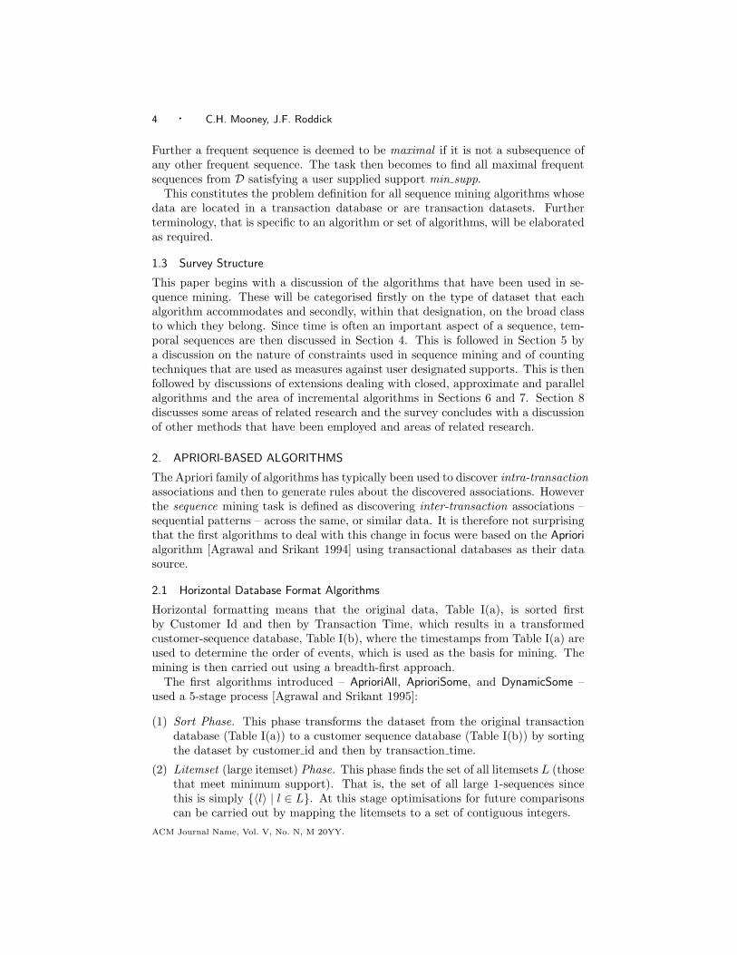
Using regular expressions and minimum frequency constraints combines bothanti-monotonic (frequency) and non-anti-monotonic (regular expressions) prun-ing techniques as has already been discussed for the SPIRIT family of algorithms.The RE-Hackle algorithm (Regular Expression-Highly Adaptive Constrained LocalExtractor) [Albert-Lorincz and Boulicaut 2003b] uses a hierarchical representationof Regular Expressions which it stores in a Hackle-tree rather than the Finite StateAutomaton used in the SPIRIT algorithms. They build their RE-constraints formining using RE’s built over an alphabet using three operators: union (denoted+), concatenation (denoted by ◦k, where k is the overlap deleted from the result)and Kleene closure (denoted ∗). A Hackle-tree (see Figure 2) is a form of AbstractSyntax Tree that encodes the structure of a RE-constraint and is structured witheach inner node containing a operator and the leaves containing atomic sequences.In this manner the tree reflects the way in which the atomic sequences are as-sembled from the unions, concatenations and Kleene closures to form the initialRE-constraint.
Once the RE-constraint is constructed as a Hackle-tree, extraction functions arethen applied to the nodes of the Hackle-tree and return the candidate sequencesthat need to be counted with those that are deemed to be frequent used for the nextgeneration. This is done by creating a new extraction phrase and a new Hackle-tree is then built and the process resumes. The process terminates when no morecandidates are discovered.
The MSPS (Maximal Sequential Patterns using Sampling) algorithm combinesthe approach taken in GSP and the supersequence frequency pruning for miningmaximal frequent sequences [Luo and Chung 2004]. Supersequence frequency basedpruning is based on the fact that any subsequence of a frequent sequence is also
ACM Journal Name, Vol. V, No. N, M 20YY.
10 · C.H. Mooney, J.F. Roddick
o
C +
o
o
C +
A BC
D
*
+
A B C
C
I
II III IV
V VI
VII VIII IX
X XI XII
XIII
XIV
XV XVI
Fig. 2. Hackle-tree for C((C(A + BC)D) + (A + B + C)∗)C – [Albert-Lorincz and Boulicaut2003b].
frequent and therefore can be pruned from the set of candidates. This gives riseto the common bottom-up, breadth-first search strategy that includes, from thesecond pass over the database, mining a small random sample of the database togenerate local maximal frequent sequences. After these have been verified in a top-down fashion against the original database, so that the longest frequent sequencescan be collected, the bottom-up search is continued. In addition the authors usea signature technique to overcome any problems that may arise when a set of k -sequences will not fit into memory and candidate generation is required.
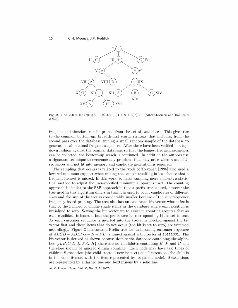
The sampling that occurs is related to the work of Toivonen [1996] who used alowered minimum support when mining the sample resulting in less chance that afrequent itemset is missed. In this work, to make sampling more efficient, a statis-tical method to adjust the user-specified minimum support is used. The countingapproach is similar to the PSP approach in that a prefix tree is used, however thetree used in this algorithm differs in that it is used to count candidates of differentsizes and the size of the tree is considerably smaller because of the supersequencefrequency based pruning. The tree also has an associated bit vector whose size isthat of the number of unique single items in the database where each position isinitialised to zero. Setting the bit vector up to assist in counting requires that aseach candidate is inserted into the prefix tree its corresponding bit is set to one.As each customer sequence is inserted into the tree it is checked against the bitvector first and those items that do not occur (the bit is set to zero) are trimmedaccordingly. Figure 3 illustrates a Prefix tree for an incoming customer sequenceof ABCD − ADEFG − B −DH trimmed against a bit vector of 10111001. Thebit vector is derived as shown because despite the database containing the alpha-bet {A,B,C, D, E, F,G, H} there are no candidates containing B, F and G andtherefore should be ignored during counting. Each node may have two types ofchildren S-extension (the child starts a new itemset) and I-extension (the child isin the same itemset with the item represented by its parent node). S-extensionsare represented by a dashed line and I-extensions by a solid line.ACM Journal Name, Vol. V, No. N, M 20YY.

Sequential Pattern Mining · 11
root
ABCD – ADEFG – B – DH
ACD – ADE – DH
1 2 3
4 5
6 7 8
9
1011
1213
A C D
CD – ADE – DH
DE – DH
C D
E – DH
E
ADE – DH
DH
A E
A
ADE – DH
DH
H
D – ADE – DH
A
ADE – DH
DH
H
DH
E
DE – DH
Bit Vector (10111001)
Candidates:
1) AC2) AD3) A – A4) A – E5) CH6) D – A7) ADE8) AD – A9) D – AE10) D – A – H
Fig. 3. A Prefix Tree of MSPS – [Luo and Chung 2004]. The labels on the edges represent recursive
calls on segments of the trimmed customer sequence.
2.2 Vertical Database Format Algorithms
Algorithmic development in the sequence mining area, to a large extent, has mir-rored that in the association rule mining field [Ceglar and Roddick 2006] in thatas improvements in performance were required they resulted from, in the first in-stance, employing a depth-first approach to the mining, and later by using patterngrowth methods (see Section 3). This shift required that the data be organised inan alternate manner, a vertical database format, where the rows of the databaseconsist of object-timestamped pairs associated with an event. This makes it easyto generate id-lists for each event that consist of object-timestamp rows of eventsthus enabling all frequent sequences to be enumerated via simple temporal joins ofthe id-lists. An example of this type of format is shown in Table IV.
Yang et al. [2002] recognised that these methods perform better when the data ismemory-resident and when the patterns are long, but also that the generation andcounting of candidates becomes easier. This shift in data layout brought about theintroduction of algorithms based on a depth-first traversal of the search space andat the same time there was an increased focus on incorporating constraints into themining process. This is due in part to the improvement in processing time but alsoas a reaction to the need to reduce the number of results.
ACM Journal Name, Vol. V, No. N, M 20YY.

12 · C.H. Mooney, J.F. Roddick
Table IV. Vertical Formatting Data Layout – [Zaki 2001b].
(a) Input-Sequence Database
Sequence Id Time Items
1 10 C D
1 15 A B C
1 20 A B F1 25 A C D F
2 15 A B F
2 20 E
3 10 A B F
4 10 D G H
4 20 B F4 25 A G H
(b) Id-Lists for the Items
A B D FSID EID SID EID SID EID SID EID
1 15 1 15 1 10 1 20
1 20 1 20 1 25 1 251 25 2 15 4 10 2 15
2 15 3 10 3 10
3 10 4 20 4 204 25 20
SID: Sequence Id
EID: Time
The SPADE (Sequential PAttern Discovery using Equivalence classes) algorithm[Zaki 2001b] and its variant cSPADE (constrained SPADE) [Zaki 2000] use combi-natorial properties and lattice based search techniques and allow constraints to beplaced on the mined sequences.
The key features of SPADE include the layout of the database in a vertical id-list database format with the search space decomposed into sub-lattices that can beprocessed independently in main memory thus enabling the database to be scannedonly three times or just once on some pre-processed data. Two search strategiesare proposed for finding sequences in the lattices:
(1) Breadth-first search: the lattice of equivalence classes is explored in a bottom-up manner and all child classes at each level are processed before moving tothe next.
(2) Depth-first search: all equivalence classes for each path are processed beforemoving to the next path.
Using the vertical id-list database in Table III(b) all frequent 1-sequences can becomputed in one database scan. Computing the F2 can be achieved in one of twoways; by pre-processing and collecting all 2-sequences above a user specified lowerbound, or by performing a vertical to horizontal transformation dynamically.
Once this has been completed the process continues by decomposing the 2-sequences into prefix-based parent equivalence classes followed by the enumera-tion of all other frequent sequences via either breadth-first or depth-first searcheswithin each equivalence class. The enumeration of the frequent sequences can beperformed by joining the id-lists in one of three ways (assume that A and B areitems and S is a sequence):
(1) Itemset and Itemset : joining AS and BS results in a new itemset ABS.(2) Itemset and Sequence: joining AS with B → S results in a new sequence
B → AS.(3) Sequence and Sequence: joining A → S with B → S gives rise to three possible
results: a new itemset AB → S, and two new sequences A → B → S andB → A → S. One special case occurs when A → S is joined with itselfresulting in A → A → S
ACM Journal Name, Vol. V, No. N, M 20YY.

Sequential Pattern Mining · 13
The enumeration process is the union or join of a set of sequences or items whosecounts are then calculated by performing an intersection of the id-lists of the ele-ments that comprise the newly formed sequence. By proceeding in this manner itis only necessary to use the first two subsequences lexicographically at the last levelto compute the support of a sequence at a given level [Zaki 1998]. This process forenumerating and computing the support for the sequence D → BF → A is shownin Table V using the data supplied in Table III(b).
Table V. Computing Support using temporal id-list joins – adapted from Zaki [2001b].
(a) Intersect D and A, D and B, D and F .
D → A D → B D → FSID EID SID EID SID EID
1 15 1 15 1 201 20 1 20 1 251 25 4 20 4 202 15 3 104 25
(b) Intersect D → B and D → A,
D → B and D → F .
D → B → A D → BFSID EID SID EID
1 20 1 201 25 4 204 25
(c) Intersect D →B → A and D →BF .
D → BF → ASID EID
1 254 25
The cSPADE algorithm [Zaki 2000] is the same as SPADE except that it incorpo-rates one or more of the following syntactic constraints as checks during the miningprocess:
(1) Length or width limitations on the sequences; allows for highly structured data,for example DNA sequence databases, to be mined without having the problemof an exponential explosion in the number of discovered frequent sequences.
(2) Minimum or maximum gap constraints on consecutive sequence elements toenable the discovery of sequences that occur after a certain minimum amountof time, and no longer than a specified maximum time ahead.
(3) Applying a time window on allowable sequences, requiring the entire sequenceto occur within the window. This differs from minimum and maximum gaps inthat it deals with the entire sequence not the time between sequence elements.
(4) Incorporating item constraints. Since the generation of individual equivalenceclasses is achieved easily by using the equivalence class approach and a verticaldatabase format, exclusion of an item becomes a simple check for the particularitem in the class and the removal from those classes where it occurs. Furtherexpansion of these classes will never contain these items.
(5) Finding sequences predictive of one or more classes (even rare ones). This isonly applicable to certain datasets (classification) where each input sequencehas a class label.
SPAM (Sequential PAttern Mining using A Bitmap Representation) [Ayres et al.2002] uses a novel depth-first traversal of the search space with various pruningmechanisms and a vertical bitmap representation of the database, which enablesefficient support counting. A vertical bitmap for each item in the database isconstructed while scanning the database for the first time with each bitmap havinga bit corresponding to each element of the sequence in the database. One potential
ACM Journal Name, Vol. V, No. N, M 20YY.

14 · C.H. Mooney, J.F. Roddick
limiting factor on its usefulness is its requirement that all of the data fit into mainmemory.
The candidates are stored in a lexicographic sequence lattice or tree (the sametype as used in PSP), which enables the candidates to be extended in one of twoways: Sequence Extended using an S-step process and Itemset Extended using anI-step process. This process is the same as the approach taken in GSP [Srikant andAgrawal 1996] and PSP [Masseglia et al. 1998] in that an item becomes a separateelement if it was a separate element in the sequence it came from or becomes partof the last element otherwise. These processes are carried out using the bitmapsfor the sequences or items in question by ANDing them to produce the result. TheS-step process requires that a transformed bitmap first be created by setting all bitsless than or equal to the item in question for any transaction to zero and all othersto one. This transformed bitmap is then used for ANDing with the item to beappended. Table V(c) and Table V(d) illustrate this using the data in Table V(a)and bitmap representation in Table V(b).
The method of pruning candidates is based on downward closure and is conductedon both S-extension and I-extension candidates of a node in the tree using a depth-first search, which guarantees all nodes are visited. However, if the support for asequence s < min supp at a particular node then no more depth-first search isrequired on s due to downward closure.
The CCSM (Cache-based Constrained Sequence Miner) algorithm [Orlando et al.2004] uses a level-wise approach initially but overcomes many problems associatedwith this type of algorithm. This is achieved by using k -way intersections of id-liststo compute the support of candidates (the same as SPADE [Zaki 2001b]) combinedwith a cache that stores intermediate id-lists for future reuse.
The algorithm is similar to GSP [Srikant and Agrawal 1996] because it adoptsa level-wise bottom-up approach in visiting the sequential patterns in the treebut it differs since after extracting the frequent F1 and F2 from the horizontaldatabase, this pruned database is transformed into a vertical one resulting in thesame configuration as SPADE [Zaki 2001b]. The major difference is the use of acache to store intermediate id-lists to speed up support counting. This is achievedin the following way - when a new sequence is generated, and if a common prefixis contained in the cache, then the associated id-list is reused and subsequent linesof the cache are rewritten. This enables only a single equality join to be performedbetween the common prefix and the new item, after which the result of the join isadded to cache.
The application goal of IBM (Indexed Bit Map for Mining Frequent Sequences)[Savary and Zeitouni 2005] is to find chains of activities that characterise a groupof entities and where the input can be composed of single items. Their approachconsists of two phases; first, data encoding and compression, and second, frequentsequence generation that is itself comprised of candidate generation and supportchecking. Four data structures are used for the encoding and compression as follows:A Bit Map that is a binary matrix representing the distinct sequences, an SV vectorto encode all of the ordered combinations of sequences, an index on the Bit Mapto facilitate direct access to sequences and an NB table also associated with theBit Map to hold the frequencies of the sequences. The algorithm only makes oneACM Journal Name, Vol. V, No. N, M 20YY.

Sequential Pattern Mining · 15
Table VI. SPAM data representation – [Ayres et al. 2002].
(a) Data sorted by CID and TID.
Customer ID (CID) TID Itemset
1 1 {a, b, c}1 3 {b, c, d}1 6 {b, c, d}
2 2 {b}2 4 {a, b, c}
3 5 {a, b}3 7 {b, c, d}
(b) Bitmap representation of the dataset in (a)
CID TID {a} {b} {c} {d}
1 1 1 1 0 11 3 0 1 1 11 6 0 1 1 1- - 0 0 0 0
2 2 0 1 0 02 2 1 1 1 0- - 0 0 0 0- - 0 0 0 0
3 5 1 1 0 03 7 0 1 1 1- - 0 0 0 0- - 0 0 0 0
(c) S-Step processing
({a}) ({a})s {b} ({a}, {b})
1 0 1 00 1 1 10 1 1 10 1 0 0
0 S-step 0 1 result 01 −→ 1 & 1 −→ 00 process 1 0 00 1 0 0
1 0 1 00 1 1 10 1 0 00 1 0 0
(d) I-step processing
({a}, {b}) {d} ({a}, {b, d})
0 1 01 1 11 1 10 0 0
0 0 result 00 & 0 −→ 00 0 00 0 0
0 0 01 1 10 0 00 0 0
scan of the database to collect the number of distinct sequences, their frequenciesand the number of sequences by size and in doing so allows for the computingof support for each generated sequence. Candidate generation is conducted inthe same manner as GSP [Srikant and Agrawal 1996], PSP [Masseglia et al. 1998]and SPAM [Ayres et al. 2002], except in IBM there is only a need to use the I-extension process since the data has been encoded to single item values. Uponcompletion of candidate generation, support is determined by first accessing theIBM at the cell where the size of the sequence in question is encoded and thenusing the SV vector to determine if the candidate is contained in subsequent linesof the IBM. The candidate is then accepted as frequent if the count is larger thana user specified support. The process terminates under the same conditions as theother algorithms, that is when either no candidates can be generated or there are
ACM Journal Name, Vol. V, No. N, M 20YY.

16 · C.H. Mooney, J.F. Roddick
Table VII. A summary of Apriori-based algorithms.
Algorithm Name Author Year Notes
Candidate Generation: Horizontal Database Format
Apriori (All, Some, Dynamic Some) [Agrawal andSrikant]
1995
Generalised Sequential Patterns
(GSP)
[Srikant and
Agrawal]
1996 Max/Min Gap,
Window,Taxonomies
PSP [Masseglia et al.] 1998 Retrieval
optimisations
Sequential Pattern mIning with
Regular expressIon consTraints
(SPIRIT)
[Garofalakis et al.] 1999 Regular
Expressions
Maximal Frequent Sequences (MFS) [Zhang et al.] 2001 Based on GSP,
uses Sampling
Regular Expression-Highly AdaptiveConstrained Local Extractor
(RE-Hackle)
[Albert-Lorinczand Boulicaut]
2003 RegularExpressions,
similar to SPIRIT
Maximal Sequential Patterns usingSampling (MSPS)
[Luo and Chung] 2004 Sampling
Candidate Generation: Vertical Database Format
Sequential PAttern Discovery usingEquivalence classes (SPADE)
[Zaki] 2001 EquivalenceClasses
Sequential PAttern Mining (SPAM) [Ayres et al.] 2002 Bitmap
representation
LAst Position INduction (LAPIN) [Yang and
Kitsuregawa]
2004 Uses last position
Cache-based Constrained Sequence
Miner (CCSM)
[Orlando et al.] 2004 k-way
intersections,
cache
Indexed Bit Map (IBM) [Savary and
Zeitouni]
2005 Bit Map, Sequence
Vector, Index, NB
table
LAst Position INduction Sequential
PAttern Mining (LAPIN-SPAM)
[Yang and
Kitsuregawa]
2005 Uses SPAM, Uses
last position
no frequent sequences obtained.Yang and Kitsuregawa [2005] base LAPIN-SPAM (Last Position INduction Sequ-
ential PAttern Mining) on the same principles as SPAM [Ayres et al. 2002] withthe exception of the methods for candidate verification and counting. Where SPAMuses many ANDing operations, LAPIN avoids this through the observation that ifthe last position of item α is smaller than, or equal to, the position of the last itemACM Journal Name, Vol. V, No. N, M 20YY.

Sequential Pattern Mining · 17
in a sequence s, then item α cannot be appended to s as a (k + 1)-length sequenceextension in the same sequence [Yang et al. 2005]. This transfers similarly to theI-step extensions. In order to exploit this observation the algorithm maintains anITEM IS EXIST TABLE in which the last position information is recorded for eachspecific position and during each iteration of the algorithm there only needs to be acheck of this table to ascertain whether the candidate is behind the current position.
3. PATTERN GROWTH ALGORITHMS
It was recognised early that the number of candidates that were generated usingApriori-type algorithms are, in the worst case, exponential. That is, if there was afrequent sequence of 100 elements then 2100 ≈ 1030 candidates had to be generatedto find such a sequence. Although methods have been introduced to alleviate thisproblem, such as constraints, the candidate generation and prune method suffersgreatly under circumstances when the datasets are large. Another inherent prob-lem is the repeated scanning of the dataset to check a large set of candidates bysome method of pattern matching. The recognition of these problems in the firstinstance in association mining gave rise to, in that domain, the frequent patterngrowth paradigm and the FP-Growth algorithm [Han and Pei 2000]. This was simi-larly recognised by researchers in the sequence mining domain and algorithms weredeveloped to exploit this methodology.
The frequent pattern growth paradigm removes the need for the candidate gen-eration and prune steps that occur in the Apriori type algorithms and does so bycompressing the database representing the frequent sequences into a frequent pat-tern tree and then dividing this tree into a set of projected databases, which aremined separately [Han et al. 2000].
In comparison to Apriori-type algorithms, pattern growth algorithms, while gen-erally more complex to develop, test and maintain, can be faster when given largevolumes of data. Moreover, the opportunity to undertake multiple scans of streamdata are limited and thus single-scan pattern growth algorithms are often the onlyoption.
The sequence database shown in Table VIII will be used as a running examplefor both FreeSpan and PrefixSpan.
Table VIII. A sequence database, S, for use with ex-amples for FreeSpan and PrefixSpan – [Pei et al. 2001].
Sequence id Sequence
10 〈a(abc)(ac)d(cf)〉30 〈(ad)c(bc)(ae)〉30 〈(ef)(ab)(df)cb〉40 〈eg(af)cbc〉
FreeSpan (Frequent pattern-projected Sequential Pattern Mining) [Han et al.2000] aims to integrate the mining of frequent sequences with that of frequentpatterns and use projected sequence databases to confine the search and growth ofthe subsequence fragments [Han et al. 2000].
By using projected sequence databases the method greatly reduces the gener-ation of candidate sub-sequences. The algorithm firstly generates the frequent
ACM Journal Name, Vol. V, No. N, M 20YY.
18 · C.H. Mooney, J.F. Roddick
1-sequences, F1, termed an f list, by scanning the sequence database, and thensorts them into support descending order, for example from the sequence databasein Table VIII, f list = 〈a : 4, b : 4, c : 4, d : 3, e : 3, f : 3〉, where 〈pattern〉 : count isthe sequence and its associated frequency. This set can be divided into six subsets:those having item f , those having item e but no f , those having item d but no eor f , and so on until a is reached. This is followed by the construction of a lower-triangular frequent item matrix that is used to generate the F2 patterns and a setof projected databases. Items that are infrequent such as g are removed and donot take part in the construction of projected databases. The projected databasesare then used to generate F3 and longer sequential patterns. This mining processis outlined below [Han et al. 2000; Pei et al. 2001]:
To find the sequential patterns containing only item a. This is achieved byscanning the database. In the example, the two patterns that are found containingonly item a are 〈a〉 and 〈aa〉.
To find the sequential patterns containing the item b but no item afterb in f list. By constructing the {b}-projected database and for a sequence α in Scontaining item b a subsequence α′ is derived by removing from α all items afterb in f list. Next α′ is inserted into the {b}-projected database resulting in the {b}-projected database containing the following four sequences: 〈a(ab)a〉, 〈aba〉, 〈(ab)b〉and 〈ab〉. By scanning the projected database one more time all frequent patternscontaining b but no item after b in f list are found, which are 〈b〉, 〈ab〉,〈ba〉, 〈(ab)〉.
Finding other subsets of sequential patterns. This is achieved by using thesame process as outlined above on the {c}-, {d}-, . . . , {f}-projected databases.
All of the single projected databases are constructed on the first scan of theoriginal database and the process outlined above is performed recursively on allprojected databases while there are still longer candidate patterns to be mined.
PrefixSpan (Prefix-projected Sequential Pattern Mining) [Pei et al. 2001] buildson the concept of FreeSpan but instead of projecting sequence databases it examinesonly the prefix subsequences and projects only their corresponding postfix subse-quences into projected databases. Using the sequence database, S, in Table VIIIwith a min supp = 2 the mining is as follows.
The length-1 sequential patterns are the same as for the f list in FreeSpan –〈a〉 : 4, 〈b〉 : 4, 〈c〉 : 4, 〈d〉 : 3, 〈e〉 : 3, 〈f〉 : 3. As for FreeSpan, the complete set canbe divided into six subsets according to the six prefixes. These are then used togather those sequences that have them as a prefix. Using the prefix a as an example,when performing this operation FreeSpan considers subsequences prefixed by thefirst occurrence of a, i.e., in the sequence 〈(ef)(ab)(df)cb〉, only the subsequence〈( b)(df)cb〉 should be considered, (( b) means the last element in the prefix, in thiscase a, together with b form an element).
The sequences in S containing 〈a〉 are next projected with respect to 〈a〉 toform the 〈a〉-projected database, followed by those with respect to 〈b〉 and so on.By way of example the 〈b〉-projected database consists of four postfix sequences:〈( c)(ac)d(cf)〉, 〈( c)(ae)〉, 〈(df)cb〉 and 〈 c〉. By scanning these projected databasesall of the length-2 patterns having the prefix 〈b〉 can be found. These are 〈ba〉:2,〈bc〉:3, 〈(bc)〉:3, 〈bd〉:2, and 〈bf〉:2. This process is then conducted recursively bypartitioning the patterns as above to give those having prefix 〈ba〉, 〈bc〉 and so on,ACM Journal Name, Vol. V, No. N, M 20YY.

Sequential Pattern Mining · 19
1 10
Length of sequence
0.0001
0.001
s s′: SVE of sSupport
Length-decreasing support constraint f(l)
Fig. 4. A typical length-decreasing support constraint and the smallest valid extension (SVE)property – [Seno and Karypis 2002].
and these are mined by constructing projected databases and mining each of themrecursively. This is done for each of the remaining single prefixes, 〈c〉, 〈d〉, 〈e〉 and〈f〉 respectively.
The major benefit of this approach is that no candidate sequences need to begenerated or tested that do not exist in a projected database. That is, PrefixS-pan only grows longer sequential patterns from shorter frequent ones, thus makingthe search space smaller. This results in the major cost being the construction ofthe projected databases, which can be alleviated by two optimisations. The first,by using a bi-level projection method to reduce the size and number of the pro-jected databases, and second a pseudo-projection method to reduce the cost whena projected database can be wholly contained in main memory.
The SLPMiner algorithm [Seno and Karypis 2002] follows the projection-basedapproach for generating frequent sequences but uses a length-decreasing supportconstraint for the purpose of finding not only short sequences with high supportbut also long sequences with a lower support. To this end the authors extendedthe model they introduced for length-decreasing support in association rule mining[Seno and Karypis 2001; 2005], to use the length of a sequence not an itemset. Thisis formally defined as follows: Given a sequential database D and a function f(l))that satisfies 1 ≥ f(l) ≥ f(l + 1) ≥ 0 for any positive integer l, a sequence s isfrequent if and only if σD(s) ≥ f(|s|).
Under this constraint a sequence can be frequent while its subsequences are infre-quent so pruning cannot be performed solely using the downward closure principleand therefore three types of pruning are introduced that are derived from knowledgeabout the length at which an infrequent sequence becomes frequent. This knowl-edge about the increase in length is termed the smallest valid extension property (orSVE ) and uses the fact that if a line is drawn parallel to the x-axis at y = σD(s)until it intersects the support curve then the length of the extended sequence isthe minimum length the original sequence must attain before it becomes frequent.Figure 4 shows both the length-decreasing support function and the SVE property.
The three methods of pruning are as follows:
(1) sequence pruning removes sequences that occur at every node in the prefix treeACM Journal Name, Vol. V, No. N, M 20YY.

20 · C.H. Mooney, J.F. Roddick
from the projected databases. A sequence s can be pruned if the value of thelength-decreasing function f(|s|+ |p|), where p is the pattern represented at aparticular node, is greater than the value of the support for p in the database D.
(2) item pruning removes some of the infrequent items from short sequences. Sincethe inverse function of the length-decreasing support function yields the lengthof a particular sequence, an item i can be pruned by determining if the lengthof a sequence plus the length of the prefix at a node, |s| + |p|, is less thanthe value of the inverse function of the support for the item i in the projecteddatabase D′ at the current node.
(3) min-max pruning eliminates a complete projected database. This is achievedby splitting the projected database into two subsets and determining if eachof them is too small to be able to support any frequent sequential patterns. Ifthis is the case then the entire projected database can be removed.
Although these pruning methods are elaborated for use with SLPMiner the au-thors note that many of the methods can be incorporated into other algorithmsand cite PrefixSpan [Pei et al. 2001] and SPADE [Zaki 2001b] as two possibilities.
4. TEMPORAL SEQUENCES
The data used for sequence mining is not limited to data stored in overtly temporalor longitudinally maintained datasets. In such domains data can be viewed as aseries of events occurring at specific times and therefore the problem becomes asearch for collections of events that occur frequently together. Solving this problemrequires a different approach, and several types of algorithm have been proposedfor different domains.
4.1 Problem Statement and Notation for Episode and Event-based Algorithms
The first algorithmic framework developed to mine datasets that were deemed tobe episodic in nature was introduced by Mannila et al. [1995]. The task addressedwas to find all episodes that occur frequently in an event sequence, given a class ofepisodes and an input sequence of events. An episode was defined to be:
“... a collection of events that occur relatively close to each other in agiven partial order, and ... frequent episodes as a recurrent combinationof events” [Mannila et al. 1995]
Table IX. A summary of pattern growth algorithms.
Algorithm Name Author Year Notes
Pattern Growth
FREquEnt pattern-projectedSequential PAtterN mining
(FreeSpan)
[Han et al.] 2000 Projected sequencedatabase
PREFIX-projected Sequential
PAtterN mining (PrefixSpan)
[Pei et al.] 2001 Projected prefix
database
Sequential pattern mining withLength-decreasing suPport
(SLPMiner )
[Seno and Karypis] 2002 Length-decreasingsupport
ACM Journal Name, Vol. V, No. N, M 20YY.

Sequential Pattern Mining · 21
The notation used is as follows.E is a set of event types and an event is a pair (A, t), where A ∈ E is an event
type and t is an integer (time / occurrence) of the event. There are no restrictionson the number of attributes that an event type may contain, or be made up of, butthe original work only considered single values with no loss of generality. An eventsequence s on E is a triple (s, Ts, Te), where s = 〈(A1, t1), (A2, t2), . . . , (An, tn)〉 isan ordered sequence of events such that Ai ∈ E for all i = 1, . . . , n, and ti ≤ ti+1
for all i = 1, . . . , n− 1. Further Ts < Te are integers, Ts is termed the starting timeand Te the ending time, and Ts ≤ ti < Te for all i = 1, . . . , n.
For example, Figure 5 depicts the event sequence s = (s, 29, 68), where s =〈(A, 31), (F, 32), (B, 33), (D, 35), (C, 37), . . . , (F, 67)〉.
In order for episodes to be considered interesting they must occur close enoughin time, which can be defined by the user through a time window of a certainwidth. These time windows are partially overlapping slices of the event sequenceand the number of windows that an episode must occur in to be considered frequent,min freq, is also defined by the user. Notationally a window on event sequenceS = (s, Ts, Te) is an event sequence w = (w, ts, te) where ts < Te , te > Ts and wconsists of those pairs (A, t) from s where ts ≤ t < te. The time span te − ts istermed the width of the window w denoted width(w). Given an event sequences and an integer win, the set of all windows w on s such that width(w) = win isdenoted by W(s,win). Given the event sequence s = (s, Ts, Te) and window widthwin, the number of windows in W(s,win) is Te − Ts + win − 1.
An episode ϕ = (V,≤, g) is a set of nodes V , a partial order ≤ on V , and amapping g : V → E associating each node with an event type. The interpretationof an episode is that it has to occur in the order described by ≤.
There are two types of episodes considered:
Serial. – where the partial order relation ≤ is a total order resulting in forexample an event A preceding an event B which precedes event C. This is shownin Figure 6(a).
Parallel. – where there are no constraints on the relative order of events, thatis if the partial order relation ≤ is trivial: (x � y ∀ x 6= y). This is shown inFigure 6(b).
The frequency of an episode is defined to be the number of windows in which theepisode occurs. That is, given an event sequence s and a window width win, thefrequency of an episode ϕ in s is:
fr(ϕ, s,win) =|{w ∈ W(s,win)|ϕ occurs in w}|
|W(s,win)|
30 35 40 45 50 55 60 65
AFB D CEAB E F CDF E ABE CADAEB D F
Fig. 5. An example event sequence and two windows of width 7.
ACM Journal Name, Vol. V, No. N, M 20YY.

22 · C.H. Mooney, J.F. Roddick
A B C
(a)
C
B
A
(b)
Fig. 6. Depiction of a serial and parallel episode – [Mannila et al. 1995].
Thus, given a frequency threshold min freq, ϕ is frequent if fr(ϕ, s,win) ≥ min freq .The task is to discover all frequent episodes (serial or parallel) from a given classE of episodes.
The goal of WINEPI [Mannila et al. 1995] was given an event sequence s, a setε of episodes, a window width win, and a frequency threshold min freq, to findthe set of frequent episodes F with respect to s, win and min freq denoted asF(s, win, min freq). The algorithm follows a traditional level-wise (breadth-first)search starting with the general episodes (one event). At each subsequent level thealgorithm first computes a collection of candidate episodes, checks their frequencyagainst min freq and, if greater, the episode is added to a list of frequent episodes.This cycle continues until there are no more candidates generated or no candidatesmeet the minimum frequency. This is a typical Apriori-like algorithm under whichthe downward closure principal holds – if α is frequent then all sub-episodes β � αare frequent.
In order to recognise episodes in sequences two methods are necessary, one forparallel episodes and one for serial episodes. However since both of these methodsshare a similar feature, namely that two adjacent windows are typically similar toeach other, the recognition can be done incrementally. For parallel episodes a countis maintained that indicates how many events are present in any particular windowand when this count reaches the length of episode (at any given iteration of thealgorithm) the index of the window is saved. When the count decreases, indicatingthat the episode is not entirely in the window, the occurrence field is incrementedby the number of windows in which the episode was fully contained. Serial episodesare recognised using state automata that accept the candidate episodes and ignoreall other input [Mannila et al. 1995]. A new instance of the automata is initialisedfor each serial episode every time the first event appears in the window, and theautomata is removed when this same event leaves the window. To count the numberof occurrences, an automata is said to be in the accepting state when the entireepisode is in the window and each time this occurs the automata is removed and itswindow index is saved. When there are no automata left for the particular episodethe occurrence is incremented by the number of saved indexes.
Mannila and Toivonen [1996] extended this work by considering only minimaloccurrences of episodes, which are defined as follows. Given an episode ϕ and anevent sequence s, then the interval [ts, te) is a minimal occurrence of ϕ in s if
(1) ϕ occurs in the window w = (w, ts, te) on s, and,(2) ϕ does not occur in any proper subwindow on w, that is, @w′ = (w′, t′s, t
′e) on
ACM Journal Name, Vol. V, No. N, M 20YY.

Sequential Pattern Mining · 23
s such that ts ≤ t′s, t′e ≤ te and width(w′) < width(w).
The algorithm MINEPI takes advantage of this new formalism and follows thesame basic principles as WINEPI with the exception that minimal occurrences ofcandidate episodes are located during the candidate generation phase of the algo-rithm. This is performed by selecting from a candidate episode ϕ two subepisodesϕ1 and ϕ2 such that ϕ1 contains all events of ϕ except the last one and ϕ2 containsall events except the first one. From these two subepisodes the minimal occurrencesof ϕ are found using the following specification [Mannila and Toivonen 1996]:
mo(ϕ) = {[ts, ue) | ∃ [ts, te) ∈ mo(ϕ1) ∧ [us, ue) ∈ mo(ϕ2)such that ts < us, te < ue and [ts, ue) is minimal}
These minimal occurrences are then used to obtain a statistical confidences of theepisode rules without the need to rescan the data.
Typically, WINEPI produces rules that are similar to association rules. For ex-ample, if ABC is a frequent sequence then AB ⇒ C (confidence γ) states thatif A occurs followed by B then some time later C occurs. The MINEPI and itsnew formalism of episodes allows for more useful rule formulations for example:“Dept Home Page”, “Sem. I 2005” [15s] ⇒ “Classes in Sem. I 2005” [30s] (γ 0.83).This is read as if a person navigated to the Department Home Page followed bythe Semester I page within 15 seconds then within the next 30 seconds they wouldnavigate to the Semester I Classes page 83% of the time.
Huang et al. [2004] introduced the algorithm PROWL (Projected Window Lists)to mine inter-transaction rules and the concept of frequent continuities to distin-guish their rules from those of intra-transaction or association rules. They alsointroduced a don’t care symbol into the sequence to allow for partial periodicity.PROWL is a two phase algorithm for mining such frequent continuities and utilisesa projected window list and a depth first enumeration of the search space.
The definition of a sequence follows the pattern from Section 4.1 however, theauthors do not define the complete event sequence as a triple but as a tuple of theform (tid, xi) where tid is a time instant and xi is an event. The continuity patternis defined to be a nonempty sequence with window W, P = (p1, p2, . . . , pw) wherep1 is an event and the remainder can either be events or the ∗ (don’t care) token.A continuity pattern is termed an i-continuity or has length i if exactly i positionsin P contain an event. For example, {A,∗ ,∗ } is a 1-continuity and {A,∗ , C} is a2-continuity. They define the problem to be the discovery of all patterns P with awindow W where any subsequence of W in S supports P.
The algorithm uses a Projected Window List (PWL) to grow the sequences wherea PWL is defined as P = {e1, e2, . . . , ek} and P.PWL = {w1, w2, . . . , wk}, wi =ei+1 for 1 ≤ i ≤ k. By concatenating each event with the events in the PWL, longersequences can be generated for which the number of events in the concatenated listcan be checked against the given support and accepted as frequent if it equals orexceeds the value. This process is applied recursively until the projected windowlists become empty or the window of a continuity is greater than the maximumwindow. Table X shows the vertical layout of the event sequences and Figure 7shows the recursive process for the continuity pattern {A}.
ACM Journal Name, Vol. V, No. N, M 20YY.

24 · C.H. Mooney, J.F. Roddick
Table X. Vertical layout of the event sequences for the PROWL algorithm –
[Huang et al. 2004].
Event Time List Projected Window List
A 1, 4, 7, 8, 11, 14 2, 5, 8, 9, 12, 15
B 3, 6, 9, 12, 16 4, 7, 10, 13C 2, 10, 15 3, 11, 16
D 5, 13 6, 14
Support and confidence are defined in a similar fashion to association rule miningand therefore rules can be formed which are an implication of the form X ⇒Y , where X and Y are continuity patterns with window w1 and w2 respectivelyand the concatenation X · Y is a continuity pattern with window w1 + w2. Thisleads to support being equal to the support of the concatenation divided by thenumber of transactions in the event sequence, and confidence as the support of theconcatenation divided by the support of either continuity depending on the requiredimplication.
{A}
PA.list = {1, 4, 7, 8, 11, 14}PA.P W L = {2, 5, 8, 9, 12, 15}
{A, A}
PAA.list = {8}
{A, B}
PAB.list = {9, 12}
{A, C}
PAC .list = {2}
{A,∗ }
PA∗ .list = {2, 5, 8, 9, 12, 15}PA∗ .P W L = {3, 6, 9, 10, 13, 16}
{A,∗ , B}
PA∗B.list = {3, 6, 9, 16}PA∗B.P W L = {4, 7, 10}
{A,∗ , C}
PA∗C .list = {10}
{A,∗ ,∗ }
PA∗∗ .list = {3, 6, 9, 10, 13, 16}PA∗∗ .P W L = {4, 7, 10, 11, 14}
{A,∗ , B, A}
PA∗BA.list = {4, 7}
{A,∗ , B, C}
PA∗BC .list = {10}
{A,∗ ,∗ , A}
PA∗∗A.list = {4, 7, 11, 14}
{A,∗ ,∗ , C}
PA∗∗C .list = {10}
Fig. 7. The recursive process for the continuity pattern {A} – [Huang et al. 2004].
4.2 Event-Oriented Patterns
Sun et al. [2003] approach the problem of mining sequential patterns as that ofmining temporal event sequences that lead to a specific target event, rather thanfinding all frequent patterns. They discuss two types of patterns; an Existencepattern α with a temporal constraint T that is a set of event values and a Sequentialpattern β also with a temporal constraint T . Their method is used to produce rulesof the type r =
{LHS
T→ e}
, where e is a target event value and LHS is a patternof type α or β. T is a time interval that specifies both the temporal relationshipACM Journal Name, Vol. V, No. N, M 20YY.

Sequential Pattern Mining · 25
t
c g d g e d b e c e d be e e
t1 t2 t3 t4 t5 t6 t7 t8 t9 t10 t11t12
w1 w2
w3
Fig. 8. Sequence fragments of size T (w1 = 〈(g, t2), (d, t3), (g, t4)〉, w2 = 〈(d, t6), (b, t7)〉, w3 =
〈(b, t7), (e, t8), (c, t9)〉) for the target event e in an event sequence s – [Sun et al. 2003].
between LHS and e and also the temporal constraint pattern of LHS. To find theLHS patterns they first locate all of the target events in the event sequence andcreate a timestamp set by using a T-sized window extending back from the targetevent. The sequence fragments (fi) that are created from this process is termedthe dataset of target event e (see Figure 8 for an example).
The support for a rule is then given by the number of sequence fragments con-taining a specified pattern divided by the total number of sequence fragments in theevent sequence. As the authors point out, this method finds frequent sequences thatoccur not only before target events but elsewhere in the event sequence and there-fore it cannot be concluded that these patterns relate to the given target events. Inorder to prune these non-related patterns a confidence measure is introduced whichevaluates the number of times the pattern actually leads to the target event dividedby the total number of times the pattern occurs. Both of these values are definedas window sets. The formal definition of the problem is then: Given a sequence s,target event value e, window size T , two thresholds s0 and c0, find the completeset of rule r =
{LHS
T→ e}
such that supp(r) ≥ s0 and con(r) ≥ c0.
4.3 Pattern Directed Mining
Guralnik et al. [1998] present a framework for the mining of frequent episodes usinga pattern language for specifying episodes of interest. A sequential pattern tree isused to store the relationships specified by the pattern language and a standardbottom-up mining algorithm can then be used to generate the frequent episodes.The specification for mining follows the notation described earlier (see Section 4.1)with the addition of a selection constraint on an event, which is a unary predicateα(e, ai) on a domain Di where ai is an attribute of e, and a join constraint on eventse and f , which is a binary predicate β(e.ai, f.aj) on a domain Di × Dj where ai
and aj are attributes of e and f respectively. They also define a sequential patternas a combination of partially ordered event specifications constructed from bothselection and join constraints. To facilitate the mining process the user-specifiedpatterns are stored in a Sequential Pattern Tree (SP Tree) where the leaf nodesrepresent events and the interior nodes represent ordering constraints. In addition,each node holds events matching constraints of that node and attached to the nodeis a boolean expression that represents the attribute constraints associated with thenode (see Figure 9 for two examples).
The mining algorithm constructs the frequent episodes in a bottom-up fashion bytaking an SP Tree T and a sequence of events S and at the leaf level matching eventsagainst any selection constraints and pruning out those that do not match. The
ACM Journal Name, Vol. V, No. N, M 20YY.

26 · C.H. Mooney, J.F. Roddick
interior nodes merge events of left and right children according to any ordering andjoin constraints, again pruning out those that do not match the node specifications.The process is continued recursively until all events in S have been visited.
→
e f
(a) SP Tree for the user
specified pattern e → f .
e
=
e.name microsoft
(b) SP Tree for the user specified pat-
tern e{e.name = ‘microsoft’}.
Fig. 9. Two examples of SP Trees – [Guralnik et al. 1998].
Table XI. A summary of temporal sequence algorithms.
Algorithm Name Author Year Notes
Candidate Generation: Episodes
WINEPI [Mannila et al.] [1995],
1996
State automata,
Window
WINEPI, MINEPI [Mannila et al.] 1997 State automata,
Window, Maximal
Pattern Directed Mining [Guralnik et al.] 1998 Pattern language
Event-Oriented Patterns [Sun et al.] 2003 Target events
Pattern Growth: Episodes
PROjected Window Lists (PROWL) [Huang et al.] 2004 Projected windowlists
5. CONSTRAINTS AND COUNTING
5.1 Types of Constraints
Constraints to guide the mining process have been employed by many algorithms,not only in sequence mining but also in association mining [Fu and Han 1995; Nget al. 1998; Chakrabarti et al. 1998; Bayardo and Agrawal 1999; Pei et al. 2001;Ceglar et al. 2003]. In general constraints that are imposed on sequential patternmining, regardless of the algorithms employed, can be categorized into one of eightmain types1. Other types of constraints will be discussed as they arise, however in
1This is not a complete list but categorises those that are of most interest and are currently in
use. Many of these were discussed first by Pei et al. [2002].
ACM Journal Name, Vol. V, No. N, M 20YY.

Sequential Pattern Mining · 27
general a constraint C on a sequential pattern α is a boolean function of the formC(α). For the constraints listed below only the duration and gap constraints relyon a support threshold (min supp) to confine the mined patterns; for the others,whether or not a given pattern satisfies a constraint can be determined by thepattern itself. These constraints rely on a set of definitions that are outlined below.
Let I = {x1, . . . , xn} be a set of items, each possibly being associated with a setof attributes, such as value, price, period, and so on. The value of attribute A ofitem x is denoted as x.A. An itemset is a non-empty subset of items, and an itemsetwith k items is termed a k-itemset. A sequence α = 〈X1 . . . Xl〉 is an ordered listof itemsets. An itemset Xi, (1 ≤ i ≤ l) in a sequence is termed a transaction. Atransaction Xi may have a special attribute, time-stamp, denoted as Xi.time, thatregisters the time when the transaction was executed. The number of transactionsin a sequence is termed the length of the sequence. A sequence α with length lis termed an l -sequence, denoted as len(α) = l, with the i -th item denoted asα[i]. A sequence α = 〈X1 . . . Xn〉 is termed a subsequence of another sequenceβ = 〈Y1 . . . Ym〉 (n ≤ m), and β a super-sequence of α, denoted as α v β, ifthere exist integers 1 ≤ i1 < . . . < in ≤ m such that X1 ⊆ Yi1 , . . . , Xn ⊆ Yin
. Asequence database SDB is a set of 2-tuples (sid, α), where sid is a sequence-idand α a sequence. A tuple (sid, α) in a sequence database SDB is said to contain asequence γ if γ is a subsequence of α. The number of tuples in a sequence databaseSDB containing sequence γ is termed the support of γ, denoted as sup(γ).
The categories of constraints given below appear throughout (expanded from [Peiet al. 2002]).
(1) Item Constraint: This type of constraint indicates which type of items, sin-gular or groups, are to be included or removed from the mined patterns. Theform is Citem(α) ≡ (ϕi : 1 ≤ i ≤ len(α), α[i] θ V ), or Citem(α) ≡ (ϕi :1 ≤ i ≤ len(α), α[i] ∩ V 6= ∅), where V is a subset of items, ϕ ∈ {∀,∃} andθ ∈ {⊆, *,⊇, +,∈, /∈}.For example, when mining sequential patterns from medical data a user mayonly be interested in patterns that have a reference to a particular hospital. IfH is the set of hospitals, the corresponding item constraint is Chospital(α) ≡(∃i : 1 ≤ i ≤ len(α), α[i] ⊆ H).
(2) Length Constraint: This type of constraint specifies the length of the pat-terns to be mined either as the number of elements or the number of transac-tions that comprises the pattern. This basic definition may also be modified toinclude only unique or distinct items.For example, a user may only be interested in discovering patterns of at least20 elements in length that occur in the analysis of a sequence of web log clicks.This might be expressed as a length constraint Clen(α) ≡ (len(α) ≤ 20).
(3) Model-based Constraint: These types of constraints are those that look forpatterns that are either sub-patterns or super-patterns of some given pattern.A super-pattern constraint is in the form of Cpat(α) ≡ (∃γ ∈ P ∧γ v α), whereP is a given set of patterns. Simply stated this says find patterns that containa particular set of patterns as sub-patterns.For example, an electronics shop may employ an analyst to mine their trans-action database and in doing so may be interested in all patterns that contain
ACM Journal Name, Vol. V, No. N, M 20YY.

28 · C.H. Mooney, J.F. Roddick
first buying a PC then a digital camera and a photo-printer together. This canbe expressed as Cpat(α) ≡ 〈(PC)(digital camera, photo-printer)〉 v α.
(4) Aggregate Constraint: These constraints are imposed on an aggregate ofitems in a pattern, where the aggregate function can be, avg, min, max, etc.For example, the analyst in the electronics shop may also only be interested inpatterns where the average price of all the items is greater than $500.
(5) Regular Expression Constraint: This is specified using the establishedset of regular expression operators – disjunction, Kleene closure, etc. For asequential pattern to satisfy a particular regular expression constraint, CRE , itmust be accepted by its equivalent deterministic finite automata.For example, to discover sequential patterns about a patient who was admittedwith measles and was given a particular treatment, a regular expression ofthe form Admitted(Measles | German Measles)(Treatment A | Treatment B |Treatment C) where “|” indicates disjunction.
(6) Duration Constraint: For these constraints to be defined, every transac-tion in the sequence database or each item in a temporal sequence must havean associated time-stamp. The duration is determined by the time differencebetween the first and last transaction, or first and last item, in the patternand can be either longer or shorter than a given period. Formally, a durationconstraint is in the form of Dur(α)θ ∆t, where θ ∈ {≤,≥} and ∆t is a value in-dicating the temporal duration. A sequence α satisfies the constraint (checkingsatisfaction is achieved by examining the SDB) if and only if |{β ∈ SDB|∃1 ≤i1 < · · · < ilen(α) ≤ len(β) s.t. α[1] v β[i1], . . . , α[len(α)] v β[ilen(α)], and(β[ilen(α)].time− β[i1].time)θ ∆t}| ≥ min supp.In algorithms that have temporal sequences as their input this type of constraintis usually implemented as a ‘sliding window’ across the event set.
(7) Gap Constraint: The patterns that are discovered using this type of con-straint are similarly derived from sequence databases or temporal sequencesthat include time-stamps. The gap is determined by the time difference be-tween adjacent items, or transactions and must be longer or shorter than agiven gap. Formally, a gap constraint is in the form of Gap(α)θ ∆t, whereθ ∈ {≤,≥} and ∆t is a value indicating the size of the gap. A sequence αsatisfies the constraint (to check the satisfaction of this constraint the SDBmust be examined) if and only if |{β ∈ SDB|∃1 ≤ i1 < · · · < ilen(α) ≤len(β) s.t. α[1] v β[i1], . . . , α[len(α)] v β[ilen(α)], and for all 1 < j ≤ len(α),(β[ij ].time− β[ij−1].time)θ ∆t}| ≥ min supp.
(8) Timing Marks: Some tokens in a string may have links to absolute timesuch as being tokens representing clock ticks. As a result, sequences can beconstrained to be not only on time stamps (such as those discussed in thetwo cases above) but also in terms of the maximum (or minimum) number ofspecific timing marks (as special tokens). In this case, the duration and gap con-straints can be modified to be of the form DurTM (α)θ τm or GapTM (α)θ τm,where θ ∈ {≤,≥} and τm is a value indicating the number of timing marksallowed/required within the sequence [Mooney and Roddick 2006].
ACM Journal Name, Vol. V, No. N, M 20YY.
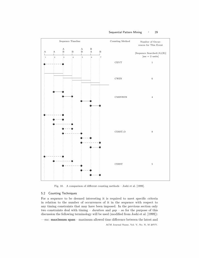
Sequential Pattern Mining · 29
Sequence Timeline Counting Method Number of Occur-
rences for This Event
[Sequence Searched:(A)(B)]
[ms = 2 units]
A A B B B A B
1 2 3 4 5 6 7
A A B
CEVT 1
CWIN 6
CMINWIN 4
CDIST O 8
CDIST 5
Fig. 10. A comparison of different counting methods – Joshi et al. [1999].
5.2 Counting Techniques
For a sequence to be deemed interesting it is required to meet specific criteriain relation to the number of occurrences of it in the sequence with respect toany timing constraints that may have been imposed. In the previous section onlytwo constraints deal with timing – duration and gap – so for the purpose of thisdiscussion the following terminology will be used (modified from Joshi et al. [1999]):
—ms: maximum span – maximum allowed time difference between the latest andACM Journal Name, Vol. V, No. N, M 20YY.

30 · C.H. Mooney, J.F. Roddick
earliest occurrences of events in the entire sequence.—ws: event-set window size – maximum allowed time difference between the
latest and earliest occurrences of events in any event-set. Here the term event-setis equivalent to the term transaction in Section 5.1.
—xg : maximum gap – maximum allowed time difference between the latest oc-currence of an event in an event-set and the earliest occurrence of an event in itsimmediately preceding event-set.
—ng : minimum gap – minimum required time difference between the earliestoccurrence of an event in an event-set and the latest occurrence of an event inits immediately preceding event-set.
These four parameters can be used to define five different counting techniques thatcan be divided into three groups. The first group CEVT (count event) searches forthe given sequence in the entire sequence timeline. The second group deals withcounting the number of windows (windows equate to the maximum span (ms))in which the given sequence occurs and consists of CWIN (count windows) andCMINWIN (count minimum windows). The third group deals with distinct eventswithin the window that is of size ms (maximum span) and comprises CDIST (countdistinct) and CDIST O (count distinct with the possibility of overlap). The use ofany of these methods depends on the specific application area and on the usersexpertise in the domain of the area being mined. Figure 10 shows the differencesbetween the counting methods, and highlights the need for careful considerationwhen choosing a counting method.
6. EXTENSIONS
6.1 Closed Frequent Patterns
The mining of frequent patterns for both sequences and itemsets has proved tobe valuable but in some cases, particularly when using candidate generation andtest techniques, and when low support is used, the performance of algorithms candegrade dramatically. This has led to algorithms such as CHARM [Zaki and Hsiao2002], CLOSET [Pei et al. 2000], CLOSET+ [Wang et al. 2003], CARPENTER [Panet al. 2003] and Frecpo [Pei et al. 2006], that produce frequent closed itemsets,which overcome some of these difficulties and produce smaller yet complete set ofresults. In the sequence mining field there are few algorithms that deal with thisproblem, however those that do are generally extensions of algorithms that mine thecomplete set of sequences with improvements in search space pruning and traversaltechniques.
A closed subsequence is a sequence that contains no super-sequence with the samesupport. Formally this is defined as follows – given a set of frequent sequences,FS, which includes all of the sequences whose support is greater than or equalto min supp, then the set of closed sequences, CS, is CS = {ϕ|ϕ ∈ FS and@γ ∈ FS such that ϕ v γ and support(ϕ) = support(γ)}. This results in CS ⊆ FSand the problem of closed sequence mining becomes the search for CS above aspecified support.
Closed Sequential pattern mining [Yan et al. 2003] follows the candidate genera-tion and test paradigm and stores the generated sets of candidates in a hash-indexedACM Journal Name, Vol. V, No. N, M 20YY.

Sequential Pattern Mining · 31
result-tree following which post-pruning is conducted to produce the closed set offrequent sequences. The algorithm uses a lexicographic sequence tree to store thegenerated sequences using both I -extension and S -extension mechanisms and thesame search tree structure as PrefixSpan to discover all of the frequent sequences(closed and non-closed). Pruning is conducted using early termination by equiva-lence, a backward sub-pattern and backward super-pattern methods.
BI-Directional Extension based frequent closed sequence mining mines frequentclosed sequences without the need for candidate maintenance [Wang and Han 2004].Furthermore pruning is made more efficient by adopting a BackScan method andthe ScanSkip optimisation technique. The mining is performed using a methodtermed BI-Directional Extension where the forward directional extension is usedto grow all of the prefix patterns and check for closure of these patterns, whilethe backward directional extension is used to both check for closure and prune thesearch space.
Closed PROjected Window Lists [Huang et al. 2005] is an extension to thePROWL algorithm [Huang et al. 2004] that mines the set of closed frequent con-tinuities. A closed frequent continuity is a continuity which has no propersuper-continuity with the same support. This is defined as follows – given two con-tinuities P = [p1, p2, . . . , pu] and P ′ = [p′1, p
′2, . . . , p
′v] then P is a super-continuity
of P ′ (and therefore P ′ is a sub-continuity of P ) if and only if, for each non-*pattern p′j (1 ≤ j ≤ w), p′j ⊆ pj+o is true for some integer o and the integer ois termed the offset of P . This added constraint marks the only difference in themining compared to that of PROWL.
In many situations, sequences are not presented to the user totally ordered andthus the search for closed partially ordered sequences can be important [Casas-Garriga 2005; Pei et al. 2005; Pei et al. 2006]. Frecpo (or Frequent closed partialorders) [Pei et al. 2006] mines strings to produce representative sequences wherethe order of some elements may not be fixed and thus can provide a more completeand in some cases a smaller set of useful results.
6.2 Hybrid Methods
DISC - DIrect Sequence Comparison [Chiu et al. 2004] combines the candidatesequence and pruning strategy, database partitioning and projection with a strategythat recognises the frequent sequences of a specific length k without having tocompute the support of the non-frequent sequences. This is achieved by usingk -sorted databases to find all frequent k -sequences, which skips many of the non-frequent k -sequences by checking only the conditional k -minimum subsequences.The basic DISC strategy is as follows. The first position in a k -sorted database istermed the candidate k-sequence and denoted by α1. Further, given a minimumsupport count of δ, the k -minimum subsequence at the δ-th position is denoted αδ.These two candidates are compared and if they are equal then α1 is frequent sincethe first δ customer sequences in the k -sorted database take α1 as their k -minimumsubsequence and if α1 < αδ then α1 is non-frequent and all subsequences up to andincluding αδ can be skipped. This process is then repeated for the next k -minimumsubsequence in the resorted k -sorted database. The proposed algorithm uses apartitioning method similar to SPADE [Zaki 2001b], SPAM [Ayres et al. 2002] andPrefixSpan [Pei et al. 2001] for generating frequent 2-sequences and 3-sequences and
ACM Journal Name, Vol. V, No. N, M 20YY.
32 · C.H. Mooney, J.F. Roddick
then employs the DISC strategy to generate the remaining frequent sequences.
6.3 Approximate Methods
ApproxMAP - Approximate Multiple Alignment Pattern mining [Kum et al. 2002;Kum et al. 2007b] mines consensus patterns from large databases by a two stepstrategy. A consensus pattern is one shared by many sequences and covers manyshort patterns but may not be exactly contained in any one sequence. It has twosteps:
(1) In the first step sequences are clustered by similarity and then from theseclusters consensus patterns are mined directly through a process of multiplealignment. To enable the clustering of sequences a modified version of thehierarchical edit distance metric is used in a density-based clustering algorithm.Once this stage is completed, each cluster contains similar sequences and asummary of the general pattern of each cluster
(2) The second step is trend analysis. First the density for each sequence is cal-culated and the sequences in each cluster are sorted in density descending or-der, second the multiple alignment process is carried out using a weightedsequence, which records the statistics of the alignment of the sequences inthe cluster. Consensus patterns are then selected based on the parts of theweighted sequence that are shared by many sequences in the cluster using astrength threshold (similar to support) to remove items whose strength is lessthan the threshold.
Kum et al. [2007b] provide a comparison showing the reduction in the numberof patterns produced under the approximate model compared to the traditionalsupport model.
ProMFS - Probabilistic Mining Frequent Sequences - is based on estimatedstatistical characteristics of the appearance of elements of the sequence being minedand their order [Tumasonis and Dzemyda 2004]. The main thrust of this techniqueis to generate a smaller sequence based on these estimated characteristics and thenmake decisions about the original sequence based on analysis of the shorter one.Once the generation of the shorter sequence has concluded then analysis can beundertaken using GSP [Srikant and Agrawal 1996] or any other suitable algorithm.
Fuzzy logic has also been applied to the problem [Fiot et al. 2007; Hu et al. 2003;Hu et al. 2004; Hong et al. 2001]. For example, Fiot et al. [2007] propose threealgorithms, based around the PSP algorithm [Masseglia et al. 1998] for discoveringsequential patterns from numeric data that differ according to the scale of fuzzinessdesired by the user, while Hu et al. [2003] propose a fuzzy grids approach basedaround the Apriori class of miner.
6.4 Parallel Algorithms
With the discovery of sequential patterns becoming increasingly useful and the sizeof the available datasets growing rapidly there is a growing need for both efficientand scalable algorithms. To this end a number of algorithms have been developedto take advantage of distributed memory parallel computer systems and in doingso their computational power. For example, Demiriz and Zaki [2002] developedwebSPADE, a modification of the SPADE algorithm, [Zaki 2001b] to enable it to beACM Journal Name, Vol. V, No. N, M 20YY.

Sequential Pattern Mining · 33
run on shared-memory parallel computers and was developed to analyse web logdata that had been cleaned and stored in a data warehouse.
Guralnik and Karypis [2004] developed two static distribution algorithms, basedon the tree projection algorithm for frequent itemset discovery [Agrawal et al. 1999],to take advantage of either data- or task-parallelism. The data-parallel algorithmpartitions the database across different processors whereas the task-parallel algo-rithm partitions the lattice of frequent patterns, and both take advantage of adynamic load-balancing scheme.
The Par-CSP (Parallel Closed Sequential Pattern mining) algorithm [Cong et al.2005] is based on the BIDE algorithm [Wang and Han 2004] and mines closed se-quential patterns on a distributed memory system. The process is divided intoindependent tasks to minimise inter-processor communication while using a dy-namic scheduling scheme to reduce processor idle time. This algorithm also uses aload-balancing scheme.
6.5 Other Methods
Antunes and Oliveira [2003] use a modified string edit distance algorithm to detectwhether a given sequence approximately matches a given constraint, expressed asa regular language, based on a generation cost. The algorithm, ε-accepts, can beused with any algorithm that uses regular expressions as a constraint mechanismi.e. the SPIRIT [Garofalakis et al. 1999] family of algorithms.
Yang et al. [2002] developed a method that uses a compatibility matrix, a con-ditional probability matrix that specifies the likelihood of symbol substitution, inconjunction with a match metric (aggregated amount of occurrences) to discoverlong sequential patterns using primarily gene sequence data as the input.
Hingston [2002] viewed the problem of sequence mining as one of inducing a finitestate automaton model that is a compact summary of the sequential data set inthe form of a generative model or grammar and then using that model to answerqueries about the data.
All of the algorithms discussed thus far are either 1- or 2-dimensional but someresearch has been conducted on multi-dimensional sequence mining. Yu and Chen[2005] introduce two algorithms, the first of which modifies the traditional Apriorialgorithm [Agrawal and Srikant 1994] and the second by modifying the PrefixSpanalgorithm [Pei et al. 2001]. Pinto et al. [2001] propose a theme of multi-dimensionalsequential pattern mining, which integrates both multi-dimensional analysis andsequential pattern mining and further explores feasible combinations of these twomethods and makes recommendations on the proper selection with respect to par-ticular datasets.
7. INCREMENTAL MINING ALGORITHMS
The ever increasing amount of data being collected has also introduced the problemof how to handle the addition of new data and the possible non-relevance of olderdata. In common with association rule mining, there have been many methodsproposed to deal with this.
Incremental Discovery of Sequential Patterns was an early algorithm where thedatabase can be considered in two modes [Wang and Tan 1996; Wang 1997]:
ACM Journal Name, Vol. V, No. N, M 20YY.

34 · C.H. Mooney, J.F. Roddick
(1) As a single long sequence of events in which a frequent sequential pattern is asubsequence and an update is either the insertion or deletion of a subsequenceat either end.
(2) As a collection of sequences and a frequent sequential pattern as a subsequenceand an update is the insertion or deletion of a complete sequence.
Interactive Sequence Mining [Parthasarathy et al. 1999] is built on the SPADEalgorithm [Zaki 2001b] and aims to minimise the I/O and computational require-ments inherent in incremental updates and is concerned with both the additionof new customers and new transactions. It consists of two phases - the first theupdating of the supports of elements in Negative Border2 (NB) and Frequent Se-quences (FS ) and the second the addition to NB and FS beyond the first phase.The algorithm also maintains an Incremental Sequence Lattice ISL, which consistsof the frequent sequences plus sequences in the NB in the original database, alongwith the supports for each.
Incremental Sequence Extraction [Masseglia et al. 2000] is an algorithm for up-dating frequent sequences where new transactions are appended to customers whoalready exist in the original database. This is achieved by using information fromthe frequent sequences of previous mining runs. Firstly, if k is the longest frequentsequence in DB (the original database), it finds all new frequent sequences of sizej ≤ (k + 1) considering three type of sequences;
(1) Those that are embedded in DB that become frequent due to an increase insupport due to the increment database db,
(2) frequent sequences embedded in db,and
(3) those sequences of DB that become frequent by the addition of an item from atransaction in db,
and second, it finds all frequent sequences of size j > (k + 1). In the first passthe algorithm finds frequent 1-sequences by considering all items in db that occuronce and then by considering all items in DB to determine which items of db arefrequent in U (DB ∪ db), which are denoted Ldb
1 . These frequent 1-sequences canbe used as seeds to discover new frequent sequences of the following types:
(1) previous frequent sequences in DB which can be extended by items of Ldb1
(2) frequent sub-sequences in DB which are predecessor items in Ldb1
(3) candidate sequences generated from Ldb1
This process is continued iteratively (since after the first step frequent 2-sequencesare obtained to be used in the same manner as described above) until no morecandidates are generated.
Incrementally/Decreasingly Updating Sequences are two algorithms for discov-ering frequent sequences when new data is added to an original database and fordeleting old sequences that are no longer frequent after the addition of new data re-spectively [Zheng et al. 2002]. The IUS algorithm makes use of the negative border
2The negative border is the collection of all sequences that are not frequent but both of whose
generating subsequences are frequent.
ACM Journal Name, Vol. V, No. N, M 20YY.

Sequential Pattern Mining · 35
sequences and the frequent sequences of the original database in a similar fashionto the ISM algorithm [Parthasarathy et al. 1999] but introduces an added sup-port threshold for the negative border. This added support metric (Min nbd supp)means that only those sequences whose support is between the original min suppvalue and Min nbd supp can be members of the negative border set. Both prefixesand suffixes of the original frequent sequences are extended to generate candidatesfor the updated database. DUS recomputes the negative border and frequent se-quences in the updated database based on the results of a previous mining run andprunes accordingly.
Zhang et al. [2002] created two algorithms based on the non-incremental versionsfrom which they are named – GSP [Srikant and Agrawal 1996] and MFS [Zhanget al. 2001]. The problem of incremental maintenance here is one of updates viainsertions of new sequences and deletions via removal of old sequences and followsa similar pattern to previous algorithms by taking advantage of the informationfrom a previous mining run. The modifications to both GSP and MFS are based onthree observations [Zhang et al. 2002]:
(1) The portion of the database that has not been changed, which in many casesis the majority, need not be processed since the support of a frequent sequencein the updated database can be deduced by only processing the inserted anddeleted customer sequences.
(2) If a sequence is infrequent in the old database then in order for it to becomefrequent in the updated database then its support in the inserted portion hasto be large enough and therefore it is possible to determine whether a candi-date should be considered by only using the portion of the database that haschanged.
(3) If both the old database and the new updated database share a non-trivial setof common sequences, then the set of frequent sequences that have already beenmined will give a good indication of likely frequent sequences in the updateddatabase.
These observations are used to develop pruning tests in order to minimise thescanning of the old database to count the support of candidate sequences.
Incremental Sequential Pattern mining [Cheng et al. 2004] is based on the non-incremental sequential pattern mining algorithm PrefixSpan [Pei et al. 2001] anduses a similar approach to Zheng et al. [2002] by buffering semi-frequent sequences(SFS) for use as candidates for newly appearing sequences in the updated database.This buffering is achieved by using a buffer ratio µ ≤ 1 to lower the min supp andthen maintaining the set of sequences, in the original database, that meet this mod-ified min supp. The assumption is that the majority of the frequent subsequencesintroduced by the updated part of the database (D′) would come from these SFSor are already frequent in the original database (D) and therefore according toCheng et al. [2004] the SFS′ and FS′ in D′ are derived from the following cases:
(1) A pattern which is frequent in D is still frequent in D′
(2) A pattern which is semi-frequent in D becomes frequent in D′
(3) A pattern which is semi-frequent in D is still semi-frequent in D′
(4) An appended database ∆db brings new items (either frequent or semi-frequent)ACM Journal Name, Vol. V, No. N, M 20YY.

36 · C.H. Mooney, J.F. Roddick
(5) A pattern which is infrequent in D becomes frequent in D′
(6) A pattern which is infrequent in D becomes semi-frequent in D′
For cases (1)-(3) the information required to update the support and project D′ tofind all frequent/semi-frequent sequences is already in FS and SFS and is thereforea trivial exercise.
Case (4): Property: An item which does not appear in D and is brought by∆db has no information in FS or SFS.
Solution: Scan the database LDB3 for single items and then use any newfrequent item as a prefix to construct a projected database and recursively applythe PrefixSpan method to discover frequent and semi-frequent sequences.
Case (5): Property: If an infrequent sequence p′ in D becomes frequent in D′,all of its prefix subsequences must also be frequent in D′. Then at least one of itsprefix subsequences p is in FS.
Solution: Start from its frequent prefix p in FS and construct a p-projecteddatabase on D′ and use the PrefixSpan method to discover p′.
Case (6): Property: If an infrequent sequence p′ becomes semi-frequent in D′,all of its prefix subsequences must be either frequent of semi-frequent. Then atleast one of its prefix subsequences, p, is in FS or SFS.
Solution: Start from its prefix p in FS or SFS and construct a p-projecteddatabase on D′ and use the PrefixSpan method to discover p′.
The task of the algorithm is thus, given an original database D, and appendeddatabase D′, a threshold min supp, a buffer ratio µ, a set of frequent sequencesFS and a set of semi-frequent sequences, SFS, to find all FS′ in D′ [Cheng et al.2004]. This is a two step process in which LDB is scanned for single items (Case(4)) and then every pattern in FS and SFS in LDB are checked to adjust thesupport of them. If a pattern becomes frequent add it to FS′. If it meets theprojection condition (suppLDB(p) ≥ (1 − µ) ∗ min supp) then use it as a prefixto project a database as in Case (5) and if the pattern is semi-frequent add itto SFS′. Optimisation techniques dealing with pattern matching and projecteddatabase generation are also applied.
Nguyen et al. [2005] found that IncSpan may fail to mine the complete set ofsequential patterns from an updated database. Furthermore, they clarify the weak-nesses in the algorithm and provide a solution, IncSpan+ which rectifies them.The weaknesses identified are for Cases (4)-(6) and proofs are given, in the formof counter examples. For Case (4) they prove that not all single frequent/semi-frequent items can be found by scanning LDB and propose a solution that scansthe entire D′ for new single items. For Case (5) they show that it is possible thatnone of the prefix subsequences p of an infrequent sequence, p′ in D that becomesfrequent in D′ are in FS and propose to not only mine the set of FS but alsothose of SFS. For Case (6) it is shown that it is possible that none of the prefixsubsequences of p of an infrequent sequence, p′ in D that becomes semi-frequent inD′ are in FS or SFS and propose to not only mine the set of FS but also those ofSFS based on the projection condition. By implementing these changes IncSpan+not only guarantees the correctness of the incremental mining result, but also main-
3The LDB is the set of sequences in D′ which are appended with items/itemsets
ACM Journal Name, Vol. V, No. N, M 20YY.

Sequential Pattern Mining · 37
tains the complete set of semi-frequent sequences for future updates [Nguyen et al.2005].
8. AREAS OF RELATED RESEARCH
8.1 Streaming Data
Mining data streams is an area of related research that is still in its infancy, how-ever there is a significant and growing interest in the creation of algorithms toaccommodate different datasets. Among these researchers are Lin et al. [2003] wholook at a symbolic representation of time series and the implications with respectto streaming algorithms. Giannella et al. [2003] who mine frequent patterns indata stream using multiple time granularities, and Cai et al. [2004] and Teng et al.[2003] who use multidimensional regression methods to solve the problem. Lauret al. [2005] evaluate a statistical technique that biases the estimation of the sup-port of sequential patterns, so as to maximise either the precision or the recall andlimits the degradation of the any other criteria and Marascu and Masseglia [2005]use the sequence alignment method ApproxMAP [Kum et al. 2002] to find patternsin web usage data streams. A review of the field of mining data streams can befound elsewhere [Gaber et al. 2005; Aggarwal 2007].
8.2 String Matching and Searching
An older yet related field is that of approximate string matching and searching,where the strings are viewed as sequences of tokens. Research in this area has beenactive for some time and includes not only algorithms for string matching usingregular expressions [Hall and Dowling 1980; Aho 1990; Breslauer and Gasieniec1995; Bentley and Sedgewick 1997; Landau et al. 1998; Sankoff and Kruskal 1999;Chan et al. 2002; Amir et al. 2000], but also algorithms in the related area of editdistance [Wagner and Fischer 1974; Tichy 1984; Bunke and Csirik 1992; Oommenand Loke 1995; Oommen and Zhang 1996; Cole and Hariharan 1998; Arslan andEgecioglu 1999; 2000; Cormode and Muthukrishnan 2002; Batu et al. 2003; Hyyro2003]. For a survey on this field refer to the work of Navarro [2001].
There is however no reason why text cannot be viewed in the same way andAhonen et al. [Ahonen et al. 1997; 1998] and Rajman and Besancon [1998] haveapplied similar techniques, based on generalised episodes and episode rules, to textanalysis tasks.
8.3 Rule Inference
The purpose of generating frequent sequences, no matter which techniques are used,is to be able to infer some type of rule, or knowledge, from the results. For example,given the sequence A . . . B . . . C occurring in a string multiple times, rules such as:token (or event) A appears (occurs) then B and then C, can be expressed. It hasbeen argued by Padmanabhan and Tuzhilin [1996] that these types of inference,and hence the temporal patterns, have a limited expressive power. For this reasonmining for sequences and the generation of rules based on first-order temporal logic(FOTL), carried out by Padmanabhan and Tuzhilin [1996], has extended the workof Mannila et al. [1995] to include inferences of the type Since, Until, Next, Always,Sometimes, Before, After and While, by searching the database for specific patterns
ACM Journal Name, Vol. V, No. N, M 20YY.

38 · C.H. Mooney, J.F. Roddick
that satisfy a particular temporal logic formula (TLF). One disadvantage to thisapproach is that no intermediate results are obtained and thus any mining for adifferent pattern must be conducted on the complete database, which could incura significant overhead.
Hoppner and Klawonn [Hoppner 2001; Hoppner and Klawonn 2002] use modifiedrule semantics, J-Measure and rule specialisation to find temporal rules from a setof frequent patterns in a state sequence. The method described uses a windowingapproach, similar to that used to discover frequent episodes, and then imposesAllen’s interval logic [Allen 1983] to describe rules that exist within these temporalpatterns. Kam and Fu [2000] deal with temporal data for events that last over aperiod of time and introduce the concept of temporal representation and discuss theview that this can be used to express relationships between interval based events,using Allen’s temporal logic. Sun et al. [2003] use ‘Event-oriented patterns’ inorder to generate rules, with a given minimum confidence, that are in the form ofLHS
T→ e, conf(θ).
9. DISCUSSION AND FUTURE DIRECTIONS
This paper has surveyed the field of sequential pattern mining with a focus on thealgorithmic approaches required to meet different requirements and the inclusionof constraints, and counting methods for windowing based algorithms.
A number of future areas of research are likely to be explored in the future:
(1) While the rules produced from the majority of approaches are simple, in thesense they do not take into account the use of temporal logic algebras andtheir derivatives, some algorithms are starting to produce rules that are moreexpressive [Padmanabhan and Tuzhilin 1996; Sun et al. 2003]. This is an areathat will likely develop further in the future.
(2) Some sequences are an example of relative ordering in time. However, with fewexceptions, pinning some of the events to absolute time points and the implica-tion this has for pattern mining has not been investigated. For example, thereare few algorithms that could state that a given sequence occurs on Mondaysbut not on other days.
(3) More generally, accommodating interval semantics as well as point based tokensin the event stream would provide richer rulesets. This might simply be doneby adding the start and end of intervals in as tokens in the sequence but morepowerful and efficient algorithms might also be developed.
(4) The GSP algorithm [Srikant and Agrawal 1996] discussed the handling of eventsthat formed a part of a hierarchy. However, this is an aspect that has not beenpursued. Indeed, the confluence of ontologies/taxonomies and data mining isan area that has to date only received minor attention.
(5) Finally, with the improvements in incremental sequential pattern mining andthe growing field of stream data mining the need to express rules with a moreexpressive nature is becoming more appealing and has the potential to availthe sequence mining paradigm to more diverse and complex domains.
REFERENCES
Aggarwal, C. C. 2007. Data streams: models and algorithms. Springer-Verlag Inc, New York.
ACM Journal Name, Vol. V, No. N, M 20YY.

Sequential Pattern Mining · 39
Agrawal, R. and Srikant, R. 1994. Fast algorithms for mining association rules. In 20th
International Conference on Very Large Data Bases, (VLDB), J. B. Bocca, M. Jarke, andC. Zaniolo, Eds. Morgan Kaufmann, Santiago, Chile, 487–499.
Agrawal, R. and Srikant, R. 1995. Mining sequential patterns. In 11th International Con-
ference on Data Engineering (ICDE’95), P. S. Yu and A. S. P. Chen, Eds. IEEE ComputerSociety Press, Taipei, Taiwan, 3–14.
Agrawal, R. C., Aggarwal, C. C., and Prasad, V. V. V. 1999. A tree projection algorithm
for generation of frequent itemsets. In High Performance Data Mining Workshop. ACM Press,Puerto Rico.
Aho, A. 1990. Algorithms for Finding Patterns in Strings. Vol. A: Algorithms and Complexity.
MIT Press, Cambridge, MA, USA, 255 – 300.
Ahonen, H., Heinonen, O., Klemettinen, M., and Verkamo, A. I. 1997. Applying datamining techniques in text analysis. Tech Report C-1997-23, University of Helsinki, Department
of Computer Science.
Ahonen, H., Heinonen, O., Klemettinen, M., and Verkamo, A. I. 1998. Applying data miningtechniques for descriptive phrase extraction in digital document collections. In Proceedings of
the Advances in Digital Libraries Conference. IEEE Computer Society, Santa Barbara, Cali-
fornia, 2.
Albert-Lorincz, H. and Boulicaut, J.-F. 2003a. A framework for frequent sequence mining
under generalized regular expression constraints. In Proceedings of the Second International
Workshop on Inductive Databases KDID, J.-F. Boulicaut and S. Dzeroski, Eds. Rudjer BoskovicInstitute, Zagreb, Croatia, Cavtat-Dubrovnik, Croatia, 2–16.
Albert-Lorincz, H. and Boulicaut, J.-F. 2003b. Mining frequent sequential patterns under
regular expressions: A highly adaptive strategy for pushing contraints. In Proceedings of the
Third SIAM International Conference on Data Mining, D. Barbara and C. Kamath, Eds.SIAM, San Francisco, CA.
Allen, J. F. 1983. Maintaining knowledge about temporal intervals. Communications of the
ACM 26, 11, 832–843.
Amir, A., Lewenstein, M., and Porat, E. 2000. Faster algorithms for string matching with
k mismatches. In 11th Annual ACM-SIAM Symposium on Discrete Algorithms. Society for
Industrial and Applied Mathematics, San Francisco, CA, USA, 794–803.
Antunes, C. and Oliveira, A. L. 2003. Sequential pattern mining with approximated con-
straints.
Arslan, A. N. and Egecioglu, O. 1999. An efficient uniform-cost normalized edit distance
algorithm. In 6th Symposium on String Processing and Information Retrieval (SPIRE’99).IEEE Comp. Soc, Cancun, Mexico, 8–15.
Arslan, A. N. and Egecioglu, O. 2000. Efficient algorithms for normalized edit distance.
Journal of Discrete Algorithms 1, 1, 3–20.
Ayres, J., Flannick, J., Gehrke, J., and Yiu, T. 2002. Sequential pattern mining using a bitmap
representation. In 8th ACM SIGKDD International Conference on Knowledge Discovery andData Mining. ACM Press, Edmonton, Alberta, Canada, 429–435.
Batu, T., Ergun, F., Kilian, J., Magen, A., Raskhodnikova, S., Rubinfeld, R., and Sami, R.2003. A sublinear algorithm for weakly approximating edit distance. In 35th ACM Symposium
on Theory of Computing. ACM Press, San Diego, CA, USA, 316–324.
Bayardo, R. J. and Agrawal, R. 1999. Mining the most interesting rules. In 5th InternationalConference on Knowledge Discovery and Data Mining, S. Chaudhuri and D. Madigan, Eds.
ACM Press, San Diego, CA, USA, 145–154.
Bentley, J. L. and Sedgewick, R. 1997. Fast algorithms for sorting and searching strings. In 8thAnnual ACM/SIAM Symposium on Discrete Algorithms. Society for Industrial and Applied
Mathematics, New Orleans, Louisiana, USA, 360–369.
Breslauer, D. and Gasieniec, L. 1995. Efficient string matching on coded texts. In 6th An-nual Symposium on Combinatorial Pattern Matching, Z. Galil and E. Ukkonen, Eds. Springer,
Berlin, Espoo, Finland, 27–40.
ACM Journal Name, Vol. V, No. N, M 20YY.

40 · C.H. Mooney, J.F. Roddick
Bunke, H. and Csirik, J. 1992. Edit distance of run-length coded strings. In 1992 ACM/SIGAPP
Symposium on Applied Computing. ACM Press, Kansas City, Missouri, USA, 137–143.
Cai, Y. D., Clutter, D., Pape, G., Han, J., Welge, M., and Auvil, L. 2004. Maids: mining
alarming incidents from data streams. In SIGMOD ’04: Proceedings of the 2004 ACM SIGMOD
international conference on Management of data. ACM Press, Paris, France, 919–920.
Casas-Garriga, G. 2005. Summarizing sequential data with closed partial orders. In 5th SIAM
International Conference on Data Mining, H. Kargupta, J. Srivastava, and A. Chandrika Ka-
math, Eds. Vol. 119. Newport beach, CA, 380–391.
Ceglar, A. and Roddick, J. F. 2006. Association mining. ACM Computing Surveys 38, 2.
Ceglar, A., Roddick, J. F., and Calder, P. 2003. Guiding Knowledge Discovery Through
Interactive Data Mining. Idea Group Pub., Hershey, PA, 45–87. Ch. 4.
Chakrabarti, S., Sarawagi, S., and Dom, B. 1998. Mining surprising patterns using temporaldescription length. In 24th International Conference on Very Large Data Bases, (VLDB’98),
A. Gupta, O. Shmueli, and J. Widom, Eds. Morgan Kaufmann, New York, NY, 606–617.
Chan, S., Kao, B., Yip, C. L., and Tang, M. 2002. Mining emerging substrings. Tech ReportTR-2002-11, HKU CSIS.
Chen, Y. L. and Hu, Y. H. 2006. Constraint-based sequential pattern mining: The consideration
of recency and compactness. Decision Support Systems 42, 2, 1203–1215.
Cheng, H., Yan, X., and Han, J. 2004. Incspan: incremental mining of sequential patterns in
large database. In 10th ACM SIGKDD International conference on Knowledge Discovery and
Data Mining, KDD ’04. ACM Press, New York, NY, USA, Seattle, WA, USA, 527–532.
Chiu, D.-Y., Wu, Y.-H., and Chen, A. L. P. 2004. An efficient algorithm for mining frequent
sequences by a new strategy without support counting. In Proceedings of the 20th International
Conference on Data Engineering, ICDE 2004. IEEE Computer Society, Boston, MA, USA,375–386.
Cole, R. and Hariharan, R. 1998. Approximate string matching: a simpler faster algorithm. In
9th Annual ACM-SIAM Symposium on Discrete Algorithms. Society for Industrial and AppliedMathematics, San Francisco, CA, USA, 463–472.
Cong, S., Han, J., and Padua, D. A. 2005. Parallel mining of closed sequential patterns. In
Proceedings of the Eleventh ACM SIGKDD International Conference on Knowledge Discoveryand Data Mining, R. Grossman, R. Bayardo, and K. P. Bennett, Eds. ACM, Chicago, Illinois,
562–567.
Cormode, G. and Muthukrishnan, S. 2002. The string edit distance matching problem withmoves. In 13th Annual ACM-SIAM Symposium on Discrete Algorithms. Society for Industrial
and Applied Mathematics, San Francisco, CA, USA, 667–676.
Demiriz, A. and Zaki, M. J. 2002. webSPADE: A parallel sequence mining algorithm to analyzethe web log data.
El-Sayed, M., Ruiz, C., and Rundensteiner, E. A. 2004. FS-miner: efficient and incremental
mining of frequent sequence patterns in web logs. In Sixth ACM International Workshop
on Web Information and Data Management (WIDM 2004), A. H. F. Laender, D. Lee, andM. Ronthaler, Eds. ACM, Washington, DC, USA, 128–135.
Fiot, C., Laurent, A., and Teisseire, M. 2007. From crispness to fuzziness: Three algorithms
for soft sequential pattern mining. IEEE Transactions on Fuzzy Systems 15, 6, 1263–1277.
Fu, Y. and Han, J. 1995. Meta-rule-guided mining of association rules in relational databases.
In 1st International Workshop on Integration of Knowledge Discovery with Deductive andObject-Oriented Databases (KDOOD’95). Singapore, 39–46,.
Gaber, M. M., Zaslavsky, A., and Krishnaswamy, S. 2005. Mining data streams: a review.SIGMOD Record 34, 2, 18–26.
Garofalakis, M. N., Rastogi, R., and Shim, K. 1999. SPIRIT: Sequential pattern mining withregular expression constraints. In 25th International Conference on Very Large Databases,VLDB’99. Edinburgh, Scotland, 223–234.
Giannella, C., Han, J., Pei, J., Yan, X., and Yu, P. S. 2003. Mining frequent patterns indata streams at multiple time granularities. In Next Generation Data Mining, H. Kargupta,
A. Joshi, K. Sivakumar, and Y. Yesha, Eds. 191–212.
ACM Journal Name, Vol. V, No. N, M 20YY.

Sequential Pattern Mining · 41
Giannotti, F., Nanni, M., Pinelli, F., and Pedreschi, D. 2007. Trajectory pattern mining. In
13th ACM SIGKDD international conference on Knowledge discovery and data mining. ACM,San Jose, California, 330–339.
Guralnik, V., Garg, N., and Karypis, G. 2001. Parallel tree projection algorithm for sequence
mining. In Euro-Par 2001: Parallel Processing, Proceedings of the 7th International Euro-
Par Conference, R. Sakellariou, J. Keane, J. R. Gurd, and L. Freeman, Eds. Lecture Notes inComputer Science, vol. 2150. Springer, Manchester, UK, 310–320.
Guralnik, V. and Karypis, G. 2004. Parallel tree-projection-based sequence mining algorithms.
Parallel Computing 30, 4, 443–472.
Guralnik, V., Wijesekera, D., and Srivastava, J. 1998. Pattern directed mining of sequence
data. In Proceedings of the Fourth International Conference on Knowledge Discovery and DataMining (KDD-98), R. Agrawal, P. E. Stolorz, and G. Piatetsky-Shapiro, Eds. AAAI Press, New
York City, New York, 51–57.
Hall, P. A. V. and Dowling, G. R. 1980. Approximate string matching. ACM Computing
Surveys 12, 4, 381–402.
Han, J., Cheng, H., Xin, D., and Yan, X. 2007. Frequent pattern mining: current status andfuture directions. Data Mining and Knowledge Discovery 15, 1, 55–86.
Han, J., Koperski, K., and Stefanovic, N. 1997. GeoMiner: A system prototype for spatial
data mining. In ACM SIGMOD International Conference on the Management of Data, SIG-
MOD’97, J. Peckham, Ed. ACM Press, Tucson, AZ, USA, 553–556.
Han, J. and Pei, J. 2000. Mining frequent patterns by pattern growth: Methodology and impli-cations. SIGKDD Explorations Newsletter 2, 2, 14–20.
Han, J., Pei, J., Mortazavi-Asl, B., Chen, Q., Dayal, U., and Hsu, M.-C. 2000. Freespan:
frequent pattern-projected sequential pattern mining. In 6th ACM SIGKDD International
Conference on Knowledge Discovery and Data Mining. ACM Press, Boston, MA, USA, 355–359.
Han, J., Pei, J., and Yin, Y. 2000. Mining frequent patterns without candidate generation. In
Proceedings of the 2000 ACM SIGMOD International Conference on Management of Data.
SIGMOD ’00. ACM, Dallas, Texas, United States, 1–12.
Hingston, P. 2002. Using finite state automata for sequence mining. In 25th AustralasianConference on Computer Science (ACSC2002). Australian Computer Society, Inc., Melbourne,
Victoria, Australia, 105–110.
Hirate, Y. and Yamana, H. 2006a. Generalized sequential pattern mining with item intervals.
Journal of Computers 1, 3, 51–60.
Hirate, Y. and Yamana, H. 2006b. Sequential pattern mining with time intervals. In 10thPacific-Asia Conference on Knowledge Discovery and Data Mining (PAKDD 2006). LNCS,
vol. 3918. Singapore, 775–779.
Hong, T. P., Lin, K. Y., and Wang, S. L. 2001. Mining fuzzy sequential patterns from multiple-
item transactions. In Joint 9th IFSA World Congress and 20th NAFIPS International Con-ference. Vol. 3. IEEE, Vancouver, Canada, 1317–1321 vol. 3.
Hoppner, F. 2001. Discovery of temporal patterns - learning rules about the qualitative behaviour
of time series.
Hoppner, F. and Klawonn, F. 2002. Finding informative rules in interval sequences. Intelligent
Data Analysis 6, 6, 237–255.
Hsu, C. M., Chen, C. Y., Liu, B. J., Huang, C. C., Laio, M. H., Lin, C. C., and Wu, T. L.2007. Identification of hot regions in protein-protein interactions by sequential pattern mining.
BMC bioinformatics 8, Suppl 5, S8.
Hu, Y. C., Chen, R. S., Tzeng, G. H., and Shieh, J. H. 2003. A fuzzy data mining algorithm for
finding sequential patterns. International Journal of Uncertainty, Fuzziness and KnowledgeBased Systems 11, 2, 173–194.
Hu, Y. C., Tzeng, G. H., and Chen, C. M. 2004. Deriving two-stage learning sequences from
knowledge in fuzzy sequential pattern mining. Information Sciences 159, 1-2, 69–86.
ACM Journal Name, Vol. V, No. N, M 20YY.

42 · C.H. Mooney, J.F. Roddick
Huang, J. W., Tseng, C. Y., Ou, J. C., and Chen, M. S. 2008. A general model for sequential
pattern mining with a progressive database. IEEE Transactions on Knowledge and DataEngineering 20, 9, 1153–1167.
Huang, K.-Y., Chang, C.-H., and Lin, K.-Z. 2004. PROWL: An efficient frequent continuity
mining algorithm on event sequences. In Data Warehousing and Knowledge Discovery, 6thInternational Conference, DaWaK 2004, Y. Kambayashi, M. K. M. and, and W. Woß, Eds.
Lecture Notes in Computer Science, vol. 3181. Springer, Zaragoza, Spain, 351–360.
Huang, K.-Y., Chang, C.-H., and Lin, K.-Z. 2005. ClosedPROWL: Efficient mining of closedfrequent continuities by projected window list technology. In SIAM International Conference
on Data Mining. Newport Beach, Ca.
Hyyro, H. 2003. A bit-vector algorithm for computing levenshtein and damerau edit distances.
Nordic Journal of Computing 10, 1, 29–39.
Joshi, M. V., Karypis, G., and Kumar, V. 1999. Universal formulation of sequential patterns.
Technical Report #99-21, Department of Computer Science, University of Minnesota.
Kam, P.-S. and Fu, A. W.-C. 2000. Discovering temporal patterns for interval-based events. In2nd International Conference on Data Warehousing and Knowledge Discovery (DaWaK 2000),
Y. Kambayashi, M. K. Mohania, and A. M. Tjoa, Eds. LNCS, vol. 1874. Springer, London, UK,
317–326.
Kim, C., Lim, J. H., Ng, R. T., and Shim, K. 2007. Squire: Sequential pattern mining with
quantities. Journal of Systems and Software 80, 10, 1726–1745.
Kum, H.-C., Chang, J. H., and Wang, W. 2006. Sequential pattern mining in multi-databases
via multiple alignment. Data Mining and Knowledge Discovery 12, 2, 151–180.
Kum, H.-C., Chang, J. H., and Wang, W. 2007a. Benchmarking the effectiveness of sequential
pattern mining methods. Data and Knowledge Engineering 60, 1, 30–50.
Kum, H.-C., Chang, J. H., and Wang, W. 2007b. Intelligent sequential mining via alignment: Op-timization techniques for Very Large Databases. In 11th Pacific-Asia conference on Advances
in knowledge discovery and data mining. PAKDD’07. Springer-Verlag Berlin, Heidelberg, Nan-
jing, China, 587 – 597.
Kum, H.-C., Pei, J., Wang, W., and Duncan, D. 2002. ApproxMAP: Approximate mining ofconsensus sequential patterns. In Mining Sequential Patterns from Large Data Sets, W. Wang
and J. Yang, Eds. Vol. 28. Springer Series: The Kluwer International Series on Advances inDatabase Systems, 138 – 160. Originally published as Technical Report TR02–031, UNC–CH.
See also Proc. of SDM, pp. 311–315, 2003.
Landau, G. M., Myers, E. W., and Schmidt, J. P. 1998. Incremental string comparison. SIAM
Journal on Computing 27, 2, 557–582.
Laur, P.-A., Symphor, J.-E., Nock, R., and Poncelet, P. 2005. Mining sequential patterns
on data streams: A near-optimal statistical approach. In Second International Workshop on
Knowledge Discovery from Data Streams. Porto, Portugal.
Lin, J., Keogh, E., Lonardi, S., and Chiu, B. 2003. A symbolic representation of time series,
with implications for streaming algorithms. In DMKD ’03: Proceedings of the 8th ACM SIG-MOD workshop on Research issues in data mining and knowledge discovery. ACM Press, SanDiego, California, 2–11.
Lin, M.-Y. and Lee, S.-Y. 2004. Interactive sequence discovery by incremental mining. Infor-
mation Sciences 165, 3-4, 187–205.
Luo, C. and Chung, S. M. 2004. A scalable algorithm for mining maximal frequent sequencesusing sampling. In 16th IEEE International Conference on Tools with Artificial Intelligence
(ICTAI 2004). IEEE Computer Society, Boca Raton, FL, USA, 156–165.
Ma, C. and Li, Q. 2005. Parallel algorithm for mining frequent closed sequences. In Au-tonomous Intelligent Systems: Agents and Data Mining, International Workshop, AIS-ADM
2005, V. Gorodetsky, J. Liu, and V. A. Skormin, Eds. Lecture Notes in Computer Science.Springer, St. Petersburg, Russia.
Mabroukeh, N. R. and Ezeife, C. I. 2010. A taxonomy of sequential pattern mining algorithms.
ACM Computing Surveys 43, 1, 3.
ACM Journal Name, Vol. V, No. N, M 20YY.

Sequential Pattern Mining · 43
Mannila, H. and Toivonen, H. 1996. Discovering generalized episodes using minimal occur-
rences. In 2nd International Conference on Knowledge Discovery and Data Mining (KDD’96).AAAI Press, Portland, Oregon, 146–151.
Mannila, H., Toivonen, H., and Verkamo, A. I. 1995. Discovering frequent episodes in se-
quences. In 1st International Conference on Knowledge Discovery and Data Mining (KDD-95), U. M. Fayyad and R. Uthurusamy, Eds. AAAI Press, Menlo Park, CA, USA, Montreal,
Canada, 210–215.
Mannila, H., Toivonen, H., and Verkamo, A. I. 1997. Discovery of frequent episodes in eventsequences. Data Mining and Knowledge Discovery 1, 3, 259–289.
Marascu, A. and Masseglia, F. 2005. Mining sequential patterns from temporal streaming
data. In Proceedings of the first ECML/PKDD Workshop on Mining Spatio-Temporal Data(MSTD’05), held in conjunction with the 9th European Conference on Principles and Practice
of Knowledge Discovery in Databases (PKDD’05). Porto, Portugal.
Masseglia, F., Cathala, F., and Poncelet, P. 1998. The PSP approach for mining sequentialpatterns. In 2nd European Symposium on Principles of Data Mining and Knowledge Discovery
(PKDD’98). LNAI, vol. 1510. Springer Verlag, Nantes, France, 176–184.
Masseglia, F., Poncelet, P., and Teisseire, M. 2000. Incremental mining of sequential patterns
in large databases. Technical report, LIRMM.
Masseglia, F., Teisseire, M., and Poncelet, P. 2005. Sequential pattern mining: A survey on
issues and approaches. In Encyclopedia of Data Warehousing and Mining. Vol. II. Information
Science Publishing, 1028–1032.
Miller, T. W. 2005. Data and Text Mining A Business Applications Approach. Pearson Edu-
cation Inc., Upper Saddle River, New Jersey.
Mooney, C. H. and Roddick, J. F. 2006. Marking time in sequence mining. In Australasian DataMining Conference (AusDM 2006), P. Christen, P. Kennedy, J. Li, S. Simoff, and G. Williams,
Eds. Vol. 61. Conferences in Research and Practice in Information Technology (CRPIT), Syd-
ney, Australia.
Navarro, G. 2001. A guided tour to approximate string matching. ACM Computing Sur-
veys 33, 1, 31–88.
Ng, R. T., Lakshmanan, L. V. S., Han, J., and Pang, A. 1998. Exploratory mining and pruningoptimizations of constrained associations rules. In Proceedings of the 1998 ACM SIGMOD
International Conference on Management of Data. SIGMOD ’98. ACM, Seattle, Washington,
United States, 13–24.
Nguyen, S. N., Sun, X., and Orlowska, M. E. 2005. Improvements of incspan: Incremental
mining of sequential patterns in large database. In Proceedings of the 9th Pacific-Asia Con-
ference, PAKDD 2005, T. B. Ho, D. Cheung, and H. Liu, Eds. Vol. 3518. Springer, Hanoi,Vietnam, 442–451.
Oommen, B. J. and Loke, R. K. S. 1995. Pattern recognition of strings with substitutions,insertions, deletions and generalized transpositions. In IEEE International Conference onSystems, Man and Cybernetics. Vol. 2. 1154–1159.
Oommen, B. J. and Zhang, K. 1996. The normalized string editing problem revisited. IEEE
Transactions on Pattern Analysis and Machine Intelligence 18, 6, 669–672.
Orlando, S., Perego, R., and Silvestri, C. 2004. A new algorithm for gap constrained sequencemining. In SAC Proceedings of the 2004 ACM Symposium on Applied Computing (SAC). ACM
Press, Nicosia, Cyprus, 540–547.
Ouh, J. Z., Wu, P. H., and Chen, M. S. 2001. Experimental results on a constrained basedsequential pattern mining for telecommunication alarm data. In 2nd International Conference
on Web Information Systems Engineering (WISE’01). IEEE Computer Society, Kyoto, Japan,
186–193.
Padmanabhan, B. and Tuzhilin, A. 1996. Pattern discovery in temporal databases: a temporallogic approach. In 2nd International Conference on Knowledge Discovery and Data Mining,
E. Simoudis, J. Han, and U. Fayyad, Eds. AAAI Press, Portland, Oregon, 351–354.
Pan, F., Cong, G., Tung, A. K. H., Yang, J., and Zaki, M. J. 2003. Carpenter: finding
closed patterns in long biological datasets. In 9th ACM SIGKDD International Conference
ACM Journal Name, Vol. V, No. N, M 20YY.

44 · C.H. Mooney, J.F. Roddick
on Knowledge Discovery and Data Mining (KDD ’03). ACM Press New York, NY, USA,
Washington, D.C, 637–642.
Parthasarathy, S., Zaki, M. J., Ogihara, M., and Dwarkadas, S. 1999. Incremental andinteractive sequence mining. In Proceedings of the 1999 ACM CIKM International Conference
on Information and Knowledge Management. ACM, Kansas City, Missouri, USA, 251–258.
Pei, J. and Han, J. 2002. Constrained frequent pattern mining: a pattern-growth view. SIGKDD
Explorations 4, 1, 31–39.
Pei, J., Han, J., and Lakshmanan, L. V. S. 2001. Mining frequent itemsets with convertibleconstraints. In Proceedings of the 17th International Conference on Data Engineering. IEEE
Computer Society, Washington, DC, USA, 433–442.
Pei, J., Han, J., and Mao, R. 2000. CLOSET: An efficient algorithm for mining frequent closed
itemsets. In ACM SIGMOD International Workshop on Data Mining. ACM Press, Dallas,
Texas, 21–30.
Pei, J., Han, J., Mortazavi-Asl, B., Pinto, H., Chen, Q., Dayal, U., and Hsu, M.-C. 2001.PrefixSpan mining sequential patterns efficiently by prefix projected pattern growth. In 2001
International Conference of Data Engineering (ICDE’01). Heidelberg, Germany, 215–226.
Pei, J., Han, J., Mortazavi-Asl, B., and Zhu, H. 2000. Mining access patterns efficiently from
web logs. In 4th Pacific-Asia Conference, (PAKDD 2000). LNCS, vol. 1805. Kyoto, Japan,,396–407.
Pei, J., Han, J., and Wang, W. 2002. Mining sequential patterns with constraints in large
databases. In 11th International Conference on Information and Knowledge Management.
ACM Press, McLean, Virginia, USA, 18–25.
Pei, J., Han, J., and Wang, W. 2007. Constraint-based sequential pattern mining: the pattern-growth methods. Journal of Intelligent Information Systems 28, 2, 133–160.
Pei, J., Liu, J., Wang, H., Wang, K., Yu, P. S., and Wang, J. 2005. Efficiently mining frequent
closed partial orders. In 5th IEEE International Conference on Data Mining. IEEE, Houston,
Texas, 753–756.
Pei, J., Wang, H., Liu, J., Wang, K., Wang, J., and Yu, P. S. 2006. Discovering frequent closedpartial orders from strings. IEEE Transactions on Knowledge and Data Engineering 18, 11,
1467–1481.
Pinto, H., Han, J., Pei, J., Wang, K., Chen, Q., and Dayal, U. 2001. Multi-dimensional
sequential pattern mining. In 10th International Conference on Information and KnowledgeManagement. ACM Press, Atlanta, Georgia, USA, 81–88.
Rajman, M. and Besancon, R. 1998. Text mining – knowledge extraction from unstructuredtextual data. In 6th Conference of International Federation of Classification Societies (IFCS-
98). Rome.
Sankoff, D. and Kruskal, J. B. 1999. Time warps, string edits, and macromolecules / The
theory and practice of sequence comparison, Reissue ed. ed. David Hume series. Center for theStudy of Language and Information, Stanford, Calif.
Savary, L. and Zeitouni, K. 2005. Indexed bit map (ibm) for mining frequent sequences. InPKDD Knowledge Discovery in Databases: PKDD 2005, 9th European Conference on Princi-
ples and Practice of Knowledge Discovery in Databases, A. Jorge, L. Torgo, P. Brazdil, R. Ca-macho, and J. a. Gama, Eds. Lecture Notes in Computer Science, vol. 3721. Springer, Porto,
Portugal, 659–666.
Seno, M. and Karypis, G. 2001. LPMiner: An algorithm for finding frequent itemsets usinglength-decreasing support constraint. In 1st IEEE Conference on Data Mining.
Seno, M. and Karypis, G. 2002. SLPMiner: An algorithm for finding frequent sequential patternsusing length-decreasing support. Technical Report #02-023, University of Minnesota.
Seno, M. and Karypis, G. 2005. Finding frequent patterns using length-decreasing supportconstraints. IEEE Transactions on Knowledge and Data Engineering 10, 3, 197–228.
Srikant, R. and Agrawal, R. 1996. Mining sequential patterns: Generalizations and perfor-
mance improvements. In 5th International Conference on Extending Database Technology,(EDBT’96), P. M. G. Apers, M. Bouzeghoub, and G. Gardarin, Eds. LNCS, vol. 1057. Springer,
Avignon, France, 3–17.
ACM Journal Name, Vol. V, No. N, M 20YY.

Sequential Pattern Mining · 45
Srivastava, J., Cooley, R., Deshpande, M., and Tan, P.-N. 2000. Web usage mining: Discovery
and applications of usage patterns from web data. SIGKDD Explorations 1, 2, 12–23.
Sun, X., Orlowska, M. E., and Zhou, X. 2003. Finding event-oriented patterns in long temporal
sequences. In 7th Pacific-Asia Conference, PAKDD 2003, K.-Y. Whang, J. J. and, K. S. and,and J. Srivastava, Eds. LNCS, vol. 2637. Springer, Seoul, Korea, 15–26.
Teng, W.-G., Chen, M.-S., and Yu, P. S. 2003. A regression-based temporal pattern miningscheme for data streams. In VLDB 2003, Proceedings of 29th International Conference on Very
Large Data Bases, J. C. Freytag, P. C. Lockemann, S. Abiteboul, M. J. Carey, P. G. Selinger,
and A. Heuer, Eds. Morgan Kaufmann, Berlin, Germany, 93–104.
Tichy, W. F. 1984. The string-to-string correction problem with block moves. ACM Transactions
on Computer Systems (TOCS) 2, 4, 309–321.
Toivonen, H. 1996. Discovery of frequent patterns in large data collections. Technical report
a-1996-5, Department of Computer Science, University of Helsinki.
Tumasonis, R. and Dzemyda, G. 2004. The probabilistic algorithm for mining frequent se-
quences. In ADBIS (Local Proceedings).
Wagner, R. A. and Fischer, M. J. 1974. The string-to-string correction problem. Journal of
the ACM (JACM) 21, 1, 168–173.
Wang, J. and Han, J. 2004. Bide: Efficient mining of frequent closed sequences. In Proceedingsof the International Conference on Data Engineering (ICDE’04). Boston, MA.
Wang, J., Han, J., and Pei, J. 2003. CLOSET+: searching for the best strategies for miningfrequent closed itemsets. In 9th ACM SIGKDD International Conference on Knowledge Dis-
covery and Data Mining, L. Getoor, T. E. Senator, P. Domingos, and C. Faloutsos, Eds. ACM
Press, Washington, DC, USA, 236–245.
Wang, K. 1997. Discovering patterns from large and dynamic sequential data. Journal of Intel-
ligent Information Systems 9, 1, 33–56.
Wang, K. and Tan, J. 1996. Incremental discovery of sequential patterns. In ACM SIGMOD
Workshop on Research Issues on Data Mining and Knowledge Discovery. Montreal, Canada.
Wang, K., Xu, Y., and Yu, J. X. 2004. Scalable sequential pattern mining for biological se-
quences. In 13th ACM International Conference on Information and Knowledge Management(CIKM’04). ACM, Washington D.C., 178–187.
Wu, P. H., Peng, W. C., and Chen, M. S. 2001. Mining sequential alarm patterns in a telecom-
munication database. In Databases in Telecommunications II, W. Jonker, Ed. LNCS, vol. 2209.Springer, 37–51.
Yan, X., Han, J., and Afshar, R. 2003. CloSpan: Mining closed sequential patterns in largedatasets. In 2003 SIAM International Conference on Data Mining (SDM’03). San Fransisco,
CA.
Yang, J., Wang, W., Yu, P. S., and Han, J. 2002. Mining long sequential patterns in a noisy
environment. In ACM SIGMOD International Conference on Management of Data (SIG-
MOD’02).
Yang, Z. and Kitsuregawa, M. 2005. LAPIN-SPAM: An improved algorithm for mining se-quential pattern. In ICDEW ’05: Proceedings of the 21st International Conference on DataEngineering Workshops. IEEE Computer Society, Tokyo, Japan, 1222.
Yang, Z., Wang, Y., and Kitsuregawa, M. 2005. LAPIN: Effective sequential pattern mining al-gorithms by last position induction. In The 21st International Conference on Data Engineering
(ICDE 2005). Tokyo, Japan.
Yu, C.-C. and Chen, Y.-L. 2005. Mining sequential patterns from multidimensional sequencedata. IEEE Transactions on Knowledge and Data Engineering 17, 1, 136–140.
Yun, U. and Leggett, J. J. 2006. WSpan: Weighted sequential pattern mining in large sequencedatabases. In 3rd International IEEE Conference on Intelligent Systems. IEEE, London, 512–
517.
Zaki, M., Lesh, N., and Ogihara, M. 1998. Planmine: Sequence mining for plan failures. In 4th
International Conference on Knowledge Discovery and Data Mining (KDD’98), R. Agrawal,
ACM Journal Name, Vol. V, No. N, M 20YY.

46 · C.H. Mooney, J.F. Roddick
P. Stolorz, and G. Piatetsky-Shapiro, Eds. ACM Press, New York, NY, 369–373. A more de-
tailed version appears in Artificial Intelligence Review, special issue on the Application of DataMining, 1999.
Zaki, M. J. 1998. Efficient enumeration of frequent sequences. In 7th International Conference
on Information and Knowledge Management. ACM Press, Bethesda, Maryland, United States,68–75.
Zaki, M. J. 2000. Sequence mining in categorical domains: Incorporating constraints. In 9th
International Conference on Information and Knowledge Management (CIKM2000), A. Agah,
J. Callan, and E. Rundensteiner, Eds. ACM Press, McLean, VA, USA, 422–429.
Zaki, M. J. 2001a. Parallel sequence mining on shared-memory machines. Journal of Paralleland Distributed Computing 61, 3, 401–426.
Zaki, M. J. 2001b. SPADE: An efficient algorithm for mining frequent sequences. Machine
Learning 42, 1/2, 31–60.
Zaki, M. J. and Hsiao, C.-J. 2002. CHARM: An efficient algorithm for closed itemset mining.In 2nd SIAM International Conference on Data Mining (SDM’02), R. L. Grossman, J. Han,
V. Kumar, H. Mannila, and R. Motwani, Eds. SIAM, Arlington, VA, USA, 457–473.
Zhang, M., Kao, B., Cheung, D. W.-L., and Yip, C. L. 2002. Efficient algorithms for incremental
update of frequent sequences. In Pacific-Asia Conference on Knowledge Discovery and DataMining. 186–197.
Zhang, M., Kao, B., Yip, C., and Cheung, D. 2001. A GSP-based efficient algorithm for mining
frequent sequences. In In Proceedings of IC-AI’001. Las Vegas, Nevada, USA.
Zhao, Q. and Bhowmick, S. S. 2003. Sequential pattern mining: A survey. Tech. rep., NanyangTechnological University, Singapore.
Zheng, Q., Xu, K., Ma, S., and Lv, W. 2002. The algorithms of updating sequential patterns. In
5th International Workshop on High Performance Data Mining, in conjunction with the 2ndSIAM Conference on Data Mining.
ACM Journal Name, Vol. V, No. N, M 20YY.