Clim. Past, 7, 1041–1059, 2011www.clim-past.net/7/1041/2011/doi:10.5194/cp-7-1041-2011© Author(s) 2011. CC Attribution 3.0 License.

Climateof the Past

Sensitivity of interglacial Greenland temperature andδ18O:ice core data, orbital and increased CO2 climate simulations

V. Masson-Delmotte1, P. Braconnot1, G. Hoffmann1, J. Jouzel1, M. Kageyama1, A. Landais1, Q. Lejeune1, C. Risi2,L. Sime3, J. Sjolte4, D. Swingedouw1, and B. Vinther4

1Laboratoire des Sciences du Climat et de l’Environnement, UMR8212, CEA-CNRS-UVS, Gif-sur-Yvette, France2CIRES, U. Colorado, Boulder, USA3British Antarctic Survey, Cambridge, UK4Centre for Ice and Climate, Niels Bohr Institute, University of Copenhagen, Copenhagen, Denmark

Received: 17 May 2011 – Published in Clim. Past Discuss.: 23 May 2011Revised: 2 September 2011 – Accepted: 2 September 2011 – Published: 29 September 2011

Abstract. The sensitivity of interglacial Greenland tem-perature to orbital and CO2 forcing is investigated usingthe NorthGRIP ice core data and coupled ocean-atmosphereIPSL-CM4 model simulations. These simulations were con-ducted in response to different interglacial orbital configu-rations, and to increased CO2 concentrations. These differ-ent forcings cause very distinct simulated seasonal and lat-itudinal temperature and water cycle changes, limiting theanalogies between the last interglacial and future climate.However, the IPSL-CM4 model shows similar magnitudes ofArctic summer warming and climate feedbacks in responseto 2× CO2 and orbital forcing of the last interglacial period(126 000 years ago).

The IPSL-CM4 model produces a remarkably linear re-lationship between TOA incoming summer solar radiationand simulated changes in summer and annual mean centralGreenland temperature. This contrasts with the stable iso-tope record from the Greenland ice cores, showing a multi-millennial lagged response to summer insolation. Duringthe early part of interglacials, the observed lags may be ex-plained by ice sheet-ocean feedbacks linked with changes inice sheet elevation and the impact of meltwater on ocean cir-culation, as investigated with sensitivity studies.

A quantitative comparison between ice core data and cli-mate simulations requires stability of the stable isotope –temperature relationship to be explored. Atmospheric sim-ulations including water stable isotopes have been conductedwith the LMDZiso model under different boundary condi-tions. This set of simulations allows calculation of a temporal

Correspondence to:V. Masson-Delmotte(valerie.masson@cea.fr)

Greenland isotope-temperature slope (0.3–0.4 ‰ per◦C)during warmer-than-present Arctic climates, in response toincreased CO2, increased ocean temperature and orbital forc-ing. This temporal slope appears half as large as the modernspatial gradient and is consistent with other ice core esti-mates. It may, however, be model-dependent, as indicatedby preliminary comparison with other models. This sug-gests that further simulations and detailed inter-model com-parisons are also likely to be of benefit.

Comparisons with Greenland ice core stable isotope datareveals that IPSL-CM4/LMDZiso simulations strongly un-derestimate the amplitude of the ice core signal duringthe last interglacial, which could reach +8–10◦C at fixed-elevation. While the model-data mismatch may result frommissing positive feedbacks (e.g. vegetation), it could also beexplained by a reduced elevation of the central Greenland icesheet surface by 300–400 m.

1 Introduction

Greenland ice cores, such as the longest NorthGRIP record,spanning the last 123 000 years (NorthGRIP-community-members, 2004), offer continuous and quantitative archivesof past local climate variability at orbital time scales(e.g. Vinther et al., 2009) as well as the evidence for abruptclimate events (e.g. Capron et al., 2010a). Ice core data allowus to explore the past magnitudes and rates of changes of cen-tral Greenland temperature prior to the instrumental period(Masson-Delmotte et al., 2006a), even with uncertainties re-lated to the conversion of ice core proxies into past temper-atures, to the age scales, and to the glaciological processes(Vinther et al., 2009).

Published by Copernicus Publications on behalf of the European Geosciences Union.

1042 V. Masson-Delmotte et al.: Sensitivity of interglacial Greenland temperature andδ18O

In principle, these data can provide a benchmark to test theability of climate models to correctly represent climate feed-backs (Otto-Bliesner et al., 2006). Past changes in orbitalforcing indeed provide natural externally forced experimentson the Earth’s climate, leading to past interglacial periodswith Arctic temperatures warmer than present-day and largechanges in Greenland ice sheet volume (Kopp et al., 2009;Vinther et al., 2009). In particular, the last interglacial pe-riod, about 130–120 thousand years before present (ka), isproposed to be a good analogue for future climate changedriven by anthropogenic greenhouse gas emissions (Clarkand Huybers, 2009; Otto-Bliesner et al., 2006; Sime et al.,2009; Turney and Jones, 2010), especially in the Arctic.

In this manuscript, we address the following questions:

– What is the Greenland ice core quantitative informationon past surface temperature changes during the currentand last interglacial, and how is it related to orbital forc-ing? This requires the relationship between Greenlandsurface temperature and snowfall isotopic composition,and the various processes that can modify this relation-ship through time, to be understood.

– Which changes in Greenland climate are produced byan ocean-atmosphere model in response to different in-terglacial orbital configurations? For this purpose, weanalyze long snapshot simulations conducted with theIPSL-CM4 model forced only by the orbital configura-tion of key periods of the current and last interglacial at0, 6, 9.5, 115 and 126 ka. For 126 ka, we also considera sensitivity test to a simple parameterization of Green-land ice sheet melt allowing representation of the impactof meltwater on the ocean circulation (Swingedouw etal., 2009).

– What are the analogies and differences between the cli-mate response to the forcings associated with increasedCO2 concentrations and to changes in orbital configu-ration? For this purpose, we compare the IPSL-CM4response to higher atmospheric CO2 concentrations andto the last interglacial insolation change, with a focuson Greenland climate. Indeed, climate projections (2×

and 4× CO2) give access to climate states with 3 to8◦C warmer central Greenland annual mean tempera-ture (Masson-Delmotte et al., 2006b).

– Is the climate model able to capture the magnitude ofchanges derived from the ice core data? For directmodel-data comparisons, we use the sea surface con-ditions (sea surface temperature, SST and sea ice) fromthe coupled climate model to drive its atmospheric com-ponent equipped with the explicit modeling of precipita-tion isotopic composition (LMDZiso). This also allowsthe stability of the isotope-temperature change throughtime and the mechanisms that can alter this relationshipto be explored.

– What was the change in central Greenland ice sheet to-pography during the last interglacial? The IPSL-CM4and LMDZiso simulations appear to underestimate themagnitude of last interglacial temperature and precip-itation isotopic composition changes compared to theGreenland ice core data. Assuming that the model-datamismatch is mainly caused by a reduced ice sheet ele-vation, we can estimate the magnitude of this elevationchange.

In order to address these questions, Sect. 2 is dedicated tothe information obtained from the NorthGRIP ice core. Sec-tion 3 describes the results of the IPSL-CM4 coupled ocean-atmosphere model climate under different orbital configu-rations. The response of the central Greenland climate toorbital forcing is also compared to its response to projec-tions of higher greenhouse gas concentrations. An analysisof the key radiative feedbacks affecting the top of the atmo-sphere radiative budget is proposed. In Sect. 4, we investigatethe Greenland isotope-temperature relationship for warmer-than-present climates using isotopic atmospheric general cir-culation models (LMDZiso and HadAM3iso) and discuss theimplications for past central Greenland temperature and pos-sible elevation changes.

2 Ice core information on past Greenland temperature

2.1 Water stable isotopes – climate relationships

Continuous records of water stable isotopes (δ18O or δD)have been measured along several deep Greenland ice cores;the longest record published so far was obtained fromthe NorthGRIP ice core (NorthGRIP-community-members,2004) (Fig. 1). The initial vapour is formed by evaporationat the ocean surface. Its isotopic composition is affected byevaporation conditions through equilibrium and kinetic frac-tionation processes, and it depends on moisture sources tem-perature and relative humidity. Along the air mass trajec-tories to Greenland, the isotopic composition of the atmo-spheric water vapour undergoes mixing by convection, up-load of new water vapor from different sources, and distilla-tion linked with the progressive air mass cooling and succes-sive condensation, as well as kinetic effects on ice crystals.Altogether, these physical processes result in a linear rela-tionship between the air temperature and the snowfall iso-topic composition in central Greenland. Forδ18O, the slopeof the modern spatial relationship is 0.7 ‰ per◦C for the firstice core sites (e.g. Dye 3, Camp Century) (Dansgaard, 1964),and 0.8 ‰ per◦C for all available data including coastal sta-tions (Dansgaard, 1964; Sjolte et al, 2011).

In addition to the impact of condensation temperature, sev-eral effects can affect the precipitation isotopic compositionand modify the temporal isotope-temperature relationship

– deposition effects, caused by precipitation intermittencyor changes in the relationship between the temperature

Clim. Past, 7, 1041–1059, 2011 www.clim-past.net/7/1041/2011/

V. Masson-Delmotte et al.: Sensitivity of interglacial Greenland temperature andδ18O 1043

-44

-42

-40

-38

-36

-34

-32

-30

NG

RIP

δ18

O (o / oo

)

140120100806040200Age (ky)

-25

-20

-15

-10

-5

0

NG

RIP ΔT (°C

)

40x10-3200

-20-40

Precession

0.420.410.400.39

Obl

iqui

ty

40x10-3

30

20

10

Eccentricity

280

260

240

220

200CO

2 (p

pmv)

-80

-40

0 Sea level (m)

560

520

48075°N

June

(W/m

²)

0 6 9.5 115122

126

Fig. 1. From top to bottom: black dots, atmospheric CO2 concen-tration (Vostok and EDC ice cores) on the EDC3 age scale (Barnolaet al., 1987; Lourantou et al., 2010); solid black line with uncer-tainties, estimation of eustatic sea level (Waelbroeck et al., 2002);NorthGRIP ice coreδ18O data on a 20 year resolution on GICC05and EDC3 age scale (Capron et al., 2010a). The orbital componentof the record is displayed (thick black line) and was calculated usingthe first three components of a singular spectrum analysis. A tenta-tive estimate of the temperature change is also displayed, followingMasson-Delmotte et al. (2005b) (right axis). The reconstruction ofthe Holocene Greenland temperature (at fixed elevation) (Vinther etal., 2009) is displayed as a bold blue line. Summer (red) and annualmean (green) temperature anomalies simulated by the IPSL modelare displayed as open circles for 6, 9.5, 115, 122, and 126 ka. The75◦ N June insolation (black line, W m−2) and orbital parameters(precession parameter – long dashed line, obliquity – short dashedline, and eccentricity – solid black line) are displayed in the twolowest panels.

at the condensation level and the surface tempera-ture (Jouzel et al., 1997). Modern observations sug-gest greater summer than winter precipitation in cen-tral Greenland (Shuman et al., 1995), which differsfrom deposition seasonality in Antarctica (Laepple et

al., 2011). Atmospheric models have shown a largedeposition effect for Greenland glacial climate, due tostrongly reduced winter precipitation (Krinner et al.,1997; Werner et al., 2000). In this manuscript, weassess the “precipitation-weighting effect” by compar-ing the average temperature change to the monthlyprecipitation-weighted temperature change;

– source effects, caused by changes in evaporation condi-tions or moisture origin (Johnsen et al., 1989; Jouzel etal., 2007; Masson-Delmotte et al., 2005a,c);

– glaciological effects, caused by changes in ice sheettopography which affects surface air temperature andstable isotopic composition (Vinther et al., 2009). Wetherefore introduce the notion of temperature estimate“at fixed elevation”, by contrast with the information onair temperature at the ice sheet surface classically de-rived from stable isotope data (Masson-Delmotte et al.,2005a).

Alternative information on past Greenland temperature isavailable from the borehole temperature profiles (Dahl-Jensen et al., 1998) and from firn gas fractionation dur-ing abrupt warmings (Capron et al., 2010a; Severinghauset al., 1998). The latter method allows the estimation ofthe interstadial isotope-temperature slope to range between0.30± 0.05 and 0.60± 0.05 ‰ ofδ18O per◦C (Capron et al.,2010a), therefore quite different from the spatial slope. Thislikely results from deposition and source effects (Masson-Delmotte et al., 2005a). In Sect. 4, we will use isotopic sim-ulations to quantify the isotope-temperature relationship inwarmer-than-present climate conditions.

2.2 Greenland Holocene climate and ice sheet elevation

Recently, Vinther et al. (2009) conducted a synthesis ofthe Greenland ice core Holocene stable isotope information.It combines ice core records from coastal ice caps (wherechanges in elevation are limited) and from the central icesheet (where higher elevation changes can significantly af-fect the isotopic signals). The authors extract a common andhomogeneous annual mean Greenland temperature signal “atfixed elevation”, together with regional changes in the icesheet topography. The new “fixed elevation” temperature his-tory from this study (Fig. 1, central panel, blue line) reveals apronounced Holocene climatic optimum in Greenland coin-ciding with a maximum thinning near the ice sheet margins.These results also imply that the NorthGRIP ice coreδ18Odata can be converted to temperature with a temporal slopeof 0.45 ‰ per◦C.

They calculate that the elevation of the NorthGRIP sitehas decreased by∼140 m since 9.5 kyr and by∼60 m from6 ka to present. The central Greenland temperature “at fixedelevation” is estimated to be∼2.3◦C higher at 9.5 ka and∼2.0◦C at 6 ka than during the last millennium, with a multi-millennial warm plateau encountered between 9.3 and 6.8 ka.

www.clim-past.net/7/1041/2011/ Clim. Past, 7, 1041–1059, 2011

1044 V. Masson-Delmotte et al.: Sensitivity of interglacial Greenland temperature andδ18O

This plateau occurs 1.8 to 4.3 kyr (thousand years) later thanthe maximum in 75◦ N June insolation. The early Holocenewarmth is partly masked in the central Greenland ice corestable isotope records because of the larger volume and ele-vation of the ice sheet.

2.3 Links between NorthGRIPδ18O and 75◦ N summerinsolation

We extract the orbital components of the NorthGRIP recordusing the first components of a Singular Spectrum Analy-sis performed on the whole series and corresponding to pe-riodicities longer than 3 kyr (Fig. 1, bold line, central panel).With the available ice core age scales (Capron et al., 2010b;Svensson et al., 2008), the orbital component of the North-GRIP δ18O appears to lag the reversed precession parame-ter (in phase with local June insolation) by several millen-nia (Fig. 1). A significant correlation (R2 = 0.27) is obtainedbetween the smoothed NorthGRIPδ18O and 4 kyr earlier75◦ N June insolation. The four most recent optima in thissmoothed NorthGRIPδ18O record lag maxima in 75◦ N Juneinsolation by 4.8, 4.8, 3.1 and 3.5 kyr, respectively (Fig. 1,dashed vertical lines). These lags are significantly largerthan the GICC05 (Rasmussen et al., 2006; Svensson et al.,2008)) age scale uncertainty (∼80 years at 10 ka,∼440 yearsat 20 ka,∼1000 years at 30 ka and∼2600 years at 60 ka) andoccur both under glacial and interglacial contexts.

For the Holocene, it is obvious that the Greenland op-timum (at ∼7–10 ka) occurs later than the 11 ka preces-sion minimum (local June insolation maximum), likely be-cause of the negative feedback linked with the Laurentideice sheet albedo and weaker northward advection of heat inthe Atlantic Ocean caused by the meltwater from deglaciat-ing Northern Hemisphere ice sheets (Renssen et al., 2009).The NorthGRIP record does not allow this aspect to beexplored for the last interglacial because it does not spanthe whole length of this period (NorthGRIP-community-members, 2004). Marine sediment records of North At-lantic sea surface temperature suggest a pattern similar to theHolocene with a lag between peak insolation and peak iso-topic values (Masson-Delmotte et al., 2010a). During theend of the interglacials (after optima in insolation and inδ18O), parallel decreasing trends in 75◦ N June insolation andNorthGRIPδ18O are observed. For the mid to late Holocene(the last 8 kyr), theδ18O-insolation slope is 0.02 ‰ perW m−2 (0.03 to 0.06◦C per W m−2), much weaker thanfor the end of the last interglacial (121 to 115 ka), where itreaches 0.10 ‰ per W m−2 (∼0.17 to 0.33◦C per W m−2).

2.4 Last interglacial Greenland climate

The ice core information on central Greenland climate dur-ing the last interglacial is not as precise as for the Holocenedue to the age scale uncertainty, the end of the NorthGRIPrecord at∼123 ka, and the lack of information from borehole

thermometry to constrain the isotope-temperature-elevationhistories. Based on the shape of north Atlantic SST recordssynchronized on the EDC3 age scale (Masson-Delmotte etal., 2010a), one may assume that the isotopic values of thedeepest part of the NorthGRIP ice core may be represen-tative of a multi-millennial temperature plateau. Consider-ing the uncertainty on the isotope-temperature relationship(between 0.3 and 0.8 ‰ per◦C), the NorthGRIP Last In-terglacial∼3 ‰ δ18O anomaly would translate into a 3.8–10.0◦C surface temperature anomaly. The signal for the lastinterglacial is without doubt larger than for the early to midHolocene (see Sect. 2.2), as expected from the larger orbitalforcing (Fig. 1).

By themselves, the data do not allow us to quantify thedeposition or glaciological effects affecting this temperatureestimate, motivating the use of climate models to explore themechanisms controlling precipitation isotopic composition.

3 Climate modelling

3.1 IPSL-CM4 coupled climate model simulations

The IPSL-CM4 coupled climate model has been extensivelyused for CMIP3 and PMIP2 simulations (Alkama et al.,2008; Born et al., 2010; Braconnot et al., 2007, 2008;Kageyama et al., 2009; Marti et al., 2010; Swingedouw etal., 2006). The model couples the atmospheric componentLMDZ (Hourdin et al., 2006) with the OPA ocean compo-nent (Madec and Imbard, 1996). A sea ice model (Fichefetand Maqueda, 1997) which computes the ice thermodynam-ics and physics is coupled with the ocean-atmosphere model.The ocean and atmosphere exchange momentum, heat andfreshwater fluxes, as well as surface temperature and sea iceonce a day, using the OASIS coupler (Valcke, 2006). None ofthe fluxes are corrected or adjusted. The model is run with ahorizontal resolution of 96 points in longitude and 71 pointsin latitude (3.75◦ × 2.5◦) for the atmosphere and 182 pointsin longitude and 149 points in latitude for the ocean. Thereare 19 vertical levels in the atmosphere and 31 levels in theocean, where the highest resolution (10 m) is focused on theupper 150 m. The model reproduces the main features ofmodern climate, although large temperature or precipitationbiases can be partly related to the resolution (Marti et al.,2010). The North Atlantic is often marked by large cold bi-ases in coupled climate models. This is also the case forIPSL-CM4 where a weak Atlantic Meridional Oceanic Cir-culation (AMOC) (Swingedouw et al., 2007) is linked with acold bias for central Greenland.

The IPSL-CM4 model results have previously been com-pared with the ice core information and other model results interms of polar amplification under glacial conditions or cli-mate projection scenarios (Masson-Delmotte et al., 2006a,b)as well as briefly for the last interglacial (Masson-Delmotte

Clim. Past, 7, 1041–1059, 2011 www.clim-past.net/7/1041/2011/

V. Masson-Delmotte et al.: Sensitivity of interglacial Greenland temperature andδ18O 1045

et al., 2010b). These previous studies showed that the IPSL-CM4 model response is comparable to other climate modelsand generally seems to underestimate the magnitude of tem-perature changes compared to those derived from the ice coredata.

A set of simulations has been conducted to explore the re-sponse of the model to various orbital configurations encoun-tered during the current and last interglacial (see the grey ver-tical bars in Fig. 1 and the simulation descriptions in Table 1),with all other boundary conditions kept as for the modelcontrol simulation (pre-industrial). Small changes in atmo-spheric composition (CO2, CH4) leading to radiative pertur-bations<0.4 W m−2 during the current and last interglacialwere neglected, except for the 6 ka simulation following thePMIP2 protocol (Braconnot et al., 2007). The time periodsfor these simulations (at 0, 6, 9.5, 115, 122 and 126 ka) werechosen to represent contrasting changes in the seasonal cy-cle of insolation, with different combinations of precession(rather similar at 0 and 115 ka, 122 and 6 ka, 9.5 and 126 ka),obliquity (maximum at 9.5 and minimum at 115 ka) and ec-centricity (minimum at 0 ka and maximum at 115 ka) con-figurations (Braconnot et al., 2008). These simulations wereintegrated from 300 to 1000 years depending on the time pe-riod (Table 1). Since changes in Earth’s orbital parametersonly marginally affect the global annual mean simulations,these simulations adjust very rapidly to the insolation forc-ing (50–100 years) from the same initial state. We considerhere mean annual cycles computed from 150 to 400 years.Our analysis focuses on the most contrasting simulations,126 ka and 115 ka. Note that the Antarctic ice core data de-pict atmospheric CO2 levels close to the pre-industrial (273–276 ppmv) during these two time periods (Masson-Delmotteet al., 2010a).

We have also used a similar approach to that of Simeet al. (2008) whilst exploring different forms of warmerGreenland climates. We have therefore also analyzed sim-ulations run under projected increased CO2 concentrations.The 2× CO2 simulation has been integrated for 250 years.Beginning from a pre-industrial simulation, the atmosphericCO2 concentration is increased by 1 % per year until it dou-bles within 70 years (from 280 to 560 ppmv). It is thenkept constant for the remaining 180 years. The same pro-tocol is followed for the 4× CO2 simulation (quadrupling ofCO2 in 140 years and then kept constant for the remaining110 years). We have used the model outputs averaged overthe last 100 years of these simulations.

While the topography of the Greenland and Antarctic icesheet is constant for all the simulations, a parameterizationof Greenland melt has been implemented in order to explorethe feedbacks between Greenland warming, Greenland melt-water flux and thermohaline circulation (Swingedouw et al.,2009) with implications for monsoon areas (Braconnot et al.,2008). A simulation including this parameterisation under126 ka orbital forcing was integrated for 350 years. The ther-mohaline circulation is affected by an additional freshwater

flux and adjusts within 150 years to the forcing. After thisadjustment, the deep ocean drift is limited.

3.2 Impact of orbital forcing on IPSL-CM4 simulatedcentral Greenland climate

Figure 2 displays the model results for central Greenland us-ing the same definition as in Masson-Delmotte et al. (2006a),that is the temperature averaged at places where ice sheet el-evation is above 1.3 km. For each simulation, monthly meanvalues of central Greenland temperatures are displayed as afunction of monthly mean values of 75◦ N top of atmosphere(hereafter TOA) incoming solar radiation. The elliptic shapeof the plots reflects the one month seasonal lag between sur-face air temperature and insolation, mostly because of thethermal inertia of the surrounding oceans affecting heat ad-vection to central Greenland. Orbital forcing alone has lim-ited impacts on the simulated winter temperature (because ofa weak incoming insolation at that season and latitude) and astrong impact on summer-fall temperatures.

The simulated change in summer temperature is domi-nating the simulated annual mean temperature change (Ta-ble 2). Compared with the pre-industrial control simulation,July (respectively annual mean) temperature changes vary by−2.5◦C (−0.5◦C) for 115 ka to +5.8◦C (+0.9◦C) for 126 ka.The model results for summer and annual mean temperatureare depicted in Fig. 1 with red and green open circles, respec-tively. This comparison suggests that the IPSL-CM4 simula-tion has the right sign of temperature changes, but underes-timates the magnitude of annual mean changes compared tothe ice core derived information. We now explore the sim-ulated deposition effects, which can impact the model-datacomparison, focusing on the precipitation weighting effect.

For all orbital contexts, the IPSL-CM4 model showsa positive precipitation weighting effect (difference be-tween monthly precipitation-weighted temperature and an-nual mean temperature) (Table 2, last column). This effectis minimum at 115 ka (1.8◦C), maximum at 126 ka (5.2◦C)and is strongly enhanced with increasing local summer inso-lation. This is due to a strong (non linear) enhancement ofsummer precipitation for warmer summer temperatures (Ta-ble 2). The IPSL-CM4 model therefore points to a large de-position effect, suggesting that the Greenland ice core warmsinterglacial proxy records such as stable isotopes, but also10Be (Wagner et al., 2001; Yiou et al., 1997) may be biasedtowards summer. The simulated changes in precipitation-weighted temperature are intermediate between the summerand annual mean temperature and vary between−1.1◦C (at115 ka) and +3.6◦C (at 126 ka) (Table 2).

In the IPSL-CM4 simulations, the maximum summer tem-perature change (occurring in July) appears to be stronglylinearly related (R2 = 0.99) with maximum 75◦ N incom-ing summer insolation (occurring in June), with a slope of0.08◦C per W m−2 (Fig. 2b). We first observe that, evenconsidering this largest signal (July temperature), the model

www.clim-past.net/7/1041/2011/ Clim. Past, 7, 1041–1059, 2011

1046 V. Masson-Delmotte et al.: Sensitivity of interglacial Greenland temperature andδ18O

Table 1. Description of the simulations. The LMDZiso simulations were run for 5 years with climatological forcing averaged from theIPSL-CM4 ouputs, and results analysed for the last 3 years of this simulation. AMIP (Atmospheric Modelling Intercomparison Project)boundary conditions are derived from observed SST and sea-ice (1979 to 2007). Atmospheric composition refers to prescribed changes ingreenhouse gas concentrations (e.g. CO2). In the orbital forcing column,e, o andp respectively stand for eccentricity, obliquity (in◦), andperihelia-180◦.

Name Orbital Atmospheric Greenland Oceanforcing composition melt surface

IPSL-0 ka 0 ka pre-industrial No Calculatede = 0.016o = 23.4p = 102

IPSL-6 ka 6 ka 6 ka No Calculatede = 0.0187o = 24.1p = 0.89

IPSL-9.5 ka 9.5 ka pre-industrial No Calculatede = 0.0194o = 24.2p = 303

IPSL-115 ka 115 ka pre-industrial No Calculatede = 0.0414o = 22.4p = 111

IPSL-122 ka 122 ka pre-industrial No calculatede = 0.0407o = 23.2p = 356

IPSL-126 ka 126 ka pre-industrial No calculatede = 0.0397o = 23.9p = 291

IPSL-126 ka GM 126 ka pre-industrial Yes calculatedIPSL-2× CO2 0 ka CMIP3 No CalculatedIPSL-4× CO2 0 ka CMIP3 No calculatedLMDZiso-ctrl 0 ka 348 ppmv No Prescribed from AMIPLMDZiso-6ky 6 ka 280 ppmv No Prescribed as

AMIP + (IPSL6 kyr−IPSL0 kyr)

LMDZiso-126 kyr 126 ka 280 ppmv No Prescribed asAMIP + (IPSL126 kyr−IPSL0 kyr)

LMDZiso-126 kyr GM 126 ka 280 ppmv Prescribed Prescribed asfrom AMIP + (IPSL126 kyrIPSL-126 kyr GM GM−IPSL0 kyr)

LMDZisoSST 0 ka 280 ppmv No AMIP + 4◦CLMDZiso2× CO2 0 ka 2× 348 ppmv No IPSL2× CO2LMDZiso4x× CO2 0 ka 4× 348 ppmv No IPSL 4× CO2

response to summer insolation therefore appears at least halfas large as that derived from the ice core data for the tran-sition from 122 to 115 ka (0.17 to 0.33◦C per W m−2, seeSect. 2.3). In Sect. 3.2, we investigate the changes affecting

the top of the atmosphere radiative budget and key radiativefeedbacks in order to better describe the processes responsi-ble for such a linear model response to the orbital forcing.

Clim. Past, 7, 1041–1059, 2011 www.clim-past.net/7/1041/2011/

V. Masson-Delmotte et al.: Sensitivity of interglacial Greenland temperature andδ18O 1047

Table 2. IPSL-CM4 results for Greenland (from grid points located above 1300 m elevation): annual mean, July and precipitation-weightedtemperature (◦C) as well as deposition effect (difference between precipitation-weighted and annual mean temperature) and ratio of summer(April–September) to annual precipitation. Results are given for the different simulations in response to orbital forcing only. Absolute valuesare given as well as anomalies with respect to the control simulation (numbers shown between parentheses).

Simulation Annual mean July Greenland Ratio of summer Precipitation DepositionGreenland temperature half year (April– weighted effecttemperature (anomaly) (◦C) September) to Greenland (anomaly) (◦C)(anomaly) (◦C) annual temperature

precipitation (anomaly)(percentage of (◦C)change)

Control simulation −28.3 −12.9 0.60 −25.9 2.46 ka −27.9 (+0.4) −10.6 (+2.3) 0.62 (+3 %) −24.7 (+1.2) 3.2 (+0.7)9.5 ka −27.5 (+0.8) −8.5 (+4.4) 0.65 (+8 %) −23.3 (+2.6) 4.2 (+1.8)115 ka −28.8 (−0.5) −15.4 (−2.5) 0.58 (−3 %) −27.0 (−1.1) 1.8 (−0.7)122 ka −28.1 (+0.2) −11.9 (+1.0) 0.62 (+3 %) −25.1 (+0.8) 3.0 (+0.6)126 ka −27.4 (+0.9) −7.1 (+5.8) 0.68 (+13 %) −22.3 (+3.6) 5.2 (+2.7)

-16-14-12-10-8-6

War

mes

t mon

th T

(°C

)

560520480440Maximum monthly insolation (W/m²)

-40

-35

-30

-25

-20

-15

-10

-5

Mon

thly

tem

pera

ture

(°C

)

6005004003002001000Monthly insolation (W/m²)

y=0.08x-51.97 (R²=0.99)

a) b)

1 23

4

5

6

7

8

9

10

1112

0 6 9.5 115 122 126

Fig. 2. (a)Seasonal cycle of IPSL model simulated central Green-land (>1300 m) temperature (◦C) as a function of the seasonal cy-cle of TOA incoming solar radiation at 75◦ N (W m−2) for differentorbital configurations (0, 6, 9.5, 115, 122 and 126 ka). For eachperiod, the monthly data are displayed; black numbers indicate thenumber of the month (from 1 for January to 12 for December). Theelliptic shape results from the phase lag between temperature andinsolation. (b) Regression between maximum monthly insolationand the IPSL model central Greenland maximum monthly summertemperature (occurring one month after maximum insolation). Alinear relationship is observed, with a slope of 0.08◦C per W m−2.The same color code is used as in panel a for the various simula-tions.

When taking into account the ocean circulation changeslinked with a parameterization of Greenland melt at 126 ka,the IPSL-CM4 model simulates a 0.6◦C weaker July(resp. 0.4◦C annual) warming than in the standard 126 kasimulation (not shown in Table 2). In this simulation, the

AMOC is weakened because deep water formation in theNorth Atlantic/Nordic Seas is reduced by the Greenland icesheet meltwater. The meridional heat transport by the atmo-spheric circulation is enhanced to compensate for the reduc-tion in ocean heat transport but the Arctic cools because of alarger sea ice extent. Therefore, taking into account the im-pact of ice sheet melting on the ocean circulation increasesthe model-data mismatch.

3.3 Differences between increased CO2 and orbitallyforced IPSL-CM4 climate responses

The orbital forcing has a negligible impact as such on theglobal and annual radiative forcing (<0.3 W m−2 over thelast 130 ka), which contrasts with the 3.7 W m−2 radiativeforcing for 2× CO2 (resp. 7.4 W m−2 for 4× CO2). Notethat obliquity affects the latitudinal distribution of annual in-solation, with opposite effects at low and high latitudes (notshown), and a range of variations of resp. 4.5 to 10.5 W m−2

at 75◦ N along the current and last interglacial (0–12 ka and115–130 ka).

Moreover, the diurnal and seasonal distributions of orbitaland 2× CO2 forcings are drastically different. For 126 ka,anomalies (relative to pre-industrial) in summer insolationexceed 50 W m−2 at mid and high northern latitudes (Fig. 3a,showing TOA radiative budget) at 126 ka, with large sea-sonal and latitudinal contrasts (Fig. 3b). This differs fromthe more homogeneous forcing caused by increased CO2concentrations.

We now focus on the 126 ka simulation, because of thelarge magnitude of the seasonal insolation change causedby the combination of precession and eccentricity for thisperiod, and compare it with the 2× CO2 simulation. Fig-ure 3 (panels c and d) shows the differences between last

www.clim-past.net/7/1041/2011/ Clim. Past, 7, 1041–1059, 2011

1048 V. Masson-Delmotte et al.: Sensitivity of interglacial Greenland temperature andδ18O

   (b)  2xCO2c-­‐PRE      (a)  126Kc-­‐PRE  

Months   Months  

W/m2  

°C   °C  

(d) (c) 

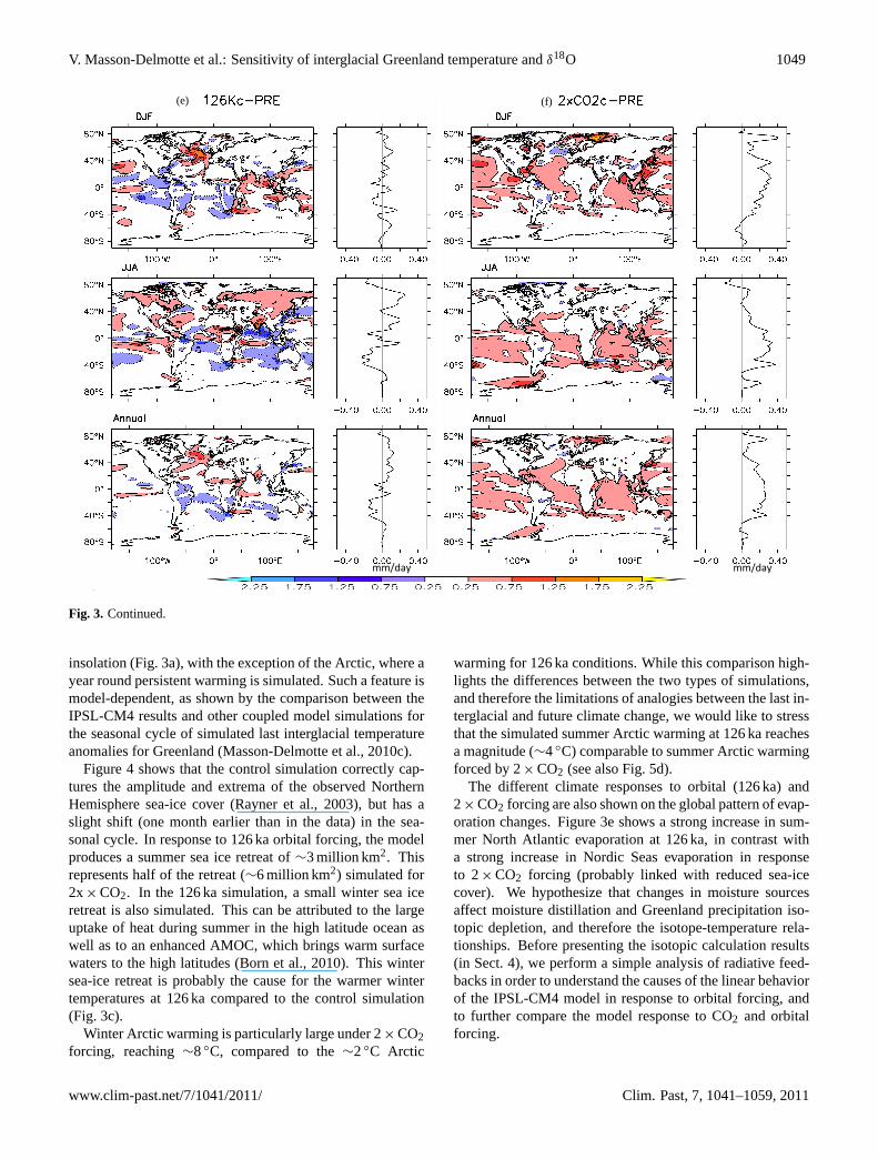
Fig. 3. Comparison of anomalies between the last interglacial and pre-industrial control IPSL model simulations (left panel) and 2× CO2and pre-industrial control simulation (right panel) for :(a) and(b) TOA net radiative budget (W m−2); (c) and(d) surface air temperature(◦C) and(e) and(f) evaporation (mm day−1). For panels(a) and(b), anomalies are displayed as a function of month number (horizontalaxis) and latitude (vertical axis). For panels(c) to (f), anomalies are displayed as a function of longitude and latitude, for DJF (December-January-February), JJA (June-July-August) and for the annual mean. On the right side of each panel(c) to (f), zonal mean anomalies are alsodisplayed as a function of latitude.

interglacial (126 ka) and pre-industrial for JJA, DJF and an-nual mean temperature, as well as their zonal mean, andcompares them to the differences between 2× CO2 andpresent day for JJA, DJF and annual mean temperature. In-creased CO2 leads to simulated warming at low latitudesand a larger magnitude of warming at both poles (relative

to pre-industrial control simulation), especially in the winterseason. By contrast the 126 ka orbital forcing leads to a smallannual mean cooling at low to mid latitudes, a small annualmean warming anomaly around 60◦ S and a large (∼4◦C)warming in the Arctic. The model response to 126 ka or-bital forcing follows the latitudinal and seasonal anomalies of

Clim. Past, 7, 1041–1059, 2011 www.clim-past.net/7/1041/2011/

V. Masson-Delmotte et al.: Sensitivity of interglacial Greenland temperature andδ18O 1049

mm/day  mm/day  

(e) (f)

Fig. 3. Continued.

insolation (Fig. 3a), with the exception of the Arctic, where ayear round persistent warming is simulated. Such a feature ismodel-dependent, as shown by the comparison between theIPSL-CM4 results and other coupled model simulations forthe seasonal cycle of simulated last interglacial temperatureanomalies for Greenland (Masson-Delmotte et al., 2010c).

Figure 4 shows that the control simulation correctly cap-tures the amplitude and extrema of the observed NorthernHemisphere sea-ice cover (Rayner et al., 2003), but has aslight shift (one month earlier than in the data) in the sea-sonal cycle. In response to 126 ka orbital forcing, the modelproduces a summer sea ice retreat of∼3 million km2. Thisrepresents half of the retreat (∼6 million km2) simulated for2x× CO2. In the 126 ka simulation, a small winter sea iceretreat is also simulated. This can be attributed to the largeuptake of heat during summer in the high latitude ocean aswell as to an enhanced AMOC, which brings warm surfacewaters to the high latitudes (Born et al., 2010). This wintersea-ice retreat is probably the cause for the warmer wintertemperatures at 126 ka compared to the control simulation(Fig. 3c).

Winter Arctic warming is particularly large under 2× CO2forcing, reaching∼8◦C, compared to the∼2◦C Arctic

warming for 126 ka conditions. While this comparison high-lights the differences between the two types of simulations,and therefore the limitations of analogies between the last in-terglacial and future climate change, we would like to stressthat the simulated summer Arctic warming at 126 ka reachesa magnitude (∼4◦C) comparable to summer Arctic warmingforced by 2× CO2 (see also Fig. 5d).

The different climate responses to orbital (126 ka) and2× CO2 forcing are also shown on the global pattern of evap-oration changes. Figure 3e shows a strong increase in sum-mer North Atlantic evaporation at 126 ka, in contrast witha strong increase in Nordic Seas evaporation in responseto 2× CO2 forcing (probably linked with reduced sea-icecover). We hypothesize that changes in moisture sourcesaffect moisture distillation and Greenland precipitation iso-topic depletion, and therefore the isotope-temperature rela-tionships. Before presenting the isotopic calculation results(in Sect. 4), we perform a simple analysis of radiative feed-backs in order to understand the causes of the linear behaviorof the IPSL-CM4 model in response to orbital forcing, andto further compare the model response to CO2 and orbitalforcing.

www.clim-past.net/7/1041/2011/ Clim. Past, 7, 1041–1059, 2011

1050 V. Masson-Delmotte et al.: Sensitivity of interglacial Greenland temperature andδ18O

Fig. 4. Monthly seasonal cycle of Northern Hemisphere sea iceextent for present day (black), 126 ka (red) and 2× CO2 (blue) sim-ulated by IPSL-CM4. Present day (1900–2010) climatological data(Rayner et al., 2003) are also displayed (dashed grey).

3.4 Analysis of radiative feedbacks

Following Braconnot et al. (2007), a simple feedback anal-ysis was performed in order to quantify the main drivers ofchanges in the top of the atmosphere radiative budget (TOA)at high latitudes (60–80◦ N). The methodology for this anal-ysis is described in Appendix A.

Figure 5 displays analyses of the TOA radiative budgetterms and key feedbacks (represented by symbols) aroundGreenland. The different simulations are represented by thesame colors as in Fig. 2. The specific radiative budgetsfor June–July are shown for all the orbitally forced simu-lations (Fig. 5a) and for each month for 126 ka (Fig. 5b)and 2× CO2 simulations (Fig. 5c). We do not display thechanges in heat and water transport and only focus on thelocal radiation fluxes within the atmospheric column.

Figure 5a characterises the radiative feedbacks involvedin the linear response of the IPSL-CM4 simulated summerGreenland surface temperature with respect to summer in-solation. At high northern latitudes, the different compo-nents of the radiative budget depict a linear relationshipwith respect to the change in incoming solar radiation at thetop of the atmosphere1SWisimul. The net TOA shortwaveflux (1SWnsimul, represented by “x”symbols) appears rel-atively close to the prescribed insolation change and onlypartially compensated for by increased longwave emission(1LWnsimul, represented by filled diamonds) so that the netradiative budget is positive (not shown).

At 6, 9.5, 122 and 126 ka, a strong positive shortwavefeedback is linked with the total (surface and cloud) albedoeffect (1ALBsimul, represented by “+” symbols). This ef-fect is dominated by the clear sky (surface) albedo ef-fect (1ALB cssimul represented by the triangle symbols),only partly compensated by an enhanced negative cloudshortwave feedback (difference between1ALB cssimul and

1ALBsimul). The albedo feedback is consistent with changesin sea ice (Fig. 4). It increases almost linearly with the insola-tion forcing, stressing that the changes in clear sky shortwavesurface radiation drive the surface radiative budget, surfacetemperature and thereby the snow and ice extent. Note thatby construction, the total albedo feedback between the dif-ferent simulations lies on a line proportional to the planetaryalbedo of the control simulation. At 115 ka, clear sky andcloud albedo feedbacks have opposite signs and have a muchsmaller magnitude (with respect to the magnitude of the or-bital forcing) compared to other orbital simulations. The dif-ferent effects are thus not symmetrical for increased or re-duced insolation, certainly due to the temperature thresholdsneeded to build and melt snow and ice.

In addition, the longwave radiative budget changes(1LWnsimul, filled diamonds) appear to be driven by thechanges in Planck emission directly caused by changes insurface temperature (1Plsimul, open diamonds). There isonly a small increase in the atmospheric greenhouse effectcaused by changes in the vertical temperature profile, wa-ter vapour content, and infra-red cloud radiative feedbacks(difference between the filled and open diamond symbols).This greenhouse feedback is too small to drive a non-linearresponse of the radiative budget around Greenland.

While this approach ignores the dynamical heat advectioneffects, it suggests that the top of the atmosphere radiativebudget at high northern latitude is relatively linear with re-spect to orbital forcing and highlights the importance of thepositive feedbacks linked with the surface albedo. The mag-nitude of the atmospheric greenhouse effect and the short-wave cloud negative feedback increase with the magnitudeof the insolation forcing. In this model, the cloud feedbackis enhanced for a warmer Arctic. Compensations of non-linearities of the Planck, albedo and cloud radiative effects at115 ka likely explain the overall linearity of the IPSL-CM4model high northern latitude temperature response to sum-mer insolation forcing.

Figure 5b and c show a comparison of the seasonal cy-cle and magnitude feedbacks at play in 126 ka and 2× CO2simulations, respectively. As previously mentioned, theyreach similar magnitudes of summer temperature changeover Greenland. As expected, the changes in greenhouseeffect are larger for the 2x× CO2forcing than for insola-tion forcing. The net radiative budget is positive in sum-mer. The net shortwave radiation reflects the total albedoeffect. Again, the clear sky albedo feedback is the dominantcontribution during summer, and the cloud feedback only ac-counts for a small fraction of changes in shortwave radiation,even though its magnitude is larger than for the insolationforcing. This comparison shows that the albedo, cloud andatmospheric greenhouse feedbacks have comparable magni-tude and sign in summer. These simulated feedbacks seemconsistent with ongoing changes related with Arctic sea-iceretreat and warming (Screen and Simmonds, 2010). Thisanalysis also highlights the different seasonality effects, with

Clim. Past, 7, 1041–1059, 2011 www.clim-past.net/7/1041/2011/

V. Masson-Delmotte et al.: Sensitivity of interglacial Greenland temperature andδ18O 1051

6

4

2

0

-2

Prec

ipita

ble

wat

er a

nom

aly

86420-2-4Temperature anomaly (°C)

-80

-60

-40

-20

0

20

40

60

80

Rad

iativ

e bu

dget

ano

mal

y (W

/m²)

121086420Month

-80

-60

-40

-20

0

20

40

60

80

Rad

iativ

e bu

dget

ano

mal

y (W

/m²)

12108642Month

-80

-60

-40

-20

0

20

40

60

80

Rad

iativ

e bu

dget

ano

mal

y (W

/m²)

-80 -40 0 40 80 ΔSWisimul (W/m²)

d) c) 2xCO2

b) 126 kaa) June-July feedbacks

115

1226 9.5126

2xCO2

126 ka

115 ka

cloud

greenhouse

summer

greenhouse

cloud

cloud

greenhouse

summer

winter

winter

summer

winter

ΔSWisimul

ΔSWnsimul

ΔALB cssimul

ΔALB simul

ΔLWnsimul

ΔPlsimul

Fig. 5. Analysis of atmospheric feedbacks affecting the TOA radiative budget.(a) June–July changes in radiative budget terms (see textand figure legend for details) as a function of June-July incoming solar radiation (W m−2), for different orbital contexts (6 ka, orange;9.5 ka, violet; 115 ka, green; 122 ka, pink; and 126 ka, red). Arrows depict the magnitude of albedo (difference between “+” and trianglesymbols), cloud (difference between “+” and “x” symbols) and greenhouse (difference between open and filled diamonds) feedbacks for126 ka.(b) Monthly values of the radiative budget 126 ka anomalies with respect to the control simulation (see text and legend for details)(W m−2). (c) Same as(b) but for 2× CO2. (d) Seasonal cycle of precipitable water anomaly as a function of temperature anomaly (◦C) withrespect to the control simulation, for 115 ka (green), 126 ka (red) and 2× CO2 (blue).

larger greenhouse feedbacks for 2× CO2 in winter, as wellas an earlier albedo feedback for 2× CO2, likely caused bythe strongly reduced winter sea-ice cover in this simulationthan for 126 ka (Fig. 4).

In order to better characterize the links between changes insurface temperature and atmospheric water content, Fig. 5dcompares the seasonal cycle of atmospheric precipitable wa-ter anomaly as a function of surface temperature anomalyfor 115, 126 ka and 2× CO2 simulations. The asymmetrybetween atmospheric moisture changes at 115 and 126 ka isobvious. Despite a completely different seasonality of thechanges (with the 2× CO2 simulations showing its largesttemperature changes in winter), the 126 ka and 2× CO2 sim-ulations again depict similar magnitudes of temperature andprecipitable water changes, in summer.

4 Atmospheric modeling of water stable isotopes

4.1 Set up of the LMDZiso simulations

While water stable isotopes are not yet available in the cou-pled IPSL-CM4 model, they have been implemented in its at-mospheric component, LMDZ4 (Risi et al., 2010b) (hereaftercalled LMDZiso), with a standard resolution of 2.5◦

× 3.75◦.The ability of the model to capture the modern and LastGlacial Maximum (LGM) Greenland precipitation isotopiccomposition has been previously analysed (Risi et al., 2010b;Steen-Larsen et al., 2011). These comparisons have shownthat the model correctly captures the 0.8 ‰ per◦C mod-ern spatial isotope-temperature relationship obtained fromGreenland data (see Sect. 2). In central and North Greenland,the model has a warm bias (up to 8◦C) and produces tooenriched precipitation (by 5 ‰). This contrasts with a cold

www.clim-past.net/7/1041/2011/ Clim. Past, 7, 1041–1059, 2011

1052 V. Masson-Delmotte et al.: Sensitivity of interglacial Greenland temperature andδ18O

and enriched bias at coastal stations. Comparable biases arefound by other atmospheric models that include water stableisotopes (e.g. ECHAM and REMO-iso) (Sjolte et al., 2011).

A suite of simulations has been conducted with theLMDZiso model, forced by the sea surface conditions andassociated external forcings (6 ka and 126 ka orbital parame-ters, and increased greenhouse gas concentrations) simulatedby the IPSL-CM4 model; a sensitivity test with 4◦C homo-geneous artificial increase in sea surface temperature com-pared to present-day (AMIP) has also been performed (Ta-ble 1). The isotopic simulations were run for 5 years, whichis sufficient for the equilibration between the atmosphere andland surface reservoirs. We verified that trends in tempera-ture and stable isotopes over Greenland over the first 3 yearsof the simulations are lower than the standard deviations ofthe last 3 years, which were used for this study. We also ver-ified, using a longer 126 ka simulation (16 years), that thestandard deviations calculated over a period of 3 years werenot decreasing with a longer spin up period.

4.2 LMDZiso isotope-temperature relationships

Consistent with the coupled IPSL-CM4 simulations dis-cussed in Sect. 3, annual mean temperature changes simu-lated in central Greenland remain very small for the sim-ulations corresponding to changes in orbital configurations(<1◦C) (Fig. 6). They reach 4◦C for 2× CO2, 6◦C forSST + 4◦C and ∼9◦C for 4× CO2 simulations (Fig. 7).Deposition effects can be considered both for temperatureand δ18O by calculating either annual mean or precipita-tion weighted values (Fig. 7). As discussed previously, thiseffect is particularly large for the orbitally forced simula-tions (up to 2◦C and 1 ‰, reaching magnitudes compara-ble to the climate change signal). Because the CO2 forcingincreases both winter and summer temperature and precip-itation (Fig. 6), the resulting precipitation weighting effectis smaller (typically 1◦C and 0.5 ‰ for 4× CO2). This ef-fect enhances the magnitude of precipitation weightedδ18Oanomalies (Fig. 7) and therefore slightly increases the “warmclimate” isotope-temperature slope (from 0.30 to 0.36 ‰ per◦C). Within all the studied simulations, the strength of thecorrelation is comparable between annual mean precipita-tion isotopic composition and temperature, and precipitationweighted isotopic composition and temperature (R2 > 0.95,n = 6) and larger than the correlation between precipita-tion weighted isotopic signal and annual mean temperature(R2 = 0.86,n = 6). This suggests that the ice core data (cap-turing precipitation weighted information) should best beinterpreted in terms of changes in precipitation-weightedtemperature.

When considering all the available simulations, a lin-ear regression leads to a mean “warm climate” isotope-temperature slope of 0.31 ‰ per◦C, with values rangingfrom 0.26 to 0.39 ‰ per◦C. This uncertainty is estimatedby using either annual mean or precipitation weighting for

-35

-30

-25

-20

-15

-10

-5

0

Temperature (°C

)

242220181614121086420

Month

14x10-6

12

10

8

6

4

2

Precipitation

-38

-36

-34

-32

-30

-28

-26

-24

-22

δ18Ο

(ο / οο)

Control 6ka 126 ka 126 ka THC 2xCO2 4xCO2 SST+4

Fig. 6. Monthly seasonal cycle of temperature, precipitation andprecipitation δ18O simulated by LMDZiso for different sets ofboundary conditions (AMIP control, 6 ka, 126 ka, +4◦C SST, 2×and 4x× CO2 concentrations) prescribed using the IPSL-CM4 seasurface conditions (see Table 1). For readability, the seasonal cyclehas been repeated over 2 years (24 months).

temperature andδ18O, and by selections of 5 of the 6 sim-ulations to assess the uncertainty on each slope, which isabout 0.03 ‰ per◦C. This simulated slope is consistent withthe lowest values derived from interstadial warming events(Capron et al., 2010a), with the slopes obtained using theborehole information at the glacial-interglacial scale (Cuffeyand Clow, 1997; Dahl-Jensen et al., 1998), and lower than theslopes estimated during the current interglacial period afteraccounting for elevation changes (Vinther et al., 2009). Thisfinding is also consistent with a small isotope-temperatureslope simulated by the GISS model for the Holocene forGreenland (Legrande and Schmidt, 2009).

At 126 ka, the simulated change in Greenland precipita-tion isotopic composition is very small (0.75 ‰) comparedto the ice core data. Indeed, a∼3 ‰ anomaly above thelast millennium level is consistently recorded in the deep-est part of the NorthGRIP ice core (at 123 ka), in ice fromthe last interglacial found in the disturbed bottom layers

Clim. Past, 7, 1041–1059, 2011 www.clim-past.net/7/1041/2011/

V. Masson-Delmotte et al.: Sensitivity of interglacial Greenland temperature andδ18O 1053

y = 0.36xR² = 0.83

y = 0.31xR² = 0.95

3

4Last interglacial, ice core anomaly

4xCO2

y = 0.29xR² = 0.96

1

2

3

mal

y (‰

)SST+4°C

126 ka

6 ka

elevation ? 

0

1

δ18 O

ano

m

mean T, weighted O

2xCO2

126 ka flux

6 ka

-2

-1

-2 0 2 4 6 8 10

mean T, mean O

weighted T, weighted O

f

2 0 2 4 6 8 10

Temperature anomaly (°C)

Fig. 7. Simulated anomalies of Greenland precipitation-weightedδ18O as a function of mean temperature (black open circles) andprecipitation-weighted temperature (red filled circles). Simulated anomalies of Greenland annual meanδ18O as a function of annual meantemperature (grey open circles) are also displayed for all the LMDZiso simulations. Anomalies are calculated with respect to the AMIPcontrol simulation. Linear regressions are also displayed.

at Summit (Landais et al., 2004; Masson-Delmotte et al.,2010a; Suwa et al., 2006) and in preliminary measurementsfrom the NEEM ice core, recently drilled in northwesternGreenland (unpublished data).

The deposition effect alone cannot explain why theisotope-temperature slope is particularly weak for thesewarmer-than-present climates. Larger spring-summer tem-perature anomalies in the 4× CO2 simulation are only asso-ciated with a small Greenland precipitationδ18O anomaly.This is also the case, but in a weaker proportion, for the126 ka simulation. Source effects linked with geographi-cal shifts of the origin of the moisture source (as hintedby changes in evaporation, Fig. 3) are likely the cause fora reduced isotopic depletion despite strong summer Arcticwarming.

4.3 LMDZiso changes in moisture origin

We conducted a water tagging experiment (Risi et al., 2010a)in which the high latitude (North of 50◦ N) oceanic evapora-tion was tagged for the control and 4× CO2 experiments (inorder to explore the largest anomaly). For central Greenland,14 % of present-day moisture originates from high latitude(>50◦ N) evaporation. High latitude evaporation is stronglyisotopically enriched compared to the global mean atmo-spheric water vapour. The modern spatial slope in Green-land is 0.8 ‰ per◦C including all moisture sources. The wa-ter tagging simulation shows that, without the Arctic mois-ture source, this spatial slope would be reduced to 0.7 ‰ per

◦C. This arises from a spatial gradient in the contribution of(enriched) high latitude moisture to Greenland precipitation.This contribution decreases poleward, because air mass tra-jectories reaching northern Greenland are transported at highelevation and are less exposed to high latitude evaporation.

In the 4× CO2 experiment, the proportion of high latitudemoisture decreases by about 40 % in winter and 60 % in sum-mer, due to enhanced poleward moisture transport from thesubtropics and decreased high latitude evaporation (Fig. 3).This source effect quantitatively explains the difference be-tween the Rayleigh isotope-temperature slope (0.7 ‰ per◦C)and the actual temporal isotope-temperature slope (0.3 ‰ per◦C). This analysis shows that changes in high latitude recy-cling explain why the isotope-temperature slopes for warmerclimates are much smaller in LMDZiso than the modern spa-tial slope. We now compare the LMDZiso model results withother available isotopic model results.

4.4 Comparison with other isotope model results

Small slopes are simulated by the LMDZiso model forGreenland for projections and interglacial configurations,and by the GISS model for the Holocene for Greenland(Legrande and Schmidt, 2009).

Here we also briefly examine results from Greenland usingHadAM3iso simulations previously published for Antarctica(Sime et al., 2008). We focus on a snapshot simulation forthe year 2100 in response to SST and sea ice outputs from thecoupled Hadley model simulation using the A1B greenhouse

www.clim-past.net/7/1041/2011/ Clim. Past, 7, 1041–1059, 2011

1054 V. Masson-Delmotte et al.: Sensitivity of interglacial Greenland temperature andδ18O

concentration scenario. This is relatively comparable to theLMDZiso 2× CO2 simulation.

Whilst seasonal cycles of LMDZiso 2× CO2 andHadAM3iso 2100 outputs show relatively comparable mag-nitudes of Arctic sea ice, central Greenland temperature andprecipitation changes, albeit with slightly different seasonalaspects (Supplement, Fig. S1),δ18O anomalies (with re-spect to the reference period) are higher for HadAM3iso (notshown). The HadAM3isoδ18O anomalies are positive allyear round, while LMDZiso 2× CO2 shows very small (orslightly negative)δ18O anomalies for that season. As a re-sult, the HadAM3iso model produces larger shifts inδ18Ofor a comparable warming, compared with LMDZiso. Theaverage central Greenland shift is about 3 ‰ in HadAM3iso,which is slightly closer to the observed interglacial shift,compared with LMDZiso. However, note that since this shiftoccurs due to CO2 forcing, rather than a more realistic orbitalforced warming, it is difficult to know the pertinence of thisresult for the last interglacial climate.

The difference between the models likely arises fromdifferences in moisture advection to central Greenland.HadAM3iso 2100 evaporation changes have comparable pat-terns but larger magnitudes at high northern latitudes, com-pared to 2× CO2 LMD4iso results (Figs. 3 and 8). Thissuggests that, whilst LMDZ4iso enhances the transport ofdepleted subtropical moisture towards Greenland (see pre-vious section), the specific 2100 simulation examined heremay be allowing HadAM3iso to transport more moisturefrom nearby sea ice free high latitude oceans during the CO2warming. Present day observations also depict shifts be-tween local and advected moisture during the autumn icegrowth season with distinct isotopic fingerprints which alsotends to support the idea that this local-distal moisture trans-port balance mechanism could be important (Kurita, 2011).

We conclude from this that changes in deposition(bias towards summer precipitation for orbitally drivenwarm climates) and source effects (varying contributionof Arctic moisture for all simulations) are responsible forthe LMDZiso Greenland isotope-temperature slope beingsmaller than the modern spatial slope for warmer-than-present climates. The magnitude of changes in moistureorigins and transport pathways could affect the isotope-temperature slope between different models and differentsimulations. Additional investigations (differences in sur-face boundary conditions, isotopic composition of the atmo-spheric water vapor, moisture advection paths) are neededto assess better and understand the reasons for inter-modeldifferences.

4.5 Implications of IPSL-CM4/LMDZiso results forcentral Greenland ice sheet elevation during the lastinterglacial

The LMDZiso low temporal slope appears consistent withprevious results obtained for glacial (Capron et al., 2010a)

and Holocene (Vinther et al., 2009) climates. The IPSL-CM4and LMDZiso models do underestimate the magnitude oftemperature and precipitation isotopic composition changescompared to the ice core data. This mismatch may re-sult from either missing feedbacks (e.g. vegetation changes),model sensitivity to forcings (e.g. magnitude of sea ice, watervapour and moisture origin, cloud etc. feedbacks), or, alter-natively, from changes in Greenland elevation, which are notconsidered in the climate simulations.

Assuming that the LMDZ/IPSL-CM4 model correctlycaptures the first order of the response to 126 ka insola-tion, the model-data comparison leaves aδ18O anomalyof ∼2.25 ‰ to explain. Given the modern∼ −0.6 ‰ per100 mδ18O-elevation gradient in Greenland (Vinther et al.,2009), this suggests that the central Greenland ice sheet ele-vation may have been reduced by at most 325–450 m at theend of the last interglacial. Such a reduced elevation in cen-tral Greenland is expected to result from stronger melt in thecoastal ablation zone and dynamical ice sheet response dur-ing the last interglacial compared to today. So far, no infor-mation can be extracted from the deepest parts of the North-GRIP ice core regarding elevation changes. Air content mea-surements from the deepest parts of the GRIP ice core (Ray-naud et al., 1997) suggest little change in Summit elevation.It is expected that the undisturbed parts of the NEEM ice corecould bring further constraints.

Simulations including the parameterization of Greenlandmelt at 126 ka produce, however, a reduced AMOC and lim-ited Greenland warming (reduced by 0.6◦C in summer and0.4◦C in annual mean compared to the standard 126 ka sim-ulation), further reducing the magnitude of the simulatedchange in annual temperature and precipitation isotopic com-position. In this case (not shown), LMDZiso produces a verysmall precipitation weightedδ18O anomaly (0.13 ‰) (Fig. 7)which increases the model-data mismatch and would requirelarger elevation changes (400 to 1000 m, depending on theisotope-elevation slope) to bring the climate simulations inagreement with the NorthGRIP data. This result calls forconsistent analyses of the estimates of the ice-sheet feed-backs at the regional scale in central Greenland (elevationeffects) and at the larger scale (impacts on the thermohalinecirculation and consequences for Arctic-Greenland climate,water cycle and stable isotopes).

5 Conclusions and perspectives

This manuscript has explored several aspects of past inter-glacials in Greenland from the available ice core informationand the perspective of climate-isotope modeling.

The ice core data, within age scale uncertainty, show alagged response ofδ18O optima with respect to precessionwithin a few millennia. It is very likely that these optimaare caused by ice sheet response to insolation, modulat-ing the Greenland surface elevation (affecting the ice core

Clim. Past, 7, 1041–1059, 2011 www.clim-past.net/7/1041/2011/

V. Masson-Delmotte et al.: Sensitivity of interglacial Greenland temperature andδ18O 1055

temperature records) and the large-scale ocean circulationand climate (through the meltwater flux). Parallel decreasingtrends between Northern Hemisphere summer insolation andice core stable isotope data are found at the end of the cur-rent and last interglacials, albeit with different magnitudesof slopes. New information is expected from the NEEMdeep ice core. There is data-based evidence from other pa-leothermometry methods (borehole data for the Holocene tolast glacial variability, gas thermometry during abrupt glacialwarming events) that the isotope-temperature slope variesbetween 0.3 and 0.6 ‰ per◦C.

The comparison between climate model simulations andice core data is obviously complicated by uncertainties onthe ice sheet topography and the impact of ice sheet melt-ing on ocean circulation (as forcings for coupled ocean-atmosphere models), and also by the uncertainties on theisotope-temperature slopes. Here, we make use of coupledocean-atmosphere simulations, using IPSL-CM4, under dif-ferent orbital and CO2 forcings.

At 126 ka, this model has a strong summer temperatureresponse compared to earlier published runs (e.g. .Otto-Bliesner et al., 2006; Groger et al., 2007), and propagatesthe orbitally forced summer Arctic warming towards winterseason. There is evidence for a strong sea ice retreat in someArctic areas during the last interglacial (Polyak et al., 2010),possibly larger than in the IPSL-CM4 simulations. New seaice proxy records would be extremely useful to assess the re-alism of the modeled sea ice response. In these simulations,the IPSL-CM4 model does not include the feedbacks associ-ated with vegetation changes. Increased boreal forest cover(CAPE, 2006) could be expected to induce continental springwarming due to the albedo effect, and summer cooling dueto increased evapotranspiration (Otto, 2011).

The IPSL-CM4 model depicts a very strong linear re-lationship between simulated summer Greenland tempera-ture and summer insolation forcing from 6 orbital configu-rations (0, 6, 9.5, 115, 122 and 126 ka). The slope of thisrelationship appears smaller than the one which can be es-timated from the NorthGRIP data for the late interglacialtrends. This may be due to the lack of feedbacks such asice sheet elevation changes. Sensitivity tests with parameter-isations of Greenland melt however highlight the fact that alarge Greenland meltwater flux (about 10 mm yr−1) (Swinge-douw et al., 2009) acts as a local negative feedback throughthe impact of a reduced AMOC, decreasing the magnitudeof 126 ka Greenland warming by about 0.5◦C. These tests,however, do not account for any changes in Greenland icesheet topography.

The quantitative interpretation of the ice core data relieson estimates of the temporal isotope-temperature relation-ship. Because the simulated 126 ka annual mean tempera-ture change is modest (<1◦C), and lower than expected fromthe ice core data, we also explore simulations conducted us-ing boundary conditions from 2× CO2 and 4× CO2 as wellas 4◦C warmer SST climates. Because there is no physical

analogy between the greenhouse and orbital forcings, theIPSL-CM4 model response strongly differs in terms of sea-sonal and latitudinal temperature or water cycle changes.Inter-model differences in their response to orbital and green-house forcing can however be large.

During the last interglacial, the mid to high latitudesummer warming occurs without a clear tropical or globalanomaly and persists in winter at high latitudes; obliquitychanges indeed induce reduced annual mean tropical insola-tion and ocean temperatures. This strongly differs from theimpact of increased greenhouse gas concentrations, markedby year round tropical warming and strong winter warm-ing at high latitudes. However, the magnitude of summerArctic warming is very similar in the IPSL-CM4 126 ka and2× CO2 simulations. Moreover, our simple analysis of feed-backs affecting the TOA radiative budget has also demon-strated comparable magnitudes of changes in the albedo,cloud and atmospheric greenhouse feedbacks in summer.Given the importance of summer temperature on ice sheet ab-lation, these comparable magnitudes have relevance regard-ing the assessment of climate model feedbacks, changes inGreenland ice sheet mass balance, and implications for sealevel.

The LMDZiso model outputs show strong shifts in theprecipitation seasonality due to increased summer precip-itation in response to the 6 ka and 126 ka orbital forcings(proportionally stronger than for increased CO2 simulations).If true, this suggests that the Greenland ice core inter-glacial data must be cautiously interpreted in terms of pre-cipitation weighted signals with a summer bias. In thewarm climate simulations, LMDZiso produces an isotope-temperature slope of∼0.3 ‰ (within a 30 % uncertainty).Shifts in moisture origin under warm summer conditionsclearly reduce the imprint of Greenland temperature changesin the simulatedδ18O. Such changes may be caused bychanges in storm tracks or in the Hadley cell (Fischer andJungclaus, 2010), in response to changing latitudinal tem-perature gradients, sea ice and land sea contrasts. The differ-ences between isotopic modelδ18O shifts may be due to dif-ferent changes in moisture origin (especially the proportionof Arctic versus low latitude moisture). This aspect woulddeserve to be further investigated, perhaps using water tag-ging methods, and/or second order stable isotope information(e.g. deuterium excess, oxygen 17-excess) which could allowthe realism of changes in moisture source characteristics tobe tested (Kurita, 2011).

For LMDZiso, the simulated 6 ka and 126 kaδ18O is muchweaker than the ice core signals. Given the range of isotope-temperature responses obtained under strongly warmer cli-mates (+4◦C SST, 4× CO2), the last interglacial ice core sig-nal (∼3 ‰) is only compatible with very large (precipitation-weighted) temperature shifts (8 to 10◦C) (at fixed elevation).The 126 ka LMDZiso simulation can also be reconciled withthe ice core data, assuming a 300–400 m reduced elevation incentral Greenland (and even larger surface elevation changes

www.clim-past.net/7/1041/2011/ Clim. Past, 7, 1041–1059, 2011

1056 V. Masson-Delmotte et al.: Sensitivity of interglacial Greenland temperature andδ18O

when considering the impact of meltwater on climate). In thefuture, this should be compared with information obtainedfrom air content data (Raynaud et al., 1997) from the recentNEEM deep ice core, and with ice sheet model results (Otto-Bliesner et al., 2006; Robinson et al., 2011). The robustnessof this finding should be assessed by comparing last inter-glacial precipitation isotopic composition simulations con-ducted with different climate models.

In the coming years, the PMIP3 project is expectedto allow climate model inter-comparison with standardizedboundary conditions for the last interglacial. We also aimto perform simulations at 126 ka with a prescribed reducedGreenland ice sheet, in order to better assess the impact ofelevation changes on temperature and precipitation isotopiccomposition. Intercomparisons of isotopic simulations bothunder last interglacial and increased CO2 boundary condi-tions are needed in order to better understand the robust-ness of the results. Such analysis could be also expandedto Antarctica, where the cause for the ice coreδ18O opti-mum remains debated but is of considerable interest (Holdenet al., 2010; Laepple et al., 2011; Masson-Delmotte et al.,2010c; Sime et al., 2009). Finally, the consistency betweeninterglacial changes in elevation, accumulation and meltwa-ter fluxes would benefit from robust assessment. A goodframework for this lies in coupling a water stable isotopetracer enabled interactive ice sheet- climate with a fully iso-topically enabled climate model.

Appendix A

Method for radiative feedbacks analysis

Following (Braconnot et al., 2007), a simple feedback anal-ysis was performed in order to quantify the main drivers ofchanges in the top of the atmosphere radiative budget (TOA)over and around Greenland (60–80◦ N, 60–10◦ W):

1TOAsimul = 1SWnsimul + 1LWnsimul (A1)

where1simul is the change between a forced simulation (6,9.5, 115, 122, 126 ka and 2× CO2) and the control simula-tion (ctrl); SWn is the net shortwave radiation at the top ofthe atmosphere (positive downwards) and LWn the net long-wave radiation (positive downwards).

1SWnsimul is driven by interplay between the insolationforcing and the albedo feedbacks. The actual insolation forc-ing 1SWfsimul corresponds to the net change in shortwaveradiative forcing under the assumption of a constant plane-tary albedo (Hewitt and Mitchell, 1996). The shortwave ra-diative forcing (SWf) (at fixed planetary albedo) is estimatedusing the control simulation planetary albedo (αtot

ctrl) and theprescribed change in insolation1SWisimul as:

1SWfsimul =(1 − αtot

ctrl

)1SWisimul. (A2)

The albedo feedback then results from the changes in surfacealbedo, atmospheric diffusion and clouds:

1ALB imul = 1SWnsimul − 1SWfsimul. (A3)

At first approximation, for clear sky conditions (cs), thechange in shortwave radiation at the top of the atmosphereis primary due to changes in surface albedo (even thoughone cannot distinguish the effects of changes in atmosphericproperties from changes in surface albedo). The snow andsea ice albedo effect can be thus be approximated from thedifference in simulated clear sky (cs) net shortwave radiativefluxes, as:

1ALB cssimul = 1SWn cssimul − 1SWfsimul. (A4)

The role of clouds on1SWnsimul can then be estimated asthe difference between the total and clear sky albedo feed-backs, or equivalently, by the change in cloud shortwave ra-diative forcing (with small uncertainties resulting from thedifferences in the area covered by clouds in the differentsimulations).

It is not easy to estimate the contribution of surface tem-perature, water vapour content, trace gases and lapse rateon the long wave emission at the top of the atmosphere(1LWnsimul). In the case of orbital forcing, all the terms thataffect the longwave radiation are considered as feedbacks,which contrast with the 2× CO2 forcing that exerts a directlongwave forcing. Here, we only consider a bulk estimateof the total greenhouse effect (g), considering the differencebetween the long wave emission at the surface and at the topof the atmosphere

1gsimul = 1LWnsimul − 1Plsimul (A5)

with 1Plsimul the change in direct (Planck) emission at thesurface temperature Tssimul with respect to the control simu-lation, which can be approximated by:

1Plsimul = 4 σ Ts3ctrl (Tssimul − Tsctrl). (A6)

Supplementary material related to thisarticle is available online at:http://www.clim-past.net/7/1041/2011/cp-7-1041-2011-supplement.pdf.

Acknowledgements.The research leading to these results has re-ceived funding from the French Agence Nationale de la Recherche(NEEM project) and from the European Union’s Seventh Frame-work programme (FP7/2007-2013) under grant agreement no

243908, ”Past4Future. Climate change - Learning from the pastclimate”. This is PAST4FUTURE publication 10.

Edited by: M. Siddall

Clim. Past, 7, 1041–1059, 2011 www.clim-past.net/7/1041/2011/

V. Masson-Delmotte et al.: Sensitivity of interglacial Greenland temperature andδ18O 1057

The publication of this article is financed by CNRS-INSU.

References

Alkama, R., Kageyama, M., Ramstein, G., Marti, O., Ribstein,P., and Swingedouw, D.: Impact of a realistic river routing incoupled ocean-atmosphere simulations of the Last Glacial Max-imum climate, Clim. Dynam., 30, 855–869, 2008.

Barnola, J. M., Raynaud, D., Korotkevich, Y. S., and Lorius, C.:Vostok ice core provides 160,000-year record of atmosphericCO2, Nature, 329, 408–414, 1987.

Born, A., Nisancioglu, K. H., and Braconnot, P.: Sea ice inducedchanges in ocean circulation during the Eemian, Clim. Dynam.,35(7–8), 1361–1371, 2010.

Braconnot, P., Otto-Bliesner, B., Harrison, S., Joussaume, S., Pe-terchmitt, J.-Y., Abe-Ouchi, A., Crucifix, M., Driesschaert, E.,Fichefet, Th., Hewitt, C. D., Kageyama, M., Kitoh, A., Loutre,M.-F., Marti, O., Merkel, U., Ramstein, G., Valdes, P., We-ber, L., Yu, Y., and Zhao, Y.: Results of PMIP2 coupled sim-ulations of the Mid-Holocene and Last Glacial Maximum -Part 2: feedbacks with emphasis on the location of the ITCZand mid- and high latitudes heat budget, Clim. Past, 3, 279–296,doi:10.5194/cp-3-279-2007, 2007.

Braconnot, P., Marzin, C., Gregoire, L., Mosquet, E., and Marti,O.: Monsoon response to changes in Earth’s orbital parame-ters: comparisons between simulations of the Eemian and of theHolocene, Clim. Past, 4, 281–294,doi:10.5194/cp-4-281-2008,2008.

CAPE: Last Interglacial Arctic warmth confirms polar amplificationof climate change, Quaternary Sci. Rev., 25, 1383–1400, 2006.

Capron, E., Landais, A., Chappellaz, J., Schilt, A., Buiron, D.,Dahl-Jensen, D., Johnsen, S. J., Jouzel, J., Lemieux-Dudon, B.,Loulergue, L., Leuenberger, M., Masson-Delmotte, V., Meyer,H., Oerter, H., and Stenni, B.: Millennial and sub-millennialscale climatic variations recorded in polar ice cores over the lastglacial period, Clim. Past, 6, 345–365,doi:10.5194/cp-6-345-2010, 2010a.

Capron, E., Landais, A., Lemieux-Dudon, B., Schilt, A., Masson-Delmotte, V., Buiron, D., Chappellaz, J., Dahl-Jensen, D.,Johnsen, S., Leuenberger, M., Loulergue, L., and Oerter, H.:Synchronising EDML and NorthGRIP ice cores usingδ18O ofatmospheric oxygen and CH4 measurements over MIS5 (80–123 ka), Quarternary Sci. Rev., 29, 235–246, 2010b.

Clark, P. U. and Huybers, P.: Global change: Interglacial and futuresea level, Nature, 462, 856–857, 2009.

Cuffey, K. M. and Clow, G. D.: Temperature, accumulation, and icesheet elevation in central Greenland through the last deglacialtransition, J. Geophys. Res.-Oceans, 102, 26383–26396, 1997.

Dahl-Jensen, D., Mosegaard, K., Gundestrup, N., Clow, G. D.,Johnsen, S. J., Hansen, A. W., and Balling, N.: Past temperaturesdirectly from the Greenland ice sheet, Science, 282, 268–271,1998.

Dansgaard, W.: Stable isotopes in precipitation, Tellus, 16, 436–468, 1964.

Fichefet, T. and Maqueda, M. A. M.: Sensitivity of a global sea icemodel to the treatment of ice thermodynamics and dynamics, J.Geophys. Res.-Oceans, 102, 12609–12646, 1997.

Fischer, N. and Jungclaus, J. H.: Effects of orbital forcing on at-mosphere and ocean heat transports in Holocene and Eemianclimate simulations with a comprehensive Earth system model,Clim. Past, 6, 155–168,doi:10.5194/cp-6-155-2010, 2010.

Groger, M., Maier-Reimer, E., Mikolajewicz, U., Schurgers, G.,Vizcaino, M. and Wingurth, A.: Changes in the hydrologicalcycle, ocean circulation and carbon/nutrient cycling during thelast interglacial and glacial transitions, Paleoceanography, 22,PA4205,doi:10.1029/2006PA001375, 2007.

Hewitt, C. D. and Mitchell, J. F. B.: GCM simulations of the climateof 6 k BP: mean changes and inter-decadal variability, J. Climate,9, 3505–3529, 1996.

Holden, P. B., Edwards, N. R., Wolff, E. W., Lang, N. J., Singarayer,J. S., Valdes, P. J., and Stocker, T. F.: Interhemispheric coupling,the West Antarctic Ice Sheet and warm Antarctic interglacials,Clim. Past, 6, 431–443,doi:10.5194/cp-6-431-2010, 2010.

Hourdin, F., Musat, I., Bony, S., Braconnot, P., Codron, F.,Dufresne, J. L., Fairhead, L., Filiberti, M. A., Friedlingstein,P., Grandpeix, J. Y., Krinner, G., Levan, P., Li, Z. X., and Lott,F.: The LMDZ4 general circulation model: climate performanceand sensitivity to parameterizations, Clim. Dynam., 27, 787–813,2006.

Johnsen, S., Dansgaard, W., and White, J.: The origin of Arcticprecipitation under present and glacial conditions, Tellus B, 41,452–468, 1989.

Jouzel, J., Alley, R. B., Cuffey, K. M., Dansgaard, W., Grootes, P.,Hoffmann, G., Johnsen, S. J., Koster, R. D., Peel, D., Shuman,C. A., Stievenard, M., Stuiver, M., and White, J.: Validity of thetemperature reconstruction from water isotopes in ice cores, J.Geophys. Res., 102, 26471–26487, 1997.

Jouzel, J., Stievenard, M., Johnsen, S. J., Landais, A., Masson-Delmotte, V., Sveinbjornsdottir, A., Vimeux, F., v. Grafenstein,U., and White, J. W. C.: The GRIP deuterium-excess record,Quaternary Sci. Rev., 26, 1–17, 2007.

Kageyama, M., Mignot, J., Swingedouw, D., Marzin, C., Alkama,R., and Marti, O.: Glacial climate sensitivity to different statesof the Atlantic Meridional Overturning Circulation: results fromthe IPSL model, Clim. Past, 5, 551–570,doi:10.5194/cp-5-551-2009, 2009.

Kopp, R. E., Simons, F. J., Mitrovica, J. X., Maloof, A. C., andOppenheimer, M.: Probabilistic assessment of sea level duringthe last interglacial stage, Nature, 462, 863–851, 2009.

Krinner, G., Genthon, C., and Jouzel, J.: GCM analysis of localinfluences on ice coreδ signals, Geophys. Res. Lett., 24, 2825–2828, 1997.

Kurita, N.: Origin of Arctic water vapor during the ice-growth season, Geophys. Res. Lett., 38(2), L02709,doi:10.1029/2010GL046064, 2011.

Laepple, T., Werner, M., and Lohmann, G.: Synchronicity ofAntarctic temperature and local solar insolation on orbital timescales, Nature, 471, 91–94, 2011.

Landais, A., Steffensen, J. P., Caillon, N., Jouzel, J., Masson-Delmotte, V., and Schwander, J.: Evidence for stratigraphic dis-tortion in the Greenland Ice Core Project (GRIP) ice core during

www.clim-past.net/7/1041/2011/ Clim. Past, 7, 1041–1059, 2011

1058 V. Masson-Delmotte et al.: Sensitivity of interglacial Greenland temperature andδ18O

Event 5e1 (120 kyr BP) from gas isotopes, J. Geophys. Res., 109,D06103,doi:10.1029/2003JD004193, 2004.

LeGrande, A. N. and Schmidt, G. A.: Sources of Holocene vari-ability of oxygen isotopes in paleoclimate archives, Clim. Past,5, 441–455,doi:10.5194/cp-5-441-2009, 2009.

Lourantou, A., Chappellaz, J., Barnola, J. M., Masson-Delmotte, V.,and Raynaud, D.: Changes in atmospheric CO2 and its carbonisotopic composition during the penultimate deglaciation, Quar-ternary Sci. Rev., 29, 1983–1992, 2010.

Madec, G. and Imbard, M.: A global ocean mesh to overcome theNorth Pole singularity, Clim. Dynam., 12, 381–388, 1996.

Marti, O., Braconnot, P., Dufresne, J. L., Bellier, J., Benshila, R.,Bony, S., Brockmann, P., Cadule, P., Caubel, A., Codron, F., deNoblet, N., Denvil, S., Fairhead, L., Fichefet, T., Foujols, M. A.,Friedlingstein, P., Goosse, H., Grandpeix, J. Y., Guilyardi, E.,Hourdin, F., Idelkadi, A., Kageyama, M., Krinner, G., Levy, C.,Madec, G., Mignot, J., Musat, I., Swingedouw, D., and Talandier,C.: Key features of the IPSL ocean atmosphere model and itssensitivity to atmospheric resolution, Clim. Dynam., 34, 1–26,2010.

Masson-Delmotte, V., Jouzel, J., Landais, A., Stievenard, M.,Johnsen, S. J., White, J. W. C., Sveinbjornsdottir, A., and Fuhrer,K.: Deuterium excess reveals millennial and orbital scale fluc-tuations of Greenland moisture origin, Science, 309, 118–121,2005a.

Masson-Delmotte, V., Jouzel, J., Landais, A., Stievenard, M.,Johnsen, S. J., White, J. W. C., Werner, M., Sveinbjornsdottir,A., and Fuhrer, K.: GRIP deuterium excess reveals rapid andorbital-scale changes in Greenland moisture origin, Science, 309,118–121, 2005b.

Masson-Delmotte, V., Landais, A., Stievenard, M., Cattani, O.,Falourd, S., Jouzel, J., Johnsen, S. J., Dahl-Jensen, D., Sveins-bjornsdottir, A., White, J. W. C., Popp, T., and Fischer, H.:Holocene climatic changes in Greenland : different deuteriumexcess signals at GRIP and NorthGRIP. J. Geophys. Res., 110,D14102,doi:10.1029/2004JD005575, 2005c.

Masson-Delmotte, V., Dreyfus, G., Braconnot, P., Johnsen, S.,Jouzel, J., Kageyama, M., Landais, A., Loutre, M.-F., Nouet,J., Parrenin, F., Raynaud, D., Stenni, B., and Tuenter, E.: Pasttemperature reconstructions from deep ice cores: relevance forfuture climate change, Clim. Past, 2, 145–165,doi:10.5194/cp-2-145-2006, 2006a.

Masson-Delmotte, V., Kageyama, M., Braconnot, P., Charbit, S.,Krinner, G., Ritz, C., Guilyardi, E., Jouzel, J., Abe-Ouchi,A., Crucifix, M., Gladstone, R. M., Hewitt, C. D., Kitoh, A.,Legrande, A., Marti, O., Merkel, U., Motoi, T., Ohgaito, R.,Otto-Bliesner, B., Peltier, R. W., Ross, I., Valdes, P., Vet-toretti, G., Weber, S. L., and Wolk, F.: Past and future po-lar amplification of climate change: climate model intercom-parisons and ice-core constraints, Clim. Dynam, 27, 437–440,doi:10.1007/s00382-005-0081-9, 2006b.

Masson-Delmotte, V., Stenni, B., Blunier, T., Cattani, O., Chap-pellaz, J., Cheng, H., Dreyfus, G., Edwards, R. L., Falourd, S.,Govin, A., Kawamura, K., Johnsen, S. J., Jouzel, J., Landais, A.,Lemieux-Dudon, B., Lourantou, A., Marshall, G., Minster, B.,Mudelsee, M., Pol, K., Rothlisberger, R., Selmo, E., and Wael-broeck, C.: Abrupt change of Antarctic moisture origin at the endof Termination II, P. Natl. Acad. Sci. USA, 107, 12091–12094,2010a.

Masson-Delmotte, V., Stenni, B., Pol, K., Braconnot, P., Cattani, O.,Falourd, S., Kageyama, M., Jouzel, J., Landais, A., Minster, B.,Barnola, J. M., Chappellaz, J., Krinner, G., Johnsen, S., Roth-lisberger, R., Hansen, J., Mikolajewicz, U., and Otto-Bliesner,B.: EPICA Dome C record of glacial and interglacial intensities,Quaternary Sci. Rev., 29(, 113-128, 2010b.

NorthGRIP-community-members: High resolution climate recordof the northern hemisphere reaching into last interglacial period,Nature, 431, 147–151, 2004.

Otto, J., Raddatz, T., and Claussen, M.: Strength of forest-albedofeedback in mid-Holocene climate simulations, Clim. Past Dis-cuss., 7, 809–840,doi:10.5194/cpd-7-809-2011, 2011.

Otto-Bliesner, B. L., Marshall, S. J., Overpeck, J. T., Miller, G. H.,Hu, A., and members, C.l.i.p.: Simulating Arctic climate warmthand icefield retreat in the last interglaciation, Science, 311, 1751–1753, 2006.

Polyak, L., Alley, R. B., Andrews, J. T., Brigham-Grette, J., Cronin,T. M., Darby, D. A., Dyke, A., Fitzpatrick, J. J., Funder, S., Hol-land, M., Jennings, A. E., Miller, G. H., O’Regan, M., Savelle, J.,Serreze, M., St John, K., White, J. W. C., and Wolff, E.: Historyof sea ice in the Arctic, Quaternary Sci. Rev., 29, 1757–1778,2010.

Rasmussen, S. O., Andersen, K. K., Svensson, A. M., Steffensen,J. P., Vinther, B. M., Clausen, H. B., Siggaard-Andersen, M.-L., Johnsen, S. J., Larsen, L. B., Dahl-Jensen, D., Bigler, M.,Rothlisberger, R., Fischer, H., Goto-Azuma, K., Hansson, M.E., and Ruth, U.: A new Greenland ice core chronology forthe last glacial termination, J. Geophys. Res., 111, D06102,doi:10.1029/2005JD006079, 2006.

Raynaud, D., Chappellaz, J., Ritz, C., and Martinerie, P.: Air con-tent along the GRIP core: a record of surface climatic parametersand elevation in Central Greeland, J. Geophys. Res., 102, 26607–26613, 1997.

Rayner, N. A., Parker, D. E., Horton, E. B., Folland, C. K., Alexan-der, L. V., Rowell, D. P., Kent, E. C., and Kaplan, A.: Globalanalyses of sea surface temperature, sea ice, and night marine airtemperature since the late nineteenth century, J. Geophys. Res.-Atmos., 108, 4407,doi:10.1029/2002JD002670, 2003.

Renssen, H., Seppa, H., Heiri, O., Roche, D. M., Goosse, H.,and Fichefet, T.: The spatial and temporal complexity of theHolocene thermal maximum, Nat. Geosci., 2, 411–414, 2009.

Risi, C., Bony, S., Vimeux, F., Frankenberg, C., Noone, D., andWorden, J.: Understanding the Sahelian water budget throughthe isotopic composition of water vapor and precipitation, J. Geo-phys. Res., 115, D24110,doi:10.1029/2009JD013255, 2010a.

Risi, C., Bony, S., Vimeux, F., and Jouzel, J.: Water stable iso-topes in the LMDZ4 general circulation model: model evaluationfor present day and past climates and application to climatic in-terpretations in tropical isotopic records, J. Geophys. Res., 115,D24110,doi:10.1029/2009JD013255, 2010b.

Robinson, A., Calov, R., and Ganopolski, A.: Greenland ice sheetmodel parameters constrained using simulations of the EemianInterglacial, Clim. Past, 7, 381–396,doi:10.5194/cp-7-381-2011,2011.

Screen, J. A. and Simmonds, I.: The central role of diminishingsea ice in recent Arctic temperature amplification, Nature, 464,1334–1337, 2010.

Clim. Past, 7, 1041–1059, 2011 www.clim-past.net/7/1041/2011/

V. Masson-Delmotte et al.: Sensitivity of interglacial Greenland temperature andδ18O 1059

Severinghaus, J. P., Sowers, T., Brook, E., Alley, R. B., and Bender,M. L.: Timing of abrupt climate change at the end of the YoungerDryas interval from thermally fractionated gases in polar ice, Na-ture, 391, 141–146, 1998.

Shuman, C. A., Alley, R. B., Anandakrishnan, S., White, J. W. C.,Grootes, P. M., and Stearns, C. R.: Temperature and accumu-lation at the Greenland Summit: Comparison of high-resolutionisotope profiles and satellite passive microwave brightness tem-perature trends, J. Geophys. Res., 100, 9165–9177, 1995.

Sime, L. C., Tindall, J. C., Wolff, E. W., Connolley, W. M.,and Valdes, P. J.: Antarctic isotopic thermometer during aCO2 forced warming event, J. Geophys. Res., 113, D24119,doi:10.1029/2008JD010395, 2008.

Sime, L. C., Wolff, E. W., Oliver, K. I. C., and Tindall, J. C.: Ev-idence for warmer interglacials in East Antarctic ice cores, Na-ture, 462, 342–345, 2009.

Sjolte, J., Johnsen, S., Vinther, B. M., Masson-Delmotte, V., andSturm, K.: Modeling the water isotopes in Greenland precipita-tion 1959–2001 with the meso-scale model REMOiso, J. Geo-phys. Res., 116, D18105,doi:10.1029/2010JD015287, 2011.

Steen-Larsen, H. C., Masson-Delmotte, V., Sjolte, J., Johnsen, S.J., Vinther, B. M., Breon, F. M., Clausen, H. B., Dahl-Jensen,D., Falourd, S., Fettweis, X., Gallee, H., Jouzel, J., Kageyama,M., Lerche, H., Minster, B., Picard, G., Punge, H. J., Risi, C.,Salas, D., Schwander, J., Steffen, K., Sveinbjornsdottir, A. E.,Svensson, A., and White, J.: Understanding the climatic signal inthe water stable isotope records from the NEEM shallow firn/icecores in northwest Greenland, J. Geophys. Res., 116, D06108,doi:10.1029/2010JD014311, 2011.

Suwa, M., von Fischer, J. C., Bender, M. L., Landais, A., andBrook, E. J.: Chronology reconstruction for the disturbed bot-tom section of the GISP2 and the GRIP ice cores: implicationsfor termination II in Grenland, J. Geophys. Res., 111, D02101,doi:10.1029/2005JD006032, 2006.

Svensson, A., Andersen, K. K., Bigler, M., Clausen, H. B., Dahl-Jensen, D., Davies, S. M., Johnsen, S. J., Muscheler, R., Parrenin,F., Rasmussen, S. O., Rothlisberger, R., Seierstad, I., Steffensen,J. P., and Vinther, B. M.: A 60 000 year Greenland stratigraphicice core chronology, Clim. Past, 4, 47–57,doi:10.5194/cp-4-47-2008, 2008.

Swingedouw, D., Braconnot, P., and Marti, O.: Sensitivity of theAtlantic Meridional Overturning Circulation to the melting fromnorthern glaciers in climate change experiments, Geophys. Res.Lett., 33, L07711,doi:10.1029/2006GL025765, 2006.

Swingedouw, D., Mignot, J., Braconnot, P., Mosquet, E.,Kageyama, M., and Alkama, R.: Impact of Freshwater Releasein the North Atlantic under Different Climate Conditions in anOAGCM, J. Climate, 22, 6377–6403, 2009.

Swingedouw, D., Delecluse, P., Guilyardi, E., and Marti, O.: Theimpact of global freshwater forcing on the thermohaline circula-tion: adjustment of North Atlantic convection sites in a CGCM,Clim. Dynam., 28, 291–305, 2007.

Turney, C. S. M. and Jones, R. T.: Does the Agulhas Current am-plify global temperatures during super-interglacials?, J. Quater-nary Sci., 25, 839–843, 2010.

Valcke, S.: OASIS3 User Guide, CERFACS, Toulouse, 2006.Vinther, B. M., Buchardt, S. L., Clausen, H. B., Dahl-Jensen, D.,

Johnsen, S. J., Fischer, D. A., Koerner, R. M., Raynaud, D.,Lipenkov, V., Andersen, K. K., Blunier, T., Rasmussen, S. O.,Steffensen, J. P., and Svensson, A. M.: Holocene thinning of theGreenland ice sheet, Nature, 461, 385–388, 2009.

Waelbroeck, C., Labeyrie, L., Michel, E., Duplessy, J. C., Mc-Manus, J. F., Lambeck, K., Balbon, E., and Labracherie, M.:Sea-level and deep water temperature changes derived from ben-thic foraminifera isotopic records. Quaternary Sci. Rev., 21, 295–305, 2002.

Wagner, G., Laj, C., Beer, J., Kissel, C., Muscheler, R., Mazarik,J., and Synal, H. A.: Reconstruction of the paleoaccumulationrate of central Greenland during the last 75 kyr using the cosmo-genic radionuclides36Cl and10Be and geomagnetic field inten-sity data, Earth Planet. Sc. Lett., 193, 515–521, 2001.

Werner, M., Mikolajewicz, U., Heimann, M., and Hoffmann, G.:Borehole versus isotope temperatures on Greenland: Seasonalitydoes matter, Geophys. Res. Lett., 27, 723–726, 2000.

Yiou, F., Raisbeck, G. M., Baumgartner, S., Beer, J., Hammer, C.,Johnsen, J., Jouzel, J., Kubik, P. W., Lestringuez, J., Stievenard,M., Suter, M., and Yiou, P.: Beryllium 10 in the Greenland IceCore Project ice core at Summit Greenland, J. Geophys. Res.,102, 26783–26794, 1997.

www.clim-past.net/7/1041/2011/ Clim. Past, 7, 1041–1059, 2011