semiparametric two-component mixture model with a known component: an asymptotically normal...
TRANSCRIPT
Semiparametric two-component mixture
model with a known component: an
asymptotically normal estimator
Laurent Bordes and Pierre Vandekerkhove
Laboratoire de Mathematiques Appliquees
UMR CNRS 5142
Universite de Pau et des Pays de l’Adour
France
E-mail: [email protected]
Laboratoire d’Analyse et de Mathematiques
Appliquees - UMR CNRS 8050
Universite de Marne-la-Vallee
France
E-mail: [email protected]
Phone: +33 (0) 1 60 95 75 25
Fax: +33 (0) 1 60 95 75 45
Abstract: In this paper we consider a two-component mixture model one
component of which has a known distribution while the other is only known
to be symmetric. The mixture proportion is also an unknown parameter of
the model. This mixture model class has proved to be useful to analyze gene
expression data coming from microarray analysis. In this paper is proposed
a general estimation method leading to a joint central limit result for all
the estimators. Applications to basic testing problems related to this class
of models are proposed, and the corresponding inference procedures are
illustrated through some simulation studies.
AMS 2000 subject classifications: Primary 62G05, 62G20; secondary
62E10..
Keywords and phrases: Semiparametric, two-component mixture model,
functional delta method, asymptotic normality, chi-square tests..
1

L. Bordes and P. Vandekerkhove/Mixture model with a known component 2
1. Introduction
Let us consider n independent and identically distributed random variables
X1, . . . , Xn coming from the two-component mixture model with density func-
tion (df) g defined by
g(x) = (1− p)f0(x) + pf(x− µ), ∀x ∈ R, (1.1)
where f0 is a known df and where the unknown parameters are the mixture
proportion p ∈ (0, 1), the non-null location parameter µ and the df f ∈ F (the
set of even df). This class of models extends classical two-component mixture
models in the sense that one component is supposed to be symmetric only, with-
out assuming that it belongs to a known parametric family. In the parametric
setup this model is sometimes referred as contamination model (see Naylor and
Smith, 1983, for application to chemistry, see Pal and Sengupta, 2000, for appli-
cation to reliability, see also McLachlan and Peel, 2000, for further applications).
This class of models is especially suitable for gene expression data coming from
microarray analysis. An application to two bovine gestation mode comparison
is performed in Bordes, Delmas and Vandekerkhove (2006). Connexions be-
tween model (1.1) and false discovery rate is also extensively discussed in Efron
(2007). In Robin, Bar-Hen, Daudin and Pierre (2007) a convergent algorithm is
proposed for model (1.1) without assuming that the nonparametric component
is symmetric.
Nonparametric estimation of finite mixture models with learning data had
been extensively studied in the eighties (see e.g. Hall and Titterington, 1985,
Titterington, Smith and Makov, 1985). Because finite mixture models were re-
puted nonparametrically nonidentifiable very few authors tried to work on non-
parametric finite mixture model without learning data. It is worth to point out
the work of Hettmansperger and Thomas (2000) and later Cruz-Medina and
Hettmansperger (2004), that considered ways to estimate the mixing propor-
tions in a finite mixture distribution without making parametric assumptions

L. Bordes and P. Vandekerkhove/Mixture model with a known component 3
about the component distributions. Note that other types of semiparametric
mixture models are also discussed in Lindsay and Lesperance (1995).
Recently new classes of semiparametric mixture models has been consid-
ered. Qin (1999) investigates a real-valued two-component mixture model for
which the log-likelihood ratio of the unknown components is an affine function.
Hall and Zhou (2003) consider a Rp-valued two-component mixture model for
which the component distributions have independent components. This model
is extended into a more general model in Hall, Neeman, Pakyari and Elmore
(2005). Bordes, Mottelet and Vandekerkhove (2006) and Hunter, Wang and
Hettmansperger (2007) consider real-valued finite mixture models the compo-
nents of which are symmetric and equal up to a shift parameter. In Bordes,
Delmas and Vandekerkhove (2006) model (1.1) is under consideration but the
estimation method based on minimum Lq-distance estimation was shown to be
numerically instable and did not allow to derive a central limit theorem. For all
these models one of the crucial issue is to derive the identifiability of the model
parameters when there is no learning data. For the above models estimation
methods are generally linked to the model structure (invertible nonlinear sys-
tem in Hall, Neeman, Pakyari and Elmore, 2005; symmetry of the unknown
component distribution in Bordes, Mottelet and Vandekerkhove, 2006, Bor-
des, Delmas and Vandekerkhove 2006, and Hunter, Wang and Hettmansperger,
2007) but general stochastic EM-algorithm such as the one developed in Bor-
des, Chauveau and Vandekerkhove (2007) can be adapted to estimate all the
above mentioned semi- or non-parametric mixture models. However obtaining
the asymptotic behavior of these estimators remains an open question.
There are very few results concerning central limit theory for the above men-
tioned semiparametric mixture models. In Bordes, Mottelet, and Vandekerkhove
(2006), the authors only prove that their estimators are n−1/4+α a.s. consistent
for all α > 0, whereas in Hunter, Wang and Hettmansperger (2007) the authors
prove under abstract technical conditions, that the Euclidean part of their es-

L. Bordes and P. Vandekerkhove/Mixture model with a known component 4
timators is asymptotically normally distributed. In Hall and Zhou (2003) and
Hall, Neeman, Pakyari and Elmore (2005), the rate OP (n−1/2) is obtained for
the whole parameters but none of the above papers propose a joint central limit
theory for the whole parameters with consistent estimators of the asymptotic
covariance function. Recently in Sugakova (2009), Maiboroda and Sugakova
(2009), the authors consider a generalized estimating equations (GEE) method
to estimate the Euclidean parameters of model (1.1). They prove, under mild
conditions adapted to the GEE approach, the consistency and asymptotic nor-
mality of their estimators. The later is the main goal of this paper. In addition
we stress that these results are certainly the preamble to omnibus tests con-
struction in order to check that one model component belongs to a parametric
family. The paper is organized in the following way. Section 2 is devoted to the
estimation method whereas in Section 3 are gathered the large sample results
and the estimators of various asymptotic expressions. In Section 4 we apply our
large sample results to simple hypothesis testing which is illustrated by a Monte
Carlo study.
2. Estimation method
Suppose that we observe n independent and identically distributed random vari-
ablesX1, . . . , Xn with cumulative distribution function (cdf)G defined by model
(1.1), that is
G(x) = (1− p)F0(x) + pF (x− µ), ∀x ∈ R, (2.1)
where G, F0 and F are cumulative distribution functions (cdf) corresponding
to df g, f0 and f respectively. Let us denote by ϑ the Euclidean part (p, µ)
of the model parameters taking values in Θ. We say that the parameters of
model (1.1) are semiparametrically identifiable on Θ× F if for ϑ = (p, µ) ∈ Θ,
ϑ′ = (p′, µ′) ∈ Θ and (f, f ′) ∈ F2
(1− p)f0(·) + pf(· − µ) = (1− p′)f0(·) + p′f ′(· − µ′) λ− a.e.,
L. Bordes and P. Vandekerkhove/Mixture model with a known component 5
we have ϑ = ϑ′ and f = f ′ λ-a.e. on R where λ is the Lebesgue measure on R.
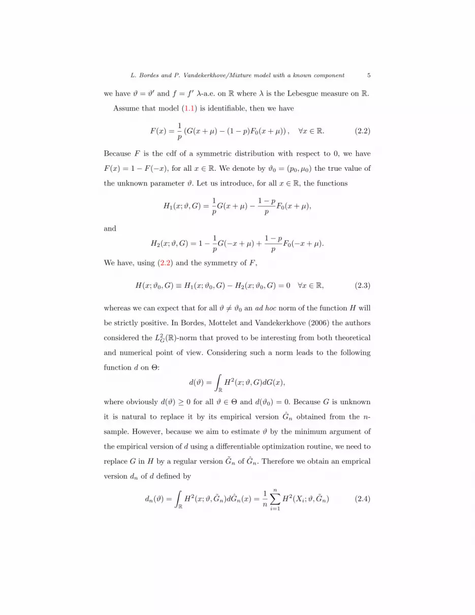
Assume that model (1.1) is identifiable, then we have
F (x) =1p
(G(x+ µ)− (1− p)F0(x+ µ)) , ∀x ∈ R. (2.2)
Because F is the cdf of a symmetric distribution with respect to 0, we have
F (x) = 1− F (−x), for all x ∈ R. We denote by ϑ0 = (p0, µ0) the true value of
the unknown parameter ϑ. Let us introduce, for all x ∈ R, the functions
H1(x;ϑ,G) =1pG(x+ µ)− 1− p
pF0(x+ µ),
and
H2(x;ϑ,G) = 1− 1pG(−x+ µ) +
1− pp
F0(−x+ µ).
We have, using (2.2) and the symmetry of F ,
H(x;ϑ0, G) ≡ H1(x;ϑ0, G)−H2(x;ϑ0, G) = 0 ∀x ∈ R, (2.3)
whereas we can expect that for all ϑ 6= ϑ0 an ad hoc norm of the function H will
be strictly positive. In Bordes, Mottelet and Vandekerkhove (2006) the authors
considered the L2G(R)-norm that proved to be interesting from both theoretical
and numerical point of view. Considering such a norm leads to the following
function d on Θ:
d(ϑ) =∫
RH2(x;ϑ,G)dG(x),
where obviously d(ϑ) ≥ 0 for all ϑ ∈ Θ and d(ϑ0) = 0. Because G is unknown
it is natural to replace it by its empirical version Gn obtained from the n-
sample. However, because we aim to estimate ϑ by the minimum argument of
the empirical version of d using a differentiable optimization routine, we need to
replace G in H by a regular version Gn of Gn. Therefore we obtain an emprical
version dn of d defined by
dn(ϑ) =∫
RH2(x;ϑ, Gn)dGn(x) =
1n
n∑i=1
H2(Xi;ϑ, Gn) (2.4)

L. Bordes and P. Vandekerkhove/Mixture model with a known component 6
where
Gn(x) =1n
n∑i=1
1Xi≤x, ∀x ∈ R,
and Gn(x) =∫ x
−∞gn(t)dt denotes the smoothed version of the empirical cdf Gn
since gn is a kernel density estimator of g defined by
gn(x) =1nhn
n∑i=1
q
(x−Xi
hn
), ∀x ∈ R,
with hn → 0, nhn → +∞ and q is a symmetric kernel density function. For
example we can choose q(x) = (1−|x|)1−1≤x≤1. Note that additional conditions
on the bandwidth hn and the kernel function q will be specified afterward.
Finally we propose to estimate ϑ0 by
ϑn = (pn, µn) = arg minϑ∈Θ
dn(ϑ).
Using the relation (2.2) we can estimate F by:
Fn(x) =1pn
(Gn(x+ µn)− (1− pn)F0(x+ µn)
), ∀x ∈ R.
Note that generally Fn is not a legitimate cdf since it is generally not nondecreas-
ing on the whole real line. However, the Glivenko-Cantelli strong consistency
result obtained in Section 3 shows that it is not a serious drawback whenever
the sample size is large enough.
Again by formula (2.2) a natural estimator of the df f is defined by
fn(x) =1pn
(gn(x+ µn)− (1− pn)f0(x+ µn)) , ∀x ∈ R.
Because generally fn will not be a density, it can be modified into a legitimate
df estimator fn defined by
fn =1snfn1fn≥0,
where sn =∫
Rfn(x)1fn(x)≥0dx.
The advantage of choosing the above L2G(R)-norm is that it leads to an ex-
plicit empirical function dn since replacing G by Gn transforms the integral sign

L. Bordes and P. Vandekerkhove/Mixture model with a known component 7
into a simple sum. However other choices are possible. In Bordes, Delmas and
Vandekerkhove (2006), Lq(R) (1 ≤ q < +∞) distances between H1 and H2 are
discussed. These authors show also that it is possible to reduce the Euclidean
parameter to one of the two parameters p and µ using the first order moment of
G that can be estimated directly from the n-sample. However such a reduction
of parameters can lead to serious numerical instability when the product pµ is
small, which is frequent, e.g., for applications to microarray experiments.
3. Identifiability, consistency and asymptotic normality
3.1. General conditions and identifiability
In this section we give a set of conditions for which we obtain identifiability of
the model parameters, consistency and asymptotic normality of our estimators.
We denote by ϑ0 = (p0, µ0) the true value the unknown Euclidean parameter
ϑ = (p, µ) of model (1.1). Let us denote by m0 and m the second-order moments
of f0 and f respectively. We introduce the set
Φ = R∗×]0,+∞[\ ∪k∈N∗ Φk
where
Φk ={
(µ,m) ∈ R∗×]0,+∞[;m = m0 + µ2 k ± 23k
}.
Let us define Fq = {f ∈ F ;∫
R |x|qf(x)dx < +∞} for q ≥ 1. Denoting by f0 the
Fourier transform of the df f0 we consider one assumption, for which the semi-
parametric identifiability of the model (1.1) parameters is obtained, see Bordes,
Delmas and Vandekerkhove (2006, Proposition 2, p. 736).
Identifiability condition (I). Let (f0, f) ∈ F23 , f0 > 0 and (µ0,m) ∈ Φc
where Φc a compact subset of Φ. We have ϑ0 = (p0, µ0) ∈ Θ where Θ is a
compact subset of (0, 1)× Ξ where Ξ = {µ; (µ,m) ∈ Φc}.

L. Bordes and P. Vandekerkhove/Mixture model with a known component 8
Comments and remarks. Note that condition (I) is fulfilled if f0 is the den-
sity function of a centered gaussian (not necessarily normalized).
As it is mentioned in Bordes, Delmas and Vandekerkhove (2006), there exists
various non-identifiability cases for model (1.1). Let us focus our attention on
the following one:
(1− p)ϕ(x) + pf(x− µ) = (1− p
2)ϕ(x) +
p
2ϕ(x− 2µ), ∀x ∈ R, (3.1)
where a is a real number, ϕ is an even df, p ∈ (0, 1) and f(x) = (ϕ(x − a) +
ϕ(x + a))/2. This example is particularly interesting since it clearly shows the
danger of estimating model (1.1) when the df of the unknown component has
exactly the same shape as the known df.
An other very important point which needs to be explained is the fact that
the value µ = 0 must be rejected from the parametric space. In fact it is easy to
check that for all p ∈ (0, 1), ϑ = (p, 0) is always a solution of d(ϑ) = 0. Indeed
for all p ∈ (0, 1) and all cdf G satisfying (2.1), we have
∀x ∈ R, H1(x; (p, 0), G) = F (x), H2(x; (p, 0), G) = 1− F (−x) = F (x).
It follows that µ = 0 does not match the contrast property of d. Even if µ = 0 is
a forbidden value by Condition (I), when the true value of µ is close to zero the
empirical contrast may fail in finding a good estimate of the location parameter.
Note however that in microarray experiments a value of µ that is close to 0 may
be balanced by a large sample size. The same remark holds for p = 0.
Kernel conditions (K).
(i) The even kernel density function q is bounded, uniformly continuous,
square integrable, of bounded variations and has second order moment.
(ii) The function q has first order derivative q′ ∈ L1(R) and q′(x) → 0 as
|x| → +∞. In addition if γ is the square root of the continuity modulus

L. Bordes and P. Vandekerkhove/Mixture model with a known component 9
of q, we have ∫ 1
0
(log(1/u))1/2dγ(u) <∞.
Comments. More general conditions on the kernel function q may be founded,
e.g., in Silverman (1978) and in Gine and Guillou (2002). From a practical point
of view triangular, gaussian, cauchy or many other standard kernels satisfy these
conditions.
Bandwidth conditions (B).
(i) hn ↘ 0, nhn → +∞ and√nh2
n = o(1),
(ii) nhn/| log hn| → +∞, | log hn|/ log log n → +∞ and there exists a real
number c such that hn ≤ ch2n for all n ≥ 1,
(iii) | log hn|/(nh3n)→ 0.
Comments. The two first conditions in (B) (i) are necessary to obtain the
pointwize consistency of g kernel estimators. The third condition allows to con-
trol the distance between the empirical cdf Gn and its regularized version Gn.
By using Corollary 1 in Shorack and Wellner (1986, p. 766) we obtain∥∥∥Gn − Gn∥∥∥∞
= Oa.s.(h2n) (3.2)
which by (i) and the law of iterated logarithm, leads to
∥∥∥Gn −G∥∥∥∞
= Oa.s.
((log log n
n
)−1/2). (3.3)
Conditions (ii) and (iii) allows to obtain the following result.
Lemma 3.1. Suppose that the kernel function q satisfies Conditions (K) and
that the bandwidth (hn) satisfies Conditions (B).
(i) If g and g′ are uniformly continuous on R, then
‖gn − g‖∞ = oa.s.(1) and ‖g′n − g′‖∞ = oa.s.(1).

L. Bordes and P. Vandekerkhove/Mixture model with a known component 10
(ii) If g is Lipschitz on R, then
‖gn − g‖∞ = Oa.s.
((| log hn|nhn
)1/2)
+O(hn).
Proof. Result (i) is given in Silverman (1978, Theorems A and C). For (ii) we
have
‖gn − g‖∞ ≤ ‖gn − E(gn)‖∞ + ‖E(gn)− g‖∞.
From Gine and Guillou (2002) we have
‖gn − E(gn)‖∞ = Oa.s.
((| log hn|nhn
)1/2),
whereas the O(hn) term holds because g is Lipschitz on R.
Remark 3.1. The convergence rate given by Gine and Guillou (2002) for the
multivariate case was given in Silverman (1978) under stronger conditions on
the bandwidth. Note that we put conditions in order to obtain simultaneously (i)
and (ii) of Lemma 3.1. However each of the two results do not require all the
assumptions made in (K) and (B) to hold. Finally it is worth to note that for
example the bandwidth rate n−1/4−δ, with δ ∈ (0, 1/8), is convenient since it
meets all the conditions that are given in (B).
3.2. Consistency and preliminary convergence rate
We denote for simplicity by h(ϑ) and h(ϑ) the gradient vector and hessian
matrix of any real function h (when it makes sense) with respect to argument
ϑ ∈ R2.
Lemma 3.2. Assume that Condition (I) is satisfied and that Θ is a compact
subset of (0, 1)× Φc.
(i) The function d is continuous on Θ.
(ii) If G is strictly increasing then d is a contrast function, i.e. for all ϑ ∈ Φc,
d(ϑ) ≥ 0 and d(ϑ) = 0 if and only if ϑ = ϑ0.

L. Bordes and P. Vandekerkhove/Mixture model with a known component 11
(iii) If F0 and F are Lipschitz on R, then d is Lipschitz on Θ and supϑ∈Φc|dn(ϑ)−
d(ϑ)| = oa.s.(n−1/2+α), for all α > 0.
(iv) If supp(g) = R then
d(ϑ0) = 2∫
RH(x;ϑ0, G)HT (x;ϑ0, G)dG(x) > 0.
Proof. Let us show (i). The function ϑ 7→ H(x;ϑ,G) being bounded and
continuous at any point ϑ ∈ Θ for all fixed x ∈ R, the wanted result is a direct
consequence of the Lebesgue dominated convergence Theorem.
Let us show (ii). If ϑ = ϑ0 then d(ϑ) = 0. To prove the reciprocal let us remark
that d(ϑ) = 0 implies H1(·;ϑ,G) = H2(·;ϑ,G) which leads, because G is strictly
increasing on R, to
g(x+ µ)− (1− p)f0(x+ µ) = g(−x+ µ)− (1− p)f0(−x+ µ), ∀ x ∈ R.
Using (1.1) with ϑ = ϑ0 we obtain for all x ∈ R
(1− p0)f0(x+ µ) + p0(x+ µ− µ0)− (1− p)f0(x+ µ)
= (1− p0)f0(−x+ µ) + p0(−x+ µ− µ0)− (1− p)f0(−x+ µ).
Assume now that ϑ 6= ϑ0. Considering the Fourier transform of the above equal-
ity we obtain
(p− p0) sin(tµ)f0(t) = p0 sin(t(µ− µ0))f(t), ∀ t ∈ R. (3.4)
Since f0(t) > 0, it comes that t(µ − µ0) ∈ πZ ⇒ tµ ∈ πZ, which proves that
it exists k0 ∈ Z such that |µ| / |µ− µ0| = k0. Taking in addition the first and
third order derivatives of (3.4) at t = 0 we obtain
p0µ0 = pµ and (p−p0)µ(3m0 +µ2) +p0(µ−µ0)(3m+ (µ−µ0)2) = 0. (3.5)
The above results imply that
m = m0 + µ20
k0 ± 23k0
, (3.6)

L. Bordes and P. Vandekerkhove/Mixture model with a known component 12
and then (µ,m) ∈ ∪k∈N∗Φk, which in turn implies that (µ,m) /∈ Φc. It follows
that ϑ = ϑ0.
Let us show (iii). Let ϑ and ϑ′ be two points in Θ. We have
|d(ϑ)− d(ϑ′)|
≤∫
R|H(x;ϑ,G) +H(x;ϑ′, G)| × |H(x;ϑ,G)−H(x;ϑ′, G)| dG(x)
≤ c
∫R|H(x;ϑ,G)−H(x;ϑ′, G)| dG(x), (3.7)
where c is a constant coming from the boundedness of (x, ϑ) 7→ H(x;ϑ,G) on
R × Θ. Moreover, using the compacity of Θ and properties of cdf it is easy to
show that there exist constants α, β and γ such that
|H(x;ϑ,G)−H(x;ϑ′, G)|
≤ α (|F (x− µ)− F (x− µ′)|+ |F (x+ µ)− F (x+ µ′)|)
+β (|F0(x− µ)− F0(x− µ′)|+ |F0(x+ µ)− F0(x+ µ′)|) + γ|p− p′|.
Using (3.7) and the above inequality we obtain that there exists a constant c′
such that |d(ϑ)− d(ϑ′)| ≤ c′‖ϑ− ϑ′‖2, where ‖ · ‖2 denote the Euclidean norm
on R2.
Considering for all k ≥ 0 the random variable Zk(ϑ) = H2(Xk;ϑ,G), we have
for all ϑ ∈ Θ
|dn(ϑ)− d(ϑ)| ≤
∣∣∣∣∣ 1nn∑k=1
(H2(Xk;ϑ, Gn)−H2(Xk;ϑ,G)
)∣∣∣∣∣+
∣∣∣∣∣ 1nn∑k=1
(Zk(ϑ)− E(Zk(ϑ)))
∣∣∣∣∣≤ Oa.s.(||Gn −G||∞) + sup
ϑ∈Θ
∣∣∣∣∣ 1nn∑k=1
(Zk(ϑ)− E(Zk(ϑ)))
∣∣∣∣∣ .Noticing that ||Gn − G||∞ is Oa.s.(
√n−1 log log n) (see Shorack and Wellner,
1986, p. 766) and that the last term of the right hand side is the supremum of
an empirical process indexed by a class of Lipschitz bounded function, which

L. Bordes and P. Vandekerkhove/Mixture model with a known component 13
is known to be a oa.s.(n−1/2+α) for α > 0 (see Bordes, Mottelet and Vandek-
erkhove, 2006, for the details), we get the wanted result.
Let us show (iv). First we have
d(ϑ0) = 2∫
R
(H(x;ϑ0, G)H(x;ϑ0, G) + H(x;ϑ0, G)HT (x;ϑ0, G)
)dG(x)
= 2∫
RH(x;ϑ0, G)HT (x;ϑ0, G)dG(x)
because H(·;ϑ0, G) ≡ 0 on R. Let v be a vector in R2, we have
vT d(ϑ0)v = 2∫
R
(vT H(x;ϑ0, G)
)2
dG(x) ≥ 0.
It follows that d(ϑ0) is a positive 2×2 real valued matrix. Let us show that it is
also definite. Let v ∈ R2 be a non null column vector such that vT d(ϑ0)v = 0,
then vT H(·;ϑ0, G) = 0 λ-everywhere on R. It is straightforward to show that
∂H
∂µ(x;ϑ0, G) = 2f(x), (3.8)
and∂H
∂p(x;ϑ0, G) =
1p0
[F0(x+ µ0) + F0(µ0 − x)− 1] . (3.9)
Therefore, using the above derivatives with the condition vT H(·;ϑ0, G) = 0 we
obtain the proportionality of the functions f and F0(· + µ0) + F0(µ0 − ·) − 1.
Because f0 is an even function we obtain
f(x) =F0(x+ µ0)− F0(x− µ0)∫
R (F0(x+ µ0)− F0(x− µ0)) dx=
12µ0
(F0(x+ µ0)− F0(x− µ0)) .
Finally, computing the second order moment of f , we obtain by the integration
by part formula
m =∫
Rx2f(x)ds =
12µ0
∫Rx2 (F0(x+ µ0)− F0(x− µ0)) dx
=2µ0m0
2µ0= m0,
which is not possible, by Condition (I), sincem is different fromm0+µ20(k±2)/3k
for all k ∈ N∗ (hence from m0 taking k = 2). �

L. Bordes and P. Vandekerkhove/Mixture model with a known component 14
Theorem 3.1.
(i) Suppose that Condition (I) is satisfied, Θ is a compact subset of (0, 1)×Φc,
G is strictly increasing on R, and that F0 and F are Lipschitz on R. Then
the estimator ϑn converges almost surely to ϑ0.
(ii) If in addition F0 and F are twice continuously differentiable with second
derivatives in L1(R), then we have |ϑn − ϑ0| = oa.s.(n−1/4+α) for all
α > 0.
Proof. Let us show (i). This proof follows entirely the proof of i) in Theorem 1
given in Bordes et al. (2006b) by using (i)–(iii) of Lemma 3.2.
Let us show (ii). By Lemma 3.2 (iv) there exists α > 0 such that for all
v ∈ R2, vT d(µ0)v > α‖v‖22. By a two order Taylor expansion of d at ϑ0, we can
find η > 0 such that for all v satisfying ‖v‖2 < η and ϑ0 + v ∈◦Θ, we have
d(ϑ0 + v) ≥ α
4‖v‖22. (3.10)
Let us considerB0(ηn) the open ball centered at ϑ0 with radius ηn > 0. Following
the proof of Theorem 3.3 in Bordes, Mottelet and Vandekerkhove (2006) we show
that for all ϑ ∈ Θ \B0(ηn), we have the following events inclusion
lim supn
{ϑn /∈ B0(ηn)
}⊆ lim sup
n
{inf
ϑ∈Θ\B0(ηn)d(ϑ) < γn
}∪ lim sup
n
{γn ≤ 2 sup
ϑ∈Θ|dn(ϑ)− d(ϑ|
}.
for any arbitrary sequence γn. Choosing now γn = n−1/2+α, and ηn = n−1/4+β/2,
with 0 < α < β taken arbitrarily small, it follows from (3.10) and the uniform
almost sure rate of convergence of dn towards d given in Lemma 3.2 (iii), that
P
(lim sup
n
{inf
ϑ∈Θ\B0(ηn)d(ϑ) < γn
})= 0,
and
P
(lim sup
n
{γn ≤ 2 sup
ϑ∈Θ|dn(ϑ)− d(ϑ)|
})= 0.
L. Bordes and P. Vandekerkhove/Mixture model with a known component 15
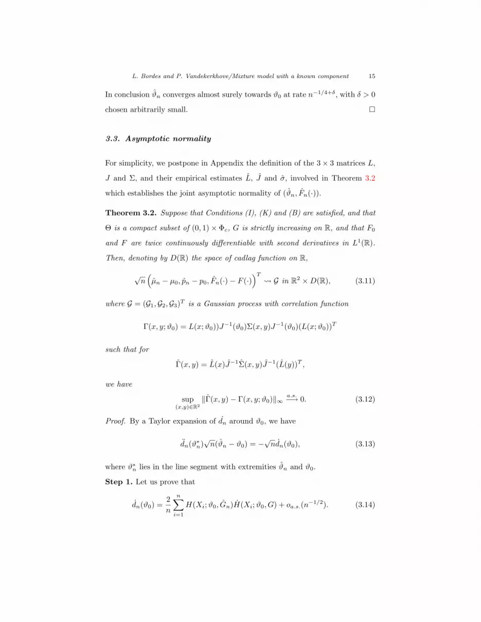
In conclusion ϑn converges almost surely towards ϑ0 at rate n−1/4+δ, with δ > 0
chosen arbitrarily small.
3.3. Asymptotic normality
For simplicity, we postpone in Appendix the definition of the 3× 3 matrices L,
J and Σ, and their empirical estimates L, J and σ, involved in Theorem 3.2
which establishes the joint asymptotic normality of (ϑn, Fn(·)).
Theorem 3.2. Suppose that Conditions (I), (K) and (B) are satisfied, and that
Θ is a compact subset of (0, 1)× Φc, G is strictly increasing on R, and that F0
and F are twice continuously differentiable with second derivatives in L1(R).
Then, denoting by D(R) the space of cadlag function on R,
√n(µn − µ0, pn − p0, Fn(·)− F (·)
)T G in R2 ×D(R), (3.11)
where G = (G1,G2,G3)T is a Gaussian process with correlation function
Γ(x, y;ϑ0) = L(x;ϑ0))J−1(ϑ0)Σ(x, y)J−1(ϑ0)(L(x;ϑ0))T
such that for
Γ(x, y) = L(x)J−1Σ(x, y)J−1(L(y))T ,
we have
sup(x,y)∈R2
‖Γ(x, y)− Γ(x, y;ϑ0)‖∞a.s.−→ 0. (3.12)
Proof. By a Taylor expansion of dn around ϑ0, we have
dn(ϑ∗n)√n(ϑn − ϑ0) = −
√ndn(ϑ0), (3.13)
where ϑ∗n lies in the line segment with extremities ϑn and ϑ0.
Step 1. Let us prove that
dn(ϑ0) =2n
n∑i=1
H(Xi;ϑ0, Gn)H(Xi;ϑ0, G) + oa.s.(n−1/2). (3.14)
L. Bordes and P. Vandekerkhove/Mixture model with a known component 16
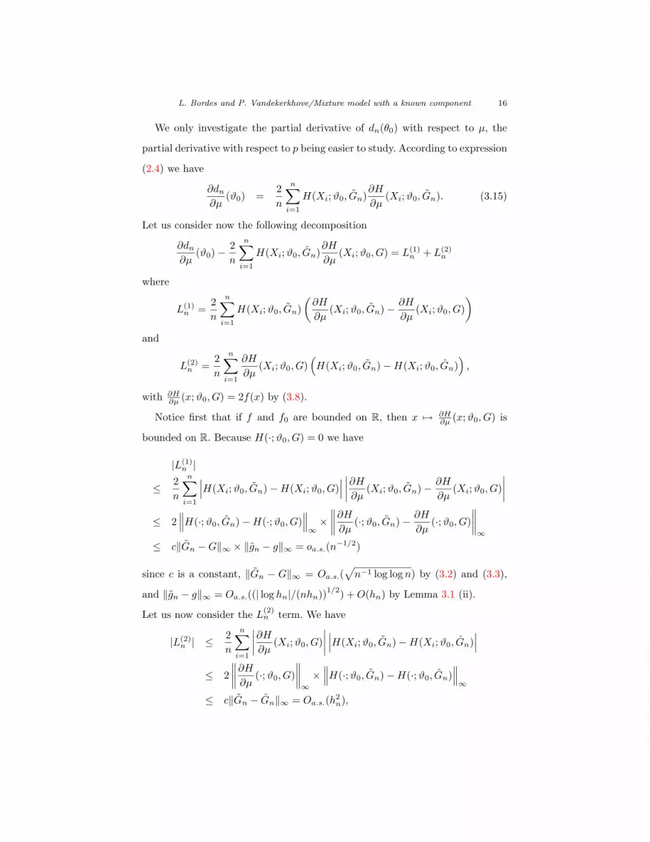
We only investigate the partial derivative of dn(θ0) with respect to µ, the
partial derivative with respect to p being easier to study. According to expression
(2.4) we have
∂dn∂µ
(ϑ0) =2n
n∑i=1
H(Xi;ϑ0, Gn)∂H
∂µ(Xi;ϑ0, Gn). (3.15)
Let us consider now the following decomposition
∂dn∂µ
(ϑ0)− 2n
n∑i=1
H(Xi;ϑ0, Gn)∂H
∂µ(Xi;ϑ0, G) = L(1)
n + L(2)n
where
L(1)n =
2n
n∑i=1
H(Xi;ϑ0, Gn)(∂H
∂µ(Xi;ϑ0, Gn)− ∂H
∂µ(Xi;ϑ0, G)
)and
L(2)n =
2n
n∑i=1
∂H
∂µ(Xi;ϑ0, G)
(H(Xi;ϑ0, Gn)−H(Xi;ϑ0, Gn)
),
with ∂H∂µ (x;ϑ0, G) = 2f(x) by (3.8).
Notice first that if f and f0 are bounded on R, then x 7→ ∂H∂µ (x;ϑ0, G) is
bounded on R. Because H(·;ϑ0, G) = 0 we have
|L(1)n |
≤ 2n
n∑i=1
∣∣∣H(Xi;ϑ0, Gn)−H(Xi;ϑ0, G)∣∣∣ ∣∣∣∣∂H∂µ (Xi;ϑ0, Gn)− ∂H
∂µ(Xi;ϑ0, G)
∣∣∣∣≤ 2
∥∥∥H(·;ϑ0, Gn)−H(·;ϑ0, G)∥∥∥∞×∥∥∥∥∂H∂µ (·;ϑ0, Gn)− ∂H
∂µ(·;ϑ0, G)
∥∥∥∥∞
≤ c‖Gn −G‖∞ × ‖gn − g‖∞ = oa.s.(n−1/2)
since c is a constant, ‖Gn − G‖∞ = Oa.s.(√n−1 log log n) by (3.2) and (3.3),
and ‖gn − g‖∞ = Oa.s.((| log hn|/(nhn))1/2) +O(hn) by Lemma 3.1 (ii).
Let us now consider the L(2)n term. We have
|L(2)n | ≤
2n
n∑i=1
∣∣∣∣∂H∂µ (Xi;ϑ0, G)∣∣∣∣ ∣∣∣H(Xi;ϑ0, Gn)−H(Xi;ϑ0, Gn)
∣∣∣≤ 2
∥∥∥∥∂H∂µ (·;ϑ0, G)∥∥∥∥∞×∥∥∥H(·;ϑ0, Gn)−H(·;ϑ0, Gn)
∥∥∥∞
≤ c‖Gn − Gn‖∞ = Oa.s.(h2n),

L. Bordes and P. Vandekerkhove/Mixture model with a known component 17
which in turn gives the wanted result because by Condition (B) we have√nh2
n =
o(1). This finishes the proof of the first step.
Step 2. We need to prove that
dn(ϑ∗n) a.s.−→ I(ϑ0), (3.16)
where I(ϑ0) =∫
R H(x;ϑ0, G)HT (x;ϑ0, G)dG(x) > 0.
In order to prove statement (3.16) let us remark that
dn(ϑ∗n) =2n
n∑k=1
H(Xk;ϑ∗n, Gn)H(Xk;ϑ∗n, Gn)
+2n
n∑k=1
H(Xk;ϑ∗n, Gn)HT (Xk;ϑ∗n, Gn)
= T (1)n + T (2)
n + T (3)n ,
where
T (1)n =
2n
n∑k=1
(H(Xk;ϑ∗n, Gn)−H(Xk;ϑ0, G)
)H(Xk;ϑ∗n, Gn),
T (2)n =
2n
n∑k=1
H(Xk;ϑ∗n, Gn)HT (Xk;ϑ∗n, Gn)
− 2n
n∑k=1
H(Xk;ϑ0, G)HT (Xk;ϑ0, G),
T (3)n =
2n
n∑k=1
H(Xk;ϑ0, G)HT (Xk;ϑ0, G).
Because the df f and f0 are bounded it easy to show that the strong law of large
numbers holds for T (3)n and therefore T (3)
n → I(ϑ0) almost surely. It remains to
show that T (1)n and T (2)
n converge almost surely to 0. For T (1)n let us remark that
T (1)n ≤
∥∥∥H(·;ϑ∗n, Gn)−H(·;ϑ0, G)∥∥∥∞×∥∥∥H(·;ϑ∗n, Gn)
∥∥∥∞. (3.17)
Because H = H1 − H2 and H1 and H2 are very similar, we only prove that
the supremum norm of each term in H1(·;ϑ∗n, Gn) matrix is bounded. We only
handle the more complicated term in H1(·;ϑ∗n, Gn) which is the second order

L. Bordes and P. Vandekerkhove/Mixture model with a known component 18
derivative with respect to µ. We have
∂2H1
∂µ2(x;ϑ∗n, Gn) =
1png′n(x+ µn)− 1− pn
pnf ′0(x+ µn),
where g′n = G′′n is an estimator of g′. Because f ′ and f ′0 are bounded we have∥∥∥∥∂2H1
∂µ2(·;ϑ∗n, Gn)
∥∥∥∥∞≤ Oa.s. (‖g′n − g′‖∞) +Oa.s.(1).
According to Silverman (1978), dealing with the uniform consistency of kernel
estimators of a density and its derivatives, we have
‖gn − g‖∞ = oa.s. (1) and ‖g′n − g′‖∞ = oa.s. (1) .
Finally we obtain∥∥∥H(·;ϑ∗n, Gn)∥∥∥∞
= oa.s. (1) +Oa.s.(1) = Oa.s.(1).
Painfull but straitghforward calculations lead to∥∥∥H(·;ϑ∗n, Gn)−H(·;ϑ0, G)∥∥∥∞≤ Oa.s.
(‖ϑn − ϑ0‖2
)+Oa.s.
(‖Gn −G‖∞
).
According to Corollary 1 in Shorack and Wellner (1986, p. 766) and the Law
of the Iterated Logarithm for the empirical cdf, we have
‖Gn −G‖∞ = Oa.s(√n−1 log log(n)),
hence by (3.17) and the above results we have
T (1)n = Oa.s.
(‖ϑ∗n − ϑ0‖2 +
√n−1 log log(n)
). (3.18)
Finally by Theorem 3.1 we have that ‖ϑ∗n−ϑ0‖2 = oa.s.(n−1/4+α) for any α > 0,
then T(1)n converges almost surely to 0.
The same kind of calculations allow to prove that T (2)n → 0 almost surely,
which concludes the proof of statement (3.16).
Step 3. Using the fact that at the√n-rate Gn and Gn are interchangeable, and
using the properties of F and F0 we obtain the following uniform (with respect
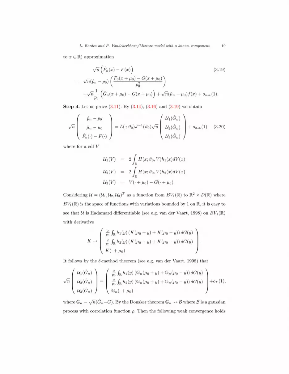
L. Bordes and P. Vandekerkhove/Mixture model with a known component 19
to x ∈ R) approximation
√n(Fn(x)− F (x)
)(3.19)
=√n(pn − p0)
(F0(x+ µ0)−G(x+ µ0)
p20
)+√n
1p0
(Gn(x+ µ0)−G(x+ µ0)
)+√n(µn − µ0)f(x) + oa.s.(1).
Step 4. Let us prove (3.11). By (3.14), (3.16) and (3.19) we obtain
√n
pn − p0
µn − µ0
Fn(·)− F (·)
= L(·;ϑ0)J−1(ϑ0)√n
U1(Gn)
U2(Gn)
U3(Gn)
+ oa.s.(1), (3.20)
where for a cdf V
U1(V ) = 2∫
RH(x;ϑ0, V )h1(x)dV (x)
U2(V ) = 2∫
RH(x;ϑ0, V )h2(x)dV (x)
U3(V ) = V (·+ µ0)−G(·+ µ0).
Considering U = (U1,U2,U3)T as a function from BV1(R) to R2 ×D(R) where
BV1(R) is the space of functions with variations bounded by 1 on R, it is easy to
see that U is Hadamard differentiable (see e.g. van der Vaart, 1998) on BV1(R)
with derivative
K 7→
2p0
∫R h1(y) (K(µ0 + y) +K(µ0 − y)) dG(y)
2p0
∫R h2(y) (K(µ0 + y) +K(µ0 − y)) dG(y)
K(·+ µ0)
.
It follows by the δ-method theorem (see e.g. van der Vaart, 1998) that
√n
U1(Gn)
U2(Gn)
U3(Gn)
=
2p0
∫R h1(y) (Gn(µ0 + y) + Gn(µ0 − y)) dG(y)
2p0
∫R h2(y) (Gn(µ0 + y) + Gn(µ0 − y)) dG(y)
Gn(·+ µ0)
+oP (1),
where Gn =√n(Gn−G). By the Donsker theorem Gn B where B is a gaussian
process with correlation function ρ. Then the following weak convergence holds

L. Bordes and P. Vandekerkhove/Mixture model with a known component 20
in R2 ×D(R)
√n
U1(Gn)
U2(Gn)
U3(Gn)
H =
2p0
∫R h1(y) (B(µ0 + y) + B(µ0 − y)) dG(y)
2p0
∫R h2(y) (B(µ0 + y) + B(µ0 − y)) dG(y)
B(·+ µ0)
,
where H is a gaussian process as a linear form on B the correlation function of
which is defined by Σ(x, y) = E[H(x)HT (y)
]. This with (3.20) lead to (3.11).
Step 5. It remains to prove (3.12). For this purpose it is sufficient to prove the
convergence in probability of Jij to J(ϑ0), that
maxi=1,2,3
‖hi − hi(·;ϑ0)‖∞a.s.−→ 0,
(which gives the strong uniform convergence of L to L(·;ϑ0)) and that
sup(x,y)∈R2
|σij(x, y)− σij(x, y)| a.s.−→ 0,
for all 1 ≤ i, j ≤ 3. Because the proof is quite repetitive, we only consider one
of the more difficult terms, other terms can be handled in the same way. First
supx∈R|h1(x)− h1(x)| a.s.−→ 0,
by the strong consistency result of Theorem 3.1 and the Lipschitz property of
F0. Using repetively the telescoping rule we show that
supx∈R|fn(x)− f(x)|
≤ 1pn
(‖g − g‖∞ + ‖g(·+ µn)− g(·+ µ0)‖∞ + ‖f0(·+ µn)− f0(·+ µ0)‖∞)
+‖g‖∞ + ‖f0‖∞
p0pn|pn − p0|.
The above inequality with the strong consistency result of Theorem 3.1 and the
Lipschitz properties of f0 and g lead to
supx∈R|fn(x)− f(x)| a.s.−→ 0.
L. Bordes and P. Vandekerkhove/Mixture model with a known component 21
Now recall that sn =∫
R fn(x)1fn(x)dxa.s.−→ 1 (see Bordes, Mottelet and Van-
dekerkhove, 2006), then we can write
|fn(x)− fn(x)| ≤ ‖fn‖∞|1− sn|sn
+ |fn(x)|1fn(x)<0,
where because f is bounded and ‖fn − f‖∞a.s.−→ 0, the right hand side of the
above inequality converges strongly to 0. It follows that
supx∈R|h2(x)− h2(x)| a.s.−→ 0.
By similar arguments we prove the uniform strong convergence of ρ, ˆ and k
to ρ, ` and k respectively. Now let us show that σ12 converges strongly to σ12.
Let us consider, for example, the convergence of σ12. From previous results it is
straightforward to obtain
σ12 =8
n(n− 1)p20
n∑i=2
i−1∑j=1
h1(Xi)h2(Xj)k(Xi, Xj) + oa.s.(1),
where by the strong law of large numbers the right hand side term is a 2-order U -
statistic, with kernel function (u, v) 7→ h(u, v) = h1(u)h2(v)k(u, v), converging
strongly to σ12 = 4E(h(X1, X2))/p20.
4. Applications to testing and simulations
The aim of this section is not to develop some sophisticated testing procedures,
the aim is rather to show how to apply our CLT in order to build, quite directly,
some basic tests adapted to few hypotheses relative to the semiparametric mix-
ture model (1.1). However, more general testing procedures could be developed.
For example it should be possible to test the hypothesis that the nonparametric
component belongs to a parametric family, but such a test is beyond the scope
of the paper and will be developed elsewhere for a larger class of semiparametric
mixture models. First we propose a chi-square test for a simple hypothesis for
the three parameters of model (1.1) next the same type of test is proposed to
L. Bordes and P. Vandekerkhove/Mixture model with a known component 22
check the hypothesis that the nonparametric component of the mixture model
has a symmetric distribution.
4.1. Testing some simple hypothesis
We propose in this section to consider the following simple hypothesis testing
problem:
H0 : (p, µ, F ) = (p?, µ?, F?) versus H1 : (p, µ, F ) 6= (p?, µ?, F?),
where (p?, µ?) ∈ Θ and F? is a known cdf function. Because under H0 the joint
asymptotic behavior of√n(pn − p?, µn − p?, Fn − F?) is known, it is possible
to base a testing procedure on the asymptotic distribution. Such a procedure
requires to choose a discrepancy measure between the estimates and the esti-
mators, and of course, several choices are possible. The test we propose is based
on the frequently used chi-square measure, leading to chi-square type tests. Let
us fix k real numbers s1 < · · · < sk such that 0 < F?(s1) < · · · < F?(sk) < 1.
Because Moore (1971) and Ruymgaart (1975) proved that under smooth condi-
tions chi-square statistics can also be constructed using random cells boundaries
it is generally possible to choose equidistributed cells to increase the probabil-
ity that there are enough data in each interval ]s`−1, s`] for ` = 1, . . . , k with
s0 = −∞.
We consider now the random vector Wn defined by
Wn =√n
pn − p?
µn − µ?
Fn(s1)− F?(s1)...
Fn(sk)− F?(sk)
.
According to Theorem 3.2 we have
Wn N (0, V ) ,

L. Bordes and P. Vandekerkhove/Mixture model with a known component 23
where V is the (k + 2)× (k + 2) correlation matrix with entries defined by
vij = Γij , for 1 ≤ i ≤ j ≤ 2,
v1j = Γ13(sj−2) and v2j = Γ23(sj−2), for 3 ≤ j ≤ k + 2,
and
vij = Γ33(si−2, sj−2), for 3 ≤ i ≤ j ≤ k + 2.
Defining V as V but using Γ instead of Γ (see the beginning of section 3), we
obtain that
WTn V−1Wn χ2
k+2,
where χ2m is the chi-square distribution with m degrees of freedom. We reject H0
at the level α ∈ (0, 1) if WTn V−1Wn > χ2
k+2,1−α where χ2k+2,1−α is the quantile
of order 1− α of the χ2k+2 distribution.
4.2. Testing the symmetry of the nonparametric component
Testing the symmetry of the nonparametric component is equivalent to test the
hypothesis
H0 : F (x) + F (−x) = 1, for all x ∈ R+,
versus
H1 : there exists x ∈ R+ such that F (x) + F (−x) 6= 1.
It is therefore necessary to compare on R+ the random maps x 7→ Fn(x) +
Fn(−x) to x 7→ F (x)+F (−x) which is constant equal to 1 underH0. When p = 1
in model (1.1), there are several ways to testH0. Some test statistics are based on
ranks (see e.g. Shorack and Wellner, 1986) while others are based on empirical
cdf (see e.g. Schuster and Barker, 1987). Again, for simplicity, we choose a
chi-square measure to test H0. Note that combination of maximum deviation
measure with bootstrapped critical value proposed Schuster and Barker (1987)
and studied by Arcones and Gine (1991) could certainly be used here. Let us

L. Bordes and P. Vandekerkhove/Mixture model with a known component 24
consider k positive real numbers 0 < s1 < · · · < sk satisfying F (s1) < · · · <
F (sk) under H0. We consider the following discrepancy measure
Zn =√n
Fn(−s1) + Fn(s1)− 1
...
Fn(−sk) + Fn(sk)− 1
.
Then, under H0 we have Zn = AYn where A is the k × 2k matrix defined
by A = (Ik, Ik) with Ik is the identity matrix of order k, and Yn is the 2k-
dimensional random vector defined by
Yn =√n
Fn(s1)− F (s1)...
Fn(sk)− F (sk)
Fn(−s1)− F (−s1)...
Fn(−sk)− F (−sk)
.
According to Theorem 3.2 we have
Yn N (0,Λ) ,
where Λ is the 2k × 2k correlation matrix with entries λij defined by
λij = Γ33(s∗i , s∗j ), for 1 ≤ i, j ≤ 2k,
where s∗i = si for 1 ≤ i ≤ k and s∗i = −si for k + 1 ≤ i ≤ 2k.
Defining Λ as Λ but using Γ instead of Γ, we obtain that
ZTn (AΛAT )−1Zn χ2k.
We reject H0 at the level α ∈ (0, 1) if ZTn (AΛAT )−1Zn > χ2k,1−α.
4.3. Simulation study
Let Φ be the cdf of a N (0, 1) distribution. In this section data are simulated
from model (2.1) with p = 0.7, µ = 3, F0 = Φ and F = Φ(·/0.5). We performed
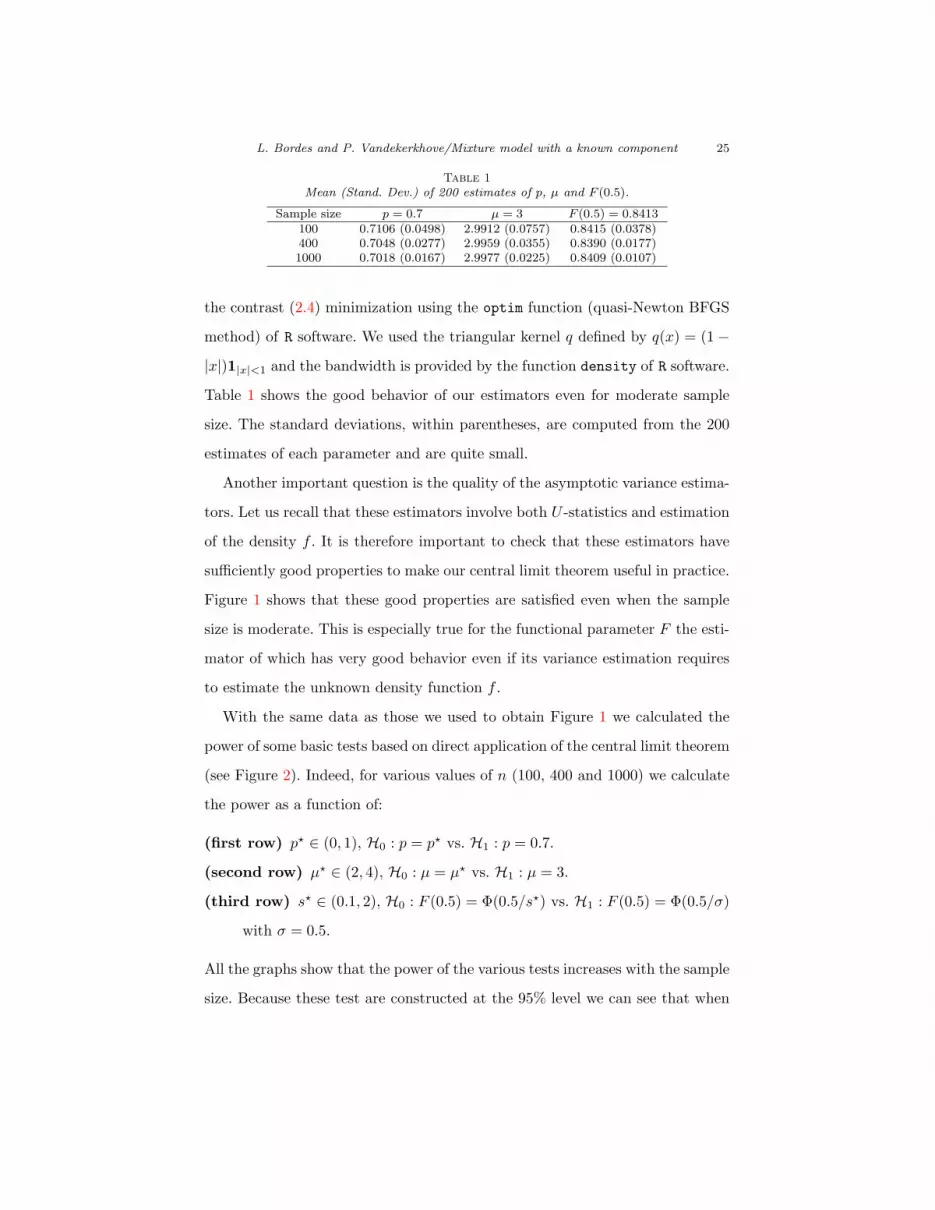
L. Bordes and P. Vandekerkhove/Mixture model with a known component 25
Table 1Mean (Stand. Dev.) of 200 estimates of p, µ and F (0.5).
Sample size p = 0.7 µ = 3 F (0.5) = 0.8413100 0.7106 (0.0498) 2.9912 (0.0757) 0.8415 (0.0378)400 0.7048 (0.0277) 2.9959 (0.0355) 0.8390 (0.0177)1000 0.7018 (0.0167) 2.9977 (0.0225) 0.8409 (0.0107)
the contrast (2.4) minimization using the optim function (quasi-Newton BFGS
method) of R software. We used the triangular kernel q defined by q(x) = (1−
|x|)1|x|<1 and the bandwidth is provided by the function density of R software.
Table 1 shows the good behavior of our estimators even for moderate sample
size. The standard deviations, within parentheses, are computed from the 200
estimates of each parameter and are quite small.
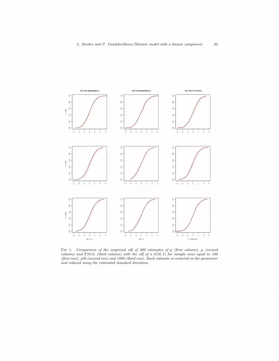
Another important question is the quality of the asymptotic variance estima-
tors. Let us recall that these estimators involve both U -statistics and estimation
of the density f . It is therefore important to check that these estimators have
sufficiently good properties to make our central limit theorem useful in practice.
Figure 1 shows that these good properties are satisfied even when the sample
size is moderate. This is especially true for the functional parameter F the esti-
mator of which has very good behavior even if its variance estimation requires
to estimate the unknown density function f .
With the same data as those we used to obtain Figure 1 we calculated the
power of some basic tests based on direct application of the central limit theorem
(see Figure 2). Indeed, for various values of n (100, 400 and 1000) we calculate
the power as a function of:
(first row) p? ∈ (0, 1), H0 : p = p? vs. H1 : p = 0.7.
(second row) µ? ∈ (2, 4), H0 : µ = µ? vs. H1 : µ = 3.
(third row) s? ∈ (0.1, 2), H0 : F (0.5) = Φ(0.5/s?) vs. H1 : F (0.5) = Φ(0.5/σ)
with σ = 0.5.
All the graphs show that the power of the various tests increases with the sample
size. Because these test are constructed at the 95% level we can see that when

L. Bordes and P. Vandekerkhove/Mixture model with a known component 26
H0 and H1 are identical the 5% rejection rate is well satisfied.
To finish this section let us show that chi-square tests proposed in Sections 4.1
and 4.2 have the expected asymptotically free chi-square distributions. Figure
3 shows the level plot of the power as a function of p? and µ? in testing H0 :
(p, µ) = (p?, µ?) versus H1 : (p, µ) = (0.7, 3). The sample size is quite large and
as a consequence the power is quickly close to one whenever (p, µ) moves away
from (0.7, 3).
In Figure 4 we compare the asymptotic chi-square cdf of the symmetry tests
we proposed in Section 4.2 with the empirical cdf obtained from 200 tests
produced under the null hypothesis. The test is based on the comparison of
F (−x)+F (x) and 1. For one value of x (first row) the asymptotic distribution is
a chi-square distribution with 1 degree of freedom, whereas for two (resp. three)
values of x (second row) (resp. third row) the asymptotic law is a chi-square
distribution with 2 (resp. 3) degrees of freedom. The asymptotic distribution is
generally well reached even if from time to time the test may appear a little bit
conservative.

L. Bordes and P. Vandekerkhove/Mixture model with a known component 27
0 2 4 6 8
0.0
0.2
0.4
0.6
0.8
1.0
F(x)+F(−x)=1 for x=0.5
Chi
2(1)
0 2 4 6 8
0.0
0.2
0.4
0.6
0.8
1.0
F(x)+F(−x)=1 for x=0.35
0 2 4 6 8
0.0
0.2
0.4
0.6
0.8
1.0
F(x)+F(−x)=1 for x=0.2
0 2 4 6 8 10 12
0.0
0.2
0.4
0.6
0.8
1.0
F(x)+F(−x)=1 for x=0.5 and 0.35
Chi
2(2)
0 2 4 6 8 10 12
0.0
0.2
0.4
0.6
0.8
1.0
F(x)+F(−x)=1 for x=0.5 and 0.2
0 2 4 6 8 10 12
0.0
0.2
0.4
0.6
0.8
1.0
F(x)+F(−x)=1 for x=0.35 and 0.2
0 2 4 6 8 10 12 14
0.0
0.2
0.4
0.6
0.8
1.0
F(x)+F(−x)=1 for x=0.5, 0.35 and 0.2
Chi
2(3)
Fig 4. Empirical cdf of 200 simulated values of the Chi-square symmetry test for n = 1000.
First row: testing at one point, second row: testing at two points, and third row: testing at
three points. The horizontal lines correspond to the 95% level.

L. Bordes and P. Vandekerkhove/Mixture model with a known component 28
Appendix A: Matrices of Theorem 3.2
We define the 3 × 3 real valued matrix Σ(x, y) by its components σij(x, y)
(1 ≤ i, j ≤ 3) where for (x, y) ∈ R2
σ11(x, y) ≡ σ11 =4p2
0
∫R2h1(u)h1(v)k(u, v)dG(u)dG(v),
σ22(x, y) ≡ σ22 =4p2
0
∫R2h2(u)h2(v)k(u, v)dG(u)dG(v),
σ12(x, y) ≡ σ21 =4p2
0
∫R2h1(u)h2(v)k(u, v)dG(u)dG(v),
σ13(x, y) ≡ σ13(y) =2p0
∫Rh1(u)`(y, u)dG(u),
σ23(x, y) ≡ σ23(y) =2p0
∫Rh2(u)`(y, u)dG(u),
σ31(x, y) = σ13(x),
σ32(x, y) = σ23(x),
σ33(x, y) = ρ(x+ µ0, y + µ0),
with
h1(x) =1p0
(F0(µ0 + x) + F0(µ0 − x)− 1) ,
h2(x) = 2f(x),
ρ(x, y) = G(x ∧ y)(1−G(x ∨ y)),
`(x, y) = ρ(µ0 + x, µ0 + y) + ρ(µ0 + x, µ0 − y),
k(x, y) = `(x, y) + `(−x, y).

L. Bordes and P. Vandekerkhove/Mixture model with a known component 29
Note that (h1, h2)T is equal to H(·;ϑ0, G) by (3.8) and (3.9). Let J(ϑ0) =
(Jij(ϑ0))1≤i,j≤3 be the 3× 3 real valued matrix with entries
J11(ϑ0) = −2∫
Rh2
1(u)dG(u),
J12(ϑ0) = J21(ϑ0) = −2∫
Rh1(u)h2(u)dG(u),
J22(ϑ0) = −2∫
Rh2
2(u)dG(u),
J13(ϑ0) = J23(ϑ0) = J31(ϑ0) = J32(ϑ0) = 0,
J33(ϑ0) = 1.
We also define the 3× 3 real valued matrix L(x;ϑ0) by
L(x;ϑ0) =
1 0 0
0 1 0
h3(x) f(x) 1/p0
,
where
h3(x) =F0(x+ µ0)−G(x+ µ0)
p20
.
For each of the above quantities we can define natural estimators. Let us
define
h1(x) =1pn
(F0(µn + x) + F0(µn − x)− 1) ,
h2(x) = 2fn(x),
h3(x) =F0(x+ µn)− Gn(x+ µn)
p2n
,
ρ(x, y) = Gn(x ∧ y)(1− Gn(x ∨ y)),
ˆ(x, y) = ρ(µn + x, µn + y) + ρ(µn + x, µn − y),
k(x, y) = ˆ(x, y) + ˆ(−x, y).

L. Bordes and P. Vandekerkhove/Mixture model with a known component 30
Then we can estimate Σ(x, y) by Σ(x, y) where
σ11(x, y) ≡ σ11 =8
n(n− 1)p2n
∑1≤i<j≤n
h1(Xi)h1(Xj)k(Xi, Xj),
σ22(x, y) ≡ σ22 =8
n(n− 1)p2n
∑1≤i<j≤n
h2(Xi)h2(Xj)k(Xi, Xj),
σ12(x, y) ≡ σ21 =4
n(n− 1)p2n
∑1≤i6=j≤n
h1(Xi)h2(Xj)k(Xi, Xj),
σ13(x, y) ≡ σ13(y) =2npn
n∑i=1
h1(Xi)ˆ(y,Xi),
σ23(x, y) ≡ σ23(y) =2npn
n∑i=1
h2(Xi)ˆ(y,Xi),
σ31(x, y) = σ13(x),
σ32(x, y) = σ23(x),
σ33(x, y) = ρ(x+ µn, y + µn),
and J = (Jij)1≤i,j≤3 with
J11 = − 2n
n∑i=1
h21(Xi), J12 = J21 = − 2
n
n∑i=1
h1(Xi)h2(Xi),
J22 = − 2n
n∑i=1
h22(Xi),
J13 = J23 = J31 = J32 = 0 and J33 = 1.
The L(x;ϑ0) matrix is estimated by L(x) the third line of which being therefore
(h3(x), h2(x)/2, 1/pn).
References
[1] Arcones, M. A. and Gine, E. (1991). Some bootstrap tests of symme-
try for univariate continuous distributions. Ann. Statist. 19 1496–1511.
MR1126334
[2] Bordes, L., Mottelet, S. and Vandekerkhove, P. (2006a). Semi-
parametric estimation of a two-component mixture model. Ann. Statist.
34 1204–1232. MR2278356

L. Bordes and P. Vandekerkhove/Mixture model with a known component 31
[4] Bordes, L., Delmas, C. and Vandekerkhove, P. (2006b). Semipara-
metric estimation of a two-component mixture model when a component
is known. Scand. J. Statist. 33 733–752. MR2300913
[4] Bordes, L., Chauveau, D. and Vandekerkhove, P. (2007). A
stochastic EM algorithm for a semiparametric mixture model. Comput.
Statist. Data Anal. 51 5429–5443.
[5] Cruz-Medina, I. R. and Hettmansperger, T. P. (2004). Nonpara-
metric estimation in semiparametric univariate mixture models. Journal
of Statistical Computation and Simulation 74 513–524. MR2073229
[6] Efron, B. (2007). Size, power and false discovery rate. Ann. Statist. 35
1351–1377.
[7] Gine, E. and Guillou A. (2002). Rates of Strong Uniform Consistency
for Multivariate Kernel density estimators. Ann. Inst. H. Poincare 38
503–522. MRMR1955344
[8] Hall, P. and Zhou, X. H. (2003). Nonparametric estimation of com-
ponent distributions in a multivariate mixture. Ann. Statist. 31 201–224.
MR1962504
[9] Hall, P., Neeman, A., Pakyari, R. and Elmore, R. (2005). Non-
parametric inference in multivariate mixtures. Biometrika 92 667–678.
MR2202653
[10] Hettmansperger, T. P. and Thomas, H. (2000). Almost nonparamet-
ric inference for repeated measures in mixture models. J. Royal Statist.
Soc. Ser. B 62 811–825. MR1796294
[11] Hunter, D. R., Wang, S. and Hettmansperger, T. P. (2007). Infer-
ence for mixtures of symmetric distributions. Ann. Statist. 35 224–251.
[12] Lindsay, B. G. and Lesperance, M. L. (1995). A review of semipara-
metric mixture models. J. Statist. Plann. Inf. 47 29–39. MRMR1360957
[13] McLachlan, G. J. and Peel, D. (2000). Finite Mixture Models. Wiley,
New York. MR1789474

L. Bordes and P. Vandekerkhove/Mixture model with a known component 32
[14] Maiboroda, R. and Sugakova, O. (2009). Generalized estimating equa-
tions for symmetric distributions observed with admixture. Preprint.
[15] Moore, D.S. (1971). A chi-square statistic with random cell boundaries.
Ann. Math. Statist. 42 147–156. MR0275601
[16] Naylor, J. C. and Smith, A. F. M. (1983). A contamination model in
clinical chemistry: an illustration of a method for the efficient computation
of posterior distributions. The Statistician 32 82–87.
[17] Pal, C. and Sengupta, A. (2000). Optimal tests for no contamination
in reliability models. Lifetime Data Anal. 6 281–290. MR1786803
[18] Ruymgaart, F. H. (1975). A note on chi-square statistics with random
cell boundaries. Ann. Statist. 3 965–968. MR0378183
[19] Robin, S. A., Bar-Hen, A., Daudin, J-J. and Pierre, L. (2007).
Semi-parametric approach for mixture models: Application to local false
discovery rate estimation. Comput. Statist. Data Anal. In press.
[20] Shorack, G. R. and Wellner, J. A. (1986). Empirical Processes with
Applications to Statistics. Wiley, New York. MR0838963
[21] Schuster, E. F. and Barker, R. C. (1987). Using the bootstrap in
testing symmetry versus asymmetry. Comm. Statist. Simulation Comput.
16 69–84. MR0883122
[22] Silverman, B. W. (1978). Weak and strong consistency of the kernel esti-
mate of a density and its derivatives. Ann. Statist. 6 177–184. MR0471166
[23] Sougakova, O. (2009) Estimation of location parameter by observations
with admixture. Theorija Imovirnosti ta Matematychna Statystyka, 80, to
appear.
[24] Titterington, D. M., Smith, A. F. M. and Makov, U. E. (1985).
Statistical Analysis of Finite Mixture Distributions, Wiley, Chichester.
MR0838090
[25] van der Vaart, A. W. (2000). Asymptotic Statistics. Cambridge Uni-
versity Press, New York. MR1652247
L. Bordes and P. Vandekerkhove/Mixture model with a known component 33
−3 −2 −1 0 1 2 3
0.0
0.2
0.4
0.6
0.8
1.0
CLT for parameter p
n =
100
−3 −2 −1 0 1 2 3
0.0
0.2
0.4
0.6
0.8
1.0
CLT for parameter µ
−3 −2 −1 0 1 2 3
0.0
0.2
0.4
0.6
0.8
1.0
CLT for F at x=0.5
−3 −2 −1 0 1 2 3
0.0
0.2
0.4
0.6
0.8
1.0
n =
400
−3 −2 −1 0 1 2 3
0.0
0.2
0.4
0.6
0.8
1.0
−3 −2 −1 0 1 2 3
0.0
0.2
0.4
0.6
0.8
1.0
−3 −2 −1 0 1 2 3
0.0
0.2
0.4
0.6
0.8
1.0
p0 = 0.7
n =
100
0
−3 −2 −1 0 1 2 3
0.0
0.2
0.4
0.6
0.8
1.0
µ0 = 3
−3 −2 −1 0 1 2 3
0.0
0.2
0.4
0.6
0.8
1.0
F ~ N(0,0.5) =
Fig 1. Comparison of the empirical cdf of 200 estimates of p (first column), µ (secondcolumn) and F (0.5) (third column) with the cdf of a N (0, 1) for sample sizes equal to 100(first row), 400 (second row) and 1000 (third row). Each estimate is centered on the parameterand reduced using the estimated standard deviation.

L. Bordes and P. Vandekerkhove/Mixture model with a known component 34
−0.6 −0.4 −0.2 0.0 0.2
0.0
0.2
0.4
0.6
0.8
1.0
Power as a function of p*
n =
100
−1.0 −0.5 0.0 0.5 1.0
0.0
0.2
0.4
0.6
0.8
1.0
Power as a function of µ*
0.0 0.5 1.0 1.5 2.0
0.0
0.2
0.4
0.6
0.8
1.0
Power as a function of F*=N(0,s*)
−0.6 −0.4 −0.2 0.0 0.2
0.0
0.2
0.4
0.6
0.8
1.0
n =
400
−1.0 −0.5 0.0 0.5 1.0
0.0
0.2
0.4
0.6
0.8
1.0
0.0 0.5 1.0 1.5 2.0
0.0
0.2
0.4
0.6
0.8
1.0
−0.6 −0.4 −0.2 0.0 0.2
0.0
0.2
0.4
0.6
0.8
1.0
p* (p0 = 0.7)
n =
1000
−1.0 −0.5 0.0 0.5 1.0
0.0
0.2
0.4
0.6
0.8
1.0
µ* (µ0 = 3))
0.0 0.5 1.0 1.5 2.0
0.0
0.2
0.4
0.6
0.8
1.0
s* (s0 = 0.5)
Fig 2. Power calculations for n = 100 (first row), 400 (second row) and 1000 (third row) fortesting p = p? (first column), µ = µ? (second column) and F (0.5) = F ?(0.5) ≡ Φ(0.5/s?).Under H1 we have (p, µ, F (0.5) = (0.7, 3,Φ(1)). The horizontal lines correspond to the 5%level.

L. Bordes and P. Vandekerkhove/Mixture model with a known component 35
mixing weight p
loca
tion
pa
ram
ete
r µ
0.60 0.65 0.70 0.75 0.80
2.8
2.9
3.0
3.1
3.2
Fig 3. Power estimation based on 200 estimates of (p, µ). The null hypothesis is that (p, µ) ∈[0.6, 0.8]× [2.8, 3.2] against (p, µ) = (0.7, 3). The sample size is n = 1000.