Semiparametric Estimation of a Heteroskedastic Sample Selection ModelAuthor(s): Songnian Chen and Shakeeb KhanSource: Econometric Theory, Vol. 19, No. 6 (Dec., 2003), pp. 1040-1064Published by: Cambridge University PressStable URL: http://www.jstor.org/stable/3533489Accessed: 09/07/2009 00:50

Your use of the JSTOR archive indicates your acceptance of JSTOR's Terms and Conditions of Use, available athttp://www.jstor.org/page/info/about/policies/terms.jsp. JSTOR's Terms and Conditions of Use provides, in part, that unlessyou have obtained prior permission, you may not download an entire issue of a journal or multiple copies of articles, and youmay use content in the JSTOR archive only for your personal, non-commercial use.

Please contact the publisher regarding any further use of this work. Publisher contact information may be obtained athttp://www.jstor.org/action/showPublisher?publisherCode=cup.

Each copy of any part of a JSTOR transmission must contain the same copyright notice that appears on the screen or printedpage of such transmission.

JSTOR is a not-for-profit organization founded in 1995 to build trusted digital archives for scholarship. We work with thescholarly community to preserve their work and the materials they rely upon, and to build a common research platform thatpromotes the discovery and use of these resources. For more information about JSTOR, please contact support@jstor.org.

Cambridge University Press is collaborating with JSTOR to digitize, preserve and extend access toEconometric Theory.

http://www.jstor.org

Econometric Theory, 19, 2003, 1040-1064. Printed in the United States of America. DOI: 10.1017/S0266466603196077

SEMIPARAMETRIC ESTIMATION OF A HETEROSKEDASTIC SAMPLE

SELECTION MODEL

SONGNIAN CHEN Hong Kong University of Science and Technology

SHAKEEB KHAN University of Rochester

This paper considers estimation of a sample selection model subject to condi- tional heteroskedasticity in both the selection and outcome equations. The form of heteroskedasticity allowed for in each equation is multiplicative, and each of the two scale functions is left unspecified. A three-step estimator for the param- eters of interest in the outcome equation is proposed. The first two stages involve nonparametric estimation of the "propensity score" and the conditional interquar- tile range of the outcome equation, respectively. The third stage reweights the data so that the conditional expectation of the reweighted dependent variable is of a partially linear form, and the parameters of interest are estimated by an ap- proach analogous to that adopted in Ahn and Powell (1993, Journal of Econo- metrics 58, 3-29). Under standard regularity conditions the proposed estimator is shown to be V/--consistent and asymptotically normal, and the form of its limit- ing covariance matrix is derived.

1. INTRODUCTION AND MOTIVATION

Estimation of economic models is often confronted with the problem of sample selectivity, which is well known to lead to specification bias if not properly accounted for. Sample selectivity arises from nonrandomly drawn samples, which can be due to either self-selection by the economic agents under investigation or to the selection rules established by the econometrician. In labor economics, the most studied example of sample selectivity is the estimation of the labor

supply curve, where hours worked are only observed for agents who decide to

participate in the labor force. Examples include the seminal works of Gronau

(1974) and Heckman (1976, 1979). It is well known that the failure to account for the presence of sample selection in the data may lead to inconsistent esti-

We are grateful to B. Honore, R. Klein, E. Kyriazidou, L.-F. Lee, J. Powell, two anonymous referees, and the co-editor D. Andrews and also to seminar participants at Princeton, Queens, UCLA, and the University of To- ronto for helpful comments. Chen's research was supported by RGC grant HKUST 6070/01H from the Research Grants Council of Hong Kong. Address correspondence to: Shakeeb Khan, Department of Economics, Univer- sity of Rochester, Rochester, NY 14627, USA; e-mail: skhan@troi.cc.rochester.edu.

? 2003 Cambridge University Press 0266-4666/03 $12.00 1040

HETEROSKEDASTIC SAMPLE SELECTION 1041

mation of the parameters aimed at capturing the behavioral relation between the variables of interest.

Econometricians typically account for the presence of sample selectivity by estimating a bivariate equation model known as the sample selection model (or, using the terminology of Amemiya, 1985, the type 2 Tobit model). The first equation, typically referred to as the "selection" equation, relates the bi- nary selection rule to a set of regressors. The second equation, referred to as the "outcome" equation, relates a continuous dependent variable, which is only observed when the selection variable is 1, to a set of possibly different regressors.

Parametric approaches to estimating this model require the specification of the joint distribution of the bivariate disturbance term. The resulting model is then estimated by maximum likelihood or parametric "two-step" methods. This approach yields inconsistent estimators if the distribution of the disturbance vector is parametrically misspecified and/or conditional heteroskedasticity is present. This negative result has motivated estimation procedures that are ro- bust to either distributional misspecification or the presence of conditional het- eroskedasticity. Powell (1989), Choi (1990), and Ahn and Powell (1993) propose two-step estimators that impose no distributional assumptions on the distur- bance vector, but none of these are robust to the presence of conditional het- eroskedasticity in the outcome equation. Alternatively, Donald (1995) proposes a two-step estimator that allows for general forms of conditional heteroskedas- ticity but requires the disturbance vector to have a bivariate normal distribu- tion. Chen (1999) recently relaxed the normality assumption but still requires joint symmetry of the error distribution.'

Given the observed characteristics of some types of microeconomic data, such as differing variability across agents with differing characteristics, and also em- pirical distributions exhibiting asymmetry and/or tails thicker than would be consistent with a Gaussian distribution,2 it appears important to address the issues of both heteroskedasticity and nonnormality/asymmetry simultaneously. This paper attempts to do so by considering a model that exhibits nonparamet- ric multiplicative heteroskedasticity in each of the two equations. This allows for conditional heteroskedasticity of general forms and does not require a para- metric specification or a symmetric shape restriction for the distribution of the disturbance vector.3

In this paper we show that \/n-consistent estimation of the parameters in the outcome equation is still possible with the presence of nonparametric multipli- cative heteroskedasticity. Our estimation approach involves three stages. The first stage concentrates on the selection equation, estimating the "propensity scores" introduced in Rosenbaum and Rubin (1983). In the second stage, non- parametric quantile regression methods are used to estimate the conditional in- terquartile range of the outcome equation dependent variable for the selected observations. It will be shown that the conditional interquartile range is a prod- uct of the outcome equation scale function and an unknown function of the propensity score. This fact implies that when the dependent variable and regres-

1042 SONGNIAN CHEN AND SHAKEEB KHAN

sors are reweighted by dividing by the conditional interquartile range, the con- ditional expectation of the reweighted outcome equation is of the partially linear form that arises in homoskedastic sample selection models. Since the nonpara- metric component of the partially linear model is a function of the propensity score, the first-stage estimated values can be used in combination with the re- weighted values to estimate the parameters of interest in a fashion analogous to the approaches used in Ahn and Powell (1993), Donald (1995), and Kyriazidou (1997).

The rest of the paper is organized as follows. The next section describes the model in detail and further details the estimation procedure. Sections 3 and 4 detail the regularity conditions imposed and establish the asymptotic properties of the estimator, respectively. Section 5 concludes and suggests topics for fu- ture research. The Appendix collects the proofs of the asymptotic arguments.

2. HETEROSKEDASTIC MODEL AND ESTIMATION PROCEDURE

We consider estimation of the following model:

di = I [,(wi) - o-l(wi) vi > 0], (2.1)

Yi = di y = di-(xi[ p + o2(Xi)Ei), (2.2)

where /30o g d+ are the unknown parameters of interest, xi,wi are observed vectors of explanatory variables (with possibly common elements), xu(wi), ol1(wi),a2(xi) are unknown functions of the explanatory variables, and vi,Ei are unobserved disturbances, which are independent of the regressors but not necessarily independent of each other. The observed dependent variable di in the selection equation is binary, with I[.] denoting the usual indicator func- tion, and the dependent variable of the outcome equation, y*, is only observed when the di = 1.

Of interest is to estimate 3o from n observations of a random sample of the quadruple (di, yi, w, x')', where ' denotes the transpose of a vector. We show in this paper that -n-consistent estimation of 130 is possible, and we propose a three-step estimator that achieves this rate of convergence. The following three sections discuss each of the stages in detail.

2.1. First Stage: Kernel Estimation of the Propensity Score

The first stage estimates the probability of selection conditional on the selec- tion equation regressors. Following frequently used terminology, we refer to these conditional probabilities as "propensity scores." We denote the propen- sity score as

Pi P (wi) = E[d wi ] P(di = wi) = F, () (2.3)

HETEROSKEDASTIC SAMPLE SELECTION

where Fy(.) denotes the cumulative distribution function (c.d.f.) of the random variable vi and is assumed to be strictly monotonic. Noting that the propensity score is merely a conditional expectation, it can be estimated using nonpara- metric methods for estimating the conditional mean. Denoting the estimated value by ip1, we consider the Nadaraya-Watson kernel estimator:

j*i hln Pi= w, (2.4)

joi hln

where K(.) is a kernel function and hln is a "bandwidth" converging to 0 as the sample size increases to infinity. Additional conditions imposed on K(.) and hln are discussed in the section detailing regularity conditions.

2.2. Second Stage: Nonparametric Estimation of the Conditional Interquartile Range

In the second stage, we turn attention to the outcome equation. Specifically, we estimate two conditional quantile functions. Let zi denote the vector of distinct elements of the vector (w[, x )'. For a fixed number a E (0,1), we denote the a conditional quantile function as

qa(zi) =

Qa(Yi di = 1, xi), (2.5)

where Qa(-) denotes the a quantile of the distribution of Yi conditional on di = 1 and xi. This quantile function can be estimated using nonparametric meth- ods on the subsample of observations for which di = 1. Although there exist various nonparametric estimation procedures in the literature, we adopt the lo- cal polynomial estimator introduced in Chaudhuri (1991a, 1991b), which is also used as a preliminary estimator in Chaudhuri, Doksum, and Samarov (1997), Chen and Khan (2000, 2001), Khan (2001), and Khan and Powell (2001). We first introduce some new notation that will help facilitate a description of the local polynomial procedure.

First, we assume that the regressor vector zi, whose distribution function we denote by Fz(.), can be partitioned as (z s),z(), where the kds-dimensional vector z(ds) is discretely distributed and the k,-dimensional vector zc) is con- tinuously distributed.

We let Cn(zi) denote the cell of observation zi and let h2n denote the se- quence of bandwidths that govern the size of the cell. For some observa- tion zj, j : i, we let zj E Cn(zi) denote that (ds and (c) lies in the k,-dimensional cube centered at zi( with side length h2n.4

Next, we let e denote the assumed order of differentiability of the quantile functions with respect to zc), and we let A denote the set of all kc-dimensional

1043

1044 SONGNIAN CHEN AND SHAKEEB KHAN

vectors of nonnegative integers bl, where the sum of the components of each bl, which we denote by [bl], is less than or equal to e. We order the elements of the set A such that its first element corresponds to [bl] = 0, and we let s(A) denote the number of elements in A.

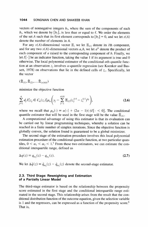
For any s(A)-dimensional vector 5, we let ~(/) denote its Ith component, and for any two s (A) -dimensional vectors a,b, we let ab denote the product of each component of a raised to the corresponding component of b. Finally, we let I [ ] be an indicator function, taking the value 1 if its argument is true and 0 otherwise. The local polynomial estimator of the conditional ath quantile func- tion at an observation zi involves a-quantile regression (see Koenker and Bas- sett, 1978) on observations that lie in the defined cells of zi. Specifically, let the vector

((1), X (2) *

... (s(A)))

minimize the objective function

n s(A)

dIl[zj Cn(zi)]pyP E ()c)- Z )) (2.6) j=l 1=1

where we recall that p,(*) - a'I + (2a - 1)(.)I[. < 0]. The conditional

quantile estimator that will be used in the first stage will be the value S(i). A computational advantage of using this estimator is that its evaluation can

be carried out by linear programming techniques, whereby a solution can be reached in a finite number of simplex iterations. Since the objective function is globally convex, the solution found is guaranteed to be a global minimizer.

The second stage of the estimation procedure involves this local polynomial estimation procedure of the conditional quantile function, at two particular quan- tiles, 0 < al < a2 < 1.5 From these two estimators, we can estimate the con- ditional interquartile range, defined as

Aq(z)- qa2(Z) qa(Z). (2.7)

We let Aq^(z) - q,(z) - q, (z) denote the second-stage estimator.

2.3. Third Stage: Reweighting and Estimation of a Partially Linear Model

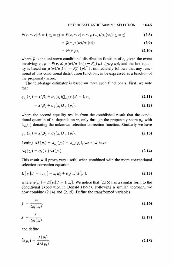
The third-stage estimator is based on the relationship between the propensity score estimated in the first stage and the conditional interquartile range esti- mated in the second stage. This relationship arises from the result that the con- ditional distribution function of the outcome equation, given the selection variable is 1 and the regressors, can be expressed as a function of the propensity score.6 That is,

HETEROSKEDASTIC SAMPLE SELECTION

P(Ei < c I di = , Zi = Z) = P(Ei < C Vi ' d,(Wi)/ll(Wi),Zi = Z) (2.8)

= (c,/ (w)/crl(w)) (2.9)

= H(c, p), (2.10)

where g is the unknown conditional distribution function of Ei given the event

involving vi, p = P(vi < ,u(w)/cr (w)) F,, (u (w)/l (w)), and the last equal- ity is based on /u(w)/o l(w) = F^,'(p).7 It immediately follows that any func- tional of this conditional distribution function can be expressed as a function of the propensity score.

The third-stage estimator is based on three such functionals. First, we note that

qa2(zi) = x Po + 2(xi)Qa2(Eidi = 1, z) (2.11)

- x o0 + o2(Xi)A,a2(Pi), (2.12)

where the second equality results from the established result that the condi- tional quantile of Ei depends on wi only through the propensity score Pi, with

Aa2(.) denoting the unknown selection correction function. Similarly we have

qa,(Zi) = XIPo + o-2(Xi)Aa,(Pi) (2.13)

Letting AA(pi) = A,,(pi) - A,(pi), we now have

Aq(zi) = o2(xi)AA(pi). (2.14)

This result will prove very useful when combined with the more conventional selection correction equation

E[yi di = 1, zi] = x'p0 + o'2(xi)A(pi), (2.15)

where A(pi) = E[Ei di = 1, zi]. We notice that (2.15) has a similar form to the conditional expectation in Donald (1995). Following a similar approach, we now combine (2.14) and (2.15). Define the transformed variables

Yi Y(i)= y

(2.16) Aq(zi)'

Xi X =

q( z) (2.17) Aq(zi)

and define

A(p) = A(pi)(2.18) AA(pi)'

1045

1046 SONGNIAN CHEN AND SHAKEEB KHAN

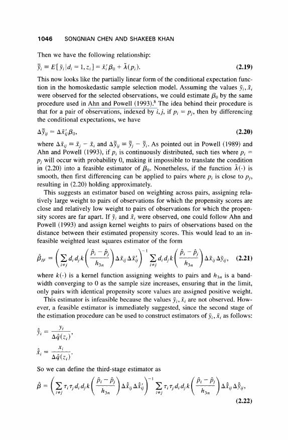
Then we have the following relationship:

i - E[yi Idi = 1, zi] = X[ 3o + A(Pi). (2.19)

This now looks like the partially linear form of the conditional expectation func- tion in the homoskedastic sample selection model. Assuming the values yi, xi were observed for the selected observations, we could estimate /o by the same procedure used in Ahn and Powell (1993).8 The idea behind their procedure is that for a pair of observations, indexed by i,j, if Pi = pj, then by differencing the conditional expectations, we have

AYij = AXP30, (2.20)

where Aijy - -xi and Ayij - j - Yi. As pointed out in Powell (1989) and Ahn and Powell (1993), if pi is continuously distributed, such ties where Pi =

pj will occur with probability 0, making it impossible to translate the condition in (2.20) into a feasible estimator of o3. Nonetheless, if the function A(.) is smooth, then first differencing can be applied to pairs where pi is close to pj, resulting in (2.20) holding approximately.

This suggests an estimator based on weighting across pairs, assigning rela- tively large weight to pairs of observations for which the propensity scores are close and relatively low weight to pairs of observations for which the propen- sity scores are far apart. If Yi and ji were observed, one could follow Ahn and Powell (1993) and assign kernel weights to pairs of observations based on the distance between their estimated propensity scores. This would lead to an in- feasible weighted least squares estimator of the form

8IF ~=l~ SiiJ 1 di djJ hc S hijjA, (2.21) H i~j \ 3n / i j \ h3n

where k(.) is a kernel function assigning weights to pairs and h3n is a band- width converging to 0 as the sample size increases, ensuring that in the limit, only pairs with identical propensity score values are assigned positive weight.

This estimator is infeasible because the values Yi, xi are not observed. How- ever, a feasible estimator is immediately suggested, since the second stage of the estimation procedure can be used to construct estimators of Yi, xi as follows:

^ Yi Yi =

Xi xi =

Aq(zi)'

So we can define the third-stage estimator as

=3 --

Z T i Tj di dj k ax< Axij -Ti Tj di dj k A Aj \i-J ( h3n ( ' ijdi h 5i,3n

(2.22)

HETEROSKEDASTIC SAMPLE SELECTION

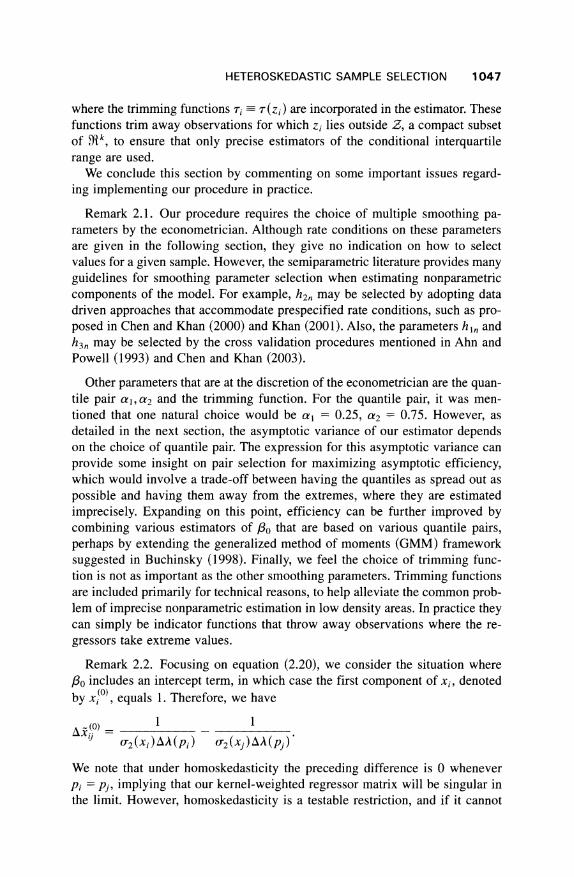
where the trimming functions ri r= (zi) are incorporated in the estimator. These functions trim away observations for which zi lies outside Z, a compact subset of gSk, to ensure that only precise estimators of the conditional interquartile range are used.

We conclude this section by commenting on some important issues regard- ing implementing our procedure in practice.

Remark 2.1. Our procedure requires the choice of multiple smoothing pa- rameters by the econometrician. Although rate conditions on these parameters are given in the following section, they give no indication on how to select values for a given sample. However, the semiparametric literature provides many guidelines for smoothing parameter selection when estimating nonparametric components of the model. For example, h2n may be selected by adopting data driven approaches that accommodate prespecified rate conditions, such as pro- posed in Chen and Khan (2000) and Khan (2001). Also, the parameters hi, and h3n may be selected by the cross validation procedures mentioned in Ahn and Powell (1993) and Chen and Khan (2003).

Other parameters that are at the discretion of the econometrician are the quan- tile pair al, a2 and the trimming function. For the quantile pair, it was men- tioned that one natural choice would be a1 = 0.25, a2 = 0.75. However, as detailed in the next section, the asymptotic variance of our estimator depends on the choice of quantile pair. The expression for this asymptotic variance can provide some insight on pair selection for maximizing asymptotic efficiency, which would involve a trade-off between having the quantiles as spread out as possible and having them away from the extremes, where they are estimated imprecisely. Expanding on this point, efficiency can be further improved by combining various estimators of /o that are based on various quantile pairs, perhaps by extending the generalized method of moments (GMM) framework suggested in Buchinsky (1998). Finally, we feel the choice of trimming func- tion is not as important as the other smoothing parameters. Trimming functions are included primarily for technical reasons, to help alleviate the common prob- lem of imprecise nonparametric estimation in low density areas. In practice they can simply be indicator functions that throw away observations where the re- gressors take extreme values.

Remark 2.2. Focusing on equation (2.20), we consider the situation where 30o includes an intercept term, in which case the first component of xi, denoted

by xi?), equals 1. Therefore, we have

1 1 A (0) =

o 2(xi)AA(pi) O2(Xj) AA(pj)'

We note that under homoskedasticity the preceding difference is 0 whenever Pi = pj, implying that our kernel-weighted regressor matrix will be singular in the limit. However, homoskedasticity is a testable restriction, and if it cannot

1047

1048 SONGNIAN CHEN AND SHAKEEB KHAN

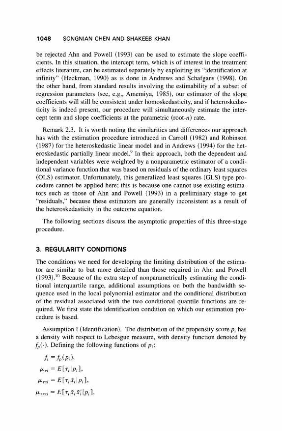
be rejected Ahn and Powell (1993) can be used to estimate the slope coeffi- cients. In this situation, the intercept term, which is of interest in the treatment effects literature, can be estimated separately by exploiting its "identification at infinity" (Heckman, 1990) as is done in Andrews and Schafgans (1998). On the other hand, from standard results involving the estimability of a subset of regression parameters (see, e.g., Amemiya, 1985), our estimator of the slope coefficients will still be consistent under homoskedasticity, and if heteroskedas- ticity is indeed present, our procedure will simultaneously estimate the inter- cept term and slope coefficients at the parametric (root-n) rate.

Remark 2.3. It is worth noting the similarities and differences our approach has with the estimation procedure introduced in Carroll (1982) and Robinson (1987) for the heteroskedastic linear model and in Andrews (1994) for the het- eroskedastic partially linear model.9 In their approach, both the dependent and independent variables were weighted by a nonparametric estimator of a condi- tional variance function that was based on residuals of the ordinary least squares (OLS) estimator. Unfortunately, this generalized least squares (GLS) type pro- cedure cannot be applied here; this is because one cannot use existing estima- tors such as those of Ahn and Powell (1993) in a preliminary stage to get "residuals," because these estimators are generally inconsistent as a result of the heteroskedasticity in the outcome equation.

The following sections discuss the asymptotic properties of this three-stage procedure.

3. REGULARITY CONDITIONS

The conditions we need for developing the limiting distribution of the estima- tor are similar to but more detailed than those required in Ahn and Powell (1993).10 Because of the extra step of nonparametrically estimating the condi- tional interquartile range, additional assumptions on both the bandwidth se- quence used in the local polynomial estimator and the conditional distribution of the residual associated with the two conditional quantile functions are re- quired. We first state the identification condition on which our estimation pro- cedure is based.

Assumption I (Identification). The distribution of the propensity score pi has a density with respect to Lebesgue measure, with density function denoted by fp(.). Defining the following functions of pi:

fi =fp(pi),

Z-rxi = E[7ii I Pi],

HETEROSKEDASTIC SAMPLE SELECTION

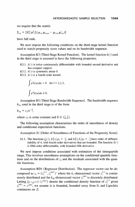
we require that the matrix

Exx = 2E[pi f( ri rxxi - - irxi xrxi)]

have full rank.

We next impose the following conditions on the third-stage kernel function used to match propensity score values and on its bandwidth sequence.

Assumption K3 (Third-Stage Kernel Function). The kernel function k(.) used in the third stage is assumed to have the following properties.

K3.1. k(.) is twice continuously differentiable with bounded second derivative and has compact support.

K3.2. k(.) is symmetric about 0. K3.3. k(.) is a fourth-order kernel:

fu'k(u)du = 0 for 1 = 1,2,3,

fu4k(u)du + 0.

Assumption H3 (Third-Stage Bandwidth Sequence). The bandwidth sequence h3n used in the third stage is of the form

h3n = c3n-,

where C3 is some constant and 8 E (8,6).

The following assumption characterizes the order of smoothness of density and conditional expectation functions.

Assumption S1 (Order of Smoothness of Functions of the Propensity Score).

Sl.1. The functions fp(.), E[rilpi = *], and E[rixi Pi = '] have order of differen- tiability of 4, with fourth-order derivatives that are bounded. The function A(-) is fifth-order differentiable, with bounded fifth derivative.

We next impose conditions associated with estimation of the interquartile range. This involves smoothness assumptions on the conditional quantile func- tions and on the distributions of zi and the residuals associated with the quan- tile functions.

Assumption RD1 (Regressor Distribution). The regressor vector can be de-

composed as zi = (z(c), z(ds)')' where the kc-dimensional vector z(c) is contin-

uously distributed and the kds-dimensional vector z(ds) is discretely distributed.

Letting fz(clzd (. z(ds)) denote the conditional density function of z() given z(ds) = z(ds) we assume it is bounded, bounded away from 0, and Lipschitz continuous on Z.

1049

1050 SONGNIAN CHEN AND SHAKEEB KHAN

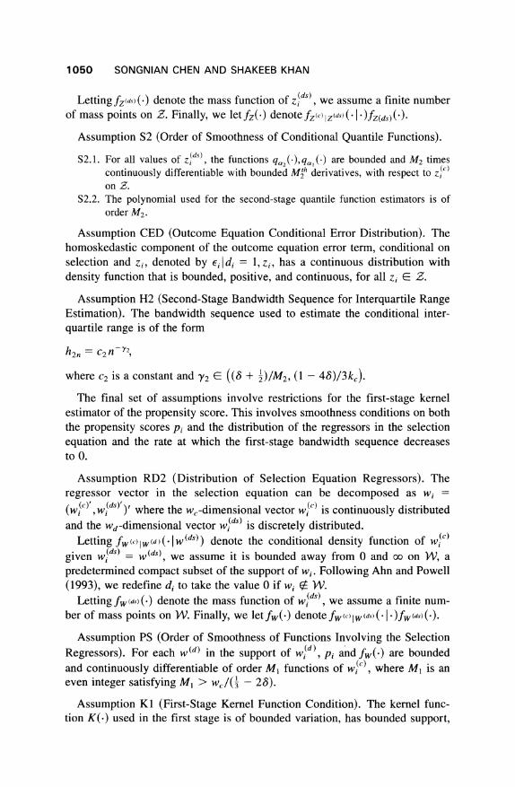
Letting fz(ds(.) denote the mass function of zds), we assume a finite number of mass points on Z. Finally, we let fz() denote fzc lz(ds)( z(d)(').

Assumption S2 (Order of Smoothness of Conditional Quantile Functions).

S2.1. For all values of zds), the functions qa2(.),q^,() are bounded and M2 times continuously differentiable with bounded M2h derivatives, with respect to z on Z.

S2.2. The polynomial used for the second-stage quantile function estimators is of order M2.

Assumption CED (Outcome Equation Conditional Error Distribution). The homoskedastic component of the outcome equation error term, conditional on selection and Zi, denoted by Ei di = 1,zi, has a continuous distribution with

density function that is bounded, positive, and continuous, for all zi E Z.

Assumption H2 (Second-Stage Bandwidth Sequence for Interquartile Range Estimation). The bandwidth sequence used to estimate the conditional inter- quartile range is of the form

h2n = C2-2n

where c2 is a constant and Y2 E ((6 + )/M2, (1 - 45)/3kc).

The final set of assumptions involve restrictions for the first-stage kernel estimator of the propensity score. This involves smoothness conditions on both the propensity scores pi and the distribution of the regressors in the selection equation and the rate at which the first-stage bandwidth sequence decreases to O.

Assumption RD2 (Distribution of Selection Equation Regressors). The regressor vector in the selection equation can be decomposed as wi =

(w(c) , w(d)') where the wc-dimensional vector w(c) is continuously distributed and the wd-dimensional vector w(ds) is discretely distributed.

Letting f(c) l(d )(I w(ds)) denote the conditional density function of w(c)

given w(ds) = w(ds), we assume it is bounded away from 0 and oo on W, a

predetermined compact subset of the support of wi. Following Ahn and Powell (1993), we redefine di to take the value 0 if wi X W.

Lettingfw(d) (-) denote the mass function of w(ds), we assume a finite num- ber of mass points on W. Finally, we let fw(.) denote fww(c) w(ds) ( | )fW(d)(-).

Assumption PS (Order of Smoothness of Functions Involving the Selection

Regressors). For each w(d) in the support of w d), Pi and fw(') are bounded and continuously differentiable of order Ml functions of w (), where Ml is an even integer satisfying M1 > Wc/(3 - 26).

Assumption K1 (First-Stage Kernel Function Condition). The kernel func- tion K(.) used in the first stage is of bounded variation, has bounded support,

HETEROSKEDASTIC SAMPLE SELECTION

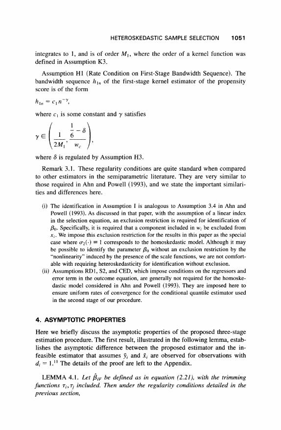
integrates to 1, and is of order M1, where the order of a kernel function was defined in Assumption K3.

Assumption Hi (Rate Condition on First-Stage Bandwidth Sequence). The bandwidth sequence hi, of the first-stage kernel estimator of the propensity score is of the form

hln = cl n-Y,

where cl is some constant and y satisfies

/ 1- 6 yE 1 6

\2M1 w,

where 8 is regulated by Assumption H3.

Remark 3.1. These regularity conditions are quite standard when compared to other estimators in the semiparametric literature. They are very similar to those required in Ahn and Powell (1993), and we state the important similari- ties and differences here.

(i) The identification in Assumption I is analogous to Assumption 3.4 in Ahn and Powell (1993). As discussed in that paper, with the assumption of a linear index in the selection equation, an exclusion restriction is required for identification of ,80. Specifically, it is required that a component included in wi be excluded from xi. We impose this exclusion restriction for the results in this paper as the special case where o2(.) = 1 corresponds to the homoskedastic model. Although it may be possible to identify the parameter 13o without an exclusion restriction by the "nonlinearity" induced by the presence of the scale functions, we are not comfort- able with requiring heteroskedasticity for identification without exclusion.

(ii) Assumptions RD1, S2, and CED, which impose conditions on the regressors and error term in the outcome equation, are generally not required for the homoske- dastic model considered in Ahn and Powell (1993). They are imposed here to ensure uniform rates of convergence for the conditional quantile estimator used in the second stage of our procedure.

4. ASYMP I U IC PROPERTIES

Here we briefly discuss the asymptotic properties of the proposed three-stage estimation procedure. The first result, illustrated in the following lemma, estab- lishes the asymptotic difference between the proposed estimator and the in- feasible estimator that assumes Yi and xi are observed for observations with

di = 1.11 The details of the proof are left to the Appendix.

LEMMA 4.1. Let plF be defined as in equation (2.21), with the trimming functions ri, rj included. Then under the regularity conditions detailed in the previous section,

1051

1052 SONGNIAN CHEN AND SHAKEEB KHAN

in

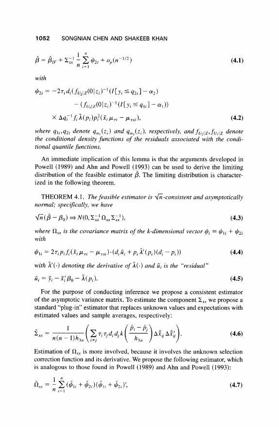
/3 = 3I + Ex;'- / 2, + op(n-1/2) (4.1) n i=

with

qi2i = -27idi(fu21l(O0zi)-1 (i[yi < q2i] - ?2)

- (fu,lz(OIzi)- (l[yi qli]- oa,))

x A-qfi ;A(pi)p2(Xi /ri - ,xi), (4.2)

where qli,q2i denote qal(zi) and qa2(zi), respectively, andfu2lz,fu, z denote the conditional density functions of the residuals associated with the condi- tional quantile functions.

An immediate implication of this lemma is that the arguments developed in Powell (1989) and Ahn and Powell (1993) can be used to derive the limiting distribution of the feasible estimator /3. The limiting distribution is character- ized in the following theorem.

THEOREM 4.1. The feasible estimator is 'n-consistent and asymptotically normal; specifically, we have

x/1 (/3 -

i0o) N(O, Ex xxJ ), (4.3)

where fl, is the covariance matrix of the k-dimensional vector i = 1qli + 12i with

?i = 27iPifi(i ( i - LA7xi)'(dii ui + Pi A'(Pi)(di - Pi)) (4.4)

with A'(.) denoting the derivative of A(.) and uii is the "residual"

iii = Yi - 30o - (pi). (4.5)

For the purpose of conducting inference we propose a consistent estimator of the asymptotic variance matrix. To estimate the component Ex we propose a standard "plug-in" estimator that replaces unknown values and expectations with estimated values and sample averages, respectively:

n (nl3xx= ( r7i rj di dj k (Ah)xij Axu) (4.6) n(n - i)h3,, iy i i j

Estimation of flxx is more involved, because it involves the unknown selection correction function and its derivative. We propose the following estimator, which is analogous to those found in Powell (1989) and Ahn and Powell (1993):

1 i= n i= l

HETEROSKEDASTIC SAMPLE SELECTION

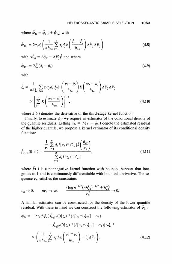
where /lli = lli + -+12i with

~lji = 27idi ( nh- E d- k A h A ij (4.8)

with Abui = Aji - AxiJ, and where

12i = 2i(di - i) (4.9)

with

nh3n /j h3n hln

1 WI - Wi (4.10) X K^ h , (4.10)

where k'(.) denotes the derivative of the third-stage kernel function. Finally, to estimate I2i we require an estimator of the conditional density of

the quantile residuals. Letting 2i di(yi - q2i) denote the estimated residual of the higher quantile, we propose a kernel estimator of its conditional density function:

inl 2i -E dl [zlE Cnil ] - n I= 1 n

2,z(Olzi) = n , (4.11)

dll[zl E Cni] 1=1

where k(.) is a nonnegative kernel function with bounded support that inte- grates to 1 and is continuously differentiable with bounded derivative. The se- quence ,, satisfies the constraints

(log n)'/2(nh2k,)-1/2 + h22 Vn , nv - O , , 2 -0.

'n

A similar estimator can be constructed for the density of the lower quantile residual. With these in hand we can construct the following estimator of i2i:

42i = -2ridii(fu2z(Ozi) (I[Yi < q2i - a2)

--fU, iz(OiZi)-'(I[yi qli] -- al))Aq^i-

( nh j d k - j Axij . (4.12)

h3n j= 1 h3n

1053

1054 SONGNIAN CHEN AND SHAKEEB KHAN

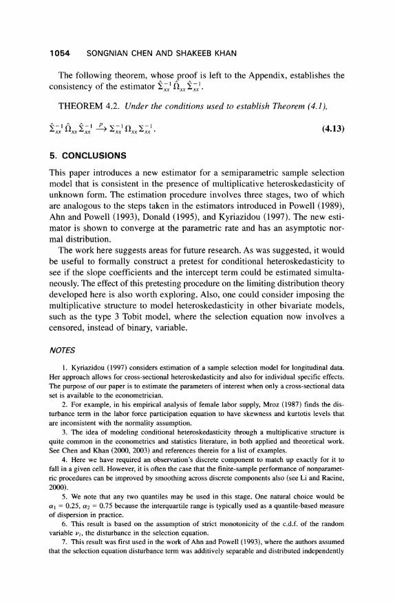
The following theorem, whose proof is left to the Appendix, establishes the

consistency of the estimator 'xx Sl xx xl.

THEOREM 4.2. Under the conditions used to establish Theorem (4.1),

C OlCxx Uxx S xx S;axx * (4.13)

5. CONCLUSIONS

This paper introduces a new estimator for a semiparametric sample selection model that is consistent in the presence of multiplicative heteroskedasticity of unknown form. The estimation procedure involves three stages, two of which are analogous to the steps taken in the estimators introduced in Powell (1989), Ahn and Powell (1993), Donald (1995), and Kyriazidou (1997). The new esti- mator is shown to converge at the parametric rate and has an asymptotic nor- mal distribution.

The work here suggests areas for future research. As was suggested, it would be useful to formally construct a pretest for conditional heteroskedasticity to see if the slope coefficients and the intercept term could be estimated simulta-

neously. The effect of this pretesting procedure on the limiting distribution theory developed here is also worth exploring. Also, one could consider imposing the

multiplicative structure to model heteroskedasticity in other bivariate models, such as the type 3 Tobit model, where the selection equation now involves a

censored, instead of binary, variable.

NOTES

1. Kyriazidou (1997) considers estimation of a sample selection model for longitudinal data. Her approach allows for cross-sectional heteroskedasticity and also for individual specific effects. The purpose of our paper is to estimate the parameters of interest when only a cross-sectional data set is available to the econometrician.

2. For example, in his empirical analysis of female labor supply, Mroz (1987) finds the dis- turbance term in the labor force participation equation to have skewness and kurtotis levels that are inconsistent with the normality assumption.

3. The idea of modeling conditional heteroskedasticity through a multiplicative structure is

quite common in the econometrics and statistics literature, in both applied and theoretical work. See Chen and Khan (2000, 2003) and references therein for a list of examples.

4. Here we have required an observation's discrete component to match up exactly for it to fall in a given cell. However, it is often the case that the finite-sample performance of nonparamet- ric procedures can be improved by smoothing across discrete components also (see Li and Racine, 2000).

5. We note that any two quantiles may be used in this stage. One natural choice would be al = 0.25, a2 = 0.75 because the interquartile range is typically used as a quantile-based measure of dispersion in practice.

6. This result is based on the assumption of strict monotonicity of the c.d.f. of the random variable vi, the disturbance in the selection equation.

7. This result was first used in the work of Ahn and Powell (1993), where the authors assumed that the selection equation disturbance term was additively separable and distributed independently

HETEROSKEDASTIC SAMPLE SELECTION

of the regressors. Although we relax their homoskedasticity assumption, we require additive sepa- rability and multiplicative heteroskedasticity to express the distribution function as a function of the propensity score.

8. We note that any of the existing estimators for the partially linear model, such as in Rob- inson (1988) and Andrews (1991, 1994), could be used in this stage.

9. This type of procedure is also used to estimate a heteroskedastic nonlinear regression model in Delgado (1992) and Hildago (1992).

10. In this section we assume that p0 does include an intercept term to be estimated. As dis- cussed in Remark 2.2, the intercept cannot be consistently estimated under conditional homoske- dasticity, though the slope coefficients can be. Thus we are implicitly assuming that either conditional heteroskedasticity is present or that the parameter of interest is the last k components of 0o.

11. We note that this result is in contrast to the results found in Carroll (1982) and Robinson (1987) for the heteroskedastic linear regression model and in Andrews (1994) for the (partially) heteroskedastic partially linear model, where asymptotic equivalence is established for their GLS- type procedures.

REFERENCES

Ahn, H. & J.L. Powell (1993) Semiparametric estimation of censored selection models with a non- parametric selection mechanism. Journal of Econometrics 58, 3-29.

Amemiya, T. (1985) Advanced Econometrics. Cambridge: Harvard University Press. Andrews, D.W.K. (1991) Asymptotic normality for nonparametric and semiparametric regression

models. Econometrica 59, 307-345. Andrews, D.W.K. (1994) Asymptotics for semiparametric econometric models via stochastic equi-

continuity. Econometrica 62, 43-72. Andrews, D.W.K. & M.M.A. Schafgans (1998) Semiparametric estimation of the intercept of a

sample selection model. Review of Economic Studies 65, 497-517. Bierens, H.J. (1987) Kernel estimators of regression functions. In T.F. Bewley (ed.), Advances in

Econometrics, Fifth World Congress, vol. 1, pp. 99-144. Cambridge: Cambridge University Press. Buchinsky, M. (1998) Recent advances in quantile regression models: A practical guideline for

empirical research. Journal of Human Resources 33, 88-126. Carroll, R.J. (1982) Adapting for heteroskedasticity in linear models. Annals of Statistics 10,

1224-1233. Chaudhuri, P. (1991a) Nonparametric estimates of regression quantiles and their local Bahadur

representation. Annals of Statistics 19, 760-777. Chaudhuri, P. (1991b) Global nonparametric estimation of conditional quantiles and their deriva-

tives. Journal of Multivariate Analysis 39, 246-269. Chaudhuri, P., K. Doksum, & A. Samarov (1997) On average derivative quantile regression. An-

nals of Statistics 25, 715-744. Chen, S. (1999) Semiparametric estimation of heteroskedastic binary choice sample selection mod-

els under symmetry. Manuscript, Hong Kong University of Science and Technology. Chen, S. & S. Khan (2000) Estimating censored regression models in the presence of nonparamet-

ric multiplicative heteroskedasticity. Journal of Econometrics 98, 283-316. Chen, S. & S. Khan (2001) Semiparametric estimation of a partially linear censored regression

model. Econometric Theory 17, 567-590. Chen, S. & S. Khan (2003) Rates of convergence for estimating regression coefficients in hetero-

skedastic discrete response models. Journal of Econometrics, in press. Choi, K. (1990) Semiparametric Estimation of the Sample Selection Model Using Series Expan-

sion and the Propensity Score. Manuscript, University of Chicago. Delgado, M. (1992) Semiparametric generalized least squares in the multivariate nonlinear regres-

sion model. Econometric Theory 8, 203-222. Donald, S.G. (1995) Two-step estimation of heteroscedastic sample selection models. Journal of

Econometrics 65, 347-380.

1055

1056 SONGNIAN CHEN AND SHAKEEB KHAN

Gronau, R. (1974) Wage comparisons: A selectivity bias. Journal of Political Economy 82, 1119-1144.

Heckman, J.J. (1976) The common structure of statistical models of truncation, sample selection, and limited dependent variables and a simple estimator of such models. Annals of Economic and Social Measurement 15, 475-492.

Heckman, J.J. (1979) Sample selection bias as a specification error. Econometrica 47, 153-161. Heckman, J.J. (1990) Varieties of selection bias. American Economic Review 80, 313-318.

Hildago, J. (1992) Adaptive estimation in time series models with heteroskedasticity of unknown form. Econometric Theory 8, 161-187.

Horowitz, J.L. (1992) A smoothed maximum score estimator for the binary response model. Econ- ometrica 60, 505-531.

Khan, S. (2001) Two stage rank estimation of quantile index models. Journal of Econometrics 100, 319-355.

Khan, S. & J.L. Powell (2001) Two-step quantile estimation of semiparametric censored regression models. Journal of Econometrics 103, 73-110.

Koenker, R. & G.S. Bassett, Jr. (1978) Regression quantiles. Econometrica 46, 33-50.

Kyriazidou, E. (1997) Estimation of a panel data sample selection model. Econometrica 65, 1335-1364.

Li, Q. & J. Racine (2000) Nonparametric Estimation of Regression Functions with Both Categori- cal and Continuous Data. Manuscript, Texas A&M University.

Mroz, T.A. (1987) The sensitivity of an empirical model of married women's hours of work to economic and statistical assumptions. Econometrica 55, 765-799.

Powell, J.L. (1989) Semiparametric Estimation of Censored Selection Models. Manuscript, Univer-

sity of Wisconsin. Robinson, P.M. (1987) Asymptotically efficient estimation in the presence of heteroskedasticity of

unknown form. Econometrica 56, 875-891. Robinson, P.M. (1988) Root-N-consistent semiparametric regression. Econometrica 56, 931-954. Rosenbaum, P.R. & D.B. Rubin (1983) The central role of the propensity score in observational

studies for causal effects. Biometrika 70, 41-55. Sherman, R.P. (1994) Maximal inequalities for degenerate U-processes with applications to opti-

mization estimators. Annals of Statistics 22, 439-459.

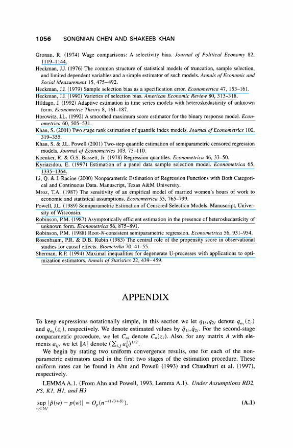
APPENDIX

To keep expressions notationally simple, in this section we let qli,q2i denote qa,(zi) and q C2(Zi), respectively. We denote estimated values by qli,q2i. For the second-stage nonparametric procedure, we let Cni denote Cz(zi). Also, for any matrix A with ele- ments aij, we let I All denote (i,j a2)1/2.

We begin by stating two uniform convergence results, one for each of the non-

parametric estimators used in the first two stages of the estimation procedure. These

uniform rates can be found in Ahn and Powell (1993) and Chaudhuri et al. (1997),

respectively.

LEMMA A. 1. (From Ahn and Powell, 1993, Lemma A.1). Under Assumptions RD2, PS, Kl, HI, and H3

(A.1) sup Lp(w)-p(w)l = Op(n-(1/3+s)). wEW

HETEROSKEDASTIC SAMPLE SELECTION

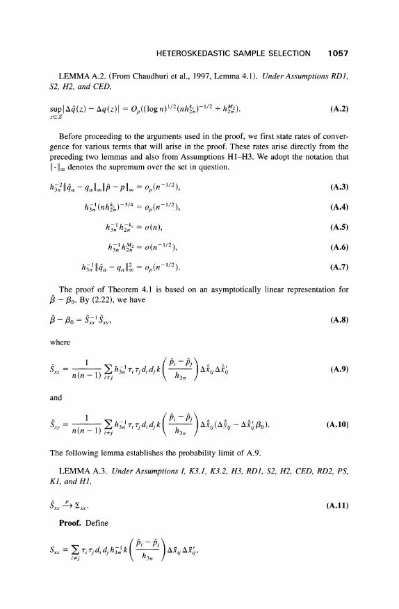
LEMMA A.2. (From Chaudhuri et al., 1997, Lemma 4.1). Under Assumptions RD1, S2, H2, and CED,

sup A(z)- Aq(z)) = Op((log n)1/2(nhk)-1/2 + h2). (A.2) zEZ

Before proceeding to the arguments used in the proof, we first state rates of conver-

gence for various terms that will arise in the proof. These rates arise directly from the

preceding two lemmas and also from Assumptions H1-H3. We adopt the notation that 1 Iloo denotes the supremum over the set in question.

h3211q - q, P-P = Op(n-1/2) (A.3)

h3l(nh2kc)-3/4 = Op(,n-1/2), (A.4)

h3-n h2nkc = o(n), (A.5)

h3 h2 2= o(n-1/2), (A.6)

hl , - q,q 12 = Op(n -1/2). (A.7)

The proof of Theorem 4.1 is based on an asymptotically linear representation for /, - Po. By (2.22), we have

-Po = Sxx1 Sxy, (A.8)

where

n(n - 1) i rdidjk (A.9)

and

Sy= n 1

3nij di dj i k ( h A (A -A1o) (A.10) SXY 3n i - Aij(Aij ijO) nn (nY- ) - h

The following lemma establishes the probability limit of A.9.

LEMMA A.3. Under Assumptions I, K3.1, K3.2, H3, RDI, S2, H2, CED, RD2, PS, K1, and HI,

pxx L lxx*. (A.11)

Proof. Define

Sxx = 7i Tj di dj h 3n k AX^ ij A -x, S ~ 3n-1

kPi -13j h .3n

1057

1058 SONGNIAN CHEN AND SHAKEEB KHAN

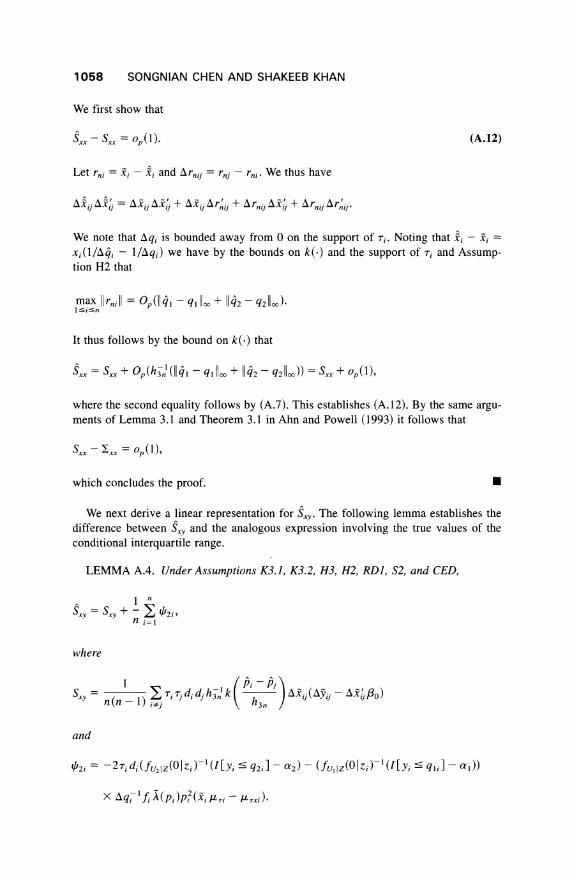
We first show that

xx - Sxx = op(l). (A.12)

Let rni = xi - Xi and Arnij = rnj - ri. We thus have

AijXij A iji. A Arnij + Arnij AX + A rnijAr.

We note that Aqi is bounded away from 0 on the support of ri. Noting that -i - ji =

Xi(I/Aqi - 1/Aqi) we have by the bounds on k(.) and the support of ri and Assump- tion H2 that

max ||rni| = Op( - q lloo + 112 - q2loo).

It thus follows by the bound on k(.) that

Sxx + 1 lll + 2 - q2 = Sx +(q- loo + 12-q ) = S + (1),

where the second equality follows by (A.7). This establishes (A.12). By the same argu- ments of Lemma 3.1 and Theorem 3.1 in Ahn and Powell (1993) it follows that

xx - Lx = op(l),

which concludes the proof. 1

We next derive a linear representation for Sxy. The following lemma establishes the difference between Sxy and the analogous expression involving the true values of the conditional interquartile range.

LEMMA A.4. Under Assumptions K3.1, K3.2, H3, H2, RDI, S2, and CED,

x= S +-i2, n sxy = sxy + -

1 2i n, 1

where

Sxy i jdi dj hA.k P(

-

Aij(/ij -

A.[j0o ) n (n- 1) ij rjdid h3n

and

?2i = -2ridi(fu2lz(Olzi)- (I[yi < q2i] - a2) - (fu1lz(Ozi)-l1(I[yi qli]

- a1))

X Aqi-lfi (pi)pi2(.xi! -

iXLi).

HETEROSKEDASTIC SAMPLE SELECTION

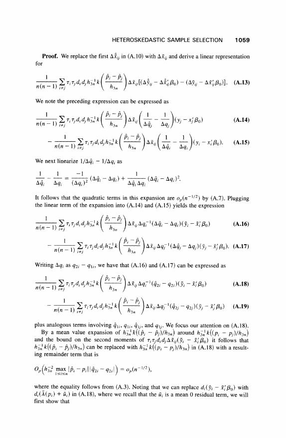
Proof. We replace the first Axi in (A.10) with Axij and derive a linear representation for

I i rj di djh 1(Aj [(A -- AxI3o)-(Ay-A )]. (A.13) n(n - 1) i6j d d h3n n k

We note the preceding expression can be expressed as

n(n- -i 7didjh hk k ( ) ( (yj( - -)(yx ) (A.14)

ni(n - 1)j 3n 3j qj

-n(n- l) Z y

i~didjy^ ^*h3nk

- 7j Tjdi djh 3no k (A.15) n(n - 1) i:ij h3n Aq i Aqi

We next linearize 1/A4i - 1/Aqi as

1 1 -1 1 ---= 2 ( /--) + (^i.-A^qi)2

Aq4i Aqi (Aqi)2 -

Aq,) i a qi

It follows that the quadratic terms in this expansion are op(n-1/2) by (A.7). Plugging the linear term of the expansion into (A.14) and (A.15) yields the expression

n 1

Ti Tjdi dj hn k (hr Aqj'( A,i - Aqi)(i , - -xi;3) (A.16) n nn - 1) j3j h n

n(- n1) TiTjdid jh3' k

h3 ) AxiJ qj -(A -Aqj)(yj-x1o).

(A.17) n(n - 1) itj \ 3n

Writing Aqi as q2i - qli, we have that (A.16) and (A.17) can be expressed as

n(n - 1) ;j ij h 3nh2

id1d.h .-k( A xi A qjq - q2i)(i - X j,3o) (A.18)

n(n -) i? ( h3n )

plus analogous terms involving q1i, q1i, qj, and qlj. We focus our attention on (A.18). By a mean value expansion of h32 k((pi - pj)/h3n) around h3 k((pi - pj)/h3n)

and the bound on the second moments of rir.didjAxI (yi - Xi'0) it follows that h k((pi - p3)/h3n) can be replaced with h3 k((p, - p)/h3n) in (A.18) with a result-

ing remainder term that is

Op (h3 max Ip i-Pi q2i

- q2 I) = op(n 1/2),

where the equality follows from (A.3). Noting that we can replace di(yi - X o0) with di(A(pi) + ii) in (A.18), where we recall that the ii, is a mean 0 residual term, we will first show that

1059

1060 SONGNIAN CHEN AND SHAKEEB KHAN

. 1 rri^ddkhp Y o,(n 1/2) (A.20)

n(n -

7) j i d didjh3 h k h3 n, j

AiAq I(q2i -

q2i)ui = op(n-1/2 (A.20) n (n -) i Aj \ h3n /

and we will then derive a linear representation for

n(n-1) j idi Tj d djh3 l k h ( APij Aq (q2i

- q2A(Pi)- (A.21) (n 3) h \i d 1

To show (A.20), we use the local Bahadur representations for the local polynomial es- timator established in Chaudhuri (1991a) and Chaudhuri et al. (1997). In our context this can be expressed as

2i- q2i = k fUz(, zi) (-) E dkl[Zk E Cni](I[yk, q(k,i)]

- a2) + Rni, (A.22) nn2n kZi

where q2(k,i) denotes the Taylor polynomial approximation of q2k for Zk close to zi,

fu2,z('-') denotes the joint density function of the quantile residual and Zk; Rni is a re- mainder term converging to 0 at a rate depending on the bandwidth h2n. Using the same arguments as in Chen and Khan (2000, 2001), it can be shown that under Assumptions RD1, S2, H2, and H3 that

sup h3 IRnil = Op(h3(nhk 3/4) - op(n-1/2), ZiEZ

where the second equality follows from (A.4). Thus to show (A.20), it will suffice to show the asymptotic negligibility of the following third-order U-statistic:

1 7) i .j di dj h 1-n kP(i -P

I n (n - 1)(n - 2) i T 4

X (I[yk < q2(k,i)]- Oa2)fu2,z(, zi) h2nk AXijdkI[Zk E Cni ]i (A.23)

We next replace q2(k,i) with q2k. By Assumption S2.1, this replacement results in a remainder term that is Op(h3' hM2), which is Op(n-1/2) by (A.6). Let Xi =

(yi,zi,q2i,Pi, 2i, Ti,ri,di)'. Let n(Xi, Xj, Xk) denote the expression in the preceding triple summation after this replacement. It follows after a change of variables that

E[Jl,(., ,.)112] = O(h3 h2-nk) = o(n),

where the second equality follows from (A.5). We can thus apply the projection theo- rem for U-statistics in Ahn and Powell (1993). We note that

E[fn(-,',-)] = E[F,n(Xi,.,.)] E['n(,X, )] =- E[Fn(.,.,Xk)] = 0,

where the last three terms denote expectations conditional on first, second, and third

arguments, respectively, and the last term is 0 because of the presence of ii. We thus have by Lemma A.3 in Ahn and Powell (1993) that

n(n- )(- 2) n(Xi, Xj,Xk) =

op(n-1/2), n(n

- 1)(n

- 2) i0J,k

establishing (A.20).

HETEROSKEDASTIC SAMPLE SELECTION 1061

It thus remains to derive a linear representation for (A.21). To do so we again plug in the linear representation for the conditional quantile estimator; this yields another mean O third-order U-statistic after showing that the bias term is asymptotically negligible. We will let .F3n( Xi, Xj, Xk) denote the term in the triple summation of this U-statistic. As before, we have E[E3,(-,,.)] = ELF3T,(Xi,,.)] - E[JF(3,Xj,.)] - 0, and will derive a linear representation for

in I E[3,(-, "Xk)] (A.24)

n k=1

Once again, we ignore the bias component of the nonparametric estimator, as it con- verges to 0 at the parametric rate. We will thus derive a linear representation for

in dk c4(Iyk I q2k] - a2)Afln(Zk), (A.25)

n k= 1

where

=ln(Zk) f b jAXijh2n&I [Zk E Cni ]?qi 'fu2,z(O, zi)-' dF(zi jpi) dF(zj Ipj)

x A(pi)pipjf(pi)f(pj) dpi dpj.

To derive an expression for (A.25), we will again use Chebyshev's inequality. Since each term in the summation has mean 0, we will show that

E[l*ln(Zk)] -- - fU2 Z(OzkAqk 1fk TkA(Pk)P(k /Lkk k - ILXk) (A.26)

To do so, we make a change of variables in the definition of '1,(Zk). Using the change of variables ui = (z c) - Z>c)/h2n and vi = (p, - p)/h3, by the dominated conver- gence theorem,

A-4 ln(Zk) fxk)Aqk 1 fu2,z(O, Zk)-l dF(ZkIPj) dF(zjIp )A(p )p7f(p)2dpi.

Expression (A.26) follows by noting that pi is a function of zi. Thus we have shown that (A.21) has the following linear representation:

in - ~ rfi2j I(O jzi)-'di(lIyy I q2i] - a2)Aqi i i (Px)p( + op (n 1/2),

(A.27)

and identical arguments can be used to show that double summations involving (42j - q2j), (4ii - qli), and (41j - q1j) have analogous linear representations. Combin- ing these results, we get that (A.13) has the following linear representation:

I n - ~- 2,rdi (fu2tz(0jzj) 1(IEyi ? q2i] - a2) -fu1jz(0jzi)_ (I[y,i

- qli] - a,)) ni

X Aqi' 1f (pi)p72(_i A,_i - IL7r) + op(n 1/2)( (A.28)

1062 SONGNIAN CHEN AND SHAKEEB KHAN

The remaining step involves showing that

n (n- l

) i rrj1di d h3 k ( h ) (Ai - - AijA ) ijAXi jo) = op(n /2). (A.29)

n(n - 1) ij i hid3 n

This can be done by using similar arguments as before, so we only sketch the details. First, we note that we can replace h3lk((pi - pj)/h3n) with h3 k((pi

- pj)/h3n),

and the remainder term is asymptotically negligible as shown previously. We can also

replace (A/ij - Axi/3o) with (Ajy,i - A I/30), and the remainder terms are of order (Acti - Aqi)2 and (Aqj - Aqj)2, which are (uniformly) of order Op(n-1/2). Thus we will show

Z i Tj di dj h k )(ax j-

a )(Ayj

- A 0) =

Op(n-/2). (A.30) n(n - 1) ij

3n h3

k

Note that we can replace (Ajy - AXi,/3o) with A(p) - A(pi) + Atij. We also note that we need only show negligibility of the term involving xi - Xj because the same argu- ment can be used for Xi - Xi. We can write Xj - Xj as xj(4qj - qj-) and as before linearize the difference and plug in the linear representation of the conditional quantile estimator, yielding a centered third-order U-statistic plus a remainder term that is

Op(n-1/2). The term in the U-statistic involving Aiij is negligible by the same argu- ments as used in showing (A.23). The term in the U-statistic involving A(pj) - A(pi) is also negligible, as a result of presence of h3' k((pi - pj)/h3n), the smoothness assump- tion on A(-) (Assumption S1.1), and the rate condition on h3n (Assumption H3). This shows (A.30) and hence (A.29).

This proves the lemma and establishes the asymptotic difference between the feasible and infeasible estimators, as stated in Lemma 4.1. U

The final step in deriving the limiting distribution of the estimator is to establish a linear representation for Sxy This is done in the following lemma, whose proof is omit- ted because it follows from identical arguments used in the proof of Theorem 3.1 (ii) of Ahn and Powell (1993).

LEMMA A.5. Under Assumptions K3, H3, SI, RD2, PS, Kl, and HI,

1n

Sxy-- -E i = (n-1/2). (A.31) n i=l

The limiting distribution in Theorem 4.1 now easily follows.

Proof of Theorem 4.2. We note that the consistency of ix follows easily from Lemma A.3. To show consistency of ixx we first define vi as

-i = 2riPifi (xi i

- ltrxi)'Pi A'(Pi)'

We show the following lemma.

LEMMA A.6. Under the assumptions,

supllii- = op(l). ri>0

HETEROSKEDASTIC SAMPLE SELECTION

Proof. First we note that by standard results from kernel estimation (e.g., Bierens, 1987) the expression

1 W i -

WiK ,

n hlncKI h

converges uniformly (in wi) in probability to the density of wi, fw(wi), so we focus on the expression

n2h12 wh 717ldldj (k )K( i) v n h3nhln i hj 3n hln

We decompose A1 AxA2lj as

/AYX Axl- f\xiljP0 A x

and decompose vi accordingly. Concentrating on the first term after this decomposition, we note that by the bounds on k'(.), K(.), the trimming functions, and xl, xj in the sup- port of the trimming functions, and also by the moment conditions on Yl, yj, we can replace AyjAlxlj with A5jLAXj, and the resulting remainder term (uniformly in i) is Op(h3 2hlnWclq4 - q1Jo1), which by (A.3) and Assumptions H1 and H3, is op(l). Simi- larly, exploiting the result that /3 - 03o = Op(n-1/2) the second term (involving Ax'l3 Ij0 j) can be replaced with AxI'/oAX j with a resulting remainder term that is uniformly Op(1). We can thus turn our attention to the expression

n2h E rj d k'l#PiKW-wi v 3n In l/j 3n hIn

We replace Pi - pj with pi - pj. Again exploiting boundedness (this time involving the second derivative of k(.)) and moment conditions, this time the remainder term is uni- formly Op(11 - p ooh33hl-n), which also is op(l) by Assumptions H1 and H3, and Lemma A. 1. We are thus left with the expression

1 ( (p-Pj) (Wi-Wi) I wST T7j di t Adjk'

WI - Wi A A

n h2nhlc . i h3 h ) tj I

We treat wi as fixed and multiply the preceding expression by n/(n - 1); we have a second-order U-statistic. We note that the expectation of the squared norm of this U-statistic is O(h33 h1, c), which is o(n) by Assumptions H1 and H3. Thus by Lemma A.3(i) in Ahn and Powell (1993), the U-statistic converges in probability to the ex- pected value of the term in the double summation divided by h2, hWc. Working with this sequence of expected values, the usual change of variables, and the bounded conver- gence theorem, the sequence of expected values converges to fifw(wi). Furthermore, it follows by uniform laws of large numbers for U-statistics (see, e.g., Sherman, 1994) that this convergence is uniform in wi. This establishes the lemma. i

1063

1064 SONGNIAN CHEN AND SHAKEEB KHAN

Next we define

i = 27iPifp(ii (rX i t- /7Xi ) ' (di ii)

and

t12/ =

2Ti Pifi(xi i,ri -

!rxi) (Pi A'(Pi) (di -Pi)).

An immediate consequence of the lemma, using the uniform convergence of Pi to Pi, is that h12i converges uniformly in i to I12i. We note that similar, though simpler, argu- ments used in Lemma A.6 can be used to establish the uniform convergence of llii to fli. As a final step we show uniform convergence of '2i to /2i. We first show uni- form convergence offu2lz(zi) tofu21z(zi). A mean value expansion of k(i2i/vn) around

k(u2i/P,) yields a remainder term of order Pn-212 - q2lloo which is op(l) by the con- ditions on vn and Lemma A.2.

Also, similar, though simpler, arguments than used in Lemma A.6 can be used to establish uniform convergence of

nhI C E d k h D.ij. AxA n3n=J h3n = 9

to fiA(pi)pi(xii,ri - LLrxi). The uniform convergence of 22i to 22i then follows from the uniform convergence of Pi,qli,q2i to pi,qli,q2i, respectively.

It immediately follows that

1 1 n - ( i-+ 2i)(ki + 2i) =) - - (fAi + ?2i)(?1i + ?2i)' + p(l). n i=l n i=l

Thus by the law of large numbers, we have flxx -> Qxx. Slutsky's theorem then implies Theorem 4.2. X