semi-streaming quantization for remote sensing data

Semi-streaming Quantizaton for Remote-sensing Data

Amy Braverman∗, Eric Fetzer∗, Annmarie Eldering∗, Silvia Nittel†, and Kelvin Leung‡

May 7, 2003

Abstract

We describe a strategy for reducing the size and complexity of very large, remote sensing

data sets acquired from NASA’s Earth Observing System. We apply the quantization paradigm

from, and algorithms developed in signal processing, to the problem of summarization. Since

data arrive in discrete chunks, we formulate a semi-streaming strategy that partially processes

chunks as they become available, and stores the results. At the end of the summary time period,

we reingest the partial summaries, and summarize them. We show that mean squared errors

between the final summaries and the original data can be computed from the mean squared

errors incurred at the two stages without directly accessing the original data. The procedure is

demonstrated using data from JPL’s Atmospheric Infrared Sounder.

1 Introduction

The motivation for this work is the need to facilitate exploratory data analysis of very large

data sets produced by NASA Earth Observing System (EOS) satellites. EOS intends these data

to be used by the greater research community in the study of Earth’s climate system. However,

for many researchers these data are too voluminous for the type of interactive, exploratory data

analysis needed to formulate hypotheses and point the way to more detailed investigations.

To ameliorate this problem, NASA instrument teams produce low volume, lower resolution,

summary data sets typically comprised of means, standard deviations and other simple statistics

for certain variables over an appropriate time period, and at coarse spatial resolution. For

example, typical summary products might be aggregated daily or monthly over half, one, or

five degree latitude-longitude spatial grid cells. Data processing constraints make this strategy

∗Earth and Space Sciences Division, Jet Propulsion Laboratory†Department of Spatial Information and Engineering, University of Maine‡Department of Computer Science, UCLA

1

attractive because means and standard deviations can be calculated in a “streaming” mode: one

simply accumulates totals for each grid cell over the summary time period, and performs the

appropriate division. Unfortunately, almost all distributional information is lost in this process,

and this may be the information of greatest interest. For instance, subtle changes with time and

space in the number of modes or occurrences of outliers may reflect important physical changes.

In Braverman (2002) we proposed a method for producing nonparametric, multivariate dis-

tribution estimates by grid cell. The method is an adaptation of the Entropy-constrained Vector

Quantization (ECVQ) algorithm developed for signal processing by Chou, Lookabaugh and Gray

(1989). The adaptation in Braverman (2002) was to make the method practical for large geo-

physical data sets and our data processing constraints. We demonstrated the method on a

month’s data from a fairly small but important cloud data set for half the northern hemisphere.

Data from two EOS satellites, Terra and Aqua, have come online, and we now have to deal with

more challenging circumstances.

In this paper we propose and demonstrate a semi-streaming version of the ECVQ-based

method using three days of global data from a JPL instrument on Aqua, the Atmospheric

Infrared Sounder (AIRS). Whereas the original method in Braverman (2002) required ingesting

all data be summarized at once, the new method processes the data in chunks. A chunk is some

amount of data which can be held in memory. Each chunk is partially summarized, and set aside.

After all chunks are processed, the results are combined and summarized again. For example,

in this paper we use a three day chunk of AIRS data which is partially summarized by applying

a randomized version of the K-means algorithm to data in each grid cell. The cluster centroids,

numbers of members, and within-cluster mean squared errors are recorded, and constitute a

representation of the original data. These are then further summarized by applying a randomized

version of ECVQ modified to account for input data with different masses. The example here

uses a single three-day chunk, but in practice we envision summarizing a month of data in ten,

three day chunks at the first stage. The advantage of this strategy is ingestion data in parts, so

ECVQ can then be applied to partially reduced data. ECVQ requires some experimentation to

set algorithm parameters, an unwieldy process if done on more voluminous, original data. The

disadvantage is that the final summaries’ mean squared errors may be higher. The consequences

depend on the analysis for which the summary data will be used. In our example below, results

appear acceptably close to those obtained had the analysis been performed on the original data.

This paper is organized as follows. In Section 2 we introduce the AIRS instrument and

data. In Section 3 we discuss relevant aspects of quantization theory and how they apply

to our statistical model of the relationship between original and summarized, or compressed,

data. We also show how the practical constraints of our problem lead to the two-stage, semi-

2

streaming approach. In Section 4 we derive an expression for the mean squared error of the final

summarized data relative to the original from the mean squared errors in the two processing

stages. In Section 5 we report a sample data analysis using summarized AIRS data, and in

Section 6 we discuss our conclusions.

2 Atmospheric Infrared Sounder Data and Science

Data used in this exercise are from the Atmospheric Infrared Sounder (AIRS). AIRS is a JPL

instrument on-board NASA’s EOS-Aqua satellite, launched on May 4, 2002. Aqua is in sun

synchronous, polar orbit 705 kilometers above Earth, and crosses the equator during the as-

cending, or northward, part of its orbit at 1:30 pm local time. AIRS successively scans across a

1500 kilometer field of view taking data in 90 circular footprints as shown in Figure 1. As the

spacecraft advances, the sensor resets and obtains another scan line. 135 scans are completed

in six minutes, and this 90 by 135 footprint spatial array constitutes a “granule” of data. AIRS

collects 240 granules per day, 120 on the day-time, ascending portions of orbits and 120 on

night-time, descending portions. Granule ground footprints precess so granule 1 on a given day

is not coincident with granule 1 on the next day. The descending granule map for July 20, 2002

is shown in Figure 2 as an example. At each of the 12,150 footprints in a granule, AIRS observes

Earth and its atmosphere in 2378 infrared spectral channels. Roughly speaking, the channels

sense the surface or different altitudes in the atmosphere. The instrument counts photons at the

different wavenumbers, or inverse wavelengths. These counts are converted to brightness tem-

peratures ranging from zero to about 340 degrees Kelvin. Certain atmospheric characteristics

are related to photon emission, and these characteristics can be retrieved by solving complex

sets of equations.

In this paper we use AIRS data acquired July 20 through 22, 2002 for channels listed in

Table 1. The channels sample much of the vertical range of the atmosphere. The test data

set contains the following variables: latitude (u), longitude (v), and eleven measurements at

the wavenumbers shown in Table 1 x′n = {xn1, xn2, . . . , xn11} for descending granules only.

Each observation represents one AIRS footprint on the ground, and the test data comprise

about 850 MB. The science question we address is whether the variance among channels 2

through 11 provides information about the presence of clouds. As AIRS looks down at Earth,

different channels observe different levels of the atmosphere. If a scene is cloud-free, variation

in brightness temperature across channels should be evident. If clouds are present, the view is

interrupted and all channels see the same thing, namely the cloud. In this case, the variance

should be lower. Channel 1 is excluded because it sees an atmospheric level above that of clouds.

3

Channel Wavenumber (cm−1) Sensitivity

1 724.742 CO2, upper troposphere



4 917.209 surface

5 1231.190 H2O, deep troposphere

6 1285.323 H2O, upper troposphere

7 1345.174 H2O, upper troposphere

8 2412.562 CO2, low troposphere

9 2450.020 surface

10 2500.313 surface

11 2616.095 surface

Table 1: AIRS channels included in test data, and the geophysical characteristics to which they are

sensitive. Wavenumbers are inverse wavelengths.

To summarize the test data, we partition them according to membership in 1◦ × 1◦ spatial

grid cells, and reindex the xn’s as xuvn where u = −90,−89, . . . , +89 indexes latitude, v =

−180,−179, . . . , +179 indexes longitude, and n indexes 11-dimensional observations within grid

cell. Let Nuv· be the total number of observations in the grid cell located at (u, v). At one

degree resolution average channel variation using channels 2 through 11 in grid cell (u, v) is

wuv· =1

Nuv·

Nuv·jX

n=1

1

10

11X

i=2

(xuvni − xuvn·)2, (1)

where i indexes channel components of the observation vector xuvni, and a “·” indicates that a

quantity is computed over all values of the corresponding index. While in principle it is possible

to calculate quantities like wuv· exactly, in practice it can be difficult to do so in the context of

real-time, interactive exploratory data analysis. For example, if one wants to see what happens

if channel 1 is included, the entire analysis has to be redone from scratch.

Braverman (2002) suggested and demonstrated a method for producing reduced volume and

complexity proxy data sets that could be used in place of the original data for interactive,

exploratory data analysis. The basic idea is as follows. We first spatially stratify the data by

partitioning them into disjoint subsets based on membership in 1◦ spatial grid cells. Then, we

replace the data in each cell with a smaller collection of representative, differentially weighted

vectors. For example, if a grid cell subset has 1000 observations, we may replace it with five

representative data points having weights 300, 300, 200, 100 and 100 respectively. The first

4

representative stands in for 300 of the original data values, the second for 300, the third for

200, and so on. The representatives vectors are centroids of points they represent. The set of

observations sharing the same representative form a cluster. We call the set of representatives,

their weights, and within cluster mean squared errors a “summary” of the subset. The collection

of summaries for all 180 × 360 = 64, 800 subsets is a compressed, or quantized, version of the

data.

Figures 3 and 4 describe our new algorithm for creating grid cell summaries. This version is

easier to implement within the constraints of our data processing system than is the algorithm

described in Braverman (2002) because this version is semi-streaming: we process the data in

chunks as they arrive, and set the results aside. Then, we read these “pseudodata” back in,

and summarize them in a second stage of processing. This avoids the need to hold all data in

memory at once. Our data processing requirements make it impossible to accumulate an entire

month of data into memory. Instead, we accumulate data collected during the first three days

of the month, process them, and store the results. This repeated for each three day period,

called a “chunk”. At the end of the month we read the chunk summaries back in as a proxy

for the original data, and summarize them. In a month with 28, 29, or 31 days, the last chunk

may be larger or smaller than the others. The monthly summaries generated this way may not

be as accurate as those generated using a single stage implementation, but this is the price of

applying the method in practice.

A key requirement of the two-stage method is that we be able to calculate the mean squared

error between the final summaries and the original data without going back to the original data.

As shown in Section 3.1, this is indeed possible by combining the mean squared errors from the

two stages. First, however, we establish a statistical framework for describing, evaluating and

comparing summaries.

3 Quantization

Our methodology borrows from quantization and souce coding theory. In this section we re-

view relevant background material, and discuss a statistical model describing the relationship

between original and summarized data. We then introduce practical considerations and modifi-

cations necessary to accommodate them. In particular, the framework introduced in this section

explicitly addresses the effects of limiting output file sizes, and the need for summaries to be

comparable to one another with respect to distributional features.

From here on, where it is clear we are discussing a single, one degree data subset, we drop

the u and v spatial indices from the notation.

5

3.1 A Statistical Model for Quantized Data

Consider data belonging to a single one degree grid cell. In the case of the AIRS test data, this

is a collection of N , eleven-dimensional data points, x1, x2, . . . , xN . xn = (xn1, xn2, . . . , xn11)′,

where prime indicates vector transpose. The empirical distribution function of the data assigns

probability 1/N to each xn, and for conceptual purposes we let X be an eleven dimensional

random vector having this distribution. To summarize these data, we group the xn’s into

clusters and use the set of cluster mean vectors and their associated proportions of members as

a coarsened version of the original, empirical distribution. Figure 5 illustrates the basic idea.

Suppose Y is a random vector possessing the coarsened distribution. Then Y is a function

of X determined by the way in which the xn’s are grouped. In other words, the support of Y ’s

distribution is {y1, y2, . . . , yK}, K < N , with y

kthe average of all xn belonging to cluster k:

yk

=1

Mk

MkX

n=1

xn1[α(xn) = k].

α(xn) is an integer-valued function identifying to which of the K clusters xn is assigned: if xn is

assigned to cluster k, then α(xn) = k. 1[·] is the indicator function, and Mk =P

N

n=1 1[α(xn) =

k]. The mass associated with yk

is Mk/N . In terms of random vectors, Y = E(X|α(X)) =

E(X|Y ). Tarpey and Flury call this condition self-consistency of Y for X (Tarpey and Flury,

1996), and it implies that yk

is a minimum mean squared error estimate of all xn’s belonging

to cluster k regardless of how the xn’s are assigned to clusters.

The accuracy with which Y represents X is measured by mean squared error (MSE), also

called distortion δ:

δ(Y , X) =1

N

NX

n=1

‖xn − yα(xn)‖2 = E‖X − Y ‖2 = trCov(Y − X),

where yα(·) is the representative of the cluster to which xn is assigned by α, and ‖·‖ is the usual

vector norm. δ thus provides an upper bound on all elements of the error covariance matrix,

Cov(Y −X), and this may be useful in propagating uncertainties through calculations that use

Y as a proxy for X. Moreover,

trCov(Y − X) = trE(XX′) − 2trE(XY

′) + trE(Y Y′) = trE(XX

′) − trE(Y Y′),

since E(XY ′) = E[E(XY ′|Y )] = E[E(X|Y )Y ′] = E(Y Y ′). This implies that the mini-

mum MSE assignment of x’s to clusters is the one that maximimzes trE(XY ′), which in turn

maximizes trCov(X, Y ) + c with c = E(Y ′Y ) = E(X′X). K-means and similar algorithms

iteratively search for such clusterings.

We measure data reduction in terms of the entropy of the distribution of Y :

h(Y ) = −

KX

k=1

P (Y = yk) log P (Y = y

k) = −

KX

k=1

Mk

Nlog

Mk

N= −E log p(Y ).

6

where p(Y ) is a function of the random vector Y realizing the value P (Y = y) when Y = y. A

natural measure of data reduction is the difference in entropies of the distributions of X and Y ,

but since h(X) = log N is fixed, data reduction is maximized when h(Y ) is minimized. Entropy

is a well recognized measure of information content (Ash, 1969, for example), and so we are

quantifying data reduction as a decrease information.

Reducing information content comes at the cost of higher MSE (Cover and Thomas, 1991).

Our goal is to find an assignment function, α, that simplifies the representation of the data by

reducing h(Y ) relative to h(X), and but does not incur large δ(Y , X). Source coding theory,

discussed in the next section, provides a formal framework for studying this trade-off.

3.2 Rate-distortion Characteristics

Source coding theory in signal processing provides a formal framework for studying the balance

between quality of representation and data reduction. Source coding theory deals with the

following problem. A stream of stochastic signals, X1, X2, . . . is to be sent over a channel for

which the average number of bits per transmission is limited. It is impossible to transmit the

signals exactly, since this would require bit strings longer than allowed by the capacity. So signals

are encoded by assigning them to groups, and group indices sent instead. An encoding function,

α(X), returns an integer in {0, 1, . . . , K − 1} specifying group membership. This requires no

more than log K bits per transmission where the logarithm is base 2. If the groups are labeled in

a way that assigns low index numbers to the most frequently occurring groups, then the average

number of bits per transmission is minimized and equal to the entropy of the distribution

of the indices, h(α(X)). At the receiver, indices are replaced by group representatives as

estimates of the original signals. The minimum mean squared error representatives are the

group means, β(k). Figure 6 is a schematic diagram of the procedure. The MSE of the estimate

is δ(X, β(α(X)) = E‖X − β(α(X))‖2. Assuming bits are assigned to groups in a way that

minimizes entropy and minimum mean squared error representatives are used, the characteristics

of the system are determined by the distribution of the signals and the encoder, α.

Every signal stream, or information source in the language of signal processing, has an

associated function that describes the best combinations of distortion and entropy that can be

obtained for it. The distortion-rate function is

δ(h0) = minα:h(Y )≤h0

δ(X, Y ). (2)

This function is non-increasing (Cover and Thomas, 1991), which conforms to our intuition

that the more complex a clustering is, the better will be the quality of the representation.

The function is also convex: it becomes progressively more costly to reduce error as entropy

7

increases. δ(h0) provides the distortion-entropy combinations that are theoretically possible for

signals from a given source distribution.

In this application we identify the signal stream with independent, random draws from a

data set, and α with a clustering of its data points. We never actually draw from the data

set or transmit a signal, but rather use the distortion-rate paradigm as a way to quantify the

choices available in clustering the data. Two issues must be overcome in order to make use

of the distortion-rate paradigm in this way: we must estimate the distortion-rate function,

and determine which among the possible distortion-entropy combinations is the best for our

purposes. It’s easiest to discuss the latter issue first, as if the theoretical distortion-rate function

were known, then to return to the problem of estimating δ(h0).

The left panel of Figure 7 is a graphical device for comparing clusterings of a data set. We

can represent any clustering as a point in the (δ, h) plane by calculating its δ(X, Y ) and h(Y )

values. If α1 and α2 are two such clusterings, α1 is unambiguously better than α2 if δ1 < δ2

and h1 ≤ h2, or h1 < h2 and δ1 ≤ δ2. α2 is unambiguously better if δ2 < δ1 and h2 ≤ h1, or

h2 < h1 and δ2 ≤ δ1. Otherwise, whether one is better than the other depends on whether one

values low distortion more than low entropy. This is depicted by the two lines with different

slopes, −λ1 and −λ2, which represent two different relative evaluations.

Relative importance of entropy and distortion can be specified as the increase in distortion

we are willing to accept in exchange for a one bit reduction in the entropy of Y : λ = −∆δ/∆h.

A line in (δ, h)-space with slope −λ therefore expresses a set of equally desirable clusterings.

The endpoints of the line give the maximum tolerable distortion or entropy, and points on the

line represent all allowable combinations of the two. Such lines can be thought of as a sort of

compression budget, describing the distortion-entropy combinations we are willing to accept. All

lines with the same slope represent the same distortion-entropy trade-off, but lines shifted closer

to the origin are better in the sense that they represent combinations with lower expenditures.

The right panel of Figure 7 shows a typical distortion-rate function when the number of

clusters, K, is allowed to range between one and the number of data points, N . This case is

labeled δ(h), K = N . Two extreme results are possible. First, every data point is assigned to

its own cluster in which case δ = 0 and h = log N . Second, all points are assigned to a single

cluster in which case δ = N−1P

N

n=1 ‖xn − x‖2 = trCov(X). x is the data set centroid. If the

number of clusters is restricted to K < N , the distortion-rate function shifts in the direction of

greater distortion because at least one cluster will have to have at least two points assigned to it.

Note that δ(0) remains fixed because h = 0 implies all x are assigned to one cluster regardless

of K. In the implementation discussed later it will be necessary to impose such a restriction to

ensure that output files are within size limitations. In either case, the optimal position along

8

δ(h) is where a line with slope −λ is tangent to δ(h), since this is the clustering at which the

trade-off between distortion and entropy in the data is equal to the desired rate given by −λ.

We estimate the rate-distortion function for a data set by evaluating the function at discrete

points. One way to do this is to choose a set of h values, and for each find the minimum

distortion clustering among all those with entropies less than or equal to each value of h. Instead

of minimizing distortion subject to a constraint on entropy, we use a randomized version of the

ECVQ algorithm modified for large data sets (Braverman, 2002). We minimize the lagrangian

loss function:

L(λ) =N

X

n=1

‖xn − yα(xn)‖2 + λ

»

− logMα(xn)

N

–

, (3)

where Mα(xn) is the number of data points assigned to the cluster to which xn is assigned, and

the logarithm is base two. The distortion-rate function is estimated by applying ECVQ to the

data for a set of λ values. Of course, if we have already fixed λ a priori, there is no need to

estimate δ(h) at other values of λ.

3.3 Practical Considerations

This discussion now comes full-circle because we admit we do not know λ a priori. In fact,

without any further information the best choice of λ would be zero because this minimizes

MSE. ECVQ then becomes equivalent to K-means. However, a unique, crucial aspect of this

application creates a requirement that goes beyond the general need to achieve accuracy and

parsimony. It provides an additional constraint that leads us to consider non-zero λ values.

The unique aspect here is that we are not summarizing a single data set in isolation; we are

summarizing 64,800 grid cell data subsets in concert. These summaries need to be comparable

to one another in the sense that conclusions drawn by comparing them should approximate

the conclusions that would’ve been drawn by comparing the underlying, original grid cell data.

Analyses based on grid cell summaries that appear different only because some provide better

descriptions of their data than do others, are misleading. We must ensure that apparent differ-

ences among summaries are due to real differences in the data, not due to differences in how well

summaries fit their data. This observation provides a criterion for setting λ in the loss function

in Equation (3): choose λ to minimize the variance among distortions across grid cell subsets,

and use the same λ in all subsets. By setting λ to equalize distortions as much as possible, we

sacrifice quality in some summaries to achieve comparability across grid cells.

A significant drawback to this strategy is that λ must be found by experimentation. This

requires repeated applications of the ECVQ algorithm in all, or at least a representative sample

of grid cells as described in Braverman 2002. Although the testing procedure can be parallelized

9

by running different grid cells on different processors, it is still computationally intensive. To

mitigate the problem we capitalize on another aspect of this applicaton that might at first seem

like an obstacle: data volume and their arrival schedule.

Recall that AIRS data are collected and processed by granule, and that a given grid cell

receives data contributions from multiple granules acquired on multiple days. Data in that

cell from the same granule are relatively close spatially, and are acquired at nearly the same

time. In general we expect them to be more correlated with each other than with data from

other granules or days. It therefore seems reasonable to summarize the granule contributions in

chunks defined in units of days, as they arrive. In fact, this is a practical necessity. There is too

much data to accumulate, say, an entire month before starting processing. In addition, we are

unable to choose λ by the criterion discussed above without access to the complete data, and so

we have no choice but to use λ = 0 at this point. The result is less uniform quality across grid

cells than we would like, but we can correct for that in the second stage. The stage one output

are small enough to permit experiments with λ.

Two modifications are necessary for this approach. First, the pseudo-data points have un-

equal masses, and this must be taken into account in computing centroids and evaluating the

ECVQ loss function in the second stage. This is not difficult; it just requires computing weighted

averages. Second, we need to be able to reconstruct the MSE between the raw data and the

final summaries without going back to the raw data. Fortunately, this is possible, as shown

next.

4 Two-stage Quantization

Suppose now we have separate subsets which have been previously summarized, and we wish

to combine them. Assume we have T summaries from T chunks in a one degree grid cell.

Each chunk provides one subset. A random draw from the tth subset is represented by the

random vector Xt having the empirical distribution of that subset. Let the number of data

points in subset t be Nt, and let V be an integer valued random variable such that P (V = t) =

Nt/P

T

s=1 Ns independent of the Xt’s. Let Y t = q(Xt) be the representative of Xt.

Next, define Y and X as follows:

Y =T

X

t=1

Y t1[V = t],

X =

TX

t=1

Xt1[V = t].

Let δ(Y t, Xt) be the distortion resulting from the summarization of Xt, and let h(Y t) be the

10

entropy. We would’ve liked to cluster the combined data represented by X, but we have only

the summarized data represented by the Y t’s, and the resulting δ(Y t, Xt)’s. We create W

by summarizing the Y t’s, and therefore have δ(W , Y ) also. We would like to reconstruct the

distortion δ(W , X) from the information we have available. Note that

δ(W , X) = E‖W − X‖2 = E‖(W − Y ) + (Y − X)‖2

= E‖W − Y ‖2 + E‖Y − X‖2 + 2E[W ′Y − W

′X − Y

′Y + Y

′X]

= δ(W , Y ) + δ(Y , X). (4)

The crossterm in (4) is zero because E(W ′Y ) = E(Y ′Y ) and E(W ′X) = E(Y ′X):

E`

W′Y

´

=E`

E(Y |W )′Y´

= E`

E(Y ′Y |W )

´

= E`

Y′Y

´

,

E`

W′X

´

=E`

E(Y |W )′X´

= Eˆ

E (E(Y |W ))′X|X˜

=E`

E(Y ′X|X, W )

´

= E`

Y′X

´

.

Therefore, the distortion between the grand summary constructed the individual subset sum-

maries, W , and the original data, X, can be reconstructed as the sum of the distortions of the

two stages. Moreover,

δ(Y , X) = E||

TX

t=1

Y t1[V = t] −

TX

t=1

Xt1[V = t]||2

=T

X

t=1

E(Y t − Xt)′(Y t − Xt)P (V = t)

=

TX

t=1

δ(Y t, Xt)P (V = t).

Thus, the total distortion of the two stage procedure, δ(W , X), is the distortion from the second

stage, δ(W , Y ), plus a weighted average of the distortions from the first stage with weights given

by P (V = t) = N−1t

P

T

s=1 Ns:

δ(W , X) = δ(W , Y ) +T

X

t=1

δ(Y t, Xt)Nt

P

T

s=1 Ns

. (5)

5 Creating and Analyzing Summarized AIRS Data

5.1 Computations

Figures 3 and 4 depict the two-stage algorithm used to summarize the AIRS test data in our

example. Briefly, the first stage uses a randomized version of K-means clustering to partially

reduce the data. We run K-means S times on each grid cell using a different random sample

on each trial as initial cluster seeds. We choose the minimum MSE summary to represent the

11

original data. For the second stage, we concatenate the first stage summaries for the grid cell,

and summarize them using a randomized version of the ECVQ algorithm modified to account

for the fact that the data points have different masses. We use weighted averages to calculate

cluster representatives, distortions, and the objective function. As in the first stage, ECVQ is

run S times with different random samples as cluster seeds. For each of the resulting sets of

representatives, we calculate the MSE between the second stage input and the set. The minimum

MSE set is selected as the final summary of the data. Additional details concerning the basic

version of the ECVQ algorithm can be found in Braverman (2002) and Chou, Lookabaugh and

Gray (1989).

For this exercise, we processed data from 360 descending granules from July 20 through

22, 2002, comprising about 850 MB. The first-stage, randomized K-means used S = 30 trials

and K = 20 clusters for all grid cells. This yields δ(Y t, Xt) for t = 1. Here, we process the

test data in one chunk for demonstration purposes. The second-stage, randomized ECVQ used

S = 30 trials, K = 15 as the maximum number of clusters allowed, and λ = .06. Second

stage processing yields δ(W , Y ). Algorithm parameter settings were determined as follows. λ

was selected by experimentation as described in Section 3.3 using the first-stage output. For a

more algorithmic description of how λ is determined, see Braverman (2002). For both stages,

S was chosen as small as possible, but still according to the basic rule-of-thumb for generating

“large” samples. The values of K were chosen as small as possible given we wanted to have some

confidence that a randomly selected set of K data points would be representative of the two-

dimensional sub-space spanned by the two most important principle components of the original

data. These account for about 90 percent of the data set’s variance. In fact, we performed both

the K-means and ECVQ clustering procedures on data projected into that subspace. Resulting

cluster assignments were used to compute new representatives in the original 11-dimensional

space.

For timing comparisons, we selected a small spatial region in the western Pacific, and also

ran the single stage version of the algorithm (see Braverman 2002) on these data. The one-stage

version is analogous to what is shown in Figure 4 except that the original data are input rather

than the first stage output. For this we used K = 15 and λ = .06 a priori. Table 2 provides

some statistics concerning the original data, and the two implementations on an average per-

grid-cell basis. CPU time does not include time necessary to determine the correct value of λ

in the second stage. That involves experimenting with various candidate values and running

the algorithm repeatedly on a sample of grid cells in the one-stage implementation, or on all

grid cells in the two-stage version. Typically, the task takes about fifteen times longer for the

one-stage implementation than is shown in the table. However, the comparison is academic

12

One-stage Two-stage implementation

Characteristic Original data implementation after first stage after second stage

Records 134.25 11.11 19.5 9.06

CPU seconds NA 2.95 4.95 6.63

MSE 0 27.93 30.23 43.26

Table 2: Performance statistics for single and two-stage implementations. All quantities are on an

average-per-grid cell basis. Note that the CPU time for the two-stage implementation is broken into

two parts. The ‘after second stage’ figure is total time, and includes the ‘after first stage’ figure.

Also, CPU times do not include time necessary to determine the proper value of λ.

because the one-stage implementation is simply not viable in our processing environment.

The estimated average value of w by grid cell is shown in Figure 9. The calculation uses the

summarized data:

wuv· =1

Nuv·

KuvX

k=1

Muvk

1

10

11X

i=2

(yuvki − yuvk·)2, (6)

where uv indexes spatial location, Kuv is the number of clusters, yuvki is the ith component of

the kth cluster representative, and Muvk is the number of observations in cluster k. The true

value for the grid cell at latitude u and longitude v is wuv·, given in Equation (1).

Figure 10 is a map of the MSE’s between summaries and the original data by grid cell,

δ(W , X), calculated using Equation (5):

δuv(W , X) = δuv(W , Y ) + δuv(Y 1, X1).

Note that MSE is relatively uniform across most grid cells. The high MSE areas in Anarctica,

the Himalayas, and along the equator appear due to zero values on channels 10 and 11 in the

raw data; a known problem discussed below.

To get a feel for the significance of elevated mean squared errors in the equitorial region, we

calculated the true values of w using Equation (1) for the grid cells in the study area identified

by the white box in Figure 10. Figure 11 is a map of this area, which extends from 15◦ to 30◦

north latitude, and from 135◦ to 165◦ west longitude, showing the ratio (w/w). All values are

less than or equal to one, consistent with Jensen’s Inequality for convex functions. Even in this

high MSE area, the ratio is near one for all but a handful of cells. This provides some measure

of assurance that the information in Figure 9 is reliable.

13

5.2 Data Analysis: Characterizations of Cloudiness

We now ask whether the distributional characteristics expressed by grid cell summaries reveal

meaningful information about the nature of physical phenomena that would otherwise be difficult

to obtain. Figure 11 concentrates on the western Pacific in part because of the prominent

feature in that area in Figure 9. The feature looks roughly like a backwards “c” of low w values

embedded in an area of high values. We find a number of distributionally interesting grid cell

summaries in that region. In particular, summaries for (16N, 158E) and (21N, 154E) are shown

in Figure 12. The left panels show the cluster representatives in the form of parallel coordinate

plots, and the right panels show numbers of cluster members in the form of histograms. In the

histograms, cluster indices between 0 to Kuv − 1 are shown on the extreme right, and the count

associated with each cluster is in green on the left. The colors of the bars match those of the

lines of corresponding cluster representatives in the parallel coordinate plots. This is somewhat

difficult to see in these static graphics. In our analysis we used an interactive tool to click on a

line on the left or a bar on the right, and see the corresponding bar or line highlighted.

Figure 13 contains daily images of the AIRS test data at wavelength 980 cm−1 in the western

Pacific study area. 980 cm−1 is relatively close to our channel 4, and is sensitive to either

surface temperature, or to the temperature of any intervening clouds. A swirl of cold clouds

with brightness temperatures less than 220 Kelvin is shown in blue in the July 21 image. It

can also be seen on the right side of the July 20 image, and less clearly in the left side of the

July 22 image. On July 21 a small warm spot exists in the center of the blue structure. This

is the signature of a tropical storm or hurricane, including the warm, clear, eye. A check of

tropical storm archives showed this to be Typhoon Fengshen, one of the most powerful storms of

2002. Fengshen moved slowly westward though our study area, and later caused heavy rainfall

in Japan and Korea. A second, smaller tropical storm that did not attain typhoon status is also

apparent to the west of Typhoon Fengshen on July 20.

The parallel coordinate plot for (16N, 158E) shows three types of clusters in 11-dimensional

space. The top group generally exceeds 250 Kelvin, and shows the most variability across

channels 2 through 11. Since they are warm and variable, this group corresponds to clear areas

seen as yellow or red in Figure 13. The morphology of these parallel coordinate lines is typical of

clear scenes in other areas where AIRS views to the ocean surface. Of the 75 data points in this

grid cell, 22 are represented by these clear-scene clusters, and these observations appear to be

contributed mostly on July 22. The bottom group of clusters in the parallel coordinate plot show

fairly consistent temperatures on channels 2 through 11, and are very cold at about 200 Kelvin.

This is the signature of high, cold clouds indicating severe storminess. These clusters represent

34 of 75 data points in (16N, 158E), and correspond the blue areas around that location in the

14

upper two panels of Figure 13. Finally, the middle group of clusters at about 225◦ indicate

intermediate cases. Their parallel coordinate lines suggest cloudiness, but their temperatures

suggest they are at middle or low altitudes. This is consistent with the aftermath of a storm,

as indicated by the green areas in and around this grid cell on July 21 and 22.

The parallel coordinate plot for (21N, 154E) shows two types of cluster signatures, one with

an unusual feature. The upper, warmer group of four clusters represent 9 of 49 data points in

the grid cell, with 6 data points belonging to the warmest cluster. Three of these clusters exhibit

intermediate variability across channels. The fourth contains one data point, distinguished by

an unusual combination of low variability and warm temperature. Its signature crosses that

of the adjacent cluster at channel 3, quite unusual among grid cell distributions. The data

point is also warmer at upper altitudes compared to the other clusters, as shown by channels

1, 2, and 3, but cooler at lower altitudes, as shown by channel 8. Also, the underlying ocean

surface is relatively cool, as shown by lower values on channels 9, 10, and 11. These thermal

characteristics are consistent with the eye of Typhoon Fengsheng as seen in Figure 13.

The bottom set of clusters in Figure 13 clearly contain some anomalous data. Zero values

on some channels are associated with poor signal to noise ratios, a common problem for short

wavelength channels when viewing cold scenes. This is not expected to occur with warm scenes,

and examination of the data summaries in other areas bear this out.

This analysis shows the scientific utility of summarizing AIRS data by quantization. The

meteorological significance of these data is well understood, and the current challenge is to utilize

the enormous amount of information they contain. Here we begin the process of understanding

relationships between certain types of geophysical phenomena and distributional features of data

generated by them.

6 Summary and Conclusions

In this paper we described and demonstrated a method for summarizing large remote-sensing

data sets. It is a two-stage procedure in which the first stage is semi-streaming. That is, the data

are processed in three-day blocks, called chunks. The first stage summaries are stored, and at

the end of the summary period we summarize the summaries in the second stage of processing.

We demonstrated the procedure with one chunk of data from NASA’s AIRS instrument. We

argued that a quantization method developed in signal processing applies as well to constructing

data summaries. These summaries optimally balance reduction in complexity and size against

increased error. In Section 3.1 we showed that the final summary errors can be determined from

errors calculated in two stages, without direct access to the original data. This is a key feature

15

of streaming algorithms. Finally, we demonstrated the scientific utility of our method by using

the summarized data to identify and study physical features of Typhoon Fengshen.

There are three conclusions from this exercise. First, the summaries do capture important

distributional features of the data related to physical processes. We paid special attention to

ensuring that summaries for different grid cells are comparable by carefully choosing the second-

stage algorithm’s λ parameter. A second conclusion is that additional modifications may be

necessary to make this method practical for our data production environment. Five processing

seconds per grid cell for the first stage translates to ((5 × 64800)/3600 =) 90 hours per chunk.

We can speed this up by lowering K, the number of clusters, lowering S the number of trials, or

by using sampling in determining cluster representatives (Braverman, 2002). These strategies

will most likely result in summaries with higher mean squared errors, although magnitudes

are uncertain because they depend on data characteristics. We will perform experiments to

determine how best to cope with this. Our third conclusion is that interactivity is key to

making the best use of summarized data for exploratory science analysis. We made heavy use

of a Java tool written especially for viewing summaries interactively. This allowed us to quickly

compare different grid cells, understand how summaries change as a function of spatial location,

and draw connections between physical phenomena and distributional characteristics. We are

encouraged by the results of this exploration, and eagerly anticipate moving forward on this

project.

Acknowledgements

The authors would like to thank Bill Shannon for his helpful comments, and our colleagues

on the AIRS team at JPL for their support. This work was performed at the Jet Propulsion

Laboratory, California Institute of Technology, under contract with the National Aeronautics

and Space Administration.

References

[1] Ash, Robert B. (1965), Information Theory, Dover, New York.

[2] Braverman, Amy (2002), “Compressing Massive Geophysical Datasets Using Vector Quan-

tization”, Journal of Computational and Graphical Statistics, 11, 44-62.

[3] Chou, P.A., Lookabaugh, T., and Gray, R.M. (1989), “Entropy-constrained Vector Quanti-

zation,” IEEE Transactions on Acoustics, Speech, and Signal Processing, 37, 31-42.

16

[4] Cover, Thomas, and Thomas, Joy A. (1991), Elements of Information Theory, Wiley, New

York.

[5] Gray, Robert M. (1990), Source Coding Theory, Kluwer Academic Publishers, Norwell, MA.

[6] MacQueen, James B. (1967), “Some Methods for Classification and Analysis of Multivariate

Observations,” Proceedings of the Fifth Berkeley Symposium on Mathematical Statistics and

Probability, 1, 281-296.

[7] Tarpey, Thaddeus and Flury, Bernard (1996), “Self-Consistency: A Fundamental Concept

in Statistics,” Statistical Science, 11, 3, 229-243.

Figure 1: AIRS scan geometry. Left: Ground-tracks for ascending portion of orbit. Center: AIRS

instrument and ground footprints in one scan line. Right: AIRS, AMSU and HSB views of one

footprint. AMSU and HSB are two other instruments on Aqua.

17

Figure 2: Descending granule map for July 20, 2002.

18

Randomly assigndata points to 20clusters

Compute clustercentroids andcounts

Reassign datapoints to closestclusters

Test forconvergence

K-meansmodule:

repeat 30 times

20 representatives,counts and distortions



30summariesInput data:

data from one chunkin one grid cell

Chooseminimumdistortionsummary

Best grid cell-granulesummary: 20representatives,counts and distortions

Standardize/project to PC space

. . . . . .

Convert back to data space

Yes

No

Figure 3: Schematic diagram depicting the first stage of quantization for a single 1◦ latitude by

1◦ longitude grid cell. Individual chunk subsets are clustered using a randomized version of the

K-means algorithm. K-means is repeated S = 30 times, using a different set of randomly selected

cluster seeds each time. The data summary is the set of K cluster centroids, and their associated

numbers of members and within-cluster mean squared errors. The input data may be standardized

or projected into a principal component subspace to reduce dimensionality. If so, the representatives

are converted back to data space.

19

Randomly assigndata points to 15clusters

Compute clustercentroids andcounts

Reassign datapoints to minimumloss clusters

Test forconvergence

ECVQ module:repeat 30 times

Input data:Concatenated

first-stage summariesfor one grid cell

15 or fewerrepresentatives



Summary: 15 or fewerrepresentatives,counts and distortions



Assign to closestrepresentative,update

Chooseminimumdistortionsummary

Best grid cellsummary: 15 or fewerrepresentatives,counts and distortions

30 final summaries

Assign to closestrepresentative,update Assign to closest

representative,update

Standardize/project to PC space

. . . . . .

Convert back to data space

. . . .

30 sets ofrepresent-atives

Yes

No

Figure 4: Schematic diagram depicting second stage quantization of single 1◦× 1◦ cell. The three

individual first-stage summaries are concatenated to form a new input data set in which data points

have different mass. These data are summarized using a randomized version of the ECVQ algorithm.

20

1

12

2

12

3

12

4

12

y1

y2

y3

y4

1

12

x1 x2 x3x4 x5 x6x7x8x9 x10 x11 x12

Figure 5: Schematic diagram of quantization. Although shown here as if scalar-valued, x’s and y’s

are vectors.

Encoder

Convert tobits

Transmitter Receiver

Convertfrom bits

DecoderX β(α(X)) = Y

α(X)

10111011

α(X)

Channel

Figure 6: Schematic diagram of signal encoding, transmission and decoding.

21

δ1

δ2

δ3

δ4

h1 h2h3h4

δ

hh0

δ0

α1

α2

α3

α4

slope = −λ

δ(h), K = N

δ(h), K < N

slope = −λ1

slope = −λ2

Figure 7: Left: rate-distortion plane. Entropy is on the horizontal axis and distortion is on the

vertical axis. The clustering specified by α1 is superior to the others because it has lower distortion

and entropy. α2 is inferior to the others because it has higher distortion and entropy. Which of

α3 and α4 is better depends on whether low distortion is valued more than low entropy. If λ1

reflects our relative valuation, then α4 is preferred. If λ2 reflects our relative valuation then α3 is

preferred. Note that all points along the line with slope −λ2 are equally desirable, and lines parallel

lines to the interior represent more desirable clusterings. Right: distortion-rate space showing δ(h),

the distortion-rate function for a data set or information source. δ(h) shows the minimum possible

distortion among all clusterings having entropy less than or equal to h. λ represents the rate at

which one is willing to accept additional distortion for a reduction in entropy. The optimal location

along δ(h) for a given λ is the tangent point of the line with slope −λ with δ(h). Restricting the

number of clusters to be less than the number of data points (K < N) causes δ(h) to shift in the

direction of greater distortion.

AIRS Granules

1◦ grid cell

Figure 8: The spatial dimensions and relative locations of three chunks are shown in red, green

and blue. The black square shows the spatial dimensions and relative location of a grid cell which

receives data from all three. Here, the chunks are shown as different, overlapping granules as would

be the case if chunks were separate days.

22

Figure 9: Estimated value of w from summarized data. Units are degrees Kelvin.

Figure 10: Mean squared error between summarized and original data. Units are degrees Kelvin.

The white box shows the study area, 15N to 30N latitude, 135E to 165E longitude.

23

Figure 11: Ratio of estimated to true values of w (w/w) for the western Pacific test area.

Figure 12: Cluster representatives, left, and counts, right for three grid cells. Top: 16N, 158E.

Bottom: 21N, 154E.

24

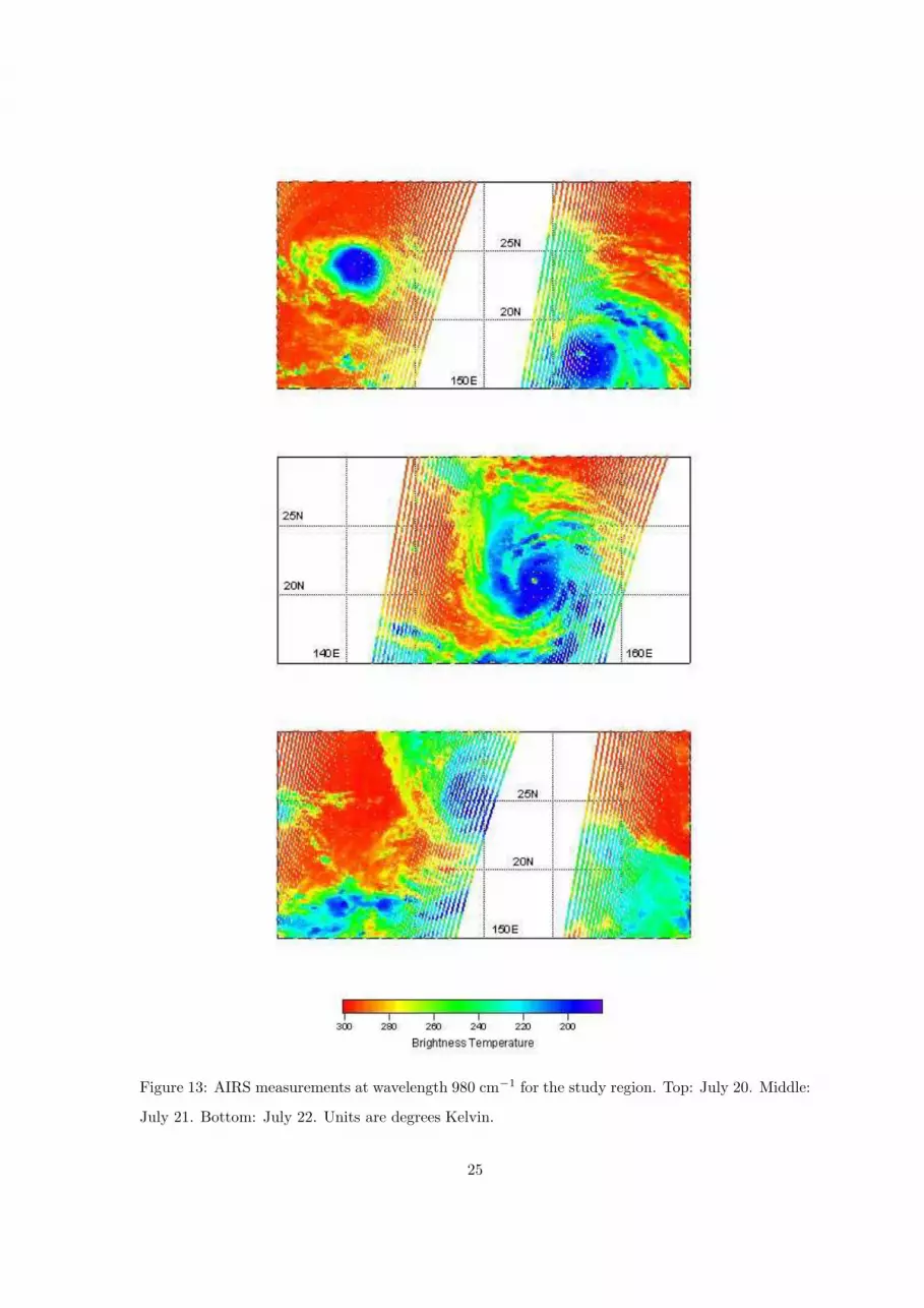
Figure 13: AIRS measurements at wavelength 980 cm−1 for the study region. Top: July 20. Middle:

July 21. Bottom: July 22. Units are degrees Kelvin.

25

semi-streaming quantization for remote sensing data

Documents