selfsimilar solutions in a sector for a quasilinear parabolic equation
TRANSCRIPT
arX
iv:1
008.
3626
v3 [
mat
h.A
P] 1
8 Ju
n 20
14
SELF-SIMILAR SOLUTIONS IN A SECTOR FOR A
QUASILINEAR PARABOLIC EQUATION∗
Bendong Lou
Department of Mathematics, Tongji UniversityShanghai 200092, China
(Communicated by Aim Sciences)
Dedicated to Professor Hiroshi Matano on the occasion of his 60th birthday
Abstract. We study a two-point free boundary problem in a sector for aquasilinear parabolic equation. The boundary conditions are assumed to be
spatially and temporally “self-similar” in a special way. We prove the existence,uniqueness and asymptotic stability of an expanding solution which is self-similar at discrete times. We also study the existence and uniqueness of ashrinking solution which is self-similar at discrete times.
1. Introduction
Consider the problem
(1)
ut = a(ux)uxx, −ξ1(t) < x < ξ2(t), t > 0,ux(x, t) = −k1(t, u(x, t)), u(x, t) = −x tanβ for x = −ξ1(t), t > 0,ux(x, t) = k2(t, u(x, t)), u(x, t) = x tanβ for x = ξ2(t), t > 0,
where a ∈ C2(R), a(·) > 0, β ∈ (0, π2 ) and k1, k2 ∈ C2([0,∞) × [0,∞),R). In thisproblem, u, ξ1, ξ2 are unknown positive functions to be determined.
The equation in (1) includes the heat equation and the curvature flow equationas special examples. In [2, 3, 4, 8, 9, 12], the authors considered problem (1) withconstant ki (i = 1, 2), that is,
(2)
ut = a(ux)uxx, −ζ1(t) < x < ζ2(t), t > 0,ux(x, t) = −γ1, u(x, t) = −x tanβ for x = −ζ1(t), t > 0,ux(x, t) = γ2, u(x, t) = x tanβ for x = ζ2(t), t > 0,
where γ1, γ2 are constants. They proved the existence of solutions of (2) for someinitial data. Moreover, in [2, 4, 12], they proved that when γ1 + γ2 > 0, any time-global solution u is expanding (that is, it moves upward to infinity) and it converges
asymptotically to a self-similar solution:√2t ϕ
(x/
√2t). In [3, 8, 9], they proved
that when γ1 + γ2 < 0, any solution shrinks to 0 as t → T for some T > 0; if a isanalytic, then the rescaled solution u/
√2(T − t) converges to a shrinking/backward
self-similar solution with the form: ψ(x/√2(T − t)
)as t→ T .
1991 Mathematics Subject Classification. Primary: 35C06, 35C07; Secondary: 35K59, 35B40.Key words and phrases. Discrete self-similar solution, spatially and temporally inhomogeneous
boundary condition, quasilinear parabolic equation.∗ This work is supported by NSFC (No. 11271285) and by the Fundamental Research Funds
for the Central Universities (Tongji University).
1

2 BENDONG LOU
Problem (2) arises in the model of flame propagation in combustion theory. Italso arises in the study of the motion of interface moving with curvature in whichthe studied problem is confined in the conical region bounded by two straight linesand the interface has prescribed touching angles with these two straight lines (cf.[2, 3, 4, 7, 8, 9, 12] etc.). In this paper we will consider a more general problem(1). In this new problem, the boundary conditions are spatially and temporallyinhomogeneous, which mean that the touching angles between the interface andthe boundaries of the sector domain depend on the spatial and temporal variables.Clearly, self-similar functions like
√2t ϕ(x/
√2t) or
√2(T − t) ψ
(x/√2(T − t)
)is
no longer a solution of (1). We have to adopt new concepts for the analogue of self-similar solutions. Our results in this paper show that problem (1) has an expandingsolution which is self-similar at discrete times if k1, k2 have some special “self-similarity” (see (5) below) and if min k1 +min k2 > 0. On the other hand, problem(1) has a shrinking solution which is self-similar at discrete times if k1, k2 have somespecial “self-similarity” (see (11) or (14) below) and if max k1 +max k2 < 0.
Definition 1.1. Let (u, ξ1, ξ2) = (U,Ξ1,Ξ2) be a solution of (1) defined for t ∈(0,∞). It is called an expanding self-similar solution if
(3) bU(x, t) ≡ U(bx, b2t
)for − Ξ1(t) 6 x 6 Ξ2(t), t > 0,
for some b > 1, and if
(4) b Ξi(t) = Ξi
(b2t)
for t > 0 (i = 1, 2).
From (3) we see that, for any t0 > 0,
· · · = bU(b−1x, b−2t0) = U(x, t0) = b−1U(bx, b2t0) = · · · .This means that U(x, t) is similar to U(x, t0) only at discrete times: t = b2mt0 (m ∈Z). In this sense we may also say that (U,Ξ1,Ξ2) (or, just U) is a discrete expanding
self-similar solution and√2t ϕ(x/
√2t) is a classical expanding self-similar solution.
It is easily seen that a necessary condition for the existence of a discrete expandingself-similar solution is that k1 and k2 are self-similar in a special way:
(5) ki(t, u) = ki(b2t, bu
)for t, u > 0.
We will give more explanation on this condition near the end of this section. Forsimplicity, we also impose another technical conditions on ki: there exists σ ∈(0, tanβ) such that
(6) |ki(t, u)| 6 (tanβ)− σ for t, u > 0 (i = 1, 2).
Theorem 1.2. Assume that k1, k2 satisfy conditions (5) and (6). Assume also that
(7) min k1 +min k2 > 0
holds. Then problem (1) has a discrete expanding self-similar solution (U,Ξ1,Ξ2).In addition, if ki(t, u) ≡ ki(u) (i = 1, 2), then
(i) the expanding self-similar solution is unique and Ut > 0, Ξ1t > 0, Ξ2t > 0for all t > 0;
(ii) U is asymptotically stable in the sense that
(8) dH(Γ(t), γ(t)) 6 Ct−1/2 as t→ ∞,
where Γ(t) is the graph of U , γ(t) is the graph of any time-global solution uof (1) and dH denotes the Hausdorff distance.
SELF-SIMILAR SOLUTIONS IN A SECTOR 3
The existence, uniqueness and asymptotic stability conclusions in this theorem areproved in subsections 3.6, 3.8 and 3.7, respectively.
Next we consider self-similar solutions which shrink to 0 in finite time.
Definition 1.3. Given T > 0. Let (u, ξ1, ξ2) = (U , Ξ1, Ξ2) be a solution of (1) for
t ∈ [0, T ). If ‖U(·, t)‖L∞ → 0, Ξ1(t) → 0, Ξ2(t) → 0 as t → T − 0,
(9) U(x, t) ≡ b U(b−1x, b−2t+ (1− b−2)T
)for − Ξ1(t) 6 x 6 Ξ2(t), 0 6 t < T,
for some b > 1, and if
(10) Ξi(t) = b Ξi
(b−2t+ (1− b−2)T
)for 0 6 t < T (i = 1, 2),
then (U , Ξ1, Ξ2) (or, just U) is called a shrinking/backward self-similar solution of(1) on time interval [0, T ).
Since U(x, t) is similar to U(x, t0) only at discrete times: t = b−2mt0+(1−b−2m)T
(m ∈ Z and 2m > log(T−t0T )/ log b), we may also say that (U , Ξ1, Ξ2) is a discrete
shrinking self-similar solution on [0, T ).A necessary condition for the existence of such a solution is that
(11) ki(t, u) = ki(b−2t+ (1− b−2)T, b−1u
)for 0 6 t < T, u > 0.
Replacing t by T − t′ then we see that (9), (10) and (11) are equivalent to
(12) U(x, T − t′) ≡ b U(b−1x, T − b−2t′
)
for −Ξ1(T − t′) 6 x 6 Ξ2(T − t′), 0 < t′ 6 T ,
(13) Ξi(T − t′) = b Ξi
(T − b−2t′
)for 0 < t′ 6 T (i = 1, 2),
and
(14) ki(T − t′, u) = ki(T − b−2t′, b−1u) for 0 < t′ 6 T, u > 0 (i = 1, 2),
respectively.
Theorem 1.4. Given T > 0, assume that k1, k2 satisfy condition (11) or (14).Assume also that (6) and
(15) max k1 +max k2 < 0
hold. Then problem (1) has a discrete shrinking self-similar solution (U , Ξ1, Ξ2) on[0, T ).
In addition, if ki(t, u) ≡ ki(u) (i = 1, 2), then the discrete shrinking self-similar
solution is unique and Ut < 0, Ξ1t < 0, Ξ2t < 0 for t ∈ [0, T ).
The uniqueness for shrinking self-similar solutions is not necessary to be true,even for the special problem (2) (cf. [8, 9])). But the above theorem shows that itcan be unique under certain assumptions.
Definition 1.3 and Theorem 1.4 deal with shrinking solutions on finite time in-terval [0, T ). If we take a time shift, these solutions can be regarded as solutions
defined on [−T, 0). More precisely, let (U , Ξ1, Ξ2) be a shrinking self-similar solutionof (1) on [0, T ). Then
U(x, t;T ) := U(x, T + t) for − Ξ1(t;T ) 6 x 6 Ξ2(t;T ), t ∈ [−T, 0),and
Ξi(t;T ) := Ξi(T + t) for t ∈ [−T, 0) (i = 1, 2)
4 BENDONG LOU
satisfy
(16) U(x, t) ≡ b U(b−1x, b−2t) for − Ξ1(t) 6 x 6 Ξ2(t), −T 6 t < 0,
and
(17) Ξi(t) = b Ξi(b−2t) for − T 6 t < 0 (i = 1, 2).
So (U , Ξ1, Ξ2) (which is defined on [−T, 0) and shrinks to 0 as t → 0 − 0) is aself-similar solution of(18)
ut = a(ux)uxx, −ξ1(t) < x < ξ2(t), t < 0,ux(x, t) = −k1(T + t, u(x, t)), u(x, t) = −x tanβ for x = −ξ1(t), t < 0,ux(x, t) = k2(T + t, u(x, t)), u(x, t) = x tanβ for x = ξ2(t), t < 0.
We now consider shrinking self-similar solutions defined in (−∞, 0).
Definition 1.5. Assume that ki(t, u) ≡ ki(u) (i = 1, 2). Let (U , Ξ1, Ξ2) be asolution of (18) defined for t ∈ (−∞, 0). If it satisfies (16) and (17) for some b > 1and t ∈ (−∞, 0), then it is called a discrete shrinking/backward self-similar solutionof (18) in (−∞, 0).
Theorem 1.6. Assume that k1 ≡ k1(u) and k2 ≡ k2(u) satisfy (6), (15) andki(u) = ki(bu) for all u > 0 and some b > 1. Then problem (18) has a unique
discrete shrinking self-similar solution (U , Ξ1, Ξ2) in (−∞, 0), and Ut < 0, Ξ1t <
0, Ξ2t < 0 for t ∈ (−∞, 0).
Our theorems extend the results about classical self-similar solutions in [2, 3,4, 8, 9, 12] to problem (1) with nonlinear boundary conditions. Our approachis essentially different from theirs though we will use their classical self-similarsolutions as lower and upper solutions to give the growth bound for the solution of(1). We will convert probe (1) by changing variables to a new problem in a fixeddomain. Then we use a convergence result in [1] to show that the ω-limit of theunknown in the new problem is a periodic solution, which corresponds to a discreteself-similar solution of (1).
Our boundary conditions are given by functions k1 and k2 which are self-similaras in (5). We now give some examples and/or backgrounds on such kind of self-similarity. First, some reactions in chemistry occur in a media with obstacles (cf.[18]). When the obstacles arrange in a regular way, it is possible to be studied froma mathematical point of view. For example, if we consider a Belousov-Zhabotinsky(BZ) reaction in a media with obstacles arranging in columns, then the interfacepropagation in the BZ experiment can be studied through a curvature flow in a banddomain with undulating boundaries (cf. [15, 16]). Similarly, if we consider the BZreaction in a media with obstacles arranging in radial rays with center at origin O,and if the ratios of the sizes of adjacent obstacles are constant, then the interfacepropagation can be studied through a curvature flow in a sector with undulatingboundaries, which is essentially a similar problem as our (1). Another example isthe following. In geology, Liesegang rings are colored bands of cement observedin sedimentary rocks, which are often referred to as great examples of geochemicalself-organization (cf. [17]). Generally, the Liesegang rings are arranged in a regularself-similar way: the ratios of the widths of adjacent annuluses are constant (cf.[10, 11, 17]). If we cut off a sector with apex at the center of the rings and considerthe interface propagation in this notch, then the problem is reduced to one like (1).
SELF-SIMILAR SOLUTIONS IN A SECTOR 5
In Section 2 we give some preliminaries, including the selection of the initial data,the local existence result and comparison principles. In Section 3 we consider theexpanding case and prove Theorem 1.2. In Section 4 we consider the shrinking caseand prove Theorems 1.4 and 1.6.
2. Preliminaries
We use notation S := (x, y) | y > |x| tanβ, x ∈ R, and use ∂1S and ∂2Sto denote the left and right boundaries of S, respectively. For any t0 > 0, let(u(x, t), ξ1(t), ξ2(t)) be a classical solution of (1) on the time interval [0, t0] withsome initial data. Then we write
Qt0 := (x, t) | − ξ1(t) < x < ξ2(t) and 0 < t 6 t0.
2.1. Initial data. We will consider the problem (1) with initial data
(19) u(x, 0) = u0(x), −ξ01 6 x 6 ξ02,
where u0(x) > 0, ξ01 > 0 and ξ02 > 0 satisfy
(20) u0(−ξ01) = ξ01 tanβ, u0(ξ02) = ξ02 tanβ
and the compatibility conditions:
(21) (u0)x(−ξ01) = −k1(0, u0(−ξ01)), (u0)x(ξ02) = k2(0, u0(ξ02)).
Since our main purpose in this paper is to construct self-similar solutions, wewill not focus on general solutions of (1) and (19) for general u0 as it was done in[2, 8, 12], but choose u0 ∈ C2+µ([−ξ01, ξ02]) for some µ ∈ (0, 1), and only considerclassical solution u of (1) and (19) in C2+µ,1+µ/2(Qt0) for t0 > 0. Moreover, werequire that u0 satisfies
(22) |(u0)x(x)| 6 tanβ − σ for − ξ01 6 x 6 ξ02,
where σ is as in (6). This inequality does not conflict with the compatibility condi-tions by (6).
In summary, in this paper we choose initial data from the following set of admis-sible functions:
(23) C2+µad :=
u0
∣∣∣∣u0 ∈ C2+µ([−ξ01, ξ02]) for some µ ∈ (0, 1), whereξ01, ξ02 > 0 and u0(·) > 0 satisfy (20), (21) and (22)
.
2.2. Gradient bound of u.
Lemma 2.1. Let u0 ∈ C2+µad for some µ ∈ (0, 1), u(x, t) ∈ C2+µ,1+µ/2(Qt0) be a
solution of (1) and (19) on [0, t0]. Then
(24) |ux(x, t)| 6 tanβ − σ for (x, t) ∈ Qt0 .
Proof. By (6) we have
ux(ξ2(t), t) = k2(t, u(ξ2(t), t)) 6 tanβ − σ,
and
ux(−ξ1(t), t) = −k1(t, u(−ξ1(t), t)) 6 tanβ − σ.
Combining these inequalities with (22) we obtain ux 6 tanβ − σ by maximumprinciple. ux > − tanβ + σ is proved similarly.
6 BENDONG LOU
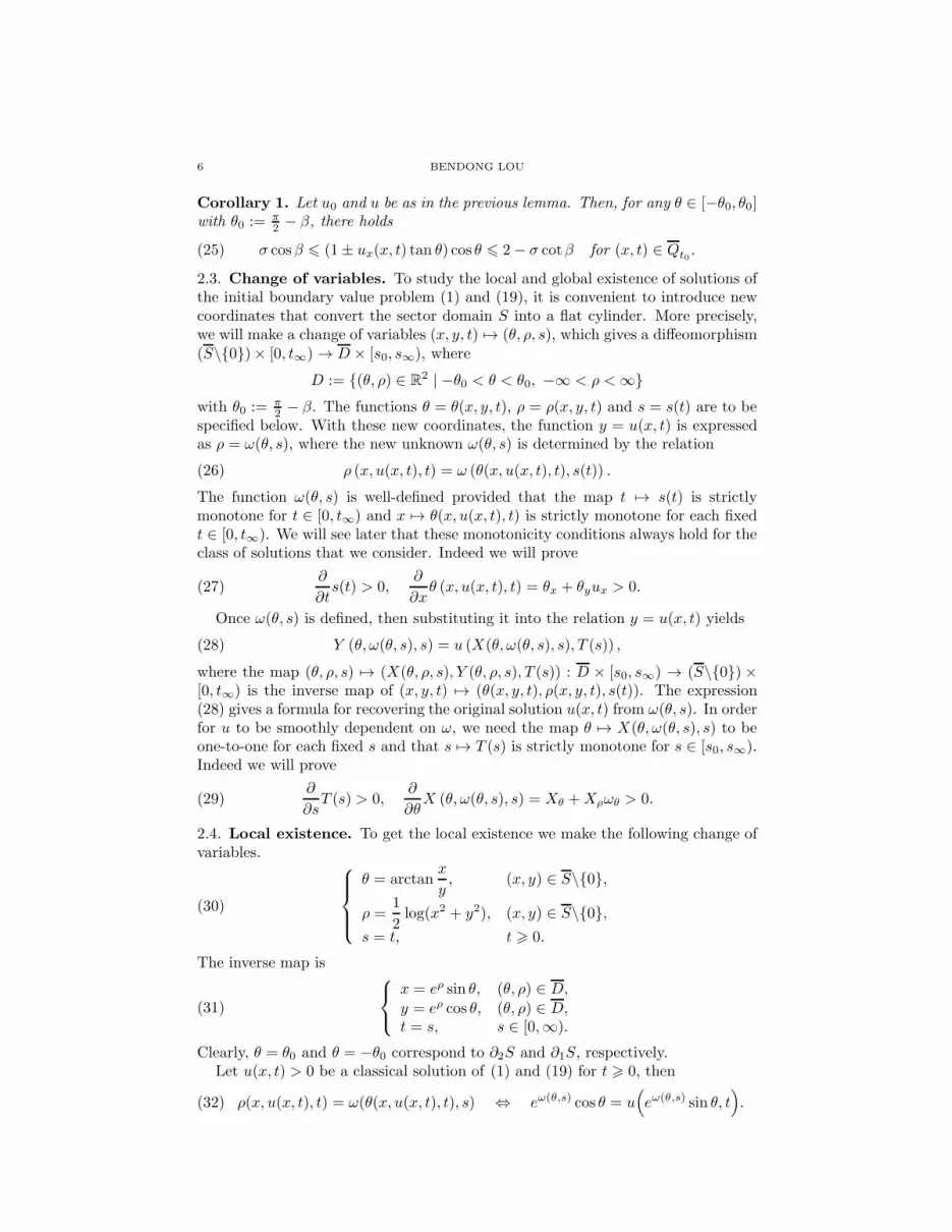
Corollary 1. Let u0 and u be as in the previous lemma. Then, for any θ ∈ [−θ0, θ0]with θ0 := π
2 − β, there holds
(25) σ cosβ 6 (1± ux(x, t) tan θ) cos θ 6 2− σ cotβ for (x, t) ∈ Qt0 .
2.3. Change of variables. To study the local and global existence of solutions ofthe initial boundary value problem (1) and (19), it is convenient to introduce newcoordinates that convert the sector domain S into a flat cylinder. More precisely,we will make a change of variables (x, y, t) 7→ (θ, ρ, s), which gives a diffeomorphism(S\0)× [0, t∞) → D × [s0, s∞), where
D := (θ, ρ) ∈ R2 | −θ0 < θ < θ0, −∞ < ρ <∞
with θ0 := π2 − β. The functions θ = θ(x, y, t), ρ = ρ(x, y, t) and s = s(t) are to be
specified below. With these new coordinates, the function y = u(x, t) is expressedas ρ = ω(θ, s), where the new unknown ω(θ, s) is determined by the relation
(26) ρ (x, u(x, t), t) = ω (θ(x, u(x, t), t), s(t)) .
The function ω(θ, s) is well-defined provided that the map t 7→ s(t) is strictlymonotone for t ∈ [0, t∞) and x 7→ θ(x, u(x, t), t) is strictly monotone for each fixedt ∈ [0, t∞). We will see later that these monotonicity conditions always hold for theclass of solutions that we consider. Indeed we will prove
(27)∂
∂ts(t) > 0,
∂
∂xθ (x, u(x, t), t) = θx + θyux > 0.
Once ω(θ, s) is defined, then substituting it into the relation y = u(x, t) yields
(28) Y (θ, ω(θ, s), s) = u (X(θ, ω(θ, s), s), T (s)) ,
where the map (θ, ρ, s) 7→ (X(θ, ρ, s), Y (θ, ρ, s), T (s)) : D × [s0, s∞) → (S\0)×[0, t∞) is the inverse map of (x, y, t) 7→ (θ(x, y, t), ρ(x, y, t), s(t)). The expression(28) gives a formula for recovering the original solution u(x, t) from ω(θ, s). In orderfor u to be smoothly dependent on ω, we need the map θ 7→ X(θ, ω(θ, s), s) to beone-to-one for each fixed s and that s 7→ T (s) is strictly monotone for s ∈ [s0, s∞).Indeed we will prove
(29)∂
∂sT (s) > 0,
∂
∂θX (θ, ω(θ, s), s) = Xθ +Xρωθ > 0.
2.4. Local existence. To get the local existence we make the following change ofvariables.
(30)
θ = arctanx
y, (x, y) ∈ S\0,
ρ =1
2log(x2 + y2), (x, y) ∈ S\0,
s = t, t > 0.
The inverse map is
(31)
x = eρ sin θ, (θ, ρ) ∈ D,
y = eρ cos θ, (θ, ρ) ∈ D,t = s, s ∈ [0,∞).
Clearly, θ = θ0 and θ = −θ0 correspond to ∂2S and ∂1S, respectively.Let u(x, t) > 0 be a classical solution of (1) and (19) for t > 0, then
(32) ρ(x, u(x, t), t) = ω(θ(x, u(x, t), t), s) ⇔ eω(θ,s) cos θ = u(eω(θ,s) sin θ, t
).

SELF-SIMILAR SOLUTIONS IN A SECTOR 7
defines a new unknown ρ = ω(θ, s) for s > 0. This function is well-defined since
∂
∂xθ(x, u(x, t), t) =
∂
∂x
(arctan
x
u(x, t)
)=
1− ux tan θ
u · (1 + tan2 θ)> 0
by (25).Differentiating the expression eω(θ,s) cos θ = u(eω(θ,s) sin θ, t) twice by θ and once
by t we obtain
ux =ωθ cos θ − sin θ
cos θ + ωθ sin θ, uxx =
ωθθ − ω2θ − 1
eω(cos θ + ωθ sin θ)3, ut =
eωωs
cos θ + ωθ sin θ.
Therefore, problem (1) with (19) is converted into the following problem(33)
ωs = a
(ωθ cos θ − sin θ
cos θ + ωθ sin θ
)ωθθ − ω2
θ − 1
e2ω(cos θ + ωθ sin θ)2, θ ∈ (−θ0, θ0), s ∈ (0,∞),
ωθ(−θ0, s) = −h01(s, ω(−θ0, s)), s ∈ [0,∞),ωθ(θ0, s) = h02(s, ω(θ0, s)), s ∈ [0,∞),ω(θ, 0) = ω(θ), θ ∈ [−θ0, θ0].
where ω is defined by (32) at t = s = 0 and
(34) h0i (s, ω) =sin θ0 + ki(s, e
ω cos θ0) cos θ0cos θ0 − ki(s, eω cos θ0) sin θ0
(i = 1, 2).
Estimate (24) implies that
(35) σ − tanβ 6 ux =ωθ cos θ − sin θ
cos θ + ωθ sin θ6 tanβ − σ for θ ∈ [−θ0, θ0], s > 0.
Thus cos θ+ωθ sin θ > 0 since it is positive at θ = 0 and it can not be zero by (35).Considering the second inequality in (35) we have
(36) ωθ[cos θ − sin θ(tanβ − σ)] 6 sin θ + (tanβ − σ) cos θ.
Note that, for θ ∈ [−θ0, θ0] (θ0 = π2 − β), we have
cos θ − sin θ(tan β − σ) > cos θ0[1− tan θ0(tanβ − σ)] > σ cosβ,
cos θ − sin θ(tanβ − σ) 6 cos θ[1 + tan θ0(tanβ − σ)] 6 2− σ cotβ.
So
ωθ 6sin θ + (tanβ − σ) cos θ
cos θ − sin θ(tanβ − σ)6 Ω1 :=
1 + tanβ − σ
σ cosβ.
Using the first inequality in this formula we have, for θ 6 0,
cos θ + ωθ sin θ >1
cos θ − sin θ(tanβ − σ)> ε1 :=
1
2− σ cotβ.
Similarly, considering the first inequality in (35) we have
ωθ >sin θ − (tanβ − σ) cos θ
cos θ + sin θ(tanβ − σ)> −Ω1,
and cos θ + ωθ sin θ > ε1 for θ > 0.Summarizing the above results we have
(37) |ωθ(θ, s)| 6 Ω1 and cos θ + ωθ sin θ > ε1 > 0
for θ ∈ [−θ0, θ0] and s > 0.By the standard theory for parabolic equations, we see that (33) has a classical
solution on time interval s ∈ [0, 2τ ] for positive τ = τ(k1, k2, µ, ω).

8 BENDONG LOU
The second inequality in (37) implies that, once the solution ω of (33) is obtainedthen we can recover it to the original solution u of (1). In fact,
∂
∂θX(θ, ω(θ, s), s) =
∂
∂θeω(θ,s) sin θ = eω(θ,s)(cos θ + ωθ sin θ) > 0.
Consequently, we have the following local existence result.
Lemma 2.2. Problem (1) with initial data u0(x) ∈ C2+µad (µ ∈ (0, 1)) has a classical
solution u on time interval [0, 2τ ], where τ depends only on k1, k2, µ and u0.
2.5. Comparison principle. Let v1(x), v2(x) be two functions whose graphs liein S and meet the two boundaries of S. Hereafter, when we write
v1 6 v2 (resp. v1 ≪ v2 ),
we mean that v1(x) 6 v2(x) (resp. v1(x) < v2(x)) for all x with (x, vi(x)) ∈ S (i =1, 2); when we write
v1 v2
we mean that v1(x) 6 v2(x) and the “equality” holds at some x.Assume further that |v1x|, |v2x| < tanβ. Then for each x with (x, v1(x)) ∈
S\O, there exists a unique Z(x) such that
x · v2(Z(x)) = Z(x) · v1(x),that is, (x, v1(x)) and (Z(x), v2(Z(x))) lie on the same line passing the origin. Bya simple geometric observation we have
(38) v1 6 v2 ⇔ x2 + v21(x) 6 Z2(x) + v22(Z(x)) for x with (x, v1(x)) ∈ S\Oand
(39) v1 ≪ v2 ⇔ x2 + v21(x) < Z2(x) + v22(Z(x)) for x with (x, v1(x)) ∈ S\O.
For some t0 > 0, let u1(x, t) ∈ C2,1(Q
(1)t0
)and u2(x, t) ∈ C2,1
(Q
(2)t0
)be two
positive functions, where, for i = 1, 2,
Q(i)t0 := (x, t) | −ξ(i)1 (t) < x < ξ
(i)2 (t), 0 < t 6 t0,
ui(−ξ(i)1 (t), t) = ξ(i)1 (t) · tanβ, ui(ξ
(i)2 (t), t) = ξ
(i)2 (t) · tanβ, 0 < t 6 t0,
and |(ui)x(x, t)| < tanβ.
Definition 2.3. Let t0 > 0 and ui ∈ C2,1(Q
(i)t0
)(i = 1, 2) be positive functions as
above. Then u1 is called a lower solution of (1) on [0, t0] if
(40)
u1t 6 a(u1x)u1xx for − ξ(1)1 (t) < x < ξ
(1)2 (t), 0 6 t 6 t0,
u1x(x, t) > −k1(t, u1(x, t)) for x = −ξ(1)1 (t), 0 6 t 6 t0,
u1x(x, t) 6 k2(t, u1(x, t)) for x = ξ(1)2 (t), 0 6 t 6 t0.
Similarly, u2 is called an upper solution of (1) if the opposite inequalities hold.
The following comparison principle holds.
Lemma 2.4. Let t0 > 0. Assume that u1(x, t) and u2(x, t) are lower solution andupper solution of (1) on [0, t0], respectively. If u1(·, 0) 6 u2(·, 0), then u1(·, t) 6
u2(·, t) for 0 6 t 6 t0. If u1(·, 0) 6 u2(·, 0) and u1(x, 0) 6≡ u2(x, 0), then u1(·, t) ≪u2(·, t) for 0 < t 6 t0.

SELF-SIMILAR SOLUTIONS IN A SECTOR 9
Proof. We change variables by (30) and (31), that is, using
eρi cos θ = ui(eρi sin θ, s),
we define implicit functions ρi = ωi(θ, s) (i = 1, 2). Since u1(x, t) is a lower solutionof (1), it is easily seen that ω1(θ, s) is a lower solution of (33):
ω1s 6 a
(ω1θ cos θ − sin θ
cos θ + ω1θ sin θ
)ω1θθ − ω2
1θ − 1
e2ω1(cos θ + ω1θ sin θ)2, θ ∈ (−θ0, θ0), s ∈ (0, t0],
ω1θ(−θ0, s) > −h01(s, ω1(−θ0, s)), s ∈ [0, t0],ω1θ(θ0, s) 6 h02(s, ω1(θ0, s)), s ∈ [0, t0].
Similarly, ω2(θ, s) is an upper solution of (33). By (38), u1(·, t) 6 u2(·, t) is equiva-lent to ω1(θ, s) 6 ω2(θ, s). The latter follows from the comparison principle for (33),which is a problem in a fixed domain. Similarly, the conclusion u1(·, t) ≪ u2(·, t)can be proved by using (39).
3. Expanding self-similar solutions
In this section we always assume that (7) holds.
3.1. Classical expanding self-similar solutions. Wewill use classical self-similarsolutions of (2) as upper and lower solutions of (1) to give the growth bound forthe solution u of (1) and (19). For any γ1, γ2 ∈ R, consider the problem
(41)
a(ϕ′(z))ϕ′′(z) = ϕ(z)− zϕ′(z), z ∈ R,ϕ′(−p1) = −γ1, ϕ(−p1) = p1 tanβ,ϕ′(p2) = γ2, ϕ(p2) = p2 tanβ.
In [2, 4, 12], the authors obtained the following result.
Lemma 3.1. For any given γ1, γ2 with γ1 + γ2 > 0, there exists a unique pairp1, p2 > 0 such that problem (41) has a solution ϕ(z; γ1, γ2), which is positive on[−p1, p2].
It is easily seen that the function
√2t ϕ
(x√2t; γ1, γ2
)for − ζ1(t) < x < ζ2(t), t > 0,
with ζi(t) = pi√2t (i = 1, 2) is an expanding self-similar solution of (2). Set
(42) k0i := min ki(t, u) and K0i := max ki(t, u) (i = 1, 2),
and define
ϕ−(z) := ϕ(z; k01 , k02), ϕ+(z) := ϕ(z;K0
1 ,K02 ).
Then√2t ϕ−(x/
√2t) and
√2t ϕ+(x/
√2t) (both are expanding self-similar solutions
of (2)) are lower and upper solutions of (1), respectively.Since the initial data u0 > 0, there exist t+, t− > 0 such that
(43)√2t− ϕ−
( ·√2t−
)6 u0(·) 6
√2t+ ϕ+
( ·√2t+
).
The comparison principle implies that
(44)√2(t+ t−) ϕ−
(·√
2(t+ t−)
)6 u(·, t) 6
√2(t+ t+) ϕ+
(·√
2(t+ t+)
).

10 BENDONG LOU
3.2. Changes of variables. In subsection 2.4 we gave a local existence result. Onedifficulty for deriving the global existence is the lack of the growth bound for ω. Togive the global existence we adopt another change of variables.
Let τ be the constant in Lemma 2.2 and let t− > 0 be as in (43). For any n ∈ N
satisfying
(45) n >1
t−and n >
1
τ,
we introduce new variables by
(46)
θ = arctanx
y, (x, y) ∈ S\0,
ρ =1
2log
n(x2 + y2)
nt+ 1, (x, y) ∈ S\0, t > 0,
s =1
2log(t+
1
n
), t > 0.
The inverse map is
(47)
x = eseρ sin θ, (θ, ρ) ∈ D, s ∈ [− 12 logn,∞),
y = eseρ cos θ, (θ, ρ) ∈ D, s ∈ [− 12 logn,∞),
t = e2s − 1n , s ∈ [− 1
2 logn,∞).
Clearly, θ = θ0 and θ = −θ0 correspond to ∂2S and ∂1S, respectively.Let u(x, t) > 0 be a solution of (1) and (19) for t > 0, then a similar discussion
as in subsection 2.4 shows that(48)
ρ(x, u(x, t), t) = v(θ(x, u(x, t), t), s(t)) ⇔ esev(θ,s) cos θ = u(esev(θ,s) sin θ, e2s− 1
n
)
defines a new unknown ρ = v(θ, s) for s ∈ [− 12 logn,∞). Differentiating the second
equality twice by θ and once by s we obtain
ux =vθ cos θ − sin θ
cos θ + vθ sin θ, uxx =
vθθ − v2θ − 1
esev(cos θ + vθ sin θ)3, ut =
ev(1 + vs)
2es(cos θ + vθ sin θ).
Therefore, problem (1) is converted into the following problem(49)
vs = 2a
(vθ cos θ − sin θ
cos θ + vθ sin θ
)vθθ − v2θ − 1
e2v(cos θ + vθ sin θ)2− 1, |θ| < θ0, s > − 1
2 logn,
vθ(−θ0, s) = −g1(s, v(−θ0, s)), s > − 12 logn,
vθ(θ0, s) = g2(s, v(θ0, s)), s > − 12 logn,
where
(50) gi(s, v) =sin θ0 + ki
(e2s − 1
n , esev cos θ0
)cos θ0
cos θ0 − ki
(e2s − 1
n , esev cos θ0
)sin θ0
(i = 1, 2).
3.3. Gradient bound of v. In a similar way as deriving (37) in subsection 2.4 onecan obtain
(51) |vθ(θ, s)| 6 Ω2(σ, β) and cos θ + vθ sin θ > ε2(σ, β) > 0
for θ ∈ [−θ0, θ0] and s ∈ [− 12 log n,∞).
The second inequality in (51) implies that, once the solution v of (49) is obtainedthen we can recover it to the original solution u of (1), since
∂
∂θX(θ, v(θ, s), s) =
∂
∂θesev(θ,s) sin θ = esev(θ,s)(cos θ + vθ sin θ) > 0.

SELF-SIMILAR SOLUTIONS IN A SECTOR 11
3.4. Bound of v. The local existence result Lemma 2.2 implies that v exists ons ∈ [− 1
2 logn,12 log(2τ + 1
n )]. We have changed u(x, t) to a new unknown v(θ, s).Similarly, we define v± by ϕ± in the following way
esev±
cos θ =
√2(e2s − 1
n+ t±
)ϕ±
esev±
sin θ√2(e2s − 1
n + t±)
.
By (44) we have esev+
cos θ > u(esev+
sin θ, e2s− 1n ). Noting e
sev cos θ = u(esev sin θ,
e2s − 1n ) we have
(ev+ − ev) cos θ > ux
(ϑ, e2s − 1
n
)· [(ev+ − ev) sin θ],
where ϑ = es sin θ(ςev + (1− ς)ev+
) for some ς ∈ [0, 1]. Therefore v+ > v by (25).On the other hand, by the definition of v+ we have
(52)
ev+
cos θ = ϕ+(·)√
2 +(t+ − 1
n
)e−2s 6
√2 + t+/τ maxϕ+ for s >
1
2log τ.
So
v(θ, s) 6 v+(θ, s) 6 log
[√2 + t+/τ maxϕ+
sinβ
]for θ ∈ [−θ0, θ0], s >
1
2log τ.
A similar discussion as above shows that
v(θ, s) > v−(θ, s) > log[2 minϕ−
]for θ ∈ [−θ0, θ0], s >
1
2log τ.
Remark 1. The definition of v depends on n, it is not easy to give a uniform (inn) bound for v on [− 1
2 logn,∞), but the above results show that a uniform bound
for v is possible on [ 12 log τ,∞).
3.5. Global existence. Now we consider problem (49) with initial data v(θ,− 12 logn) =
v0(θ), which is defined by (48) at s = − 12 logn. Using the growth bound and gra-
dient bound in the previous subsections and using the standard theory of parabolicequations (cf. [5, 6, 13, 14]) we can get the following conclusions.
Lemma 3.2. Problem (49) with initial data v(θ,− 12 logn) = v0(θ) has a unique,
time-global solution v(θ, s) ∈ C2+µ,1+µ/2([−θ0, θ0]× [− 12 logn,∞)) and
(53) ‖v(θ, s)‖C2+µ,1+µ/2([−θ0,θ0]×[ 12log τ,∞)) 6 C0 <∞,
where C0 depends on k1, k2, µ and u0 but not on s and n.
This lemma implies the global existence of u.
Lemma 3.3. Problem (1) and (19) has a unique, time-global solution u(x, t). More-over, u ∈ C2+µ,1+µ/2(Q∞), where Q∞ := (x, t) | −ξ1(t) < x < ξ2(t), t > 0. Forany t0 > τ ,
‖u(x, t)‖C2+µ,1+µ/2(Qt0\Qτ )
6 C1(t0, k1, k2, µ, u0, τ) <∞.
Indeed, studying the relations between v and umore precisely, it is not difficult tosee that C1 in this lemma can be replaced by C2
√t0+C3 for some C2, C3 depending
on k1, k2, µ, u0 and τ .

12 BENDONG LOU
3.6. Existence of self-similar solution. Since the solution v in Lemma 3.2 isdefined for s > − 1
2 logn, we write it as vn. By Cantor’s diagonal argument, one
can find a function V ∈ C2+µ,1+µ/2([−θ0, θ0] × [ 12 log τ,∞)) and a subsequenceni ⊂ n such that, as i→ ∞,
(54) vni(θ, s) → V (θ, s) in C2,1loc
([−θ0, θ0]×
[12log τ,∞
))topology.
Moreover, V satisfies the estimate
(55) ‖V (θ, s)‖C2+µ,1+µ/2([−θ0,θ0]×[ 12log τ,∞)) 6 C0 <∞,
and V is a solution of(56)
vs = 2a
(vθ cos θ − sin θ
cos θ + vθ sin θ
)vθθ − v2θ − 1
e2v(cos θ + vθ sin θ)2− 1, |θ| < θ0, s >
12 log τ,
vθ(−θ0, s) = −G1(s, v(−θ0, s)), s > 12 log τ,
vθ(θ0, s) = G2(s, v(θ0, s)), s > 12 log τ,
where
(57) Gi(s, v) =sin θ0 + ki
(e2s, esev cos θ0
)cos θ0
cos θ0 − ki
(e2s, esev cos θ0
)sin θ0
(i = 1, 2).
Here G1 and G2 are log b-periodic functions in s by (5).Now we use a result in [1].
Lemma 3.4. Let u be a time-global solution of
(58)
ut = d(t, x, u, ux)uxx + f(t, x, u, ux), t > 0, 0 < x < 1,ux(i, t) = g∗i (t, u(i, t)), i = 0, 1, t > 0,
where d, f, g∗i are C2 functions, T -periodic in t. If u(·, t) is bounded in H2(0, 1), thenthere exists a T -periodic solution p of (58) such that lim
t→∞‖u(·, t)−p(·, t)‖H2(0,1) = 0.
By this lemma, problem (56) has a solution P (θ, s) ∈ H2(−θ0, θ0), which islog b-periodic in s, and
lims→∞
‖V (·, s)− P (·, s)‖H2(−θ0,θ0) = 0.
By (55) we indeed have
(59) ‖P (θ, s)‖C2+µ,1+µ/2([−θ0,θ0]×R) 6 C0
and
(60) limk→∞
‖V (θ, s+ k log b)− P (θ, s)‖C2,1([−θ0,θ0]×[0,log b]) = 0.
We now recover P to a solution of (1), the corresponding change of variablesshould be the limiting version as n → ∞ of (46) and (47), or for s ∈ (−∞,∞).Using these variables we define U by
(61) eseP cos θ = U(eseP sin θ, e2s) for θ ∈ [−θ0, θ0], s ∈ (−∞,∞).
By (51), (54) and (60) we have
∂
∂θX(θ, P (θ, s), s) =
∂
∂θ
(eseP (θ,s) sin θ
)= eseP (θ,s)(Pθ sin θ + cos θ) > 0,
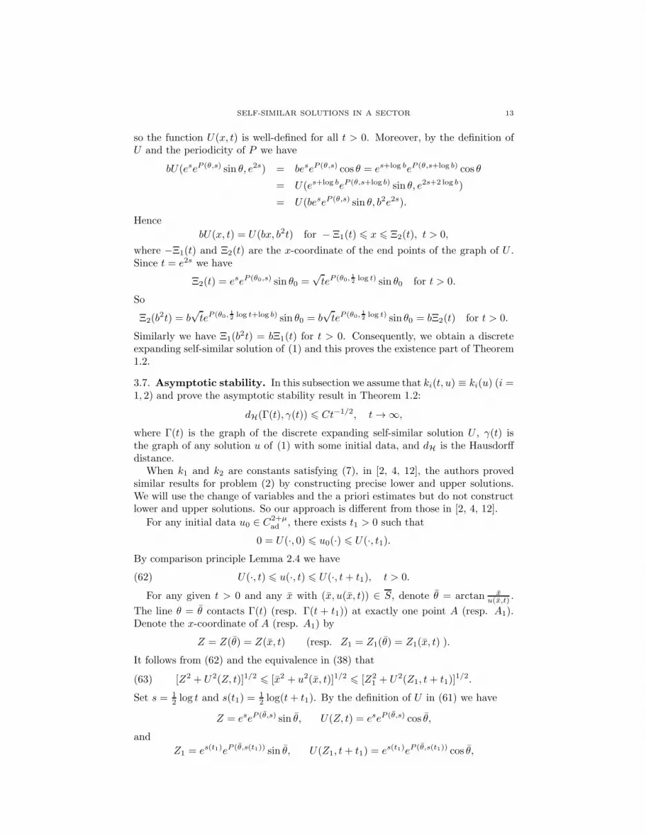
SELF-SIMILAR SOLUTIONS IN A SECTOR 13
so the function U(x, t) is well-defined for all t > 0. Moreover, by the definition ofU and the periodicity of P we have
bU(eseP (θ,s) sin θ, e2s) = beseP (θ,s) cos θ = es+log beP (θ,s+log b) cos θ
= U(es+log beP (θ,s+log b) sin θ, e2s+2 log b)
= U(beseP (θ,s) sin θ, b2e2s).
Hence
bU(x, t) = U(bx, b2t) for − Ξ1(t) 6 x 6 Ξ2(t), t > 0,
where −Ξ1(t) and Ξ2(t) are the x-coordinate of the end points of the graph of U .Since t = e2s we have
Ξ2(t) = eseP (θ0,s) sin θ0 =√teP (θ0,
12log t) sin θ0 for t > 0.
So
Ξ2(b2t) = b
√teP (θ0,
12log t+log b) sin θ0 = b
√teP (θ0,
12log t) sin θ0 = bΞ2(t) for t > 0.
Similarly we have Ξ1(b2t) = bΞ1(t) for t > 0. Consequently, we obtain a discrete
expanding self-similar solution of (1) and this proves the existence part of Theorem1.2.
3.7. Asymptotic stability. In this subsection we assume that ki(t, u) ≡ ki(u) (i =1, 2) and prove the asymptotic stability result in Theorem 1.2:
dH(Γ(t), γ(t)) 6 Ct−1/2, t→ ∞,
where Γ(t) is the graph of the discrete expanding self-similar solution U , γ(t) isthe graph of any solution u of (1) with some initial data, and dH is the Hausdorffdistance.
When k1 and k2 are constants satisfying (7), in [2, 4, 12], the authors provedsimilar results for problem (2) by constructing precise lower and upper solutions.We will use the change of variables and the a priori estimates but do not constructlower and upper solutions. So our approach is different from those in [2, 4, 12].
For any initial data u0 ∈ C2+µad , there exists t1 > 0 such that
0 = U(·, 0) 6 u0(·) 6 U(·, t1).By comparison principle Lemma 2.4 we have
(62) U(·, t) 6 u(·, t) 6 U(·, t+ t1), t > 0.
For any given t > 0 and any x with (x, u(x, t)) ∈ S, denote θ = arctan xu(x,t) .
The line θ = θ contacts Γ(t) (resp. Γ(t + t1)) at exactly one point A (resp. A1).Denote the x-coordinate of A (resp. A1) by
Z = Z(θ) = Z(x, t) (resp. Z1 = Z1(θ) = Z1(x, t) ).
It follows from (62) and the equivalence in (38) that
(63) [Z2 + U2(Z, t)]1/2 6 [x2 + u2(x, t)]1/2 6 [Z21 + U2(Z1, t+ t1)]
1/2.
Set s = 12 log t and s(t1) =
12 log(t+ t1). By the definition of U in (61) we have
Z = eseP (θ,s) sin θ, U(Z, t) = eseP (θ,s) cos θ,
and
Z1 = es(t1)eP (θ,s(t1)) sin θ, U(Z1, t+ t1) = es(t1)eP (θ,s(t1)) cos θ,

14 BENDONG LOU
where P is that in (59). Since
s(t1)− s =t12t
+ o(1t
)(as t→ ∞),
by (59) we have
[Z21 + U2(Z1, t+ t1)]
1/2 − [Z2 + U2(Z, t)]1/2 = es(t1)eP (θ,s(t1)) − eseP (θ,s)
6 C1t−1/2, as t→ ∞,
where C1 depends on t1 and C0 in (59), but not on θ and t. Therefore, we have
dH(Γ(t), γ(t)) 6 dH(Γ(t),Γ(t+ t1)) 6 C1t−1/2 as t→ ∞.
3.8. Uniqueness of self-similar solutions. In this subsection we still assumeki(t, u) ≡ ki(u) (i = 1, 2) and to prove the uniqueness conclusion in Theorem 1.2.The uniqueness for general ki(t, u) is still open.
We begin with choosing a convex initial data u0, that is,
a(u0x)u0xx > ǫ
for some ǫ > 0. Such a choice is possible. For example, draw a line ℓ1 fromA1 := (−1, tanβ) with slope −k1(tanβ). Denote the contacting point between ℓ1and ∂2S by A′
2, then A′2 := (x′, x′ tanβ) with
x′ :=tanβ − k1(tanβ)
tanβ + k1(tanβ).
Choose A2 := (x′ + ǫ′, (x′ + ǫ′) tanβ) ∈ ∂2S for some small ǫ′ > 0, then A2 is aboveA′
2. Draw a line ℓ2 from A2 with slope k2((x′ + ǫ′) tanβ). Since
k2((x′ + ǫ′) tanβ) > k02 > −k01 > −k1(tanβ),
ℓ2 must contact ℓ1 at some point A3 ∈ S provided ǫ′ > 0 is small enough. Now wesmoothen A1A3 + A3A2 such that the smoothened curve C is strictly convex, it istangent to A1A3 at A1, tangent to A3A2 at A2. Now the corresponding functionu0 of C is a desired initial data.
Let u be the solution of (1) with the above constructed initial data u0. Denoteη = ut. Differentiating the problem (1) by t we have
ηt = a(ux)ηxx + a′(ux)uxxηx, −ξ1(t) < x < ξ2(t), t > 0,ηx(−ξ1(t), t) = f1(t)η(−ξ1(t), t), ηx(ξ2(t), t) = f2(t)η(ξ2(t), t), t > 0,η(x, 0) = a(u0x)u0xx > ǫ > 0,
where f1 and f2 are continuous functions. Maximum principle implies that η = ut >0 for t > 0. In a similar way as in the previous subsection 3.6 we can get a discreteexpanding self-similar solution (U,Ξ1,Ξ2). Moreover, using the same notions asabove we have 1 + vs > 0 and so 1 + Vs > 0 for s > 1
2 log τ . Using (60) one has1 + Ps > 0 for all s ∈ R, this implies that Ut > 0. Finally, the strong maximumprinciple implies that Ut > 0 for all t > 0, and so Ξ1t(t) > 0, Ξ2t(t) > 0 for t > 0.
Suppose that (U∗,Ξ∗1,Ξ
∗2) is another discrete self-similar solution of (1). We want
to prove that U(x, t) ≡ U∗(x, t). Otherwise, either
(64) U∗(·, t) 6 U(·, t) and U(x, t) 6≡ U∗(x, t) for all t > 0,
or
(65) U(·, t) 6 U∗(·, t) and U(x, t) 6≡ U∗(x, t) for all t > 0,
holds. We now derive a contradiction from (64).

SELF-SIMILAR SOLUTIONS IN A SECTOR 15
Since U(x, t) → 0 as t → 0, for any t0 > 0, there exists τ ∈ (0, t0) such thatU(·, t0 − τ) ≪ U∗(·, t0). Set
τ(t0) := infτ | U(·, t0 − τ) ≪ U∗(·, t0).Then either
(a) U(x, t0 − τ(t0)) ≡ U∗(x, t0), or(b) U(x, t0 − τ(t0)) 6≡ U∗(x, t0) and U(·, t0 − τ(t0)) U∗(·, t0)
holds. By (64) and by Ut > 0 it is easily seen that τ(t0) > 0, and so τ(t0) ∈ (0, t0).We first show that (b) is impossible. Otherwise, by Lemma 2.4 we have
U(·, t0 − τ(t0) + (b2 − 1)t0) ≪ U∗(·, t0 + (b2 − 1)t0) = U∗(·, b2t0).On the other hand, by the self-similarity we have
U(bx, b2(t0 − τ(t0))) ≡ bU(x, t0 − τ(t0)) bU∗(x, t0) ≡ U∗(bx, b2t0).
Combining these inequalities with the fact that Ut > 0 we have
b2t0 − τ(t0) < b2(t0 − τ(t0)).
This is a contradiction.Now, (a) implies that, for any t > 0, there exists τ(t) ∈ (0, t) such that U(x, t−
τ(t)) ≡ U∗(x, t). Hence, for any t, s > 0 we have
U(x, t− τ(t) + s) ≡ U∗(x, t+ s) ≡ U(x, t+ s− τ(t + s)).
So τ(t+s) = τ(t) for all t, s > 0. Thus, τ(t) is a constant τ∗ > 0 and U(x, t− τ∗) ≡U∗(x, t) for all t > 0. Taking limits as t→ τ∗ + 0 we have U∗(x, τ∗) = U(x, 0) = 0,and so τ∗ = 0, a contradiction.
The above discussion shows that (64) is impossible. In a similar way, one canshow that (65) is also impossible. So U(x, t) ≡ U∗(x, t), and (U,Ξ1,Ξ2) is theunique discrete expanding self-similar solution of (1). This proves the uniquenessresult in Theorem 1.2.
4. Shrinking self-similar solutions
In this section we always assume that (15) holds.
4.1. Classical shrinking/backward self-similar solutions. First, recall theclassical self-similar solutions of (2). For any γ1, γ2 ∈ R, consider the problem
(66)
a(ψ′(z))ψ′′(z) = zψ′(z)− ψ(z), z ∈ R,ψ′(−q1) = −γ1, ψ(−q1) = q1 tanβ,ψ′(q2) = γ2, ψ(q2) = q2 tanβ.
In [8, 9], the authors obtained the following result.
Lemma 4.1. For any γ1, γ2 satisfying γ1 + γ2 < 0, there exists a pair q1, q2 > 0such that problem (66) has solution ψ(z; γ1, γ2), which is positive on [−q1, q2].
It is easily seen that the function
√2(T − t) ψ
(x√
2(T − t)
)for − ζ1(t) < x < ζ2(t), t > 0,
with ζi(t) = qi√2(T − t) (i = 1, 2) is a classical shrinking/backward self-similar
solution of (2).

16 BENDONG LOU
We use (ψ−(z), q−1 , q−2 ) to denote the solution of (66) with γi = k0i (i = 1, 2),
use (ψ+(z), q+1 , q+2 ) to denote the solution of (66) with γi = K0
i (i = 1, 2), where k0iand K0
i are those in (42).By (15), K0
1 + K02 < 0 and so (ψ±)′′ < 0. For any T0 > 0, the function√
2(T0 − t) ψ−(x/√2(T0 − t)) and the function
√2(T0 − t) ψ+(x/
√2(T0 − t)) (both
are shrinking/backward self-similar solutions of (2)) are lower and upper solutionsof (1), respectively. Since the initial data u0 > 0, there exists T+, T− > 0 such that
(67)√2T− ψ−
( ·√2T−
) u0(·)
√2T+ ψ+
( ·√2T+
).
Comparison principle implies that(68)√2(T− − t) ψ−
(·√
2(T− − t)
)≪ u(·, t) ≪
√2(T+ − t) ψ+
(·√
2(T+ − t)
)
on the time interval where these three functions are defined.
Lemma 4.2. Let ψ± and T± be as in (67). Then T+ > T− > δT+, where
δ = δ(β, σ, k0i ,K0i ) :=
σ4
(2 tanβ − σ)4· (q
+2 )
2
(q−2 )2> 0.
Proof. We first prove T+ > T−. The areas D±(t) of the regions enclosed by the
graph of√2(T± − t) ψ±(x/
√2(T± − t)), ∂1S and ∂2S are given by
D±(t) =
∫ ζ2(t)
−ζ1(t)
√2(T± − t) ψ±
(x√
2(T± − t)
)dx− 1
2[ζ21 (t) + ζ22 (t)] tanβ.
A simple computation shows that
(D+)′(t) =
∫ K02
−K01
a(p)dp, (D−)′(t) =
∫ k02
−k01
a(p)dp.
Since D+(T+) = D−(T−) = 0 we have
(69) D+(0) =
∫ T+
0
dt
∫ −K01
K02
a(p)dp, D−(0) =
∫ T−
0
dt
∫ −k01
k02
a(p)dp.
By (15) we have k02 < K02 < −K0
1 < −k01 , and by (67) we have D+(0) > D−(0).Therefore, we have T+ > T− by (69).
Next we prove T− > δT+. For i = 1, 2, denote Q+i (resp. Q−
i ) the end points of
the graph of√2T+ ψ+(x/
√2T+) (resp. the graph of
√2T− ψ−(x/
√2T−)) on ∂iS,
respectively.
Connecting Q+1 and Q+
2 we get a line segment Q+1 Q
+2 . It is below the graph of√
2T+ ψ+(x/√2T+) since (ψ+)′′ < 0. Draw a line from Q+
1 (resp. Q+2 ) with slope
− tanβ+ σ (resp. tanβ− σ). Assume that it contacts ∂2S (resp. ∂1S) at A2 (resp.A1).
By (67) the graph of u0 contacts the line segment Q+1 Q
+2 . Since |u0x| 6 tanβ−σ,
we see that the graph of u0 is above the line segment A1A2.If for some T0 > 0, the graph of
√2T0 ψ
−(x/√2T0) is tangent to A1A2 from
above, then (note |(ψ−)′| 6 tanβ − σ) the graph of√2T0 ψ
−(x/√2T0) lies above
the line segment B1B2, where B1 (resp. B2) is the contacting point between the

SELF-SIMILAR SOLUTIONS IN A SECTOR 17
line passing A2 (resp. A1) with slope tanβ − σ (resp. − tanβ + σ) and the leftboundary ∂1S (resp. right boundary ∂2S). Therefore, Q
−i are above Bi for i = 1, 2.
Using the coordinates of Q+i = ((−1)iri cosβ, ri sinβ), where
ri =
√2T+q+icosβ
(i = 1, 2),
one can easily calculate the coordinates of B1 and B2:
Bi =((−1)iσ2ri cosβ
(2 tanβ − σ)2,
σ2ri sinβ
(2 tanβ − σ)2
)(i = 1, 2).
The fact that Q−2 is above B2 implies that
√2T−q−2 >
σ2 cosβ
(2 tanβ − σ)2·√2T+q+2cosβ
.
So
T−
T+>
[σ2q+2
q−2 (2 tanβ − σ)2
]2.
This proves the lemma.
4.2. Shrinking time for solutions of (1) and (19). In this subsection we con-sider the shrinking time for the solution u = u(x, t;u0) of (1) with initial data u0.We give two results. The first one is about the shrinking time of u = u(x, t;u0) forany given u0, the second one is about the existence of u0 for given shrinking timeT .
Lemma 4.3. Let u0 ∈ C2+µad (µ ∈ (0, 1)) be an initial data. If it satisfies (67), then
there exists T ∈ (T−, T+) such that the solution u(x, t;u0) of (1) and (19) existson time interval [0, T ), and
(70) ‖u(·, t)‖L∞ → 0, ξ1(t) → 0, ξ2(t) → 0 as t→ T.
Proof. We use polar coordinates x = r sin θ, y = r cos θ for θ ∈ [−θ0, θ0], that is,r cos θ = u(r sin θ, t)
defines an implicit function r = r(θ, t) by (25). Problem (1) is then converted into
(71)
rt = a
(rθ cos θ − r sin θ
rθ sin θ + r cos θ
)rrθθ − 2r2θ − r2
r(rθ sin θ + r cos θ)2, θ ∈ [−θ0, θ0], t > 0,
rθ(−θ0, t) = −h1(t, r(−θ0, t)), t > 0,
rθ(θ0, t) = h2(t, r(θ0, t)), t > 0,
where
hi(t, r) :=sin θ0 + ki(t, r cos θ0) cos θ0cos θ0 − ki(t, r cos θ0) sin θ0
r (i = 1, 2).
By (68) we have r cos θ = u(r sin θ, t) 6√2T+maxψ+. So 0 6 r(θ, t) 6√
2T+maxψ+/ sinβ. By (24) and (25) we have
|rθ| =∣∣∣∣sin θ + ux cos θ
cos θ − ux sin θr
∣∣∣∣ 61 + tanβ − σ
σ cosβ·√2T+maxψ+
sinβ.
Thus the standard a priori estimates (cf. [5, 6, 13, 14]) show that the solution of(71) with initial data r(θ, 0) will not develop singularity till min r(·, t) → 0 as t→ Tfor some T > 0. Moreover, T− < T < T+ follows from (68) and Lemma 4.2.
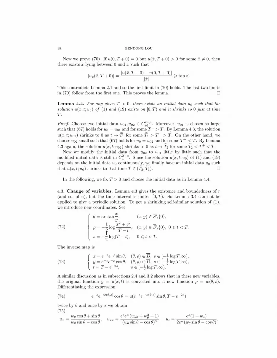
18 BENDONG LOU
Now we prove (70). If u(0, T + 0) = 0 but u(x, T + 0) > 0 for some x 6= 0, thenthere exists x lying between 0 and x such that
|ux(x, T + 0)| = |u(x, T + 0)− u(0, T + 0)||x| > tanβ.
This contradicts Lemma 2.1 and so the first limit in (70) holds. The last two limitsin (70) follow from the first one. This proves the lemma.
Lemma 4.4. For any given T > 0, there exists an initial data u0 such that thesolution u(x, t;u0) of (1) and (19) exists on [0, T ) and it shrinks to 0 just at timeT .
Proof. Choose two initial data u01, u02 ∈ C2+µad . Moreover, u01 is chosen so large
such that (67) holds for u0 = u01 and for some T− > T . By Lemma 4.3, the solution
u(x, t;u01) shrinks to 0 as t → T1 for some T1 > T− > T . On the other hand, wechoose u02 small such that (67) holds for u0 = u02 and for some T+ < T . By Lemma
4.3 again, the solution u(x, t;u02) shrinks to 0 as t→ T2 for some T2 < T+ < T .Now we modify the initial data from u02 to u01 little by little such that the
modified initial data is still in C2+µad . Since the solution u(x, t;u0) of (1) and (19)
depends on the initial data u0 continuously, we finally have an initial data u0 such
that u(x, t;u0) shrinks to 0 at time T ∈ (T2, T1).
In the following, we fix T > 0 and choose the initial data as in Lemma 4.4.
4.3. Change of variables. Lemma 4.3 gives the existence and boundedness of r(and so, of u), but the time interval is finite: [0, T ). So Lemma 3.4 can not beapplied to give a periodic solution. To get a shrinking self-similar solution of (1),we introduce new coordinates. Set
(72)
θ = arctanx
y, (x, y) ∈ S\0,
ρ = −1
2log
x2 + y2
T − t, (x, y) ∈ S\0, 0 6 t < T,
s = −1
2log(T − t), 0 6 t < T.
The inverse map is
(73)
x = e−se−ρ sin θ, (θ, ρ) ∈ D, s ∈ [− 12 logT,∞),
y = e−se−ρ cos θ, (θ, ρ) ∈ D, s ∈ [− 12 logT,∞),
t = T − e−2s, s ∈ [− 12 log T,∞).
A similar discussion as in subsections 2.4 and 3.2 shows that in these new variables,the original function y = u(x, t) is converted into a new function ρ = w(θ, s).Differentiating the expression
(74) e−se−w(θ,s) cos θ = u(e−se−w(θ,s) sin θ, T − e−2s)
twice by θ and once by s we obtain(75)
ux =wθ cos θ + sin θ
wθ sin θ − cos θ, uxx =
esew(wθθ + w2θ + 1)
(wθ sin θ − cos θ)3, ut =
es(1 + ws)
2ew(wθ sin θ − cos θ).

SELF-SIMILAR SOLUTIONS IN A SECTOR 19
Therefore, problem (1) is converted into the following problem
(76)
ws = 2e2wa
(wθ cos θ + sin θ
wθ sin θ − cos θ
)wθθ + w2
θ + 1
(wθ sin θ − cos θ)2− 1,
−θ0 < θ < θ0, s ∈ [− 12 logT,∞),
wθ(−θ0, s) = g1(s, w(−θ0, s)), s ∈ [− 12 logT,∞),
wθ(θ0, s) = −g2(s, w(θ0, s)), s ∈ [− 12 logT,∞),
where
(77) gi(s, w) =sin θ0 + ki(T − e−2s, e−se−w cos θ0) cos θ0cos θ0 − ki(T − e−2s, e−se−w cos θ0) sin θ0
(i = 1, 2).
4.4. Bound of w. We derive the boundedness of w in a series time intervals:[0, δ2T ], [δ2T, T − (1− δ2)2T ], [T − (1− δ2)2T, T − (1− δ2)3T ], · · · , where δ ∈ (0, 1)is that in Lemma 4.2.
In the first step, we choose ψ± and T± as in (67), and consider (1) on timeinterval t ∈ [0, δ2T ] (note that δ2T < δ2T+ 6 δT− < δT < δT+ 6 T−), or,equivalently, consider (76) on time-interval s ∈ [− 1
2 logT,− 12 logT − 1
2 log(1− δ2)].In this period,
e−2s = T − t > (1− δ2)T ⇒ e2sT 61
1− δ2.
Thus,
e2s(T+ − t) 6 e2s[(T+ − T−) + (T − t)] 6 e2s[1− δ
δT− + (T − t)
]
61− δ
δe2sT + 1 6 δ1 := 1 +
1
δ(1 + δ).
By (68) we have, for t ∈ [0, δ2T ] or s ∈ [− 12 logT,− 1
2 logT − 12 log(1− δ2)],
e−se−w cos θ = u(·, T − e−2s) 6√2(T+ − t)maxψ+.
So
e−w 6maxψ+
cos θ0es√2(T+ − t) 6
maxψ+
cos θ0
√2δ1.
On the other hand, in the same time interval t ∈ [0, δ2T ] we have
T − T−
T − t6T − T−
T − δ2T6
T − δT
T − δ2T=
1
1 + δ.
So
e2s(T− − t) =(T− − T ) + (T − t)
T − t> 1− 1
1 + δ=
δ
1 + δ.
Thus by
e−se−w cos θ = u(·, T − e−2s) >√2(T− − t)minψ−,
we have
e−w> minψ−es
√2(T− − t) > minψ−
√2δ
1 + δ.
Therefore we obtain the bound of w for s ∈ [− 12 logT,− 1
2 logT − 12 log(1− δ2)]:
(78) − log
[maxψ+
cos θ0
√2δ1
]6 w 6 − log
[minψ−
√2δ
1 + δ
].
Note that the lower and upper bounds do not depend on s.

20 BENDONG LOU
Take a another pair T+∗ , T
−∗ > 0 such that
√2T−
∗ ψ−
(·√2T−
∗
) u(·, δ2T )
√2T+
∗ ψ+
(·√2T+
∗
).
Lemma 4.2 implies that T+∗ > T−
∗ > δT+∗ . From time δ2T , u will shrink to 0 in
time T2 := (1 − δ2)T , we consider another time interval: t ∈ [δ2T, δ2T + δ2T2] =[δ2T, T − (1 − δ2)2T ], or s ∈ [− 1
2 logT − 12 log(1 − δ2),− 1
2 logT − log(1 − δ2)].Replacing T± by T±
∗ in the above discussion we see that (78) holds on this timeinterval.
Repeat such processes infinite times we obtain the estimate (78) for w on [0, T ).
4.5. A priori estimate for w. The gradient bound of w is similar as that for ωin subsection 2.4 and that for v in subsection 3.3. Using the standard theory ofparabolic equations (cf. [5, 6, 13, 14]) we can get the following conclusions.
Lemma 4.5. Problem (76) with initial data w(θ,− 12 logT ) (which is defined by (74)
at s = − 12 logT ) has a unique, time-global solution w(θ, s) ∈ C2+µ,1+µ/2 ([−θ0, θ0]×
[− 12 logT,∞)) and
‖w(θ, s)‖C2+µ,1+µ/2([−θ0,θ0]×[− 12log T,∞)) 6 C <∞,
where C depends only on µ, ki, σ and β but not on t, T and u0.
The global existence of w is not new, it has been obtained from the existence ofr on [0, T ) in subsection 4.2. The estimate is important and will be used below.
4.6. Proof of Theorem 1.4. In this subsection we prove the existence and unique-ness of a discrete shrinking self-similar solution on [0, T ). Conditions (11) and (14)imply that g1(s, w) and g2(s, w) are log b-periodic in s. A similar discussion as in
subsection 3.6 shows that (76) has a solution P (θ, s), which is log b-periodic in s,
(79) ‖P (θ, s)‖C2+µ,1+µ/2([−θ0,θ0]×R) 6 C(µ, k1, k2, σ, β),
and ‖w(·, s)− P (·, s)‖C2([−θ0,θ0]) → 0 as s→ ∞.
Now we recover P (θ, s) back to a corresponding solution of (1), that is, define
U , Ξi (i = 1, 2) by
(80)e−se−P cos θ = U(e−se−P sin θ, T − e−2s),
Ξi(T − e−2s) = (−1)ie−se−P (θ0,s) sin θ0, for s > − 12 logT.
They are well-defined as in previous subsections. Moreover,
b−1U(e−se−P (θ,s) sin θ, T − e−2s) = b−1e−se−P (θ,s) cos θ
= e−s−log be−P (θ,s+log b) cos θ
= U(b−1e−se−P (θ,s) sin θ, T − b−2e−2s)
and for i = 1, 2,
b−1Ξi(T − e−2s) = (−1)ie−s−log be−P (θ0,s+log b) sin θ0 = Ξi(T − e−2s−2 log b).
Hence, for t′ := e2s ∈ (0, T ] and −Ξ1(T − t′) 6 x 6 Ξ2(T − t′) we have(81)
b−1U(x, T − t′) = U(b−1x, T − b−2t′), b−1Ξi(T − t′) = Ξi(T − b−2t′) (i = 1, 2).

SELF-SIMILAR SOLUTIONS IN A SECTOR 21
This means that (U , Ξ1, Ξ2) is a discrete shrinking self-similar solution of (1) on[0, T ).
We now prove the uniqueness result under the assumption that
ki(t, u) ≡ ki(u) (i = 1, 2).
First, it is convenient to take a time shift and consider the problem on [−T, 0).More precisely, as in section 1, we define
(82) U(x, t;T ) := U(x, T + t) for − Ξ1(t;T ) 6 x 6 Ξ2(t;T ), t ∈ [−T, 0),with
Ξi(t;T ) := Ξi(T + t) for t ∈ [−T, 0) (i = 1, 2).
Then (81) implies that U , Ξ1 and Ξ2 satisfy (16) and (17). So (U , Ξ1, Ξ2) is a
discrete self-similar solution of (18) on time-interval t ∈ [−T, 0), and U , Ξ1, Ξ2 allconverge to 0 as t→ 0− 0.
Next, we construct self-similar solutions which decrease monotonically. Indeed,as in subsection 3.8, under the assumption (15), we can choose a concave initial datau∗0 such that a(u∗0x)u
∗0xx < 0. Let u∗(x, t) be the solution of (1) with initial data
u∗0, then u∗t (x, t) < 0 by maximum principle, and u∗(x, t) shrinks to 0 as t→ T ∗ for
some T ∗ > 0. Moreover, for any given T > 0, we can choose u∗0 sufficiently largesuch that T ∗ > T .
Converting this u∗(x, t) to a new unknown w∗(θ, s) as in subsection 4.3 we have
1+w∗s(θ, s) < 0 by (75), and so the ω-limit P ∗ of w∗ as in (79) satisfies 1+P ∗
s (θ, s) 6
0. Consequently, the corresponding functions U∗, Ξ∗1 and Ξ∗
2 defined by P ∗ as in
(80) satisfy U∗t 6 0. In addition, U∗ is a shrinking self-similar solution of (1) on
[0, T ∗). Hence,
(83) U∗(x, t;T ∗) := U∗(x, T ∗ + t),
which is defined for t ∈ [−T ∗, 0) and
−Ξ∗1(t) := −Ξ1(T
∗ + t) 6 x 6 Ξ2(T∗ + t) =: Ξ∗
2(t),
is a shrinking self-similar solution of (18) on [−T ∗, 0). By U∗t 6 0 we have U∗
t 6 0.By the strong maximum principle we even have
(84) U∗t < 0, Ξ∗
1t < 0, Ξ∗2t < 0 for t ∈ [−T ∗, 0).
Lemma 4.6. Let U be as in (82) and U∗ be as in (83). Then U(x, t) ≡ U∗(x, t)for t ∈ [−T, 0).Proof. Suppose on the contrary that, there exists t0 ∈ [−T, 0) such that
(85) U(·, t0) 6 U∗(·, t0) but U(x, t0) 6≡ U∗(x, t0),
or
(86) U∗(·, t0) 6 U(·, t0) but U∗(x, t0) 6≡ U(x, t0).
Then we derive a contradiction from (85) (In a similar way one can derive a con-tradiction from (86)).
By (85) and by U∗t < 0, there exists τ(t0) ∈ [0,−t0) such that
(87) U(·, t0) U∗(·, t0 + τ(t0)).
By comparison result Lemma 2.4 we have
U(·, t0b2
)= U
(·, t0 +
t0b2
− t0
)≪ U∗
(·, t0 + τ(t0) +
t0b2
− t0
)= U∗
(·, τ(t0) +
t0b2
).

22 BENDONG LOU
On the other hand, by (87) and the self-similarity (16) we have
U(·, t0b2
) U∗
(·, t0 + τ(t0)
b2
).
Combining these inequalities with the fact that U∗t < 0 we have τ(t0) > b2τ(t0), a
contradiction. This proves the lemma.
This completes the proof of Theorem 1.4.
4.7. Proof of Theorem 1.6. Under the assumption ki(t, u) ≡ ki(u) (i = 1, 2),Theorem 1.6 follows from the previous subsection easily.
Indeed, we can define positive functions Ξ1(t) and Ξ
2(t) for t ∈ (−∞, 0) by
Ξi(t) := Ξ∗
i (t) for t ∈ [−T ∗, 0), i = 1, 2,
and define U (x, t) on (x, t) ∈ [−Ξ1(t),Ξ
2(t)]× (−∞, 0) by
U (x, t) := U∗(x, t) for x ∈ [−Ξ1(t),Ξ
2(t)], t ∈ [−T ∗, 0).
Lemma 4.6 implies that the functions U (x, t), Ξ1(t) and Ξ
2(t) are well-defined
(i.e., they do not depend on T ∗). The triple (U , Ξ1, Ξ
2) is unique on time interval
[−T, 0) for any T > 0, and so is unique in (−∞, 0). Moreover, we have
U t (x, t) < 0, Ξ
1t(t) < 0, Ξ2t(t) < 0 for t < 0
by (84). This proves Theorem 1.6.
Acknowledgments
The author would like to thank Professors Hiroshi Matano and Ken-Ichi Naka-mura for helpful discussion. He also thanks the referees for valuable suggestions.
References
[1] (MR1148285) P. Brunovsky, P. Polacik and B. Sandstede, Convergence in general peri-
odic parabolic equation in one space dimension, Nonlinear Anal., 18 (1992), 209–215.[2] (MR1993377) Y.-L. Chang, J.-S. Guo and Y. Kohsaka, On a two-point free boundary
problem for a quasilinear parabolic equation, Asymptotic Anal., 34 (2003), 333–358.[3] (MR2794911) X. Chen and J.-S. Guo, Motion by curvature of planar curves with end
points moving freely on a line, Math. Ann., 350 (2011), 277–311.[4] (MR1992860) H.-H. Chern, J.-S. Guo and C.-P. Lo, The self-similar expanding curve for
the curvature flow equation, Proc. Amer. Math. Soc., 131 (2003), 3191–3201.[5] (MR0985445) G. Dong, Initial and nonlinear oblique boundary value problems for fully
nonlinear parabolic equations, J. Partial Differential Equations, 1 (1988), 12–42.[6] (MR0181836) A. Friedman, “Partial Differential Equations of Parabolic Type,” Prentice-
Hall, Inc., Englewood Cliffs, N.J. 1964.[7] (MR2192293) M.-H. Giga, Y. Giga and H. Hontani, Selfsimilar expanding solutions in a
sector for a crystalline flow, SIAM J. Math. Anal., 37 (2005), 1207–1226.[8] (MR2259046) J.-S. Guo and B. Hu, A shrinking two-point free boundary problem for a
quasilinear parabolic equation, Quart. Appl. Math., 64 (2006), 413–431.
[9] (MR1927223) J.-S. Guo and Y. Kohsaka, Self-similar solutions of two-point free boundary
problem for heat equation, in “Nonlinear Diffusion Systems and Related Topics,” RIMSKokyuroku 1258, Kyoto University, (2002), pp. 94–107.
[10] (MR2505728) D. Hilhorst, R. van der Hout, M. Mimura and I. Ohnishi, A mathematical
study of the one-dimensional Keller and Rubinow model for Liesegang bands, J. Stat.Phys., 135 (2009), 107–132.
[11] (MR0612579) J.B. Keller and S.I. Rubinow, Recurrent precipitation and Liesegang rings,J. Chem. Phys., 74 (1981), 5000–5007.
[12] (MR1845031) Y. Kohsaka, Free boundary problem for quasilinear parabolic equation with
fixed angle of contact to a boundary, Nonlinear Anal., 45 (2001), 865–894.

SELF-SIMILAR SOLUTIONS IN A SECTOR 23
[13] (MR1465184) G.M. Lieberman, “Second Order Parabolic Differential Equations,” WorldScientific Publishing Co., Inc., NJ, 1996.
[14] (MR0241821) O.A. Ladyzhenskia, V.A. Solonnikov and N.N. Uraltseva, “Linear andQuasi-linear Equations of Parabolic Type,” Amer. Math. Soc., Providence, Rhode Island,1968.
[15] B. Lou, H. Matano and K.I. Nakamura, Recurrent traveling waves in a two-dimensional
saw-toothed cylinder and their average speed, preprint.[16] (MR2276253) H. Matano, K.I. Nakamura and B. Lou, Periodic traveling waves in a two-
dimensional cylinder with saw-toothed boundary and their homogenization limit, Netw.Heterog. Media, 1 (2006), 537–568.
[17] D.A.V. Stow, “Sedimentary Rocks in the Field: A Color Guide,” Academic Press, 2005.[18] K.H.W.J. ten Tusscher and A.V. Panfilov, Wave propagation in excitable media with
randomly distributed obstacles, Multiscale Model. Simul., 3 (2005), 265–282.
Received xxxx 20xx; revised xxxx 20xx.
E-mail address: [email protected]