self-similarity and power-like tails in nonconservative kinetic models
TRANSCRIPT
arX
iv:1
009.
2760
v1 [
mat
h.A
P] 1
4 Se
p 20
10
Self–similarity and power–like tails
in nonconservative kinetic models
Lorenzo Pareschi∗ Giuseppe Toscani†
January 11, 2006
Abstract
In this paper, we discuss the large–time behavior of solution of a simple kineticmodel of Boltzmann–Maxwell type, such that the temperature is time decreasingand/or time increasing. We show that, under the combined effects of the nonlinearityand of the time–monotonicity of the temperature, the kinetic model has non trivialquasi-stationary states with power law tails. In order to do this we consider a suitableasymptotic limit of the model yielding a Fokker-Planck equation for the distribution.The same idea is applied to investigate the large–time behavior of an elementarykinetic model of economy involving both exchanges between agents and increasingand/or decreasing of the mean wealth. In this last case, the large–time behavior ofthe solution shows a Pareto power law tail. Numerical results confirm the previousanalysis.
Keywords. Granular gases, overpopulated tails, Boltzmann equation, wealth andincome distributions, Pareto distribution.
Contents
1 Introduction 2
2 Kinetic models and Fokker-Planck asymptotics 3
2.1 Nonconservative kinetic models . . . . . . . . . . . . . . . . . . . . . . . . . 32.2 Pareto tails in kinetic models of economy . . . . . . . . . . . . . . . . . . . 8
3 The Fourier transform of the kinetic equations 10
3.1 Uniqueness and asymptotic behavior . . . . . . . . . . . . . . . . . . . . . . 123.2 Convergence to self–similarity . . . . . . . . . . . . . . . . . . . . . . . . . . 153.3 The grazing collision asymptotics . . . . . . . . . . . . . . . . . . . . . . . . 183.4 A comparison of tails . . . . . . . . . . . . . . . . . . . . . . . . . . . . . . . 203.5 Kinetic models of economy . . . . . . . . . . . . . . . . . . . . . . . . . . . 22
∗Department of Mathematics and Center for Modelling Computing and Statistics (CMCS), Universityof Ferrara, Via Machiavelli 35 I-44100 Ferrara, Italy. [email protected]
†Department of Mathematics, University of Pavia, via Ferrata 1, 27100 Pavia, [email protected]
1
4 Numerical examples 25
5 Conclusions 26
1 Introduction
A well–known phenomenon in the large–time behavior of the Boltzmann equation withdissipative interactions is the formation of overpopulated tails [BK00, EB02a, EB02b].Exact results on the behavior of these tails have been obtained for simplified models, inparticular for a gas of inelastic Maxwell particles. Our goal here is to show that, at leastfor some simplified kinetic model, the formation of overpopulated tails is not only a be-havior typical of systems where there is dissipation of the temperature (cooling), but moregenerally is a consequence of the fact that the temperature is not conserved. One canindeed conjecture that the formation of overpopulated tails in a kinetic model dependson the breaking of energy conservation. In kinetic theory of rarefied gases, formation ofoverpopulated tails has been first observed for inelastic Maxwell models [EB02a, EB02b].Inelastic Maxwell models share with elastic Maxwell molecules the property that the colli-sion rate in the Boltzmann equation is independent of the relative velocity of the collidingpair. These models are of interest for granular fluids in spatially homogeneous states be-cause of the mathematical simplifications resulting from a velocity independent collisionrate. Among others properties, the inelastic Maxwell models exhibit similarity solutions,which represent the intermediate asymptotic of a wide class of initial conditions [BCT03].Recently, the study of a dissipative kinetic model obtained by generalizing the classicalmodel known as Kac caricature of a Maxwell gas [PT03], led to new ideas on the mecha-nism of the formation of tails. Indeed, in [PT03] connections between the cooling problemfor the dissipative model and the classical central limit theorem for stable laws of prob-ability theory were found. A second point in favor of our conjecture on tails formationcomes out from some recent applications to economy of one–dimensional kinetic modelsof Maxwell type [S03, P04, CPT04]. The main physical law here is that a strong econ-omy produces growth of the mean wealth (which of course is the opposite phenomenonto the dissipation). Nevertheless, the kinetic model led to an immediate explanation ofthe formation of Pareto tails [P897]. Having this in mind, in the next Section we study aone–dimensional Boltzmann–like equation which is able to describe both dissipation andproduction of energy. This model has been recently considered in [BBLR03] with theaim of recovering exact self-similar solutions. The analysis of [BBLR03], based on thepossibility to use Fourier transform techniques to investigate properties of the self-similarprofiles, shows that in many cases there is evidence of algebraic decay of the velocitydistributions. On the other hand, except in particular cases, no exact results can beachieved. To obtain a almost complete description of the large time behavior of the solu-tion, we resort to a different approach. After a brief description of the model, in Section2 we introduce a suitable asymptotic analysis, which reduces the Boltzmann equation toa Fokker–Planck like equation which has an explicitly computable stationary state withpower–like tails. In Section 3, we show how similar ideas can be fruitfully applied todescribe the large–time behavior of some elementary kinetic models of an open economy.
2
Here, the underlying Fokker–Planck equation takes the form of a similar one introducedrecently in [BM00, CPT04]. The rest of the paper is devoted to the proof of mathematicaldetails. Numerical experiments on the Boltzmann models can be found at the end of thepaper.
2 Kinetic models and Fokker-Planck asymptotics
In this section we will study the large–time behavior of solutions to one–dimensional kineticmodels of Maxwell-Boltzmann type, where the binary interaction between particles obeyto the law
v∗ = pv + qw, w∗ = qv + pw; p > q > 0. (1)
The positive constants p and q represent the interacting parameters, namely the portionof the pre–collisional velocities (v,w) which generate the post–collisional ones (v∗, w∗). Asit will be clear after Subsection 2.2, the choice p > q is natural in mimicking economicinteractions, so that we will assume it even in molecular dynamics. As a matter of fact,the mixing parameters p and q can be exchanged, which corresponds to the exchange ofpost–collision velocities, without any change in the global collision evolution.
2.1 Nonconservative kinetic models
Let f(v, t) denote the distribution of particles with velocity v ∈ IR at time t ≥ 0. Thekinetic model can be easily derived by standard methods of kinetic theory, considering thatthe change in time of f(v, t) depends on a balance between the gain and loss of particleswith velocity v due to binary collisions. This leads to the following integro-differentialequation of Boltzmann type [BBLR03],
∂f
∂t=
∫
IR
(1
Jf(v∗)f(w∗)− f(v)f(w)
)dw (2)
where (w∗, w∗) are the pre-collisional velocities that generate the couple (v,w) after theinteraction. In (2) J = p2−q2 is the Jacobian of the transformation of (v,w) into (v∗, w∗).Note that, since we fixed p > q, the Jacobian J is positive and that the unique situationcorresponding to J = 1 is obtained taking p = 1 and q = 0 for which the collision operatorvanishes.
The kinetic equation (2) is the analogous of the Boltzmann equation for Maxwellmolecules [Bo88, CIP94], where the collision frequency is assumed to be constant. Also,it presents several similarities with the one-dimensional Kac model [Ka59, MK66]. It iswell-known to people working in kinetic theory that this simplification allows for a betterunderstanding of the qualitative behavior of the solutions.
Without loss of generality, we can fix the initial density to satisfy
∫
IRf0(v) dv = 1 ;
∫
IRvf0(v) dv = 0
∫
IRv2f0(v) dv = 1. (3)
3
To avoid the presence of the Jacobian, and to study approximation to the collision operatorit is extremely convenient to write equation (2) in weak form. It corresponds to consider,for all smooth functions φ(v), the equation
d
dt
∫
IRφ(v)f(v, t) dv =
∫
IR2
f(v)f(w)(φ(v∗)− φ(v))dvdw. (4)
One can alternatively use the symmetric form
d
dt
∫
IRf(v)φ(v) dv =
1
2
∫
IR2
f(v)f(w)
(5)(φ(v∗) + φ(w∗)− φ(v) − φ(w))dv dw .
A remarkable fact is that equations (4) and (5) can be studied for all values of the mixingparameters p and q, including the case p = q, which could not be considered in equation(2).
Choosing φ(v) = v, (respectively φ(v) = v2) shows that
m(t) =
∫
IRvf(v, t) dv = m(0) exp {(p+ q − 1)t} . (6)
Hence, since the initial density f0 satisfies (3), m(0) = 0 and m(t) = 0 for all t > 0.Consequently,
E(t) =
∫
IRv2f(v, t) dv = exp
{(p2 + q2 − 1)t
}. (7)
Higher order moments can be evaluated recursively, remarking that the integrals∫vnf(v, t)
obey a closed hierarchy of equations [BK00].Note that the second moment of the solution is not conserved, unless the collision
parameters satisfyp2 + q2 = 1.
If this is not the case, the energy can grow to infinity or decrease to zero, depending onthe sign of p2+ q2− 1. In both cases, however, stationary solutions of finite energy do notexist, and the large–time behavior of the system can at best be described by self-similarsolutions. The standard way to look for self–similarity is to scale the solution accordingto the role
g(v, t) =√
E(t)f(v√
E(t), t). (8)
This scaling implies that∫v2g(v, t) = 1 for all t ≥ 0. Elementary computations show that
g = g(v, t) satisfies the equation
∂g
∂t− 1
2
(p2 + q2 − 1
) ∂
∂v(vg) =
∫
IR
(1
Jg(v∗)g(w∗)− g(v)g(w)
)dw. (9)
In weak form, equation (9) reads
d
dt
∫
IRφ(v)g(v, t) dv − 1
2
(p2 + q2 − 1
) ∫
IRφ(v)
∂
∂v(vg) dv =
4
∫
IR2
g(v)g(w)(φ(v∗)− φ(v))dvdw. (10)
Assuming that φ vanishes at infinity, we can integrate by parts the second integral on theright–hand side of (10) to obtain
d
dt
∫
IRφ(v)g(v, t) dv +
1
2
(p2 + q2 − 1
) ∫
IRφ′(v)vg(v) dv =
=
∫
IR2
g(v)g(w)(φ(v∗)− φ(v))dvdw. (11)
By the collision rule (1),v∗ − v = (p− 1)v + qw.
Let us use a second order Taylor expansion of φ(v∗) around v
φ(v∗)− φ(v) = ((p − 1)v + qw)φ′(v) +1
2((p− 1)v + qw)2 φ′′(v),
where, for some 0 ≤ θ ≤ 1v = θv∗ + (1− θ)v.
Inserting this expansion in the collision operator, we obtain the equality
∫
IR2
g(v)g(w)(φ(v∗)− φ(v))dvdw =
∫
IR2
g(v)g(w) ((p − 1)v + qw)φ′(v)dvdw+
1
2
∫
IR2
g(v)g(w) ((p − 1)v + qw)2 φ′′(v)dvdw +R(p, q), (12)
where
R(p, q) =1
2
∫
IR2
((p− 1)v + qw)2(φ′′(v)− φ′′(v)
)g(v)g(w)dv dw. (13)
Recalling that g(v, t) satisfies (3), we can simplify into (12) to obtain
∫
IR2
g(v)g(w)(φ(v∗)− φ(v))dvdw = (p− 1)
∫
IRvg(v)φ′(v)dv+
1
2
∫
IRg(v)
((p − 1)2v2 + q2
)φ′′(v)dv +R(p, q). (14)
Substituting (14) into (11), and grouping similar terms, we conclude that g(v, t) satisfies
d
dt
∫
IRφ(v)g(v, t) dv +
1
2
((p− 1)2 + q2
) ∫
IRφ′(v)vg(v) dv =
1
2
∫
IRg(v)
((p − 1)2v2 + q2
)φ′′(v)dv +R(p, q). (15)
Hence, if we setτ = q2t, h(v, τ) = g(v, t), (16)
5

which implies g0(v) = h0(v), h(v, τ) satisfies
d
dτ
∫
IRφ(v)h(v, τ) dv +
1
2
((p− 1
q
)2
+ 1
)∫
IRφ′(v)vh(v) dv =
1
2
∫
IRh(v)
((p− 1
q
)2
v2 + 1
)φ′′(v)dv +
1
q2R(p, q). (17)
Suppose now that the remainder in (17) is small for small values of the parameter q.Then equation (17) gives the behavior of g(v, t) for large values of time. Moreover, takingp = p(q) such that, for a given constant λ
limq→0
p(q)− 1
q= λ, (18)
equation (17) is well–approximated by the equation (in weak form)
d
dτ
∫
IRφ(v)h(v, τ) dv +
1
2
(λ2 + 1
) ∫
IRφ′(v)vh(v) dv =
1
2
∫
IRh(v)
(λ2v2 + 1
)φ′′(v)dv. (19)
Equation (19) is nothing but the weak form of the Fokker-Planck equation
∂h
∂τ=
1
2
(∂2
∂v2((1 + λ2v2)h
)+(1 + λ2
) ∂
∂v(vh)
), (20)
which has a unique stationary state of unit mass, given by
Mλ(v) = cλ
(1
1 + λ2v2
) 3
2+ 1
2λ2
, (21)
where
cλ =|λ|√π
Γ
(3λ2 + 1
2λ2
)
Γ
(1 + 2λ2
2λ2
) . (22)
Remark 2.1 The derivation of the Fokker-Planck equation (20) presented in this sectionis largely formal. The main objective here was to show that there are regimes of the mixingparameters for which we can expect formation of self-similar solutions to the kinetic modelwith overpopulated tails. We postpone the detailed proof and the mathematical technicalitiesto the second part of the paper.
6
Remark 2.2 The conservative case p2 + q2 = 1 can be treated likewise. In this case oneis forced to choose p =
√1− q2, which gives λ = 0 as unique possible value. In the limit
one then obtains the linear Fokker–Planck equation
∂h
∂τ=
1
2
(∂2h
∂v2+
∂
∂v(vh)
). (23)
Note that in this case the stationary solution M(v) is the Maxwell density
M(v) =1√2π
e−v2/2, (24)
for all q < 1/√2. On the contrary, the non conservative cases are characterized by a λ
different from zero, which produces a stationary state with overpopulated tails. Note thatfrom (22) we have cλ → 1/
√2π as λ → 0 and thus M(v) = limλ→0 Mλ(v).
Remark 2.3 The possibility to pass to the limit in (18), with λ > 0, is restricted to thecases p2 + q2 < 1 and p2 + q2 > 1, but p > 1. In the case p2 + q2 > 1, p < 1, it holds
0 <(1− p)2
q2<
1− p
1 + p,
which forces λ towards zero as p → 1. This case, as the conservative one, gives in thelimit the linear Fokker–Planck equation. Hence, formation of tails is expected in case ofdissipation of energy, as well in case of production of energy, but only when the mixingparameter p > 1.
Remark 2.4 In addition to the conservative case, a second one deserves to be mentioned.If p = 1− q, the kinetic models is nothing but the model for granular dissipative collisionsintroduced and studied in [MY93, BK00, BMP02] as a one–dimensional caricature of theMaxwell–Boltzmann equation [BCG00, BC03]. In this case λ = −1, and the stationarystate is
M1(v) =2
π
(1
1 + v2
)2
. (25)
This solution solves the kinetic equation (10), for any value of the parameter q < 1/2.
Remark 2.5 The asymptotic procedure considered in this section is the analogue of theso-called grazing collision limit of the Boltzmann equation [V98a, V98b], which relies inconcentrating the rate functions on collisions which are grazing, so leaving the collisionalvelocities unchanged. It is well–known that in this (conservative) case, while the Boltzmannequation changes into the Landau–Fokker–Planck equation, the stationary distribution re-mains of Maxwellian type.
7
2.2 Pareto tails in kinetic models of economy
In this section we show how to extend the asymptotic analysis of the previous section tothe case in which the kinetic model describes the time evolution of a density f(v, t), whichnow denotes the distribution of wealth v ∈ IR+ among economic agents at time t ≥ 0.The collision (1) represents now a trade between individuals. For a deep insight into thematter, we address the interested reader to [DY00, GGPS03, IKR98, PGS03, PB03], andto the references therein. With the convention f(v, t) = 0 if v < 0, the kinetic model reads[CPT04, P04].
∂f(v)
∂t=
∫
IR+
(1
Jf(v∗)f(w∗)− f(v)f(w)
)dw (26)
where (v∗, w∗) ∈ IR+ are the post-trade wealths generated by the couple (v,w) after theinteraction, along the rule (1). As before, the jacobian J = p2 − q2. Since the v-variabletakes values in IR+, the collision rules (1) lead to a remarkable difference with respect tothe case treated in the previous section. The pair (v∗, w∗) of pre-collision variables thatgenerate the pair (v,w) is given by
v∗ =pv − qw
J, w∗ =
pw − qv
J.
While in the former case this pair is always admissible ( v∗, w∗ ∈ IR), in the latter we haveto discard all pairs of pre-collision variables for which v∗ < 0 or w∗ < 0. This shows that,for any given v ∈ IR+, the product f(v∗)f(w∗) in (26) is different from zero only on theset B = {(q/p)v < w < (p/q)v}. This implies in other words that, if we fix the wealthv ∈ IR+ as outcome of a single trade, the other outcome w can only lie on the subset B.
A great simplification is obtained writing equation (26) in weak form, where the pres-ence of pre-collision wealths is avoided,
d
dt
∫
IR+
φ(v)f(v, t) dv =
∫
IR2+
f(v, t)f(w, t)(φ(v∗)− φ(v))dvdw. (27)
Remark 2.6 The role of the energy is now played by the mean m(t) =∫vf(v, t) dv. Note
however that one can think to equation (26) as the analogous of the isotropic form of ahard-sphere Boltzmann equation for a density function f(v′, t), v′ ∈ IR written with respectto energy variable v = (v′)2/2. In this sense it is again the non conservation of the energythat will originate the power law tails.
To look for self–similarity we scale our solution according to
g(v, t) = m(t)f (m(t)v, t) , (28)
which implies that∫vg(v, t) = 1 for all t ≥ 0. Moreover g = g(v, t) satisfies the equation
d
dt
∫
IR+
φ(v)g(v, t) dv − (p+ q − 1)
∫
IR+
φ(v)∂
∂v(vg) dv =
8
∫
IR2+
g(v)g(w)(φ(v∗)− φ(v))dvdw. (29)
Performing the same computations of the previous section, and mutatis mutandis we con-clude that g(v, t) satisfies
d
dt
∫
IR+
φ(v)g(v, t) dv + q
∫
IRφ′(v)(v − 1)g(v) dv =
1
2
∫
IRg(v)
((p− 1)2v2 + q2w2 + 2(p − 1)qvw
)φ′′(v)dv +R(p, q). (30)
The form of the remainder R(p, q) is analogous to that of (13). It is clear that the correctscaling for small values of the parameter q is now
τ = qt, h(v, τ) = g(v, t), (31)
which implies that h(v, τ) satisfies the equation
d
dτ
∫
IR+
φ(v)h(v, τ) dv +
∫
IRφ′(v)(v − 1)h(v) dv =
1
2
∫
IRh(v)
(p − 1)2
qv2φ′′(v)dv +R1(p, q), (32)
where the remainder R1 is given by
R1(p, q) =1
2
∫
IR+
(qw2 + 2(p − 1)vw
)φ′′(v)dv +
1
qR(p, q).
Let us consider a parameter p = p(q) such that, for a given constant λ > 0
limq→0
(p(q)− 1)2
q= λ. (33)
Then, equation (32) is well–approximated by the equation (in weak form)
d
dτ
∫
IRφ(v)h(v, τ) dv +
∫
IRφ′(v)(v − 1)h(v) dv =
λ
2
∫
IRh(v)v2φ′′(v)dv. (34)
Equation (34) is nothing but the weak form of the Fokker-Planck equation
∂h
∂τ=
λ
2
∂2
∂v2(v2h)+
∂
∂v(vh) , (35)
which admits a unique stationary state of unit mass, given by the Γ-distribution [BM00,CPT04]
Mλ(v) =(µ− 1)µ
Γ(µ)
exp(−µ−1
v
)
v1+µ(36)
9
where
µ = 1 +2
λ> 1.
This stationary distribution exhibits a Pareto power law tail for large v’s.Note that this equation is essentially the same Fokker-Planck equation derived from a
Lotka-Volterra interaction in [BM00, So98, BMRS02].
Remark 2.7 The formal analysis shows that the Fokker–Planck equation (34) followsfrom the kinetic model independently of the sign of the quantity p+q−1, which can produceexponential growth of wealth (when positive), or exponential dissipation of wealth (whennegative). Hence, Pareto tails are produced in both situations, as soon as the compatibilitycondition (33) holds. As discussed in Remark 2.3, condition (33) is always admissible ifp + q − 1 < 0, while one has to require p > 1 if p + q − 1 > 0. This is quite remarkablesince it shows that this uneven distribution of money which characterizes most westerneconomies may not only be produced as the effect of a growing economy but also undercritical economical circumstances.
Remark 2.8 The model studied in [S03] corresponds to the choice p = 1−q+ǫ, with ǫ > 0.This interaction implies exponential growth of wealth, and convergence of the solution tothe Fokker-Planck equation if ǫ = ǫ(q) satisfies
limq→0
ǫ2(q)
q= λ.
Since the same limit equation is derived within the choice p = 1 − q − ǫ, we are free tochoose ǫ negative. The particular choice
ǫ = −2√q + 2q,
which implies µ = 3/2 and thus λ = 4, leads to the stationary state [S03]
M4(v) =1√2π
exp(− 1
2v
)
v5/2, (37)
which solves the kinetic equation (29) for all values of the scaling parameter q < 1/4.
3 The Fourier transform of the kinetic equations
The formal results of Sections 2.1 and 2.2 suggest that, at least in the limit p → 1 andq → 0, the large-time behavior of the solution to the kinetic model (9) is characterizedby the presence of overpopulated tails. In what follows, we will justify rigorously thisbehavior, at least for a certain domain of the mixing parameters p and q. We start ouranalysis with a detailed study of the Boltzmann model (2).
The initial value problem for this model can be easily studied using its weak form (4).Let M0 the space of all probability measures in IR+ and by
Mα =
{µ ∈ M0 :
∫
IR|v|αµ(dv) < +∞, α ≥ 0
}, (38)
10
the space of all Borel probability measures of finite momentum of order α, equipped withthe topology of the weak convergence of the measures.
By a weak solution of the initial value problem for equation (2), corresponding tothe initial probability density f0(w) ∈ Mα, α > 2 we shall mean any probability densityf ∈ C1(IR,Mα) satisfying the weak form of the equation
d
dt
∫
IRφ(v)f(v, t) dv =
∫
IR2
f(v)f(w)(φ(v∗)− φ(v))dvdw, (39)
for t > 0 and all smooth functions φ, and such that for all φ
limt→0
∫
IRφ(v)f(v, t) dv =
∫
IRφ(v)f0(v) dv. (40)
In the rest of this section, we shall study the weak form of equation (2), with the normal-ization conditions (3). It is equivalent to use the Fourier transform of the equation [Bo88]:
∂f(ξ, t)
∂t= Q
(f , f
)(ξ, t), (41)
where f(ξ, t) is the Fourier transform of f(x, t),
f(ξ, t) =
∫
IRe−iξv f(v, t) dv,
andQ(f , f
)(ξ) = f(pξ)f(qξ)− f(ξ)f(0). (42)
The initial conditions (3) turn into
f(0) = 1, f ′(0) = 0, f ′′(0) = −1,
f ∈ C2(IR). Hence equation (41) can be rewritten as
∂f(ξ, t)
∂t+ f(ξ, t) = f(pξ)f(qξ). (43)
Equation (43) is a special case of equation (4.8) considered by Bobylev and Cercignani in[BC03]. Consequently, most of their conclusions applies to the present situation as well.The main difference here is that the mixing parameters p and q are allowed to assumevalues bigger than 1.
We introduce a metric on Mp by
ds(f, g) = supξ∈IR
|f(ξ)− g(ξ)||ξ|s (44)
Let us write s = m+ α, where m is an integer and 0 ≤ α < 1. In order that ds(F,G)be finite, it suffices that F and G have the same moments up to order m.
The norm (44) has been introduced in [GTW95] to investigate the trend to equilibriumof the solutions to the Boltzmann equation for Maxwell molecules. There, the case s =2+α, α > 0, was considered. Further applications of ds can be found in [CGT99, CCG00,TV99, GJT02].
11
3.1 Uniqueness and asymptotic behavior
We will now study in details the asymptotic behavior of the scaled function g(v, t).As briefly discussed before, a related analysis has been performed in the framework ofthe study of self–similar profiles for the Boltzmann equation for Maxwell molecules in[BC03, BCT03]. Likewise, the role of the Fourier distance in the asymptotic study ofnonconservative kinetic equations has been evidenced in [PT03]. Consequently, part ofthe results presented here fall into the results of [BC03, PT03], and could be skipped.Nevertheless, for the sake of completeness, we will discuss the point in an exhaustive way.
The existence of a solution to equation (2) can be seen easily using the same methodsavailable for the elastic Kac model. In particular, a solution can be expressed as a Wildsum [Bo88, CGT99]. In order to prove uniqueness, we use the method first introducedin [GTW95]. Let f1 and f2 be two solutions of the Boltzmann equation (2), correspondingto initial values f1,0 and f2,0 satisfying conditions (3), and f1, f2 their Fourier transforms.Given any positive constant s, with 2 ≤ s ≤ 3, let us suppose in addition that ds(f1,0, f2,0)is bounded. Then, it holds
∂
∂t
(f1 − f2
)
|ξ|s +f1(ξ)− f2(ξ)
|ξ|s =f1(pξ)f1(qξ)− f2(pξ)f2(qξ)
|ξ|s . (45)
Now, since |f1(ξ)| ≤ 1 (|f2(ξ)| ≤ 1), we obtain∣∣∣∣∣f1(pξ)f1(qξ)− f2(pξ)f2(qξ)
|ξ|s
∣∣∣∣∣ ≤ |f1(pξ)|∣∣∣∣∣f1(qξ)− f2(qξ)
|qξ|s
∣∣∣∣∣ qs+
+ |f2(qξ)|∣∣∣∣∣f1(pξ)− f2(pξ)
|pξ|s
∣∣∣∣∣ ps ≤ sup
∣∣∣∣∣f1 − f2|ξ|s
∣∣∣∣∣ (ps + qs). (46)
We set
h(t, ξ) =f1(ξ)− f2(ξ)
|ξ|s .
The preceding computation shows that∣∣∣∣∂h
∂t+ h
∣∣∣∣ ≤ (ps + qs)‖h‖∞. (47)
Gronwall’s lemma proves at once that
‖h(t)‖∞ ≤ exp {(ps + qs − 1)t} ‖h0‖∞.
We have
Theorem 3.1 Let f1(t) and f2(t) be two solutions of the Boltzmann equation (2), cor-responding to initial values f1,0 and f2,0 satisfying conditions (3). Then, if for some2 ≤ s ≤ 3, ds(f1,0, f2,0) is bounded, for all times t ≥ 0,
ds(f1(t), f2(t)) ≤ exp {(ps + qs − 1)t} ds(f1,0, f2,0). (48)
12
In particular, let f0 be a nonnegative density satisfying conditions (3). Then, there existsa unique weak solution f(t) of the Boltzmann equation, such that f(0) = f0. In caseps + qs − 1 < 0 the distance ds is contracting exponentially in time.
Let us remark that, given a constant a > 0,
supξ∈IR
|f1(aξ)− f2(aξ)||ξ|s = as sup
ξ∈IR
|f1(aξ)− f2(aξ)||aξ|s = asds(f1, f2). (49)
Hence, if g(t) represents the solution f(t) scaled by its energy like in (8),
g(ξ) = f
(ξ√E(t)
),
and from (49) we obtain the bound
ds(g1(t), g2(t)) = supξ∈IR
|g1(ξ, t)− g2(ξ, t)||ξ|s =
(1√E(t)
)s
ds(f1(t), f2(t)). (50)
Using (48), we finally conclude that, if g1(t) and g2(t) are two solutions of the scaledBoltzmann equation (9), corresponding to initial values f1,0 and f2,0 satisfying conditions(3), then, if 2 ≤ s ≤ 3, for all times t ≥ 0,
ds(g1(t), g2(t)) ≤ exp{[
(ps + qs − 1)− s
2(p2 + q2 − 1)
]t}ds(f1,0, f2,0). (51)
Let us define, for δ ≥ 0,
Sp,q(δ) = p2+δ + q2+δ − 1− 2 + δ
2
(p2 + q2 − 1
). (52)
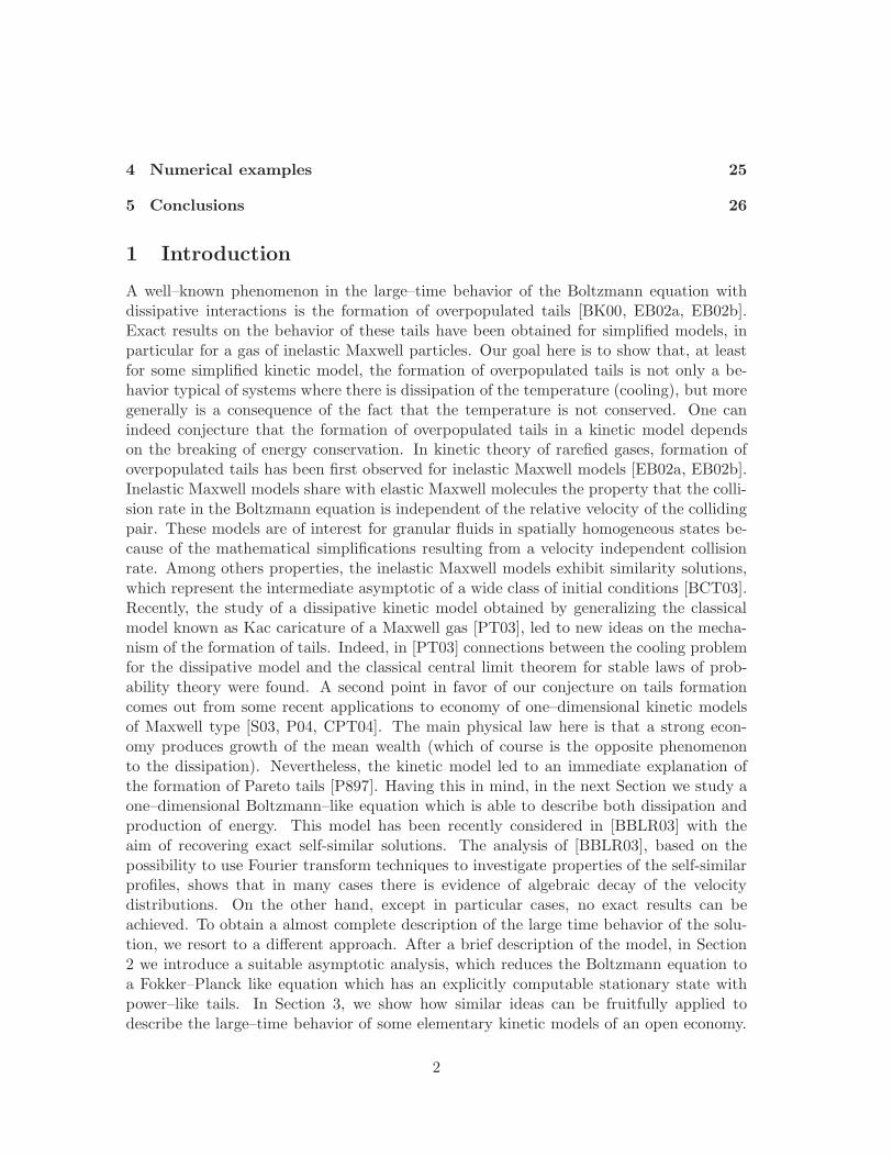
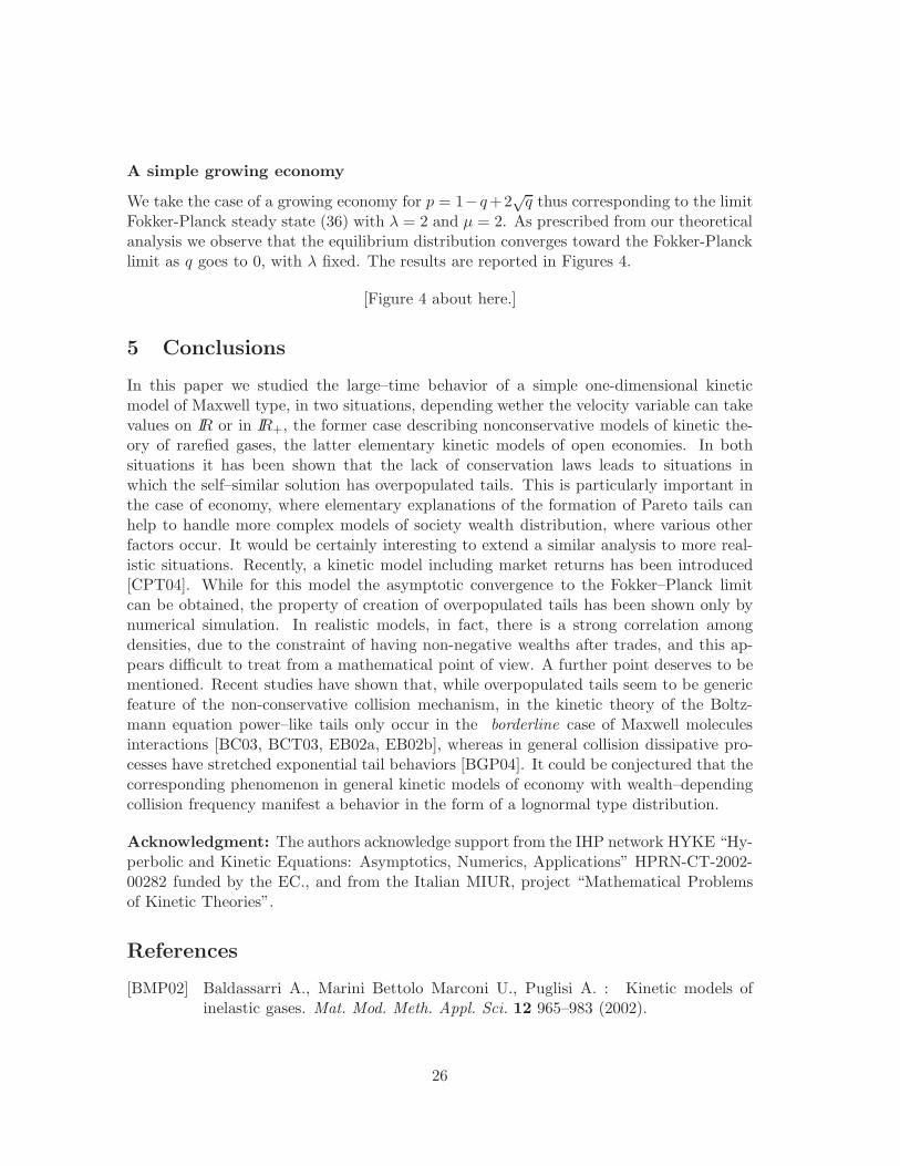
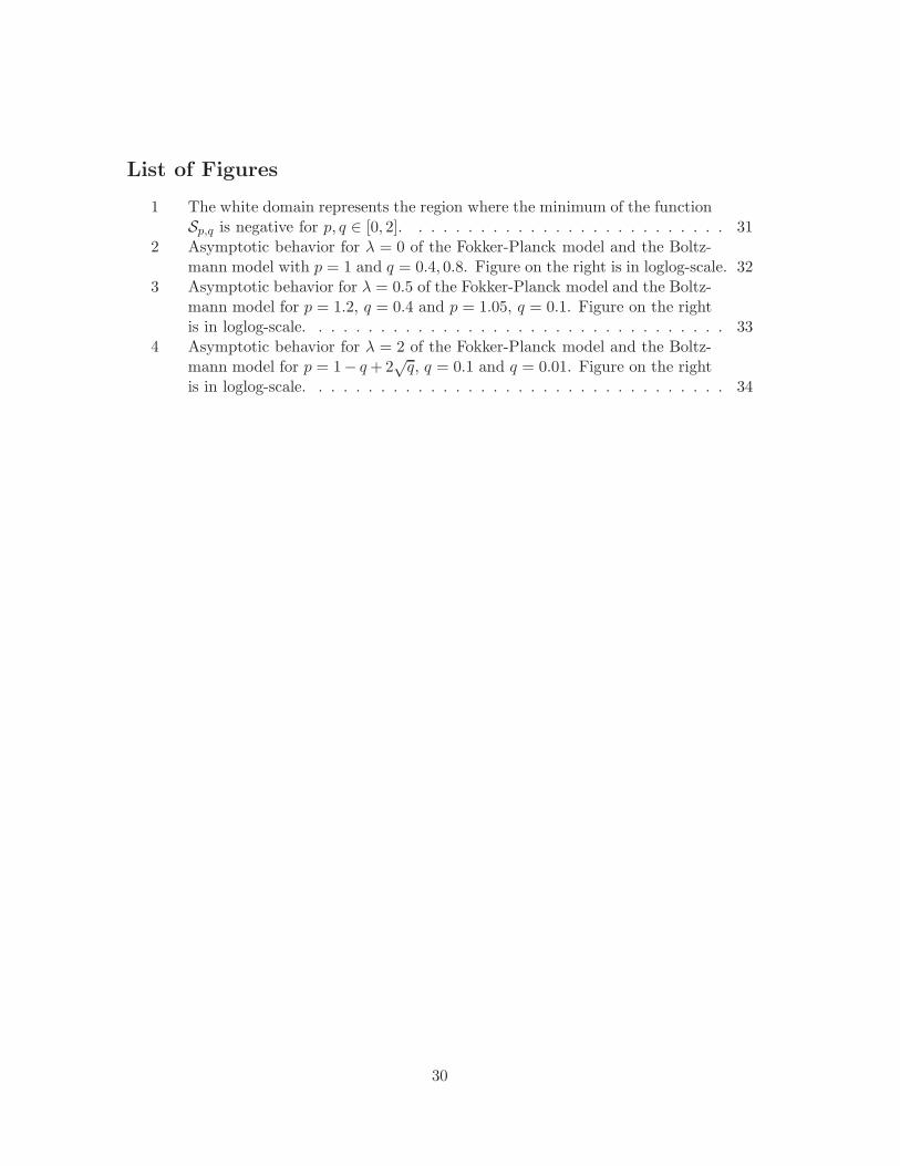
Then, the sign of Sp,q determines the asymptotic behavior of the distance ds(g1(t), g2(t)).In particular, if there exists an interval 0 < δ < δ in which Sp,q(δ) < 0, we can conclude thatd2+δ(g1(t), g2(t)) converges exponentially to zero. Note that, by construction, Sp,q(0) = 0,and thus minδ{Sp,q} ≤ 0. The function (52) was first considered by Bobylev and Cercignaniin [BC03]. The sign of Sp,q, however was studied mainly for p = 1 − q, namely the caseof the dissipative Boltzmann equation. In Figure 1 a numerical evaluation of the regionwhere the minimum of the function Sp,q is negative for p, q ∈ [0, 2] is reported.
[Figure 1 about here.]
Remark 3.2 The behavior of Sp,q(δ) when p2 + q2 = 1 is clear. In this case in fact, bothp and q are less than 1, which implies
Sp,q(δ) = p2+δ + q2+δ − 1 < 0,
for all δ > 0. We can draw the same conclusion when p2 + q2 > 1, while both p < 1 andq < 1.
13
Consider now the case p2 + q2 > 1, with p > 1. In this case, while −2+δ2
(p2 + q2 − 1
)
decreases linearly, p2+δ increases exponentially, and the sign of Sp,q(δ) becomes positivefor large values of δ.
If finally p2 + q2 < 1, the sign of Sp,q(δ) for large values of δ is positive, since, whilep2+δ + q2+δ − 1 ≥ −1,
−2 + δ
2
(p2 + q2 − 1
)≥ 1
for
δ ≥ 2(p2 + q2)
1− (p2 + q2).
The previous remark indicates that in the general case one can at best hope that Sp,q(δ)is negative in an interval (0, δ). To show that this is really the case, one has to investigatecarefully the behavior of Sp,q(δ) in a neighborhood of zero. Since the function Sp,q(δ) isconvex for δ ≥ 0,
d2Sp,q(δ)
dδ2= p2+δ(log p)2 + q2+δ(log q)2 > 0,
and Sp,q(0) = 0, in all cases where Sp,q(δ) is positive for large values of δ, a sufficientcondition for Sp,q(δ) be negative in some interval 0 < δ < δ is that
dSp,q(δ)
dδ
∣∣∣∣δ=0
= p2 log p+ q2 log q − 1
2
(p2 + q2 − 1
)< 0.
Let us discuss before the case p2 + q2 < 1. Given λ > 0, we introduce a dependencebetween p and q by setting p = 1 − λq. Since p > q, this relationship is possible only ifq < 1/(1+λ). Moreover p2+q2 < 1 requires q < (2λ)/(1+λ2). Using this, it is immediateto show that there is an interval 0 ≤ q ≤ q in which S ′
p,q(0) < 0. We have
dSp,q(δ)
dδ
∣∣∣∣δ=0
= G(q) = (1− λq)2 log(1− λq) + q2 log q − 1
2
((1− λq)2 + q2 − 1
).
Clearly, G(0) = 0. Moreover
G′(q) = 2q log q − 2λ(1− λq) log(1− λq),
andG′′(q) = 2(1 + log q) + 2λ2 (1 + log(1− λq)) .
Now G′′(q) < 0 in some interval (0, q1), which implies that G′(q) is decreasing in the sameinterval. But, since G′(0) = 0, G′(q) < 0 in the interval (0, q), where q solves
2q log q − 2λ(1− λq) log(1− λq) = 0
Consequently, G(q) < 0 at least in the same interval.Let us now treat the case p2 + q2 > 1, with p > 1. Let us set p = 1 + λq. We have
dSp,q(δ)
dδ
∣∣∣∣δ=0
= G(q) = (1 + λq)2 log(1 + λq) + q2 log q − 1
2
((1 + λq)2 + q2 − 1
).
14
In this caseG′(q) = 2q log q + 2λ(1 + λq) log(1 + λq),
andG′′(q) = 2(1 + log q) + 2λ2 (1 + log(1 + λq)) .
As before, G′′(q) < 0 in some interval (0, q2), which implies that G′(q) is decreasing in thesame interval. But, since G′(0) = 0, G′(q) < 0 in the interval (0, q), where q now solves
2q log q + 2λ(1 + λq) log(1 + λq) = 0
Consequently, G(q) < 0 at least in the same interval.We proved
Lemma 3.3 Let Sp,q(δ), δ ≥ 0 be the function defined by (52). Given a constant λ > 0, ifp2 + q2 < 1, let us define p = 1− λq . Then, provided q < min
{1/(1 + λ), (2λ)/(1 + λ2)
}
there exists an interval I− = (0, δ−(q)) such that Sp,q(δ) < 0 for δ ∈ I−. If p2 + q2 > 1,and p = 1 + λq there exists an interval I+ = (0, δ+(q)) such that Sp,q(δ) < 0 for δ ∈ I+.In the remaining cases, namely when p2 + q2 = 1 or p2 + q2 > 1 but p < 1, Sp,q(δ) < 0 forall δ > 0.
Lemma 3.3 has important consequences both in the behavior of the solution to theBoltzmann equation (9), and in the limit procedure introduced in Sections 2.1 and 2.2.The main consequence of the lemma is contained into the following.
Theorem 3.4 Let g1(t) and g2(t) be two solutions of the Boltzmann equation (9), cor-responding to initial values f1,0 and f2,0 satisfying conditions (3). Then, there exists aconstant δ > 0 such that, if 2 < s < 2 + δ, for all times t ≥ 0,
ds(g1(t), g2(t)) ≤ exp {−Cst} ds(f1,0, f2,0). (53)
The constant Cs = −Sp,q(s − 2) is strictly positive, and the distance ds is contractingexponentially in time.
3.2 Convergence to self–similarity
By means of the estimates of Section 3.1, we will now discuss the evolution of momentsfor the solution to equation (9). By construction, the second moment of g(v, t) is constantin time, and equal to 1 thanks to the normalization conditions (3). We can use thecomputations leading to the Fokker-Planck equation (23), choosing φ(v) = |v|2+δ , wherefor the moment the positive constant δ ≤ 1. Suppose that the initial density g0(v) = f0(v)is such that ∫
IR|v|2+δg0(v) dv = mδ < ∞. (54)
Then, since the contribution due to the term ∂∂v (vg(v)) can be evaluated integrating by
parts, ∫
IR|v|2+δ ∂
∂v(vg(v)) dv = −(2 + δ)
∫
IR|v|2+δg(v, t) dv,
15
we obtain
d
dt
∫
IR|v|2+δg(v, t) dv + (2 + δ)
p2 + q2 − 1
2
∫
IR|v|2+δg(v, t) dv =
∫
IR2
dv dw(|pv + qw|2+δ − |v|2+δ
)g(v)g(w) . (55)
Let us recover a suitable upper bound for the last integral in (55). Given any two constantsa, b, and 0 < δ ≤ 1 the following inequality holds
(|a|+ |b|)δ ≤ |a|δ + |b|δ . (56)
Hence, choosing a = p|v| and b = q|w|,
|pv + qw|2+δ ≤ (pv + qw)2(pδ|v|δ + qδ|w|δ
).
Substituting into the right-hand side of (55), recalling that the mean value of g is equalto zero, and the second moment of g equal to one, gives
∫
IR2
|pv + qw|2+δg(v)g(w) dv dw ≤
∫
IR2
(pv + qw)2(pδ|v|d + qδ|w|d
)g(v)g(w) dv dw =
(p2+δ + q2+δ
)∫
IR|v|2+δg(v) dv +
(p2qδ + q2pδ
) ∫
IR|v|δ dv.
Grouping all these inequalities, and recalling the expression of Sp,q(δ) given by (52)we obtain the differential inequality
d
dt
∫
IR|v|2+δg(v, t) dv ≤ Sp,q(δ)
∫
IR|v|2+δg(v, t) dv +Bp,δ, (57)
where, by Holder inequalityBp,δ ≤ p2qδ + q2pδ. (58)
By Lemma 3.3, for any δ < δ, Sp,q(δ) < 0. In this case, inequality (57) gives an upperbound for the moment, that reads
∫
IR|v|2+δg(v, t) dv ≤ mδ +
Bp,δ
|Sp,q(δ)|< ∞. (59)
In the case δ > 3 we can easily iterate our procedure to obtain that any moment of order2 + δ, with δ < δ which is bounded initially, remains bounded at any subsequent time.The only difference now is that the explicit expression of the bound is more and moreinvolved.
If δ < δ, we can immediately draw conclusions on the large–time convergence of classof probability densities {g(v, t)}t≥0, By virtue of Prokhorov theorem (cfr. [LR79]) the
16
existence of a uniform bound on moments implies that this class is tight, so that anysequence {g(v, tn)}n≥0 contains an infinite subsequence which converges weakly to some
probability measure g∞. Thanks to our bound on moments, provided δ < δ, g∞ possessesmoments of order 2 + δ, for 0 < δ < δ.
It is now immediate to show that this limit is unique. To this aim, let us consider twoinitial densities f0,1(v) and f0,2(v) such that, for some 0 < δ < δ,
∫
R
|v|2+δf0,1(v) dv < +∞,
∫
R
|v|2+δf0,2(v) dv < +∞.
Then, by Theorem 3.4, the distance ds(f1(t), f2(t)) between the solutions converges expo-nentially to zero with respect to time, as soon as 2 < s < 2 + δ. Let now f0(v) possessfinite moments of order 2 + δ, with 0 < δ < δ. Thanks to our previous computations onmoments, for any fixed time T > 0, the corresponding solution f(v, T ) has finite momentsof order 2+δ. Choosing f0,1(v) = f0(v), and f0,2(v) = f(v, T ) shows that ds(f(t), f(t+T ))converges exponentially to zero in time. It turns out that the ds-distance between subse-quences converges to zero as soon as Sp,q(s− 2) < 0.
We can now show that the limit function g∞(v) is a stationary solution to (9). Weknow that if condition (54) holds, both the solution g(v, t) to equation (9) and g∞(v)have moments of order 2 + δ, with 0 < δ < δ uniformly bounded. Hence, for any t ≥ 0,proceeding as in the proof of Theorem 3.1, we obtain
ds (Q(g(t), g(t)), Q(g∞ , g∞)) ≤ (ps + qs + 1) ds (g(t), g∞) . (60)
This implies the weak* convergence of Q(g(t), g(t)) towards Q(g∞, g∞). In particular,due to the equivalence among different metrics which metricize the weak* convergence ofmeasures [GTW95, TV99], if C1
0 (R) denotes the set of compactly supported continuouslydifferentiable functions, endowed with its natural norm ‖ · ‖1, for all φ ∈ C1
0 (R),∫
IRφ(v)Q(g(t), g(t))(v) dv →
∫
IRφ(v)Q(g∞, g∞)(v) dv. (61)
On the other hand, for all φ ∈ C10 (R), integration by parts gives
∫
IRφ(v)
∂
∂v(vg(v, t)) dv = −
∫
IRvφ ′(v)g(v, t) dv. (62)
Since |vφ ′(v)| ≤ |v|‖φ ′‖1, and the second moment of g(v, t) is equal to unity, the conver-gence of ds (g(t), g∞) to zero implies
∫
IRvφ ′(v)g(v, t) dv →
∫
IRvφ ′(v)g∞(v) dv. (63)
Finally, for all φ ∈ C10 (R) it holds
∫
IRφ(v)
{∂
∂v(vg∞(v))−Q(g∞, g∞)(v)
}dv = 0. (64)
This shows that g∞ is the unique stationary solution to (9). We have
17
Theorem 3.5 Let δ > 0 be such that Sp,q(δ) < 0, and let g∞(v) be the unique stationarysolution to equation (9). Let g(v, t) be the weak solution of the Boltzmann equation (9),corresponding to the initial density f0 satisfying
∫|v|2+δ f0(v) dv < ∞.
Then, g(v, t) satisfies ∫|v|2+δ g(v, t) dv ≤ cδ < ∞.
If 0 < δ ≤ 1 the constant cδ is given by (59). Moreover, g(v, t) converges exponentiallyfast in Fourier metric towards g∞(v), and the following bound holds
d2+δ(g(t), g∞) ≤ d2+δ(f0, g∞) exp {−|Sp,q(δ)|t} (65)
where Sp,q(δ) is given by (52).
Depending of the values of the mixing parameters p and q, the stationary solution g∞can have overpopulated tails. We can easily check the presence of overpopulated tails bylooking at the singular part of the Fourier transform [EB02a]. Since the Fourier transformof g∞ satisfies the equation
− p2 + q2 − 1
2ξ∂g
∂ξ+ g(ξ) = g(pξ)g(qξ), (66)
we setg(ξ) = 1− |ξ|2 +A|ξ|2+δ + . . . (67)
which takes into account the fact that g∞ satisfies conditions (3). The leading small ξ-behavior of the singular component will reflect an algebraic tail of the velocity distribution.Substitution of expression (67) into (66) shows that the coefficient of the power |ξ|2+δ isASp,q(δ). Thus, the term A|ξ|2+δ can appear in the expansion of g(ξ) as soon as δ is suchthat Sp,q(δ) = 0, δ > 0. In other words, tails in the stationary distributions are presentin all cases in which there exists a δ = δ > 0 such that Sp,q(δ) = 0. Now the answer iscontained into Lemma 3.3.
3.3 The grazing collision asymptotics
The results of the previous section are at the basis of the rigorous derivation of the Fokker-Planck asymptotics formally derived in Section 2.1 and 2.2. Suppose that the initial densityg0(v) = f0(v) satisfies condition (54). Using a Taylor expansion, we obtain
|pv + qw|2+δ − |v|2+δ =
(2 + δ)|v|δv((p − 1)v + qw) +1
2(1 + δ)|v|δ((p − 1)v + qw)2, (68)
where, for some 0 ≤ θ ≤ 1,v = θ(pv + qw) + (1− θ)v.
18
Using this into equality (55), one has
d
dt
∫
IR|v|2+δg(v, t) dv + (2 + δ)
p2 + q2 − 1
2
∫
IR|v|2+δg(v, t) dv =
(2 + δ)
∫
IR2
(|v|δv((p − 1)v + qw)
)g(v)g(w) dv dw
+1
2(2 + δ)(1 + δ)
∫
IR2
|v|δ((p − 1)v + qw)2g(v)g(w) dv dw. (69)
Since the momentum of g is equal to zero, we can rewrite (69) as
d
dt
∫
IR|v|2+δg(v, t) dv +
2 + δ
2
[(p− 1)2 + q2
] ∫
IR|v|2+δg(v, t) dv ≤
+1
2(2 + δ)(1 + δ)
∫
IR2
|v|δ((p − 1)v + qw)2g(v)g(w) dv dw. (70)
Assuming 0 < δ < 1,|v| ≤ (1 + p)δ|v|δ + qδ|w|δ .
Hence, if |p− 1|/q = λ, we obtain the bound
d
dt
∫
IR|v|2+δg(v, t) dv +
2 + δ
2q2[1 + λ2
] ∫
IR|v|2+δg(v, t) dv ≤
+1
2(2 + δ)(1 + δ)q2
∫
IR2
((1 + p)δ|v|δ + qδ|w|δ
)(λv + w)2g(v)g(w) dv dw,
or, what is the same,
d
dt
∫
IR|v|2+δg(v, t) dv ≤ q2C(λ, q)
∫
IR|v|2+δg(v, t) dv . (71)
If we now use (31), it holds
d
dτ
∫
IR|v|2+δh(v, τ) dv ≤ C(λ, q)
∫
IR|v|2+δh(v, τ) dv , (72)
namely the uniform boundedness of the (2 + δ)-moment of h(v, τ) with respect to q, forany fixed time τ .
Consider now the remainder (13), which can be rewritten as
R(p, q) =q2
2
∫
IR2
(p− 1
qv + w
)2 (φ′′(v)− φ′′(v)
)h(v)h(w)dv dw. (73)
We need the following
19
Definition 3.6 Let Fs(IR), be the class of all real functions φ on IR such that φ(m)(v) isHolder continuous of order δ,
‖φ(m)‖δ = supv 6=w
|φ(m)(v)− φ(m)(w)||v − w|δ < ∞, (74)
the integer m and the number 0 < δ ≤ 1 are such that m + δ = s, and φ(m) denotes them-th derivative of g.
If φ ∈ Fs(IR), with s = 2 + δ,
∣∣φ′′(v)− φ′′(v)∣∣ ≤ ‖φ′′‖δ |v − v|δ ≤ ‖φ′′‖δ|(p − 1)v + qw|δ. (75)
In this case,
R(p, q) ≤ q2+δ
2‖φ′′‖δ
∫
IR2
(p− 1
qv + w
)2+δ
h(v)h(w)dv dw ≤
q2+δ
2‖φ′′‖δC2(λ, q)
∫
IR2
|v|2+δh(v) dv. (76)
Thanks to the uniform bound on (2 + δ)-moment of h(v, τ) , it follows that, for any fixedtime τ > 0,
limq→0
1
q2R(p, q) = 0 (77)
as soon as φ ∈ Fs(IR), with s = 2 + δ. This implies that the limit equation is theFokker-Planck equation (19). We proved
Theorem 3.7 Let the probability density f0 ∈ Mα, where α = 2+ δ for some δ > 0, andlet the mixing parameters satisfy
(p− 1)2
q2= λ2,
for some constant λ fixed. Then, as q → 0, for all φ ∈ Fs(IR), with s = 2 + δ theweak solution to the Boltzmann equation (17) for the scaled density h(v, τ) = g(v, t), withτ = q2t converges, up to extraction of a subsequence, to a probability density h(w, τ). Thisdensity is a weak solution of the Fokker-Planck equation (19).
3.4 A comparison of tails
The result of Section 3.3 establishes a rigorous connection between the collisional kineticequation (2) and the Fokker–Planck equation (19). The result of Lemma 3.3, coupledwith the comment of Remark 2.3 then shows that there exists a link between tails of thestationary solution of Fokker–Plank and Boltzmann equations. In fact, one can chooseλ2 > 0 in Theorem 20 if and only if the mixing parameters p and q satisfy the conditionsof the aforementioned Lemma 3.3. Since the reckoning of the size of the tails is immediate
20
in the Fokker–Planck case, it would be important to know if one can extract from thisknowledge information about size of the tails of the Boltzmann equation.
Since the size of tails in the Boltzmann equation is given by the positive root of theequation
Sp,q(δ) = 0,
where Sp,q is the function (52), we will try to extract information by comparing thisroot with the value of the parameter λ that characterizes the tails of the Fokker–Planckequation. If p > 1, using a Taylor expansion of Sp,q(δ), with p = 1 + λq, we obtain
Sp,q(δ)
q2=
2 + δ
2
[(λ2δ − 1
)+
2
2 + δqδ +
(1 + δ)δ
3λ3 q
3
q2
], (78)
where 0 ≤ q ≤ q. This shows that, in the scaling of Theorem 20, the positive root δ∗(q)of Sp,q(δ) = 0 converges, as q → 0 to the value 1/λ2, which characterizes the tails of theFokker–Planck equation. When λ > 0, one can easily argue that δ∗(q) < 1/λ2. In thiscase, in fact,
Sp,q(δ)
q2=
2 + δ
2
[(λ2δ − 1
)+A
], (79)
where A > 0 if q > 0. Hence
Sp,q(1/λ2)
q2=
2 + δ
2A > 0, (80)
that, by virtue of the convexity properties of Sp,q(δ) implies δ∗(q) < 1/λ2.A weaker information can be extracted when p < 1 while p2 + q2 < 1. In this case,
writing p = 1− λq, λ > 0, we obtain
Sp,q(δ)
q2=
2 + δ
2
[(λ2δ − 1
)+
2
2 + δqδ − (1 + δ)δ
3λ3 q
3
q2
], (81)
where 0 ≤ q ≤ q. Let us set
q ≤ Bλ
1 + λ2, (82)
where B ≤ 2. In fact, when p < 1 Lemma 3.3 implies that there is formation of tails onlywhen p and q are such that p2 + q2 < 1, which is equivalent to the condition
q <2λ
1 + λ2. (83)
Hence, when q satisfies (82), from (81) we obtain the inequality
Sp,q(δ)
q2≥ 2 + δ
2
[(λ2δ − 1
)−B
(1 + δ)δ
3
λ4
1 + λ2
]. (84)
Easy computations then show that, if δ = rλ2, with 0 < r < 1, the right–hand side of (84)is nonnegative as soon as
3r(1− r)(1 + λ2) ≥ B(1 + rλ2).
21
Hence, the biggest value of B for which the right–hand side of (84) is nonnegative isattained when r = 1/2. In this case, B = 3/4, and δ∗(q) < 2/λ2. We can collect theprevious analysis into the following
Lemma 3.8 Let the mixing parameters satisfy
(p− 1)2
q2= λ2,
for some constant λ fixed. Then, if p > 1 the positive root δ∗(q) of the equation Sp,q(δ) = 0,characterizing the tails of the Boltzmann equation, satisfies the bound δ∗(q) < 1/λ2. Ifp > 1, and at the same time q satisfies the bound (82) with B = 3/4, the positive rootδ∗(q) of the equation Sp,q(δ) = 0, satisfies the bound δ∗(q) < 2/λ2.
We remark here that, in the case p < 1, setting δ = 1 we obtain an exact formula forSp,q(1),
Sp,q(1)
q2=
3
2
[(λ2 − 1
)+
2
3q − 2
3λ3q
]. (85)
Choosing λ = 1, we get Sp,q(1) = 0. This case, that corresponds to the conservation ofmomentum in the Boltzmann equation has tails which are invariant with respect to q (seeRemark 2.4).
3.5 Kinetic models of economy
The analysis of Sections 3, 3.1, 3.2 and 3.3 can be easily extended to equation (26) forthe wealth distribution. We can in fact resort to the methods introduced for the kineticequation on the whole real line simply setting
F (v, t) = f(v, t)I(v ≥ 0), v ∈ IR, (86)
where I(A) is the indicator function of the set A. With this notation, equation (26) canbe rewritten as equation (2),
∂F (v)
∂t=
∫
IR
(1
JF (v∗)F (w∗)− F (v)F (w)
)dw. (87)
Likewise, the weak form (27) reads
d
dt
∫
IRφ(v)F (v, t) dv =
∫
IR2
F (v, t)F (w, t)(φ(v∗)− φ(v))dvdw. (88)
We recall that the role of the energy is now supplied by the mean m(t) =∫vF (v, t) dv.
To look for self–similarity we scale our solution according to
G(v, t) = m(t)F (m(t)v, t) , (89)
22
which implies that∫vG(v, t) = 1 for all t ≥ 0. Hence, without loss of generality, if we fix
the initial density to satisfy∫
IRF0(v) dv = 1 ;
∫
IRvF0(v) dv = 1 , (90)
the solution G(v, t) satisfies (90). Then, the same computations of Section 3 show thefollowing
Theorem 3.9 Let f1(t) and f2(t) be two solutions of the Boltzmann equation (26), cor-responding to initial values f1,0 and f2,0 satisfying conditions (90). Then, if for some1 ≤ s ≤ 2, ds(f1,0, f2,0) is bounded, for all times t ≥ 0,
ds(f1(t), f2(t)) ≤ exp {(ps + qs − 1)t} ds(f1,0, f2,0). (91)
In particular, let f0 be a nonnegative density satisfying conditions (3). Then, there existsa unique weak solution f(t) of the Boltzmann equation, such that f(0) = f0. In caseps + qs − 1 < 0 the distance ds is contracting exponentially in time.
Since by (89)
G(ξ) = G
(ξ
m(t)
),
from (49) we obtain the bound
ds(g1(t), g2(t)) = supξ∈IR
|G1(ξ, t)− G2(ξ, t)||ξ|s =
(1
m(t)
)s
ds(f1(t), f2(t)). (92)
Using (91), we finally conclude that, if g1(t) and g2(t) are two solutions of the scaledBoltzmann equation (26), corresponding to initial values f1,0 and f2,0 satisfying conditions(90), Then, if 1 ≤ s ≤ 2, for all times t ≥ 0,
ds(g1(t), g2(t)) ≤ exp {[(ps + qs − 1)− s(p+ q − 1)] t} ds(f1,0, f2,0). (93)
Let us define, for δ ≥ 0,
Rp,q(δ) = p1+δ + q1+δ − 1− (1 + δ) (p+ q − 1) . (94)
Then, the sign ofRp,q now determines the asymptotic behavior of the distance ds(g1(t), g2(t)).With few differences, the proof leading to Lemma 3.3 can be repeated, obtaining
Lemma 3.10 Let Rp,q(δ), δ ≥ 0 be the function defined by (94). Given a constant λ > 0,if p+ q < 1, let us define p = 1− λ
√q . Then, provided q < 1/λ2 there exists an interval
I− = (0, δ−(q)) such that Rp,q(δ) < 0 for δ ∈ I−. If p + q > 1, and p = 1 + λ√q there
exists a interval I+ = (0, δ+(q)) such that Rp,q(δ) < 0 for δ ∈ I+. In the remaining cases,namely when p+ q = 1 or p+ q > 1 but p < 1, Rp,q(δ) < 0 for all δ > 0.
The main consequence of Lemma 3.10 is contained into the following.
23
Theorem 3.11 Let g1(t) and g2(t) be two solutions of the Boltzmann equation (26), cor-responding to initial values f1,0 and f2,0 satisfying conditions (90). Then, there exists aconstant δ > 0 such that, if 1 < s < 1 + δ, for all times t ≥ 0,
ds(g1(t), g2(t)) ≤ exp {−Cst} ds(f1,0, f2,0). (95)
The constant Cs = −Rp,q(s − 1) is strictly positive, and the distance ds is contractingexponentially in time.
Existence and uniqueness of the stationary solution to equation (29) follows along thesame lines of Section 3.2. The main result is now contained into the following.
Theorem 3.12 Let δ > 0 be such that Rp,q(δ) < 0, and let g∞(v) be the unique stationarysolution to equation (29). Let g(v, t) be the weak solution of the Boltzmann equation (29),corresponding to the initial density f0 satisfying
∫
IR+
|v|1+δ f0(v) dv < ∞.
Then, g(v, t) satisfies ∫
IR+
|v|1+δ g(v, t) dv ≤ cδ < ∞,
for some constant cδ depending only on p and q. Moreover, g(v, t) converges exponentiallyfast in Fourier metric towards g∞(v), and the following bound holds
d1+δ(g(t), g∞) ≤ d1+δ(f0, g∞) exp {−|Rp,q(δ)|t} (96)
where Rp,q(δ) is given by (94).
Depending on the values of the mixing parameters p and q, the stationary solution g∞can have overpopulated tails. The Fourier transform of g∞ satisfies the equation
− (p + q − 1)ξ∂G
∂ξ+ G(ξ) = G(pξ)G(qξ). (97)
We setG(ξ) = 1− iξ +A|ξ|1+δ + . . . (98)
which takes into account the fact that g∞ satisfies conditions (90). The leading small ξ-behavior of the singular component will reflect an algebraic tail of the velocity distribution.Substitution of expression (98) into (97) shows that the coefficient of the power |ξ|1+δ isARp,q(δ). Thus, the term A|ξ|1+δ can appear in the expansion of G(ξ) as soon as δ issuch that Rp,q(δ) = 0, δ > 0. As before, tails in the stationary distributions are presentin all cases in which there exists a δ = δ > 0 such that Rp,q(δ) = 0. Now the answer iscontained into Lemma 3.10.
Last, one can justify rigorously the passage to the Fokker-Planck equation (35).
24
Theorem 3.13 Let the probability density f0 ∈ Mα, where α = 1 + δ for some δ > 0,and let the mixing parameters satisfy
(p− 1)2
q= λ,
for some λ > 0 fixed. Then, as q → 0, for all φ ∈ Fs(IR), with s = 1+δ the weak solution tothe Boltzmann equation (32) for the scaled density h(v, τ) = g(v, t), with τ = qt converges,up to extraction of a subsequence, to a probability density h(w, τ). This density is a weaksolution of the Fokker-Planck equation (35).
We finally remark that the discussion of Section 3.4, with minor modifications, can beadapted to establish connections between the size of the tails of the kinetic and Fokker–Planck models.
4 Numerical examples
In this paragraph, we shall compare the self–similar stationary results obtained by usingMonte Carlo simulation of the kinetic model with the stationary state of the Fokker-Planckmodel. The method we adopted is based on Bird’s time counter approach at each timestep followed by a renormalization procedure according to the self-similar scaling used.We refer to [PR01] for more details on the use of Monte Carlo method for Boltzmannequations.
We used N = 5000 particles and perform several iterations until a stationary state isreached. The distribution is then averaged over the next 4000 iterations in order to reducestatistical fluctuations. Clearly, due to the slow convergence of the Monte Carlo methodnear the tails, some small fluctuations are still present for large velocities.
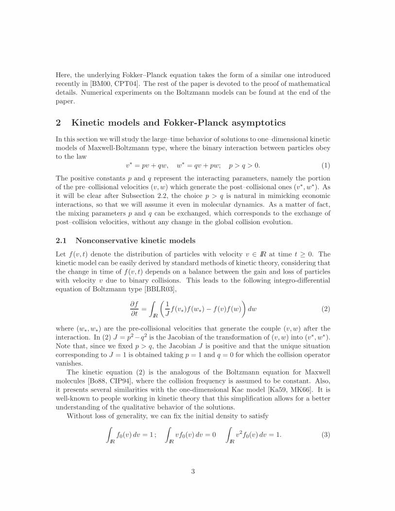
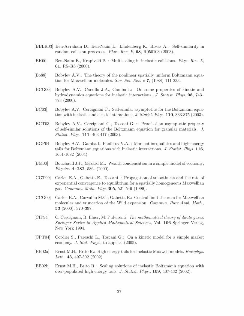
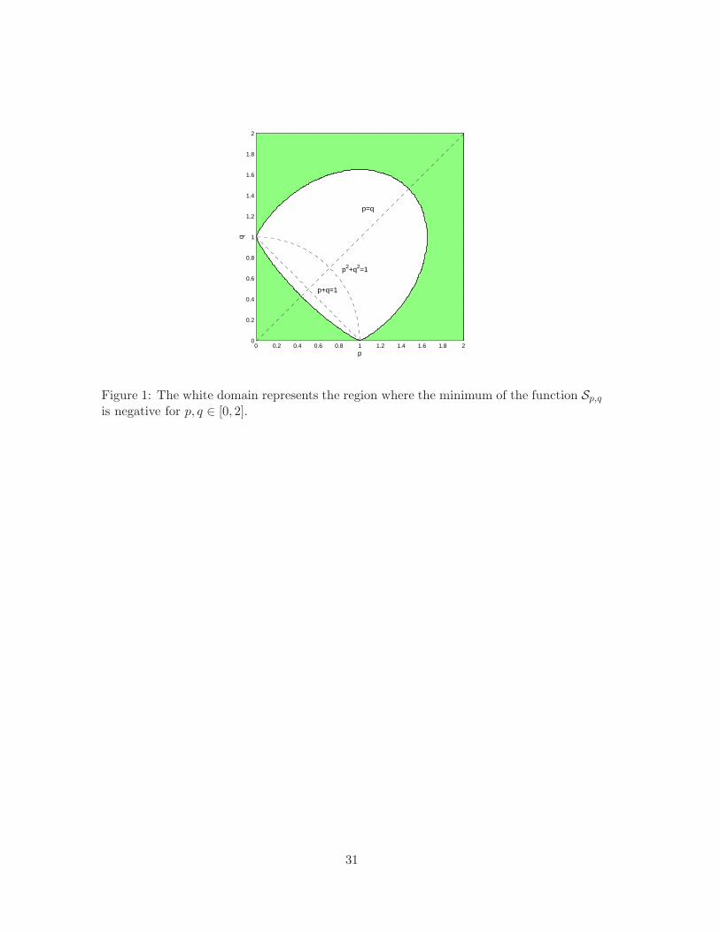
Gaussian behavior
First we consider the case λ = 0 for which the steady state of the Fokker-Planck asymptoticis the Gaussian (24). We fix p = 1 so that for q < 1/
√2 we expect Gaussian behavior also
in the kinetic model. We report the results obtained for q = 0.4 and q = 0.8 in Figure 2.
[Figure 2 about here.]
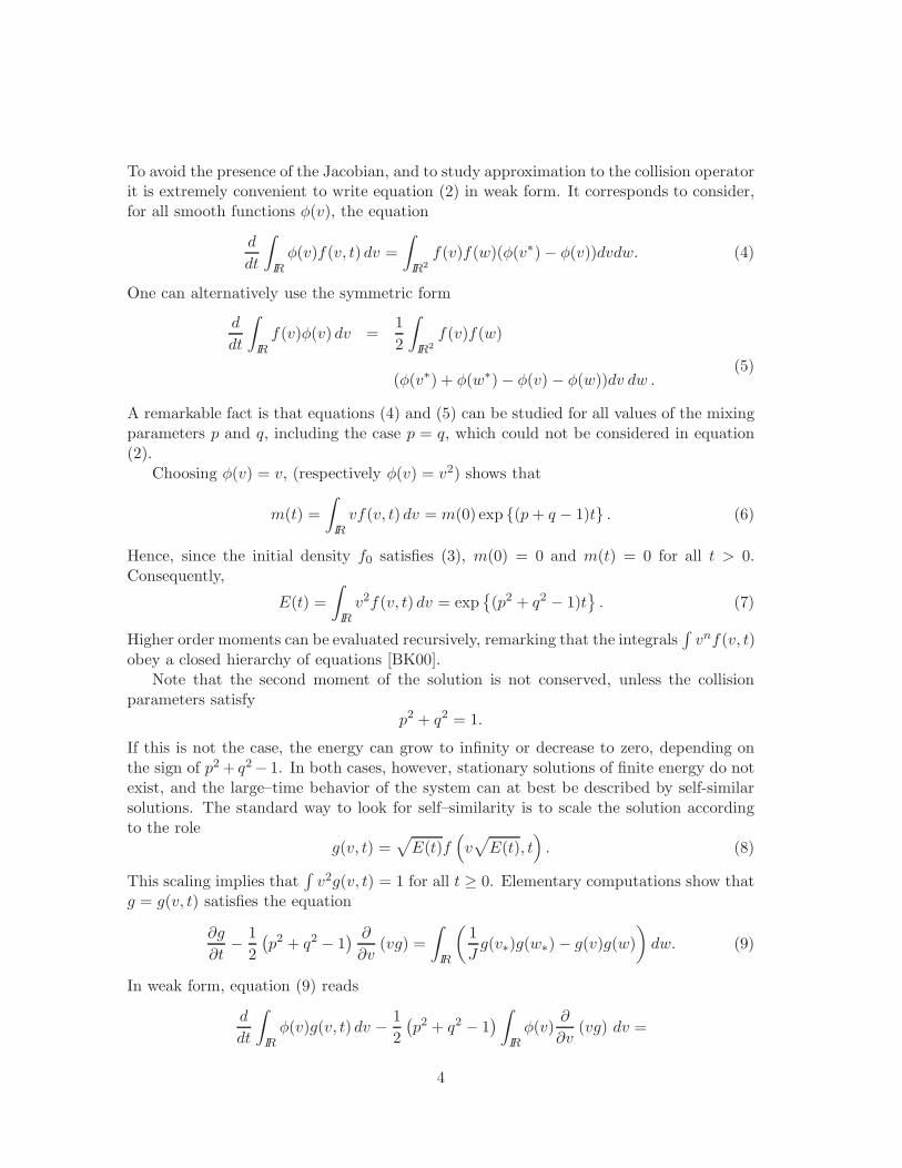
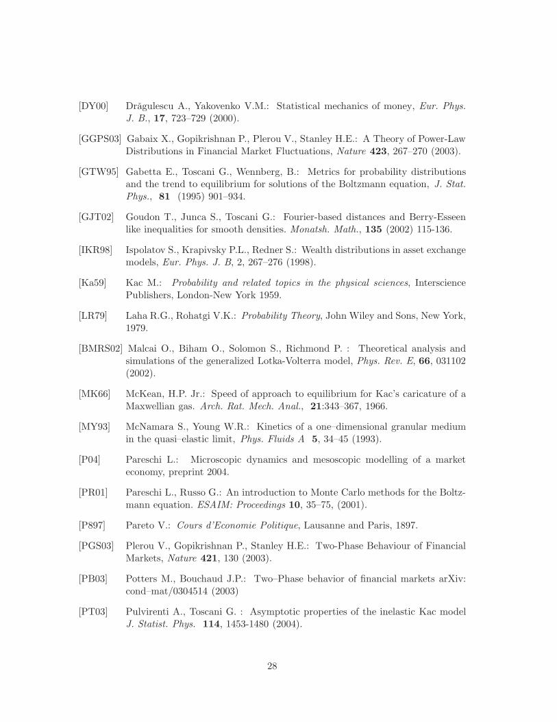
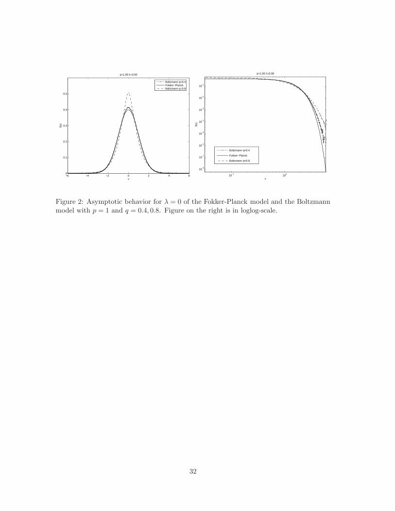
Formation of power laws
Next we simulate the formation of power laws for positive λ. We take p = 1.2 and q = .4which correspond to λ = 0.5. Keeping the same value of λ we then take q = 0.1 andp = 1.05. In Figure 2 we plot the results showing convergence towards the Fokker-Planckbehavior.
[Figure 3 about here.]
25
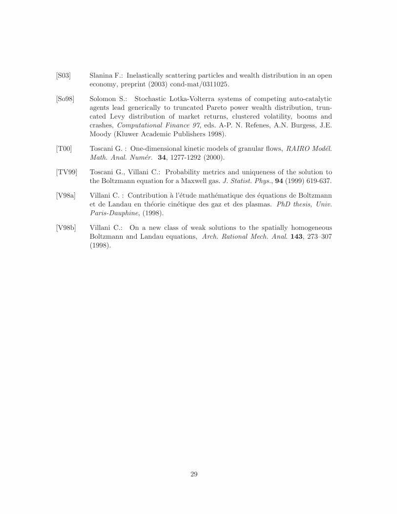
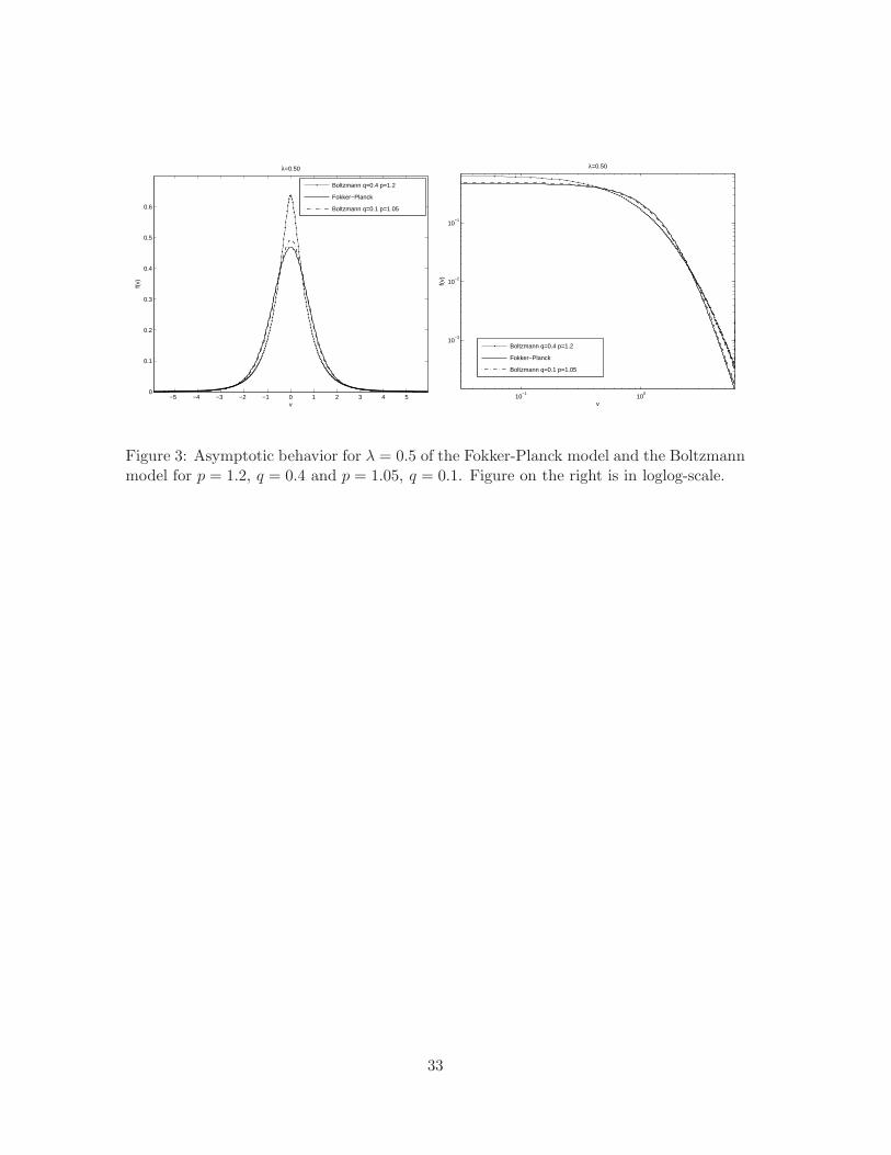
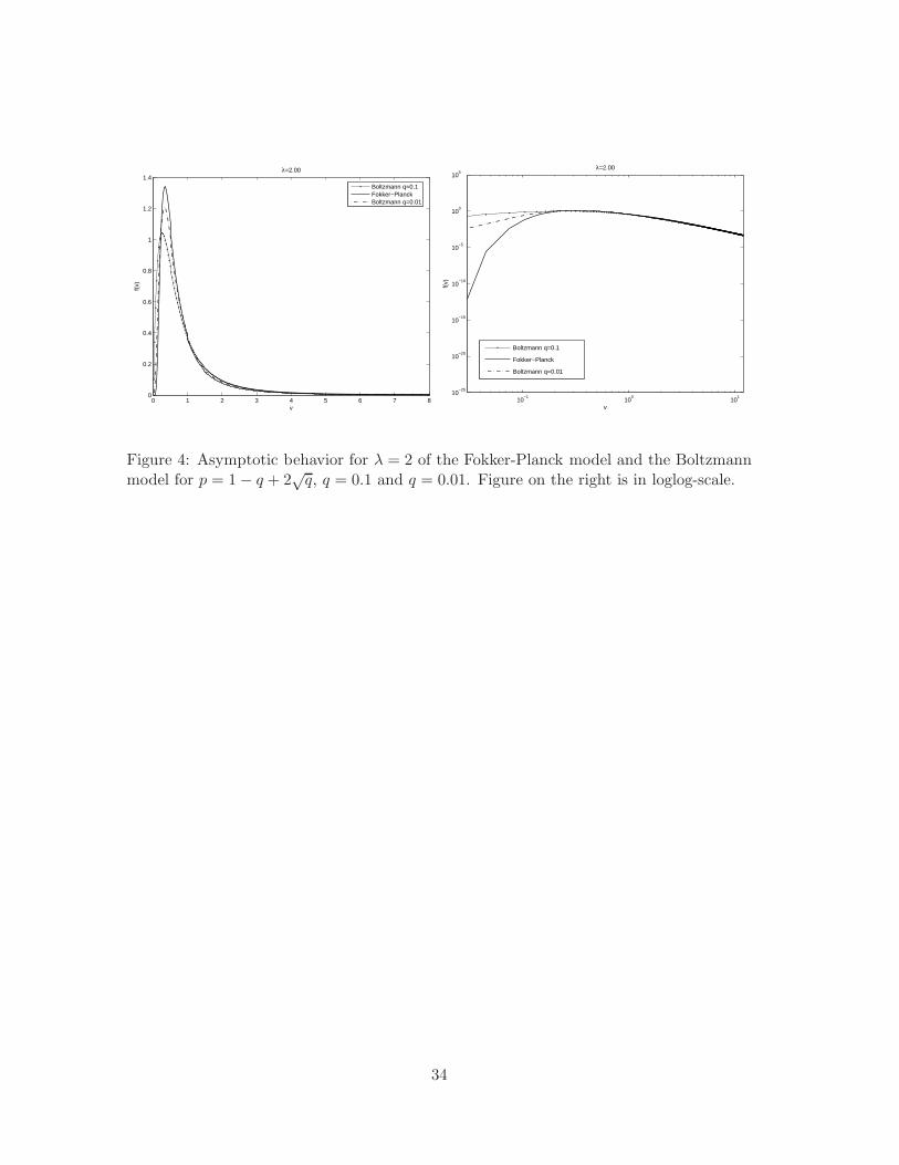
A simple growing economy
We take the case of a growing economy for p = 1−q+2√q thus corresponding to the limit
Fokker-Planck steady state (36) with λ = 2 and µ = 2. As prescribed from our theoreticalanalysis we observe that the equilibrium distribution converges toward the Fokker-Plancklimit as q goes to 0, with λ fixed. The results are reported in Figures 4.
[Figure 4 about here.]
5 Conclusions
In this paper we studied the large–time behavior of a simple one-dimensional kineticmodel of Maxwell type, in two situations, depending wether the velocity variable can takevalues on IR or in IR+, the former case describing nonconservative models of kinetic the-ory of rarefied gases, the latter elementary kinetic models of open economies. In bothsituations it has been shown that the lack of conservation laws leads to situations inwhich the self–similar solution has overpopulated tails. This is particularly important inthe case of economy, where elementary explanations of the formation of Pareto tails canhelp to handle more complex models of society wealth distribution, where various otherfactors occur. It would be certainly interesting to extend a similar analysis to more real-istic situations. Recently, a kinetic model including market returns has been introduced[CPT04]. While for this model the asymptotic convergence to the Fokker–Planck limitcan be obtained, the property of creation of overpopulated tails has been shown only bynumerical simulation. In realistic models, in fact, there is a strong correlation amongdensities, due to the constraint of having non-negative wealths after trades, and this ap-pears difficult to treat from a mathematical point of view. A further point deserves to bementioned. Recent studies have shown that, while overpopulated tails seem to be genericfeature of the non-conservative collision mechanism, in the kinetic theory of the Boltz-mann equation power–like tails only occur in the borderline case of Maxwell moleculesinteractions [BC03, BCT03, EB02a, EB02b], whereas in general collision dissipative pro-cesses have stretched exponential tail behaviors [BGP04]. It could be conjectured that thecorresponding phenomenon in general kinetic models of economy with wealth–dependingcollision frequency manifest a behavior in the form of a lognormal type distribution.
Acknowledgment: The authors acknowledge support from the IHP network HYKE “Hy-perbolic and Kinetic Equations: Asymptotics, Numerics, Applications” HPRN-CT-2002-00282 funded by the EC., and from the Italian MIUR, project “Mathematical Problemsof Kinetic Theories”.
References
[BMP02] Baldassarri A., Marini Bettolo Marconi U., Puglisi A. : Kinetic models ofinelastic gases. Mat. Mod. Meth. Appl. Sci. 12 965–983 (2002).
26
[BBLR03] Ben-Avraham D., Ben-Naim E., Lindenberg K., Rosas A.: Self-similarity inrandom collision processes, Phys. Rev. E, 68, R050103 (2003).
[BK00] Ben-Naim E., Krapivski P. : Multiscaling in inelastic collisions. Phys. Rev. E,61, R5–R8 (2000).
[Bo88] Bobylev A.V.: The theory of the nonlinear spatially uniform Boltzmann equa-tion for Maxwellian molecules. Sov. Sci. Rev. c 7, (1988) 111-233.
[BCG00] Bobylev A.V., Carrillo J.A., Gamba I.: On some properties of kinetic andhydrodynamics equations for inelastic interactions. J. Statist. Phys. 98, 743–773 (2000).
[BC03] Bobylev A.V., Cercignani C.: Self-similar asymptotics for the Boltzmann equa-tion with inelastic and elastic interactions. J. Statist. Phys. 110, 333-375 (2003).
[BCT03] Bobylev A.V., Cercignani C., Toscani G. : Proof of an asymptotic propertyof self-similar solutions of the Boltzmann equation for granular materials. J.Statist. Phys. 111, 403-417 (2003).
[BGP04] Bobylev A.V., Gamba I., Panferov V.A. : Moment inequalities and high–energytails for Boltzmann equations with inelastic interactions. J. Statist. Phys. 116,1651-1682 (2004).
[BM00] Bouchaud J.P., Mezard M.: Wealth condensation in a simple model of economy,Physica A, 282, 536- (2000).
[CGT99] Carlen E.A., Gabetta E., Toscani .: Propagation of smoothness and the rate ofexponential convergence to equilibrium for a spatially homogeneous Maxwelliangas. Commun. Math. Phys.305, 521-546 (1999).
[CCG00] Carlen E.A., Carvalho M.C., Gabetta E.: Central limit theorem for Maxwellianmolecules and truncation of the Wild expansion. Commun. Pure Appl. Math.,53 (2000), 370–397.
[CIP94] C. Cercignani, R. Illner, M. Pulvirenti, The mathematical theory of dilute gases.Springer Series in Applied Mathematical Sciences, Vol. 106 Springer–Verlag,New York 1994.
[CPT04] Cordier S., Pareschi L., Toscani G.: On a kinetic model for a simple marketeconomy. J. Stat. Phys., to appear, (2005).
[EB02a] Ernst M.H., Brito R.: High energy tails for inelastic Maxwell models. Europhys.Lett, 43, 497-502 (2002).
[EB02b] Ernst M.H., Brito R.: Scaling solutions of inelastic Boltzmann equation withover-populated high energy tails. J. Statist. Phys., 109, 407-432 (2002).
27
[DY00] Dragulescu A., Yakovenko V.M.: Statistical mechanics of money, Eur. Phys.J. B., 17, 723–729 (2000).
[GGPS03] Gabaix X., Gopikrishnan P., Plerou V., Stanley H.E.: A Theory of Power-LawDistributions in Financial Market Fluctuations, Nature 423, 267–270 (2003).
[GTW95] Gabetta E., Toscani G., Wennberg, B.: Metrics for probability distributionsand the trend to equilibrium for solutions of the Boltzmann equation, J. Stat.Phys., 81 (1995) 901–934.
[GJT02] Goudon T., Junca S., Toscani G.: Fourier-based distances and Berry-Esseenlike inequalities for smooth densities. Monatsh. Math., 135 (2002) 115-136.
[IKR98] Ispolatov S., Krapivsky P.L., Redner S.: Wealth distributions in asset exchangemodels, Eur. Phys. J. B, 2, 267–276 (1998).
[Ka59] Kac M.: Probability and related topics in the physical sciences, IntersciencePublishers, London-New York 1959.
[LR79] Laha R.G., Rohatgi V.K.: Probability Theory, John Wiley and Sons, New York,1979.
[BMRS02] Malcai O., Biham O., Solomon S., Richmond P. : Theoretical analysis andsimulations of the generalized Lotka-Volterra model, Phys. Rev. E, 66, 031102(2002).
[MK66] McKean, H.P. Jr.: Speed of approach to equilibrium for Kac’s caricature of aMaxwellian gas. Arch. Rat. Mech. Anal., 21:343–367, 1966.
[MY93] McNamara S., Young W.R.: Kinetics of a one–dimensional granular mediumin the quasi–elastic limit, Phys. Fluids A 5, 34–45 (1993).
[P04] Pareschi L.: Microscopic dynamics and mesoscopic modelling of a marketeconomy, preprint 2004.
[PR01] Pareschi L., Russo G.: An introduction to Monte Carlo methods for the Boltz-mann equation. ESAIM: Proceedings 10, 35–75, (2001).
[P897] Pareto V.: Cours d’Economie Politique, Lausanne and Paris, 1897.
[PGS03] Plerou V., Gopikrishnan P., Stanley H.E.: Two-Phase Behaviour of FinancialMarkets, Nature 421, 130 (2003).
[PB03] Potters M., Bouchaud J.P.: Two–Phase behavior of financial markets arXiv:cond–mat/0304514 (2003)
[PT03] Pulvirenti A., Toscani G. : Asymptotic properties of the inelastic Kac modelJ. Statist. Phys. 114, 1453-1480 (2004).
28
[S03] Slanina F.: Inelastically scattering particles and wealth distribution in an openeconomy, preprint (2003) cond-mat/0311025.
[So98] Solomon S.: Stochastic Lotka-Volterra systems of competing auto-catalyticagents lead generically to truncated Pareto power wealth distribution, trun-cated Levy distribution of market returns, clustered volatility, booms andcrashes, Computational Finance 97, eds. A-P. N. Refenes, A.N. Burgess, J.E.Moody (Kluwer Academic Publishers 1998).
[T00] Toscani G. : One-dimensional kinetic models of granular flows, RAIRO Model.Math. Anal. Numer. 34, 1277-1292 (2000).
[TV99] Toscani G., Villani C.: Probability metrics and uniqueness of the solution tothe Boltzmann equation for a Maxwell gas. J. Statist. Phys., 94 (1999) 619-637.
[V98a] Villani C. : Contribution a l’etude mathematique des equations de Boltzmannet de Landau en theorie cinetique des gaz et des plasmas. PhD thesis, Univ.Paris-Dauphine, (1998).
[V98b] Villani C.: On a new class of weak solutions to the spatially homogeneousBoltzmann and Landau equations, Arch. Rational Mech. Anal. 143, 273–307(1998).
29
List of Figures
1 The white domain represents the region where the minimum of the functionSp,q is negative for p, q ∈ [0, 2]. . . . . . . . . . . . . . . . . . . . . . . . . . 31
2 Asymptotic behavior for λ = 0 of the Fokker-Planck model and the Boltz-mann model with p = 1 and q = 0.4, 0.8. Figure on the right is in loglog-scale. 32
3 Asymptotic behavior for λ = 0.5 of the Fokker-Planck model and the Boltz-mann model for p = 1.2, q = 0.4 and p = 1.05, q = 0.1. Figure on the rightis in loglog-scale. . . . . . . . . . . . . . . . . . . . . . . . . . . . . . . . . . 33
4 Asymptotic behavior for λ = 2 of the Fokker-Planck model and the Boltz-mann model for p = 1− q+2
√q, q = 0.1 and q = 0.01. Figure on the right
is in loglog-scale. . . . . . . . . . . . . . . . . . . . . . . . . . . . . . . . . . 34
30
0 0.2 0.4 0.6 0.8 1 1.2 1.4 1.6 1.8 20
0.2
0.4
0.6
0.8
1
1.2
1.4
1.6
1.8
2
p
q
p2+q2=1
p=q
p+q=1
Figure 1: The white domain represents the region where the minimum of the function Sp,q
is negative for p, q ∈ [0, 2].
31
−6 −4 −2 0 2 4 60
0.1
0.2
0.3
0.4
0.5
p=1.00 λ=0.00
v
f(v)
Boltzmann q=0.4Fokker−PlanckBoltzmann q=0.8
10−1
100
10−8
10−7
10−6
10−5
10−4
10−3
10−2
10−1
p=1.00 λ=0.00
v
f(v)
Boltzmann q=0.4
Fokker−Planck
Boltzmann q=0.8
Figure 2: Asymptotic behavior for λ = 0 of the Fokker-Planck model and the Boltzmannmodel with p = 1 and q = 0.4, 0.8. Figure on the right is in loglog-scale.
32
−5 −4 −3 −2 −1 0 1 2 3 4 50
0.1
0.2
0.3
0.4
0.5
0.6
λ=0.50
v
f(v)
Boltzmann q=0.4 p=1.2
Fokker−Planck
Boltzmann q=0.1 p=1.05
10−1
100
10−3
10−2
10−1
λ=0.50
v
f(v)
Boltzmann q=0.4 p=1.2
Fokker−Planck
Boltzmann q=0.1 p=1.05
Figure 3: Asymptotic behavior for λ = 0.5 of the Fokker-Planck model and the Boltzmannmodel for p = 1.2, q = 0.4 and p = 1.05, q = 0.1. Figure on the right is in loglog-scale.
33
0 1 2 3 4 5 6 7 80
0.2
0.4
0.6
0.8
1
1.2
1.4λ=2.00
v
f(v)
Boltzmann q=0.1Fokker−PlanckBoltzmann q=0.01
10−1
100
101
10−25
10−20
10−15
10−10
10−5
100
105
λ=2.00
v
f(v)
Boltzmann q=0.1
Fokker−Planck
Boltzmann q=0.01
Figure 4: Asymptotic behavior for λ = 2 of the Fokker-Planck model and the Boltzmannmodel for p = 1− q + 2
√q, q = 0.1 and q = 0.01. Figure on the right is in loglog-scale.
34