arX

iv:h

ep-e

x/00

0601

1v2

7 A

ug 2

000

Search for New Physics in eµX Data at DØ Using Sleuth: AQuasi-Model-Independent Search Strategy for New Physics

B. Abbott,49 M. Abolins,46 V. Abramov,22 B.S. Acharya,15 D.L. Adams,56 M. Adams,33 G.A. Alves,2 N. Amos,45

E.W. Anderson,38 M.M. Baarmand,51 V.V. Babintsev,22 L. Babukhadia,51 A. Baden,42 B. Baldin,32 S. Banerjee,15

J. Bantly,55 E. Barberis,25 P. Baringer,39 J.F. Bartlett,32 U. Bassler,11 A. Bean,39 M. Begel,50 A. Belyaev,21

S.B. Beri,13 G. Bernardi,11 I. Bertram,23 A. Besson,9 V.A. Bezzubov,22 P.C. Bhat,32 V. Bhatnagar,13

M. Bhattacharjee,51 G. Blazey,34 S. Blessing,30 A. Boehnlein,32 N.I. Bojko,22 F. Borcherding,32 A. Brandt,56

R. Breedon,26 G. Briskin,55 R. Brock,46 G. Brooijmans,32 A. Bross,32 D. Buchholz,35 M. Buehler,33 V. Buescher,50

V.S. Burtovoi,22 J.M. Butler,43 F. Canelli,50 W. Carvalho,3 D. Casey,46 Z. Casilum,51 H. Castilla-Valdez,17

D. Chakraborty,51 K.M. Chan,50 S.V. Chekulaev,22 D.K. Cho,50 S. Choi,29 S. Chopra,52 B.C. Choudhary,29

J.H. Christenson,32 M. Chung,33 D. Claes,47 A.R. Clark,25 J. Cochran,29 L. Coney,37 B. Connolly,30 W.E. Cooper,32

D. Coppage,39 M.A.C. Cummings,34 D. Cutts,55 O.I. Dahl,25 G.A. Davis,50 K. Davis,24 K. De,56 K. Del Signore,45

M. Demarteau,32 R. Demina,40 P. Demine,9 D. Denisov,32 S.P. Denisov,22 H.T. Diehl,32 M. Diesburg,32

G. Di Loreto,46 S. Doulas,44 P. Draper,56 Y. Ducros,12 L.V. Dudko,21 S.R. Dugad,15 A. Dyshkant,22 D. Edmunds,46

J. Ellison,29 V.D. Elvira,32 R. Engelmann,51 S. Eno,42 G. Eppley,58 P. Ermolov,21 O.V. Eroshin,22 J. Estrada,50

H. Evans,48 V.N. Evdokimov,22 T. Fahland,28 S. Feher,32 D. Fein,24 T. Ferbel,50 F. Filthaut,18 H.E. Fisk,32

Y. Fisyak,52 E. Flattum,32 F. Fleuret,25 M. Fortner,34 K.C. Frame,46 S. Fuess,32 E. Gallas,32 A.N. Galyaev,22

P. Gartung,29 V. Gavrilov,20 R.J. Genik II,23 K. Genser,32 C.E. Gerber,32 Y. Gershtein,55 B. Gibbard,52

R. Gilmartin,30 G. Ginther,50 B. Gomez,5 G. Gomez,42 P.I. Goncharov,22 J.L. Gonzalez Solıs,17 H. Gordon,52

L.T. Goss,57 K. Gounder,29 A. Goussiou,51 N. Graf,52 P.D. Grannis,51 J.A. Green,38 H. Greenlee,32 S. Grinstein,1

P. Grudberg,25 S. Grunendahl,32 A. Gupta,15 S.N. Gurzhiev,22 G. Gutierrez,32 P. Gutierrez,54 N.J. Hadley,42

H. Haggerty,32 S. Hagopian,30 V. Hagopian,30 K.S. Hahn,50 R.E. Hall,27 P. Hanlet,44 S. Hansen,32

J.M. Hauptman,38 C. Hays,48 C. Hebert,39 D. Hedin,34 A.P. Heinson,29 U. Heintz,43 T. Heuring,30 R. Hirosky,33

J.D. Hobbs,51 B. Hoeneisen,8 J.S. Hoftun,55 A.S. Ito,32 S.A. Jerger,46 R. Jesik,36 K. Johns,24 M. Johnson,32

A. Jonckheere,32 M. Jones,31 H. Jostlein,32 A. Juste,32 S. Kahn,52 E. Kajfasz,10 D. Karmanov,21 D. Karmgard,37

R. Kehoe,37 S.K. Kim,16 B. Klima,32 C. Klopfenstein,26 B. Knuteson,25 W. Ko,26 J.M. Kohli,13 A.V. Kostritskiy,22

J. Kotcher,52 A.V. Kotwal,48 A.V. Kozelov,22 E.A. Kozlovsky,22 J. Krane,38 M.R. Krishnaswamy,15

S. Krzywdzinski,32 M. Kubantsev,40 S. Kuleshov,20 Y. Kulik,51 S. Kunori,42 V. Kuznetsov,29 G. Landsberg,55

A. Leflat,21 F. Lehner,32 J. Li,56 Q.Z. Li,32 J.G.R. Lima,3 D. Lincoln,32 S.L. Linn,30 J. Linnemann,46 R. Lipton,32

A. Lucotte,51 L. Lueking,32 C. Lundstedt,47 A.K.A. Maciel,34 R.J. Madaras,25 V. Manankov,21 S. Mani,26

H.S. Mao,4 T. Marshall,36 M.I. Martin,32 R.D. Martin,33 K.M. Mauritz,38 B. May,35 A.A. Mayorov,36

R. McCarthy,51 J. McDonald,30 T. McMahon,53 H.L. Melanson,32 X.C. Meng,4 M. Merkin,21 K.W. Merritt,32

C. Miao,55 H. Miettinen,58 D. Mihalcea,54 A. Mincer,49 C.S. Mishra,32 N. Mokhov,32 N.K. Mondal,15

H.E. Montgomery,32 M. Mostafa,1 H. da Motta,2 E. Nagy,10 F. Nang,24 M. Narain,43 V.S. Narasimham,15

H.A. Neal,45 J.P. Negret,5 S. Negroni,10 D. Norman,57 L. Oesch,45 V. Oguri,3 B. Olivier,11 N. Oshima,32

P. Padley,58 L.J. Pan,35 A. Para,32 N. Parashar,44 R. Partridge,55 N. Parua,9 M. Paterno,50 A. Patwa,51

B. Pawlik,19 J. Perkins,56 M. Peters,31 R. Piegaia,1 H. Piekarz,30 B.G. Pope,46 E. Popkov,37 H.B. Prosper,30

S. Protopopescu,52 J. Qian,45 P.Z. Quintas,32 R. Raja,32 S. Rajagopalan,52 E. Ramberg,32 N.W. Reay,40

S. Reucroft,44 J. Rha,29 M. Rijssenbeek,51 T. Rockwell,46 M. Roco,32 P. Rubinov,32 R. Ruchti,37 J. Rutherfoord,24

A. Santoro,2 L. Sawyer,41 R.D. Schamberger,51 H. Schellman,35 A. Schwartzman,1 J. Sculli,49 N. Sen,58

E. Shabalina,21 H.C. Shankar,15 R.K. Shivpuri,14 D. Shpakov,51 M. Shupe,24 R.A. Sidwell,40 V. Simak,7 H. Singh,29

J.B. Singh,13 V. Sirotenko,34 P. Slattery,50 E. Smith,54 R.P. Smith,32 R. Snihur,35 G.R. Snow,47 J. Snow,53

S. Snyder,52 J. Solomon,33 V. Sorın,1 M. Sosebee,56 N. Sotnikova,21 K. Soustruznik,6 M. Souza,2 N.R. Stanton,40

G. Steinbruck,48 R.W. Stephens,56 M.L. Stevenson,25 F. Stichelbaut,52 D. Stoker,28 V. Stolin,20 D.A. Stoyanova,22

M. Strauss,54 K. Streets,49 M. Strovink,25 L. Stutte,32 A. Sznajder,3 W. Taylor,51 S. Tentindo-Repond,30

J. Thompson,42 D. Toback,42 T.G. Trippe,25 A.S. Turcot,52 P.M. Tuts,48 P. van Gemmeren,32 V. Vaniev,22

R. Van Kooten,36 N. Varelas,33 A.A. Volkov,22 A.P. Vorobiev,22 H.D. Wahl,30 H. Wang,35 Z.-M. Wang,51

J. Warchol,37 G. Watts,59 M. Wayne,37 H. Weerts,46 A. White,56 J.T. White,57 D. Whiteson,25 J.A. Wightman,38

S. Willis,34 S.J. Wimpenny,29 J.V.D. Wirjawan,57 J. Womersley,32 D.R. Wood,44 R. Yamada,32 P. Yamin,52

T. Yasuda,32 K. Yip,32 S. Youssef,30 J. Yu,32 Z. Yu,35 M. Zanabria,5 H. Zheng,37 Z. Zhou,38 Z.H. Zhu,50

M. Zielinski,50 D. Zieminska,36 A. Zieminski,36 V. Zutshi,50 E.G. Zverev,21 and A. Zylberstejn12

(DØ Collaboration)

1Universidad de Buenos Aires, Buenos Aires, Argentina2LAFEX, Centro Brasileiro de Pesquisas Fısicas, Rio de Janeiro, Brazil

3Universidade do Estado do Rio de Janeiro, Rio de Janeiro, Brazil

1

4Institute of High Energy Physics, Beijing, People’s Republic of China5Universidad de los Andes, Bogota, Colombia6Charles University, Prague, Czech Republic

7Institute of Physics, Academy of Sciences, Prague, Czech Republic8Universidad San Francisco de Quito, Quito, Ecuador

9Institut des Sciences Nucleaires, IN2P3-CNRS, Universite de Grenoble 1, Grenoble, France10CPPM, IN2P3-CNRS, Universite de la Mediterranee, Marseille, France

11LPNHE, Universites Paris VI and VII, IN2P3-CNRS, Paris, France12DAPNIA/Service de Physique des Particules, CEA, Saclay, France

13Panjab University, Chandigarh, India14Delhi University, Delhi, India

15Tata Institute of Fundamental Research, Mumbai, India16Seoul National University, Seoul, Korea

17CINVESTAV, Mexico City, Mexico18University of Nijmegen/NIKHEF, Nijmegen, The Netherlands

19Institute of Nuclear Physics, Krakow, Poland20Institute for Theoretical and Experimental Physics, Moscow, Russia

21Moscow State University, Moscow, Russia22Institute for High Energy Physics, Protvino, Russia23Lancaster University, Lancaster, United Kingdom

24University of Arizona, Tucson, Arizona 8572125Lawrence Berkeley National Laboratory and University of California, Berkeley, California 94720

26University of California, Davis, California 9561627California State University, Fresno, California 93740

28University of California, Irvine, California 9269729University of California, Riverside, California 9252130Florida State University, Tallahassee, Florida 32306

31University of Hawaii, Honolulu, Hawaii 9682232Fermi National Accelerator Laboratory, Batavia, Illinois 60510

33University of Illinois at Chicago, Chicago, Illinois 6060734Northern Illinois University, DeKalb, Illinois 6011535Northwestern University, Evanston, Illinois 6020836Indiana University, Bloomington, Indiana 47405

37University of Notre Dame, Notre Dame, Indiana 4655638Iowa State University, Ames, Iowa 50011

39University of Kansas, Lawrence, Kansas 6604540Kansas State University, Manhattan, Kansas 6650641Louisiana Tech University, Ruston, Louisiana 71272

42University of Maryland, College Park, Maryland 2074243Boston University, Boston, Massachusetts 02215

44Northeastern University, Boston, Massachusetts 0211545University of Michigan, Ann Arbor, Michigan 48109

46Michigan State University, East Lansing, Michigan 4882447University of Nebraska, Lincoln, Nebraska 6858848Columbia University, New York, New York 1002749New York University, New York, New York 10003

50University of Rochester, Rochester, New York 1462751State University of New York, Stony Brook, New York 11794

52Brookhaven National Laboratory, Upton, New York 1197353Langston University, Langston, Oklahoma 73050

54University of Oklahoma, Norman, Oklahoma 7301955Brown University, Providence, Rhode Island 02912

56University of Texas, Arlington, Texas 7601957Texas A&M University, College Station, Texas 77843

58Rice University, Houston, Texas 7700559University of Washington, Seattle, Washington 98195

2

Abstract

We present a quasi-model-independent search for the physics responsible for electroweak symmetry

breaking. We define final states to be studied, and construct a rule that identifies a set of relevant

variables for any particular final state. A new algorithm (“Sleuth”) searches for regions of excess

in those variables and quantifies the significance of any detected excess. After demonstrating the

sensitivity of the method, we apply it to the semi-inclusive channel eµX collected in 108 pb−1 of pp

collisions at√

s = 1.8 TeV at the DØ experiment during 1992–1996 at the Fermilab Tevatron. We

find no evidence of new high pT physics in this sample.

3

Contents

I Introduction 4

II Search strategy 5

A General prescription . . . . . . . . . . . 51 Final states . . . . . . . . . . . . . . 52 Variables . . . . . . . . . . . . . . . 6

B Search strategy: DØ Run I . . . . . . . 71 Object definitions . . . . . . . . . . 72 Variables . . . . . . . . . . . . . . . 8

III Sleuth algorithm 8

A Overview . . . . . . . . . . . . . . . . . 8B Steps 1 and 2: Regions . . . . . . . . . 9

1 Variable transformation . . . . . . . 92 Voronoi diagrams . . . . . . . . . . 103 Region criteria . . . . . . . . . . . . 10

C Step 3: Probabilities and uncertainties 111 Probabilities . . . . . . . . . . . . . 112 Systematic uncertainties . . . . . . 11

D Step 4: Exploration of regions . . . . . 12E Steps 5 and 6: Hypothetical similar ex-

periments, Part I . . . . . . . . . . . . 12F Step 7: Hypothetical similar experi-

ments, Part II . . . . . . . . . . . . . . 12G Interpretation of results . . . . . . . . . 13

1 Combining the results of many finalstates . . . . . . . . . . . . . . . . . 13

2 Confirmation . . . . . . . . . . . . . 13

IV The eµX data set 13

V Sensitivity 14

A Search for WW and tt in mock samples 15B Search for tt in mock samples . . . . . 15C New high pT physics . . . . . . . . . . 16

VI Results 17

A Search for WW and tt in data . . . . . 17B Search for tt in data . . . . . . . . . . . 18C Search for physics beyond the standard

model . . . . . . . . . . . . . . . . . . . 19

VII Conclusions 19

APPENDIXES 20

A Further comments on variables 20

B Transformation of variables 20

C Region criteria 21

D Search heuristic details 22

I. INTRODUCTION

It is generally recognized that the standard model, anextremely successful description of the fundamental par-ticles and their interactions, must be incomplete. Al-though there is likely to be new physics beyond the cur-rent picture, the possibilities are sufficiently broad thatthe first hint could appear in any of many different guises.This suggests the importance of performing searches thatare as model-independent as possible.

The word “model” can connote varying degrees of gen-erality. It can mean a particular model together withdefinite choices of parameters [e.g., mSUGRA [1] withspecified m1/2, m0, A0, tanβ, and sign(µ)]; it can meana particular model with unspecified parameters (e.g.,mSUGRA); it can mean a more general model (e.g.,SUGRA); it can mean an even more general model (e.g.,gravity-mediated supersymmetry); it can mean a class ofgeneral models (e.g., supersymmetry); or it can be a setof classes of general models (e.g., theories of electroweaksymmetry breaking). As one ascends this hierarchy ofgenerality, predictions of the “model” become less pre-cise. While there have been many searches for phenom-ena predicted by models in the narrow sense, there havebeen relatively few searches for predictions of the moregeneral kind.

In this article we describe an explicit prescription forsearching for the physics responsible for stabilizing elec-troweak symmetry breaking, in a manner that relies onlyupon what we are sure we know about electroweak sym-metry breaking: that its natural scale is on the orderof the Higgs mass [2]. When we wish to emphasize thegenerality of the approach, we say that it is quasi-model-independent, where the “quasi” refers to the fact that thecorrect model of electroweak symmetry breaking shouldbecome manifest at the scale of several hundred GeV.

New sources of physics will in general lead to an excessover the expected background in some final state. A gen-eral signature for new physics is therefore a region of vari-able space in which the probability for the background tofluctuate up to or above the number of observed events issmall. Because the mass scale of electroweak symmetrybreaking is larger than the mass scale of most standardmodel backgrounds, we expect this excess to populateregions of high transverse momentum (pT ). The methodwe will describe involves a systematic search for such ex-cesses (although with a small modification it is equallyapplicable to searches for deficits). Although motivatedby the problem of electroweak symmetry breaking, thismethod is generally sensitive to any new high pT physics.

An important benefit of a precise a priori algorithmof the type we construct is that it allows an a posteri-ori evaluation of the significance of a small excess, inaddition to providing a recipe for searching for such aneffect. The potential benefit of this feature can be seenby considering the two curious events seen by the CDFcollaboration in their semi-inclusive eµ sample [3] and

4

one event in the data sample we analyze in this article,which have prompted efforts to determine the probabil-ity that the standard model alone could produce such aresult [4]. This is quite difficult to do a posteriori, as oneis forced to somewhat arbitrarily decide what is meantby “such a result.” The method we describe provides anunbiased and quantitative answer to such questions.

“Sleuth,” a quasi-model-independent prescription forsearching for high pT physics beyond the standard model,has two components:

• the definitions of physical objects and final states,and the variables relevant for each final state; and

• an algorithm that systematically hunts for an ex-cess in the space of those variables, and quantifiesthe likelihood of any excess found.

We describe the prescription in Secs. II and III. InSec. II we define the physical objects and final states,and we construct a rule for choosing variables relevantfor any final state. In Sec. III we describe an algorithmthat searches for a region of excess in a multidimensionalspace, and determines how unlikely it is that this excessarose simply from a statistical fluctuation, taking accountof the fact that the search encompasses many regions ofthis space. This algorithm is especially useful when ap-plied to a large number of final states. For a first appli-cation of Sleuth, we choose the semi-inclusive eµ data set(eµX) because it contains “known” signals (pair produc-tion of W bosons and top quarks) that can be used toquantify the sensitivity of the algorithm to new physics,and because this final state is prominent in several modelsof physics beyond the standard model [5,6]. In Sec. IV wedescribe the data set and the expected backgrounds fromthe standard model and instrumental effects. In Sec. Vwe demonstrate the sensitivity of the method by ignoringthe existence of top quark and W boson pair production,and showing that the method can find these signals inthe data. In Sec. VI we apply the Sleuth algorithm tothe eµX data set assuming the known backgrounds, in-cluding WW and tt, and present the results of a searchfor new physics beyond the standard model.

II. SEARCH STRATEGY

Most recent searches for new physics have followed awell-defined set of steps: first selecting a model to betested against the standard model, then finding a mea-surable prediction of this model that differs as much aspossible from the prediction of the standard model, andfinally comparing the predictions to data. This is clearlythe procedure to follow for a small number of compellingcandidate theories. Unfortunately, the resources requiredto implement this procedure grow almost linearly withthe number of theories. Although broadly speaking thereare currently only three models with internally consistent

methods of electroweak symmetry breaking — supersym-metry [7], strong dynamics [8], and theories incorporatinglarge extra dimensions [9] — the number of specific mod-els (and corresponding experimental signatures) is in thehundreds. Of these many specific models, at most one isa correct description of nature.

Another issue is that the results of searches for newphysics can be unintentionally biased because the numberof events under consideration is small, and the details ofthe analysis are often not specified before the data areexamined. An a priori technique would permit a detailedstudy without fear of biasing the result.

We first specify the prescription in a form that shouldbe applicable to any collider experiment sensitive to phys-ics at the electroweak scale. We then provide aspectsof the prescription that are specific to DØ. Other ex-periments wishing to use this prescription would specifysimilar details appropriate to their detectors.

A. General prescription

We begin by defining final states, and follow by mo-tivating the variables we choose to consider for eachof those final states. We assume that standard par-ticle identification requirements, often detector-specific,have been agreed upon. The understanding of all back-grounds, through Monte Carlo programs and data, is cru-cial to this analysis, and requires great attention to de-tail. Standard methods for understanding backgrounds— comparing different Monte Carlos, normalizing back-ground predictions to observation, obtaining instrumen-tal backgrounds from related samples, demonstratingagreement in limited regions of variable space, and cali-brating against known physical quantities, among manyothers — are needed and used in this analysis as in anyother. Uncertainties in backgrounds, which can limit thesensitivity of the search, are naturally folded into thisapproach.

1. Final states

In this subsection we partition the data into finalstates. The specification is based on the notions of ex-clusive channels and standard particle identification.

a. Exclusiveness. Although analyses are frequentlyperformed on inclusive samples, considering only exclu-sive final states has several advantages in the context ofthis approach:

• the presence of an extra object (electron, photon,muon, . . . ) in an event often qualitatively affectsthe probable interpretation of the event;

• the presence of an extra object often changes thevariables that are chosen to characterize the finalstate; and

5

• using inclusive final states can lead to ambiguitieswhen different channels are combined.

We choose to partition the data into exclusive categories.b. Particle identification. We now specify the label-

ing of these exclusive final states. The general principleis that we label the event as completely as possible, aslong as we have a high degree of confidence in the la-bel. This leads naturally to an explicit prescription forlabeling final states.

Most multipurpose experiments are able to identifyelectrons, muons, photons, and jets, and so we begin byconsidering a final state to be described by the number ofisolated electrons, muons, photons, and jets observed inthe event, and whether there is a significant imbalance intransverse momentum ( /ET ). We treat /ET as an object inits own right, which must pass certain quality criteria. Ifb-tagging, c-tagging, or τ -tagging is possible, then we candifferentiate among jets arising from b quarks, c quarks,light quarks, and hadronic tau decays. If a magnetic fieldcan be used to obtain the electric charge of a lepton, wesplit the charged leptons ℓ into ℓ+ and ℓ− but considerfinal states that are related through global charge conju-gation to be equivalent in pp or e+e− (but not pp) colli-sions. Thus e+e−γ is a different final state than e+e+γ,but e+e+γ and e−e−γ together make up a single finalstate. The definitions of these objects are logically spec-ified for general use in all analyses, and we use thesestandard identification criteria to define our objects.

We can further specify a final state by identifying anyW or Z bosons in the event. This has the effect (for ex-ample) of splitting the eejj, µµjj, and ττjj final statesinto the Zjj, eejj, µµjj, and ττjj channels, and split-ting the e /ET jj, µ /ET jj, and τ /ET jj final states into Wjj,e /ET jj, µ /ET jj, and τ /ET jj channels.

We combine a ℓ+ℓ− pair into a Z if their invari-ant mass Mℓ+ℓ− falls within a Z boson mass window(82 ≤ Mℓ+ℓ− ≤ 100 GeV for DØ data) and the eventcontains neither significant /ET nor a third charged lep-ton. If the event contains exactly one photon in additionto a ℓ+ℓ− pair, and contains neither significant /ET nor athird charged lepton, and if Mℓ+ℓ− does not fall withinthe Z boson mass window, but Mℓ+ℓ−γ does, then theℓ+ℓ−γ triplet becomes a Z boson. If the experiment isnot capable of distinguishing between ℓ+ and ℓ− and theevent contains exactly two ℓ’s, they are assumed to haveopposite charge. A lepton and /ET become a W bosonif the transverse mass MT

ℓ /ETis within a W boson mass

window (30 ≤ MTℓ /ET

≤ 110 GeV for DØ data) and the

event contains no second charged lepton. Because the Wboson mass window is so much wider than the Z bosonmass window, we make no attempt to identify radiativeW boson decays.

We do not identify top quarks, gluons, nor W or Zbosons from hadronic decays because we would have lit-tle confidence in such a label. Since the predicted crosssections for new physics are comparable to those for theproduction of detectable ZZ, WZ, and WW final states,

we also elect not to identify these final states.c. Choice of final states to study. Because it is not

realistic to specify backgrounds for all possible exclusivefinal states, choosing prospective final states is an im-portant issue. Theories of physics beyond the standardmodel make such wide-ranging predictions that neglect ofany particular final state purely on theoretical groundswould seem unwise. Focusing on final states in whichthe data themselves suggest something interesting canbe done without fear of bias if all final states and vari-ables for those final states are defined prior to examiningthe data. Choosing variables is the subject of the nextsection.

2. Variables

We construct a mapping from each final state to a listof key variables for that final state using a simple, well-motivated, and short set of rules. The rules, which aresummarized in Table I, are obtained through the follow-ing reasoning:

• There is strong reason to believe that the physicsresponsible for electroweak symmetry breaking oc-curs at the scale of the mass of the Higgs boson,or on the order of a few hundred GeV. Any newmassive particles associated with this physics cantherefore be expected to decay into objects withlarge transverse momenta in the final state.

• Many models of electroweak symmetry breakingpredict final states with large missing transverseenergy. This arises in a large class of R-parity con-serving supersymmetric theories containing a neu-tral, stable, lightest supersymmetric particle; intheories with “large” extra dimensions containinga Kaluza-Klein tower of gravitons that escape intothe multidimensional “bulk space” [9]; and moregenerally from neutrinos produced in electroweakboson decay. If the final state contains significant/ET , then /ET is included in the list of promisingvariables. We do not use /ET that is reconstructedas a W boson decay product, following the pre-scription for W and Z boson identification outlinedabove.

• If the final state contains one or more leptons weuse the summed scalar transverse momenta

∑

pℓT ,

where the sum is over all leptons whose identitycan be determined and whose momenta can be ac-curately measured. Leptons that are reconstructedas W or Z boson decay products are not includedin this sum, again following the prescription forW and Z boson identification outlined above. Wecombine the momenta of e, µ, and τ leptons be-cause these objects are expected to have compara-ble transverse momenta on the basis of lepton uni-

6

versality in the standard model and the negligiblevalues of lepton masses.

• Similarly, photons and W and Z bosons are mostlikely to signal the presence of new phenomenawhen they are produced at high transverse momen-tum. Since the expected transverse momenta of theelectroweak gauge bosons are comparable, we use

the variable∑

pγ/W/ZT , where the scalar sum is over

all electroweak gauge bosons in the event, for finalstates with one or more of them identified.

• For events with one jet in the final state, the trans-verse energy of that jet is an important variable.For events with two or more jets in the final state,previous analyses have made use of the sum of thetransverse energies of all but the leading jet [10].The reason for excluding the energy of the leadingjet from this sum is that while a hard jet is often ob-tained from QCD radiation, hard second and thirdradiative jets are relatively much less likely. Wetherefore choose the variable

∑′ pjT to describe the

jets in the final state, where∑′ pj

T denotes pj1T if

the final state contains only one jet, and∑n

i=2 pji

Tif the final state contains two or more jets. SinceQCD dijets are a large background in all-jets fi-nal states,

∑′pj

T refers instead to∑n

i=3 pji

T for fi-nal states containing n jets and nothing else, wheren ≥ 3.

When there are exactly two objects in an event (e.g.,one Z boson and one jet), their pT values are expectedto be nearly equal, and we therefore use the average pT

of the two objects. When there is only one object in anevent (e.g., a single W boson), we use no variables, andsimply perform a counting experiment.

Other variables that can help pick out specific signa-tures can also be defined. Although variables such asinvariant mass, angular separation between particular fi-nal state objects, and variables that characterize eventtopologies may be useful in testing a particular model,these variables tend to be less powerful in a generalsearch. Appendix A contains a more detailed discussionof this point. In the interest of keeping the list of vari-ables as general, well-motivated, powerful, and short aspossible, we elect to stop with those given in Table I. Weexpect evidence for new physics to appear in the high

tails of the /ET ,∑

pℓT ,∑

pγ/W/ZT , and

∑′pj

T distribu-tions.

B. Search strategy: DØ Run I

The general search strategy just outlined is applica-ble to any collider experiment searching for the physicsresponsible for electroweak symmetry breaking. Any par-ticular experiment that wishes to use this strategy needsto specify object and variable definitions that reflect the

If the final state includes then consider the variable

/ET /ET

one or more charged leptons∑

pℓT

one or more electroweak bosons∑

pγ/W/ZT

one or more jets∑

′

pjT

TABLE I. A quasi-model-independently motivated list ofinteresting variables for any final state. The set of variablesto consider for any particular final state is the union of thevariables in the second column for each row that pertains tothat final state. Here ℓ denotes e, µ, or τ . The notation∑

′

pjT is shorthand for pj1

T if the final state contains only

one jet,∑n

i=2pji

T if the final state contains n ≥ 2 jets, and∑n

i=3pji

T if the final state contains n jets and nothing else,with n ≥ 3. Leptons and missing transverse energy that arereconstructed as decay products of W or Z bosons are notconsidered separately in the left-hand column.

capabilities of the detector. This section serves this func-tion for the DØ detector [11] in its 1992–1996 run (RunI) at the Fermilab Tevatron. Details in this subsectionsupersede those in the more general section above.

1. Object definitions

The particle identification algorithms used here forelectrons, muons, jets, and photons are similar to thoseused in many published DØ analyses. We summarizethem here.

a. Electrons. DØ had no central magnetic field inRun I; therefore, there is no way to distinguish be-tween electrons and positrons. Electron candidates withtransverse energy greater than 15 GeV, within the fidu-cial region of | η |< 1.1 or 1.5 <| η |< 2.5 (whereη = − ln tan(θ/2), with θ the polar angle with respectto the colliding proton’s direction), and satisfying stan-dard electron identification and isolation requirements asdefined in Ref. [12] are accepted.

b. Muons. We do not distinguish between positivelyand negatively charged muons in this analysis. We acceptmuons with transverse momentum greater than 15 GeVand | η |< 1.7 that satisfy standard muon identificationand isolation requirements [12].

c. /ET . The missing transverse energy, /ET , is theenergy required to balance the measured energy in theevent. In the calorimeter, we calculate

/ETcal =|

∑

i

Ei sin θi(cosφi x + sin φi y) |, (1)

where i runs over all calorimeter cells, Ei is the energydeposited in the ith cell, and φi is the azimuthal and θi

the polar angle of the center of the ith cell, measuredwith respect to the event vertex.

An event is defined to contain a /ET “object” only if weare confident that there is significant missing transverse

7

energy. Events that do not contain muons are said to

contain /ET if /ETcal

> 15 GeV. Using track deflection inmagnetized steel toroids, the muon momentum resolutionin Run I is

δ(1/p) = 0.18(p− 2)/p2 ⊕ 0.003, (2)

where p is in units of GeV, and the ⊕ means addition inquadrature. This is significantly coarser than the electro-magnetic and jet energy resolutions, parameterized by

δE/E = 15%/√

E ⊕ 0.3% (3)

and

δE/E = 80%/√

E, (4)

respectively. Events that contain exactly one muon aredeemed to contain /ET on the basis of muon number con-servation rather than on the basis of the muon momen-tum measurement. We do not identify a /ET object inevents that contain two or more muons.

d. Jets. Jets are reconstructed in the calorimeterusing a fixed-size cone algorithm, with a cone size of∆R =

√

(∆φ)2 + (∆η)2 = 0.5 [13]. We require jets tohave ET > 15 GeV and |η |< 2.5. We make no attemptto distinguish among light quarks, gluons, charm quarks,bottom quarks, and hadronic tau decays.

e. Photons. Isolated photons that pass standardidentification requirements [14], have transverse energygreater than 15 GeV, and are in the fiducial region|η |< 1.1 or 1.5 <|η |< 2.5 are labeled photon objects.

f. W bosons. Following the general prescription de-scribed above, an electron (as defined above) and /ET be-come a W boson if their transverse mass is within the Wboson mass window (30 ≤ MT

ℓ /ET≤ 110 GeV), and the

event contains no second charged lepton. Because themuon momentum measurement is coarse, we do not usea transverse mass window for muons. From Sec. c, anyevent containing a single muon is said to also contain /ET ;thus any event containing a muon and no second chargedlepton is said to contain a W boson.

g. Z bosons. We use the rules in the previous sectionfor combining an ee pair or eeγ triplet into a Z boson.We do not attempt to reconstruct a Z boson in eventscontaining three or more charged leptons. For eventscontaining two muons and no third charged lepton, wefit the event to the hypothesis that the two muons aredecay products of a Z boson and that there is no /ET

in the event. If the fit is acceptable, the two muons areconsidered to be a Z boson.

2. Variables

The variables provided in the general prescriptionabove also need minor revision to be appropriate for theDØ experiment.

a.∑

pℓT . We do not attempt to identify τ leptons,

and the momentum resolution for muons is coarse. Forevents that contain no leptons other than muons, we de-fine

∑

pℓT =

∑

pµT . For events that contain one or more

electrons, we define∑

pℓT =

∑

peT . This is identical to

the general definition provided above except for eventscontaining both one or more electrons and one or moremuons. In this case, we have decided to define

∑

pℓT as

the sum of the momenta of the electrons only, rather thancombining the well-measured electron momenta with thepoorly-measured muon momenta.

b. /ET . /ET is defined by /ET = /ETcal, where /ET

cal is themissing transverse energy as summed in the calorimeter.This sum includes the pT of electrons, but only a negli-gible fraction of the pT of muons.

c.∑

pγ/W/ZT . We use the definition of

∑

pγ/W/ZT pro-

vided in the general prescription: the sum is over all elec-troweak gauge bosons in the event, for final states withone or more of them. We note that if a W boson is formedfrom a µ and /ET , then pW

T = /ETcal

.

III. SLEUTH ALGORITHM

Given a data sample, its final state, and a set of vari-ables appropriate to that final state, we now describe thealgorithm that determines the most interesting region inthose variables and quantifies the degree of interest.

A. Overview

Central to the algorithm is the notion of a “region”(R). A region can be regarded simply as a volume inthe variable space defined by Table I, satisfying certainspecial properties to be discussed in Sec. III B. The re-gion contains N data points and an expected number of

background events bR. We can consequently compute theweighted probability pR

N , defined in Sec. III C 1, that thebackground in the region fluctuates up to or beyond theobserved number of events. If this probability is small,we flag the region as potentially interesting.

In any reasonably-sized data set, there will always beregions in which the probability for bR to fluctuate up toor above the observed number of events is small. The rel-evant issue is how often this can happen in an ensemble ofhypothetical similar experiments (hse’s). This questioncan be answered by performing these hypothetical simi-lar experiments; i.e., by generating random events drawnfrom the background distribution, finding the least prob-able region, and repeating this many times. The fractionof hypothetical similar experiments that yields a proba-bility as low as the one observed in the data provides theappropriate measure of the degree of interest.

Although the details of the algorithm are complex, theinterface is straightforward. What is needed is a datasample, a set of events for each background process i,

8

and the number of background events bi ± δbi from eachbackground process expected in the data sample. Theoutput gives the region of greatest excess and the fractionof hypothetical similar experiments that would yield suchan excess.

The algorithm consists of seven steps:

1. Define regions R about any chosen set of N =1, . . . , Ndata data points in the sample of Ndata datapoints.

2. Estimate the background bR expected within theseR.

3. Calculate the weighted probabilities pRN that bR can

fluctuate to ≥ N .

4. For each N , determine the R for which pRN is min-

imum. Define pN = minR (pRN ).

5. Determine the fraction PN of hypothetical similarexperiments in which the pN (hse) is smaller thanthe observed pN(data).

6. Determine the N for which PN is minimized. De-fine P = minN (PN ).

7. Determine the fraction P of hypothetical similarexperiments in which the P (hse) is smaller thanthe observed P (data).

Our notation is such that a lowercase p represents a prob-ability, while an uppercase P or P represents the frac-tion of hypothetical similar experiments that would yielda less probable outcome. The symbol representing theminimization of pR

N over R, pN over N , or PN over N iswritten without the superscript or subscript representingthe varied property (i.e., pN , p, or P , respectively). Therest of this section discusses these steps in greater detail.

B. Steps 1 and 2: Regions

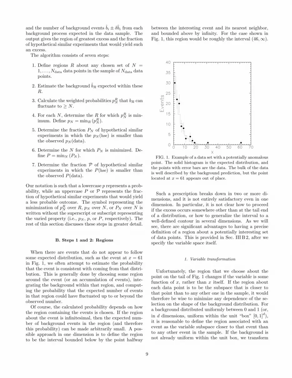
When there are events that do not appear to followsome expected distribution, such as the event at x = 61in Fig. 1, we often attempt to estimate the probabilitythat the event is consistent with coming from that distri-bution. This is generally done by choosing some regionaround the event (or an accumulation of events), inte-grating the background within that region, and comput-ing the probability that the expected number of eventsin that region could have fluctuated up to or beyond theobserved number.

Of course, the calculated probability depends on howthe region containing the events is chosen. If the regionabout the event is infinitesimal, then the expected num-ber of background events in the region (and thereforethis probability) can be made arbitrarily small. A pos-sible approach in one dimension is to define the regionto be the interval bounded below by the point halfway

between the interesting event and its nearest neighbor,and bounded above by infinity. For the case shown inFig. 1, this region would be roughly the interval (46,∞).

FIG. 1. Example of a data set with a potentially anomalouspoint. The solid histogram is the expected distribution, andthe points with error bars are the data. The bulk of the datais well described by the background prediction, but the pointlocated at x = 61 appears out of place.

Such a prescription breaks down in two or more di-mensions, and it is not entirely satisfactory even in onedimension. In particular, it is not clear how to proceedif the excess occurs somewhere other than at the tail endof a distribution, or how to generalize the interval to awell-defined contour in several dimensions. As we willsee, there are significant advantages to having a precisedefinition of a region about a potentially interesting setof data points. This is provided in Sec. III B 2, after wespecify the variable space itself.

1. Variable transformation

Unfortunately, the region that we choose about thepoint on the tail of Fig. 1 changes if the variable is somefunction of x, rather than x itself. If the region abouteach data point is to be the subspace that is closer tothat point than to any other one in the sample, it wouldtherefore be wise to minimize any dependence of the se-lection on the shape of the background distribution. Fora background distributed uniformly between 0 and 1 (or,

in d dimensions, uniform within the unit “box” [0, 1]d),it is reasonable to define the region associated with anevent as the variable subspace closer to that event thanto any other event in the sample. If the background isnot already uniform within the unit box, we transform

9

the variables so that it becomes uniform. The details ofthis transformation are provided in Appendix B.

With the background distribution trivialized, the restof the analysis can be performed within the unit boxwithout worrying about the background shape. A con-siderable simplification is therefore achieved through thistransformation. The task of determining the expectedbackground within each region, which would have re-quired a Monte Carlo integration of the background dis-tribution over the region, reduces to the problem of de-termining the volume of each region. The problem isnow completely specified by the transformed coordinatesof the data points, the total number of expected back-

ground events b, and its uncertainty δb.

2. Voronoi diagrams

Having defined the variable space by requiring a uni-form background distribution, we can now define moreprecisely what is meant by a region. Figure 2 showsa 2-dimensional variable space V containing seven datapoints in a unit square. For any v ∈ V , we say that vbelongs to the data point Di if | v − Di |<| v − Dj | forall j 6= i; that is, v belongs to Di if v is closer to Di

than to any other data point. In Fig. 2(a), for example,any v lying within the variable subspace defined by thepentagon in the upper right-hand corner belongs to thedata point located at (0.9, 0.8). The set of points in Vthat do not belong to any data point [those points on thelines in Fig. 2(a)] has zero measure and may be ignored.

We define a region around a set of data points in avariable space V to be the set of all points in V that arecloser to one of the data points in that set than to anydata points outside that set. A region around a singledata point is the union of all points in V that belong tothat data point, and is called a 1-region. A region abouta set of N data points is the union of all points in V thatbelong to any one of the data points, and is called an N -region; an example of a 2-region is shown as the shadedarea in Fig. 2(b). Ndata data points thus partition V intoNdata 1-regions. Two data points are said to be neighborsif their 1-regions share a border – the points at (0.75, 0.9)and (0.9, 0.8) in Fig. 2, for example, are neighbors. Adiagram such as Fig. 2(a), showing a set of data pointsand their regions, is known as a Voronoi diagram. Weuse a program called HULL [15] for this computation.

3. Region criteria

The explicit definition of a region that we have justprovided reduces the number of contours we can draw inthe variable space from infinite to a mere 2Ndata −1, sinceany region either contains all of the points belonging tothe ith data event or it contains none of them. In fact,because many of these regions have a shape that makes

FIG. 2. A Voronoi diagram. (a) The seven data points areshown as black dots; the lines partition the space into sevenregions, with one region belonging to each data point. (b) Anexample of a 2-region.

them implausible as “discovery regions” in which newphysics might be concentrated, the number of possibleregions may be reduced further. For example, the re-gion in Fig. 2 containing only the lower-leftmost and theupper-rightmost data points is unlikely to be a discoveryregion, whereas the region shown in Fig. 2(b) contain-ing the two upper-rightmost data points is more likely(depending upon the nature of the variables).

We can now impose whatever criteria we wish uponthe regions that we allow Sleuth to consider. In generalwe will want to impose several criteria, and in this casewe write the net criterion cR = c1

Rc2R . . . as a product

of the individual criteria, where ciR is to be read “the

extent to which the region R satisfies the criterion ci.”The quantities ci

R take on values in the interval [0, 1],where ci

R → 0 if R badly fails ci, and ciR → 1 if R easily

satisfies ci.Consider as an example c = AntiCornerSphere, a sim-

ple criterion that we have elected to impose on the regionsin the eµX sample. Loosely speaking, a region R will sat-isfy this criterion (cR → 1) if all of the data points insidethe region are farther from the origin than all of the datapoints outside the region. This situation is shown, forexample, in Fig. 2(b). For every event i in the data set,denote by ri the distance of the point in the unit box tothe origin, let r′ be r transformed so that the backgroundis uniform in r′ over the interval [0, 1], and let r′i be thevalues ri so transformed. Then define

cR =

0 ,(

12 +

r′inmin−r′out

max

ξ

)

< 0(

12 +

r′inmin−r′out

max

ξ

)

, 0 ≤(

12 +

r′inmin−r′out

max

ξ

)

≤ 1

1 , 1 <(

12 +

r′inmin−r′out

max

ξ

)

(5)

where r′inmin = mini∈R (r′i), r′outmax = maxi6∈R (r′i), and

ξ = 1/(4Ndata) is an average separation distance betweendata points in the variable r′.

Notice that in the limit of vanishing ξ, the criterion c

10

becomes a boolean operator, returning “true” when allof the data points inside the region are farther from theorigin than all of the data points outside the region, and“false” otherwise. In fact, many possible criteria have ascale ξ and reduce to boolean operators when ξ vanishes.This scale has been introduced to ensure continuity ofthe final result under small changes in the backgroundestimate. In this spirit, the “extent to which R satisfiesthe criterion c” has an alternative interpretation as the“fraction of the time R satisfies the criterion c,” where theaverage is taken over an ensemble of slightly perturbedbackground estimates and ξ is taken to vanish, so that“satisfies” makes sense. We will use cR in the next sectionto define an initial measure of the degree to which R isinteresting.

We have considered several other criteria that couldbe imposed upon any potential discovery region to en-sure that the region is “reasonably shaped” and “in abelievable location.” We discuss a few of these criteria inAppendix C.

C. Step 3: Probabilities and uncertainties

Now that we have specified the notion of a region, wecan define a quantitative measure of the “degree of inter-est” of a region.

1. Probabilities

Since we are looking for regions of excess, the appro-priate measure of the degree of interest is a slight modifi-cation of the probability of background fluctuating up toor above the observed number of events. For an N -region

R in which bR background events are expected and bR isprecisely known, this probability is

∞∑

i=N

e−bR(bR)i

i!. (6)

We use this to define the weighted probability

pRN =

(

∞∑

i=N

e−bR(bR)i

i!

)

cR + (1 − cR), (7)

which one can also think of as an “average probability,”where the average is taken over the ensemble of slightlyperturbed background estimates referred to above. Byconstruction, this quantity has all of the properties weneed: it reduces to the probability in Eq. 6 in the limitthat R easily satisfies the region criteria, it saturates atunity in the limit that R badly fails the region criteria,and it exhibits continuous behavior under small pertur-bations in the background estimate between these twoextremes.

2. Systematic uncertainties

The expected number of events from each backgroundprocess has a systematic uncertainty that must be takeninto account. There may also be an uncertainty in theshape of a particular background distribution — for ex-ample, the tail of a distribution may have a larger sys-tematic uncertainty than the mode.

The background distribution comprises one or morecontributing background processes. For each backgroundprocess we know the number of expected events and thesystematic uncertainty on this number, and we have a setof Monte Carlo points that tell us what that backgroundprocess looks like in the variables of interest. A typicalsituation is sketched in Fig. 3.

2 4 6 8 10x

0.2

0.4

0.6

0.8

1b(x)

FIG. 3. An example of a one-dimensional background dis-tribution with three sources. The normalized shapes of the in-dividual background processes are shown as the dashed lines;the solid line is their sum. Typically, the normalizations forthe background processes have separate systematic errors.These errors can change the shape of the total backgroundcurve in addition to its overall normalization. For example, ifthe long-dashed curve has a large systematic error, then thesolid curve will be known less precisely in the region (3, 5)than in the region (0, 3) where the other two backgroundsdominate.

The multivariate transformationdescribed in Sec. III B 1 is obtained assuming that thenumber of events expected from each background pro-cess is known precisely. This fixes each event’s positionin the unit box, its neighbors, and the volume of the sur-

rounding region. The systematic uncertainty δbR on thenumber of background events in a given region is com-puted by combining the systematic uncertainties for eachindividual background process. Eq. 7 then generalizes to

pRN = cR

∫ ∞

0

∞∑

i=N

e−bbi

i!

1√2π(δbR)

×

exp

(

− (b − bR)2

2(δbR)2

)

db

+ (1 − cR), (8)

11

which is seen to reduce to Eq. 7 in the limit δbR → 0.This formulation provides a way to take account of sys-

tematic uncertainties on the shapes of distributions, aswell. For example, if there is a larger systematic uncer-tainty on the tail of a distribution, then the backgroundprocess can be broken into two components, one describ-ing the bulk of the distribution and one describing thetail, and a larger systematic uncertainty assigned to thepiece that describes the tail. Correlations among the var-ious components may also be assigned.

We vary the number of events generated in the hypo-thetical similar experiments according to the systematicand statistical uncertainties. The systematic errors areaccounted for by pulling a vector of the “true” number

of expected background events ~b from the distribution

p(~b) =1

√

2π |Σ |exp

(

−1

2(bi − bi)Σ

−1ij (bj − bj)

)

, (9)

where bi is the number of expected background eventsfrom process i, as before, and bi is the ith component of~b. We have introduced a covariance matrix Σ, which is

diagonal with components Σii = (δbi)2 in the limit that

the systematic uncertainties on the different backgroundprocesses are uncorrelated, and we assume summation onrepeated indices in Eq. 9. The statistical uncertainties inturn are allowed for by choosing the number of events Ni

from each background process i from the Poisson distri-bution

P (Ni) =e−bibNi

i

Ni!, (10)

where bi is the ith component of the vector ~b just deter-mined.

D. Step 4: Exploration of regions

Knowing how to calculate pRN for a specific N -region

R allows us to determine which of two N -regions is moreinteresting. Specifically, an N -region R1 is more interest-ing than another N -region R2 if pR1

N < pR2

N . This allowsus to compare regions of the same size (the same N),although, as we will see, it does not allow us to compareregions of different size.

Step 4 of the algorithm involves finding the most in-teresting N -region for each fixed N between 1 and Ndata.This most interesting N -region is the one that minimizespR

N , and these pN = minR(pRN ) are needed for the next

step in the algorithm.Even for modestly sized problems (say, two dimen-

sions with on the order of 100 data points), there arefar too many regions to consider an exhaustive search.We therefore use a heuristic to find the most interestingregion. We imagine the region under consideration to bean amoeba moving within the unit box. At each step in

the search the amoeba either expands or contracts ac-cording to certain rules, and along the way we keep trackof the most interesting N -region so far found, for eachN . The detailed rules for this heuristic are provided inAppendix D.

E. Steps 5 and 6: Hypothetical similar experiments,

Part I

At this point in the algorithm the original events havebeen reduced to Ndata values, each between 0 and 1: thepN (N = 1, . . . , Ndata) corresponding to the most inter-esting N -regions satisfying the imposed criteria. To findthe most interesting of these, we need a way of compar-ing regions of different size (different N). An N1-regionRN1 with pdata

N1is more interesting than an N2-region RN2

with pdataN2

if the fraction of hypothetical similar experi-

ments in which phseN1

< pdataN1

is less than the fraction of

hypothetical similar experiments in which phseN2

< pdataN2

.To make this comparison, we generate Nhse1 hypothet-

ical similar experiments. Generating a hypothetical sim-ilar experiment involves pulling a random integer fromEq. 10 for each background process i, sampling this num-ber of events from the multidimensional background den-sity b(~x), and then transforming these events into the unitbox.

For each hse we compute a list of pN , exactly as forthe data set. Each of the Nhse1 hypothetical similar ex-periments consequently yields a list of pN . For each N ,we now compare the pN we obtained in the data (pdata

N )

with the pN ’s we obtained in the hse’s (phse1iN , where

i = 1, . . . , Nhse1). From these values we calculate PN ,

the fraction of hse’s with phse1

N < pdataN :

PN =1

Nhse1

Nhse1∑

i=1

Θ(

pdataN − p

hse1iN

)

, (11)

where Θ(x) = 0 for x < 0, and Θ(x) = 1 for x ≥ 0.The most interesting region in the sample is then the

region for which PN is smallest. We define P = PNmin ,where PNmin is the smallest of the PN .

F. Step 7: Hypothetical similar experiments, Part II

A question that remains to be answered is what frac-tion P of hypothetical similar experiments would yielda P less than the P obtained in the data. We calculateP by running a second set of Nhse2 hypothetical similarexperiments, generated as described in the previous sec-tion. (We have written hse1 above to refer to the first setof hypothetical similar experiments, used to determinethe PN , given a list of pN ; we write hse2 to refer to thissecond set of hypothetical similar experiments, used todetermine P from P .) A second, independent set of hse’s

12

is required to calculate an unbiased value for P. Thequantity P is then given by

P =1

Nhse2

Nhse2∑

i=1

Θ(

P data − P hse2i

)

. (12)

This is the final measure of the degree of interest of themost interesting region. Note that P is a number be-tween 0 and 1, that small values of P indicate a samplecontaining an interesting region, that large values of Pindicate a sample containing no interesting region, andthat P can be described as the fraction of hypotheticalsimilar experiments that yield a more interesting resultthan is observed in the data. P can be translated intounits of standard deviations (P [σ]) by solving the unitconversion equation

P =1√2π

∫ ∞

P [σ]

e−t2/2 dt (13)

for P [σ].

G. Interpretation of results

In a general search for new phenomena, Sleuth willbe applied to Nfs different final states, resulting in Nfs

different values for P. The final step in the procedure isthe combination of these results. If no P value is smallerthan ≈ 0.01 then a null result has been obtained, as nosignificant signal for new physics has been identified inthe data.

If one or more of the P values is particularly low, thenwe can surmise that the region(s) of excess correspondseither to a poorly modeled background or to possibleevidence of new physics. The algorithm has pointed outa region of excess (R) and has quantified its significance(P). The next step is to interpret this result.

Two issues related to this interpretation are combiningresults from many final states, and confirming a Sleuthdiscovery.

1. Combining the results of many final states

If one looks at many final states, one expects even-tually to see a fairly small P , even if there really is nonew physics in the data. We therefore define a quantityP to be the fraction of hypothetical similar experimentalruns1 that yield a P that is smaller than the smallest P

1In the phrase “hypothetical similar experiment,” “experi-ment” refers to the analysis of a single final state. We use“experimental runs” in a similar way to refer to the analy-sis of a number of different final states. Thus a hypotheticalsimilar experimental run consists of Nfs different hypotheticalsimilar experiments, one for each final state analyzed.

observed in the data. Explicitly, given Nfs final states,

with bi background events expected in each, and P i cal-culated for each one, P is given to good approximationby2

P = 1 −Nfs∏

i=1

ni−1∑

j=0

e−bi bji

j!, (14)

where ni is the smallest integer satisfying

∞∑

j=ni

e−bi bji

j!≤ Pmin = min

iP i. (15)

2. Confirmation

An independent confirmation is desirable for any po-tential discovery, especially for an excess revealed by adata-driven search. Such confirmation may come froman independent experiment, from the same experimentin a different but related final state, from an indepen-dent confirmation of the background estimate, or fromthe same experiment in the same final state using inde-pendent data. In the last of these cases, a first samplecan be presented to Sleuth to uncover any hints of newphysics, and the remaining sample can be subjected to astandard analysis in the region suggested by Sleuth. Anexcess in this region in the second sample helps to con-firm a discrepancy between data and background. If wesee hints of new physics in the Run I data, for example,we will be able to predict where new physics might showitself in the upcoming run of the Fermilab Tevatron, RunII.

IV. THE eµX DATA SET

As mentioned in Sec. I, we have applied the Sleuthmethod to DØ data containing one or more electronsand one or more muons. We use a data set correspond-ing to 108.3±5.7 pb−1 of integrated luminosity, collectedbetween 1992 and 1996 at the Fermilab Tevatron with theDØ detector. The data set and basic selection criteria areidentical to those used in the published tt cross sectionanalysis for the dilepton channels [12]. Specifically, weapply global cleanup cuts and select events containing

2Note that the naive expression P = 1 − (1 − Pmin)Nfs isnot correct, since this requires P → 1 for Nfs → ∞, andthere are indeed an infinite number of final states to examine.The resolution of this paradox hinges on the fact that onlyan integral number of events can be observed in each finalstate, and therefore final states with bi ≪ 1 contribute verylittle to the value of P . This is correctly accounted for in theformulation given in Eq. 14.

13

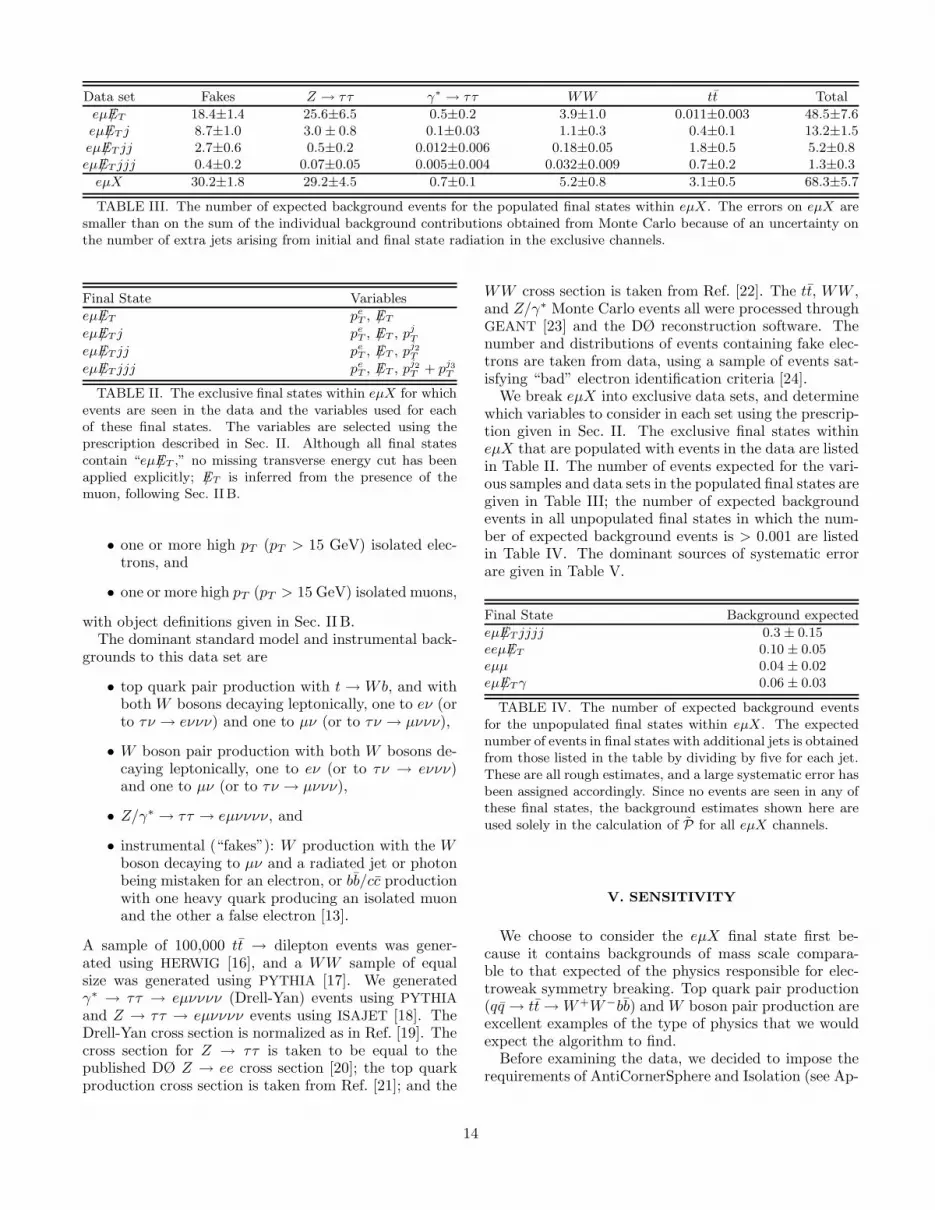
Data set Fakes Z → ττ γ∗ → ττ WW tt Total

eµ/ET 18.4±1.4 25.6±6.5 0.5±0.2 3.9±1.0 0.011±0.003 48.5±7.6eµ/ET j 8.7±1.0 3.0 ± 0.8 0.1±0.03 1.1±0.3 0.4±0.1 13.2±1.5eµ /ET jj 2.7±0.6 0.5±0.2 0.012±0.006 0.18±0.05 1.8±0.5 5.2±0.8eµ /ET jjj 0.4±0.2 0.07±0.05 0.005±0.004 0.032±0.009 0.7±0.2 1.3±0.3

eµX 30.2±1.8 29.2±4.5 0.7±0.1 5.2±0.8 3.1±0.5 68.3±5.7

TABLE III. The number of expected background events for the populated final states within eµX. The errors on eµX aresmaller than on the sum of the individual background contributions obtained from Monte Carlo because of an uncertainty onthe number of extra jets arising from initial and final state radiation in the exclusive channels.

Final State Variables

eµ /ET peT , /ET

eµ /ET j peT , /ET , pj

T

eµ /ET jj peT , /ET , pj2

T

eµ /ET jjj peT , /ET , pj2

T + pj3T

TABLE II. The exclusive final states within eµX for whichevents are seen in the data and the variables used for eachof these final states. The variables are selected using theprescription described in Sec. II. Although all final statescontain “eµ /ET ,” no missing transverse energy cut has beenapplied explicitly; /ET is inferred from the presence of themuon, following Sec. IIB.

• one or more high pT (pT > 15 GeV) isolated elec-trons, and

• one or more high pT (pT > 15 GeV) isolated muons,

with object definitions given in Sec. II B.The dominant standard model and instrumental back-

grounds to this data set are

• top quark pair production with t → Wb, and withboth W bosons decaying leptonically, one to eν (orto τν → eννν) and one to µν (or to τν → µννν),

• W boson pair production with both W bosons de-caying leptonically, one to eν (or to τν → eννν)and one to µν (or to τν → µννν),

• Z/γ∗ → ττ → eµνννν, and

• instrumental (“fakes”): W production with the Wboson decaying to µν and a radiated jet or photonbeing mistaken for an electron, or bb/cc productionwith one heavy quark producing an isolated muonand the other a false electron [13].

A sample of 100,000 tt → dilepton events was gener-ated using HERWIG [16], and a WW sample of equalsize was generated using PYTHIA [17]. We generatedγ∗ → ττ → eµνννν (Drell-Yan) events using PYTHIA

and Z → ττ → eµνννν events using ISAJET [18]. TheDrell-Yan cross section is normalized as in Ref. [19]. Thecross section for Z → ττ is taken to be equal to thepublished DØ Z → ee cross section [20]; the top quarkproduction cross section is taken from Ref. [21]; and the

WW cross section is taken from Ref. [22]. The tt, WW ,and Z/γ∗ Monte Carlo events all were processed throughGEANT [23] and the DØ reconstruction software. Thenumber and distributions of events containing fake elec-trons are taken from data, using a sample of events sat-isfying “bad” electron identification criteria [24].

We break eµX into exclusive data sets, and determinewhich variables to consider in each set using the prescrip-tion given in Sec. II. The exclusive final states withineµX that are populated with events in the data are listedin Table II. The number of events expected for the vari-ous samples and data sets in the populated final states aregiven in Table III; the number of expected backgroundevents in all unpopulated final states in which the num-ber of expected background events is > 0.001 are listedin Table IV. The dominant sources of systematic errorare given in Table V.

Final State Background expected

eµ /ET jjjj 0.3 ± 0.15eeµ/ET 0.10 ± 0.05eµµ 0.04 ± 0.02eµ /ET γ 0.06 ± 0.03

TABLE IV. The number of expected background eventsfor the unpopulated final states within eµX. The expectednumber of events in final states with additional jets is obtainedfrom those listed in the table by dividing by five for each jet.These are all rough estimates, and a large systematic error hasbeen assigned accordingly. Since no events are seen in any ofthese final states, the background estimates shown here areused solely in the calculation of P for all eµX channels.

V. SENSITIVITY

We choose to consider the eµX final state first be-cause it contains backgrounds of mass scale compara-ble to that expected of the physics responsible for elec-troweak symmetry breaking. Top quark pair production(qq → tt → W+W−bb) and W boson pair production areexcellent examples of the type of physics that we wouldexpect the algorithm to find.

Before examining the data, we decided to impose therequirements of AntiCornerSphere and Isolation (see Ap-

14

Source Error

Trigger and lepton identification efficiencies 12%P (j →“e”) 7%Multiple Interactions 7%Luminosity 5.3%σ(tt→ eµX) 12%σ(Z → ττ → eµX) 10%σ(WW → eµX) 10%σ(γ∗ → ττ → eµX) 17%Jet modeling 20%

TABLE V. Sources of systematic uncertainty on the num-ber of expected background events in the final states eµ /ET ,eµ /ET j, eµ /ET jj, and eµ /ET jjj. P (j →“e”) denotes the prob-ability that a jet will be reconstructed as an electron. “Jetmodeling” includes systematic uncertainties in jet productionin PYTHIA and HERWIG in addition to jet identificationand energy scale uncertainties.

pendix C) on the regions that Sleuth is allowed to con-sider. The reason for this choice is that, in addition toallowing only “reasonable” regions, it allows the searchto be parameterized essentially by a single variable —the distance between each region and the lower left-handcorner of the unit box. We felt this would aid the in-terpretation of the results from this initial application ofthe method.

We test the sensitivity in two phases, keeping in mindthat nothing in the algorithm has been “tuned” to find-ing WW and tt in this sample. We first consider thebackground to comprise fakes and Z/γ∗ → ττ only, tosee if we can “discover” either WW or tt. We then con-sider the background to comprise fakes, Z/γ∗ → ττ , andWW , to see whether we can “discover” tt. We apply thefull search strategy and algorithm in both cases, first (inthis section) on an ensemble of mock samples, and then(in Sec. VI) on the data.

A. Search for WW and tt in mock samples

In this section we provide results from Sleuth for thecase in which Z/γ∗ → ττ and fakes are included in thebackground estimates and the signal from WW and tt is“unknown.” We apply the prescription to the exclusiveeµX final states listed in Table II.

Figure 4 shows distributions of P for mock samplescontaining only Z/γ∗ → ττ and fakes, where the mockevents are pulled randomly from their parent distribu-tions and the numbers of events are allowed to varywithin systematic and statistical errors. The distribu-tions are uniform in the interval [0, 1], as expected, be-coming appropriately discretized in the low statisticslimit. (When the number of expected background events

b <∼ 1, as in Fig. 4(d), it can happen that zero or oneevents are observed. If zero events are observed thenP = 1, since all hypothetical similar experiments yield a

result as interesting or more interesting than an emptysample. If one event is observed then there is only oneregion for Sleuth to consider, and P is simply the prob-

ability for b± δb to fluctuate up to exactly one event. InFig. 4(d), for example, the spike at P = 1 contains 62%of the mock experiments, since this is the probability for0.5 ± 0.2 to fluctuate to zero events; the second spikeis located at P = 0.38 and contains 28% of the mockexperiments, since this is the probability for 0.5 ± 0.2to fluctuate to exactly one event. Similar but less pro-nounced behavior is seen in Fig. 4(c).) Figure 5 showsdistributions of P when the mock samples contain WWand tt in addition to the background in Fig. 4. Again,the number of events from each process is allowed to varywithin statistical and systematic error. Figure 5 showsthat we can indeed find tt and/or WW much of the time.

Figure 6 shows P computed for these samples. In over50% of these samples we find P [σ] to correspond to morethan two standard deviations.

℘ ℘

℘ ℘FIG. 4. Distributions of P for the four exclusive final states

(a) eµ /ET , (b) eµ /ET j, (c) eµ /ET jj, and (d) eµ /ET jjj. Thebackground includes only Z/γ∗ → ττ and fakes, and the mocksamples making up these distributions also contain only thesetwo sources. As expected, P is uniform in the interval [0, 1] forthose final states in which the expected number of backgroundevents b ≫ 1, and shows discrete behavior for b <∼ 1.

B. Search for tt in mock samples

In this section we provide results for the case in whichZ/γ∗ → ττ , fakes, and WW are all included in the back-

15

℘ ℘

℘ ℘FIG. 5. Distributions of P for the four exclusive final states

(a) eµ /ET , (b) eµ /ET j, (c) eµ /ET jj, and (d) eµ /ET jjj. Thebackground includes only Z/γ∗ → ττ and fakes. The mocksamples for these distributions contain WW and tt in addi-tion to Z/γ∗ → ττ and fakes. The extent to which thesedistributions peak at small P can be taken as a measure ofSleuth’s ability to find WW or tt if we had no knowledge ofeither final state. The presence of WW in eµ/ET causes thetrend toward small values in (a); the presence of tt causes thetrend toward small values in (c) and (d); and a combinationof WW and tt causes the signal seen in (b).

ground estimate, and tt is the “unknown” signal. Weagain apply the prescription to the exclusive final stateslisted in Table II.

Figure 7 shows distributions of P for mock samplescontaining Z/γ∗ → ττ , fakes, and WW , where the mockevents are pulled randomly from their parent distribu-tions, and the numbers of events are allowed to varywithin systematic and statistical errors. As found inthe previous section, the distributions are uniform in theinterval [0, 1], becoming appropriately discretized whenthe expected number of background events becomes <∼ 1.Figure 8 shows distributions of P when the mock sam-ples contain tt in addition to Z/γ∗ → ττ , fakes, andWW . Again, the number of events from each process isallowed to vary within statistical and systematic errors.The distributions in Figs. 8(c) and (d) show that we canindeed find tt much of the time. Figure 9 shows that thedistribution of P [σ] is approximately a Gaussian centeredat zero of width unity for the case where the backgroundand data both contain Z/γ∗ → ττ , fakes, and WW pro-duction, and is peaked in the bin above 2.0 for the samebackground when the data include tt.

℘[σ]∼

FIG. 6. Distribution of P [σ] from combining the four exclu-sive final states eµ /ET , eµ/ET j, eµ/ET jj, and eµ/ET jjj. Thebackground includes only Z/γ∗ → ττ and fakes. The mocksamples making up the distribution shown as the solid linecontain WW and tt in addition to Z/γ∗ → ττ and fakes, andcorrespond to Fig. 5; the mock samples making up the distri-bution shown as the dashed line contain only Z/γ∗ → ττ andfakes, and correspond to Fig. 4. All samples with P [σ] > 2.0

appear in the rightmost bin. The fact that P [σ] > 2.0 in 50%of the mock samples can be taken as a measure of Sleuth’ssensitivity to finding WW and tt if we had no knowledge ofthe existence of the top quark or the possibility of W bosonpair production.

C. New high pT physics

We have shown in Secs. VA and VB that the Sleuthprescription and algorithm correctly finds nothing whenthere is nothing to be found, while exhibiting sensitivityto the expected presence of WW and tt in the eµX sam-ple. Sleuth’s performance on this “typical” new physicssignal is encouraging, and may be taken as some measureof the sensitivity of this method to the great variety ofnew high pT physics that it has been designed to find.Making a more general claim regarding Sleuth’s sensi-tivity to the presence of new physics is difficult, sincethe sensitivity obviously varies with the characteristicsof each candidate theory.

That being said, we can provide a rough estimate ofSleuth’s sensitivity to new high pT physics with the fol-lowing argument. We have seen that we are sensitiveto WW and tt pair production in a data sample cor-responding to an integrated luminosity of ≈ 100 pb−1.

16

℘ ℘

℘ ℘FIG. 7. Distributions of P for the four exclusive final states

(a) eµ /ET , (b) eµ /ET j, (c) eµ /ET jj, and (d) eµ /ET jjj. Thebackground includes Z/γ∗ → ττ , fakes, and WW , and themock samples making up these distributions also containthese three sources. As expected, P is uniform in the interval[0, 1] for those final states in which the expected number ofbackground events b ≫ 1, and shows discrete behavior whenb <∼ 1.

These events tend to fall in the region peT > 40 GeV,

/ET > 40 GeV, and∑′

pjT > 40 GeV (if there are any

jets at all). The probability that any true eµX event pro-duced will make it into the final sample is about 15% dueto the absence of complete hermeticity of the DØ detec-tor, inefficiencies in the detection of electrons and muons,and kinematic acceptance. We can therefore state thatwe are as sensitive to new high pT physics as we were tothe roughly eight WW and tt events in our mock samplesif the new physics is distributed relative to all standardmodel backgrounds as WW and tt are distributed rela-tive to backgrounds from Z/γ∗ → ττ and fakes alone,and if its production cross section × branching ratio intothis final state is >∼ 8/(0.15× 100 pb−1) ≈ 600 fb. Read-ers who are interested in a possible signal with a differentrelative distribution, or who prefer a more rigorous def-inition of “sensitivity,” should adjust this cross sectionaccordingly.

VI. RESULTS

In the previous section we studied what can be ex-pected when Sleuth is applied to eµX mock samples. In

℘ ℘

℘ ℘FIG. 8. Distributions of P for the four exclusive final states

(a) eµ /ET , (b) eµ /ET j, (c) eµ /ET jj, and (d) eµ /ET jjj. Thebackground includes Z/γ∗ → ττ , fakes, and WW . Themock samples for these distributions contain tt in additionto Z/γ∗ → ττ , fakes, and WW . The extent to which thesedistributions peak at small P can be taken as a measure ofSleuth’s sensitivity to finding tt if we had no knowledge of thetop quark’s existence or characteristics. Note that P is flatin eµ /ET , where the expected number of top quark events isnegligible, peaks slightly toward small values in eµ/ET j, andshows a marked low peak in eµ /ET jj and eµ/ET jjj.

this section we confront Sleuth with data. We observe39 events in the eµ /ET final state, 13 events in eµ /ET j,5 events in eµ /ET jj, and a single event in eµ /ET jjj, ingood agreement with the expected background in Ta-ble III. We proceed by first removing both WW and ttfrom the background estimates, and next by removingonly tt, to search for evidence of these processes in thedata. Finally, we include all standard model processes inthe background estimates and search for evidence of newphysics.

A. Search for WW and tt in data

The results of applying Sleuth to DØ data with onlyZ/γ∗ → ττ and fakes in the background estimate areshown in Table VI and Fig. 10. Sleuth finds indicationsof an excess in the eµ /ET and eµ /ET jj states, presum-ably reflecting the presence of WW and tt, respectively.The results for the eµ /ET j and eµ /ET jjj final states areconsistent with the results in Fig. 5. Defining r′ as thedistance of the data point from (0, 0, 0) in the unit box

17

℘[σ]∼

FIG. 9. Distribution of P [σ] from combining the four exclu-sive final states eµ /ET , eµ /ET j, eµ /ET jj, and eµ /ET jjj. Thebackground includes Z/γ∗ → ττ , fakes, and WW . The mocksamples making up the distribution shown as the solid linecontain tt in addition to Z/γ∗ → ττ , fakes, and WW , corre-sponding to Fig. 8; the mock samples making up the distri-bution shown as the dashed line contain only Z/γ∗ → ττ ,fakes, and WW , and correspond to Fig. 7. All sampleswith P [σ] > 2.0 appear in the rightmost bin. The fact that

P [σ] > 2.0 in over 25% of the mock samples can be taken asa measure of Sleuth’s sensitivity to finding tt if we had noknowledge of the top quark’s existence or characteristics.

(transformed so that the background is distributed uni-formly in the interval [0, 1]), the top candidate eventsfrom DØ’s recent analysis [25] are the three events withlargest r′ in the eµ /ET jj sample and the single event inthe eµ /ET jjj sample, shown in Fig. 10. The presence ofthe WW signal can be inferred from the events desig-nated interesting in the eµ /ET final state.

B. Search for tt in data

The results of applying Sleuth to the data with Z/γ∗ →ττ , fakes, and WW included in the background estimateare shown in Table VII and Fig. 11. Sleuth finds anindication of excess in the eµ /ET jj events, presumablyindicating the presence of tt. The results for the eµ /ET ,eµ /ET j, and eµ /ET jjj final states are consistent with theresults in Fig. 8. The tt candidates from DØ’s recentanalysis [25] are the three events with largest r′ in theeµ /ET jj sample, and the single event in the eµ /ET jjj sam-

Data set Peµ /ET 0.008eµ /ET j 0.34eµ/ET jj 0.01eµ /ET jjj 0.38

P 0.03

TABLE VI. Summary of results on the eµ /ET , eµ /ET j,eµ /ET jj, and eµ /ET jjj channels when WW and tt are not in-cluded in the background. Sleuth identifies a region of excessin the eµ /ET and eµ /ET jj final states, presumably indicatingthe presence of WW and tt in the data. In units of standarddeviation, P [σ] = 1.9.

℘ = 0.008

℘ = 0.34

℘ = 0.010 ℘ = 0.38

FIG. 10. Positions of data points following the transforma-tion of the background from fake and Z/γ∗ sources in thespace of variables in Table I to a uniform distribution in theunit box. The darkened points define the region Sleuth foundmost interesting. The axes of the unit box in (a) are sugges-tively labeled (pe

T ) and ( /ET ); each is a function of both peT

and /ET , but (peT ) depends more strongly on pe

T , while ( /ET )more closely tracks /ET . r′ is the distance of the data pointfrom (0, 0, 0) (the “lower left-hand corner” of the unit box),transformed so that the background is distributed uniformlyin the interval [0, 1]. The interesting regions in the eµ /ET andeµ /ET jj samples presumably indicate the presence of WWsignal in eµ /ET and of tt signal in eµ /ET jj. We find P = 0.03(P [σ] = 1.9).

ple, shown in Fig. 11.A comparison of this result with one obtained using

a dedicated top quark search illustrates an importantdifference between Sleuth’s result and the result from adedicated search. DØ announced its discovery of the top

18

Data set Peµ/ET 0.16eµ/ET j 0.45eµ /ET jj 0.03eµ /ET jjj 0.41

P 0.11

TABLE VII. Summary of results on the eµ /ET , eµ /ET j,eµ /ET jj, and eµ /ET jjj channels when tt production is not in-cluded in the background. Sleuth identifies a region of excessin the eµ /ET jj final state, presumably indicating the presenceof tt in the data. In units of standard deviation, P [σ] = 1.2.

℘ = 0.16

℘ = 0.45

℘ = 0.030 ℘ = 0.41

FIG. 11. Positions of data points following the transforma-tion of the background from the three sources Z/γ∗ → ττ ,fakes, and WW in the space of variables in Table I to a uni-form distribution in the unit box. The darkened points definethe region Sleuth found most interesting. The interesting re-gion in the eµ/ET jj sample presumably indicates the presenceof tt. We find P = 0.11 (P [σ] = 1.2).

quark [26] in 1995 with 50 pb−1 of integrated luminosityupon observing 17 events with an expected backgroundof 3.8±0.6 events, a 4.6σ “effect,” in the combined dilep-ton and single-lepton decay channels. In the eµ channelalone, two events were seen with an expected backgroundof 0.12 ± 0.03 events. The probability of 0.12 ± 0.03events fluctuating up to or above two events is 0.007,corresponding to a 2.5σ “effect.” In a subsequent mea-surement of the top quark cross section [12], three can-didate events were seen with an expected backgroundof 0.21 ± 0.16, an excess corresponding to a 2.75σ “ef-fect.” Using Sleuth, we find P = 0.03 in the eµ /ET jj

sample, a 1.9σ “effect,” when complete ignorance of thetop quark is feigned. When we take into account the factthat we have also searched in all of the final states listedin Table III, we find P = 0.11, a 1.2σ “effect.” The dif-ference between the 2.75σ “effect” seen with a dedicatedtop quark search and the 1.2σ “effect” that Sleuth re-ports in eµX lies partially in the fact that Sleuth is notoptimized for tt; and partially in the careful accountingof the many new physics signatures that Sleuth consid-ered in addition to tt production, and the correspond-ingly many new physics signals that Sleuth might havediscovered.

C. Search for physics beyond the standard model

In this section we present Sleuth’s results for the case inwhich all standard model and instrumental backgroundsare considered in the background estimate: Z/γ∗ → ττ ,fakes, WW , and tt. The results are shown in Table VIIIand Fig. 12. We observe excellent agreement with thestandard model. We conclude that these data contain noevidence of new physics at high pT , and calculate thata fraction P = 0.72 of hypothetical similar experimen-tal runs would produce a more significant excess thanany observed in these data. Recall that we are sensi-tive to new high pT physics with production cross sec-tion × branching ratio into this final state as describedin Sec. VC.

Data set Peµ /ET 0.14eµ /ET j 0.45eµ/ET jj 0.31eµ /ET jjj 0.71

P 0.72

TABLE VIII. Summary of results on all final states withineµX when all standard model backgrounds are included. Theunpopulated final states (listed in Table IV) have P = 1.0;these final states are included in the calculation of P . Weobserve no evidence for the presence of new high pT physics.

VII. CONCLUSIONS

We have developed a quasi-model-independent tech-nique for searching for the physics responsible for stabi-lizing electroweak symmetry breaking. Our prescriptioninvolves the definition of final states and the constructionof a rule that identifies a set of relevant variables for anyparticular final state. An algorithm (Sleuth) systemati-cally searches for regions of excess in those variables, andquantifies the significance of any observed excess. Thistechnique is sufficiently a priori that it allows an ex postfacto, quantitative measure of the degree to which curious

19

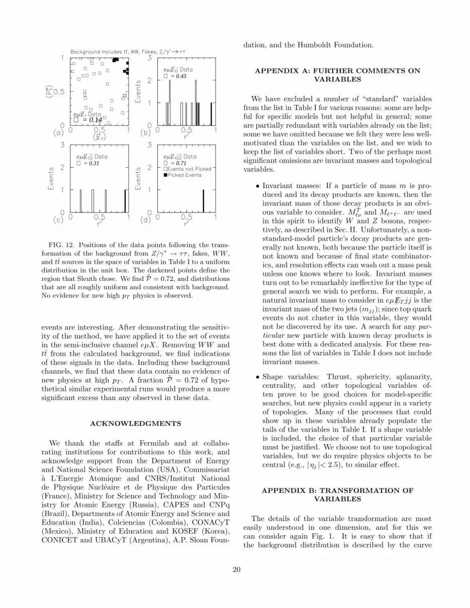
℘ = 0.14

℘ = 0.45

℘ = 0.31 ℘ = 0.71

FIG. 12. Positions of the data points following the trans-formation of the background from Z/γ∗ → ττ , fakes, WW ,and tt sources in the space of variables in Table I to a uniformdistribution in the unit box. The darkened points define theregion that Sleuth chose. We find P = 0.72, and distributionsthat are all roughly uniform and consistent with background.No evidence for new high pT physics is observed.

events are interesting. After demonstrating the sensitiv-ity of the method, we have applied it to the set of eventsin the semi-inclusive channel eµX . Removing WW andtt from the calculated background, we find indicationsof these signals in the data. Including these backgroundchannels, we find that these data contain no evidence ofnew physics at high pT . A fraction P = 0.72 of hypo-thetical similar experimental runs would produce a moresignificant excess than any observed in these data.

ACKNOWLEDGMENTS

We thank the staffs at Fermilab and at collabo-rating institutions for contributions to this work, andacknowledge support from the Department of Energyand National Science Foundation (USA), Commissariata L’Energie Atomique and CNRS/Institut Nationalde Physique Nucleaire et de Physique des Particules(France), Ministry for Science and Technology and Min-istry for Atomic Energy (Russia), CAPES and CNPq(Brazil), Departments of Atomic Energy and Science andEducation (India), Colciencias (Colombia), CONACyT(Mexico), Ministry of Education and KOSEF (Korea),CONICET and UBACyT (Argentina), A.P. Sloan Foun-

dation, and the Humboldt Foundation.

APPENDIX A: FURTHER COMMENTS ON

VARIABLES

We have excluded a number of “standard” variablesfrom the list in Table I for various reasons: some are help-ful for specific models but not helpful in general; someare partially redundant with variables already on the list;some we have omitted because we felt they were less well-motivated than the variables on the list, and we wish tokeep the list of variables short. Two of the perhaps mostsignificant omissions are invariant masses and topologicalvariables.

• Invariant masses: If a particle of mass m is pro-duced and its decay products are known, then theinvariant mass of those decay products is an obvi-ous variable to consider. MT

ℓν and Mℓ+ℓ− are usedin this spirit to identify W and Z bosons, respec-tively, as described in Sec. II. Unfortunately, a non-standard-model particle’s decay products are gen-erally not known, both because the particle itself isnot known and because of final state combinator-ics, and resolution effects can wash out a mass peakunless one knows where to look. Invariant massesturn out to be remarkably ineffective for the type ofgeneral search we wish to perform. For example, anatural invariant mass to consider in eµ /ET jj is theinvariant mass of the two jets (mjj); since top quarkevents do not cluster in this variable, they wouldnot be discovered by its use. A search for any par-

ticular new particle with known decay products isbest done with a dedicated analysis. For these rea-sons the list of variables in Table I does not includeinvariant masses.

• Shape variables: Thrust, sphericity, aplanarity,centrality, and other topological variables of-ten prove to be good choices for model-specificsearches, but new physics could appear in a varietyof topologies. Many of the processes that couldshow up in these variables already populate thetails of the variables in Table I. If a shape variableis included, the choice of that particular variablemust be justified. We choose not to use topologicalvariables, but we do require physics objects to becentral (e.g., |ηj |< 2.5), to similar effect.

APPENDIX B: TRANSFORMATION OF

VARIABLES

The details of the variable transformation are mosteasily understood in one dimension, and for this wecan consider again Fig. 1. It is easy to show that ifthe background distribution is described by the curve

20

b(x) = 15e−x/5 and we let y = 1 − e−x/5, then y is dis-

tributed uniformly between 0 and 1. The situation ismore complicated when the background is given to us asa set of Monte Carlo points that cannot be described bya simple parameterization, and it is further complicatedwhen these points live in several dimensions.

There is a unique solution to this problem in one di-mension, but an infinity of solutions in two or more di-mensions. Not all of these solutions are equally reason-able, however — there are two additional properties thatthe solution should have.

• Axes should map to axes. If the data live in a three-dimensional space in the octant with all coordinatespositive, for example, then it is natural to map thecoordinate axes to the axes of the box.

• Points that are near each other should map topoints that are near each other, subject to the con-straint that the resulting background probabilitydistribution be flat within the unit box.

This somewhat abstract and not entirely well-posedproblem is helped by considering an analogous physicalproblem:

The height of the sand in a d-dimensional unitsandbox is given by the function b(~x), where~x is a d-component vector. (The counting ofdimensions is such that a physical sandboxhas d = 2.) We take the d-dimensional lidof the sandbox and squash the sand flat. Theresult of this squashing is that a sand grain atposition ~x has moved to a new position ~y, andthe new function b′(~y) describing the heightof the sand is a constant. Given the functionb(~x), determine the mapping ~x → ~y.

For this analogy to help, the background first needsto be put “in the sandbox.” Each of the backgroundevents must also have the same weight (the reason for thiswill become clear shortly). The background probabilitydensity is therefore estimated in the original variablesusing Probability Density Estimation [27], and M eventsare sampled from this distribution.

These M events are then put “into the sandbox” bytransforming each variable (individually) into the interval[0, 1]. The new variable is given by

xj → x′j =

1

M

∫ xj

−∞

M∑

i=1

1√2πσjh

exp

(

−(t − µij)

2

2σ2j h2

)

dt,

(B1)

where µij is the value of the jth variable for the ith back-ground event, σj is the standard deviation of the distri-

bution in the jth variable, and h = M− 1d+4 , where d is

the dimensionality of the space.

The next step is to take these M events and map eachof them to a point on a uniform grid within the box.The previous paragraph defines a mapping from the orig-inal variables into the unit sandbox; this step defines amapping from a lumpy distribution in the sandbox to aflat distribution. The mapping is continued to the entirespace by interpolating between the sampled backgroundevents.

The mapping to the grid is done by first assigning eachsampled background point to an arbitrary grid point.Each background point i is some distance dij away fromthe grid point j with which it is paired. We then loopover pairs of background points i and i′, which are associ-ated with grid points j and j′, and swap the associations(associate i with j′ and i′ with j) if max(dij , di′j′) >max(di′j , dij′ ). This looping and swapping is continueduntil an equilibrium state is reached.

APPENDIX C: REGION CRITERIA

In Sec. III B 3 we introduced the formal notion of regioncriteria — properties that we require a region to have forit to be considered by Sleuth. The two criteria that wehave decided to impose in the analysis of the eµX dataare Isolation and AntiCornerSphere.

a. Isolation We want the region to include events

that are very close to it. We define ξ = 14N

− 1d

data as ameasure of the mean distance between data points intheir transformed coordinates, and call a region isolated

if there exist no data points outside the region that arecloser than ξ to a data point inside the region. We gener-alize this boolean criterion to the interval [0, 1] by defin-ing

cIsolationR = min

(

1,min |(~x)in − (~x)out |

2ξ

)

, (C1)

where the minimum is taken over all pairwise combina-tions of data points with (~x)in inside R and (~x)out outsideR.

b. AntiCornerSphere One must be able to draw asphere centered on the origin of the unit box containingall data events outside the region and no data eventsinside the region. This is useful if the signal is expectedto lie in the upper right-hand corner of the unit box. Wegeneralize this boolean criterion to the interval [0, 1] asdescribed in Sec. III B 3.

A number of other potentially useful region criteria maybe imagined. Among those that we have consideredare Connectivity, Convexity, Peg, and Hyperplanes. Al-though we present only the boolean forms of these crite-ria here, they may be generalized to the interval [0, 1] byintroducing the scale ξ in the same spirit as above.

c. Connectivity We generally expect a discovery re-gion to be one connected subspace in the variables we use,rather than several disconnected subspaces. Although

21

one can posit cases in which the signal region is not con-nected (perhaps signal appears in the two regions η > 2and η < −2), one should be able to easily avoid this withan appropriate choice of variables. (In this example, weshould use | η | rather than η.) We defined the conceptof neighboring data points in the discussion of regions inSec. III B 2. A connected region is defined to be a regionin which given any two points a and b within the region,there exists a list of points p1 = a, p2, . . . , pn−1, pn = bsuch that all the pi are in the region and pi+1 is a neigh-bor of pi.

d. Convexity We define a non-convex region as a re-gion defined by a set of N data points P , such that there

exists a data point ~p not within P satisfying

N∑

i=1

~piλi = ~p (C2)

∑

i

λi = 1 (C3)

λi ≥ 0 ∀ i, (C4)

for suitably chosen λi, where ~pi are the points within P .A convex region is then any region that is not non-convex;intuitively, a convex region is one that is “roundish,”without protrusions or intrusions.

e. Peg We may want to consider only regions thatlive on the high tails of a distribution. More generally,we may want to only consider regions that contain oneor more of n specific points in variable space. Call thisset of points xi, where i = 1, . . . , n. We transform thesepoints exactly as we transformed the data in Sec. III Bto obtain a set of points yi that live in the unit box. Aregion R is said to be pegged to these points if there existsat least one i ∈ 1, . . . , n such that the closest data pointto yi lies within R.

f. Hyperplanes Connectivity and Convexity are cri-teria that require the region to be “reasonably-shaped,”while Peg is designed to ensure that the region is “in a be-lievable location.” It is possible, and may at times be de-sirable, to impose a criterion that judges both shape andlocation simultaneously. A region R in a d-dimensionalunit box is said to satisfy Hyperplanes if, for each datapoint p inside R, one can draw a (d − 1)-dimensionalhyperplane through p such that all data points on theside of the hyperplane containing the point ~1 (the “up-per right-hand corner of the unit box”) are inside R.

More complicated region criteria may be built from com-binations and variations of these and other basic ele-ments.

APPENDIX D: SEARCH HEURISTIC DETAILS

The heuristic Sleuth uses to search for the region ofgreatest excess may usefully be visualized as a set of rules

for an amoeba to move within the unit box. We monitorthe amoeba’s progress by maintaining a list of the mostinteresting region of size N (one for each N) that theamoeba has visited so far. At each state, the amoeba isthe region under consideration, and the rules tell us whatregion to consider next.

The initial location and size of the amoeba is deter-mined by the following rules for seeding:

1. If we have not yet searched this data set at all, thestarting amoeba fills the entire box.

2. Otherwise, the amoeba starts out as the regionaround a single random point that has not yet in-habited a “small” region that we have consideredso far. We consider a region R to be small if addingor removing an individual point can have a sizeableeffect on the pR

N ; in practice, a region is small if N<∼ 20.

3. If there is no point that has not yet inhabited asmall region that we have considered so far, thesearch is complete.

At each stage, the amoeba either grows or shrinks. Itbegins by attempting to grow. The rules for growth are:

1. Allow the amoeba to encompass a neighboring datapoint. Force it to encompass any other data pointsnecessary to make the expanded amoeba satisfy allcriteria. Check to see whether the pR

N of the ex-panded amoeba is less than the pR

N of the regionon the list of the same size. If so, the amoeba hassuccessfully grown, the list of the most interestingregions is updated, and the amoeba tries to growagain. If not, the amoeba shrinks back to its formersize and repeats the same process using a differentneighboring data point.

2. If the amoeba has tried all neighboring data pointsand has not successfully grown, it shrinks.

The rules for shrinking are:

1. Force the amoeba to relinquish the data point thatowns the most background, subject to the require-ment that the resulting shrunken amoeba be con-sistent with the criteria.

2. If the amoeba has shrunk out of existence or canshrink no further, we kill this amoeba and reseed.

The result of this process is a list of regions of lengthNdata (one region for each N), such that the N th regionin the list is the most interesting region of size N foundin the data set.

22

[1] L. Hall, J. Lykken and S. Weinberg, Phys. Rev. D 27,2359 (1983).

[2] J. Gunion, H. E. Haber, G. L. Kane, and S. Dawson, TheHiggs Hunter’s Guide (Addison-Wesley, Redwood City,1990).

[3] M. Hohlmann, Ph. D. thesis, University of Chicago(1997).

[4] R. M. Barnett and L. J. Hall, Phys. Rev. Lett. 77, 3506(1996).

[5] P. Nath and R. Arnowitt, Mod. Phys. Lett. A 2, 331(1987); R. Barbieri et al., Nucl. Phys. B 367, 28 (1991);H. Baer and X. Tata, Phys. Rev. D 47, 2739 (1993);J. Lopez et al., Phys. Rev. D 48, 2062 (1993).

[6] G. Valencia and S. Willenbrock, Phys. Rev. D 50, 6843(1994).

[7] H. Haber and G. Kane, Phys. Rev. 117, 75 (1985).[8] S. Weinberg, Phys. Rev. D 13, 974 (1976); ibid. 19, 1277

(1979); L. Susskind, Phys. Rev. D 20, 2619 (1979); S. Di-mopoulos and L. Susskind, Nuc. Phys. B 155, 237 (1979);E. Eichten and K. Lane, Phys. Lett. B 90, 125 (1980).

[9] N. Arkani-Hamed, S. Dimopoulos, and G. Dvali, Phys.Lett. B 429, 263 (1998).

[10] DØ Collaboration, S. Abachi et al., Phys. Rev. Lett. 79,1197 (1997).

[11] DØ Collaboration, S. Abachi et al., Nucl. Instr. andMethods A338, 185 (1994).

[12] DØ Collaboration, S. Abachi et al., Phys. Rev. Lett. 79,1203 (1997).

[13] DØ Collaboration, S. Abachi et al., Phys. Rev. D 52,4877 (1995).

[14] DØ Collaboration, S. Abachi et al., Phys. Rev. Lett. 78,2070 (1997).

[15] K. Clarkson, http://cm.bell-labs.com/netlib/voronoi/hull.html (1996).

[16] G. Marchesini et al., hep-ph/9607393, 1996 (unpub-lished); G. Marchesini et al., Comp. Phys. Comm. 67,465 (1992). We used v5.7.

[17] T. Sjostrand, Comp. Phys. Comm. 82, 74 (1994). Weused v5.7.

[18] F. Paige and S. Protopopescu, BNL Report No. 383041986 (unpublished). We used v7.22 with CTEQ2L partondistribution functions.

[19] J. McKinley, Ph.D. thesis, Michigan State University,1996 (unpublished).

[20] DØ Collaboration, B. Abbott et al., Phys. Rev. D 61,072001 (2000).

[21] E. Laenen, J. Smith and W. van Neerven, Phys. Lett. B321, 254 (1994).

[22] J. Ohnemus, Phys. Rev. D 44, 1403 (1991).[23] R. Brun and F. Carminati, CERN Program Library Long

Writeup W5013, 1993 (unpublished).[24] DØ Collaboration, S. Abachi et al., Phys. Rev. D 58,

052001 (1998).[25] H. Singh, Ph.D. thesis, University of California at River-

side, 1999 (unpublished).[26] DØ Collaboration, S. Abachi et al., Phys. Rev. Lett. 74,

2632 (1995).[27] L. Holmstrom, S. R. Sain, and H. E. Miettinen, Comp.

Phys. Commun. 88, 195 (1995).

23