Scilab Textbook Companion forFundamentals of Fluid Mechanics

by B. R. Munson, D. F. Young And T. H.Okiishi1

Created byMeghana Sundaresan

B.Tech (pursuing)Chemical Engineering

Visvesvaraya National Institue of TechnologyCollege Teacher

NACross-Checked by

Santosh Kumar, IITB

July 31, 2019

1Funded by a grant from the National Mission on Education through ICT,http://spoken-tutorial.org/NMEICT-Intro. This Textbook Companion and Scilabcodes written in it can be downloaded from the ”Textbook Companion Project”section at the website http://scilab.in

Book Description

Title: Fundamentals of Fluid Mechanics

Author: B. R. Munson, D. F. Young And T. H. Okiishi

Publisher: Wiley India, New Delhi

Edition: 5

Year: 2007

ISBN: 98-1253-221-8

1

Scilab numbering policy used in this document and the relation to theabove book.

Exa Example (Solved example)

Eqn Equation (Particular equation of the above book)

AP Appendix to Example(Scilab Code that is an Appednix to a particularExample of the above book)

For example, Exa 3.51 means solved example 3.51 of this book. Sec 2.3 meansa scilab code whose theory is explained in Section 2.3 of the book.

2

Contents

List of Scilab Codes 4

1 basic properties of fluids 6

2 Fluids at rest pressure and its effects 15

3 Fluids in motion Bernoulli equation 24

4 Kinematics of fluid motion 32

5 Flow analysis using control volumes 33

6 Flow Analysis of Using Differential Methods 50

7 Dimensional Analysis Modelling and Similitude 55

8 Pipe flow 60

9 External Flow Past Bodies 80

10 Flow in Open Channels 88

11 Analysis of Compressible Flow 96

12 Pumps and Turbines 110

3

List of Scilab Codes

Exa 2 force by tank . . . . . . . . . . . . . . . . . 6Exa 3 density and weight of air . . . . . . . . . . . 6Exa 4 reynolds number calculation . . . . . . . . . 7Exa 5 shearing stress calculation . . . . . . . . . . 7Exa 6 final pressure calculation . . . . . . . . . . . 7Exa 7 ratio of speeds . . . . . . . . . . . . . . . . . 7Exa 8 diameter of tube . . . . . . . . . . . . . . . 8Exa 1.2 force by tank . . . . . . . . . . . . . . . . . 8Exa 1.3 density and weight of air . . . . . . . . . . . 8Exa 1.4 reynolds number calculation . . . . . . . . . 10Exa 1.5 shearing stress calculation . . . . . . . . . . 10Exa 1.6 final pressure calculation . . . . . . . . . . . 11Exa 1.7 ratio of speeds . . . . . . . . . . . . . . . . . 12Exa 1.8 diameter of tube . . . . . . . . . . . . . . . 13Exa 2.1 pressure at interface . . . . . . . . . . . . . 15Exa 2.2 pressure depth variation . . . . . . . . . . . 16Exa 2.3 pressure at bottom . . . . . . . . . . . . . . 17Exa 2.4 reading of gage . . . . . . . . . . . . . . . . 18Exa 2.5 pressure drop calculation . . . . . . . . . . . 18Exa 2.6 force on plane . . . . . . . . . . . . . . . . . 19Exa 2.7 hydrostatic pressure force . . . . . . . . . . 20Exa 2.8 pressure prism concept . . . . . . . . . . . . 21Exa 2.9 force on curve . . . . . . . . . . . . . . . . . 22Exa 2.10 tension in cable . . . . . . . . . . . . . . . . 23Exa 2.11 maximum acceleration calculation . . . . . . 23Exa 3.6 pitot static tube . . . . . . . . . . . . . . . 24Exa 3.7 determination of flowrate . . . . . . . . . . . 25Exa 3.8 flowrate and pressure . . . . . . . . . . . . . 26

4

Exa 3.10 maximum height determination . . . . . . . 27Exa 3.11 pressure difference range . . . . . . . . . . . 28Exa 3.12 flow through channel . . . . . . . . . . . . . 28Exa 3.13 increased flowrate determination . . . . . . 29Exa 3.15 stagnation pressure calculation . . . . . . . 30Exa 3.17 stagnation pressure determination . . . . . . 31Exa 4.6 delivery speed calculation . . . . . . . . . . 32Exa 5.1 Minimum Pumping capacity . . . . . . . . . 33Exa 5.2 average velocity calculation . . . . . . . . . 33Exa 5.3 Mass Flowrate determination . . . . . . . . 34Exa 5.5 change in depth . . . . . . . . . . . . . . . . 34Exa 5.6 mass flowrate estimation . . . . . . . . . . . 35Exa 5.7 Speed of water . . . . . . . . . . . . . . . . 36Exa 5.8 Speed of plunger . . . . . . . . . . . . . . . 37Exa 5.9 change in depth . . . . . . . . . . . . . . . . 37Exa 5.11 Anchoring force determination . . . . . . . . 37Exa 5.12 Anchoring force calculation . . . . . . . . . 38Exa 5.13 Frictional force determination . . . . . . . . 39Exa 5.15 nominal thrust calculation . . . . . . . . . . 39Exa 5.17 force determination . . . . . . . . . . . . . . 40Exa 5.18 resisting torque calculation . . . . . . . . . . 41Exa 5.19 estimation of power . . . . . . . . . . . . . . 42Exa 5.20 Determination of power . . . . . . . . . . . 43Exa 5.21 work output calculation . . . . . . . . . . . 44Exa 5.22 temperature change determination . . . . . 44Exa 5.23 volume flowrates comparison . . . . . . . . . 45Exa 5.24 useful work determination . . . . . . . . . . 46Exa 5.25 flowrate and powerloss . . . . . . . . . . . . 47Exa 5.26 nonuniform velocity profile . . . . . . . . . . 47Exa 5.29 expanded air velocity . . . . . . . . . . . . . 48Exa 6.4 inviscid flow pressure . . . . . . . . . . . . . 50Exa 6.5 Volume rate calculation . . . . . . . . . . . 50Exa 6.7 pressure at elevation . . . . . . . . . . . . . 51Exa 6.10 flow in annulus . . . . . . . . . . . . . . . . 52Exa 7.5 prototype performance prediction . . . . . . 55Exa 7.6 reynolds number similarity . . . . . . . . . . 56Exa 7.7 predicting prototype performance . . . . . . 57Exa 7.8 froude number similarity . . . . . . . . . . . 58

5

Exa 8.1 calculating time required . . . . . . . . . . . 60Exa 8.2 laminar pipe flow . . . . . . . . . . . . . . . 61Exa 8.3 net force calculation . . . . . . . . . . . . . 62Exa 8.4 turbulent pipe flow . . . . . . . . . . . . . . 63Exa 8.5 pressure drop calculation . . . . . . . . . . . 65Exa 8.6 minor losses calculation . . . . . . . . . . . 65Exa 8.7 duct size determination . . . . . . . . . . . . 66Exa 8.8 determining pressure drop . . . . . . . . . . 68Exa 8.9 determining head loss . . . . . . . . . . . . 71Exa 8.10 air flowrate determination . . . . . . . . . . 73Exa 8.11 flowrate through turbine . . . . . . . . . . . 74Exa 8.12 minimum pipe diameter . . . . . . . . . . . 74Exa 8.13 pipe diameter calculation . . . . . . . . . . 75Exa 8.14 flowrate in reservoir . . . . . . . . . . . . . . 77Exa 8.15 diameter of nozzle . . . . . . . . . . . . . . 78Exa 9.1 lift and drag . . . . . . . . . . . . . . . . . . 80Exa 9.5 boundary layer transition . . . . . . . . . . 80Exa 9.7 drag estimation . . . . . . . . . . . . . . . . 81Exa 9.10 speed of grain . . . . . . . . . . . . . . . . . 82Exa 9.11 velocity of updraft . . . . . . . . . . . . . . 84Exa 9.12 drag and deceleration . . . . . . . . . . . . . 84Exa 9.13 torque estimation . . . . . . . . . . . . . . . 85Exa 9.15 lift and power . . . . . . . . . . . . . . . . . 86Exa 9.16 angular velocity determination . . . . . . . . 86Exa 10.2 elevation of surface . . . . . . . . . . . . . . 88Exa 10.3 froude number determination . . . . . . . . 89Exa 10.4 determining flow depth . . . . . . . . . . . . 90Exa 10.7 flowrate estimation . . . . . . . . . . . . . . 91Exa 10.8 aspect ratio determination . . . . . . . . . . 91Exa 10.9 hydraulic jump . . . . . . . . . . . . . . . . 92Exa 11.1 Internal Energy enthalphy . . . . . . . . . . 96Exa 11.2 change in entropy . . . . . . . . . . . . . . . 97Exa 11.3 speed of sound . . . . . . . . . . . . . . . . 97Exa 11.4 Mach cone . . . . . . . . . . . . . . . . . . . 98Exa 11.5 mass flowrate determination . . . . . . . . . 98Exa 11.6 mass flowrate calculation . . . . . . . . . . . 100Exa 11.7 flow velocity determination . . . . . . . . . 100Exa 11.11 fanno flow . . . . . . . . . . . . . . . . . . . 101

6

Exa 11.12 choked fanno flow . . . . . . . . . . . . . . . 102Exa 11.13 effect of duct length on choked fanno flow . 104Exa 11.14 unchoked fanno flow . . . . . . . . . . . . . 105Exa 11.15 rayleigh flow . . . . . . . . . . . . . . . . . . 106Exa 11.18 supersonic flow . . . . . . . . . . . . . . . . 107Exa 11.19 converging diverging duct . . . . . . . . . . 108Exa 12.2 shaft power calculation . . . . . . . . . . . . 110Exa 12.3 NPSH calculation . . . . . . . . . . . . . . . 110Exa 12.5 pump scaling laws . . . . . . . . . . . . . . 111Exa 12.6 pelton wheel turbine . . . . . . . . . . . . . 111Exa 12.8 dental drill characteristics . . . . . . . . . . 111

7

List of Figures

1.1 density and weight of air . . . . . . . . . . . . . . . . . . . . 91.2 final pressure calculation . . . . . . . . . . . . . . . . . . . . 121.3 diameter of tube . . . . . . . . . . . . . . . . . . . . . . . . 14

2.1 pressure depth variation . . . . . . . . . . . . . . . . . . . . 172.2 force on plane . . . . . . . . . . . . . . . . . . . . . . . . . . 20

3.1 pitot static tube . . . . . . . . . . . . . . . . . . . . . . . . . 253.2 determination of flowrate . . . . . . . . . . . . . . . . . . . . 273.3 flow through channel . . . . . . . . . . . . . . . . . . . . . . 30

5.1 change in depth . . . . . . . . . . . . . . . . . . . . . . . . . 355.2 resisting torque calculation . . . . . . . . . . . . . . . . . . . 425.3 volume flowrates comparison . . . . . . . . . . . . . . . . . . 465.4 flowrate and powerloss . . . . . . . . . . . . . . . . . . . . . 48

6.1 pressure at elevation . . . . . . . . . . . . . . . . . . . . . . 526.2 flow in annulus . . . . . . . . . . . . . . . . . . . . . . . . . 54

7.1 reynolds number similarity . . . . . . . . . . . . . . . . . . . 577.2 froude number similarity . . . . . . . . . . . . . . . . . . . . 59

8.1 net force calculation . . . . . . . . . . . . . . . . . . . . . . 638.2 minor losses calculation . . . . . . . . . . . . . . . . . . . . . 678.3 determining pressure drop . . . . . . . . . . . . . . . . . . . 71

8

8.4 determining pressure drop . . . . . . . . . . . . . . . . . . . 728.5 determining head loss . . . . . . . . . . . . . . . . . . . . . . 738.6 minimum pipe diameter . . . . . . . . . . . . . . . . . . . . 768.7 pipe diameter calculation . . . . . . . . . . . . . . . . . . . . 77

9.1 drag estimation . . . . . . . . . . . . . . . . . . . . . . . . . 829.2 speed of grain . . . . . . . . . . . . . . . . . . . . . . . . . . 83

10.1 elevation of surface . . . . . . . . . . . . . . . . . . . . . . . 8910.2 aspect ratio determination . . . . . . . . . . . . . . . . . . . 9210.3 hydraulic jump . . . . . . . . . . . . . . . . . . . . . . . . . 9410.4 hydraulic jump . . . . . . . . . . . . . . . . . . . . . . . . . 95

11.1 Mach cone . . . . . . . . . . . . . . . . . . . . . . . . . . . . 9911.2 fanno flow . . . . . . . . . . . . . . . . . . . . . . . . . . . . 10311.3 rayleigh flow . . . . . . . . . . . . . . . . . . . . . . . . . . . 107

9

Chapter 1

basic properties of fluids

Scilab code Exa 2 force by tank

1 m=36; // kg2 acc =7; // f t / sq s e c

Scilab code Exa 3 density and weight of air

1 V=0.84; // f t ˆ32 p=50; // p s i3 T=70; // d e g r e e f a r e n h e i t4 atmp =14.7; // p s i

10

Scilab code Exa 4 reynolds number calculation

1 vis =0.38; //Ns/mˆ22 sg =0.91; // s p e c i f i c g r a v i t y o f Newtonian f l u i d3 dia =25; //mm4 vel =2.6; //m/ s

Scilab code Exa 5 shearing stress calculation

1 vis =0.04; // l b ∗ s e c / f t ˆ22 vel =2; // f t / s e c3 h=0.2; // i n c h e s

Scilab code Exa 6 final pressure calculation

1 p1 =14.7; // p s i ( abs )2 V1=1; // f t ˆ33 V2=0.5; // f t ˆ3

Scilab code Exa 7 ratio of speeds

1 s=550; // (mph)2 h=35000; // f t3 T=-66; // d e g r e e s f a r e n h e i t4 k=1.40;

11

Scilab code Exa 8 diameter of tube

1 T=20; // d e g r e e c e l c i u s2 h=1; //mm

Scilab code Exa 1.2 force by tank

1 clc;

2 clear;

3 m=36; // kg4 acc =7; // f t / sq s e c5 W=m*9.81;

6 disp(”W=”)7 disp(W)

8 //F=W+m∗ acc9 // 1 f t= 0 . 3 0 4 8 m

10 F=W+(m*acc *0.3048);

11 disp(”N”,F,”F=”)

Scilab code Exa 1.3 density and weight of air

1 clc;

2 clear;

3 V=0.84; // f t ˆ34 p=50; // p s i5 T=70; // d e g r e e f a r e n h e i t6 atmp =14.7; // p s i

12

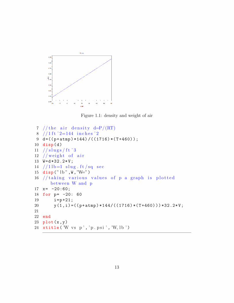
Figure 1.1: density and weight of air

7 // the a i r d e n s i t y d=P/(RT)8 // 1 f t ˆ2=144 i n c h e s ˆ29 d=((p+atmp)*144) /((1716) *(T+460));

10 disp(d)

11 // s l u g s / f t ˆ312 // we ight o f a i r13 W=d*32.2*V;

14 // 1 l b=1 s l u g . f t / sq s e c15 disp(” l b ”,W,”W=”)16 // t a k i n g v a r i o u s v a l u e s o f p a graph i s p l o t t e d

between W and p17 x= -20:60;

18 for p= -20: 60

19 i=p+21;

20 y(1,i)=((p+atmp)*144/((1716) *(T+460)))*32.2*V;

21

22 end

23 plot(x,y)

24 xtitle( ’W vs p ’ , ’ p . p s i ’ , ’W, l b ’ )

13

Scilab code Exa 1.4 reynolds number calculation

1 clc;

2 clear;

3 vis =0.38; //Ns/mˆ24 sg =0.91; // s p e c i f i c g r a v i t y o f Newtonian f l u i d5 dia =25; //mm6 vel =2.6; //m/ s7

8 // c a l c u l a t i n g i n SI u n i t s9 // f l u i d d e n s i t y d=sg ∗ ( d e n s i t y o f water @ 277K)10 d=sg *1000; // kg /mˆ311 // Reynolds number Re=d∗ v e l ∗ d i a / v i s12 Re=(d*vel*dia)/(vis *1000);// (kgm/ s e c ˆ2) /N13 disp (156,”Re i n SI u n i t s=”)14 // c a l c u l a t i n g i n BG u n i t s15 d1=d*1.94/1000 // s l u g s / f t ˆ316 vel1=vel *3.281 // f t / s17 dia1=(dia /1000) *3.281 // f t18 vis1=vis *(2.089/100) // l b ∗ s / f t ˆ219 Re1=(d1*vel1*dia1)/vis1;// ( s l u g s . f t / s e c ˆ2) / l b20 disp(Re1 ,”Re i n Bg u n i t s=”)

Scilab code Exa 1.5 shearing stress calculation

1 clc;

2 clear;

3 vis =0.04; // l b ∗ s e c / f t ˆ24 vel =2; // f t / s e c5 h=0.2; // i n c h e s6

7 // g i v e n u=(3∗ v e l /2) (1−(y/h ) ˆ2)8 // s h e a r i n g s t r e s s t=v i s ∗ ( du/dy )9 // ( du/dy ) =−(3∗ v e l ∗y/h )

10 // a l ong the bottom o f the w a l l y=−h

14

11 // ( du/dy ) =(3∗ v e l /h )12 t=vis *(3* vel/(h/12));// l b / f t ˆ213 disp(” l b / f t ˆ2 ”,t,” s h a e r i n g s t r e s s t on bottom w a l l=”

)

14 // a l ong the midplane y=015 // ( du/dy )=016 t1=0; // l b / f t ˆ217 disp(” l b / f t ˆ2 ”,t1 ,” s h e a r i n g s t r e s s t on midplane=”)

Scilab code Exa 1.6 final pressure calculation

1 clc;

2 clear;

3 p1 =14.7; // p s i ( abs )4 V1=1; // f t ˆ35 V2=0.5; // f t ˆ36 // f o r i s e n t r o p i c compres s ion , ( p1 ( d1ˆk ) ) =(p2 /( d2ˆk ) )7 // volume∗ d e n s i t y=c o n s t a n t ( mass )8 ratd=V1/V2;

9 p2=(( ratd)^1.66)*p1;// p s i ( abs )10 disp(” p s i ( abs ) ”,p2 ,” f i n a l p r e s s u r e p2=”)11

12 i=1;

13 ratV =0.01:0.01:1.0;

14

15 for j=0.01:0.01:1.0

16 pres(i)=p1/((j)^1.66);

17 i=i+1;

18

19 end

20

21 plot2d(ratV ,pres ,rect =[0 ,0 ,1 ,1000])

22 xtitle( ’ p2 vs V2/V1 ’ , ’V2/V1 ’ , ’ p2 p s i ’ )

15

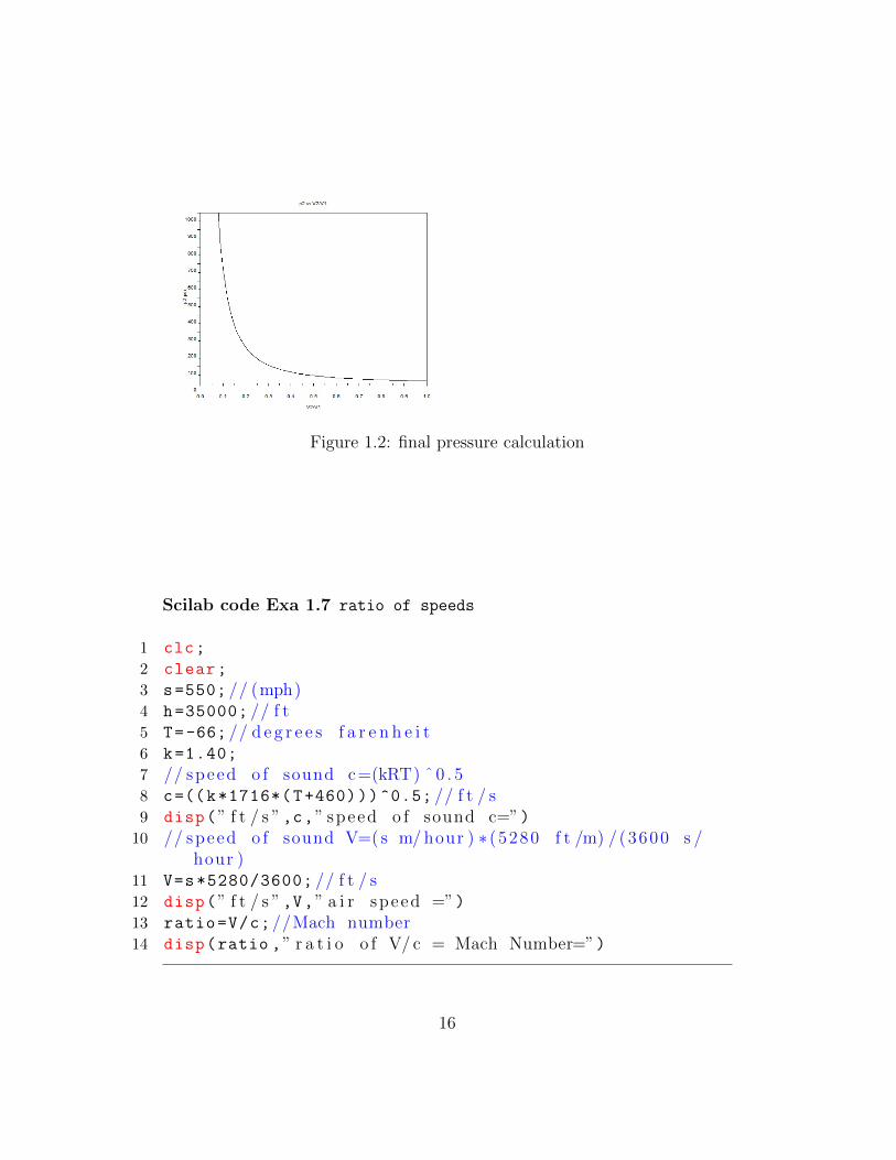
Figure 1.2: final pressure calculation

Scilab code Exa 1.7 ratio of speeds

1 clc;

2 clear;

3 s=550; // (mph)4 h=35000; // f t5 T=-66; // d e g r e e s f a r e n h e i t6 k=1.40;

7 // speed o f sound c=(kRT) ˆ 0 . 58 c=((k*1716*(T+460)))^0.5; // f t / s9 disp(” f t / s ”,c,” speed o f sound c=”)

10 // speed o f sound V=( s m/ hour ) ∗ (5280 f t /m) /(3600 s /hour )

11 V=s*5280/3600; // f t / s12 disp(” f t / s ”,V,” a i r speed =”)13 ratio=V/c;//Mach number14 disp(ratio ,” r a t i o o f V/ c = Mach Number=”)

16

Scilab code Exa 1.8 diameter of tube

1 clc;

2 clear;

3 T=20; // d e g r e e c e l c i u s4 h=1; //mm5 //h=(2∗ s t ∗ co s ( x ) /( sw∗R) )6 // where s t= n s u r f a c e t e n s i o n , x= a n g l e o f contac t ,

sw= s p e c i f i c we ight o f l i q u i d , R= tube r a d i u s7 st= 0.0728; //N/m8 sw =9.789; //kN/mˆ39 x=0;

10 R=(2*st*cos(x))/(sw *1000*h/1000);//m11 D=2*R*1000; //mm12 disp(”mm”,D,”minimum r e q u i r e d tube d iamete r= ”)13 h=0.1:0.1:2;

14 for i=0.1:0.1:2

15 R=(2*st*cos(x))/(sw *1000*i/1000);

16 dia(i*10) =2*R*1000;

17 end

18

19 plot2d(h,dia ,rect =[0 ,0 ,2 ,100])

20 xtitle(”D vs h”,”h , mm”, ”D, mm”)

17

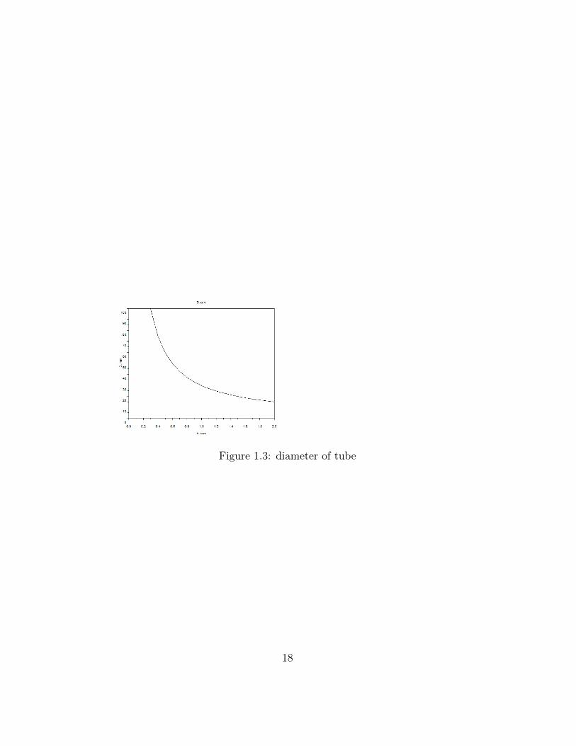
Figure 1.3: diameter of tube

18

Chapter 2

Fluids at rest pressure and itseffects

Scilab code Exa 2.1 pressure at interface

1 clc;

2 clear;

3 sg =0.68; // s p e c i f i c g r a v i t y o f g a s o l i n e4 htg =17; // f t ( h e i g h t o f g a s o l i n e )5 htw =3; // f t ( h e i g h t o f water )6 // p r e s s u r e p= (gamma∗h )+atmp ;7 // p r e s s u r e at water− g a s o l i n e i n t e r f a c e p1 =sg ∗g∗ htg

+atmp8 p1=sg *62.4* htg; //atmp=0 , p1 i s i n l b / f t ˆ29 pr1=p1/144; // l b / i n ˆ2

10 // p r e s s u r e head as f e e t o f water H11 H= p1 /62.4; // f t12 // s i m i l a r l y p r e s s u r e p2 at tank bottom13 p2 =62.4* htw+p1;// l b / f t ˆ214 pr2 = p2/144; // l b / i n ˆ215 // p r e s s u r e head as f t o f water H116 H1=p2 /62.4; // f t17 disp(” l b / i n ˆ2 ”,pr1 ,” l b / f t ˆ2 =”, p1,” p r e s s u r e at

i n t e r f a c e=”)

19

18 disp(” f t ”,H,” p r e s s u r e head at i n t e r f a c e i n f e e t o fwater =”)

19 disp(” l b / i n ˆ2 ”,pr2 ,” l b / f t ˆ2 =”, p2,” p r e s s u r e atbottom=”)

20 disp(” f t ”,H1 ,” p r e s s u r e head at bottom i n f e e t o fwater =”)

Scilab code Exa 2.2 pressure depth variation

1 clc;

2 clear;

3 h=1250; // f t4 T=59; // d e g r e e f a r e h e i t5 p=14.7; // p s i ( abs )6 sw =0.0765; // l b / f t ˆ3 , ( s p e c i f i c we ight o f a i r a t p )7

8 // c o n s i d e r i n g a i r to be c o m p r e s s i b l e9 // p1/p2= exp (−(g ∗ ( z1−z2 ) ) /(R∗T) )10 ratp=exp ( -(32.2*h)/(1716*(59+460)));

11 disp(ratp ,” r a t i o o f p r e s s u r e at the top to tha t atthe base c o n s i d e r i n g a i r to be c o m p r e s s i b l e=”)

12

13 // c o n s i d e r i n g a i r to be i n c o m p r e s s i b l e14 // p2=p1−(sw ∗ ( z2−z1 ) ) ;15 ratp1 =1-((sw*h)/(p*144));

16 disp(ratp1 ,” r a t i o o f p r e s s u r e at the top to tha t atthe base c o n s i d e r i n g a i r to be i n c o m p r e s s i b l e=”)

17 count =1;

18 zdiff =0:5000;

19

20 for i= 0:5000

21 j(count)=1-((sw*i)/(p*144));

22 count=count +1;

23 end

24 num =1;

20

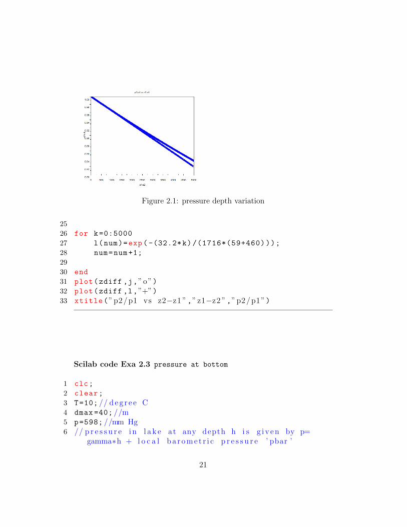
Figure 2.1: pressure depth variation

25

26 for k=0:5000

27 l(num)=exp ( -(32.2*k)/(1716*(59+460)));

28 num=num+1;

29

30 end

31 plot(zdiff ,j,”o”)32 plot(zdiff ,l,”+”)33 xtitle(”p2/p1 vs z2−z1 ”,” z1−z2 ”,”p2/p1”)

Scilab code Exa 2.3 pressure at bottom

1 clc;

2 clear;

3 T=10; // d e g r e e C4 dmax =40; //m5 p=598; //mm Hg6 // p r e s s u r e i n l a k e at any depth h i s g i v e n by p=

gamma∗h + l o c a l b a r o m e t r i c p r e s s u r e ’ pbar ’

21

7 // pbar /(gamma Hg) =598 mm= . 5 9 8 m ; (gamma Hg) = 133kN/mˆ3

8 pbar =0.598*133; //kN/mˆ29 // (gamma water ) =9.804 kN/mˆ3 at 10 d e r g r e e C10 p=(9.804*40)+pbar;//kN/mˆ211 disp(”kPa”,pbar ,”The l o c a l b a r o m e t r i c p r e s s u r e=”)12 disp(”kPa”,p,”The a b s o l u t e p r e s s u r e at a depth o f 40

m i n the l a k e=”)

Scilab code Exa 2.4 reading of gage

1 clc;

2 clear;

3 sg1 =0.90; // s p e c i f i c g r a v i t y o f o i l4 sg2 =13.6; // s p e c i f i c g r a v i t y o f Hg5 h1=36; // i n c h e s6 h2=6; // i n c h e s7 h3=9; // i n c h e s8 // p r e s s u r e e q u a t i o n : a i r p+h1∗ sg1 ∗ (gamma water )+h2∗

sg1 ∗ (gamma water )−h3∗ sg2 ∗ (gamma water )=09 airp=-(sg1 *62.4*(( h1/12)+(h2/12)))+(sg2 *62.4*( h3/12)

);// l b / f t ˆ210 // gage p r e s s u r e = a i r p11 pgage=airp /144;

12 disp(” p s i ”,pgage ,”Gage p r e s s u r e=”)

Scilab code Exa 2.5 pressure drop calculation

1 clc;

2 clear;

3 gamma1 =9.8; //kN/mˆ34 gamma2 =15.6; //kN/mˆ35 h1=1; //m

22

6 h2=0.5; //m7 //pA−(gamma1) ∗h1−h2 ∗ ( gamma2) +(gamma1) ∗ ( h1+h2 )=pB8 //pA−pB=d i f f p9 diffp =(( gamma1)*h1+h2*( gamma2)-(gamma1)*(h1+h2));

10 disp(”kPa”,diffp ,”The d i f f e r e n c e i n p r e s s u r e s at Aand B =”)

Scilab code Exa 2.6 force on plane

1 clc;

2 clear;

3 dia =4; //m4 sw=9.8; //kN/mˆ 3 ; s p e c i f i c we ight o f water5 hc=10; //m6 ang =60; // d e g r e e s7 A=%pi*(dia ^2) /4;

8 fres=sw*hc*A;

9 // f o r the c o o r d i n a t e system shown xc=x r e s =010 Ixc=%pi*((dia /2)^4)/4;

11 yc=hc/(sin (ang*%pi /180));

12 yres= (Ixc/(yc*A))+yc;

13 ydist=yres -yc;

14 disp(”kN”,fres ,”The r e s u l t a n t f o r c e a c t i n g on thega t e o f the r e s e r v o i r =”);

15 disp(”m below the s h a f t and i s p e r p e n d i c u l a r to thega t e s u r f a c e . ”,ydist ,”The r e s u l t a n t f o r c e a c t sthrough a p o i n t a l ong the d i amete r o f the ga t e at

a d i s t a n c e o f ”)16 M=fres*( ydist)*1000;

17 disp(”N∗m”,M,”Moment r e q u i r e d to open the ga t e=”)18 hc =1:30;

19 for i=1:30

20 ydist(i)=((Ixc/(i/(sin (ang*%pi /180))*A)));

21 end

22

23

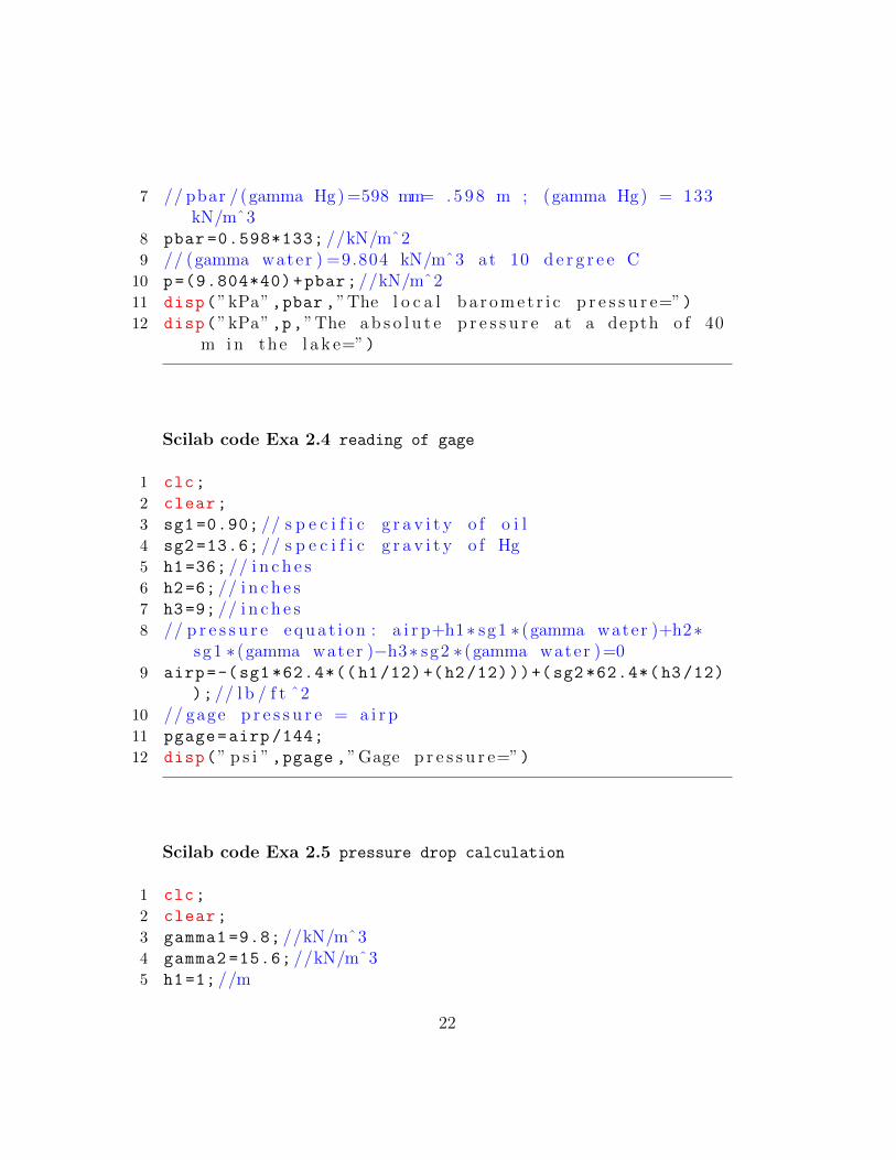
Figure 2.2: force on plane

23 plot2d(hc,ydist)

24 xtitle(” yre s−yc m vs hc m”,” hc m”,” yre s−yc m”)

Scilab code Exa 2.7 hydrostatic pressure force

1 clc;

2 clear;

3 sw=64; // l b / f t ˆ 3 ; s p e c i f i c we ight o f water4 h=10; // f t5 a=3; // f t6 b=3; // f t7

8 // shape i s t r i a n g u l a r , hence hc=h−(a /3)9 hc=h-(a/3);

10 A=(0.5*a*b);// f t ˆ 3 ; a r ea o f the r i g h t ang l edt r i a n g l e

11 fres=sw*hc*A;// l b12 Ixc=b*(a^3) /36;

13 Ixyc=b*(a^2)*(b)/72;

24

14 // a c c o r d i n g to the c o o r d i n a t e system taken yc=hc andxc=0

15 yres=(Ixc/(hc*A))+hc;

16 xres=(Ixyc/(hc*A));

17 ydist=yres -hc;

18 disp(” l b ”,fres ,”The r e s u l t a n t f o r c e on the a r eashown i s=”)

19 disp(” f t ”,yres ,”yR=”)20 disp(” f t ”,xres ,”xR=”)21 disp(” f t below the c e n t r o i d o f the a r ea . ”,ydist ,” f t

to the r i g h t o f and ”,xres ,”The c e n t r e o fp r e s s u r e i s ”)

Scilab code Exa 2.8 pressure prism concept

1 clc;

2 clear;

3 sg=0.9; // s p e c i f i c g r a v i t y o f o i l4 a=0.6; //m5 pgage =50; //kPa6 h1=2; //m7 h2=2.6; //m8

9 // the f o r c e on the t r a p e z o i d i s the sum o f the f o r c eon the r e c t a n g l e f 1 and f o r c e on t r i a n g l e f 2

10 f1=(( pgage *1000) +(sg *1000*9.81* h1))*(a^2);//N11 f2=sg *1000*9.81*(h2-h1)*(a^2) /2; //N12 fres=f1+f2;//N13 // to f i n d v e r t i c a l l o c a t i o n o f f r e s ; f r e s ∗ y r e s =( f 1 ∗ (

a /2) ) +( f 2 ∗ ( h1−h2 ) )14 yres =((f1*(a/2))+(f2*(a/3)))/fres;//m15 disp(”kN” ,(fres /1000) ,”The r e s u l t a n t f o r c e on the

p l a t e i s=”)16 disp(”m above the bottom p l a t e a lond the v e r t i c a l

l i n e o f symmetry . ”,yres ,”The f o r c e a c t s at a

25

d i s t a n c e o f ”)

Scilab code Exa 2.9 force on curve

1 clc;

2 clear;

3 dia =6; // f t4 l=1; // f t5

6 // h o r i z o n t a l f o r c e f 1=sw∗hc∗A7 hc=dia/4; // f t8 sw =62.4; // l b / f t ˆ39 A=dia/2*l;// f t ˆ2

10 f1=sw*hc*A;// l b11 // t h i s f o r c e f 1 a c t s at a h e i g h t o f r a d i u s /3 f t

above the bottom12 ht=(dia/2) /3; // f t13 // we ight w = sw∗volume14 w=sw*((dia /2) ^2)*%pi/4*l;// l b15 // t h i s f o r c e a c t s through c e n t r e o f g r a v i t y which i s

4∗ r a d i u s /(3∗%pi ) r i g h t o f the c e n t r e o f c o n d u i t16 dist =(4* dia /2) /(3* %pi);// f t17 // h o r i z o n t a l f o r c e tha t tank e x e r t s on f l u i d = f 118 // v e r t i c a l f o r c e tha t tank e x e r t s on f l u i d = w19 // r e s u l t a n t f o r c e f r e s =(( f 1 ) ˆ2+(w) ˆ2) ˆ 0 . 520 fres =((f1)^2+(w)^2) ^0.5; // l b21 disp(” l b ”,fres ,”The r e s u l t a n t f o r c e e x e r t e d by the

tank on the f l u i d=”);22 disp(” f t ”,dist ,” above the bottom o f the c o n d u i t and

to the r i g h t o f the a x i s o f the c o n d u i t at ad i s t a n c e o f ”,” f t ”,ht ,”The f o r c e a c t s at ad i s t a n c e o f ”)

26

Scilab code Exa 2.10 tension in cable

1 clc;

2 clear;

3 dia =1.5; //m4 wt=8.5; //kN5 // t e n s i o n i n c a b l e T=bouyant f o r c e (Fb)−wt6 // f l u i d i s water7 sw =10.1; //kN/mˆ38 vol=%pi*dia ^3/6; //mˆ39 Fb=sw*vol;//kN10 T=Fb -wt;//kN11 disp(”kN”,T,”The t e n s i o n i n the c a b l e =”)

Scilab code Exa 2.11 maximum acceleration calculation

1 clc;

2 clear;

3 sg =0.65;

4 l1 =0.75; // f t5 l2=0.5; // f t6 // 0 . 5 f t =z1 (max)7 // 0 . 5 = 0 . 7 5∗ ( ay (max) /g )8 aymax =(0.5*32.2) /0.75; // f t / s ˆ29 disp(” f t / s ˆ2 ”,aymax ,”The max a c c e l e r a t i o n tha t can

occu r b e f o r e the f u e l l e v e l drops below thet r a n s d u c e r=”)

27

Chapter 3

Fluids in motion Bernoulliequation

Scilab code Exa 3.6 pitot static tube

1 clc;

2 clear;

3 v1=100; //mi/ hr4 ht =10000; // f t5 // from standard t a b l e f o r s t a t i c p r e s s u r e at an

a l t i t u d e6 p1=1456 // l b / f t ˆ2( abs )7 P1 =1456*0.006947; // p s i8 d=0.001756; // s l u g s / f t ˆ39 // 1 mi/ hr = 1 . 4 6 7 f t / s

10 p2=p1+(d*(v1 *1.467) ^2/2);// l b / f t ˆ311 // i n terms o f gage p r e s s u r e p2g12 p2g=p2 -p1;// l b / f t ˆ213 // 1 l b / f t ˆ2 = 0 . 0 0 6 9 4 7 p s i14 P2=p2 *0.006947; // p s i15 P2g=p2g *0.006947; // p s i16 // p r e s s u r e d i f f e r e n c e i n d i c a t e d by the p i t o t tube =

p d i f f17 pdiff=P2-P1;// p s i

28

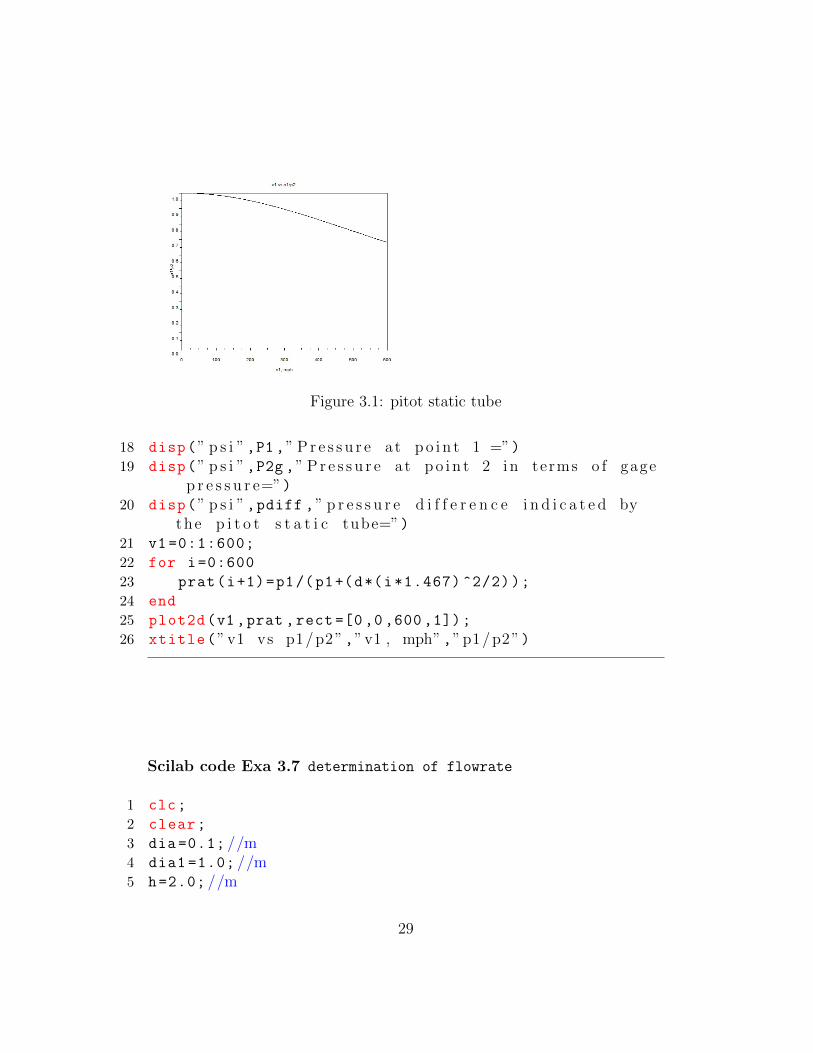
Figure 3.1: pitot static tube

18 disp(” p s i ”,P1 ,” P r e s s u r e at p o i n t 1 =”)19 disp(” p s i ”,P2g ,” P r e s s u r e at p o i n t 2 i n terms o f gage

p r e s s u r e=”)20 disp(” p s i ”,pdiff ,” p r e s s u r e d i f f e r e n c e i n d i c a t e d by

the p i t o t s t a t i c tube=”)21 v1 =0:1:600;

22 for i=0:600

23 prat(i+1)=p1/(p1+(d*(i*1.467) ^2/2));

24 end

25 plot2d(v1,prat ,rect =[0 ,0 ,600 ,1]);

26 xtitle(” v1 vs p1/p2”,”v1 , mph”,”p1/p2”)

Scilab code Exa 3.7 determination of flowrate

1 clc;

2 clear;

3 dia =0.1; //m4 dia1 =1.0; //m5 h=2.0; //m

29

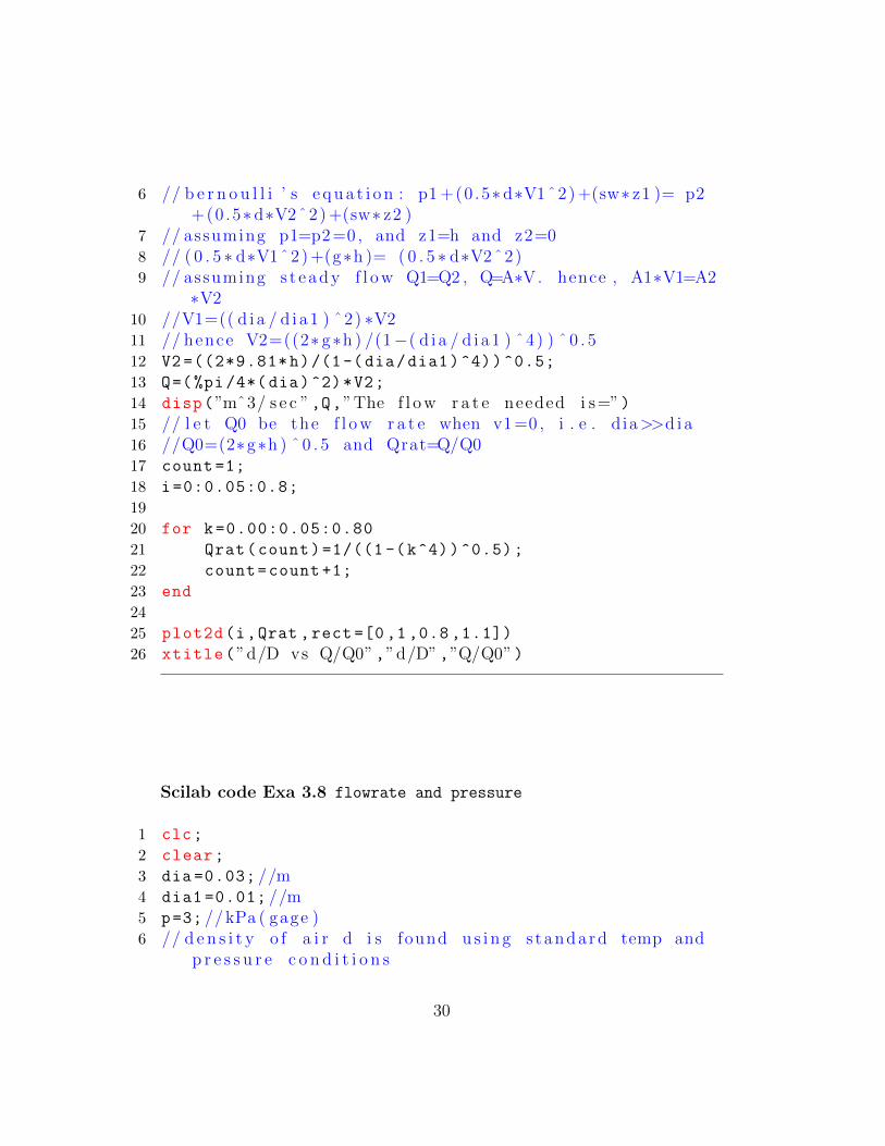
6 // b e r n o u l l i ’ s e q u a t i o n : p1 +(0 .5∗d∗V1ˆ2) +(sw∗ z1 )= p2+(0 .5∗d∗V2ˆ2) +(sw∗ z2 )

7 // assuming p1=p2=0 , and z1=h and z2=08 // ( 0 . 5 ∗ d∗V1ˆ2) +(g∗h )= ( 0 . 5 ∗ d∗V2ˆ2)9 // assuming s t eady f l o w Q1=Q2 , Q=A∗V. hence , A1∗V1=A2

∗V210 //V1=(( d i a / d i a1 ) ˆ2) ∗V211 // hence V2=((2∗ g∗h ) /(1−( d i a / d i a1 ) ˆ4) ) ˆ 0 . 512 V2 =((2*9.81*h)/(1-(dia/dia1)^4))^0.5;

13 Q=(%pi /4*( dia)^2)*V2;

14 disp(”mˆ3/ s e c ”,Q,”The f l o w r a t e needed i s=”)15 // l e t Q0 be the f l o w r a t e when v1 =0 , i . e . d ia>>d i a16 //Q0=(2∗g∗h ) ˆ 0 . 5 and Qrat=Q/Q017 count =1;

18 i=0:0.05:0.8;

19

20 for k=0.00:0.05:0.80

21 Qrat(count)=1/((1 -(k^4))^0.5);

22 count=count +1;

23 end

24

25 plot2d(i,Qrat ,rect =[0 ,1 ,0.8 ,1.1])

26 xtitle(”d/D vs Q/Q0”,”d/D”,”Q/Q0”)

Scilab code Exa 3.8 flowrate and pressure

1 clc;

2 clear;

3 dia =0.03; //m4 dia1 =0.01; //m5 p=3; //kPa ( gage )6 // d e n s i t y o f a i r d i s found u s i n g s tandard temp and

p r e s s u r e c o n d i t i o n s

30

Figure 3.2: determination of flowrate

7 d=(p+101) *1000/((286.9) *(15+273));

8 // a p p l y i n g B e r n o u l l i ’ s e q u a t i o n at p o i n t s 1 ,2 and 3 ;p=p1

9 v3=((2*p*1000)/d)^0.5;

10 Q=%pi /4*( dia1 ^2)*v3;

11 // by c o n t i n u i t y equat i on , A2∗v2=A3∗v312 v2=(( dia1/dia)^2)*v3;

13 p2=(p*1000) -(0.5*d*(v2^2));

14 disp(”mˆ3/ s ”,Q,” F lowrate =”)15 disp(”N/mˆ2 ”,p2 ,” P r e s s u r e i n the hose=”)

Scilab code Exa 3.10 maximum height determination

1 clc;

2 clear;

3 T=60; // d e g r e e f a r e n h e i t4 z1=5; // f t5 atmp =14.7; // p s i a6 // a p p l y i n g b e r n o u l l i e q u a t i o n at p o i n t s 1 ,2 and 37 z3=-5; // f t8 v1=0; // l a r g e tank

31

9 p1=0; // open tank10 p3=0; // open j e t11 // a p p l y i n g c o n t i n u i t y e q u a t i o n A2∗v2=A3∗v3 ; A2=A3 ;

so v2=v312 v3 =(2*32.2*(z1-z3))^0.5;

13 // vapor p r e s s u r e o f water at 60 d e g r e e f a r e n h e i t =p2 =0.256 p s i a

14 p2 =0.256;

15 z2=z1 -((((p2 -atmp)*144) +(0.5*1.94* v3^2))/62.4);

16 disp(” f t ”,z2 ,”The maximum h e i g h t ove r which thewater can be s iphoned wi thout c a v i t a t i o n o c c u r i n g=”)

Scilab code Exa 3.11 pressure difference range

1 clc;

2 clear;

3 sg =0.85;

4 Q1 =0.005; //mˆ3/ s5 Q2 =0.05; //mˆ3/ s6 dia1 =0.1; //m7 dia2 =0.06; //m8

9 //A2/A1=d ia2 / d i a110 d=sg *1000;

11 Arat=(dia2/dia1)^2;

12 A2=%pi /4*( dia2 ^2);

13 pdiffs =(Q1^2)*d*(1-( Arat ^2))/(2*1000*( A2^2));

14 pdiffl =(Q2^2)*d*(1-( Arat ^2))/(2*1000*( A2^2));

15 disp(”kPa”,pdiffl ,” to ”,”kPa”,pdiffs ,”kPa”,”Thep r e s s u r e d i f f e r e n c e r a n g e s from =”)

Scilab code Exa 3.12 flow through channel

32

1 clc;

2 clear;

3 z1=5; //m4 a=0.8; //m5 b=6; //m6 Cc =0.61; // s i n c e a/ z1=r a t i o =0.16 <0 .2 ; Cc=

c o n t r a c c t i o n c o e f f i c i e n t7 z2=Cc*a;

8 //Q/b=f l o w r a t e9 flowrate=z2 *((2*9.81*(z1 -z2))/(1 -((z2/z1)^2)))^0.5;

10 // c o n s i d e r i n g z1>>z2 and n e g l e c t i n g k i n e t i c ene rgyo f the upstream f l u i d

11 flowrate1=z2 *(2*9.81* z1)^0.5;

12 disp(”mˆ2/ s ”,flowrate ,”The f l o w r a t e per u n i t width=”)

13 disp(”mˆ2/ s ”,flowrate1 ,”The f l o w r a t e per u n i t widthwhen we c o n s i d e r z1>>z2=”)

14 count =1;

15 j=5:15;

16 for i=5:15

17 fr(count)=z2 *((2*9.81*(i-z2))/(1 -((z2/i)^2)))

^0.5;

18 count=count +1;

19 end

20 plot2d(j,fr,rect =[0,0 ,15,9])

21 xtitle(”Q/b vs z1 ”,” z1 ,m”,”Q/b , mˆ2/ s ”)

Scilab code Exa 3.13 increased flowrate determination

1 clc;

2 clear;

3 //Q=A∗V=(Hˆ2) ∗ tan ( t h e t a /2) ∗ (C2∗ (2∗ g∗H) ˆ 0 . 5 )4 //Q3H0/QH0=(3H0) ˆ 2 . 5 / ( H0) ˆ2 . 5=3ˆ2 .5

33

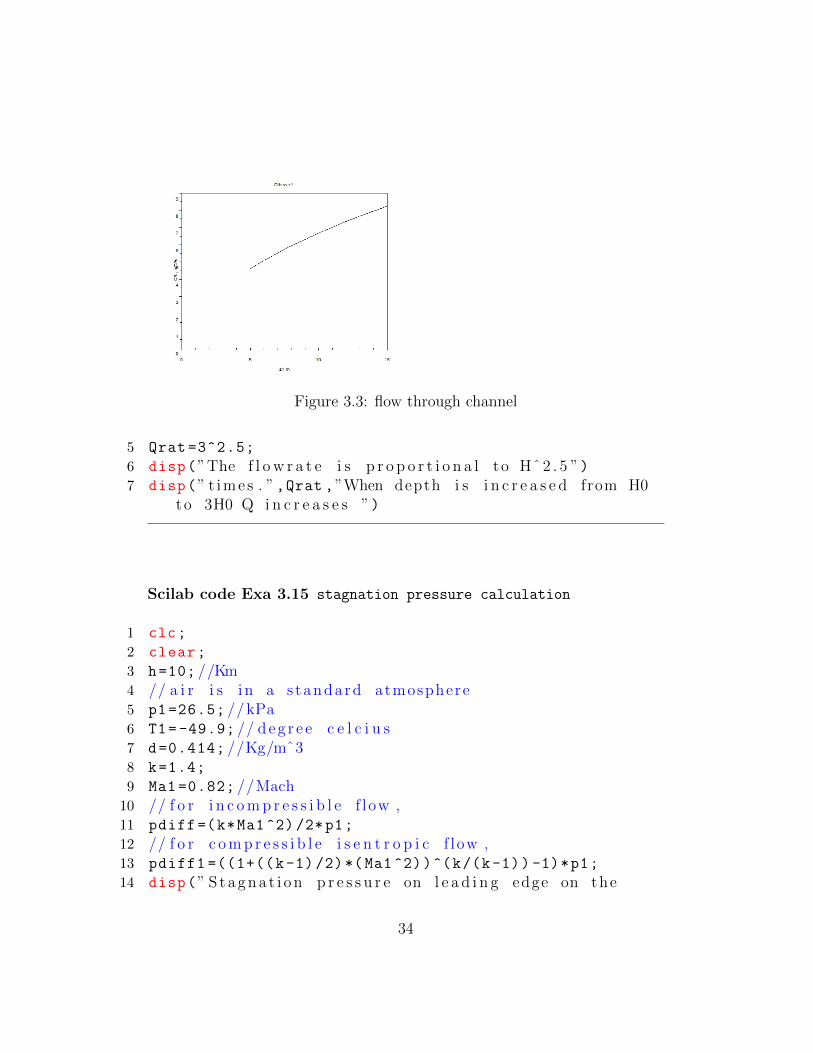
Figure 3.3: flow through channel

5 Qrat =3^2.5;

6 disp(”The f l o w r a t e i s p r o p o r t i o n a l to Hˆ 2 . 5 ”)7 disp(” t imes . ”,Qrat ,”When depth i s i n c r e a s e d from H0

to 3H0 Q i n c r e a s e s ”)

Scilab code Exa 3.15 stagnation pressure calculation

1 clc;

2 clear;

3 h=10; //Km4 // a i r i s i n a s tandard atmosphere5 p1 =26.5; //kPa6 T1= -49.9; // d e g r e e c e l c i u s7 d=0.414; //Kg/mˆ38 k=1.4;

9 Ma1 =0.82; //Mach10 // f o r i n c o m p r e s s i b l e f low ,11 pdiff=(k*Ma1^2)/2*p1;

12 // f o r c o m p r e s s i b l e i s e n t r o p i c f low ,13 pdiff1 =((1+((k-1)/2)*(Ma1 ^2))^(k/(k-1)) -1)*p1;

14 disp(” S t a g n a t i o n p r e s s u r e on l e a d i n g edge on the

34

wing o f the Boeing : ”)15 disp(”kPa”,pdiff ,” f l o w i s i m c o m p r e s s i b l e =”)16 disp(”kPa”,pdiff1 ,” f l o w i s c o m p r e s s i b l e and

i s e n t r o p i c =”)

Scilab code Exa 3.17 stagnation pressure determination

1 clc;

2 clear;

3 V=5; //m/ s4 sg =1.03;

5 h=50; //m6 // s i n c e s t a t i c p r e s s u r e i s g r e a t e r than s t a g n a t i o n

p r e s s u r e , B e r n o u l l i ’ s e q u a t i o n i s i n c o r r e c t7 // p2=(d ∗ (V1ˆ2) /2) +(d∗g∗h ) ; V1=V8 p2=(((sg *1000) *(V^2) /2) + (sg *1000*9.81*h))/1000; //

kPa9 disp(”kPa”,p2 ,”The p r e s s u r e at s t a g n a t i o n p o i n t 2 =”

)

35

Chapter 4

Kinematics of fluid motion

Scilab code Exa 4.6 delivery speed calculation

1 clc;

2 clear;

3 pratet =-8; // d o l l a r s / hr4 pratex =0.2; // d o l l a r s /mi5 exec(”C: \ Program F i l e s \ s c i l a b −5 .3 . 0\ b in \TCP\4 6 d a t a .

s c i ”);6 u=(-pratet)/pratex;

7 disp(”mi/ hr ”,u,”The d e l i v e r y speed=”)

36

Chapter 5

Flow analysis using controlvolumes

Scilab code Exa 5.1 Minimum Pumping capacity

1 clc;

2 clear;

3 v2=20; //m/ s4 dia2= 40; //mm5

6 //m1=m27 // d1∗Q1=D2∗Q2 ; where d1=d2 i s d e n s i t y o f s e a w a t e r8 // hence Q1=Q29 Q=v2*(%pi*(( dia2 /1000) ^2)/4);//mˆ3/ s e c

10 disp(”mˆ3/ s e c ”,Q,” F lowrate=”)

Scilab code Exa 5.2 average velocity calculation

1 clc;

2 clear;

3 v2 =1000; // f t / s e c

37

4 p1=100; // p s i a5 p2 =18.4; // p s i a6 T1=540; // d e g r e e R7 T2=453; // d e g r e e R8 dia =4; // i n c h e s9 //m1=m210 // d1∗A1∗v1=d2∗A2∗v211 //A1=A2 and d=p /(R∗T) ; s i n c e a i r a t p r e s s u r e s and

t e m p e r a t u r e s i n v o l v e d behaves as an i d e a l gas12 v1=p2*T1*v2/(p1*T2);

13 disp(” f t / s e c ”,v1 ,” V e l o c i t y at s e c t i o n 1 =”)

Scilab code Exa 5.3 Mass Flowrate determination

1 clc;

2 clear;

3 m1=22; // s l u g s / hr4 m3=0.5; // s l u g s / hr5 //−m1+m2+m3=06 m2=m1-m3;

7 disp(” s l u g s / hr ”,m2 ,”Mass f l o w r a t e o f the dry a i r andwater vapour l e a v i n g the d e h u m i d i f i e r=”)

Scilab code Exa 5.5 change in depth

1 clc;

2 clear;

3 Q=9; // g a l /min4 l=5; // f t5 b=2; // f t6 H=1.5; // f t

38

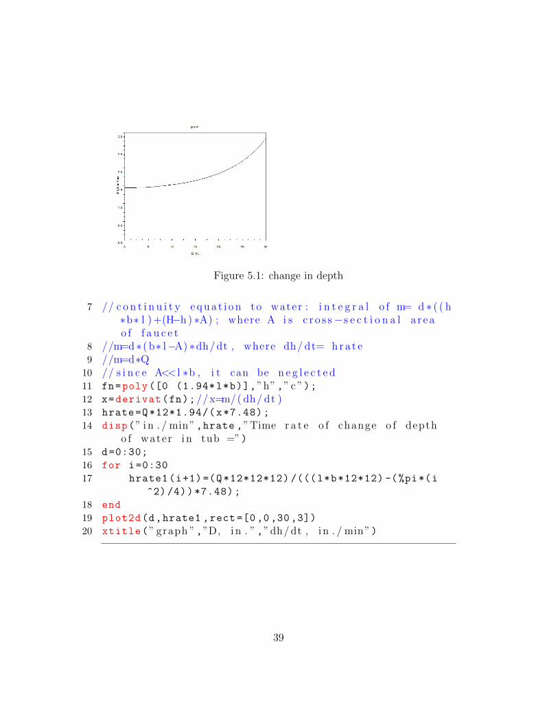
Figure 5.1: change in depth

7 // c o n t i n u i t y e q u a t i o n to water : i n t e g r a l o f m= d ∗ ( ( h∗b∗ l ) +(H−h ) ∗A) ; where A i s c r o s s−s e c t i o n a l a r eao f f a u c e t

8 //m=d ∗ ( b∗ l−A) ∗dh/ dt , where dh/ dt= h r a t e9 //m=d∗Q10 // s i n c e A<< l ∗b , i t can be n e g l e c t e d11 fn=poly ([0 (1.94*l*b)],”h”,” c ”);12 x=derivat(fn);//x=m/( dh/ dt )13 hrate=Q*12*1.94/(x*7.48);

14 disp(” i n . / min”,hrate ,”Time r a t e o f change o f deptho f water i n tub =”)

15 d=0:30;

16 for i=0:30

17 hrate1(i+1)=(Q*12*12*12) /(((l*b*12*12) -(%pi*(i

^2) /4))*7.48);

18 end

19 plot2d(d,hrate1 ,rect =[0 ,0,30,3])

20 xtitle(” graph ”,”D, i n . ”,”dh/ dt , i n . / min”)

39

Scilab code Exa 5.6 mass flowrate estimation

1 clc;

2 clear;

3 v=971; //km/ hr4 v2 =1050; //km/ hr5 A1 =0.80; //mˆ26 d1 =0.736; //Kg/mˆ37 A2 =0.558; //mˆ28 d2 =0.515; //Kg/mˆ39

10 //w1=v=i n t a k e v e l o c i t y11 // mass f l o w r a t e o f f u e l i n t a k e = d2∗A2∗w2 − d1∗A1∗

w112 w2=v2+v;

13 m=(d2*A2*w2 - d1*A1*v)*1000;

14 disp(” kg / hr ”,m,”The mass f l o w r a t e o f f u e l i n t a k e =”)

Scilab code Exa 5.7 Speed of water

1 clc;

2 clear;

3 Q=1000; //ml/ s4 A2=30; //mmˆ25 rotv =600; //rpm6

7 // mass i n = mass out8 w2=(Q*0.001*1000000) /(2*A2 *1000);

9 disp(”m/ s ”,w2 ,” Average speed o f water l e a v i n g eachn o z z l e when s p r i n k l e head i s s t a t i o n a r y and wheni t r o t a t e s with a c o n s t a n t speed o f 600rpm =”)

40

Scilab code Exa 5.8 Speed of plunger

1 clc;

2 clear;

3 Ap=500; //mmˆ24 Q2=300; //cmˆ3/ min5 Qleak =0.1* Q2;//cmˆ3/ min6 //A1=Ap7 // mass c o n s e r v a t i o n i n c o n t r o l volume8 //−d∗A1∗V + m2 + d∗Qleak =0; m2=d∗Q29 //V=(Q2+Qleak ) /Ap10 V=(Q2+Qleak)*1000/ Ap;

11 disp(”mm/min”,V,”The speed at which the p l u n g e rshou ld be advanced=”)

Scilab code Exa 5.9 change in depth

1 clc;

2 clear;

3 Q=9; // g a l /min4 l=5; // f t5 b=2; // f t6 H=1.5; // f t7 // de fo rming c o n t r o l volume8 // h r a t e=Q/( l ∗b−A)9 //A<< l ∗b

10 hrate=Q*12/(l*b*7.48);

11 disp(” i n . / min”,hrate ,”Time r a t e o f change o f deptho f water i n tub =”)

Scilab code Exa 5.11 Anchoring force determination

1 clc;

41

2 clear;

3 dia1 =16; //mm4 h=30; //mm5 dia2 =5; //mm6 Q=0.6; // l i t r e / s e c7 mass =0.1; // kg8 p1=464; //kPa9 d=999; // kg /mˆ310 m=d*Q/1000; // kg / s11 A1=%pi*(( dia1 /1000) ^2)/4; //mˆ212 w1=Q/(A1 *1000);//m/ s13 A2=%pi*(( dia2 /1000) ^2)/4; //mˆ214 w2=Q/(A2 *1000);//m/ s15 Wnozzle=mass *9.81; //N16 volwater =((1/12) *(%pi)*(h)*(( dia1 ^2)+(dia2 ^2)+(dia1*

dia2)))/(1000^3);//mˆ317 Wwater=d*volwater *9.81; //N18 F=m*(w1-w2)+Wnozzle +(p1 *1000* A1)+Wwater;//N19 disp(”N”,F,”The a n c h o r i ng f o r c e=”)

Scilab code Exa 5.12 Anchoring force calculation

1 clc;

2 clear;

3 A=0.1; // f t ˆ24 v=50; // f t / s5 p1=30; // p s i a6 p2=24; // p s i a7

8 d=1.94; // s l u g s / f t ˆ39 // v1=v2=v and A1=A2=A

10 m=d*v*A;

11 Fay=-m*(v+v) -((p1 -14.7)*A*144) -((p2 -14.7)*A*144);

12 disp(” l b ” ,0,” and the x component o f a n c h o r i n g f o r c ei s ”,” l b ”,Fay ,”The y component o f a n c h o r i n g f o r c e

42

i s ”)

Scilab code Exa 5.13 Frictional force determination

1 clc;

2 clear;

3 p1=100; // p s i a4 p2 =18.4; // p s i a5 T1=540; // d e g r e e R6 T2=453; // d e g r e e R7 V2 =1000; // f t / s8 V1=219; // f t / s9 dia =4; // i n

10

11 //m=m1=m212 A2=%pi *((4/12) ^2)/4; // f t ˆ213 // e q u a t i o n o f s t a t e d∗R∗T=p14 d2=p2 *144/(1716* T2);

15 m=A2*d2*V2;// s l u g s / s16 Rx=A2 *144*(p1 -p2) -(m*(V2 -V1));// l b17 disp(” l b ”,Rx ,” F r i c t i o n a l f o r c e e x e r t e d by p ipe w a l l

on a i r f l o w=”)

Scilab code Exa 5.15 nominal thrust calculation

1 clc;

2 clear;

3 v1=200; //m/ s4 v2=500; //m/ s5 A1=1; //mˆ26 p1 =78.5; //kPa ( abs )7 T1=268; //K8 p2=101; //kPa ( abs )

43

9

10 //F=−p1∗A1 + p2∗A2 + m∗ ( v2−v1 )11 //m=d1∗A1∗v112 // d1=(p1 ) /(R∗T1)13 d1=(p1 *1000) /(286.9* T1);

14 m=d1*v1*A1;

15 F=-((p1-p2)*A1 *1000) + m*(v2-v1);

16 disp(”N”,F,”The t h r u s t f o r which the s tand i s to bed e s i g n e d=”)

Scilab code Exa 5.17 force determination

1 clc;

2 clear;

3 v1=100; // f t / s e c4 v0=20; // f t / s e c5 ang =45; // d e g r e e s6 A1 =0.006; // f t ˆ27 l=1; // f t8 //m1=m2=m; c o n t i n u i t y e q u a t i o n9 //d=d e n s i t y o f water= c o n s t a n t

10 //w=speed o f water r e l a t i v e to the moving c o n t r o lvolume=c o n s t a n t=w1=w2

11 //w1=v1−v012 w=v1 -v0;

13 d=1.94; // s l u g s / f t ˆ314 //−Rx=(w1) (−m1) +(w2cos ( ang ) ) (m2)15 Rx=d*(w^2)*A1*(1-cos(ang*%pi /180));

16 // wwater=( s p e c i f i c wt o f water ) ∗A1∗ l17 wwater =62.4* A1*l;

18 Rz=(d*(w^2)*(sin(ang*%pi /180))*A1)+wwater;

19 R=((Rx^2)+(Rz^2))^0.5;

20 angle=(atan(Rz/Rx))*180/( %pi);

21 disp(” l b ”,R,”The f o r c e e x e r t e d by stream o f water onvane s u r f a c e=”)

44

22 disp(” d e g r e e s ”,angle ,”The f o r c e p o i n t s r i g h t anddown from the x d i r e c t i o n at an a n g l e o f=”)

Scilab code Exa 5.18 resisting torque calculation

1 clc;

2 clear;

3 Q=1000; //ml/ s e c4 A=30; //mmˆ25 r=200; //mm6 n=500; // rev /min7 // v2 i s t a n g e n t i a l ; v2=vang28 m=(Q/1000000) *999; // kg / s e c9 //m=2∗d ∗ (A) ∗v2=d∗Q

10 v2=(Q)/(2*A);//m/ s e c11 // Torque r e u i r e d to ho ld s p r i n k l e r s t a t i o n a r y12 Tshaft =(-(r/1000) *(v2)*m);//Nm13 // u2=speed o f n o z z l e=r ∗omega14 // v21=v2−u215 omega=n*(2* %pi)/60; // rad / s e c16 v21=v2 -(r*omega /1000);

17 // r e s i s t i n g to r q u e when s p r i n k e r i s r o t a t i n g at ac o n s t a n t speed o f n r ev /min

18 Tshaft1 =(-(r/1000) *(v21)*m);//Nm19 //when no r e s i s t i n t g t o r q ue i s a p p l i e d20 // Tsha f t=021 omega1=v2/(r/1000);

22 n1=( omega1)*60/(2* %pi);//rpm23 disp(”Nm”,Tshaft ,” R e s i s t i n g t o r q ue r e q u i r e d to ho ld

the s p r i n k e r s t a t i o n a r y=”)24 disp(”Nm”,Tshaft1 ,” R e s i s t i n g t o r q ue when s p r i n k e r i s

r o t a t i n g at a c o n s t a n t speed o f 500 r ev /min=”)25 disp(”rpm”,n1 ,” Speed o f s p r i k l e r when no r e s i s t i n g

t o rq u e i s a p p l i e d=”)26 x=0:800;

45

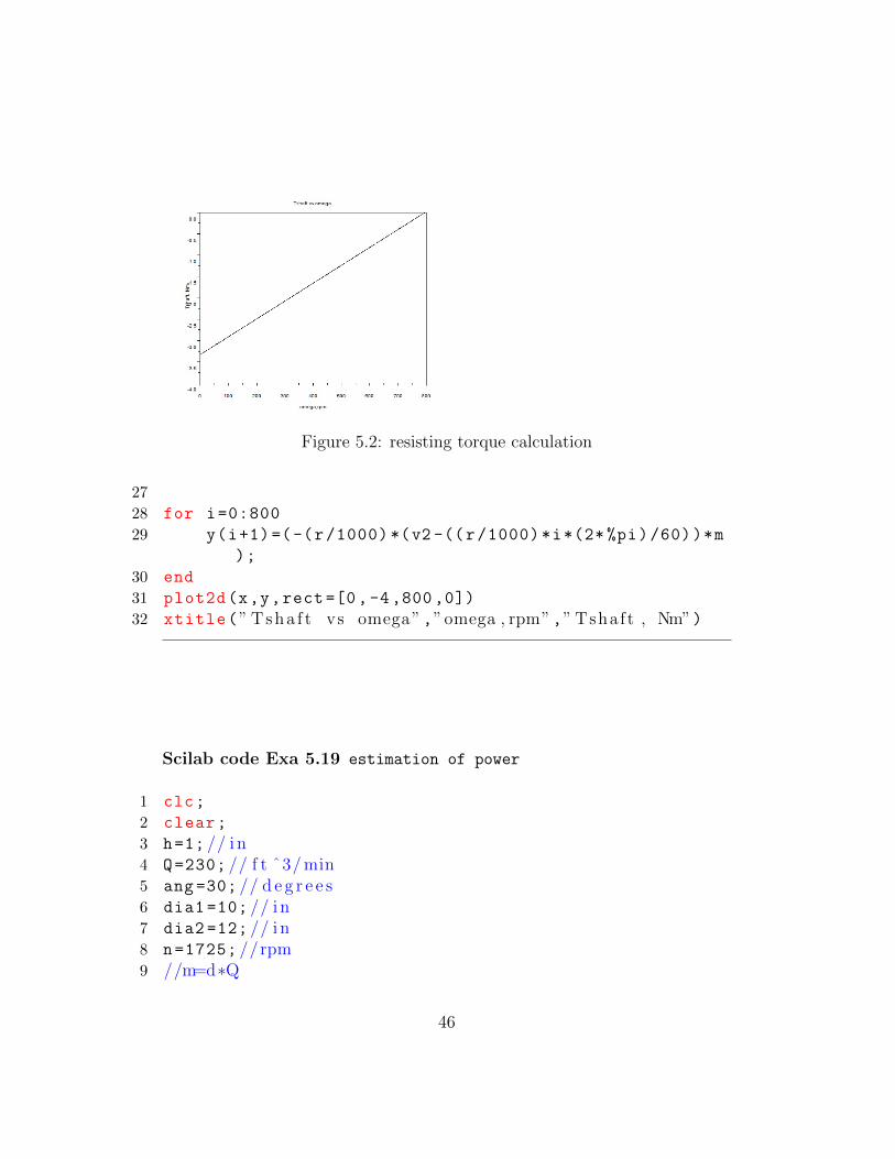
Figure 5.2: resisting torque calculation

27

28 for i=0:800

29 y(i+1)=(-(r/1000) *(v2 -((r/1000)*i*(2* %pi)/60))*m

);

30 end

31 plot2d(x,y,rect =[0,-4,800,0])

32 xtitle(” Tsha f t vs omega”,”omega , rpm”,” Tshaft , Nm”)

Scilab code Exa 5.19 estimation of power

1 clc;

2 clear;

3 h=1; // i n4 Q=230; // f t ˆ3/ min5 ang =30; // d e g r e e s6 dia1 =10; // i n7 dia2 =12; // i n8 n=1725; //rpm9 //m=d∗Q

46

10 m=(2.38/1000)*Q/60;

11 // u2=r o t o r b l ade speed12 u2=(dia2 /2)*(n*2*( %pi)/(12*60));

13 //m=d∗A2∗Vr2 and A2=2∗%pi∗ r2 ∗h and r2=d ia2 /214 // hence , m=d∗2∗%pi∗ r2 ∗h∗Vr215 // Vr2=w2∗ s i n ( ang )16 w2=m*12*12/((2.38/1000) *2*( %pi)*(dia2 /2)*(h)*sin(ang

*(%pi)/180));// f t / s e c17 Vang2=u2 -(w2*cos(ang*(%pi)/180));// f t / s e c18 Wshaft=m*u2*Vang2 /(550);//hp19 disp(”hp”,Wshaft ,”The power r e q u i r e d to run the fan=

”)

Scilab code Exa 5.20 Determination of power

1 clc;

2 clear;

3 Q=300; // g a l /min4 d1=3.5; // i n .5 p1=18; // p s i6 d2=1; // i n .7 p2=60; // p s i8 diffu =3000; // f t ∗ l b / s l u g9

10 // ene rgy e q u a t i o n11 //m( u2−u1+(p1/d )−(p2/d ) +(( v2 ˆ2)−(v1 ˆ2) ) /2 + g ∗ ( z2−z1

) )=q−Wshaft12 m=Q*1.94/(7.48*60);// s l u g s / s e c13 v1=Q*12*12/( %pi*(d1^2) *60*7.48/4);

14 v2=Q*12*12/( %pi*(d2^2) *7.48*60/4);

15 Wshaft=m*( diffu + (p2 *144/1.94) - (p1 *144/1.94) +

(((v2^2) -(v1^2))/2))/550; //hp16 disp(”hp”,Wshaft ,”The power r e q u i r e d by the pump=”)17 disp(”hp”,m*( diffu /550) ,”The i n t e r n a l ene rgy change

a c c o u n t s f o r =”)

47

18 disp(”hp”,m*(((p2 *144/1.94) - (p1 *144/1.94))/550),”The p r e s s u r e r i s e a c c o u n t s f o r =”)

19 disp(”hp”,m*(((v2^2) -(v1^2))/(550*2)),”The k i n e t i cene rgy change a c c o u n t s f o r =”)

Scilab code Exa 5.21 work output calculation

1 clc;

2 clear;

3 v1=30; //m/ s4 h1 =3348; // kJ/ kg5 v2=60; //m/ s6 h2 =2550; // kJ/ kg7

8 // ene rgy e q u a t i o n9 // w s h a f t i n=Wshaft in /m= ( h2−h1 + ( ( v2 ˆ2)−(v1 ˆ2) ) /2)

10 // wsha f t ou t=−w s h a f t i n11 wshaftout=h1 -h2 + (((v1^2) -(v2^2))/2000);

12 disp(”KJ/ kg ”,wshaftout ,”The work output i n v o l v e d peru n i t mass o f steam through−f l o w=”)

Scilab code Exa 5.22 temperature change determination

1 clc;

2 clear;

3 z=500; // f t4 // ene rgy e q u a t i o n5 //T2−T1 = ( u2 − u1 ) / c = g ∗ ( z2 − z1 ) / c ; c=s p e c i f i c

heat o f water = 1 Btu /( lbm∗ d e g r e e R)6 diffT = 32.2*z/(778*32.2);// d e g r e e R7 disp(” d e g r e e R”,diffT ,”The tempera tu r e change

a s s o c i a t e d with t h i s f l o w=”)

48

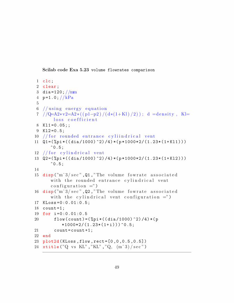
Scilab code Exa 5.23 volume flowrates comparison

1 clc;

2 clear;

3 dia =120; //mm4 p=1.0; //kPa5

6 // u s i n g ene rgy e q u a t i o n7 //Q=A2∗v2=A2 ∗ ( ( p1−p2 ) /( d∗(1+Kl ) /2) ) ; d =d e n s i t y , Kl=

l o s s c o e f f i c i e n t8 Kl1 =0.05;;

9 Kl2 =0.5;

10 // f o r rounded e n t r a n c e c y l i i n d r i c a l vent11 Q1=(%pi*(( dia /1000) ^2)/4)*(p*1000*2/(1.23*(1+ Kl1)))

^0.5;

12 // f o r c y l i n d r i c a l vent13 Q2=(%pi*(( dia /1000) ^2)/4)*(p*1000*2/(1.23*(1+ Kl2)))

^0.5;

14

15 disp(”mˆ3/ s e c ”,Q1 ,”The volume f o w r a t e a s s o c i a t e dwith the rounded e n t r a n c e c y l i n d r i c a l ventc o n f i g u r a t i o n =”)

16 disp(”mˆ3/ s e c ”,Q2 ,”The volume f o w r a t e a s s o c i a t e dwith the c y l i n d r i c a l vent c o n f i g u r a t i o n =”)

17 KLoss =0:0.01:0.5;

18 count =1;

19 for i=0:0.01:0.5

20 flow(count)=(%pi*((dia /1000) ^2)/4)*(p

*1000*2/(1.23*(1+i)))^0.5;

21 count=count +1;

22 end

23 plot2d(KLoss ,flow ,rect =[0 ,0 ,0.5 ,0.5])

24 xtitle(”Q vs KL”,”KL”,”Q, (mˆ3) / s e c ”)

49

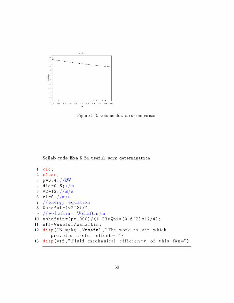
Figure 5.3: volume flowrates comparison

Scilab code Exa 5.24 useful work determination

1 clc;

2 clear;

3 p=0.4; //kW4 dia =0.6; //m5 v2=12; //m/ s6 v1=0; //m/ s7 // ene rgy e q u a t i o n8 Wuseful =(v2^2) /2;

9 // w s h a f t i n= Wshaft in /m10 wshaftin =(p*1000) /(1.23* %pi *(0.6^2) *12/4);

11 eff=Wuseful/wshaftin;

12 disp(”N.m/ kg ”,Wuseful ,”The work to a i r whichp r o v i d e s u s e f u l e f f e c t −=”)

13 disp(eff ,” F lu id mechan i ca l e f f i c i e n c y o f t h i s f an=”)

50

Scilab code Exa 5.25 flowrate and powerloss

1 clc;

2 clear;

3 p=10; //hp4 z=30; // f t5 hl=15; // f t6 // ene rgy e q u a t i o n7 // hs=Wshaft in /( sw∗Q) = h l+z8 Q=(p*550) /((hl+z)*62.4);

9 wloss =62.4*Q*hl /550;

10 disp(” f t ˆ3/ s ”,Q,” F lowrate =”)11 disp(”hp”,wloss ,”Power l o s s=”)12 loss =0:25;

13 for i=0:25

14 q(i+1)=(p*550) /((i+z)*62.4);

15 end

16 plot2d(loss ,q,rect =[0 ,0 ,25 ,3.5])

17 xtitle(” F lowrate vs h e a d l o s s ”,” hs , f t ”,”Q, f t ˆ3/ s e c ”)

Scilab code Exa 5.26 nonuniform velocity profile

1 clc;

2 clear;

3 m=0.1; // kg /min4 dia1 =60; //mm5 alpha1 =2.0;

6 dia2 =30; //mm7 alpha2 =1.08;

8 p=0.1; //kPa

51

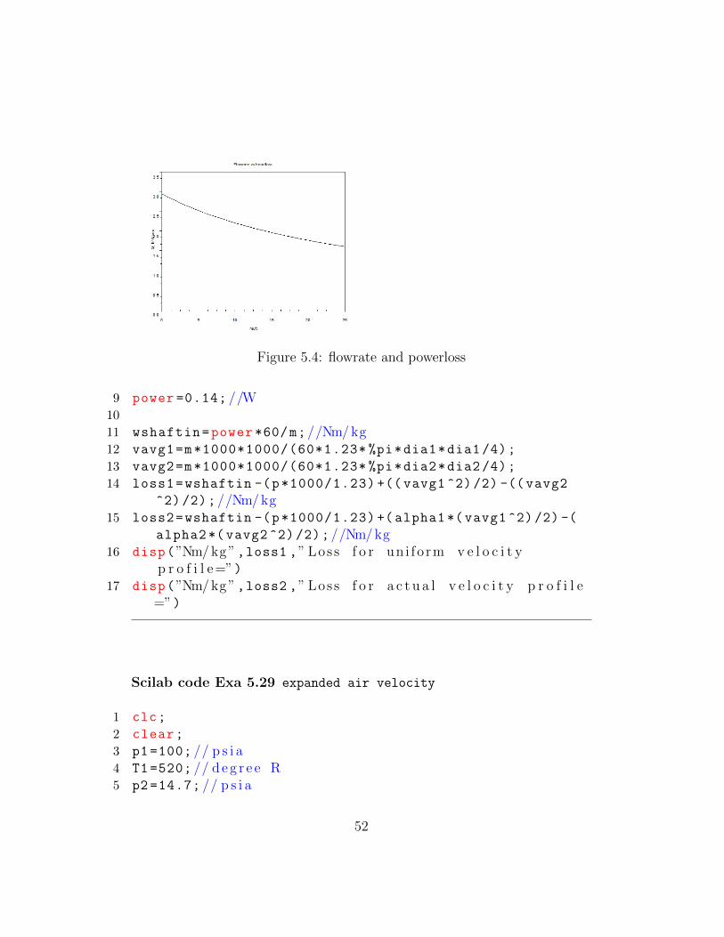
Figure 5.4: flowrate and powerloss

9 power =0.14; //W10

11 wshaftin=power *60/m;//Nm/ kg12 vavg1=m*1000*1000/(60*1.23* %pi*dia1*dia1 /4);

13 vavg2=m*1000*1000/(60*1.23* %pi*dia2*dia2 /4);

14 loss1=wshaftin -(p*1000/1.23) +(( vavg1 ^2) /2) -((vavg2

^2) /2);//Nm/ kg15 loss2=wshaftin -(p*1000/1.23) +( alpha1 *(vavg1 ^2)/2) -(

alpha2 *( vavg2 ^2)/2);//Nm/ kg16 disp(”Nm/ kg ”,loss1 ,” Loss f o r un i fo rm v e l o c i t y

p r o f i l e=”)17 disp(”Nm/ kg ”,loss2 ,” Loss f o r a c t u a l v e l o c i t y p r o f i l e

=”)

Scilab code Exa 5.29 expanded air velocity

1 clc;

2 clear;

3 p1=100; // p s i a4 T1=520; // d e g r e e R5 p2 =14.7; // p s i a

52

6

7 // f o r i n c o m p r e s s i b l e f l o w8

9 d=p1 *144/(1716* T1);// where d=d e n s i t y , c a l c u l a t e d byassuminng a i r to behave l i k e an i d e a l gas

10 // B e r n o u l l i e q u a t i o n11 v2=(2*(p1-p2)*144/d)^0.5; // f t / s e c12 disp(” f t / s e c ”,v2 ,”The v e l o c i t y o f expanded a i r

c o n s i d e r i n g i n c o m p r e s s i b l e f l o w =”)13

14 // f o r c o m p r e s s i b l e f l o w15

16 k=1.4; // f o r a i r17 d1=d;

18 d2=d1*((p2/p1)^(1/k));// where d2=d e n s i t y o f expandeda i r

19 // b e r n o u l l i e q u a t i o n20 V2=((2*k/(k-1))*((p1*144/ d1) -(p2*144/d2)))^0.5; // f t /

s21 disp(” f t / s ”,V2 ,”The v e l o c i t y o f expanded a i r

c o n s i d e r i n g c o m p r e s s i b l e f l o w =”)

53

Chapter 6

Flow Analysis of UsingDifferential Methods

Scilab code Exa 6.4 inviscid flow pressure

1 clc;

2 clear;

3 p1=30; //kPa4 d=1000; // kg /(mˆ3)5 r1=1; //m6 r2=0.5; //m7 // a p p l y i n g ene rgy e q u a t i o n between p o i n t s ( 1 ) and

( 2 ) and u s i n g the e q u a t i o n Vˆ2=16∗( r ˆ2)8 V1 =(16*( r1^2))^0.5; //m/ s e c9 V2 =(16*( r2^2))^0.5; //m/ s e c10 p2=((p1 *1000) +(d*((V1^2) -(V2^2)))/2) /1000; //kPa11 disp(”kPa”,p2 ,”The p r e s s u r e at p o i n t ( 2 ) =”)

Scilab code Exa 6.5 Volume rate calculation

1 clc;

54

2 clear;ang1 =0; // r a d i a n s3 ang2=%pi/6; // r a d i a n s4 vp= ’−2∗ l o g ( r ) ’ ;5 // vr=d ( vp ) /d ’ r6 // vr =(−2)/ r ;7 // vang =(1/ r ) ∗ ( d ( vp ) /d ( ang ) )8 vang =0;

9 q=( integrate( ’−2 ’ , ’ ang ’ ,ang1 ,ang2));10 disp(” f t ˆ2/ s e c ”,q,”Volume r a t e o f f l o w ( per u n i t

l e n g t h ) i n t o the open ing = ”)

Scilab code Exa 6.7 pressure at elevation

1 clc;

2 clear;

3 h=200; // f t4 U=40; //mi/ hr5 d=0.00238; // s l u g s / f t ˆ36 //Vˆ2= (Uˆ2) ∗ (1 + (2∗b∗ co s ( ang ) / r ) + ( ( b ˆ2) /( r ˆ2) ) )7 // at p o i n t 2 , ang=%pi /28 // r=b ∗ ( %pi−ang ) / s i n ( ang ) =(%pi∗b /2)9 V=U*(1+(4/( %pi^2)))^0.5; //mi/ hr10 y2=h/2; // f t11 // b e r n o u l l i e q u a t i o n12 //p1−p2= d ∗ ( ( V2ˆ2)−(V1ˆ2) ) + ( sw ∗ ( y2−y1 ) )13 V1=U*(5280/3600);

14 V2=V*(5280/3600);

15 pdiff =((d*((V2^2) -(V1^2))/2) + (d*32.2*( y2)))/144; //p s i

16 disp(”mi/ hr ”,V,”The magnitude o f v e l o c i t y at ( 2 ) f o ra 40 mi/ hr approach ing wind =”)

17 disp(” p s i ”,pdiff ,”The p r e s s u r e d i f f e r e n c e betweenp o i n t s ( 1 ) and ( 2 )=”)

18 u=0:100;

19

55

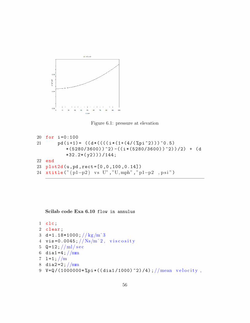
Figure 6.1: pressure at elevation

20 for i=0:100

21 pd(i+1)= ((d*((((i*(1+(4/( %pi^2)))^0.5)

*(5280/3600))^2) -((i*(5280/3600))^2))/2) + (d

*32.2*( y2)))/144;

22 end

23 plot2d(u,pd,rect =[0 ,0 ,100 ,0.14])

24 xtitle(” ( p1−p2 ) vs U”,”U, mph”,”p1−p2 , p s i ”)

Scilab code Exa 6.10 flow in annulus

1 clc;

2 clear;

3 d=1.18*1000; // kg /mˆ34 vis =0.0045; //Ns/mˆ2 , v i s c o s i t y5 Q=12; //ml/ s e c6 dia1 =4; //mm7 l=1; //m8 dia2 =2; //mm9 V=Q/(1000000* %pi*(( dia1 /1000) ^2) /4);//mean v e l o c i t y ,

56

m/ s e c10 Re=(d*V*dia1 /1000)/vis;

11 disp(” i s w e l l be low c r i t i c a l v a l u e o f 2100 so f l o wi s l amina r . ”,Re ,”a ) The Reynolds number ”)

12 pdiff =(8* vis*(l)*(12/1000000) /(%pi*(dia1 /2000) ^4))

/1000; //kPa13 disp(”kPa”,pdiff ,”The p r e s s u r e drop a l ong a 1 m

l e n g t h o f the tube which i s f a r from the tubee n t r a n c e so tha t the on ly component o f v e l o c i t yi s p a r a l l e l to the the tube a x i s=”)

14 // f o r f l o w i n the annu lus15 V1=Q/(1000000* %pi *((( dia1 /1000) ^2) -((dia2 /1000) ^2))

/4);//mean v e l o c i t y , m/ s e c16 Re1=d*((dia1 -dia2)/1000)*V1/vis;

17 disp(” i s w e l l be low c r i t i c a l v a l u e o f 2100 so f l o wi s l amina r . ”,Re1 ,”b ) The Reynolds number ”)

18 r1=dia1 /2000;

19 r2=dia2 /2000;

20 pdiff1 =((8* vis*(l)*(12/1000000) /(%pi))*((r1^4) -(r2

^4) -((((r1^2) -(r2^2))^2)/(log(r1/r2))))^(-1))

/1000; //kPa21 disp(”kPa”,pdiff1 ,”The p r e s s u r e drop a l ong a 1 m

l e n g t h o f the symmetr ic annu lus =”)22

23 rratio =0.001:0.001:0.5;

24 count =1;

25 for i=0.001:0.001:0.5

26 pratio(count)=1/((i^4) *((1/(i^4)) -1 -((((1/(i^2))

-1)^2)/log (1/i))));

27 count=count +1;

28 end

29 plot2d(rratio ,pratio ,rect =[0 ,0 ,0.5 ,8])

30 xtitle(” r i / ro vs p d i f f ( annu lus ) / p d i f f ( tube ) ”,” r i / ro ”,” p d i f f ( annu lus ) / p d i f f ( tube ) ”)

57

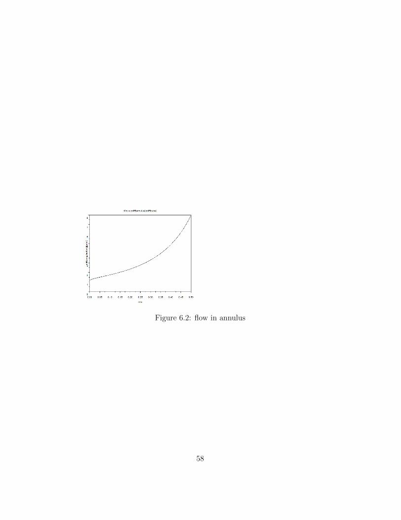
Figure 6.2: flow in annulus

58

Chapter 7

Dimensional AnalysisModelling and Similitude

Scilab code Exa 7.5 prototype performance prediction

1 clc;

2 clear;

3 D=0.1; //m4 H=0.3; //m5 v=50; //km/ hr6 Dm=20; //mm7 T=20; // d e g r e e C8 fm =49.9; //Hz ; f r e q u e n c y f o r the model9 // f=func (D,H,V, d , v i s )

10 // f=Tˆ(−1) ; D=l ; H=L ; V=L∗ (Tˆ(−1) ) ; d=M∗ (Lˆ(−3) ) ;v i s=M∗ (Lˆ(−1) ) ∗ (Tˆ(−1) )

11 // by a p p l y i n g p i theorem ,12 // ( f ∗D/V)=f u n c t ( (D/H) , ( d∗V∗D/ v i s ) )13 // hence ; Dm/Hm = D/H, dm∗Vm∗Dm/ vism = d∗V∗D/ v i s , and

( f ∗D/V) =(fm∗Dm/Vm)14 Hm=(Dm*H*1000/(D*1000));//mm15 V=v*1000/3600; //m/ s16 vism =1/1000; // kg /(m∗ s )17 vis =1.79/100000; // kg /(m∗ s )

59

18 d=1.23; // kg /(mˆ3)19 dm=998; // kg /(mˆ3)20 Vm=(vism*d*D*V*1000) /(vis*dm*Dm);//m/ s21 f=(V/Vm)*(Dm/(D*1000))*fm;//Hz22 disp(”mm”,Hm ,”The model d imens ion =”)23 disp(”m/ s ”,Vm ,”The v e l o c i t y at which the t e s t shou ld

be per fo rmed=”)24 disp(”Hz”,f,”The p r e d i c t e d p r o t o t y p e v o r t e x

s h r e d d i n g f r e q u e n c y =”)

Scilab code Exa 7.6 reynolds number similarity

1 clc;

2 clear;

3 D=2; // f t4 Q=30; // c f s5 Dm=3; // i n6 //Rem=Re ; hence (Vm∗Dm/ kvism ) =(V∗D/ k v i s ) ; where k v i s

i s k i n e m a t i c v i s c o s i t y7 // k v i s=kvism ; same f l u i d i s used f o r model and

p r o t o t y p e8 // (Vm/V) =(D/Dm)9 //Q=VA; hence Qm/Q = (Vm∗Am) /(V∗A) =(Dm/D)10 Qm=(Dm/12)*Q/D;// c f s11 disp(” c f s ”,Qm ,”The r e q u i r e d f l o w r a t e i n the model=”)12 Drat =0.04:0.01:1;

13 count =1;

14 for i=0.04:0.01:1

15 Vrat(count)=1/i;

16 count=count +1;

17 end

18 plot2d(Drat ,Vrat ,rect =[0 ,0,1 ,25])

19 xtitle(”Vm/V vs Dm/D”,”Dm/D”,”Vm/V”)

60

Figure 7.1: reynolds number similarity

Scilab code Exa 7.7 predicting prototype performance

1 clc;

2 clear;

3 V=240; //mph4 ratio =1/10;

5 Vair =240; //mph6 Fm=1; // l b ; Fm =drag f o r c e on model7 p=14.7; // p s i a ; s t andard a tmosphe r i c p r e s s u r e8 //Re=Rem9 // ( d∗V∗ l / v i s ) =(dm∗Vm∗ lm/ vism )

10 // he r e Vm=V and lm/ l=r a t i o11 // assumpt ion made i s tha t an i n c r e a s e i n p r e s s u r e

does not s i g n i f i c a n t l y change v i s c o s i t y12 drat=V/( ratio*Vair);// where d ra t=dm/d13 // f o r an i d e a l gas p=d∗R∗T14 //T=Tm15 // hence , pm/p=dm/d ; pm/p=pra t

61

16 pm=p*drat;

17 //F / ( 0 . 5 ∗ d ∗ (Vˆ2) ∗ ( l ˆ2) )=Fm/ ( 0 . 5 ∗dm∗ (Vmˆ2) ∗ ( lm ˆ2) )18 F=(1/ drat)*((V/Vair)^2) *((1/ ratio)^2)*Fm;

19 disp(” p s i a ”,pm ,”The r e q u i r e d a i r p r e s s u r e i n thet u n n e l=”)

20 disp(” l b ”,F,”The c o r r o s p o n d i n g drag on the p r t o t y p ef o r a 1 l b drag on the model=”)

Scilab code Exa 7.8 froude number similarity

1 clc;

2 clear;

3 w=20; //m4 Q=125; // (mˆ3) / s5 ratio =1/15;

6 t=24; // hours7 wm=ratio*w;//m8 //Vm/(gm∗ lm ) ˆ 0 . 5 = V/( g∗ l ) ˆ 0 . 59 //gm=g10 //Q=VA and lm/ l =1/1511 // hence Qm/Q = ( ( lm/ l ) ˆ 0 . 5 ) ∗ ( ( lm/ l ) ˆ2) = r a t i o ˆ 2 . 512 Qm=( ratio ^2.5)*Q;

13 //V=l / t14 //tm/ t =(V/Vm) ∗ ( lm/ l )=r a t i o ˆ 0 . 515 tm=( ratio ^0.5)*t;// hours16 disp(”m”,wm ,”The r e q u i r e d model width=”)17 disp(” (mˆ3) / s ”,Qm ,”The r e q u i r e d model f l o w r a t e=”)18 disp(” h r s ”,tm ,”The o p e r a t i n g t ime f o r the model=”)19 lrat =0.01:0.01:0.5;

20 count =1;

21 for i=0.01:0.01:0.5

22 tmodel(count)=(i^0.5)*t;

23 count=count +1;

24 end

25 plot2d(lrat ,tmodel ,rect =[0 ,0 ,0.5 ,20])

62

Figure 7.2: froude number similarity

26 xtitle(”tm vs lm/ l ”,”lm/ l ”,”tm , hr ”)

63

Chapter 8

Pipe flow

Scilab code Exa 8.1 calculating time required

1 clc;

2 clear;

3 T1=50; // d e g r e e f a r e n h e i t4 D=0.73; // i n5 vol =0.0125; // f t ˆ36 T2=140; // d e g r e e f a r e n h e i t7

8 vis1 =2.73/100000; // l b ∗ s / f t ˆ2 at 50 d e g r e e f a r e n h e i t9 vis2 =0.974/100000; // l b ∗ s / f t ˆ2 at 140 d e g r e e

f a r e n h e i t10

11 // f o r 50 d e g r e e f a r e n h e i t12 // i f f l o w i s laminar , maximum Re=2100; Re=d∗V∗D/ v i s13 V1 =2100* vis1 /(1.94*D/12);

14 t1=vol/(%pi*((D/12) ^2)/4*V1);

15 // i f f l o w i s t u r b u l e n t , minimum Re=400016 V2 =4000* vis1 /(1.94*D/12);

17 t2=vol/(%pi*((D/12) ^2)/4*V2);

18

19 // f o r 140 d e g r e e f a r e n h e i t20 // i f f l o w i s laminar , maximum Re=2100; Re=d∗V∗D/ v i s

64

21 V3 =2100* vis2 /(1.94*D/12);

22 t3=vol/(%pi *((D/12) ^2)/4*V3);

23 // i f f l o w i s t u r b u l e n t , minimum Re=400024 V4 =4000* vis2 /(1.94*D/12);

25 t4=vol/(%pi *((D/12) ^2)/4*V4);

26

27 disp(” For l amina r f l o w ”)28 disp(” s e c o n d s ”,t1 ,”The t ime taken to f i l l the g l a s s

at 50 d e g r e e F=”)29 disp(” s e c o n d s ”,t3 ,”The t ime taken to f i l l the g l a s s

100 d e g r e e F=”)30 disp(” For t u r b u l e n t f l o w : ”)31 disp(” s e c o n d s ”,t2 ,”The t ime taken to f i l l the g l a s s

at 50 d e g r e e F=”)32 disp(” s e c o n d s ”,t4 ,”The t ime taken to f i l l the g l a s s

at 140 d e g r e e F=”)

Scilab code Exa 8.2 laminar pipe flow

1 clc;

2 clear;

3 vis =0.4; //Ns /(mˆ2)4 d=900; // kg /(mˆ3)5 D=0.02; //m6 Q=2.0*(10^ -5);// (mˆ3) / s7 x1=0;

8 x2=10; //m9 p1=200; //kPa

10 x3=5; //m11 V=Q/(%pi*(D^2)/4);//m/ s12 Re=d*V*D/vis;

13 disp(” Hence the f l o w i s l amina r . ”,Re ,”a ) Reynoldsnumber =”)

14 pdiff =128* vis*(x2-x1)*Q/(%pi*(D^4) *1000);

15 // f o r pa r t b0 p1=p2 ; Q=%pi ∗ ( p d i f f −(sw∗ l ∗ s i n ( ang ) ) ) ∗ (

65

Dˆ4) /(128∗ v i s ∗ l )16 ang=(asin ( -128* vis*Q/(%pi*d*9.81*(D^4))))*180/ %pi;

17 // s i n c e s i n ( ang ) doesn= not depend on p d i f f , the thep r e s s u r e i s c o n s t a n t a l l a l ong the p ipe

18 // hence f o r c )19 p3=p1;//kPa20 disp(”kPa . ”,pdiff ,”The p r e s s u r e drop r e q u i r e d i f the

p ip e i s h o r i z o n t a l=”)21 disp(” d e g r e e s . ”,ang ,”b ) The a n g l e o f the h i l l the

p ip e must be on i f the o i l i s to f l o w at the samer a t e as a ) but with ( p1=p2 ) =”)

22 disp(”kPa”,p3 ,” c ) For c o n d i t i o n s o f pa r t b ) , thep r e s s u r e at x3=5 m = ”)

Scilab code Exa 8.3 net force calculation

1 clc;

2 clear;

3 T=[60 80 100 120 140 160]; // d e g r e e F4 d=[2.07 2.06 2.05 2.04 2.03 2.02]; // ( s l u g s /( f t ˆ3) )5 vis =[0.04 0.019 0.0038 0.00044 0.000092 0.000023]; //

l b ∗ s e c /( f t ˆ2)6 Q=0.5; // ( f t ˆ3) / s e c7 T1=100; // d e g r e e F8 l=6; // f t9 D=3; // i n

10 //Q=K∗ p d i f f ; where p d i f f=p1−p211 // hence K=%pi ∗ (Dˆ4) /(128∗ v i s ∗ l )12 count =1;

13 for i=1:6

14 K(i)=(%pi*((D/12) ^4))/(128* vis(i)*l);

15 end

16 plot2d(T,K,logflag= ’ n l ’ )17 xtitle(”K vs T”,”T, d e g r e e F”,”K, ( f t ˆ5) /( l b . s e c ) ”)18 pdiff =(128*Q*vis(3)*l)/(%pi*((D/12) ^4));//when

66

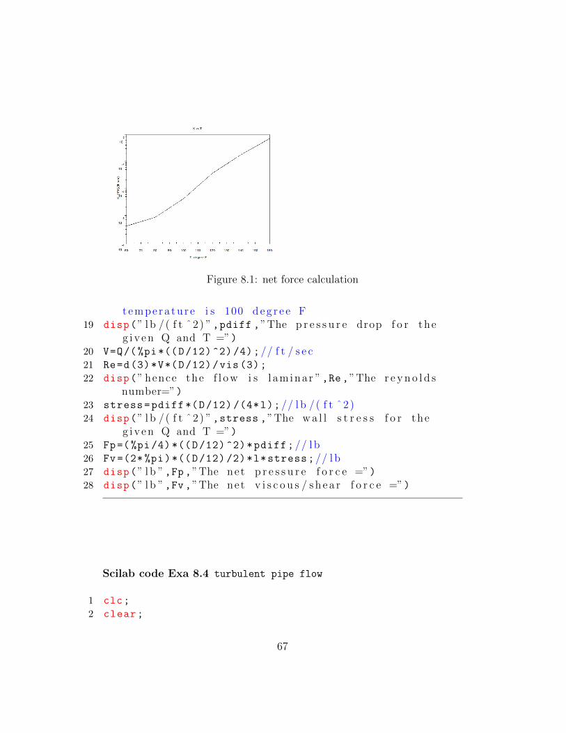
Figure 8.1: net force calculation

t empera tu re i s 100 d e g r e e F19 disp(” l b /( f t ˆ2) ”,pdiff ,”The p r e s s u r e drop f o r the

g i v e n Q and T =”)20 V=Q/(%pi*((D/12) ^2)/4);// f t / s e c21 Re=d(3)*V*(D/12)/vis (3);

22 disp(” hence the f l o w i s l amina r ”,Re ,”The r e y n o l d snumber=”)

23 stress=pdiff*(D/12) /(4*l);// l b /( f t ˆ2)24 disp(” l b /( f t ˆ2) ”,stress ,”The w a l l s t r e s s f o r the

g i v e n Q and T =”)25 Fp=(%pi/4) *((D/12) ^2)*pdiff;// l b26 Fv=(2* %pi)*((D/12) /2)*l*stress;// l b27 disp(” l b ”,Fp ,”The net p r e s s u r e f o r c e =”)28 disp(” l b ”,Fv ,”The net v i s c o u s / s h e a r f o r c e =”)

Scilab code Exa 8.4 turbulent pipe flow

1 clc;

2 clear;

67

3 T=20; // d e g r e e C4 d=998; // kg /(mˆ3)5 kvis =1.004*(10^ -6);// (mˆ2) / s ; where k v i s=k i n e m a t i c

v i s c o s i t y6 D=0.1; //m7 Q=0.04; // (mˆ3) / s e c8 pgrad =2.59; //kPa/m; where pgrad i s p r e s s u r e g r a d i e n t9 r=0.025; //m10 stress=D*( pgrad *1000) /(4*1);//N/(mˆ2)11 uf=( stress/d)^0.5; //m/ s e c ; where u f i s f r i c t i o n a l

v e l o c i t y12 ts=5* kvis *1000/( uf);//mm; where t s i s the t h i c k n e s s

o f the v i s c o u s s u b l a y e r13 disp(”mm”,ts ,”The t h i c k n e s s o f the v i s c o u s s u b l a y e r=

”)14 V=Q/(%pi*(D^2)/4);//m/ s15 Re=V*D/kvis;

16 disp(” hence the f l o w i s t u r b u l e n t . ”,Re ,”The r e y n o l d snumber=”)

17 n=8.4; // from t u r b u l e n t f l o w v e l o c i t y p r o f i l e diagram18

19 //Q=(%pi ) ∗ (Rˆ2) ∗V20 R=1; // assumpt ion21 // l e t Q/Vc=x22 x=integrate( ’ ((1−( r /R) ) ˆ(1/ n ) ) ∗ (2∗%pi∗ r ) ’ , ’ r ’ ,0,R);23 q=%pi*(R^2)*V;

24 Vc=q/x;//m/ s25 disp(”m/ s ”,Vc ,”The approx imate c e n t e r l i n e v e l o c i t y=”

)

26 stress1 =(2* stress*r)/D;//N/(mˆ2)27 //d ( uavg ) / dr=u r a t e=−(Vc /( n∗R) ) ∗((1−( r /R) ) ˆ((1−n ) /n ) )

; where uavg=ave rage v e l o c i t y28 urate=-(Vc/(n*(D/2)))*((1-(r/(D/2)))^((1-n)/n));// s

ˆ(−1)29 stresslam=-(kvis*d*urate);//N/(mˆ2)30 stressratio =(stress1 -stresslam)/stresslam;

31 disp(stressratio ,”The r a t i o o f t eh t u r b u l e n t tol amina r s t r e s s at a p o i n t midway between the

68

c e n t r e l i n e and the p ipe w a l l =”)

Scilab code Exa 8.5 pressure drop calculation

1 clc;

2 clear;

3 D=4; //mm4 V=50; //m/ s e c5 l=0.1; //m6 d=1.23; // kg /(mˆ3)7 vis =1.79/100000; //N∗ s e c /(mˆ2)8 Re=d*V*(D/1000)/vis;

9 // i f f l o w i s l amina r10 f=64/Re;

11 pdiff=f*l*0.5*d*(V^2)/((D/1000) *1000);//kPa12 disp(”kPa”,pdiff ,”The p r e s s u r e drop i f the f l o w i s

l amina r=”)13 // i f f l o w i s t u r b u l e n t14 // roughne s s =0 .0015 ; hence f =0.02815 f1 =0.028;

16 pdiff1=f1*l*0.5*d*(V^2) /((D/1000) *1000);//kPa17 disp(”kPa”,pdiff1 ,”The p r e s s u r e drop i f f l o w i s

t u r b u l e n t=”)

Scilab code Exa 8.6 minor losses calculation

1 clc;

2 clear;

3 A=[22 28 35 35 4 4 10 18 22];

4 V=[36.4 28.6 22.9 22.9 200 200 80 44.4 36.4];

5 //minimum area i s at l o c a t i o n 5 , hence max v e l o c i t yi s at 5

6 c5 =(1.4**1716*(460+59))^0.5; // f t / s e c

69

7 Ma5=V(5)/c5;

8 // a p p l y i n g ene rgy e q u a t i o n between l o c a t i o n s 1 and9

9 //hL=hp=(p1−p9 ) /sw=p d i f f /sw10 //Pa=sw∗Q∗hp=sw∗A( 5 ) ∗V( 5 ) ∗hL11 KLcorner =0.2;

12 KLdif =0.6;

13 KLscr =4;

14 hL=(( KLcorner *(((V(7))^2)+((V(8))^2)+((V(2))^2)+((V

(3))^2))) + (KLdif *(((V(6))^2))) + (KLcorner *((V

(5))^2)) + (KLscr *((V(4))^2)))/(2*32.2);// f t15 Pa =0.0765*A(5)*V(5)*hL/550; //hp16 pdiff =0.0765* hL /144; // p s i17 disp(” p s i ”,pdiff ,”The v a l u e o f ( p1−p9 )=”)18 disp(”hp”,Pa ,”The hor sepower s u p p l i e d to the f l u i d

by the fan=”)19 v=50:300;

20 count =1;

21 for i=50:300

22 power(count)=0.0765*(((( KLcorner *((A(5)*i/A(7))

^2) +((A(5)*i/(A(8)))^2) +((A(5)*i/A(2))^2)+((A

(5)*i/A(3))^2))) + (KLdif *(((A(5)*i/A(6))^2)))

+ (KLcorner *((i)^2)) + (KLscr *((A(5)*i/A(4))

^2)))/(2*32.2))*(A(5))*i/550;

23 count=count +1;

24 end

25 plot2d(v,power ,rect =[0 ,0 ,300 ,250])

26 xtitle(”Pa vs V5”,”V5 , f t / s e c ”,”Pa , hp”)

Scilab code Exa 8.7 duct size determination

1 clc;

2 clear;

70

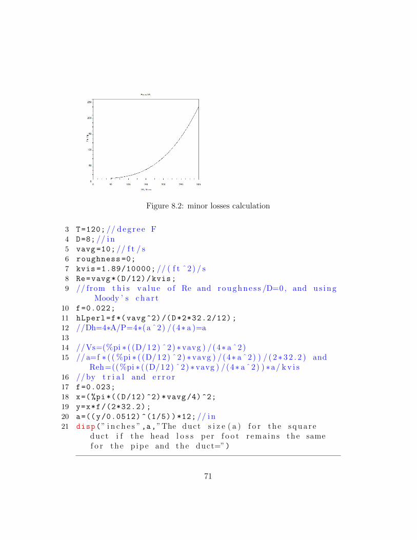
Figure 8.2: minor losses calculation

3 T=120; // d e g r e e F4 D=8; // i n5 vavg =10; // f t / s6 roughness =0;

7 kvis =1.89/10000; // ( f t ˆ2) / s8 Re=vavg*(D/12)/kvis;

9 // from t h i s v a l u e o f Re and roughne s s /D=0 , and u s i n gMoody ’ s c h a r t

10 f=0.022;

11 hLperl=f*(vavg ^2)/(D*2*32.2/12);

12 //Dh=4∗A/P=4∗( a ˆ2) /(4∗ a )=a13

14 //Vs=(%pi ∗ ( (D/12) ˆ2) ∗vavg ) /(4∗ a ˆ2)15 // a=f ∗ ( ( %pi ∗ ( (D/12) ˆ2) ∗vavg ) /(4∗ a ˆ2) ) / ( 2 ∗ 3 2 . 2 ) and

Reh=(( %pi ∗ ( (D/12) ˆ2) ∗vavg ) /(4∗ a ˆ2) ) ∗a/ k v i s16 // by t r i a l and e r r o r17 f=0.023;

18 x=(%pi*((D/12) ^2)*vavg /4)^2;

19 y=x*f/(2*32.2);

20 a=((y/0.0512) ^(1/5))*12; // i n21 disp(” i n c h e s ”,a,”The duct s i z e ( a ) f o r the squa r e

duct i f the head l o s s per f o o t rema ins the samef o r the p ip e and the duct=”)

71

Scilab code Exa 8.8 determining pressure drop

1 clc;

2 clear;

3 T=60; // d e g r e e F4 D=0.0625; // f t5 Q=0.0267; // ( f t ˆ3) / s e c6 Df=0.5; // i n7 l1=15; // f t8 l2=10; // f t9 l3=5; // f t

10 l4=10; // f t11 l5=10; // f t12 l6=10; // f t13 V1=Q/(%pi*(D^2)/4);// f t / s e c14 V2=Q/(%pi *((Df/12) ^2) /4);// f t / s e c15 d=1.94; // s l u g s / f t16 vis =2.34/100000; // l b ∗ s e c /( f t ˆ2)17 Re=d*V1*D/vis;

18 disp(” hence the f l o w i s t u r b u l e n t ”,Re ,”The r e y n o l d snumber =”)

19 // a p p l y i n g ene rgy e q u a t i o n between p o i n t s 1 and 220 //when a l l head l o s s e s a r e exc luded21 p1=(d*32.2*( l2+l4))+(0.5*d*((V2^2) -(V1^2)));// l b /( f t

ˆ2)22 disp(” p s i ”,p1/144,”a ) The p r e s s u r e at p o i n t 1 when

a l l head l o s s e s a r e n e g l e c t e d=”)23 // i f major l o s s e s a r e i n c l u d e d24 f=0.0215;

25 hLmajor=f*(l1+l2+l3+l4+l5+l6)*(V1^2)/(D*2*32.2);

26 p11=p1+(d*32.2* hLmajor);// l b /( f t ˆ2)27 disp(” p s i ”,p11/144,”b ) The p r e s s u r e at p o i n t 1 when

on ly major head l o s s e s a r e i n c l u d e d=”)28 // i f major and minor l o s s e s a r e i n c l u d e d

72

29 KLelbow =1.5;

30 KLvalve =10;

31 KLfaucet =2;

32 hLminor =( KLvalve +(4* KLelbow)+KLfaucet)*(V1^2)

/(2*32.2);

33 p12=p11+(d*32.2* hLminor);// l b /( f t ˆ2)34 disp(” p s i ”,p12/144,” c ) The p r e s s u r e at p o i n t 1 when

both major and minor head l o s s e s a r e i n c l u d e d=”)35 H=(p1 /(32.2*1.94))+(V1*V1 /(2*32.2));// f t36 dist =0:60;

37 for i=0:15

38 press(i+1)=p1 /144;

39 press1(i+1)=((d*32.2*( l2+l4))+(0.5*d*((V2^2) -(V1

^2)))+(d*32.2*(f*(l1+l2+l3+l4+l5+l6-i)*(V1^2)

/(D*2*32.2)))+(d*32.2*( KLvalve +(4* KLelbow)+

KLfaucet)*(V1^2) /(2*32.2)))/144;

40 head(i+1)=H;

41 head1(i+1)=(( press1(i+1))*144/(32.2*1.94))+((V1

^2) /(2*32.2));

42 end

43 for i=16:25

44 press(i+1)=((d*32.2*(( l2+l4) -(i-15)))+(0.5*d*((

V2^2) -(V1^2))))/144;

45 press1(i+1)=((d*32.2*(( l2+l4)-(i-15)))+(0.5*d*((

V2^2) -(V1^2)))+(d*32.2*f*(l1+l2+l3+l4+l5+l6 -i

)*(V1^2)/(D*2*32.2))+(d*32.2*( KLvalve +(3*

KLelbow)+KLfaucet)*(V1^2) /(2*32.2)))/144;

46 head(i+1)=H;

47 head1(i+1)=( press1(i+1) *144/(32.2*1.94))+((V1^2)

/(2*32.2))+(i-l1);

48 end

49 for i=26:30

50 press(i+1)=((d*32.2*(( l2+l4) -(25-15)))+(0.5*d*((

V2^2) -(V1^2))))/144;

51 press1(i+1)=((d*32.2*(( l2+l4) -(25-15)))+(0.5*d

*((V2^2) -(V1^2)))+(d*32.2*(f*(l1+l2+l3+l4+l5

+l6 -i)*(V1^2)/(D*2*32.2)))+(d*32.2*( KLvalve

+(2* KLelbow)+KLfaucet)*(V1^2) /(2*32.2)))

73

/144;

52 head(i+1)=H;

53 head1(i+1)=( press1(i+1) *144/(32.2*1.94))+((V1^2)

/(2*32.2))+l2;

54 end

55 for i=31:40

56 press(i+1)=((d*32.2*(( l2+l4) -(i-l1-l3)))+(0.5*d

*((V2^2) -(V1^2))))/144;

57 press1(i+1)=((d*32.2*(( l2+l4)-(i-l1-l3)))+(0.5*d

*((V2^2) -(V1^2)))+(d*32.2*(f*(l1+l2+l3+l4+l5+

l6 -i)*(V1^2)/(D*2*32.2)))+(32.2*d*( KLvalve +(

KLelbow)+KLfaucet)*(V1^2) /(2*32.2)))/144;

58 head(i+1)=H;

59 head1(i+1)=( press1(i+1) *144/(32.2*1.94))+((V1^2)

/(2*32.2))+(i-(l1+l3));

60 end

61 for i=41:50

62 press(i+1)=((d*32.2*(( l2+l4) -(40-l1-l3)))+(0.5*d

*((V2^2) -(V1^2))))/144;

63 press1(i+1)=((d*32.2*(( l2+l4) -(40-l1 -l3)))+(0.5*

d*((V2^2) -(V1^2)))+(d*32.2*(f*(l1+l2+l3+l4+l5

+l6 -i)*(V1^2)/(D*2*32.2)))+(d*32.2*( KLvalve+

KLfaucet)*(V1^2) /(2*32.2)))/144;

64 head(i+1)=H;

65 head1(i+1)=( press1(i+1) *144/(32.2*1.94))+((V1^2)

/(2*32.2))+(l2+l4);

66 end

67 for i=51:60

68 press(i+1)=((d*32.2*(( l2+l4) -(40-l1-l3)))+(0.5*d

*((V2^2) -(V1^2))))/144;

69 press1(i+1)=((d*32.2*(( l2+l4) -(40-l1 -l3)))

+(0.5*d*((V2^2) -(V1^2)))+(d*32.2*(f*(l1+l2+

l3+l4+l5+l6 -i)*(V1^2)/(D*2*32.2)))+d*32.2*((

KLfaucet)*(V1^2) /(2*32.2)))/144;

70 head(i+1)=H;

71 head1(i+1)=( press1(i+1) *144/(32.2*1.94))+((V1^2)

/(2*32.2))+(l2+l4);

72 end

74

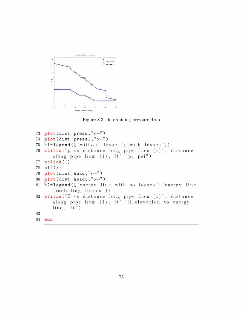
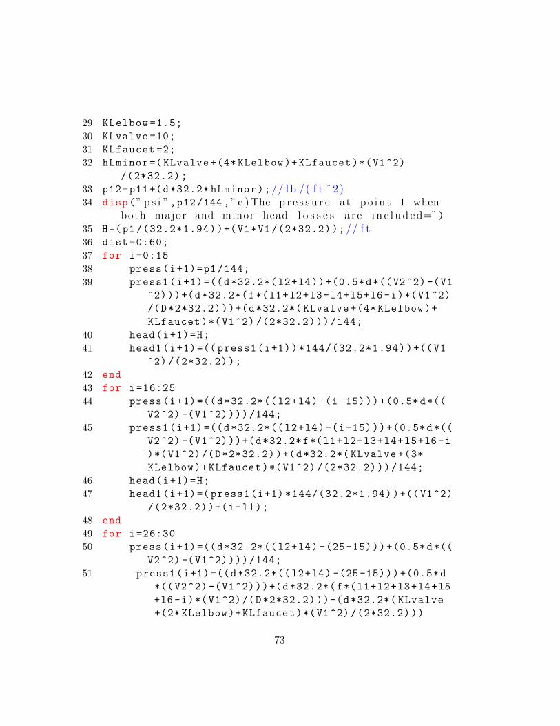
Figure 8.3: determining pressure drop

73 plot(dist ,press ,”o−”)74 plot(dist ,press1 ,”x−”)75 h1=legend ([ ’ w i thout l o s s e s ’ ; ’ with l o s s e s ’ ])76 xtitle(”p vs d i s t a n c e l ong p ipe from ( 1 ) ”,” d i s t a n c e

a l ong p ipe from ( 1 ) , f t ”,”p , p s i ”)77 xclick (1);

78 clf();

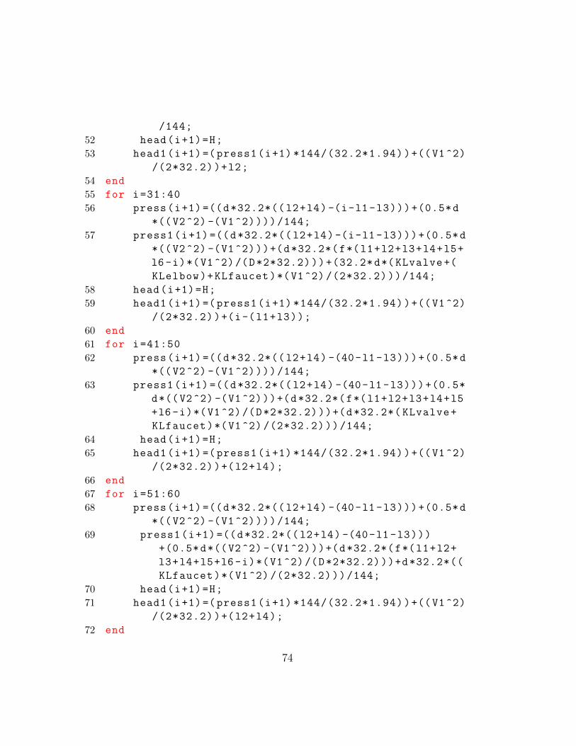
79 plot(dist ,head ,”o−”)80 plot(dist ,head1 ,”x−”)81 h2=legend ([ ’ ene rgy l i n e with no l o s s e s ’ ; ’ ene rgy l i n e

i n c l u d i n g l o s s e s ’ ])82 xtitle(”H vs d i s t a n c e l ong p ipe from ( 1 ) ”,” d i s t a n c e

a l ong p ipe from ( 1 ) , f t ”,”H, e l e v a t i o n to ene rgyl i n e , f t ”)

83

84 end

75

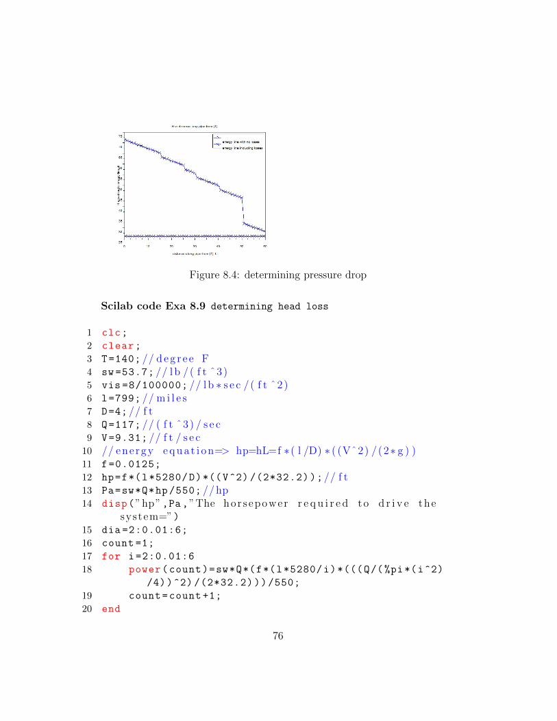
Figure 8.4: determining pressure drop

Scilab code Exa 8.9 determining head loss

1 clc;

2 clear;

3 T=140; // d e g r e e F4 sw =53.7; // l b /( f t ˆ3)5 vis =8/100000; // l b ∗ s e c /( f t ˆ2)6 l=799; // m i l e s7 D=4; // f t8 Q=117; // ( f t ˆ3) / s e c9 V=9.31; // f t / s e c

10 // ene rgy e q u a t i o n=> hp=hL=f ∗ ( l /D) ∗ ( (Vˆ2) /(2∗ g ) )11 f=0.0125;

12 hp=f*(l*5280/D)*((V^2) /(2*32.2));// f t13 Pa=sw*Q*hp/550; //hp14 disp(”hp”,Pa ,”The hor sepower r e q u i r e d to d r i v e the

system=”)15 dia =2:0.01:6;

16 count =1;

17 for i=2:0.01:6

18 power(count)=sw*Q*(f*(l*5280/i)*(((Q/(%pi*(i^2)

/4))^2) /(2*32.2)))/550;

19 count=count +1;

20 end

76

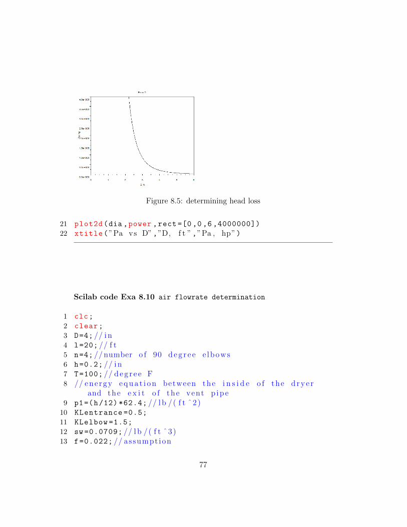
Figure 8.5: determining head loss

21 plot2d(dia ,power ,rect =[0 ,0 ,6 ,4000000])

22 xtitle(”Pa vs D”,”D, f t ”,”Pa , hp”)

Scilab code Exa 8.10 air flowrate determination

1 clc;

2 clear;

3 D=4; // i n4 l=20; // f t5 n=4; // number o f 90 d e g r e e e lbows6 h=0.2; // i n7 T=100; // d e g r e e F8 // ene rgy e q u a t i o n between the i n s i d e o f the d r y e r

and the e x i t o f the vent p ip e9 p1=(h/12) *62.4; // l b /( f t ˆ2)

10 KLentrance =0.5;

11 KLelbow =1.5;

12 sw =0.0709; // l b /( f t ˆ3)13 f=0.022; // assumpt ion

77

14 // hence ,15 V=((p1/sw)*2*32.2/(1+(f*l/(D/12))+KLentrance +(n*

KLelbow)))^0.5; // f t / s e c16 Q=V*(%pi*((D/12) ^2)/4);// ( f t ˆ3) / s e c17 disp(” ( f t ˆ3) / s e c ”,Q,”The f l o w r a t e=”)

Scilab code Exa 8.11 flowrate through turbine

1 clc;

2 clear;

3 Pa=50; //hp4 D=1; // f t5 l=300; // f t6 f=0.02;

7 z1=90; // f t8 // ene rgy e q u a t i o n between the s u r f a c e o f the l a k e

and the o u t l e t o f the p ip e9 // p1=V1=p2=z2 =0; V2=V

10 //hL=f ∗ l ∗ (Vˆ2) /(D ∗2∗ g )11 //hT=Pa /( sw∗%pi ∗ (Dˆ2) ∗V/4)12 c1=(Pa *550) /(62.4* %pi*(D^2)/4) // 56113 c2=f*l/(D*2*32.2) // 0 . 0 9 3 214 fn=poly([c1 (-z1) 0 ((1/(2*32.2))+(c2))],”V”,” c ”);15 r=roots(fn);

16 V1=r(1);// f t / s e c17 V2=r(2);// f t / s e c18 Q1=(%pi*(D^2)/4)*V1;// ( f t ˆ3) / s e c19 Q2=(%pi*(D^2)/4)*V2;// ( f t ˆ3) / s e c20 disp(” ( f t ˆ3) / s e c ”,Q2 ,”and”,” ( f t ˆ3) / s e c ”,Q1 ,”The

p o s s i b l e f l o w r a t e s a r e=”)

Scilab code Exa 8.12 minimum pipe diameter

78

1 clc;

2 clear;

3 roughness =0.0005; // f t4 Q=2; // ( f t ˆ3) / s e c5 pd=0.5; // p s i ; where pd=p r e s s u r e drop6 l=100; // f t7 d=0.00238; // s l u g s /( f t ˆ3)8 vis =3.74*(10^( -7));// l b ∗ s e c /( f t ˆ2)9 x=Q/(%pi/4);// where x =V∗ (Dˆ2)

10 // ene rgy e q u a t i o n with z1=z2 and V1=V211 y=l*d*(x^2) *0.5/( pd *144);// where y=(Dˆ5) / f12 f=0.027; // u s i n g r e y n o l d s number , r oughne s s and moody

’ s c h a r t13 D=(y*f)^(1/5);// f t14 disp(” f t ”,D,”The d iamete r o f the p ip e shou ld be =”)15 q=0.01:0.01:3;

16 count =1;

17 for i=0.01:0.01:3

18 dia(count)=((l*d*((i/(%pi /4))^2) *0.5/( pd *144))*f

)^(1/5);

19 count=count +1;

20 end

21 plot2d(q,dia ,rect =[0 ,0 ,3 ,0.25])

22 xtitle(”D vs Q”,”Q, ( f t ˆ3) / s e c ”,”D, f t ”)

Scilab code Exa 8.13 pipe diameter calculation

1 clc;

2 clear;

3 T=60; // d e g r e e F4 kvis =1.28*(10^( -5));// ( f t ˆ2) / s e c5 l=1700; // f t6 roughness =0.0005; // f t

79

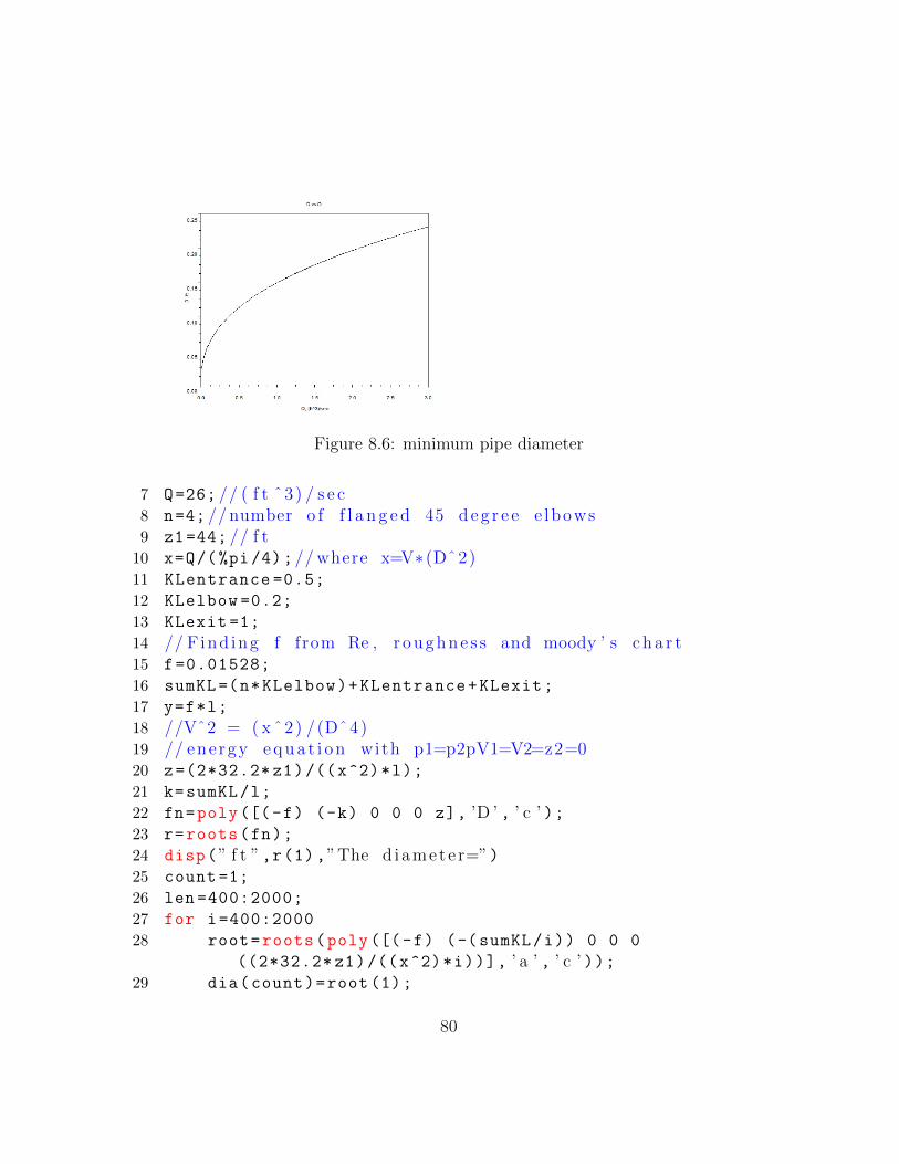
Figure 8.6: minimum pipe diameter

7 Q=26; // ( f t ˆ3) / s e c8 n=4; // number o f f l a n g e d 45 d e g r e e e lbows9 z1=44; // f t

10 x=Q/(%pi/4);// where x=V∗ (Dˆ2)11 KLentrance =0.5;

12 KLelbow =0.2;

13 KLexit =1;

14 // F ind ing f from Re , r oughne s s and moody ’ s c h a r t15 f=0.01528;

16 sumKL=(n*KLelbow)+KLentrance+KLexit;

17 y=f*l;

18 //Vˆ2 = ( x ˆ2) /(Dˆ4)19 // ene rgy e q u a t i o n with p1=p2pV1=V2=z2=020 z=(2*32.2* z1)/((x^2)*l);

21 k=sumKL/l;

22 fn=poly([(-f) (-k) 0 0 0 z], ’D ’ , ’ c ’ );23 r=roots(fn);

24 disp(” f t ”,r(1),”The d iamete r=”)25 count =1;

26 len =400:2000;

27 for i=400:2000

28 root=roots(poly([(-f) (-(sumKL/i)) 0 0 0

((2*32.2* z1)/((x^2)*i))], ’ a ’ , ’ c ’ ));29 dia(count)=root (1);

80

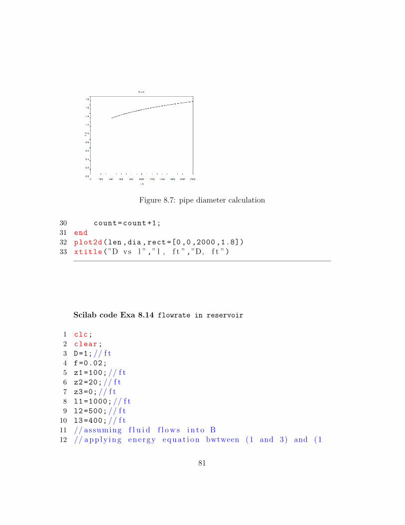
Figure 8.7: pipe diameter calculation

30 count=count +1;

31 end

32 plot2d(len ,dia ,rect =[0 ,0 ,2000 ,1.8])

33 xtitle(”D vs l ”,” l , f t ”,”D, f t ”)

Scilab code Exa 8.14 flowrate in reservoir

1 clc;

2 clear;

3 D=1; // f t4 f=0.02;

5 z1=100; // f t6 z2=20; // f t7 z3=0; // f t8 l1 =1000; // f t9 l2=500; // f t

10 l3=400; // f t11 // assuming f l u i d f l o w s i n t o B12 // a p p l y i n g ene rgy e q u a t i o n bwtween (1 and 3) and (1

81

and 2) and u s i n g the r e l a t i o n V1=V2+V313 c1=z1 *32.2*2/(f*l1);

14 c2=(z1-z2)*32.2*2/(f*l1);

15 x=(c1-c2)/(l3/l1);// 16016 y=(l2/l1)/(l3/l1);// 1 . 2 517 a=c2 -x;// 9818 b=(a*2*(y+(l2/l1)));// 53919 c=4*x+b;// 117920 d=-((y+(l2/l1))^2) +(4*y);// −2.562521 e=-(a^2);//−960422 fn=poly([e 0 c 0 d], ’V2 ’ , ’ c ’ );23 r=roots(fn);

24 V2=r(1);

25 V1=(c2 -(l2/l1)*V2)^0.5;

26 A=(%pi /4*(D^2));

27 Q1=V1*A;

28 Q2=V2*A;

29 Q3=Q1-Q2;

30 disp(” ( f t ˆ3) / s e c ”,Q1 ,”Q1 ( out o f A)=”)31 disp(” ( f t ˆ3) / s e c ”,Q2 ,”Q2 ( i n t o B)=”)32 disp(” ( f t ˆ3) / s e c ”,Q3 ,”Q3 ( i n t o C)=”)

Scilab code Exa 8.15 diameter of nozzle

1 clc;

2 clear;

3 D=60; //mm4 pdiff =4; //kPa5 Q=0.003; // (mˆ3) / s e c6 d=789; // kg /(mˆ3)7 vis =1.19*(10^( -3));//N∗ s e c /(mˆ2)8 Re=d*4*Q/(%pi*D*vis);

9 // assuming B=d i a /D=0.577 , where d i a=d iamete r o fn oz z l e , and o b t a i n i n g Cn from Re as 0 . 9 7 2

10 Cn =0.972;

82

11 B=0.577;

12 dia =((4*Q/(Cn*%pi))/((2* pdiff *1000/(d*(1-(B^4))))

^0.5))^0.5;

13 disp(”mm”,dia*1000,” Diameter o f the n o z z l e=”)

83

Chapter 9

External Flow Past Bodies

Scilab code Exa 9.1 lift and drag

1 clc;

2 clear;

3 U=25; // f t / s e c4 p=0; // gage5 b=10; // f t6 t=1.24*(10^ -3);// where t=s t r e s s ∗ ( x ˆ 0 . 5 )7 a=0.744; // where a=p /(1−(( y ˆ2) /4) )8 p1= -0.893; // l b /( f t ˆ2)9 drag1 =2* integrate( ’ t ∗b /( x ˆ 0 . 5 ) ’ , ’ x ’ ,0,4);

10 drag2=integrate( ’ ( ( ( a ∗(1−(( y ˆ2) /4) ) ) )−p1 ) ∗b ’ , ’ y ’,-2,2);

11 disp(” l b ”,drag1 ,”The drag when p l a t e i s p a r a l l e l tothe upstream f l o w=”)

12 disp(” l b ”,drag2 ,”The drag when p l a t e i sp e r p e n d i c u l a r to the upstream f l o w=”)

Scilab code Exa 9.5 boundary layer transition

84

1 clc;

2 clear;

3 U=10; // f t / s e c4 Twater =60; // d e g r e e F5 Tglycerin =68; // d e g r e e F6 kviswater =1.21*(10^ -5);// ( f t ˆ2) / s e c7 kvisair =1.57*(10^ -4);// ( f t ˆ2) / s e c8 kvisglycerin =1.28*(10^ -2);// ( f t ˆ2) / s e c9 Re =5*(10^5);// assumpt ion10 xcrwater=kviswater*Re/U;// f t11 xcrair=kvisair*Re/U;// f t12 xcrglycerin=kvisglycerin*Re/U;// f t13 btwater =5*( kviswater*xcrwater/U)^0.5; // f t ; where bt=

t h i c k n e s s o f boundary l a y e r14 btair =5*( kvisair*xcrair/U)^0.5; // f t15 btglycerin =5*( kvisglycerin*xcrglycerin/U)^0.5; // f t16 disp(”a )WATER”)17 disp(,” f t ”,xcrwater ,” l o c a t i o n at which boundary

l a y e r becomes t u r b u l e n t=”)18 disp(” f t ”,btwater ,” Th i ckne s s o f the boundary l a y e r=”

)

19 disp(”b )AIR”)20 disp(,” f t ”,xcrair ,” l o c a t i o n at which boundary l a y e r

becomes t u r b u l e n t=”)21 disp(” f t ”,btair ,” Th i ckne s s o f the boundary l a y e r=”)22 disp(” c )GLYCERIN”)23 disp(,” f t ”,xcrglycerin ,” l o c a t i o n at which boundary

l a y e r becomes t u r b u l e n t=”)24 disp(” f t ”,btglycerin ,” Th i ckne s s o f the boundary

l a y e r=”)

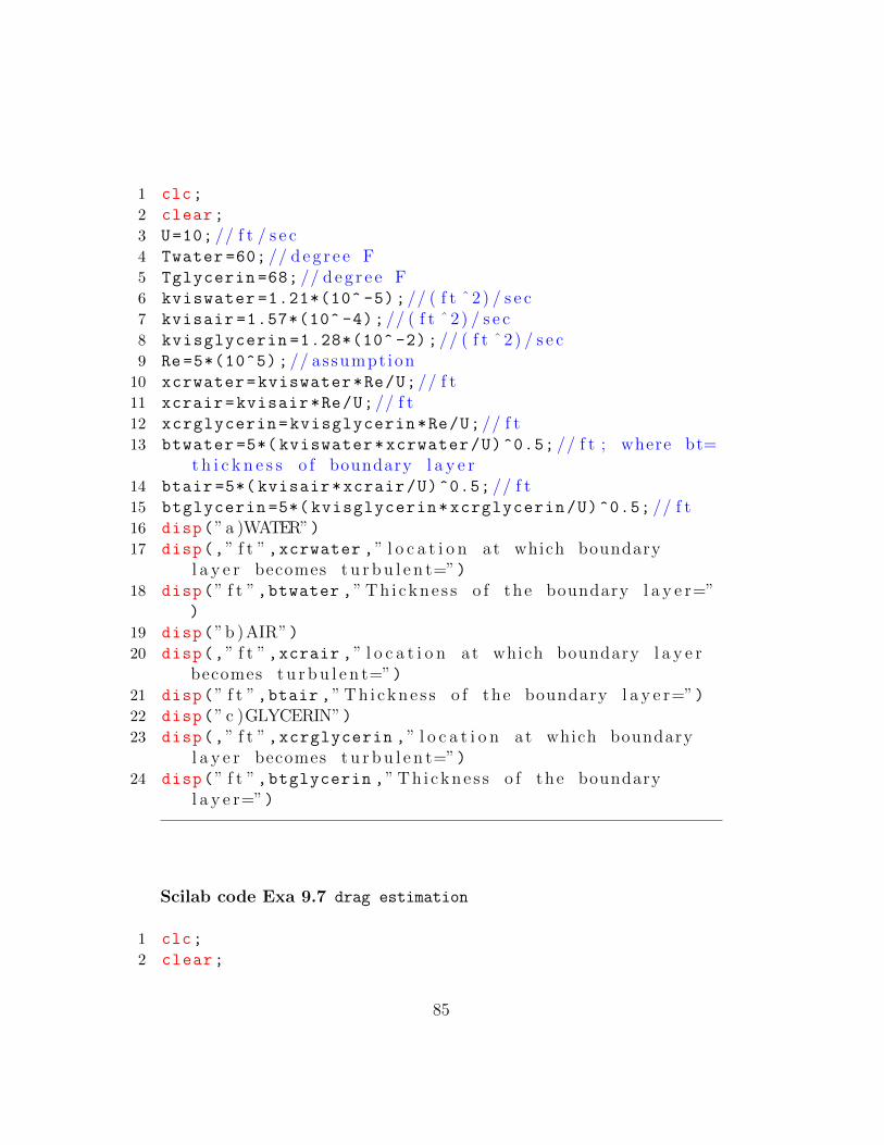
Scilab code Exa 9.7 drag estimation

1 clc;

2 clear;

85

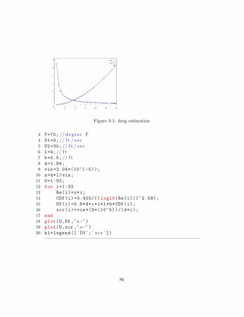
Figure 9.1: drag estimation

3 T=70; // d e g r e e F4 U1=0; // f t / s e c5 U2=30; // f t / s e c6 l=4; // f t7 b=0.5; // f t8 d=1.94;

9 vis =2.04*(10^( -5));

10 x=d*l/vis;

11 U=1:U2;

12 for i=1:U2

13 Re(i)=x*i;

14 CDf(i)=0.455/(( log10(Re(i)))^2.58);

15 Df(i)=0.5*d*i*i*l*b*CDf(i);

16 xcr(i)=vis *(5*(10^5))/(d*i);

17 end

18 plot(U,Df,”x−”)19 plot(U,xcr ,”o−”)20 h1=legend ([ ’ Df ’ ; ’ x c r ’ ])

86

Figure 9.2: speed of grain

Scilab code Exa 9.10 speed of grain

1 clc;

2 clear;

3 D=0.1; //mm4 sg=2.3;

5 vis =1.12*(10^( -3));//N∗ s /(mˆ2)6 // by f r e e body diagram and assuming CD=24/Re7 U=(sg -1) *999*9.81*((D/1000) ^2) /(18* vis);

8 disp(”m/ s e c ”,U,”The v e l o c i t y o f the p a r t i c l e throughs t i l l water =”)

9 dia =0:0.001:0.1;

10 count =1;

11 for i=0:0.001:0.1

12 u(count)=(sg -1) *999*9.81*((i/1000) ^2) /(18* vis);

13 count=count +1;

14 end

15 plot2d(dia ,u,rect =[0 ,0 ,0.1 ,0.007])

16 xtitle(”U vs D”,”D, mm”,”U, m/ s ”)

87

Scilab code Exa 9.11 velocity of updraft

1 clc;

2 clear;

3 D=1.5; // i n4 // assuming CD=0.5 and v e r i f y i n g t h i s v a l u e u s i n g

v a l u e o f Re5 CD=0.5;

6 dice =1.84; // s l u g s /( f t ˆ3) ; d e n s i t y o f i c e7 dair =2.38*(10^( -3));// s l u g s /( f t ˆ3)8 U=(4* dice *32.2*(D/12) /(3* dair*CD))^0.5; // f t / s e c9 disp(”mph”,U*3600/5275 , ”The v e l o c i t y o f the u p d r a f t

needed=”)

Scilab code Exa 9.12 drag and deceleration

1 clc;

2 clear;

3 Dg =1.69; // i n .4 Wg =0.0992; // l b5 Ug=200; // f t / s e c6 Dt=1.5; // i n .7 Wt =0.00551; // l b8 Ut=60; // f t / s e c9 kvis =(1.57*(10^( -4)));// ( f t ˆ2) / s e c

10 Reg=Ug*Dg/kvis;

11 Ret=Ut*Dt/kvis;

12 // the c o r r e s p o n d i n g drag c o e f f i c i e n t s a r e c a l c u l a t e das

13 CDgs =0.25; // s tandard g o l f b a l l14 CDgsm =0.51; // smooth g o l f b a l l15 CDt =0.5; // t a b l e t e n n i s b a l l16 Dgs =0.5*0.00238*( Ug^2)*%pi *((Dg/12) ^2)*CDgs /4; // l b17 Dgsm =0.5*0.00238*( Ug^2)*%pi*((Dg/12) ^2)*CDgsm /4; // l b18 Dt =0.5*0.00238*( Ut^2)*%pi*((Dt/12) ^2)*CDt /4; // l b

88

19 // the c o r r e s p o n d i n g d e c e l e r a t i o n s a r e a=D/ s=g∗D/W20 // d e c e l e r a t i o n r e l a t i v e to g=D/W21 decgs=Dgs/Wg;

22 decgsm=Dgsm/Wg;

23 dect=Dt/Wt;

24 disp(”STANDARD GOLF BALL : ”)25 disp(” l b ”,Dgs ,”The drag c o e f f i c i e n t=”)26 disp(decgs ,”The d e c e l e r a t i o n r e l a t i v e to g=”)27 disp(”SMOOTH GOLF BALL: ”)28 disp(” l b ”,Dgsm ,”The drag c o e f f i c i e n t=”)29 disp(decgsm ,”The d e c e l e r a t i o n r e l a t i v e to g=”)30 disp(”TABLE TENNIS BALL : ”)31 disp(” l b ”,Dt ,”The drag c o e f f i c i e n t=”)32 disp(dect ,”The d e c e l e r a t i o n r e l a t i v e to g=”)

Scilab code Exa 9.13 torque estimation

1 clc;

2 clear;

3 U=88; // f p s4 Ds=40; // f t5 Dc=15; // f t6 b=50; // f t7 Res=U*Ds /(1.57*(10^( -4)));

8 Rec=U*Dc /(1.57*(10^( -4)));

9 // from t h e s e v a l u e s o f Re drag c o e f f i c i e n t s a r efound as

10 CDs =0.3;

11 CDc =0.7;

12 // by summing moments about the base o f the tower13 Drs =0.5*0.00238*(U^2)*%pi*(Ds^2)*CDs /4; // l b14 Drc =0.5*0.00238*(U^2)*b*Dc*CDc;// l b15 M=(Drs*(b+(Ds/2)))+(Drc*(b/2));// f t ∗ l b16 disp(” f t ∗ l b ”,M,”The moment needed to p r even t the

tower from t r i p p i n g=”)

89

Scilab code Exa 9.15 lift and power

1 clc;

2 clear;

3 U=15; // f t / s e c4 b=96; // f t5 c=7.5; // f t6 W=210; // l b7 CD =0.046;

8 eff =0.8; // power t r a i n e f f i c i e n c y9 d=2.38*(10^( -3));// s l u g s /( f t ˆ3)

10 //W=L11 CL=2*W/(d*(U^2)*b*c);

12 D=0.5*d*(U^2)*b*c*CD;

13 P=D*U/(eff *550);//hp14 disp(CL,”The l i f t c o e f f i c i e n t=”)15 disp(”hp”,P,”The power r e q u i r e d by the p i l o t=”)

Scilab code Exa 9.16 angular velocity determination

1 clc;

2 clear;

3 W=2.45*(10^( -2));//N4 D=3.8*(10^( -2));//m5 U=12; //m/ s6

7 //W=L8 d=1.23; // kg /(mˆ3)9 CL=2*W/(d*(U^2)*%pi*(D^2)/4);

10 W=0.5*d*(U^2)*(D^2)*%pi*CL/4;

11 // u s i n g t h i s v a l u e o f CL , omega∗D/(2∗U)=x i s foundas

90

12 x=0.9;

13 omega =2*U*x/D;// rad / s e c14 angvel=omega *60/(2* %pi);//rpm ; where a ng v e l i s

a n g u l a r v e l o c i t y15 disp(”rpm”,angvel ,”The a n g u l a r v e l o c i t y=”)

91

Chapter 10

Flow in Open Channels

Scilab code Exa 10.2 elevation of surface

1 clc;

2 clear;

3 z2=0.5; // f t4 q=5.75; // ( f t ˆ2) / s e c5 y1=2.3; // f t6 z1=0; // f t7 V1=2.5; // f t / s e c8 // b e r n o u l l i e q u a t i o n9 a=y1+((V1^2) /(2*32.2))+z1 -z2;// f t ; where a=y2 +((Vˆ2)

/(2∗ g ) )10 // c o u n t i n u i t y e q u a t i o n11 b=(y1*V1);// ( f t ˆ2/ s e c ) ; where b=(y2∗V2)12 c1 =2*32.2;

13 c2=(-c1)*a;

14 c3=b^2;

15 fn=poly([c3 0 c2 c1],” y2 ”,” c ”);16 y2=roots(fn);

17 sum1=y2(3)+z2;// f t18 sum2=y2(1)+z2;// f t19 E1=y1+(c3/(y1^2));// f t20 Emin =3*((q^2) /(32.2^(1/3)))/2; // f t

92

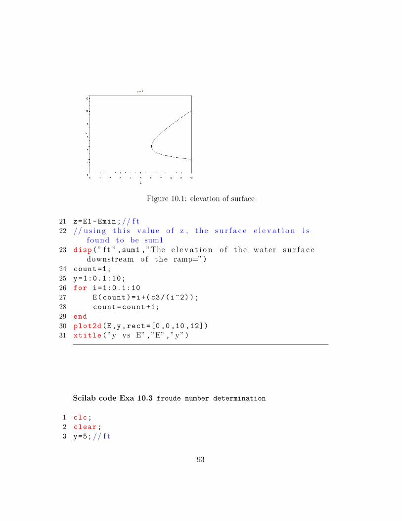
Figure 10.1: elevation of surface

21 z=E1 -Emin;// f t22 // u s i n g t h i s v a l u e o f z , the s u r f a c e e l e v a t i o n i s

found to be sum123 disp(” f t ”,sum1 ,”The e l e v a t i o n o f the water s u r f a c e

downstream o f the ramp=”)24 count =1;

25 y=1:0.1:10;

26 for i=1:0.1:10

27 E(count)=i+(c3/(i^2));

28 count=count +1;

29 end

30 plot2d(E,y,rect =[0 ,0 ,10 ,12])

31 xtitle(”y vs E”,”E”,”y”)

Scilab code Exa 10.3 froude number determination

1 clc;

2 clear;

3 y=5; // f t

93

4 angle =40; // d e g r e e5 l=12; // f t6 rate =1.4; // f t per 1000 f t o f l e n g t h7 K=1.49;

8 A=(l*y)+(y*y/tan(angle*%pi /180));// f t9 P=(l+(2*y/sin(angle*%pi /180)));// f t

10 Rh=A/P;

11 S0=rate /1000;

12 x=K*(A)*(Rh ^(2/3))*(S0^0.5);// where Rh=Q∗n13 n=0.012;

14 Q=x/n;// c f s15 disp(” c f s ”,Q,”The f l o w r a t e=”)16 V=Q/A;// f t / s e c17 Fr=V/(32.2*y)^0.5;

18 disp(Fr,” Froude number=”)

Scilab code Exa 10.4 determining flow depth

1 clc;

2 clear;

3 y=5; // f t4 angle =40; // d e g r e e5 l=12; // f t6 rate =1.4; // f t per 1000 f t o f l e n g t h7 Q=10; //mˆ3/ s e c8 //A=( l ∗y ) +(y∗y/ tan ( a n g l e ∗%pi /180) ) f t ˆ29 bw=l*1/3.281; //m; where bw=bottom width 3 . 6 6

10 //P=bw(2∗ y/ s i n ( a n g l e ∗%pi /180) ) m11 //Rh=A/P12 n=0.03;

13 c1=1/tan(angle*%pi /180);// 1 . 1 914 c2=(Q*n/(( rate /1000) ^0.5))^3; // 51515 c3=2/sin(angle*%pi /180);// 3 . 1 116 fn=poly([(-c2*bw*bw) (-c2*2*c3*bw) (-c2*c3*c3) 0 0 (

bw^5) (5*c1*bw^4) (10*(c1^2)*(bw^3)) (10*( c1^3)*(

94

bw^2)) (5*(c1^4)*(bw)) (c1^5)],”y”,” c ”);17 r=roots(fn);

18 disp(”m”,r(1),”The depth o f the f l o w=”)

Scilab code Exa 10.7 flowrate estimation

1 clc;

2 clear;

3 S0 =1/500;

4 n1 =0.02;

5 z1=0.6; // f t6 n2 =0.015;

7 n3 =0.03;

8 z2=0.8; // f t9 l1=3; // f t10 l2=2; // f t11 l3=3; // f t12 y=z1+z2;// f t13 K=1.49;

14 A1=l1*(z1);// f t ˆ215 A2=l2*(y);// f t ˆ216 A3=l3*(z1);// f t ˆ217 P1=l1+z1;// f t18 P2=l2+(2*z2);// f t19 P3=l3+z1;// f t20 Rh1=A1/P1;// f t21 Rh2=A2/P2;// f t22 Rh3=A3/P3;// f t23 Q=K*(S0 ^0.5) *((A1*(Rh1 ^(2/3))/n1)+(A3*(Rh3 ^(2/3))/n3

)+(A2*(Rh2 ^(2/3))/n2));// ( f t ˆ3) / s e c24 disp(” ( f t ˆ3) / s e c ”,Q,”The f l o w r a t e=”)

Scilab code Exa 10.8 aspect ratio determination

95

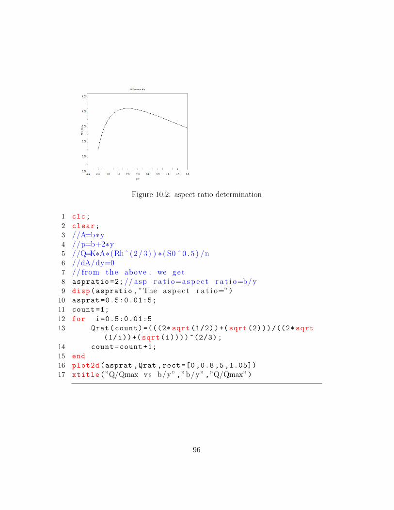
Figure 10.2: aspect ratio determination

1 clc;

2 clear;

3 //A=b∗y4 //p=b+2∗y5 //Q=K∗A∗ (Rhˆ ( 2 / 3 ) ) ∗ ( S0 ˆ 0 . 5 ) /n6 //dA/dy=07 // from the above , we ge t8 aspratio =2; // asp r a t i o=a s p e c t r a t i o=b/y9 disp(aspratio ,”The a s p e c t r a t i o=”)10 asprat =0.5:0.01:5;

11 count =1;

12 for i=0.5:0.01:5

13 Qrat(count)=(((2* sqrt (1/2))+(sqrt (2)))/((2* sqrt

(1/i))+(sqrt(i))))^(2/3);

14 count=count +1;

15 end

16 plot2d(asprat ,Qrat ,rect =[0 ,0.8 ,5 ,1.05])

17 xtitle(”Q/Qmax vs b/y”,”b/y”,”Q/Qmax”)

96

Scilab code Exa 10.9 hydraulic jump

1 clc;

2 clear;

3 w=100; // f t4 y1=0.6; // f t5 V1=18; // f t / s e c6 Fr1=V1 /(32.2* y1)^0.5;

7 disp(Fr1 ,”The Froude number b e f o r e the jump=”)8 yratio =0.5*( -1+(1+(8*( Fr1 ^2)))^0.5);// where y r a t i o=

y2 / y19 y2=y1*yratio;// f t10 disp(” f t ”,y2 ,”The depth a f t e r the jump=”)11 //Q1=Q2 , hence12 V2=(y1*V1)/y2;// f t / s e c13 Fr2=V2 /(32.2* y2)^0.5;

14 disp(Fr2 ,”The f r o u d e number a f t e r the jump=”)15 Q=w*y1*V1;// ( f t ˆ3) / s e c16 hL=(y1+(V1*V1 /(32.2*2)))-(y2+(V2*V2 /(2*32.2)));// f t17 Pd =62.4* hL*Q/550; //hp18 disp(”hp”,Pd ,”Power d i s s i p a t e d w i t h i n the jump=”)19 depth1 =0.4:0.01:1.53;

20 count =1;

21 for i=0.4:0.01:1.53

22 power(count)=62.4*(((i+((Q/(i*w))^2) /(32.2*2)))

-((i*(0.5*( -1+(1+(8*(((Q/(i*w))/(32.2*i)^0.5)

^2)))^0.5)))+((((i*(Q/(i*w)))/(i

*(0.5*( -1+(1+(8*(((Q/(i*w))/(32.2*i)^0.5) ^2))

)^0.5))))^2) /(2*32.2))))*Q/550;

23 count=count +1;

24 end

25 plot2d(depth1 ,power ,rect =[0 ,0 ,1.6 ,1000])

26 xtitle(”Pa vs y1 ”,”y1 , f t ”,”Pa , hp”)27 xclick (1);

28 clf();

29 y=0.5:0.01:4;

30 n=1;

31 for i=0.5:0.01:4

97

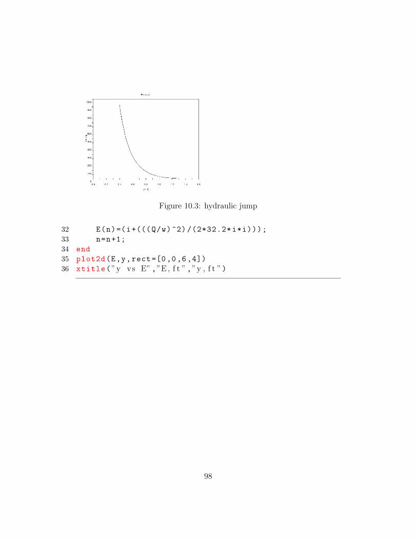
Figure 10.3: hydraulic jump

32 E(n)=(i+(((Q/w)^2) /(2*32.2*i*i)));

33 n=n+1;

34 end

35 plot2d(E,y,rect =[0,0,6,4])

36 xtitle(”y vs E”,”E , f t ”,”y , f t ”)

98

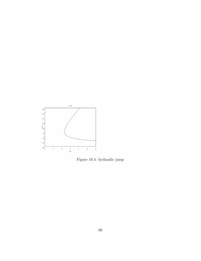
Figure 10.4: hydraulic jump

99

Chapter 11

Analysis of Compressible Flow

Scilab code Exa 11.1 Internal Energy enthalphy

1 clc;

2 clear;

3 D=4; // i n4 T1=540; // d e g r e e R5 p1=100; // p s i a6 T2=453; // d e g r e e R7 p2 =18.4; // p s i a8 k=1.4;

9 R=1716/32.174; // f t ∗ l b /( lbm ∗ ( d e g r e e R) )10 cv=R/(k-1);// f t ∗ l b /( lbm ∗ ( d e g r e e R) )11 udiff=cv*(T2 -T1);// f t ∗ l b / lbm ; change i n i n t e r n a l

ene rgy12 disp(” f t ∗ l b / lbm”,udiff ,”a ) The change i n i n t e r n a l

ene rgy between ( 1 ) and ( 2 )=”)13 cp=k*cv;// f t ∗ l b /( lbm ∗ ( d e g r e e R) )14 hdiff=cp*(T2 -T1);// f t ∗ l b / lbm ; change i n en tha lpy15 disp(” f t ∗ l b / lbm”,hdiff ,”b ) The change i n e n t h a l p l

ene rgy between ( 1 ) and ( 2 )=”)16 ddiff =(1/R)*((p2*144/ T2) -(p1*144/ T1));// lbm /( f t ˆ3) ;

change i n d e n s i t y17 disp(” lbm /( f t ˆ3) ”,ddiff ,”The change i n d e n s i t y

100

betwenn ( 1 ) and ( 2 )=”)

Scilab code Exa 11.2 change in entropy

1 clc;

2 clear;

3 D=4; // i n4 T1=540; // d e g r e e R5 p1=100; // p s i a6 T2=453; // d e g r e e R7 p2 =18.4; // p s i a8 cv = 133;

9 R =53.3;

10 dratio =(p1/T1)*(T2/p2);

11 sdif=(cv*(log(T2/T1)))+(R*(log(dratio)));// f t ∗ l b / lbm∗ ( d e g r e e R) ; change i n ent ropy

12 disp(” f t ∗ l b / lbm ∗ ( d e g r e e R) ”,sdif ,”The change i nent ropy between ( 1 ) and ( 2 )=”)

Scilab code Exa 11.3 speed of sound

1 clc;

2 clear;

3 T=0; // d e g r e e C4 R=286.9; // J /( kg∗K)5 k=1.401;

6 c=(R*(T+273.15)*k)^0.5; //m/ s7 disp(”m/ s e c ”,c,”The speed o f sound f o r a i r a t 0

d e g r e e C =”)

101

Scilab code Exa 11.4 Mach cone

1 clc;

2 clear;

3 z=1000; //m4 Ma=1.5;

5 T=20; // d e g r e e C6 // a lpha=atan ( z /x ) , x=V∗ t , and Ma=(1/ s i n ( a lpha ) ) ;

where a lpha i s the a n g l e o f the Mach cone7 //V=Ma∗ c8 c=343.3; //m/ s found from the v a l u e o f t empera tu r e9 V=Ma*c;//m/ s e c

10 t=z/(Ma*c*tan(asin (1/Ma)));// s e c11 disp(” s e c ”,t,”The number o f s e c o n d s to wa i t a f t e r

the p l ane p a s s e s over−head b e f o r e i t i s heard=”)12 Mach =0.01:0.01:4;

13 count =1;

14 for i=0.01:0.01:4

15 time(count)=z/(i*c*tan(asin (1/i)));

16 count=count +1;

17 end

18 plot2d(Mach ,time ,rect =[0,0,4,3])

19 xtitle(” t vs Ma”,”Ma”,” t , s e c ”)

Scilab code Exa 11.5 mass flowrate determination

1 clc;

2 clear;

3 A=1*(10^( -4));//mˆ24 p1=80; //kPa ( abs )5 p2=40; //kPa ( abs )6 p0=101; //kPa ( abs )7 pcritical =0.528* p0;//kPa ( abs )

102

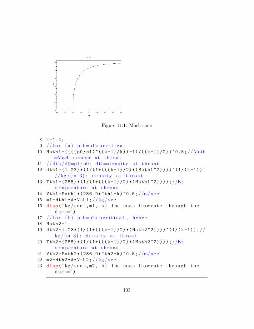
Figure 11.1: Mach cone

8 k=1.4;

9 // f o r ( a ) pth=p1>p c r i t i c a l10 Math1 =(((( p0/p1)^((k-1)/k)) -1)/((k-1)/2))^0.5; //Math

=Mach number at t h r o a t11 // dth /d0=p1/p0 ; dth=d e n s i t y at t h r o a t12 dth1 =(1.23) *(1/(1+(((k-1)/2)*( Math1 ^2))))^(1/(k-1));

// kg /(mˆ3) ; d e n s i t y at t h r o a t13 Tth1 =(288) *(1/(1+(((k-1) /2)*( Math1 ^2))));//K;

t empera tu re at t h r o a t14 Vth1=Math1 *(286.9* Tth1*k)^0.5; //m/ s e c15 m1=dth1*A*Vth1;// kg / s e c16 disp(” kg / s e c ”,m1 ,”a ) The mass f l o w r a t e through the

duct=”)17 // f o r ( b ) pth=p2<p c r i t i c a l , hence18 Math2 =1;

19 dth2 =1.23*(1/(1+(((k-1) /2)*( Math2 ^2))))^(1/(k-1));//kg /(mˆ3) ; d e n s i t y at t h r o a t

20 Tth2 =(288) *(1/(1+(((k-1) /2)*( Math2 ^2))));//K;t empera tu re at t h r o a t

21 Vth2=Math2 *(286.9* Tth2*k)^0.5; //m/ s e c22 m2=dth2*A*Vth2;// kg / s e c23 disp(” kg / s e c ”,m2 ,”b ) The mass f l o w r a t e through the

duct=”)

103

Scilab code Exa 11.6 mass flowrate calculation

1 clc;

2 clear;

3 A=1*(10^( -4));//mˆ24 p1=80; //kPa ( abs )5 p2=40; //kPa ( abs )6

7 p0=101; //kPa ( abs )8 k=1.4;

9 // f o r ( a )10 pratio1=p1/p0;

11 // f o r t h i s v a l u e o f p1/p0 ,12 Math1 =0.59;

13 Tratio1 =0.94; //=Tth/T014 dratio1 =0.85; //=dth /d015 Tth1=Tratio1 *(288);//K16 dth1=dratio1 *(1.23);// kg /(mˆ3)17 Vth1=Math1 *(286.9* Tth1*k)^0.5; //m/ s e c18 m1=(dth1*A*Vth1);// kg / s e c19 disp(” kg / s e c ”,m1 ,”a ) The mass f l o w r a t e=”)20 // f o r ( b )21 Math2 =1;

22 Tratio2 =0.83; //=Tth/T023 dratio2 =0.64; //=dth /d024 Tth2=Tratio2 *(288);//K25 dth2=dratio2 *(1.23);// kg /(mˆ3)26 Vth2=Math2 *(286.9* Tth2*k)^0.5; //m/ s e c27 m2=(dth2*A*Vth2);// kg / s e c28 disp(” kg / s e c ”,m2 ,”b ) The mass f l o w r a t e=”)

Scilab code Exa 11.7 flow velocity determination

104

1 clc;

2 clear;

3 pratio =0.82; // r a t i o o f s t a t i c to s t a g n a t i o n p r e s s u r e4 T=68; // d e g r e e F5 // f o r ( a )6 // f o r the v a l u e o f p r a t i o g i v e n Ma i s c a l c u l a t e d as7 Ma1 =0.54;

8 k1=1.4;

9 Tratio1 =0.94; //T/T010 T1=Tratio1 *(T+460);// d e g r e e R11 V1=(Ma1 *(53.3* T1*k1)^0.5) *(32.2^0.5);// f t / s e c12 // f o r ( b )13 k2 =1.66;

14 Ma2 =((((1/ pratio)^((k2 -1)/k2)) -1)/((k2 -1)/2))^0.5;

15 Tratio2 =1/(1+(((k2 -1)/2)*(Ma2^2)));//T/T016 T2=Tratio2 *(T+460);// d e g r e e R17 V2=(Ma2 *(386* T2*k2)^0.5) *(32.2^0.5);// f t / s e c18 disp(” f t / s e c ”,V1 ,”The f l o w v e l o c i t y i f f l u i d i s a i r=

”)19 disp(” f t / s e c ”,V2 ,”The f l o w v e l o c i t y i f f l u i d i s

he l ium=”)

Scilab code Exa 11.11 fanno flow

1 clc;

2 clear;

3 k=1.4;

4 T0 =518.67; // d e g r e e R5 T1 =514.55; // d e g r e e R6 p1 =14.3; // p s i a7 R=53.3; // ( f t ∗ l b ) /( lbm∗ d e g r e e R)8 cp=R*k/(k-1);// ( f t ∗ l b /( lbm∗ d e g r e e R) )9 Tratio=T1/T0;

10 Ma =(((1/ Tratio) -1)/((k-1)/2))^0.5;

11 x=(R*T1*k*32.2) ^0.5; // f t / s e c ; where x=(R∗T1∗k ) ˆ 0 . 5

105

12 y=p1 *144/(R*T1)*(Ma*x);// lbm / ( ( f t ˆ2) ∗ s e c ) ; where y=d∗V

13 // f o r p=7 p s i a14 p=7; // p s i a15 fn=poly([(-T0) 1 ((y*y/(2*cp*p*p*144*144/(R^2)))

/32.2)],”T”,” c ”);16 r=roots(fn);

17 T=r(1);//K18 sdif=(cp*log(T/T1)) -(R*log(p/p1));// ( f t ∗ l b ) /( lbm∗

d e g r e e R)19 disp(”K”,T,”The c o r r o s p o n d i n g v a l u e o f t empera tu r e

f o r Fanno f o r downstream p r e s s u r e o f 7 p s i a=”)20 disp(” ( f t ∗ l b ) /( lbm∗ d e g r e e R) ”,sdif ,”The

c o r r o s p o n d i n g v a l u e o f en t ropy change f o r Fannof o r downstream p r e s s u r e o f 7 p s i a=”)

21 count =1;

22 for i=1.4:0.1:7

23 root=roots(poly([(-T0) 1 ((y*y/(2*cp*i*i

*144*144/(R^2)))/32.2)],”T”,” c ”));24 temp(count)=root (1);

25 s(count)=(cp*log(temp(count)/T1))-(R*log(i/p1));

26 count=count +1;

27 end

28 plot2d(s,temp)

29 xtitle(”T vs s−s1 ”,” s−s1 , ( ( f t ∗ l b ) /( lbm∗ d e g r e e R) ) ”,”T, Degree R”)

Scilab code Exa 11.12 choked fanno flow

1 clc;

2 clear;

3 T0=288; //K4 p0=101; //kPa ( abs )

106

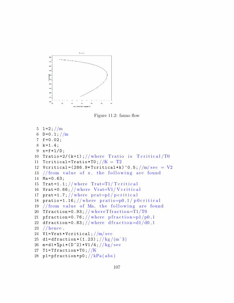
Figure 11.2: fanno flow

5 l=2; //m6 D=0.1; //m7 f=0.02;

8 k=1.4;

9 x=f*l/D;

10 Tratio =2/(k+1);// where T r a t i o i s T c r i t i c a l /T011 Tcritical=Tratio*T0;//K = T212 Vcritical =(286.9* Tcritical*k)^0.5; //m/ s e c = V213 // from v a l u e o f x , the f o l l o w i n g a r e found14 Ma =0.63;

15 Trat =1.1; // where Trat=T1/ T c r i t i c a l16 Vrat =0.66; // where Vrat=V1/ V c r i t i c a l17 prat =1.7; // where p ra t=p1/ p c r i t i c a l18 pratio =1.16; // where p r a t i o=p0 , 1 / p 0 c r i t i c a l19 // from v a l u e o f Ma, the f o l l o w i n g a r e found20 Tfraction =0.93; // w h e r e T f r a c t i o n=T1/T021 pfraction =0.76; // where p f r a c t i o n=p1/p0 , 122 dfraction =0.83; // where d f r a c t i o n=d1/d0 , 123 // hence ,24 V1=Vrat*Vcritical;//m/ s e c25 d1=dfraction *(1.23);// kg /(mˆ3)26 m=d1*%pi*(D^2)*V1/4; // kg / s e c27 T1=Tfraction*T0;//K28 p1=pfraction*p0;//kPa ( abs )

107

29 T01=T0;//K and T01=T0230 p01=p0;//kPa ( abs )31 p2=(1/ prat)*( pfraction)*p01;// kpa ( abs )32 p02 =(1/ pratio)*p01;//kPa ( abs )33 disp(”K”,Tcritical ,” C r i t i c a l t empera tu r e=”)34 disp(”m/ s e c ”,Vcritical ,” C r i t i c a l v e l o c i t y=”)35 disp(”m/ s e c ”,V1 ,” V e l o c i t y at i n l e t=”)36 disp(” kg / s e c ”,m,”Maximum mass f l o w r a t e=”)37 disp(”K”,T1 ,” Temperature at i n l e t=”)38 disp(”kPa ( abs ) ”,p1 ,” P r e s s u r e at i n l e t=”)39 disp(”K”,T01 ,” s t a g n a t i o n t empera tu r e at i n l e t and

e x i t=”)40 disp(”kPa ( abs ) ”,p01 ,”The s t a g n a t i o n p r e s s u r e at

i n l e t=”)41 disp(”kPa ( abs ) ”,p2 ,” P r e s s u r e at e x i t=”)42 disp(”kPa ( abs ) ”,p02 ,”The s t a g n a t i o n p r e s s u r e at e x i t

=”)

Scilab code Exa 11.13 effect of duct length on choked fanno flow

1 clc;

2 clear;

3 T0=288; //K4 p0=101; //kPa ( abs )5 l=2; //m6 D=0.1; //m7 f=0.02;

8 pd=45; //kPa ( abs )9 f=0.02;

10 k=1.4;

11 lnew =(50/100)*l;

12 x=lnew*f/D;

13 // from t h i s v a l u e o f x , f o l l o w i n g a r e found14 Ma=0.7;

15 prat =1.5; // where p ra t=p1/ p c r i t i c a l

108

16 // from t h i s v a l u e o f Ma, f o l l o w i n g a r e found17 pratio =0.72; // where p r a t i o=p1/p018 dratio =0.79; // where d r a t i o=d1/d0 , 119 Vratio =0.73; // where V r a t i o=V1/ V c r i t i c a l20 // hence ,21 p2=(1/ prat)*pratio*p0;//kPa ( abs )22 pcritical=p2;

23 //we f i n d tha t pd<p c r i t i c a l24 d1=dratio *(1.23);// kg /(mˆ3)25 Vcritical =(286.9* Tcritical*k)^0.5; //m/ s e c = V226 V1=Vratio*Vcritical;//m/ s e c27 m=d1*%pi*(D^2)*V1/4; // kg / s e c28 disp(” kg / s e c ” ,1.65,” i s l e s s than the f l o w r a t e f o r

the l o n g e r tube =”,” kg / sec , ”,m,”The f l o w r a t e f o rthe s m a l l e r tube=”)

Scilab code Exa 11.14 unchoked fanno flow

1 clc;

2 clear;

3 T0=288; //K4 p0=101; //kPa ( abs )5 l=2; //m6 D=0.1; //m7 f=0.02;

8 pd=45; //kPa ( abs )9 f=0.02;

10 m=1.65; // kg / s e c11 lnew=l/2; //m12

13 x=f*l/D;

14 // from t h i s v a l u e o f x , Ma at e x i t i s found as15 Ma=0.7;

16 // and p2/ p c r i t i c a l i s found as17 pratio =1.5;

109

18 // and , from example 1 1 . 1 2 ,19 prat =1.7; // where p ra t=p1/ p c r i t i c a l20 pfraction =0.76; // where p f r a c t i o n=p1/p0 , 121 // Hence ,22 p2=pratio *(1/ prat)*pfraction*p0;//kPa ( abs )23 disp(Ma,”The Mach number at the e x i t=”)24 disp(”kPa ( abs ) ”,p2 ,”The back p r e s s u r e r e q u i r e d=”)

Scilab code Exa 11.15 rayleigh flow

1 clc;

2 clear;

3 k=1.4;

4 T0 =518.67; // d e g r e e R5 T1 =514.55; // d e g r e e R6 p1 =14.3; // p s i a7

8 R=53.3; // ( f t ∗ l b ) /( lbm∗ d e g r e e R)9 cp=R*k/(k-1);// ( f t ∗ l b /( lbm∗ d e g r e e R) )

10 Tratio=T1/T0;

11 Ma =(((1/ Tratio) -1)/((k-1)/2))^0.5;

12 x=(R*T1*k*32.2) ^0.5; // f t / s e c ; where x=(R∗T1∗k ) ˆ 0 . 513 y=p1 *144/(R*T1)*(Ma*x);// lbm / ( ( f t ˆ2) ∗ s e c ) ; where y=d

∗V14 z=R*T1/(p1*144);// ( f t ˆ3) / lbm15 c=(p1)+(y*y*z/(32.2*144));// p s i a ; =c o n s t a n t16 //when downstream p r e s s u r e p=13.5 p s i a17 p=13.5; // p s i a18 a=(y^2)*R/(p*144*32.2*144);// ( l b /( i n ˆ2) ) / d e g r e e R19 fn=poly ([(p-c) a],”T”,” c ”);20 T=roots(fn);// d e g r e e R21 sdif=(cp*log(T/T1)) -(R*log(p/p1));// f t ∗ l b /( lbm∗

d e g r e e R)22 disp(” d e g r e e R”,T,”The c o r r o s p o n d i n g v a l u e o f

t empera tu re f o r the downstream p r e s s u r e o f 1 3 . 5

110

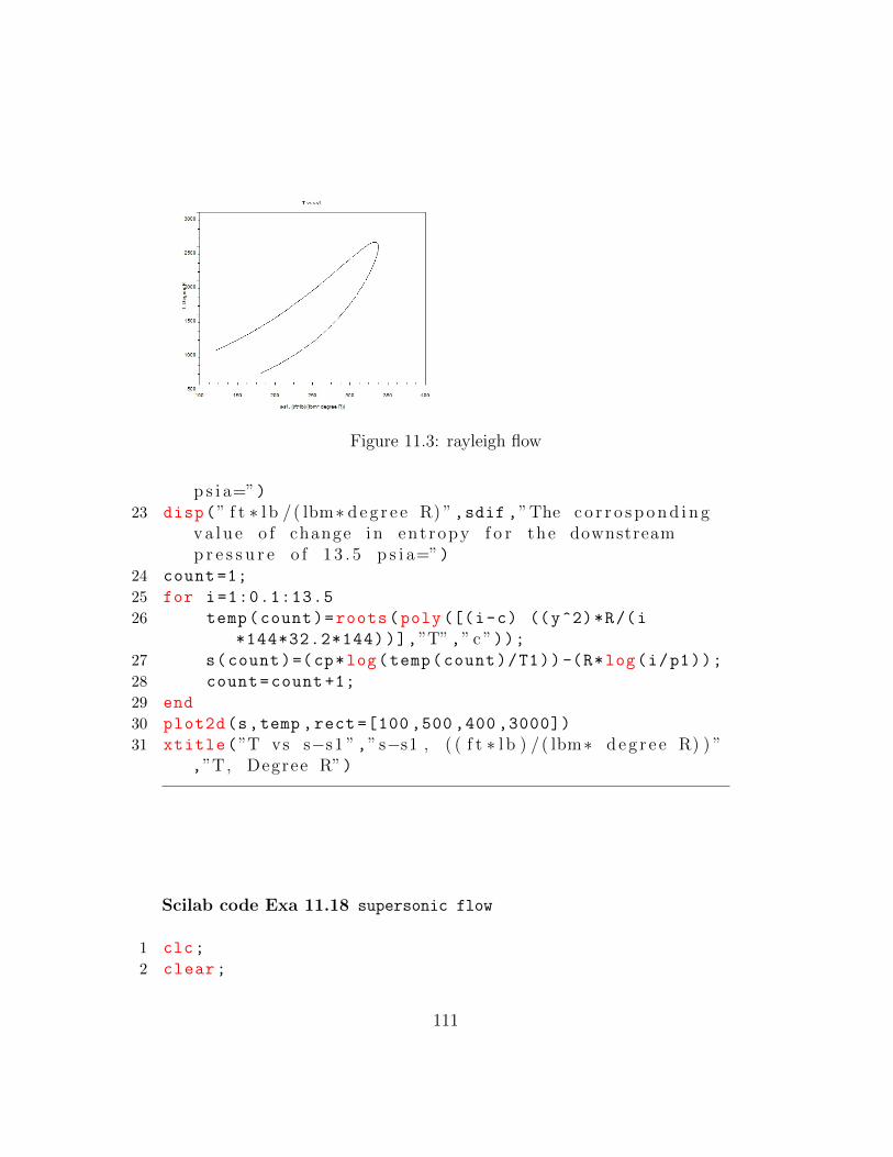
Figure 11.3: rayleigh flow

p s i a=”)23 disp(” f t ∗ l b /( lbm∗ d e g r e e R) ”,sdif ,”The c o r r o s p o n d i n g

v a l u e o f change i n ent ropy f o r the downstreamp r e s s u r e o f 1 3 . 5 p s i a=”)

24 count =1;

25 for i=1:0.1:13.5

26 temp(count)=roots(poly ([(i-c) ((y^2)*R/(i

*144*32.2*144))],”T”,” c ”));27 s(count)=(cp*log(temp(count)/T1))-(R*log(i/p1));

28 count=count +1;

29 end

30 plot2d(s,temp ,rect =[100 ,500 ,400 ,3000])

31 xtitle(”T vs s−s1 ”,” s−s1 , ( ( f t ∗ l b ) /( lbm∗ d e g r e e R) ) ”,”T, Degree R”)

Scilab code Exa 11.18 supersonic flow

1 clc;

2 clear;

111

3 p=60; // p s i a4 T=1000; // d e g r e e R5 px=12; // p s i a6 k=1.4;

7 R=53.3; // f t ∗ l b /( lbm∗ d e g r e e R)8 pratio=p/px;

9 // f o r t h i s v a l u e o f p r a t i o , Max i s c a l c u l a t e d as10 Max =1.9;

11 // u s i n g t h i s v a l u e o f Max , Tx/T0 , x i s found as12 Tratio =0.59;

13 //T=T0 , x=T0 , y14 Tx=Tratio*T;// d e g r e e R15 cx=(R*Tx*k)^0.5; // f t / s e c16 Vx =1.87* cx *(32.2^0.5);// f t / s e c17 disp(Max ,”The Mach number f o r the f l o w=”)18 disp(” f t / s e c ”,Vx ,”The v e l o c i t y o f the f l o w=”)

Scilab code Exa 11.19 converging diverging duct

1 clc;

2 clear;

3 x1=0.5; //m4 x2=0.3; //m5 Acritical =0.1; //mˆ26 // at x1 , Max1 i s found as7 Max1 =2.8;

8 // and px/p0 , x i s found as9 pratio1 =0.04;

10 // For t h i s v a l u e o f Max , py/px i s found as11 prat1 =9;

12 pfraction1=prat1*pratio1;// where p f r a c t i o n=py/p0 , x =p I I I /p0 , x

13 // at x2 , Max2 i s found as14 Max2 =2.14;

15 // f o r t h i s v a l u e o f Max2 , the f o l l o w i n g a r e found

112

16 prat2 =5.2;

17 prat22 =0.66; // where p ra t22=p0 , y/p0 , x18 May =0.56;

19 // f o r t h i s v a l u r o f May , Ay/ A c r i t i c a l i s found as20 Aratio =1.24;

21 Arat=( Acritical +(x1^2))/( Acritical +(x2^2));// whereA r a t i o=A2/Ay

22 Afraction=Aratio*Arat;// where A f r a c t i o n=A2/ A c r i t i c a l23 A2=Acritical +(x1^2);//mˆ224 Acritical1=A2/Afraction;// where A c r i t i c a l 1 c r i t i c a l

a r ea f o r the i s e n t r o p i c f l o w downstream o f theshock

25 // with the v a l u e o f A f r a c t i o n , the f o l l o w i n g a r efound

26 Ma2 =0.26;

27 pfraction =0.95; // where p f r a c t i o n=p2/p0 , y28 // hence ,29 pfrac=pfraction*prat22;// where p f r a c=p2/p0 , x30 disp(pfraction1 ,”The r a t i o o f back p r e s s u r e to i n l e t

s t a g n a t i o n p r e s s u r e tha t w i l l r e s u l t i n a normalshock at the e x i t o f the duct=”)

31 disp(pfrac ,”The v a l u e o f back p r e s s u r e to i n l e ts t a g n a t i o n p r e s s u r e r e q u i r e d to p o s i t i o n theshock at ( x =0.3 m)=”)

113

Chapter 12

Pumps and Turbines

Scilab code Exa 12.2 shaft power calculation

1 Q=1400; //gpm2 N=1750; //rpm3 b=2; // i n4 r1=1.9; // i n5 r2=7.0; // i n6 beta2 =23; // d e g r e e s7 alpha1 =90; // d e g r e e s

Scilab code Exa 12.3 NPSH calculation

1 Q=0.5; // ( f t ˆ3) / s e c2 NPSHr =15; // f t3 T=80; // d e g r e e F4 patm =14.7; // p s i5 KL=20;

114

6 D=4; // i n

Scilab code Exa 12.5 pump scaling laws

1 D1=8; // i n2 N1 =1200; //rpm3 D2=12; // i n4 N2 =1000; //rpm5 T=60; // d e g r e e F

Scilab code Exa 12.6 pelton wheel turbine

1 z0=200; // f t2 l=1000; // f t3 f=0.02;

4 D=8; // i n .5 B=150; // d e g r e e6 R=1.5; // f t7 z1=0; // f t

Scilab code Exa 12.8 dental drill characteristics

1 ri =0.133; // i n .2 ro =0.168; // i n .3 N=300000; //rpm

115

116