Working Paper Series on

Impact Evaluation of Education Reforms

Paper No. 2

School Quality, School Cost, and the Public/Private School

Choices of Low-Income Households in Pakistan

Harold Aldermana

Peter F. Orazemb

Elizabeth M. Paternob

December 1996

Poverty and Human Resources Division

Policy Research Department

The World Bank

_______________ aWorld Bank. bIowa State University. All opinions expressed herein are those of the authors, have not been formally cleared by the World Bank, and do not represent the official view of the World Bank. We are grateful to Shahid Kardar and Stuti Khemani for data collection and research assistance, and to Guilherme Sedlacek for numerous helpful conversations on this study.

Abstract

Variation in school attributes, proximity, and fees across neighborhoods is used to

identify factors which affect whether poor households send their children to government school,

private school, or no school. Analysis shows that even the poorest households use private

schools extensively, and that utilization increases with income. Lowering private school fees or

distance or raising measured quality raises private school enrollments, partly by transfers from

government schools and partly from enrollments of children who otherwise would not have gone

to school. The strong demand for private schools is consistent with evidence of greater

mathematics and language achievement in private schools than in government schools. These

results strongly support an increased role for private delivery of schooling services to poor

households in developing countries.

School Quality, School Cost and the Public/Private School Choices

of Low Income Households in Pakistan

I. INTRODUCTION

Illiteracy remains a major impediment to economic development in many countries.

Expanding access to primary schooling is a widely accepted priority in the fight against poverty.

Nevertheless, developing countries face a daunting task in their efforts to expand the delivery of

educational services due to rapidly expanding populations and tight government budgets.

Moreover, public educational expenditures are often used inefficiently, providing school

buildings where they are unneeded, paying teachers that are unqualified or who do not perform,

and providing school supplies that are inadequate and ill-timed.

Increasingly, parents are responding to perceived inadequate public education by

enrolling their children in private schools. As Kingdon (1996a) illustrates, the extent of this

phenomena in developing countries may be under appreciated. Governments occasionally

prohibit, often regulate, and frequently ignore private schooling. Thus, data on the extent and

distribution of such schooling is seldom collected by statistical agencies. Yet, as Hammer

(forthcoming) argues in the case of health investments, the impact of public investments can only

be fully assessed in light of an understanding of private alternatives.

A principal reason for the reluctance of governments to recognize private education as

contributing to its overall educational policy is a concern for equity; equality of access to

schooling may reduce earning inequality without the necessity of controversial asset or income

transfers. It is not clear that poor households are able to pay enough to support the alternative of

quality private schools. Conversely, private schools which can deliver services at low enough

fees to attract poor families may not deliver quality services. Some contend that private schools

which cater to the poor are exploiting low income, often illiterate, parents who are not capable of

assessing if their children are learning or not.

The consensus from studies of the relative effectiveness of public versus private schools

in developing countries is that the predicted performance of children in private schools is higher

than predicted performance in government schools. However, choice of public versus private

school in these studies e.g., Cox and Jimenez (1991), Jimenez, Lockheed and Paqueo (1991),

Kingdon (1996b) excludes the option of not attending school at all. If policies to expand private

delivery of education are targeted toward children not currently in school, then these studies do

not shed light on how fees, quality or distance affect education or learning of the target group.

A few studies have examined how fees, distance or school quality affect the likelihood of

the no school option, although they do not address public versus private delivery. Gerther and

Glewwe (1990) estimate how distance to local schools and the quality of local teachers influence

the choice of going to no school, local secondary school, or boarding school. King (1995)

estimates how distance, fees and available space affects primary and secondary enrollments.

Both of these studies highlight the importance of school proximity to the probability that a child

is enrolled.

This study explores the potential impact on enrollments and achievement of expanding

delivery of private school services to low income neighborhoods in Lahore, Pakistan. The

analysis requires that we have measures of schooling opportunities available to households. To

accomplish this, we design a unique area frame strategy that yields information on 1,650

households in 50 different sampling clusters. The choices of government and private schools

made by households in each cluster are used to define the universe of available schooling

choices of households in each neighborhood. This provides sufficient variation in school

distances, prices, and quality indicators across neighborhoods to identify impacts on household

decisions. First, we examine whether private schools charge fees low enough or locate schools

close enough to induce low income students to attend. Finding that even very poor households

send their children to private schools, we estimate how choice of private school, government

school, and no school options are influenced by household income and the fees, proximity, and

measured quality attributes of public and private schools in the neighborhood. Finally, we

examine how home and school attributes affect child achievement.

Our results show that schooling choices of poor households are sensitive to government

and private school fees, distance, and quality. In particular, lowering private school fees or

distance will increase private school enrollments of poor children. The increased enrollments are

partly from transfers from government school, but also come from increased enrollments of

children who would not have gone to school otherwise. Furthermore, private schools raise

measured math and language achievement relative to government schools, holding observed and

unobserved child and home attributes fixed. These outcomes suggest a substantial public return

from increasing private sector delivery of schooling services to poor families.

II. MODEL AND EMPIRICAL SPECIFICATION

Parents are assumed to derive utility from their own consumption of goods (C) and from

the human capital of their children (H). The utility function has the form )H[A]U(C,U = ,

where the child's human capital is assumed to depend upon the attributes of the school which the

child attends (A). Sending children to school requires that the household sacrifice current

consumption by investing in fees and schooling supplies. In addition, the household may have to

sacrifice child time which could be used for market or household production activities.

We consider three choices parents face: to keep a child out of school, to send the child to

private school, or to send the child to a government school. These choices involve different

schooling costs, and consequently, different levels of commodity consumption. Let Y be

household income available for all purposes. If the household sends a child to government

school, it pays PG in fees, supplies, and lost child labor, so household consumption is

GG PYC −= . A year in a government school generates human capital equal to HG. If instead,

the household sends the child to a private school, household consumption is Pp PYC −= and

learning in private school is equal to HP. Finally, if the household opts not to send the child to

school, consumption is YC0 = and learning is H0. In this case, the child’s human capital is

produced only with household inputs. The household selects the option with the highest

expected utility, so that

)U,U,(UmaxU PG0* = (1)

where U* is maximum expected utility across the three possible choices.

To operationalize the model, we need two further steps. First, we specify how

consumption enters the utility across alternatives. Gertler, Locay and Sanderson (1987) have

shown that income can affect school choice only if consumption enters the utility function

nonlinearly. Following Gertler and Glewwe (1990), a specification which satisfies the

requirement that at equal levels of consumption, marginal utility of consumption is equal across

alternatives is

PG,0,j;PYC

εCαCαHαU

jiij

ij2ij2ij1ij0ij

=−=

+++=

(2)

where ith household income Yi, net of the cost of the jth schooling alternative, is assumed to equal household consumption of goods. For the no school option, 0Pj = and ii0 YC = .

Second, we need to specify the human capital production function embedded in the

model. We assume this to be of the form

PG,0,j;δFβSγHα jijjjij0 =++= (3)

where Sj is a vector of jth school attributes available to the household and Fi is a vector of family

attributes which contribute to learning in school. For the no school choice, the vector of school

attributes is a null vector. By allowing the coefficients to vary by alternative, we allow

schooling inputs to have different productivities in different school types. This is of particular

importance in assessing parental choices between government and private school. Government

schools have much higher per pupil expenditures, but these expenditures may not translate into

higher human capital production in government schools if these resources are used inefficiently.

The schooling choices are analyzed within the framework of a weighted nested

multinomial logit specification. The schooling decision is broken down into two parts. In the

first, parents decide whether to send the child to school.1 Conditional on choosing the schooling

option, parents decide between public or private school. The error terms in the school versus no

school choice are independent, but the error terms in the government and private school

alternatives are allowed to be correlated.

The probability of choosing the no schooling option is

( ) ( ) ( )[ ] ( )[ ]{ } ./σεUexp/σεUexpεUexp

)εexp(UUU*P σ

PPGG00

000r −+−+−

−== (4)

The probabilities of choosing one of the schooling alternatives are

( ) ( )[ ] ( )[ ][ ] ( )[ ]{ }σPPGG

jj0j /σεUexp/σεUexp

/σεUexpUU*Pr1UU*Pr

−+−

−=−== (5)

where s is equal to one minus the correlation between eG and eP . The reasonable assumption

that public and government school options are closer substitutes than are either school alternative

and the no school option can be tested. This assumption requires that 1.σ0 << A finding that

1σ > would reject the nested specification we have imposed.

Estimation involves inserting (2) and (3) into (4) and (5) and then specifying the

empirical counterparts to the vectors Pj, Sj and Fi. The measures of Pj, the price of attending a

school of type j, include the school fees and other materials expenditures (books, uniforms,

supplies, transportation and tutorial services) required to attend a type j school. In addition the

time a child spends in school has an opportunity cost to the household in the form of lost

potential household production or market work. Because we restrict the sample to children in a

single city in the age range between six and ten, we assume a common wage for boys and a

common wage for girls.

Opportunity costs in terms of lost home or market production is likely to differ between

boys and girls. In particular, it is widely believed that girls are more likely than boys to help

their mothers in housework and child care and may therefore have a higher opportunity cost for

schooling. On the other hand, there may be more market opportunities for boys, especially since

boys are more likely to be allowed to venture alone outside the home. If income net of schooling

costs is (Y - Pj) for boys and (Y - Pj - µF) for girls where µF is the difference in opportunity cost

of schooling between boys and girls. A different opportunity cost for girls implies that constant

terms and the coefficients on consumption differ between boys and girls.2

The vector of school attributes includes distance to school, instructional expenditures per

pupil, and pupil-teacher ratios. School distance may affect learning in school to the extent that

travel to and from school is not productive.3 More important is the disutility associated with

having a child farther from home. This disutility may be particularly important in the case of

girls because of cultural prohibitions against girls being out in public and/or outside the

protection of male household members.

Per pupil instructional expenditures are a measure of teacher resources available to

students. Instructional expenditures are primarily teacher salaries. Because salaries rise with

teacher education and experience, the measure should reflect teacher quality. Higher

expenditures per pupil can indicate both higher salaries per teacher and lower numbers of pupils

per teacher. Because of the interest in distinguishing teacher quality from school crowding

effects, we also control for the number of pupils per teacher, so the coefficient on per pupil

instructional expenditures can be interpreted as a teacher quality effect, holding class size

constant. The impacts of instructional expenditures and pupil-teacher ratios are allowed to vary

across government and private schools, reflecting likely differences in marginal productivities of

inputs across school types.

Family attributes, Fi, do not differ across the school alternatives. If these attributes had

similar effects on child human capital production across the schooling alternatives, then they

would affect utility equally in all alternatives, would not affect schooling choice, and could be

excluded from the empirical model. However, parental education is likely to be complementary

with schooling in human capital production. As a consequence, the level of parental education

can influence schooling choices for their children.

Data

To capture the effects of school quality and cost on school choices of low income

households, we require measured variation in schooling opportunities available to a

representative sample of low income households. Available data sets fell short of these

requirements in two ways. First, a representative sample of low income households requires

knowledge of the universe of households. Since political in-fighting has prevented a completed

census of population in Pakistan since 1981, knowledge of the universe is incomplete at best.

Rapid natural population growth and urbanization have greatly altered the distribution and

location of low income households since 1981, which would invalidate a sample design based on

Census data. While nationally representative surveys have been conducted in Pakistan these do

not have sufficient detail on available school choices to identify the parameters in equations (2-

3).

An alternative might be to base a sample on the universe of schools. Unfortunately,

existing listings of schools are believed to be incomplete. Particularly underrepresented are

unregistered private schools which may also atypically service poorer households. Registration

means that a school’s grades will be accepted by other schools, but it also means that the school

is subject to taxation and other regulation. Because students in unregistered schools can quality

for higher-level education through an examination process, lack of registration may not serve as

an impediment to students.

To finesse the joint problems of incomplete knowledge of the universe of poor

households and the universe of schools catering to poor households, we utilized an area frame

sampling methodology. Low and middle income areas of Lahore, the second largest city in

Pakistan, were identified on a map. Low income areas were initially identified on the basis of

housing quality. Fifty points on the map were selected in these poor areas, and initial screening

verified that households were of low or middle incomes.

In each of the fifty locations, a 250 meter square “neighborhood” was defined. To

identify the schools which service each area, information on school choice was elicited from

twenty households with at least one child aged 6-10 in school. All schools chosen by the twenty

households were taken to be the set of schooling choices available to that neighborhood.

The 1000 households surveyed in the initial survey identified 273 different schools.

These schools were then surveyed to obtain detailed information on school fees, facilities,

teachers, and costs. This information was aggregated to generate averages of private and

government school fees and school quality measures for each neighborhood. As argued by

Deaton (1988) in another context, the fees and characteristics of the specific school which the

child attends are chosen jointly with the type of school, and must be considered endogenous.

Neighborhood averages of fees, costs, distance, and school inputs serve as measures of the

options available to parents in the neighborhood before the specific schooling decision was

made. Thus, all of the school attributes in the vectors Pj and Sj of the parental school choice

equation enter as neighborhood averages which do not differ across households within a

neighborhood.

By design, the initial 1000 households surveyed had children in school. However, we

also want to model how available school choices affect decisions to withhold children from

school. For this reason, a second survey was conducted in 26 of the 50 neighborhoods. Twenty

five additional households with children aged 6-10 were surveyed, irrespective of whether or not

the children were in school. This second survey was used to generate estimates of the proportion

of children not enrolled in school. This second sample was also used to establish sample

weights. Because the combined samples overweight children in school, our sample weights

allow us to translate our choice-based sample into population equivalents. In this way, our area

frame allows us to generate enrollment rates that are representative of the fifty low income

neighborhoods as a whole.

The weighted choice-based sample generates the distributions of schooling decisions

reported in Table 1. Given the deliberate choice of low income neighborhoods, the sample

strategy identified a large number of low income households. Fifty-five percent of the sampled

children are in households earning less than 3500 rupees ($100) per month, corresponding to

below $1 per person per day. Despite the low incomes, a surprisingly large proportion of

children are in school. Only 11 percent of the boys and 8 percent of the girls aged 6-10 were not

enrolled in school. However, the probability of withholding a child from school drops rapidly as

income rises. The lowest income households withheld 25 percent of their boys and 21 percent of

their girls from school. In contrast, almost all children in households earning above Rs 3500 are

in school.

Not only is enrollment high, a high share of children are enrolled in private schools, even

children from the poorest families. Only in the poorest category in Table 1 is the share of

children in government schools greater than in private schools, and then only barely so. As

household income increases, the share of children in private school increases dramatically. This

particular finding is replicated in other urban centers in Pakistan, for example, Karachi (Kardar

1995).

The high proportion of children in private schools is even more surprising, given the

share of household income that must be sacrificed. Even though the amount spent per child rises

with income, the share of income spent declines. In addition, for the lowest income households,

the difference in expenses between private and government schools is not large.4 This suggests

that some private schools can compete with government schools on price. The survey verified

the costs of the schools by interviewing staff and managers; operating costs of private schools

are relatively low despite relatively higher teacher pupil ratios due to lower salary structures.

The sample means of the regressors used to explain the enrollment choices are included

in Table 2. Comparisons across choices reveal several important points. Household income and

parental education is lowest for children who are not in school and highest for children in private

school. In these poor neighborhoods, average distance to schools suggest that private schools

are as conveniently located as government schools. Despite paying much lower salaries to their

teachers, private schools have instructional salaries per pupil that are 55 percent higher than in

government schools. Part of the reason is the 69 percent larger class-size in government school,

and part is due to greater expenditures per pupil on educational materials in the private schools.

Girls were less likely to be in private school, as likely to be in government school and less likely

to be out of school than boys.

Results

The results of the nested logit maximum likelihood estimation are reported in Table 3.

The parameters that are held constant across all three choices are presented in the first stage with

signs indicating the relative utility from selecting the no schooling option versus the schooling

option. Results which allow differential utility across the private and government school

alternatives are presented in the second stage. The estimate of s is between 0 and 1, supporting

the use of the nested specification which assumes that private and government schools are closer

substitutes for each other than for the no school option.5

The first stage outcomes imply that marginal utility of consumption rises at a decreasing

rate. The quadratic shape implies that the relative marginal utility of the no schooling option

decreases as income increases. Parents’ education significantly reduces the relative utility of the

no schooling option,6 consistent with a presumption of complimentarily between school inputs

and parental education. Girls are no less likely than boys to be withheld from school.7

School attributes affect school choices in a manner consistent with their presumed

impacts on parental utility and human capital production. Increasing distance to a school type

lowers the relative utility of choosing that option. The effect is more significant for government

schools than for private schools. After controlling for the effect of fees on total consumption,

instructional expenditures per pupil raise the relative utility of both private and government

schools, indicating that parents attach some value to the quality of instructional resources

available in a school.

Higher pupil-teacher ratios lower utility in the government schools, but raise utility in

private schools. The difference in parental response across the school types is undoubtedly

related to the much higher average pupil-teacher ratios in government than in private schools.

With an average class size of 42.5, government schools with above average pupil-teacher ratios

are very crowded. Adding additional students would clearly tax the ability of a teacher to teach.

On the other hand, average class size of 25 in private schools are within the manageable range

for effective teaching. Unusually small private school class sizes may signal low quality to

parents. In other words, parents may view a private school with low class sizes as having failed

to validate their quality in the eyes of other parents in the neighborhood. Reliance on other

parents to validate a school choice is likely to be more important to parents with little education

who may have trouble validating a school’s quality on their own.

Table 3 also presents separate estimates for boys and girls. The test of equality of the

school choice coefficients across boys and girls strongly rejects the null hypothesis of equality.

The main differences are that girls are more sensitive to distance and that boys education is more

sensitive to parental education. The only sign difference is that pupil teacher ratios lower utility

of sending girls to government school.

The results in Table 3 are difficult to interpret directly because the coefficients refer to

relative differences between choices rather than probabilities. In addition, the nonlinearities in

income and fees make it difficult to establish how enrollment is affected by variation in price and

income. For these reasons, we computed elasticities showing how the probability of choosing

each of the three choices responds to changes in income, fees, distance, and school quality

indicators. These elasticities are reported in Table 4. All elasticities are computed at sample

means.

The income elasticities show that as income increases, demand for private school rises.

The magnitude of the elasticity implies that private schools are viewed as a necessity. On the

other hand, government schools are inferior goods, although the elasticity is almost zero. The no

school option is clearly an inferior good, with the probability of withholding children declining

30 percent with every 10 percent increase in income.

The response to costs and fees reveal that demand for private and government schools are

inelastic. The cross-price effects between government and private schools are both positive, so

the two school types are viewed as substitutes. However, the cross price elasticities are quite

small; government and private schools are not particularly close substitutes. Increases in private

and government school fees also cause an increase in the no school option.

School distance affects schooling choice in much the same way as school fees. Private

school choice is less sensitive than government school choice to distance. The cross-effects

indicate that increased distance to one school type increases enrollment in the other school type

and also increases use of the no school option.

Response to school quality measures are also consistent with expectations. Increasing

per pupil instructional expenditures in one school type increases use of that school type and

reduces use of the alternatives. The effect is stronger for private schools, presumably because

variation in instructional expenditures is more directly related to perceived output in private than

in government schools.

The parameters in Table 3 may also be used to generate measures of parental willingness

to pay for school improvements or improved proximity to schools. The calculations involve

estimating rupee equivalent measures for the change in utility associated with a change in school

attributes.8 The willingness-to-pay estimates for households with monthly incomes of 1500 and

3000 rupees are reported in Table 5.

The poorer households are willing to pay 7 rupees per month for a reduction of .5

kilometers in the distance to a private school. They would pay 10 rupees for a similar reduction

in distance to a government school. If we use 40 students as a standard class-size, this suggests

that poor parents would pay 280-400 rupees for closer proximity to a classroom. This would

hardly pay the salary of a teacher, so the cost of increasing proximity to schools in these poor

urban communities cannot be borne by the community. Although willingness to pay increases

with income, it does not increase by enough to suggest that poor households could provide

enough revenue to induce additional school entry into their neighborhoods.

The poorest households are willing to pay about one-tenth of the cost of increased private

school instructional expenditures per pupil. Households earning 3000 rupees per month would

be willing to pay 20 percent of the cost. Households would only be willing to pay 1.8 to 3.5

percent of the cost of increased per pupil instructional expenditures in the government schools.

As discussed above, parents would not pay to decrease class sizes in private schools.

They would pay a modest amount to decrease class sizes in government schools. If we set up a

hypothetical school with 300 students and 6 teachers, reducing average class size by five (from

50 to 45) would be equivalent to adding .67 teachers to the school. Parents earning 1500 rupees

would pay an aggregate of 549 rupees (300 x 1.83) to attain that reduction. Parents earning 3000

rupees monthly would pay 1053 rupees (300 x 3.51), very close to the amount needed to employ

a part-time instructor.

Simulations

Because of the nonlinearity in income and fees, elasticities vary as income varies. We

use simulations to illustrate how these responses change with income. In Figure 1, we show how

estimated probabilities of selecting the three alternatives changes as income changes, holding all

other variables at their sample means. The patterns are also shown separately for boys and girls.

Boys

0.000.100.200.300.400.500.600.700.800.901.00

0

1000

2000

3000

4000

5000

Income

Pro

babi

lity

Pr(attend private school)

Pr(attend public school)Pr(not go to school)

Girls

0.000.100.200.300.400.500.600.700.800.901.00

0

1000

2000

3000

4000

5000

Income

Pro

babi

lity

Pr(attend private school)Pr(attend public school)Pr(not go to school)

All Children

0.000.100.200.300.400.500.600.700.800.901.00

0

1000

2000

3000

4000

5000

Income

Prob

abilit

yPr(attend private school)Pr(attend public school)Pr(not go to school)

Figure 1: Simulated Response to Changes in Income

All three simulations show similar patterns. At very low income levels, the probability of being

out of school is 90 percent. Even at the lowest incomes, the probability of attending private

school exceeds the probability of attending government school. As income rises, the probability

of the no school option drops rapidly. At household incomes above 4000 rupees per month, the

probability of the no school option falls to zero. At 4000 rupees, the private school probability is

70 percent for boys and 60 percent for the girls. In fact, the simulations show that over half of

boys and girls would be in private school with household incomes as low as 2000 rupees.

Clearly, private schools are the dominant choice for even very poor households.

Figure 2 repeats the simulation in response to private and government school fees. The

simulations fix income first at 1500 and then at 3000 rupees. At lower incomes, the simulations

show that if private schools were free (equivalent to the issuance of a voucher for the cost of

private school), over 50 percent of children would attend private school. As private school fees

rise, the probability of attending private school falls. Not all children switch to government

schools -- some opt for the no school option as private school fees rise.

Simulated Response to Changes in Public School Fees

0.00

0.10

0.20

0.30

0.40

0.50

0.60

0.70

0 30 60 90 120

150

180

210

Monthly Fees (rupees)

Prob

abilit

y

Pr(attend public school | income=1500)Pr(attend public school | income=3000)Pr(not go to school | income=1500)Pr(not go to school | income=3000)

Simulated Response to Changes in Private School Fees

0.00

0.10

0.20

0.300.40

0.50

0.60

0.70

0 30 60 90 120

150

180

210

Monthly Fees (rupees)

Pro

babi

lity

Pr(attend private school | income=1500)Pr(attend private school | income=3000)Pr(not go to school | income=1500)Pr(not go to school | income=3000)

Figure 2: Simulated Response to Changes in Fees

Household with incomes of 3000 are less sensitive to the level of private school fees.

The drop in probability of private enrollment is smaller as the level of fees rises, and the increase

in the no school option is smaller.

Similar impacts occur as government school fees increase. For the lower income

households, fee increases for government schools raise the probability of both the no school

option and the private school option. At higher incomes, the drop in government school

enrollment is almost entirely absorbed by increases in private school enrollments.

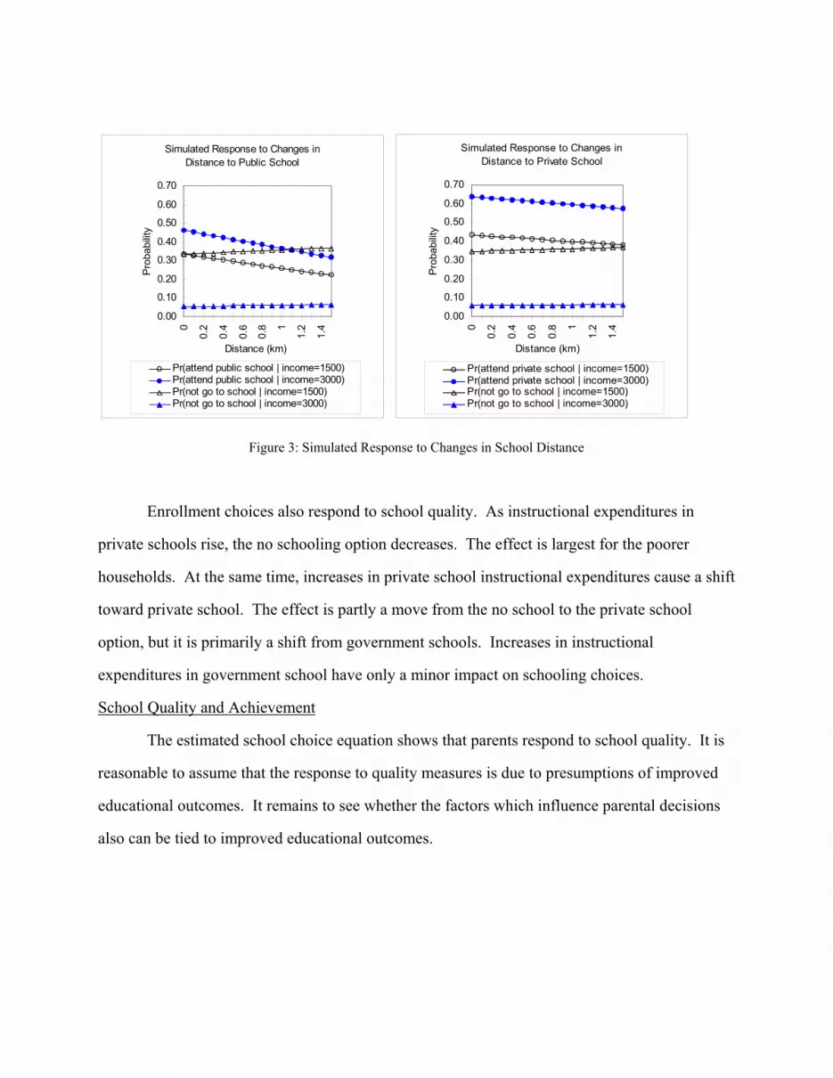
Figure 3 shows how enrollment probabilities change as proximity to private and

government schools change. Because average distance was just over one kilometer, the smaller

distances can be viewed as the impact of increased proximity to schools on school choice. For

the lower income group, increased proximity to private school causes a small increase in private

enrollment and an even smaller decrease in probability of the no school option. As income rises,

the no school option becomes insensitive to proximity to private schools, but private school

enrollments rise due to switching from government schools. Schooling choices respond

similarly to changes in proximity to government schools. The no schooling option falls more in

response to proximity to government school than to proximity to private school. As income

rises, the sensitivity of the no schooling option to distance decreases.

Simulated Response to Changes in

Distance to Public School

0.00

0.10

0.20

0.30

0.40

0.50

0.60

0.700

0.2

0.4

0.6

0.8 1

1.2

1.4

Distance (km)

Pro

babi

lity

Pr(attend public school | income=1500)Pr(attend public school | income=3000)Pr(not go to school | income=1500)Pr(not go to school | income=3000)

Simulated Response to Changes in Distance to Private School

0.00

0.10

0.20

0.30

0.40

0.50

0.60

0.70

0

0.2

0.4

0.6

0.8 1

1.2

1.4

Distance (km)

Pro

babi

lity

Pr(attend private school | income=1500)Pr(attend private school | income=3000)Pr(not go to school | income=1500)Pr(not go to school | income=3000)

Figure 3: Simulated Response to Changes in School Distance

Enrollment choices also respond to school quality. As instructional expenditures in

private schools rise, the no schooling option decreases. The effect is largest for the poorer

households. At the same time, increases in private school instructional expenditures cause a shift

toward private school. The effect is partly a move from the no school to the private school

option, but it is primarily a shift from government schools. Increases in instructional

expenditures in government school have only a minor impact on schooling choices.

School Quality and Achievement

The estimated school choice equation shows that parents respond to school quality. It is

reasonable to assume that the response to quality measures is due to presumptions of improved

educational outcomes. It remains to see whether the factors which influence parental decisions

also can be tied to improved educational outcomes.

Simulated Response to Changes in Public School Instructional Expenditures

0.00

0.100.20

0.300.40

0.500.60

0.70

0 75 150

225

300

375

per pupil expenditure

Pro

babi

lity

Pr(attend public school | income=1500)Pr(attend public school | income=3000)Pr(not go to school | income=1500)Pr(not go to school | income=3000)

Simulated Response to Changes in Private School Instructional Expenditures

0.00

0.10

0.20

0.30

0.40

0.50

0.60

0.70

0 75 150

225

300

375

per pupil expenditure

Pro

babi

lity

Pr(attend private school | income=1500)Pr(attend private school | income=3000)Pr(not go to school | income=1500)Pr(not go to school | income=3000)

Figure 4: Simulated Response to Changes in Instructional Expenditures

A subset of the children who were in the third grade were given a test of Urdu language

and mathematics.9 Generally the exams were given in the classrooms, but where necessary the

exams were administered in the children's homes. Because of the area frame sampling

methodology, these children should be representative of third grade children in these fifty

neighborhoods. Outcomes on these exams are assumed to be a function of parental inputs,

school attributes, and a separate constant term for private schools. To control for nonrandom

assignment into private schools, we use the estimated predicted probability of private school

enrollment based on the parameter estimates in Table 3. We also use the model in Table 3 to

estimate a selection correction for the fact that we only have test scores on children who enrolled

in school.

The results are reported in Table 6. We could not reject the null hypothesis of equality of

coefficients across boys and girls, so just the pooled results are presented. Test scores are not

significantly affected by household income, but are tied to parental education. Both father’s and

mother’s education raise the child’s performance on the exams, although the effect is only

significant for mother’s education. The greater impact of mother’s education on child learning is

consistent with the fact that mothers spend more time with children in these age groups than do

fathers. That parent’s education is complementary with schooling in the production of human

capital is consistent with the impact of parental education on schooling choices for the children

in Table 3.

School quality has mixed effects on student achievement. Instructional expenditures per

pupil do not have a significant impact on achievement, and the coefficient is negative for math

and the combined score. However, additional analysis which allows private and public schools

to have different input productivities reveals positive effects of per pupil expenditures in private

schools. The difference in the impact of expenditures is consistent with the differences of

instructional expenditures in demand. High pupil teacher ratios have a uniform negative effect

on student achievement, with the effect being particularly pronounced on language skills. This is

also consistent with the large negative effect of pupil teacher rates on probability of selecting

government schools. Finally, private schools have better outcomes than government schools

holding fixed measured home and school inputs into the human capital production process. This

is consistent with the apparent revealed preference for private schools over government schools,

even by low income households facing higher costs for private schooling.

Conclusions

This study demonstrates that schooling choices of poor households are very sensitive to

school fees, proximity and quality. Rather than being exploited by private schools, evidence

suggests that strong demand for private schools is in response to better quality and learning

opportunities offered by private schools. However, additional entry of private schools into poor

neighborhoods cannot be accomplished without government subsidy -- the poorest households

are not willing (or able) to generate sufficient resources needed to induce entry of additional

private schooling resources. However, the lower cost and higher achievement tests for private

schools suggest that public subsidy of private schools are a viable option for increased delivery

of schooling services to poor households.

References Alderman, H., J. Behrman, D. Ross, and R. Sabot. 1996. “Decomposing the Gender Gap in

Cognitive Skills in a Poor Rural Economy.” Journal of Human Resources 32(1):229-254. Cox, Donald and Emmanuel Jimenez. 1991. “The Relative Effectiveness of Private and Public

Schools: Evidence from Two Developing Countries.” Journal of Development Economics 34:99-121.

Deaton, Angus. 1988. “Quality, Quantity and Spatial Variation of Price.” The American

Economic Review 78(3):418-430. Gertler, Paul and Paul Glewwe. 1990. “The Willingness to Pay for Education in Developing

Countries: Evidence from Rural Peru.” Journal of Public Economics 42:251-275. Hammer, Jeffrey. Forthcoming. “Economic Analysis for Health Projects.” World Bank

Research Observer. Herriges, Joseph A., and Catherine L. Kling. 1996. “Nonlinear Income Effects in Random

Utility Models.” Department of Economics, Iowa State University. Mimeo. Jimenez, Emmanuel, Marlaine E. Lockheed, and Vincent Paqueo. 1991. “The Relative

Efficiency of Private and Public Schools in Developing Countries.” The World Bank Research Observer 6(2):205-218.

Kardar, Shahid. 1995. “Demand for Education. Survey of Households in Karachi.” Karachi:

Systems Limited. Mimeo. King, Elizabeth. 1995. “Does the Price of Schooling Matter? Fees, Opportunity Costs, and

Enrollment in Indonesia.” World Bank. Mimeo. Kingdon, Geeta. 1996a. “Private Schooling in India: Size, Nature, and Equity Effects.”

London: STICERD, London School of Economics Working Paper #72. Kingdon, Geeta. 1996b. “The Quality and Efficiency of Private and Public Education: A Case

Study of Urban India.” Oxford Bulletin of Economics and Statistics 58(1): 57-82. Lee, Lung-Fei. 1983. “Generalized Econometric Models with Selectivity.” Econometrica

51(2):507-512. McFadden, Daniel. 1995. “Computing Willingness to Pay in Random Utility Models.”

Department of Economics, University of California-Berkeley. Mimeo. Small, Kenneth A., and Harvey S. Rosen. 1981. “Applied Welfare Economics with Discrete

Choice Models.” Econometrica 49(1):105-130.

Notes

1. While the wording here suggests a sequential choice, the NMNL does not necessarily

imply a temporal process. 2. Utility for boys includes terms in α1(Y - Pj) and α2(Y - Pj)2, while utility for girls

includes α1(Y - Pj), α2(Y - Pj)2, -µF(α1 - α2 µF), and - 2α2 µF (Y - Pj). 3. Note that the rupee cost of transportation is included in the fees. 4. The biggest expense for private school is the fee, while in government school, over half

the expenses are for uniforms, books and supplies. 5. We also estimated the model using household income per capita in place of total

household income. While it is common in the literature to use per capita income, theoretical arguments suggest that total household income should enter the reduced form schooling demand specification. In addition, the per-capita income specification adds a potentially endogenous choice on family size as an explanatory variable. Specifications using per capita income yielded similar parameter estimates to those reported herein with the unreasonable exception that exceeded one.

6. We restricted the effect of parents’ education on schooling choice to be the same across

the government and private school options. While this was done to conserve on parameters, it is consistent with the Gertler and Glewwe (1990) finding that father’s and mother’s education levels had virtually identical impacts on choices of schooling alternatives.

7. The primary explanation for gender differences for enrollment in rural Pakistan is

differences in access to suitable schools (Alderman et al 1996). This is not as much a concern in urban areas.

8. The derivation is based on Small and Rosen (1981). McFadden (1996) has shown that

the Small and Rosen derivation only applies for linear-in-income utility, and that nonlinear income requires a laborious bootstrapping methodology. However, Herriges and Kling (1996) have shown that the bias from using the Small and Rosen approximation is small.

9. The exam was developed and piloted by the late Sar Khan. The exam was based on the

official curriculum which all schools, public or private, are expected to follow. The curriculum sets minimum objectives for each grade level.

Table 1A: Proportion of Children Enrolled in Lahore, by Income, Gender, and School Type

No School Private School Government School Share of All Households in

Group Income Group Boys Girls All Boys Girls All Boys Girls All

< 2000 .25 .21 .23 .35 .37 .37 .40 .41 .40 .143

2000 to 3500 .05 .04 .04 .59 .52 .56 .36 .45 .40 .407

3500 to 5000 .01 .01 .01 .78 .66 .72 .21 .33 .26 .215

5000 to 7000 .00 .00 .00 .84 .65 .73 .17 .35 .27 .110

7000 to 10000 .00 .00 .00 .88 .72 .79 .13 .28 .21 .080

> 10000 .00 .00 .00 .88 .81 .84 .12 .19 .16 .045

All .11 .08 .10 .61 .55 .58 .28 .37 .32 1.000

Table 1B: Average Monthly Rupee Expenditure and Percent of Income (in parentheses) Spent on a Child’s Education, by Income Group, Gender, and School Type

Average Monthly Expenditure (Percent of income)

Income Group Boys Girls Private Government

< 2000 162.4 (10.8) 156.4 (10.4) 178.7 (11.9) 142.0 (9.5)

2000 to 3500 215.8 (7.8) 199.1 (7.2) 227.2 (8.3) 181.3 (6.6)

3500 to 5000 304.1 (7.2) 262.4 (6.2) 317.5 (7.5) 198.8 (4.7)

5000 to 7000 355.6 (5.9) 344.9 (5.7) 395.1 (6.6) 225.8 (3.8)

7000 to 10000 584.2 (6.9) 434.5 (5.1) 544.8 (6.4) 346.6 (4.1)

> 10000 735.1 (5.9) 625.1 (5.0) 740.2 (5.9) 377.3 (3.0)

All 291.5 (7.8) 263.9 (7.0) 326.3 (7.9) 191.2 (6.5)

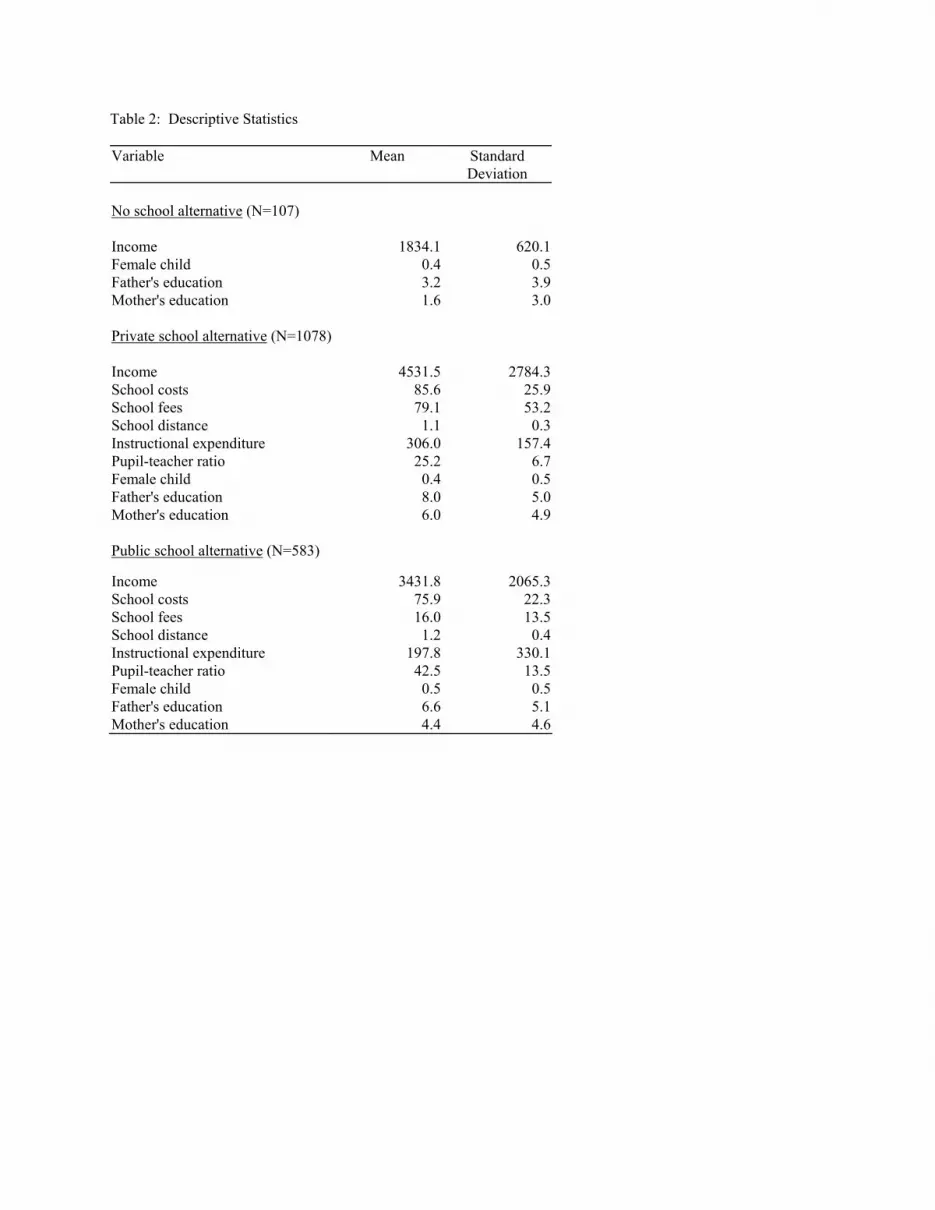
Table 2: Descriptive Statistics Variable Mean Standard

Deviation

No school alternative (N=107) Income 1834.1 620.1Female child 0.4 0.5Father's education 3.2 3.9Mother's education 1.6 3.0

Private school alternative (N=1078) Income 4531.5 2784.3School costs 85.6 25.9School fees 79.1 53.2School distance 1.1 0.3Instructional expenditure 306.0 157.4Pupil-teacher ratio 25.2 6.7Female child 0.4 0.5Father's education 8.0 5.0Mother's education 6.0 4.9

Public school alternative (N=583)

Income 3431.8 2065.3School costs 75.9 22.3School fees 16.0 13.5School distance 1.2 0.4Instructional expenditure 197.8 330.1Pupil-teacher ratio 42.5 13.5Female child 0.5 0.5Father's education 6.6 5.1Mother's education 4.4 4.6

Table 3: Nested Multinomial Logit of Demand for Schooling Choice

All children

Girls

Boys

Stage 1: No School versus School Option Consumption (α1)a 35.42 40.11 43.33

(9.69) (15.70) (13.30) Consumption squared (α2)b -24.59 -27.46 -31.14

(7.87) (13.28) (10.60) Female child -0.27

(0.19) Father's education -0.07 -0.03 -0.09

(0.03) (0.04) (0.03) Mother's education -0.12 -0.11 -0.13

(0.03) (0.05) (0.04) Sigma ( )σ 0.55 0.48 0.45

(0.17) (0.22) (0.16)

Stage 2: Private versus Government School Private School alternative: Constant -4.77 -3.74 -5.89

(0.91) (1.15) (1.18) School distance -0.18 -0.39 0.05

(0.20) (0.29) (0.39) Instructional expenditurec 0.13 0.11 0.12

(0.04) (0.05) (0.05) Pupil-Teacher Ratiod 0.26 0.09 0.41

(0.09) (0.13) (0.13)

Government School alternative Constant -3.87 -2.64 -5.35

(0.87) (1.08) (1.12) School distance -0.42 -0.54 -0.25

(0.13) (0.22) (0.17) Instructional expenditurec 0.04 0.01 0.06

(0.02) (0.03) (0.03) Pupil-teacher ratiod -0.08 -0.19 0.03

(0.04) (0.06) (0.06)

- Log Likelihood 1403.3 661.1 720.8 Sample size 1768 828 940 Standard errors in parentheses aVariable divided by 10000 for estimation bVariable divided by (10000)2 for estimation cVariable divided by 100 for estimation dVariable divided by 10 for estimation

Table 4: Estimated School Choice Arc Elasticitiesa with Respect to School Price and Quality

Alternative Private

school Government school

No school

Household income 0.122 -0.019 -3.026

Costs and fees Private school -0.108 0.174 0.263 Government school 0.053 -0.100 0.090

School distance Private school -0.072 0.123 0.067 Government school 0.180 -0.326 0.098

Instructional expenditure

Private school 0.143 -0.244 -0.133 Government school -0.027 0.049 -0.015

Pupil-teacher ratio Private school 0.235 -0.404 -0.221 Government school 0.116 -0.210 0.063 aThe probability of choosing each schooling option was predicted at two different levels of the respective school price or quality indicator. The elasticity of demand was then calculated as the ratio of the percentage change in the probability of choosing the option to the percentage change in price.

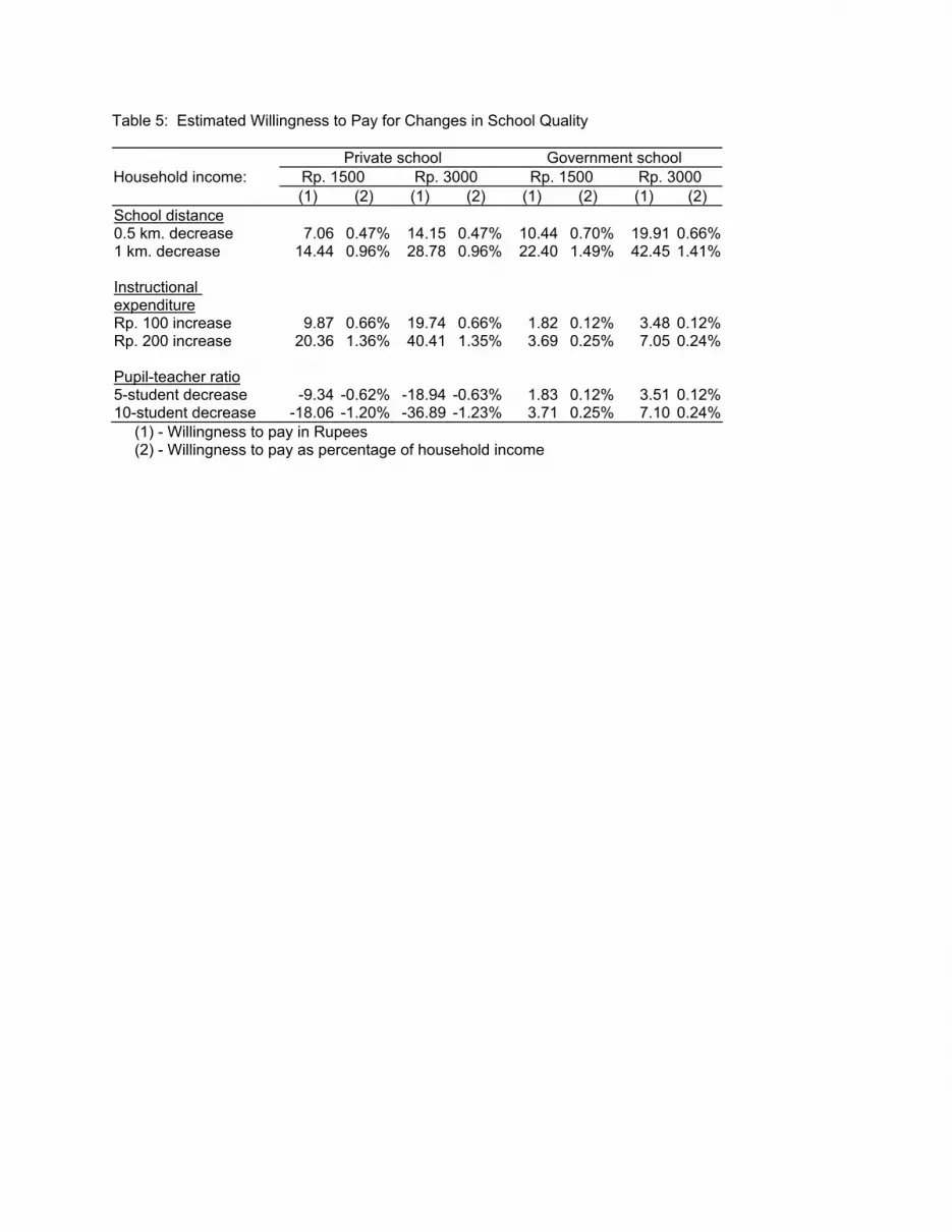
Table 5: Estimated Willingness to Pay for Changes in School Quality

Private school Government school Household income: Rp. 1500 Rp. 3000 Rp. 1500 Rp. 3000

(1) (2) (1) (2) (1) (2) (1) (2) School distance 0.5 km. decrease 7.06 0.47% 14.15 0.47% 10.44 0.70% 19.91 0.66% 1 km. decrease 14.44 0.96% 28.78 0.96% 22.40 1.49% 42.45 1.41%

Instructional expenditure

Rp. 100 increase 9.87 0.66% 19.74 0.66% 1.82 0.12% 3.48 0.12% Rp. 200 increase 20.36 1.36% 40.41 1.35% 3.69 0.25% 7.05 0.24%

Pupil-teacher ratio 5-student decrease -9.34 -0.62% -18.94 -0.63% 1.83 0.12% 3.51 0.12% 10-student decrease -18.06 -1.20% -36.89 -1.23% 3.71 0.25% 7.10 0.24% (1) - Willingness to pay in Rupees (2) - Willingness to pay as percentage of household income

Table 6: Analysis of Achievement Test Scores

Math score + Language

score

Math score

Language

score Constant 25.07 10.66 14.41

(4.48) (2.59) (2.44)Female child 0.85 -0.11 0.96

(1.09) (0.63) (0.59)Father's education 0.12 0.10 0.03

(0.13) (0.08) (0.07)Mother's education 0.40 0.20 0.20

(0.13) (0.08) (0.07)Incomea -2.54 -2.21 -0.33

(2.49) (1.44) (1.35)Instructional expenditureb -0.11 -0.11 0.01

(0.14) (0.08) (0.08)Pupil-teacher ratioc -0.45 -0.14 -0.31

(0.29) (0.17) (0.16)Private schoold 15.89 10.61 5.28

(6.37) (3.68) (3.46)λ e 4.05 2.18 1.87

(4.49) (2.60) (2.44)

R2 .102 .096 .086Sample size 263 263 263 Standard errors in parentheses. Sample means for mathematics and language scores were 17.9 and 19.0 for private schools and 16.3 and 17.4 for government schools. aVariable divided by 10000 for estimation bVariable divided by 100 for estimation cVariable divided by 10 for estimation dPredicted probability of attending a private school from the nested logit model in Table 3 eFollowing Lee (1983), λ = φ(Hj)/Φ(Hj) where φ(⋅) is the normal density function, Φ(⋅) is the cumulative normal distribution function, and Hj = Φ-1(1-Pj), Pj = predicted probability of the no school option for child j generated by the nested logit model in Table 3.