Scaling and comparison of fluid limits of queues appliedto call centers with time-varying parameters∗

Tania Jimenez‡ Ger Koole§†

‡ CESIMO, Universidad de los Andes, Merida, Venezuela

§ Department of Mathematics, Vrije Universiteit Amsterdam, The Netherlands

OR Spectrum 26: 413–422 (Special issue on Call Center Management), 2004

Abstract

Temporary overload situations in queues can be approximated by fluid queues.We strengthen earlier results on the comparison of multi-server tandem systems withtheir fluid limits. At the same time we give conditions under which economies ofscale hold. We apply the results to call centers.

Keywords: call centers, fluid limits, economies of scale, inhomogeneous Poissonprocesses.

1 Introduction

Queueing systems with inhomogeneous Poisson arrivals are extremely hard to analyzeexactly. However, in practice, constant rate Poisson input is the exception. For example,in call centers traffic is usually modeled as arriving according to an inhomogeneous Poissonprocess with a piecewise constant arrival rate. As long as the system is stable under allpossible arrival rates, then a simple approximation based on stationarity often suffices,see Green & Kolesar [4]. The idea of this pointwise stationary approximation (PSA) isthat the performance at each moment is approximated by the stationary performanceof the system with the parameters as they are at that point in time. This method ofcomputing the performance is indeed common practice in call centers, where usually theErlang delay formula is chosen to approximate stationary performance. See Gans et al. [2]for an overview of the modeling of call centers.

The situation changes when an overload situation occurs during some of the time. Sta-tionarity cannot be used during the overload period, as this would result in an infinite queue

∗Copyright Springer-Verlag. The original publication is available at http://www.springerlink.com†Communicating author. Full address: Department of Mathematics, Vrije Universiteit, De Boelelaan

1081a, 1081 HV Amsterdam, The Netherlands. Email koole@few.vu.nl, fax +31 20 4447653

1

length, while in reality the queue length remains finite, it is just building up. And worse,stationarity fails also in subsequent underload intervals, because of the large quantities ofjobs that are transferred to later intervals.

There are several potential ways to deal with temporary overload situations. In thispaper we focus on the use of fluid limits, but let us first discuss some other possibilities.

In Jennings et al. [6] a non-homogeneous multi-server queue is approximated by aninfinite-server ‘queue’. This is relevant to time-inhomogeneous systems because serversstill being busy due to a high load earlier in time are modeled. On the other hand,queueing phenomena including a queue building up in overload are not modeled. For thisreason this method is expected to work better than the PSA in situations when the ratechanges quickly, because then queueing hardly ever occurs. This intuition is confirmed bythe results in Jennings et al. [6] and Massey & Whitt [10]. In this paper we are interestedin situations where delayed customers due to longer overload periods play a crucial role.Therefore a method based on an infinite-server queue is less suitable.

An exact, but numerically demanding method is uniformization (see, e.g., Section 6.7of Ross [13]). In Ingolfsson et al. [5] this method is successfully used in the context of callcenters. (This method is only exact for piecewise homogeneous processes.) In this paperwe use simulation to verify the results based on fluid models.

The idea of using fluid limits to model overload situations dates back to Newell [11].He sees the fluid limit as the average over many samples of the input. This results, forexponential service times, in multiplying the arrival rate and the service rate with the samenumber k. The limit as k →∞ is the fluid limit. In Altman, Jimenez, & Koole [1] it wasshown for an important class of systems and objectives that this fluid limit has a lowervalue than the original system. A second way to define a fluid limit is by scaling the arrivalrate and the number of servers, but keeping the service rate constant. This converges to adifferent fluid limit (see Mandelbaum, Massey & Reiman [8]), that has in general a highervalue than the fluid limit first introduced. We start with showing that this second fluidlimit is again a lower bound on the performance of the real system, by considering first,using coupling arguments, the effects of scaling. This gives results on scaling that areinteresting on their own.

Next we move to call centers and approximations using fluid limits. In Mandelbaum,Massey, Reiman & Rider [9] it is shown that the second fluid limit approximates the realperformance exceptionally well in the situation of call centers. However, there numericalexamples deal almost exclusively with overload situations. Indeed, the examples in [1] showthat the first fluid limit gives a poor approximation in situations with a low load. This isnot different for the second fluid limit. This leads us to the following simple performanceapproximation, to be used in all situations: the performance at some point in time tis approximated by the maximum of the performance of the fluid limit at t and of theperformance of the stationary M/M/s queue with as input rate the minimal rate up to t.For obvious reasons this is again a lower bound of the performance. Intuitively this boundperforms well in clear underload and overload situations. The approximation is worst incases where the system is very close to the critical load. This is also numerically shown.

We illustrate these ideas in the context of call centers, where we base our analysis on

2

data from an existing call center.

2 Economies of scale

Fluid limits for queueing systems can be taken in several ways. In this paper we look ata method that consists of increasing the number of servers and the arrival rate with thesame factor. This means that the number of customers in the system increases as well,thus the performance measure (e.g., the number of customers) has to be scaled as well.This is actually equivalent to increasing the scale of the system.

In this section we answer the question of when increasing scale leads to improved results,i.e., when economies of scale hold. That the answer to the last question is non-trivial isshown by the following numerical example.

Consider first the stationary M(λ)/M(µ)/s system, and let Wq(λ, s) be its waitingtime distribution. Then Wq(λ, s) is exponentially distributed with parameter sµ− λ withprobability C(s, λ/µ) (the so-called delay probability), and Wq(λ, s) = 0 with probability1 − C(s, λ/µ). It is well-known that C(ks, kλ/µ) ≤ C(s, λ/µ) for k ∈ IN. From this itfollows that IP(Wq(λ, s) > t) ≥ IP(Wq(kλ, ks) > t). This result does, surprisingly enough,not hold for the transient system. To see this, consider an initially empty M(λt)/M/1 queuewhere λt � µ for small t: we only consider arrivals until u with u such that

∫ u0 λtdt = 2.

Denote with Wqt the waiting time of a customer that arrives at t. Note that Wqu(λt, 1) > 0if there is one customer in the system at u. Because λt � µ we find that IP(Wqu(λt, 1) >0) ≈ IP(1 arrival in Poisson process with parameter 2). Similarly, Wqu(2λt, 2) > 0 if thereare two customers in the system at u. Thus IP(Wqu(λt, 1) > 0) ≈ 1 − e−2 ≈ 0.86, butIP(Wqu(2λt, 2) > 0) ≈ 1 − e−4 − 4e−4 ≈ 0.91. Thus the probability of being servedimmediately is bigger in the single-server system, therefore increasing scale does not giveadvantages.

The question we will answer next is for which types of performance measures an increaseof scale leads to performance improvements. Let Qt (Qk

t ) be the queue length process ofan M(λt)/M/s (M(kλt)/M/ks) queue. We are interested in comparing (functions of) Qt

and Qkt for all or some t > 0. To be able to do so we first couple both systems, leading to

the following theorem.

Theorem 2.1 Let Q(1)t , . . . , Q

(k)t represent k independent copies of Qt. Then Q

(1)t , . . . , Q

(k)t

and Qkt can be coupled such that for all realizations Q

(1)t (ω), . . . , Q

(k)t (ω) and Qk

t (ω) we have

Q(1)t (ω) + · · ·+ Q

(k)t (ω) ≥ Qk

t (ω), assuming that it holds initially.

Proof We will consider the k parallel M(λt)/M/s queues as a single system. Bothsystems can be coupled as follows: when an arrival occurs at the M(kλt)/M/ks queuethere is also an arrival at one of the parallel queues, each with probability 1/k. Thedepartures are coupled in the following way: there are ks independent Poisson processes,each governing the potential departures of a server in each system. The systems arecoupled in such a way that an active server in the M(kλt)/M/ks queue corresponds to an

3

active server in one of the M(λt)/M/s queues. With this coupling it is easily seen that

Q(1)t (ω) + · · ·+ Q

(k)t (ω) ≥ Qk

t (ω) is preserved.

Remark Up to now we have assumed that only the arrival rate changes over time. Itis also possible to make the service rate and the number of servers change, without anyadditional difficulties.

Next we introduce performance measures C and Ck, which are functions of the stateof the original and the scaled system. In this paper we will use increasing and convex inthe non-strict sense. With ≤s we indicate the usual stochastic order: X ≤s Y means thatX and Y can be coupled such that X(ω) ≤ Y (ω) for all ω.

Theorem 2.2 Let Ck be increasing and convex and Ck(kx) ≤ C(x). Then IECk(Qkt ) ≤

IEC(Qt) for all t, assuming that initially Qk0 ≤s kQ0.

Proof According to Theorem 2.1 and the fact that the current initial condition is strongerthan in Theorem 2.1, Qk

t and Qt can be coupled such that for Q(i)t (ω) = xi and Qk

t (ω) = x,x1 + · · ·+ xk ≥ x. By Ck(kx) ≤ C(x) we have

C(x1) + · · ·+ C(xk) ≥ Ck(kx1) + · · ·+ Ck(kxk).

Next, by convexity of Ck we find

Ck(kx1) + · · ·+ Ck(kxk)

k≥ Ck((kx1 + · · ·+ kxk)/k) = Ck(x1 + · · ·+ xk).

Finally, as Ck is increasing, we have

Ck(x1 + · · ·+ xk) ≥ Ck(x).

Combining all and taking expectations gives IEC(Qt) ≥ IECk(Qkt ).

Let us interpret Theorem 2.2, by considering some relevant cost functions and see ifthey satisfy the conditions. Consider the expected number of calls in the system. If weincrease the scale by a factor k we expect, due to economies of scale, that the number ofcalls increases by less than k, i.e., we expect IEQk

t ≤ IEkQt. This follows directly fromTheorem 2.2 by taking C(x) = x and Ck(x) = x/k, and for which choice Ck(kx) = C(x).We see that, in correspondence with the fluid limit, we have to scale the queue lengths aswell. Other cost functions can be of interest, such as the expected number of customers inthe queue C(x) = max{x−s, 0} = (x−s)+ and its scaled counterpart Ck(x) = (x−ks)+/k.The function Ck is convex and again Ck(kx) = (x− s)+ = C(x).

Next we consider waiting times. The expected waiting time IEWqt is given by IEWqt =(Qt + 1− s)+/(sµ), for the scaled system by IEW k

qt = (Qkt + 1− ks)+/(ksµ). Thus C(x) =

(x + 1− s)+/(sµ) and Ck(x) = (x + 1− ks)+/(ksµ). It is easily seen that Ck(kx) ≤ C(x);note that Ck(kx) < C(x) if x > s.

4

Through a counterexample we saw earlier in this section that IP(W kqt > v) ≤ IP(Wqt > v)

does not hold in general. This is because of the fact that IP(W kqt > v) is not convex in the

queue length. We work this out for v = 0, then IP(W kqt > v) = II{Qk

t > s}, with II theindicator function: II{A} = 1 if A holds, 0 otherwise. This function is increasing, but notconvex. A performance indicator that is convex and relevant to call centers is IE(Wqt−v)+,the expected time that waiting exceeds v (see Koole [7]). This can be seen as follows. LetE1, E2, . . . be independent exponential random variables (r.v.s) with parameter sµ, anddefine the gamma distributions Gn = E1 + · · ·+ En. Define also G0 = 0. Then

IE(Wqt − v)+ = IEQt−s∑n=0

IP(Gn ≤ v < Gn+1)Qt + 1− s− n

sµ= IE

Qt−s∑n=0

IP(v < Gn+1)1

sµ.

From this we deduce that C(x) =∑x−s

n=0 IP(v < Gn+1)1sµ

. Thus C(x) = 0 as long as x < s,

if x ≥ s then C(x) − C(x − 1) = IP(v < Gx−s+1)1sµ

. This number is increasing in x, andtherefore C is convex.

Now consider the scaled system, with performance IE(W kqt−v)+. Similarly, let Ek

1 , Ek2 , . . .

be independent exponential r.v.s with parameter ksµ, and take Gkn = Ek

1 + · · ·Ekn, Gk

0 = 0.Then Ck(x) =

∑x−ksn=0 IP(v < Gk

n+1)1

ksµ. This is again convex, the question that remains to

be answered is whether Ck(kx) ≤ C(x), which is equivalent to:

IE(Gkkn+1 − v)+ ≤ IE(Gn+1 − v)+,

which follows from the fact that Gkkn is stochastically less variable than Gn (see Ross [12],

Section 8.5).

3 Fluid limits and performance bounds

In general, there are different ways to take fluid limits. In our context it is crucial that thetime is not scaled, because we are interested in modeling a non-stationary arrival process.Then there are two ways of taking fluid limits. Let us briefly discuss the classical onebefore we continue with the one we focus on in this paper.

The classical method (already proposed by Newell [11] in 1971) consists of averaging thearrival process over multiple realizations. This is, for the M(λt)/M(µ)/s queue, equivalentto scaling λt and µ. In the limit the amount of work that arrives during a period [t0, t1] isequal to

∫ t−1t0

λtdt/µ a.s. It disappears at a fixed rate sµ, as long as there is fluid. The limitis thus a continuous non-negative function zt, with z0 given, and derivative z′t = λt − sµ ifzt > 0, and z′t = (λt − sµ)+ if zt = 0.

This type of fluid limit can also be obtained for general service times. The method is lesssuitable for multi-server queues, as it gives the same limit as for single-server queues (withthe server speed appropriately scaled). This way of scaling is therefore most appropriatefor the Mt/G/1 queue. See Altman et al. [1] for results concerning comparison with fluidlimits that parallel the results obtained here with for the fluid limit discussed next.

5

The second way of taking fluid limits is by increasing s and λ with the same factor. Thisis actually equivalent to increasing the scale of the system. It also means that the numberof customers in the system increases as well, and therefore the performance measure (e.g.,the number of customers) has to be scaled. The resulting fluid limit zt = limk→∞ Qk

t /k isdefined by its derivative z′t = λt −min(zt, s)µ. As a result single and multi-server queuesgive different limits.

We are interested in limk→∞ IECk(Qkt ). We have the following result, showing that for

well-chosen Ck and C this fluid limit gives again a lower bound to the performance.

Theorem 3.1 For Ck increasing and convex for each k ∈ IN and Ck(kx) ≤ C(x) for allk, x then C(x) = lim supk→∞ Ck(kx) is such that C(zt) ≤ C(Qt).

Proof The function C is well-defined because C(x) ≤ supk Ck(kx) ≤ C(x). By domi-nated convergence, using Theorem 2.2, we find C(zt) = lim supk→∞ IECk(Qk

t ). Combiningthis with IECk(Qk

t ) ≤ IEC(Qt) gives the desired result.

A special case of Theorem 3.1 is when Ck(kx) = C(x). Then C = C. This was thecase when considering the number of calls in the system. This shows that the fluid limit isa lower bound for the number of calls in the system. In the case of expected waiting timeslimk→∞ Ck(kx) = (x − s)+/(sµ) = C(x). In the case of the expected time that waitingexceeds v we find limk→∞ Ck(kx) = (x− v)+.

Theorem 3.1, together with the following lemma, motivates us to concentrate on thefluid limit zt.

Lemma 3.2 If z0 = z0, then zt ≥ zt for all t ≥ 0.

Proof If zt = zt, then z′t = λt − min(zt, s)µ ≥ λt − II{zt}sµ = z′t. From this the resultfollows directly.

In Mandelbaum et al. [9] z is used for a call center, but mainly in overload. For astable system with a constant arrival rate (i.e., λ < sµ) the fluid limit tends to λ/µ: ifzt > λ/µ, then z′t < 0, and vice versa. This explains why the fluid approximation is so badfor these systems: for the M/M/1 queue for example, the average queue length is given by∑∞

n=1 n(1− λ/µ)(λ/µ)n = λ/(λ− µ).In both fluid limits waiting does not occur due to random fluctuations. In the first type

of limit that is because the randomness is averaged out of the arrival process, in the secondtype this is due to the scaling of the system. Waiting can still occur because of fluctuationsin the arrival rate. It is exactly for these reasons that fluid limits are useful for transientanalysis, especially because there are no exact results for models with a non-homogeneousarrival process.

As an example, take the stationary M(λ)/M/1 queue. The average number of cus-tomers in the system is given by λ/(µ − λ). The limit for the first fluid limit is 0, andfor the second it is λ/µ: this is the fraction of servers that is busy. Customers spend

6

respectively on average 1/(µ− λ), 0, and 1/µ time units in the system. Note that for thefirst fluid limit customers become infinitesimally small; this explains the sojourn time of 0.

We consider a queueing system in [0, T ]. We assume that [0, T ] is divided in n intervals[0, t1], [t1, t2], . . . , [tn−1, T ] (with 0 = t0 < t1 < · · · < tn−1 < tn = T ). During interval i(from ti−1 to ti) customers arrive according to a Poisson process with rate λi. As beforewe keep µ and s constant. We consider thus an M/M/s system with inhomogeneouspiecewise constant arrival rate. Furthermore, we assume that the system is in a stationarysituation for some arrival rate λ0 (with λ0 < sµ) at time 0. This is the usual way tomodel call centers, see Gans et al. [2], although it is advisable in many situations to modelabandonments as well. Also the choice to keep s constant is not very realistic, although wewill show an application in which it is the case. Making s time-dependent is possible, butto keep the exposition simple we choose not to do it. Both abandonments and time-varyingnumbers of servers are subject of ongoing research.

Now consider some performance measure C that is increasing. Define

λ∗t = min{λ0, mini|ti−1<t

λi},

the minimal rate up to t. Denote with Qλ the stationary distribution of the M(λ)/M(µ)/squeue.

Lemma 3.3 IEC(Qt) ≥ IEC(Qλ∗t) for all t ≥ 0.

Proof Using a coupling argument it is easily seen that Qt ≥s Qλ∗tfor all t. The result

follows because C is increasing.

Now assume we also have some C(x) = lim supk Ck(kx) with all Ck convex and in-creasing. We propose the following approximation for the performance at t, denoted byLt:

Lt = max{C(zt), IEC(Qλ∗t)},

which is the maximum of the performance of the fluid limit at t and of the performanceof the stationary M/M/s queue with as input rate the minimal rate up to t. Thanks toLemma 3.3 and Theorem 3.1 we know that this is a lower bound to the system performance,i.e., IEC(Qt) ≥ Lt.

In the next section we show how this approximation works in the context of a callcenter.

4 A call center application

In this section we study a simple time-varying model for a call center. After introducingthe model we apply the results of the previous section to obtain a lower bound on theperformance.

7

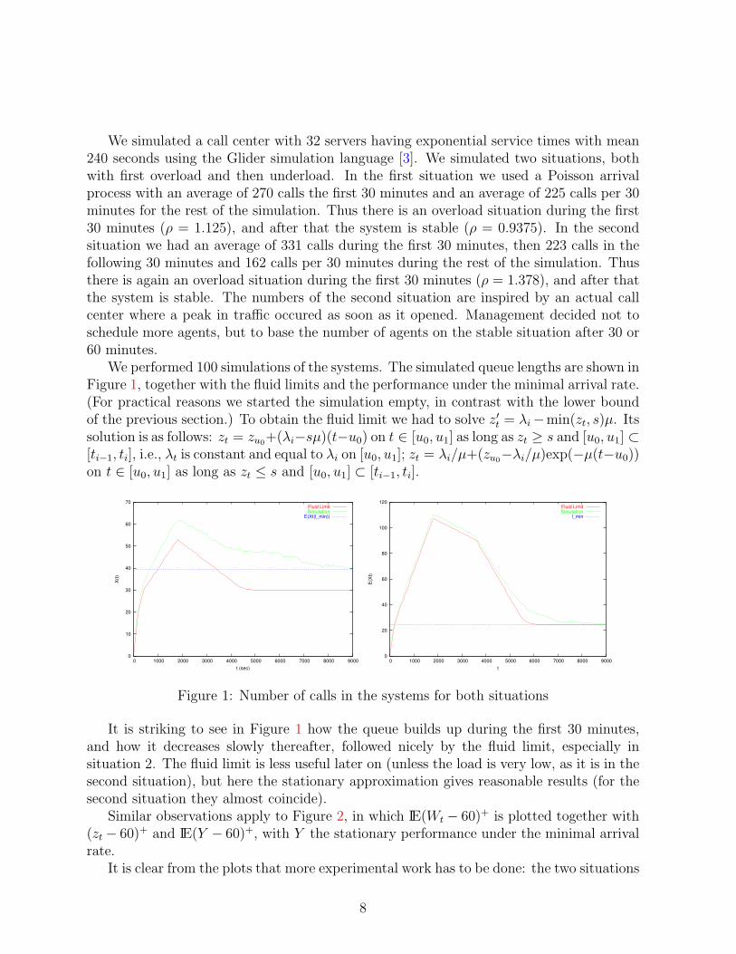
We simulated a call center with 32 servers having exponential service times with mean240 seconds using the Glider simulation language [3]. We simulated two situations, bothwith first overload and then underload. In the first situation we used a Poisson arrivalprocess with an average of 270 calls the first 30 minutes and an average of 225 calls per 30minutes for the rest of the simulation. Thus there is an overload situation during the first30 minutes (ρ = 1.125), and after that the system is stable (ρ = 0.9375). In the secondsituation we had an average of 331 calls during the first 30 minutes, then 223 calls in thefollowing 30 minutes and 162 calls per 30 minutes during the rest of the simulation. Thusthere is again an overload situation during the first 30 minutes (ρ = 1.378), and after thatthe system is stable. The numbers of the second situation are inspired by an actual callcenter where a peak in traffic occured as soon as it opened. Management decided not toschedule more agents, but to base the number of agents on the stable situation after 30 or60 minutes.

We performed 100 simulations of the systems. The simulated queue lengths are shown inFigure 1, together with the fluid limits and the performance under the minimal arrival rate.(For practical reasons we started the simulation empty, in contrast with the lower boundof the previous section.) To obtain the fluid limit we had to solve z′t = λi−min(zt, s)µ. Itssolution is as follows: zt = zu0+(λi−sµ)(t−u0) on t ∈ [u0, u1] as long as zt ≥ s and [u0, u1] ⊂[ti−1, ti], i.e., λt is constant and equal to λi on [u0, u1]; zt = λi/µ+(zu0−λi/µ)exp(−µ(t−u0))on t ∈ [u0, u1] as long as zt ≤ s and [u0, u1] ⊂ [ti−1, ti].

0

10

20

30

40

50

60

70

0 1000 2000 3000 4000 5000 6000 7000 8000 9000

X(t)

t (sec)

Fluid LimitSimulation

E(Xt(l_min))

0

20

40

60

80

100

120

0 1000 2000 3000 4000 5000 6000 7000 8000 9000

E(X

t)

t

Fluid LimitSimulation

l_min

Figure 1: Number of calls in the systems for both situations

It is striking to see in Figure 1 how the queue builds up during the first 30 minutes,and how it decreases slowly thereafter, followed nicely by the fluid limit, especially insituation 2. The fluid limit is less useful later on (unless the load is very low, as it is in thesecond situation), but here the stationary approximation gives reasonable results (for thesecond situation they almost coincide).

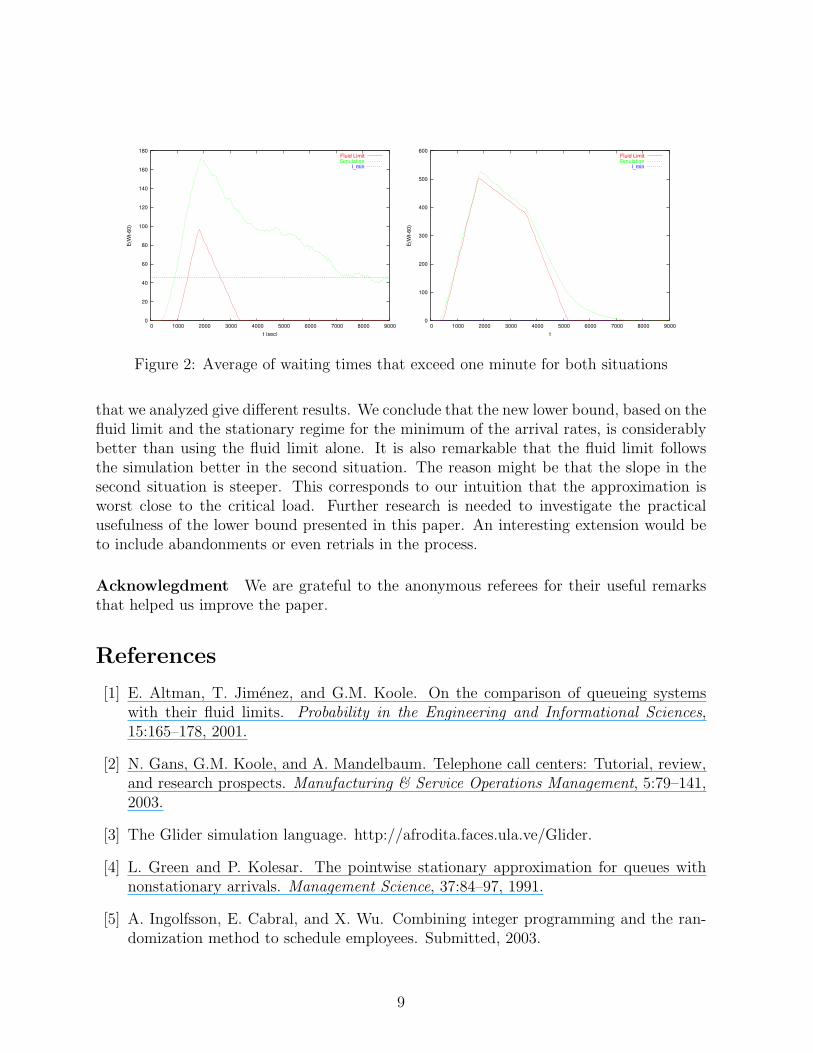
Similar observations apply to Figure 2, in which IE(Wt − 60)+ is plotted together with(zt − 60)+ and IE(Y − 60)+, with Y the stationary performance under the minimal arrivalrate.

It is clear from the plots that more experimental work has to be done: the two situations

8

0

20

40

60

80

100

120

140

160

180

0 1000 2000 3000 4000 5000 6000 7000 8000 9000

E(W

t-60)

t (sec)

Fluid LimitSimulation

l_min

0

100

200

300

400

500

600

0 1000 2000 3000 4000 5000 6000 7000 8000 9000

E(W

t-60)

t

Fluid LimitSimulation

l_min

Figure 2: Average of waiting times that exceed one minute for both situations

that we analyzed give different results. We conclude that the new lower bound, based on thefluid limit and the stationary regime for the minimum of the arrival rates, is considerablybetter than using the fluid limit alone. It is also remarkable that the fluid limit followsthe simulation better in the second situation. The reason might be that the slope in thesecond situation is steeper. This corresponds to our intuition that the approximation isworst close to the critical load. Further research is needed to investigate the practicalusefulness of the lower bound presented in this paper. An interesting extension would beto include abandonments or even retrials in the process.

Acknowlegdment We are grateful to the anonymous referees for their useful remarksthat helped us improve the paper.

References

[1] E. Altman, T. Jimenez, and G.M. Koole. On the comparison of queueing systemswith their fluid limits. Probability in the Engineering and Informational Sciences,15:165–178, 2001.

[2] N. Gans, G.M. Koole, and A. Mandelbaum. Telephone call centers: Tutorial, review,and research prospects. Manufacturing & Service Operations Management, 5:79–141,2003.

[3] The Glider simulation language. http://afrodita.faces.ula.ve/Glider.

[4] L. Green and P. Kolesar. The pointwise stationary approximation for queues withnonstationary arrivals. Management Science, 37:84–97, 1991.

[5] A. Ingolfsson, E. Cabral, and X. Wu. Combining integer programming and the ran-domization method to schedule employees. Submitted, 2003.

9

[6] O.B. Jennings, A. Mandelbaum, W.A. Massey, and W. Whitt. Server staffing to meettime-varying demand. Management Science, 42:1383–1394, 1996.

[7] G.M. Koole. Redefining the service level in call centers. Working paper, 2003.

[8] A. Mandelbaum, W.A. Massey, and M.I. Reiman. Strong approximations for Marko-vian service networks. Queueing Systems, 30:149–201, 1998.

[9] A. Mandelbaum, W.A. Massey, M.I. Reiman, and R. Rider. Time varying multiserverqueues with abandonments and retrials. In P. Key and D. Smith, editors, Proceedingsof the 16th International Teletraffic Conference, 1999.

[10] W.A. Massey and W. Whitt. Peak congestion in multi-server service systems withslowly varying arrival rates. Queueing Systems, 25:157–172, 1997.

[11] G.F. Newell. Applications of Queueing Theory. Chapman and Hall, 1971.

[12] S.M. Ross. Stochastic Processes. Wiley, 1983.

[13] S.M. Ross. Introduction to Probability Models. Academic Press, 7th edition, 1997.

10