scaling analysis of dark matter models

Astroparticle Physics

ELSEVIER Astroparticle Physics 5 (1996) 53-68

Scaling analysis of dark matter models G. Murante”, A. Provenzalea, S. Borgani b,c, A. Campos d, G. Yepese

a Istituto di Cnsmogeojisica de1 CNR, Corso Fiume 4, I-10133 Torino. Italy

h INFN - Sezione di Perqiu, c/o Dip, di Fisica dell’liniversita’, Via A. Pascoli, l-06100 Perugia. Ital)

’ SISSA. International Schoolfor Advanced Studies, via Beirut 2, I-34014 Trieste. Italy

’ Dept. of’ Physics. University of Durham, Durham. DHI 3LE. UK

’ Dept. Fisica Tenrica C-XI, Univ. Autonoma de Madrid. Cantoblanco 28049. Mudrid, Spin

Received 19 November 1995; revised 16 January 1996

Abstract

We discuss the scaling analysis of CDM and CHDM simulations. We show that on scales larger than about 4-5 h-’ Mpc the two models behave quite differently. In particular, CDM simulations with bias b = I .5 reveal a smooth transition from small-scale nonlinear clustering to homogeneity, while CDM models with bias b = 1 are characterised by the existence of an intermediate scaling regime with generalized dimensions between 2 and 3. The CHDM models tend to generate an intermediate scaling regime with values of the generalized dimensions smaller than 2. Correspondingly. the value of the tilling factor on intermediate scales. defined as the fraction of non-empty volumes sampling the distribution, is different for CDM and CHDM simulations: the CHDM model is less “space-filling” than the standard CDM. These results indicate that the scaling analysis is a valuable tool for distinguishing between different cosmological models and that a careful evaluation of the behavior of the galaxy distribution in the weakly nonlinear regime between about 5 and 20 h-’ Mpc could provide hints about the reliability of different DM models.

Kqword,~: Galaxy clustering; Galaxy formation; Statistical methods; Large-scale structure of Universe

1. Introduction

In the last ten years the available galaxy redshift samples have revealed a wide variety of structures, like voids, long filaments and clusters, which characterize the global texture of the large-scale structure of the Universe [ I 1. On the scales of nonlinear clustering (5 5 h-’ Mpc) the galaxy distribution displays a hierarchical distribution, characterized by approximate scaling properties, see [2] for a review. Consistent with these findings, the scaling analysis of N-body simulations [ 3-51 has shown that non-linear gravitational dynamics is capable of producing scaling behavior on small scales.

On larger scales, however, the non-trivial pattern of the galaxy distribution represents a serious challenge for any theory on the formation and evolution of cosmic structures. In particular, the large structures en- countered on the scales between the break-up of the non-linear scaling regime and the crossover to homogeneity (say between about 5 and 30 h-’ Mpc) represent an important information, which may both shed light on the weakly non-linear gravitational evolution and put quantitative constraints on the shape of the initial fluctuation spectrum. In particular, one of the most eminent victims of the presence of large-scale clustering is the standard Cold Dark Matter (CDM) scenario. In its minimal version, this model assumes

0927.6.505/96/$15.00 @ 1996 Elsevier Science B.V. All rights reser PII SO927-6505( 96)00005-9

54 G. Murante et al./Astroparricle Physics 5 (1996) 53-68

a flat Universe with 0~ = 1, Gaussian adiabatic initial fluctuations, a post-inflationary Zel’dovich spectrum modulated by a suitable CDM transfer function [6] and galaxies substantially more clustered than DM, by a factor 0 = 2. This model has troubles to repro- duce a variety of observational constraints, such as the level of CMB anisotropy [ 71, angular [ 81 and spatial [ 9, IO] galaxy correlations, large-scale velocity fields [ 111 and cluster correlations [ 12-161. Normalizing CDM to COBE data, b N 1, improves to some extent the large-scale behavior, but provides too large galaxy velocity dispersion on small scales [ 17,181.

On the other hand, adding a hot DM component, still requiring the COBE normalization improves the shape of the power-spectrum on 2 20 h-’ Mpc scales, while keeping peculiar velocities on N 1 h-’ Mpc to an adequate level (see [ 191 and references therein for a recent review of CDM and its main variants). The resulting Cold+Hot DM (CHDM, hereafter) mixture with 0~0~ N 0.2-0.3 is able to account for a large variety of observational constraints (see e.g. [ 181 and references therein). Assuming neutrinos for the hot component, the above requirement leads to a neutrino mass in the range m, cx 4.5-7 eV.

In [ 181 it was found that the COBE-normalized CHDM model with b = 1.5 passes a list of observational tests, including both small- and large-scale velocity fields. Klypin, Nolthenius & Primack [ 201 used higher resolution CHDM simulations and found agreement with IRAS and CfA galaxy power spectra. In [ 2 I] it was found that the properties of CHDM galaxy groups agree with those of CfA groups. Yepes et al. [22] estimated the angular correlation function for CHDM and compared it with the APM results, finding that the CHDM model is the best to fit the observations although there is a discrepancy of 40 % between the CHDM and the APM that seems real. Bonometto et al. [ 231 realized a detailed study of high-order correlation functions and void-probability-function devel- oped by CDM and CHDM initial spectra. They found that on the scales of non-linear clustering the resulting galaxy distributiondisplay hierarchical scaling, re- markably close to that implied by observational data.

In this paper we use the same set of high-resolution simulations to pursue a detailed scaling analysis of CDM and CHDM peak distributions. Since precise re- lations exist between scaling properties and hierarchical behavior of n-points correlation functions [ 21 we

expect this to represent an alternative approach to that followed in [ 231. In particular, we show that the scaling analysis of the peak distribution on intermediate scales (r 5 20 h-’ Mpc) may be used as a tool to test cosmological models.

In Section 2 we describe the simulations and the galaxy identification scheme. Section 3 is devoted to a brief introduction to scaling and to the description of the analysis methods. In Section 4 we present the results of the analysis; discussion and conclusions are presented in Section 5.

2. Simulations and galaxy identification

We analyze two CHDM and two CDM simulations, realized in 50 h-’ Mpc boxes. A Particle-Mesh (PM) code with 5123 force resolution (i.e., 98 h-’ kpc for the grid size) was used for the simulations. The CDM simulations had 256” = 16.8 x lo6 cold particles; the CHDM simulations had an additional 2 x 2563 hot particles, for a total of 50.3 x 1 O6 particles. The cold particles have masses of 2.1 x 1 O9 h-t Ma in the CDM simulations and 1.4 x lo9 h-‘M. in the CHDM simulations; the hot particles had masses of 3.1 x 1 OS h-’ MS in the CHDM simulations. Each pair of the hot particles was given oppositely directed “thermal” velocities drawn from a redshifted Fermi-Dirac distribution [ 181. The CHDM simulations were made for the case .a cdm = 0.6, flbarwn = 0.1, and L&, = 0.3, using the power spectra given in [ 181. The power spectrum of Bardeen et al. [ 61 was used to set initial conditions for the CDM simulations. For both models a Zel’dovich post-inflationary spectrum is assumed.

Two different realizations of CHDM are considered, CHDMl and CHDM2, corresponding to different as- signements of random initial phases. The two CHDM simulations were started at redshift z = 15 and normalized to the linear bias parameter b = 1.5.

The CDM simulations were done with exactly the same random phases as in CHDMt, so that all large features in these simulations correspond. One of the CDM simulations (CDMI ) was started at z = 27.5 with bias b = 1. The second CDM configuration is obtained by taking z = 18 for the starting redshift. Therefore, at z = 0 it is b = 1.5 (CDM1.5). In this way, CDMl is normalized exactly as CHDM on large scales, while CDMl.5 has the same small-scale

G. Murante er al. /A.woparricle Physics 5 (I 996) 53-68

CHDMZ

CDM b=l.5

CDM b=l

Fig. I. Distribution of density peaks with p > SO{ p) m the four simulations considered in the analysis.

(8 h-’ Mpc) normalization as CHDM. Fig. 1 shows largest waves in the CHDMt and CDM simulations the distribution of peaks with density p > 50(p) for had amplitude about 1.3-I .4 times larger than ex- the four simulations considered here. More details on petted for an average realization. This statistical fluke the simulations are given in [ 201. We note that the has a probability of occurrence of about 1096, so it is

56 G. Murmte et ~tI./Astroprrrticle Physics 5 (1996) 53-68

not unlikely. CHDM2 has a more typical power spectrum; a comparison of these two CHDM simulations thus gives some idea on the cosmic variance.

A delicate point in the analysis of any purely gravitational N-body simulation concerns the identification of galaxies. The original idea of identifying galaxies as peaks of the linear density field [ 61 has been recently questioned with the availability of high-resolution simulations; only a weak correlation has been found between peak positions in the linear and in the non- linear (evolved) density field [ 241. On the other hand, gravitational collapse leads to a serious overmerging, with the formation in the evolved field of huge density peaks. Therefore, in order to identify galaxies one would need a prescription to suitably break such massive halos in more than one galaxy [ 251.

In order to seek the effects of assuming different galaxy identifications, we follow three different pro- cedurcs.

( I ) Fixing a density threshold and weighting each peak according to its mass, which is defined as the mass of the peak grid point plus the masses of the 26 neighbors grid points (see also [ 181). We choose two different threshold values, namely p > 50(p) and p > 200(p). The consideration of the peak distribution is relevant from a dynamical point of view, since it allows to follow the development of non-linear clustering in the mass distribution within high-density con- ccntrations. Choosing objects with different density threshold allows for studying the clustering properties of the collisionless self-gravitating cosmic fluid in different stages of dynamical evolution, However, it has only a weak relationship with observed galaxies, since WC do not fix a priori any observational characteris- tics like, for instance, the average galaxy separation. Therefore. it is not clear whether a direct comparison with the observed galaxy distribution is allowed.

(2) Assigning one galaxy to each peak. In this case, we fix the average separation, from which the density threshold follows. We choose two different values of the mean separation, d = 2.5 k-’ Mpc and d = 4.5 Iz-’ Mpc, which respectively correspond to the characteristic separations of galaxies in deep angular samples and of bright galaxies in redshift surveys. The corresponding density thresholds are in general different for different simulation models (see Table I ). Note that this model assumes no fragmentation of massive halos, which should led to an underestimate

Table I

Parameters for galaxy identification. We list the average galaxy

qeparation and the density threshold for the three methods de-

wibed in the text and for each simulation model.

d( k-’ Mpc) P/(P)

mass weighting CHDM,

CHDM?

CDM I..5

CDM 1

no fragmentation CHDM,

CHDM2

CDM I.5

CDM I

fragmentation CHDM,

CHDMz

CDM I .5

CDM I

2.1 so 3.7 200

2.0 so

3.6 200

I .7 so

2.7 200

1.8 SO

2.8 200

23

4.5

2,s

4.5

2.5

4.5

2.5

4.9

2.5

4.5

2.5

4.5

2.5

4.5

2.5

4.5

81

310

85

325

I65

750

I41

715

I60

496

169

511

361

II29

402

1390

of the density threshold. The importance of “numerical overmerging” and the role of mass segregation for the same CDM and CHDM simulations considered here has been discussed by Campos et al. [ 261 in the context of scaling analysis.

(3) Fragmentation of massive halos, taking fixed the mean galaxy density separation d. The halo fragmentation proceeds as follows. Let NXLll = (50 k-’ Mpc/d)’ be the total number of galaxies in the simulation box. The ith density maximum contributes for N, = [w,/tG] galaxies, where [xl is the integer part of X. The ~3 parameter (E mass per “galaxy”) is then chosen in such a way that the number of “galaxies” xi N, is equal to the expected number Nh’,{/ of galaxies inside our box (see also [ 231). This prescription produces a small mean ratio N,/M;, for peaks near the threshold where, on average, a weight 11 1.5@ is required to give a galaxy, while no galaxies are found for w; < W. For Wi >> W,

G. Murante Ed al./Astropnrticie Plzpicr 5 (1996) 53-68 51

instead, the average weight-per-galaxy is = W. Most halos were resolved and correspond to one galaxy. Very large “overmergers” (the number of them is very small) are broken into smaller galaxies. We ex- plicitly note that, since the mean galaxy separation d is fixed, the number density of produced objects is the same in the CDH and CHDM samples. With this prescription, all galaxies have nearly the same mass. As a result, we expect to generate in this way an excess of fragmentation.

Note that methods (2) and (3) represent two extreme cases of no fragmentation and over-fragmentation. Therefore, comparing the corresponding results we should have an idea of the relevance of a proper galaxy identification scheme in our analysis. In Table 1 we indicate the density thresholds and the mean separations for the three methods mentioned above and for each simulation.

3. The analysis method

In this section we briefly review the basic concepts of scaling and generalized dimensions, and we intro- duce the analysis methods which are used in this work (see [ 271 for a comparison of different methods).

A straightforward and efficient approach to the evaluation of the generalized dimensions of a point distribution is based on the correlation integral (CI) method [ 28-3 I 1. In this approach, one evaluates the partition function

(3.1)

where N is the total number of points in the set. In the above equation, the correlation integral

C;(r) = ’ C,F, w.,e(lXi - Xj/ - r)

‘C;“=, WI (3.2)

represents the total “mass” carried by points lying within the distance r from x;. In the above expres- sion, N is the total number of points, Wj the weigth of the ,jth point and the symbol ’ c means that the point i = j is excluded from the sum. Note that, according to the galaxy identification schemes discussed in the previous section, the first method amounts to take for

w,i the mass of the jth peak, while w., = 1 for the other two methods. This corresponds to changing the measure on the point distribution.

If the partition function has a power-law behavior, Z (4, r) (x Y(q), then the point distribution is said to have scaling properties. The scaling behavior in general depends on the choice of the measure; an example of this is discussed in Section 4 when considering different galaxy identification algorithms. For a scaling distribution, the generalized dimensions D, are then defined as

Dq=s. (3.3)

The case 9 = 0 provides an estimate of the box- counting dimension [28] while q = 2 provides the so-called correlation dimension.

The spectrum of generalized dimensions D, defines the scaling properties of the distribution. The simplest case is that of homogeneous scaling, which is characterized by a single dimension and by a unique scaling behavior; for these distributions D, = D,I for any q and q’. More complex distributions are characterized by inhomogeneous scaling (sometimes called multi- fractality. see e.g. [29] for a review). In this case, a single dimension is not sufficient to characterize the scaling properties of the distribution and the entire spectrum of generalized dimensions D, is required. For these distributions, D, < D,c for q > q’.

According to the definition of Z( q, r), for 9 > I overdense regions are mostly weighted, while negative order dimensions deal with the scaling of the distribution inside the underdense regions. Different values of q correspond to different weights given to the overdense regions with respect to each other. The spectrum of generalized dimensions is therefore able to characterize the clustering properties of regions in different stages of dynamical evolution. This information is also provided by the n-points correlation functions; however, since the latters are differential quantities, it is difficult to have a statistically significant evaluation of the n-points correlation functions for IZ > 3-4.

For q < 0, one deals with the undersampled parts of the distribution, so that the partition functions have troubles to converge to a correct dimension estimate [27,32]. For this reason, in the scaling analysis we discuss only the results of the CI method for positive q’s. That is, we study the scaling properties of over-

R (h ’ Mpc)

G. Murmte et ~1. /Astropurricle Phy,sics 5 (1996) 53-68

CDM 1

m- ---7 .--~! I 06 10 30 60 100

R (h Mpc)

0 06 10 30 60 100

R (h.’ Mpc)

q= 60

r /O’ ‘-i pl<p> = 200

I I 1 ,‘I, 06 10 30 50 100

R (h ’ Mpc)

F:I~. 2. Local dimension for the density peaks in the CDMI simulation, evaluated by means of n S-point log-log local linear regression OVCI’ Ihe ~lopc of the corresponding CI partition functions. The three panels in each line refer to r, = 2. 9 = 4 and L, = 6 respectively. The upper and lower panels refer to the distribution of peaks with overdensity p/( p} > 50 and p/(p) > 200 respectively. Each peak is weighted according to its mass. Errorbars correspond to 3~ scatter in 20 resamplings of the points used as centers.

dense regions. For each point distribution we evaluate the local dimensions through a 5 point log-log lin- car regression on the corresponding partition functions obtained by the CI method (equivalent results are ob- taincd by log-log regression with a different number of points). In the scaling range, we expect the local dimensions to be constant. Therefore. the dependence of the local dimensions on Y provides information on both the presence of a scaling (self-similar) behavior and on the extent of the scaling range.

In order to have an estimate of the sampling errors in Ihc determination of D, ( y), we resort to a resampling procedure of the set of points used as centers in the calculation of the correlation integrals [ 331. For each rcsampling WC evaluate the local dimension. The er-

rorbars plotted in the following figures represent three times the rms scatter within an ensamble of 20 resamplings. In all the analyses discussed here, periodic boundary conditions are consistently assumed for the simulations, so that we do not need any correction of boundary effects.

A potential problem in the analysis of N-body simulations lies in neglecting modes larger than the box size. Although no rigorous methods exist to overcome this problem (unless enlarging the box size), one can resort to some approximations. For instance, in the case of the 2-point correlation function, if tmeas(u) is the measured quantity for the simulated “galaxy” distribution, it can be related to the “true” one, [(Y), according to

C. Murunte et al./Astrcqmrti~le Physics 5 (1996) 53-68 s9

CDM 1.5

06 10 30 60 100

R (h’ Mpc)

R (h’ Mpc)

Fig

Smc;,r(~) = T(r)

h’ bxn

sin (kr) __ / P(k)Fk2dk. 257’

h

o-r-m-- -~I- 06 10 30 60 ,on

R (h ’ Mpc)

q= 60

3 1--,,--,--, - 7

(3.4)

p1<p> = 50

O+-F--T7’ 06 10 30 60 100

R (h ’ Mpc)

0+---,-d 06 10 30 60 100

R (h ’ Mpc)

3. The satne as in Fig. 2, but for the CDM I .5 simulation

In the above equation, P(k) is the linear power spectrum. while kbox = 27r/L corresponds to the funda- mental mode of the box. Therefore, the integral term in the r.h.s. of the above equation accounts for the finite box size under the assumptions that (a) galaxy and dark matter distributions are simply related through the linear biasing prescription, with biasing parameter b, and (0) that, on the scales where the correction is relevant. linear theory exactly applies. Under these assumptions, we can use Eq. (3.4) to correct the estimate of the correlation dimension D2. In fact, for q = 2, the CI partition function in Eq. (3.1) is propor-

tional to the first-order moments for neighbor counts, (N), which, in turn, is related to l(y) according to

(N) +[I +t(r’,], (3.5)

0

where II is the average object number density [ 341. Therefore, since the correction term in Eq. (3.4) is expected to be relevant only on large scales, where c(r) is small, it should not seriously affect the quantity I + t(r), and, consequently, the estimate of Dz. Actually, we corrected the correlation dimension according to this prescription and found that the 02 cs- timate is left substantially unchanged. This result provides some indication that the results of the present analysis should be robust against finite box size effects; clearly, a definitive evaluation of the effects of

60 G. Muranfe et d./Asmparticle Physics 5 (1996) 53-68

CHDM,

R (h ’ Mpc)

06 10 30 60 100 R (h.’ Mpc) R (h-’ Mpc)

0: 8,’ I, I ‘, I

06 10 30 60 100

R (h ’ Mpc)

0-u 06 10 30 60 100

R (h.’ Mpc)

P/</l> = 200

Fig. 4. The same as in Fig. 2, but for the CHDMt simulation.

the box size on higher order moments may only come from the analysis of larger simulations.

4. Results

We now discuss the results of the analysis of the four simulation models described in Section 2. After describing the global differences between these mod- cls, we concentrate on studying how the various galaxy identification algorithms affect the corresponding scaling properties. Finally, we discuss the results based on the estimation of the filling factor, as an important discriminator between different DM models.

(a) Comparison between different models. First we study the clustering properties of the mass distribution in the density peaks with overdensity larger than p/(p) = 50 and p/(p) = 200. These threshold

values fix a mean distance between peaks which is respectively d z 3.3 h-t Mpc for CDM and d M 4.1 h-‘Mpc for CHDM in the case p/(p) = 50; d xz 5.4 h-’ Mpc for CDM and d M 7.4 h-l Mpc for CHDM for p/(p) = 200.

Fig. 2 shows the results for the CDM model with bias b = I. The upper panels refer to the threshold p/(p) = 50 and the lower panels to p/(p) = 200. The three panels in each line refer to q = 2,4,6 respectively. From this figure, we note the existence of an approximate scaling regime with D, M 1 for q > 2 at small scales, say for r less than about 3-4 h-’ Mpc. This scaling regime is produced by the strongly non- linear gravitational clustering and confirms the analogous result obtained in [ 31, based on a P’M code having different lenght and mass resolution. On larger scales, there is some evidence of a second scaling regime for r between about 8 and 20 h-’ Mpc. A sim-

I’ / 06 10 30 60 100

R (h ’ Mpc)

R (h’ Mpc)

G. Mm-ante et al./Astroparticle Physics 5 (I 996) 53-68

CHDM,

R (h.’ Mpc)

o- 06 10 30 60 100 R (h ’ Mpc)

q=60

01 06 IO 30 60 100

R (h ’ Mpc)

I

2- f - p/<p> = 200

‘- ‘I!

,td

It,” 4

0+74 06 10 30 60 100

R (h ’ Mpc)

61

Fig. 5. The same as in Fig. 2, but for the CHDM2 simulation.

ilar result has been found in [5] in the case of more evolved (0 = 0.8)) high-resolution CDM simulations. This second scaling regime is characterized by D2 x 2.6, with the generalized dimensions decreasing toward a value of 2 as the order of the moment increases.

Fig. 3 is the same as Fig. 2, but for the CDM with bias b = 1.5. In this case, stopping the simulation to a less evolved stage produces important consequences. The small-scale regime is still present, even though less clear, but on intermediate scales there is no evidence for any other scaling regime. Thus, in CDM with bias b = 1.5 the peak distribution displays some scaling properties on small scales and a smooth transition toward homogeneity on larger scales, consistent with a less evolved situation. This indicates that both scaling regimes, on small and intermediate scales, are a product of nonlinear clustering.

In Figs. 4 and 5 we show the results for the thresh-

olds p/ ( p) = 50 and p/(p) = 200, for the two CHDM realizations. The small-scale clustering regime is less defined, some evidence of D, z I for 4 > 2 are found in the range 0.6 h-’ Mpc 5 Y 5 4 h-’ Mpc. On smaller scales, the effective dimensions display an in- crease to larger values. This behaviour is presumably associated with the fact that overdense regions have not yet evolved to the highly clustered state, due to the presence of significant thermal velocities which wash out very small scale structures by neutrino streaming.

On larger scales, a second scaling regime for CHDM is evident, especially in the high-density regions (as indicated by the fact that the scaling is more evident for large values of 4). Note also that, despite the qual- itatively similar behavior of the two CHDM runs, the values of the dimension in the second scaling regime and the involved scale-range are different. The anoma- lous amplitude of the longest mode in the CHDMr

62

o- 06 10 30 60 100

R (h.’ Mpc)

06 10 30 60 100 06 10 30 60 100 R (h ’ Mpc) R (h ’ Mpc)

CDM 1 No Fragmentation

01 06 10 30 60 100

R (h ’ Mpc)

d = 2.5 h.’ Mpc

OI 06 IO 30 60 100

R (h.’ Mpc)

d=4.5h’Mpc

06 10 30 60 100

R (h ’ Mpc)

Fio 6. Local dimensions for the CDMI simulations. Each galaxy is now assumed to be associated with one density peaks. Upper and

Iot:eL:el. panels correspond to peak populations having mean separations of 2.5 h-’ Mpc and 4.5 It-’ Mpc, respectively. The three panels in

each line refer to q = 2. y = 4 and q = 6.

simulation generates a regime with D, z 2 up to the largest sampled scales. In the CHDM2 case, the scaling regime is narrower, with slightly smaller D, val- ucs. In any case, the careful measure of the scaling properties of the distribution of density peaks on intermediate scales may provide important indications for distinguishing between different types of initial conditions.

(h) Dependence or1 object identi$cation algorithm. From a purely dynamical point of view, the study of the mass distribution is the most informative. In order to compare the results of the numerical simulations with real galaxy catalogs, however, it is necessary to consider appropriate galaxy identification algorithms. Accepting galaxies to be somehow associated with high density peaks, we recall that the scaling proper-

ties of the galaxy distribution and of the background density field are the same only if the density field is characterized by homogeneous scaling, and if the galaxy are connected to the matter density by a simple biassing mechanism. Both hypoteses may result in a drastic oversimplification; in particular, the results of the analysis of the matter distribution have already indicated the presence of inhomogeneous scaling in the density field.

In the following we consider the effects of the two object identification algorithms discussed in Section 2.

First we consider the most naive identification, i.e., we analyze the pure number density of peaks, not weighted by their mass. The threshold for peak selec- tion is fixed by the requirement that the mean distance between selected peaks should have a given value; this fixes a minimum mass for the objects considered in

I’ ” ,‘,‘I,

06 10 30 60 100

R (h ’ Mpc)

i

0+--7--r, 06 10 30 60 100

R (h Mpc)

CHDM, No Fragmentation

d = 2.5 h.’ Mpc

OL, I, /III, I’ 0.6 10 30 60 100

R (h’ Mpc)

R (h’ Mpc) R (h ’ Mpc)

d = 4.5 h ’ Mpc

Fig. 7. The same as in Fig. 6, but for the CHDM? simulation

the analysis. In particular, we consider two values for the mean separation, namely, d = 2.5h-’ Mpc and d = 4.51~~’ Mpc. The corresponding values of the density threshold are reported in Table 1.

In Fig. 6 we show the results of the CI method for the CDM model with bias b = 1. The three upper panels refer to the case d = 2.5h-’ Mpc and the lower panels refer to d = 4.5h-’ Mpc. Fig. 7 shows the results of the CI method for the CHDM? simulation. Again. the three upper panels refer to the case d = 2.5/7-’ Mpc and the lower panels refer to d = 4.5/z-’ Mpc.

In the CDM case, the results obtained using the number density of peaks do not indicate any well- defined scaling regimes on small scales, presumably due to overmerging problems, which are most important for spectra having a large amount of small-scale power. This effect is less dramatic for the CHDM

case, where the generalized dimensions D, for q > 2 take the correct value also when considering the peak number density. This is consistent with the fact that the CHDM spectrum has less small-scale power than CDM, so to reduce the effects of overmerging. Note that with this simple identification algorithm, the ab- sence of fragmentation is reflected in larger values of the effective generalized dimensions on small scales. On the other hand, the large-scale behavior remains almost unaffected with respect to the previous galaxy identification scheme. This is consistent with the fact that overmerging affects mainly the clustering on small scales.

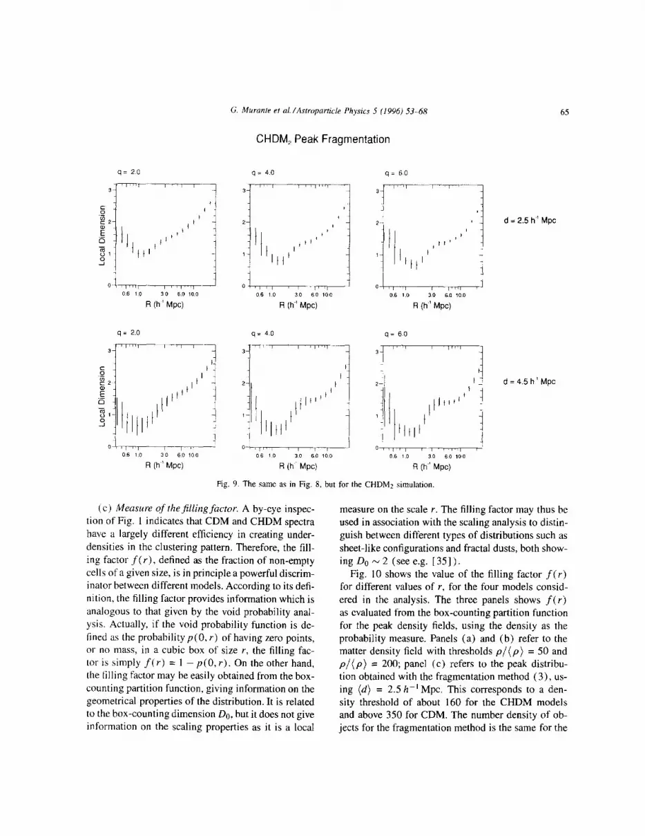
A step towards a more realistic dark halo identification algorithm is provided by the fragmentation method, which attempts to separate overmerged structures. Figs. 8 and 9 show the results of the CI method for the CDMl and CHDMz simulations respectively.

64 G. Muranre et al./Astroparticle Physics 5 (1996) 53-68

CDM 1 Peak Fragmentation

q= 4.0

3-

0, I, , ,’ I’/‘, 06 10 30 60 100

R (h.’ Mpc)

06 10 30 60 100 R (h ’ Mpc)

o- 0.6 1 0 3.0 60 100

R (h.’ Mpc)

q= 4.0

0 06 10 30 60 10.0 R (h ’ Mpc)

t-

q = 6.0

:;y] d=2.5h-‘Mpc

J-----G 06 10 3.0 6.0 100

R (h-’ Mpc)

(I/II d = 4.5 h.’ Mpc

06 10 30 6.0 100

R (h ’ Mpc)

Fig. 8. Local dimensions for the CDMl distribution of galaxies, which are now identified by the peak fragmentation method described in

Section 2. Again, upper and lower panels are for galaxies with mean separations of 2.5 h-’ Mpc and 4.5 h-’ Mpc, respectively. The three

panels in each line refer to q = 2, q = 4 and y = 6.

As before, the three upper panels refer to d = 2.5h-’ Mpc and the lower panels refer to d = 4.5h-’ Mpc.

On large scales, the results obtained by the fragmentation method are similar to those obtained by an- alyzing the mass distribution. The CDMl model is characterized by a scaling behavior with generalized dimensions between 2 and 3 and the CHDM model is characterized by a large-scale scaling behavior with generalized dimensions between 1 and 2 at large 9’s. On small scales, the fragmentation model generates an oscillating behavior of the local dimensions around values which are always smaller than one. The reason for that may be twofold. First, the underestimate of the dimensions may be due to lack of statistics at these separations in the fragmentation method. On the other hand, since the fragmentation model imposes a higher threshold on the density peaks, the lower di-

mension can be just the effect of the steepening of the

Summarising the above results, we conclude that the correlation function with the threshold amplitude.

scaling properties on large scales do not strongly depend on the object identification algorithm employed. Therefore, they provide a reliable test for distinguishing between different models. On the contrary, the object identification algorithms have important effects on small scales. In this regime, the dimension estimates and the same existence of a scaling regime depend on our definition of a “galaxy”. In particular, the lack of fragmentation tends to generate larger values of the generalized dimensions while an excess of fragmentation decreases the values of the generalized dimensions. This call for a better uderstanding of the galaxy formation processes, so to reliably pick out luminous objects from “dark” simulations.

06 10 30 6.0 100

R (h ’ Mpc)

R (h ’ Mpc)

G. Murante et aL/Asiroparticle Physics 5 (1996) 53-68

CHDM, Peak Fragmentation

q = 6.0

R (h ’ Mpc) R (h ’ Mpc)

q = 4.0

06 10 30 60 100 R (h ’ Mpc)

65

d = 2.5 h.’ Mpc

q= 6.0

T---l 2 d=45h’Mpc I

OM 60 100 R (h.’ Mpc)

Fig. 9. The same as in Fig. 8, but for the CHDMz simulation

(c) Measure of thefilling factor. A by-eye inspec- tion of Fig. 1 indicates that CDM and CHDM spectra have a largely different efficiency in creating under- densities in the clustering pattern. Therefore, the filling factor f(y), defined as the fraction of non-empty cells of a given size, is in principle a powerful discriminator between different models. According to its definition, the filling factor provides information which is analogous to that given by the void probability analysis. Actually, if the void probability function is defined as the probability ~(0, r) of having zero points, or no mass, in a cubic box of size Y, the filling factor is simply f(r) = 1 - ~(0, r). On the other hand, the tilling factor may be easily obtained from the box- counting partition function, giving information on the geometrical properties of the distribution. It is related to the box-counting dimension DO, but it does not give information on the scaling properties as it is a local

measure on the scale r. The filling factor may thus be used in association with the scaling analysis to distinguish between different types of distributions such as sheet-like configurations and fractal dusts, both showing DO N 2 (see e.g. [ 351).

Fig. 10 shows the value of the filling factor f(r) for different values of I, for the four models considered in the analysis. The three panels shows f(r) as evaluated from the box-counting partition function for the peak density fields, using the density as the probability measure. Panels (a) and (b) refer to the matter density field with thresholds p/(p) = 50 and p,/(p) = 200; panel (c) refers to the peak distribution obtained with the fragmentation method (3)) using (d) = 2.5 h-’ Mpc. This corresponds to a density threshold of about 160 for the CHDM models and above 350 for CDM. The number density of objects for the fragmentation method is the same for the

66 G. Murante et al./Astroparticle Physics 5 (1996) 53-68

1.1 ,,,,,,,,,,,,,,,,,,,~‘,,

4 (a)

R (h ‘Mpc)

d=2 5

I I #,I I I,I,III,I,I,I,I’

0 1 2 3 4 5 6 7 6 9 10 11

R (h.‘Mpc)

1.1 , , , , , , , , , T I - (cl

1 o-

09-

0.8- i

07-

[r '= 0.6-

t

0 ti -

2 0.5- i t

UJ _ 2 c 04-

0.3s

,',lll,l,'T~,l,l,',l,~

0 1 2 3 4 5 6 7 8 9 10 11

R (h ‘Mpc)

Fiu 10. Filling factor for the peak distribution in the four models considered in this work. Panel (a) refers to peaks with density p y 50(p); panel (b) to peaks with p > 200(p); panel (c) refers to a distribution of object obtained with the fragmentation method (3) (see text) with average distance d = 2.5 h-’ Mpc. Open squares refers to CDM1.5; filled squares to CDMl; open circles to CHDM, and filled circles to CHDMz.

G. Murante et al./A.~oqmrticle Physics 5 (1996) 53-68 61

four distributions which are analyzed, as the number of identified objects is fixed in this case by the prese- lected average distance (d).

The difference between CDM and CHDM is evident: for both threshold values, CDM is much more space filling than CHDM. A similar result has been found in [ 361 in the analysis of realistic galaxy redshift surveys, extracted from the same set of simulations which we have analyzed here. For the distribution of large peaks, the difference between the different models is striking: at about 7 h-’ Mpc, the filling factor for CDM is f(r) M 0.9 while for CHDM is

f(r) z 0.6. The measure of the filling factor and, correspondingly, of the void probability function may thus be considered as an important test to be applied to real data in order to distinguish between different clustering models. We note that the difference between the different models does not vanish for distributions with the same number of points, as in the case of the fragmentation method. Therefore, the observed difference is not simply determined by the different peak number density of the distributionsconsidered in Figs. I Oa and 1 Ob.

In general, the results on the filling factor confirm the more clustered nature of the CHDM models on large scales, and possibly shed some light on the nature of the intermediate scaling regimes. The scaling properties on intermediate scales may in fact have a “topological” nature, being dynamically generated by the process of pancake formation [ 351. Along these lines, the different clustering properties of the CDM and CHDM models would be associated with a different mass distribution on the large scale structures. In particular, the mass distribution should be more uni- form for the pure CDM model, still being in the process of forming the pancakes; this is reflected in the fact that D, > 2 for CDM. By contrast, for the CHDM simulations the matter should have already formed the pancakes, starting flowing from the flattened structures towards the filaments at the pancake intersections and the knots, generating a more filamentary distribution and values of the generalized dimensions less than two.

5. Discussion and conclusions

The results of the present analysis confirm the presence of an approximate scaling regime with D, + 1

for 4 > 2 for the CDM models on small scales and suggest its existence for the CHDM models as well. The analysis also indicates the existence of a second scaling regime on intermediate scales for the CHDM model and for the CDMI case. On scales between about 5 and 30 h-’ Mpc, the CHDM models show scaling behavior with D, between one and two and the CDMl simulation shows evidence of scaling with generalized dimensions D, between about two and three for 4 > 2. By contrast, the CDM1.5 model does not display any evidence of this second scaling regime.

We thus conclude that on small scales, the CDM and CHDM models cannot be easily distinguished on the basis of the scaling properties. The real difference between CDM and CHDM is observed on intermediate scales (5-30 h-’ Mpc). This difference in the clustering properties is also reflected in a very different value of the filling factor f(r) for the two models, showing that the peak distribution is much more space-filling for CDM than for CHDM. As a word of caution, we recall that we have herein analyzed just a few simulations, and that we observed some difference between two different realizations of the CHDM model. A detailed analysis of the role of cosmic variance in affect- ing the scaling behavior at intermediate scales is thus necessary in order to put quantitative statistical limits on the differences between the various models. This work is presently in progress.

An interesting problem concerns the nature of the intermediate scaling regime. Our results indicate that such a regime seems to be a natural product of the non- linear evolution when either there is sufficient power on large scales (CHDM cases) or the clustering has enough time to evolve (CDMI case). The CDM 1.5 model is less evolved and the scaling regime has not yet been formed. The difference between the values of the generalized dimensions for the CDMl and CHDM simulations then reflects the different power spectrum shape on intermediate scales.

Note, in particular, that the scaling regime on intermediate scales does not necessarily implies fractal behavior. In fact, a “topological” scaling regime is pos- sible, which may give D E 1 or D E 2 depending upon the presence of filaments or sheets. The results discussed here may be interpreted by admitting that the weakly non-linear dynamics on large scales may tend to create a distribution of “walls” where the matter is not homogeneously distributed but it is flowing

68 G. Murante et al./Astroparticie Physics 5 (1996) 53-68

towards the intersections and the knots. The evolutive stage is more advanced for models with large power on these scales, such as the CHDM.

As a final remark, we stress the fact that the scaling analysis discussed in this work provides a well- defined result which may be compared with the observational data: CDM and CHDM initial conditions generate a rather different scaling behavior in the 5 5 Y 5 20 h-’ Mpc scale range. These predictions may thus be tested against observational data. Attempts in this direction suggest the existence of a second scaling regime at r 2 4 h-’ Mpc with D2 z 2, see e.g. [ 371, in apparent agreement with the picture provided by CHDM simulations. A more crucial test on the CDM versus CHDM models will clearly be provided by the scaling analysis of the large-scale clustering of the galaxy distribution.

Acknowledgments

We thank A. Klypin for having provided us the out- puts of the CDM and CHDM numerical simulations and for useful comments on this work. We are grate- ful to S.A. Bonometto and J.R. Primack for enlighting conversations and support.

References

[ I 1 M.J. Geller and J. P Huchra. Science 246 ( 1993) 897. 12 I S. Borgani, Phys. Rep. 251 ( 1995) 1.

13 I R. Valdamini, S. Borgani and A. Provenzale, Astrophys. J. 394 ( 1992) 422.

141 S. Colombi, ER. Bouchet and R. Schaeffer, Astron.

Astrophys. 263 ( 1992) 1. 15 1 G. Yepes, R. Dominguez-Tenreiro and H.M.P. Couchman,

Astrophys. J. 401 (1992) 40. 16 I J.M. Bardeen, J.R. Bond, N. Kaiser and A.S. Szalay,

Astrophys. J. 304 (1986) 15. 17 I G. F. Smoot et al., Astrophys. J. 396 ( 1992) LI. [ 8 1 S.J. Maddox, G. Efstathiou, W.J. Sutherland and J. Loveday,

Mon. Not. Roy. Astron. Sot. 242 (1990) 43. [ 9 I W. Saunders, C.S. Frenk, M. Rowan-Robinson,G. Efstathiou,

A. Lawrence, N. Kaiser, R. Ellis, J. Crawford, X.-J. Xia and

1. Parry, Nature 338 (1991) 562. [ 101 J. Loveday, G. Efstathiou, B.A. Peterson and S.J. Maddox,

Astrophys. J. 400 (1992) L43.

[Ill

iI21

1131 I141

I151

1161

[I71

1181

[I91 f201

1211

1221

1231

1241

I251

1261

[271

[281

[291 1301

f311

f321

1331

1341

[351

1361

I371

A. Dckel, in “Proceeding of the Milan0 Conference on Observational Cosmology”, G. Chincarini, A. Iovino, T.

Maccacaro and D. Maccagni Eds. (San Francisco: ASP Conference Series, 1993), p. 194. S.D.M. White, C.S. Frenk, M. Davis and G. Efstathiou, Astrophys. J., 313 (1987) 505.

N.A. Bahcall and R. Cen, Astrophys. J. 398 (1992) L81. S.S. Olivier, J.R. Primack, G.R. Blumenthal and A. Dekel, Astrophys. J. 408 ( 1993) 17.

R.A.C. Croft and G. Efstathiou, Mon. Not. Roy. Astron. Sot. 267 (1994) 390. S. Borgani, P Coles and L. Moscardini, Mon. Not. Roy.

Astron. Sot. 271 (1994) 223. M. Davis, G. Efstathiou, C.S. Frenk and S.D. White, Nature

356 (1992) 489. A. Klypin, J. Holtzman, J.R. Primack and E. Regos,

Astrophys. J. 416 (1993) I. A. R. Liddle and D.H. Lyth, Phys. Rep. 231 (1993) I.

A. Klypin, R. Nolthenius and and J.R. Primack, Astrophys. J. (1995) in press. R. Nolthenius, A. Klypin and J.R. Primack, Astrophys. J.

422 ( 1994) L45. G. Yepes, A. Klypin, A. Campos and R. Fong, Astrophys. J. (1995). in press.

S.A. Bonometto, S Borgani, S. Ghigna, A. Klypin and J.R. Primack, Mon. Not. Roy. Astron. Sot. 273 ( 1995) 101. N. Katz, T. Quinn and J.M. Gelb, Mon. Not. Roy. Astron.

Sot. 265 (1993) 689. J.M. Gelb and E. Bettschinger, Astrophys. J. 436 (1994) 491.

A. Campos, G. Yepes, A. Klypin, G. Murante, A. Provenzale, S. Borgani, Astrophys. J. 446 (1995) 54.

S. Borgani, G. Murante, A. Provenzale and R. Valdamini, Phys. Rev. E 47 (1993) 3879.

B.B. Mandelbrot, The Fractal Geometry of Nature (San Francisco: Freeman, 1982) G. Paladin and A. Vulpiani, Phys. Rep. 156 (1987) 147.

P. Grassberger and 1. Procaccia, Phys. Rev. L&t. 50 ( 1983) 346. G. Paladin and A. Vulpiani, Lett. Nuovo Cimento 41 ( 1984)

82. V.J. Martinez, B.J.T. Jones, R. Dominguez-Tenreiro and R. van de Weigaert, Astrophys. J. 357 ( 1990) 50.

E.N. Ling, C.S. Frenk and J.D. Barrow, Mon. Not. Roy.

Astron. Sot. 223 (1986) 21. P.J.E. Peebles, The Large Scale Structure of the Universe (Princeton: Princeton University Press, 1980)

A. Provenzale, L. Guzzo and G. Murante, Mon. Not. Roy. Astron. Sot. 266 (1994) 555.

S. Ghigna, S. Borgani, S.A. Bonometto, L. Guzzo, A. Klypin, J.R. Primack, R. Giovanelli and M.P. Haynes, Astrophys. J. 437 (1995) L71. L. Guzzo, A. Iovino, G. Chincarini, R. Giovanelli and M.P.

Haynes, Astrophys. J. 382 (1991) L5.

scaling analysis of dark matter models

Documents