sangati 2007 emergence,
TRANSCRIPT
Emergence, Evolution and Maintenance of
Communication Conventions
Federico Sangati
May 12, 2007
Abstract: We report the results of a simulation investigating in which cir-cumstances communicative conventions emerge and can be maintained within apopulation of agents under different selective pressures. We will give a game the-oretical analysis of few relevant cases. We will then report our empirical resultsof the error threshold phenomenon analytically proved in Nowak et al. [2].
Introduction
Communication systems can be characterized as a mapping from a set of mean-ings to a set of signals. We attempt in this paper to set a general frameworkto describe under which circumstances an optimal convention (or SaussureanCommunication) can be established within a population of individuals.
The model
We will consider a scenario of 400 communicative individuals in an unbounded,torus shaped space. This scenario is similar to the one described in Oliphant1994 [3].The population of agents shares a finite set of signals used to convey a corre-sponding amount of shared meanings. Each individual is born with a trans-mitting system specifying which signal is associated with each meaning and areceiving system mapping back each symbol to a specific meaning. We will takeinto consideration the very general case in which the receiving system doesn’tnecessary mirror the transmitting system.Each agent has 8 neighbours and goes through 5 life stages; after the fifth thefirst follows. In each stage the agents try to establish 8 random communica-tions with their neighbours. In every communication two agents act alternatelyas speakers and listeners. The speaker picks one random meaning out of themeaning space and sends the associated signal to the hearer (according to itstransmitting system). The hearer uses its receiving system to find the meaningassociated with the received signal. If this meaning is the same as originallychosen, the communication is said to be successful.
1
During the fist stage, an individual selects a teacher from the set of its neigh-bours according to the communication success (fitness) they have accumulatedduring the previous life stage (a neighbour with double fitness has double proba-bility to be selected). The newborn agent then acquires with a certain precisionthe communication system of its teacher: each mapping in the teacher’s com-munication system is learned with probability 1− µ and it is randomly chosenwith probability µ (mutation rate).
The simulation
In order to start with the simulations we need to take into consideration severalparameters. Each set of parameters corresponds to a specific communicationscheme. The aim of this study is therefore to understand for which communica-tion schemes a Saussurean Communication can emerge and can be maintainedwithin the population. We can describe the parameters as follows:
N: number of meanings used by the agents, equivalent to the number of forms(symbols) they are able to express.
µ: the mutation rate characterizing the acquisition phase.
Initialization : whether in the starting point of the simulation each agent isinitialized with a random communication system (random start) or witha unique optimal communication system (optimal start).
Payoff Matrix: when communicating to its neighbours, each agent cumulatesa transmission and reception success rate. The payoff matrix specifieshow the fitness function is calculated in respect to these two values. Twogeneral cases are taken into consideration: the case where the fitness isthe average of the two values (both speakers and listeners are rewarded),and the case where the fitness coincides with the reception success rate(only listeners rewarded).
Spatial organization: whether the agents keep the same position during thelife cycle (spatially organized) or are randomly displaced at each iteration(non spatially organized).
Iterative: this is an optional mode; when active each agent has two possiblecommunication systems: in each communication attempt each agents usesthe first communication system if the previous reception was successful,the second if unsuccessful. Each communication between two agents isiterated 16 times.
2
Oliphant’s Results
We will run here the 4 simulations reported in Oliphant. In all the cases wehave N = 2 and a random initialization startup: each agent is initialized with arandom communication system and a random age (life stage).
Simulation 1
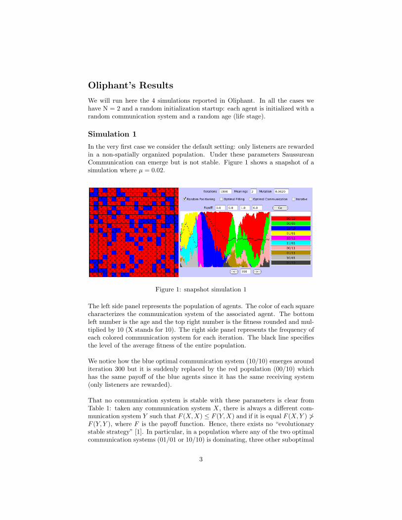
In the very first case we consider the default setting: only listeners are rewardedin a non-spatially organized population. Under these parameters SaussureanCommunication can emerge but is not stable. Figure 1 shows a snapshot of asimulation where µ = 0.02.
Figure 1: snapshot simulation 1
The left side panel represents the population of agents. The color of each squarecharacterizes the communication system of the associated agent. The bottomleft number is the age and the top right number is the fitness rounded and mul-tiplied by 10 (X stands for 10). The right side panel represents the frequency ofeach colored communication system for each iteration. The black line specifiesthe level of the average fitness of the entire population.
We notice how the blue optimal communication system (10/10) emerges arounditeration 300 but it is suddenly replaced by the red population (00/10) whichhas the same payoff of the blue agents since it has the same receiving system(only listeners are rewarded).
That no communication system is stable with these parameters is clear fromTable 1: taken any communication system X, there is always a different com-munication system Y such that F (X, X) ≤ F (Y, X) and if it is equal F (X, Y ) ≯F (Y, Y ), where F is the payoff function. Hence, there exists no “evolutionarystable strategy” [1]. In particular, in a population where any of the two optimalcommunication systems (01/01 or 10/10) is dominating, three other suboptimal
3
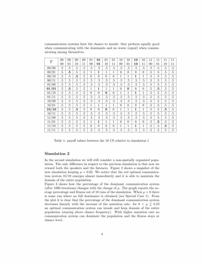
communication systems have the chance to invade: they perform equally goodwhen communicating with the dominants and no worse (equal) when commu-nicating among themselves.
F00 00 00 00 01 01 01 01 10 10 10 10 11 11 11 1100 01 10 11 00 01 10 11 00 01 10 11 00 01 10 11
00/00 .5 .5 .5 .5 .5 .5 .5 .5 .5 .5 .5 .5 .5 .5 .5 .500/01 .5 .5 .5 .5 1 1 1 1 0 0 0 0 .5 .5 .5 .500/10 .5 .5 .5 .5 0 0 0 0 1 1 1 1 .5 .5 .5 .500/11 .5 .5 .5 .5 .5 .5 .5 .5 .5 .5 .5 .5 .5 .5 .5 .501/00 .5 .5 .5 .5 .5 .5 .5 .5 .5 .5 .5 .5 .5 .5 .5 .501/01 .5 .5 .5 .5 1 1 1 1 0 0 0 0 .5 .5 .5 .501/10 .5 .5 .5 .5 0 0 0 0 1 1 1 1 .5 .5 .5 .501/11 .5 .5 .5 .5 .5 .5 .5 .5 .5 .5 .5 .5 .5 .5 .5 .510/00 .5 .5 .5 .5 .5 .5 .5 .5 .5 .5 .5 .5 .5 .5 .5 .510/01 .5 .5 .5 .5 1 1 1 1 0 0 0 0 .5 .5 .5 .510/10 .5 .5 .5 .5 0 0 0 0 1 1 1 1 .5 .5 .5 .510/11 .5 .5 .5 .5 .5 .5 .5 .5 .5 .5 .5 .5 .5 .5 .5 .511/00 .5 .5 .5 .5 .5 .5 .5 .5 .5 .5 .5 .5 .5 .5 .5 .511/01 .5 .5 .5 .5 1 1 1 1 0 0 0 0 .5 .5 .5 .511/10 .5 .5 .5 .5 0 0 0 0 1 1 1 1 .5 .5 .5 .511/11 .5 .5 .5 .5 .5 .5 .5 .5 .5 .5 .5 .5 .5 .5 .5 .5
Table 1: payoff values between the 16 CS relative to simulation 1
Simulation 2
In the second simulation we will still consider a non-spatially organized popu-lation. The only difference in respect to the previous simulation is that now wereward both the speakers and the listeners. Figure 2 shows a snapshot of thenew simulation keeping µ = 0.02. We notice that the red optimal communica-tion system 10/10 emerges almost immediately and it is able to maintain thedomain of the entire population.Figure 3 shows how the percentage of the dominant communication system(after 1000 iterations) changes with the change of µ. The graph reports the av-erage percentage and fitness out of 10 runs of the simulation. When µ = 0 thereis some run where no full dominance is obtained (see Special Case 1). Fromthe plot it is clear that the percentage of the dominant communication systemdecreases linearly with the increase of the mutation rate: for 0 < µ . 0.10an optimal communication system can invade and keep domain of the entirepopulation (staying above chance frequency). With higher mutation rate nocommunication system can dominate the population and the fitness stays atchance level.
4
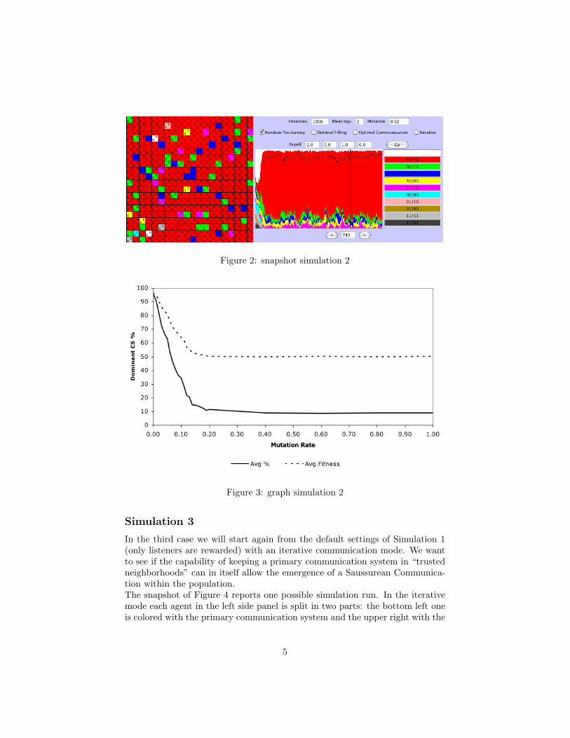
Figure 2: snapshot simulation 2
Figure 3: graph simulation 2
Simulation 3
In the third case we will start again from the default settings of Simulation 1(only listeners are rewarded) with an iterative communication mode. We wantto see if the capability of keeping a primary communication system in “trustedneighborhoods” can in itself allow the emergence of a Saussurean Communica-tion within the population.The snapshot of Figure 4 reports one possible simulation run. In the iterativemode each agent in the left side panel is split in two parts: the bottom left oneis colored with the primary communication system and the upper right with the
5

secondary one.The optimal red communication system 10/10 is able to invade after around 200iterations and keeps the domain of the entire population until the last iteration.It is important to note from the snapshot that, once the Saussurean Commu-nication takes place, the majority of the secondary transmission systems differsfrom the red primary transmission system. If for some chance it would driftto the primary transmission system, any non trusted opponent would benefitfrom it. This possibility mentioned in Oliphant’s paper as a major source ofinstability seems to affect very few simulations and mainly in cases where themutation rate is kept very low (µ . 0.005).
Figure 4: snapshot simulation 3
The graph in Figure 5 shows the percentage of the dominant communication sys-tem with increasing µ. Here there is a relatively sudden jump around µ = 0.05.After this threshold the dominant communication system stays at chance fre-quency. It is also possible to see a rise in fitness from 0 < µ < 0.01 This confirmsour previous result that for very low mutation rates, a random drift leading tothe optimality of the secondary transmission system, can compromise the main-tenance of a Saussurean Communication.The results seem to prove that the iterative communication mode can be asufficient element to allow the emerge and maintenance of an optimal commu-nication system for 0.01 < µ < 0.05. The analogue iterated mode simulationreported by Oliphant, characterized by an instability of the Saussurean Com-munication, considers the case in which the mutation rate falls in the criticalregion (∼ 0.0041).
In the actual implementation of the iterative mode, if the speaker fails/succeedsto convey a certain meaning, only the listener stops/starts to trust the oppo-
1The mutation system introduced in Oliphant is based on mutation affecting the entiregenome (.27%) and crossing-over. The existence of a precise way to convert it into our metricis in doubt.
6
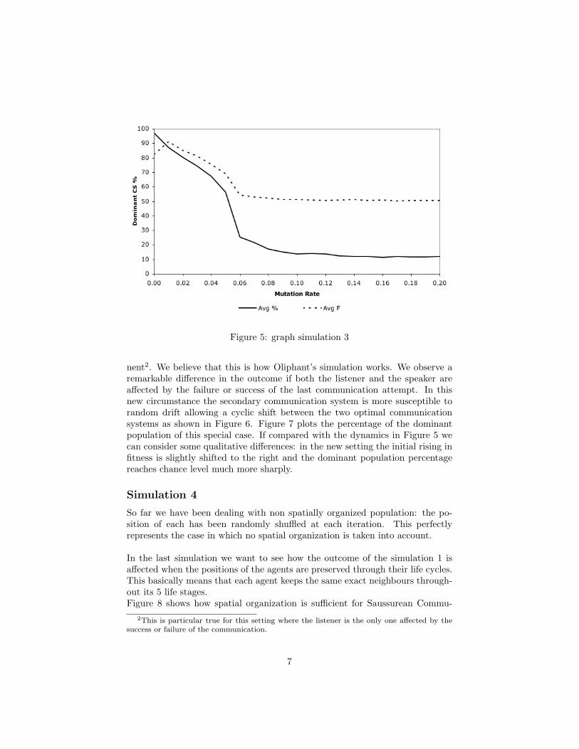
Figure 5: graph simulation 3
nent2. We believe that this is how Oliphant’s simulation works. We observe aremarkable difference in the outcome if both the listener and the speaker areaffected by the failure or success of the last communication attempt. In thisnew circumstance the secondary communication system is more susceptible torandom drift allowing a cyclic shift between the two optimal communicationsystems as shown in Figure 6. Figure 7 plots the percentage of the dominantpopulation of this special case. If compared with the dynamics in Figure 5 wecan consider some qualitative differences: in the new setting the initial rising infitness is slightly shifted to the right and the dominant population percentagereaches chance level much more sharply.
Simulation 4
So far we have been dealing with non spatially organized population: the po-sition of each has been randomly shuffled at each iteration. This perfectlyrepresents the case in which no spatial organization is taken into account.
In the last simulation we want to see how the outcome of the simulation 1 isaffected when the positions of the agents are preserved through their life cycles.This basically means that each agent keeps the same exact neighbours through-out its 5 life stages.Figure 8 shows how spatial organization is sufficient for Saussurean Commu-
2This is particular true for this setting where the listener is the only one affected by thesuccess or failure of the communication.
7
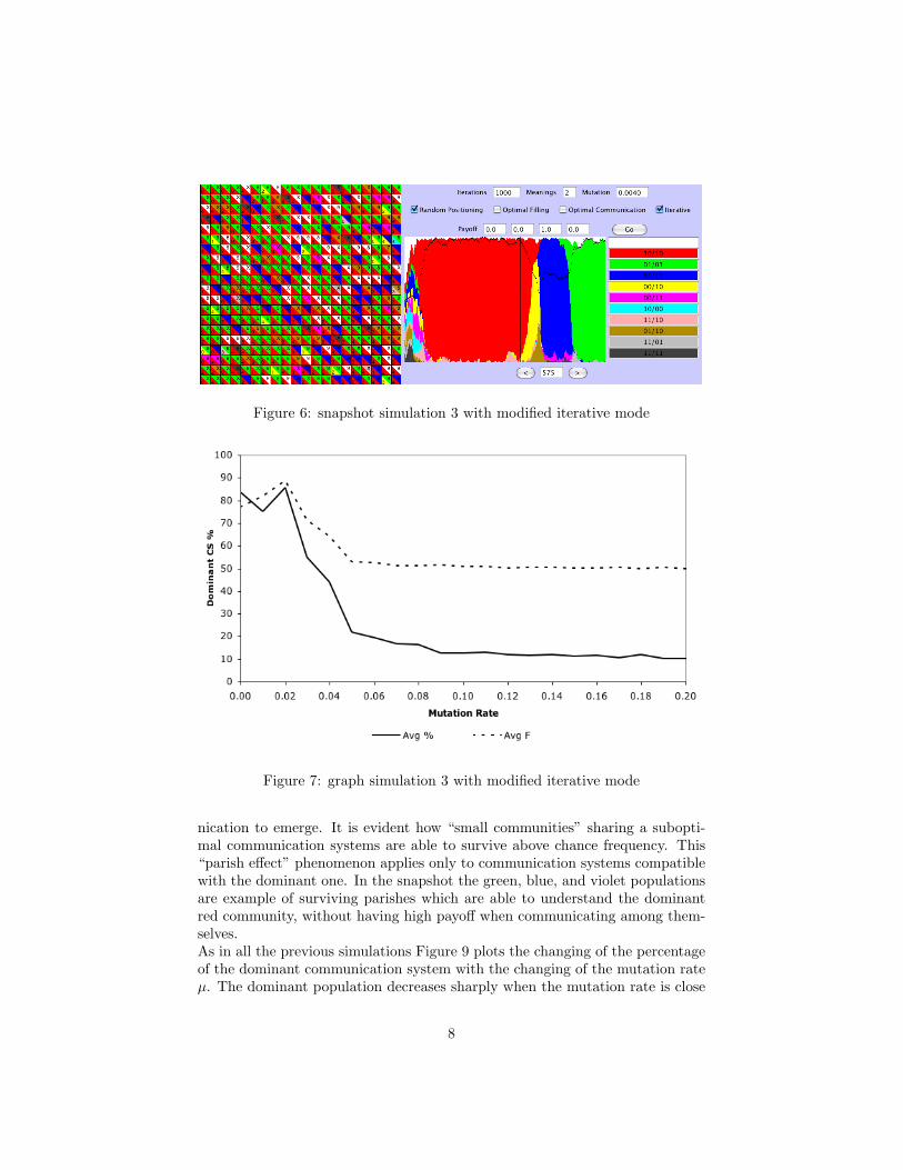
Figure 6: snapshot simulation 3 with modified iterative mode
Figure 7: graph simulation 3 with modified iterative mode
nication to emerge. It is evident how “small communities” sharing a subopti-mal communication systems are able to survive above chance frequency. This“parish effect” phenomenon applies only to communication systems compatiblewith the dominant one. In the snapshot the green, blue, and violet populationsare example of surviving parishes which are able to understand the dominantred community, without having high payoff when communicating among them-selves.As in all the previous simulations Figure 9 plots the changing of the percentageof the dominant communication system with the changing of the mutation rateµ. The dominant population decreases sharply when the mutation rate is close
8
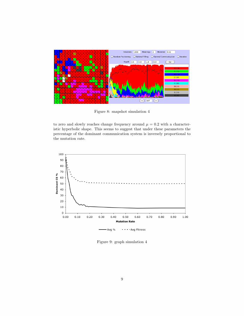
Figure 8: snapshot simulation 4
to zero and slowly reaches change frequency around µ = 0.2 with a character-istic hyperbolic shape. This seems to suggest that under these parameters thepercentage of the dominant communication system is inversely proportional tothe mutation rate.
Figure 9: graph simulation 4
9
Case studies
In this section we will take into consideration 3 case studies which will be an-alyzed in detail within a game theoretical framework. As before we will keepN = 2.
Case Study 1 - Two symmetric communication systems
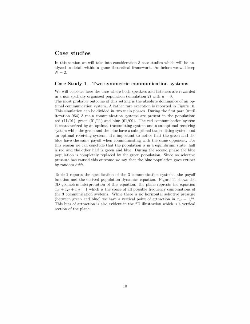
We will consider here the case where both speakers and listeners are rewardedin a non spatially organized population (simulation 2) with µ = 0.The most probable outcome of this setting is the absolute dominance of an op-timal communication system. A rather rare exception is reported in Figure 10.This simulation can be divided in two main phases. During the first part (untiliteration 964) 3 main communication systems are present in the population:red (11/01), green (01/11) and blue (01/00). The red communication systemis characterized by an optimal transmitting system and a suboptimal receivingsystem while the green and the blue have a suboptimal transmitting system andan optimal receiving system. It’s important to notice that the green and theblue have the same payoff when communicating with the same opponent. Forthis reason we can conclude that the population is in a equilibrium state: halfis red and the other half is green and blue. During the second phase the bluepopulation is completely replaced by the green population. Since no selectivepressure has caused this outcome we say that the blue population goes extinctby random drift.
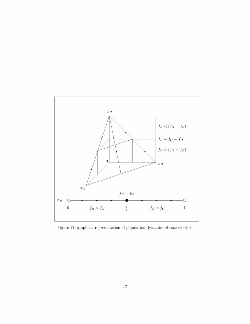
Table 2 reports the specification of the 3 communication systems, the payofffunction and the derived population dynamics equation. Figure 11 shows the3D geometric interpretation of this equation: the plane represts the equationxR + xG + xB = 1 which is the space of all possible frequency combinations ofthe 3 communication systems. While there is no horizontal selective pressure(between green and blue) we have a vertical point of attraction in xR = 1/2.This bias of attraction is also evident in the 2D illustration which is a verticalsection of the plane.
10
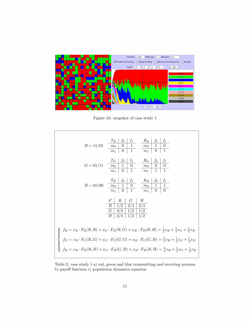
Figure 10: snapshot of case study 1
R = 11/01TR f0 f1
m0 0 1m1 0 1
RR f0 f1
m0 1 0m1 0 1
G = 01/11TG f0 f1
m0 1 0m1 0 1
RG f0 f1
m0 0 0m1 1 1
B = 01/00TB f0 f1
m0 1 0m1 0 1
RB f0 f1
m0 1 1m1 0 0
F R G BR 1/2 3/4 3/4G 3/4 1/2 1/2B 3/4 1/2 1/2
fR = xR · FR(R,R) + xG · FR(R,G) + xB · FR(R,B) = 1
2xR + 34xG + 3
4xB
fG = xR · FG(R,G) + xG · FG(G, G) + xB · FG(G, B) = 34xR + 1
2xG + 12xB
fB = xR · FB(R,B) + xG · FB(G, B) + xB · FB(B,B) = 34xR + 1
2xG + 12xB
Table 2: case study 1 a) red, green and blue transmitting and receiving systemsb) payoff function c) population dynamics equation
11
��
��
��������������������
������������������
@@
@@
@@
@@
@@
@@
���������
DDDDDDDDDDDDDDD
��
�
W
R
�
O I
fR < (fG = fB)
fR = fG = fB
fR > (fG = fB)
0
xR
xG
xB
xR f0
v12
f1fR > fG
fR = fG
fR < fG
- - - � � �
Figure 11: graphical representation of population dynamics of case study 1
12
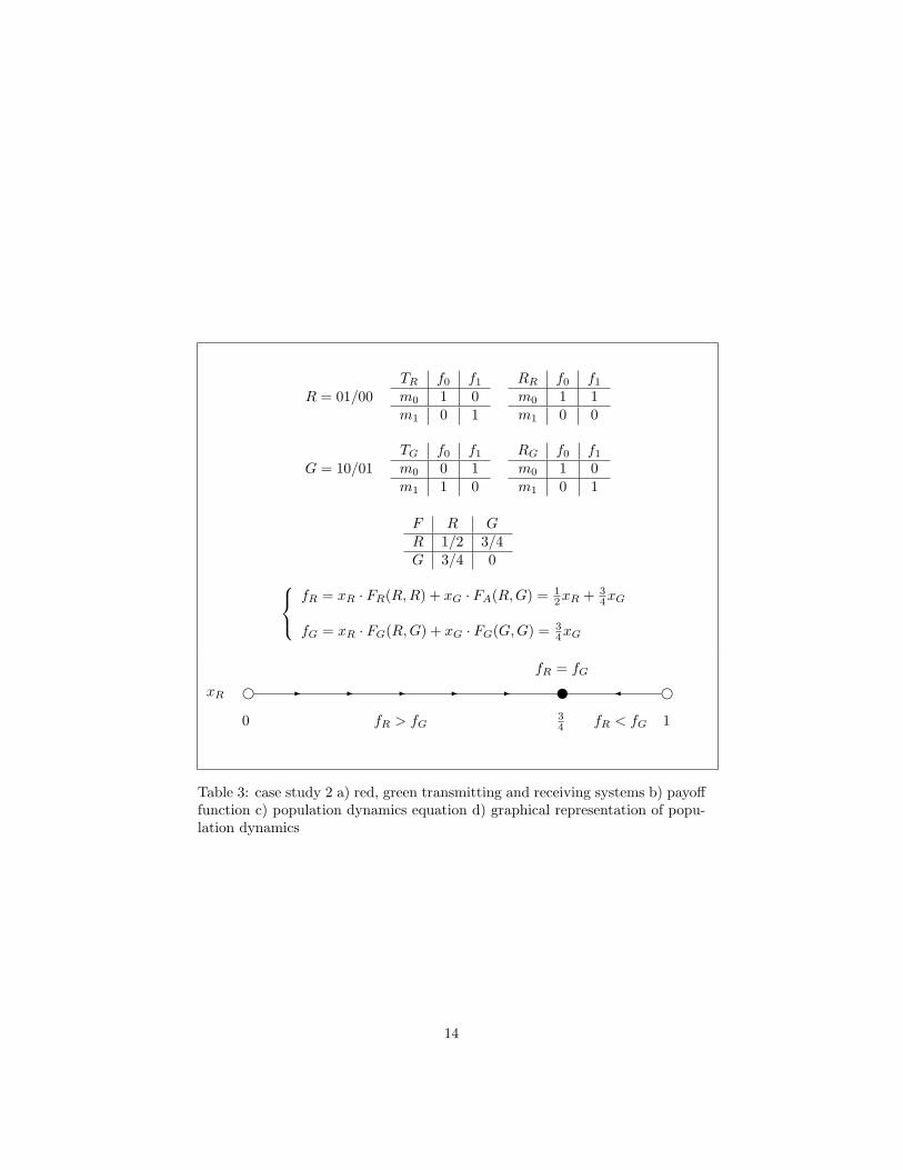
Case Study 2 - Two asymmetric communication systems
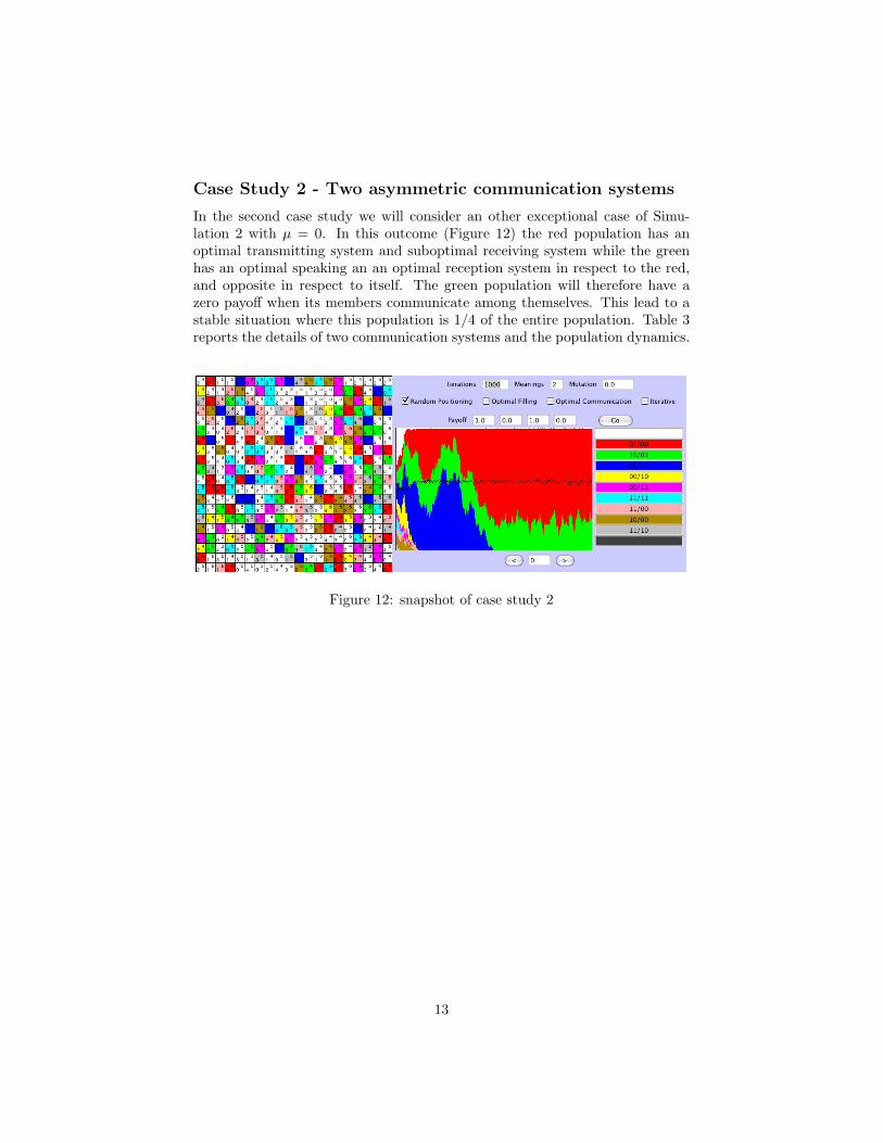
In the second case study we will consider an other exceptional case of Simu-lation 2 with µ = 0. In this outcome (Figure 12) the red population has anoptimal transmitting system and suboptimal receiving system while the greenhas an optimal speaking an an optimal reception system in respect to the red,and opposite in respect to itself. The green population will therefore have azero payoff when its members communicate among themselves. This lead to astable situation where this population is 1/4 of the entire population. Table 3reports the details of two communication systems and the population dynamics.
Figure 12: snapshot of case study 2
13
R = 01/00TR f0 f1
m0 1 0m1 0 1
RR f0 f1
m0 1 1m1 0 0
G = 10/01TG f0 f1
m0 0 1m1 1 0
RG f0 f1
m0 1 0m1 0 1
F R GR 1/2 3/4G 3/4 0 fR = xR · FR(R,R) + xG · FA(R,G) = 1
2xR + 34xG
fG = xR · FG(R,G) + xG · FG(G, G) = 34xG
xR f0
v34
f1fR > fG
fR = fG
fR < fG
- - - - - �
Table 3: case study 2 a) red, green transmitting and receiving systems b) payofffunction c) population dynamics equation d) graphical representation of popu-lation dynamics
14

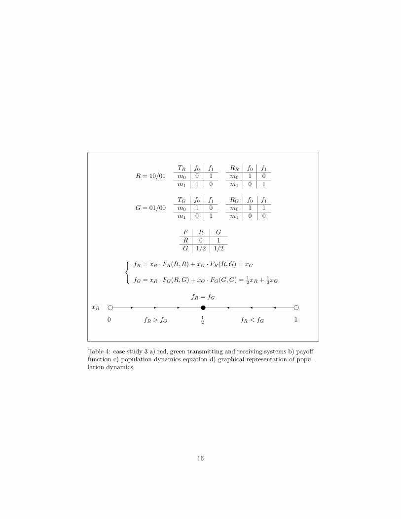
Case Study 3 - Two symmetric communication systemswith only listeners rewarded
In the last case study we consider the case where only listeners are rewarded ina non spatially organized population (simulation 1) with µ = 0. In this case wehave an equilibrium between the red and the green population each occupyinghalf of the space. The red population has a high payoff when communicatingwith the green but zero payoff against itself. Table 4 reports the specificationof the population dynamics.
Figure 13: snapshot of case study 3
15
R = 10/01TR f0 f1
m0 0 1m1 1 0
RR f0 f1
m0 1 0m1 0 1
G = 01/00TG f0 f1
m0 1 0m1 0 1
RG f0 f1
m0 1 1m1 0 0
F R GR 0 1G 1/2 1/2 fR = xR · FR(R,R) + xG · FR(R,G) = xG
fG = xR · FG(R,G) + xG · FG(G, G) = 12xR + 1
2xG
xR f0
v12
f1fR > fG
fR = fG
fR < fG
- - - � � �
Table 4: case study 3 a) red, green transmitting and receiving systems b) payofffunction c) population dynamics equation d) graphical representation of popu-lation dynamics
16
Analytic analysis of communication systems
Introduction
This section will present a mathematical framework for the analysis of the evo-lution and maintenance of communication conventions, according to the math-ematical model used in Nowak et al. [2]. We will compare this analysis with theempirical results we can obtain from our simulation. We will limit our studyto the case where both speakers and listeners are rewarded in a non spatiallydistributed population (as in Simulation 2).
The two models
In order to compare the two models we will need to define our set of variables:
N is the size of the meanings space (as before).G is the number of communication systems or grammars.dij is the number of mappings differing between grammar i and j.eij is the number of mappings in common between grammar i and j.A is the compatibility matrix specifying to which degree grammar i is com-
patible with grammar j.F is the payoff matrix specifying the payoff between any two grammars i, j.xi is the frequency of individuals using grammar i.fi is the average payoff of a individuals using grammar i.Q is the acquisition matrix specifying for each i, j what is the probabil-
ity that an agent learning from a teacher with grammar i will end upspeaking grammar j.
φ is the average fitness of the population.x i is the population dynamic of grammar i: it represents how much the
frequency of grammar i changed from last iteration (in a continuoustimeline it is the derivate of frequency with respect to time).
The main difference between the two models lies on the complexity behind thegrammars of the agents. In Nowak’s model the grammars are assumed to beequally distant from one another while in Oliphant’s the hierarchical structurebehind the communication system leads to a more complex distance space ofthe type found in Table 1. This difference causes the mutation rate to havedifferent scopes in the two models: in Nowak’s µ is related to the probabilityof going from one grammar to any other grammar, while in Oliphant’s µ refersto the probability of changing each single unit of the grammar. In Table 5 wereport how the formulas behind the two models are related.
Results
Oliphant’s model results in a more complex population dynamics formula whichis hard to derive analytically. We therefore choose to approximate the resultnumerically. In the first iteration the frequency of each grammar is set: in an
17
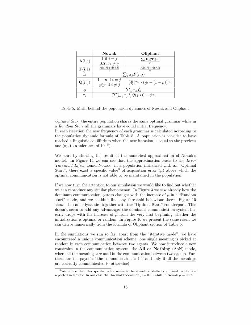
Nowak Oliphant
A(i, j)1 if i = j
0.5 if i 6= j
Pi Rj(Ti)=i
N
F(i, j) A(i,j)+A(j,i)2
A(i,j)+A(j,i)2
fi∑
j xjF (i, j)
Q(i, j)1− µ if i = j
µG−1 if i 6= j
( µN )dij · ( µ
N + (1− µ))eij
φ∑
k xkfk
xi (∑n
j=1 xjfjQ(j, i))− φxi
Table 5: Math behind the population dynamics of Nowak and Oliphant
Optimal Start the entire population shares the same optimal grammar while ina Random Start all the grammars have equal initial frequency.In each iteration the new frequency of each grammar is calculated according tothe population dynamic formula of Table 5. A population is consider to havereached a linguistic equilibrium when the new iteration is equal to the previousone (up to a tolerance of 10−5).
We start by showing the result of the numerical approximation of Nowak’smodel. In Figure 14 we can see that the approximation leads to the ErrorThreshold Effect found Nowak: in a population initialized with an “OptimalStart”, there exist a specific value3 of acquisition error (µ) above which theoptimal communication is not able to be maintained in the population.
If we now turn the attention to our simulation we would like to find out whetherwe can reproduce any similar phenomenon. In Figure 3 we saw already how thedominant communication system changes with the increase of µ in a “Randomstart” mode, and we couldn’t find any threshold behaviour there. Figure 15shows the same dynamics together with the “Optimal Start” counterpart. Thisdoesn’t seem to add any advantage: the dominant communication system lin-early drops with the increase of µ from the very first beginning whether theinitialization is optimal or random. In Figure 16 we present the same result wecan derive numerically from the formula of Oliphant section of Table 5.
In the simulations we run so far, apart from the ”iterative mode”, we haveencountered a unique communication scheme: one single meaning is picked atrandom in each communication between two agents. We now introduce a newconstraint in the communication system, the All or Nothing (AoN) mode,where all the meanings are used in the communication between two agents. Fur-thermore the payoff of the communication is 1 if and only if all the meaningsare correctly communicated (0 otherwise).
3We notice that this specific value seems to be somehow shifted compared to the onereported in Nowak. In our case the threshold occurs on µ = 0.16 while in Nowak µ = 0.07.
18

Figure 14: Numeric approximation of Nowak population dynamics with aij=0.5and G = 10
Figure 15: Simulation in standard mode with N=2 (G=16)
19

Figure 16: Numeric approximation of Oliphant population dynamics in “Nor-mal” mode with N=2 (G=16)
We want to test whether AoN can bring us closer to the threshold effect. Fig-ure 17 shows the dominant communication system dynamics from our simulationin the new mode with N=2. The frequency is now decreasing in a qualitativedifferent way than before but still far away from replicating the threshold dy-namics. Figure 18 shows a similar dynamics for N=10.We try to replicate such dynamic using numeric approximation. We first modifythe formula behind the payoff Fij between any two grammars i and j (Table 5).While before it was defined as the average of their reciprocal compatibilities,we now use the floor value of the average (Fij is rounded to 0 whenever theaverage of the reciprocal compatibilities is less than 1). Figure 19 shows thenew dynamic with N = 2. Although the curve looks pretty similar to the onewe encountered before in Figure 17, it doesn’t seem to have the expected hy-perbolic shape. If we now analyze the F matrix, we realize that the constraintwe imposed, selects 4 communication system pairs to have positive (and maxi-mum) fitness. Besides the trivial case of the 2 optimal grammars (10/10, 01/01)each having positive fitness when communicating with itself, we have 2 othercomplementar grammars (01/10, 10/01) wich score positive fitness when com-municating with one another. In order to exclude the latter pair, we have toput a new constraint, restricting a pair of grammars to have maximum payoffonly when each separately has maximum fitness against itself. Figure 20 showsthe expected dynamic with this last modification.4
4Unfortunately our numeric approximation cannot verify our simulation result in the casewhere N=10. In order to do so we would have to deal with 1020 possible grammars.
20

Figure 17: Simulation in “All or Nothing” mode with N=2 (G=16)
Figure 18: Simulation in “All or Nothing” mode with N=10 (G=1020)
21
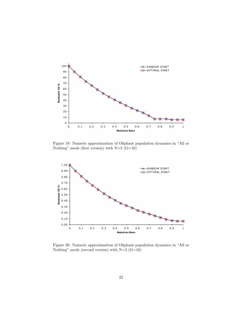
Figure 19: Numeric approximation of Oliphant population dynamics in “All orNothing” mode (first version) with N=2 (G=16)
Figure 20: Numeric approximation of Oliphant population dynamics in “All orNothing” mode (second version) with N=2 (G=16)
22
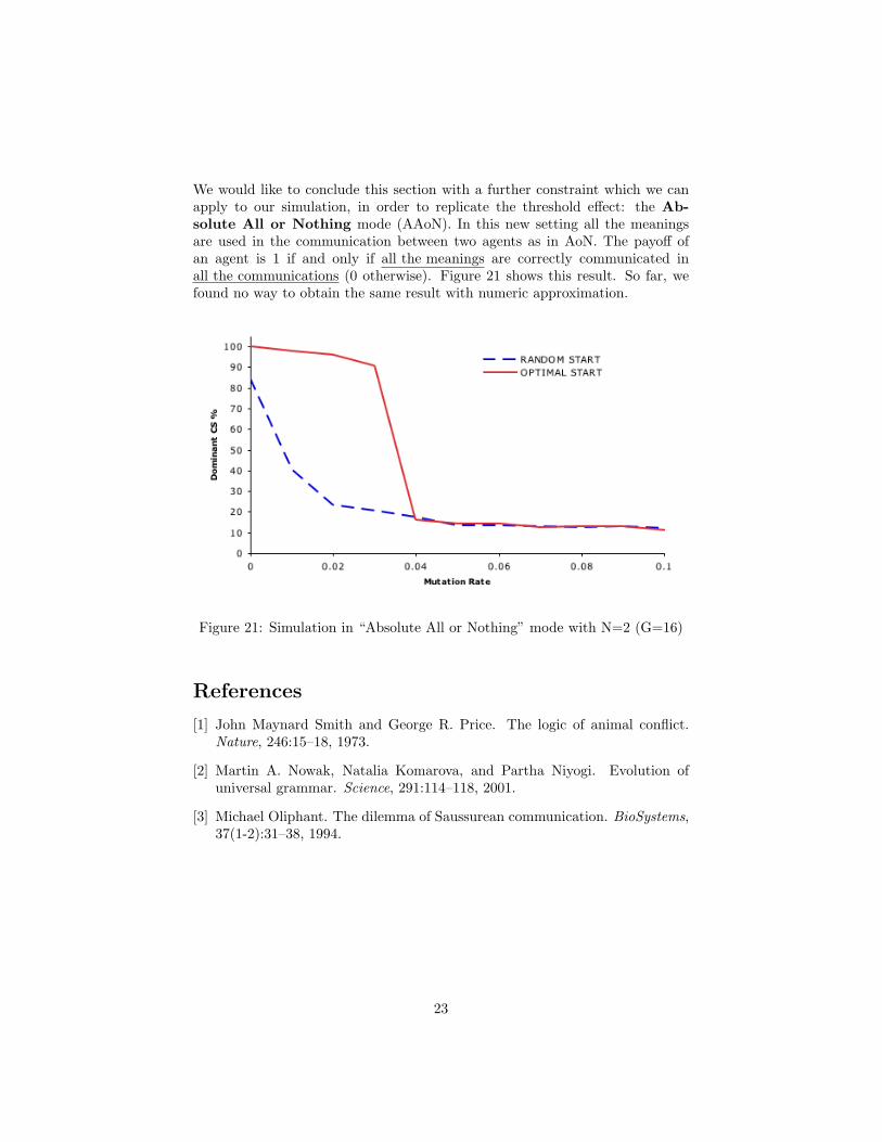
We would like to conclude this section with a further constraint which we canapply to our simulation, in order to replicate the threshold effect: the Ab-solute All or Nothing mode (AAoN). In this new setting all the meaningsare used in the communication between two agents as in AoN. The payoff ofan agent is 1 if and only if all the meanings are correctly communicated inall the communications (0 otherwise). Figure 21 shows this result. So far, wefound no way to obtain the same result with numeric approximation.
Figure 21: Simulation in “Absolute All or Nothing” mode with N=2 (G=16)
References
[1] John Maynard Smith and George R. Price. The logic of animal conflict.Nature, 246:15–18, 1973.
[2] Martin A. Nowak, Natalia Komarova, and Partha Niyogi. Evolution ofuniversal grammar. Science, 291:114–118, 2001.
[3] Michael Oliphant. The dilemma of Saussurean communication. BioSystems,37(1-2):31–38, 1994.
23