saltwater upconing due to cyclic pumping by horizontal wells in freshwater lenses

Saltwater Upconing Due to Cyclic Pumpingby Horizontal Wells in Freshwater Lensesby Pieter S. Pauw1,2,3, Sjoerd E.A.T.M. van der Zee2, Anton Leijnse2, and Gualbert H.P. Oude Essink1,4

AbstractThis article deals with the quantification of saltwater upconing below horizontal wells in freshwater lenses using analytical

solutions as a computationally fast alternative to numerical simulations. Comparisons between analytical calculations and numericalsimulations are presented regarding three aspects: (1) cyclic pumping; (2) dispersion; and (3) finite horizontal wells in a finitedomain (a freshwater lens). Various hydrogeological conditions and pumping regimes within a dry half year are considered. Theresults show that the influence of elastic and phreatic storage (which are not taken into account in the analytical solutions) on theupconing of the interface is minimal. Furthermore, the analytical calculations based on the interface approach compare well withnumerical simulations as long as the dimensionless interface upconing is below 1/3, which is in line with previous studies on steadypumping. Superimposing an analytical solution for mixing by dispersion below the well over an analytical solution based on theinterface approach is appropriate in case the vertical flow velocity around the interface is nearly constant but should not be usedfor estimating the salinity of the pumped groundwater. The analytical calculations of interface upconing below a finite horizontalwell compare well with the numerical simulations in case the distance between the horizontal well and the initial interface does notvary significantly along the well and in case the natural fluctuation of the freshwater lens is small. In order to maintain a low levelof salinity in the well during a dry half year, the dimensionless analytically calculated interface upconing should stay below 0.25.

IntroductionFreshwater lenses are important for freshwater sup-

ply in coastal areas (Bear et al. 1999; Werner et al. 2013).Pumping from freshwater lenses generally leads to salt-water upconing, that is, a local rise of saline groundwaterbelow the well (Dagan and Bear 1968). As long as salt-water upconing remains limited, freshwater lenses canbe sustainably exploited. In case of excessive saltwaterupconing, however, there is a high risk of an undesiredsalinity in the well. Excessive saltwater upconing has ledto the closure of wells in many coastal areas (Custo-dio and Bruggeman 1987; Stuyfzand 1996). Evidently,

1Department of Soil and Groundwater, Deltares, P.O. Box85467, 3508 AL, Utrecht, The Netherlands

2Department of Soil Physics and Land Management,Wageningen University, P.O. Box 47, Wageningen, 6700 AA, TheNetherlands

3Corresponding author: Department of Soil and Groundwater,Deltares, P.O. Box 85457, 3508 AL, Utrecht, The Netherlands; (31)623786887; [email protected]

4Department of Physical Geography, Utrecht University, 3584CS, Utrecht, The Netherlands

Article impact statement: Applying analytical solutions forquantifying saltwater upconing due to cyclic pumping by horizontalwells in freshwater lenses.

Received January 2015, accepted August 2015.© 2015, National Ground Water Association.doi: 10.1111/gwat.12382

quantitative analyses on saltwater upconing are importantfor preventing this type of overexploitation.

Saltwater upconing can be quantified using numer-ical models or analytical solutions. Analytical solutionsfor saltwater upconing are mainly based on the interfaceapproach. In this approach, fresh and saline groundwaterare separated by an interface and are considered as immis-cible fluids with a different density and, in some cases,a different dynamic viscosity. Analytical solutions basedon the miscible approach (i.e., based on dispersive solutetransport) and variable groundwater density flow are notavailable due to the mathematical complexity. Using theinterface approach, Bower et al. (1999) presented analyti-cal solutions to determine the critical steady-state pumpingrate in case of a partially penetrating well in an aquiferoverlain by a leaky confining layer. Below the criticalpumping rate, the well pumps only fresh groundwater,whereas above the critical pumping rate, the interfacebelow the well has increased above a critical rise, whereit is not stable and will rise quickly to the well screen.A steady-state analytical solution to determine the criticalpumping rate was also presented by Garabedian (2013)for the case of a partially penetrating well in an aquiferwith no-flow conditions at the top and bottom and a con-stant head boundary condition at a defined radial distancefrom the well. Zhang et al. (1997) presented an analyti-cal solution for the case of an infinitely long horizontalwell in a confined aquifer. Assuming a critical rise of the

NGWA.org Groundwater 1

interface, Das Gupta and Gaikwad (1987) and Motz(1992) presented analytical solutions to calculate the crit-ical pumping rate. Dagan and Bear (1968) presented ana-lytical solutions for the rise of the interface due to pump-ing for a point well (i.e., axi-symmetric flow) and for aninfinite horizontal well. Schmorak and Mercado (1969)used the analytical solutions of Dagan and Bear (1968) todetermine the critical pumping rate of a point well in caseof infinitely thick and confined freshwater and saltwaterzones and to calculate the downward movement of theinterface after the pumping stops.

Numerical models can also be used to quantifysaltwater upconing. Numerical models based on theinterface approach have, amongst others, been used byDas Gupta (1983) and Reilly et al. (1987a) to quantifyinterface upconing. In recent years, numerical modelsbased on the miscible approach (e.g., SEAWAT version 4[Langevin et al. 2007]) are used increasingly. However,the application of these numerical models to saltwaterupconing problems is still often accompanied by relativelylong simulation runtimes.

This article deals with the quantification of saltwaterupconing below horizontal wells in freshwater lensesusing analytical solutions as a computationally fast alter-native to numerical simulations. The considered pumpingregime is cyclic and representative of the extraction offresh groundwater for irrigation during a dry half year.In coastal areas, horizontal wells are often preferred oververtical wells as they induce less saltwater upconing pervolume of extracted groundwater (Yeh and Chang 2013).Analytical solutions based on the interface approach andsuperimposed analytical solutions used to account formixing are compared with numerical simulations basedon the miscible approach. Three aspects are considered,that is, (1) cyclic pumping; (2) dispersion; and (3)horizontal wells with finite length in a finite domain (afreshwater lens). The first aspect is considered as onlya few previous studies on saltwater upconing have dealtwith cyclic pumping even though it is common whenwater is extracted for irrigation purposes. The secondaspect is important because dispersion adversely affectsthe salinity of the pumped groundwater. Comparisonsregarding the third aspect are presented because theanalytical interface solutions of Dagan and Bear (1968)that were used in this paper were derived for an infinitedomain, whereas in reality, both freshwater lenses andhorizontal wells are finite, which can be simulated usingnumerical simulations. For all three aspects, analyticalcalculations and numerical simulations are compared fora wide range of hydrogeological parameters and pumpingregimes during a dry half year.

The reader is encouraged to consult the SupportingInformation section of this article. It contains some of theresults of this study as well as background information onthe analytical solutions, the parameter combinations thatwere used, the set-up of the numerical models, and a listof symbols.

Material and Methods

Two-Dimensional (2D) and Three-Dimensional (3D)Models

Cyclic pumping and dispersion were investigated byapplying numerical simulations and analytical calculationsto a two-dimensional (2D) model. In the 2D model, thelength of the horizontal well and the horizontal extentare assumed to be infinite. A finite horizontal well in afinite domain was investigated using a three-dimensional(3D) model. SEAWAT (Langevin et al. 2007) was usedfor all the numerical simulations. Grid convergencetests were performed for the numerical simulations tomake sure that numerical dispersion was kept to aminimum.

In the following sections and paragraphs up to the“Results” section, the 2D and 3D model approaches forthe three aspects (i.e., cyclic pumping, dispersion, and ahorizontal well with a finite length in a finite domain)are explained. The sections and paragraphs also describehow the numerical simulations and analytical calculationswere applied to these models and which parameters werevaried.

Cyclic Pumping (2D Model)The 2D model that was used to investigate cyclic

pumping is shown in Figure 1. The extent of the modeldomain is infinite in the horizontal x (L) direction withthe origin of the x axis (x = 0) located at the well. Inview of vertical symmetry at x = 0, only half of the modeldomain was considered. In the vertical z (L) direction,the domain is finite with thickness D (L). The z coordinateis 0 at the top and is positive upwards. Groundwater witha density ρf (M/L3) of 1000 kg/m3, which is referred toin this article as “fresh” groundwater, is situated on top ofsaline groundwater with a higher density ρs (M/L3). Thefreshwater density corresponds with a salt concentration C(M/L3) of 0 kg/m3. In the saline groundwater with densityρs, the concentration is equal to C s (M/L3). The densityof the groundwater varies linearly with concentration. Theaquifer has a homogeneous porosity (n) and horizontal(κx) and vertical permeabilities (κz) (both [L2]). Thehorizontal (Kx) and vertical (Kz) hydraulic conductivities(L/T) based on fresh groundwater are defined as:

Kx = κxρfg

μf, Kz = κzρfg

μf, (1)

in which g is the gravitational acceleration (L/T2), andμf is the dynamic viscosity based on fresh groundwater(M/(L T)). Elastic storage (storage coefficient) accountsfor the compressibility of the groundwater, and porousmedium and phreatic storage (specific yield) is used toaccount for the drainage at the water table (Domenicoand Schwartz 1990).

Initially, at time t (T) = 0, the fresh and the salinegroundwater are at rest, and the hydraulic head h (L) atthe top of the aquifer is 0 m. The depth of the interfacebetween fresh and saline groundwater ζ (L) is where

2 P.S. Pauw et al. Groundwater NGWA.org

Figure 1. 2D cross-sectional conceptual model that was usedin the analytical calculations and numerical simulations. Theinitial conditions (i.e., prior to pumping) are shown.

C = 0.5Cs. The initial thickness of the freshwater zone a(L) is defined as the distance between the initial interfacedepth and the top of the aquifer. The initial thicknessof the saline groundwater zone b (L) is defined as thedistance between the initial interface depth and the bottomof the aquifer. The well, which has a negligible screenlength, is located at a vertical distance d (L) from theinitial interface depth.

The initial thickness of the mixing zone M (L) aroundthe interface (C = 0.5Cs), in which the vertical concen-tration is normally distributed (Gaussian), is defined astwice the distance between the interface and the depth atwhich the concentration equals 0.024Cs, that is, two stan-dard deviations from 0.5C s. A distinction is made betweeninterface upconing (i.e., the interface approach) and saltwater upconing (i.e., the miscible approach). Interfaceupconing is defined as the rise of the interface relativeto the initial interface depth. Saltwater upconing is moregenerally defined than interface upconing, that is, saltwa-ter upconing is the rise of the saline groundwater relativeto its initial depth, regardless of its salinity (i.e., any con-centration higher than freshwater).

A cyclic pumping regime is considered, which takesplace during a period T p (T) of 180 d. T p represents adry half year when irrigation is needed and consists ofa number of cycles (ncyc) in which fresh groundwater ispumped during a period T on (T) followed by a period ofno pumping T off (T):

ncyc = Tp

Ton + Toff(2)

During T on, fresh groundwater is pumped with a rate Qd

(L2/T) (the pumping rate of the well per unit length of thewell).

Numerical Simulations and Analytical CalculationsA 2D numerical model was constructed based on

the model shown in Figure 1. A constant hydraulic headand constant concentration boundary condition was usedat x = 200 m. Testing showed that, for the parametervariations that were considered, this was far enoughto approximate an infinite domain. The hydraulic head

at this boundary is 0 m at the top and hydrostaticdownwards. The concentration at this boundary as wellas the initial concentration was specified according to theinitial thickness of the freshwater and saltwater zones (aand b) and the thickness of the mixing zone M .

The groundwater flow equation in the numericalsimulations was solved using the PCG package. Theadvection part of the solute transport equation was solvedusing the MOC solver with a minimum number of 27particles and a relatively low Courant number of 0.1. Thedispersion part of the solute transport equation was solvedusing the GCG package. Detailed information about thesethree equations, the methods (packages) that were used tosolve them, and the method of coupling variable densitygroundwater flow and solute transport can be found inthe manual of SEAWAT (Langevin et al. 2007). A regulargrid with a column width of 0.1 m and a layer thicknessof 0.05 m was used.

The analytical interface solution presented by Daganand Bear (1968) (their equation 43) using the transfor-mation procedures for anisotropy presented by Bear andDagan (1965) was applied to the model shown in Figure 1:

ζan (x, t) = Qd

δπ√

KxKz

∫ ∞

0

1

λ

cosh [λ (a − d)]

sinh (λa)

×[

1 − exp−λt

nδKz

coth (aλ) + nδKz

coth (bλ)

]

× cos

(λx

√Kz

Kx

)dλ − a, (3)

where ζ an (L) is the analytically calculated depth of theinterface, δ is defined as:

δ = ρs − ρf

ρf, (4)

and λ is the variable of integration. The superpositionprinciple was used for cyclic pumping. For more infor-mation about this superposition procedure, the reader isasked to refer to the Supplemental Information. This alsocontains some background theories and a brief derivationof Equation 3.

An important aspect of Equation 3 is that it shouldonly be used up to a certain degree of interface upconing.This is related to the method of small perturbations thatDagan and Bear (1968) used for the derivation. Daganand Bear (1968) recommended using Equation 3 forcases where the interface upconing is less than 1/3 d ,based on comparison with laboratory experiments. Thedimensionless interface upconing dζ is defined as theanalytically calculated interface upconing divided by d .

Parameter Variations and DefinitionsThe analytical calculations were compared with

numerical simulations for various parameter combina-tions. The parameters T p (180 d), n (0.3), a (12 m),b (18 m), d (7 m), and ρf (1000 kg/m3) were kept con-stant as they were considered irrelevant or superfluous.

NGWA.org P.S. Pauw et al. Groundwater 3

Table 1Variation of Parameters in the 2D Model toInvestigate Cyclic Pumping and Dispersion

Parameter Variations Units

Q tot (18) 36, 54, 72, 80, 98 m3/mncyc (90) 180, 45, 30, 10, 1 —Qd (0.2) 20.0, 4.0, 2.0, 0.4, 0.16, 0.13,

0.11m3/(m/d)

Kx (10) 1, 5, 50, 100 m/dKx/Kz (1) 2.0, 5.0 m/dC s (35) 17.5, 8.25 kg/m3

αL (0.1) 0.01, 1.0 mS s (1E-5) 0 m–1

S y (0.15) 0 —M (0) 1.4, 2.8 m

As certain parameters are related, a complete overview of all parametercombinations is given in the Supporting Information of this paper. Valuesbetween parentheses denote the reference values. The reference values forT on and T off are both 1 d. The storage parameters were only varied in thenumerical simulations.

The molecular diffusion coefficient (Dm [L2/T]) and thetransverse dispersivity (αT [L]) in the numerical simu-lations were 8.64E – 5 m2/d and αL/10 m, respectively.The influence of the parameters Q tot (the total amount ofextracted fresh groundwater during T p [L3]), ncyc, Qd, Kx,Kx/Kz, C s, and αL (the longitudinal dispersivity [L]) wasinvestigated with respect to a set of reference parameters(Table 1). In addition to these parameters, the influence ofthe specific storage (S s [L–1]) and specific yield (S y [–] )parameters was also investigated using numerical simula-tions as in Equation 3, it is assumed that the aquifer andgroundwater are both incompressible.

The difference in the numerically simulated interfacedepth ζ num(x , t) (L) and the analytically calculatedinterface depth ζ an(x , t) (L) was calculated right belowthe well at the end of the pumping period (t = T p). Thisdifference is referred to as εζ (L) and was calculatedusing:

εζ = ζan(0, Tp

) − ζnum(0, Tp

)(5)

In the Results section, εζ is shown for each simulationusing the parameter combinations listed in Table 1.

Dispersion (2D Model)

Numerical Simulations and Analytical CalculationsAs Equation 3 is based on the interface approach,

an analytical solution was superimposed on Equation 3to account for dispersion. In this approach, which wasbased on the one used by Schmorak and Mercado (1969),mixing takes place by longitudinal dispersion due to the(cyclic) movement of the interface. It is thereby assumedthat the saltwater upconing is governed by vertical flow(advection) and longitudinal dispersion, so mixing dueto diffusion and transversal dispersion are neglected. Inaddition, it is assumed that the pore water velocity in the

vertical does not vary (i.e., that it is equal to the velocityof the interface) and that the vertical concentrationdistribution around ζ is normally distributed. The samenumerical simulations and analytical calculations thatwere used to investigate cyclic pumping were used toinvestigate the dispersion aspect.

The following equation was used to calculate zC an

(L), the analytically calculated depth of a concentrationC :

zCan (x, t, C) = ζan (x, t) + 2√

αL(η + |s|)erfc−1(

2C

Cs

).

(6)

|s| (L) is the total travelled distance of the analyticallycalculated interface ζ an after time t . |s| can be calculatedusing Equation 3. η (L), the equivalent travelled distanceof the interface, is defined as:

η (M, αL) =(

0.5M

2erfc−1(0.048)

)2

αL(7)

η was derived by calculating |s| in Equation 6 usingC /Cs = 0.024 (refer the definition of the initial widthof the mixing zone M ) and using the correspondingvalues of ζ an and zC an. It represents the width of themixing zone in the form of the equivalent travelleddistance of the interface. More details on this procedure,including derivations of Equations 6 and 7, are given inthe Supporting Information section.

Parameter Variations and DefinitionsUsing the parameter combinations of the 2D model

(Table 1 and Figure 1), the numerical and analytical resultsof two concentration values were analyzed:

C1σ = 0.16Cs

C2σ = 0.024Cs (8)

C 1σ and C 2σ (both M/L3) are the concentrations at onestandard deviation and two standard deviations from themean concentration (0.5C s), respectively. The referencevalue of C s is equal to 35 kg/m3 and represents the totaldissolved solids in ocean water. C 2σ is then equal to0.84 kg/m3, which is representative of the drinking waterstandard (WHO 2011).

C 1σ -an(x ,t) and C 1σ -num(x ,t) are defined as the con-centration C 1σ in the analytical calculations (i.e., usingEquation 6 with zC an(x , t , C 1σ )) and numerical simu-lations, respectively, and zC 1σ -an(x,t) and zC 1σ -num(x,t)are their corresponding depths. In a similar way, C 2σ -an,C 2σ -num, zC 2σ -an, and zC 2σ -num are defined with respectto C 2σ . ε1σ (L) and ε2σ (L) are defined as the differencein the analytically calculated and numerically simulateddepths of C 1σ and C 2σ , right below the well at the endof the pumping period T p:


Figure 2. Overview of the 3D conceptual model prior topumping. z is positive upwards. The light grey area shows thefreshwater lens at the end of the initialization period. Notethat the mixing zone between fresh and saline groundwateris not shown.

ε1σ = zC1σ−an(0, Tp

) − zC1σ−num(0, Tp

),

ε2σ = zC2σ−an(0, Tp

) − zC2σ−num(0, Tp

)(9)

In the Results section, ε1σ and ε2σ are shown foreach simulation using the parameter combinations listedin Table 1.

Horizontal Wells with a Finite Length in a Finite Domain(3D Model)

Numerical simulations and analytical solutions wereapplied to a 3D model to investigate the finite length ofboth the horizontal well and the domain. In Figure 2, aquarter of this model is shown as the model is symmet-rical along the x and y axes. Prior to pumping (in theinitialization period), a freshwater lens is present in a finitedomain with horizontal length Lx (L) and Ly (L) and thick-ness D . The freshwater lens terminates at the boundariesx = 0.5Lx and y = 0.5Ly. The outflow level at the bound-aries is equal to 0 m. Inflow can take place along thetotal vertical depth at the boundaries with a density ρs

and corresponding concentration C s. The vertical pressuredistribution at the boundaries is hydrostatic.

The thickness of the freshwater lens in the initializa-tion period varies due to natural recharge at the top ofthe total model area during a period T rch (T ) followed bya period T dry (T ), in which there is no natural recharge.T rch has a length of 180 d in which the recharge rate (N[L/T]) is constant (0.002 m/d). The length of T dry is also180 d. The freshwater lens is in dynamic equilibrium, thatis, the thickness of the freshwater lens is constant at theend of successive periods T rch.

The end of the T rch period is the initial condition fora period T p of 180 d where cyclic pumping takes place.The well has a finite horizontal length Lwell (L). Similar tothe 2D model, during T on, pumping takes place, whereasduring T off, there is no pumping. The pumping rate of thewell during T on is Q (L3/T). An important assumption inthe 3D model is that the discharge along the horizontalwell is constant, so the frictional head losses in the welland the flow pattern around the well do not influence theinflow along the well. The well is located in the centre

of the freshwater lens and oriented in the direction ofthe y-axis, the longest axis. The initial thickness of thefreshwater and saltwater zones (a and b) and the thicknessof the mixing zone M are considered at the centre of thehorizontal well.

Numerical Simulations and Analytical CalculationsA 3D numerical model was constructed based on the

model shown in Figure 2. The set-up of this numericalmodel is described in the Supplemental Informationsection. In the analytical calculations, the initial condition(i.e., the freshwater lens) was not simulated, but an infinitehorizontal domain was assumed. The finite horizontal wellwas simulated by superposition of point sinks along thelength of the well. This procedure is briefly explainedin the Supporting Information section. For further details,the reader is referred to Reilly et al. (1987b) and Langsethet al. (2004). The following equation was used for eachpoint sink:

ζan (r, t) = Q

δ2π√

KxKz

∫ ∞

0

cosh [λ (a − d)]

sinh (λa)

×[

1 − exp−λt

nδKz

coth (aλ) + nδKz

coth (bλ)

]

×J0

(λr

√Kz

Kx

)dλ − a (10)

J 0 is a Bessel function of the first kind (order zero),and r (L) is the horizontal radial distance from the well.This equation is based on equation 69 of Dagan and Bear(1968). Dagan and Bear derived this equation in a similarway as Equation 3, but it was used for a cylindrical,axisymmetric infinite domain with a vertical rotation axisat the location of the well. As this analytical solutionwas also derived using a perturbation approximation,it is subjected to the same applicability condition asEquation 3. The Supporting Information section providesbackground information on Equation 10.

Parameter Variations and DefinitionsFor the comparison of the 3D numerical simulations

with the analytical calculations, saltwater upconing duringthe period T p was analyzed. Similar to the 2D compar-isons, reference parameters were chosen (Table 2), andsome parameters were varied. However, fewer parame-ters were varied due to the computational effort of thenumerical simulations. Most of parameters are equal tothe reference values in the 2D model; the exceptions areshown in Table 2.

The reference parameter values result in a dimen-sionless, analytically calculated interface upconing (dζ )below 1/3. Variations of Q tot were used to investigatethe salinity of the water in the well in case dζ is closeror equal to 1/3. In addition, the length of the well wasincreased to investigate the influence of the finite domain(Table 2).


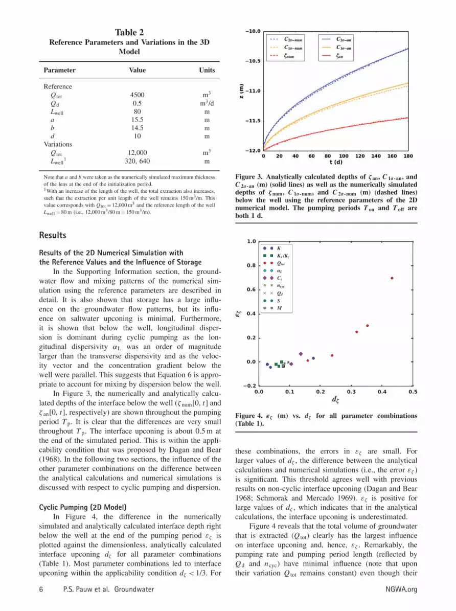
Table 2Reference Parameters and Variations in the 3D

Model

Parameter Value Units

ReferenceQ tot 4500 m3

Qd 0.5 m3/dLwell 80 ma 15.5 mb 14.5 md 10 m

VariationsQ tot 12,000 m3

Lwell1 320, 640 m

Note that a and b were taken as the numerically simulated maximum thicknessof the lens at the end of the initialization period.1With an increase of the length of the well, the total extraction also increases,such that the extraction per unit length of the well remains 150 m3/m. Thisvalue corresponds with Q tot = 12,000 m3 and the reference length of the wellLwell = 80 m (i.e., 12,000 m3/80 m = 150 m3/m).

Results

Results of the 2D Numerical Simulation withthe Reference Values and the Influence of Storage

In the Supporting Information section, the ground-water flow and mixing patterns of the numerical sim-ulation using the reference parameters are described indetail. It is also shown that storage has a large influ-ence on the groundwater flow patterns, but its influ-ence on saltwater upconing is minimal. Furthermore,it is shown that below the well, longitudinal disper-sion is dominant during cyclic pumping as the lon-gitudinal dispersivity αL was an order of magnitudelarger than the transverse dispersivity and as the veloc-ity vector and the concentration gradient below thewell were parallel. This suggests that Equation 6 is appro-priate to account for mixing by dispersion below the well.

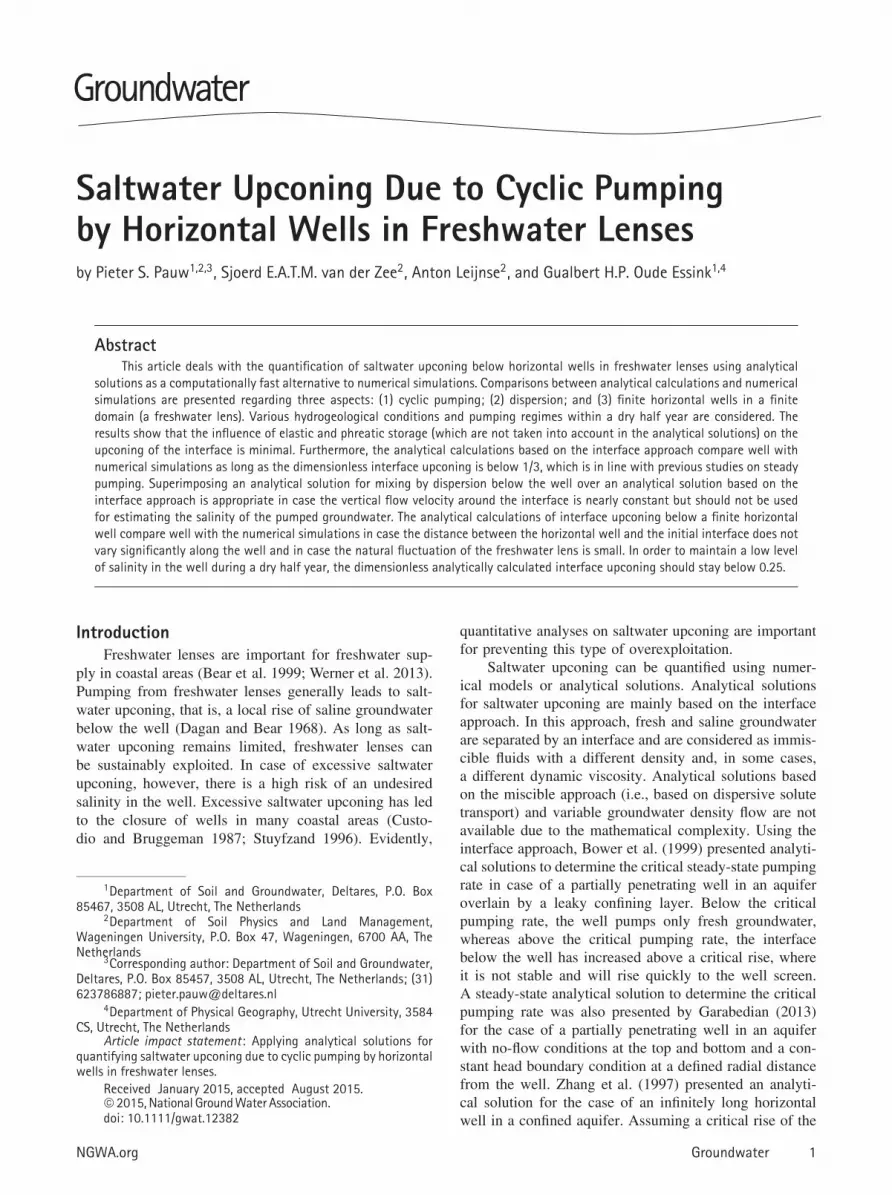
In Figure 3, the numerically and analytically calcu-lated depths of the interface below the well (ζ num[0, t] andζ an[0, t], respectively) are shown throughout the pumpingperiod T p. It is clear that the differences are very smallthroughout T p. The interface upconing is about 0.5 m atthe end of the simulated period. This is within the appli-cability condition that was proposed by Dagan and Bear(1968). In the following two sections, the influence of theother parameter combinations on the difference betweenthe analytical calculations and numerical simulations isdiscussed with respect to cyclic pumping and dispersion.

Cyclic Pumping (2D Model)In Figure 4, the difference in the numerically

simulated and analytically calculated interface depth rightbelow the well at the end of the pumping period εζ isplotted against the dimensionless, analytically calculatedinterface upconing dζ for all parameter combinations(Table 1). Most parameter combinations led to interfaceupconing within the applicability condition dζ < 1/3. For

Figure 3. Analytically calculated depths of ζ an, C 1σ -an, andC 2σ -an (m) (solid lines) as well as the numerically simulateddepths of ζ num, C 1σ -num, and C 2σ -num (m) (dashed lines)below the well using the reference parameters of the 2Dnumerical model. The pumping periods T on and T off areboth 1 d.

Figure 4. εζ (m) vs. dζ for all parameter combinations(Table 1).

these combinations, the errors in εζ are small. Forlarger values of dζ , the difference between the analyticalcalculations and numerical simulations (i.e., the error εζ )is significant. This threshold agrees well with previousresults on non-cyclic interface upconing (Dagan and Bear1968; Schmorak and Mercado 1969). εζ is positive forlarge values of dζ , which indicates that in the analyticalcalculations, the interface upconing is underestimated.

Figure 4 reveals that the total volume of groundwaterthat is extracted (Q tot) clearly has the largest influenceon interface upconing and, hence, εζ . Remarkably, thepumping rate and pumping period length (reflected byQd and ncyc) have minimal influence (note that upontheir variation Q tot remains constant) even though their


variation is relatively large. In case ncyc is equal to 1, thepumping period is 90 d and therefore the simulation isclose to steady state. This indicates that for both cyclicpumping and with steady-state simulations, the interfaceupconing and εζ are controlled by the total volume of thegroundwater extracted (Q tot).

Dispersion (2D Model)In the case of the reference parameters, the differ-

ence between the numerical simulation and analyticalcalculation right below the well with respect to the con-centration contours C1σ and C2σ are very small throughoutT p (Figure 3). Therefore, for these parameter combi-nations, it is appropriate to use Equation 6 to accountfor dispersion. In Figure 5, ε1σ and ε2σ (the differencebetween the numerical simulation and analytical calcula-tion right below the well at the end of the period T p withrespect to the concentration contours C1σ and C2σ , respec-tively) are plotted against dζ (the dimensionless interfaceupconing) for all parameter combinations. ε1σ and ε2σ arepositive in case of significant interface upconing, similarto εζ . This indicates that the depth of the concentrationcontours are underestimated in the analytical calculations.ε1σ and ε2σ are both higher than εζ . This is because inEquation 7, it is assumed that the vertical flow distri-bution around the interface is constant, whereas in thenumerical simulations, the vertical flow velocity variesspatially due to the radial flow resistance induced by thesmall well screen. Toward the well, the flow velocitiesincrease inverse-proportionally, which also explains whyε2σ is higher than ε1σ at high values of dζ . Moreover, incase of a wide initial mixing zone M , the errors ε1σ andε2σ are also high.

Similar to εζ , parameter variations of the total amountof extracted groundwater (Q tot) have the largest influenceon ε1σ and ε2σ . For Q tot, ε2σ increases with increasingdζ (Figure 5) except for dζ = 0.35 and dζ = 0.43. Inthese cases, the numerically simulated C 2σ -num has almostreached the well screen, and therefore, the difference withthe analytically calculated C 2σ -an decreases, which leadsto a lower value of ε2σ .

For some of the Qd (pumping rate per unit length ofthe well) and ncyc (number of pumping cycles) parametervariations, ε1σ and ε2σ are negative. The negative valuesindicate that dispersion is overestimated in the analyticalcalculations. The overestimation can be attributed to stor-age. The effect of the difference in storage between thenumerical simulation and the analytical calculation is thatsaltwater upconing in the analytical calculations is higherthan in the numerical simulation if the pumping rate ishigh (as is the case in some of the Qd and ncyc param-eter variations). In case the pumping rate is high and nostorage is simulated (see Table 1), ε1σ and ε2σ are bothpositive. For the parameter combinations that are consid-ered in this article, the effect of the storage on saltwaterupconing is relatively small.

For all parameter combinations except for the vari-ations in the concentration of the saline groundwaterC s, C 2σ represented the drinking water standard. From

Figure 5, it is clear that using Equations 3 and 6 toestimate the depth of the contour of the drinking waterconcentration below the well leads to substantial errorswhen dζ increases, which indicates a practical limitationof the analytical solutions to estimate the concentration inthe well in case of substantial saltwater upconing. For theparameter combinations listed in Table 1, the numericallysimulated concentration in the well (Cwellnum [M/L3])was compared with the analytically calculated, dimen-sionless interface upconing (expressed as dζ ). Q tot wasnot varied but kept constant at a high value (108 m3/m) toensure that the salinity in the well at the end of the numeri-cal simulations was higher than C 2σ (approximately equalto the WHO drinking water limit). For the concentration ofthe saline groundwater C s, an additional concentrationvalue of 3.5 kg/m3 was investigated. For the longitudi-nal dispersivitiy αL, the highest value of 1.0 m was notconsidered as this value is not very realistic for the typeof aquifers that are considered here.

In Figure 6, Cwellnum is plotted against dζ at the endof every T on (“pumping on”) and T off (“pumping off”)period throughout T p for the three values of the maximumconcentration of the ambient saline groundwater (C s).Remarkably, Cs has a minor influence on the degreeof interface upconing (as calculated with the analyticalsolution) at which the WHO drinking water limit isexceeded. The drinking water limit (0.84 kg/m3) inthe well is exceeded at an analytically calculated,dimensionless interface upconing dζ = 0.3, 0.31, and 0.35for C s = 35, 17.5, and 3.5 kg/m3, respectively. This canbe explained by two effects that counteract each other.One effect is related to the absolute value of the maximumconcentration C s. The lower the C s, the lower the salinityin the well. The other effect is related to the maximumgroundwater density ρs. The lower the ρs, the fastersaline groundwater flows toward the well. In case thelargest value of the thickness of the mixing zone Mis neglected, all parameter combinations yield a salinitylower than the drinking water in the well as long asdζ < 1/3.

Horizontal Wells with a Finite Length in a Finite Domain(3D Model)

In Figure 7, the analytically and numerically deter-mined values of the interface ζ and the concentrationvalues C 1σ and C 2σ using the reference parameters justbelow the well are shown throughout T p. In the analyt-ical calculation, ζ an is underestimated by about 0.35 mat the end of T p. This is proportionally more than whatwas observed in the 2D model concept with the referenceparameters, although still below the critical value of 1/3.The difference between the 2D and 3D results is attributedto the upward movement of the freshwater lens in a dryperiod (natural fluctuation of the lens), which increasesthe saltwater upconing.

In Figure 8, the analytical and numerical resultsusing the same parameters as the reference values, butwith a total volumetric extraction (Q tot) of 12,000 m3,are shown. As a result of the higher Q tot, the saltwater


(a) (b)

Figure 5. ε1σ (a) and ε2σ (b) and corresponding dζ for all parameter combinations and the end of T p.

Figure 6. C well num (kg/m3), the numerically simulated concentration in the well, vs. dζ , at the end of every periods T on andT off during T p, for the three values of C s. The horizontal dashed line indicates the WHO drinking water limit (0.84 kg/m3).

upconing is larger than for the reference parameters. Asexpected, the differences between analytical calculationsand numerical simulations with respect to ζ , C 1σ , and C 2σ

are also larger. For this value of Q tot, the dimensionless,analytically calculated interface upconing dζ at the endof the total pumping period T p is 0.28. The numericallysimulated concentration in the well is 0.88 kg m-3, which isslightly higher than the drinking water limit of 0.84 kg/m3.The drinking water limit is exceeded at dζ = 0.27. In

the 2D numerical simulations, the concentration in thewell did not exceed the drinking water limit as long asthe corresponding dζ was less than 0.3. This differenceis again attributed to the half-yearly variation of thethickness of the freshwater lens.

In Figure 9, the three variations of the length of thewell Lwell are shown at the end of T p. In case Lwell = 80 m,both the analytical calculation and numerical simulationshow the largest interface upconing below the centre of


Figure 7. Analytically calculated depths of ζ an, C 1σ -an, andC 2σ -an (m) (solid lines) as well as the numerically simulateddepths of ζ num, C 1σ -num, and C 2σ -num (m) (dashed lines)below the centre of the well using the reference parametersof the 3D conceptual model.

Figure 8. Analytically calculated depths of ζ an, C 1σ -an, andC 2σ -an (m) (solid lines) as well as the numerically simulateddepths of ζ num, C 1σ -num, and C 2σ -num (m) (dashed lines)below the centre of the well using the reference parametersof the 3D conceptual model, but with a Q tot of 12,000 m3.

the well and show that the interface upconing decreasestowards the outer end of the well. This is attributed to thedifference in flow pattern between the centre and the outerend of the well, which induces less drawdown of the watertable and less saltwater upconing at the outer end of thewell, compared to the centre of the well. From the outerend of the well toward the end of the freshwater lens,the difference in ζ between the analytical and numericalresults increases, which is related to the finite numericalmodel (i.e., the freshwater lens) and the analytical solutionbased on an infinite domain.

In case Lwell = 320 m, the analytical and numericalresults show the same similarities and differences whencompared with Lwell = 80 m except that the interfaceupconing is larger as well as constant over a significant

length of the well. The reason for this is that in caseLwell = 320 m, the flow pattern at the outer ends does notinfluence (i.e. reduce) the drawdown and the saltwaterupconing at the centre, in contrast to the case whereLwell = 80 m. For Lwell = 640 m, the numerical simulationshows that the largest saltwater upconing occurs at theouter end of the horizontal well, not at the centre. Thereason for this is that in the numerical simulation, thefreshwater lens decreases in the direction of the edges,and therefore, the distance between the depth of the welland the initial depth of the interface (i.e., the distanced ) decreases. Based on these results, it can be expectedthat the analytical solution gives appropriate indications ofsaltwater upconing in case the initial distance between theinterface and the well d does not vary significantly belowthe horizontal well. In case Lwell = 320 m, the numericallysimulated concentration in the well did not exceed thedrinking water limit in case dζ = 0.27 (the threshold thatwas found in case Lwell = 80 m).

DiscussionRegarding the cyclic pumping regimes presented in

this article, it is expected that the analytical solutions ofDagan and Bear (1968) also closely resemble numericalsimulations for other (e.g., more irregular) pumpingregimes than that were analyzed, provided that thedimensionless interface upconing remains below 1/3. Thislimitation of a cyclic pumping regime is in line withprevious studies that have dealt with steady-state pumping(Dagan and Bear 1968; Schmorak and Mercado 1969),where this limitation has been referred to as “criticalrise.” For brevity, a discussion on the concept of criticalrise is given in the Supporting Information section.Below the critical rise, the analytical solutions can be acomputationally fast alternative to numerical models forcalculating the interface upconing.

Regarding dispersion, mixing below the well wasdominated by longitudinal dispersion during cyclicpumping as the longitudinal dispersivity was an order ofmagnitude larger than the transverse dispersivity (sim-ilar as found or assumed in many previous studies,for example, Gelhar et al. (1992) and Jankovic et al.(2009)) and as the velocity vector and the concentrationgradient below the well were parallel. Unfortunately, forestimating the concentration in the well, superimposingthe effect of longitudinal dispersion on the analyticalinterface solutions was inappropriate. This has also beennoted in previous studies (Schmorak and Mercado 1969;Wirojanagud and Charbeneau 1985) but has not beenanalyzed as in this study.

For the analytical calculation of saltwater upconingbelow horizontal wells with a finite length in freshwaterlenses, the natural (seasonal) variation of the thickness ofthe freshwater is not taken into account. The results of the3D model showed that the drinking water limit inthe numerical model was exceeded at an analyticallycalculated, dimensionless interface upconing (dζ ) of 0.27,a lower value than what was obtained in the 2D results


Figure 9. Analytically calculated depths of ζ an, C 1σ -an, and C 2σ -an (m) (solid lines) as well as the numerically simulateddepths of ζ num, C 1σ -num, and C 2σ -num (m) (dashed lines) below the well using three different lengths of the well (Lwell) wherethe extraction per unit length of the well is equal to 150 m3/m. Note the values of Lwell hold for the total length of the well,but that (given the symmetry) only half of the well is indicated. The centre of the well is located at x = 0.

(0.3). As the effect of the natural variation of thefreshwater lens was not investigated in great detail, it isadvised here that for maintaining a salinity of the pumpedgroundwater lower than that of the drinking water limit,dζ should be kept relatively small (e.g., 0.25). However, itshould be noted here that this holds only for one half yearwhen irrigation is needed, which is an important limitationof this study. The differences between analytical solutionsand the numerical models for the long term are expected todepend strongly on the groundwater recharge. This aspectis left for further study.

For the analytical calculation of saltwater upconingdue to pumping by a horizontal well with a finiteextent, it was assumed that the frictional head losses(Rushton and Brassington 2013) within the horizontal wellare negligible. In case the head losses are significant,however, the inflow along the horizontal well variessignificantly. Moreover, even if the frictional head lossin the horizontal well is negligible, the inflow along thehorizontal well varies as the flow pattern at the edgesof well is different than in the centre of the well. Theseissues are left for further study. It should be noted herethat if the variation of inflow along the well is calculatedor measured, the analytical solution and the superpositionprinciple can account for the variable inflow along thewell by giving each point sink along the horizontal wellan extraction rate according to the calculated inflow alongthe well.

ConclusionsComparisons between analytical solutions and

numerical simulations for the quantification of saltwaterupconing below horizontal wells in freshwater lenseshave indicated that under certain conditions, the ana-lytical solutions can be used as a computationally fastalternative to numerical simulations. The comparisonswere made regarding three aspects: (1) cyclic pumping;(2) dispersion; and (3) finite horizontal wells in a finitedomain (a freshwater lens). Regarding cyclic pumping,elastic and phreatic storage (which are not taken intoaccount in the analytical solutions) do not significantlyinfluence the upconing of the interface. Furthermore, theanalytical calculations based on the interface approachcompare well with numerical simulations as long as thedimensionless interface upconing is below 1/3, which isin line with previous studies on steady pumping. Regard-ing dispersion, superimposing an analytical solution formixing by dispersion below the well over an analyticalsolution based on the interface approach is appropriatein case the vertical flow velocity around the interfaceis nearly constant but should not be used for estimatingthe salinity of the pumped groundwater. Analyticalcalculations of a finite horizontal well are appropriatein case the distance between the horizontal well and theinitial interface does not vary significantly along the welland in case the natural fluctuation of the freshwater lensis small. For maintaining a low salinity in the well during


a dry half year, the dimensionless, analytically calculatedinterface upconing should stay below 0.25.

Authors’ NoteThe authors have no conflict of interest to disclose.

AcknowledgmentsThis work was carried out within the Dutch “Knowl-

edge for Climate” program. The numerical simulationswere pre-processed and post-processed using the Pythonlibrary FloPy (https://code.google.com/p/flopy/).

Supporting InformationAdditional Supporting Information may be found in theonline version of this article:

Appendix S1. Electronic supplement for “Saltwaterupconing due to cyclic pumping by horizontal wells infreshwater lenses.”

ReferencesBear, J., A.H.D. Cheng, S. Sorek, D. Ouazar, and I. Her-

rera. 1999. Seawater Intrusion in Coastal Aquifers. Con-cepts, Methods and Practices . Dordrecht, The Netherlands:Kluwer Academic Publishers.

Bear, J., and G. Dagan. 1965. The relationship between solutionsof flow problems in isotropic and anisotropic soils. Journalof Hydrology 3: 88–96.

Bower, J.W., L.H. Motz, and D.W. Durden. 1999. Analyticalsolution for determining the critical condition of saltwaterupconing in a leaky artesian aquifer. Journal of Hydrology221: 43–54.

Custodio, E., and G.A. Bruggeman. 1987. Groundwater prob-lems in coastal areas: A contribution to the InternationalHydrological Programme. Studies and reports in hydrology,vol. 45. Paris, France: UNESCO.

Dagan, G., and J. Bear. 1968. Solving the problem of localinterface upconing in a coastal aquifer by the methodof small perturbations. Journal of Hydraulic Research 6:15–44.

Das Gupta, A., and V.P. Gaikwad. 1987. Interface upconing dueto a horizontal well in unconfined aquifer. Ground Water25, no. 4: 466–474.

Das Gupta, A. 1983. Steady interface upconing beneath a coastalinfiltration gallery. Ground Water 21, no. 4: 465–474.

Domenico, P.A., and F.W. Schwartz. 1990. Physical andChemical Hydrology . New York: John Wiley and Sons.

Garabedian, S.P. 2013. Estimation of salt water upconing usinga steady-state solution for partial completion of a pumpedwell. Ground Water 51, no. 6: 927–934.

Gelhar, L.W., W. Welty, and K.W. Rehfeldt. 1992. A criticalreview of data on field-scale dispersion of aquifers. WaterResources Research 28, no. 4: 1955–1974.

Jankovic, I., D.R. Steward, R.J. Barnes, and G. Dagan.2009. Is transverse macrodispersivity in three-dimensionalgroundwater transport equal to zero? A counterexample.Water Resources Research 45, no. 8: 1–10.

Langevin, C.D., D.T. Thorne Jr., A.M. Dausman, M.C. Sukop,and W. Guo. 2007. SEAWAT Version 4: A ComputerProgram for Simulation of Multi-Species Solute and HeatTransport: U.S. Geological Survey Techniques and MethodsBook 6 Chapter A22, 39. Reston, Virginia: U.S. GeologicalSurvey.

Langseth, D.E., A.H. Smyth, and J. May. 2004. A method forevaluating horizontal well pumping tests. Ground Water 42,no. 5: 689–699.

Motz, L.H. 1992. Salt-water upconing in an aquifer overlain bya leaky confining bed. Ground Water 30, no. 2: 192–198.

Reilly, T.E., M.H. Frimpter, D.R. LeBlanc, and A.S. Goodman.1987a. Analysis of steady-state salt-water upconing withapplication at Truro well field, Cape Cod, Massachusetts.Ground Water 25, no. 2: 194–206.

Reilly, T.E., L.O. Franke, and G.D. Bennett. 1987b. The Prin-ciple of Superposition and Its Application in Ground-WaterHydraulics. U.S. Geological Survey Techniques of Water-Resources Investigations Book 3 Chapter B6. Denver, Col-orado: U.S. Geological Survey.

Rushton, K.R., and F.C. Brassington. 2013. Significance ofhydraulic head gradients within horizontal wells in uncon-fined aquifers of limited saturated thickness. Journal ofHydrology 492: 281–289.

Schmorak, S., and A. Mercado. 1969. Upconing of fresh water-sea water interface below pumping wells, field study. WaterResources Research 5, no. 6: 1290–1311.

Stuyfzand, P.J. 1996. Salinization of drinking water in theNetherlands: Anamnesis, diagnosis and remediation. InProceedings of the 14th Salt Water Intrusion Meeting,Malmo, Sweden , June 16–21, Malmo, Sweden.

Werner, A.D., M. Bakker, V.E.A. Post, A. Vandenbohede, C.Lu, B. Ataie-Ashtiani, and C.T. Simmons. 2013. Sea-water intrusion processes, investigation and management:recent advances and future challenges. Advances in WaterResources 51: 3–26.

WHO. 2011. Guidelines for drinking-water quality, 4th ed.http://www.who.int/water_sanitation_health/publications/2011/dwq_guidelines/en/ (accessed September 24, 2015).

Wirojanagud, B.P., and R.J. Charbeneau. 1985. Saltwaterupconing in unconfined aquifers. Journal of HydraulicEngineering 111, no. 3: 417–434.

Yeh, H.D., and Y.C. Chang. 2013. Recent advances in modelingof well hydraulics. Advances in Water Resources 51:27–51.

Zhang, H., G.C. Hocking, and D.A. Barry. 1997. An analyticalsolution for critical withdrawal of layered fluid through aline sink in a porous medium. The Journal of the AustralianMathematical Society. Series B. Applied Mathematics 39:271–279.


saltwater upconing due to cyclic pumping by horizontal wells in freshwater lenses

Documents