robust determination of the circular velocity of dwarf irregular
TRANSCRIPT
MNRAS 466, 4159–4192 (2017) doi:10.1093/mnras/stw3285Advance Access publication 2016 December 17
LITTLE THINGS in 3D: robust determination of the circular velocityof dwarf irregular galaxies
G. Iorio,1,2‹ F. Fraternali,1,3 C. Nipoti,1 E. Di Teodoro,4 J. I. Read5 and G. Battaglia6,7
1Dipartimento di Fisica e Astronomia, Universita di Bologna, Viale Berti Pichat 6/2, I-40127 Bologna, Italy2INAF – Osservatorio Astronomico di Bologna, via Ranzani 1, I-40127 Bologna, Italy3Kapteyn Astronomical Institute, University of Groningen, Postbus 800, NL-9700 AV Groningen, the Netherlands4Research School of Astronomy and Astrophysics – The Australian National University, Canberra, ACT 2611, Australia5Department of Physics, University of Surrey, Guildford GU2 7XH Surrey, UK6Instituto de Astrofisica de Canarias, calle Via Lactea s/n, E-38205 La Laguna, Tenerife, Spain7Dpto. Astrofisica, Universidad de La Laguna, E-38206 La Laguna, Tenerife, Spain
Accepted 2016 December 14. Received 2016 November 11; in original form 2016 September 17
ABSTRACTDwarf irregular galaxies (dIrrs) are the smallest stellar systems with extended H I discs. Thestudy of the kinematics of such discs is a powerful tool to estimate the total matter distributionat these very small scales. In this work, we study the H I kinematics of 17 galaxies extractedfrom the ‘Local Irregulars That Trace Luminosity Extremes, The H I Nearby Galaxy Survey’(LITTLE THINGS). Our approach differs significantly from previous studies in that wedirectly fit 3D models (two spatial dimensions plus one spectral dimension) using the software3DBAROLO, fully exploiting the information in the H I data cubes. For each galaxy, we derivethe geometric parameters of the H I disc (inclination and position angle), the radial distributionof the surface density, the velocity-dispersion (σv) profile and the rotation curve. The circularvelocity (Vc), which traces directly the galactic potential, is then obtained by correcting therotation curve for the asymmetric drift. As an initial application, we show that these dIrrslie on a baryonic Tully–Fisher relation in excellent agreement with that seen on larger scales.The final products of this work are high-quality, ready-to-use kinematic data (Vc and σv) thatwe make publicly available. These can be used to perform dynamical studies and improve ourunderstanding of these low-mass galaxies.
Key words: galaxies: dwarf – galaxies: ISM – galaxies: kinematics and dynamics – galaxies:structure.
1 IN T RO D U C T I O N
The H I 21 cm emission line is a powerful tool for studying thedynamics of late-type galaxies since it is typically detected well be-yond the optical disc and is not affected by dust extinction. Decadesago, the rise of the radio-interferometers allowed many authors toobtain high-resolution rotation curves for large samples of spiralgalaxies (e.g. Bosma 1978, 1981; Bosma, Goss & Allen 1981; vanAlbada et al. 1985; Begeman 1987). These studies found that thegas rotation remains nearly flat also in the outermost disc, where thevisible matter fades and one would expect a nearly Keplerian fall-offof the rotation curve. The flat rotation curves of spirals are one ofthe most robust indications for the existence of dark matter (DM);gas-rich late-type galaxies are an ideal laboratory for studying theproperties of DM haloes. In this context, dwarf irregular galaxies(dIrrs) are also studied with great interest. Unlike large spirals, theyappear to be dominated by DM down to their very central regions.
� E-mail: [email protected]
Thus, the determination of the DM density distribution is nearly in-dependent of the mass-to-light ratio of the stellar disc (e.g. Casertano& van Gorkom 1991; Cote, Carignan & Freeman 2000).
The standard method to extract a galaxy rotation curve is basedon the fitting of a tilted-ring model to a 2D velocity field (e.g.Begeman 1987; Schoenmakers, Franx & de Zeeuw 1997). The ve-locity field is extracted from the H I data cube by deriving the repre-sentative velocity of the line profile at each spatial pixel. There aredifferent methods to define a representative velocity, for instanceusing the intensity-weighted mean (e.g. Rogstad & Shostak 1971),or by fitting functional forms (e.g. single Gaussian, Begeman 1987or multiple Gaussians, Oh et al. 2015, hereafter O15). The 2Dapproach has been used in several numerical algorithms such asROTCUR (Begeman 1987), RESWRI (Schoenmakers et al. 1997),KINEMETRY (Krajnovic et al. 2006) and DISKFIT (Spekkens &Sellwood 2007). All of these codes have been very useful to im-prove our understanding of the kinematics of late-type galaxies.However, working in 2D has a drawback: the results depend on theassumptions made when extracting the velocity field and are also
C© 2016 The AuthorsPublished by Oxford University Press on behalf of the Royal Astronomical Society
Dow
nloaded from https://academ
ic.oup.com/m
nras/article/466/4/4159/2712521 by guest on 13 March 2022
4160 G. Iorio et al.
affected by the instrumental resolution (the so-called beam smear-ing; Bosma 1978; Begeman 1987). These problems are especiallyrelevant in the study of the kinematics of dIrrs since the H I lineprofiles can be heavily distorted by both non-circular motions andnoise. As a consequence, the extraction of the velocity field can bechallenging (see e.g. Oh et al. 2008). Furthermore, dIrrs are oftenobserved with a limited number of resolution elements because oftheir limited extension on the sky. The effect of beam smearing canalso make the estimate of both the rotation curve and the inclinationof the disc uncertain (Begeman 1987).
The pioneering work of Swaters (1999) showed that these prob-lems can be solved with an alternative approach: the properties ofthe H I disc can be retrieved with a direct modelling of the 3D datacube (two spatial axes plus one spectral axis) without explicitlyextracting velocity fields. In practice, a 3D method consists of adata-model comparison of nch maps (where nch is the number ofspectral channels) instead of the single map represented by the ve-locity field. The best advantage of this approach is that the data cubemodels are convolved with the instrumental response, so the final re-sults are not affected by the beam smearing. Swaters (1999), Gentileet al. (2004), Lelli, Fraternali & Sancisi (2010) and Lelli, Verheijen& Fraternali (2014b) used a 3D visual comparison between datacubes and model cubes to correct and improve the results obtainedwith the classical 2D methods. However, a by-eye inspection of thedata is time intensive and subjective. Modern software like TIRIFIC
(Jozsa et al. 2007) and 3DBAROLO (hereafter 3DB; Di Teodoro &Fraternali 2015) can perform a full 3D numerical minimization onthe whole data cube.
In this paper, we exploit the power of the 3D approach by ap-plying 3DB to a sample of 17 dIrrs taken from the Local IrregularsThat Trace Luminosity Extremes, The H I Nearby Galaxy Survey(LITTLE THINGS; hereafter LT) sample (Hunter et al. 2012). 3DBhas been extensively tested on mock H I data cubes correspondingto low-mass isolated dIrrs. Read et al. (2016c) show that the rotationcurve is well recovered even for a starbursting dwarf, provided thatthe inclination of the H I disc is higher than 40◦.
The final products of our analysis are ready-to-use rotationcurves corrected for the instrumental effects (see Section 3.2) andfor the asymmetric drift (see Section 4.3.1). The rotation curvescan be used to study the dynamics of dIrrs (e.g. van Eymerenet al. 2009b; Read et al. 2016a,c) or to extend the study of thescaling relations on small scales (e.g. Brook, Santos-Santos &Stinson 2016; Lelli, McGaugh & Schombert 2016). An unbiasedestimate of the rotation curves of dIrrs is also essential to shedlight on the well-known cosmological tensions on small scale: thelong debated ‘cusp–core problem’ (de Blok & Bosma 2002; Ohet al. 2011; Read, Agertz & Collins 2016b), the ‘missing-satellitesproblem’ (Klypin et al. 1999; Read et al. 2016a) and the ‘too-big-to-fail problem’ (Read et al. 2006; Boylan-Kolchin, Bullock &Kaplinghat 2011; Read et al. 2016a). These ‘problems’ are discrep-ancies between the properties of DM haloes predicted by cosmo-logical simulations and those inferred from observations. In thiscontext, it is therefore crucial to obtain reliable estimates of the DMdistribution in real galaxies.
In this work, we focus in particular on the asymmetric-drift cor-rection (see Section 4.3.1). This correction term is usually appliedwithout considering the errors made in its calculation, but these canbe very large and should be taken into account. The propagation ofthe asymmetric-drift errors has a great impact on the determinationof the circular velocity of galaxies in which the contribution of thegas velocity dispersion is important (see for example DDO 210 inSection 5). We developed a method to calculate and propagate the
asymmetric-drift uncertainties: as a result, the quoted errors on thefinal corrected rotation curves are a robust description of the realuncertainties.
The paper is organized as follows. In Section 2, we illustrate thesample and the data used in this work. In Section 3, we brieflyintroduce the tilted-ring model and 3DB. In Section 4, we describein detail the analysis applied to our data. Section 5 shows the resultsof our analysis for each galaxy in our sample. In Section 6, welook at whether the low-mass dIrrs that we study here lie on thebaryonic Tully–Fisher relation (BTFR). In Section 7, we discussthe assumptions made to derive the rotation curves and we compareour results with previous work. A summary is given in Section 8.
2 SA M P L E A N D DATA
2.1 Sample selection
The galaxies used in this work represent a sub-sample of the galaxiesof the LT survey (Hunter et al. 2012), which is a sample of 37 dIrrsand 4 blue compact dwarfs (BCDs) located in the Local Volumewithin 11 Mpc from the Milky Way. LT combines archival andnew H I observations taken with the very large array to obtain avery high spatial and spectral resolution data set (see Table 1). Theobjects in the LT sample have been chosen to be both isolated andrepresentative of the full range of dIrr properties (Hunter et al. 2012).
We built our sample selecting dIrrs that are well suited to studythe circular motion of the H I discs. To this end, we excluded fromour selection all the objects seen at low inclination angles and thefour BCDs. The inclination angle i is defined as the angle betweenthe plane of the disc and the line of sight such that i = 90◦ for anedge-on galaxy and i = 0◦ for a face-on galaxy. The estimate of iin nearly face-on galaxies (i < 40◦) is extremely difficult both fromthe kinematic fit (Begeman 1987) and from the analysis of the H I
map (Read et al. 2016c). Moreover, for i < 40◦, relatively smallerrors on i have a great impact on the deprojection of the observedrotational velocity (see equation 1). As a consequence, the finalrotation curves of these nearly face-on galaxies could be biased andunreliable with both 2D (Oman et al. 2016) and 3D methods (Readet al. 2016c). Among the objects with i > 40◦, we selected 17 dIrrs,about half of the original LT sample.
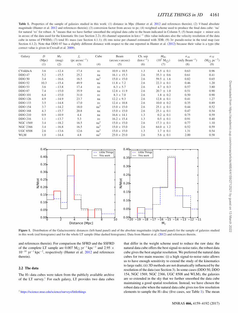
We checked, using a Kolmogorov–Smirnov (KS) test, that oursub-sample preserves the statistical distribution of the galactic prop-erties such as distance (KS p-value 0.96), absolute magnitude (KSp-value 0.99), star formation rate density (SFRD, KS p-value 0.92)and baryonic mass (KS p-value 0.99). Because of our rejection cri-terion, the average i in our sub-sample (58◦) is higher than the onemeasured in the LT sample (50◦). Fig. 1 shows the distributions ofthe distances and of the absolute magnitudes of our sample and theoriginal LT sample.
It is worth pointing out that our rejection criterion is based on iestimated for the stellar disc from the V-band photometry (Hunter &Elmegreen 2006). When we re-estimated i from the H I data cubes(see Section 4.2), we found that four galaxies (DDO 47, DDO50, DDO 53 and DDO 133) have an average i lower than 40◦ (seeTable 2). We did not exclude these galaxies from our sample, but ourresults for these objects should be treated with caution. In particular,the formal errors on the velocities and on i could underestimate thereal uncertainties (see notes on the individual galaxies in Section 5).
In conclusion, our sample comprises 17 objects covering thestellar mass range 5 × 10⁵ � M∗/M� � 108, with a mean SFRDof about 0.006 M� yr−1 kpc−2 and a mean specific SFRD (SSFRD)of about 2.26 × 10⁻¹⁰ yr−1 kpc−2 (data from Hunter et al. 2012
MNRAS 466, 4159–4192 (2017)
Dow
nloaded from https://academ
ic.oup.com/m
nras/article/466/4/4159/2712521 by guest on 13 March 2022
LITTLE THINGS in 3D 4161
Table 1. Properties of the sample of galaxies studied in this work: (1) distance in Mpc (Hunter et al. 2012 and references therein); (2) V-band absolutemagnitude (Hunter et al. 2012 and references therein); (3) conversion factor from arcsec to pc; (4) weighted scheme used to produce the final data cube: ‘na’for natural ‘ro’ for robust. A †means that we have further smoothed the original data cube to the beam indicated in Column 5; (5) beam major × minor axisin arcsec of the data used for the kinematic fits (see Section 2.2); (6) channel separation in km s−1 (this value indicates also the velocity resolution of the datacube in terms of FWHM); (7) total H I mass (see Section 4.1.1); (8) rms noise per channel estimated with 3DB; (9) 3σ pseudo-noise in the total map (seeSection 4.1.2). Note that DDO 87 has a slightly different distance with respect to the one reported in Hunter et al. (2012) because their value is a typo (thecorrect value is given in Croxall et al. 2009).
Galaxy D MV fc Cube Beam Ch. sep MH I σ ch σ 3T
(Mpc) (mag) (pc arcsec−1) (arcsec×arcsec) (km s−1) (107 M�) (mJy Beam−1) (M� pc−2)(1) (2) (3) (4) (5) (6) (7) (8) (9)
CVnIdwA 3.6 −12.4 17.4 ro 10.9 × 10.5 1.3 4.5 ± 0.1 0.63 0.96DDO 47 5.2 −15.5 25.2 na 16.1 × 15.3 2.6 35.3 ± 0.6 0.61 0.41DDO 50 3.4 −16.6 16.5 na† 15.0 × 15.0 2.6 59.5 ± 1.6 0.82 0.65DDO 52 10.3 −15.4 49.9 na 11.8 × 7.2 2.6 22.3 ± 0.1 0.46 1.20DDO 53 3.6 −13.8 17.4 ro 6.3 × 5.7 2.6 4.7 ± 0.3 0.57 3.80DDO 87 7.4 −15.0 35.9 na 12.8 × 11.9 2.6 20.7 ± 1.0 0.51 0.90DDO 101 6.4 −15.0 31.0 ro 8.3 × 7.0 2.6 1.8 ± 0.2 0.50 0.90DDO 126 4.9 −14.9 23.7 na 12.2 × 9.3 2.6 12.8 ± 0.1 0.41 1.27DDO 133 3.5 −14.8 17.0 ro 12.4 × 10.8 2.6 10.0 ± 0.2 0.35 0.89DDO 154 3.7 −14.2 18.0 na† 15.0 × 15.0 2.6 25.1 ± 0.1 0.44 0.52DDO 168 4.3 −15.7 20.8 na 15.0 × 15.0 2.6 25.1 ± 0.1 0.47 0.54DDO 210 0.9 −10.9 4.4 na 16.6 × 14.1 1.3 0.2 ± 0.1 0.75 0.59DDO 216 1.1 −13.7 5.3 ro 16.2 × 15.4 1.3 0.5 ± 0.1 0.91 0.40NGC 1569 3.4 −18.2 16.5 na† 15.0 × 15.0 2.6 17.3 ± 0.1 0.77 1.10NGC 2366 3.4 −16.8 16.5 na† 15.0 × 15.0 2.6 64.0 ± 1.2 0.52 0.59UGC 8508 2.6 −13.6 12.6 na† 15.0 × 15.0 1.3 1.7 ± 0.1 1.31 0.54WLM 1.0 −14.4 4.8 na† 25.0 × 25.0 2.6 5.6 ± 0.1 2.00 0.58
Figure 1. Distribution of the Galactocentric distances (left-hand panel) and of the absolute magnitudes (right-hand panel) for the sample of galaxies studiedin this work (red histograms) and for the whole LT sample (blue dashed histograms). Data from Hunter et al. (2012) and references therein.
and references therein). For comparison the SFRD and the SSFRDof the complete LT sample are 0.007 M� yr−1 kpc−2 and 2.95 ×10⁻¹⁰ yr−1 kpc−2, respectively (Hunter et al. 2012 and referencestherein).
2.2 The data
The H I data cubes were taken from the publicly available archiveof the LT survey.1 For each galaxy, LT provides two data cubes
1 https://science.nrao.edu/science/surveys/littlethings
that differ in the weight scheme used to reduce the raw data: thenatural data cube offers the best signal-to-noise ratio, the robust datacube gives the best angular resolution. We preferred the natural datacubes for two main reasons: (i) a high signal-to-noise ratio allowsus to have enough sensitivity to extend the study of the kinematicsto large radii; (ii) 3D methods are not dramatically influenced by theresolution of the data (see Section 3). In some cases (DDO 50, DDO154, NGC 1569, NGC 2366, UGC 8508 and WLM), the galaxiesare so extended in the sky that we further smoothed the data cubemaintaining a good spatial resolution. Instead, we have chosen therobust data cube when the natural data cube gives too few resolutionelements to sample the H I disc (five cases, see Table 1). The mean
MNRAS 466, 4159–4192 (2017)
Dow
nloaded from https://academ
ic.oup.com/m
nras/article/466/4/4159/2712521 by guest on 13 March 2022
4162 G. Iorio et al.
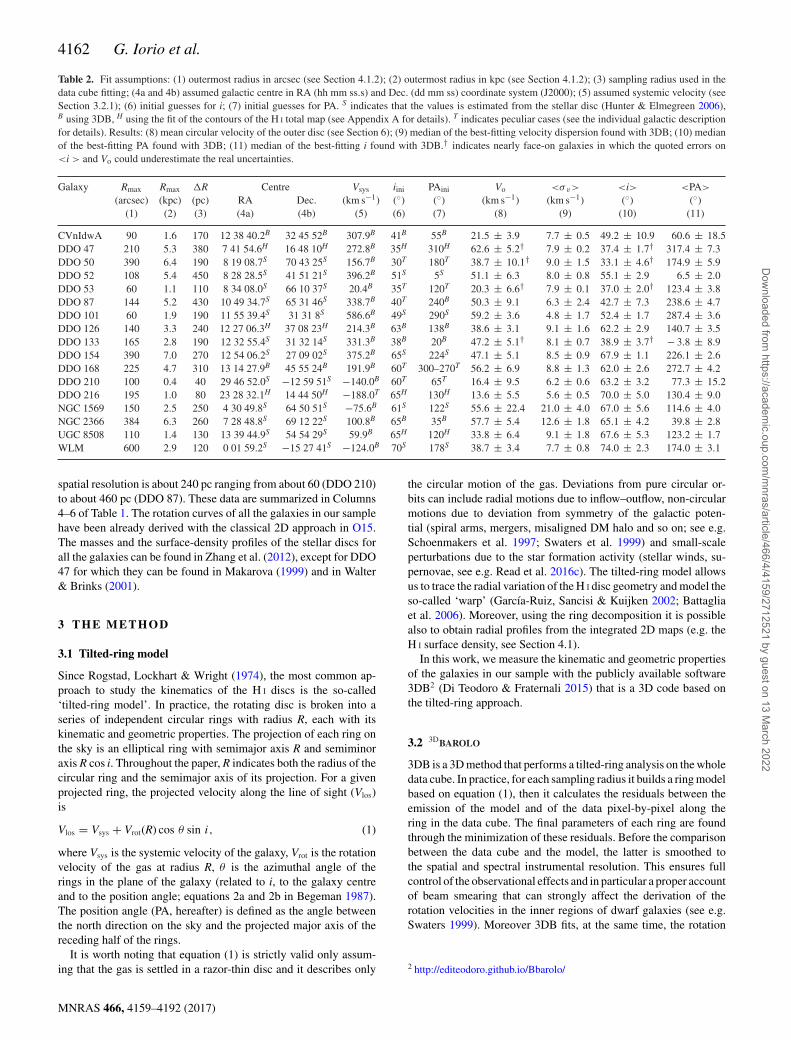
Table 2. Fit assumptions: (1) outermost radius in arcsec (see Section 4.1.2); (2) outermost radius in kpc (see Section 4.1.2); (3) sampling radius used in thedata cube fitting; (4a and 4b) assumed galactic centre in RA (hh mm ss.s) and Dec. (dd mm ss) coordinate system (J2000); (5) assumed systemic velocity (seeSection 3.2.1); (6) initial guesses for i; (7) initial guesses for PA. S indicates that the values is estimated from the stellar disc (Hunter & Elmegreen 2006),B using 3DB, H using the fit of the contours of the H I total map (see Appendix A for details). T indicates peculiar cases (see the individual galactic descriptionfor details). Results: (8) mean circular velocity of the outer disc (see Section 6); (9) median of the best-fitting velocity dispersion found with 3DB; (10) medianof the best-fitting PA found with 3DB; (11) median of the best-fitting i found with 3DB.† indicates nearly face-on galaxies in which the quoted errors on<i > and Vo could underestimate the real uncertainties.
Galaxy Rmax Rmax �R Centre Vsys iini PAini Vo <σv> <i> <PA>
(arcsec) (kpc) (pc) RA Dec. (km s−1) (◦) (◦) (km s−1) (km s−1) (◦) (◦)(1) (2) (3) (4a) (4b) (5) (6) (7) (8) (9) (10) (11)
CVnIdwA 90 1.6 170 12 38 40.2B 32 45 52B 307.9B 41B 55B 21.5 ± 3.9 7.7 ± 0.5 49.2 ± 10.9 60.6 ± 18.5DDO 47 210 5.3 380 7 41 54.6H 16 48 10H 272.8B 35H 310H 62.6 ± 5.2† 7.9 ± 0.2 37.4 ± 1.7† 317.4 ± 7.3DDO 50 390 6.4 190 8 19 08.7S 70 43 25S 156.7B 30T 180T 38.7 ± 10.1† 9.0 ± 1.5 33.1 ± 4.6† 174.9 ± 5.9DDO 52 108 5.4 450 8 28 28.5S 41 51 21S 396.2B 51S 5S 51.1 ± 6.3 8.0 ± 0.8 55.1 ± 2.9 6.5 ± 2.0DDO 53 60 1.1 110 8 34 08.0S 66 10 37S 20.4B 35T 120T 20.3 ± 6.6† 7.9 ± 0.1 37.0 ± 2.0† 123.4 ± 3.8DDO 87 144 5.2 430 10 49 34.7S 65 31 46S 338.7B 40T 240B 50.3 ± 9.1 6.3 ± 2.4 42.7 ± 7.3 238.6 ± 4.7DDO 101 60 1.9 190 11 55 39.4S 31 31 8S 586.6B 49S 290S 59.2 ± 3.6 4.8 ± 1.7 52.4 ± 1.7 287.4 ± 3.6DDO 126 140 3.3 240 12 27 06.3H 37 08 23H 214.3B 63B 138B 38.6 ± 3.1 9.1 ± 1.6 62.2 ± 2.9 140.7 ± 3.5DDO 133 165 2.8 190 12 32 55.4S 31 32 14S 331.3B 38B 20B 47.2 ± 5.1† 8.1 ± 0.7 38.9 ± 3.7† − 3.8 ± 8.9DDO 154 390 7.0 270 12 54 06.2S 27 09 02S 375.2B 65S 224S 47.1 ± 5.1 8.5 ± 0.9 67.9 ± 1.1 226.1 ± 2.6DDO 168 225 4.7 310 13 14 27.9B 45 55 24B 191.9B 60T 300–270T 56.2 ± 6.9 8.8 ± 1.3 62.0 ± 2.6 272.7 ± 4.2DDO 210 100 0.4 40 29 46 52.0S −12 59 51S −140.0B 60T 65T 16.4 ± 9.5 6.2 ± 0.6 63.2 ± 3.2 77.3 ± 15.2DDO 216 195 1.0 80 23 28 32.1H 14 44 50H −188.0T 65H 130H 13.6 ± 5.5 5.6 ± 0.5 70.0 ± 5.0 130.4 ± 9.0NGC 1569 150 2.5 250 4 30 49.8S 64 50 51S −75.6B 61S 122S 55.6 ± 22.4 21.0 ± 4.0 67.0 ± 5.6 114.6 ± 4.0NGC 2366 384 6.3 260 7 28 48.8S 69 12 22S 100.8B 65B 35B 57.7 ± 5.4 12.6 ± 1.8 65.1 ± 4.2 39.8 ± 2.8UGC 8508 110 1.4 130 13 39 44.9S 54 54 29S 59.9B 65H 120H 33.8 ± 6.4 9.1 ± 1.8 67.6 ± 5.3 123.2 ± 1.7WLM 600 2.9 120 0 01 59.2S −15 27 41S −124.0B 70S 178S 38.7 ± 3.4 7.7 ± 0.8 74.0 ± 2.3 174.0 ± 3.1
spatial resolution is about 240 pc ranging from about 60 (DDO 210)to about 460 pc (DDO 87). These data are summarized in Columns4–6 of Table 1. The rotation curves of all the galaxies in our samplehave been already derived with the classical 2D approach in O15.The masses and the surface-density profiles of the stellar discs forall the galaxies can be found in Zhang et al. (2012), except for DDO47 for which they can be found in Makarova (1999) and in Walter& Brinks (2001).
3 TH E M E T H O D
3.1 Tilted-ring model
Since Rogstad, Lockhart & Wright (1974), the most common ap-proach to study the kinematics of the H I discs is the so-called‘tilted-ring model’. In practice, the rotating disc is broken into aseries of independent circular rings with radius R, each with itskinematic and geometric properties. The projection of each ring onthe sky is an elliptical ring with semimajor axis R and semiminoraxis R cos i. Throughout the paper, R indicates both the radius of thecircular ring and the semimajor axis of its projection. For a givenprojected ring, the projected velocity along the line of sight (Vlos)is
Vlos = Vsys + Vrot(R) cos θ sin i, (1)
where Vsys is the systemic velocity of the galaxy, Vrot is the rotationvelocity of the gas at radius R, θ is the azimuthal angle of therings in the plane of the galaxy (related to i, to the galaxy centreand to the position angle; equations 2a and 2b in Begeman 1987).The position angle (PA, hereafter) is defined as the angle betweenthe north direction on the sky and the projected major axis of thereceding half of the rings.
It is worth noting that equation (1) is strictly valid only assum-ing that the gas is settled in a razor-thin disc and it describes only
the circular motion of the gas. Deviations from pure circular or-bits can include radial motions due to inflow–outflow, non-circularmotions due to deviation from symmetry of the galactic poten-tial (spiral arms, mergers, misaligned DM halo and so on; see e.g.Schoenmakers et al. 1997; Swaters et al. 1999) and small-scaleperturbations due to the star formation activity (stellar winds, su-pernovae, see e.g. Read et al. 2016c). The tilted-ring model allowsus to trace the radial variation of the H I disc geometry and model theso-called ‘warp’ (Garcıa-Ruiz, Sancisi & Kuijken 2002; Battagliaet al. 2006). Moreover, using the ring decomposition it is possiblealso to obtain radial profiles from the integrated 2D maps (e.g. theH I surface density, see Section 4.1).
In this work, we measure the kinematic and geometric propertiesof the galaxies in our sample with the publicly available software3DB2 (Di Teodoro & Fraternali 2015) that is a 3D code based onthe tilted-ring approach.
3.2 3DBAROLO
3DB is a 3D method that performs a tilted-ring analysis on the wholedata cube. In practice, for each sampling radius it builds a ring modelbased on equation (1), then it calculates the residuals between theemission of the model and of the data pixel-by-pixel along thering in the data cube. The final parameters of each ring are foundthrough the minimization of these residuals. Before the comparisonbetween the data cube and the model, the latter is smoothed tothe spatial and spectral instrumental resolution. This ensures fullcontrol of the observational effects and in particular a proper accountof beam smearing that can strongly affect the derivation of therotation velocities in the inner regions of dwarf galaxies (see e.g.Swaters 1999). Moreover 3DB fits, at the same time, the rotation
2 http://editeodoro.github.io/Bbarolo/
MNRAS 466, 4159–4192 (2017)
Dow
nloaded from https://academ
ic.oup.com/m
nras/article/466/4/4159/2712521 by guest on 13 March 2022
LITTLE THINGS in 3D 4163
velocity and the velocity dispersion instead of treating them asseparate components as done in the classical 2D approach (e.g.Tamburro et al. 2009; O15).
In conclusion, 3DB fits up to eight parameters for each ring inwhich the galaxy is decomposed: central coordinates, Vsys, i, PA,H I surface density (�), H I thickness (zd), Vrot and the velocitydispersion (σ v). 3DB separates the genuine H I emission from thenoise by building a mask: only the pixels containing a signal abovea certain threshold from the noise are taken into account. The noiseestimated with 3DB for each galaxy is reported in the Column 8of Table 1. Further details on 3DB can be found in Di Teodoro &Fraternali (2015).
3DB works well both on high-resolution and low-resolution data(Di Teodoro & Fraternali 2015). This allows us to use the optimalcompromise between spatial resolution and sensitivity, as alreadydiscussed in Section 2.2. Read et al. (2016c) showed that 3DB iscapable of obtaining a good estimate of the kinematic parametersof mock H I data cubes corresponding to low-mass isolated dIrrs,similar to those that we will study here.
3.2.1 Assumptions
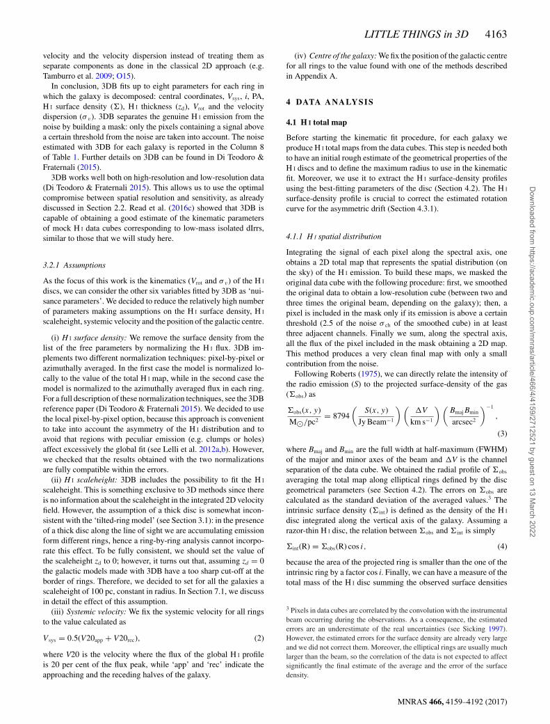
As the focus of this work is the kinematics (Vrot and σ v) of the H I
discs, we can consider the other six variables fitted by 3DB as ‘nui-sance parameters’. We decided to reduce the relatively high numberof parameters making assumptions on the H I surface density, H I
scaleheight, systemic velocity and the position of the galactic centre.
(i) H I surface density: We remove the surface density from thelist of the free parameters by normalizing the H I flux. 3DB im-plements two different normalization techniques: pixel-by-pixel orazimuthally averaged. In the first case the model is normalized lo-cally to the value of the total H I map, while in the second case themodel is normalized to the azimuthally averaged flux in each ring.For a full description of these normalization techniques, see the 3DBreference paper (Di Teodoro & Fraternali 2015). We decided to usethe local pixel-by-pixel option, because this approach is convenientto take into account the asymmetry of the H I distribution and toavoid that regions with peculiar emission (e.g. clumps or holes)affect excessively the global fit (see Lelli et al. 2012a,b). However,we checked that the results obtained with the two normalizationsare fully compatible within the errors.
(ii) H I scaleheight: 3DB includes the possibility to fit the H I
scaleheight. This is something exclusive to 3D methods since thereis no information about the scaleheight in the integrated 2D velocityfield. However, the assumption of a thick disc is somewhat incon-sistent with the ‘tilted-ring model’ (see Section 3.1): in the presenceof a thick disc along the line of sight we are accumulating emissionform different rings, hence a ring-by-ring analysis cannot incorpo-rate this effect. To be fully consistent, we should set the value ofthe scaleheight zd to 0; however, it turns out that, assuming zd = 0the galactic models made with 3DB have a too sharp cut-off at theborder of rings. Therefore, we decided to set for all the galaxies ascaleheight of 100 pc, constant in radius. In Section 7.1, we discussin detail the effect of this assumption.
(iii) Systemic velocity: We fix the systemic velocity for all ringsto the value calculated as
Vsys = 0.5(V20app + V20rec), (2)
where V20 is the velocity where the flux of the global H I profileis 20 per cent of the flux peak, while ‘app’ and ‘rec’ indicate theapproaching and the receding halves of the galaxy.
(iv) Centre of the galaxy: We fix the position of the galactic centrefor all rings to the value found with one of the methods describedin Appendix A.
4 DATA A NA LY SIS
4.1 H I total map
Before starting the kinematic fit procedure, for each galaxy weproduce H I total maps from the data cubes. This step is needed bothto have an initial rough estimate of the geometrical properties of theH I discs and to define the maximum radius to use in the kinematicfit. Moreover, we use it to extract the H I surface-density profilesusing the best-fitting parameters of the disc (Section 4.2). The H I
surface-density profile is crucial to correct the estimated rotationcurve for the asymmetric drift (Section 4.3.1).
4.1.1 H I spatial distribution
Integrating the signal of each pixel along the spectral axis, oneobtains a 2D total map that represents the spatial distribution (onthe sky) of the H I emission. To build these maps, we masked theoriginal data cube with the following procedure: first, we smoothedthe original data to obtain a low-resolution cube (between two andthree times the original beam, depending on the galaxy); then, apixel is included in the mask only if its emission is above a certainthreshold (2.5 of the noise σ ch of the smoothed cube) in at leastthree adjacent channels. Finally we sum, along the spectral axis,all the flux of the pixel included in the mask obtaining a 2D map.This method produces a very clean final map with only a smallcontribution from the noise.
Following Roberts (1975), we can directly relate the intensity ofthe radio emission (S) to the projected surface-density of the gas(�obs) as
�obs(x, y)
M�/pc2= 8794
(S(x, y)
Jy Beam−1
) (�V
km s−1
) (BmajBmin
arcsec2
)−1
,
(3)
where Bmaj and Bmin are the full width at half-maximum (FWHM)of the major and minor axes of the beam and �V is the channelseparation of the data cube. We obtained the radial profile of �obs
averaging the total map along elliptical rings defined by the discgeometrical parameters (see Section 4.2). The errors on �obs arecalculated as the standard deviation of the averaged values.3 Theintrinsic surface density (�int) is defined as the density of the H I
disc integrated along the vertical axis of the galaxy. Assuming arazor-thin H I disc, the relation between �obs and �int is simply
�int(R) = �obs(R) cos i, (4)
because the area of the projected ring is smaller than the one of theintrinsic ring by a factor cos i. Finally, we can have a measure of thetotal mass of the H I disc summing the observed surface densities
3 Pixels in data cubes are correlated by the convolution with the instrumentalbeam occurring during the observations. As a consequence, the estimatederrors are an underestimate of the real uncertainties (see Sicking 1997).However, the estimated errors for the surface density are already very largeand we did not correct them. Moreover, the elliptical rings are usually muchlarger than the beam, so the correlation of the data is not expected to affectsignificantly the final estimate of the average and the error of the surfacedensity.
MNRAS 466, 4159–4192 (2017)
Dow
nloaded from https://academ
ic.oup.com/m
nras/article/466/4/4159/2712521 by guest on 13 March 2022
4164 G. Iorio et al.
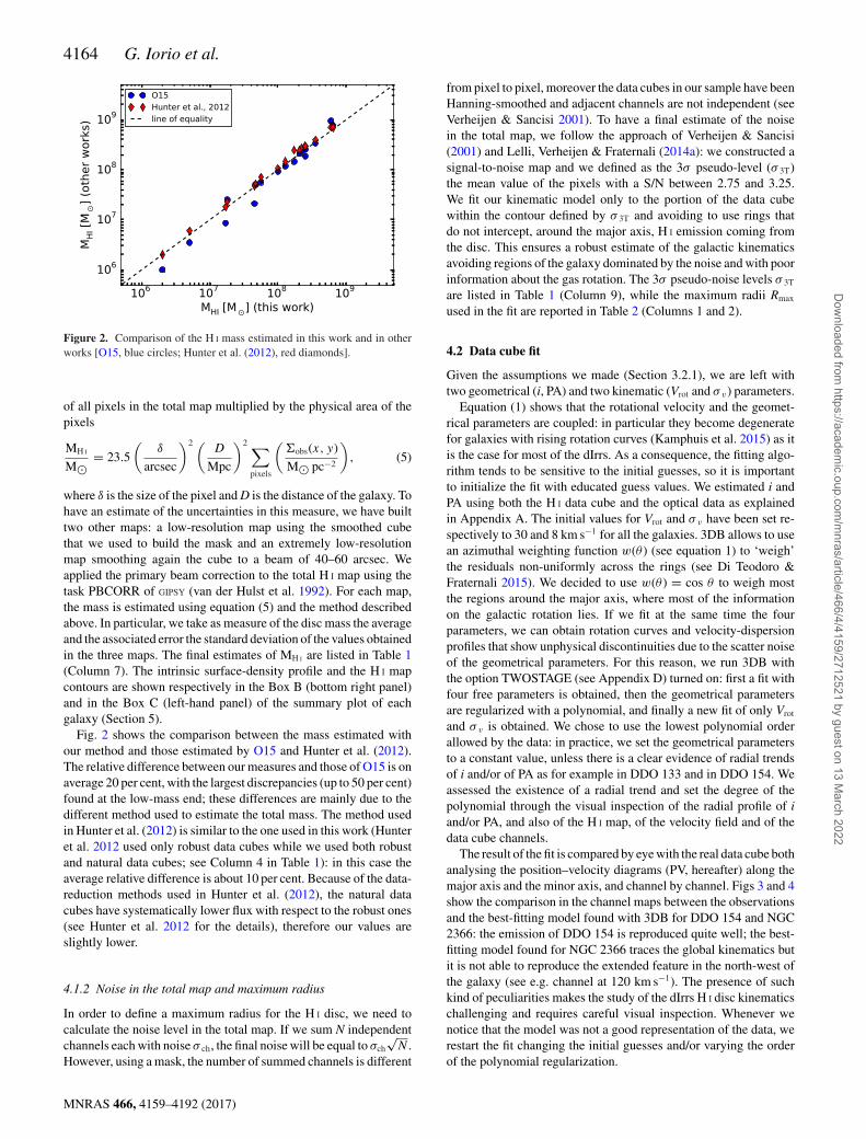
Figure 2. Comparison of the H I mass estimated in this work and in otherworks [O15, blue circles; Hunter et al. (2012), red diamonds].
of all pixels in the total map multiplied by the physical area of thepixels
MH I
M�= 23.5
(δ
arcsec
)2 (D
Mpc
)2 ∑pixels
(�obs(x, y)
M� pc−2
), (5)
where δ is the size of the pixel and D is the distance of the galaxy. Tohave an estimate of the uncertainties in this measure, we have builttwo other maps: a low-resolution map using the smoothed cubethat we used to build the mask and an extremely low-resolutionmap smoothing again the cube to a beam of 40–60 arcsec. Weapplied the primary beam correction to the total H I map using thetask PBCORR of GIPSY (van der Hulst et al. 1992). For each map,the mass is estimated using equation (5) and the method describedabove. In particular, we take as measure of the disc mass the averageand the associated error the standard deviation of the values obtainedin the three maps. The final estimates of MH I are listed in Table 1(Column 7). The intrinsic surface-density profile and the H I mapcontours are shown respectively in the Box B (bottom right panel)and in the Box C (left-hand panel) of the summary plot of eachgalaxy (Section 5).
Fig. 2 shows the comparison between the mass estimated withour method and those estimated by O15 and Hunter et al. (2012).The relative difference between our measures and those of O15 is onaverage 20 per cent, with the largest discrepancies (up to 50 per cent)found at the low-mass end; these differences are mainly due to thedifferent method used to estimate the total mass. The method usedin Hunter et al. (2012) is similar to the one used in this work (Hunteret al. 2012 used only robust data cubes while we used both robustand natural data cubes; see Column 4 in Table 1): in this case theaverage relative difference is about 10 per cent. Because of the data-reduction methods used in Hunter et al. (2012), the natural datacubes have systematically lower flux with respect to the robust ones(see Hunter et al. 2012 for the details), therefore our values areslightly lower.
4.1.2 Noise in the total map and maximum radius
In order to define a maximum radius for the H I disc, we need tocalculate the noise level in the total map. If we sum N independentchannels each with noise σ ch, the final noise will be equal to σch
√N .
However, using a mask, the number of summed channels is different
from pixel to pixel, moreover the data cubes in our sample have beenHanning-smoothed and adjacent channels are not independent (seeVerheijen & Sancisi 2001). To have a final estimate of the noisein the total map, we follow the approach of Verheijen & Sancisi(2001) and Lelli, Verheijen & Fraternali (2014a): we constructed asignal-to-noise map and we defined as the 3σ pseudo-level (σ 3T)the mean value of the pixels with a S/N between 2.75 and 3.25.We fit our kinematic model only to the portion of the data cubewithin the contour defined by σ 3T and avoiding to use rings thatdo not intercept, around the major axis, H I emission coming fromthe disc. This ensures a robust estimate of the galactic kinematicsavoiding regions of the galaxy dominated by the noise and with poorinformation about the gas rotation. The 3σ pseudo-noise levels σ 3T
are listed in Table 1 (Column 9), while the maximum radii Rmax
used in the fit are reported in Table 2 (Columns 1 and 2).
4.2 Data cube fit
Given the assumptions we made (Section 3.2.1), we are left withtwo geometrical (i, PA) and two kinematic (Vrot and σ v) parameters.
Equation (1) shows that the rotational velocity and the geomet-rical parameters are coupled: in particular they become degeneratefor galaxies with rising rotation curves (Kamphuis et al. 2015) as itis the case for most of the dIrrs. As a consequence, the fitting algo-rithm tends to be sensitive to the initial guesses, so it is importantto initialize the fit with educated guess values. We estimated i andPA using both the H I data cube and the optical data as explainedin Appendix A. The initial values for Vrot and σ v have been set re-spectively to 30 and 8 km s−1 for all the galaxies. 3DB allows to usean azimuthal weighting function w(θ ) (see equation 1) to ‘weigh’the residuals non-uniformly across the rings (see Di Teodoro &Fraternali 2015). We decided to use w(θ ) = cos θ to weigh mostthe regions around the major axis, where most of the informationon the galactic rotation lies. If we fit at the same time the fourparameters, we can obtain rotation curves and velocity-dispersionprofiles that show unphysical discontinuities due to the scatter noiseof the geometrical parameters. For this reason, we run 3DB withthe option TWOSTAGE (see Appendix D) turned on: first a fit withfour free parameters is obtained, then the geometrical parametersare regularized with a polynomial, and finally a new fit of only Vrot
and σ v is obtained. We chose to use the lowest polynomial orderallowed by the data: in practice, we set the geometrical parametersto a constant value, unless there is a clear evidence of radial trendsof i and/or of PA as for example in DDO 133 and in DDO 154. Weassessed the existence of a radial trend and set the degree of thepolynomial through the visual inspection of the radial profile of iand/or PA, and also of the H I map, of the velocity field and of thedata cube channels.
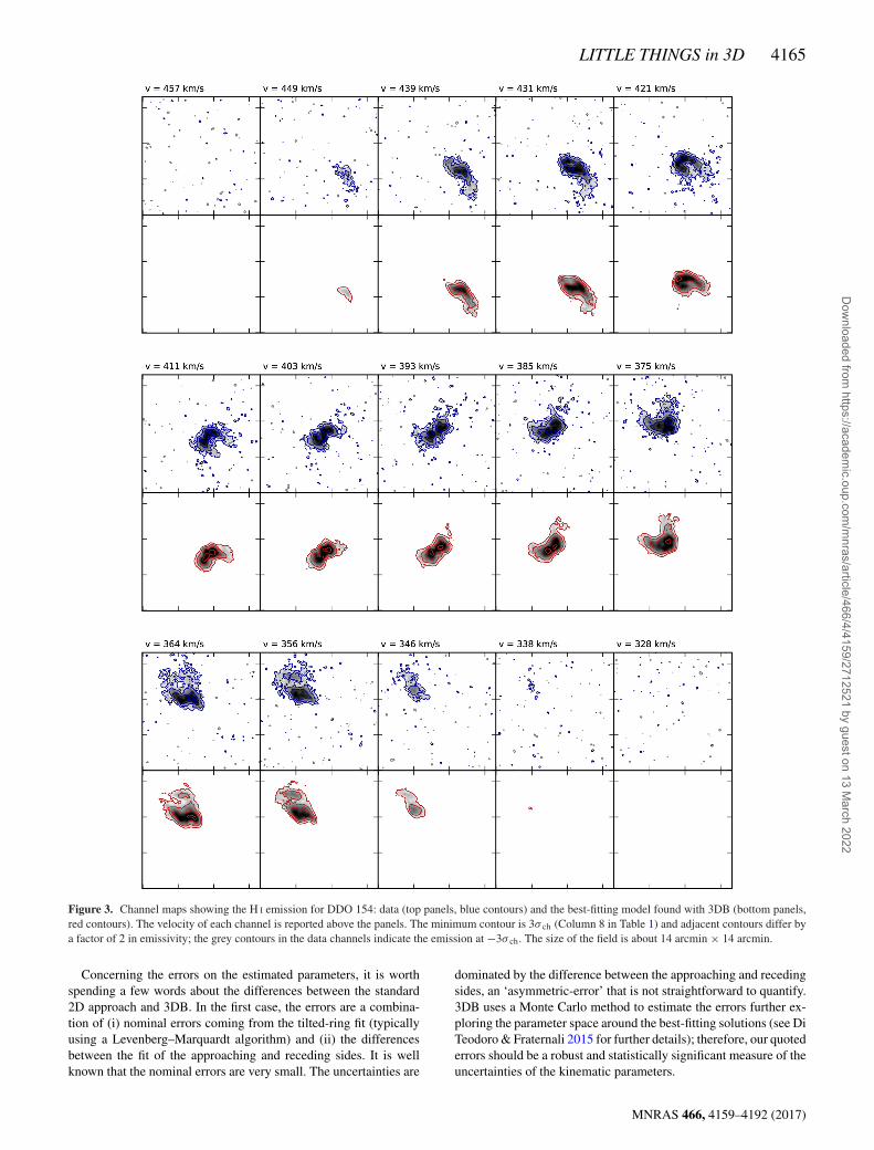
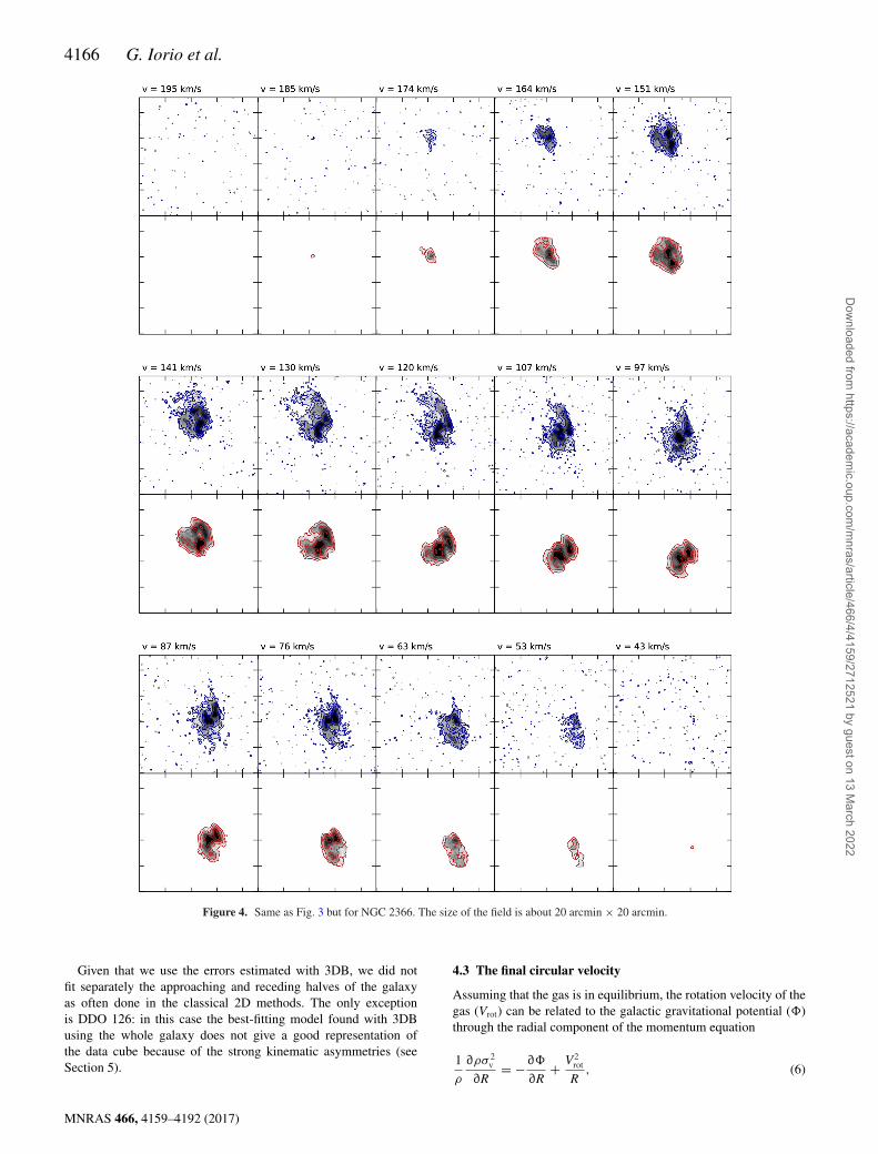
The result of the fit is compared by eye with the real data cube bothanalysing the position–velocity diagrams (PV, hereafter) along themajor axis and the minor axis, and channel by channel. Figs 3 and 4show the comparison in the channel maps between the observationsand the best-fitting model found with 3DB for DDO 154 and NGC2366: the emission of DDO 154 is reproduced quite well; the best-fitting model found for NGC 2366 traces the global kinematics butit is not able to reproduce the extended feature in the north-west ofthe galaxy (see e.g. channel at 120 km s−1). The presence of suchkind of peculiarities makes the study of the dIrrs H I disc kinematicschallenging and requires careful visual inspection. Whenever wenotice that the model was not a good representation of the data, werestart the fit changing the initial guesses and/or varying the orderof the polynomial regularization.
MNRAS 466, 4159–4192 (2017)
Dow
nloaded from https://academ
ic.oup.com/m
nras/article/466/4/4159/2712521 by guest on 13 March 2022
LITTLE THINGS in 3D 4165
Figure 3. Channel maps showing the H I emission for DDO 154: data (top panels, blue contours) and the best-fitting model found with 3DB (bottom panels,red contours). The velocity of each channel is reported above the panels. The minimum contour is 3σ ch (Column 8 in Table 1) and adjacent contours differ bya factor of 2 in emissivity; the grey contours in the data channels indicate the emission at −3σ ch. The size of the field is about 14 arcmin × 14 arcmin.
Concerning the errors on the estimated parameters, it is worthspending a few words about the differences between the standard2D approach and 3DB. In the first case, the errors are a combina-tion of (i) nominal errors coming from the tilted-ring fit (typicallyusing a Levenberg–Marquardt algorithm) and (ii) the differencesbetween the fit of the approaching and receding sides. It is wellknown that the nominal errors are very small. The uncertainties are
dominated by the difference between the approaching and recedingsides, an ‘asymmetric-error’ that is not straightforward to quantify.3DB uses a Monte Carlo method to estimate the errors further ex-ploring the parameter space around the best-fitting solutions (see DiTeodoro & Fraternali 2015 for further details); therefore, our quotederrors should be a robust and statistically significant measure of theuncertainties of the kinematic parameters.
MNRAS 466, 4159–4192 (2017)
Dow
nloaded from https://academ
ic.oup.com/m
nras/article/466/4/4159/2712521 by guest on 13 March 2022
4166 G. Iorio et al.
Figure 4. Same as Fig. 3 but for NGC 2366. The size of the field is about 20 arcmin × 20 arcmin.
Given that we use the errors estimated with 3DB, we did notfit separately the approaching and receding halves of the galaxyas often done in the classical 2D methods. The only exceptionis DDO 126: in this case the best-fitting model found with 3DBusing the whole galaxy does not give a good representation ofthe data cube because of the strong kinematic asymmetries (seeSection 5).
4.3 The final circular velocity
Assuming that the gas is in equilibrium, the rotation velocity of thegas (Vrot) can be related to the galactic gravitational potential (�)through the radial component of the momentum equation
1
ρ
∂ρσ 2v
∂R= −∂�
∂R+ V2
rot
R, (6)
MNRAS 466, 4159–4192 (2017)
Dow
nloaded from https://academ
ic.oup.com/m
nras/article/466/4/4159/2712521 by guest on 13 March 2022
LITTLE THINGS in 3D 4167
where ρ is the volumetric density of the gas and σv is the velocitydispersion. Therefore, the observed Vrot is not a direct tracer of thegalactic potential when the pressure support term (ρσ 2
v ) due to therandom gas motions is non-negligible.
4.3.1 Asymmetric-drift correction
Equation (6) can be re-written as
V2c − V2
rot = −R
ρ
∂ρσ 2v
∂R= −Rσ 2
v
∂ ln(ρσ 2
v
)∂R
= V2A, (7)
where Vc =√
R ∂�∂R is the circular velocity and VA is the asymmet-
ric drift, which becomes increasingly important at large radii andis heavily dependent on the value of the velocity dispersion. Whenthe rotation velocity is much higher than the velocity dispersion theasymmetric-drift correction is negligible. This is the case in spiralgalaxies where usually Vrot/σ v > 10 (e.g. de Blok et al. 2008).Instead, for several dIrrs the rotation velocity is comparable to thevelocity dispersion, making the asymmetric-drift correction indis-pensable for an unbiased estimate of the galactic potential.
The volumetric density in the equatorial plane (z = 0) is propor-tional to the ratio of the intrinsic surface density and the verticalscaleheight (zd); therefore, the asymmetric drift V 2
A is given by
V 2A = −Rσ 2
v
∂ ln(σ 2
v �intz−1d
)∂R
. (8)
We can ignore the term with the radial derivative of zd assumingthat the thickness of the gaseous layer is independent of radius (butsee Section 7.1). Furthermore, assuming that the H I disc is thin,the ratio between the intrinsic and the observed surface density isjust the cosine of i (equation 4). Under these assumptions, fromequation (8) we derive the classical formulation of the asymmetric-drift correction (see e.g. O15):
V 2A = −Rσ 2
v
∂ ln(σ 2
v �obs cos i)
∂R. (9)
Except for DDO 168, NGC 1569 and UGC 8508, all the analysedgalaxies have a constant i and the cosine in equation (9) can also beignored.
4.3.2 Application to real data
Fluctuations of the observed surface density and of the measuredvelocity dispersion at similar radii can have dramatic effects on thenumerical calculation of the radial derivative in equation (9). Asa consequence, the final asymmetric-drift correction can be veryscattered causing abrupt variations in the final estimate of the circu-lar velocity. For this reason, we decided to use functional forms todescribe both the velocity dispersion and the argument of the log-arithm in equation (9). The velocity dispersion is regularized witha polynomial σ p(R, np) with degree np lower than 3. If there is nota clear radial trend, we consider a fixed velocity dispersion takingthe median of σ v(R). The radial variation of the velocity dispersionis usually small; therefore, the radial trend of �intσ
2v is dominated
by the behaviour of the surface density: this falls off exponentiallyat large radii, while in the centre it is almost constant or it shows aninner depression. In analogy with Bureau & Carignan (2002), wechose to fit �intσ
2v with the function
f (R) = f0
(Rc
arcsec+ 1
) (Rc
arcsec+ e
RRd
)−1
, (10)
where f0 is a normalization coefficient, and Rc and Rd are character-istic radii. The function f is characterized by an exponential declineat large radii and by an inner core almost equal to f0. Read et al.(2016c) showed that equation (10) is a good compromise between apure exponential that overestimates the asymmetric-drift correctionin the inner radii, and a functional form with an inner depression thatcan produce unphysical negative values of V 2
rot. Combining equa-tions (9) and (10), we can write the asymmetric-drift correctionas
V 2A = R
σ 2p (R, np)e
RRd
Rd
(Rc
arcsec+ e
RRd
)−1
. (11)
4.3.3 Error estimates
We can calculate the final errors on Vc by applying the propagationof errors to equation (7) to obtain
δc =√
V 2rotδ
2rot + V 2
Aδ2A
Vc, (12)
where δrot is the error found with 3DB and δA is the uncertaintyassociated with the estimated values of the asymmetric-drift term.Usually δA is simply ignored (e.g. Bureau & Carignan 2002; O15),thus the uncertainties on the final corrected rotation curve are equalto δrot. This is a reasonable assumption if the rotational terms inequation (12) are dominant, but for some galaxies in our sample (e.g.DDO 210) the final circular rotation curve is heavily dependent onthe asymmetric-drift correction. In these cases, it is important thatδc includes the uncertainties introduced by the operations describedin Section 4.3.2. We decided to estimate δc with a Monte Carloapproach:
(i) First we make N realizations of the radial profile of both thevelocity dispersion and of the surface density. For each samplingradius R, the values of a single realization σ i
v(R) or �iint(R) are
extracted randomly from a normal distribution with the centre andthe dispersion taken respectively from the values and errors of theparent populations.
(ii) For each of the N realizations, we apply the method describedin Section 4.3.2 to obtain the asymmetric-drift correction at eachsampling radius V i
A(R).(iii) The final asymmetric-drift correction is calculated as
VA(R) = mediani(V iA(R)), where each V i
A is obtained with equa-tion (11). The associated errors are δA(R) = K × MAD(V i
A(R)),where the MAD is the median absolute deviation around the me-dian. The factor K links the MAD with the standard deviation of thesample (K ≈ 1.48 for a normal distribution). We chose to use themedian and the MAD because they are less biased by the presenceof outliers with respect to the mean and the standard deviation.
We found that N = 1000 is enough to obtain a good descriptionof the error introduced by the asymmetric-drift correction.
4.3.4 Final notes
The method described in the above sections has been built to makethe asymmetric-drift correction terms as smooth as possible. Thisensures that our final rotation curves are not affected by non-physical noise related to the derivative term in equation (9). Thedrawback of this approach is that intrinsic scatter on VA is hid-den and the final errors δA could be several times larger than thepoint-to-point scatter. However, we are confident that the quoted
MNRAS 466, 4159–4192 (2017)
Dow
nloaded from https://academ
ic.oup.com/m
nras/article/466/4/4159/2712521 by guest on 13 March 2022
4168 G. Iorio et al.
values of δA truly trace the degree of uncertainties introduced bythe asymmetric-drift correction at different radii. In galaxies wherethe final circular velocity is totally dependent on the asymmetric-drift correction (e.g. DDO 210, see Section 5 and Fig. 16) the scatterin Vrot could be smoothed out, but in these cases also the final errorsare dominated by the errors on the asymmetric drift and δc is still agood representation of the global uncertainties.
In some cases the velocity dispersion found with 3DB is notwell constrained, so there are galaxies where at some radii σv isdiscrepant or peculiar (e.g. very small error) with respect to theglobal trend. In general, the presence of a single ‘rogue’ σv (e.g.DDO 87, Fig. 10 or DDO 133, Fig. 13) does not have a signif-icant influence on the estimate of the VA and on the median ofσ v (see Table 2). However, if the discrepant σv is in a peculiarposition (e.g. the last radius in DDO 210, Fig. 16) or the regionwith ‘rogues’ is extended by more than one ring (e.g. DDO 216,empty circles in Fig. 17), the correction for the asymmetric driftand the estimate of the circular velocities are biased. In these cases,we exclude the radii with discrepant σ v both from the calculationof the asymmetric-drift correction and from the calculation of themedian.
5 R ESULTS
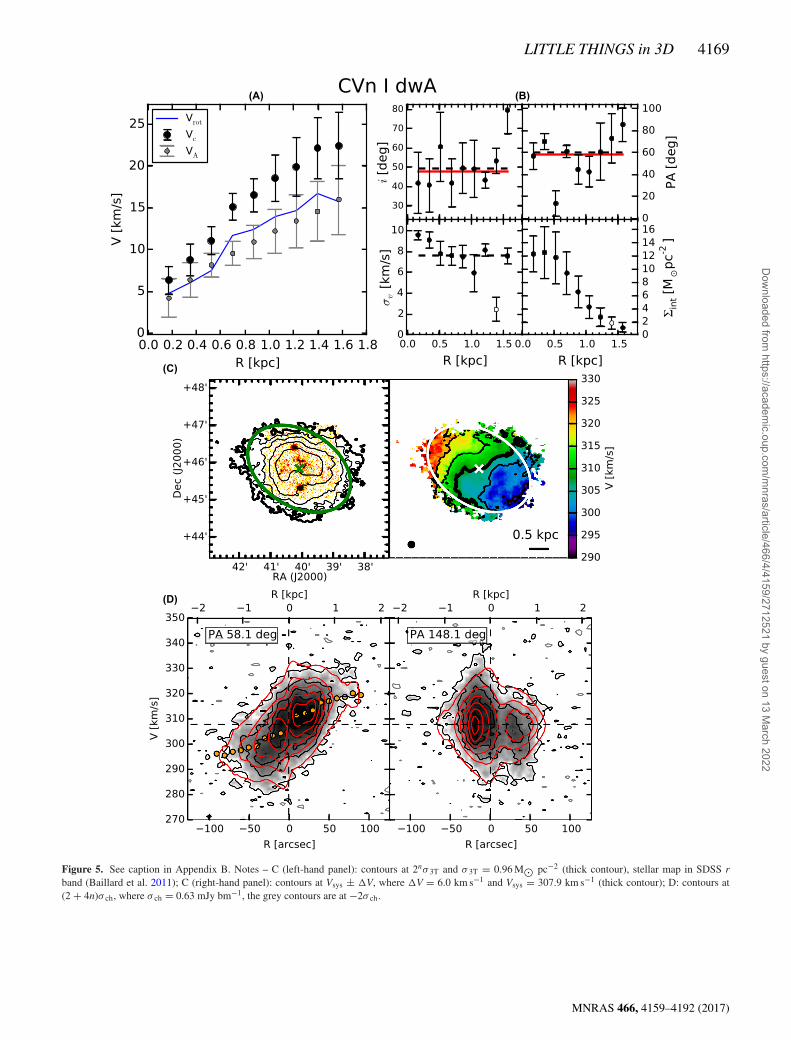
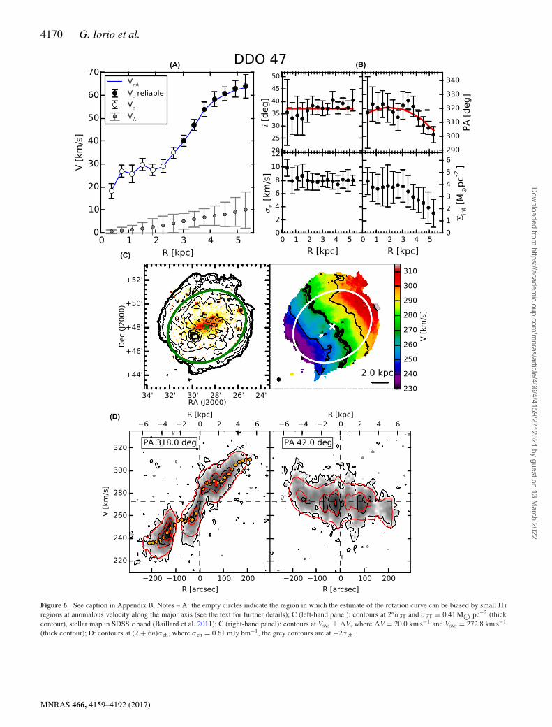
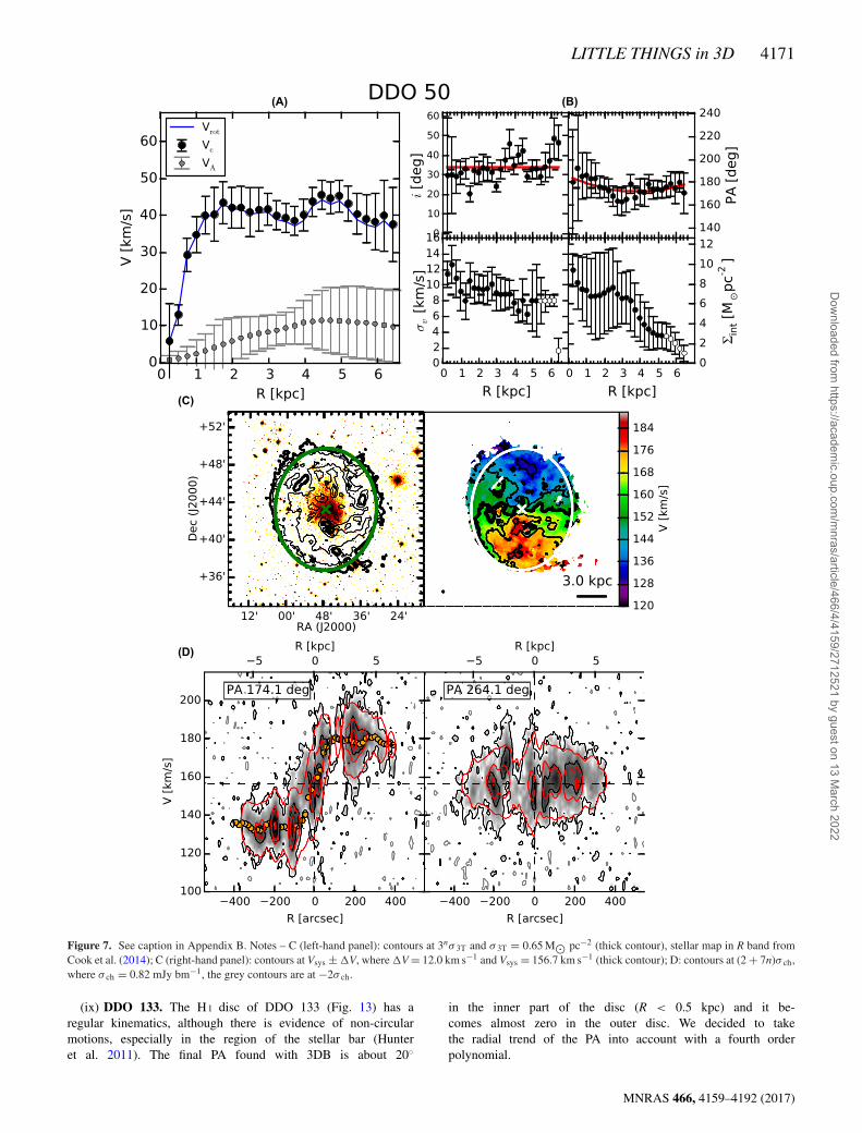
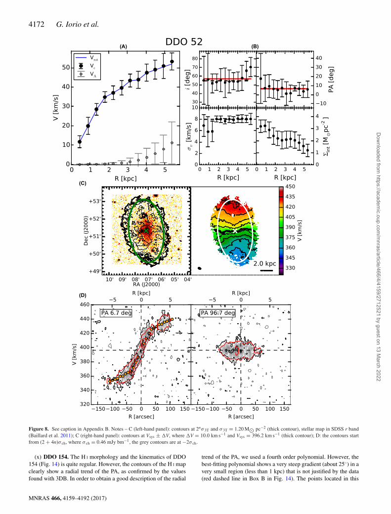
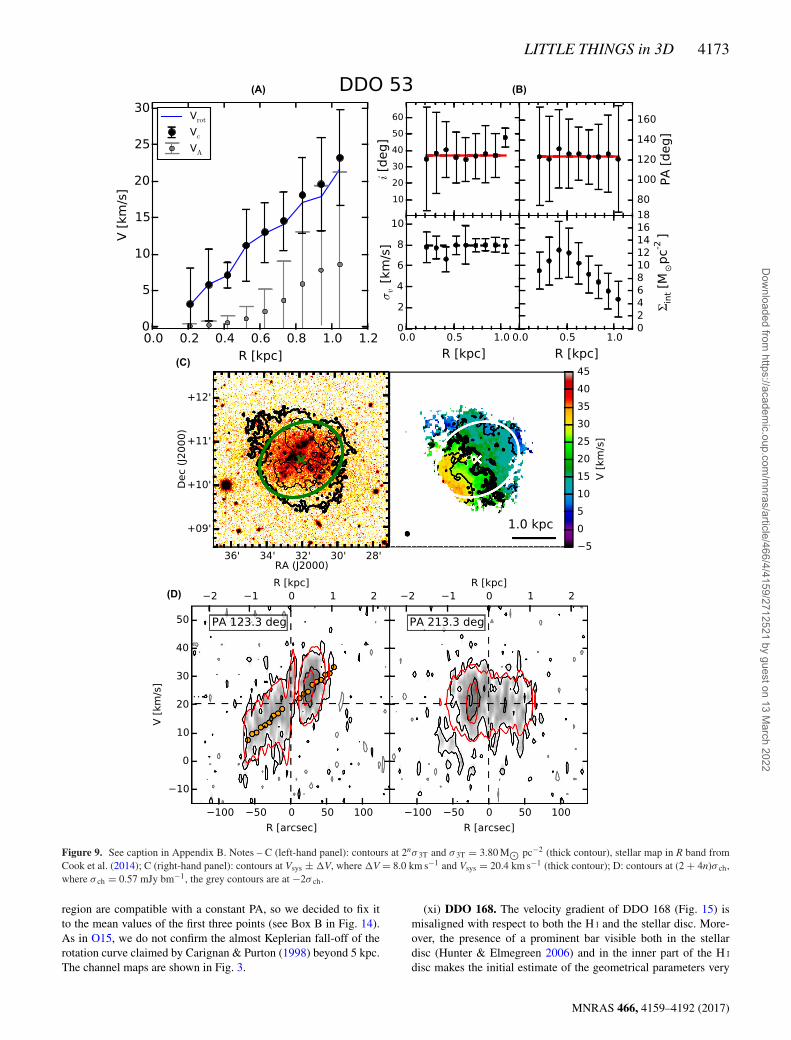
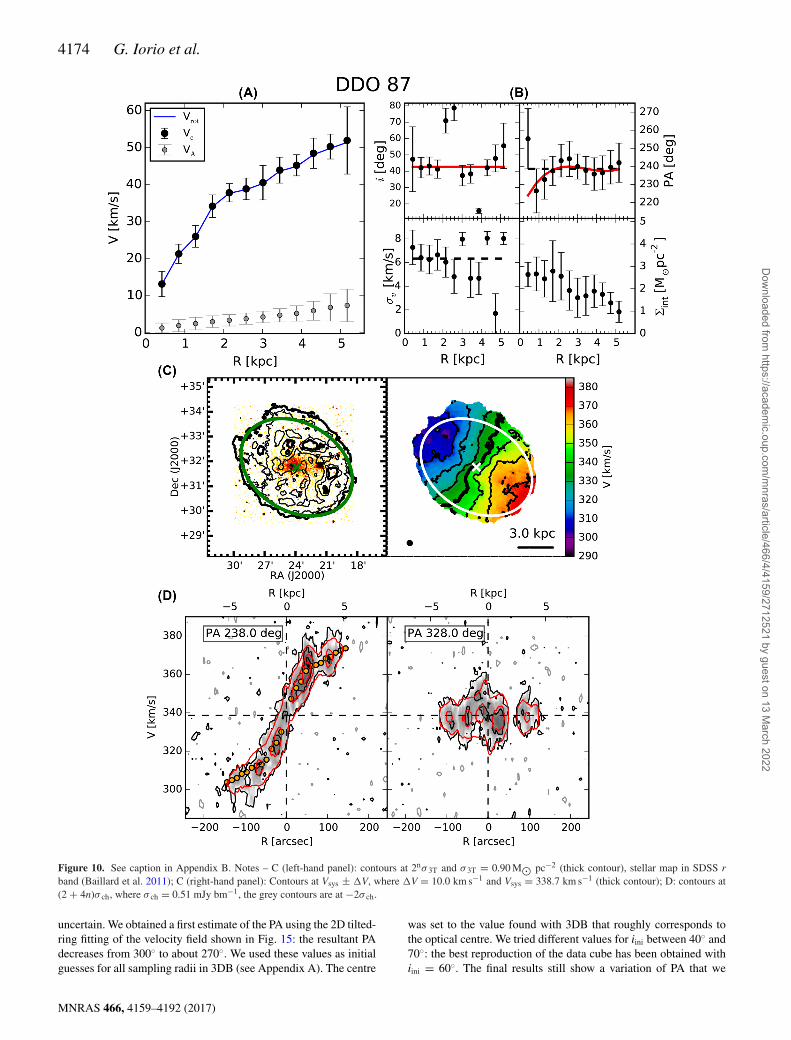
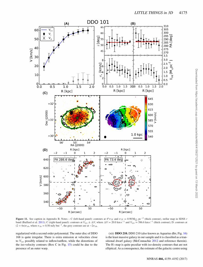
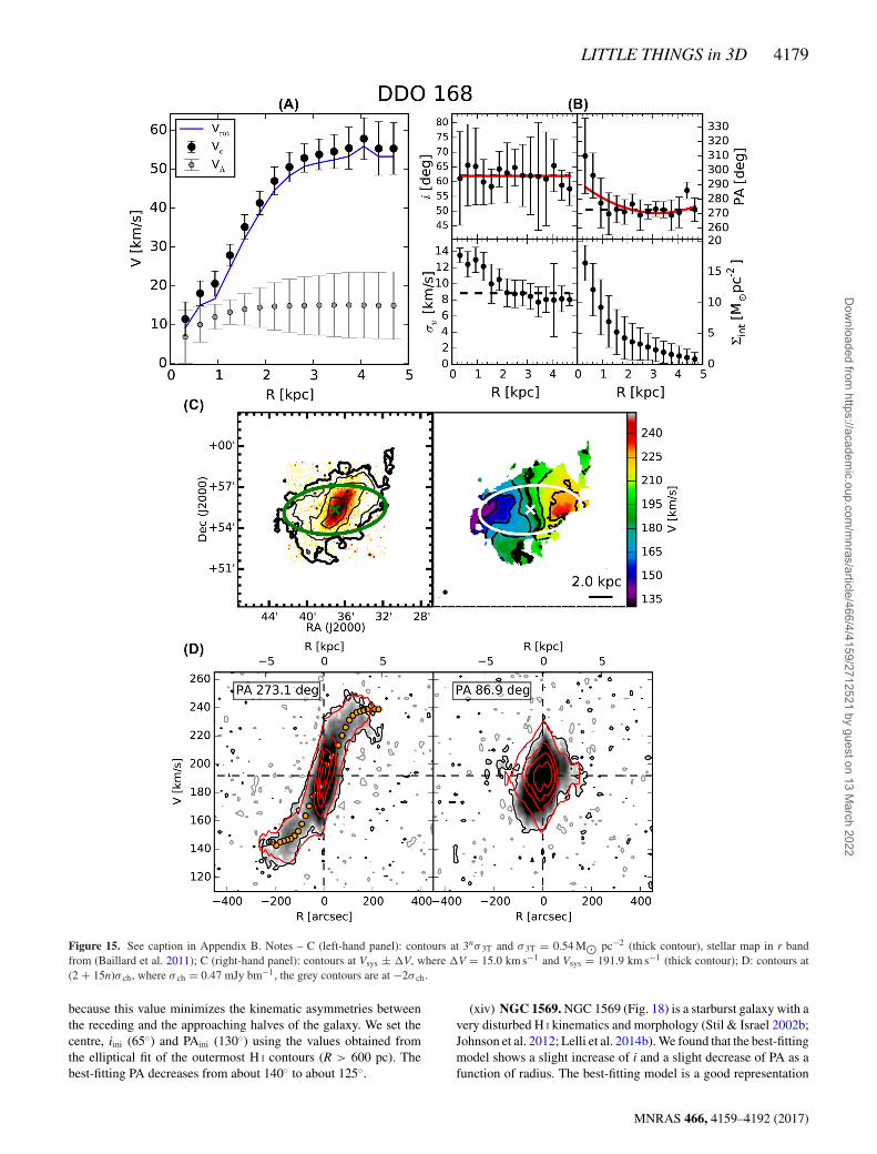
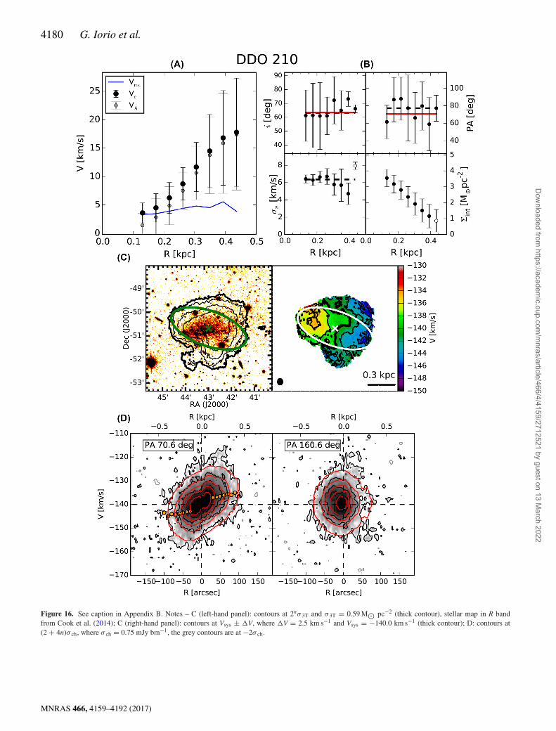
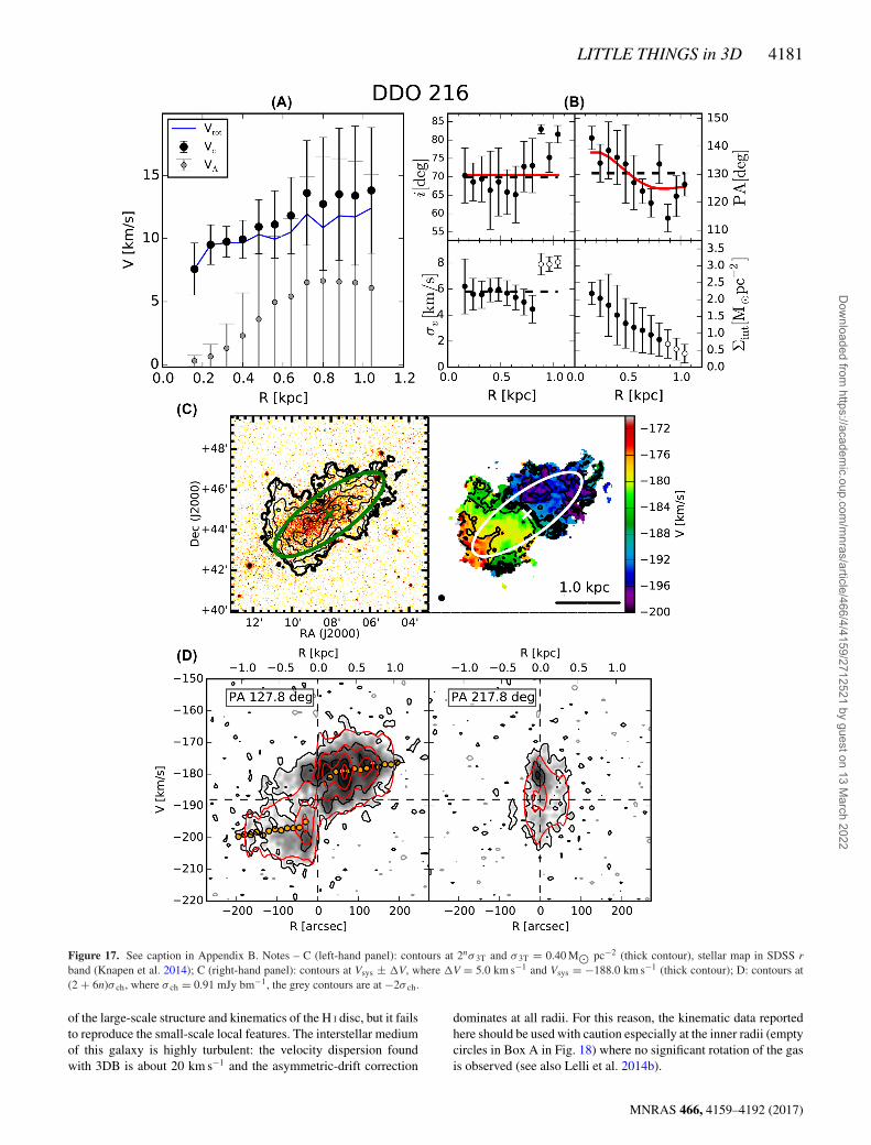
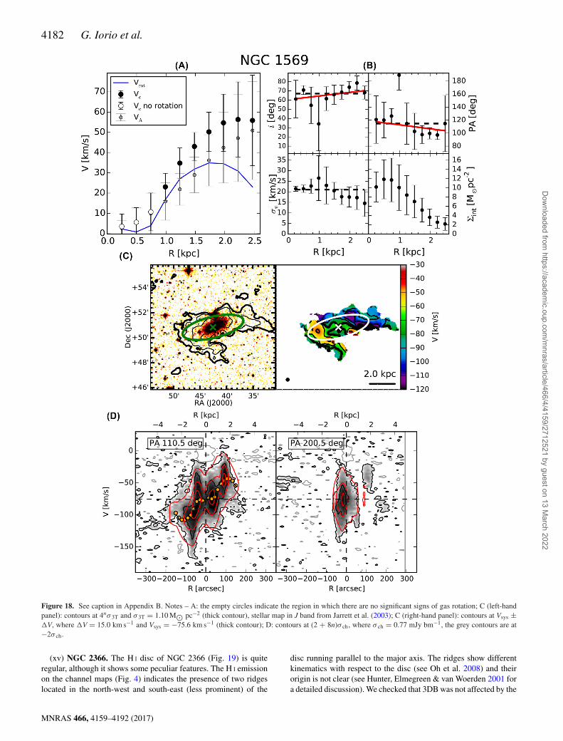
For each analysed galaxy, we produced a summary plot of its prop-erties (Figs 5–21). Each plot is divided in four boxes: Box A showsthe rotation curve, the circular-velocity profile and the correctionfor the asymmetric drift; Box B shows the velocity dispersion, theintrinsic surface density, i and PA obtained with 3DB; Box C showsthe total H I map and the velocity field; Box D shows the PV dia-grams along the major and the minor axis for both model and data.The physical radii have been calculated assuming the distance inTable 1 (Column 1). A detailed description of the plot layout can befound in Appendix B. For reference, Table 2 lists the assumptionsand the initial guesses used in 3DB (Columns 1–7) and a summaryof the results of the data cube fit (Columns 8–11). Here, belowwe report notes on individual galaxies. In the following notes, iini
and PAini indicate the initial guesses for i and PA, respectively (seeColumns 6 and 7 in Table 2).
(i) CVnIdwA. The H I morphology of CVnIdwA (Fig. 5) looksregular, but the orientation of the H I iso-density contours isquite different with respect to the direction of the velocity gra-dient. The emission of the stellar disc is very patchy, so we esti-mated the geometrical parameters of the H I disc using 3DB (seeAppendix A).
(ii) DDO 47. The H I disc of DDO 47 (Fig. 6) is nearly face-on, while the stellar disc looks highly inclined at 64◦ (Hunter &Elmegreen 2006). An inclination of 64◦ is not compatible with theH I contours of the total map and the stellar disc probably hostsa bar-like structure (Georgiev, Karachentsev & Tikhonov 1997).Therefore, we decided to estimate iini and PAini by fitting ellipses onthe contours of the total H I map (see Appendix A). The discrepancybetween the galactic centre estimated with the H I contours and theoptical centre is very small (0.7 arcsec in RA and 2 arcsec in Dec.),so we decided to use the H I centre. The best-fitting i (see Table 2)is consistent with previous works (35◦ in Gentile et al. 2005, 30◦
in de Blok & Bosma 2002 and Stil & Israel 2002b) and seemsa reasonable upper limit for this galaxy (see ellipses in Box C inFig. 6). The final rotation curve shows a flattening at R < 120′′ arcsecthat could be the sign of the presence of strong non-circular motion.Moreover, in the approaching half of the galaxy there is a large
hole that can be clearly seen both on the total map and on the PValong the major axis: the presence of such hole could further biasthe estimate of the gas rotation. For these reasons, we retain thevelocities for R < 120 arcsec not completely reliable (empty circlesin Box A in Fig. 6).
(iii) DDO 50. The gaseous disc of DDO 50 (Fig. 7) is quite pe-culiar: it is ‘drilled’ by medium-large H I holes ranging from 100 pcto 1.7 kpc (Puche et al. 1992) and it also shows clumpy regions withhigh density. Therefore, the H I surface density evaluated acrossthe rings could be very discontinuous with very high peaks and/orregions without emission. As a consequence, the quoted errors onthe intrinsic surface density profile (see Section 4.1.1) are large andthey are probably overestimating the real statistical uncertainties,especially in the inner disc (R < 3 kpc). Despite this peculiarity, thelarge-scale kinematics is quite regular and typical of a flat rotationcurve. The estimates of the i and PA are difficult given that thisgalaxy is nearly face-on. The value of i estimated with the isophotalfitting of the optical disc (47◦) is too high to be compatible withthe flattening of the H I contours that favour an i < 40◦. The bestagreement between the data cube and the model has been foundusing initial values of 30◦ for iini and 180◦ for PAini. The centre wasset using the coordinates of the centre of the stellar disc (Hunter &Elmegreen 2006).
(iv) DDO 52. The best-fitting i of DDO 52 (Fig. 8) tends to bemore edge-on at the end of the disc. However, the analysis of thechannels and of the PVs indicates that the model with a constant igives a better representation of the data.
(v) DDO 53. The stellar disc and the H I disc of DDO 53 (Fig. 9)are misaligned and the galaxy is nearly face-on. As a consequence,i and PA are very difficult to constrain: we tried different values inthe range 30◦–50◦ for iini and 100◦–140◦ for PAini. The best matchwith the data has been found using iini = 35◦ and PA = 120◦, but therotational and the circular velocities should be taken with caution. Inthe northern part of the galaxy, there is some extra emission possiblyconnected with an inflow/outflow: this region is clearly visible inthe PV along the minor axis around −50 arcsec at a velocity ofabout 5 km s−1.
(vi) DDO 87. The morphology of DDO 87 (Fig. 10) is clearlyirregular in the inner part, but the outer disc looks more regu-lar. We decided to set the initial guesses for the PA using 3DB(see Appendix A). We tried different initial guesses for i: the bestrepresentation of the data has been obtained with iini = 40◦ andPAini = 240◦, approximately 15◦ lower than the orientation of theoptical disc (Hunter & Elmegreen 2006).
(vii) DDO 101. The H I disc of DDO 101 (Fig. 11) is extendedonly slightly beyond the optical disc and the H I emission is almostconstant with some high density structures around 1.0 kpc. Noticethat the estimates of the distance for this galaxy are very uncertain(ranging from 5 to 16 Mpc) since they all rely on a poor dis-tance estimator (Tully–Fisher relation, e.g. Karachentsev, Makarov& Kaisina 2013).
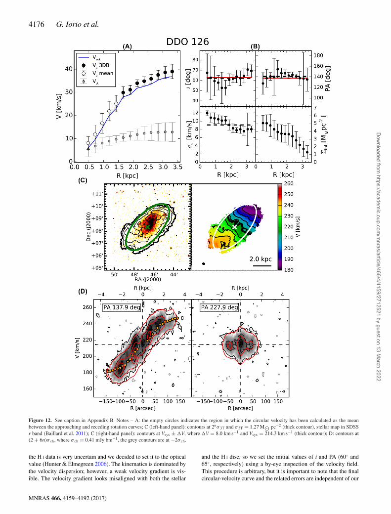
(viii) DDO 126. DDO 126 (Fig. 12) shows kinematic asym-metries, so we separately run 3DB also on the approaching andthe receding halves of the galaxy. Beyond 1.5 kpc the fit on thewhole galaxy gives a good representation of the data cube and theerrors found with 3DB are larger than (or comparable to) the differ-ences due to the kinematic asymmetries (black circles in Box A inFig. 12). The inner regions are less regular and the best model hasbeen found taking the mean between the approaching and recedingrotation curves (empty circles in Box A in Fig. 12), while the errorshave been calculated as half the difference between the two valuesfollowing the recipe of Swaters (1999).
MNRAS 466, 4159–4192 (2017)
Dow
nloaded from https://academ
ic.oup.com/m
nras/article/466/4/4159/2712521 by guest on 13 March 2022
LITTLE THINGS in 3D 4169
(A)
(C)
(D)
(B)
Figure 5. See caption in Appendix B. Notes – C (left-hand panel): contours at 2nσ 3T and σ 3T = 0.96 M� pc−2 (thick contour), stellar map in SDSS rband (Baillard et al. 2011); C (right-hand panel): contours at Vsys ± �V, where �V = 6.0 km s−1 and Vsys = 307.9 km s−1 (thick contour); D: contours at(2 + 4n)σ ch, where σ ch = 0.63 mJy bm−1, the grey contours are at −2σ ch.
MNRAS 466, 4159–4192 (2017)
Dow
nloaded from https://academ
ic.oup.com/m
nras/article/466/4/4159/2712521 by guest on 13 March 2022
4170 G. Iorio et al.
(A)
(C)
(D)
(B)
Figure 6. See caption in Appendix B. Notes – A: the empty circles indicate the region in which the estimate of the rotation curve can be biased by small H I
regions at anomalous velocity along the major axis (see the text for further details); C (left-hand panel): contours at 2nσ 3T and σ 3T = 0.41 M� pc−2 (thickcontour), stellar map in SDSS r band (Baillard et al. 2011); C (right-hand panel): contours at Vsys ± �V, where �V = 20.0 km s−1 and Vsys = 272.8 km s−1
(thick contour); D: contours at (2 + 6n)σ ch, where σ ch = 0.61 mJy bm−1, the grey contours are at −2σ ch.
MNRAS 466, 4159–4192 (2017)
Dow
nloaded from https://academ
ic.oup.com/m
nras/article/466/4/4159/2712521 by guest on 13 March 2022
LITTLE THINGS in 3D 4171
(A)
(C)
(D)
(B)
Figure 7. See caption in Appendix B. Notes – C (left-hand panel): contours at 3nσ 3T and σ 3T = 0.65 M� pc−2 (thick contour), stellar map in R band fromCook et al. (2014); C (right-hand panel): contours at Vsys ± �V, where �V = 12.0 km s−1 and Vsys = 156.7 km s−1 (thick contour); D: contours at (2 + 7n)σ ch,where σ ch = 0.82 mJy bm−1, the grey contours are at −2σ ch.
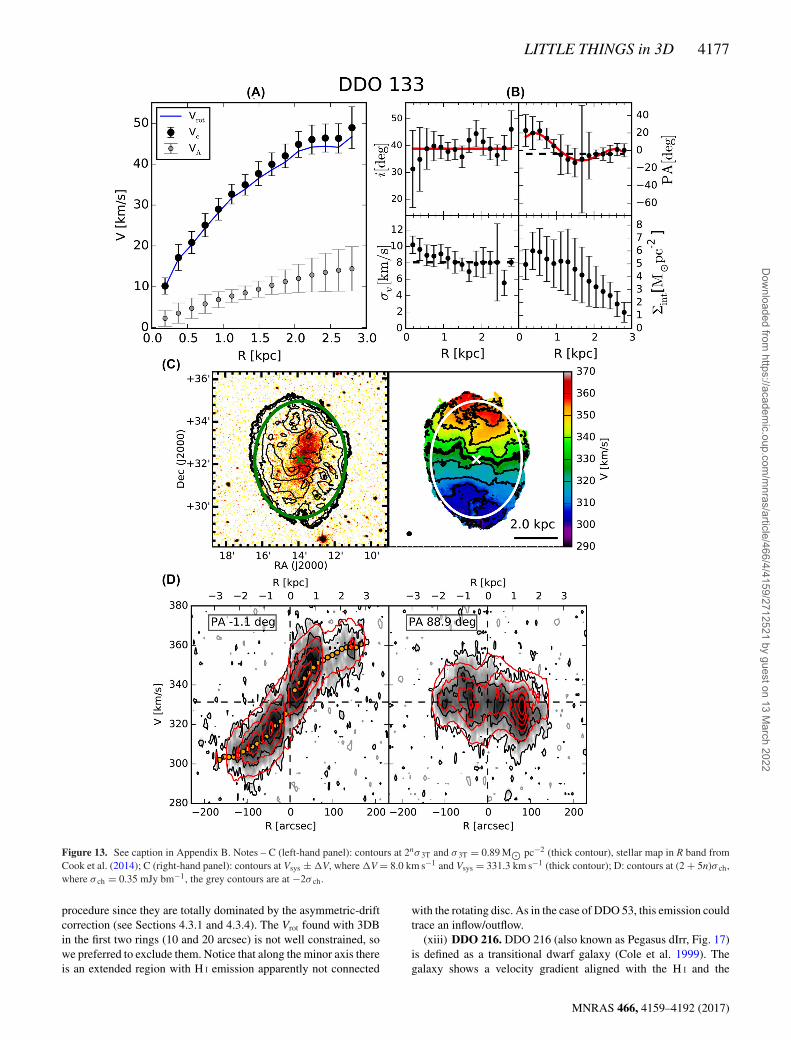
(ix) DDO 133. The H I disc of DDO 133 (Fig. 13) has aregular kinematics, although there is evidence of non-circularmotions, especially in the region of the stellar bar (Hunteret al. 2011). The final PA found with 3DB is about 20◦
in the inner part of the disc (R < 0.5 kpc) and it be-comes almost zero in the outer disc. We decided to takethe radial trend of the PA into account with a fourth orderpolynomial.
MNRAS 466, 4159–4192 (2017)
Dow
nloaded from https://academ
ic.oup.com/m
nras/article/466/4/4159/2712521 by guest on 13 March 2022
4172 G. Iorio et al.
(A)
(C)
(D)
(B)
Figure 8. See caption in Appendix B. Notes – C (left-hand panel): contours at 2nσ 3T and σ 3T = 1.20 M� pc−2 (thick contour), stellar map in SDSS r band(Baillard et al. 2011); C (right-hand panel): contours at Vsys ± �V, where �V = 10.0 km s−1 and Vsys = 396.2 km s−1 (thick contour); D: the contours startfrom (2 + 4n)σ ch, where σ ch = 0.46 mJy bm−1, the grey contours are at −2σ ch.
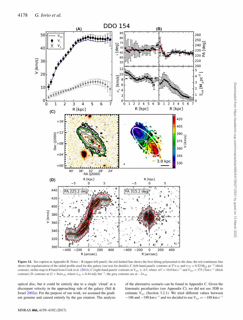
(x) DDO 154. The H I morphology and the kinematics of DDO154 (Fig. 14) is quite regular. However, the contours of the H I mapclearly show a radial trend of the PA, as confirmed by the valuesfound with 3DB. In order to obtain a good description of the radial
trend of the PA, we used a fourth order polynomial. However, thebest-fitting polynomial shows a very steep gradient (about 25◦) in avery small region (less than 1 kpc) that is not justified by the data(red dashed line in Box B in Fig. 14). The points located in this
MNRAS 466, 4159–4192 (2017)
Dow
nloaded from https://academ
ic.oup.com/m
nras/article/466/4/4159/2712521 by guest on 13 March 2022
LITTLE THINGS in 3D 4173
(A)
(C)
(D)
(B)
Figure 9. See caption in Appendix B. Notes – C (left-hand panel): contours at 2nσ 3T and σ 3T = 3.80 M� pc−2 (thick contour), stellar map in R band fromCook et al. (2014); C (right-hand panel): contours at Vsys ± �V, where �V = 8.0 km s−1 and Vsys = 20.4 km s−1 (thick contour); D: contours at (2 + 4n)σ ch,where σ ch = 0.57 mJy bm−1, the grey contours are at −2σ ch.
region are compatible with a constant PA, so we decided to fix itto the mean values of the first three points (see Box B in Fig. 14).As in O15, we do not confirm the almost Keplerian fall-off of therotation curve claimed by Carignan & Purton (1998) beyond 5 kpc.The channel maps are shown in Fig. 3.
(xi) DDO 168. The velocity gradient of DDO 168 (Fig. 15) ismisaligned with respect to both the H I and the stellar disc. More-over, the presence of a prominent bar visible both in the stellardisc (Hunter & Elmegreen 2006) and in the inner part of the H I
disc makes the initial estimate of the geometrical parameters very
MNRAS 466, 4159–4192 (2017)
Dow
nloaded from https://academ
ic.oup.com/m
nras/article/466/4/4159/2712521 by guest on 13 March 2022
4174 G. Iorio et al.
Figure 10. See caption in Appendix B. Notes – C (left-hand panel): contours at 2nσ 3T and σ 3T = 0.90 M� pc−2 (thick contour), stellar map in SDSS rband (Baillard et al. 2011); C (right-hand panel): Contours at Vsys ± �V, where �V = 10.0 km s−1 and Vsys = 338.7 km s−1 (thick contour); D: contours at(2 + 4n)σ ch, where σ ch = 0.51 mJy bm−1, the grey contours are at −2σ ch.
uncertain. We obtained a first estimate of the PA using the 2D tilted-ring fitting of the velocity field shown in Fig. 15: the resultant PAdecreases from 300◦ to about 270◦. We used these values as initialguesses for all sampling radii in 3DB (see Appendix A). The centre
was set to the value found with 3DB that roughly corresponds tothe optical centre. We tried different values for iini between 40◦ and70◦: the best reproduction of the data cube has been obtained withiini = 60◦. The final results still show a variation of PA that we
MNRAS 466, 4159–4192 (2017)
Dow
nloaded from https://academ
ic.oup.com/m
nras/article/466/4/4159/2712521 by guest on 13 March 2022
LITTLE THINGS in 3D 4175
Figure 11. See caption in Appendix B. Notes – C (left-hand panel): contours at 4nσ 3T and σ 3T = 0.90 M� pc−2 (thick contour), stellar map in SDSS rband (Baillard et al. 2011); C (right-hand panel): contours at Vsys ± �V, where �V = 20.0 km s−1 and Vsys = 586.6 km s−1 (thick contour); D: contours at(2 + 6n)σ ch, where σ ch = 0.50 mJy bm−1, the grey contours are at −2σ ch.
regularized with a second order polynomial. The outer disc of DDO168 is quite irregular. There is extra emission at velocities closeto Vsys possibly related to inflow/outflow, while the distortions ofthe iso-velocity contours (Box C in Fig. 15) could be due to thepresence of an outer warp.
(xii) DDO 210. DDO 210 (also known as Aquarius dIrr, Fig. 16)is the least massive galaxy in our sample and it is classified as a tran-sitional dwarf galaxy (McConnachie 2012 and reference therein).The H I map is quite peculiar with iso-density contours that are notelliptical. As a consequence, the estimate of the galactic centre using
MNRAS 466, 4159–4192 (2017)
Dow
nloaded from https://academ
ic.oup.com/m
nras/article/466/4/4159/2712521 by guest on 13 March 2022
4176 G. Iorio et al.
Figure 12. See caption in Appendix B. Notes – A: the empty circles indicates the region in which the circular velocity has been calculated as the meanbetween the approaching and receding rotation curves; C (left-hand panel): contours at 2nσ 3T and σ 3T = 1.27 M� pc−2 (thick contour), stellar map in SDSSr band (Baillard et al. 2011); C (right-hand panel): contours at Vsys ± �V, where �V = 8.0 km s−1 and Vsys = 214.3 km s−1 (thick contour); D: contours at(2 + 6n)σ ch, where σ ch = 0.41 mJy bm−1, the grey contours are at −2σ ch.
the H I data is very uncertain and we decided to set it to the opticalvalue (Hunter & Elmegreen 2006). The kinematics is dominated bythe velocity dispersion; however, a weak velocity gradient is vis-ible. The velocity gradient looks misaligned with both the stellar
and the H I disc, so we set the initial values of i and PA (60◦ and65◦, respectively) using a by-eye inspection of the velocity field.This procedure is arbitrary, but it is important to note that the finalcircular-velocity curve and the related errors are independent of our
MNRAS 466, 4159–4192 (2017)
Dow
nloaded from https://academ
ic.oup.com/m
nras/article/466/4/4159/2712521 by guest on 13 March 2022
LITTLE THINGS in 3D 4177
Figure 13. See caption in Appendix B. Notes – C (left-hand panel): contours at 2nσ 3T and σ 3T = 0.89 M� pc−2 (thick contour), stellar map in R band fromCook et al. (2014); C (right-hand panel): contours at Vsys ± �V, where �V = 8.0 km s−1 and Vsys = 331.3 km s−1 (thick contour); D: contours at (2 + 5n)σ ch,where σ ch = 0.35 mJy bm−1, the grey contours are at −2σ ch.
procedure since they are totally dominated by the asymmetric-driftcorrection (see Sections 4.3.1 and 4.3.4). The Vrot found with 3DBin the first two rings (10 and 20 arcsec) is not well constrained, sowe preferred to exclude them. Notice that along the minor axis thereis an extended region with H I emission apparently not connected
with the rotating disc. As in the case of DDO 53, this emission couldtrace an inflow/outflow.
(xiii) DDO 216. DDO 216 (also known as Pegasus dIrr, Fig. 17)is defined as a transitional dwarf galaxy (Cole et al. 1999). Thegalaxy shows a velocity gradient aligned with the H I and the
MNRAS 466, 4159–4192 (2017)
Dow
nloaded from https://academ
ic.oup.com/m
nras/article/466/4/4159/2712521 by guest on 13 March 2022
4178 G. Iorio et al.
Figure 14. See caption in Appendix B. Notes – B (upper-left panel): the red dashed line shows the best-fitting polynomial to the data, the red continuous lineshows the regularization of the radial profile used for this galaxy (see text for details); C (left-hand panel): contours at 2nσ 3T and σ 3T = 0.52 M� pc−2 (thickcontour), stellar map in R band from Cook et al. (2014); C (right-hand panel): contours at Vsys ± �V, where �V = 10.0 km s−1 and Vsys = 375.2 km s−1 (thickcontour); D: contours at (2 + 8n)σ ch, where σ ch = 0.44 mJy bm−1, the grey contours are at −2σ ch.
optical disc, but it could be entirely due to a single ‘cloud’ at adiscrepant velocity in the approaching side of the galaxy (Stil &Israel 2002a). For the purpose of our work, we assumed the gradi-ent genuine and caused entirely by the gas rotation. The analysis
of the alternative scenario can be found in Appendix C. Given thekinematic peculiarities (see Appendix C), we did not use 3DB toestimate Vsys (Section 3.2.1). We tried different values between−186 and −190 km s−1 and we decided to use Vsys = −188 km s−1
MNRAS 466, 4159–4192 (2017)
Dow
nloaded from https://academ
ic.oup.com/m
nras/article/466/4/4159/2712521 by guest on 13 March 2022
LITTLE THINGS in 3D 4179
Figure 15. See caption in Appendix B. Notes – C (left-hand panel): contours at 3nσ 3T and σ 3T = 0.54 M� pc−2 (thick contour), stellar map in r bandfrom (Baillard et al. 2011); C (right-hand panel): contours at Vsys ± �V, where �V = 15.0 km s−1 and Vsys = 191.9 km s−1 (thick contour); D: contours at(2 + 15n)σ ch, where σ ch = 0.47 mJy bm−1, the grey contours are at −2σ ch.
because this value minimizes the kinematic asymmetries betweenthe receding and the approaching halves of the galaxy. We set thecentre, iini (65◦) and PAini (130◦) using the values obtained fromthe elliptical fit of the outermost H I contours (R > 600 pc). Thebest-fitting PA decreases from about 140◦ to about 125◦.
(xiv) NGC 1569. NGC 1569 (Fig. 18) is a starburst galaxy with avery disturbed H I kinematics and morphology (Stil & Israel 2002b;Johnson et al. 2012; Lelli et al. 2014b). We found that the best-fittingmodel shows a slight increase of i and a slight decrease of PA as afunction of radius. The best-fitting model is a good representation
MNRAS 466, 4159–4192 (2017)
Dow
nloaded from https://academ
ic.oup.com/m
nras/article/466/4/4159/2712521 by guest on 13 March 2022
4180 G. Iorio et al.
Figure 16. See caption in Appendix B. Notes – C (left-hand panel): contours at 2nσ 3T and σ 3T = 0.59 M� pc−2 (thick contour), stellar map in R bandfrom Cook et al. (2014); C (right-hand panel): contours at Vsys ± �V, where �V = 2.5 km s−1 and Vsys = −140.0 km s−1 (thick contour); D: contours at(2 + 4n)σ ch, where σ ch = 0.75 mJy bm−1, the grey contours are at −2σ ch.
MNRAS 466, 4159–4192 (2017)
Dow
nloaded from https://academ
ic.oup.com/m
nras/article/466/4/4159/2712521 by guest on 13 March 2022
LITTLE THINGS in 3D 4181
Figure 17. See caption in Appendix B. Notes – C (left-hand panel): contours at 2nσ 3T and σ 3T = 0.40 M� pc−2 (thick contour), stellar map in SDSS rband (Knapen et al. 2014); C (right-hand panel): contours at Vsys ± �V, where �V = 5.0 km s−1 and Vsys = −188.0 km s−1 (thick contour); D: contours at(2 + 6n)σ ch, where σ ch = 0.91 mJy bm−1, the grey contours are at −2σ ch.
of the large-scale structure and kinematics of the H I disc, but it failsto reproduce the small-scale local features. The interstellar mediumof this galaxy is highly turbulent: the velocity dispersion foundwith 3DB is about 20 km s−1 and the asymmetric-drift correction
dominates at all radii. For this reason, the kinematic data reportedhere should be used with caution especially at the inner radii (emptycircles in Box A in Fig. 18) where no significant rotation of the gasis observed (see also Lelli et al. 2014b).
MNRAS 466, 4159–4192 (2017)
Dow
nloaded from https://academ
ic.oup.com/m
nras/article/466/4/4159/2712521 by guest on 13 March 2022
4182 G. Iorio et al.
Figure 18. See caption in Appendix B. Notes – A: the empty circles indicate the region in which there are no significant signs of gas rotation; C (left-handpanel): contours at 4nσ 3T and σ 3T = 1.10 M� pc−2 (thick contour), stellar map in J band from Jarrett et al. (2003); C (right-hand panel): contours at Vsys ±�V, where �V = 15.0 km s−1 and Vsys = −75.6 km s−1 (thick contour); D: contours at (2 + 8n)σ ch, where σ ch = 0.77 mJy bm−1, the grey contours are at−2σ ch.
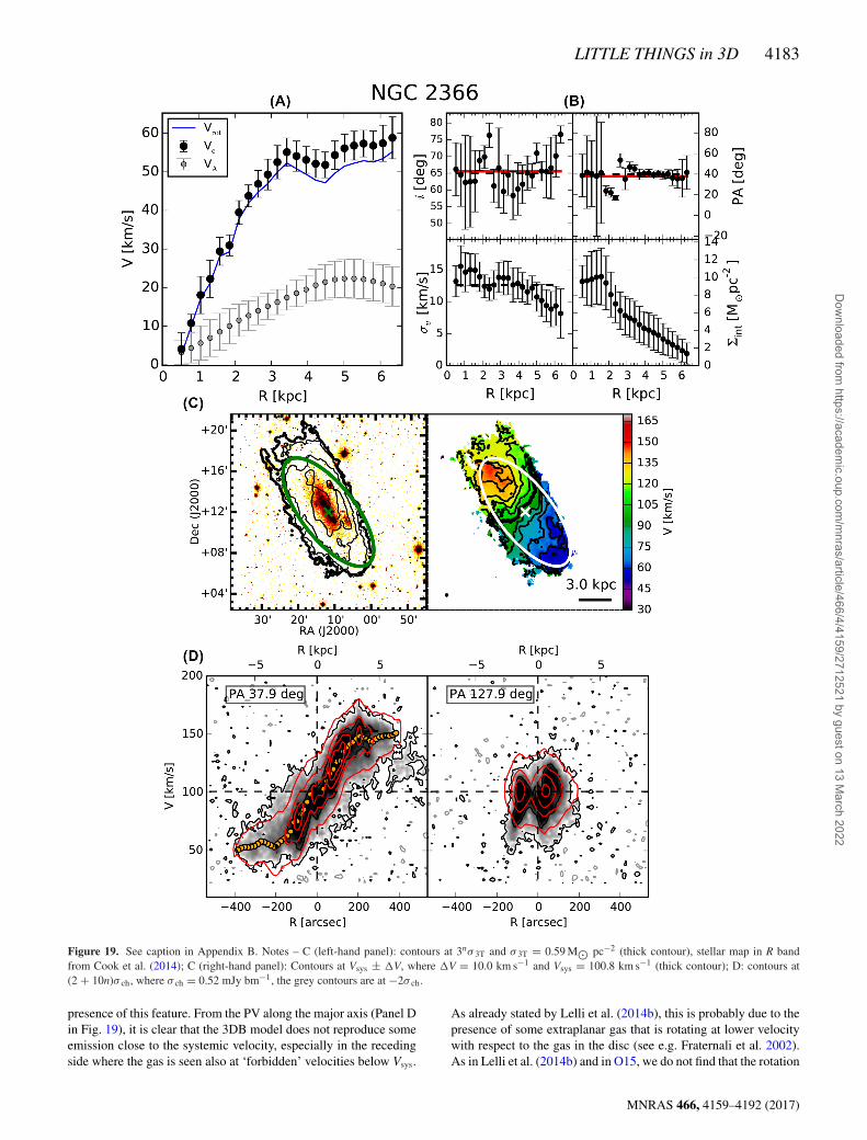
(xv) NGC 2366. The H I disc of NGC 2366 (Fig. 19) is quiteregular, although it shows some peculiar features. The H I emissionon the channel maps (Fig. 4) indicates the presence of two ridgeslocated in the north-west and south-east (less prominent) of the
disc running parallel to the major axis. The ridges show differentkinematics with respect to the disc (see Oh et al. 2008) and theirorigin is not clear (see Hunter, Elmegreen & van Woerden 2001 fora detailed discussion). We checked that 3DB was not affected by the
MNRAS 466, 4159–4192 (2017)
Dow
nloaded from https://academ
ic.oup.com/m
nras/article/466/4/4159/2712521 by guest on 13 March 2022
LITTLE THINGS in 3D 4183
Figure 19. See caption in Appendix B. Notes – C (left-hand panel): contours at 3nσ 3T and σ 3T = 0.59 M� pc−2 (thick contour), stellar map in R bandfrom Cook et al. (2014); C (right-hand panel): Contours at Vsys ± �V, where �V = 10.0 km s−1 and Vsys = 100.8 km s−1 (thick contour); D: contours at(2 + 10n)σ ch, where σ ch = 0.52 mJy bm−1, the grey contours are at −2σ ch.
presence of this feature. From the PV along the major axis (Panel Din Fig. 19), it is clear that the 3DB model does not reproduce someemission close to the systemic velocity, especially in the recedingside where the gas is seen also at ‘forbidden’ velocities below Vsys.
As already stated by Lelli et al. (2014b), this is probably due to thepresence of some extraplanar gas that is rotating at lower velocitywith respect to the gas in the disc (see e.g. Fraternali et al. 2002).As in Lelli et al. (2014b) and in O15, we do not find that the rotation
MNRAS 466, 4159–4192 (2017)
Dow
nloaded from https://academ
ic.oup.com/m
nras/article/466/4/4159/2712521 by guest on 13 March 2022
4184 G. Iorio et al.
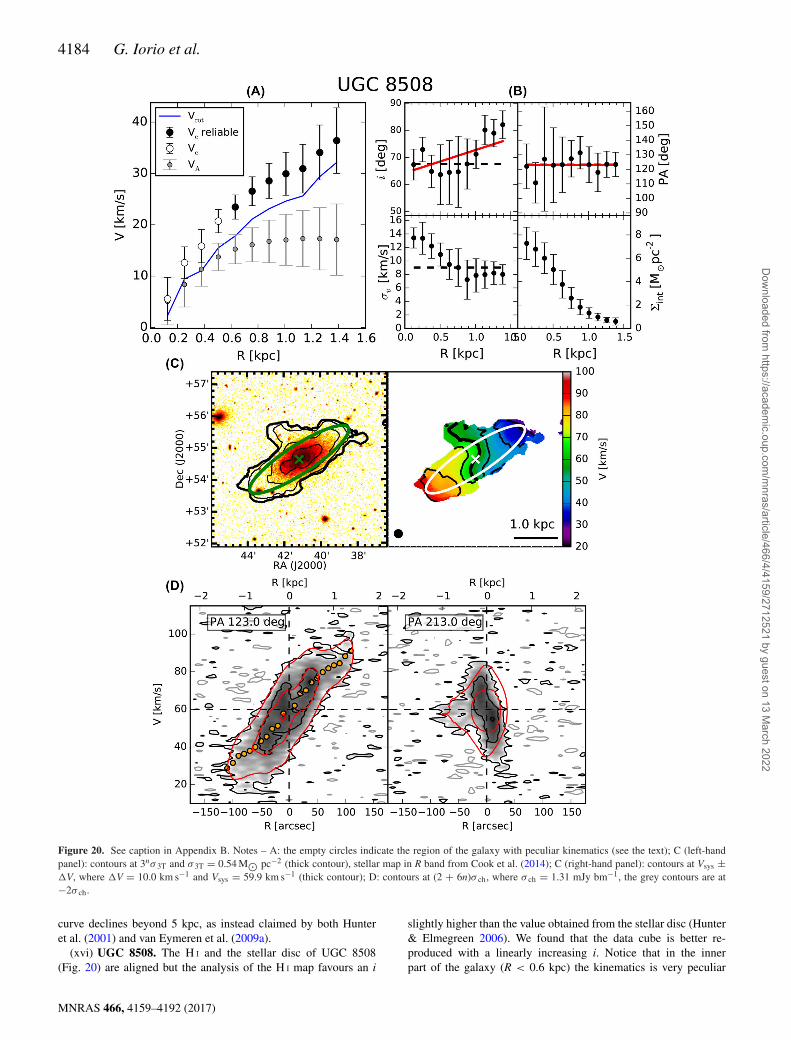
Figure 20. See caption in Appendix B. Notes – A: the empty circles indicate the region of the galaxy with peculiar kinematics (see the text); C (left-handpanel): contours at 3nσ 3T and σ 3T = 0.54 M� pc−2 (thick contour), stellar map in R band from Cook et al. (2014); C (right-hand panel): contours at Vsys ±�V, where �V = 10.0 km s−1 and Vsys = 59.9 km s−1 (thick contour); D: contours at (2 + 6n)σ ch, where σ ch = 1.31 mJy bm−1, the grey contours are at−2σ ch.
curve declines beyond 5 kpc, as instead claimed by both Hunteret al. (2001) and van Eymeren et al. (2009a).
(xvi) UGC 8508. The H I and the stellar disc of UGC 8508(Fig. 20) are aligned but the analysis of the H I map favours an i
slightly higher than the value obtained from the stellar disc (Hunter& Elmegreen 2006). We found that the data cube is better re-produced with a linearly increasing i. Notice that in the innerpart of the galaxy (R < 0.6 kpc) the kinematics is very peculiar
MNRAS 466, 4159–4192 (2017)
Dow
nloaded from https://academ
ic.oup.com/m
nras/article/466/4/4159/2712521 by guest on 13 March 2022
LITTLE THINGS in 3D 4185
as it is visible by the S-shaped iso-velocity contours (right-handpanel C in Fig. 20). This kind of distortions can be related to anabrupt variation of the PA and/or to the presence of radial motions(Fraternali et al. 2001) as well as to a deviation from axisymme-try of the galactic potential (Swaters et al. 1999). We tested thehypothesis of a radially varying PA and the presence of non-zeroradial velocities (Vrad) performing a 2D analysis of the velocity fieldwith ROTCUR (Begeman 1987). We found that the combination ofthe two effects can partially explain the distortions of the velocityfield, but their magnitude is too large to be physically plausible.Fortunately, the final rotation curves obtained including radial mo-tions and/or the varying PA are compatibles with the results wefound with 3DB, though the inner points (empty circles in Box Ain Fig. 20) should be treated with caution.
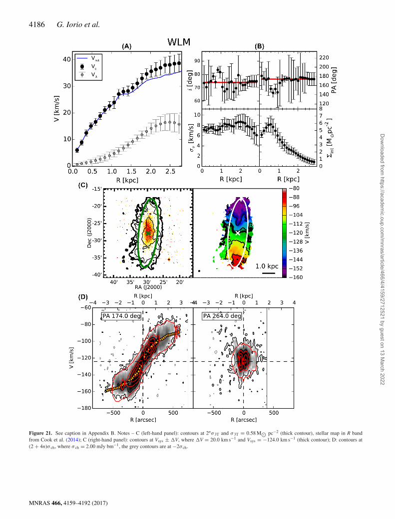
(xvii) WLM. The H I and the optical discs of WLM (Fig. 21)are well aligned, but the best-fitting i looks slightly too edge-onwith respect to the H I contours (see ellipses in Fig. 21). The excessof the emission around the minor axis could be partially due tothe thickness of the gaseous layer (Section 7.1, see also Leamanet al. 2012). Further details on the analysis of WLM can be foundin Read et al. (2016c).
6 A P P L I C ATI O N : T E S T O F TH E BA RYO N I CT ULLY– FISHER RELATION
The BTFR links a characteristic circular velocity (V) of a galaxywith its total baryonic mass (Mbar). The relation, in the logarithmicform
log
(Mbar
M�
)= s log
(V
km s−1
)+ A, (13)
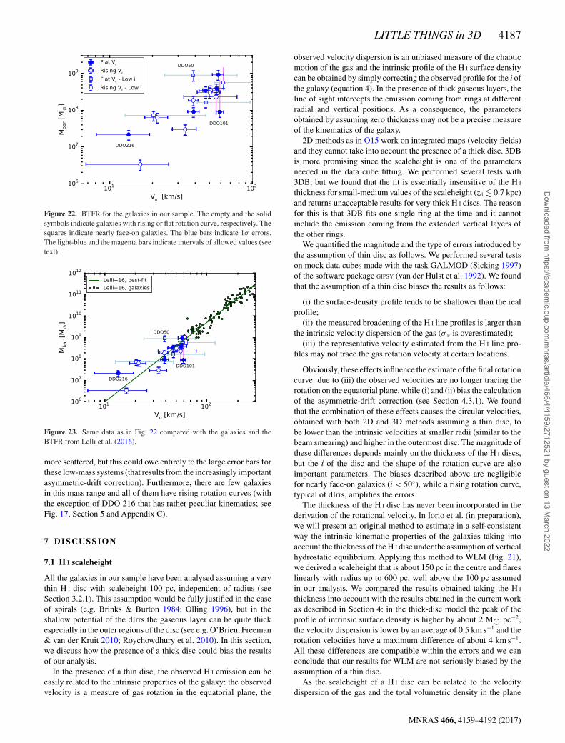
is very tight and extends over six decades in Mbar (McGaugh 2012;Lelli et al. 2016). The existence of this relation represents a funda-mental benchmark for cosmological models and for galaxy forma-tion theories (McGaugh et al. 2000; Brook et al. 2016; Di Cintio &Lelli 2016). In this context, it is very important to extend the study ofthe BTFR down to extremely low-mass dwarf galaxies (e.g. Begumet al. 2008). In this section, we present the BTFR for the galaxiesin our sample (Fig. 22) and then we compare it with the results ofLelli et al. (2016, Fig. 23). The derivation of the baryonic mass andof the characteristic velocity is described below.
(i) Rotation velocity. The rotation velocities used in the Tully–Fisher relation (TFR) are W20 and Vflat: W20 is the velocity width ofthe global H I line profiles, while Vflat is the value of the flat portionof the rotation curve. Verheijen (2001) found that Vflat minimizes thescatter in the TFR, so it is the best way to study the BTFR using high-resolution H I data (see also Brook et al. 2016). However, severalrotation curves of dIrrs do not reach the flat part (e.g. DDO 53, Fig. 9)or the flattening is entirely due to the asymmetric-drift correction(e.g. NGC 1569, Fig. 18). As indicator of the rotation velocity, wetherefore used the velocity of the outer disc (Vo) defined as the meancircular velocity of the last three fitted rings (see Section 4.2). Vo isa measure of Vflat for galaxies in which the flat part of the rotationcurve is observed. For galaxies with a rising rotation curve, Vo isan estimate of the maximum circular velocity within the consideredradial range. Galaxies with rising rotation curves are indicated withempty markers in Figs 22 and 23. The error on Vo is conservativelyassumed as the maximum error between the three values used tocalculate Vo. In the five galaxies with a low i (squares in Figs 22and 23), the uncertainties on i and on the velocities can be largelyunderestimated (see Section 5 and Table 2), so we present these
galaxies with a bar that indicates the interval between a minimum(assuming i = 40◦) and a maximum (assuming i = 20◦) value of Vo
(see equation 1).(ii) Baryonic mass. The total baryonic mass of the galaxies has
been calculated as
Mbar = M∗ + 1.33MH I, (14)
where M∗ is the stellar mass, MH I is the mass of the atomic hydro-gen and the factor 1.33 takes into account the presence of Helium(Begum et al. 2008; Lelli et al. 2016). The molecular gas is likelyirrelevant in the mass budget of dwarf galaxies (Taylor, Kobulnicky& Skillman 1998). The mass of atomic gas is measured from theH I data cubes (Section 4.1.1 and Table 1), while the stellar massesare from Walter & Brinks (2001) for DDO 47 and from Zhanget al. (2012) for all the other galaxies. The estimate of the mass isproportional to the square of the galactic distance, therefore errorson the distance add further uncertainties on the final estimate ofthe baryonic mass. Unfortunately, the works we used to take thestellar masses (Walter & Brinks 2001; Zhang et al. 2012) and thedistances (Hunter et al. 2012) do not report the errors on their mea-sures, so we assumed a conservative error of the 30 per cent for Mbar.We also performed a deeper analysis for the distance uncertainties.The relative difference between the masses estimated assuming twodifferent distances is
δD = M(D1) − M(D2)
M(D1)= D2
1 − D22
D21
. (15)
For each galaxy in our sample, we choose the best distanceestimator4 available on NASA/IPAC Extragalactic Database (NED)and we considered the minimum (Dmin
NED) and the maximum (DmaxNED)
estimate of the distance, then using equation (15) we calculated
δmin / maxD = 1 −
(min(D, Dmin / max
NED )
max(D, Dmin / maxNED )
)2
, (16)
where D is the distance assumed in this work (see Table 1). When δD
is large the error on the total mass is dominated by the uncertaintyon the distance. Three galaxies have δD larger than the 60 per cent:DDO 47 (δmax
D = 62 per cent), DDO 101 (δmaxD = 85 per cent) and
NGC 1569 (δminD = 68 per cent). For these galaxies, we do not show
the 1σ error on the baryonic mass, but a magenta bar indicating theinterval of mass found assuming the distance D or the distanceDmin / max
NED .
In Fig. 23, we compare our data with a recent fit to the BTFR(Lelli et al. 2016). Interestingly our data overlap between 108 and109 M�. In this range, our data are perfectly compatible with theparameters of the BTFR estimated in Lelli et al. (2016) (s = 3.95and A = 1.86 in equation 13); moreover, we have fitted our datawith a linear relation leaving the intrinsic scatter (f) as the onlyfree parameter (the other parameters have been fixed to the valuesfound by Lelli et al. 2016). The best-fitting result is f = 0.1 ± 0.1,so we also confirm the very small scatter around the relation incontrast to Begum et al. (2008). This remains the case, even whenincluding galaxies with rising rotation curves: the only two outliersare DDO 50 (a nearly face-on galaxy) and DDO 101 (for whichthe uncertainty on the distance is large; Section 5, see also Readet al. 2016c). Below 108 M� the distribution of the galaxies looksagain compatible with the relation of Lelli et al. (2016). It appears
4 The scale of distance estimators is, from the best to the worst: Cepheids,RGB-Tip, CMD, Brightest-Stars, Tully–Fisher relation.
MNRAS 466, 4159–4192 (2017)
Dow
nloaded from https://academ
ic.oup.com/m
nras/article/466/4/4159/2712521 by guest on 13 March 2022
4186 G. Iorio et al.
Figure 21. See caption in Appendix B. Notes – C (left-hand panel): contours at 2nσ 3T and σ 3T = 0.58 M� pc−2 (thick contour), stellar map in R bandfrom Cook et al. (2014); C (right-hand panel): contours at Vsys ± �V, where �V = 20.0 km s−1 and Vsys = −124.0 km s−1 (thick contour); D: contours at(2 + 4n)σ ch, where σ ch = 2.00 mJy bm−1, the grey contours are at −2σ ch.
MNRAS 466, 4159–4192 (2017)
Dow
nloaded from https://academ
ic.oup.com/m
nras/article/466/4/4159/2712521 by guest on 13 March 2022
LITTLE THINGS in 3D 4187
Figure 22. BTFR for the galaxies in our sample. The empty and the solidsymbols indicate galaxies with rising or flat rotation curve, respectively. Thesquares indicate nearly face-on galaxies. The blue bars indicate 1σ errors.The light-blue and the magenta bars indicate intervals of allowed values (seetext).
Figure 23. Same data as in Fig. 22 compared with the galaxies and theBTFR from Lelli et al. (2016).
more scattered, but this could owe entirely to the large error bars forthese low-mass systems (that results from the increasingly importantasymmetric-drift correction). Furthermore, there are few galaxiesin this mass range and all of them have rising rotation curves (withthe exception of DDO 216 that has rather peculiar kinematics; seeFig. 17, Section 5 and Appendix C).
7 D ISCUSSION
7.1 H I scaleheight
All the galaxies in our sample have been analysed assuming a verythin H I disc with scaleheight 100 pc, independent of radius (seeSection 3.2.1). This assumption would be fully justified in the caseof spirals (e.g. Brinks & Burton 1984; Olling 1996), but in theshallow potential of the dIrrs the gaseous layer can be quite thickespecially in the outer regions of the disc (see e.g. O’Brien, Freeman& van der Kruit 2010; Roychowdhury et al. 2010). In this section,we discuss how the presence of a thick disc could bias the resultsof our analysis.
In the presence of a thin disc, the observed H I emission can beeasily related to the intrinsic properties of the galaxy: the observedvelocity is a measure of gas rotation in the equatorial plane, the
observed velocity dispersion is an unbiased measure of the chaoticmotion of the gas and the intrinsic profile of the H I surface densitycan be obtained by simply correcting the observed profile for the i ofthe galaxy (equation 4). In the presence of thick gaseous layers, theline of sight intercepts the emission coming from rings at differentradial and vertical positions. As a consequence, the parametersobtained by assuming zero thickness may not be a precise measureof the kinematics of the galaxy.
2D methods as in O15 work on integrated maps (velocity fields)and they cannot take into account the presence of a thick disc. 3DBis more promising since the scaleheight is one of the parametersneeded in the data cube fitting. We performed several tests with3DB, but we found that the fit is essentially insensitive of the H I
thickness for small-medium values of the scaleheight (zd � 0.7 kpc)and returns unacceptable results for very thick H I discs. The reasonfor this is that 3DB fits one single ring at the time and it cannotinclude the emission coming from the extended vertical layers ofthe other rings.
We quantified the magnitude and the type of errors introduced bythe assumption of thin disc as follows. We performed several testson mock data cubes made with the task GALMOD (Sicking 1997)of the software package GIPSY (van der Hulst et al. 1992). We foundthat the assumption of a thin disc biases the results as follows:
(i) the surface-density profile tends to be shallower than the realprofile;
(ii) the measured broadening of the H I line profiles is larger thanthe intrinsic velocity dispersion of the gas (σv is overestimated);
(iii) the representative velocity estimated from the H I line pro-files may not trace the gas rotation velocity at certain locations.
Obviously, these effects influence the estimate of the final rotationcurve: due to (iii) the observed velocities are no longer tracing therotation on the equatorial plane, while (i) and (ii) bias the calculationof the asymmetric-drift correction (see Section 4.3.1). We foundthat the combination of these effects causes the circular velocities,obtained with both 2D and 3D methods assuming a thin disc, tobe lower than the intrinsic velocities at smaller radii (similar to thebeam smearing) and higher in the outermost disc. The magnitude ofthese differences depends mainly on the thickness of the H I discs,but the i of the disc and the shape of the rotation curve are alsoimportant parameters. The biases described above are negligiblefor nearly face-on galaxies (i < 50◦), while a rising rotation curve,typical of dIrrs, amplifies the errors.
The thickness of the H I disc has never been incorporated in thederivation of the rotational velocity. In Iorio et al. (in preparation),we will present an original method to estimate in a self-consistentway the intrinsic kinematic properties of the galaxies taking intoaccount the thickness of the H I disc under the assumption of verticalhydrostatic equilibrium. Applying this method to WLM (Fig. 21),we derived a scaleheight that is about 150 pc in the centre and flareslinearly with radius up to 600 pc, well above the 100 pc assumedin our analysis. We compared the results obtained taking the H I
thickness into account with the results obtained in the current workas described in Section 4: in the thick-disc model the peak of theprofile of intrinsic surface density is higher by about 2 M� pc−2,the velocity dispersion is lower by an average of 0.5 km s−1 and therotation velocities have a maximum difference of about 4 km s−1.All these differences are compatible within the errors and we canconclude that our results for WLM are not seriously biased by theassumption of a thin disc.
As the scaleheight of a H I disc can be related to the velocitydispersion of the gas and the total volumetric density in the plane
MNRAS 466, 4159–4192 (2017)
Dow
nloaded from https://academ
ic.oup.com/m
nras/article/466/4/4159/2712521 by guest on 13 March 2022
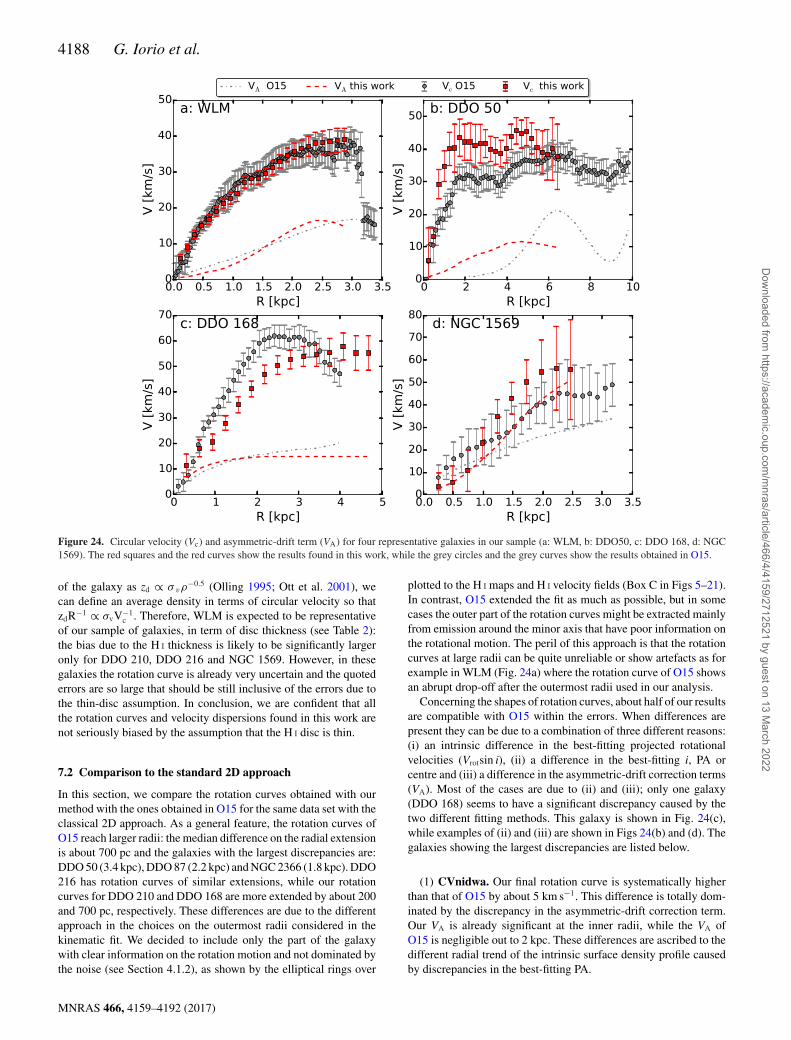
4188 G. Iorio et al.
Figure 24. Circular velocity (Vc) and asymmetric-drift term (VA) for four representative galaxies in our sample (a: WLM, b: DDO50, c: DDO 168, d: NGC1569). The red squares and the red curves show the results found in this work, while the grey circles and the grey curves show the results obtained in O15.
of the galaxy as zd ∝ σ vρ−0.5 (Olling 1995; Ott et al. 2001), we
can define an average density in terms of circular velocity so thatzdR−1 ∝ σvV−1
c . Therefore, WLM is expected to be representativeof our sample of galaxies, in term of disc thickness (see Table 2):the bias due to the H I thickness is likely to be significantly largeronly for DDO 210, DDO 216 and NGC 1569. However, in thesegalaxies the rotation curve is already very uncertain and the quotederrors are so large that should be still inclusive of the errors due tothe thin-disc assumption. In conclusion, we are confident that allthe rotation curves and velocity dispersions found in this work arenot seriously biased by the assumption that the H I disc is thin.
7.2 Comparison to the standard 2D approach
In this section, we compare the rotation curves obtained with ourmethod with the ones obtained in O15 for the same data set with theclassical 2D approach. As a general feature, the rotation curves ofO15 reach larger radii: the median difference on the radial extensionis about 700 pc and the galaxies with the largest discrepancies are:DDO 50 (3.4 kpc), DDO 87 (2.2 kpc) and NGC 2366 (1.8 kpc). DDO216 has rotation curves of similar extensions, while our rotationcurves for DDO 210 and DDO 168 are more extended by about 200and 700 pc, respectively. These differences are due to the differentapproach in the choices on the outermost radii considered in thekinematic fit. We decided to include only the part of the galaxywith clear information on the rotation motion and not dominated bythe noise (see Section 4.1.2), as shown by the elliptical rings over
plotted to the H I maps and H I velocity fields (Box C in Figs 5–21).In contrast, O15 extended the fit as much as possible, but in somecases the outer part of the rotation curves might be extracted mainlyfrom emission around the minor axis that have poor information onthe rotational motion. The peril of this approach is that the rotationcurves at large radii can be quite unreliable or show artefacts as forexample in WLM (Fig. 24a) where the rotation curve of O15 showsan abrupt drop-off after the outermost radii used in our analysis.
Concerning the shapes of rotation curves, about half of our resultsare compatible with O15 within the errors. When differences arepresent they can be due to a combination of three different reasons:(i) an intrinsic difference in the best-fitting projected rotationalvelocities (Vrotsin i), (ii) a difference in the best-fitting i, PA orcentre and (iii) a difference in the asymmetric-drift correction terms(VA). Most of the cases are due to (ii) and (iii); only one galaxy(DDO 168) seems to have a significant discrepancy caused by thetwo different fitting methods. This galaxy is shown in Fig. 24(c),while examples of (ii) and (iii) are shown in Figs 24(b) and (d). Thegalaxies showing the largest discrepancies are listed below.
(1) CVnidwa. Our final rotation curve is systematically higherthan that of O15 by about 5 km s−1. This difference is totally dom-inated by the discrepancy in the asymmetric-drift correction term.Our VA is already significant at the inner radii, while the VA ofO15 is negligible out to 2 kpc. These differences are ascribed to thedifferent radial trend of the intrinsic surface density profile causedby discrepancies in the best-fitting PA.
MNRAS 466, 4159–4192 (2017)
Dow
nloaded from https://academ
ic.oup.com/m
nras/article/466/4/4159/2712521 by guest on 13 March 2022
LITTLE THINGS in 3D 4189
(2) DDO 47. The circular velocity shows a discrepancy of about7 km s−1 in the inner part of the disc (R < 2 kpc) due to a discrepancyon the best-fitting i: O15 used i ≈ 55◦ while we used i = 37◦
independent of radius.(3) DDO 50. Discrepancies of about 10 km s−1 (see Fig. 24b) are
due to the different assumption on the value of i (about 50◦ in O15and 33◦ in this work). Our curve is also less extended (see Fig. 7).
(4) DDO 52. The final rotation curve of O15 is systemicallyhigher due to the different values of i (about 37◦ in O15 and 55◦ inthis work).
(5) DDO 87. Our final rotation curve shows a steeper rising dueto a discrepancy in the assumed i: we used i = 40◦ independent ofradius, while in O15 i varies between 60◦ and 40◦.
(6) DDO 168. The final rotation curves are quite different (seeFig. 24c). In O15, the curve flattens at about 2 kpc and starts to de-crease at 3 kpc, while our rotation curve shows a less steep rising inthe inner part and a flattening at about 3.5 kpc. These discrepanciesare due mainly to an intrinsic difference in the best-fitting projectedrotation curve found with the two methods. The differences are fur-ther increased by the different assumptions on i (i ≈ 60◦ in thiswork, i ≈ 40◦ in O15).
(7) NGC 1569. The circular rotation curve found in this workrises steeper with respect to the rotation curve reported in O15(see Fig. 24d). The difference is caused by the asymmetric-driftcorrection given that with our 3D method we find a different radialtrend of both the velocity dispersion and the intrinsic surface density.
(8) NGC 2366. Our final rotation curve is systematically lower inthe inner disc (R < 2 kpc). The cause is a combination of a differentposition of the galactic centre and different PA. We used a constantPA of about 40◦, while in O15 the PA grows from 20◦ to 40◦ in thefirst two kpc.
8 SU M M A RY
We presented a study of the kinematics of the H I discs for 17 dIrrstaken from the public survey LITTLE THINGS (Hunter et al. 2012).The main goal of this work is to make available to the communitya sample of high-quality rotation curves of dIrrs ready-to-use toperform dynamical studies. The tabulated quantities (Vrot, Vc, VA,σ v) and H I surface-density profile (�int) are available in the onlineversion of the paper. The key points of this work are listed below.
(1) We derived the rotation curves from the H I data cubes witha state-of-art technique: the publicly available software 3DBAROLO
(Di Teodoro & Fraternali 2015). It fits 3D models to the data cubeswithout explicitly extracting velocity fields. The fit in the 3D spaceof the data cubes ensures full control of the observational effectsand in particular a proper account of beam smearing.
(2) The maximum radii used in the fits have been chosen withgreat care from the H I total map. This ensures a robust estimateof the kinematics avoiding regions of the galaxy dominated by thenoise and with scant information about the gas rotation.
(3) We developed a method to take into account the uncertaintiesof the asymmetric-drift correction. As a consequence, the quotederrors on the rotation curves are representative of the real uncer-tainties. The inclusion of these errors is fundamental in galaxies forwhich the calculation of the circular velocity is highly dominatedby the asymmetric-drift correction (e.g. DDO 210).
(4) We estimated how our results can be biased by the assump-tion of a thin H I disc. We analysed in detail the galaxy WLM andwe found that the H I layer flares linearly from about 150 to 600 pc,well above the 100 pc assumed in our analysis. The presence of
such thick disc introduces systematic errors on the estimate of thevelocity dispersion, intrinsic H I surface density and circular ve-locity. However, the differences are compatible within the quoteduncertainties. The thickness of WLM should be representative ofthe galaxies of our sample, so we can conclude that our results arenot seriously biased by the assumption of thin disc.
(5) The rotation curves obtained in this work have been used totest the BTFR in the low-mass regime (106 � Mbar/M� � 109).We found that our results are compatible in slope, normalizationand scatter with the work of Lelli et al. (2016) at higher mass(Mbar > 108 M�).
AC K N OW L E D G E M E N T S
This research made use of the ‘Local Irregulars That Trace Luminos-ity Extremes, The H I Nearby Galaxy Survey’ (LITTLE THINGS)’data sample. We would like to thank the referee Mark Wilkinsonand Antonino Marasco for useful comments that improved thismanuscript, and Se-Heon Oh and Federico Lelli for kindly mak-ing their data available. GB acknowledges financial support by theSpanish Ministry of Economy and Competitiveness (MINECO)under the Ramon y Cajal Programme (RYC-2012-11537). JIRwould like to acknowledge support from STFC consolidated grantST/M000990/1 and the MERAC foundation. The research has madeuse of the NASA/IPAC Extragalactic Database (NED) that is oper-ated by the Jet Propulsion Laboratory, California Institute of Tech-nology, under contract with the National Aeronautics and SpaceAdministration.
R E F E R E N C E S
Baillard A. et al., 2011, A&A, 532, A74Battaglia G., Fraternali F., Oosterloo T., Sancisi R., 2006, A&A, 447, 49Begeman K. G., 1987, PhD thesis, Kapteyn InstituteBegum A., Chengalur J. N., Karachentsev I. D., Sharina M. E., 2008,
MNRAS, 386, 138Bosma A., 1978, PhD thesis, Groningen Univ.Bosma A., 1981, AJ, 86, 1791Bosma A., Goss W. M., Allen R. J., 1981, A&A, 93, 106Boylan-Kolchin M., Bullock J. S., Kaplinghat M., 2011, MNRAS, 415, L40Brinks E., Burton W. B., 1984, A&A, 141, 195Brook C. B., Santos-Santos I., Stinson G., 2016, MNRAS, 459, 638Bureau M., Carignan C., 2002, AJ, 123, 1316Carignan C., Purton C., 1998, ApJ, 506, 125Casertano S., van Gorkom J. H., 1991, AJ, 101, 1231Cole A. A. et al., 1999, AJ, 118, 1657Cook D. O. et al., 2014, MNRAS, 445, 881Cote S., Carignan C., Freeman K. C., 2000, AJ, 120, 3027Croxall K. V., van Zee L., Lee H., Skillman E. D., Lee J. C., Cote S.,
Kennicutt R. C., Jr, Miller B. W., 2009, ApJ, 705, 723de Blok W. J. G., Bosma A., 2002, A&A, 385, 816de Blok W. J. G., Walter F., Brinks E., Trachternach C., Oh S.-H., Kennicutt
R. C., Jr, 2008, AJ, 136, 2648Di Cintio A., Lelli F., 2016, MNRAS, 456, L127Di Teodoro E. M., Fraternali F., 2015, MNRAS, 451, 3021Fraternali F., Oosterloo T., Sancisi R., van Moorsel G., 2001, ApJ, 562, L47Fraternali F., van Moorsel G., Sancisi R., Oosterloo T., 2002, AJ, 123, 3124Garcıa-Ruiz I., Sancisi R., Kuijken K., 2002, A&A, 394, 769Gentile G., Salucci P., Klein U., Vergani D., Kalberla P., 2004, MNRAS,
351, 903Gentile G., Burkert A., Salucci P., Klein U., Walter F., 2005, ApJ, 634, L145Georgiev T. B., Karachentsev I. D., Tikhonov N. A., 1997, Astron. Lett., 23,
514Hunter D. A., Elmegreen B. G., 2006, ApJS, 162, 49
MNRAS 466, 4159–4192 (2017)
Dow
nloaded from https://academ
ic.oup.com/m
nras/article/466/4/4159/2712521 by guest on 13 March 2022
4190 G. Iorio et al.
Hunter D. A., Elmegreen B. G., van Woerden H., 2001, ApJ, 556, 773Hunter D. A., Elmegreen B. G., Oh S.-H., Anderson E., Nordgren T. E.,
Massey P., Wilsey N., Riabokin M., 2011, AJ, 142, 121Hunter D. A. et al., 2012, AJ, 144, 134Jarrett T. H., Chester T., Cutri R., Schneider S. E., Huchra J. P., 2003, AJ,
125, 525Johnson M., Hunter D. A., Oh S.-H., Zhang H.-X., Elmegreen B., Brinks
E., Tollerud E., Herrmann K., 2012, AJ, 144, 152Jozsa G. I. G., Kenn F., Klein U., Oosterloo T. A., 2007, A&A, 468, 731Kamphuis P., Jozsa G. I. G., Oh S.-H., Spekkens K., Urbancic N., Serra P.,
Koribalski B. S., Dettmar R.-J., 2015, MNRAS, 452, 3139Karachentsev I. D., Makarov D. I., Kaisina E. I., 2013, AJ, 145, 101Kirby E. N., Bullock J. S., Boylan-Kolchin M., Kaplinghat M., Cohen J. G.,
2014, MNRAS, 439, 1015Klypin A., Kravtsov A. V., Valenzuela O., Prada F., 1999, ApJ, 522, 82Knapen J. H., Erroz-Ferrer S., Roa J., Bakos J., Cisternas M., Leaman R.,
Szymanek N., 2014, A&A, 569, A91Krajnovic D., Cappellari M., de Zeeuw P. T., Copin Y., 2006, MNRAS, 366,
787Leaman R. et al., 2012, ApJ, 750, 33Lelli F., Fraternali F., Sancisi R., 2010, A&A, 516, A11Lelli F., Verheijen M., Fraternali F., Sancisi R., 2012a, A&A, 537, A72Lelli F., Verheijen M., Fraternali F., Sancisi R., 2012b, A&A, 544, A145Lelli F., Verheijen M., Fraternali F., 2014a, MNRAS, 445, 1694Lelli F., Verheijen M., Fraternali F., 2014b, A&A, 566, A71Lelli F., McGaugh S. S., Schombert J. M., 2016, ApJ, 816, L14McConnachie A. W., 2012, AJ, 144, 4McGaugh S. S., 2012, AJ, 143, 40McGaugh S. S., Schombert J. M., Bothun G. D., de Blok W. J. G., 2000,
ApJ, 533, L99Makarova L., 1999, A&AS, 139, 491O’Brien J. C., Freeman K. C., van der Kruit P. C., 2010, A&A, 515, A62Oh S.-H., de Blok W. J. G., Walter F., Brinks E., Kennicutt R. C., Jr, 2008,
AJ, 136, 2761Oh S.-H., Brook C., Governato F., Brinks E., Mayer L., de Blok W. J. G.,
Brooks A., Walter F., 2011, AJ, 142, 24Oh S.-H. et al., 2015, AJ, 149, 180 (O15)Olling R. P., 1995, AJ, 110, 591Olling R. P., 1996, AJ, 112, 481Oman K. A., Navarro J. F., Sales L. V., Fattahi A., Frenk C. S., Sawala T.,
Schaller M., White S. D. M., 2016, MNRAS, 460, 3610Ott J., Walter F., Brinks E., Van Dyk S. D., Dirsch B., Klein U., 2001, AJ,
122, 3070Puche D., Westpfahl D., Brinks E., Roy J.-R., 1992, AJ, 103, 1841Read J. I., Wilkinson M. I., Evans N. W., Gilmore G., Kleyna J. T., 2006,
MNRAS, 367, 387Read J. I., Iorio G., Agertz O., Fraternali F., 2016a, preprint
(arXiv:1607.03127)Read J. I., Agertz O., Collins M. L. M., 2016b, MNRAS, 459, 2573Read J. I., Iorio G., Agertz O., Fraternali F., 2016c, MNRAS, 462, 3628Roberts M. S., 1975, Radio Observations of Neutral Hydrogen in Galaxies.
Univ. Chicago Press, Chicago, p. 309Rogstad D. H., Shostak G. S., 1971, A&A, 13, 99Rogstad D. H., Lockhart I. A., Wright M. C. H., 1974, ApJ, 193, 309Roychowdhury S., Chengalur J. N., Begum A., Karachentsev I. D., 2010,
MNRAS, 404, L60Schoenmakers R. H. M., Franx M., de Zeeuw P. T., 1997, MNRAS, 292,
349Sicking F. J., 1997, PhD thesis, Univ. GroningenSpekkens K., Sellwood J. A., 2007, ApJ, 664, 204Stil J. M., Israel F. P., 2002a, A&A, 389, 42Stil J. M., Israel F. P., 2002b, A&A, 392, 473Swaters R. A., 1999, PhD thesis, Rijksuniversiteit GroningenSwaters R. A., Schoenmakers R. H. M., Sancisi R., van Albada T. S., 1999,
MNRAS, 304, 330Tamburro D., Rix H.-W., Leroy A. K., Mac Low M.-M., Walter F., Kennicutt
R. C., Brinks E., de Blok W. J. G., 2009, AJ, 137, 4424Taylor C. L., Kobulnicky H. A., Skillman E. D., 1998, AJ, 116, 2746
van Albada T. S., Bahcall J. N., Begeman K., Sancisi R., 1985, ApJ, 295,305
van der Hulst J. M., Terlouw J. P., Begeman K. G., Zwitser W., RoelfsemaP. R., 1992, in Worrall D. M., Biemesderfer C., Barnes J., eds, ASPConf. Ser. Vol. 25, Astronomical Data Analysis Software and SystemsI. Astron. Soc. Pac., San Francisco, p. 131
van Eymeren J., Marcelin M., Koribalski B., Dettmar R.-J., Bomans D. J.,Gach J.-L., Balard P., 2009a, A&A, 493, 511
van Eymeren J., Marcelin M., Koribalski B. S., Dettmar R.-J., Bomans D.J., Gach J.-L., Balard P., 2009b, A&A, 505, 105
Verheijen M. A. W., 2001, ApJ, 563, 694Verheijen M. A. W., Sancisi R., 2001, A&A, 370, 765Walter F., Brinks E., 2001, AJ, 121, 3026Whiting M. T., 2012, MNRAS, 421, 3242Zhang H.-X., Hunter D. A., Elmegreen B. G., Gao Y., Schruba A., 2012,
AJ, 143, 47
S U P P O RT I N G IN F O R M AT I O N
Supplementary data are available at MNRAS online.
BTFR_data.txtresults.zip
Please note: Oxford University Press is not responsible for thecontent or functionality of any supporting materials supplied bythe authors. Any queries (other than missing material) should bedirected to the corresponding author for the article.
APPENDI X A : ESTI MATE O F THEG E O M E T R I C A L PA R A M E T E R S
It is important to initialize the fit of the H I data cubes with goodestimates of the geometrical parameters: centre, i and PA of the H I
disc (see Section 4.2). We used three different methods:
(i) 3DB: 3DB can automatically estimate the geometrical pa-rameters analysing the zeroth moment (H I total map) and the firstmoment (velocity field) of the data cube. The i is estimated by fit-ting H I model maps to the observed H I total map, while the PA iscalculated as the orientation of the line that maximizes the veloc-ity gradient in the velocity field. Finally, the centre is estimated asthe flux-weighted average position of the source. 3DB builds thetotal map and the velocity field using a source-finding algorithm(DUCHAMP, Whiting 2012), separating the source pixels from thenoise pixels on the basis of a S/N threshold. As a consequence,the final maps and the estimate of the disc parameters depend onthe choice of this threshold. For this reason, we repeat this analy-sis using S/N threshold ranging from 2.5 to 5. Finally, we averagethe values on the range of S/N where the estimated parameters arealmost constant.
(ii) RingFit: We developed a simple script, called RingFit, to fitellipses to the iso-density contours at different radii of our total H I
maps (Section 4.1.1). From the properties of the fitted ellipses, wecan estimate the geometrical parameters of the H I disc at differentradii.
(iii) Isophotal fitting of the optical maps: The geometrical pa-rameters are derived from the V-band photometry by Hunter &Elmegreen (2006).
Figs A1 and A2 show two examples of the estimate of i with thethree different methods. In the first case (DDO 52) the methods arein good agreement, while in the second case (DDO 210) the resultsare not compatible (notice that in this case the H I contours deviatestrongly from elliptical shape, see Box C in Fig. 16). Usually, the
MNRAS 466, 4159–4192 (2017)
Dow
nloaded from https://academ
ic.oup.com/m
nras/article/466/4/4159/2712521 by guest on 13 March 2022
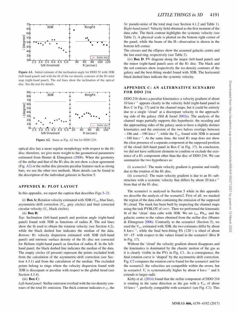
LITTLE THINGS in 3D 4191
Figure A1. Initial estimate of the inclination angle for DDO 52 with 3DB(left-hand panel) and with the fit of the iso-density contours of the H I totalmap (right-hand panel). The red lines show the inclination of the opticaldisc. See the text for details.
Figure A2. Same as Fig. A1 but for DDO 210.
optical disc has a more regular morphology with respect to the H I
disc; therefore, we give more weight to the geometrical parametersestimated from Hunter & Elmegreen (2006). When the geometryof the stellar and that of the H I disc do not show a clear agreement(Fig. A2) or the stellar disc presents peculiar features such as strongbars, we use the other two methods. More details can be found inthe description of the individual galaxies in Section 5.
A P P E N D I X B: PL OT LAYO U T
In this appendix, we report the caption that describes Figs 5–21.
(i) Box A: Rotation velocity estimated with 3DB (Vrot, blue line),asymmetric-drift correction (VA, grey circles) and final correctedcircular velocity (Vc, black circles).
(ii) Box B:Top: Inclination (left-hand panel) and position angle (right-handpanel) found with 3DB as functions of radius R. The red linesshow the fit used to obtain the rotation velocity (see Section 4.2),while the black dashed line indicates the median of the data.Bottom: H I velocity dispersion estimated with 3DB (left-handpanel) and intrinsic surface density of the H I disc not correctedfor Helium (right-hand panel) as function of radius R. In the left-hand panel, the black dashed line indicates the median of the data.The empty circles (if present) represent the points excluded bothfrom the calculation of the asymmetric-drift correction (see Sec-tion 4.3.1) and from the calculation of the median. The excludedpoints belong to rings where the velocity dispersion found with3DB is discrepant or peculiar with respect to the global trend (seeSection 4.3.4).
(iii) Box C:Left-hand panel: Stellar emission overlaid with the iso-density con-tours of the total H I emission. The thick contour indicates σ 3T, the
3σ pseudo-noise of the total map (see Section 4.1.2 and Table 1).Right-hand panel: Velocity field obtained as the first moment of thedata cube. The thick contour highlights the systemic velocity (seeTable 2). A physical scale is plotted on the bottom right corner ofthe panel, while the beam of the H I observation is shown in thebottom left corner.The crosses and the ellipses show the assumed galactic centre andthe last used ring, respectively (see Table 2).
(iv) Box D: PV diagram along the major (left-hand panel) andthe minor (right-hand panel) axes of the H I disc. The black andthe red contours show respectively the iso-density contours of thegalaxy and the best-fitting model found with 3DB. The horizontalblack dashed lines indicate the systemic velocity.
APPENDI X C : A N A LTERNATI VE SCENAR IOF O R D D O 2 1 6
DDO 216 shows a peculiar kinematics: a velocity gradient of about10 km s−1 appears clearly in the velocity field (right-hand panel inBox C in Fig. 17) and in the channel maps, but it could be entirelydue to a single ‘cloud’ at a discrepant velocity in the approach-ing side of the galaxy (Stil & Israel 2002a). The analysis of thechannel maps partially supports this hypothesis: the receding andthe approaching sides of the galaxy seem to have a slightly distinctkinematics and the emission of the two halves overlaps between−186 and −190 km s−1, while the Vsys found with 3DB is around−180 km s−1. At the same time, the total H I map does not showthe clear presence of a separate component at the supposed positionof the cloud (left-hand panel in Box C in Fig. 17). In conclusion,we did not have sufficient elements to confirm or exclude the exis-tence of a H I component other than the disc of DDO 216. We cansummarize the two hypotheses as:
(i) scenario1: The main velocity gradient is genuine and totallydue to the rotation of the H I disc.
(ii) scenario2: The main velocity gradient is due to an H I sub-structure with a systemic velocity that differs by about 20 km s−1
from that of the H I disc.
The scenario1 is analysed in Section 5 while in this appendixwe describe the analysis of the scenario2. First of all, we maskedthe region of the data cube containing the emission of the supposedH I cloud. The mask has been built by inspecting the channel mapsusing the task PYBLOT of GIPSY. Then we performed the kinematicfit of the ‘clean’ data cube with 3DB. We set iini, PAini and thegalactic centre to the values obtained from the stellar disc (Hunter& Elmegreen 2006). Contrarily to the scenario1 (Section 5), weused the Vsys estimated with 3DB, the two estimates differ by about8 km s−1, while the final best-fitting PA (120◦) is tilted of about10◦–15◦ with respect to the values found in the scenario1 (Box Bin Fig. 17).
Without the ‘cloud’ the velocity gradient almost disappears andthe kinematics is dominated by the chaotic motion of the gas asit is clearly visible in the PVs in Fig. C1. As a consequence, thefinal rotation curve is ‘shaped’ by the asymmetric-drift correction.Fig. C2 compares the rotation curve found for the scenario1 and forthe scenario2: the velocities are compatible within the errors, butin scenario1 Vc is systematically higher by about 4 km s−1 and itextends to larger radii.
Kirby et al. (2014) found that the stellar component of DDO 216is rotating in the same direction as the gas with a Vrot of about10 km s−1, perfectly compatible with scenario1 (see Fig. C2). This
MNRAS 466, 4159–4192 (2017)
Dow
nloaded from https://academ
ic.oup.com/m
nras/article/466/4/4159/2712521 by guest on 13 March 2022
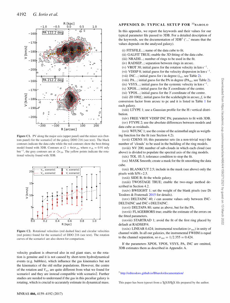
4192 G. Iorio et al.
Figure C1. PV along the major axis (upper panel) and the minor axis (bot-tom panel) for the scenario2 of the galaxy DDO 216 (see text). The blackcontours indicate the data cube while the red contours show the best-fittingmodel found with 3DB. Contours at (2 + 6n)σ ch, where σ ch = 0.91 mJybm−1, the grey contours are at -2σ ch. The yellow points indicate the rota-tional velocity found with 3DB.
Figure C2. Rotational velocities (red dashed line) and circular velocities(red points) found for the scenario2 of DDO 216 (see text). The rotationcurves of the scenario1 are also shown for comparison.
velocity gradient is observed also in red giant stars, so the rota-tion is genuine and it is not caused by short-term hydrodynamicalevents (e.g. bubbles), which influence the gas kinematics but notthe kinematics of the old stellar populations. However, the centreof the rotation and Vsys are quite different from what we found forscenario1 and they are instead compatible with scenario2. Furtherstudies are needed to understand if the gas in this peculiar galaxy isrotating, which is crucial to accurately estimate its dynamical mass.
A P P E N D I X D : T Y P I C A L S E T U P FO R 3DBARO LO
In this appendix, we report the keywords and their values for ourtypical parameter file passed to 3DB. For a detailed description ofthe keywords, see the documentation of 3DB5 (‘...’ means that thevalues depends on the analysed galaxy).
(i) FITSFILE...; name of the data cube to fit.(ii) GALFIT TRUE; enable the 3D fitting of the data cube.(iii) NRADII...; number of rings to be used in the fit.(iv) RADSEP...; separation between rings in arcsec.(v) VROT 30; initial guess for the rotation velocity in km s−1.(vi) VDISP 8; initial guess for the velocity dispersion in km s−1.(vii) INC...; initial guess for i in degree (iini, see Table 2).(viii) PA...; initial guess for the PA in degree (PAini, see Table 2).(ix) VSYS...; initial guess for the systemic velocity in km s−1.(x) XPOS...; initial guess for the X coordinate of the centre.(xi) YPOS...; initial guess for the Y coordinate of the centre.(xii) Z0 100/fc; initial guess for the scaleheight in arcsec, fc is the
conversion factor from arcsec to pc and it is listed in Table 1 foreach galaxy.
(xiii) LTYPE 1; use a Gaussian profile for the H I vertical distri-bution.
(xiv) FREE VROT VDISP INC PA; parameters to fit with 3DB.(xv) FTYPE 2; use the absolute differences between models and
data cube as residuals.(xvi) WFUNC 1; use the cosine of the azimuthal angle as weigth-
ing function for the fit (see Section 4.2).(xvii) CDENS 10; this parameter sets (in a non-trivial way) the
number of ‘clouds’ to be used in the building of the ring models.(xviii) NV 200; number of sub-clouds in which each cloud (see
above) is divided to populate the spectral axis of the ring models.(xix) TOL 1E-3; tolerance condition to stop the fit.(xx) MASK Smooth; create a mask for the fit smoothing the data
cube.(xxi) BLANKCUT 2.5; include in the mask (see above) only the
pixels with S/N>2.5.(xxii) SIDE B; fit the whole galaxy.(xxiii) TWOSTAGE TRUE; enable the two-stage method de-
scribed in Section 4.2.(xxiv) BWEIGHT 1; set the weight of the blank pixels (see Di
Teodoro & Fraternali 2015 for details).(xxv) DELTAINC 40; i can assume values only between INC-
DELTAINC and INC+DELTAINC.(xxvi) DELTAPA 80; same as above, but for the PA.(xxvii) FLAGERRORS true; enable the estimate of the errors on
the fitted parameters.(xxviii) STARTRAD 1; avoid the fit of the first ring placed by
default at RADSEP/4.(xxix) LINEAR 0.424; instrumental resolution (σ inst) in unity of
channel width. In all our galaxies, the instrumental FWHM is equalto the channel separation, so σ inst = 1/2.355 = 0.424.
If the parameters XPOS, YPOS, VSYS, PA, INC are omitted,3DB estimates them as described in Appendix A.
5 http://editeodoro.github.io/Bbarolo/documentation/
This paper has been typeset from a TEX/LATEX file prepared by the author.
MNRAS 466, 4159–4192 (2017)
Dow
nloaded from https://academ
ic.oup.com/m
nras/article/466/4/4159/2712521 by guest on 13 March 2022