Restless bandits, partial conservation laws and indexability

Jose Ni~no-Mora�

December 13, 1999

�Dept. of Economics and Business, Universitat Pompeu Fabra, E-08005 Barcelona, Spain. E-mail: jose.nino-mora@econ.upf.es. This work was supported in part by Spanish National R & D Program Grant CICYT TAP98-0229.A preliminary version of this paper was presented at the 10th INFORMS Applied Probability Conference, in Ulm, Ger-many, July 26–28, 1999.

1

Abstract

We show that if performance measures in a stochastic scheduling problem satisfy a set of

so-calledpartial conservation laws(PCL), which extend previously studied generalized con-

servation laws (GCL), then the problem is solved optimally by a priority-index policy for an

appropriate range of linear performance objectives, where the optimal indices are computed by

a one-pass adaptive-greedy algorithm, based on Klimov's. We further apply this framework to

investigate the indexability property of restless bandits introduced by Whittle, obtaining the fol-

lowing results: (1) we identify a class of restless bandits (PCL-indexable) which are indexable;

membership in this class is tested through a single run of the adaptive-greedy algorithm, which

also computes the Whittle indices when the test is positive; this provides a tractable sufficient

condition for indexability; (2) we further identify the class of GCL-indexable bandits, which

includes classical bandits, having the property that they are indexable under any linear reward

objective. The analysis is based on the so-called achievable region method, as the results follow

from new linear programming formulations for the problems investigated.

Key words: Stochastic scheduling, Markov decision chains, bandit problems, achievable region.

Journal of Economic Literature Classification:C60, C61.

2

1 Introduction

The exact solution of stochastic scheduling problems, which involves designing a dynamic resource

allocation policy in order to optimize a performance objective, appears to be, in most relevant mod-

els, an unreachable goal. Yet the identification and study of restricted problem classes whose special

structure yields a tractable solution remains of prime research interest: not only such well-solved

problems are often of intrinsic interest, but their optimal solutions may provide building blocks for

constructing well-grounded heuristic solutions to more complex models. The latter situation is epito-

mized by Whittle's [14] pioneering approach to what is arguably the most promising extension to the

classical multiarmed bandit model: therestless bandit problem.

Both bandit models, classical and restless, are concerned with designing an optimal sequential

resource allocation policy for a collection of stochastic projects, each of which is modeled as a finite

Markov decision chain (MDC) having two actions at each state, with associated rewards: anactive

action, which corresponds to engaging the project, and apassiveaction, which corresponds to letting

it go. These models are therefore paradigms of the fundamental conflict between taking actions that

yield high current reward, or taking instead actions that sacrifice current gains with the prospect of

reaping better returns in the future. In the classical model, a single resource is to be allocated, so that

at each time only one project is engaged, and passive projects do not change state. In the restless

model, a fixed number of resources (which may be larger than one) is to be allocated, so that at each

time a fixed number of projects is active, and passive projects can change state, in general through

a different transition rule. The performance objective to be maximized in both models may be the

time-discounted total expected reward, or the time-average reward rate.

While the classical model is well-known to be solved optimally by Gittins [6]priority-index policy

(an index is computed for each project state; then a project with larger current index is engaged at

each time), its restless extension has been proven in [9] to bePSPACE-hard, which most likely rules

out the possibility of describing explicitly an optimal policy.

Yet the rich modeling power of restless bandits makes the development and analysis of a sound

heuristic policy a problem of significant research importance: Whittle [14] proposed applications in

the areas of clinical trials, aircraft surveillance and worker scheduling. Other applications studied in

the literature include control of a make-to-stock queue [11], and behavior coordination in robotics

3

[5].

In his seminal paper on the subject, Whittle [14] presented a simple heuristic policy, together with

a related bound on the optimum problem value, both of which can be efficiently computed. Whittle's

policy, like Gittins' , is a priority-index rule: an index is computed for each project state; one then

engages at each time the required number of projects, sayK out of theM available, with larger

indices. The heuristic is grounded on the tractable optimal solution to arelaxedproblem version,

whose optimum value gives the aforementioned bound: instead of requiring thatK projects be active

at each time, it is required instead thatK projects be activeon average.

Whittle showed that such problemrelaxationis solved optimally by a policy characterized by a set

of indices attached to project states, provided each project in isolation satisfies a certainindexability

property. For a given restless project (i.e., a finite-state two-action MDC), such property refers to

a parametric family of single-project subproblems, where all passive rewards (obtained when the

passive action is chosen) are subsidized by a constant amountγ: the property states that, as the passive

subsidyγ grows, the set of states where it is optimal to take the passive action increases monotonically

from the empty set to the full state space. The priority indices in Whittle's heuristic for the states of

a project are precisely the corresponding breakpoints. The appealing properties of such rule include

(1) the fact that it extends the Gittins optimal policy for classical bandits; (2) the fact that Whittle's

indices, like Gittins' , can be computed separately for each project; and (3) its asymptotic optimality,

under regularity conditions, whenK andM tend to infinity in a constant ratio, as established by Weber

and Weiss in [12], [13].

Given a restless project, testing whether it is or is not indexable, and computing the Whittle in-

dices in the affirmative case, are tasks which can be efficiently accomplished through straightforward

application of the definition of indexability, combined with the well-known linear programming (LP)

formulations for MDC (see, e.g., [10]): they involven Simplex pivot steps, carried out on an LP

problem having 2n variables andn constraints,n being the number of states. Such purely numerical

procedure, however, does not provide any qualitative insight as to which projects are indexable. It

does not appear therefore suitable for attaining our main research goal, namely, to identify and an-

alyze relevant classes of indexable bandits, defined by conditions on their parameters. Whittle [14]

stated that

4

... one would very much like to have simple sufficient conditions for indexability; at the

moment, none are known.

To the best of our knowledge, no further progress on the matter has been achieved prior to the

results we present in this paper.

Our approach to the study of the indexability property for restless bandits is based on theachiev-

able region method(cf. [4]): we shall show that the indexability property can be (partially) explained

through a corresponding structural property on the underlying polyhedralachievable performance

regionof a restless bandit (spanned by performance measures under all admissible policies).

Specifically, our contribution in this paper is twofold. First, we present a general polyhedral

framework for investigating stochastic scheduling problems having the followingpartial indexability

property: priority-index policies are optimal for an appropriately restricted range of linear perfor-

mance objectives. This framework extends that given in [1] for investigating scheduling problems

for which priority-index policies are optimal underany linear performance objective (general in-

dexability). The framework in [1] was based on obtaining afull polyhedral characterization of the

system's achievable performance region from the satisfaction by performance measures of so-called

generalized conservation laws(GCL). The extension we present here is based instead on exploiting a

partial polyhedral characterization of the achievable performance region, from the satisfaction of an

appropriate subset of the previous laws, which we callpartial conservation laws(PCL). We show, in

particular, that if the performance measures of interest satisfy PCL, then (1) the problem is partially

indexable for an appropriate range of linear performance objectives, which is defined algorithmi-

cally; and (2) the optimal priority indices are computed by a one-passadaptive-greedy algorithm,

which extends that utilized in the GCL framework.

Second, we apply the PCL framework to investigate the indexability property in restless ban-

dits. In particular, we identify a class of restless bandits (PCL-indexable), defined through checkable

conditions on their parameters, which are indexable for a range of reward coefficients. This range is

characterized algorithmically through a single run of the adaptive-greedy algorithm mentioned above.

We further characterize the subclass of PCL-indexable bandits that satisfy GCL (GCL-indexable):

these bandits are indexable underany set of reward coefficients. The conditions defining this class,

of which classical bandits are the main example, provide qualitative insight on their nature.

5

The rest of the paper is structured as follows: in Section 2 we describe the restless bandit prob-

lem, and review Whittle's relaxation and index heuristic. In Section 3 we present the general PCL

framework. The framework is applied to the analysis of the indexability property in discounted rest-

less bandits in Section 4. The corresponding analysis under the time-average criterion is developed in

Section 5. Section 6 presents some examples where the previous results are applied. Finally, Section

7 ends the paper with some concluding remarks.

2 Whittle's relaxation and index heuristic

We review in this section the problem relaxation and heuristic index policy proposed by Whittle [14]

for the restless bandit problem. Consider the problem faced by a decision maker seeking to maximize

the average reward earned from a collection ofM stochastic projects, of which 1� K < M must be

engaged at each discrete time epocht � 0. Projectm2 M = f1; : : : ;Mg is modeled as a Markov

decision chain (MDC) that evolves in a finite state spaceNm, and has two actionsa2 f0;1g available

at each statei 2 Nm. We shall assume, for convenience of notation, that the state spaces for theM

projects are disjoint, and denote theiraggregate state spaceby N = [Mm=1Nm. Theactive (a = 1)

and passiveactions (a = 0) correspond, respectively, to engaging or not a project. Taking action

a2 f0;1g on a project in statei has two effects: first, it yields an instant rewardRai ; then, it causes the

state to evolve in a Markovian fashion, moving at the next time into statej with probability pai j . We

write Ra = (Rai )i2N andPa = (pa

i j )i; j2N , for a= 0;1. Both the time-discounted and the time-average

versions of the problem will be considered.

Under the discounted criterion, rewards are time-discounted by factor 0< β < 1, and the problem

consists in finding ascheduling policy uOPT, belonging in the spaceU of stationarypolicies (which

base decisions on current project states), that maximizes the expected net present value of rewards

earned over an infinite horizon:

ZOPT(β) = maxu2U

Eu

"∞

∑t=0

�Ra1(t)

i1(t)+ � � �+RaM(t)

iM(t)

�βt

#: (1)

In formulation (1),ZOPT(β) denotes the optimum problem value,im(t) andam(t) denote the state and

action corresponding to projectmat timet, andEu[�] represents the expectation operator under policy

6

u. This expectation is conditional on initial project states, as given by a known vectorα = (αi)i2N ,

where

αi =

8><>:

1 if a project is in statei at timet = 0

0 otherwise.

Under the time-average criterion, we are concerned with finding a stationary scheduling policy

uOPT that maximizes the long-run time-average reward rate (which is well defined under suitable

regularity conditions):

ZOPT(1) = maxu2U

limT!∞

1T

Eu

"T

∑t=0

�Ra1(t)

i1(t)+ � � �+RaM(t)

iM(t)

�#: (2)

Note that in formulation (2) we denote the optimal problem value byZOPT(1), thus identifying, for

notational convenience, the time-average criterion with the valueβ = 1. Using this convention will

allow us to discuss below the time-discounted and time-average cases in parallel.

Whittle's relaxation is based on consideration of a modified problem version: the requirement

thatK projects be activeat each timeis relaxedby requiring instead thatK projects be activeon av-

erage. The optimum value of the relaxed problem is hence an upper bound for the original problem's

optimum value. Furthermore, this bound can be efficiently computed by solving a polynomial-size

linear program (cf. [2]). To see this, let us associate aperformance measurewith each stationary

scheduling policyu2U, project statei 2N , and actiona2 f0;1g, defined in the discounted case by

xai (β;u) = Eu

"∞

∑t=0

I ai (t)βt

#; (3)

and in the time-average case by

xai (1;u) = lim

T!∞

1T

Eu

"T

∑t=0

I ai (t)

#; (4)

7

where

I ai (t) =

8>><>>:

1 if actiona is taken at a project in statei at timet

0 otherwise.

Performance measurexai (β;u) (resp. xa

i (1;u)) represents the total expected discounted number of

times (resp. the long-run fraction of time) that actiona is taken at a project in statei under policy

u. Now, it follows directly from the standard LP formulations for discounted and time-average MDC

(see, e.g., [10]) that Whittle's relaxation can be formulated as the LP problem

ZW(β) = max ∑j2N

R1j x1

j + ∑j2N

R0j x0

j (5)

subject to

(x0j ;x

1j ) j2Nm

2 Pm(β); for m= 1; : : : ;M

∑j2N

x1j = K s(β); (6)

where

s(β) =

8><>:

1=(1�β) if 0 < β < 1

1 if β = 1;

Pm(β) = f(x0j ;x

1j ) j2Nm

� 0 : ∑a2f0;1g

xaj �β ∑

a2f0;1g∑

i2Nm

pai j xa

i = α j ; j 2Nmg; (7)

for 0< β < 1, is the polytope defined by the standard LP constraints for the discounted MDC model-

ing projectm, and

Pm(1) = f(x0j ;x

1j ) j2Nm

� 0 : ∑a2f0;1g

xaj � ∑

a2f0;1g∑

i2Nm

pai j xa

i = 0; j 2Nm and ∑a2f0;1g

∑j2Nm

xaj = 1g (8)

is the corresponding polytope for the time-average case. In linear program (5), the variablesxaj

correspond to performance measuresxaj (β;u), and constraint (6) formulates the relaxed requirement

8

thatK projects be active on average. Note that this linear program has polynomial size on the prob-

lem's defining data, and is therefore known to be solvable in polynomial time by LP interior point

algorithms.

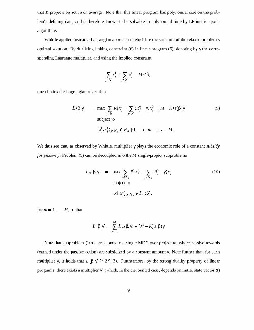
Whittle applied instead a Lagrangian approach to elucidate the structure of the relaxed problem's

optimal solution. By dualizing linking constraint (6) in linear program (5), denoting byγ the corre-

sponding Lagrange multiplier, and using the implied constraint

∑j2N

x1j + ∑

j2Nx0

j = M s(β);

one obtains the Lagrangian relaxation

L(β;γ) = max ∑j2N

R1j x1

j + ∑j2N

(R0j + γ)x0

j � (M�K)s(β)γ (9)

subject to

(x0j ;x

1j ) j2Nm

2 Pm(β); for m= 1; : : : ;M:

We thus see that, as observed by Whittle, multiplierγ plays the economic role of a constantsubsidy

for passivity. Problem (9) can be decoupled into theM single-project subproblems

Lm(β;γ) = max ∑j2Nm

R1j x1

j + ∑j2Nm

(R0j + γ)x0

j (10)

subject to

(x0j ;x

1j ) j2Nm

2 Pm(β);

for m= 1; : : : ;M, so that

L(β;γ) =M

∑m=1

Lm(β;γ)� (M�K)s(β)γ

Note that subproblem (10) corresponds to a single MDC over projectm, where passive rewards

(earned under the passive action) are subsidized by a constant amountγ. Note further that, for each

multiplier γ, it holds thatL(β;γ) � ZW(β). Furthermore, by the strong duality property of linear

programs, there exists a multiplierγ� (which, in the discounted case, depends on initial state vectorα)

9

such thatL(β;γ�) = ZW(β). In the regular case whereγ� 6= 0, LP complementary slackness ensures

that any optimal solution to Lagrangian relaxation (9) (withγ = γ�) must satisfy linking constraint

(6), and will therefore be optimal for the LP formulation of Whittle's relaxation in (5).

Whittle identified a key structural property that makes the solution to the parametric family of

single-project MDC subproblems formulated in (10) particularly simple.

Definition 1 (Whittle [14]) A project is said to beindexablefor a given discount factor0< β� 1 if

the set of states where the passive action is optimal in the corresponding single-project subproblem

(10) increases monotonically from the empty set to the full set of states as the passive subsidyγ

increases from�∞ to +∞.

It follows from Definition 1 that, for an indexable project, there exist break-even valuesγi for each

statei, such that an optimal policy for the corresponding subproblem (10) can be given as follows:

take the active action in statesi with γi < γ, and the passive action otherwise. Note that forγ = γi

both the active and the passive actions are optimal. If each project is indexable, andγ� 6= 0, it follows

from the above that an optimal policy for Whittle's relaxation is obtained by applying independently

to each project the single-project policy just described, lettingγ = γ�.

Whittle used the above indices to define a priority-index heuristic for the original problem: acti-

vate at each timeK projects with larger indices. Note that it follows from the definition of Whittle's

indices that they reduce to Gittins' when applied to classical multiarmed bandits, and therefore the

heuristic is optimal in that special case.

3 Partial conservation laws

In this section we develop a general framework for investigating thepartial indexabilityproperty in

stochastic scheduling problems, outlined in Section 1. The framework extends that introduced in [1]

for studying thegeneral indexabilityproperty in stochastic scheduling.

Consider a general dynamic and stochastic service system catering to a finite setN = f1; : : : ;ng

of job classes. Service resources (e.g., servers) are to be allocated over time to jobs vying for their

attention, on the basis of ascheduling policy u, which belongs in a spaceU of admissible policies.

The performance of a policyu 2 U over a job classi 2 N is evaluated by aperformance measure

10

xi(u)� 0, which we assume to be an expectation. We denote byx(u) = (xi(u))i2N the corresponding

performance vector. We further assume the system admits a consistent notion of servicepriority

among classes: to each permutationπ = (π1; : : : ;πn) of the classes is associated a correspondingπ-

priority policy, which assigns higher priority to classπi over classπ j if i < j, so that classπ1 has top

priority. We refer to all such policies aspriority policies. We further say that a policy gives priority

to classes in a subsetS� N (S-jobs) if it gives priority to any job classi 2 S over any job class

j 2 Sc = N nS.

Consider now, for a givenreward vectorR = (Ri)i2N 2ℜn, theoptimal scheduling problem

ZOPT(R) = supf∑i2N

Ri xi(u) : u2Ug; (11)

which involves finding a scheduling policyuOPT(R) maximizing the linear performance objective in

(11), and computing the corresponding optimum valueZOPT(R).

A wide variety of scheduling models fitting formulation (11), such as classical multiarmed ban-

dits, possess the following structural property, which we callgeneral indexability: for any reward

vector R 2 ℜn, problem (11) is solved optimally by a priority-index policy, i.e., a priority policy

where the optimal priorities are determined by a set of class-ranking indices (with higher priorities

corresponding to larger indices). A general framework providing a sufficient condition for prob-

lem (11) to be generally indexable was presented in [1]: satisfaction by performance vectorx(u) of

so-calledgeneralized conservation laws(GCL) implies general indexability; furthermore, in such

case the optimal priority indices can be efficiently computed by means of ann-stepadaptive-greedy

algorithm due to Klimov [7].

In the context of certain models, however, general indexability appears as too strong a require-

ment: the relevant concern may be instead to establish the optimality of a restricted family of priority

policies under a limited range of linear performance objectives. We call such propertypartial index-

ability. That is the case, e.g., in much studied models involving the control of arrivals into a single

queue, where researchers typically aim to prove the optimality of threshold policies (shut off arrivals

only when the queue length exceeds a given threshold value) under strong structural assumptions on

linear reward/cost coefficients. See [8]. More generally, as we shall demonstrate in Sections 4 and 5,

11

the problem of determining whether a given restless bandit is indexable may be formulated in terms

of checking the partial indexability of a problem of the form ( 11).

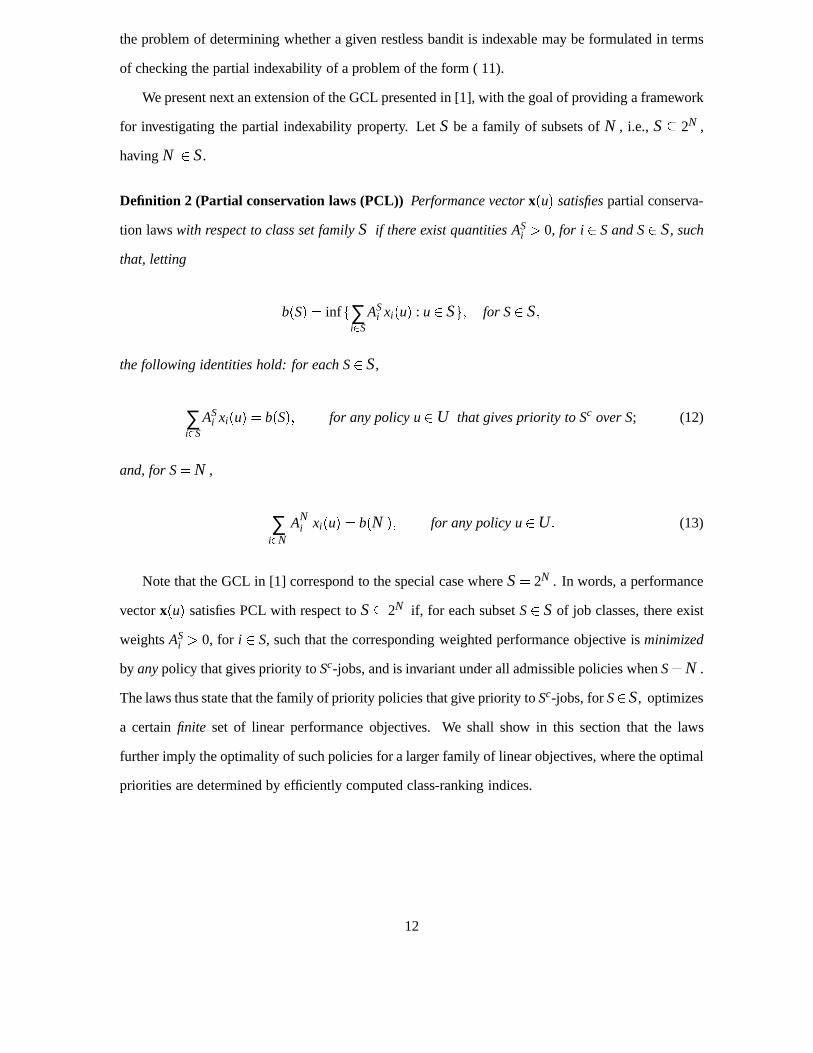
We present next an extension of the GCL presented in [1], with the goal of providing a framework

for investigating the partial indexability property. LetS be a family of subsets ofN , i.e., S � 2N ,

havingN 2 S .

Definition 2 (Partial conservation laws (PCL)) Performance vectorx(u) satisfiespartial conserva-

tion lawswith respect to class set familyS if there exist quantities ASi > 0, for i 2 S and S2 S , such

that, letting

b(S) = inf f∑i2S

ASi xi(u) : u2 Sg; for S2 S ;

the following identities hold: for each S2 S ,

∑i2S

ASi xi(u) = b(S); for any policy u2U that gives priority to Sc over S; (12)

and, for S= N ,

∑i2N

ANi xi(u) = b(N ); for any policy u2U: (13)

Note that the GCL in [1] correspond to the special case whereS = 2N . In words, a performance

vectorx(u) satisfies PCL with respect toS � 2N if, for each subsetS2 S of job classes, there exist

weightsASi > 0, for i 2 S, such that the corresponding weighted performance objective isminimized

by anypolicy that gives priority toSc-jobs, and is invariant under all admissible policies whenS= N .

The laws thus state that the family of priority policies that give priority toSc-jobs, forS2 S , optimizes

a certainfinite set of linear performance objectives. We shall show in this section that the laws

further imply the optimality of such policies for a larger family of linear objectives, where the optimal

priorities are determined by efficiently computed class-ranking indices.

12

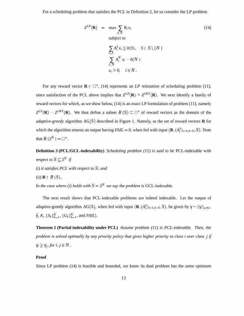
For a scheduling problem that satisfies the PCL in Definition 2, let us consider the LP problem

ZLP(R) = max ∑i2N

Ri xi (14)

subject to

∑i2S

ASi xi � b(S); S2 S nfN g

∑i2N

ANi xi = b(N )

xi � 0; i 2N :

For any reward vectorR 2 ℜn, (14) represents anLP relaxationof scheduling problem (11),

since satisfaction of the PCL above implies thatZLP(R) � ZOPT(R). We next identify a family of

reward vectors for which, as we show below, (14) is anexactLP formulation of problem (11), namely

ZLP(R) = ZOPT(R). We thus define a subsetR (S) � ℜn of reward vectors as thedomainof the

adaptive-greedyalgorithm AG(S) described in Figure 1. Namely, as the set of reward vectorsR for

which the algorithm returns an output havingFAIL= 0, when fed with input(R;(ASi )i2S;S2S ;S). Note

thatR (2N ) = ℜn.

Definition 3 (PCL/GCL-indexability) Scheduling problem (11) is said to bePCL-indexable with

respect toS � 2N if

(i) it satisfies PCL with respect toS ; and

(ii) R 2 R (S):

In the case where (i) holds withS = 2N we say the problem isGCL-indexable.

The next result shows that PCL-indexable problems are indeed indexable. Let the output of

adaptive-greedy algorithm AG(S), when fed with input(R;(ASi )i2S;S2S ;S), be given byγ = (γi)i2N ,

y, K, fSkgKk=1, fGkg

Kk=1, andFAIL).

Theorem 1 (Partial indexability under PCL) Assume problem (11) is PCL-indexable. Then, the

problem is solved optimally by any priority policy that gives higher priority to class i over class j if

γi � γ j , for i; j 2N .

Proof

Since LP problem (14) is feasible and bounded, we know its dual problem has the same optimum

13

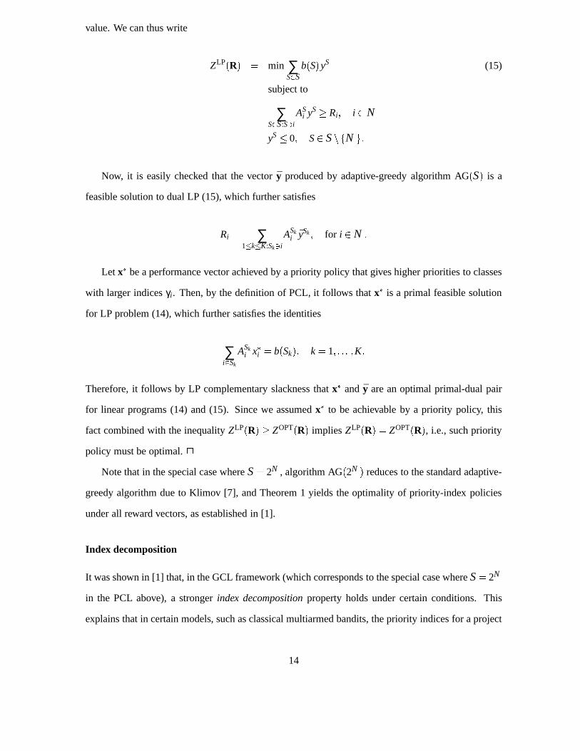
value. We can thus write

ZLP(R) = min ∑S2S

b(S)yS (15)

subject to

∑S2S :S3i

ASi yS� Ri; i 2N

yS� 0; S2 S nfN g:

Now, it is easily checked that the vectory produced by adaptive-greedy algorithm AG(S) is a

feasible solution to dual LP (15), which further satisfies

Ri = ∑1�k�K:Sk3i

ASki ySk; for i 2N :

Let x� be a performance vector achieved by a priority policy that gives higher priorities to classes

with larger indicesγi . Then, by the definition of PCL, it follows thatx� is a primal feasible solution

for LP problem (14), which further satisfies the identities

∑i2Sk

ASki x�i = b(Sk); k = 1; : : : ;K:

Therefore, it follows by LP complementary slackness thatx� and y are an optimal primal-dual pair

for linear programs (14) and (15). Since we assumedx� to be achievable by a priority policy, this

fact combined with the inequalityZLP(R) � ZOPT(R) impliesZLP(R) = ZOPT(R), i.e., such priority

policy must be optimal.2

Note that in the special case whereS = 2N , algorithm AG(2N ) reduces to the standard adaptive-

greedy algorithm due to Klimov [7], and Theorem 1 yields the optimality of priority-index policies

under all reward vectors, as established in [1].

Index decomposition

It was shown in [1] that, in the GCL framework (which corresponds to the special case whereS = 2N

in the PCL above), a strongerindex decompositionproperty holds under certain conditions. This

explains that in certain models, such as classical multiarmed bandits, the priority indices for a project

14

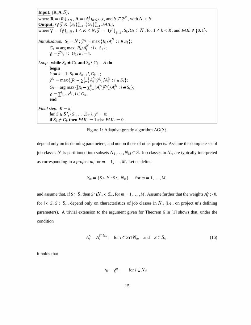
Input: (R;A;S),whereR = (Ri)i2N , A = (AS

i )i2S;S2S , andS � 2N , with N 2 S .Output: (γ; y;K;fSkg

Kk=1;fGkg

Kk=1;FAIL),

whereγ = (γi)i2N , 1� K � N, y =�yS�

S2S , Sk;Gk �N , for 1� k� K, andFAIL 2 f0;1g.

Initialization. S1 = N ; yS1 = maxfRi=ANi : i 2 S1g;

G1 = arg maxfRi=ANi : i 2 S1g;

γi = yS1, i 2G1; k := 1.

Loop. while Sk 6= Gk and Sk nGk 2 S dobegink := k+1; Sk = Sk�1 nGk�1;

ySk = maxf[Ri �∑k�1j=1A

Sji ySj ]=ASk

i : i 2 Skg;

Gk = arg maxf[Ri �∑k�1j=1 A

Sji ySj ]=ASk

i : i 2 Skg;

γi = ∑kj=1 ySj , i 2Gk.

end

Final step. K= k;for S2 S nfS1; : : : ;SKg, yS= 0;if Sk 6= Gk then FAIL := 1 elseFAIL := 0.

Figure 1: Adaptive-greedy algorithm AG(S).

depend only on its defining parameters, and not on those of other projects. Assume the complete set of

job classesN is partitioned into subsetsN1; : : : ;NM 2 S . Job classes inNm are typically interpreted

as corresponding to aproject m, for m= 1; : : : ;M. Let us define

Sm = fS2 S : S�Nmg; for m= 1; : : : ;M;

and assume that, ifS2 S , thenS\Nm2 Sm, for m=1; : : : ;M. Assume further that the weightsASi > 0,

for i 2 S, S2 Sm, depend only on characteristics of job classes inNm (i.e., on projectm's defining

parameters). A trivial extension to the argument given for Theorem 6 in [1] shows that, under the

condition

ASi = AS\Nm

i ; for i 2 S\Nm and S2 Sm; (16)

it holds that

γi = γmi ; for i 2Nm;

15

where theγmi 's, for i 2 Nm, are the indices computed by running adaptive-greedy algorithm AG(Sm)

on input((Ri)i2Nm;(AS

i )i2S;S2Sm).

Theorem 2 (Index decomposition)Under condition (16), the priority indices corresponding to job

classes inNm depend only on characteristics of project m, and can be computed by running the

adaptive-greedy algorithmAG(Sm) on input((Ri)i2Nm;(AS

i )i2S;S2Sm).

4 PCL for restless bandits: the discounted case

In this section we apply the PCL framework developed in Section 3 to investigate Whittle's indexa-

bility property for restless bandits. We focus here on the discounted case, deferring discussion of the

undiscounted case to the next section.

We thus consider a single restless bandit, as described in Section 2: it is modeled as a discrete-time

MDC, having state spaceN = f1; : : : ;ng, transition probability matricesPa = (pai j )i; j2N , and reward

vectorsRa = (Rai )i2N , corresponding to the active (a= 1) and passive (a= 0) actions, respectively.

Rewards are discounted in time by factor 0< β < 1. The initial state probabilities are given by vector

α = (αi)i2N , whereαi is the 0/1 indicator of the initial project state beingi. Our concern is to identify

sufficient conditions on model parameters under which the bandit is indexable. From the definition of

indexability, we thus need to investigate the parametric family of single-project subproblems whose

LP formulation was given in (10), which we formulate here as

ZOPT(γ;R1;R0) = maxu2U

Eu

"∞

∑t=0

∑i2N

R1i I1

i (t)βt +∞

∑t=0

∑i2N

(R0i + γ) I0

i (t)βt

#; (17)

for each value of the passive subsidyγ 2 ℜ. In (17), I ai (t) represents the indicator corresponding to

taking actiona2 f0;1g at timet, andU denotes the space of stationary policies. We note that the

standard LP formulation of problem (17) given in (10) can be rewritten, using vector notation, as

ZOPT(γ;R1;R0) = x1 R1+x0(R0+ γ1) (18)

subject to

x1 (I�βP1)+x0(I�βP0) = α

x1;x0 � 0;

16

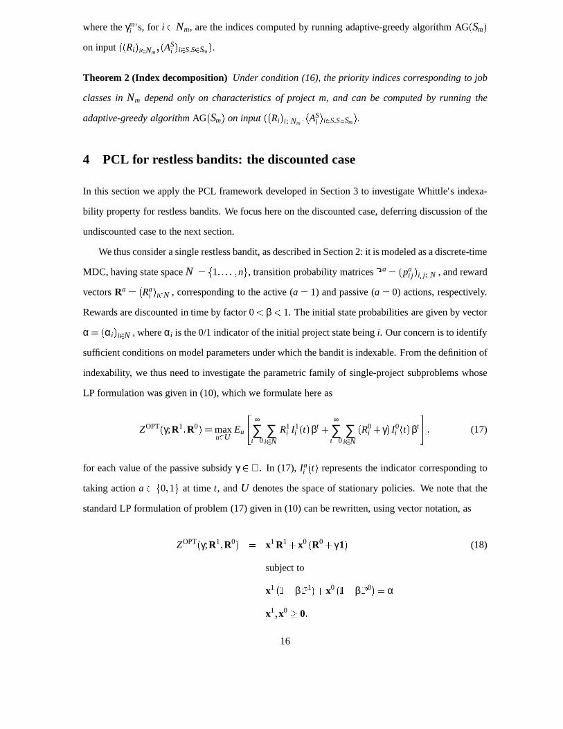
R11γ R1

2

pa00 = 1 pa

11 pa12 pa

22

pa21

0 1 2

Server

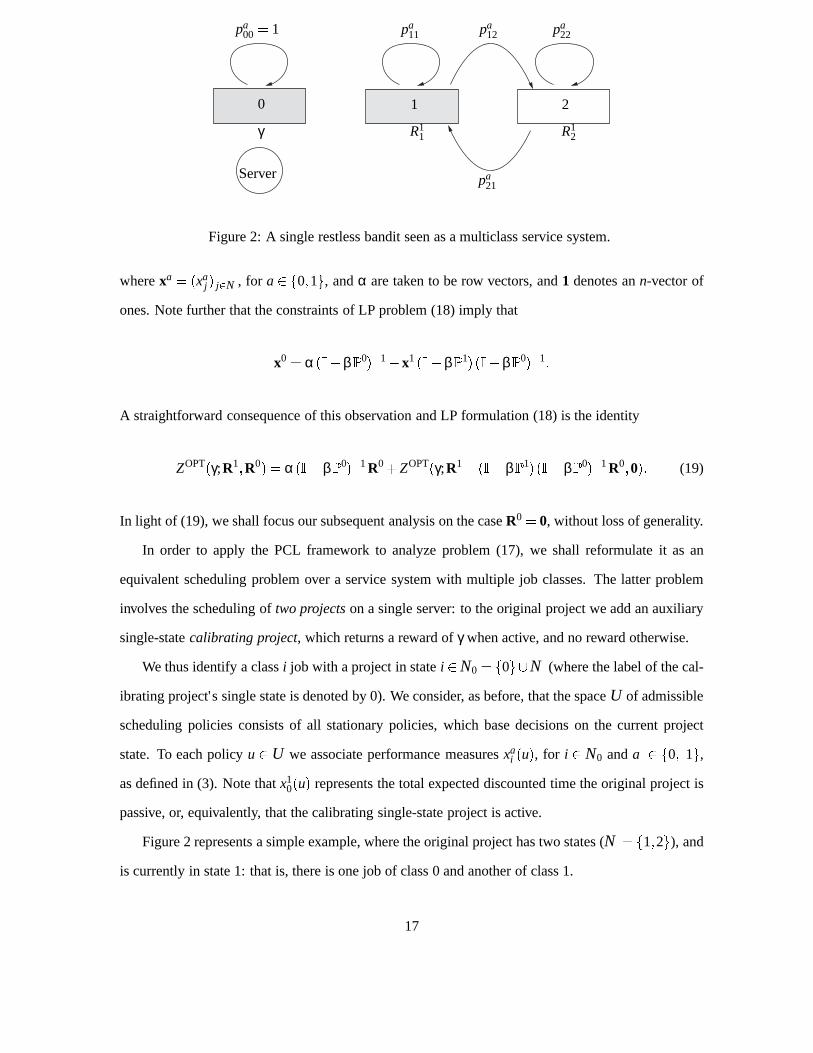
Figure 2: A single restless bandit seen as a multiclass service system.

wherexa = (xaj ) j2N , for a2 f0;1g, andα are taken to be row vectors, and1 denotes ann-vector of

ones. Note further that the constraints of LP problem (18) imply that

x0 = α (I�βP0)�1�x1(I�βP1)(I�βP0)�1:

A straightforward consequence of this observation and LP formulation (18) is the identity

ZOPT(γ;R1;R0) = α(I�βP0)�1R0+ZOPT(γ;R1� (I�βP1)(I�βP0)�1R0;0): (19)

In light of (19), we shall focus our subsequent analysis on the caseR0 = 0, without loss of generality.

In order to apply the PCL framework to analyze problem (17), we shall reformulate it as an

equivalent scheduling problem over a service system with multiple job classes. The latter problem

involves the scheduling oftwo projectson a single server: to the original project we add an auxiliary

single-statecalibrating project, which returns a reward ofγ when active, and no reward otherwise.

We thus identify a classi job with a project in statei 2N0 = f0g[N (where the label of the cal-

ibrating project's single state is denoted by 0). We consider, as before, that the spaceU of admissible

scheduling policies consists of all stationary policies, which base decisions on the current project

state. To each policyu 2 U we associate performance measuresxai (u), for i 2 N0 anda 2 f0; 1g,

as defined in (3). Note thatx10(u) represents the total expected discounted time the original project is

passive, or, equivalently, that the calibrating single-state project is active.

Figure 2 represents a simple example, where the original project has two states (N = f1;2g), and

is currently in state 1: that is, there is one job of class 0 and another of class 1.

17

It will be convenient in what follows to use the following additional notation: given a vector

x = (xi)i2N , a matrixP = (pi j )i; j2N , and subsetsS;T � N , we shall writexS = (xi)i2S and

PST = (pi j )i2S; j2T . Recall thatSc = N nS, for S�N .

We next define certain project parameters, derived from model primitives, which will be required

in our analysis. We start by considering, for each class/state subsetS�N , a correspondingS-active

policy: this takes the active action on the original project when its state lies inS, and the passive

action otherwise. Let us further defineVSi , for i 2N , as thetotal expected discounted time the project

state lies in S under the S-active policy, provided the initial state is i. For a givenS�N , theVSi 's are

determined as the unique solution to the system of linear equations

VSi = 1+β ∑

j2Np1

i j VSj ; for i 2 S

VSi = β ∑

j2Np0

i j VSj ; for i 2 Sc:

It will be convenient for our analysis to rewrite this system, using the matrix notation introduced

above, as

VSS = 1S+βP1

SSVSS+βP1

SSc VSSc (20)

VSSc = βP0

ScSVSS+βP0

ScSc VSSc; (21)

where1S denotes a vector of ones indexed by classes/states inS, VSS= (VS

i )i2S andVSSc = (VS

i )i2Sc.

We next use theVSi 's as building blocks to define quantitiesAS

i , for i 2N andS�N , by

ASc

i = 1+β ∑j2N

(p1i j � p0

i j )VSj : (22)

Note that

A/0i = AN

i = 1; for i 2N :

18

Furthermore, it is straightforward from (20)–(22) that

ASS = 1S+βP1

SN VSc

N � VSc

S ; (23)

ASSc = VSc

Sc�βP0ScN VSc

N ; (24)

whereASS= (AS

i )i2S andASSc = (AS

i )i2Sc. We further defineAf0g[Si , for i 2 f0g[SandS�N , by

Af0g[Si =

8>><>>:

ASi if i 2 S

1 if i = 0:

We complete the definitions by lettingb(T), for T �N0, be given by

b(T) =

8>><>>:

11�β �∑i2N αi VSc

i if 0 2 T andS= T \N 6= /0

0 otherwise:

Our next result will play a central role in our analysis of the indexability property of restless

bandits via PCL. It formulates a family ofdecomposition laws, where a linear combination of ac-

tive performance measures is shown to decompose, under any admissible policy, as the sum of a

policy-invariant term plus a linear combination of passive performance measures. We note that such

identities are analogous to thework decomposition lawssatisfied by certain single-server multiclass

queueing systems (cf. Theorem 5 in [3]): in the latter, a linear combination of mean queue lengths

corresponding to a class subset is decomposed as the sum of a policy-invariant term plus terms relating

to the mean workload when other classes are in service, or when the server is idle.

Lemma 3 (Decomposition laws)For any admissible policy u and for any S�N ,

x10(u)+∑

i2S

ASi x1

i (u) = b(f0g[S)+ ∑i2Sc

ASi x0

i (u); (25)

in particular, for S= N ,

x10(u)+ ∑

i2Nx1

i (u) = b(N0):

19

Proof

To simplify notation, we shall write in what followsxa(u) = xa, for a= 0;1, and consider thexa's to

be row vectors. We first note that the standard linear programming formulation for discounted MDC,

applied to the restless project under study, yields that performance vectorsxa, for a= 0;1, satisfy the

matrix equation

x0 (I�βP0)+x1(I�βP1) = α: (26)

We now rewrite system (26), in terms of a given subsetS�N , as

�x0

S x0Sc

� 264IS�βP0SS �βP0

SSc

�βP0ScS ISc�βP0

ScSc

375+

�x1

S x1Sc

� 264IS�βP1SS �βP1

SSc

�βP1ScS ISc�βP1

ScSc

375=

�αS αSc

�;

or, equivalently,

x0S(IS�βP0

SS) = αS+βx0ScP

0ScS+βx1

ScP1ScS�x1

S(IS�βP1SS)

x1Sc (ISc�βP1

ScSc) = αSc +βx0SP

0SSc +βx1

SP1SSc�x0

Sc (ISc�βP0ScSc):

Solving forx0S in the first of the last two equations, and substituting for it in the second, yields

x1Sc

�ISc�βP1

ScSc�β2P

1ScS(IS�βP0

SS)�1P

0SSc

�= αSc +βαS(IS�βP0

SS)�1P

0SSc

+βx1S

�P

1SSc� (IS�βP1

SS)(I�βP0SS)

�1P

0SSc

��x0

Sc

�ISc�βP0

ScSc�β2P

0ScS(IS�βP0

SS)�1P

0SSc

�:

Now, postmultiplying both sides of the above equation byVSc

Sc, and simplifying the resulting expres-

sion using (20)–(24), and the identity (which follows from the definition ofASS)

ASS= 1S+β

�P

1SSc � (IS�βP1

SS)(IS�βP0SS)

�1P

0SSc

�VSc

Sc;

20

we obtain

x1Sc 1Sc = αVSc

+x1S

�AS

S�1S��x0

Sc ASSc:

Note further that the requirement that at each time one of the two projects be active implies that

x10+x1

S1S+x1Sc 1Sc = x1

0+ ∑i2N

x1i =

11�β

:

Combining the last two equations yields

x10+x1

SASS=

11�β

�αVSc+x0

Sc ASSc;

which is precisely (25). The caseS= N is immediate.2

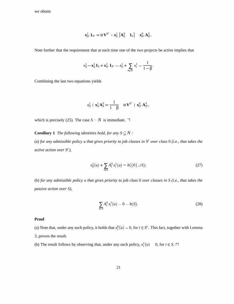
Corollary 1 The following identities hold, for any S�N :

(a) for any admissible policy u that gives priority to job classes in Sc over class0 (i.e., that takes the

active action over Sc),

x10(u)+∑

i2S

ASi x1

i (u) = b(f0g[S); (27)

(b) for any admissible policy u that gives priority to job class0 over classes in S (i.e., that takes the

passive action over S),

∑i2S

ASi x1

i (u) = 0= b(S): (28)

Proof

(a) Note that, under any such policy, it holds thatx0i (u) = 0, for i 2Sc. This fact, together with Lemma

3, proves the result.

(b) The result follows by observing that, under any such policy,x1i (u) = 0, for i 2 S. 2

21

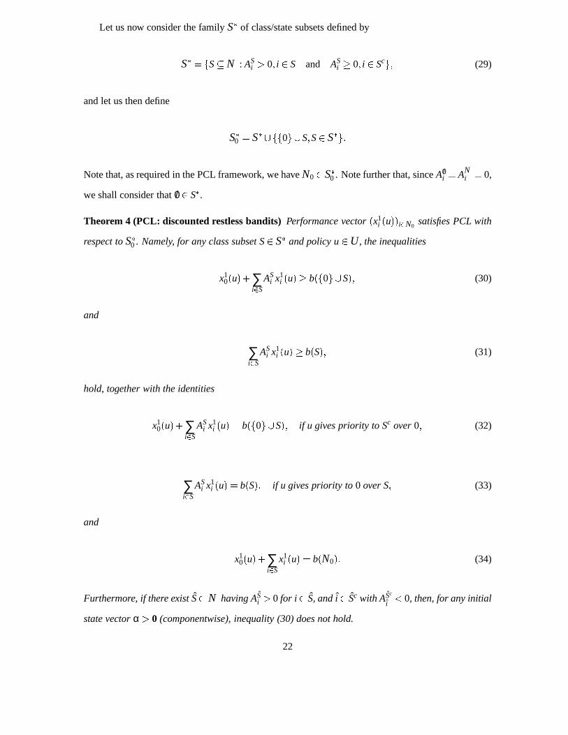
Let us now consider the familyS � of class/state subsets defined by

S � = fS�N : ASi > 0; i 2 S and AS

i � 0; i 2 Scg; (29)

and let us then define

S �0 = S �[ff0g[S;S2 S �g:

Note that, as required in the PCL framework, we haveN02 S �0 . Note further that, sinceA/0i �AN

i � 0,

we shall consider that/0 2 S�.

Theorem 4 (PCL: discounted restless bandits)Performance vector(x1i (u))i2N0

satisfies PCL with

respect toS �0 . Namely, for any class subset S2 S � and policy u2U, the inequalities

x10(u)+∑

i2S

ASi x1

i (u)� b(f0g[S); (30)

and

∑i2S

ASi x1

i (u)� b(S); (31)

hold, together with the identities

x10(u)+∑

i2S

ASi x1

i (u) = b(f0g[S); if u gives priority to Sc over0; (32)

∑i2S

ASi x1

i (u) = b(S); if u gives priority to0 over S; (33)

and

x10(u)+∑

i2S

x1i (u) = b(N0): (34)

Furthermore, if there existS�N having ASi > 0 for i 2 S, andi 2 Sc with ASc

i< 0, then, for any initial

state vectorα > 0 (componentwise), inequality (30) does not hold.

22

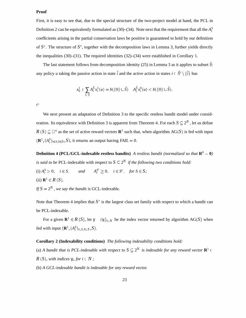
Proof

First, it is easy to see that, due to the special structure of the two-project model at hand, the PCL in

Definition 2 can be equivalently formulated as (30)–(34). Note next that the requirement that all theASi

coefficients arising in the partial conservation laws be positive is guaranteed to hold by our definition

of S �. The structure ofS �, together with the decomposition laws in Lemma 3, further yields directly

the inequalities (30)–(31). The required identities (32)–(34) were established in Corollary 1.

The last statement follows from decomposition identity (25) in Lemma 3 as it applies to subsetS:

any policyu taking the passive action in statei and the active action in statesi 2 Scnfig has

x10+∑

i2S

ASi x1

i (u) = b(f0g[ S)+ASi x0

i (u)< b(f0g[ S):

2

We next present an adaptation of Definition 3 to the specific restless bandit model under consid-

eration. Its equivalence with Definition 3 is apparent from Theorem 4. For eachS � 2N , let us define

R (S)�ℜn as the set of active reward vectorsR1 such that, when algorithm AG(S) is fed with input

(R1;(ASi )i2S;S2S ;S), it returns an output havingFAIL = 0.

Definition 4 (PCL/GCL-indexable restless bandits)A restless bandit (normalized so thatR0 = 0)

is said to bePCL-indexable with respect toS � 2N if the following two conditions hold:

(i) ASi > 0; i 2 S; and ASc

i � 0; i 2 Sc; for S2 S ;

(ii) R1 2 R (S).

If S = 2N , we say the bandit isGCL-indexable.

Note that Theorem 4 implies thatS � is the largest class set family with respect to which a bandit can

be PCL-indexable.

For a givenR1 2 R (S), let γ = (γi)i2N be the index vector returned by algorithm AG(S) when

fed with input(R1;(ASi )i2S;S2S ;S).

Corollary 2 (Indexability conditions) The following indexability conditions hold:

(a) A bandit that is PCL-indexable with respect toS � 2N is indexable for any reward vectorR1 2

R (S), with indicesγi , for i 2N ;

(b) A GCL-indexable bandit is indexable for any reward vector.

23

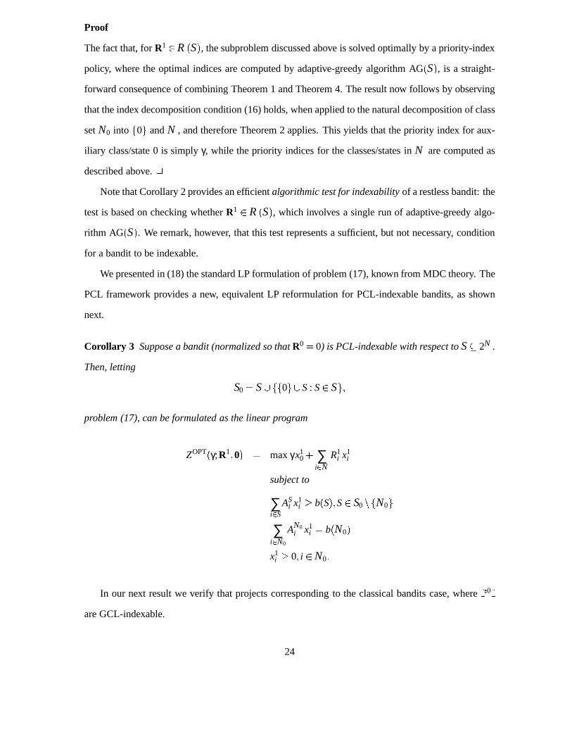
Proof

The fact that, forR1 2R (S), the subproblem discussed above is solved optimally by a priority-index

policy, where the optimal indices are computed by adaptive-greedy algorithm AG(S), is a straight-

forward consequence of combining Theorem 1 and Theorem 4. The result now follows by observing

that the index decomposition condition (16) holds, when applied to the natural decomposition of class

setN0 into f0g andN , and therefore Theorem 2 applies. This yields that the priority index for aux-

iliary class/state 0 is simplyγ, while the priority indices for the classes/states inN are computed as

described above.2

Note that Corollary 2 provides an efficientalgorithmic test for indexabilityof a restless bandit: the

test is based on checking whetherR1 2 R (S), which involves a single run of adaptive-greedy algo-

rithm AG(S). We remark, however, that this test represents a sufficient, but not necessary, condition

for a bandit to be indexable.

We presented in (18) the standard LP formulation of problem (17), known from MDC theory. The

PCL framework provides a new, equivalent LP reformulation for PCL-indexable bandits, as shown

next.

Corollary 3 Suppose a bandit (normalized so thatR0 = 0) is PCL-indexable with respect toS � 2N .

Then, letting

S0 = S [ff0g[S: S2 Sg;

problem (17), can be formulated as the linear program

ZOPT(γ;R1;0) = maxγx10+ ∑

i2NR1

i x1i

subject to

∑i2S

ASi x1

i � b(S);S2 S0nfN0g

∑i2N0

AN0i x1

i = b(N0)

x1i � 0; i 2N0:

In our next result we verify that projects corresponding to the classical bandits case, whereP0I

are GCL-indexable.

24

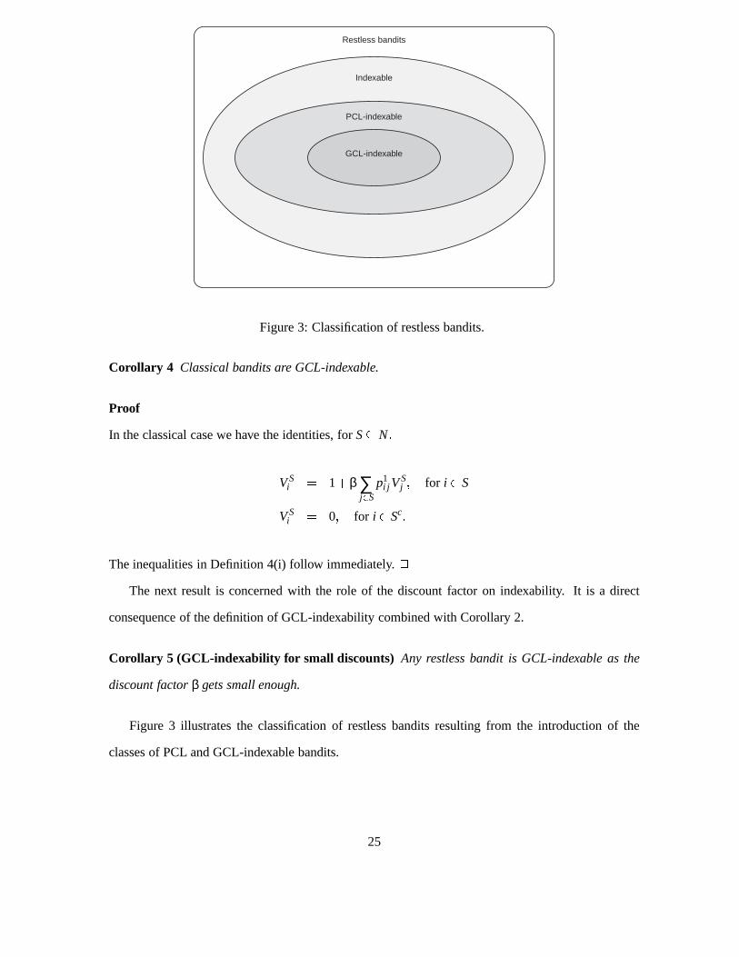
Restless bandits

Indexable

PCL-indexable

GCL-indexable

Figure 3: Classification of restless bandits.

Corollary 4 Classical bandits are GCL-indexable.

Proof

In the classical case we have the identities, forS� N;

VSi = 1+β ∑

j2S

p1i j V

Sj ; for i 2 S

VSi = 0; for i 2 Sc:

The inequalities in Definition 4(i) follow immediately.2

The next result is concerned with the role of the discount factor on indexability. It is a direct

consequence of the definition of GCL-indexability combined with Corollary 2.

Corollary 5 (GCL-indexability for small discounts) Any restless bandit is GCL-indexable as the

discount factorβ gets small enough.

Figure 3 illustrates the classification of restless bandits resulting from the introduction of the

classes of PCL and GCL-indexable bandits.

25

Interpretation of GCL-indexability

We next consider the intuitive interpretation of GCL-indexability, we note that, for anyS� N , we

can write

ASc

i =

8><>:

VSi �β ∑ j2N p0

i j VSj i 2 S

1+β ∑ j2N p1i j V

Sj �VS

i i 2 Sc:

Let us focus on a givenS� N . Recall the interpretation ofVSi as the total expected discounted

time the project is active (active time, for short) under theS-active policy (which takes the active

action on states inS, and the passive action otherwise), when starting in statei 2 N . The condition

ASc

i > 0, for i 2 Sc, states therefore that, by changing the initial action (in statei) from passive to

active, and following theS-active policy onwards, the project expected active time becomes larger.

Furthermore, the conditionASc

i � 0, for i 2S, states that, by changing the initial action (in statei) from

active to passive, and following theS-active policy onwards, the project expected active time does not

become larger. Note further from the above discussion that the coefficientsASc

i representactive time

differentialscorresponding to changing the initial action in statei under theS-active policy.

5 PCL for restless bandits: the time-average case

In this section we outline how the results in Section 4 for the time-discounted case can be extended

to analyze restless bandits under the time-average criterion.

We shall thus consider a general restless bandit, as described in Section 4, on which we shall

impose the additional requirement stated next.

Assumption 1 (Ergodicity) For any subset S�N of bandit states, the Markov chain overN having

transition probability matrix

P(S) =

264 P

1SN

P0ScN

375 (35)

is ergodic.

26

Note thatP(S), defined by (35), is the transition probability matrix for theS-active policy con-

sidered in our study of the discounted case. Furthermore, as in the previous section, we need only

consider the case where passive reward vector isR0 = 0, since the general case can be equivalently

reduced to it.

Our approach to the time-average case is based on studying the asymptotic behavior, as the dis-

count factorβ % 1, of the quantities and results appearing in our analysis of the discounted case.

Hence, to avoid confusion, in what follows we shall make explicit the dependence on discount factor

β in the quantities defined in Section 4, writing, e.g.,VSi (β), AS

i (β) andxui (u;β).

To relate the discounted and the time-average cases we shall apply the result that, under Assump-

tion 1, for any bandit statei 2 N and state subsetS�N, we can expressVSi (β) as follows:

VSi (β) =

VS

1�β+vS

i +O(1�β) asβ% 1. (36)

In identity (36),VS represents thelong-run time-average fraction of time the bandit is active under

the S-active policy, whereasvSi represents the correspondingtotal expected active time differential

due to starting in state i. Substituting for theVSi (β)'s in equations (20)–(21) using (36), and letting

β% 1, we obtain the system of linear equations

VS+vSi = 1+ ∑

j2N

p1i j vS

j , for i 2 S (37)

VS+vSi = ∑

j2N

p0i j vS

j , for i 2 Sc: (38)

Note that equations (37)–(38) determinevSi , for i 2 N, in terms ofVS. Furthermore,VS can be

computed as the sum of the equilibrium probabilities for states inS corresponding to the ergodic

Markov chain having transition probability matrixP(S).

We next apply (36)–(38) to study the asymptotics of the coefficientsASi (β) appearing in the PCL

obtained in the discounted case. Substituting for theVSi (β)'s in equations (22) using (36), and letting

β% 1, yields the result that eachASi (β) converges to a limitAS

i , given by

27

ASi = 1+ ∑

j2N

(p1i j � p0

i j )vSj , for i 2 N, S� N: (39)

The performance measures of interest are now the time-average state-action frequencies: we

denote byxai (u) the time-average fraction of time that the project is in statei and actiona is taken

under policyu. We further writexa(u) = (xai (u))i2N . It is well known that in the ergodic case under

discussion it holds that, for any stationary policyu,

xa(u) = limβ%1

(1�β)xa(u;β): (40)

In order to investigate the indexability property under the time-average criterion we consider the

equivalent two-project restless bandits model discussed in Section 4, where an auxiliarycalibrating

project having a single state 0 is introduced, yielding a reward ofγ when active (or, equivalently,

when the original project is passive).

We further define, as in the discounted case, quantitiesAf0g[Si , for i 2 f0g[SandS�N , by

Af0g[Si =

8>><>>:

ASi if i 2 S

1 if i = 0:

We complete the definitions by lettingb(T), for T � f0g[N, be given by

b(T) =

8>><>>:

1�VScif 0 2 T andS= T \N 6= /0

0 if T = f0g or T �N :

With these definitions, all the results of the previous section carry over, in a verbatim fashion, to

the time-average case under discussion by taking appropriate limits asβ% 1.

6 Examples

In this section we analyze several special cases of restless bandits using the results developed above.

28

6.1 Two-state restless bandits

We first consider the case of restless bandits having two states. The corresponding two-project restless

bandit problem discussed in Section 4 is precisely that represented in Figure 2. In the discounted case,

the relevantASi coefficients are readily calculated as follows:

Af1g1 =1+β�β p1

11�β p122

1+β�β p011�β p1

22

Af1g2 =1+β�β p0

11�β p022

1+β�β p011�β p1

22

Af2g1 =1+β�β p0

11�β p022

1+β�β p111�β p0

22

Af2g2 =1+β�β p1

11�β p122

1+β�β p022�β p1

11

:

It follows that, for any discount factor 0< β < 1, Af1gi ;Af2gi > 0, for i = 1;2. Therefore, it follows that

discounted two-state restless projects are GCL-indexable, hence indexable under any reward vector.

By taking the limit asβ% 1 the corresponding result is obtained for the time-average case, provided

the ergodicity requirement in Assumption 1 holds.

Furthermore, ifR11 � R1

2 (we assume as before that passive rewards are 0), the Whittle indices

produced by the adaptive-greedy algorithm AG(2f1;2g) are

γ1 = R1

and

γ2 = R1+R2�Af1;2g

2 R1

Af2g2

= R1�1+β�β p0

22�β p111

1+β�β p111�β p1

22

(R1�R2)

=β(p0

22� p122)R1+(1+β�β p0

22�β p111)R2

1+β�β p111�β p1

22

:

As will be seen in the next example, three-state restless bandits need not be GCL-indexable.

29

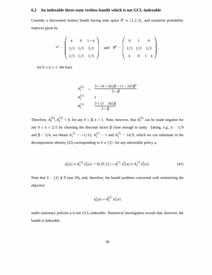
6.2 An indexable three-state restless bandit which is not GCL-indexable

Consider a discounted restless bandit having state spaceN = f1;2;3g, and transition probability

matrices given by

P1 =

0BBBB@

ε 0 1� ε

1=3 1=3 1=3

1=3 1=3 1=3

1CCCCA and P

0 =

0BBBB@

0 1 0

1=3 1=3 1=3

ε 0 1� ε

1CCCCA ;

for 0< ε < 1. We have

Af3g1 =3� (4�3ε)β� (1�2ε)β2

3�βAf3g2 = 1

Af3g3 =3+(1�3ε)β

3�β:

Therefore,Af3g2 ;Af3g3 > 0, for any 0< β; ε < 1. Note, however, thatAf3g1 can be made negative for

any 0< ε < 2=5 by choosing the discount factorβ close enough to unity. Taking, e.g.,ε = 1=9

andβ = 3=4, we obtainAf3g1 = �1=12, Af3g2 = 1 andAf3g3 = 14=9, which we can substitute in the

decomposition identity (25) corresponding toS= f3g: for any admissible policyu,

x10(u)+Af3g3 x1

3(u) = b(f0;3g)+Af3g1 x01(u)+Af3g2 x0

2(u): (41)

Note thatS= f3g =2 S (see 29), and, therefore, the bandit problem concerned with minimizing the

objective

x10(u)+Af3g3 x1

3(u)

under stationary policiesu is not GCL-indexable. Numerical investigation reveals that, however, the

bandit is indexable.

30

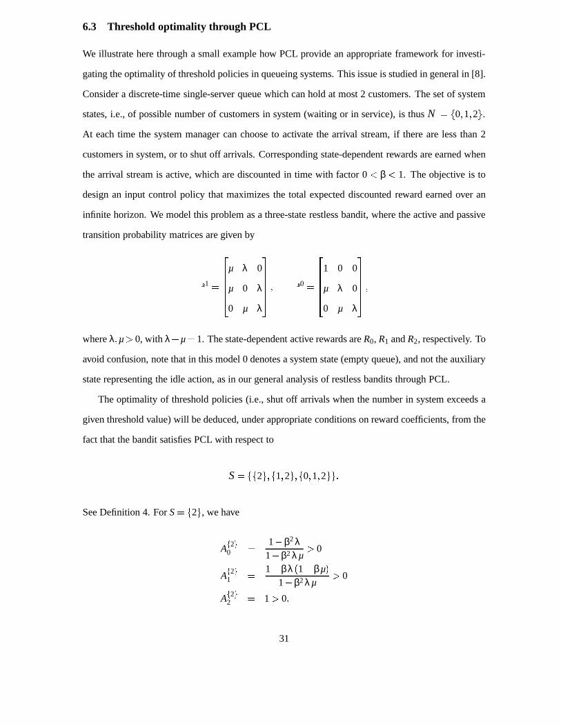
6.3 Threshold optimality through PCL

We illustrate here through a small example how PCL provide an appropriate framework for investi-

gating the optimality of threshold policies in queueing systems. This issue is studied in general in [8].

Consider a discrete-time single-server queue which can hold at most 2 customers. The set of system

states, i.e., of possible number of customers in system (waiting or in service), is thusN = f0;1;2g.

At each time the system manager can choose to activate the arrival stream, if there are less than 2

customers in system, or to shut off arrivals. Corresponding state-dependent rewards are earned when

the arrival stream is active, which are discounted in time with factor 0< β < 1. The objective is to

design an input control policy that maximizes the total expected discounted reward earned over an

infinite horizon. We model this problem as a three-state restless bandit, where the active and passive

transition probability matrices are given by

P1 =

266664

µ λ 0

µ 0 λ

0 µ λ

377775 ; P

0 =

266664

1 0 0

µ λ 0

0 µ λ

377775 ;

whereλ;µ> 0, withλ+µ= 1. The state-dependent active rewards areR0, R1 andR2, respectively. To

avoid confusion, note that in this model 0 denotes a system state (empty queue), and not the auxiliary

state representing the idle action, as in our general analysis of restless bandits through PCL.

The optimality of threshold policies (i.e., shut off arrivals when the number in system exceeds a

given threshold value) will be deduced, under appropriate conditions on reward coefficients, from the

fact that the bandit satisfies PCL with respect to

S = ff2g;f1;2g;f0;1;2gg:

See Definition 4. ForS= f2g, we have

Af2g0 =1�β2λ

1�β2λµ> 0

Af2g1 =1�βλ(1+βµ)

1�β2λµ> 0

Af2g2 = 1> 0:

31

For S= f1;2g,

Af1;2g0 = 1�βλ > 0

Af1;2g1 = 1�

β2λµ1�βλ

> 0

Af1;2g2 = 1> 0:

For S= f0;1;2g, we have

Af0;1;2gi = 1; i 2 f0;1;2g:

Therefore, the bandit satisfies PCL with respect toS . Let us now characterize the corresponding

reward subsetR (S), as the domain of adaptive-greedy algorithm AG(S). The conditions defining

R (S) are easily seen to be as follows:

R0 �max(R1;R2) andR1�R0

Af1;2g1

�R2�R0

Af1;2g2

: (42)

Therefore, under conditions (42) on reward coefficients, the bandit is PCL-indexable with respect

to S . The corresponding Whittle indices, as given by adaptive-greedy algorithm AG(S) are

γ0 = R0; γ1 = R0+R1�R0

Af1;2g1

; γ2 = γ1+R2�R0�Af1;2g2 (γ1� γ0):

7 Conclusions

We identified a class of restless bandits, called PCL-indexable, which are guaranteed to be indexable.

Membership of a given restless bandit in this class can be efficiently tested through a single run of an

adaptive-greedy algorithm, which also computes the Whittle indices when the test is positive. Given

the rich modeling power of restless bandits, we believe the notion of PCL-indexability introduced in

this paper opens the way to analyze a variety of stochastic control models in, e.g., queueing systems,

within a unifying, polyhedral framework.

Our analysis further reveals the power of the achievable region method (cf. [4]) to analyze

stochastic optimization problems, as our analyses are based on new linear programming formula-

32

tions of the problems investigated. A previous study (see [2]) also utilized the achievable region

approach to obtain a priority-index heuristic, different from Whittle's, and improved LP relaxations,

for general (possibly nonindexable) restless bandits.

References

[1] Bertsimas, D. and Ni~no-Mora, J. (1996). Conservation laws, extended polymatroids and multi-

armed bandit problems; a unified approach to indexable systems.Math. Oper. Res.21257–306.

[2] Bertsimas, D. and Ni~no-Mora, J. (1994). Restless bandits, linear programming relaxations, and

a primal-dual index heuristic. Working paper, Operations Research Center, MIT. Forthcoming

in Oper. Res.

[3] Bertsimas, D. and Ni~no-Mora, J. (1999). Optimization of multiclass queueing networks with

changeover times via the achievable region method: Part I, the single-station case.Math. Oper.

Res.24306–330.

[4] Dacre, M., Glazebrook, K.D. and Ni~no-Mora, J. (1999). The achievable region approach to the

optimal control of stochastic systems (with discussion).J. Roy. Statist. Soc. Ser. B61 747–791.

[5] Faihe, Y. and M¨uller, J.-P. (1998). Behaviors coordination using restless bandits allocation in-

dexes.Proceedings of the Fifth International Conference on Simulation of Adaptive Behavior

(SAB98).

[6] Gittins, J. C. (1979). Bandit processes and dynamic allocation indices (with discussion).J. Roy.

Statist. Soc. Ser. B41 148–177.

[7] Klimov, G.P. (1974). Time sharing service systems I.Theory Probab. Appl.19 532–551.

[8] Ni~no-Mora, J. (1999). Threshold optimality in queueing systems: a polyhedral approach via

partial conservation laws. Working paper, UPF.

[9] Papadimitriou, C. H. and Tsitsiklis, J. N. (1999). The complexity of optimal queueing network

control.Math. Oper. Res.24 293–305

33

[10] Puterman, M.L. (1994).Markov Decision Processes: Discrete Stochastic Dynamic Program-

ming, Wiley, New York.

[11] Veatch, M. and Wein, L. M. (1996). Scheduling a make-to-stock queue: Index policies and

hedging points.Oper. Res.44 634–647.

[12] Weber, R. R. and Weiss, G. (1990). On an index policy for restless bandits.J. Appl. Prob.27

637–648.

[13] Weber, R. R. and Weiss, G. (1991). Addendum to “On an index policy for restless bandits.”Adv.

Appl. Prob.23429–430.

[14] Whittle, P. (1988). Restless bandits: Activity allocation in a changing world. InA Celebration

of Applied Probability, J. Gani (Ed.),J. Appl. Prob.25A 287-298.

34