Resource Estimation in T20 Cricket

Harsha Perera and Tim B. Swartz ∗

Abstract

This paper investigates the suitability of the Duckworth-Lewis method as an approach

to resetting targets in interrupted T20 cricket matches. Whereas the Duckworth-Lewis

method has been adopted in both international T20 matches and in the Indian Premier

League, there has been growing objections to its use in T20. In this paper, we develop

methodology for the estimation of a resource table designed for T20 cricket. The

approach differs from previous analyses in the literature by considering an enhanced

dataset. It is suggested that there exist meaningful differences in the scoring patterns

between one-day cricket and T20.

Keywords: Constrained estimation, Duckworth-Lewis method, Gibbs sampling, T20 cricket.

∗Harsha Perera is a Phd candidate and Tim Swartz is Professor, Department of Statistics and Actuarial

Science, Simon Fraser University, 8888 University Drive, Burnaby BC, Canada V5A1S6. Swartz has been

partially supported by grants from the Natural Sciences and Engineering Research Council of Canada. The

authors are appreciative of the comments provided by two anonymous referees.

1

1 INTRODUCTION

In 2003, the most recent version of cricket known as T20 (or Twenty20) was introduced.

The matches were contested between English and Welsh domestic sides in what was known

as the Twenty20 Cup.

Since its inception, T20 cricket has exploded in popularity. At an international level,

three T20 World Cups have been constested with India, Pakistan and England prevailing

in the years 2007, 2009 and 2010 respectively. Although international T20 cricket matches

take place on a regular basis, the Indian Premier League (IPL) has been the major source of

growth and excitement with respect to T20 cricket. The IPL has completed four successul

seasons (2008, 2009, 2010 and 2011). Apart from the second season which was hosted in

South Africa, IPL matches are played in major centres spread across India. In the 2011

season, the IPL expanded from 8 to 10 teams where special considerations were given (e.g.

retention of players) to fuel regional support. In addition, team salary constraints have been

introduced to maintain competitive balance, and the league has been promoted through its

ties with Bollywood ownership and support. An IPL season typically begins in the spring

(March or April) and is completed within six weeks time. The accelerated pace of the IPL

season allows international players to return to their home country to resume training with

their home nation. The tight schedule is also believed to keep fans riveted. The IPL is so

popular that all 74 matches in 2011 were televised live in Canada, a nation with a limited

cricket history.

T20 is a limited overs version of cricket which is very similar to one-day cricket. The

main difference is that each batting side is given 20 overs in T20 whereas 50 overs are alloted

in one-day cricket. Consequently, T20 matches last roughly three hours in duration, a time

more in keeping with the popular professional sports of football, soccer, rugby, baseball,

basketball and hockey. Another consequence of the reduced overs in T20 is that the style of

2

batting is more aggressive. Batsmen are less concerned with dismissals as the 10 wickets are

more easily preserved over fewer balls (i.e. overs).

One of the carryovers of one-day cricket to T20 has been the adoption of the Duckworth-

Lewis method. In interrupted matches, particularly rain-interrupted matches, sometimes

matches need to be shortened. In doing so, the target for the team batting second may need

to be adjusted as the team batting second may not be provided the same number of overs as

the team batting first. The method of resetting the target is known as the Duckworth-Lewis

method.

The Duckworth-Lewis method (Duckworth and Lewis, 1998, 2004) was developed for one-

day cricket based on a large-scale analysis of scoring patterns observed in one-day cricket.

It is natural to ask whether the scoring patterns are the same in one-day cricket and T20.

Equivalently, one may ask whether the Duckworth-Lewis method is suitable for use in T20

cricket.

Initially, the use of Duckworth-Lewis methodology in T20 did not cause much of a stir. A

reason for this may be that inclement weather in T20 cricket tends to lead to the cancellation

rather than the shortening of matches. And in the few matches where Duckworth-Lewis was

applied, the targets appeared reasonable. However, over time, discontent has grown with

various applications of Duckworth-Lewis in T20. For example,

• May 3, 2010: On Duckworth-Lewis applied in the 2010 World Cup match between

West Indies and England, captain Paul Collingwood of England complained “Ninety-

five percent of the time when you get 191 runs on the board you are going to win the

game”. He then added, “There is a major problem with Duckworth-Lewis in this form

of the game”.

• May 5, 2010: Commenting on a variety of issues in cricket, former Pakistani bowler

Abdul Qadir expressed the opinion, “One needs to revisit and rethink the D/L method

3

and on top of that its use in T20 format”.

• April 18, 2011: Chennai Super Kings coach Stephen Fleming on Duckworth-Lewis

after loss to Kochi where Duckworth-Lewis was applied, “it is rubbish for Twenty20”.

We suggest that we are now at a point in time where a sufficiently large dataset of

T20 matches has accumulated to adequately assess whether there is a difference in scoring

patterns between one-day cricket and T20. This paper is concerned with the comparison

of scoring patterns in the two versions of cricket. Accordingly, we develop a resource table

analogous to the Duckworth-Lewis resource table for the resetting of targets in interrupted

T20 matches.

A T20 resource table is a matrix of the resources remaining relative to the status of a

match. The table has rows corresponding to overs available, ranging from 20 to 1, and the

table has columns corresponding to wickets lost, ranging from 0 to 9. Accordingly, a T20

resource matrix should logically contain strictly decreasing entries along both the rows and

the columns. Using constrained maximum likelihood estimation for the unknown cell entries,

a problem is that maxima often occur along the boundaries, and this is unrealistic for resource

tables. Consequently, our approach to constrained estimation is Bayesian where estimated

entries correspond to posterior means. This ensures that strictly decreasing entries are

obtained along both rows and columns. Other advantages of our Bayesian implementation

are the simplicity of computation where we generate from straightforward full conditional

distributions, the handling of missing data and the opportunity to introduce prior knowledge.

In Section 2, we review the Duckworth-Lewis method used in one-day cricket and how it

is currently applied in T20 matches. We provide a list of suspicions as to why Duckworth-

Lewis may not be appropriate for T20. In Section 3, we review aspects of Bhattacharya, Gill

and Swartz (2010) which was the first attempt at assessing the suitability of Duckworth-

Lewis in T20. We modify the Battacharya, Gill and Swartz (2010) methodology, hereafter

4

referred to as BGS, and apply it to a much larger dataset than originally studied by BGS. In

Section 4, we develop new methodology for the estimation of a resource table in T20 which

overcomes a prominent weakness of BGS. In particular, we do not aggregrate scoring over

all matches but retain the variability due to individual matches. The new approach differs

from the Duckworth-Lewis construction in that it does not assume a parametric form on

resources. The approach is Bayesian and is implemented using Markov chain Monte Carlo

methodology with estimation on a constrained parameter space. The new resource table

confirms some of the findings in BGS. We conclude with a short discussion in Section 4.

2 REVIEW OF DUCKWORTH-LEWIS

For resetting targets in interrupted one-day cricket matches, the Duckworth-Lewis method

(Duckworth and Lewis, 1998, 2004) supplanted the method of run-rates in the late 1990’s and

has since been adopted by all major cricketing boards. With the sport of cricket having three

billion followers worldwide, the Duckworth-Lewis method may be considered the greatest

contribution to the sporting world from a mathematical, statistical and operational research

perspective. What makes the acceptance of the Duckworth-Lewis method so remarkable is

that the method is largely viewed by the public as a black-box procedure. The sporting world

tends to like simple rules and simple statistics. From this point of view, the adoption of the

Duckworth-Lewis method was a masterpiece in overcoming political hurdles. Although a

number of competitors to the Duckworth-Lewis method have been proposed over the years

(Clarke 1988, Christos 1998, Jayadevan 2002, Carter and Guthrie 2004), the Duckworth-

Lewis method has passed the test of time and has been updated every four years to take

into account changes in the one-day game.

The fundamental concept underlying the Duckworth-Lewis method is that of resources.

5

In a one-day cricket match, the team batting first begins with 50 overs and 10 wickets at their

disposal. They continue batting until either their overs are completed or 10 wickets have

fallen. It is the combination of wickets and overs remaining in an innings that provides the

capacity for scoring runs. The Duckworth-Lewis quantification of the combination of wickets

and overs is known as resources. When innings are reduced due to a rain-interruption, then

targets are reset to “fair” values based on the resources remaining. In one-day cricket, a

team has 100% of its resources remaining at the beginning of its innings (50 overs and 0

wickets lost). When a team has used up all of its 50 overs, then 0% of its resources are

remaining. Similarly, when 10 wickets are lost, a team has 0% of its resources remaining.

The application of the Duckworth-Lewis method to T20 cricket considers the status of a

one-day cricket match when 20 overs and 10 wickets are available. At this state of a match,

according to the Standard Edition of the Duckworth-Lewis table, 56.6% of the batting team’s

resources remain. Therefore, the modified Duckworth-Lewis table for T20 is obtained from

the original Duckworth-Lewis table by dividing each cell entry by 0.566. In Table 1, we

provide the Duckworth-Lewis table (Standard Edition) scaled for T20. We observe that the

table begins with 100% resources when 20 overs are available and 0 wickets are lost (top left

hand corner). The table is monotonic decreasing in both the columns and rows indicating

that resources diminish as overs are utilized and wickets are lost.

As an illustration of the use of Table 1, consider a T20 match in which the team batting

first scores 150 runs in their innings. Then suppose that it rains, the game is delayed, and

the team batting second is given only 12 overs for batting. It would be unfair for the target

to be set at 151 runs since the team batting second has fewer overs to reach its target than

the team batting first. From Table 1, we see that the team batting second has 66.4% of its

resources remaining based on 12 available overs and 0 wickets lost. Therefore the target for

winning is set at 150(0.664) = 99.6→ 100 runs.

6

Although the scaling of resources from one-day cricket to T20 is an intuitive and seemingly

sensible procedure, there are a number of suspicions that the scoring patterns in one-day

cricket and T20 may not be identical. These include:

• the powerplay in T20 occurs in the first 6 overs (comprising 30% of the overs) whereas

the initial powerplay in one-day cricket occurs in the first 10 overs (comprising 20% of

the overs)

• the composition of teams may not be the same in the two forms of cricket; for example,

there is some indication that the T20 game has a preference towards “heavy” hitters,

those more able to hit 4’s and 6’s at higher rates

• the mapping of the one-day resource table to the T20 table involves different contexts;

for example, when 20 overs and 10 wickets are available in one-day cricket, batsmen

have reached a comfort level at this stage of a match whereas in T20, the batsmen are

only beginning to adjust to the bowler, the ball and the pitch

For the various reasons listed above and more, it seems prudent to investigate the suit-

ability of the Duckworth-Lewis method in the context of T20 cricket.

3 REVIEW AND IMPLEMENTATION OF BGS

In a preliminary analysis of the suitability of the Duckworth-Lewis method in T20, BGS

considered first innings scoring results from n = 85 T20 matches. The matches took place

between February 17, 2005 through November 9, 2009 and involved international ties between

nations belonging to the International Cricket Council (ICC). Second innings data were not

used as it is well-known that second innings batting tactics depend on the state of the match

and the target score.

7

For each match, BGS defined x(u,w(u)) as the runs scored from the stage in the first

innings where u overs are available and w(u) wickets are lost until the end of the first innings.

The estimates ru,w were then obtained where ru,w is the percentage of resources remaining

when u overs are available and w wickets are lost, u = 1, . . . , 20 and w = 0, . . . , 9. BGS

calculated ru,w/100% by averaging x(u,w(u)) over all matches where w(u) = w and dividing

by the average of x(20, 0) over all matches. The sample standard deviation corresponding

to ru,w was denoted by σu,w. In the case of missing values, BGS set ru,w equal to the

corresponding Duckworth-Lewis table entry and σu,w = 5.0.

Motivated by isotonic regression in two variables, BGS then constructed a resource table

consisting of the posterior means of the yu,w which were estimated via Gibbs sampling from

the full conditional distributions

[yu,w | ·] ∼ Normal[ru,w, σ2u,w] (1)

subject to y20,0 = 100, y0,w = 0, yu,10 and the table monotonicity constraints yu,w ≥ yu,w+1

and yu,w ≥ yu−1,w for u = 1, . . . , 20 and w = 0, . . . , 9. Sampling from (1) is easily carried out

using a normal generator and rejection sampling according to the constraints.

Unlike the Duckworth-Lewis estimation procedure which assumes an exponential form on

resources, the BGS procedure is nonparametric in the sense that no functional relationship

is imposed on the y’s. In addition, whereas the Duckworth-Lewis estimation procedure is

based on an unlimited overs formulation involving an asymptote, the BGS procedure takes

the limited overs nature of T20 into account.

We now consider the implementation of BGS on a much larger dataset. We have taken

first innings data from all international matches involving ICC nations during the period

February 17, 2005 through June 1, 2011. This provides 146 matches excluding the few

matches whose first innings were shortened. In addition, we include the 242 first innings data

corresponding to the first four IPL regular seasons and playoffs. In total, this comprehensive

8

dataset provides n = 388 matches involving T20 sides of the highest standard.

To investigate the suitability of pooling the international T20 data with the IPL data,

we calculated percentages rINT,u,w based on the 146 international matches, and percentages

rIPL,u,w based on the 242 IPL matches. We restricted our attention to the 88 pairs (rINT, rIPL)

where both percentages are based on at least 10 observations. As a very rough guide, we

calculated independent t-tests between the pairs using the assumption of common variances.

We observed that only four of the 88 pairs were rejected as having different means at the 5%

level of significance. This provides some motivation in pooling the international T20 data

with the IPL data.

We make one improvement to the BGS estimation procedure. Rather than use the

estimates ru,w described above, we set ru,w/100% equal to the average of x(u,w(u)) over all

matches where w(u) = w divided by the average of x(20, 0) in the corresponding matches. In

the Appendix, we see that the proposed estimates have some advantages in terms of reduced

variability. In addition, the improvement prevents non-sensical values such as r19,2 = 110.2

as was reported in Bhattacharya, Gill and Swartz (2010).

Using the enhanced dataset, Table 2 provides a BGS resource table using the estimated

posterior means of the y’s obtained through Gibbs sampling. The computations posed no

difficulties and the estimates stabilized after 50,000 iterations. There are three main discrep-

ancies between the Duckworth-Lewis table for T20 (Table 1) and the new BGS Table 2. The

first discrepancy occurs along the top of the tables where BGS values exceed the Duckworth-

Lewis table entries. This is generally not problematic since matches rarely (never) correspond

to this section of the table. However, we note that the new BGS table is nonsensical in the

top right corner where 18.1% resources remain when 20 overs are available and 9 wickets

are lost. Clearly, the last batsman is weaker than batsmen at the beginning of the batting

order, and hence, the maximum value for that cell is 10%. The second discrepancy between

9

Table 1 and Table 2 occurs in the bottom right corner which is a realistic scenario. The new

BGS entries in the bottom right corner are roughly 5% less than in the Duckworth-Lewis

table. The third discrepancy seldomly occurs in practice and involves the last 7 overs when

zero wickets are lost. Here, the new BGS table has entries that are roughly 3% larger than

the Duckworth-Lewis table. With respect to the second and third discrepancies, a similar

pattern was also observed in Bhattacharya, Gill and Swartz (2010). As one might expect,

increasing the dataset from n = 85 used in Bhattacharya, Gill and Swartz (2010) to n = 388

in our new BGS implementation resulted in some improved estimates. A discussion of these

improvements is provided in Perera (2011).

4 A NEW RESOURCE TABLE FOR T20 CRICKET

A weakness of the BGS procedure is that the observed resource percentages ru,w are calcu-

lated as aggregates over all matches. For the estimation of resources, it is desirable to avoid

the unnecessary summarization of data, and instead account for the variability of scoring

patterns with respect to individual matches. In this section, we propose a more sophisticated

statistical model which utilizes the individual match data.

We vary the notation and let ri = (ri,20, . . . , ri,ni)′ for match i = 1, . . . , n where ri,u is the

percentage of runs scored in match i with u overs available until the end of the first innings,

u = 20, 19, . . . , ni. Note that ni > 1 implies that the batting team used up all of its wickets.

For example, ri,20 = 100% and ri,19 is the percentage of runs scored in the first innings since

the end of the first over. The covariate wi,u is the number of wickets lost at the stage of the

ith match where u overs are available.

Let [A | B] generically denote the density function or probability mass function corre-

sponding to A given B. Then using conditional probability, the likelihood of the first innings

10

data is given by

n∏i=1

[ri,20, . . . , ri,ni] =

n∏i=1

[ri,ni| ri,ni+1] · · · [ri,19 | ri,20]. (2)

The goal is to obtain a resource table whose entries θu,w are the expected percentage

of resources remaining when u overs are available and w wickets are lost. The percentages

satisfy the constraints θ20,0 = 100%, θ0,w = θu,10 = 0%, θu,w ≥ θu−1,w and θu,w ≥ θu,w+1, for

u = 1, . . . , 20, w = 1, . . . , 9. Our key modelling assumption is that

[ri,u | ri,u+1] ∼ Normal[ri,u+1 + θu,wi,u− θu+1,wi,u+1

, σ2] (3)

which states that the observed change in resources ri,u− ri,u+1 is centred about the expected

change. As with BGS, the proposed model does not imply a functional relationship on

resources; the goal is to allow the data to determine the resource percentages θu,w, subject

to the monotonicity constraints. It is possible to introduce a specific σ for each pair (u,w)

but this essentially doubles the number of parameters from 101 to 200. Furthermore, it does

not lead to appreciably improved results.

To facilitate the estimation of θu,w, we consider a Bayesian approach based on Markov

chain methodology where we impose a flat prior [θ] ∝ 1 and a standard reference prior

[σ2] ∼ Inverse Gamma[1.0, 1.0]. A good reference on Markov chain methods is the edited

text by Gilks, Richardson and Spiegelhalter (1996). Using the likelihood (2), the modelling

assumption (3) and the prior specification, we obtain the full conditional distribution

[σ2 | ·] ∼ Inverse Gamma.[mu,w + 1, (mu,w + 2)/2] (4)

wheremu,w is the number of matches that pass through (u,w). The remaining full conditional

distributions are given by

[θu,w | ·] ∼ Normal[τu,w, σ2/(2mu,w)] (5)

11

subject to the constraints max(θu−1,w, θu,w+1) ≤ θu,w ≤ min(θu+1,w, θu,w−1) for u = 1, . . . , 19

and w = 1, . . . , 9, where

τu,w =1

2mu,w

∑(ri,u − ri,u+1 + θu+1,wi,u+1

+ ri,u − ri,u−1 + θu−1,wi,u−1)

and the sum is taken over all matches i that pass through (u,w).

We have coded a Gibbs sampling algorithm which iteratively simulates from the full

conditional distributions in (4) and (5). Using 50,000 iterations, we estimated the posterior

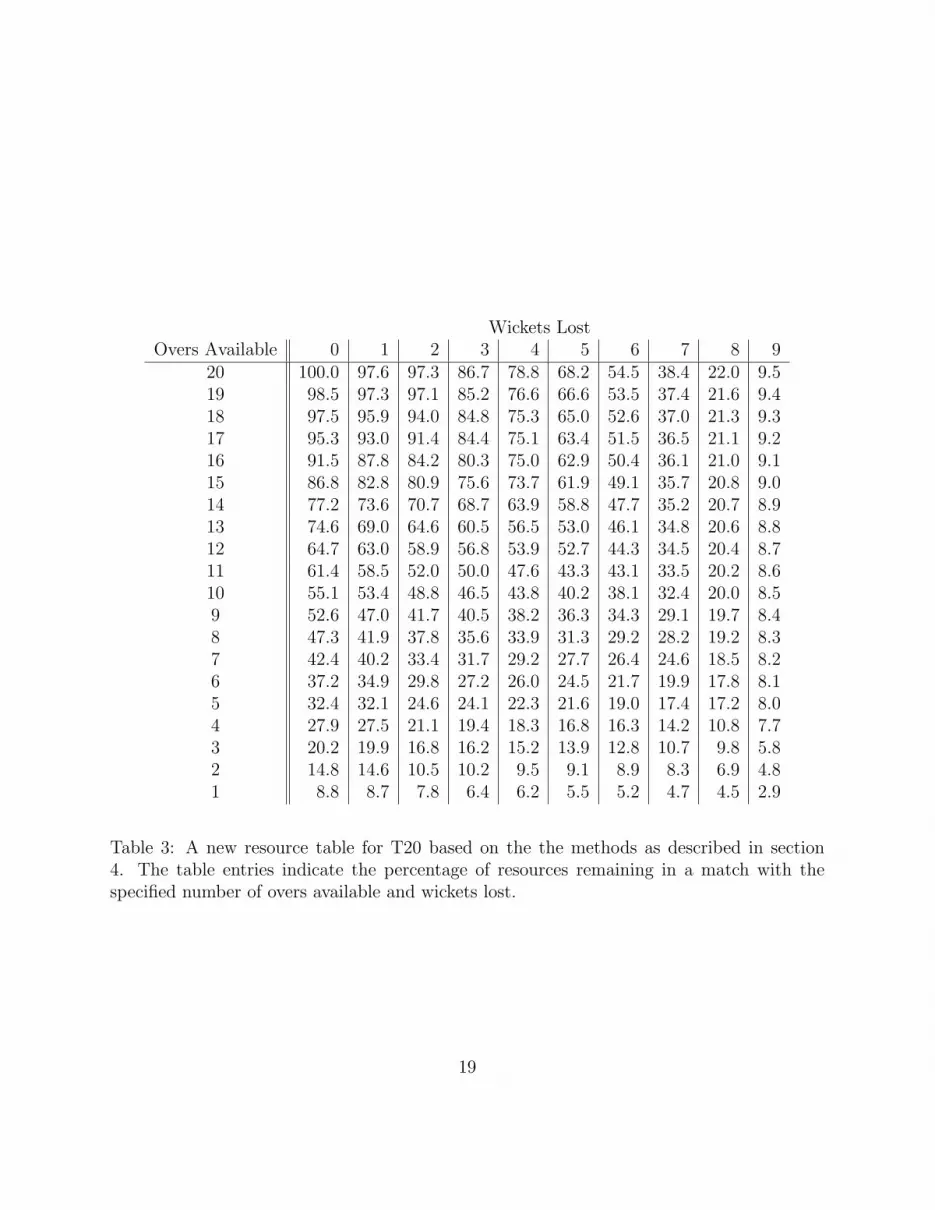
means of the θu,w leading to the resource table shown in Table 3. This required roughly 30

minutes of computation. To help facilitate the comparison between the Duckworth-Lewis

table 1 and the new Table 3, we refer to the heat map in Figure 1. The darkest shades of

the heat map represent changes of roughly 8%. As was found in the BGS implementation

(Table 2), our new Table 3 has the greatest differences when compared to Duckworth-Lewis

Table 1 along the main diagonal. In the upper-left corner, our resource table provides more

resources than Duckworth-Lewis. A possible explantion for this is that the upper-left corner

corresponds to the beginning of a match where batsmen are gaining familiarity with the

match conditions (i.e. the bowler, the pitch, the ball). Consequently, batsmen are more

cautious in the early parts of the match, and therefore few resources are utilized in this

part of the table. Recall that the Duckworth-Lewis table for T20 at this stage of a match

was mapped from the Duckworth-Lewis one-day table where 20 overs are available and

zero wickets are lost. In one-day cricket, this corresponds to a period of more aggressive

batting where the batsmen are comfortable. In the middle section of the diagonal, the new

resource Table 3 has fewer resources than the Duckworth-Lewis Table 1. This departure

from Duckworth-Lewis was also observed in Bhattacharya, Gill and Swartz (2010) and in

the BGS implementation of Section 3 leading to Table 2. Although the shading in the

lower-left hand corner of the heat map is not as intense as in the diagonal section, these

differences are meaningful and are worthy of comment. In the discussion, we look back at

12

matches where this section of the table was relevant. We see that the new resource Table 3

has more resources in the lower-left corner than does the Duckworth-Lewis Table 1. Finally,

we observe that the upper-right hand corner of the new resourse table is in accordance with

Duckworth-Lewis. This is an advantage of the new resource Table 3 over BGS (Table 3)

which gave non-sensical results in the upper-right hand corner.

5 DISCUSSION

Before looking at real examples, we emphasize again that there is now a sufficient number of

T20 matches to assess differences in the scoring patterns between one-day cricket and T20.

Moreover, unlike Duckworth-Lewis, the new methodology of section 4 leading to Table 3

does not make any parametric assumptions about resources. The methodology allows the

data to determine the cell entries. The methodology is also preferable to BGS in that it

takes into account the variability of individual matches.

We conclude our discussion with two examples where the application of Duckworth-Lewis

in T20 has been criticized.

England vs West Indies, June 15/09: England batted first and made 161 for 6 wickets

in 20 overs. After a rain interruption, the West Indies innings was reduced to 9 overs.

The Duckworth-Lewis method (Professional Edition) was used to reset the target to

80 runs. The West Indies achieved the target in 8.2 overs and the result was criticized

on the basis of the target being too low. Using the new table 3, the target would have

been 86 runs.

England vs West Indies, May 3/10: England batted first and made 191 for 5 wickets

in 20 overs. After a rain interruption, the West Indies innings was reduced to 6 overs.

The Duckworth-Lewis method (Professional Edition) was used to reset the target to

13

60 runs. The West Indies achieved the target in 5.5 overs and the result was again

criticized on the basis of the target being too low. Using the new table 3, the target

would have been 73 runs.

Finally, we state that our intention is not to supplant the Duckworth-Lewis method, but

to highlight its shortcomings in T20 cricket so that it can be improved upon from the point

of view of players, officials, and fans.

6 REFERENCES

Bhattacharya, R., Gill, P.S. and Swartz, T.B. (2010). Duckworth-Lewis and twenty20 cricket.

Journal of the Operational Research Society, doi: 10.1057/jors.2010.175.

Carter, M. and Guthrie, G. (2004). Cricket interruptus: fairness and incentive in limited overs

cricket matches. Journal of the Operational Research Society, 55: 822-829.

Christos, G.A. (1998). It’s just not cricket. In Mathematics and Computers in Sport (N. de Mestre

and K. Kumar, editors), Bond University, Queensland, Australia, pp 181-188.

Clarke, S.R. (1988). Dynamic programming in one-day cricket - optimal scoring rates. Journal of

the Operational Research Society, 39: 331-337.

Duckworth, F.C. and Lewis, A.J. (1998). A fair method for resetting targets in one-day cricket

matches. Journal of the Operational Research Society, 49: 220-227.

Duckworth, F.C. and Lewis, A.J. (2004). A successful operational research intervention in one-day

cricket. Journal of the Operational Research Society, 55: 749-759.

Gilks, W.R., Richardson, S. and Spiegelhalter, D.J. (editors) (1996). Markov Chain Monte Carlo

in Practice. Chapman and Hall: London.

14

Jayadevan, D. (2002). A new method for the computation of target scores in interrupted, limited

over cricket matches. Current Science, 83, 577-586.

Perera, H. (2011). A second look at Duckworth-Lewis in Twenty20 cricket. MSc project, Simon

Fraser University, Department of Statistics and Actuarial Science.

7 APPENDIX

We consider the estimation of ru,w in section 3. For ease of notation, we drop the subscript

u,w and let the index i = 1, . . . ,m denote the matches which pass through the stage of the

first innings where u overs are available and w wickets are lost. Further, let xi be the runs

scored from that juncture in the ith match until the end of the first innings, let yi be the

total first innings runs in the ith match, and let zj be the total first innings runs in the jth

match, j = 1, . . . , n − m where the index j corresponds to the remaining matches in the

dataset. The data are of the form x1

y1

, . . . , xm

ym

iid

with E(xi) = µ1, Var(xi) = σ21, E(yi) = µ2, Var(yi) = σ2

2 and Cov(xi, yi) = σ12. We assume

that the correlation

σ12

σ1σ2

> 1/2 (6)

reflecting the tendency that high (low) scoring matches are typically high (low) scoring

throughout the match. In addition, there are independent data

z1, . . . , zn−m iid

with E(zj) = µ2 and Var(zj) = σ22.

15

Using the above notation, the BGS estimator takes the form

rBGS/100% =

∑mi=1 xi/m(∑m

i=1 yi +∑n−mj=1 zj

)/n

=x(

mn

)y +

(n−mn

)z

(7)

and the new estimator takes the form

rnew/100% =

∑mi=1 xi/m∑mi=1 yi/m

=x

y. (8)

An application of the delta method to the expressions (7) and (8) then gives

Var(rBGS/100%) ≈ σ21

mµ22

− 2µ1σ12

nµ32

+µ2

1σ22

nµ42

and

Var(rnew/100%) ≈ σ21

mµ22

− 2µ1σ12

mµ32

+µ2

1σ22

mµ42

.

Now suppose that the variability in runs scored is roughly proportional to the number of

expected runs scored (i.e. σ1/σ2 ≈ µ1/µ2). Then

Var(rBGS/100%)− Var(rnew/100%) ≈ (n−m)µ1

mnµ32

(2σ12 − µ1σ2

2

µ2

)≈ (n−m)µ1

mnµ32

(2σ12 − σ1σ2)

> 0

using the correlation assumption (6). Hence the estimator rnew is preferred over rBGS in

terms of variability.

To investigate the suitability of assumption (6), we calculated the sample correlation

coefficient between x and y for various combinations of u and w. Specifically, we chose

u = 15, 14, . . . , 6 to assess the “middle” stages of a match. The corresponding value of w for

a particular u is the value for which the sample size m is greatest. The respective sample

correlations are 0.45, 0.50, 0.57, 0.62, 0.59, 0.66, 0.58, 0.80, 0.79 and 0.82 which tend to exceed

0.5. Hence, there is evidence that assumption (6) is sensible.

16

Wickets LostOvers Available 0 1 2 3 4 5 6 7 8 9

20 100.0 96.8 92.6 86.7 78.8 68.2 54.4 37.5 21.3 8.319 96.1 93.3 89.2 83.9 76.7 66.6 53.5 37.3 21.0 8.318 92.2 89.6 85.9 81.1 74.2 65.0 52.7 36.9 21.0 8.317 88.2 85.7 82.5 77.9 71.7 63.3 51.6 36.6 21.0 8.316 84.1 81.8 79.0 74.7 69.1 61.3 50.4 36.2 20.8 8.315 79.9 77.9 75.3 71.6 66.4 59.2 49.1 35.7 20.8 8.314 75.4 73.7 71.4 68.0 63.4 56.9 47.7 35.2 20.8 8.313 71.0 69.4 67.3 64.5 60.4 54.4 46.1 34.5 20.7 8.312 66.4 65.0 63.3 60.6 57.1 51.9 44.3 33.6 20.5 8.311 61.7 60.4 59.0 56.7 53.7 49.1 42.4 32.7 20.3 8.310 56.7 55.8 54.4 52.7 50.0 46.1 40.3 31.6 20.1 8.39 51.8 51.1 49.8 48.4 46.1 42.8 37.8 30.2 19.8 8.38 46.6 45.9 45.1 43.8 42.0 39.4 35.2 28.6 19.3 8.37 41.3 40.8 40.1 39.2 37.8 35.5 32.2 26.9 18.6 8.36 35.9 35.5 35.0 34.3 33.2 31.4 29.0 24.6 17.8 8.15 30.4 30.0 29.7 29.2 28.4 27.2 25.3 22.1 16.6 8.14 24.6 24.4 24.2 23.9 23.3 22.4 21.2 18.9 14.8 8.03 18.7 18.6 18.4 18.2 18.0 17.5 16.8 15.4 12.7 7.42 12.7 12.5 12.5 12.4 12.4 12.0 11.7 11.0 9.7 6.51 6.4 6.4 6.4 6.4 6.4 6.2 6.2 6.0 5.7 4.4

Table 1: The Duckworth-Lewis resource table (Standard Edition) scaled for T20. The tableentries indicate the percentage of resources remaining in a match with the specified numberof overs available and wickets lost.

17

Wickets LostOvers Available 0 1 2 3 4 5 6 7 8 9

20 100.0 98.6 96.9 93.7 83.9 73.8 60.1 45.4 29.1 18.119 98.2 96.7 95.4 91.6 80.6 70.4 56.7 42.9 26.6 15.818 95.3 93.4 91.9 90.4 78.5 68.3 54.6 41.3 25.2 14.517 91.1 88.3 85.7 82.4 77.1 66.6 52.6 40.1 24.0 13.416 86.3 83.3 80.6 77.6 73.3 65.3 50.8 39.0 23.1 12.515 81.6 78.5 75.9 73.0 69.3 64.4 49.0 38.1 22.1 11.714 77.0 73.9 71.3 68.5 65.3 61.2 47.2 37.1 21.3 11.013 72.8 69.6 66.8 64.2 61.2 56.9 45.2 36.2 20.4 10.312 68.4 65.3 62.7 60.1 57.1 52.8 43.1 35.4 19.5 9.711 64.0 60.9 58.3 55.8 52.7 48.5 40.7 34.6 18.5 9.110 59.2 56.1 53.6 51.3 48.2 43.9 38.3 33.9 17.6 8.59 54.7 51.7 49.2 46.9 43.8 40.0 35.9 33.2 16.6 7.88 50.1 47.2 44.7 42.5 39.7 36.2 32.7 29.1 15.5 7.17 45.6 42.5 40.2 38.0 35.5 32.2 28.8 24.2 14.2 6.46 40.5 37.5 35.3 33.2 31.1 28.4 24.8 20.4 12.4 5.55 32.8 31.0 29.3 27.6 25.8 23.7 20.8 16.9 10.7 4.64 29.1 26.5 24.8 23.1 21.3 19.3 16.9 13.5 8.8 3.83 23.3 20.1 18.9 17.6 16.4 14.8 12.9 10.1 6.7 2.82 17.3 14.1 13.2 12.2 11.2 10.1 8.7 6.9 4.4 1.81 10.0 6.1 5.7 5.3 4.8 4.3 3.7 2.9 1.9 0.8

Table 2: A resource table for T20 based on a slight modification of the methods of BGS asdescribed in section 3. The table entries indicate the percentage of resources remaining in amatch with the specified number of overs available and wickets lost.

18

Wickets LostOvers Available 0 1 2 3 4 5 6 7 8 9

20 100.0 97.6 97.3 86.7 78.8 68.2 54.5 38.4 22.0 9.519 98.5 97.3 97.1 85.2 76.6 66.6 53.5 37.4 21.6 9.418 97.5 95.9 94.0 84.8 75.3 65.0 52.6 37.0 21.3 9.317 95.3 93.0 91.4 84.4 75.1 63.4 51.5 36.5 21.1 9.216 91.5 87.8 84.2 80.3 75.0 62.9 50.4 36.1 21.0 9.115 86.8 82.8 80.9 75.6 73.7 61.9 49.1 35.7 20.8 9.014 77.2 73.6 70.7 68.7 63.9 58.8 47.7 35.2 20.7 8.913 74.6 69.0 64.6 60.5 56.5 53.0 46.1 34.8 20.6 8.812 64.7 63.0 58.9 56.8 53.9 52.7 44.3 34.5 20.4 8.711 61.4 58.5 52.0 50.0 47.6 43.3 43.1 33.5 20.2 8.610 55.1 53.4 48.8 46.5 43.8 40.2 38.1 32.4 20.0 8.59 52.6 47.0 41.7 40.5 38.2 36.3 34.3 29.1 19.7 8.48 47.3 41.9 37.8 35.6 33.9 31.3 29.2 28.2 19.2 8.37 42.4 40.2 33.4 31.7 29.2 27.7 26.4 24.6 18.5 8.26 37.2 34.9 29.8 27.2 26.0 24.5 21.7 19.9 17.8 8.15 32.4 32.1 24.6 24.1 22.3 21.6 19.0 17.4 17.2 8.04 27.9 27.5 21.1 19.4 18.3 16.8 16.3 14.2 10.8 7.73 20.2 19.9 16.8 16.2 15.2 13.9 12.8 10.7 9.8 5.82 14.8 14.6 10.5 10.2 9.5 9.1 8.9 8.3 6.9 4.81 8.8 8.7 7.8 6.4 6.2 5.5 5.2 4.7 4.5 2.9

Table 3: A new resource table for T20 based on the the methods as described in section4. The table entries indicate the percentage of resources remaining in a match with thespecified number of overs available and wickets lost.

19

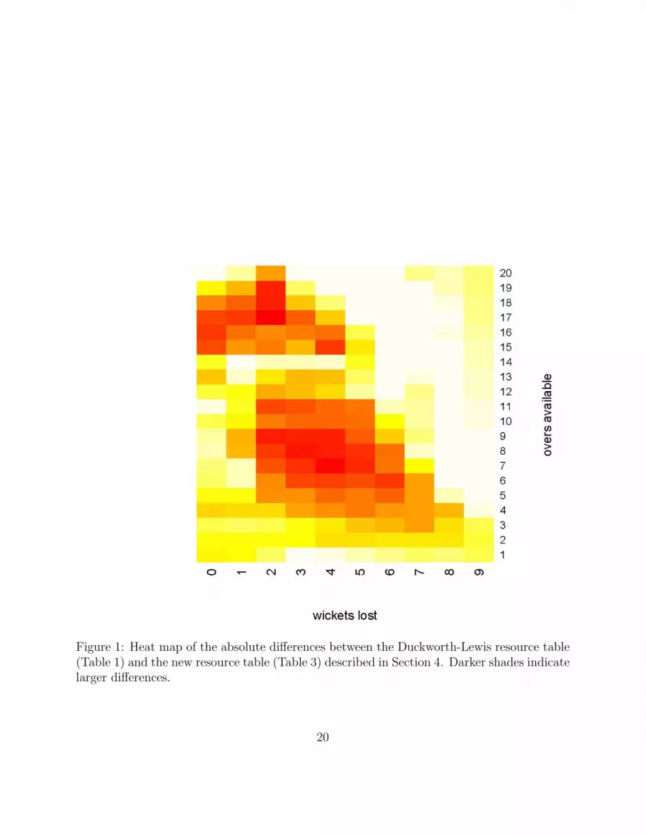
Figure 1: Heat map of the absolute differences between the Duckworth-Lewis resource table(Table 1) and the new resource table (Table 3) described in Section 4. Darker shades indicatelarger differences.

20