Reset–Driven Fault Tolerance

Joao Carlos Cunha12, Antonio Correia2, Jorge Henriques2,Mario Zenha Rela2, and Joao Gabriel Silva2

1 Dep. Eng. Informatica e Sistemas, Instituto Superior de Engenharia de Coimbra,3030 Coimbra, Portugal

jcunha@isec.pt2 CISUC/Dep. Eng. Informatica, Universidade de Coimbra,

3030 Coimbra, Portugal{scorreia, jh, mzrela, jgabriel}@dei.uc.pt

Abstract. A common approach in embedded systems to achieve fault--tolerance is to reboot the computer whenever some non-permanent erroris detected. All the system code and data are recreated from scratch, anda previously established checkpoint, hopefully not corrupted, is used torestart the application data. The confidence is thus restored on the ac-tivity of the computer. The idea explored in this paper is that of uncon-ditionally resetting the computer in each control frame (the classic readsensors → calculate control action → update actuators cycle). A stable--storage based in RAM is used to preserve the system’s state betweenconsecutive cleanups and a standard watchdog timer guarantees that areset is forced whenever an error crashes the system. We have evaluatedthis approach by using fault-injection in the controller of a standard tem-perature control system. The experimental observations show that theReset–Driven Fault Tolerance is a very simple yet effective technique toimprove reliability at an extremely low cost since it is a conceptuallysimple, software only solution with the advantage of being applicationindependent.

1 Introduction

The correct functioning of embedded computing systems is essential to moderncivilization. We depend on a myriad of embedded computing devices from chipsinside credit cards and mobile phones, to automatic teller machines (ATM’s) andtraffic controllers. We can now carry our medical record in a credit card-like me-dia or use contactless tickets in public transportation services. A digital camerahas now more memory and processing power than a five-year-old desktop com-puter. Luxury cars carry a full network linking some tens of microcontrollers tohandle from comfort to safety-critical features such as ABS. Everywhere we canfind an embedded system that silently fulfils its role in our technologically drivensocieties.† This work was partially supported by the Portuguese Foundation for Science

and Technology under the POSI programme and the FEDER programme ofthe European Union, through the R&D Unit 326/94 (CISUC) and the projectPRAXIS/P/EEI/10205/1998 (CRON).

The need for fault-tolerance in such small embedded computing systems isdemanding due its growing importance. However, such systems pose a formidablechallenge to dependability: they are a case on their own due their small dimen-sions, low power available, trimmed-down hardware and the mandatory require-ment to maintain costs low. Any additional cent in consumer electronic devicesmay prevent a product economic feasibility. Therefore, the use of hardware re-dundancy is not an option.

The main class of computer faults are transients: voltage fluctuations, elec-tromagnetic interference, heat, moisture, all contribute to the generation of suchfaults. Only a minority of faults are permanent, thus the common approachof “fixing” most computing systems by simply resetting them. Such transientmisbehavior can also be attributable to the software, namely unexpected inter-actions between correct modules or unexpected inputs from its environment. Itis virtually impossible to identify clearly if a transient fault has been caused byhardware or software. Nevertheless, what is clear is that the number of tran-sients is much larger than permanent failures and its share is rising due to theincreasing complexity of software and the smaller geometries and lower powerlevels of integrated circuits [15], [17].

In this paper we propose a novel approach that provides a simple and yet veryeffective solution for this class of applications: by resetting systematically thecomputer to flush any latent errors from it’s internal state, we guarantee a statecleanup before every new control cycle is started. The main memory is used as astable-storage medium to preserve the relevant data across reset boundaries. Thisapproach avoids the need to pack a delicate and complex set of fault-tolerancetechniques into resource scarce computing systems. It is a very low cost solutionsince it is a conceptually simple software-only operation. Moreover, it is notapplication dependent. Some studies on software rejuvenation [8] have a similarapproach to deal with software aging. When software continuously executes forlong time, some error conditions such as memory leaks, memory fragmentation,broken pointers, missing scheduling deadlines, etc., accumulate and eventuallylead to system failure. This approach involves resetting the system periodicallyand then starting with clean internal states, thus flushing latent software errors.

This paper is organized as follows: in the next section, we discuss how thetraditional fault-tolerance approaches are applicable to small embedded comput-ing systems. In section 3, the details of using Reset–Driven fault tolerance arepresented. In section 4, the results from the experimental evaluation of this ap-proach through fault-injection are presented and discussed. The paper concludeswith an overview of the proposed technique and discussion of the work currentlyunderway.

2 Fault-Tolerance in a Resource Scarce Environment

Redundancy is the key to achieve fault-tolerance. If systems had strictly theresources required to fulfill their intended functional goals, they could not handlethe additional tasks required to cope with the abnormal circumstances that result

from the occurrence of faults. Redundancy can be hardware, software or time. Insmall scale systems there is a short supply of any of them: due to the economic,space and power constraints hardware cannot be added, software uses scarceRAM, FLASH-RAM or ROM silicon space. Depending on the application, timemay be the only slack resource available; due to the physical-world inertia thesesystems spend most of their time idle. Slow clock rates are mandatory wheneverpower consumption is critically restricted such as in mobile devices. Nevertheless,at least a minimum hardware redundancy devoted to fault-tolerance is required:in case a permanent fault occurs, the system should be brought into a safe-state (if one exists), so that at least its outputs do not produce random ordangerous results: in furnaces the heating is turned off, elevators automaticallygo down to the nearest floor, valves in tanks are seldom left unchanged, andalarms are set. In case of failure, the outputs are brought to these default values.A “redundant” hardware component that can be found in every controller systemis the ubiquitous watchdog timer. This is a timer set to trigger a reset on thetarget controller if it is not refreshed in a predefined time interval. This lastresort mechanism detects system hang-ups.

Software redundancy can also be used to detect the occurrence of errors ifthe system is able to continue after recovery and/or reconfiguration. However,traditional software techniques such as recovery blocks [13] and N-version [2] areinadequate to handle hardware transients: there is no need to have alternate ormulti-version code since the software is assumed correct. Moreover, budgetaryconstraints as well as memory-size limitations prevent such approaches: they areusually reserved for high critical applications. For the class of systems under con-sideration, software correctness is assumed since the applications are normallynot very demanding.

The designer or even the system at run-time can also use a measure of qualityof service to trade-off hardware or software redundancy vs. time [9]. Instead ofhaving extra space resources to recover from an error in time to produce thecorrect result, it may produce an imprecise result in a fast way (e.g. simplymaintaining the previous result) while recovering. In face of the above-referredconstraints, in practice small embedded systems are restricted to use behavioralerror detection mechanisms such as checking the reasonableness of the resultsproduced or coding checks (CRC’s, checksums, parity). These are low overheadtechniques that pay off the error coverage they provide. It is in such resourcescarce environments that the Reset–Driven fault tolerance (RDFT) approach,described in the next section, can best be applied.

3 Reset–Driven Fault Tolerance

We illustrate the RDFT approach using a real-time control system applicationas example. This is because if RDFT can handle the constraints of such systemsit can also be applied to a broader class of applications. However, it must beclear that some characteristics of continuous control systems may not apply todiscrete applications. We shall discuss such differences where applicable.

3.1 System Model

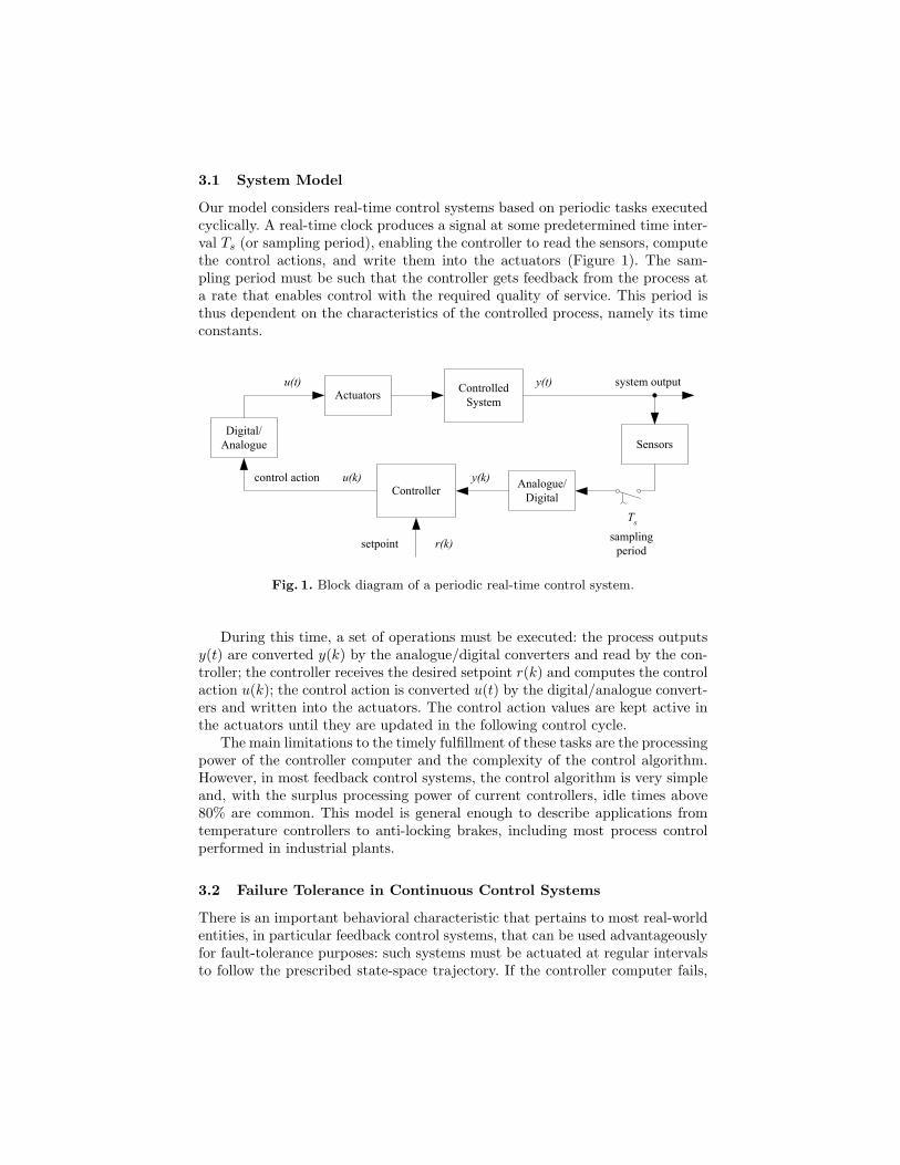
Our model considers real-time control systems based on periodic tasks executedcyclically. A real-time clock produces a signal at some predetermined time inter-val Ts (or sampling period), enabling the controller to read the sensors, computethe control actions, and write them into the actuators (Figure 1). The sam-pling period must be such that the controller gets feedback from the process ata rate that enables control with the required quality of service. This period isthus dependent on the characteristics of the controlled process, namely its timeconstants.

ControlledSystem

Controller

Actuators

Sensors

Analogue/Digital

Digital/Analogue

system outputy(t)

y(k)

r(k)

u(k)

Ts

u(t)

setpoint samplingperiod

control action

Fig. 1. Block diagram of a periodic real-time control system.

During this time, a set of operations must be executed: the process outputsy(t) are converted y(k) by the analogue/digital converters and read by the con-troller; the controller receives the desired setpoint r(k) and computes the controlaction u(k); the control action is converted u(t) by the digital/analogue convert-ers and written into the actuators. The control action values are kept active inthe actuators until they are updated in the following control cycle.

The main limitations to the timely fulfillment of these tasks are the processingpower of the controller computer and the complexity of the control algorithm.However, in most feedback control systems, the control algorithm is very simpleand, with the surplus processing power of current controllers, idle times above80% are common. This model is general enough to describe applications fromtemperature controllers to anti-locking brakes, including most process controlperformed in industrial plants.

3.2 Failure Tolerance in Continuous Control Systems

There is an important behavioral characteristic that pertains to most real-worldentities, in particular feedback control systems, that can be used advantageouslyfor fault-tolerance purposes: such systems must be actuated at regular intervalsto follow the prescribed state-space trajectory. If the controller computer fails,

it produces wrong, late or missing control actions. However, since feedback con-trol algorithms are designed to compensate for external disturbances that thecontrolled process may suffer, many of the wrong control actions are also com-pensated for by those algorithms so that no particular fault-tolerance mechanismis needed to handle them. This is possible because the controlled process does notcollapse instantaneously due to its physical inertia (mechanical, chemical, etc.),giving the algorithm time to recover. This inertia, known as grace-time[10], isnot an exceptional behavior, but rather an intrinsic characteristic of a large num-ber of physical systems. In [5] and [16] it has been showed that feedback controlalgorithms can indeed compensate for many computer malfunctions, not justdisturbances affecting the controlled process. The fail-silent model [11] wouldflag as failures very many situations where the system in fact does not sufferany negative impact at all. Essentially, for these types of systems, the fail-silentmodel lacks the notion of time (a single erroneous controller output is not sig-nificant, only a sequence of erroneous outputs is) and fails to take into accountthe fact that the natural inertia of the controlled process filters out short-liveddisturbances. If we are able to do a quick recover from a controller failure, avoid-ing a long sequence of erroneous control actions, there is a high probability thatthe system could tolerate such controller failure. It must be clear, however, thatthis grace-time is heavily application dependent and can only be used accordingto the dynamics of the physical system under control.

Whenever we are not dealing with a continuous application, this “error filter-ing” by the application may not apply. For example, the control of a bottle-fillingconveyor is clearly event driven. What matters is whether a bottle is between twosensors, whether the conveyor is moving or not, etc. Fortunately, discrete-eventapplications have their own characteristics that heavily simplify the error detec-tion. Such event-driven systems are modeled by state transitions, so a state-flowchecking can easily detect wrong paths/transitions performed (the destinationstate can always check whether it has been correctly reached). In fact, suchsystems are usually programmed as a large transition table whose correctnesscan be dynamically checked. Thus, while discrete applications are distinct fromcontinuous applications, that does not prevent the use of the RDFT approach.Another point to be stressed is that in many applications the process state isoften irrelevant. All that matters is the data state: given the appropriate inputsand a piece of code the computing system can produce the correct outputs. Insuch systems the data state, not the process state is the critical asset to be pre-served from faults. This reasoning does not apply only to transactional systems,but also to many real-time applications. An example: in a running vehicle thethrottle control task may be killed and restarted. As long as the restarted taskcan access its predecessor’s state and the throttle valve output follows the pre-scribed state trajectory, it is not relevant whether a task or its clone is running.

3.3 Periodic Controller Reset

The previous sections show that: i) in most systems the only available resourcemay be time; ii’) a continuous process physical inertia can be used to filter

transient erroneous or missing outputs from the controller as long as correctcontrol is resumed shortly, or ii”) the discrete nature of an application providesan effective reasonableness check; and iii) the data state is often the relevantasset to be preserved from faults.

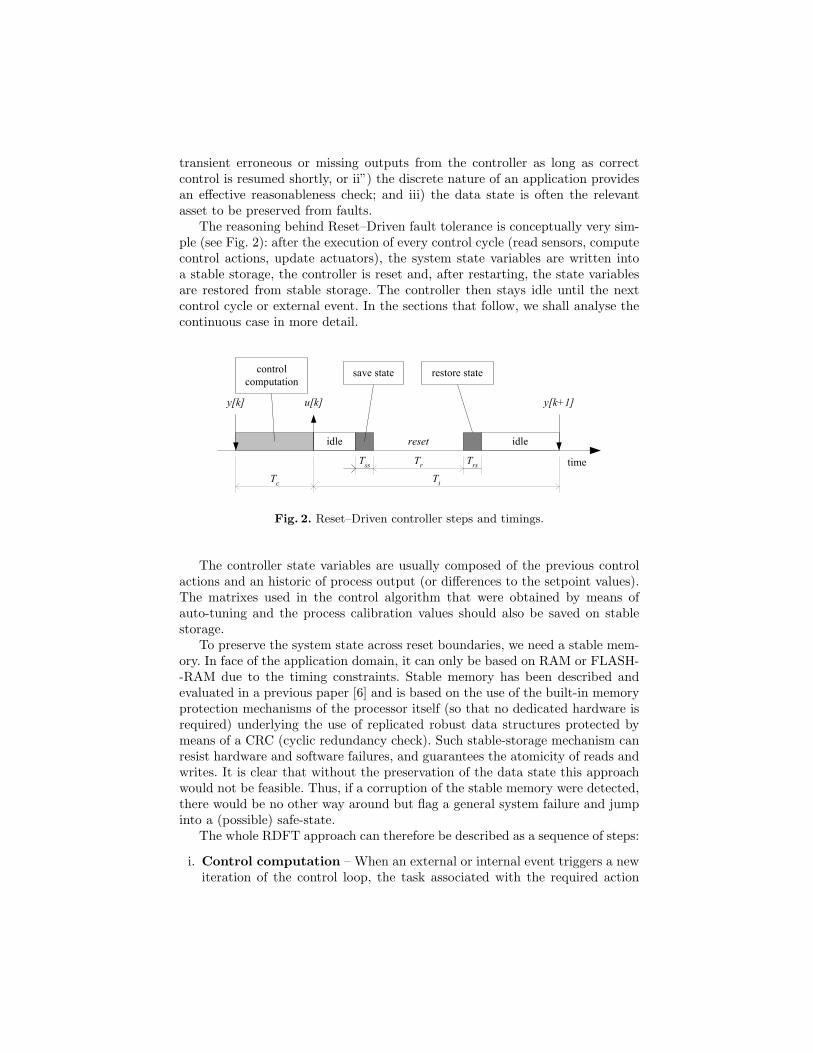
The reasoning behind Reset–Driven fault tolerance is conceptually very sim-ple (see Fig. 2): after the execution of every control cycle (read sensors, computecontrol actions, update actuators), the system state variables are written intoa stable storage, the controller is reset and, after restarting, the state variablesare restored from stable storage. The controller then stays idle until the nextcontrol cycle or external event. In the sections that follow, we shall analyse thecontinuous case in more detail.

idle

y[k] y[k+1]u[k]

controlcomputation

time

reset

save state restore state

Tc

TrTssTi

Trs

idle

Fig. 2. Reset–Driven controller steps and timings.

The controller state variables are usually composed of the previous controlactions and an historic of process output (or differences to the setpoint values).The matrixes used in the control algorithm that were obtained by means ofauto-tuning and the process calibration values should also be saved on stablestorage.

To preserve the system state across reset boundaries, we need a stable mem-ory. In face of the application domain, it can only be based on RAM or FLASH--RAM due to the timing constraints. Stable memory has been described andevaluated in a previous paper [6] and is based on the use of the built-in memoryprotection mechanisms of the processor itself (so that no dedicated hardware isrequired) underlying the use of replicated robust data structures protected bymeans of a CRC (cyclic redundancy check). Such stable-storage mechanism canresist hardware and software failures, and guarantees the atomicity of reads andwrites. It is clear that without the preservation of the data state this approachwould not be feasible. Thus, if a corruption of the stable memory were detected,there would be no other way around but flag a general system failure and jumpinto a (possible) safe-state.

The whole RDFT approach can therefore be described as a sequence of steps:

i. Control computation – When an external or internal event triggers a newiteration of the control loop, the task associated with the required action

starts its execution, by reading any inputs (e.g. from the process sensors).The system converts these values into a usable format (e.g. from a 12-bitformat into a floating-point), and executes the code associated with theaction to be performed, by making use of any additional internal data (e.g.the previous iteration state). The result is again converted to a suitableformat (e.g. 12-bit format) and sent to the actuators.

ii. Save state – The state variables and any constants that were initialised inrun-time (e.g. during process calibration or self-tuning) are written into astable storage.

iii. Reset – The controller reset may be triggered either by software or by hard-ware. In the first case the control software makes a call to a reset procedure.If the controller fails by hanging and delays its restart, the watchdog timereventually resets the system. This guarantees that in any case the reset willbe applied and that the system will be ready for the next control iteration.As is clear, the hardware reset period must be synchronized with the controlloop, in order not to reset the controller while it is executing the controlcomputation.Two different reset types can be applied: hot or cold reset. In a cold reset, thecomputer system is fully restarted and all data is initialised. The computeris brought to the same state as in a normal power up. In a hot reset, thesystem just refreshes the code and data, and starts executing from the systemstarting point. Code and data refreshing can be made by copying their imagefrom a fixed memory location or another non-volatile memory into RAM,while checking its integrity by checksumming. In either case, the controllersystem needs to distinguish a refreshing reset from an error-induced reset orfrom the initial power-up, i.e. if it is in control of a process. This can be doneby storing an identifier (“magic number”) at a known address in non-volatilestorage, such as the CMOS memory in the computer boards where the BIOSstores configuration data.

iv. Reboot and restore state – After restarting, the system restores all datastructures from stable storage and the watchdog timer is initialized. It thendetects that a refreshing reset has happened and becomes idle until a newiteration begins. This idle time can be spent either in a low-power mode orused to run diagnosis tests.

v. Error-induced reset – In the case that an error is detected by the intrinsicerror-detection mechanisms (e.g. a processor or operating system exception),the system is immediately reset, either hot or cold. If the system hangs, thewatchdog timer triggers the reset. It then follows the previously explainedsteps to reboot and restore state. However, when it detects that this is nota refreshing reset, it restarts immediately the control computation. If thecontrol action from the previous iteration has already been sent to the actu-ators, the controlled process would probably receive two control actions inthe same sampling period. If not, the process would probably receive the con-trol action from the current sampling period later than usual. In either case,this sporadic situation does not usually induce any meaningful disturbancesto the controlled process.

This last description deserves an additional comment: we are consenting acontroller to fail, either by outputting an erroneous value or by disrespectingthe time constraints. However, for embedded control systems, the distinctionbetween the computer and the application is somehow blurred, since none canbe though without the other. This means that the pair controller + controlledprocess should not be viewed separately. Thus, we should only consider as afailure an error that is observable outside of this pair (e.g. the driver feels thatthe engine is not running smoothly). In fact, for a large number of embeddedapplications, internal errors are not observable so, for every practical purpose,they never occurred.

If an error occurs during reset, it may abort and be restarted again, in whichcase the error is flushed; the system cannot hang since the WDT is always active.On the other hand, the system may restart in an erroneous state, maybe withlatent errors. This situation is not different from a “typical” latent error: it willbe either detected by the integrity checks or flushed in the next reset. Wheneversuch an error is detected, the system is restarted immediately. If errors leadto successive restarts, we are in the presence of permanent faults to which thisapproach is not adequate (e.g. if the error corrupts the code or data image).Anyway, as long as the error does not generate a new output, the previous valuesare maintained. Of course, the outputs can always be brought into a default safe--state through dedicated hardware if the criticality of the application requiresit.

3.4 Timing Analysis

The proposed approach requires that there is enough time to reset and restartthe controller. Considering the sampling period Ts and the computation time Tc,the system stays idle for Ti = Ts − Tc in every control cycle. The Reset–Drivenapproach can thus be used if the time to reset the controller (Tr) plus the timeto save (Tss) and restore (Trs) the system state fits within the idle time, that is:

Tr + Tss + Trs < Ts − Tc (1)

– The sampling period (Ts) depends upon the time constants of the con-trolled process. A time constant is a measure of the time taken by the con-trolled process to respond to a change in input or load [3].

– The computation time (Tc) is dependent on the performance of the pro-cessing unit and on the complexity of the control algorithm. Control algo-rithms for feedback control systems are often based on PID (Proportional,Integral and Derivative) algorithms, due to its ability to control almost anysort of linear physical processes. This control algorithm usually consists on afew lines of code in a high-level language. It is thus very common to have alarge fraction of processing time being used by the idle task or in low-powermode. Discrete applications, represented by a set of state-machines are evenless demanding in processing power since such systems states are usuallyprogrammed through a simple table lookup.

– The time to save and to restore the system state variables (Tss, Trs)does not usually represent a significant amount of time, since state variablesnormally sum up to a few tens of bytes. In real-time embedded systems itis unthinkable to use any sort of disk based stable storage, and thus data isstored in non-volatile memory, like battery-backup RAM, or FLASH-RAM.

– The time to reset the controller (Tr) is mainly dependent on the timefor integrated circuits to reset. The advantage of using a hot instead of acold restart derives from this physical constraint. By using a hot restart, weachieved a restart time (Tr) of about 50 milliseconds on a standard PC.

On error-free situations, the control action is sent to the actuators after Tc

time from the start of the control iteration. If an error occurs and causes an error-induced reset, the control action sent to the process after restart may presentdifferent timings:

– If the reset occurs before the control action from the current iteration hasbeen sent to the actuators (i.e., occurs before the end of Tc), then the con-trol action is output within a maximum delay from the start of the controliteration of Tc + Tr + Trs + Tc . If this time exceeds the sampling period Ts,then the current iteration failed to update the process actuators, and thusthe control action from the previous iteration is still valid to the process.As already explained, this situation does not usually cause any significantdisturbance to the system.

– If the reset occurs after the control action from the current iteration hasbeen sent to the actuators (i.e., occurs after the end of Tc), then if thecontroller is able to restart and recalculate the control action before thefollowing iteration ((reset moment+Tr +Trs +Tc < Ts), the process wouldreceive two control actions in the same cycle. If not, the process would receivethe control action in the following iteration, with a maximum delay from thestart of the iteration of Tr +Trs+Tc (this is the case when the error occurs atthe very last moment in the control cycle). In these situations, an erroneouscontrol action could have been delivered to the process. Again, this sporadiccontroller failure is usually tolerated by the system.

4 Experimental Validation

We have used a physical process and a PC-based controller to validate the Reset-–Driven control approach. We have prepared the controller to reset in everycontrol cycle and injected a comprehensive set of hardware transient faults inthe main functional units of the CPU and in memory. The physical processchosen was a hot-air blower, a standard thermal control process widely used incontrol systems research and education.

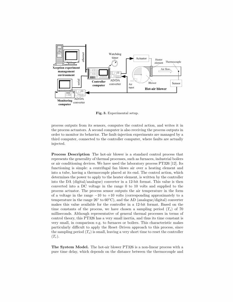
4.1 The Experimental Setup

The main elements of our experimental setup are depicted in Fig. 3. The hot-airblower process is being controlled by a controller computer that receives the

AD/DAconverter

AD/DAconverter

Xception experimentmanagementenvironment

Monitoringcomputer

ethe

rnet

seria

l

Air flow

Hot-air blowerSensor

ThermocoupleHeaterelement

BlowerAirinput

Watchdogtimer Actuator

Controllercomputer

Fig. 3. Experimental setup.

process outputs from its sensors, computes the control action, and writes it inthe process actuators. A second computer is also receiving the process outputs inorder to monitor its behavior. The fault-injection experiments are managed by athird computer, connected to the controller computer, where faults are actuallyinjected.

Process Description The hot-air blower is a standard control process thatrepresents the generality of thermal processes, such as furnaces, industrial boilersor air conditioning devices. We have used the laboratory process PT326 [12]. Itsfunctioning is simple: a centrifugal fan blows air over a heating element andinto a tube, having a thermocouple placed at its end. The control action, whichdetermines the power to apply to the heater element, is written by the controllerinto the DA (digital/analogue) converter in a 12-bit format. This value is thenconverted into a DC voltage in the range 0 to 10 volts and supplied to theprocess actuator. The process sensor outputs the air temperature in the formof a voltage in the range −10 to +10 volts (corresponding approximately to atemperature in the range 26◦ to 60◦C), and the AD (analogue/digital) convertermakes this value available for the controller in a 12-bit format. Based on thetime constants of the process, we have chosen a sampling period (Ts) of 70milliseconds. Although representative of general thermal processes in terms ofcontrol theory, this PT326 has a very small inertia, and thus its time constant isvery small, in comparison e.g. to furnaces or boilers. This characteristic makesparticularly difficult to apply the Reset–Driven approach to this process, sincethe sampling period (Ts) is small, leaving a very short time to reset the controller(Tr).

The System Model. The hot-air blower PT326 is a non-linear process with apure time delay, which depends on the distance between the thermocouple and

the heating element, and on the air flow rate. The process can be described as afirst order system by the following equation:

y(k) = a.y(k − 1) + b.u(k − d) (2)

where y(k) is the system output at discrete time k, u(k) is the the input,a and b are constants that characterize the process and d is the time delay insampling periods. We have used a traditional PID control algorithm, since thiskind of control is widely used due to its simplicity and ability to regulate mostindustrial processes with dissimilar specifications. A PID controller is describedby the following equation:

u(k) = u(k1) + q0.e(k) + q1.e(k1) + q2.e(k2) (3)

where e(k) is the control error, defined by the difference between the refer-ence and the process output (e(k) = r(k) − y(k)), and q0, q1 and q2 are thePID parameters. In our experiments, we have used q0 = 0.17, q1 = 0.09, andq2 = 0.002, obtained by means of a pole placement method [1].

The Controller Computer. The controller computer is a standard 90MHzIntel Pentium based PC-board with 8M of RAM. The control application is run-ning on top of SMX c© (Simple Multitasking Executive) [14], a COTS real-timekernel from Micro Digital, Inc. If any error is detected by the intrinsic errordetection mechanisms of the system, such as processor exceptions or operatingsystem checks, the normal procedure is to immediately reset the system. A stan-dard watchdog timer card is responsible to reset the system if it hangs. We havemeasured the time (Tc) to read the input ports from the AD/DA card, calculatethe control action and write the results into the output ports of the same card,and got values no greater than 1.5 milliseconds (input and output took most ofthis time).

Stable Storage. We have used a RAM-based stable storage [6] to collect thedata that should survive resets. This data is composed of the state variables fromthe control algorithm, the process status, the setpoint generator, and on constantvalues obtained from the process calibration. If the control matrixes were ob-tained by means of self-tuning (which is not the case in our experiments), theseshould also be saved on stable storage. Nevertheless, we have also saved them.In total, we have placed 120 bytes of data in stable storage. Every data structurewritten in stable storage has a 16-bit CRC appended to it. Our stable storagemechanism follows each write with a simple correctness verification: the CRC isrecalculated and, if wrong, the write is repeated. Writes are also performed in anatomic way, by using two separated memory regions. Only after the write in thefirst memory region succeeds, a copy of the data is written in the second mem-ory region and checked again. Only then does the write to the stable memorycommit. At each system restart following a reset, data is recovered from stablestorage and, if any corruption is detected by means of the CRC verification, it

is alternatively recovered from the copy in the second memory region. The timeto save the system state variables (Tss) was measured to be no greater than 200microseconds, and the time to restore the system state variables (Trs) was lessthan 450 microseconds.

Controller Reset. From the above measurements and calculations, we haveobtained the following figures for our system: the sampling period (Ts) is 70milliseconds, the maximum computation time (Tc) is 1.5 milliseconds, and themaximum time to save and restore the system state variables (Tss and Trs) is,respectively, 0.2 and 0.45 milliseconds. This means, from Equation (1), that wehave a maximum time to reset the system (Tr) of 67.85 milliseconds. Some PChardware components have long reset delays, well above 100 milliseconds, whichmake cold reset unfeasible in our system. We have thus adopted the hot resetapproach in this target system. The reset may be triggered by a software call(just after state storage), by the CPU exception handlers, or by the kernel errorhandling routines. The watchdog timer is also able to trigger reset by meansof a non-maskable interrupt. The hot reset procedure follows a series of steps,namely:

i. The caller type (software call, exception ID, etc.) is stored in CMOS memory.ii. The processor is switched from protected into real mode and the control flow

jumps to the starting address of the BIOS (address F000:FFF0).iii. After performing the system test, the BIOS calls the operating system kernel,

that was previously loaded into a fixed memory area, which initialises itsstructures and switches into protected mode.

iv. It then copies an image of the operating system and control application, alsoin main memory, to another memory area where they will run. This data istested for corruption by means of a checksum.

v. When the control application is called, it begins by resetting the watchdogtimer and restoring the system state variables.

All these steps take no longer than 51.5 milliseconds, thus below the 67.85milliseconds of idle time available.

4.2 Experiment Definition

Our experiments consisted on the injection of more than 7500 transient faultsin the controller’s CPU and memory.

The Fault Injection Tool. The disturbances internal to the controller wereproduced using RT–Xception [7], the real-time version of the Xception tool [4].This version adds to the original Xception the benefit of not having almost anyprobe effect, i.e., it induces a negligible and bounded time overhead on the targetapplication. RT–Xception had to be adapted for the Reset–Driven approach,since it has to preserve its state during resets. This is done transparently to theapplication.

The Fault Model We have injected transient bit flips, affecting only one ma-chine instruction and one processor functional unit at a time (Registers, IntegerALU, Floating-point ALU, Data bus, Address Bus, and Memory ManagementUnit). Some faults were also injected in main memory (code and data areas).Only one bit was affected by each fault. The faults were time triggered so thatthey occurred randomly at any point during the execution of the program. Inorder to speed-up the experiments, the probability to inject faults while runningthe idle task has been reduced by using a spatial trigger located at the beginningof the iteration programmed to start the time trigger after a random number oftimes. Then, the time trigger starts the fault-injection after a random time, setto fall inside the execution of the controller code. We have also injected faultsaimed specifically to the state variables and constants. The previous experimentsdescribed in [5] have shown that those faults have the greatest impact on thecontroller behavior.

Outcome Classification Feedback control systems are usually designed tofollow a reference path ( setpoint). Due to external disturbances, inexactnessesof the process model and other environment variables, the system outputs areexpected to show some deviations from the specified setpoint. It is thus normalto specify a valid state-space region around the setpoint, based in performancerequirements. Even so, going out of the valid state-space does not necessar-ily have catastrophic consequences, provided the process outputs return to thisregion within a maximum delay. We have thus classified the outcomes of theexperiment with the PT326 process as:

– Tolerated (benign) – even if an erroneous output is produced, the air tem-perature stayed inside the valid state-space region. This includes also errorsthat simply vanished without being detected and without producing erro-neous outputs;

– Out of valid state-space – the temperature left the valid state-space region,but re-entered it within a maximum specified delay;

– Collapsed – the temperature left the valid state-space region for longer thanthe maximum delay.

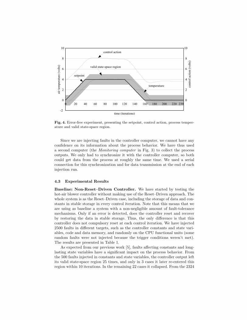
We have defined a setpoint as presented in Fig. 4, and monitored the processoutputs under normal conditions (without fault-injection). Due to the time theair takes to cross the tube from the actuator until the sensor, the process outputspresent a constant delay to the setpoint of about 770 milliseconds (11 controliterations). The valid state-space region was thus defined with a tolerance of 1volt (about 1.7◦C) to the setpoint, with a delay of 11 iterations:

y(k) < r(k − 11) + 1 and y(k) > r(k − 11)− 1 (4)

The collapse condition occurs if the process output violates the valid state--space region for more than 10 iterations (700 milliseconds). The experimentswere limited to 240 iterations (16.8 seconds), which complete a full setpointcycle.

10

-2

0

2

4

6

8

0 20 40 60 80 100 120 140 160 180 200 220

air t

empe

ratu

re (v

olts

)

10

0

2

4

6

8

cont

rol a

ctio

n (v

olts

)

time (iterations)

239

control action

setpoint

valid state-space region

temperature

Fig. 4. Error-free experiment, presenting the setpoint, control action, process temper-ature and valid state-space region.

Since we are injecting faults in the controller computer, we cannot have anyconfidence on its information about the process behavior. We have thus useda second computer (the Monitoring computer in Fig. 3) to collect the processoutputs. We only had to synchronize it with the controller computer, so bothcould get data from the process at roughly the same time. We used a serialconnection for this synchronization and for data transmission at the end of eachinjection run.

4.3 Experimental Results

Baseline: Non-Reset–Driven Controller. We have started by testing thehot-air blower controller without making use of the Reset–Driven approach. Thewhole system is as the Reset–Driven case, including the storage of data and con-stants in stable storage in every control iteration. Note that this means that weare using as baseline a system with a non-negligible amount of fault-tolerancemechanisms. Only if an error is detected, does the controller reset and recoverby restoring the data in stable storage. Thus, the only difference is that thiscontroller does not compulsory reset at each control iteration. We have injected2500 faults in different targets, such as the controller constants and state vari-ables, code and data memory, and randomly on the CPU functional units (somerandom faults were not injected because the trigger conditions weren’t met).The results are presented in Table 1.

As expected from our previous work [5], faults affecting constants and long-lasting state variables have a significant impact on the process behavior. Fromthe 500 faults injected in constants and state variables, the controller output leftits valid state-space region 25 times, and only in 3 cases it later re-entered thisregion within 10 iterations. In the remaining 22 cases it collapsed. From the 2324

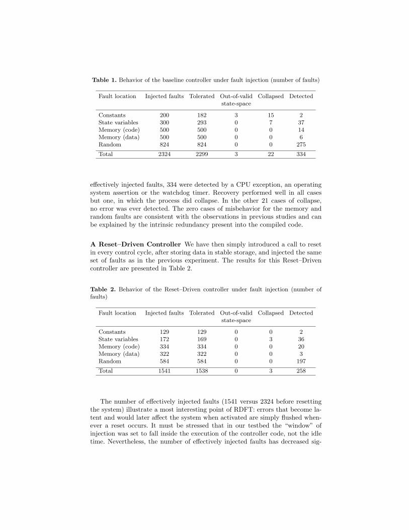
Table 1. Behavior of the baseline controller under fault injection (number of faults)

Fault location Injected faults Tolerated Out-of-valid Collapsed Detectedstate-space

Constants 200 182 3 15 2State variables 300 293 0 7 37Memory (code) 500 500 0 0 14Memory (data) 500 500 0 0 6Random 824 824 0 0 275

Total 2324 2299 3 22 334

effectively injected faults, 334 were detected by a CPU exception, an operatingsystem assertion or the watchdog timer. Recovery performed well in all casesbut one, in which the process did collapse. In the other 21 cases of collapse,no error was ever detected. The zero cases of misbehavior for the memory andrandom faults are consistent with the observations in previous studies and canbe explained by the intrinsic redundancy present into the compiled code.

A Reset–Driven Controller We have then simply introduced a call to resetin every control cycle, after storing data in stable storage, and injected the sameset of faults as in the previous experiment. The results for this Reset–Drivencontroller are presented in Table 2.

Table 2. Behavior of the Reset–Driven controller under fault injection (number offaults)

Fault location Injected faults Tolerated Out-of-valid Collapsed Detectedstate-space

Constants 129 129 0 0 2State variables 172 169 0 3 36Memory (code) 334 334 0 0 20Memory (data) 322 322 0 0 3Random 584 584 0 0 197

Total 1541 1538 0 3 258

The number of effectively injected faults (1541 versus 2324 before resettingthe system) illustrate a most interesting point of RDFT: errors that become la-tent and would later affect the system when activated are simply flushed when-ever a reset occurs. It must be stressed that in our testbed the “window” ofinjection was set to fall inside the execution of the controller code, not the idletime. Nevertheless, the number of effectively injected faults has decreased sig-

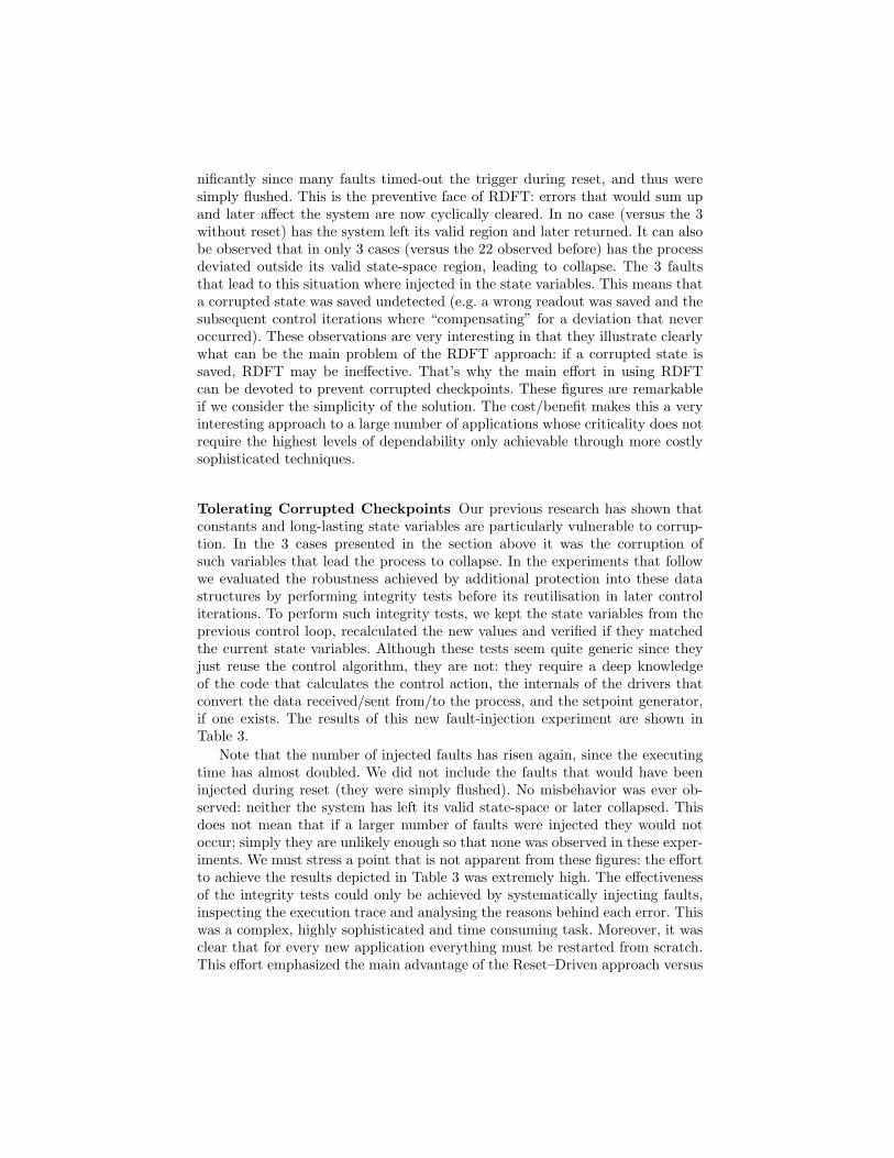
nificantly since many faults timed-out the trigger during reset, and thus weresimply flushed. This is the preventive face of RDFT: errors that would sum upand later affect the system are now cyclically cleared. In no case (versus the 3without reset) has the system left its valid region and later returned. It can alsobe observed that in only 3 cases (versus the 22 observed before) has the processdeviated outside its valid state-space region, leading to collapse. The 3 faultsthat lead to this situation where injected in the state variables. This means thata corrupted state was saved undetected (e.g. a wrong readout was saved and thesubsequent control iterations where “compensating” for a deviation that neveroccurred). These observations are very interesting in that they illustrate clearlywhat can be the main problem of the RDFT approach: if a corrupted state issaved, RDFT may be ineffective. That’s why the main effort in using RDFTcan be devoted to prevent corrupted checkpoints. These figures are remarkableif we consider the simplicity of the solution. The cost/benefit makes this a veryinteresting approach to a large number of applications whose criticality does notrequire the highest levels of dependability only achievable through more costlysophisticated techniques.

Tolerating Corrupted Checkpoints Our previous research has shown thatconstants and long-lasting state variables are particularly vulnerable to corrup-tion. In the 3 cases presented in the section above it was the corruption ofsuch variables that lead the process to collapse. In the experiments that followwe evaluated the robustness achieved by additional protection into these datastructures by performing integrity tests before its reutilisation in later controliterations. To perform such integrity tests, we kept the state variables from theprevious control loop, recalculated the new values and verified if they matchedthe current state variables. Although these tests seem quite generic since theyjust reuse the control algorithm, they are not: they require a deep knowledgeof the code that calculates the control action, the internals of the drivers thatconvert the data received/sent from/to the process, and the setpoint generator,if one exists. The results of this new fault-injection experiment are shown inTable 3.

Note that the number of injected faults has risen again, since the executingtime has almost doubled. We did not include the faults that would have beeninjected during reset (they were simply flushed). No misbehavior was ever ob-served: neither the system has left its valid state-space or later collapsed. Thisdoes not mean that if a larger number of faults were injected they would notoccur; simply they are unlikely enough so that none was observed in these exper-iments. We must stress a point that is not apparent from these figures: the effortto achieve the results depicted in Table 3 was extremely high. The effectivenessof the integrity tests could only be achieved by systematically injecting faults,inspecting the execution trace and analysing the reasons behind each error. Thiswas a complex, highly sophisticated and time consuming task. Moreover, it wasclear that for every new application everything must be restarted from scratch.This effort emphasized the main advantage of the Reset–Driven approach versus

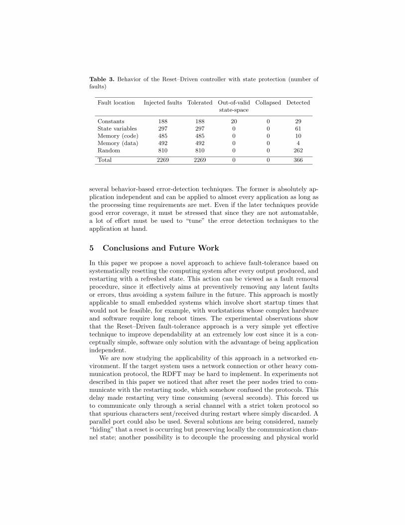
Table 3. Behavior of the Reset–Driven controller with state protection (number offaults)

Fault location Injected faults Tolerated Out-of-valid Collapsed Detectedstate-space

Constants 188 188 20 0 29State variables 297 297 0 0 61Memory (code) 485 485 0 0 10Memory (data) 492 492 0 0 4Random 810 810 0 0 262

Total 2269 2269 0 0 366

several behavior-based error-detection techniques. The former is absolutely ap-plication independent and can be applied to almost every application as long asthe processing time requirements are met. Even if the later techniques providegood error coverage, it must be stressed that since they are not automatable,a lot of effort must be used to “tune” the error detection techniques to theapplication at hand.

5 Conclusions and Future Work

In this paper we propose a novel approach to achieve fault-tolerance based onsystematically resetting the computing system after every output produced, andrestarting with a refreshed state. This action can be viewed as a fault removalprocedure, since it effectively aims at preventively removing any latent faultsor errors, thus avoiding a system failure in the future. This approach is mostlyapplicable to small embedded systems which involve short startup times thatwould not be feasible, for example, with workstations whose complex hardwareand software require long reboot times. The experimental observations showthat the Reset–Driven fault-tolerance approach is a very simple yet effectivetechnique to improve dependability at an extremely low cost since it is a con-ceptually simple, software only solution with the advantage of being applicationindependent.

We are now studying the applicability of this approach in a networked en-vironment. If the target system uses a network connection or other heavy com-munication protocol, the RDFT may be hard to implement. In experiments notdescribed in this paper we noticed that after reset the peer nodes tried to com-municate with the restarting node, which somehow confused the protocols. Thisdelay made restarting very time consuming (several seconds). This forced usto communicate only through a serial channel with a strict token protocol sothat spurious characters sent/received during restart where simply discarded. Aparallel port could also be used. Several solutions are being considered, namely“hiding” that a reset is occurring but preserving locally the communication chan-nel state; another possibility is to decouple the processing and physical world

interface from the communication hardware (e.g. using an autonomous networkcard).

There is a large number of ubiquitous small embedded computer systemswhose criticality does not justify the cost of the more sophisticated error detec-tion techniques. However, their dependability requirements may not be achievedby the simpler, most traditional approaches. We think that’s where the Reset-–Driven Fault Tolerance can be very cost-effectively used.

References

1. Astrom, K.J., Hagglund, T.: PID Controllers: Theory, Design, and Tuning. Secondedition. Instrument Society of America (1995) ISBN 1–55617–516–7

2. Avizienis, A., Kelly, J.P.J.: Fault Tolerance by Design Diversity: Concepts andExperiments. IEEE Computer, Vol. 17. No. 8, August (1984) 67–80

3. Bennet, S. Real-time Computer Control – An Introduction. Second edition, Pren-tice Hall Series in Systems and Control Engineering, M.J.Grimble ed. (1994)

4. Carreira, J., Madeira, H., Silva, J.G.: Xception: A Technique for the ExperimentalEvaluation of Dependability in Modern Computers. IEEE Transactions on SoftwareEngineering, February (1998) 125–135

5. Cunha, J.C., Maia, R., Rela, M.Z., Silva, J.G.: A Study on Failure Models inFeedback Control Systems. International Conference on Dependable Systems andNetworks, Goteborg, Sweden (2001)

6. Cunha, J.C., Silva, J.G.: Software-Implemented Stable Storage in Main Memory.Brazilian Symposium on Fault-Tolerant Computing, Florianopolis, Brazil (2001)

7. Cunha, J.C., Rela, M.Z., Silva, J.G.: Can Software-Implemented Fault-Injection beused on Real-Time Systems? 3rd European Dependable Computing Conference,Prague, Czech Republic (1999)

8. Huang, Y., Kintala, C., Kolettis, N., Fulton, N.D.: Software Rejuvenation: Anal-ysis, Module and Applications. 25th International Symposium on Fault TolerantComputing Systems (1995) 381–390

9. Jahanian, F.: Fault-Tolerance in Embedded Real-Time Systems. Hardware andSoftware Architectures for Fault Tolerance, Michel Banatre and Peter A. Lee Eds.Springer-Verlag (1994)

10. Kopetz, H.: Real-Time Systems: Design Principles for Distributed Embedded Ap-plications. Kluwer Academic Series in Engineering and Computer Science, John A.Stankovic ed. (1997)

11. Powell, D., Verıssimo, P., Bonn, G., Waeselynck, F., Seaton, D.: The Delta–4 Ap-proach to Dependability in Open Distributed Computing Systems. InternationalSymposium on Fault Tolerant Computing Systems, Tokyo (1988)

12. Process Trainer PT326. Feedback Instruments Limited. http://www.fbk.com13. Randell, B.: System Sructure for Software Fault–Tolerance. IEEE Transactions on

Software Engineering, Vol. SE–1, No.2, June (1975) 220–23214. SMX Simple Multitasking Executive. http://www.smxinfo.com15. Somani, A. K., Vaidya, N.H.: Understanding Fault Tolerance and Reliability. IEEE

Computer, April (1997) 45–5016. Vinter, J., Aidemark, J., Folkesson, P., Karlsson, J.: Reducing Critical Failures for

Control Algorithms Using Executable Assertions and Best Effort Recovery. Int.Conference on Dependable Systems and Networks, Goteborg, Sweden (2001)

17. Yurcik, W., Doss, D.: Achieving Fault-Tolerant Software with Rejuvenation andReconfiguration. IEEE Software, July/August (2001) 48–52