reproduced by permission! of hmso - citeseerx
TRANSCRIPT

RE~PORT NO NCRF/IZ
March 1972
THE THEORY OF EXPLOSIONINDUCED SHIP WHIPPING
Reproduced by Permission!of HMSO
This documeat is the property of Her Majesty'sGovernment ati Crown copyright is reserved.Requests for permission to publish its contentsoutside official circles should be addreased tothe Issuing Authority.
Naval Construction Research EstablishmentSt Leonard's Hill
D~nfermlineFife
'Pll 11,,t, #

REPORT NO NCREIR579-
Mar ch 1972 -
THE THEORY OF EXPLOSION INDUCEDSHIP WHIPPING MOTIONS
ABSTRACT
The report presents a comprehensive account of the mechanics of, and methodsfor predicting, the interaction between the vertical vibration modes of a sur-face ship and a nearby underwater explosion. It summarises earlier work in thefield and gives a full unified aocount of the author's recent work (reprtedpiecemeal elsewhere).
This document is the property of Her Majesty'sGovernment and Crown copyright is reserved.Requests for permission to publish its contentsoutside official circles should be addressed tothe Issuing Authority.
Naval Construction Research EstablishmentSt Leonard's Hill
Dunfermline
Fife Approved for issue
S.:)eri ntr- nden t
1-,: •- .rV i • , . ;., •.. .... •,'• • ...... •:;' :• .. .. .. T • . . . . - • ......... A.

ACKNOWLEDGEMENTS
The help and encouragement of Professor D C Pack of Strathclyde
University, of Professor J L King of Edinburgh University and
Mr S B Kendrick are gratefully acknowledged, both during the work,
and for making it possible in the first place.
I should also like to acknowledge a great debt to my wife for
her continual support and patience during many 'quiet' evenings.
iii

SUMMARY
The principal aim of the thesis is to devc:cp, fuid show how to solve,
equations describing the flexural motions caused in a ship by the pulsa-
tions of the bubble of gaseous products from a nearby underwater explosion.
Equations for this purpose were developed in the USA 15-20 years ago and
the thtsis presents an alternative, finite element formulation which is
more general and which leads to equations in matrix form. In this form
the equations are much more suitable for evaluution by computer. The
method of solution of these equations of elastic motion, in terias of
normal mode shapes, is described.
The approximations ii.volved in the hydrodynamics of the bubble-ship inter-
action are examined in some detail and tt.".' limits of application of the
theory are illustrated. The principal approximation in the hydrodynamics
is the use of strip theory since this cannot allow for either the longitud-
inal flow which occurs when the bubble is close to the ship, or for the
flow around the end of the ship when the bubble is in such a region. The
accuracy of strip theory is examined in both these cases. A. alternative
to strip theory for describing the flow around a vibrating ship is presented.
This approximates the full three-dimensional flow field around the ship by
means of a set of line distributions of vertically oriented dipoles at the
waterplane-ship centreline axis. The technique could also be of value for
the determination of added water mass around a vibrating ship in more usual
vibration problems.
The original American derivation of the equations assumed that the pulsating
bubble was non-migrating. Suitable equations are developed to describe the
upward migration of the bubble due to gravity and the effect of this migra-
tion on the motion of the ship.
For severe flexural motions of the ship some plastic yielding or even buck-
ling could occur and a direct solution of the original finite element
iv

equations, modified to include such effects, is presented. This shows tht
way in which they can c.hange the motion of the ship.
The entire thesis is a theoretical exercise although the results for the
non-migrating Lubble case are compared with a few iuudel test results
published in connection with the original American work.
=v
• V
CONTEN'rS~
C 0 N T E N T s
Title eDeclaration IiAcknowledgement iiiSummary iv
SECT ION
A Introdu' tion I
D Background 4
C The Elastic Representation of the Ship 12
D The Hlydrodynamic Forces on the Ship 19
Hydrodynamic Forces in roving Water 24
E Equations of Motion 34
F The Normal Mlode Equations 38
G Use of the Modal Fquations for Free VJ ration 42
a. Uniform Solid Beam 4*2b. lollow Rectangular Box-Beam 47c. Full Scale Ship 52
H Explosion Induced Forcing Function 60
I Description and Computer Program I 71
J Complete Example 74
K The Early Compressible Phise 31
L An Alternative to the Strip Theory Flow Miethodfor the Added liater Mass 85
"-M....,,,.atcal rl'el for an Axi-Symmetrical Ship 87Comuparison of taesults with known Exact ForceDistributions 92a. Vibrating Prolate Spheroid 92b. Infinite Circular Cylinder 97A;.•lication of the Technique to Non-axi-sy-nmetric ships 98Use of the Full lounoary Condition 99Modification of the Normal M1ode Equations 104Application to S.ii., ýib'ation Calculation 105Conclusions !,egarding the lydrodynamic Flow 107
M Limits of Applicability of the Theory 112
a. Spherical Flow Divergence 114b. The Force D)istri.,ution Near the Bow and Stern 120c. Bernoulli Pressures 12,)
N 'iodification of the Forcing Function Due to LocalIarnage 138
vi

0 The Effect of iOubble ::igration 150
The Free Surface Effect 156Inclusiun of a Drag Terin 160Effect of Migration on Whipping Response 1-7Bubble Jets 1o9
P Description of Computer Progrun II 177
Q Comparat ive Cat c.l at ions 179
R Plastic .Deformation of the Target 183
APPENDIX Approximate Analysis for Bilge Kcel Effect 201
'1I

A introduction
When a fairly large explosive charge is detonated underwater
close to a ship the shock wave it transmits to the water can do
considerable damage to the ship. If close enough the hull plating MW
rupture and for charges further away there may still be considerable
deformation of the structure nearest the charge. The shock wave also
is partially transmitted into the structure and can cause further
shock damage to internally mounted equipment. These effects follow
close behind tihe detonation, typically witnin times of the order of
15 to 20 milliseconds, and are usually confined to the region of the
ship closest to the explosion.
The explosion may however also excite a very different kind cf
response. Ships near underwater explosions often sheke and bend
overall in violent flexural vibrations. Such vibrations are usually
confined largely to a vertical plane and, although very violent, are
of much lower frequency (typicalky $-5 Hz) than the shock motions
acconapa~iyng the local damage, The amplitudes can be very large and
can cause considerable structural damage to the ship. Unlike the
direct shock damage, this damage can or~cur at parts of the ship
quite remote from the site of the explosion. These bending motions
are commonly termed 'whipping' motions. They also occur in severe
storms if the bow of a ship emerges from the water and then slams
back onto it. They constitute a superposition of the well know.r low
frequency vertical bending vibration modes of the ship, excited to
unusually large amplitudes. It is the aim of this titesis to investi-
gete the nature of the interaction between the explosion and the ship
which causes these whipping motions, and to develop suitable
equations from which whipping motions can be calculated.
!
It is already known from earlier work principally by 0 Chertock
(and described briefly in Section B) that such motions are
connected closely to the motion of the water around the bubble of
gaseous combustion products from the explosion. This bubble i3 well
known to pulsate vigorously and the period of the pulsation is often
very close to the low frequency vibration modes of ships. Chertockts
work showed that the whipping is primarily due to the coupling between
the vibration modes and the pulsating flow. This thesis extends the
earlier work, investigates the hydrodynamic interaction between the
explosion and the ship in more detail and, by using a different
initial approach, provides a set of equations for calculating the
ship response which show more clearly the nature of the forces
acting on the shtp and are also more readily solved by standard
matrix methods on a computer.
The mechanics of the interaction involves several standard
fields of study; the elastic nature of the ship, the hydrodynamics
of vibration and the hydrodynamics of underwater explosions. The
thesis attempts to tie together only the simplest ideas from each
and to extend standard methods in each only where they appeared to
be deficient from a whipping viewpoint: for example the strip theoTy
of ship vibration and the equations for a pulsating migrating
bubble. In consequence the bibliographies given in each field are
rather basic; they are aimed simply at providing sufficient back-
ground information to apply adequately the methods developed. The
first part of this thesis, sections A to K, is largely based on
existing methods, although the methods have not previously been
used for this particular applicationand is concerned largely with
establishing the equivalence of the present mnethods to the earlier work.
2

Section D extends strip theory to allow for the explosion induced motion
of the surrounding water. Section G includes a simple approach to making
an allomance for the effect of small bilge keels on the added water mass.
Section I describes a large computer program written to evaluate tht
equations developed in sections Cto 11. Most of the new material in the
thesis is contained in sections L to 0 and in .,. Section L describes an
alternative to the custo,,ary ship theory for the flow around the ship.
Section M investigates the limits of application of the approximate analysis
by comparing the forces predicted by the approximate method with exact
solutions for very simple cases. Section N dcvelops an approximate methou
for making an allowance for the effect of shock wave damage to the target.
Section 0 investigates the effect of gravity on the explosion buible and
on the forces the bubble produces on the ship. Section R describes how the
basic equations for the ship motion can be modified to allow for plastic
yielding and buckling of the ship. Two further major programs were
developed to evaluate the ship response (including allowances for gravity
migration of the bubble and plastic deformation of the target) and are
described in sections P and !,. Several minor computer programs were
develo.,ed to evalu.ite the exact solutions for comparison with the approxi-
mate analysis.
To make each section of the thesis as self-contained as possible the refer-
ences and figures for each section are grouped at the end of the section.
B Iacjund
Although a considerable amount of work has been carried out on
the vibration and %larmins aspects of ship whipping. very little work
has been published on the explosion induced shipping motions. What
work has been published is due entirely to a single author, G Chertock.
His wort. is deecribed in references (i1 to [B31but, as it appears to be
the sole predecessor of the work here it is worth describing it in
sqam detail.
The ship target is assumed to be equivalent to an elastic free-
free beam whose transverse displacements c ar therefore be represented
by
y(x,t) =qi(T i W
where x is the longitudinal distance along the axis of the ship,
y the verticol displacement of the cross-section at x (assumed rigid),
Si(x) the ith normal mode shape for transverse vibration in vacto.th
and qi is a generalised co-ordinate for the i mode (e.g. the
amplitude at the bow or, alternatively, the root mean square displace-
ment). The nor1ial modes for such motions are orthogonal with the
mass per unit length, m(x), as a weighting function.
z mW)i(x)IF.(x)dx = M 6ij (B2)
thwhere M . is the generalised mass associated with the i mode.
By usin, the orthogonality condition the equations o; vertical
transverse motion due to an arbitrary distribution of pressure over
the surface of the ship can be written
MI(q, + a ) = Qi= - j' sp(st)'cos6B dc i = 0,1,2,. ,. (B3)
where Q0i is the circular frequency for mode i, Qi the generalised
force and da an element of area of tne surface of the ship. The
4
angle P is the angle between the vertical and the normal to the
surface 'and s refers to a point on the ship surface.2
By neglecting the Bernoulli pressures, .-. u , compared with
the unsteady forces p-. in the usual Bernoulli pressure equation
for incompressible flow, the fluid pressure on the ship can be expressed
as a linear sum of the pressure due to the explosion induced fluid flow
on the structure, assumed rigid, and the pressures due to the motion
of the target in its various modes, so that
p(s,t) = Poo(s,t) + ZP (s,t) (B4)
where p 0 is due to the explosion and p. to the ith mode.
With this assumption of linearity, induced modal mass coefficient
can be defined by
ELi = - p pj(s't)Tj.Lco spd ]/qi (t (B5)
and will be independent of time. Substituted into equation (B3)
this gives
(IV + L. )(q + W2q ) : - HP oo!cospda - Z L..q.; i = 0,1,2q...1 1 i •0 00i.
2 (B6)
2 M
1• + L..
In these equations the elastic modes are clearly coupled to each
other by the entrained water around the ship through the coefficients
Lij, i X j. By a suitable transformation of the normal mode shapes
T. and co-ordinates qi it was shown that the equations can be
uncoupled into
M= -+Ip o•'cospdo (B7)
The procedure however is extremely difficult to carry out in prartice
. due to the necessity to evaluate the cross-coupling cotfficicr.ts.
These can only be determined exactly by the sollAions :)f a series
of integral equations where the integrals are over khe whole surface

of the ship hull. In practice, for physical reasons the L.. 's
are expected to be fairly si*ill if the ship is long and slender or
if there is sufficient fore-and-aft syrunetry. Chertock avoided
defennination of the L.. by assuming that ships are 'proportional
bodies '
i.e. by his definition, ýp1 cosp ds = aipm(x)W.(x)
where the intcgral is a line integral taken round a ship cross-
section, p is the density of water, and the relatio-a a:,plies at all
ship cross-sections, i.e. for all j,ai is assumed, for proportional
bodies, to be a constant, indepe,,dent of x. With this definition,
by multiplying by T i and integrating over the length of the ship,J
L. .. ffpj(s,t)'Tcospda = -. '6'.dx�p. cospds _ -J-f m' '7 dx
i.e. L - 8.I 13
so that the cross-coupling terms all vanish arid the mode shapes in
air and water are identical, although the frequencies will change
due to the non-zero entrai,'-d water masses 1....1.1
For the term po', representing the pressure on the ship, if
it were rigid, due to the flow around the explosion bubble, the well
known result L3B4]that the flow around a non-migrating bubble is
equivalent to that of a simple source was used. Since the rate
of change of the bubble volume is V(t), the strength of the source
is V/4it and its potential isV
The pressure in the absence of the target is therefore
Vpo = = (B=)
and the integral -ffp o0icospda will be representable in the formS00V
46[6

where V is a factor depending only on the charge position and the
ship aiv; modc shapes. For a clkarge sufficiently far from the ship
the factor A was shown to be given approximately by
mL.. .
~. (pA + IL.(B9)Pi = 4X• M. 3-. (9i r
where • is tic height of the uxis ef th2 ship abovw the charge centre
and r is the standoff of the particular point on the ship axis from
the charge centre. The final modal equation of motion is therefore
(M + L q) - IV(t); (BIO)
To determine the response of the ship then, equation (BIO)
is to be solved for each mode, using free-field values for the
explosion bubble volume acceleration, V, and the modal components
may then be sui:',ed to give the displacement function y(x,t). The
principal assumptions made in the derivation are:
a. The chard is far enough from the ship for the
explosion bubble motion not to be affected
by the ship.
b. The ship motlons remain completely elastic.
c. The ship is a 'proportional body', i.e. there
is no fluid coupling between the 'in vacuo' elastic
vibration modes when the ship is in the water.
d. The charge is at a distance fro|, the ship large com-
pared with the ship cross-section, so that the
approximation (B9) applies.
e. There is no significant migration of the bubble
during the motion.
f. Only incompressible water motions are of importance.
g. Structural and hydrodynamic damping are negligible.
To check the accuracy of his equations, Chertock carried out
7

two series o' experiments on model t:irgets. The first series
used a 1.2 Zri charge under a floating rectangular box 1O ft long
by 9 iris wide by 6 ins deep. ",is target was slender, symnetric
and nearly uniform and the mode shapes in air and water were
indistinguis:,able so that the target certainly satisfied the
requirement kc). The charge depth of 13 ins was carefu!ly selected
so that the iiormal repulsion from a free surface exactly balanced
the upward buoyancy migration due to gravity so that requirement (e)
was also satisfied. At the given depth the maximum bubble radius
is about 6 ins so that (a) is satisfied and the geometry is clearly
such that (d) is not really violated although it might be thought
near the limits of acceptability since the cross-sectional dimensions
are nearly comparable to the standoff. For the fundamental, 2-node
whipping modc the predicted results agreed very well with the experi-
mental (Reference B3) but for the3 -node mode the measured amplitudes were
about 30 less than those predicted. For the 2-node mode the varia-
tion of %%hi. :,ing amplitude with the longitudinal location of the
charge aireed very well 1ýith exl.eriment.
The second series of tests used a su.,mcrged cylindrical model
8 ft long by 9 ins in diameter and two charge sizes, 1.2 gins and
8.2 gins were used. The charge and target were lowered to a series
of dcpths and the variation in amplitude of the 2-node and 3-node
modes were menasured as the bubble period varied, due to dcpth, from
in phase to out of phase witi the modes. The effect of charge
standoff was a-so investigated. For the 2-node mode agreem.ent was
again goou cv'ryw;acre but for t.,i '-node :iode the ex.:eri!.ental
ai.:.;)litsides %re now greater thon predicLcd. Prior to the tests
vibratiorn :e.-sur.ements iere :.r:.'e both in air and water t,, deten.line
the i,.ode sha..cs a•tx: f re, ,'ncies and to deternine thc valies of L..
8
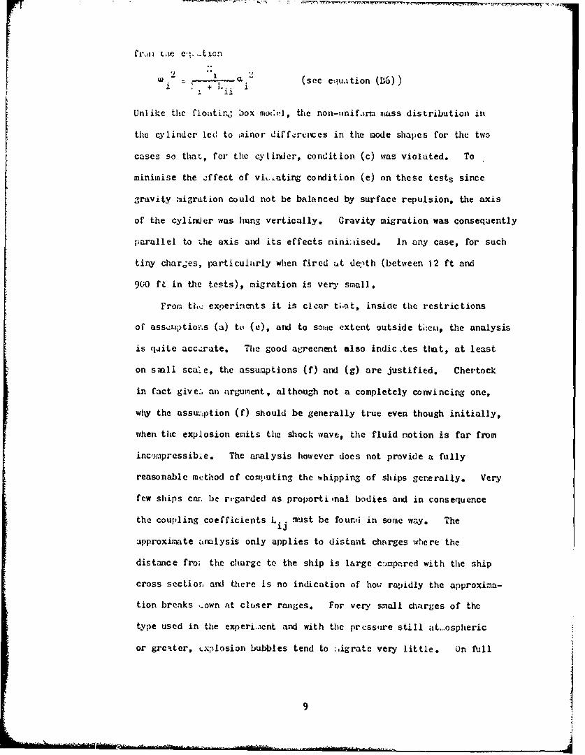
fr.,* tae e.".. ti-n
W (see equaition (B6))
Unlike the floatinj box model, the non-tnif.rm muss distribution in
the cylinder led to iiinor diff~reices in the mode shapes for the two
cases so that, for the cylinder, condition (c) was violated. To
minimise the effect of vit..ating condition (e) on these tests since
gravity migration could not be balanced by surface repulsion, the axis
of the cylinder was hung vertically. Gravity migration was consequently
parallel to the axis and its effects mini:iised. In any case, for such
tiny charges, particularly when fired ut death (between 12 ft and
900 ft in the tests), nigration is very small.
From thi experiments it is clear ti.at, insiue the restrictions
of assmiptions (a) to (e), and to sowe extent outside tC.c, the analysis
is quite accxrate. The good agreement also indic Aes that, at least
on siall scale, the assumptions (f) and (g) are justified. Chertock
in fact give an argument, although not a completely convincing one,
why the assu,::ption (f) should be generally true even though initially,
when the explosion emits the shock wave, the fluid notion is far from
incompressible. The analysis however does not provide a fully
reasonable method of com!%uting the whipping of ships generally. Very
few ships car. be regarded as proporti 'nal bodies and in consequence
the coupling coefficients L.. must be foundi in some way. The
approximate amlysis only applies to distant charges where the
distance fro; the charge to the ship is large c:'mpared with the ship
cross sectiorn and there is no indication of hou rapidly the approxima-
tion breaks ,.own at closer ranges. For very small carges of the
type used in the experi..tent and with the pressitre still at...ospheric
or greater, cxplosion bubbles tend to :,igratc very little. On full
9

scale this L-, tiot true atl bubbles nigrate very vigorously. Such
i,;iiration ca:, lead to m.arLed dliffere, ces in the resionse of ships
to clhrrges vcrtzicilly beneath thema compared to charges at sorme distance
to one side. In Chertock's analysis conditi.ns change only slowly
with stand-off from the ship's centreline. Lastly, bein.- entirely
dependent on elastic modes of vibration, it is very difficult to
extend the analysis as it stands to the analysis of ship motions
whieh are violent enough for plastic deformation to occur.
These points are all investigated in some detail in the thesis
and a practical camputation scheme is developed. Since methods of
calculating the normal mode frequencies and shapes of ships have been
well established over the last half century, their basis, strip theory
for the hydrodynamzics and an elastic free-free bean representation
for the ship, is used here to re-formulate the wh.pping equations
to anply to .Jl ships, including those which are not proportional.
The forcing iction or the bubble ptlsations on the ship can then be
interpreted in ten.s of strip theory, wiiich provides also a very simr le
.eans of including the effects of bubble migration. Use of the basic
equations of an elastic beam also permits a relatively simple extension
to cover pla.;tic hinge formation in the ship. The equations used
are dzvelope, in the subsequent sections.
To enab.c th., powerful ,atrix .ianipulation subroutines readily
available in most couptiters to be used in computing the ship response
a finite c.e,-ent/'::.ped mass model has been used.
10
References:
1l Chertock, G.; "The Flexural Response of a Subrmerged Solid toa Pulsating Gas Bubble", Jn. Applied Physics,Vol. 24, No. 2 (Feb. 1953).
R2 Chertoc%, G.; "Effects of Underwater Explosioms on ElasticStructures", Fourth Synposium on Naval ilydro-dynamics, ACR-92, Aug. 1962.
33 Chert, k, G.; "Excitation of Transient Vibrations of IdealisedShip Models by Underwater Explosions", 77thMeeting of the Acoustical Society of America,8th April 1969.
B4 Cole, R. If. "Underwater Explosions", Princeton Univ. Press.192.
=I11

C Th- Elastic Pepresentation of the Ship
Since the latter part of the last century it '..is been custompary
to i-e-rescnt a shin as an elastic bext. Initially this was larg•ly
a necessary assumption to make strength calculations tractable but
eventually, ill 1905, a aeries of static ben!ing ,omzient experi.L.ents were
carried out on a destroyer !IUMS INI.ILF (CI). These confir:.ied that the
us',al thih 'J. e tu:ations gave a).)roxiil;,tely the correct longitudinal
,tress distribution across each cross-section, although some deviations
fro:m a linear stres, distribution were apparent near the deck.
The results indicated the tapparent' modulus of elasticity to be
close to the usualtetnsile test'value for low bending noments but
to fall in value for the higher maments. Calculated deflections,
when com.tpared with the measured deflections gave mnuch lower ay;parent
values for tie modulus. The discrepancy in the deflections was
later shovwn to be due to the neglect of shear deform.ations and in 1924
Taylor prcsentcd an excellent paper (C2) describing a nodification to
the straight-forward bea:mi theory which made allowance for the effect
of shear lag on the distribution of stress in beans of ship type
cross-section. 'He showed tha'. under typical corxlitions shcar could
rmake significant contributions to the total shi: dcfl.tction.
Since that tine, until very recently when three-dimensional
finite ele:.ment stress analysis computer programs became available to
calculate stress distributions with so:me accuracy, the position
has not chenged greatly. A number of static betiding experi..ents
C3-C8 have been carried out on ships and all have confir:1-'c that beaL:
theory is quite satisfactiry for computing hoth stresses and deflecti ns
even to the i:oint of failure (C3 and C-3) provided that long deck houses
are not involved. Such dec:;houses appear to behave in a variety nf
12
ways dc..endi:&g on how they are supported. Instead of the stresses
increasing away from the neutral axis, except in very long well
supported decfhouses, the stresses decrease. If the dec*: on which
they are sup.,orted is flexible enough, they may even have a curvaturc
cpposite to that of the main hull. IHowever, in calculating the
effect of deckdhouses on longitudinal deflectiors it has become
custormary totreat the dcc:house as a normal art of t-.he beam (if
it is long enoush) but to assign to it a reduced effectiveness factor
depending on its size shape and support. Theories and ,etn•ods for
calculating such effectiveness faltors arc given in Refcrences C9-
C.2.
The a:'D .ication of beai theory t, the vibration of ships has a
history as long as its ap, lication to static calculations and
Reference C13 gives an excellent review of the work. So long as
shear deflecLions are included and an entrained mass o& water allowed
for, excellent results can be achieved in calculating the vibration
frequencies of the first few lowest modes. However, shear deflections
play anizcreasingly important part for the higher modes and the
distortions of plane sections (assumed to remain plane in normal beam
theory) becor..e important. Also, higher nodes begin to have frequencies
similar to so:ne of the transverse distortion modes and combined modes
appear. r :i:ally tlh usual strip theory m~etnod for allowing for the
entrc.incd water maass becomes increasingly iraccurate for the higher
nodes. In c.-nsequence, although high accuracy has been claimed
(C14) tor calculations of this type up to the W0 tno;e mode, it is
gencrally accepted that only the first few modes, with up to about
5-nhdes, c:m be calculatcd with confidence. Fortuiately in explosion
induced whipping it is the lowest few modes which turn out to be the
most significant.
13

To a:,);ly the lumped mass/weightless beam idealisation to a
ship it iwiy be assumed divided into a number of equal length sections.
If, as is norrmally the case, the ship structure changes little in
the length ol aiy section, it can be assumed constant within each
section with charucteris tics corresponding to those at the centre
of the section. The forces and moments acting at the ends of any
section are %hen readily detervined in terms of the deflections and
rotations there, all the ship weight, buoyancy and inertial forces
)eing considered as lumped at the ends of sections. With the sign
convention shown in Figure CI , the standard beam equations are
dSQ= 0.x
,2.M, = I--
dx
If the angl. of rotation at a cross-section is y, then the slope
of the deflection curve is
dy S
s
where A is the area of the cross-section effective in shear, ands
G the shear r.:odulus. The integral of these equations may then be
expressed in the form
I 2 x3rE 2I- M 2 rYL
y x x
l0 I2E L (Ci)
0I 00 x L
-S 0 0 0 1 -SL
where the suffix L refers to conditions at the left hand end of the
beam section. If the conditions at the right hand end are substituted
the equations may be inverted to give the forces and moments required
14

at each end of the beam to maintain there givir displacements and
rotations. Th.-e equations are
I--I + 2
HL•n (o i r -"( I antiy , 3lo Ck(IL e) y o (C2)
-j P L 2 cL
where
C 1(+v)Iand a 2 (03)S2 Z3~(1 + 2e)
aI the are (n;-) beam sections andthe displacemet• =(y1-.i.)
androtation (y1i)*n) arctevues impoed by(a)t the n t beam sectionens
Omd 1 an )(considered positive anticlockwise) necessary to maintain
the imposed shape will be given by
where Lth) el:enk:: fth :95(xn) matricesA,, B and C are giv en by i1
22a.. -3 _1_ ;6. ; . )L& c.=a.&i = 1_1. _
Here ( -. a..) are the values given by (C0) for the i thbeanm sectioni, I
and a and c are defined to be zero.0

The stiffness matrix in equation (C4) may be readily sl-.,.In
to allow the two degrees of freedom in the vertical plane (translation
and rotation) expected of a free-free beam, without giving rise to
forces or moments. It is therefore of rank (n-2).
tinder conditions where the applied moments are known to be very
small it is not possible U specify the rotations. These will ther.
be related to the displacements by the equation
.f =-iT BTy 0c5)
and the forces necessary to maintain the displacements y are then
[= A- IC-IBBTy (C6)
This form can be useful since for ship vibrations the rotary inertias
are generally small enough to be neglected.
F.
LirI

References:
1. Biles, J.H.; "The Strength of Ships with Special Reference toExperiments and Calculations M'ade upon IBIS WOLF."Trans. J.N.A., Vol XLVII, 1905.
2. Taylor, J.L.; "The Theorj of Longitudinal Bending of Ships."Trans. North East Coast Institution of Engineers andShipbuilders, Vol. XLI, 1924-25.
3. Kell, C.O. ; "Investigation of Structural Characteristics ofDestroyers PRESTON and BRUCE, Part 2 - Analysis ofData and Results." Trans. SNAME, Vol. 40, 1932.
4. Shephearc, R.B. and Turnbull, J. ; "Structural Investigation inStill Water on the Welded Tanker NEVERITA, Part II -The Tests and Their Results." Trans, I.N°A.,Volume 88, 1946.
5. Shcpheard, R. B. and Bull, F.B. ; "Structural Investigations inStill Water on the Tanker NEWCO:.:31A." Trans. NorthEast Coast Institute of Engineering and Shipbuilders,Vol. 63, 1947.
6. Vasta, J. ; "Structural Tests on the Liberty Ship S.S.PHILIP SCHUJYLER." Trans. SNAME, Vol. 55, 1947.
7. Vasta, J. ; "Structural Tests on the Passenger ShipS.S. PRESIDENT WILSON - Interaction BetweenSuperstructure and Main hull Girder." Trans.SNAME, Vol. 57, 1949.
8. Lang, D. W. and Ivrren, W. G. ; "Structural Strength Investigationson Destroyer ALBUERA." Trans. I.N.A., Vol. 94,1952.
9. Chapman, J. C. ; "The Interaction Between a Ship's Hull and aLong Superstructure." Trans. I.N.A., Vol. 99,No. 4, Oct. 1957.
10. Johnson, A. J. ; "Stresses in Deckhouses and Superstructures"Trans. I.N.A., Vol. 99, No. 4, Oct. 1957.
11. Caldwell, J. B. ; "The Effect of Superstructures on theLongitudinal Strength of Ships." T.ans. I.N.A.Vol. 99, No. 4, Oct. 1957.
12. Schade, 11. A. ; "Two Beam Deckhouses Theory with Shear Effects."Schiff und Hlafen, Heft 5/1966, 13. Jahrgang.
13. Todd, F. H. ; "Ship Hull Vibration." Edward Arnold(Publishers) Ltd.
14. Arnerson, G. and Normand, K. ; "A Method for the Calculation ofVertical Vibration with Several Nodes and someother Aspects of Ship Vibration." Trans. I..A.,Vole III, No 3,367, July 1969.
"17

w
�0z
Yb � I-
U, �* �1I
zw
'S
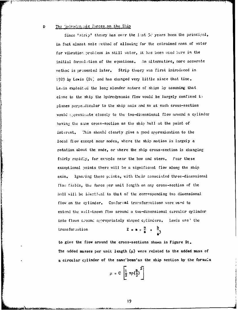
D The 'iydratn•.y :ic -.irces on the Ship
Since tstrip' theory has ovvr the l.'.st 5, years been thie rincipal,
in fact almost sole rethod of allowing for the entrained mass of water
for vibration !ruoi•Iczs in still watcr, it has been used :icre in the
initial fornul.)tion of the equations. An alternative, more accurate
method is presented later. Strip theory was first introduced in
1929 by Lewis (Di. and has changed very little since that time.
Le,;is expl.oitcd the lon, slender nature of ships lby assuming that
close to the ship the hydredynamic flow would be largely confined t,-
planes perpe:.dicular to the ship axis and so at each cross-section
would i,,proxi:,ate closely to the two-diuensional flow around a cylinder
having the same cross-section as the ship hull at the point of
interest. T'his should clearly give a good approximation to the
local flow except near nodes, where the ship motion is largely a
rotation about the node, or where the ship cross-section is changing
fairly rapidly, for exim.ple near the bow and stern. 3,'ear these
exceptional points there will be a significant flow along the ship
axis. Igno.,ing these pzints, with their associated three-dimensional
flow. fields, the force per unit length on any cross-section of the
hull uill be idcnt'.;al to that of the corresponding two dimiensional
flow on the cylinder. Confor'mal tra:,sfornaations .-,were used to
extend the wcll-L.nown flow around a two-dimensional circular cylinder
into flows aýoun'cd' a•.ropriately shaped cylinders. Lewis use ' the
a btransfor:.ition Z = B + ; + i3
to give the flow around the cross-sections shown in Figure Dl.
The added masses per unit length (ýt) were related to the added mass of
a circular cylinder of the same'beam'as the ship section by the formula
C 9
19

The coefficients C are given for the cross-sections in Figure 1.
In order to allow, at least partially, for the three-dimensional
flow effects, Lewis compared the strip theory flow around a prolate
spheroid, vibrdting in a certain 'lodet shape similar to a ship
vibration Aode, to the exact flow deduced by an expansion of the
flow in terms of spheroidal harmonic functions. The kinetic
energy of the approximate flow is naturally greater than that
of the exact flow (Kelvin's minimum energy theorem)
so tlat the deduced added :.-ass will also be greater. Lewis
suggestcd that the calculated added mass distribution for the ship
siha:'e should ',e reduced by a factor J, the ratio of the exact to
the a ,-rexima.ite kinetic energies fop a spheroid with the same
beam to lenzgth ratio as the ship.
The wh:,l. :)rocedure g.ves very good results for the lower
frequency viiration io('es of ships and forns the basis of aluost
all cuurent .;ethcds for calculatin- the effect of the water.
It has t-wo rither basic disar vant-,,ges however. Firstly, the
reduction f:iztor J for the 3-D flow effect del.cnds on the shade
of the -node ýo be ccaculated, which rz :es it diAfiatlt to for,-kulate
a siZle e',: ition whose ci-envalues arc the ship fre.iuencies;
a dif,'crcnt ,:,uation has to be solved for each mode. Sccondln1
there is no &varanteŽ La. .n exact reduction factor would not
vary along t'.c length of the ship, arI in general this is the ca.se.
Al.thoou'h the method is still the basis for entrined :-.ss
calcul;ttions, numerous :.inor i;,,)rovcieats have been :;-do since :,ewi:;'
paper, Tay .or (D2), :-rrived at the s%:ie a 1-roxi.at:: strip t';eopy
isndedtl.., of Lewis and again calculhted i red'c'.i.on f-.ctor b"
co:.-p.azrison w..th the solution for a spheroid. Po;ever, i:'lor's
solution for the splerical, vibration allo;.:ed a bending tyi-c of
20

-A'11 - - - -PM.*
:notion, as v...l as Lhe shearing motions, on wnt'ic1h Lewis calculatioias
were based, in the boundarj, condition on the spheroid. In consequence
his reduction factors give smaller entrcincd masses than those of
Lewis. Curves for both types of reduction coefficient are shown,
for the 2-node vibration mode, in Figure D2. Taylor also gave a
second se; o' reduction coefficients based on an exact solution
for the three dimensional motion of an infinite cylinder vibrating;
transvcrsely, its velocity distribution var/ing sinusoidally
along its length. These reduction factors are also included in
Figure D2. To calculate them the Taylor Form of ellipsoid motion
2 ' 2was assumed. This has nodes at + L(I-2B/L ) /215, measured from
its centre. The distance b)etween t:ecsc nondes was assuned to be
the half wavelength for the cylinder motion hihence the appropriate
reduction factor can be readily found. That they agree slightly
better with Lewis' ori inal results is not surprising since the
boundary conc.'.A'_'ons used by the two methods coincide when the
vibrating body has a constant cross-section. Only when appreciable
changes in section occur, as close to ends of the spheroidr or, to
a lesser extent, near the bow and ster-n of ships, do the boundary
conditions and hcncc the calculated reduction factors differ.
Prohaska (D3), considerably general is ed Lewis' two-dimensional
cross-sections by considering the transforrntion
Z = a + )/ m + b/ n.
for the cnses (ri,n) = (1,5), (1,7) and t3,7). Lewis' sections of
course arc fcr (im, n) = (I, 3). From these results l'rohaska found
that for sections with some parts concave outwards, the added mass
was very close tn tha' for the same section with the concavity
replaced by ", tangent line. I.oaking use of this device he then
!I

found the coefficient C could be determined with good accuracy as a
function simply of the section area coefficiento (the under•,'ater area
divided by b•an x draft, BD) and the ratio bearýdraft. He gave
the functional form as the graph reproduced in Figure D3. This
graph enables the added mass to be found to reasonable accuracy
without the tedious com:narison of the actubl cross-section u:ith
those of Lewis to find tMe best fit.
The set of cross-sectional shapes fo.r ubich the added mass is
known has been furthea extended in recent years by Landseber and
1Kacagno and co-workers 14, D5. These authors used a three parameter
fit for the sections rather than the two param.,etcr fits used by
Lewis and Pr.)haskr., !:acagno also made use of 'close-fit' conformal
mappings of sections, and other authors, e.g. lIoffman(D6)have
demonstrated similar methods. These use an arbitrary number of
coefficients in the series
= Z + +_ + .. +
zto obtain as close a fit to the actual section as desired. Quite
complicated co.iputer programs have to be used however to obtain the
coefficients for the best fit transformation.
.'endel(r7)ýas given the added mass for a squai.- cross-section
with 'bilge-iceels'; plates projecting at 451 from each corner.
These rc.lults are particularly interesting as they appear to be the
only ones available on the effects of such keels. The ;n-ethod used
to obtain tht-zm was an application of the Schwarz-Christoffel transforma-
tion. infortunately, the method is very tedious to apuly rndJ the
results were not extended to general rectangles with bilge keels.
The results for such shapes can however probably be estimated
fairly well by Prohaska's method; simply using the added mass for
the rectrZgle which circumscribes the ends of the bilge keels
22
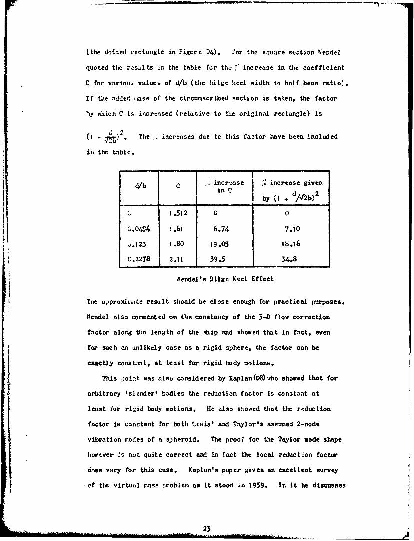
(the dotted rectangle in Figure )4). For the square section Wendel
quoted the rz.sults in the table for the increase in the coefficient
C for various values of d/b (the bilge keel width to half bean ratio).
If the added nass of the circumscribed section is taken, the factor
'y which C is increased (relative to the original rectangle) is
(I + 2. The increases due tc this fa.tor have been included
in the table.
/b C increase " increase given
inb I d 2n by (I + /-12b)
- 1.512 0 0
(;.04% 1.61 6.74 7.10
j•.123 i .80 19.05 18.16
0.2278 2.11 39.5 34.3
Wendel's Bilge Keel Effect
The adproxinidte result should be close enough for practical purposes,
Wendel also commented on the constancy of the 3-D flow correction
factor along the length of the ship and showed that in fact, even
for such an unlikely case as a rigid sphere, the factor can be
exactly constant, at least for rigid body motions.
This point was also considered by Kaplan(DS)who showed that for
arbitrary 'slcnder' bodies the reduction factor is constant at
least for rizid body motions, lie also showed that the reduction
factor is constant for both Lewis' and Taylor's assumed 2-node
vibration modes of a spheroid. The proof for the Taylor mode shape
how-,ver 's not quite correct and. in fact the local reduction factor
cnes vary for this case. Kaplan's paper gives an excellent survey
of the virtu,,l mass problem as it stood ;n 1959, In it he discusses
23

tVe ef:*ccts c visc:)sity, curnpressibi!ity and surf.-cc .. ives and
concludes th,.t all should be very szx.)l (except possibly viscosity)
for nor-.ial vibration frcquencies.
The surface wave r'r.!)le. has been coisidcred by a r.uraber of
authors, e.g. Ursell(D(j), Porter(D.O)nnd Choung "!ook Lee,(DI1).
The results all shot, that for the pitching and heavirn s:iip modes
the effect of the surface ",'aves changes the added mass appreciably
,and provides significant damping. However, for the vibration modes,
which are of rather higher frequency, the effect of surface waves
becomes negli:3ible.
llydrodynamic Forces in Moving water.
Accordinj to strip theory the hydrodanamic force on a ship
cross-s ctc ,i'" which ',-s n accel.,'tion ; is
-• per unit len-th where i = CJ ()D)
B is the ship beam, p the density of water, C a factor derived from
a 2-dimensional flow problem and J is a correction factor for 3-D
flow effects. To help detc-mine the force when the surrounding
water is also in motio,. it is helpful to shor the dependncce of C
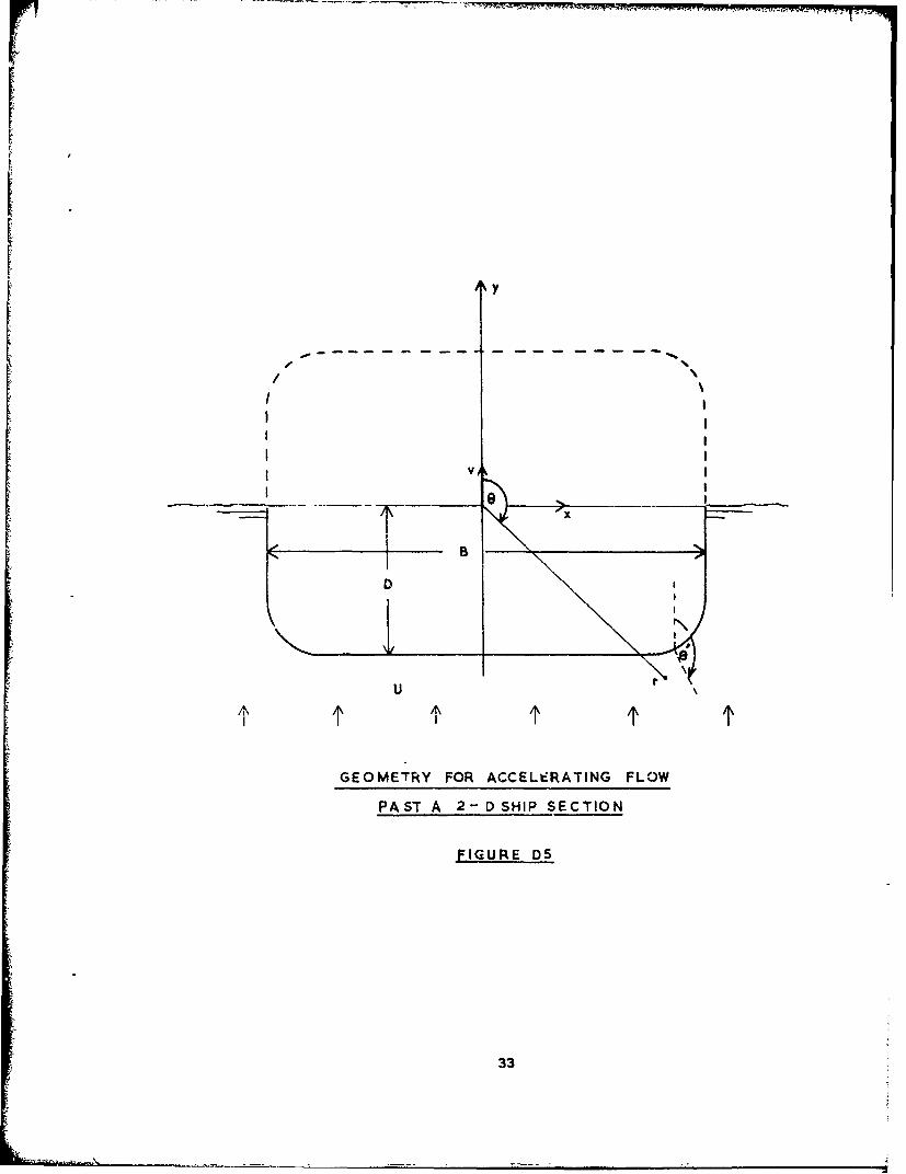
on the potential 0 of the 2-D flow problem. With the geometry of
FigureD5 the potential 0 satisfies the following equations:-
V 24 o (incompressible flow)
S= 0(.), rvf (only a dipole field at large. distances)
= - v cosO' on r (the ship-sha.ed cylinder cross-section)cn n
If the potential for t!n -.asev = I is denoted by 1, then 4 = v
and 4 satisfies 2-
24
C. S on I' (D2)
"11Ce t~icforxi. of Deraiuilli's C ~iatioi. £,ives the r.-ssurc in the
fluid
f- r. is thic k,.-tros t.-.tic 2ire:;urc z.iid u L::- 1(-,: 1 velocity.
*;cglcctind; Pu co:ipnr:uxd to p ýat ivcs .1 pv,ý :.nLd t:.c >--rc
actin'; on th"w cylinU;Cr is si-1iily
-r( -P4 L (D4)
r r
su that, co. *Žarin,; -.-ith (DI),
ýx~aft 5)dr
The fractor *.-.I ! ows for t:.e u p~er !,-ir f a'thce fluid! not :,Ciný;
!)re-cnt since y = o is the frez: st- face.
.:nth, s.:rroundiný; fluid a~lso h-as -i veloci ty, U, at infinity,
the potentkiz.1 P* mst sritisfy thu e'ittations
4?=-Ey + c() .r
=-V COSO 7n I
ýIlcarly t:-ais .*mtci-til is Z~iven b~y 47-Ly - (U-v)? mor t:dis s--tisifies
the first tv.3 conditions nnd on r
= -= coso - (".-v) (-coso) -v Cos 0an n ar
as re~uircd.
The pressurc it. t,,c -at..r is no.. (. -in e'Iectin,, pu- L:.nrs)
0 + t
and the forc on tihe cyl inaecr is
-4 ~ ~ 60e=pUyi + p( V)4 do
25

; yd* is the .rza %.itUin the cont'm)r r, i.e. 2A whicre \ is the
,'nJl-r..ater ,,rea of the cross-section, so that the force )n the
under..Lter section is
fr =PAU + 4( - V) (D6)
which reduces to the :irevious case when U = o. This equation is
in fact rather obvious. The second term is the inertial- force due
to thL relative acceleration of the cylinder and the fluid and the
first is thc 'buoyancy' force due to the pressure gradient required
in the water to give it the acceleration U. Under gravity the
fluid effectively has an acceleration 1' = g ai-l the first tern
beco;ies the -wei:;ht of thi • is':ýiýced wvat-r, ;,.s is assumed in
hydrostatic calculat ions.
This resilt is a;-,lied in the sa:Ae way as normal strip theory.
The vertical velocity of the water due to the explosion bubble motion
can be calcu~ated at ench point of the ship axis, (the intersection
of its centreplane v:ith the watcrlinc --Ic.,) as though the ship were
not present. If the charge is far enough from the ship for this
velocity distriLution to vary only slvly along the lenZt1 1',cn
at each cross-section the disturbance :;otential necessary to correct
the local flow for thc presence of the ship w;ill, ns albove, be
approxi.natel. -(U-v)? (, býir• api'3iiriatc to the section sha',e)
and the force or. the shi.' will be as z;iven by (D6).
Since i ,s been ex)rssed in the fani
Ii ,= C . ".P
it is cot.,'en-ent to exprcss , si.il. rly so tlht
{ )Ap 1;7C J
In this case ý.owever, since the 'buoyancy' force ,lepends on a
pressure gradient independent of the shu;c of the ship, no three-
dinensional correction factor is required. The values of the
coefficient C for Lewis' sections have ,een added to Figure D1.
Cis related to the usual section area coefficient, 3, by
S3D
References
I. Lewis, F M ; "The Inertia of the I'later Surrounding a VibratingShip." Trans. SNA.?!E, Vol 37, 1929.
2. Taylor, J L ; "Soiae IHydrodynamical Inertia Coeffic-',nts."Phil I'ng S.7, Vol 9, No 55, Jan 1930.
3. Prohaska,C 9; "The Vertical Vibration of Ships."The Shipbuilder and *.:arine Engine Builder, 1947.
4. Landweber, L and Iacagno, IN ; "Added P'ass of a Three ParameterFamily of Two-Dimensional FormL Oscillatingin a Free Surface." Jn of Ship Research, Vol 2No 4, 1959.
5. M!acagno, , ; "A comparison of Three Yethods for Computingthe ",dded .lasses of Ship Sections", Jn. ofShip Rc earch, Vol 12, No I, 1968.
6. Roffr man, D ; "Conformal Mapping Techniques in ShipHydrodynanics." Webb Inst of Naval ArchitectureReport No 41-1, 1969.
7. liendel, X ; "IIydrodj-namic Vasses and L'oments of Inertia."Jahrbuch der Schif Af1m.tcchnische Gesellschaft,Vol 44, 1950; (also DT:B Translation 260, 1956).
3. Kaplan, P *A Study of the Virtual Mass Associated withthe Vertical Vibration of Ships in Water."Stevens Inst. Tech., Davidson Lab. Report 734,1959.
9. Ursell, 7 ; "On the ileaving ;.:otion of a Circular Cylinderon the Surface of a Fluid." Quart. Jn. Vech.and ':,Alied Maths, 2, 19/49.
10. Porcr,. R ; "The I ressure Distrilution, Added l;hss andDamping Coefficient for a 'yiinder Oscillatingin a Free Surface." Univ. Calif. Inst.Eng. Res. Series 32, Issue ;6, 196,.
1!. Choung look Lee ; "The Second Crdcr Theory of Cyl indcrsOscillating in a Free Surface." Jn. Ship"Research, Vol ;2, No. 4, 1963.
27

CURVES *Igam TO UNDIRWATER
CROSS SKCTlONAL. ^NARA*) Wi()c
"•, •"
00
HeR04FT a 0D
404
00
o d -0-d 0
o 009
0ji -' -t3S
4 4
VALUE OF INERTIA COEFFICIENTS C ANDC
HALF SEAM 8Ha DRAFT 2D
FIGURE 01(s)
28

1-5,
00
0*
IL 6
VALUE OF INERTIA COEFFICIENTS C ANDC
HALF BEAM B
DRAFT 2 D

0.9-
S~TAYLOR'S-U ~~~CYLINDER ,-"
S~0.
JI
U)
w
0-6V S 6 7 8 9 10 II 12 13
L lB
THREE- DIMENSIONAL REDUCTION COEFFICIENT
FIGURE D230

01
*112
CA
ItI
TWO -- DMNINLSCINv~uLMS OPIIN
FIUR 0D3
o-1S

- ! 1
o I
. /
* W.DE• ECAGEWI BLG Ea
FIGUE D
a *32
)y
/D
uI
GEOMETRY FOR ACCELERATING FLOW
PAST A 2-DSHIP SECTION
FIGURE D5
33

E Equations of Motioi
The only external forces acting on the ship are the hydrodynamic ones
discussed in the previous section. These form a continuous distribution
of force along tht ship. In addition to these, the inertial forces due to
the ship's own mass also act and again form a distribution along the entire
length. The form.lation of the elastic nature of the ship assumed only
forces acting at the discrete tnodest between the beam sections. Current
methods of finite element analysis generally use consistent-mass matrices
derived from energy considerations. These divide the mass between the
element nodes in t:e most effective manner. However, for the beam
displacement shapcs inherent in the elastic formulation the split. is rather
complicated and ai•o much of the ship mass comes from material such as
machinery, transverse bulkheads, etc., which is not continuously distributed.
It is consequently convenient and reasorable to simply split the ship into
n equal sections, lump the total mass and inertia of each section into a single
mass and inertia at the centre of the section, and take the elastic beams
to be the (n-0) equal lengths connecting these masses. The length 8
of each elemental :eam is L/n. If the variation in cross-sectional shape
is fairly slow, the lumped hydrodynamic force and moment at the ith mass
will be from (D6) (i again being the added mass per unit length),
Shdi = [vi.(ui-y.i) + Viui].
d .. d4. dyi di u. 4'U
Mhd = dx y.) + ~pi-. -! + -- u. + ý. __L..]hdi d u ÷ dx dx dx dx 12 (El)
2 dwhere all terms of order 4: and 2have been neglected.
dx d
The corresponding hydrostatic terms (loss of buoyancy due to upward
displacement will be
S= -B.t y.Shsi B Z
"dB. dy 43-.y + B (E2)hsi dx i idx 12
34

The normal i. .rttal force aud moment are
Si -miY (I5)
dy.
Mli idx
Comdbination of (-,-..At ions (!K I to (13) givvs
=. di+mwzy. - k.y.+(n. +~)
I i )y WI WI i
M.~- y -k. y , - r' +r '.U. (r.+r.)Y-k Y. +I Wi - WI wi i i÷i i-1r i
dth.
(r +r ) - 1wi wi UT
S 22 2where mi t ai'nw Pi 4C r~v L m2 z i=
ki = .4is i . -i 122
k i ' kri d . i I 2 -k d Z.
3 12rw i- d% WI 12 dx.
1 dE.ri 12 dx
In matrix form the .e equations (E4) become
2_M+I K 01 [M ]t +51+ R+R Rr + R'k*R' (E5)L-LLW] L
where u = and the su'b•;atrices are all diagonal with the obviousaIx
elements. This equation is slijitly inconvenient as it involves the
off-diagonal submatrices R', 9" and K'. Over most of the length of aw W rship the cross-section is almost constant so that these terms will be
very small except possibly near the ends. Strip theory already ignores
longitudinal flow Jue to changing cross-section in these regions. It is
therefore consistent with strip theory to neglect the terms and use the
35"

equationri w Ew ] i= =I - + (E6)
L 0 R+R i K 0 Rw+ U IL L rw "
On applying D',\lemli.rt's Principle, these arc the forces and moinents ncces-.ry
to maintain the displacement shape (y, y) in the elastic equations (C4).
The equations of forced motion of the ship are therefore:-
M+ 0A+K B [ +R • 0 ]E[)
L L _Rj Liand for the still-water vibration the right hand side may be dropped.
In general, for ship vibration, it has been found that rotary inertia
effects are usually fairly small. On neglecting the appropriate terms and putting
RR =K =RW =0,W r w
T = -C-1 BT
and
(Ii + M )y + (A+K - BC-1BT)y = 01w+Mw)U (ES)w w w-
Neglect of rotary inertia in these lumped mass equations of motion differs
from its neglect from the norntal Timoshenko beam equations since here it has
a slightly different meaning. In the Timoshenko beam equation rotary
inertia refers to the inertia of an infinitesimally thin cross-sectional
slice of the beam, and so is related purely to the depth of the beam and the
amount of material away from the centre of rotation, Here the rotary inertia
includes this term but also includes a term due to part of each lumped mass
being a finite distance from tha mass in the longitudinal direction. It
therefore depends on the distance between the lumped masses and so is a
36

function of Lhe beam represe;,ration rather than an intrinsic property
of cross-sections of the beam. Only if the number of lumped masses
representing the beau were allowed to ternd to infinity would the
two forms of rotary inertia coincide. In the equations used here,
eh fluid rotary inertia is entirely due to this lum.•ping of
longitudinal torces ilitt' :A -),)int load and so vanishes entirely in
the limit of an infinite number of lumped masses.
It may be noticed that if the ship is in still water and is not
vibrating then the equations (E7) or 498) are satisfied by zero
deflections everywhere. They therefore do not include any static
bending moments and shear forces due to mismatcher, between the
hydrostatic buoyancy and weight distributions. These static terms
were omitted in equation (E4) for simplicity in the dynamic equations.
Any stresses deduced from equations (E7) and (E8) during motion are
to be superimposed on the existing static stress distribution in the
ship.
The equations include the buoyancy terms K and K and so containr
the heaving and pitching ship frequencies, at least for small
displacements where the additional hydrostatic buoyancy forces are
linear functions of the displacement.
37
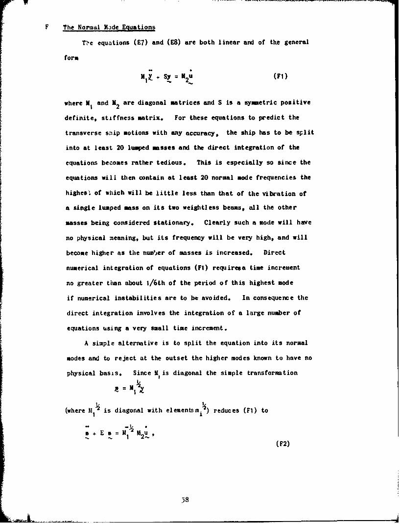
F The Normal Mode Equations
TVe equations (E7) and (E8) are both linear and of the general
form
mi SY = 121u (Fl)
where ¥1 and M2 are diagonal matrices and S is a symmetric positive
definite, stiffness matrix. For these equations to predict the
transverse snip motions with any accuracy, the ship has to be split
into at least 20 lumped masses and the direct integration of the
equations becomes rather tedious. This is especially so since the
equations will then contain at least 20 normal mode frequencies the
highest. of which will be little less than that of the vibration of
a single lumped mass on its two weightless beams, all the other
masses being considered stationary. Clearly such a mode will have
no physical meaning, but its frequency will be very high, and will
become higher as the num'jer of masses is increased. Direct
numerical integration of equations (FI) requiresa time increment
no greater than about I/6th of the period of this highest mode
if numerical instabilities are to be avoided. In consequence the
direct integration involves the integration of a large number of
equations using a very small time increment.
A simple alternative is to split the equation into its normal
modes and to reject at the outset the higher modes known to have no
physical basis. Since MI is diagonal the simple transformation
a=M
(where MI1 is diagoral with elementsm .) reduces (FI) to
+ E =K u
(F2)
38
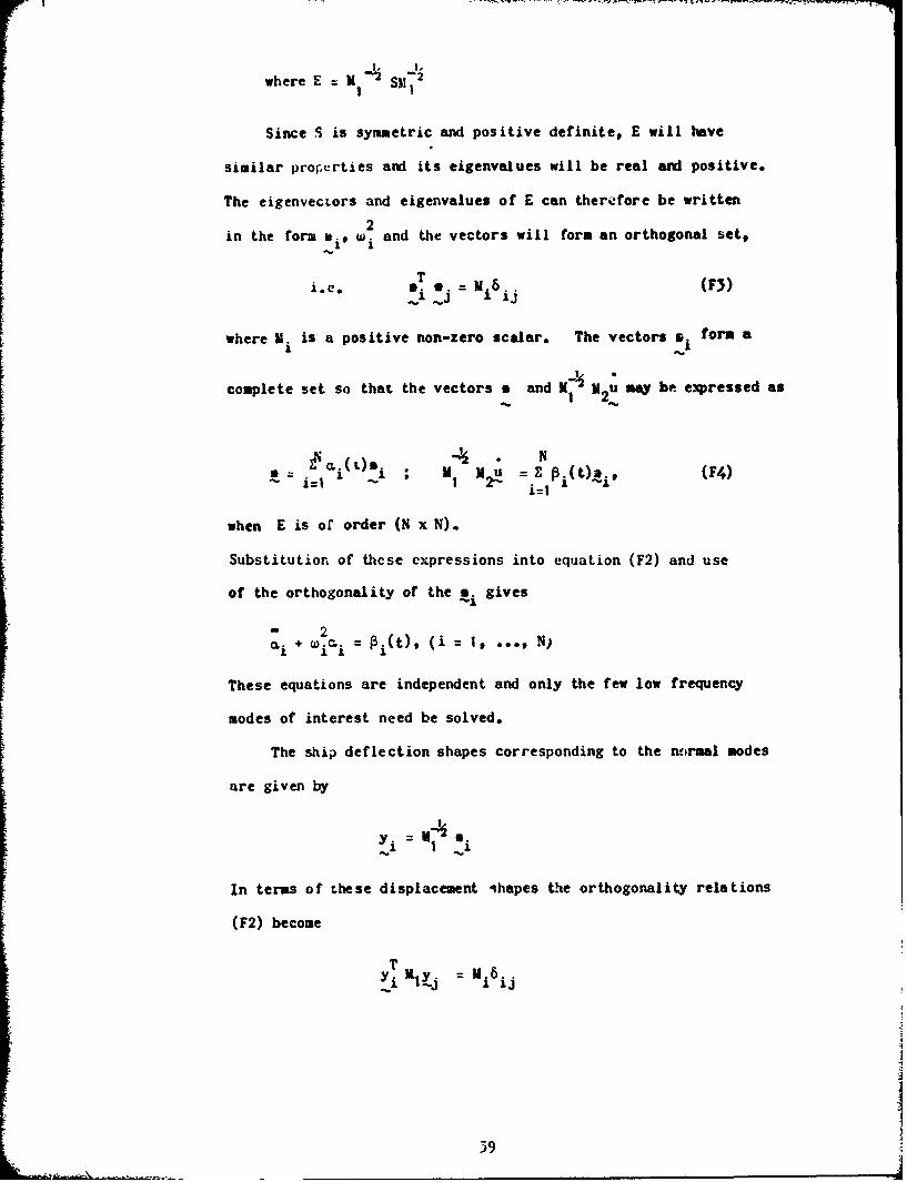
1, I,
where E = M -2 S11-21 1
Since S is symmetric and positive definite, E will have
similar prorerties and its eigenvalues will be real and positive.
The eigenvecLors and eigenvalues of E can therefore be written2
in the form ij, w.2 and the vectors will form an orthogonal set,
Ti.e. a M 0 = Ni& (F3)
%IJ i ii
where M is a positive non-zero scalar. The vectors m. form a
complete set so that the vectors a and K M au ay be expressed as
LN CLi (L)& i ; N1 N ~ = ai, (F4)
when E is or order (N x N).
Substitution of these expressions into equation (F2) and use
of the orthogonality of the p gives
- 2c•i + W~i =_ •i(t)9 (i = 1, *eel N)
These equations are independent and only the few low frequency
modes of interest need be solved.
The ship deflection shapes corresponding to the neirmal modes
are given by
I
In terms of Ohese displacement ihapes the orthogonality relations
(F2) become
T[i h*.. : Ui 6
39

Nie z kYkiYkj - Miij (F5)
k=l
Similarly, multiplying the second of equations ()gives the
forcing function Pj(t) as
T T M2 N2-7 ýjt 2,; : ,- "'2Vkj k2 N
and ~(~ +~~i~) =Ni • 2k'ki~k ,( = 1, ... ,N) (F6)and Mit + •0imlt)2 E ai ak(A
which gives the ergations for the ith mode coefficients i(t)
in terms of the hydrodynamic mass distributions, the displacement
shape of the ith mode and the fluid accelerations at all the
lumped mass positions.
If the coefficients M.(t) are found by integration of
equations (F6) the actual ship displacements, stresses etc. are
easily deternined from the equations:
N
displacement y(xt) = Z=£ o(t)yi(x)
Nvelocity J(x~t) = E. 'ii(t)yi(x)
N
bending moment M(xt) = E Qi(t)Xi(x) (F7)i=I
deck stress a(xt) = M(xt) ( y distance of thedeck above the
neutral axis )
Nshear force S(x9t) = 'M 1, Ms i(x)
i=4
40

where yi(X), S"(x) and S.(x) are the displacement, moment and shear
force at the position x when the ship is in the ith mode (unit
amplitude). With the normal mode shapes known (Yki' Tki known at
the kth mass) the displacement, moment and shear force for a point
at a distance x -xk from the left hand end are given by
-2" " - •2 -2 x (I -E )
Y.(x) I x 21 Ek YkiSki
1M.(W) = 0 0 1 JiL (F8)
Si(x) 0 0 0 1 SL
where UL and SL are given by equation (C2).
41

G Use of the Modal Equations for Free Vibration
To illustrate the use of the modal equations for free vibrations
and to estimate their accuracy when used in ship calculations, three
examples are considered:
a. A uniform solid bean in air and water
b. A hollow rectangular box-beam in air and water
c. A full scale ship
In some of the previous vibration calculations inthe literature ships have been
divided into up to 40 sections but 20 is the more usual number and
has usually been found acceptable for the low modes. The examples
are therefore based on 20 lumped masses. The calculations were
carried out using the computer program I described later in section
I.
a. Uniform Solid Beam
In 1928 in an early series of experiments on the effect of
entrained water on the vibration of ships, Moullin and Browne
(GO used a series of uniform rectangular mild steel bars. The
bars were 78 inches long, 2 inches deep and of varying thickness.
The principal thickness was I inch. The cross-sectional moment
for such a beam is 2BD3 (see Figure GI) i.e. 1/6 in 4 .3
The shear area for a rectangular section is 2/3rds of the cross-
4. 2sectional area, i.e. !in . Then, for representing the beam by
20 equal lengths the equations of section C give:-
, = 3.9"; 1 = .1667 in 4 ; A = 1.333 in 2
3 = 30.106 psi; Y = 0.3
12(1+v)I 0.1282 ; a= 2EI 0.1342.10 61b/in.
242

The matrices A, B and C are then the (20 x 20) matrices
r .805 -. 805 0 0 ... 0
-. 805 i.610 -. 805 0 • • 0
6 0 -. 805 1.61o -. 805 0 .. • 0A 10 lb/in
-. 8o5 1.6io -. 805
o 0 -. 805 .805
r 1 . 5 70 1.570 0 •.. o
-I 1.570 0 1.570 0 ... 0
0 -1.570 0 1.570. 0
B 106 lb
-1.570 0 1 .570
0 0 -. 1570 -1.570
4.35 1.781 0 0 to 00
1.781 8.70 1.781 0 O
0 1.781 8.70 1.781... 0
C t, •lb-in
1 .781 8.70 1.781
0 1.781 4.35
and h"es,: define the shear forces Si(lb) and bending moments
Mi(lb.in' for a given displacement shape y. (in), yi (radians)
"43

according to
L"] = [T €]~
Since the density of steel is .284 lb/in , the mass of each
'lumped mass' is 2.216 lb. For the rectangular cross section one
of the curves in Lewis' paper (G2) gives C = 1.361. Thc uncorrected
added mass for each section is therefore
2S) = o.601 lb
(the usual factor ý has been dropped since for a fully submerged
bar no surface correction factor is necessary). For a beam with
L/B = 39, the 3-D reduction factor is 0.983 so that 3-D flow affects
the bar very little. The buoyancy term is not actually needed for
the free-vibration calculation but for this example it is
pAZ = 2pBDC = .2815 lb. The immersion force k. is of course zero for a1
submerged bar. The rotary inertia of each section about its ceitre
Ps- BDU(t2+4D2) = 2.99 lb.in The rotary inertia of the
2surrounding water is 1/12m w4 and of the buoyancy it isw
1/12u;t.2 so that
mi = 2.216 Ib; %. = .591 lb; ;wi = .282 Ib
r= 2,99 b.in.2; rwi .749 lb.in. 2; rw= .358 lb.in..2
Using these values, the normal mode analysis described in section
F is readily carried out using standard computer matrix manipulation
44

subroutines. FGr the beam vibrating in air alone (awi = wi = 0),
and with shear deflections suppressed, (A. made very large) the
calculated frequencies are compared with the exact frequencies
for a free-free uniform beam in the following table. The exact
frequencies are given by
xi E
where x has the values
4.730, 7.853, 10.995, 14.137, 17.278, 20.420, 23.561, 26.703,
29.845, 32.986, ... (the roots of cos x Lash x = 1)
and these frequencies do not include the effect of shear deflections.
COMPARISON OF EXACT AND LUMPED MASS FREQUENCIESFOR A UNIFORM BEAM VIBRATING IN AIR
Number of nodes 2 3 4 5 6
Exact frequency 34.13 94.1 184.4 304.9 455.5
Calculated frequency 34.08 93.6 182.4 299.0 442.2
% error 0.15 0.53 1.08 1.94 2.92
Number of nodes 7 8 9 10
Exact frequency 636.2 846,9 1088 1359
Calculated frequency 610.1 801.3 1013 1243
% error 4.10 5.39 6.90 8.54
The agreement to within 0.15% for the basic two node frequency
is quite reasonable and confirms the general accuracy of the lumped-
mass formulation and the computer routines used. For the higher
44,5

modes the accuracy naturally falls off but that it should be only
830S in error for the ten node frequency is surprising considering
that only a 20 lumped mass system was used so that there are only
two lumped masses per half wavelength.
To show the effects of rotary inertia, shear deflections and
immersion in water on this beam a series of calculations were run
to produce the results in the table. The 'exact' results again
contain no correction for shear effects.
FREQUENCIES FOR A UNIFORM BEAM IN AIR AND WATER
Number ofnodes
Case 2 3
IA 34.1 94.1 184 305 4562A 34.3 94.7 186 308 462
3A 34.1 93.6 182 299 424A 34.3 94.6 186 307 4585A 34.1 93.5 182 298 439
6A 33.5 - - - -
1W 30.3 83.6 164 271 4052W 30.4 84.1 165 274 410
3W 30.3 83.2 162 266 3934W 30.4 84.1 165 273 407
5W 30.3 83.1 162 265 391
6W 30.2 82 - - -
Cases: I ; 'Exact' uniform beam frequencies (without shear)
2 ; Calculated excluding shear and rotary inertia
3 ; Calculated excluding shear but includirg rotary inertia
4 ; Calculated including shear but excluding rotary inertia
5 ; Calculated including both shear and rotary inertia
6 ; Measured value
46

Clearly neither rotary inertia nor shear affects the frequencies
greatly for this beam. Shear in fact has almost no effect but
inclusion of rotary inertias drops the 6-node frequency by about
4o. The agreement with the measured frequencies is within the
experimental error.
The main conclusion from this example is that for a normal
beam, with well defined physical properties, the method is capable
of giving good results and quite high accuracy can be obtained for
the first fcw modes by using a 20-lumped-mass model.
b. Hollow Pectangular Box-Beam
In his experiments on the whipping induced by underwater
explosions, Chertock (G3) used a thin-walled, stiffened, rectangular
box-beam. The dimensions are shown in Figure G1. In this case the
steucture cnnrot be aefined quite so exactly as for the solid beam.
The top of the box had a 4" wide opening along its entire length,
and during tests a cover was bolted on to close the opening.
The degree of fixity of the cover, and its strength, will affect the
cross-sectional inertia considerably. It is assumed that the
bolts were really tight and that the cover was simply equivalent
to the missing material. Ignoring the stiffeners, the elastic
data is
6E = 29.10 psi, v 0.3, P = 6 inches
I = 9.51 in/4, A = .529 in2.
The total ballastea weight was 105 lb so that the draft was 2.70B
in. Then H = 2 = 1.668 and the added mass coefficient C = 1.40
(again from Lewis' paper (G2)). The lengthVbreadth ratio L/B =
13.33 so that J = 0.903 and this time the effect of the 3-D
flow correction is quite significant.
A47

In the calculation of the added masses the factor "' is
included to allow for the free surface effect, The lumped mass
data is:-
in. 5,25 Ib; mi. = 8.69 Ib; in wi 5.25 Ib; k. = 1.947 lb/in2 2
S50 lb.in- r 26.0 lb.in•; rwi = 15.8 lb.in
kri = 5.85 lb.in
Here the structure lumped inertia is a rough estimate since the
exact figure would vary from mass to mass (the stiffeners being
discrete an(, several transverse bulkheads being present).
A table of results for the same cases as for the uniform
beam is reaily constructed:-
Cases: 1; 'Exact' uniform beam frequencies (without shear)
2; Calculated excluding shear and rotary inertia
3; Calculated excluding shear but including rotary inertia
4; Calculated including shear but excluding rotaryinertia
5; Calculated including both shear and rotary inertiausing the Taylor formulation of shear area.
5a; Calculatcd including both shear and rotary inertiausing the Taylor formulation of shear area.
6; Measured frequencies
/t8

FREQUENCIES FOR CHIRTOCK'S BOX BEAM MODEL
S~Number of
0 1 2 3 4 5Case
0A 0 0 86 238 466 771
2A 0 0 88 244 479 794
3A 0 0 87 235 451 726
4A 0 0 86 227 414 628
5A 0 0 85 221 399 602
5(a)A 0 0 85 217 389 580
6A 0 0 81 191-197 - -
1W - - 53 146 286 473
2W 1.07 1.26 54 150 294 487
3W 0.96 1.34 54 146 284 462
4W 1.16 1.17 53 139 254 385
5W i.t1 1.22 53 137 249 376
5%a)w 1.11 1.22 52 135 242 362
6w 1.15- 1.15- 49- 98- _ _1.35 1.35 " 51 108
The agreement this time is much less satisfactory. The 'exact t
uniform beam results still agree well with the appropriate case 3,
and the remaining calculated results are all quite consistent.
Unfortunately there is i considerable difference between the
calculated results and those measured on the model. For the
fundamental modes in air and water the calculated frequencies are
higher than those measured by 4.7o and 4r respectively, and for the
three node modes the correspondLng figures are 120 and 31%. Since
the lumped mass model has been shown to be accurate for such low
modes, and still agrees with the lexactt uniform beam solution,
the difference must be due either to non-beam-like behaviour of
the model or to incorrect assignment to parameter values (masses,
sectional inertias, shear areas etc.).
S~49

In addition to the natural frequencies, the mode shapes and
longitudinal strain distributions were also measured in Chertock's
experiments and the strains deduced from the curvatures in the
normal modes were found to be rather greater than the measured
strains suggesting that either large shear deflections were
occurring or the sectional inertias were lower thanexpected.
The above calculated results, in appropriate cases, contain the
effect of shear but it was thought that perhaps the simple beam
theory shear area formula
ItA it
s m
(where I is the cross-sectional inertia, t the thickness of
material on the neutral axis and m i•s the moment of the area on
one side of the neutral axis) might not be very accurate for the
thin-walled box beam. By using an alternative formula, due to Taylor (G4),
for the shear area of thin walled girder, a smaller value for the
shear area was obtained and this gave the results for case5(a) above.
A common practice in ship calculations is to assume the shear area
is simply eqnal to the area of vertical plating. The three types
of shear area for the box beam model are:-
actual cross-sectional area = 1 .44 in2
( area of vertical plate = 0.576 in 2
(shear ( beam type shear area = 0.529 in 2
areas (( Taylor shear area = 0.429 in
It is clear from the results however that the differences in shear
area do not account for the discrepancy in frequencies. An
alternative partial explanation could be that the cross-sectional
inertia, I was too large. As moted earlier, the model in fact
had a 4 inch wide gap in the centre of the top plating, which was
50
•' ,• •k._
"• .r• ++ • - •+ •'+'" ''- '.. . • • ''+''• -r+ Q +•..... . . +: ... • -• +•"=• -- '+ +++ ''+••'•i '- ' •' "•=--•.... - A•

closed off dut'ing the tests by a bolted-on lid. Assuming that the
lid was totally ineffective, the moment of inertia and shear area
become
I = 7.51 in 4 As 0.513 in
2instead of I = 9.51, A = 0.529 in as with the lid.
The change in inertia will reduce the calculated frequencies by the
factor
so that the new frequencies in air and water will be approximately
No. of nodes 2 3 4 5
frequency in 76 193 346 515air
frequency in 4 120 215 322water
The fundamental modefrequeniy is now too low but that of the 3 node mode is about
right. It is possible that any relative motion between the lid and
the main box could affect the modes rather differently and this
seems a plausible reason for the differences in frequencies.
This beam shows up the usual features of ship structures:
the added water mass is very large, 1.6 times the structure mass,
the three dimension fluid flow correction is appreciable; 10% of the
added mass, and shear deflections are very important, particularly
for the higher modes. The shear correction for the 5-node mode
frequency is 26%. The data for this model however are not adequate
to differentiate between the 3-D flow corrections of Taylor and Lewis
or between the normal beam-type shear area and Taylor's shear area.

c. Full Scale Ship
The data for a destroyer were recently calculated as part of
a vibration test and are given in the following table. As for the
uniform beams, the ship was divided into 20 equal length sections
and the mass and rotary inertia of each section was lumped at its
centre. The lumped masses are then connected by 19 equal length
weightless beams whose elastic characteristics correspond to cross-
sections mid-way between the masses. If x = o corresponds to the
bow and L is the length of the ship, the lumped masses are at the
positions
x. - (i - ")L/20 ; i 1, ... , 20
and the cross-sections characterising the weightless beams are at
x. iL/20 ; i = it .*j, 19
The data require some explanation. The ship mass and buoyancy
are fairly easily obtained from the ship's design drawings. The
added mass was obtained from Lewis' formula by calculating the
parameters a and b of the Lewis transformation with the correct
beaidraft ratio and passing through a selected point of the cross-
section. Several other points on the cross-section were then
computed to verify the acceptability of the fit. The appropriate
values of C and C were cupted and comparison of the buoyancy
calculated from C with the ship design value gave further general
confirmation of the fit.
"52

C4 '4 - -
.Q.a J --.' - - -. - - --oo - -- - - - - - -- -- - -
=~~~~ ~ ~~~ ,,, e " o,•' 'DI°0 8 0 0• °' 0 0 0' IL4 -4 0%r LIN 0 0 C4 ~4.'0 00 -,'0 \% 0 000 0\4 r
v0 0 r. i 00t- r \-O UM
-~ -s -- -
0
4 j- v _ \ t D & - % oWC00 000 00000
0 0 O '0 0' 0% t'. 0 0 0% C
tn . ... a\ . ... %C tn .* .
0 r.0 til If-0^ C4 W
r -4
0 0..4 0tn3 .-. 0-. Ot0 0 Q t .- 0
C4 Ln C4 r-00 0\ r\%D n C• . u. . 0 9 0 *9 0, 0 0 * 0 .
r_ tn \4.rN-0sr.n ci LtA\ n CIS 0 N nr. a\ -t,% \r--0 x a, Go 00 Z i '.\D N % \0 11% !
0 -0 - -. - - - - - - - t.Q r\'ttn~
ds0 - - - N " N ' N N C4l N' C4 - - - H1ý El4
USr t -e -4%t0 tt-v\ A'o 00 -r r- a 0 1~-O \.0 st00
:9 N - - - - -00 ~ 0 4 0 0 '0, cI 0- 4.' ~ -N
r-.0 m0. '.t -\ %0 CIS '- 4. 0 %DC4u~' 000 \0 N
V) o. n. n-C' \,D~ ' 00 0 04 n ' tn r-ý a\ 0 N 4 0-.44 L. ~ C4 C' ~ .
US .0' -4 te%. r- 00 0\ 0 - C4 n -.r Lt'\. %a '00 0\ 0
53
The method is considerably more complex than applying
Prohaska's curves but ensurea good representation of the section
and, once progrs ed for a computer, is straightforward. Choosing
the collocatoim point either at 1i/3rd of the draft above the keel,
or at the point of attachment of the bilge keel gave the most reason-
able results. The existence of a bilge keel in the midship region
is itself a complication. To allow for its effect references
C13 and G5 both rccommend the use of Wendel's correction factor (07).
Applying Wendel's figures for the square gives an increase of
1-' ' (since the beam is 19 feet and the keel width 2 feet). Applying
the a.proximation of section D (the draft was only 12 feet) gives
the value 14g. Since both of these values appeared to be rather
large en alternative approach was tried. The radius of curvature
at the turn of bilge was rather larger than the width of the
bilge keel so it was assumed that the flow near the keel would
be fairly similar to the flow along a flat wall with a plate project-
ing out at right angles. The latter flow is simply one half of
the two-dimensional flow normal to an isolated flat plate. This
flow is well known. The velocity of the flow past the plate can
be related to the vertical velonity of the ship section by computing
the velocity which would exist at ti,, root of the bilge keel
according to Lewis' transformation, iC the keel were not present.
Suitable resolution of the resulting force on the keel then gives
an appropriate added mass. The method is described fully in
Appendix 1. The correction for the bilge keel is found by this
method to be between 9 and 4o and this is the value which is
included in the table. In fact the keel is not particularly
important in whipping calculations since using the full Wendel
value instead of the value used here would reduce the basic 2-node
54
vibration frequency by about 2'j only. For vibration purposes this
difference might be more significant.
To correct the added mass for the three-dimensional flow effects,
the Taylor correction factor for the 2-node mode of vibration
was used. For this ship, with a length/beam ratio of 9.3 the factor
is 0.807 and so is again quite significant; without it tie added
mass would be 750 tons greater and the basic frequency would be
dropped by around 6V.. Lewis, reduction factor for this case is
0.847 which would increase the added mass by about 150 tons and so
reduce the frequency by a little over 1%.
Calculation of the rotary inertias is extremely time consuming
and was not carried out for this ship. It had however been carried
out earlier for a fairly sitailar ship and the values for that ship
have been scaled to apply to the present one.
The cross-sectional moments of inertia for the beam sections were
calculated in the usual way with all continuous longitudinal material
up to and including the main deck being considered effective. The
forecastle deck was also included entirely right back to the break
of fo'c'sle. The deck houses however were so short that no
correction was necessary. One common method of estimating the
shear area is to take the area of all vertical plating. This was
tried bat led to frequencies which were too high. The shear areas
calculated by beam theory, i.e.
its m
ere about half the values given by the vertical plating method
and lead to much better frequencies. Even this method however is
questionable since it depends heavily on b, tne thickness of the
side plating at the neutral axis. For a few cross-sections the
neutral axis occurs within inches of the waterline, where, for amour
55

reasons, there is an abrupt change in plating thickness. Applying
the above equation rigorously could lead to the shear area changing
by a factor 2 if the neutral axis moved a few inches. Clearly some
kind of average is required. Taylor's method for the shear areas
of thin walled box girders applies well in this case and several of
the inertias calculated by the normal beam formula were recalculated
in this way. The results confirmed the beam formula exceptionally
well.
The normai made frequencies given by the computer program for
the four cases:-
1. Shear deflections suppressed, rotary inertia suppressed
2. Shear deflections suppressed, rotary inertia included
3. Shear deflection included, rotary inertia suppressed
4. Shear deflection included, rotary inertia included
are shown in the table, together with the actual frequency where this
was known.
CALCLIATED DESTROYER FREQUENCIES
Frequency (Hz)Number of Nodes Calculated Measured
_ 2 3 _
0 Heave 0.21 0.21 0.21 0.21 -
I Pitch 0.23 0.23 0.23 0.23 -2 1.68 1.66 1.54 1.53 1.59
3 ) 3.98 3.93 3.13 3.11 3.20
4 p 6.90 6.75 4.67 4.64 4.775 L. 0 11.02 10.64 6.41 6.37 6.29
6 ) 16.04 15.59 8.09 8.05 -
7 22.54 21.13 9.61 9.56 -
56
The agreement is quite satisfactory for the four vibration
codes for which an experimental frequency is known, except for the
basic pode. Even this mode is quite adequate for whipping
calculations where only a few cycles are of interest. Once again
rotary inertia is a very minor effect whereas shear is very important,
reducing even the basic mode by 9%o and for the higher, 6 and 7 modes,
the frequency is more than halved. The calculated and measured
mode shapes are compared in Figure 2. The agreement is again very
good except for the basic mode. This shape however could not be
compared directly as the vibration generator was incapable of
providing a sinusoidal input at such a low frequency and an.estimated
91 contamination of the first mode by the second has been removed
from the plotted experimental values. Part of the frequency
discrepancy may be due to errors in the assumed mass distribution.
A sister ship in a similar displacement condition was found to have
a frequency of 1.51 Hz.
References
1. Moullin E B and "On the Periods of a Free-Free bar ImmersedBrowne A D; in Water." Proc. Phil. Soc., Vol. 24,
Pt III (1928).
2. Lewis F M; "The Inertia of the Water Surrounding aVibrating Ship." Trans. SNAME Vol. 37, 1929.
3. Chertock G; "Transinat F1_cxurai ?ibrations of Ship-like Structures:tructurcs Exjosed to Underwater Explosions":Jn Acoustical Soc of Amaerica, Vol 43, No I(Fart 2), July, 19/0.
4. Taylor J L; "The Theory of Longitudinal Bending of Ships."North East Coast Eng & Shipbuilders Inst.Vol. XLI 1924-25.
5. Leibowitz RC "Theory of Freely Vibrating Non-Uniformand Kenaard E H; Beams, Including Methods of Solution and
Application to Ships." DTMB Rep. 1317, 1961.
57

z~nh0
cc,
4 WZU4-
w
o x
0ILL
2 , Az
WW
-J J
m iao zxi
z
00
53

K .. MEASU•iED POINTS
MASS NUMBER
bow 2 4 1 6 ' 1 2STERN
-X-
VBOW 2 4 a 10 K 12 14 16 .. S 2STERN
• MASS 4NUMBERU
-.J
inx
x
0 x
BOW
MASS NUMBER
MBOW •M II I 16 8 2 STERN
N MAS NUMBERSK
CALCULATED AND MEASURED MODE SHAPES FOR
A DaSTROYER
FIGURE G2S9

H Explosion Induc.d Forcing Function
Following Chertock's original analysis, which was found
satisfactory for the models, the compressible phase of the
explosion pressure wave, and the migration of the bubble of
explosion products, are both neglected here, They will be
discussed later. Under these assumptions the flow, in the
absence of the ship and any boundary surfaces (eg the free surface
or the bottom) will be spherically syimetric and if the volume of
the bubble is V(t) the velocity at a distance r from the bubble
centre will be given by
u = V/r 2 (I)
The acceleration of the water will therefore be
V 2V dr V
4%r 4ux-- dt 4xr 8x r
The second term clearly decays much more rapidly than the first
away from the bubble and•in any case.it is consistent with the
earlier development of the forces via strip theory to neglect
forces of the type kpu , so the second term is neglected here.
The possible magnitude of this and similar terms is investigated
later. The water acceleration is therefore, in the present
approximation,
U= (H2)
4zr
Referring to the geometry shown in FigureHi, this acceleration,
when resolved vertically at the ship axis gives
s V VD R2 2 2 2a.Cost. R 2D + H .(x-X)4-2R. iv •R.3 ;
60I
__!

To allow for the presence of a .'ree surface at the shbp axis,
an image bubble of opposite stg:, to the real one must be added at
the reflection position above the free surface. At the free
surface the image will have the effect of doubling the vertical
accelerations and cancelling out any horizontal ones, so that the
final vertical acceleration is
VD (H3)
Substituting this into equation (F6) gives the modal equation
""kz wk + PAk)Y /RZ '
+ W. ). = X. ; k= m + ki k "H4)Ii i 2• E .3 21) k
k=1 k WK ki
for the case where rotary inertias are neglected. The same
equation applies, uut with an obvious modification to XK, wheni
rotary inertias are included. The similarity of equation (H4)
to equation (BIO), given by Chertock's analysis, is clear. The
factor 2 between the expressions is due to including the effect
of the free surface in equation (4). Equation (H4) is slightly
less accurate than (BIO), due t. the 'lunping' procedure, but is
more general since it is not restricted to tproportional bodies'.
It is however still restricted to slender bodies where .Ftrip
theory is applicable.
The equations (H/+) require only initial conditions. and
specification of the bubble volime history for their s)lutian.
The equations governing tue pulsations of a non-migrating bubn).,
are well known except vei7 late in the hisb.,Ie collapse i%,:S,. ",rc
matheaatical instabilities in tic equntioni reflect an clserv',',
physical ins. abilLiy. An excellent account of the e(iuaon, .--id
"their derivation 1s given by Coc (OIl), but a brief cutline t.-
,'|

included here as it, provides a useful lead-in to the modifications
for migration effects.
The velocity in the water is given by equation (Hi), i.e.
a a
U :--- -f24r
where a is the bubble radius. The kinetic energy is therefore
KE = ýP .oI,~r2 = 2y
a
The potential energy of the bubble is a combination of the
internal energy of the gas products and the potential energy of
the hole in the water, so that
PE -4-ap 4 3 po3 y-i 3
where p is the gas pressure, and p the ambient pressure at the
bubble centre. Since the pulsations are very rapid the adiabatic
equation of state is appropriate, i.e.
k Wyp=kPY -
ig 4a3y
where IV is the charge weight. If E is the total energy tiedo
up in the bubble motion and Z is the hydrostatic head of water0
at the bubble (2), the equation of energy conservation ispg
E3.2 4 3 kIWE= KE +PE = 2paa• + 3- pa~gZ°+L. k3(1)Eo E + P 7 a E a S 4 'x y-1 3(y -1 )
(Y-) (T) a
This may be written more simply in terms of the non-dimensional
variables x = a/L, T = t/T;
62

- - ---- L .• • •¸r' • -• . +, • • . • • • • • , r•, • •.j
1/ I/
F 3E 1/ [T ] L (H5)L =;
as
x3 2 x + k/x3 (Y-1) =1 , (H6)
k being the constant
(pgZ )Y-lk = kyI-I
0
Equation(H6) is the differential equation satisfied by the bubble
radius and applies so long as the bubble is spherical and remote
from all surfaces. In practice small bubbles fairly deep remain
spherical throughout their motion except for very short periods
centred about the bubble minimum. At these times the bubble surface
is unstable and greatly distorts. The bubble minimum and maximum
radii are given by (H6) when x = o, i.e.
3 k 1 (H7)
and for small k are approximately
x 0 k -L3 1 + ky-1/34y-1I; minimum (H8)
xI - k 1 + (Y- ý) ; maximum
The various constants in these equations have been determined
empirically by Arons[2]. He found that, for TNT, the correct
variation of bubble period (from explosion to minimum) with depth
could only be reproduced by equation (H6) if
"63

Y - 5/4
and then the actual value of the period is correct if
E = eW0
where E, the energy per unit mass of charge is approximately 490
cal/gm, Comparing further the experimental peak bubble pressure
with the predicted value gives
1/4k .0552 Z (H9)"0
Together with the theoretical expression for k given after equation
(H6) this provides the gas equation of state
p = 8,15p~'4
where p is in kbars and P g in gus/cc. Jones (H3) had some time
earlier predicted theoretically that this equation should be
10.25p = 7.8pg,
for the low pressures involved during most of the bubble period.
With Aron's values, the scale constants L and T and the
bubble maximum radius a and period T are given approximately by,U p
1i/3/ 1/3L = 13.6 /Z 0 t
T = 2.94 WI1!/ g5/6 secondsS~(8io)
a. a 12.6 wl/3/Z 1/3 ft
T= 4.36 W! o5/6 seconds
where W is the weight of the charge ir. lbs of TNT and Z is the0
hydrostatic head in feet of water. The bubble volume acceleration
64
is then given by
L3 /3 x 2/ 32V(t) 3 (x3) 1220 W/Zo2/3 ()) ft)/sec (HI1)
3T 0"°3
where x , by differentiating (6), is given by
32 . 2 3x~ 3.7!x x .=. Xxx -x i/x _ -4 (3Y-4)k/x (H12)
The pressures in the water around the bubble are also
proportional to x 3for, except close to the bubble where !ipu2 terms
are important, the pressure is simply
p = PC
Here p is the velocity potential for the flow around the bubble i.e.
4ar
so that
pPV (H13)4itr
and with the same units as before
pr = - (x3) psi-ft. (H14)
The equations (1110) for the period and amplitude of the bubble
motion apply strictly only to TNT. To produce bubble details for
close comparison with Chertock's experiments the basic bubble
equations can be used. The detonator which produced Chertock's
bubble was fired 13 inches below the model, ice. at a depth of
16 inches below the surface so that Z = 33 + 1.33 = 34.33.o
The observed radius was 5.4 inches and ihe period 23.5 msecs.
This period will have been reduced somewhat from the free-water
period given by equation (1116) due to the proximity of the water
surface. The empirical correction factor for this effect is
65
- "- fr -x - • ^ • . .. . * . ," - . . . . ..- " -- - -- - a a 1 .• ' • - , • •- -: -' ' -- I - * • • , • , - .-- .-• --'

a(see reference 14) (I - 0.2 -A) i.e. 0.932 for this bubble.
The equivalent free-water period is consequently 23.5/.932 = 25.2
msecs. Now
T~ Ir/2
a L x g-Z (1115)m- m o m
so that the ratio of period to amplitude is independent of the energy
release and depends only on Z and on k (through r a x ). From0 ;m•
reference H3, the solutions of equation (H6) for y 1.25 give
k x x 0 -/xm o m a
0 1.0000 0,0000 1.492 1.4920.1 0.9645 0.0464 1.4821 1.537
0.2 0.9235 0.1172 1.4804 i.603
0.3 0.8742 0.2031 1.4918 1.706
0.4 0.8100 0.3064 1.5120 1.867
From equationOll5), for Chertock's detonator,
T 2gZ 1 /2 T-. (_..)' .-£ = 1.520
xM 3 a.
so that k =0.066 (for TNT at the same depth the value would have
been 0.134) and x = 0.978, v = 1.483. Then, to give the correct
radius,
L = 5.52 inches and so T = 16.95 msecs.
With these values,
Pr V =- V T- -: ~~ 18.71 x psi-inches4x 4x T2x
These results apply only up to the first bubble minimum since near
the minimum energy is lost from the pulsation both by acoustic
radiation and by cooling from water spray projected into the bubble
66

as its surface becomes unstable. By a simailar process to the above,
again making allowance for the surface effect, the observed values
17.6 msecs, 3.9 inches and 15.2 msecs, 3.2 inches for the period
and radius for the second and third pulses lead to the values:
k = 0.120, T 13.1 msecs, L = 4.25 inches (second pulsatios)
k 0.217, T - 1Ci' msecs, L = 3.48 inches (third pulsation)
These give results for the first three bubble pulsation which
are compared with the measured values of pr in Figure 2. Chertock's
theoretical values for pr were very similar to these but were
obtained for a constant k =0.134 (corresponding to TNT) and neglecting
the surface effect. His length and time scales were arbitrarily
chosen to give the observed values. The steady increase in k found
here for the later pulsations is to be expected since, from equation
(H6), k is proportional to (E0)-Y and for successive pulses E
becomes steadily smaller.
To produce pressure or particle velocity histories similar to
those in Figure 2 the differential equation (116) has to be integrated
and then (H12) gives the necessary values of ;. The integration
is most conveniently carried out using the technique described
irt reference (16). This technique uses Tschebyscheff polynomials
to evaluate the definite integral which equation (H6) gives for
the time taken to expand from minimum radius to maximum radius.
The technique may be readily extended to give the indefinite
integral for r(x). The method gives high accuracy with very few
terms.
References
HI. Cole R H; "Underwater !:xplosions"o Princeton Univ. Press1948
H2. Arons A B; "Secondary Pressure Pulses Due to Gas GlobeOscillation in Underwater Explosions. IISelection of Adiabatic Parameters in the Theoryof Oscillation." Und. Exp. Res. Vol. II -
The Gas Globe, ONR.
b7

H13. Jones, 1i and; "The Detonation of Solid Explosive. TheMiller, A R Equilibrium Conditions in the Detonation Wave
Front and the Adiabatic Expansion of theProducts of Detonation". Proc Roy SocSeries A Vol 194, No 1039 (Nov 1948).
H4. Kennard, E H; "Migration of Underwater Gas Globes dueto Gravity and Neighbouring Surfaces".Underwater Exp Res Vol II - The GasGlobe, ONR.
F5. Swift, E and "Measurement of Bubble Pulse Phenomena, IIIDecius, J C; Radius and Period Studies".
Und Exp Res Vol II - Tte Gas Globe,ONR.
116. Shiffman, M and "Studies on the Gas Bubbie Resulting fromSFriedman, B; Underwater Explosions: On the Best Locationof a Mine Near the Seabed'.
Und Exp Res Vol II - The Gas 0lobe, ONR.
68

ty
SHIP I EXPLOSION GEOMETRY
FIGURE HI
69

0
0
6o
"NI - "rSd *Jd o
00 c
o 0o o
Ox
0 u
o ce
0, a0 0 0 0
0• i
70
N1-1 0d0 W
x
00
3;(x
1 0 x
0 0 0
70 N - "'' dI
I. Description of Computer Program I
To simplify the application of the preceeding equations to actual
cases a computer program was written in FORTRAN and implemented on
Atlas, KDF-9 and IBM 7090 computers. Copies of the program are held
at the Naval Construction Research Establishment and a detailed
specification for the program structure, the data format and units
and types of output which can be produced are given in Reference
(II]. A brief description of the program is given here. It i3
possible that the normal mode part of the program could have
application to ship vertical vibration problems. The program
produced all the results described in Section G.
The elastic nature of the ship structure is specified by giving
the number a of lumped masses to be used in the representation
(up to 40 on Atlas), the cross-sectional inertias and shear areas
of the (n-1) beams connecting the masses awd the elastic constants
(Young's Modulus and Poisson's Ratio) of the hull material. The
ship inertial properties are specified by giving a ship mass to be
associated with each lumped mass together with an added water mass
and the mass of water displaced by the section of ship associated
with the lumped mass. If rotery inertia is thought to be
significant the rotary inertia to be associated with each lumped
massdue to the ship mass must also be given. Added water rotary
inertias are assigned by the program. Normal pitch and heave
motions are included anid at each lumped mass an immersion force
per unit submergence may be given.
From the elastic structure data the computer builds up the
stiffness matrices in equation (C4) and, if rotary inertia is not
required, eliminates the rotations as in equation (C6)o The
i-aertia mass data are then used tt. build up the mass matrices in
equation (E9). The transfor-.:'iiaa described in section F is
71

used to produce a symmetric matrix whose eigenvalues and vectors
are found by anHGV type of eigenvalue subroutine.
If a series of positions (up to 20 on Atlas) are specified
along the ship the program then calculates the coefficients yi(x)W
M.(x) and Si(x) from equation (F8) for use in equations (M7).1
The program then integrates the modal coefficient equation (H4) and
recombines the equations as in (M7) to produce histories of the
relevant quantities at each of the specified positions aloi. the
ship. It is necessary to give the position of the charge relative
to the ship in the data so that the program can form the forcing
function coefficients X. in equations (M4). The bubble volumeI
history is specified by a subroutine. A table of values of
(', x3(t)) is used for interpolation.
Normally the program carries out the integration assuming that
initially the ai and their time derivatives a. arc all zero but,
if a particular initial velocity distribution is specified in the
data, the program rtsolves it into an equivalent set of non-zero
I..s to start the integration.
In order to integrate the differential equations by step-by-
step methods a time increment is required. For the linear
oscillator e.wrations the Runge-Kutta integration routine is stable
if this increment is less than about 1/6th of the period of the
highest frequency mode present. The data needed for the program
includes the number of steps to be used in each such period.
Ten steps seems to give quite accurate results judged by comparing
with a similar integration using 20 steps per period. Although
this increment ensures stability of the differential equations
72

it is far too large to give an adequate representation of the
bubbl- forcing function near the positive pressure 'spikes'. In
these regions the program automatically reduces the step length to
ensure the representation is reasonable.
References
II. Hicks A N ; "The Elastic Theory of Explosion InaucedWhipping Computer Program Specification."NCRE Report R550, September 1968.
73
73

J Complete Example
For the box model described in section G, together with the
bubble forcing function derived in section H, the computer program
was used to predict the motion of the model in Chertock's experimental
tests. Figure JI compares the measured and predicted result for
the two-node mode coefficient for a charge fired at 16 inches beneath
the free surface, directly under the centre of the model. The
agreement for the early motion is quite good but in the later
motion the experimental amplitudes become slightly less than predicted
and also the two curves gradually swing out of phase. The
differences in phase are possibly due to a reduction in the model
frequency due to the amplitude of the motion. The difference
first shows significantly at around 27 mseconds, at which time the
strains in the model are about 3/4 of yield. Prior to this time,
the difference between the two curves is very small and explainable
by the 2Hz spread in the measured frequeincy. The reduced experimental
amplitudes could well be due either to e-aping, *hich is neglected
in the theoretical model, or to minor inaccuracies in the bubble
forcing function, which is not known at all accurately in the later
stages.
Figureji also shows the lowest frequency rigid body mode and
it is clear that the vertical displacement of the model largely
follows the changes in the bubble volume. The mode shape shown
is not actually either n pxire heaving or pure pitching mode. The
frequencies of the two motions were so close that, to the accuracy
specified in the eigenvalue routine in the computer program, they
were identical and, although the routine always produces orthogonal
vectors for multiple eigenvalues, the first is arbitrarily chosen
in thm corresponding eigenvector space. For this geometry the
74

two rigid body modes, when taken together, produce a pure heaving
mot ion.
Figures J2, J3 and 34 show the relative effect of variations
in the charge position: longitudinally, athwartship and in depth,
for the first three whipping modes. For the 2-node mode the
experimental results given by Chertock have been added to the
f.'gres and the agreement is excellent. The effect of mode shape
on the longitudinal variation is evident. For the transverse and
depth variations no curves have been given for the second (3-node)
whipping mode since at all points in the transverse plane through
the model centre (where these results apply) the amplitude induced
for this mode is zero, the centre being a node. From the curves
it may be seen that the amplitude of the third mode decays slightly
more rapidly than that for the basic mode, both transversely and
with depth. To produce such comparisons it is not necessary to
carry out complete integrations. Since the equations are linear
and, excepu for very minor variations in the bubble period with
depth, the bubble volume acceleration is the same for a.D charge
locationý, the modal amplitudes are proportional to the forcing
function coefficients (X. in section 11). It is these coefficients
which are compared in Figures J2, J3 and J4.
The results of this example sb.'-" that the lumped mass/weighLless
beam ideal isation of the ship, together with the strip theory
approximation for fluid effects, can represent the whipping motions
of i small scale model quite accurately. Comparison with Chertock's
original work bhows that the present theoretical model is as
accurate as his original formulation, while being slightly mor.
general in that it applies also to non-proportional bodies. It.
is also more adaptable and can rcadily be extended to include other
75

effects such as gravity migration and plastic deformation of the
target. The use here of strip theory shows up particularly clearly
the nature of the forces acting on the ship and their distribution
alon, ig.

0-2.
u0I
0- .
, i
I 030 40 soTIME -m SECONDS
CL
LIs
-0EDI2TE AN EAUEDR ONSETIA
00
FOCE TO RTI EORETL
0
0.
10 2030 40 .5T IME-r SECONDS
PREDICTED AND MEASURED RESPONSES
FOR CHERTOCK'S MODEL
FIGURE J I
77

0 BASIC MODE
-0.8
THEORETICAL
r 0o6 0 0 o EXPERIMENTAL
-0-4
S"0-2 DISTANCE FROM CENTRELINE -INCHES
20 40 60 80 100 120
- -0.2w
_-04
-0-6
0"4
-20 40020 so!00 120
a.
. -DISTANCE FROM CENTRELINE -INCHES
-- -\-0 "4,(
wu SECOND MODE
-0-9f [0-6
40-4
a. 0.2 DISTANCE FROM CENTRELINE -INCHES
20 40 ,0 8o 100 120
Ia,< ,V ;\ : .
0-
•,• THIRD MODE
/-0-6
RELATIVE VARIATION OF WhsOPING MODE AMPLITUDES
WITH LONGITUDINAL CH, RGE POSITION
FiGURE J2
78
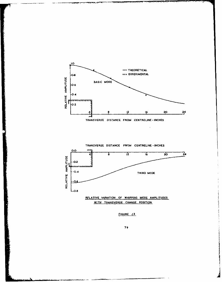
1.0
- THEORETICAL
.O.8 *eco EXPERIMENTAL
sI-IC MODEQ.0
0.4
0. 0.2
48 2 16 20 24
TRANSVERSE DISTANCE FROM CENTRELINE -INCHES
TRANSVERSE DISTANCE FROM CENTRELINE -INCHES
0.0
_02
uJ
.- 0-8
RELATIVE VARIATION OF WHIPPING MODE AMPLITUDES
WITH TRANSVERSE CHARGE POSITION
FIGURE J3
79
S•F " i ",l -' • •, ,: .. .. ..Jr .., , .. ... .. .- •,. ... "

t - 0 4
'I°
IL BASIC MODE -THEORETICAL10.6 0 00 EXPERIMENTAL
0.4
a 16 24 32 40 48
DEPTH BELOW FREE SURFACE-INCHES
-*l.
--0.89L 'THIRD MODEI
-06w
-0.4
0.01 a 16 24 32 40 48
DEPTH BELOW FREE SURFACE- INCHES
RELATIVE VARIATION OF WHIPPING MODE AMPLITUDE
WITH CUARGE DEPTH
FIGURE J4
80

X The Early Compressible Phase
In the development of the theory as presented in sections E,
F and H, it has been assumed that the motion of the ship is independent
of the initial shock wave, that in fact the ship behaves as though
initially a highly compressed bubble of gas were suddenly released
from rest to accelerate and expand outward and then pulsate. In fact
the bubble at no stage can be considered to be at rest and the
water surrounding it does not accelerate to high velocities in the
way this model suggests. What actually happens is that when the
detonation wave in the explosive reaches the water it transmits a
shock wave into the water and almost instantaneously raised the
bubble surface to a very high velocity. Similarly in the surrounding
water the shock wave raises the velocity to a high value and all
these initial high velocities gradully decay until they fall to the
incompressible velocities, after which normal incompressible bubble
motion takes place. Even the initial bubble size assumed in
section 11 is fictitious, being uzually considerably larger than the
original charge size. It is merely the size of bubble which, if
the water were really incompressible, would pulsate with the
period and maximum radius which are observed in experiments.
Chertock's original work (B1) gave a qualitative argument,
based on an appliction'of Green's theorem to the flow potentials,
assuming them to be solutions of the wave equation, why it should
be expected that the acoustic snock wave phase would not produce
significant motion. In fact his arguments ao not rigorously
apply to the type of discontinuous function involved in the early
interaction and, in addition, did not really include all the inter-
action waves (reflected, diffracted, etc.). In addition, for
surface ships at least, non-linear effects are certainly present
during the initial phases as cavitation effects are well established
81

=
(KI) during the shock wave hull plating interaction phase of the
motion. Cavitation has the effect of largely preventing any
reflection of incident momentum, so ensuring that the momentum in the
shock wave is fully absorbed by the ship.
In consequence the neglect of the shock wave, or at least its
replacement by a zero velocity, high pressure bubble, must be
considered to be justified principally by the experimental evidence.
On small scale the agreement between the observed and predicted
model motions certainly fully justifies the assumed artificial
bubble. However, the scaling laws of underwater explosions are
such that it is generally true that shock wave effects are relatively
much smaller than bubble effects on small scale. The assumption
cannot therefore be considered established for a larger scale
by the small scale experiment.
There are however other heuristic reasons for expecting that
it should still be valid at least for some conditions. For a
target deep enough for cavitation not to be significant Murray,
(K2), showed by an exact solution that when a spherical acoustic wave
interacts with an infinite neutrally buoyant, circular cylinder
(considered to be rigid in cross-section but infinitely flexible
in shear along its length), the transverse velocity of the cylinder
asymptotically tends to the nearby water particle velocity of the
incident wave. lie found in fact that initially the cylinder
jumped to a considerably higher velocity which then decayed to
the incomprcssible value after a period equivalent to several
transit times of the cylinder diameter by the acoustic wave.
For non-neutrally buoyant circular cylinders, the associated
two-dimensional problem of a plane wave incident on a circular
cylinder of elastic cross-section has been considered by Haywood
82

-'V
(K3) who found that in this case the cylinder, after again
reaching a fairly high initial velocity, slowed down to the
asymptotic velocity
2u K1)1 + pv/a 2p
where u is the undisturbed water particle velocity at the cylinder
centre, due to the passage of tbe shockwave. In Lhis equation a
is the cylinder radius and ji is the mass of the cylinder per unit
lengtn. The previous incompressible assumption gives the same
result, as the fluid impulse which produces a velocity u in the
Aater imparts a momentum (Vw + a w)u per unit length of the
cylinder. This momentum is given to the cylinder and its added
water mass so that, if the resulting cylinder velocity is v,
S+ = (4w + Vw)u" (K2)
For a circular cylinder the added mass per unit length, p w' is
npa as also is the buoyancy per unit length, ýiw Whence*2) gives
the same value for v as(KO.
These results suggest that, at least when cavitation is not
important, the incompressible assumption at the start will lead to
quite good results in the later motion. Where cavitation leads
to most of the momentum in the shock wave being absorbed by the
target again the deviation from the incompressible theory should
be small because the total momentum in the initial positive phase
is generally at least 80%i due to the 'incompressible' pressures
which follow behind the very short duration compressible shock
wave head of the positive phase. The subsequent motion of
the ship and its entrained water will therefore again be largely
as though the incompressible motion only were present at the
start.
83

References
KI, Taylor G i ; "The Pressure and Impulse of Submarine ExplosionWaves on Plates", Underwater Explosion ResearchVol. I - The Shock %ave, Off. Naval Research(1950).
K2. Murray W W; "Interaction of a Spherical Acoustic Wave with aBeam of Circular Cross Section", UERD Report1-55 (1958).
K3. Haywood J H; "Response of an Elastic Cylindrical Shell toa Pressure Pulse", Quart. Jn. of Mech. & App.Math., Vol XI, Part 2, 1958.
84
"An alternative to the Strip Flow Method for the Added Water Mass
The usual theory for calculating the hydrodynamic forces on a
ship, applied as described in Section D, is clearly an extremely simple,
and, for the 2-node mode a% least, very accurate method of determining
such forces. For the higher whipping modes the experimental evidence
is very limited. The strip theory does however have one possible
drawback in the present application. In the development of the
normal mode form of the equations described in section F, all
the *ode frequencies and shapes were found simultaneously through the
eigen values of a single matrix. This matrix naturally involves
the strip theory added water masses and, through them, the correction
factor J which compensates for Three dimension flow effects. In
consequence, in the development used here the same value for J is
applied to all the modes. This conflicts with the customary use
of the factor , where a different value for J is used for each mde
shape (including the pitch and heave modes). To use the customary
method here would mean developing a separate matrix (using the
appropriate value for J) for each mode, and extracting just the
appropriate eigen root and vector from each matrix. In the examples
given earlier the simpler alternative was adopted of applying the
2-node mode correction factor to the added masses (since that is
the mode contributing most to flexural stresses) and ignoring
the fact that all the other modes, pitch and heave included,
will be somewhat in error.
The type of correction factor which should be used in vibration
calculations has been the subject of a great deal of discussion ever
since strip theory was first used. The two independent oiiginators
of the theory, Lewis (LI) and Taylor (L2) both presented reduction
factors but, due to assuming slightly different boundary conditions
they arrived at differeiAt reduction factors. Which factor to use,
Lewi.! or Taylor's, isstill discussed today. A furtf..,, difficulty,
which has been raised in numerous papers ((L3) contains a useful
discussion) is that it has never been rigorously established that
the correction factor should be constant over the length of the ship,
as is implicitly assumed in normal useage. In fact, in at least
one recent paper (14) a correction factor has been presented which
does vary along the length, although in this particular case no
basis for the given variation was presented.
Because of these basic difficulties in the customary strip theory,
particularly as applied to the whipping problem, the alternative
approach described here has been developed. The fundamental weakness
of strip theory is that the force it predicts on each cross-section
is related only to the motion of that cross-section and not to the
probably slightly different motions of neighbouring cross-sections.
In the notations used in section E, the vertical hydrodynamic force
S w. on the ith mass is, according to strip theory, S. = -mwi
and the total vector of hydrodynamic forces is
S M -Li)Y
where Mw is a diagonal added mass matrix. rhis standard form of
strip theory (quation clearly cannot be valid for general motionq.
If one section of the ship is accelerating upward it will certainly
experience a downward hydrodyntaznic force so a diagonal term is
certainly expected. However, its upward acceleration will induce
a downward fluid acceleration around it as fluid moves to fill the
space vacated beneath it. Parr of this flow will be around
neighbouring cross-sections and so will induce a downward forces
on these section. too. For the above equation to be generally
true then it is necessary for M to contain also off-diagonalW

elenIents. In fact all element,- of Atw should be nonzero but, since
each section will affect principally its nearest neighbours, the
magnitude of the off diagonal elements will decay rapidly away from
the main diagonal. The problem is to approximate the eler.-_as of
M in a simple, readily calculable manner. Since- the general shipw
problem is much more complex, attention is directed first to the case
of an exisymmetric ship. A method for applying the axi-symmet-ic
results to a normal ship is described later.
Mathematical Model ior ýn Axi-Syametric Ship
For such a ship it Js possible to satisfy fairly well the fluid
.,oundary condition of equality of hull and fluid velocities along
the normals to the hull by means of a vertical dipole distribution
along the axis of the ship. This distribution should normally be
continuous but, if the ship is considered to be divided into a
number of sections and the number is large enough, then it should
be reasonable to assume that the line distribution in each section,
i. has a constant strength jLi.
Since the velocity potential at the point (r,6,x) due to a
dipole at the point (o,o,s) (referred to the cylindrical polar
coordinates of Figure 1) is given by
i p ~r cos 6 V@
S2]/2 ,where u
the potential due to a line distribution of dipoles of strength
' per unit length and extending from x. 1 12 to X.1 1 2 isxi-1/2ds 1/
Oi(rOx) ircosO T-.2
xi. 1/2
67

5..L. cos6 0 X-xi~/
whence O . = 2- i-I 2
I r "[r 2+(x-xi 1 / j2/2
i+ 1/2 (L2)
[r2+(x-x i+1/2) 2]1/2
The radial velocity u produced by the distribution is given byr
(x)= - l• ucose X i-1/2
-r- (r +(x-x 1i-,2) j
xxi+1/2 + r2 (x-x L-I/)
2r +(x-x 1 2/2)2 I [r +(x-xi_/ 2) 2]3/2
9r(-i+1/2)
7xxj j} (L-3)
Ux(X- i
•( - i x= 1i rCO)O [r2+( i 2)3i2
I[r2+(x~~xi[ +/21/2} x4
The total velocities produced by all the distributions are therefore
n nu(X) = Eu W(X) and ux) W =Eu Wr j=x j=1
The boundary condition at the hull is that the velocities of
the fluid and the hull, resolved in the direction of the norhal to
the hull, should be equal. For the axi-symmetric shape considered,
the angle ) between the nornal to the hull and the radial direction
fa V"a=- tan- b' where b(x) is the radius of the ship, and
• Q ••________

b'= db/dx. The boundary condition is thereforc-,
vcosk - v'bsinX = u cos% + u sinX (15)I- X
where v(x) is the distribution of vertical velocity along the length.
This condition allows for both shearing and flexing of theship.
For the more interesting, lower frequency, modes of vibration,
v'b will be small compared to v since the wavelength will be much
k greate," than the half beam. X will also normally be small except
possibly in the immediate neighbourhood of the stern. The term
v'bsinX will therefore be very small. ux , the flow along the
ship, is produced partly by the variation in v along the ship (i.e.
by v') and partly by the changing shape of the ship (bW). It too
will therefore, normally be small when vand b are small. It is
generally possible then to simplify the boundary condition(L5) to
v =u (L6)r
except when rapid changes occur in either the ship underwater cross-
sectional area or in the velocity distribution along its length
(e.g. for high modes). This simplification in the boundary
condition reduces slightly the amount of data needed to specify
the ship and its motion. It is roughly equivalent to neglecting
rotary inertia in the dynamic equations of the ship itself.
Neither of the boundary conditions (L5) or (L6) can be
satisfied everywhere by the assumed velocity potential. However,
either can be satisfied at up to n 'collocation' points along the
ship and if these points are suitably chosen the boundary condition
will not be seriously violated anywhere. The most convenient
choice for the collocation points is at the mid-points, xi, of
the ship sections and satisfying equation(L6) at these points gives
89

Fi (3 -u) Ali
where b is the maximum value of b(x), y(x) the vertical velocity of
the ship, u(x) the vertical velocity at the ship due to the
explosion and the matrix A = (ki ) where
' b 1 22b I.( x , +4/2-2] )2]2/2 +
ba i [bi-+(Xi-x ÷ /2) [b 2 i+(x-x .-4/2
bi2 (xi-x,+/2). b 2(x.-x, /2)
[bi2.(xi-x + /2 ) 213/2 [ ib2 i+(xi-x.4/2 ) 2]3/2 )
Equation(WL) may then be inverted to determine the strengths
ýL of the line distributions necessary to satisfy the boundary
condition(L6) for the given velocity distribution y . This gives
2 -1 *ji b A (y )
The upward vertical force per unit length on the section at
the point x. is given byI
fi = -2f p cos e bide0
where p = p; is the fluid pressure.n
Here the potential 0 = + Z •. since the fluid motion due toj=1
the explosion (and having the potential 0bo) is included. Thus
fi -2pro biX cos OdO 2p b f7 Cos 2edB-2 b ni 7E fCos2 6dO
=p ui - Pllijl'j (1.9)
090

4x Cx,-x3'/2
wnere b- ~ 2-1/tI jbi +( i-x +4t/2) J
x -x -Z/ 2.b. +(x. -x.+e/2 )2]1/2 }
In the vicinity of the ship, 4o has been approximated by o0 -uy =
-ub. cos e on the ship surface. The velocity u is the explosion
induced velocity at the ship axis.
Since in any actual motion conditions along the ship will be
continuous, the upward force/unit length at the centre of the section
will approximate the average force/unit length over the whole section
and the total upward force S., on the section will be approximately
Si = g fi = xPbi.2 di " xpb En P.iij=1
M., u - 7,obE~ : u xp__B-' 6# • (LIo)
where B is the matrix (ij ) and M w is the diagonal matrix with
elements wiý,pbi 2 . The matrix Kw is exactly the same 'buoyancy'
matrix as found before in section E.
The required inertial water mass matrix M is therefore given byw
Mw = %b3pBA-i (1.11)
This matrix depends only on the shape of the ship and is completely
independent of the type of motion (or vibration mode). With Mw
known the force distribution for -kny vertical acceleration distribution
y is readily found. A short computer routine has been written to
compute the non-dimensional matrix BA"1 and the force distributions
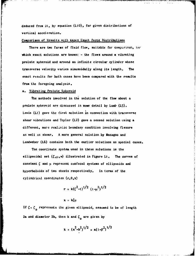
deduced from it, by equation (LIO), for given distributions of
vertical acceleration.
Comparison of Results with known Exact Force Distributions
There are two forms of fluid flow, suitable for comparison, ior
which exact solutions are known: - the flows around a vibratingprolate spheroid and arour. an• infinite circular cylinder whose
transverse velocity varies sinusoidally along its length. The
exact results for both cases have been compared with the results
from the foregoing analysis.
a. Vibrating Prolate Spheroid
The methods involved in the solution of the flow about a
prolate spheroid are discussed in some detail by Lamb (L5).
Lewis (LI) gave the first solution in connection with transverse
shear vibrations and Taylor (L2) gave a second solution using a
different, more real~sLic boundary condition involving flexure
as well as shear. A more general solution by Macagno and
Landweber (L6) contains both the earlier solutions as special cases.
The coordinate system used in these solutions is the
ellipsoidal set (C,•,w) illustrated in Figure Li. The curves of
constant C and ýt represent confocal systems of ellipsoids and
hyperboloids of two sheets respectively. In terms of the
cylindrical coordinates (r,6,x)
r = k(-1)/2 (I-p2)1/2
x = ki
If C= C represents the given ellipsoid, assumed to be of length0
2a and diameter 2b, then k and C are given by0
k =(a 2-b 2)1/2 2 a 1~p)/2]
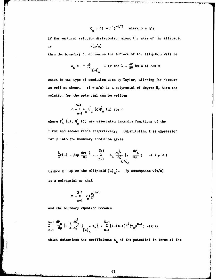
0o It - )/2 where / = Wa
If the vertical velocity distribution along the axis of the ellipsoid
is v(),/a)
then the boundary condition on the surface of the ellipsoid will be
U= -- = (v cos X.- t bsin)X) cos8Un an ý-0 dx
which is the type of condition used by Taylor, allowing for flexure
as well as shear. if v(x/a) is a polyromial of degree N, then the
solution for the potential can be written
N+1nZ a (1) C03
n=1t 1
where Fn n (C) are associated Legendre functions of the
first and second kinds respectively. Substituting this expression
for 0 into the boundary condition gives
k dv(jp) N+1 addlnC41 = n dT dJii~' - f
n=1
(since x = ap on the ellipsoid 0=). By assumption v(x/a)
is a polynomial so that
N+1 n-Iv v ()
n=1
and the boundary equation becomes
N+1 dPn dQ ' N+1 2]v n-1
dl ý ± k dF na n=1n=1 C=Co n=1
which determines the coefficients a of the potentiel in terms of the
nj
93I

coefficients v of the velocity distribution. This equation is
most easily solved by first integrating with respect to ýi, givisg
N+I~ N÷I i.(n-l)p 2 nE ).n(P n (t) -Pn (O)]=En j
n=1 n=1
I dQ'where X represents -ank a o Multiplying by Pn(p) and
integrating from -I to +1 gives, using the orthogonality relation
for Legendre Polynomials
=( +.I4 ) i-(n-I)E2 v 2,
iii n n I mn=1
+1where I f gnP (j)dd = o, n < m or (n-r) odd
-I
n(n-1)...(n-m+2) (n-r) even
From these equations, given v, n is easily found and so then,
from its definition, is a m
With the coefficients a known in the expression for then
velocity potential, the force distribution on the ellipsoid is
readily found from
f(x) = -2 ° b(x)p cos dO where p p0
i.e.
N+Iif(x) = --,pb(x) Z a Q"o )PI (x/a) (L12)
n al on
"- • ~94

A snort computer routine has been writLen to compute the values
of '(x)/xpb2 given b/a and values for the coefficients 1 ..••'v 5 "
It is limited to velocity distributions which can be represented by
quartic equations but this is sufficient for the lowest few modes.
Figures L2 and L3 compare the exact force distributions given
by the above equation with the results given by the approximate
3-D flow method, for two ellipsoids with b/a ratios of 1/5th and
1/10th. The values given by normal strip theory, i.e.
2 2 N+1 x) n-1=(I -x /a ) X ( (L13)xpb 2 =n-1 n a
have also been added to the figures. The Lewis correction factors
have been used for the strip theory results since these are known
for four of the five nodes. The values used for the coefficients
v1 * 0e5 for these cases were
Co e fficient - - -
1, 2 3 4 5Mode I
Heave 1 0 0 0 0
Pitch 0 1 0 0 0
2-node vertical -0.2 0 1 0 0
3-node vertical 0 -0.429 0 1 0
4-node vertical 0.0274 0 -0,534 0 1
the first four of these distributions being those used by Lewis.
The fifth distribution has nodes at 0.155L, 0.38L, 0.62L, 0.845L,
L being the total length. These nodes are in about the correct
position for a 4-node ship vibration mode but the relative amplitudes
are not good since the distribution gives too much prominence to
the ends and too little to the central section.
95

ior the W/a = 1/10th ellipsoid (for a ship with a length to beam
ratio of 10) the results of the 3-D approximation and strip theory
[ioth agree well with the exact analysis and there is little to
choose between them. Near the centre of the ellipsoid, where
changes in the radius are smallest, the 3-D approximation is slightly
better but at the ends, where the radius is changing rapidly, strip
theory is the better. For the b/a = 1/5th (L/B = 5) ellipsoid the
results are similar but the divergence of both approximations from
the exact solution is quite serious near the ends, even for modes
as low as the second vibration mode. Again there is little to
choose between the approximate 3-D flow and strip theory.
However, in each case the strip theory uses a different correction
factor for each mode whereas the 3-D approximation deduces all the
forces from a single matrix equation.
One point which should be borne in mind in these comparisons
is that the boundary conditions are not quite the same for the
three methods. Strip theory necessarily uses a shear type
boundary condition since it can only relate the force on a section
to the vertical velocity there. The 3-D approximate analysis
too, based on equation (L9), also includes only shearing motions.
The definition of matrix A (equation L8) is based on the approximate
form of the boundary condition equation (L6), which is equivalent
to including shear only. The exact solution includes flexure
as well as shear. The necessary modifications to the 3-D approxi-
mation in order to satisfy the more exact boundary equation (L5),
and the results it gives, are described later.
96

b. Infinite Circular Cylinder
Taylor (1.2) was the first to consider this example in a ship
vibration context. The infinitely long cylinder is assumed to have
a transverse velocity distribution
v(x) = v cos kx0
The velocity poten~tial for this distribution Taylor found to be
VoKI (kr)k@_ '(b cos 6 cos kxkK1•(kb)
where b is the cylinder radius and K is a modified Bessel function
of the second kind. The force distribution may be found as before
and is
v K (kb):1 coskx (1.14)
f(x) =-2 1P cos ObdO =-2pbf OcosOdO TO -ox (1,14
0 0 kbK0(kb)
The wavelength of this distribution is of course = 27,/k.
The example is not ideal for comparing with the 3-D approximation
since the latter is firmly tied to a body of finite length (although
it could obviously be modified to deal with a periodic distribution
of infinite length). To compare results the approximate analysis
was e.pplied to a finite length of cylinder, 3 full wavelengths being
the selected length in the hope that the central wavelength would
be free of end effects. Since the computer program for the 3-D
approximation is restricted to only 20 sections this gives only
6 different dipole distribution regions per wavelength. The
results are compared with the exact values from the above equation
in the table. In this case, because the cylinder is of uniform
diameter there is no difference in the two forms of boundary
condition.
9 7

5 exact -. 44W 0 .448 .448 0 -. 440 -. 448 0 4483-4 -. 445 -. 00 o445 -. 0014 -. 0014 -. 449 -. 452 -. 0140 .383
Io exact -. 631 0 .631 .631 0 -. 631 -. 631 0 .6913-4 -.609 -. 0003 .609 .609 -.0013 -. 611 -. 616 -. 0189 .511
15 exact -. 762 0 .762 .762 0 -. 762 -. 762 0 .7623-D -. 741 -. 0001 .741 .741 -. 0004 -. 744 -. 745 -. 0096 .674
0 exact -. 826 0 .826 .826 0 -. 826 -.826 0 .82634 -. 839 -. 0007 .839 .839 .0007 -. S39 -. 840 1-005 .823
Values or F(x)Apb v for an Infinite Cylinder
For all values of X/b, the forces are clearly very accurate near
the centre being within 4; of the exact value in E.l cases. The points
given were the only ones used, indicating the coarseness of the
representation; equivalent in a ship representation to using twenty
points to represent the fifth vibration mode (6 nodes). Since the
values from the 3-D approximation are constant to at least WX/ =
7A/b, the differences from the exact result are due to the coarse
mesh rather than the finite length. For the ?Vb = 5 case the
lengths of the sections are near!y equal to their radii, whereas for
the VAb = 20 case the sections are each nearly 9 radii long.
Application of the Technique to non-axisymmetric Ships
Clearly it would be possible in principle to extend the 3-D
approximation by adding distributions of higher multipoles along
the ship axis, and determining their strength by satisfying a
boundary condition around the circumference of the ship as well
as along it. Alternatively (and more accurately) surface
distributions of sources could be used over the surface of the
ship. Either technique would, however, require very large amounts
S= -
of data to represent the ship shape and would require the inversion
of a very large matrix. The success of the strip method using Lewis
sections for the cross-sectional shapes points to simpler approaches.
In the solution of the two dimensional flows about ship-type
cross-sections, although the velocity potential may in fact consist
of a super-position of 2-D multipoles of all orders, the added 1ass
of each section depends only on the dipole term, the shape of the
section determining its strength. In the 3-D case it should, there-
fore, be approximately correct to account for the shape of the section
via the strengths of the dipole distributions.
Since Lewis' original work, it has been customary to represent
the added mss per unit length of the 2-D cross-sections in the form
p b2C
where b is Lhe half beam of the section and C is a constant depending
on the section shape. Values for C have been computed for a great
variety of shapes (References LI, L2, L7, L8, L9, LIO and Lii). The
above value for the added mass is also t'at due to a circular
cylinder of radius
bequiv =b (Li)
For a non-axisymmetric ship then, each cross-section may be compared
with the known shapes, C determined, and then (15) gives the
appropriate radius for an axisymmetric approximation to the actual
shape. There are no reasonably simple non-axisynetric 3-D flows
with exact solutions which can be used for comparison but the
procedure should give reasonable results. Certainly in the 2-node
vibration mode, in the central section of the ship there the added
99

wss is most important, the technique will give very good answers
since in this region the flow is very nearly 2-D and in the 2-D case
the method is exact.
Use of the Full Poundary Condition
The results given so far for the 3-D approximation have all
been based on the approximate equation (L6) for the boundary equation
at the ship surface instead of the correct equation (L5), If the
full equation is to be used, then the bending rotations yi of the
ship must be included. If the expressions (L3) and (14) for u r(x)
and ux(x) are substituted into the boundary condition (L5) the
result is
n nY- Uo + b(y- u) [vrj.(xi)-biuxj'(x-)] AbI E C6
1 o 01 01 n i xi o ' =
where
2 2 V -/CLj = -it + bbblbi 2 + (Xb " xj + 4 , 2 )2]"f 2 -
[b12 + (xi - xj - t/2)21- 3 / 21
This may be written in the matrix form
b
where l is a diagonal matrix with elements bibi'. u is again
the water motion at the ship axis due to the explosion (calculated
!-I-• ,I 80 .. . ....

as though the ship were not present), and u' is its derivative with
respect to x.
Inverting the equation gives
• 2=bA (y-u)+bA B(- u) (L17)
and the force distribution f(x) follows as before. Since changes
in the cross-section are now included it is appropriate in this
case to deduce from f(x) both the force and moment at each lumped
mass by means of the integrals
x i +I/2 xi+ 1/2
S. ff(x)dx: M.i = f (x-xi)f(x)dxi -i/2 i -1/2
whence S = M u - C
((18)
where the elements of the matrices C and D are given by
ij (I+b 2 )-'2 (rJ -rI_ r2 ±r_)
xl -aI a1 +)+rl + x2-a2 a2 r2+- -o--_ log ( ' ---2)
x x - ox g+4/2 x -x .4/2 L bb. b/e +2 If Ib1
where x .i ....... i a 1 =
bi/Z -xI b131 =
1+b..2
r ( ,2 r2 2 2)4
rI Ua+ 1 +2 ; M= I +P , with
101

similar expressions for m2 9 t29 r 2 + and r 2 -#
ai •2 21b, )•d. ~~I I 2- 2 21b 2't~. ~r 2 -~)2
l2 +;+ r + P22 2 2+
+ log (-L ) lo 2+ )2
2 I "2I x2- 2(X
X -2ci, I r r x 2-2(L 21+ 1- 2 " (r2+ 2-+ ~ ~ ~ 1 1--p )r r 1 T( 2 -r
C. + b CL 21+ P-')'22 2 2 2+2.2
X 2 .121 ,+ 2 -
(LI 9)
Thus -1 -
7L 2 __-
W- . :j L] -"-JL L DA B ][i~e.
(L20)
which gives the hydrodynamic force and moment at each lumped mass.
Use of this equation instead of equation E(t) in the derivation of the
equations of motion gives, in place of equation E(8),* the equation
SW1ow 2 W

wA+K B y M , 1 .w1 Y y W1 I
As in section E, since rotary inertia effects appear to be minor they
can be neglected and
MY C-I M~
so that the reduced equation of motion is
•+ w!- BT•+ E(A*K)-I•2"B T~y =(MXw + + w) 2+(L22)
Here not all rotary inertia terms have been neglected. The terms
affecting the displacement equation (the dw 2 terms) are retained
since these are the terms which differntiatc between the tsheari
and 'shear plus flexure' boundary conditions. Even when normal
rotary inertia is suppressed these terms can have some effect on the
hydrodynamic forces.
The force distributions given by equation (LO8) (with A = o)
have been added to Figures L2 and L3 where they differ appreciably
from the simpler 3-D approach used earlier. The significant
improvement in the accuracy of the results for the higher modes,
particularly for the smaller length/beam ratio ellipsoid, is evident.
The results using equation (L08) (based on the full boundary
condition (05)) are everywhere almost identical to the exact values.
In computing the results from equation (L18), in order to ensure
that no more data should be used than is normally necessary in ship
vibration calculations, the' slopes b'of tne ellipsoids were estijmated
numerically from tne given radius b. at the collocation points. TheI
method appeirz to be adequate for the rather extreme slopes involved
in ellipsoids and so should be quite satisfactory for ship forms
where shape changes are less severe.
Modification of tLi: Normal Mode Equations
Because the matrix t I in the new equations of motion
M Y + Sy = Md + M ad° (L23)I- -, 3-
is now no longer 2di.,,,: matrix, the transformation
I=M1 1y (L24)
used in section F can no longer be applied. In fact MI is no longer
a symnetric matrix and the transformation technique should not really
be applied at all. An alternative, once asymmetry is accepted would
be to re-write the equation as
y + M Sy = M -IM +M-I -- 1 2 1 3,.
and solve the homogenous part
- -1Iy + MI Sy =0
directly. This unfortunately would considerably restrict the
available computer routines since most of the really efficient routines
deal only with symmetric matrices. However, in all cases so far
considered, the matrix M, has been found to be almost symmetric,
except for elements corresponding to the end lumped masses, and there the
actual values of the elements tend to be small. To avoid having
to use general matrix methods the matrix M was arbitrarily made
symmetric by replacing all the elements mlij by (mlij + m ji)/2.
GARij

The forces resulting from this amended ratrix were compared with
those produced by the correct matrix for the two ellipsoid cases
and the two sets of forces were found to differ by no more than 3o
anywhere. Over most of the length of the ellipsoid the forces
were identical. Since the vibration frequencies depend approxi.nately,
on the sqiare root of these forces, even this small difference will
be further reduced in the effect ols the eigenvalues and use of the
modified matrix seems justified.
With M symmetric, a standard Choleski decomposition routine
(L14) may be used to generate a matrix L such that
TLL (M + M) (L25)
and the transformation(L24) is replaced by
Tz L Ly
giving
-1 U0 0.z+E! z=L X +LMu2- 3ý
where E L - SL - -T, a symmetric matrix. The eigenvalues and vecto:s
of E can be found just as before and the normal mode technique
can then be applied exactly as in section F.
Application to a Ship Vibration Calculation
For the destroyer considered in section G the samE basic data
were used, with a modified version of the computer program, to predi.:t
the normal mode vibration frequencies. The results obtained are
compared in the table with the straighLforward strip theoiry
technique. The calculated results are for the cases
I Normal strip theory with the Taylor correction for the 2-nidemode
"- 105

2. 3-D approximation based on equ•Jtion (LII) (theapproximate boundary condition)
3. 3-D approximation based on equation (L22) (the fullboundary condition).
In each of these cases the effect of shear deflection is included
but that of rotary inertid has been suppressed.
Frequency (Hz)
Number S Calculated MeasureaNodes
2 3
0 Heave 0.21 0.20 0.20
I Pitch 0.23 0,22 0.22
2 ) 1.54 1.51 1.52 1.59) • (1.50)
3 3.13 3.14 3.17 3.20) u (3.09)
4 ) 2. 4.67 4.77 4.81 4.77
Sb.41 6,72 6.78 6.296 ) 8.09 8.68 8.79 -
7 L 9.61 10.45 i0.61 -
It is clear that the method changes the results little, which
is to be expected since the length to beam ratio of the destroyer
is close to that of the more slender of the two ellipsoids, where
the exact, strip theory and 3-D approximation force distributions
were found to be all very similar. The large difference between
the calculated results and the mer..ured values reflects mainly the
inaccuracy of the ship data since measurements on a sister ship
in a similar displacement condition, gave the values shown in
brackets. Unfortunately the higher mode frequencies were not
measured for the second ship.
For a different class of destroyer similar results were
obtained and are shown in the following table.
106

SFrequency (itZ)
Number of Calculated ,easuredN od~ U______ b_____
S2 3
0 Heave 0.20 o.20 0.20
I Pitch 0,22 0.23 0.23 -:! ) 1i.64, 1.64 1 .66 1 .68
3 ,3.16 3.20 3.22 3.35)Vibration
4 ) Modes 4.92 4.96 5.00 4.97
5) 6.90 6.96 7.03 6.63
In each of these cases the calculated mode shapes were virtually
independtitc of the hydrodynamuic approximation used.
Conclusions gegarding the ilydrodynamic F.low
The results for the force distribution on ellipsoids show that
in general the 3-D flow approximation, using the full boundary
condition, should provide more accurate results than normal strip
theory. However, the difference is only marked for small values
(=5) of the ratio (length/beam). For a value of this ratio of
Iu the 3-D flow approximation was still very accurate but strip
theory also gave good results even close to the ends.
The considerable difference between the inertial mass matrices
given by strip theory and by the 3-D approximation, and the close
agreement of the results they give, suggests that, so far as
vibration of the ship as a beam of rigid cross-section is concerned,
lit.tle improvement from more exact ideal fluid theories is possible.
Any remaining discrepancies bctween measured and predicted iydrodynamic
forces are probably largely due to non-ideal flow, free surface
effects, non-linear Bernoulli forces or the distortion of
cross-sections.
107

Lewis F .11 ; "The Inertia of the Water Surrounding a Vibrating Ship."Trans. SNAME, Vo!. 37, 1929.
L2 Taylor J L; "Some Ilydrodynamical Inertia Coefficients." Phil. Mag. S.7Vol 9, No. 55 Jan 1930.
L3 Kaplan P ; "A Study of the Virtual Mass Associated with the VerticalVibration of Ships in Water." Stevens Inst. Tech.,Davidson Lab. Report 734, 1959.
L4 Anderson G; "A Method for the Calculation of Vertical Vibration withSNorrand K Several Nodes and Some Other Aspects of Ship Vibration."
Paper read to the INA Dec. 15 1968.
L3 Lamb, 1 ; "Hydrodynamics" 6 Edition, Cambridge Univ. Press, 1932.
L6 Nacagno E 0 "Inrotational '.lotion of the Liquid Surrounding a Vibrating& Lbndweber Ellipsoid of Revolution." Jn. Ship Research, Vol. 2,L ; No. 1, 1958.
L7 Prohaska "The Vertical Vibration of Ships." The Shipbuilder andC W ; Marine Engine Builder, 1947.
LS ,endel K ; "Hlydrodynamic Masses and Moments of Inertia" Jahrobuch derSchiffbautcehnische Gesellschaft Vol 44, 1950.
L.9 Landweber L; "Added .ass of Two-Dimensional Forms Oscillating in a Free& .lacagno M Surface." Jn. Ship Research, Vol 1, 1957.
LIO Landweber L; "Added Masses of a Three-Parameter Family of Two-Dimensional.& lacagno M Forms Oscillating in a Free Surface." Jn. Ship Research,
Vol 2, No 4 (1959).
Lii. Macagno ,1 ; "A comparison of Three Methods for Computing the Added Massesof Ship Sections." Jn Ship Research Vol 12, No 4, 1968.
.13 Hoffman D ; "Conformal Mapping Techniques in Ship Hydrodynamics.",,ebb inst. of Naval Architecture Report No 41-1, 1969.
.14 \Vartin R S ; Reduction of the Symmetric Eigenproblem Ax = Xpx and Related& Wilkinson Problems to Standard Form." Numerische Mathematik, 11,J Hl 99-110, 1963.
108

Trr~~ r ~ -rr~' ~ - var'¶~rr -- ~ A'
I-0
zx40
00
AftX
\ II /
109
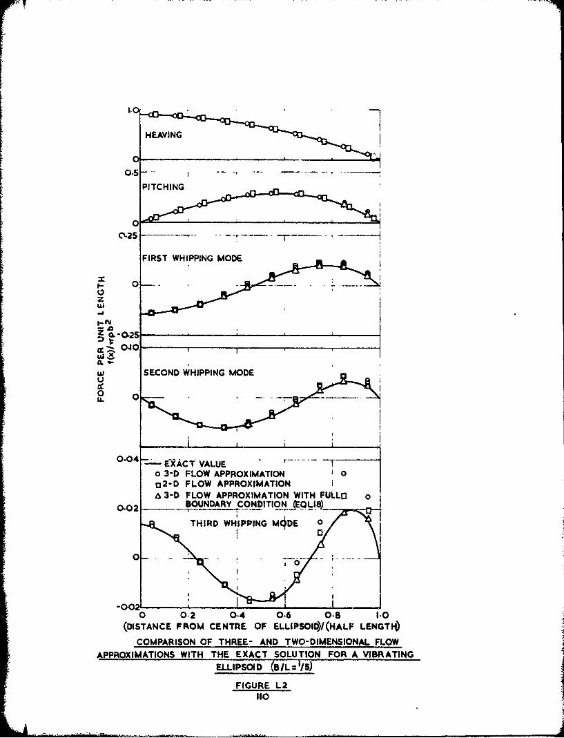
0
z
w.
uJ SECOND WHIPPING MODE
0
0.04 - XACT VALUEr- T
0 3-D FLOW APPROXIMATION 002-D FLOW APPROXIMATION
S3-D FLOW APPROXIMATION WITH FULLO oBOUNDARY CONDITO __ ___S
0.02 -r-___ TI- QLBTHIRD WH'IPPING M4DE 0
0 0.2 0.4 0.6 0.8 1.0(DISTANCE FROM CENTRE OF ELLIPSOID)/I(HALF LENGTH)
COMPARISON OF THREE- AND TWO-DIMENSIONAL FLOWAPPROXIMATIONS WITH THE EXACT SOLUTION FOR A VIBRATING
ELLIPSOID (B/L:115)
FIGURE L2110

1.0 -
HFIRTAWIPPNGG O
0__
0.5
0[ECN WHIPPIN MODE!G OD
- EA
(DISANC FROW CENPREOFIMIONI~(AL EGH
COMPA2ISONLOF APPREX-MANDTWODMNION ALO0 - LWAPPROXIMATIONS WIHTH XCTSLTIOHO ITN
ELIPOI (BL A/0
ol~~~~FGR FULBUDAY 3NITO(GL
SEODIHPPNIMD
M Li%-xt: of Applicability of the Theory
The theory as so far presented has been shown to give very
;ood aigreement with the limited experimental results available
but involves a number of assumptions, some of them quite drastic.
In this section some of these assumptions are discussed in more
dctail to shos more clearly the limitations of the theory.
-ost of the ap,.:roximations are those normally encountered in
bip vibrations and in consequence they have been investigated
extensively already. The limitations of beam theory for the
elastic representation of the ship are beginning to be appreciated
and alternative approaches, e.g. (MI) have been proposed. In
general though, particularly for slender ships, beam theory
has been found quite adequate. In the hydrodynamics of ship
vibrations it is customary to neglect the 'Bernoulli$, ' 2pu
pressure terms, and, for the free surface condition even the
linear gravity terms are neglected. Both these points have been
considered by several authors, e.g. (M2) and (M3) and have been
found small for the vibration modes although they can be significant
in the pitch and heave motions. For example, the inclusion of a
linear free surface effect changes the added mass, and adds a
damping force to the motion if the 'Froude number', (where
b is the half beam, w the circular frequency and g the acceleration
of gravity), is less than about 4. For the heave and pitch motionsb2
of the destroyers described earlier, 7 1 and these modes and
the deduced rigid body motions may be expected to be slightly in2
error, but for even the lowest frequency vibration mode L * 25g
and the approximations may be expected to be very good.
Compressible effects it, ship vibration have been considered
by both Taylor (D2) and Kaplan (DS) and have been found negligible.

Viscous effects seem generally to have received iess attention
but, since with the small amplitudes involved in the vibration
frequencies a full wake cannot form beneath the ship when it is
moving up, only skin drag is likely to nmatter. For flexural
vibration tVe Reynolds number is of order 10' and such forces will
be small. 3oth compressibjiity and viscous effects lead principally
to damping which is very small in vibrating ships. In ship
vibration work :Jampi:g is usti.ly attributed largely to internal
effects and structur,.1 damping rather than to the hydrodynamics.
Even minor da:at'ing is important in such work since it irmits the
amplitudes of vibrations produced by sources operating close to
one of the naturai frequencies. In the explosion induced whipping
application however the vibration exciter (the explosion bubble)
is only effective over about two basic whipping cycles and the
effect of damping is very small.
Another possible -curce of error in vibration work is sympathetic
vibration of local str,.. ture. Even if the frequency of the bottom
of the ship (distorting as a panel, or two panels, over its whole
width is :much higher than the ship frequency, it rmiay be forced in
and out at the ship frequency and so reduce the amount of water
being niovedvdth the ship. The effect has been investigated in
(•,4) and shown to be important for modes higher than the 4-node,
mode but below this the effect seems to be srtall.
Aside from the general and well known limitations, there
are several approximations which are related to the interaction
betieen the explosion and the ship and which are consequently
exclusive to the whipping problem. The principal such approximation
is tae determination of the force Gistribution acting on the ship
through the use of the fluid accelerations which would be induced
Dny •e ex,ilosion at tic si,ip axis .'f £th ship, were not #)rCsent.
In both Lne strip theory and the 3-D flow theory this Approximation
im)licitly assumes thia, in the absence of the ship, the
acceleration would be uniform throughout a region around the ship
position wl ,hich is large compared to the ship cross-section. ('nder
such conuiitionfl very little flow will be induced along the ship axis
•: t..e snip ant it can be cxpectcd that the approximation will be good
b•:t for fairly close charges, the spherical flow divergence around
tr:c cihir:;e wil certainly lead to non-uniform conditions. The
,0orce.S Uill be actin:-; on a short l ength of ship, considerable flow
alon\; t.,e axis will occur and the undisturbed flow at any cross-section
will certainly not be uniform. This s.herical divergence will
.iomose an inner limit to the range at which the 'distant flow'
approximation can be !xpected to apply.
A second possible limitation of the 'strip theory' type forces
is t:,at, even for distant charges where conditions are uniform,
nc..-r the bow and stern of the ship flow along the axis (around the
en-:s) can be expected. The 3-D approximation should, in principle,
be capable of allowing for such flow but strip theory is not.
A third nossible source of error is the neglect of Bernoulli
pressures tuee to the bubble flow. Although such pressures can be
neglected when they relate to the induced ship vibration, the
direct flow due to the bubble expansion, when the explosion is
close, could possibly lead to more effective pressures of this type.
These three possible sources of error are considered in the
fol lowing naragraphs.
a. Spherical Flow Divergence
Because of the linearity of the assumed forces on the ship,
the equations of notion derived in section E are equivalent to a
114
)sciar!Lion of the problem into two parts:-
-! (i) the detennination of the forces acting on the ship,
assumed rigid and motionless, due to the explosion bubble.
(ii) The response of the ship to these forces, calculated as
though the bubble were not present.
In consequence, to investigate the effect of spherical flow divergence,
etc., it is only necessary to consider the forces on a rigid target
The most convenient idealisation for such a target is an infinite
rigid circular cylinder, As before the effect of the explosion is
assumed to be equivalent to a point source of varying strength e(t),
e being given by
e(t) - v(t)
w•are V is the bubble volume. The problem to be solved is then that
ol' a pcint source near an infinite circular cylinder, the geometry
and c,,ordinate system being as illustrated in Figure Mi.
For the geometry shown, the source induced velocity at the
cylintler axis is
e e
r2 (by+xy)
;Zesolving this velocity perpendicularly to the axis gives
eb
(b2+X 2)3/
Since the strip theory added mass gw per unit length and 'buoyancy'2
per unit length are both simply %pa for the cylinder, the
distribution of force per unit length, on the basis of the distant
flow approximation, is given by
f I (x) = (I w +ýw)u p =( 2+xpu2 )3/b 27Cp A (P 23/
in terms of the dimensionless quantities x = ,Va, 3 = b/a.
115;-A

The problem has been solved, exactly and inde;endently, by at
least two authors. Savic (M5) solved for the potential flow in
order to estimate the effect of the cylinder on the bubble
puls:,tion, and Murray (,16) solved the similar but more difficult
case of the interaction between a spherical acoustic source and an
infinite cylinder. The methods used were also similar.
Savic's solution for the velocity potential is
C= e n cos n f n [K n(aX)in(r )_n (a)Kn(rX)Jn--o X,:o Kna)
cos(xX)dX ; r<b (M2)
2 Co K n (r?.)_=- •e ~ cos nO f r. ['(aX)In(bX) - I '(aX)K(bk)]_Sn n
7L ;ýo n X~o K "(AX) K
cos(xX)dX ; r>b
where co = 1, En = 2 (n"i) and In (x), K (x) are Bessel functions of
the second kind. On the surface of the cylinder, r = a, the
Wronskian relation
In(x)K(x) - K,(x)1 1 (x) -
simplifies the potential to
2eooZ e cosnO n (03,F9)
~a ~o 6n 4n
c~K (PX),
)X=o XK p(X)n
Since the pressure is given by
P =p@
i6

the force per unit length of tile cylinder can be fount! by
integrati n-; round the circuaif crence of the cy iinder and is giv en by
,• 2;
f,,(x) (,•adv)cos6 = 2ap fc cos Oda = 2ap [- , s
so that the exact inertial force corresponding to (Mll)is
w K (pX)f,(x) = -4pe I cos (.,)d) (4f4)
- X=o XK'(X)
FigureM2 shov. s the function -K (AX)AK'(X) for several values of •.
The curves show that most of the contribution to the integral will come
from v^ry small values of X since the function decays very rapidly
-,s X increitses, except for i5 very close to unity (the charge very
ciose to the target). In fact
K1 ("7 eAX; 0.); =i- ,
so that the integral converges for all (P,•) except p = 1, 0 = O,
where it has a logarithmic singularity.
For P > 5 FigureN2 shows that there will be very little contribution
to the integral in (M4) from values of )X 1> For values of X in the
range 0 < ), < i, the denominator of the integrand, IX().), is
represented quite well by the first term of its power expansion in X.
Thus, for P > 5 the denominator may be replaced by the leading terms
of its power expansion and the integral can be represented approximately
by
cos(•)d)k - - XKI (X) cos (C).)dC. -
117

i/ X3iog x cos (QL) dX -
0
2+ log 2 j>3K1 (PX) cos (EX) dG
0
62HH2 1ý + -log 2 3H
+ '2 apaa _
where40
"1"= f (oA') cos M) 2 =/2a0
0 - 2~ [log (2a 2)+r 2j0
H is a well known integral given in reference NM7]. H2 was deduced
from HI by Fraenkel [M8J for the asymptotic evaluation of a very
similar integral. Substitution of these expressions gives the
asymptotic expression, valid for large •,
f2(x) 2; 22372 - 3xpe 2
( +, F. + e) ''aq:2
35]
*118
+ e)
I ox-; 0 0-6 log 0)(w +eo
The leading term in this expansion is simply the 'distant flow'
approximation given in equation [III].
1181

The results given for f(x)/4p by the 'distant flow$ approxima-
tton (equation [L1]), the asymptotic expansion (equation [15]) and
direct numerical integration of the exact integral in equation (141
are compared in Figure U3 and in the following table.
Exact and Asymptotic Force Distributions
0.0 0.5 I1.0 3.0 '0.0
1 .972 0.776 0.390 0.068 0.0032 Exact (numerical) (4)1 .111 .1 .272 0.965 v,523 0.053 0.0017 Distant flow (M)
1 3.347 0.673 -0.189 0.087 0.0033 Asymptotic (5)- I i -i-i
1 .243 0.710 0.381 0.o69 1.0033. Exact (4)1.250, 1.0051 0.805 0.479 0.057 0.0019 Distant flow (1)
I2.87 0.761 0.003 0.08i 00.0033 Asmptotic (5)
0.60010.488 0.318 0.070 Exact (4)1.667ý 0.566 0.497 0.357 0.065 0.0025 Distant flowr (W)
10.851 0.560 0.224 0.071 0.0036 Asymptotic (5)
*0,246 0.232 0.195 0.066 0.0043 Exact (4)2.500! 0.251 0.237 0.201 0.066 0.0036 Distaut flow (1)
* 0.283 0.252 0.190 0.063 0.0044 Asymptotic (5)
io.o6o 0.o6o o.o58 o.o396 .oo59 Exact (4)5.000' 0.0631 0.062 0.059 0.0396 0.0056 Distant flow (i)
1 0.0621 0.061 0.058 0.0386 0.0060 Asymptotic (5)
Thc results show that, for • = 5 the three methods give almost identi-
cal answers. For A < 5 the asymptotic solution continues to
represent the exact solution well for large F, even for P as small
as 1.Ifl. The distant flow aproximation (just the first term of the
asymptotic series) is far less satisfactory in tlis region and for
S= i.ii, . = 10.0 is in error by a factor of almost 2. This region
of large F however represents the part of the clinder well away from
tne point source, where the flow is directed principally along the
axis rather than across it, and the transverse force is very small.
119

For the smaller values of F., closer to the point source, the
4syaptotic series is much less satisfactory and, surprisingly, its
first term alone (the distant flow approximation)represents the
integral far more accurataly. This is most clearly seen in the
Figure M3. Although only expected to apply for P > 5, even for P
as small as 1.4 the distant flow approximation is in error by only
12% for small F. Since the small values of F correspond to points
near the point source, where the transverse forces are largest, the
distant flow approximation is a far better approximation for
practical use than the more extended asymptotic result [15], and can
be applied down to very short ranges (A a 1.4).
b. The Force Distribution Near the Bow and Stern
While the strip theory force distribution can reasonably be
expected to apply over most of the length of the ship, near the bow
and stern it might be expected that flow around the ends could
relieve the fluid pressures and so alter the force distributions in
these areas. For the overall still water vibration problem, the
inaccuracies found earlier (Section L) for the strip theory forces
did not make such difference to the frequencies. However, for a
charge close to either the bow or stern, most of the force acting on
the target will be applied in this error prone region and it seems
possible that small errors could lead to large differences in the
forcing function. Since it can allow for such flow the 3-D
approximation should not be so likely to cause error. The accuracy
of both the strip theory and the 3-D approximation are investigated
here.
The simplest idealisation to use in this case is an ellipsoidal
target, with a point source to represent the explosion bubble. As
in Section L the ellipsoidal co-ordinates (Cs pt w) ore used (they
120
are shown in Fisare MO4), They are related to cylindrical co-ordi-
nates (r, 8, x) by
r 2!k(' 2 1- )
x k Cp
8 W where k is a constant. [36J
In terms of the ellipsoidal co-ordinates the general solution of
Laplacdis equation for the velocity potential •, is of the form
Go nE E (An cos ,t + Bn sin uwo)(CnP 1 +
!1=O 1R_=O
Qa (CTon€) (tL 71
where Tm (x), P (x), Q (x) are associated Legendre functions of then n a
first and second kinds and are defined here as
TR (x) (-)n Ci -o 2n t - Pn(x) -W1 INSdx
3• (•) (x2 -)•' 2- n • (i [s]
Q Wx) x2 >n nx
For the problem of a point source of strength e(t) at the
position ( 1 = C1'W = o) near the ellipsoid C = 0 the
potential can be written as
where O is the potential of the point source alone and * represents
the disturbance potential due to the presence of the rigid ellipsoid.
*is the potential needed to reduce the velocity of the fluid at the

ellipsoid to zero in the direction of normals to the ellipsoid.
According to [E9] the potertial 01 in the forn [K7], is given by
•t e -- C (2n + I))P
r nkot (n- Qn() Pn (CI) P(,A) P n)(P) +
2 Z (_, )m In - Q1,2 Qm (C) P" (C ) TI (I) To (PI) cos18=1 ' .n 1wl
for values of C > C1 and
2 k (2E ÷On ) n ( P (+C ) M P () P () +(P I01 kn=o Qn I A a n+
n2 ) (n - ).1)2 an a{).-Z,(-IC)T PToP)
cos m];
Since ; must be continuous and finite everywhere outside the ellipse
CO= C its expansion must be of the form
"-- a • (C) Pn (p) + , b Q (C) ? (p)
cos M] ; C > CO
where the coefficients an, b are to be chosen to mke
8n ona
a aSince on the ellipsoid n this condition becomes
ac C= o C o
122

so that
an Q'() = - (2n *) Q+ (I ) P((Co) Prn (I)11(0 -n )0 2
a b Q *(o) = - (2n + 1). 2(-I)o j(n - Q)j2
nn n no (n +
(from the orthogonality of the functions cos aw and T" (i) over the
ranges (0, 2%), (-1, +I) respectively).
whence
+ Oft . (2n.1) n(CI Pn (Pan1=o
n( (C:) +
I,-1
•'it th abve efiiti ns fp and2 Z (C ((iQ n 14 oP n
(n - n n-Pn(; "• •(0 Q n M{ = n - .): 1"93
so tht on the ellipsoid e = ao the potential red aces to
123

E (2n + P) -l +F(C Q) (C)n2 1n 0
£(2n +r)ft A I m(n0
Once again, the inertial pressure in the water is simply p = pi
so that, resolving in the direction away from the charge and
integrating around the ellipsoid, the force distribution is given by
f(x) = fpr dO cos 0 = pr J ; cose dO , r being the radius
0 0
of the ellipsoid at the position x. This gives
f(x) -2n+1 T (p), T' 1 f [Nil))=)2 ?n" C n(n 1) n n Ik(C•o - •)n•Qn (CO)
If the given ellipsoid has semi-major axis a and semi-minor axis b
then
k,=and C0 o /k
so that
f)(-2n +1) 1 F ) 2 11
~T; (CI) (rn
Uxpe n--.I
(C2 -1 )" Q' o(C[)
Here P= x/a andC, C F` are given IV
x1 = k( (19P "
x -kC
124
•'+- ' ++" • z•'+' = +''''+ - - % •++' + •+ +•-+124"+-• a. i + a I.
A computer routine was written to evaluate this series at a
specified set of values of x along the ellipsoid for given values of
a, b, c ard x1o The Legendre functions are readily generated from
tht usual recurrence relation except for the Q's, which have arguments
greater than unity. To avoid the divergent solution in this case it
Ls necessary to use the common technique of starting with Qn 0 o,
Qn-I = 1 and working back. This gives a value Q for Qo and
multiplying all the generated Q's by gives the corrected
0
values. Many terms in the series are necessary as the charge
approaches the ellipsoid and for a = 10, b = 1, c = 1.5,150 terms
are necessary to achieve reasonable accuracy (0.1%). For a = 10,
b = 1, c = 2.5, 50 terms are sufficient.
The results given by the program are compared in Figure N5 with
the results produced by both strip theory and by the 3-D flow tech-
nique. The strip theory result corresponding to [M12] is
2 2f Wx b 2c (1 istrip -7 [(113]2• e [2 2 3X-X)] /2
The 3-D flow result, in the notation of Section L (equation CL17]) is
+ [(114]
*~ 22where B is the diagonal matrix (b./t2) and u is given by
2
"0 12 + (X I
125

"a',ae •csult.s show that in fact there is little difference between
the exact result, strip theory, and the 3-D approximation when the
charge is at one end of the ellipsoid, even when it is very close
(c/b = 1.5). Strip theory, although slightly less accurate than the
3-D flow approximation near the peak force region is nevertheless
quite accurate. The table shows detailed values for the charge
directly opposite the end of the ellipsoid. The two 3-D flow sets
of values refer to the results given by equation [u14J above firstly
with A in place of A and secondly direct. Although significantin
the vibration case, the correction is everywhere very small for the
explosion induced force distribution.
The table also includes values for the case of the charge
opposite the centre of the ellipsoid (illustrated in Figure M6).
Again strip theory is a very good approximation, even for the very
close geometry but, surprisingly, in this case the 3-D approximation
is rather less satisfactory, particularly opposite the charge. The
difference cannot be attributed to the coarseness of the dipole
distribution representation since doubling the number of constant
dipole segments (giving forty segments over the ellipsoid length)
confirmed the values shown. Considering the closeness of the charge
however, even the 3-D flow results are quite reasonable.
The analysis shows that as regards the forcing function the
strip theory and the 3-D flow are roughly comparable, strip theory
giving better results near the target centre and 3-D flow being
slightly better near the target ends. In either case both methods
give very reasonable results, particularly since it is not the
actual values of force per unit length which are important but
integrals of this function along the target length. It is clear
from the figures that the inaccuracies in such integrals will be
126

0 C, 1.)0 0 0 C., f ( '0 1 C ;4
.-0 0000 .. U0C 0000 0000
a, C,'.4r
-N :'f. r( 1. t .;(p
f- 0 0000 0000 0000 0000
')0 0000 0000 0000 0000
MR � 'o- g R: 0\ ooo7 ýo~
"?' 000 C00 000 00
*:0 0000 C000 0000 0000
ý"% ",CAS0 FUW'Y.
000 000
-~0 0000o 0000 0000 0000
000"I' '7' '9 0 % 8.0 000.0
Q7 ok0o 0 0000 u0 0 0 0 0 00
.. s~~ o. 853)S 0 00
0 000C.) o000 0000) 0'000
000 'A000 0 0
0yo 0000 0000o 0000 00
r- %0 ct-. 0% ..2 4ý 8808 00 000~
0 000 0000 044; 0006 0000
VI'. .-.r OP r- -'R~ co ~ ~ A ;.00r
r 0 0000 0000 0 000 0C30 00
* ~ C 0 0a 000 0a0
I 00 0000 0000 0000
Uu [A M00I0 0010
*t*. I. .. W1 0 0:0 0 Q 00r. 0000'v' (000
81 1 8-8~ C880 4L,0 C000 0000o C.. C;Lý
0 '.-'N. -el C.
I0 0000 0000 0000 0000
00000 0000 0000 0000
I 0 C.000 0000 0000 00
oj .,I. 1 C! -
0 M 0 mo a
A 1 2?
even less than in the values of force per unit length.
It may be noticed from Figures M5 and M6, or from Figure M3,
that even when the charge is very close the force distribution on
the target is spread over a considerable length of the target. This
means that the overall forces will only be marginally affected by
local distortion of the target and also that even when the charge is
very close the loading is never really equivalent to a point load.
In terms of the normal modes excited~this wide load region means that
the higher modes will be much less important than for a point load,
c. Bernoulli Pressurcs
The full equation for the pressure in a fluid in unsteady motion
is
p=p+p - u"
where p. is the ambient pressure, u the fluid velocity and * the
velocity potential. Throughout the theory so far it has been assumed
that the inertial pressure p was much more important than the
2tBernoullil pressure ½u . It has long been accepted that this is
certainly a reasonable assumption so far as the still water vibration
modes are concerned but it has yet to be established for the flow
around the bubble. As described earlier the undisturbed flow around
the bubble can be represented quite well by the source potential
it _ V
The inertial pressure is therefore
VPinertial P'oo= 4%r

and the Bernoulli pressure is
~2 .2
PBern = Pu 4 ( 2 = 2. r, I32,qr 4
The ratio of the two pressures is therefore
PBern i2
Pinert 8%~r 3V
On using the bubble scaling factors L and T defined in Section H,
equation (H5], and the corresponding non-dimensional variables x and
T, this becomes
Pb~ern L 3_ 3
Pinert 6r 3 J
Clearly there are times during the bubble motion when x3 is almost
zero and x3 is large so that the inertial term dominates. Equally
3 "3there are instants when x is zero, and at these x is obviously a
maximum so that the stagnation term dominates. What is important is
the relative magnitudes of the maxima of x3 and • and their
durations.
From the bubble equations given in Section N, the volume
acceleration will have a short duration but very high maximum at the
bubble minimum, and a long duration much lower secondary 'maximum'
(a suction) at the bubble maximum. The equations give
max 2 2
129

so that, at the bubble minimum,
x3 .2 (Y - -. 200 at moderate depths2 2Cyi
and at the bubble maximum,
X3-2- -(y- -4 at moderate depths.2 3"
For (X3)max, x3 must be zero and, from equation [H12] this will occur
wvhen x3 I. Then, from equation [H6],
(xl)max ' 1.75 again at moderate depths.
On using these values it is clear that
a3
Bern IL m where a is the maximum bubble radius
Pinert I 8r3 7 r3 m
(normally between 0.9L and O.94L). Hence, the maximum Bernoulli
stagnation pressures are much smaller than the bubble underpressures
even at very short range and decrease vcry rapidly compared to the
inertial pressures at all greater rdnges. In addition, the duration
of the Bernoulli pressures, being related to the period when the
bubble volume expansion rate is high, will be much less than that of
underpressure phase and so will be of much lesser importance.
Compared to the peak bubble overpressures the stagnation pressures
are completely negligible. The stagnation pressures can
consequently be ignored at all ranges down at least to the raiize at
which the bubble touches the target at its maximum.

References
1. Kline and Clough; "Dynamic Response of a Ship's Hull as;nfluenced by Proportions, Arrangement, Loading and StructuralStiffness", Paper read at Spring Meeting of SNAME in Montrealon 23-26 July 1967.
2. Porter; "Pressure Distributions, Added Mass and DampingCoefficients of Cylinders in a Free Surface", Univ ofCalifornia Inst Eng Res, Series 82, Issue 16, July 1960.
3. Choung Mook Lee; "The Second Order Theory of CylindersOscillating Vertically in a Free Surface", Jn Ship Research,Vol 12, No 4, December 1968.
4. Kumai, T; "Influence of the Virtual Inertia of VibratingBottom Panels on the Hull Natural Frequencies", Reportsof Research Inst for App Mech, Kyushu Univ, Vol XVII, No 58,1969.
5. Savic, P; "Behaviour of an Underwater Explosion Bubble Nearan Infinitely Long Rigid Circular Cylinder", Admiralty UndexWorks Report No AUW/TRI.14/RP20, 1944.
6. Murray, W W; "Interaction of a Spherical Acoustic Wave with aBeam of Circular Cross Section", UERD Report 1-55 (1955).
7. Watson, G N; "A Treatise on the Theory of Bessel Functions",Cambridge Univ Press (1944).
8. Fraenkel, L E; "Incompressible Flow Past Quasi-CylindricalBodies and Some associated Problems", Quart Jn Mech & AppMath, Vol XI, p212 (1958).
9. MacRobert, T I9; "Spherical Harmonics", Methven & Co Ltd,London, 1947.
-~-- -----~---.~131
IIz
R
132

I I
I I
,I I "-!I
* I
I ' jh
I °0
* I.gn •o00
"I z
0
00
o ~ 0
6 6 6
133

17•
4L-
0, ,..• .
0. ZZ Z
0 .. xK 2-
0~-F .4. A _
1400 0
•x~o0
W ooU. I- I I--
oz z IL&L• •I I I/ccI
_,__ , - 1 *1 *4 ,•0
1-g-* 4 "" ,
>- I.
o 6 o 6 6 6 0 o96
134
IiILUs L MA. FEUh
~~ 0 Iaf0 0 T1d 00
0 Z =P: 0 0 0a
34
LOlo|

I-
z00
U /
I /
Nw
13S-
N N\
! 4
130

* 2
-I0 --8 -6 -4 -2 2 4 6 8 10
-2-
-O4-
04RE DRADIAL STANEDOFF 2
,I
Im 02 Y0
X 0 a 9X 0 0 sl
-tO -8 -6 -4 -2 * 2 4 6 8 10
-EXACT
-12 ~--~STRIP THEORYo 03-D APPROXIMATION
1' *v.08.
Jl RADIAL STANDOFF 1-5
K .04 X,.,
-10 -S -6 -4 -2 0 2 4 6 S 10
FORCE DISTRIBUTIONS ON ELLIPSOID
CHARGE NEAR ENDS
136

I ' ' S
2"u
0.2- RADIAL STANDOFF-2.S
~I,
-tO -8 -6 -4 -2 0 2 4 6 Sb 10
- EXACT
x-- -x STRIP THEORY
O O 3-D APPROXIMATION
RADIAL STANDOFF I 1.
0.-
0 #
-10 -8 -6 -4 -2 2 4 6 8 10
FORCE DISTRIBUTIONS ON ELLIPSOID
CHARGE AT CENTRE
FIGURE M6
137

N Modification of the Forcing Function Due to Local Damage
The discussion in Section M showed that the forcing functions
described in Section H, based on the 'distant flow' approximation,
are valid down to very short ranges. The discussions however assumed
throughout that the target remained sensibly rigid. Since,
particularly at short rarges, the magnitudesof possible relative
displacements of the target cross-sections are small compared to
the fluid particle displacements, the rigid cross-section assumption
should be valid unless very severe damge occurs. The type of severe
damage which would most dramatically change the fluid flow fields is
hull rupture since the presence of a hole, at a constant, sensibly
zero pressure, will divert part of the. flow into the hole instead of
out around the target.
An approximation to the local flow near such a hole is obtained
by considering the flow due to a point source on the axis of a
circular hole in a flat plate. This problem has been considered by
Haywood [Ni], using the oblate ellipsoidai coordinates (C,F.,o) shown
in Figure NIM These coordinates are related to the cylindrical
coordinates also shown by the equations
r a(I + 2 0 (
x =aC
0=to
The surfaces c = const form a family of confocal oblate ellipsoids
and the surfaces e = const form the orthogonal family of confocal
hyperboloids of one sheet. The hole, of radius a, is the surface
0= O. The plate around it is the surface . = 0. The axis through
the centre of the hole is the line F = I (a degenerate hyperboloid).
138
Haywood found that the velocity potential for the flow produced
by a source of strength e at a distance x from the centre of the
hole (which is assumd to be a surface at constant zero potential)
can be written
e=• e _ 2e|( ) (,-)()R1 2 F(C, F.) +F(C, -E)I (NO)RI R2 1%
where R and R are the distances from the source and its image
respectively. The function F(C, F) is given by
F(C, ') (C - t)" [o - t) 2 + (0 + t 2 )W e) dt (N2)
i
the source being at the point (Co = x/a, . = 1). The first two
terms in equation (NI) give the usual potential for a source near a
free surface. The third term represents the disturbance in the flow
due to presence of the plate, which acts as a baffle.
The integral (N2) can be written
F(, ) =- i sin-1)]
F. [Finh ('Ml - ip 1 ) + sinh-I (-ci
F(C,.~) i1 a~l (N3)
( " - [sinh- 2R( .- 'P 2)+ sijh- ( -Q 2 P2
where aI + ,, 2 )(C'o 0 C )
(.+c )(i + C 0 - g
2 2 E2_ (C. _CC) . (, + (C M _•)
2 2½ 2½)_(I + C• .19
S.... ... •139

0(Cc- O(c +1)
(1+ C2)(1 + C -2 _S~(N4)
A2 (CO. +C) 2 + 0I + C 2), M C2)0 2 2 2 2
(1 + ,C2)(i + 2o)'(O -•2'
0
If sinh-I (a. - ip) is written in the form y + 16, then y and & are
given by
2i2 2 a 2 +)40?] 2 2i_2sinh~v Y M - 0 -( 2-2
(N5)and 2 sin28 =1+ CL + •2_ I+ 2 + 0 /j
where positive values are to be taken for the square roots. Clearly
both y and 8 are multi-valued; both being indeterminate in sign and
6 also being indeterminate to a multiple of 7. The correct values to
be used must be selected to ensure that 4 is continuous within the
fluid. From (N5), y changes sign only when a = 0 so that the real
parts of sinh-I (m - ip) and sinh-I (--m -ip) are equal and opposite
and F(C, F) and F(C, -F) are both purely imaginary. The potential 5
is therefore real as required. Similarly, & can only change
sign when P = 0 and, since P is always 0 0, cannot change sign.
It is therefore restricted to the range 0 < 6 < x. This leaves open
which of the ranges (0, V/2) and (-x/2, i) 8 occupies. It is clear
from (05) that 8 can change from one of these ranges to the other
only when 0. = 0 and then only if > • I. For F(C, E), m. = 0 when
F= C/C and then P end so is always < 1. 6 will2+
+ C
0I140

therefore be confined to the range (0, &/2). For F(C, - &), a.2 = 0
(Co +when C 0 and then which is alw.ays > I.
o e)
Consequently 82 changes from one of the ranges (0, V/2) and (,/2, it)
to the other when c62 changes sign. Since ( must be zero for # = 0,
the range (0, 1/2) corresponds to 0, < 0.
These results may be summarised by
e-e 2e [I(NQ)R R WR Ri
where 8 and 8 are the positive angles given by equations (N4) and1 82
(N5), with 81 in the range (0, 7/2) and 62 in the range (0, %/2) or
(iV2, %) according as a.2 is less than or greater than zero. A
simple verification is provided by two special cases:-
(i) a -4 • ( so that there is no plate, only a sowuce near a
free surface).
Then, for moderate values of x, x and r
xx 2 2t _• •(o -,o -x) + r
r ar
and so 81 0 0. Also,
a,2 Q- (o+ x) (X + x) r 22r P 2 " x ar -
so that 8 tends to either 0 orx. Since 02 C 0,62- 0
and 4 CT I-T

which is the usual potential for a source near a free
sur face.
(ii) a -* 0 (so that there is no hole in the plate).
x0- x
Then a- - 0
xI 0+ X
r ; P2- 0
and again S1 " 0. This time since m2 > 0, 82 -x z and
the potential S has the limiting value
e 2e [0 e eR I R 2 itR2 R = R +1 2
which again is the correct potential for a source near a
rigid plate.
Neglecting the Bernoulli pressures (in keeping with the
previous approximations) the pressure on the plate is given by
P= P = -X [S1 2] - (N7)
since a2 > 0 for =0.
If there were no hole in the plate, 1 would be zero and the
pressure on the plate would be simply
p= 2o*
The effect of the hole is consequently to reduce the pressures by
the factor (0 - -) from the value for the plate without a hole.
142

Figure N2 shnws the values of p(r)/2pý for several values of x /a.
28For large values of r, the factor (I -- ) rapidly approaches its
asymptotic value
R _ Z tan-I (N8)
0
so that, except very close to the hole, the pressures everywhere are
given by
P PRp = PO R
where p0 is the pressure ignoring the hole. This approximation
provit-cs a very reasonable method for allowing for the effect of the
hole. All forces on the target are calculated as though the forcing
function were reduced in strength by the factor R
The factor R has a simple physical interpretation. The amount
of fluid flowing through the hole per unit time may be shown by
integration across the hole to be given by 8 eptan-! (a/x 0 ). Since
the total mass of fluid flowing from the source per unit time is
Ijape the fraction of this which enters the hole is
2 -1a2 tan-x0
and the remaining traction of fluid, which avoids the hole, is
simply R , The source and hole together consequently appear, at a
distance, as a source of reduced strength eR . Figure N3 shows the
"variation of R with the ratio x /a.*
N>

This approximation should be quite reasonable when the charge is
close to the target but as the charge standoff is increased the
curvature of the cylinder will begin to affect the quantity of water
which is deflected through the hole. It will become easier for the
fluid to flow around the cylinder. In consequence less water will be
lost through the hole and the factor R will become slightly larger
than for the corresponding standoff from a flat plate. The magnitude
of this effect is readily estimated. The new value of R must
obviously be less than the value which would pertain if there were no
plate at all to deflect flow into the hole, just a hole in the fluid.
This extremely artificial case can be solved fairly easily.
Bryant IN2] determined the potential due to a point source on the
axis of a rigid circular disc to be
e2 2r2
(r) I + e cot-, ; r < a (N9)X2o2'2 a r2V r + x~)
on the surface of the disc facing the source. In the problem to
be solved, the same boundary condition over the rear of the disc
applies, ielt = Obut over the front face the condition should now
be 4P = 0. The potential for this problem may be found from Bryant's
by adding a 'disturbance' potential *2 given by
02 =e an Qn (ic) Pn (9) (NIO)n=0
where the coefficients a are chosen to satisfyn
2= - for the front face of the disc
142
1441

and (NI I-)
S2 = 0 on the rear face.
This mixed type of boundary condition is difficult to satisfy
exactly but if the series for *2 is assumed to be convergent then the
first few coefficients can be found approximately by simply
satisfying the appropriate boundary conditions at an arbitrary set
of collocation points. From the nature of the problem it is likely
that these collocation points would be best chosen as the zero's of
an appropriate Tschebyscheff polynomial. However, for simplicity a
set of equally spaced points was in fact used. The condition on the
front face was satisfied at n internal points and also at the rim of
the hole. The condition on the rear face was satisfied at n internal
points. A short computer program was used to solve for the first
(2n +1) coefficients in the series. The coefficients were determined
for several values of n and their values were found to be rather
slowly convergent but the value of the first coefficient, a hado
settled to under 0.25% variation for n = 10, ie for a 21 term
approximation to the solution.
With the coefficients in (NIO) known the quantity of fluid
flowing into the hole is most easily found by considering the flow
at very large distances from the origin. Then the ellipsoids
= const are very nearly spheres of radius aC so that the outward
flow across such a surface per unit time, due to the disturbance
potential 021 is approximately
2 (g2 . a2 24•(a4 7 C a =-_ 4%aei; a Q(iC )Pn(F.
n=o
•. 14.5
Now, for large Q Q i - .3.3....(2n + 1) 0-C) + 03)
(referenceN3, art 106), so that in the limit as 2 -Q n --) 0
for all n 4 I and the outflow at co is simply
47xaei a0
The outflow due to the original potential is the source outflow
4te so that -4zaeia represents the decrease in outflow due to0
the hole. The reduction coefficient in this case is then simply
R I+ iaa0
This function is compared with R in Figure N3. For very small
values of xla the source sees only the hole, not the plate orG/ or
fluid surrounding it and so R and R are identical. As x
increases the effect of the difference becomes apparent but is
always relatively small. Since R is an upper limit for the true
reduction coefficient, which would be expected to be much closer
to R than to R, use of R for cylinders seems completely
justified.
References
N1* Haywood, J H; "The Importance of the Surrounding Baffle onAfterflow Reloading of Target Plates", NCRE Report R359.(1956).
N2 Bryant, A R; "The Pressures Exerted by an Underwater ExplosionBubble on a Circular Target Plate in a Disc-like Baffle",Proc Phys Soc of London, Vol XI p341 (1945).
N3 Lamb, H; "Hydrodynamics", Cambridge Univ Press, 1932(Sixth Edition).
• "This re')ýirt is not nucccr-.;v.ly nv.iilaole to :.mab :rs of the ubilicor to co;.c•rci .1 orýanir:,t)ons"
1 46
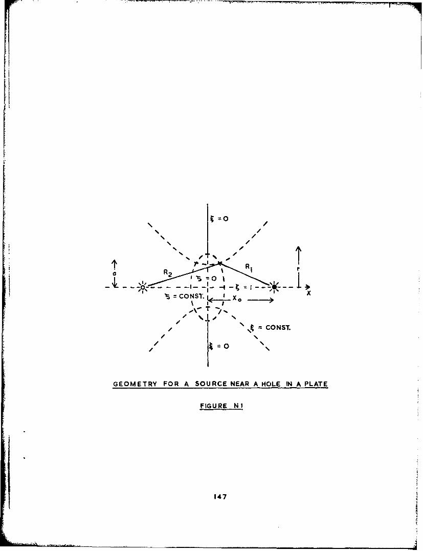
0
R ý,
H0
R2 I
0 1
S>CCO NST. xCX
/ \•,• =CONST.
/ 40I '4
GEOMETRY FOR A SOURCE NEAR A HOLE IN A PLATE
FIGURE N I
147

olpm.
z I
x~ x inuA
x VI
w- -IAI0 OA. OS- , IlIIl
_ _ 0a-~ ~ C .W *gifL)
0-0
C *-~ ~s0 I-
ii6 0
IL J
IIIu I

IR
0.8
0-6
REDUCTION FOR HOLE INAPLATE
REDUCTION FOR HOLE IN A FLUID
0.4
o-2
0-00 2 4 6 8 to
X0 /a
ASYMPTOTIC REDUCTION FACTOR AS A FUNCTION
OFSTANDOFF/HOLE RADIUS RATIO
FIGURE N3
149

0 The Effect of Bubble Migration
Throughout the entire discussion so far on the limitations of
the theory it has been assumed that the bubble remained fixed in
space throughout its pulsations. For small charges of the type used
in Chertock's experiments this is a reasonable assumption since,
except in special circumstances (eg an underpressure tank), the
pressure difference across the bubble is small compared to the
absolute hydrostatic pressure. For larger charges, of the sizes
likely to affect ships, the pressure differences will be very such
larger but the hydrostatic pressure will not change greatly. For
example, consider the model in Chertock's experiments. It was
10 ft ling and the maximum bubble radius was about 6 ins when the
charge was suspended 16 ins beneath the water surface. On full
scale the target might be 40 times as big so that a scaled bubble
would have a 20 ft radius and its centre would be 50 ft beneath the
surface. In the model case the ratio of (presstre difference
between the bubble top and bottom) over (pressure at bubble centre)
is
p pmodel - 33 ft 0.031 where atmospheric pressure.is equivalent to a 33 fthead of water
On full scale the comparable ratio is
S40 o0.48
p full scale 33 + 51D
Clearly in this case the relative buoyancy forces acting on the
bubble will be sixteena times greater than on the small scale and
migration will be more important.
130

The mechanism of bubble migration is ve•:. well understood
(reference 01). During the early expansion very little migration
occurs since the bubble is small and the hydrostatic force on it
(its displacement) is similarly small. During its underpressure
phase, when it is large, the buoyancy force is very large but so is
the effective mass of the bubble; although the gas within the iW*hble
has a negligible mass compared with the mas3 of water displaced by
it, the added mass associated with the flow of water around the
bubble is not negligible - for a spherical bubble it is half the
mass of the displaced water. In consequence the bubble accelerates
upwards but does not have time to achieve a significant displace-
ment or velocity before the bubble contraction occurs. It does
however have time to acquire a considerable momentum (actually
contained in the water around it). During the contraction phase the
mass of water displaced is reduced to a very small fraction of
maximum displacement and the added mass is raturally similarly
reduced. Since the momentum acquired during the underpressure phase
is still associated with the bubble the reduction in added mass
implies an equivalent increase in vertical velocity and the bubble
shoots upwards when near its minimum. During this phase it distorts
greatly, the bottom surface itwerts and forms a jet which penetrates
through the bubble, producing a toroidal shape. During re-expansion
the bubble regains an approximately spherical shape and its velocity
falls as its added mass rises. Thus the bubble is almost stationary
during the phase when the vertical forces on it are large, but
migrates rapidjy later when the vertical force, are least. During
"the rapid migration phase, since the vertical force is small the
momentum is almost constant so that the product of bub'le volume and
vertical velocity is almost constant.
S... ... ... ", ...... ... ,•,•,•1.51 _

'rz .ain ard most obvious effect of migration is to bring the
point of emission of the first bubble pulse much nearer to the surface
of the water. Since this pulse, as discussed earlier, can be almost
twice as effective as the initial expansion, this can considerably
affect the motion of a target above the bubble. There are however
other effects. The peak pressure during the bubble pulse is well
known to be considerably reduced by vigorous migration (reference 01).
The reduction in pressure however is accompanied by an increase in
duration so that the Im.pulse is less affected. In addition, the
motion of the bubble causes - dipole pressure field around it in
addition to the usual radial field. This dipole field was first
investigated by Taylor (02] who showed how very intense it can be,
although of course it decays much more rapidly with distance from
the bubble than the radial field and is seldom observed in pressure
gauge measurements.
Another effect due to gravity is distortion of the bubble from
its spherical form. Such deviations have been the subject of a
number of studies, eg [03] and [04], but in the main these have been
based on perturbation techniques and have only applied to the early
bubble deformations. Quite recently, purely numerical techniques
have been used to describe the flow around pulsating bubbles,
particularly around collapsing cavitation bubbles. These have shown
clearly [05] the sort of distortions suffered by a bubble collapsing
in an external pressure gradient, although in the case of [05] the
gradient was due to the presence of a rigid wall rather than a
gravity field. These distortions are related to multipole terms in
the flow field of higher order than dipole. These higher order terms
decay with distance even more rapidly than the dipole terms and so
are neglected here. The distortions lead to drastic changes in the
L 3

motion of the bubble during the collapse phase when near the minimum
and a significant redistribution of energy occurs at this time.
Since such effects cannot at present be treated analytically, they
are allowed for here only on an empirical basis.
With the geometry of Figure 01, assuming first that the explosion
is deep so that the effect of the water surface can be neglected, the
velocity potential for the migrating bubble will be approximately
e e2S•2 -- s e 1 (01)rI
While the bubble is spherical this will represent the motion exactly
but late during the bubble collapse phase, when it begins to distort,
higher order terms will also be present. Since these will affect the
flow only very close to the bubble surface they are neglected and
equation (01) is assumed to apply throughout the motion, the bubble
being assumed to remain spherical at all times. The strengths e• and
e 2 are then readily found to be related to the bubble volume V(t) and
velocity v(t) by
e1 =V/47C and e 2:= v (02)
From equation (01) the vertical velocity due to the pulsating
migrating bubble is
uy (y (0-) - - (03)
Since the bubble is rising with velocity v, the vertical accelera-
tion u is given by
153

a au (Y4) + 2T Z v y 3" 3 r
r13 rI 1 rl13
322r,1
The nature of the four terms is easily seen by substituting the
expressions (02) for eI and e2* The first term, proportional to
is therefore proportional to the bubble volume accelerationt, V,
and so in principle is the same as for the non-migrating bubble
(although the value of V will be changed). The second term is
proportional to A.(Vv). Now the mass of the bubble itsel f is
dt
negligible compared to the added mass of the water moving around it,
which for a spherical bubble is just one half the displaced water
mass. The quantity Vv is therefore proportional to the momentum
associated with the moving bubble and the term e2 is consequently
proportional to the rate of change of bubble momentum, and so also
to the force acting on the bubble. This force is simply the
buoyancy force due to the gravity induced pressure gradient in the
water, ie pVg. The second term is therefore proportional to the
bubble volume. It will be negligible in the early expansion and
again later near the bubble minimum. It will be greatest during
the long expansion phase. The third term is proportional to
eI v c Vv and will therefore be greatest when V and v are both
154

large, ie late in the collapse phase and again early in the
subsequent re-expansion. It will be very small during the under-
pressure phase since then both V and v are very small, and will
also be small at the bubble minimum since V is zero then. The
fourth term is proportional to e2 v c Vv2 c m2/V where m is the
vertical momentum of the bubble. It will consequently be largest
at the bubble minimsa.
On assuming that the bubble remains spherical, the kinetic
energy equation given in section H, when applied to the woving
bubble, becomes
3o 2 o3a2 +' i N't
EC= ,pa a +yt3u+
1 Pa3V2 (05a)
Equating the buoyancy force to the rate of change of momentum
gives the migration equation
d .1 XPa3v= - Kxa&3 g (05b)
In terms of the non-dimensional variables x and r defined in
section H, and with Z,/L = •, these equations become
92 +e/6 + CC /3Y1)
and the four terms in the expression (04) for the fluid accelera-
tion may be re-written (for the surface y = 0)
155

f1 x' ; rL=p d/Lr 1 P
f2 (I - -= - 2 32) - X
S2 (07)3 r l 3 () 9 P3
3e 2vd d)3,f4 (3- 2 r2 j
In each of these terms the acceleration is measured in units of g,
the acceleration of gravity. The expressions (07) have all been
multiplied by the factor 2 to allow for usual doubling effect of
the free surface. Since, for rapid motions where surface waves can
be neglected, the boundary condition to be satisfied is 0 0, the
condition is satisfied by a negative image above the surface which
produces the assumed enhanced acceleration.
The Free Surface Effect
The free surface is well known to affect not only the
accelerations near it but also the motion of the bubble itself if
it is within a few bubble maximum radii. The velocity potential in
such cases is given approximately by
e, e20 1 e2S= + osOI--- + _cos 02 (08)r1 2rI r2r2
for the geometry of Figure 01. In this case, as Taylor showed, the
source and dipole stregths are, to order (a2/d2)6
156

29 v a a ;e -
12 2 4
The kinetic energy of the flow, to the same order, is
T= 22 p a3 ;2 ( - 2 + p a -2 p a2 a 23
and the energy equation becomes
E 2 (a + 302 7C3* 2 3E=2cpa~a I aZ+-p A-+xa8
• °=20 aa 2d 3 2 d2
0 d
a % (09)3Y -.
where p is the pressure within the bubble.
The migration equation may in this case be derived from the
Lagrangian form of the equations of motion, ie
(T - V) = (T -V)
In terms of the previous non-dimensional variables the resulting
equations are
k
(oj o)
[ 3Xx4;2 _5 _ X= 4 8 42 C0
157

Since Z = d + h, h being the static head of water equivalent to
atmospheric pressure, 6 = C - C where C I h/L. For computational
purposes these equations are best reduced to the equivalent set of
first order equations
x + +- '
3 =-•3Y + ( I
+- -" )' (3 (010NxLo 223 T]
r?-o 482
where two parameters a, and p have been introduced to ene.ble the
same equations to cover three distinct cases of idealised bubble
motion. The appropriate values for m and P are
M I Type of Motion
0 0 Non-migrating
0 Migrating
1 I Migrating near a free surface
The appropriate initial conditions are those used earlier in the
non-migrating case, ie
a =0
158
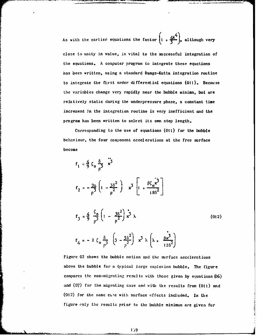
As with the earlier equations the factor (I +. I' although very
close to unity in value, is vital to the successful integration of
the equations. A computer program to integrate these equations
has been written, using a standard Runge-Kutta integration routine
to integrate the first order differential equations (011). Because
the variables change very rapidly near the bubble minima, but are
relatively static during the underpressure phase, a constant time
increment in the integration routine is very inefficient and the
program has been written to select its own step length.
Corresponding to the use of equations (011) for the bubble
behaviour, the four component accelerations at the free surface
become
p3 X3
f -= Lo 2 (02
3 9 3 3 ;
P P
4 0 128 21
Figure 02 shows the bubble motion and the surface accelerations
above the bubble for a typical large explosion bubble. The figure
compares the non-migrating results with those given by equations (06)
and (07) for the migrating case ardl with the results from (01) and
(012) for the same ca-e with surface effects included. In the
figure only the results prior to the bubble minimum are given for
159
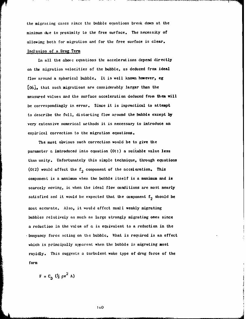
the migrating cases since the bubble equations break down at the
minimum due to proximity to the free surface. The necessity of
allowing both for migration ard for the free surface is clear.
Inclusion of a Drag Term
In all the above equations the accelerations depend directly
on the migration velocities of the bubble, as deduced from ideal
flow around a spherical bubble. It is well known however, eg
[063, that such migrations are considerably larger than the
measured values and the surface acceleration deduced from them will
be correspondingly in error. Since it is impractical to attempt
to describe the full, distorting flow around the bubble except by
very extensive numerical methods it is necessary to introduce an
empirical correction to the migration equations.
The most obvious such correction would be to give the
parameter a introduced into equation (011) a suitable value less
than unity. Unfortunately this simple technique, through equations
(012) would affect the f 2 component of the acceleration. This
component is a maximum when the bubble itself is a maximum and is
scarcely moving, ic when the ideal flow conditions are most nearly
satisfied and it would be expected that the component f2 should be
most accurate. Also, it would affect small weakly migrating
bubbles relatively as much as large strongly migrating ones since
a reduction in the value of a. is equivalent to a reduction in the
buoyancy force acting on the bubble. What is required is an effect
which is principally apparent when the bubble is migrating most
rapidly. This suggests a turbulent wake type of drag force of the
form
F = CD (• pv2 A)
luO

where A is the bub',le cross-sectional area transverse co the mo•ion
and CD is a drag coefficient. If the bubble were , solid sphere
such a drag term would certainly exist as a typical bubble from a
large explosion could easily be 5 ft in radius when near its
minimum and moving at up to 200 ft/sec. The Reynolds nir.mer for
such E, motion is of the order of 108. Since the actual bubble is
a surface of constant pressure, the mechanism of wa!-e formation is
not so obvious as for a solid body but some sch force seems likely.
A correct physical picture is not however ,-equired of an empirical
correction, It is sufficient that the assumed force should lead to
realistic results.
Assuming the existence of a force of the above type, the motion
of the bubble will be expending energy at the rate
FY -2 p=- 3
Similarly momentum is being lost to the wake at the rate F
ie P C a2 v2 tPC a2 2
Although the Lagrangian derivation of the bubble motion equations
is no longer available, the simpler type of tderivationt due to
Taylor leads to the equations
Xýk i CD 2 3
,i61

d 3_I =-L +L + 8+ xliI +D 2 ?2
dv 3 r2o 4
These equations are equivalent to the first order equations
X = a
1 T- • 13- r• C 0o x3y + I
OXx' Xý A
(C2+ 71 tX)l/2( )
482 + C it
C 2
The oorresponding component accelerations at the free surface
become
9 = 0 P3
33 C
PPC 3C
Pp 1882P3 P
05 k 2 128)P, p
1021
itv2

The computer program for the bubble motion, which was described
earlier, in fact integrates equations (013) (all the previous cases
can be obtained from (013) using suitable values for cm, P and CD).
A series of calculations were carried out for a 500 lb charge of TNT
at a depth of 150 ft using a series of values for CD* The results
are summarised in the Table.
Migration Variables for Different Drag Coefficientsfor a 500 lb Charge at 150 Ft
Migration to P EdissipatedDrag Coefficient First PulseE
CD (ft) 0
0.00 16.9 0.47 0.000.50 15.0 0.37 0.19
1.00 13.3 0.40 0.22
1.50 12.3 0.46 0.192.00 11.3 0.52 0.15
2.25 10.9 0.56 0.12
Experimental Result 11.0 0.63 0.15
In the table pI is any pressure which would be measured at large
(o)standoff and p1 is the pressure which would be measured at the
same point if the bubble did not migrate. In the near field the
pressures will be affected by the dipole field but at large
distances only the radial field will be felt and the rdtio
p1 Stends quite rapidly to a limiting value. The experimental
p1
value for p1 is subject to considerable scatter. The texperimental'
value for p1 is estimated from the empirical formula for bubble
pulse prssures. The table shows that for this particular charge
163

size and U't:ch the value CD = 2.25 makes both the migration and the
Piratio -0 approximately correct.
P1
The large value of CD precl.;.les its direct physical identifi-
cation with a normal Aake-type drag coefficient since its value
would normally be fairly close to unity. However, for the strongly
migrating bubbles for which the value was derived the bubble would
haive flattened considerably near the minimum (as is observed on
small scale) so that the area to which CD is related would actually
have been rather larger than a.surned. Had a m,.re realistic value
for the area been used a lower more realistic va.ue of CD would
have resulted. However, a complete physical picturc is not required
here, just a simple mechanism for producing the correct bubble
migrations.
One of the equations from which the bubble motion equations
were derived was the energy balance equation. The addition of the
drag term implies that the bubble loses energy continually through-
out the motion. Most of this energy loss naturally occurs at the
bubble minimum when the velocity is very high. It is well known
that the period of a pulsating bubble is quite a good measure of
the bubble energy and this fact has long been used to measure the
bubble encrgy. By comparing the periods of the first and second
bubble pulsations estimates have been made of the total energy loss
which occurs at the bubble minimum (reference £06]). The energy
still retained by the bubble at its minimum was - Iculated for the
cases given in the table and the energy dissipated up to this time,
as a fracfion of the original energy, has been added to the table.
164

The experimental value for the energy losý for this charge size and
depth is 40%o of the original bubble energy, of which 1OUo is estimated
to be due to acoustic radiation (neglected in this analysis). - If it
is assumed that roughly half the remaining dissipation occurs before
the minimum, this gives the 15%, quoted in the table, for the
experimental dissipation. The value CD = 2.25 therefore gives about
the right total energy dissipation. lt is of interest zhat the value
CD = 1.00 corresponds to a maximum in the energy dissipated.
One significant point regarding the energy loss is that although
for very weakly migrating bubbles an energy dissipation mechanism is
quit ! clear, the same is not true of strongly migrating bubblts. For
small bubbles, or very deep ones, which do not migrate significantly,
the bubble surface remains fairly spherical until late in the collapse
phase when the bubble pressure rises above the aebient level and
starts to decelerate the bubble surface. The acceleration then being
directed from the less dense fluid to the more dense one, causes the
usual Taylor surface instability to occur. High speed films show
thM.t the instability occurs as a very large number of needle like
jets being projected into the bubble. Due to its adiabatic compres-
sion the gas will be very hot at this time and such an intense spray
of cold water will remove much energy. For strongly migrating
bubbles this f)rm of instability does not seem to occur. An over-
all distortion, first into an oblate spheroid, occurs instead and
later the bottom inverts and penetrates through the bubble turning
it into a toroid. Since intimate mixing of the gas and water no
longer occurs an alternative mechanism is required to account for
the observation that migrating bubbles dissipate as much energy as
non-migrating ones. The 'wake' theory provides such a dissipation

mechanism. The energy is not so mauch dissipated as transferred to
water which loses its association with the bubble. The mechanism
assumes that both momentum and energy are transferred to water
behind the bubble, principally when the bubble is small and its
velocity great. As the bubble begins to re-expand and slow down,
it has no way of stopping the narrow following wake which could
penetrate it and form a vertical water jet. The large plumes which
are so evident on the surface above an explosion are known to
originate at the bubble pulses and are perhaps due to such jets.
One important result of the transfer of energy and momentum
to the 'wakel of the bubble is that the bubble motion is no longer
symmetrical -bout the minimum. Figure 03 shows the displacement
time history calculated for the bubble centre for the 500 lb
charge at 50 ft, with CD = 2.25. The bubble appears to come to a
rather abrupt halt shortly after the minimum. Although this sort
of motion was not described in early photographic studies of
bubble motion, the actual motion of the bubble 'centrel in such
studies is very difficult to measure because of the drastic shape
changes which are occurring. Such behaviour has however been
reported in some recent studies [07).
To further confirm the usefulness of the modified migration
equations, they were integrated for several other charge depths.
The results are summarized in the following table.

Migration Migration PICharge (ft) Max Bub. Radius(Depth p(ft) , , ...
Calcl Meas Calc Meas Calc Meas
50 26.9 24.2 1.15 1.06 0.18 0.A5
100 15.71 15.1 0.80 0.78 0.40 0.33
150 10.9 11.0 0.62 0.63 0.56 0.63
450 3.2 4.2 0.26 0.32 0.92 0.97
Again the agreement is very reasonable. The underestimation of the
migration for the deep case is to be expected since little overall
bubble distortion will occur in this case and the value of CD
will accordingly be too high.
Effect of Migration on Whipp-ng Response
As the modified equations seem to give results in reasonable
accord with measured results for the migration and the far field
pressures, they are adopted here to show the sort of differences
in whioping response to be expected for migrating bubbles. Figure 04
shows the surface accelerations near a 5001b charge of TNT at 50 ft
depth and shows a considerable change in the bubble pulse. Directly
over the charge the peak acceleration at the pulse is slightly reduced
Lo't the duration of the positive phase is greatly increased. ro the
side the shape becomes mcre similar to the non-migratUng pulse shape
(ait!ough still of increase.d duration) but the peak acceleration is
much reduced. Apart from the slight change in the phasing o. the bub-
ble pulse relative to the ship motion, the only sigaificant change in
the forcing function is in the bubble pulse. Since the positive
phase of this is still much shorter than the basic ship period it can
be considered impulsive. The bubble pulse impulse and also the
initial expansion impulse for both a 1001b and the 5001b charge have
167

been calculated for a large selection of depths and horizontal stand-
offs. The re:tulting impulses have been normalised to an arbitrary
impulse and the resulting relative impulse contours are shown in
Figures 05 and 06. In comparing the initial impulses with the bubble
pulse impulses it should be remembered that for a non-migrating bub-
ble with rio energy losses the latter impulse is exactl3 twice the
former. At shallow depths the bubble equations break down and the
position of the contours shown by the dashed line is conjecture only.
The figures show clearly that over a considerable depth range the
bubble impulse is greatly enhanced by migration effects: for example
at a depth of 4t5 ft the bubble pulse gives over seven times the
impulse due to the initial expansion. At 50 ft the ratio drops to
3 to 1. At points not directly above the charge the enhancement is
much reduced and can fall well below the factor 2 expected for a non-
migrating bubble. For the more strongly migrating 5001b charge the
maximum horizontal standoffs at which given impulse levels are reached
during the initial expansion and during the bubble pulse are almost
the same. For the 1OOlb charge migration effects are clearly of much
less importance.
The extent to which the enhancements in the bubble pulse impulse
are due to its increased duration is emphasised in Figures 07 and 08
which show the relative peak accelerations during the initial expan-
sion and the bubble pulse. Only for a very small depth range, and
only directly over the charge, are the peak accelerations increased
by migration. At all other points there is a reduction in peak
acceleration.
The impulses illustrated in Figures 05 and 06 are -ot directly
i'elated to the total iu'u.nose on the ship. At any point on the ship
axis the impulse per unit length of ship will be proportional to the
168

iumpulse.< shown, the constant of proportionality being the sum of the
displacement and added ma,s (again per unit length) at the point
concerned. The overall effect on the ship will be an integral of
these impulses along the ship. The contours do however give some
idea of the importance of including migration.
Bubble Jets
As discussed earlier, much of the momentum and eneigy lost by
a migrating bubble during the bubble pulse will simply have been
transferred to a column of water which then will travel on upward,
initially at a speed close to the maximum bubble vertical velocity.
For charges directly beneath a ship such jets will presumably transfer
much of their momentum to the ship. Unfortunately the nature of such
jets, their length, diameter and transmission characteristics, is
presently unknown. Only one study of any kind seems to have been
made (reference 07) and that only considers the pressure pulse emit-
ted by the jet at its moment of creation. The pressure pulse analysis
is rather dubious and since it does not consider the subsequent
motion of the jet through the water the work is unsuitable for quanti-
fying the jet effect.
Since the motion of small scale bubbles in underpressure tanks
is knowrn to closely resemble that of full scale bubbles (except for
the periods when internal bubble pressure is important), the nature
and motion of any jets could probably be investigated quite effective-
ly ;n such tanks. The problem is not pursued in this thesh.
1 b9

References
01 Cole, R H1; "Underwater Explosions", Princeton UnivPress, 1948
02 TaylorG 1; "Vertical Motion of a Spherical Bubble andthe Pressure Surrounding It", UnderwaterExplosion Research, Vol I[, "The Gas Globe",0 N R (1950)
03 Penney, W G; "On the Changing Form of a Nearly Sphericaland Submarine Bubble", Underwater Explosion
Price, A T Research, Vol II, "The Gas Globe" 0 N R
(1950)
04 Kolodner, I I; "Underwater Explosion Bubbles II. The Effectand of Gravity and the Change of Shape",
Keller J B New York Univ Rep IMMI-NYU 197 (1953)
Plesset, .1 S; "Collapse of an Initially Spherical Vapourand Cavity in the Neighbourhood of a Solid Bound-
Chapman, R B ary", Cal Inst of Tech Rep No 85-49 (1970)
06 Snay, It G; "Underwater Explosion Phenomena: the Para-meters of Migrating Bubbles", NAVORD Report
4185 (1962)
07 Farley, T E; "A Simplified Analysis of the Bubble Jetand Pulse", NOLTR 68-42 (1968)
Snay, H G
Z
1-70

2 I IMAGE BUBBLE
______ ____WATER SURFACE
zd
,- EXPLOSION BUBBLE
GEOMETRY FOR MIGRATING BUBBLE EQUATIONS
FIGURE 01
171

., I
=- r
Z 4- - NON - MIGRATING
MIGRATING ii- --- MIGRATING WITH SURFACE EFFECTS /..
T E - ,M S O N LE SS / /u -2 -50-75 ,0I SO
0~1.25
II
TOTAL SURFACE ACCELERATION ABOVE BUBBLE
Z "
0 PULSATION TERM I
4.BUOYANCY TERM 24w-- ..SOURCE MIGRATION 3"Ii --- DIPOLE MIGRATION 4
T TIME DIMENSIONLESS
COMPONENT SURFACE ACCELERATIONS FOR MIGRATING BUBBLE -,I
WITH SURFACE EFFECTS \C !EWATER SURFAC
°-i.s -go -is -00 1-'25 Ii-o
I- 10 SURFACE•
UT. EFFECTS
2172
---- UPPER SURFACE OF BUBBLE.0-n 30. ,.
,-,, WITHOUT
SURFACE40, EFFECTS
SO -- B8UB8BLE CENTRE
BUBBLE MOTION - MIGRATING WITH SURFACE EFFECTS INCLUDED
THE EFFECTS OF BUBBLE MIGRATION
FIGURE 02
172

WATER SURFACE
10
S20 BUBBLE UPPER SURFACE
30.
O ON-MIGRATING B BBLE-' .
040 BUBBE CENT40
•.2 -4 "6 .6 !.0 I-2 1"4 !'6 1.8 2"0 2"2
TIME-DIMENSION LESS
BUBBLE MIGRATION FOR A 500 L11
CHARGE AT 50 FEET DEPTH
173
/'

12
zI'2
zz
I I-
• (NNDIESONL, 1" I'S 1"
suRF-ACE ACCELERATIONS DIRECTLY OVeR THE RUBBLE
4. I 7
Mii
0 cc
us I
U (NON - DIM ENS|IONAL)
SURFACE ACCELERATIONS AT IS FEET HORIZONTAL STANDOFF
zI M
2 eJ
UC I U ,< M
STIME
u (NON- DIMSIONA) I-I . 1.4 1.6,3 1.4 1.s 1.6
-4 SURFACE ACCELERATIONS AT 310 FEET HORIZONTAL STANDOFF
EFFECT OF BUBBLE MIGRATION ON THE SURFACE AkCCELERATrIoNS FROM
A 50016 CHARGE AT 50 FEET DEPTH
FIGURZ 0 4174
*>l

20 .3-0
SII
20 4= 3:0;'3
0. 17x
w40 - 3o 60 -
w
S60 :r so
u,
0..1003 , _____ _ _
0 20 40 60 0 20 40 60
CHARGE HORIZONTAL STANDOFF IN FT. CHA RGE HORIZONTAL STANDOFF IN FT.
100- POUND CHARGE OF TNT 500 - POUND CHARGE OF TNT
EFFECT OF CHARGE GEOMETRY ON THE RELATIVE INITIAL ACCELERATION
IMPULSE AT A POINT ON THE WATER SURFACE
FIGURE 05
I . . . I. . j
'20 75 .20
2 53' j ILl• O. i. l
1-0%
40 40 40 6 0 20 40 -0
170 "5 2
= 60 0 .003'4 0-50
030
(DOTTED PAR I Or CURVES__________ ____IS CONJECTURE ONLY)If0 20 40 60 0 20 40 60
CHARGE HORIZONTAL STANDOFF IN FT CHARGE HORIZONTAL STANDOFF IN FT.
100 -POLND CHARGE OF TNT 500 -POUND CHARGE OF TNT
EFFECT OF CHARGE GEOMETRY ON THE RELATIVE SIJBBLE PULSE
ACCELERATION IMPULSE AT A POINT ON THE WATER SURFACE
FIGURE 06175

II
0 T 0 30
T2.0'
20 20
. .0z 0.75'
840 -- x4 "0 0
T--1001 100 -
0 20 40 60 0 20 40 60
CHARGE HORIZONTAL S'ANDOFF IN FT CHARGE HORIZONTAL STANDOFF IN FT.
100 - POUND CHARGE OF TNT SO0- POUND CHARGE OF TNT
EFFECT OF CHARGE GEOMETRY ON THE RELATIVE PEAK INITIAL
ACCELERATION AT A POINT ON THE WATER SURFACE
FIGURE 070 01-2
20 Oz 20
z, I-S.I- I- d-
ý.Or.us w040 40
"w 0-2 " 60-
= 0.10u60 - x 60ý02
10- '000I80 _ _ _ 1 _ _ i _ _ __80- _-_._
0 20 AO 60 0 20 40 60
CHARGE HORIZONTAL STANDOFF IN FT. CHARGE HORIZONTAL STANDOFF IN FT
100- POUND CHARGE OF TNT 500 -POUND CHANGE OF TNT
EFFECTOF CHARGE GEOMETRY ON THE RELATIVE BUBBLE PULSE
ACCELERATION AT A POIN? ON THE WATF.R SURFACE
fIGURE 0O176

1%. Descrip~tion of Computer- Program 11
The general features described in Sections L, N and 0, it. the
3-D V.L•dtdal mass, the effect of uj hole in the target and the effect
of bubble migrdLton, have adl been incorporated into a computer
program. The program is written in FORTRAN and has been implemented
on boa' an IBM 7090 ,and a KDF-9 computer. As for the computer
program I, rhe program and detailed specifications for its structure,
tt.e datia format and units, and the type of output it gives are all
held at the Naval Construction Research Establishment. Again as for
the program I, the program has been written so that it splits
naturally into t%o sections, the first evaluating the vertical
vibration modes of the ship, and the second using these modes to-
gether %,ith additional details on charge size and location, to
determine the whipping response. The main differences from the
first. programn are su.marised below.
The elastic nature of the ship is specified in the sam way as
for program I but the inertial properties are given in a different
form. Instead of specifying the added mass and the displaced water
mass at each node the related Lewis type coefficients C and C are
defined, together with the ship beam. Since rotary inertia effects
appear to be generally small this program does not include them. The
program uses the 3-D flow approximation equations to determine the
fluid inertia matrix as described in section L. A Choleski routine
is used to split the total inertia matrix into the form LLT and an
HGOW eigenvalue subroutine then determines the ship frequencies and
transformed mode shapes frci. the symmetric matrix L-1 S LT where S
is the elastic stiffneis matrix. This part of the program produced
the ship frequency results described in section L.
177

Using; these modes the program will then calculate the positional
mode coefficients yi(x), Mi(x) and Si(x) described in section I for
use in computing the eventual response by combining the individual
modal responses. The solution of the modal equations is more com-
plicated than for program I since the forcing function is no longer
proportional to the bubble volume acceleration. Due to the use of
the migrating bubble equations the forcing function is
TT 2 (t)
where M. is the water inertia matrix defined by equations (L20),
(L22) and (L23), Xiis the ith mode shape and uj(t) is given by
equations (013) and (014). In consequence a matrix multiplication is
involved at each time step and for each mode. In computing the
values of W(t) allowance is made (if so required) for the effect of
a hole in the target, as described in Section N.
As before, the modal equations are integrated by a standard
Runge-Kutta integration subroutine and the initial conditions are
that the mode coefficients and their first time derivatives are all
zero,
)j78
-• : .. ... .. - ... .... '- 178 -: ".. . . . .• • •. . " 'i ' .. . .. . . ..... ..

Q. Com:,parative Calculatiot~s
The computer program II has been used to carry out an extensive
set of calculations and typical results are shown in figures QI to Q3.
These figures compare the results of calculations carried out first
with migration included and then without it. Figure Qi shows the effect
of migration on the amplitudes of the heaving mode and the basic
whipping mode for a charge directly beneath the centre of the ship, and
also for a similar charge at the same depth but off to one side.
Figure Q2 shows the same charge and geometries but compares the vertical
midship displacements and the corresponding midship longitudinal deck
strains. Figure Q3 shows the vertical displacements and strains for
the same charge at a slightly greater depth.
The most obvious feature of the graphs is that, despite the great
enhancement of the local force above the charge which was shown in
section 0 (Figure 06), the inclusion of migration does not markedly change
the motion of the ship. At the shallower depth the deck strains are
increased by 20% but to the side, and at the greater depth, the motion
is little affected. This is presumably due to the considerable length of
ship which is affected by the whipping forces. Section 0 showed that
the forces on the ship, although greatly increased above the charge,
were reduced at points some way off the vertical. The integrated
effect of parts of the ship away from the charge evidently offsets the
local intensified loading.
For deeper charges, later bubble pulses will begin to have an
effect on the ship and in such cases gravity migration would be much
more significant as it could bring the bubble from too far away to be
important, in to potentially damaging ranges. Such later pulses are
less well known than the first pulse and have been excluded from the
analysis. The bubble equations will predict several oscillations for
deep charges but the accuracy is not known.
179

Conmparison of tiburc. ,i1 and 02 shows that the basic whipping mode
is the one principally responsible for the observed strains but that
the higher modes still have a significant effect. The higher mode
concerned in these calculations is the third whipping mode, since the
longitudinal charge position is close enough to a node of the second
whip,'ing mode Cor it t' be little excited. Only the first three
[lhipping modes, and the two rigid body modes, are included in the
calculations.
The computer program 11 was used to produce both the migrating
curves and non-migrating ones so that minor differences in the bubble
equations and the ship representation should not be included in the
results. Program I1 has a facility for suppressing .he migration
terms in the bubble equations. Unfortunately, since the bubble motion
is derived from direct integration of the bubble equations, when
migration is suppressed the motion is that due to an undamped bubble
with no energy losses. If such losses were included the bubble pilse
would be slightly reduced and the amplitudes for the non-migrating case
would be correspondingly reduced. A second minor deficiency in the
graphs is in the displacement curves. The program automatically cuts
off the bubble pulsations just after the first bubble pulse. This is
biecause of uncertainties in the bubble forces after the pulse. In
consequence an upard impulse is imparted during the pulse but the
subsequent suction which, physically, should follow, has been
suppressed. The ship then has only gr'-vity restraining it and, sipce
gravity has a mnuch smaller effect than the bubble forces, the ship
dis:ilacement grows at a steady rate over the time period concerned.
This is mozt obvious in the heaving mode shown in figure QI(a).
Since the strains in the ship are virtually independent of the rigid
body motion they are little affected.
Ij
i 80I $0

z 0Z, uJ
Z 0 -0
% on
aa0 U.
.1 1go J
z0z
LaaI~
J 2a04 04
2 O
S 0 5 2
'II'
%% U.% z 0 z
z 00 Z
0.
.000a S
-----0 0
30 ~Id4 3I-4 anicny3lei
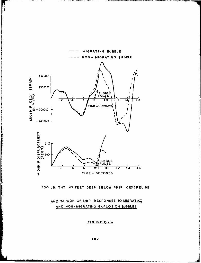
MIGRATING BUBBLE
NON- MIGRATING BUBBLE
4000 •z
S.- 2000 \ !
u- 4000Ee
U-
ZI
j- .2 .4 .6 *8 10 '12 1-41 1-6~.~~ -2000TIM E-SECONDS%
0 -
-4000
z~ul
Suiu I-0 -U.
,• ~~ýJ 0J UI • B
.• 2 -4 -6 -8 ': 1 H 3 1-2 - 1-4 1 .60 T!ME- SECONDS
500 LB. TNT 45 FEET DEEP BELOW SHIP CENTRELINE
COMPARISON OF SHIP RESPONSES 1O MIGRATINZ
AND NON-MIGRATING EXPLOSION BUBBLES
FIGURE Q2 a
182

-- MIGRATING BUBBLENON- MIGRATING BUBBLE
4000z -
BUBBLE3000 PULSE i
u 2 S-4000
I p
-2 -4 .6 .8,r 1-0 1.2 1I4 1.6
'BUBBLEPULSE
500 LB. TNT 4S FEET DEEP 30 FEET OFF CENTRELINE
COMPARISON OF SHIP RESPONSES TO MIGRATIN!G
AND NON-MIGRATING EXPLOSION BUBBLES
FIGURE Q2b
11
1 33

It
Z4000
I-,i 2000 /•" TME -SErCONDS
UJ-
,.oz .2 -:4 "./ A'e 10• 1-2 1/ 14 1-!6"•.= / ,I BUB1LE •• '
- -2000 PULSE
S-4000
zw
w2-00 A
O• " TIME - SECONDS
0*3: 2 4 "1"•• . '0 1"2 1'4 1.6
'BUBBLEo PULSE
500 LB. TNT 60 FEET BELOW SHIP CENTRELINE
COMPARISON OF SHIP RESPONSES TO MIGRATING
AND NON - MIGRATING EXPLOSION BUBBLES
FIGURE q3
184

R. Plastic Deformation of the Target
So far the entire analysis has been based on elastic deformations
of the target. If the stresses in the main girder reach yield in
tension then plastic yielding will occur and the elastic equations
will no longer apply. Nevertheless, so long as the total duration of
such plastic yielding in each vibration cycle is short compared to
the basic elastic vibration period, the motion of the ship will not
differ greatly from the fully elastic motion, If however the stresses
in one of the girder flanges reach either yield stress or the flange
buckling stress, in compression, then the flange will buckle and the
stiffness at the section will fall dramatically. Such failure has
been observed in static tests on naval vessels (references [CA] and
LC8]) and the buckling has been found to be very localised. The
drastic reduction in stiffness at the buckled section allows the
girder on either side to rotate to relieve the moments which caused
the buckle. This type of failure will clearly modify greatly all
subsequent target motion. To show the type of motion which results,
approximate equations to describe the motion are developed here. The
plastic equations described are not intended to be particularly
accurate, but merely to be close enough to reality to show the type
of motion which is likely to occur.
With the geometry of Figure Ri, the equations of motion of the
ith mass aie clearly
Mi yi = SLi " SR i-I + P
Si = -MR i-i + 4i
where Pi and Qi are the external force and moment. P1 and Qi are of
course hydrodynamic and hydrostatic in origin and for simplicity
the strip theory forces are assumed. Thus

Pi % i 6 1 i +i wi i - kjy
(R2)
Q-r • ± 1 ) + Tr - kry 1
and the equations (RI) become
(mi + %i) Y;i SLi S SRi + (%i + i) ui " kiYi
(R3)
(ri +r wi) e: i ML,-i + (rwi '-, i) ; - k r.i
When the deformations are elastic, the shear forces S and bending
moments M transmitted by the beams on either side of the lumped mass
are determined by the equations of Section C and the equations (R3)
are identical to those already considered. The plastic nature of
the problem is ent iriy determined by these terms.
In the theoretical model, since the beams are considered to be
weightless the shear force in each is constant and the bending
moment is a linear function of the distance from the end. The
maximum bending moment will consequently necessarily occur at one of
the ends and yielding will start at such a point. In a physical
model yielding would then spread outward along the beam but, to keep
the model as simple as possible, it is assumed here that the dis-
tributed 'excess' curvature near the mass is equivalent to a
discrete rotation of the beam end relative to the lumped mass. The
rotation is assumed to take place at a constant, plastic, bending
moment. When the rotation exceeds a specified amount it is assumed
that the beam will buckle. This again is assumed to be simply a
rotation of the beam end relative to the lumped mass but at a much
lower value of the constant plastic moment. The complete moment/
plastic rotation diagram assumed is illustrated in Figure R2. The
fully elastic motions already considered involve no plastic rotations

and so lie entirely on the line GOA. For the plastic case, if the
lumped mass displacements and rotations are such that the moment at
one end of a beam section is tending to increase, the moment will
rise elastically from zero at 0 until it reaches the plastic
moment Moo After this the plastic yielding will be equivalent to
a rotation of the beam end, at constant plastic moment V P1 until the
point B is reached, at a plastic rotation OMo Actually a more likely
route to B is indicated by the dotted line, but OAB should be a
re.sonable approximation. At B it is assumed that the section
buckles and the beam end instantaneously rotates to reduce the
moment at the end to Mp2, The moment/rotation curve *jumps' from
B to B'. The rotation then increases at constant moment Mp2 until
the tendency for the moment to try to increase further stops, say
aL C. If the tendency then is for the moment to reduce, the beams
either side of the hinge will unload elastically and normal elastic
vibration could occur up and down CD. A continued tendency to unbend
would lead to the plastic moment -2 and plastic rotation along DE.
From E', the buckled flange would start to straighten out and carry
aA increasing load, possibly as indicated by the dotted line, but DEF
is a simple approximation for the return to full strergth. Plastic
rotation would then continue at the constant moment -M P1 until
the opposite flange buckled, say at H, and a jump to the point H,
occurred. Along any of the horizontal branches of the curve, a
reversal in the tendency of 0 to change would lead to elastic motionP
along a vertical.
187

The whole moment/rotation relation is clearly highly over-
simplified; for example the negative plastic moment would really be
of different magnitude to the positive ones, the section would
buckle at a lower moment the second time than the first since the
plastic strain reversal between the two would not completely
straighten the flange, etc. As a simple model however it probably
contains most of the essential features.
For shear, since the shear force is constant along each beam,
i.t is reasonable to assume that the beam acquires a uniform shear
angle along its whole length once the shear force exceeds the full
plastic shear force. A shear force/shear angle relation similar to
that for the moment has been assumed although, in this case, the
reduction in stiffness is probably less dramatic.
To produce an algorithm quantifying the above characteristics,
the plastic rotations e 0i ~ and 0si as defined in Figure R3, are
introduced, In terms of these angles it is possible to define a
deflection and rotation of the right hand eixi of the beam, relative
to the left, in the form
yp= yi1- E,+ z y + Ri+ e,,)]
(R4)
vR = (y+i + e Li+1) - (Yi + d
These are the deflections which give rise to elastic stresses within
the beams. The shear force and bending moments in a beam with these
relative deflections are:-
IML = af 13YR + ( C 1I) 4t RJ
MR =ML 'SL = GAE-3YR+ (C +2) tv R (R5)
SR = SL 6a-[yR &.1
1 88

where, as in Section C.
El 12(0 + )I
In the (YR' LYR) plane curves of constant MLM and SR are straight
lines of slopes -3/(c - 1), 31(a + 2) and 2 respectively, so that
the elastic region in the (yR 49R) plane has boundaries of the form
shown in Figure R4. Initially, Y. and v. will be zero and the
bending moments and shear force will all be zero. When the explosion
occurs the yi and yi will start to change and, for each beam section
the values of YR and tvR calculated from (R4) will describe a carve
in the (YR' 4VR) plane. The motion of the ship will be entirely
elastic until one of these curves meets a boundary. After this the
value of the appropriate plastic rotation (ORi" eLi+l' Os) will
begin to vary in such a way that the appropriate force or moment
remains constart. The point in the (YR' 4tvR) plane will either
remain fixed at the boundary or will slide along the boundary. In
any practical computing scheme the integration of the equations of
motion will proceed in a series of time steps and at each step the
corresponding point in the ypR' tvR) plane will jump to a new
neighbouring position. Consequently instead of sliding along the
boundary the point may jump just outside it. It may then be brought
back to the boundary by adjustment of the appropriate plastic
rotation. Changes in the different rotations move the point in the
directions:
189

Ri at 45' to the yR axis
+ ; parallel to the tvR axisLi+1 R
s parallel to the Y. axis
In any of the regions marked I, only one of the plastic conditions
is violated and there is one way to bring the point back to the
elastic boundary so that its position is uniquely defined. In a&
of the regions marked II, two conditions are violated and the eventual
posit ion of the point on the boundary depends on the order in which
L.ie two adjustments are made. The non-uniqueness is not normally a
problem however since the point will always end up close to the
corner, which is where it would have been had its motion been
continuous rather than in discrete steps. The only time when non-
uniqueness is really a difficulty is when buckling occurs and one
pair of boundary lines suddenly moves in to the new plastic moment
position and leaves the point far outside. In this case it is clear
which rotation should be amended first and if the movement of the
boundaries is considered as a continuous process, the eventual
location of the point is obvious. If the amended position of the
point takes it outside one of the other boundaries it should be left
at the intersection of the two boundaries which is %here it would
have ended had the transition been continuous. This particular
problem is principally a computer programming one. In the regions
marked III, all the plastic conditions are violated. In general
such regions cannot be reached with a reasonable time step length,
except for very exceptional boundaries.
Unlike solid beams, a ship's hull girder is usually designed,
in order to give an efficient structure, to have most of the cross-
S• • '" * " i• • •° • -, •r • . .. •i• ".... , - - , 119.0,;

sectional material as far as possible from the neutral axis, In a
small ship (eg a destroyer) most of the strength (cross-sectional
inertia) is provided by the main deck and the bottom near the keel,
with the neutral axis about halfway between. In conseqaence, instead
of having a moment/curvature relation which changes slowly from fully
elastic to fully plastic, as for a solid bean, the ship behaves fully
plastically almost as soon as it starts yielding at the outermost
fibres. It has been found conwenient in the computer program to
define the plastic moments 9 p1 and TMp2 in the form
M f Mp1 I y
9 p2 = f 2 My
with
- - , the moment at which yielding first starts, W/YS= y
being the section modulus. Similarly, for shear failure
S p2 f 4 S (R7)
with Sy mA ay
The factors f to f4 can be specified as part of the data for the
program.
One further detail regarding the plastic moments is that, since
the initial yielding at the moment NMp1 really represents plastic
curvature in the region around ft lumpetl mass instead of a rotation
at it as assumed by the program, the changeover to 'p2 in the
program has been arranged to occur Ahen the total rotation (6O1i -L±)

dt a mss exceeds a given critical rotation 7.9 In this way the
program ensures that both sides of a lumped mass reduce in plastic
moment together.
Because the rotations of the masses in the plastic case form a
vital part of the analysis and can no longer be readily related to
displacements elsewhere, as in the fully elastic case, it is not
possible to halve the number of equations by dropping all rotary
terms. In consequence, instead of having say five second order
equations to solve, as in the normal mode elastic analysis, each
plastic integration involves two second order equations for each
lumped mass, ie forty equations for a 20 mass model. This means that
the time step must be very small, being restricted to a small fraction
of the shortest period present (rotary oscillations of a single
lumped mass with a consequent very short period). The combination
of a large number of equations coupled with a very short time step
leads to excessive computing times and a simple damping technique was
introduced to control the instability of the integration routine and
enable the normal step length stability criterion to be violated
safely. Linear velocity damping was introduced between each mass and
its two adjacent masses. Such damping affects principally the
independent motions of each mass while leaving the overall low
frequency modes largely unaltered. The final equations solved were
(=i + %d) Y*i S Ri " S.Li + (mwi + ýfi) '•i - k1it +
(mi + %wi) %d 'i-l + Yi+1 "
(ri + rwi) :• R - -Mu"1÷ ", + "• i • krLY1 +
(ri + rwi) "rd (Yi)- + -J+" 2y1 ) (R8)
1921

With this technique it cannot be expected that motion equivalent
to vibrations of higher modes will be reproduced but the features of
interest in whipping should be preserved. The damping constants were
chosen so that the predicted strains for elastic cases were similar to
those predicted by the computer program II. Even with the damping
included the largest incremental time consistent with stability was
found to be considerably smaller than for the corresponding normal mode
case and the computing times were found to be about 20 times as great.
Since the method of solution of the basic equations for the
plastic hinging program is very different from that for the elastic
programs I and II, it is of interest to compare the results given by
the two types of analysis for a case where plastic deformation does not
occur. The results of such calculations are shown in figure R5. The
agreement is very good for the early motion but falls off considerably
later in the motion due to the damping included in the plastic program.
The damping is actually a little too severe but the calculation shows
the general agreement expected. It also shows that, as expected, the
high modes are more heavily damped than the low ones. As for the
earlier programs the bubble effects have been suppressed shortly after
the first pulse.
Figure R6 shows a similar pair of calculations for a larger charge,
where the elastic limit has been exceeded. The strains are those at the
middle of the ship, very close to where buckling occurs in the plastic
calculation so that, after buckling, very little bending moment is
present and the longitudinal strains are small. This would not be true
at other parts of the ship. The displacement curve shows that the
motion of the centre of the sa.ip is altered drastically by the plastic
hinging. This is even clearer in figure R7 where the ship profiles for
the same example are shown. It is of interest that in this case the
charge geometry is such that the hinge occurs during the suction phase
193

of the bubble and bends towards the explosion rather than away as might
bc expected. The later impulse from the bubble pulse is also very
evident. It occurs very close to the ship and the loading is fairly
local. The high shear stresses indicated at this time lead to heavy
local plastic shearing deformations. Although the figures do not show
it, the stresses were high throughout most of the length of the ship
and minor yielding, both in shear and bending, occurred at numerous
points. The plastic rotation needed to allow buckling was reached
first at the centre and then the deformation there partially relieved
the stresses elsewhere.
194

M RL- I SLL M SR1Pi thfh LL.'-f L~~thL
MASS %r I1* MASS
S R MLL SLi MR'
SQ.....•Q,+ Itl'P• LPL4I
NOMENCLATURE AND SIGN CONVENTION FOR
THE PLASTIC ANALYSIS IDEALISATIONFIGURE RI
AM
L A- --
J ~ ~Mp lrae
j K' K.
prp
H' E ME2
_ M p,I - 'H G F
IDEALISED MOMENT/ PLASTIC ROTATION RELAYION
FIGURE R2
th8 RL
MASS
t h th -
MASS
PLASTIC SHEAR ANGLEPLASTIC ROTATION ANGLES
DEFINITION OF PLASTIC ANGLES
FIGURE R3
19S

.7L
III
196

CHARGE WEIGHT 60 LB. TNT AMIDSHIP AND 45 FEET DEEP
°°1000
z
.2 0 -S OI01-
looo LELASTIC PROGRAM
PLASTIC PROGRAM O
.5z
u
w
(A w Iu 1.U2SR
U ..a.,-.
Io.
0'o
0.25 -50 .75 [00 1-25
COMPARISON OF RESULTS FROM PLASTIC AND ELASTIC WHIPPING
PROGRAMS: ELASTIC! MOTION ONLY
FIGURE IRS197
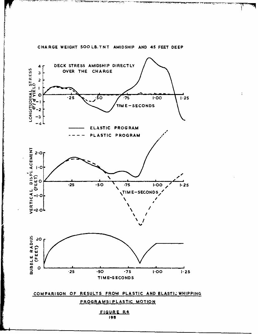
CHARGE WEIGHT 500 L8.TNT AMIDSHIP AND 45 FEET DEEP
4r DECK STRESS AMIDSHIP DIRECTLY
V) 3i OVER THE CHARGEw1- S2
So- EAT PROGR.A M•>-2•oZ~~ -3i•/ E-SECONDS
-0 3-4L
'-----ELASTIC PROG RAM
PLASTIC PROGRAM
• 25.0 7S1000I.2u .
1-0
wxU.
_j %0 \TIM E-SECOND S/-i.0
20 -
wo
t o
t 0 ---------,-IZ -25 .50 -75 1.00 1.-25
TI\MTE-SCECONDES
COMPARISON OF RESULTS FROM PLASTIC AND ELASTI.,-*WHIPPING
PR.OGRAMS: PLASTIC MOTION
19s

so 5-- 10 is 20 STERN,-r -- -
I-
w
5~ BOW
U.
0,
.8J
0
0
''PLASTIC SHEAR ANGLE > 1/20
SHIP PROFILES DURING PLASTIC HINGING
500 LB. TNT CHARGE 45 FEET DEEP BELOW SHIP CENTRELINE
- - COMPARATIVE PROFILES FOR PLASTIC AND ELASTIC WHIPPING
FIGURE R7a
199

IL'
-3*3.
..7CU-
0
-7 -
.99
SHIP PROFILES DURING ELASTIC MOTION
SOO LS.TN7 CHARGE 45 FEET BELOW SHIP CENTRELINE
COMPARATIVE PROF-ILES FOR PLASTIC AND ELASTIC WHIPPING
FIGURE Rib
200

Appendix
ADoroxiimate Analysis for Bilge Keel Effect
Consider a ship section as shown in Figure 1. The free surface
can be allowed for in the usual way (for whipping frequencies) by
considering the flow around the underwater section and its image
(the dotted .urve) in the free surface. Suppose that the potential Oo
is known for the flow around the section without the bilge keels. If
the length d of the bilge keel is very small compared to the
dimensions of the section then its presence will not greatly alter
the main flow and the new potential will be 0 = 00 + % wher: ob is
only significant close to the keel and is the disturbance potential
necessary to adjust the original flow to the flow around the keel.
In the original flow, without the keel, the fluid at the bilge
keel position nad the velocity
U 40=- U cos en an 0
away from the plating and the velocity
U as=- -=-•
tangential to it. The factor a (positive) can be found from the
known potenti.al 0o"
If the length of the bilge keel is small compared t- the local
radius of curvature of the section, the flow loca! to the bilge keel
attachment point will be almost like the flow past a flat plate as
in Figure 2. The motion of both water and plate normal to the plate
is ignored. It is clear that the relative velocity of the plate and
water is
V = U(aL + sin od
201

T•e necessary form of the disturbance potential j6b is then that for
t:ne flow along a wall with a projecting plate as in Figure 3, This
flow is identical to the flow normal to a flat plate of twice the
width anr is a well known flow. The added mass of a plate of width
2d is opd2 per unit length, so on the half pertinent to our problem
the normal force on the bilge keel will be approximately
Wd 2 ('. + sin o0) ;
This force is perpendicular to the keel so that, resolving verticallyg
the downward force on the section will be
Wod 2 (a. + sino ) sin U6 .
In the flow normal to a plate there is also a pressure distribution
induced along the centre line of the flow. In the problem of flow past a
plate on a wall,along the plate this pressure distribution will act on the wall
(ship bottom) and a component of this pressure distribution will be
vertical. However, neglecting Bernoulli pressures, as is customary
in added mass calculations, the positive pressures in front of the
plate will be compensated by negative pressures behind and there
will be no nett force, only a couple, on the ship bottom. Even the
couple is balanced overall by that from th- other bilge keel. The
plate normal force component can therefore be ignored.
The total downward force on the whole section (image ind uded)
due to the bilge keels will be four times that given above, so, if
C is the added mass coefficient for the section without keels and C'
the coefficient with the keels, it follows from the force equation
202
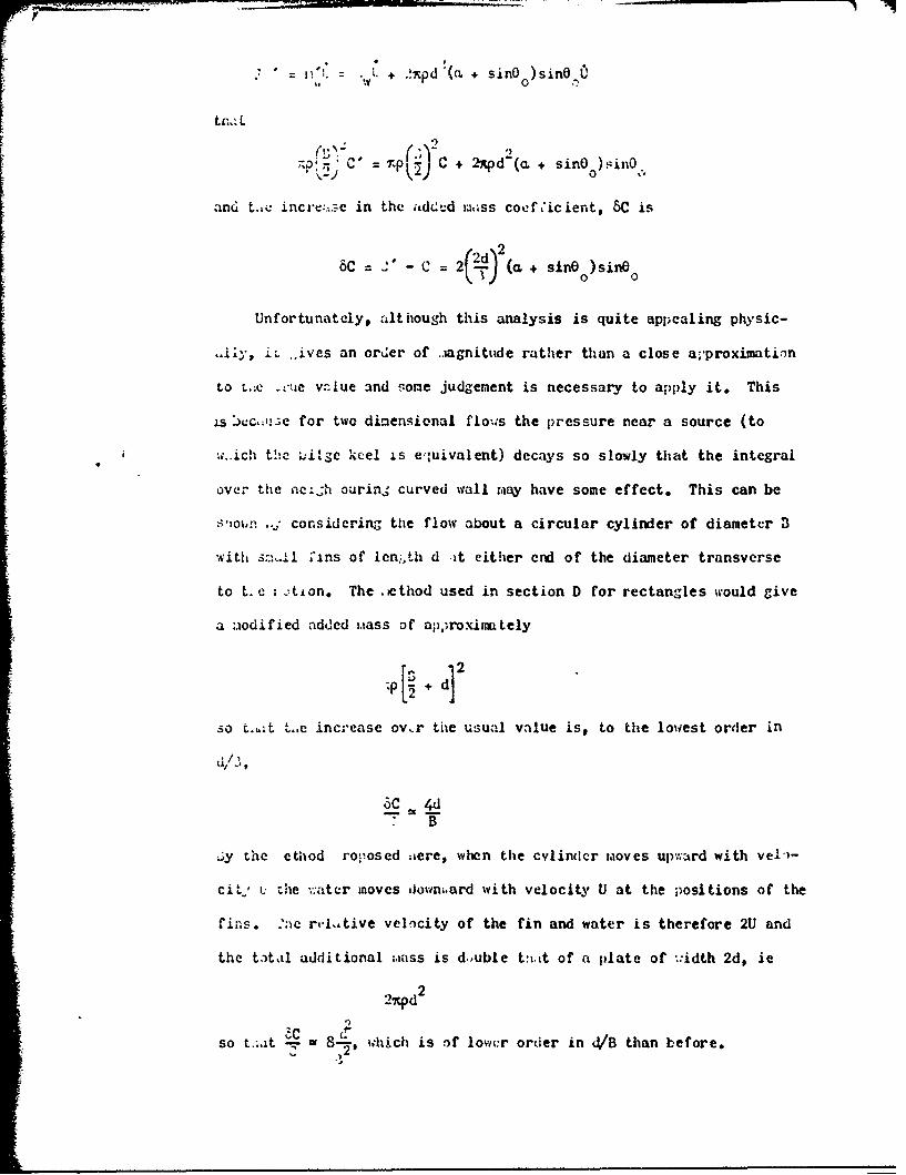
W= l. + .!xpd la, + sine
t C.. L0
"P" C-k~ i"• p• C + 2xpd'(a. + sineo)siniO,
and t.,u incre.-..3e in the ;idcud i:,ass coef,'icient, SC is
6C = 2- C = 2( ) + isnOe )sin0
Unfortunately, although this analysis is quite appealing physic-
,.i1y, i* .,ives an order of ..iagnitude rather than a close a;.proximati.n
to *.-e .'ue vclue and some judgenent is necessary to apply it. This
is , for two dinensional flows the pressure near a source (to
w-..ich the !iAle keel is e--uivalent) decays so slowly that the integral
over the nch ourinj curved wall rmiay have some effect. This can be
S• •,,, *.. considering the flow about a circular cylinder of diameter B
-with s..il 'ins of lcn:,th d .At either cnd of the diameter transverse
to t. a : ,tion. The .cthod used in section D for rectangles would give
a ;.iodified added mass of ap.yroximately
+ d] 2
so t.,,.t t.,c increase ovr the usual value is, to the lowest order in
L y the ethod rolposed aere, when the cylindcr maoves upw-ard with vel-)-
cit. L. the :.'ater moves doviný.ard with velocity U at the positions of the
fins. 'nc rl.,tive velocity of the fin and water is therefore 2U and
the ttal additional mass is d.,uble t:,tt of a plate of w:idth 2d, ie
2p•cd2
so t..It 31- 8-, hich is of lower order in J/B than before.-a
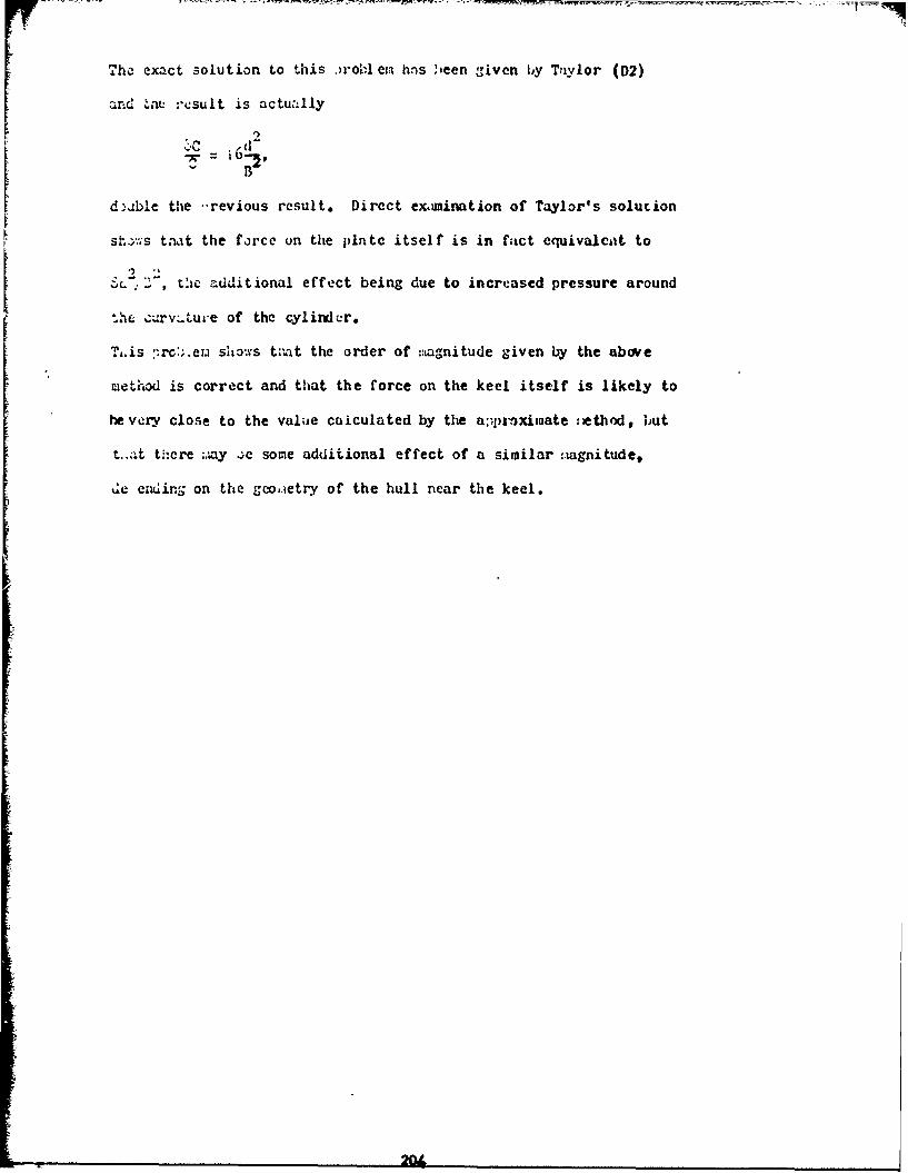
The exact solution to this ,rool eMi hns !,een given lby T'aylor (D2)
and Une :'csult is actuzally
-- = au-2 ,
B-
d.)-ble the 'revious result. Direct exmination of Taylor's solution
sh.',s tnat the force on the plate itself is in faict equivalcat to
Sc, ", t'ic additional effect being due to increased pressure around
"the zurw tIure of the qylinder.
LJS ""..c...em shows tfat the order of ::,agnitude given by the above
method is correct and that the force on the keel itself is likely to
hevery close to the value caiculated by the a;-pwxiimate iethod, but
t..at there :.my .ýc some additional effect of a similar :.iagnitude,
dc enuing on the gco~..etry of the hull near the keel.
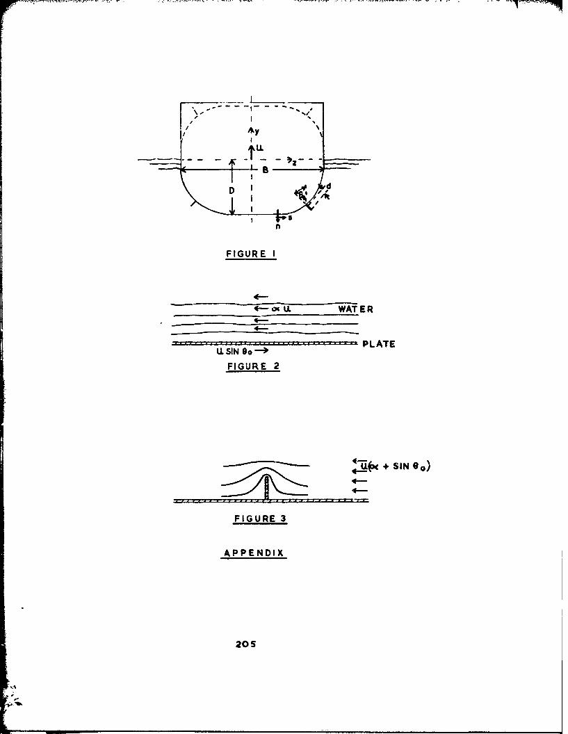
D ~ ,,
;L( ++, SI 9.
II
FIGURE I
4--<-- o+ U WAT:ER
4---
S.. .. .. .. ... .. .. .. ... .. .. .. PLATEU, SIN Oo '-'
FIGURE 2
---- -- -" -- • +,<+ SIN eo)
FIGURE 3
APPENDIX
205