replica wormholes and the entropy of hawking radiation
TRANSCRIPT
Replica Wormholes and the Entropy of Hawking Radiation
Ahmed Almheiri,1 Thomas Hartman,2 Juan Maldacena,1
Edgar Shaghoulian,2 and Amirhossein Tajdini2
1 Institute for Advanced Study, Princeton, New Jersey, USA
2 Department of Physics, Cornell University, Ithaca, New York, USA
Abstract
The information paradox can be realized in anti-de Sitter spacetime joined to a
Minkowski region. In this setting, we show that the large discrepancy between the von
Neumann entropy as calculated by Hawking and the requirements of unitarity is fixed
by including new saddles in the gravitational path integral. These saddles arise in the
replica method as complexified wormholes connecting different copies of the black hole.
As the replica number n → 1, the presence of these wormholes leads to the island rule
for the computation of the fine-grained gravitational entropy. We discuss these replica
wormholes explicitly in two-dimensional Jackiw-Teitelboim gravity coupled to matter.
arX
iv:1
911.
1233
3v2
[he
p-th
] 2
4 A
pr 2
020
Contents
1 Introduction 3
1.1 The island rule for computing gravitational von Neumann entropies . . . . . 5
1.2 Two dimensional eternal black holes and the information paradox . . . . . . . 6
1.3 Replica wormholes to the rescue . . . . . . . . . . . . . . . . . . . . . . . . . 8
2 The replica trick for the von Neumann entropy 12
2.1 The replicated action for n ∼ 1 becomes the generalized entropy . . . . . . . 13
2.2 The two dimensional JT gravity theory plus a CFT . . . . . . . . . . . . . . 15
3 Single interval at finite temperature 20
3.1 Geometry of the black hole . . . . . . . . . . . . . . . . . . . . . . . . . . . . 22
3.2 Quantum extremal surface . . . . . . . . . . . . . . . . . . . . . . . . . . . . . 22
3.3 Setting up the replica geometries . . . . . . . . . . . . . . . . . . . . . . . . . 23
3.4 Replica solution as n→ 1 . . . . . . . . . . . . . . . . . . . . . . . . . . . . . 25
3.5 Entropy . . . . . . . . . . . . . . . . . . . . . . . . . . . . . . . . . . . . . . . 27
3.6 High-temperature limit . . . . . . . . . . . . . . . . . . . . . . . . . . . . . . . 28
4 Single interval at zero temperature 29
4.1 Quantum extremal surface . . . . . . . . . . . . . . . . . . . . . . . . . . . . . 30
4.2 Replica wormholes at zero temperature . . . . . . . . . . . . . . . . . . . . . . 31
5 Two intervals in the eternal black hole 32
5.1 Review of the QES . . . . . . . . . . . . . . . . . . . . . . . . . . . . . . . . . 32
5.2 Replica wormholes . . . . . . . . . . . . . . . . . . . . . . . . . . . . . . . . . 34
5.3 Purity of the total state . . . . . . . . . . . . . . . . . . . . . . . . . . . . . . 35
6 Comments on reconstructing the interior 36
7 Discussion 38
A Derivation of the gravitational action 41
B Linearized solution to the welding problem 44
C The equation of motion in Lorentzian signature 46
2
1 Introduction
Hawking famously noted that the process of black hole formation and evaporation seems to
create entropy [1]. We can form a black hole from a pure state. The formation of the black
hole horizon leaves an inaccessible region behind, and the entanglement of quantum fields
across the horizon is responsible for the thermal nature of the Hawking radiation as well as
its growing entropy.
A useful diagnostic for information loss is the fine-grained (von Neumann) entropy of the
Hawking radiation, SR = −Tr ρR log ρR, where ρR is the density matrix of the radiation.
This entropy initially increases, because the Hawking radiation is entangled with its partners
in the black hole interior. But if the evaporation is unitary, then it must eventually fall back
to zero following the Page curve [2,3]. On the other hand, Hawking’s calculation predicts an
entropy that rises monotonically as the black hole evaporates.
Hawking’s computation of the entropy seems straightforward. It can be done far from
the black hole where the effects of quantum gravity are small, so it is unclear what could
have gone wrong. An answer to this puzzle was recently proposed [4–6] (see also [7–19]).
The proposal is that Hawking used the wrong formula for computing the entropy. As the
theory is coupled to gravity, we should use the proper gravitational formula for entropy: the
gravitational fine-grained entropy formula studied by Ryu and Takayanagi [20] and extended
in [21–23], also allowing for spatially disconnected regions, called “islands,” see figure 1. Even
though the radiation lives in a region where the gravitational effects are small, the fact that
we are describing a state in a theory of gravity implies that we should use the gravitational
formula for the entropy, including the island rule.
In this paper we consider a version of the information paradox formulated recently
in [4, 5] (see also [24]) where a black hole in anti-de Sitter spacetime radiates into an at-
tached Minkowski region. We show that the first principles computation of the fine-grained
entropy using the gravitational path integral description receives large corrections from non-
perturbative effects. The effects come from new saddles in the gravitational path integral —
replica wormholes — that dominate over the standard Euclidean black hole saddle, and lead
to a fine-grained entropy consistent with unitarity.
We will discuss the saddles explicitly only in some simple examples related to the in-
formation paradox for eternal black holes in two-dimensional Jackiw-Teitelboim (JT) grav-
ity [25–27], reviewed below, but we can nonetheless compute the effect on the fine-grained
entropy more generally. The same answer for the entropy was obtained holographically
in [6, 15,16]. Our goal is to provide a direct, bulk derivation without using holography.
3
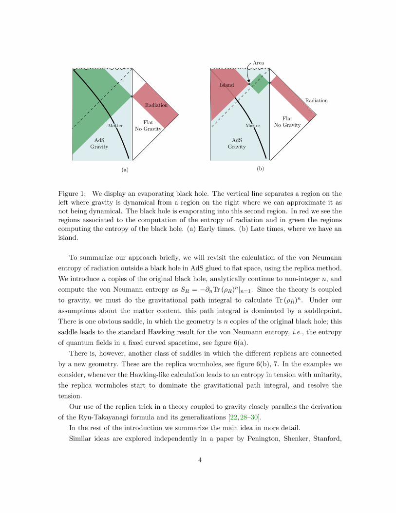
Figure 1: We display an evaporating black hole. The vertical line separates a region on theleft where gravity is dynamical from a region on the right where we can approximate it asnot being dynamical. The black hole is evaporating into this second region. In red we see theregions associated to the computation of the entropy of radiation and in green the regionscomputing the entropy of the black hole. (a) Early times. (b) Late times, where we have anisland.
To summarize our approach briefly, we will revisit the calculation of the von Neumann
entropy of radiation outside a black hole in AdS glued to flat space, using the replica method.
We introduce n copies of the original black hole, analytically continue to non-integer n, and
compute the von Neumann entropy as SR = −∂nTr (ρR)n|n=1. Since the theory is coupled
to gravity, we must do the gravitational path integral to calculate Tr (ρR)n. Under our
assumptions about the matter content, this path integral is dominated by a saddlepoint.
There is one obvious saddle, in which the geometry is n copies of the original black hole; this
saddle leads to the standard Hawking result for the von Neumann entropy, i.e., the entropy
of quantum fields in a fixed curved spacetime, see figure 6(a).
There is, however, another class of saddles in which the different replicas are connected
by a new geometry. These are the replica wormholes, see figure 6(b), 7. In the examples we
consider, whenever the Hawking-like calculation leads to an entropy in tension with unitarity,
the replica wormholes start to dominate the gravitational path integral, and resolve the
tension.
Our use of the replica trick in a theory coupled to gravity closely parallels the derivation
of the Ryu-Takayanagi formula and its generalizations [22,28–30].
In the rest of the introduction we summarize the main idea in more detail.
Similar ideas are explored independently in a paper by Penington, Shenker, Stanford,
4
and Yang [31].
1.1 The island rule for computing gravitational von Neumann entropies
We begin by reviewing the recent progress on the information paradox in AdS/CFT [4,5].
The classic information paradox is difficult to study in AdS/CFT, because large black
holes do not evaporate. Radiation bounces off the AdS boundary and falls back into the
black hole. For this reason, until recently, most discussions of the information paradox in
AdS/CFT have focused on exponentially small effects, such as the late-time behavior of
boundary correlation functions [32–35].
In contrast, the discrepancy in the Page curve is a large, O(1/GN ), effect. This classic
version of the information paradox can be embedded into AdS/CFT by coupling AdS to an
auxiliary system that absorbs the radiation, allowing the black hole to evaporate [4, 5] (see
also [7, 36, 37]). This is illustrated in fig. 1 in the case where the auxiliary system is half
of Minkowski space, glued to the boundary of AdS. There is no gravity in the Minkowski
region, where effectively GN → 0, but radiation into matter fields is allowed to pass through
the interface.
In this setup, the Page curve of the black hole was calculated in [4, 5]. It is important
to note that this calculation gives the Page curve of the black hole, not the radiation, which
is where the paradox lies; we return to this momentarily. The entropy of the black hole
is given by the generalized entropy of the quantum extremal surface (QES) [23], which is
a quantum-corrected Ryu-Takayanagi (or Hubeny-Rangamani-Takayanagi) surface [20, 21].
According to the QES proposal, the von Neumann entropy of the black hole is
SB = extQ
[Area(Q)
4GN+ Smatter(B)
](1.1)
where Q is the quantum extremal surface, and B is the region between Q and the AdS
boundary. Smatter denotes the von Neumann entropy of the quantum field theory (including
perturbative gravitons) calculated in the fixed background geometry. The extremization is
over the choice of surface Q. If there is more than one extremum, then Q is the surface with
minimal entropy. For dilaton gravity in AdS2, Q is a point, and its ‘area’ means the value of
the dilaton.
The black hole Page curve is the function SB(t), where t is the time on the AdS boundary
where B is anchored. It depends on time because the radiation can cross into the auxiliary
system. It behaves as expected: it grows at early times, then eventually falls back to zero [4,5].
A crucial element of this analysis is that at late times, the dominant quantum extremal surface
5
sits near the black hole horizon, as in fig. 1.
This does not resolve the Hawking paradox, which involves the radiation entropy Smatter(R),
where R is a region outside the black hole containing the radiation that has come out. Clearly
the problem is that neither R nor B includes the region I behind the horizon, called the is-
land, see figure 1. The state of the quantum fields on R ∪ B is apparently not pure, and,
apparently SR 6= SB. Only if we assume unitarity, or related holographic input such as
entanglement wedge reconstruction [4], can we claim that the QES computes the entropy of
the radiation. It does, however, tell us what to aim for in a unitary theory.
With this motivation, in [6], the evaporating black hole in Jackiw-Teitelboim (JT) gravity
in AdS2 was embedded into a holographic theory in one higher dimension. The AdS2 black
hole lives on a brane at the boundary of AdS3, similar to a Randall-Sundrum model [38,39],
with JT gravity on the brane (see also [10] for an analogous construction on an AdS4 boundary
of AdS5). In this setup, [6] derived the QES prescription for the radiation using AdS3
holography. It was found that the von Neumann entropy of the radiation in region R,
computed holographically in AdS3, agrees with the black hole entropy in (1.1). This led to
the conjecture that in a system coupled to gravity, the ordinary calculation of von Neumann
entropy should be supplemented by the contribution from “islands” according to the following
rule:
S(ρR) = extQ
[Area(Q)
4GN+ S(ρI∪R)
], (1.2)
up to subleading corrections. Here ρR is the density matrix of the region R in the full theory
coupled to quantum gravity, and ρI∪R is the density matrix of the state prepared via the
semi-classical path integral on the Euclidean black hole saddle. This is equal to (1.1), since
the quantum fields are pure on the full Cauchy slice I∪B∪R. Thus the tension with unitarity
is resolved within three-dimensional holography.
In this paper we explain how the surprising island rule (1.2) follows from the standard
rules for computing gravitational fine-grained entropy, without appealing to higher dimen-
sional holography.
1.2 Two dimensional eternal black holes and the information paradox
We consider an AdS2 JT gravity theory coupled to a 2d CFT. This CFT also lives in non-
gravitational Minkowski regions, and has transparent boundary conditions at the AdS bound-
ary. The dilaton goes to infinity at the AdS2 boundary so it is consistent to freeze gravity
on the outside [5,37]. We will assume that the matter CFT has a large central charge c 1,
but we will not assume that it is holographic, as all our calculations are done directly in
the 2d theory. For example it could be c free bosons. Taking the central charge large is to
6
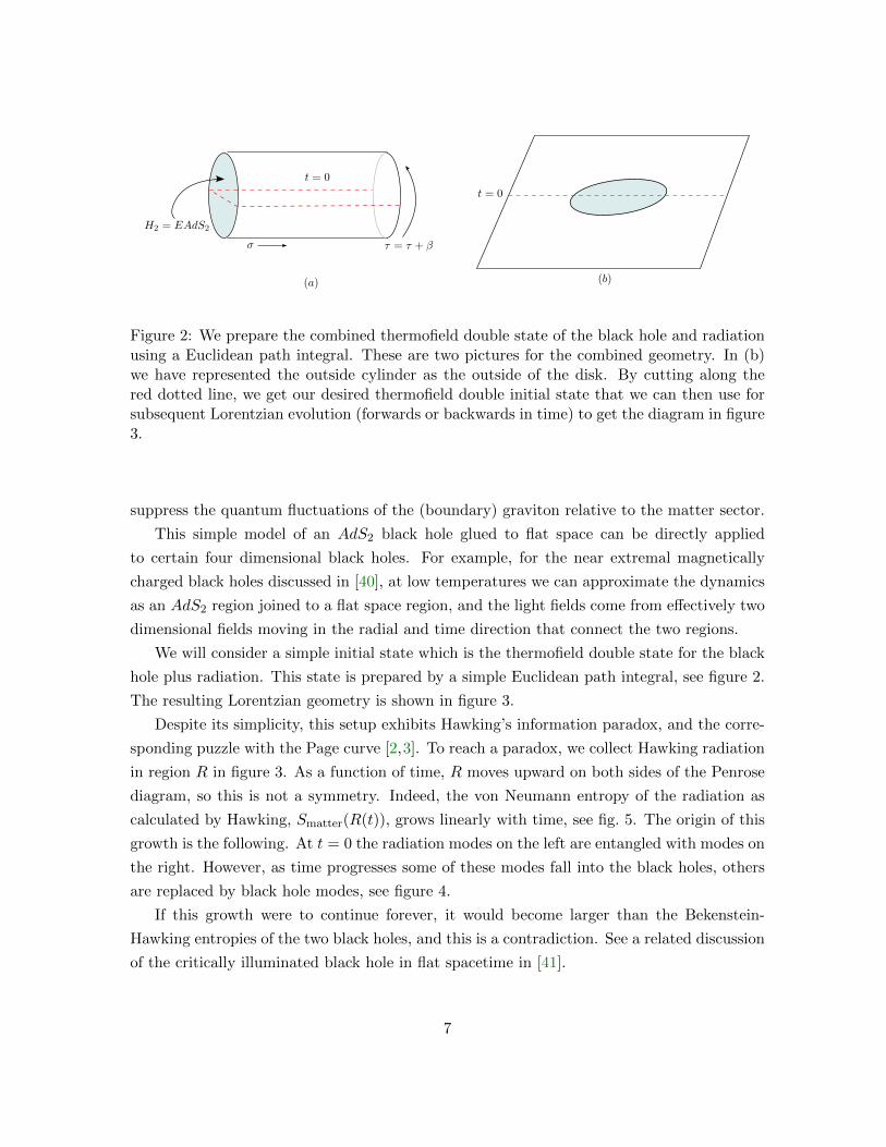
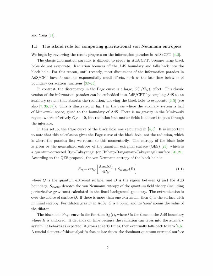
Figure 2: We prepare the combined thermofield double state of the black hole and radiationusing a Euclidean path integral. These are two pictures for the combined geometry. In (b)we have represented the outside cylinder as the outside of the disk. By cutting along thered dotted line, we get our desired thermofield double initial state that we can then use forsubsequent Lorentzian evolution (forwards or backwards in time) to get the diagram in figure3.
suppress the quantum fluctuations of the (boundary) graviton relative to the matter sector.
This simple model of an AdS2 black hole glued to flat space can be directly applied
to certain four dimensional black holes. For example, for the near extremal magnetically
charged black holes discussed in [40], at low temperatures we can approximate the dynamics
as an AdS2 region joined to a flat space region, and the light fields come from effectively two
dimensional fields moving in the radial and time direction that connect the two regions.
We will consider a simple initial state which is the thermofield double state for the black
hole plus radiation. This state is prepared by a simple Euclidean path integral, see figure 2.
The resulting Lorentzian geometry is shown in figure 3.
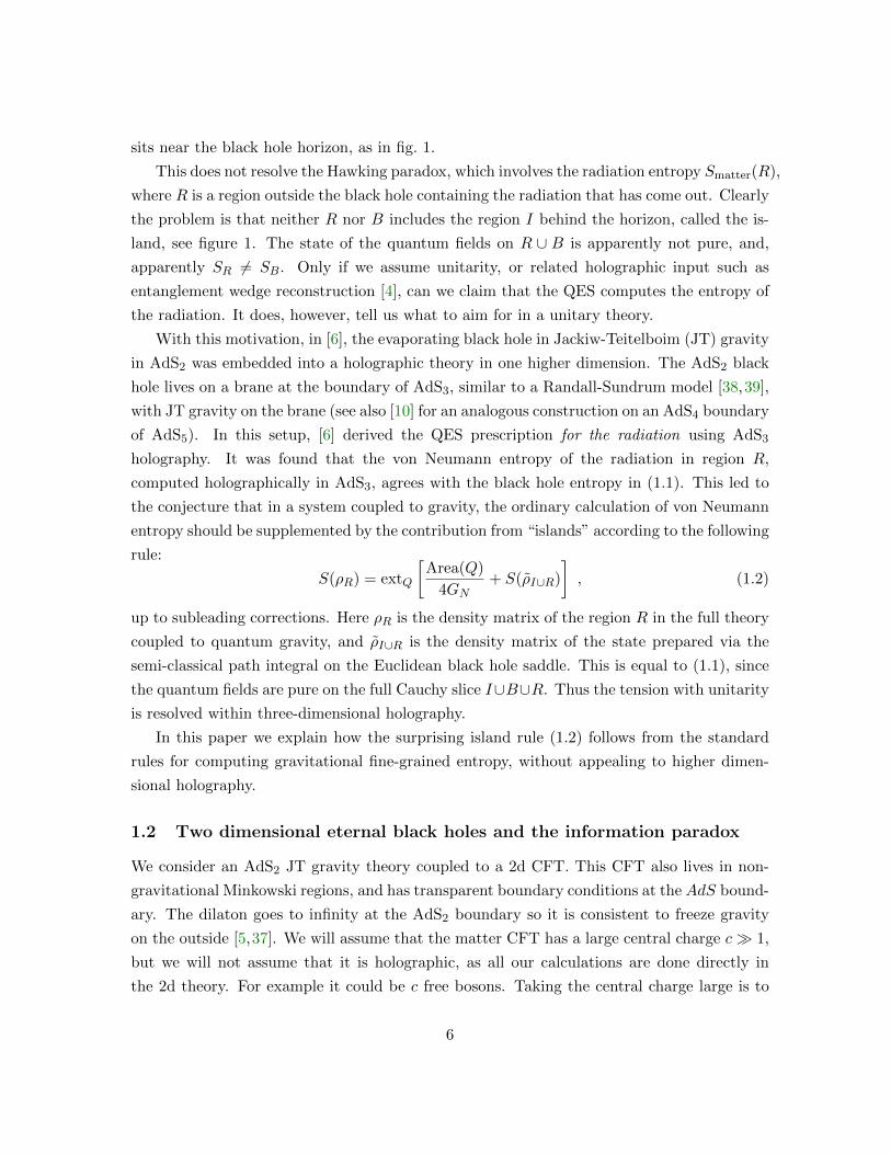
Despite its simplicity, this setup exhibits Hawking’s information paradox, and the corre-
sponding puzzle with the Page curve [2,3]. To reach a paradox, we collect Hawking radiation
in region R in figure 3. As a function of time, R moves upward on both sides of the Penrose
diagram, so this is not a symmetry. Indeed, the von Neumann entropy of the radiation as
calculated by Hawking, Smatter(R(t)), grows linearly with time, see fig. 5. The origin of this
growth is the following. At t = 0 the radiation modes on the left are entangled with modes on
the right. However, as time progresses some of these modes fall into the black holes, others
are replaced by black hole modes, see figure 4.
If this growth were to continue forever, it would become larger than the Bekenstein-
Hawking entropies of the two black holes, and this is a contradiction. See a related discussion
of the critically illuminated black hole in flat spacetime in [41].
7
Figure 3: Eternal black hole in AdS2, glued to Minkowski space on both sides. Hawkingradiation is collected in region R, which has two disjoint components. Region I is the island.The shaded region is coupled to JT gravity.
In a unitary theory, SR(t) should saturate at around the twice the Bekenstein-Hawking
entropy of each black hole, see figure 5. This was confirmed using the island rule in [14].
1.3 Replica wormholes to the rescue
To reproduce the unitary answer directly from a gravity calculation, we will use the replica
method to compute the von Neumann entropy of region R. The saddles relevant to the
unitary Page curve will ultimately be complex solutions of the gravitational equations. The
idea is to do Euclidean computations and then analytically continue to Lorentzian signature.
Consider n = 2 replicas. The replica partition function Tr (ρR)2 is computed by a Eu-
clidean path integral on two copies of the Euclidean system, with the matter sector sewed
together along the cuts on region R. Since we are doing a gravitational path integral, we do
not specify the geometry in the gravity region; we only fix the boundary conditions at the
edge. Gravity then fills in the geometry dynamically, see fig. 6.
We consider two different saddles with the correct boundary conditions. The first is
the Hawking saddle, see figure 6(a). The corresponding von Neumann entropy is the usual
answer, Smatter(R(t)), which grows linearly forever. The second is the replica wormhole,
which, as we will show, reproduces the entropy of the island rule, see figure 6(b). A replica
8
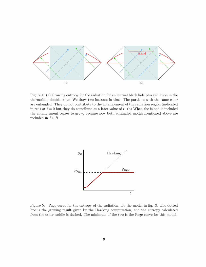
Figure 4: (a) Growing entropy for the radiation for an eternal black hole plus radiation in thethermofield double state. We draw two instants in time. The particles with the same colorare entangled. They do not contribute to the entanglement of the radiation region (indicatedin red) at t = 0 but they do contribute at a later value of t. (b) When the island is includedthe entanglement ceases to grow, because now both entangled modes mentioned above areincluded in I ∪R.
Figure 5: Page curve for the entropy of the radiation, for the model in fig. 3. The dottedline is the growing result given by the Hawking computation, and the entropy calculatedfrom the other saddle is dashed. The minimum of the two is the Page curve for this model.
9
(a) (b)
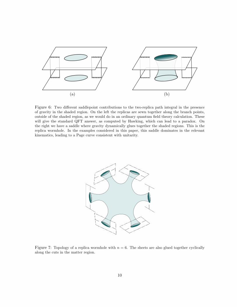
Figure 6: Two different saddlepoint contributions to the two-replica path integral in the presenceof gravity in the shaded region. On the left the replicas are sewn together along the branch points,outside of the shaded region, as we would do in an ordinary quantum field theory calculation. Thesewill give the standard QFT answer, as computed by Hawking, which can lead to a paradox. Onthe right we have a saddle where gravity dynamically glues together the shaded regions. This is thereplica wormhole. In the examples considered in this paper, this saddle dominates in the relevantkinematics, leading to a Page curve consistent with unitarity.
Figure 7: Topology of a replica wormhole with n = 6. The sheets are also glued together cyclicallyalong the cuts in the matter region.
10
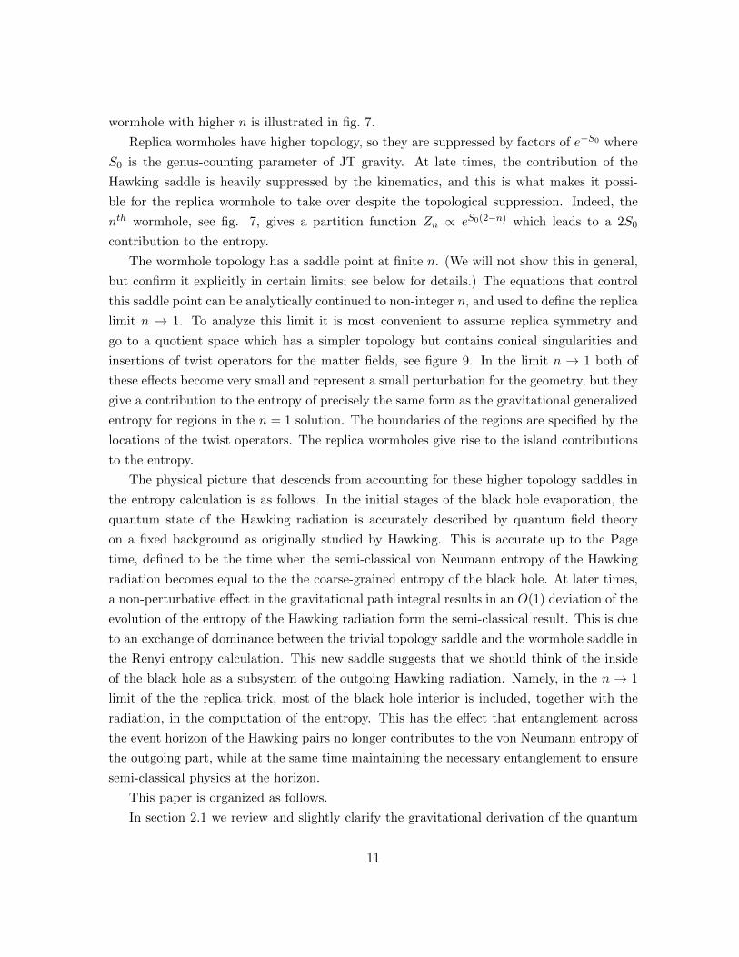
wormhole with higher n is illustrated in fig. 7.
Replica wormholes have higher topology, so they are suppressed by factors of e−S0 where
S0 is the genus-counting parameter of JT gravity. At late times, the contribution of the
Hawking saddle is heavily suppressed by the kinematics, and this is what makes it possi-
ble for the replica wormhole to take over despite the topological suppression. Indeed, the
nth wormhole, see fig. 7, gives a partition function Zn ∝ eS0(2−n) which leads to a 2S0
contribution to the entropy.
The wormhole topology has a saddle point at finite n. (We will not show this in general,
but confirm it explicitly in certain limits; see below for details.) The equations that control
this saddle point can be analytically continued to non-integer n, and used to define the replica
limit n → 1. To analyze this limit it is most convenient to assume replica symmetry and
go to a quotient space which has a simpler topology but contains conical singularities and
insertions of twist operators for the matter fields, see figure 9. In the limit n → 1 both of
these effects become very small and represent a small perturbation for the geometry, but they
give a contribution to the entropy of precisely the same form as the gravitational generalized
entropy for regions in the n = 1 solution. The boundaries of the regions are specified by the
locations of the twist operators. The replica wormholes give rise to the island contributions
to the entropy.
The physical picture that descends from accounting for these higher topology saddles in
the entropy calculation is as follows. In the initial stages of the black hole evaporation, the
quantum state of the Hawking radiation is accurately described by quantum field theory
on a fixed background as originally studied by Hawking. This is accurate up to the Page
time, defined to be the time when the semi-classical von Neumann entropy of the Hawking
radiation becomes equal to the the coarse-grained entropy of the black hole. At later times,
a non-perturbative effect in the gravitational path integral results in an O(1) deviation of the
evolution of the entropy of the Hawking radiation form the semi-classical result. This is due
to an exchange of dominance between the trivial topology saddle and the wormhole saddle in
the Renyi entropy calculation. This new saddle suggests that we should think of the inside
of the black hole as a subsystem of the outgoing Hawking radiation. Namely, in the n → 1
limit of the the replica trick, most of the black hole interior is included, together with the
radiation, in the computation of the entropy. This has the effect that entanglement across
the event horizon of the Hawking pairs no longer contributes to the von Neumann entropy of
the outgoing part, while at the same time maintaining the necessary entanglement to ensure
semi-classical physics at the horizon.
This paper is organized as follows.
In section 2.1 we review and slightly clarify the gravitational derivation of the quantum
11
extremal surface presciption from the replica trick in a general theory [22,28–30]. The slight
improvement is that we show that the off shell action near n ∼ 1 becomes the generalized
entropy, so that the extremality condition follows directly from the extremization of the
action. In section 2.2 we discuss some general aspects of replica manifolds for the case of JT
gravity plus a CFT.
In section 3 we discuss the computation of the entropy for an interval that contains the
degrees of freedom living at the AdS boundary. In this case the quantum extremal surface
is slightly outside the horizon. We set up the discussion of the Renyi entropy computations
for this case. We reduce the problem to an integro-differential equation for a single function
θ(τ) that relates the physical time τ to the AdS time θ. We solve this equation for n → 1
recovering the quantum extremal surface result. We also solve the problem for relatively
high temperatures but for any n.
In section 4 we discuss the special case of the zero temperature limit, and we comment
on some features of the island in that case.
In section 5 we discuss aspects of the two intervals case, which is the one most relevant
for the information problem for the eternal black hole.
In section 6 we make the connection to entanglement wedge reconstruction of the black
hole interior.
We end in section 7 with conclusions and discussion.
2 The replica trick for the von Neumann entropy
The replica trick for computing the von Neumann entropy is based on the observation that
the computation of Tr[ρn] can be viewed as an observable in n copies of the original system
[42]. In particular, for a quantum field theory the von Neumann entropy of some region
can be computed by considering n copies of the original theory and choosing boundary
conditions that connect the various copies inside the interval in a cyclic way, see e.g. [43]
for a review. This can be viewed as the insertion of a “twist operator” in the quantum
field theory containing n copies of the original system. This unnormalized correlator of
twist operators can also be viewed as the partition function of the theory on a topologically
non-trivial manifold, Zn = Z[Mn] = 〈T1 · · · Tk〉. Then the entropy can be computed by
analytically continuing in n and setting
S = − ∂n(
logZnn
)∣∣∣∣n=1
(2.1)
12
We will now review the argument for how this is computed in theories of gravity. Then we
will consider the specific case of the JT gravity theory.
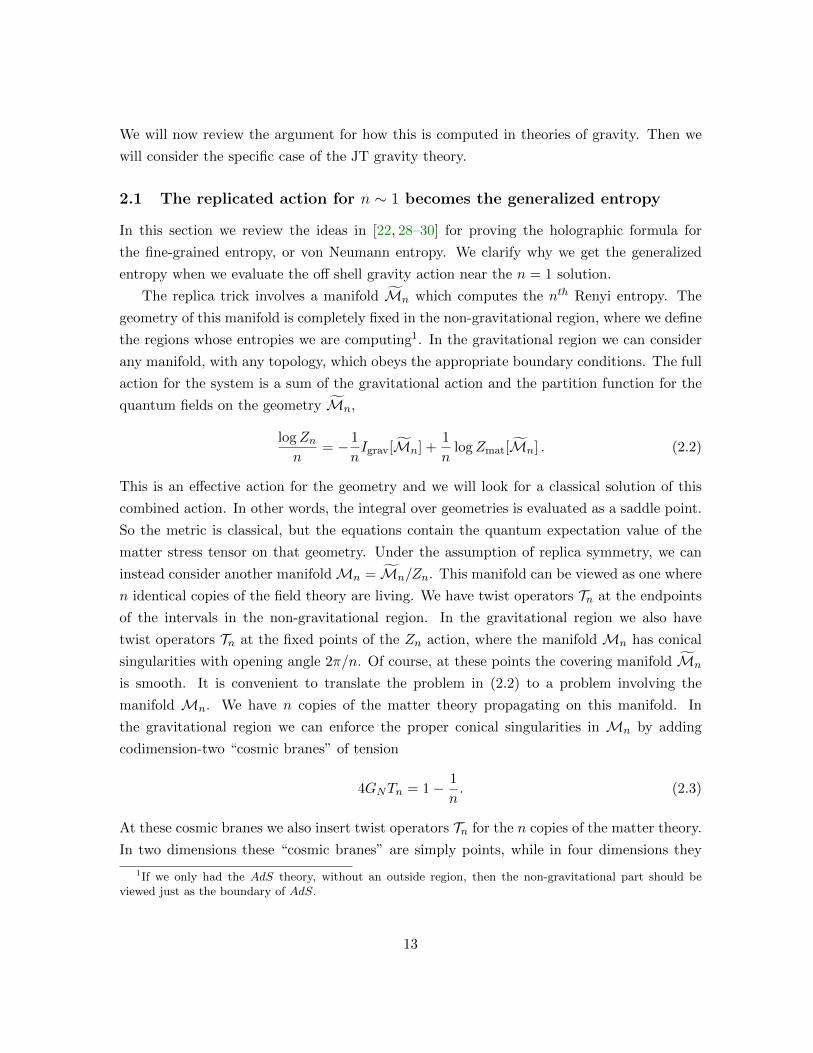
2.1 The replicated action for n ∼ 1 becomes the generalized entropy
In this section we review the ideas in [22, 28–30] for proving the holographic formula for
the fine-grained entropy, or von Neumann entropy. We clarify why we get the generalized
entropy when we evaluate the off shell gravity action near the n = 1 solution.
The replica trick involves a manifold Mn which computes the nth Renyi entropy. The
geometry of this manifold is completely fixed in the non-gravitational region, where we define
the regions whose entropies we are computing1. In the gravitational region we can consider
any manifold, with any topology, which obeys the appropriate boundary conditions. The full
action for the system is a sum of the gravitational action and the partition function for the
quantum fields on the geometry Mn,
logZnn
= − 1
nIgrav[Mn] +
1
nlogZmat[Mn] . (2.2)
This is an effective action for the geometry and we will look for a classical solution of this
combined action. In other words, the integral over geometries is evaluated as a saddle point.
So the metric is classical, but the equations contain the quantum expectation value of the
matter stress tensor on that geometry. Under the assumption of replica symmetry, we can
instead consider another manifoldMn = Mn/Zn. This manifold can be viewed as one where
n identical copies of the field theory are living. We have twist operators Tn at the endpoints
of the intervals in the non-gravitational region. In the gravitational region we also have
twist operators Tn at the fixed points of the Zn action, where the manifold Mn has conical
singularities with opening angle 2π/n. Of course, at these points the covering manifold Mn
is smooth. It is convenient to translate the problem in (2.2) to a problem involving the
manifold Mn. We have n copies of the matter theory propagating on this manifold. In
the gravitational region we can enforce the proper conical singularities in Mn by adding
codimension-two “cosmic branes” of tension
4GNTn = 1− 1
n. (2.3)
At these cosmic branes we also insert twist operators Tn for the n copies of the matter theory.
In two dimensions these “cosmic branes” are simply points, while in four dimensions they
1If we only had the AdS theory, without an outside region, then the non-gravitational part should beviewed just as the boundary of AdS.
13
are “cosmic strings.” The positions of these cosmic branes are fixed by solving the Einstein
equations. We then replace the gravitational part of the action in (2.2) by
1
nIgrav[Mn] = Igrav[Mn] + Tn
∫Σd−2
√g. (2.4)
As opposed to [28], here we add the action of these cosmic branes explicity and we also
integrate the Einstein term through the singularity, which includes a δ function for the
curvature. These two extra terms cancel out so that we get the same final answer as in
[28] where no contribution from the singularity was included. We will see that the present
prescription is more convenient2.
In the part of the manifold where the metric is dynamical the position of these cosmic
branes is fixed by the Einstein equations. Also, the reparametrization symmetry implies we
cannot fix these points from the outside.
When n = 1 we have the manifold M1 = M1, which is the original solution to the
problem. It is a solution of the action Itot1 . In order to find the manifold Mn for n ∼ 1 we
need to add the cosmic branes. Then the action is(Itot
n
)n→1
= I1 + δ
(I
n
)(2.5)
where δI contains extra terms that arise from two effects, both of which are of order n− 1.
The first comes from the tension of the cosmic brane (the second term in (2.4). The second
comes from the insertion of the twist fields at the position of this cosmic brane. To evaluate
the action perturbatively, we start from the solutionM1, we add the cosmic brane and twist
fields, and we also consider a small deformation of the geometry away from M1, where all
these effects are of order n− 1. Because theM1 geometry is a solution of the original action
I1 in (2.5), any small deformation of the geometry drops out of the action. For the extra
term δ(I/n) in (2.5), we can consider the cosmic brane action and twist fields as living on
the old geometry M1 since these extra terms are already of order n− 1.
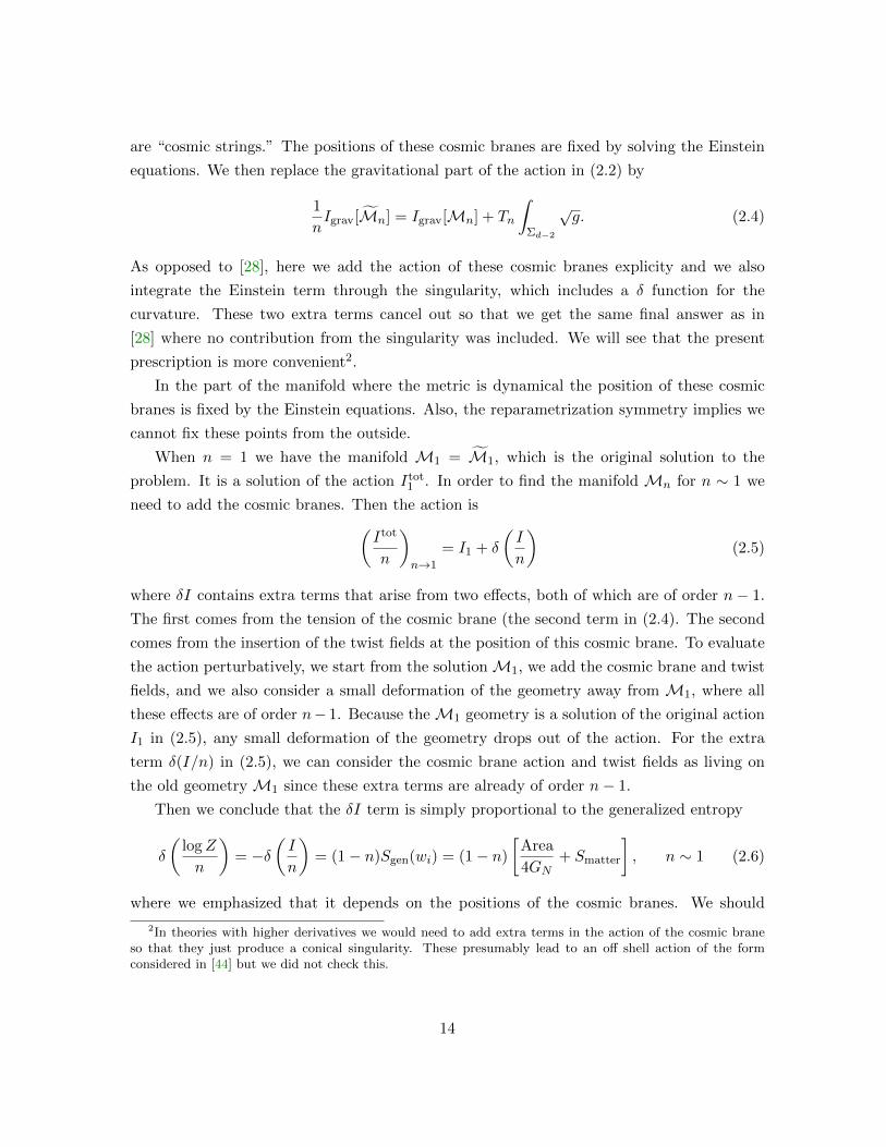
Then we conclude that the δI term is simply proportional to the generalized entropy
δ
(logZ
n
)= −δ
(I
n
)= (1− n)Sgen(wi) = (1− n)
[Area
4GN+ Smatter
], n ∼ 1 (2.6)
where we emphasized that it depends on the positions of the cosmic branes. We should
2In theories with higher derivatives we would need to add extra terms in the action of the cosmic braneso that they just produce a conical singularity. These presumably lead to an off shell action of the formconsidered in [44] but we did not check this.
14
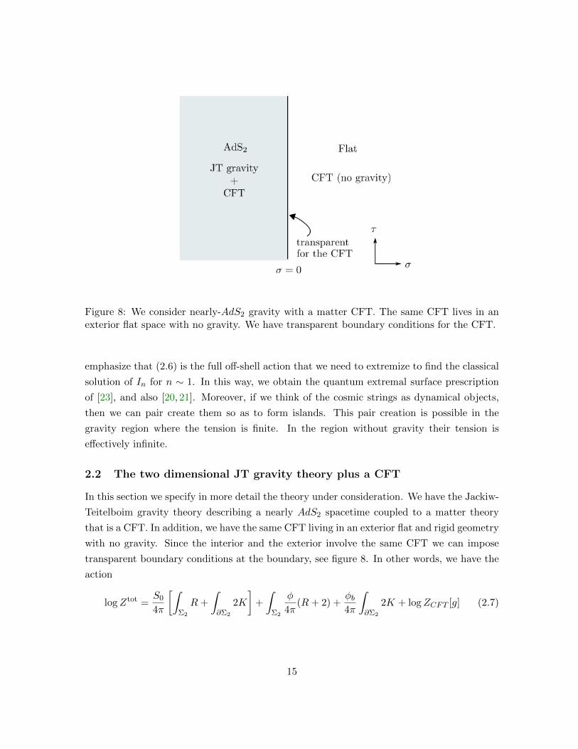
Figure 8: We consider nearly-AdS2 gravity with a matter CFT. The same CFT lives in anexterior flat space with no gravity. We have transparent boundary conditions for the CFT.
emphasize that (2.6) is the full off-shell action that we need to extremize to find the classical
solution of In for n ∼ 1. In this way, we obtain the quantum extremal surface prescription
of [23], and also [20, 21]. Moreover, if we think of the cosmic strings as dynamical objects,
then we can pair create them so as to form islands. This pair creation is possible in the
gravity region where the tension is finite. In the region without gravity their tension is
effectively infinite.
2.2 The two dimensional JT gravity theory plus a CFT
In this section we specify in more detail the theory under consideration. We have the Jackiw-
Teitelboim gravity theory describing a nearly AdS2 spacetime coupled to a matter theory
that is a CFT. In addition, we have the same CFT living in an exterior flat and rigid geometry
with no gravity. Since the interior and the exterior involve the same CFT we can impose
transparent boundary conditions at the boundary, see figure 8. In other words, we have the
action
logZtot =S0
4π
[∫Σ2
R+
∫∂Σ2
2K
]+
∫Σ2
φ
4π(R+ 2) +
φb4π
∫∂Σ2
2K + logZCFT [g] (2.7)
15
where the CFT action is defined over a geometry which is rigid in the exterior region and
is dynamical in the interior region. We are setting 4GN = 1 so that the area terms in the
entropies will be just given by the value of φ, Area4GN
= S0 + φ.
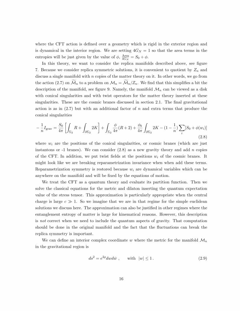
In this theory, we want to consider the replica manifolds described above, see figure
7. Because we consider replica symmetric solutions, it is convenient to quotient by Zn and
discuss a single manifold with n copies of the matter theory on it. In other words, we go from
the action (2.7) on Mn to a problem onMn = Mn/Zn. We find that this simplifies a bit the
description of the manifold, see figure 9. Namely, the manifold Mn can be viewed as a disk
with conical singularities and with twist operators for the matter theory inserted at these
singularities. These are the cosmic branes discussed in section 2.1. The final gravitational
action is as in (2.7) but with an additional factor of n and extra terms that produce the
conical singularities
− 1
nIgrav =
S0
4π
[∫Σ2
R+
∫∂Σ2
2K
]+
∫Σ2
φ
4π(R+ 2) +
φb4π
∫∂Σ2
2K − (1− 1
n)∑i
[S0 + φ(wi)]
(2.8)
where wi are the positions of the conical singularities, or cosmic branes (which are just
instantons or -1 branes). We can consider (2.8) as a new gravity theory and add n copies
of the CFT. In addition, we put twist fields at the positions wi of the cosmic branes. It
might look like we are breaking reparametrization invariance when when add these terms.
Reparametrization symmetry is restored because wi are dynamical variables which can be
anywhere on the manifold and will be fixed by the equations of motion.
We treat the CFT as a quantum theory and evaluate its partition function. Then we
solve the classical equations for the metric and dilaton inserting the quantum expectation
value of the stress tensor. This approximation is particularly appropriate when the central
charge is large c 1. So we imagine that we are in that regime for the simple euclidean
solutions we discuss here. The approximation can also be justified in other regimes where the
entanglement entropy of matter is large for kinematical reasons. However, this description
is not correct when we need to include the quantum aspects of gravity. That computation
should be done in the original manifold and the fact that the fluctuations can break the
replica symmetry is important.
We can define an interior complex coordinate w where the metric for the manifold Mn
in the gravitational region is
ds2 = e2ρdwdw , with |w| ≤ 1 . (2.9)
16
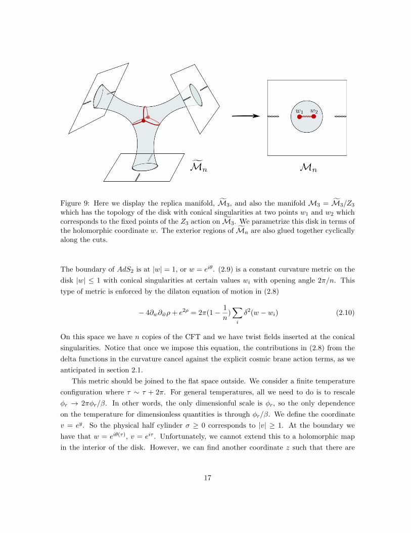
Figure 9: Here we display the replica manifold, M3, and also the manifold M3 = M3/Z3
which has the topology of the disk with conical singularities at two points w1 and w2 whichcorresponds to the fixed points of the Z3 action on M3. We parametrize this disk in terms ofthe holomorphic coordinate w. The exterior regions of Mn are also glued together cyclicallyalong the cuts.
The boundary of AdS2 is at |w| = 1, or w = eiθ. (2.9) is a constant curvature metric on the
disk |w| ≤ 1 with conical singularities at certain values wi with opening angle 2π/n. This
type of metric is enforced by the dilaton equation of motion in (2.8)
− 4∂w∂wρ+ e2ρ = 2π(1− 1
n)∑i
δ2(w − wi) (2.10)
On this space we have n copies of the CFT and we have twist fields inserted at the conical
singularities. Notice that once we impose this equation, the contributions in (2.8) from the
delta functions in the curvature cancel against the explicit cosmic brane action terms, as we
anticipated in section 2.1.
This metric should be joined to the flat space outside. We consider a finite temperature
configuration where τ ∼ τ + 2π. For general temperatures, all we need to do is to rescale
φr → 2πφr/β. In other words, the only dimensionful scale is φr, so the only dependence
on the temperature for dimensionless quantities is through φr/β. We define the coordinate
v = ey. So the physical half cylinder σ ≥ 0 corresponds to |v| ≥ 1. At the boundary we
have that w = eiθ(τ), v = eiτ . Unfortunately, we cannot extend this to a holomorphic map
in the interior of the disk. However, we can find another coordinate z such that there are
17
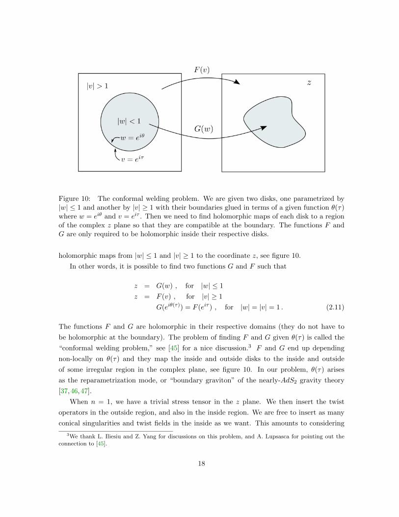
Figure 10: The conformal welding problem. We are given two disks, one parametrized by|w| ≤ 1 and another by |v| ≥ 1 with their boundaries glued in terms of a given function θ(τ)where w = eiθ and v = eiτ . Then we need to find holomorphic maps of each disk to a regionof the complex z plane so that they are compatible at the boundary. The functions F andG are only required to be holomorphic inside their respective disks.
holomorphic maps from |w| ≤ 1 and |v| ≥ 1 to the coordinate z, see figure 10.
In other words, it is possible to find two functions G and F such that
z = G(w) , for |w| ≤ 1
z = F (v) , for |v| ≥ 1
G(eiθ(τ)) = F (eiτ ) , for |w| = |v| = 1 . (2.11)
The functions F and G are holomorphic in their respective domains (they do not have to
be holomorphic at the boundary). The problem of finding F and G given θ(τ) is called the
“conformal welding problem,” see [45] for a nice discussion.3 F and G end up depending
non-locally on θ(τ) and they map the inside and outside disks to the inside and outside
of some irregular region in the complex plane, see figure 10. In our problem, θ(τ) arises
as the reparametrization mode, or “boundary graviton” of the nearly-AdS2 gravity theory
[37,46,47].
When n = 1, we have a trivial stress tensor in the z plane. We then insert the twist
operators in the outside region, and also in the inside region. We are free to insert as many
conical singularities and twist fields in the inside as we want. This amounts to considering
3We thank L. Iliesiu and Z. Yang for discussions on this problem, and A. Lupsasca for pointing out theconnection to [45].
18
various numbers of islands in the gravity region. We will only discuss cases with one or two
inside insertions in the subsequent sections. This gives us a non-trivial stress tensor Tzz(z)
and Tzz(z). We can then compute the physical stress tensor that will appear in the equation
of motion using the conformal anomaly,
Tyy =
(dF (eiy)
dy
)2
Tzz −c
24πF (eiy), y (2.12)
and a similar expression for Tyy. The expression for the physical stress tensor in the w plane
involves the function G and also a conformal anomaly contribution from ρ in the metric (2.9).
Let us now turn to the problem of writing the equations of motion for the boundary
reparametrization mode. Naively we are tempted to write the action just as eiθ, τ. This
would be correct if there were no conical singularities in the interior. However, the presence
of those conical singularities implies that the metric (2.9) has small deviations compared to
the metric of a standard hyperbolic disk
ds2 = e2ρdwdw , e2ρ =4
(1− |w|2)2e2δρ (2.13)
where δρ goes as
δρ ∼ −(1− |w|)2
3U(θ) , as |w| → 1 . (2.14)
The function U depends on the positions of the conical singularities and therefore also on
the moduli of the Riemann surface. This then implies that the Schwarzian term, and the full
equation of motion can now be written as
φr2π
d
dτ
[eiθ, τ+ U(θ)θ′
2]
= i(Tyy − Tyy) = Tτσ . (2.15)
The term in brackets is proportional to the energy. This equation relates the change in energy
to the energy flux from the flat space region. Here the flux of energy on the right hand side
is that of one copy, or the flux of the n copies divided by n. The action can be derived from
the extrinsic curvature term in the same way that was discussed in [37,46,47], see appendix
A, where we also discuss the explicit derivation of the equation of motion (2.15).
There are also equations that result from varying the moduli of the Riemann surface, or
the positions of the conical singularities. They have the form
− (1− 1
n)∂wφ(wi) + ∂wi
(logZmat
n
n
)= 0 , (2.16)
19
where we used that the wi dependence of the gravitational part of the action comes only
from the last term in (2.8).
In the n→ 1 limit we can replace the n = 1 value for the dilaton in (2.16). Similarly the
value of logZmatn /n near n = 1 involves the matter entropy. Therefore (2.16) reduces to the
condition on the extremization of the generalized entropy, as we discussed in general above.
For general n, we need to compute the dilaton by solving its equations of motion in order
to write (2.16). This can be done using the expression for the stress tensor in the interior of
the disk. We have not attempted to simplify it further. However, we should note that for
the particular case of one interval, discussed in section 3, there is only one point and there
are no moduli for the Riemann surface. Therefore this equation is redundant and in fact, it
is contained in (2.15) as will be discussed in section 3.
Next we apply this general discussion to the calculation of the entropy of various sub-
regions of the flat space CFT. The goal is to understand how configurations of the gravity
region contribute to the entropy of those CFT regions.
3 Single interval at finite temperature
We begin with the simple case of a single interval that contains one of the AdS2 boundaries,
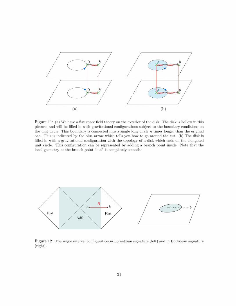
as shown in figure 11(a). This is the interval B ≡ [0, b].
To compute the entropy of this region we must consider the Euclidean path integral
that evaluates the trace of powers of the density matrix Tr[ρnB]. This is given by the path
integral on n copies of the theory identified across the region B, as shown in figure 11. The
crucial point is that the presence of the branch point on the unit circle, which is where the
asymptotic AdS boundary lives, elongates this circle by a factor of n. The Euclidean gravity
configurations we must consider are all smooth manifolds with a single boundary that is
identified with this elongated AdS boundary.
The simplest configuration to consider will be that with the topology of a disk. All other
higher genus manifolds will be subleading since each extra handle will come with a cost of
e−S0 . Filling out the gravity region has the effect of extending the identification across the
different sheets into the gravity region, which ends on some point “−a” in figure 11. The
location of the point “−a” will be dynamically determined by the saddle point of the path
integral.
We will now construct replica wormholes explicitly for a single interval in the eternal
black hole in AdS2. The Lorentzian and Euclidean geometries are shown in figure 12. We
20
(a) (b)
Figure 11: (a) We have a flat space field theory on the exterior of the disk. The disk is hollow in thispicture, and will be filled in with gravitational configurations subject to the boundary conditions onthe unit circle. This boundary is connected into a single long circle n times longer than the originalone. This is indicated by the blue arrow which tells you how to go around the cut. (b) The disk isfilled in with a gravitational configuration with the topology of a disk which ends on the elongatedunit circle. This configuration can be represented by adding a branch point inside. Note that thelocal geometry at the branch point “−a” is completely smooth.
Figure 12: The single interval configuration in Lorentzian signature (left) and in Euclidean signature(right).
21
will first review of the result of the QES calculation [14], then proceed to derive it from
replica wormholes.
3.1 Geometry of the black hole
The metric of eternal black hole, glued to flat space on both sides, is
ds2in =
4π2
β2
dydy
sinh2 πβ (y + y)
, ds2out =
1
ε2dydy , (3.1)
y = σ + iτ, y = σ − iτ , τ = τ + β . (3.2)
The subscript ‘in’ refers to the gravity zone, and ‘out’ refers to the matter zone4. The
interface is along the circle σ = −ε. Lorenztian time t is τ = −it. The welding maps of figure
10 are trivial and we have
z = v = w = e2πy/β , y =β
2πlogw . (3.4)
The Euclidean solution is therefore the w-plane with gravity inside the unit disk, |w| < 1− 2πεβ .
The metric is
ds2in =
4dwdw
(1− |w|2)2, ds2
out =β2
4π2ε2dwdw
|w|2. (3.5)
The dilaton, which is defined only on the inside region, is rotationally invariant on the w-
plane,
φ =2πφrβ
1 + |w|2
1− |w|2= −2πφr
β
1
tanh 2πσβ
. (3.6)
with φ = φr/ε at the boundary. In what follows, we will usually set ε = 0, and rescale the
exterior coordinate by ε so that ds2out = dydy.
3.2 Quantum extremal surface
We now review the computation of the entropy of the region B = [0, b] which includes the
AdS2 boundary, see figure 11. In gravity this will involve an interval [−a, b], with a, b > 0,
see figure 12.
4The Poincare coordinates are x = tanh πyβ
, ds2in = 4dxdx/(x+ x)2. The Schwarzschild coordinates are
y =β
2πlog
r√r(r + 4π/β)
+ iτ , ds2in = r(r +4π
β)dτ2 +
dr2
r(r + 4πβ
). (3.3)
22
The generalized entropy of the region [−a, b] is
Sgen = S0 + φ(−a) + SCFT([−a, b]) . (3.7)
The entanglement entropy of a CFT on the interval [w1, w2] in the metric ds2 = Ω−2dwdw is
SCFT(w1, w2) =c
6log
(|w1 − w2|2
ε1,UV ε2,UV Ω(w1, w1)Ω(w2, w2)
). (3.8)
Using the map w = e2πy/β and the conformal factors in (3.5) this becomes
SCFT([−a, b]) =c
6log
2β sinh2(πβ (a+ b)
)εa,UV εb,UV π sinh
(2πaβ
) (3.9)
Then, using the dilaton in (3.6), (3.7) becomes
Sgen([−a, b]) = S0 +2πφrβ
1
tanh(
2πaβ
) +c
6log
2β sinh2(πβ (a+ b)
)πε sinh
(2πaβ
) . (3.10)
The UV divergence εa,UV was absorbed into S0 and we dropped the outside one at point b.
The quantum extremal surface is defined by extremizing Sgen over a
∂aSgen = 0 → sinh
(2πa
β
)=
12πφrβc
sinh(πβ (b+ a)
)sinh
(πβ (a− b)
) (3.11)
This is a cubic equation for e2πa/β. For b & β2π and φr/(βc) & 1, the solution is
a ≈ b+β
2πlog
(24πφrβc
), or e
− 2πaβ ≈ βc
24πφre− 2πb
β (3.12)
Since we’ve restricted to one side of the black hole in this calculation, the configuration is
invariant under translations in the Schwarzschild t direction. Therefore the general extremal
surface at t 6= 0 is related by a time translation; for an interval that starts at tb and σb = b,
the other endpoint is at ta = tb and σa = −a, with a as in (3.11).
3.3 Setting up the replica geometries
We will do the replica calculation in Euclidean signature, with a, b real. We set β = 2π, and
reintroduce it later by dimensional analysis.
23
The replica wormhole that we seek is an n-fold cover of the Euclidean black hole, branched
at the points a and b, see figure (12). This manifold will have a nontrivial gluing at the unit
circle (unlike the black hole itself), so it is more convenient to introduce different coordinates
on the inside and outside. We use w, with |w| < 1, for the inside and v = ey, with |v| > 1
for the outside. The gluing function is θ(τ), with w = eiθ, v = eiτ , as in (2.11). We write
the branch points as
w = A = e−a , v = B = eb . (3.13)
The Schwarzian equation is simplest in a different coordinate,
w =
(w −A1−Aw
)1/n
. (3.14)
This coordinate uniformizes n copies of the unit disk, so here we have the standard hyperbolic
metric,
ds2in =
4|dw|2
(1− |w|2)2. (3.15)
Defining w = eiθ at the boundary, the Schwarzian equation is
φr2π∂τeiθ, τ = i(Tyy(iτ)− Tyy(−iτ)) . (3.16)
We can now return to the w-disk using the Schwarzian composition identity
eiθ, τ = eiθ, τ+1
2
(1− 1
n2
)R(θ) , (3.17)
with
R(θ) = −(1−A2)2(∂τθ)2
|1−Aeiθ|4. (3.18)
This puts the equation of motion (3.16) into exactly the form of equation (2.15), which
we have just derived by a slightly different route. In appendix A we show that they are
equivalent.
The stress tensor appearing on the right-hand side of (3.16) is obtained through the
conformal welding. That is, we define the z coordinate by the map G on the inside and F on
the outside as in (2.11). These maps each have an ambiguity under SL(2, C) transformations
of z, which we may use to map the twist operator at w = A to z = 0, and the twist operator
at v = B to z =∞. We further discuss the symmetries of the conformal welding problem in
appendix B.
The z-coordinate covers the full plane holomorphically. It has twist points at the origin
24
and at infinity, which can be removed by the standard mapping, z = z1/n. On the z plane,
the stress tensor vanishes, so on the z-plane,
Tzz(z) = − c
24πz1/n, z = − c
48π
(1− 1
n2
)1
z2. (3.19)
Finally the stress tensor Tyy comes from inverting the conformal welding map to return to
the v-plane, and using v = ey:
Tyy(y) = e2y[F ′(v)2Tzz −
c
24πF, v
]− 1
2. (3.20)
Putting it all together, the equation of motion (3.16) is
24πφrcβ
∂τ
[eiθ(τ), τ+
1
2(1− 1
n2)R(θ(τ))
]= ie2iτ
[−1
2(1− 1
n2)F ′(eiτ )2
F (eiτ )2− F, eiτ
]+ cc
(3.21)
This equation originated on the smooth replica manifold Mn, but has now been written
entirely on the quotient manifold Mn = Mn/Zn. We have restored the nontrivial tempera-
ture dependence5. In particular, note that θ(τ + 2π) = θ + 2π. The τ → −τ symmetry of
the insertions allows us to choose a function θ(τ) = −θ(−τ) which will automatically obey
θ(0) = 0, θ′′(0) = 0. In addition, we should then impose θ(π) = π and θ′′(π) = 0. The
problem now is such that n appears as a continuous parameter and there is no difficulty in
analytically continuing in n.
This is our final answer for the equation of motion at finite n. It is quite complicated,
because the welding map F depends implicitly on the gluing function θ(τ). We will solve it
in two limits: β → 0 at any n, and n→ 1 at any β.
3.4 Replica solution as n→ 1
We will now show that the equation of motion (3.21) reproduces the equation for the quantum
extremal surface.
We start with the solution for n = 1. In this case the welding problem is trivial and we
can set w = v everywhere. It is convenient to set
z = F (v) =v −AB − v
= G(w) , w = v (3.22)
At n = 1 any choice of A can do. Different choices of A can be related by an SL(2, R)
5The trivial temperature dependence is restored by τ → 2πβτphys, with τphys the physical Euclidean time
with period β.
25
transformation that acts on w. It will be convenient for us to choose A so that when we go
to n ∼ 1, it corresponds to the position of the conical singularity.
We now go near n ∼ 1 and expand
eiθ = eiτ + eiτ iδθ(τ) , (3.23)
where δθ is of order n−1. We aim to solve (3.21) for δθ. The first step is to find the welding
map perturbatively in (n− 1). In appendix B, we show that
e2iτF, eiτ = −δeiθ, τ− = −(δθ′′′ + δθ′)− (3.24)
where we used
δeiθ, τ ≡ eiτ+iδθ, τ − eiτ , τ = δθ′′′ + δθ′ (3.25)
The minus subscript indicates that this is projected onto negative-frequency modes. This can
be written neatly using the Hilbert transform, H, which is defined by the action H · eimτ =
−sgn(m)eimτ (and H · 1 = 0). Then
e2iτF, eiτ = −1
2(1 + H)(δθ′′′ + δθ′). (3.26)
Wherever else F appears in (3.21), it is multiplied by (n− 1), so there we can set F = v−AB−v ,
as in (3.22). Therefore the equation of motion for the perturbation is
∂τ (δθ′′′ + δθ′) +ic
12φrH · (δθ′′′ + δθ′) = (n− 1)
[c
12φrF − ∂τR(τ)
](3.27)
where
F = −i e2iτ (A−B)2
(eiτ −A)2(eiτ −B)2+ cc . (3.28)
Equation (3.27) is nonlocal, due to the Hilbert transform. We can solve it by expanding
both sides in a Fourier series. The important observation is that, due to the structure of
derivatives in each term of the left hand side of (3.27), the terms with Fourier modes of the
form eikτ for k = 0,±1 are automatically zero in the left hand side. Therefore, in order to
solve this equation, we must impose the same condition on the right-hand side. The k = 1
mode requires ∫ 2π
0dτe−iτ
(c
12φrF − ∂τR(τ)
)= 0 . (3.29)
26
Doing the integrals, this gives the condition
c
6φr
sinh a−b2
sinh b+a2
=1
sinh a. (3.30)
This matches the equation for the quantum extremal surface (3.11) that came from the
derivative of the generalized entropy. The term with k = 0 is automatically zero in the right
hand side, as ∂τR is explicitly a total derivative and∫ 2π
0 dτF = 0.
Thus we have reproduced the QES directly from the equations of motion. Once the QES
condition is imposed, it is straightforward to solve for the rest of the the Fourier modes of
δθ to confirm that there is indeed a solution.
The Hilbert transform that appeared in the equations of motion (3.27) has a natural in-
terpretation in Lorentzian signature as the term responsible for dissipation of an evaporating
black hole into Hawking radiation. This is elaborated upon in appendix C.
3.5 Entropy
To calculate the entropy, we must evaluate the action to leading order in n − 1. By the
general arguments of section 2.1, this will reproduce the generalized entropy in the bulk.
Here we will check this explicitly.
The gravitational action (2.8) in terms of the Schwarzian is
− Igrav = S0 +φr2πn
∫ 2π
0dτ
(eiθ, τ+
1
2(1− 1
n2)R(θ)
). (3.31)
The first term is −S0 times the Euler characteristic of the replica wormholes, χ = 1 in this
case. After normalizing, the contribution to − log Tr(ρR)n for n ≈ 1 is
− Igrav(n) + nIgrav(1) ≈ (1− n)S0 + (n− 1)φr2π
∫ 2π
0dτR(τ) + (n− 1)
φr2π
∫ 2π
0dτ∂neiθ, τ .
(3.32)
The first two terms give the area term in the generalized entropy. The second term is the
dilaton at the branch point,
φr2π
∫ 2π
0dτR(τ) = − φr
tanh a(3.33)
The leading term in the matter action is the von Neumann entropy of the CFT,6 plus a
6This is derived in the standard way, for example by integrating the CFT Ward identity for ∂b logZM [48].
27
contribution from an order (n− 1) change in the metric
logZmatn − n logZmat
1 = −(n− 1)Sbulk([−a, b]) + δg logZM . (3.34)
The matter action is evaluating on the manifold with the dynamical twist point in the gravity
region, so the bulk entropy includes the island, I. By the equation of motion at n = 1, the
last term in (3.32) cancels the last term in (3.34), leading to
log Tr(ρB)n ≈ (1− n)Sgen([−a, b]) → S([0, b]) = Sgen([−a, b]) , (3.35)
as predicted by the general arguments reviewed in section 2.1 [30].
3.6 High-temperature limit
For general n is is convenient to write the equation as follows. The problem has an SL(2, R)
gauge symmetry that acts on w and A. We can use it to gauge fix A = 0. Then the equation
(3.21) becomes
∂τeiθ(τ)/n, τ = κie2iτ
[−1
2(1− 1
n2)F ′(eiτ )2
F (eiτ )2− F, eiτ
]+ cc (3.36)
Where we introduced
κ ≡ cβ
24πφr(3.37)
This is proportional to the ratio of c and the near extremal entropy of the black hole S−S0.
When this parameter is small, the equations simplify. This essentially corresponds to weak
gravitational coupling. In this section we will study the equations for small κ 1.
To leading order, we can ignore the effects of welding and set F = G with
F (v) =v
B − v, G(w) =
w
B − w(3.38)
This eliminates all the effects of welding, so the equation of motion is a completely explicit
differential equation for θ(τ). We expand
θ(τ) = τ + δθ(τ) , (3.39)
with δθ of order κ. The equation (3.36) is
∂τ
(δθ′′′ +
1
n2δθ′)
=κ
2(1− 1
n2)F (3.40)
28
with
F = −i(
1− eiτ
B
)−2
+ cc . (3.41)
We can expand this in a power series. The constant Fourier mode is absent in the right hand
side of (3.40). After solving (3.40) in Fourier space we get
δθ = −iκ2
(1− 1
n2)∞∑m=1
(m+ 1)
m2(m2 − 1n2 )
eimτ
Bm+ c.c. (3.42)
This is the solution to this order. Inserting this into the action we can compute the Renyi
entropies. We can go to higher orders by solving the conformal welding problem for θ = τ+δθ,
as explained in [45], computing the flux to next order, and solving again the Schwarzian
equation to find the next approximation for θ(τ). In this way we can systematically go to
any order we want.
As a check of (3.42), we can consider the n→ 1 limit. In this case all Fourier coefficients
of (3.42) go to zero except m = ±1 so that we get
δθ = −i κB
(eiτ − e−iτ ) (3.43)
In order to compare with the results of the quantum extremal surface calculation we should
recall that we have gauge fixed A to be zero. Indeed the final solution (3.43) looks like an
infinitesimal SL(2, R) transformation of the θ = τ solution. This is precisely what results
from the transformation
eiθ ∼ eiτ (1 + iδθ) ∼ eiτ −A1−Aeiτ
∼ eiτ (1−Ae−iτ +Aeiτ ) , A ∼ κ
B 1 (3.44)
for small A as in (3.12). This shows that the finite-n solution at high temperatures has the
right n→ 1 limit.
4 Single interval at zero temperature
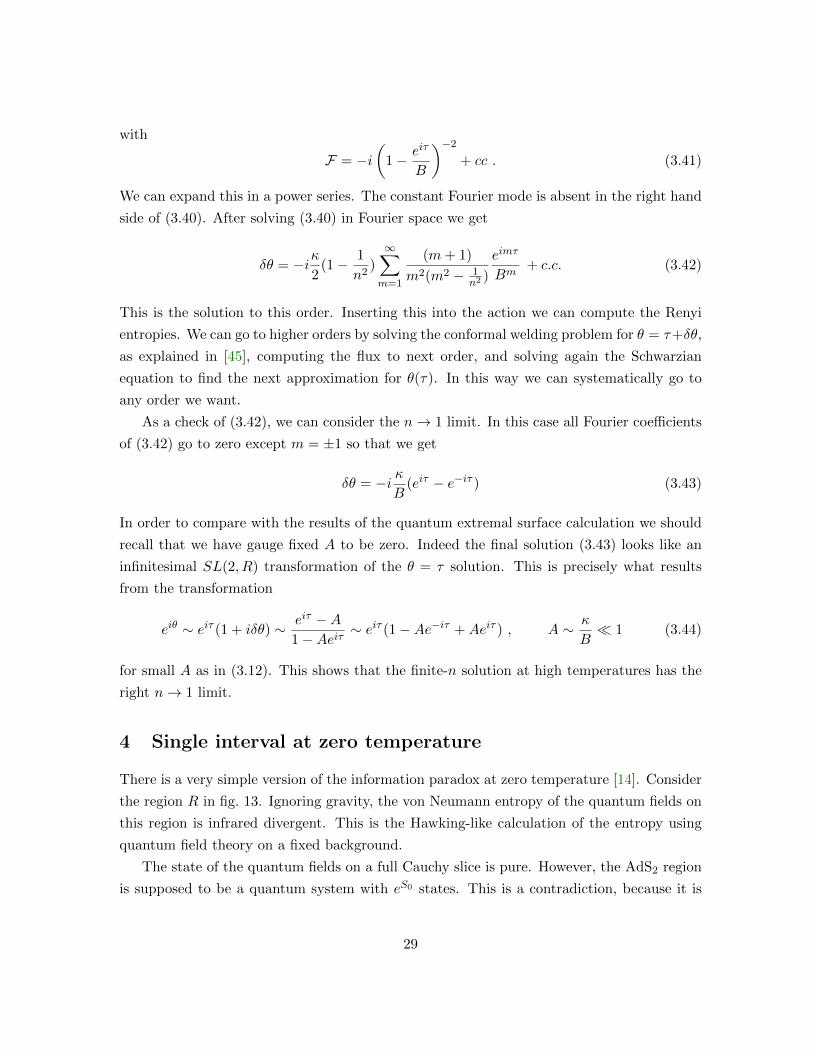
There is a very simple version of the information paradox at zero temperature [14]. Consider
the region R in fig. 13. Ignoring gravity, the von Neumann entropy of the quantum fields on
this region is infrared divergent. This is the Hawking-like calculation of the entropy using
quantum field theory on a fixed background.
The state of the quantum fields on a full Cauchy slice is pure. However, the AdS2 region
is supposed to be a quantum system with eS0 states. This is a contradiction, because it is
29
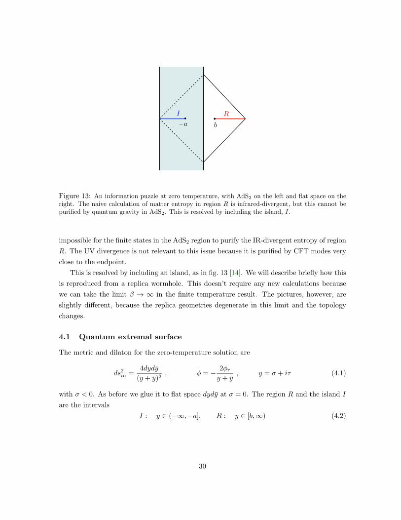
Figure 13: An information puzzle at zero temperature, with AdS2 on the left and flat space on theright. The naive calculation of matter entropy in region R is infrared-divergent, but this cannot bepurified by quantum gravity in AdS2. This is resolved by including the island, I.
impossible for the finite states in the AdS2 region to purify the IR-divergent entropy of region
R. The UV divergence is not relevant to this issue because it is purified by CFT modes very
close to the endpoint.
This is resolved by including an island, as in fig. 13 [14]. We will describe briefly how this
is reproduced from a replica wormhole. This doesn’t require any new calculations because
we can take the limit β → ∞ in the finite temperature result. The pictures, however, are
slightly different, because the replica geometries degenerate in this limit and the topology
changes.
4.1 Quantum extremal surface
The metric and dilaton for the zero-temperature solution are
ds2in =
4dydy
(y + y)2, φ = − 2φr
y + y, y = σ + iτ (4.1)
with σ < 0. As before we glue it to flat space dydy at σ = 0. The region R and the island I
are the intervals
I : y ∈ (−∞,−a], R : y ∈ [b,∞) (4.2)
30
Figure 14: Replica wormhole at zero temperature. On the right, the disk is glued to n copies of thehalf-plane, as indicated by the dashed lines.
at t = 0. The generalized entropy, including the island, is
Sgen(I ∪R) =φra
+c
6log
(a+ b)2
a. (4.3)
Setting ∂aSgen = 0 gives the position of the QES,
a =1
2(k + b+
√b2 + 6bk + k2) , k ≡ 6φr
c. (4.4)
4.2 Replica wormholes at zero temperature
The replica partition function Tr(ρA)n is given by the path integral in fig. 14. The boundary
condition for the gravity region is n copies of the real line. The Hawking saddle fills in the
gravity region with n independent copies of H2. The replica wormhole, shown in the figure,
fills in the gravity region with a single copy of H2. To see all n sheets of the gravity region,
we go to the uniformizing coordinate
w =
(a+ y
a− y
)1/n
. (4.5)
This maps the full gravity region to a single hyperbolic disk, |w| < 1. This disk is a wormhole
connecting n copies of flat space. The nth copy is glued to the segment with arg w ∈ [−πn ,
πn ].
The equation of motion, and the answer for the position of the QES, is found by taking
β → ∞ in the results of section 3. This of course agrees with (4.4). (It is also possible to
solve this problem directly at zero temperature, but we found it easier to treat the welding
problem at finite temperature where the gluing is compact. In the end, the welding effects
31
drop out in the determination of the position of the QES, as we saw below (3.27).)
5 Two intervals in the eternal black hole
We now turn to the information paradox in the eternal black hole [14], described in the
introduction and pictured in fig. 3. In the late-time regime relevant to the information
paradox, the generalized entropy, including the island, is simply twice the answer for a single
interval. We would like to understand how this is reproduced from wormholes. This is
essentially just putting together the general discussion of section 2 with the single-interval
results of section 3, so we will be brief. We will only discuss the saddles near n = 1; it would
be nice to have a more complete understanding of the finite-n wormholes in this setup.
5.1 Review of the QES
We set β = 2π. The points in fig. 3 have (σ, t) coordinates
P1 = (−a, ta) , P2 = (b, tb) , P3 = (−a,−ta + iπ) , P4 = (b,−tb + iπ) . (5.1)
The radiation region is
R = [P4,∞L) ∪ [P2,∞R) , (5.2)
and the island is
I = [P3, P1] . (5.3)
The CFT state is pure on the full Cauchy slice, so
SCFT(I ∪R) = SCFT([P4, P3] ∪ [P1, P2]) . (5.4)
This entropy is non-universal; it depends on the CFT. In the theory of c free Dirac fermions
[49], the entanglement entropy of the region
[x1, x2] ∪ [x3, x4] , (5.5)
with metric ds2 = Ω−2dxdx, is
Sfermions =c
6log
[|x21x32x43x41|2
|x31x42|2Ω1Ω2Ω3Ω4
]. (5.6)
32
where we dropped the UV divergences. With our kinematics and conformal factors, this
gives
Sfermions(I ∪R) =c
3log
[2 cosh ta cosh tb |cosh(ta − tb)− cosh(a+ b)|
sinh a cosh(a+b−ta−tb2 ) cosh(a+b+ta+tb
2 )
](5.7)
In a general CFT, the two-interval entanglement entropy is a function of the conformal cross-
ratios (z, z) which agrees with (5.7) in the OPE limits z → 0 and z → 1. For concreteness
we will do the calculations for the free fermion, but the regime of interest for the information
paradox will turn out to be universal.
The generalized entropy, including the island, is
Sgen(I ∪R) = 2S0 +2φr
tanh a+ Sfermions(I ∪R) , (5.8)
Without an island, the entropy is the CFT entropy on the complement of R, the interval
[P4, P2], which is
Sno islandgen = Sfermions(R) =
c
3log (2 cosh tb) (5.9)
At t = 0,
Sislandgen = 2S0 +
2φrtanh a
+c
3log
(4 tanh2 a+b
2
sinh a
). (5.10)
The extremality condition ∂aSislandgen = 0 at ta = tb = 0 gives
6φrc
sinh(a+ b) = 2 sinh2 a− sinh a cosh a sinh(a+ b) . (5.11)
Whether this has a real-valued solution depends on the parameters b and φr/c. For example,
if b = 0, then it has a real solution minimizing Sislandgen when φr/c is small, but not otherwise.
At late times, the extremality condition ∂aSislandgen = 0 always has a real solution. The
true entropy, according to the QES prescription, is
S(R) = minSno island
gen , Sislandgen
. (5.12)
The island always exists and dominates the entropy at late times, because the non-island
entropy grows linearly with t, see fig. 5. This solution is in the OPE limit where we can
approximate the entanglement entropy by twice the single-interval answer,
Smatter(I ∪R) ≈ 2Smatter([P1, P2]) =c
3log
(2| cosh(a+ b)− cosh(ta − tb)|
sinh a
). (5.13)
33
and the QES condition sets ta = tb.
5.2 Replica wormholes
We would like to discuss some aspects of the wormhole solutions that lead to the island
prescription.
For general n these are wormholes which have the topology shown in figures 6(b), 7.
Already from these figures we can derive the S0-dependent contribution (2.7) since it involves
only the topology of the manifold. The replica wormhole that involves nontrivial connections,
see figure (7), has the topology of a sphere with n holes. This gives a contribution going
like Zn ∝ eS0(2−n) and a contribution of 2S0 = (1 − n∂n) logZn|n=1 for the von Neumann
entropy. This is good, since the island contribution indeed had such a term (5.10).
It is useful to assume replica symmetry and view the Riemann surface as arising from a
single disk with n copies of the matter theory and with pairs of twist operators that connect
all these n copies in a cyclic fashion, see figure 9. In order to find the full answer, we need
to solve the equations (2.15) (2.16). The important point is that, at this stage, we have that
n appears purely as a parameter and we can analytically continue the equations in n. We
have not managed to solve the equations for finite n. But let us discuss some properties we
expect. In the limit of large cβ/φr, it is likely that solutions exist in Euclidean signature.7
We can put points P2 and P4 at v = ±Be±iϕ. Once this solution is found, we can analytically
continue ϕ→ −it to generate the Lorentzian solution. That Lorentzian solution at late times
t is expected to exist even for low values of cβ/φr. In principle, it should be possible, and
probably easier, to analyze directly the late-times Lorentzian equation. In fact, we expect
that there should be a way to relate the single interval solution to the two interval solution
in this regime. The intuitive reason is that at late times the distance between the two
horizons is increasing and so the distance between the two cosmic branes is increasing. We
have an external source cosmic brane outside the gravitational region, at the tip of region
R. The cosmic brane has some tension, as well as a twist operator on it. For the Hawking
saddle, the one without the replica wormholes, the twist operators, and the topological line
operators8 that connect them, generate a contribution that grows linearly in time, due to
the behavior of Renyi entropies for the matter quantum field theory, as well as the fact
that the wormhole length grows with time. At late times the topological line operator can
break by pair producing cosmic branes, with their twist operators. The cost of creating
a pair of cosmic branes is finite in the gravitational region, because the dilaton is finite.
7For low values of cβ/φr we have already seen, in (5.11), that near n ∼ 1 the solutions can be complex.8These topological line operators exchange the n copies in a cyclic way. They are represented by red lines
in figure 9(b).
34
This cost would be infinite in the non-gravitational region. But once the external cosmic
brane is screened by the cosmic brane that appeared in the gravity region we expect to have
two approximately independent single interval problems. The reason is that the distance
between the left and right sides is growing with time. This is somewhat analogous to two
point charges that generate a two dimensional electric field. As one separates the charges it
might be convenient to create a pair of charges that screens the electric field. For this it is
important that the charges one creates have finite mass.
In the n→ 1 limit we can analyze the solution and we get the generalized entropy. This
is not too surprising since the arguments in [30] say that this should always work. Here
the non-trivial input is the ansatz for the configuration of intervals which follows from the
structure of the Riemann surfaces. As discussed in section 2.1, the effective action reduces
to the action of certain cosmic branes which are manifestly very light in the n → 1 limit.
So in this case, the argument of the previous paragraph can be explicitly checked and one
indeed obtains that we get the sum over the two single interval problems [14].
5.3 Purity of the total state
One can take the perspective that our model is defined via a quantum theory living on the
flat space region including its boundary endpoints. The global pure state we consider should
be a pure state of this region, and a natural question is whether this is captured in the gravity
description. Replica wormholes do indeed capture this feature.
The computation of the entropy of this region is given by evaluating the path integral on
the manifold shown in figure 15. The branch cuts split the entire flat space region including its
boundaries, identifying one half of one sheet with the other half of the next sheet. The most
obvious gravitational saddle is the one that connects these consecutive sheets and thereby
naturally extending the branch cut through the entire gravity region. A simple rearranging of
these sheets shows that this contribution to the Renyi entropy factorizes. This disconnected
saddle satisfies Zn = Zn1 , and evaluating the on shell action on this configuration will give
vanishing entropy since
Tr ρn =ZnZn1
= 1 . (5.14)
This saddle clearly dominates over all other configurations.
Since the different sheets are not coupled at all in the flat space region, it’s plausible
that this disconnected saddle is the only saddle that exists. Other off-shell contributions can
indeed exist, but we speculate they should give a vanishing contribution in a model with a
35
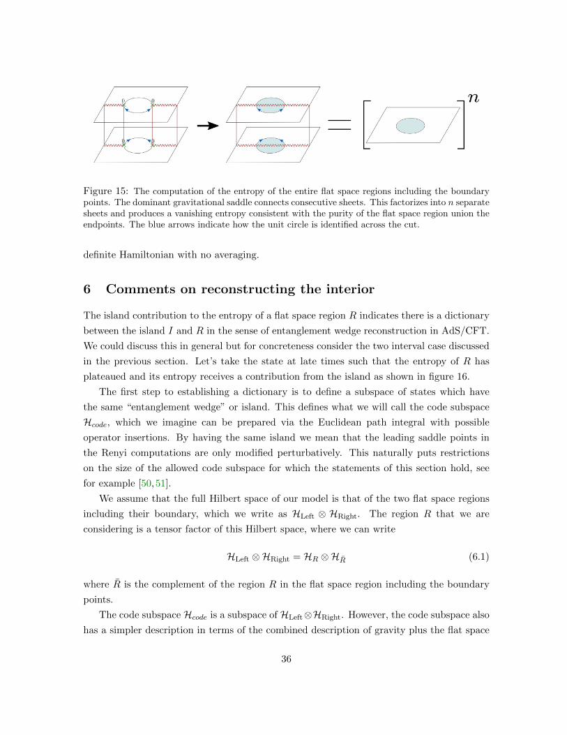
Figure 15: The computation of the entropy of the entire flat space regions including the boundarypoints. The dominant gravitational saddle connects consecutive sheets. This factorizes into n separatesheets and produces a vanishing entropy consistent with the purity of the flat space region union theendpoints. The blue arrows indicate how the unit circle is identified across the cut.
definite Hamiltonian with no averaging.
6 Comments on reconstructing the interior
The island contribution to the entropy of a flat space region R indicates there is a dictionary
between the island I and R in the sense of entanglement wedge reconstruction in AdS/CFT.
We could discuss this in general but for concreteness consider the two interval case discussed
in the previous section. Let’s take the state at late times such that the entropy of R has
plateaued and its entropy receives a contribution from the island as shown in figure 16.
The first step to establishing a dictionary is to define a subspace of states which have
the same “entanglement wedge” or island. This defines what we will call the code subspace
Hcode, which we imagine can be prepared via the Euclidean path integral with possible
operator insertions. By having the same island we mean that the leading saddle points in
the Renyi computations are only modified perturbatively. This naturally puts restrictions
on the size of the allowed code subspace for which the statements of this section hold, see
for example [50,51].
We assume that the full Hilbert space of our model is that of the two flat space regions
including their boundary, which we write as HLeft ⊗ HRight. The region R that we are
considering is a tensor factor of this Hilbert space, where we can write
HLeft ⊗HRight = HR ⊗HR (6.1)
where R is the complement of the region R in the flat space region including the boundary
points.
The code subspace Hcode is a subspace of HLeft⊗HRight. However, the code subspace also
has a simpler description in terms of the combined description of gravity plus the flat space
36
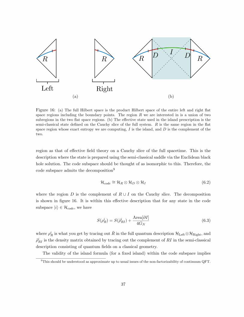
(a) (b)
Figure 16: (a) The full Hilbert space is the product Hilbert space of the entire left and right flatspace regions including the boundary points. The region R we are interested in is a union of twosubregions in the two flat space regions. (b) The effective state used in the island prescription is thesemi-classical state defined on the Cauchy slice of the full system. R is the same region in the flatspace region whose exact entropy we are computing, I is the island, and D is the complement of thetwo.
region as that of effective field theory on a Cauchy slice of the full spacetime. This is the
description where the state is prepared using the semi-classical saddle via the Euclidean black
hole solution. The code subspace should be thought of as isomorphic to this. Therefore, the
code subspace admits the decomposition9
Hcode ∼= HR ⊗HD ⊗HI (6.2)
where the region D is the complement of R ∪ I on the Cauchy slice. The decomposition
is shown in figure 16. It is within this effective description that for any state in the code
subspace |i〉 ∈ Hcode, we have
S(ρiR) = S(ρiRI) +Area[∂I]
4GN(6.3)
where ρiR is what you get by tracing out R in the full quantum description HLeft⊗HRight, and
ρiRI is the density matrix obtained by tracing out the complement of RI in the semi-classical
description consisting of quantum fields on a classical geometry.
The validity of the island formula (for a fixed island) within the code subspace implies
9This should be understood as approximate up to usual issues of the non-factorizability of continuum QFT.
37
the equivalence of the relative entropy in the exact state and the semi-classical state:
SRel(ρR|σR) = SRel(ρRI |σRI) (6.4)
A similar observation in the context of AdS/CFT [52] was key in proving entanglement wedge
reconstruction [53] using the quantum error correction interpretation of the duality [54]. The
same line of argument can be applied here to establish the dictionary. In particular, one can
show that for any operator OI (and its Hermitian conjugate) acting within the Hcode and
supported on the island one can find an operator supported on R such that:
OI |i〉 = OR|i〉 (6.5)
O†I |i〉 = O†R|i〉 (6.6)
The operator OR is given by a complicated operator on R involving the matrix elements of
OI within the code subspace.
In summary, we are using the fine grained entropy formula to understand how the in-
terior is encoded in the full Hilbert space. The relative entropy equality (6.4) tells us that
distinguishable states in the interior (the island) are also distinguishable in the radiation,
within the full exact quantum description.
7 Discussion
In this paper, we have exhibited non-perturbative effects that dramatically reduce the late
time von Neumann entropy of quantum fields outside a black hole.
The computation of the Renyi entropies corresponds to the expectation value of a swap
or cyclic permutation operator in n copies of the theory. Systems with very high entropy
have very small, exponentially small, expectation values for this observable. This means that
non-perturbative effects can compete with the naive answers. In particular, the Hawking-
like computation of the Renyi entropies of radiation corresponds to a computation on the
leading gravitational background. A growing entropy corresponds to an exponentially de-
creasing expectation value for the cyclic permutation operator. It decreases exponentially as
time progresses. For this reason, we need to pay attention to other geometries, with other
topologies. These other topologies give exponentially small effects, but they do not continue
decreasing with time for long times. Said in this way, the effects are vaguely similar to the
ones discussed for corrections of other exponentially small effects [32–35]. Though the Renyi
entropies are small, the von Neumann entropy is large and the new series of saddles gives rise
38
to a constant von Neumann entropy at late times. More precisely, we can think of the com-
putation of the Renyi entropies in the two interval case as an insertion of a pair of external
cosmic branes in the non-gravitational region. As time progresses these are separated further
and further through the wormhole. Eventually the dominant contribution is one where a pair
of cosmic branes is created in the gravitational region that “screen” the external ones, giving
an entropy which is the same as that of two copies of the single interval entropy.
These other topologies are present as subleading saddles also at short times (perhaps as
complex saddles) where we can analyze them using Euclidean methods and then analytically
continue. We have only done this analytic continuation for the von Neumann entropies, not
the Renyi entropies. It would be interesting to do it more explicitly for the Renyi entropies.
There have been discussions on whether small corrections to the density matrix, of or-
der e−SBH , could or could not restore unitarity. These results suggest that they interfere
constructively to give rise to the right expression for the entropy.
This is evidence that including nonperturbative gravitational effects can indeed lead to
results compatible with unitarity. However, we emphasize that this is not a full microscopic
resolution of the information paradox. We have not given a gravitational description for
the S-matrix describing how infalling matter escapes into the radiation. In this sense, these
results are on a footing similar to the Bekenstein-Hawking calculation of the entropy, which
uses a Euclidean path integral to compute the right answer but does not give an explicit
Hilbert space picture for what it is counting. In contrast, the Strominger-Vafa computation
of the entropy [55] gives us an explicit Hilbert space, but not a detailed description of the
microstates in the gravity variables. Something similar can be said of the CFT description
in AdS/CFT. Hopefully these results will be useful for providing a more explicit map.
It is amusing to note that wormholes were initially thought to destroy information [56–58].
But more recently the work of [34, 35], as well as the present discussion, and [31], suggests
that the opposite is true. Wormholes are important for producing results that are compatible
with unitarity. For earlier work in this direction see also [59–61].
We assumed that c 1 as a blanket justification for analyzing the equations classically.
However, even for small c ∼ 1, the basic picture for the Page curve can be justified. The
basic point is simple. First consider the single interval computation. In that case for c ∼ 1
we see that the correction to the black hole solution is very small, for all the Renyi entropies.
In other words, we find that A is small, and we can probably not distinguish such a small
value of A from zero but that does not matter, the geometries and the entropies are basically
those of a black hole. Now when we go to two intervals, and we consider the late time
situation, then all that really matters is that we can do an OPE-like expansion of the twist
operator insertions. The important observation is that the twist operator insertions in the
39
interior of the black hole are very far from each other. This is the fact that the wormhole
is getting longer [62,63]. Then the solution becomes similar to two non-interacting copies of
the single interval solution. The fact that c is small only implies that we will have to wait
longer for the island solution to dominate. We just have to wait a time of order the entropy,
t ∝ β(S − S0)/c for it to dominate.
In [34], it was argued that pure JT gravity should be interpreted in terms of an average
over Hamiltonians. In addition, higher genus corrections were precisely matched. This has
raised the question of whether the corrections we are discussing in this paper crucially involve
an average over Hamiltonians, or whether they would also apply to a system which has a
definite Hamiltonian. Though JT gravity plus a CFT probably does not define a complete
quantum gravity theory, it seems likely that well defined theories could be approximated by
JT gravity plus a CFT. For example, we could imagine an AdS/CFT example that involves
an extremal black hole such that it also has a CFT on its geometry. All we need is this
low energy description, the theory might have lots of other massive fields which will not
drastically participate in the discussion. They might lead to additional saddles, but it seems
that they will not correct the saddles we have been discussing. And we have the seen that
the saddles we discussed already give an answer consistent with unitarity, at least for the
entropy. In contrast with [34], we are not doing the full path integral, we are simply using a
saddle point approximation, so the JT gravity plus CFT only needs to be valid around these
saddles.
As we mentioned in the introduction, the setup in this paper can be viewed as an ap-
proximation to some magnetically charged near extremal four dimensional black holes [40].
But one could analyze more general asymptotically flat black holes and wonder how to define
either exactly or approximately the various entropies involved. In particular, to have a sharp
definition of the entropy of radiation it seems important to go to null infinity.
Another interesting question is whether we can give a Lorentzian interpretation to the
modification of the density matrix implied by the existence of replica wormholes.
It has been pointed out that a black hole as seen from outside looks like a system obeying
the laws of hydrodynamics. For this reason, it is sometimes thought that gravity is just an
approximation that intrinsically loses information. Here we see that if we include the black
hole interior, and we do a more complete gravity computation, we can get results compatible
with unitarity. The fact that gravity is more than dissipative hydrodynamics is already
contained in the Ryu-Takayanagi formula for the fine grained entropy, which shows that the
geometry of the interior can discriminate between pure and mixed states for a black hole.
40
Acknowledgments We are grateful to Tarek Anous, Raphael Bousso, Kanato Goto,
Daniel Harlow, Luca Iliesiu, Alexei Kitaev, Alexandru Lupsasca, Raghu Mahajan, Alexei
Milekhin, Shiraz Minwalla, Geoff Penington, Steve Shenker, Julian Sonner, Douglas Stanford,
Andrew Strominger, Sandip Trivedi and Zhenbin Yang for helpful discussions of this and
related work. AA and TH thank the organizers of the workshop Quantum Information In
Quantum Gravity at UC Davis, August 2019, and AA, TH, and JM thank the organizers of
the workshop Quantum Gravity in the Lab at Google X, November 2019. A.A. is supported
by funds from the Ministry of Presidential Affairs, UAE. The work of ES is supported by the
Simons Foundation as part of the Simons Collaboration on the Nonperturbative Bootstrap.
The work of TH and AT is supported by DOE grant DE-SC0020397. J.M. is supported in
part by U.S. Department of Energy grant DE-SC0009988 and by the Simons Foundation
grant 385600.
A Derivation of the gravitational action
In this appendix we derive the action that leads to the equation of motion (2.15).
We start with the expansion of the metric near the boundary (2.13) (2.14)
ds2 =4dwdw
(1− |w|2)2
(1− 2
3(1− |w|)2U(θ) + · · ·
). (A.1)
We now write in terms of the variables w = e−γeiθ and expand it in powers of γ as
ds2 =dθ2
γ2+dγ2
γ2− 2
3dθ2U(θ) . (A.2)
We now equate this to ds = dτε , we set θ = θ(τ) and solve for γ in a power series
γ = εθ′
[1 + ε2
(1
2
θ′′2
θ′2− 1
3U(θ)θ′
2
)+ · · ·
]. (A.3)
We can now compute the tangent vector to the curve tµ and the normal vector nµ and
compute the extrinsic curvature from
K = tµtν∇µnν = 1 + ε2[θ, τ+
(1
2+ U(θ)
)θ′
2]. (A.4)
Up to the purely topological term, the gravitational action (2.8) reduces to the extrinsic
41
curvature term
− Igrav =1
4π
φrε
∫dτ
ε2K =
2φr4πε2
∫dτ +
φr2π
∫dτ
[θ(τ), τ+
(1
2+ U(θ)
)θ′
2]
+ o(ε) .
(A.5)
The first term is a purely local divergence that can be viewed as the correction to the vacuum
energy. We should also remark that we can always choose a coordinate x where the metric
locally looks like the standard Poincare coordinates. In those coordinates the action is simply
x, τ. However, we will have a nontrivial identification for x as we move from τ → τ + 2π.
Here we simplified the boundary condition, it is just θ = θ + 2π, but we complicated a bit
the action. Notice that we can think of U(θ) as a stress tensor, the change of coordinates is
basically the same that we use to transform this stress tensor to zero. In other words, x(θ)
is a function which obeys x, θ = 12 + U(θ).
The conserved energy of the system is given by
E =φr2π
[θ(τ), τ+
(1
2+ U(θ)
)θ′
2]. (A.6)
We now compute U(θ) for the case when we put a conical defect at point A in the w
plane. We have the metric (3.15) and the change of coordinates (3.14) which imply that
ds2 =
∣∣∣∣dwdw∣∣∣∣2 4|dw|2
(1− |w|2)2
=4|dw|2
(1− |w|2)2
[1− 2
3(1− |w|)2U(θ) + · · ·
], as |w| → 1 (A.7)
with
U(θ) = −1
2
(1− 1
n2
)(1−A2)2
(eiθ −A)2(e−iθ −A)2, (A.8)
which leads to the same action as (3.18)
We now would like to derive the equations of motion for this action. In particular, we
would like to see that as θ → θ + δθ we get the right equations of motion. The change in
gravitational action is simple, we just have
− δIgrav = −φr2π
∫dτ
[θ(τ), τ+ (1
2 + U(θ))θ′2]′
θ′δθ . (A.9)
Now, let us do the variation of the CFT part. Imagine that we choose locally complex
coordinates so that
logw = s+ iθ (A.10)
42
We also have the outside coordinates y = σ + iτ and we can locally think of the relation
between the two in terms of logw = iθ(−iy). Now imagine that we do a small change
θ(τ) → θ + δθ with δθ with compact support. This would change the relation between the
two sides. However, let us imagine we instead keep the relation fixed, set by θ(τ) and we
redefine the outside coordinate by an infinitesimal reparametrization, y = y + ζy in such a
way that the relation between the new variables is the same as the old one
logw = iθ(−iy) = iθ(−iy) + iδθ(−iy) = iθ(−iy) + θ′(−iy)ζy → ζy = iδθ
θ′(A.11)
and we have the complex conjugate expression for ζ y. We can then extend this reparametriza-
tion in a non-holomorphic way in the region outside, defining
ζy = iδθ(−iy)
θ′(−iy)h(σ) , ζ y = −iδθ(iy)
θ′(iy)h(σ) (A.12)
where h(σ) is one for σ = 0 and quickly goes to zero at σ increases. An example is h(σ) =
θ(σ0 − σ) for a small σ0. This change of coordinates is equivalent to a change in metric
ds2 = dydy = dyd¯y − 2∂αζβdyαdyβ , δgαβ = −2∂(αζβ) (A.13)
This differs from the original metric by some terms that are localized near the point where
we are doing the variation. The relation between logw and the y variable was the same as it
was before we did the variation, due to our choice of y variable in (A.11). Furthermore, far
from the region where we are doing the variation, both variables coincide. Thus, the only
thing we are doing is locally changing the metric of the outside region. Using the definition
of the stress tensor, Tαβ = − 2√g
δδgαβ
logZ, we get
δ log ZM = −1
2
∫dϕdσ(Tyyδg
yy + Tyyδgyy)
= −2
∫dϕdσ(Tyy∂yζ
y + Tyy∂yζy) , (A.14)
where we used that the background metric is flat and that the trace of the stress tensor is
zero. We now use evaluate the derivatives
∂yζy =
i
2
δθ(−iy)
θ′(−iy)h′(σ) , ∂yζ
y = − i2
δθ(iy)
θ′(iy)h′(σ) , h′ = −δ(σ − σ0) . (A.15)
Here we used that the arguments of δθ and θ′ are holomorphic or antiholomorphic, so the
derivative receives only a contribution from h, which is just a delta function. Inserting this
43
into (A.14), integrating over σ, and taking σ0 → 0, we get
δ log ZM = i
∫dτ(Tyy − Tyy)
δθ
θ′. (A.16)
Using (A.9) we get the appropriate equation (2.15) after cancelling the 1/θ′ factor from both
sides.
B Linearized solution to the welding problem
Let us start with a discussion of the symmetries of the welding problem (2.11). First we
can imagine doing SL(2, C) transformations of the z plane. These move around the point at
infinity, and we would need to allow a pole in the functions F or G. If we fix that F (∞) =∞,
then we can then impose that the functions are holomorphic everywhere, with no poles, and
this group is reduced to just translations, scalings and rotations of the plane z. None of these
transformations change the data for the welding problem which is θ(τ). In addition, we have
two SL(2, R) transformations, one acting on w and one acting on v, both preserving the
circles |w| = 1 and |v| = 1. These change the data of the welding problem by an SL(2, R)
transformation of eiθ or eiτ respectively. They map a solution of a welding problem with
θ(τ) to a solution of a different welding problem given by the transformed function. In
our combined gravity plus CFT problem, we are integrating over θ(τ), so we can look for
symmetries that change θ(τ). It turns out that the SL(2, R)v that acts on the v plane is
not a symmetry. It changes the Schwarzian action, for example. On the other hand, the
SL(2, R)w is actually a gauge symmetry, when we also act with the SL(2, R) transformation
on the possible locations, wi, of the conical singularities.
Consider a plane with coordinate w inside the unit disk, and v outside, as in fig. 10. The
plane is glued along the unit circle with a gluing function θ(τ), where w = eiθ and v = eiτ .
The solution to the welding problem is a pair of functions
z = G(w) (inside) (B.1)
z = F (v) (outside) (B.2)
where G is holomorphic inside the disk, and F is holomorphic outside the disk. In this
appendix we will solve for F,G perturbatively, assuming the gluing is close to the identity,
θ(τ) = τ + δθ(τ). Here we are considering δθ(τ) to be a fixed input to the problem of finding
F and G.
44
Expand in Fourier modes,
θ(τ) = τ +∞∑
m=−∞cme
imτ , G(w) = w +∞∑`=0
g`w` , F (v) = v +
2∑`=−∞
f`v` . (B.3)
Here cm, d`1, and d`2 are considered small. There is an SL(2) ambiguity in the zeroth order
solution, which we have gauge-fixed to set these maps to the identity. (Note that this is
different from the choice in the main text around eqn (3.38).) The matching condition on
the unit circle is
G(eiθ(τ)) = F (eiθ) . (B.4)
At the linearized level, this sets
f`+1 = ic` (` ≤ −2) (B.5)
g`+1 = −ic` (` ≥ 2) (B.6)
and
ic−1 = f2 − g2 , ic0 = f1 − g1 , ic1 = f2 − g2 . (B.7)
There an ambiguity by a small SL(2, C) action on the z plane. We can fix it by setting
G(0) = 0, F (v) = v+constant, as v → ∞. This amounts to three complex conditions that
set
g0 = f2 = f1 = 0 (B.8)
This now implies that we get a unique solution for the remaining coefficients in terms of the
cm
fl = ic`−1, for ` ≤ 0 ; g` = −ic`−1 , for ` > 0 . (B.9)
From here we can calculate
v2F, v =−2∑
`=−∞`(`2 − 1)ic`v
` . (B.10)
Comparing to w, τ = eiθ, τ gives the relation used in the main text,
e2iτF, v = −δw, τ− = −(δθ′′′ + δθ′)− . (B.11)
45
C The equation of motion in Lorentzian signature
The Hilbert transform appearing in the equation of motion (3.27) has a nice interpretation
in Lorentzian signature. It is responsible for the dissipation of energy into the thermal bath
outside. This makes contact with the Schwarzian equation for black hole evaporation studied
in [5, 37].
In this appendix we set n = 1, but allow for CFT operators inserted in the non-
gravitational region. The perturbative Schwarzian equation in Euclidean signature is
∂τS + iκH · S = iκF (C.1)
where S = δeiθ, τ and
F = Tyy(iτ)− Tyy(−iτ) . (C.2)
We separate this into positive and negative frequencies on the Euclidean τ -circle,
∂τS+ − iκS+ = iκF+ (C.3)
∂τS− + iκS− = iκF− . (C.4)
Here the ‘+’ terms include only the non-negative powers of ey, and the ‘−’ terms have the
negative powers. Now continuing to Lorentzian signature with τ = it, this becomes
∂tS± ± κS± = −κF± (C.5)
This is the Lorentzian equation of motion. As an example, consider a state with two scalar
operators O(y1)O(y2) inserted at
y1 = L+ iδ, y2 = y1 = L− iδ , (C.6)
with 0 < δ L. This creates a shockwave that falls into the AdS region at time t ≈ L. The
state is time-symmetric, so there is also a shockwave exiting the AdS region at t ≈ −L. The
stress tensor is
Tyy(y) = −hO2π
v2(v1 − v2)2
(v − v1)2(v − v2)2, (C.7)
with v = ey. The projections onto positive and negative Euclidean frequencies are
F+ = −hO2π
v2(v1 − v2)2
(v − v1)2(v − v2)2, F− =
hO2π
v2(v1 − v2)2
(1− v1v)2(1− v1v)2. (C.8)
46
In Lorentzian signature this becomes
F+ =hO sin2 δ
2π(cos δ − cosh(L+ t))2(C.9)
F− = − hO sin2 δ
2π(cos δ − cosh(L− t))2(C.10)
As δ → 0, these vanishes away from the singularities, leading to
∂tS+ + κS+ = −κEOδ(t+ L) (C.11)
∂tS− − κS− = κEOδ(t− L) , (C.12)
where EO = hO/δ. The delta functions are the shockwaves exiting and entering the AdS
region. The signs here, and in particular the extra minus sign from the Hilbert transform,
ensure that there is a sensible solution for the Schwarzian, which is time-symmetric and goes
to zero as t→ ±∞. The solution is
S+ = Θ(−t− L)κE0eκ(t+L) , S− = Θ(t− L)κE0e
κ(L−t) . (C.13)
For t > 0, this is essentially the same solution as the evaporating black hole in [5], which had
a shockwave produced by a joining quench rather than an operator insertion.
References
[1] S. W. Hawking, Breakdown of Predictability in Gravitational Collapse, Phys. Rev. D14,
2460–2473, 1976.
[2] D. N. Page, Information in black hole radiation, Phys. Rev. Lett. 71, 3743–3746, 1993,
[arXiv:hep-th/9306083 [hep-th]].
[3] D. N. Page, Time Dependence of Hawking Radiation Entropy, JCAP 1309, 028, 2013,
[arXiv:1301.4995 [hep-th]].
[4] G. Penington, Entanglement Wedge Reconstruction and the Information Paradox, 2019,
[arXiv:1905.08255 [hep-th]].
[5] A. Almheiri, N. Engelhardt, D. Marolf and H. Maxfield, The entropy of bulk quantum fields
and the entanglement wedge of an evaporating black hole, 2019, [arXiv:1905.08762 [hep-th]].
[6] A. Almheiri, R. Mahajan, J. Maldacena and Y. Zhao, The Page curve of Hawking radiation
from semiclassical geometry, 2019, [arXiv:1908.10996 [hep-th]].
[7] T. G. Mertens, Towards Black Hole Evaporation in Jackiw-Teitelboim Gravity, JHEP 07, 097,
2019, [arXiv:1903.10485 [hep-th]].
47
[8] C. Akers, A. Levine and S. Leichenauer, Large Breakdowns of Entanglement Wedge
Reconstruction, 2019, [arXiv:1908.03975 [hep-th]].
[9] U. Moitra, S. K. Sake, S. P. Trivedi and V. Vishal, Jackiw-Teitelboim Model Coupled to
Conformal Matter in the Semi-Classical Limit, 2019, [arXiv:1908.08523 [hep-th]].
[10] A. Almheiri, R. Mahajan and J. E. Santos, Entanglement islands in higher dimensions, 2019,
[arXiv:1911.09666 [hep-th]].
[11] Z. Fu and D. Marolf, Bag-of-gold spacetimes, Euclidean wormholes, and inflation from domain
walls in AdS/CFT, JHEP 11, 040, 2019, [arXiv:1909.02505 [hep-th]].
[12] P. Zhang, Evaporation dynamics of the Sachdev-Ye-Kitaev model, 2019, [arXiv:1909.10637
[cond-mat.str-el]].
[13] C. Akers, N. Engelhardt and D. Harlow, Simple holographic models of black hole evaporation,
2019, [arXiv:1910.00972 [hep-th]].
[14] A. Almheiri, R. Mahajan and J. Maldacena, Islands outside the horizon, 2019,
[arXiv:1910.11077 [hep-th]].
[15] M. Rozali, J. Sully, M. Van Raamsdonk, C. Waddell and D. Wakeham, Information radiation in
BCFT models of black holes, 2019, [arXiv:1910.12836 [hep-th]].
[16] H. Z. Chen, Z. Fisher, J. Hernandez, R. C. Myers and S.-M. Ruan, Information Flow in Black
Hole Evaporation, 2019, [arXiv:1911.03402 [hep-th]].
[17] R. Bousso and M. Tomasevic, Unitarity From a Smooth Horizon?, 2019, [arXiv:1911.06305
[hep-th]].
[18] D. L. Jafferis and D. K. Kolchmeyer, Entanglement Entropy in Jackiw-Teitelboim Gravity,
2019, [arXiv:1911.10663 [hep-th]].
[19] A. Blommaert, T. G. Mertens and H. Verschelde, Eigenbranes in Jackiw-Teitelboim gravity,
2019, [arXiv:1911.11603 [hep-th]].
[20] S. Ryu and T. Takayanagi, Holographic derivation of entanglement entropy from AdS/CFT,
Phys. Rev. Lett. 96, 181602, 2006, [arXiv:hep-th/0603001 [hep-th]].
[21] V. E. Hubeny, M. Rangamani and T. Takayanagi, A Covariant holographic entanglement
entropy proposal, JHEP 07, 062, 2007, [arXiv:0705.0016 [hep-th]].
[22] T. Faulkner, A. Lewkowycz and J. Maldacena, Quantum corrections to holographic
entanglement entropy, JHEP 11, 074, 2013, [arXiv:1307.2892 [hep-th]].
[23] N. Engelhardt and A. C. Wall, Quantum Extremal Surfaces: Holographic Entanglement
Entropy beyond the Classical Regime, JHEP 01, 073, 2015, [arXiv:1408.3203 [hep-th]].
[24] S. D. Mathur, What is the dual of two entangled CFTs?, 2014, [arXiv:1402.6378 [hep-th]].
[25] R. Jackiw, Lower Dimensional Gravity, Nucl. Phys. B252, 343–356, 1985.
48
[26] C. Teitelboim, Gravitation and Hamiltonian Structure in Two Space-Time Dimensions, Phys.
Lett. B126, 41–45, 1983.
[27] A. Almheiri and J. Polchinski, Models of AdS2 backreaction and holography, JHEP 11, 014,
2015, [arXiv:1402.6334 [hep-th]].
[28] A. Lewkowycz and J. Maldacena, Generalized gravitational entropy, JHEP 08, 090, 2013,
[arXiv:1304.4926 [hep-th]].
[29] X. Dong, A. Lewkowycz and M. Rangamani, Deriving covariant holographic entanglement,
JHEP 11, 028, 2016, [arXiv:1607.07506 [hep-th]].
[30] X. Dong and A. Lewkowycz, Entropy, Extremality, Euclidean Variations, and the Equations of
Motion, JHEP 01, 081, 2018, [arXiv:1705.08453 [hep-th]].
[31] G. Penington, S. H. Shenker, D. Stanford and Z. Yang, Replica wormholes and the black hole
interior, 2019, [arXiv:1911.11977 [hep-th]].
[32] J. M. Maldacena, Eternal black holes in anti-de Sitter, JHEP 04, 021, 2003,
[arXiv:hep-th/0106112 [hep-th]].
[33] P. Saad, S. H. Shenker and D. Stanford, A semiclassical ramp in SYK and in gravity, 2018,
[arXiv:1806.06840 [hep-th]].
[34] P. Saad, S. H. Shenker and D. Stanford, JT gravity as a matrix integral, 2019,
[arXiv:1903.11115 [hep-th]].
[35] P. Saad, Late Time Correlation Functions, Baby Universes, and ETH in JT Gravity, 2019,
[arXiv:1910.10311 [hep-th]].
[36] J. V. Rocha, Evaporation of large black holes in AdS: Coupling to the evaporon, JHEP 08, 075,
2008, [arXiv:0804.0055 [hep-th]].
[37] J. Engelsoy, T. G. Mertens and H. Verlinde, An investigation of AdS2 backreaction and
holography, JHEP 07, 139, 2016, [arXiv:1606.03438 [hep-th]].
[38] L. Randall and R. Sundrum, An Alternative to compactification, Phys. Rev. Lett. 83,
4690–4693, 1999, [arXiv:hep-th/9906064 [hep-th]].
[39] A. Karch and L. Randall, Locally localized gravity, JHEP 05, 008, 2001,
[arXiv:hep-th/0011156 [hep-th]].
[40] J. Maldacena, A. Milekhin and F. Popov, Traversable wormholes in four dimensions, 2018,
[arXiv:1807.04726 [hep-th]].
[41] T. M. Fiola, J. Preskill, A. Strominger and S. P. Trivedi, Black hole thermodynamics and
information loss in two-dimensions, Phys. Rev. D50, 3987–4014, 1994, [arXiv:hep-th/9403137
[hep-th]].
[42] C. G. Callan, Jr. and F. Wilczek, On geometric entropy, Phys. Lett. B333, 55–61, 1994,
[arXiv:hep-th/9401072 [hep-th]].
49
[43] H. Casini and M. Huerta, Entanglement entropy in free quantum field theory, J. Phys. A42,
504007, 2009, [arXiv:0905.2562 [hep-th]].
[44] X. Dong, Holographic Entanglement Entropy for General Higher Derivative Gravity, JHEP 01,
044, 2014, [arXiv:1310.5713 [hep-th]].
[45] E. Sharon and D. Mumford, 2D-Shape Analysis Using Conformal Mapping, International
Journal of Computer Vision 70, 55, 2006.
[46] K. Jensen, Chaos and hydrodynamics near AdS2, 2016, [arXiv:1605.06098 [hep-th]].
[47] J. Maldacena, D. Stanford and Z. Yang, Conformal symmetry and its breaking in two
dimensional Nearly Anti-de-Sitter space, PTEP 2016, 12C104, 2016, [arXiv:1606.01857
[hep-th]].
[48] P. Calabrese and J. L. Cardy, Entanglement entropy and quantum field theory, J. Stat. Mech.
0406, P06002, 2004, [arXiv:hep-th/0405152 [hep-th]].
[49] H. Casini, C. D. Fosco and M. Huerta, Entanglement and alpha entropies for a massive Dirac
field in two dimensions, J. Stat. Mech. 0507, P07007, 2005, [arXiv:cond-mat/0505563
[cond-mat]].
[50] P. Hayden and G. Penington, Learning the Alpha-bits of Black Holes, 2018, [arXiv:1807.06041
[hep-th]].
[51] P. Hayden and G. Penington, Approximate quantum error correction revisited: Introducing the
alpha-bit, 2017.
[52] D. L. Jafferis, A. Lewkowycz, J. Maldacena and S. J. Suh, Relative entropy equals bulk relative
entropy, JHEP 06, 004, 2016, [arXiv:1512.06431 [hep-th]].
[53] X. Dong, D. Harlow and A. C. Wall, Reconstruction of Bulk Operators within the
Entanglement Wedge in Gauge-Gravity Duality, Phys. Rev. Lett. 117, 021601, 2016,
[arXiv:1601.05416 [hep-th]].
[54] A. Almheiri, X. Dong and D. Harlow, Bulk Locality and Quantum Error Correction in
AdS/CFT, JHEP 04, 163, 2015, [arXiv:1411.7041 [hep-th]].
[55] A. Strominger and C. Vafa, Microscopic origin of the Bekenstein-Hawking entropy, Phys. Lett.
B379, 99–104, 1996, [arXiv:hep-th/9601029 [hep-th]].
[56] S. W. Hawking, Quantum Coherence Down the Wormhole, Phys. Lett. B195, 337, 1987.
[57] G. V. Lavrelashvili, V. A. Rubakov and P. G. Tinyakov, Disruption of Quantum Coherence
upon a Change in Spatial Topology in Quantum Gravity, JETP Lett. 46, 167–169, 1987.
[58] S. B. Giddings and A. Strominger, Axion Induced Topology Change in Quantum Gravity and
String Theory, Nucl. Phys. B306, 890–907, 1988.
[59] S. R. Coleman, Black Holes as Red Herrings: Topological Fluctuations and the Loss of
Quantum Coherence, Nucl. Phys. B307, 867–882, 1988.
50
[60] S. B. Giddings and A. Strominger, Loss of Incoherence and Determination of Coupling
Constants in Quantum Gravity, Nucl. Phys. B307, 854–866, 1988.
[61] J. Polchinski and A. Strominger, A Possible resolution of the black hole information puzzle,
Phys. Rev. D50, 7403–7409, 1994, [arXiv:hep-th/9407008 [hep-th]].
[62] T. Hartman and J. Maldacena, Time Evolution of Entanglement Entropy from Black Hole
Interiors, JHEP 05, 014, 2013, [arXiv:1303.1080 [hep-th]].
[63] L. Susskind, Entanglement is not enough, Fortsch. Phys. 64, 49–71, 2016, [arXiv:1411.0690
[hep-th]].
51