REPEATED DILUTION OF DIFFUSELY HELD DEBT

Ulrich Hege∗ Pierre Mella-Barral†

April 2002

Abstract

Debt with many creditors is analyzed in a continuous-time pricing model of the

levered firm in the presence of corporate taxes. We specifically allow for debtor oppor-

tunism in form of repeated strategic renegotiation offers and default threats. Dispersed

creditors will only accept coupon concessions in exchange for guaranteed liquidation

rights, e.g. collateral. The ex ante optimal debt contract is secured with assets which

gradually become worthless as the firm approaches the preferred liquidation conditions,

in order to allow for sufficient, but delayed renegotiability. Compared with single-

creditor debt, dispersed debt offers a larger debt capacity, and it is preferable ex-ante

if the value of collateralizable assets is then reduced. Our model can explain credit

risk premia in excess of those supported by a single creditor model with opportunistic

renegotiation.

JEL Nos.: G12, G32, G33.

Keywords: Debt Reorganization, Multiple Creditors, Priority of Claims, Debt Pricing.

∗HEC School of Management, CentER and CEPR. Address: HEC School of Management, Departmentof Finance and Economics, 1 rue de la Liberation, F-78351 Jouy-en-Josas Cedex, France. Tel. +33 1 3967

7299, Fax +33 1 3967 7085. Email hege@hec.fr.†London Business School and CEPR. Address: Sussex Place, Regents Park, London NW1 4AS, UK. Tel.

+44-(0)20-7262.50.50 ext. 3478. Email: pmellabarral@london.edu.

Financial support for this project from the Financial Markets Group at the LSE and the hospitality of

Tilburg University is gratefully acknowledged. We are grateful to seminar audiences at Aarhus, ESSEC,

Groningen, LSE, Queen Mary and Westfield London, Mannheim, Odense, Rotterdam, Tilburg, Vienna, the

CEPR Financial Markets Conference in Louvain-la-Neuve, and the CEPR Corporate Finance Conference

in Courmayeur for helpful comments. We also wish to thank Sudipto Bhattacharya, Lara Cathart, Jon

Danielsson, Darrell Duffie, Jan Ericsson, Martin Hellwig, David Webb and an anonymous referee for useful

comments and advise. Any errors remain our responsibility.

Recently, a growing body of literature has introduced corporate finance concepts into

valuation models of defaultable securities. Variables such as the capital structure choice,

the lower reorganization bound and the outcome of bargaining between debtor and creditors

have been endogenized in fully dynamic models.1 Yet in all the existing work incorporating

capital structure theory or bargaining models into debt valuation theory, the number of

creditors has been ignored and implicitly, a fiction has been invoked that the borrower is

confronted with a single “representative” creditor.

The purpose of this paper is to explicitly model the strategic interaction between share-

holders and creditors when there are multiple creditors. We study dynamic strategies of

debt renegotiation and default in this environment and analyze the impact of the optimal

opportunistic debtor strategy on the value of defaultable bonds and on financing decisions.

There is little reason to assume that creditors would coordinate their responses to a

renegotiation offer or a default threat: An individual creditor will prefer to free-ride on the

debt restructuring effort of others, and the larger the number of creditors, the stronger this

tendency to hold out.2 Individual creditors are not inclined to make concessions, although

they realize that doing so would be in their collective interest. The importance of the

hold-out effect is highlighted by numerous empirical studies showing that out-of-court debt

restructurings with many creditors bear a substantial risk of failure.3

This issue plays a prominent role in recent literature on the choice between private (or

concentrated) and public (or dispersed) debt, which has discussed the advantages of sticky

renegotiation. Bolton and Scharfstein (1996) and Berglof and von Thadden (1994) argue that

the lack of renegotiability can be an important advantage of dispersed debt, since it makes

strategic default less attractive and mitigates risk-shifting incentives. Similarly, Dewatripont

and Maskin (1995) and Bolton and Freixas (2000) argue that some firms will deliberately

disperse their debt in order to signal their commitment to good behavior. Focusing on

differences in how dispersed or concentrated debt claims are monitored, Diamond (1991),

Rajan (1992) and Chemmanur and Fulghieri (1994) argue that some firms will prefer to

borrow at arm’s length in order to signal their strength or to avoid the pitfalls of an exclusive

lending relationship.

Diffusely held debt is not simply immune to renegotiation efforts. But if creditors are

dispersed, debt restructuring proposals must be engineered so as to spoil the attractiveness of

1Building on Black and Cox (1976), Leland (1994) and Leland and Toft (1996) endogenize the share-

holders’ decision to trigger liquidation and determine the optimal capital structure of firm. Anderson and

Sundaresan (1996), Mella-Barral and Perraudin (1997) and Mella-Barral (1999) extend the analysis to allow

for the strategic interaction between shareholders and debtholders in debt renegotiation, prior to liquida-

tion. Ericsson (2000) and Leland (1998) provide models that account for the asset subtitution or risk shifting

effect. Goldstein, Ju and Leland (2001) further consider releverage opportunities.2More precisely, an individual investors’ incentives to hold out depends on the probability of being “piv-

otal” for success or failure of the tender offer, quite similar to the analogous effect in takeover bids. See e.g.

Detragiache and Garella (1996) and Hege (2002) for an analysis.

1

the hold-out option. Opportunistic shareholders faced with a non-cohesive group of creditors

have actually powerful devices at hand to dilute the value of creditors rejecting the offer.

These dilution devices have in common that they (i) impose a scheme of wealth transfers

from creditor to creditor, and (ii) make these transfers implicitly conditional on rejection of

the debt restructuring proposal. These strategies are thus not applicable if the debt issuer

faces a single creditor, and they are coercive since creditors stand to lose if they do not

accept the restructuring proposal, relative to those who do. Creditors are made to rush in

to tender, in particular if the number of new contracts is limited and they are served on a

first-come-first-serve basis.

Empirical literature suggests that debt-for-debt exchange offers proposing more liqui-

dation rights are the leading case of such dilution threats and are in fact very common.

A well-known example are the so-called “exit consents”, where the right to participate in

the exchange or tender offer is explicitly tied to a vote approving the exit from a covenant

restricting the issuance of new debt (Roe (1987)). Bondholders will then first rush in to

waive the covenant to secure their right to exchange; once the covenant is stripped, each

bondholder prefers to tender because if he were the only one to hold out, the liquidation

value of his claim, as well as the secondary market value of a severely illiquid bond issue,

would suffer.

This paper examines the optimal debt renegotiation strategy of an opportunistic debtor

facing a non-coordinated group of creditors in a continuous-time model of the levered firm.

The set-up of the model is adapted from Mella-Barral (1999) to allow for multiple creditors

and the tax advantage of debt. We allow for a rich set of actions at the discretion of the debtor

and study strategies of repeated debt exchange offers and dilution threats. The exchange

offer strategies available to shareholders follow closely typical procedures in debt exchange

offers, allowing the debtor to offer more liquidation rights in exchange for concessions, as

well as the possibility to default strategically. Importantly, these opportunistic actions can

be taken at any time, and as often as the debtor likes.

The dynamic dimension turns out to be crucial: The possibility of subsequent renegotia-

tion rounds severely limits the size of concessions that can be obtained. That is, an exchange

offer cannot succeed if tendering creditors are only offered liquidation rights which can be

re-expropriated later on. To be successful, it must offer additional liquidation rights which

are guaranteed, in the sense that they are immune to subsequent dilution.

We solve for the shareholder’s ex post optimal exchange offer strategy, and show that the

shareholder will successively trade coupon concessions for increases in guaranteed liquidation

rights, until all expected liquidation proceeds are fully impaired by guaranteed liquidation

3Empirical work by Brown, James and Mooradian (1993)(1994), James (1995)(1996) Franks and Torous

(1989)(1994), Gilson, John and Lang (1990), Gilson (1997), Asquith, Gertner and Scharfstein (1994), Helwege

(1999), Chatterjee, Dhillon and Ramirez (1995) and Hotchkiss (1995) shows evidence in this respect.

2

rights. Creditors’ initial entitlement to a share of the liquidation proceeds which are not

guaranteed turns out to have simply no value since it will subsequently be expropriated.

Moving backwards in time, we examine the optimal ex ante policy of the firm. The

optimal debt contract will withhold the entire value of the liquidation rights at the anticipated

abandonment point for use in contingent renegotiation. The optimal capital structure trades

off the fiscal advantage of debt against an increasingly inefficient abandonment decision. We

derive closed-form solutions for the value of equity and defaultable bonds.

We then compare the characteristics of renegotiable dispersed debt to those of debt issues

that cannot be renegotiated, as they have been studied in Merton (1974) type models, notably

by Leland (1994). We observe that if all assets are initially guaranteed in our setting, then

dispersed debt is not renegotiable, facilitiating this comparison. We find that the option to

renegotiate debt is always valuable, since it allows to issue more debt ex ante.

We explore also the choice between dispersed (public) debt and debt held by a single

creditor (private debt). Debt renegotiation models with a single creditor4 show that share-

holders, when faced with a single creditor, can strategically obtain concessions by threatening

to walk away. We find that creditor dispersion enhances the ex ante borrowing capacity of

the firm, because it credibly limits the size of concessions the opportunistic debtor can obtain

ex post. As a result, the ex-ante optimal leverage of the firm and its debt tax shield are

typically larger with dispersed debt, but single creditor debt guarantees an efficient ex post

decision. The smaller the initial debt capacity of concentrated debt, the more attractive is

the issue of dispersed debt.

Finally, we undertake an implementation of our model for a standard parameter structure

with simple closed form solutions, and we perform a numerical simulation by means of an

example. This analysis confirms that the optimal leverage ratio and the resulting credit

spreads are very sensitive with respect to the model specification. It is numerically important

to correctly account for the presence of multiple creditors and/or initial collateral or other

guaranteed liquidation rights when choosing the bond valuation model.

As a result of the high optimal leverage ratio typically obtained with dispersed debt,

our model is capable of explaining substantial credit risk premia under realistic parameter

assumptions, and in excess of the risk premia obtained with a single creditor. Creditor dis-

persion may thus be one of the factors helping to explain why Merton-type debt models

typically fail to generate credit spreads of the magnitude that is observed in practice. Inter-

estingly, while the issue of dispersed debt dramatically affects the optimal financial structure

and implied credit risk, the benefits in terms of overall firm value appear to be much more

modest.

We present the set-up in Section I. In Section II, we define exchange offer strategies and

4See Anderson and Sundaresan (1996), Mella-Barral and Perraudin (1997) and Mella-Barral (1999).

3

explain the mechanism of dilution. In Section III, we solve for the shareholder’s ex post

optimal strategy. In Section IV, we examine the consequences for the creditors’ willingness

to lend at entry. We determine the ex ante optimal debt contracts and capital structure of

the firm. In Section V, we compare with the cases of non-renegotiable and of single-creditor

debt. In Section VI, we provide closed form solutions and study a numerical example to

assess the quantitative importance of the distinction we analyzed. Section VII documents

that our model is consistent with empirical evidence on the use of dilution threats in practice.

Section VIII looks at possible extensions and Section IX concludes.

I. The Model

A. Operations and the Abandonment Decision

Consider a firm and its real assets, controlled by a person, called the manager, from date

t = 0 on. The cash generating ability of the firm’s assets is related to a single uncertain state

variable, xt, which summarizes economic fundamentals, and follows a diffusion process:

dxt = µ(xt) dt + σ(xt) dBt , (1)

where B is a standard Brownian motion. Once the firm is set up, the manager can do the

following:

1. She can generate a period income flow, combining her human capital and protected

technology with the purchased real assets. Let Π(xt) denote the pre-tax present value

of a perpetual claim on the income flow that results from such operations, assuming

no limited liability.

2. Although she could operate the firm forever, she can also abandon operations. We

denote by V ∗(xt) the liquidation value of the firm’s real assets, net of bankruptcycosts.

We assume that an abandonment decision is irreversible.5 Furthermore, there are some

states of the world x where other parties, like competitors, have a better use for the assets

than the incumbent. In these poor states, V ∗(x) is actually greater than Π(x) and the

abandonment decision is desirable, as formalized by Assumption 1 below. We assume that

Π(x) is increasing in x; this is not necessarily the case for V ∗(x).

5Abandoning is akin to invoking the formal liquidation bankruptcy procedure (Chapter 7 of the US

Bankruptcy Code of 1978). However, the set-up allows for a wider interpretation of the abandonment

decision, without necessarily referring to the formal bankruptcy code. It allows, for example, to capture

aspects of the property rights view of the firm: abandonment means then that relation-specific investments

with a reduced value outside the firm are dismantled and parts of the cash generating ability of the firm is

lost, and irreversibility means that the restoring of the combination of human and physical capital, after a

period of abandonment, is not costless.

4

B. Unlevered Value of the Firm

It is convenient to begin the analysis deriving the value of the firm if no debt was issued,

as this is simple to do and serves as a reference case in the subsequent analysis. The tax

advantage of debt is denoted by τ .6

The unlevered value of the firm, for a given closure policy, is readily obtained. If opera-

tions are abandoned the first time the state variable xt reaches a lower level y, the after-tax

value of the firm is

U(xt | y) ≡ (1− τ )³Π(xt) + [V ∗(y)− Π(y)] P(xt ¤ y)

´. (2)

The first term on the right hand side, (1 − τ)Π(xt), is the after-tax value of a perpetual

entitlement on the current flow of income. The second term is the product of the change in

asset value intervening when the irreversible regime switch occurs, (1 − τ ) [V ∗(y)− Π(y)],

and a probability-weighted discount factor for this event, P(xt ¤ y) which we now define.We assume risk neutrality and a constant safe interest rate, ρ.7 We denote by T ≡ inf{ t |

xt = y } the first time at which the state variable xt hits the level y, and by ft(T ) the densityof T conditional on information at t. Then the probability-weighted discount factor P(xt¤y)is just the Laplace transform of ft(T )

P(xt ¤ y) =

Z ∞

t

e−ρ(T−t)ft(T ) dT . (3)

Clearly, the optimal closure policy consists of selecting the abandonment trigger level, y,

in order to maximize U(xt | y). The ex ante optimal abandonment trigger level, which wedenote y, must therefore satisfy the first order condition

∂U(xt | y)∂y

= 0 . (4)

The existence and uniqueness of the optimal abandonment trigger level y is then guar-

anteed by:

Assumption 1 At entry (state x0), the option value of triggering liquidation at y,

(1− τ ) [V ∗(y) − Π(y) ] P(x0 ¤ y) , (5)

is a strictly concave function in y, maximized at a trigger level y strictly smaller than x0.

6As Miller (1977) pointed out, taking into account differences in personal taxation, τ = 1− (1− τc)(1−τV )/(1− τL) where τc is the corporation tax rate. τV and τL are respectively the personal tax rate on equity

and debt income. We assume that the firm obtains full tax loss offset. This means that tax carryforwards

and -backwards are possible without limit and earn interest at the riskfree rate; moreover, any accrued but

unclaimed tax credits can be sold upon abandonment of the firm. This assumption avoids that the value of

tax effects depends on the firm history.7Harrison and Kreps (1979) show how to extend the results of the paper to a world without risk-neutrality,

by using an equivalent martingale measure.

5

Note that y does not depend on the tax rate τ . We furthermore assume that the manager has

the best use for the assets in the good states, and that the manager’s presence is indispensable

to unlock the value Π(x). But in low states of the world it becomes eventually optimal for

the firm to abandon and sell these assets. Figure 1 illustrates this set-up.

This structural model of the firm and its uncertain environment, summarized by

{x;Π(x);µ(x); σ(x); ρ; τ ;V ∗(x)}, is expressed in rather general terms. In Section VI, we willconsider a standard parametrization of the model, which will permit to derive closed-form

solutions for the securities values and the key variables.

The set-up so far is the same as in Mella-Barral (1999), with the only difference that we

consider taxes. This similarity is deliberate since it will allow for a direct comparison of the

results, and hence for an analysis of the differences between a firm choosing to finance with

private debt and a firm issuing publicly traded debt. We will next also adapt Mella-Barral’s

model to allow for multiple creditors.

C. Debt Financing and Shareholder Opportunism

The preferential tax treatment of debt is the reason why the manager finds it optimal, at

date t = 0, to issue a certain amount of debt. We will eventually determine the optimal

capital structure of the firm, but need first to introduce the available debt instruments. We

restrict attention to debt contracts of infinite maturity. Thus, at date t = 0, the incumbent

issues bond contracts, D0, which promise a perpetual flow of coupon payments, δ0, and

give the right to trigger liquidation of the firm if the manager defaults on her debt service

obligation. If such a default event occurs in state y, each bond carries liquidation rights

whose expected value we denote by D∗0(y). A more detailed specification of the structure ofthe debt contracts, in particular as to components and allocation of the liquidation rights,

is postponed until Section II.E, after the fundamental time-consistency conflicts have been

introduced.

We assume that there are N such bonds issued and that each creditor holds only one

bond. The number of creditors N is so large that each creditor will behave atomistically,

and in particular completely neglect his impact on success or failure of a debt restructuring

proposal.8 Out-of-court renegotiation is assumed costless, whereas court-supervised reorga-

nization (Chapter 11 of the US Bankruptcy Code of 1978) is assumed to be costly, hence the

manager will always renegotiate out-of-court. We furthermore consider that in liquidation,

the Absolute Priority Rule is applied and that shareholders receives nothing.

These are clearly simplifying assumptions: In practice, Chapter 11 is often used in the

US and deviations from the Absolute Priority Rule are the rule rather than the exception.

Technically, the model could be extended to make court-supervised reorganization eventually

desirable and to allow for deviations from the Absolute Priority Rule.9 These features are

8This is a standard assumption since Grossman and Hart (1980).9For example, following Briys and de Varenne (1997).

6

not central to the mechanisms developed in this paper, but incorporating them would greatly

complicate the presentation of results and intuition.

Concerning the basic conflict of interest between shareholders and bondholders, we as-

sume that the manager exercises residual control rights,10 i.e. the right to freely decide on

the use of the assets as long as they meet their contractual obligations. The final control

decision appertaining to the manager is the selection of the abandonment trigger level, y.

The manager is assumed to act in the best interests of shareholders, abstracting from the

insider-outsider agency conflict between shareholders and management.

The manager decides in continuous time whether and when to renegotiate the debt con-

tract. She decides on a sequence of offers launched to obtain concessions from the creditors.

The decisions on the renegotiation offers and the final abandonment decision are interdepen-

dent since the total amount of concessions on the debt services determines when the manager

will find it optimal to trigger the abandonment decision.

The dispersed creditors (bondholders) act as a non-coordinated group in contract renego-

tiation, and the manager has the possibility to exploit this non-cohesiveness of creditors. She

is in a position to make opportunistic take-it-or-leave-it offers to the non-coordinated group

of creditors. She enforces every exchange offer with a strategic default threat: If the offer is

rejected, then the manager is committed to default and walk away. The creditors then react

optimally by rejecting or accepting the offer without coordinating their responses.11 Notice

that such a strong shareholder bargaining position is certainly even more characteristic and

appealing in the context of dispersed creditors than in the single-creditor case considered in

Anderson and Sundaresan (1996) and Mella-Barral and Perraudin (1997).

Trading of assets occurs continuously in perfect and frictionless markets with no asym-

metry of information. The manager therefore maximizes solely the value of equity and acts

in a purely opportunistic fashion vis-a-vis the bondholders. Shareholders and creditors an-

ticipate fully the impact of the manager’s renegotiation offers on her choice of abandonment

trigger level, y.

10This terminology follows Grossman and Hart (1986) and Hart and Moore (1990).11Thus, the game played at every instant is a hierarchical Stackelberg equilibria. The leader (shareholder)

commits to a particular strategy, and the follower (creditors) then react optimally, taking the leader’s strategy

as given. Technically speaking, we consider a stochastic differential game where strategies are Markov, open

loop (state dependent), and perfect state (perfect information). Basar and Olsder (1994) provide an extensive

discussion of such games.

7

II. Debt Renegotiation with Multiple Creditors

A. Exchange Offer Strategies and Dilution Threats

We account for shareholders’ option to make repeated opportunistic take-it-or-leave-it-offers

which exploit the non-cohesiveness of creditors considering that the manager can pursue an

exchange offer strategy formally defined as follows:

Definition 1 An exchange offer strategy, s ≡ { (xk, nk,Dk) | k ∈ {1; . . . ;K} }, is a col-lection of sequential debt exchange offers (xk, nk,Dk): When the state variable reaches thethreshold level, xk, the k

th offer proposes the nk first tendering creditors, to exchange their

old debt contract for a new one. The new contract, Dk, has the same contractual form than

the contract it replaces, Dk−1.

An exchange offer is a proposal of a possibly limited number of new debt contracts in

exchange for voluntary surrender of old contracts, and an exchange offer strategy is a series

of such exchange offers. The manager will choose the exchange offer strategy that maximizes

equity value. In each offer, the manager, as the Stackelberg leader, commits to cease debt

service payments and have shareholders walk away if the offer is rejected, leaving creditors

with no other option than to seize the court and to distribute the liquidation value V ∗(x)according to contractual priority.

The number of exchange offers, K, is endogenously determined by the game between

shareholders and creditors. Notice that the manager cannot ex ante commit to a certain

number K. We will consider that K is a finite number, but this restriction is without loss

of generality since the last offer is well defined, as we show. Therefore, any exchange offer

strategy can be represented as a finite sequence.

Now, the size of acceptable coupon reductions is clearly limited by incentive compatibility

conditions of the creditors. One important consequence of these incentive compatibility

conditions is well-known: Gertner and Scharfstein (1991),12 among others, have shown that

pari passu offers (equal seniority) will not be accepted. To see the reason, recall that every

debt value can be decomposed into two components: (i) the value of pre-abandonment

income rights (debt service payments) and (ii) the value of post-abandonment income rights

(liquidation rights). Since a non-tendering creditor can assure himself the initial coupon

without any negative consequences, he cannot be made to accept a lower coupon without

receiving a higher value of his liquidation right.

Since all liquidation proceeds will belong to the creditors anyway (by virtue of the Ab-

solute Priority Rule), the increase in the residual claim must come at the expense of other

creditors. Therefore, a successful exchange offer must threaten to relocate wealth between

12See Proposition 1 in Gertner and Scharfstein (1991), p. 1200.

8

creditors, or in other words it must dilute the liquidation rights of holdouts. Notice that

dilution threats can only work if there are multiple creditors who cannot coordinate their

strategies, since a redistribution of wealth between creditors can only be engineered then.

B. Engineering Dilution: Covenants and Bondholder Votes

Therefore, we need only consider exchange offer strategies implying dilution, i.e. a reduc-

tion in the liquidation rights of those creditors who decline the offer. We will next introduce

devices which are sufficient conditions to engineer this dilution, and we do so by closely

following popular procedures in debt exchange offers.

In practice, covenants in the bond indentures often stand in the way of any alterations

in the priority structure; this is in particular the case for subordinated debt claims most

vulnerable to dilution threats. Typically, bond indentures require some majority or super-

majority of m ≥ 0.5 to alter any covenant. The covenant can, however, be removed usingan exit consent, also known as a consent solicitation,13 which ties the right to tender for the

new bonds to prior approval of the covenant stripping.

Moreover, popular devices in exchange offers are to ration the number of newly available

contracts, i.e. to offer strictly less bonds than there are eligible bonds, and to make the offer

conditional on a high minimum acceptance rate. The rationing is usually interpreted as a

means to make creditors “rush in” to tender. The minimum acceptance rate should increase

pressure on the bondholders, to make sure that enough consenting votes will be cast.

Therefore, we consider exchange offer strategies using the following dilution devices:

1. A covenant protects every debt contract, D0, D1, ... DK , from the issuance of secured

debt or debt of equal or higher seniority.

2. This covenant can be stripped by a majority of m = 0.5 of the bondholders.

3. The kth exchange offer is made conditional on at least nk creditors tendering.

4. The number of contracts available for exchange in each round is rationed, that is,

nk ≤ nk−1 for all k ∈ {1; . . . ;K} .14

The most recent contract carries then a protective covenant against the issuance of se-

cured or senior debt, and this covenant must first be removed before the next offer can be

13Section 316(b) of the US Trust Indenture Act of 1939 requires that each individual bondholder agrees

to any change in a core term of a bond issue such as principal amount, interest rate, or maturity. However,

protective covenants that limit the firm’s capacity to issue senior debt can be altered through a majority or

super-majority vote.14The assumption that the number of available new contracts is shrinking with each exchange offer sim-

plifies the calculations greatly: It allows to analyze the strategy choice of an individual creditor without any

strategic spillovers, i.e. the value functions of a creditor for its various options vis-a-vis an exchange offer

are independent of the other creditors’ choices.

9

made. Therefore, the next exchange offer will necessarily be made to the creditors holding

the most recently issued contract: They are the only ones protected by a covenant, and

without their approval of the covenant stripping, no subsequent offer can be made. Their

claims are guaranteed to be the exclusive target of the next offer, since every exchange offer

seeks only a single class of debt (Definition 1).15

The assumption that the kth exchange offer is made conditional on nk creditors tendering,

is without loss of generality because in the equilibria described below, all creditors will tender.

We will make use of the accounting convention n0 = N .

C. Exchange Trigger Points, Regimes and Asset Valuation

It will not be optimal for the manager to trigger new offers unless conditions worsen,

so the asset valuation problem will be path-dependent only as far as the minimum state

is concerned. Therefore, one additional state variable, xt, is sufficient to keep track of the

path-dependence. xt denotes the historical minimum reached by the state variable xt since

the date the initial debt contracts are issued:

xt ≡ inf0≤κ≤t

{xκ}. (6)

The time interval between the kth and the k + 1th exchange offer will be referred to as

“regime” k. Given that these offers are respectively triggered the first time xt reaches the

levels xk and xk+1, regime k corresponds to xt ∈ (xk+1;xk]. Immediately after entry the

firm is in regime 0, after the first offer in regime 1, and so on until the last regime K which

is maintained until abandonment.

For all xt ∈ (xk+1; xk], the value of the shares will be denoted by S(k)(xt) where the

superscript (n) designates the regime k. TheK+1 regimes give a sufficiently fine information

partition for our purposes, and we will use the regimes rather than xt in our notation.

After K debt exchanges are completed, the final decision that the manager will take is the

abandonment decision, by repudiating debt contracts when xt reaches the abandonment

level, y.

We denote by Tk the set of successfully tendering debtholders in the kth exchange offer,and by Hk the set of debtholders that are being held out (or are holding out) in the k

th

round for the first time.

Notice that creditors in both sets Tk and Hk have successfully tendered in all previous

rounds: They are being offered new contracts in the kth round, because the covenant re-

placement mechanism ensures that the set of creditors who tendered in the previous offer,

Tk−1 = Tk∪Hk, have held without interruption the right to strip the debt from its covenant.

The value, in regime k, of the claim of each debtholder who tendered and succeeded

15We can show that our analysis remains virtually unchanged if we allowed for exchange offer strategies

with simultaneous offers, i.e. offers that seek in every round one or several of the outstanding debt contracts.

10

in obtaining the new contract in the most recent offer (the kth offer) will be denoted by

D(k)i∈Tk(xt). The value, in regime k, of the claim of each debtholder who was held out in

the most recent offer (hence succeeded in all prior offers) will be denoted by D(k)i∈Hk

(xt).

Consequently, the total value of debt outstanding is, in regime k,PN

i=1D(k)i∈{Tk∪Hj≤k}(xt).

After the kth offer, the value of the claim of a creditor i ∈ Hj , a creditor held out (or

holding out) in the jth round, is easily determined: Once he is held out, a creditor’s expected

residual claim value remains unchanged and equal to D∗j−1(y). If shareholders will ultimatelyabandon in the state y, then this creditor’s claim is worth

D(k)i∈Hj

(xt) =δj−1ρ

+

·D∗j−1(y) −

δj−1ρ

¸P(xt ¤ y) where j ∈ {1, . . . , k} (7)

Here, δj denotes the new coupon offered to tendering debtholders in the jth round. We

can also write the value of the nk debt contracts holding the dilution preventing covenant,

when the k+ 1th offer will be made, the first time xt reaches xk+1: At the time of the k+ 1th

offer, bondholders will rush in to tender their old contracts, but know that they will succeed

in getting the new one with probability nk+1/nk, and fail with probability (nk − nk+1)/nk.The value of the claim of a tendering creditor i ∈ Tk is therefore

D(k)i∈Tk(x

+k+1) =

nk − nk+1nk

D(k)i∈Hk+1

(xk+1) +nk+1nk

D(k)i∈Tk+1(xk+1) . (8)

Therefore, the value of the nk debt contracts held by creditors who have always exchanged,

before the k + 1th offer occurs can be expressed in the following recursive form

D(k)i∈Tk(xt) =

δkρ+

·D(k)i∈Tk(x

+k+1) −

δkρ

¸P(xt ¤ xk+1) . (9)

D. The Role of Guaranteed Liquidation Rights

For the kth offer to be accepted, it must be engineered so that the proposed new contract,

Dk, is more desirable than the current one, Dk−1 at the time of the offer, making tenderingdebtholders i ∈ Tk better off than holdouts, i ∈ Hk.

Since the problem is recursive in nature, this is less straightforward than it might appear:

This incentive-compatibility condition contains value functions which depend on possible

subsequent exchange offers. For a bondholder to tender in state xt, it must be the case that

(i) the value from holding out is smaller than the value from tendering, and (ii) the value

from tendering must correctly discount for the bondholder’s exposure to more strategic

exchange offers in the future. A feasible exchange offer strategy must take this recursive

structure of the incentive-compatibility constraints into account. As we show next, this

yields considerable cutting power as to the set of feasible exchange offer strategies.

Let us for a moment consider only exchange offer strategies where the expected value of

bond liquidation rights does not evolve, i.e. D∗k(x) = D∗k−1(x) for some k ∈ {1, . . . ,K}. In

11

other words the only reward given to tendering creditors is (i) a non-subordinated claim (i.e.

claim of the highest priority level) on the proceeds from a liquidation sale and (ii) the right

to strip this newly created debt from its protective covenant.

Under such strategies, debtholders held out in earlier rounds are always better off than

those held out in later rounds. This is because the former will ultimately have accepted less

reductions in coupon than the latter. Therefore, in any regime k,

D(k)i∈Hj

(xt) < D(k)i∈Hl

(xt) for all j > l, where j and l ∈ {1, . . . , k − 1} . (10)

In this context, repeated offers suffer from a time consistency problem: Debtholders always

reject a first exchange offer, because, if the manager has later the possibility to make a

second offer, then holding out in the first offer is the only way for creditors to protect

against further expropriation. The repeated nature of the problem imposes an important

credibility constraint on feasible strategies of shareholders, which will ultimately enhance the

ex-ante borrowing ability of the firm and provide a justification for the usage of dispersed

(public) debt.

Creditors will not tender in a first offer if the total expected liquidation rights value

strategically handed out to the creditors tendering in a second offer can be as high as the

expected value of liquidation rights of the bonds held by targeted creditors in the first

offer. The manager has to refine her offer and to give tendering bondholders more than just

seniority (which was sufficient in the static world of Gertner and Scharfstein (1991)): She

must be able to commit that the rewards cannot be diluted again in subsequent offers.

Lemma 1 An exchange offer must give tendering creditors an increased amount of liquida-

tion rights which are immune to subsequent dilution threats.

Proof: A proof is given in the Appendix.

Recall that the number of offers, K, is endogenous and that the manager can always

propose yet another offer. Therefore, as long as the liquidation rights are not secure, the

manager can and will launch a subsequent offer which expropriates the liquidation rights

through the attribution of more senior claims.

According to Lemma 1, the manager must provide a guarantee that the value gain in

residual claims of tendering creditors cannot be fully expropriated in subsequent renegotia-

tion rounds. Any such guarantee must set some liquidation rights aside and exclude them

from further dilution. In the following, we call guaranteed liquidation rights all devices that

offer such a credible commitment. Guaranteed liquidation rights correspond notably to col-

lateral, but, if a part of the assets cannot be collateralized, also to debt in the highest class of

seniority as determined by the applicable Bankruptcy Code. This will be further discussed

in Section VII.

12

E. Structure of Debt Contracts

We are now in a position to finally clarify the structure of the debt contracts. In Section

II.C, we had introduced the liquidation rights in deliberately vague terms, saying merely

that each bond would give rise to an expected liquidation value of D∗0(x) if default occursin state x. Lemma 1 provides the crucial insight that this expected liquidation value must

involve guaranteed liquidation rights. Let G∗k(x) denote the guaranteed liquidation rightsattached to the debt contract offered in the kth exchange offer. We redefine the components

of available debt contracts, which we denote Dk ≡ {δk;G∗k(x)} where k ∈ {0, . . . ,K}, in thefollowing form:

1. A promise of a perpetual flow of coupon payments, δk.

2. The right, if the manager repudiates the contract, to impose a prespecified sharing

of the liquidation proceeds V ∗(y) (invoking debt collection law). The details of thissharing rule are as follows:

(a) A portion G∗k(x) of the proceeds of the liquidation sale, V∗(x), is guaranteed.

(b) Each debtholder is entitled to a par value, P = δk/ρ, before shareholders receive

anything. The proceeds of the liquidation sale which are not guaranteed are

distributed according to the Absolute Priority Rule.

Exchange offer strategies of the kind analyzed here can be viewed as transfers from pre-

default income rights to increased liquidation rights. Our analysis therefore applies to re-

structuring package offering this combination in order to overcome the hold-out effect. The

repeated nature of possible dilution threats essentially implies that they can only be success-

ful if accompanied by a (credible) pledge that part of the newly extended liquidation right

is irreversible.

III. Ex Post Optimal Exchange Offer Strategy

In this section we study the ex post behavior of the manager, acting in the best interests of

shareholders, that is, we examine the optimal opportunistic exchange offer strategy she can

implement, once N given debt contracts of the form D0 = {δ0;G∗0(x)} are issued.A. The Manager’s Optimization Problem

When solving for the shareholders’ ex post optimal exchange offer strategy, s, the manager

works backwards in time, evaluating the entire sequence of decisions available to her, from

the final abandonment to the point of entry. Therefore, the manager’s ex post optimization

problem will be broken down into a recursive sequence of constrained optimization problems.

The objective function in the kth regime is the equity value S(k)(xt | y), which can be obtainedfrom the firm value of the levered after subtracting the value of all debt claims. The value

13

of the levered firm corresponds to the value of the unlevered firm plus the value of the debt

tax shield,16

U(xt | y) + τNXi=1

D(k)i∈{Tk∪Hj≤k}(xt) . (11)

Subtraction of all debt claims in the kth regime yields the equity value,

S(k)(xt | y) = U(xt | y) − (1− τ )NXi=1

D(k)i∈{Tk∪Hj≤k}(xt) . (12)

For any given exchange offer strategy, s = { (xk, nk,Dk) | k ∈ {1; . . . ;K} }, the managerfirst calculates the optimal abandonment trigger level, ys, which occurs after all exchange

offers have been played out. This trigger level ys, solves

ys ≡ argmaxy

S(K)(xt | y) . (13)

Proceeding backwards, the manager then calculates the sequence of optimal offers, from

the last exchange offer to the point of entry. She optimizes recursively each one of the K

offers, for a given prior exchange offer strategy. She does this for all k ∈ {1; . . . ;K}, startingat k = K and finishing at k = 1. The result of previous optimizations k ∈ {j + 1; . . . ;K}are fed back into the jth exchange offer optimization problem.

The characteristic parameters, (xk, nk,Dk), of the shareholders’ optimal kth exchangeoffer, maximize the value of the equity in regime k − 1,

maxxk,nk,Dk

S(k−1)(xt | ys) , (14)

subject to: nk−1 ≥ nk ≥ 1 , (15)

D(k)i∈Tk(xk) ≥ D

(k)i∈Hk

(xk) (16)

xk ≤ xk−1 . (17)

Equation (15) is called the “kth rationing constraint”, as it reflects the condition that the

number of new contracts will be (weakly) lower to the number of contracts previously holding

the dilution preventing covenant.

Equation (16) is called the “kth tendering constraint”, guaranteeing that tendering the

old debt contract is better than holding out. Equation (17) simply insures that kth offer is

made after the k − 1th.

B. Satisfying the Tendering Condition

In the kth exchange offer, as shown in Lemma 1, a commitment against further dilution

consists of increased guaranteed liquidation rights, G∗k(x), replacing the old ones, G∗k−1(x),

16The debt tax shield τPN

i=1 D(k)i∈{Tk∪Hj≤k}(xt) consists of the coupon right component as well as of the

liquidation value component of the debt value. This follows from our assumption of full loss offset.

14

for each tendering creditor. Even if held out in future renegotiations, each tendering creditor

is then assured to receive at least G∗k(x), if abandonment occurs in state x. We can nowalso clarify how the number of exchange offers, K, is determined. The last or Kth exchange

offer is the offer where the last part of the liquidation rights are fully guaranteed, i.e. when

V ∗(x) =PK

j=1(nj−1−nj)G∗j−1(x) + nKG∗K(x). Subsequent offers will be rejected, accordingto Lemma 1, and are irrelevant for the equilibrium outcome.

The question is then how much new guaranteed liquidation rights must be added at every

round for the exchange offer to be dynamically incentive-compatible, i.e. to be acceptable for

creditors rationally anticipating that further exchange offers are possible. We find that:

Lemma 2 The kth tendering condition, D(k)i∈Tk(xk) ≥ D

(k)i∈Hk

(xk), can be written

G∗k(ys) − G∗k−1(ys) ≥ (δk−1 − δk)

ρ

[1 − P(xk ¤ ys)]P(xk ¤ ys)

. (18)

Proof: A proof is given in the Appendix.

Starting from the observation that an exchange must contain an irrevocable pledge of

more guaranteed liquidation rights (Lemma 1), Lemma 2 quantifies the minimum value of

this irreversible additional pledge. Each of the K consecutive offers must offer sufficient

new guaranteed liquidation rights to meet condition (18). After the kth successful offer, the

remaining claims to the liquidation value that the manager can still redistribute strategically

in subsequent offers is bounded by the value of not yet guaranteed liquidation rights, V ∗(x)−Pkj=1(nj−1 − nj)G∗j−1(x) − nkG∗k(x).Throughout, we restrict attention to the following equilibrium outcome in each exchange

offer: Once the incentive constraint, D(k)i∈Tk(xk) ≥ D(k)

i∈Hk(xk), is satisfied, all of the remain-

ing nk−1 creditors tender. This implies that all nk new contracts on offer will actually beexchanged. This is a subgame perfect equilibrium outcome since the sequence of dynamic

incentive constraints ensures that the creditors’ strategies are best responses.

This outcome is typically not unique,17 but selecting this particular equilibrium can be

justified on the grounds that it is the efficient equilibrium as long as debt renegotiation adds

value to the firm - and this is indeed the case as we will show (Proposition 2). Restricting

attention to the efficient equilibrium is a frequently used approach for coordination games

like the present one, and game theory provides various arguments justifying this selection.18

17For example, if nk−1−1 creditors reject the offer in the kth renegotiation round, then rejecting constitutesa (subgame perfect) equilibrium response for the remaining creditor even if the incentive constraint (18) holds

strictly and the outcome is independent of the last creditor’s response.18In particular, evolutionary game theory concepts (see e.g. Kandori, Mailath and Rob (1993)) or the

Harsanyi-Selten equilibrium selection theory.

15

C. Optimal Exchange Offers

We can now rewrite the manager’s optimization problem (14) - (17), by replacing the kth

tendering constraint (16) with the more specific condition (18), in terms of the characteristic

variables (xk, nk, δk, G∗k(x)) that she uses to directly control the exchange offer strategy.

To make further progress, we first establish the following crucial Lemma:

Lemma 3 If exchange offer strategy s is optimal, then the tendering constraint (18) is bind-

ing for every exchange offer k ∈ {1; . . . ;K}.

Proof: A proof is given in the Appendix.

This Lemma has a straightforward intuition (though the formal demonstration is in-

volved), since in every exchange offer, reducing the new coupon on offer promises share-

holders a twofold gain. First, it reduces the debt service payments value over the expected

time horizon until the firm is liquidated. Second, since the abandonment trigger level y is

monotonic in the final aggregate coupon value, it prolongs the life expectancy of the firm,

and over the additional life span, the equity value must be positive. Thus, the manager

reduces the new coupon on offer until the tendering constraint binds.

The fact that the tendering constraint is binding at every exchange turns out to be

powerful in this model: Taking the expression for D(k)i∈Hj

(xt) in equation (9), it implies

D(k)i∈Tk(xk) = D

(k)i∈Hk

(xk) =δk−1ρ+

·G∗k−1(ys) −

δk−1ρ

¸P(xk ¤ ys), (19)

for all k ∈ {1; . . . ;K}. In particular, this is true for k = 1,

D(1)i∈T1(x1) = D

(1)i∈H1

(x1) =δ0ρ+

·G∗0(ys) −

δ0ρ

¸P(x1 ¤ ys). (20)

Therefore replacing in the value of a bond in the initial regime,

D(0)(xt) =δ0ρ+

·D(1)i∈T1(x1) −

δ0ρ

¸P(xt ¤ x1) , (21)

=δ0ρ+

·G∗0(ys)−

δ0ρ

¸P(xt ¤ ys) . (22)

Obviously, once the debt is issued, a bondholder can always decide never to tender, and

by doing so, guarantee himself a coupon flow of δ0 until operations are abandoned and then

the guaranteed liquidation rights G∗0(x) initially contracted upon. The debt value cannotpossibly be reduced below this reservation value, whatever the manager’s dilution efforts.

But then note that Equation (22) expresses precisely this reservation value. Thus, we have

established that the manager is always able to define a strategy that squeezes creditors to this

reservation value. In essence, creditor’s initial entitlement to a share of the proceeds from

16

a liquidation sales which cannot be qualified as guaranteed liquidation rights is worthless

since it will be expropriated through an exchange offer strategy, before repudiation. Hence

we have established that D∗k(x) = G∗k(x), for all k ∈ {0, . . . , K}: The ex ante value of non-

guaranteed liquidation rights is ex post fully appropriated by the opportunistic shareholder.

Solving for the managers’ ex post optimal offer strategy, we find that the manager is able to

keep the debt value to the creditor reservation value.

Replacing equation (22) into equation (12), we can rewrite the equity value as

S(0)(xt | ys) = U(xt | ys) − (1− τ )N D(0)(xt) , (23)

where the abandonment trigger ys is as defined in (13).

IV. Ex Ante Financing and Contract Design

So far, we studied the ex post behavior of the shareholder, assuming the project to be

financed with N given debt contracts D0 ≡ {δ0;G∗0(x)}. Working backwards in time, weturn to the question of optimizing the firm’s capital structure. Taking the opportunistic ex

post optimization into account, we determine which debt contract shareholder and creditors

will find feasible and optimal at the date of entry.

A. Ex Ante Optimization Problem

At the date of entry, the optimal capital structure (the optimal N debt contracts D0 ≡{δ0;G∗0(x)}) maximizes the total value of the firm, S(0)(x0 | ys) +N D(0)(x0), or

maxδ0,G∗0(x)

©S(0)(x0 | ys) + N D(0)(x0)

ª(24)

subject to: 0 ≤ N G∗0(x) ≤ V ∗(x) , for all x (25)

ys = argmaxyS(0)(x0 | y) . (26)

The choice of the function of initially guaranteed liquidation rights, G∗0(x), must befeasible. This requires that (i) G∗0(x) ≥ 0, since creditors are protected by limited liabilityand hence their guaranteed payoff in case of liquidation cannot be negative; and (ii) the

guarantees cannot pledge more than the total liquidation value available, G∗0(x) ≤ V ∗(x)/N .Within these limits, we assume that the functional form G∗0(x) can be freely chosen so as tomaximize the ex ante value. Without loss of generality, we assume that the manager chooses

a differentiable function G∗0(x).19

The manager is constrained to choose a path that she is able to follow through ex post,

i.e. a path that is time consistent at any moment. We show in the Appendix, Result 1, that

19Typically, the value of the guaranteed liquidation rights will evolve according to the value of the assets

assigned as collateral. In essence, we assume that either enough flexibility exists in the choice of a subset

among the firm’s assets that is given as collateral, or that financial engineering permits to circumvent any

restrictions imposed by the firm’s assets.

17

once the manager has identified her ex ante preferred abandonment point, she will be able to

adopt a strategy that ensures she will stick to this abandonment point after every possible

future path. The initially optimal policy is thus time-consistent.

Ex ante, the manager seeks to choose the two instruments of the debt contract, δ0 and

G∗0(xt) in such a way as to maximize the ex ante value, S(x0 | ys) + ND(0)(x0), by taking

into account that her abandonment decision ys will be a function of δ0 and of G∗0(xt). In

particular, this maximization implies that

d

dδ0

¡S(x0 | ys) +ND(0)(x0)

¢= 0 . (27)

After a few manipulations, condition (27) allows for the following insight.

Lemma 4 The manager will raise the initial coupon δ0 until the marginal tax benefit is just

equal to the marginal loss from premature abandonment,

τ∂ND(0)(x0)

∂δ0= − 1

(1− τ )

∂U(x0 | ys)∂ys

∂ys∂δ0. (28)

Proof: A proof is given in the Appendix.

Thus, the manager’s ex ante capital structure choice is characterized by the familiar

“static trade-off” between the tax advantage of leverage and increasing expected bankruptcy

costs - here represented by early abandonment of the firm - that is a staple of corporate

finance and that is also at the heart of Leland’s (1994) model. As in Leland’s case, in

the absence of taxes (τ = 0), condition (28) implies abandonment at the first best, ys = y,

whereas for any positive tax rate τ > 0, we have ys > y. Here, the fact that debt renegotiation

is possible does not change fundamentally this ex-ante trade-off.

For a given abandonment point y, the larger the debt value N D(0)(x0), the higher will

be the shareholders’ ex ante value U(x0 | y) + τ N D(0)(x0). This is a direct consequence

of the tax advantage of debt. The policy that maximizes the initial debt value, among all

the capital structure policies leading to the same abandonment decision y, will be ex ante

optimal.

Therefore, we proceed by determining the minimal ex ante equity level that is compatible

with the manager pursuing ex post an optimal exchange offer strategy and abandoning at a

given y. One possible alternative strategy for the manager is easily identified: the manager

has ex post always the possibility to never renegotiate. In this case, her ex post optimal

abandonment level is a function of the initial coupon δ0 alone. We will denote this optimal

abandonment level by yf(δ0), and the associated equity value by S(0)f (x0 | yf).

Obviously, the manager will only adopt the optimal exchange offer strategy s if the

resulting equity value S(0)(x0 | ys) is at least as large than her value under this alternative

18

strategy, S(0)f (x0 | yf ). In equilibrium, this incentive constraint will indeed be binding (see

the Appendix):

S(0)(x0 | ys) = S(0)f (x0 | yf ) . (29)

B. Optimal Debt Contract

We will next have a closer look at the optimal balance between the two instruments of the

debt contract, the coupon δ0 and the guaranteed liquidation rights G∗0(xt). The larger the

coupon δ0, the earlier will the manager abandon ex post; likewise, the larger is the terminal

value of guaranteed liquidation rights G∗0(xt)), the less concessions can be obtained and hencethe earlier will be abandonment. Thus, there is a range of combinations (δ0, G

∗0(xt)) that

will give rise to the same abandonment point y, and the two instruments are substitutes over

this range. Following the argument developed earlier, the optimal point within the range

of combinations leading to the same abandonment decision y will be the combination that

gives rise to the highest ex ante debt value D(0)(x0). Finding this optimum, however, is

not immediately obvious since the initial debt value is monotonically increasing in both the

coupon value and the value of guaranteed liquidation rights.

The optimum is in fact characterized by a corner solution. Namely, as we compare

different combinations (δ0, G∗0(xt)) for a given y, we find that the debt value is always rising

more in the coupon increase than it is falling in the corresponding reduction in G∗0(y), neededto keep y constant. Hence, in an optimal debt contract,

G∗0(ys) = 0 . (30)

A proof of equation (30) is given in the Appendix. Note that this insight pins down the value

of guaranteed liquidation rights only for the abandonment point ys. In general, G∗0(x) > 0

for all x > ys will be required, as we will discuss shortly.

We summarize our results rewriting the characteristic equations (28), (29), (30) and (26)

in terms of the inputs of the model, and restating the valuation equations (22) and (23):

Proposition 1 The ex-ante optimal debt contract, D0 ≡ {δ0;G∗0(x)}, is characterized by

Nτ

ρ[1− P(x0 ¤ ys)] +

∂¡[V ∗(ys)− Π(ys)] P(x0 ¤ ys)

¢∂ ys

∂ys∂δ0

= 0 , (31)

δ0 =ρ

N [1− P(yf ¤ ys) ]hΠ(yf) + (V ∗(ys)−Π(ys) ))P(yf ¤ ys)

i, (32)

G∗0(ys) = 0 , (33)

∂

∂ ys

³[V ∗(ys)−Π(ys)−NG∗0(ys) +Nδ0/ρ] P(x0 ¤ ys)

´= 0 . (34)

These four equations determine the coupon δ0, the value and slope of the guaranteed liq-

uidation rights at abandonment, G∗0(ys) and dG∗0(ys)/dys, and ys. yf corresponds to ys for

G∗0(x) = V∗(x)/N .

19

This contract induces the manager to follow a non-cooperative optimal exchange offer

strategy s such that the first renegotiation takes place after the first time yf is reached and

abandonment ultimately occurs at ys > y.

The associated values of each bond and the equity are, respectively, for all xt > yf ,

D(0)(xt) =δ0ρ[1 − P(xt ¤ ys)] , (35)

S(0)(xt | ys) = U(xt | ys) − (1− τ )N D(0)(xt) . (36)

Proof: A proof is given in the Appendix.

Note that once we add a standard parameter structure for the values Π(xt), V∗(xt) and

the underlying process xt (see Section VI.), the characterization of the optimal debt contract

in Proposition 1 will yield closed form expressions for the value of assets.

In economic terms, the conditions (31) - (33) reflect the following considerations deter-

mining the optimal choice of the instruments (δ0, G∗0(x)). On the one hand, the option to

renegotiate when the firm approaches the lower reorganization bound (low xt) allows to in-

crease the debt tax shield and hence the firm value. On the other hand, creditors must be

given protection from the premature exercise of the imbedded debt renegotiation options, and

this is achieved through a judicious choice of the slope of G∗0(x). The slope of G∗0(x) must

be sufficiently steep so as to reward the manager for being patient in proposing exchange

offers. That is, the longer she waits, and the lower is therefore y, the more valuable must

be her effective bargaining chip, V ∗(y) − N G∗0(y). We have already seen that G∗0(ys) = 0.Hence, since V ∗(x) ≥ N G∗0(x) for all x, the lower the final abandonment point y, the largermust be NG∗(x) initially, i.e. at the earliest possible abandonment point.

As a consequence, renegotiable debt with multiple creditors imposes conditions on the

design of the function of guaranteed liquidation rights, G∗0(x), that can be illustrated asfollows. Consider the extreme case where the initial contract does never contain any guar-

anteed liquidation rights, i.e. the initial debt contract D0 ≡ {δ0;G∗0(x)} involves G∗0(x) = 0for all x. If G∗0(x) = 0 for all x, the shareholder’s optimal strategy would be to make a singleexchange offer leading to full guaranteeing of the debt’s liquidation rights immediately at

the date of entry, x0, irrespective of the coupon δ0. The same holds if the shareholder were

to issue guaranteed liquidation rights with a value evolution proportional to the liquidation

value of the firm’s assets, N G∗0(x) = αV ∗(x) for some constant α.

In either case, the option value of contingent renegotiation. Intuitively, this value arises

from the possibility to maintain a high coupon value as long as the firm is able to afford it,

and to deploy the renegotiation option in a contingent manner when the firm falls on hard

times.

20

V. The Value of Renegotiable Debt and of Debt Dispersion

Having characterized the optimal debt contract, we turn to a closer investigation of the

two important characteristics of the type of debt considered in this paper: the fact that debt

is raised from many creditors, and that it is renegotiable. We compare the debt contract

characterized in Proposition 1 with non-renegotiable debt on the one hand and debt held by

a single creditor on the other hand.

A. Non-Renegotiable Debt

Consider the case where the debt’s liquidation right is fully guaranteed, i.e. the initial

debt contract D0 = {δ0;G∗0(x)} involves G∗0(x) = V ∗(x)/N for all x. This extreme case

allows us to derive the following important insight follows directly from Lemma 1:

Corollary 1 Debt with fully guaranteed liquidation rights cannot be renegotiated.

Corollary 1 sheds light on a prominent special case in the structural pricing literature, the

valuation of non-renegotiable debt claims, as they are assumed in Merton (1974), Leland

(1994) and Leland and Toft (1996) in particular. In other words, our model can explain

the two joint conditions which make the assumption of non-renegotiability realistic: (i) debt

claims are widely dispersed and (ii) shareholders have no latitude to make dilution threats.

The latter is true when all liquidation rights are guaranteed.

For this special case, since there will be no renegotiation, the optimal abandonment point

can be directly determined from the initial debt contract D0 = (δ0;G∗0(x)). We will denoteby yf the shareholders’ optimal abandonment trigger level in this case, i.e. yf is ys for the

special case of fully guaranteed debt.20 We can then immediately derive the values of each

bond and the equity, which for clarity we will denote D(0)f (xt) and S

(0)f (xt), respectively.

D(0)f (xt) =

δ0ρ+

·V ∗(yf )N

− δ0ρ

¸P(xt ¤ yf) , (37)

S(0)f (xt) = (1− τ )

·Π(xt)− δ0

ρ−µΠ(yf)− δ0

ρ

¶P(xt ¤ yf )

¸. (38)

Obviously, the abandonment point yf is identical to the abandonment point if the man-

ager voluntarily does not renegotiate, an option we had already discussed in Section IV. (cf.

Proposition 1). It is a function of the initial coupon only, yf(δ0), since the level of initial guar-

antees is by definition fixed at its maximum. Now an increase in the coupon obligation precip-

itates shareholder’s abandonment, hence increases yf . That is, since −N [1−P(xt¤y)]δ0/ρ isnegative and strictly increasing in y, for all y < xt, Assumption 1 implies ∂ yf (δ0) /∂ δ0 > 0 .

20We already introduced the notation ys etc. for the isomorphic case where the manager voluntarily does

not renegotiate.

21

To summarize, for debt contracts where N G∗0(x) = V∗(x), for all x ≤ x0, i.e., for fully

collateralized debt, we know that debt will never be renegotiated (Corollary 1), and the final

abandonment point will be at yf .

B. The Role of Debt Renegotiability

We can establish the following key insight on the value of having renegotiable debt:

Proposition 2 It is always possible to achieve a larger ex ante company value by issuing

renegotiable debt compared with the optimal issue of fully collateralized debt.

Proof: A proof is given in the Appendix.

Thus, the capacity to renegotiate debt ex post is valuable, because it allows to exploit

the tax advantage of debt without incurring large losses from premature liquidation. The

renegotiation option adds value on both sides of the capital structure trade-off: First, creditor

concessions imply that the abandonment point ys will be closer to the efficient point, y.

Second, it allows to raise more debt initially, which is especially valuable during good times.

It is actually possible to show that (i) the ex ante optimal debt value and (ii) the initial

coupon level are actually both always larger with renegotiable debt compared with non-

renegotiable debt.

C. Single Creditor Debt

Our next question is whether the manager should borrow from a single creditor, who effi-

ciently internalizes the value created in every renegotiation round, or whether she should

borrow from dispersed creditor whose non-cohesiveness can be exploited. To better under-

stand the relationship between creditor dispersion and debt capacity, we have to compare to

the case where there is just a single creditor, i.e. N = 1. We consider, as we have considered

so far, that the manager is in a position to make opportunistic offers to the creditor.

This case has been studied in Anderson and Sundaresan (1996) and Mella-Barral and

Perraudin (1997), and Mella-Barral (1999).21 When there is a single creditor (holding all N

bonds), and the manager is in a position to make strategic default threats (take-it-or-leave-it

offers after defaulting) to the creditor, the debt is first renegotiated at a certain threshold

level, xs. In our setting, which incorporates taxes in Mella-Barral (1999), the values of each

bond and the equity are

Ds(xt) ≡ δ0ρ+

·V ∗(xs)N

− δ0ρ

¸P(xt ¤ xs) (39)

21In Anderson and Sundaresan (1996) and Mella-Barral and Perraudin (1997), concessions consist of

temporary debt service holidays. The shareholder, as the Stackelberg leader, makes take-it-or-leave-it offers

to her creditor, strategically paying less than the originally contracted coupon. In Mella-Barral (1999), the

shareholder asks for permanent reductions of debt obligations, forcing her creditor repeatedly to forgive part

of her debt. In all models, the (blackmailed) creditor will have to accept any concession giving him a new

debt value of exactly V ∗(x), his outside option.

22

Ss(xt) ≡ U(xt | y) − (1− τ) N Ds(xt) , (40)

where xs solves ∂Ds(xs)/∂xs = 0 and shareholders’ ex post optimal abandonment point

y = argmax(1− τ)n³

Π(xt) + [V ∗(y)− Π(y)] P(xt ¤ y)´−N Ds(x0)

o= y . (41)

D. The Role of Creditor Dispersion

Creditor dispersion has a drastic effect on the debt capacity of the firm. This is the

absolute limit to the amount creditors are willing to lend, or the highest feasible aggregate

value of bonds issued at the entry point x0. Denote by Λ(x0) and Λs(x0) the debt capacity

of the firm (a) with dispersed creditors and (b) with a single creditor, respectively

Λ(x0) ≡ N maxδ0,G∗0(x)

©D(0)(x0)

ª, and Λs(x0) ≡ N max

δ0){ Ds(x0) } . (42)

Now, because of the presence of the strategic default threat, the absolute limit to the

amount a single creditor is willing to lend at entry, Λs(x0) = N maxD(0)s (x0), is exactly equal

to the liquidation value of the firm, Λs(x0) = V∗(x0).22 We then obtain:

Lemma 5 The debt capacity with dispersed creditors, Λ(x0), is always strictly larger than

the debt capacity with a single creditor, Λs(x0).

Proof: A proof is given in the Appendix.

The reason for the larger debt capacity23 is that with dispersed creditors, the strategic

default threat does not work: recall that any individual creditor is so small that her accep-

tance/rejection decision is not decisive for the outcome. Hence, if all other creditors were to

accept the offer reducing their aggregate value to V ∗(x), the best strategy for an individualcreditor would be to hold out. With dispersed debtholders, strategic default threats do not

improve the bargaining position of the manager, and her only way to get concessions is to

pledge additional guaranteed liquidation rights as described earlier.

Based on this insight, we will next explore the implications of our model for the choice

between concentrated and dispersed debt. There are in fact two differences between single-

creditor debt and dispersed debt that constitute the determinants of this choice. First, when

facing a single creditor, the debt capacity is limited by the expectation that the manager can

default strategically, whereas dispersed debt amounts to a credible commitment that strategic

default threats cannot be used. Second, with a single creditor, the ultimate abandonment

decision will always be at the ex post efficient point y, whereas with dispersed creditors,

abandonment will be premature (Lemma 4).

22See Equation (44), Section 6.1., of Mella-Barral (1999).23Berglof, Roland and von Thadden (2000) come to similar conclusions about debt capacity and creditor

dispersion in an incomplete contracts model.

23

With a single creditor, any feasible increase in the debt level does not lead to a higher

liquidation loss, since abandonment will remain fixed at the efficient point y. Therefore,

the unique optimal capital structure is to push the initial debt level up to the maximum

feasible level, N D(0)s (x0) = V

∗(x0). By issuing widely dispersed debt, the manager is able toborrow more than by borrowing from just one lender, but she faces the prospect of inefficient

abandonment. Thus, the trade-off between the larger debt capacity of dispersed debt and

the lower expected liquidation loss with a single creditor determines which of the two is

preferable:

Proposition 3 It is optimal to issue dispersed debt for low initial liquidation values V ∗(x0),and single-creditor debt for high values of V ∗(x0).

Proof: A proof is given in the Appendix.

VI. Implementing the Model

In this Section, we add conditions under which closed-from solutions can be obtained for

all the concepts and results of the paper. The closed-form solution allows for a quantitative

appraisal of the effects presented here, and to examine the importance of creditor dispersion

and guaranteed liquidation rights dimensions for the valuation of debt claims.

A. Closed-Form Solutions

To obtain closed-form solutions, additional structural assumptions are required in order to (i)

express the Laplace transform, P(xt¤y), in simple fashion and to (ii) solve explicitly for thedifferent optimal decision trigger levels, using the relevant first order optimality conditions.

We propose a structure, namely Geometric Brownian Motion plus linear income processes,

which is reasonably general24 and simple. There also exist alternative model specifications

allowing to implement closed-form solutions.

Assumption 2 (GBM-Linear Structure) : (i) The uncertain state variable, xt, describ-

ing the current status of the firm follows a geometric Brownian motion,

dxt = µxt dt + σ xt dBt , (43)

where µ < ρ and σ are constants, and Bt is a standard Brownian motion.

(ii) The value of the firm’s operations income flow, Π(xt), and the liquidation value of the

24This structure actually encompasses that of many existing corporate debt valuation models, including

Merton (1974), Black and Cox (1976), Brennan and Schwartz (1984), Fischer, Heinkel and Zechner (1989),

Mello and Parsons (1992), Kim, Ramaswamy and Sundaresan (1993), Longstaff and Schwartz (1995), Leland

(1994), Leland and Toft (1996), Fries, Miller and Perraudin (1997) and Mella-Barral and Perraudin (1997).

They either take the total value of the firm’s assets or the price of the commodity produced as the driving

process, and all assume xt to follow a geometric Brownian motion.

24

firm, V ∗(xt), are linear functions of the uncertain state variable,

Π(xt) = Θ0 + Θ1 xt , and V ∗(xt) = Θ∗0 + Θ∗1 xt , (44)

where the constants Θ0, Θ1, Θ∗0, and Θ∗1, are such that Θ0 < Θ∗0 and Θ1 > Θ∗1.

25

Under Assumption 2, P(x¤ y) can be expressed as

P(x¤ y) =µx

y

¶λ

, where λ ≡ σ−2[−(µ− σ2/2)− ((µ− σ2/2)2 + 2ρσ2)1/2]. (45)

Secondly, all asset pricing formulas have a simple functional form

A(xt) = aA + bA xt + cA xλt , where (aA, bA, cA) ∈ R3 , (46)

for A(xt) ∈ {S(0)(xt) ; D(0)(xt) ; S(0)f (xt) ; D

(0)f (xt) ; Ss(xt) ; Ds(xt) ; V (xt | y) }. Solving for

the decision trigger levels also yields simple expressions.

Table 1 contains the explicit expressions of the constants (aA, bA, cA) for all asset A(xt),

as well as the abandonment points of (a) the unlevered firm, y, (b) the levered firm with

non-renegotiable debt, yf , (c) the first renegotiation point for a levered firm with diffusely

held debt, yf (δ0), and (d) the first renegotiation point with single-creditor debt, xs.

Finally, the characteristics of the ex-ante optimal contract with dispersed creditors given

by equations (32), (31), (33) and (31) become respectively

δ0 =ρ

N [1− (yf/ys)λ ]

"Θ0 +Θ1yf +

hΘ∗0 −Θ0 + (Θ

∗1 −Θ1)ys

iµyfys

¶λ#, (47)

ys =1

(1− λ)(Θ1 −Θ∗1)

Ã−λ(Θ∗0 −Θ0) + τ

"µysx0

¶λ

− 1

#·N

δ0ρ+ Θ∗0 −Θ0

¸!,(48)

G∗0(ys) = 0 , (49)

dG∗0(ys)d ys

=1

N ys

h(1− λ)(Θ∗1 −Θ1) ys − λ (Θ∗0 −Θ0 +Nδ0/ρ)

i. (50)

B. Model Specification and its Impact on Capital Structure and Debt Pricing

The practitioner’s question will be: does the model specification matter? We will therefore

examine the impact of (i) creditor dispersion and (ii) the guaranteeing of the debt’s liquida-

tion rights on the optimal capital structure of the firm and on the security prices. We will

then proceed to evaluate the potential error due to a misspecification of the debt type, to see

whether the prediction errors for the capital structure and credit spreads are economically

relevant.

25Notice that Assumption 1 is satisfied under these conditions.

25

To investigate the importance of a correct specification of the debt model, we implement

the comparison introduced in Section V., between our model and (i) the non-renegotiable

debt model (debt with fully guaranteed liquidation rights), tantamount to an adaptation of

the Leland (1994) model and (ii) the single-creditor debt model, tantamount to the Mella-

Barral (1999) model.

For each type of debt, we determine the ex-ante optimal debt contract issued at a common

entry point, x0. This immediately gives us the optimal capital structure of the firm and its

total value. We then calculate the resulting differences in credit spreads and associated risk

premium under these respectively optimal capital structures.

We present a simple numerical application of the closed-form pricing formulas derived

under the“GBM-Linear” structure in order to gain a quantitative appraisal of the impact of

the debt model specification.

Input Parameters: The entry state is x0 = 30. The income uncertainty process, xt,

fluctuates with µ = 3% and σ = 30%. The value of the firm’s operations income flow,

Π(xt) = Θ0 + Θ1xt, is such that Θ0 = −4 and Θ1 = 1. The liquidation value of the firm,

V ∗(xt) = Θ∗ + Θ∗1xt, is such that Θ∗0 = 4 and Θ∗1 = 0.1. The interest rate is ρ = 6%. The

effective tax advantage of debt is τ = 13%.26

These input parameters correspond to a firm with a substantial operating rent at the

entry point, x0 = 30. The value of assets is largely firm specific (the slope Θ1 = 1 is much

larger than Θ∗1 = 0.1), but outsiders’ ability to generate cash with the firm’s assets, whichdetermines its liquidation value, is much superior in low states (the intercept Θ∗0 = 4 is muchlarger than Θ0 = −4), hence abandonment is eventually optimal (Assumption 1).

For each type of debt, Table 2 exhibits the ex-ante optimal (a) debt contract (b) capital

structure at entry. It then gives the resulting (c) firm value, (d) credit spreads, (e) risk

premium, as well as (f) first renegotiation trigger levels and (g) liquidation trigger levels.

Differences in (a) optimal debt contract and (b) optimal capital structure are very sub-

stantial. Single creditor debt with opportunistic shareholder behavior being the most threat-

ening type of debt for creditors, the optimal leverage is in that case 29 %. This is 63% lower

than the optimal leverage with dispersed creditors + optimal guaranteeing which is 80%.

Dispersed creditors are vulnerable to dilution threats, but are largely protected from strate-

gic default threats. As a precommitment device against excessive shareholder opportunistic

behavior, issuing publicly traded debt enhances the borrowing ability of the firm and because

creditors are more willing to lend, yields a much higher ex-ante optimal level of borrowing.

Differences in (c) firm value are surprisingly small by comparison. In spite of the consid-

erable increase in leverage, the optimal type of debt (here dispersed creditors plus optimal

26This is the mean effective tax advantage of debt τ = 1− (1 − τc)(1 − τV )/(1 − τL) found by Graham

(1996) for the period 1981-1992.

26

guaranteeing) only yields a 3 % improvement in total firm value. The timing of events is

nevertheless very different. With dispersed creditors plus optimal guaranteeing (f) the first

renegotiation takes places much later than with a single creditor, but (g) the inefficiency of

early liquidation is much more severe than in any other case because of the higher leverage.

Importantly, compared with non-renegotiable debt, (d) credit spreads and (e) risk premia

are 2 1/2 to 3 times larger, and this is true both for dispersed creditors and for single-creditor

debt, considering optimal contracts in each case. The main criticism of Merton-type debt

valuation models (including the Leland model), which consider non-renegotiable debt, is that

they fail to generate the level of credit spreads observed in the market. Here, once the capital

structure ex-ante optimization is taken into account, our dispersed creditor model generates

a credit spread of 298 bps. This is much larger than the 104 bps credit spread obtained with

non-renegotiable debt. What is even more significant, it is also larger than the 257 bps credit

spread obtained with single-creditor debt. The latter difference is explained predominantly

by the higher leverage, but also the higher default risk due to early abandonment. Thus, the

correct specification of renegotiable dispersed debt may contribute to an explanation of the

credit spread puzzle.

Clearly, these numbers depend on the input parameters for the firm, {x;Θ0;Θ1;Θ∗0;Θ

∗1},

and the economic environment, {µ;σ; ρ; τ}. We do not extend our numerical simulations,since our intention is merely to illustrate a qualitative insight. Unrecorded simulations with

different input parameters have, however, consistently yielded the same message: Optimal

capital structure, default risk premia and credit spreads are substantially different of the

pricing model specification correctly accounts for the multiplicity of creditors and/or initial

guaranteed liquidation rights. In other words, if the pricing model wrongly specifies the

type of debt, the estimated optimal capital structure could be half, and the estimated credit

spread could be a third of the correct one.

VII. Prioritization and Dilution Threats in Practice

This Section discusses the the consistency of our results with empirical evidence about ex-

change offers and priority of claims.

A. Priority of Claims and its Role in Debt Exchanges

The most important form of a guaranteed liquidation right in practice, akin to G∗n(x) in ourmodel, is certainly collateral. A lien gives the creditor exclusive access to the sales proceeds

of the collateralized asset, and hence guaranteed priority. The use of secured credit is wide-

spread: In a comprehensive study, Barclay and Smith (1995) report that on average 36 % of

all debt claims of listed firms in the period 1981-95 were secured, making secured debt the

most important category of debt even for large, stock market-listed firms.

But senior debt often also has the status of guaranteed liquidation rights, since typically

not all of the liquidation value of a firm can be pledged as collateral. Growth opportunities

27

and other intangible assets will lead to sales proceeds in liquidation, but the ownership of

these assets cannot be separated from the rest of the firm, and hence no lien on them can

be enforced. Under Chapter 7 of the US Bankruptcy Code of 1978, the estate value of

the non-collateralized assets will be distributed pro rata among all claims which have been

allowed. While all claims enjoy in principle equality, §510 of the Bankruptcy Code recognizesexplicitly contractual agreements between creditors giving priority to senior creditors at the

expense of junior claimants.

Empirical investigations confirm that secured claims and seniority agreements are largely

enforced in practice. Weiss (1990) reports in an analysis of 37 bankruptcy cases that priority

is almost always maintained with respect to secured creditors. Altman and Kishore (1996)

calculate that across all reported corporate bond defaults in the period 1978-95, the mean

recovery rate on secured debt is nearly double that of subordinated debt, and that of senior

unsecured debt is more than 50 % higher than that on subordinated debt.27 In a sample

of Chapter 11-reorganizations, Franks and Torous (1989) find substantial deviations from

absolute priority, benefiting both equity and junior debt classes, but they also note that (p.

755) their “results suggest that unsecured creditors receive only a small fraction of what

secured creditors obtain”. Franks and Torous (1994) show that in Chapter 11-proceedings,

junior claimants recover on average only 28,9 % of their face value, while senior creditors

recover 47 % and secured creditors, 80,1 %.28

Our model predicts29 that when renegotiating dispersed debt claims, firms will try to

increase the level of guaranteed priority rights and of collateral. The empirical literature

shows indeed that higher priority is routinely attributed in a majority or large proportion

of cases.30 As Gertner and Scharfstein (1991) note, these samples may understate the true

extent of prioritization because higher priority, whether explicit or implicit in the covenants,

may often not be discernible from the publicized terms of the exchange offer.

In line with our model, James (1996) reports that the larger the number of contracts,

the larger the amount of senior debt offered. Equally consistent with the predictions, James

27Since their calculations do not control for the actual debt structure of defaulting firms, one would expect

that these numbers underestimate the difference in recovery rates within a single firm that has both secured

(or senior) and junior claims outstanding.28When interpreting Chapter 11 data, one should note that 2/3 of securityholders in each class of claims

must accept the reorganization plan, making deviations from absolute priority more likely than in liquidation.

Also, Chapter 11 filings cannot automatically be equated to an abandonment decision y in the terminology of

our model. Successful Chapter 11-reorganization leaves the firm as a going-concern and attributes a positive

value to shareholders, and in many cases its economic significance is rather closer to a debt exchange offer

round in our model. This is notably true for prepackaged bankruptcies. Peterson (1993) reports that 12 %

of exchange and tender offers in the 1990-92 period were filed as prepackaged bankruptcies.29Other papers including Gertner and Scharfstein (1991) also predict this.30The following fractions where more senior debt is offered are reported: James (1996) 64 %, Chatter-

jee, Dhillon and Ramirez (1995) 76 %, Brown, James and Mooradian (1993) 43 %, Asquith, Gertner and

Scharfstein (1994) 41 %.

28

(1996) and Gilson (1997) find that the amount of concessions decreases in the number of

debt contract outstanding.

B. Collateralization in Debt Restructurings

There is also evidence that the level of collateral is raised as a consequence of debt restruc-

turing efforts. Brady bonds are a prominent example in this respect. Arguably, holdout

problems are even more severe in sovereign debt restructurings than in corporate workouts.31

After several attempts to reschedule sovereign debt in the late 80s had failed, the solution

that finally succeeded involved a substantial collateral portion. Under the Brady plan of

1989, the par value and a rolling window of three coupon payments are guaranteed by col-

lateral deposited at the Federal Reserve of New York.

In the corporate area, there is evidence that creditors demand more secured debt as firms

approach the financial distress bound. For firms outside distress, levels of secured debt are

significant, but far from exhausting all collateralizable assets. Houston and James (1996)

find that virtually all publicly listed US-firms relied on bank credit to some extent, but only

a third had secured bank debt. By contrast, James (1995, 1996) points out that virtually

all bank debt of financially distressed firms is secured.

Our model predicts that highly collateralized firms with dispersed debt will have little

success in renegotiating the claims out-of-court. Consistent with this, Asquith, Gertner and

Scharfstein (1994) find that the chances of a distressed junk bond issuer to avoid bankruptcy

via debt renegotiation decreases significantly in the fraction of debt which is secured. Their

regressions indicate that “a shift from none of the debt being secured to all of it being secured

increases the estimated probability of bankruptcy by 0.34”.

Moreover, we predict that debtors would use all instruments to dilute the liquidation

rights of creditors, before they would finally abandon operations. Note that our model does

not predict that only secured creditors will recover value in liquidation; rather, it predicts

that the fraction of liquidation proceeds recouped by non-secured creditors increases in the

value of non-collateralizable assets.32 Consistent with this view, Barclay and Smith (1995)

find that across all listed US-firms the fraction of secured debt significantly decreases in the

market-to-book ratio, the proxy for growth opportunities non-collateralizable assets.

C. Other Dilution Devices

While we focus on debt-for-debt exchanges in this paper, we wish to emphasize that other ve-

hicles are frequently deployed, generating much the same economic coercion effect as priority,

and which therefore should be regarded as equivalent dilution threats.

Many debt-for-debt exchange offers shorten the maturity of the debt claims, thereby

31In sovereign workouts, among other things, large debtholders facilitating renegotiation are usually absent.32In our model, non-secured creditors should receive normally a positive payoff in liquidation, in all but

those cases where all liquidation proceeds could be fully collateralized.

29

increasing the expected value of a tendering creditor’s residual claim at the expense of

holdouts. Gertner and Scharfstein (1991) report that 75 % of debt-for-debt exchange offers

in their sample propose maturity shortening. The extreme form of maturity shortening is

a cash payment. Tender offers, where only cash is offered, are very common: Chatterjee,

Dhillon and Ramirez (1995) and Peterson (1993) report as many tender offers as exchange

offers in their samples of distressed workouts; and in Kahan and Tuckman (1993), the number

of tender offers is three times higher than that of exchange offers. And even when new

securities are offered, the exchange offers often propose packages containing new claims as

well as a cash component. Gertner and Scharfstein (1991) report that cash was offered in

23 % of all exchange offers. Empirical studies show that consent solicitations are even more

popular in tender offers than in exchange offers (Peterson (1993) and Chatterjee, Dhillon

and Ramirez (1995)).

A very common dilution threat consists of asset sales occurring in parallel to the debt

restructuring. The cash proceeds of asset sales can be used to finance a cash tender offer, thus

diminishing the value of existing liquidation rights twofold, via the drain on cash reserves and

the reduction in the expected liquidation value as assets have been sold off. Gilson (1997)

finds that 51 % of firms sold assets during a year in which they renegotiated their debt,

and including the preceding year, 69 % had asset sales. Crucially, he finds that these asset

sales significantly increase the chances of a firm to get concessions on the debt outstanding.

Creating a similar dilution effect, valuable assets are sometimes spun off into a different legal

entity beyond the reach of existing debtholders.33

VIII. Possible Extensions

A. Releveraging

In our model, the optimal debt level can be shown to be a monotonically increasing function

of x0. If xt falls, capturing a deterioration in the conditions of the firm, the debt level will

be adjusted via repeated renegotiation rounds, as discussed in Section III. In the model with

dispersed creditors, it is easy to see why a debt buyback is not attractive for the manager:

debt would have to be bought back at the full value that a hold-out strategy could secure, i.e.

the coupon level until the equilibrium stopping point ys. The total payout to debtholders

would then be the same in our model as if the debt was fully serviced until ys. As a

consequence, debt buybacks will never be used, even if possible, because they would only

delay the stopping decision beyond the point that is optimal after entry.

By contrast, if xt rises beyond the entry level x0, the manager wishes to issue additional

debt. The firm will want to relever as its earnings reach new historic highs xt to benefit form

a larger tax shield, as in Goldstein, Ju and Leland (2001).34. In other words, new growth

33See Amihud, Garbade and Kahan (1999) for an example.34We are grateful to the referee for raising the issue of subsequent debt issues.

30

opportunities, loosely represented by an increased market value of the firm, should translate

into new debt issues.

Debt renegotiation, however, makes the analysis considerably more complicated than

Goldstein, Ju and Leland (2001), who do not consider this issue. We are then considering a

two-sided problem with debt renegotiation on the downside and releveraging on the upside.

Importantly, the firm will not wish to increase leverage at xt > x0 exactly to the level

that it would have chosen at entry if xt had been the entry point. The reason is that

the function G∗(x) chosen initially commits the firm to a more patient approach to debt

renegotiation than appears optimal when looked at from xt.35 Even more, if the firm has

begun to renegotiate, it would optimally releverage if it recovers, but less aggressively so, as

parts of its bargaining chip V ∗(ys)−NG∗(ys) has already irreversibly been pledged away inpast rounds of renegotiation. Thus, the optimal releveraging policy is history dependent in

a very complex fashion.

What would be the optimal seniority level of the new debt? In our model, only two

seniority levels exist: claims secured by guaranteed liquidated rights, and unsecured claims.

No further distinction has any economic significance, since the firm honors all coupon obliga-

tion alike before defaulting, and only guaranteed liquidation rights have value in the case of

default. Therefore, and considering that the firm has already more liquidation rights pledged

away than it wished to have at the time of the new issue, the new debt would be entirely

unsecured, and hence either be subordinated to the existing claims or have equal priority.

This outcome of our model is reminiscent of the observation that many firms tend to issue

junior claims when new growth opportunities arise.

B. Bank Debt, Large Debtholders and Mixed Debt Structures

Firms often have more complicated debt structures than in our model where there is initially

just a single class of public debt. Many firms have mixed debt structures combining con-

centrated blocks of debt, like bank debt and private placements, and dispersed or publicly

traded debt. The interaction between bank debt restructurings and the terms and success

probability of public debt exchange offers is important in practice, as has been observed

notably by Asquith, Gertner and Scharfstein (1994) and James (1996).36

Our model would predict that a bank would agree to a debt-for-equity swap if it is the

single important creditor of the firm, but it will be reluctant to do so if there are competing

dispersed debt claims for fear of “buoying up” the value of these claims. This seems to be

consistent with the evidence.37

35The abandonment point ys that maximizes the initial static trade-off is normally increasing in x0.36Asquith, Gertner and Scharfstein (1994) report for their sample of distressed junk bond issuers that 86

% restructure bank debt, but only 50 % attempt to reschedule their public debt. A fifth of the bank debt

restructurings in their sample lead to an increase in bank collateral.37Brown, James and Mooradian (1993) report that firms have public debt outstanding in 75 % of the cases

where banks increase the collateral level, but only in 27 % of the cases where bank accept equity positions.

31

Including banks’ renegotiation strategies provides, in our view, the most promising av-

enue to incorporate debt-for-equity swaps into our model. The frequency of debt-for-equity

swaps presents a puzzle for a theoretical model like ours based on the hold-out incentives

of dispersed debtholders, as Gertner and Scharfstein (1991) note. To account for bank be-

havior could be an interesting avenue to explain this puzzle, since debt-for-equity offers in

bond workouts often are imposed by banks. James (1996) finds that the larger the bank

concession, the less senior debt will be offered to bondholders, presumably since exclusive

seniority is a condition for banks to make concessions.38

C. Asset Characteristics and Alternative Commitment Devices

Our analysis has assumed that the manager can choose the function G∗0(x), within thefeasibility bounds, so as to commit to abandonment at the ex ante preferred point, ys. We

wish to emphasize that the nature of collateralizable assets certainly puts limitations on the

ability to define this function. Collateral consists of a collection of assets whose liquidation

values is determined by their physical characteristics. In practice, we would certainly expect

that physical asset characteristics impose substantial restrictions on the shareholder’s ex

ante choice of the initial guaranteed liquidation rights, G∗0(x). The assets with liquidationvalue V ∗0 (x) may not be malleable enough to approximate the optimal function G

∗0(x).

There exist, however, a couple of interesting contractual devices having the potential to

solve the manager’s problem, namely to commit her to not default before the second best

point ys. We want to briefly discuss two rather well-known contract features, callability and

maturity, that have the potential to make the manager more patient and to increase ex ante

firm value.

(i) Callable Debt. Suppose the firm issues fully collateralized debt at x0, as a combination

of several bonds. Some bond issue have zero initial collateral, but there is also at least one

bond which carries a high aggregate collateral and which is callable: The shareholder can

call the zero bond at any time for a fixed call price. This call feature is attached only to

the bonds which carry collateral. Therefore, only after calling a collateralized bond can the

shareholder use the portion of the liquidation value over which she just gained discretion

in order to renegotiate coupon concession from the holders of the non-collateralized coupon

bonds. Consequently, setting the right call prices, the shareholder can credibly commit to

James (1996) finds that concomitant bank concessions significantly increase the concessions obtained in

exchange offers of dispersed debt, and the odds for exchange offers to succeed. The evidence in non-US

financial systems is consistent with the view that banks increase their collateral as firms go into financial

distress, as Harhoff and Koerting (1998) report for Germany and Franks and Sussman (2000) for the UK.38For example, banks might impose debt-for-equity swaps on public creditors, as a precondition for their

making of concessions, as a means to avoid institutional barriers on their own equity holdings. A debt-for-

equity swap can be engineered in such a way that it is based on a dilution threat, for example if high cash

flow promises are made, which implicitly lower the liquidation value of holdouts. A debt-for-equity swap

might also be attractive to signal the poor prospects of the distressed firm, as explained by Brown, James

and Mooradian (1993).

32

exercise the calls exactly at the right trigger points.

(ii) Maturity Structure. A short debt maturity represents a vehicle committing the

debtor to abstain from a premature use of the option to renegotiate. The intuition is as

follows: Under short maturity, a given fraction of the debt will have to be refinanced between

the exchange offer trigger point and the final abandonment trigger level. The earlier the

exchange offer trigger point, the higher this probability. Therefore, investors anticipate that

the probability for enjoying full repayment of the principal is increasing if the renegotiation

proposal is launched early rather than late. As a result, debtholders will require a more

generous exchange offer in order to be willing to surrender their contracts.

The choice of average maturity determines what fraction of debt is expected to be refi-

nanced between renegotiation and abandonment: If maturity is very long, none of the debt

is expected to be refinanced, with the incentive consequences studied earlier. If maturity is

very short, almost all of the debt is fully and instantaneously refinanced, so the debtor has

no incentive at all to propose exchange offers, just as with fully collateralized debt.

IX. Conclusion

This paper presents a fully dynamic analysis of debt renegotiation with many creditors. In

this framework, it becomes clear that demands for concessions lack intertemporal consistency

if they are not backed up by additional liquidation rights which are safe from continued

expropriation. This insight provides a natural explanation for the notion that creditors

derive some protection against opportunistic default threats if debt is widely dispersed.

The repeated and dynamic nature of our analysis enables us to identify the debtor’s com-

mitment problem: to make debt renegotiation possible, the debtor must be able to commit to

liquidation rights which are guaranteed. This provides a justification for the existence of (i)

secured liquidation rights (collateral as well as debt-seniority, depending on the intangibility

of firm assets), (ii) protective covenants limiting debt-issuance and (iii) seemingly coercive

voting practices such as exit-consent solicitations, which can all be valuable by fostering

renegotiability.

The possibility of subsequent debt renegotiation rounds severely limits the size of con-

cessions that an opportunistic debtor can obtain. This can be attractive from an ex ante

perspective: Debt dispersion protects creditors from excessive opportunistic expropriation.

As a result, the debt capacity is larger than in the single-creditor case. This paper identifies

the capacity to sustain a higher level of borrowing and thus a higher debt tax shield as an

important motive behind the issue of dispersed (public) debt.

We find that treating dispersed debt as if it was concentrated debt leads to substantial

pricing errors. Anything else would have been sheer coincidence, given that debt renegotia-

tion relies on such fundamentally different economic mechanisms. We furthermore find large

33

differences in both the optimal capital structure policy and the debt riskiness, although the

resulting ex ante firm value is about equal.

An important insight of our model is that it cannot only explain substantial default

spreads, but that the default spread may even be larger than in the case of a single creditor.

This difference is explained both by the higher level of debt and by the fact that the optimal

abandonment decision is premature, which raises the risk for existing debt claims.

Understanding the dynamics of mixed debt structures, combining concentrated and dis-

persed debt claims as well as multiple layers of priority, presents an empirically pertinent

and theoretically intriguing agenda for future research.

34

Appendix

Proof of Lemma 1: Assume that n1 debtholders have accepted one offer, even though

the shareholder can make a second offer in the future. These senior creditors are receiving

a coupon δ1 since accepting the first offer, at x1. Now, the most opportunistic second offer

the shareholder could make is such that tendering is marginally better than holding out,

D(2)i∈T2(x2) = D

(2)i∈H2

(x2) .

Therefore, just before this second offer, the value of these debtholders’ claim can be reduced

to

D(1)i∈T1(x

+2 ) =

δ1ρ+

·D∗0(y) −

δ1ρ

¸P(x2 ¤ y) .

The value of their claim in this current regime 1, i.e. for xt ∈ [x2, x1), is therefore

D(1)i∈T1(xt) =

δ1ρ+

·D∗0(y) −

δ1ρ

¸P(xt ¤ y) .

However, bondholders who did not tender during the first offer currently hold a claim worth

D(1)i∈H1

(xt) =δ0ρ+

·D∗0(y) −

δ0ρ

¸P(xt ¤ y) .

Therefore, when the first offer was made, the tendering condition was clearly violated

D(1)i∈T1(x1) < D

(2)i∈H1

(x1) .

This contradicts the initial assumption, that n1 bondholders have accepted one offer. QED.

Proof of Lemma 2: Consider that the kth tendering condition is binding:

D(k)i∈Tk(xk) = D

(k)i∈Hk

(xk) =δk−1ρ

+

·G∗k−1(ys) −

δk−1ρ

¸P(xk ¤ ys) .

In regime k, i.e. for xt ∈ (xk+1, xk], debtholders who have tendered receive a coupon δk until the

k + 1th offer, which occurs at xk+1. The value of their claim is

D(k)i∈Tk(xt) =

δkρ+

·D(k)i∈Hk

(x+k+1) −δkρ

¸P(xt ¤ xk+1) .

We have two expressions for the value of this claim, just after the kth offer, i.e. for (xt) = (x+k ),

δkρ+

·D(k)i∈Tk(x

+k+1) −

δkρ

¸P(xk ¤ xk+1) =

δk−1ρ

+

·G∗k−1(ys) −

δk−1ρ

¸P(xk ¤ ys) .

Therefore the value of tendering debtholders’ claim just before the k+1th offer is already determined,

D(k)i∈Tk(x

+k+1) =

δkρ+

µδk−1 − δk

ρ+

·G∗k−1(ys) −

δk−1ρ

¸P(xk ¤ ys)

¶1

P(xk ¤ xk+1).

35

Now, when the k + 1th exchange offer is triggered at (xt) = (xk+1), the most opportunistic offer

the shareholder could make is such that the k + 1th tendering constraint is binding

D(k+1)i∈Tk+1(xk+1) = D

(k+1)i∈Hk+1

(xk+1) =δkρ+

·G∗k(ys) −

δkρ

¸P(xk+1 ¤ ys) .

To be time consistent, the kth exchange offer must guarantee that the future value of tendering

debtholders’ claim just before the k + 1th offer is greater or equal to its value if the shareholder

decides then to make the most opportunistic k + 1th offer possible. The kth exchange offer must

ensure that

δkρ+

µδk−1 − δk

ρ+

·G∗k−1(ys) −

δk−1ρ

¸P(xk ¤ ys)

¶1

P(xk ¤ xk+1)≥ δk

ρ+

·G∗k(ys) −

δkρ

¸P(xk+1 ¤ ys) .

The kth exchange offer must involve an increase in guaranteed liquidation rights at least equal to

G∗k(ys) − G∗k−1(ys) ≥·δk−1 − δk

ρ

¸[1 − P(xk ¤ ys)]

P(xk ¤ ys). QED.

Proof of Lemma 3: The proof is by backwards induction. First, we show that the tendering

constraint must be binding in the last (the Kth) exchange offer. Then, we show that by induction,

the tendering constraint must also be binding in all previous exchange offers. After the Kth offer,

the value of a creditor who successfully tenders in this last round is given by:

D(K)i∈TK (xt) =

δKρ+

"V ∗(y)−PK

j=1(nj−1 − nj)G∗j−1(y)nK

− δKρ

#P(xt ¤ y) (51)

Expression (51) takes into account that, after the last offer, any liquidation rights which are not

guaranteed to creditors previously held out, are equally distributed among the nK creditors who

successfully tender in the last round, hence D∗K(y) = V ∗(y)−PKj=1(nj−1−nj)G∗j−1(y), The value

in the last regime of a creditor held out in the Kth offer is as stated in (7).

To simplify notation, we consider strategies where nk = K, for all k ∈ {1; ...;K}, i.e. the debtoroffers K new contracts in each round. This is without loss of generality.

The optimal abandonment trigger level, ys, solves

ys = argmaxy

½(1− τ )

·−Π(y) + N

δKρ

¸P(x¤ y)

¾.

The value of all debt claims right after and right before the Kth offer are equal:

NδKρ

+

·V ∗(ys)−N δK

ρ

¸P(xK ¤ ys) =

NXi=1

D(K−1)i∈TK−1∪Hj≤K−1(x

+K) .

Therefore, the value of all debt claims before this Kth offer, i.e. in regime K−1 for xt ∈ [xK , xK−1),NXi=1

D(K−1)i∈TK−1∪Hj≤K−1(xt) = N

δK−1ρ

+

"NXi=1

D(K−1)i∈TK−1∪Hj≤K−1(x

+K)−N

δK−1ρ

#P(xt ¤ xK) ,

= NδK−1ρ

+

·NδKρ

+

µV ∗(ys)−N δK

ρ

¶P(xK ¤ ys) − N

δK−1ρ

¸P(xt ¤ xK) .

36

Next, we develop an argument which holds for any given sequence of guaranteed liquidation

rights changes, G∗k(x), for k = 0, 1, ...,K. This argument must then also be valid for any optimalsequence of guaranteed liquidation rights values. Replacing in the shareholder’s problem in regime

K − 1, for xt ∈ [xK , xK−1):

max(δK ,xK)

(1− τ)Π(xt)− (1− τ)Π(ys)P(xt ¤ ys) − N (1− τ)δK−1ρ

[1− P(xt ¤ xK)]

−N (1− τ)δKρ[P(xt ¤ xK)− P(xt ¤ ys)] (52)

s.t. G∗K(ys) − G∗K−1(ys) ≥(δK−1 − δK)

ρ

[1 − P(xK ¤ ys)]P(xK ¤ ys)

, (53)

xt ≥ xK ≥ ys (54)

ys = argmax

½·V ∗(y)−N G∗K(y)− (1− τ)Π(y) +N (1− τ)

δKρ

¸P(x¤ y)

¾, (55)

We know that the second part of the constraint (54) cannot be binding, because in regime K−1,δK−1 < δK . We can disregard this constraint when setting up the (Kuhn-Tucker) Lagrangian of

this problem, which we write as:

maxδK ,xK

L = (1− τ)Π(xt)− (1− τ)Π(ys)P(xt ¤ ys) −N (1− τ)δK−1ρ

[1− P(xt ¤ xK)]

− N (1− τ)δKρ[P(xt ¤ xK)− P(xt ¤ ys)]

−µ·(δK−1 − δK)

ρ

[1 − P(xK ¤ ys)]P(xN ¤ ys)

− ¡G∗K(ys) − G∗K−1(ys)¢¸ − ν [xK − xt]

The proof is by contradiction. Suppose to the contrary that the Kth tendering constraint (53)

is not binding, i.e. µ = 0. We distinguish two cases:

Case A: ν = 0, i.e. the first part of (54) is not binding. Then µ = ν = 0. The (Kuhn-Tucker)

Lagrangian becomes:

maxδK ,xK

L = (1− τ)Π(xt)− (1− τ)Π(ys)P(xt ¤ ys) −N (1− τ )δK−1ρ

[1− P(xt ¤ xK)]

−N (1− τ)δKρ[P(xt ¤ xK)− P(xt ¤ ys)] .

Maximizing gives the FOC:

∂L

∂xK= −N (1− τ)

·δK−1 − δK

ρ

¸∂P(xK ¤ ys)

∂xK. (56)

By construction, δK < δK−1. Hence ∂L/∂xK > 0, contradicting the assumption that µ = ν = 0.

Case B: ν 6= 0, i.e. the first part of (54) is binding. We have then µ = 0 and ν 6= 0 and hencexK = xt. The (Kuhn-Tucker) Lagrangian becomes:

maxδK ,xK

L = (1− τ)Π(xt)− (1− τ)Π(ys)P(xt ¤ ys)

−N (1− τ)δKρ[1− P(xt ¤ ys)]− ν [xK − xt] .

37

Maximizing gives the FOC:

∂L

∂δK= −N (1− τ)

ρ[1− P(xt ¤ ys)] + ∂

∂ys

½(1− τ)

·−Π(ys) + N

δKρ

¸P(x¤ ys)

¾∂ys∂δK

(57)

which simplifies to ∂L/∂δK = −N (1 − τ)/ρ [1− P(xt ¤ ys)] by the envelope theorem. Hence

∂L/∂δK < 0, contradicting the assumption that µ = 0.

Thus, in Case A and in Case B there is a contradiction to the assumption that µ = 0. This

concludes the proof that the Kth tendering constraint is binding.

It remains to develop the induction argument. Consider regime k < K, with a coupon of δk.

The proof by contradiction mirrors the one for the Kth regime. Consider Case A where µ = ν = 0.

At any state xt in the regime k, the first order condition of the Lagrangian yields as in Eq. (56):

∂L

∂xk+1= −N (1− τ)

·δk − δk+1

ρ

¸∂P(xt ¤ xk+1)

∂xk+1,

giving a contradiction as ∂L∂xk+1

6= 0 is implied by δk > δk+1. Hence if µ = 0, necessarily ν 6= 0.

Consider Case B where µ = 0 but ν 6= 0. At any state xt in the regime k, the first order conditionof the Lagrangian becomes in analogy to condition (57):

∂L

∂δk= −N (1− τ)

ρ[1− P(xt ¤ ys)] + ∂

∂ys

½(1− τ)

·−Π(ys) + N

δkρ

¸P(x¤ ys)

¾∂ys∂δk

,

which simplifies to ∂L/∂δk = −N (1 − τ)/ρ [1− P(xt ¤ ys)] < 0 by the envelope theorem, contra-dicting µ = 0. QED.

Result 1 (Invariance of ex post optimal abandonment strategy) There exists a feasible strat-

egy where the shareholder will abandon exactly at ys, where ys denotes the shareholders’ value max-

imizing abandonment trigger point right after entry.

Proof: Since all exchange offers along an optimal exchange offer strategy s will be binding by

virtue of Lemma 3, S(0)(xt) can be written as in (23). Then consider the following single exchange

offer strategy s where K = 1. Let δ be a coupon such that

ys = argmaxy

(V (xt | y) − N

"δ

ρ+

ÃV ∗(y)N

− δ

ρ

!P(xt ¤ y)

#). (58)

That is, if δ is the average coupon after debt’s liquidation rights are fully guaranteed (non-

renegotiable), then the shareholder will ultimately abandon exactly at the point ys. Next, define x

as the point such that

V ∗(ys)/N − G∗0(ys) =(δ0 − δ)

ρ

[1 − P(x¤ ys)]P(x¤ ys) . (59)

That is, if the shareholder proposes the first exchange offer exactly at x and if the shareholder

proposes to guarantee all not initially guaranteed liquidation rights, V ∗(x)−N G∗0(x), in this offer,he obtains an coupon reduction of N (δ0 − δ) in exchange.

38

Consider then a single exchange offer strategy (x, δ, n1,D1), with a new contract of D1 =(δ1, V

∗(x) − NG∗0(x))/n1), where δ1 = δ0 − N(δ0 − δ)/n1. This implies that the average coupon

after the exchange is δ = n1δ1 + (N − n1)δ0. First, by construction of δ in Eq. (58), this couponreduction is just enough to ensure that the shareholder’s ex post optimal abandonment point will

be ys. Therefore, this single exchange offer strategy is optimal at any point prior to reaching x for

the first time, since it implies that the upper bound of the equity value is reached, S(xt). Second,

this single exchange offer strategy is optimal at any point after reaching x for the first time, since

then debt’s liquidation rights are fully guaranteed and no further exchange offers can succeed.

The existence proof is finished by noting that P(x¤ ys) is strictly decreasing and continuousin x, and P(x¤ ys)→ 1 as x→ y. For any coupon δ ≤ δ0 and debt contract (δ0, G

∗0(x)) such that

V ∗(ys)/N − G∗0(ys) <(δ0 − δ)

ρ

[1 − P(x0 ¤ ys)]P(x0 ¤ ys) , (60)

there will be an interior solution x ∈ (ys, x0) at which the shareholder can launch an optimal singleexchange offer.

Finally, note that other optimal exchange offer strategies may exist as well. Any optimal

strategy s must, in any regime k, satisfy the condition:

y ≡ argmaxy

(V (xt | y) − N

"δkρ+

ÃG∗k(y) −

δkρ

!P(xt ¤ y)

#). (61)

N δk =Pkj=1(nj−1−nj)δj−1+nk δk is the aggregate coupon andN Gk(x) =

Pk1(nj−1−nj)G∗j−1(x)+

nkG∗k(x) is the aggregate value of guaranteed liquidation rights in the k

th regime. QED.

Proof of Equation (29): Consider the following deviation strategy for the manager: do not

renegotiate, and abandon at yf (δ0). This gives the following incentive constraint

S(0)(x0 | ys) ≥ S(0)f (x0 | yf ) . (62)

Clearly, G∗0(x) can always be designed in a way such that any other deviation strategy of themanager is less attractive than abandoning either at yf (without renegotiating) or at ys (after

optimal renegotiation). To see this, consider a differentiable approximation of the following function

G∗0(x): G∗0(x) = NV ∗(x) for all x > ys and G∗0(ys) = 0.

Therefore, the lowest ex ante equity value that is incentive-compatible is the value where (62)

is just binding. QED.

Proof of Equation (30): Condition (29) can be written as

NG∗0(ys) = V ∗(ys)−Π(ys) +N δ0ρ+

µΠ(yf )−N δ0

ρ

¶1

P(yf ¤ ys) . (63)

Using (63) to rewrite D(0)(x0) gives

D(0)(x0) =δ0ρ+

·Π(yf )

N− δ0

ρ

¸P(x0 ¤ yf ) + 1

N[V ∗(ys −Π(ys]P(x0 ¤ ys) . (64)

39

Differentiating (64) we obtain

dD(0)(x0)

d δ0=1

ρ+

µ∂Π(yf )

∂yf

∂yf∂δ0− N

ρ

¶ P(x0 ¤ yf )N

+

µΠ(yf )

N− δ

ρ

¶∂P(x0 ¤ yf )

∂δ0(65)

=1

ρ(1− P(x0 ¤ yf )) > 0 . QED.

Proof of Lemma 4: Note that

∂S(x0 | ys)∂ys

=∂¡U(x0 | ys) − (1− τ)ND(0)(x0)

¢∂ys

= 0 , (66)

hence

∂D(0)(x0)

∂ys=

1

N (1− τ)

∂U(x0 | ys)∂ys

. (67)

Note also that ∂U(x0 | ys)/∂δ0 = 0. Using these equalities, the derivatived¡S(x0 | ys) +ND(0)(x0)

¢dδ0

=∂¡U(x0 | ys) + τND(0)(x0)

¢∂δ0

+∂¡S(x0 | ys) +ND(0)(x0)

¢∂ys

∂ys∂δ0

(68)

= τ∂ND(0)(x0)

∂δ0+

∂ND(0)(x0)

∂ys

∂ys∂δ0

= τ∂ND(0)(x0)

∂δ0+

1

(1− τ)

∂U(x0 | ys)∂ys

∂ys∂δ0

. QED.

Proof of Proposition 1: Expression (36) is identical to (23), and expression (35) is obtained

after substituting (33) into the expression for the debt value. Equations (31), (31), (32) and (33)

are obtained developing (26), (28), (29) and (30), respectively, using notably (2).

Finally, equation (29), S(0)(x0 | ys) = S(0)f (x0 | yf ), implies S(0)(x | ys) = S

(0)f (x | yf ) for all

x ≥ yf , given that S(0)f corresponds to the no-renegotiation case. But then, S(0)(x | ys) = S(0)f (x |yf ) for all x ≥ yf implies that no difference in the income flow stream between the two cases occursbefore yf is first reached, and consequently renegotiation only takes places after. QED.

Proof of Proposition 2: Consider the firm values when an identical coupon δ0 is issued in (i)

non-renegotiable (fully guaranteed) debt contracts and (ii) renegotiable (not fully guaranteed) debt

contract. These are respectively, for xt ≥ yf ,

S(0)f (xt | yf ) +ND(0)f (xt) = U(xt | yf ) + τ

δ0ρ(1− P(xt ¤ yf )) + τV ∗(yf )P(xt ¤ yf ) , (69)

S(0)(xt | ys) +ND(0)(xt) = U(xt | ys) + τ D(0)(xt) (70)

= U(xt | yf ) + τδ0ρ(1− P(xt ¤ yf ))− (1− τ)V ∗(yf )P(xt ¤ yf )

+

·U(yf | ys) + τ

δ0ρ(1− P(yf ¤ ys))

¸P(xt ¤ yf ) (71)

= U(xt | yf ) + τδ0ρ(1− P(xt ¤ yf ))− (1− τ)V ∗(yf )P(xt ¤ yf )

+hS(0)(yf | ys) +ND(0)(yf )

iP(xt ¤ yf ) . (72)

Now, from equation (29), S(0)(x | ys) = S(0)f (x | yf ) for all x ≥ yf , hence S

(0)(yf | ys) = 0.

Using (70), the debt value is then equal to the unlevered firm value D(0)(yf ) = U(yf | ys)/(1− τ).

40

Therefore, the firm value at yf is S(0)(yf | ys) + ND(0)(yf ) = U(yf | ys)/(1 − τ) = Π(yf ) +

[V ∗(ys)−Π(ys)]P(yf ¤ ys). Replacing in (72), the difference (72) - (69) is equal tohS(0)(xt | ys) +ND(0)(xt)

i−hS(0)f (xt | yf ) +ND(0)f (xt)

i= (73)³

Π(yf )− V ∗(yf ) + [V ∗(ys)−Π(ys)]P(yf ¤ ys)´P(xt ¤ yf ) , (74)

which is strictly positive under Assumption 1. QED.

Proof of Lemma 5:

Suppose the firm issues debt (δ0, G∗0(x)) such that G

∗0(ys) = 0 as in (30) and the coupon δ0 is

chosen such that the firm is 100% levered at x0, i.e.

δ0ρ(1− P(x0 B ys)) = D(0)(x0) = U(x0 | ys) + τD(0)(x0)

Hence

U(x0 | ys) + τD(0)(x0) =U(x0 | ys)1− τ

= Π(x0) + [V∗(ys)−Π(ys)]P(x0 ¤ ys) (75)

By construction, S(0)(x0 | ys) = 0. Now our finding that there cannot be debt renegotiation

prior to yf , together with equality (29), imply that

S(0)f (x0 | yf ) = 0 (76)

and hence yf = x0, since the equity value without renegotiation S(0)f (x0 | y) is strictly concave

in y (implied by Assumption 1) with a maximum at yf .

Consider a single exchange offer strategy (as in the proof of Result 1) with renegotiation at

x1 ≤ x0. There is zero collateral prior to renegotiation, G∗0(ys) = 0, and full collateral, G∗1(ys) =V ∗(ys)/N after the single exchange offer, hence δ1 < δ0, from Lemma 3. By construction of the

single exchange offer strategy, ys = yf (δ1). Hencedyf (δ1)dδ1

> 0 and yf (δ0) = x0 imply that ys < x0.

But then from (75),

D(0)(x0) = Π(x0) + [V∗(ys)−Π(ys)]P(x0 ¤ ys) > V ∗(x0) ,

proving the claim, since V ∗(x0) is the debt capacity with a single creditor.

For the debt contract considered (G∗0(ys) = 0 and leverage of 100%, ys < x0) to be feasible,

it must be true that xK < x0, where xK being the point x of the last debt renegotiation round,

i.e. renegotiation is delayed. But then note that in our single exchange offer strategy, x1 < x0,

otherwise either S(0)(x0 | ys) > 0 or S(0)f (x0 | yf ) < 0, contradicting our starting assumption or

(76). Thus, xK < x0. QED.

Proof of Proposition 3: At the optimal capital, the firm with single-creditor debt is at its debt

capacity Λs(x0) = V∗(x0):

Ss(x0 | y) +NDs(x0) = U(x0 | y) + τ V ∗(x0) . (77)

41

First Part: Following the proof of Proposition 2,

S(0)(x0 | ys) +ND(0)(x0) >hS(0)f (x0 | yf ) +ND(0)f (x0)

i+³

Π(yf )− V ∗(yf ) + [V ∗(ys)−Π(ys)]P(yf ¤ ys)´P(x0 ¤ yf ) . (78)

Now S(0)f (xt | yf ) + ND(0)f (xt) > U(x0 | y), since S(0)f (xt | yf ) + ND(0)f (xt), the value under the

optimal capital structure with non-renegotiable debt, is larger than the value when non-renegotiable

debt is kept to the level such that yf = y, which in turn is larger than U(x0 | y). Therefore

S(0)(x0 | ys) +ND(0)(x0) > U(x0 | y) +³Π(yf )− V ∗(yf ) + [V ∗(ys)−Π(ys)]P(yf ¤ ys)

´P(x0 ¤ yf ) . (79)

Therefore, equations (77) and (79) yield:

V ∗(x0) ≤ 1

τ

³Π(yf )− V ∗(yf ) + [V ∗(ys)−Π(ys)]P(yf ¤ ys)

´P(x0 ¤ yf ) (80)

⇒ S(0)(x0 | ys) +ND(0)(x0) ≥ Ss(x0 | y) +NDs(x0) . (81)

Second Part: At the optimal capital with widely held renegotiable debt contracts

S(0)(x0 | ys) +ND(0)(x0) = U(x0 | ys) + τ Nδ0ρ[1− P(x0 ¤ ys)]. (82)

From (32),

τ N D(0)(x0) = τ

µ1− P(x0 ¤ ys)1− P(yf (δ0)¤ ys)

¶ hΠ(yf (δ0)) + (V ∗(ys)−Π(ys) ))P(yf (δ0)¤ ys)

i. (83)

Therefore, given that U(x0 | y) > U(x0 | ys), equations (76), (82) and (83) yield:

V ∗(x0) >

µ1− P(x0 ¤ ys)1− P(yf (δ0)¤ ys)

¶U(yf (δ0) | ys)1− τ

(84)

⇒ S(0)(x0 | ys) +ND(0)(x0) < Ss(x0 | y) +NDs(x0) . QED.

42

References

Altman, Edward I. and Vellore M. Kishore, 1996, Almost Everything You Wanted to Knowabout Recoveries on Defaulted Bonds, Financial Analysts Journal, November/December1996, 57-64.

Amihud, Y. Garbade, K. and M. Kahan, 1999, A New Governance Structure for CorporateBonds, Stanford Law Review, 51, 447-492.

Anderson, Ronald W., and Suresh Sundaresan, 1996, Design and Valuation of Debt Con-tracts, Review of Financial Studies, 9, 37-68.

Asquith, Paul, Robert Gertner and David Scharfstein, 1994, Anatomy of Financial Distress:An Examination of Junk-Bond Issuers, Quarterly Journal of Economics, 109, 625-658.

Barclay, Michael J. and Clifford W. Smith, 1995, The Priority Structure of Corporate Lia-bilities, Journal of Finance, 50, 899-917.

Basar, Tamer. and Geert J. Olsder, 1994, Dynamic Noncooperative Game Theory (2/e).Academic Press, London.

Berglof, Erik, Gerard Roland and Ernst-Ludwig von Thadden, 2000, An Incomplete Con-tracts Approach to Corporate Bankruptcy, mimeo.

Berglof, Erik and Ernst-Ludwig von Thadden, 1994, Short-Term versus Long-Term Interests:Capital Structure with Multiple Investors, Quarterly Journal of Economics, 109, 1055-84.

Black, Fischer, and John C. Cox, 1976, Valuing Corporate Securities: Some Effects of BondIndenture Provisions, Journal of Finance, 31, 351-367.

Bolton, Patrick and Xavier Freixas, 2000, Equity, Bonds, and Bank Debt: Capital Struc-ture and Financial Market Equilibrium under Asymmetric Information, Journal of PoliticalEconomy, 108, 324-351.

Bolton, Patrick and David Scharfstein, 1996, Optimal debt structure and the number ofcreditors, Journal of Political Economy, 104, 1-25.

Brennan, Michael J., and Eduardo S. Schwartz, 1984, Valuation of Corporate Claims, Jour-nal of Finance, 39, 593-607.

Briys, Eric and Francois de Varenne, 1997, Valuing Risky Fixed Rate Debt: An Extension,Journal of Financial and Quantitative Analysis, 32, 239-48.

Brown, David T., Christopher M. James and Robert M. Mooradian, 1993, The informationcontent of distressed restructurings involving public and private debt claims, Journal of Fi-nancial Economics, 33, 93-118.

Brown, David T., Christopher M. James and Robert M. Mooradian, 1994, Asset Sales byFinancially Distressed Firms, Journal of Corporate Finance, 1, 1994, 233-57.

Chatterjee, Sris, Upinder S. Dhillon and Gabriel G. Ramirez, 1995, Coercive tender andexchange offers in distressed high-yield debt restructurings: An empirical analysis, Journalof Financial Economics, 38, 333- 360.

Chemmanur, Thomas J. and Paolo Fulghieri, 1994, Reputation, renegotiation and the choicebetween bank loans and publicly traded debt, Review of Financial Studies, 7, 475-506.

43

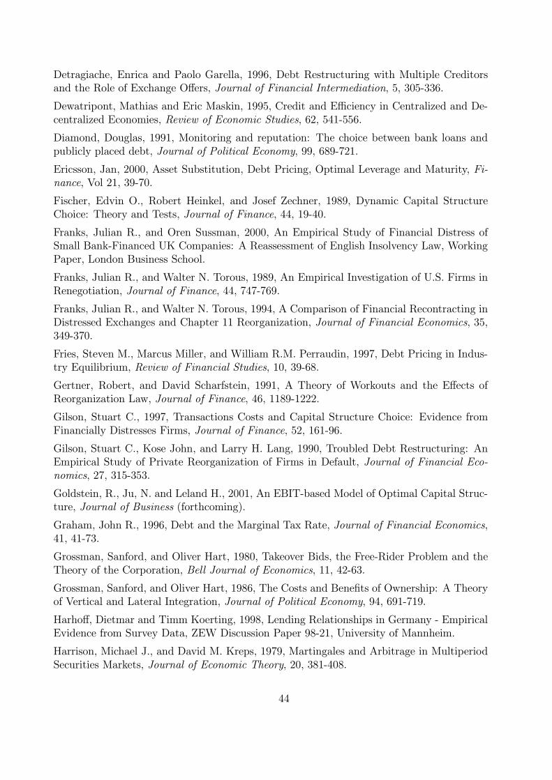
Detragiache, Enrica and Paolo Garella, 1996, Debt Restructuring with Multiple Creditorsand the Role of Exchange Offers, Journal of Financial Intermediation, 5, 305-336.

Dewatripont, Mathias and Eric Maskin, 1995, Credit and Efficiency in Centralized and De-centralized Economies, Review of Economic Studies, 62, 541-556.

Diamond, Douglas, 1991, Monitoring and reputation: The choice between bank loans andpublicly placed debt, Journal of Political Economy, 99, 689-721.

Ericsson, Jan, 2000, Asset Substitution, Debt Pricing, Optimal Leverage and Maturity, Fi-nance, Vol 21, 39-70.

Fischer, Edvin O., Robert Heinkel, and Josef Zechner, 1989, Dynamic Capital StructureChoice: Theory and Tests, Journal of Finance, 44, 19-40.

Franks, Julian R., and Oren Sussman, 2000, An Empirical Study of Financial Distress ofSmall Bank-Financed UK Companies: A Reassessment of English Insolvency Law, WorkingPaper, London Business School.

Franks, Julian R., and Walter N. Torous, 1989, An Empirical Investigation of U.S. Firms inRenegotiation, Journal of Finance, 44, 747-769.

Franks, Julian R., and Walter N. Torous, 1994, A Comparison of Financial Recontracting inDistressed Exchanges and Chapter 11 Reorganization, Journal of Financial Economics, 35,349-370.

Fries, Steven M., Marcus Miller, and William R.M. Perraudin, 1997, Debt Pricing in Indus-try Equilibrium, Review of Financial Studies, 10, 39-68.

Gertner, Robert, and David Scharfstein, 1991, A Theory of Workouts and the Effects ofReorganization Law, Journal of Finance, 46, 1189-1222.

Gilson, Stuart C., 1997, Transactions Costs and Capital Structure Choice: Evidence fromFinancially Distresses Firms, Journal of Finance, 52, 161-96.

Gilson, Stuart C., Kose John, and Larry H. Lang, 1990, Troubled Debt Restructuring: AnEmpirical Study of Private Reorganization of Firms in Default, Journal of Financial Eco-nomics, 27, 315-353.

Goldstein, R., Ju, N. and Leland H., 2001, An EBIT-based Model of Optimal Capital Struc-ture, Journal of Business (forthcoming).

Graham, John R., 1996, Debt and the Marginal Tax Rate, Journal of Financial Economics,41, 41-73.

Grossman, Sanford, and Oliver Hart, 1980, Takeover Bids, the Free-Rider Problem and theTheory of the Corporation, Bell Journal of Economics, 11, 42-63.

Grossman, Sanford, and Oliver Hart, 1986, The Costs and Benefits of Ownership: A Theoryof Vertical and Lateral Integration, Journal of Political Economy, 94, 691-719.

Harhoff, Dietmar and Timm Koerting, 1998, Lending Relationships in Germany - EmpiricalEvidence from Survey Data, ZEW Discussion Paper 98-21, University of Mannheim.

Harrison, Michael J., and David M. Kreps, 1979, Martingales and Arbitrage in MultiperiodSecurities Markets, Journal of Economic Theory, 20, 381-408.

44

Hart, Oliver, and John Moore, 1990, Property Rights and the Nature of the Firm, Journalof Political Economy, 98, 1119-1158.

Hege, Ulrich, 2002, Workouts, Court-Supervised Reorganization and the Choice betweenPrivate and Public Debt, Journal of Corporate Finance, forthcoming.

Helwege, Jean, 1999, How Long do Junk Bonds Spend in Default? Journal of Finance, 54,341-357.

Hotchkiss, Edith Shwalb, 1995, Postbankruptcy Performance and Management Turnover,Journal of Finance, 50, 3 - 22.

Houston, Joel and Christopher James, 1996, Bank information Monopolies and the Mix ofPrivate and Public Debt Claims, Journal of Finance, 51, 1863-1889.

James, Christopher M., 1995, Why Do Banks Take Equity in Debt Restructurings?, Reviewof Financial Studies, 8, 1209-1234.

James, Christopher M., 1996, Bank Debt Restructurings and the Composition of ExchangeOffers in Financial Distress, Journal of Finance, 51, 711-728.

Kahan, Marcel and Bruce Tuckman, 1993, Do Bondholders Lose form Junk Bond Covenants? Journal of Business, 66, 499-516.

Kandori, Michihiro, George Mailath and Rafael Rob, 1993, Learning, Mutation, and Long-Run Equilibria in Games, Econometrica, 61, 29-56.

Kim, In Joon, Krishna Ramaswamy, and Suresh Sundaresan, 1993, Does Default Risk inCoupons Affect the Valuation of Corporate Bonds?: A Contingent Claims Model, FinancialManagement, Autumn, 117-131.

Leland, Hayne E., 1994, Risky Debt, Bond Covenants and Optimal Capital Structure, Jour-nal of Finance, 49, 1213-1252.

Leland, Hayne E., 1998, Agency Costs, Risk Management, and Capital Structure, Journalof Finance, 53, 1213-1243.

Leland, Hayne E., and Klaus B. Toft, 1996, Optimal Capital Structure, Endogenous Bankruptcy,and the Term Structure of Credit Spreads, Journal of Finance, 51, 987-1019.

Longstaff, Francis A., and Eduardo S. Schwartz, 1995, A Simple Approach to Valuing Riskyand Floating Rate Debt, Journal of Finance 50, 789-819.

Mella-Barral, Pierre, 1999, The Dynamics of Default and Debt Reorganization, Review ofFinancial Studies, 12, 535-578.

Mella-Barral, Pierre, and William R.M. Perraudin, 1997, Strategic Debt Service, Journal ofFinance, 52, 531-556.

Mello, Antonio S., and John E. Parsons, 1992, The Agency Costs of Debt, Journal of Fi-nance, 47, 1887-1904. Merton, Robert C., 1974, On the Pricing of Corporate Debt: TheRisk Structure of Interest Rates, Journal of Finance 29, 449-470.

Miller, Merton H., 1977, Debt and Taxes, Journal of Finance, 32, 261-275.

Peterson, Lewis S., 1993, Who’s Being Greedy? A Theoretical and Empirical Examinationof Holdouts and Coercion in Debt Tender and Exchange Offers, Yale Law Journal, 103, 505-

45

535.

Rajan, Raghuram G., 1992, Insiders and Outsiders: The Choice between Informed and Arm’sLength Debt, Journal of Finance, 47, 1367-1400.

Roe Mark, 1987, The Voting Prohibition in Bond Workouts, The Yale Law Journal 97, 232-279.

Weiss, Lawrence A., 1990, Bankruptcy Resolution: Direct Costs and Violation of Priority ofClaims, Journal of Financial Economics, 27, 285-314.

46

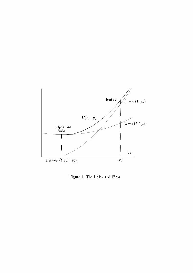
U(xt j y)

Entry

argmaxfU(xt j y)g

(1� �) �(xt)

xt

.........................

OptimalSale

...............................................................

(1� �)V �(xt)

x0

Figure 1: The Unlevered Firm

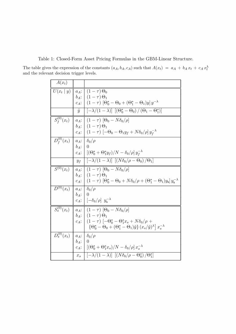
Table 1: Closed-Form Asset Pricing Formulas in the GBM-Linear Structure.

The table gives the expression of the constants (aA, bA, cA) such that A(xt) = aA + bA xt + cA xλt

and the relevant decision trigger levels.

A(xt)

U(xt | y) aA: (1− τ )Θ0

bA: (1− τ )Θ1

cA: (1− τ ) [Θ∗0 −Θ0 + (Θ∗1 −Θ1)y] y

−λ

y [−λ/(1− λ)] [(Θ∗0 −Θ0) / (Θ1 −Θ∗1)]

S(0)f (xt) aA: (1− τ ) [Θ0 −Nδ0/ρ]

bA: (1− τ )Θ1

cA: (1− τ ) [−Θ0 −Θ1yf +Nδ0/ρ] y−λf

D(0)f (xt) aA: δ0/ρ

bA: 0cA: [(Θ∗0 +Θ∗1yf)/N − δ0/ρ] y

−λf

yf [−λ/(1− λ)] [(Nδ0/ρ−Θ0) /Θ1]

S(0)(xt) aA: (1− τ ) [Θ0 −Nδ0/ρ]bA: (1− τ )Θ1

cA: (1− τ ) [Θ∗0 −Θ0 +Nδ0/ρ+ (Θ∗1 −Θ1)ys] y

−λs

D(0)(xt) aA: δ0/ρbA: 0cA: [−δ0/ρ] y−λs

S(0)s (xt) aA: (1− τ ) [Θ0 −Nδ0/ρ]

bA: (1− τ )Θ1

cA: (1− τ ) [−Θ∗0 −Θ∗1xs +Nδ0/ρ +{Θ∗0 −Θ0 + (Θ

∗1 −Θ1)y} (xs/y)λ

¤x−λs

D(0)s (xt) aA: δ0/ρ

bA: 0cA: [(Θ∗0 +Θ∗1xs)/N − δ0/ρ] x

−λs

xs [−λ/(1− λ)] [(Nδ0/ρ−Θ∗0) /Θ∗1]

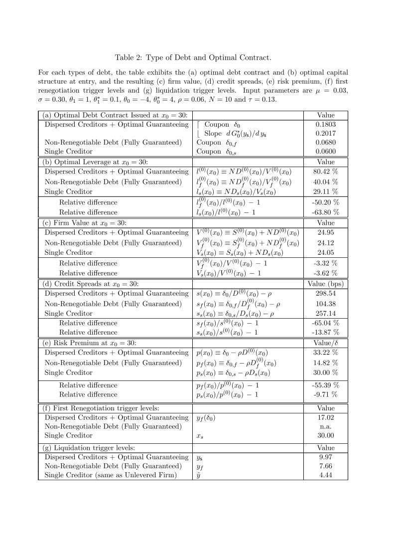
Table 2: Type of Debt and Optimal Contract.

For each types of debt, the table exhibits the (a) optimal debt contract and (b) optimal capitalstructure at entry, and the resulting (c) firm value, (d) credit spreads, (e) risk premium, (f) firstrenegotiation trigger levels and (g) liquidation trigger levels. Input parameters are µ = 0.03,σ = 0.30, θ1 = 1, θ

∗1 = 0.1, θ0 = −4, θ∗0 = 4, ρ = 0.06, N = 10 and τ = 0.13.

(a) Optimal Debt Contract Issued at x0 = 30: Value

Dispersed Creditors + Optimal Guaranteeing d Coupon δ0 0.1803b Slope dG∗0(ys)/d ys 0.2017

Non-Renegotiable Debt (Fully Guaranteed) Coupon δ0,f 0.0680Single Creditor Coupon δ0,s 0.0600

(b) Optimal Leverage at x0 = 30: Value

Dispersed Creditors + Optimal Guaranteeing l(0)(x0) ≡ ND(0)(x0)/V (0)(x0) 80.42 %

Non-Renegotiable Debt (Fully Guaranteed) l(0)f (x0) ≡ ND(0)f (x0)/V (0)f (x0) 40.04 %

Single Creditor ls(x0) ≡ NDs(x0)/Vs(x0) 29.11 %

Relative difference l(0)f (x0)/l

(0)(x0) − 1 -50.20 %

Relative difference ls(x0)/l(0)(x0) − 1 -63.80 %

(c) Firm Value at x0 = 30: Value

Dispersed Creditors + Optimal Guaranteeing V (0)(x0) ≡ S(0)(x0) +ND(0)(x0) 24.95

Non-Renegotiable Debt (Fully Guaranteed) V(0)f (x0) ≡ S(0)f (x0) +ND

(0)f (x0) 24.12

Single Creditor Vs(x0) ≡ Ss(x0) +NDs(x0) 24.05

Relative difference V(0)f (x0)/V

(0)(x0) − 1 -3.32 %

Relative difference Vs(x0)/V(0)(x0) − 1 -3.62 %

(d) Credit Spreads at x0 = 30: Value (bps)

Dispersed Creditors + Optimal Guaranteeing s(x0) ≡ δ0/D(0)(x0)− ρ 298.54

Non-Renegotiable Debt (Fully Guaranteed) sf (x0) ≡ δ0,f/D(0)f (x0)− ρ 104.38

Single Creditor ss(x0) ≡ δ0,s/Ds(x0)− ρ 257.14

Relative difference sf (x0)/s(0)(x0) − 1 -65.04 %

Relative difference ss(x0)/s(0)(x0) − 1 -13.87 %

(e) Risk Premium at x0 = 30: Value/δ

Dispersed Creditors + Optimal Guaranteeing p(x0) ≡ δ0 − ρD(0)(x0) 33.22 %

Non-Renegotiable Debt (Fully Guaranteed) pf (x0) ≡ δ0,f − ρD(0)f (x0) 14.82 %

Single Creditor ps(x0) ≡ δ0,s − ρDs(x0) 30.00 %

Relative difference pf (x0)/p(0)(x0) − 1 -55.39 %

Relative difference ps(x0)/p(0)(x0) − 1 -9.71 %

(f) First Renegotiation trigger levels: Value

Dispersed Creditors + Optimal Guaranteeing yf (δ0) 17.02Non-Renegotiable Debt (Fully Guaranteed) n.a.Single Creditor xs 30.00

(g) Liquidation trigger levels: Value

Dispersed Creditors + Optimal Guaranteeing ys 9.97Non-Renegotiable Debt (Fully Guaranteed) yf 7.66Single Creditor (same as Unlevered Firm) y 4.44