release 0.6.8 calliope contributors
TRANSCRIPT

Calliope DocumentationRelease 0.6.8
Calliope contributors
Mar 10, 2022


CONTENTS
1 User guide 31.1 Introduction . . . . . . . . . . . . . . . . . . . . . . . . . . . . . . . . . . . . . . . . . . . . . . . 31.2 Download and installation . . . . . . . . . . . . . . . . . . . . . . . . . . . . . . . . . . . . . . . . 51.3 Building a model . . . . . . . . . . . . . . . . . . . . . . . . . . . . . . . . . . . . . . . . . . . . . 71.4 Running a model . . . . . . . . . . . . . . . . . . . . . . . . . . . . . . . . . . . . . . . . . . . . . 151.5 Analysing a model . . . . . . . . . . . . . . . . . . . . . . . . . . . . . . . . . . . . . . . . . . . . 181.6 Tutorials . . . . . . . . . . . . . . . . . . . . . . . . . . . . . . . . . . . . . . . . . . . . . . . . . 211.7 Advanced constraints . . . . . . . . . . . . . . . . . . . . . . . . . . . . . . . . . . . . . . . . . . . 361.8 Advanced features . . . . . . . . . . . . . . . . . . . . . . . . . . . . . . . . . . . . . . . . . . . . 471.9 Configuration and defaults . . . . . . . . . . . . . . . . . . . . . . . . . . . . . . . . . . . . . . . . 551.10 Troubleshooting . . . . . . . . . . . . . . . . . . . . . . . . . . . . . . . . . . . . . . . . . . . . . 701.11 More info (reference) . . . . . . . . . . . . . . . . . . . . . . . . . . . . . . . . . . . . . . . . . . . 741.12 Development guide . . . . . . . . . . . . . . . . . . . . . . . . . . . . . . . . . . . . . . . . . . . . 112
2 API documentation 1192.1 API Documentation . . . . . . . . . . . . . . . . . . . . . . . . . . . . . . . . . . . . . . . . . . . 1192.2 Index . . . . . . . . . . . . . . . . . . . . . . . . . . . . . . . . . . . . . . . . . . . . . . . . . . . 126
3 Release history 1273.1 Release History . . . . . . . . . . . . . . . . . . . . . . . . . . . . . . . . . . . . . . . . . . . . . . 127
4 License 141
Bibliography 143
Python Module Index 145
Index 147
i

ii

Calliope Documentation, Release 0.6.8
v0.6.8 (Release history)
This is the documentation for version 0.6.8. See the main project website for contact details and other useful informa-tion.
Calliope focuses on flexibility, high spatial and temporal resolution, the ability to execute many runs based on the samebase model, and a clear separation of framework (code) and model (data). Its primary focus is on planning energysystems at scales ranging from urban districts to entire continents. In an optional operational mode it can also testa pre-defined system under different operational conditions. Calliope’s built-in tools allow interactive exploration ofresults:
A model based on Calliope consists of a collection of text files (in YAML and CSV formats) that define the technologies,locations and resource potentials. Calliope takes these files, constructs an optimisation problem, solves it, and reportsresults in the form of xarray Datasets which in turn can easily be converted into Pandas data structures, for easy analysiswith Calliope’s built-in tools or the standard Python data analysis stack.
Calliope is developed in the open on GitHub and contributions are very welcome (see the Development guide).
Key features of Calliope include:
• Model specification in an easy-to-read and machine-processable YAML format
• Generic technology definition allows modelling any mix of production, storage and consumption
• Resolved in space: define locations with individual resource potentials
• Resolved in time: read time series with arbitrary resolution
• Able to run on high-performance computing (HPC) clusters
• Uses a state-of-the-art Python toolchain based on Pyomo, xarray, and Pandas
• Freely available under the Apache 2.0 license
CONTENTS 1

Calliope Documentation, Release 0.6.8
2 CONTENTS

CHAPTER
ONE
USER GUIDE
1.1 Introduction
The basic process of modelling with Calliope is based on three steps:
1. Create a model from scratch or by adjusting an existing model (Building a model)
2. Run your model (Running a model)
3. Analyse and visualise model results (Analysing a model)
1.1.1 Energy system models
Energy system models allow analysts to form internally coherent scenarios of how energy is extracted, converted,transported, and used, and how these processes might change in the future. These models have been gaining renewedimportance as methods to help navigate the climate policy-driven transformation of the energy system.
Calliope is an attempt to design an energy system model from the ground of up with specific design goals in mind(see below). Therefore, the model approach and data format layout may be different from approaches used in othermodels. The design of the nodes approach used in Calliope was influenced by the power nodes modelling frameworkby [Heussen2010], but Calliope is different from traditional power system modelling tools, and does not provide featuressuch as power flow analysis.
Calliope was designed to address questions around the transition to renewable energy, so there are tools that are likelyto be more suitable for other types of questions. In particular, the following related energy modelling systems areavailable under open source or free software licenses:
• SWITCH: A power system model focused on renewables integration, using multi-stage stochastic linear optimi-sation, as well as hourly resource potential and demand data. Written in the commercial AMPL language andGPL-licensed [Fripp2012].
• Temoa: An energy system model with multi-stage stochastic optimisation functionality which can be de-ployed to computing clusters, to address parametric uncertainty. Written in Python/Pyomo and AGPL-licensed[Hunter2013].
• OSeMOSYS: A simplified energy system model similar to the MARKAL/TIMES model families, which canbe used as a stand-alone tool or integrated in the LEAP energy model. Written in GLPK, a free subset of thecommercial AMPL language, and Apache 2.0-licensed [Howells2011].
Additional energy models that are partially or fully open can be found on the Open Energy Modelling Initiative’s wiki.
3

Calliope Documentation, Release 0.6.8
1.1.2 Rationale
Calliope was designed with the following goals in mind:
• Designed from the ground up to analyze energy systems with high shares of renewable energy or other variablegeneration
• Formulated to allow arbitrary spatial and temporal resolution, and equipped with the necessary tools to deal withtime series input data
• Allow easy separation of model code and data, and modular extensibility of model code
• Make models easily modifiable, archiveable and auditable (e.g. in a Git repository), by using well-defined andhuman-readable text formats
• Simplify the definition and deployment of large numbers of model runs to high-performance computing clusters
• Able to run stand-alone from the command-line, but also provide an API for programmatic access and embeddingin larger analyses
• Be a first-class citizen of the Python world (installable with conda and pip, with properly documented and testedcode that mostly conforms to PEP8)
• Have a free and open-source code base under a permissive license
1.1.3 Acknowledgments
Development has been partially funded by several grants throughout throughout the years. We would particularly liketo acknowledge the following:
• The Grantham Institute at Imperial College London.
• the European Institute of Innovation & Technology’s Climate-KIC program.
• Engineering and Physical Sciences Research Council, reference number: EP/L016095/1.
• The Swiss Competence Center for Energy Research Supply of Electricity (SCCER SoE), contract number1155002546.
• Swiss Federal Office for Energy (SFOE), grant number SI/501768-01.
• European Research Council TRIPOD grant, grant agreement number 715132.
• The SENTINEL project of the European Union’s Horizon 2020 research and innovation programme under grantagreement No 837089.
1.1.4 License
Calliope is released under the Apache 2.0 license, which is a permissive open-source license much like the MIT orBSD licenses. This means that Calliope can be incorporated in both commercial and non-commercial projects.
Copyright since 2013 Calliope contributors listed in AUTHORS
Licensed under the Apache License, Version 2.0 (the "License");you may not use this file except in compliance with the License.You may obtain a copy of the License at
http://www.apache.org/licenses/LICENSE-2.0
(continues on next page)
4 Chapter 1. User guide

Calliope Documentation, Release 0.6.8
(continued from previous page)
Unless required by applicable law or agreed to in writing, softwaredistributed under the License is distributed on an "AS IS" BASIS,WITHOUT WARRANTIES OR CONDITIONS OF ANY KIND, either express or implied.See the License for the specific language governing permissions andlimitations under the License.
1.1.5 References
1.1.6 Citing Calliope in academic literature
Calliope is published in the Journal of Open Source Software. We encourage you to use this academic reference.
1.2 Download and installation
1.2.1 Requirements
Calliope has been tested on Linux, macOS, and Windows.
Running Calliope requires four things:
1. The Python programming language, version 3.7 or higher.
2. A number of Python add-on modules (see below for the complete list).
3. A solver: Calliope has been tested with CBC, GLPK, Gurobi, and CPLEX. Any other solver that is compatiblewith Pyomo should also work.
4. The Calliope software itself.
1.2.2 Recommended installation method
The easiest way to get a working Calliope installation is to use the free conda package manager, which can install allof the four things described above in a single step.
To get conda, download and install the “Miniconda” distribution for your operating system (using the version forPython 3).
With Miniconda installed, you can create a new environment called "calliope" with all the necessary modules,including the free and open source GLPK solver, by running the following command in a terminal or command-linewindow
$ conda create -c conda-forge -n calliope calliope
To use Calliope, you need to activate the calliope environment each time
$ conda activate calliope
You are now ready to use Calliope together with the free and open source GLPK solver. However, we recommend tonot use this solver where possible, since it performs relatively poorly (both in solution time and stability of result).Indeed, our example models use the free and open source CBC solver instead, but installing it on Windows requires anextra step. Read the next section for more information on installing alternative solvers.
1.2. Download and installation 5

Calliope Documentation, Release 0.6.8
1.2.3 Updating an existing installation
If following the recommended installation method above, the following command, assuming the conda environment isactive, will update Calliope to the newest version
$ conda update -c conda-forge calliope
1.2.4 Solvers
You need at least one of the solvers supported by Pyomo installed. CBC (open-source) or Gurobi (commercial) arerecommended for large problems, and have been confirmed to work with Calliope. Refer to the documentation of yoursolver on how to install it.
CBC
CBC is our recommended option if you want a free and open-source solver. CBC can be installed via conda on Linuxand macOS by running `conda install -c conda-forge coincbc`. Windows binary packages are somewhatmore difficult to install, due to limited information on the CBC website, but can be found within their list of binaries.We recommend you download the relevant binary for CBC 2.10 and add cbc.exe to a directory known to PATH (e.g.an Anaconda environment ‘bin’ directory).
GLPK
GLPK is free and open-source, but can take too much time and/or too much memory on larger problems. If using therecommended installation approach above, GLPK is already installed in the calliope environment. To install GLPKmanually, refer to the GLPK website.
Gurobi
Gurobi is commercial but significantly faster than CBC and GLPK, which is relevant for larger problems. It needs alicense to work, which can be obtained for free for academic use by creating an account on gurobi.com.
While Gurobi can be installed via conda (conda install -c gurobi gurobi) we recommend downloading andinstalling the installer from the Gurobi website, as the conda package has repeatedly shown various issues.
After installing, log on to the Gurobi website and obtain a (free academic or paid commercial) license, then activate iton your system via the instructions given online (using the grbgetkey command).
CPLEX
Another commercial alternative is CPLEX. IBM offer academic licenses for CPLEX. Refer to the IBM website fordetails.
6 Chapter 1. User guide

Calliope Documentation, Release 0.6.8
1.2.5 Python module requirements
Refer to requirements/base.yml in the Calliope repository for a full and up-to-date listing of required third-party pack-ages.
Some of the key packages Calliope relies on are:
• Pyomo
• Pandas
• Xarray
• Plotly
• Jupyter (optional, but highly recommended, and used for the example notebooks in the tutorials)
1.3 Building a model
In short, a Calliope model works like this: supply technologies can take a resource from outside of the modeledsystem and turn it into a specific energy carrier in the system. The model specifies one or more locations along withthe technologies allowed at those locations. Transmission technologies can move energy of the same carrier from onelocation to another, while conversion technologies can convert one carrier into another at the same location. Demandtechnologies remove energy from the system, while storage technologies can store energy at a specific location. Puttingall of these possibilities together allows a modeller to specify as simple or as complex a model as necessary to answera given research question.
In more technical terms, Calliope allows a modeller to define technologies with arbitrary characteristics by “inher-iting” basic traits from a number of included base tech groups – supply, supply_plus, demand, conversion,conversion_plus, and transmission. These groups are described in more detail in Abstract base technologygroups.
1.3.1 Terminology
The terminology defined here is used throughout the documentation and the model code and configuration files:
• Technology: a technology that produces, consumes, converts or transports energy
• Location: a site which can contain multiple technologies and which may contain other locations for energybalancing purposes
• Resource: a source or sink of energy that can (or must) be used by a technology to introduce into or removeenergy from the system
• Carrier: an energy carrier that groups technologies together into the same network, for example electricityor heat.
As more generally in constrained optimisation, the following terms are also used:
• Parameter: a fixed coefficient that enters into model equations
• Variable: a variable coefficient (decision variable) that enters into model equations
• Set: an index in the algebraic formulation of the equations
• Constraint: an equality or inequality expression that constrains one or several variables
1.3. Building a model 7

Calliope Documentation, Release 0.6.8
1.3.2 Files that define a model
Calliope models are defined through YAML files, which are both human-readable and computer-readable, and CSVfiles (a simple tabular format) for time series data.
It makes sense to collect all files belonging to a model inside a single model directory. The layout of that directorytypically looks roughly like this (+ denotes directories, - files):
+ example_model+ model_config
- locations.yaml- techs.yaml
+ timeseries_data- solar_resource.csv- electricity_demand.csv
- model.yaml- scenarios.yaml
In the above example, the files model.yaml, locations.yaml and techs.yaml together are the model definition.This definition could be in one file, but it is more readable when split into multiple. We use the above layout in theexample models and in our research!
Inside the timeseries_data directory, timeseries are stored as CSV files. The location of this directory can bespecified in the model configuration, e.g. in model.yaml.
Note: The easiest way to create a new model is to use the calliope new command, which makes a copy of one ofthe built-in examples models:
$ calliope new my_new_model
This creates a new directory, my_new_model, in the current working directory.
By default, calliope new uses the national-scale example model as a template. To use a different template, you canspecify the example model to use, e.g.: --template=urban_scale.
See also:
YAML configuration file format, Built-in example models, Time series data
1.3.3 Model configuration (model)
The model configuration specifies all aspects of the model to run. It is structured into several top-level headings (keysin the YAML file): model, techs, locations, links, and run. We will discuss each of these in turn, starting withmodel:
model:name: 'My energy model'timeseries_data_path: 'timeseries_data'reserve_margin:
power: 0subset_time: ['2005-01-01', '2005-01-05']
Besides the model’s name (name) and the path for CSV time series data (timeseries_data_path), group constraintscan be set, like reserve_margin.
8 Chapter 1. User guide

Calliope Documentation, Release 0.6.8
To speed up model runs, the above example specifies a time subset to run the model over only five days of time series data(subset_time: [‘2005-01-01’, ‘2005-01-05’])– this is entirely optional. Usually, a full model will containat least one year of data, but subsetting time can be useful to speed up a model for testing purposes.
See also:
National scale example model, Model configuration
1.3.4 Technologies (techs)
The techs section in the model configuration specifies all of the model’s technologies. In our current example, this isin a separate file, model_config/techs.yaml, which is imported into the main model.yaml file alongside the filefor locations described further below:
import:- 'model_config/techs.yaml'- 'model_config/locations.yaml'
Note: The import statement can specify a list of paths to additional files to import (the imported files, in turn, mayinclude further files, so arbitrary degrees of nested configurations are possible). The import statement can either givean absolute path or a path relative to the importing file.
The following example shows the definition of a ccgt technology, i.e. a combined cycle gas turbine that deliverselectricity:
ccgt:essentials:
name: 'Combined cycle gas turbine'color: '#FDC97D'parent: supplycarrier_out: power
constraints:resource: infenergy_eff: 0.5energy_cap_max: 40000 # kWenergy_cap_max_systemwide: 100000 # kWenergy_ramping: 0.8lifetime: 25
costs:monetary:
interest_rate: 0.10energy_cap: 750 # USD per kWom_con: 0.02 # USD per kWh
Each technology must specify some essentials, most importantly a name, the abstract base technology it is inheritingfrom (parent), and its energy carrier (carrier_out in the case of a supply technology). Specifying a color isoptional but useful for using the built-in visualisation tools (see Analysing a model).
The constraints section gives all constraints for the technology, such as allowed capacities, conversion efficiencies,the life time (used in levelised cost calculations), and the resource it consumes (in the above example, the resource isset to infinite via inf).
The costs section gives costs for the technology. Calliope uses the concept of “cost classes” to allow accounting formore than just monetary costs. The above example specifies only the monetary cost class, but any number of other
1.3. Building a model 9

Calliope Documentation, Release 0.6.8
classes could be used, for example co2 to account for emissions. Additional cost classes can be created simply byadding them to the definition of costs for a technology.
By default, only the monetary cost class is used in the objective function, i.e., the default objective is to minimize totalcosts.
Multiple cost classes can be considered in the objective by setting the cost_class key. It must be a dictionary of costclasses and their weights in the objective, e.g. objective_options: {‘cost_class’: {‘monetary’: 1,‘emissions’: 0.1}}. In this example, monetary costs are summed as usual and emissions are added to this, scaledby 0.1 (emulating a carbon price).
To use a different sense (minimize/maximize) you can set sense: objective_options: {‘cost_class’: ...,‘sense’: ‘minimize’}.
To use a single alternative cost class, disabling the consideration of the default monetary, set the weight of themonetary cost class to zero to stop considering it and the weight of another cost class to a non-zero value, e.g.objective_options: {‘cost_class’: {‘monetary’: 0, ‘emissions’: 1}}.
See also:
Per-tech constraints, Per-tech costs, tutorials, built-in examples
Allowing for unmet demand
For a model to find a feasible solution, supply must always be able to meet demand. To avoid the solver failing to finda solution, you can ensure feasibility:
run:ensure_feasibility: true
This will create an unmet_demand decision variable in the optimisation, which can pick up any mismatch betweensupply and demand, across all energy carriers. It has a very high cost associated with its use, so it will only appearwhen absolutely necessary.
Note: When ensuring feasibility, you can also set a big M value (run.bigM). This is the “cost” of unmet demand. Itis possible to make model convergence very slow if bigM is set too high. default bigM is 1x10 9, but should be closeto the maximum total system cost that you can imagine. This is perhaps closer to 1x10 6 for urban scale models.
1.3.5 Time series data
For parameters that vary in time, time series data can be added to a model in two ways:
• by reading in CSV files
• by passing pandas dataframes as arguments in calliope.Model called from a python session.
Reading in CSV files is possible from both the command-line tool as well running interactively with python (seeRunning a model for details). However, passing dataframes as arguments in calliope.Model is possible only whenrunning from a python session.
10 Chapter 1. User guide

Calliope Documentation, Release 0.6.8
Reading in CSV files
To read in CSV files, specify resource: file=filename.csv to pick the desired CSV file from within the config-ured timeseries data path (model.timeseries_data_path).
By default, Calliope looks for a column in the CSV file with the same name as the location. It is also possible to specifya column to use when setting resource per location, by giving the column name with a colon following the filename:resource: file=filename.csv:column
For example, a simple photovoltaic (PV) tech using a time series of hour-by-hour electricity generation data might looklike this:
pv:essentials:
name: 'Rooftop PV'color: '#B59C2B'parent: supplycarrier_out: power
constraints:resource: file=pv_resource.csvenergy_cap_max: 10000 # kW
By default, Calliope expects time series data in a model to be indexed by ISO 8601 compatible time stampsin the format YYYY-MM-DD hh:mm:ss, e.g. 2005-01-01 00:00:00. This can be changed by setting model.timeseries_dateformat based on strftime` directives <http://strftime.org/>`_, which defaultsto ``'%Y-%m-%d %H:%M:%S'.
For example, the first few lines of a CSV file, called pv_resource.csv giving a resource potential for two locationsmight look like this, with the first column in the file always being read as the date-time index:
,location1,location22005-01-01 00:00:00,0,02005-01-01 01:00:00,0,112005-01-01 02:00:00,0,182005-01-01 03:00:00,0,492005-01-01 04:00:00,11,1102005-01-01 05:00:00,45,3002005-01-01 06:00:00,90,458
Reading in timeseries from pandas dataframes
When running models from python scripts or shells, it is also possible to pass timeseries directly as pandas dataframes.This is done by specifying resource: df=tskey where tskey is the key in a dictionary containing the relevantdataframes. For example, if the same timeseries as above is to be passed, a dataframe called pv_resource may be inthe python namespace:
pv_resource
t location1 location22005-01-01 00:00:00 0 02005-01-01 01:00:00 0 112005-01-01 02:00:00 0 182005-01-01 03:00:00 0 492005-01-01 04:00:00 11 110
(continues on next page)
1.3. Building a model 11

Calliope Documentation, Release 0.6.8
(continued from previous page)
2005-01-01 05:00:00 45 3002005-01-01 06:00:00 90 458
To pass this timeseries into the model, create a dictionary, called timeseries_dataframes here, containing all rele-vant timeseries identified by their tskey. In this case, this has only one key, called pv_resource:
timeseries_dataframes = {'pv_resource': pv_resource}
The keys in this dictionary must match the tskey specified in the YAML files. In this example, specifying resource:df=pv_resource will identify the pv_resource key in timeseries_dataframes. All relevant timeseries must beput in this dictionary. For example, if a model contains three timeseries referred to in the configuration YAML files,called demand_1, demand_2 and pv_resource, the timeseries_dataframes dictionary may look like
timeseries_dataframes = {'demand_1': demand_1,'demand_2': demand_2,'pv_resource': pv_resource}
where demand_1, demand_2 and pv_resource are dataframes of the relevant timeseries. Thetimeseries_dataframes can then be called in calliope.Model:
model = calliope.Model('model.yaml', timeseries_dataframes=timeseries_dataframes)
Just like when using CSV files (see above), Calliope looks for a column in the dataframe with the same name as thelocation. It is also possible to specify a column to use when setting resource per location, by giving the column namewith a colon following the filename: resource: df=tskey:column.
The time series index must be ISO 8601 compatible time stamps and can be a standard pandas DateTimeIndex (seediscussion above).
Note:
• If a parameter is not explicit in time and space, it can be specified as a single value in the model definition (or,using location-specific definitions, be made spatially explicit). This applies both to parameters that never varythrough time (for example, cost of installed capacity) and for those that may be time-varying (for example, atechnology’s available resource). However, each model must contain at least one time series.
• Only the subset of parameters listed in file_allowed in the model configuration can be loaded from file ordataframe in this way. It is advised not to update this default list unless you are developing the core code,since the model will likely behave unexpectedly.
• You _cannot_ have a space around the = symbol when pointing to a timeseries file or dataframe key, i.e.resource: file = filename.csv is not valid.
• If running from a command line interface (see Running a model), timeseries must be read from CSV and cannotbe passed from dataframes via df=....
• It’s possible to mix reading in from CSVs and dataframes, by setting some config values as file=... and someas df=....
• The default value of timeseries_dataframes is None, so if you want to read all timeseries in from CSVs, youcan omit this argument. When running from command line, this is done automatically.
12 Chapter 1. User guide

Calliope Documentation, Release 0.6.8
1.3.6 Locations and links (locations, links)
A model can specify any number of locations. These locations are linked together by transmission technologies. Byconsuming an energy carrier in one location and outputting it in another, linked location, transmission technologiesallow resources to be drawn from the system at a different location from where they are brought into it.
The locations section specifies each location:
locations:region1:
coordinates: {lat: 40, lon: -2}techs:
unmet_demand_power:demand_power:ccgt:
constraints:energy_cap_max: 30000
Locations can optionally specify coordinates (used in visualisation or to compute distance between them) and mustspecify techs allowed at that location. As seen in the example above, each allowed tech must be listed, and canoptionally specify additional location-specific parameters (constraints or costs). If given, location-specific parameterssupersede any group constraints a technology defines in the techs section for that location.
The links section specifies possible transmission links between locations in the form location1,location2:
links:region1,region2:
techs:ac_transmission:
constraints:energy_cap_max: 10000
costs.monetary:energy_cap: 100
In the above example, an high-voltage AC transmission line is specified to connect region1 with region2. For thisto work, a transmission technology called ac_transmission must have previously been defined in the model’stechs section. There, it can be given group constraints or costs. As in the case of locations, the links section canspecify per-link parameters (constraints or costs) that supersede any model-wide parameters.
The modeller can also specify a distance for each link, and use per-distance constraints and costs for transmissiontechnologies.
See also:
Per-tech constraints, Per-tech costs.
1.3.7 Run configuration (run)
The only required setting in the run configuration is the solver to use:
run:solver: cbcmode: plan
the most important parts of the run section are solver and mode. A model can run in planning mode (plan), op-erational mode (operate), or SPORES mode (spores). In planning mode, capacities are determined by the model,
1.3. Building a model 13

Calliope Documentation, Release 0.6.8
whereas in operational mode, capacities are fixed and the system is operated with a receding horizon control algorithm.In SPORES mode, the model is first run in planning mode, then run N number of times to find alternative systemconfigurations with similar monetary cost, but maximally different choice of technology capacity and location.
Possible options for solver include glpk, gurobi, cplex, and cbc. The interface to these solvers is done through thePyomo library. Any solver compatible with Pyomo should work with Calliope.
For solvers with which Pyomo provides more than one way to interface, the additional solver_io option can be used.In the case of Gurobi, for example, it is usually fastest to use the direct Python interface:
run:solver: gurobisolver_io: python
Note: The opposite is currently true for CPLEX, which runs faster with the default solver_io.
Further optional settings, including debug settings, can be specified in the run configuration.
See also:
Run configuration, Troubleshooting, Specifying custom solver options, documentation on operational mode, documen-tation on SPORES mode.
1.3.8 Scenarios and overrides
To make it easier to run a given model multiple times with slightly changed settings or constraints, for example, varyingthe cost of a key technology, it is possible to define and apply scenarios and overrides. “Overrides” are blocks of YAMLthat specify configurations that expand or override parts of the base model. “Scenarios” are combinations of any numberof such overrides. Both are specified at the top level of the model configuration, as in this example model.yaml file:
scenarios:high_cost_2005: ["high_cost", "year2005"]high_cost_2006: ["high_cost", "year2006"]
overrides:high_cost:
techs.onshore_wind.costs.monetary.energy_cap: 2000year2005:
model.subset_time: ['2005-01-01', '2005-12-31']year2006:
model.subset_time: ['2006-01-01', '2006-12-31']
model:...
run:...
Each override is given by a name (e.g. high_cost) and any number of model settings – anything in the model configu-ration can be overridden by an override. In the above example, one override defines higher costs for an onshore_windtech while the two other overrides specify different time subsets, so would run an otherwise identical model over twodifferent periods of time series data.
14 Chapter 1. User guide

Calliope Documentation, Release 0.6.8
One or several overrides can be applied when running a model, as described in Running a model. Overrides can alsobe combined into scenarios to make applying them at run-time easier. Scenarios consist of a name and a list of overridenames which together form that scenario.
Scenarios and overrides can be used to generate scripts that run a single Calliope model many times, either sequentially,or in parallel on a high-performance cluster (see Generating scripts to run a model many times).
Note: Overrides can also import other files. This can be useful if many overrides are defined which share large partsof model configuration, such as different levels of interconnection between model zones. See Importing other YAMLfiles in overrides for details.
See also:
Generating scripts to run a model many times, Importing other YAML files in overrides
1.4 Running a model
There are essentially three ways to run a Calliope model:
1. With the calliope run command-line tool.
2. By programmatically creating and running a model from within other Python code, or in an interactive Pythonsession.
3. By generating and then executing scripts with the calliope generate_runs command-line tool, which isprimarily designed for running many scenarios on a high-performance cluster.
1.4.1 Running with the command-line tool
We can easily run a model after creating it (see Building a model), saving results to a single NetCDF file for furtherprocessing
$ calliope run testmodel/model.yaml --save_netcdf=results.nc
The calliope run command takes the following options:
• --save_netcdf={filename.nc}: Save complete model, including results, to the given NetCDF file. This isthe recommended way to save model input and output data into a single file, as it preserves all data fully, andallows later reconstruction of the Calliope model for further analysis.
• --save_csv={directory name}: Save results as a set of CSV files to the given directory. This can be handyif the modeler needs results in a simple text-based format for further processing with a tool like Microsoft Excel.
• --save_plots={filename.html}: Save interactive plots to the given HTML file (see Analysing a model forfurther details on the plotting functionality).
• --debug: Run in debug mode, which prints more internal information, and is useful when troubleshooting failingmodels.
• --scenario={scenario} and --override_dict={yaml_string}: Specify a scenario, or one or severaloverrides, to apply to the model, or apply specific overrides from a YAML string (see below for more information)
• --help: Show all available options.
Multiple options can be specified, for example, saving NetCDF, CSV, and HTML plots simultaneously
1.4. Running a model 15

Calliope Documentation, Release 0.6.8
$ calliope run testmodel/model.yaml --save_netcdf=results.nc --save_→˓csv=outputs --save_plots=plots.html
Warning: Unlike in versions prior to 0.6.0, the command-line tool in Calliope 0.6.0 and upward does not saveresults by default – the modeller must specify one of the -save options.
Applying a scenario or override
The --scenario can be used in three different ways:
• It can be given the name of a scenario defined in the model configuration, as in --scenario=my_scenario
• It can be given the name of a single override defined in the model configuration, as in--scenario=my_override
• It can be given a comma-separated string of several overrides defined in the model configuration, as in--scenario=my_override_1,my_override_2
In the latter two cases, the given override(s) is used to implicitly create a “scenario” on-the-fly when running the model.This allows quick experimentation with different overrides without explicitly defining a scenario combining them.
Assuming we have specified an override called milp in our model configuration, we can apply it to our model with
$ calliope run testmodel/model.yaml --scenario=milp --save_netcdf=results.nc
Note that if both a scenario and an override with the same name, such as milp in the above example, exist, Calliopewill raise an error, as it will not be clear which one the user wishes to apply.
It is also possible to use the –override_dict option to pass a YAML string that will be applied after anything appliedthrough --scenario
$ calliope run testmodel/model.yaml --override_dict="{'model.subset_time': [→˓'2005-01-01', '2005-01-31']}" --save_netcdf=results.nc
See also:
Analysing a model, Scenarios and overrides
1.4.2 Running interactively with Python
The most basic way to run a model programmatically from within a Python interpreter is to create a Model instancewith a given model.yaml configuration file, and then call its run() method:
import calliopemodel = calliope.Model('path/to/model.yaml')model.run()
Note: If config is not specified (i.e. model = Model()), an error is raised. See Built-in example models forinformation on instantiating a simple example model without specifying a custom model configuration.
Other ways to load a model interactively are:
16 Chapter 1. User guide

Calliope Documentation, Release 0.6.8
• Passing an AttrDict or standard Python dictionary to the Model constructor, with the same nested format asthe YAML model configuration (top-level keys: model, run, locations, techs).
• Loading a previously saved model from a NetCDF file with model = calliope.read_netcdf(‘path/to/saved_model.nc’). This can either be a pre-processed model saved before its run method was called, whichwill include input data only, or a completely solved model, which will include input and result data.
After instantiating the Model object, and before calling the run() method, it is possible to manually inspect and adjustthe configuration of the model. The pre-processed inputs are all held in the xarray Dataset model.inputs.
After the model has been solved, an xarray Dataset containing results (model.results) can be accessed. At this point,the model can be saved with either to_csv() or to_netcdf(), which saves all inputs and results, and is equivalent tothe corresponding --save options of the command-line tool.
See also:
An example of interactive running in a Python session, which also demonstrates some of the analysis possibilities afterrunning a model, is given in the tutorials. You can download and run the embedded notebooks on your own machine(if both Calliope and the Jupyter Notebook are installed).
Scenarios and overrides
There are two ways to override a base model when running interactively, analogously to the use of the command-linetool (see Applying a scenario or override above):
1. By setting the scenario argument, e.g.:
model = calliope.Model('model.yaml', scenario='milp')
2. By passing the override_dict argument, which is a Python dictionary, an AttrDict, or a YAML string of over-rides:
model = calliope.Model('model.yaml',override_dict={'run.solver': 'gurobi'}
)
Note: Both scenario and override_dict can be defined at once. They will be applied in order, such that scenarios areapplied first, followed by dictionary overrides. As such, the override_dict can be used to override scenarios.
Tracking progress
When running Calliope in the command line, logging of model pre-processing and solving occurs automatically.Interactively, for example in a Jupyter notebook, you can enable verbose logging by setting the log level usingcalliope.set_log_verbosity(level) immediately after importing the Calliope package. By default, calliope.set_log_verbosity() also sets the log level for the backend model to DEBUG, which turns on output of solver out-put. This can be disabled by calliope.set_log_verbosity(level, include_solver_output=False). Possi-ble log levels are (from least to most verbose):
1. CRITICAL: only show critical errors.
2. ERROR: only show errors.
3. WARNING: show errors and warnings (default level).
1.4. Running a model 17

Calliope Documentation, Release 0.6.8
4. INFO: show errors, warnings, and informative messages. Calliope uses the INFO level to show a message ateach stage of pre-processing, sending the model to the solver, and post-processing, including timestamps.
5. DEBUG: SOLVER logging, with heavily verbose logging of a number of function outputs. Only for use whentroubleshooting failing runs or developing new functionality in Calliope.
1.4.3 Generating scripts for many model runs
Scripts to simplify the creation and execution of a large number of Calliope model runs are generated with the calliopegenerate_runs command-line tool. More detail on this is available in Generating scripts to run a model many times.
1.4.4 Improving solution times
Large models will take time to solve. The easiest is often to just let a model run on a remote device (another computer,or a high performance computing cluster) and forget about it until it is done. However, if you need results now, thereare ways to improve solution time.
Details on strategies to improve solution times are given in Troubleshooting.
1.4.5 Debugging failing runs
What will typically go wrong, in order of decreasing likelihood:
• The model is improperly defined or missing data. Calliope will attempt to diagnose some common errors andraise an appropriate error message.
• The model is consistent and properly defined but infeasible. Calliope will be able to construct the model andpass it on to the solver, but the solver (after a potentially long time) will abort with a message stating that themodel is infeasible.
• There is a bug in Calliope causing the model to crash either before being passed to the solver, or after the solverhas completed and when results are passed back to Calliope.
Calliope provides help in diagnosing all of these model issues. For details, see Troubleshooting.
1.5 Analysing a model
Calliope inputs and results are designed for easy handling. Whatever software you prefer to use for data processing,either the NetCDF or CSV output options should provide a path to importing your Calliope results. If you prefer to notworry about writing your own scripts, then we have that covered too! The built-in plotting functions in plot are builton Plotly’s interactive visualisation tools to bring your data to life.
1.5.1 Accessing model data and results
A model which solved successfully has two primary Datasets with data of interest:
• model.inputs: contains all input data, such as renewable resource capacity factors
• model.results: contains all results data, such as dispatch decisions and installed capacities
In both of these, variables are indexed over concatenated sets of locations and technologies, over a dimension we callloc_techs. For example, if a technology called boiler only exists in location X1 and not in locations X2 or X3,then it will have a single entry in the loc_techs dimension called X1::boiler. For parameters which also consider
18 Chapter 1. User guide

Calliope Documentation, Release 0.6.8
different energy carriers, we use a loc_tech_carrier dimension, such that we would have, in the case of the priorboiler example, X1::boiler::heat.
This concatenated set formulation is memory-efficient but cumbersome to deal with, so the model.get_formatted_array(name_of_variable) function can be used to retrieve a DataArray indexed over separatedimensions (any of techs, locs, carriers, costs, timesteps, depending on the desired variable).
Note: On saving to CSV (see the command-line interface documentation), all variables are saved to a single file each,which are always indexed over all dimensions rather than just the concatenated dimensions.
1.5.2 Visualising results
In an interactive Python session, there are four primary visualisation functions: capacity, timeseries,transmission, and summary. To gain access to result visualisation without the need to interact with Python, thesummary plot can also be accessed from the command line interface (see below).
Refer to the API documentation for the analysis module for an overview of available analysis functionality.
Refer to the tutorials for some basic analysis techniques.
Plotting time series
The following example shows a timeseries plot of the built-in urban scale example model:
In Python, we get this function by calling model.plot.timeseries(). It includes all relevant timeseries information,from both inputs and results. We can force it to only have particular results in the dropdown menu:
# Only inputs or only resultsmodel.plot.timeseries(array='inputs')model.plot.timeseries(array='results')
# Only consumed resourcemodel.plot.timeseries(array='resource_con')
# Only consumed resource and 'power' carrier flowmodel.plot.timeseries(array=['power', 'resource_con'])
The data used to build the plots can also be subset and ordered by using the subset argument. This uses xarray’s ‘loc’indexing functionality to access subsets of data:
# Only show region1 data (rather than the default, which is a sum of all locations)model.plot.timeseries(subset={'locs': ['region1']})
# Only show a subset of technologiesmodel.plot.timeseries(subset={'techs': ['ccgt', 'csp']})
# Assuming our model has three techs, 'ccgt', 'csp', and 'battery',# specifying `subset` lets us order them in the stacked barchartmodel.plot.timeseries(subset={'techs': ['ccgt', 'battery', 'csp']})
When aggregating model timesteps with clustering methods, the timeseries plots are adjusted accordingly (examplefrom the built-in time_clustering example model):
1.5. Analysing a model 19

Calliope Documentation, Release 0.6.8
See also:
API documentation for the analysis module
Plotting capacities
The following example shows a capacity plot of the built-in urban scale example model:
Functionality is similar to timeseries, this time called by model.plot.capacity(). Here we show capacity limits setat input and chosen capacities at output. Choosing dropdowns and subsetting works in the same way as for timeseriesplots
Plotting transmission
The following example shows a transmission plot of the built-in urban scale example model:
By calling model.plot.transmission() you will see installed links, their capacities (on hover), and the locationsof the nodes. This functionality only works if you have physically pinpointed your locations using the coordinateskey for your location.
The above plot uses Mapbox to overlay our transmission plot on Openstreetmap. By creating an account at Mapboxand acquiring a Mapbox access token, you can also create similar visualisations by giving the token to the plottingfunction: model.plot.transmission(mapbox_access_token=’your token here’).
Without the token, the plot will fall back on simple country-level outlines. In this urban scale example, the backgroundis thus just grey (zoom out to see the UK!):
Note: If the coordinates were in x and y, not lat and lon, the transmission trace would be given on a cartesian plot.
Plotting flows
The following example shows an energy flow plot of the built-in urban scale example model:
By calling model.plot.flows() you will see a plot similar to transmission. However, you can see carrier productionat each node and along links, at every timestep (controlled by moving a slider). This functionality only works if youhave physically pinpointed your locations using the coordinates key for your location. It is possible to look at onlya subset of the timesteps in the model using the timestep_index_subset argument, or to show only every X timestep(where X is an integer) using the timestep_cycle argument.
Note: If the timestep dimension is particularly large in your model, you will find this visualisation to be slow. Timesubsetting is recommended for such a case.
If you cannot see the carrier production for a technology on hovering, it is likely masked by another technology at thesame location or on the same link. Hide the masking technology to get the hover info for the technology below.
20 Chapter 1. User guide

Calliope Documentation, Release 0.6.8
Summary plots
If you want all the data in one place, you can run model.plot.summary(to_file=’path/to/file.html’), whichwill build a HTML file of all the interactive plots (maintaining the interactivity) and save it to ‘path/to/file.html’. ThisHTML file can be opened in a web browser to show all the plots. This funcionality is made available in the commandline interface by using the command --save_plots=filename.html when running the model.
See an example of such a HTML plot here.
See also:
Running with the command-line tool
Saving publication-quality SVG figures
On calling any of the three primary plotting functions, you can also set to_file=path/to/file.svg for a highquality vector graphic to be saved. This file can be prepared for publication in programs like Inkscape.
Note: For similar results in the command line interface, you’ll currently need to save your model to netcdf(--save_netcdf={filename.nc}) then load it into a Calliope Model object in Python. Once there, you can usethe above functions to get your SVGs.
1.5.3 Reading solutions
Calliope provides functionality to read a previously-saved model from a single NetCDF file:
solved_model = calliope.read_netcdf('my_saved_model.nc')
In the above example, the model’s input data will be available under solved_model.inputs, while the results (if themodel had previously been solved) are available under solved_model.results.
Both of these are xarray.Datasets and can be further processed with Python.
See also:
The xarray documentation should be consulted for further information on dealing with Datasets. Calliope’s NetCDFfiles follow the CF conventions and can easily be processed with any other tool that can deal with NetCDF.
1.6 Tutorials
The tutorials are based on the built-in example models, they explain the key steps necessary to set up and run simplemodels. Refer to the other parts of the documentation for more detailed information on configuring and running morecomplex models. The built-in examples are simple on purpose, to show the key components of a Calliope model withwhich models of arbitrary complexity can be built.
The first tutorial builds a model for part of a national grid, exhibiting the following Calliope functionality:
• Use of supply, supply_plus, demand, storage and transmission technologies
• Nested locations
• Multiple cost types
The second tutorial builds a model for part of a district network, exhibiting the following Calliope functionality:
1.6. Tutorials 21

Calliope Documentation, Release 0.6.8
• Use of supply, demand, conversion, conversion_plus, and transmission technologies
• Use of multiple energy carriers
• Revenue generation, by carrier export
The third tutorial extends the second tutorial, exhibiting binary and integer decision variable functionality (extendedan LP model to a MILP model)
1.6.1 Tutorial 1: national scale
This example consists of two possible power supply technologies, a power demand at two locations, the possibility forbattery storage at one of the locations, and a transmission technology linking the two. The diagram below gives anoverview:
Fig. 1: Overview of the built-in national-scale example model
Supply-side technologies
The example model defines two power supply technologies.
The first is ccgt (combined-cycle gas turbine), which serves as an example of a simple technology with an infiniteresource. Its only constraints are the cost of built capacity (energy_cap) and a constraint on its maximum builtcapacity.
Fig. 2: The layout of a supply node, in this case ccgt, which has an infinite resource, a carrier conversion efficiency(𝑒𝑛𝑒𝑟𝑔𝑦𝑒𝑓𝑓 ), and a constraint on its maximum built 𝑒𝑛𝑒𝑟𝑔𝑦𝑐𝑎𝑝 (which puts an upper limit on 𝑒𝑛𝑒𝑟𝑔𝑦𝑝𝑟𝑜𝑑).
The definition of this technology in the example model’s configuration looks as follows:
ccgt:essentials:
name: 'Combined cycle gas turbine'color: '#E37A72'parent: supplycarrier_out: power
constraints:resource: infenergy_eff: 0.5energy_cap_max: 40000 # kWenergy_cap_max_systemwide: 100000 # kWenergy_ramping: 0.8lifetime: 25
costs:monetary:
interest_rate: 0.10energy_cap: 750 # USD per kWom_con: 0.02 # USD per kWh
There are a few things to note. First, ccgt defines essential information: a name, a color (given as an HTML color code,for later visualisation), its parent, supply, and its carrier_out, power. It has set itself up as a power supply technology.
22 Chapter 1. User guide

Calliope Documentation, Release 0.6.8
This is followed by the definition of constraints and costs (the only cost class used is monetary, but this is where other“costs”, such as emissions, could be defined).
Note: There are technically no restrictions on the units used in model definitions. Usually, the units will be kW andkWh, alongside a currency like USD for costs. It is the responsibility of the modeler to ensure that units are correct andconsistent. Some of the analysis functionality in the postprocess module assumes that kW and kWh are used whendrawing figure and axis labels, but apart from that, there is nothing preventing the use of other units.
The second technology is csp (concentrating solar power), and serves as an example of a complex supply_plus tech-nology making use of:
• a finite resource based on time series data
• built-in storage
• plant-internal losses (parasitic_eff)
Fig. 3: The layout of a more complex node, in this case csp, which makes use of most node-level functionality available.
This definition in the example model’s configuration is more verbose:
csp:essentials:
name: 'Concentrating solar power'color: '#F9CF22'parent: supply_pluscarrier_out: power
constraints:storage_cap_max: 614033energy_cap_per_storage_cap_max: 1storage_loss: 0.002resource: file=csp_resource.csvresource_unit: energy_per_areaenergy_eff: 0.4parasitic_eff: 0.9resource_area_max: infenergy_cap_max: 10000lifetime: 25
costs:monetary:
interest_rate: 0.10storage_cap: 50resource_area: 200resource_cap: 200energy_cap: 1000om_prod: 0.002
Again, csp has the definitions for name, color, parent, and carrier_out. Its constraints are more numerous: it definesa maximum storage capacity (storage_cap_max), an hourly storage loss rate (storage_loss), then specifies thatits resource should be read from a file (more on that below). It also defines a carrier conversion efficiency of 0.4 anda parasitic efficiency of 0.9 (i.e., an internal loss of 0.1). Finally, the resource collector area and the installed carrierconversion capacity are constrained to a maximum.
The costs are more numerous as well, and include monetary costs for all relevant components along the conversion from
1.6. Tutorials 23

Calliope Documentation, Release 0.6.8
resource to carrier (power): storage capacity, resource collector area, resource conversion capacity, energy conversioncapacity, and variable operational and maintenance costs. Finally, it also overrides the default value for the monetaryinterest rate.
Storage technologies
The second location allows a limited amount of battery storage to be deployed to better balance the system. Thistechnology is defined as follows:
Fig. 4: A storage node with an 𝑒𝑛𝑒𝑟𝑔𝑦𝑒𝑓𝑓 and 𝑠𝑡𝑜𝑟𝑎𝑔𝑒𝑙𝑜𝑠𝑠.
battery:essentials:
name: 'Battery storage'color: '#3B61E3'parent: storagecarrier: power
constraints:energy_cap_max: 1000 # kWstorage_cap_max: infenergy_cap_per_storage_cap_max: 4energy_eff: 0.95 # 0.95 * 0.95 = 0.9025 round trip efficiencystorage_loss: 0 # No loss over time assumedlifetime: 25
costs:monetary:
interest_rate: 0.10storage_cap: 200 # USD per kWh storage capacity
The contraints give a maximum installed generation capacity for battery storage together with a maximum ratio ofenergy capacity to storage capacity (energy_cap_per_storage_cap_max) of 4, which in turn limits the storagecapacity. The ratio is the charge/discharge rate / storage capacity (a.k.a the battery reservoir). In the case of a storagetechnology, energy_eff applies twice: on charging and discharging. In addition, storage technologies can lose storedenergy over time – in this case, we set this loss to zero.
Other technologies
Three more technologies are needed for a simple model. First, a definition of power demand:
Fig. 5: A simple demand node.
demand_power:essentials:
name: 'Power demand'color: '#072486'parent: demandcarrier: power
Power demand is a technology like any other. We will associate an actual demand time series with the demand tech-nology later.
24 Chapter 1. User guide

Calliope Documentation, Release 0.6.8
What remains to set up is a simple transmission technology. Transmission technologies (like conversion technologies)look different than other nodes, as they link the carrier at one location to the carrier at another (or, in the case ofconversion, one carrier to another at the same location):
Fig. 6: A simple transmission node with an 𝑒𝑛𝑒𝑟𝑔𝑦𝑒𝑓𝑓 .
ac_transmission:essentials:
name: 'AC power transmission'color: '#8465A9'parent: transmissioncarrier: power
constraints:energy_eff: 0.85lifetime: 25
costs:monetary:
interest_rate: 0.10energy_cap: 200om_prod: 0.002
free_transmission:essentials:
name: 'Local power transmission'color: '#6783E3'parent: transmissioncarrier: power
constraints:energy_cap_max: infenergy_eff: 1.0
costs:monetary:
om_prod: 0
ac_transmission has an efficiency of 0.85, so a loss during transmission of 0.15, as well as some cost definitions.
free_transmission allows local power transmission from any of the csp facilities to the nearest location. As thename suggests, it applies no cost or efficiency losses to this transmission.
Locations
In order to translate the model requirements shown in this section’s introduction into a model definition, five locationsare used: region-1, region-2, region1-1, region1-2, and region1-3.
The technologies are set up in these locations as follows:
Fig. 7: Locations and their technologies in the example model
Let’s now look at the first location definition:
1.6. Tutorials 25

Calliope Documentation, Release 0.6.8
region1:coordinates: {lat: 40, lon: -2}techs:
demand_power:constraints:
resource: file=demand-1.csv:demandccgt:
constraints:energy_cap_max: 30000 # increased to ensure no unmet_demand in first␣
→˓timestep
There are several things to note here:
• The location specifies a dictionary of technologies that it allows (techs), with each key of the dictionary referringto the name of technologies defined in our techs.yaml file. Note that technologies listed here must have beendefined elsewhere in the model configuration.
• It also overrides some options for both demand_power and ccgt. For the latter, it simply sets a location-specificmaximum capacity constraint. For demand_power, the options set here are related to reading the demand timeseries from a CSV file. CSV is a simple text-based format that stores tables by comma-separated rows. Notethat we did not define any resource option in the definition of the demand_power technology. Instead, this isdone directly via a location-specific override. For this location, the file demand-1.csv is loaded and the columndemand is taken (the text after the colon). If no column is specified, Calliope will assume that the column namematches the location name region1-1. Note that in Calliope, a supply is positive and a demand is negative, sothe stored CSV data will be negative.
• Coordinates are defined by latitude (lat) and longitude (lon), which will be used to calculate distance of trans-mission lines (unless we specify otherwise later on) and for location-based visualisation.
The remaining location definitions look like this:
region2:coordinates: {lat: 40, lon: -8}techs:
demand_power:constraints:
resource: file=demand-2.csv:demandbattery:
region1-1.coordinates: {lat: 41, lon: -2}region1-2.coordinates: {lat: 39, lon: -1}region1-3.coordinates: {lat: 39, lon: -2}
region1-1, region1-2, region1-3:techs:
csp:
region2 is very similar to region1, except that it does not allow the ccgt technology. The three region1- locationsare defined together, except for their location coordinates, i.e. they each get the exact same configuration. They allowonly the csp technology, this allows us to model three possible sites for CSP plants.
For transmission technologies, the model also needs to know which locations can be linked, and this is set up in themodel configuration as follows:
region1,region2:techs:
(continues on next page)
26 Chapter 1. User guide

Calliope Documentation, Release 0.6.8
(continued from previous page)
ac_transmission:constraints:
energy_cap_max: 10000region1,region1-1:
techs:free_transmission:
region1,region1-2:techs:
free_transmission:region1,region1-3:
techs:free_transmission:
We are able to override constraints for transmission technologies at this point, such as the maximum capacity of thespecific region1 to region2 link shown here.
Running the model
We now take you through running the model in a Jupyter notebook, which you can view here. After clicking on thatlink, you can also download and run the notebook yourself (you will need to have Calliope installed).
1.6.2 Tutorial 2: urban scale
This example consists of two possible sources of electricity, one possible source of heat, and one possible source ofsimultaneous heat and electricity. There are three locations, each describing a building, with transmission links betweenthem. The diagram below gives an overview:
Fig. 8: Overview of the built-in urban-scale example model
Supply technologies
This example model defines three supply technologies.
The first two are supply_gas and supply_grid_power, referring to the supply of gas (natural gas) andelectricity, respectively, from the national distribution system. These ‘inifinitely’ available national commoditiescan become energy carriers in the system, with the cost of their purchase being considered at supply, not conversion.
Fig. 9: The layout of a simple supply technology, in this case supply_gas, which has a resource input and a carrieroutput. A carrier conversion efficiency (𝑒𝑛𝑒𝑟𝑔𝑦𝑒𝑓𝑓 ) can also be applied (although isn’t considered for our supplytechnologies in this problem).
The definition of these technologies in the example model’s configuration looks as follows:
supply_grid_power:essentials:
name: 'National grid import'color: '#C5ABE3'parent: supply
(continues on next page)
1.6. Tutorials 27

Calliope Documentation, Release 0.6.8
(continued from previous page)
carrier: electricityconstraints:
resource: infenergy_cap_max: 2000lifetime: 25
costs:monetary:
interest_rate: 0.10energy_cap: 15om_con: 0.1 # 10p/kWh electricity price #ppt
supply_gas:essentials:
name: 'Natural gas import'color: '#C98AAD'parent: supplycarrier: gas
constraints:resource: infenergy_cap_max: 2000lifetime: 25
costs:monetary:
interest_rate: 0.10energy_cap: 1om_con: 0.025 # 2.5p/kWh gas price #ppt
The final supply technology is pv (solar photovoltaic power), which serves as an inflexible supply technology. Ithas a time-dependant resource availablity, loaded from file, a maximum area over which it can capture its resource(resource_area_max) and a requirement that all available resource must be used (force_resource: True). Thisemulates the reality of solar technologies: once installed, their production matches the availability of solar energy.
The efficiency of the DC to AC inverter (which occurs after conversion from resource to energy carrier) is consideredin parasitic_eff and the resource_area_per_energy_cap gives a link between the installed area of solar panelsto the installed capacity of those panels (i.e. kWp).
In most cases, domestic PV panels are able to export excess energy to the national grid. We allow this here by specifyingan export_carrier. Revenue for export will be considered on a per-location basis.
The definition of this technology in the example model’s configuration looks as follows:
pv:essentials:
name: 'Solar photovoltaic power'color: '#F9D956'parent: supply_power_plus
constraints:export_carrier: electricityresource: file=pv_resource.csv:per_area # Already accounts for panel efficiency␣
→˓- kWh/m2. Source: Renewables.ninja Solar PV Power - Version: 1.1 - License: https://→˓creativecommons.org/licenses/by-nc/4.0/ - Reference: https://doi.org/10.1016/j.energy.→˓2016.08.060
resource_unit: energy_per_areaparasitic_eff: 0.85 # inverter losses
(continues on next page)
28 Chapter 1. User guide

Calliope Documentation, Release 0.6.8
(continued from previous page)
energy_cap_max: 250resource_area_max: 1500force_resource: trueresource_area_per_energy_cap: 7 # 7m2 of panels needed to fit 1kWp of panelslifetime: 25
costs:monetary:
interest_rate: 0.10energy_cap: 1350
Finally, the parent of the PV technology is not supply_plus, but rather supply_power_plus. We use this to show thepossibility of an intermediate technology group, which provides the information on the energy carrier (electricity)and the ultimate abstract base technology (supply_plus):
tech_groups:supply_power_plus:
essentials:parent: supply_pluscarrier: electricity
Intermediate technology groups allow us to avoid repetition of technology information, be it in essentials,constraints, or costs, by linking multiple technologies to the same intermediate group.
Conversion technologies
The example model defines two conversion technologies.
The first is boiler (natural gas boiler), which serves as an example of a simple conversion technology with one inputcarrier and one output carrier. Its only constraints are the cost of built capacity (costs.monetary.energy_cap),a constraint on its maximum built capacity (constraints.energy_cap.max), and an energy conversion efficiency(energy_eff).
Fig. 10: The layout of a simple node, in this case boiler, which has one carrier input, one carrier output, a carrierconversion efficiency (𝑒𝑛𝑒𝑟𝑔𝑦𝑒𝑓𝑓 ), and a constraint on its maximum built 𝑒𝑛𝑒𝑟𝑔𝑦𝑐𝑎𝑝 (which puts an upper limit on𝑐𝑎𝑟𝑟𝑖𝑒𝑟𝑝𝑟𝑜𝑑).
The definition of this technology in the example model’s configuration looks as follows:
boiler:essentials:
name: 'Natural gas boiler'color: '#8E2999'parent: conversioncarrier_out: heatcarrier_in: gas
constraints:energy_cap_max: 600energy_eff: 0.85lifetime: 25
costs:monetary:
(continues on next page)
1.6. Tutorials 29

Calliope Documentation, Release 0.6.8
(continued from previous page)
interest_rate: 0.10om_con: 0.004 # .4p/kWh
There are a few things to note. First, boiler defines a name, a color (given as an HTML color code), and a stack_weight.These are used by the built-in analysis tools when analyzing model results. Second, it specifies its parent, conversion,its carrier_in gas, and its carrier_out heat, thus setting itself up as a gas to heat conversion technology. This is followedby the definition of constraints and costs (the only cost class used is monetary, but this is where other “costs”, such asemissions, could be defined).
The second technology is chp (combined heat and power), and serves as an example of a possible conversion_plustechnology making use of two output carriers.
Fig. 11: The layout of a more complex node, in this case chp, which makes use of multiple output carriers.
This definition in the example model’s configuration is more verbose:
chp:essentials:
name: 'Combined heat and power'color: '#E4AB97'parent: conversion_plusprimary_carrier_out: electricitycarrier_in: gascarrier_out: electricitycarrier_out_2: heat
constraints:export_carrier: electricityenergy_cap_max: 1500energy_eff: 0.405carrier_ratios.carrier_out_2.heat: 0.8lifetime: 25
costs:monetary:
interest_rate: 0.10energy_cap: 750om_prod: 0.004 # .4p/kWh for 4500 operating hours/yearexport: file=export_power.csv
See also:
The conversion_plus tech
Again, chp has the definitions for name, color, parent, and carrier_in/out. It now has an additional carrier(carrier_out_2) defined in its essential information, allowing a second carrier to be produced at the same timeas the first carrier (carrier_out). The carrier ratio constraint tells us the ratio of carrier_out_2 to carrier_out that wecan achieve, in this case 0.8 units of heat are produced every time a unit of electricity is produced. to produce theseunits of energy, gas is consumed at a rate of carrier_prod(carrier_out) / energy_eff, so gas consumption isonly a function of power output.
As with the pv, the chp an export eletricity. The revenue gained from this export is given in the file export_power.csv, in which negative values are given per time step.
30 Chapter 1. User guide

Calliope Documentation, Release 0.6.8
Demand technologies
Electricity and heat demand are defined here:
demand_electricity:essentials:
name: 'Electrical demand'color: '#072486'parent: demandcarrier: electricity
demand_heat:essentials:
name: 'Heat demand'color: '#660507'parent: demandcarrier: heat
Electricity and heat demand are technologies like any other. We will associate an actual demand time series with eachdemand technology later.
Transmission technologies
In this district, electricity and heat can be distributed between locations. Gas is made available in each location withoutconsideration of transmission.
Fig. 12: A simple transmission node with an 𝑒𝑛𝑒𝑟𝑔𝑦𝑒𝑓𝑓 .
power_lines:essentials:
name: 'Electrical power distribution'color: '#6783E3'parent: transmissioncarrier: electricity
constraints:energy_cap_max: 2000energy_eff: 0.98lifetime: 25
costs:monetary:
interest_rate: 0.10energy_cap_per_distance: 0.01
heat_pipes:essentials:
name: 'District heat distribution'color: '#823739'parent: transmissioncarrier: heat
constraints:energy_cap_max: 2000
(continues on next page)
1.6. Tutorials 31

Calliope Documentation, Release 0.6.8
(continued from previous page)
energy_eff_per_distance: 0.975lifetime: 25
costs:monetary:
interest_rate: 0.10energy_cap_per_distance: 0.3
power_lines has an efficiency of 0.95, so a loss during transmission of 0.05. heat_pipes has a loss rate per unit dis-tance of 2.5%/unit distance (or energy_eff_per_distance of 97.5%). Over the distance between the two locationsof 0.5km (0.5 units of distance), this translates to 2.50.5 = 1.58% loss rate.
Locations
In order to translate the model requirements shown in this section’s introduction into a model definition, four locationsare used: X1, X2, X3, and N1.
The technologies are set up in these locations as follows:
Fig. 13: Locations and their technologies in the urban-scale example model
Let’s now look at the first location definition:
X1:techs:
chp:pv:supply_grid_power:
costs.monetary.energy_cap: 100 # cost of transformerssupply_gas:demand_electricity:
constraints.resource: file=demand_power.csvdemand_heat:
constraints.resource: file=demand_heat.csvavailable_area: 500coordinates: {x: 2, y: 7}
There are several things to note here:
• The location specifies a dictionary of technologies that it allows (techs), with each key of the dictionary referringto the name of technologies defined in our techs.yaml file. Note that technologies listed here must have beendefined elsewhere in the model configuration.
• It also overrides some options for both demand_electricity, demand_heat, and supply_grid_power. Forthe latter, it simply sets a location-specific cost. For demands, the options set here are related to reading thedemand time series from a CSV file. CSV is a simple text-based format that stores tables by comma-separatedrows. Note that we did not define any resource option in the definition of these demands. Instead, this is donedirectly via a location-specific override. For this location, the files demand_heat.csv and demand_power.csvare loaded. As no column is specified (see national scale example model) Calliope will assume that the columnname matches the location name X1. Note that in Calliope, a supply is positive and a demand is negative, so thestored CSV data will be negative.
• Coordinates are defined by cartesian coordinates x and y, which will be used to calculate distance of transmissionlines (unless we specify otherwise later on) and for location-based visualisation. These coordinates are abstract,
32 Chapter 1. User guide

Calliope Documentation, Release 0.6.8
unlike latitude and longitude, and can be used when we don’t know (or care) about the geographical location ofour problem.
• An available_area is defined, which will limit the maximum area of all resource_area technologies to thee.g. roof space available at our location. In this case, we just have pv, but the case where solar thermal panelscompete with photovoltaic panels for space, this would the sum of the two to the available area.
The remaining location definitions look like this:
X2:techs:
boiler:costs.monetary.energy_cap: 43.1 # different boiler costs
pv:costs.monetary:
om_prod: -0.0203 # revenue for just producing electricityexport: -0.0491 # FIT return for PV export
supply_gas:demand_electricity:
constraints.resource: file=demand_power.csvdemand_heat:
constraints.resource: file=demand_heat.csvavailable_area: 1300coordinates: {x: 8, y: 7}
X3:techs:
boiler:costs.monetary.energy_cap: 78 # different boiler costs
pv:constraints:
energy_cap_max: 50 # changing tariff structure below 50kWcosts.monetary:
om_annual: -80.5 # reimbursement per kWp from FITsupply_gas:demand_electricity:
constraints.resource: file=demand_power.csvdemand_heat:
constraints.resource: file=demand_heat.csvavailable_area: 900coordinates: {x: 5, y: 3}
X2 and X3 are very similar to X1, except that they do not connect to the national electricity grid, nor do they containthe chp technology. Specific pv cost structures are also given, emulating e.g. commercial vs. domestic feed-in tariffs.
N1 differs to the others by virtue of containing no technologies. It acts as a branching station for the heat network,allowing connections to one or both of X2 and X3 without double counting the pipeline from X1 to N1. Its definitionlook like this:
N1: # location for branching heat transmission networkcoordinates: {x: 5, y: 7}
For transmission technologies, the model also needs to know which locations can be linked, and this is set up in themodel configuration as follows:
1.6. Tutorials 33

Calliope Documentation, Release 0.6.8
X1,X2:techs:
power_lines:distance: 10
X1,X3:techs:
power_lines:X1,N1:
techs:heat_pipes:
N1,X2:techs:
heat_pipes:N1,X3:
techs:heat_pipes:
The distance measure for the power line is larger than the straight line distance given by the coordinates of X1 and X2,so we can provide more information on non-direct routes for our distribution system. These distances will override anyautomatic straight-line distances calculated by coordinates.
Revenue by export
Defined for both PV and CHP, there is the option to accrue revenue in the system by exporting electricity. This exportis considered as a removal of the energy carrier electricity from the system, in exchange for negative cost (i.e.revenue). To allow this, carrier_export: electricity has been given under both technology definitions and anexport value given under costs.
The revenue from PV export varies depending on location, emulating the different feed-in tariff structures in the UK forcommercial and domestic properties. In domestic properties, the revenue is generated by simply having the installation(per kW installed capacity), as export is not metered. Export is metered in commercial properties, thus revenue isgenerated directly from export (per kWh exported). The revenue generated by CHP depends on the electricity gridwholesale price per kWh, being 80% of that. These revenue possibilities are reflected in the technologies’ and locations’definitions.
Running the model
We now take you through running the model in a Jupyter notebook, which you can view here. After clicking on thatlink, you can also download and run the notebook yourself (you will need to have Calliope installed).
1.6.3 Tutorial 3: Mixed Integer Linear Programming
This example is based on the urban scale example model, but with an override. In the model’s scenarios.yamlfile overrides are defined which trigger binary and integer decision variables, creating a MILP model, rather than aconventional LP model.
34 Chapter 1. User guide

Calliope Documentation, Release 0.6.8
Units
The capacity of a technology is usually a continuous decision variable, which can be within the range of 0 andenergy_cap_max (the maximum capacity of a technology). In this model, we introduce a unit limit on the CHPinstead:
chp:constraints:
units_max: 4energy_cap_per_unit: 300energy_cap_min_use: 0.2
costs:monetary:
energy_cap: 700purchase: 40000
A unit maximum allows a discrete, integer number of CHP to be purchased, each having a capacity ofenergy_cap_per_unit. Any of energy_cap_max, energy_cap_min, or energy_cap_equals are now ignored,in favour of units_max, units_min, or units_equals. A useful feature unlocked by introducing this is the abil-ity to set a minimum operating capacity which is only enforced when the technology is operating. In the LP model,energy_cap_min_use would force the technology to operate at least at that proportion of its maximum capacity ateach time step. In this model, the newly introduced energy_cap_min_use of 0.2 will ensure that the output of theCHP is 20% of its maximum capacity in any time step in which it has a non-zero output.
Purchase cost
The boiler does not have a unit limit, it still utilises the continuous variable for its capacity. However, we have introduceda purchase cost:
boiler:costs:
monetary:energy_cap: 35purchase: 2000
By introducing this, the boiler now has a binary decision variable associated with it, which is 1 if the boiler has anon-zero energy_cap (i.e. the optimisation results in investment in a boiler) and 0 if the capacity is 0. The purchasecost is applied to the binary result, providing a fixed cost on purchase of the technology, irrespective of the technologysize. In physical terms, this may be associated with the cost of pipework, land purchase, etc. The purchase cost is alsoimposed on the CHP, which is applied to the number of integer CHP units in which the solver chooses to invest.
MILP functionality can be easily applied, but convergence is slower as a result of integer/binary variables. It is recom-mended to use a commercial solver (e.g. Gurobi, CPLEX) if you wish to utilise these variables outside this examplemodel.
1.6. Tutorials 35

Calliope Documentation, Release 0.6.8
Asynchronous energy production/consumption
The heat pipes which distribute thermal energy in the network may be prone to dissipating heat in an unphysical way. I.e.given that they have distribution losses associated with them, in any given timestep, a link could produce and consumeenergy in the same timestep, losing energy to the atmosphere in both instances, but having a net energy transmissionof zero. This allows e.g. a CHP facility to overproduce heat to produce more cheap electricity, and have some way ofdumping that heat. The asynchronous_prod_con binary constraint ensures this phenomenon is avoided:
heat_pipes:constraints:
force_asynchronous_prod_con: true
Now, only one of carrier_prod and carrier_con can be non-zero in a given timestep. This constraint can also beapplied to storage technologies, to similarly control charge/discharge.
Running the model
We now take you through running the model in a Jupyter notebook, which you can view here. After clicking on thatlink, you can also download and run the notebook yourself (you will need to have Calliope installed).
1.7 Advanced constraints
This section, as the title suggests, contains more info and more details, and in particular, information on some ofCalliope’s more advanced functionality.
We suggest you read the Building a model, Running a model and Analysing a model sections first.
1.7.1 The supply_plus tech
The plus tech groups offer complex functionality, for technologies which cannot be described easily. Supply_plusallows a supply technology with internal storage of resource before conversion to the carrier happens. This could beemulated with dummy carriers and a combination of supply, storage, and conversion techs, but the supply_plus techallows for concise and mathematically more efficient formulation.
Fig. 14: Representation of the supply_plus technology
An example use of supply_plus is to define a concentrating solar power (CSP) technology which consumes a solarresource, has built-in thermal storage, and produces electricity. See the national-scale built-in example model for anapplication of this.
See the listing of supply_plus configuration in the abstract base tech group definitions for the additional constraints thatare possible.
Warning: When analysing results from supply_plus, care must be taken to correctly account for the lossesalong the transformation from resource to carrier. For example, charging of storage from the resource may have aresource_eff-associated loss with it, while discharging storage to produce the carrier may have a different lossresulting from a combination of energy_eff and parasitic_eff. Such intermediate conversion losses need tobe kept in mind when comparing discharge from storage with carrier_prod in the same time step.
36 Chapter 1. User guide

Calliope Documentation, Release 0.6.8
1.7.2 The conversion_plus tech
The plus tech groups offer complex functionality, for technologies which cannot be described easily.Conversion_plus allows several carriers to be converted to several other carriers. Describing such a technologyrequires that the user understands the carrier_ratios, i.e. the interactions and relative efficiencies of carrier inputsand outputs.
Fig. 15: Representation of the most complex conversion_plus technology available
The conversion_plus technologies allows for up to three carrier groups as inputs (carrier_in, carrier_in_2and carrier_in_3) and up to three carrier groups as outputs (carrier_out, carrier_out_2 and carrier_out_3).A carrier group can contain any number of carriers.
The efficiency of a conversion_plus tech dictates how many units of carrier_out are produced per unit of consumedcarrier_in. A unit of carrier_out_2 and of carrier_out_3 is produced each time a unit of carrier_out is produced.Similarly, a unit of Carrier_in_2 and of carrier_in_3 is consumed each time a unit of carrier_in is consumed. Withina given carrier group (e.g. carrier_out_2) any number of carriers can meet this one unit. The carrier_ratio of anycarrier compares it either to the production of one unit of carrier_out or to the consumption of one unit of carrier_in.
In this section, we give examples of a few conversion_plus technologies alongside the YAML formulation requiredto construct them:
Combined heat and power
A combined heat and power plant produces electricity, in this case from natural gas. Waste heat that is produced can beused to meet nearby heat demand (e.g. via district heating network). For every unit of electricity produced, 0.8 unitsof heat are always produced. This is analogous to the heat to power ratio (HTP). Here, the HTP is 0.8.
chp:essentials:
name: Combined heat and powercarrier_in: gascarrier_out: electricitycarrier_out_2: heatprimary_carrier_out: electricity
constraints:energy_eff: 0.45energy_cap_max: 100carrier_ratios.carrier_out_2.heat: 0.8
Air source heat pump
The output energy from the heat pump can be either heat or cooling, simulating a heat pump that can be useful inboth summer and winter. For each unit of electricity input, one unit of output is produced. Within this one unit ofcarrier_out, there can be a combination of heat and cooling. Heat is produced with a COP of 5, cooling with aCOP of 3. If only heat were produced in a timestep, 5 units of it would be available in carrier_out; similarly 3 units forcooling. In another timestep, both heat and cooling might be produced with e.g. 2.5 units heat + 1.5 units cooling = 1unit of carrier_out.
1.7. Advanced constraints 37

Calliope Documentation, Release 0.6.8
ahp:essentials:
name: Air source heat pumpcarrier_in: electricitycarrier_out: [heat, cooling]primary_carrier_out: heat
constraints:energy_eff: 1energy_cap_max: 100carrier_ratios:
carrier_out:heat: 5cooling: 3
Combined cooling, heat and power (CCHP)
A CCHP plant can use generated heat to produce cooling via an absorption chiller. As with the CHP plant, electricityis produced at 45% efficiency. For every unit of electricity produced, 1 unit of carrier_out_2 must be produced,which can be a combination of 0.8 units of heat and 0.5 units of cooling. Some example ways in which the model coulddecide to operate this unit in a given time step are:
• 1 unit of gas (carrier_in) is converted to 0.45 units of electricity (carrier_out) and (0.8 * 0.45) units of heat(carrier_out_2)
• 1 unit of gas is converted to 0.45 units electricity and (0.5 * 0.45) units of cooling
• 1 unit of gas is converted to 0.45 units electricity, (0.3 * 0.8 * 0.45) units of heat, and (0.7 * 0.5 * 0.45) units ofcooling
cchp:essentials:
name: Combined cooling, heat and powercarrier_in: gascarrier_out: electricitycarrier_out_2: [heat, cooling]primary_carrier_out: electricity
constraints:energy_eff: 0.45energy_cap_max: 100carrier_ratios.carrier_out_2: {heat: 0.8, cooling: 0.5}
38 Chapter 1. User guide

Calliope Documentation, Release 0.6.8
Advanced gas turbine
This technology can choose to burn methane (CH:sub:4) or send hydrogen (H:sub:2) through a fuel cell to produceelectricity. One unit of carrier_in can be met by any combination of methane and hydrogen. If all methane, 0.5 unitsof carrier_out would be produced for 1 unit of carrier_in (energy_eff). If all hydrogen, 0.25 units of carrier_out wouldbe produced for the same amount of carrier_in (energy_eff * hydrogen carrier ratio).
gt:essentials:
name: Advanced gas turbinecarrier_in: [methane, hydrogen]carrier_out: electricity
constraints:energy_eff: 0.5energy_cap_max: 100carrier_ratios:
carrier_in: {methane: 1, hydrogen: 0.5}
Complex fictional technology
There are few instances where using the full capacity of a conversion_plus tech is physically possible. Here, we have afictional technology that combines fossil fuels with biomass/waste to produce heat, cooling, and electricity. Different‘grades’ of heat can be produced, the higher grades having an alternative. High grade heat (high_T_heat) is producedand can be used directly, or used to produce electricity (via e.g. organic rankine cycle). carrier_out is thus acombination of these two. carrier_out_2 can be 0.3 units mid grade heat for every unit carrier_out or 0.2 units cooling.Finally, 0.1 units carrier_out_3, low grade heat, is produced for every unit of carrier_out.
complex:essentials:
name: Complex fictional technologycarrier_in: [coal, gas, oil]carrier_in_2: [biomass, waste]carrier_out: [high_T_heat, electricity]carrier_out_2: [mid_T_heat, cooling]carrier_out_3: low_T_heatprimary_carrier_out: electricity
constraints:energy_eff: 1energy_cap_max: 100carrier_ratios:
carrier_in: {coal: 1.2, gas: 1, oil: 1.6}carrier_in_2: {biomass: 1, waste: 1.25}carrier_out: {high_T_heat: 0.8, electricity: 0.6}carrier_out_2: {mid_T_heat: 0.3, cooling: 0.2}carrier_out_3.low_T_heat: 0.15
A primary_carrier_out must be defined when there are multiple carrier_out values defined, similarlyprimary_carrier_in can be defined for carrier_in. primary_carriers can be defined as any carrier in a tech-
1.7. Advanced constraints 39

Calliope Documentation, Release 0.6.8
nology’s input/output carriers (including secondary and tertiary carriers). The chosen output carrier will be the one towhich production costs are applied (reciprocally, input carrier for consumption costs).
Note: Conversion_plus technologies can also export any one of their output carriers, by specifying that carrier ascarrier_export.
1.7.3 Resource area constraints
Several optional constraints can be used to specify area-related restrictions on technology use.
To make use of these constraints, one should set resource_unit: energy_per_area for the given technologies.This scales the available resource at a given location for a given technology with its resource_area decision variable.
The following related settings are available:
• resource_area_equals, resource_area_max, resource_area_min: Set uppper or lower bounds on re-source_area or force it to a specific value
• resource_area_per_energy_cap: False by default, but if set to true, it forces resource_area to fol-low energy_cap with the given numerical ratio (e.g. setting to 1.5 means that resource_area == 1.5 *energy_cap)
By default, resource_area_max is infinite and resource_area_min is 0 (zero).
1.7.4 Group constraints
Group constraints are applied to named sets of locations and techs, called “constraint groups”, specified through atop-level group_constraints key (sitting alongside other top-level keys like model and run).
The below example shows two such named groups. The first does not specify a subset of techs or locations and isthus applied across the entire model. In the example, we use cost_max with the co2 cost class to specify a model-wide emissions limit (assuming the technologies in the model have co2 costs associated with them). We also use thedemand_share_min constraint to force wind and PV to supply at least 40% of electricity demand in Germany, whichis modelled as two locations (North and South):
run:...
model:...
group_constraints:# A constraint group to apply a systemwide CO2 capsystemwide_co2_cap:
cost_max:co2: 100000
# A constraint group to enforce renewable generation in Germanyrenewable_minimum_share_in_germany:
techs: ['wind', 'pv']locs: ['germany_north', 'germany_south']demand_share_min:
electricity: 0.4
40 Chapter 1. User guide

Calliope Documentation, Release 0.6.8
When specifying group constraints, a named group must give at least one constraint, but can list an arbitrary amountof constraints, and optionally give a subset of techs and locations:
group_constraints:group_name:
techs: [] # Optional, can be left out if emptylocs: [] # Optional, can be left out if empty# Any number of constraints can be specified for the given groupconstraint_1: ...constraint_2: ......
The below table lists all available group constraints.
Note that when computing the share for demand_share constraints, only demand technologies are counted, and thatwhen computing the share for supply_share constraints, supply and supply_plus technologies are counted.
Table 1: Group constraintsConstraint Dimensions Descriptiondemand_share_mincarriers Minimum share of carrier demand met from a set of technologies across a
set of locations, on average over the entire model period.demand_share_maxcarriers Maximum share of carrier demand met from a set of technologies across a
set of locations, on average over the entire model period.demand_share_equalscarriers Share of carrier demand met from a set of technologies across a set of loca-
tions, on average over the entire model period.demand_share_per_timestep_mincarriers Minimum share of carrier demand met from a set of technologies across a
set of locations, in each individual timestep.demand_share_per_timestep_maxcarriers Maximum share of carrier demand met from a set of technologies across a
set of locations, in each individual timestep.demand_share_per_timestep_equalscarriers Share of carrier demand met from a set of technologies across a set of loca-
tions, in each individual timestep.demand_share_per_timestep_decisioncarriers Turns the per-timestep share of carrier demand met from a set of technolo-
gies across a set of locations into a model decision variable.carrier_prod_share_mincarriers Minimum share of carrier production met from a set of technologies across
a set of locations, on average over the entire model period.carrier_prod_share_maxcarriers Maximum share of carrier production met from a set of technologies across
a set of locations, on average over the entire model period.carrier_prod_share_equalscarriers Share of carrier production met from a set of technologies across a set of
locations, on average over the entire model period.carrier_prod_share_per_timestep_mincarriers Minimum share of carrier production met from a set of technologies across
a set of locations, in each individual timestep.carrier_prod_share_per_timestep_maxcarriers Maximum share of carrier production met from a set of technologies across
a set of locations, in each individual timestep.carrier_prod_share_per_timestep_equalscarriers Share of carrier production met from a set of technologies across a set of
locations, in each individual timestep.net_import_share_mincarriers Minimum share of demand met from transmission technologies into a set of
locations, on average over the entire model period. All transmission tech-nologies of the chosen carrier are added automatically and technologies mustthus not be defined explicitly.
net_import_share_maxcarriers Maximum share of demand met from transmission technologies into a setof locations, on average over the entire model period. All transmission tech-nologies of the chosen carrier are added automatically and technologies mustthus not be defined explicitly.
continues on next page
1.7. Advanced constraints 41

Calliope Documentation, Release 0.6.8
Table 1 – continued from previous pageConstraint Dimensions Descriptionnet_import_share_equalscarriers Share of demand met from transmission technologies into a set of locations,
on average over the entire model. All transmission technologies of the cho-sen carrier are added automatically and technologies must thus not be de-fined explicitly. period.
carrier_prod_mincarriers Minimum absolute sum of supplied energy (carrier_prod) over all timestepsfor a set of technologies across a set of locations.
carrier_prod_maxcarriers Maximum absolute sum of supplied energy (carrier_prod) over all timestepsfor a set of technologies across a set of locations.
carrier_prod_equalscarriers Exact absolute sum of supplied energy (carrier_prod) over all timesteps fora set of technologies across a set of locations.
carrier_con_mincarriers Minimum sum of consumed energy (carrier_con) over all timesteps for aset of conversion/demand technologies across a set of locations. Values arenegative and are relative to zero, i.e. a minimum value of -1 means thatconsumed energy must be < -1
carrier_con_maxcarriers Maximum sum of consumed energy (carrier_con) over all timesteps for aset of conversion/demand technologies across a set of locations. Values arenegative and are relative to zero, i.e. a maximum value of -1 means thatconsumed energy must be > -1
carrier_con_equalscarriers Exact sum of consumed energy (carrier_con) over all timesteps for a set ofconversion/demand technologies across a set of locations. Values are nega-tive.
cost_max costs Maximum total cost from a set of technologies across a set of locations.cost_min costs Minimum total cost from a set of technologies across a set of locations.cost_equals costs Total cost from a set of technologies across a set of locations must equal
given value.cost_var_max costs Maximum variable cost from a set of technologies across a set of locations.cost_var_min costs Minimum variable cost from a set of technologies across a set of locations.cost_var_equalscosts Variable cost from a set of technologies across a set of locations must equal
given value.cost_investment_maxcosts Maximum investment cost from a set of technologies across a set of loca-
tions.cost_investment_mincosts Minimum investment cost from a set of technologies across a set of locations.cost_investment_equalscosts Investment cost from a set of technologies across a set of locations must
equal given value.energy_cap_share_min– Minimum share of installed capacity from a set of technologies across a set
of locations.energy_cap_share_max– Maximum share of installed capacity from a set of technologies across a set
of locations.energy_cap_share_equals– Exact share of installed capacity from a set of technologies across a set of
locations.energy_cap_min – Minimum installed capacity from a set of technologies across a set of loca-
tions.energy_cap_max – Maximum installed capacity from a set of technologies across a set of loca-
tions.energy_cap_equals– Exact installed capacity from a set of technologies across a set of locations.resource_area_min– Minimum resource area used by a set of technologies across a set of loca-
tions.resource_area_max– Maximum resource area used by a set of technologies across a set of loca-
tions.resource_area_equals– Exact resource area used by a set of technologies across a set of locations.
continues on next page
42 Chapter 1. User guide

Calliope Documentation, Release 0.6.8
Table 1 – continued from previous pageConstraint Dimensions Descriptionstorage_cap_min– Minimum installed storage capacity from a set of technologies across a set
of locations.storage_cap_max– Maximum installed storage capacity from a set of technologies across a set
of locations.storage_cap_equals– Exact installed storage capacity from a set of technologies across a set of
locations.
For specifics of the mathematical formulation of the available group constraints, see Group constraints in the mathe-matical formulation section.
See also:
The built-in national-scale example’s scenarios.yaml shows two example uses of group constraints: limiting sharedcapacity with energy_cap_max and enforcing a minimum shared power generation with carrier_prod_share_min.
demand_share_per_timestep_decision
The demand_share_per_timestep_decision constraint is a special case amongst group constraints, as it introducesa new decision variable, allowing the model to set the share of demand met by each technology given in the constraint’sgroup, across the locations given in the group. The fraction set in the constraint is the fraction of total demand overwhich the model has control. Setting this to anything else than 1.0 only makes sense when a subset of technologies istargeted by the constraint.
It can also be set to .inf to permit Calliope to decide on the fraction of total demand to cover by the constraint. Thiscan be necessary in cases where there are sources of carrier consumption other than demand in the locations coveredby the group constraint: when using conversion techs or when there are losses from storage and transmission, as theshare may then be higher than 1, leading to an infeasible model if it is forced to 1.0.
This constraint can be useful in large-scale models where individual technologies should not fluctuate in their relativeshare from time step to time step, for example, when modelling the relative share of heating demand from differentheating technologies.
Note: In some model setups, numerical issues in the solving process can cause model infeasibility due to this groupconstraint. It may therefore be necessary to ‘relax’ this constraint, such that the requirement for a technology to havea specific demand share in each timestep is relax by a few percent. To enfore this relaxation, you can set the runconfiguration option run.relax_constraint.demand_share_per_timestep_decision_main_constraint tosomething other than 0 (default). E.g. a value of 0.01 will set a 1% relaxation (lhs == rhs -> lhs >= 0.99 * rhs& lhs <= 1.01 * rhs).
Warning: It is easy to create an infeasible model by setting several conflicting group constraints, in particularwhen demand_share_per_timestep_decision is involved. Make sure you think through the implications whensetting up these constraints!
1.7. Advanced constraints 43

Calliope Documentation, Release 0.6.8
1.7.5 Per-distance constraints and costs
Transmission technologies can additionally specify per-distance efficiency (loss) with energy_eff_per_distanceand per-distance costs with energy_cap_per_distance:
techs:my_transmission_tech:
essentials:...
constraints:# "efficiency" (1-loss) per unit of distanceenergy_eff_per_distance: 0.99
costs:monetary:
# cost per unit of distanceenergy_cap_per_distance: 10
The distance is specified in transmission links:
links:location1,location2:
my_transmission_tech:distance: 500constraints:
energy_cap.max: 10000
If no distance is given, but the locations have been given lat and lon coordinates, Calliope will compute distancesautomatically (based on the length of a straight line connecting the locations).
1.7.6 One-way transmission links
Transmission links are bidirectional by default. To force unidirectionality for a given technology along a given link,you have to set the one_way constraint in the constraint definition of that technology, for that link:
links:location1,location2:
transmission-tech:constraints:
one_way: true
This will only allow transmission from location1 to location2. To swap the direction, the link name must beinverted, i.e. location2,location1.
1.7.7 Cyclic storage
With storage and supply_plus techs, it is possible to link the storage at either end of the timeseries, using cyclicstorage. This allows the user to better represent multiple years by just modelling one year. Cyclic storage is activated bydefault (to deactivate: run.cyclic_storage: false). As a result, a technology’s initial stored energy at a givenlocation will be equal to its stored energy at the end of the model’s last timestep.
For example, for a model running over a full year at hourly resolution, the initial storage at Jan 1st 00:00:00 willbe forced equal to the storage at the end of the timestep Dec 31st 23:00:00. By setting storage_initial for a
44 Chapter 1. User guide

Calliope Documentation, Release 0.6.8
technology, it is also possible to fix the value in the last timestep. For instance, with run.cyclic_storage: trueand a storage_initial of zero, the stored energy must be zero by the end of the time horizon.
Without cyclic storage in place (as was the case prior to v0.6.2), the storage tech can have any amount of stored energyby the end of the timeseries. This may prove useful in some cases, but has less physical meaning than assuming cyclicstorage.
Note: Cyclic storage also functions when time clustering, if allowing storage to be tracked between clusters (see Timeresolution adjustment). However, it cannot be used in operate run mode.
1.7.8 Revenue and export
It is possible to specify revenues for technologies simply by setting a negative cost value. For example, to consider afeed-in tariff for PV generation, it could be given a negative operational cost equal to the real operational cost minusthe level of feed-in tariff received.
Export is an extension of this, allowing an energy carrier to be removed from the system without meeting demand.This is analogous to e.g. domestic PV technologies being able to export excess electricity to the national grid. A cost(or negative cost: revenue) can then be applied to export.
Note: Negative costs can be applied to capacity costs, but the user must an ensure a capacity limit has been set.Otherwise, optimisation will be unbounded.
1.7.9 The group_share constraint (deprecated)
Warning: group_share is deprecated as of v0.6.4 and will be removed in v0.7.0. Use the new, more flexiblefunctionality Group constraints to replace it.
The group_share constraint can be used to force groups of technologies to fulfill certain shares of supply or capacity.
For example, assuming a model containing a csp and a cold_fusion power generation technology, we could force atleast 85% of power generation in the model to come from these two technologies with the following constraint definitionin the model settings:
model:group_share:
csp,cold_fusion:carrier_prod_min:
power: 0.85
Possible group_share constraints with carrier-specific settings are:
• carrier_prod_min
• carrier_prod_max
• carrier_prod_equals
Possible group_share constraints with carrier-independent settings are:
• energy_cap_min
1.7. Advanced constraints 45

Calliope Documentation, Release 0.6.8
• energy_cap_max
• energy_cap_equals
These can be implemented as, for example, to force at most 20% of energy_cap to come from the two listed tech-nologies:
model:group_share:
csp,cold_fusion:energy_cap_max: 0.20
1.7.10 Binary and mixed-integer constraints
Calliope models are purely linear by default. However, several constraints can turn a model into a binary or mixed-integer model. Because solving problems with binary or integer variables takes considerably longer than solving purelylinear models, it usually makes sense to carefully consider whether the research question really necessitates goingbeyond a purely linear model.
By applying a purchase cost to a technology, that technology will have a binary variable associated with it, describingwhether or not it has been “purchased”.
By applying units.max, units.min, or units.equals to a technology, that technology will have a integer variableassociated with it, describing how many of that technology have been “purchased”. If a purchase cost has been appliedto this same technology, the purchasing cost will be applied per unit.
Warning: Integer and binary variables are a recent addition to Calliope and may not cover all edge cases asintended. Please raise an issue on GitHub if you see unexpected behavior.
See also:
Tutorial 3: Mixed Integer Linear Programming
Asynchronous energy production/consumption
The asynchronous_prod_con binary constraint ensures that only one of carrier_prod and carrier_con can benon-zero in a given timestep.
This constraint can be applied to storage or transmission technologies. This example shows use with a heat transmissiontechnology:
heat_pipes:constraints:
force_asynchronous_prod_con: true
In the above example, heat pipes which distribute thermal energy in the network may be prone to dissipating heat inan unphysical way. I.e. given that they have distribution losses associated with them, in any given timestep, a linkcould produce and consume energy in the same timestep, losing energy to the atmosphere in both instances, but havinga net energy transmission of zero. This might allow e.g. a CHP facility to overproduce heat to produce more cheapelectricity, and have some way of dumping that heat. Enabling the asynchronous_prod_con constraint ensures thatthis does not happen.
46 Chapter 1. User guide

Calliope Documentation, Release 0.6.8
1.7.11 User-defined custom constraints
It is possible to pass custom constraints to the Pyomo backend, using the backend interface. This requires an under-standing of the structure of Pyomo constraints. As an example, the following code reproduces the constraint whichlimits the maximum carrier consumption to less than or equal to the technology capacity:
model = calliope.Model(...)model.run() # or `model.run(build_only=True)` if you don't want the model to be␣→˓optimised before adding the new constraint
constraint_name = 'max_capacity_90_constraint'constraint_sets = ['loc_techs_supply']
def max_capacity_90_constraint_rule(backend_model, loc_tech):
return backend_model.energy_cap[loc_tech] <= (backend_model.energy_cap_max[loc_tech] * 0.9
)
# Add the constraintmodel.backend.add_constraint(constraint_name, constraint_sets, max_capacity_90_→˓constraint_rule)
# Rerun the model with new constraint.new_model = model.backend.rerun() # `new_model` is a calliope model *without* a backend,␣→˓it is only useful for saving the results to file
Note:
• We like the convention that constraint names end with ‘constraint’ and constraint rules have the same text, withan appended ‘_rule’, but you are not required to follow this convention to have a working constraint.
• model.run(force_rerun=True) will not implement the new constraint, model.backend.rerun() is re-quired. If you run model.run(force_rerun=True), the backend model will be rebuilt, killing any changesyou’ve made.
1.8 Advanced features
Once you’re comfortable with building, running, and analysing one of the built-in example models, you may want toexplore Calliope’s advanced functionality. With these features, you will be able to build and run complex models in notime.
1.8. Advanced features 47

Calliope Documentation, Release 0.6.8
1.8.1 Time resolution adjustment
Models have a default timestep length (defined implicitly by the timesteps of the model’s time series data). This defaultresolution can be adjusted over parts of the dataset by specifying time resolution adjustment in the model configuration,for example:
model:time:
function: resamplefunction_options: {'resolution': '6H'}
In the above example, this would resample all time series data to 6-hourly timesteps.
Calliope’s time resolution adjustment functionality allows running a function that can perform arbitrary adjustments tothe time series data in the model.
The available options include:
1. Uniform time resolution reduction through the resample function, which takes a pandas-compatible rule de-scribing the target resolution (see above example).
2. Deriving representative days from the input time series, by applying the clustering method implemented incalliope.time.clustering, for example:
model:time:
function: apply_clusteringfunction_options:
clustering_func: kmeanshow: meank: 20
When using representative days, a number of additional constraints are added, based on the study undertaken by Kotzuret al. These constraints require a new decision variable storage_inter_cluster, which tracks storage between all thedates of the original timeseries. This particular functionality can be disabled by including storage_inter_cluster:false in the function_options given above.
Note: It is also possible to load user-defined representative days, by pointing to a file in clustering_func in the sameformat as pointing to timeseries files in constraints, e.g. clustering_func: file=clusters.csv:column_name.Clusters are unique per datestep, so the clustering file is most readable if the index is at datestep resolution. But, theclustering file index can be in timesteps (e.g. if sharing the same file as a constraint timeseries), with the cluster numberrepeated per timestep in a day. Cluster values should be integer, starting at zero.
3. Heuristic selection of time steps, that is, the application of one or more of the masks defined in calliope.time.masks, which will mark areas of the time series to retain at maximum resolution (unmasked) and areas whereresolution can be lowered (masked). Options can be passed to the masking functions by specifying options. Atime.function can still be specified and will be applied to the masked areas (i.e. those areas of the time seriesnot selected to remain at the maximum resolution), as in this example, which looks for the week of minimumand maximum potential wind generation (assuming a wind technology was specified), then reduces the rest ofthe input time series to 6-hourly resolution:
model:time:
masks:- {function: extreme, options: {padding: 'calendar_week', tech: 'wind', how:
→˓'max'}} (continues on next page)
48 Chapter 1. User guide

Calliope Documentation, Release 0.6.8
(continued from previous page)
- {function: extreme, options: {padding: 'calendar_week', tech: 'wind', how:→˓'min'}}
function: resamplefunction_options: {'resolution': '6H'}
Warning: When using time clustering or time masking, the resulting timesteps will be assigned different weightsdepending on how long a period of time they represent. Weights are used for example to give appropriate weightto the operational costs of aggregated typical days in comparison to individual extreme days, if both exist inthe same processed time series. The weighting is accessible in the model data, e.g. through model.inputs.timestep_weights. The interpretation of results when weights are not 1 for all timesteps requires caution. Pro-duction values are not scaled according to weights, but costs are multiplied by weight, in order to weight differenttimesteps appropriately in the objective function. This means that costs and production values are not consistentwithout manually post-processing them by either multipyling production by weight (production would then be in-consistent with capacity) or dividing costs by weight. The computation of levelised costs and of capacity factorstakes weighting into account, so these values are consisten and can be used as usual.
See also:
See the implementation of constraints in calliope.backend.pyomo.constraints for more detail on timestepweights and how they affect model constraints.
1.8.2 Setting a random seed
By specifying model.random_seed in the model configuration, any alphanumeric string can be used to initialise therandom number generator at the very start of model processing.
This is useful for full reproducibility of model results where time series clustering is used, as clustering methods suchas k-means depend on randomly generated initial conditions.
Note that this affects only the random number generator used in Calliope’s model preprocessing and not in any waythe solver used to solve the model (any solver-specific options need to be set specifically for that solver; see Specifyingcustom solver options).
1.8.3 Using tech_groups to group configuration
In a large model, several very similar technologies may exist, for example, different kinds of PV technologies withslightly different cost data or with different potentials at different model locations.
To make it easier to specify closely related technologies, tech_groups can be used to specify configuration sharedbetween multiple technologies. The technologies then give the tech_group as their parent, rather than one of theabstract base technologies.
You can as well extend abstract base technologies, by adding an attribute that will be in effect for all technologiesderived from the base technology. To do so, use the name of the abstract base technology for your group, but omit theparent.
For example:
tech_groups:supply:
constraints:(continues on next page)
1.8. Advanced features 49

Calliope Documentation, Release 0.6.8
(continued from previous page)
monetary:interest_rate: 0.1
pv:essentials:
parent: supplycarrier: power
constraints:resource: file=pv_resource.csvlifetime: 30
costs:monetary:
om_annual_investment_fraction: 0.05depreciation_rate: 0.15
techs:pv_large_scale:
essentials:parent: pvname: 'Large-scale PV'
constraints:energy_cap_max: 2000
costs:monetary:
energy_cap: 750pv_rooftop:
essentials:parent: pvname: 'Rooftop PV'
constraints:energy_cap_max: 10000
costs:monetary:
energy_cap: 1000
None of the tech_groups appear in model results, they are only used to group model configuration values.
1.8.4 Removing techs, locations and links
By specifying exists: false in the model configuration, which can be done for example through overrides, modelcomponents can be removed for debugging or scenario analysis.
This works for:
• Techs: techs.tech_name.exists: false
• Locations: locations.location_name.exists: false
• Links: links.location1,location2.exists: false
• Techs at a specific location: locations.location_name.techs.tech_name.exists: false
• Transmission techs at a specific location: links.location1,location2.techs.transmission_tech.exists: false
• Group constraints: group_constraints.my_constraint.exists: false
50 Chapter 1. User guide

Calliope Documentation, Release 0.6.8
1.8.5 Operational mode
In planning mode, constraints are given as upper and lower boundaries and the model decides on an optimal systemconfiguration. In operational mode, all capacity constraints are fixed and the system is operated with a receding horizoncontrol algorithm.
To specify a runnable operational model, capacities for all technologies at all locations must have be defined. Thiscan be done by specifying energy_cap_equals. In the absence of energy_cap_equals, constraints given asenergy_cap_max are assumed to be fixed in operational mode.
Operational mode runs a model with a receding horizon control algorithm. This requires two additional settings:
run:operation:
horizon: 48 # hourswindow: 24 # hours
horizon specifies how far into the future the control algorithm optimises in each iteration. window specifies how manyof the hours within horizon are actually used. In the above example, decisions on how to operate for each 24-hourwindow are made by optimising over 48-hour horizons (i.e., the second half of each optimisation run is discarded). Forthis reason, horizon must always be larger than window.
1.8.6 SPORES mode
SPORES refers to Spatially-explicit Practically Optimal REsultS. This run mode allows a user to generate any numberof alternative results which are within a certain range of the optimal cost. It follows on from previous work in the fieldof modelling to generate alternatives (MGA), with a particular emphasis on alternatives that vary maximally in thespatial dimension. This run mode was developed for and implemented in a study on the future Italian energy system.As an example, if you wanted to generate 10 SPORES, all of which are within 10% of the optimal system cost, youwould define the following in your run configuration:
run.mode: sporesrun.spores_options:
spores_number: 10 # The number of SPORES to generateslack: 0.1 # The fraction above the cost-optimal cost to set the maximum cost␣
→˓during SPORESscore_cost_class: spores_score # The cost class to optimise against when generating␣
→˓SPORESslack_cost_group: systemwide_cost_max # The group constraint name in which the␣
→˓`cost_max` constraint is assigned, for use alongside the slack and cost-optimal cost
You will also need to manually set up some other parts of your model to deal with SPORES:
1. Set up a group constraint that can limit the total cost of your system to the SPORES cost (i.e. optimal + 10%).The initial value being infinite ensures it does not impinge on the initial cost-optimal run; the constraint will beadapted internally to set a new value which corresponds to the optimal cost plus the slack.
group_constraints:systemwide_cost_max.cost_max.monetary: .inf
2. Assign a spores_score cost to all technologies and locations that you want to limit within the scope of findingalternatives. The spores_score is the cost class against which the model optimises in the generation of SPORES:technologies at locations with higher scores will be penalised in the objective function, so are less likely to bechosen. In the National Scale example model, this looks like:
1.8. Advanced features 51
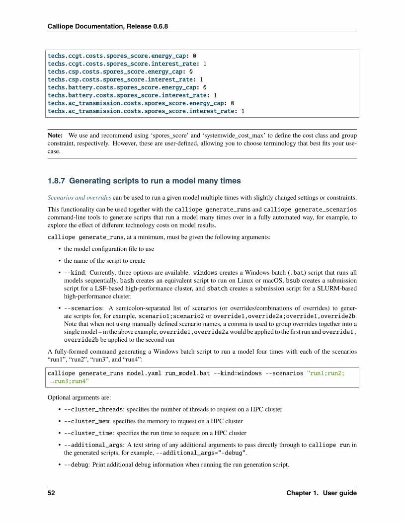
Calliope Documentation, Release 0.6.8
techs.ccgt.costs.spores_score.energy_cap: 0techs.ccgt.costs.spores_score.interest_rate: 1techs.csp.costs.spores_score.energy_cap: 0techs.csp.costs.spores_score.interest_rate: 1techs.battery.costs.spores_score.energy_cap: 0techs.battery.costs.spores_score.interest_rate: 1techs.ac_transmission.costs.spores_score.energy_cap: 0techs.ac_transmission.costs.spores_score.interest_rate: 1
Note: We use and recommend using ‘spores_score’ and ‘systemwide_cost_max’ to define the cost class and groupconstraint, respectively. However, these are user-defined, allowing you to choose terminology that best fits your use-case.
1.8.7 Generating scripts to run a model many times
Scenarios and overrides can be used to run a given model multiple times with slightly changed settings or constraints.
This functionality can be used together with the calliope generate_runs and calliope generate_scenarioscommand-line tools to generate scripts that run a model many times over in a fully automated way, for example, toexplore the effect of different technology costs on model results.
calliope generate_runs, at a minimum, must be given the following arguments:
• the model configuration file to use
• the name of the script to create
• --kind: Currently, three options are available. windows creates a Windows batch (.bat) script that runs allmodels sequentially, bash creates an equivalent script to run on Linux or macOS, bsub creates a submissionscript for a LSF-based high-performance cluster, and sbatch creates a submission script for a SLURM-basedhigh-performance cluster.
• --scenarios: A semicolon-separated list of scenarios (or overrides/combinations of overrides) to gener-ate scripts for, for example, scenario1;scenario2 or override1,override2a;override1,override2b.Note that when not using manually defined scenario names, a comma is used to group overrides together into asingle model – in the above example, override1,override2awould be applied to the first run and override1,override2b be applied to the second run
A fully-formed command generating a Windows batch script to run a model four times with each of the scenarios“run1”, “run2”, “run3”, and “run4”:
calliope generate_runs model.yaml run_model.bat --kind=windows --scenarios "run1;run2;→˓run3;run4"
Optional arguments are:
• --cluster_threads: specifies the number of threads to request on a HPC cluster
• --cluster_mem: specifies the memory to request on a HPC cluster
• --cluster_time: specifies the run time to request on a HPC cluster
• --additional_args: A text string of any additional arguments to pass directly through to calliope run inthe generated scripts, for example, --additional_args=”–debug”.
• --debug: Print additional debug information when running the run generation script.
52 Chapter 1. User guide

Calliope Documentation, Release 0.6.8
An example generating a script to run on a bsub-type high-performance cluster, with additional arguments to specifythe resources to request from the cluster:
calliope generate_runs model.yaml submit_runs.sh --kind=bsub --cluster_mem=1G --cluster_→˓time=100 --cluster_threads=5 --scenarios "run1;run2;run3;run4"
Running this will create two files:
• submit_runs.sh: The cluster submission script to pass to bsub on the cluster.
• submit_runs.array.sh: The accompanying script defining the runs for the cluster to execute.
In all cases, results are saved into the same directory as the script, with filenames of the formout_{run_number}_{scenario_name}.nc (model results) and plots_{run_number}_{scenario_name}.html (HTML plots), where {run_number} is the run number and {scenario_name} is the name of the scenario (orthe string defining the overrides applied). On a cluster, log files are saved to files with names starting with log_ in thesame directory.
Finally, the calliope generate_scenarios tool can be used to quickly generate a file with scenarios definitionfor inclusion in a model, if a large enough number of overrides exist to make it tedious to manually combine them intoscenarios. Assuming that in model.yaml a range of overrides exist that specify a subset of time for the years 2000through 2010, called “y2000” through “y2010”, and a set of cost-related overrides called “cost_low”, “cost_medium”and “cost_high”, the following command would generate scenarios with combinations of all years and cost overrides,calling them “run_1”, “run_2”, and so on, and saving them to scenarios.yaml:
calliope generate_scenarios model.yaml scenarios.yaml y2000;y2001;y2002;2003;y2004;y2005;→˓y2006;2007;2008;y2009;2010 cost_low;cost_medium;cost_high --scenario_name_prefix="run_"
1.8.8 Importing other YAML files in overrides
When using overrides (see Scenarios and overrides), it is possible to have import statements within overrides for moreflexibility. The following example illustrates this:
overrides:some_override:
techs:some_tech.constraints.energy_cap_max: 10
import: [additional_definitions.yaml]
additional_definitions.yaml:
techs:some_other_tech.constraints.energy_eff: 0.1
This is equivalent to the following override:
overrides:some_override:
techs:some_tech.constraints.energy_cap_max: 10some_other_tech.constraints.energy_eff: 0.1
1.8. Advanced features 53

Calliope Documentation, Release 0.6.8
1.8.9 Interfacing with the solver backend
On loading a model, there is no solver backend, only the input dataset. The backend is generated when a user callsrun() on their model. Currently this will call back to Pyomo to build the model and send it off to the solver, given by theuser in the run configuration run.solver. Once built, solved, and returned, the user has access to the results datasetmodel.results and interface functions with the backend model.backend.
You can use this interface to:
1. Get the raw data on the inputs used in the optimisation. By running model.backend.get_input_params() a user get an xarray Dataset which will look very similar to model.inputs, exceptthat assumed default values will be included. You may also spot a bug, where a value in model.inputsis different to the value returned by this function.
2. Update a parameter value. If you are interested in updating a few values in the model, you can run model.backend.update_param(). For example, to update the energy efficiency of your ccgt technologyin location region1 from 0.5 to 0.1, you can run model.backend.update_param(‘energy_eff’,{‘region1::ccgt: 0.1})`. This will not affect results at this stage, you’ll need to rerun the backend(point 4) to optimise with these new values.
Note: If you are interested in updating the objective function cost class weights, you will need toset ‘objective_cost_class’ as the parameter, e.g. model.backend.update_param(‘objective_cost_class’,{‘monetary’: 0.5}).
3. Activate / Deactivate a constraint or objective. Constraints can be activated and deactivate such that they willor will not have an impact on the optimisation. All constraints are active by default, but you might like toremove, for example, a capacity constraint if you don’t want there to be a capacity limit for any technologies.Similarly, if you had multiple objectives, you could deactivate one and activate another. The result wouldbe to have a different objective when rerunning the backend.
Note: Currently Calliope does not allow you to build multiple objectives, you will need to understand Pyomo and addan additional objective yourself to make use of this functionality. The Pyomo ConcreteModel() object can be accessedat model._backend_model.
4. Rerunning the backend. If you have edited parameters or constraint activation, you will need to rerun the op-timisation to propagate the effects. By calling model.backend.rerun(), the optimisation will run again,with the updated backend. This will not affect your model, but instead will return a new calliope Modelobject associated with that specific rerun. You can analyse the results and inputs in this new model, butthere is no backend interface available. You’ll need to return to the original model to access the backendagain, or run the returned model using new_model.run(force_rerun=True). In the original model,model.results will not change, and can only be overwritten by model.run(force_rerun=True).
Note: By calling model.run(force_rerun=True) any updates you have made to the backend will be overwritten.
See also:
Pyomo backend interface
54 Chapter 1. User guide

Calliope Documentation, Release 0.6.8
1.8.10 Specifying custom solver options
Gurobi
Refer to the Gurobi manual, which contains a list of parameters. Simply use the names given in the documentation(e.g. “NumericFocus” to set the numerical focus value). For example:
run:solver: gurobisolver_options:
Threads: 3NumericFocus: 2
CPLEX
Refer to the CPLEX parameter list. Use the “Interactive” parameter names, replacing any spaces with underscores (forexample, the memory reduction switch is called “emphasis memory”, and thus becomes “emphasis_memory”). Forexample:
run:solver: cplexsolver_options:
mipgap: 0.01mip_polishafter_absmipgap: 0.1emphasis_mip: 1mip_cuts: 2mip_cuts_cliques: 3
1.9 Configuration and defaults
This section lists the available configuration options and constraints along with their default values. Defaults are auto-matically applied in constraints whenever there is no user input for a particular value.
1.9. Configuration and defaults 55

Calliope Documentation, Release 0.6.8
1.9.1 Model configuration
Setting Default Commentscalliope_version Calliope framework version this model is intended forgroup_share {} Optional settings for the group_share constraint - depre-
cated and will be removed in v0.7.0name Model namerandom_seed Seed for random number generator used during cluster-
ingreserve_margin {} Per-carrier system-wide reserve marginssubset_time Subset of timesteps as a two-element list giving the
range, e.g. [‘2005-01-01’, ‘2005-01-05’], or a singlestring, e.g. ‘2005-01’
time {} Optional settings to adjust time resolution, see Time res-olution adjustment for the available options
timeseries_data_path Path to time series datatimeseries_data Dict of dataframes with time series data (when passing
in dicts rather than YAML files to Model constructor)timeseries_dateformat %Y-%m-%d
%H:%M:%STimestamp format of all time series data when read fromfile
file_allowed [‘cluster-ing_func’, ‘en-ergy_con’, ‘en-ergy_eff’, ‘en-ergy_prod’, ‘en-ergy_ramping’,‘export’,‘force_resource’,‘om_con’,‘om_prod’,‘parasitic_eff’,‘resource’,‘resource_eff’,‘storage_loss’,‘carrier_ratios’]
List of configuration options allowed to specify “file=”to load timeseries data. This can be updated if you’readding a new custom constraint that requires a newlydefined parameter to be a timeseries. If updating exist-ing parameters, you can expect existing constraints to notchange behaviour or to break on being constructed.## # Base technology groups ##
56 Chapter 1. User guide

Calliope Documentation, Release 0.6.8
1.9.2 Run configuration
Setting Default Commentsbackend pyomo Backend to use to build and solve the model. As of
v0.6.0, only pyomo is availablebigM 1000000000.0 Used for unmet demand, but should be of a similar or-
der of magnitude as the largest cost that the model couldachieve. Too high and the model will not converge
cyclic_storage True If true, storage in the last timestep of the timeseriesis considered to be the ‘previous timestep’ in the firsttimestep of the timeseries
ensure_feasibility False If true, unmet_demand will be a decision variable, toaccount for an ability to meet demand with the availablesupply. If False and a mismatch occurs, the optimisationwill fail due to infeasibility
mode plan Which mode to run the model in: ‘plan’, ‘operation’ or‘spores’
objective_options {} Arguments to pass to objective function. If cost-basedobjective function in use, should include ‘cost_class’and ‘sense’ (maximize/minimize)
objective min-max_cost_optimization
Name of internal objective function to use, currentlyonly min/max cost-based optimisation is available
operation {} Settings for operational modespores_options {} settings for SPORES (spatially-explicit, practically opti-
mal results) moderelax_constraint {} Enable relaxing some equality constraints to be min/max
constraints. The extent of relaxation is given as a frac-tion.
save_logs Directory into which to save logs and temporary files.Also turns on symbolic solver labels in the Pyomo back-end
solver_io What method the Pyomo backend should use to commu-nicate with the solver
solver_options A list of options, which are passed on to the chosensolver, and are therefore solver-dependent
solver cbc Which solver to usezero_threshold 1e-10 Any value coming out of the backend that is smaller than
this threshold (due to floating point errors, probably) willbe set to zero
1.9.3 Per-tech constraints
The following table lists all available technology constraint settings and their default values. All of these can be set bytech_identifier.constraints.constraint_name, e.g. nuclear.constraints.energy_cap.max.
1.9. Configuration and defaults 57

Calliope Documentation, Release 0.6.8
Setting Default Name Unit Commentscarrier_ratios Carrier ratios fraction Ratio of summed output of carriers
in [‘out_2’, ‘out_3’] / [‘in_2’, ‘in_3’]to the summed output of carriers in‘out’ / ‘in’. given in a nested dictio-nary.
charge_rate Charge rate hour -1 (do not use, replaced by en-ergy_cap_per_storage_cap_max)ratio of maximum charge/discharge(kW) for a given maximum storagecapacity (kWh).
en-ergy_cap_per_storage_cap_min
0 Minimum energy ca-pacity per storage ca-pacity
hour -1 ratio of minimum charge/discharge(kW) for a given storage capacity(kWh).
en-ergy_cap_per_storage_cap_max
inf Maximum energy ca-pacity per storage ca-pacity
hour -1 ratio of maximum charge/discharge(kW) for a given storage capacity(kWh).
en-ergy_cap_per_storage_cap_equals
Tie energy capacity tostorage capacity
hour -1
energy_cap_equals Specific installed en-ergy capacity
kW fixes maximum/minimumif decision variablescarrier_prod/carrier_conand overrides _max and _minconstraints.
en-ergy_cap_equals_systemwide
System-wide spe-cific installed energycapacity
kW fixes the sum to a maxi-mum/minimum, for a particulartechnology, of the decision variablescarrier_prod/carrier_con overall locations.
energy_cap_max inf Maximum installed en-ergy capacity
kW Limits decision variablescarrier_prod/carrier_conto a maximum/minimum.
en-ergy_cap_max_systemwide
inf System-wide maxi-mum installed energycapacity
kW Limits the sum to a maxi-mum/minimum, for a particulartechnology, of the decision variablescarrier_prod/carrier_con overall locations.
energy_cap_min 0 Minimum installed en-ergy capacity
kW Limits decision variablescarrier_prod/carrier_conto a minimum/maximum.
energy_cap_min_use 0 Minimum carrier pro-duction
fraction Set to a value between 0 and 1 toforce minimum carrier production asa fraction of the technology maxi-mum energy capacity. If non-zeroand technology is not defined byunits, this will force the technologyto operate above its minimum valueat every timestep.
energy_cap_per_unit Energy capacity perpurchased unit
kW/unit Set the capacity of each integer unitof a technology purchased
continues on next page
58 Chapter 1. User guide

Calliope Documentation, Release 0.6.8
Table 2 – continued from previous pageSetting Default Name Unit Commentsenergy_cap_scale 1.0 Energy capacity scale float Scale all energy_cap
min/max/equals/total_max/total_equalsconstraints by this value
energy_con False Energy consumption boolean Allow this technology to consumeenergy from the carrier (staticboolean, or from file as timeseries).
energy_eff 1.0 Energy efficiency fraction conversion efficiency (static, orfrom file as timeseries), fromresource/storage/carrier_in(tech dependent) to carrier_out.
en-ergy_eff_per_distance
1.0 Energy efficiency perdistance
frac-tion/distance
Set as value between 1 (no loss) and0 (all energy lost).
energy_prod False Energy production boolean Allow this technology to supply en-ergy to the carrier (static boolean, orfrom file as timeseries).
energy_ramping Ramping rate fraction /hour
Set to null to disable ramping con-straints, otherwise limit maximumcarrier production to a fraction ofmaximum capacity, which increasesby that fraction at each timestep.
export_cap inf Export capacity kW Maximum allowed export of pro-duced energy carrier for a technol-ogy.
export_carrier Export carrier N/A Name of carrier to be exported.Must be an output carrier of the tech-nology
force_asynchronous_prod_conFalse Force asynchronousproduction consump-tion
boolean If True, carrier_prod and car-rier_con cannot both occur in thesame timestep
force_resource False Force resource boolean Forces this technology to use allavailable resource, rather thanmaking it a maximum upper bound-ary (for production) or minimumlower boundary (for consumption).Static boolean, or from file as time-series
lifetime Technology lifetime years Must be defined if fixed capital costsare defined. A reasonable value formany technologies is around 20-25years.
one_way False One way boolean Forces a transmission technologyto only move energy in one di-rection on the link, in this casefrom default_location_from to de-fault_location_to
parasitic_eff 1.0 Plant parasitic effi-ciency
fraction Additional losses as energy getstransferred from the plant to the car-rier (static, or from file as time-series), e.g. due to plant parasiticconsumption
continues on next page
1.9. Configuration and defaults 59

Calliope Documentation, Release 0.6.8
Table 2 – continued from previous pageSetting Default Name Unit Commentsresource 0 Available resource kWh |
kWh/m2 |kWh/kW
Maximum available resource (static,or from file as timeseries). Unit dic-tated by resource_unit
resource_area_equals Specific installed re-source area
m2
resource_area_max inf Maximum usable re-source area
m2 If set to a finite value, restricts theusable area of the technology to thisvalue.
resource_area_min 0 Minimum usable re-source area
m2
re-source_area_per_energy_cap
Resource area per en-ergy capacity
m:sup:2/kW
If set, forces resource_area to fol-low energy_cap with the given nu-merical ratio (e.g. setting to 1.5means that resource_area == 1.5 * energy_cap)
resource_cap_equals Specific installedresource consumptioncapacity
kW overrides _max and _min con-straints.
re-source_cap_equals_energy_cap
False Resource capacityequals energy cpacity
boolean If true, resource_cap is forced toequal energy_cap
resource_cap_max inf Maximum installedresource consumptioncapacity
kW
resource_cap_min 0 Minimum installedresource consumptioncapacity
kW
resource_eff 1.0 Resource efficiency fraction Efficiency (static, or from file astimeseries) in capturing resource be-fore it reaches storage (if storage ispresent) or conversion to carrier.
resource_min_use 0 Minimum resourceconsumption
fraction Set to a value between 0 and 1 toforce minimum resource consump-tion for production technologies
resource_scale 1.0 Resource scale fraction Scale resource (either static value orall values in timeseries) by this value
resource_unit energy Resource unit N/A Sets the unit of resourceto either energy (i.e. kWh),energy_per_area (i.e. kWh/m2),or energy_per_cap (i.e.kWh/kW). energy_per_areauses the resource_area decisionvariable to scale the availableresource while energy_per_capuses the energy_cap decisionvariable.
continues on next page
60 Chapter 1. User guide

Calliope Documentation, Release 0.6.8
Table 2 – continued from previous pageSetting Default Name Unit Commentsstorage_cap_equals Specific storage capac-
itykWh If not defined,
energy_cap_equals *energy_cap_per_storage_cap_maxwill be used as the capacity andoverrides _max and _min con-straints.
storage_cap_max inf Maximum storage ca-pacity
kWh If not defined, energy_cap_max *energy_cap_per_storage_cap_maxwill be used as the capacity.
storage_cap_min 0 Minimum storage ca-pacity
kWh
storage_cap_per_unit Storage capacity perpurchased unit
kWh/unit Set the storage capacity of each inte-ger unit of a technology purchased.
stor-age_discharge_depth
0 Storage depth of dis-charge
fraction Defines the minimum level of stor-age state of charge, as a fraction oftotal storage capacity
storage_initial 0 Initial storage level fraction Set stored energy in device at thefirst timestep, as a fraction of totalstorage capacity
storage_loss 0 Storage loss rate frac-tion/hour
rate of storage loss per hour (static,or from file as timeseries), used tocalculate lost stored energy as (1 -storage_loss)^hours_per_timestep
units_equals Specific number ofpurchased units
integer Turns the model from LP to MILP.
units_equals_systemwide System-wide spe-cific installed energycapacity
kW fixes the sum to a specificvalue, for a particular technol-ogy, of the decision variablescarrier_prod/carrier_con overall locations.
units_max Maximum number ofpurchased units
integer Turns the model from LP to MILP.
units_max_systemwide inf System-wide maxi-mum installed energycapacity
kW Limits the sum to a maxi-mum/minimum, for a particulartechnology, of the decision variablescarrier_prod/carrier_con overall locations.
units_min Minimum number ofpurchased units
integer Turns the model from LP to MILP.
1.9. Configuration and defaults 61

Calliope Documentation, Release 0.6.8
1.9.4 Per-tech costs
These are all the available costs, which are set to 0 by default for every defined cost class. Costs are set bytech_identifier.costs.cost_class.cost_name, e.g. nuclear.costs.monetary.energy_cap.
Setting Default Name Unit Commentsenergy_cap 0 Cost of energy capac-
itykW gross
-1
en-ergy_cap_per_distance
0 Cost of energy capac-ity, per unit distance
kW gross-1
/ distanceApplied to transmission links only
export 0 Carrier export cost kWh -1 Usually used in the negative sense,as a subsidy.
interest_rate 0 Interest rate fraction Used when computing levelizedcosts
om_annual 0 Yearly O&M costs kWenergy_cap-1
om_annual_investment_fraction0 Fractional yearlyO&M costs
fraction /total in-vestment
om_con 0 Carrier consumptioncost
kWh -1 Applied to carrier consumption of atechnology
om_prod 0 Carrier production cost kWh -1 Applied to carrier production of atechnology
purchase 0 Purchase cost unit -1 Triggers a binary variable for thattechnology to say that it has beenpurchased or is applied to integervariable units
resource_area 0 Cost of resource area m-2
resource_cap 0 Cost of resource con-sumption capacity
kW -1
storage_cap 0 Cost of storage capac-ity
kWh -1
Technology depreciation settings apply when calculating levelized costs. The interest rate and life times must be setfor each technology with investment costs.
1.9.5 Group constraints
See Group constraints for a full listing of available group constraints.
1.9.6 Abstract base technology groups
Technologies must always define a parent, and this can either be one of the pre-defined abstract base technology groupsor a user-defined group (see Using tech_groups to group configuration). The pre-defined groups are:
• supply: Supplies energy to a carrier, has a positive resource.
• supply_plus: Supplies energy to a carrier, has a positive resource. Additional possible constraints, includingefficiencies and storage, distinguish this from supply.
• demand: Demands energy from a carrier, has a negative resource.
62 Chapter 1. User guide

Calliope Documentation, Release 0.6.8
• storage: Stores energy.
• transmission: Transmits energy from one location to another.
• conversion: Converts energy from one carrier to another.
• conversion_plus: Converts energy from one or more carrier(s) to one or more different carrier(s).
A technology inherits the configuration that its parent group specifies (which, in turn, may inherit from its own parent).
Note: The identifiers of the abstract base tech groups are reserved and cannot be used for user-defined technologies.However, you can amend an abstract base technology group for example by a lifetime attribute that will be in effect forall technologies derived from that group (see Using tech_groups to group configuration).
The following lists the pre-defined base tech groups and the defaults they provide.
supply
Default constraints provided by the parent tech group:
essentials:parent:
constraints:energy_prod: trueresource: infresource_unit: energy
costs: {}
Required constraints, allowed constraints, and allowed costs:
required_constraints: []allowed_constraints:- energy_cap_equals- energy_cap_equals_systemwide- energy_cap_max- energy_cap_max_systemwide- energy_cap_min- energy_cap_min_use- energy_cap_per_unit- energy_cap_scale- energy_eff- energy_prod- energy_ramping- export_cap- export_carrier- force_resource- lifetime- resource- resource_area_equals- resource_area_max- resource_area_min- resource_area_per_energy_cap
(continues on next page)
1.9. Configuration and defaults 63

Calliope Documentation, Release 0.6.8
(continued from previous page)
- resource_min_use- resource_scale- resource_unit- units_equals- units_equals_systemwide- units_max- units_max_systemwide- units_minallowed_costs:- depreciation_rate- energy_cap- export- interest_rate- om_annual- om_annual_investment_fraction- om_con- om_prod- purchase- resource_area
supply_plus
Default constraints provided by the parent tech group:
essentials:parent:
constraints:energy_prod: trueresource: infresource_eff: 1.0resource_unit: energy
costs: {}
Required constraints, allowed constraints, and allowed costs:
required_constraints: []allowed_constraints:- charge_rate- energy_cap_per_storage_cap_min- energy_cap_per_storage_cap_max- energy_cap_per_storage_cap_equals- energy_cap_equals- energy_cap_equals_systemwide- energy_cap_max- energy_cap_max_systemwide- energy_cap_min- energy_cap_min_use- energy_cap_per_unit- energy_cap_scale- energy_eff
(continues on next page)
64 Chapter 1. User guide

Calliope Documentation, Release 0.6.8
(continued from previous page)
- energy_prod- energy_ramping- export_cap- export_carrier- force_resource- lifetime- parasitic_eff- resource- resource_area_equals- resource_area_max- resource_area_min- resource_area_per_energy_cap- resource_cap_equals- resource_cap_equals_energy_cap- resource_cap_max- resource_cap_min- resource_eff- resource_min_use- resource_scale- resource_unit- storage_cap_equals- storage_cap_max- storage_cap_min- storage_cap_per_unit- storage_initial- storage_loss- units_equals- units_equals_systemwide- units_max- units_max_systemwide- units_minallowed_costs:- depreciation_rate- energy_cap- export- interest_rate- om_annual- om_annual_investment_fraction- om_con- om_prod- purchase- resource_area- resource_cap- storage_cap
1.9. Configuration and defaults 65

Calliope Documentation, Release 0.6.8
demand
Default constraints provided by the parent tech group:
essentials:parent:
constraints:energy_con: trueforce_resource: trueresource_unit: energy
costs: {}
Required constraints, allowed constraints, and allowed costs:
required_constraints:- resourceallowed_constraints:- energy_con- force_resource- resource- resource_area_equals- resource_scale- resource_unitallowed_costs:- om_con
storage
Default constraints provided by the parent tech group:
essentials:parent:
constraints:energy_con: trueenergy_prod: truestorage_cap_max: inf
costs: {}
Required constraints, allowed constraints, and allowed costs:
required_constraints: []allowed_constraints:- charge_rate- energy_cap_per_storage_cap_min- energy_cap_per_storage_cap_max- energy_cap_per_storage_cap_equals- energy_cap_equals- energy_cap_equals_systemwide- energy_cap_max- energy_cap_max_systemwide
(continues on next page)
66 Chapter 1. User guide

Calliope Documentation, Release 0.6.8
(continued from previous page)
- energy_cap_min- energy_cap_min_use- energy_cap_per_unit- energy_cap_scale- energy_con- energy_eff- energy_prod- energy_ramping- export_cap- export_carrier- force_asynchronous_prod_con- lifetime- storage_cap_equals- storage_cap_max- storage_cap_min- storage_cap_per_unit- storage_initial- storage_loss- storage_time_max- storage_discharge_depth- units_equals- units_equals_systemwide- units_max- units_max_systemwide- units_minallowed_costs:- depreciation_rate- energy_cap- export- interest_rate- om_annual- om_annual_investment_fraction- om_prod- purchase- storage_cap
transmission
Default constraints provided by the parent tech group:
essentials:parent:
constraints:energy_con: trueenergy_prod: true
costs: {}
Required constraints, allowed constraints, and allowed costs:
1.9. Configuration and defaults 67

Calliope Documentation, Release 0.6.8
required_constraints: []allowed_constraints:- energy_cap_equals- energy_cap_min- energy_cap_max- energy_cap_per_unit- energy_cap_scale- energy_con- energy_eff- energy_eff_per_distance- energy_prod- force_asynchronous_prod_con- lifetime- one_wayallowed_costs:- depreciation_rate- energy_cap- energy_cap_per_distance- interest_rate- om_annual- om_annual_investment_fraction- om_prod- purchase- purchase_per_distance
conversion
Default constraints provided by the parent tech group:
essentials:parent:
constraints:energy_con: trueenergy_prod: true
costs: {}
Required constraints, allowed constraints, and allowed costs:
required_constraints: []allowed_constraints:- energy_cap_equals- energy_cap_equals_systemwide- energy_cap_max- energy_cap_max_systemwide- energy_cap_min- energy_cap_min_use- energy_cap_per_unit- energy_cap_scale- energy_con- energy_eff
(continues on next page)
68 Chapter 1. User guide

Calliope Documentation, Release 0.6.8
(continued from previous page)
- energy_prod- energy_ramping- export_cap- export_carrier- lifetime- units_equals- units_equals_systemwide- units_max- units_max_systemwide- units_minallowed_costs:- depreciation_rate- energy_cap- export- interest_rate- om_annual- om_annual_investment_fraction- om_con- om_prod- purchase
conversion_plus
Default constraints provided by the parent tech group:
essentials:parent:
constraints:energy_con: trueenergy_prod: true
costs: {}
Required constraints, allowed constraints, and allowed costs:
required_constraints: []allowed_constraints:- carrier_ratios- energy_cap_equals- energy_cap_equals_systemwide- energy_cap_max- energy_cap_max_systemwide- energy_cap_min- energy_cap_min_use- energy_cap_per_unit- energy_cap_scale- energy_con- energy_eff- energy_prod- energy_ramping- export_cap
(continues on next page)
1.9. Configuration and defaults 69

Calliope Documentation, Release 0.6.8
(continued from previous page)
- export_carrier- lifetime- units_equals- units_equals_systemwide- units_max- units_max_systemwide- units_minallowed_costs:- depreciation_rate- energy_cap- export- interest_rate- om_annual- om_annual_investment_fraction- om_con- om_prod- purchase
1.10 Troubleshooting
1.10.1 General strategies
• Building a smaller model: model.subset_time allows specifying a subset of timesteps to be used. This canbe useful for debugging purposes as it can dramatically speed up model solution times. The timestep subset canbe specified as [startdate, enddate], e.g. [‘2005-01-01’, ‘2005-01-31’], or as a single time period,such as 2005-01 to select January only. The subsets are processed before building the model and applying timeresolution adjustments, so time resolution reduction functions will only see the reduced set of data.
• Retaining logs and temporary files: The setting run.save_logs, disabled by default, sets the directory intowhich to save logs and temporary files from the backend, to inspect solver logs and solver-generated model files.This also turns on symbolic solver labels in the Pyomo backend, so that all model components in the backendmodel are named according to the corresponding Calliope model components (by default, Pyomo uses shortrandom names for all generated model components).
• Analysing the optimisation problem without running the model: If you are comfortable with navigatingPyomo objects, then you can build the Pyomo model backend without running the optimisation problem, us-ing model.run(build_only=True). Pyomo objects are then accessible within model._backend_model.For instance, the constraint limiting energy capacity can be viewed by calling model._backend_model.energy_capacity_constraint.pprint(‘hi’). Alternatively, if you are working from the command lineor have little experience with Pyomo, you can generate an LP file. The LP file contains the mathematical modelformulation of a fully built Calliope model. It is a standard format that can be passed to various solvers. Exam-ining the LP file manually or using additional tools (see below) can help find issues when a model is infeasibleor unbounded. To build a model and save it to LP without actually solving it, use:
calliope run my_model.yaml --save_lp=my_saved_model.lp
or, interactively:
model.to_lp('my_saved_model.lp')
70 Chapter 1. User guide

Calliope Documentation, Release 0.6.8
1.10.2 Improving solution times
One way to improve solution time is to reduce the size of a problem (another way is to address potential numericalissues, which is dealt with further below in Understanding infeasibility and numerical instability).
Number of variables
The sets locs, techs, timesteps, carriers, and costs all contribute to model complexity. A reduction of any ofthese sets will reduce the number of resulting decision variables in the optimisation, which in turn will improve solutiontimes.
Note: By reducing the number of locations (e.g. merging nearby locations) you also remove the technologies linkingthose locations to the rest of the system, which is additionally beneficial.
Currently, we only provide automatic set reduction for timesteps. Timesteps can be resampled (e.g. 1hr -> 2hr intervals),masked (e.g. 1hr -> 12hr intervals except one week of particular interest), or clustered (e.g. 365 days to 5 days, eachrepresenting 73 days of the year, with 1hr resolution). In so doing, significant solution time improvements can beacheived.
See also:
Time resolution adjustment, Stefan Pfenninger (2017). Dealing with multiple decades of hourly wind and PV timeseries in energy models: a comparison of methods to reduce time resolution and the planning implications of inter-annual variability. Applied Energy.
Complex technologies
Calliope is primarily an LP framework, but application of certain constraints will trigger binary or integer decisionvariables. When triggered, a MILP model will be created.
In both cases, there will be a time penalty, as linear programming solvers are less able to converge on solutions of prob-lems which include binary or integer decision variables. But, the additional functionality can be useful. A purchasingcost allows for a cost curve of the form 𝑦 = 𝑀𝑥+ 𝐶 to be applied to a technology, instead of the LP costs which areall of the form 𝑦 = 𝑀𝑥. Integer units also trigger per-timestep decision variables, which allow technologies to be “on”or “off” at each timestep.
Additionally, in LP models, interactions between timesteps (in storage technologies) can lead to longer solution time.The exact extent of this is as-yet untested.
Model mode
Solution time increases more than linearly with the number of decision variables. As it splits the model into ~dailychunks, operational mode can help to alleviate solution time of big problems. This is clearly at the expense of fixingtechnology capacities. However, one solution is to use a heavily time clustered plan mode to get indicative modelcapacities. Then run operate mode with these capacities to get a higher resolution operation strategy. If necessary,this process could be iterated.
See also:
Operational mode
1.10. Troubleshooting 71

Calliope Documentation, Release 0.6.8
1.10.3 Influence of solver choice on speed
The open-source solvers (GLPK and CBC) are slower than the commercial solvers. If you are an academic researcher,it is recommended to acquire a free licence for Gurobi or CPLEX to very quickly improve solution times. GLPK inparticular is slow when solving MILP models. CBC is an improvement, but can still be several orders of magnitudeslower at reaching a solution than Gurobi or CPLEX.
We tested solution time for various solver choices on our example models, extended to run over a full year (8760hours). These runs took place on the University of Cambridge high performance computing cluster, with a maximumrun time of 5 hours. As can be seen, CBC is far superior to GLPK. If introducing binary constraints, although CBC isan improvement on GLPK, access to a commercial solver is preferable.
National scale example model size
• Variables : 420526 [Nneg: 219026, Free: 105140, Other: 96360]
• Linear constraints : 586972 [Less: 315373, Greater: 10, Equal: 271589]
MILP urban scale example model
• Variables: 586996 [Nneg: 332913, Free: 78880, Binary: 2, General Integer: 8761, Other: 166440]
• Linear constraints: 788502 [Less: 394226, Greater: 21, Equal: 394255]
Solution time
Solver Solution timeNational Urban
GLPK 4:35:40 >5hrsCBC 0:04:45 0:52:13Gurobi (1 thread) 0:02:08 0:03:21CPLEX (1 thread) 0:04:55 0:05:56Gurobi (4 thread) 0:02:27 0:03:08CPLEX (4 thread) 0:02:16 0:03:26
See also:
Specifying custom solver options
1.10.4 Understanding infeasibility and numerical instability
Note: A good first step when faced with an infeasible model is often to remove constraints, in particular more complexconstraints. For example, different combinations of group constraints can easily introduce mutually exclusive require-ments on capacities or output from specific technologies. Once a minimal model works, more complex constraints canbe turned on again one after the other.
72 Chapter 1. User guide

Calliope Documentation, Release 0.6.8
Using the Gurobi solver
To understand infeasible models:
• Set run.solver_options.DualReductions: 0 to see whether a model is infeasible or unbounded.
• To analyse infeasible models, save an LP file with the --save_lp command-line option, then use Gurobi togenerate an Irreducible Inconsistent Subsystem that shows which constraints are infeasible:
gurobi_cl ResultFile=result.ilp my_saved_model.lp
More detail on this is in the official Gurobi documentation.
To deal with numerically unstable models, try setting run.solver_options.Presolve: 0, as large numeric rangescan cause the pre-solver to generate an infeasible or numerically unstable model. The Gurobi Guidelines for NumericalIssues give detailed guidance for strategies to address numerically difficult optimisation problems.
Using the CPLEX solver
There are two ways to understand infeasibility when using the CPLEX solver, the first is quick and the second is moreinvolved:
1. Save solver logs for your model (run.save_logs: path/to/log_directory). In the directory,open the file ending in ‘.cplex.log’ to see the CPLEX solver report. If the model is infeasible orunbounded, the offending constraint will be identified (e.g. “SOLVER: Infeasible variable = slackc_u_carrier_production_max_constraint(region1_2__csp__power_2005_01_01_07_00_00)_”). This may beenough to understand why the model is failing, if not. . .
2. Open the LP file in CPLEX interactive (run cplex in the command line to invoke a CPLEX interactive session).The LP file for the problem ends with ‘.lp’ in the log folder (read path/to/file.lp). Once loaded, you can try relaxingvariables / constraints to see if the problem can be solved with relaxation (FeasOpt). You can also identifyconflicting constraints (tools conflict) and print those constraints directly (display conflict all). There are manymore commands available to analyse individual constraints and variables in the Official CPLEX documentation.
Similar to Gurobi, numerically unstable models may lead to unexpected infeasibility, so you can try run.solver_options.preprocessing_presolve: 0 or you can request CPLEX to more aggressively scale the prob-lem itself using the solver option read_scale: 1 . The CPLEX documentation page on numeric difficulties goesinto more detail on numeric instability.
1.10.5 Rerunning a model
After running, if there is an infeasibility you want to address, or simply a few values you dont think were quite right,you can change them and rerun your model. If you change them in model.inputs, just rerun the model as model.run(force_rerun=True).
Note: model.run(force_rerun=True) will replace you current model.results and rebuild he entire model backend.You may want to save your model before doing this.
Particularly if your problem is large, you may not want to rebuild the backend to change a few small values. Instead youcan interface directly with the backend using the model.backend functions, to update individual parameter values andswitch constraints on/off. By rerunning the backend specifically, you can optimise your problem with these backendchanges, without rebuilding the backend entirely.
1.10. Troubleshooting 73

Calliope Documentation, Release 0.6.8
Note: model.inputs and model.results will not be changed when updating and rerunning the backend. Instead,a new xarray Dataset is returned.
See also:
Interfacing with the solver backend
1.10.6 Debugging model errors
Calliope provides a method to save its fully built and commented internal representation of a model to a single YAMLfile with Model.save_commented_model_yaml(path). Comments in the resulting YAML file indicate where orig-inal values were overridden.
Because this is Calliope’s internal representation of a model directly before the model_data xarray.Dataset isbuilt, it can be useful for debugging possible issues in the model formulation, for example, undesired constraints thatexist at specific locations because they were specified model-wide without having been superseded by location-specificsettings.
Further processing of the data does occur before solving the model. The final values of parameters used by the backendsolver to generate constraints can be analysed when running an interactive Python session by running model.backend.get_input_params(). This provides a user with an xarray Dataset which will look very similar to model.inputs,except that assumed default values will be included. An attempt at running the model has to be made in order to beable to run this command.
See also:
If using Calliope interactively in a Python session, we recommend reading up on the Python debugger and (if usingJupyter notebooks) making use of the %debug magic.
1.11 More info (reference)
This section contains additional information useful as reference: a list of all example models and their configuration, alisting of different possible configuration values, and the detailed mathematical formulation.
We suggest you read the Building a model, Running a model and Analysing a model sections first before referring tothis section.
1.11.1 Built-in example models
This section gives a listing of all the YAML configuration files included in the built-in example models. Refer to thetutorials section for a brief overview of how these parts together provide a working model.
The example models are accessible in the calliope.examples module. To create an instance of an example model,call its constructor function, e.g.
urban_model = calliope.examples.urban_scale()
The available example models and their constructor functions are:
calliope.examples.national_scale(*args, **kwargs)Returns the built-in national-scale example model.
calliope.examples.time_clustering(*args, **kwargs)Returns the built-in national-scale example model with time clustering.
74 Chapter 1. User guide

Calliope Documentation, Release 0.6.8
calliope.examples.time_resampling(*args, **kwargs)Returns the built-in national-scale example model with time resampling.
calliope.examples.urban_scale(*args, **kwargs)Returns the built-in urban-scale example model.
calliope.examples.milp(*args, **kwargs)Returns the built-in urban-scale example model with MILP constraints enabled.
calliope.examples.operate(*args, **kwargs)Returns the built-in urban-scale example model in operate mode.
calliope.examples.time_masking(*args, **kwargs)Returns the built-in urban-scale example model with time masking.
National-scale example
Available as calliope.examples.national_scale.
Model settings
The layout of the model directory is as follows (+ denotes directories, - files):
- model.yaml- scenarios.yaml+ timeseries_data
- csp_resource.csv- demand-1.csv- demand-2.csv
+ model_config- locations.yaml- techs.yaml
model.yaml:
import: # Import other files from paths relative to this file, or absolute paths- 'model_config/techs.yaml' # This file specifies the model's technologies- 'model_config/locations.yaml' # This file specifies the model's locations- 'scenarios.yaml' # Scenario and override group definitions
# Model configuration: all settings that affect the built modelmodel:
name: National-scale example model
# What version of Calliope this model is intended forcalliope_version: 0.6.8
# Time series data path - can either be a path relative to this file, or an absolute␣→˓pathtimeseries_data_path: 'timeseries_data'
subset_time: ['2005-01-01', '2005-01-05'] # Subset of timesteps
# Run configuration: all settings that affect how the built model is run(continues on next page)
1.11. More info (reference) 75

Calliope Documentation, Release 0.6.8
(continued from previous page)
run:solver: cbc
ensure_feasibility: true # Switches on the "unmet demand" constraint
bigM: 1e6 # Sets the scale of unmet demand, which cannot be too high, otherwise the␣→˓optimisation will not converge
zero_threshold: 1e-10 # Any value coming out of the backend that is smaller than␣→˓this (due to floating point errors, probably) will be set to zero
mode: plan # Choices: plan, operate
objective_options.cost_class: {monetary: 1}
scenarios.yaml:
### Scenarios are optional, named combinations of overrides##scenarios:
cold_fusion_with_production_share: ['cold_fusion', 'cold_fusion_prod_share']cold_fusion_with_capacity_share: ['cold_fusion', 'cold_fusion_cap_share']
### Overrides are the building blocks from which scenarios can be defined##overrides:
profiling:model.name: 'National-scale example model (profiling run)'model.subset_time: ['2005-01-01', '2005-01-15']run.solver: cbc
time_resampling:model.name: 'National-scale example model with time resampling'model.subset_time: '2005-01'# Resample time resolution to 6-hourlymodel.time: {function: resample, function_options: {'resolution': '6H'}}
time_clustering:model.random_seed: 23model.name: 'National-scale example model with time clustering'model.subset_time: null # No time subsetting# Cluster timesteps using k-meansmodel.time: {function: apply_clustering, function_options: {clustering_func:
→˓'kmeans', how: 'closest', k: 10}}
spores:run.mode: sporesrun.spores_options:
score_cost_class: 'spores_score'(continues on next page)
76 Chapter 1. User guide

Calliope Documentation, Release 0.6.8
(continued from previous page)
slack_cost_group: 'systemwide_cost_max'slack: 0.1spores_number: 3objective_cost_class: {'monetary': 0, 'spores_score': 1}
run.objective_options.cost_class: {'monetary': 1, 'spores_score': 0}group_constraints:
systemwide_cost_max.cost_max.monetary: 1e10 # very large, non-infinite value
techs.ccgt.costs.spores_score.energy_cap: 0techs.ccgt.costs.spores_score.interest_rate: 1techs.csp.costs.spores_score.energy_cap: 0techs.csp.costs.spores_score.interest_rate: 1techs.battery.costs.spores_score.energy_cap: 0techs.battery.costs.spores_score.interest_rate: 1techs.ac_transmission.costs.spores_score.energy_cap: 0techs.ac_transmission.costs.spores_score.interest_rate: 1
operate:run.mode: operaterun.operation:
window: 12horizon: 24
model.subset_time: ['2005-01-01', '2005-01-10']locations:
region1.techs.ccgt.constraints.energy_cap_equals: 30000
region2.techs.battery.constraints.energy_cap_equals: 1000region2.techs.battery.constraints.storage_cap_equals: 5240
region1-1.techs.csp.constraints.energy_cap_equals: 10000region1-1.techs.csp.constraints.storage_cap_equals: 244301region1-1.techs.csp.constraints.resource_area_equals: 130385
region1-2.techs.csp.constraints.energy_cap_equals: 0region1-2.techs.csp.constraints.storage_cap_equals: 0region1-2.techs.csp.constraints.resource_area_equals: 0
region1-3.techs.csp.constraints.energy_cap_equals: 2534region1-3.techs.csp.constraints.storage_cap_equals: 25301region1-3.techs.csp.constraints.resource_area_equals: 8487
links:region1,region2.techs.ac_transmission.constraints.energy_cap_equals: 3231region1,region1-1.techs.free_transmission.constraints.energy_cap_equals: 9000region1,region1-2.techs.free_transmission.constraints.energy_cap_equals: 0region1,region1-3.techs.free_transmission.constraints.energy_cap_equals: 2281
check_feasibility:run:
ensure_feasibility: Falseobjective: 'check_feasibility'
model:(continues on next page)
1.11. More info (reference) 77
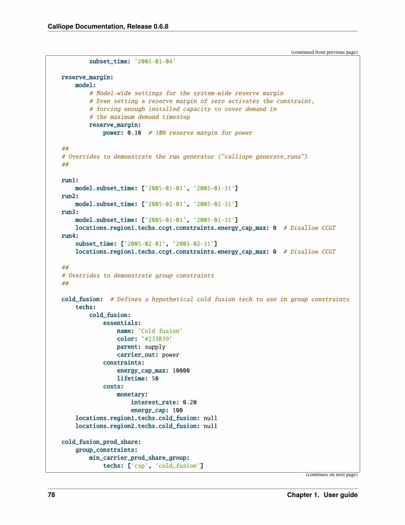
Calliope Documentation, Release 0.6.8
(continued from previous page)
subset_time: '2005-01-04'
reserve_margin:model:
# Model-wide settings for the system-wide reserve margin# Even setting a reserve margin of zero activates the constraint,# forcing enough installed capacity to cover demand in# the maximum demand timestepreserve_margin:
power: 0.10 # 10% reserve margin for power
### Overrides to demonstrate the run generator ("calliope generate_runs")##
run1:model.subset_time: ['2005-01-01', '2005-01-31']
run2:model.subset_time: ['2005-02-01', '2005-02-31']
run3:model.subset_time: ['2005-01-01', '2005-01-31']locations.region1.techs.ccgt.constraints.energy_cap_max: 0 # Disallow CCGT
run4:subset_time: ['2005-02-01', '2005-02-31']locations.region1.techs.ccgt.constraints.energy_cap_max: 0 # Disallow CCGT
### Overrides to demonstrate group constraints##
cold_fusion: # Defines a hypothetical cold fusion tech to use in group constraintstechs:
cold_fusion:essentials:
name: 'Cold fusion'color: '#233B39'parent: supplycarrier_out: power
constraints:energy_cap_max: 10000lifetime: 50
costs:monetary:
interest_rate: 0.20energy_cap: 100
locations.region1.techs.cold_fusion: nulllocations.region2.techs.cold_fusion: null
cold_fusion_prod_share:group_constraints:
min_carrier_prod_share_group:techs: ['csp', 'cold_fusion']
(continues on next page)
78 Chapter 1. User guide

Calliope Documentation, Release 0.6.8
(continued from previous page)
carrier_prod_share_min:# At least 85% of power supply must come from CSP and cold fusion␣
→˓togetherpower: 0.85
cold_fusion_cap_share:group_constraints:
max_cap_share_group:techs: ['csp', 'cold_fusion']# At most 20% of total energy_cap can come from CSP and cold fusion␣
→˓togetherenergy_cap_share_max: 0.20
locations:region1:
techs:ccgt:
constraints:energy_cap_max: 100000 # Increased to keep model feasible
minimize_emissions_costs:run:
objective_options:cost_class: {'emissions': 1, 'monetary': 0}
techs:ccgt:
costs:emissions:
om_prod: 100 # kgCO2/kWhcsp:
costs:emissions:
om_prod: 10 # kgCO2/kWh
maximize_utility_costs:run:
objective_options:cost_class: {'utility': 1 , 'monetary': 0}sense: maximize
techs:ccgt:
costs:utility:
om_prod: 10 # arbitrary utility valuecsp:
costs:utility:
om_prod: 100 # arbitrary utility value
capacity_factor:techs.ccgt.constraints.capacity_factor_min: 0.8techs.ccgt.constraints.capacity_factor_max: 0.9
(continues on next page)
1.11. More info (reference) 79

Calliope Documentation, Release 0.6.8
(continued from previous page)
eurocalliope:techs.battery.constraints.link_con_to_prod: [ccgt]locations.region2.techs.ccgt.constraints.energy_cap_max: 1000
techs.yaml:
### TECHNOLOGY DEFINITIONS##
# Note: '-start' and '-end' is used in tutorial documentation only
techs:
### Supply##
# ccgt-startccgt:
essentials:name: 'Combined cycle gas turbine'color: '#E37A72'parent: supplycarrier_out: power
constraints:resource: infenergy_eff: 0.5energy_cap_max: 40000 # kWenergy_cap_max_systemwide: 100000 # kWenergy_ramping: 0.8lifetime: 25
costs:monetary:
interest_rate: 0.10energy_cap: 750 # USD per kWom_con: 0.02 # USD per kWh
# ccgt-end
# csp-startcsp:
essentials:name: 'Concentrating solar power'color: '#F9CF22'parent: supply_pluscarrier_out: power
constraints:storage_cap_max: 614033energy_cap_per_storage_cap_max: 1storage_loss: 0.002resource: file=csp_resource.csvresource_unit: energy_per_area
(continues on next page)
80 Chapter 1. User guide

Calliope Documentation, Release 0.6.8
(continued from previous page)
energy_eff: 0.4parasitic_eff: 0.9resource_area_max: infenergy_cap_max: 10000lifetime: 25
costs:monetary:
interest_rate: 0.10storage_cap: 50resource_area: 200resource_cap: 200energy_cap: 1000om_prod: 0.002
# csp-end
### Storage### battery-startbattery:
essentials:name: 'Battery storage'color: '#3B61E3'parent: storagecarrier: power
constraints:energy_cap_max: 1000 # kWstorage_cap_max: infenergy_cap_per_storage_cap_max: 4energy_eff: 0.95 # 0.95 * 0.95 = 0.9025 round trip efficiencystorage_loss: 0 # No loss over time assumedlifetime: 25
costs:monetary:
interest_rate: 0.10storage_cap: 200 # USD per kWh storage capacity
# battery-end
### Demand### demand-startdemand_power:
essentials:name: 'Power demand'color: '#072486'parent: demandcarrier: power
# demand-end
### Transmission
(continues on next page)
1.11. More info (reference) 81

Calliope Documentation, Release 0.6.8
(continued from previous page)
##
# transmission-startac_transmission:
essentials:name: 'AC power transmission'color: '#8465A9'parent: transmissioncarrier: power
constraints:energy_eff: 0.85lifetime: 25
costs:monetary:
interest_rate: 0.10energy_cap: 200om_prod: 0.002
free_transmission:essentials:
name: 'Local power transmission'color: '#6783E3'parent: transmissioncarrier: power
constraints:energy_cap_max: infenergy_eff: 1.0
costs:monetary:
om_prod: 0# transmission-end
locations.yaml:
### LOCATIONS##
locations:# region-1-startregion1:
coordinates: {lat: 40, lon: -2}techs:
demand_power:constraints:
resource: file=demand-1.csv:demandccgt:
constraints:energy_cap_max: 30000 # increased to ensure no unmet_demand in first␣
→˓timestep# region-1-end# other-locs-start
(continues on next page)
82 Chapter 1. User guide

Calliope Documentation, Release 0.6.8
(continued from previous page)
region2:coordinates: {lat: 40, lon: -8}techs:
demand_power:constraints:
resource: file=demand-2.csv:demandbattery:
region1-1.coordinates: {lat: 41, lon: -2}region1-2.coordinates: {lat: 39, lon: -1}region1-3.coordinates: {lat: 39, lon: -2}
region1-1, region1-2, region1-3:techs:
csp:# other-locs-end
### TRANSMISSION CAPACITIES##
links:# links-startregion1,region2:
techs:ac_transmission:
constraints:energy_cap_max: 10000
region1,region1-1:techs:
free_transmission:region1,region1-2:
techs:free_transmission:
region1,region1-3:techs:
free_transmission:# links-end
Urban-scale example
Available as calliope.examples.urban_scale.
1.11. More info (reference) 83

Calliope Documentation, Release 0.6.8
Model settings
model.yaml:
import: # Import other files from paths relative to this file, or absolute paths- 'model_config/techs.yaml'- 'model_config/locations.yaml'- 'scenarios.yaml'
model:name: Urban-scale example model
# What version of Calliope this model is intended forcalliope_version: 0.6.8
# Time series data path - can either be a path relative to this file, or an absolute␣→˓pathtimeseries_data_path: 'timeseries_data'
subset_time: ['2005-07-01', '2005-07-02'] # Subset of timesteps
run:mode: plan # Choices: plan, operate
solver: cbc
ensure_feasibility: true # Switching on unmet demand
bigM: 1e6 # setting the scale of unmet demand, which cannot be too high, otherwise␣→˓the optimisation will not converge
objective_options.cost_class: {monetary: 1}
scenarios.yaml:
### Overrides for different example model configuratiions##
overrides:milp:
model.name: 'Urban-scale example model with MILP'run.solver_options.mipgap: 0.05techs:
# chp-startchp:
constraints:units_max: 4energy_cap_per_unit: 300energy_cap_min_use: 0.2
costs:monetary:
energy_cap: 700(continues on next page)
84 Chapter 1. User guide

Calliope Documentation, Release 0.6.8
(continued from previous page)
purchase: 40000# chp-end# boiler-startboiler:
costs:monetary:
energy_cap: 35purchase: 2000
# boiler-end# heat_pipes-startheat_pipes:
constraints:force_asynchronous_prod_con: true
# heat_pipes-end
mapbox_ready:locations:
X1.coordinates: {lat: 51.4596158, lon: -0.1613446}X2.coordinates: {lat: 51.4652373, lon: -0.1141548}X3.coordinates: {lat: 51.4287016, lon: -0.1310635}N1.coordinates: {lat: 51.4450766, lon: -0.1247183}
links:X1,X2.techs.power_lines.distance: 10X1,X3.techs.power_lines.distance: 5X1,N1.techs.heat_pipes.distance: 3N1,X2.techs.heat_pipes.distance: 3N1,X3.techs.heat_pipes.distance: 4
operate:run.mode: operaterun.operation:
window: 24horizon: 48
model.subset_time: ['2005-07-01', '2005-07-10']locations:
X1:techs:
chp.constraints.energy_cap_max: 300pv.constraints.energy_cap_max: 0supply_grid_power.constraints.energy_cap_max: 40supply_gas.constraints.energy_cap_max: 700
X2:techs:
boiler.constraints.energy_cap_max: 200pv.constraints.energy_cap_max: 70supply_gas.constraints.energy_cap_max: 250
X3:techs:
boiler.constraints.energy_cap_max: 0pv.constraints.energy_cap_max: 50
(continues on next page)
1.11. More info (reference) 85

Calliope Documentation, Release 0.6.8
(continued from previous page)
supply_gas.constraints.energy_cap_max: 0
links:X1,X2.techs.power_lines.constraints.energy_cap_max: 300X1,X3.techs.power_lines.constraints.energy_cap_max: 60X1,N1.techs.heat_pipes.constraints.energy_cap_max: 300N1,X2.techs.heat_pipes.constraints.energy_cap_max: 250N1,X3.techs.heat_pipes.constraints.energy_cap_max: 320
time_masking:model.name: 'Urban-scale example model with time masking'model.subset_time: '2005-01'# Resample time resolution to 6-hourlymodel.time:
masks:- {function: extreme_diff, options: {tech0: demand_heat, tech1: demand_
→˓electricity, how: max, n: 2}}function: resamplefunction_options: {resolution: 6H}
techs.yaml:
### TECHNOLOGY DEFINITIONS##
# Note: '-start' and '-end' is used in tutorial documentation only
# supply_power_plus-starttech_groups:
supply_power_plus:essentials:
parent: supply_pluscarrier: electricity
# supply_power_plus-end
techs:
##-GRID SUPPLY-### supply-startsupply_grid_power:
essentials:name: 'National grid import'color: '#C5ABE3'parent: supplycarrier: electricity
constraints:resource: infenergy_cap_max: 2000lifetime: 25
costs:monetary:
(continues on next page)
86 Chapter 1. User guide

Calliope Documentation, Release 0.6.8
(continued from previous page)
interest_rate: 0.10energy_cap: 15om_con: 0.1 # 10p/kWh electricity price #ppt
supply_gas:essentials:
name: 'Natural gas import'color: '#C98AAD'parent: supplycarrier: gas
constraints:resource: infenergy_cap_max: 2000lifetime: 25
costs:monetary:
interest_rate: 0.10energy_cap: 1om_con: 0.025 # 2.5p/kWh gas price #ppt
# supply-end
##-Renewables-### pv-startpv:
essentials:name: 'Solar photovoltaic power'color: '#F9D956'parent: supply_power_plus
constraints:export_carrier: electricityresource: file=pv_resource.csv:per_area # Already accounts for panel␣
→˓efficiency - kWh/m2. Source: Renewables.ninja Solar PV Power - Version: 1.1 - License:␣→˓https://creativecommons.org/licenses/by-nc/4.0/ - Reference: https://doi.org/10.1016/j.→˓energy.2016.08.060
resource_unit: energy_per_areaparasitic_eff: 0.85 # inverter lossesenergy_cap_max: 250resource_area_max: 1500force_resource: trueresource_area_per_energy_cap: 7 # 7m2 of panels needed to fit 1kWp of panelslifetime: 25
costs:monetary:
interest_rate: 0.10energy_cap: 1350
# pv-end
# Conversion# boiler-startboiler:
essentials:name: 'Natural gas boiler'
(continues on next page)
1.11. More info (reference) 87

Calliope Documentation, Release 0.6.8
(continued from previous page)
color: '#8E2999'parent: conversioncarrier_out: heatcarrier_in: gas
constraints:energy_cap_max: 600energy_eff: 0.85lifetime: 25
costs:monetary:
interest_rate: 0.10om_con: 0.004 # .4p/kWh
# boiler-end
# Conversion_plus# chp-startchp:
essentials:name: 'Combined heat and power'color: '#E4AB97'parent: conversion_plusprimary_carrier_out: electricitycarrier_in: gascarrier_out: electricitycarrier_out_2: heat
constraints:export_carrier: electricityenergy_cap_max: 1500energy_eff: 0.405carrier_ratios.carrier_out_2.heat: 0.8lifetime: 25
costs:monetary:
interest_rate: 0.10energy_cap: 750om_prod: 0.004 # .4p/kWh for 4500 operating hours/yearexport: file=export_power.csv
# chp-end
##-DEMAND-### demand-startdemand_electricity:
essentials:name: 'Electrical demand'color: '#072486'parent: demandcarrier: electricity
demand_heat:essentials:
name: 'Heat demand'color: '#660507'
(continues on next page)
88 Chapter 1. User guide

Calliope Documentation, Release 0.6.8
(continued from previous page)
parent: demandcarrier: heat
# demand-end
##-DISTRIBUTION-### transmission-startpower_lines:
essentials:name: 'Electrical power distribution'color: '#6783E3'parent: transmissioncarrier: electricity
constraints:energy_cap_max: 2000energy_eff: 0.98lifetime: 25
costs:monetary:
interest_rate: 0.10energy_cap_per_distance: 0.01
heat_pipes:essentials:
name: 'District heat distribution'color: '#823739'parent: transmissioncarrier: heat
constraints:energy_cap_max: 2000energy_eff_per_distance: 0.975lifetime: 25
costs:monetary:
interest_rate: 0.10energy_cap_per_distance: 0.3
# transmission-end
locations.yaml:
locations:# X1-startX1:
techs:chp:pv:supply_grid_power:
costs.monetary.energy_cap: 100 # cost of transformerssupply_gas:demand_electricity:
constraints.resource: file=demand_power.csvdemand_heat:
constraints.resource: file=demand_heat.csv(continues on next page)
1.11. More info (reference) 89
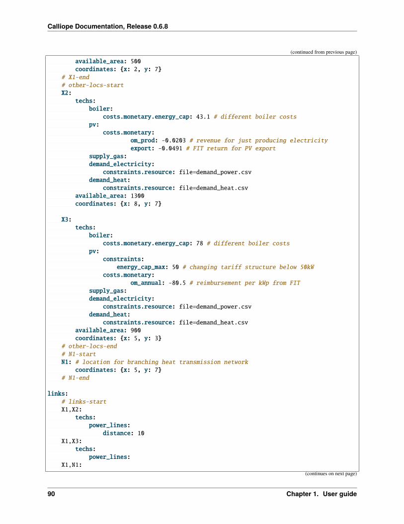
Calliope Documentation, Release 0.6.8
(continued from previous page)
available_area: 500coordinates: {x: 2, y: 7}
# X1-end# other-locs-startX2:
techs:boiler:
costs.monetary.energy_cap: 43.1 # different boiler costspv:
costs.monetary:om_prod: -0.0203 # revenue for just producing electricityexport: -0.0491 # FIT return for PV export
supply_gas:demand_electricity:
constraints.resource: file=demand_power.csvdemand_heat:
constraints.resource: file=demand_heat.csvavailable_area: 1300coordinates: {x: 8, y: 7}
X3:techs:
boiler:costs.monetary.energy_cap: 78 # different boiler costs
pv:constraints:
energy_cap_max: 50 # changing tariff structure below 50kWcosts.monetary:
om_annual: -80.5 # reimbursement per kWp from FITsupply_gas:demand_electricity:
constraints.resource: file=demand_power.csvdemand_heat:
constraints.resource: file=demand_heat.csvavailable_area: 900coordinates: {x: 5, y: 3}
# other-locs-end# N1-startN1: # location for branching heat transmission network
coordinates: {x: 5, y: 7}# N1-end
links:# links-startX1,X2:
techs:power_lines:
distance: 10X1,X3:
techs:power_lines:
X1,N1:(continues on next page)
90 Chapter 1. User guide

Calliope Documentation, Release 0.6.8
(continued from previous page)
techs:heat_pipes:
N1,X2:techs:
heat_pipes:N1,X3:
techs:heat_pipes:
# links-end
1.11.2 Configuration reference
Configuration layout
There must always be at least one model configuration YAML file, probably called model.yaml or similar. This filecan import any number of additional files.
This file or this set of files must specify the following top-level configuration keys:
• name: the name of the model
• model: model settings
• run: run settings
• techs: technology definitions
• (optionally) tech_groups: tech group definitions
• locations: location definitions
• (optionally) links: transmission link definitions
Note: Model settings (model) affect how the model and its data are built by Calliope, while run settings (run) onlytake effect once a built model is run (e.g. interactively via model.run()). This means that run settings, unlike modelsettings, can be updated after a model is built and before it is run, by modifying attributes in the built model dataset.
YAML configuration file format
All configuration files (with the exception of time series data files) are in the YAML format, “a human friendly dataserialisation standard for all programming languages”.
Configuration for Calliope is usually specified as option: value entries, where value might be a number, a textstring, or a list (e.g. a list of further settings).
Calliope allows an abbreviated form for long, nested settings:
one:two:three: x
can be written as:
1.11. More info (reference) 91

Calliope Documentation, Release 0.6.8
one.two.three: x
Calliope also allows a special import: directive in any YAML file. This can specify one or several YAML files toimport. If both the imported file and the current file define the same option, the definition in the current file takesprecedence.
Using quotation marks (' or ") to enclose strings is optional, but can help with readability. The three ways of settingoption to text below are equivalent:
option: "text"option: 'text'option: text
Sometimes, a setting can be either enabled or disabled, in this case, the boolean values true or false are used.
Comments can be inserted anywhere in YAML files with the # symbol. The remainder of a line after # is interpretedas a comment.
See the YAML website for more general information about YAML.
Calliope internally represents the configuration as AttrDicts, which are a subclass of the built-in Python dictionarydata type (dict) with added functionality such as YAML reading/writing and attribute access to keys.
1.11.3 Mathematical formulation
This section details the mathematical formulation of the different components. For each component, a link to the actualimplementing function in the Calliope code is given.
Note: Make sure to also refer to the detailed listing of constraints and costs along with their units and default values.
Decision variables
calliope.backend.pyomo.variables.initialize_decision_variables(backend_model)Defines decision variables.
92 Chapter 1. User guide

Calliope Documentation, Release 0.6.8
Variable Dimensionsenergy_cap loc_techscarrier_prod loc_tech_carriers_prod, timestepscarrier_con loc_tech_carriers_con, timestepscost costs, loc_techs_costresource_area loc_techs_area,storage_cap loc_techs_storestorage loc_techs_store, timestepsresource_con loc_techs_supply_plus, timestepsresource_cap loc_techs_supply_pluscarrier_export loc_tech_carriers_export, timestepscost_var costs, loc_techs_om_cost, timestepscost_investment costs, loc_techs_investment_costpurchased loc_techs_purchaseunits loc_techs_milpoperating_units loc_techs_milp, timestepsunmet_demand loc_carriers, timestepsunused_supply loc_carriers, timesteps
Objective functions
calliope.backend.pyomo.objective.minmax_cost_optimization(backend_model)Minimize or maximise total system cost for specified cost class or a set of cost classes. cost_class is a string ordictionary. If a string, it is automatically converted to a dictionary with a single key:value pair where value ==1. The dictionary provides a weight for each cost class of interest: {cost_1: weight_1, cost_2: weight_2, etc.}.
If unmet_demand is in use, then the calculated cost of unmet_demand is added or subtracted from the total costin the opposite sense to the objective.
𝑚𝑖𝑛 : 𝑧 =∑︁
𝑙𝑜𝑐::𝑡𝑒𝑐ℎ𝑐𝑜𝑠𝑡,𝑘
(𝑐𝑜𝑠𝑡(𝑙𝑜𝑐 :: 𝑡𝑒𝑐ℎ, 𝑐𝑜𝑠𝑡 = 𝑐𝑜𝑠𝑡𝑘)× 𝑤𝑒𝑖𝑔ℎ𝑡𝑘) +∑︁
𝑙𝑜𝑐::𝑐𝑎𝑟𝑟𝑖𝑒𝑟,𝑡𝑖𝑚𝑒𝑠𝑡𝑒𝑝
(𝑢𝑛𝑚𝑒𝑡_𝑑𝑒𝑚𝑎𝑛𝑑(𝑙𝑜𝑐 :: 𝑐𝑎𝑟𝑟𝑖𝑒𝑟, 𝑡𝑖𝑚𝑒𝑠𝑡𝑒𝑝)× 𝑏𝑖𝑔𝑀)
𝑚𝑎𝑥 : 𝑧 =∑︁
𝑙𝑜𝑐::𝑡𝑒𝑐ℎ𝑐𝑜𝑠𝑡,𝑘
(𝑐𝑜𝑠𝑡(𝑙𝑜𝑐 :: 𝑡𝑒𝑐ℎ, 𝑐𝑜𝑠𝑡 = 𝑐𝑜𝑠𝑡𝑘)× 𝑤𝑒𝑖𝑔ℎ𝑡𝑘)−∑︁
𝑙𝑜𝑐::𝑐𝑎𝑟𝑟𝑖𝑒𝑟,𝑡𝑖𝑚𝑒𝑠𝑡𝑒𝑝
(𝑢𝑛𝑚𝑒𝑡_𝑑𝑒𝑚𝑎𝑛𝑑(𝑙𝑜𝑐 :: 𝑐𝑎𝑟𝑟𝑖𝑒𝑟, 𝑡𝑖𝑚𝑒𝑠𝑡𝑒𝑝)× 𝑏𝑖𝑔𝑀)
calliope.backend.pyomo.objective.check_feasibility(backend_model)Dummy objective, to check that there are no conflicting constraints.
𝑚𝑖𝑛 : 𝑧 = 1
Constraints
Energy Balance
calliope.backend.pyomo.constraints.energy_balance.system_balance_constraint_rule(backend_model,loc_carrier,timestep)
System balance ensures that, within each location, the production and consumption of each carrier is balanced.
1.11. More info (reference) 93

Calliope Documentation, Release 0.6.8
∑︁𝑙𝑜𝑐::𝑡𝑒𝑐ℎ::𝑐𝑎𝑟𝑟𝑖𝑒𝑟𝑝𝑟𝑜𝑑∈𝑙𝑜𝑐::𝑐𝑎𝑟𝑟𝑖𝑒𝑟
𝑐𝑎𝑟𝑟𝑖𝑒𝑟𝑝𝑟𝑜𝑑(𝑙𝑜𝑐 :: 𝑡𝑒𝑐ℎ :: 𝑐𝑎𝑟𝑟𝑖𝑒𝑟, 𝑡𝑖𝑚𝑒𝑠𝑡𝑒𝑝) +∑︁
𝑙𝑜𝑐::𝑡𝑒𝑐ℎ::𝑐𝑎𝑟𝑟𝑖𝑒𝑟𝑐𝑜𝑛∈𝑙𝑜𝑐::𝑐𝑎𝑟𝑟𝑖𝑒𝑟
𝑐𝑎𝑟𝑟𝑖𝑒𝑟𝑐𝑜𝑛(𝑙𝑜𝑐 :: 𝑡𝑒𝑐ℎ :: 𝑐𝑎𝑟𝑟𝑖𝑒𝑟, 𝑡𝑖𝑚𝑒𝑠𝑡𝑒𝑝) +∑︁
𝑙𝑜𝑐::𝑡𝑒𝑐ℎ::𝑐𝑎𝑟𝑟𝑖𝑒𝑟𝑒𝑥𝑝𝑜𝑟𝑡∈𝑙𝑜𝑐::𝑐𝑎𝑟𝑟𝑖𝑒𝑟
𝑐𝑎𝑟𝑟𝑖𝑒𝑟𝑒𝑥𝑝𝑜𝑟𝑡(𝑙𝑜𝑐 :: 𝑡𝑒𝑐ℎ :: 𝑐𝑎𝑟𝑟𝑖𝑒𝑟, 𝑡𝑖𝑚𝑒𝑠𝑡𝑒𝑝) ∀𝑙𝑜𝑐 :: 𝑐𝑎𝑟𝑟𝑖𝑒𝑟 ∈ 𝑙𝑜𝑐 :: 𝑐𝑎𝑟𝑟𝑖𝑒𝑟𝑠, ∀𝑡𝑖𝑚𝑒𝑠𝑡𝑒𝑝 ∈ 𝑡𝑖𝑚𝑒𝑠𝑡𝑒𝑝𝑠
calliope.backend.pyomo.constraints.energy_balance.balance_supply_constraint_rule(backend_model,loc_tech,timestep)
Limit production from supply techs to their available resource
𝑚𝑖𝑛_𝑢𝑠𝑒(𝑙𝑜𝑐 :: 𝑡𝑒𝑐ℎ)× 𝑎𝑣𝑎𝑖𝑙𝑎𝑏𝑙𝑒_𝑟𝑒𝑠𝑜𝑢𝑟𝑐𝑒(𝑙𝑜𝑐 :: 𝑡𝑒𝑐ℎ, 𝑡𝑖𝑚𝑒𝑠𝑡𝑒𝑝) ≤ 𝑐𝑎𝑟𝑟𝑖𝑒𝑟𝑝𝑟𝑜𝑑(𝑙𝑜𝑐 :: 𝑡𝑒𝑐ℎ :: 𝑐𝑎𝑟𝑟𝑖𝑒𝑟, 𝑡𝑖𝑚𝑒𝑠𝑡𝑒𝑝)
𝜂𝑒𝑛𝑒𝑟𝑔𝑦(𝑙𝑜𝑐 :: 𝑡𝑒𝑐ℎ, 𝑡𝑖𝑚𝑒𝑠𝑡𝑒𝑝)≥ 𝑎𝑣𝑎𝑖𝑙𝑎𝑏𝑙𝑒_𝑟𝑒𝑠𝑜𝑢𝑟𝑐𝑒(𝑙𝑜𝑐 :: 𝑡𝑒𝑐ℎ, 𝑡𝑖𝑚𝑒𝑠𝑡𝑒𝑝) ∀𝑙𝑜𝑐 :: 𝑡𝑒𝑐ℎ ∈ 𝑙𝑜𝑐 :: 𝑡𝑒𝑐ℎ𝑠𝑠𝑢𝑝𝑝𝑙𝑦,∀𝑡𝑖𝑚𝑒𝑠𝑡𝑒𝑝 ∈ 𝑡𝑖𝑚𝑒𝑠𝑡𝑒𝑝𝑠
If 𝑓𝑜𝑟𝑐𝑒_𝑟𝑒𝑠𝑜𝑢𝑟𝑐𝑒(𝑙𝑜𝑐 :: 𝑡𝑒𝑐ℎ) is set:
𝑐𝑎𝑟𝑟𝑖𝑒𝑟𝑝𝑟𝑜𝑑(𝑙𝑜𝑐 :: 𝑡𝑒𝑐ℎ :: 𝑐𝑎𝑟𝑟𝑖𝑒𝑟, 𝑡𝑖𝑚𝑒𝑠𝑡𝑒𝑝)
𝜂𝑒𝑛𝑒𝑟𝑔𝑦(𝑙𝑜𝑐 :: 𝑡𝑒𝑐ℎ, 𝑡𝑖𝑚𝑒𝑠𝑡𝑒𝑝)= 𝑎𝑣𝑎𝑖𝑙𝑎𝑏𝑙𝑒_𝑟𝑒𝑠𝑜𝑢𝑟𝑐𝑒(𝑙𝑜𝑐 :: 𝑡𝑒𝑐ℎ, 𝑡𝑖𝑚𝑒𝑠𝑡𝑒𝑝) ∀𝑙𝑜𝑐 :: 𝑡𝑒𝑐ℎ ∈ 𝑙𝑜𝑐 :: 𝑡𝑒𝑐ℎ𝑠𝑠𝑢𝑝𝑝𝑙𝑦,∀𝑡𝑖𝑚𝑒𝑠𝑡𝑒𝑝 ∈ 𝑡𝑖𝑚𝑒𝑠𝑡𝑒𝑝𝑠
Where:
𝑎𝑣𝑎𝑖𝑙𝑎𝑏𝑙𝑒_𝑟𝑒𝑠𝑜𝑢𝑟𝑐𝑒(𝑙𝑜𝑐 :: 𝑡𝑒𝑐ℎ, 𝑡𝑖𝑚𝑒𝑠𝑡𝑒𝑝) = 𝑟𝑒𝑠𝑜𝑢𝑟𝑐𝑒(𝑙𝑜𝑐 :: 𝑡𝑒𝑐ℎ, 𝑡𝑖𝑚𝑒𝑠𝑡𝑒𝑝)× 𝑟𝑒𝑠𝑜𝑢𝑟𝑐𝑒_𝑠𝑐𝑎𝑙𝑒(𝑙𝑜𝑐 :: 𝑡𝑒𝑐ℎ)
if 𝑙𝑜𝑐 :: 𝑡𝑒𝑐ℎ is in 𝑙𝑜𝑐 :: 𝑡𝑒𝑐ℎ𝑠𝑎𝑟𝑒𝑎:
𝑎𝑣𝑎𝑖𝑙𝑎𝑏𝑙𝑒_𝑟𝑒𝑠𝑜𝑢𝑟𝑐𝑒(𝑙𝑜𝑐 :: 𝑡𝑒𝑐ℎ, 𝑡𝑖𝑚𝑒𝑠𝑡𝑒𝑝) = 𝑟𝑒𝑠𝑜𝑢𝑟𝑐𝑒(𝑙𝑜𝑐 :: 𝑡𝑒𝑐ℎ, 𝑡𝑖𝑚𝑒𝑠𝑡𝑒𝑝)× 𝑟𝑒𝑠𝑜𝑢𝑟𝑐𝑒_𝑠𝑐𝑎𝑙𝑒(𝑙𝑜𝑐 :: 𝑡𝑒𝑐ℎ)× 𝑟𝑒𝑠𝑜𝑢𝑟𝑐𝑒𝑎𝑟𝑒𝑎(𝑙𝑜𝑐 :: 𝑡𝑒𝑐ℎ)
calliope.backend.pyomo.constraints.energy_balance.balance_demand_constraint_rule(backend_model,loc_tech,timestep)
Limit consumption from demand techs to their required resource.
𝑐𝑎𝑟𝑟𝑖𝑒𝑟𝑐𝑜𝑛(𝑙𝑜𝑐 :: 𝑡𝑒𝑐ℎ :: 𝑐𝑎𝑟𝑟𝑖𝑒𝑟, 𝑡𝑖𝑚𝑒𝑠𝑡𝑒𝑝)× 𝜂𝑒𝑛𝑒𝑟𝑔𝑦(𝑙𝑜𝑐 :: 𝑡𝑒𝑐ℎ, 𝑡𝑖𝑚𝑒𝑠𝑡𝑒𝑝) ≥ 𝑟𝑒𝑞𝑢𝑖𝑟𝑒𝑑_𝑟𝑒𝑠𝑜𝑢𝑟𝑐𝑒(𝑙𝑜𝑐 :: 𝑡𝑒𝑐ℎ, 𝑡𝑖𝑚𝑒𝑠𝑡𝑒𝑝) ∀𝑙𝑜𝑐 :: 𝑡𝑒𝑐ℎ ∈ 𝑙𝑜𝑐 :: 𝑡𝑒𝑐ℎ𝑠𝑑𝑒𝑚𝑎𝑛𝑑,∀𝑡𝑖𝑚𝑒𝑠𝑡𝑒𝑝 ∈ 𝑡𝑖𝑚𝑒𝑠𝑡𝑒𝑝𝑠
If 𝑓𝑜𝑟𝑐𝑒_𝑟𝑒𝑠𝑜𝑢𝑟𝑐𝑒(𝑙𝑜𝑐 :: 𝑡𝑒𝑐ℎ) is set:
𝑐𝑎𝑟𝑟𝑖𝑒𝑟𝑐𝑜𝑛(𝑙𝑜𝑐 :: 𝑡𝑒𝑐ℎ :: 𝑐𝑎𝑟𝑟𝑖𝑒𝑟, 𝑡𝑖𝑚𝑒𝑠𝑡𝑒𝑝)× 𝜂𝑒𝑛𝑒𝑟𝑔𝑦(𝑙𝑜𝑐 :: 𝑡𝑒𝑐ℎ, 𝑡𝑖𝑚𝑒𝑠𝑡𝑒𝑝) = 𝑟𝑒𝑞𝑢𝑖𝑟𝑒𝑑_𝑟𝑒𝑠𝑜𝑢𝑟𝑐𝑒(𝑙𝑜𝑐 :: 𝑡𝑒𝑐ℎ, 𝑡𝑖𝑚𝑒𝑠𝑡𝑒𝑝) ∀𝑙𝑜𝑐 :: 𝑡𝑒𝑐ℎ ∈ 𝑙𝑜𝑐 :: 𝑡𝑒𝑐ℎ𝑠𝑑𝑒𝑚𝑎𝑛𝑑,∀𝑡𝑖𝑚𝑒𝑠𝑡𝑒𝑝 ∈ 𝑡𝑖𝑚𝑒𝑠𝑡𝑒𝑝𝑠
Where:
𝑟𝑒𝑞𝑢𝑖𝑟𝑒𝑑_𝑟𝑒𝑠𝑜𝑢𝑟𝑐𝑒(𝑙𝑜𝑐 :: 𝑡𝑒𝑐ℎ, 𝑡𝑖𝑚𝑒𝑠𝑡𝑒𝑝) = 𝑟𝑒𝑠𝑜𝑢𝑟𝑐𝑒(𝑙𝑜𝑐 :: 𝑡𝑒𝑐ℎ, 𝑡𝑖𝑚𝑒𝑠𝑡𝑒𝑝)× 𝑟𝑒𝑠𝑜𝑢𝑟𝑐𝑒_𝑠𝑐𝑎𝑙𝑒(𝑙𝑜𝑐 :: 𝑡𝑒𝑐ℎ)
if 𝑙𝑜𝑐 :: 𝑡𝑒𝑐ℎ is in 𝑙𝑜𝑐 :: 𝑡𝑒𝑐ℎ𝑠𝑎𝑟𝑒𝑎:
𝑟𝑒𝑞𝑢𝑖𝑟𝑒𝑑_𝑟𝑒𝑠𝑜𝑢𝑟𝑐𝑒(𝑙𝑜𝑐 :: 𝑡𝑒𝑐ℎ, 𝑡𝑖𝑚𝑒𝑠𝑡𝑒𝑝) = 𝑟𝑒𝑠𝑜𝑢𝑟𝑐𝑒(𝑙𝑜𝑐 :: 𝑡𝑒𝑐ℎ, 𝑡𝑖𝑚𝑒𝑠𝑡𝑒𝑝)× 𝑟𝑒𝑠𝑜𝑢𝑟𝑐𝑒_𝑠𝑐𝑎𝑙𝑒(𝑙𝑜𝑐 :: 𝑡𝑒𝑐ℎ)× 𝑟𝑒𝑠𝑜𝑢𝑟𝑐𝑒𝑎𝑟𝑒𝑎(𝑙𝑜𝑐 :: 𝑡𝑒𝑐ℎ)
94 Chapter 1. User guide

Calliope Documentation, Release 0.6.8
calliope.backend.pyomo.constraints.energy_balance.resource_availability_supply_plus_constraint_rule(backend_model,loc_tech,timestep)
Limit production from supply_plus techs to their available resource.
𝑟𝑒𝑠𝑜𝑢𝑟𝑐𝑒𝑐𝑜𝑛(𝑙𝑜𝑐 :: 𝑡𝑒𝑐ℎ, 𝑡𝑖𝑚𝑒𝑠𝑡𝑒𝑝) ≤ 𝑎𝑣𝑎𝑖𝑙𝑎𝑏𝑙𝑒_𝑟𝑒𝑠𝑜𝑢𝑟𝑐𝑒(𝑙𝑜𝑐 :: 𝑡𝑒𝑐ℎ, 𝑡𝑖𝑚𝑒𝑠𝑡𝑒𝑝) ∀𝑙𝑜𝑐 :: 𝑡𝑒𝑐ℎ ∈ 𝑙𝑜𝑐 :: 𝑡𝑒𝑐ℎ𝑠𝑠𝑢𝑝𝑝𝑙𝑦+ ,∀𝑡𝑖𝑚𝑒𝑠𝑡𝑒𝑝 ∈ 𝑡𝑖𝑚𝑒𝑠𝑡𝑒𝑝𝑠
If 𝑓𝑜𝑟𝑐𝑒_𝑟𝑒𝑠𝑜𝑢𝑟𝑐𝑒(𝑙𝑜𝑐 :: 𝑡𝑒𝑐ℎ) is set:
𝑟𝑒𝑠𝑜𝑢𝑟𝑐𝑒𝑐𝑜𝑛(𝑙𝑜𝑐 :: 𝑡𝑒𝑐ℎ, 𝑡𝑖𝑚𝑒𝑠𝑡𝑒𝑝) = 𝑎𝑣𝑎𝑖𝑙𝑎𝑏𝑙𝑒_𝑟𝑒𝑠𝑜𝑢𝑟𝑐𝑒(𝑙𝑜𝑐 :: 𝑡𝑒𝑐ℎ, 𝑡𝑖𝑚𝑒𝑠𝑡𝑒𝑝) ∀𝑙𝑜𝑐 :: 𝑡𝑒𝑐ℎ ∈ 𝑙𝑜𝑐 :: 𝑡𝑒𝑐ℎ𝑠𝑠𝑢𝑝𝑝𝑙𝑦+ ,∀𝑡𝑖𝑚𝑒𝑠𝑡𝑒𝑝 ∈ 𝑡𝑖𝑚𝑒𝑠𝑡𝑒𝑝𝑠
Where:
𝑎𝑣𝑎𝑖𝑙𝑎𝑏𝑙𝑒_𝑟𝑒𝑠𝑜𝑢𝑟𝑐𝑒(𝑙𝑜𝑐 :: 𝑡𝑒𝑐ℎ, 𝑡𝑖𝑚𝑒𝑠𝑡𝑒𝑝) = 𝑟𝑒𝑠𝑜𝑢𝑟𝑐𝑒(𝑙𝑜𝑐 :: 𝑡𝑒𝑐ℎ, 𝑡𝑖𝑚𝑒𝑠𝑡𝑒𝑝)× 𝑟𝑒𝑠𝑜𝑢𝑟𝑐𝑒𝑠𝑐𝑎𝑙𝑒(𝑙𝑜𝑐 :: 𝑡𝑒𝑐ℎ)
if 𝑙𝑜𝑐 :: 𝑡𝑒𝑐ℎ is in 𝑙𝑜𝑐 :: 𝑡𝑒𝑐ℎ𝑠𝑎𝑟𝑒𝑎:
𝑎𝑣𝑎𝑖𝑙𝑎𝑏𝑙𝑒_𝑟𝑒𝑠𝑜𝑢𝑟𝑐𝑒(𝑙𝑜𝑐 :: 𝑡𝑒𝑐ℎ, 𝑡𝑖𝑚𝑒𝑠𝑡𝑒𝑝) = 𝑟𝑒𝑠𝑜𝑢𝑟𝑐𝑒(𝑙𝑜𝑐 :: 𝑡𝑒𝑐ℎ, 𝑡𝑖𝑚𝑒𝑠𝑡𝑒𝑝)× 𝑟𝑒𝑠𝑜𝑢𝑟𝑐𝑒𝑠𝑐𝑎𝑙𝑒(𝑙𝑜𝑐 :: 𝑡𝑒𝑐ℎ)× 𝑟𝑒𝑠𝑜𝑢𝑟𝑐𝑒𝑎𝑟𝑒𝑎(𝑙𝑜𝑐 :: 𝑡𝑒𝑐ℎ)
calliope.backend.pyomo.constraints.energy_balance.balance_transmission_constraint_rule(backend_model,loc_tech,timestep)
Balance carrier production and consumption of transmission technologies
−1 * 𝑐𝑎𝑟𝑟𝑖𝑒𝑟𝑐𝑜𝑛(𝑙𝑜𝑐𝑓𝑟𝑜𝑚 :: 𝑡𝑒𝑐ℎ : 𝑙𝑜𝑐𝑡𝑜 :: 𝑐𝑎𝑟𝑟𝑖𝑒𝑟, 𝑡𝑖𝑚𝑒𝑠𝑡𝑒𝑝)× 𝜂𝑒𝑛𝑒𝑟𝑔𝑦(𝑙𝑜𝑐 :: 𝑡𝑒𝑐ℎ, 𝑡𝑖𝑚𝑒𝑠𝑡𝑒𝑝) = 𝑐𝑎𝑟𝑟𝑖𝑒𝑟𝑝𝑟𝑜𝑑(𝑙𝑜𝑐𝑡𝑜 :: 𝑡𝑒𝑐ℎ : 𝑙𝑜𝑐𝑓𝑟𝑜𝑚 :: 𝑐𝑎𝑟𝑟𝑖𝑒𝑟, 𝑡𝑖𝑚𝑒𝑠𝑡𝑒𝑝) ∀𝑙𝑜𝑐 :: 𝑡𝑒𝑐ℎ : 𝑙𝑜𝑐 ∈ 𝑙𝑜𝑐𝑠 :: 𝑡𝑒𝑐ℎ𝑠 : 𝑙𝑜𝑐𝑠𝑡𝑟𝑎𝑛𝑠𝑚𝑖𝑠𝑠𝑖𝑜𝑛,∀𝑡𝑖𝑚𝑒𝑠𝑡𝑒𝑝 ∈ 𝑡𝑖𝑚𝑒𝑠𝑡𝑒𝑝𝑠
Where a link is the connection between 𝑙𝑜𝑐𝑓𝑟𝑜𝑚 :: 𝑡𝑒𝑐ℎ : 𝑙𝑜𝑐𝑡𝑜 and 𝑙𝑜𝑐𝑡𝑜 :: 𝑡𝑒𝑐ℎ : 𝑙𝑜𝑐𝑓𝑟𝑜𝑚 for locations to andfrom.
calliope.backend.pyomo.constraints.energy_balance.balance_supply_plus_constraint_rule(backend_model,loc_tech,timestep)
Balance carrier production and resource consumption of supply_plus technologies alongside any use of resourcestorage.
𝑠𝑡𝑜𝑟𝑎𝑔𝑒(𝑙𝑜𝑐 :: 𝑡𝑒𝑐ℎ, 𝑡𝑖𝑚𝑒𝑠𝑡𝑒𝑝) = 𝑠𝑡𝑜𝑟𝑎𝑔𝑒(𝑙𝑜𝑐 :: 𝑡𝑒𝑐ℎ, 𝑡𝑖𝑚𝑒𝑠𝑡𝑒𝑝𝑝𝑟𝑒𝑣𝑖𝑜𝑢𝑠)× (1− 𝑠𝑡𝑜𝑟𝑎𝑔𝑒_𝑙𝑜𝑠𝑠(𝑙𝑜𝑐 :: 𝑡𝑒𝑐ℎ, 𝑡𝑖𝑚𝑒𝑠𝑡𝑒𝑝))𝑡𝑖𝑚𝑒𝑠𝑡𝑒𝑝_𝑟𝑒𝑠𝑜𝑙𝑢𝑡𝑖𝑜𝑛(𝑡𝑖𝑚𝑒𝑠𝑡𝑒𝑝) + 𝑟𝑒𝑠𝑜𝑢𝑟𝑐𝑒𝑐𝑜𝑛(𝑙𝑜𝑐 :: 𝑡𝑒𝑐ℎ, 𝑡𝑖𝑚𝑒𝑠𝑡𝑒𝑝)× 𝜂𝑟𝑒𝑠𝑜𝑢𝑟𝑐𝑒(𝑙𝑜𝑐 :: 𝑡𝑒𝑐ℎ, 𝑡𝑖𝑚𝑒𝑠𝑡𝑒𝑝)− 𝑐𝑎𝑟𝑟𝑖𝑒𝑟𝑝𝑟𝑜𝑑(𝑙𝑜𝑐 :: 𝑡𝑒𝑐ℎ :: 𝑐𝑎𝑟𝑟𝑖𝑒𝑟, 𝑡𝑖𝑚𝑒𝑠𝑡𝑒𝑝)
𝜂𝑒𝑛𝑒𝑟𝑔𝑦(𝑙𝑜𝑐 :: 𝑡𝑒𝑐ℎ, 𝑡𝑖𝑚𝑒𝑠𝑡𝑒𝑝)× 𝜂𝑝𝑎𝑟𝑎𝑠𝑖𝑡𝑖𝑐(𝑙𝑜𝑐 :: 𝑡𝑒𝑐ℎ, 𝑡𝑖𝑚𝑒𝑠𝑡𝑒𝑝)∀𝑙𝑜𝑐 :: 𝑡𝑒𝑐ℎ ∈ 𝑙𝑜𝑐 :: 𝑡𝑒𝑐ℎ𝑠𝑠𝑢𝑝𝑝𝑙𝑦+ ,∀𝑡𝑖𝑚𝑒𝑠𝑡𝑒𝑝 ∈ 𝑡𝑖𝑚𝑒𝑠𝑡𝑒𝑝𝑠
If no storage is defined for the technology, this reduces to:
𝑟𝑒𝑠𝑜𝑢𝑟𝑐𝑒𝑐𝑜𝑛(𝑙𝑜𝑐 :: 𝑡𝑒𝑐ℎ, 𝑡𝑖𝑚𝑒𝑠𝑡𝑒𝑝)× 𝜂𝑟𝑒𝑠𝑜𝑢𝑟𝑐𝑒(𝑙𝑜𝑐 :: 𝑡𝑒𝑐ℎ, 𝑡𝑖𝑚𝑒𝑠𝑡𝑒𝑝) =𝑐𝑎𝑟𝑟𝑖𝑒𝑟𝑝𝑟𝑜𝑑(𝑙𝑜𝑐 :: 𝑡𝑒𝑐ℎ :: 𝑐𝑎𝑟𝑟𝑖𝑒𝑟, 𝑡𝑖𝑚𝑒𝑠𝑡𝑒𝑝)
𝜂𝑒𝑛𝑒𝑟𝑔𝑦(𝑙𝑜𝑐 :: 𝑡𝑒𝑐ℎ, 𝑡𝑖𝑚𝑒𝑠𝑡𝑒𝑝)× 𝜂𝑝𝑎𝑟𝑎𝑠𝑖𝑡𝑖𝑐(𝑙𝑜𝑐 :: 𝑡𝑒𝑐ℎ, 𝑡𝑖𝑚𝑒𝑠𝑡𝑒𝑝)∀𝑙𝑜𝑐 :: 𝑡𝑒𝑐ℎ ∈ 𝑙𝑜𝑐 :: 𝑡𝑒𝑐ℎ𝑠𝑠𝑢𝑝𝑝𝑙𝑦+ ,∀𝑡𝑖𝑚𝑒𝑠𝑡𝑒𝑝 ∈ 𝑡𝑖𝑚𝑒𝑠𝑡𝑒𝑝𝑠
1.11. More info (reference) 95

Calliope Documentation, Release 0.6.8
calliope.backend.pyomo.constraints.energy_balance.balance_storage_constraint_rule(backend_model,loc_tech,timestep)
Balance carrier production and consumption of storage technologies, alongside any use of the stored volume.
𝑠𝑡𝑜𝑟𝑎𝑔𝑒(𝑙𝑜𝑐 :: 𝑡𝑒𝑐ℎ, 𝑡𝑖𝑚𝑒𝑠𝑡𝑒𝑝) = 𝑠𝑡𝑜𝑟𝑎𝑔𝑒(𝑙𝑜𝑐 :: 𝑡𝑒𝑐ℎ, 𝑡𝑖𝑚𝑒𝑠𝑡𝑒𝑝𝑝𝑟𝑒𝑣𝑖𝑜𝑢𝑠)× (1− 𝑠𝑡𝑜𝑟𝑎𝑔𝑒_𝑙𝑜𝑠𝑠(𝑙𝑜𝑐 :: 𝑡𝑒𝑐ℎ, 𝑡𝑖𝑚𝑒𝑠𝑡𝑒𝑝))𝑟𝑒𝑠𝑜𝑙𝑢𝑡𝑖𝑜𝑛(𝑡𝑖𝑚𝑒𝑠𝑡𝑒𝑝) − 𝑐𝑎𝑟𝑟𝑖𝑒𝑟𝑐𝑜𝑛(𝑙𝑜𝑐 :: 𝑡𝑒𝑐ℎ :: 𝑐𝑎𝑟𝑟𝑖𝑒𝑟, 𝑡𝑖𝑚𝑒𝑠𝑡𝑒𝑝)× 𝜂𝑒𝑛𝑒𝑟𝑔𝑦(𝑙𝑜𝑐 :: 𝑡𝑒𝑐ℎ, 𝑡𝑖𝑚𝑒𝑠𝑡𝑒𝑝)− 𝑐𝑎𝑟𝑟𝑖𝑒𝑟𝑝𝑟𝑜𝑑(𝑙𝑜𝑐 :: 𝑡𝑒𝑐ℎ :: 𝑐𝑎𝑟𝑟𝑖𝑒𝑟, 𝑡𝑖𝑚𝑒𝑠𝑡𝑒𝑝)
𝜂𝑒𝑛𝑒𝑟𝑔𝑦(𝑙𝑜𝑐 :: 𝑡𝑒𝑐ℎ, 𝑡𝑖𝑚𝑒𝑠𝑡𝑒𝑝)∀𝑙𝑜𝑐 :: 𝑡𝑒𝑐ℎ ∈ 𝑙𝑜𝑐 :: 𝑡𝑒𝑐ℎ𝑠𝑠𝑡𝑜𝑟𝑎𝑔𝑒,∀𝑡𝑖𝑚𝑒𝑠𝑡𝑒𝑝 ∈ 𝑡𝑖𝑚𝑒𝑠𝑡𝑒𝑝𝑠
calliope.backend.pyomo.constraints.energy_balance.balance_storage_inter_cluster_rule(backend_model,loc_tech,dat-estep)
When clustering days, to reduce the timeseries length, balance the daily stored energy across all days of theoriginal timeseries.
Ref: DOI 10.1016/j.apenergy.2018.01.023
𝑠𝑡𝑜𝑟𝑎𝑔𝑒𝑖𝑛𝑡𝑒𝑟_𝑐𝑙𝑢𝑠𝑡𝑒𝑟(𝑙𝑜𝑐 :: 𝑡𝑒𝑐ℎ, 𝑑𝑎𝑡𝑒𝑠𝑡𝑒𝑝) = 𝑠𝑡𝑜𝑟𝑎𝑔𝑒𝑖𝑛𝑡𝑒𝑟_𝑐𝑙𝑢𝑠𝑡𝑒𝑟(𝑙𝑜𝑐 :: 𝑡𝑒𝑐ℎ, 𝑑𝑎𝑡𝑒𝑠𝑡𝑒𝑝𝑝𝑟𝑒𝑣𝑖𝑜𝑢𝑠)× (1− 𝑠𝑡𝑜𝑟𝑎𝑔𝑒_𝑙𝑜𝑠𝑠(𝑙𝑜𝑐 :: 𝑡𝑒𝑐ℎ, 𝑡𝑖𝑚𝑒𝑠𝑡𝑒𝑝))24 + 𝑠𝑡𝑜𝑟𝑎𝑔𝑒(𝑙𝑜𝑐 :: 𝑡𝑒𝑐ℎ, 𝑡𝑖𝑚𝑒𝑠𝑡𝑒𝑝𝑓𝑖𝑛𝑎𝑙,𝑐𝑙𝑢𝑠𝑡𝑒𝑟(𝑑𝑎𝑡𝑒𝑠𝑡𝑒𝑝))) ∀𝑙𝑜𝑐 :: 𝑡𝑒𝑐ℎ ∈ 𝑙𝑜𝑐 :: 𝑡𝑒𝑐ℎ𝑠𝑠𝑡𝑜𝑟𝑒,∀𝑑𝑎𝑡𝑒𝑠𝑡𝑒𝑝 ∈ 𝑑𝑎𝑡𝑒𝑠𝑡𝑒𝑝𝑠
Where 𝑡𝑖𝑚𝑒𝑠𝑡𝑒𝑝𝑓𝑖𝑛𝑎𝑙,𝑐𝑙𝑢𝑠𝑡𝑒𝑟(𝑑𝑎𝑡𝑒𝑠𝑡𝑒𝑝𝑝𝑟𝑒𝑣𝑖𝑜𝑢𝑠)) is the final timestep of the cluster in the clustered timeseries cor-responding to the previous day
calliope.backend.pyomo.constraints.energy_balance.storage_initial_rule(backend_model,loc_tech)
If storage is cyclic, allow an initial storage to still be set. This is applied to the storage of the final timestep/datestepof the series as that, in cyclic storage, is the ‘storage_previous_step’ for the first timestep/datestep.
If clustering and storage_inter_cluster exists:
𝑠𝑡𝑜𝑟𝑎𝑔𝑒𝑖𝑛𝑡𝑒𝑟_𝑐𝑙𝑢𝑠𝑡𝑒𝑟(𝑙𝑜𝑐 :: 𝑡𝑒𝑐ℎ, 𝑑𝑎𝑡𝑒𝑠𝑡𝑒𝑝𝑓𝑖𝑛𝑎𝑙)× ((1− 𝑠𝑡𝑜𝑟𝑎𝑔𝑒𝑙𝑜𝑠𝑠) * *24) = 𝑠𝑡𝑜𝑟𝑎𝑔𝑒𝑖𝑛𝑖𝑡𝑖𝑎𝑙(𝑙𝑜𝑐 :: 𝑡𝑒𝑐ℎ)× 𝑠𝑡𝑜𝑟𝑎𝑔𝑒𝑐𝑎𝑝(𝑙𝑜𝑐 :: 𝑡𝑒𝑐ℎ) ∀𝑙𝑜𝑐 :: 𝑡𝑒𝑐ℎ ∈ 𝑙𝑜𝑐 :: 𝑡𝑒𝑐ℎ𝑠𝑠𝑡𝑜𝑟𝑒,∀𝑑𝑎𝑡𝑒𝑠𝑡𝑒𝑝 ∈ 𝑑𝑎𝑡𝑒𝑠𝑡𝑒𝑝𝑠
Where 𝑑𝑎𝑡𝑒𝑠𝑡𝑒𝑝𝑓𝑖𝑛𝑎𝑙 is the last datestep of the timeseries
Else: .. container:: scrolling-wrapper
𝑠𝑡𝑜𝑟𝑎𝑔𝑒(𝑙𝑜𝑐 :: 𝑡𝑒𝑐ℎ, 𝑡𝑖𝑚𝑒𝑠𝑡𝑒𝑝𝑓𝑖𝑛𝑎𝑙)× ((1− 𝑠𝑡𝑜𝑟𝑎𝑔𝑒𝑙𝑜𝑠𝑠) * *24) = 𝑠𝑡𝑜𝑟𝑎𝑔𝑒𝑖𝑛𝑖𝑡𝑖𝑎𝑙(𝑙𝑜𝑐 :: 𝑡𝑒𝑐ℎ)× 𝑠𝑡𝑜𝑟𝑎𝑔𝑒𝑐𝑎𝑝(𝑙𝑜𝑐 :: 𝑡𝑒𝑐ℎ) ∀𝑙𝑜𝑐 :: 𝑡𝑒𝑐ℎ ∈ 𝑙𝑜𝑐 :: 𝑡𝑒𝑐ℎ𝑠𝑠𝑡𝑜𝑟𝑒,∀𝑡𝑖𝑚𝑒𝑠𝑡𝑒𝑝 ∈ 𝑡𝑖𝑚𝑒𝑠𝑡𝑒𝑝𝑠
Where 𝑡𝑖𝑚𝑒𝑠𝑡𝑒𝑝𝑓𝑖𝑛𝑎𝑙 is the last timestep of the timeseries
Capacity
calliope.backend.pyomo.constraints.capacity.storage_capacity_constraint_rule(backend_model,loc_tech)
Set maximum storage capacity. Supply_plus & storage techs only
The first valid case is applied:
𝑠𝑡𝑜𝑟𝑎𝑔𝑒𝑐𝑎𝑝(𝑙𝑜𝑐 :: 𝑡𝑒𝑐ℎ)
⎧⎪⎨⎪⎩= 𝑠𝑡𝑜𝑟𝑎𝑔𝑒𝑐𝑎𝑝,𝑒𝑞𝑢𝑎𝑙𝑠(𝑙𝑜𝑐 :: 𝑡𝑒𝑐ℎ), if 𝑠𝑡𝑜𝑟𝑎𝑔𝑒𝑐𝑎𝑝,𝑒𝑞𝑢𝑎𝑙𝑠(𝑙𝑜𝑐 :: 𝑡𝑒𝑐ℎ)≤ 𝑠𝑡𝑜𝑟𝑎𝑔𝑒𝑐𝑎𝑝,𝑚𝑎𝑥(𝑙𝑜𝑐 :: 𝑡𝑒𝑐ℎ), if 𝑠𝑡𝑜𝑟𝑎𝑔𝑒𝑐𝑎𝑝,𝑚𝑎𝑥(𝑙𝑜𝑐 :: 𝑡𝑒𝑐ℎ)
unconstrained, otherwise∀𝑙𝑜𝑐 :: 𝑡𝑒𝑐ℎ ∈ 𝑙𝑜𝑐 :: 𝑡𝑒𝑐ℎ𝑠𝑠𝑡𝑜𝑟𝑒
96 Chapter 1. User guide

Calliope Documentation, Release 0.6.8
and (if equals not enforced):
𝑠𝑡𝑜𝑟𝑎𝑔𝑒𝑐𝑎𝑝(𝑙𝑜𝑐 :: 𝑡𝑒𝑐ℎ) ≥ 𝑠𝑡𝑜𝑟𝑎𝑔𝑒𝑐𝑎𝑝,𝑚𝑖𝑛(𝑙𝑜𝑐 :: 𝑡𝑒𝑐ℎ) ∀𝑙𝑜𝑐 :: 𝑡𝑒𝑐ℎ ∈ 𝑙𝑜𝑐 :: 𝑡𝑒𝑐ℎ𝑠𝑠𝑡𝑜𝑟𝑒
calliope.backend.pyomo.constraints.capacity.energy_capacity_storage_constraint_rule_old(backend_model,loc_tech)
Set an additional energy capacity constraint on storage technologies, based on their use of charge_rate.
This is deprecated and will be removed in Calliope 0.7.0. Instead of charge_rate, please use en-ergy_cap_per_storage_cap_max.
𝑒𝑛𝑒𝑟𝑔𝑦𝑐𝑎𝑝(𝑙𝑜𝑐 :: 𝑡𝑒𝑐ℎ) ≤ 𝑠𝑡𝑜𝑟𝑎𝑔𝑒𝑐𝑎𝑝(𝑙𝑜𝑐 :: 𝑡𝑒𝑐ℎ)× 𝑐ℎ𝑎𝑟𝑔𝑒_𝑟𝑎𝑡𝑒(𝑙𝑜𝑐 :: 𝑡𝑒𝑐ℎ) ∀𝑙𝑜𝑐 :: 𝑡𝑒𝑐ℎ ∈ 𝑙𝑜𝑐 :: 𝑡𝑒𝑐ℎ𝑠𝑠𝑡𝑜𝑟𝑒
calliope.backend.pyomo.constraints.capacity.energy_capacity_storage_min_constraint_rule(backend_model,loc_tech)
Limit energy capacities of storage technologies based on their storage capacities.
𝑒𝑛𝑒𝑟𝑔𝑦𝑐𝑎𝑝(𝑙𝑜𝑐 :: 𝑡𝑒𝑐ℎ) ≥ 𝑠𝑡𝑜𝑟𝑎𝑔𝑒𝑐𝑎𝑝(𝑙𝑜𝑐 :: 𝑡𝑒𝑐ℎ)× 𝑒𝑛𝑒𝑟𝑔𝑦_𝑐𝑎𝑝_𝑝𝑒𝑟_𝑠𝑡𝑜𝑟𝑎𝑔𝑒_𝑐𝑎𝑝_𝑚𝑖𝑛(𝑙𝑜𝑐 :: 𝑡𝑒𝑐ℎ)
∀𝑙𝑜𝑐 :: 𝑡𝑒𝑐ℎ ∈ 𝑙𝑜𝑐 :: 𝑡𝑒𝑐ℎ𝑠𝑠𝑡𝑜𝑟𝑒
calliope.backend.pyomo.constraints.capacity.energy_capacity_storage_max_constraint_rule(backend_model,loc_tech)
Limit energy capacities of storage technologies based on their storage capacities.
𝑒𝑛𝑒𝑟𝑔𝑦𝑐𝑎𝑝(𝑙𝑜𝑐 :: 𝑡𝑒𝑐ℎ) ≤ 𝑠𝑡𝑜𝑟𝑎𝑔𝑒𝑐𝑎𝑝(𝑙𝑜𝑐 :: 𝑡𝑒𝑐ℎ)× 𝑒𝑛𝑒𝑟𝑔𝑦_𝑐𝑎𝑝_𝑝𝑒𝑟_𝑠𝑡𝑜𝑟𝑎𝑔𝑒_𝑐𝑎𝑝_𝑚𝑎𝑥(𝑙𝑜𝑐 :: 𝑡𝑒𝑐ℎ)
∀𝑙𝑜𝑐 :: 𝑡𝑒𝑐ℎ ∈ 𝑙𝑜𝑐 :: 𝑡𝑒𝑐ℎ𝑠𝑠𝑡𝑜𝑟𝑒
calliope.backend.pyomo.constraints.capacity.energy_capacity_storage_equals_constraint_rule(backend_model,loc_tech)
Limit energy capacities of storage technologies based on their storage capacities.
𝑒𝑛𝑒𝑟𝑔𝑦𝑐𝑎𝑝(𝑙𝑜𝑐 :: 𝑡𝑒𝑐ℎ) = 𝑠𝑡𝑜𝑟𝑎𝑔𝑒𝑐𝑎𝑝(𝑙𝑜𝑐 :: 𝑡𝑒𝑐ℎ)× 𝑒𝑛𝑒𝑟𝑔𝑦_𝑐𝑎𝑝_𝑝𝑒𝑟_𝑠𝑡𝑜𝑟𝑎𝑔𝑒_𝑐𝑎𝑝_𝑒𝑞𝑢𝑎𝑙𝑠(𝑙𝑜𝑐 :: 𝑡𝑒𝑐ℎ)∀𝑙𝑜𝑐 :: 𝑡𝑒𝑐ℎ ∈ 𝑙𝑜𝑐 :: 𝑡𝑒𝑐ℎ𝑠𝑠𝑡𝑜𝑟𝑒
calliope.backend.pyomo.constraints.capacity.resource_capacity_constraint_rule(backend_model,loc_tech)
Add upper and lower bounds for resource_cap.
The first valid case is applied:
𝑟𝑒𝑠𝑜𝑢𝑟𝑐𝑒𝑐𝑎𝑝(𝑙𝑜𝑐 :: 𝑡𝑒𝑐ℎ)
⎧⎪⎨⎪⎩= 𝑟𝑒𝑠𝑜𝑢𝑟𝑐𝑒𝑐𝑎𝑝,𝑒𝑞𝑢𝑎𝑙𝑠(𝑙𝑜𝑐 :: 𝑡𝑒𝑐ℎ), if 𝑟𝑒𝑠𝑜𝑢𝑟𝑐𝑒𝑐𝑎𝑝,𝑒𝑞𝑢𝑎𝑙𝑠(𝑙𝑜𝑐 :: 𝑡𝑒𝑐ℎ)≤ 𝑟𝑒𝑠𝑜𝑢𝑟𝑐𝑒𝑐𝑎𝑝,𝑚𝑎𝑥(𝑙𝑜𝑐 :: 𝑡𝑒𝑐ℎ), if 𝑟𝑒𝑠𝑜𝑢𝑟𝑐𝑒𝑐𝑎𝑝,𝑚𝑎𝑥(𝑙𝑜𝑐 :: 𝑡𝑒𝑐ℎ)
unconstrained, otherwise∀𝑙𝑜𝑐 :: 𝑡𝑒𝑐ℎ ∈ 𝑙𝑜𝑐 :: 𝑡𝑒𝑐ℎ𝑠𝑓𝑖𝑛𝑖𝑡𝑒_𝑟𝑒𝑠𝑜𝑢𝑟𝑐𝑒_𝑠𝑢𝑝𝑝𝑙𝑦_𝑝𝑙𝑢𝑠
and (if equals not enforced):
𝑟𝑒𝑠𝑜𝑢𝑟𝑐𝑒𝑐𝑎𝑝(𝑙𝑜𝑐 :: 𝑡𝑒𝑐ℎ) ≥ 𝑟𝑒𝑠𝑜𝑢𝑟𝑐𝑒𝑐𝑎𝑝,𝑚𝑖𝑛(𝑙𝑜𝑐 :: 𝑡𝑒𝑐ℎ) ∀𝑙𝑜𝑐 :: 𝑡𝑒𝑐ℎ ∈ 𝑙𝑜𝑐 :: 𝑡𝑒𝑐ℎ𝑠𝑓𝑖𝑛𝑖𝑡𝑒_𝑟𝑒𝑠𝑜𝑢𝑟𝑐𝑒_𝑠𝑢𝑝𝑝𝑙𝑦_𝑝𝑙𝑢𝑠
1.11. More info (reference) 97

Calliope Documentation, Release 0.6.8
calliope.backend.pyomo.constraints.capacity.resource_capacity_equals_energy_capacity_constraint_rule(backend_model,loc_tech)
Add equality constraint for resource_cap to equal energy_cap, for any technologies which have defined re-source_cap_equals_energy_cap.
𝑟𝑒𝑠𝑜𝑢𝑟𝑐𝑒𝑐𝑎𝑝(𝑙𝑜𝑐 :: 𝑡𝑒𝑐ℎ) = 𝑒𝑛𝑒𝑟𝑔𝑦𝑐𝑎𝑝(𝑙𝑜𝑐 :: 𝑡𝑒𝑐ℎ) ∀𝑙𝑜𝑐 :: 𝑡𝑒𝑐ℎ ∈ 𝑙𝑜𝑐 :: 𝑡𝑒𝑐ℎ𝑠𝑓𝑖𝑛𝑖𝑡𝑒_𝑟𝑒𝑠𝑜𝑢𝑟𝑐𝑒_𝑠𝑢𝑝𝑝𝑙𝑦_𝑝𝑙𝑢𝑠 if 𝑟𝑒𝑠𝑜𝑢𝑟𝑐𝑒_𝑐𝑎𝑝_𝑒𝑞𝑢𝑎𝑙𝑠_𝑒𝑛𝑒𝑟𝑔𝑦_𝑐𝑎𝑝 = True
calliope.backend.pyomo.constraints.capacity.resource_area_constraint_rule(backend_model,loc_tech)
Set upper and lower bounds for resource_area.
The first valid case is applied:
𝑟𝑒𝑠𝑜𝑢𝑟𝑐𝑒𝑎𝑟𝑒𝑎(𝑙𝑜𝑐 :: 𝑡𝑒𝑐ℎ)
⎧⎪⎨⎪⎩= 𝑟𝑒𝑠𝑜𝑢𝑟𝑐𝑒𝑎𝑟𝑒𝑎,𝑒𝑞𝑢𝑎𝑙𝑠(𝑙𝑜𝑐 :: 𝑡𝑒𝑐ℎ), if 𝑟𝑒𝑠𝑜𝑢𝑟𝑐𝑒𝑎𝑟𝑒𝑎,𝑒𝑞𝑢𝑎𝑙𝑠(𝑙𝑜𝑐 :: 𝑡𝑒𝑐ℎ)≤ 𝑟𝑒𝑠𝑜𝑢𝑟𝑐𝑒𝑎𝑟𝑒𝑎,𝑚𝑎𝑥(𝑙𝑜𝑐 :: 𝑡𝑒𝑐ℎ), if 𝑟𝑒𝑠𝑜𝑢𝑟𝑐𝑒𝑎𝑟𝑒𝑎,𝑚𝑎𝑥(𝑙𝑜𝑐 :: 𝑡𝑒𝑐ℎ)
unconstrained, otherwise∀𝑙𝑜𝑐 :: 𝑡𝑒𝑐ℎ ∈ 𝑙𝑜𝑐 :: 𝑡𝑒𝑐ℎ𝑠𝑎𝑟𝑒𝑎
and (if equals not enforced):
𝑟𝑒𝑠𝑜𝑢𝑟𝑐𝑒𝑎𝑟𝑒𝑎(𝑙𝑜𝑐 :: 𝑡𝑒𝑐ℎ) ≥ 𝑟𝑒𝑠𝑜𝑢𝑟𝑐𝑒𝑎𝑟𝑒𝑎,𝑚𝑖𝑛(𝑙𝑜𝑐 :: 𝑡𝑒𝑐ℎ) ∀𝑙𝑜𝑐 :: 𝑡𝑒𝑐ℎ ∈ 𝑙𝑜𝑐 :: 𝑡𝑒𝑐ℎ𝑠𝑎𝑟𝑒𝑎
calliope.backend.pyomo.constraints.capacity.resource_area_per_energy_capacity_constraint_rule(backend_model,loc_tech)
Add equality constraint for resource_area to equal a percentage of energy_cap, for any technologies which havedefined resource_area_per_energy_cap
𝑟𝑒𝑠𝑜𝑢𝑟𝑐𝑒𝑎𝑟𝑒𝑎(𝑙𝑜𝑐 :: 𝑡𝑒𝑐ℎ) = 𝑒𝑛𝑒𝑟𝑔𝑦𝑐𝑎𝑝(𝑙𝑜𝑐 :: 𝑡𝑒𝑐ℎ)× 𝑎𝑟𝑒𝑎_𝑝𝑒𝑟_𝑒𝑛𝑒𝑟𝑔𝑦_𝑐𝑎𝑝(𝑙𝑜𝑐 :: 𝑡𝑒𝑐ℎ) ∀𝑙𝑜𝑐 :: 𝑡𝑒𝑐ℎ ∈ 𝑙𝑜𝑐𝑠 :: 𝑡𝑒𝑐ℎ𝑠𝑎𝑟𝑒𝑎 if 𝑎𝑟𝑒𝑎_𝑝𝑒𝑟_𝑒𝑛𝑒𝑟𝑔𝑦_𝑐𝑎𝑝(𝑙𝑜𝑐 :: 𝑡𝑒𝑐ℎ)
calliope.backend.pyomo.constraints.capacity.resource_area_capacity_per_loc_constraint_rule(backend_model,loc)
Set upper bound on use of area for all locations which have available_area constraint set. Does not considerresource_area applied to demand technologies
∑︁𝑡𝑒𝑐ℎ
𝑟𝑒𝑠𝑜𝑢𝑟𝑐𝑒𝑎𝑟𝑒𝑎(𝑙𝑜𝑐 :: 𝑡𝑒𝑐ℎ) ≤ 𝑎𝑣𝑎𝑖𝑙𝑎𝑏𝑙𝑒_𝑎𝑟𝑒𝑎 ∀𝑙𝑜𝑐 ∈ 𝑙𝑜𝑐𝑠 if 𝑎𝑣𝑎𝑖𝑙𝑎𝑏𝑙𝑒_𝑎𝑟𝑒𝑎(𝑙𝑜𝑐)
calliope.backend.pyomo.constraints.capacity.energy_capacity_constraint_rule(backend_model,loc_tech)
Set upper and lower bounds for energy_cap.
The first valid case is applied:
𝑒𝑛𝑒𝑟𝑔𝑦𝑐𝑎𝑝(𝑙𝑜𝑐 :: 𝑡𝑒𝑐ℎ)
𝑒𝑛𝑒𝑟𝑔𝑦𝑐𝑎𝑝,𝑠𝑐𝑎𝑙𝑒(𝑙𝑜𝑐 :: 𝑡𝑒𝑐ℎ)
⎧⎪⎨⎪⎩= 𝑒𝑛𝑒𝑟𝑔𝑦𝑐𝑎𝑝,𝑒𝑞𝑢𝑎𝑙𝑠(𝑙𝑜𝑐 :: 𝑡𝑒𝑐ℎ), if 𝑒𝑛𝑒𝑟𝑔𝑦𝑐𝑎𝑝,𝑒𝑞𝑢𝑎𝑙𝑠(𝑙𝑜𝑐 :: 𝑡𝑒𝑐ℎ)≤ 𝑒𝑛𝑒𝑟𝑔𝑦𝑐𝑎𝑝,𝑚𝑎𝑥(𝑙𝑜𝑐 :: 𝑡𝑒𝑐ℎ), if 𝑒𝑛𝑒𝑟𝑔𝑦𝑐𝑎𝑝,𝑚𝑎𝑥(𝑙𝑜𝑐 :: 𝑡𝑒𝑐ℎ)
unconstrained, otherwise∀𝑙𝑜𝑐 :: 𝑡𝑒𝑐ℎ ∈ 𝑙𝑜𝑐 :: 𝑡𝑒𝑐ℎ𝑠
98 Chapter 1. User guide

Calliope Documentation, Release 0.6.8
and (if equals not enforced):
𝑒𝑛𝑒𝑟𝑔𝑦𝑐𝑎𝑝(𝑙𝑜𝑐 :: 𝑡𝑒𝑐ℎ)
𝑒𝑛𝑒𝑟𝑔𝑦𝑐𝑎𝑝,𝑠𝑐𝑎𝑙𝑒(𝑙𝑜𝑐 :: 𝑡𝑒𝑐ℎ)≥ 𝑒𝑛𝑒𝑟𝑔𝑦𝑐𝑎𝑝,𝑚𝑖𝑛(𝑙𝑜𝑐 :: 𝑡𝑒𝑐ℎ) ∀𝑙𝑜𝑐 :: 𝑡𝑒𝑐ℎ ∈ 𝑙𝑜𝑐 :: 𝑡𝑒𝑐ℎ𝑠
calliope.backend.pyomo.constraints.capacity.energy_capacity_systemwide_constraint_rule(backend_model,tech)
Set constraints to limit the capacity of a single technology type across all locations in the model.
The first valid case is applied:
∑︁𝑙𝑜𝑐
𝑒𝑛𝑒𝑟𝑔𝑦𝑐𝑎𝑝(𝑙𝑜𝑐 :: 𝑡𝑒𝑐ℎ)
⎧⎪⎨⎪⎩= 𝑒𝑛𝑒𝑟𝑔𝑦𝑐𝑎𝑝,𝑒𝑞𝑢𝑎𝑙𝑠,𝑠𝑦𝑠𝑡𝑒𝑚𝑤𝑖𝑑𝑒(𝑙𝑜𝑐 :: 𝑡𝑒𝑐ℎ), if 𝑒𝑛𝑒𝑟𝑔𝑦𝑐𝑎𝑝,𝑒𝑞𝑢𝑎𝑙𝑠,𝑠𝑦𝑠𝑡𝑒𝑚𝑤𝑖𝑑𝑒(𝑙𝑜𝑐 :: 𝑡𝑒𝑐ℎ)
≤ 𝑒𝑛𝑒𝑟𝑔𝑦𝑐𝑎𝑝,𝑚𝑎𝑥,𝑠𝑦𝑠𝑡𝑒𝑚𝑤𝑖𝑑𝑒(𝑙𝑜𝑐 :: 𝑡𝑒𝑐ℎ), if 𝑒𝑛𝑒𝑟𝑔𝑦𝑐𝑎𝑝,𝑚𝑎𝑥,𝑠𝑦𝑠𝑡𝑒𝑚𝑤𝑖𝑑𝑒(𝑙𝑜𝑐 :: 𝑡𝑒𝑐ℎ)
unconstrained, otherwise∀𝑡𝑒𝑐ℎ ∈ 𝑡𝑒𝑐ℎ𝑠
Dispatch
calliope.backend.pyomo.constraints.dispatch.carrier_production_max_constraint_rule(backend_model,loc_tech_carrier,timestep)
Set maximum carrier production. All technologies.
𝑐𝑎𝑟𝑟𝑖𝑒𝑟𝑝𝑟𝑜𝑑(𝑙𝑜𝑐 :: 𝑡𝑒𝑐ℎ :: 𝑐𝑎𝑟𝑟𝑖𝑒𝑟, 𝑡𝑖𝑚𝑒𝑠𝑡𝑒𝑝) ≤ 𝑒𝑛𝑒𝑟𝑔𝑦𝑐𝑎𝑝(𝑙𝑜𝑐 :: 𝑡𝑒𝑐ℎ)× 𝑡𝑖𝑚𝑒𝑠𝑡𝑒𝑝_𝑟𝑒𝑠𝑜𝑙𝑢𝑡𝑖𝑜𝑛(𝑡𝑖𝑚𝑒𝑠𝑡𝑒𝑝)× 𝑝𝑎𝑟𝑎𝑠𝑖𝑡𝑖𝑐_𝑒𝑓𝑓(𝑙𝑜𝑐 :: 𝑡𝑒𝑐)
calliope.backend.pyomo.constraints.dispatch.carrier_production_min_constraint_rule(backend_model,loc_tech_carrier,timestep)
Set minimum carrier production. All technologies except conversion_plus.
𝑐𝑎𝑟𝑟𝑖𝑒𝑟𝑝𝑟𝑜𝑑(𝑙𝑜𝑐 :: 𝑡𝑒𝑐ℎ :: 𝑐𝑎𝑟𝑟𝑖𝑒𝑟, 𝑡𝑖𝑚𝑒𝑠𝑡𝑒𝑝) ≥ 𝑒𝑛𝑒𝑟𝑔𝑦𝑐𝑎𝑝(𝑙𝑜𝑐 :: 𝑡𝑒𝑐ℎ)× 𝑡𝑖𝑚𝑒𝑠𝑡𝑒𝑝_𝑟𝑒𝑠𝑜𝑙𝑢𝑡𝑖𝑜𝑛(𝑡𝑖𝑚𝑒𝑠𝑡𝑒𝑝)× 𝑒𝑛𝑒𝑟𝑔𝑦𝑐𝑎𝑝,𝑚𝑖𝑛_𝑢𝑠𝑒(𝑙𝑜𝑐 :: 𝑡𝑒𝑐)
calliope.backend.pyomo.constraints.dispatch.carrier_consumption_max_constraint_rule(backend_model,loc_tech_carrier,timestep)
Set maximum carrier consumption for demand, storage, and transmission techs.
𝑐𝑎𝑟𝑟𝑖𝑒𝑟𝑐𝑜𝑛(𝑙𝑜𝑐 :: 𝑡𝑒𝑐ℎ :: 𝑐𝑎𝑟𝑟𝑖𝑒𝑟, 𝑡𝑖𝑚𝑒𝑠𝑡𝑒𝑝) ≥ −1× 𝑒𝑛𝑒𝑟𝑔𝑦𝑐𝑎𝑝(𝑙𝑜𝑐 :: 𝑡𝑒𝑐ℎ)× 𝑡𝑖𝑚𝑒𝑠𝑡𝑒𝑝_𝑟𝑒𝑠𝑜𝑙𝑢𝑡𝑖𝑜𝑛(𝑡𝑖𝑚𝑒𝑠𝑡𝑒𝑝)
calliope.backend.pyomo.constraints.dispatch.resource_max_constraint_rule(backend_model,loc_tech, timestep)
Set maximum resource consumed by supply_plus techs.
𝑟𝑒𝑠𝑜𝑢𝑟𝑐𝑒𝑐𝑜𝑛(𝑙𝑜𝑐 :: 𝑡𝑒𝑐ℎ, 𝑡𝑖𝑚𝑒𝑠𝑡𝑒𝑝) ≤ 𝑡𝑖𝑚𝑒𝑠𝑡𝑒𝑝_𝑟𝑒𝑠𝑜𝑙𝑢𝑡𝑖𝑜𝑛(𝑡𝑖𝑚𝑒𝑠𝑡𝑒𝑝)× 𝑟𝑒𝑠𝑜𝑢𝑟𝑐𝑒𝑐𝑎𝑝(𝑙𝑜𝑐 :: 𝑡𝑒𝑐ℎ)
1.11. More info (reference) 99

Calliope Documentation, Release 0.6.8
calliope.backend.pyomo.constraints.dispatch.storage_max_constraint_rule(backend_model,loc_tech, timestep)
Set maximum stored energy. Supply_plus & storage techs only.
𝑠𝑡𝑜𝑟𝑎𝑔𝑒(𝑙𝑜𝑐 :: 𝑡𝑒𝑐ℎ, 𝑡𝑖𝑚𝑒𝑠𝑡𝑒𝑝) ≤ 𝑠𝑡𝑜𝑟𝑎𝑔𝑒𝑐𝑎𝑝(𝑙𝑜𝑐 :: 𝑡𝑒𝑐ℎ)
calliope.backend.pyomo.constraints.dispatch.storage_discharge_depth_constraint_rule(backend_model,loc_tech,timestep)
Forces storage state of charge to be greater than the allowed depth of discharge.
𝑠𝑡𝑜𝑟𝑎𝑔𝑒(𝑙𝑜𝑐 :: 𝑡𝑒𝑐ℎ, 𝑡𝑖𝑚𝑒𝑠𝑡𝑒𝑝) >= 𝑠𝑡𝑜𝑟𝑎𝑔𝑒𝑑𝑖𝑠𝑐ℎ𝑎𝑟𝑔𝑒𝑑𝑒𝑝𝑡ℎ∀𝑙𝑜𝑐 :: 𝑡𝑒𝑐ℎ ∈ 𝑙𝑜𝑐 :: 𝑡𝑒𝑐ℎ𝑠𝑠𝑡𝑜𝑟𝑎𝑔𝑒,∀𝑡𝑖𝑚𝑒𝑠𝑡𝑒𝑝 ∈ 𝑡𝑖𝑚𝑒𝑠𝑡𝑒𝑝𝑠
calliope.backend.pyomo.constraints.dispatch.ramping_up_constraint_rule(backend_model,loc_tech_carrier,timestep)
Ramping up constraint.
𝑑𝑖𝑓𝑓(𝑙𝑜𝑐 :: 𝑡𝑒𝑐ℎ :: 𝑐𝑎𝑟𝑟𝑖𝑒𝑟, 𝑡𝑖𝑚𝑒𝑠𝑡𝑒𝑝) ≤ 𝑚𝑎𝑥_𝑟𝑎𝑚𝑝𝑖𝑛𝑔_𝑟𝑎𝑡𝑒(𝑙𝑜𝑐 :: 𝑡𝑒𝑐ℎ :: 𝑐𝑎𝑟𝑟𝑖𝑒𝑟, 𝑡𝑖𝑚𝑒𝑠𝑡𝑒𝑝)
calliope.backend.pyomo.constraints.dispatch.ramping_down_constraint_rule(backend_model,loc_tech_carrier,timestep)
Ramping down constraint.
−1×𝑚𝑎𝑥_𝑟𝑎𝑚𝑝𝑖𝑛𝑔_𝑟𝑎𝑡𝑒(𝑙𝑜𝑐 :: 𝑡𝑒𝑐ℎ :: 𝑐𝑎𝑟𝑟𝑖𝑒𝑟, 𝑡𝑖𝑚𝑒𝑠𝑡𝑒𝑝) ≤ 𝑑𝑖𝑓𝑓(𝑙𝑜𝑐 :: 𝑡𝑒𝑐ℎ :: 𝑐𝑎𝑟𝑟𝑖𝑒𝑟, 𝑡𝑖𝑚𝑒𝑠𝑡𝑒𝑝)
calliope.backend.pyomo.constraints.dispatch.ramping_constraint(backend_model, loc_tech_carrier,timestep, direction=0)
Ramping rate constraints.
Direction: 0 is up, 1 is down.
𝑚𝑎𝑥_𝑟𝑎𝑚𝑝𝑖𝑛𝑔_𝑟𝑎𝑡𝑒(𝑙𝑜𝑐 :: 𝑡𝑒𝑐ℎ :: 𝑐𝑎𝑟𝑟𝑖𝑒𝑟, 𝑡𝑖𝑚𝑒𝑠𝑡𝑒𝑝) = 𝑒𝑛𝑒𝑟𝑔𝑦𝑟𝑎𝑚𝑝𝑖𝑛𝑔(𝑙𝑜𝑐 :: 𝑡𝑒𝑐ℎ, 𝑡𝑖𝑚𝑒𝑠𝑡𝑒𝑝)× 𝑒𝑛𝑒𝑟𝑔𝑦𝑐𝑎𝑝(𝑙𝑜𝑐 :: 𝑡𝑒𝑐ℎ)
𝑑𝑖𝑓𝑓(𝑙𝑜𝑐 :: 𝑡𝑒𝑐ℎ :: 𝑐𝑎𝑟𝑟𝑖𝑒𝑟, 𝑡𝑖𝑚𝑒𝑠𝑡𝑒𝑝) = (𝑐𝑎𝑟𝑟𝑖𝑒𝑟𝑝𝑟𝑜𝑑(𝑙𝑜𝑐 :: 𝑡𝑒𝑐ℎ :: 𝑐𝑎𝑟𝑟𝑖𝑒𝑟, 𝑡𝑖𝑚𝑒𝑠𝑡𝑒𝑝) + 𝑐𝑎𝑟𝑟𝑖𝑒𝑟𝑐𝑜𝑛(𝑙𝑜𝑐 :: 𝑡𝑒𝑐ℎ :: 𝑐𝑎𝑟𝑟𝑖𝑒𝑟, 𝑡𝑖𝑚𝑒𝑠𝑡𝑒𝑝))/𝑡𝑖𝑚𝑒𝑠𝑡𝑒𝑝_𝑟𝑒𝑠𝑜𝑙𝑢𝑡𝑖𝑜𝑛(𝑡𝑖𝑚𝑒𝑠𝑡𝑒𝑝)− (𝑐𝑎𝑟𝑟𝑖𝑒𝑟𝑝𝑟𝑜𝑑(𝑙𝑜𝑐 :: 𝑡𝑒𝑐ℎ :: 𝑐𝑎𝑟𝑟𝑖𝑒𝑟, 𝑡𝑖𝑚𝑒𝑠𝑡𝑒𝑝− 1) + 𝑐𝑎𝑟𝑟𝑖𝑒𝑟𝑐𝑜𝑛(𝑙𝑜𝑐 :: 𝑡𝑒𝑐ℎ :: 𝑐𝑎𝑟𝑟𝑖𝑒𝑟, 𝑡𝑖𝑚𝑒𝑠𝑡𝑒𝑝− 1))/𝑡𝑖𝑚𝑒𝑠𝑡𝑒𝑝_𝑟𝑒𝑠𝑜𝑙𝑢𝑡𝑖𝑜𝑛(𝑡𝑖𝑚𝑒𝑠𝑡𝑒𝑝− 1)
calliope.backend.pyomo.constraints.dispatch.storage_intra_max_rule(backend_model, loc_tech,timestep)
When clustering days, to reduce the timeseries length, set limits on intra-cluster auxiliary maximum storagedecision variable. Ref: DOI 10.1016/j.apenergy.2018.01.023
𝑠𝑡𝑜𝑟𝑎𝑔𝑒(𝑙𝑜𝑐 :: 𝑡𝑒𝑐ℎ, 𝑡𝑖𝑚𝑒𝑠𝑡𝑒𝑝) ≤ 𝑠𝑡𝑜𝑟𝑎𝑔𝑒𝑖𝑛𝑡𝑟𝑎_𝑐𝑙𝑢𝑠𝑡𝑒𝑟,𝑚𝑎𝑥(𝑙𝑜𝑐 :: 𝑡𝑒𝑐ℎ, 𝑐𝑙𝑢𝑠𝑡𝑒𝑟(𝑡𝑖𝑚𝑒𝑠𝑡𝑒𝑝)) ∀𝑙𝑜𝑐 :: 𝑡𝑒𝑐ℎ ∈ 𝑙𝑜𝑐 :: 𝑡𝑒𝑐ℎ𝑠𝑠𝑡𝑜𝑟𝑒,∀𝑡𝑖𝑚𝑒𝑠𝑡𝑒𝑝 ∈ 𝑡𝑖𝑚𝑒𝑠𝑡𝑒𝑝𝑠
Where 𝑐𝑙𝑢𝑠𝑡𝑒𝑟(𝑡𝑖𝑚𝑒𝑠𝑡𝑒𝑝) is the cluster number in which the timestep is located.
100 Chapter 1. User guide

Calliope Documentation, Release 0.6.8
calliope.backend.pyomo.constraints.dispatch.storage_intra_min_rule(backend_model, loc_tech,timestep)
When clustering days, to reduce the timeseries length, set limits on intra-cluster auxiliary minimum storagedecision variable. Ref: DOI 10.1016/j.apenergy.2018.01.023
𝑠𝑡𝑜𝑟𝑎𝑔𝑒(𝑙𝑜𝑐 :: 𝑡𝑒𝑐ℎ, 𝑡𝑖𝑚𝑒𝑠𝑡𝑒𝑝) ≥ 𝑠𝑡𝑜𝑟𝑎𝑔𝑒𝑖𝑛𝑡𝑟𝑎_𝑐𝑙𝑢𝑠𝑡𝑒𝑟,𝑚𝑖𝑛(𝑙𝑜𝑐 :: 𝑡𝑒𝑐ℎ, 𝑐𝑙𝑢𝑠𝑡𝑒𝑟(𝑡𝑖𝑚𝑒𝑠𝑡𝑒𝑝)) ∀𝑙𝑜𝑐 :: 𝑡𝑒𝑐ℎ ∈ 𝑙𝑜𝑐 :: 𝑡𝑒𝑐ℎ𝑠𝑠𝑡𝑜𝑟𝑒,∀𝑡𝑖𝑚𝑒𝑠𝑡𝑒𝑝 ∈ 𝑡𝑖𝑚𝑒𝑠𝑡𝑒𝑝𝑠
Where 𝑐𝑙𝑢𝑠𝑡𝑒𝑟(𝑡𝑖𝑚𝑒𝑠𝑡𝑒𝑝) is the cluster number in which the timestep is located.
calliope.backend.pyomo.constraints.dispatch.storage_inter_max_rule(backend_model, loc_tech,datestep)
When clustering days, to reduce the timeseries length, set maximum limit on the intra-cluster and inter-datestored energy. intra-cluster = all timesteps in a single cluster datesteps = all dates in the unclustered timeseries(each has a corresponding cluster) Ref: DOI 10.1016/j.apenergy.2018.01.023
𝑠𝑡𝑜𝑟𝑎𝑔𝑒𝑖𝑛𝑡𝑒𝑟_𝑐𝑙𝑢𝑠𝑡𝑒𝑟(𝑙𝑜𝑐 :: 𝑡𝑒𝑐ℎ, 𝑑𝑎𝑡𝑒𝑠𝑡𝑒𝑝) + 𝑠𝑡𝑜𝑟𝑎𝑔𝑒𝑖𝑛𝑡𝑟𝑎_𝑐𝑙𝑢𝑠𝑡𝑒𝑟,𝑚𝑎𝑥(𝑙𝑜𝑐 :: 𝑡𝑒𝑐ℎ, 𝑐𝑙𝑢𝑠𝑡𝑒𝑟(𝑑𝑎𝑡𝑒𝑠𝑡𝑒𝑝)) ≤ 𝑠𝑡𝑜𝑟𝑎𝑔𝑒𝑐𝑎𝑝(𝑙𝑜𝑐 :: 𝑡𝑒𝑐ℎ) ∀𝑙𝑜𝑐 :: 𝑡𝑒𝑐ℎ ∈ 𝑙𝑜𝑐 :: 𝑡𝑒𝑐ℎ𝑠𝑠𝑡𝑜𝑟𝑒,∀𝑑𝑎𝑡𝑒𝑠𝑡𝑒𝑝 ∈ 𝑑𝑎𝑡𝑒𝑠𝑡𝑒𝑝𝑠
Where 𝑐𝑙𝑢𝑠𝑡𝑒𝑟(𝑑𝑎𝑡𝑒𝑠𝑡𝑒𝑝) is the cluster number in which the datestep is located.
calliope.backend.pyomo.constraints.dispatch.storage_inter_min_rule(backend_model, loc_tech,datestep)
When clustering days, to reduce the timeseries length, set minimum limit on the intra-cluster and inter-date storedenergy. intra-cluster = all timesteps in a single cluster datesteps = all dates in the unclustered timeseries (eachhas a corresponding cluster) Ref: DOI 10.1016/j.apenergy.2018.01.023
𝑠𝑡𝑜𝑟𝑎𝑔𝑒𝑖𝑛𝑡𝑒𝑟_𝑐𝑙𝑢𝑠𝑡𝑒𝑟(𝑙𝑜𝑐 :: 𝑡𝑒𝑐ℎ, 𝑑𝑎𝑡𝑒𝑠𝑡𝑒𝑝)× (1− 𝑠𝑡𝑜𝑟𝑎𝑔𝑒_𝑙𝑜𝑠𝑠(𝑙𝑜𝑐 :: 𝑡𝑒𝑐ℎ, 𝑡𝑖𝑚𝑒𝑠𝑡𝑒𝑝))24 + 𝑠𝑡𝑜𝑟𝑎𝑔𝑒𝑖𝑛𝑡𝑟𝑎_𝑐𝑙𝑢𝑠𝑡𝑒𝑟,𝑚𝑖𝑛(𝑙𝑜𝑐 :: 𝑡𝑒𝑐ℎ, 𝑐𝑙𝑢𝑠𝑡𝑒𝑟(𝑑𝑎𝑡𝑒𝑠𝑡𝑒𝑝)) ≥ 0 ∀𝑙𝑜𝑐 :: 𝑡𝑒𝑐ℎ ∈ 𝑙𝑜𝑐 :: 𝑡𝑒𝑐ℎ𝑠𝑠𝑡𝑜𝑟𝑒,∀𝑑𝑎𝑡𝑒𝑠𝑡𝑒𝑝 ∈ 𝑑𝑎𝑡𝑒𝑠𝑡𝑒𝑝𝑠
Where 𝑐𝑙𝑢𝑠𝑡𝑒𝑟(𝑑𝑎𝑡𝑒𝑠𝑡𝑒𝑝) is the cluster number in which the datestep is located.
Costs
calliope.backend.pyomo.constraints.costs.cost_constraint_rule(backend_model, cost, loc_tech)Combine investment and time varying costs into one cost per technology.
𝑐𝑜𝑠𝑡(𝑐𝑜𝑠𝑡, 𝑙𝑜𝑐 :: 𝑡𝑒𝑐ℎ) = 𝑐𝑜𝑠𝑡𝑖𝑛𝑣𝑒𝑠𝑡𝑚𝑒𝑛𝑡(𝑐𝑜𝑠𝑡, 𝑙𝑜𝑐 :: 𝑡𝑒𝑐ℎ) +∑︁
𝑡𝑖𝑚𝑒𝑠𝑡𝑒𝑝∈𝑡𝑖𝑚𝑒𝑠𝑡𝑒𝑝𝑠
𝑐𝑜𝑠𝑡𝑣𝑎𝑟(𝑐𝑜𝑠𝑡, 𝑙𝑜𝑐 :: 𝑡𝑒𝑐ℎ, 𝑡𝑖𝑚𝑒𝑠𝑡𝑒𝑝)
calliope.backend.pyomo.constraints.costs.cost_investment_constraint_rule(backend_model, cost,loc_tech)
Calculate costs from capacity decision variables.
Transmission technologies “exist” at two locations, so their cost is divided by 2.
𝑐𝑜𝑠𝑡𝑖𝑛𝑣𝑒𝑠𝑡𝑚𝑒𝑛𝑡(𝑐𝑜𝑠𝑡, 𝑙𝑜𝑐 :: 𝑡𝑒𝑐ℎ) = 𝑐𝑜𝑠𝑡𝑓𝑟𝑎𝑐𝑡𝑖𝑜𝑛𝑎𝑙_𝑜𝑚(𝑐𝑜𝑠𝑡, 𝑙𝑜𝑐 :: 𝑡𝑒𝑐ℎ) + 𝑐𝑜𝑠𝑡𝑓𝑖𝑥𝑒𝑑_𝑜𝑚(𝑐𝑜𝑠𝑡, 𝑙𝑜𝑐 :: 𝑡𝑒𝑐ℎ) + 𝑐𝑜𝑠𝑡𝑐𝑎𝑝(𝑐𝑜𝑠𝑡, 𝑙𝑜𝑐 :: 𝑡𝑒𝑐ℎ)
𝑐𝑜𝑠𝑡𝑐𝑎𝑝(𝑐𝑜𝑠𝑡, 𝑙𝑜𝑐 :: 𝑡𝑒𝑐ℎ) = 𝑑𝑒𝑝𝑟𝑒𝑐𝑖𝑎𝑡𝑖𝑜𝑛_𝑟𝑎𝑡𝑒 * 𝑡𝑠_𝑤𝑒𝑖𝑔ℎ𝑡 * (𝑐𝑜𝑠𝑡𝑒𝑛𝑒𝑟𝑔𝑦_𝑐𝑎𝑝(𝑐𝑜𝑠𝑡, 𝑙𝑜𝑐 :: 𝑡𝑒𝑐ℎ)× 𝑒𝑛𝑒𝑟𝑔𝑦𝑐𝑎𝑝(𝑙𝑜𝑐 :: 𝑡𝑒𝑐ℎ) + 𝑐𝑜𝑠𝑡𝑠𝑡𝑜𝑟𝑎𝑔𝑒_𝑐𝑎𝑝(𝑐𝑜𝑠𝑡, 𝑙𝑜𝑐 :: 𝑡𝑒𝑐ℎ)× 𝑠𝑡𝑜𝑟𝑎𝑔𝑒𝑐𝑎𝑝(𝑙𝑜𝑐 :: 𝑡𝑒𝑐ℎ) + 𝑐𝑜𝑠𝑡𝑟𝑒𝑠𝑜𝑢𝑟𝑐𝑒_𝑐𝑎𝑝(𝑐𝑜𝑠𝑡, 𝑙𝑜𝑐 :: 𝑡𝑒𝑐ℎ)× 𝑟𝑒𝑠𝑜𝑢𝑟𝑐𝑒𝑐𝑎𝑝(𝑙𝑜𝑐 :: 𝑡𝑒𝑐ℎ) + 𝑐𝑜𝑠𝑡𝑟𝑒𝑠𝑜𝑢𝑟𝑐𝑒_𝑎𝑟𝑒𝑎(𝑐𝑜𝑠𝑡, 𝑙𝑜𝑐 :: 𝑡𝑒𝑐ℎ))× 𝑟𝑒𝑠𝑜𝑢𝑟𝑐𝑒𝑎𝑟𝑒𝑎(𝑙𝑜𝑐 :: 𝑡𝑒𝑐ℎ)
𝑑𝑒𝑝𝑟𝑒𝑐𝑖𝑎𝑡𝑖𝑜𝑛_𝑟𝑎𝑡𝑒 =
{︃= 1/𝑝𝑙𝑎𝑛𝑡_𝑙𝑖𝑓𝑒, if 𝑖𝑛𝑡𝑒𝑟𝑒𝑠𝑡_𝑟𝑎𝑡𝑒 = 0
= 𝑖𝑛𝑡𝑒𝑟𝑒𝑠𝑡_𝑟𝑎𝑡𝑒×(1+𝑖𝑛𝑡𝑒𝑟𝑒𝑠𝑡_𝑟𝑎𝑡𝑒)𝑝𝑙𝑎𝑛𝑡_𝑙𝑖𝑓𝑒
(1+𝑖𝑛𝑡𝑒𝑟𝑒𝑠𝑡_𝑟𝑎𝑡𝑒)𝑝𝑙𝑎𝑛𝑡_𝑙𝑖𝑓𝑒−1, if 𝑖𝑛𝑡𝑒𝑟𝑒𝑠𝑡_𝑟𝑎𝑡𝑒0
𝑡𝑠_𝑤𝑒𝑖𝑔ℎ𝑡 =∑︁
𝑡𝑖𝑚𝑒𝑠𝑡𝑒𝑝∈𝑡𝑖𝑚𝑒𝑠𝑡𝑒𝑝𝑠
(𝑡𝑖𝑚𝑒_𝑟𝑒𝑠(𝑡𝑖𝑚𝑒𝑠𝑡𝑒𝑝)× 𝑤𝑒𝑖𝑔ℎ𝑡(𝑡𝑖𝑚𝑒𝑠𝑡𝑒𝑝))× 1
8760
1.11. More info (reference) 101

Calliope Documentation, Release 0.6.8
calliope.backend.pyomo.constraints.costs.cost_var_constraint_rule(backend_model, cost,loc_tech, timestep)
Calculate costs from time-varying decision variables
𝑐𝑜𝑠𝑡𝑣𝑎𝑟(𝑐𝑜𝑠𝑡, 𝑙𝑜𝑐 :: 𝑡𝑒𝑐ℎ, 𝑡𝑖𝑚𝑒𝑠𝑡𝑒𝑝) = 𝑐𝑜𝑠𝑡𝑝𝑟𝑜𝑑(𝑐𝑜𝑠𝑡, 𝑙𝑜𝑐 :: 𝑡𝑒𝑐ℎ, 𝑡𝑖𝑚𝑒𝑠𝑡𝑒𝑝) + 𝑐𝑜𝑠𝑡𝑐𝑜𝑛(𝑐𝑜𝑠𝑡, 𝑙𝑜𝑐 :: 𝑡𝑒𝑐ℎ, 𝑡𝑖𝑚𝑒𝑠𝑡𝑒𝑝)
𝑐𝑜𝑠𝑡𝑝𝑟𝑜𝑑(𝑐𝑜𝑠𝑡, 𝑙𝑜𝑐 :: 𝑡𝑒𝑐ℎ, 𝑡𝑖𝑚𝑒𝑠𝑡𝑒𝑝) = 𝑐𝑜𝑠𝑡𝑜𝑚_𝑝𝑟𝑜𝑑(𝑐𝑜𝑠𝑡, 𝑙𝑜𝑐 :: 𝑡𝑒𝑐ℎ, 𝑡𝑖𝑚𝑒𝑠𝑡𝑒𝑝)× 𝑤𝑒𝑖𝑔ℎ𝑡(𝑡𝑖𝑚𝑒𝑠𝑡𝑒𝑝)× 𝑐𝑎𝑟𝑟𝑖𝑒𝑟𝑝𝑟𝑜𝑑(𝑙𝑜𝑐 :: 𝑡𝑒𝑐ℎ :: 𝑐𝑎𝑟𝑟𝑖𝑒𝑟, 𝑡𝑖𝑚𝑒𝑠𝑡𝑒𝑝)
𝑝𝑟𝑜𝑑_𝑐𝑜𝑛_𝑒𝑓𝑓 =
{︃= 𝑟𝑒𝑠𝑜𝑢𝑟𝑐𝑒𝑐𝑜𝑛(𝑙𝑜𝑐 :: 𝑡𝑒𝑐ℎ, 𝑡𝑖𝑚𝑒𝑠𝑡𝑒𝑝), if 𝑙𝑜𝑐 :: 𝑡𝑒𝑐ℎ ∈ 𝑙𝑜𝑐_𝑡𝑒𝑐ℎ𝑠_𝑠𝑢𝑝𝑝𝑙𝑦_𝑝𝑙𝑢𝑠=
𝑐𝑎𝑟𝑟𝑖𝑒𝑟𝑝𝑟𝑜𝑑(𝑙𝑜𝑐::𝑡𝑒𝑐ℎ::𝑐𝑎𝑟𝑟𝑖𝑒𝑟,𝑡𝑖𝑚𝑒𝑠𝑡𝑒𝑝)𝑒𝑛𝑒𝑟𝑔𝑦𝑒𝑓𝑓(𝑙𝑜𝑐::𝑡𝑒𝑐ℎ,𝑡𝑖𝑚𝑒𝑠𝑡𝑒𝑝) , if 𝑙𝑜𝑐 :: 𝑡𝑒𝑐ℎ ∈ 𝑙𝑜𝑐_𝑡𝑒𝑐ℎ𝑠_𝑠𝑢𝑝𝑝𝑙𝑦
𝑐𝑜𝑠𝑡𝑐𝑜𝑛(𝑐𝑜𝑠𝑡, 𝑙𝑜𝑐 :: 𝑡𝑒𝑐ℎ, 𝑡𝑖𝑚𝑒𝑠𝑡𝑒𝑝) = 𝑐𝑜𝑠𝑡𝑜𝑚_𝑐𝑜𝑛(𝑐𝑜𝑠𝑡, 𝑙𝑜𝑐 :: 𝑡𝑒𝑐ℎ, 𝑡𝑖𝑚𝑒𝑠𝑡𝑒𝑝)× 𝑤𝑒𝑖𝑔ℎ𝑡(𝑡𝑖𝑚𝑒𝑠𝑡𝑒𝑝)× 𝑝𝑟𝑜𝑑_𝑐𝑜𝑛_𝑒𝑓𝑓
Export
calliope.backend.pyomo.constraints.export.update_system_balance_constraint(backend_model,loc_carrier,timestep)
Update system balance constraint (from energy_balance.py) to include export
Math given in system_balance_constraint_rule()
calliope.backend.pyomo.constraints.export.export_balance_constraint_rule(backend_model,loc_tech_carrier,timestep)
Ensure no technology can ‘pass’ its export capability to another technology with the same carrier_out, by limitingits export to the capacity of its production
𝑐𝑎𝑟𝑟𝑖𝑒𝑟𝑝𝑟𝑜𝑑(𝑙𝑜𝑐 :: 𝑡𝑒𝑐ℎ :: 𝑐𝑎𝑟𝑟𝑖𝑒𝑟, 𝑡𝑖𝑚𝑒𝑠𝑡𝑒𝑝) ≥ 𝑐𝑎𝑟𝑟𝑖𝑒𝑟𝑒𝑥𝑝𝑜𝑟𝑡(𝑙𝑜𝑐 :: 𝑡𝑒𝑐ℎ :: 𝑐𝑎𝑟𝑟𝑖𝑒𝑟, 𝑡𝑖𝑚𝑒𝑠𝑡𝑒𝑝) ∀𝑙𝑜𝑐 :: 𝑡𝑒𝑐ℎ :: 𝑐𝑎𝑟𝑟𝑖𝑒𝑟 ∈ 𝑙𝑜𝑐𝑠 :: 𝑡𝑒𝑐ℎ :: 𝑐𝑎𝑟𝑟𝑖𝑒𝑟𝑠𝑒𝑥𝑝𝑜𝑟𝑡,∀𝑡𝑖𝑚𝑒𝑠𝑡𝑒𝑝 ∈ 𝑡𝑖𝑚𝑒𝑠𝑡𝑒𝑝𝑠
calliope.backend.pyomo.constraints.export.update_costs_var_constraint(backend_model, cost,loc_tech, timestep)
Update time varying cost constraint (from costs.py) to include export
𝑐𝑜𝑠𝑡𝑣𝑎𝑟(𝑐𝑜𝑠𝑡, 𝑙𝑜𝑐 :: 𝑡𝑒𝑐ℎ, 𝑡𝑖𝑚𝑒𝑠𝑡𝑒𝑝)+ = 𝑐𝑜𝑠𝑡𝑒𝑥𝑝𝑜𝑟𝑡(𝑐𝑜𝑠𝑡, 𝑙𝑜𝑐 :: 𝑡𝑒𝑐ℎ, 𝑡𝑖𝑚𝑒𝑠𝑡𝑒𝑝)× 𝑐𝑎𝑟𝑟𝑖𝑒𝑟𝑒𝑥𝑝𝑜𝑟𝑡(𝑙𝑜𝑐 :: 𝑡𝑒𝑐ℎ :: 𝑐𝑎𝑟𝑟𝑖𝑒𝑟, 𝑡𝑖𝑚𝑒𝑠𝑡𝑒𝑝) * 𝑡𝑖𝑚𝑒𝑠𝑡𝑒𝑝𝑤𝑒𝑖𝑔ℎ𝑡 ∀𝑐𝑜𝑠𝑡 ∈ 𝑐𝑜𝑠𝑡𝑠,∀𝑙𝑜𝑐 :: 𝑡𝑒𝑐ℎ ∈ 𝑙𝑜𝑐 :: 𝑡𝑒𝑐ℎ𝑠𝑐𝑜𝑠𝑡𝑣𝑎𝑟,𝑒𝑥𝑝𝑜𝑟𝑡,∀𝑡𝑖𝑚𝑒𝑠𝑡𝑒𝑝 ∈ 𝑡𝑖𝑚𝑒𝑠𝑡𝑒𝑝𝑠
calliope.backend.pyomo.constraints.export.export_max_constraint_rule(backend_model,loc_tech_carrier,timestep)
Set maximum export. All exporting technologies.
𝑐𝑎𝑟𝑟𝑖𝑒𝑟𝑒𝑥𝑝𝑜𝑟𝑡(𝑙𝑜𝑐 :: 𝑡𝑒𝑐ℎ :: 𝑐𝑎𝑟𝑟𝑖𝑒𝑟, 𝑡𝑖𝑚𝑒𝑠𝑡𝑒𝑝) ≤ 𝑒𝑥𝑝𝑜𝑟𝑡𝑐𝑎𝑝(𝑙𝑜𝑐 :: 𝑡𝑒𝑐ℎ) ∀𝑙𝑜𝑐 :: 𝑡𝑒𝑐ℎ :: 𝑐𝑎𝑟𝑟𝑖𝑒𝑟 ∈ 𝑙𝑜𝑐𝑠 :: 𝑡𝑒𝑐ℎ :: 𝑐𝑎𝑟𝑟𝑖𝑒𝑟𝑠𝑒𝑥𝑝𝑜𝑟𝑡,∀𝑡𝑖𝑚𝑒𝑠𝑡𝑒𝑝 ∈ 𝑡𝑖𝑚𝑒𝑠𝑡𝑒𝑝𝑠
If the technology is defined by integer units, not a continuous capacity, this constraint becomes:
𝑐𝑎𝑟𝑟𝑖𝑒𝑟𝑒𝑥𝑝𝑜𝑟𝑡(𝑙𝑜𝑐 :: 𝑡𝑒𝑐ℎ :: 𝑐𝑎𝑟𝑟𝑖𝑒𝑟, 𝑡𝑖𝑚𝑒𝑠𝑡𝑒𝑝) ≤ 𝑒𝑥𝑝𝑜𝑟𝑡𝑐𝑎𝑝(𝑙𝑜𝑐 :: 𝑡𝑒𝑐ℎ)× 𝑜𝑝𝑒𝑟𝑎𝑡𝑖𝑛𝑔𝑢𝑛𝑖𝑡𝑠(𝑙𝑜𝑐 :: 𝑡𝑒𝑐ℎ, 𝑡𝑖𝑚𝑒𝑠𝑡𝑒𝑝)
102 Chapter 1. User guide

Calliope Documentation, Release 0.6.8
MILP
calliope.backend.pyomo.constraints.milp.unit_commitment_milp_constraint_rule(backend_model,loc_tech,timestep)
Constraining the number of integer units 𝑜𝑝𝑒𝑟𝑎𝑡𝑖𝑛𝑔𝑢𝑛𝑖𝑡𝑠(𝑙𝑜𝑐𝑡𝑒𝑐ℎ, 𝑡𝑖𝑚𝑒𝑠𝑡𝑒𝑝) of a technology which can operatein a given timestep, based on maximum purchased units 𝑢𝑛𝑖𝑡𝑠(𝑙𝑜𝑐𝑡𝑒𝑐ℎ)
𝑜𝑝𝑒𝑟𝑎𝑡𝑖𝑛𝑔_𝑢𝑛𝑖𝑡𝑠(𝑙𝑜𝑐 :: 𝑡𝑒𝑐ℎ, 𝑡𝑖𝑚𝑒𝑠𝑡𝑒𝑝) ≤ 𝑢𝑛𝑖𝑡𝑠(𝑙𝑜𝑐 :: 𝑡𝑒𝑐ℎ) ∀𝑙𝑜𝑐 :: 𝑡𝑒𝑐ℎ ∈ 𝑙𝑜𝑐 :: 𝑡𝑒𝑐ℎ𝑠𝑚𝑖𝑙𝑝,∀𝑡𝑖𝑚𝑒𝑠𝑡𝑒𝑝 ∈ 𝑡𝑖𝑚𝑒𝑠𝑡𝑒𝑝𝑠
calliope.backend.pyomo.constraints.milp.unit_capacity_milp_constraint_rule(backend_model,loc_tech)
Add upper and lower bounds for purchased units of a technology
𝑢𝑛𝑖𝑡𝑠(𝑙𝑜𝑐 :: 𝑡𝑒𝑐ℎ)
⎧⎪⎨⎪⎩= 𝑢𝑛𝑖𝑡𝑠𝑒𝑞𝑢𝑎𝑙𝑠(𝑙𝑜𝑐 :: 𝑡𝑒𝑐ℎ), if 𝑢𝑛𝑖𝑡𝑠𝑒𝑞𝑢𝑎𝑙𝑠(𝑙𝑜𝑐 :: 𝑡𝑒𝑐ℎ)≤ 𝑢𝑛𝑖𝑡𝑠𝑚𝑎𝑥(𝑙𝑜𝑐 :: 𝑡𝑒𝑐ℎ), if 𝑢𝑛𝑖𝑡𝑠𝑚𝑎𝑥(𝑙𝑜𝑐 :: 𝑡𝑒𝑐ℎ)
unconstrained, otherwise∀𝑙𝑜𝑐 :: 𝑡𝑒𝑐ℎ ∈ 𝑙𝑜𝑐 :: 𝑡𝑒𝑐ℎ𝑠𝑚𝑖𝑙𝑝
and (if equals not enforced):
𝑢𝑛𝑖𝑡𝑠(𝑙𝑜𝑐 :: 𝑡𝑒𝑐ℎ) ≥ 𝑢𝑛𝑖𝑡𝑠𝑚𝑖𝑛(𝑙𝑜𝑐 :: 𝑡𝑒𝑐ℎ) ∀𝑙𝑜𝑐 :: 𝑡𝑒𝑐ℎ ∈ 𝑙𝑜𝑐 :: 𝑡𝑒𝑐ℎ𝑠𝑚𝑖𝑙𝑝
calliope.backend.pyomo.constraints.milp.carrier_production_max_milp_constraint_rule(backend_model,loc_tech_carrier,timestep)
Set maximum carrier production of MILP techs that aren’t conversion plus
𝑐𝑎𝑟𝑟𝑖𝑒𝑟𝑝𝑟𝑜𝑑(𝑙𝑜𝑐 :: 𝑡𝑒𝑐ℎ :: 𝑐𝑎𝑟𝑟𝑖𝑒𝑟, 𝑡𝑖𝑚𝑒𝑠𝑡𝑒𝑝) ≤ 𝑒𝑛𝑒𝑟𝑔𝑦𝑐𝑎𝑝,𝑝𝑒𝑟𝑢𝑛𝑖𝑡(𝑙𝑜𝑐 :: 𝑡𝑒𝑐ℎ)× 𝑡𝑖𝑚𝑒𝑠𝑡𝑒𝑝_𝑟𝑒𝑠𝑜𝑙𝑢𝑡𝑖𝑜𝑛(𝑡𝑖𝑚𝑒𝑠𝑡𝑒𝑝)× 𝑜𝑝𝑒𝑟𝑎𝑡𝑖𝑛𝑔_𝑢𝑛𝑖𝑡𝑠(𝑙𝑜𝑐 :: 𝑡𝑒𝑐ℎ, 𝑡𝑖𝑚𝑒𝑠𝑡𝑒𝑝)× 𝜂𝑝𝑎𝑟𝑎𝑠𝑖𝑡𝑖𝑐(𝑙𝑜𝑐 :: 𝑡𝑒𝑐ℎ, 𝑡𝑖𝑚𝑒𝑠𝑡𝑒𝑝) ∀𝑙𝑜𝑐 :: 𝑡𝑒𝑐ℎ ∈ 𝑙𝑜𝑐 :: 𝑡𝑒𝑐ℎ𝑠𝑚𝑖𝑙𝑝,∀𝑡𝑖𝑚𝑒𝑠𝑡𝑒𝑝 ∈ 𝑡𝑖𝑚𝑒𝑠𝑡𝑒𝑝𝑠
𝜂𝑝𝑎𝑟𝑎𝑠𝑖𝑡𝑖𝑐 is only activated for supply_plus technologies
calliope.backend.pyomo.constraints.milp.carrier_production_max_conversion_plus_milp_constraint_rule(backend_model,loc_tech,timestep)
Set maximum carrier production of conversion_plus MILP techs
∑︁𝑙𝑜𝑐::𝑡𝑒𝑐ℎ::𝑐𝑎𝑟𝑟𝑖𝑒𝑟∈𝑙𝑜𝑐::𝑡𝑒𝑐ℎ::𝑐𝑎𝑟𝑟𝑖𝑒𝑟𝑠𝑜𝑢𝑡
𝑐𝑎𝑟𝑟𝑖𝑒𝑟𝑝𝑟𝑜𝑑(𝑙𝑜𝑐 :: 𝑡𝑒𝑐ℎ :: 𝑐𝑎𝑟𝑟𝑖𝑒𝑟, 𝑡𝑖𝑚𝑒𝑠𝑡𝑒𝑝) ≤ 𝑒𝑛𝑒𝑟𝑔𝑦𝑐𝑎𝑝,𝑝𝑒𝑟𝑢𝑛𝑖𝑡(𝑙𝑜𝑐 :: 𝑡𝑒𝑐ℎ)× 𝑡𝑖𝑚𝑒𝑠𝑡𝑒𝑝_𝑟𝑒𝑠𝑜𝑙𝑢𝑡𝑖𝑜𝑛(𝑡𝑖𝑚𝑒𝑠𝑡𝑒𝑝)× 𝑜𝑝𝑒𝑟𝑎𝑡𝑖𝑛𝑔_𝑢𝑛𝑖𝑡𝑠(𝑙𝑜𝑐 :: 𝑡𝑒𝑐ℎ, 𝑡𝑖𝑚𝑒𝑠𝑡𝑒𝑝)× 𝜂𝑝𝑎𝑟𝑎𝑠𝑖𝑡𝑖𝑐(𝑙𝑜𝑐 :: 𝑡𝑒𝑐ℎ, 𝑡𝑖𝑚𝑒𝑠𝑡𝑒𝑝) ∀𝑙𝑜𝑐 :: 𝑡𝑒𝑐ℎ ∈ 𝑙𝑜𝑐 :: 𝑡𝑒𝑐ℎ𝑠𝑚𝑖𝑙𝑝,𝑐𝑜𝑛𝑣𝑒𝑟𝑠𝑖𝑜𝑛+ ,∀𝑡𝑖𝑚𝑒𝑠𝑡𝑒𝑝 ∈ 𝑡𝑖𝑚𝑒𝑠𝑡𝑒𝑝𝑠
calliope.backend.pyomo.constraints.milp.carrier_production_min_milp_constraint_rule(backend_model,loc_tech_carrier,timestep)
Set minimum carrier production of MILP techs that aren’t conversion plus
𝑐𝑎𝑟𝑟𝑖𝑒𝑟𝑝𝑟𝑜𝑑(𝑙𝑜𝑐 :: 𝑡𝑒𝑐ℎ :: 𝑐𝑎𝑟𝑟𝑖𝑒𝑟, 𝑡𝑖𝑚𝑒𝑠𝑡𝑒𝑝) ≥ 𝑒𝑛𝑒𝑟𝑔𝑦𝑐𝑎𝑝,𝑝𝑒𝑟𝑢𝑛𝑖𝑡(𝑙𝑜𝑐 :: 𝑡𝑒𝑐ℎ)× 𝑡𝑖𝑚𝑒𝑠𝑡𝑒𝑝_𝑟𝑒𝑠𝑜𝑙𝑢𝑡𝑖𝑜𝑛(𝑡𝑖𝑚𝑒𝑠𝑡𝑒𝑝)× 𝑜𝑝𝑒𝑟𝑎𝑡𝑖𝑛𝑔_𝑢𝑛𝑖𝑡𝑠(𝑙𝑜𝑐 :: 𝑡𝑒𝑐ℎ, 𝑡𝑖𝑚𝑒𝑠𝑡𝑒𝑝)× 𝑒𝑛𝑒𝑟𝑔𝑦𝑐𝑎𝑝,𝑚𝑖𝑛𝑢𝑠𝑒(𝑙𝑜𝑐 :: 𝑡𝑒𝑐ℎ) ∀𝑙𝑜𝑐 :: 𝑡𝑒𝑐ℎ ∈ 𝑙𝑜𝑐 :: 𝑡𝑒𝑐ℎ𝑠𝑚𝑖𝑙𝑝,∀𝑡𝑖𝑚𝑒𝑠𝑡𝑒𝑝 ∈ 𝑡𝑖𝑚𝑒𝑠𝑡𝑒𝑝𝑠
1.11. More info (reference) 103

Calliope Documentation, Release 0.6.8
calliope.backend.pyomo.constraints.milp.carrier_production_min_conversion_plus_milp_constraint_rule(backend_model,loc_tech,timestep)
Set minimum carrier production of conversion_plus MILP techs
∑︁𝑙𝑜𝑐::𝑡𝑒𝑐ℎ::𝑐𝑎𝑟𝑟𝑖𝑒𝑟∈𝑙𝑜𝑐::𝑡𝑒𝑐ℎ::𝑐𝑎𝑟𝑟𝑖𝑒𝑟𝑠𝑜𝑢𝑡
𝑐𝑎𝑟𝑟𝑖𝑒𝑟𝑝𝑟𝑜𝑑(𝑙𝑜𝑐 :: 𝑡𝑒𝑐ℎ :: 𝑐𝑎𝑟𝑟𝑖𝑒𝑟, 𝑡𝑖𝑚𝑒𝑠𝑡𝑒𝑝) ≥ 𝑒𝑛𝑒𝑟𝑔𝑦𝑐𝑎𝑝,𝑝𝑒𝑟𝑢𝑛𝑖𝑡(𝑙𝑜𝑐 :: 𝑡𝑒𝑐ℎ)× 𝑡𝑖𝑚𝑒𝑠𝑡𝑒𝑝_𝑟𝑒𝑠𝑜𝑙𝑢𝑡𝑖𝑜𝑛(𝑡𝑖𝑚𝑒𝑠𝑡𝑒𝑝)× 𝑜𝑝𝑒𝑟𝑎𝑡𝑖𝑛𝑔_𝑢𝑛𝑖𝑡𝑠(𝑙𝑜𝑐 :: 𝑡𝑒𝑐ℎ, 𝑡𝑖𝑚𝑒𝑠𝑡𝑒𝑝)× 𝑒𝑛𝑒𝑟𝑔𝑦𝑐𝑎𝑝,𝑚𝑖𝑛𝑢𝑠𝑒(𝑙𝑜𝑐 :: 𝑡𝑒𝑐ℎ) ∀𝑙𝑜𝑐 :: 𝑡𝑒𝑐ℎ ∈ 𝑙𝑜𝑐 :: 𝑡𝑒𝑐ℎ𝑠𝑚𝑖𝑙𝑝,𝑐𝑜𝑛𝑣𝑒𝑟𝑠𝑖𝑜𝑛+ ,∀𝑡𝑖𝑚𝑒𝑠𝑡𝑒𝑝 ∈ 𝑡𝑖𝑚𝑒𝑠𝑡𝑒𝑝𝑠
calliope.backend.pyomo.constraints.milp.carrier_consumption_max_milp_constraint_rule(backend_model,loc_tech_carrier,timestep)
Set maximum carrier consumption of demand, storage, and transmission MILP techs
𝑐𝑎𝑟𝑟𝑖𝑒𝑟𝑐𝑜𝑛(𝑙𝑜𝑐 :: 𝑡𝑒𝑐ℎ :: 𝑐𝑎𝑟𝑟𝑖𝑒𝑟, 𝑡𝑖𝑚𝑒𝑠𝑡𝑒𝑝) ≥ −1 * 𝑒𝑛𝑒𝑟𝑔𝑦𝑐𝑎𝑝,𝑝𝑒𝑟𝑢𝑛𝑖𝑡(𝑙𝑜𝑐 :: 𝑡𝑒𝑐ℎ)× 𝑡𝑖𝑚𝑒𝑠𝑡𝑒𝑝_𝑟𝑒𝑠𝑜𝑙𝑢𝑡𝑖𝑜𝑛(𝑡𝑖𝑚𝑒𝑠𝑡𝑒𝑝)× 𝑜𝑝𝑒𝑟𝑎𝑡𝑖𝑛𝑔_𝑢𝑛𝑖𝑡𝑠(𝑙𝑜𝑐 :: 𝑡𝑒𝑐ℎ, 𝑡𝑖𝑚𝑒𝑠𝑡𝑒𝑝)× 𝜂𝑝𝑎𝑟𝑎𝑠𝑖𝑡𝑖𝑐(𝑙𝑜𝑐 :: 𝑡𝑒𝑐ℎ, 𝑡𝑖𝑚𝑒𝑠𝑡𝑒𝑝) ∀𝑙𝑜𝑐 :: 𝑡𝑒𝑐ℎ ∈ 𝑙𝑜𝑐 :: 𝑡𝑒𝑐ℎ𝑠𝑚𝑖𝑙𝑝,𝑐𝑜𝑛,∀𝑡𝑖𝑚𝑒𝑠𝑡𝑒𝑝 ∈ 𝑡𝑖𝑚𝑒𝑠𝑡𝑒𝑝𝑠
calliope.backend.pyomo.constraints.milp.energy_capacity_units_milp_constraint_rule(backend_model,loc_tech)
Set energy capacity decision variable as a function of purchased units
𝑒𝑛𝑒𝑟𝑔𝑦𝑐𝑎𝑝(𝑙𝑜𝑐 :: 𝑡𝑒𝑐ℎ) = 𝑢𝑛𝑖𝑡𝑠(𝑙𝑜𝑐 :: 𝑡𝑒𝑐ℎ)× 𝑒𝑛𝑒𝑟𝑔𝑦𝑐𝑎𝑝,𝑝𝑒𝑟𝑢𝑛𝑖𝑡(𝑙𝑜𝑐 :: 𝑡𝑒𝑐ℎ) ∀𝑙𝑜𝑐 :: 𝑡𝑒𝑐ℎ ∈ 𝑙𝑜𝑐 :: 𝑡𝑒𝑐ℎ𝑠𝑚𝑖𝑙𝑝
calliope.backend.pyomo.constraints.milp.storage_capacity_units_milp_constraint_rule(backend_model,loc_tech)
Set storage capacity decision variable as a function of purchased units
𝑠𝑡𝑜𝑟𝑎𝑔𝑒𝑐𝑎𝑝(𝑙𝑜𝑐 :: 𝑡𝑒𝑐ℎ) = 𝑢𝑛𝑖𝑡𝑠(𝑙𝑜𝑐 :: 𝑡𝑒𝑐ℎ)× 𝑠𝑡𝑜𝑟𝑎𝑔𝑒𝑐𝑎𝑝,𝑝𝑒𝑟𝑢𝑛𝑖𝑡(𝑙𝑜𝑐 :: 𝑡𝑒𝑐ℎ) ∀𝑙𝑜𝑐 :: 𝑡𝑒𝑐ℎ ∈ 𝑙𝑜𝑐 :: 𝑡𝑒𝑐ℎ𝑠𝑚𝑖𝑙𝑝,𝑠𝑡𝑜𝑟𝑒
calliope.backend.pyomo.constraints.milp.energy_capacity_max_purchase_milp_constraint_rule(backend_model,loc_tech)
Set maximum energy capacity decision variable upper bound as a function of binary purchase variable
The first valid case is applied:
𝑒𝑛𝑒𝑟𝑔𝑦𝑐𝑎𝑝(𝑙𝑜𝑐 :: 𝑡𝑒𝑐ℎ)
𝑒𝑛𝑒𝑟𝑔𝑦𝑐𝑎𝑝,𝑠𝑐𝑎𝑙𝑒(𝑙𝑜𝑐 :: 𝑡𝑒𝑐ℎ)
⎧⎪⎨⎪⎩= 𝑒𝑛𝑒𝑟𝑔𝑦𝑐𝑎𝑝,𝑒𝑞𝑢𝑎𝑙𝑠(𝑙𝑜𝑐 :: 𝑡𝑒𝑐ℎ)× 𝑝𝑢𝑟𝑐ℎ𝑎𝑠𝑒𝑑(𝑙𝑜𝑐 :: 𝑡𝑒𝑐ℎ), if 𝑒𝑛𝑒𝑟𝑔𝑦𝑐𝑎𝑝,𝑒𝑞𝑢𝑎𝑙𝑠(𝑙𝑜𝑐 :: 𝑡𝑒𝑐ℎ)≤ 𝑒𝑛𝑒𝑟𝑔𝑦𝑐𝑎𝑝,𝑚𝑎𝑥(𝑙𝑜𝑐 :: 𝑡𝑒𝑐ℎ)× 𝑝𝑢𝑟𝑐ℎ𝑎𝑠𝑒𝑑(𝑙𝑜𝑐 :: 𝑡𝑒𝑐ℎ), if 𝑒𝑛𝑒𝑟𝑔𝑦𝑐𝑎𝑝,𝑚𝑎𝑥(𝑙𝑜𝑐 :: 𝑡𝑒𝑐ℎ)
unconstrained, otherwise∀𝑙𝑜𝑐 :: 𝑡𝑒𝑐ℎ ∈ 𝑙𝑜𝑐 :: 𝑡𝑒𝑐ℎ𝑠𝑝𝑢𝑟𝑐ℎ𝑎𝑠𝑒
calliope.backend.pyomo.constraints.milp.energy_capacity_min_purchase_milp_constraint_rule(backend_model,loc_tech)
Set minimum energy capacity decision variable upper bound as a function of binary purchase variable
and (if equals not enforced):
𝑒𝑛𝑒𝑟𝑔𝑦𝑐𝑎𝑝(𝑙𝑜𝑐 :: 𝑡𝑒𝑐ℎ)
𝑒𝑛𝑒𝑟𝑔𝑦𝑐𝑎𝑝,𝑠𝑐𝑎𝑙𝑒(𝑙𝑜𝑐 :: 𝑡𝑒𝑐ℎ)≥ 𝑒𝑛𝑒𝑟𝑔𝑦𝑐𝑎𝑝,𝑚𝑖𝑛(𝑙𝑜𝑐 :: 𝑡𝑒𝑐ℎ)× 𝑝𝑢𝑟𝑐ℎ𝑎𝑠𝑒𝑑(𝑙𝑜𝑐 :: 𝑡𝑒𝑐ℎ) ∀𝑙𝑜𝑐 :: 𝑡𝑒𝑐ℎ ∈ 𝑙𝑜𝑐 :: 𝑡𝑒𝑐ℎ𝑠
104 Chapter 1. User guide

Calliope Documentation, Release 0.6.8
calliope.backend.pyomo.constraints.milp.storage_capacity_max_purchase_milp_constraint_rule(backend_model,loc_tech)
Set maximum storage capacity.
The first valid case is applied:
𝑠𝑡𝑜𝑟𝑎𝑔𝑒𝑐𝑎𝑝(𝑙𝑜𝑐 :: 𝑡𝑒𝑐ℎ)
⎧⎪⎨⎪⎩= 𝑠𝑡𝑜𝑟𝑎𝑔𝑒𝑐𝑎𝑝,𝑒𝑞𝑢𝑎𝑙𝑠(𝑙𝑜𝑐 :: 𝑡𝑒𝑐ℎ)× 𝑝𝑢𝑟𝑐ℎ𝑎𝑠𝑒𝑑, if 𝑠𝑡𝑜𝑟𝑎𝑔𝑒𝑐𝑎𝑝,𝑒𝑞𝑢𝑎𝑙𝑠≤ 𝑠𝑡𝑜𝑟𝑎𝑔𝑒𝑐𝑎𝑝,𝑚𝑎𝑥(𝑙𝑜𝑐 :: 𝑡𝑒𝑐ℎ)× 𝑝𝑢𝑟𝑐ℎ𝑎𝑠𝑒𝑑, if 𝑠𝑡𝑜𝑟𝑎𝑔𝑒𝑐𝑎𝑝,𝑚𝑎𝑥(𝑙𝑜𝑐 :: 𝑡𝑒𝑐ℎ)
unconstrained, otherwise∀𝑙𝑜𝑐 :: 𝑡𝑒𝑐ℎ ∈ 𝑙𝑜𝑐 :: 𝑡𝑒𝑐ℎ𝑠𝑝𝑢𝑟𝑐ℎ𝑎𝑠𝑒,𝑠𝑡𝑜𝑟𝑒
calliope.backend.pyomo.constraints.milp.storage_capacity_min_purchase_milp_constraint_rule(backend_model,loc_tech)
Set minimum storage capacity decision variable as a function of binary purchase variable
if equals not enforced for storage_cap:
𝑠𝑡𝑜𝑟𝑎𝑔𝑒𝑐𝑎𝑝(𝑙𝑜𝑐 :: 𝑡𝑒𝑐ℎ) ≥ 𝑠𝑡𝑜𝑟𝑎𝑔𝑒𝑐𝑎𝑝,𝑚𝑖𝑛(𝑙𝑜𝑐 :: 𝑡𝑒𝑐ℎ)× 𝑝𝑢𝑟𝑐ℎ𝑎𝑠𝑒𝑑(𝑙𝑜𝑐 :: 𝑡𝑒𝑐ℎ) ∀𝑙𝑜𝑐 :: 𝑡𝑒𝑐ℎ ∈ 𝑙𝑜𝑐 :: 𝑡𝑒𝑐ℎ𝑠𝑝𝑢𝑟𝑐ℎ𝑎𝑠𝑒,𝑠𝑡𝑜𝑟𝑒
calliope.backend.pyomo.constraints.milp.update_costs_investment_units_milp_constraint(backend_model,cost,loc_tech)
Add MILP investment costs (cost * number of units purchased)
𝑐𝑜𝑠𝑡𝑖𝑛𝑣𝑒𝑠𝑡𝑚𝑒𝑛𝑡(𝑐𝑜𝑠𝑡, 𝑙𝑜𝑐 :: 𝑡𝑒𝑐ℎ)+ = 𝑢𝑛𝑖𝑡𝑠(𝑙𝑜𝑐 :: 𝑡𝑒𝑐ℎ)× 𝑐𝑜𝑠𝑡𝑝𝑢𝑟𝑐ℎ𝑎𝑠𝑒(𝑐𝑜𝑠𝑡, 𝑙𝑜𝑐 :: 𝑡𝑒𝑐ℎ) * 𝑡𝑖𝑚𝑒𝑠𝑡𝑒𝑝𝑤𝑒𝑖𝑔ℎ𝑡 * 𝑑𝑒𝑝𝑟𝑒𝑐𝑖𝑎𝑡𝑖𝑜𝑛 ∀𝑐𝑜𝑠𝑡 ∈ 𝑐𝑜𝑠𝑡𝑠,∀𝑙𝑜𝑐 :: 𝑡𝑒𝑐ℎ ∈ 𝑙𝑜𝑐 :: 𝑡𝑒𝑐ℎ𝑠𝑐𝑜𝑠𝑡𝑖𝑛𝑣𝑒𝑠𝑡𝑚𝑒𝑛𝑡,𝑚𝑖𝑙𝑝
calliope.backend.pyomo.constraints.milp.update_costs_investment_purchase_milp_constraint(backend_model,cost,loc_tech)
Add binary investment costs (cost * binary_purchased_unit)
𝑐𝑜𝑠𝑡𝑖𝑛𝑣𝑒𝑠𝑡𝑚𝑒𝑛𝑡(𝑐𝑜𝑠𝑡, 𝑙𝑜𝑐 :: 𝑡𝑒𝑐ℎ)+ = 𝑝𝑢𝑟𝑐ℎ𝑎𝑠𝑒𝑑(𝑙𝑜𝑐 :: 𝑡𝑒𝑐ℎ)× 𝑐𝑜𝑠𝑡𝑝𝑢𝑟𝑐ℎ𝑎𝑠𝑒(𝑐𝑜𝑠𝑡, 𝑙𝑜𝑐 :: 𝑡𝑒𝑐ℎ) * 𝑡𝑖𝑚𝑒𝑠𝑡𝑒𝑝𝑤𝑒𝑖𝑔ℎ𝑡 * 𝑑𝑒𝑝𝑟𝑒𝑐𝑖𝑎𝑡𝑖𝑜𝑛 ∀𝑐𝑜𝑠𝑡 ∈ 𝑐𝑜𝑠𝑡𝑠,∀𝑙𝑜𝑐 :: 𝑡𝑒𝑐ℎ ∈ 𝑙𝑜𝑐 :: 𝑡𝑒𝑐ℎ𝑠𝑐𝑜𝑠𝑡𝑖𝑛𝑣𝑒𝑠𝑡𝑚𝑒𝑛𝑡,𝑝𝑢𝑟𝑐ℎ𝑎𝑠𝑒
calliope.backend.pyomo.constraints.milp.unit_capacity_systemwide_milp_constraint_rule(backend_model,tech)
Set constraints to limit the number of purchased units of a single technology type across all locations in themodel.
The first valid case is applied:
∑︁𝑙𝑜𝑐
𝑢𝑛𝑖𝑡𝑠(𝑙𝑜𝑐 :: 𝑡𝑒𝑐ℎ) + 𝑝𝑢𝑟𝑐ℎ𝑎𝑠𝑒𝑑(𝑙𝑜𝑐 :: 𝑡𝑒𝑐ℎ)
⎧⎪⎨⎪⎩= 𝑢𝑛𝑖𝑡𝑠𝑒𝑞𝑢𝑎𝑙𝑠,𝑠𝑦𝑠𝑡𝑒𝑚𝑤𝑖𝑑𝑒(𝑡𝑒𝑐ℎ), if 𝑢𝑛𝑖𝑡𝑠𝑒𝑞𝑢𝑎𝑙𝑠,𝑠𝑦𝑠𝑡𝑒𝑚𝑤𝑖𝑑𝑒(𝑡𝑒𝑐ℎ)
≤ 𝑢𝑛𝑖𝑡𝑠𝑚𝑎𝑥,𝑠𝑦𝑠𝑡𝑒𝑚𝑤𝑖𝑑𝑒(𝑡𝑒𝑐ℎ), if 𝑢𝑛𝑖𝑡𝑠𝑚𝑎𝑥,𝑠𝑦𝑠𝑡𝑒𝑚𝑤𝑖𝑑𝑒(𝑡𝑒𝑐ℎ)
unconstrained, otherwise∀𝑡𝑒𝑐ℎ ∈ 𝑡𝑒𝑐ℎ𝑠
calliope.backend.pyomo.constraints.milp.asynchronous_con_milp_constraint_rule(backend_model,loc_tech,timestep)
BigM limit set on carrier_con, forcing it to either be zero or non-zero, depending on whether con is zero or one,respectively.
1.11. More info (reference) 105

Calliope Documentation, Release 0.6.8
−𝑐𝑎𝑟𝑟𝑖𝑒𝑟𝑐𝑜𝑛[𝑙𝑜𝑐 :: 𝑡𝑒𝑐ℎ :: 𝑐𝑎𝑟𝑟𝑖𝑒𝑟, 𝑡𝑖𝑚𝑒𝑠𝑡𝑒𝑝] ≤ bigM × (1− 𝑝𝑟𝑜𝑑𝑐𝑜𝑛𝑠𝑤𝑖𝑡𝑐ℎ[𝑙𝑜𝑐 :: 𝑡𝑒𝑐ℎ, 𝑡𝑖𝑚𝑒𝑠𝑡𝑒𝑝])∀𝑙𝑜𝑐 :: 𝑡𝑒𝑐ℎ ∈ 𝑙𝑜𝑐 :: 𝑡𝑒𝑐ℎ𝑠𝑎𝑠𝑦𝑛𝑐ℎ𝑟𝑜𝑛𝑜𝑢𝑠𝑝𝑟𝑜𝑑𝑐𝑜𝑛,∀𝑡𝑖𝑚𝑒𝑠𝑡𝑒𝑝 ∈ 𝑡𝑖𝑚𝑒𝑠𝑡𝑒𝑝𝑠
calliope.backend.pyomo.constraints.milp.asynchronous_prod_milp_constraint_rule(backend_model,loc_tech,timestep)
BigM limit set on carrier_prod, forcing it to either be zero or non-zero, depending on whether prod is zero orone, respectively.
𝑐𝑎𝑟𝑟𝑖𝑒𝑟𝑝𝑟𝑜𝑑[𝑙𝑜𝑐 :: 𝑡𝑒𝑐ℎ :: 𝑐𝑎𝑟𝑟𝑖𝑒𝑟, 𝑡𝑖𝑚𝑒𝑠𝑡𝑒𝑝] ≤ bigM × 𝑝𝑟𝑜𝑑𝑐𝑜𝑛𝑠𝑤𝑖𝑡𝑐ℎ[𝑙𝑜𝑐 :: 𝑡𝑒𝑐ℎ, 𝑡𝑖𝑚𝑒𝑠𝑡𝑒𝑝]∀𝑙𝑜𝑐 :: 𝑡𝑒𝑐ℎ ∈ 𝑙𝑜𝑐 :: 𝑡𝑒𝑐ℎ𝑠𝑎𝑠𝑦𝑛𝑐ℎ𝑟𝑜𝑛𝑜𝑢𝑠𝑝𝑟𝑜𝑑𝑐𝑜𝑛,∀𝑡𝑖𝑚𝑒𝑠𝑡𝑒𝑝 ∈ 𝑡𝑖𝑚𝑒𝑠𝑡𝑒𝑝𝑠
Conversion
calliope.backend.pyomo.constraints.conversion.balance_conversion_constraint_rule(backend_model,loc_tech,timestep)
Balance energy carrier consumption and production
−1 * 𝑐𝑎𝑟𝑟𝑖𝑒𝑟𝑐𝑜𝑛(𝑙𝑜𝑐 :: 𝑡𝑒𝑐ℎ :: 𝑐𝑎𝑟𝑟𝑖𝑒𝑟, 𝑡𝑖𝑚𝑒𝑠𝑡𝑒𝑝)× 𝜂𝑒𝑛𝑒𝑟𝑔𝑦(𝑙𝑜𝑐 :: 𝑡𝑒𝑐ℎ, 𝑡𝑖𝑚𝑒𝑠𝑡𝑒𝑝) = 𝑐𝑎𝑟𝑟𝑖𝑒𝑟𝑝𝑟𝑜𝑑(𝑙𝑜𝑐 :: 𝑡𝑒𝑐ℎ :: 𝑐𝑎𝑟𝑟𝑖𝑒𝑟, 𝑡𝑖𝑚𝑒𝑠𝑡𝑒𝑝)× 𝜂𝑒𝑛𝑒𝑟𝑔𝑦(𝑙𝑜𝑐 :: 𝑡𝑒𝑐ℎ, 𝑡𝑖𝑚𝑒𝑠𝑡𝑒𝑝) ∀𝑙𝑜𝑐 :: 𝑡𝑒𝑐ℎ ∈ 𝑙𝑜𝑐𝑠 :: 𝑡𝑒𝑐ℎ𝑠𝑐𝑜𝑛𝑣𝑒𝑟𝑠𝑖𝑜𝑛,∀𝑡𝑖𝑚𝑒𝑠𝑡𝑒𝑝 ∈ 𝑡𝑖𝑚𝑒𝑠𝑡𝑒𝑝𝑠
calliope.backend.pyomo.constraints.conversion.cost_var_conversion_constraint_rule(backend_model,cost,loc_tech,timestep)
Add time-varying conversion technology costs
𝑐𝑜𝑠𝑡𝑣𝑎𝑟(𝑙𝑜𝑐 :: 𝑡𝑒𝑐ℎ, 𝑐𝑜𝑠𝑡, 𝑡𝑖𝑚𝑒𝑠𝑡𝑒𝑝) = 𝑐𝑎𝑟𝑟𝑖𝑒𝑟𝑝𝑟𝑜𝑑(𝑙𝑜𝑐 :: 𝑡𝑒𝑐ℎ :: 𝑐𝑎𝑟𝑟𝑖𝑒𝑟, 𝑡𝑖𝑚𝑒𝑠𝑡𝑒𝑝)× 𝑡𝑖𝑚𝑒𝑠𝑡𝑒𝑝𝑤𝑒𝑖𝑔ℎ𝑡(𝑡𝑖𝑚𝑒𝑠𝑡𝑒𝑝)× 𝑐𝑜𝑠𝑡𝑜𝑚,𝑝𝑟𝑜𝑑(𝑙𝑜𝑐 :: 𝑡𝑒𝑐ℎ, 𝑐𝑜𝑠𝑡, 𝑡𝑖𝑚𝑒𝑠𝑡𝑒𝑝) + 𝑐𝑎𝑟𝑟𝑖𝑒𝑟𝑐𝑜𝑛(𝑙𝑜𝑐 :: 𝑡𝑒𝑐ℎ :: 𝑐𝑎𝑟𝑟𝑖𝑒𝑟, 𝑡𝑖𝑚𝑒𝑠𝑡𝑒𝑝)× 𝑡𝑖𝑚𝑒𝑠𝑡𝑒𝑝𝑤𝑒𝑖𝑔ℎ𝑡(𝑡𝑖𝑚𝑒𝑠𝑡𝑒𝑝)× 𝑐𝑜𝑠𝑡𝑜𝑚,𝑐𝑜𝑛(𝑙𝑜𝑐 :: 𝑡𝑒𝑐ℎ, 𝑐𝑜𝑠𝑡, 𝑡𝑖𝑚𝑒𝑠𝑡𝑒𝑝) ∀𝑙𝑜𝑐 :: 𝑡𝑒𝑐ℎ ∈ 𝑙𝑜𝑐 :: 𝑡𝑒𝑐ℎ𝑠𝑐𝑜𝑠𝑡𝑣𝑎𝑟,𝑐𝑜𝑛𝑣𝑒𝑟𝑠𝑖𝑜𝑛
Conversion_plus
calliope.backend.pyomo.constraints.conversion_plus.balance_conversion_plus_primary_constraint_rule(backend_model,loc_tech,timestep)
Balance energy carrier consumption and production for carrier_in and carrier_out
∑︁𝑙𝑜𝑐::𝑡𝑒𝑐ℎ::𝑐𝑎𝑟𝑟𝑖𝑒𝑟∈𝑙𝑜𝑐::𝑡𝑒𝑐ℎ::𝑐𝑎𝑟𝑟𝑖𝑒𝑟𝑠𝑜𝑢𝑡
𝑐𝑎𝑟𝑟𝑖𝑒𝑟𝑝𝑟𝑜𝑑(𝑙𝑜𝑐 :: 𝑡𝑒𝑐ℎ :: 𝑐𝑎𝑟𝑟𝑖𝑒𝑟, 𝑡𝑖𝑚𝑒𝑠𝑡𝑒𝑝)
𝑐𝑎𝑟𝑟𝑖𝑒𝑟_𝑟𝑎𝑡𝑖𝑜(𝑙𝑜𝑐 :: 𝑡𝑒𝑐ℎ :: 𝑐𝑎𝑟𝑟𝑖𝑒𝑟, ‘𝑜𝑢𝑡′)= −1 *
∑︁𝑙𝑜𝑐::𝑡𝑒𝑐ℎ::𝑐𝑎𝑟𝑟𝑖𝑒𝑟∈𝑙𝑜𝑐::𝑡𝑒𝑐ℎ::𝑐𝑎𝑟𝑟𝑖𝑒𝑟𝑠𝑖𝑛
(𝑐𝑎𝑟𝑟𝑖𝑒𝑟𝑐𝑜𝑛(𝑙𝑜𝑐 :: 𝑡𝑒𝑐ℎ :: 𝑐𝑎𝑟𝑟𝑖𝑒𝑟, 𝑡𝑖𝑚𝑒𝑠𝑡𝑒𝑝) * 𝑐𝑎𝑟𝑟𝑖𝑒𝑟_𝑟𝑎𝑡𝑖𝑜(𝑙𝑜𝑐 :: 𝑡𝑒𝑐ℎ :: 𝑐𝑎𝑟𝑟𝑖𝑒𝑟, ‘𝑖𝑛′) * 𝜂𝑒𝑛𝑒𝑟𝑔𝑦(𝑙𝑜𝑐 :: 𝑡𝑒𝑐ℎ, 𝑡𝑖𝑚𝑒𝑠𝑡𝑒𝑝)) ∀𝑙𝑜𝑐 :: 𝑡𝑒𝑐ℎ ∈ 𝑙𝑜𝑐 :: 𝑡𝑒𝑐ℎ𝑠𝑐𝑜𝑛𝑣𝑒𝑟𝑠𝑖𝑜𝑛+ ,∀𝑡𝑖𝑚𝑒𝑠𝑡𝑒𝑝 ∈ 𝑡𝑖𝑚𝑒𝑠𝑡𝑒𝑝𝑠
calliope.backend.pyomo.constraints.conversion_plus.carrier_production_max_conversion_plus_constraint_rule(backend_model,loc_tech,timestep)
Set maximum conversion_plus carrier production.
∑︁𝑙𝑜𝑐::𝑡𝑒𝑐ℎ::𝑐𝑎𝑟𝑟𝑖𝑒𝑟∈𝑙𝑜𝑐::𝑡𝑒𝑐ℎ::𝑐𝑎𝑟𝑟𝑖𝑒𝑟𝑠𝑜𝑢𝑡
𝑐𝑎𝑟𝑟𝑖𝑒𝑟𝑝𝑟𝑜𝑑(𝑙𝑜𝑐 :: 𝑡𝑒𝑐ℎ :: 𝑐𝑎𝑟𝑟𝑖𝑒𝑟, 𝑡𝑖𝑚𝑒𝑠𝑡𝑒𝑝) ≤ 𝑒𝑛𝑒𝑟𝑔𝑦𝑐𝑎𝑝(𝑙𝑜𝑐 :: 𝑡𝑒𝑐ℎ)× 𝑡𝑖𝑚𝑒𝑠𝑡𝑒𝑝_𝑟𝑒𝑠𝑜𝑙𝑢𝑡𝑖𝑜𝑛(𝑡𝑖𝑚𝑒𝑠𝑡𝑒𝑝) ∀𝑙𝑜𝑐 :: 𝑡𝑒𝑐ℎ ∈ 𝑙𝑜𝑐 :: 𝑡𝑒𝑐ℎ𝑠𝑐𝑜𝑛𝑣𝑒𝑟𝑠𝑖𝑜𝑛+ ,∀𝑡𝑖𝑚𝑒𝑠𝑡𝑒𝑝 ∈ 𝑡𝑖𝑚𝑒𝑠𝑡𝑒𝑝𝑠
106 Chapter 1. User guide

Calliope Documentation, Release 0.6.8
calliope.backend.pyomo.constraints.conversion_plus.carrier_production_min_conversion_plus_constraint_rule(backend_model,loc_tech,timestep)
Set minimum conversion_plus carrier production.
∑︁𝑙𝑜𝑐::𝑡𝑒𝑐ℎ::𝑐𝑎𝑟𝑟𝑖𝑒𝑟∈𝑙𝑜𝑐::𝑡𝑒𝑐ℎ::𝑐𝑎𝑟𝑟𝑖𝑒𝑟𝑠𝑜𝑢𝑡
𝑐𝑎𝑟𝑟𝑖𝑒𝑟𝑝𝑟𝑜𝑑(𝑙𝑜𝑐 :: 𝑡𝑒𝑐ℎ :: 𝑐𝑎𝑟𝑟𝑖𝑒𝑟, 𝑡𝑖𝑚𝑒𝑠𝑡𝑒𝑝) ≤ 𝑒𝑛𝑒𝑟𝑔𝑦𝑐𝑎𝑝(𝑙𝑜𝑐 :: 𝑡𝑒𝑐ℎ)× 𝑡𝑖𝑚𝑒𝑠𝑡𝑒𝑝_𝑟𝑒𝑠𝑜𝑙𝑢𝑡𝑖𝑜𝑛(𝑡𝑖𝑚𝑒𝑠𝑡𝑒𝑝)× 𝑒𝑛𝑒𝑟𝑔𝑦𝑐𝑎𝑝,𝑚𝑖𝑛𝑢𝑠𝑒(𝑙𝑜𝑐 :: 𝑡𝑒𝑐ℎ) ∀𝑙𝑜𝑐 :: 𝑡𝑒𝑐ℎ ∈ 𝑙𝑜𝑐 :: 𝑡𝑒𝑐ℎ𝑠𝑐𝑜𝑛𝑣𝑒𝑟𝑠𝑖𝑜𝑛+ ,∀𝑡𝑖𝑚𝑒𝑠𝑡𝑒𝑝 ∈ 𝑡𝑖𝑚𝑒𝑠𝑡𝑒𝑝𝑠
calliope.backend.pyomo.constraints.conversion_plus.cost_var_conversion_plus_constraint_rule(backend_model,cost,loc_tech,timestep)
Add time-varying conversion_plus technology costs
𝑐𝑜𝑠𝑡𝑣𝑎𝑟(𝑙𝑜𝑐 :: 𝑡𝑒𝑐ℎ, 𝑐𝑜𝑠𝑡, 𝑡𝑖𝑚𝑒𝑠𝑡𝑒𝑝) = 𝑐𝑎𝑟𝑟𝑖𝑒𝑟𝑝𝑟𝑜𝑑(𝑙𝑜𝑐 :: 𝑡𝑒𝑐ℎ :: 𝑐𝑎𝑟𝑟𝑖𝑒𝑟𝑝𝑟𝑖𝑚𝑎𝑟𝑦, 𝑡𝑖𝑚𝑒𝑠𝑡𝑒𝑝)× 𝑡𝑖𝑚𝑒𝑠𝑡𝑒𝑝𝑤𝑒𝑖𝑔ℎ𝑡(𝑡𝑖𝑚𝑒𝑠𝑡𝑒𝑝)× 𝑐𝑜𝑠𝑡𝑜𝑚,𝑝𝑟𝑜𝑑(𝑙𝑜𝑐 :: 𝑡𝑒𝑐ℎ, 𝑐𝑜𝑠𝑡, 𝑡𝑖𝑚𝑒𝑠𝑡𝑒𝑝) + 𝑐𝑎𝑟𝑟𝑖𝑒𝑟𝑐𝑜𝑛(𝑙𝑜𝑐 :: 𝑡𝑒𝑐ℎ :: 𝑐𝑎𝑟𝑟𝑖𝑒𝑟𝑝𝑟𝑖𝑚𝑎𝑟𝑦, 𝑡𝑖𝑚𝑒𝑠𝑡𝑒𝑝)× 𝑡𝑖𝑚𝑒𝑠𝑡𝑒𝑝𝑤𝑒𝑖𝑔ℎ𝑡(𝑡𝑖𝑚𝑒𝑠𝑡𝑒𝑝)× 𝑐𝑜𝑠𝑡𝑜𝑚,𝑐𝑜𝑛(𝑙𝑜𝑐 :: 𝑡𝑒𝑐ℎ, 𝑐𝑜𝑠𝑡, 𝑡𝑖𝑚𝑒𝑠𝑡𝑒𝑝) ∀𝑙𝑜𝑐 :: 𝑡𝑒𝑐ℎ ∈ 𝑙𝑜𝑐 :: 𝑡𝑒𝑐ℎ𝑠𝑐𝑜𝑠𝑡𝑣𝑎𝑟,𝑐𝑜𝑛𝑣𝑒𝑟𝑠𝑖𝑜𝑛+
calliope.backend.pyomo.constraints.conversion_plus.balance_conversion_plus_tiers_constraint_rule(backend_model,tier,loc_tech,timestep)
Force all carrier_in_2/carrier_in_3 and carrier_out_2/carrier_out_3 to follow carrier_in and carrier_out (respec-tively).
If tier in [‘out_2’, ‘out_3’]:
∑︁𝑙𝑜𝑐::𝑡𝑒𝑐ℎ::𝑐𝑎𝑟𝑟𝑖𝑒𝑟∈𝑙𝑜𝑐::𝑡𝑒𝑐ℎ::𝑐𝑎𝑟𝑟𝑖𝑒𝑟𝑠𝑜𝑢𝑡
(𝑐𝑎𝑟𝑟𝑖𝑒𝑟𝑝𝑟𝑜𝑑(𝑙𝑜𝑐 :: 𝑡𝑒𝑐ℎ :: 𝑐𝑎𝑟𝑟𝑖𝑒𝑟, 𝑡𝑖𝑚𝑒𝑠𝑡𝑒𝑝)
𝑐𝑎𝑟𝑟𝑖𝑒𝑟_𝑟𝑎𝑡𝑖𝑜(𝑙𝑜𝑐 :: 𝑡𝑒𝑐ℎ :: 𝑐𝑎𝑟𝑟𝑖𝑒𝑟, ‘𝑜𝑢𝑡′)=
∑︁𝑙𝑜𝑐::𝑡𝑒𝑐ℎ::𝑐𝑎𝑟𝑟𝑖𝑒𝑟∈𝑙𝑜𝑐::𝑡𝑒𝑐ℎ::𝑐𝑎𝑟𝑟𝑖𝑒𝑟𝑠𝑡𝑖𝑒𝑟
(𝑐𝑎𝑟𝑟𝑖𝑒𝑟𝑝𝑟𝑜𝑑(𝑙𝑜𝑐 :: 𝑡𝑒𝑐ℎ :: 𝑐𝑎𝑟𝑟𝑖𝑒𝑟, 𝑡𝑖𝑚𝑒𝑠𝑡𝑒𝑝)
𝑐𝑎𝑟𝑟𝑖𝑒𝑟_𝑟𝑎𝑡𝑖𝑜(𝑙𝑜𝑐 :: 𝑡𝑒𝑐ℎ :: 𝑐𝑎𝑟𝑟𝑖𝑒𝑟, 𝑡𝑖𝑒𝑟)∀ tier ∈ [‘𝑜𝑢𝑡′2, ‘𝑜𝑢𝑡
′3],∀𝑙𝑜𝑐 :: 𝑡𝑒𝑐ℎ ∈ 𝑙𝑜𝑐 :: 𝑡𝑒𝑐ℎ𝑠𝑐𝑜𝑛𝑣𝑒𝑟𝑠𝑖𝑜𝑛+ ,∀𝑡𝑖𝑚𝑒𝑠𝑡𝑒𝑝 ∈ 𝑡𝑖𝑚𝑒𝑠𝑡𝑒𝑝𝑠
If tier in [‘in_2’, ‘in_3’]:
∑︁𝑙𝑜𝑐::𝑡𝑒𝑐ℎ::𝑐𝑎𝑟𝑟𝑖𝑒𝑟∈𝑙𝑜𝑐::𝑡𝑒𝑐ℎ::𝑐𝑎𝑟𝑟𝑖𝑒𝑟𝑠𝑖𝑛
𝑐𝑎𝑟𝑟𝑖𝑒𝑟𝑐𝑜𝑛(𝑙𝑜𝑐 :: 𝑡𝑒𝑐ℎ :: 𝑐𝑎𝑟𝑟𝑖𝑒𝑟, 𝑡𝑖𝑚𝑒𝑠𝑡𝑒𝑝)
𝑐𝑎𝑟𝑟𝑖𝑒𝑟_𝑟𝑎𝑡𝑖𝑜(𝑙𝑜𝑐 :: 𝑡𝑒𝑐ℎ :: 𝑐𝑎𝑟𝑟𝑖𝑒𝑟, ‘𝑖𝑛′)=
∑︁𝑙𝑜𝑐::𝑡𝑒𝑐ℎ::𝑐𝑎𝑟𝑟𝑖𝑒𝑟∈𝑙𝑜𝑐::𝑡𝑒𝑐ℎ::𝑐𝑎𝑟𝑟𝑖𝑒𝑟𝑠𝑡𝑖𝑒𝑟
𝑐𝑎𝑟𝑟𝑖𝑒𝑟𝑝𝑟𝑜𝑑(𝑙𝑜𝑐 :: 𝑡𝑒𝑐ℎ :: 𝑐𝑎𝑟𝑟𝑖𝑒𝑟, 𝑡𝑖𝑚𝑒𝑠𝑡𝑒𝑝)
𝑐𝑎𝑟𝑟𝑖𝑒𝑟_𝑟𝑎𝑡𝑖𝑜(𝑙𝑜𝑐 :: 𝑡𝑒𝑐ℎ :: 𝑐𝑎𝑟𝑟𝑖𝑒𝑟, 𝑡𝑖𝑒𝑟)∀ tier ∈ [‘𝑖𝑛′
2, ‘𝑖𝑛′3],∀𝑙𝑜𝑐 :: 𝑡𝑒𝑐ℎ ∈ 𝑙𝑜𝑐 :: 𝑡𝑒𝑐ℎ𝑠𝑐𝑜𝑛𝑣𝑒𝑟𝑠𝑖𝑜𝑛+ ,∀𝑡𝑖𝑚𝑒𝑠𝑡𝑒𝑝 ∈ 𝑡𝑖𝑚𝑒𝑠𝑡𝑒𝑝𝑠
calliope.backend.pyomo.constraints.conversion_plus.conversion_plus_prod_con_to_zero_constraint_rule(backend_model,loc_tech_carrier_tier,timestep)
Force any carrier production or consumption for a conversion plus technology to zero in timesteps where itscarrier_ratio is zero
Network
calliope.backend.pyomo.constraints.network.symmetric_transmission_constraint_rule(backend_model,loc_tech)
Constrain e_cap symmetrically for transmission nodes. Transmission techs only.
𝑒𝑛𝑒𝑟𝑔𝑦𝑐𝑎𝑝(𝑙𝑜𝑐1 :: 𝑡𝑒𝑐ℎ : 𝑙𝑜𝑐2) = 𝑒𝑛𝑒𝑟𝑔𝑦𝑐𝑎𝑝(𝑙𝑜𝑐2 :: 𝑡𝑒𝑐ℎ : 𝑙𝑜𝑐1)
1.11. More info (reference) 107

Calliope Documentation, Release 0.6.8
Policy
calliope.backend.pyomo.constraints.policy.group_share_energy_cap_constraint_rule(backend_model,techlist,what)
Enforce shares in energy_cap for groups of technologies. Applied to supply and supply_plus technologiesonly.
∑︁𝑙𝑜𝑐::𝑡𝑒𝑐ℎ∈𝑔𝑖𝑣𝑒𝑛_𝑔𝑟𝑜𝑢𝑝
𝑒𝑛𝑒𝑟𝑔𝑦𝑐𝑎𝑝(𝑙𝑜𝑐 :: 𝑡𝑒𝑐ℎ) = 𝑓𝑟𝑎𝑐𝑡𝑖𝑜𝑛×∑︁
𝑙𝑜𝑐::𝑡𝑒𝑐ℎ∈𝑙𝑜𝑐_𝑡𝑒𝑐ℎ𝑠_𝑠𝑢𝑝𝑝𝑙𝑦𝑙𝑜𝑐_𝑡𝑒𝑐ℎ𝑠_𝑠𝑢𝑝𝑝𝑙𝑦_𝑝𝑙𝑢𝑠
𝑒𝑛𝑒𝑟𝑔𝑦𝑐𝑎𝑝(𝑙𝑜𝑐 :: 𝑡𝑒𝑐ℎ)
calliope.backend.pyomo.constraints.policy.group_share_carrier_prod_constraint_rule(backend_model,tech-list_carrier,what)
Enforce shares in carrier_prod for groups of technologies. Applied toloc_tech_carriers_supply_conversion_all, which includes supply, supply_plus, conversion, andconversion_plus.
∑︁𝑙𝑜𝑐::𝑡𝑒𝑐ℎ::𝑐𝑎𝑟𝑟𝑖𝑒𝑟∈𝑔𝑖𝑣𝑒𝑛_𝑔𝑟𝑜𝑢𝑝,𝑡𝑖𝑚𝑒𝑠𝑡𝑒𝑝∈𝑡𝑖𝑚𝑒𝑠𝑡𝑒𝑝𝑠
𝑐𝑎𝑟𝑟𝑖𝑒𝑟𝑝𝑟𝑜𝑑(𝑙𝑜𝑐 :: 𝑡𝑒𝑐ℎ :: 𝑐𝑎𝑟𝑟𝑖𝑒𝑟, 𝑡𝑖𝑚𝑒𝑠𝑡𝑒𝑝) = 𝑓𝑟𝑎𝑐𝑡𝑖𝑜𝑛×∑︁
𝑙𝑜𝑐::𝑡𝑒𝑐ℎ:𝑐𝑎𝑟𝑟𝑖𝑒𝑟∈𝑙𝑜𝑐_𝑡𝑒𝑐ℎ_𝑐𝑎𝑟𝑟𝑖𝑒𝑟𝑠_𝑠𝑢𝑝𝑝𝑙𝑦_𝑎𝑙𝑙,𝑡𝑖𝑚𝑒𝑠𝑡𝑒𝑝∈𝑡𝑖𝑚𝑒𝑠𝑡𝑒𝑝𝑠
𝑐𝑎𝑟𝑟𝑖𝑒𝑟𝑝𝑟𝑜𝑑(𝑙𝑜𝑐 :: 𝑡𝑒𝑐ℎ :: 𝑐𝑎𝑟𝑟𝑖𝑒𝑟, 𝑡𝑖𝑚𝑒𝑠𝑡𝑒𝑝)
calliope.backend.pyomo.constraints.policy.reserve_margin_constraint_rule(backend_model,carrier)
Enforces a system reserve margin per carrier.
∑︁𝑙𝑜𝑐::𝑡𝑒𝑐ℎ::𝑐𝑎𝑟𝑟𝑖𝑒𝑟∈𝑙𝑜𝑐_𝑡𝑒𝑐ℎ_𝑐𝑎𝑟𝑟𝑖𝑒𝑟𝑠_𝑠𝑢𝑝𝑝𝑙𝑦_𝑎𝑙𝑙
𝑒𝑛𝑒𝑟𝑔𝑦𝑐𝑎𝑝(𝑙𝑜𝑐 :: 𝑡𝑒𝑐ℎ :: 𝑐𝑎𝑟𝑟𝑖𝑒𝑟, 𝑡𝑖𝑚𝑒𝑠𝑡𝑒𝑝𝑚𝑎𝑥_𝑑𝑒𝑚𝑎𝑛𝑑) ≥∑︁
𝑙𝑜𝑐::𝑡𝑒𝑐ℎ::𝑐𝑎𝑟𝑟𝑖𝑒𝑟∈𝑙𝑜𝑐_𝑡𝑒𝑐ℎ_𝑐𝑎𝑟𝑟𝑖𝑒𝑟𝑠_𝑑𝑒𝑚𝑎𝑛𝑑
𝑐𝑎𝑟𝑟𝑖𝑒𝑟𝑐𝑜𝑛(𝑙𝑜𝑐 :: 𝑡𝑒𝑐ℎ :: 𝑐𝑎𝑟𝑟𝑖𝑒𝑟, 𝑡𝑖𝑚𝑒𝑠𝑡𝑒𝑝𝑚𝑎𝑥_𝑑𝑒𝑚𝑎𝑛𝑑)×−1× 1
𝑡𝑖𝑚𝑒_𝑟𝑒𝑠𝑜𝑙𝑢𝑡𝑖𝑜𝑛𝑚𝑎𝑥_𝑑𝑒𝑚𝑎𝑛𝑑× (1 + 𝑟𝑒𝑠𝑒𝑟𝑣𝑒_𝑚𝑎𝑟𝑔𝑖𝑛)
Group constraints
calliope.backend.pyomo.constraints.group.demand_share_constraint_rule(backend_model,group_name, what)
Enforces shares of demand of a carrier to be met by the given groups of technologies at the given locations, onaverage over the entire model period. The share is relative to demand technologies only.
∑︁𝑙𝑜𝑐::𝑡𝑒𝑐ℎ::𝑐𝑎𝑟𝑟𝑖𝑒𝑟∈𝑔𝑖𝑣𝑒𝑛_𝑔𝑟𝑜𝑢𝑝,𝑡𝑖𝑚𝑒𝑠𝑡𝑒𝑝∈𝑡𝑖𝑚𝑒𝑠𝑡𝑒𝑝𝑠
𝑐𝑎𝑟𝑟𝑖𝑒𝑟𝑝𝑟𝑜𝑑(𝑙𝑜𝑐 :: 𝑡𝑒𝑐ℎ :: 𝑐𝑎𝑟𝑟𝑖𝑒𝑟, 𝑡𝑖𝑚𝑒𝑠𝑡𝑒𝑝) ≤ 𝑠ℎ𝑎𝑟𝑒×∑︁
𝑙𝑜𝑐::𝑡𝑒𝑐ℎ:𝑐𝑎𝑟𝑟𝑖𝑒𝑟∈𝑙𝑜𝑐_𝑡𝑒𝑐ℎ𝑠_𝑑𝑒𝑚𝑎𝑛𝑑∈𝑔𝑖𝑣𝑒𝑛_𝑙𝑜𝑐𝑎𝑡𝑖𝑜𝑛𝑠,𝑡𝑖𝑚𝑒𝑠𝑡𝑒𝑝∈𝑡𝑖𝑚𝑒𝑠𝑡𝑒𝑝𝑠
𝑐𝑎𝑟𝑟𝑖𝑒𝑟𝑐𝑜𝑛(𝑙𝑜𝑐 :: 𝑡𝑒𝑐ℎ :: 𝑐𝑎𝑟𝑟𝑖𝑒𝑟, 𝑡𝑖𝑚𝑒𝑠𝑡𝑒𝑝)
calliope.backend.pyomo.constraints.group.demand_share_per_timestep_constraint_rule(backend_model,group_name,timestep,what)
Enforces shares of demand of a carrier to be met by the given groups of technologies at the given locations, ineach timestep. The share is relative to demand technologies only.
∑︁𝑙𝑜𝑐::𝑡𝑒𝑐ℎ::𝑐𝑎𝑟𝑟𝑖𝑒𝑟∈𝑔𝑖𝑣𝑒𝑛_𝑔𝑟𝑜𝑢𝑝
𝑐𝑎𝑟𝑟𝑖𝑒𝑟𝑝𝑟𝑜𝑑(𝑙𝑜𝑐 :: 𝑡𝑒𝑐ℎ :: 𝑐𝑎𝑟𝑟𝑖𝑒𝑟, 𝑡𝑖𝑚𝑒𝑠𝑡𝑒𝑝) ≤ 𝑠ℎ𝑎𝑟𝑒×∑︁
𝑙𝑜𝑐::𝑡𝑒𝑐ℎ:𝑐𝑎𝑟𝑟𝑖𝑒𝑟∈𝑙𝑜𝑐_𝑡𝑒𝑐ℎ𝑠_𝑑𝑒𝑚𝑎𝑛𝑑∈𝑔𝑖𝑣𝑒𝑛_𝑙𝑜𝑐𝑎𝑡𝑖𝑜𝑛𝑠
𝑐𝑎𝑟𝑟𝑖𝑒𝑟𝑐𝑜𝑛(𝑙𝑜𝑐 :: 𝑡𝑒𝑐ℎ :: 𝑐𝑎𝑟𝑟𝑖𝑒𝑟, 𝑡𝑖𝑚𝑒𝑠𝑡𝑒𝑝)𝑓𝑜𝑟𝑡𝑖𝑚𝑒𝑠𝑡𝑒𝑝 ∈ 𝑡𝑖𝑚𝑒𝑠𝑡𝑒𝑝𝑠
108 Chapter 1. User guide

Calliope Documentation, Release 0.6.8
calliope.backend.pyomo.constraints.group.demand_share_per_timestep_decision_main_constraint_rule(backend_model,group_name,loc_tech_carrier,timestep,sense,scale)
Allows the model to decide on how a fraction demand for a carrier is met by the given groups, which will allhave the same share in each timestep. The share is relative to the actual demand from demand technologies only.
The main constraint enforces that the shares are the same in each timestep.
∑︁𝑙𝑜𝑐::𝑡𝑒𝑐ℎ::𝑐𝑎𝑟𝑟𝑖𝑒𝑟∈𝑔𝑖𝑣𝑒𝑛_𝑔𝑟𝑜𝑢𝑝
𝑐𝑎𝑟𝑟𝑖𝑒𝑟𝑝𝑟𝑜𝑑(𝑙𝑜𝑐 :: 𝑡𝑒𝑐ℎ :: 𝑐𝑎𝑟𝑟𝑖𝑒𝑟, 𝑡𝑖𝑚𝑒𝑠𝑡𝑒𝑝)
=∑︁𝑙𝑜𝑐::𝑡𝑒𝑐ℎ::𝑐𝑎𝑟𝑟𝑖𝑒𝑟∈𝑔𝑖𝑣𝑒𝑛_𝑔𝑟𝑜𝑢𝑝
𝑟𝑒𝑞𝑢𝑖𝑟𝑒𝑑_𝑟𝑒𝑠𝑜𝑢𝑟𝑐𝑒(𝑙𝑜𝑐 :: 𝑡𝑒𝑐ℎ :: 𝑐𝑎𝑟𝑟𝑖𝑒𝑟, 𝑡𝑖𝑚𝑒𝑠𝑡𝑒𝑝)
×∑︁
𝑙𝑜𝑐::𝑡𝑒𝑐ℎ::𝑐𝑎𝑟𝑟𝑖𝑒𝑟∈𝑔𝑖𝑣𝑒𝑛_𝑔𝑟𝑜𝑢𝑝
𝑑𝑒𝑚𝑎𝑛𝑑_𝑠ℎ𝑎𝑟𝑒_𝑝𝑒𝑟_𝑡𝑖𝑚𝑒𝑠𝑡𝑒𝑝_𝑑𝑒𝑐𝑖𝑠𝑖𝑜𝑛(𝑙𝑜𝑐 :: 𝑡𝑒𝑐ℎ :: 𝑐𝑎𝑟𝑟𝑖𝑒𝑟)
∀𝑡𝑖𝑚𝑒𝑠𝑡𝑒𝑝 ∈ 𝑡𝑖𝑚𝑒𝑠𝑡𝑒𝑝𝑠
∀𝑡𝑒𝑐ℎ ∈ 𝑡𝑒𝑐ℎ𝑠
calliope.backend.pyomo.constraints.group.demand_share_per_timestep_decision_sum_constraint_rule(backend_model,group_name)
Allows the model to decide on how a fraction of demand for a carrier is met by the given groups,which will all have the same share in each timestep. The share is relative to the actual demand fromdemand technologies only.
The sum constraint ensures that all decision shares add up to the share of carrier demand specified inthe constraint.
This constraint is only applied if the share of carrier demand has been set to a not-None value.
𝑠ℎ𝑎𝑟𝑒 =∑︁
𝑙𝑜𝑐::𝑡𝑒𝑐ℎ::𝑐𝑎𝑟𝑟𝑖𝑒𝑟∈𝑔𝑖𝑣𝑒𝑛_𝑔𝑟𝑜𝑢𝑝
𝑑𝑒𝑚𝑎𝑛𝑑_𝑠ℎ𝑎𝑟𝑒_𝑝𝑒𝑟_𝑡𝑖𝑚𝑒𝑠𝑡𝑒𝑝_𝑑𝑒𝑐𝑖𝑠𝑖𝑜𝑛(𝑙𝑜𝑐 :: 𝑡𝑒𝑐ℎ :: 𝑐𝑎𝑟𝑟𝑖𝑒𝑟)
calliope.backend.pyomo.constraints.group.carrier_prod_share_constraint_rule(backend_model,group_name,what)
Enforces shares of carrier_prod for groups of technologies and locations, on average over the entire model period.The share is relative to supply and supply_plus technologies only.
∑︁𝑙𝑜𝑐::𝑡𝑒𝑐ℎ::𝑐𝑎𝑟𝑟𝑖𝑒𝑟∈𝑔𝑖𝑣𝑒𝑛_𝑔𝑟𝑜𝑢𝑝,𝑡𝑖𝑚𝑒𝑠𝑡𝑒𝑝∈𝑡𝑖𝑚𝑒𝑠𝑡𝑒𝑝𝑠
𝑐𝑎𝑟𝑟𝑖𝑒𝑟𝑝𝑟𝑜𝑑(𝑙𝑜𝑐 :: 𝑡𝑒𝑐ℎ :: 𝑐𝑎𝑟𝑟𝑖𝑒𝑟, 𝑡𝑖𝑚𝑒𝑠𝑡𝑒𝑝) ≤ 𝑠ℎ𝑎𝑟𝑒×∑︁
𝑙𝑜𝑐::𝑡𝑒𝑐ℎ:𝑐𝑎𝑟𝑟𝑖𝑒𝑟∈𝑙𝑜𝑐_𝑡𝑒𝑐ℎ_𝑐𝑎𝑟𝑟𝑖𝑒𝑟𝑠_𝑠𝑢𝑝𝑝𝑙𝑦_𝑎𝑙𝑙∈𝑔𝑖𝑣𝑒𝑛_𝑙𝑜𝑐𝑎𝑡𝑖𝑜𝑛𝑠,𝑡𝑖𝑚𝑒𝑠𝑡𝑒𝑝∈𝑡𝑖𝑚𝑒𝑠𝑡𝑒𝑝𝑠
𝑐𝑎𝑟𝑟𝑖𝑒𝑟𝑝𝑟𝑜𝑑(𝑙𝑜𝑐 :: 𝑡𝑒𝑐ℎ :: 𝑐𝑎𝑟𝑟𝑖𝑒𝑟, 𝑡𝑖𝑚𝑒𝑠𝑡𝑒𝑝)
calliope.backend.pyomo.constraints.group.carrier_prod_share_per_timestep_constraint_rule(backend_model,group_name,timestep,what)
Enforces shares of carrier_prod for groups of technologies and locations, in each timestep. The share is relativeto supply and supply_plus technologies only.
1.11. More info (reference) 109

Calliope Documentation, Release 0.6.8
∑︁𝑙𝑜𝑐::𝑡𝑒𝑐ℎ::𝑐𝑎𝑟𝑟𝑖𝑒𝑟∈𝑔𝑖𝑣𝑒𝑛_𝑔𝑟𝑜𝑢𝑝
𝑐𝑎𝑟𝑟𝑖𝑒𝑟𝑝𝑟𝑜𝑑(𝑙𝑜𝑐 :: 𝑡𝑒𝑐ℎ :: 𝑐𝑎𝑟𝑟𝑖𝑒𝑟, 𝑡𝑖𝑚𝑒𝑠𝑡𝑒𝑝) ≤ 𝑠ℎ𝑎𝑟𝑒×∑︁
𝑙𝑜𝑐::𝑡𝑒𝑐ℎ:𝑐𝑎𝑟𝑟𝑖𝑒𝑟∈𝑙𝑜𝑐_𝑡𝑒𝑐ℎ_𝑐𝑎𝑟𝑟𝑖𝑒𝑟𝑠_𝑠𝑢𝑝𝑝𝑙𝑦_𝑎𝑙𝑙∈𝑔𝑖𝑣𝑒𝑛_𝑙𝑜𝑐𝑎𝑡𝑖𝑜𝑛𝑠
𝑐𝑎𝑟𝑟𝑖𝑒𝑟𝑝𝑟𝑜𝑑(𝑙𝑜𝑐 :: 𝑡𝑒𝑐ℎ :: 𝑐𝑎𝑟𝑟𝑖𝑒𝑟, 𝑡𝑖𝑚𝑒𝑠𝑡𝑒𝑝)𝑓𝑜𝑟𝑡𝑖𝑚𝑒𝑠𝑡𝑒𝑝 ∈ 𝑡𝑖𝑚𝑒𝑠𝑡𝑒𝑝𝑠
calliope.backend.pyomo.constraints.group.net_import_share_constraint_rule(backend_model,group_name, what)
Enforces demand shares of net imports from transmission technologies for groups of locations, on average overthe entire model period. Transmission within the group are ignored. The share is relative to demand technologiesonly.
∑︁𝑙𝑜𝑐::𝑡𝑒𝑐ℎ::𝑐𝑎𝑟𝑟𝑖𝑒𝑟∈𝑙𝑜𝑐_𝑡𝑒𝑐ℎ_𝑐𝑎𝑟𝑟𝑖𝑒𝑟𝑠_𝑡𝑟𝑎𝑛𝑠𝑚𝑖𝑠𝑠𝑖𝑜𝑛∈𝑔𝑖𝑣𝑒𝑛_𝑙𝑜𝑐𝑎𝑡𝑖𝑜𝑛𝑠,𝑡𝑖𝑚𝑒𝑠𝑡𝑒𝑝∈𝑡𝑖𝑚𝑒𝑠𝑡𝑒𝑝𝑠
𝑐𝑎𝑟𝑟𝑖𝑒𝑟𝑝𝑟𝑜𝑑(𝑙𝑜𝑐 :: 𝑡𝑒𝑐ℎ :: 𝑐𝑎𝑟𝑟𝑖𝑒𝑟, 𝑡𝑖𝑚𝑒𝑠𝑡𝑒𝑝) +∑︁
𝑙𝑜𝑐::𝑡𝑒𝑐ℎ::𝑐𝑎𝑟𝑟𝑖𝑒𝑟∈𝑙𝑜𝑐_𝑡𝑒𝑐ℎ_𝑐𝑎𝑟𝑟𝑖𝑒𝑟𝑠_𝑡𝑟𝑎𝑛𝑠𝑚𝑖𝑠𝑠𝑖𝑜𝑛∈𝑔𝑖𝑣𝑒𝑛_𝑙𝑜𝑐𝑎𝑡𝑖𝑜𝑛𝑠,𝑡𝑖𝑚𝑒𝑠𝑡𝑒𝑝∈𝑡𝑖𝑚𝑒𝑠𝑡𝑒𝑝𝑠
𝑐𝑎𝑟𝑟𝑖𝑒𝑟𝑐𝑜𝑛(𝑙𝑜𝑐 :: 𝑡𝑒𝑐ℎ :: 𝑐𝑎𝑟𝑟𝑖𝑒𝑟, 𝑡𝑖𝑚𝑒𝑠𝑡𝑒𝑝) ≤ 𝑠ℎ𝑎𝑟𝑒×∑︁
𝑙𝑜𝑐::𝑡𝑒𝑐ℎ:𝑐𝑎𝑟𝑟𝑖𝑒𝑟∈𝑙𝑜𝑐_𝑡𝑒𝑐ℎ_𝑑𝑒𝑚𝑎𝑛𝑑∈𝑔𝑖𝑣𝑒𝑛_𝑙𝑜𝑐𝑎𝑡𝑖𝑜𝑛𝑠,𝑡𝑖𝑚𝑒𝑠𝑡𝑒𝑝∈𝑡𝑖𝑚𝑒𝑠𝑡𝑒𝑝𝑠
𝑐𝑎𝑟𝑟𝑖𝑒𝑟𝑐𝑜𝑛(𝑙𝑜𝑐 :: 𝑡𝑒𝑐ℎ :: 𝑐𝑎𝑟𝑟𝑖𝑒𝑟, 𝑡𝑖𝑚𝑒𝑠𝑡𝑒𝑝)
calliope.backend.pyomo.constraints.group.carrier_prod_constraint_rule(backend_model,group_name, what)
Enforces carrier_prod for groups of technologies and locations, as a sum over the entire model period.
∑︁𝑙𝑜𝑐::𝑡𝑒𝑐ℎ::𝑐𝑎𝑟𝑟𝑖𝑒𝑟∈𝑔𝑖𝑣𝑒𝑛_𝑔𝑟𝑜𝑢𝑝,𝑡𝑖𝑚𝑒𝑠𝑡𝑒𝑝∈𝑡𝑖𝑚𝑒𝑠𝑡𝑒𝑝𝑠
𝑐𝑎𝑟𝑟𝑖𝑒𝑟𝑝𝑟𝑜𝑑(𝑙𝑜𝑐 :: 𝑡𝑒𝑐ℎ :: 𝑐𝑎𝑟𝑟𝑖𝑒𝑟, 𝑡𝑖𝑚𝑒𝑠𝑡𝑒𝑝) ≤ 𝑐𝑎𝑟𝑟𝑖𝑒𝑟𝑝𝑟𝑜𝑑𝑚𝑎𝑥
calliope.backend.pyomo.constraints.group.carrier_con_constraint_rule(backend_model,constraint_group, what)
Enforces carrier_con for groups of technologies and locations, as a sum over the entire model period. limits arealways negative, so min/max is relative to zero (i.e. min = -1 means carrier_con must be -1 or less)
∑︁𝑙𝑜𝑐::𝑡𝑒𝑐ℎ::𝑐𝑎𝑟𝑟𝑖𝑒𝑟∈𝑔𝑖𝑣𝑒𝑛_𝑔𝑟𝑜𝑢𝑝,𝑡𝑖𝑚𝑒𝑠𝑡𝑒𝑝∈𝑡𝑖𝑚𝑒𝑠𝑡𝑒𝑝𝑠
𝑐𝑎𝑟𝑟𝑖𝑒𝑟𝑐𝑜𝑛(𝑙𝑜𝑐 :: 𝑡𝑒𝑐ℎ :: 𝑐𝑎𝑟𝑟𝑖𝑒𝑟, 𝑡𝑖𝑚𝑒𝑠𝑡𝑒𝑝) ≥ 𝑐𝑎𝑟𝑟𝑖𝑒𝑟𝑐𝑜𝑛𝑚𝑎𝑥
calliope.backend.pyomo.constraints.group.energy_cap_share_constraint_rule(backend_model,constraint_group,what)
Enforces shares of energy_cap for groups of technologies and locations. The share is relative to supply,supply_plus, conversion, and conversion_plus technologies only.
∑︁𝑙𝑜𝑐::𝑡𝑒𝑐ℎ∈𝑔𝑖𝑣𝑒𝑛_𝑔𝑟𝑜𝑢𝑝
𝑒𝑛𝑒𝑟𝑔𝑦𝑐𝑎𝑝(𝑙𝑜𝑐 :: 𝑡𝑒𝑐ℎ) ≤ 𝑠ℎ𝑎𝑟𝑒×∑︁
𝑙𝑜𝑐::𝑡𝑒𝑐ℎ∈𝑙𝑜𝑐_𝑡𝑒𝑐ℎ_𝑠𝑢𝑝𝑝𝑙𝑦_𝑎𝑙𝑙∈𝑔𝑖𝑣𝑒𝑛_𝑙𝑜𝑐𝑎𝑡𝑖𝑜𝑛𝑠
𝑒𝑛𝑒𝑟𝑔𝑦𝑐𝑎𝑝(𝑙𝑜𝑐 :: 𝑡𝑒𝑐ℎ)
calliope.backend.pyomo.constraints.group.energy_cap_constraint_rule(backend_model,constraint_group, what)
Enforce upper and lower bounds for energy_cap of energy_cap for groups of technologies and locations.
∑︁𝑙𝑜𝑐::𝑡𝑒𝑐ℎ∈𝑔𝑖𝑣𝑒𝑛_𝑔𝑟𝑜𝑢𝑝
𝑒𝑛𝑒𝑟𝑔𝑦𝑐𝑎𝑝(𝑙𝑜𝑐 :: 𝑡𝑒𝑐ℎ) ≤ 𝑒𝑛𝑒𝑟𝑔𝑦_𝑐𝑎𝑝_𝑚𝑎𝑥
∑︁𝑙𝑜𝑐::𝑡𝑒𝑐ℎ∈𝑔𝑖𝑣𝑒𝑛_𝑔𝑟𝑜𝑢𝑝
𝑒𝑛𝑒𝑟𝑔𝑦𝑐𝑎𝑝(𝑙𝑜𝑐 :: 𝑡𝑒𝑐ℎ) ≥ 𝑒𝑛𝑒𝑟𝑔𝑦_𝑐𝑎𝑝_𝑚𝑖𝑛
110 Chapter 1. User guide

Calliope Documentation, Release 0.6.8
calliope.backend.pyomo.constraints.group.storage_cap_constraint_rule(backend_model,constraint_group, what)
Enforce upper and lower bounds of storage_cap for groups of technologies and locations.
∑︁𝑙𝑜𝑐::𝑡𝑒𝑐ℎ∈𝑔𝑖𝑣𝑒𝑛_𝑔𝑟𝑜𝑢𝑝
𝑠𝑡𝑜𝑟𝑎𝑔𝑒𝑐𝑎𝑝(𝑙𝑜𝑐 :: 𝑡𝑒𝑐ℎ) ≤ 𝑠𝑡𝑜𝑟𝑎𝑔𝑒_𝑐𝑎𝑝_𝑚𝑎𝑥
∑︁𝑙𝑜𝑐::𝑡𝑒𝑐ℎ∈𝑔𝑖𝑣𝑒𝑛_𝑔𝑟𝑜𝑢𝑝
𝑠𝑡𝑜𝑟𝑎𝑔𝑒𝑐𝑎𝑝(𝑙𝑜𝑐 :: 𝑡𝑒𝑐ℎ) ≥ 𝑠𝑡𝑜𝑟𝑎𝑔𝑒_𝑐𝑎𝑝_𝑚𝑖𝑛
calliope.backend.pyomo.constraints.group.cost_cap_constraint_rule(backend_model, group_name,cost, what)
Limit cost for a specific cost class to a certain value, i.e. -constrained costs, for groups of technologies andlocations.
∑︁𝑙𝑜𝑐 :: 𝑡𝑒𝑐ℎ ∈ 𝑙𝑜𝑐_𝑡𝑒𝑐ℎ𝑠𝑔𝑟𝑜𝑢𝑝_𝑛𝑎𝑚𝑒, 𝑡𝑖𝑚𝑒𝑠𝑡𝑒𝑝 ∈ 𝑡𝑖𝑚𝑒𝑠𝑡𝑒𝑝𝑠𝑐𝑜𝑠𝑡(𝑐𝑜𝑠𝑡, 𝑙𝑜𝑐 :: 𝑡𝑒𝑐ℎ, 𝑡𝑖𝑚𝑒𝑠𝑡𝑒𝑝)
{︁≤ 𝑐𝑜𝑠𝑡_𝑚𝑎𝑥(𝑐𝑜𝑠𝑡) ≥ 𝑐𝑜𝑠𝑡_𝑚𝑖𝑛(𝑐𝑜𝑠𝑡) = 𝑐𝑜𝑠𝑡_𝑒𝑞𝑢𝑎𝑙𝑠(𝑐𝑜𝑠𝑡)
calliope.backend.pyomo.constraints.group.cost_investment_cap_constraint_rule(backend_model,group_name,cost, what)
Limit investment costs specific to a cost class to a certain value, i.e. -constrained costs, for groups of technologiesand locations.
∑︁𝑙𝑜𝑐 :: 𝑡𝑒𝑐ℎ ∈ 𝑙𝑜𝑐_𝑡𝑒𝑐ℎ𝑠𝑔𝑟𝑜𝑢𝑝_𝑛𝑎𝑚𝑒, 𝑡𝑖𝑚𝑒𝑠𝑡𝑒𝑝 ∈ 𝑡𝑖𝑚𝑒𝑠𝑡𝑒𝑝𝑠𝑐𝑜𝑠𝑡_𝑖𝑛𝑣𝑒𝑠𝑡𝑚𝑒𝑛𝑡(𝑐𝑜𝑠𝑡, 𝑙𝑜𝑐 :: 𝑡𝑒𝑐ℎ, 𝑡𝑖𝑚𝑒𝑠𝑡𝑒𝑝)
{︁≤ 𝑐𝑜𝑠𝑡_𝑖𝑛𝑣𝑒𝑠𝑡𝑚𝑒𝑛𝑡_𝑚𝑎𝑥(𝑐𝑜𝑠𝑡) ≥ 𝑐𝑜𝑠𝑡_𝑖𝑛𝑣𝑒𝑠𝑡𝑚𝑒𝑛𝑡_𝑚𝑖𝑛(𝑐𝑜𝑠𝑡) = 𝑐𝑜𝑠𝑡_𝑖𝑛𝑣𝑒𝑠𝑡𝑚𝑒𝑛𝑡_𝑒𝑞𝑢𝑎𝑙𝑠(𝑐𝑜𝑠𝑡)
calliope.backend.pyomo.constraints.group.cost_var_cap_constraint_rule(backend_model,group_name, cost, what)
Limit variable costs specific to a cost class to a certain value, i.e. -constrained costs, for groups of technologiesand locations.
∑︁𝑙𝑜𝑐 :: 𝑡𝑒𝑐ℎ ∈ 𝑙𝑜𝑐_𝑡𝑒𝑐ℎ𝑠𝑔𝑟𝑜𝑢𝑝_𝑛𝑎𝑚𝑒, 𝑡𝑖𝑚𝑒𝑠𝑡𝑒𝑝 ∈ 𝑡𝑖𝑚𝑒𝑠𝑡𝑒𝑝𝑠𝑐𝑜𝑠𝑡_𝑣𝑎𝑟(𝑐𝑜𝑠𝑡, 𝑙𝑜𝑐 :: 𝑡𝑒𝑐ℎ, 𝑡𝑖𝑚𝑒𝑠𝑡𝑒𝑝)
{︁≤ 𝑐𝑜𝑠𝑡_𝑣𝑎𝑟_𝑚𝑎𝑥(𝑐𝑜𝑠𝑡) ≥ 𝑐𝑜𝑠𝑡_𝑣𝑎𝑟_𝑚𝑖𝑛(𝑐𝑜𝑠𝑡) = 𝑐𝑜𝑠𝑡_𝑣𝑎𝑟_𝑒𝑞𝑢𝑎𝑙𝑠(𝑐𝑜𝑠𝑡)
calliope.backend.pyomo.constraints.group.resource_area_constraint_rule(backend_model,constraint_group,what)
Enforce upper and lower bounds of resource_area for groups of technologies and locations.
𝑟𝑒𝑠𝑜𝑢𝑟𝑐𝑒𝑎𝑟𝑒𝑎(𝑙𝑜𝑐 :: 𝑡𝑒𝑐ℎ) ≤ 𝑔𝑟𝑜𝑢𝑝_𝑟𝑒𝑠𝑜𝑢𝑟𝑐𝑒_𝑎𝑟𝑒𝑎_𝑚𝑎𝑥
𝑟𝑒𝑠𝑜𝑢𝑟𝑐𝑒𝑎𝑟𝑒𝑎(𝑙𝑜𝑐 :: 𝑡𝑒𝑐ℎ) ≥ 𝑔𝑟𝑜𝑢𝑝_𝑟𝑒𝑠𝑜𝑢𝑟𝑐𝑒_𝑎𝑟𝑒𝑎_𝑚𝑖𝑛
1.11. More info (reference) 111

Calliope Documentation, Release 0.6.8
1.12 Development guide
Contributions are very welcome! See our contributors guide on GitHub for information on how to contribute.
The code lives on GitHub at calliope-project/calliope. Development takes place in the master branch. Stable versionsare tagged off of master with semantic versioning.
Tests are included and can be run with py.test from the project’s root directory.
Also see the list of open issues, planned milestones and projects for an overview of where development is heading, andjoin us on Gitter to ask questions or discuss code.
1.12.1 Installing a development version
As when installing a stable version, using conda is recommended.
To actively contribute to Calliope development, or simply track the latest development version, you’ll instead want toclone our GitHub repository. This will provide you with the master branch in a known location on your local device.
First, clone the repository:
$ git clone https://github.com/calliope-project/calliope
Then install all development requirements for Calliope into a new environment, calling it e.g. calliope_dev:
$ conda env create -f requirements.yml -n calliope_dev$ conda activate calliope_dev
Finally install Calliope itself as an editable installation with pip:
$ pip install -e calliope
Note: Most of our tests depend on having the CBC solver also installed, as we have found it to be more stable thanGPLK. If you are running on a Unix system, then you can run conda install coincbc to also install the CBC solver.To install solvers other than CBC, and for Windows systems, see our solver installation instructions.
We use the code formatter black and before you contribute any code, you should ensure that you have run it throughblack. If you don’t have a process for doing this already, you can install our configured pre-commit hook which willautomatically run black on each commit:
$ pre-commit install
1.12.2 Creating modular extensions
As of version 0.6.0, dynamic loading of custom constraint generator extensions has been removed due it not not beingused by users of Calliope. The ability to dynamically load custom functions to adjust time resolution remains (seebelow).
112 Chapter 1. User guide

Calliope Documentation, Release 0.6.8
Time functions and masks
Custom functions that adjust time resolution can be loaded dynamically during model initialisation. By default, Cal-liope first checks whether the name of a function or time mask refers to a function from the calliope.core.time.masks or calliope.core.time.funcs module, and if not, attempts to load the function from an importable module:
time:masks:
- {function: week, options: {day_func: 'extreme', tech: 'wind', how: 'min'}}- {function: my_custom_module.my_custom_mask, options: {...}}
function: my_custom_module.my_custom_functionfunction_options: {...}
1.12.3 Understanding Calliope internal implementation
Worried about delving into the Calliope code? Confused by the structure? Fear not! The package is structured as bestas possible to follow a clear workflow, which takes inputs on a journey from YAML and CSV files, via Pyomo objects,to a NetCDF file of results.
Overview
Calliope enables data stored in YAML and CSV files to be prepared for optimisation in a linear solver, and the resultsof optimisation to be analysed and/or saved. The internal workflow is shown below. The python packages ruamel.yamland pandas are used to parse the YAML and CSV files, respectively. Xarray is then used to restructure the data intomultidimensional arrays, ready for saving, plotting, or sending to the backend. The pyomo package is currently usedin the backend to transform the xarray dataset into a pyomo ConcreteModel. All parameters, sets, constraints, anddecision variables are defined as pyomo objects at this stage. Pyomo produces an LP file, which can be read in by themodeller’s chosen solver. Results are extracted from pyomo into an xarray dataset, again ready to be analysed or saved.
1.12. Development guide 113

Calliope Documentation, Release 0.6.8
Internal implementation
Taking a more detailed look at the workflow, a number of data objects are populated. On initialising a model, themodel_run dictionary is created from the provided YAML and CSV files. Overrides (both from scenarios and loca-tion/link specific ones) are applied at this point. The model_run dictionary is then reformulated into multidimensionalarrays of data and collated in the model_data xarray dataset. At this point, model initialisation has completed; modelinputs can be accessed by the user, and edited if necessary.
On executing model.run(), only model_data is sent over to the backend, where the pyomo ConcreteModel is createdand pyomo parameters (Param) and sets (Set) are populated using data from model_data. Decision variables (Var),constraints (Constraint), and the objective (Obj) are also initialised at this point. The model is then sent to the solver.
Upon solving the problem, the backend_model (pyomo ConcreteModel) is attached to the Model object and the resultsare added to model_data. Post-processing also occurs to clean up the results and to calculate certain indicators, suchas the capacity factor of technologies. At this point, the model run has completed; model results can be accessed bythe user, and saved or analysed as required.
Fig. 16: Representation of Calliope internal implementation workflow. Five primary steps are shown, starting at themodel definition and implemented clockwise. From inner edge to outer edge of the rainbow are: the data objectproduced by the step, primary and auxiliary python files in which functionality to produce the data object are found,and the folder containing the relevant python files for the step.
Exposing all methods and data attached to the Model object
The Model object begins as an empty class. Once called, it becomes an empty object which is populated with methodsto access, analyse, and save the model data. The Model object is further augmented once run has been called, at whichpoint, the backend model object can be accessed, directly or via a user-friendly interface. The notebook found heregoes through each method and data object which can be accessed through the Model object. Most are hidden (usingan underscore before the method name), as they aren’t useful for the average user.
114 Chapter 1. User guide

Calliope Documentation, Release 0.6.8
Fig. 17: Representation of the Calliope Model object, growing from an empty class to having methods to view, plotand save data, and to interface with the solver backend.
1.12.4 Contribution workflow
Have a bug fix or feature addition you’d like to see in the next stable release of Calliope? First, be sure to check out ourlist of open and closed issues to see whether this is something someone else has mentioned, or perhaps has even fixed.If it’s there, you can add to the discussion, give it a thumbs up, or look to implement the change yourself. If it isn’tthere, then feel free to open your own issue, or you can head straight to implementing it. The below instructions area more detailed description of our contribution guidelines, which you can refer to if you’re already comfortable withusing pytest and GitHub flows.
Implementing a change
When you want to change some part of Calliope, whether it is the software or the documentation, it’s best to do itin a fork of the main Calliope project repository. You can find out more about how to fork a repository on GitHub’shelp pages. Your fork will be a duplicate of the Calliope master branch and can be ‘cloned’ to provide you with therepository on your own device
$ git clone https://github.com/your_username/calliope
If you want the local version of your fork to be in the same folder as your local version of the main Calliope repository,then you just need to specify a new directory name
$ git clone https://github.com/your_username/calliope your_new_directory_name
Following the instructions for installing a development environment of Calliope, you can create an environment specificto this installation of Calliope.
In making changes to your local version, it’s a good idea to create a branch first, to not have your master branch divergefrom that of the main Calliope repository
$ git branch new-fix-or-feature
Then, ‘checkout’ the branch so that the folder contents are specific to that branch
$ git checkout new-fix-or-feature
Finally, push the branch online, so it’s existence is also in your remote fork of the Calliope repository (you’ll find it inthe dropdown list of branches at https://github.com/your_repository/calliope)
1.12. Development guide 115

Calliope Documentation, Release 0.6.8
$ git push -u origin new-fix-or-feature
Now the files in your local directory can be edited with complete freedom. Once you have made the necessary changes,you’ll need to test that they don’t break anything. This can be done easily by changing to the directory into whichyou cloned your fork using the terminal / command line, and running pytest (make sure you have activated the condaenvironment and you have pytest installed: conda install pytest). Any change you make should also be covered by atest. Add it into the relevant test file, making sure the function starts with ‘test_’. Since the whole test suite takes ~25minutes to run, you can run specific tests, such as those you add in
$ pytest calliope/test/test_filename.py::ClassName::function_name
If tests are failing, you can debug them by using the pytest arguments -x (stop at the first failed test) and --pdb (enterinto the debug console).
Once everything has been updated as you’d like (see the contribution checklist below for more on this), you can committhose changes. This stores all edited files in the directory, ready for pushing online
$ git add .$ git checkout -m "Short message explaining what has been done in this commit."
If you only want a subset of edited files to go into this commit, you can specify them in the call to git add; the periodadds all edited files.
If you’re happy with your commit(s) then it is time to ‘push’ everything online using the command git push. If you’reworking with someone else on a branch and they have made changes, you can bring them into your local repositoryusing the command git pull.
Now it is time to request that these changes are added into the main Calliope project repository! You can do this bystarting a pull request. One of the core Calliope team will review the pull request and either accept it or request somechanges before it’s merged into the main Calliope repository. If any changes are requested, you can make those changeson your local branch, commit them, and push them online – your pull request will update automatically with thosechanges.
Once a pull request has been accepted, you can return your fork back to its master branch and sync it with the updatedCalliope project master
$ git remote add upstream https://github.com/calliope-project/calliope$ git fetch upstream master$ git checkout master$ git merge upstream/master
Contribution checklist
A contribution to the core Calliope code should meet the following requirements:
1. Test(s) added to cover contribution
Tests ensure that a bug you’ve fixed will be caught in future, if an update to the code causes it tooccur again. They also allow you to ensure that additional functionality works as you expect, and anychange elsewhere in the code that causes it to act differently in future will be caught.
2. Documentation updated
If you’ve added functionality, it should be mentioned in the documentation. You can find the reStruc-turedText (.rst) files for the documentation under ‘doc/user’.
116 Chapter 1. User guide

Calliope Documentation, Release 0.6.8
3. Changelog updated
A brief description of the bug fixed or feature added should be placed in the changelog (changelog.rst).Depending on what the pull request introduces, the description should be prepended with fixed,changed, or new.
4. Coverage maintained or improved
Coverage will be shown once all tests are complete online. It is the percentage of lines covered byat least one test. If you’ve added a test or two, you should be fine. But if coverage does go down itmeans that not all of your contribution has been tested!
Fig. 18: Example of coverage notification in a pull request.
If you’re not sure you’ve done everything to have a fully formed pull request, feel free to start it anyway. We can helpguide you through making the necessary changes, once we have seen where you’ve got to.
1.12.5 Profiling
To profile a Calliope run with the built-in national-scale example model, then visualise the results with snakeviz:
make profile # will dump profile output in the current directorysnakeviz calliope.profile # launch snakeviz to visually examine profile
Use mprof plot to plot memory use.
Other options for visualising:
• Interactive visualisation with KCachegrind (on macOS, use QCachegrind, installed e.g. with brew installqcachegrind)
pyprof2calltree -i calliope.profile -o calliope.calltreekcachegrind calliope.calltree
• Generate a call graph from the call tree via graphviz
# brew install gprof2dotgprof2dot -f callgrind calliope.calltree | dot -Tsvg -o callgraph.svg
1.12. Development guide 117

Calliope Documentation, Release 0.6.8
1.12.6 Checklist for new release
Pre-release
• Make sure all unit tests pass
• Build up-to-date Plotly plots for the documentation with (make doc-plots)
• Re-run tutorial Jupyter notebooks, found in doc/_static/notebooks
• Make sure documentation builds without errors
• Make sure the release notes are up-to-date, especially that new features and backward incompatible changes areclearly marked
Create release
• Change _version.py version number
• Update changelog with final version number and release date
• Commit with message “Release vXXXX”, then add a “vXXXX” tag, push both to GitHub
• Create a release through the GitHub web interface, using the same tag, titling it “Release vXXXX” (required forZenodo to pull it in)
• Upload new release to PyPI: make all-dist
• Update the conda-forge package:
– Fork conda-forge/calliope-feedstock, and update recipe/meta.yaml with:
∗ Version number: {% set version = "XXXX" %}
∗ SHA256 of latest version from PyPI: {% set sha256 = "XXXX" %}
∗ Reset build: number: 0 if it is not already at zero
∗ If necessary, carry over any changed requirements from setup.py or requirements/base.yml
– Submit a pull request from an appropriately named branch in your fork (e.g. vXXXX) to the conda-forge/calliope-feedstock repository
Post-release
• Update changelog, adding a new vXXXX-dev heading, and update _version.py accordingly, in preparation forthe next master commit
• Update the calliope_version setting in all example models to match the new version, but without the -devstring (so 0.6.0-dev is 0.6.0 for the example models)
Note: Adding ‘-dev’ to the version string, such as __version__ = '0.1.0-dev', is required for the custom codein doc/conf.py to work when building in-development versions of the documentation.
118 Chapter 1. User guide

CHAPTER
TWO
API DOCUMENTATION
Documents functions, classes and methods:
2.1 API Documentation
2.1.1 Model class
class calliope.Model(config, model_data=None, *args, **kwargs)A Calliope Model.
save_commented_model_yaml(path)Save a fully built and commented version of the model to a YAML file at the given path. Comments in thefile indicate where values were overridden. This is Calliope’s internal representation of a model directlybefore the model_data xarray.Dataset is built, and can be useful for debugging possible issues in the modelformulation.
run(force_rerun=False, **kwargs)Run the model. If force_rerun is True, any existing results will be overwritten.
Additional kwargs are passed to the backend.
get_formatted_array(var, index_format='index')Return an xr.DataArray with locs, techs, and carriers as separate dimensions.
Parameters
var [str] Decision variable for which to return a DataArray.
index_format [str, default = ‘index’] ‘index’ to return the loc_tech(_carrier) dimensions asindividual indexes, ‘multiindex’ to return them as a MultiIndex. The latter has the benefit ofhaving a smaller memory footprint, but you cannot undertake dimension specific operations(e.g. formatted_array.sum(‘locs’))
to_netcdf(path)Save complete model data (inputs and, if available, results) to a NetCDF file at the given path.
to_csv(path, dropna=True)Save complete model data (inputs and, if available, results) as a set of CSV files to the given path.
Parameters
dropna [bool, optional] If True (default), NaN values are dropped when saving, resulting insignificantly smaller CSV files.
119

Calliope Documentation, Release 0.6.8
to_lp(path)Save built model to LP format at the given path. If the backend model has not been built yet, it is builtprior to saving.
2.1.2 Time series
calliope.time.clustering.get_clusters(data, func, timesteps_per_day, tech=None, timesteps=None,k=None, variables=None, **kwargs)
Run a clustering algorithm on the timeseries data supplied. All timeseries data is reshaped into one row per daybefore clustering into similar days.
Parameters
data [xarray.Dataset] Should be normalized
func [str] ‘kmeans’ or ‘hierarchical’ for KMeans or Agglomerative clustering, respectively
timesteps_per_day [int] Total number of timesteps in a day
tech [list, optional] list of strings referring to technologies by which clustering is undertaken. Ifnone (default), all technologies within timeseries variables will be used.
timesteps [list or str, optional] Subset of the time domain within which to apply clustering.
k [int, optional] Number of clusters to create. If none (default), will use Hartigan’s rule to infera reasonable number of clusters.
variables [list, optional] data variables (e.g. resource, energy_eff ) by whose values the data willbe clustered. If none (default), all timeseries variables will be used.
kwargs [dict] Additional keyword arguments available depend on the func. For avail-able KMeans kwargs see: http://scikit-learn.org/stable/modules/generated/sklearn.cluster.KMeans.html For available hierarchical kwargs see: http://scikit-learn.org/stable/modules/generated/sklearn.cluster.AgglomerativeClustering.html
Returns
——-
clusters [dataframe] Indexed by timesteps and with locations as columns, giving cluster mem-bership for first timestep of each day.
clustered_data [sklearn.cluster object] Result of clustering using sklearn.KMeans(k).fit(X) orsklearn.KMeans(k).AgglomerativeClustering(X). Allows user to access specific attributes,for detailed statistical analysis.
calliope.time.masks.extreme(data, tech, var='resource', how='max', length='1D', n=1,groupby_length=None, padding=None, normalize=True, **kwargs)
Returns timesteps for period of length where var for the technology tech across the given list of locationsis either minimal or maximal.
Parameters
data [xarray.Dataset]
tech [str] Technology whose var to find extreme for.
var [str, optional] default ‘resource’
how [str, optional] ‘max’ (default) or ‘min’.
length [str, optional] Defaults to ‘1D’.
n [int, optional] Number of periods of length to look for, default is 1.
120 Chapter 2. API documentation

Calliope Documentation, Release 0.6.8
groupby_length [str, optional] Group time series and return n periods of length for each group.
padding [str, optional] Either Pandas frequency (e.g. ‘1D’) or ‘calendar_week’. If Pandas fre-quency, symmetric padding is undertaken, either side of length If ‘calendar_week’, paddingis fit to the calendar week in which the extreme day(s) are found.
normalize [bool, optional] If True (default), data is normalized using normalized_copy().
kwargs [dict, optional] Dimensions of the selected var over which to index. Any remainingdimensions will be flattened by mean
calliope.time.masks.extreme_diff(data, tech0, tech1, var='resource', how='max', length='1D', n=1,groupby_length=None, padding=None, normalize=True, **kwargs)
Returns timesteps for period of lengthwhere the diffence in extreme value for var between technologies tech0and tech1 is either a minimum or a maximum.
Parameters
data [xarray.Dataset]
tech0 [str] First technology for which we find the extreme of var
tech1 [str] Second technology for which we find the extreme of var
var [str, optional] default ‘resource’
how [str, optional] ‘max’ (default) or ‘min’.
length [str, optional] Defaults to ‘1D’.
n [int, optional] Number of periods of length to look for, default is 1.
groupby_length [str, optional] Group time series and return n periods of length for each group.
padding [str, optional] Either Pandas frequency (e.g. ‘1D’) or ‘calendar_week’. If Pandas fre-quency, symmetric padding is undertaken, either side of length If ‘calendar_week’, paddingis fit to the calendar week in which the extreme day(s) are found.
normalize [bool, optional] If True (default), data is normalized using normalized_copy().
kwargs [dict, optional] Dimensions of the selected var over which to index. Any remainingdimensions will be flattened by mean
calliope.time.funcs.resample(data, timesteps, resolution)Function to resample timeseries data from the input resolution (e.g. 1H), to the given resolution (e.g. 2H)
Parameters
data [xarray.Dataset] calliope model data, containing only timeseries data variables
timesteps [str or list; optional] If given, apply resampling to a subset of the timeseries data
resolution [str] time resolution of the output data, given in Pandas time frequency format. E.g.1H = 1 hour, 1W = 1 week, 1M = 1 month, 1T = 1 minute. Multiples allowed.
2.1. API Documentation 121

Calliope Documentation, Release 0.6.8
2.1.3 Analyzing models
class calliope.postprocess.plotting.plotting.ModelPlotMethods(model)
timeseries(**kwargs)
Parameters
array [str or list; default = ‘all’] options: ‘all’, ‘results’, ‘inputs’, the name/list of any energycarrier(s) (e.g. ‘power’), the name/list of any input/output DataArray(s).
User can specify ‘all’ for all input/results timeseries plots, ‘inputs’ for just input timeseries,‘results’ for just results timeseries, or the name of any data array to plot (in either inputs orresults). In all but the last case, arrays can be picked from dropdown in visualisation. Inthe last case, output can be saved to SVG and a rangeslider can be used.
timesteps_zoom [int, optional] Number of timesteps to show initially on the x-axis (if notgiven, the full time range is shown by default).
rangeslider [bool, optional] If True, displays a range slider underneath the plot for navigating(helpful primarily in interactive use).
subset [dict, optional] Dictionary by which data is subset (uses xarray loc indexing). Keysany of [‘timeseries’, ‘locs’, ‘techs’, ‘carriers’, ‘costs’].
sum_dims [str, optional] List of dimension names to sum plot variable over.
squeeze [bool, optional] Whether to squeeze out dimensions of length = 1.
html_only [bool, optional; default = False] Returns a html string for embedding the plot ina webpage
to_file [False or str, optional; default = False] Will save plot to file with the given name andextension. to_file=’plot.svg’ to save to SVG, to_file=’plot.png’ for a static PNG image.Allowed file extensions are: [‘png’, ‘jpeg’, ‘svg’, ‘webp’].
layout_updates [dict, optional] The given dict will be merged with the Plotly layout dictgenerated by the Calliope plotting function, overwriting keys that already exist.
plotly_kwarg_updates [dict, optional] The given dict will be merged with the Plotly plotfunction’s keyword arguments generated by the Calliope plotting function, overwriting keysthat already exist.
capacity(**kwargs)
Parameters
array [str or list; default = ‘all’] options: ‘all’, ‘results’, ‘inputs’, the name/list of any energycapacity DataArray(s) from inputs/results. User can specify ‘all’ for all input/results ca-pacities, ‘inputs’ for just input capacities, ‘results’ for just results capacities, or the name(s)of any data array(s) to plot (in either inputs or results). In all but the last case, arrays canbe picked from dropdown in visualisation. In the last case, output can be saved to SVG.
orient [str, optional] ‘h’ for horizontal or ‘v’ for vertical barchart
subset [dict, optional] Dictionary by which data is selected (using xarray indexing loc[]).Keys any of [‘timeseries’, ‘locs’, ‘techs’, ‘carriers’, ‘costs’]).
sum_dims [str, optional] List of dimension names to sum plot variable over.
squeeze [bool, optional] Whether to squeeze out dimensions containing only single values.
122 Chapter 2. API documentation

Calliope Documentation, Release 0.6.8
html_only [bool, optional; default = False] Returns a html string for embedding the plot ina webpage
to_file [False or str, optional; default = False] Will save plot to file with the given name andextension. to_file=’plot.svg’ to save to SVG, to_file=’plot.png’ for a static PNG image.Allowed file extensions are: [‘png’, ‘jpeg’, ‘svg’, ‘webp’].
layout_updates [dict, optional] The given dict will be merged with the Plotly layout dictgenerated by the Calliope plotting function, overwriting keys that already exist.
plotly_kwarg_updates [dict, optional] The given dict will be merged with the Plotly plotfunction’s keyword arguments generated by the Calliope plotting function, overwriting keysthat already exist.
transmission(**kwargs)
Parameters
mapbox_access_token [str, optional] If given and a valid Mapbox API key, a Mapbox mapis drawn for lat-lon coordinates, else (by default), a more simple built-in map.
html_only [bool, optional; default = False] Returns a html string for embedding the plot ina webpage
to_file [False or str, optional; default = False] Will save plot to file with the given name andextension. to_file=’plot.svg’ to save to SVG, to_file=’plot.png’ for a static PNG image.Allowed file extensions are: [‘png’, ‘jpeg’, ‘svg’, ‘webp’].
layout_updates [dict, optional] The given dict will be merged with the Plotly layout dictgenerated by the Calliope plotting function, overwriting keys that already exist.
plotly_kwarg_updates [dict, optional] The given dict will be merged with the Plotly plotfunction’s keyword arguments generated by the Calliope plotting function, overwriting keysthat already exist.
summary(**kwargs)Plot a summary containing timeseries, installed capacities, and transmission plots. Returns a HTML stringby default, returns None if to_file given (and saves the HTML string to file).
Parameters
to_file [str, optional] Path to output file to save HTML to.
mapbox_access_token [str, optional] (passed to plot_transmission) If given and a valid Map-box API key, a Mapbox map is drawn for lat-lon coordinates, else (by default), a moresimple built-in map.
2.1.4 Pyomo backend interface
class calliope.backend.pyomo.interface.BackendInterfaceMethods(model)
access_model_inputs()If the user wishes to inspect the parameter values used as inputs in the backend model, they can accessa new Dataset of all the backend model inputs, including defaults applied where the user did not specifyanything for a loc::tech
update_param(*args, **kwargs)A Pyomo Param value can be updated without the user directly accessing the backend model.
2.1. API Documentation 123

Calliope Documentation, Release 0.6.8
Parameters
param [str] Name of the parameter to update
update_dict [dict] keys are parameter indeces (either strings or tuples of strings, dependingon whether there is one or more than one dimension). Values are the new values beingassigned to the parameter at the given indeces.
Returns
Value(s) will be updated in-place, requiring the user to run the model again to
see the effect on results.
activate_constraint(*args, **kwargs)Takes a constraint or objective name, finds it in the backend model and sets its status to either active ordeactive.
Parameters
constraint [str] Name of the constraint/objective to activate/deactivate Built-in constraintsinclude ‘_constraint’
active: bool, default=True status to set the constraint/objective
rerun(*args, **kwargs)Rerun the Pyomo backend, perhaps after updating a parameter value, (de)activating a constraint/objectiveor updating run options in the model model_data object (e.g. run.solver).
Returns
new_model [calliope.Model] New calliope model, including both inputs and results, but nobackend interface.
2.1.5 Utility classes: AttrDict, Exceptions, Logging
class calliope.core.attrdict.AttrDict(source_dict=None)A subclass of dict with key access by attributes:
d = AttrDict({'a': 1, 'b': 2})d.a == 1 # True
Includes a range of additional methods to read and write to YAML, and to deal with nested keys.
copy()Override copy method so that it returns an AttrDict
init_from_dict(d)Initialize a new AttrDict from the given dict. Handles any nested dicts by turning them into AttrDicts too:
d = AttrDict({'a': 1, 'b': {'x': 1, 'y': 2}})d.b.x == 1 # True
classmethod from_yaml(f, resolve_imports=True)Returns an AttrDict initialized from the given path or file object f, which must point to a YAML file. Thepath can be a string or a pathlib.Path.
Parameters
f [str or pathlib.Path]
124 Chapter 2. API documentation

Calliope Documentation, Release 0.6.8
resolve_imports [bool or str, optional] If resolve_imports is True, top-level import:statements are resolved recursively. If resolve_imports is False, top-level``import: statements are treated like any other key and not further processed. Ifresolve_imports is a string, such as foobar, import statements underneath that keyare resolved, i.e. foobar.import:. When resolving import statements, anything definedlocally overrides definitions in the imported file.
classmethod from_yaml_string(string, resolve_imports=True)Returns an AttrDict initialized from the given string, which must be valid YAML.
set_key(key, value)Set the given key to the given value. Handles nested keys, e.g.:
d = AttrDict()d.set_key('foo.bar', 1)d.foo.bar == 1 # True
get_key(key, default=<calliope.core.attrdict.__Missing object>)Looks up the given key. Like set_key(), deals with nested keys.
If default is anything but _MISSING, the given default is returned if the key does not exist.
del_key(key)Delete the given key. Properly deals with nested keys.
as_dict(flat=False)Return the AttrDict as a pure dict (with nested dicts if necessary).
to_yaml(path=None)Saves the AttrDict to the path as a YAML file, or returns a YAML string if path is None.
keys_nested(subkeys_as='list')Returns all keys in the AttrDict, sorted, including the keys of nested subdicts (which may be either regulardicts or AttrDicts).
If subkeys_as='list' (default), then a list of all keys is returned, in the form ['a', 'b.b1', 'b.b2'].
If subkeys_as='dict', a list containing keys and dicts of subkeys is returned, in the form ['a', {'b':['b1', 'b2']}].
union(other, allow_override=False, allow_replacement=False, allow_subdict_override_with_none=False)Merges the AttrDict in-place with the passed other AttrDict. Keys in other take precedence, and nestedkeys are properly handled.
If allow_override is False, a KeyError is raised if other tries to redefine an already defined key.
If allow_replacement, allow “_REPLACE_” key to replace an entire sub-dict.
If allow_subdict_override_with_none is False (default), a key of the form this.that: None inother will be ignored if subdicts exist in self like this.that.foo: 1, rather than wiping them.
exception calliope.exceptions.ModelErrorModelErrors should stop execution of the model, e.g. due to a problem with the model formulation or input data.
exception calliope.exceptions.BackendError
exception calliope.exceptions.ModelWarningModelWarnings should be raised for possible model errors, but where execution can still continue.
exception calliope.exceptions.BackendWarning
calliope.exceptions.print_warnings_and_raise_errors(warnings=None, errors=None)Print warnings and raise ModelError from errors.
2.1. API Documentation 125

Calliope Documentation, Release 0.6.8
Parameters
warnings [list, optional]
errors [list, optional]
calliope.core.util.logging.set_log_verbosity(verbosity='info', include_solver_output=True,capture_warnings=True)
Set the verbosity of logging and setup the root logger to log to console (stdout) with timestamp output formatting.
Parameters
verbosity [str, default ‘info’] Logging level to display across all of Calliope. Can be one of‘debug’, ‘info’, ‘warning’, ‘error’, or ‘critical’.
include_solver_output [bool, default True] If True, the logging level for just the backend modelis set to DEBUG, which turns on display of solver output.
capture_warnings [bool, default True] If True, also capture all warnings and log them to theWARNING level. This results in more consistent output when running interactively.
2.2 Index
126 Chapter 2. API documentation

CHAPTER
THREE
RELEASE HISTORY
3.1 Release History
3.1.1 0.6.8 (2022-02-07)
new run configuration parameter to enable relaxation of the demand_share_per_timestep_decision constraint.
new storage_cap_min/equals/max group constraints added.
changed Updated to Pyomo 6.2, pandas 1.3, xarray 0.20, numpy 1.20.
changed backwards-incompatible parameters defaulting to False now default to None, to avoid confusion with zero. To‘switch off’ a constraint, a user should now set it to ‘null’ rather than ‘false’ in their YAML configuration.
changed INFO logging level includes logs for dataset cleaning steps before saving to NetCDF and for instantiation oftimeseries clustering/resampling (if taking place).
fixed demand_share_per_timestep_decision constraint set includes all expected (location, technology, carrier) items.In the previous version, not all expected items were captured.
fixed Mixed dtype xarray dataset variables, where one dtype is boolean, are converted to float if possible. This over-comes an error whereby the NetCDF file cannot be created due to a mixed dtype variable.
3.1.2 0.6.7 (2021-06-29)
new spores run mode can skip the cost-optimal run, with the user providing initial conditions for spores_score andslack system cost.
new Support for Pyomo’s gurobi_persistent solver interface, which enables a more memory- and time-efficient updateand re-running of models. A new backend interface has been added to re-build constraints / the objective in the Gurobipersistent solver after updating Pyomo parameters.
new A scenario can now be a mix of overrides and other scenarios, not just overrides.
new model.backend.rerun() can work with both spores and plan run modes (previously only plan worked). In thespores case, this only works with a built backend that has not been previously run (i.e. model.run(build_only=True)),but allows a user to update constraints etc. before running the SPORES method.
changed backwards-incompatible Carrier-specific group constraints are only allowed in isolation (one constraint in thegroup).
changed If ensure_feasibility is set to True, unmet_demand will always be returned in the model results, even if themodel is feasible. Fixes issue #355.
changed Updated to Pyomo 6.0, pandas 1.2, xarray 0.17.
127

Calliope Documentation, Release 0.6.8
changed Update CBC Windows binary link in documentation.
fixed AttrDict now has a __name__ attribute, which makes pytest happy.
fixed CLI plotting command has been re-enabled. Fixes issue #341.
fixed Group constraints are more robust to variations in user inputs. This entails a trade-off whereby some previouslyaccepted user configurations will no longer be possible, since we want to avoid the complexity of processing them.
fixed demand_share_per_timestep_decision now functions as expected, where it previously did not enforce the per-timestep share after having decided upon it.
fixed Various bugs squashed in running operate mode.
fixed Handle number of timesteps lower than the horizon length in operate mode (#337).
3.1.3 0.6.6 (2020-10-08)
new spores run mode now available, to find Spatially-explicit Practically Optimal REsultS (SPORES)
new New group constraints carrier_con_min, carrier_con_max, carrier_con_equals which restrict the total consumedenergy of a subgroup of conversion and/or demand technologies.
new Add ability to pass timeseries as dataframes in calliope.Model instead of only as CSV files.
new Pyomo backend interfaces added to get names of all model objects (get_all_model_attrs) and to attach customconstraints to the backend model (add_constraint).
changed Parameters are assigned a domain in Pyomo based on their dtype in model_data
changed Internal code reorganisation.
changed Updated to Pyomo 5.7, pandas 1.1, and xarray 0.16
fixed One-way transmission technologies can have om costs
fixed Silent override of nested dicts when parsing YAML strings
3.1.4 0.6.5 (2020-01-14)
new New group constraints energy_cap_equals, resource_area_equals, and energy_cap_share_equals to add the equal-ity constraint to existing min/max group constraints.
new New group constraints carrier_prod_min, carrier_prod_max, and carrier_prod_equals which restrict the absoluteenergy produced by a subgroup of technologies and locations.
new Introduced a storage_discharge_depth constraint, which allows to set a minimum stored-energy level to be pre-served by a storage technology.
new New group constraints net_import_share_min, net_import_share_max, and net_import_share_equals which re-strict the net imported energy of a certain carrier into subgroups of locations.
changed backwards-incompatible Group constraints with the prefix supply_share are renamed to use the prefix car-rier_prod_share. This ensures consistent naming for all group constraints.
changed Allowed ‘energy_cap_min’ for transmission technologies.
changed Minor additions made to troubleshooting and development documentation.
changed backwards-incompatible The backend interface to update a parameter value (Model.backend.update_param())has been updated to allow multiple values in a parameter to be updated at once, using a dictionary.
128 Chapter 3. Release history

Calliope Documentation, Release 0.6.8
changed Allowed om_con cost for demand technologies. This is conceived to allow better representing generic inter-national exports as demand sinks with a given revenue (e.g. the average electricity price on a given bidding zone), notrestricted to any particular type of technology.
changed backwards-incompatible model.backend.rerun() returns a calliope Model object instead of an xarray Dataset,allowing a user to access calliope Model methods, such as get_formatted_array.
changed Carrier ratios can be loaded from file, to allow timeseries carrier ratios to be defined, e.g. carrier_ratios.carrier_out_2.heat: file=ratios.csv.
changed Objective function options turned into Pyomo parameters. This allows them to update through theModel.backend.update_param() functionality.
changed All model defaults have been moved to defaults.yaml, removing the need for model.yaml. A default location,link and group constraint have been added to defaults.yaml to validate input model keys.
changed backwards-incompatible Revised internal logging and warning structure. Less critical warnings during modelchecks are now logged directly to the INFO log level, which is displayed by default in the CLI, and can be enabledinteractively by calling calliope.set_log_verbosity() without any options. The calliope.set_log_level function has beenrenamed to calliope.set_log_verbosity and includes the ability to easily turn on and off the display of solver output.
changed All group constraint values are parameters so they can be updated in the backend model
fixed Operate mode checks cleaned up to warn less frequently and to not be so aggressive at editing a users model tofit the operate mode requirements.
fixed Documentation distinctly renders inline Python, YAML, and shell code snippets.
fixed Tech groups are used to filter technologies to which group constraints can be applied. This ensures that transmis-sion and storage technologies are included in cost and energy capacity group constraints. More comprehensive testshave been added accordingly.
fixed Models saved to NetCDF now include the fully built internal YAML model and debug data so thatModel.save_commented_model_yaml() is available after loading a NetCDF model from disk
fixed Fix an issue preventing the deprecated charge_rate constraint from working in 0.6.4.
fixed Fix an issue that prevented 0.6.4 from loading NetCDF models saved with older versions of Calliope. It is stillrecommended to only load models with the same version of Calliope that they were saved with, as not all functionalitywill work when mixing versions.
fixed backwards-incompatible Updated to require pandas 0.25, xarray 0.14, and scikit-learn 0.22, and verified Python3.8 compatibility. Because of a bugfix in scikit-learn 0.22, models using k-means clustering with a specified randomseed may return different clusters from Calliope 0.6.5 on.
3.1.5 0.6.4 (2019-05-27)
new New model-wide constraint that can be applied to all, or a subset of, locations and technologies in a model,covering:
• demand_share, supply_share, demand_share_per_timestep, supply_share_per_timestep, each of which canspecify min, max, and equals, as well as energy_cap_share_min and energy_cap_share_max. These supersedethe group_share constraints, which are now deprecated and will be removed in v0.7.0.
• demand_share_per_timestep_decision, allowing the model to make decisions on the per-timestep shares of car-rier demand met from different technologies.
• cost_max, cost_min, cost_equals, cost_var_max, cost_var_min, cost_var_equals, cost_investment_max,cost_investment_min, cost_investment_equals, which allow a user to constrain costs, including those not usedin the objective.
3.1. Release History 129

Calliope Documentation, Release 0.6.8
• energy_cap_min, energy_cap_max, resource_area_min, resource_area_max which allow to constrain installedcapacities of groups of technologies in specific locations.
new asynchronous_prod_con parameter added to the constraints, to allow a user to fix a storage or transmission tech-nology to only be able to produce or consume energy in a given timestep. This ensures that unphysical dissipation ofenergy cannot occur in these technologies, by activating a binary variable (prod_con_switch) in the backend.
new Multi-objective optimisation problems can be defined by linear scalarisation of cost classes, usingrun.objective_options.cost_class (e.g. {‘monetary’: 1, ‘emissions’: 0.1}, which models an emissions price of 0.1units of currency per unit of emissions)
new Storage capacity can be tied to energy capacity with a new energy_cap_per_storage_cap_equals constraint.
new The ratio of energy capacity and storage capacity can be constrained with a new energy_cap_per_storage_cap_minconstraint.
new Easier way to save an LP file with a --save_lp command-line option and a Model.to_lp method
new Documentation has a new layout, better search, and is restructured with various content additions, such as a sectionon troubleshooting.
new Documentation for developers has been improved to include an overview of the internal package structure and aguide to contributing code via a pull request.
changed backwards-incompatible Scenarios in YAML files defined as list of override names, not comma-separatedstrings: fusion_scenario: cold_fusion,high_cost becomes fusion_scenario: [‘cold_fusion’, ‘high_cost’]. No change tothe command-line interface.
changed charge_rate has been renamed to energy_cap_per_storage_cap_max. charge_rate will be removed in Calliope0.7.0.
changed Default value of resource_area_max now is inf instead of 0, deactivating the constraint by default.
changed Constraint files are auto-loaded in the pyomo backend and applied in the order set by ‘ORDER’ variablesgiven in each constraint file (such that those constraints which depend on pyomo expressions existing are built after theexpressions are built).
changed Error on defining a technology in both directions of the same link.
changed Any inexistent locations and / or technologies defined in model-wide (group) constraints will be caught andfiltered out, raising a warning of their existence in the process.
changed Error on required column not existing in CSV is more explicit.
changed backwards-incompatible Exit code for infeasible problems now is 1 (no success). This is a breaking changewhen relying on the exit code.
changed get_formatted_array improved in both speed and memory consumption.
changed model and run configurations are now available as attributes of the Model object, specifically as editable dic-tionaries which automatically update a YAML string in the model_data xarray dataset attribute list (i.e. the informationis stored when sending to the solver backend and when saving to and loading from NetCDF file)
changed All tests and example models have been updated to solve with Coin-CBC, instead of GLPK. Documentationhas been updated to reflect this, and aid in installing CBC (which is not simple for Windows users).
changed Additional and improved pre-processing checks and errors for common model mistakes.
fixed Total levelised cost of energy considers all costs, but energy generation only from supply, supply_plus,conversion, and conversion_plus.
fixed If a space is left between two locations in a link (i.e. A, B instead of A,B), the space is stripped, instead of leadingto the expectation of a location existing with the name ` B`.
fixed Timeseries efficiencies can be included in operate mode without failing on preprocessing checks.
130 Chapter 3. Release history

Calliope Documentation, Release 0.6.8
fixed Name of data variables is retained when accessed through model.get_formatted_array()
fixed Systemwide constraints work in models without transmission systems.
fixed Updated documentation on amendments of abstract base technology groups.
fixed Models without time series data fail gracefully.
fixed Unknown technology parameters are detected and the user is warned.
fixed Loc::techs with empty cost classes (i.e. value == None) are handled by a warning and cost class deletion, insteadof messy failure.
3.1.6 0.6.3 (2018-10-03)
new Addition of flows plotting function. This shows production and how much they exchange with other locations.It also provides a slider in order to see flows’ evolution through time.
new calliope generate_runs in the command line interface can now produce scripts for remote clusters whichrequire SLURM-based submission (sbatch...).
new backwards-incompatible Addition of scenarios, which complement and expand the existing overrides func-tionality. overrides becomes a top-level key in model configuration, instead of a separate file. The callioperun command has a new --scenario option which replaces –override_file, while calliope generate_runs hasa new --scenarios option which replaces –override_file and takes a semicolon-separated list of scenario names orof group1,group2 combinations. To convert existing overrides to the new approach, simply group them under a top-level overrides key and import your existing overrides file from the main model configuration file with import:['your_overrides_file.yaml'].
new Addition of calliope generate_scenarios command to allow automating the construction of scenarios whichconsist of many combinations of overrides.
new Added --override_dict option to calliope run and calliope generate_runs commands
new Added solver performance comparison in the docs. CPLEX & Gurobi are, as expected, the best options. If goingopen-source & free, CBC is much quicker than GLPK!
new Calliope is tested and confirmed to run on Python 3.7
changed resource_unit - available to supply, supply_plus, and demand technologies - can now be defined as ‘en-ergy_per_area’, ‘energy’, or ‘energy_per_cap’. ‘power’ has been removed. If ‘energy_per_area’ then available re-source is the resource (CSV or static value) * resource_area, if ‘energy_per_cap’ it is resource * energy_cap. Defaultis ‘energy’, i.e. resource = available_resource.
changed Updated to xarray v0.10.8, including updates to timestep aggregation and NetCDF I/O to handle updatedxarray functionality.
changed Removed calliope convert command. If you need to convert a 0.5.x model, first use calliope convertin Calliope 0.6.2 and then upgrade to 0.6.3 or higher.
changed Removed comment persistence in AttrDict and the associated API in order to improve compatibility withnewer versions of ruamel.yaml
fixed Operate mode is more robust, by being explicit about timestep and loc_tech indexing in storage_initial preparationand resource_cap checks, respectively, instead of assuming an order.
fixed When setting ensure_feasibility, the resulting unmet_demand variable can also be negative, accounting for pos-sible infeasibility when there is unused supply, once all demand has been met (assuming no load shedding abilities).This is particularly pertinent when the force_resource constraint is in place.
3.1. Release History 131

Calliope Documentation, Release 0.6.8
fixed When applying systemwide constraints to transmission technologies, they are no longer silently ignored. Instead,the constraint value is doubled (to account for the constant existence of a pair of technologies to describe one link) andapplied to the relevant transmission techs.
fixed Permit groups in override files to specify imports of other YAML files
fixed If only interest_rate is defined within a cost class of a technology, the entire cost class is correctly removed afterdeleting the interest_rate key. This ensures an empty cost key doesn’t break things later on. Fixes issue #113.
fixed If time clustering with ‘storage_inter_cluster’ = True, but no storage technologies, the model doesn’t break. Fixesissue #142.
3.1.7 0.6.2 (2018-06-04)
new units_max_systemwide and units_equals_systemwide can be applied to an integer/binary constrained tech-nology (capacity limited by units not energy_cap, or has an associated purchase (binary) cost). Constraint workssimilarly to existing energy_cap_max_systemwide, limiting the number of units of a technology that can be pur-chased across all locations in the model.
new backwards-incompatible primary_carrier for conversion_plus techs is now split into primary_carrier_inand primary_carrier_out. Previously, it only accounted for output costs, by separating it, om_con and om_prodare correctly accounted for. These are required conversion_plus essentials if there’s more than one input and outputcarrier, respectively.
new Storage can be set to cyclic using run.cyclic_storage. The last timestep in the series will then be used asthe ‘previous day’ conditions for the first timestep in the series. This also applies to storage_inter_cluster, ifclustering. Defaults to False, with intention of defaulting to True in 0.6.3.
new On clustering timeseries into representative days, an additional set of decision variables and constraints is gener-ated. This addition allows for tracking stored energy between clusters, by considering storage between every datestepof the original (unclustered) timeseries as well as storage variation within a cluster.
new CLI now uses the IPython debugger rather than built-in pdb, which provides highlighting, tab completion, andother UI improvements
new AttrDict now persists comments when reading from and writing to YAML files, and gains an API to view, add andremove comments on keys
fixed Fix CLI error when running a model without transmission technologies
fixed Allow plotting for inputs-only models, single location models, and models without location coordinates
fixed Fixed negative om_con costs in conversion and conversion_plus technologies
3.1.8 0.6.1 (2018-05-04)
new Addition of user-defined datestep clustering, accessed by clustering_func:file=filename.csv:column in time aggre-gation config
new Added layout_updates and plotly_kwarg_updates parameters to plotting functions to override the generatedPlotly configuration and layout
changed Cost class and sense (maximize/minimize) for objective function may now be specified in run configuration(default remains monetary cost minimization)
changed Cleaned up and documented Model.save_commented_model_yaml() method
fixed Fixed error when calling --save_plots in CLI
fixed Minor improvements to warnings
132 Chapter 3. Release history

Calliope Documentation, Release 0.6.8
fixed Pure dicts can be used to create a Model instance
fixed AttrDict.union failed on all-empty nested dicts
3.1.9 0.6.0 (2018-04-20)
Version 0.6.0 is an almost complete rewrite of most of Calliope’s internals. See user/whatsnew_060 for a more detaileddescription of the many changes.
Major changes
changed backwards-incompatible Substantial changes to model configuration format, including more verbose namesfor most settings, and removal of run configuration files.
new backwards-incompatible Complete rewrite of Pyomo backend, including new various new and improved function-ality to interact with a built model (see user/whatsnew_060).
new Addition of a calliope convert CLI tool to convert 0.5.x models to 0.6.0.
new Experimental ability to link to non-Pyomo backends.
new New constraints: resource_min_use constraint for supply and supply_plus techs.
changed backwards-incompatible Removal of settings and constraints includes subset_x, subset_y, s_time, r2,r_scale_to_peak, weight.
changed backwards-incompatible system_margin constraint replaced with reserve_margin constraint.
changed backwards-incompatible Removed the ability to load additional custom constraints or objectives.
3.1.10 0.5.5 (2018-02-28)
• fixed Allow r_area to be non-zero if either of e_cap.max or e_cap.equals is set, not just e_cap.max.
• fixed Ensure static parameters in resampled timeseries are caught in constraint generation
• fixed Fix time masking when set_t.csv contains sub-hourly resolutions
3.1.11 0.5.4 (2017-11-10)
Major changes
• fixed r_area_per_e_cap and r_cap_equals_e_cap constraints have been separated from r_area and r_cap con-straints to ensure that user specified r_area.max and r_cap.max constraints are observed.
• changed technologies and location subsets are now communicated with the solver as a combined loca-tion:technology subset, to reduce the problem size, by ignoring technologies at locations in which they havenot been allowed. This has shown drastic improvements in Pyomo preprocessing time and memory consumptionfor certain models.
3.1. Release History 133

Calliope Documentation, Release 0.6.8
Other changes
• fixed Allow plotting carrier production using calliope.analysis.plot_carrier_production if that carrier does nothave an associated demand technology (previously would raise an exception).
• fixed Define time clustering method (sum/mean) for more constraints that can be time varying. Previously onlyincluded r and e_eff.
• changed storage technologies default s_cap.max to inf, not 0 and are automatically included in the loc_tech_storesubset. This ensures relevant constraints are not ignored by storage technologies.
• changed Some values in the urban scale MILP example were updated to provide results that would show thefunctionality more clearly
• changed technologies have set colours in the urban scale example model, as random colours were often hideous.
• changed ruamel.yaml, not ruamel_yaml, is now used for parsing YAML files.
• fixed e_cap constraints for unmet_demand technologies are ignored in operational mode. Capacities are fixedfor all other technologies, which previously raised an exception, as a fixed infinite capacity is not physicallyallowable.
• fixed stack_weights were strings rather than numeric datatypes on reading NetCDF solution files.
3.1.12 0.5.3 (2017-08-22)
Major changes
• new (BETA) Mixed integer linear programming (MILP) capabilities, when using purchase cost and/or units.max/min/equals constraints. Integer/Binary decision variables will be applied to the relevant technology-location sets, avoiding unnecessary complexity by describing all technologies with these decision variables.
Other changes
• changed YAML parser is now ruamel_yaml, not pyyaml. This allows scientific notation of numbers in YAMLfiles (#57)
• fixed Description of PV technology in urban scale example model now more realistic
• fixed Optional ramping constraint no longer uses backward-incompatible definitions (#55)
• fixed One-way transmission no longer forces unidirectionality in the wrong direction
• fixed Edge case timeseries resource combinations, where infinite resource sneaks into an incompatible constraint,are now flagged with a warning and ignored in that constraint (#61)
• fixed e_cap.equals: 0 sets a technology to a capacity of zero, instead of ignoring the constraint (#63)
• fixed depreciation_getter now changes with location overrides, instead of just checking the technology levelconstraints (#64)
• fixed Time clustering now functions in models with time-varying costs (#66)
• changed Solution now includes time-varying costs (costs_variable)
• fixed Saving to NetCDF does not affect in-memory solution (#62)
134 Chapter 3. Release history

Calliope Documentation, Release 0.6.8
3.1.13 0.5.2 (2017-06-16)
• changed Calliope now uses Python 3.6 by default. From Calliope 0.6.0 on, Python 3.6 will likely become theminimum required version.
• fixed Fixed a bug in distance calculation if both lat/lon metadata and distances for links were specified.
• fixed Fixed a bug in storage constraints when both s_cap and e_cap were constrained but no c_rate was given.
• fixed Fixed a bug in the system margin constraint.
3.1.14 0.5.1 (2017-06-14)
new backwards-incompatible Better coordinate definitions in metadata. Location coordinates are now specified by adictionary with either lat/lon (for geographic coordinates) or x/y (for generic Cartesian coordinates), e.g. {lat: 40,lon: -2} or {x: 0, y: 1}. For geographic coordinates, the map_boundary definition for plotting was alsoupdated in accordance. See the built-in example models for details.
new Unidirectional transmission links are now possible. See the documentation on transmission links.
Other changes
• fixed Missing urban-scale example model files are now included in the distribution
• fixed Edge cases in conversion_plus constraints addressed
• changed Documentation improvements
3.1.15 0.5.0 (2017-05-04)
Major changes
new Urban-scale example model, major revisions to the documentation to accommodate it, and a new calliope.examples module to hold multiple example models. In addition, the calliope new command now accepts a--template option to select a template other than the default national-scale example model, e.g.: calliope newmy_urban_model --template=UrbanScale.
new Allow technologies to generate revenue (by specifying negative costs)
new Allow technologies to export their carrier directly to outside the system boundary
new Allow storage & supply_plus technologies to define a charge rate (c_rate), linking storage capacity (s_cap) withcharge/discharge capacity (e_cap) by s_cap * c_rate => e_cap. As such, either s_cap.max & c_rate or e_cap.max &c_rate can be defined for a technology. The smallest of s_cap.max * c_rate and e_cap.max will be taken if all three aredefined.
changed backwards-incompatible Revised technology definitions and internal definition of sets and subsets, in particu-lar subsets of various technology types. Supply technologies are now split into two types: supply and supply_plus.Most of the more advanced functionality of the original supply technology is now contained in supply_plus, makingit necessary to update model definitions accordingly. In addition to the existing conversion technology type, a newmore complex conversion_plus was added.
3.1. Release History 135

Calliope Documentation, Release 0.6.8
Other changes
• changed backwards-incompatible Creating a Model() with no arguments now raises a ModelError rather thanreturning an instance of the built-in national-scale example model. Use the new calliope.examples moduleto access example models.
• changed Improvements to the national-scale example model and its tutorial notebook
• changed Removed SolutionModel class
• fixed Other minor fixes
3.1.16 0.4.1 (2017-01-12)
• new Allow profiling with the --profile and --profile_filename command-line options
• new Permit setting random seed with random_seed in the run configuration
• changed Updated installation documentation using conda-forge package
• fixed Other minor fixes
3.1.17 0.4.0 (2016-12-09)
Major changes
new Added new methods to deal with time resolution: clustering, resampling, and heuristic timestep selection
changed backwards-incompatible Major change to solution data structure. Model solution is now returned as a singlexarray DataSet instead of multiple pandas DataFrames and Panels. Instead of as a generic HDF5 file, complete solutionscan be saved as a NetCDF4 file via xarray’s NetCDF functionality.
While the recommended way to save and process model results is by NetCDF4, CSV saving functionality has now beenupgraded for more flexibility. Each variable is saved as a separate CSV file with a single value column and as manyindex columns as required.
changed backwards-incompatible Model data structures simplified and based on xarray
Other changes
• new Functionality to post-process parallel runs into aggregated NetCDF files in calliope.read
• changed Pandas 0.18/0.19 compatibility
• changed 1.11 is now the minimum required numpy version. This version makes datetime64 tz-naive by default,thus preventing some odd behavior when displaying time series.
• changed Improved logging, status messages, and error reporting
• fixed Other minor fixes
136 Chapter 3. Release history

Calliope Documentation, Release 0.6.8
3.1.18 0.3.7 (2016-03-10)
Major changes
changed Per-location configuration overrides improved. All technology constraints can now be set on a per-locationbasis, as can costs. This applies to the following settings:
• techname.x_map
• techname.constraints.*
• techname.constraints_per_distance.*
• techname.costs.*
The following settings cannot be overridden on a per-location basis:
• Any other options directly under techname, such as techname.parent or techname.carrier
• techname.costs_per_distance.*
• techname.depreciation.*
Other changes
• fixed Improved installation instructions
• fixed Pyomo 4.2 API compatibility
• fixed Other minor fixes
3.1.19 0.3.6 (2015-09-23)
• fixed Version 0.3.5 changes were not reflected in tutorial
3.1.20 0.3.5 (2015-09-18)
Major changes
new New constraint to constrain total (model-wide) installed capacity of a technology (e_cap.total_max), in additionto its per-node capacity (e_cap.max)
changed Removed the level option for locations. Level is now implicitly derived from the nested structure given bythe within settings. Locations that define no or an empty within are implicitly at the topmost (0) level.
changed backwards-incompatible Revised configuration of capacity constraints: e_cap_max becomes e_cap.max, ad-dition of e_cap.min and e_cap.equals (analogous for r_cap, s_cap, rb_cap, r_area). The e_cap.equals constraintsupersedes e_cap_max_force (analogous for the other constraints). No backwards-compatibility is retained, mod-els must change all constraints to the new formulation. See Per-tech constraints for a complete list of all availableconstraints. Some additional constraints have name changes:
• e_cap_max_scale becomes e_cap_scale
• rb_cap_follows becomes rb_cap_follow, and addition of rb_cap_follow_mode
• s_time_max becomes s_time.max
changed backwards-incompatible All optional constraints are now grouped together, under constraints.optional:
• constraints.group_fraction.group_fraction becomes constraints.optional.group_fraction
3.1. Release History 137

Calliope Documentation, Release 0.6.8
• constraints.ramping.ramping_rate becomes constraints.optional.ramping_rate
Other changes
• new analysis.map_results function to extract solution details from multiple parallel runs
• new Various other additions to analysis functionality, particularly in the analysis_utils module
• new analysis.get_levelized_cost to get technology and location specific costs
• new Allow dynamically loading time mask functions
• changed Improved summary table in the model solution: now shows only aggregate information for transmissiontechnologies, also added missing s_cap column and technology type
• fixed Bug causing some total levelized transmission costs to be infinite instead of zero
• fixed Bug causing some CSV solution files to be empty
3.1.21 0.3.4 (2015-04-27)
• fixed Bug in construction and fixed O&M cost calculations in operational mode
3.1.22 0.3.3 (2015-04-03)
Major changes
changed In preparation for future enhancements, the ordering of location levels is flipped. The top-level locations atwhich balancing takes place is now level 0, and may contain level 1 locations. This is a backwards-incompatible change.
changed backwards-incompatible Refactored time resolution adjustment functionality. Can now give a list of masksin the run configuration which will all be applied, via time.masks, with a base resolution via time.resolution (orinstead, as before, load a resolution series from file via time.file). Renamed the time_functions submodule totime_masks.
Other changes
• new Models and runs can have a name
• changed More verbose calliope run
• changed Analysis tools restructured
• changed Renamed debug.keepfiles setting to debug.keep_temp_files and better documented debug con-figuration
138 Chapter 3. Release history

Calliope Documentation, Release 0.6.8
3.1.23 0.3.2 (2015-02-13)
• new Run setting model_override allows specifying the path to a YAML file with overrides for the modelconfiguration, applied at model initialization (path is given relative to the run configuration file used). This is inaddition to the existing override setting, and is applied first (so override can override model_override).
• new Run settings output.save_constraints and output.save_constraints_options
• new Run setting parallel.post_run
• changed Solution column names more in line with model component names
• changed Can specify more than one output format as a list, e.g. output.format: ['csv', 'hdf']
• changed Run setting parallel.additional_lines renamed to parallel.pre_run
• changed Better error messages and CLI error handling
• fixed Bug on saving YAML files with numpy dtypes fixed
• Other minor improvements and fixes
3.1.24 0.3.1 (2015-01-06)
• Fixes to time_functions
• Other minor improvements and fixes
3.1.25 0.3.0 (2014-12-12)
• Python 3 and Pyomo 4 are now minimum requirements
• Significantly improved documentation
• Improved model solution management by saving to HDF5 instead of CSV
• Calculate shares of technologies, including the ability to define groups for the purpose of computing shares
• Improved operational mode
• Simplified time_tools
• Improved output plotting, including dispatch, transmission flows, and installed capacities, and added model con-figuration to support these plots
• r can be specified as power or energy
• Improved solution speed
• Better error messages and basic logging
• Better sanity checking and error messages for common mistakes
• Basic distance-dependent constraints (only implemented for e_loss and cost of e_cap for now)
• Other improvements and fixes
3.1. Release History 139
Calliope Documentation, Release 0.6.8
3.1.26 0.2.0 (2014-03-18)
• Added cost classes with a new set k
• Added energy carriers with a new set c
• Added conversion technologies
• Speed improvements and simplifications
• Ability to arbitrarily nest model configuration files with import statements
• Added additional constraints
• Improved configuration handling
• Ability to define timestep options in run configuration
• Cleared up terminology (nodes vs locations)
• Improved TimeSummarizer masking and added new masks
• Removed technology classes
• Improved operational mode with results output matching planning mode and dynamic updating of parameters inmodel instance
• Working parallel_tools
• Improved documentation
• Apache 2.0 licensed
• Other improvements and fixes
3.1.27 0.1.0 (2013-12-10)
• Some semblance of documentation
• Usable built-in example model
• Improved and working TimeSummarizer
• More flexible masking for TimeSummarizer
• Ability to add additional constraints without editing core source code
• Some basic test coverage
• Working parallel run configuration system
Release history
140 Chapter 3. Release history

CHAPTER
FOUR
LICENSE
Copyright since 2013 Calliope contributors listed in AUTHORS
Licensed under the Apache License, Version 2.0 (the “License”); you may not use this file except in compliance withthe License. You may obtain a copy of the License at
http://www.apache.org/licenses/LICENSE-2.0
Unless required by applicable law or agreed to in writing, software distributed under the License is distributed on an“AS IS” BASIS, WITHOUT WARRANTIES OR CONDITIONS OF ANY KIND, either express or implied. See theLicense for the specific language governing permissions and limitations under the License.
141

Calliope Documentation, Release 0.6.8
142 Chapter 4. License

BIBLIOGRAPHY
[Fripp2012] Fripp, M., 2012. Switch: A Planning Tool for Power Systems with Large Shares of Intermittent RenewableEnergy. Environ. Sci. Technol., 46(11), p.6371–6378. DOI: 10.1021/es204645c
[Heussen2010] Heussen, K. et al., 2010. Energy storage in power system operation: The power nodes modeling frame-work. In Innovative Smart Grid Technologies Conference Europe (ISGT Europe), 2010 IEEE PES. pp. 1–8.DOI: 10.1109/ISGTEUROPE.2010.5638865
[Howells2011] Howells, M. et al., 2011. OSeMOSYS: The Open Source Energy Modeling System: An in-troduction to its ethos, structure and development. Energy Policy, 39(10), p.5850–5870. DOI:10.1016/j.enpol.2011.06.033
[Hunter2013] Hunter, K., Sreepathi, S. & DeCarolis, J.F., 2013. Modeling for insight using Tools for Energy Model Op-timization and Analysis (Temoa). Energy Economics, 40, p.339–349. DOI: 10.1016/j.eneco.2013.07.014
143

Calliope Documentation, Release 0.6.8
144 Bibliography

PYTHON MODULE INDEX
ccalliope, 1calliope.backend.pyomo.constraints.capacity,
96calliope.backend.pyomo.constraints.conversion,
106calliope.backend.pyomo.constraints.conversion_plus,
106calliope.backend.pyomo.constraints.costs, 101calliope.backend.pyomo.constraints.dispatch,
99calliope.backend.pyomo.constraints.energy_balance,
93calliope.backend.pyomo.constraints.export,
102calliope.backend.pyomo.constraints.group, 108calliope.backend.pyomo.constraints.milp, 103calliope.backend.pyomo.constraints.network,
107calliope.backend.pyomo.constraints.policy,
108calliope.backend.pyomo.objective, 93calliope.backend.pyomo.variables, 92calliope.core.util.logging, 126calliope.examples, 74calliope.exceptions, 125calliope.time.clustering, 120calliope.time.funcs, 121calliope.time.masks, 120
145

Calliope Documentation, Release 0.6.8
146 Python Module Index

INDEX
Aaccess_model_inputs() (cal-
liope.backend.pyomo.interface.BackendInterfaceMethodsmethod), 123
activate_constraint() (cal-liope.backend.pyomo.interface.BackendInterfaceMethodsmethod), 124
as_dict() (calliope.core.attrdict.AttrDict method), 125asynchronous_con_milp_constraint_rule()
(in module cal-liope.backend.pyomo.constraints.milp), 105
asynchronous_prod_milp_constraint_rule()(in module cal-liope.backend.pyomo.constraints.milp), 106
AttrDict (class in calliope.core.attrdict), 124
BBackendError, 125BackendInterfaceMethods (class in cal-
liope.backend.pyomo.interface), 123BackendWarning, 125balance_conversion_constraint_rule()
(in module cal-liope.backend.pyomo.constraints.conversion),106
balance_conversion_plus_primary_constraint_rule()(in module cal-liope.backend.pyomo.constraints.conversion_plus),106
balance_conversion_plus_tiers_constraint_rule()(in module cal-liope.backend.pyomo.constraints.conversion_plus),107
balance_demand_constraint_rule() (in module cal-liope.backend.pyomo.constraints.energy_balance),94
balance_storage_constraint_rule()(in module cal-liope.backend.pyomo.constraints.energy_balance),95
balance_storage_inter_cluster_rule()(in module cal-
liope.backend.pyomo.constraints.energy_balance),96
balance_supply_constraint_rule() (in module cal-liope.backend.pyomo.constraints.energy_balance),94
balance_supply_plus_constraint_rule()(in module cal-liope.backend.pyomo.constraints.energy_balance),95
balance_transmission_constraint_rule()(in module cal-liope.backend.pyomo.constraints.energy_balance),95
Ccalliope
module, 1calliope.backend.pyomo.constraints.capacity
module, 96calliope.backend.pyomo.constraints.conversion
module, 106calliope.backend.pyomo.constraints.conversion_plus
module, 106calliope.backend.pyomo.constraints.costs
module, 101calliope.backend.pyomo.constraints.dispatch
module, 99calliope.backend.pyomo.constraints.energy_balance
module, 93calliope.backend.pyomo.constraints.export
module, 102calliope.backend.pyomo.constraints.group
module, 108calliope.backend.pyomo.constraints.milp
module, 103calliope.backend.pyomo.constraints.network
module, 107calliope.backend.pyomo.constraints.policy
module, 108calliope.backend.pyomo.objective
module, 93calliope.backend.pyomo.variables
147

Calliope Documentation, Release 0.6.8
module, 92calliope.core.util.logging
module, 126calliope.examples
module, 74calliope.exceptions
module, 125calliope.time.clustering
module, 120calliope.time.funcs
module, 121calliope.time.masks
module, 120capacity() (calliope.postprocess.plotting.plotting.ModelPlotMethods
method), 122carrier_con_constraint_rule() (in module cal-
liope.backend.pyomo.constraints.group), 110carrier_consumption_max_constraint_rule()
(in module cal-liope.backend.pyomo.constraints.dispatch),99
carrier_consumption_max_milp_constraint_rule()(in module cal-liope.backend.pyomo.constraints.milp), 104
carrier_prod_constraint_rule() (in module cal-liope.backend.pyomo.constraints.group), 110
carrier_prod_share_constraint_rule() (in mod-ule calliope.backend.pyomo.constraints.group),109
carrier_prod_share_per_timestep_constraint_rule()(in module cal-liope.backend.pyomo.constraints.group),109
carrier_production_max_constraint_rule()(in module cal-liope.backend.pyomo.constraints.dispatch),99
carrier_production_max_conversion_plus_constraint_rule()(in module cal-liope.backend.pyomo.constraints.conversion_plus),106
carrier_production_max_conversion_plus_milp_constraint_rule()(in module cal-liope.backend.pyomo.constraints.milp), 103
carrier_production_max_milp_constraint_rule()(in module cal-liope.backend.pyomo.constraints.milp), 103
carrier_production_min_constraint_rule()(in module cal-liope.backend.pyomo.constraints.dispatch),99
carrier_production_min_conversion_plus_constraint_rule()(in module cal-liope.backend.pyomo.constraints.conversion_plus),
107carrier_production_min_conversion_plus_milp_constraint_rule()
(in module cal-liope.backend.pyomo.constraints.milp), 104
carrier_production_min_milp_constraint_rule()(in module cal-liope.backend.pyomo.constraints.milp), 103
check_feasibility() (in module cal-liope.backend.pyomo.objective), 93
conversion_plus_prod_con_to_zero_constraint_rule()(in module cal-liope.backend.pyomo.constraints.conversion_plus),107
copy() (calliope.core.attrdict.AttrDict method), 124cost_cap_constraint_rule() (in module cal-
liope.backend.pyomo.constraints.group), 111cost_constraint_rule() (in module cal-
liope.backend.pyomo.constraints.costs), 101cost_investment_cap_constraint_rule() (in mod-
ule calliope.backend.pyomo.constraints.group),111
cost_investment_constraint_rule() (in modulecalliope.backend.pyomo.constraints.costs), 101
cost_var_cap_constraint_rule() (in module cal-liope.backend.pyomo.constraints.group), 111
cost_var_constraint_rule() (in module cal-liope.backend.pyomo.constraints.costs), 102
cost_var_conversion_constraint_rule()(in module cal-liope.backend.pyomo.constraints.conversion),106
cost_var_conversion_plus_constraint_rule()(in module cal-liope.backend.pyomo.constraints.conversion_plus),107
Ddel_key() (calliope.core.attrdict.AttrDict method), 125demand_share_constraint_rule() (in module cal-
liope.backend.pyomo.constraints.group), 108demand_share_per_timestep_constraint_rule()
(in module cal-liope.backend.pyomo.constraints.group),108
demand_share_per_timestep_decision_main_constraint_rule()(in module cal-liope.backend.pyomo.constraints.group),109
demand_share_per_timestep_decision_sum_constraint_rule()(in module cal-liope.backend.pyomo.constraints.group),109
148 Index

Calliope Documentation, Release 0.6.8
Eenergy_cap_constraint_rule() (in module cal-
liope.backend.pyomo.constraints.group), 110energy_cap_share_constraint_rule() (in module
calliope.backend.pyomo.constraints.group),110
energy_capacity_constraint_rule() (in modulecalliope.backend.pyomo.constraints.capacity),98
energy_capacity_max_purchase_milp_constraint_rule()(in module cal-liope.backend.pyomo.constraints.milp), 104
energy_capacity_min_purchase_milp_constraint_rule()(in module cal-liope.backend.pyomo.constraints.milp), 104
energy_capacity_storage_constraint_rule_old()(in module cal-liope.backend.pyomo.constraints.capacity),97
energy_capacity_storage_equals_constraint_rule()(in module cal-liope.backend.pyomo.constraints.capacity),97
energy_capacity_storage_max_constraint_rule()(in module cal-liope.backend.pyomo.constraints.capacity),97
energy_capacity_storage_min_constraint_rule()(in module cal-liope.backend.pyomo.constraints.capacity),97
energy_capacity_systemwide_constraint_rule()(in module cal-liope.backend.pyomo.constraints.capacity),99
energy_capacity_units_milp_constraint_rule()(in module cal-liope.backend.pyomo.constraints.milp), 104
export_balance_constraint_rule() (in module cal-liope.backend.pyomo.constraints.export), 102
export_max_constraint_rule() (in module cal-liope.backend.pyomo.constraints.export),102
extreme() (in module calliope.time.masks), 120extreme_diff() (in module calliope.time.masks), 121
Ffrom_yaml() (calliope.core.attrdict.AttrDict class
method), 124from_yaml_string() (calliope.core.attrdict.AttrDict
class method), 125
Gget_clusters() (in module calliope.time.clustering),
120get_formatted_array() (calliope.Model method), 119get_key() (calliope.core.attrdict.AttrDict method), 125group_share_carrier_prod_constraint_rule()
(in module cal-liope.backend.pyomo.constraints.policy),108
group_share_energy_cap_constraint_rule()(in module cal-liope.backend.pyomo.constraints.policy),108
Iinit_from_dict() (calliope.core.attrdict.AttrDict
method), 124initialize_decision_variables() (in module cal-
liope.backend.pyomo.variables), 92
Kkeys_nested() (calliope.core.attrdict.AttrDict method),
125
Mmilp() (in module calliope.examples), 75minmax_cost_optimization() (in module cal-
liope.backend.pyomo.objective), 93Model (class in calliope), 119ModelError, 125ModelPlotMethods (class in cal-
liope.postprocess.plotting.plotting), 122ModelWarning, 125module
calliope, 1calliope.backend.pyomo.constraints.capacity,
96calliope.backend.pyomo.constraints.conversion,
106calliope.backend.pyomo.constraints.conversion_plus,
106calliope.backend.pyomo.constraints.costs,
101calliope.backend.pyomo.constraints.dispatch,
99calliope.backend.pyomo.constraints.energy_balance,
93calliope.backend.pyomo.constraints.export,
102calliope.backend.pyomo.constraints.group,
108calliope.backend.pyomo.constraints.milp,
103calliope.backend.pyomo.constraints.network,
107
Index 149

Calliope Documentation, Release 0.6.8
calliope.backend.pyomo.constraints.policy,108
calliope.backend.pyomo.objective, 93calliope.backend.pyomo.variables, 92calliope.core.util.logging, 126calliope.examples, 74calliope.exceptions, 125calliope.time.clustering, 120calliope.time.funcs, 121calliope.time.masks, 120
Nnational_scale() (in module calliope.examples), 74net_import_share_constraint_rule() (in module
calliope.backend.pyomo.constraints.group),110
Ooperate() (in module calliope.examples), 75
Pprint_warnings_and_raise_errors() (in module
calliope.exceptions), 125
Rramping_constraint() (in module cal-
liope.backend.pyomo.constraints.dispatch),100
ramping_down_constraint_rule() (in module cal-liope.backend.pyomo.constraints.dispatch),100
ramping_up_constraint_rule() (in module cal-liope.backend.pyomo.constraints.dispatch),100
rerun() (calliope.backend.pyomo.interface.BackendInterfaceMethodsmethod), 124
resample() (in module calliope.time.funcs), 121reserve_margin_constraint_rule() (in module cal-
liope.backend.pyomo.constraints.policy), 108resource_area_capacity_per_loc_constraint_rule()
(in module cal-liope.backend.pyomo.constraints.capacity),98
resource_area_constraint_rule() (in module cal-liope.backend.pyomo.constraints.capacity), 98
resource_area_constraint_rule() (in module cal-liope.backend.pyomo.constraints.group), 111
resource_area_per_energy_capacity_constraint_rule()(in module cal-liope.backend.pyomo.constraints.capacity),98
resource_availability_supply_plus_constraint_rule()(in module cal-
liope.backend.pyomo.constraints.energy_balance),95
resource_capacity_constraint_rule() (in modulecalliope.backend.pyomo.constraints.capacity),97
resource_capacity_equals_energy_capacity_constraint_rule()(in module cal-liope.backend.pyomo.constraints.capacity),98
resource_max_constraint_rule() (in module cal-liope.backend.pyomo.constraints.dispatch), 99
run() (calliope.Model method), 119
Ssave_commented_model_yaml() (calliope.Model
method), 119set_key() (calliope.core.attrdict.AttrDict method), 125set_log_verbosity() (in module cal-
liope.core.util.logging), 126storage_cap_constraint_rule() (in module cal-
liope.backend.pyomo.constraints.group), 111storage_capacity_constraint_rule() (in module
calliope.backend.pyomo.constraints.capacity),96
storage_capacity_max_purchase_milp_constraint_rule()(in module cal-liope.backend.pyomo.constraints.milp), 105
storage_capacity_min_purchase_milp_constraint_rule()(in module cal-liope.backend.pyomo.constraints.milp), 105
storage_capacity_units_milp_constraint_rule()(in module cal-liope.backend.pyomo.constraints.milp), 104
storage_discharge_depth_constraint_rule()(in module cal-liope.backend.pyomo.constraints.dispatch),100
storage_initial_rule() (in module cal-liope.backend.pyomo.constraints.energy_balance),96
storage_inter_max_rule() (in module cal-liope.backend.pyomo.constraints.dispatch),101
storage_inter_min_rule() (in module cal-liope.backend.pyomo.constraints.dispatch),101
storage_intra_max_rule() (in module cal-liope.backend.pyomo.constraints.dispatch),100
storage_intra_min_rule() (in module cal-liope.backend.pyomo.constraints.dispatch),100
storage_max_constraint_rule() (in module cal-liope.backend.pyomo.constraints.dispatch), 99
150 Index

Calliope Documentation, Release 0.6.8
summary() (calliope.postprocess.plotting.plotting.ModelPlotMethodsmethod), 123
symmetric_transmission_constraint_rule()(in module cal-liope.backend.pyomo.constraints.network),107
system_balance_constraint_rule() (in module cal-liope.backend.pyomo.constraints.energy_balance),93
Ttime_clustering() (in module calliope.examples), 74time_masking() (in module calliope.examples), 75time_resampling() (in module calliope.examples), 74timeseries() (calliope.postprocess.plotting.plotting.ModelPlotMethods
method), 122to_csv() (calliope.Model method), 119to_lp() (calliope.Model method), 119to_netcdf() (calliope.Model method), 119to_yaml() (calliope.core.attrdict.AttrDict method), 125transmission() (cal-
liope.postprocess.plotting.plotting.ModelPlotMethodsmethod), 123
Uunion() (calliope.core.attrdict.AttrDict method), 125unit_capacity_milp_constraint_rule() (in mod-
ule calliope.backend.pyomo.constraints.milp),103
unit_capacity_systemwide_milp_constraint_rule()(in module cal-liope.backend.pyomo.constraints.milp), 105
unit_commitment_milp_constraint_rule()(in module cal-liope.backend.pyomo.constraints.milp), 103
update_costs_investment_purchase_milp_constraint()(in module cal-liope.backend.pyomo.constraints.milp), 105
update_costs_investment_units_milp_constraint()(in module cal-liope.backend.pyomo.constraints.milp), 105
update_costs_var_constraint() (in module cal-liope.backend.pyomo.constraints.export), 102
update_param() (cal-liope.backend.pyomo.interface.BackendInterfaceMethodsmethod), 123
update_system_balance_constraint() (in modulecalliope.backend.pyomo.constraints.export),102
urban_scale() (in module calliope.examples), 75
Index 151