reduced order modeling for the nonlinear geometric response of some joined wings

Reduced Order Modeling For The Nonlinear Geometric Response Of A

Curved Beam

by

Yao-Wen Chang

A Thesis Presented in Partial Fulfillment of the Requirements for the Degree

Master of Science

Approved July 2011 by the Graduate Supervisory Committee:

Marc Mignolet, Chair

Joseph Davidson Stephen Spottswood

ARIZONA STATE UNIVERSITY

August 2011

i

ABSTRACT

The focus of this investigation is on the renewed assessment of nonlinear

reduced order models (ROM) for the accurate prediction of the geometrically

nonlinear response of a curved beam. In light of difficulties encountered in an

earlier modeling effort, the various steps involved in the construction of the

reduced order model are carefully reassessed. The selection of the basis functions

is first addressed by comparison with the results of proper orthogonal

decomposition (POD) analysis. The normal basis functions suggested earlier, i.e.

the transverse linear modes of the corresponding flat beam, are shown in fact to

be very close to the POD eigenvectors of the normal displacements and thus

retained in the present effort. A strong connection is similarly established between

the POD eigenvectors of the tangential displacements and the dual modes which

are accordingly selected to complement the normal basis functions.

The identification of the parameters of the reduced order model is

revisited next and it is observed that the standard approach for their identification

does not capture well the occurrence of snap-throughs. On this basis, a revised

approach is proposed which is assessed first on the static, symmetric response of

the beam to a uniform load. A very good to excellent matching between full finite

element and ROM predicted responses validates the new identification procedure

and motivates its application to the dynamic response of the beam which exhibits

both symmetric and antisymmetric motions. While not quite as accurate as in the

static case, the reduced order model predictions match well their full Nastran

counterparts and support the reduced order model development strategy.

ii

DEDICATION

To my parents, my twin brother, and my sister.

iii

ACKNOWLEDGMENTS

I would like to thank my advisor, Dr. Mignolet, for all his guidance;

support and the opportunity. Thanks to Dr. Davidson for his teaching and

participation in my committee and to Dr. Spottswood for being one of my

committee member and his time and effort in traveling to the defense. I would

also like to acknowledge Dr. Wang, who has given me so much help and

instruction.

iv

TABLE OF CONTENTS

Page

LIST OF TABLES ....................................................................................................... v

LIST OF FIGURES .................................................................................................... vi

CHAPTER

1 INTRODUCTION .................................................................................. 1

2 PARAMETRIC FORMS OF NONLINEAR REDUCED ORDER

MODELS ......................................................................................... 3

3 INDENTIFICATION OF THE REDUCED ORDER MODEL

PARAMETERS ............................................................................... 8

4 BASIS SELECTION ............................................................................ 19

Section 4.1 Introduction .................................................................... 19

Section 4.2 Representation Error...................................................... 20

Section 4.3 Dual Modes .................................................................... 21

Section 4.4 Curved Beam – Observations ....................................... 28

Section 4.5 Curved Beam – Normal Basis Functions ...................... 35

Section 4.6 Curved Beam – Tangenital Basis Functions ............... 38

5 CURVED BEAM STATIC RESPONSE VALIDATION ................ 41

6 CURVED BEAM DYNAMIC RESPONSE VALIDATION ........... 49

7 SUMMARY ........................................................................................ 58

REFERENCES ........................................................................................................ 59

v

LIST OF TABLES

Table Page

3.1. Lowest eigenvalue of the matrix BK for different STEP identified

models and a LS identified model ..................................................... 15

4.1. Maximum absolute normal and tangential displacements of some

uniform negative pressure loads on the curved beam (in thickness) 28

5.1. Representation error (in percentage) of the basis for some uniform

pressure static loadings ...................................................................... 43

6.1. Representation error (in percentage) of the basis on the snapshots

with symmetric normal components ................................................. 50


with antisymmetric tangential components ...................................... 50


with antisymmetric normal components ........................................... 50


with symmetric tangential components ............................................. 50

vi

LIST OF FIGURES

Figure Page

2.1 Reference and deformed configurations [16] ..................................... 3

3.1 Curved beam geometry ..................................................................... 12

3.2 Comparison of static responses predicted by Nastran and by the

reduced order model, curved beam, P = 2 lb/in.

(a) Normal and (b) tangential displacements. .................................. 13

3.3 Modal forces versus modal displacements curves of 1-mode models

identified by STEP and LS ............................................................... 14

3.4 Modal forces versus modal displacements curves of 12-mode models

identified by STEP and LS ................................................................ 15

4.2 Comparison of dual modes and POD eigenvectors of static and

dynamic responses, clamped-clamped flat beam ............................. 27

4.3 Linear modes of the curved beam.

(a) Modes 1, 2 and 3 – Normalized normal displacement .............. 29

(b) Modes 1, 2 and 3 – Tangential displacement ............................ 29

(c) Modes 4, 7, and 8 – Normalized normal displacement ............. 30

(d) Modes 4, 7, and 8 – Tangential displacement ........................... 30

4.4 Normalized static responses of the curved beam to uniform loads P.

(a) Normalized normal displacement .............................................. 31

(b) Normalized tangential displacement ......................................... 31

4.5 Snap-shots of the dynamic response of the curved beam – I.


vii


4.6 Snap-shots of the dynamic response of the curved beam – II.



4.7 Comparison of the POD eigenvectors of static and dynamic responses

in normal direction of the curved beam and the corresponding flat

beam transverse modes ..................................................................... 37

4.8 Comparison of the POD eigenvectors of static and dynamic responses

in tangential direction and the dual modes, curved beam ................ 40

5.1 Relation between applied static pressure and vertical displacement of

the beam middle, curved beam, predicted by Nastran and ROM ... 42


reduced order model, curved beam, P=1.7 lb/in.

(a) Normal and (b) tangential displacements. ................................ 45


reduced order model, curved beam, P=3 lb/in.








viii

6.1 Curved beam quarter-point power spectral density for random loading

of RMS of 0.5 lb/in, [0, 500Hz].

(a) X and (b) Y displacements ......................................................... 52


of RMS of 1 lb/in, [0, 500Hz].





6.4 Curved beam center-point power spectral density for random loading

of RMS of 0.5 lb/in, [0, 500Hz].








1

Chapter 1

INTRODUCTION

Modal models have long been recognized as the computationally efficient

analysis method of complex linear structural dynamic systems, yielding a large

reduction in computational cost but also allowing a convenient coupling with

other physics code, e.g. with aerodynamics/CFD codes for aeroelastic analyses.

Further, these modal models are easily derived from a finite element model of the

structure considered and thus can be obtained even for complex geometries and

boundary conditions. However, a growing number of applications require the

consideration of geometric nonlinearity owing to the large structural

displacements. For example, panels of supersonic/hypersonic vehicles have often

in the past been treated in this manner because of the large acoustic loading they

are subjected to as well as possible thermal effects. Novel, very flexible air

vehicles have provided another, more recent class of situations in which

geometric nonlinearity must be included.

For such problems, it would be very desirable to have the equivalent of the

modal methods exhibiting: (i) high computational efficiency, (ii) an ease of

coupling to other physics codes, and (iii) generality with respect to the structure

considered and its boundary conditions. To this end, nonlinear reduced order

modeling techniques have been proposed and validated in the last decade [1-13].

Although several variants exist, their construction share the same aspects. First,

they involve a parametric form of the model, i.e. one in which the nonlinearity is

only on the “stiffness” and includes linear, quadratic, and cubic terms of the

2

displacement field generalized coordinates (see chapter below). Second, they rely

on an identification strategy of the parameters of the model, i.e. the linear,

quadratic, and cubic stiffness coefficients, from a finite element model of the

structure for a particular set of “modes” or basis functions. Differences between

the existing methods center in particular on the way the linear and nonlinear

stiffness coefficients are estimated from a finite element model and on the extent

and specificity of the basis functions, i.e. modeling of only the displacements

transverse to the structure or all of them.

As may be expected, the first validations of these reduced order models

focused on flat structures, beams and plates, and an excellent match between

responses predicted by the reduced order models and their full finite element

counterparts have been demonstrated. Curved structures, curved beam most

notably, have also been investigated in the last few years and a very good match

of reduced order model and full finite element results was obtained. Yet, the

construction of the reduced order model was not as straightforward in this case as

it had been in flat structure, instabilities of the model were sometime obtained.

The issue of constructing stable and accurate nonlinear reduced order

models for curved structures is revisited here and an extension of the

displacement-based (STEP) identification procedure [14, 8] is first proposed.

Then, its application to a curved beam model is demonstrated, and shown to lead

to an excellent matching between reduced order model and full finite element

predictions.

3

Chapter 2

PARAMETRIC FORMS OF NONLINEAR REDUCED ORDER MODELS

The reduced order models considered here are representations of the

response of elastic geometrically nonlinear structures in the form

( ) ( ) ( )∑

=ψ=

M

n

nini XtqtXu

1

)(ˆ,ˆ , i = 1, 2, 3 (2.1)

where ( )tXui ,ˆ denotes the displacement components at a point X = (𝑋1,𝑋2,𝑋3),

see Fig. 2.1, of the structure and at time t. Further, ( )Xni

)(ψ are specified,

constant basis functions and ( )tqn are the time dependent generalized coordinates.

Figure 2.1. Reference and deformed configurations [16].

A general derivation of linear modal models is classically carried out from

linear (infinitesimal) elasticity and it is thus desired here to proceed similarly but

with finite deformation elasticity to include the full nonlinear geometric effects.

Then, the first issue to be addressed is in what configuration, deformed or

undeformed, the governing equations ought to be written. In this regard, note that

4

the basis functions ( )Xni

)(ψ are expected to (a) be independent of time and (b)

satisfy the boundary conditions (at least the geometric or Dirichlet ones). These

two conditions are not compatible if the basis functions are expressed in the

deformed configuration as the locations at which the boundaries are will vary with

the level of deformations or implicitly with time. However, these conditions are

compatible if one proceeds in the undeformed configuration and thus X in Eq.

(2.1), will denote the coordinates of a point in the undeformed configuration.

Accordingly, the equations of motion of an infinitesimal element can be

expressed as (e.g. see [15, 16], summation over repeated indices assumed)

( ) iijkijk

ubSFX

0

00 ρ=ρ+

∂∂ for 0Ω∈X (2.2)

where S denotes the second Piola-Kirchhoff stress tensor, 0ρ is the density in the

reference configuration, and 0b is the vector of body forces, all of which are

assumed to depend on the coordinates iX . Further, in Eq. (2.2), the deformation

gradient tensor F is defined by its components ijF as

j

iij

j

iij X

uXxF

∂∂

+δ=∂∂

=ˆ

(2.3)

where ijδ denotes the Kronecker symbol and the displacement vector is u = x -

X, x being the position vector in the deformed configuration. Finally, 0Ω denotes

the domain occupied by the structure in the undeformed configuration. It has a

boundary 0Ω∂ composed of two parts: t0Ω∂ on which the tractions 0t are given

5

and u0Ω∂ on which the displacements are specified (assumed zero here). Thus, the

boundary conditions associated to Eq. (2.2) are

00ikjkij tnSF = for tX 0Ω∂∈ (2.4)

u = 0 for uX 0Ω∂∈ (2.5)

Note in Eqs (2.2) and (2.4) that the vectors 0b and 0t correspond to the transport

(“pull back”) of the body forces and tractions applied on the deformed

configuration, i.e. b and t, back to the reference configuration (see [15, 16]).

To complete the formulation of the elastodynamic problem, it remains to

specify the constitutive behavior of the material. In this regard, it will be assumed

here that the second Piola-Kirchhoff stress tensor S is linearly related to the Green

strain tensor E defined as

( )ijkjkiij FFE δ−=21 (2.6)

That is,

klijklij ECS = (2.7)

where ijklC denotes the fourth order elasticity tensor.

Introducing the assumed displacement field of Eq. (2.1) in Eqs (2.2)-(2.7)

and proceeding with a Galerkin approach leads, after some manipulations, to the

desired governing equations, i.e.

ipljijlpljijljijjijjij FqqqKqqKqKqDqM =++++ )3()2()1( (2.8)

6

in which ijM are mass components, )1(ijK , )2(

ijlK , and )3(ijlpK are the linear,

quadratic, and cubic stiffness coefficients, and iF are the modal forces. Note that

the damping term jij qD has been added in Eq. (2.8) to collectively represent

various dissipation mechanisms. Further, the symmetrical role of j and l in the

quadratic terms and j, l, and p in the cubic ones indicates that the summations

over those indices can be restricted to p ≥ l ≥ j.

Once the generalized coordinates ( )tq j have been determined from Eq.

(2.8), the stress field can also be evaluated from Eqs. (2.3), (2.6), and (2.7).

Specifically, it is found that every component of the second Piola-Kirchhoff stress

tensor can be expressed as

∑∑ ++=nm

nmnm

ijm

mm

ijijij qqSqSSS,

),()( ~ˆ (2.9)

where the coefficients ijS , )(ˆ mijS , and ),(~ nm

ijS depend only on the point X

considered.

The governing equations for the full finite element model can be derived

as in Eqs (2.1)-(2.8) but with the coordinates iq replaced by the finite element

degrees of freedom iu and the basis functions ( )Xni

)(ψ becoming the element

interpolation functions. This process accordingly leads to the equations

ipljijlpljijljijjijjij FuuuKuuKuKuDuM ˆˆˆˆˆˆ )3()2()1( =++++ (2.10)

Introducing in Eq. (2.10) a modal expansion of the form of Eq. (2.1), i.e.

7

( ) ( )∑

=ψ=

M

n

nn tqtu

1

)( (2.11)

where )(nψ are basis functions and ( )tqn are the associated generalized

coordinates recovers Eq. (2.8) and Eq. (2.9) as expected.

8

Chapter 3

INDENTIFICATION OF THE REDUCED ORDER MODEL PARAMETERS

One of the key component of the present as well as related nonlinear

reduced order modeling approaches (see introduction) is the identification of the

parameters of Eqs (2.8) and (2.9) from a finite element model of the structure

considered in a standard (e.g. Nastran, Abaqus, Ansys) software. The reliance on

such commercial codes gives access to a broad database of elements, boundary

conditions, numerical algorithms, etc. but is a challenge from the standpoint of the

determination of the parameters of Eqs (2.8) and (2.9) as one has only limited

access to the detailed element information and matrices.

The estimation of the mass components ijM and modal forces iF is

achieved as in linear modal models, i.e.

)()( jFE

Tiij MM ψψ= (3.1)

( )tFF Ti

i)(ψ= (3.2)

where FEM is the finite element mass matrix and F(t) is the excitation vector on

the structure.

Next is the determination of the stiffness coefficients )1(ijK , )2(

ijlK , and

)3(ijlpK . In this regard, note first that the linear coefficients )1(

ijK could be

determined as in linear modal models, i.e.

)()1()()1( jFE

Tiij KK ψψ= (3.3)

9

where )1(FEK is the finite element linear stiffness matrix. Another approach must

be adopted however for )2(ijlK and )3(

ijlpK as nonlinear stiffness matrices are

typically not available. Two approaches have been proposed to identify these

parameters (and potentially the linear ones as well) from a series of static finite

element solutions. The first one relies on prescribing a series of load cases and

projecting the induced responses on the basis functions )(nψ to obtain the

corresponding generalized coordinates values )( pjq , p being the index of the load

cases. Then, introducing these values into Eq. (2.8) for each load case yields

)()()()()3()()()2()()1( pi

pr

pl

pjijlr

pl

pjijl

pjij FqqqKqqKqK =++

i = 1, ..., M (3.4)

Proceeding similarly for P load cases yields a set of linear algebraic

equations for the coefficients )2(ijlK and )3(

ijlpK , and possibly the linear stiffness

coefficients )1(ijK as well, which can be solved in a least squares format to

complete the identification of the stiffness parameters.

An alternate strategy has also been proposed (e.g. see [14]) in which the

displacements are prescribed and the required force distributions are obtained

from the finite element code. The corresponding modal forces are then evaluated

from Eq. (3.3) and a set of equations of the form of Eq. (3.5) is again obtained.

Appropriately selecting the displacement fields to be imposed can lead to a

10

particularly convenient identification of the stiffness coefficients. Specifically, the

imposition of displacements proportional to the basis function )(nψ only, i.e.

)(nnqu ψ=

)(ˆˆ nnqu ψ=

)(~~ nnqu ψ=

(3.5)

leads to the 3 sets of equations

ininnnninnnin FqKqKqK =++ 3)3(2)2()1(

ininnnninnnin FqKqKqK ˆˆˆˆ 3)3(2)2()1( =++

ininnnninnnin FqKqKqK ~~~~ 3)3(2)2()1( =++

(no sum on n)

(3.6)

for i = 1, ..., M. In fact, these 3 sets of equations permit the direct evaluation of the

coefficients )1(inK , )2(

innK , and )3(innnK for all i. Repeating this effort for n = 1, ..., M

thus yields a first set of stiffness coefficients.

Proceeding similarly but with combinations of two basis functions, i.e.

)()( mm

nn qqu ψ+ψ= m ≥ n (3.7)

and relying on the availability of the coefficients )1(inK , )2(

innK , )3(innnK and )1(

imK ,

)2(immK , )3(

immmK determined above, leads to equations involving the three

coefficients )2(inmK , )3(

innmK , and )3(inmmK . Thus, imposing three sets of

11

displacements of the form of Eq. (3.8) provides the equations needed to also

identify )2(inmK , )3(

innmK , and )3(inmmK .

Finally, imposing displacement fields linear combination of three modes,

i.e.

)()()( rr

mm

nn qqqu ψ+ψ+ψ= r ≥ m ≥ n (3.8)

permits the identification of the last coefficients, i.e. )3(inmrK .

The above approach, referred to as the STEP (STiffness Evaluation

Procedure), has often been used and has generally led to the reliable identification

of the reduced order model parameters, especially in connection with flat

structures, with values of the generalized coordinates nq of the order of, or

smaller than, the thickness. However, in some curved structures, e.g. the curved

beam of [11], models identified by the STEP process are sometimes found to be

unstable, i.e. a finite valued static solution could not be obtained with a time

marching algorithm, when the applied load magnitude exceeded a certain

threshold. This problem occurred most notably for loads inducing a snap-through

of the curved beam. On other occasions, the matching obtained was poor although

the basis appeared sufficient (see section 4.2 for discussion of this issue) for an

accurate representation.

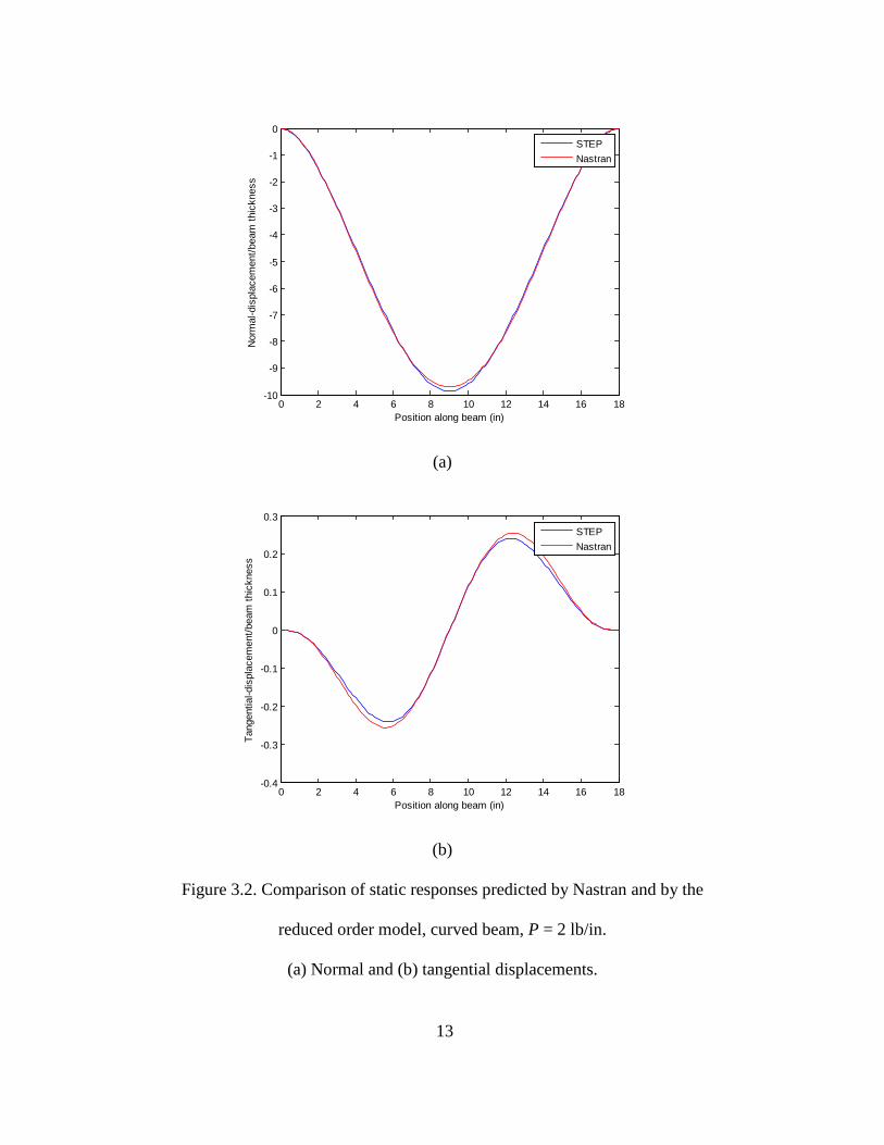
Such a situation is shown in Fig. 3.2 for the curved beam of Fig. 3.1 with

the ROM of [11]. The model identified as above was indeed unstable when loaded

to a static force of P = 3 lb/in. This issue led in [11] to an ad hoc zeroing out of

some of the coefficients of the model leading to the predictions shown in Fig. 3.2.

12

These results match quite well their Nastran counterparts but such an effort is not

easily repeated to any other structure for which the terms to be zeroed out are not

easily predicted.

Figure 3.1. Curved beam geometry.

It was conjectured from [11] that the difficulty in capturing a stable snap-

through response is due to the lack of continuity in the corresponding

displacement vs. load curve. To assess better the difficulties, the snap-through

Nastran displacement field corresponding to the uniform load P = 2 lb/in was

scaled through a broad range of amplitudes. Each such displacement field was

imposed in Nastran and the forces necessary to achieve it were determined.

Projecting these forces on the scaled displacement provided the “modal force”

required.

n t

t = 0.09 in w = 1 in

13

(a)

(b)

Figure 3.2. Comparison of static responses predicted by Nastran and by the


(a) Normal and (b) tangential displacements.

0 2 4 6 8 10 12 14 16 18-10

-9

-8

-7

-6

-5

-4

-3

-2

-1

0

Position along beam (in)

Nor

mal

-dis

plac

emen

t/bea

m th

ickn

ess

STEPNastran

0 2 4 6 8 10 12 14 16 18-0.4

-0.3

-0.2

-0.1

0

0.1

0.2

0.3


Tang

entia

l-dis

plac

emen

t/bea

m th

ickn

ess

STEPNastran

14

Then, shown in Fig. 3.3, curve labeled Nastran, is the obtained modal

force vs. modal displacement (i.e. the scaling of the Nastran displacement of Fig.

3.2) curve. The mass normalized P = 2 lb/in displacement was then used as a

single mode and the STEP identification was performed to get the corresponding

linear, quadratic, and cubic coefficients for various values of the parameter 1q of

Eq. (3.5). The corresponding modal force vs. modal displacement curves are also

shown in Fig. 3.3. Differences clearly occur between the Nastran and STEP

curves, either at low or high displacement levels. A similar process was repeated

with the 12-mode model of [11] before the zeroing out operation and the

comparison with the Nastran results is shown in Fig. 3.4 which shows larger

differences than in Fig. 3.3. This observation suggests that the identification of an

accurate model becomes more challenging as the number of modes increases.

Figure 3.3. Modal forces versus modal displacements curves of 1-mode models

identified by STEP and LS.

0 0.002 0.004 0.006 0.008 0.01 0.012 0.014-1

-0.5

0

0.5

1

1.5

2

2.5

3

3.5

4x 10

4

Modal displacement

Mod

al fo

rce

NastranSTEP 4e-5STEP 4e-4STEP 4e-3STEP 2e-2STEP 4e-2LS

15

Figure 3.4. Modal forces versus modal displacements curves of 12-mode models

identified by STEP and LS.

Table 3.1. Lowest eigenvalue of the matrix BK for different STEP identified

models and a LS identified model.

q1 1 mode 12 modes

STEP 4.00E-05 2.17E+04 2.21E+04

STEP 4.00E-04 2.52E+04 2.39E+04

STEP 4.00E-03 7.06E+04 6.48E+04

STEP 2.00E-02 1.77E+04 -2.54E+05

STEP 4.00E-02 2.43E+04 -1.20E+06

LS 4.00E-04 1.31E+05 1.42E+05

0 0.002 0.004 0.006 0.008 0.01 0.012 0.014-1.5

-1

-0.5

0

0.5

1

1.5

2

2.5

3

3.5x 10

4

Modal displacement

Mod

al fo

rce

NastranSTEP 4e-5STEP 4e-4STEP 4e-3STEP 2e-2STEP 4e-2LS

16

The lack of a close matching in Fig. 3.3 and 3.4 of the STEP results with

their Nastran counterpart suggests that neither the 1-mode nor the 12-mode model

would provide a close fit of the displacements on Fig. 3.2 but does not seem to

justify the instability observed. A different perspective on this issue can be

obtained by analyzing the eigenvalues of the matrix BK , see [18], defined for a

single mode as

= )3(

1111)2(

111

)2(111

)1(11

23/23/2

KKKK

BK . (3.9)

and which should be positive definite. The lowest eigenvalue of BK for the

STEP identified models considered for Figs 3.3 and 3.4 are shown in Table 3.1.

Note that two of these models (both based on 12-mode) yield non-physical

negative eigenvalues. Further, there is a significant sensitivity of this lowest

eigenvalue to the specific value of 1q used. These findings confirm the difficulties

involved in identifying an accurate model using the STEP procedure, Eqs (3.5)-

(3.8).

The perceived weakness of this procedure is that the identification is

conducted near the undeformed configuration for which the linear terms are much

larger than the quadratic ones, themselves much larger than the cubic terms. That

is, in conditions in which the critical balance of the terms on the left-hand-side

does not take place. In this light, it was proposed to shift the baseline point around

which the identification is achieved from the undeformed state to one in or near

the expected difficult conditions, e.g. in a snap-through configuration of the

curved beam. This baseline solution admits the representation

17

∑=

ψ=M

n

nnqu

1

)(0,0 (3.10)

Then, the test displacement fields imposed for identification are

)(0

nnquu ψ+= (3.11)

)()(0

mm

nn qquu ψ+ψ+= m ≥ n (3.12)

)()()(0

rr

mm

nn qqquu ψ+ψ+ψ+= r ≥ m ≥ n (3.13)

More specifically, for each value of n = 1, ..., M, three cases of the form of

Eq. (3.11) were considered with nq = +q, -q, and q/2 as before with q typically

smaller than the thickness. The four cases corresponding to positive and negative

values of nq and mq in Eq. (3.12) were also included for each n and m ≥ n.

Finally, all eight cases associated with positive and negative values of nq , mq ,

and rq for r ≥ m ≥ n and all n were used.

The displacement fields of Eqs (3.11)-(3.13) include generalized

coordinates along all basis functions and thus no simplification of Eq. (3.4) takes

place as in Eq. (3.6). Accordingly, the stiffness coefficients were obtained by a

least squares solution of Eq. (3.4) with the complete set of displacement fields

imposed by Eq. (3.11)-(3.13). Note that the linear, quadratic, and cubic stiffness

coefficients are often of very different magnitudes and thus an appropriate scaling

of the terms is recommended to keep low the condition number of the least

squares matrix. It was also found beneficial to include the equations

corresponding to two different baseline displacement fields 0u .

18

A preliminary assessment of the above revised model identification

approach was obtained by computing the modal force vs. modal displacement

curves corresponding to the Nastran scaled displacement of Fig. 3.2. This effort

was accomplished first in a single mode format using the two baseline solutions

with modal displacements of 3.328e-4 and 1.14e-2 and 1q = 4e-4. The

corresponding curve, named “LS”, see Fig. 3.3, matches very closely its Nastran

counterpart. The computation was also repeated with the 12-mode model of [11]

with baseline solutions corresponding to the projection on this basis of the

Nastran displacements induced by the load P = 1.7 lb/in and P = 2 lb/in. The

results, named “LS”, see Fig. 3.4, again match very closely those obtained with

Nastran. Finally, the eigenvalues of the matrix BK were also recomputed for the

two models and the results are shown in Table 3.1. Note that these values are

significantly larger than those obtained with the STEP algorithm highlighting the

difference in the identified models.

19

Chapter 4

BASIS SELECTION

4.1 Introduction

The two previous chapters have focused on the derivation of the

parametric form of the reduced order model governing equations, Eqs (2.8) and

(3.5), and on the estimation of the parameters from a set of well chosen finite

element solutions. The last key aspect of the construction of reduced order models

is the selection of the basis functions )(nψ . In this regard, the expected features of

the reduced order model are that (i) it leads to an accurate representation of the

full finite element results and (ii) it includes a “reasonably” small number of basis

functions.

The selection of such a basis is not as straightforward a task as in linear

systems. Consider for example a flat homogenous structure subjected to

transverse loads. In the linear response range, only transverse deflections result

from the loading. However, these deflections induce a stretching in the in-plane

direction and thus give rise to in-plane motions as well which are a second order

effect and thus not captured by linear analyses. Nevertheless, such motions must

be captured when constructing the nonlinear reduced order model.

As another example of complexity introduced by nonlinear effects, note

the existence of “symmetry breaking bifurcations”. The response of the

symmetric curved beam shown in Fig. 4.1 to a uniform dynamic loading is known

(see [4]) to be symmetric, as in the linear case, for small loading levels. However,

when the response becomes large enough, antisymmetry arises through a

20

nonlinear coupling of antisymmetric and symmetric modes. In such cases, it is

thus necessary to also include antisymmetric modes in the basis to accurately

capture the beam response.

In light of the above observations, this chapter is focused on the

clarification of the steps followed for the selection of the basis used in connection

with the curved beam of Fig. 3.1.

4.2 Representation Error

Since the selection of the basis is not a straightforward task, it is necessary

to quantify the appropriateness of a particular choice of modes for the

representation of the response. It is proposed here to introduce the representation

error

Erep =

u − u𝑝𝑟𝑜𝑗

u (4.1)

where u is a particular response of the finite element model (referred to as a test

case) and u𝑝𝑟𝑜𝑗

is its projection on the basis selected, i.e.

∑=

ψ=M

n

nprojnproj qu

1

)(, (4.2)

where

uMq FETn

projn)(

, ψ= (4.3)

assuming that the basis functions )(nψ are orthonormalized with respect to the

finite element mass matrix FEM .

21

A basis will be considered to be acceptable for the modeling of the

structural response when the representation error for a series of test cases,

including both static and dynamic ones, is below a certain threshold. Visual

correlations of the responses u and their projections suggest that this threshold

should be taken of the order of 0.01.

Note that even a zero representation error does not guarantee that the

reduced order model constructed with the basis will lead to a good match of the

ROM and finite element predicted displacement fields as the generalized

coordinates ( )tqn will not be obtained from Eq. (4.3) but rather through the

governing equations, Eqs (2.8) and (3.5). So, the representation error should be

considered as only an indicator, not an absolute measure of the appropriateness of

the basis. Further, the worth of the representation error is dependent on the test

cases selected which must span the space of loading and responses of interest. For

example, including only symmetric basis functions and considering test cases in

which this symmetry also holds may suggest that the basis is appropriate while in

fact it may not if symmetry breaking does take place for some loadings of interest.

4.3 Dual Modes

The discussion of section 4.1 highlights that the basis appropriate for a

nonlinear geometric ROM must include other modes than those considered for a

linear modal model but provides no guidance on how to select them. This issue

has been investigated recently, see [8], and it has been suggested that the “linear

basis”, i.e. the modes necessary in linear cases, be complemented by “dual

modes” which capture the nonlinear interactions in the structure.

22

While the construction of the dual modes is applicable to any structural

modeling, it is most easily described in the context of an isotropic flat structure,

e.g. beam or plate, subjected to a transverse loading. Selecting an appropriate

basis for the transverse displacements follows the same steps as in a linear

analysis in which no further modeling is necessary. When the response level is

large enough for nonlinear geometric effects to be significant, small in-plane

displacements appear in the full solution which are associated with the

“membrane stretching” effect. While small, these in-plane motions induce a

significant softening of the stiffening nonlinearity associated with pure transverse

motions.

One approach to construct a full basis, i.e. modeling both transverse and

in-plane displacements, appropriate for the modeling of the nonlinear response is

to focus specifically on capturing the membrane stretching effects. The key idea

in this approach is thus to subject the structure to a series of “representative” static

loadings, determine the corresponding nonlinear displacement fields, and extract

from them additional basis functions, referred to as the “dual modes” that will be

appended to the linear basis, i.e. the modes that would be used in the linear case.

In this regard, note that the membrane stretching effect is induced by the

nonlinear interaction of the transverse and in-plane displacements, not by an

external loading. Thus, the dual modes can be viewed as associated (the adjective

“companion” would have been a better description than “dual”) with the

transverse displacements described by the linear basis. The representative static

loadings should then be selected to excite primarily the linear basis functions and,

23

in fact, in the absence of geometric nonlinearity (i.e. for a linear analysis) should

only excite these “modes”. This situation occurs when the applied load vectors on

the structural finite element model are of the form

∑ ψα=i

iFE

mi

m KF )()1()()( (4.4)

where )(miα are coefficients to be chosen with m denoting the load case number.

A detailed discussion of the linear combinations to be used is presented in [8] but,

in all validations carried out, it has been sufficient to consider the cases

)()1()()( iFE

mi

mi KF ψα= i = dominant mode (4.5)

[ ])()1()()1()(

)(2

jFE

iFE

mim

ij KKF ψψα

=

i = dominant mode, ij ≠

(4.6)

where a “dominant” mode is loosely defined as one providing a large component

of the response. The ensemble of loading cases considered is formed by selecting

several values of )(miα for each dominant mode in Eq. (4.2) and also for each

mode ij ≠ in Eq. (4.3). Note further that both positive and negative values of

)(miα are suggested and that their magnitudes should be such that the

corresponding displacement fields )(miu and )(m

iju range from near linear cases to

some exhibiting a strong nonlinearity.

The next step of the basis construction is the extraction of the nonlinear

effects in the obtained displacement fields which is achieved by removing from

24

the displacements fields their projections on the linear basis, i.e. by forming the

vectors

[ ] ss

miFE

Ts

mi

mi uMuv ψψ−= ∑ )()()( (4.7)

[ ] ss

mijFE

Ts

mij

mij uMuv ψψ−= ∑ )()()( (4.8)

assuming that the finite element mass matrix serves for the orthonormalization of

the basis functions )(nψ (including the linear basis functions and any dual mode

already selected).

A proper orthogonal decomposition (POD) of each set of “nonlinear

responses” )(miv and )(m

ijv is then sequentially carried out to extract the dominant

features of these responses which are then selected as dual modes. The POD

eigenvectors rφ selected as dual modes should not only be associated with a large

eigenvalue but should also induce a large strain energy, as measured by

rFETr K φφ )1( , since the membrane stretching that the dual modes are expected to

model is a stiff deformation mode.

To exemplify the above process, a flat aluminum beam (see [17] for

details), cantilevered on both ends was considered and the duals corresponding to

the first four symmetric transverse modes are shown in Fig. 4.2. Note that these

duals are all antisymmetric as expected from the symmetry of the transverse

motions assumed. To obtain a better sense of the appropriateness of these

functions, a POD analysis of an ensemble of nonlinear responses was carried out

25

and also shown on Fig. 4.2 are the mass normalized POD eigenvectors found for

the in-plane displacements. In fact, two such analyses were conducted, one using

a series of static responses and the other using snapshots obtained during a

dynamic run. It is seen from these results that the dual modes proposed in [8] are

in fact very close to the POD eigenvectors obtained from both static and dynamic

snapshots. Note that both POD eigenvectors and dual modes are dependent on the

responses, e.g. their magnitude, from which they are derived. The results of Fig.

4.2 were obtained with responses ranging typically from 0.08 to 0.8 beam

thickness. In fact, in this range of displacements, the POD analysis of the static

responses yielded only two eigenvectors with significant eigenvalue and thus no

POD-static curve is present in Figs 4.2(c) and 4.2(d).

26

(a)

(b)

0 0.05 0.1 0.15 0.2 0.25-1

-0.8

-0.6

-0.4

-0.2

0

0.2

0.4

0.6

0.8

1


Nor

mal

ized

X D

ispl

acem

ent

POD-Static-1POD-Dynamic-1Dual-Mode1

0 0.05 0.1 0.15 0.2 0.25-1

-0.8

-0.6

-0.4

-0.2

0

0.2

0.4

0.6

0.8

1


Nor

mal

ized

X D

ispl

acem

ent

POD-Static-2POD-Dynamic-2Dual-Mode2

27

(c)

(d)

Figure 4.2. Comparison of dual modes and POD eigenvectors of static and

dynamic responses, clamped-clamped flat beam.

0 0.05 0.1 0.15 0.2 0.25-1

-0.8

-0.6

-0.4

-0.2

0

0.2

0.4

0.6

0.8

1


Nor

mal

ized

X D

ispl

acem

ent

POD-Dynamic-3Dual-Mode3

0 0.05 0.1 0.15 0.2 0.25-1

-0.8

-0.6

-0.4

-0.2

0

0.2

0.4

0.6

0.8

1


Nor

mal

ized

X D

ispl

acem

ent

POD-Dynamic-4Dual-Mode4

28

4.4 Curved Beam - Observations

The first step in the selection of the basis for the curved beam of Fig. 4.1

was the determination of its linear mode shapes and of a series of static and

dynamic nonlinear test cases to be used in the evaluation of the representation

error, Eq. (4.1). Shown in Fig. 4.3 are the first 6 modes with dominant

components in the plane of the beam. Modes 5 and 6 were found to be out-of-

plane modes and thus were not included in the reduced order model as no such

motion was observed in the validation cases considered. Displayed in Fig. 4.3 are

modal displacements along the locally normal and tangential directions, not along

the global X and Y coordinates.

Shown similarly in Fig. 4.4 are static responses of the curved beam

induced by a uniform pressure P acting along the negative Y axis, see Fig. 4.1. For

ease of presentation, the responses were scaled by their respective peak values

which are given in Table 4.1. Note that the cases P = 1 and 1.5 lb/in lead to

nonlinear deflections but no snap-through while the load of P = 2 lbs/in does

induce such an event. Further, the normal components are all symmetric while the

tangential ones are antisymmetric, consistent with the symmetry of the beam and

its excitation.

Table 4.1. Maximum absolute normal and tangential displacements of some

uniform negative pressure loads on the curved beam (in thickness).

P=1 P=1.5 P=2

Max Normal Disp. 0.158 0.262 9.7

29

Max Tangential Disp. 0.0028 0.0046 0.2551

(a)

(b)

0 2 4 6 8 10 12 14 16 18-1

-0.8

-0.6

-0.4

-0.2

0

0.2

0.4

0.6

0.8

1


Nor

mal

ized

Nor

mal

Dis

plac

emen

t

Mode1Mode2Mode3

0 2 4 6 8 10 12 14 16 18-0.03

-0.02

-0.01

0

0.01

0.02

0.03

0.04

0.05

0.06

0.07


Nor

mal

ized

Tan

gent

ial D

ispl

acem

ent

Mode1Mode2Mode3

30

(c)

(d)

Figure 4.3. Linear mode shapes 1, 2, 3, 4, 7, and 8 of the curved beam.

(a) Modes 1, 2 and 3 – Normalized normal displacement.

(b) Modes 1, 2 and 3 – Tangential displacement.

(c) Modes 4, 7, and 8 – Normalized normal displacement.

(d) Modes 4, 7, and 8 – Tangential displacement.

0 2 4 6 8 10 12 14 16 18-1

-0.8

-0.6

-0.4

-0.2

0

0.2

0.4

0.6

0.8

1


Nor

mal

ized

Nor

mal

Dis

plac

emen

t

Mode4Mode7Mode8

0 2 4 6 8 10 12 14 16 18-0.03

-0.02

-0.01

0

0.01

0.02

0.03

0.04


Nor

mal

ized

Tan

gent

ial D

ispl

acem

ent

Mode4Mode7Mode8

31

(a)

(b)

Figure 4.4. Normalized static responses of the curved beam to uniform loads P.

(a) Normalized normal displacement.

(b) Normalized tangential displacement.

0 2 4 6 8 10 12 14 16 18-1

-0.9

-0.8

-0.7

-0.6

-0.5

-0.4

-0.3

-0.2

-0.1

0


Nor

mal

ized

Nor

mal

Dis

plac

emen

t

P=1P=1.5P=2

0 2 4 6 8 10 12 14 16 18-0.03

-0.02

-0.01

0

0.01

0.02

0.03


Nor

mal

ized

Tan

gent

ial D

ispl

acem

ent

P=1P=1.5P=2

32

Snap-shots of the dynamic response of the beam are shown in Figs 4.5 and

4.6. On the former figure, the responses are strongly symmetric in the normal

direction and antisymmetric in the tangential, although not exactly as in the static

cases, see Fig. 4.4. However, in the latter figure 4.6, no symmetry of the

responses is observed, either exactly or even approximately. These observations

confirm the observations of [4,11] that a symmetry breaking bifurcation takes

place dynamically and thus the lack of symmetry will need to be reflected in the

basis.

33

(a)

(b)

Figure 4.5. Snap-shots of the dynamic response of the curved beam - I.



0 2 4 6 8 10 12 14 16 18-1

-0.8

-0.6

-0.4

-0.2

0

0.2

0.4

0.6

0.8

1


Nor

mal

ized

Nor

mal

Dis

plac

emen

t

Snapshot1Snapshot2Snapshot3

0 2 4 6 8 10 12 14 16 18-0.025

-0.02

-0.015

-0.01

-0.005

0

0.005

0.01

0.015

0.02

0.025


Nor

mal

ized

Tan

gent

ial D

ispl

acem

ent


34

(a)

(b)

Figure 4.6. Snap-shots of the dynamic response of the curved beam - II.



0 2 4 6 8 10 12 14 16 18-1

-0.8

-0.6

-0.4

-0.2

0

0.2

0.4

0.6

0.8

1


Nor

mal

ized

Nor

mal

Dis

plac

emen

t


0 2 4 6 8 10 12 14 16 18-0.07

-0.06

-0.05

-0.04

-0.03

-0.02

-0.01

0

0.01


Nor

mal

ized

Tan

gent

ial D

ispl

acem

ent


35

4.5 Curved Beam - Normal Basis Functions

Consistently with linear modal models, the appropriateness of the linear

mode shapes to represent the nonlinear responses was first investigated. From Fig.

4.3, it is seen that all mode shapes exhibit at least one zero of the normal

displacements which thus alternate (except mode 3) between positive and

negative values. However, all static responses and most large dynamic ones do

not, their normal displacements are all one sided and no zero at the middle (as the

linear mode 3). To get an overall perspective on that issue, the ensembles of static

and dynamic responses were analyzed separately in a POD format to extract the

dominant features of the beam response. The corresponding POD eigenvectors of

the normal components (treated separately of the tangential ones), shown in Fig

4.7, do indeed confirm the above impression: the first normal POD eigenvector of

both static and dynamic responses does indeed exhibit a one-sided normal

displacement reaching its maximum value at the middle, at the contrary of the

linear mode shapes. However, the second normal POD eigenvector is somewhat

similar to the second (lowest symmetric) mode shape. While the mode shapes are

known to form a complete basis for all deflections, linear or nonlinear, of the

curved beam, the above observations suggest that the convergence with the

number of modes used may be slow.

On this basis, it was decided here not to use the linear mode shapes but

rather a set of basis functions that is consistent with the POD eigenvectors of Fig.

4.7. Certainly, the POD eigenvectors themselves could have been selected but it

was desired to select basis functions originating from a natural family of modes.

36

In this regard, a strong similarity was observed between the normal POD

eigenvectors and the mode shapes of a flat beam spanning the same distance, see

Figs 4.7. Accordingly, it was decided to use these mode shapes as basis functions

for the normal direction. Note that the value of the modal displacement of the flat

beam in the transverse direction was directly used for the curved beam basis

functions as a normal component with zero tangential counterpart.

(a)

(b)

0 2 4 6 8 10 12 14 16 18-1

-0.9

-0.8

-0.7

-0.6

-0.5

-0.4

-0.3

-0.2

-0.1

0


Nor

mal

ized

Nor

mal

Dis

plac

emen

t

POD-static-1POD-dynamic-1Beam-Mode1

0 2 4 6 8 10 12 14 16 18-1

-0.8

-0.6

-0.4

-0.2

0

0.2

0.4

0.6

0.8

1


Nor

mal

ized

Nor

mal

Dis

plac

emen

t


37

(c)

(d)

Figure 4.7. Comparison of the POD eigenvectors of static and dynamic responses

in normal direction of the curved beam and the corresponding flat beam

transverse modes.

0 2 4 6 8 10 12 14 16 18-1

-0.8

-0.6

-0.4

-0.2

0

0.2

0.4

0.6

0.8

1


Nor

mal

ized

Nor

mal

Dis

plac

emen

t


0 2 4 6 8 10 12 14 16 18-1

-0.8

-0.6

-0.4

-0.2

0

0.2

0.4

0.6

0.8

1


Nor

mal

ized

Nor

mal

Dis

plac

emen

t


38

4.6 Curved Beam - Tangential Basis Functions

The basis functions introduced in the previous sections do not have any

tangential component and thus cannot provide a complete representation of the

beam response. This situation closely parallels the flat beam where the modes first

selected were purely transverse. For that structure, the “dual modes” of section

4.3 were successfully used to complement the transverse modes suggesting a

similar choice for the curved beam using the normal basis functions as linear

basis. In fact, the dual modes and POD eigenvectors were found to be very similar

for the flat beam, see Fig. 4.2 and it was desired to first assess whether a similar

property would hold for the curved beam.

Since the normal basis functions do not have any tangential component, it

was decided that the dual modes that would be used should exhibit purely

tangential displacements and the procedure of section 4.3 was modified

accordingly by zeroing the normal components of the “nonlinear responses” )(miv

and )(mijv before performing the POD analysis. The resulting dual modes

corresponding to the symmetric normal basis functions are compared in Fig. 4.8

to the POD eigenvectors obtained from the ensemble of static and dynamic

tangential responses. A good qualitative agreement is observed although the

quantitative match is not as close as seen for the flat beam, see Fig. 4.2. On the

basis of this successful comparison, the dual modes were selected to complement

the normal basis functions for the representation of the curved beam response.

39

(a)

(b)

0 2 4 6 8 10 12 14 16 18-1

-0.8

-0.6

-0.4

-0.2

0

0.2

0.4

0.6

0.8

1


Nor

mal

ized

Tan

geni

tal D

ispl

acem

ent

POD-static-1POD-dynamic-1Dual-Mode1

0 2 4 6 8 10 12 14 16 18-1

-0.8

-0.6

-0.4

-0.2

0

0.2

0.4

0.6

0.8

1


Nor

mal

ized

Tan

geni

tal D

ispl

acem

ent


40

(c)

(d)

Figure 4.8. Comparison of the POD eigenvectors of static and dynamic responses

in tangential direction and the dual modes, curved beam.

0 2 4 6 8 10 12 14 16 18-1

-0.8

-0.6

-0.4

-0.2

0

0.2

0.4

0.6

0.8

1


Nor

mal

ized

Tan

geni

tal D

ispl

acem

ent


0 2 4 6 8 10 12 14 16 18-1

-0.8

-0.6

-0.4

-0.2

0

0.2

0.4

0.6

0.8

1


Nor

mal

ized

Tan

geni

tal D

ispl

acem

ent


41

Chapter 5

CURVED BEAM STATIC RESPONSE VALIDATION

This chapter presents static response validation for the identification

strategy based on Eqs (3.10)-(3.13) using the clamped-clamped curved beam of [4,

5, 11], see Fig. 4.1. The beam has an elastic modulus of 10.6×106 psi, shear

modulus of 4.0×106 psi, and density of 2.588×10-4 lbf-sec2/in4. A Nastran finite

element model with 144 CBEAM elements was developed to first construct the

reduced order model and then assess its predictive capabilities. The reduced order

model development aimed at the dynamic response to a pressure uniform in space

but varying in time. This chapter focuses solely on the static response to such a

loading, i.e. F(t) = P constant, and shown in Fig. 5.1 is the vertical displacement

induced at the middle of the beam as a function of P. Note that the beam exhibits

a snap-through at P = 1.89 lb/in and that the magnitude of the snap-through

deformation is quite large, of the order of 10 thicknesses. If the beam is unloaded

from this point, it will not go back to the neighborhood of the undeformed

position, i.e. on the left branch, until the load reduces to approximately 0.45 lb/in,

which represents the snap-back condition.

42

Figure 5.1. Relation between applied static pressure and vertical displacement of

the beam middle, curved beam, predicted by Nastran and ROM.

The basis used for the reduced order model included the first 6 normal

basis functions, see section 4.5, and the corresponding 6 dual modes with the first

normal basis function dominant, see section 4.6. This process led for the present

static computations to a 12-mode model similar to the one considered in [11]. To

get a first perspective of how well this 12-mode basis might capture the uniform

pressure static responses, the representation error was computed for a few load

cases, see Table 5.1. The small magnitudes of these errors suggest that the basis is

probably acceptable for the representation of the response.

0 2 4 6 8 10 120

0.5

1

1.5

2

2.5

3

3.5

4

4.5

5

Vertical displacement (in)

Pre

ssur

e (lb

/in)

NastranROM

43

Table 5.1. Representation error (in percentage) of the basis for some uniform

pressure static loadings.

P=1 lb/in P=1.7 lb/in P=2 lb/in P=3 lb/in

Normal 1.095e-002 1.159e-002 1.478e-002 1.848e-002

Tangential 2.152e-002 1.637e-002 2.418e-002 4.749e-002

The construction of the reduced order model according to the STEP

procedure of Eqs (3.5)-(3.8) led to the same difficulties as those encountered in

[11] and described in chapter 3, i.e. difficulty in obtaining a finite valued static

solution by a time marching integration of the reduced order equations of Eq.

(2.8). Even when a solution could be found, it led to a poor matching of the finite

element results. This issue was resolved in [11] by a detailed study of coefficients

and a zeroing out of those that drove the instability; a model matching well the

full finite element results was then obtained.

The present effort relied instead on the revised identification procedure, i.e.

Eqs (3.10)-(3.13). Specifically, two baseline solutions were considered that

correspond to the projection of the full finite element results at P = 1.7lb/in on the

left branch, i.e. below the snap-through limit, and at P = 2lb/in, i.e. above the

snap-through transition. No instability of the model was found in any of the

computations carried out thereby suggesting that this phenomenon was indeed

related to the near cancelation of terms and demonstrating the benefit of the

revised identification of Eqs (3.10)-(3.13).

44

The assessment of the reduced model in matching the full finite element

results was carried out in two phases corresponding to the two branches, left and

right, of the response curve of Fig. 5.2. Shown in Fig. 5.3 are the normal and

tangential displacements obtained at the load of P = 1.7lb/in which are typical of

the left branch. An excellent match between Nastran and reduced order model

results is obtained. A similar analysis was conducted with loading conditions on

the right branch and shown in Fig. 5.4 are the normal and tangential

displacements obtained for P = 3 lb/in. Both Nastran and reduced order models

were then unloaded to P = 1 lb/in, see Fig. 5.5. Finally, a load of P = 10 lb/in was

also considered and the responses are shown in Fig. 5.6. In all of these cases, an

excellent match is obtained between the full finite element model results and the

reduced order model predictions.

Even with these excellent comparisons, it should be noted that the reduced

order model does not predict correctly the snap-through load. Indeed, the load-

deflection corresponding to the reduced order model, also shown in Fig. 5.1,

indicates that its snap-through occurs at a load of 2.3lb/in vs. the 1.89lb/in for the

finite element model. Nevertheless, these overall results indicate that the

identification algorithm based on Eqs (3.10)-(3.13) has led to a very reliable

reduced order model.

45

(a)

(b)


reduced order model, curved beam, P = 1.7 lb/in.


0 2 4 6 8 10 12 14 16 18-0.35

-0.3

-0.25

-0.2

-0.15

-0.1

-0.05

0


Nor

mal

-dis

plac

emen

t/bea

m th

ickn

ess

ROMNastran

0 2 4 6 8 10 12 14 16 18-6

-4

-2

0

2

4

6x 10

-3


Tang

entia

l-dis

plac

emen

t/bea

m th

ickn

ess

ROMNastran

46

(a)

(b)




0 2 4 6 8 10 12 14 16 18-12

-10

-8

-6

-4

-2

0


Nor

mal

-dis

plac

emen

t/bea

m th

ickn

ess

ROMNastran

0 2 4 6 8 10 12 14 16 18-0.4

-0.3

-0.2

-0.1

0

0.1

0.2

0.3


Tang

entia

l-dis

plac

emen

t/bea

m th

ickn

ess

ROMNastran

47

(a)

(b)


reduced order model, curved beam, P = 1 lb/in (right branch).


0 2 4 6 8 10 12 14 16 18-9

-8

-7

-6

-5

-4

-3

-2

-1

0


Nor

mal

-dis

plac

emen

t/bea

m th

ickn

ess

ROMNastran

0 2 4 6 8 10 12 14 16 18-0.25

-0.2

-0.15

-0.1

-0.05

0

0.05

0.1

0.15

0.2

0.25


Tang

entia

l-dis

plac

emen

t/bea

m th

ickn

ess

ROMNastran

48

(a)

(b)




0 2 4 6 8 10 12 14 16 18-12

-10

-8

-6

-4

-2

0


Nor

mal

-dis

plac

emen

t/bea

m th

ickn

ess

ROMNastran

0 2 4 6 8 10 12 14 16 18-0.4

-0.3

-0.2

-0.1

0

0.1

0.2

0.3

0.4


Tang

entia

l-dis

plac

emen

t/bea

m th

ickn

ess

ROMNastran

49

Chapter 6

CURVED BEAM DYNAMIC RESPONSE VALIDATION

The 12-mode reduced order model obtained in the previous chapter only

includes symmetric normal modes and thus is not appropriate for dynamic loads

because of the potential occurrence of symmetry breaking. Accordingly, this

chapter focuses on the construction and validation of an extended ROM that is

appropriate for such dynamic loadings, i.e. includes anti-symmetric normal basis

functions and corresponding dual modes.

Normal basis functions were first considered and 7 such functions were

selected, more specifically 3 anti-symmetric and 4 symmetric ones, all based on

the linear modes of the corresponding straight beam. Next, the 6 antisymmetric

dual modes of chapter 5 were retained and complemented by 5 mostly symmetric

dual modes created with the first symmetric and first antisymmetric normal basis

functions as dominant. These dual modes were also made purely tangential by

stripping their normal components. This process led to an 18-mode model.

Before identifying the stiffness parameters associated to this model, its

adequacy to represent both static and dynamic responses of test cases was first

assessed. Specifically, the representation error was computed for a series of

snapshots of the dynamic response. The snapshots selected here exhibited

strongly dominant symmetric or antisymmetric normal or tangential components

to judge each group of the 18-mode basis separately.

50

Table 6.1. Representation error (in percentage) of the basis on the snapshots with

symmetric normal components.

Snap-shot1 Snap-shot2 Snap-shot3 Snap-shot4

Normal 2.46E-01 1.13E-02 4.69E-02 1.69E-01


antisymmetric tangential components.


Tangential 2.49E-02 1.68E-02 1.38E-02 1.73E-01


antisymmetric normal components.


Normal 1.82E-01 1.31E-01 1.37E-01 2.23E-01


symmetric tangential components.


Tangential 1.63E-01 1.48E-01 3.39E-02 2.97E-01

The representation errors, given in Table 6.1-6.4, were found to be low

enough to proceed with the identification of the stiffness parameters.

Accomplishing this effort requires the selection of at least one, two were selected,

51

baseline solutions. To exercise all basis functions, it was desired that the baseline

solutions exhibit a lack, notable preferably, of symmetry. To this end, the baseline

solutions were selected as the static responses to pressure distributions linearly

varying along the beam. The first such distribution varied from 0.98lb/in on the

left side to 1.82 lb/in on the right one. The second varied similarly from 1.4 to 2.6

lb/in. The baseline loading P = 1.4-2.6 lb/in has a mean value of 2 lb/in and leads

to a snap-through response but it is very close to symmetric. However, the

baseline solution induced by the pressure P = 0.98-1.82 lb/in is not a snap-through

but exhibits a significant lack of symmetry.

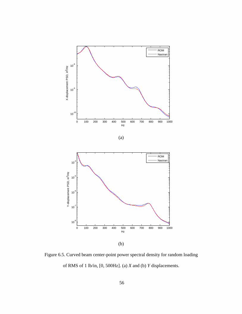
The dynamic validation was achieved by comparing the power spectra of

the stationary responses of the center and quarter points of the beam in the global

X and Y directions obtained by a full Nastran analysis and the reduced order

model. The random excitation considered was uniform along the beam, in the

global Y direction, and varied with time as a bandlimited white noise with a flat

spectrum in the range of [0, 500Hz]. Three excitations levels were considered

yielding RMS forces of 0.5, 1, and 2 lb/in, see [11]. The higher levels 1 and 2

lb/in displayed intermittent and nearly continuous snap-through excursions,

respectively. The comparison of power spectra for these 3 cases and 2 locations,

see Figs 6.1-6.6, demonstrates a good to very good matching, most notably at the

two smallest levels, suggesting indeed the appropriateness of the reduced order

model.

52

(a)

(b)

Figure 6.1. Curved beam quarter-point power spectral density for random loading

of RMS of 0.5 lb/in, [0, 500Hz]. (a) X and (b) Y displacements.

0 100 200 300 400 500 600 700 800 900 1000

10-11

10-10

10-9

10-8

Hz

X-d

ispl

acem

ent P

SD

, in2 /

Hz

ROMNastran

0 100 200 300 400 500 600 700 800 900 1000

10-9

10-8

10-7

10-6

Hz

Y-d

ispl

acem

ent P

SD

, in2 /

Hz

ROMNastran

53

(a)

(b)


of RMS of 1 lb/in, [0, 500Hz]. (a) X and (b) Y displacements.

0 100 200 300 400 500 600 700 800 900 1000

10-10

10-9

10-8

Hz

X-d

ispl

acem

ent P

SD

, in2 /

Hz

ROMNastran

0 100 200 300 400 500 600 700 800 900 100010

-8

10-7

10-6

10-5

Hz

Y-d

ispl

acem

ent P

SD

, in2 /

Hz

ROMNastran

54

(a)

(b)



0 100 200 300 400 500 600 700 800 900 1000

10-9

10-8

Hz

X-d

ispl

acem

ent P

SD

, in2 /

Hz

ROMNastran

0 100 200 300 400 500 600 700 800 900 1000

10-7

10-6

10-5

10-4

Hz

Y-d

ispl

acem

ent P

SD

, in2 /

Hz

ROMNastran

55

(a)

(b)

Figure 6.4. Curved beam center-point power spectral density for random loading

of RMS of 0.5 lb/in, [0, 500Hz]. (a) X and (b) Y displacements.

0 100 200 300 400 500 600 700 800 900 100010

-11

10-10

10-9

10-8

Hz

X-d

ispl

acem

ent P

SD

, in2 /

Hz

ROMNastran

0 100 200 300 400 500 600 700 800 900 100010

-9

10-8

10-7

10-6

Hz

Y-d

ispl

acem

ent P

SD

, in2 /

Hz

ROMNastran

56

(a)

(b)



0 100 200 300 400 500 600 700 800 900 1000

10-10

10-9

10-8

Hz

X-d

ispl

acem

ent P

SD

, in2 /

Hz

ROMNastran

0 100 200 300 400 500 600 700 800 900 1000

10-8

10-7

10-6

10-5

10-4

Hz

Y-d

ispl

acem

ent P

SD

, in2 /

Hz

ROMNastran

57

(a)

(b)



0 100 200 300 400 500 600 700 800 900 1000

10-9

10-8

Hz

X-d

ispl

acem

ent P

SD

, in2 /

Hz

ROMNastran

0 100 200 300 400 500 600 700 800 900 1000

10-7

10-6

10-5

10-4

Hz

Y-d

ispl

acem

ent P

SD

, in2 /

Hz

ROMNastran

58

Chapter 7

SUMMARY

The present investigation focused on a revisit and extension of existing

approaches for the reduced order modeling of the geometrically nonlinear

response of a curved beam. The work carried out addressed two particular aspects

of the ROM development: the selection of the basis and the identification of the

coefficients. In regards to the basis, a close relation between the recently

introduced dual modes and proper orthogonal decomposition (POD) eigenvectors

of the response was demonstrated for both the curved beam and its flat

counterpart. This POD analysis also supported the earlier choice of normal basis

functions as the linear modes of the flat beam.

In regards to the identification of the parameters, the difficulties, i.e.

instability of the reduced order model, encountered in the past were first analyzed.

This effort then served as the basis for the formulation of a revised identification

procedure of the parameters of the reduced order model, see Eqs (3.10)-(3.13).

The application of this procedure to the curved beam model removed the

instability issue previously encountered and led to an excellent matching of

reduced order model and finite element predictions for a broad range of external,

static or dynamic, loading. Further, this matching was obtained without

performing the zeroing out process suggested in an earlier investigation. The

present results extend previous validation studies in demonstrating the worth of

reduced order modeling of nonlinear geometric structures.

59

REFERENCES

[1] McEwan, M.I., Wright, J.R., Cooper, J.E., and Leung, A.Y.T, "A combined Modal/Finite Element Analysis Technique for the Dynamic Response of a Nonlinear Beam to Harmonic Excitation", Journal of Sound and Vibration 243 (2001): 601-624. [2] Hollkamp, J.J., Gordon, R.W., and Spottswood, S.M, "Nonlinear Modal Models for Sonic Fatigue Response Prediction: A Comparison of Methods", Journal of Sound and Vibration 284 (2005): 1145-1163. [3] Radu, A., Yang, B., Kim, K., and Mignolet, M.P, "Prediction of the Dynamic Response and Fatigue Life of Panels Subjected to Thermo-Acoustic Loading", Proceedings of the 45th Structures, Structural Dynamics, and Materials Conference. Palm Springs, California, 2004. AIAA Paper AIAA-2004-1557. [4] Przekop, A. and Rizzi, S.A, "Nonlinear Reduced Order Finite Element Analysis of Structures With Shallow Curvature", AIAA Journal 44, no. 8 (2006): 1767-1778. [5] Gordon, R.W. and Hollkamp, J.J, "Reduced-Order Modeling of the Random Response of Curved Beams using Implicit Condensation", AIAA Journal (2006). [6] Spottswood, S.M., Hollkamp, J.J., and Eason, T.G, "On the Use of Reduced-Order Models for a Shallow Curved Beam Under Combined Loading", Proceedings of the 49th Structures, Structural Dynamics, and Materials Conference. Schaumburg, Illinois, 2008. AIAA Paper AIAA-2008-1873 [7] Kim, K., Khanna, V., Wang, X.Q., Mignolet, M.P, "Nonlinear Reduced Order Modeling of Flat Cantilevered Structures", Proceeding of the 50th Structures, Structural Dynamics, and Materials Conference. Palm Springs, 2009. AIAA Paper AIAA-2009-2492. [8] Kim, K., Wang, X.Q., and Mignolet, M.P, "Nonlinear Reduced Order Modeling of Functionally Graded Plates", Proceedings of the 49th Structures, Structural Dynamics, and Materials Conference. Schaumburg, Illinois, Apr. 7-10, 2008. AIAA Paper AIAA-2007-2014 [9] Perez, R., Wang, X.Q., Mignolet, M.P, "Nonlinear reduced order models for thermoelastodynamic response of isotropic and FGM panels", AIAA Journal 49 (2011): 630-641. [10] Perez, R., Wang, X.Q., Mignolet, M.P, "Reduced order modeling for the nonlinear geometric response of cracked panels", Proceeding of the 52th

60

Structures, Structural Dynamics and Materials Conference. Denver, 2011. AIAA Paper AIAA-2011-2018. [11] Spottswood, S.M., Eason, T.G., Wang, X.Q., Mignolet, M.P, "Nonlinear reduced order modeling of curved beams: a comparison of methods", Proceeding of the 50th Structures, Structural Dynamics, and Materials Conference. Palm Springs, 2009. AIAA Paper AIAA-2009-2433. [12] Rizzi, S.A. Przekop, A, "System identification-guided basis selection for reduced-order nonlinear response analysis", Journal of Sound and Vibration 315 (2008): 467-485. [13] Przekop, A. Rizzi, S.A, "Nonlinear reduced-order analysis with time-varying spatial loading distributions", Journal of Aircraft 46 (2009): 1395-1402. [14] Muravyov, A.A. and Rizzi, S.A, "Determination of Nonlinear Stiffness with Application to Random Vibration of Geometrically Nonlinear Structures", Computers and Structures 81 (2003): 1513-1523. [15] Fung, Y.C., and Tong, P, Classical and Computational Solid Mechanics. River Edge, New Jersey: World Scientific, 2001. [16] Bonet, J., and Wood, R.D., Nonlinear Continuum Mechanics for Finite Element Analysis, Cambridge: Cambridge University Press, 1997. [17] Kerschen, G., Golinval, J.-C., Vakakis, A.F., Bergman, L.A., "The method of proper orthogonal decomposition for dynamical characterization and order reduction of mechanical systems: an overview", Nonlinear Dynamics 41 (2005): 147-169. [18] Mignolet, M.P, Soize, C., "Stochastic reduced order models for uncertain geometrically nonlinear dynamical systems", Computer Methods in Applied Mechanics and Engineering 197 (2008): 3951-3963.

reduced order modeling for the nonlinear geometric response of some joined wings

Documents