recurring local sequence motifs in proteins

JMB—MS 665 Cust. Ref. No. FC 19/95 [SGML]

J. Mol. Biol. (1995) 251, 176–187

Recurring Local Sequence Motifs in Proteins

Karen F. Han 1 and David Baker 2*

We describe a completely automated approach to identifying local sequence1Graduate Group inmotifs that transcend protein family boundaries. Cluster analysis is used toBiophysics, University of

California, San Francisco identify recurring patterns of variation at single positions and in shortsegments of contiguous positions in multiple sequence alignments for aCA 94143, USAnon-redundant set of protein families. Parallel experiments on simulated2Dept of Biochemistry data sets constructed with the overall residue frequencies of proteins but not

University of Washington the inter-residue correlations show that naturally occurring proteinSeattle, WA 98195, USA sequences are significantly more clustered than the corresponding random

sequences for window lengths ranging from one to 13 contiguous positions.The patterns of variation at single positions are not in general surprising:chemically similar amino acids tend to be grouped together. Moreinteresting patterns emerge as the window length increases. The patterns ofvariation for longer window lengths are in part recognizable patterns ofhydrophobic and hydrophilic residues, and in part less obviouscombinations. A particularly interesting class of patterns features highlyconserved glycine residues. The patterns provide a means to abstract theinformation contained in multiple sequence alignments and may be usefulfor comparison of distantly related sequences or sequence families and forprotein structure prediction.

7 1995 Academic Press Limited

Keywords: multiple sequence alignments; sequence comparison;*Corresponding author substitution matrices; protein structure prediction; sequence motifs

Introduction

Are there recurring local patterns in the amino acidsequences that encode proteins? Global similarityis often used to classify sequences into families;are there local patterns that transcend familyboundaries?

Given that all viable protein sequences must besuch that the proteins they encode can fold and haveat least marginal stability, it is reasonable to expectthat not all 20N amino acid sequences of length Nare equally probable. There are far too few distinctprotein families to tabulate meaningful statisticson the frequencies of occurrence of the differentpeptides of length N for N greater than two (Gonnetet al., 1994). An alternative approach is to use clusteranalysis to identify recurring sequence patterns. Thisrequires a suitable measure of similarity betweentwo sequences.

Global sequence comparisons almost always relyon amino acid substitution matrices compiled byaveraging over large sets of related sequences. Thedisadvantages of using a single substitution matrixhave been pointed out on numerous occasions(Johnson et al., 1993; Risler et al., 1988). The majorproblem is that at different positions in proteinstructures, different sets of amino acid sequences are

likely to substitute for one another. In other words,there is no single and universally applicable set ofdistances (or similarities) between the 20 aminoacids. Rather, similarity can be quite context-dependent.

A more natural measure, which does not requirethe assumption of a single substitution matrix, isavailable for comparison of protein families if thereare a number of sequences in each family. For eachposition in a set of multiply aligned sequences, onecan calculate the frequency of occurrence of each ofthe amino acids. The resulting sequence of frequencydistributions is often called a profile (Gribskov et al.,1990). To evaluate the distance between two alignedprofile segments, one can compare the frequencydistributions at corresponding positions.

Here we use such a distance measure in conjunc-tion with cluster analysis to identify patterns thatoccur frequently in multiple sequence alignmentsfor proteins of known structure. Because only onemultiple sequence alignment is included of eachfamily, the patterns are necessarily common to manydifferent protein families and are distinct from thefamily-specific patterns compiled in the Prosite data-base (Bairoch & Bucher, 1994). Because the patternsare universal but still fairly detailed, they present apossible route to overcoming some of the limitations

0022–2836/95/310176–12 $08.00/0 7 1995 Academic Press Limited

JMB—MS 665

Recurring local sequence motifs in proteins 177

of the global amino acid substitution matrices usedin sequence comparisons and the individual residuesecondary structure and solvent accessibility pro-pensities used in local protein structure prediction.The work described in this paper is a first steptowards correlating local sequence patterns withlocal structural motifs.

Results

If there are a finite number of distinct chemicalenvironments in proteins, there should be a finitenumber of patterns of variation in sets of multiplyaligned sequences. Here we use cluster analysis toidentify recurring patterns of variation at single pos-itions and in short segments of contiguous positionsin multiple sequence alignments. A non-redundantset of global multiple sequence alignments for pro-teins of known structure was extracted from theHSSP database (Sander & Schneider, 1991) as de-scribed in Methods. After excluding positions inwhich fewer than 20 sequences contributed to thealignment, the data set contained approximately20,000 individual columns from 154 protein families.

Patterns at single positions

The frequencies of occurrence of the 20 aminoacids at each position were calculated, and theK-means algorithm was used to group similar fre-quency distributions using the simple ‘‘city block’’metric (d1, see Methods).

The amino acid groupings obtained (Table 1) areconsistent with expectation. The mean of the fre-quency distributions belonging to a given clusterprovides a convenient summary statistic. To savespace, the mean values of each of the 20 amino acidsin each cluster are not shown, instead only the aminoacids whose mean frequency of occurrence in acluster is greater than 0.1 (upper case) or between0.07 and 0.1 (lower case) are listed (Table 1, column 3).

The degree of conservation of these primary com-ponents is reflected in the variability index(column 4), which gives the number of amino acidcomponents whose mean frequency of occurrence isgreater than 0.05.

The patterns generally fall into either hydrophobic(clusters 1, 2 and 3) or polar (clusters 4 through 8)classes (Table 1, column 6). However, the differentclusters contain different combinations of hydro-phobic and hydrophillic groups. For example,cluster 1 contains primarily V, I and L while cluster 2contains primarily I, L and M. Cluster 3 contains onlyaromatic residues while cluster 6 contains onlynegatively charged residues. Amino acid residueswith special structural properties are prominent inclusters 9 (P) and 10 (G). Although the RMS deviationof points within a cluster is not dramatically less thanthat of points in the entire dataset (see Methods), theproducts of the variances are considerably lower inthe former than in the latter (Table 1, column 6). Asoutlined in Methods, the patterns were independentof the choice of starting cluster centers implicit inthe K-means algorithm. Patterns similar to those inTable 1 were obtained in a Dirichlet mixture decom-position of multiple sequence alignments (Brownet al., 1993).

The first ten patterns in Table 1 are the result of alow resolution subdivision of sequence space (tenclasses were allowed). More subtle patterns arerevealed when the number of classes is increased(see Methods). For example, in cluster 11, primarilyL, R and K, the common feature is the long aliphaticside-chain of all three residues. Pattern 13 isdominated by the beta branched residues V, I and T.A cluster with conserved cysteine residues alsoemerges when more classes are allowed. Thus,although hydrophobicity appears to be the majorfeature distinguishing the largest clusters, otherchemical properties are often important in thesmaller clusters.

How clustered are the frequency distributions insequence space? The K-means algorithm can always

Table 1. Recurrent patterns at individual positions

DominantRelative

No. ofsubstitutions

Variability clusterCluster no. members index Hydrophobicity volume

1 2449 V,I,I 3 0.832 2.3e-42 1971 L,i,m 5 0.853 5.4e-43 1521 Y,F,w 4 0.818 1.6e-34 1166 N,H,d 4 0.151 7.4e-45 2263 R,K,q 4 0.163 5.8e-36 2396 D,E 4 0.148 2.5e-37 1401 T,s 3 0.237 2.4e-48 1412 S,a,t 3 0.199 3.3e-49 2214 P,A 3 0.538 1.2e-3

10 1349 G 2 0.166 4.3e-411 84 L,R,K 4 0.450 2.8e-312 150 G,N,k 4 0.101 2.4e-613 114 V,I,T 4 0.687 1.1e-5

The amino acids which occur with frequencies greater than 0.1 are shown in upper case, thosewhich occur at frequencies between 0.07 and 0.1, in lower case (column 3). The number of aminoacids which occur at frequencies greater than 0.05 is given in column 4. The average summedfrequency of occurrence of the amino acids A, V, I, L, M, F, W and C is listed in column 5.

JMB—MS 665

Recurring local sequence motifs in proteins178

(a) (b)

(c)

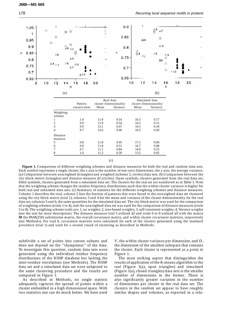
Figure 1. Comparison of different weighting schemes and distance measures for both the real and random data sets.Each symbol represents a single cluster; the x axis is the number of non-zero dimensions, the y axis, the average variance.(a) Comparison between unweighted (triangles) and weighted (scheme 2, circles) data sets. (b) Comparison between thecity block metric (triangles) and distance measure d2 (circles). Open symbols, clusters generated from the real data set;filled symbols, clusters generated from a simulated data set. The clusters for the real set are numbered as in Table 1. Notethat the weighting scheme changes the residue frequency distributions such that the within-cluster variance is higher forboth real and simulated data sets. (c) Summary of statistics for the different weighting schemes and distance measures.Column 1 describes the trial, column 2 lists the fraction of patterns that were found in the unweighted data set clusteredusing the city block metric (trial 1), columns 3 and 4 list the mean and variance of the cluster dimensionality for the realdata set; columns 5 and 6, the same quantities for the simulated data set. The city block metric was used for the comparisonof weighting schemes (trials 1 to 4), and the unweighted data set was used for the comparison of distance measures (trials5 to 8). The weighting scheme trails are: 1, no weights; 2, tree-based weights; 3, self consistent weights; 4, Voronoi weights(see the text for more description). The distance measure trial 5 utilized d2 and trials 6 to 8 utilized d3 with the matrixM the PAM(250) substitution matrix, the overall covariance matrix, and within cluster covariance matrices, respectively(see Methods). For trial 8, covariance matrices were calculated for each of the clusters generated using the standardprocedure (trial 1) and used for a second round of clustering as described in Methods.

Real data Simulated dataPattern cluster dimensionality cluster dimensionality

conservation Mean Variance Mean Variance

Weightingscheme1 1.0 11.8 0.54 16.3 0.172 0.9 11.8 0.54 16.5 0.153 0.9 12.1 0.47 16.5 0.184 0.7 12.6 0.46 16.5 0.20

Distancemeasure5 0.8 11.8 0.45 17.5 0.066 0.9 11.8 0.51 16.7 0.087 0.7 11.1 0.84 14.9 0.258 1.0 11.3 0.39 13.5 0.02

subdivide a set of points into convex subsets anddoes not depend on the ‘‘clumpiness’’ of the data.To investigate this question, random data sets weregenerated using the individual residue frequencydistributions of the HSSP database but lacking theinter-residue correlations (see Methods). The HSSPdata set and a simulated data set were subjected tothe same clustering procedure and the results arecompared in Figure 1.

As described in Methods, no single statisticadequately captures the spread of points within acluster embedded in a high dimensional space. Withtwo statistics one can do much better. We have used

V, the within cluster variance per dimension, and D,the dimension of the smallest subspace that containsthe cluster. Each cluster is represented as a point inFigure 1.

The most striking aspect that distinguishes theresults of application of the K-means algorithm to thereal (Figure 1(a), open triangles) and simulated(Figure 1(a), closed triangles) data sets is the smallernumber of dimensions in the former. There isalso significantly greater variation in the numberof dimensions per cluster in the real data set. Theclusters in the random set appear to have roughlysimilar shapes and volumes, as expected in a rela-

JMB—MS 665


tively uniform distribution. In contrast, the sizes andshapes of the clusters obtained for the real data setvary considerably, presumably because differentsequence patterns in protein families are constrainedto different extents.

Comparison of weighting schemes anddistance measures

Frequency distributions from multiple sequencealignments can be taken as estimators of the ‘‘true’’probability distributions for substitution of the20 amino acids at a given position in a protein, butthere are two important caveats. First, there are alimited number of sequences in each family, so thatobserved frequencies may be inaccurate estimatesbecause of small sample size effects. We have dealtwith this problem by excluding poorly representedfamilies and positions from the analysis. Second, andperhaps more serious, the different sequences in afamily are not independent observations. Rather,they are highly correlated. Frequency distributionsderived from sets of evolutionarily related sequencesmay be heavily biased. A particular amino acid maybe highly represented in a particular position simplybecause it was present in a common ancester, and notbecause of any underlying structural constraint.

A number of different weighting schemes havebeen proposed for compensation of the heavilybiased sampling in evolutionarily related sequencesets (Vingron & Sibbald, 1993). We experimentedwith (1) a weighting scheme similar to that describedby Altschul et al. (1989) and van Ooyen & Hogeweg(1990) in which weights are derived from a treeconstructed from pairwise distances between thealigned sequences; (2) the self-consistent weight-ing scheme of Sander & Schneider (1991), and(3) the Monte Carlo approach to estimating Voronoivolumes described by Sibbald & Argos (1990).Frequency distributions were recalculated for eachof the weighting schemes and subjected along withcorresponding simulated data sets to the K-meansclustering procedure.

Space limitations prohibit the display of scatterplots for each of the weighting schemes. However,the essence of these plots can be roughly captured bythe mean and variance of D, the cluster dimensional-ity (Figure 1). The results obtained with frequencydistributions weighted using scheme (1) were verysimilar to those obtained with the unweighted distributions (Figure 1, compare circles to triangles).

The average cluster dimensionality was verysimilar for all the weighted data sets (Figure 1(c),column 3), indicating that the interrelationshipsamong the frequency distributions are not substan-tially changed by the different weighting schemes.Furthermore, the resulting sequence patterns werenot greatly altered by any of the weighting schemes(Figure 1(c), column 2). Since both the relative weighton a particular sequence and the probability ofmisalignment increase with sequence divergence,attempts at correcting the biased sampling throughunequal sequence weighting may increase noise

from misalignment errors. Because of the lack ofdependence of the results on the weighting scheme,unit weights were used for simplicity in the experi-ments described in the following sections.

A similar approach was used to evaluate alter-native distance measures. The Euclidean distancemetric gave results very similar to that of the cityblock metric d1 (data not shown). Because differencesbetween amino acid frequencies of 0.8 and 0.6 arelikely to be less significant than differences betweenfrequencies of 0.2 and 0.0, we experimented withthe somewhat ad hoc distance measure d2 whicheffectively down-weights differences of the formertype. Again, the clusters obtained with distancemeasures d2 had similar overall properties to thoseobtained with d1 (Figure 1(b)). We also experimentedwith a PAM (250) matrix based distance measure andwith the use of the overall covariance matrix aswell as individual cluster covariance matrices toadjust for the different frequencies of the differentamino acids and to relax the assumption of sphericalclusters implicit in the K-means algorithm (seeMethods for details).

As summarized in Figure 1(c), the different dis-tance measures gave qualitatively similar results,with the real data set consistently more clusteredthan the random data set (Figure 1(c), columns 2 and4). The simplicity of the city block metric and theEuclidean metric makes them preferable over theother distance measures. Because of complicationsassociated with the use of the Euclidean metric forclustering frequency distributions (see Methods),the city block metric was chosen for the studiesdescribed in Tables 1 and 3. The lack of sensitivity tothe details of the weighting scheme and distancemeasure argue that the groupings shown in Table 1are inherent in the data and not simply imposed bythe clustering algorithm, a conclusion supported bythe degree to which the patterns agree with intuition.

Results of contiguous position classification

The clustering procedure can be readily general-ized to treat segments of contiguous positions asdescribed in Methods. To investigate the types ofpatterns occurring on different length scales, theclustering procedure was repeated for segmentlengths ranging from 3 to 15 residues using a fixednumber (200) of clusters. Table 2 lists the averagecluster dimensionality per position for both the realand simulated data sets. As the window lengthincreased, the variation in the average number ofdimensions increased (Table 2, column 4). In contrast,the variation of the simulated data set was relativelyconstant (Table 2, column 6). Thus, the clusters adopta wider range of shapes at larger window lengths.

Space limitations preclude the description of thepatterns for each segment length. Instead, the follow-ing analysis is focused on the results for segmentlength nine. A detailed description of all patterns forwindow lengths two to 15 can be obtained from theauthors.

JMB—MS 665


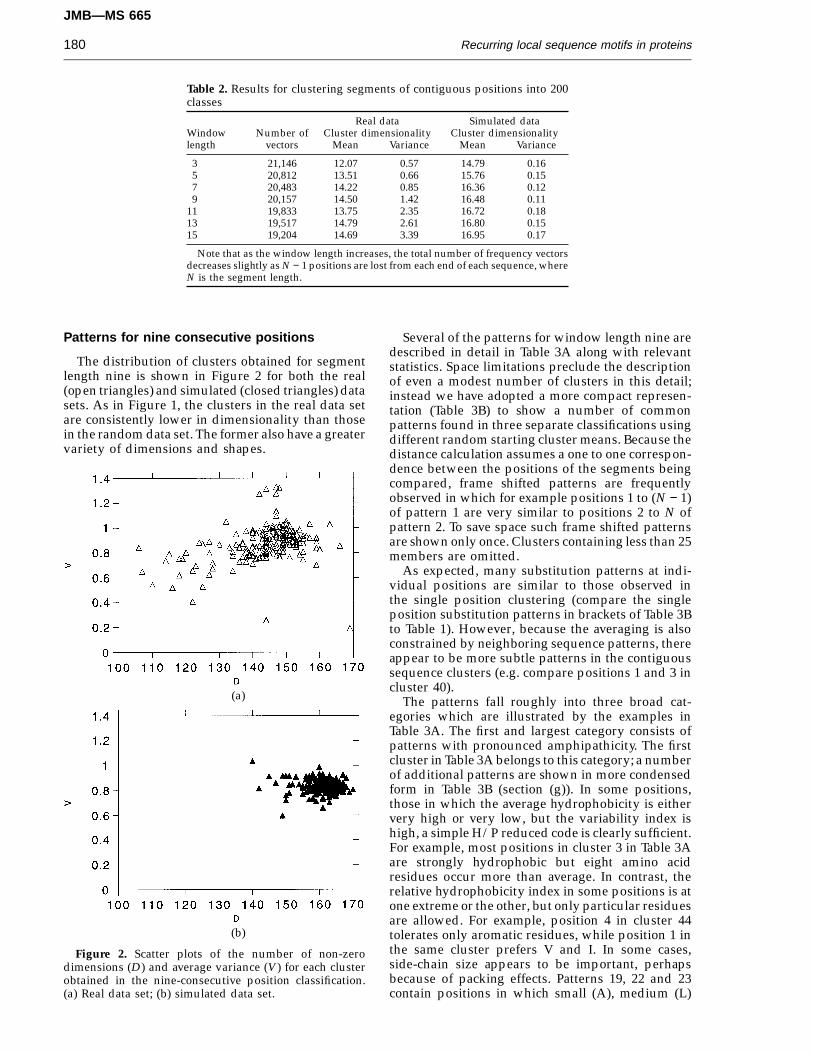
Table 2. Results for clustering segments of contiguous positions into 200classes

Real data Simulated dataWindow Number of Cluster dimensionality Cluster dimensionalitylength vectors Mean Variance Mean Variance

3 21,146 12.07 0.57 14.79 0.165 20,812 13.51 0.66 15.76 0.157 20,483 14.22 0.85 16.36 0.129 20,157 14.50 1.42 16.48 0.11

11 19,833 13.75 2.35 16.72 0.1813 19,517 14.79 2.61 16.80 0.1515 19,204 14.69 3.39 16.95 0.17

Note that as the window length increases, the total number of frequency vectorsdecreases slightly as N − 1 positions are lost from each end of each sequence, whereN is the segment length.

Patterns for nine consecutive positions

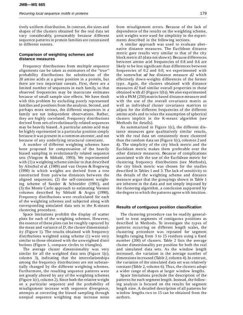
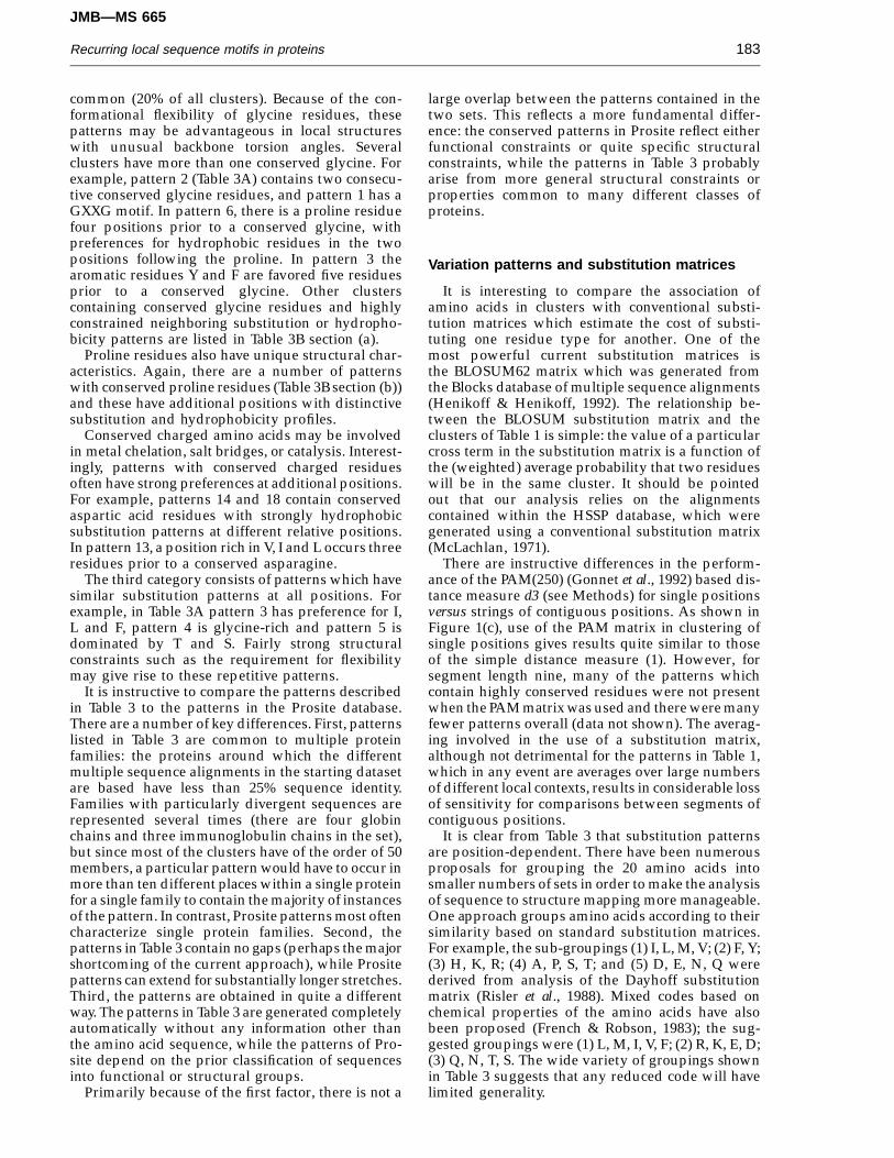
The distribution of clusters obtained for segmentlength nine is shown in Figure 2 for both the real(open triangles) and simulated (closed triangles) datasets. As in Figure 1, the clusters in the real data setare consistently lower in dimensionality than thosein the random data set. The former also have a greatervariety of dimensions and shapes.

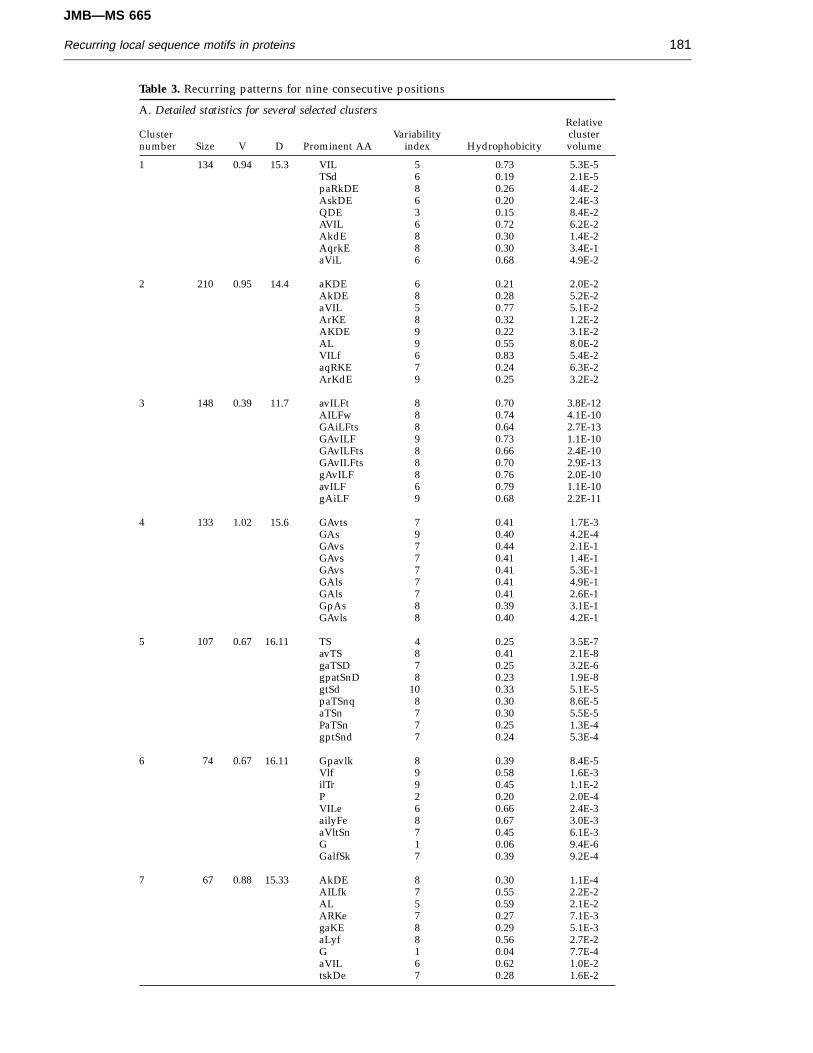
Several of the patterns for window length nine aredescribed in detail in Table 3A along with relevantstatistics. Space limitations preclude the descriptionof even a modest number of clusters in this detail;instead we have adopted a more compact represen-tation (Table 3B) to show a number of commonpatterns found in three separate classifications usingdifferent random starting cluster means. Because thedistance calculation assumes a one to one correspon-dence between the positions of the segments beingcompared, frame shifted patterns are frequentlyobserved in which for example positions 1 to (N − 1)of pattern 1 are very similar to positions 2 to N ofpattern 2. To save space such frame shifted patternsare shown only once. Clusters containing less than 25members are omitted.

As expected, many substitution patterns at indi-vidual positions are similar to those observed inthe single position clustering (compare the singleposition substitution patterns in brackets of Table 3Bto Table 1). However, because the averaging is alsoconstrained by neighboring sequence patterns, thereappear to be more subtle patterns in the contiguoussequence clusters (e.g. compare positions 1 and 3 incluster 40).

The patterns fall roughly into three broad cat-egories which are illustrated by the examples inTable 3A. The first and largest category consists ofpatterns with pronounced amphipathicity. The firstcluster in Table 3A belongs to this category; a numberof additional patterns are shown in more condensedform in Table 3B (section (g)). In some positions,those in which the average hydrophobicity is eithervery high or very low, but the variability index ishigh, a simple H/P reduced code is clearly sufficient.For example, most positions in cluster 3 in Table 3Aare strongly hydrophobic but eight amino acidresidues occur more than average. In contrast, therelative hydrophobicity index in some positions is atone extreme or the other, but only particular residuesare allowed. For example, position 4 in cluster 44tolerates only aromatic residues, while position 1 inthe same cluster prefers V and I. In some cases,side-chain size appears to be important, perhapsbecause of packing effects. Patterns 19, 22 and 23contain positions in which small (A), medium (L)

(a)

(b)

Figure 2. Scatter plots of the number of non-zerodimensions (D) and average variance (V) for each clusterobtained in the nine-consecutive position classification.(a) Real data set; (b) simulated data set.

JMB—MS 665


Table 3. Recurring patterns for nine consecutive positions

A. Detailed statistics for several selected clustersRelative

Cluster Variability clusternumber Size V D Prominent AA index Hydrophobicity volume

1 134 0.94 15.3 VIL 5 0.73 5.3E-5TSd 6 0.19 2.1E-5paRkDE 8 0.26 4.4E-2AskDE 6 0.20 2.4E-3QDE 3 0.15 8.4E-2AVIL 6 0.72 6.2E-2AkdE 8 0.30 1.4E-2AqrkE 8 0.30 3.4E-1aViL 6 0.68 4.9E-2

2 210 0.95 14.4 aKDE 6 0.21 2.0E-2AkDE 8 0.28 5.2E-2aVIL 5 0.77 5.1E-2ArKE 8 0.32 1.2E-2AKDE 9 0.22 3.1E-2AL 9 0.55 8.0E-2VILf 6 0.83 5.4E-2aqRKE 7 0.24 6.3E-2ArKdE 9 0.25 3.2E-2

3 148 0.39 11.7 avILFt 8 0.70 3.8E-12AILFw 8 0.74 4.1E-10GAiLFts 8 0.64 2.7E-13GAvILF 9 0.73 1.1E-10GAvILFts 8 0.66 2.4E-10GAvILFts 8 0.70 2.9E-13gAvILF 8 0.76 2.0E-10avILF 6 0.79 1.1E-10gAiLF 9 0.68 2.2E-11

4 133 1.02 15.6 GAvts 7 0.41 1.7E-3GAs 9 0.40 4.2E-4GAvs 7 0.44 2.1E-1GAvs 7 0.41 1.4E-1GAvs 7 0.41 5.3E-1GAls 7 0.41 4.9E-1GAls 7 0.41 2.6E-1GpAs 8 0.39 3.1E-1GAvls 8 0.40 4.2E-1

5 107 0.67 16.11 TS 4 0.25 3.5E-7avTS 8 0.41 2.1E-8gaTSD 7 0.25 3.2E-6gpatSnD 8 0.23 1.9E-8gtSd 10 0.33 5.1E-5paTSnq 8 0.30 8.6E-5aTSn 7 0.30 5.5E-5PaTSn 7 0.25 1.3E-4gptSnd 7 0.24 5.3E-4

6 74 0.67 16.11 Gpavlk 8 0.39 8.4E-5Vlf 9 0.58 1.6E-3ilTr 9 0.45 1.1E-2P 2 0.20 2.0E-4VILe 6 0.66 2.4E-3ailyFe 8 0.67 3.0E-3aVltSn 7 0.45 6.1E-3G 1 0.06 9.4E-6GalfSk 7 0.39 9.2E-4

7 67 0.88 15.33 AkDE 8 0.30 1.1E-4AILfk 7 0.55 2.2E-2AL 5 0.59 2.1E-2ARKe 7 0.27 7.1E-3gaKE 8 0.29 5.1E-3aLyf 8 0.56 2.7E-2G 1 0.04 7.7E-4aVIL 6 0.62 1.0E-2tskDe 7 0.28 1.6E-2

JMB—MS 665


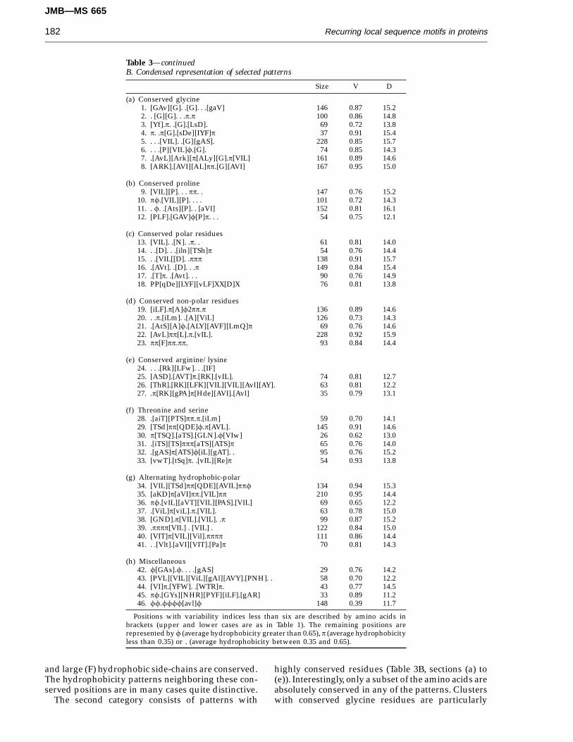
Table 3—continuedB. Condensed representation of selected patterns

Size V D

(a) Conserved glycine1. [GAv][G]. .[G]. . .[gaV] 146 0.87 15.22. . [G][G]. . .p.p 100 0.86 14.83. [Yf].p. .[G].[LsD]. 69 0.72 13.84. p. .p[G].[sDe][IYF]p 37 0.91 15.45. . . .[VIL]. .[G][gAS]. 228 0.85 15.76. . . .[P][VIL]f.[G]. 74 0.85 14.37. .[AvL][Ark][p[ALy][G].p[VIL] 161 0.89 14.68. [ARK].[AVI][AL]pp.[G][AVI] 167 0.95 15.0

(b) Conserved proline9. [VIL][P]. . . pp. . 147 0.76 15.2

10. pf.[VIL][P]. . . . 101 0.72 14.311. . f. .[Ats][P]. . [aVI] 152 0.81 16.112. [PLF].[GAV]f[P]p. . . 54 0.75 12.1

(c) Conserved polar residues13. [VIL]. .[N]. .p. . 61 0.81 14.014. . .[D]. . .[iln][TSh]p 54 0.76 14.415. . .[VIL[[D]. .ppp 138 0.91 15.716. .[AVt]. .[D]. . .p 149 0.84 15.417. .[T]p. .[Avt]. . . 90 0.76 14.918. PP[qDe][LYF][vLF]XX[D]X 76 0.81 13.8

(d) Conserved non-polar residues19. [iLF].p[A]f2pp.p 136 0.89 14.620. . .p.[iLm]. .[A][ViL] 126 0.73 14.321. .[AtS][A]f.[ALY][AVF][LmQ]p 69 0.76 14.622. [AvL]pp[L].p.[vIL]. 228 0.92 15.923. pp[F]pp.pp. 93 0.84 14.4

(e) Conserved arginine/lysine24. . . .[Rk][LFw]. . .[IF]25. [ASD].[AVT]p.[RK].[vIL]. 74 0.81 12.726. [ThR].[RK][LFK][VIL][VIL][Avl][AY]. 63 0.81 12.227. .p[RK][gPA]p[Hde][AVI].[Avl] 35 0.79 13.1

(f) Threonine and serine28. .[aiT][PTS]pp.p.[iLm] 59 0.70 14.129. [TSd]pp[QDE]f.p[AVL]. 145 0.91 14.630. p[TSQ].[aTS].[GLN].f[VIw] 26 0.62 13.031. .[iTS][TS]ppp[aTS][ATS]p 65 0.76 14.032. .[gAS]p[ATS]f[iL][gAT]. . 95 0.76 15.233. [vwT].[tSq]p. .[vIL][Re]p 54 0.93 13.8

(g) Alternating hydrophobic-polar34. [VIL][TSd]pp[QDE][AVIL]ppf 134 0.94 15.335. [aKD]p[aVI]pp.[VIL]pp 210 0.95 14.436. pf.[vIL][aVT][VIL][PAS].[VIL] 69 0.65 12.237. .[ViL]p[viL].p.[VIL]. 63 0.78 15.038. [GND].p[VIL].[VIL]. .p 99 0.87 15.239. .pppp[VIL] . [VIL] . 122 0.84 15.040. [VIT]p[VIL][Vil].pppp 111 0.86 14.441. . .[Vlt].[aVI][VIT].[Pa]p 70 0.81 14.3

(h) Miscellaneous42. f[GAs].f. . . .[gAS] 29 0.76 14.243. [PVL][VIL][ViL][gAl][AVY].[PNH]. . 58 0.70 12.244. [VI]p.[YFW]. .[WTR]p. 43 0.77 14.545. pf.[GYs][NHR][PYF][iLF].[gAR] 33 0.89 11.246. ff.ffff[avl]f 148 0.39 11.7

Positions with variability indices less than six are described by amino acids inbrackets (upper and lower cases are as in Table 1). The remaining positions arerepresented by f (average hydrophobicity greater than 0.65), p (average hydrophobicityless than 0.35) or . (average hydrophobicity between 0.35 and 0.65).

and large (F) hydrophobic side-chains are conserved.The hydrophobicity patterns neighboring these con-served positions are in many cases quite distinctive.

The second category consists of patterns with

highly conserved residues (Table 3B, sections (a) to(e)). Interestingly, only a subset of the amino acids areabsolutely conserved in any of the patterns. Clusterswith conserved glycine residues are particularly

JMB—MS 665


common (20% of all clusters). Because of the con-formational flexibility of glycine residues, thesepatterns may be advantageous in local structureswith unusual backbone torsion angles. Severalclusters have more than one conserved glycine. Forexample, pattern 2 (Table 3A) contains two consecu-tive conserved glycine residues, and pattern 1 has aGXXG motif. In pattern 6, there is a proline residuefour positions prior to a conserved glycine, withpreferences for hydrophobic residues in the twopositions following the proline. In pattern 3 thearomatic residues Y and F are favored five residuesprior to a conserved glycine. Other clusterscontaining conserved glycine residues and highlyconstrained neighboring substitution or hydropho-bicity patterns are listed in Table 3B section (a).

Proline residues also have unique structural char-acteristics. Again, there are a number of patternswith conserved proline residues (Table 3B section (b))and these have additional positions with distinctivesubstitution and hydrophobicity profiles.

Conserved charged amino acids may be involvedin metal chelation, salt bridges, or catalysis. Interest-ingly, patterns with conserved charged residuesoften have strong preferences at additional positions.For example, patterns 14 and 18 contain conservedaspartic acid residues with strongly hydrophobicsubstitution patterns at different relative positions.In pattern 13, a position rich in V, I and L occurs threeresidues prior to a conserved asparagine.

The third category consists of patterns which havesimilar substitution patterns at all positions. Forexample, in Table 3A pattern 3 has preference for I,L and F, pattern 4 is glycine-rich and pattern 5 isdominated by T and S. Fairly strong structuralconstraints such as the requirement for flexibilitymay give rise to these repetitive patterns.

It is instructive to compare the patterns describedin Table 3 to the patterns in the Prosite database.There are a number of key differences. First, patternslisted in Table 3 are common to multiple proteinfamilies: the proteins around which the differentmultiple sequence alignments in the starting datasetare based have less than 25% sequence identity.Families with particularly divergent sequences arerepresented several times (there are four globinchains and three immunoglobulin chains in the set),but since most of the clusters have of the order of 50members, a particular pattern would have to occur inmore than ten different places within a single proteinfor a single family to contain the majority of instancesof the pattern. In contrast, Prosite patterns most oftencharacterize single protein families. Second, thepatterns in Table 3 contain no gaps (perhaps the majorshortcoming of the current approach), while Prositepatterns can extend for substantially longer stretches.Third, the patterns are obtained in quite a differentway. The patterns in Table 3 are generated completelyautomatically without any information other thanthe amino acid sequence, while the patterns of Pro-site depend on the prior classification of sequencesinto functional or structural groups.

Primarily because of the first factor, there is not a

large overlap between the patterns contained in thetwo sets. This reflects a more fundamental differ-ence: the conserved patterns in Prosite reflect eitherfunctional constraints or quite specific structuralconstraints, while the patterns in Table 3 probablyarise from more general structural constraints orproperties common to many different classes ofproteins.

Variation patterns and substitution matrices

It is interesting to compare the association ofamino acids in clusters with conventional substi-tution matrices which estimate the cost of substi-tuting one residue type for another. One of themost powerful current substitution matrices isthe BLOSUM62 matrix which was generated fromthe Blocks database of multiple sequence alignments(Henikoff & Henikoff, 1992). The relationship be-tween the BLOSUM substitution matrix and theclusters of Table 1 is simple: the value of a particularcross term in the substitution matrix is a function ofthe (weighted) average probability that two residueswill be in the same cluster. It should be pointedout that our analysis relies on the alignmentscontained within the HSSP database, which weregenerated using a conventional substitution matrix(McLachlan, 1971).

There are instructive differences in the perform-ance of the PAM(250) (Gonnet et al., 1992) based dis-tance measure d3 (see Methods) for single positionsversus strings of contiguous positions. As shown inFigure 1(c), use of the PAM matrix in clustering ofsingle positions gives results quite similar to thoseof the simple distance measure (1). However, forsegment length nine, many of the patterns whichcontain highly conserved residues were not presentwhen the PAM matrix was used and there were manyfewer patterns overall (data not shown). The averag-ing involved in the use of a substitution matrix,although not detrimental for the patterns in Table 1,which in any event are averages over large numbersof different local contexts, results in considerable lossof sensitivity for comparisons between segments ofcontiguous positions.

It is clear from Table 3 that substitution patternsare position-dependent. There have been numerousproposals for grouping the 20 amino acids intosmaller numbers of sets in order to make the analysisof sequence to structure mapping more manageable.One approach groups amino acids according to theirsimilarity based on standard substitution matrices.For example, the sub-groupings (1) I, L, M, V; (2) F, Y;(3) H, K, R; (4) A, P, S, T; and (5) D, E, N, Q werederived from analysis of the Dayhoff substitutionmatrix (Risler et al., 1988). Mixed codes based onchemical properties of the amino acids have alsobeen proposed (French & Robson, 1983); the sug-gested groupings were (1) L, M, I, V, F; (2) R, K, E, D;(3) Q, N, T, S. The wide variety of groupings shownin Table 3 suggests that any reduced code will havelimited generality.

JMB—MS 665


Discussion

We have described a completely automatedapproach to identifying recurring sequence motifs inprotein families. The patterns identified here (seeTables 1 and 3) probably include most of the localmotifs which transcend protein family boundariesfor proteins of known structure. Because of thenumerous factors which enter into the determinationof protein structures, the data set is probablysomewhat biased and there may well be additionalpatterns in the large number of protein families forwhich structures are not available.

The clustering procedure used here, althoughsimple, appears to be quite adequate for modelingthe data: the local covariances of residue occurrencesfound in multiple sequence alignments. First, theindependence of the results from the choice ofstarting cluster centers required for the K-meansalgorithm attests to the numerical stability ofthe procedure. Second, the results are surprisinglyrobust to changes in the distance metric and se-quence weighting schemes (Table 1 and Figure 2).Third, most of the patterns obtained for individualpositions (Table 1) and many of the patterns obtainedfor segments of contiguous positions (Table 3) areconsistent with expectation (the division betweenhydrophobic and polar patterns in Table 1 is perhapsthe simplest example).

Our results permit limited but significant general-izations about the distribution of protein amino acidsequences in sequence space. The robustness of theresults suggests that the majority of the patterns arereasonably well separated from one another. Fur-thermore, the distribution of sequences in proteinfamilies appears to be considerably more ‘‘clumpy’’than random distributions. The clusters obtained forthe real protein sequence data are consistently lowerin dimensionality than those identified in appli-cations of the same clustering procedure to randomdatasets (Figures 1 and 2, Tables 1 to 3).

The classification of positions into different clus-ters provides a simple yet potentially powerfulmeans to abstract the information contained inmultiple sequence alignments into a higher levelrepresentation. A multiple sequence alignment canbe replaced by a sequence of cluster numbers withrelatively little loss of information. The resultinghigher level sequences can be subjected to muchthe same types of analysis as normal amino acidsequences in efforts to correlate sequence withstructure (Rost & Sander, 1993).

Our results may have useful applications forsequence comparisons, in particular for the identifi-cation of distant homologs for newly determinedsequences. It is well established that searches withprofiles constructed from sets of aligned sequencesare considerably more sensitive to distant homologsthan searches with single sequences. The reason forthis is simple: a sequence profile contains at eachposition family-specific information about the likeli-hood of different amino acids to substitute at thatposition, while a search with a single sequence

typically uses the same global substitution matrix ateach position. As mentioned in the Introduction,the use of a single substitution matrix may averageout weak but important similarities, whereas ourclusters are in fact strings of distinct substitutionmatrices. One can imagine using the clusters as‘‘generalization rules’’ whereby the substitutionmatrices generated from the closest cluster orclusters to each segment of a query sequence areused for scoring sequence alignments.

A similar strategy may facilitate extrapolatingfrom a small number of aligned sequences. The ideais that given a small sample of the variation possibleat a given position, the closest clusters can be identi-fied to predict the variation likely to be observed innew members of the same family. Generalization inthis fashion may permit the power of profile-basedsearching to be employed with only a few examplesfrom the sequence family (or perhaps from only oneexample).

One way to implement the strategy described inthe previous paragraph would be to use the variationpatterns of Table 3 to generate a rough profile or setsof profiles for new sequences which have no closerelatives: for each segment of nine residues in thesequence, select the closest pattern (or a weightedaverage of nearby patterns) and build a profileby splicing together the variation patterns for thedifferent segments. Next, search the database withthis inferred profile. This procedure potentially cir-cumvents the limitations associated with usingthe same substitution matrix at each position of asequence. The method may also be useful for gener-alizing from a small number of aligned sequences,but once there are more than five to ten, the substi-tution patterns are probably better inferred directlyfrom the aligned sequence set.

There are also potential applications to proteinstructure prediction. There is a significant correlationbetween the local structures adopted by members ofa given cluster, although the extent of correlationvaries from cluster to cluster. For example, more than80% of the occurrences of the first two patterns inTable 3A in known protein structures are in a-helices.Intriguingly, the conserved charged residues inpatterns 13, 15 and 16 in Table 3B are buried in morethan 70% of the occurrences of the patterns. Pattern7 in Table 3A is very similar to the Schellman helixC-terminal capping motif (Aurora et al., 1994) and asexpected occurs frequently in helix caps. A moreextensive analysis of the structural correlates of thesequence patterns will be presented elsewhere. Thetracing of the structural correlates of sequencepatterns is essentially the inverse of the morestandard (and very powerful) procedure of tabulat-ing the frequencies of occurrence of the 20 aminoacids in different structural environments (Bowieet al., 1991; Chou et al., 1978).

Finally, we should note that the results describedhere are highly dependent on the quality of the start-ing multiple sequence alignments. As the amountof sequence data increases and multiple sequencealignment algorithms are improved, approaches

JMB—MS 665


similar to the one described here should becomeincreasingly powerful.

Methods

The data

Multiple sequence alignments for proteins of knownstructure were taken from a non-redundant subset (PDBselect 25; Rost & Sander, 1993) of the HSSP database(Sander & Schneider, 1991). No two multiple sequencealignments in this subset have parent sequences withgreater than 25% identity. Because of the wide degree ofsequence variation in families such as the globins and theimmunoglobulins, the PDB select 25 list does include morethan one chain per family in several cases (there are fourglobin chains and three immunoglobulin chains, forexample). To reduce the problems associated with smallsample size, families with fewer than 20 members wereexcluded from the analysis. Insertions common to less than20 members of larger families were also excluded (theHSSP database consists of global sequence alignments).The final data set included 154 protein families with anaverage of 98 sequences per family.

Distance measure

Cluster analysis requires a metric on the space to beclustered. An advantage of using multiple sequencealignments is that there is a natural choice of metrics: thedifference in the frequency distributions. A particularlysimple choice is the ‘‘city block’’ metric:

d1(i, j ) = s20

k = 1

=F(i, k) − F( j, k)= (1)

where d1(i, j) is the distance between frequency distri-butions i and j and F(i, k) is the frequency of occurrence ofthe kth amino acid at position i, S20

k = 1 F(i, k) = 1. A distancemeasure for comparing single positions can be readilygeneralized to treat strings of contiguous positions. Thedistance between one segment of a multiple sequencealignment and a second segment of the same length isconveniently defined to be the sum of the distancesbetween each of the corresponding positions:

dN (i, j ) = sN − 1

n = 0

d(i + n, j + n) (2)

where N is the length of the window, i and j are thestarting positions of the first and second segments, andd(i + n, j + n) is for example distance measure d1 above.

Cluster analysis

The data set consists of roughly 20,000 frequency distri-butions. Most clustering algorithms become extremelytime consuming with data sets of over 1000 members. TheK-means algorithm is one of the few that can be used withextremely large data sets. In brief, a set of K initial clustercenters are chosen at random and each datum point isassigned to the closest center. New cluster centers are thendetermined by taking the mean of all of the data points ineach cluster, and each datum point is re-assigned to theclosest center in another pass through the data set (Everitt,1993). This simple iterative scheme of recalculating clustermeans and re-assigning data points to clusters is repeateduntil no data points are moved from cluster to cluster.

For technical reasons, the city block metric is somewhatpreferable to the Euclidean metric for clustering frequencydistributions using the K-means algorithm. Viewed asvectors in a 20N dimensional space, the frequency distri-butions vary widely in absolute magnitude (for windowlength one, a position in which only one amino acidoccurs is represented by a vector of length one, while aposition in which all 20 amino acids occur with equalprobabilities is represented by a vector with length[20 × (1/20)2]1/2 = 0.22). The Euclidean distance between aposition in which ten of the amino acids occur with equalfrequencies and a position in which the other ten aminoacids occur with equal frequencies is 0.45, while the dis-tance between two positions in which different residuesare absolutely conserved is 1.4. The city block distancebetween the two sets of positions is the same (1.0) in bothcases, a more satisfactory result since no residues are incommon in either pair. To avoid the problems associatedwith the use of the Euclidean metric with variablemagnitude frequency vectors, the frequency vectors can benormalized to unit magnitude. However, the updatingprocedure basic to the K-means algorithm also changes theabsolute magnitude of the cluster centers. The latter can bekept fixed, but this requires a somewhat awkwardrenormalization step after each re-assignment of vectors toclusters in the K-means procedure.

Error measures

How is the extent of clustering best evaluated? Anexplicit example illustrates the difficulties with evaluatingdifferent clustering strategies in high dimensional spaces,and in particular with data of the type involved here.Consider a position which can tolerate either of two aminoacids, for example valine and isoleucine. With a small andpossibly biased sample, the frequency of occurrences ofthe two residues may range from 0.0 to 1.0; the constraintbeing that the variation is contained within a two-dimensional subspace of the entire 20-dimensional space(only valine and isoleucine are allowed). The maximumdistance between two points in this subspace is the sameas the maximum distance between two points in the entire20-dimensional space (two in both cases). The meandistance of the members of a cluster from the cluster meanis clearly a poor measure of the dimensionality of thecluster.

Two statistics which have proved useful for capturing thedistribution of points within a given cluster are D, thenumber of dimensions for which the cluster mean exceeds0.02 (chosen empirically), and V, the average variance inthese dimensions. D clearly indicates the dimensionality ofthe subspace in which the cluster lies, and V, the averagespread within this subspace.

To assess the extent of clustering of the sequence data,parallel experiments were carried out on simulated datasets. To construct these sets, the frequency distributions foreach of the 20 amino acids were evaluated and then usedto generate randomized versions of the HSSP database.The statistics of the simulated data sets are essentiallythose of the HSSP database with all covariances betweensubstitutions at particular positions or between nearbypositions set to zero. For each weighting scheme, a separatesimulated dataset was generated based on the amino acidfrequency distributions of the corresponding weighteddataset. We note that the more standard procedure ofrandomization by shuffling does not apply here since weare not seeking family-specific patterns.

A single composite statistic, the product of the variancesof the individual residue frequencies, is also given in

JMB—MS 665


several of the Tables to facilitate comparison betweendifferent positions within the same cluster. This crudevolume measure is normalized by division by thecorresponding quantity for the whole data set:

Volume (l) =

t20

k = 1

1Ml

sMl

j = 1

=Fl ( j, k) − �Fl ( j, k)�=

t20

k = 1

1S s

S

j = 1

=F( j, k) − �F( j, k)�=

where FI ( j, k) is the frequency of the kth amino acid in thejth distribution in cluster I, �FI ( j, k)� is the center of the Ithcluster, and �F( j, k)� is the center of the entire data set. MI

is the number of vectors (or distributions) in cluster I, andS, the number in the whole dataset. To reduce the effectsof small sample size artifacts, 0.001 is added to the termsin the product in the numerator (again, the value of 0.001was determined empirically).

Numerical stability, alternative distance measuresand the K-means algorithm

A disadvantage of the K-means algorithm is that boththe number of clusters and the starting cluster centers mustbe specified in advance. In practice, use of more than thenatural number of groupings results in the subdivision ofseveral of the larger clusters. This is easily recognized, andeach pattern is shown only once in Tables 1 to 3. Thenumerical stability of the algorithm and the dependence ofthe results on the starting cluster centers were assessedby carrying out multiple independent calculations usingdifferent sets of starting centers. Only the recurrentclusters are reported in the Tables.

A potential disadvantage of distance measure d1(equation (1)) is that a difference in frequency of 0.1 istreated similarly regardless of whether the difference isbetween 0.7 and 0.6 or between 0.1 and 0.0. Because oflineage effects, the former is likely to be less informativethan the latter. A simple exponential scaling was used toemphasize differences of the latter type:

d2(i, j ) = s20

k = 1

=exp[−F(i, k)] − exp[−F( j, k)]= (3)

The K-means algorithm implicitly assumes the clustersto be spherical. If several variables are highly correlatedor have significantly different variances, clusters mayresemble prolate ellipsoids more closely than spheres.Non-spherical clusters can be accommodated by calculat-ing the within-cluster covariance matrix and using thegeneralized Mahalonobus distance given by equation (4)when assigning data points to clusters (Everitt, 1993):

d3(i, j ) = [=Fi − Fj =]M[=Fi − Fj =] (4)

where Fi = F(i, k) and M is the inverse of a covariancematrix.

If the number of dimensions is of the same order as thenumber of data points in individual clusters, the matrixinversion required is not possible. In this case the inverseof the covariance matrix can be approximated by invertingthe diagonal elements (the variances) and setting off-diagonal elements to zero. The modified K-means methodin this case leads to minimization of the effective volumeof the clusters rather than the average within-clusterdistances.

Distance measure d3, with M equal to an amino acidsubstitution matrix such as a PAM matrix, weights differ-ences according to the likelihood of substitution of one

residue type for another (Dayhoff et al., 1972). This is asimple generalization of the similarity measure used incomparing single sequences that are distantly related. Thismeasure, essentially a return to the single substitutionmatrix approach mentioned in the Introduction, is clearlyonly useful in the limit of small numbers of sequences perfamily.

AcknowledgementsWe thank H. Schneider for the HSSP database; D. A.

Agard for encouragement and computational resources;N. Hunt for compiling the PDB/f-c dataset; S. Henikoff,J. Henikoff, S. Pietrokovski, D. Yee, K. Zhang, N. Hunt,T. Defay, M. Robinson, D. Teller, S. Karlin, L. Brocchieri,and members of the Agard laboratory for critical readingof the manuscript. K.F.H. is supported by the HowardHughes Medical Institute Predoctoral Fellowship. Thiswork was partially supported by the National ScienceFoundation, Science and Technology Center CooperativeAgreement BIR-9214821 and young investigator awards toD.B. from the NSF and the Packard Foundation.

ReferencesAltschul, S. F., Carroll, R. J. & Lipman, D. J. (1989). Weights

for data related by a tree. J. Mol. Biol. 20, 647–653.Aurora, R., Srinivasan, R. & Rose, G. D. (1994). Rules

for alpha-helix termination by glycine. Science, 264,1126–1130.

Bairoch, A. & Bucher, P. (1994). PROSITE: recent develop-ments. Nucl. Acids. Res. 22, 3583–3589.

Bowie, J. U., Luthy, R. & Eisenberg, D. (1991). A methodto identify protein sequences that fold into a knownthree-dimensional structure. Science, 253, 164–170.

Brown, M., Hughey, R., Krogh, A., Mian, I., Sjolander, K.& Haussler, D. (1993). Using Direchlet mixture priorsto derive hidden Markov models for protein families.In First International Conference on Intelligent Systemsfor Molecular Biology (Hunter, L., Searls, D. & Shavit, J.,eds), pp. 47–55, AAAI Press, Washington, DC.

Chou, P. Y. & Fasman, G. D. (1974). Prediction of proteinconformation. Biochemistry, 13, 222–245.

Dayhoff, M. O., Eck, R. V. & Park, C. M. (1972). A modelof evolutionary change in proteins. In Atlas of ProteinSequence and Structure. National Biomedical ResearchFoundation, Washington, DC.

Everitt, B. (1993) Cluster Analysis. Halsted Press, New York.French, S. & Robson, B. (1983). What is a conservative

substitution? J. Mol. Evol. 19, 171–175.Gonnet, G., Cohen, M. & Benner, S. (1992). Exhaustive

matching of the entire protein sequence database.Science 256, 1443–1445.

Gonnet, G., Cohen, M. & Benner, S. (1994). Analysis ofamino acid substitution during divergent evolution:the 400 by 400 dipeptide substitution matrix. Biochem.Biophys. Res. Commun. 199, 496–498.

Gribskov, M., Luthy, R. & Eisenberg, D. (1990). Profileanalysis. Methods Enzymol. 183, 146–159.

Henikoff, S. & Henikoff, J. G. (1992). Amino acid substi-tution matrices from protein blocks. Proc. Natl Acad.Sci. USA, 89, 10915–10919.

Johnson, M., Overington, J. & Blundell, T. (1993). Align-ment and searching for common protein folds using adata bank of structural templates. J. Mol. Biol. 231,735–752.

JMB—MS 665


McLachlan, A. D. (1971). Identification of commonmolecular subsequences. J. Mol. Biol. 61, 409–424.

Risler, J. L., Delorme, H. D. & Henaut, A. (1988). Amino acidsubstitutions in structurally related proteins, a patternrecognition approach. J. Mol. Biol. 204, 1019–1029.

Rost, B. & Sander, C. (1993). Prediction of protein second-ary structure at better than 70% accuracy. J. Mol. Biol.232, 584–599.

Sander, C. & Schneider, R. (1991). Database of homology-derived protein structures and the structural meaningof sequence alignment. Proteins: Struct. Funct. Genet. 9,56–68.

Sibbald, P. & Argos, P. (1990). Weighting aligned proteinor nucleic acid sequences to correct for unequalrepresentation. J. Mol. Biol. 216, 813–818.

van Ooyen, A. & Hogeweg, P. (1990). Iterative characterweighting based on mutation frequency: a newmethod for constructing phyletic trees. J. Mol. Evol. 31,330–342.

Vingron, M. & Sibbald, P. R. (1993). Weighting in SequenceSpace: A comparison of methods in terms of general-ized sequences. Proc. Natl Acad. Sci. USA, 90,8777–8781.

Edited by F. Cohen

(Received 3 March 1995; accepted in revised form 23 May 1995)

recurring local sequence motifs in proteins

Documents