Recreational fishing and boating: Are the determinants the same?

Marina Farr a,n, Natalie Stoeckl a, Stephen Sutton b

a School of Business, James Cook University, Townsville, Queensland 4811, Australiab School of Earth and Environmental Sciences, James Cook University, Townsville, Queensland 4811, Australia

a r t i c l e i n f o

Article history:Received 9 December 2013Received in revised form13 February 2014Accepted 13 February 2014Available online 12 March 2014

Keywords:Determinants of the demandGreat Barrier ReefHurdle modelNegative binomialRecreational boating and fishing

a b s t r a c t

The research uses household survey data collected from 656 people in Townsville (adjacent to the GreatBarrier Reef, Australia) within a hurdle model to investigate key factors influencing both the probabilityof participating and the frequency of (a) boating trips which involve fishing; (b) boating trips which donot involve fishing; and (c) land-based fishing trips. The findings suggest that there are differences indeterminants, highlighting the importance of disaggregating the fishing/boating and boat/land-basedexperience (an uncommon practice in the literature) if wishing to obtain information for use in thedesign of monitoring programs, policy and/or for developing monitoring and enforcement strategiesrelating to fishing and boating.

& 2014 Elsevier Ltd. All rights reserved.

1. Introduction

It is increasingly recognised that the sustainable managementof marine resources requires managers and policy makers tounderstand (a) the way in which recreational boaters and fishersmake decisions about their participation and the frequency ofusing the marine resources and (b) the factors that impact theirbehaviour, choices and welfare. However, the relative scarcity ofregionally relevant recreational boating and fishing1 data increasesthe challenges facing policy makers and resource managers whohave to balance sustainable use with protection of the environ-ment while maintaining high quality recreational experiences [1].

Most published studies on the value of recreational fishing [4–8]and boating [9–12] have been done in the USA, Canada and Europe,although some have also been done in New Zealand [13,14], indifferent parts of Australia [15–18] and on the Great Barrier Reef(GBR) [19–21]. But – most pertinent here – the vast majority ofthese studies have looked at boating and fishing as if it were asingle, homogenous, good [6,19,20–24]. Others have treated boatand land-based fishing as similar [25–30]. This is problematic, since

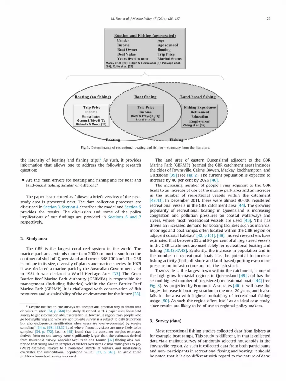
treating them as a single, aggregated ‘good’ is equivalent toassuming that the drivers for boating and fishing and for boat andland-based fishing are the same but they may not be. As such, keyindicators of recreational boating and fishing activities that havebeen identified by previous research (see Fig. 1) may apply to eitherboating, or fishing, or either boat fishing, or land-based fishing butnot necessarily all.

The key point to note here, is that there are only a limitednumber of studies that have looked at fishing by itself – that ofZhang et al. [32]; Rolfe and Prayaga [31] and Loret et al. [8]. Thefirst study looked at land-based fishing, whilst the other twolooked at boat fishing. To the best of our knowledge no previousstudy has comprehensively investigated and compared differenttypes of fishing (land and boat-based) with non-fishing relatedboating activities. As alluded to before, this knowledge gap isproblematic, since some policy implementations and monitoringprograms require information about boating and fishing to beconsidered separately (e.g. policies about boat-ramps and coast-guards versus policies about fishing limits). Hence, there is a needto disaggregate the fishing and boating experience as well as boatfishing and land-based fishing.

The research described in this paper helps to redress thatproblem by demonstrating that it is indeed possible to look atboating and fishing separately. It uses the Townsville region nearthe Great Barrier Reef (GBR) as a case-study area, and analysesdata collected from 656 householders in a hurdle model to identifyimportant determinants of recreational boating and fishing. Itlooks at factors which influence both the probability of participat-ing in boating and fishing activities and also at factors influencing

Contents lists available at ScienceDirect

journal homepage: www.elsevier.com/locate/marpol

Marine Policy

http://dx.doi.org/10.1016/j.marpol.2014.02.0140308-597X & 2014 Elsevier Ltd. All rights reserved.

n Corresponding author. Tel.: þ61 7 4781 5014; fax: þ61 7 4781 4019.E-mail addresses: marina.farr@my.jcu.edu.au, marina.farr@jcu.edu.au (M. Farr),

natalie.stoeckl@jcu.edu.au (N. Stoeckl), stephen.sutton@jcu.edu.au (S. Sutton).1 Recreational boats in this study are those that used for the purposes of

recreation and not for any type of business, trade or commerce [2].‘Recreationalfishing’ is used in accordance with definition by FRDC [3]. The recreational fishingsector comprises enterprises and individuals involved in recreational, sport orsubsistence fishing activities that do not involve selling the products of theseactivities.

Marine Policy 47 (2014) 126–137

the intensity of boating and fishing trips.2 As such, it providesinformation that allows one to address the following researchquestion:

� Are the main drivers for boating and fishing and for boat andland-based fishing similar or different?

The paper is structured as follows: a brief overview of the case-study area is presented next. The data collection processes arediscussed in Section 3. Section 4 describes the model and Section 5provides the results. The discussion and some of the policyimplications of our findings are provided in Sections 6 and 7respectively.

2. Study area

The GBR is the largest coral reef system in the world. Themarine park area extends more than 2000 km north–south on thecontinental shelf off Queensland and covers 348,700 km2. The GBRis unique in its size, diversity of plants and marine species. In 1975it was declared a marine park by the Australian Government andin 1981 it was declared a World Heritage Area [33]. The GreatBarrier Reef Marine Park Authority (GBRMPA) is responsible formanagement (including fisheries) within the Great Barrier ReefMarine Park (GBRMP). It is challenged with conservation of fishresources and sustainability of the environment for the future [38].

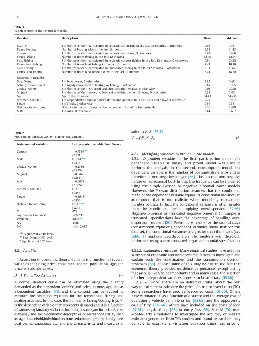
The land area of eastern Queensland adjacent to the GBRMarine Park (GBRMP) (termed the GBR catchment area) includesthe cities of Townsville, Cairns, Bowen, Mackay, Rockhampton, andGladstone [39] (see Fig. 2). The current population is expected toincrease by 40 per cent by 2026 [40].

The increasing number of people living adjacent to the GBRleads to an increase of use of the marine park area and an increasein the number of recreational vessels within the catchment[42,43]. In December 2011, there were almost 90,000 registeredrecreational vessels in the GBR catchment area [44]. The growingpopularity of recreational boating in Queensland is increasingcongestion and pollution pressures on coastal waterways andrivers, where most recreational vessels are used [45]. ‘This hasdriven an increased demand for boating facilities such as marinas,moorings and boat ramps, often located within the GBR region oradjacent coastal habitats’ [42, p.101], [46]. Indeed researchers haveestimated that between 63 and 90 per cent of all registered vesselsin the GBR catchment are used solely for recreational boating andfishing [19,43,47,48]. Evidently, the increase in population and inthe number of recreational boats has the potential to increasefishing activity (both off-shore and land-based) putting even morepressure on infrastructure and on the fish stock.

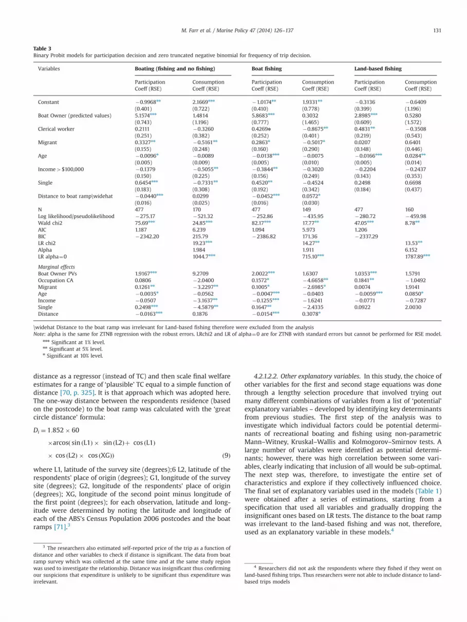
Townsville is the largest town within the catchment, is one ofthe high growth coastal regions in Queensland [49] and has thesecond highest number of (registered) recreational boats [44] (seeFig. 3). As projected by Economic Associates [46] it will have thelargest increase in boat registration in the next 20 years, and it alsofalls in the area with highest probability of recreational fishingusage [50]. As such the region offers itself as an ideal case study,since results are likely to be of use to regional policy makers.

3. Survey (data)

Most recreational fishing studies collected data from fishers atfor example boat ramps. This study is different, in that it collecteddata via a mailout survey of randomly selected households in theTownsville region. As such it collected data from both participantsand non- participants in recreational fishing and boating. It shouldbe noted that it is also different with regard to the nature of data:

Trip PriceIncome

SubstitutesGurmu & Trivedi [9];

Siderelis & Moore [10]

Fishing ExperienceRetirementEducation

EmploymentZhang et al. [32]

Trip PriceIncome

Rolfe & Prayaga [31]; Lloret et al.[8]

Boating and Fishing (aggregated)Gender AgeIncome Age squaredBoat Owner BoatingBoat Value Trip PriceYears lived in area Marital Status

Morey et al. [22]; Bilgic & Florkowski [6]; Prayaga et al. [20]; Rolfe et al. [21]

Boating Fishing

Boating (no fishing) Boat fishing Land-based fishing

Fig. 1. Determinants of recreational boating and fishing – summary from the literature.

2 Despite the fact on-site surveys are ‘cheaper and practical way to obtain dataon visits to sites’ [34, p. 568] the study described in this paper uses householdsurvey to get information about recreation in Townsville region from people whogo boating/fishing and who are not. On-site survey is a subject to only truncationbut also endogenous stratification when users are ‘over-represented by on-sitesampling’ [[34, p. 568], [35,37]] and where ‘frequent visitors are more likely to besampled’ [34, p. 572]. Loomis [35] found that the consumer surplus estimatesderived from on-site survey were significantly larger than the estimates derivedfrom household survey. González-Sepúlveda and Loomis [37] finding also con-firmed that ‘using on-site samples of visitors overstates visitor willingness to pay(WTP) estimates relative to a household sample of visitors, and substantiallyoverstates the unconditional population values’ [37, p. 561]. To avoid theseproblems household survey was used.

M. Farr et al. / Marine Policy 47 (2014) 126–137 127

researchers did not ask about a single trip/experience but ratherabout the (average) number of trips per annum each respondenttook and about the characteristics of the ‘average’ trip.

The household data used in this study were collected using amail-out survey [51]. The survey was designed to collect data on awide range of social and demographic factors which previousresearchers had found to influence boating and fishing including:fishing and boating participation, preferences, consumptive orien-tation, occupation and education, migration and householdincome. The introductory letter with the questionnaire and hand-written envelops was mailed in August 2011 to 2120 residents. Thereminder letter and a replacement survey were mailed four weekslater. Out of 2120 survey initially mailed, 656 valid responses werereceived while 173 letters were returned due to incorrect

addresses or because the recipient had moved away or wasdeceased. The overall response rate was thus 33.7%.

Forty four per cent of respondents were male. The average agewas about 54 years and 18.4% of the respondents were born andhad lived all their life in Townsville. The majority of people (35%)who moved to Townsville were from Brisbane or other parts ofQLD. Twenty one per cent of the respondents had never beenfishing as an adult and 56.3% had not been fishing during theprevious two years. This is consistent with Rolfe et al. [21] whocollected their data from QLD coastal cities between Cairns (NorthQLD) and Bundaberg using household survey and found that 42%of respondents went fishing/boating over the last two years.

The majority of respondents preferred outdoor to indoorrecreational activities and indicated that camping could be a

Fig. 2. The GBR and the survey area [41].

M. Farr et al. / Marine Policy 47 (2014) 126–137128

substitute for recreational boating and/or fishing. The number oftimes respondents went fishing (on average) was greater than thenumber of times they went boat-fishing justifying our decision tolook at the demand for both boat-based and land-based fishingtrips separately.

Compared to demographic data from the ABS Census 2006 [52]for the Townsville region, this sample slightly underrepresentsmales but overrepresents people who are more than 33 years ofage. This is in accordance with other household surveys (e.g. Rolfeet al. [21]): females and older people are more likely to completequestionnaires than their younger, male counterparts. Our samplealso overrepresents professionals, people with university degreesand those on relatively high household incomes – an observationwhich is also typical for household surveys.

It may also be subject to self-selection bias because those whoare interested in outdoor activities may have been more likely torespond to a survey on outdoor activities than those who have nointerest. Thus, motivation can be overrepresented. This suspicionis partially substantiated by the fact that fishing participation inour sample is 42% but Taylor et al. [82] estimated fishingparticipation rate at 20% in the Northern region (covering Towns-ville and Ingham). Thus this sample seems to be overrepresentedby fishers – although more than half of the sample (56.3%) havenot been fishing so it is still possible to use the data to compare thecharacteristics of those who do fish, with those who do not. Theaverage size of household was smaller (2.4) in this samplecompared to 2.5–3 for Townsville region ABS Census 2006 data.One should, therefore, be careful not to naively extrapolateobservations from this sample to the population as a whole.

4. The model

4.1. Modelling issues

It can be assumed that the decision to participate and thedecision about trip frequency can be influenced by differentfactors. These decisions can be modelled by two separate models‘to reflect the reality that people first choose if they will engage in

the activity’ and then decide ‘the frequency of use’ [21, p. 5].Mullahy [53] suggested using modified count data models wherethese two processes are not constrained to be the same and wherea binomial probability manages the binary outcome (whether acount is zero or positive). If it is positive, the hurdle is crossed andthe conditional distribution of positive outcomes is managed by atruncated (at zero) count data model [9]. The decision to partici-pate and the decision about trip frequency are thus estimated in atwo stage process: the first stage models people's choices aboutwhether or not to participate; the second stage explores decisionsabout the quantity of recreational trips (given the choice toparticipate in this activity). It is this two-stage decision process(hurdle approach) that was used here.

Following Gurmu and Trivedi [9] and Bilgic and Florkowski [6]let yij, j¼0, 1, 2,…n be the number of trips for ith individual. Letθ1i ¼ expðx1i' β1Þ be the negative binomial model 2 (NB2) meanparameter for the case of zero counts and θ2i ¼ expðx2i' β2Þ for thecase of positive counts. Where x1i and x2i are ðk� 1Þ covariatevectors of the explanatory variables to be used in to be used in thefirst and second hurdle stages, respectively and β1 and β2 are k –

dimensional vectors of unknown parameters associated with thefirst and second hurdle stages respectively. Further define theindicator function Ii ¼ 1 if yij40 and Ii ¼ 0 if yij ¼ 0 and α is adispersion parameter.

For the negative binomial distribution with k¼0 the followingprobabilities can be obtained:

P1ðyij ¼ 0jx1iÞ ¼ ð1þα1θ1iÞ�1=α1 ; j¼ 0 ð1Þ

1�P1ðyij ¼ 0jx1iÞ ¼ 1�ð1þα1θ1iÞ�1=α1 ð2Þ

P2ðyijjx2i; yij40Þ ¼ Γðyijþα�12 Þ

Γðα�12 ÞΓðyijþ1Þ

1

ð1þα2θ2iÞ1=α2 �1

!

� θ2i

θ2iþα�12

!yij

ð3Þ

The density function for the observations is

½P1ðyij ¼ 0jx1iÞ�1� Ii � ½ð1�P1ðyij ¼ 0jx1iÞÞP2ðyijjx2i; yij40Þ�Ii ð4Þ

and its related log-likelihood is

LnLh1ðβ1;α1Þ ¼ ∑i ¼ 1

ð1� IiÞ � ln ½P1ðyij ¼ 0jx1iÞ�þ Ii

� ln ½ð1�P1ðyij ¼ 0jx1iÞÞ� ð5Þ

LnLh2ðβ2;α2Þ ¼ ∑i ¼ 1

Ii � ln ½P2ðyijjx2i; yij40Þ� ð6Þ

As noted by Bilgic and Florkowski [6, p. 480]

� Lh1 can be considered as ‘a log-likelihood function for thebinary (zero/positive) outcome, e.g., logit, and Lh2 is a log-likelihood function for a truncated-at-zero model of a positivenumber’ of trips.

� The decision to take boating or fishing trip is the first hurdlewhich is a binary probability distribution and while the secondhurdle ‘truncates non-zero counts in the underlying negativebinomial distribution’.

� ‘The maximum likelihood estimates of β1and β2 can beobtained separately from Lh1 and Lh2’.

To simplify the estimation, the researchers have followed thelead of Gurmu and Trivedi [9] and used α1¼1, which is equivalentto the use of a ‘logit model’ (3) at the first stage.

Fig. 3. Registered vessels for the GBR catchment area December 2011 (Source:GBRMPA [44]).

M. Farr et al. / Marine Policy 47 (2014) 126–137 129

4.2. Variables

According to economic theory, demand is a function of severalvariables including price, consumer income, population, age, theprice of substitutes etc.

D¼ f P; Inc; Pop;Age:::etcð Þ: ð7ÞA normal demand curve can be estimated using the quantitydemanded as the dependent variable and price, income, age, etc. asindependent variables [54], and this concept can be applied toestimate the visitation equation for the recreational fishing andboating activities. In this case, the number of fishing/boating trips Vi

is the dependent variable that represents demand and it is a functionof various explanatory variables including a surrogate for price Pi (i.e.,distance), and socio-economic descriptives of recreationalists Xi suchas age, household/individual income, education, gender, family size,boat owner, experience etc. and site characteristics and measures of

substitutes Zi [55,32]

Vi ¼ f ðPi;Xi; ZiÞ ð8Þ

4.2.1. Identifying variables to include in the models4.2.1.1. Dependent variable. In the first, participation model, thedependent variable is binary and probit model was used toperform the analysis. In the second, consumption model, thedependent variable is the number of boating/fishing trips and is,therefore, a non-negative integer [56]. The discrete non-negativenature of recreational boat/fishing trip frequency can be modelledusing the simple Poisson or negative binomial count models.However, the Poisson distribution assumes that the conditionalmean of the dependent variable equals its conditional variance, anassumption that is not realistic when modelling recreationalnumber of trips. In fact, the conditional variance is often greaterthan the conditional mean implying overdispersion [57,56].Negative binomial or truncated negative binomial (if sample istruncated) specifications have the advantage of handling over-dispersion problem [20]. Preliminary results for the second stage(consumption equation) dependent variables show that for thisdata set, the conditional variances are greater than the means (seeTable 1) implying overdispersion. The analysis was, therefore,performed using a zero truncated negative binomial specification.

4.2.1.2. Explanatory variables. Many empirical studies have used thesame set of economic and non-economic factors to investigate andexplain both the participation and the consumption decisionprocesses [58]. At least some of this may be due to the fact thateconomic theory provides no definitive guidance (except notingthat price is likely to be important) and in many cases, the selectionof other independent variables appears to be arbitrary [59,60].

4.2.1.2.1. Price. There are no definitive ‘rules’ about the bestway to estimate or calculate the price of a trip or travel costs (TC).Some researchers have used self-reported costs [61,20]. Othershave estimated TC as a function of distance and the average cost ofoperating a vehicle per mile or km [62,63] and the opportunitycost of time [64–66]; others have included on-site costs of food[67,61]; length of trip [68], or entry fees [69]. Stoeckl [70] usedMonte-Carlo simulations to investigate the accuracy of welfareestimates generated from TCs studies and found researchers maybe able to estimate a visitation equation using just price of

Table 1Variables used in the empirical models.

Variable Description Mean Std. dev.

Boating 1 if the respondent participated in recreational boating in the last 12 months, 0 otherwise 0.36 0.481Times Boating Number of boating trips in the last 12 months 9.28 11.46Fishing 1 if the respondent participated in recreational fishing, 0 otherwise 0.43 0.496Times Fishing Number of times fishing in the last 12 months 12.55 18.74Boat Fishing 1 if the respondent participated in recreational boat fishing in the last 12 months, 0 otherwise 0.31 0.462Times Boat Fishing Number of times boat fishing in the last 12 months 8.22 10.29Land Fishing 1 if the respondent participated in land-based fishing in the last 12 months, 0 otherwise 0.33 0.46Times Land Fishing Number of times land-based fishing in the last 12 months 8.74 18.70

Explanatory variablesBoat Owner 1 if boat owner, 0 otherwise 0.23 0.421Activity Commitment 1 if highly committed to boating or fishing, 0 otherwise 0.16 0.365Clerical worker 1 if the respondent is clerical and administration worker, 0 otherwise 0.10 0.296Migrant 1 if the respondent moved to Townsville within the last 10 years, 0 otherwise 0.28 0.451Age Age of the respondent 54.43 14.736Income4$100,000 1 if respondent's i annual household income per annum is $100,000 and above, 0 otherwise 0.29 0.457Single 1 if Single, 0 otherwise 0.18 0.381Distance to boat ramp Distance to the boat ramp for the respondent i based on the postcode 6.71 4.470Male 1 if male, 0 otherwise 0.44 0.497

Table 2Probit model for Boat Owner (endogenous variable).

Instrumental variables Instrumented variable Boat Owner

Constant �0.7359nn

(0.371)Male 0.5584nnn

(0.132)Clerical worker �0.2726

(0.256)Migrant �0.1767

(0.153)Age �0.0074

(0.005)Income4$100,000 0.0935

(0.152)Single �0.3645n

(0.190)Distance to boat ramp 0.0339nn

(0.014)N 479Log pseudo likelihood �247.93Wald chi2 40.54nnn

AIC 1.069BIC �2410.995

nnn Significant at 1% level.nn Significant at 5% level.n Significant at 10% level.

M. Farr et al. / Marine Policy 47 (2014) 126–137130

distance as a regressor (instead of TC) and then scale final welfareestimates for a range of ‘plausible’ TC equal to a simple function ofdistance [70, p. 325]. It is that approach which was adopted here.The one-way distance between the respondents residence (basedon the postcode) to the boat ramp was calculated with the ‘greatcircle distance’ formula:

Di ¼ 1:852� 60

�arcosð sin ðL1Þ � sin ðL2Þþ cos ðL1Þ� cos ðL2Þ � cos ðXGÞÞ ð9Þ

where L1, latitude of the survey site (degrees);6 L2, latitude of therespondents' place of origin (degrees); G1, longitude of the surveysite (degrees); G2, longitude of the respondents' place of origin(degrees); XG, longitude of the second point minus longitude ofthe first point (degrees); for each observation, latitude and long-itude were determined by noting the latitude and longitude ofeach of the ABS's Census Population 2006 postcodes and the boatramps [71].3

4.2.1.2.2. Other explanatory variables. In this study, the choice ofother variables for the first and second stage equations was donethrough a lengthy selection procedure that involved trying outmany different combinations of variables from a list of ‘potential’explanatory variables – developed by identifying key determinantsfrom previous studies. The first step of the analysis was toinvestigate which individual factors could be potential determi-nants of recreational boating and fishing using non-parametricMann–Witney, Kruskal–Wallis and Kolmogorov–Smirnov tests. Alarge number of variables were identified as potential determi-nants; however, there was high correlation between some vari-ables, clearly indicating that inclusion of all would be sub-optimal.The next step was, therefore, to investigate the entire set ofcharacteristics and explore if they collectively influenced choice.The final set of explanatory variables used in the models (Table 1)were obtained after a series of estimations, starting from aspecification that used all variables and gradually dropping theinsignificant ones based on LR tests. The distance to the boat rampwas irrelevant to the land-based fishing and was not, therefore,used as an explanatory variable in these models.4

Table 3Binary Probit models for participation decision and zero truncated negative binomial for frequency of trip decision.

Variables Boating (fishing and no fishing) Boat fishing Land-based fishing

Participation Consumption Participation Consumption Participation ConsumptionCoeff (RSE) Coeff (RSE) Coeff (RSE) Coeff (RSE) Coeff (RSE) Coeff (RSE)

Constant �0.9968nn 2.1669nnn �1.0174nn 1.9331nn �0.3136 �0.6409(0.401) (0.722) (0.410) (0.778) (0.399) (1.196)

Boat Owner (predicted values) 5.1574nnn 1.4814 5.8683nnn 0.3032 2.8985nnn 0.5280(0.743) (1.196) (0.777) (1.465) (0.609) (1.572)

Clerical worker 0.2111 �0.3260 0.4269n �0.8675nn 0.4831nn �0.3508(0.251) (0.382) (0.252) (0.401) (0.219) (0.543)

Migrant 0.3327nn �0.5161nn 0.2863n �0.5017n 0.0207 0.6401(0.155) (0.248) (0.160) (0.290) (0.148) (0.446)

Age �0.0096n �0.0089 �0.0138nnn �0.0075 �0.0166nnn 0.0284nn

(0.005) (0.009) (0.005) (0.010) (0.005) (0.014)Income4$100,000 �0.1379 �0.5055nn �0.3844nn �0.3020 �0.2204 �0.2437

(0.150) (0.225) (0.156) (0.249) (0.143) (0.353)Single 0.6454nnn �0.7331nn 0.4520nn �0.4524 0.2498 0.6698

(0.183) (0.308) (0.192) (0.342) (0.184) (0.437)Distance to boat ramp\widehat �0.0440nnn 0.0299 �0.0452nnn 0.0572n

(0.016) (0.025) (0.016) (0.030)N 477 170 477 149 477 160Log likelihood/pseudolikelihood �275.17 �521.32 �252.86 �435.95 �280.72 �459.98Wald chi2 75.69nnn 24.85nnn 82.17nnn 17.77nn 47.05nnn 8.78nn

AIC 1.187 6.239 1.094 5.973 1.206BIC �2342.20 215.79 �2386.82 171.36 �2337.29LR chi2 19.23nnn 14.27nn 13.53nn

Alpha 1.984 1.911 6.152LR alpha¼0 1044.7nnn 715.10nnn 1787.89nnn

Marginal effectsBoat Owner PVs 1.9167nnn 9.2709 2.0022nnn 1.6307 1.0353nnn 1.5791Occupation CA 0.0806 �2.0400 0.1572n �4.6658nn 0.1841nn �1.0492Migrant 0.1261nn �3.2297nn 0.1005n �2.6985n 0.0074 1.9141Age �0.0035n �0.0562 �0.0047nnn �0.0403 �0.0059nnn 0.0850n

Income �0.0507 �3.1637nn �0.1255nnn �1.6241 �0.0771 �0.7287Single 0.2498nnn �4.5879nn 0.1647nn �2.4335 0.0922 2.0030Distance �0.0163nnn 0.1876 �0.0154nnn 0.3078n

\widehat Distance to the boat ramp was irrelevant for Land-based fishing therefore were excluded from the analysisNote: alpha is the same for ZTNB regression with the robust errors. LRchi2 and LR of alpha¼0 are for ZTNB with standard errors but cannot be performed for RSE model.

nnn Significant at 1% level.nn Significant at 5% level.n Significant at 10% level.

3 The researchers also estimated self-reported price of the trip as a function ofdistance and other variables to check if distance is significant. The data from boatramp survey which was collected at the same time and at the same study regionwas used to investigate the relationship. Distance was insignificant thus confirmingour suspicions that expenditure is unlikely to be significant thus expenditure wasirrelevant.

4 Researchers did not ask the respondents where they fished if they went onland-based fishing trips. Thus researchers were not able to include distance to land-based trips models

M. Farr et al. / Marine Policy 47 (2014) 126–137 131

The researchers also conducted several checks to test for multi-collinearity for all explanatory variables in all models. For thesemodels ‘tolerance’ values ranged between 0.69 and 0.90 and theVIFs ranged between 1.06 and 1.49. There were also no significantdifferences in Eigenvalues and Condition Indexes for each dimen-tion in the ‘Collinearity Diagnostics’ table. Evidently multicollinear-ity is not a significant issue in this instance [72].5

The researchers suspected that endogeneity might also be anissue – particularly given the likely association between thedecisions about boating/fishing trips, trip frequency and boatownership. So researchers conducted an augmented regressiontest (Durbin–Wu–Hausman test) for endogeneity suggested byDavidson and MacKinnon [73]. The null hypothesis that boatownership is exogenous was rejected at the 1% levels for bothstages, indicating that the instrumental variables should be usedto estimate boat ownership functions. The instrument Male andother exogenous explanatory variables from the final nodel suchas Clerical worker, Migrant, Age, Income4$100,000, Single andDistance to boat ramp were used to obtain predicted values forboat ownership. The instruments were chosen based on signifi-cance of coefficients when regressing it on all exogenous vari-ables in the model for all types of activities.6 The researchers thenused predicted values of ‘Boat Owner’ in the participation andtrip frequency models.

5. Results

5.1. Participation equations

The results of the Probit model for Boat ownership arepresented in Table 2.7,8 The Wald chi-square statistic for the modelis highly significant indicating good model fit. Being male andliving a longer distance from most popular boat ramps (all ofwhich are located in the middle of the city) positively influenceboat ownership. This positive relation between the distance andboat ownership almost certainly reflects the (much) higher prop-erty prices in the city and the smaller property sizes (e.g. apart-ments) with less room to keep boats. In other words people whoown boats are more likely to live outside in outer-city suburbs.Single people are less likely to be boat owners.

The results from models describing participation decisions areshown in Table 3. Note that these results are those generated fromSTATA's Probit routine with robust standard errors (RSE) and thuscontrol for heteroskedasticity [79].

The Wald chi-square statistics for both models are highlysignificant indicating good model fits. The Pearson goodness-of-fit test and a model specification link tests were conducted for allfour participation models. The results indicated that all fourmodels fit reasonably well and the link test confirmed that themodels do not have specification errors.

The models show that those who own a boat are more likelyto have taken a boating or fishing trip in the last 12 months. Agecoefficients are highly significant and have a negative sign for allactivities: a result that is consistent with previous research[80,6]. Younger people are more likely to take either boat, boatfishing or land-based fishing trips. As expected the coefficient onDistance to boat ramp (a proxy for price) is negative and highlysignificant for the Boating (fishing and no fishing) and Boatfishing models. The further the distance to travel between‘home’ and the inner city boat ramps the lower the probabilitythat a person will participate in boating and fishing. Being singleor being a recent migrant increases the probability of goingboating (with fishing and no fishing) as well as the probability ofparticipating in boat fishing.

The probability of participating in a recent boat fishing trip islower for those on high incomes than for those with householdincomes below $100,000 per annum. This is consistent with thefindings of other researchers: Floyd et al. [80] suggest thatrecreational fishers are mostly belonging to the middle incomegroup; Bilgic and Florlowski [6, p. 482] found ‘the participationrate declines for those with the income exceeding $75 000’.

People employed as a clerical or administrative workers weremore likely to have participated in a boat or land-based fishing tripwithin the last 12 months.

5.2. Consumption equations

The second stage of the analysis modelled the frequency oftrips – results are presented in Table 3. The estimates of thedispersion parameter (alpha) and the LR test for alpha¼0 (equiva-lent to a Zero-Truncated Poisson model) for all four modelsindicate that the data are overdispersed and that the ZTNB modelsare thus preferable to a Zero-Truncated Poisson model [81]. Thelikelihood ratio (LR) chi-square test suggests that a high level ofmodel fit for all four models is being achieved.

The results indicate that recent migrants, single people andindividuals with annual household incomes which exceed $100,000per annum went boating less often than others. This later findingconfirms results from other studies [55]. Recent migrants andpeople who were employed as a clerical or administrative workers,went boat-fishing less frequently than others. The positive relation-ship between the frequency of boat fishing trips and distance canperhaps be explained by the fact that frequent boat-fishers arethose that own boats (part one of the modelling relationship) andthese people mostly live in outer-city suburbs, thus needing totravel longer distances to get to the boat ramps (which are locatedin the inner city) [54,6]. The positive coefficient on Age for land-based fishing support previous research. Boat ownership is insig-nificant for all types of activities.9

5 ‘Tolerance’, the ‘variance inflation factor’ (VIF) and ‘Collinearity Diagnostics’have been used to examine the presence of multicollinearity. Menard [74]suggested if a tolerance value is less than 0.1 it ‘almost certainly indicates a seriouscollinearity problem’ [[75], p.297] and that a value that is less than 0.2 could also bea concern. There is no particular rule about which value of the VIF should be asubject of concern but Myers [76] suggested that a VIF value greater than 10 shouldbe cause of worry [72].

6 The instruments for instrumented variables ‘Boat owner’ were chosen basedon the significance of the coefficients using Stepwise LR methods

7 The majority of previous studies have not differentiated between participa-tion (yes/no) and frequency of trips. They also treated boat ownership as exogenousvariable (e.g. [21]). However, boat ownership is likely to be endogenous and it iswhat we have found in our model. Thus we estimated it as a function of otherexogenous explanatory variables (checking first to rule out potential problemsassociated with multicollinearity), and then used the predicted values of boatownership in the model, thus formally controlling for endogeneity.

8 As regards all four participation models were tested for weak instrumentsand overidentification using IV Probit and the Conditional Likelihood-Ratio (CLR)test, Anderson–Rubin (AR) statistics [77], Kleibergen–Moreira Lagrange multiplier(LM) test [78,85], a combination of the LM and overidentification J (LM-J) and Waldtests. The statistics for all tests were significant at 1% and 5% level thus researchersrejected the null of weak instruments and overidentification.

9 Researchers also estimated participation and consumption models usingpredicted values of both ‘Activity Commitment’ and ‘Boat ownership’ (see Appen-dix A, Table A.1 Model 1) and using only ‘Activity Commitment’ instead of ‘Boatownership’ (see Appendix A, Table A.1 Model 2). First researchers tested ActivityCommitment for endogeneity and found it to be endogenous. The instruments for‘Activity Commitment’ equation (for obtaining predicted values for Model 2) wereMale and the same set of exogenous explanatory variables from the final modelthat were used to obtain predicted values for Boat Owner (see Appendix A, TableA.2). However, based on the model performance researchers reported only modelsthat include Boat Owner instrumented variable.

M. Farr et al. / Marine Policy 47 (2014) 126–137132

6. Discussion

The boat ownership equations simply show the characteristicsof those who are most likely to own a boat. The participationequations show how likely it is that someone will participate inthe activity at least once. The consumption equations show howfrequently someone will participate in the activity given that he/she owns a boat. This modelling approach is important becausethese decisions are different and combining those decisions into asingle model would lead to missing some important subtle effects.Researchers found that married people who live a long way fromthe boat ramps are more likely to have a boat. This could perhapsbe due to the fact that these people live in the outer suburbs sothey are able to keep their boats in the backyards. These people arealso more likely to go boating frequently. Single people who livenear the boat ramp are more likely to have gone fishing at leastonce in the last two years – perhaps joining other people on theirboat trips.

Recent migrants are less likely to own a boat but they aremore likely to have joined someone else on a boating and/orboat fishing trip at least once during the last two years thanlonger term residents. Interestingly, although they have beenat least once recently, they do not do so on a regular basis.This could be something to do with the novelty of having justmoved to the region and wanting to try a new experience,but not necessarily wanting to adopt the activity as a frequenthobby.

Participation in land-based fishing decreases with age.Moreover, it seems that when people get older, they are lesslikely to have been boating, boat or land-based fishing evenonce in the last two years. This is probably because they havean established life style and do not want to start somethingnew. However, the frequency of land-based fishing tripsincreases with age. Evidently, keen fishers want to keep fishing,even as they grow older: they might not be able to manage aboat or may find boat maintenance too costly but if they stilllove to go fishing then fishing from the shore is a viable optionfor this group of people.

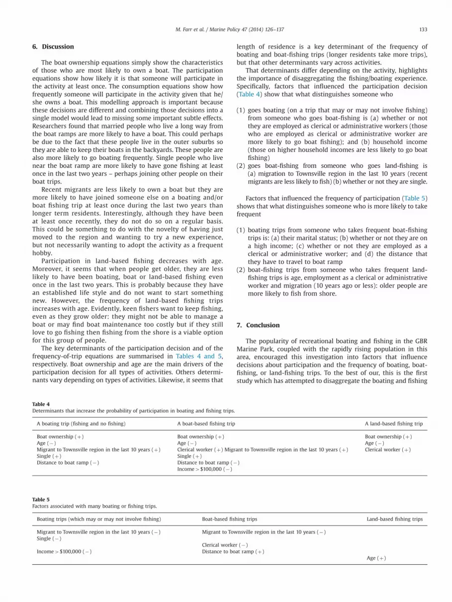
The key determinants of the participation decision and of thefrequency-of-trip equations are summarised in Tables 4 and 5,respectively. Boat ownership and age are the main drivers of theparticipation decision for all types of activities. Others determi-nants vary depending on types of activities. Likewise, it seems that

length of residence is a key determinant of the frequency ofboating and boat-fishing trips (longer residents take more trips),but that other determinants vary across activities.

That determinants differ depending on the activity, highlightsthe importance of disaggregating the fishing/boating experience.Specifically, factors that influenced the participation decision(Table 4) show that what distinguishes someone who

(1) goes boating (on a trip that may or may not involve fishing)from someone who goes boat-fishing is (a) whether or notthey are employed as clerical or administrative workers (thosewho are employed as clerical or administrative worker aremore likely to go boat fishing); and (b) household income(those on higher household incomes are less likely to go boatfishing)

(2) goes boat-fishing from someone who goes land-fishing is(a) migration to Townsville region in the last 10 years (recentmigrants are less likely to fish) (b) whether or not they are single.

Factors that influenced the frequency of participation (Table 5)shows that what distinguishes someone who is more likely to takefrequent

(1) boating trips from someone who takes frequent boat-fishingtrips is: (a) their marital status; (b) whether or not they are ona high income; (c) whether or not they are employed as aclerical or administrative worker; and (d) the distance thatthey have to travel to boat ramp

(2) boat-fishing trips from someone who takes frequent land-fishing trips is age, employment as a clerical or administrativeworker and migration (10 years ago or less): older people aremore likely to fish from shore.

7. Conclusion

The popularity of recreational boating and fishing in the GBRMarine Park, coupled with the rapidly rising population in thisarea, encouraged this investigation into factors that influencedecisions about participation and the frequency of boating, boat-fishing, or land-fishing trips. To the best of our, this is the firststudy which has attempted to disaggregate the boating and fishing

Table 4Determinants that increase the probability of participation in boating and fishing trips.

A boating trip (fishing and no fishing) A boat-based fishing trip A land-based fishing trip

Boat ownership (þ) Boat ownership (þ) Boat ownership (þ)Age (�) Age (�) Age (�)Migrant to Townsville region in the last 10 years (þ) Clerical worker (þ) Migrant to Townsville region in the last 10 years (þ) Clerical worker (þ)Single (þ) Single (þ)Distance to boat ramp (�) Distance to boat ramp (�)

Income4$100,000 (�)

Table 5Factors associated with many boating or fishing trips.

Boating trips (which may or may not involve fishing) Boat-based fishing trips Land-based fishing trips

Migrant to Townsville region in the last 10 years (�) Migrant to Townsville region in the last 10 years (�)Single (�)

Clerical worker (�)Income4$100,000 (�) Distance to boat ramp (þ)

Age (þ)

M. Farr et al. / Marine Policy 47 (2014) 126–137 133

experience (most previous research considers boating and boat-fishing as a single, composite, good), and the results clearlyindicate that there are different drivers for these activities.

The key drivers of decisions surrounding boating (fishing andno fishing) are income, migration and marital status. However,there are a small, but nonetheless significant number of boatersthat either do not fish at all or for whom fishing is only a part ofother recreational activities while out on a boat. The resultsindicate that whether or not people fish whilst on the boat (andthe frequency of their fishing activity), depends upon income andmarital status. Thus it seems that it might also be useful for theGBRMPA to monitor some of these other variables (particularlyhousehold incomes): changes in these might also affect participa-tion rates and/or frequency of boat-trips, signalling a potentialneed to monitor boat-related infrastructures and policies in theregion (e.g. those relating to boat ramps, sewage, pollution andmarine crowding). The researchers do understand that theGBRMPA is currently working with scientists from the Common-wealth Scientific and Industrial Research Organisation to developsuch a monitoring programme and the results of this studysupport the need for it.

Migration and employment determine frequency of boat fish-ing trips. The GBRMPA already monitors boat registrations – usingthem as an indicator of demand for both boat-fishing and boatingand as an indicator of fishing pressure. However, the results fromour study suggest that boat ownership determines only participa-tion in boating, boat and land-based fishing activities; not thefrequencies of boating or fishing trips. The research suggests thatrecent migrants tend to fish less often than longer term residents;a finding that is consistent with previous research showing adecline in participation rates over recent years [82]. Similarly, aspeople grow older they are inclined to reduce their number of boatand boat-fishing trips. It thus seems that an aging population maydecrease boating and boat-fishing activities but this may not havemuch impact on land-based fishing. These indicators are impor-tant when making decisions about fishing pressures and resourceallocation, requirement for coast and marine guards, fishingfacilities, planning, monitoring and enforcement of fishingactivities.

That there are different drivers for boating, boat fishing andland-based fishing, implies that one should consider theseactivities as related, but nonetheless separate – certainly inthis study area, and probably also elsewhere. Clearly moreresearch is needed to investigate these issues further and itwould be valuable to use insights from research such as this tomake predictions about the potential longer-term impact ofpopulation growth, aging population, migration and change inhousehold composition on the demand for fishing and boating.Better still would be research that could extend such investi-gations to draw inferences about the potential impact of suchdemographic changes on the fish stock. That said, the results ofthis study are a useful step in the right direction. They help toimprove our knowledge about anglers and boaters and aboutthe drivers of boating, boat-fishing, and land-fishing activities.There are differences; and knowing of their existence isimportant when formulating marketing strategies, marine parkpolicies or making other management decisions relating tofishing and boating.

Acknowledgements

We would like to acknowledge James Cook University, theAustralian Government's Marine and Tropical Sciences ResearchFacility and the Australian Government's National EnvironmentalResearch Program (the Terrestrial Ecosystem's Hub) for theirinstitutional support. We also would like to say very special thanksto Townsville residents who were willing to participate in ourhousehold survey and who were happy to share their experiencesand opinions with us.

Appendix A

Tables A1 and A2.

Table A1Binary Probit models for participation decision and zero truncated negative binomial for frequency of trip decision.

Variable Boating (fishing and nofishing)

Fishing (boat and land-based)

Boat Fishing Land-based Fishing

M1 Coeff(RSE)

M2 Coeff(RSE)

M1 Coeff(RSE)

M2 Coeff(RSE)

M1 Coeff(RSE)

M2 Coeff(RSE)

M1 Coeff(RSE)

M2 Coeff(RSE)

Participation equations Probit modelConstant �0.832n �0.164 �0.123 0.761nn �0.729 �0.064 0.335 0.184

(0.453) (0.358) (0.449) (0.357) (0.460) (0.364) (0.612) (0.346)Boat Owner (predicted values) 4.053nnn 5.199nnn 4.118nnn �0.812

(1.472) (1.506) (1.503) (2.703)Activity Commitment (predictedvalues)

0.904 4.525nnn 0.739 5.381nnn 1.459 5.107nnn 3.639 2.880nnn

(1.143) (0.648) (1.181) (0.677) (1.149) (0.672) (2.602) (0.584)Occupation CA 0.100 �0.322 0.555nn 0.016 0.245 �0.184 0.126 0.206

(0.287) (0.234) (0.274) (0.214) (0.290) (0.233) (0.340) (0.208)Migrant 0.306n 0.098 0.212 �0.038 0.225 0.018 �0.135 �0.101

(0.168) (0.149) (0.168) (0.152) (0.179) (0.154) (0.187) (0.146)Age �0.010nn �0.015nnn �0.022nnn �0.028nnn �0.015nnn �0.020nnn �0.021nnn �0.020nnn

(0.005) (0.005) (0.005) (0.005) (0.005) (0.005) (0.006) (0.005)Income �0.074 0.143 �0.472nnn �0.210 �0.287n �0.057 �0.016 �0.060

(0.166) (0.144) (0.169) (0.145) (0.172) (0.148) (0.199) (0.142)Single 0.581nnn 0.405nn 0.308 0.072 0.349n 0.177 0.075 0.115

(0.194) (0.175) (0.199) (0.180) (0.202) (0.183) (0.224) (0.176)Distance �0.037nn �0.023 �0.032n �0.012 �0.036nn �0.021

(0.017) (0.015) (0.016) (0.014) (0.017) (0.015)N 470 477 470 477 470 477 477 477Log likelihood/pseudolikelihood �271.33 �274.85 �267.06 �270.29 �248.60 �252.72 �279.79 �279.83

M. Farr et al. / Marine Policy 47 (2014) 126–137134

Table A1 (continued )

Variable Boating (fishing and nofishing)

Fishing (boat and land-based)

Boat Fishing Land-based Fishing

M1 Coeff(RSE)

M2 Coeff(RSE)

M1 Coeff(RSE)

M2 Coeff(RSE)

M1 Coeff(RSE)

M2 Coeff(RSE)

M1 Coeff(RSE)

M2 Coeff(RSE)

Wald chi2 74.57nnn 75.24nnn 96.54nnn 96.21nnn 83.74nnn 82.20nnn 48.66nnn 48.64nnn

AIC 1.193 1.186 1.175 1.167 1.096 1.093 1.207 1.203BIC �2293.73 �2342.8 �2302.27 -2351.98 �2339.20 �2387.11 �2332.98 �2339.06

Marginal effectsBoat Owner PVs 1.509nnn 2.053nnn 1.408nnn �0.289Activity Commitment PVs 0.336 1.681nnn 0.292 2.125nnn 0.499 1.745nnn 1.299 1.028nnn

Occupation CA 0.038 �0.112 0.218nn 0.006 0.088 �0.060 0.046 0.076Migrant 0.116n 0.036 0.084 �0.015 0.078 0.006 �0.047 �0.035Age �0.004nn �0.005nnn �0.008nnn �0.011nnn �0.005nnn �0.007nnn �0.007nnn �0.007nnn

Income �0.027 0.053 �0.182nnn �0.082 �0.095n �0.019 �0.006 �0.021Single 0.225nnn 0.156nn 0.122 0.028 0.126n 0.062 0.027 0.042Distance �0.013nn �0.008 �0.012n �0.005 �0.012nn �0.007

Consumption equations zero truncated negative binomialConstant 2.259nnn 2.378nnn 2.050nnn 2.427nnn 1.964nnn �0.338 �0.561

(0.804) (0.614) (0.746) (0.858) (0.642) (1.651) (1.018)Boat Owner (predicted values) 0.813 �4.300nn �2.746 �1.233

(2.766) (2.126) (3.194) (7.739)Activity Commitment(predictedvalues)

0.547 1.440 4.239nnn 2.351 0.273 1.739 0.565(2.015) (1.035) (2.195) (1.209) (7.735) (1.339)

(1.543)Occupation CA �0.428 �0.519 �1.109nn �1.317nn �0.902nnn �0.494 �0.390

(0.538) (0.329) (0.463) (0.598) (0.326) (0.826) (0.515)Migrant �0.552nn �0.581nn �0.292 �0.697nn �0.512n 0.549 0.613

(0.282) (0.237) (0.253) (0.337) (0.271) (0.657) (0.428)Age �0.009 �0.010 0.009 0.009 �0.007 0.026n 0.027nn

(0.009) (0.008) (0.009) (0.010) (0.009) (0.016) (0.013)Income �0.483nn �0.419n 0.018 �0.174 �0.283 �0.146 �0.214

(0.243) (0.235) (0.200) (0.294) (0.246) (0.541) (0.321)Single �0.775nn �0.796nnn 0.141 �0.650n �0.463 0.592 0.648

(0.332) (0.287) (0.408) (0.366) (0.246) (0.541) (0.497)Distance 0.033 0.035 0.040 0.075nn 0.057nn

(0.028) (0.022) (0.026) (0.035) (0.026)N 170 170 212 148 149 160 160Log likelihood/pseudolikelihood �521.29 �521.16 �715.46 �433.73 �435.93 �459.95 �459.96Wald chi2 25.68nnn 25.46nnn 19.61nn 19.07nn 17.68nn 8.84nn 8.81nn

AIC 6.250 6.237 6.844 5.99 5.97 5.862 5.850BIC 220.85 215.46 348.90 177.85 171.31 153.56 148.51LR chi2 19.30nn 19.56nnn 18.65nn 15.48nn 14.31nn 13.58nn 13.56nn

Alpha 1.9878 1.978 1.7630 1.8395 1.911 6.132 6.143LR alpha¼0 1041.5nnn 1044.9nnn 2419.8nnn 709.17nnn 715.35nnn 1787.0nnn 1787.4nnn

Marginal effectsBoat Owner PVs 5.086 �15.014 �3.694Attachment PVs 3.425 9.012 12.856 2.005 5.210 1.691Occupation CA �2.681 �3.247 �7.202nn �4.852nn �1.481 �1.168Migrant �3.456nn �3.635nn �3.814nn �2.753n 1.644 1.836Age �0.057 �0.066 �0.051 -0.042 0.079 0.083n

Income �3.021n �2.624n �0.956 �1.522 �0.437 �0.641Single �4.846nn �4.981nnn �3.554n �2.494 1.775 1.939Distance 0.212 0.220 0.413nn 0.308nn

Note: Model 1 includes both Boat Owner and Activity Commitment predicted values (that were instrumented) and their predicted values were used as explanatory variables.Model 2 includes only ‘Activity Commitment’ predicted values as an explanatory variable. Other explanatory variables are the same for each type of activity. Distance wasirrelevant to land-based fishing model thus excluded from land-based fishing.Consumption models for Fishing (boat and land-based) with Boat Owner (predicted values) only and Activity Commitment (predicted values) only were performing poor, allvariables in the models were insignificant except constant thus the results for Model 2 were not presented here – validating your assertion that we need to deal with theseseparatelyFor Model 1 Activity Commitment instrumented variable were estimated with all the instruments plus an extra one- ‘level of education’ (was highly significant at 1% level inthe instrumented variable model) because ‘Male’ was already used in ‘Boat Owner’ function and we needed another exogeneous variable to estimate ‘Activity Commitment’function when including both in final model (Model 1).

nnn Significant at 1% level.nn Significant at 5% level.n Significant at 10% level.

M. Farr et al. / Marine Policy 47 (2014) 126–137 135

References

[1] Smallwood CB, Beckley LE. Benchmarking recreational boating pressure in theRottnest Island reserve, Western Australia. Tour Mar Environ 2009;5(4):301–17.

[2] MSQ. Licensing 2008: descriptions of various licensing arrangements ofmarine vessels. Brisbane, Queensland, Australia; 2007.

[3] FRDC. Investing for tomorrow's fish: the FRDC's research and developmentplan, 2000 to 2005. FRDC, Canberra, Australia; 2000.

[4] Berrens R, Bergland O, Adams RM. Valuation issues in an urban recreationalfishery: Spring Chinoook Salmon in Portland, Oregon. J Leis Res 1993;25(1):70–83.

[5] Curtis JA. Estimating the demand for Salmon Angling in Ireland. Econ Soc Rev2002;33:319–32.

[6] Bilgic A, Florkowski WJ. Application of a hurdle negative binomial count datamodel to demand for bass fishing in the southeastern United States. J EnvironManag 2007;83:478–90.

[7] Carson RT, Hanemann WM, Wegge TCA. Nested logit model of recreationalfishing demand in Alaska. Mar Resour Econ 2009;24:101–29.

[8] Lloret J, Zaragoza N, Caballero D, Riera V. Biological and socioeconomicimplications of recreational boat fishing for the management of fisheryresources in the marine reserve of Cap de Creus (NW Mediterranean). FishRes 2008;91:252–9.

[9] Gurmu S, Trivedi P. Excess zeros in count models for recreational trips. J BusEcon Stat 1996;14(4):469–77.

[10] Siderelis C, Moore RL. Recreation demand and the influence of site preferencevariables. J Leis Res 1998;30(3):301–18.

[11] Connelly NA, Brown TL, Brown JW. Measuring the net economic value ofrecreational boating as water levels fluctuate. J Am Water Resour Assoc2007;43(4):1016–23.

[12] Tresng Y-P, Kyle GT, Shafer CS, Graefe AR, Bradle TA, Schuett MA. Exploring thecrowding–satisfaction relationship in recreational boating. Environ Manag2009;43(3):496–507.

[13] Wheeler S, Damania R. Valuing New Zealand recreational fishing and anassessment of the validity of the contingent valuation estimates. Aust J AgricResour Econ 2001;45(4):599–621.

[14] Kerr GN, Greer G. New Zealand river management: economic values ofRangitata river fishery protection. Aust J Environ Manag 2004;11:139–49.

[15] Sant M. Accommodating recreational demand: boating in Sydney HarbourAustralia. Geoforum 1990;21(1):97–109.

[16] Raguragavana J, Hailua A, Burtona M. Economic valuation of recreationalfishing in Western Australia. Working paper 1001. The University of WesternAustralia, Crawley; 2010.

[17] Smallwood CB, Beckley LE, Moore SA, Kobryn HT. Assessing patterns ofrecreational use in large marine parks: a case study from Ningaloo MarinePark, Australia. Ocean Coast Manag 2011;54:330–4.

[18] Yamazaki S, Rust S, Jennings S, Lyle J, Frijlink SA. Contingent valuation ofrecreational fishing in Tasmania. Australia: Institute for Marine and AntarcticStudies, University of Tasmania; 2011.

[19] Blamey RK, Hundloe TK. Characteristics of recreational boat fishing in theGreat Barrier Reef Region. A report to the Great Barrier Reef Marine ParkAuthority. Australia: Institute of Applied Environmental Research, GriffithUniversity; 1993.

[20] Prayaga P, Rolfe J, Stoeckl N. The value of recreational fishing in the GreatBarrier Reef, Australia: a pooled revealed preference and contingent behaviourmodel. Mar Policy 2010;34(2):244–51.

[21] Rolfe J, Gregg D, Tucker G. Valuing local recreation in the Great Barrier Reef,Australia. Environmental economics research hub research report no. 102.Canberra, Australia; 2011.

[22] Morey ER, Shaw WD, Rowe RDA. Discrete-choice model of recreationalparticipation, site choice, and activity valuation when complete trip data arenot available. J Environ Econ Manag 1991;20:181–201.

[23] KPMG. Economic and financial values of the Great Barrier Reef Marine Park.GBRMPA, Townsville, Australia; 2000.

[24] Asafu-Adjaye J, Brown R, Straton A. On measuring wealth: a case study on thestate of Queensland. J Environ Manag 2005;75(2):145–55.

[25] Greene G, Moss CB, Spreen TH. Demand for recreational fishing in Tampa Bay,Florida: a random utility approach. Mar Resour Econ 1997;12:293–305.

[26] Jones CA, Lupi F. The effect of modeling substitute activities on recreationalbenefit estimates. Mar Resour Econ 1999;14:357–74.

[27] Parsons GR, Plantinga AJ, Boyle KJ. Narrow choice sets in a random utilitymodel of recreation demand. Land Econ 2000;76(1):86–99.

[28] Hauber AB, Parsons GR. The effect of nesting structure specification on welfareestimation in a random utility model of recreation demand: an application tothe demand for recreational fishing. Am J Agric Econ 2000;82:501–14.

[29] Shrestha RK, Seidl AF, Moraes AS. Value of recreational fishing in the BrazilianPantanal: a travel cost analysis using count data models. Ecol Econ2002;42:289–99.

[30] Ojumu O, Hite D, Fields D. Estimating demand for recreational fishing alabamausing travel cost model. Selected paper prepared for presentation at thesouthern agricultural economics association annual meeting, January 31–February 3. Atlanta, Georgia; 2009.

[31] Rolfe J, Prayaga P. Estimating values for recreational fishing at freshwaterdams in Queensland. Aust J Agric Resour Econ 2007;51(2):157–74.

[32] Zhang J, Hertzler G, Burton M. Valuing Western Australia's recreationalfisheries. In: Proceedings of the 47th annual conference of the Australianagricultural and resource economics society Fremantle, 11–14 FebruaryAustralia; 2003.

[33] GBRMPA. Frequently asked questions Great Barrier Reef world heritage area.Available from: ⟨http://www.gbrmpa.gov.au/corp_site/key_issues/conservation/world_heritage_faq⟩; 2010 [cited 15.08.10].

[34] Martinez-Espineira R, Loomis JB, Amoako-Tuffour J, Hilbe J. Comparingrecreation benefits from on-site versus household surveys in count data travelcost demand models with overdispersion. Tour Econ 2008;14(3):567–76.

[35] Loomis J. Travel cost demand model-based river recreation benefit estimateswith on-site and household surveys: comparative results and a correctionprocedure. Water Resourc Res 2003;39(4):1105.

[37] González-Sepúlveda JM, Loomis JB, Do CVM. Welfare estimates suffer from on-site sampling bias? A comparison of on-site and household visitor surveysAgric Resour Econ Rev 2010;39(3):561–70.

[38] GBRMPA. Our organisation. Available from: ⟨http://www.gbrmpa.gov.au/about-us/our-organisation⟩; 2012 [cited 10.07.12].

[39] Productivity Commission. Industries, land use and water quality in the GreatBarrier Reef catchment. Productivity Commission, Australia; 2003.

[40] Office of Economic and Statistical Research. Projected population by statisticaldivision, Queensland 2006 and 2031. Available from: ⟨http://www.oesr.qld.gov.au/queenslandby- theme/demography/population/tables/pop-proj/proj-popsd- qld/index.shtml⟩; 2010 [cited 06.10.10].

[41] Stoeckl N, Esparon M, Tobin R, Gooch M. Socioeconomic systems and reefresilience. Milestone report, JCU, Townsville, Australia; 2012.

[42] GBRMPA. Great Barrier Reef outlook report 2009. Great Barrier Reef MarinePark Authority, Townsville, Australia; 2009.

[43] Fernbach M. A review of recreational activities undertaken in the Great BarrierReef Marine Park (recreation review stage 1). Research publication 93,GBRMPA, Townsville, Australia; 2008.

[44] GBRMPA. Vessel registration levels for Great Barrier Reef Coastal communities.Available from: ⟨http://www.gbrmpa.gov.au/visit-the-reef/environmental-management-charge/gbr_visitation/vessel-registration-levels-for-great-barrier-reef-coastal-communities⟩; 2012 [cited 10.10.12].

Table A2Probit model for Activity Commitment. (endogenous variable).

Instrumentalvariables

Instrumented variable Activity CommitmentCoefficient(RSE)

Constant �1.4264nnn

(0.442)Male 0.9409nnn

(0.171)Occupation CA 0.2509

(0.285)Migrant �0.0433

(0.182)Age �0.0061

(0.006)Income 0.1337

(0.178)Single �0.3038

(0.178)Distance 0.0315nn

(0.015)N 453Logpseudolikelihood

�166.51

Wald chi2 35.74nnn

AIC 0.770BIC �2388.53

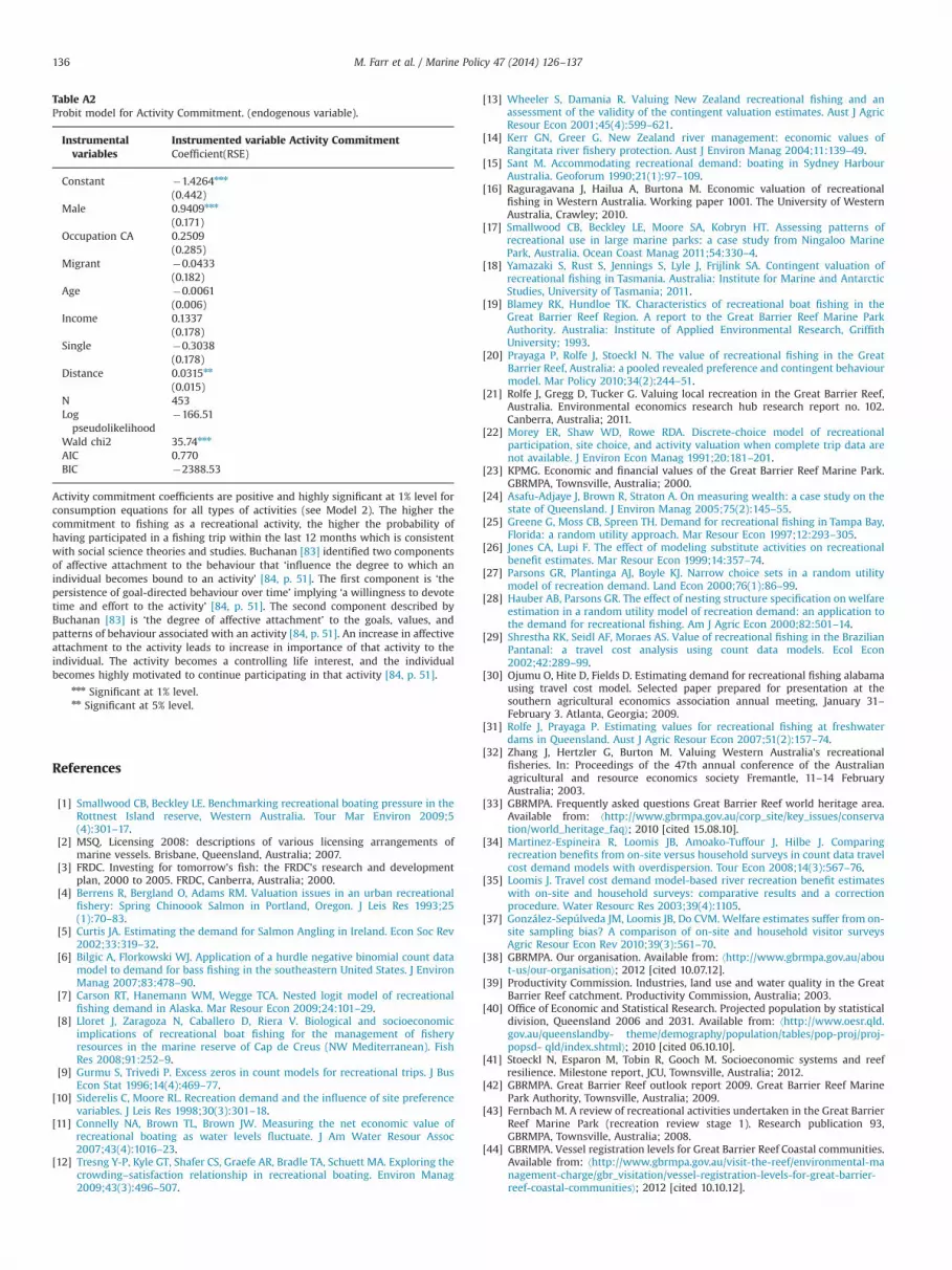
Activity commitment coefficients are positive and highly significant at 1% level forconsumption equations for all types of activities (see Model 2). The higher thecommitment to fishing as a recreational activity, the higher the probability ofhaving participated in a fishing trip within the last 12 months which is consistentwith social science theories and studies. Buchanan [83] identified two componentsof affective attachment to the behaviour that ‘influence the degree to which anindividual becomes bound to an activity’ [84, p. 51]. The first component is ‘thepersistence of goal-directed behaviour over time’ implying ‘a willingness to devotetime and effort to the activity’ [84, p. 51]. The second component described byBuchanan [83] is ‘the degree of affective attachment’ to the goals, values, andpatterns of behaviour associated with an activity [84, p. 51]. An increase in affectiveattachment to the activity leads to increase in importance of that activity to theindividual. The activity becomes a controlling life interest, and the individualbecomes highly motivated to continue participating in that activity [84, p. 51].

nnn Significant at 1% level.nn Significant at 5% level.

M. Farr et al. / Marine Policy 47 (2014) 126–137136

[45] MSQ. Recreational boating survey report 2006. Maritime Safety Queensland,Brisbane, Australia; 2006.

[46] Economic associates. Recreational boating facilities demand forecasting studyNorthern region. Available from: ⟨http://www.msq.qld.gov.au/About-us/MSQ-headlines/Headlines-demand-forecasting-study.aspx⟩; 2011 [cited04.06.11].

[47] Innes J, Gorman KA. Social and economic profile of Great Barrier Reef coastalcommunities. Report prepared for the GBRMPA, Townsville, Australia; 2002.

[48] GBRMPA. An economic and social valuation of implementing the representa-tive areas program by rezoning the Great Barrier Reef Marine Park. GBRMPA,Townsville, Australia; 2003.

[49] Australian Bureau of Statistics. Regional population growth, Australia, 2008–09 Queensland. Cat no. 3218.0. Canberra, Australia; 2010.

[50] GBRMPA. Recreational fishing effort proxy on GBR Coast. Available from:⟨http://www.gbrmpa.gov.au/corp_site/about_us/great_barrier_reef_outlook_report/outlook_report/evidence/01_standard_evidence_page190⟩; 2010 [cited30.06.10].

[51] Dillman DA. Mail and telephone surveys: the total design method. New York:John Wiley and Sons; 1978.

[52] Australian Bureau of Statistics. 1379.0.55.001 national regional profile, Towns-ville City Part A and B, 2006–2010. Canberra, Australia; 2011.

[53] Mullahy J. Specification and testing in some modified count models. J Econ1986;33:341–65.

[54] Walsh RG, John KH, McKean JR, Hof JG. Effect of price on forecasts ofparticipation in fish and wildlife recreation: an aggregate demand model. JLeis Res 1992;24(2):140–56.

[55] Gillig D, Ozuna T Jn, Griffin WL. The value of the Gulf of Mexico recreationalred snapper fishery. Mar Resour Econ 2000;15:127–39.

[56] Wang E, Li Z, Little BB, Yang Y. The economic impact of tourism in XinghaiPark, China: a travel cost value analysis using count data regression models.Tour Econ 2009;15(2):413–25.

[57] Cameron AC, Trivedi PK. Econometric models based on count data: compar-isons and applications of some estimators and tests. J Appl Econ1986;1:29–53.

[58] Keelan CD, Henchion MM, Newman CF. A double-hurdle model of Irishhouseholds' food service expenditure patterns. JIFAM 2009;21(4):269–85.

[59] Newman C, Henchion M, Matthews A. A double-hurdle model of Irishhousehold expenditure on prepared meals. J Appl Econ 2003;35(9):1053–61.

[60] Moffatt P. Hurdle models of loan default. J Oper Res Soc 2005;56:1063–71.[61] Herath G, Kennedy J. Estimating the economic value of Mount Buffalo National

Park with the travel cost and contingent valuation models. Tour Econ 2004;10(1):63–78.

[62] Carpio CE, Wohlgenant MK, Boonsaeng T. The demand for agritourism in theUnited States. J Agric Resour Econ 2008;33(2):254–69.

[63] Fleming CM, Cook A. The recreational value of Lake McKenzie, Fraser Island:an application of the travel cost method. Tour Manag 2008;29(6):1197–205.

[64] Cesario F. Value of time in recreation benefit studies. Land Econ 1976;52(1):32–41.

[65] Coupal RH, Bastian C, May J, Taylor DT. The economic benefits of snowmobil-ing to Wyoming residents: a travel cost approach with market segmentation. JLeis Res 2001;33(4):492–510.

[66] Bin O, Landry CE, Ellis CL, Vogelsong H. Some consumer surplus estimates forNorth Carolina beaches. Mar Resour Econ 2005;20:145–61.

[67] Chen W, Hong H, Liu Y, Zhang L, Hou X, Raymond M. Recreation demand andeconomic value: an application of travel cost method for Xiamen Island. ChinaEcon Rev 2004;15(4):398–406.

[68] Poor JP, Smith JM. Travel cost analysis of a cultural heritage site: the case ofhistoric St. Mary's City of Maryland. J Cult Econ 2004;28:217–29.

[69] Prayaga P, Rolfe J, Sinden J. A travel cost analysis of the value of special events:Gemfest in Central Queensland. Tour Econ 2006;12(3):403–20.

[70] Stoeckl N. A ‘quick and dirty’ travel cost model. Tour Econ 2003;9(3):325–35.[71] Geoscience Australia. As the Cocky Flies, online distance calculation tool.

Available from: ⟨http://www.ga.gov.au/map/names/distance.jsp⟩; 2013 [cited20.05.13].

[72] UCLA statistical consulting group. Regression with SPSS: chapter 2 – regres-sion diagnostics. Available from: ⟨http://www.ats.ucla.edu/stat/spss/webbooks/reg/chapter2/spssreg2.htm⟩; 2013 [cited 16.05.13].

[73] Davidson R, MacKinnon JG. Estimation and inference in econometrics. NewYork: Oxford University Press; 1993.

[74] Menard S. Applied logistic regression analysis. Sage university paper series onquantitative applications in the social sciences, 07–106. Thousand Oaks, CA:Sage; 1995.

[75] Field A. Discovering statistics using SPSS. 3rd ed.. London: Sage Publication;2009.

[76] Myers R. Classical and modern regression with applications. 2nd ed.. Boston,MA: Duxbury; 1990.

[77] Anderson TW, Rubin H. Estimation of the parameters of a single equation in acomplete system of stochastic equations. Ann Math Stat 1949;20:46–63.

[78] Moreira MJ. A conditional likelihood ratio test for structural models. Econo-metrica 2003;71:1027–48.

[79] Pitts HM, Thacher JA, Champ PA, Berrens RPA. Hedonic price analysis of theoutfitter market for trout fishing in the rocky mountain west. Hum DimensWildl 2012;17(6):446–62.

[80] Floyd MF, Nicholas L, Lee I, Lee J-H, Scott D. Social stratification in recreationalfishing participation: research and policy implications. Leis Sci 2006;28(4):351–68.

[81] UCLA statistical consulting group. Stata data analysis examples: zero-truncated negative binomial. Available from: ⟨http://www.ats.ucla.edu/stat/stata/dae/ztnb.htm⟩; 2013 [17.05.13].

[82] Taylor S, Webley J, McInnes K. Statewide recreational fishing survey. Finalreport. Australia: State of Queensland, Department of Agriculture, Fisheriesand Forestry; 2010; 2012.

[83] Buchanan T. Commitment and leisure behaviour: a theoretical perspective.Leis Sci 1985;7:401–20.

[84] Sutton SG, Ditton RB. Understanding catch-and-release behavior among U.S.Atlantic Bluefin Tuna Anglers. Hum Dimens Wildl 2001;6(1):49–66.

[85] Kleibergen F. Generalizing weak instrument robust IV statistics towardsmultiple parameters, unrestricted covariance matrices and identificationstatistics. J Econ 2007;139:181–216.

M. Farr et al. / Marine Policy 47 (2014) 126–137 137