recent theoretical results on coronal heating

RECENT THEORETICAL RESULTS ON CORONAL HEATING

DANIEL O. GOMEZ1,∗, PABLO A. DMITRUK1,† and LEONARDO J. MILANO2,†

1Department of Physics, University of Buenos Aires, Ciudad Universitaria,1428 Buenos Aires, Argentina

2National Solar Observatory, P.O.Box 62, Sunspot, NM 88349, U.S.A.

(Received 20 September 1999; accepted 1 March 2000)

Abstract. The scenario of magnetohydrodynamic turbulence in connection with coronal active re-gions has been actively investigated in recent years. According to this viewpoint, a turbulent regimeis driven by footpoint motions and the incoming energy is efficiently transferred to small scales dueto a direct energy cascade. The development of fine scales to enhance the dissipation of either wavesor DC currents is therefore a natural outcome of turbulent models. Numerical integrations of thereduced magnetohydrodynamic equations are performed to simulate the dynamics of coronal loopsdriven at their bases by footpoint motions. These simulations show that a stationary turbulent regimeis reached after a few photospheric times, displaying a broadband power spectrum and a dissipationrate consistent with the energy loss rates of the plasma confined in these loops. Also, the functionaldependence of the stationary heating rate with the physical parameters of the problem is obtained,which might be useful for an observational test of this theoretical framework.

1. Introduction

Recent X-ray and EUV observations of the solar corona reveal a highly structuredbrightness distribution, which is the consequence of magnetic fields confining theX-ray emitting plasma and governing its dynamics. Observations made with high

spatial resolution (Schrijveret al., 1999; Golubet al., 1990; Golub and Pasachoff,1997) show coronal magnetic loops with a highly filamentary internal structure.

Coronal heating theories have traditionally been classified into two broad cate-gories: (a)AC or wave models, for which energy is provided by waves generatedat the photosphere and, (b)DC or stress models, which assume that energy dissi-pates in magnetic stresses driven by slow footpoint motions. Although these twoconcepts seem mutually exclusive, the following assumptions are shared by bothclasses of models: (i) the ultimate source for coronal heating is the kinetic energyof the photospheric velocity field, (ii) the dissipation mechanism is Joule heating,although viscosity might also play an important role, (iii) the existence of finestructure in the coronal magnetic field is invoked to speed up Joule (or viscous)dissipation. Recent review articles on coronal heating (Narain and Ulmschneider,

∗Also at: Instituto de Astronomıa y Fısica del Espacio, C.C.67, Suc.28, 1428 Buenos Aires,Argentina.

†Presently at: Bartol Research Institute, University of Delaware, Newark, DE 19716, U.S.A.

Solar Physics195: 299–318, 2000.© 2000Kluwer Academic Publishers. Printed in the Netherlands.

300 D. O. GOMEZ, P. A. DMITRUK, AND L. J. MILANO

1996, 1990; Gómez, 1990; Zirker, 1993), explore the various theoretical models infurther detail.

As mentioned, the natural candidate for the energy dissipation is Joule heating,but the typical time scale to dissipate coronal magnetic stresses on the length scaleof the driving photospheric motions is exceedingly long. This time-scale can beestimated asl2/η ∼ 106 years (l = 103 km: length scale of photospheric motions,η = 103 cm2 s−1: resistivity). Therefore, most of the current theories of coro-nal heating deal with different mechanisms to speed up dissipation (Parker, 1972,1983; Heyvaerts and Priest, 1983; van Ballegooijen, 1986). Numerical integrationsof the MHD equations have also been performed (Mikic, Schnack, and van Hoven,1989; Longcope and Sudan, 1994), to study the dynamics of coronal loops drivenat their bases by convective motions. These simulations show the development ofsmall spatial structures (current sheets), which contribute to enhance dissipation.

One of the promising scenarios is the assumption that the magnetic and velocityfields of the coronal plasma are in a turbulent state (Gómez and Ferro Fontan,1988, 1992; Heyvaerts and Priest, 1992; Einaudiet al., 1996; Hendrix and vanHoven, 1996; Dmitruk and Gómez, 1997). Since the dynamics of coronal loops isdominated by their magnetic field, turbulent fluctuations of both the velocity andthe magnetic fields are generated predominantly in the directions perpendicularto the main magnetic field (for details on the MHD turbulent scenario, see, forinstance Biskamp, 1993). In a turbulent regime, energy is transferred from photo-spheric motions to the magnetic field. This energy cascades toward small scalesdue to nonlinear interactions, until highly structured electric currents are formed.The development of fine scales to enhance the dissipation of either waves or DCcurrents, is therefore a natural outcome of turbulent models. On the other hand, thedynamics of the solar photosphere is dominated by its velocity field, and thereforean essentially hydrodynamic turbulence is observed in this region (Nesiset al.,1999).

We present numerical integrations of the reduced magnetohydrodynamic equa-tions, to simulate the dynamics of coronal loops driven at their bases by footpointmotions. These simulations show that after a few photospheric turnover times astationary turbulent regime is reached, displaying a broadband power spectrumand a dissipation rate consistent with the energy loss rates of the plasma confinedin these loops. In Section 2 we briefly describe recent observational results whichare relevant to the problem of coronal heating. The reduced MHD approximationis described in Section 3, and various results from recent numerical simulationsof the RMHD equations are summarized in Section 4. An interesting scaling law,which relates the heating rate with the physical parameters of the loop is given inSection 5. A statistics of dissipation events arising from time-extended 2D MHDsimulations, which displays a slope quite comparable to those reported for flare(Hudson, 1991) and microflare (Shimizu, 1995) events, is shown in Section 6.Finally, in Section 7 we summarize our conclusions.

RECENT THEORETICAL RESULTS ON CORONAL HEATING 301

2. Recent Observational Results

The Transition Region and Coronal Explorer (TRACE) is showing us the spatialstructure and dynamics of the solar corona with unprecedented quality. Activeregions observed by TRACE are composed by bundles of long and thin loopsdisplaying a highly dynamic behavior, which involve not only kinematic motionsof the magnetic structure, but also rapid changes in the temperature and density ofindividual loops.

The extremely dynamic nature of coronal loops is suggestive of a rather in-termittent heating process, both in space and time. Typical time-scales for thisvariability are a few minutes or less, while spatial structures of all sizes are ob-served, down to the resolution limit of 700 km (Schrijveret al., 1999). A spatiallyintermittent heating would qualitatively explain the rich transverse structure, sinceonly those field lines connected to locations where heating pulses occur will lightup. On the other hand, a temporally intermittent heating would force these loops toadjust their internal structures, i.e., their densities, temperatures and longitudinalvelocities. In some active regions, transverse oscillations of loops have also beenobserved, and it has been suggested that the kinetic energy associated to theseoscillations might play a role in the heating of the region (Nakariakovet al., 1999).

3. Reduced MHD Approximation

In view of the observed features mentioned above, in what follows we concentrateon the theoretical description of a relatively homogeneous bundle of field lines. Theloop footpoints are deeply rooted into the photosphere, which moves individualfield lines around, thus generating magnetic stresses in the coronal portion of theloop. Two important time-scales arise in this process: the Alfvén time,tA, which isthe time it takes for an Alfvén wave to travel along the loop; and the photospherictime tp, which is the turnover time of photospheric granules. IftA � tp, i.e.,if the driving time-scale is much shorter than the response time of the loop, ACheating processes might be important (Ionson, 1982; Heyvaerts and Priest, 1983;Hollweg, 1985; Ofman, Davila, and Steinolfson, 1995). On the other hand, when-evertA � tp, DC heating is dominant. Under the assumption that a coronal loopreaches a stationary turbulent state, its response to a broad range of photosphericdriving frequencies can be modeled by a closure model. At least for photosphericpower spectra decreasing as power laws of both the wavenumber and the timefrequency, the heating of the loop is dominated by DC heating (Milano, Dmitruk,and Mandrini, 1997) (see also Heyvaerts and Priest (1992) and Gómez and FerroFontán (1992) for closure models applied to a magnetic arcade and to a loop drivenby stationary footpoint motions, respectively).

In the present paper, the aim is to study the heating of a topologically simpleloop, which can be regarded as a sub-structure or building block of the much more


Z

Z

vA

Z=L

=0 ll

V

p

p

2π2π

p

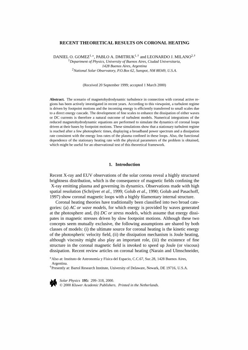
Figure 1. Perturbed field line in a coronal loop. The planesz = 0 and z = L represent thephotosphere.

complex active regions. The idea behind this approach is that if we manage toexplain the heating of simple loops, then we should be able to explain the heatingof complex superpositions of these structures, although it seems clear that complexstructures might provide extra heating. Furthermore, we take advantage of the (typ-ically) large aspect ratio of observed loops andstraighten them up, thus neglectingtoroidal effects, i.e., effects arising from the curvature of loops. Also, oscillatorymotions of the loop as a whole are neglected, as well as its interactions with othermagnetic structures.

We therefore consider a simplified model of a coronal magnetic loop with lengthL and cross section 2πlp×2πlp, wherelp is the length scale of typical photosphericmotions. For elongated loops, i.e., such that 2πlp � L, it is reasonable to neglecttoroidal effects. The main magnetic fieldB0 is assumed to be uniform and parallelto the axis of the loop (thez axis). The planes atz = 0 andz = L correspond tothe loop footpoints at the photosphere, as shown in Figure 1.


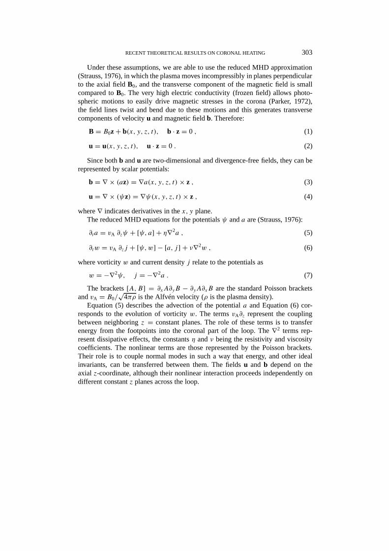
Under these assumptions, we are able to use the reduced MHD approximation(Strauss, 1976), in which the plasma moves incompressibly in planes perpendicularto the axial fieldB0, and the transverse component of the magnetic field is smallcompared toB0. The very high electric conductivity (frozen field) allows photo-spheric motions to easily drive magnetic stresses in the corona (Parker, 1972),the field lines twist and bend due to these motions and this generates transversecomponents of velocityu and magnetic fieldb. Therefore:

B = B0z+ b(x, y, z, t), b · z= 0 , (1)

u = u(x, y, z, t), u · z= 0 . (2)

Since bothb andu are two-dimensional and divergence-free fields, they can berepresented by scalar potentials:

b = ∇ × (az) = ∇a(x, y, z, t) × z , (3)

u = ∇ × (ψz) = ∇ψ(x, y, z, t) × z , (4)

where∇ indicates derivatives in thex, y plane.The reduced MHD equations for the potentialsψ anda are (Strauss, 1976):

∂ta = vA ∂zψ + [ψ, a] + η∇2a , (5)

∂tw = vA ∂zj + [ψ,w] − [a, j ] + ν∇2w , (6)

where vorticityw and current densityj relate to the potentials as

w = −∇2ψ, j = −∇2a . (7)

The brackets[A,B] = ∂xA∂yB − ∂yA∂xB are the standard Poisson bracketsandvA = B0/

√4πρ is the Alfvén velocity (ρ is the plasma density).

Equation (5) describes the advection of the potentiala and Equation (6) cor-responds to the evolution of vorticityw. The termsvA∂z represent the couplingbetween neighboringz = constant planes. The role of these terms is to transferenergy from the footpoints into the coronal part of the loop. The∇2 terms rep-resent dissipative effects, the constantsη andν being the resistivity and viscositycoefficients. The nonlinear terms are those represented by the Poisson brackets.Their role is to couple normal modes in such a way that energy, and other idealinvariants, can be transferred between them. The fieldsu and b depend on theaxial z-coordinate, although their nonlinear interaction proceeds independently ondifferent constantz planes across the loop.


4. Turbulent Heating

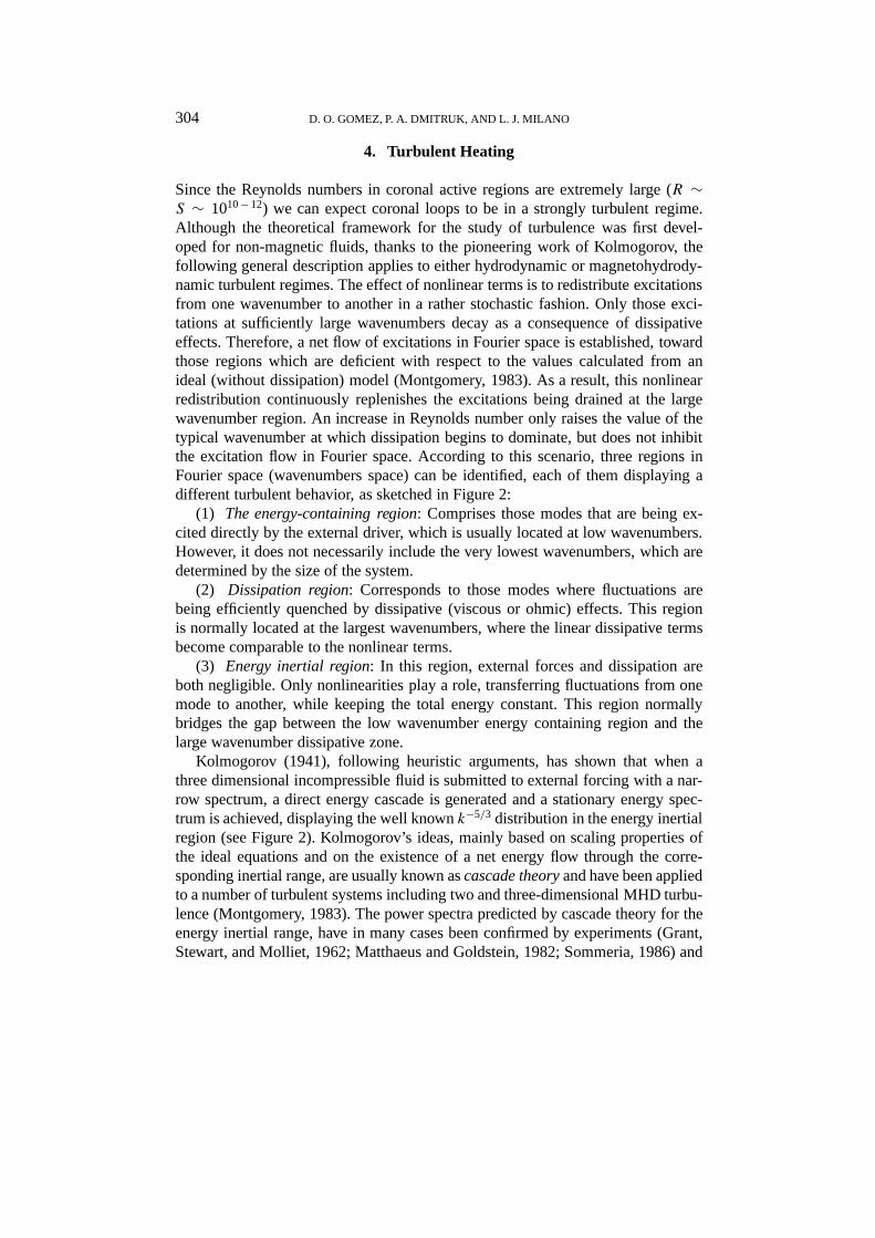
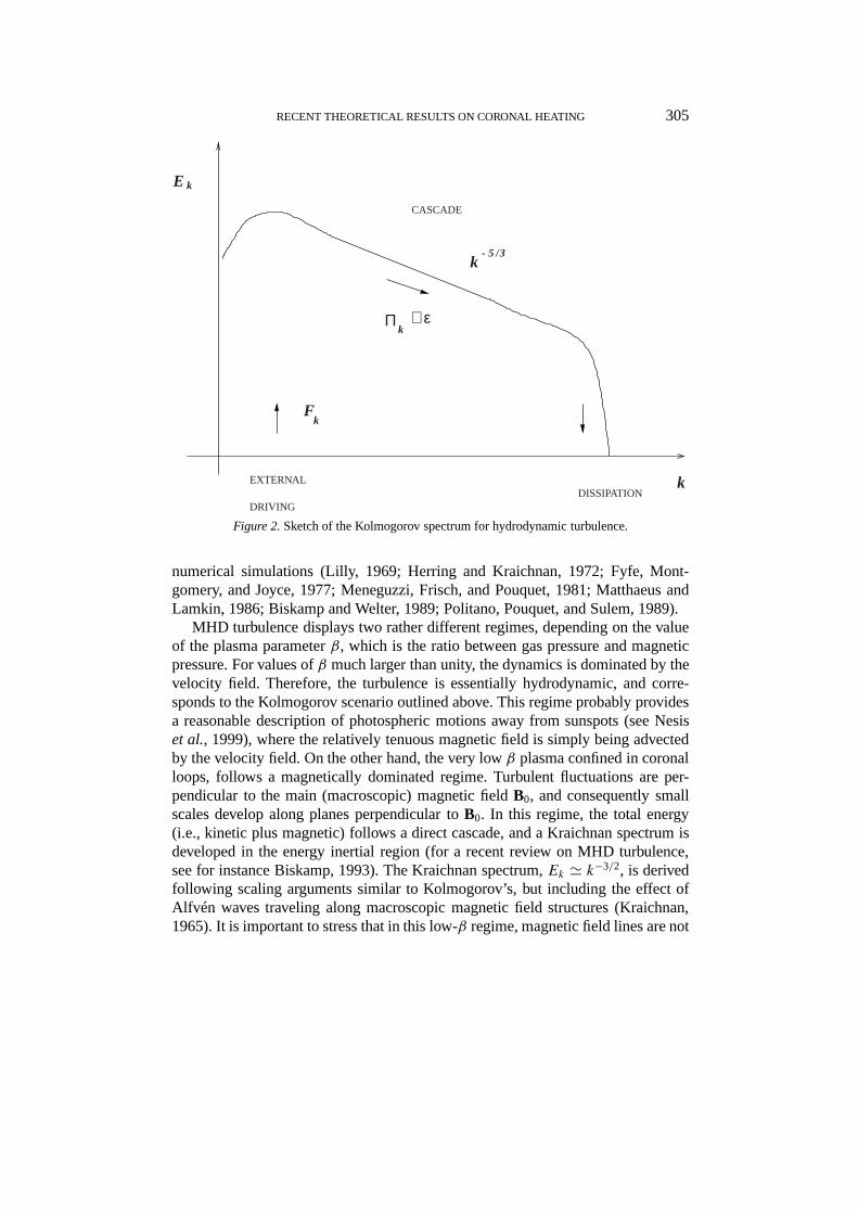
Since the Reynolds numbers in coronal active regions are extremely large (R ∼S ∼ 1010− 12) we can expect coronal loops to be in a strongly turbulent regime.Although the theoretical framework for the study of turbulence was first devel-oped for non-magnetic fluids, thanks to the pioneering work of Kolmogorov, thefollowing general description applies to either hydrodynamic or magnetohydrody-namic turbulent regimes. The effect of nonlinear terms is to redistribute excitationsfrom one wavenumber to another in a rather stochastic fashion. Only those exci-tations at sufficiently large wavenumbers decay as a consequence of dissipativeeffects. Therefore, a net flow of excitations in Fourier space is established, towardthose regions which are deficient with respect to the values calculated from anideal (without dissipation) model (Montgomery, 1983). As a result, this nonlinearredistribution continuously replenishes the excitations being drained at the largewavenumber region. An increase in Reynolds number only raises the value of thetypical wavenumber at which dissipation begins to dominate, but does not inhibitthe excitation flow in Fourier space. According to this scenario, three regions inFourier space (wavenumbers space) can be identified, each of them displaying adifferent turbulent behavior, as sketched in Figure 2:

(1) The energy-containing region: Comprises those modes that are being ex-cited directly by the external driver, which is usually located at low wavenumbers.However, it does not necessarily include the very lowest wavenumbers, which aredetermined by the size of the system.

(2) Dissipation region: Corresponds to those modes where fluctuations arebeing efficiently quenched by dissipative (viscous or ohmic) effects. This regionis normally located at the largest wavenumbers, where the linear dissipative termsbecome comparable to the nonlinear terms.

(3) Energy inertial region: In this region, external forces and dissipation areboth negligible. Only nonlinearities play a role, transferring fluctuations from onemode to another, while keeping the total energy constant. This region normallybridges the gap between the low wavenumber energy containing region and thelarge wavenumber dissipative zone.

Kolmogorov (1941), following heuristic arguments, has shown that when athree dimensional incompressible fluid is submitted to external forcing with a nar-row spectrum, a direct energy cascade is generated and a stationary energy spec-trum is achieved, displaying the well knownk−5/3 distribution in the energy inertialregion (see Figure 2). Kolmogorov’s ideas, mainly based on scaling properties ofthe ideal equations and on the existence of a net energy flow through the corre-sponding inertial range, are usually known ascascade theoryand have been appliedto a number of turbulent systems including two and three-dimensional MHD turbu-lence (Montgomery, 1983). The power spectra predicted by cascade theory for theenergy inertial range, have in many cases been confirmed by experiments (Grant,Stewart, and Molliet, 1962; Matthaeus and Goldstein, 1982; Sommeria, 1986) and


EXTERNAL

DRIVING

CASCADE

DISSIPATION

F

E

k

k

Π

k

k

- 5/3

∼ ε

k

Figure 2.Sketch of the Kolmogorov spectrum for hydrodynamic turbulence.

numerical simulations (Lilly, 1969; Herring and Kraichnan, 1972; Fyfe, Mont-gomery, and Joyce, 1977; Meneguzzi, Frisch, and Pouquet, 1981; Matthaeus andLamkin, 1986; Biskamp and Welter, 1989; Politano, Pouquet, and Sulem, 1989).

MHD turbulence displays two rather different regimes, depending on the valueof the plasma parameterβ, which is the ratio between gas pressure and magneticpressure. For values ofβ much larger than unity, the dynamics is dominated by thevelocity field. Therefore, the turbulence is essentially hydrodynamic, and corre-sponds to the Kolmogorov scenario outlined above. This regime probably providesa reasonable description of photospheric motions away from sunspots (see Nesiset al., 1999), where the relatively tenuous magnetic field is simply being advectedby the velocity field. On the other hand, the very lowβ plasma confined in coronalloops, follows a magnetically dominated regime. Turbulent fluctuations are per-pendicular to the main (macroscopic) magnetic fieldB0, and consequently smallscales develop along planes perpendicular toB0. In this regime, the total energy(i.e., kinetic plus magnetic) follows a direct cascade, and a Kraichnan spectrum isdeveloped in the energy inertial region (for a recent review on MHD turbulence,see for instance Biskamp, 1993). The Kraichnan spectrum,Ek ' k−3/2, is derivedfollowing scaling arguments similar to Kolmogorov’s, but including the effect ofAlfvén waves traveling along macroscopic magnetic field structures (Kraichnan,1965). It is important to stress that in this low-β regime, magnetic field lines are not


simply being advected by footpoint motions, but also generate their own non-linearresponse to the forcing, developing small scale structures, as shown below.

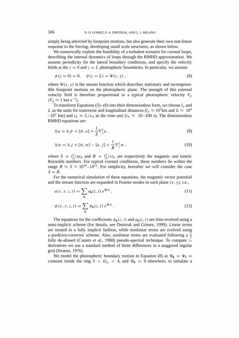
We numerically explore the feasibility of a turbulent scenario for coronal loops,describing the internal dynamics of loops through the RMHD approximation. Weassume periodicity for the lateral boundary conditions, and specify the velocityfields at thez = 0 andz = L photospheric boundaries. In particular, we assume

ψ(z = 0) = 0, ψ(z = L) = 9(x, y) , (8)

where9(x, y) is the stream function which describes stationary and incompress-ible footpoint motions on the photospheric plane. The strength of this externalvelocity field is therefore proportional to a typical photospheric velocityVp(Vp ≈ 1 km s−1).

To transform Equations (5)–(6) into their dimensionless form, we chooselp andL as the units for transverse and longitudinal distances (lp ≈ 103km andL ≈ 104

–105 km) andtA ≡ L/vA as the time unit (tA ≈ 10–100 s). The dimensionlessRMHD equations are:

∂ta = ∂zψ + [ψ, a] + 1

S∇2⊥a , (9)

∂tw = ∂zj + [ψ,w] − [a, j ] + 1

R∇2⊥w , (10)

whereS = l2p/ηtA andR = l2p/νtA are respectively the magnetic and kineticReynolds numbers. For typical coronal conditions, these numbers lie within therangeR ≈ S ≈ 1010–1012. For simplicity, hereafter we will consider the caseS = R.

For the numerical simulation of these equations, the magnetic vector potentialand the stream function are expanded in Fourier modes in each plane(x, y), i.e.,

a(x, y, z, t) =∑

k

ak(z, t) eik·x , (11)

ψ(x, y, z, t) =∑

k

ψk(z, t) eik·x . (12)

The equations for the coefficientsψk(z, t) andak(z, t) are time-evolved using asemi-implicit scheme (for details, see Dmitruk and Gómez, 1999). Linear termsare treated in a fully implicit fashion, while nonlinear terms are evolved usinga predictor-corrector scheme. Also, nonlinear terms are evaluated following a2

3fully de-aliased (Canutoet al., 1988) pseudo-spectral technique. To computez-derivatives we use a standard method of finite differences in a staggered regulargrid (Strauss, 1976).

We model the photospheric boundary motion in Equation (8) as9k = 90 =constant inside the ring 3< klp < 4, and9k = 0 elsewhere, to simulate a


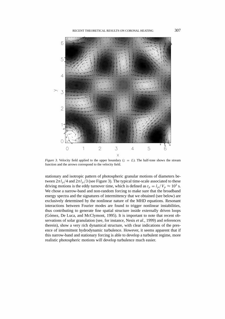
Figure 3. Velocity field applied to the upper boundary (z = L). The half-tone shows the streamfunction and the arrows correspond to the velocity field.

stationary and isotropic pattern of photospheric granular motions of diameters be-tween 2πlp/4 and 2πlp/3 (see Figure 3). The typical time-scale associated to thesedriving motions is the eddy turnover time, which is defined astp = lp/Vp ≈ 103 s.We chose a narrow-band and non-random forcing to make sure that the broadbandenergy spectra and the signatures of intermittency that we obtained (see below) areexclusively determined by the nonlinear nature of the MHD equations. Resonantinteractions between Fourier modes are found to trigger nonlinear instabilities,thus contributing to generate fine spatial structure inside externally driven loops(Gómez, De Luca, and McClymont, 1995). It is important to note that recent ob-servations of solar granulation (see, for instance, Nesiset al., 1999) and referencestherein), show a very rich dynamical structure, with clear indications of the pres-ence of intermittent hydrodynamic turbulence. However, it seems apparent that ifthis narrow-band and stationary forcing is able to develop a turbulent regime, morerealistic photospheric motions will develop turbulence much easier.


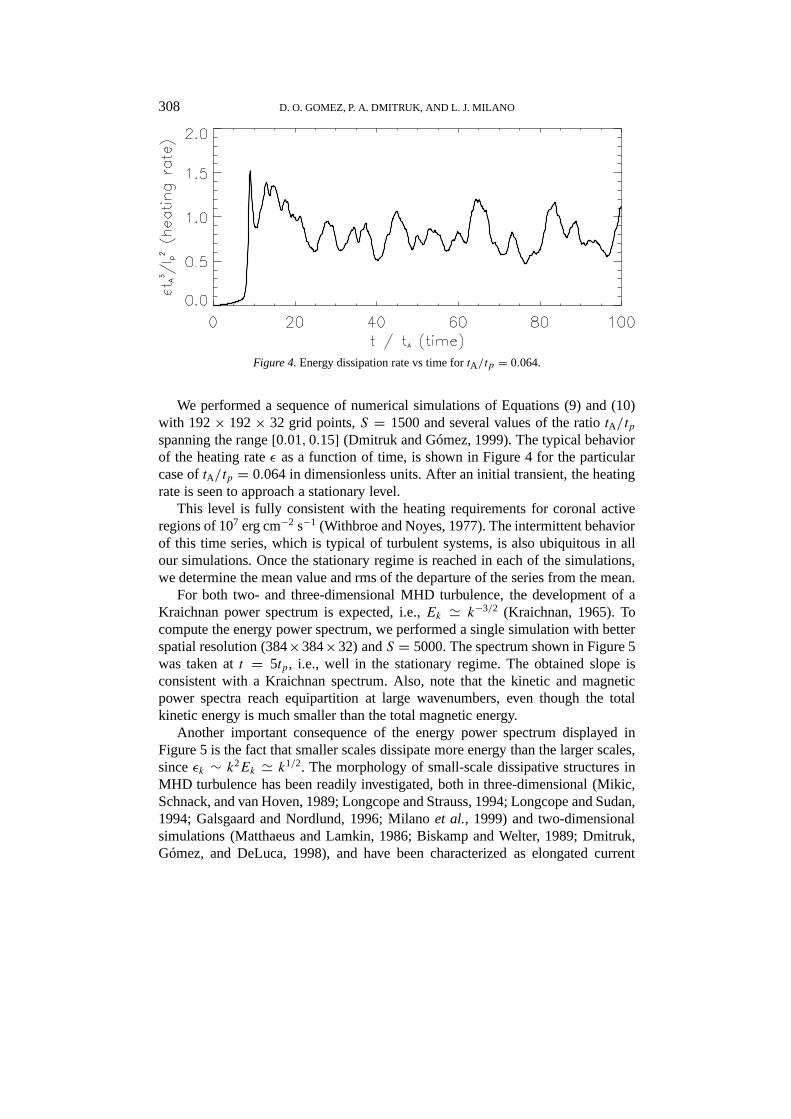
Figure 4.Energy dissipation rate vs time fortA/tp = 0.064.

We performed a sequence of numerical simulations of Equations (9) and (10)with 192× 192× 32 grid points,S = 1500 and several values of the ratiotA/tpspanning the range[0.01,0.15] (Dmitruk and Gómez, 1999). The typical behaviorof the heating rateε as a function of time, is shown in Figure 4 for the particularcase oftA/tp = 0.064 in dimensionless units. After an initial transient, the heatingrate is seen to approach a stationary level.

This level is fully consistent with the heating requirements for coronal activeregions of 107 erg cm−2 s−1 (Withbroe and Noyes, 1977). The intermittent behaviorof this time series, which is typical of turbulent systems, is also ubiquitous in allour simulations. Once the stationary regime is reached in each of the simulations,we determine the mean value and rms of the departure of the series from the mean.

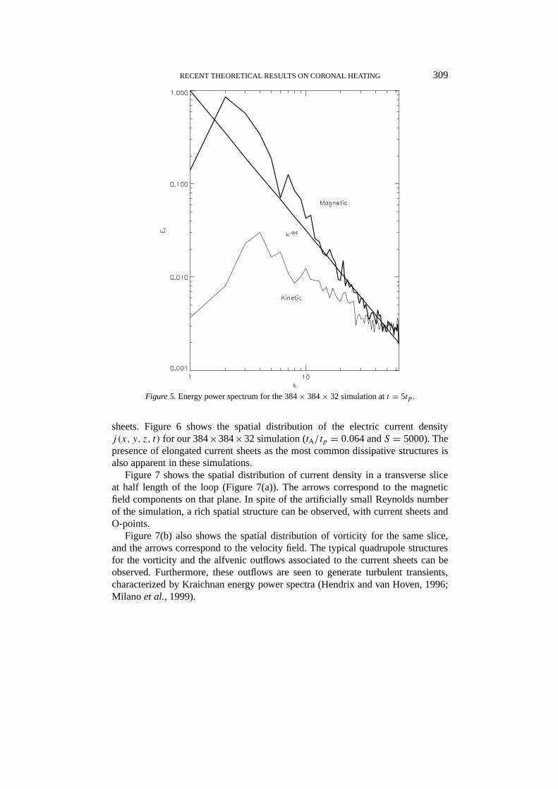
For both two- and three-dimensional MHD turbulence, the development of aKraichnan power spectrum is expected, i.e.,Ek ' k−3/2 (Kraichnan, 1965). Tocompute the energy power spectrum, we performed a single simulation with betterspatial resolution (384×384×32) andS = 5000. The spectrum shown in Figure 5was taken att = 5tp, i.e., well in the stationary regime. The obtained slope isconsistent with a Kraichnan spectrum. Also, note that the kinetic and magneticpower spectra reach equipartition at large wavenumbers, even though the totalkinetic energy is much smaller than the total magnetic energy.

Another important consequence of the energy power spectrum displayed inFigure 5 is the fact that smaller scales dissipate more energy than the larger scales,sinceεk ∼ k2Ek ' k1/2. The morphology of small-scale dissipative structures inMHD turbulence has been readily investigated, both in three-dimensional (Mikic,Schnack, and van Hoven, 1989; Longcope and Strauss, 1994; Longcope and Sudan,1994; Galsgaard and Nordlund, 1996; Milanoet al., 1999) and two-dimensionalsimulations (Matthaeus and Lamkin, 1986; Biskamp and Welter, 1989; Dmitruk,Gómez, and DeLuca, 1998), and have been characterized as elongated current


Figure 5.Energy power spectrum for the 384× 384× 32 simulation att = 5tp.

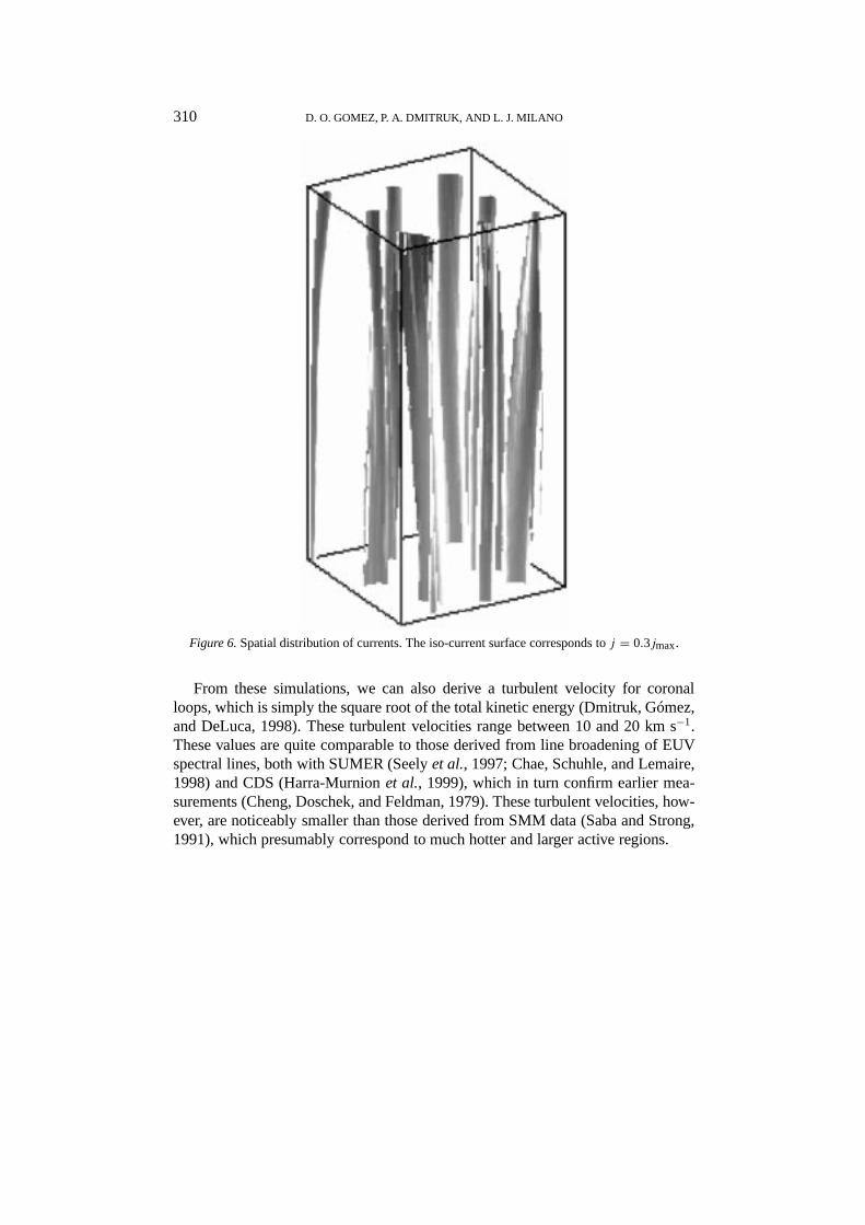
sheets. Figure 6 shows the spatial distribution of the electric current densityj (x, y, z, t) for our 384×384×32 simulation (tA/tp = 0.064 andS = 5000). Thepresence of elongated current sheets as the most common dissipative structures isalso apparent in these simulations.

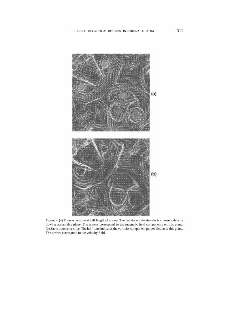
Figure 7 shows the spatial distribution of current density in a transverse sliceat half length of the loop (Figure 7(a)). The arrows correspond to the magneticfield components on that plane. In spite of the artificially small Reynolds numberof the simulation, a rich spatial structure can be observed, with current sheets andO-points.

Figure 7(b) also shows the spatial distribution of vorticity for the same slice,and the arrows correspond to the velocity field. The typical quadrupole structuresfor the vorticity and the alfvenic outflows associated to the current sheets can beobserved. Furthermore, these outflows are seen to generate turbulent transients,characterized by Kraichnan energy power spectra (Hendrix and van Hoven, 1996;Milano et al., 1999).


Figure 6.Spatial distribution of currents. The iso-current surface corresponds toj = 0.3jmax.

From these simulations, we can also derive a turbulent velocity for coronalloops, which is simply the square root of the total kinetic energy (Dmitruk, Gómez,and DeLuca, 1998). These turbulent velocities range between 10 and 20 km s−1.These values are quite comparable to those derived from line broadening of EUVspectral lines, both with SUMER (Seelyet al., 1997; Chae, Schuhle, and Lemaire,1998) and CDS (Harra-Murnionet al., 1999), which in turn confirm earlier mea-surements (Cheng, Doschek, and Feldman, 1979). These turbulent velocities, how-ever, are noticeably smaller than those derived from SMM data (Saba and Strong,1991), which presumably correspond to much hotter and larger active regions.


Figure 7.(a) Transverse slice at half length of a loop. The half-tone indicates electric current densityflowing across this plane. The arrows correspond to the magnetic field components on this plane.(b) Same transverse slice. The half-tone indicates the vorticity component perpendicular to this plane.The arrows correspond to the velocity field.


5. Scaling Law

As mentioned in the previous section, the Reynolds number (S = R) is the onlydimensionless parameter explicitly present in Equations (9) and (10). The bound-ary condition (Equation (8)) brings a second dimensionless parameter into play,namely the ratio between the photospheric velocityVp and our velocity unitlp/tA.SinceVp = lp/tp, this velocity ratio is equivalent to the ratio between the Alfvéntime tA and the photospheric turnover timetp.

It is essential to note at this point that to integrate Equations (9) and (10) with theboundary condition Equation (8), only two dimensionless parameters are needed:S andtA/tp. Therefore, from purely dimensional considerations, we can derive thefollowing important result:for any physical quantity, its dimensionless versionQshould be an arbitrary function of the only two dimensionless parameters of theproblem, i.e.,

Q = F

(tA

tp, S

). (13)

For the important case of the heating rate per unit mass, i.e.,ε/ρ, its dimension-less version is

Q = ε

ρ

t3A

l2p= F

(tA

tp, S

). (14)

One of Kolmogorov’s hypotheses in his celebrated theory for stationary turbu-lent regimes at very large Reynolds numbers (Kolmogorov, 1941) states that thedissipation rate is independent of the Reynolds number (see also Frisch, 1996).We have already shown that externally driven coronal loops eventually reach astationary turbulent regime. If we therefore assume that the dissipation rateε islargely independent of the Reynolds numberS, we obtain

ε = ρl2p

t3AF

(tA

tp

). (15)

From a sequence of numerical simulations for different values of the ratiotA/tp(Dmitruk and Gómez, 1999), we find that the functionF is a power law with aslopes = 1.51± 0.04, i.e.,

ε ∝ ρl2p

t3A

(tA

tp

)3/2

. (16)

This result is fully consistent with the prediction arising from a two-dimensionalMHD model (Dmitruk and Gómez, 1997),s2D = 3

2, which is assumed to simulatethe dynamics of a generic transverse slice of a loop. This coincidence between bothscalings suggests that two-dimensional simulations provide an adequate descrip-tion of the dynamics of coronal loops (Hendrix and van Hoven, 1996; Matthaeus


et al., 1998; Oughton, Gosh, and Matthaeus, 1998), provided that the external forc-ing in Equations (5) and (6) is approximated as (Einaudiet al., 1996; Dmitruk andGómez, 1997)

f = vA∂zψ ≈ lpVp

tA, g = vA∂zj ≈ 0 , (17)

which stems from the assumption that field lines remain relatively straight whiletheir footpoints are being moved about. In this two-dimensional version of theproblem, parameters such asVp, vA andL arise only indirectly, through the forcingtermf (see Equation (5)). As in the previous section, we also assume: (i) a typicalgranule length scalelp for the forcing and, (ii) a dissipation rateε independent ofthe Reynolds numberS. Therefore, from dimensional arguments we find that theheating rate per unit mass (ε/ρ) can only depend on the relevant parameterslp andf in the following fashion:

ε

ρ∼ f 3

lp= l2p

t3A

(tA

tp

)3/2

, (18)

which exactly matches the scaling derived empirically from the sequence of RMHDsimulations (see Equation (16)). Alternative laws have been derived by other au-thors (Hendrixet al., 1996) considering two extra parameters, namely, a milddependence on the Reynolds numberS and a photospheric correlation time (apartfrom the granules turnover time).

Scaling laws like the one displayed in Equation (16), corresponding to a widevariety of coronal heating theories, have been reviewed in an excellent paper byMandrini, Démoulin, and Klimchuk (2000). In their study, the authors report astatistical correlation between the lengths of loops and their average magnetic field,based on magnetogram extrapolations for a large number of active regions. Thiscorrelation has the form〈B〉 ∼ L−0.9±0.3, confirming an earlier result (Porter andKlimchuk, 1995). By combining this law with the approximate dependence of theheating rate likeL−2 (arising from a static balance between a uniform heatingsource, thermal conduction and radiative losses), they can test different models ofcoronal heating. They find that DC models are in generally better agreement withthese observational constraints than AC heating models.

6. Statistics of Events

To perform extended time simulations we focus on the dynamics in a given trans-verse plane, that is, we study the evolution of a generic two-dimensional slice of aloop. To this end, we model thevA∂z terms as indicated in the previous section.

In spite of the narrow forcing and even though velocity and magnetic fields areinitially zero, nonlinear terms quickly populate all the modes across the spectrumand a turbulent state develops, with features quite comparable to the ones displayed


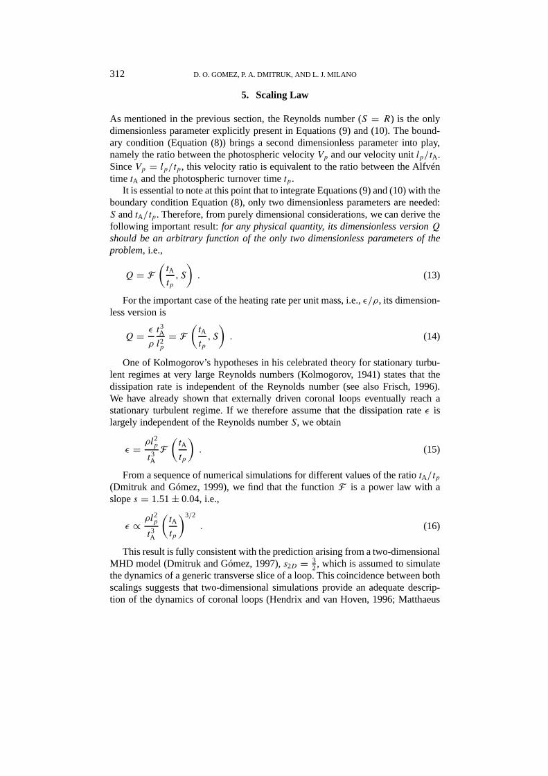
Figure 8.Energy dissipation rate vs time.

by the RMHD equations. Long time-series of the energy dissipation rate are ob-tained, as the one shown in Figure 8. These time series exhibit the intermittentbehavior also shown in Figure 4 for the RMHD case, which is characteristic ofturbulent systems.

Parker (1988) proposed that the energy dissipation of the stressed magneticstructures takes place in a large number of small events, which he termed ‘nanoflares’.The superposition of a large number of such events would give the global appear-ance of a spatially homogeneous and stationary heating process. From a turbulentscenario, it seems straightforward to relate this spiky (both in space and time)heating, to the internal intermittency present in all turbulent regimes. We thereforeassociate the peaks of energy dissipation displayed in Figure 8 to the so-callednanoflares (Dmitruk and Gómez, 1997; Dmitruk, Gómez, and DeLuca, 1998). Weestimate the occurrence rate for these nano-events, i.e., the number of events perunit energy and time,P(E) = dN/dE, so that

R =Emax∫Emin

dE P(E) (19)

is the total number of events per unit time and

ε(2πlp)2L =

Emax∫Emin

dE EP(E) (20)

is the total heating rate (in erg s−1) contributed by all events in the energy range[Emin;Emax]. We define events simply as the excesses of dissipation with respectto a threshold valueε0 of the order of the heating rate time average. Further details


of this derivation can be found elsewhere (Dmitruk and Gómez, 1997; Dmitruk,Gómez, and DeLuca, 1998).

The occurrence rate as a function of energy is found to display a power-lawbehavior

P(E) = AE−1.5±0.2 , (21)

in the energy range spanned fromEmin ' 1025 erg toEmax' 2×1026 erg. We alsocomputed the distribution of events as a function of peak fluxes which is a powerlaw with slopeαP = 1.7± 0.3 (Dmitruk, Gómez, and DeLuca, 1998). This slopeis consistent with the one derived by Crosby, Aschwanden, and Dennis (1993)(1.68) from X-ray events and somewhat flatter than those reported by Hudson(1991) (1.8). Similar event distributions have been derived by other authors, bothfrom MHD simulations (Georgoulis, Velli, and Einaudi, 1998) and from cellularautomata models (Lu and Hamilton, 1991; Luet al., 1993; Vlahoset al., 1995).Other important results from this statistical analysis are the correlations betweenthe different parameters of these events. For instance, the energy released vs eventdurationτ can be fitted by a power lawE ∼ τ 2 (Dmitruk, Gómez, and DeLuca,1998). This result is consistent with the correlation reported by (Lee, Petrosian,and McTiernan, 1993) from hard X-ray observations.

7. Conclusion

The main results of the present study can be summarized as follows:(1) TRACE movies show that coronal active regions are extremely dynamic

and inhomogeneous objects. This ubiquitous spatial and temporal variability sug-gests the presence of a rather intermittent heating mechanism for these regions. Wepropose that the development of MHD turbulence in coronal loops driven at theirfootpoints will naturally produce intermittent dissipation.

(2) Numerical integrations of the RMHD equations, driven by a stationarypattern of large-scale footpoint motions show that the system reaches a turbulentstationary regime, characterized by a Kraichnan energy power spectrum. Also,the ensuing energy cascade enhances the average dissipation rate to the levelsrequired by the conductive and radiative losses of the coronal plasma. Most ofthe dissipation occurs in current sheets approximately parallel to the loop axis.

(3) The MHD turbulence developed in coronal loops is magnetically domi-nated, i.e., the magnetic energy is much larger than the kinetic energy. Turbulentvelocities of about 10–20 km s−1 are obtained, which are fully consistent withthose inferred by various authors from the broadening of EUV spectral lines.

(4) By combining dimensional arguments on the RMHD equations with asequence of numerical simulations, a scaling law is derived, which relates theturbulent heating rate with the various relevant physical parameters (Dmitruk andGómez, 1999). This kind of scaling law, arising from theoretical heating models,


can be tested against observational constraints (Mandrini, Démoulin, and Klim-chuk, 2000).

(5) The intermittent nature of energy dissipation suggests that the heatingmechanism can be interpreted as a stochastic superposition of discrete events ornanoflares(Parker, 1988). In this regard, it is important to note that the turbulentscenario is not inconsistent with Parker’s scenario (Longcope and Sudan, 1994;Hendrix et al., 1996). Furthermore, it could perhaps be considered as its naturalextension to dissipative plasmas, since the tangential discontinuities arising in anideal plasma will become thin current sheets if a small amount of dissipation isallowed. A statistics of dissipation events obtained from numerical simulations,yields a power law energy occurrence rate. The slope of this distribution is ap-proximately 1.5, which is quite comparable to similar analysis performed for theoccurrence of flares (Hudson, 1991; Crosby, Aschwanden, and Dennis, 1993) andmicroflares (Shimizu, 1995).

Acknowledgements

The authors wish to express their gratitude to the local organizers of the Physics ofthe Solar Corona and Transition Region Workshop, where this paper was presented,Drs Karel Schrijver, Zoe Frank, and Neal Hurlburt, for such a superb meeting andfor their kind hospitality. This work is supported by the University of Buenos Aires(grant UBACYT TX065/98), and the Agencia Nacional de Promoción de Ciencia yTecnología (grant PICT 02305/97). DG is Member of the Carrera del InvestigadorCientífico of CONICET, Argentina.

References

Biskamp, D.: 1993,Nonlinear Magnetohydrodynamics, Cambridge University Press, Cambridge.Biskamp, D. and Welter, H.: 1989,Phys. FluidsB1, 1964.Canuto, C., Hussaini, M. Y., Quarteroni, A., and Zang, T. A.: 1988,Spectral Methods in Fluid

Dynamics, Springer-Verlag, New York.Chae, J., Schuhle, U., and Lemaire, P.: 1998,Astrophys. J.505, 957.Cheng, C., Doschek, G. and Feldman U.: 1979,Astrophys. J.227, 1037.Crosby, N. B., Aschwanden, M. J., and Dennis, B. R.: 1993,Solar Phys.143, 275.Dmitruk, P. and Gómez, D. O.: 1997,Astrophys. J.484, L83.Dmitruk, P. and Gómez, D.O.: 1999,Astrophys. J.527, L63.Dmitruk, P., Gómez, D. O., and DeLuca, E. E.: 1998,Astrophys. J.505, 974.Einaudi, G., Velli, M., Politano, H., and Pouquet, A.: 1996,Astrophys. J.457, L113.Frisch, U.: 1996,Turbulence, Cambridge University Press, Cambridge.Fyfe, D., Montgomery, D., and Joyce, G.: 1977,J. Plasma Phys.17, 369.Galsgaard, K. and Nordlund, A.: 1996,J. Geophys. Res.101, 13445.Georgoulis, M., Velli, M., and Einaudi, G.: 1998,Astrophys. J.497, 957.Golub, L. and Pasachoff, J.: 1997,The Solar Corona, Cambridge University Press, Cambridge.


Golub, L., Herant, M., Kalata, K., Louvas, I., Nystrom, G., Pardo, F., Spiller, E., and Wilczynski,J. S.: 1990,Nature344, 842.

Gómez, D. O.: 1990,Fund. Cosmic Phys.14, 361.Gómez, D. O. and Ferro Fontan, C.: 1988,Solar Phys.116, 33.Gómez, D. O. and Ferro Fontán, C.: 1992,Astrophys. J.394, 662.Gómez, D. O., De Luca, E. E., and Mc Clymont, A. N.: 1995,Astrophys. J.448, 954.Grant, H. L., Stewart, R. W., and Molliet, A.: 1962,J. Fluid Mech.12, 241.Harra-Murnion, L. K., Matthews, S. A., Hara, H., and Ichimoto, K.: 1999,Astron. Astrophys.345,

1011.Hendrix, D. L. and van Hoven, G.: 1996,Astrophys. J.467, 887.Hendrix, D. L., van Hoven, G., Mikic, Z., and Schnack, D. D.: 1996,Astrophys. J.470, 1192.Herring, J. and Kraichnan, R. H.: 1972, in M. Rosenblatt and C. van Atta (eds.), ‘Statistical Models

and Turbulence’, Springer-Verlag, Berlin.Heyvaerts, J. and Priest, E. R.: 1983,Astron. Astrophys.117, 220.Heyvaerts, J. and Priest, E. R.: 1992,Astrophys. J.390, 297.Hollweg, J. V.: 1985, in B. Buti (ed.),Advance Space Plasma Physics, World Science Publ. Co.,

Singapore, p. 77.Hudson, H. S.: 1991,Solar Phys.133, 357.Ionson, J. A.: 1982,Astrophys. J.254, 318.Kolmogorov, A. N.: 1941,Dokl. Acad. Sci. URSS30, 301.Kraichnan, R. H.: 1965,Phys. Fluids8, 138.Lee, T. T., Petrosian, V., and McTiernan, J. M.: 1993,Astrophys. J.412, 401.Lilly, D. K.: 1969, Phys. Fluids12, 240.Longcope, D. W. and Strauss, H. R.: 1994,Astrophys. J.426, 742.Longcope, D. W. and Sudan, R. N.: 1994,Astrophys. J.437, 491.Lu, E. T. and Hamilton, R. J.: 1991,Astrophys. J.380, L89.Lu, E., Hamilton, R., McTiernan, J., and Bromund, K.: 1993,Astrophys. J.412, 841.Mandrini, C. H., Démoulin, P., and Klimchuk, J. A.: 2000,Astrophys. J.530, in press.Matthaeus, W. H., and Goldstein, G. L.: 1982,J. Geophys. Res.87, 6011.Matthaeus, W. H. and Lamkin, S. L.: 1986,Phys. Fluids29, 2513.Matthaeus, W. H., Oughton, S., Ghosh, S., and Hossain, M.: 1998,Phys. Rev. Letters81, 2056.Meneguzzi, M., Frisch, U., and Pouquet, A.: 1981,Phys. Rev. Letters47, 1060.Mikic, Z., Schnack, D. D., and van Hoven, G.: 1989,Astrophys. J.338, 1148.Milano, L. J., Gómez, D. O., and Martens, P. C. H. 1997,Astrophys. J.490, 442.Milano, L. J., Dmitruk, P., Mandrini, C. H., Gómez, D. O., and Démoulin, P.: 1999,Astrophys. J.

521, 889.Montgomery, D.: 1983, in M. Neugebauer (ed.), ‘Solar Wind V’, NASA Conf. Publ. 2280, p. 107.Nakariakov, V. M., Ofman, L., DeLuca, E. E., Roberts, B., and Davila, J. M.: 1999,Nature285, 862.Narain, U. and Ulmschneider, P.: 1990,Space Sci. Rev.54, 377.Narain, U. and Ulmschneider, P.: 1996,Space Sci. Rev.75, 453.Nesis, A., Hammer, R., Kiefer, M., Schleicher, H., Sigwarth, M., and Staiger, J.: 1999,Astron.

Astrophys.345, 265.Ofman, L., Davila, J. M., and Steinolfson, R. S.: 1995,Astrophys. J.444, 471.Oughton, S., Ghosh, S., and Matthaeus, W. H.: 1998,Phys. Plasmas5, 4235.Parker, E. N.: 1972,Astrophys. J.174, 499.Parker, E. N.: 1983,Astrophys. J.264, 642.Parker, E. N.: 1988,Astrophys. J.330, 474.Politano, H., Pouquet, A., and Sulem, P. L.: 1989,Phys. FluidsB1, 2330.Porter, L. J. and Klimchuk, J. A.: 1995,Astrophys. J.454, 499.Saba, J. and Strong, K.: 1991,Astrophys. J.375, 789.Schrijver, C. J. and 16 co-authors: 1999,Solar Phys., 187, 261.


Seely, N.et al.: 1997,Astrophys. J.484, L87.Shimizu, T.: 1995,Publ. Astr. Soc. Japan47, 251.Sommeria, J.: 1986,J. Fluid Mech.170, 139.Strauss, H.: 1976,Phys. Fluids19, 134.van Ballegooijen, A. A.: 1986,Astrophys. J.311, 1001.Vlahos, H., Georgoulis, M., Kluiving, R., and Paschos, P.: 1995,Astron. Astrophys.299, 897.Withbroe, G. L. and Noyes, R. W.: 1977,Ann. Rev. Astron. Astrophys.15, 363.Zirker, J. B. 1993,Solar Phys.148, 43.

recent theoretical results on coronal heating

Documents