recent advances in tracs

Recent advances in TRACS

Ann S K Kwan1, Margaret E Parker, Raymond S K Kwan, Sarah Fores, Les Proll, Anthony Wren

School of Computing , University of Leeds, Leeds LS2 9JT, U.K.

Keywords: driver scheduling, transport, set covering problem

Abstract

TRACS is an established driver scheduling system [2, 3, 4, 6, 8, 9]. Its variant BusTRACS is being used by 29 bus companies, and TrainTRACS is being used by the train operator ScotRail. TrainTRACS has also been used in scheduling projects for several other train operators. As the transport operators start using the system, difficult problem issues arising from individual companies are carefully investigated. These investigations have led to some advanced scheduling strategies being developed. This paper briefly explains the problem of driver scheduling, reviews the developments leading to the current system, discusses the system’s recent advancement in the last few years. The ability to tackle large and complex problems is becoming a very important issue for transport operators. Some recent advances in TRACS are focused on this issue. Three categories of large and complex problems and the strategies for tackling them will be discussed.

1. Introduction

The research and development of TRACS and its predecessors, notably IMPACS [10], can be tracked throughout this series of international conferences/workshops. Around the time of the last event, CASPT 2000 in Berlin, TRACS was adopted by First, which is the largest group of bus companies in the UK. First had a “wish list” of enhancements to TRACS at the beginning. While the enhancements were implemented in the last three years, a few more were added to the list as new requirements and aspirations emerged during the roll-out programme. Since then, TRACS has also been installed or used in large scale trials by some train companies. These interactions with real schedulers in the past few years have continued to spark off advances, which will be reported in this paper.

Driver scheduling is one of the core activities of public transport operators. Having produced the

schedules these are then used as the primary input to rostering and payroll systems. Drivers often account for the largest proportion of operating costs, e.g. in UK bus operations, this may be over 45% of operating costs [1] and the proportion is likely to rise as there is a general shortage of drivers in the U.K. Within the bounds of the physical and operational constraints, transport operators still have much opportunity to manipulate the driver conditions to produce efficiency and savings. In this changing world, operators must be able to react quickly to the forces of competition, which lead to many what-if scenarios based on many different scheduling rules. Hence there is a demand for driver scheduling systems to be ever more versatile in meeting the needs of the operators.

Driver scheduling is a well-known NP-hard problem which has already been described in many

papers. For the sake of clarity of terms used and completeness, we shall nevertheless give a brief introduction.

Driver scheduling is the process of constructing shifts, each of which obeys a set of labour rules

which determine its legality and its desirability, based on a predetermined and fixed set of vehicle workings such that all the vehicle work is covered by the minimum number of drivers at the cheapest possible cost. Drivers can only be changed when a vehicle passes one of a number of designated relief

1 email: [email protected]

points; the times at which vehicles pass these points are called relief opportunities. The work of a vehicle and the relief opportunities for a day may be represented diagrammatically in the form of a vehicle graph:

0618 0715 0841 1057 1132 1259 1501 1602 1730 2001 2050 2301

^----^----^-----^-----^----^-----^----^-----^-------^----^---------^

G A A B C B C B C A A G

Figure 1. A vehicle graph The horizontal line represents the time that the vehicle needs a driver and each ‘^’ represents a relief

opportunity. The vehicle work between two consecutive relief opportunities is called a piece of work; a spell contains one or more consecutive pieces of work on the same vehicle. A day’s work for a driver is called a shift. A shift consists of a number of spells usually drawn from a number of vehicles. The length of a shift from sign on to sign off is called spreadover. Minimising costs here implies minimising the number of shifts in a schedule such that all the vehicle work is covered.

The driver scheduling problem was first tackled in the early 1960's and the subject has been well researched since then and reported in this series of international conferences/workshops on computer-aided scheduling of public transport [2, 3, 4, 5 6, 7, 8, 9]. The approaches can be divided into two groups: • Heuristic approaches which include constructive and improvement techniques [14] or a mixture of

heuristics and other algorithms such as the matching algorithm or the assignment algorithm. Some of the matching or assignment approaches may involve the use of a mathematical programming formulation.

• Set covering or set partitioning approaches which usually involve mathematical programming [10,

11] or metaheuristics such as evolutionary algorithms. [12, 13]

The classifications are not distinctive because it is usual to find that some Mathematical Programming approaches may involve heuristic techniques to some extent; some metaheuristic approaches may involve Mathematical programming, etc.

TRACS belongs to the set covering category. Its predecessor, the IMPACS system [10], was

developed in the 70’s and was implemented in Manchester and London for bus in the early 1980s, the BUSMAN system derived from it was used by about 40 bus companies since the 1980s. Since the early 1990s, extensive research, development and trials have been carried out for the rail industry [15, 16, 17] resulting in the TRACS system. The rail problem is generally considered to be more complex than, but has generic applicability to, that for bus.

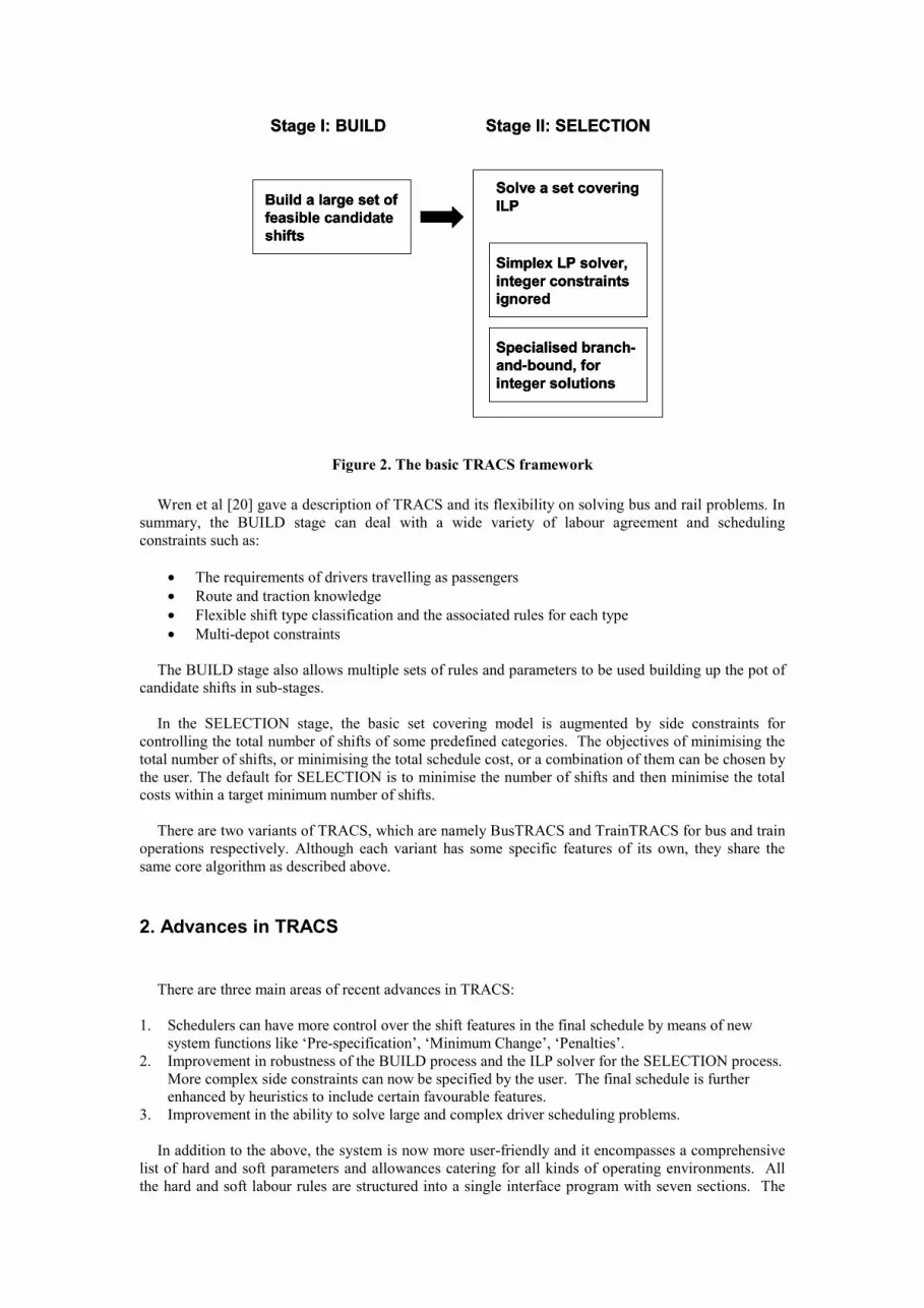
The TRACS process has two stages as illustrated in Figure 2, which is flexible enough to cater for different sets of driver working conditions. The first stage of the method is called the BUILD stage which builds a large set of feasible candidate shifts. The first stage is driven by parameters which represent the driver work rules and various time allowances. The second stage is called the SELECTION stage, which selects a subset from the candidate shifts to form the solution schedule. The selection technique used is based on the set covering model, and is relatively problem domain independent.

Stage I: BUILD Stage II: SELECTION

Build a large set of feasible candidate shifts

Solve a set covering ILP

Specialised branch-and-bound, for integer solutions

Simplex LP solver, integer constraints ignored

Stage I: BUILD Stage II: SELECTION









Figure 2. The basic TRACS framework Wren et al [20] gave a description of TRACS and its flexibility on solving bus and rail problems. In

summary, the BUILD stage can deal with a wide variety of labour agreement and scheduling constraints such as:

• The requirements of drivers travelling as passengers • Route and traction knowledge • Flexible shift type classification and the associated rules for each type • Multi-depot constraints

The BUILD stage also allows multiple sets of rules and parameters to be used building up the pot of

candidate shifts in sub-stages. In the SELECTION stage, the basic set covering model is augmented by side constraints for

controlling the total number of shifts of some predefined categories. The objectives of minimising the total number of shifts, or minimising the total schedule cost, or a combination of them can be chosen by the user. The default for SELECTION is to minimise the number of shifts and then minimise the total costs within a target minimum number of shifts.

There are two variants of TRACS, which are namely BusTRACS and TrainTRACS for bus and train

operations respectively. Although each variant has some specific features of its own, they share the same core algorithm as described above.

2. Advances in TRACS

There are three main areas of recent advances in TRACS:

1. Schedulers can have more control over the shift features in the final schedule by means of new system functions like ‘Pre-specification’, ‘Minimum Change’, ‘Penalties’.

2. Improvement in robustness of the BUILD process and the ILP solver for the SELECTION process. More complex side constraints can now be specified by the user. The final schedule is further enhanced by heuristics to include certain favourable features.

3. Improvement in the ability to solve large and complex driver scheduling problems. In addition to the above, the system is now more user-friendly and it encompasses a comprehensive

list of hard and soft parameters and allowances catering for all kinds of operating environments. All the hard and soft labour rules are structured into a single interface program with seven sections. The

new interface has helped schedulers to experiment easily with different configurations of labour rules, including many what-ifs.

2.1 Control over the choice of shifts in the final schedule

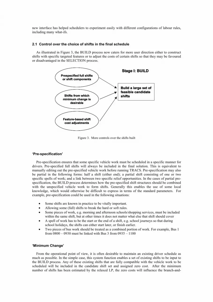
As illustrated in Figure 3, the BUILD process now caters for more user direction either to construct shifts with specific targeted features or to adjust the costs of certain shifts so that they may be favoured or disadvantaged in the SELECTION process.

Stage I: BUILD


Prespecified full shifts or shift components

Shifts from which minimum change is

desirable

Feature-based shift cost adjustments

Stage I: BUILD


Stage I: BUILD






desirable


desirable



Figure 3. More controls over the shifts built

‘Pre-specification’

Pre-specification ensures that some specific vehicle work must be scheduled in a specific manner for drivers. Pre-specified full shifts will always be included in the final solution. This is equivalent to manually editing out the pre-specified vehicle work before running TRACS. Pre-specification may also be partial in the following forms: half a shift (either end); a partial shift consisting of one or two specific spells of work; and a link between two specific relief opportunities. In the cases of partial pre-specification, the BUILD process determines how the pre-specified shift structures should be combined with the unspecified vehicle work to form shifts. Generally this enables the use of some local knowledge, which would otherwise be difficult to express in terms of the standard parameters. For example, pre-specification could be used in the following situations:

• Some shifts are known in practice to be vitally important. • Allowing some (full) shifts to break the hard or soft rules. • Some pieces of work, e.g. morning and afternoon schools/shopping services, must be included

within the same shift, but at other times it does not matter what else that shift should cover • A spell of work has to be the start or the end of a shift, e.g. school journeys so that during

school holidays, the shifts can either start later, or finish earlier. • Two pieces of bus work should be treated as a combined portion of work. For example, Bus 1

from 0800 – 0930 must be linked with Bus 3 from 0935 – 1100

‘Minimum Change’

From the operational point of view, it is often desirable to maintain an existing driver schedule as much as possible. In the simple case, this system function enables a set of existing shifts to be input to the BUILD process. Any of these existing shifts that are fully compatible with the vehicle work to be scheduled will be included in the candidate shift set and assigned zero cost. After the minimum number of shifts has been estimated by the relaxed LP, the zero costs will influence the branch-and-

bound process to select as many of these existing shifts as possible. In the case that only part of an existing shift is compatible with the new vehicle work, it would be difficult to determine how near a new shift resembles the existing shift and therefore achieving ‘minimum change’ in that context is complex requiring further research. Nevertheless, the ‘pre-specification’ system function discussed above could be used to ensure that desirable partial structures of the existing shifts could be preserved.

‘Penalties’ - Feature-based shift cost adjustments

Every candidate shift has an associated cost, normally reflecting the wage cost, which is to be minimised for the whole schedule at the SELECTION stage. The unit of shift cost is a minute in TRACS. The ‘Penalties’ system function allows the user to adjust the shift costs by putting weights on specific features in the shifts. An increased cost usually has the effect of discouraging the shift, and hence its undesirable features, from being selected for the solution schedule. We found from experience with many real life data sets that using penalties of between 100 to 200 minutes seemed to be most effective.

One example of a feature that may be deemed unfavourable is when a shift contains continuous driving exceeding a certain threshold. Another example is a shift with a tight mealbreak or when the mealbreak starts or ends at a time zone unpopular to the drivers. The undesirable features are not violating hard constraints, therefore despite the high costs the penalised shifts might still be selected if they fit well with other shifts to form a good schedule. However, the higher the penalties, the more distortion to the true shift cost and this may result in a more expensive solution than if penalties were not used. Even if there is no real cause for penalising any particular features, from our experience, the use of penalties can encourage the ILP to find a good solution more quickly than would otherwise be possible. This may be because more variability is introduced to the costs and this helps the branch-and-bound process to find a good solution. As a general guideline, shifts with two or more breaks should be slightly penalised because they are usually less desirable from the operational point of view.

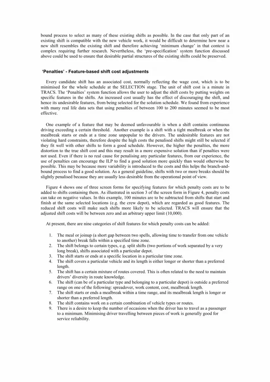
Figure 4 shows one of three screen forms for specifying features for which penalty costs are to be

added to shifts containing them. As illustrated in section 3 of the screen form in Figure 4, penalty costs can take on negative values. In this example, 100 minutes are to be subtracted from shifts that start and finish at the same selected locations (e.g. the crew depot), which are regarded as good features. The reduced shift costs will make such shifts more likely to be selected. TRACS will ensure that the adjusted shift costs will be between zero and an arbitrary upper limit (10,000).

At present, there are nine categories of shift features for which penalty costs can be added:

1. The meal or joinup (a short gap between two spells, allowing time to transfer from one vehicle

to another) break falls within a specified time zone. 2. The shift belongs to certain types, e.g. split shifts (two portions of work separated by a very

long break), shifts associated with a particular depot. 3. The shift starts or ends at a specific location in a particular time zone. 4. The shift covers a particular vehicle and its length is either longer or shorter than a preferred

length. 5. The shift has a certain mixture of routes covered. This is often related to the need to maintain

drivers’ diversity in route knowledge. 6. The shift (can be of a particular type and belonging to a particular depot) is outside a preferred

range on one of the following: spreadover, work content, cost, mealbreak length. 7. The shift starts or ends a mealbreak within a time range, and its mealbreak length is longer or

shorter than a preferred length. 8. The shift contains work on a certain combination of vehicle types or routes. 9. There is a desire to keep the number of occasions when the driver has to travel as a passenger

to a minimum. Minimising driver travelling between pieces of work is generally good for service reliability.

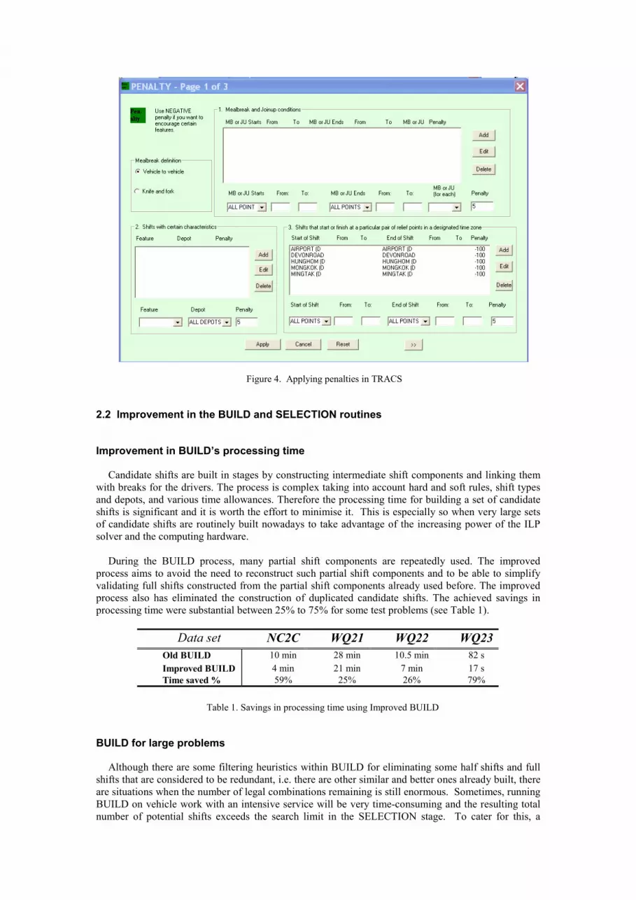
Figure 4. Applying penalties in TRACS

2.2 Improvement in the BUILD and SELECTION routines

Improvement in BUILD’s processing time

Candidate shifts are built in stages by constructing intermediate shift components and linking them with breaks for the drivers. The process is complex taking into account hard and soft rules, shift types and depots, and various time allowances. Therefore the processing time for building a set of candidate shifts is significant and it is worth the effort to minimise it. This is especially so when very large sets of candidate shifts are routinely built nowadays to take advantage of the increasing power of the ILP solver and the computing hardware.

During the BUILD process, many partial shift components are repeatedly used. The improved

process aims to avoid the need to reconstruct such partial shift components and to be able to simplify validating full shifts constructed from the partial shift components already used before. The improved process also has eliminated the construction of duplicated candidate shifts. The achieved savings in processing time were substantial between 25% to 75% for some test problems (see Table 1).

Data set NC2C WQ21 WQ22 WQ23

Old BUILD 10 min 28 min 10.5 min 82 s Improved BUILD 4 min 21 min 7 min 17 s Time saved % 59% 25% 26% 79%

Table 1. Savings in processing time using Improved BUILD

BUILD for large problems

Although there are some filtering heuristics within BUILD for eliminating some half shifts and full shifts that are considered to be redundant, i.e. there are other similar and better ones already built, there are situations when the number of legal combinations remaining is still enormous. Sometimes, running BUILD on vehicle work with an intensive service will be very time-consuming and the resulting total number of potential shifts exceeds the search limit in the SELECTION stage. To cater for this, a

‘restrained’ BUILD system function has been designed to limit the number of possible combinations. It restricts the formation of half shifts and full shifts by some adaptive heuristics which are dependent on the number of candidate spells formed. Besides the number of potential shifts formed being greatly reduced, the processing time is also much reduced.

For example, in one test using ‘restrained’ BUILD on a Pentium IV 2.56 GHz machine, it created

2042 spells, 13076 half shifts and 166459 full shifts in 479 seconds. Using the standard BUILD it created 2042 spells, 90985 half shifts and then exhausted the computer memory after running for more than 20 hours and formed over 3 million candidate shifts. ‘Restrained’ BUILD could be tried if the standard BUILD run is likely to produce millions of shifts. Since it does not consider all possible shift combinations as comprehensively as the standard BUILD, for ordinary problem instances the standard BUILD should be used. ‘Restrained’ BUILD can also be used in conjunction with the ‘Clone and Reduce’ strategy, which is described in section 3, for solving large and complex problems.

Variable allowances

Certain allowances between relief points are allowed to vary by the time of day. Schedulers will be able to use more realistic allowances according to the time of day and traffic conditions. Allowances that can be variable are sign on, sign off, mealbreak length, travel allowances and allowances before and after mealbreak. Schedulers can use these allowances to build in robustness within the schedule. For example, the user can specify minimum mealbreak lengths at some relief points for only certain periods of the day, e.g. minimum 40 minutes is required for a mealbreak except between 07:30 and 10:00 when 55 minutes is the minimum.

SELECTION stage

As noted earlier we use a generate and select approach in which the optimisation kernel, discussed in

detail in [11] is domain independent. An advantage of this approach is that adaptation of the system to new domains is delegated to the BUILD phase and that only generic changes need be made to the more complex optimisation kernel. Our experience with the variety of labour practices and operating conditions confirms our belief in this approach. Nevertheless, encounters of large and complex scheduling problems have motivated some enhancements to the solution algorithm.

The relaxed LP solver uses a SPRINT-like approach [21] in which only a subset of the generated

shifts is retained at any stage. An initial subset is gradually expanded until the solution cannot be improved further, at which point the linear programme is terminated and the branch-and-bound phase is entered. To make the algorithm more efficient for problems of different sizes and complexity, adaptive rules have been developed to set the size of the initial subset and the sizes of the incremental expansions.

We also have developed more advanced branching strategies in the branch-and-bound phase. In

particular some of the new search strategies are designed for finding better solutions to multi-depot problems and problems with complex side constraints. The more complex problems have also led to a richer set of constraints which limits the composition of the final schedule in terms of shift type, home depot etc. Additional objective functions, e.g., minimising total spreadover, have also been introduced. Whilst there are many algorithmic options in the kernel which can be user-controlled, we recognised that most of our users are unsophisticated and would treat the selection components of the system as a black box. Based on extensive experimentation we have incorporated effective default strategies, which can be overridden by the advanced users.

Improved in Robustness

In the past, the default setting for the ILP is to impose a side constraint, TOTAL <= N where N is the target total number of shifts which is estimated from the relaxed LP solution. During the branch-and-bound process, there may be occasions when no integer solution could be found after searching a large number of nodes. This situation often happens when the problem instance has more than three

crew depots which is typical in train operation. This may indicate that no integer solution exists with N shifts for the set of potential shifts input. It is probable that some integer solutions do exist, but their objective values are outside the search region defined internally by the ILP process, and the total number of shifts may have to be higher than N.

TRACS now checks the number of depots in the problem instance. If there are more than three

depots, a side constraint TOTAL >= N is imposed instead. There is a tolerance T which controls how close the search is allowed to approach the optimal cost, OC, obtained in the relaxed LP solution. If an integer solution has been found and the cost of which is within the range between OC and OC/T, the branch-and-bound process will terminate. In the past, T is usually set very near to 1 (0.999999) so that the quality of the solution is always very good, often at the expense of processing time. T is now lowered to 0.999 so that a reasonable solution could be found quickly. Once a solution (M shifts) has been found, the ILP then looks for solutions with fewer shifts than M, rather than looking for cheaper solutions with M shifts. This strategy now ensures the ILP process will find an answer quickly for multi-depot problems. This is especially useful for a first TRACS attempt on a new problem because schedulers may want to check the labour agreement or allowance settings rather than to aim for a final solution. Schedulers can further improve the solution by imposing side constraints on total costs.

To identify critical pieces of work

If the relaxed LP solution is very near to an integer, say, 80.1 shifts, although the integer solution would need at least 81 shifts, it may be worthwhile to find out which pieces of work might be causing the extra shift. If the user then imposes a constraint TOTAL <= 80, the ILP process will indicate which piece or pieces of work would be left uncovered. Schedulers can have the discretion of re-arranging or absorbing in some way the critical pieces of work to save a shift in subsequent runs.

Complex side constraints

Schedulers can have a variety of constraints on the type of shift, which can be specific to particular depots. A recent feature available to schedulers is to minimise total spreadover instead of minimising cost. Also, schedulers can choose to minimise either total spreadover with a target total on cost or vice versa.

Final schedule stage

There is a general preference for bus companies to have shifts signing on and signing off in the same order. It is also considered to be beneficial to have as many shifts similar in length or work content in the schedule. These features are difficult to control by using penalties which only apply to the characteristics of individual shifts. These criteria are difficult to formulate in the ILP process but are often crucial for the schedulers in devising acceptable rotas. Having obtained a schedule from the SELECTION phase, it is possible that it could be improved by using heuristic techniques to swap portions of work around between shifts in the final schedule. The objective of the heuristic is to produce new legal shifts if doing so would reduce the cost, or shift lengths. The swap will also take place even if there is no improvement in either cost or shift lengths if the resulting new shift lengths are more even compared with those before the swapping. One of the results of this is the aligning of shift signing on and off times. For a system which minimises shift costs and where shifts do not have paid meal breaks, there is usually no difference in total cost if a pair of shifts sign off in the wrong order. A change which would make a pair of shifts more similar in spreadover would be considered beneficial provided there is no increase to the total cost of the schedule.

3. Tackling large/complex problems

TRACS can generally produce good results for the majority of operators. With the increase in

computer power, TRACS can now handle problems much larger than before. For example, it has been successful in solving a bus problem with around 1500 work piece constraints with over one million

candidate shifts constructed. However, there are operators which have even larger and more complex scheduling problems, with many relief opportunities. These could easily exceed the limits of TRACS if it is used in the conventionally way. Some companies have a vast network covering both rural and urban services. These companies may have complex scheduling rules with different vehicle types and multiple labour agreements operating within the same bus network. The labour agreements can be very flexible or very restrictive with specific requirements for different groups of staff.

In the following, three scenarios are discussed, for which strategies have been devised for using

TRACS to deal with large and/or complex problems.

Large problems

This often involves operating a very intensive service on a relatively large network in an urban environment. Typically the problem instance has a very large number, e.g. over 2000, of relief opportunities, causing BUILD to create an enormous number of potential shifts. However, such large problems may not be complex in terms of the labour agreements, which are usually well-defined, and may have less than three crew depots.

Tackling this type of problem, a ‘Clone and Reduce’ strategy, illustrated in Figure 5, which

progressively improves the solutions has been devised. The idea of the strategy is to get a schedule as quickly as possible regardless of quality and improve upon it. This also has the advantage that schedulers can quickly check the first driver schedule to see if the parameters have been set correctly.

Initial Run‘Restrained’ BUILD, e.g. use tight parameters and limited search depths; and SELECTION

Problem cloned

Reduce: Suppress ROsnot used in the solution

Re-instatesome ROs,relax some parameters, etc. andRun again

Initial Run‘Restrained’ BUILD, e.g. use tight parameters and limited search depths; and SELECTION

Problem cloned

Reduce: Suppress ROsnot used in the solution

Re-instatesome ROs,relax some parameters, etc. andRun again

Figure 5. The ‘Clone and Reduce’ strategy

The schedule obtained in each iteration would be no worse, and often better, than the last schedule. Also, it is possible to include some de-selected relief opportunities during subsequent iterations. For example, relief opportunities after lunch and before the start of the afternoon peak, or after the morning peak, or around midday can be added progressively so as to allow work pieces to be broken up into reasonable lengths and this would therefore allow better shifts to be formed. There is an option for the system to reinstate some more relief opportunities automatically in a random manner. The time taken in each step of the above strategy is very quick since it only works on a cut-down version of the original problem instance at each iteration. Each step may only take a few minutes to complete.

Table 2 shows the results of a ‘Clone and Reduce’ experiment on a test problem instance. It shows

the improvement to the solutions in each iteration. The whole process took no more than an hour on a Pentium IV 2.56 GHz Pc. This problem is from a bus company operating in a major city and has 2700:36 vehicle hours and there are 2339 relief opportunities. This problem has only one crew depot. The labour agreement rules are well-defined. In order to create the required type of shifts, rules defining the legality of shifts were set at a level which generated several millions of potential shifts. The resulting total exceeded that allowed by the SELECTION stage. Using this strategy a reduction of 28 shifts for an increase in cost of only 45:56 hours was achieved.

In a real life problem which is very similar to the above test problem instance, the company’s

original schedule has 308 shifts, 2707:30 cost and 8:47 average cost, 10:14 average spreadover (shift length) of which 136 shifts are three-part shifts. After performing around 20 iterations, the scheduler obtained a schedule with 306 shifts, 2704:30 cost, 8:51 average cost and 10:24 average spreadover and 131 three-part shifts. He then used the ‘Penalties’ feature to penalise any three-part shifts and obtained a schedule with 306 shifts, 2706:10 cost, 8:51 average cost, 10:23 average spreadover but only 102

three-part shifts. From the operational point of view, three-part shifts are less attractive compared with two-part shifts because three-part shifts have one more break and therefore have higher risks of being delayed.

Reducing / Re-instating ROs

No. of relief opportunities

No. of shifts

Cost (hh:mm)

Starting solution 2339 335 2805:05 + 279 mins overcover*

1. Reducing+Reinstating 1206 309 2852:38 2. Reducing+Reinstating 1128 309 2847:23 3. Reducing+Reinstating 1142 308 2856:19 4. Reducing+Reinstating 1219 307 2859:08 5. Reducing+Reinstating 1316 307 2857:05 6. Reducing+Reinstating 1180 307 2854.02 7. Reducing+Reinstating 1140 307 2851:01

*Overcover occurs when two drivers are assigned to the same bus work

Table 2. Results of ‘Clone and Reduce’ experiments with selective reinstatement of some relief opportunities

The above bus company has been experimenting with this strategy on their large problems and they

are now satisfied that this method gets them a better answer more quickly than before. Before ‘Clone and Reduce’ was available, the schedulers would have to de-select many the relief opportunities manually, which could be very tedious and not yield good results. This strategy has now been used to produce effective results on many real life problems.

Complex problems with many different features

The second situation arises when a mixture of urban and sub-urban/rural services is operated. There are many different crew depots scattered around a large network requiring extensive use of passenger travelling for drivers. The vehicle work may not be very intensive, but there are often several relief opportunities each hour in many of the blocks of vehicle work. This type of problem may be complicated by the lack of well-defined scheduling conditions. Usually, the contractual rules and soft rules can be complex in terms of definition and implementation. In order to reflect the current labour agreement rules accurately, it is necessary to run BUILD several times using different sets of labour agreement and the appropriate vehicle and route knowledge. This complicates the running of the ‘Clone and Reduce’ strategy.

In some situations, the problem can be divided into several sub-problems, most of which are

interlinked. These relate to the grouping of services to form rotas of drivers for specific work. This can either be for operational reasons (special type of service) or legal reasons (E.U. driver hours regulations on longer services). There is mixing between the groups to achieve overall schedule efficiency, but minimising such mixing is desirable. The way in which work can be mixed is complex and it is difficult to get the right balance. This is further complicated by multi-depot constraints. Passenger travel is also used as some routes do not pass any driver depot. A typical problem consists of between 700 and 1000 relief opportunities. The number of crew depots for this type of problem is usually more than three. In the past, it was sometimes difficult for the ILP to arrive at an integer solution within reasonable time. Recent advancement in the ILP kernel has improved the situation.

Difficulties arise in modelling the existing situation due to the complex interworking and the need to

work with tightly defined parameters. When using the ‘Clone and Reduce’ strategy it is important that the starting solution be as realistic as possible in areas of route group interworking, otherwise the wrong relief opportunities will be retained and any solutions based on them will not be workable.

Large and complex problems

This is by far the most difficult type of problem, which is a combination of the above two categories.

A typical problem instance is an undertaking with intensive urban operation and extensive rural interworking. For example, a major bus company operates in a region crossing county boundaries. Drivers from four different crew depots work around a city and drivers from the several outstations will also do portions of city driving work as part of their shifts to maximise efficiency. To simplify the problem instance, work exclusive to these outstations is not included in the scheduling exercise. One of the crew depots is in the city centre but all buses are garaged at the other three locations (known as ‘outside depots’) which are outside the city. There is a mixture of work and shift types within the problem, but all crew reliefs take place within the city centre and drivers are required to sign on and sign off at the same crew base. This requires drivers from the outside depots to travel as passengers from their crew base to city centre or vice versa. The problem instance can be roughly divided into three sub-problems relating to the type of service: ‘Park and Ride’, ‘Country’ and ‘City’. The ‘Park and Ride’ involves very intensive service with relief opportunities averaging every ten minutes. Both the ‘Park and Ride’ and ‘Country’ service are compiled with as few shifts as possible whilst taking in ‘City’ bus work as efficiently as possible.

There are two types of shifts, namely, 5-day-week (5D) shifts and 4-day-week (4D) shifts. 5D shifts

are shorter than 4D shifts and usually have only one mealbreak. 5D shifts have a maximum length of 8:40 and 4D shifts can be up to 13 hours long although 12:45 is the preferred maximum length. 4D shifts must have at least two mealbreaks and usually have three mealbreaks. The minimum lengths of these mealbreaks are not uniform. All shifts are paid on their entire length, i.e. from sign on to sign off. Continuous work on a bus should not exceed 4:08 excluding starting and finishing allowances. This does not apply to Country services where the bus is away from depot for a longer period and can have a maximum spell of 4:40.

Scheduling requirements are complex. For the city centre crew depot, 4D type shifts are not

allowed. But work for this depot can be on all the above three types of service. Apart from the city centre depot drivers, only two out of the three outside depot drivers can work on the Park and Ride service and these must be of 4D type. Similarly, apart from the city centre depot drivers, only one outside depot can work on the Country service and these must also be of 4D type. We have to model the restrictions of shift type for each depot by using dummy depots. These dummy depots are duplicated depots but with different restrictions. Hence the total number of notional depots in the whole problem is seven.

In this instance, there are 1584 relief opportunities forming 1452 work piece constraints. The shift

length can be up to 13 hours and the maximum continuous driving is just over 4 hours. This requires a number of shifts with more than three spells of work on different buses. This, plus the size of the problem gives rise to well over several million potential shifts in the BUILD stage and the SELECTION process was unable to yield a feasible solution. A ‘Divide and Conquer’ strategy combined with ‘Clone and Reduce’ are used to solve the whole problem. All the processing was run on a 2.53 GHz Pentium IV PC. The manual schedule was compiled by an experience scheduler with local knowledge. Before the advancements in TRACS were introduced, we could not solve this problem satisfactorily to produce quality schedules in reasonable time compared with the experienced scheduler.

Divide and Conquer Strategy

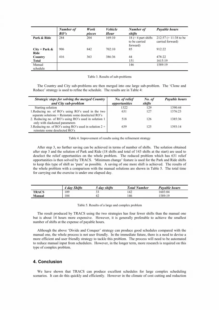
This strategy involves first sub-dividing the three services into three sub-problems and solving them as standalone problems. Local knowledge of the problem is important in dividing the problem into sub-problems. For Park and Ride service, there is a need to keep the shifts as ‘pure’ Park and Ride as possible whilst at the same time drawing in city bus work to achieve efficient schedules. Hence, after solving the Park and Ride sub-problem, a small amount of bus work is cascaded onto the City service sub-problem. The results of solving the three sub-problems are shown in Table 3:

Number of RO’s

Work pieces

Vehicle Hour

Number of shifts

Payable hours

Park & Ride 284 204 169:10 18 (+ 4 part shifts to be carried forward)

212:57 (+ 11:38 to be carried forward)

City + Park & Ride

906 842 702:10 85 912:22

Country 416 363 386:36 44 478:22 Total 151 1615:19 Manual schedule

146 1589:19

Table 3. Results of sub-problems

The Country and City sub-problems are then merged into one large sub-problem. The ‘Clone and

Reduce’ strategy is used to refine the schedule. The results are in Table 4:

Strategic steps for solving the merged Country and City sub-problem

No. of relief opportunities

No. of shifts

Payable hours

Starting solution 1322 129 1390:44 1.Reducing no. of RO’s using RO’s used in the two

separate solutions + Reinstate some deselected RO’s 631 127 1376:23

2. Reducing no. of RO’s using RO’s used in solution 1 only with slackened parameters

518 126 1385:36

3.Reducing no. of RO’s using RO’s used in solution 2 + reinstate some deselected RO’s

639 125 1393:14

Table 4. Improvement of results using the refinement strategy

After step 3, no further saving can be achieved in terms of number of shifts. The solution obtained

after step 3 and the solution of Park and Ride (18 shifts and total of 143 shifts at the start) are used to deselect the relief opportunities on the whole problem. The reduced problem which has 631 relief opportunities is then solved by TRACS. ‘Minimum change’ feature is used for the Park and Ride shifts to keep this type of shift as ‘pure’ as possible. A saving of one more shift is achieved. The results of the whole problem with a comparison with the manual solutions are shown in Table 5. The total time for carrying out the exercise is under one elapsed day. 4 day Shifts 5 day shifts Total Number Payable hours TRACS 109 33 142 1603:04 Manual 104 42 146 1589:19

Table 5. Results of a large and complex problem The result produced by TRACS using the two strategies has four fewer shifts than the manual one

but is about 14 hours more expensive. However, it is generally preferable to achieve the smallest number of shifts at the expense of payable hours.

Although the above ‘Divide and Conquer’ strategy can produce good schedules compared with the

manual one, the whole process is not user friendly. In the immediate future, there is a need to devise a more efficient and user friendly strategy to tackle this problem. The process will need to be automated to reduce manual input from schedulers. However, in the longer term, more research is required on this type of complex problem.

4. Conclusion

We have shown that TRACS can produce excellent schedules for large complex scheduling scenarios. It can do this quickly and efficiently. However in the climate of cost cutting and reduction

of manpower, schedulers will be continually devising more schemes to produce cheaper but acceptable schedules.

Large and complex problems have always been challenging for the set covering model. We have

discussed three situations which had previously been difficult for TRACS to solve. Recent advancement in TRACS enables us to solve these types of problem satisfactorily. We expect to improve further its capability so that it will be easier for schedulers to use.

The use of these strategies by schedulers will no doubt increase our knowledge and experience in

dealing with these types of problem, their feedback will be invaluable in developing further refinements.

The TRACS system provides financial benefits for public transport companies in that it can produce

quality schedules quickly and save drivers’ wages. For a large bus group, a 1% swing in cost may involve several million pounds. The system has been flexible enough to cope with most scheduling conditions. In many cases, the system can produce driver schedules in a very short time and the schedulers can easily produce solutions close to the day of operation, efficiently accommodating late schedule changes. Management can also use the system to investigate strategic decisions for evaluating the costs of proposed rule changes.

Acknowledgements

We are grateful to Michael Meilton who managed the scheduling project in First and gave us invaluable guidance, support and friendship throughout the rollout program. We would like to thank many colleagues within the bus and rail industries for their help and advice. We are grateful to the UK Engineering and Physical Sciences Research Council for their support under grants GR/M23205, K79024 and K07256.

References

[1] Meilton, M. (2001) Selecting and implementing a computer aided scheduling system for a large bus company. In S Voss and JR Daduna (Eds.), Computer-Aided Scheduling of Public Transport, Springer-Verlag, Berlin, 203-214.

[2] Preprints of the International Workshop on Automated Techniques for Scheduling of Vehicle Operators for

Urban Public Transportation Services, Chicago, 1975. [3] A. Wren (ed.), Computer Scheduling of Public Transport, Proceedings of the Second International Workshop

on Computer-Aided Scheduling of Public Transport (North-Holland, 1981). [4] J.-M. Rousseau (ed.) Computer Scheduling of Public Transport 2, Proceedings of the Third International

Workshop on Computer-Aided Scheduling of Public Transport (North-Holland, 1985). [5] J. R. Daduna and A. Wren (eds.), Computer-Aided Transit Scheduling, Proceedings of the Fourth

International Workshop on Computer-Aided Scheduling of Public Transport (Springer-Verlag, 1988). [6] M. Desrochers and J.-M. Rousseau (eds.), Computer-Aided Transit Scheduling, Proceedings of the Fifth

International Workshop on Computer-Aided Scheduling of Public Transport (Springer-Verlag, 1992). [7] J. R. Daduna, I. Branco and J. Paixáo (eds.), Computer-Aided Transit Scheduling, Proceedings of the Sixth

International Workshop on Computer-Aided Scheduling of Public Transport (Springer-Verlag, 1995). [8] N. H. M. Wilson (ed.), Computer-Aided Transit Scheduling, Proceedings of the Seventh International

Workshop on Computer-Aided Scheduling of Public Transport (Springer-Verlag, 1999). [9] S. Voss, J. R. Daduna (ed.), Computer-Aided Transit Scheduling, Proceedings of the Seventh International

Workshop on Computer-Aided Scheduling of Public Transport (Springer-Verlag, 2001).

[10] Smith, B.M. and Wren, A. A bus crew scheduling system using a set covering formulation. In:

Transportation Research, vol.22A, pp. 97-108 [11] S. Fores, L. Proll and A. Wren, TRACS : a hybrid IP/heuristic driver scheduling system for public

transport. Journal of the Operational Research Society, 53:1093-1100, 2002. [12] Kwan, Raymond S K; Kwan, Ann S K; Wren, Anthony. Evolutionary driver scheduling with relief chains.

Evolutionary Computation, vol. 9, pp. 445-460. 2001. [13] Li, Jingpeng; Kwan, Raymond S K. A fuzzy genetic algorithm for driver scheduling. European Journal of

Operational Research, vol. 147, pp. 334-344. 2003. [14] Shen, Yindong; Kwan, Raymond S K. Tabu search for driver scheduling in: Voß, S & Daduna J R (editors)

Computer-Aided Scheduling of Public Transport, pp. 121-135 Springer-Verlag. 2001. [15] Kwan, A S K, Kwan, R S K, Parker, M E, Wren, A. Producing train driver schedules under differing

operating strategies in: In: Wilson NHM. (Ed.) Computer-Aided Transit Scheduling, Springer Verlag, pp. 129-154 1999.

[16] Kwan, A S K, Kwan, R S K, Parker, M E, Wren, A. (1996) Producing train driver shifts by computer in:

Allan, J, Brebbia, C A, Hill, R J, Sciutto, G & Sone, S (editors) Computers in Railways V, vol. 1: Railway Systems and Management, pp. 421-435 Computational Mechanics Publications.

[17] Kwan, A S K; Kwan, R S K; Parker, M E; Wren, A. (2000) Proving the versatility of Automatic Driver

Scheduling on Difficult Train and Bus Problems, Presented at CASPT 2000, Berlin June 2000. [18] Fores S, Proll L and Wren A. (1999) An Improved ILP System for Driver Scheduling. In: Wilson NHM.

(Ed.) Computer-Aided Transit Scheduling, Springer Verlag, pp.43-62. [19] Fores S, Proll L and Wren A. (2001) Experiences with a Flexible Driver Scheduler. In: Voβ S and Daduna JR

(Eds.) Computer-Aided Scheduling of Public Transport, Springer-Verlag, 137-152. [20] Wren, Anthony; Fores, Sarah; Kwan, Ann; Kwan, Raymond; Parker, Margaret; Proll, Les (2003) A flexible

system for scheduling drivers, Journal of Scheduling, vol. 6, pp.437-455 [21] R.E. Bixby, J. W. Gregory, I. L. Lustig, R. J. Marsten and D. F. Shanno, Very large scale linear programming:

a case study in combining interior point and simplex methods, Operations Research 40, 885-897 (1992)

recent advances in tracs

Documents