1

Real-Time Estimation of Arterial Travel Time under Congested Conditions Henry X. Liu* Department of Civil Engineering 500 Pillsbury Drive S.E. Minneapolis, MN 55455 Phone: (612) 625-6347 Fax: (612) 625-7750 E-mail: henryliu@umn.edu (*Corresponding Author) Wenteng Ma Department of Civil Engineering 500 Pillsbury Drive S.E. Minneapolis, MN 55455 Phone: (612) 625-0249 Fax: (612) 625-7750 E-mail: maxxx130@umn.edu Xinkai Wu Department of Civil Engineering 500 Pillsbury Drive S.E. Minneapolis, MN 55455 Phone: (612) 625-0249 Fax: (612) 625-7750 E-mail: wuxxx273@umn.edu Heng Hu Department of Civil Engineering 500 Pillsbury Drive S.E. Minneapolis, MN 55455 Phone: (612) 625-0249 Fax: (612) 625-7750 E-mail: huxxx186@umn.edu To Appear in Transportmetrica

November 2009

2

Abstract: It is well-known that accurate estimation of arterial travel time on signalized arterials is not an easy task because of the periodic disruption on traffic flow by signal lights. It becomes even more difficult when the signal links are congested with long queues because under such situations the queue length cannot be estimated using the traditional cumulative input-output curves. In this paper, we extend the virtual probe model previously proposed by the authors to estimate arterial travel time with congested links. Specifically, we introduce a new queue length estimation method that can handle long queues. The queue length defined in this paper includes both the standing queue, i.e. the motionless stacked vehicles behind the stop line, and the moving queue, i.e. those vehicles joining the discharging traffic after the last vehicle in the standing queue starts to move. The moving queue concept is important for the virtual probe method because moving queue also influences the maneuver behavior of a virtual probe. We show that, using the “event” data (including both time-stamped signal phase changes and vehicle-detector actuations) collected from traffic signal systems, time-dependent queue length (including both standing queue and moving queue) can be derived by examining the changes in advance detector’s occupancy profile within a cycle. The effectiveness of the improved virtual probe model for estimating arterial travel time under congested conditions is demonstrated through a field study at an 11-intersection corridor along France Avenue in Minneapolis, Minnesota.

Keywords: Travel Time Estimation, Traffic Signal, Virtual Probe, Queue Length Estimation, High-resolution event-based data.

3

1. Introduction

Travel time is an important measure for the evaluation of transportation network performance and also one of the most understood measures for road users that can help them make informed travel decisions. However, it is well-known that accurate estimation of arterial travel time on signalized arterials is not an easy task because of the periodic disruption on traffic flow by signal lights. It becomes even more difficult when the signal links are congested with long queues. So far to the best of our knowledge, no reliable method is readily available to estimate real-time arterial travel times under congested conditions. Although a number of regression (Turner et al., 1996; Frechette & Khan, 1998; Zhang, 1999) and heuristic methods (Takaba et al., 1991; Cheu et al., 2001) were proposed, these studies are mainly targeted to provide offline steady state assessment using low-resolution (5-minute or longer) traffic volume and signal timing data.

Recently, Liu and Ma (2009) developed a virtual probe model to estimate real-time arterial travel time by tracing an imaginary vehicle from origin to destination. At each time step, the maneuver decision (acceleration, deceleration or no-speed-change) of the virtual probe is determined by its own state and its surrounding traffic conditions. Surrounding traffic states include the status of the queue ahead of the virtual probe and the signal status. The proposed model is data-intensive, which utilizes both vehicle-actuation and signal phase change data from existing traffic signal systems. The availability of time-stamped signal status and vehicle-detector actuation data essentially allows us to reconstruct the history of traffic signal events along the arterial street; therefore, we can trace an imaginary vehicle (a virtual probe) to estimate arterial travel time.

Although the virtual probe model offers a feasible approach for real-time arterial travel time estimation, it requires a known time-dependent queue length profile for each intersection along the arterial. It is self-evident that the accuracy of travel time estimation will be dependent on how well we can estimate the queue length. Accurate queue length information becomes particularly important for travel time estimation under congested conditions.

The traditional queue length estimation method, i.e. the input-output method has an inherent drawback. It cannot handle congested situations with long queues (long queue is defined here as that the queue length is longer than distance from intersection stop-bar to advance detector), unless a link entrance detector is available, which is usually not the case. Liu et al. (2009) addressed the long queue estimation problem by examining the queue discharge process and the intersection shockwave characteristics. Since the queue estimation method described in Liu et al. (2009) does not depend on the measurement of traffic arrival volume to the intersection, it can estimate the queue length that is much longer than the distance from intersection stop-bar to the advance

4

detector. We should note that the focus of Liu et al. (2009) is to estimate the length of the standing queue, i.e. the motionless stacked vehicles behind the stop line.

In order to estimate arterial travel time while signal links are congested with long queues, in this paper, we extend the algorithm discussed in Liu and Ma (2009) by incorporating an easily implementable queue estimation module into the virtual probe method. The proposed queue estimation module is particularly suitable for the virtual probe approach because we introduce a new definition of queue, which includes both the standing queue and the moving queue. Here the moving queue is referred to those vehicles joining the discharging traffic after the last vehicle in the standing queue starts to move, and it can be represented as “dummy vehicles” added to the rear of the standing queue. The moving queue concept is important for the virtual probe method because the moving queue also influences the maneuver behavior of the virtual probe. The virtual probe may start to decelerate earlier because of the moving queue. This is more realistic because, in reality, those vehicles decelerate behind the standing queue will also impact the speed of a following vehicle. It turns out, the estimation of the queue length that includes both standing queue and moving queue, is much simpler than the shockwave method proposed in Liu et al. (2009). Comparing with the method proposed in Liu et al (2009), this method is easier to implement and more suitable to the virtual probe method for the estimation of arterial travel time with long queues. In addition, the queue length estimation method in this paper is more practical for urban streets with short links, where the shockwave approach may be difficult to be implemented because of the metering effects of upstream intersections.

For the sake of completeness, in what follows we first review the related research work briefly, including the data collection system, by which event-based signal data are collected and archived, and the arterial travel time estimation model, i.e. the virtual probe approach. Section 3 provides a detailed discussion on queue length estimation, including both short queue and long queue scenarios. Field implementation on a major arterial corridor in Minneapolis, MN, is described in Section 4. Finally, concluding remarks and future research directions are offered in Section 5.

2. Data Collection and Virtual Probe Method

In this section, we briefly review our data collection system and the virtual probe based travel time estimation method. Interested readers should refer to Liu and Ma (2009) for further details.

In general, two types of raw data can be retrieved from the signal controller cabinet. One is the data from the vehicle detection unit and the other is signal status data. A detector call or a signal phase change is regarded as an “event”, which can be retrieved from the controller cabinet. At each intersection, an industrial PC with a data

5

acquisition card is installed, and event data (including both vehicle actuation events and signal phase change events) collected at each intersection are transmitted to the data server in the master controller cabinet through the existing communication line between signalized intersections. The data is then compressed at the field server and sent back to the database server at the University of Minnesota through Internet. Once the event-based data are collected and stored, performance measures can be derived by various modules and also stored in the database. Users can then access the estimated performance measures through web interfaces. This real-time arterial performance measurement system we developed is named as SMART-SIGNAL (Systematic Monitoring of Arterial Road Traffic Signals).SMART-SIGNAL has been installed on 11 intersections of France Avenue in Minneapolis, Minnesota since February 2007. France Avenue was selected for field deployment because it has a wide variety of traffic conditions and it is one of the most congested urban arterials in the Twin Cities Metropolitan Area.

To estimate real-time arterial travel time, in Liu and Ma (2009) we proposed a virtual probe approach by tracing an imaginary vehicle from origin to destination. Assume the journey of the virtual probe can be equally divided into many small time steps. At each time step, the states of the virtual probe, including its position and speed, current signal status, and queue length ahead, are examined to determine the maneuver in the next time step. One of the three maneuvers, acceleration, deceleration or no-speed-change, is selected based on the current states of the virtual probe. The position and speed of the virtual probe at the next time step can then be calculated correspondingly. The step-by-step maneuver selection continues until the virtual probe “arrives” at the destination, and the difference between the starting time and the ending time is the arterial travel time. Detailed description of the virtual probe approach is provided in Liu and Ma (2009). Since the queue length ahead of the virtual probe is crucial to the travel time estimation, in the following we will focus on the queue estimation, particularly for the congested link with long queues.

3. Queue Length Estimation

3.1 Definition of Queue

The definitions of queue need to be clarified before we discuss the queue length estimation model. According to the Highway Capacity Manual 2000, queue is defined as: “a line of vehicles, bicycles, or persons waiting to be served by the system in which the flow rate from the front of the queue determines the average speed within the queue. Slowly moving vehicles or people joining the rear of the queue are usually

6

considered part of the queue.” Such a definition indicates that a queue at an intersection contains not only stacked vehicles but also approaching vehicles that are affected. Therefore, in this paper, a queue is divided into two parts: the standing queue which is composed of motionless stacked vehicles behind the stop line, and the moving queue which is composed of moving vehicles that are impacted (i.e., forced to decelerate) by the signal or the standing queue. Since both standing queue and moving queue will affect the driving behavior of the virtual probe, both of them need to be included in queue estimation.

The concept of “moving queue” is difficult to define because queued vehicles are approaching the standing queue with various speeds. To overcome the difficulty for the estimation of moving queue, “dummy vehicles” are added to the rear of the original standing queue to represent the effect of the moving queue. As shown in Fig. 1, assuming Vehicle Q is the last queued vehicle of the moving queue, and it would stop at the location of Vehicle Q’. Therefore, Vehicle Q’ is the representative vehicle of Vehicle Q because they have the similar impact to the following vehicles in terms of maneuver decisions. In the following of this paper, the definition of the queue is the “equivalent standing queue”, which includes both standing queue and additional dummy vehicles representing moving queue. Queue length is the distance from the stop line to the rear of the “equivalent standing queue”, and queue size is the number of vehicles in the “equivalent standing queue”. We should note that the shockwave-based queue length estimation method discussed in Liu et al. (2009) is only applicable for the estimation of the standing queue length. It does not include the length of the moving queue. However, moving queue is important for the virtual probe method because those vehicles in the moving queue also affect the maneuver decision of the virtual probe. It turns out, by introducing the concept of “equivalent standing queue”, a much simpler and more practical method for queue estimation can be developed, comparing with the shockwave-based method developed in Liu et al. (2009). This method, as demonstrated in the following sections, significantly improves the accuracy of travel time estimation when traffic is congested.

StopLine

Standing Queue Moving Queue

Equivalent Standing Queue

NewArrival

Q

Q'

Fig. 1. Queue at a Signalized Intersection

7

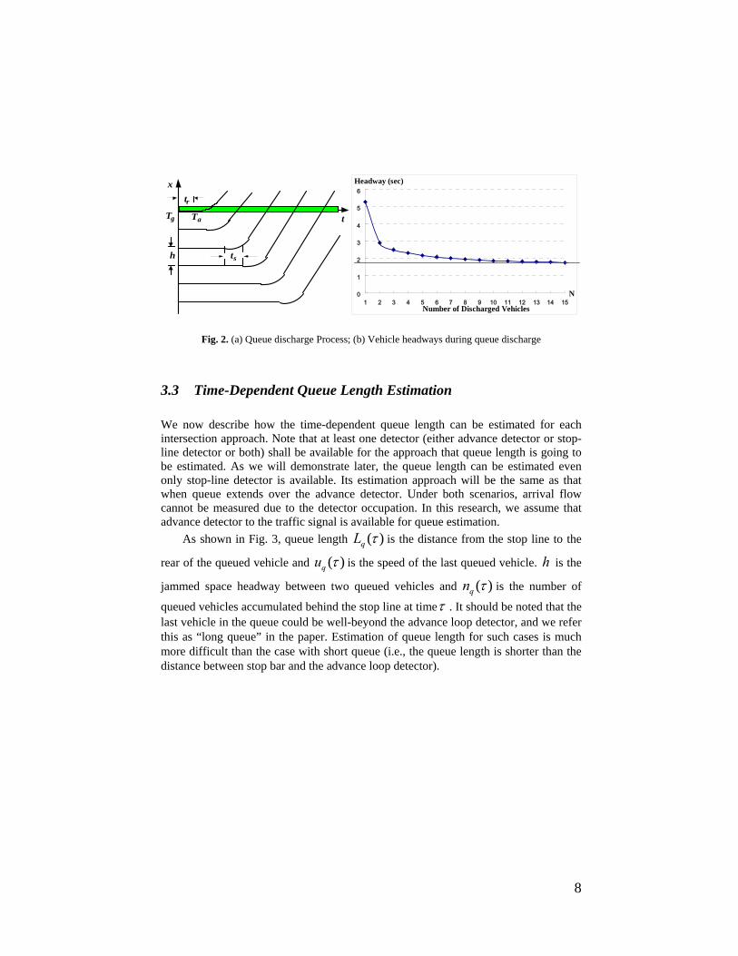
3.2 Queue Discharging Process

As we will show later, the queue estimation model proposed in this paper will mainly rely on the characteristics of queue discharging process. We first need to verify that the assumptions we made to describe the queue discharging process is reasonable.

Assuming that gT is the starting time of green, rt is the reaction time of the first

queued vehicle, and st is the uniform starting time difference between two adjacent

queued vehicles, then the queue discharge propagates from the front to the rear as

shown in Fig. 2(a): the first vehicle starts at time g rT t , the second vehicle starts at

time g r sT t t , …, and the nth vehicle in the queue starts at time ( 1)g r sT t n t .

The rationality of such queue discharging assumption can be validated by a time headway analysis at the stop line. According to the above queue discharging pattern,

the first vehicle passes the stop line at time g rT t (here we use the time when

vehicle’s front bumper passes the stop line); the second vehicle passes the stop line at

time 2 /g r s aT t t h ( h is the jammed space headway and a is the

acceleration rate); and the nth vehicle passes the stop line at time

( 1) 2 / 1ln g r s aT T t n t h n Therefore, the first measured time

headway at the stop line should be 2 /s at h ; the second measured time headway

at the stop line should be 2 / ( 2 1)s at h ; and the nth measured time headway

at the stop line is 2 / ( 1)hn s at t h n n . The time headway of the

discharging queue is then shown as Fig. 2(b). As vehicles released from the stop line,

the time headway captured at the stop line becomes stable to a constant value st . A

similar figure can be found as Figure 17.1 in the Traffic Engineering textbook (Roess, et al. 2004). Such a simple queue discharging process is also consistent with Newell’s simplified car-following theory (Newell, 2002; Ahn, et al. 2004), which states that the time-space trajectory of a vehicle discharging on a homogeneous intersection approach is essentially the same as that of its leader, except for a translation in space and time. This demonstrates that the queue discharge assumption made in this research is reasonable.

8

tr

ts

x

h

tTg Ta

0

1

2

3

4

5

6

1 2 3 4 5 6 7 8 9 10 11 12 13 14 15

Headway (sec)

Number of Discharged Vehicles

N

Fig. 2. (a) Queue discharge Process; (b) Vehicle headways during queue discharge

3.3 Time-Dependent Queue Length Estimation

We now describe how the time-dependent queue length can be estimated for each intersection approach. Note that at least one detector (either advance detector or stop-line detector or both) shall be available for the approach that queue length is going to be estimated. As we will demonstrate later, the queue length can be estimated even only stop-line detector is available. Its estimation approach will be the same as that when queue extends over the advance detector. Under both scenarios, arrival flow cannot be measured due to the detector occupation. In this research, we assume that advance detector to the traffic signal is available for queue estimation.

As shown in Fig. 3, queue length ( )qL is the distance from the stop line to the

rear of the queued vehicle and ( )qu is the speed of the last queued vehicle. h is the

jammed space headway between two queued vehicles and ( )qn is the number of

queued vehicles accumulated behind the stop line at time . It should be noted that the last vehicle in the queue could be well-beyond the advance loop detector, and we refer this as “long queue” in the paper. Estimation of queue length for such cases is much more difficult than the case with short queue (i.e., the queue length is shorter than the distance between stop bar and the advance loop detector).

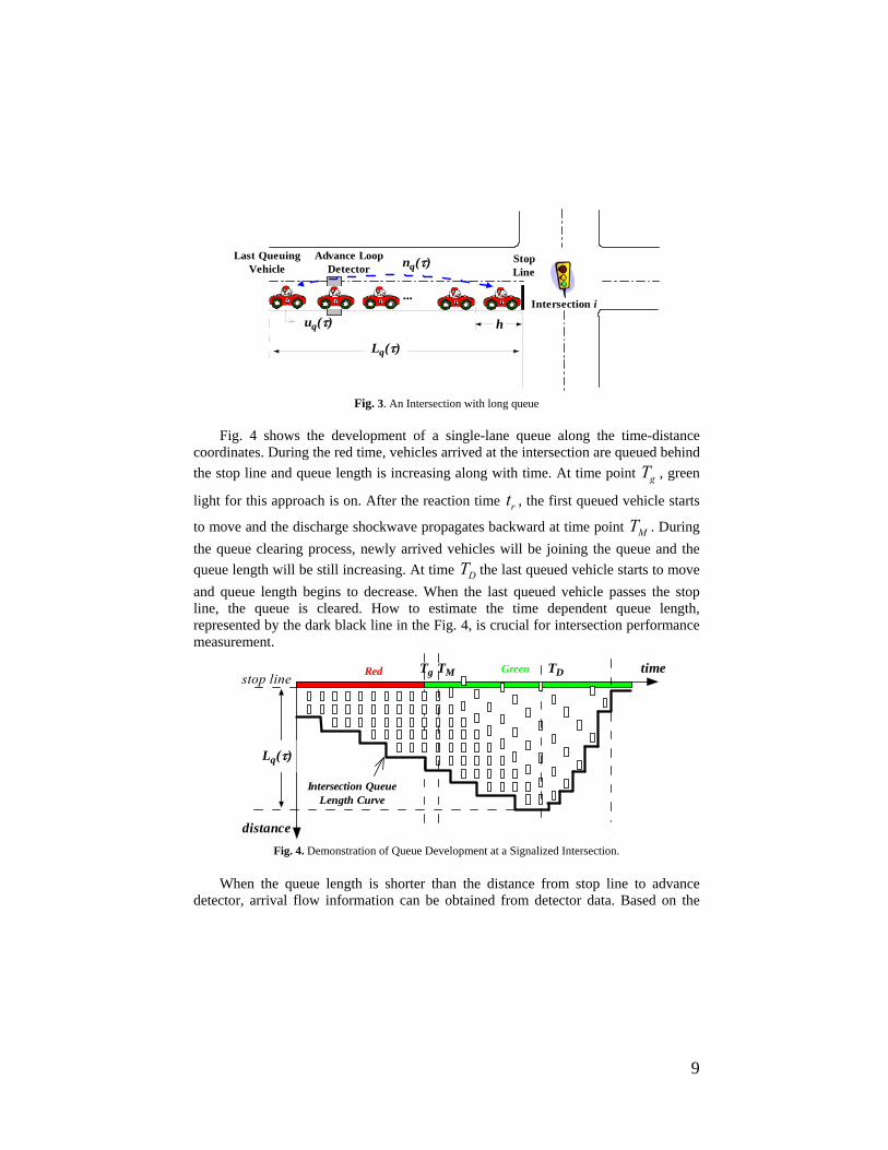
9

Advance LoopDetector

Last QueuingVehicle

StopLine

Intersection i

uq()

Lq()

h

...

nq()

Fig. 3. An Intersection with long queue

Fig. 4 shows the development of a single-lane queue along the time-distance

coordinates. During the red time, vehicles arrived at the intersection are queued behind

the stop line and queue length is increasing along with time. At time point gT , green

light for this approach is on. After the reaction time rt , the first queued vehicle starts

to move and the discharge shockwave propagates backward at time point MT . During

the queue clearing process, newly arrived vehicles will be joining the queue and the

queue length will be still increasing. At time DT the last queued vehicle starts to move

and queue length begins to decrease. When the last queued vehicle passes the stop line, the queue is cleared. How to estimate the time dependent queue length, represented by the dark black line in the Fig. 4, is crucial for intersection performance measurement.

time

distance

Lq()

Intersection QueueLength Curve

TDTg TMRed Greenstop line

Fig. 4. Demonstration of Queue Development at a Signalized Intersection.

When the queue length is shorter than the distance from stop line to advance

detector, arrival flow information can be obtained from detector data. Based on the

10

queue forming and discharging assumptions made before, DT can be calculated as in

Eq. 1, where ( )qn is the number of queued vehicles accumulated behind the stop line

from the starting of red time rT to time within a cycle.

( ( ) 1)D g r s qT T t t n (1)

Assuming ( )dn t is the number of vehicles passing the advance loop detector within a

time interval t , ( )qn can be calculated as in Eq. 2:

( ) ( ) ( ), ;

( )

( ), .r

t

A r D r d r Dt Tq

q D

N T N T n t T Tn

n T otherwise

(2)

where ( ) ( )A r D rN T N T is the net difference between the arrival counts and the

departure counts at the beginning of last red time rT , i.e., the residual queue from last

cycle. AN can be obtained from the advance loop detector, and

DN can be calculated

based on an assumed discharging rate if no stop-bar detector is available.

Once ( )qn can be calculated, before the discharge wave propagate to the rear of

queue ( DT ), queue length ( )qL  can be estimated as ( )qn h , based on an

known jammed space headway h. After the rear of queue begins to move ( DT ), an

acceleration process is assumed and the position and speed of the last queued vehicle can be estimated using a simple physical equation.

When a queue spills over the advance loop detector or even back to the upstream intersections under congestion, the advance detector is occupied by a queued vehicle

and ( )qn cannot be directly measured using the volume data from the detector.

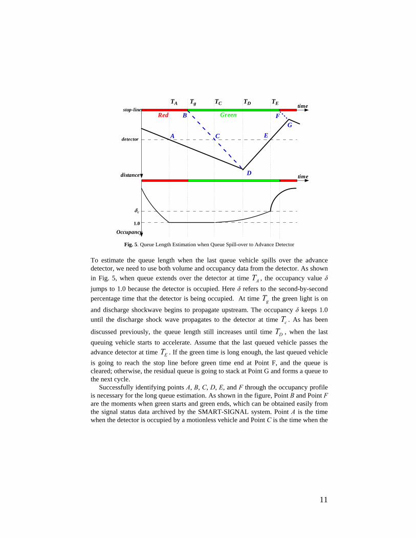
Therefore we cannot estimate the queue length in the current cycle. However, given the known process of queue discharge at a signalized intersection, we can estimate the queue length for the immediate past cycle thanks to the availability of archived traffic signal data. Fig. 5 shows the queue development process for a long queue case.

11

detector

time

B

D

E

F

G

A C

stop-line

Occupancy

1.0

c

timedistance

Red Green

Tg TC TD TETA

Fig. 5. Queue Length Estimation when Queue Spill-over to Advance Detector

To estimate the queue length when the last queue vehicle spills over the advance detector, we need to use both volume and occupancy data from the detector. As shown

in Fig. 5, when queue extends over the detector at time AT , the occupancy value δ

jumps to 1.0 because the detector is occupied. Here δ refers to the second-by-second

percentage time that the detector is being occupied. At time gT the green light is on

and discharge shockwave begins to propagate upstream. The occupancy δ keeps 1.0

until the discharge shock wave propagates to the detector at time cT . As has been

discussed previously, the queue length still increases until time DT , when the last

queuing vehicle starts to accelerate. Assume that the last queued vehicle passes the

advance detector at time ET . If the green time is long enough, the last queued vehicle

is going to reach the stop line before green time end at Point F, and the queue is cleared; otherwise, the residual queue is going to stack at Point G and forms a queue to the next cycle.

Successfully identifying points A, B, C, D, E, and F through the occupancy profile is necessary for the long queue estimation. As shown in the figure, Point B and Point F are the moments when green starts and green ends, which can be obtained easily from the signal status data archived by the SMART-SIGNAL system. Point A is the time when the detector is occupied by a motionless vehicle and Point C is the time when the

12

detector is “released”, so the occupancy δ between Point A and Point C is always 1.0, which can be identified easily from the occupancy profile. Point A can be identified by searching the occupancy value keeping 1.0 for more than 2 seconds; and Point C can be found after the occupancy value drops from 1.0. Between Point C and Point E, saturated traffic from the queue discharging process passes the detector. The occupancy δ during time interval [TC, TE] is usually not 1.0, but still keeps higher than a critical value δc since queue discharges at capacity flow rate (by forming a vehicle platoon). The traffic pattern detected at the detector should be different before and after Point E. In practice, we use the criterion that the state of zero occupancy lasts for more than 3 seconds to identify this point. After Point E the traffic flow pattern is dependent on the vehicle arrival process from upstream, which most likely is different with the traffic flow pattern during queue discharge. Correspondingly, the occupancy δ drops after Point E. Therefore, δc can be used as a threshold to identify time TE.

It should be noted that when spillover happens, i.e. intersection is blocked due to downstream congestion, it is likely that Point C will be postponed because the departure shockwave cannot not reach the advance detector according to queue discharging speed. This does not impact the validity of the proposed model. However, the model does have a limitation with underestimated queue length if Point E cannot be identified, i.e. vehicles keep discharging at saturation flow rate during the entire green time. In such cases, the model will report only the discharged vehicle queue, and indicate that a cycle failure has occurred.

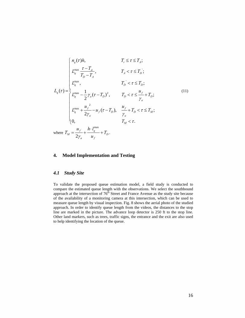
Maximum Queue Length Estimation

Once TE is identified, the maximum queue length maxqL during the last cycle can be

estimated. We denote the distance between the advance detector and the stop-line as dl, the travel time for the last queued vehicle to pass the advance loop detector as tl , the

desired vehicle speed as uf, and the acceleration rate a . The relationship of the

variables can be formulated as the following: 2

2 max

max

2

1, ;

2 2

, .2

fa l q l

aq l

ff l

a

ut L d

L du

u t otherwise

(3)

Additionally denote the maximum queue size at time TD as nq(TD), then maxqL can be

calculated as:

13

max ( )q q DL n T h                                    4  

Consider that we assume uniform starting time difference between two adjacent queued vehicles, and

( ( ) 1)E g r q D s lT T t n T t t (5)

Equations (3), (4), and (5) can be solved if TE can be detected from the detector

occupancy profile, and the maximum queue length maxqL is thus generated.

Time-Dependent Queue Length Curve Estimation

Once the maximum queue length maxqL is calculated, the time-dependent queue length

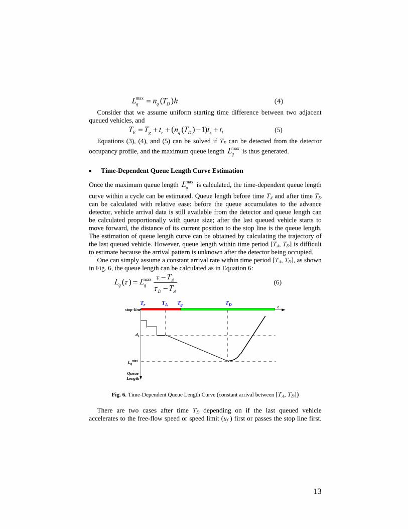
curve within a cycle can be estimated. Queue length before time TA and after time TD can be calculated with relative ease: before the queue accumulates to the advance detector, vehicle arrival data is still available from the detector and queue length can be calculated proportionally with queue size; after the last queued vehicle starts to move forward, the distance of its current position to the stop line is the queue length. The estimation of queue length curve can be obtained by calculating the trajectory of the last queued vehicle. However, queue length within time period [TA, TD] is difficult to estimate because the arrival pattern is unknown after the detector being occupied.

One can simply assume a constant arrival rate within time period [TA, TD], as shown in Fig. 6, the queue length can be calculated as in Equation 6:

max( ) Aq q

D A

TL L

T

(6)

tTD

stop-line

QueueLength

Lqmax

TgTATr

dl

Fig. 6. Time-Dependent Queue Length Curve (constant arrival between [TA, TD])

There are two cases after time TD depending on if the last queued vehicle accelerates to the free-flow speed or speed limit (uf ) first or passes the stop line first.

14

If the last queued vehicle passes the stop line first, the time-depend queue length

( )qL within the cycle can be calculated as Equation 7:

max

maxmax 2

( ) , ;

, ;

2( ) 1( ) , ;

2

2 0,

q r A

Aq A D

D A

qqq a D D D

a

n h T T

TL T T

T T

LLL T T T

L

max

.qD

a

T

(7)

If the last queued vehicle reaches uf first, the time-depend queue length ( )qL

within the cycle can be calculated as in Equation 8:

max

max 2

2max

( ) , ;

, ;

1( ) ( ) , ;

2

( ), ;2

0,

q r A

Aq A D

D A

fq q a D D D

a

f fq f D D M

a a

n h T T

TL T T

T T

uL L T T T

u uL u T T T

.MT

(8)

where

max

2f q

M Da f

u h lT T

u

.

When the links between intersections are short, vehicles arrivals to an intersection are more likely in a platoon mode than with a constant rate. The queue length curve between time TA and TD can be also assumed as a piece-wise linear curve as shown in Fig. 7. In this case, vehicles constantly arrive at the intersection between time TA and TD’, and no vehicles would join the queue between time TD’ and TD. In such cases, the through movement vehicles and left-turn vehicles from upstream intersection form the queue at the beginning of the red time, and no vehicle would arrive at the intersection once the right-of-way from upstream intersection to the subject intersection is

15

prohibited. The queue reaches its maximum length before time TD (at time TD') so the

queue length during the time interval [TD', TD] is a constant value maxqL . Here we still

assume that between time TA and TD’, vehicle arrivals are uniform as a straight line. The time that vehicle reaches its maximum value can be calculated as in Equation 9:

max' ( )q

D r A rl

LT T T T

d (9)

tTD

stop-line

QueueLength

Lqmax

Tg TD'TATr

dl

Fig. 7. Time-Dependent Queue Length Curve (piece-wise linear curve between [TA, TD])

Correspondingly, time-dependent queue length ( )qL within the cycle can be

calculated as in Equation 10 if the last queued vehicle passes the stop line first:

max ''

max '

maxmax 2

( ) , ;

, ;

, ;

( ) 21( ) , ;

2

0,

q r A

Aq A D

D A

q D D

q qq a D D D

a

n h T T

TL T T

T T

L T T

L LL T T T

max2 .q

Da

LT

(10)

and as in Equation 11 the last queued vehicle reaches uf first:

16

max '

max '

max 2

2max

( ) , ;

, ;

, ;

( ) 1( ) , ;

2

(2

q r A

Aq A D

D A

q D D

q fq a D D D

a

fq f

a

n h T T

TL T T

T T

L T T

L uL T T T

uL u

), ;

0, .

fD D M

a

M

uT T T

T

(11)

where

max

2f q

M Da f

u h lT T

u

.

4. Model Implementation and Testing

4.1 Study Site

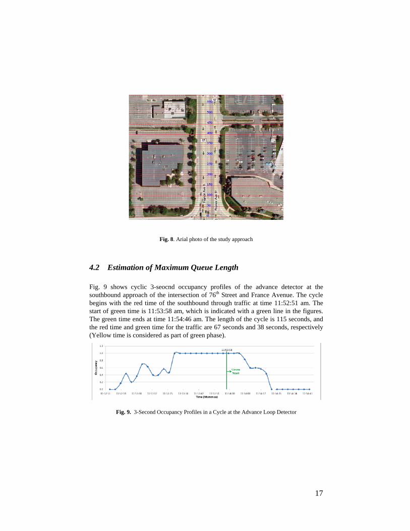
To validate the proposed queue estimation model, a field study is conducted to compare the estimated queue length with the observations. We select the southbound approach at the intersection of 76th Street and France Avenue as the study site because of the availability of a monitoring camera at this intersection, which can be used to measure queue length by visual inspection. Fig. 8 shows the aerial photo of the studied approach. In order to identify queue length from the videos, the distances to the stop line are marked in the picture. The advance loop detector is 250 ft to the stop line. Other land markers, such as trees, traffic signs, the entrance and the exit are also used to help identifying the location of the queue.  

17

 

Fig. 8. Arial photo of the study approach

4.2 Estimation of Maximum Queue Length

Fig. 9 shows cyclic 3-seocnd occupancy profiles of the advance detector at the southbound approach of the intersection of 76th Street and France Avenue. The cycle begins with the red time of the southbound through traffic at time 11:52:51 am. The start of green time is 11:53:58 am, which is indicated with a green line in the figures. The green time ends at time 11:54:46 am. The length of the cycle is 115 seconds, and the red time and green time for the traffic are 67 seconds and 38 seconds, respectively (Yellow time is considered as part of green phase).

Fig. 9. 3-Second Occupancy Profiles in a Cycle at the Advance Loop Detector

18

It can be clearly seen that the occupancy profile fluctuates at the beginning of the red time, which indicates the queue formulation process before the queue reaches the detector. At time 11:53:26, the occupancy becomes a constant value 1.0, when the detector is occupied. The queue starts to discharge from the stop line as the green light starts. The discharge shockwave reaches the detector after 9 seconds at time 11:54:07, and then the occupancy profile becomes fluctuated but with high occupancy values until time 11:54:22, when the rear of the queue passes the detector, which is the break point TE as we discussed previously.

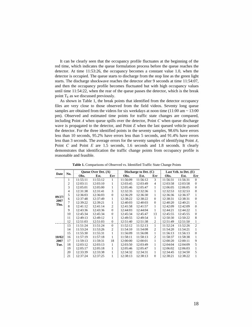
As shown in Table 1, the break points that identified from the detector occupancy files are very close to those observed from the field videos. Seventy long queue samples are obtained from the videos for six weekdays at noon time (11:00 am ~ 13:00 pm). Observed and estimated time points for traffic state changes are compared, including Point A when queue spills over the detector, Point C when queue discharge wave is propagated to the detector, and Point E when the last queued vehicle passed the detector. For the three identified points in the seventy samples, 98.6% have errors less than 10 seconds, 95.2% have errors less than 5 seconds, and 91.4% have errors less than 3 seconds. The average errors for the seventy samples of identifying Point A, Point C and Point E are 1.5 seconds, 1.6 seconds and 1.8 seconds. It clearly demonstrates that identification the traffic change points from occupancy profile is reasonable and feasible.

Table 1. Comparisons of Observed vs. Identified Traffic State Change Points

Date No. Queue Over Det. (A) Discharge to Det. (C) Last Veh. to Det. (E)

Obs. Est. Err Obs. Est. Err Obs. Est. Err

09/27/2007 Thu.

1 11:55:11 11:55:12 1 11:56:09 11:56:12 3 11:56:31 11:56:31 0 2 12:03:11 12:03:10 1 12:03:45 12:03:49 4 12:03:58 12:03:58 0 3 12:05:01 12:05:00 1 12:05:46 12:05:47 1 12:06:05 12:06:05 0 4 12:31:38 12:31:41 3 12:32:35 12:32:36 1 12:32:53 12:32:53 0 5 12:36:03 12:36:03 0 12:36:29 12:36:30 1 12:36:36 12:36:37 1 6 12:37:48 12:37:49 1 12:38:22 12:38:22 0 12:38:31 12:38:31 0 7 12:39:22 12:39:21 1 12:40:03 12:40:03 0 12:40:20 12:40:21 1 8 12:41:12 12:41:14 2 12:41:58 12:41:57 1 12:42:09 12:42:09 0 9 12:43:36 12:43:36 0 12:44:03 12:44:04 1 12:44:21 12:44:22 1 10 12:45:34 12:45:34 0 12:45:34 12:45:47 13 12:45:55 12:45:55 0 11 12:49:13 12:49:12 1 12:49:55 12:49:54 1 12:50:30 12:50:22 8 12 12:51:03 12:51:03 0 12:51:40 12:51:38 2 12:51:49 12:51:50 1

10/02/2007 Tue.

13 11:51:24 11:51:24 0 11:52:12 11:52:13 1 11:52:24 11:52:26 2 14 11:53:24 11:53:26 2 11:54:10 11:54:08 2 11:54:20 11:54:21 1 15 11:55:30 11:55:31 1 11:56:09 11:56:08 1 11:56:13 11:56:13 0 16 11:57:19 11:57:18 1 11:58:11 11:58:13 2 11:58:37 11:58:38 1 17 11:59:13 11:59:31 18 12:00:00 12:00:01 1 12:00:20 12:00:11 9 18 12:03:12 12:03:13 1 12:03:50 12:03:49 1 12:04:04 12:04:09 5 19 12:05:17 12:05:18 1 12:05:46 12:05:47 1 12:06:02 12:06:03 1 20 12:33:39 12:33:38 1 12:34:32 12:34:31 1 12:34:45 12:34:50 5 21 12:37:24 12:37:25 1 12:38:13 12:38:13 0 12:38:21 12:38:22 1

19

20 12:39:28 12:39:29 1 12:40:04 12:40:05 1 12:40:13 12:40:14 1 23 12:41:34 12:41:35 1 12:42:03 12:42:05 2 12:42:12 12:42:13 1 24 12:43:21 12:43:21 0 12:44:08 12:44:08 0 12:44:09 12:44:09 0 25 12:45:19 12:45:23 4 12:46:03 12:46:06 3 12:46:22 12:46:15 7 26 12:47:14 12:47:17 3 12:47:44 12:47:44 0 12:47:55 12:47:59 4 27 12:49:15 12:49:16 1 12:49:50 12:49:51 1 12:50:22 12:50:23 1 28 12:53:06 12:53:06 0 12:53:31 12:53:34 3 12:53:39 12:53:40 1

10/03/2007 Wed.

29 11:53:35 11:53:33 2 11:54:27 11:54:24 3 11:54:43 11:54:44 1 30 11:55:47 11:55:52 5 11:56:20 11:56:20 0 11:56:33 11:56:41 8 31 11:59:42 11:59:42 0 12:00:16 12:00:16 0 12:00:35 12:00:35 0 32 12:03:37 12:03:34 3 12:04:06 12:04:04 2 12:04:21 12:04:24 3 33 12:09:28 12:09:28 0 12:09:45 12:09:47 2 12:09:59 12:10:01 2 34 12:24:33 12:24:31 2 12:25:12 12:25:09 3 12:25:33 12:25:33 0 35 12:35:39 12:35:38 1 12:36:40 12:36:40 0 12:37:00 12:37:01 1 36 12:39:34 12:39:32 2 12:40:16 12:40:15 1 12:40:39 12:40:44 5 37 12:41:35 12:41:35 0 12:42:25 12:42:24 1 12:42:37 12:42:38 1 38 12:47:46 12:47:44 2 12:48:11 12:48:09 2 12:48:26 12:48:24 2 39 12:49:18 12:49:17 1 12:49:58 12:49:56 2 12:50:07 12:50:06 1

10/04/2007 Thu.

40 11:51:49 11:51:49 0 11:52:35 11:52:33 2 11:52:42 11:52:42 0 41 11:57:40 11:57:38 2 11:58:03 11:58:00 3 11:58:08 11:58:08 0 42 12:28:03 12:28:04 1 12:28:49 12:28:50 1 12:28:51 12:28:50 1 43 12:38:09 12:38:10 1 12:38:36 12:38:37 1 12:38:43 12:38:44 1 44 12:39:31 12:39:29 2 12:40:20 12:40:18 2 12:40:33 12:40:35 2 45 12:41:50 12:41:50 0 12:42:26 12:42:25 1 12:42:41 12:42:43 2 46 12:47:43 12:47:43 0 12:48:05 12:48:07 2 12:48:24 12:48:24 0 47 12:49:09 12:49:07 2 12:50:04 12:50:07 3 12:50:10 12:50:11 1 48 12:51:34 12:51:35 1 12:51:59 12:52:02 3 12:52:14 12:52:16 2 49 12:55:19 12:55:19 0 12:55:40 12:55:39 1 12:55:58 12:55:59 1

10/08/2007 Mon.

50 11:51:33 11:51:42 9 11:52:23 11:52:20 3 11:52:30 11:52:31 1 51 11:55:48 11:55:50 2 11:56:25 11:56:25 0 11:56:34 11:56:34 0 52 11:57:40 11:57:40 0 11:58:05 11:58:03 2 11:58:08 11:58:07 1 53 12:01:31 12:01:28 3 12:02:02 12:02:00 2 12:02:10 12:02:14 4 54 12:29:56 12:30:00 4 12:30:45 12:30:45 0 12:30:58 12:30:58 0 55 12:31:55 12:31:53 2 12:32:35 12:32:35 0 12:32:43 12:32:43 0 56 12:39:37 12:39:37 0 12:40:17 12:40:18 1 12:40:39 12:40:39 0 57 12:41:35 12:41:37 2 12:42:18 12:42:20 2 12:42:25 12:42:24 1 58 12:45:50 12:45:51 1 12:46:13 12:46:14 1 12:46:22 12:46:22 0 59 12:49:27 12:49:28 1 12:50:01 12:49:59 2 12:50:15 12:50:21 6

10/09/2007 Tue.

60 11:49:43 11:49:43 0 11:50:26 11:50:25 1 11:50:41 11:50:41 0 61 11:53:39 11:53:39 0 11:54:22 11:54:23 1 11:54:34 11:54:34 0 62 11:59:48 11:59:47 1 12:00:14 12:00:16 2 12:00:21 12:00:20 1 63 12:05:28 12:05:28 0 12:05:52 12:05:53 1 12:06:10 12:06:11 1 64 12:30:20 12:30:19 1 12:30:47 12:30:46 1 12:30:49 12:30:49 0 65 12:41:58 12:41:59 1 12:42:17 12:42:17 0 12:42:31 12:42:32 1 66 12:45:32 12:45:32 0 12:46:04 12:46:01 3 12:46:10 12:46:16 6 67 12:47:32 12:47:33 1 12:47:57 12:47:59 2 12:48:10 12:48:10 0 68 12:49:46 12:49:45 1 12:50:07 12:50:06 1 12:50:14 12:50:14 0 69 12:51:34 12:51:33 1 12:51:49 12:51:51 2 12:52:25 12:52:09 16 70 12:53:29 12:53:28 1 12:53:57 12:53:59 2 12:54:18 12:54:19 1

Average 1.5 1.6 1.8

20

4.3 Result Analysis

The values of the parameters for the estimation of the queue length and arterial travel time are obtained either from published sources (Institute of Transportation Engineers, 1999) or field experiences. In this paper, the desired speed uf is 40 mph, the acceleration rate γa is 3.6 ft/s2, the deceleration rate γd is 10 ft/s2, the jammed space headway h is 30 ft, the reaction time tr is 1 second, the starting time difference between two adjacent queued vehicles ts is 1.2 second, and the vehicle tracing step Δt is 1 second. Note the values of some parameters are different with what we used in the previous paper (Liu & Ma, 2009), in which h is 24 ft and ts is 0.5 sec. From our field observations, the values adopted in this paper are more realistic.

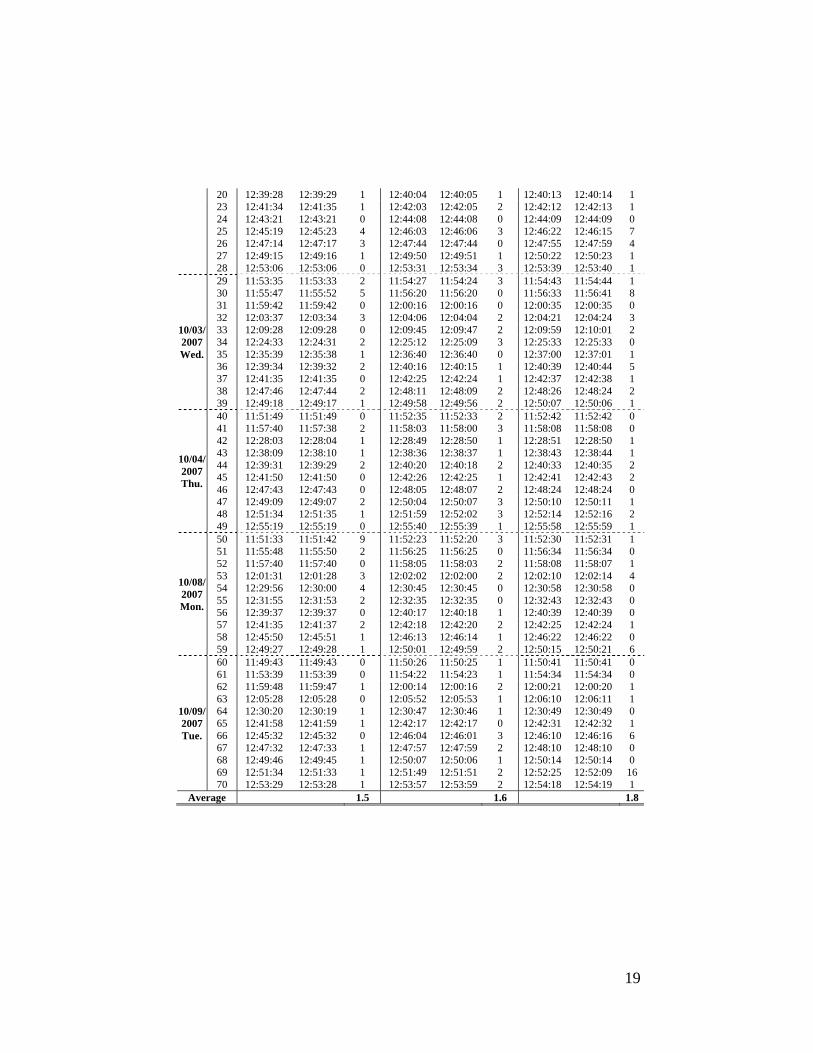
Maximum Queue Estimation

Fig. 10a demonstrates the comparison of observed and estimated maximum queue length. The blue lines are the observed data from videos and the red lines are the estimated results from the proposed model. The figure indicates that the estimation values are very close to the observed data. The average maximum queue length estimation error is 31.9 ft, which is 7.5% off the average of the observed values. 78.6% estimated maximum queue lengths have errors within 10 percent.

a)

b)

Fig. 10. a) Comparisons of Observed vs. Estimated Maximum Queue Length; b) Comparisons of

Observed vs. Estimated Maximum Queue Size

Fig. 10b demonstrates the comparison of observed and estimated maximum queue size (number of vehicles in the queue). The blue lines represent the observed data from

21

videos and the red lines are the estimated results from the proposed model. The average error of maximum queue size is 1.4 vehicles, which is 9.4% of the observed maximum queue size. Considering the limited detector data we can use for queue estimation, the results are very encouraging.

Cyclic Queue Length Curve

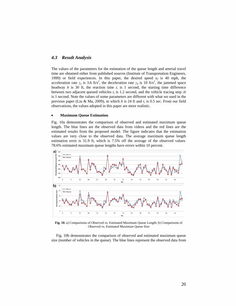
Fig. 11 shows the comparison of a cyclic queue length curve from one of the seventy samples. The blue line is the queue length captured from the video. The red line is the queue length estimated from Equations 7 and 8. It can be seen that the two lines are close, which indicates that proposed model has good estimation on the time-dependent queue length curve.

Fig. 11. Comparison of Observed vs. Estimated Cyclic Queue Length Curve

Travel Time Estimation

A field study was undertaken to obtain the ground truth travel time of the arterial corridor. Twenty-three floating car runs were performed on three different weekdays during the afternoon peak hours with a desired speed around 40 mph. The time instants when the floating car passed the stop lines of the intersections were recorded with a stop watch. Fig. 12 shows the estimated arterial travel time along the studied 11 intersections (total 1.8 miles) on France Ave. without consideration of long queue. As can be seen, the estimated data line (red line) is close to the observed data line (blue line) on April 19th and 25th, 2007; however, the model does not generate good estimations on May 14th, 2007, when the traffic condition was congested due to a retiming effort on France Avenue. The average estimation error for the overall 23 samples is 8.6%, which is 29.7 seconds, and the overall RMSP is 0.1564. The estimation error for the 15 samples on April 19th and 25th is only 4.2%, which is equal to 13.5 seconds; however, the estimation error on May 14th increases as large as 16.9%, which is equal to 60.3 seconds. The result indicates that, although overlooking long queue case can still generate good travel time estimations under uncongested traffic conditions; it will have significant errors on the travel time estimation under congested

22

traffic conditions. We shall note that, even without considering long queue, parameters of the virtual probe model can be adjusted to achieve better estimation results, as shown in Figure 11 of Liu and Ma (2009). As we indicated before, different values of h and ts are used in that paper.

Fig. 12. Travel Time Estimation without Consideration of Long Queues

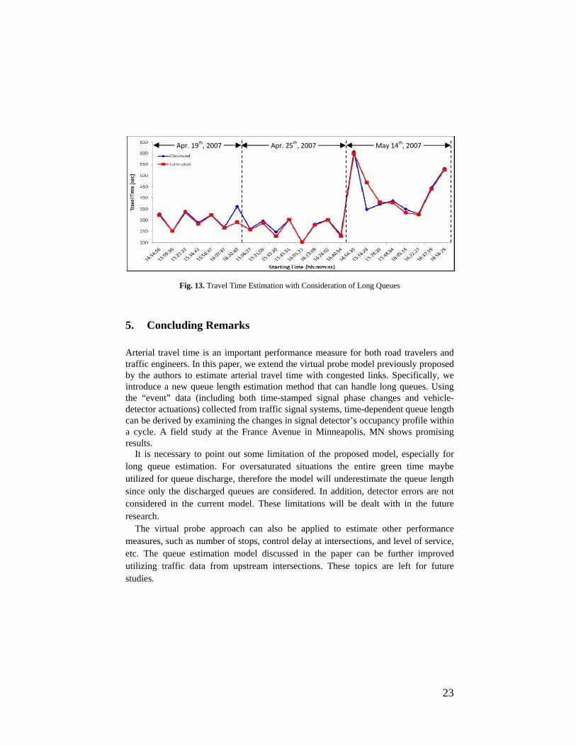
Fig. 13 shows the estimated travel time with the consideration of long queue. As can be seen, the estimated data line (red line) is close to the observed data line (blue line) on all of the three days. The average estimation error for the overall 23 samples decreases to 4.1%, which is 13.8 seconds, and the overall RMSP is 0.0856. The estimation error for the 15 samples on April 19th and 25th is 3.0%, which is equal to 9.3 seconds; the estimation error on May 14th is 6.1%, which is equal to 22.4 seconds. The result shows with long queue consideration, the error for the 23 samples is half of those without long queue consideration. Consideration of long queue is necessary for travel time estimation under congested traffic conditions. The proposed long queue model can significantly improve the accuracy of travel time estimation.

Apr. 19th, 2007  Apr. 25

th, 2007 May 14

th, 2007 

23

Fig. 13. Travel Time Estimation with Consideration of Long Queues

5. Concluding Remarks

Arterial travel time is an important performance measure for both road travelers and traffic engineers. In this paper, we extend the virtual probe model previously proposed by the authors to estimate arterial travel time with congested links. Specifically, we introduce a new queue length estimation method that can handle long queues. Using the “event” data (including both time-stamped signal phase changes and vehicle-detector actuations) collected from traffic signal systems, time-dependent queue length can be derived by examining the changes in signal detector’s occupancy profile within a cycle. A field study at the France Avenue in Minneapolis, MN shows promising results.

It is necessary to point out some limitation of the proposed model, especially for long queue estimation. For oversaturated situations the entire green time maybe utilized for queue discharge, therefore the model will underestimate the queue length since only the discharged queues are considered. In addition, detector errors are not considered in the current model. These limitations will be dealt with in the future research.

The virtual probe approach can also be applied to estimate other performance measures, such as number of stops, control delay at intersections, and level of service, etc. The queue estimation model discussed in the paper can be further improved utilizing traffic data from upstream intersections. These topics are left for future studies.

Apr. 19th, 2007  Apr. 25

th, 2007 May 14

th, 2007 

24

Acknowledgments The work described in this paper was supported by Minnesota Local Road Research Board and the University of Minnesota’s Intelligent Transportation Systems Institute. We gratefully acknowledge the assistance of Mr. James Grube and Mr. Eric Drager of Hennepin County Transportation Department for the data collection effort on France Ave.

References Ahn, S., Cassidy, M.J., and Laval, J. (2004) Verification of a simplified car-following theory,

Transportation Research Part B, 38(5), 431-440. Cheu, R.L., Lee, D-H, and Xie, C., (2001). An Arterial Speed Estimation Model Fusing Data from

Stationary and Mobile Sensors. Proceedings of the IEEE Intelligent Transportation Systems Conference, Oakland, CA, pp. 573-578.

Frechette, L. A., and Khan, A. M., (1998). Bayesian Regression-based Urban Traffic Models. Transportation Research Record, 1644, pp. 157-165.

Institute of Transportation Engineers (1999). Traffic Engineering Handbook. Washington D.C Liu, H., and Ma, W. (2009) A Virtual Probe Approach for Time-Dependent Arterial Travel Time

Estimation, Transportation Research Part C, 17 (1), pp. 11-26. Liu, H.., Wu, X., Ma, W. and Hu, H. (2009) Real-Time Queue Length Estimation for Congested

Signalized Intersections, Transportation Research Part C,17(4), 412-427. Newell, G.F., 2002. A simplified car-following theory: a lower order model. Transportation Research

36B, pp. 195–205. Roess, R., Prassas, E., & McShane, W. R. (2004). Traffic Engineering, Third Edition. Prentice-Hall. Takaba, S., Morita, T., Hada, T., Usami, T. and Yamaguchi, M., (1991). Estimation and

Measurement of Travel Time by Vehicle Detectors and License Plate Readers. Proceedings of Vehicle Navigation and Information Systems Conference, Vol. 1, pp. 257-267.

Turner, S., Lomax, T. J., & Levinson, H. S. (1996). Measuring and Estimating Congestion using Travel Time-based Procedures. Transportation Research Record, 1564, 11-19.

Zhang, M. H., (1999). Link-journey-speed Model for Arterial Traffic. Transportation Research Record, 1676, pp. 109-115.