real-time 3-d saft-ut system evaluation and validation
TRANSCRIPT
NUREG/CR-6344PNNL-10571
Real-Time 3-D SAFT-UT SystemEvaluation and Validation
DEC 2 3 1SSS
OSTI
Prepared byS. R. Doctor, G. J. Schuster, L. D. Reid, T. E. Hall
Pacific Northwest National Laboratory
Prepared forU.S. Nuclear Regulatory Commission
AVAILABILITY NOTICE
Availability of Reference Materials Cited in NRC Publications
Most documents cited in NRC publications will be available from one of the following sources:
1. The NRC Public Document Room, 2120 L Street. NW., Lower Level, Washington. DC 20555-0001
2. The Superintendent of Documents, U.S. Government Printing Office, P. O. Box 37082, Washington, DC20402-9328
3. The National Technical Information Service, Springfield, VA 22161-0002
Although the listing that follows represents the majority of documents cited in NRC publications, it is not in-tended to be exhaustive.
Referenced documents available for inspection and copying for a fee from the NRC Public Document Roominclude NRC correspondence and internal NRC memoranda; NRC bulletins, circulars, information notices, in-spection and investigation notices; licensee event reports; vendor reports and correspondence; Commissionpapers; and applicant and licensee documents and correspondence.
The following documents In the NUREG series are available for purchase from the Government Printing Office:formal NRC staff and contractor reports, NRC-sponsored conference proceedings, international agreementreports, grantee reports, and NRC booklets and brochures. Also available are regulatory guides, NRC regula-tions In the Code of Federal Regulations, and Nuclear Regulatory Commission Issuances.
Documents available from the National Technical Information Service include NUREG-series reports and tech-nical reports prepared by other Federal agencies and reports prepared by the Atomic Energy Commission,forerunner agency to the Nuclear Regulatory Commission.
Documents available from public and special technical libraries include all open literature items, such as books,journal articles, and transactions. Federal Register notices. Federal and State legislation, and congressionalreports can usually be obtained from these libraries.
Documents such as theses, dissertations, foreign reports and translations, and non-NRC conference pro-ceedings are available for purchase from the organization sponsoring the publication cited.
Single copies of NRC draft reports are available free, to the extent of supply, upon written request to the Officeof Administration, Distribution and Mail Services Section, U.S. Nuclear Regulatory Commission, Washington,DC 20555-0001.
Copies of industry codes and standards used in a substantive manner in the NRC regulatory process are main-tained at the NRC Library, Two White Flint North, 11545 Rockville Pike, Rockville. MD 20852-2738. for use by
, the public. Codes and standards are usually copyrighted and may be purchased from the originating organiza-tion or, if they are American National Standards. from the American National Standards Institute, 1430 Broad-way, New York, NY 10018-3308.
DISCLAIMER NOTICE
This report was prepared as an account of work sponsored by an agency of the United States Government.Neitherthe United States Government norany agency thereof, nor any of their employees, makes any warranty,expressed or implied, or assumes any legal liability or responsibility for any third party's use, or the results ofsuch use, of any information, apparatus, product, or process disclosed in this report, or represents that its useby such third party would not infringe privately owned rights.
fywaLpii test ayaitaJbie etfpy.,
v t
;-
NUREG/CR-6344PNNL-10571
Real-Time 3-D SAFT-UT SystemEvaluation and Validation
Manuscript Completed: March 1995Date Published: September 1996
Prepared byS. R. Doctor, G. J. Schuster, L. D. Reid, T. E. Hall
Pacific Northwest National LaboratoryRichland,WA 99352
J. Muscara, NRC Project Manager
Prepared forDivision of Engineering TechnologyOffice of Nuclear Regulatory ResearchU.S. Nuclear Regulatory CommissionWashington, DC 20555-0001NRC Job Codes B2467, B2913
DISTRIBUTION OF THIS DOCUMENT !§ U M T S ) \ \
Abstract
SAFT-UT technology is shown to provide significantenhancements to the inspection of materials used inU.S. nuclear power plants. This report provides guide-lines for the implementation of SAFT-UT technologyand shows the results from its application.
An overview of the development of SAFT-UT is provid-ed so that the reader may become familiar with thetechnology. Then the basic fundamentals are presentedwith an extensive list of references. A comprehensiveoperating procedure, which is used in conjunction withthe SAFT-UT field system developed by Pacific North-west Laboratory (PNL), provides the recipe for bothSAFT data acquisition and analysis.
The specification for the hardware implementation isprovided for the SAFT-UT system along with a descrip-tion of the subsequent developments and improvements.One development of technical interest is the SAFT realtime processor. Performance of the real-time processoris impressive and comparison is made of this dedicatedparallel processor to a conventional computer and tothe newer high-speed computer architectures designedfor image processing. Descriptions of other improve-ments, including a robotic scanner, are provided.
Laboratory parametric and application studies, per-formed by PNL and not previously reported, are dis-cussed followed by a section on field application workin which SAFT was used during inservice inspections ofoperating reactors.
•«,•
NUREG/CR-6344
DISCLAIMER
Portions of this document may be illegiblein electronic image products. Images areproduced from the best available originaldocument
DISCLAIMER
This report was prepared as an account of work sponsored by an agency of theUnited States Government Neither the United States Government nor any agencythereof, nor any of their employees, makes any warranty, express or implied, orassumes any legal liability or responsibility for the accuracy, completeness, or use-fulness of any information, apparatus, product, or process disclosed, or representsthat its use would not infringe privately owned rights. Reference herein to any spe-cific commercial product, process, or service by trade name, trademark, manufac-turer, or otherwise does not necessarily constitute or imply its endorsement, recom-mendation, or favoring by the United States Government or any agency thereof.The views and opinions of authors expressed herein do not necessarily state orreflect those of the United States Government or any agency thereof.
Contents
Abstract iii
Executive Summary xvii
1.0 Introduction 1.1
2.0 Overview of SAFT Fundamentals 2.12.1 Background and History of SAFT 2.12.2 Overview of SAFT Fundamentals 2.4
3.0 Where to Go for Additional Information 3.13.1 Bibliography 3.13.2 Synopses of Key SAFT Documents 3.5
3.2.1 Review and Discussion of the Development of Synthetic Aperture Focusing Technique (SAFT-UT) (Busse, Collins, and Doctor 1984) 3.5
3.2.2 Development and Validation of a Real-Time SAFT-UT System for the Inspection of LightWater Reactor Components, Vol. 1 (Doctor et al. 1986) 3.6
3.2.3 Development and Validation of a Real-Time SAFT-UT System for the Inspection of LightWater Reactor Components, Vol. 2 (Doctor et al. 1987a) 3.7
3.2.4 Development and Validation of a Real-Time SAFT-UT System for the Inspection of LightWater Reactor Components, Vol. 3 (Doctor et al. 1987b) 3.8
3.2.5 The SAFT-UT Real-Time Inspection System Operational Principles and Implementation (Hall,Reid, and Doctor 1988) 3.9
3.2.6 Program for Field Validation of the Synthetic Aperture Focusing Technique for UltrasonicTesting (SAFT-UT) (Hamlin 1985) 3.10
3.2.7 Development of a Real-Time Residue Number Processor for SAFT Inspection, Phase II FinalReport, September 1984 through April 1986 (Polky 1986) 3.10
3.2.8 An Ultra-High Speed Residue Processor for SAFT Inspection System Image Enhancement,Final Report, October 1983 through March 1984 (Polky and Miller 1985) 3.11
3.2.9 Design and Development of a Special Purpose SAFT System for Nondestructive Evaluation ofNuclear Reactor Vessels and Piping Components (Ganapathy et al. 1985) 3.11
4.0 SAFT-UT Field System Operating Procedures 4.14.1 Getting Started 4.1
4.1.1 Background Information 4.14.1.2 Power-Up and Log-On Procedures 4.24.1.3 Initiating the Data Acquisition Software 4.24.1.4 General Header Requirements 4.34.1.5 Pulser/Driver Setup 4.54.1.6 Mode Selection 4.54.1.7 Time Variable Gain Setup 4.54.1.8 Beginning a Scan 4.54.1.9 Data Acquisition Software Entry Points 4.74.1.10 System Shutdown Procedures 4.7
4.2 Single Transducer Pulse-Echo Operation 4.84.2.1 Pulse-Echo Configurations 4.84.2.2 Piping Considerations 4.84.2.3 Thick-Section Considerations 4.9
NUREG/CR-6344
Contents
4.3 Dual-Transducer, Tandem Operation 4.104.3.1 Tandem Configurations 4.104.3.2 Piping Considerations 4.124.3.3 Thick-Section Considerations 4.124.3.4 Tandem Processing Parameters 4.13
4.4 SAFT Data Analysis Techniques 4.134.4.1 General Information 4.134.4.2 Pulse-Echo Analysis 4.144.43 Tandem Analysis 4.15
5.0 Laboratory Application Research Studies 5.15.1 Investigation of SAFT Imaging in Thick Material 5.1
5.1.1 TSAFT-3 Development 5.25.2 Application of Advanced Signal Processing Techniques to Improve SAFT-UT Performance on CCSS
Material 5.35.2.1 Applying the Spectral Analysis and Subsequent Filter Technique to a CCSSRRT Data File 5.45.2.2 Software Tools Used to Define the Optimal Bandpass Filter Used to Enhance the SAFT-
Processed Image 5.55.2.3 Statistical Analysis of Defect and NonDefect CCSS A-Scans 5.65.2.4 Composite Spectra of the CCSSRRT 5.75.2.5 Conclusions - 5.9
6.0 Laboratory Parametric Studies 6.16.1 TSAFT-2 Configuration Velocity and Thickness Parametric Study 6.16.2 Bandwidth Compensation Study 6.2
7.0 Employing the SAFT Technology in the Field 7.17.1 Indian Point Station Unit II Inservice Inspection 7.1
7.1.1 Examinations Performed 7.17.1.2 Data Analysis 7.37.1.3 Discussion 7.37.1.4 Conclusion 7.4
7.2 Trojan Nuclear Power Plant 7.47.2.1 Examinations Performed 7.47.2.2 Data Analysis 7.67.2.3 Conclusion 7.8
7.3 Conclusion 7.9
8.0 SAFT Real-Time Processor Performance Analysis and Overview 8.18.1 Pulse-Echo Configuration 8.18.2 TSAFT/TSAFT-2 Configuration Performance 8.48.3 Overview of the Software Implementation of the SAFT-UT Real-Time Processor 8.6
8.3.1 Development History 8.68.3.2 The SAFT Calculation 8.68.3.3 Configuration Modifications 8.98.3.4 Tandem SAFT 8.108.3.5 Flow Chart Commentary 8.10
NUREG/CR-6344
Contents
9.0 Upgrading the SAFT-UT Field System 9.19.1 SAFT System Architecture 9.19.2 Installation of a MicroVAX m 9.29.3 Other System Upgrades for the Inspection of Nuclear Reactor Pressure Vessels 9.29.4 SAFT-UT Upgrades for NRCs NDE Mobile Laboratory 9.3
10.0 SAFT-UT Validation 10.110.1 Validation of SAFT-UT in the Mini-Round Robin 10.1
10.1.1 The Mini-Round Robin 10.110.1.2 SAFT-UT Inspection Procedure 10.310.1.3 SAFT-UT Analysis Procedure 10.310.1.4 SAFT-UT Performance Results and Discussion 10.310.1.5 Conclusions of the SAFT-UT Performance on the MRR 10.4
10.2 Validation of SAFT-UT for IGSCC Sizing 10.410.2.1 SAFT-UT Validation Testing Procedure 10.410.2.2 Discussion of SAFT-UT Sizing Results 10.510.2.3 Conclusions of SAFT-UT from the IGSCC Sizing Test 10.5
10.3 Validation of SAFT-UT for IGSCC Detection 10.510.3.1 SAFT-UT Detection Test Procedure 10.510.3.2 SAFT-UT Detection Test Results and Discussions 10.610.3.3 Conclusions Based on the IGSCC Detection Test 10.7
10.4 Validation of the SAFT-UT on the PISC-IH Full-Scale Vessel Test 10.710.4.1 Overview of the FSV Test 10.710.4.2 FSV SAFT-UT Results 10.710.4.3 Conclusions Based on FSV Test 10.9
10.5 Conclusions 10.9
11.0 Conclusions 11.1
12.0 References 12.1
Appendix A: Detailed Description of the SAFT-UT Field Inspection System A.1
Appendix B: Tutorial Procedure for Operating the SAFT-UT Robotic Scanner B.I
Appendix C: Changes to the SAFT Header C.1
Appendix D: Definition of SAFT-UT ASCII Header D.I
vii NUREG/CR-6344
Figures
2.1. Schematic of the Results Produced by the Original SAFT-UT Experiments 2.5
2.2. Demonstration of Signal-to-Noise Improvement Gained by Subtraction of Front Surface Signal 2.6
2.3. Illustration of the Effect of Front Surface Signal Removed upon SAFT-UT Processed Images 2.7
4.1. SAFT-UT Field System Identifying Switches, Knobs, and Modules 4.18
4.2. SAFT-UT Scan Conventions 4.19
4.3. Date and Time Prompts 4.20
4.4. Transducer Configuration Menu 4.20
4.5. Selection of Tandem Mode 4.21
4.6. Main Menu for SAFT-UT Parameters 4.21
4.7. View of Current Parameters (Pulse-Echo) 4.22
4.8. View of Current Parameters (Tandem) 4.22
4.9. Transducer Header Information 4.23
4.10. Material Header Information 4.23
4.11. Sampling Header Information 4.23
4.12. Scan Header Information (Pulse-Echo) 4.23
4.13. Scan Header Information (Tandem) 4.24
4.14. Command Selection Menu 4.24
4.15. Prompt to Change the Initial Delay 4.25
4.16. View of Header Information Before Scanning 4.25
4.17. Repositioning the Scanner 4.26
4.18. Data Transfer Menu 4.26
4.19. Connection to the VAX Host Computer 4.27
4.20. Starting Data Collection on the VAX Host Computer 4.27
4.21. SAFT Processing Options 4.28
4.22. SAFT Processing Options, Continued 4.28
NUREG/CR-6344 viii
Figures
4.23. Selection of Sampling Reduction 4.29
4.24. Entering Comments and Setting the Scanner Speed 4.29
4.25. Normal-Beam Pulse-Echo Inspection Using a Water Column 430
4.26. Angle-Beam Pulse-Echo Inspection Using a Lucite Wedge and Small-Diameter Transducer 4.31
4.27. Comparison Between Pulse-Echo (top) and Tandem Images of a 03-in.-deep (0.8-cm) Semicircular
Sawcut in a 0.6-in.-thick (1.5-cm) Aluminum Coupon 4.32
4.28. Angle-Beam Tandem Inspection Using a Lucite Wedge and Small-Diameter Transducers 4.33
4.29. Four Propagation Paths for Ultrasonic Energy Produced by the Tandem Transmission Technique 4.34
4.30. TSAFT-2 Configuration Using 1/2-Vee Transmit Path 4.35
4.31. TSAFT-2 Image of 0.7-in.-deep (1.8-cm) Sawcut in 9-in.-thick (22.9-cm) Specimen, 54° Transmitter and
47.2° Receiver 4.35
4.32. TSAFT-3 Initial (a) and Ending (b) Transducer Positions for a Single Sweep ^ 436
4.33. TSAFT-3 Configuration Showing Paths Contributing to the Real (Path 2) and Conjugate (Path 1) Image . 4.36
4.34. Side Views of TSAFT-3 Setups Showing 9-in.-thick (22.9-cm) Steel Block with 0.7-in.-deep (1.8-in.) Sawcutand Fictitious Material Thickness with "Folded" Transmit/Receive Paths 4.37
4.35. TSAFT-3 Image of 0.7-in.-deep (1.8-cm) Sawcut in 9-in.-thick (22.9-cm) Specimen, 47.2° Transmitter andReceiver 4.38
4.36. Additional Tandem Processing Parameters, Initial Screen Display 4.38
4.37. Additional Tandem Processing Parameters, Subsequent Screen Display 4.39
4.38. Pulse-Echo Image of a 0.2-in.-diameter (0.5-cm), Side-Drilled Hole, 0.5 in. (1.3 cm) up from the Far
Surface of a 2-in.-thick (5.1-cm) Steel Block 4.40
5.1. Pulse-Echo Image of 0.050-in.-deep (0.13-cm) Sawcut in a 9-in.-thick (22.86-cm) Steel Block 5.10
5.2. Pulse-Echo Image of 0.700-in.-deep (1.8-cm) Sawcut in a 9-in.-thick (22.86-cm) Steel Block 5.10
5.3. TSAFT-2 Image of 0.050-in.-deep (0.13-cm) Sawcut in a 9-in.-thick (22.86-cm) Steel Block 5.11
5.4. TSAFT-2 Image of 0.700-in.-deep (1.8-cm) Sawcut in 9-in.-thick (22.86-cm) Steel Block 5.11
5.5. Images of Specimen 5 of the CCSSRRT Data Set 5.12
5.6. Image of Specimen 5, Selected A-Scans, and Spectra Obtained After Application of Step-Wise Filter toData Prior to SAFT Processing 5.13
IX NUREG/CR-6344
Figures
5.7. Image of Specimen 5, Selected A-Scans, and Spectra Obtained After Application of Time Derivative Filterto Data Prior to SAFT Processing 5.14
5.8. Image of Specimen 5, Selected A-Scans, and Spectra After Application of Time Derivative and Stepwise
Filter to Data Prior to SAFT Processing 5.15
5.9. Maximum Correlation Values at Different Frequencies for Equiaxed Material 5.16
5.10. Maximum Correlation Values at Different Frequencies for Columnar Material 5.16
5.11. Composite Power Spectra for Sawcut Test File 5.17
5.12(a). Composite Power Spectra Plot for Equiaxed Shear-Wave Data Files 5.18
5.12(b). Specimen 3 Images Showing Before (top) and After (bottom) Processed Images (Filter parameters forsr image were selected from the power spectra plot.) 5.18
5.13(a). Composite Power Spectra Plot for Columnar Shear-Wave Data Files 5.19
5.13(b). Specimen 4 Images Showing Before (top) and After (bottom) Processed Images (Filter parameters for
After image were selected from the power spectra plot.) 5.19
5.13(c). Single Slice End View 0.5 in. (1.3 cm) from Weld Center 5.20
5.13(d). Single Slice End View at Weld Center 5.20
5.14. Images of the Equiaxed Side of Specimen 6 Showing the Before (top) and After (bottom) ProcessedImages (Filter Parameters for After Image were Selected From the Equiaxed Power Spectra Plot) 5.21
5.15. Images of the Columnar Side of Specimen 6 Showing the Before (top) and After (bottom) ProcessedImages (Filter Parameters for After Image were Selected From the Columnar Power Spectra Plot) 5.21
5.16. Plot Showing the Composite Power Spectra for Equiaxed Shear-Wave Specimens that had a HighProbability of Detection 5.22
5.17. Composite Power Spectra for Columnar Shear-Wave Specimens Having High Probability of Detection . . . 5.22
6.1. TSAFT-2 Images of a 0.3-in.-deep (0.8-cm) Sawcut in 0.750-in.-thick (1.9-cm) Aluminum Material with theProcessing Velocity Set as Noted 6.4
6.2. TSAFT-2 Images of a 0.3-in.-deep (0.8-cm) Sawcut in 0.750-in.-thick (1.9-cm) Aluminum Material with the
Processing Thickness Set as Noted 6.5
6.3. Image of Unprocessed Data (C-Scan View) from 0.5-in.-diameter (1.3-cm) Steel Sphere 6.6
6.4. A-Scan Near Center of Unprocessed Data from 0.5-in.-diameter (1.3-cm) Steel Sphere 6.66.5. A-Scan Showing Only Echo Trace from 0.5-in.-diameter (1.3-cm) Steel Sphere 6.7
6.6. Fourier Transform Plot of Echo Trace from 0.5-in.-diameter (1.3-cm) Steel Sphere 6.7
NUREG/CR-6344 x
Figures
6.7. C-Scan View of SAFT Processed Echo Trace from 0.5-in.-diameter (13-cm) Steel Sphere 6.8
6.8. C-Scan View of Time Derivative Raw Data Echo Trace from 0.5-in.-diameter (1.3-cm) Steel Sphere 6.8
6.9. A-Scan Near Center of Unprocessed Time Derivative Data from 0.5-in.-diameter (1.3-cm) Steel Sphere . . . . 6.9
6.10. Fourier Transform Plot of Time Derivative Data from 0.5-in.-diameter (1.3-cm) Steel Sphere 6.9
6.11. C-Scan View of SAFT Processed Time Derivative Data from 0.5-in.-diameter (1.3-cm) Steel Sphere 6.10
6.12. C-Scan View of SAFT Processed Echo Trace from 0.5-in.-diameter (1.3-cm) Steel Sphere After ApplyingSquare Function to Intensity Values 6.10
6.13. Pulse-Echo Image of Raw Data from 0.3-in.-deep (0.8-cm) Sawcut in 0.585-in.-thick (1.5-cm) StainlessSteel Coupon 6.11
6.14. A-Scan Near Center of Raw Data from 0.3-in.-deep (0.8-cm) Sawcut in 0.585-in.-thick (1.5-cm) StainlessSteel Coupon 6.11
6.15. Time Derivative of A-Scan Near Center of Raw Data from 0.3-in.-deep (0.8-cm) Sawcut in 0.585-in.-thick(1.5-cm) Stainless Steel Coupon 6.12
6.16. Pulse-Echo Image of Time Derivative Raw Data from 0.3-in.-deep (0.8-cm) Sawcut in 0.585-in.-thick (1.5-cm) Stainless Steel Coupon 6.12
6.17. Pulse-Echo Image of SAFT-Processed Time Derivative Data from 0.3-in.-deep (0.8-cm) Sawcut in 0.585-in.-thick (1.5-cm) Stainless Steel Coupon 6.13
6.18. Pulse-Echo Image of SAFT-Processed Data from 0.3-in.-deep (0.8-cm) Sawcut in 0.585-in.-thick StainlessSteel Coupon After Applying Square Function to Intensity Values 6.13
7.1. 45° Shear-Wave Image of Corner-Trap Echo of 0.3-in.-deep (0.8-cm) Notch in 9-in.-thick (22.9-cm)Cladded Vessel Calibration Block (Waltz Mill) 7.9
7.2. 45° Shear-Wave Image of Corner-Trap Echo of 0.3-in.-deep (0.8-cm) Notch in 9-in.-thick (22.9-cm)Uncladded Calibration Block (PNL) 7.10
7.3. 45° Shear-Wave Image (3-D Processed) of the Vessel Indication at Indian Point Unit II 7.11
7.4. 45° Longitudinal-Wave Image (3-D Processed) of the Vessel Indication at Indian Point Unit II 7.12
7.5. 45° Shear-Wave Image (3-D Processed) of 0.2-in.-diameter (0.5-cm) Side-Drilled Hole 0.5 in. (1.3 cm) from
Far Surface of 2.0-in.-thick (5.1-cm) Steel Block 7.13
7.6. Composite Spectra Plot of Suspected Defect and Non-defect Areas of Data File TR9SH5D 7.14
7.7(a). B-Scan Side View and C-Scan Top View of Data File TR9SH5A 7.15
7.7(b). Expanded View of Indication #2, TR9SH5A 7.15
xi NUREG/CR-6344
Figures
7.7(c). Expanded View of Indication #3, TR9SH5A 7.16
7.7(d). Expanded View of Indication #5, TR9SH5A 7.16
7.8(a). B-Scan Side View and C-Scan Top View of Data File TR9SH5C 7.17
7.8(b). Expanded View of Indication #2, TR9SH5C 7.17
7.8(c). Expanded View of Indication #3, TR9SH5C 7.18
7.8(d). Expanded View of Indication #5, TR9SH5C 7.18
7.8(e). Expanded View of Indication A, TR9SH5C 7.19
7.8(f). Expanded View of Indication B, TR9SH5C 7.19
7.9(a). B-Scan Side View and C-Scan Top View of Data File TR9SH5D 7.20
7.9(b). Expanded View of Indication #4, TR9SH5D 7.20
7.10. B-Scan Side View and C-Scan Top View of Data File TR9SH5G 7.21
8.1. SAFT Computational Device or Real-Time Processor 8.12
8.2. Real-Time Processor Performance on Pipe Data File with Selective Processing Disabled and OutputRecord Size Compression Factor Set to 1 8.13
8.3. Real-Time Processor Performance on Pipe Data File with Selective Processing Disabled and OutputRecord Size Compression Factor Set to 5 8.13
8.4. Real-Time Processor Performance on Pipe Data File with Selective Processing Set to -20 dB and OutputRecord Size Compression Factor Set to 1 8.14
8.5. Real-Time Processor Performance on Pipe Data File with Selective Processing Set to -20 dB and OutputRecord Size Compression Factor Set to 5 8.14
8.6. Real-Time Processor Performance on PISC II Data File with Selective Processing Disabled and OutputRecord Size Compression Factor Set to 1 » 8.15
8.7. Real-Time Processor Performance on PISC II Data File with Selective Processing Disabled and OutputRecord Size Compression Factor Set to 5 8.15
8.8. Real-Time Processor Performance on PISC II Data File with Selective Processing Set to -20 dB andOutput Record Size Compression Factor Set to 1 8.16
8.9. Real-Time Processor Performance on PISC II Data File with Selective Processing Set to -20 dB andOutput Record Size Compression Factor Set to 5 8.16
8.10. Real-Time Processor Performance, Tandem Configuration, on Thin-Pipe Data File (TSAFT; 0.585 in.thick [1.49 cm]) with Selective Processing Disabled and Output Record Size Compression Factor Set to 1 . 8.17
NUREG/CR-6344 xii
Figures
8.11. Real-Time Processor Performance, Tandem Configuration, on Thick-Pipe Data File (TSAFT; 1.5 in. thick[3.8 cm]) with Selective Processing Disabled and Output Record Size Compression Factor Set to 1 8.17
8.12. Real-Time Processor Performance, Tandem Configuration, on Thick-Pipe Data File (TSAFT-2; 1.5 in.thick [3.8 cm]) with Selective Processing Disabled and Output Record Size Compression Factor Set to 1 . . 8.18
8.13. Real-Time Processor Performance, Tandem Configuration, on Thin-Pipe Data File (TSAFT; 0.585 in.thick [1.49 cm]) with Selective Processing Disabled and Output Record Size Compression Factor Set to 5 . 8.18
8.14. Real-Time Processor Performance, Tandem Configuration, on Thick-Pipe Data File (TSAFT; 1.5 in.thick [3.8 cm]) with Selective Processing Disabled and Output Record Size Compression Factor Set to 5 . . 8.19
8.15. Real-Time Processor Performance, Tandem Configuration, on Thick-Pipe Data File (TSAFT-2; 1.5 in.thick [3.8 cm]) with Selective Processing Disabled and Output Record Size Compression Factor Set to 5 . . 8.19
8.16. Real-Time Processor Performance, Tandem Configuration, on Thin-Pipe Data File (TSAFT; 0.585 in.thick [1.49 cm]) with Selective Processing Set to -20 dB and Output Record Size Compression Factor Setto 1 8.20
8.17. Real-Time Processor Performance, Tandem Configuration, on Thick-Pipe Data File (TSAFT; 1.5 in.thick [3.8 cm]) with Selective Processing Set to -20 dB and Output Record Size Compression Factor Set to1 8.20
8.18. Real-Time Processor Performance, Tandem Configuration, on Thick-Pipe Data File.(TSAFT-2; 1.5 in.thick [3.8 cm]) with Selective Processing Set to -20 dB and Output Record Size Compression Factor Set to1 8.21
8.19. Real-Time Processor Performance, Tandem Configuration, on Thin-Pipe Data File (TSAFT; 0.585 in.thick [1.49 cm]) with Selective Processing Set to -20 dB and Output Record Size Compression Factor Setto 5 8.21
8.20. Real-Time Processor Performance, Tandem Configuration, on Thick-Pipe Data File (TSAFT; 1.5 in.thick [3.8 cm]) with Selective Processing Set to -20 dB and Output Record Size Compression Factor Set to5 8.22
8.21. Real-Time Processor Performance, Tandem Configuration, on Thick-Pipe Data File (TSAFT-2; 1.5 in.thick [3.8 cm]) with Selective Processing Set to -20 dB and Output Record Size Compression Factor Set to5 8.22
8.22. Example of How Transducer Locations Translate to Memory Locations 8.23
8.23. Logical Flow of Events During SAFT Data Processing Using Real-Time Processor 8.24
9.1. SAFT-UT Field System 9.5
9.2. SAFT-UT Host Computer Subsystem 9.5
9.3. SAFT-UT PDPl l Data Acquisition Subsystem 9.6
9.4. SAFT-UT Field System Used at Pressure Vessel Research User Facility (PVRUF) 9.6
3dii NUREG/CR-6344
Figures
9.5. SAFT-UT Robotic Scanner 9.7
9.6. NDE Mobile Laboratory SAFT-UT Field System 9.7
9.7. Electronic Component Diagram for the NRC Mobile Laboratory SAFT-UT System 9.8
9.8. NDE Mobile Laboratory SAFT-UT Field System Scanner 9.9
9.9. First Deployment of NDE Mobile Laboratory SAFT-UT Field System Electronics at a Reactor Site-WNP-
1 9.9
9.10. NDE Mobile Laboratory SAFT-UT PC-486 9.10
9.11. NDE Mobile Laboratory SAFT-UT Host Computer 9.10
9.12. Typical Data Analysis Display from NRC Mobile Laboratory SAFT-UT System 9.11
10.1. SAFT Team ROC Curves for "D" and "S" Cracks 10.10
10.2. SAFT Team ROC Curves for "D" and "L" Cracks 10.10
10.3. Manual Teams' (Average) ROC Curves for "D" and "S" Cracks 10.11
10.4. Manual Teams' (Average) ROC Curves for "D" and "L" Cracks 10.11
10.5. Advanced Teams' (Average) ROC Curves for "D" and "S" Cracks 10.12
10.6. Advanced Teams' (Average) ROC Curves for "D" and "L" Cracks 10.1210.7. Results of SAFT-UT Technique on IGSCC Performance Demonstration Sizing Test Conducted at EPRI
NDE Center 10.13
NUREG/CR-6344
Tables
5.1. Typical Printouts of the STATANAL Utility 5.7
5.2. Intended Characteristics of CCSS Specimens 3, 4, and 6 5.8
7.1. SAFT Sizing of the Static-Cast-Elbow Indications 7.7
8.1. VAX 11/780 TSAFT/TSAFT-2 Executive Time (-20-dB selective processing implemented) 8.4
8.2. SAFT-UT Real-Time Processor TSAFT/TSAFT-2 Executive Time (-20-dB selective processing implement-
ed) 8.4
8.3. SAFT-UT Real-Time Processor TSAFT/TSAFT-2 Executive Time (selective processing disabled) 8.5
8.4. Tandem Mode Analysis (Total Number of Points Processed) 8.6
9.1. Performance for Upgrades to SAFT-UT System 9.1
10.1. Pipe Specimens Used in MRR 10.2
10.2. Properties of IGSCC Cracks in MRR Specimens 10.2
10.3. Crack/No-Crack POD and FCP, SAFT-UT 10.4
10.4. Crack/No-Crack POD and FCP, Average of Advanced Teams 10.4
10.5. Crack/No-Crack POD and FCP, Average of Manual Teams 10.4
10.6. PISC-m Action No. 2 Full-Scale Vessel Test - Phase 1 10.8
10.7. Statistical Values of SAFT-UT Performance on ALL FSV Flaws 10.9
10.8. Statistical Values of SAFT-UT Performance on All FSV Flaws Except No. 6 10.9
xv NUREG/CR-6344

Executive Summary
A multi-year program for the Development and Valida-tion of a Real-Time SAFT-UT System for InserviceInspection of Light Water Reactors was established atthe Pacific Northwest Laboratory (PNL) to develop theSynthetic Aperture Focusing Technique for UltrasonicTesting (SAFT-UT) and demonstrate the technology inreactor inservice inspections.
The objectives of this program for the Nuclear Regula-tory Commission (NRC) Office of Nuclear RegulatoryResearch include:
• Design, fabricate, and evaluate a real-time flawdetection and characterization system based onSAFT-UT for inservice inspection (ISI) of all re-quired light-water reactor (LWR) components.
• Establish calibration and field operating proce-dures.
• Demonstrate and validate the SAFT-UT systemthrough actual reactor ISIs.
• Generate an engineering data base to support theAmerican Society of Mechanical Engineers(ASME) Code acceptance of the real-time SAFT-UT technology.
The scope of the program is defined by the following:
• Conduct laboratory tests to provide engineeringdata for defining SAFT-UT system performance.
• Complete the development of a special processorto make SAFT a real-time process for ISI applica-tions.
• Fabricate and field test a real-time SAFT-UT sys-tem suitable for field inspection of nuclear reactorpiping, nozzles, and pressure vessels.
The technology has been developed and put into a formfor easy transfer to others. A substantial laboratorydata base exists for showing the effectiveness of theSAFT technology for reliably detecting and characteriz-ing defects. Some field validation work has occurred,but the extensive work for field validation can only besaid to have begun. Several field trips occurred toDresden Unit #2 and to Vermont Yankee where datawas gathered on-site but the data processing portion of
the SAFT-UT system, which became the real-timeSAFT processor, had not been developed at that time.Subsequently, data processing and analysis occurred inthe PNL laboratory.
The objectives of the program, for the NRC, have beenachieved with the end product being a transportablefield system that can achieve real-time SAFT imaging.In conjunction with Westinghouse and Dynacon, it wasshown that other commercial data acquisition equip-ment could be used to acquire suitable data, which wassubsequently SAFT processed and analyzed. Thesedata were acquired from the reactor pressure vessel atthe Indian Point Unit II Nuclear Power Plant operatedby Consolidated Edison of New York. Further demon-strations of this capability came when CombustionEngineering and Amdata, Inc. performed an ISI with an1-98 ultrasonic testing (UT) system of a static-cast el-bow in the hot-leg of the Trojan Nuclear Power Plantoperated by the Portland General Electric Company.Data was subsequently SAFT processed, analyzed, andused to further characterize the indications found.
With the evolution of the real-time SAFT processor,pre-processing techniques such as selective filteringwere used on laboratory and field data to evaluate ifimprovement in the images would result. Slow process-ing times had previously prohibited utilizing differentpre-processing techniques because feedback of theresults was too slow in coming. Pre-processing tech-niques proved most useful on coarse grained inhomoge-neous materials such as Centrifugally Cast StainlessSteel (CCSS). All the defects in round-robin studies onCCSS have generally been detected by SAFT, but theproblem has been one of a high false call rate becauseof coherent scattering from the large grains. False callswere reduced significantly by the pre-processing filter-ing, leading to the application of the technique to static-cast data files from the Trojan Nuclear Power Plant.Results from the Trojan data files were not as dramaticas were observed in the large grained CCSS data set;however, the signal-to-noise ratios of the images didimprove substantially, thereby making interpretation ofthe images more straightforward.
Subsequently, fast processing times have also openedthe door for thick section materials such as pressurevessels. Previously, thick material data files were toolarge to process in a reasonable amount of time andwould typically take days or weeks to process. The
xvnNUREG/CR-6344
Executive Summary
speed of the real-time processor performance is impres-sive. A typical thick-section pulse-echo data file thatpreviously took 36 days with 260 hours of host CPUtime was completed in 64.2 minutes and required only6.8 minutes of host CPU time! Thus, a real-timeSAFT-UT field system is a reality, meeting the primaryobjective of the NRC program.
The ability to SAFT process data files in real time hasreduced the time necessary for conducting parametricstudies that help predict the effects of errors in process-ing parameters and algorithm assumptions. Thicknessand material velocity errors in TSAFT-2 data files werestudied. The placement of the resulting image is dra-matically affected by deviations of either thickness orvelocity from the true values of the specimen undertest. However, the general image integrity is retained.Another study focused on the narrow band approxima-tion of the SAFT algorithm. By performing a timederivative prior to SAFT processing, it was found thatthe signal-to-noise ratio improved for wide-band datafiles.
Computer technology has greatly advanced since theSAFT-UT field system was first designed and developedby PNL. The original SAFT-UT field system consistsof three equipment racks plus a RAMTEK image pro-cessor. The most recent system developed at PNL, forthe NRC NDE Mobile Laboratory, fits on a single tabletop based on a 486 PC and a SUN workstation.
Beginning with an overview of SAFT history and basicfundamentals, this report provides a single source onecan use to become familiar with the SAFT technology.A comprehensive list of references as well as summa-ries of key SAFT documents are provided. Laboratoryand field application work not previously reported, acomprehensive operating procedure used in conjunctionwith the SAFT-UT field system developed by PNL, andnew parametric studies will be of interest to both thenovice and experienced SAFT investigator. The Con-clusions section highlights the significant achievementsof the SAFT program and discusses the future possibili-ties for the SAFT technology. The SAFT-UT fieldsystem was assembled from commercially availablehardware; a complete description of the specificationsof the hardware used, equipment model numbers, ad-dresses of vendors that supplied the hardware, andpertinent drawings are included as an Appendix.
NUREG/CR-6344 xvni
Acknowledgem ents
The authors would Uke to thank the many people whoover the years have worked on the evolution of theSAFT technology for the NRC. The software imple-mented on the SAFT Real-Time Field System was theresult of this evolutionary process and the effort bythese contributors should not be overlooked. Followingis a list (not a complete list) of the researchers whohave been in the forefront of the development at theirinstitutes, although many of them have moved to otherresearch activities: University of Michigan - J. R.Frederick, S. N. Ganapathy, J. A. Seydel, B. L. Jackson,C. Vandenbroek, and M. R. Hamano; from SouthwestResearch Institute - J. L. Jackson and D. R. Hamlin;and from PNL: A. J. Baldwin, R. E. Bowey, L. J.Busse, H. D. Collins, S. L. Crawford, J. D. Deffen-baugh, R. W. Gilbert, R. P. Gribble, R. J. Littlefield, G.A. Mart, P. D. Sperline, L. G. Van Fleet, and L. P. VanHouten.
We would like to thank K E. Hass of PNL for prepar-ing and editing this manuscript.
We would like to acknowledge the Combustion Engi-neering (now ABB Amdata) contribution for supportand guidance on field applications; and, in particular,Jack J^eReau and Mark Kirby.
We would like to thank Chuck Serpan of NRC RES fordefending and supporting the SAFT program. Wewould also like to thank Joe Muscara of NRC RES forsupporting and guiding the development of the SAFTtechnology over the years; and, in particular, for hisleadership in this program.
xix NUREG/CR-6344
1.0 Introduction
Since the mid-1970s, the Nuclear Regulatory Commis-sion (NRC) has supported development of the SyntheticAperture Focusing Technique for Ultrasonic Testing(SAFT-UT). Specifically, the inspection of structurallyimportant components in nuclear reactors has been themajor application emphasis. Research began at theUniversity of Michigan, which included laboratory adap-tation of existing SAFT algorithms from radar applica-tions to the ultrasonic realm. An extensive databaseand laboratory-oriented software library was developedon a Digital Equipment Corporation VAX-11/780running the UNIX operating system.
The NRC also funded Southwest Research Institute inthe late 1970s and early 1980s to take the SAFT tech-nology being developed at the University of Michiganand demonstrate technology for some limited fieldapplications.
In 1983, the research effort was transferred to the Pa-cific Northwest Laboratory (PNL) to develop a fieldablesystem based on the technology developed at the Uni-versity of Michigan. At PNL, the effort was focused onaccelerating the computation process, streamlining thesoftware package, and reducing the physical size of thehardware involved. "Portability" became the key wordin terms of both the hardware and software.
A major objective was to offer a practical and fieldabletechnology to commercial companies. This processmany times is referred to as "technology transfer." Itwas considered important to the success of technologytransfer to provide a user-friendly software package andoffer the ability of integrating the developed SAFT pro-cessing accelerator (Real-Time SAFT Processor) on theuser's host computer.
Section 2 is intended to give the reader an overview ofthe SAFT technology, beginning with background infor-mation from a historical perspective and concludingwith an overview of SAFT fundamentals. In the back-ground and history section, one is led from the earlyradar applications of the SAFT technology, through theearly ultrasonic applications at the University of Michi-gan, to the culmination of the SAFT technology atPNL. The SAFT fundamentals section provides a basicunderstanding of the logic employed to process datafiles that have been collected using the SAFT pulse-echo configuration.
Section 3 provides the reader with a complete bibliogra-phical listing of all NRC publications written about theSAFT technology, including all publications written bythe University of Michigan and PNL. Further, synopsesof key publications are included for readers whom mayhave only this SAFT final report at their disposal.
Section 4 provides a complete operating procedure forthe SAFT-UT field inspection system developed atPNL. Included is an in-depth review of the analysislogic that has evolved from the many field and laborato-ry studies that have transpired over the years. Both thenovice and experienced SAFT user will find this sectionextremely beneficial.
Section 5 reports on the outcome of a thick-sectionstudy; i.e., pressure vessels. Further, a discussion of thedevelopment of TSAFT-3 is included. Centrifugally caststainless steel (CCSS) has historically been a difficultmedium in which to reliably detect and size cracks.Included in Section 5 is a section on advanced pre-processing techniques developed at PNL, which can beused prior to SAFT processing to enhance the subse-quent images, thereby reducing the number of falsecalls and improving the inspectability of anisotropicmaterials such as CCSS.
Laboratory tests were performed to examine the effectsof thickness and velocity parameters on TSAFT-2 imag-es. Section 6 goes on to report a bandwidth compensa-tion study performed by PNL to document the-limita-tions of the narrow-band approximation used in theSAFT algorithm. A utility developed to improve theSAFT images of wide-band data files is described andexplained.
Twice SAFT was used to process data acquired by com-mercial equipment during inservice inspections of oper-ating reactors. Section 7 begins with a report on theIndian Point Unit II pressure vessel inspection, wheredata was acquired by Westinghouse/Dynacon and sub-sequently processed and analyzed by PNL using theSAFT technology. A second report describes the Tro-jan Nuclear Power Plant inservice inspection, wheredata was acquired by Combustion Engineering/Amdatafrom a static-cast stainless steel hot-leg elbow. Onceagain, data was subsequently processed and analyzed,using the SAFT technology, at PNL.
1.1 NUREG/CR-6344
1.0 Introduction
One of the most important contributions made by PNLto further the SAFT technology is the development ofthe Real-Time Processor (RTP). Section 8 covers indetail the performance benefits of the RTP for bothpulse-echo and tandem SAFT applications under vari-ous conditions. Also included in Section 8 is an over-view discussion of the implementation of the Real-TimeProcessor from a programmer's perspective.
Section 9 covers the upgrades to the SAFT-UT inspec-tion system. The field host computer, described inAppendix A, was upgraded from a VAX 11-730 to aMicroVAX HI. A robotic scanner was added to theSAFT-UT system. The robot permits the scanning oflarge objects with complex surface geometry. A newdata acquisition system, based on a PC/486 computer,was assembled and installed. This upgrade increasedthe amount at data that could be acquired in a singlescan. The SAFT code was ported to a Sun Microsys-tems, SparcStation computer. This permits SAFT dataprocessing and analysis on inexpensive graphics work-stations. A redesigned SAFT-UT system has beenassembled for the NRCs NDE Mobil Laboratory. Thisnew system is significantly smaller in overall size andsignificantly faster in operation.
Section 10 discusses the SAFT-UT technology that hasbeen validated by participation in various blind tests
including the Mini-Round Robin, the performancedemonstration test for intergranular stress corrosioncrack (IGSCC) detection and sizing and the PISC IIIFull Scale Vessel Test. These tests have shown that theSAFT-UT technology is a viable technique for detectingand characterizing defects in light water reactor materi-als.
In an effort to tie together all of the years of research,both at PNL and the University of Michigan, a conclu-sions section (Section 11) is included. In this section,the high points of the SAFT technology are reiteratedpointing out the significant achievements that havebrought the SAFT technology to where it is and aninsight as to what the future of SAFT might be.
Section 12 provides a list of references used to writethis final SAFT report.
The SAFT-UT field system was assembled from com-mercially available hardware. The specifications of thehardware used, equipment model numbers, addresses ofvendors who supplied the hardware, and pertinentdrawings are described completely in an appendix.
NUREG/CR-6344 1.2
2.0 Overview of SAFT Fundamentals
Section 2 is intended to give an overview of the SAFTtechnology, beginning with background informationfrom a historical perspective and concluding with anoverview of SAFT fundamentals. The background andhistory section leads the reader from the early radarapplications of the SAFT technology, through the earlyultrasonic applications at the University of Michigan, tothe culmination of the SAFT technology at PNL. TheSAFT fundamentals section provides a basic under-standing of the logic employed to process data files thathave been acquired employing the SAFT pulse-echoconfiguration.
2.1 Background and History of SAFT
The resolution of all imaging systems is limited by theeffective aperture area, that is, the area over which datacan be detected, collected, and processed. Before syn-thetic aperture techniques were developed, this maxi-mum aperture size was limited by the ability to fabri-cate and control the physical aperture used for datacollection; e.g., in optics and astronomy, large-aperturetelescopes were limited by lens/mirror aberrations andatmospheric turbulence; in radar and radio astronomy,the physical size of antennae was limited by the needfor portability. SAFT is an imaging method that wasdeveloped to overcome some of the limitations imposedby large physical apertures. SAFT has been successfullyapplied in a broad range of imaging contexts-radar,geophysical exploration, radio astronomy, ultrasonictesting, and others.
First applications of SAFT involved improving the later-al resolution of airborne radar mapping systems. Forairborne data collection systems, antenna size is neces-sarily limited to some fraction of the size of the air-plane being used to scan the antenna. By scanning asmall antenna over a large area, a large effective aper-ture can be synthesized and resolution can consequentlybe improved.
Analogies between SAFT processing of radar data andSAFT processing of ultrasonic data are significant; how-ever, there are some fundamental differences betweenmicrowave propagation and ultrasonic propagation.These differences have led to different implementationsof SAFT processing. First, radar frequencies are manyorders of magnitude higher than ultrasonic frequencies.This requires the use of special detection and recording
techniques to maintain phase coherence in radar sys-tems. In ultrasonic systems operating in the 1- to 10-MHz frequency range, the propagating disturbance canbe recorded directly using high-speed, analog-to-digitalconversion techniques. Second, radar imaging is per-formed in a relatively uniform medium with a singleindex of refraction and a single mode of propagation.Ultrasonic imaging, on the other hand, uses media withvariable indices of refraction. This fact leads to a num-ber of complicating phenomena such as beam steeringcaused by refraction, multiple-mode propagation causedby mode conversion, and guided-wave phenomenacaused by material anisotropy.
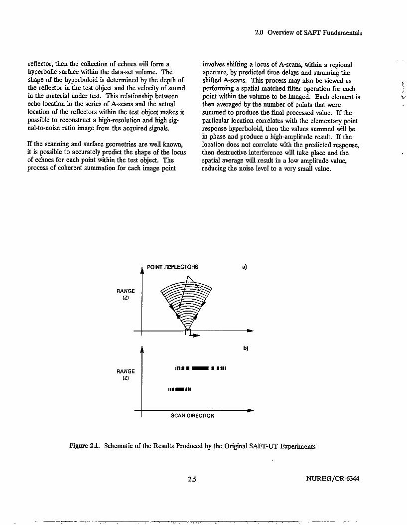
Original ultrasonic applications of SAFT followed di-rectly from the radar experience (Prine 1972; Burck-hardt, Grandchamp, and Hoffman 1974). Ultrasonicdata were recorded on photographic film by means of aphase reference or coherent demodulator. Such arecording procedure is diagrammed in Burckhardt,Grandchamp, and Hoffman (1974). The received sig-nals were amplified and mixed with a signal from areference source to provide a coherently demodulatedsignal used to modulate the intensity on the oscillo-scope. The output of the oscilloscope was recorded onfilm using a camera that was scanned in synchrony withthe scanning ultrasonic transducer. The results of sucha scanning procedure are illustrated conceptually inFigure 2.1. Figure 2.1(a) shows the plane to be imaged(including two point reflectors), the scanning ultrasonictransducer, and the divergent ultrasonic beam. Figure2.1(b) shows the data that were recorded on film. Inrange Z, the signals are highly confined. This rangeresolution, DZ, is determined by the bandwidth of theultrasonic pulse. In azimuth X, the indications from thetwo point targets are smeared laterally because of thedivergent beam used to collect the data; however, thesesmeared indications are modulated and appear as one-dimensional Fresnel zone plates. The phase variation isslow near the center of the indication and fast near theedges. The spatial frequency content of these indica-tions is directly related to the range of the point reflec-tor. This recorded data was processed optically by alaser and a series of lenses that allows refocusing of thisdata in the X direction only. The processed image wasthen recorded photographically.
Even though this mode of ultrasonic synthetic aperturefocusing has long since been outmoded, it does illus-trate a number of points inherent with SAFT:
2.1 NUREG/CR-6344
2.0 Overview of SAFT Fundamentals
• Imaging is a multiple-step process. Some kind ofcollection and storage scheme must be implement-ed to organize data for a subsequent reconstruc-tion process.
• The object being imaged must remain stationarywhile it is scanned.
• Range resolution is controlled primarily by thebandwidth of the insonifying pulse.
• Lateral resolution is controlled by the effectiveaperture. The effective aperture is limited by thedivergence of the insonifying ultrasonic beam, thedirectivity of the target, and the size of thescanned aperture.
• Lateral resolution can be independent of rangebecause points located at larger distances have alarger "effective aperture."
The first digital implementations of one-dimensionalSAFT processing in ultrasound soon followed theseinitial demonstrations. Digital SAFT processing wasdemonstrated in the area of nondestructive testing(NDT) by the University of Michigan (Frederick et al.1976) and in medical imaging at the Mayo Clinic(Johnson et al. 1975) recording, and coherent summa-tion to demonstrate the feasibility of digital SAFT. Themajor differences between the two demonstrations layin the data collection procedure. The NDT systemused a single, scanned, focused transducer to simulatean array of point sources and receivers. The medicalsystem used multiple-channel recording and an acousticarray for data collection. This method was used be-cause the medical system had to image moving objects;all the data had to be recorded before the objectsmoved an appreciable distance.
This need for high-speed data collection in medicalimaging has subsequently caused the SAFT imagingapproach to be abandoned in favor of phased-array andannular-array imaging techniques. In nondestructiveevaluation (NDE), the goals of high resolution andimaging system flexibility have far outweighed the dataacquisition speed requirements.
Research, sponsored primarily by the Nuclear Regulato-ry Commission, has been carried out at the Universityof Michigan (Frederick et al. 1976; Frederick et al.
1977; Frederick, VandenBroek, Elzinga et al. 1979;Frederick, VandenBroek, Ganapathy et al. 1979; Gana-pathy et al. 1981; Ganapathy, Wu, and Schmult 1982;Ganapathy and Schmult 1982; Ganapathy et al. 1983).In addition, cooperative programs have been carried outat the University of Missouri at Columbia (Seydel 1978;Hamano 1980) and at Southwest Research Institute(Jackson 1978a, 1978b, 1981). The original goal of thework at the University of Michigan was to demonstratethe feasibility of SAFT to "obtain improved resolutionwith respect to other NDT methods, and in this way toobtain a better idea of the size, shape, and orientationof a discontinuity in the pressure vessel or piping." Theinitial results demonstrated improved lateral and axialresolution with planar SAFT-UT applied to a series ofartificial defects (side-drilled holes) in aluminum testblocks. All of the initial work was performed withlongitudinal ultrasonic waves (Frederick, Seydel, andFairchild 1976).
The second year's work at the University of Michiganconcentrated primarily on extending the SAFT process-ing algorithm to three-dimensional data sets (Frederick,Fairchild, and Anderson 1977). This extension involvedfar-reaching changes in data collection, processing, anddisplay techniques.
During the third year of research (Frederick et al.1978), three-dimensional longitudinal-wave (L-wave)SAFT processing was demonstrated with natural andartificial defects in several series of test blocks. At thistime, the University of Michigan joined the Universityof Missouri at Columbia in a collaborative effort todevelop signal processing procedures that would yieldfurther improvements in axial flaw resolution and sup-pression of "front-surface ringdown."
Signal processing techniques studied intended to decon-volve the transducer impulse response for the reflectedultrasonic signal. Spectral division and linear predictivedeconvolution were two techniques successfully appliedto this problem. Linear predictive deconvolution wassuggested as a means for performing "real-time" decon-volution because it can be implemented in the timedomain as a recursive digital filter.
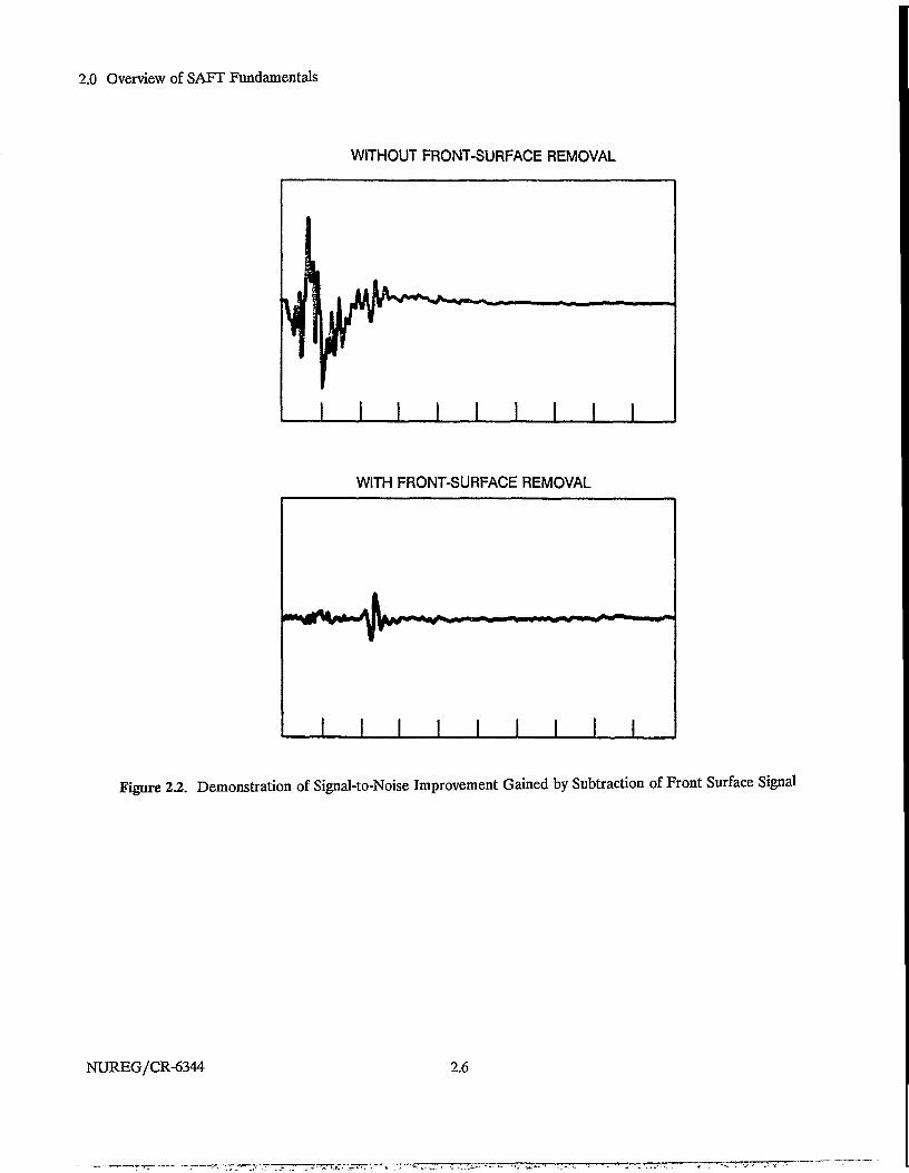
Also demonstrated was a digital subtraction techniquefor suppression of the large front-surface echo encoun-tered in L-wave SAFT. Figure 2.2 shows the benefits of
NUREG/CR-6344 2.2
2.0 Overview of SAFT Fundamentals
applying this technique. The raw A-scan shown inFigure 2.2(a) contains a large indication caused by theultrasonic signal reflected from the front surface of thetest block and from a small side-drilled hole located 4.6mm below the front surface. By subtracting only thefront-surface signal from Figure 2.2(a), it is possible toimprove the signal-to-noise ratio of the side-drilled holeindication as shown in Figure 2.2(b). Figure 2.3 showstwo SAFT-processed images derived from this type ofdata. Figure 2.3(a) shows the contour plot of a conven-tionally processed SAFT image. Figure 2.3(b) showsSAFT images produced from the same data; however,before processing, the front-surface echo was digitallysubtracted. With this sort of preprocessing of the rawradio frequency (rf) data, it appears possible to detectartificial defects within 2.0 mm of the top surface.
A significant effort during the final years of the pro-gram at the University of Michigan was the design anddevelopment of a special-purpose SAFT processor forreal-time operation. A processor was built and demon-strated by GARD, Inc. (Ganapathy et al. 1985). Thispioneering work in parallel processing established per-formance marks that proved that the SAFT processingcould be performed at rates making field implementa-tion a real-time process. However, the advances incomputer equipment and performance resulted in thedesign and fabrication of the PNL special-purposeprocessing using off-the-shelf boards. The successfulPNL SAFT real-time processor was a logical extensionof the work at the University of Michigan and GARD,Inc.
Starting in 1977, a "Program for the Field Validation ofSynthetic Aperture Focusing Technique for UltrasonicTesting" was undertaken at Southwest Research Insti-tute (SwRI) (Jackson 1978a and 1978b). The thrust ofthis program was to apply many of the techniques de-veloped by the University of Michigan group and toproduce a SAFT-UT system suitable for use during siteexamination of actual nuclear power reactors. Theinitial work performed by SwRI was aimed at improvingthe ultrasonics and electronics "front end" of the SAFT-UT system. A final report on all of the work per-formed by SwRI was published (Hamlin 1985), and thereader is referred to that report for all of the details.
Over the past twelve years, work has continued to im-prove SAFT-UT inspection systems for both field and
laboratory applications. The following list summarizesthe highlights of this work:
• Software was developed and implemented for per-forming SAFT-UT on specimens with regular sur-face topography; e.g., cylinders, planes not parallelto the scan plane.
• Software was developed and implemented for per-forming SAFT-UT on specimens with arbitrarysurface geometry.
• Software was developed to perform multi-depthfocusing and expanding aperture SAFT-UT.
• The focusing properties of SAFT-UT were numer-ically analyzed. The point spread function ofSAFT was studied as a function of aperture size,pulse attenuation, random position errors, pulsebandwidth, horizontal sample intervals, and front-surface variations.
• Advanced data presentation techniques were ana-lyzed. Perspective contour plotting, grey scale,color plotting, and interactive displays were con-sidered. Finally, a RAMTEK high-resolutiongraphics imaging display system was selected anda graphics/analysis utility was written.
• Processing needs, associated with performing real-time SAFT-UT, were analyzed. Commerciallyavailable computer systems and array processorswere analyzed and found to be either inadequateor too expensive for performing real-time SAFT-UT. The concept of a special-purpose, hardwareimplementation, SAFT processor was proposedand developed. However, this also was inade-quate (variations of the SAFT algorithm could notbe easily implemented) and a second real-timeprocessor was developed using a parallel proces-sor architecture. This second real-time processorutilized commercially available hardware and thesoftware could be easily modified to accommodatedifferent SAFT algorithms (pulse-echo, TSAFT,TSAFT-2, TSAFT-3).
• Special-purpose scanning head hardware has beendeveloped. Such hardware allows for high-speedscanning of arbitrary surfaces and allows for con-stant transducer offset. The scanning hardware
2.3 NUREG/CR-6344
2.0 Overview of SAFT Fundamentals
was further modified to accommodate multipletransducer configurations such as TSAFT-2 andTSAFT-3.
Tandem SAFT configurations were developed toovercome the ambiguities inherent in pulse-echo,single-transducer configurations. Further, a spe-cial tandem configuration (TSAFT-3) was devel-oped for thick-section materials such as reactorpressure vessels.
• Parametric studies were performed to study theeffects of errors in parameters used during SAFTprocessing. Included in these studies were effectsfrom assumptions made within the SAFT algo-rithm itself.
• The SAFT-UT field data acquisition system wasdeveloped and employed in the field during inser-vice inspections of operating reactors (Dresdenand Vermont Yankee) with subsequent data pro-cessing at PNL. Further, SAFT data was acquiredusing two different commercial data acquisitionsystems and subsequently processed and analyzedto characterize real defects in a reactor pressurevessel (Indian Point Unit II) and a static-caststainless steel elbow in the hot-leg of a reactor(Trojan Nuclear Power Plant).
• Advanced preprocessing techniques were devel-oped for anisotropic materials such as centrifugal-ly cast stainless steels.
Installation of the SAFT utilities on a VAX11/750 owned by Combustion Engineering (CE)constituted the first step in educating CE person-nel in the operation and inspection requirementsof SAFT. This step paved the way for field vali-dation testing.
• A real-time processor was built for Sandia Nation-al Laboratories and the SAFT utilities were in-stalled on a Micro-VAX computer, which wasdesignated as the host computer in the SandiaSAFT-UT system. This was the first attempt andtrial for technology transfer.
To summarize, much developmental research work hasbeen performed over the past twelve years to improveand implement SAFT-UT. Many of the basic questions
regarding the ultimate resolution and computationalcomplexity associated with performing SAFT-UT havebeen answered. Culmination of the SAFT program hasresulted in a real-time SAFT-UT field system and hand-in-hand work with commercial companies performingspecial inservice inspections on operating reactors.Transfer of the SAFT technology to the commercialsector has been a goal of the NRC. This goal has notbeen fully met, but the process has started.
2.2 Overview of SAFT Fundamentals
The reader is referred to Busse, Collins, and Doctor(1984); Frederick and Fairchild (1976); Frederick, Fair-child, Anderson (1977); Frederick, VandenBroek,Elzinga, et al. (1979); and Frederick, VandenBroek,Ganapathy, et al. (1979) for extensive details on SAFTfundamentals. The following is a brief overview of theSAFT process and why it leads to significant improve-ment in full-volume imaging. SAFT relies on the phys-ics of ultrasonic wave propagation and thus is a veryrobust technique.
Synthetic aperture focusing refers to a process in whichthe focal properties of a large-aperture focused trans-ducer are synthetically generated from data collectedover a large area using a small transducer with a diver-gent sound field. The processing required to focus thiscollection of data has been called beam-forming, coher-ent summation, or synthetic aperture processing.
Inherently, SAFT has an advantage over physical focus-ing techniques in that the resulting image is a full-vol-ume focused characterization of the inspected area.Traditional physical focusing techniques provide focuseddata only at the depth of focus of the lens. For thetypical pulse-echo data collection scheme used withSAFT-UT, a focused transducer is positioned with thefocal point located at. the surface of the part to beinspected. This configuration is used to produce abroad, divergent ultrasonic beam in the object undertest. Alternatively, a small-diameter contact transducermay be used to generate a divergent beam in the speci-men material. As the transducer is scanned over thesurface of the object, the A-scan record (rf waveform)is digitized for each position of the transducer. Eachreflector produces a collection of echoes in the A-scanrecords. If the reflector is an elementary single point
NUREG/CR-6344 2.4
2.0 Overview of SAFT Fundamentals
reflector, then the collection of echoes will form ahyperbolic surface within the data-set volume. Theshape of the hyperboloid is determined by the depth ofthe reflector in the test object and the velocity of soundin the material under test. This relationship betweenecho location in the series of A-scans and the actuallocation of the reflectors within the test object makes itpossible to reconstruct a high-resolution and high sig-nal-to-noise ratio image from the acquired signals.
If the scanning and surface geometries are well known,it is possible to accurately predict the shape of the locusof echoes for each point within the test object. Theprocess of coherent summation for each image point
involves shifting a locus of A-scans, within a regionalaperture, by predicted time delays and summing theshifted A-scans. This process may also be viewed asperforming a spatial matched filter operation for eachpoint within the volume to be imaged. Each element isthen averaged by the number of points that weresummed to produce the final processed value. If theparticular location correlates with the elementary pointresponse hyperboloid, then the values summed will bein phase and produce a high-amplitude result. If thelocation does not correlate with the predicted response,then destructive interference will take place and thespatial average will result in a low amplitude value,reducing the noise level to a very small value.
POINT REFLECTORS
RANGE(Z)
inia
mi • • in
• mi
SCAN DIRECTION
Figure 2.1. Schematic of the Results Produced by the Original SAFT-UT Experiments
2.5 NUREG/CR-6344
2.0 Overview of SAFT Fundamentals
WITHOUT FRONT-SURFACE REMOVAL
WITH FRONT-SURFACE REMOVAL
Figure 22. Demonstration of Signal-to-Noise Improvement Gained by Subtraction of Front Surface Signal
NUREG/CR-6344 2.6
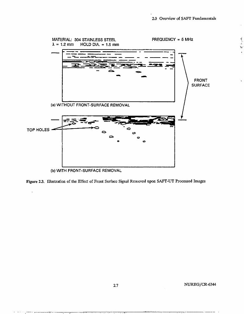
MATERIAL: 304 STAINLESS STEELA. = 1.2 mm HOLD DIA. = 1.5 mm
2.0 Overview of SAFT Fundamentals
FREQUENCY = 5 MHz
FRONTSURFACE
(a) WITHOUT FRONT-SURFACE REMOVAL
TOP HOLES - * " ^ - oc
" o
©
mmmm
35So
oo
(b) WITH FRONT-SURFACE REMOVAL
Figure 23. Illustration of the Effect of Front Surface Signal Removed upon SAFT-UT Processed Images
2.7 NUREG/CR-6344
3.0 Where to Go for Additional Information
Section 3 provides the reader with a complete biblio-graphical listing of all NRC publications and selectedother relevant publications concerning the SAFT tech-nology. This listing includes all the documents writtenby the University of Michigan and PNL. This sectionalso provides synopses of key publications for readerswho may have only the SAFT final report at their dis-posal.
3.1 Bibliography
A comprehensive, but certainly not complete, biblio-graphical listing is provided to readers interested infurther pursuing the SAFT technology.
Barna, B. A., and J. A. Johnson. 1981. "The Effects ofSurface Mapping Corrections and Synthetic Aper-ture Focusing Techniques on Ultrasonic Images."EGG-FM-5314, EG&G Idaho, Inc., Idaho Falls,ID.
Barna, B. A., and J. A. Johnson. 1982. "The Effects ofSurface Mapping Corrections with Synthetic Aper-ture Focusing Techniques on Ultrasonic Imaging,"in Review of Progress in Quantitative NDE, eds. D.O. Thompson and D. E. Chimenti, p. 753. Ple-num Press, New York, NY.
Berkhout, A. V., J. Ridder, and F. L. V. d. Wai. 1980."Acoustic Imaging by Wave Field Extrapolation,Part I: Theoretical Considerations," in AcousticalImaging, Vol. 10, eds. P. Alais and A. F. Methe-rell. Plenum Press, New York, NY.
Bracewell, R. N. 1978. The Fourier Transform and ItsApplication. Second edition, Chapter 12.McGraw-Hill, New York, NY.
Burckhardt, C. B., P. A. Grandchamp, and H. Hoff-mann. 1974. "Methods for Increasing the LateralResolution of B-Scan," in Acoustical Imaging, Vol.5, ed. P. S. Green. Plenum Press, New York, NY.
Busse, L. J., H. D. Collins, and S. R. Doctor. 1984."The Emerging Technology of Synthetic ApertureFocusing for Ultrasonic Testing," presented at1984 Pressure Vessel and Piping Conference, SanAntonio, Texas, 84-PUD-122, June 18-20, 1984.
Busse, L. J., H. D. Collins, and S. R. Doctor. 1984.Review and Discussion of the Development of Syn-thetic Aperture Focusing Technique for UltrasonicTesting (SAFT-UT). NUREG/CR-3625, PNL-4957. Pacific Northwest Laboratory, Richland,WA.
Collins, H. D., and B. P. Hildebrand. 1972. "The Ef-fects of Scanning Position and Motion Errors onHologram Resolution," in. Acoustical Imaging, Vol.4, ed. G. Wade. Plenum Press, New York, NY.
Collins, H. D., L. J. Busse, and D. K. Lemon. 1982."Acoustic Emission Linear Pulse Holography."Ultrasonics Symposium Proceedings, Cat.#82CH1823-4, Institute of Electrical and Elec-tronics Engineers, Piscataway, NJ.
Corl, P. D., G. S. Kino, C. S. DeSilets, and P. M.Grant. 1980a. "A Digital Synthetic Focus Acous-tic Imaging System," in Acoustical Imaging, Vol. 8,ed. A. F. Metherell. Plenum Press, New York,NY.
Corl, P. D., and G. S. Kino. 1980b. "A Real-Time Syn-thetic-Aperture Imaging System," in AcousticalImaging, Vol. 9, ed. K. Y. Wang. Plenum Press,New York, NY.
Doctor, S. R., L. J. Busse, S. L. Crawford, T. E. Hall,R. P. Gribble, A. J. Baldwin, and L. P. VanHouten. 1986. Development and Validation of aReal-Time SAFT-UT System for the Inspection ofLight Water Reactor Components, Semi-annualReport, April 1984 to September 1984.NUREG/CR-4583, PNL-5822, Vol. 1. PacificNorthwest Laboratory, Richland, WA.
Doctor, S. R., T. E. Hall, L. D. Reid, S. L. Crawford,R. J. Littlefield, R. W. Gilbert. 1987. Develop-ment and Validation of a Real-Time SAFT-UTSystem for the Inspection of Light Water ReactorComponents, Annual Report, October 1984 toSeptember 1985. NUREG/CR-4583, PNL-5822,Vol. 2. Pacific Northwest Laboratory, Richland,WA.
Doctor, S. R., T. E. Hall, L. D. Reid, G. A. Mart.1987. Development and Validation of a Real-TimeSAFT-UT System for the Inspection of Light Water
3.1 NUREG/CR-6344
3.0 Additional Information
Reactor Components, Annual Report, October1985 to September 1986. NUREG/CR-4583,PNL-5822, Vol. 3. Pacific Northwest Laboratory,Richland, WA.
Doctor, S. R., L. J. Busse, and H. D. Collins. 1983."The SAFT-UT Technology Evolution," in 6thInternational Conference on NDE in the NuclearIndustry, pp. 145-151. Zurich, Switzerland, No-vember 28-December 2, 1983.
Doctor, S. R., L. J. Busse, and H. D. Coffins. 1984."Development and Validation of a Real-TimeSAFT-UT System for Inservice Inspection ofLWRs," Proc. of the U.S. NRC Eleventh WaterReactor Safety Research Information Meeting, Vol.4, NUREG/CP-0048, pp. 65-80. U.S. NuclearRegulatory Commission, Washington, D.C.
Doctor, S. R., H. D. Coffins, L. P. Van Houten, S. L.Crawford, T. E. Hall, A. J. Baldwin, R. E. Bowey,and R. P. Gribble. 1985. "Development and Vali-dation of a Real-Time SAFT-UT System forInservice Inspection of LWRs," Proc. of the U.S.NRC Twelfth Water Reactor Safety Research Infor-mation Meeting, Vol. 4, NUREG/CP-0058, pp.319-341. U.S. Nuclear Regulatory Commission,Washington, D.C.
Doctor, S. R., A. J. Baldwin, L. J. Busse, H. D. Collins,5. L. Crawford, and L. P. Van Houten. 1985."SAFT-UT for Stainless Steel Pipe Inspection,"Proc. of the 7th International Conference on NDEin the Nuclear Industry, Grenoble, France, January28-February 1, 1985.
Doctor, S. R., S. L. Crawford, T. E. Hall, and L. D.Reid. 1985. "SAFT Imaging in the TandemMode - TSAFT," ASNT Topical Meeting on Digi-tal Signal Acquisition and Processing, Dallas,Texas, May 14-16, 1985.
Doctor, S. R., L. J. Busse, H. D. Collins, S. L. Craw-ford, and L. P. Van Houten. 1985. "Developmentand Validation of a Real-Time,SAFT-UT Systemfor Inservice Inspection of LWRs," Nuclear Engi-neering and Design, Vol. 86, pages 31-38, NorthHolland, Amsterdam.
Doctor, S. R., S. L. Crawford, and T. E. Hall. 1985."SAFT-UT Field Experience," presented at 1985Pressure Vessel and Piping Conference, New Or-leans, Louisiana, PVP-Vol. 98-1, pp. 203-210, June22-26, 1985.
Doctor, S. R., T. E. Hall, S. L. Crawford, and L. P. VanHouten. 1985. "Advanced Ultrasonic Imaging ofPipes in Dresden and Vermont Yankee Reactors,"8th International Conference on Structural Me-chanics in Reactor Technology, Vol. C-D, August19-23, 1985.
Doctor, S. R., T. E. Hall, and L. D. Reid. June 1986."SAFT ~ The Evolution of a Signal ProcessingTechnology for Ultrasonic Testing," NDT Inter-national, Vol. 19, No. 3, pp. 163-167.
Doctor, S. R., T. E. Hall, L. D. Reid, and G. A. Mart.1986. "Application of Real-Time 3-D SAFT in theTandem Mode," PNL-SA-14328, presented at theMPA Seminar, Stuttgart, West Germany, October10, 1986.
Doctor, S. R., T. E. Hall, L. D. Reid, G. A. Mart, R.Littlefield, and R. Gilbert. 1986. "Developmentand Validation of a Real-Time SAFT-UT Systemfor Inservice Inspection of LWRs," Proc. of Four-teenth Water Reactor Safety Information Meeting,Gaithersburg, Maryland, October 27-31, 1986, pp.19-41.
Doctor, S. R., T. E. Hall, and L. D. Reid. 1986. "Real-Time SAFT-UT for Nuclear Component Inspec-tion," presented at the 8th International Confer-ence on NDE in the Nuclear Industry, Orlando,Florida, November 17-20, 1986.
Doctor, S. R., T. E. Hall, L. D. Reid, and G. A. Mart.1987. Development and Validation of a Real-TimeSAFT-UT System for the Inspection of Light WaterReactor Components, Annual Report, October1985-September 1986. NUREG/CR-4583, PNL-5822, Vol. 3, Pacific Northwest Laboratory, Rich-land, WA.
Doctor, S. R., T. E. Hall, and L. D. Reid. 1988. TheSAFT-UT Real-Time Inspection System Operation-al Principles and Implementation. NUREG/CR-
NUREG/CR-6344 3.2
3.0 Additional Information
5075, PNL-6413, Pacific Northwest Laboratory,Richland, WA.
Frederick, J. R., J. A. Seydel, and R. C. Fairchild.1976. Improved Ultrasonic Non-Destructive Testingof Pressure Vessels. NUREG-0007-1, University ofMichigan, Ann Arbor, MI.
Frederick, J. R., R. C. Fairchild, and B. H. Anderson.1977. Improved Ultrasonic Nondestructive Testingof Pressure Vessels. NUREG-0007-2, University ofMichigan, Ann Arbor, MI.
Frederick, J. R., C. VandenBroek, R. C. Fairchild, andM. B. Elzinga. 1978. Improved Ultrasonic Nonde-structive Testing of Pressure Vessels.NUREG/CR-0135, University of Michigan, AnnArbor, MI. '
Frederick, J. R., C. VandenBroek, M. Elzinga, M.Dixon, D. Papworth, N. Hamano, and K. Gana-pathy. 1979. Improved Ultrasonic NondestructiveTesting of Pressure Vessels. NUREG/CR-0581,University of Michigan, Ann Arbor, MI.
Frederick, J. R., C. VandenBroek, S. Ganapathy, M.Elzinga, W. DeVries, D. Papworth, and N.Hamano. 1979. Improved Ultrasonic Nondestruc-tive Testing of Pressure Vessels. NUREG/CR-0909, University of Michigan, Ann Arbor, MI.
Ganapathy, S. N. Hamano, M. R. Bether, W. S. Wu, T.G. Dennehy, C. Purnaveja, M. M. Murray, M. B.Elzinga, and F. Raam. 1981. Ultrasonic ImagingTechniques for Real-time In-service Inspection ofNuclear Power Reactors. NUREG/CR-2154, Uni-versity of Michigan, Ann Arbor, MI.
Ganapathy, S., W. S. Wu, and B. Schmult. 1982."Analysis and Design Considerations for a Real-Time System for Nondestructive Evaluation in theNuclear Industry." Ultrasonics 20:249.
Ganapathy, S., and B. Schmult. 1982. "Design of aReal-time Inspection System for NDE of ReactorVessels and Piping Components." Presented at IMECH E Conference, London, England. IMECH E 1982-9.
Ganapathy, S., B. Schmult, W. S. Wu, N. Hamano, andD. Bristor. 1983. Investigation of Special PurposeProcessors for Real-Time Synthetic Aperture Focus-ing Techniques for Nondestructive Evaluation ofNuclear Reactor Vessels and Piping Components.NUREG/CR-2703, University of Michigan, AnnArbor, MI.
Ganapathy, S., B. Schmult, W. S. Wu, T. G. Dennehy,N. Moayeri, and P. Kelly. 1985 Design and De-velopment of a Special Purpose SAFT System forNondestructive Evaluation of Nuclear Reactor Ves-sels and Piping Components, NUREG/CR-4365,U.S. Nuclear Regulatory Commission, Washing-ton, D.C.
Gehlbach, S. M., and R. E. Alvarez. 1981. "DigitalUltrasound Imaging Techniques using VectorSampling and Raster Line Reconstruction." Ultra-sonic Imaging 3:83.
Hall, T. E., S. R. Doctor, and L. D. Reid. 1987. "AReal-Time SAFT System Applied to the Ultrason-ic Inspection of Nuclear Reactor Components,"Review of Progress in Quantitative NondestructiveEvaluation, Vol. 6A, pp. 509-517. Plenum Press,NY.
Hall, T. E., S. R. Doctor, L. D. Reid, R. J. Littlefield,and R. W. Gilbert. 1987. "Implementation of aReal-Time Ultrasonic SAFT System for Inspectionof Nuclear Reactor Components," Acoustical Im-aging, Vol. 15, pp. 253-266. Plenum Press, NY,
Hall, T. E., L. D. Reid, and S. R. Doctor. 1988. TheSAFT-UT Real-Time Inspection System-Operation-al Principles and Implementation. NUREG/CR-5075, PNL-6413, Pacific Northwest Laboratory,Richland, WA.
Hamano, N. 1980. "Deconvolution of Ultrasonic Non-destructive Testing Data." PhD Dissertation,Electrical Engineering Dept. University of Mis-souri, Columbia, MO.
Hamlin,D. R. 1985. Program for Field Validation ofthe Synthetic Aperture Focusing Technique for Ul-trasonic Testing (SAFT-UT). NUREG/CR-4078,Southwest Research Institute.
3.3 NUREG/CR-6344
3.0 Additional Information
Herman, G. T., H. K. Tuy, K J. Langenberg, and P. C.Sabatter. 1987. Basic Methods of Tomographyand Inverse Problems. Melvern Physics Series.IOP Publishing Ltd. Bristol, England.
Highmore, P. J., A. J. Willets and P. Clough. 1982."Circe - A Versatile Ultrasonic Digital Data Re-cording, Analysis, and Display System," in IMECH E Conference Proceedings, C154/82:209.
Hildebrand, B. P., and K A. Haines. 1969. "Hologra-phy by Scanning." /. Opt. Soc. Am. 59(1):1.
Hildebrand, B. P., and B. B. Brenden. 1972. An Intro-duction to Acoustical Holography. Plenum Press,New York, NY.
Jackson, J. L. 1978a. Program for Field Validation ofthe Synthetic Aperture Focusing Technique for Ul-trasonic Testing (SAFT-UT) -Analysis Before Test.NUREG/CR-0288, Southwest Research Institute.
Jackson, J. L. 1978b. Program for Field Validation ofthe Synthetic Aperture Focusing Technique for Ul-trasonic Testing (SAFT-UT) Midyear Progress Re-port. NUREG/CR-0290, Southwest ResearchInstitute.
Jackson, J. L. 1981. Program for Field Validation of theSynthetic Aperture Focusing Technique for Ultra-sonic Testing (SAFT-UT). NUREG/CR-1885,Vol. 1, 2, and 3, Southwest Research Institute.
Johnson, S. A., J. F. Greenleaf, F. A. Duck, A. Chu, W.R. Samayou, and B. K. Gilbert. 1975. "DigitalComputer Simulation Study of a Real-Time Col-lection, Post-Processing Synthetic Focusing Ultra-sound Cardiac Camera," in Acoustical Holography,Vol. 6, ed. N. Booth. Plenum Press, New York,NY.
Johnson, S. A., and J. F. Greenleaf. 1979. "New Ultra-sound and Related Imaging Techniques." Trans-actions on Nuclear Science NS-26:8212. IEEE.
Johnson, J. A. 1982. "Parameter Study of Synthetic-Aperture Focusing in Ultrasonics," in Review ofProgress in Quantitative NDE, eds. D. O. Thomp-
son and D. E. Chimenti. Plenum Press, NewYork, NY.
Kino, G. S., D. Corl, S. Bennett, and K. Peterson.1980. "Real Time Synthetic Aperture ImagingSystem." Ultrasonics Symposium Proceedings,Cat. #80CHJ1602-2SU, IEEE.
Kupperman, D. S., et al. 1982. "Light-Water-ReactorSafety Research Program: Quarterly Progress Re-port." Nuclear Regulatory Commission ReportNUREG/CR-2970, Vol. 1; 2-15.
Moore, M. J., and F. J. Dodd. 1982. "Real-Time Sig-nal Processing in an Ultrasonic Imaging System."Materials Evaluation 40:976.
Murgatroyd, R. A. 1982. "Automated Defect Locationand Sizing by Advanced Ultrasonic Techniques,"in Proceedings of Quantitative NDE in the Nucle-ar Industry, 82-74019:243.
Norton, S. J. 1976. "Theory of Acoustic Imaging."Stanford Technical Report No. 4956-2.
Peterson, D. K., S. D. Bennett, and G. S. Kino. 1981."Real Time Digital Imaging." Ultrasonic Sympo-sium Proceedings, Cat. #81CH1689-9SU. IEEE.
Polky, J. N., and D. D. Miller. 1985. An Ultra-HighSpeed Residue Processor for SAFT Inspection Sys-tem Image Enhancement. NUREG/CR-4170,Sigma Research Inc., Redmond, WA.
Polky, J. N. 1986. Development of a Real-Time ResidueNumber Processor for SAFT Inspection.NUREG/CR-4634, Sigma Research Inc., Red-mond, WA.
Prine, D. W. 1972. "Synthetic Aperture Ultrasonic Im-aging," in Proceedings of the Engineering Appli-cations of Holography Symposium:287. Society ofPhoto-optical Instrumentation Engineers.
Ridder, J., A. J. Berkhout, and L. F. v.d. Wai. 1980."Acoustic Imaging by Wave Field Extrapolation,Part II: Practical Considerations," in AcousticalImaging, Vol. 10, eds. P. Alais and A. F. Mether-ell. Plenum Press, New York, NY.
NUREG/CR-6344 3.4
3.0 Additional Information
Schafer, G., V. Schmitz, and W. Muller. 1983. "Com-parison of Different Signal Averaging Methods toImprove SNR for the NDT of Coarse GrainedMaterials." Nondestructive Testing Communica-tions. Gordon & Breach Science Publishers, NewYork, London, Paris.
Schmitz, V., W. Muller, and G. Schafer. 1982. "A NewUltrasonic Imaging System." Materials Evaluation40:101.
Schmitz, V., W. Muller, and G. Schafer. 1983. "Classi-fication and Reconstruction of Defects by Com-bined Acoustical Holography and Line-SAFT," inProceedings of the Germany-United States Work-shop on Research and Development of New Pro-cedures in NDT. Springer Verlag.
Schmitz, V., O. A. Barbian, and W. Gebhardt. 1983."Defect Assessment by Ultrasonic Testing," inMeasurement and Characterization of Weld Defects-A Critical Appraisal of Nondestructive Testing bythe British Welding Institute, Cambridge CB16AL England.
Seydel, J. A. 1978. (Signal Processing) Methods Devel-opment. NUREG/CR-0135, University of Mis-souri, Columbia.
VandenBroek, C, M. B. Elzinga, J. R. Frederick, andS. Ganapathy. November 1980. "Synthetic Aper-ture Ultrasonic Imaging in Metals." NationalBureau of Standards Special Publication 596.Ultrasonic Materials Characterization: 249.
3.2 Synopses of Key SAFT Documents
For readers who may have only the "SAFT Final Re-port" at their disposal, synopses of key SAFT docu-ments have been assembled. These synopses are in-tended to give an overview of past information pub-lished about the SAFT technology. For more detailedinformation, readers should acquire the particular docu-ments desired.
3.2.1 Review and Discussion of the Devel-opment of Synthetic Aperture Focusing Tech-nique (SAFT-UT) (Busse, Collins, and Doctor1984)
The synthetic aperture focusing technique for ultrasonictesting (SAFT-UT) is an ultrasonic imaging techniquedesigned to enhance the performance of conventionalultrasonic, nondestructive testing procedures for per-forming two basic functions: 1) detection of flaws anddefects within structural and functional components;and 2) classification and/or characterization of thesedetected defects in terms of size, shape, orientation,location, and composition. This enhanced performanceis brought about by a high-resolution ultrasonic image,which is the output of the SAFT process. SAFT-UT isa particularly flexible imaging method that can beadapted to many different materials, specimen geome-tries, and propagation modes. SAFT-UT is accom-plished by applying a signal processing algorithm to acollection of raw amplitude versus time data (A-scans).The algorithm allows each point within the inspectedvolume to be focused upon by mathematically simulat-ing the action of a lens specifically formed for imagingthat point in the volume. This method of image forma-tion permits each of the points to be imaged at themaximum available resolution. The images producedare volumetric; i.e., they provide a three-dimensionalmap of any defect and the surrounding area. Such amap can be accurately interpreted.
Many aspects of SAFT-UT are treated in this report:
Historical Background of SAFT-UT
Theory of SAFT-UT
• Implementation of and Results Using SAFT.
From the results presented, it appears that SAFT-UThas been truly successful in providing a flexible high-resolution imaging system for the laboratory environ-ment. This method of imaging appears to be ideal forthe inspection of critical industrial components, espe-cially in the nuclear power industry.
The application of SAFT-UT imaging methods to field-testing of reactor piping, pressure vessels, and nozzlesappears to be a feasible and highly desirable extension
3.5 NUREG/CR-6344
3.0 Additional Information
of the basic research carried out so far. With the de-velopment of a special-purpose, real-time SAFT proces-sor, this transfer of defect detection/imaging technologyfrom the laboratory to the field appears to be bothpractical and feasible.
3.2.2 Development and Validation of a Real-lime SAFT-UT System for the Inspection ofLight Water Reactor Components, Vol. 1(Doctor et al. 1986)
A three-year program for the Development and Valida-tion of a Real-Time SAFT-UT System for InserviceInspection of Light Water Reactors was established atPNL to develop SAFT and demonstrate the technologyin reactor inservice inspections.
The objectives of this NRC program include these:
• Design, fabricate, and evaluate a real-timeflaw detection and characterization systembased on SAFT-UT for inservice inspection(ISI) of all required light water reactor(LWR) components.
• Establish calibration and field operatingprocedures.
• Demonstrate and validate the SAFT-UT sys-tem through actual reactor inservice inspec-tions.
• Generate an engineering data base to sup-port ASME Code acceptance of the real-time SAFT-UT technology.
The scope of the program is defined by the following:
• Conduct laboratory tests to provide engi-neering data for defining SAFT-UT systemperformance.
• Complete the development of a special pro-cessor to make SAFT a real-time process forISI applications.
• Fabricate and field-test a real-time SAFT-UT system suitable for field inspection of
nuclear reactor piping, nozzles, and pressurevessels.
Ongoing work is advancing the evolution of the SAFT-UT field system from concept to reality. The final sys-tem was operational by the end of fiscal year 1985.Reported here are a system overview, optimization offront-end electronics, and procurement of hardware forthe final system configuration.
In demonstration tests, a special-purpose SAFT proces-sor being designed by General American Research andDevelopment, Incorporated, met its speed requirementfor real-time operation. However, because the hard-wired system was intended to implement pulse-echomode only, it could not be easily changed to accommo-date other algorithms, e.g., Tandem SAFT. Also, rede-sign was needed to produce a reliable unit suitable forfield work because the first version had been intendedonly for laboratory demonstration of the concept. PNLproposed a new design based on commercial hardware.
The theory of pulse-echo operation is described hereand extended to cover the tandem mode of operation.The tandem mode was developed to image verticallyoriented defects by overcoming the ambiguities of cor-ner-trap pulse-echo data. Laboratory experiments wereconducted to begin refinement of criteria to be used forsizing vertically oriented defects for both modes ofoperation.
SAFT data were obtained from several examinations ofmaterial samples and piping welds in the field. Samplesincluded a specimen provided by Southwest ResearchInstitute from the Duane Arnold reactor, a thick sectionof steel plate with induced defects examined by RisleyNuclear Laboratory, and plate 2 of the PISC II pro-gram. The field welds included four at the DresdenUnit 3 power plant and nine at the Vermont Yankeepower plant. Analyses of these data are presented.
Several changes were made in the SAFT processingscheme to speed up the processing of ultrasonic datafor SAFT analysis. The changes included optimizationof the SAFT algorithm on the VAX 11/780 computer,selective processing, acceleration of the envelope detec-tion algorithm, and conversion of SAFT software fromthe UNIX implementation of the C language toVAX/VMS C.
NUREG/CR-6344 3.6
3.0 Additional Information
3.2.3 Development and Validation of a Real-Time SAFT-UT System for the Inspection ofLight Water Reactor Components, Vol. 2(Doctor et al. 1987a)
A multiyear program for the Development and Valida-tion of a Real-Time SAFT-UT System for InserviceInspection of Light Water Reactors was established atPNL to develop the synthetic aperture focusing tech-nique (SAFT) and demonstrate the technology in reac-tor inservice inspections.
The objectives of this program for the NRC includethese:
• Design, fabricate, and evaluate a real-timeflaw detection and characterization systembased on SAFT-UT for ISI of all requiredLWR components.
• Establish calibration and field operatingprocedures.
• Demonstrate and validate the SAFT-UT sys-tem through actual reactor inservice inspec-tions.
• Generate an engineering data base to sup-port ASME Code acceptance of the real-time SAFT-UT technology.
The scope of the program is defined by the following:
• Conduct laboratory tests to provide engi-neering data for defining SAFT-UT systemperformance.
• Complete the development of a special pro-cessor to make SAFT a real-time process forISI applications.
• Fabricate and field test a real-time SAFT-UT system suitable for field inspection ofnuclear reactor piping, nozzles, and pressurevessels.
Ongoing work is advancing the evolution of the SAFT-UT field system from concept to reality. The final sys-tem was operational by the end of the fiscal year 1985,
and its features are described in terms of operator-oriented software designed to minimize operator com-puter skill requirements. Features such as transducerview, compare, B-scan, C-scan, and enlarge aredescribed.
The modes of signal processing with the emphasis onthe implementation of the tandem SAFT mode aredescribed. Examples, where image ambiguity isreduced, are presented. Processing speed-up routines,including selective processing and envelope detection,are described and performance is demonstrated.
The real-time SAFT processor box using the 68000family of microprocessor is described and performancematrices presented for this design versus the VAX11/780 and VAX 11/730 for both thin material (pipe)and thick material (pressure vessel) files. This designapproach clearly provides the processor speed necessaryto achieve real-time SAFT operation.
The field experience consisted of taking the SAFT-UTsystem to Commonwealth Edison and demonstratingfor the first time in-field processing of SAFT data on anarrow-gap pipe weldment containing fabrication flaws.
A detailed analysis was conducted on PISC II Plate 2data and compared to other PISC II team performanc-es. This block was the first out of laboratory testing onthe SAFT-UT data acquisition system with subsequentPNL processing of the data. Many things were learnedabout how to develop procedures to reduce potentialinspection errors. The SAFT results were very goodunder the circumstances and were better than the glob-al average and average of the advanced teams. Thedata clearly shows that image sizing criteria must beapplied as a systematic function of defect type (i.e.,planar versus volumetric); otherwise, consistent over- orunder-sizing will result. For the data presented, a loss-of-signal criterion was applied resulting in an over-sizingtrend.
Data was collected on a series of 15 centrifugally caststainless steel weldments that are part of a round robinbeing conducted under PISC II. The data collectionmethods are described, but no analysis was performedon the data during this reporting period.
3.7 NUREG/CR-6344
3.0 Additional Information
3.2.4 Development and Validation of a Real-Time SAFT-UT System for the Inspection ofLight Water Reactor Components, Vol. 3(Doctor et al. 1987b)
A multiyear program for the Development and Valida-tion of a Real-Time SAFT-UT System for InserviceInspection of Light Water Reactors was established atthe Pacific Northwest Laboratory (PNL) to develop thesynthetic aperture focusing technique (SAFT) and dem-onstrate the technology in reactor inservice inspections.
The objectives of this program for the Nuclear Regula-tory Commission (NRC) include these:
• Design, fabricate, and evaluate a real-time flawdetection and characterization system based onSAFT-UT for inservice inspection (1ST) of all re-quired LWR components.
• Establish calibration and field operating proce-dures.
• Demonstrate and validate the SAFT-UT systemthrough actual reactor inservice inspections.
• Generate an engineering data base to supportASME Code acceptance of the real-time SAFT-UT technology.
The scope of the program is defined by the following:
• Conduct laboratory tests to provide engineeringdata for defining SAFT-UT system performance.
• Complete the development of a special processorto make SAFT a real-time process for ISI applica-tions.
Fabricate and field test a real-time SAFT-UT sys-tem suitable for field inspection of nuclear reactorpiping, nozzles, and pressure vessels.
During this year, a formal agreement was put in placewith Combustion Engineering in which they joined theprogram and began assisting in validating the SAFTtechnology on nuclear power plants.
Ongoing work is focused on advancing the evolution ofthe SAFT-UT field system from concept to reality. Thefinal field system was operational by the end of fiscalyear 1985; and the emphasis this past year has been interms of parametric sensitivity studies on operationalparameters, further development of the real-time SAFTprocessor box, and detailed analysis of a number of de-fected samples.
The tandem SAFT mode was developed in 1985 toovercome some of the serious shortcomings of thepulse-echo mode. This first implementation of theTSAFT mode was developed by using a fixed sourceand scanned receiver. During this year, the TSAFT-2mode was developed, which uses a scanned source andscanned receiver. The performance of the TSAFT-2mode is clearly superior and allows defects with depthlarger than the transducer beam diameter to be sizedaccurately and shows an improvement of the resolutionperformance.
Extensive efforts were expended to conduct parametricstudies on the sensitivity of the SAFT-UT system tosome of the processing variables. The variables studiedduring this reporting period included: pulse-echo sam-pling rate, 3-D SAFT mode versus the Line-SAFTmode, TSAFT velocity changes of up to ±20%, TSAFTthickness changes of up to ±20%, TSAFT resolutionperformance, imaging of nonvertical defects, and per-formance of TSAFT and TSAFT-2 for accurately sizingvertical defects. The SAFT-UT system performed aspredicted based on theory. As the sampling rate in-creased, the imaging resolution improved until twice theNyquist sampling rate was achieved. The resolutionperformance of the 3-D SAFT mode was shown to bevery superior to the results for Line-SAFT for reflectorsexhibiting high spatial frequencies. The surprisingresult for changes in velocity and thickness was to havea large shift in the defect location and a minor blurringor resolution loss in the image. The SAFT-UT systemperformance deteriorated the same as other acousticmethods because of signal loss when defects becamenon-vertical and scattered the acoustic energy outsidethe receiver aperture. The changes are documentedand predictable from simple acoustic scattering theory.The superiority of the TSAFT-2 mode over the originalTSAFT configuration was demonstrated through aseries of sawcut sizing measurements showing the in-crease in resolution performance by a factor of 1.4.
NUREG/CR-6344 3.8
3.0 Additional Information
The evolution of the real-time SAFT processor box iscontinuing, and further studies of the performance isshowing that the real-time rates of ten A-scans persecond can be achieved when the new 68020 micropro-cessor boards are used.
Some very good studies were performed in the labora-tory on blocks and pipe specimens from a number ofsources. The SAFT performance was very good andwas within predictions for the apertures that the speci-mens allowed. TSAFT-2 was shown to provideimproved near-surface performance over pulse-echo onthe NAVSEA block. The large-diameter pipes in theMaterials Reliability Center at PNL were examined andmuch was learned about refining the SAFT procedureto minimize efforts during the data collection phase.Furthermore, it was found that if the electronics satu-rate, the resultant image will be blurred and result insystematic oversizing of the defect. Data were collectedon a series of KAPL specimens, and the images weregood although no feedback has been received on theSAFT result versus the destructive results or even in-tended defects. Results were obtained on a series ofCCSS specimens and all thermal fatigue cracks in thespecimens were detected; but at the same time, a num-ber of false calls were made. The false calls resultfrom the coherent backscattering that is produced bythe large anisotropic grain structure. Data were alsocollected on a series of 45 quadrants of pipe specimensthat are part of the Mini-Round Robin study in prog-ress at PNL. These data were analyzed and has notbeen compared with true-state destructive results. Thisis planned for next fiscal year.
3.2.5 The SAFT-UT Real-Time InspectionSystem Operational Principles and Imple-mentation (Hall, Reid, and Doctor 1988)
A multiyear program for the Development and Valida-tion of a Real-Time SAFT-UT System for Inspection ofLight Water Reactors was established at the PacificNorthwest Laboratory (PNL) to develop the syntheticaperture focusing technique (SAFT) and demonstratethis advanced imaging technology in reactor inserviceinspections. The developed system presents a visualimage of ultrasonic indications from reflectors locatedin piping and pressure vessels of nuclear reactors. Asignificant portion of the effort at PNL was orientedtoward building a system based on SAFT technology
that is transportable to field environments, and provideson-the-spot (real-time) images for defect sizing andcharacterization. This includes accelerating the compu-tation process, streamlining the software package, andreducing the physical size of the hardware involved.
In addition to field system design, it was considerednecessary for the advancement of SAFT-UT technologyto offer a software and hardware package that is easy touse and could readily be implemented by other organi-zations. "Technology transfer" became an importantitem in the scope of the project and, "Portability" be-came the key word in terms of both the hardware andsoftware.
Development of a real-time SAFT processor was animportant achievement in providing rapid SAFT-UTimages. This device is a parallel architecture peripheralto the host computer and performs all of the computa-tionally intensive SAFT computations. It significantlyaccelerates the SAFT computation and relieves the hostcomputer so that it may more effectively perform theexecutive and graphics operations.
A variety of software utilities were developed to assistthe user in processing the data collected and interpret-ing the results. These include an on-line editor for datafiles and their associated parameter blocks, an interac-tive interface to the real-time SAFT processor andSAFT processing software, and three graphic utilitiesthat provide extensive defect sizing and characterizationcapability.
A major hardware design goal of the transportable real-time field system was to implement off-the-shelf compo-nents. The purpose of this was to facilitate technologytransfer. While it is apparent that the overall size ofthe field system could be reduced through custom de-signs of certain modules, commercially available compo-nents were chosen wherever possible to make this tech-nology more available to other organizations. The fewexceptions to this objective are detailed in the finalportion of this document.
This document was written as a basis for implementingthe SAFT-UT software and hardware developed atPNL. A theoretical overview of the PNL implementa-tion of SAFT-UT is given. Included is an architecturaloverview of the SAFT-UT field system including thereal-time SAFT processor. A detailed operating de-
3.9 NUREG/CR-6344
3.0 Additional Information
scription is provided for each SAFT-UT software utilityoffered in the package. A precise description of theinstallation SAFT-UT software utilities is also given,along with an explanation of the technique for interfac-ing foreign data files to this program set. Finally, anitemized parts list and hardware description is given tocomplete the comprehensive documentation of theSAFT-UT real-time fieldable imaging system.
3.2.6 Program for Field Validation of theSynthetic Aperture Focusing Technique forUltrasonic Testing (SAFT-UT) (Hamlin 1985)
An NDE system capable of using the SAFT-UT tech-nique was developed and tested. The performancecapability of this system was evaluated and is summa-rized below:
1) SAFT-UT is a viable NDE technique capable ofperforming accurate measurements of the spatiallocation and extent of acoustically reflective sur-faces contained in objects similar to the structuralcomponents and weldments in nuclear powerreactor systems.
2) SAFT-UT inspection equipment demonstratedeffective operation at higher sensitivity levels thanis practical using conventional UT inspectionequipment.
3) Interpretation of the SAFT image displays ismuch more definitive and easier to perform thanthe evaluation of indications obtained from con-ventional UT equipment.
4) To provide a SAFT-UT system possessing theflexibility necessary to perform general field-ratedflaw analysis functions, both 0-degree and angle-beam inspection capabilities must be incorporated.
5) In contrast to the use of an immersed focused-beam inspection mode for SAFT-UT, the surfaceinspection mode can also be utilized. The surfacecontact inspection mode can be applied to compo-nent surfaces representative of actual field compo-nents. Use of this inspection mode offers engi-neering advantages over the focused-beam modebecause of greater simplification (lower cost,shorter development time, higher reliability) of
the mechanics and software control of the algo-rithms required to permit system operation.
6) The SAFT-UT technique can be used to generateimages of both volumetric and crack-type defects.
7) The SAFT-UT technique can be used to generateimages of defects located beneath cladding orlocated in the vicinity of strong geometricalreflectors.
8) SAFT-UT can be utilized to produce images of avariety of defect types and will be successful whenthe UT technique employed returns sufficientenergy to the receiving transducer for image gen-eration.
The single most important criterion limiting the abilityof SAFT-UT to image defects is the ability to definethe physics of the acoustic interactions that take placeat the surface of the defect. The SAFT-UT techniquedepends on the acoustic energy returned from the de-fect and, if not present due to orientation or otherproblems, results in failure to image the defect. Fur-ther work in evolving this technique should concentrateon defining a better understanding of the limitations ofthe UT technique itself from an acoustic physics stand-point.
3.2.7 Development of a Real-Time ResidueNumber Processor for SAFT Inspection,Phase II Final Report, September 1984through April 1986 (Polky 1986)
A high-speed SAFT-UT imaging system has been de-signed using residue number system (RNS) computa-tional methods. The imaging system is based on a newfrequency domain correlation process applied to con-ventional pulse-echo ultrasonic data, wherein the data iscollected over a two-dimensional aperture. The result-ing three-dimensional data set in x, y, and "time-of-flight" may be processed by the frequency domainSAFT (FSAFT) system in either real-time or batch(post-test) modes. In the real-time mode, it is expectedthat true flaw recognition would be of primary interestand the resulting images would be competitive withcurrent time-domain SAFT techniques. However, thegreatest benefit of FSAFT is for detailed analysis ofcritical flaw types using the high-speed batch or fast
NUREG/CR-6344 3.10
3.0 Additional Information
inspection mode. The system's performance resultsfrom using custom RNS hardware to speed the correla-tion process, which for typical sub-volumes of 64 x 128 x400 sample points would execute in 11 seconds. Thisrapid execution time includes all memory exchangeoverhead as well as forward and inverse number theo-retic transforms (NTTs) and point spread function(PSF) multiplications.
The hardware design concentrated on a custom memo-ry management processor and RNS computationalmodules. Although no hardware was fabricated, it isbelieved that a commercial system could be realizedwith conventional electronic components operating at abase clock frequency of 10 MHz.
A FORTRAN-coded software simulation was developedin conjunction with the analysis phase of this effort.Through the use of this code, it was determined thatdata volume slicing, overlap save, and frequency domaintechniques could be used effectively in the real-timehardware implementation.
It was determined by analysis and simulation that thePSF is the critical element in the effective use ofFSAFT for inspection. The PSF may be customized bythe user to affect a variety of reconstruction results.Most important of these is the ability to mold the PSFto enhance unusually difficult flaw characterizationproblems. However, more research is required tobetter understand the nature of optimum PSFs andtheir limitations in the FSAFT algorithm. Not only canthe PSF be customized for direct imaging, but it mayalso be hybridized to include image enhancement pro-cessing within the reconstruction process. The over-head incurred by forming a composite PSF is zero.Therefore, FSAFT imaging can give the user greatercapability for characterizing flaws than other methods,and can do so without any additional computationalburden.
3.2.8 An Ultra-High Speed Residue Proces-sor for SAFT Inspection System Image En-hancement, Final Report, October 1983through March 1984 (Polky and Miller 1985)
The Phase-I feasibility study of residue number system(RNS) image processing for SAFT inspection has suc-cessfully determined that an advanced inspection system
may be built using a correlation-reconstruction SAFTalgorithm, implemented with RNS techniques and off-the-shelf electronic components. Images are recon-structed in a number of theoretic transform compo-nents. All computations can be made in a highly paral-lel computational architecture. These methods alsoallow image enhancement to be easily performed forimproved flaw visualization, and with negligible speedreduction. It has been determined that high-resolutionthree-dimensional flaw images may be generated andthat a commercially viable product could result throughdevelopment of a prototype real-time RNS processor.The hardware is expected to be made up of 100-nsec bitslice microprocessor components and large RAM stor-age units. Such a processor would provide the NDEcommunity with a valuable new tool that could generatesignificant improvements in real-time flaw visualizationof critical components encountered in nuclear powerplant inspection. Special inspection conditions, such asmultiple reflections and crack tip detection in the pres-ence of corner reflecting effects, may be overcome bymodifying the functional form of the PSF. It is alsopossible that semiautomatic flaw classifications could beincluded in the process without significantly adding tothe computational burden. Based on the performanceestimates of the Phase-I effort, this new image process-ing system has the potential to acquire and focus theequivalent of 145 A-scans per second, which translatesinto an inspection rate of more than 1000 cubic inchesper minute for typical pressure vessel specimens. Anear-term prototype version can be fabricated, usingsome disk memory to reduce risk and cost, with a thro-ughput of 40 focused A-scans per second. This proto-type design may be easily upgraded to the higher throu-ghput rate for a future production model.
3.2.9 Design and Development of a SpecialPurpose SAFT System for NondestructiveEvaluation of Nuclear Reactor Vessels andPiping Components (Ganapathy et al. 1985)
This technical report describes research work perform-ed by the Ultrasonic Imaging Laboratory for the U.S.Nuclear Regulatory Commission (NRC) in fulfillmentof NRC Contract No. NRC-04-75-182, "Ultrasonic Im-aging Techniques for Real-Time In-service Inspection ofNuclear Power Reactors."
3.11 NUREG/CR-6344
3.0 Additional Information
The purpose of this multiyear contract (1980-1983) wasto develop a field-implementable real-time system basedon Synthetic Aperture Focusing Techniques (SAFT)developed previously at the University of Michigan. Toaccomplish this objective, the first year's effort wasspent on implementing improved display techmques andanalyzing potential bottlenecks in the development of afield-implementable real-time system. The secondyear's effort concentrated on the detailed analysis ofprocessing requirements and initial design of a SAFTprocessor. The results of the first two years' efforts aredetailed in the NRC reports NUREG/CR-2154 (Octo-ber 1981) and NUREG/CR-2703 (January 1983), re-spectively.
The final year was devoted to the detailed design of thespecial purpose SAFT processor and an overall designof a field-implementable SAFT-UT system. The designspecifications were subsequently handed over to Gener-al American Research and Development, Incorporated,as part of a subcontract to enable them to build a pro-totype. This prototype was successfully fabricated bylate 1983 and met the overall objectives of the design.This report, the third and final annual report, discussesthe design details and the results of the construction ofthe SAFT processor and includes recommendations onthe other components of a field- implementable NDEsystem based on SAFT.
The work was performed in the Ultrasonic ImagingLaboratory, Department of Electrical and ComputerEngineering, the University of Michigan, Ann Arbor,Michigan. The project was performed under the tech-nical direction of Prof. S. Ganapathy. The projectmonitor was Dr. J. Muscara of the U.S. Nuclear Regu-latory Commission.
This technical report covers work done primarily overthe period January 1, 1982, to September 30,1983. Thedetails of this report are based heavily on the resultsreported in earlier reports, primarily NUREG/CR-2154and NUREG/CR-2703. Details of previous work on allaspects of this research are available in one or more ofthe following NRC technical reports:
NUREG-0007-1: January 1976NUREG-0007-2: September 1977NUREG/CR-0135: May 1978NUREG/CR-0581: January 1979NUREG/CR-0909: September 1979NUREG/CR-2154: October 1981NUREG/CR-2703: January 1983.
NUREG/CR-6344 3.12
4.0 SAFT-UT Field System Operating Procedures
This section provides a general operating procedure forthe U.S. Nuclear Regulatory Commission (NRC) field-usable Synthetic Aperture Focusing Technique forUltrasonic Testing (SAFT-UT) system.
The result of the PNL effort to develop a fieldableSAFT-UT system is housed in three transportable racksand consists of four functional parts: the host computer(a VAX-11/730), graphics processing and display, dataacquisition, and real-time processor. A detailed hard-ware description may be found in Appendix A of thisdocument. All of the SAFT software utilities refer-enced throughout this section are described in detail inThe SAFT-UT Real-Time Inspection System - Operation-al Principles and Implementation (Hall, Reid, and Doc-tor 1988).
The focus of this section is on operating the SAFT-UTfield system. Each section will discuss a different as-pect of the SAFT data acquisition and/or analysis.
Section 4.1 covers turning on the power, interfacingwith the data acquisition software, making preliminaryadjustments, and beginning a scan.
Section 4.2 deals with pulse-echo data acquisition. Itincludes a discussion of things to consider when scan-ning piping or thick-section vessels.
Section 4.3 gives detailed information about the threeavailable tandem configurations. Application of thetandem configuration on piping and thick-section vesselsis also covered.
Finally, Section 4.4 provides an insight to both thestrengths and limitations of the SAFT-UT field systemas it pertains to the analysis of acquired SAFT datasets. The logic used to analyze both pulse-echo andtandem images has been developed over the years andis a result of reviewing the large data base that PNLhas acquired. A description of the analysis logic isprovided.
The integrity of the data base is important. No amountof sophisticated processing will help the resultant imageif the data base is of a low quality. One must alwayspay close attention to details when using the SAFT-UTfield system to ensure that the mechanical scanner posi-tioning, front-end analog adjustments, and file headerinformation are correct. It has been our experience at
PNL that the robust nature of the SAFT technique andalgorithm provides very high-quality ultrasonic imaging,and that the majority of erroneous interpretations havebeen due to errors made during the data acquisitionphase.
Consequently, this section will lay out a procedural for-mat that can be followed by new SAFT-UT users toprovide them with the information necessary to acquireand analyze SAFT-UT data.
4.1 Getting Started
This section provides the user with background infor-mation that should be read prior to actually operatingthe SAFT-UT field system. It then goes on to explainhow to turn on the system, interface with the dataacquisition software, and make preliminary adjustmentsto the SAFT-UT equipment. Everything necessary toset up a particular scan configuration and collect SAFTdata is covered. Figure 4.1 provides a picture of theSAFT-UT field system identifying switches, knobs,and/or modules by a number. Each function is subse-quently described in this section. As each switch, knob,and/or module is described, a number in brackets (e.g.,<1>) corresponds to one of the numbers in Figure 4.1,so the reader can easily identify the physical location.
4.1.1 Background Information
To operate the SAFT-UT field system properly, onemust have a basic understanding of the SAFT philoso-phy and scanning conventions that are used. Figure 4.2graphically shows the scan conventions assumedthroughout the SAFT software set. The Z axis repre-sents depth into the material with the axis origin locat-ed at the surface of the material; the deeper into thematerial, the larger the value of Z.
The X axis is the scan axis at the surface of the materi-al and is normally perpendicular to the wall beingscanned. The Y axis is the increment axis and is paral-lel to the weld being scanned. The scan mechanism isassumed to have
1. traveled in the positive X direction while collect-ing a plane of data
2. incremented in the Y direction
4.1 NUREG/CR-6344
4.0 Operating Procedures
3. scanned back to the original position of X withoutcollecting data
4. again traveled hi the positive X direction collect-ing the next plane of data.
It is essential that the data file A-scan records be or-dered in this manner. An A-scan record consists of apredetermined number of points describing the rf wave-form along the Z axis. SAFT utilities have been devel-oped to transform data that have been acquired withdifferent axes orientations.
For angle-beam applications, care must be taken toconform to the incident angle convention. Universally,the utilities expect the transducer to be tilted along theX (scan) axis and hi the negative direction, as shown inFigure 4.2. If the transducer is tilted so that the soundfield precedes it, then this is considered a negative inci-dent angle. In most applications, the incident angle willbe negative. Again, SAFT utilities have been developedto transform data that has been acquired using a posi-tive incident angle.
4.1.2 Power-Up and Log-On Procedures
Ensure that POWER SWITCHES <1,2,3,4> (no par-ticular order) are hi the ON position and that the DCPWR <5> and CLK <6> buttons are depressed. Twomore power switches must be ON; the first is located atthe rear of the DISK DRIVE <7> unit, and the sec-ond is located at the rear of the DEC-11/23 <8> mi-crocomputer. Each of the aforementioned switches isnormally left in the ON and/or depressed position.
Turn on the main power to the DATA ACQUISITIONRACK <9> by switching the MAIN POWERSWITCH <10> to the ON position; observe that theRUN <11> light is lit, indicating that the DEC-11/23microcomputer is on line. Turn on the power to thehost VAX and the rest of the SAFT-UT field system byturning the MAIN POWER KEY SWITCH <12> tothe LOCAL position. Depress the RUN/STOP <13>button to bring the disk drive up to speed (observe thatthe READY <14> light is lit after the disk drive co-mes up to speed). The DEC-11/23 microcomputer isnow ready for the user to log on and for the host VAXto be booted.
The terminal, connected to the data acquisition rack,should now be prompting the user for a date entry(Figure 4.3-remember to include any dashes or colons);enter the date using the prompted format (dd-mmm-yy). Next, the user is prompted for the time (Figure4.3); enter the tune using the prompted format(hh:mm:ss). Once the user has entered the date andtime, a period appears on the terminal; this is theDEC-11/23 microcomputer prompt symbol. The useris now hi the RT-11 operating system environment andmay perform any of the allowable RT-11 commands.SAFT data acquisition is controlled by the DEC-11/23microcomputer, which performs the executive function;it monitors and supervises the scanner stepper motorcontrollers, data digitization, delay gate generator, andposition encoder circuitry. Storage and interface func-tions, with respect to communication with the field hostanalysis computer (the VAX-11/730), are also con-trolled by the microcomputer. The data acquisition mi-crocomputer software serves as the operator interfacefor the real-time mode of operation. A menu-drivenformat is used to ensure that the user will correctlyenter, prior to the scan, SAFT parameters that are usedto process the raw data file.
The host VAX needs to be booted. Press the returnkey on the terminal connected to the host VAX (con-sole port); the prompt symbol ( > > > ) should be seen.Type, > > > B < return> to start the booting process.Upon successful completion of the boot process, theterminal should be prompting the user, "PLEASE EN-TER DATE AND TIME (DD-MMM-YYYYHH:MM)." Enter the date and time in the promotedformat and press the return key. Some initial programswill run and then the final message "ThePNL_SAFT_FIELD_VAX VAX-11/730 system hasbeen rebooted" will be presented to the user. TheSAFT-UT field system is now ready to use. The usermust invoke the data acquisition software that willprompt the user for information to begin collecting,processing, and displaying data.
4.1.3 Initiating the Data Acquisition Soft-ware
A command file named "SCAN," executed by typing.(5>SCAN < return > (Figure 4.3), places the user hi theSAFT data acquisition program. Figure 4.4 presentswhat the user will see next on the terminal. The user is
NUREG/CR-6344 4.2
4.0 Operating Procedures
first prompted to select the transducer configuration. Avariety of common scanner configurations are presentedto the user, each with various standoff options. Theappropriate response is to type > (a number. 1 through8) < return >. Next, the user is prompted to select thescan axis to be used (Figure 4.4; pulse-echo configura-tions only); type >(1 or 2) <return>. Finally, the useris prompted to enter if this scan is to straddle (trans-ducer scanning from the side opposite the scannerlocation) the object plane or not. This entry is neces-sary to ensure that the scan axis will be directed totravel in the correct direction to collect data in thestandard SAFT format; type, >(YorN) <return >.Figure 4.5 presents what the user would see if a tandemconfiguration were selected.
The user is now presented the menu in Figure 4.6,which allows (1) viewing the header parameters. (2)editing the transducer characteristics. (3) editing thematerial characteristics. (4) modifying the samplingdata. (5) modifying the scan parameters. (0) continuingto the next menu, and (-1) modifying the configurationmode. Each option may be exercised by selecting theappropriate code, > (1.2.3.4.5.0. or -1) < return >.
4.1.4 General Header Requirements
If the user types >1 < return >. the complete headerinformation is viewed on one screen, as shown in Figur-e 4.7 (pulse-echo configuration) and 4.8 (tandem config-uration).
The transducer header information (Figure 4.9) consistsof items such as transducer frequency, standoff criteria,angle of incidence, full beam angle, and beam entrydiameter. Parameters such as the refracted angle and fnumber are calculated from the header information.Frequency, entered in megahertz, is used for referenceonly and has no effect on the outcome of the processedimage. However, the standoff height and velocity affectthe initial delay, which determines the depth along thesound path where digitization begins. The standoffheight is entered in inches, and the standoff velocity isentered in inches per second. An error in the entry ofthese parameters will result in the initial delay (periodof time from the initial pulse to where digitization ofthe rf waveform begins) being incorrect. An error inthe initial delay may result in
not digitizing the area of interest
an error in the actual starting depth.
An error in the actual starting depth affects the correla-tion of the data when the SAFT algorithm is applied.The resulting processed image would most likely be ofpoor quality. The incident angle is the angle of thecentral ray (before entering the material) relative to animaginary line perpendicular to the near surface of thematerial under test and is entered in degrees. If thesound field precedes the transducer as it is scanned,then the angle is negative. Errors in the incident anglewill affect the initial delay and the resulting image inthe same way as errors in the standoff parameters. Thefull beam angle, also entered in degrees, will affect onlythe processed image. It determines the size of thesynthetic aperture to be used when SAFT processing isperformed. A calculated value may be entered initiallyusing Equation (4.1) for a small-diameter, flat piston-radiator:
Full Beam Angle = sin"1 ° '5 * X
where: A = the wavelength in the material given ininches (of the transducer's center fre-quency)
d = the diameter of the transducer elementgiven in inches.
Most likely, the full beam angle will be altered laterusing the DEDIT (Hall, Reid, and Doctor 1988) utilityand a new process file generated. Typically, smallbeam angles are used initially to reduce the processingtime and larger angles are used later if a higher imagequality is desired. Beam entry diameter, in inches,affects only the processed image and is normally zero.SAFT assumes a synthetic aperture with a point sourceat the beginning, expanding in the general shape of acone. Since the aperture is small at the near surface,the number of off-center A-scans used during process-ing is also small. The front surface echo is often verylarge and degrades the near-surface image; one maytake advantage of the spatial averaging inherent in theSAFT processing by entering a value for the beam entrydiameter (a diameter normally equal to one-half thetransducer element diameter is entered). The effect onthe synthetic aperture used in processing is to create a
4.3 NUREG/CR-6344
4.0 Operating Procedures
cylinder with a diameter equal to the beam entry diam-eter parameter that would extend into the material untilit intersects the normal aperture cone.
The material category (Figure 4.10) includes specimenvelocity, thickness, and pipe radius. Material velocitywill affect the initial delay. Therefore, the start of thedigitization window will be incorrect if an error exists inthe material velocity entry. As with the standoff andincident angle parameters, material velocity errors mayresult in not digitizing the area of interest and/or poorimage quality. Material velocity is entered in inchesper second.
In the tandem configuration, both the material thick-ness and the velocity will affect the position of theimage. Experimental results at PNL show the tandemimage integrity is not compromised when small errors(up to ±20%, assuming the area of interest was digi-tized) in thickness and/or velocity exist; however, theimage will be mispositioned within the image space.For this reason, the pulse-echo images are relied on forconfirmation of the defect location. In the pulse-echoconfiguration, the material thickness, in inches, is usedas a reference only, indicating the near-to-far surfaceextent of the scanned object. The pipe radius entry isused as a reference value and is entered in inches. Ifthe object is flat, then "flat" is entered.
Sampling (Figure 4.11) includes items related to thetemporal sampling of the waveform; i.e., sample period(entered in nanoseconds) and start/stop of the samplingwindow (entered in inches along the sound path).Parameters such as the number of points and initialdelay are calculated from the header information.
Temporal sampling (sample period) is a very importantparameter in a SAFT-UT system and should always bea minimum of one-fourth the wave-length period (i.e.,the wave-length period of 2.25 MHz is 444 nsec; atemporal sampling of 100 nsec will provide at least foursamples per cycle). Generally, the image quality im-proves as the temporal sampling is increased. Thesample period may range from 500,000 to 50 in a 5,2,1sequence. A sample period of 30 nsec (primarily usedfor frequencies of 5 MHz and greater) may be achievedby removing the cable from the LeCrov 8501 Program-mable Clock <15> clock 1 output jack (the other endof the cable is connected to the Programmable PulseDivider <16>) and connecting it to the clock output
jack of the Lecroy TR8837F Transient Recorder <17>.An entry of 30 nsec is then entered for the headersample period. One must remember to switch thecable back to the external clock if sample periods otherthen 30 nsec are desired. The start sampling point isentered in inches along the sound path in the materialand marks the beginning of the digitization window.The stop sampling point is also entered in inches alongthe sound path in the material and marks the end ofthe digitization window. If the digitization window isnot adequate, aperture limiting will occur and systemresolution will degrade.
Finally, lateral scan parameters (Figure 4.12) are dis-played. Default values are initially presented. All ofthe scan parameters are entered in inches. The initialreceiver X relative to the weld center entry is for refer-ence only. This entry places an arrow (when the imageis viewed with one of the graphics utilities) where theweld center or some other reference line should berelative to the image space. In the tandem configura-tion (Figure 4.13), one additional scan entry is thetransmit X relative to the initial receiver X and is mea-sured from the center of each beam entry point. Thisentry is critical in tandem configurations; an error willresult in poor image quality. In the tandem configura-tion, the number of transmit 1/2 vees to the objectplane are also displayed for reference information. Thescan increment: X.Y axes. X scan length, and Y scanlength are straightforward entries. However, in aSAFT-UT system, one must remember that the X andY increments are the spatial sampling parameters andgenerally should be no greater than one wave-length inthe material under test. As the spatial sampling be-comes more dense, the image quality typically improves.Physical aperture limiting may occur if the X and Yscan axes lengths are too small. Often, aperture limit-ing (physical or synthetic) results in the edges of theimage being poorly defined.
In general, the header entries should be made withgreat care. A wrong entry could produce erroneousresults; however, mistakes may be corrected later usingthe host computer DEDIT utility. Often the correctvalues are not available if much time has passed sincethe data was collected.
At this time, some preliminary hardware settings needto be verified before a "0" is selected to present the nextmenu. Specific setup considerations for pulse-echo and
NUREG/CR-6344 4.4
4.0 Operating Procedures
tandem configurations will be addressed in the sectionsreserved for each configuration. The remainder of thissection will address the preliminary settings and/oradjustments of the Pulser/Driver, Mode Selection, andTime Variable Gain (TVG) modules. Beginning ascan, data acquisition software entry points, and systemshutdown procedures will also be addressed.
4.1.5 Pulser/Driver Setup
Before selection "0" (Figure 4.4) is entered and theCommand Selection Menu in Figure 4.14 presented, amanual repetition rate must be selected. When in thecommand selection menu, the digitizer is read eachtime the return key is pressed. If no repetition rate isselected, no sync pulse is provided to the digitizer, andthe DEC-11/23 microcomputer is in an endless waitloop with nothing else happening. The Pulser/Driver<21> provides four preset repetition rates that may beselected by pressing the button directly below the seriesof light-emitting diodes (LEDs) labeled "REP RATE."With each push of the button, a new repetition rate isselected. The upper LED indicates "REMOTE." Inthe remote position, the repetition rate is provided bythe Programmable Pulse Divider <16> module wheneach scan increment value is reached. To the right ofthe bottom LED is a screwdriver-adjustable potentiom-eter that allows the repetition rate to be set to a user-specified value.
A range of pulse widths is available and may be select-ed by pressing the button to the right of the repetitionrate selection button. Each time the pulse-width buttonis pressed, the corresponding LED lights to indicate therange selected. The adjustment just above the pulse-width selection button is for fine-tuning the pulse widthto produce a peaked symmetrical echo when looking atthe TVG amplifier output.
4.1.6 Mode Selection
Mode selection is accomplished by pressing one of fourpushbuttons on the Mode Selection Module <18>.The upper button selects the front transducer for pulse-echo mode. The next button selects the rear transducerfor pulse-echo operation. Tandem configurations areselected by pressing the third button for a front-sourceand rear-receive transducer, or the fourth button if arear-source and front-receive transducer is desired.
When power is first applied, the SAFT-UT systemdefaults to the tandem mode with the rear transducerbeing the source and the front transducer being thereceiver.
4.1.7 Time Variable Gain Setup
Both the TVG amplifier "RF output" and "DC ramps"may be viewed on the Tektronix Oscilloscope Monitor<20>. Channel 1 of the oscilloscope monitors theTVG amplifier output, and the sensitivity should be setto 0.1 V per division. The input to the digitizer acceptsa 0.5-V peak-to-peak signal. Channel 2 of the oscillo-scope monitors the TVG ramp and the sensitivityshould be set to 1 V per division. The TVG rampvaries from 0 to 5 V. The Time Variable Gain Amplifi-er <19> may be used to compensate for materialattenuation and/or reduce the front-surface echo(pulse-echo configuration). Normally, a calibrationblock with defects at various depths is used to adjustthe slope of the TVG amplifier to obtain equal ampli-tude echoes. The upper pair of adjustments control theslope starting time relative to the initial pulse and theinitial gain. Each of the next three pairs of adjustmentsallows a complex TVG slope to be set. Each pair ad-justs the slope segment starting time relative to the endof the previous slope segment and the gain of thatsegment. The final gain is controlled by the bottomadjustment. When a scan is being set up, a flat gainshould be used to find the echoes of interest. Then, aTVG slope may be set using calibration block echoes todetermine the gain slope of the TVG amplifier.
4.1.8 Beginning a Scan
To proceed to the command selection menu, ensurethat a manual repetition rate is selected and type >0<return>. The initial delay is shown (Figure 4.15), andthe user is given the opportunity to enter a differentvalue. CAUTION: This value determines where alongthe sound path (usually the standoff time plus the de-sired depth in the material) digitization will begin, anderroneous results may occur if this value is incorrect. Ifthe user does not wish to change the initial delay, thereturn key should be pressed. The header is presented(Figure 4.16) one last time so it may be checked.Pressing the return key again presents the CommandSelection Menu shown in Figure 4.14. This menu isintended primarily to allow the user to reset encoders,
4.5 NUREG/CR-6344
4.0 Operating Procedures
position the scanner, set gains, and verify signal integri-ty. After placing the scanner in a reference location,the user may then select "RS" to reset the encodercounters and establish a "home" position. Precisemovement of the scanner may then be performed byselecting "XI," "X2," or "Y" (Figure 4.17) depending onwhich axis the user wishes to reposition. Each time aselection is made, the information at the top of thescreen (Figure 4.14) is updated. This information isrelated to the actual digitized waveform and scannerposition. Pressing the return key will digitize a newwaveform at the current location of the scanner. Atthis time, the user may view the oscilloscope that dis-plays the digitized signal to verify expected echo timingand signal gains.
The user may select a simple "help" facility from thismenu by entering "HE." Also, the header parametersmay be viewed by selecting "VI," or control may bepassed to the previous menu by selecting "CM" (changemenu) or "CS" (change to scan parameters).
When the operator is convinced that the parameters arecorrect and the scanner is positioned to begin a scan,the "SC" (scan) option is selected and control is passedto the menu shown in Figure 4.18. The user must nowdecide if the data acquisition system is to transfer thecollected data to the host VAX-11/730 computer direct-ly or store it on the local disk drive. Normally, the datais transferred directly to the host VAX. However, ifthe data acquisition system is being operated in a stand-alone mode, then local storage would be selected. Iftransfer to the host VAX is selected, a virtual terminalprogram is invoked, making the DEC-11/23 microcom-puter emulate a terminal and connecting the user to theVAX host computer. Figure 4.19 shows what the userwould see on the terminal screen. It provides the userwith some cues about what to do next. If the user hasnot previously invoked the virtual terminal program (itmay be invoked stand-alone by typing .Run VT < re-turn^.), the user name and password must be entered.The "$" is the VAX VMS prompt symbol. Once itappears, the user is in the VMS operating system envi-ronment and may invoke any of the VMS commands orutilities. To begin a scan, the user must first set thedefault directory in which data will be stored in usingthe VMS change directory format; i.e., type $ set de-fault [directory tree] < return >. If a new directory is tobe created, type $ create/directory [directory tree]<return>. The Scanrd program (Figure 4.20) may
then be started by typing $ SCANRD < return >. Thiscommand invokes the SAFT data collection utility onthe host VAX. It prompts the user to determine if anexisting data file will be used as the input or the dataacquisition system will provide the input; it also asks ifconcurrent processing and graphics will be used. Pro-cessing and analysis of the images may take place afterthe data is collected. If concurrent processing is de-sired, further parameter input is necessary.
Figures 4.21 and 4.22 are presented on the terminalwhen concurrent processing is selected. The user isprompted to enter a number of processing parameters.Processing parameters determine
if envelope detection of the processed file will oc-cur (smoothing of the processed data by removingthe high frequencies)
what threshold value will be used (only data val-ues equal to or greater than -[selected decibellevel] of the maximum value will be processed)
• the normalization mode - If a value falls belowthe threshold value, either 0 or the raw value willbe used; and if the point is processed, it will bedivided by one of the following: a) number of off-center values that were summed, b) a constant, orc) the square root of the number of off-centervalues that were summed. Each normalizationoption also provides the choice of substitutingzero or the raw data value for data not processed.
data sampling adjustment: no, automatic, or man-ual sampling adjustment - The automatic samplingoption adjusts the Z axis increment of the outputfile to be equal to the X and Y axes. Therefore, asmaller processed file will be created. Manualsampling provides the user with a method of set-ting the X, Y, and Z sampling reduction value;i.e., after selecting option 2 (Figure 4.23 for manu-al sampling adjustment), an entry of 2 for the Zand the X; Y axes would reduce the data usedduring processing by a factor of 2. The Z axis ofthe processed file may be reduced; an entry of 2would reduce the Z axis of the output file by afactor of 2.
NUREG/CR-6344 4.6
4.0 Operating Procedures
Finally, the user may select to process beyond thefar surface; if "Y" is entered, processing will occurto data that lies beyond the path time to the farsurface.
At this time, if a tandem configuration is chosen, someadditional processing parameter queries will appear.Refer to Section 4.3.4 (tandem processing parameters)before continuing.
To invoke concurrent graphics, one simply types Y < re-turn > in answer to the prompt shown in Figure 4.22.At this time, control is transferred back to the DEC-11/23 microcomputer.
Figure 4.24 shows the final menu in the sequence. Twolines of comments may be entered by the operatorrelated to the particular scan being performed. Thesecomments will become a permanent record in the datafile. The desired scanner speed is queried next-a 0 willinvoke the default speed value or the user may specify anew value in inches per second. With each stroke ofthe scanner, the speed is automatically adjusted untilthe desired scanner speed or the maximum speed rela-tive to the data acquisition loop is achieved.
Finally, the data file name is entered; i.e., XXXXXXJDDC ifthe data file is to be created on the data acquisition sys-tem or XXXXXXXXX.XXX if the data file is to be created onthe host VAX. Automatic scanning begins.
At this time, the scanner is told to travel a specifiedscan-axis distance. At specified increment intervals, theremote pulser is triggered. After the initial delay peri-od, the transient recorder digitizes the analog signal andthis waveform is stored in memory. At the end of asingle scan or stroke, the full scan length of data istransferred to the host computer while the scanner isreturning (data is taken in only one direction). If con-current processing and data display are selected, thehost computer will begin processing each scan line ofdata and present an image on the graphics display whenthe number of scan lines of data collected equal half ofthe synthetic aperture width. The user may view theimage while scanning is in progress.
The preceding is a description of the menu sequenceused to initiate a typical SAFT scanning process. Themenus have been designed to provide a logicalsequence to help the user define all the necessary
SAFT-UT parameters. Collecting data can be a time-consuming and difficult task. Therefore, a little extratime spent ensuring header parameters are correct maypreclude repeating data collection.
4.1.9 Data Acquisition Software Entry Points
The data acquisition software is actually a chain of pro-grams, and program entry may be at a different link inthe chain than the beginning. The sequence of eventswill occur normally from the point of entry. There arefive main program entry points:
• SCANMN (to execute, type .run scanmn
< return >)
• QUERY (to execute, type .run query < return >)
• SCANMU (to execute, type .run scanmu
< return >)
• SCANVT (to execute, type .run scanvt <return>)
• SCANPT (to execute, type .run scanpt < return >).A virtual terminal program called VT may be run (type.run VT < return >) to communicate with the hostVAX; however, do not attempt to run SCANRD on thehost VAX because the serial interface does not getinitialized properly. The user must run the SCANVTprogram to initialize the serial interface; SCANRD maythen be invoked on the host VAX.The user must remember that when the data acquisitionprogram is entered at other than the beginning entrypoint, previously specified parameter values will be usedfor that part of the software that is by-passed. This at-tribute is desirable if the user is doing multiple scansthat have identical parameters.
4.1.10 System Shutdown Procedures
If the field system is to be powered down after use,type CNTL P < return > on the terminal connected tothe host VAX. The user will see the system promptsymbol ( > > > ) ; type > > > H <return> to halt thehost VAX. Press the RUN/STOP <13> button tospin down the disk. When the READY <14> lampgoes off, the SAFT-UT field system power may be shut
4.7 NUREG/CR-6344
4.0 Operating Procedures
off using the MAIN POWER SWITCH <10> and theMAIN POWER KEY SWITCH <12>.
Sections 4.2 and 4.3 will address configuration-specificdetails, and Section 4.4 will discuss image analysis.
4.2 Single Transducer Pulse-Echo Op-eration
A single transducer to transmit and receive the soundwave is the fundamental configuration used with theSAFT-UT field system; i.e., the same transducer usedto generate the sound field in the material under test isalso used to receive the return echo. A rectilinearpattern is obtained by incrementing the scanner oneincrement at the completion of each stroke of the scan-ner.
This section will discuss the various uses of the pulse-echo configuration and how to apply that configurationto piping and/or thick-section vessels.
4.2.1 Pulse-Echo Configurations
When the central ray of the transducer's sound beam isperpendicular to the material under test, the inspectionis referred to as a normal-beam inspection. If thecentral ray of the transducer is not perpendicular to thematerial under test, then it is referred to as an angle-beam inspection.
A normal-beam inspection may be performed by usinga focused transducer, housed in a water column (Figure4.25), with the focal point of the transducer placed atthe near surface of the object. This placement produc-es a diverging field of sound within the material undertest. Volumetric defects, geometrical conditions, andeven weld location may be imaged using the normal-beam configuration. Application of the SAFT process-ing to the raw data set focuses the entire volume, notjust a single plane as with conventional methods.Therefore, a single normal-beam inspection may reveala multitude of information about the material undertest.
An angle-beam inspection is performed if the defectpresents a small cross-sectional area when a normal-beam inspection is performed (such as cracks). Often,many different refracted angles are tried (if the actual
orientation of the defect is not known) before the opti-mum inspection angle is found. The desired scenario isfor the central ray of the transducer to be normal tothe defect, producing a higher-amplitude echo andyielding the best signal-to-noise ratio. If a focusedtransducer is to be used, the focal point is placed at thenear surface. A water column is used to provide theproper standoff and the coupling of the sound wave intothe material. The water column is tilted at an angle toprovide the desired refracted angle of the sound fieldwithin the material. A small-diameter, contact trans-ducer may also be used for angle-beam inspections byusing a Lucite wedge to provide the proper incidentangle (Figure 4.26) and an ultrasonic gel to provide thecoupling of the sound wave into the material. Typically,shear waves are generated in the material, althoughlongitudinal waves are sometimes used when investigat-ing cracks to enhance the tip-diffracted echo. Tip-dif-fracted echoes are very weak when compared to thehigh-amplitude, corner-trap echo (the corner-trap echois from the intersection of the crack and the far surfaceof the material) and are difficult to distinguish fromacoustic noise. Longitudinal waves produce a lower-amplitude echo from the corner-trap, making the tip-diffracted echo more distinguishable because it hassimilar amplitude. Because of the nature of the pulse-echo algorithm (direct path to the defect), thicknessand velocity errors have a minimum effect on the loca-tion of the defect within the image space. Therefore,the pulse-echo configuration is relied on for defectdetection and location.
One may use any of several pulse-echo configurationsto characterize a material under test, profiting from thefull-volume focusing and spatial averaging that a SAFT-UT system provides. One of the most common applica-tions of SAFT-UT has been imaging cracks associatedwith welds that join two sections of pipe together. Thenext section describes the procedures commonly usedby PNL staff to collect data on pipe sections with theSAFT-UT field system.
4.2.2 Piping Considerations
Piping comes in many different diameters and thick-nesses. The primary problem one encounters with anypiping is the counterbore cut normally done to pipewhen preparing to weld two sections together. Otherproblems include coupling the sound into the material,
NUREG/CR-6344 4.8
4.0 Operating Procedures
physical alignment of the scanner, and physical dimen-sions of the pipe.
Often, echoes from the geometry of the counterboreare interpreted as cracks. One may use the normal-beam image to profile the far surface of the pipe, iden-tifying possible geometrical conditions created by thecounterbore or other weld preparation procedures.SAFT is particularly affected by counterbore problemsdue to the large physical aperture scanned and thedivergent nature of the sound within the material.Return echoes from the far surface, to the defect, andback to the receiver will not be the path length expect-ed if the counterbore is very severe. Image quality maydegrade because SAFT assumes that the near and farsurfaces will be parallel. Normal-beam scans are amust when scanning pipes to determine the severity ofthe counterbore.
Near-surface shrinkage in the area of the weld is com-mon when pipe sections are joined by a weld. Shrink-age of the near surface may add to the already difficultproblem of coupling the sound into the material. Cou-pling is always a problem but even more so when scan-ning a pipe, because often one must scan the pipe in aposition other than horizontal. PNL has favored miner-al oil as a couplant/lubricant. Ultrasonic gel adheresbetter when the pipe is vertical or overhead. Therefore,the gel is the usual choice in these situations. Thepressure applied to the wedge or water column alsoplays a part in how well sound is coupled into the mate-rial; too much pressure and the wedge or water columntends to act as a squeegee, reducing, or in some casestotally eliminating, coupling of the sound into the mate-rial. Plastic wedges should be arced to conform to thepipe curvature, and grooves may be filed into the front,back, and sides to improve the flow of the couplantunder the wedge, reducing the chances of the wedgeacting like a squeegee.
Accurate location of a defect is dependent on the caretaken to enter valid header information and the physicalset up of the scanner. Typically, the types of defectsone looks for in piping are cracks that lay alongcircumferential welds. Defect location is relative to acircumferential scribe reference line, usually describingthe center of the weld (the normal-beam image helpscertify this assumption). Care must be taken whenmaking measurements from the transducer to the scribeline; all measurements should be taken from the central
ray, where it enters the material under test, to thescribe line. Access to each side of the weld may belimited. Often, data is taken on the far side of the weldwith the scanner track sitting on the near side of theweld. In this case, the transducer "straddles" the weldand is looking back toward the scanner. Straddling theweld is more convenient because the scanner and thetrack need not be moved. Only the transducer holderis rotated 180°, which is a simple process. One must al-ways check that there is enough "throw" in the scan axisto allow a sufficient physical aperture to be scanned; ifnot, the scanner track may need to be moved closer tothe weld center line.
The size of the piping is also important when consider-ing SAFT-UT. A small radius pipe presents two prob-lems. First, the radius of the pipe creates an errorbetween the desired distance to be moved and theactual distance moved along the circumferential axis.The mechanical scanner must always be calibratedalong the circumferential axis by moving the scanneralong the Y axis, under program control, a predeter-mined distance (usually 6 in. [15.2 cm]). Verify theactual distance moved and edit the AMAPS.SCN file toreflect the correct counts per inch needed for both theY-axis steeper motor and encoder. Equation (4.2) maybe used to determine the corrected counts-per-inchvalue.
corrected counts-per-inch _ predetermined distanceexisting counts-per-inch actual distance moved
Second, the pipe thickness may be a problem. SAFTuses a divergent sound field, as previously mentioned,and the aperture is very small at the near surface.Therefore, not much focussing takes place near the topof the aperture cone. Thin materials inherently limitthe aperture size so focusing is limited. One may stilltake advantage of the spatial averaging inherent in theSAFT processing algorithm when a thin-section materi-al is scanned. SAFT resolution performance improvesas the thicknesses of the material increase, permitting alarger physical aperture.
4.2.3 Thick-Section Considerations
Thick-section materials such as steel pressure vesselsare well suited for a SAFT-UT system. The physical
4.9 NUREG/CR-6344
4.0 Operating Procedures
size of the divergent sound field is more than adequate,plus usually fewer obstacles prevent scanning of a largespatial aperture. One does need to be mindful of atten-uation problems and large data files.
Attenuation problems may be overcome somewhat bysetting the TVG amplifier ramp (see Section 4.1.6).The "F number" (transducer diameter to focal lengthratio) of the transducer selected should be reasonable.Too low an "F number" may result in a poor signal-to-noise ratio, and too high an "F number" will limit thephysical aperture. Experience at PNL has shown thatan F4 transducer is a good compromise for most thick-section work.
Large data files become very cumbersome to handlewhen applying any of the SAFT utilities; for this reason,data files should be kept to a manageable size. When ascan is first set up, being conscientious of the spatialaperture dimensions, digitization window, and samplingdensity will minimize the file size. Once a defect islocalized, a finer grid scan may be performed. Typic-ally, data files greater than 10,000 blocks (1 block =512 bytes) should be avoided. The data file size iscalculated and displayed (Figure 4.24) prior to begin-ning a scan. A control C at this point will abort thescan if the user wants to change some of the parame-ters to obtain a smaller file size. Equation (4.3) may beused to calculate the data file size.
File size in blocks = * ft) +32)
512
where: x = number of points in the X dimension(X length/X increment)
y = number of points in the Y dimension(Y length/Y increment)
z = number of points in the Z dimension(refer to Section 4.1.3 under sampling).The extra 32 bytes per A-scan are forheader records.
Although the pulse-echo configuration is reliable, am-biguous results may be obtained; i.e., a volumetricdefect above a surface imperfection may look like thetip-diffracted echo from a deep crack. Figure 4.27presents a comparison between a pulse-echo image anda tandem image of a 0.3-in.-deep (0.8-cm) semi-circularsawcut in a 0.6-in.-thick (1.5-cm) aluminum coupon.
The tandem image is clearly easier to interpret. Accu-rate pulse-echo vertical measurements are difficultbecause of the elusive nature of the tip-diffracted echo.The tandem configuration was implemented to elimi-nate the ambiguities present in the pulse-echo configu-ration and to improve the sizing of vertically orientedplanar defects.
43 Dual-Transducer, Tandem Opera-tion
A single-transducer, pulse-echo configuration works wellfor location and detection of a defect but may provideambiguous results. The tandem configuration reducesthe ambiguities and improves sizing of vertical defects.Three tandem configurations have evolved (TSAFT,TSAFT-2, and TSAFT-3), and each new configurationhas improved the capabilities of the SAFT-UT field sys-tem.
4.3.1 Tandem Configurations
Fundamentally, tandem SAFT, or TSAFT, consists of afixed transmitter placed in line with, or in tandem with,a scanned receiving transducer (Figure 4.28). Thetransmitter is placed such that the divergent soundbeam illuminates the primary object area. The receiveris translated to receive the direct energy reflected fromthe defect area. At the completion of each pass of thereceiver, the scanner is incremented so that a rectilinearpattern is obtained. Physically the transmitter must bepositioned far enough behind the receiver to not aper-ture-limit the receive transducer (receiver physicallyrunning into the transmitter). Typically, the transmitteris placed 3/2 vees back from the vertical object plane(the central ray strikes the far surface, the near surface,and the far surface once more before illuminating theobject plane [path 2 of Figure 4.29]), providing enoughro.om for the receiver to scan an adequate spatial aper-ture. In the case of surface-connected defects (cracks),the receiver is scanned over a larger spatial aperture sothat echoes from path 2 and path 3 (Figure 4.29) maybe received. When both paths are collected and pro-cessing occurs beyond the far surface, the result is thereal and the conjugate image (Collins and Gribble1986). Because multiple bounces off the surfaces of thematerial are used in the TSAFT configuration, errors inthe material velocity and thickness affect the location ofthe defect relative to the far surface and the illuminated
NUREG/CR-6344 4.10
4.0 Operating Procedures
object plane. As with pulse-echo, severe counterboresor other irregularities in the far surface will degrade theimage quality through distortion of the sound fields.Because of these variables, errors in vertical sizingwould occur if the far surface were used as a referenceto size the vertical extent of a surface-connected defect.For this reason, sizing is accomplished by measuring theextent of the real and conjugate images and dividing theresultant value by two.
The TSAFT implementation does not uniformly illumi-nate the vertical object plane, because the transmitter isstationary with a limited sound field aperture (due totransducer size and refraction effects) and the intensityof each ray within the aperture is not constant. Theamplitude of the received echoes vary because of notonly the characteristics of the defect but also the inten-sity of the sound field illuminating the defect. Depend-ing on the thickness, some of the vertical image planemight not even be illuminated. If a defect exists in anarea not illuminated, it would go undetected. Verticalsizing of defects was also influenced by the intensitydistribution of the sound field; deeper cracks were notuniformly or fully illuminated, and the amplitude of theupper structure would drop-off rapidly, causing one toundersize the vertical extent.
A second implementation of tandem, called TSAFT-2,provides a uniform illumination of the vertical objectplane. The central ray of the transmitter's divergentbeam is always centered on the receive transducer byscanning the transmitter synchronous but in the oppo-site direction with the receiver. Since a more uniformillumination of the vertical object plane is possible,near-surface defects will be detected, and the verticalextent of a defect will be accurately measured.
Thick-section materials inherently prohibit the use ofmultiple bounce paths normally associated with TSAFTmodes; attenuation of the sound field becomes intolera-ble. A practical solution is to limit the number ofbounces to one (before the sound strikes the verticalobject plane). Figure 4.30 shows the center ray pathsto the vertical object plane for a 1/2-vee TSAFT-2configuration. The difficulty using TSAFT-2 in thisconfiguration is the physical limitations; i.e., the trans-mitter can scan forward only until it hits the receiver.Unfortunately, a portion of the real image (path 2,Figure 4.29) and most, if not all, of the conjugate image(path 1, Figure 4.29) is lost. Figure 4.31 shows the
TSAFT-2 image (using 54° transmit and 47.2° receiveinspection angles) of a 0.7-in.-deep (1.8-ctn) sawcut thathas been placed in the far surface of a 9-in.-thick (22.9-cm) carbon steel block. The B-scan end view revealstwo weaknesses of this configuration. First, a portionof the real image is missing; second, the conjugateimage is highly degraded.
A third tandem configuration, a special case of TSAFT-2 called TSAFT-3, was implemented for thick-sectionvessels where it was not practical for the transmit trans-ducer to be 3/2-vees from the vertical image plane dueto the long material paths attenuating the sound field.TSAFT-3 overcomes the physical problems of TSAFT-2, allowing the transmit transducer to be 1/2 vee fromthe vertical object plane. The transmit transducer isoffset [when small Lucite wedges are used, the offset istypically 0.75 in. (1.9 cm)] such that it passes by thereceive transducer in a side-by-side fashion as shown inFigure 4.32. There are no provisions to compensate forthe offset distance between the transmit and receivetransducers; the long material paths from the transduc-ers to the vertical object plane make the effect of theoffset negligible when small transducers are used. Thetransmitter would initially start in front of the receivetransducer as shown in Figure 4.32(a); both transducersare scanned equal distances but, as is typical of theTSAFT configurations, in opposite directions as shownin Figure 4.32(b). TSAFT-3 provides all of the advan-tages of TSAFT-2. In addition, it allows a shortermaterial path (1/2 vee) to be used, greatly improvingthe signal-to-noise ratio in thick-section materials.
Figure 4.33 shows the positions of the transmit and re-ceive transducers when they are toward the extremes ofthe scanned aperture. Path 1 provides data for theconjugate image, and path 2 data is used for the realimage. The real and conjugate portions of the defectimage may be observed simultaneously by choosing toprocess beyond the far surface during TSAFT-2/TSAFT-3 processing. The vertical extent of a sur-face-connected defect may be accurately determined bymeasuring the full vertical extent of the image anddividing the result by two. This technique reduces thesensitivity of the vertical sizing measurements to varia-tions in material velocity and material thickness, andthe location of the far surface relative to the imageneed not be known accurately.
4.11 NUREG/CR-6344
4.0 Operating Procedures
Processing TSAFT-3 data requires manipulating threedata file header parameters; i.e., material thickness, thenumber of transmit bounces, and the number of receivebounces. If the correct material thickness is used, theimage space for TSAFT becomes too large to process.The TSAFT algorithm processes the entire materialthickness; when processing beyond the far surface ischosen, twice the material thickness is processed.
When dealing with thick-section specimens and theTSAFT modes, it is necessary to limit the depth rangethat is processed and subsequently displayed. Figure434(a) presents a typical TSAFT-3 setup, on a 9-in.-thick (22.9 cm) steel block that has a 0.7-in.-deep (1.8-cm)sawcut placed into the far surface. This setup willbe used as an example. In our example, the region ofinterest is only the lower fifth of the material thickness.Processing is selected to be beyond the far surface, butlimited in range as shown by the shaded area in Figure4.34(a). To accomplish this, a fictitious material thick-ness value, equal to the original thickness divided byfive (1.8 in. [4.6 cm]), is entered into the file headerparameters using the DEDIT utility. If a differentregion of interest were desired, the material thicknesscould be divided by any odd number. The transmit andreceive paths are then "folded" as shown in Figure4.34(b), to give equivalent material path lengths. Thecorrect number of transmit and receive bounces arecounted and entered into the file header parameters.For our example, the number of transmit bounceswould be 5 and the number of receive bounces wouldbe 4. An easy rule-of-thumb is as follows:
The number of transmit bounces will always be anodd value.
The number of receive bounces will always be oneless and an even value.
The material thickness value to be entered is thetrue material thickness divided by the number oftransmit bounces.
Once the necessary header modifications have beenmade, the TSAFT-3 data file may be processed normal-ly. Figure 4.35 shows the corresponding TSAFT-3image of the identical sawcut shown in Figure 4.30.Notice that the conjugate image is much improved andthat the full information is now available for operator
interpretation. This technique greatly improves imagingof defects in thick-section materials.
4.3.2 Piping Considerations
Thin-wall piping does not present a long enough mate-rial path; hence, the receive transducer's aperture issmall when compared to the receive aperture in thickermaterials. If the transmit transducer is placed 5/2 veesback from the object plane and the receiver is scanned3/2 vees back, a larger aperture may be realized. Thistechnique is not always easy to implement if access tothe pipe is a problem or the weld has been overlaid.As with the pulse-echo configuration, consistent cou-pling of the sound field into the material is of primaryconcern. Both the aperture size and the coupling con-sistency will affect the image quality. TSAFT-2 is thebest configuration to use on piping if space permits.TSAFT may be used if space is a problem but shouldnot be relied on for sizing information. The TSAFTconfiguration should be used only to resolve questionsabout pulse-echo results that may be ambiguous.
A different technique must be used for thick-sectionvessels. The long material paths encountered in thick-section vessels may help the image quality by allowing alarge aperture to develop within the material; at thesame time, the longer material paths may attenuate thesound field, decreasing the signal-to-noise ratio.
4.3.3 Thick-Section Considerations
Because of the large aperture present in thick-sectionvessels, an improvement in the image quality should beseen; however, a poorer signal-to-noise ratio is alsocommon when longer material paths are encountered.Thick-section vessels do not lend themselves well to thenormal tandem configurations. Both TSAFT andTSAFT-2 require the transmit transducer to be at least3/2 vees back from the object plane so the receivetransducer will not collide with the transmitter whenscanning the spatial aperture required. The materialpath would be much too long in a thick-section vessel ifthe transmitter were placed 3/2 vees back from theobject plane (i.e., a 9-in.-thick [22.7-cm] vessel wouldpresent a 51-in. [1.3-m] material path if a 45° refractedangle were used). TSAFT-3 allows the transducers topass each other in a side-by-side fashion; thus, a 1/2-vee material path may be used to reduce the effect of
NUREG/CR-6344 4.12
4.0 Operating Procedures
material thickness and velocity errors normally associat-ed with multiple-bounce TSAFT configurations.
Because the transmit and receive transducers arescanned simultaneously (TSAFT-2 or TSAFT-3 configu-rations), the path length to the defect remains constant.For this reason, if the area of interest is known, thedigitization window does not need to be very large.The total data file size may be greatly reduced by keep-ing the digitization window just large enough to encom-pass the received echo over the entire aperture.
Some additional parameters need to be known beforeprocessing tandem data files. The user is queried forthe processing mode and the number of transmit andreceive bounces before the object plane.
4.3.4 Tandem Processing Parameters
Additional processing parameters are needed when pro-cessing tandem data files. Figure 4.36 presents the que-ried format for the processing mode. The user mustenter a selection by typing >(A.B.C. or D) <return>.Typically, mode B is selected. If processing occursbeyond the far surface, provided a large enough spatialaperture is scanned, a real and conjugate image will beseen when the processed file is viewed. Processingmodes other than B are intended for experimental use,and the resultant processed files may contain erroneousresults.
Except in the case of TSAFT-3, tandem data acquisitionusually requires that the energy field bounce off thefar- and near-surface interfaces one or more timesbefore striking the object plane. After striking theobject plane, the energy may again bounce off the near-and far-surface interfaces one or more times beforebeing received. The number of bounces for both thetransmit and receive transducers are parameters thatmust be entered prior to processing a tandem data file.
Figure 4.37 graphically presents examples of 3/2- and5/2-vee transmit paths. The user enters the number oftransmit bounces prior to the object plane by typing>TNUMBER OF TRANSMIT BOUNCES') <return>.Figure 4.37 also presents examples of 0/2- and 2/2-veereceive transducer paths. As with the transmit trans-ducer, the user enters the number of bounces prior to
the object plane; i.e., > (NUMBER OF RECEIVEBOUNCES^ <return>.
Collecting tandem data is similar to collecting pulse-echo data, except tandem data should not saturate.The edges of a processed image will be bloomed if thesignal is allowed to saturate, and sizing errors will re-sult. Tandem data is more sensitive to material thick-ness and velocity errors than pulse-echo data (see Sec-tion 4.1.3) because of the multiple vee paths normallyused. Accurate values 'should be used for these headerparameters.
Both the pulse-echo and tandem processed data files ofan area of interest need to be analyzed prior to makingany decisions about the character and size of possibledefect indications.
4.4 SAFT Data Analysis Techniques
SAFT data analysis techniques have evolved over thecourse of several years as a direct result p£ reviewingthe large, diverse data base that has been acquired onan extensive range of specimens and defects.
4.4.1 General Information
An understanding of the material properties, geome-tries, and defect characteristics is a must before one canproperly analyze a processed data file. The materialproperties include the material thickness and soundvelocity, while the geometries include the shape and near-and far-surface profiles. SAFT processing assumes flat
parallel surfaces and homogeneous material. Devia-tions from these conditions may affect the position ofindications within the processed image or the imagequality. Studies have been completed showing theeffects of velocity and thickness errors on TSAFT-2images. A 0.3-in.-deep (0.8-cm) vertical sawcut in a flataluminum coupon was used as the target. Figuresshowing the results are referenced and described hiSection 4.4.3.
In general, the procedure used to size an indication(pulse-echo or tandem) is as follows:
1. Enter the APLOT utility (Hall, Reid and Doctor1988) by typing APLOT [FILENAME] <RE-
4.13 NUREG/CR-6344
4.0 Operating Procedures
TURN>. The prompt symbol will change to<APLOT>.
2. Box the indication in both the XZ and YZ viewsusing the following command sequence:
<APLOT> plane xz<APLOT> plot<APLOT> box
(At this point, select corner #1 by placingthe curser in the desired location and press-ing the enter switch located on the remotecurser control. Repeat the process for cor-ner #2.)
<APLOT> plot<APLOT> plane vz<APLOT> box I
(Repeat the aforementioned procedure.)<APLOT> plot
This allows the image to be normalized by themaximum value of a single indication. Because a-6-dB sizing criterion is used, this step is extreme-ly important. If there is a larger indication nearbythat is not discriminated against by the boxingprocedure, the image will be normalized by thelarger indication and -6-dB sizing of the smallerindication would be invalid (the indication wouldbe undersized).
3. To enter the curser sizing mode, type <APLOT>curs < return >. Press the enter switch twice toestablish the reference point, then move the curs-er to the point of measurement and press theenter switch again. The XZ or YZ (depending onthe view used to take the measurement-measure-ment can be taken only on the last view plotted)values will be given on the terminal screen ininches.
4. If the far-surface distance is accurately known, thecursor can be referenced to the far surface (indi-cated by a dashed line). Vertical measurementscan be made using the -6-dB criterion relative tothe far surface. If the far-surface distance is sus-pect, one must use the -6-dB beginning of thecorner-trap envelope (pulse-echo mode) and the -6-dB beginning of the tip-diffracted echo that isdirectly vertical for sizing references. For tandemfiles, one must measure the extent of the entire
image and divide by two. Special techniques areused if the indication is not surface- connectedand will be detailed later.
Section 4.4.2 will give a detailed description of tech-niques used when analyzing pulse-echo files, and Sec-tion 4.4.3 will go on to describe the techniques usedwhen analyzing tandem files.
4.4.2 Pulse-Echo Analysis
When analyzing a SAFT-processed file, it is importantto know as much as possible about the material, weld-ing techniques used (if applicable), and characteristicdefects that may be encountered. Often one may needto view many files. The files may have been collectedfrom different sides of the defect or perhaps the filesmade use of different insonification angles. Whateverthe case, it often requires viewing many files to ulti-mately determine what category of defect is beingviewed.
Defects may be classified into three primary categories:
1. Category 1 consists of VOLUMETRIC indica-tions. Volumetric indications include inclusionssuch as slag and/or porosity with a high degree ofcylindrical or spherical size. Most often, volumet-ric indications are not surface-connected and maypresent several echoes. Figure 4.38 presents theimage of a 0.2-in.-diameter side-drilled hole thatwas placed 0.5 in. (1.3 cm) up from the far sur-face of a 2-in.-thick steel block. The side-drilledhole emulates a volumetric defect that is not sur-face connected. Three echoes are evident. Theuppermost echo is the direct reflection, while theecho located at the far surface (represented by adashed line) is the corner-trap echo, and the echothat plots below the far-surface line is the mirrorimage.
2. Category 2 consists of PLANAR indications. Pla-nar indications include lack of fusion or inclusions.A planar indication may be surface connected andprovides a strong direct echo that is sensitive tothe angle of insonification and may be the onlyecho received.
NUREG/CR-6344 4.14
4.0 Operating Procedures
3. Category 3 consists of CRACK indications. Crackindications are normally surface-connected, diffusereflectors that provide a strong corner-trap echoand a weaker tip-diffracted echo. The sawcutemulates a crack providing a strong corner-trapecho and a weaker tip-diffracted echo. If thecrack is tilted, the tip-diffracted echo will not bedirectly vertical from the corner-trap echo but willbe displaced in the direction of the tilt. As thecrack is tilted away from the direction of insoni-fication, the tip-diffracted echo becomes strongerand will merge with the corner-trap echo as thecrack becomes perpendicular to the angle of in-soniScation.
One must first consider the processing parameters thatwill be used to process the data before analysis maybegin. Of extreme importance is the full beam anglethat will be used. Generally, the larger one can makethe beam angle, the better the focussing will be, provid-ed that information was gathered at the extremes of thedefined aperture. A corner-trap echo will ideally focusto a line, centered around the far surface. If a largerbeam angle than that over which data was actuallyacquired, the resultant image dynamic range may begreatly reduced as zero values will be averaged inwhere data does not exist.
The material velocity, couplant velocity, and incidentangle will affect how well the data correlates. Errors inthe values entered into the header will often result inan image with a reduced dynamic range and/or poorfocusing. Care should be taken to ensure data integrityand accuracy of the values used in the SAFT data head-er.
To properly analyze an image, one should have a feelfor what category of defect is expected. If the categoryof defect is not clear, invoke APLOT and plot the fullXZ view. The XZ view can be sequenced plane byplane by typing APLOT >SEQ 11 < return>. Sequenc-ing through the XZ view by single planes often "reveals"the category into which the defect will best fit. Onelooks for the mirror echo (category 1) or the weakertip-diffracted echo and strong corner-trap (category 3).Category 2 defects may require viewing several images,although the presence of a single echo above the farsurface provides a strong case. Each category of defectrealistically requires more than one image to confirmthe exact category. The shape of the indication is very
important; a pulse-echo image of a real echo will showa slanted appearance because of the different time-of-flight paths. A globular indication may be noise orsome other incoherent source. A real defect will pres-ent an indication that is present in more than oneplane, and sequencing through the image gives one afeel for the consistency of the indication as well as itsshape.
Volumetric and planar defects are measured at the -6-dB levels, and it is extremely important to use the maxi-mum beam angle possible (within the physical apertureconstraints) to ensure optimum focusing and sizing.
In conclusion, the pulse-echo defect types can be divid-ed into three categories: volumetric, planar, or crack.Sizing of a defect is normally performed by measuringthe vertical extent, (cracks) or the cross-sectional dis-tance (volumetric/planar) at the -6-dB levels, once thedefect has been isolated and the image normalized bythe maximum value of the defect to be sized. Oftenmultiple images may be required to classify the defectinto a particular category and to further confirm theshape of the defect.
Tandem sizing and analysis use techniques similar topulse-echo but provide images that are often easier tointerpret. The next section provides an insight into ana-lyzing tandem images.
4.4.3 Tandem Analysis
Tandem image analysis uses techniques similar to thoseof pulse-echo analysis. Defects may be categorized asvolumetric, planar, or crack. The primary differencebetween the tandem and pulse-echo image is that thetandem image of a crack presents the entire cross sec-tion of the crack and not just the corner-trap and tip-diffracted echoes. Often, the tip-diffracted echo is veryillusive because of the weak nature of the tip-diffractedecho compared to the very strong corner-trap echo; andwithout a tip-diffracted echo, the vertical extent of acrack is difficult to estimate. The pulse-echo imagemay be ambiguous as in Figure 4.38 where a corner-trap echo and direct echo are seen much the same as ifthey were cracks. If the mirror echo were not present,it would be hard to classify this image as a volumetricdefect. A tandem image of a volumetric defect that isnot surface-connected presents the real and conjugate
4.15 NUREG/CR-6344
4.0 Operating Procedures
(mirror) images separated by the distance of the defectfrom the far surface (Collins and Gribble 1986). If thedefect is surface-connected and vertical, the real andconjugate images would be symmetrical; but if thedefect is tilted, the image would be asymmetrical aboutthe far surface (Collins and Gribble 1986).
The signal-to-noise ratio of a tandem image is oftenmuch superior to that of a pulse-echo image, because aseparate receiver eliminates noise caused by the initialpulse, the near-surface interface, and the specular back-scatter from the given structure. The criteria developedfor sizing the SAFT images were based on the empiri-cal results that have evolved over many years of testingand analysis. Other work (Hildebrand 1986; Thome1985) has shown that one can determine a sizing criteri-on by mapping the pixel numbers versus the pixel inten-sity. Interestingly, the values those researchers havegenerated by this procedure are in agreement with thevalues that were derived empirically by the SAFT re-search. The nice thing about the pixel procedure is thatit can be accomplished automatically; no operator skillis required.
Tandem image indications are vertical in appearance, asopposed to the slanted appearance of a pulse-echoimage (Figure 4.27). The location of the indicationwithin the image space is influenced by the materialthickness, velocity, and refracted angle. Care should betaken to ensure accuracy of the tandem header entries.Errors normally do not change the appearance of theindication but do influence the location. Two perfor-mance evaluation studies were focused on the TSAFT-2configuration to determine the sensitivity of this modeto velocity errors and thickness measurement errors. Itwas also a goal of these studies to determine the degra-dation that occurs due to these variations.
The SAFT algorithm implemented at PNL assumesisotropic and homogeneous material with re,spect tovelocity; that is, the calculations performed'by theSAFT processing make the approximation that thevelocity is constant throughout the material. This, ofcourse, is not exactly true in most specimens, and thevariance depends greatly on the type of material undertest. Also, the algorithm requires that the velocity beknown to some degree of accuracy. This may seem tobe a trivial requirement, but in fact in many cases it isnot. For example, an extreme case is CCSS material,
which varies in velocity as a function of angle in thematerial.
As stated previously, the placement of the resultingimage is dramatically affected by deviations of eitherthickness or velocity from the true values of the speci-men under test. However, the encouraging result isthat the general image integrity is retained. Thus, withthe complement of both pulse-echo and tandem scansof the same region, a judgement of size and locationmay be made. The pulse-echo corner-trap image maybe used to position the defect laterally, and the TSAFT-2 image may be used to determine the horizontal andvertical extent of the defect. The characteristics of bothfiles may be used to verify the integrity of the other. Asurface-connected crack sized by using the total verticalextent of the real and conjugate images and then divid-ing the resultant value by two would provide an accu-rate value of the vertical extent of the crack, even ifthere were minor errors in the header entries thatcaused the indication to not be located symmetricallyabout the far surface. Raw data should always beviewed to verify the integrity of the data and to ensurethat the data was not aperture-limited.
The normal SAFT data analysis procedure involves anumber of sequential steps that must be followed toperform the analysis correctly. These steps are summa-rized and include
1. 0° SAFT scan with display in B- and C-scan toidentify volumetric defects, length size volumetricdefects, and all geometric conditions
2. 45° shear mode pulse-echo scan with display in B-and C-scan to identify defects and to determinedefect length
3. 45° shear mode pulse-echo scan from the oppositedirection of Step 2 to see what the defect lookslike from the other direction and to confirm de-fect length
4. 45° TSAFT in the shear mode from the two direc-tions in Steps 2 and 3 to be used for confirmingthe presence of a defect, sizing the length of thedefect, and sizing the thickness dimension of thedefect
NUREG/CR-6344 4.16
4.0 Operating Procedures
5. If the data is not consistent between views of theimages created by the steps listed above, thenother images taken at different inspection fre-quencies and inspection angles can aid in clarify-ing the interpretation.
6. For the inspection of pressure vessels from the in-side, it is very useful to conduct an inspection witha 70° longitudinal probe for the near-surfacezone since this yields a larger aperture for thenear-surface zone during SAFT processing.
7. Based on the calibration blocks, the transducerfrequency is selected with normally 2.25 MHzbeing the best except in the case of coarse-grainedmaterial in which a 1-MHz longitudinal or a 500-kHz shear works better.
8. The sizing of defects is contingent on the type ofdefect. Empirical relationships that have evolvedare to use a -6 dB-criterion for volumetric and de-fects that can be viewed by the specular reflection.In other cases, the defects are best sized by usinga loss-of-signal criterion, and the actual decibeldrop value will vary based on the noise level ofthe material. If the tip signal from planar defectscan be identified, then it should be used to sizethe defect.
9. The defect type can be determined by the imagesin which the defect can be seen and the shape ofthe response in the images. A volumetric defectshould be seen by all the inspections. If the de-fect has planar qualities, then it will be seen inonly those images (insonification) in which thescattered energy returns to the receiver.
4.17 NUREG/CR-6344
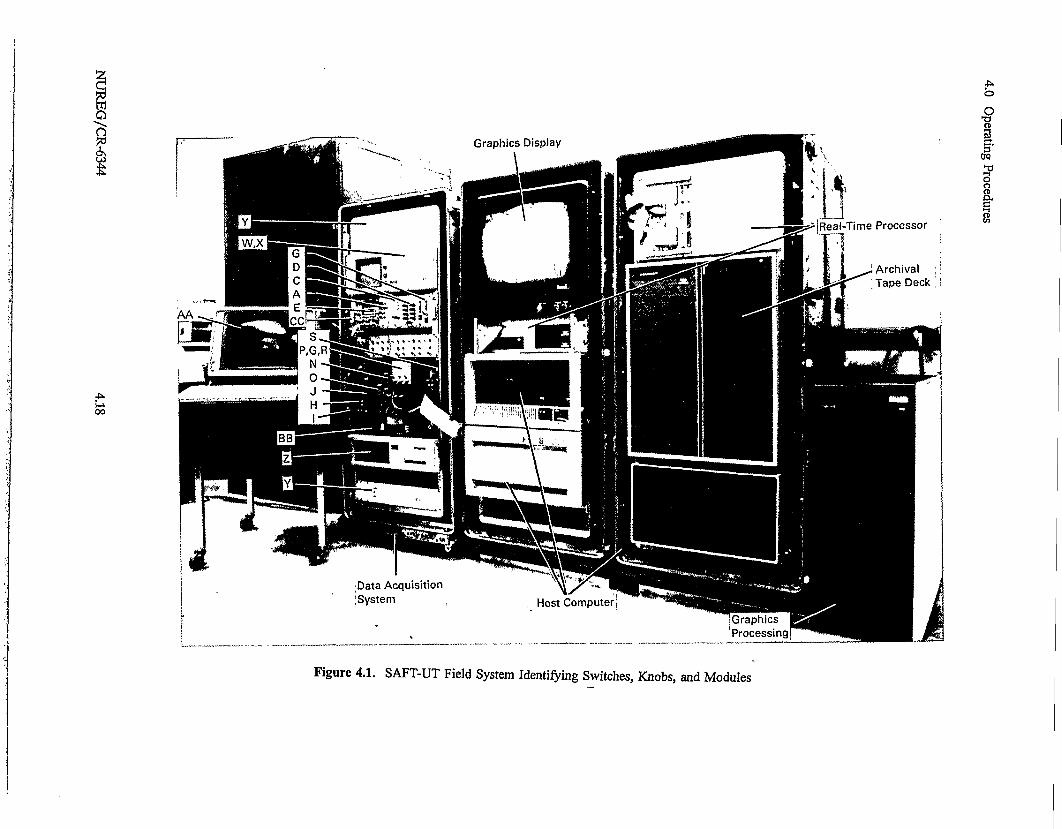
|
O(IaI'
i
Figure 4.1. SAFT-UT Field System Identifying Switches, Knobs, and Modules
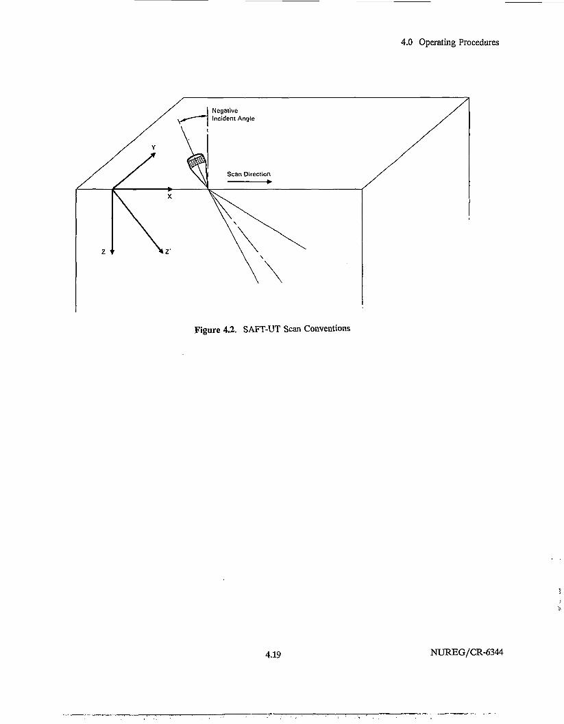
4.0 Operating Procedures
Figure 4.2. SAFT-UT Scan Conventions
4.19 NUREG/CR-6344
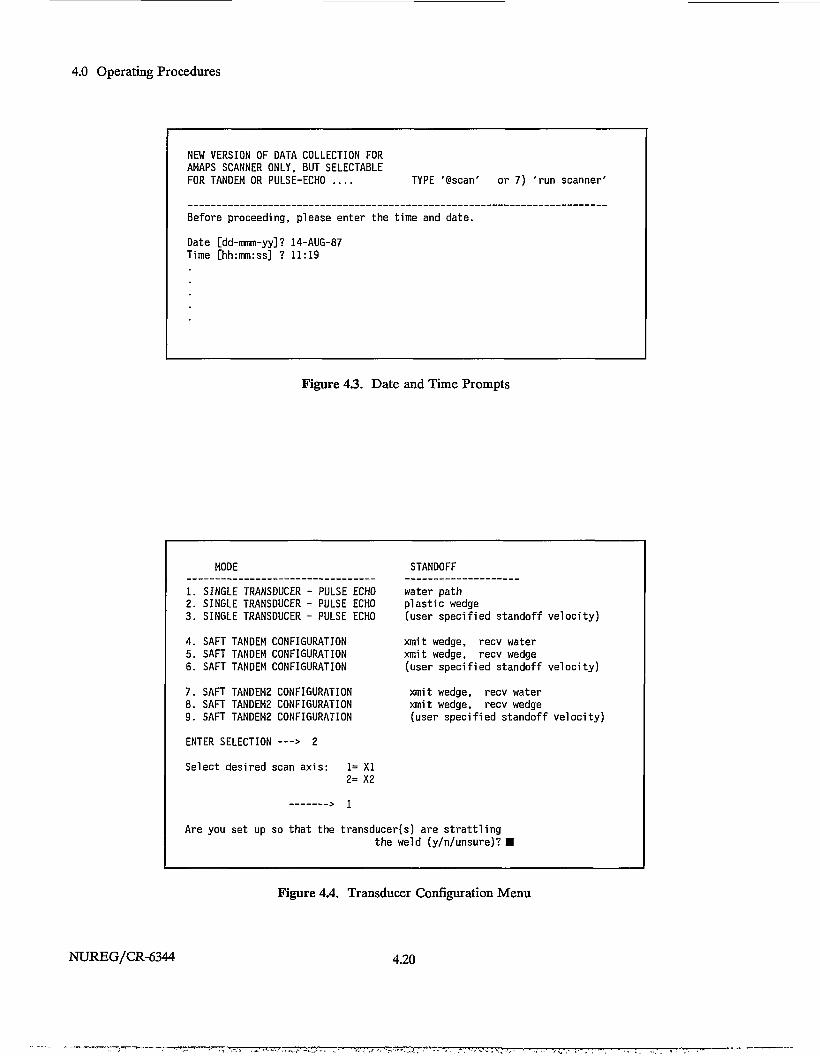
4.0 Operating Procedures
NEW VERSION OF DATA COLLECTION FORAHAPS SCANNER ONLY, BUT SELECTABLEFOR TANDEM OR PULSE-ECHO .... TYPE '@scan' or 7) 'run scanner'
Before proceeding, please enter the time and date.
Date [dd-mmm-yy]? 14-AU6-87Time [hh:mm:ss] ? 11:19
Figure 43. Date and Time Prompts
MODE
1. SINGLE TRANSDUCER - PULSE ECHO2. SINGLE TRANSDUCER - PULSE ECHO3. SINGLE TRANSDUCER - PULSE ECHO
4. SAFT TANDEM CONFIGURATION5. SAFT TANDEM CONFIGURATION6. SAFT TANDEM CONFIGURATION
7. SAFT TANDEM2 CONFIGURATION8. SAFT TANDEM2 CONFIGURATION9. SAFT TANDEM2 CONFIGURATION
ENTER SELECTION — > 2
Select desired scan axis: 1= XI2= X2
STANDOFF
water pathplastic wedge(user specified standoff
xmit wedge, recv waterxmit wedge, recv wedge(user specified standoff
xmit wedge, recv waterxmit wedge, recv wedge(user specified standoff
Are you set up so that the transducer(s) are strattlingthe weld (y/n/unsure)? •
velocity)
velocity)
velocity)
Figure 4.4. Transducer Configuration Menu
NUREG/CR-6344 4.20
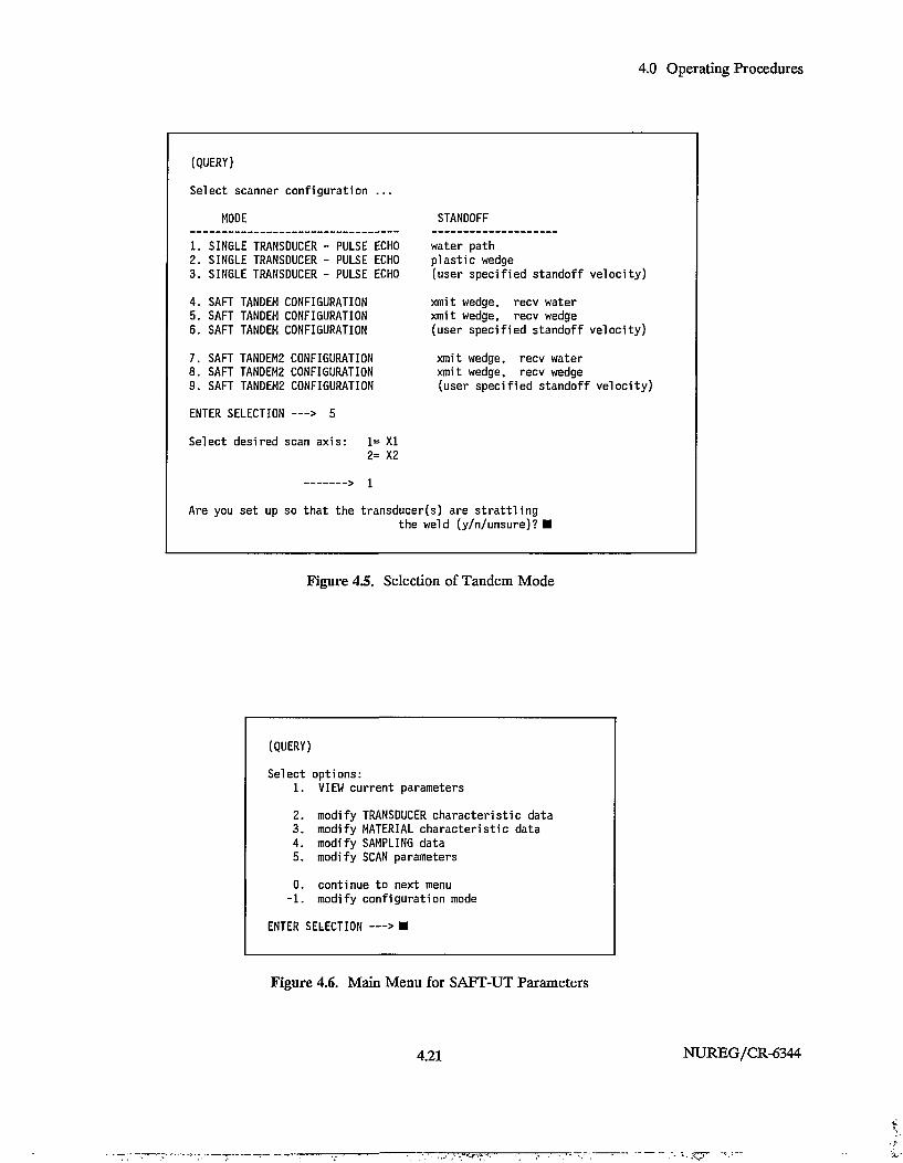
4.0 Operating Procedures
(QUERY)
Select scanner configuration ...
MODE
1. SINGLE TRANSDUCER - PULSE ECHO2. SINGLE TRANSDUCER - PULSE ECHO3. SINGLE TRANSDUCER - PULSE ECHO
4. SAFT TANDEM CONFIGURATION5. SAFT TANDEM CONFIGURATION6. SAFT TANDEM CONFIGURATION
7. SAFT TANDEM2 CONFIGURATION8. SAFT TANDEM2 CONFIGURATION9. SAFT TANDEM2 CONFIGURATION
ENTER SELECTION — > 5
Select desired scan axis: 1= XI2= X2
> 1
STANDOFF
water pathplastic wedge(user specified standoff velocity)
xmit wedge, recv waterxmit wedge, recv wedge(user specified standoff velocity)
xmit wedge, recv waterxmit wedge, recv wedge(user specified standoff velocity)
Are you set up so that the transducer(s) are strattlingthe weld (y/n/unsure)? •
Figure 43. Selection of Tandem Mode
(QUERY)
Select options:1. VIEW current parameters
2. modify TRANSDUCER characteristic data3. modify MATERIAL characteristic data4. modify SAMPLING data5. modify SCAN parameters
0. continue to next menu-1. modify configuration mode
ENTER SELECTION — > •
Figure 4.6. Main Menu for SAFT-UT Parameters
4.21 NUREG/CR-6344
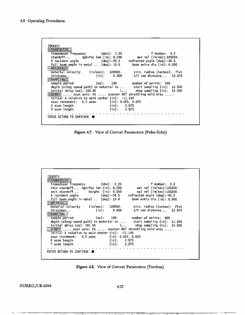
4.0 Operating Procedures
(QUERY)
transducer frequencys t a n d o f f . . . hgt=focX inc ident anglef u l l beam angle i n metal .
(mhz)len (in)
(deg)• (deg)
material velocity (in/sec):thickness...SABPU8Ssample period
( in) :
(ns):
: 2.25: 0.200:-36.5: 10.0
120000.9.000
100depth (along sound path) in material to .in i t i a l delay (us): 183.49SCftfi scan axis: XIin i t i a l X relative to welcscan increment: X,Y axesX scan lengthY scan length
ENTER RETURN TO CONTINUE •
\scanner
center ( in) :( in) : 0(in) :( in) :
f number: 3 .2mat vel (in/sec):105000.
refracted angle (deg):-46beam entry d ia. ( in) : 0.
circ. radius (inches):1/2 vee distance...
number of points: 468start sampling ( in) :
. . . stop sampling ( in) :NOT strat t l ing weld area-11.149.025, 0.025
2.9752.975
.5000
flat13.070
11.50014.500
Figure 4.7. View of Current Parameters (Pulse-Echo)
(QUERY)
transducer frequency (mhz)recv s t ando f f . . . hgt=foc len ( i n )xmit s t ando f f . . . height ( i n )X inc ident angle (deg)f u l l beam angle i n metal . . (deg)
material velocity (in/sec):thickness... ( in) :
; SAMPUHSsample period (ns):
: 2.25: 0.200: 0.000:-36.5: 10.0
120000.9.000
100depth (along sound path) in material to .i n i t i a l delay (us): 181.59 \SCftS scan axi s: XI scanneri n i t i a l X re la t ive to weld centerscan increment: X,Y axesX scan lengthY scan length
ENTER RETURN TO CONTINUE •
( in) :( in) : 0(in) :( in) :
f number: 3 .2mat vel (in/sec):105000.mat vel (in/sec):105000.
refracted angle (deg):-46beam entry d ia. ( in) : 0.
circ. radius (inches):1/2 vee distance...
number of points: 468start sampli ng ( in) :stop sampling ( in) :
NOT strat t l ing weld area . . . .-11.149.025, 0.025
2.9752.975
.5000
flat13.070
11.50014.500
Figure 4.8. View of Current Parameters (Tandem)
NUREG/CR-6344 4.22
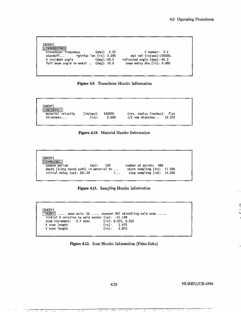
4.0 Operating Procedures
fOUERY)
transducerstandoff..X incidentfull beam
frequencyhgt=foc
angleangle in metal .
(mhz)Ten (in)
(deg)• (deg)
: 2: 0.:-36: 10
.25200.5.0
f number:mat vel (in/sec):
refracted angle (deg):beam entry dia.(in):
3.2105000.-46.50.000
Figure 4.9. Transducer Header Information
(QUERY)MATERIALmaterial velocitythickness...
(in/sec):(in):
120000.9.000
circ. radius (inches): f la t1/2 vee distance... 13.070
Figure 4.10. Material Header Information
(gUERY).• • S
"s'ampTe"p'efi od (ns): 100depth (along sound path) in material to . . .i n i t i a l delay (us): 181.59 \ . . .
number of points: 468start sampling ( in) : 11.500stop sampling ( in) : 14.500
Figure 4.11. Sampling Header Information
(QUERY)SCAttimtia
scan axisX relative to
scan increment:X scanY scan
lengthlength
X,Y
: XIweldaxes
scannercenter (in):
(in):(in):(in):
NOT-11
strattling weld area149
0.025, 0.02522975975
Figure 4.12. Scan Header Information (Pulse-Echo)
4.23 NUREG/CR-6344
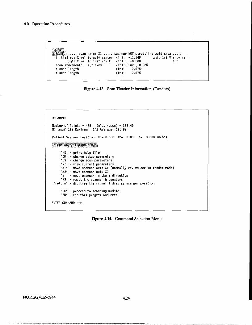
4.0 Operating Procedures
(OUERY)S£ftNinitial
scanrev X rel
xmit X relscan increment:X scanY scan
lengthlength
axis: XIto weld centerto i n i t rev XX,Y axes
scanner( in) :( in) :( in) :( in) :( in) :
NOT strat t l ing weld-11.149 xmit-0.600
0.025, 0.0252.975-2.975
area1/2 V 's to vel :
1.2
Figure 4.13. Scan Header Information (Tandem)
<SCANPT>
Number of Points = 468 Delay (usec) = 183.49Minimum" 189 Maximum" 142 AVerage= 125.92
Present Scanner Position: Xl= 0.000 X2= 0.000 Y= 0.000 inches
COHflftHD SELECTM« MM
'HE' - print help file'CM' - change setup parameters'CS' - change scan parameters'VI' - view current parameters'XI' - move scanner axis XI (normally rev xducer in tandem mode)'X2' - move scanner axis X2'Y ' - move scanner in the Y direction'RS' - reset the scanner & counters
'return' - digitize the signal & display scanner position
'SC - proceed to scanning module'EN' - end this program and exit
ENTER COMMAND -->
Figure 4.14. Command Selection Menu
NUREG/CR-6344 4.24
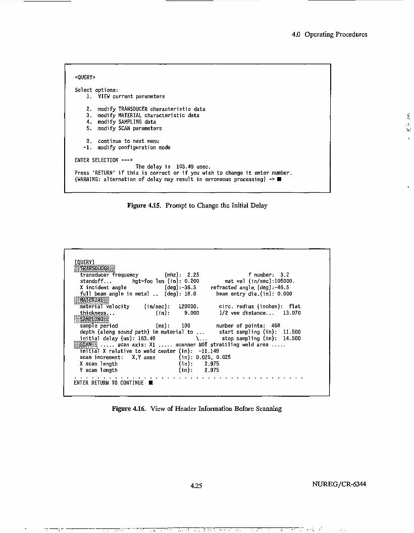
4.0 Operating Procedures
<QUERY>
Select options:1. VIEW current parameters
2. modify TRANSDUCER characteristic data3. modify MATERIAL characteristic data4. modify SAMPLING data5. modify SCAN parameters
0. continue to next menu-1. modify configuration mode
ENTER SELECTION — >The delay is 103.49 usec.
Press 'RETURN' if this is correct or if you wish to change it enter number.(WARNING: alternation of delay may result in erroneous processing) -> •
Figure 4.15. Prompt to Change the Initial Delay
(QUERY)
transducer frequency (mhz)standoff... hgt=foc len (in)X incident angle (deg)fu l l beam angle in metal . . (deg)
niaterfai velocity (in/sec):thickness... ( in) :
: 2.25 f number: 3.2: 0.200 mat vel (in/sec):105000.:-36.5 refracted angle, (deg):-46.5: 18.0 beam entry d i a . ( i n ) : 0.000
120000. c i rc . radius (inches): f l a t9.000 1/2 vee di stance... 13.070
sample period (ns): 100 number of points: 468depth (along sound path) in material to . . . start sampling ( in ) : 11.500in i t i a l delay (us): 183.49 \ . . . stop sampling ( in ) : 14.500
"' scan axis: XI scanner NOT strat t l ing weld area" in i t ia l X relative to weld center ( in) :scan increment:X scan lengthY scan length
X,Y axes (in):(in):(in)
-11.1490.025, 0.025
2.9752.975
Figure 4.16. View of Header Information Before Scanning
4.25 NUREG/CR-6344
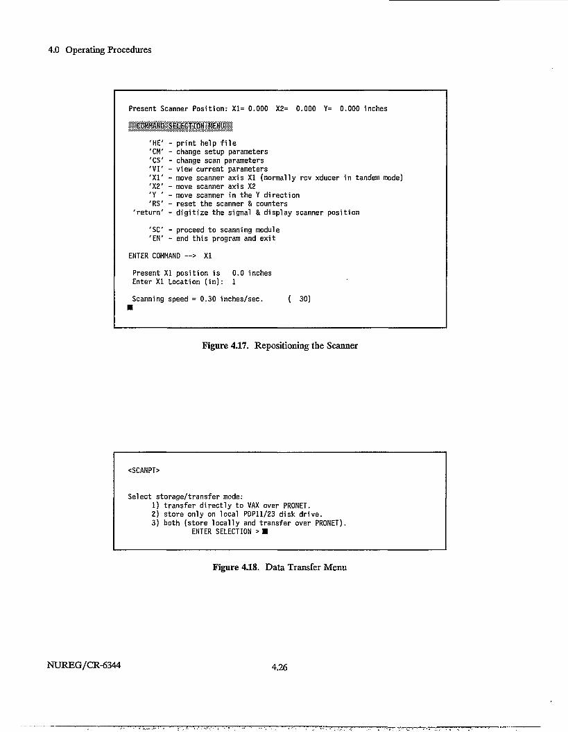
4.0 Operating Procedures
Present Scanner Position: Xl= 0.000 X2= 0.000 Y= 0.000 inches
'HE' - print help file'CM' - change setup parameters'CS' - change scan parameters'VI' - view current parameters'XI' - move scanner axis XI (normally rev xducer in tandem mode)'X2' - move scanner axis X2'Y ' - move scanner in the Y direction'RS' - reset the scanner & counters
'return' - digitize the signal & display scanner position
'SC - proceed to scanning module'EN' - end this program and exit
ENTER COMMAND — > XI
Present XI position isEnter XI Location (in):
0.0 inches1
Scanning speed = 0.30 inches/sec. ( 30)
Figure 4.17. Repositioning the Scanner
<SCANPT>
Select storage/transfer mode:1) transfer directly to VAX over PRONET.2) store only on local PDP11/23 disk drive.3) both (store locally and transfer over PRONET).
ENTER SELECTION > •
Figure 4.18. Data Transfer Menu
NUREG/CR-6344 4.26
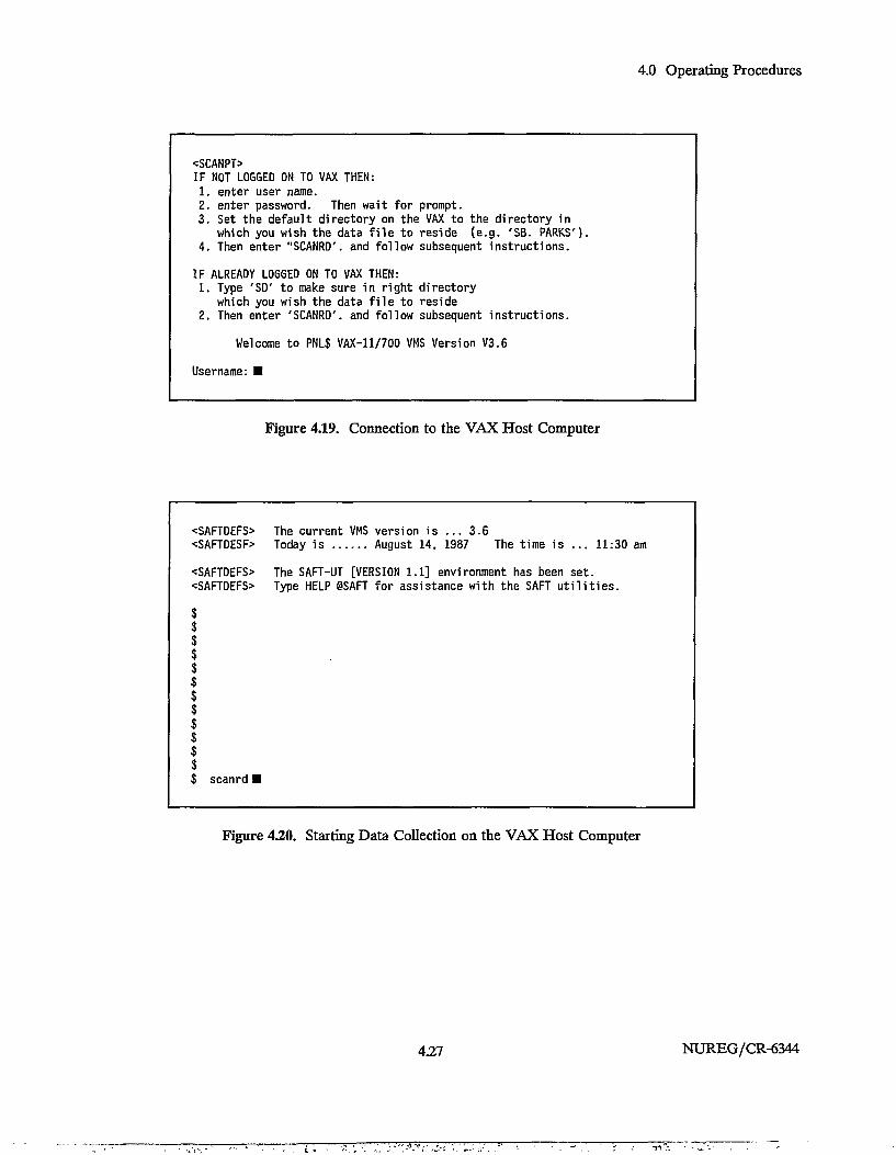
4.0 Operating Procedures
<SCANPT>IF NOT LOGGED ON TO VAX THEN:1. enter user name.2. enter password. Then wait for prompt.3. Set the default directory on the VAX to the directory in
which you wish the data file to reside (e.g. 'SB. PARKS').4. Then enter "SCANRD'. and follow subsequent instructions.
IF ALREADY LOGGED ON TO VAX THEN:1. Type 'SD' to make sure in right directory
which you wish the data file to reside2. Then enter 'SCANRD'. and follow subsequent instructions.
Welcome to PNL$ VAX-11/700 VMS Version V3.6
Username:
Figure 4.19. Connection to the VAX Host Computer
<SAFTDEFS><SAFTDESF>
<SAFTDEFS><SAFTDEFS>
*
$$$&$$$$$$$t*$ scanrd •
The currentToday is ...
VMS versior.. August
l is ... 3.614, 1987 The time is ... 11:30 am
The SAFT-UT [VERSION 1.1] environment has been set.Type HELP 0SAFT for assistance with the SAFT utilities.
Figure 4.20. Starting Data Collection on the VAX Host Computer
4.27 NUREG/CR-6344
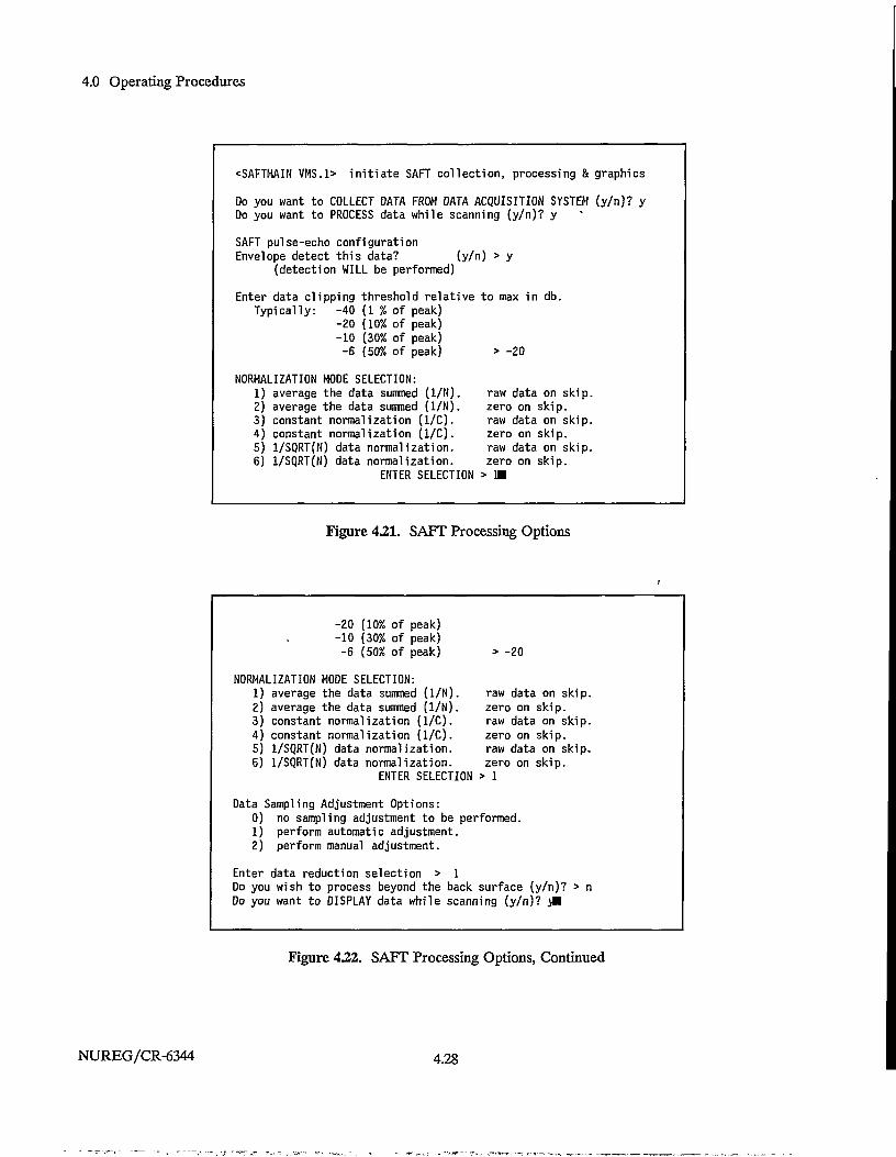
4.0 Operating Procedures
<SAFTHAIN VHS.1> in i t ia te SAFT collection, processing & graphics
Do you want to COLLECT DATA FROM DATA ACQUISITION SYSTEM (y/n)? yDo you want to PROCESS data while scanning (y/n)? y
SAFT pulse-echo configurationEnvelope detect this data? (y/n) > y
(detection WILL be performed)
Enter data clipping threshold relative to max in db.Typically: -40 (1 % of peak)
-20 (10% of peak)-10 (30% of peak)-6 (50% of peak) > -20
NORMALIZATION MODE SELECTION:1) average the data summed (1/N).2) average the data summed (1/N).3) constant normalization (1/C).4) constant normalization (1/C).5) 1/SQRT(N) data normalization.6) 1/SQRT(N) data normalization.
ENTER SELECTION > M
raw data on skip,zero on skip,raw data on skip,zero on skip,raw data on skip,zero on skip.
Figure 421. SAFT Processing Options
-20 (10% of peak)-10 (30% of peak)-6 (50% of peak)
NORMALIZATION MODE SELECTION:1)2)3)4)5)6)
average the data summed (1/N).average the data summed (1/N).constant normalization (1/C).constant normalization (1/C).1/SQRT(N) data normalization.1/SQRT(N) data normalization.
ENTER SELECTION
Data Sampling Adjustment Options:0)1)2)
EnterDo youDo you
> -20
raw data on skip.zero on skip.raw data on skip.zero on skip.raw data on skip.zero on skip.> 1
no sampling adjustment to be performed.perform automatic adjustment.perform manual adjustment.
data reduction selection > 1wish to process beyond the back surface (y/n)? > nwant to DISPLAY data while scanning {y/n)7 M
Figure 422. SAFT Processing Options, Continued
NUREG/CR-6344 4.28
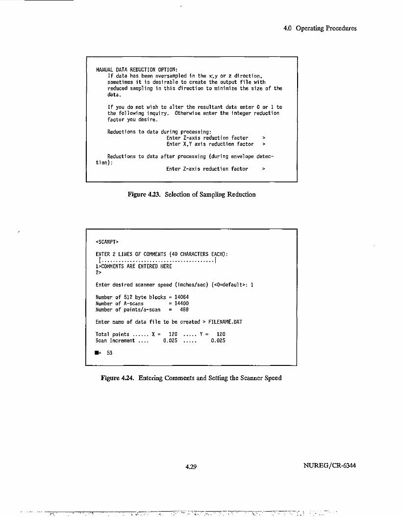
4.0 Operating Procedures
MANUAL DATA REDUCTION OPTION:If data has been oversampled in the x;y or z direction,sometimes it is desirable to create the output file withreduced sampling in this direction to minimize the size of thedata.
If you do not wish to alter the resultant data enter 0 or 1 tothe following inquiry. Otherwise enter the integer reductionfactor you desire.
Reductions to data during processing:Enter Z-axis reduction factor >Enter X,Y axis reduction factor >
Reductions to data after processing (during envelope detec-tion):
Enter Z-axis reduction factor >
Figure 423. Selection of Sampling Reduction
<SCANPT>
ENTER 2 LINES OF COMMENTS (40 CHARACTERS EACH):
1>COMMENTS ARE ENTERED HERE2>
Enter desired scanner speed (inches/sec) (<0=default>: 1
Number of 512 byte blocks = 14064Number of A-scans = 14400Number of points/a-scan = 468
Enter name of data file to be created > FILENAME.DAT
Total points X = 120 Y = 120Scan Increment 0.025 0.025
53
Figure 4.24. Entering Comments and Setting the Scanner Speed
4.29 NUREG/CR-6344
4.0 Operating Procedures
a
"oU
i03
P3
NUREG/CR-6344 4.30
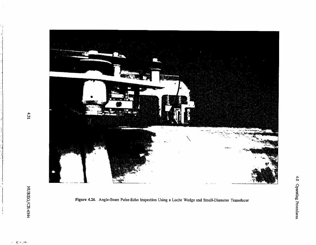
U)
O3
o Figure 4.26. Angle-Beam Pulse-Echo Inspection Using a Lucite Wedge and Small-Diameter Transducer
1
*>; •>•. .-#.
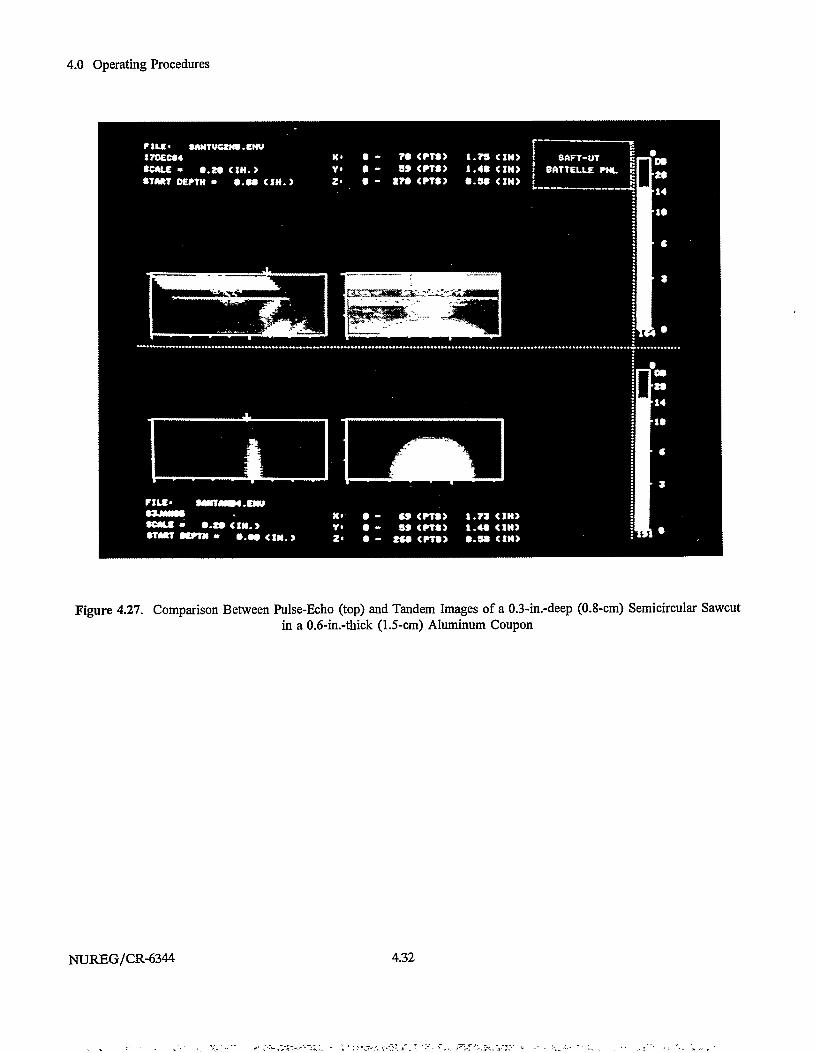
4.0 Operating Procedures
F1LK< MMTUCZtM.ENU170EC«4•CM.E - • . £ • <IH.>STMtT DEPTH - * . M < I H . >
- u» <rr«>- tn <PT«>
1.79 <IN>1.4* <IN>• .M <IH>
8AFT-UTBATTELLE PHL
•cots - « .M <IM.>tTMT KPTN • • . M
1.73 <IH)• - 89 <PTt>
Figure 4.27. Comparison Between Pulse-Echo (top) and Tandem Images of a 0.3-in.-deep (0.8-cm) Semicircular Sawcutin a 0.6-in.-thick (1.5-cm) Aluminum Coupon
NUREG/CR-6344 4.32
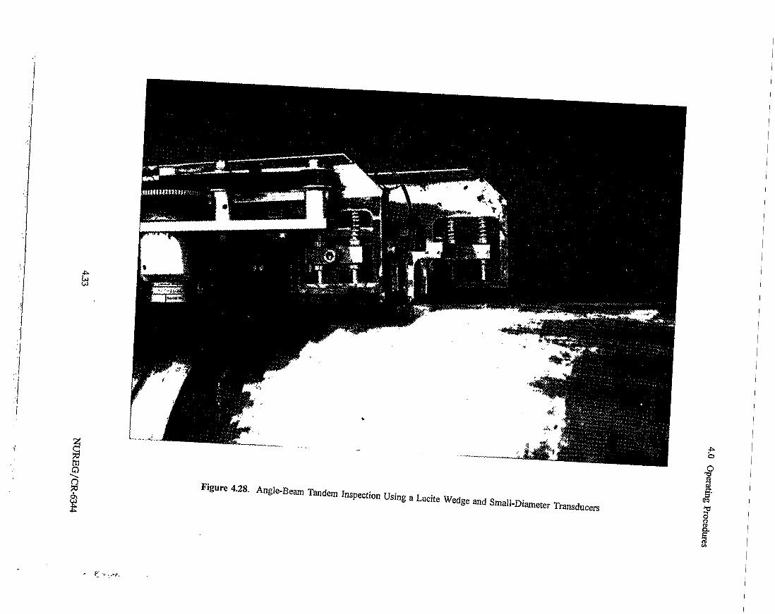
50aQ
P Figure 4.28. Angle-Beam Tandem Inspection Usinga Lucite Wedge and Small-Diameter Transducers
ICTQ
8
?;>..*#.
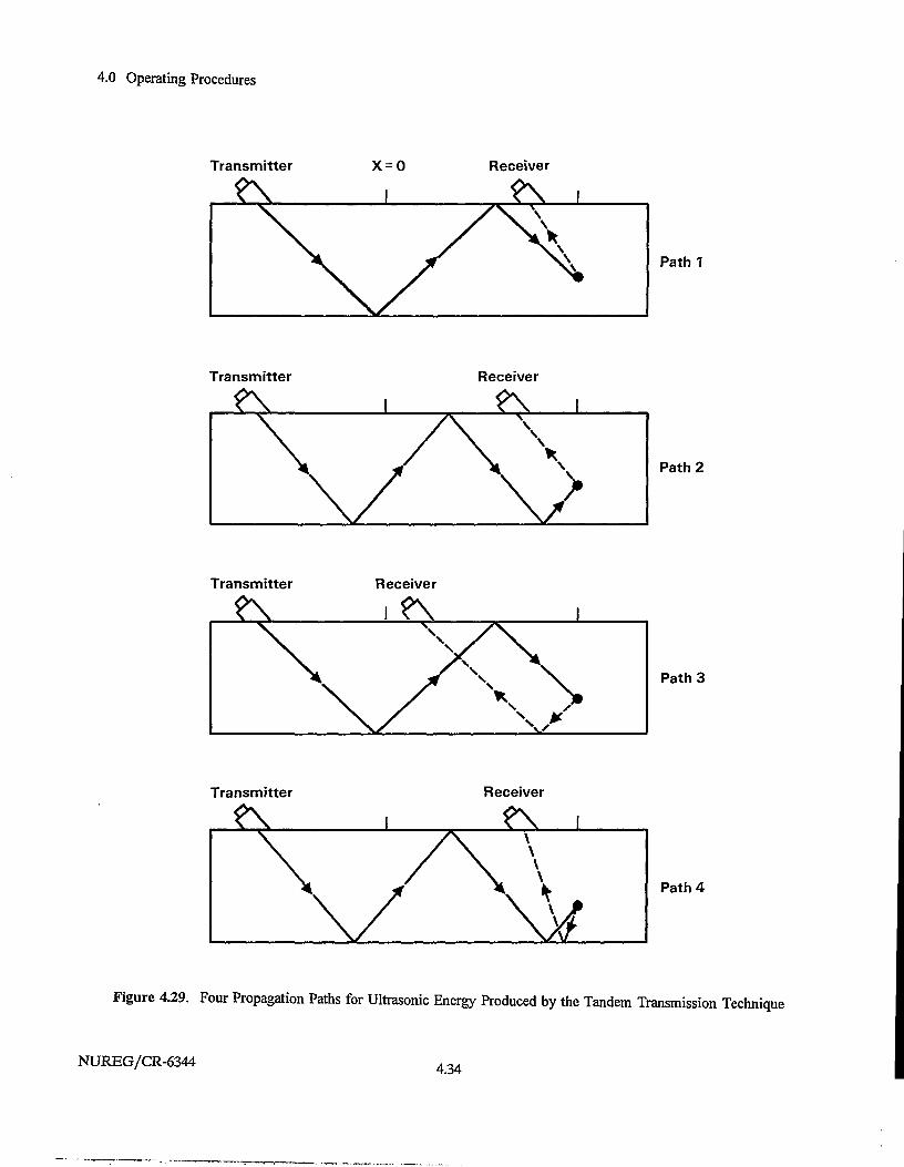
4.0 Operating Procedures
Transmitter x = o Receiver
Pathi
Transmitter Receiver
Path 2
Transmitter Receiver
Path 3
Transmitter Receiver
Path 4
Figure 4.29. Four Propagation Paths for Ultrasonic Energy Produced by the Tandem Transmission Technique
NUREG/CR-6344 4.34
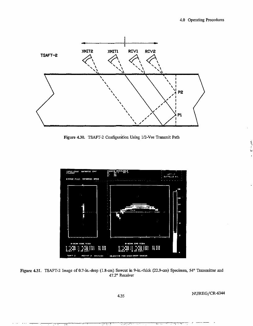
4.0 Operating Procedures
TSAFT-2XMIT2 XMIT1 RCV1 RCV2
Figure 4.30. TSAFT-2 Configuration Using 1/2-Vee Transmit Path
• - •CAN IND WICU
54 OBJECT-* 7«*'IHCH-0CCP
Figure 4.31. TSAFT-2 Image of 0.7-in.-deep (1.8-cm) Sawcut in 9-in.-thick (22.9-cm) Specimen, 54° Transmitter and47.2° Receiver
4.35NUREG/CR-6344
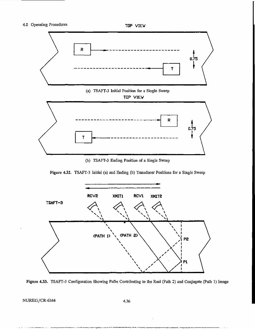
4.0 Operating Procedures TDP VIEW
(a) TSAFT-3 Initial Position for a Single Sweep
TDP VIEW
(b) TSAFT-3 Ending Position of a Single Sweep
Figure 4.32. TSAFT-3 Initial (a) and Ending (b) Transducer Positions for a Single Sweep
RCV2 XMIT1 RCV1 XMIT2
TSAFT-3
N \
<PATH 1> \ <PATH 2>
PI
Figure 4.33. TSAFT-3 Configuration Showing Paths Contributing to the Real (Path 2) and Conjugate (Path 1) Image
NUREG/CR-6344 4.36
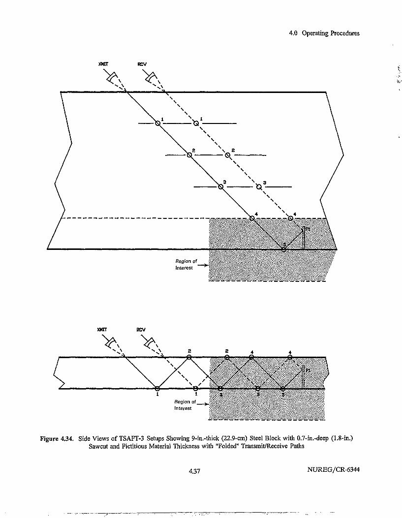
4.0 Operating Procedures
XMTT RCV
HOT RCV
Figure 4.34. Side Views of TSAFT-3 Setups Showing 9-in.-thick (22.9-cm) Steel Block with 0.7-in.-deep (1.8-in.)Sawcut and Fictitious Material Thickness with "Folded" Transmit/Receive Paths
4.37 NUREG/CR-6344
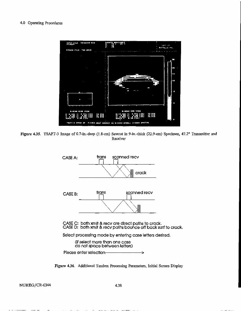
4.0 Operating Procedures
CINACt FILE 133 t«IJ
- J , J ? 1 S > < 1 M 5 " " *
ItHTI-J l"«Ct O» 7-IHCN M i r »MICUT IN J-1HCH
Figure 4.35. TSAFT-3 Image of 0.7-in.-deep (1.8-cm) Sawcut in 9-in.-thick (22.9-cm) Specimen, 47.2° Transmitter andReceiver
CASE A: trans scanned recvn n";S crack
CASE B: transn scanned recvn
CASE C: both xmlt & recv are direct paths to crack.CASE D: both xmlt & recv paths bounce off back surf to crack.
Select processing mode by entering case letters desired.
(If select more than one casedo not space between letters)
Please enter selection >
Figure 4.36. Additional Tandem Processing Parameters, Initial Screen Display
NUREG/CR-6344 4.38
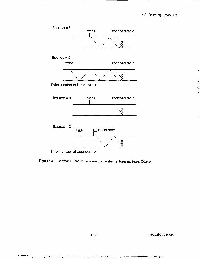
4.0 Operating Procedures
Bounce = 3
Bounce = 5
transn
transn\
scanned recvn
scanned recvn/ \ \
Enter number of bounces >
Bounce = 0 transn
scanned recv
Bounce = 2trans scanned recvn
Enter number of bounces >
Figure 4.37. Additional Tandem Processing Parameters, Subsequent Screen Display
4.39 NUREG/CR-6344
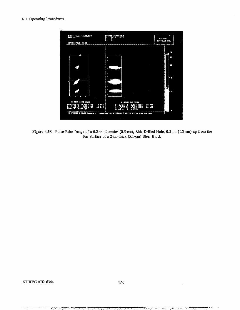
4.0 Operating Procedures
Figure 4.38. Pulse-Echo Image of a 0.2-in.-diameter (0.5-cm), Side-Drilled Hole, 0.5 in. (1.3 cm) up from theFar Surface of a 2-in.-thick (5.1-cm) Steel Block
NUREG/CR-6344 4.40
5.0 Laboratory Application Research Studies
This section describes the final extensive laboratorytesting conducted on the SAFT technology. A reviewof how well SAFT-UT performed compared to otherteams, employing both advanced and manual scanningtechniques, who participated in a mini-round robinexercise, begins Section 5. The mini-round robin exer-cise utilized piping specimens with IGSCC to evaluateadvanced and manual techniques, quantifying the re-sults. Although these were laboratory tests, they havebeen included as part of the validation work discussedin Section 10. Section 5 reports on the outcome of athick-section study i.e., pressure vessels. Further, adiscussion of the development of TSAFT-3 is included.Also included is a section on advanced preprocessingtechniques developed at PNL, which can be used priorto SAFT processing to enhance the subsequent images.Such image enhancement reduces the number of falsecalls, improving the inspectability of anisotropic materi-als such as CCSS, historically a difficult medium inwhich to reliably detect and size cracks.
For completeness, important earlier laboratory applica-tion research studies are cited as follows:
• inspection of a saft-end from the Duane Arnoldnuclear reactor, provided to PNL by SouthwestResearch Institute (SwRI) (Doctor et al. 1986)
inspection of a thick-section cladded plate withfabricated defects - data was acquired by RisleyNuclear Laboratories and sent to PNL for SAFTprocessing and analysis (Doctor et al. 1986).
• inspection of centrifugally cast stainless steel sam-ples provided by the PISCII SSRRT - Data col-lected from these samples provided an extremelyvaluable database that was later used to developpreprocessing techniques that could be applied toanisotropic materials and is discussed in detail inSection 5.3 of this report (Doctor et al. 1987a).
• inspection of a submarine hull weld test specimen;Amdata, Inc. supplied the specimen. This was thefirst application where the TSAFT-2 configurationwas employed and proved invaluable for detectingsome near surface defects (Doctor et al. 1987b)
• inspection of three welds on two large-diameter(24-in. [60.96-cm] Schedule 80) 304 stainless steeltest pipes; the pipes were located at the Materials
Reliability Center and were part of an ElectricPower Research Institute Program to studyIGSCC. The entire SAFT-UT field system wasrelocated on site and much of the processing andanalysis took place on site as well (Doctor 1987b)
inspection of four stainless steel overlay speci-mens; the specimens were supplied by KnollAtomic Power Laboratory and contained a varietyof unknown defects (Doctor 1987b).
5.1 Investigation of SAFT Imaging inThick Material
A series of tests was performed using a 9-in.-thick(22.9-cm) carbon steel specimen with a number ofmachined defects placed in the far surface of the part.This specimen represents the first step in analyzing theperformance of the SAFT-UT configurations in thickvessel material. Ten vertically oriented semicircularsawcuts were placed in this specimen, varying in depthfrom 0.050 in. to 0.700 in. (0.13 cm to 1.9 cm).
Figure 5.1 shows the B-scan side view and B-scan endview of a SAFT-UT image of the 0.050-in.-deep (0.13-cm) sawcut. The horizontal dotted line in the photo-graph represents the position of the far surface. Thisscan used a 0.25-in.-diameter (0.6-cm) transducer with acenter frequency of 2.25 MHz. A Lucite wedge wasused to cause a 47.2° center-beam angle in the carbonsteel material. Notice that the corner-trap reflection ofthis small defect is easily detected. However, the tipsignal does not appear in the image presented. This isto be expected because the system resolution is on theorder of two wave lengths (0.100 in. [0.25 cm]).
Figure 5.2 shows the corresponding SAFT-UT pulse-echo configuration image of the 0.700-in.-deep (1.8-cm)sawcut. The color scale normalization has been adjust-ed in this photograph to enhance the display of the toimage of the tip of the sawcut. Notice that the tipsignal is now imaged very well, and that accuratethrough-wall sizing can now be performed from thisimage. However, because this is a single transducerconfiguration, the ambiguity limitations inherent withthis illumination are still present. There is not a fullcharacterization of the defect, as only the corner andthe tip of the vertically oriented reflector are imaged.Therefore, it is important to implement the TSAFT-2configuration for thick vessel material.
5.1 NUREG/CR-6344
5.0 Research Studies
It is impractical to implement a multiple-bounce config-uration in thick materials, because the attenuation andgeometries become intolerable. The thick materialimplementation of TSAFT-2, then, must involve using a1/2-vee transmitter and a 1/2-vee receiver. This config-uration illuminates the object plane by bouncing off thefar surface only once, as opposed to the multiple-bounce thin material configuration. The initial config-uration that will be described here utilizes a 54° S-wavetransmitting probe and a 47.2° receiving probe. Eachtransducer used in this configuration is 0.25 in. (0.6 cm)in diameter and has a center frequency of 2.25 MHz.
Figure 5.3 shows the TSAFT-2 B-scan side view and B-scan end view image of the 0.050-in.-deep (0.13-cm)sawcut. The horizontal dotted line represents the posi-tion of the far surface, and, although one can see thereal and conjugate images of the sawcut, they are aper-ture-limited hi this image. A vertical extent ofapproximately 0.18 in. (0.46 cm) would be measuredfrom this image using a 6-db criterion. The size of thissawcut is smaller than the system resolution; conse-quently, oversizing occurs. This image becomes a mea-sure of the vertical resolution of the system.
Figure 5.4 shows a TSAFT-2 image of the 0.700-in.-deep (1.8-cm) sawcut. The B-scan end-view presenta-tion reveals two weaknesses of this configuration. Thefirst apparent characteristic is that the conjugate imageis highly degraded. This is due to limited scan in the Xdirection, because the two transducers obstruct eachother in this direction. The conjugate image is neededto reduce the sensitivity of the vertical sizing measure-ments to variations in material velocity and materialthickness.
Close observation of the B-scan end view of Figure 5.4also shows that this configuration does not image thecenter part of the reflector. The zero order (low spatialfrequencies) are lost because the wedges of the twotransducers were selected such that the center anglesare not equal. Thus only the top edge of the sawcutwas imaged.
An alternate TSAFT-2 configuration (TSAFT-3) wasconceived that eliminates the deficiencies shown inFigure 5.4. The small diameter probes were staggeredslightly (0.75 in. (1.9 cm) center-to-center) in the Ydirection so they pass by each other. Wedges werechosen to provide identical center beam angles and, as
is characteristic of the TSAFT-2 configuration, theywere scanned hi opposing directions.
The corresponding image of the identical defect usingthe TSAFT-3 configuration is shown in Figure 4.36.Notice that the conjugate image is much improved andthat the full information is now available for operatorinterpretation. This technique is expected to greatlyimprove imaging of defects in deep section material.
5.1.1 TSAFT-3 Development
Thick-section materials inherently prohibit the use ofmultiple-bounce paths normally associated with TSAFTmodes; attenuation of the sound field becomes intolera-ble. A practical solution is to limit the number ofbounces to one (before the sound strikes the verticalobject plane). Figure 4.31 shows the center ray pathsto the vertical object plane for a 1/2-vee TSAFT-2configuration. The difficulty usmg TSAFT-2 in thisconfiguration is the physical limitations; i.e., the trans-mitter can only scan forward until it hits the receiver.Unfortunately, a portion of the real image and most, ifnot all, of the conjugate image is lost. Figure 4.32shows the TSAFT-2 image (usmg 54° transmit and 47.2°receive inspection angles) of a 0.7-in.-deep (1.9 cm)sawcut that has been placed hi the far surface of a 9-in.-thick (22.7-cm) steel block. The B-scan end-view re-veals two weaknesses of this configuration. First, aportion of the real image is missing. Second, the conju-gate image is highly degraded.
A third tandem configuration, a special case of TSAFT-2 called TSAFT-3, was implemented for thick-sectionvessels where it was not practical for the transmit trans-ducer to be 3/2-vees from the vertical image plane dueto the long material paths attenuating the sound field.TSAFT-3 overcomes the physical problems of TSAFT-2, allowing the transmit transducer to be 1/2-vee fromthe vertical object plane. The transmit transducer isoffset (when small Lucite wedges are used, the offset istypically 0.75 hi. [1.9 cm) such that it passes by thereceive transducer hi a side-by-side fashion as shown inFigures 4.33(a) and 4.33(b). There are no provisions tocompensate for the offset distance between the transmitand receive transducers; the long material paths fromthe transducers to the vertical object plane make theeffect of the offset negligible when small transducersare used. The transmitter would initially start in front
NUREG/CR-6344 5.2
5.0 Research Studies
of the receive transducer as shown in Figure 4.33(a);both transducers are scanned equal distances but, as istypical of the TSAFT configurations, in opposite direc-tions as shown in Figure 4.33(b). TSAFT-3 provides allof the advantages of TSAFT-2; plus, it allows a shortermaterial path (1/2-vee) to be used, improving the sig-nal-to-noise ratio in thick-section materials.
Figure 4.34 shows the positions the transmit and receivetransducers are in when they are toward the extremesof the scanned aperture. Path 1 provides data for theconjugate image, and path 2 data is used for the realimage. The real and conjugate portions of the defectimage may be observed simultaneously by choosing toprocess beyond the far surface during TSAFT-2/TSAFT-3 processing. The vertical extent of a sur-face-connected defect may be accurately determined bymeasuring the full vertical extent of the image anddividing the result by two. This technique reduces thesensitivity of the vertical sizing measurements to varia-tions in material velocity and material thickness, andthe location of the far surface relative to the imageneed not be known accurately.
Processing TSAFT-3 data requires manipulating threedata file header parameters; i.e., material thickness, thenumber of transmit bounces, and the number of receivebounces. If the correct material thickness is used, theimage space for TSAFT becomes too large to process.The TSAFT algorithm processes the entire materialthickness, and when processing beyond the far surfaceis chosen, twice the material thickness is processed.
When dealing with thick-section specimens and theTSAFT modes, it is necessary to limit the depth rangethat is processed and subsequently displayed. Figure4.35(a) presents a typical TSAFT-3 setup, on a 9-in.-thick (22.9-cm) steel block with a 0.7-in.-deep (1.8-cm)sawcut placed into the far surface. This setup will beused as an example. In our example, the region ofinterest is only the lower fifth of the material thickness.Processing is selected to be beyond the far surface, butlimited in range as shown by the shaded area in Figure4.35(a). To accomplish this, a fictitious material thick-ness value, equal to the original thickness divided byfive (1.8 in. [4.6 cm]), is entered into the file headerparameters using the DEDIT utility. If a differentregion of interest were desired, the material thicknesscould be divided by any odd number. The transmit andreceive paths are then "folded", Figure 435(b), to give
equivalent material path lengths. The correct numberof transmit and receive bounces are counted and en-tered into the file header parameters. For our example,the number of transmit bounces would be 5 and thenumber of receive bounces would be 4. An easy rule-of-thumb is as follows:
1. The number of transmit bounces will always be anodd value,
2. the number of receive bounces will always be oneless and an even value, and
3. the material thickness value to be entered is thetrue material thickness divided by the number oftransmit bounces.
Once the necessary header modifications have beenmade, the TSAFT-3 data file may be processed normal-
5.2 Application of Advanced SignalProcessing Techniques to ImproveSAFT-UT Performance on CCSS Mate-rial
The initial results of the SAFT-UT inspection of theCCSSRRT samples were somewhat disappointing, be-cause although all the cracks were detected, the falsecall rate was unacceptable. The samples consisted oflaboratory-induced cracks in 2.4-in.-thick (6.1-cm) CCSSmaterial, with both columnar and equiaxed grain struc-tures utilized. In general, SAFT performed as well asany of the teams who inspected the blocks; however,the algorithm implemented tended to generate a signifi-cant amount of false calls. Crack detection was not aproblem, but distinguishing between cracks and coher-ent scattering from the microstructure was difficult. Inthe interest of improving SAFT performance on thistype of specimen, further analysis was undertaken.Specifically, the emphasis of this analysis was focusedon the frequency characteristics of this data base.
A distinct advantage of the SAFT-UT system is that theraw (unprocessed) data is archived and available forfurther analysis. With the SAFT-UT system, if one en-sures that the integrity of the data files are of highquality, then this becomes a data base from which
5.3 NUREG/CR-6344
5.0 Research Studies
future analysis may draw. The CCSSRRT data fallsinto this category, and as such, the complete data set isfully retrievable.
It has been known for some time that the coherentsummation algorithm incorporated in the SAFT-UToperation is a narrow-band approximation. This wasreviewed by Busse, Collins, and Doctor (1984) in thisprogram and was discussed earlier by Norton (1976) inhis thesis paper at Stanford University. The exactmethod incorporates a time derivative of the raw datafile prior to SAFT processing. When analyzing thespectral responses of data files collected on CCSS mate-rial with a 500 kHz transducer, significant componentsas low as 150 kHz and as high as 600 kHz may bepresent. This suggests that perhaps the narrow-bandapproximation may not be totally valid in this case.
Also, as will be discussed later, one sees a difference inspectrum from a cracked area and an uncracked area.This suggests that a bandpass filter incorporated in thealgorithm may enhance the image quality of the SAFT-UT system. The purpose of the experiments reportedherein is to define a bandpass filter that can be appliedto a SAFT data file, prior to processing, that wouldreduce the ambiguities that exist between the coherentscattering from microstructures and cracks.
To assist in spectral analysis of the SAFT waveforms,the APLOT (SAFT-UT analysis graphics) utility wasenhanced to provide a power spectrum plot on theRAMTEK of any selected A-scan of a given data file.Also, three additional SAFT utilities were added: oneto perform a bandpass filter operation, one to performa Fourier transform operation, and another to performthe time derivative of a given data file. The bandpassfilter routine simply rejects all frequencies below aspecified value and above a second specified value.Both of these values are user-selectable. No attemptwas made to weight this in a Gaussian form or anymore elaborate shape. The time derivative functionsimply performs the transform using the following equa-tion shown in Bracewell's (1965) text:
F(s)
where
s = frequency,F(s) = the Fourier Transform of the original data set
F'(s) = the Fourier Transform of the desired timederivative, and
5.2.1 Applying the Spectral Analysis andSubsequent Filter Technique to a CCSSRRTData File
Specimen 5 of the CCSSRRT data set (see Bates, Doc-tor and Heasler 1987) was used for an initial analysis.The parent material of this block is 2.4 in. (6.1 cm)thick and consists of columnar material on one side ofthe weld and equiaxed material on the opposite side ofthe weld. The weld is approximately 2.2 in. (5.6 cm)thick and 7.6 in. (19.3 cm) long, with a crack introduced(estimated to be about 28% of wall thickness) on thecolumnar side of the weld. The crack in this specimenbegins 4.2 in. (10.7 cm) and extends to 5.9 in. (15 cm)along the weld. SAFT data was collected from thisspecimen using a 0.5-MHz transducer in 45° shearmode. The primary data file of interest was collectedon the columnar side of the weld area (the same side asthe crack).
Figure 5.5(a) shows th& SAFT-UT image of the areascanned. On the left of the photograph is the B-scanside view; while at the right, the B-scan end view isshown. The top of the image displayed corresponds toa 1-in. (2.5-cm) depth in the material; and the dottedline, visible in the B-scan end view, represents the ex-pected position of the far surface (2.3 in. [5.8 cm] fromthe near surface). Some indications appear beyond thefar surface because of velocity variations and beamskewing. The image is apparently very noisy; and infact, from the B-scan end-view image, one would con-clude that there is a crack the full length of the scan.In fact, the crack occurs only in the last 2 to 3 in. (5.1to 7.6 cm) of the scan. The indication that is apparentin the first 2 in. (5.08 cm) (the left side of the B-scanend view) is not from a crack structure but from themicrostructures.
Figure 5.5(b) graphically shows the A-scan of an areathat was believed to be cracked, while Figure 5.5(c)
NUREG/CR-6344 5.4
5.0 Research Studies
corresponds to an area known to be uncracked. EachA-scan presented here and in subsequent figures repre-sents the full digitized return signal from this material.The digitized window includes from the front surfacethrough an equivalent material path length of 4.5 in.(11.4 cm). These images, most obviously, are very noisysignals and, consequently, are difficult to interpret.
Figures 5.5(d) and 5.5(e) show the power spectra thatcorrespond to the adjacent A-scans. If one closely re-views these figures, it can be seen that the generalspectra are wide band, in that they contain much morelow-frequency components than would be expected fora 0.5-MHz center-frequency system. Also, the largestcomponent in the uncracked region is shifted down infrequency by 70 kHz with respect to the peak value inthe cracked region. From these general observations, aseries of tests was performed, including SAFT process-ing on the time derivative of the data set, on a band-pass filtered data set, and on a combination of both.
First, the time derivative was generated from the origi-nal data set. The results of this may be seen in Figure5.6. An improvement in signal-to-noise level can beobserved in the image shown in Figure 5.6(a). Theindication in the region where no defect is located isreduced (in the B-scan end-view, this is at the 1-in. [2.5-cm] location). Also, a notable reduction in backgroundnoise is realized. When one of the spectra in this figureis compared with those shown in Figure 5.5 it can beseen that the effect of the time derivative on the powerspectrum is to de-emphasize the low-frequency com-ponents.
A second test consisted of a more direct approach toaltering the frequency spectrum of the waveforms. Astep-wise filter was applied to the data set prior toSAFT processing. This filter rejected frequencies below0.38 MHz and above 0.68 MHz. The results of this testare shown in Figure 5.7. The final image presented inFigure 5.7(a) shows a substantial improvement in sig-nal-to-noise level. The background noise is nearlyeliminated, and the false indication at the 1-in. (2.5-cm)location of the B-scan end view has vanished.
The final test consisted of a combination of the previ-ous operations. The tune derivative of the original dataset was generated. This result was then passed throughthe bandpass filter previously described. Finally, theSAFT processing was performed on this result. The
results of this are shown in Figure 5.8. The final imageshown in this figure is comparable to that generatedwith only a filter operator (Figure 5.7). This can beexpected because the narrow-band approximation be-comes valid subsequent to this filter operation, thusreducing the effectiveness of the time-derivative opera-tor.
5.2.2 Software Tools Used to Define the Op-timal Bandpass Filter Used to Enhance theSAFT-Processed Image
Initial results indicate that if an optimum bandpassfilter is defined and applied prior to SAFT processing,the resulting image is greatly enhanced and the falsecall probability is decreased. The purpose of this sec-tion is to describe the software used to accomplish thetask of defining the optimum bandpass filter limits.
From the initial results, one begins to believe that theremay be a frequency range at which defect and non-defect areas may be discriminated. Proof of this as-sumption would be a high correlation to the premisethat large components of the power spectral responsefrom A-scans containing defects will correspond tosmall components of the power spectral response of A-scans containing nondefects. Using the CCSSRRT database, a statistical analysis of the spectrum data files wasconducted.
The CCSSRRT specimens provided a data base inwhich the defect and nondefect areas are well defined.The DEDIT utility was modified to allow a flag to beset in each A-scan recording in a given data file. Thisflag represents three conditions:
1. A "0" indicates an "unsure region." These A-scansmay lay near the edge of a defect or the edge ofthe specimen itself and will not be used in thesubsequent statistical analysis process.
2. A "1" indicates a "defect region." These A-scansare in line with a defect.
3. A "-1" indicates a "nondefect region." These A-scans are not in line with a defect.
To assist in the statistical analysis, a new utility,STATANAL, was implemented. The STATANAL
5.5 NUREG/CR-6344
5.0 Research Studies
utility calculates a correlation coefficient for selectedfrequency and transducer axial position ranges. Onlyrecords with the defect flag set to a nonzero value areused for input. Data files used as input to theSTATANAL utility are first converted to spectrum datafiles using the Fourier transform utility, SPECTRUM,and each A-scan record defect flag is set to reflect thenature of the A-scan using the DEDIT utility. Thestatistical results reflect how well the data in the select-ed ranges fit the ideal (i.e., corresponding spectralvalues are of a low magnitude for nondefect areas anda high magnitude for defect areas). To better under-stand the correlation coefficient value, additional infor-mation is provided for each selected frequency andtransducer position range, as shown below:
1. the total number of defect and nondefect A-scansused in the statistical analysis
2. the arithmetic mean of the spectral magnitudes
3. the standard deviation.
It is important to ensure that the transducer positionentries are relative to the known defect location, exceptin the case of blank specimens where the transducerposition entries are relative to the weld center line.
The following is a typical scenario used when employingthe STATANAL utility:
1. Run the SPECTRUM utility, supplying the inputand output filenames.
2. Use the DEDIT utility to appropriately set the de-fect flag in each A-scan record of a selected spec-trum data file. Edit the initial transducer positionto reflect the position relative to the known defectlocation for a specimen containing a defect, orrelative to the weld center line for a specimencontaining no defect.
3. Run the STATANAL utility. The user is prompt-ed for the following input:
a.b.c.d.
selected spectrum data file namesselected X ranges (in inches)selected frequency ranges (in MHz)selected output filename.
Table 5.1 presents a typical output of the STATANALutility for a sawcut data file, using a single frequencyrange of 2.1 to 2.4 MHz and a single X position rangeof -0.7 to -0.5 in. (-1.8 to -1.3 cm) (normally, manysmall frequency and X position ranges are used). Thesawcut data file serves to check the validity of the STA-TANAL utility. The sawcut data file is a 45°, 2.25-MHzshear-wave file of a 0.3-in.-deep (0.8-cm) sawcut, placedin a 0.6-in. (1.5-cm) stainless steel coupon. A perfectcorrelation would be a +1 and an inverse correlationwould be a -1. Table 5.1 presents the maximum corre-lation coefficient for the selected frequency range.There is a near perfect correlation coefficient (+0.907)for the X position and frequency range used. Attentionis drawn to this fact by placing an asterisk next to anycorrelation coefficient values exceeding +0.9. Finally,the last portion of the STATANAL printout lists thecomposite spectra values for defect and nondefect A-scans at each frequency increment. The differencevalue presented indicates what frequencies provide thelargest magnitude difference between defect and nonde-fect A-scans.
5.2.3 Statistical Analysis of Defect and Non-Defect CCSS A-Scans
The CCSSRRT data set was split into two subsets: 1)data acquired from specimens having an equiaxed grainstructure and 2) data from specimens having a colum-nar grain structure. Each data subset was evaluated atspecific frequency and transducer position ranges todetermine which ranges yielded the highest correlationto the hypothesis A frequency range and transducerposition exists where defect spectral response componentswill be large and corresponding nondefect spectral re-sponse components will be small.
Each equiaxed and columnar spectrum data file A-scandefect flag was set to reflect the nature of the A-scan.A-scans within 0.5 in. (1.3 cm or one-half the trans-ducer diameter) of the edge of the specimen or outsidethis tolerance about the defect were considered unsure,and the defect flag was set appropriately. The remain-der of the A-scan records were either defect or non-defect in nature.
Figures 5.9 and 5.10 show the graphical results attainedfor equiaxed and columnar shear-wave spectrum datafiles. The maximum correlation value is plotted for
NUREG/CR-6344 5.6
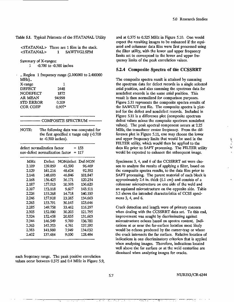
5.0 Research Studies
Table 5.1. Typical Printouts of the STATANAL Utility
<STATANAL> There are 1 files in the stack.<STATANAL> 1 SAWTVG2.SPM
Summary of X-ranges:1 -0.700 to -0.500 inches
• .. Region 1 frequency range (2.100000 to 2.400000MHz)..X-range 1DEFECT 2448NODEFECT 1872AR MEAN 94.990STD ERROR 0.209COR COEF 0.907*
— COMPOSITE SPECTRUM
NOTE: The following data was computed forthe first specified x range only (-0.700to -0.500 inches).
defect normalization factor =non-defect normalization factor =
MHz2.1092.1292.1482.1682.1872.2072.2262.2462.2652.2852.3052.3242.3442.3632.3832.402
Defect ]139.059141.216148.693156.425157.013153.118155.268157.928153.791149.758152.000152.458146.549142.353141.980137.484
NfONdefect42.59048.62446.84636.17120.3939.607
14.71823.26530.14533.46230.20520.855
9.7694.7617.9499.000
153117
Def-NON96.46992.592
101.847120.254136.620143.511140.550134.663123.646116.297121.795131.603136.780137.592134.032128.484
each frequency range. The peak positive correlationvalues occur between 0.375 and 0.4 MHz in Figure 5.9,
and at 0.375 to 0.525 MHz in Figure 5.10. One wouldexpect the resulting images to be enhanced if the equi-axed and columnar data files were first processed usingthe filter utility, with the lower and upper frequencylimits set to correspond to the lower and upper fre-quency limits of the peak correlation values.
5.2.4 Composite Spectra of the CCSSRRT
The composite spectra result is attained by summingthe spectrum data for defect records in a single selectedaxial position, and also summing the spectrum data fornondefect records in the same axial position. Thisresult is then normalized for comparison purposes.Figure 5.11 represents the composite spectra results ofthe SAWCUT test file. The composite spectra is plot-ted for the defect and nondefect records. Included inFigure 5.11 is a difference plot (composite spectrumdefect values minus the composite spectrum nondefectvalues). The peak spectral component occurs at 2.25MHz, the transducer center frequency. From the dif-ference plot in Figure 5.11, one may choose the lowerand upper frequency limits that would be used in theFILTER utility, which would then be applied to thedata file prior to SAFT processing. The FILTER utilitywould be expected to enhance the subsequent image.
Specimens 3, 4, and 6 of the CCSSRRT set were cho-sen to analyze the results of applying a filter, based onthe composite spectra results, to the data files prior toSAFT processing. The parent material of each block isapproximately 2.4 in. thick (6.1 cm) and consists of acolumnar microstructure on one side of the weld andan equiaxed microstructure on the opposite side. Table5.2 shows the intended characteristics of CCSS speci-mens 3, 4, and 6.
Crack detection and length were of primary concernwhen dealing with the CCSSRRT data set. To this end,improvement was sought by discriminating againstmicrostructure echoes based on spectra content. Indi-cations at or near the far-surface location most likelywould be echoes produced by the corner-trap or wherethe crack intersects the far surface. Relative location ofindications is one discriminatory criterion that is appliedwhen analyzing images. Therefore, indications locatedwell above the far surface or at the weld centerline aredismissed when analyzing images for cracks.
5.7 NUREG/CR-6344
5.0 Research Studies
Table 52. Intended Characteristics of CCSS Specimens 3, 4, and 6
' Specimen
3
4
6
Weld Length
7.5
7.0
7.0
Crack Offset
.15
0.5
N/A
Crack Start
4.3
5.0
N/A
Crack End
5.8
6.0
N/A
Depth
23%
21%
N/A
NOTE: Weld Length, Crack Offset, Crack Start, and Crack End are all expressed in OD inches.Crack Offset is the lateral distance of the crack from weld center.
The weld of specimen 3 is approximately 2.2 in. thick(5.6 cm) and 7.5 in. long (19.1 cm) (OD); a crack wasintroduced (estimated to be about 23% of wall thick-ness) along the equiaxed side of the weld. In this speci-men, the crack begins at 4.3 in. (10.9 cm) and extendsto 5.24 in. (13.7 cm) along the weld. SAFT data wascollected from this specimen using a 0.5-MHz transduc-er in 45° shear mode. The primary data file of interestwas collected from the equiaxed side of the weld area(the same side as the crack).
Figure 5.12(a) presents the resulting composite spectraplots (defect, nondefect, and difference) for shear-wavedata files in equiaxed material. All of the equiaxedshear-wave data files from the CCSSRRT data set wereused to arrive at the composite spectra plot shown inFigure 5.12(a). From the difference plot, one wouldchoose a lower frequency limit of 0.375 MHz and anupper frequency limit of 0.425 MHz to be used in theFILTER utility. The filtered data file is then SAFTprocessed. Figure 5.12(b) shows the before (top) andafter (bottom) results of applying the filter to specimen3. Specimen 3 contains a crack that is 1.5 in. (2.8 cm)long. Figure 5.12(b) (top image) shows the crack toextend from 1.9 to 5.8 in. (4.8 to 14.7 cm) along theweld, or 3.9 in. (9.9 cm) in length, when measured atthe -6-dB points (green/amber transition). The bottomimage of Figure 5.12(b) shows the crack to extend from4.4 to 5.8 in. (3.6 to 14.7 cm) along the weld, a lengthof 1.4 in. (3.6 cm) using the -6-dB measurement crite-rion (green/amber transition)-clearly an improvement.
The weld of specimen 4 is approximately 2.2 in. thick(5.6 cm) and 7.0 in. (OD) long (17.8 cm); a crack wasintroduced (estimated to be about 21% of wall thick-ness) on the columnar side of the weld. In this speci-men, the crack began at 5.0 in. (12.8 cm) and extendedto 6.0 in. (15.2 cm) along the weld. SAFT data wascollected from this specimen using a 0.5-MHz transduc-er in 45° shear mode. The primary data file of interestwas collected on the columnar side of the weld area(the same side as the crack).
Figure 5.13(a) presents the resulting composite spectraplots (defect, nondefect, and difference) for shear-wavedata files in columnar material. From the differenceplot, one would choose a lower frequency limit of 0.475MHz and an upper frequency limit of 0.525 MHz to beused in the FILTER utility. The filtered data file wouldthen be SAFT-processed, and an enhancement of thesubsequent image would be expected. Figure 5.13(b)shows the before (top) and after (bottom) results ofapplying the filter to specimen 4. Specimen 4 containsa crack that is 1.0 in. long (2.5 cm). Figure 5.13(b) (topimage) shows the crack to extend from 1.5 to 5.7 in.(3.8 cm to 14.5 cm) along the weld when measured atthe -6-dB points (green/amber transition), or 4.2 in.(10.7 cm) in length. The bottom image of Figure 5.13-(b) shows the crack to extend from 3.7 to 5.4 in. (9.4 to13.7 cm) along the weld-a length of 1.7 in. (4.3 cm)using the -6-dB measurement criterion (green/ambertransition)-clearly an improvement.
Further investigation revealed that the indications com-prising the bottom B-scan end view in Figure 5.13(b)
NUREG/CR-6344 5.8
5.0 Research Studies
were actually displaced laterally as evident in the B-scanside view. The actual lateral location of the crack rela-tive to the weld center is 0.5 in. (1.3 cm). Figures5.13(c) and 5.13(d) show single-slice B-scan end viewsof specimen 4. Figure 5.13(c) is taken 0.5 in. (1.3 cm)from weld center, and Figure 5.13(d) is taken exactly onweld center. Most likely, the indication shown in Fig-ure 5.13(d) is associated with the weld metal and not acrack. Therefore, Figure 5.13(c) probably better repre-sents the crack and, in fact, does correlate better to theactual crack location; i.e., Figure 5.13(c) shows thecrack starting at 4.9 and ending at 5.3 in. (13.5 cm).
Specimen 6 is a blank specimen; i.e., no cracks wereintentionally introduced and no cracks were detectedusing penetrant techniques. Specimen 6 consisted ofcolumnar and equiaxed material joined by a weld.Figure 5.14 (top image) shows the processed data file ofthe equiaxed side of specimen 6; no filtering was ap-plied to the raw data file prior to SAFT processing.Indications are seen the entire length of the image, andinitially no crack call was made because of the locationof the indications relative to the weld center and the farsurface. A bandpass filter using the equiaxed filterparameters (0.375 to 0.425 MHz) was applied to theequiaxed data file prior to SAFT processing. In Figure5.14 (bottom image), the indications are greatly re-duced; it is even easier to conclude that this side ofspecimen 6 is not cracked. Figure 5.15 (top image)shows the unfiltered SAFT-processed results of thecolumnar side of specimen 6. Once again, indicationsare seen. It would be difficult in this case not to call acrack nearly the entire length of the image and, in fact,initially a crack was called. Figure 5.15 (bottom image)shows the processed filtered image of specimen 6. A0.475- to 0.525-MHz filter was applied to the data priorto SAFT processing. The image is a vast improvementover the unfiltered image and, again, it would be easynot to call a crack. The indication seen is above the farsurface (identified by the dashed line) and beyond theweld center (indicated by the arrow), which may allowone to hypothesize that the indications are associatedwith the weld material and not from cracks.
Finally, the results of the CCSSRRT indicated thatcracks were easier to detect in some specimens thanothers. These "easy crack" specimens were used togenerate a composite spectrum to see if there are char-acteristics about these specimens that indeed resulted inthe higher detection and sizing scores. High probability
data files are defined as those specimens that had ahigh percentage of correct calls, as shown in AppendixB of Stainless Steel Round Robin Test, Centrifiigalfy CastStainless Steel Screening Phase (Bates, Doctor andHeasler 1987).
Figures 5.16 and 5.17 show the results of compositespectra for shear-wave defect and nondefect A-scans inequiaxed (Figure 5.16) and columnar (Figure 5.17)material for spectrum data files that had a high proba-bility of defect detection. Figures 5.16 and 5.17 indicatethat the defect spectra magnitudes are larger than aver-age and near the center frequency of the transducer.The nondefect spectra show smaller than average mag-nitudes, suggesting these specimens have a spectralresponse closer to homogeneous materials, which couldaccount for the higher detection rates.
5.2.5 Conclusions
Specific data files of the CCSSRRT data set seem tobenefit from applying a bandpass filter to the data filebefore the SAFT processing. A statistical and compos-ite spectra analyses of the spectrum content of theCCSSRRT data set indicates that applying a genericfilter to all CCSS specimens to discriminate defect andnondefect areas can improve the subsequent SAFTimages. More improvement in the image can be seen ifone set of filter parameters is used for equiaxedmicrostructures and a different set of filter parametersis used for columnar microstructures. The particularfilter parameters chosen are selected by first plottingthe defect and nondefect composite spectra for eachmaterial by using samples with known defect locations.Filter parameters are then selected that encompassdefect spectra and discriminate against nondefect spec-tra.
Some CCSS materials are closer in acoustic response tohomogeneous materials than others. Therefore, detec-tion of cracks may be easier and applying a filter to thedata unnecessary. However, for the vast majority ofCCSSRRT samples, application of a filter based on thespectra response of known defects did improve theimage signal-to-noise levels of the processed CCSS datafiles, thereby significantly reducing the false call rate.
5.9 NUREG/CR-6344
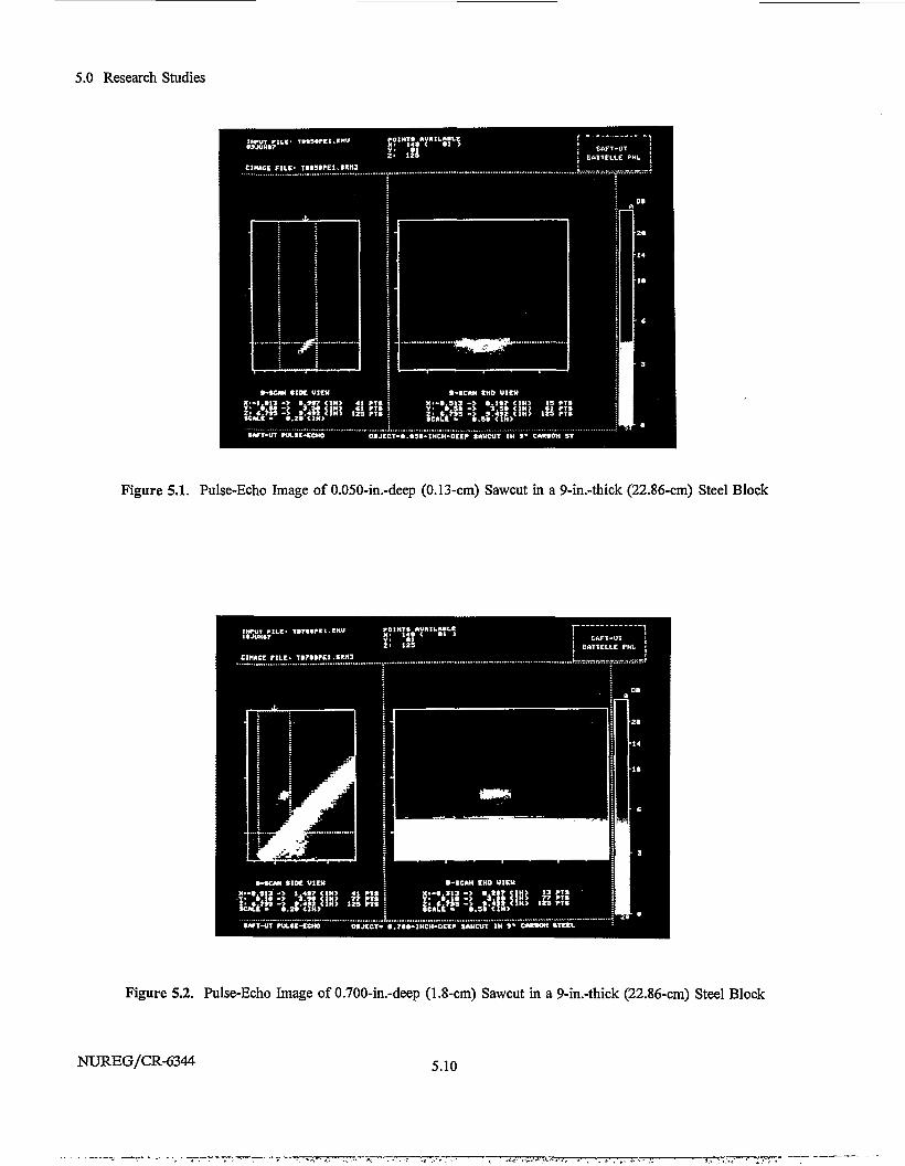
5.0 Research Studies
Figure 5.1. Pulse-Echo Image of 0.050-in.-deep (0.13-cm) Sawcut in a 9-in.-thick (22.86-cm) Steel Block
Figure 5.2. Pulse-Echo Image of 0.700-in.-deep (1.8-cm) Sawcut in a 9-in.-thick (22.86-cm) Steel Block
NUREG/CR-6344 5.10
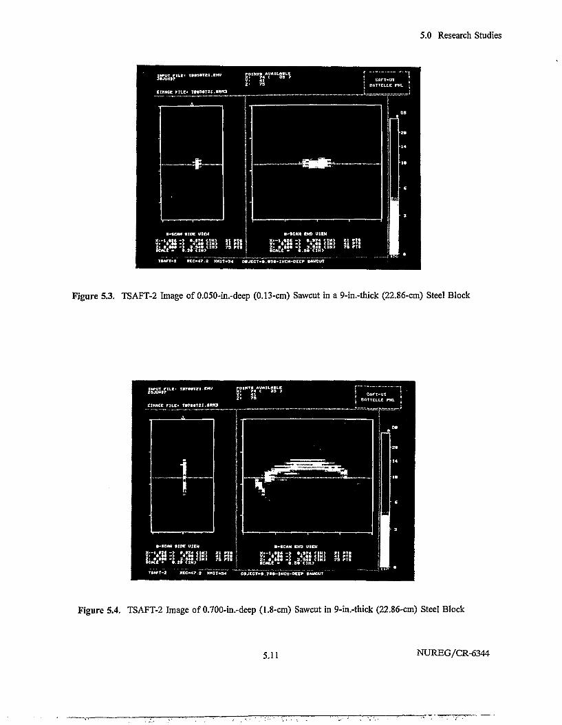
5.0 Research Studies
CIIMCE FILE. TMUTZl.tMO
•-IOW (IDC VICU B-tCAH CHO U1CH
3 SSBilB n®KC-47.2 XHIT-54
Figure 5.3. TSAFT-2 Image of 0.050-in.-deep (0.13-cm) Sawcut in a 9-in.-thick (22.86-cm) Steel Block
Figure 5.4. TSAFT-2 Image of 0.700-in.-deep (1.8-cm) Sawcut in 9-in.-thick (22.86-cm) Steel Block
5.11 NUREG/CR-6344
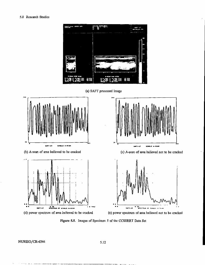
5.0 Research Studies
(a) SAFT processed image
SATT-UT SIHCLC A-tCAH •ATT-UT tlMCLC A-»CAN
(b) A-scan of area believed to be cracked (c) A-scan of area believed not to be cracked
\
1
1An
;
Fj|A"i
f|¥ \•AFT-Ut trtCTOUd Of »IHCL( A-tCAH
(d) power spectrum of area believed to be cracked (e) power spectrum of area believed not to be cracked
Figure 5.5. Images of Specimen 5 of the CCSSRRT Data Set
NUREG/CR-6344 5.12
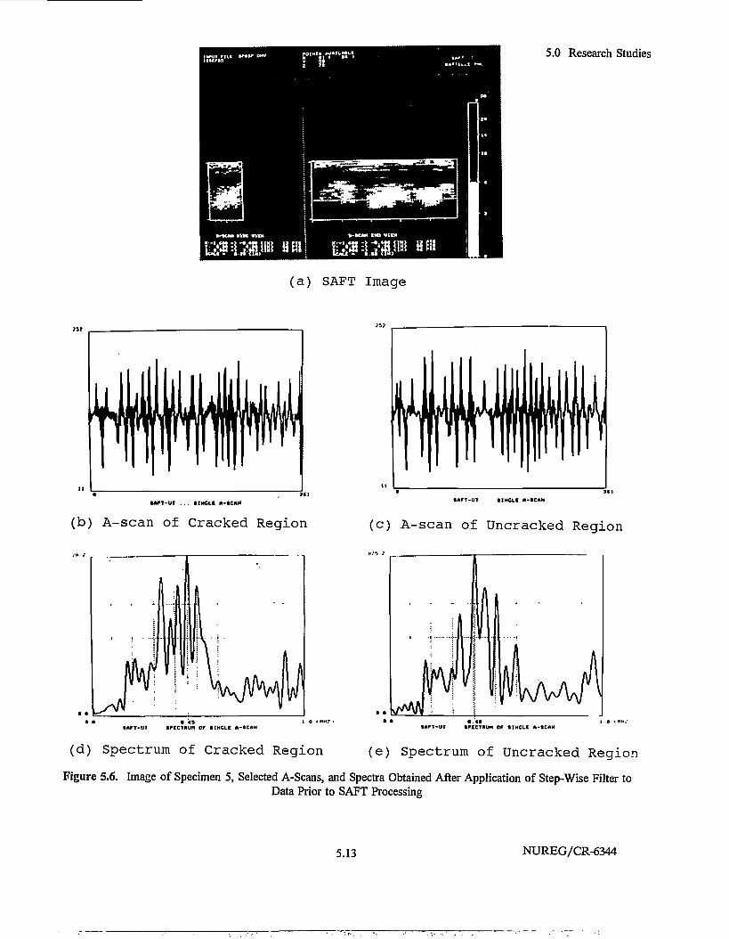
5.0 Research Studies
(a ) SAFT Image
MFT-UT . . . flHCLC A-tCAl tAFT-UT SIHCLC «-tC*M
(b) A-scan of Cracked Region (c) A-scan of Uncracked Region
Jrvill /
tAFT-UT tFECTRlM OF SIHCLC A-tCAH
(d) Spectrum of Cracked Region (e) Spectrum of Uncracked Region
Figure 5.6. Image of Specimen 5, Selected A-Scans, and Spectra Obtained After Application of Step-Wise Filter toData Prior to SAFT Processing
5.13 NUREG/CR-6344
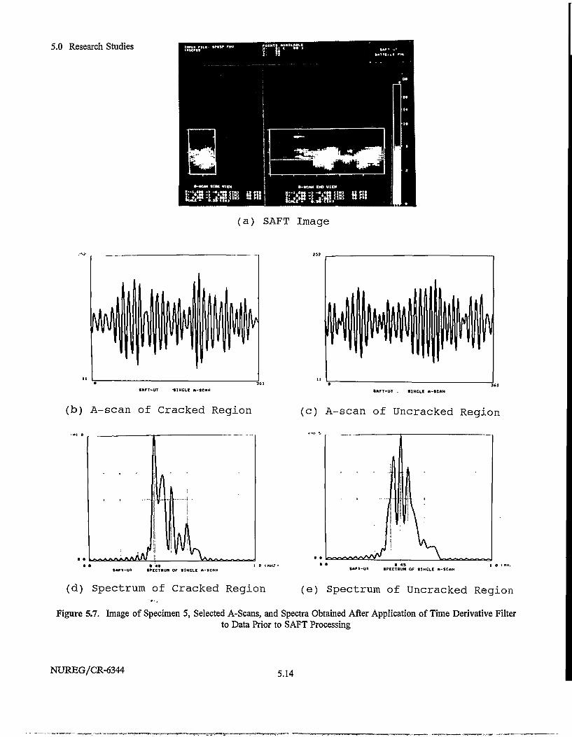
5.0 Research Studies
( a ) SAFT I m a g e
SAFT-UT -SIHCLC A-tCAH
(b) A-scan of Cracked Region (c) A-scan of Uncracked Region
• • Lss^s^Ss.
\
(d) Spectrum of Cracked Region (e) Spectrum of Uncracked Region
Figure 5.7. Image of Specimen 5, Selected A-Scans, and Spectra Obtained After Application of Time Derivative Filterto Data Prior to SAFT Processing
NUREG/CR-6344 5.14
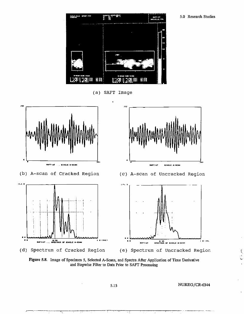
5.0 Research Studies
( a ) SAFT Image
•AFT-UT . . tlHClf A-»CAM
(b) A-scan of Cracked Region
••FT-UT S1HCLC A-tCA!
(c) A-scan of Uncracked Region
• • ! •
• • • . • « •
••"-Ill . .. »PICT«UM Of SIHCLI «-!C«H• • • 43
SAPT-UT SPECTRUM OF SIHCLE A-tCAN
(d) Spectrum of Cracked Region (e) Spectrum of Uncracked Region
Figure 5.8. Image of Specimen 5, Selected A-Scans, and Spectra After Application of Time Derivativeand Stepwise Filter to Data Prior to SAFT Processing
5.15 NUREG/CR-6344
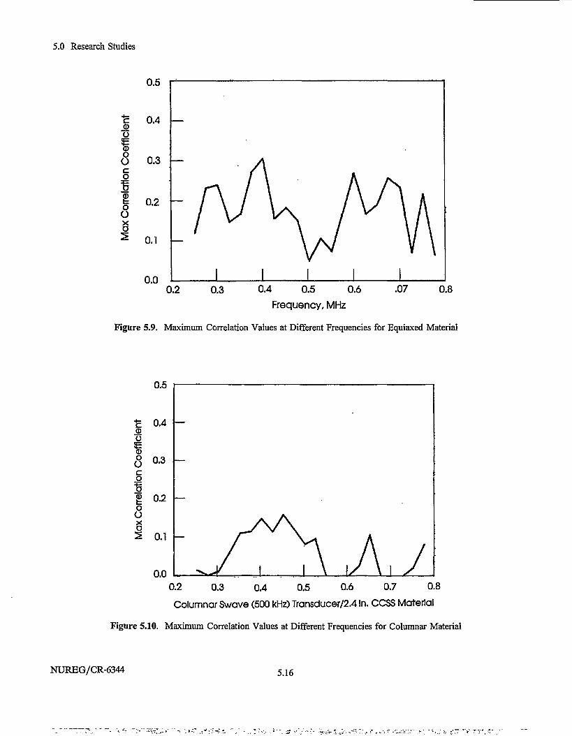
5.0 Research Studies
0.5
"E 0.4 —oioOs
0.3 —
i 0.2
1 a,
0.00.2 0.3 0.4 0.5 0.6 .07 0.8
Frequency, MHz
Figure 5.9. Maximum Correlation Values at Different Frequencies for Equiaxed Material
0.5
•£ 0.4
18 °-3
o
80.2 —
0.1 -
0.00.2 0.3 0.4 0.5 0.6 0.7 0.8
Columnar Swave (500 kHz) Transducer/2.4 In. CCSS Material
Figure 5.10. Maximum Correlation Values at Different Frequencies for Columnar Material
NUREG/CR-6344 5.16
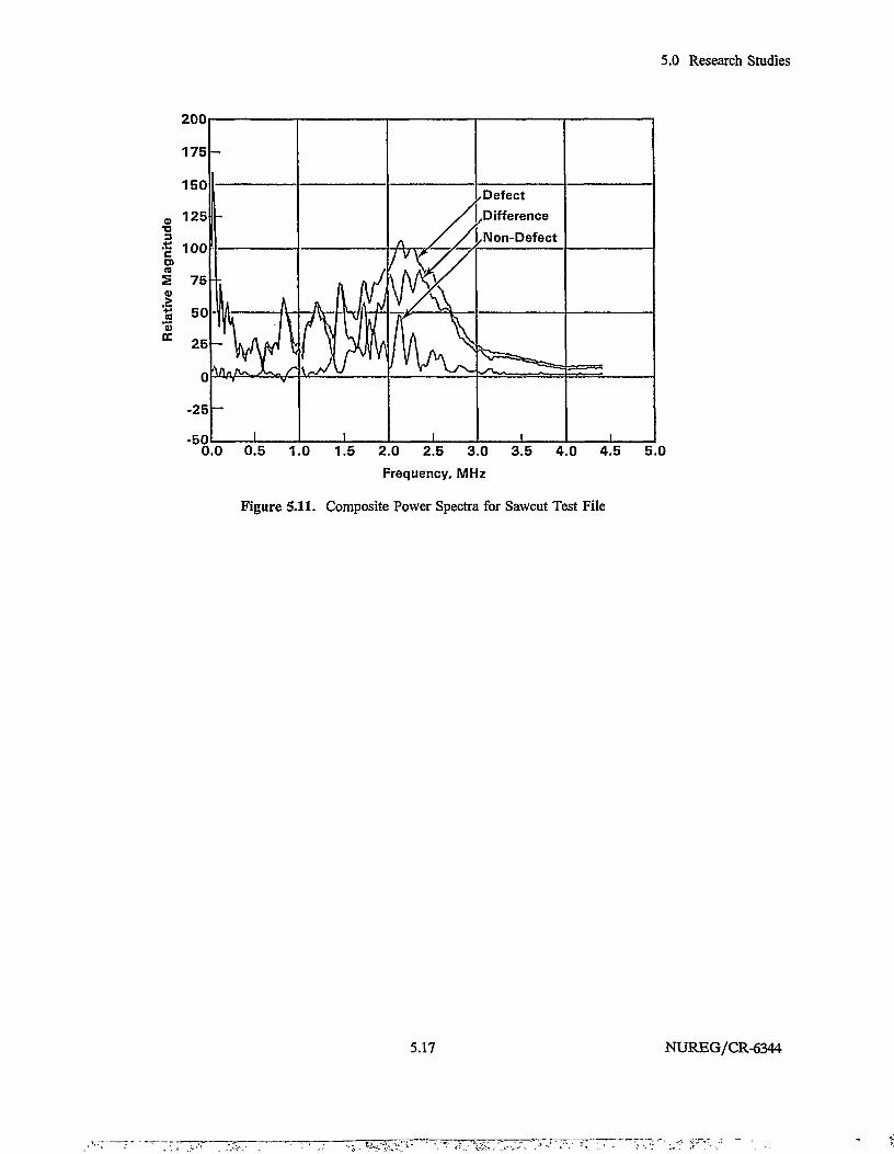
5.0 Research Studies
DefectDifference
IMon-Defect
0.0 0.5 1.0 1.5 2.0 2.5 3.0 3.5 4.0 4.5 5.0Frequency, MHz
Figure 5.11. Composite Power Spectra for Sawcut Test File
5.17 NUREG/CR-6344
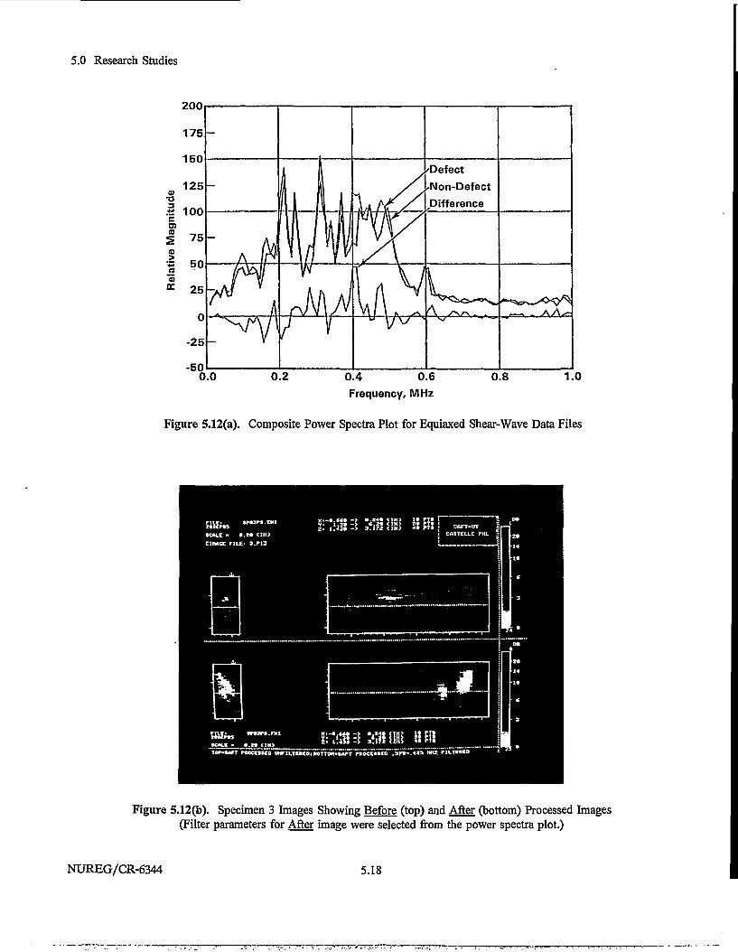
5.0 Research Studies
200
175
150
1 2 5 -•a
itu
creIB
2a
ativ
oDC
100
75
50
25
- 2 5 -
-50
-
-
Jlffi7
/ v \/v/ N
'Defect.Non-Defect^Difference
A. ^N/>. ~
0.0 0.2 0.4 0.6Frequency, MHz
0.8 1.0
Figure 5.12(a). Composite Power Spectra Plot for Equiaxed Shear-Wave Data Files
Figure 5.12(b). Specimen 3 Images Showing Before (top) and After (bottom) Processed Images(Filter parameters for After image were selected from the power spectra plot.)
NUREG/CR-6344 5.18
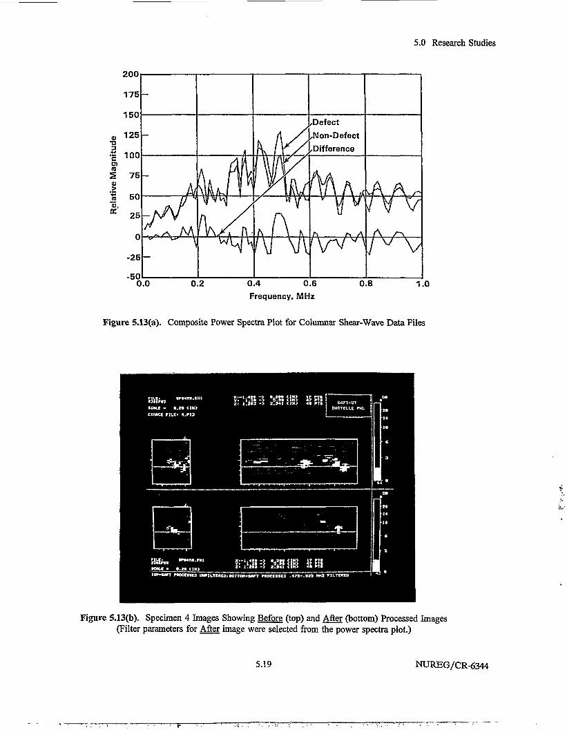
5.0 Research Studies
DefectNon-DefectDifference
0.4 0.6Frequency, MHz
Figure 5.13(a). Composite Power Spectra Plot for Columnar Shear-Wave Data Files
SOU • • . » <1H>CIIMCC FILEi 4.PI3
SftFT-UT 5,eATTELLE MO. !=[
J""*"*"**^t^
r noama amivn*aitornm-t*rj ntoeioto ,<73- .MS KHZ FILTCTTO
Figure 5.13(b). Specimen 4 Images Showing Before (top) and After (bottom) Processed Images(Filter parameters for After image were selected from the power spectra plot.)
5.19 NUREG/CR-6344
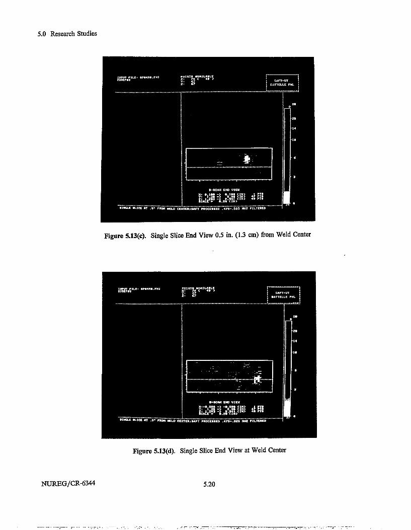
5.0 Research Studies
Figure 5.13(c). Single Slice End View 0.5 in. (1.3 cm) from Weld Center
Figure 5.13(d). Single Slice End View at Weld Center
NUKEG/CR-6344 5.20
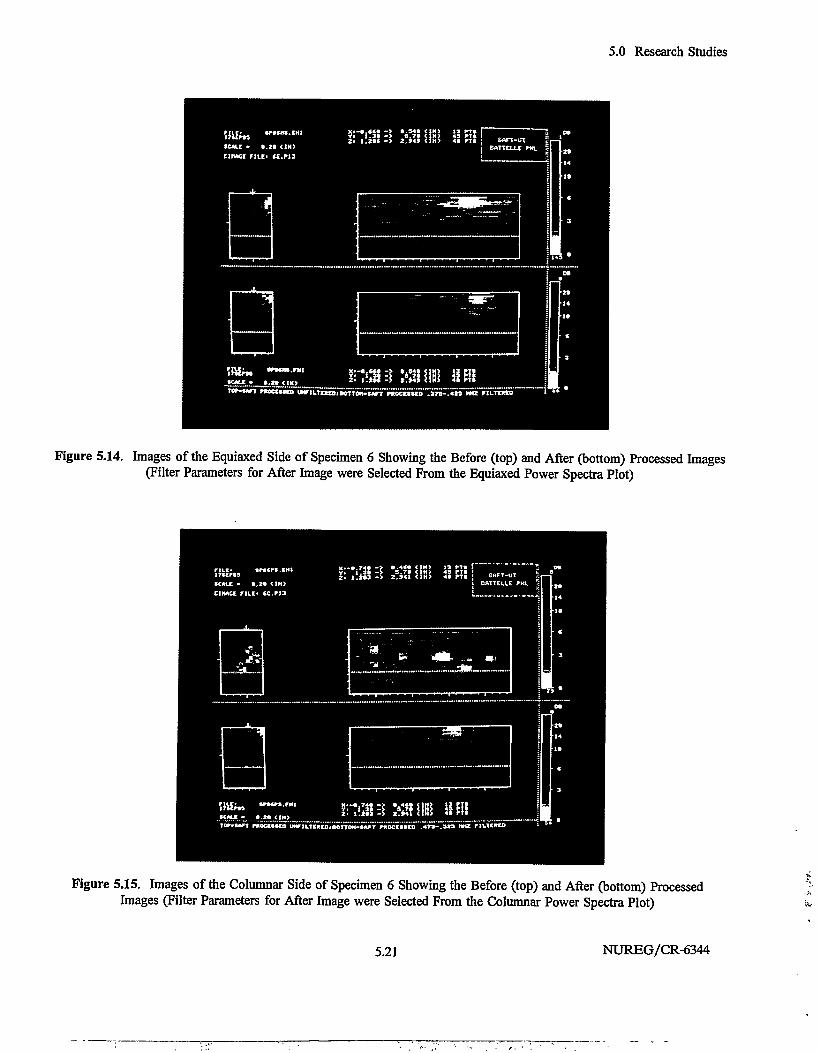
5.0 Research Studies
Figure 5.14. Images of the Equiaxed Side of Specimen 6 Showing the Before (top) and After (bottom) Processed Images(Filter Parameters for After Image were Selected From the Equiaxed Power Spectra Plot)
Figure 5.15. Images of the Columnar Side of Specimen 6 Showing the Before (top) and After (bottom) ProcessedImages (Filter Parameters for After Image were Selected From the Columnar Power Spectra Plot)
5.21 NUREG/CR-6344
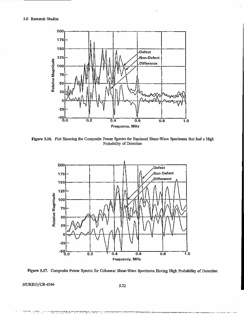
5.0 Research Studies
DefectNon-DefectDifference
0.4 0.6Frequency, MHz
Figure 5.16. Plot Showing the Composite Power Spectra for Equiaxed Shear-Wave Specimens that had a HighProbability of Detection
200
175 -
150
125 -
.•§ 100c(0
2IIoc
DefectNon-DefectDifference
- 2 5 -
0.0 0.2 0.4 0.6Frequency, MHz
Figure 5.17. Composite Power Spectra for Columnar Shear-Wave Specimens Having High Probability of Detection
NUREG/CR-6344 5.22
6.0 Laboratory Parametric Studies
Laboratory tests were performed to examine the effectsof thickness and velocity parameters on TSAFT-2 imag-es. The tests were a natural follow-on to similar studiesconducted on TSAFT images. Section 6 goes on to re-port a bandwidth compensation study performed byPNL to document the limitations of the narrow-bandapproximation used in the SAFT algorithm. A utilitywas developed to improve the SAFT images of wide-band data files.
6.1 TSAFT-2 Configuration Velocityand Thickness Parametric Study
Velocity and.thickness variation studies were performedon the TSAFT-2 configuration to augment a similarstudy performed on the TSAFT configuration in 1986.It was felt that, to be complete, a parallel investigationneeded to be performed on the simultaneous source-receiver scanning configuration of TSAFT-2.
Two performance evaluation studies were focussed onthe TSAFT-2 configuration to determine the sensitivityof this mode to velocity errors and thickness measure-ment errors. Another goal of these studies was toquantify the degradation that occurs due to these varia-tions.
The SAFT algorithm implemented at PNL assumesisotropic and homogeneous material with respect tovelocity; that is, the calculations performed by theSAFT processing make the approximation that thevelocity is constant throughout the material. This, ofcourse, is not exactly true in most specimens, and thevariance depends greatly on the type of material undertest. Also, the algorithm requires that the velocity beknown to some degree of accuracy. This may seem tobe a trivial requirement but, in many cases, is not. Forexample, an extreme .case is CCSS material, whichvaries in velocity as a function of angle in the material.The following, then, is an experimental study to deter-mine the image effects of erroneous velocity measure-ments on TSAFT-2 data files.
The data file chosen for this experiment is a TSAFT-2scan of a 0.3-in.-deep (0.8-cm) sawcut in 0.750-in.-thick(1,9-cm) aluminum material. The material is a very flatcoupon with actual characteristics that are known veryaccurately. Each element in the chosen sequence utiliz-es the same data file but simply varies the velocity
parameter in the data file header block. This simulatesacquiring the data at these velocities and should pro-duce identical results.
Figure 6.1 shows the series of images obtained by se-quencing the velocity of the material. The known veloc-ity is 122000 in./s (309880 cm/s) since the illuminationwas in shear mode. Each element in the sequencerepresents approximately a 10% change in velocity.Figure 6.1(a) was processed at 97000 in./s (246380cm/s), (b) at 109000 in./s (27686 cm/s), (c) is theactual velocity of 122000 in./s (309880 cm/s), (d) is134000 in./s (340360 cm/s), and (e) is 146000 in./s(370840 cm/s).
It should be noted that each file was processed to in-clude the complete data; therefore, both the true andconjugate images are visible. Since the object is a semi-circular shaped sawcut, then one would expect the fullyilluminated TSAFT-2 image to be elliptical with itscenterline located at the back surface line. When oneobserves the image using the actual velocity, Figure6.1(c), this is indeed the case.
The images in the sequence may now be analyzed todetermine the major differences that have occurred.The most pronounced effect of velocity differences isshown to be a vertical and lateral displacement error.As the velocity increases, it is apparent that the imageis mapped deeper into the material and translates fur-ther away from the scanning device. When observingthe vertical movement of these images, it can be notedthat, in general, for every 10% increase in materialvelocity, a vertical movement of about 1/4T is realized.This observation is important. It is apparent thatTSAFT-2 is significantly sensitive to velocity errors andresults primarily in positional errors. This response isvery similar to that observed for the TSAFT (fixedsource) configuration.
As with TSAFT, the general image quality and charac-teristics deviate much less than one might expect. Thisis important to consider. Even with dramatic velocityerrors, the image integrity is retained with respect togeneral shape and size features.
Another parameter of the TSAFT-2 that is interestingto study is the measured material thickness. Just as thematerial is assumed to be homogeneous with respect tovelocity, it is also currently assumed to have a constant
6.1 NUREG/CR-6344
6.0 Laboratory Parametric Studies
thickness along the region of illumination or, in otherwords, it assumes that the front and back surfaces areuniform and parallel. This is obviously an approxima-tion, since in many pipe materials shrinkage may occurnear the weld area or a large counterbore may be pres-ent on the ID surface. For TSAFT-2 especially, onemay wonder what effects this will have on the imagequality, since TSAFT-2 relies on multiple bounce pathsto illuminate the object zone. These paths are assumedto be well known in the image calculation but, in fact,may not be that well known.
Again, the data file chosen for this experiment is theTSAFT-2 scan of a 0.3-in.-deep (0.8-cm) sawcut in0.750-in.-thick (1.9-cm) aluminum material. The samedata file is used to create the thickness variation se-quence, with just the thickness parameter in the datafile header adjusted to the appropriate value. Thisshould accurately simulate separate scans that wereacquired using these various thickness values.
The resultant images are shown in Figure 6.2. The se-quence contains five images, incrementing the thicknessby 10% each. Figure 6.2(a) shows the image represent-ing a thickness of 0.600 in. (1.52 cm), (b) 0.675 in. (1.7cm), (c) the correct thickness value of 0.750 in. (1.9cm), (d) 0.825 in. (2.1 cm), and (e) 0.900 in. (2.29 cm).
As the assumed thickness is increased, one can observefrom these images that the algorithm maps the resultmore shallow in the material. The characteristics ofthickness deviation are very similar to velocity deviation.This should not be too unexpected, since both parame-ters directly affect where the algorithm predicts time offlight of a given signal.
As stated previously, the placement of the resultingimage is dramatically affected by deviations of eitherthickness or velocity from the true values of the speci-men under test. However, the encouraging result isthat the general image integrity is retained. Thus, withthe complement of both pulse-echo and tandem scansof the same region, a judgement of size and locationmay be made. The pulse-echo corner trap image maybe used to position the defect laterally, and the TSAFT-2 image may be used to determine the horizontal andvertical extent of the defect. The characteristics of bothfiles may be used to verify the integrity of the other.
6.2 Bandwidth Compensation Study
The SAFT algorithm currently being implemented as-sumes a homogeneous, isotropic medium. It also as-sumes that the system being implemented is of mod-erate bandwidth. It has been known for some time thatthe coherent summation algorithm incorporated in theSAFT-UT operation is a narrow-band approximation.This was reviewed by Busse, Collins, and Doctor (1984)in this program and was discussed earlier by Norton(1976) in his thesis paper at Stanford University. Theexact method incorporates a time derivative of the rawdata file prior to SAFT processing. When analyzing thespectral responses of certain data files, one may deter-mine that the narrow-band approximation may be inval-id.
A software utility was written to perform the time de-rivative on a SAFT-UT data file. This utility uses theidentity (Bracewell 1965)
q'®
where:
t = timef = frequency
F = Fourier transformF ' 1 = Inverse Fourier transform operator
it = pi
The time derivative algorithm consists of performingthe Fourier transform of each A-scan, multiplying thetransformed value by the quantity (i2irf), and perform-ing the inverse transform.
Figure 6.3 shows the C-scan projection of unprocesseddata collected in a water tank using a 0.5-in.-diameter(1.3-cm) steel sphere as an object. This data file wascollected at 2.25 MHz with a 1.0-in.-diameter (2.5-cm)4.0-in. (10.2-cm) focal point probe. The sphere wasplaced 3.0 in. (7.6 cm) from the focal point. Figure 6.4plots an A-scan near the center of this data set. Theecho shown near the beginning of the trace is from thesphere object. Figure 6.5 shows the plot of the echotrace from the specimen only. Figure 6.6 is the Fourier
NUREG/CR-6344 6.2
6.0 Laboratory Parametric Studies
transform plot of the information shown in Figure 6.5.The spectrum shows a peak at 2.27 MHz and a 6-dBbandwidth of approximately 1.5 MHz or 66%. Figure6.7 shows the C-scan view of the resulting image subse-quent to SAFT processing.
The time derivative operation was performed on thisraw data file. A display of this is shown in Figure 6.8.The plot of an A-scan near the center of the file isshown hi Figure 6.9. This corresponds to the plotshown in Figure 6.4'of the unprocessed data. Figure6.10 shows the spectrum of the echo region of this A-scan. Notice that the low-frequency components aremuch diminished as compared to the raw data versionshown in Figure 6.6. This makes sense based on Equa-tion (6.1). The derivative action in the frequency do-main consists of a linear filter; the 0-Hz component isnull, and the weighting function is simply a linear ramp.The resulting image subsequent to SAFT processing ofthis data is shown in Figure 6.11.
A substantial image improvement is apparent whencomparing Figure 6.11 with Figure 6.7. However,through close observation, the scaling range appears tobe modified. If one simply performs a square function(intensity plot) of the direct SAFT processed file, theidentical results occur. Figure 6.12 shows this image.
A more complex object was implemented in the test.Figure 6.13 shows the B-scan side view and B-scan endview of a SAFT-UT pulse-echo data set. This was col-lected with a 2.25-MHz, 0.25-in.-diameter (0.6-cm) co-ntact probe configured to provide 45° shear mode illu-mination. The object was a 0.3-in.-deep (0.8-cm) saw-cut in a 0.585-in.-thick (1.5-cm) stainless steel coupon.This image shows the unfocused raw data set. Noise ispresent from the front surface signal, and the tip signalis much subdued. Figure 6.14 shows a time series plotof an A-scan that is located near the center of the scan,and contains tip signal information. Figure 6.15 showsa plot of the derivative of this A-scan. Notice that thelow-frequency components located near the front sur-face are removed.
Figure 6.16 shows the SAFT-UT image of the raw datafile. The tip signal is apparent hi this photo, but thereis a great deal of background noise due to the amplifierring-down of the surface signal. Figure 6.17 shows theSAFT processed image of the time derivative data file.Notice that the background noise is much suppressed;however, the tip signal is also reduced. This latter phe-nomenon is due to the intensity (square of the data)distribution nature of this calculation process as statedpreviously. We can observe this by squaring the dataset displayed in Figure 6.16. This result is shown hiFigure 6.18. Note that the intensity range of this imagelooks very much like that of Figure 6.17. However, thenoise level of the time derivative image file is muchreduced.
In conclusion, it can be stated that the addition of thetime derivative in the SAFT calculation would consider-ably improve the signal-to-noise ratio. The output ofthis operation should pass through a square-root func-tion to scale the data hi a manner similar to the directSAFT-UT results. Also, a hardware array processorwould be necessary to accelerate the FFT operationsinherent hi this function to make it practical to do inreal-tune hi a reasonable time for application duringthe data analysis phase. Currently, the VAX 11/730host-executed FFT performance is unacceptable andinhibits the use of this tool.
6.3 NUREG/CR-6344
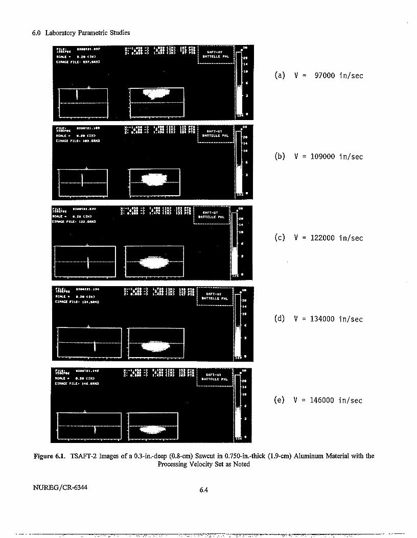
6.0 Laboratory Parametric Studies
(a) V = 97000 in/sec
l.tmm <IH> U 8 PTSSftFT-UT
BATTELLE PNL
CIIMCE FILE- tn.tiua
(b) V = 109000 in/sec
(c) V = 122000 in/sec
(d) V = 134000 in/sec
(e) V = 146000 in/sec
Figure 6.1. TSAFT-2 Images of a 0.3-in.-deep (0.8-cm) Sawcut in 0.750-in.-thick (1.9-cm) Aluminum Material with theProcessing Velocity Set as Noted
NUREG/CR-6344 6.4
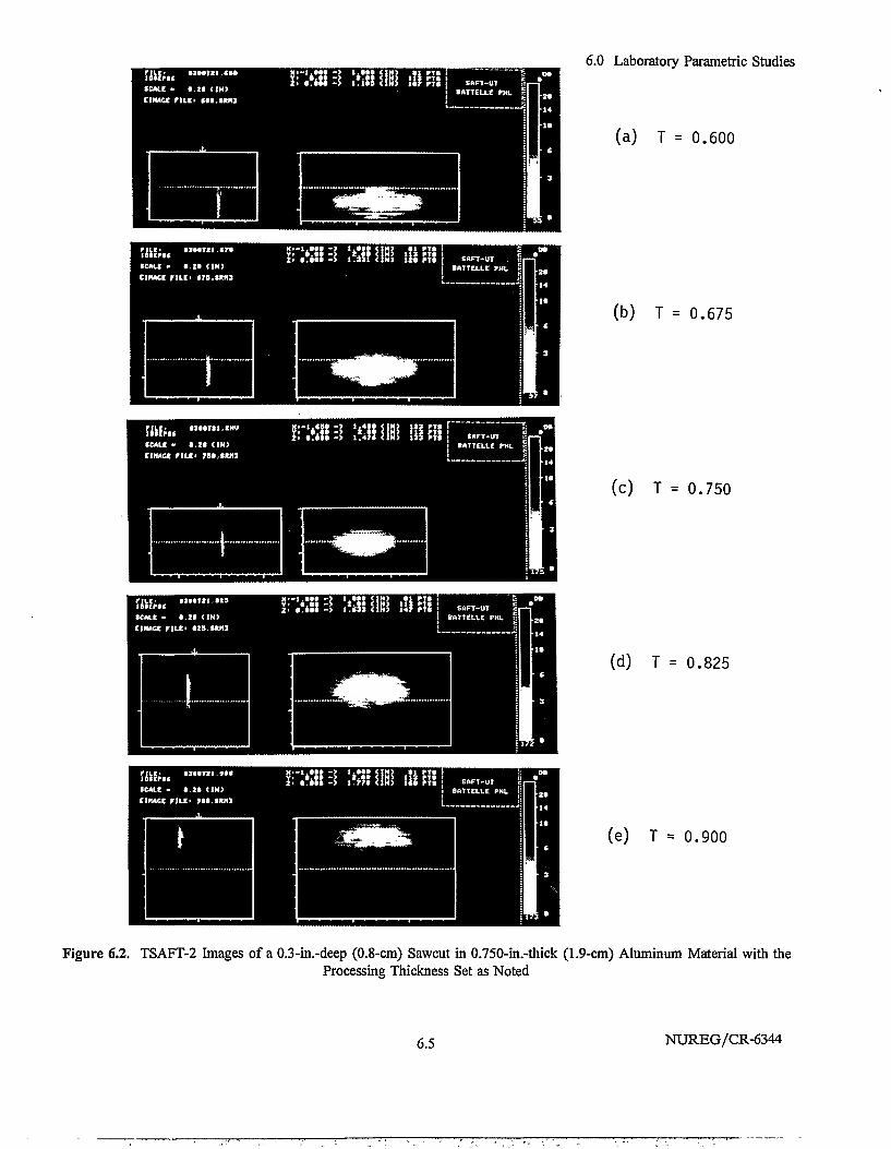
6.0 Laboratory Parametric Studies
(a) T = 0.600
(b) T = 0.675
(c) T = 0.750
(d) T = 0.825
(e) T = 0.900
Figure 6.2. TSAFT-2 Images of a 0.3-in.-deep (0.8-cm) Sawcut in 0.750-in.-thick (1.9-cm) Aluminum Material with theProcessing Thickness Set as Noted
6.5 NUREG/CR-6344
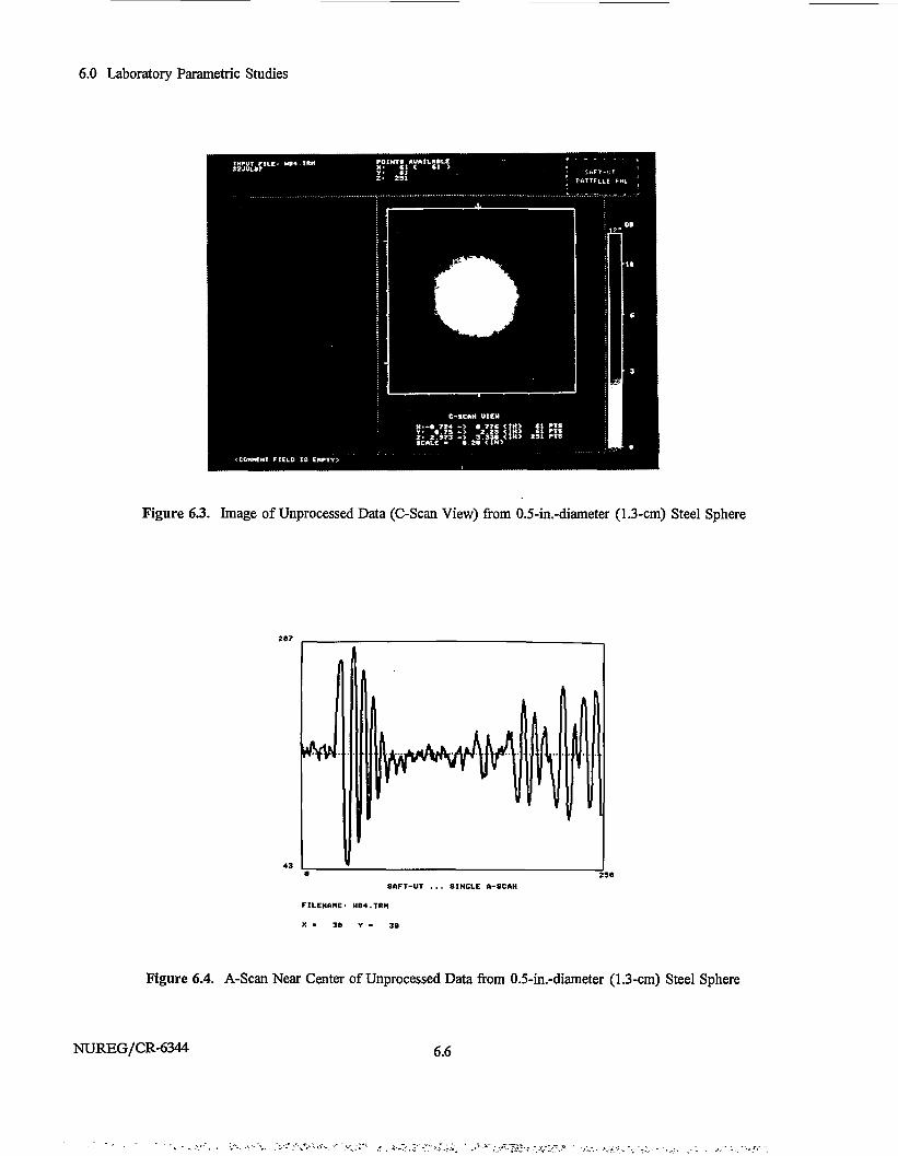
6.0 Laboratory Parametric Studies
Figure 6.3. Image of Unprocessed Data (C-Scan View) from 0.5-in.-diameter (1.3-cm) Steel Sphere
8BFT-UT .,
FILENAME' HB4.TRH
X . 39 Y - 36
• SIHCLE A-SCAN
Figure 6.4. A-Scan Near Center of Unprocessed Data from 0.5-in.-diameter (1.3-cm) Steel Sphere
NUREG/CR-6344 6.6
•'•<-••>. -* ' '.."• • - s * \ : " . i - - . , - v .
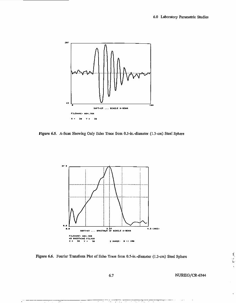
6.0 Laboratory Parametric Studies
1
1
8AFT-UT ... SINGLE A-SCAH
FILEHAHE< HB4.TRH
X - 30 Y - 38
Figure 6.5. A-Scan Showing Only Echo Trace from 0.5-in.-diameter (1.3-cm) Steel Sphere
2.278AFT-UT ... SPECTRUM OF SIHCLE A-SCAH
4.9 <HHZ>
FILENAME' U84.TRNHO SHOOTHIHC FILTERX - 38 Y - 36 2 RAHCE' • -> lt»
Figure 6.6. Fourier Transform Plot of Echo Trace from 0.5-in.-diameter (1.3-cm) Steel Sphere
6.7 NUREG/CR-6344
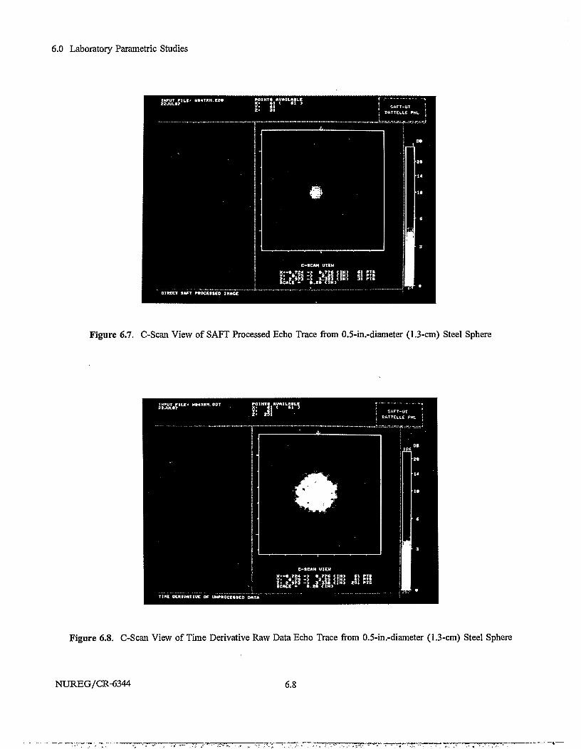
6.0 Laboratory Parametric Studies
Figure 6.7. C-Scan View of SAFT Processed Echo Trace from 0.5-in.-diameter (1.3-cm) Steel Sphere
Figure 6.8. C-Scan View of Time Derivative Raw Data Echo Trace from 0.5-in.-diameter (1.3-cm) Steel Sphere
NUREG/CR-6344 6.8
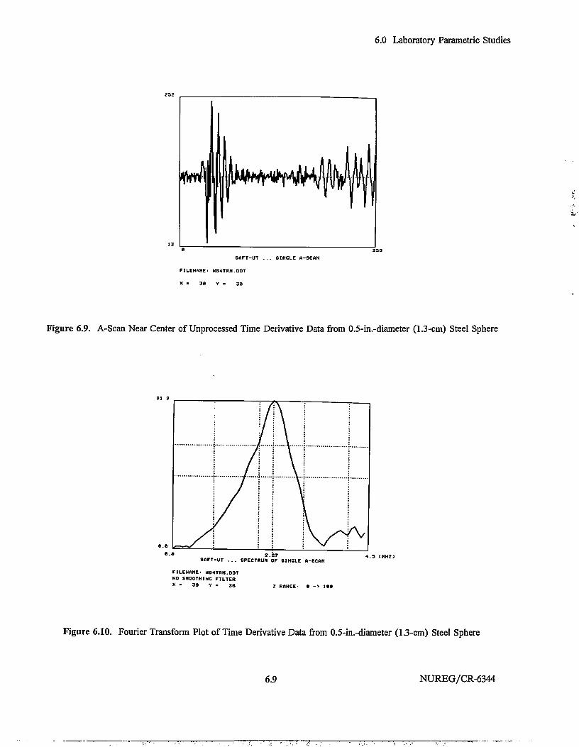
6.0 Laboratory Parametric Studies
SAFT-UT ... SINCLE A-SCAH
F1LEHAHE' UB4TRM.DDT
X > 30 Y - 30
Figure 6.9. A-Scan Near Center of Unprocessed Time Derivative Data from 0.5-in.-diameter (1.3-cm) Steel Sphere
e.a ^ /
;
/
/
\
2.27SAFT-UI ... SPECTRIM OF SIHGLE A-SCAH
4.3 <HHZ>
FILEHBME. UB4TRH.0DTNO SMOOTHING FILTERX - 30 Y . 3e Z RAHCE' • ->
Figure 6.10. Fourier Transform Plot of Time Derivative Data from 0.5-in.-diameter (1.3-cm) Steel Sphere
6.9 NUREG/CR-6344
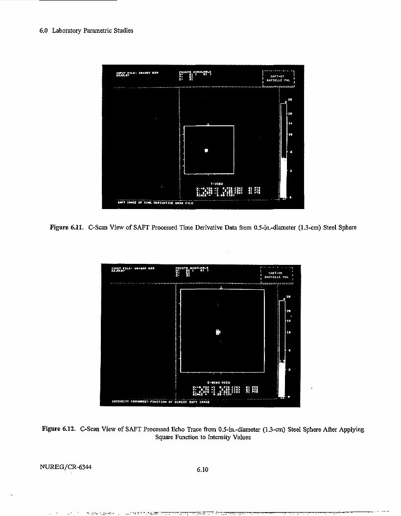
6.0 Laboratory Parametric Studies
Figure 6.11. C-Scan View of SAFT Processed Time Derivative Data from 0.5-in.-diameter (1.3-cm) Steel Sphere
Figure 6.12. C-Scan View of SAFT Processed Echo Trace from 0.5-in.-diameter (1.3-cm) Steel Sphere After ApplyingSquare Function to Intensity Values
NUREG/CR-6344 6.10
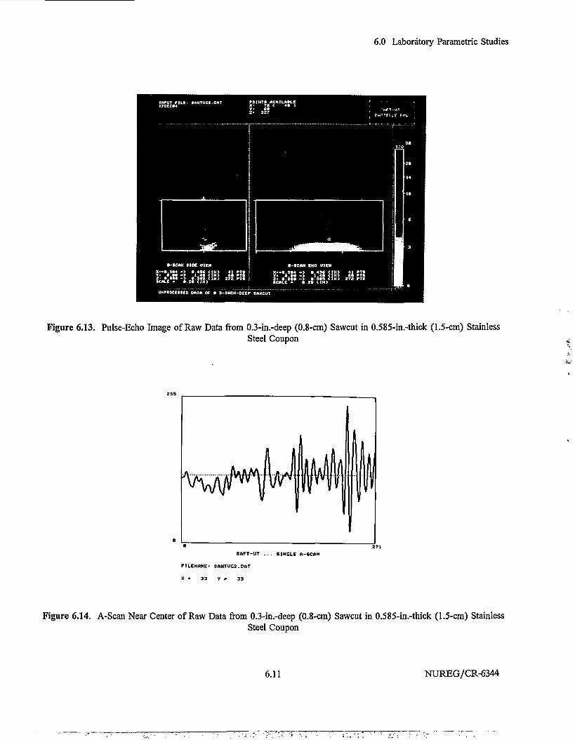
6.0 Laboratory Parametric Studies
Figure 6.13. Pulse-Echo Image of Raw Data from 0.3-in.-deep (0.8-cm) Sawcut in 0.585-in.-thick (1.5-cm) StainlessSteel Coupon
SAFT-UT ..
FILEHOME. SAUTUC2.DAT
X - 33 Y " 33
. SINCLE A-SCAH
Figure 6.14. A-Scan Near Center of Raw Data from 0.3-in.-deep (0.8-cm) Sawcut in 0.585-in.-thick (1.5-cm) StainlessSteel Coupon
6.11 NUREG/CR-6344
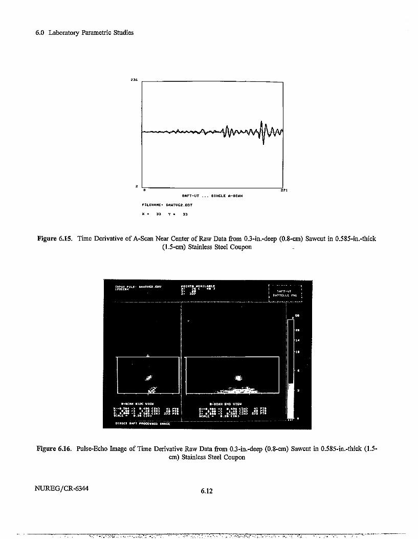
6.0 Laboratory Parametric Studies
SBFT-UT ..
FILENAME' SAMTUG2.0DT
X - 33 Y - 33
. SINCLE A-SCAH
Figure 6.15. Time Derivative of A-Scan Near Center of Raw Data from 0.3-in.-deep (0.8-cm) Sawcut in 0.585-in.-thick(1.5-cm) Stainless Steel Coupon
Figure 6.16. Pulse-Echo Image of Time Derivative Raw Data from 0.3-in.-deep (0.8-cm) Sawcut in 0.585-in.-thick (1.5-cm) Stainless Steel Coupon
NUREG/CR-6344 6.12
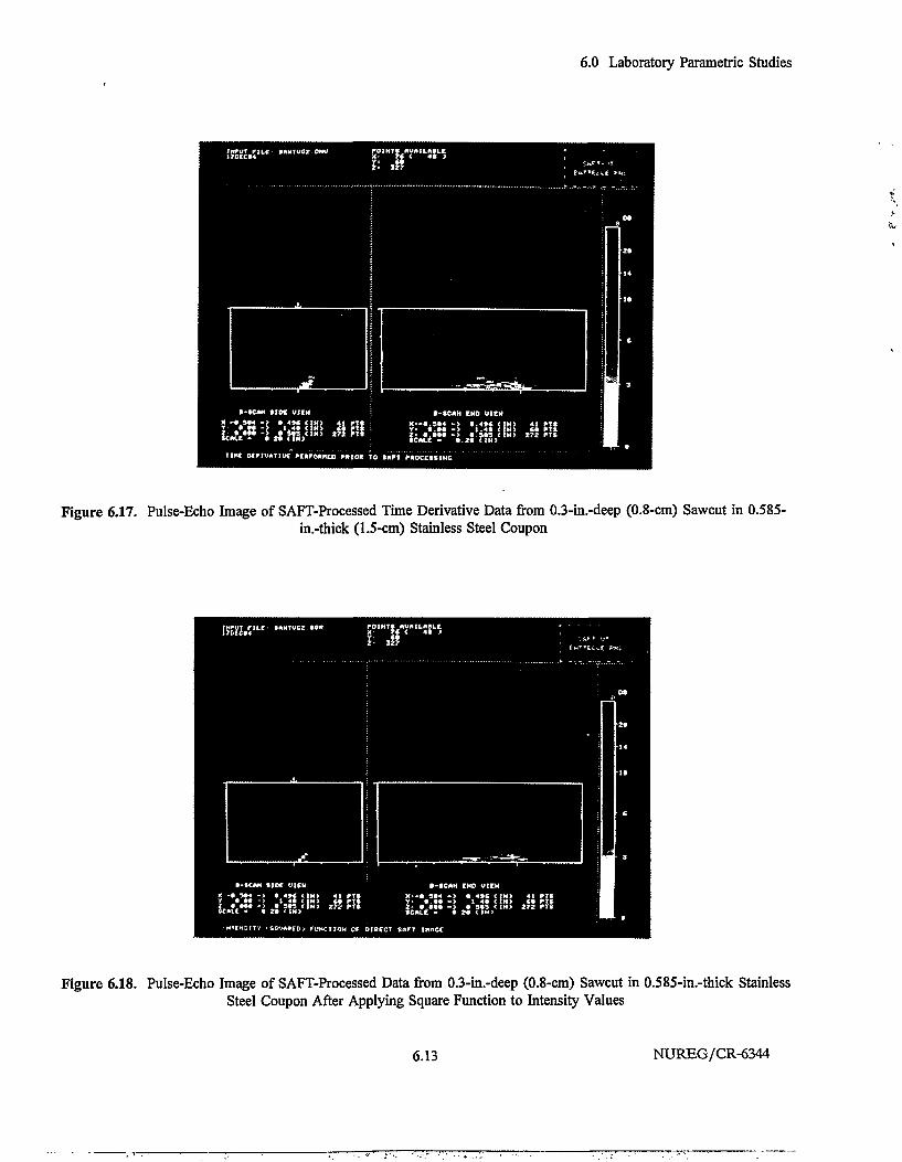
6.0 Laboratory Parametric Studies
Figure 6.17. Pulse-Echo Image of SAFT-Processed Time Derivative Data from 0.3-in.-deep (0.8-cm) Sawcut in 0.585-in.-thick (1.5-cm) Stainless Steel Coupon
Figure 6.18. Pulse-Echo Image of SAFT-Processed Data from 0.3-in.-deep (0.8-cm) Sawcut in 0.585-in.-thick StainlessSteel Coupon After Applying Square Function to Intensity Values
6.13 NUREG/CR-6344
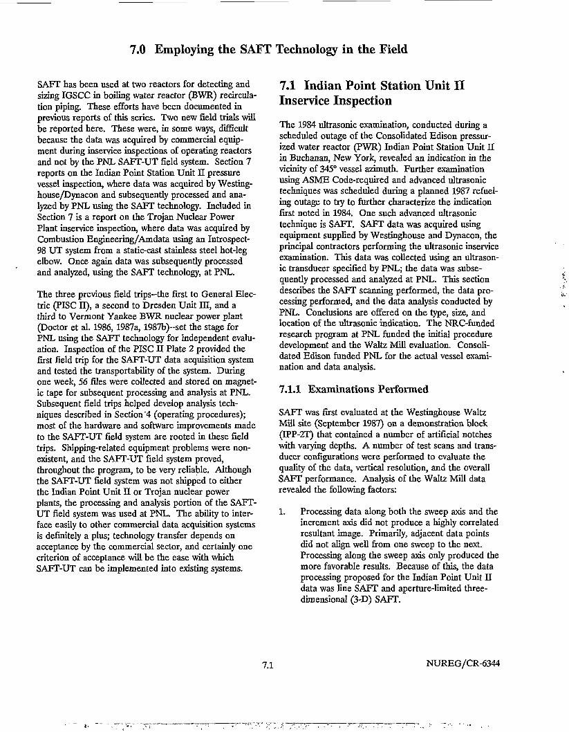
7.0 Employing the SAFT Technology in the Field
SAFT has been used at two reactors for detecting andsizing IGSCC in boiling water reactor (BWR) recircula-tion piping. These efforts have been documented inprevious reports of this series. Two new field trials willbe reported here. These were, in some ways, difficultbecause the data was acquired by commercial equip-ment during inservice inspections of operating reactorsand not by the PNL SAFT-UT field system. Section 7reports on the Indian Point Station Unit II pressurevessel inspection, where data was acquired by Westing-house/Dynacon and subsequently processed and ana-lyzed by PNL using the SAFT technology. Included inSection 7 is a report on the Trojan Nuclear PowerPlant inservice inspection, where data was acquired byCombustion Engineering/Amdata using an Introspect-98 UT system from a static-cast stainless steel hot-legelbow. Once again data was subsequently processedand analyzed, using the SAFT technology, at PNL.
The three previous field trips-the first to General Elec-tric (PISCII), a second to Dresden Unit III, and athird to Vermont Yankee BWR nuclear power plant(Doctor et al. 1986, 1987a, 1987b)~set the stage forPNL using the SAFT technology for independent evalu-ation. Inspection of the PISC II Plate 2 provided thefirst field trip for the SAFT-UT data acquisition systemand tested the transportability of the system. Duringone week, 56 files were collected and stored on magnet-ic tape for subsequent processing and analysis at PNL.Subsequent field trips helped develop analysis tech-niques described in Section "4 (operating procedures);most of the hardware and software improvements madeto the SAFT-UT field system are rooted in these fieldtrips. Shipping-related equipment problems were non-existent, and the SAFT-UT field system proved,throughout the program, to be very reliable. Althoughthe SAFT-UT field system was not snipped to eitherthe Indian Point Unit II or Trojan nuclear powerplants, the processing and analysis portion of the SAFT-UT field system was used at PNL. The ability to inter-face easily to other commercial data acquisition systemsis definitely a plus; technology transfer depends onacceptance by the commercial sector, and certainly onecriterion of acceptance will be the ease with whichSAFT-UT can be implemented into existing systems.
7.1 Indian Point Station Unit IIInservice Inspection
The 1984 ultrasonic examination, conducted during ascheduled outage of the Consolidated Edison pressur-ized water reactor (PWR) Indian Point Station Unit IIin Buchanan, New York, revealed an indication in thevicinity of 345° vessel azimuth. Further examinationusing ASME Code-required and advanced ultrasonictechniques was scheduled during a planned 1987 refuel-ing outage to try to further characterize the indicationfirst noted in 1984. One such advanced ultrasonictechnique is SAFT. SAFT data was acquired usingequipment supplied by Westinghouse and Dynacon, theprincipal contractors performing the ultrasonic inserviceexamination. This data was collected using an ultrason-ic transducer specified by PNL; the data was subse-quently processed and analyzed at PNL. This sectiondescribes the SAFT scanning performed, the data pro-cessing performed, and the data analysis conducted byPNL. Conclusions are offered on the type, size, andlocation of the ultrasonic indication. The NRC-fundedresearch program at PNL funded the initial proceduredevelopment and the Waltz Mill evaluation. Consoli-dated Edison funded PNL for the actual vessel exami-nation and data analysis.
7.1.1 Examinations Performed
SAFT was first evaluated at the Westinghouse WaltzMill site (September 1987) on a demonstration block(IPP-2T) that contained a number of artificial notcheswith varying depths. A number of test scans and trans-ducer configurations were performed to evaluate thequality of the data, vertical resolution, and the overallSAFT performance. Analysis of the Waltz Mill datarevealed the following factors:
1. Processing data along both the sweep axis and theincrement axis did not produce a highly correlatedresultant image. Primarily, adjacent data pointsdid not align well from one sweep to the next.Processing along the sweep axis only produced themore favorable results. Because of this, the dataprocessing proposed for the Indian Point Unit IIdata was line SAFT and aperture-limited three-dimensional (3-D) SAFT.
7.1 NUREG/CR-6344
7.0 SAFT in the Field
2. In an effort to limit the number of different con-figurations to be used and maintain a high degreeof resolution, a 2.25-MHz transducer was used inthe 45° shear-wave mode. Analysis of the WaltzMill data indicated that the cladded surface wasseverely impairing the weaker tip-diffracted echoused to measure the vertical extent of the notches.However, the higher amplitude corner-reflectedecho did correlate well and produced a cornertrap image showing only minor degradation.
3. Laboratory tests on a 3-in.-thick (7.6-cm) multi-wire cladded block containing a sawcut performedat PNL during the Waltz Mill data analysis re-vealed that the same transducer using the 45°longitudinal mode would generate a higher ampli-tude and more coherent tip-diffracted echo. Thetip-diffracted echo is very important in determin-ing the vertical extent of planar reflectors withsharp radiused edges such as cracks. It was feltthat the longitudinal mode scans would be veryvaluable, although the resolution would be one-half that of the shear-wave scan.
The SAFT transducer selected and used at Waltz Millwas also used at Indian Point Unit II. An immersiontransducer analysis form and data acquisition proce-dures were provided to Westinghouse. The SAFTtransducer used was a Panametrics A305S, Serial#69838, and has the following characteristics:
1. center frequency of 2.25 MHz
2. diameter of 0.75 in. (1.91 cm)
3. focal length of 3 in. (7.6 cm)
4. F number of 4
5. bandwidth approaching 50%
6. The theoretical resolution of the transducer is 0.17in. (0.43 cm) in water. The theoretical SAFTresolution in steel (for a limited SAFT aperturewith a 6° full-beam angle) is 0.19 in. (0.48 cm) forthe shear mode and 0.35 in. (0.9 cm) for the lon-gitudinal mode. The actual resolution obtained isexpected to be degraded from the theoreticalresolution because of cladding effects and systemeffects such as positional scanning tolerances.
Acquisition, of data to be processed using the SAFTalgorithm requires digitizing the rf data and sampling atleast twice per wavelength in the scanned axis directionand at least once per wavelength in the incrementalaxis. Temporal sampling must be at least four timesper wavelength and encompass the full physical aper-ture (defined as the loss of signal in both the positiveand negative directions of the scanned and incrementalaxes). This high density is required to produce the highresolution and high signal-to-noise ratio imaging. Re-sultant data files from thick-section materials, such asvessels, are inherently large and require more time toacquire, archive, and analyze.
During SAFT data collection on the Indian Point UnitII vessel, it was decided to acquire data using threescan configurations. The SAFT transducer was mount-ed in slot 29 of the Westinghouse ten-year plate. It wasdetermined that when the plate was normal to thevessel wall, the SAFT transducer would produce a 45°refracted shear wave in the vessel. Westinghouse couldrotate the plate 10.8°, producing a 45° refracted longitu-dinal wave in the vessel. Hence, with one transducerand little effort, SAFT data could be acquired in boththe shear and longitudinal modes. The shear-wave scanwould yield a higher-resolution image, and the longitu-dinal scan would enhance the tip-diffracted echo if itexisted.
The following describes the three scans in which datawere collected:
1. Scan #1 was a 45° longitudinal scan with thetransducer pointing in the clockwise direction (thisclockwise direction produced a lower-amplituderesponse than did the counterclockwise direction).The physical aperture was determined by signalloss in each direction (± scan axis and ± incre-ment axis).
2. Scans #2 and #3 were with the transducer point-ing in the counterclockwise direction (this sideproduced the largest amplitude echoes). Scan #2was a 45° longitudinal insonification, and scan #3was a 45° shear-wave scan. The physical aperturewas again determined by signal loss but encom-passed both transducer configurations to avoidprogramming the scanner twice (the programmingtask took an hour to perform because of thedense sampling parameters required).
NUREG/CR-6344 7.2
7.0 SAFT in the Field
Quality of the three data files was fair to good. Duringscan #1, a synchronization problem caused an erraticsampling from sweep to sweep. A retake of scan #1was not accomplished because it was considered a lowpriority. Scan #1 was processed but proved to be oflittle value. Scans #2 and #3 were adequate, with scan#3 providing the best signal-to-noise ratio and ultimate-ly the most information.
7.1.2 Data Analysis
SAFT data acquisition setup began around 1900 hourson October 20, 1987, and was completed at 1100 hourson October 21, 1987. The data was collected with theintent of evaluating the use of SAFT on thick-walledvessels and to further characterize the ultrasonic vesselindication. Three cases or classes of indications couldexist in the area where SAFT data was acquired:
• Case 1 - Volumetric - slag inclusion or porositywith a high degree of spherical or cylindrical size
• Case 2 - Flat - lack of fusion or inclusion (thewidth dimension being small relative to the heightor length dimension)
• Case 3 - Crack - diffuse reflector, probably sur-face-connected.
All of the images analyzed conveyed a single message—the indication seemed to be above the far surface andnot surface-connected. Figure 7.1 presents the 45°shear-wave image of the corner-trap echo of a 0.3-in.-deep (0.76-cm) notch (data acquired at Waltz Mill).The indication center is around the far surface, indicat-ed by a dashed line that has been adjusted to compen-sate for the block curvature. Furthermore, note theeffect of the cladding by observing the periodic signalloss present in the B-scan end view. Figure 7.2 presentsthe 45° image of the corner trap of a 0.3-in.-deep (0.8-cm) sawcut in a 9-in.-thick (22.9-cm) unclad steel block(data acquired at PNL). The images pictured in Fig-ures 7.1 and 7.2 are in substantial agreement, althoughthe system hardware used and the ease with which thematerials can be ultrasonically inspected differ. Figure7.3 presents the 3-D SAFT processed 45° shear-wavedata acquired on the Indian Point Unit II reactor pres-sure vessel. The indication is clearly off the far surface.(NOTE: The dashed line in Figure 7.3 represents the
vessel far surface and has not been compensated forvessel curvature. The actual vessel far surface is locat-ed 0.25 in. (0.6 cm) above the dashed line, and this isone-half a minor division on the vertical axis.) If theindication was a crack (Case 3), it would most likely besurface-connected, presenting a corner-trap echo thatwould be oriented similar to that shown in Figure 7.1.If it was a crack and not surface-connected, the tip-diffracted echo should appear if it is within the systemresolution. The 3-D SAFT-processed 45° longitudinalwave image (Figure 7.4) did not contain any tip indica-tions. (The dashed line in Figure 7.4 represents thevessel far surface and has been adjusted to compensatefor the vessel curvature.)
If the indication was volumetric with a significant acous-tic cross section (Case 1), the normal beam scans per-formed by Westinghouse should show an indication.Finally, if the indication was flat and of a proper orien-tation (Case 2), a mirror image should be seen project-ed below the far surface and possibly a corner-trapecho projected on the far surface. Figure 7.5 presentsthe image of a side-drilled hole that is 0.5 in. (1.3 cm)from the far surface of a 2.0-in.-thick (5.1-cm) steelblock showing the direct, corner-trap echo, and mirrorechoes one would expect for a volumetric defect withgood acoustic scattering properties.
The SAFT 45° shear-wave data file did not sample farenough to see the mirror echo, if it exists, and a corner-trap echo is not evident. Perhaps the geometry of theindication is such that the corner echo is severely re-duced and therefore may not be distinguishable fromthe background noise. The 45° longitudinal scans sup-port the shear-wave scans in that the indication seemsto be above the far surface. The data collected byWestinghouse sampled beyond the far surface andshould corroborate the SAFT data. Westinghouse useda much larger variety of scan configurations (normalbeam, pitch/catch, delta, 45° shear, 60° shear, and 45°longitudinal), which should help confirm the analysis ofthe SAFT data.
7.1.3 Discussion
A review of the SAFT data shows that this indicationdoes not present a geometry exhibiting tip signals or astrong corner-trap echo. This indication appears to beabove the back surface although the remaining ligament
7.3 NUREG/CR-6344
7.0 SAFT in the Field
and through-wall height cannot be established by theSAFT data alone; it is based almost entirely on the oneaperture-limited scan of 45° shear in the pulse-echomode. The SAFT performance was based on notches(vertically oriented planar reflectors), and clearly thisindication does not image like a notch. The 45° shearimage shows that the defect does not have uniformthrough-wall height over its length. The indication hasan image center that is located on average about 0.3 in.(0.8 cm) above the far surface. The indication has acontinuous length of 1.9 in. (4.8 cm) (based on a -6 dBdrop criterion) and an intermittent length of 2.4 in. (6.1cm). (The exact termination of the indication may bebeyond 2.4 in. (6.1 cm), but this area was beyond theaperture limits chosen for the examination. The longi-tudinal scan does support the length measurement, andit was not aperture limited.) The images show thatthere are acoustic hot spots, but it is not possible toconclude if this reflector is a collection of small reflec-tors or a larger reflector with some acoustical preferen-tial facets.
7.1.4 Conclusion
The main purpose of this work was to provide usefulinformation for characterizing the indications in theIndian Point Unit II reactor pressure vessel. The SAFTscans did provide useful information for locating andsizing the indication length. The SAFT data analysisclearly shows that the defect is volumetric and is notsurface-connected.
In addition, another purpose of using the SAFT tech-nology for this examination was to assess whether thetechnology could be deployed in the field with conven-tional reactor pressure vessel inspection hardware. Theconclusion derived from this work shows that somelimitations exist with conventional hardware in achievingthe accuracies needed for positioning the transducer inthe required grid pattern. As a consequence, a limitedprocessing aperture and the line SAFT mode was used.However, some very useful data and results were ob-tained. If SAFT were to be fully utilized in similarfuture applications, it will be necessary to modify theSAFT inspection protocol to include other SAFT scansto more accurately characterize indications.
7.2 Trojan Nuclear Power Plant
In May 1988, PNL personnel traveled to the Trojan Nu-clear Power Plant to advise Amdata, Inc. personnelconcerning the conduct of a special ultrasonic examina-tion on a static-cast stainless steel hot-leg elbow. Thepurpose was to acquire data from regions alreadyknown to have ultrasonic indications and subsequentlyapply SAFT to the data. PNL was to process and ana-lyze the SAFT data at its laboratory.
The SAFT technology was selected because it could beused to apply various signal processing techniques tothe data. The inspection of cast materials is difficultbecause the material is coarse-grained, anisotropic, andinhomogeneous. As a consequence, one of the majorproblems is the identification of true defects; another isaccurate characterization of the defects. Generally,typical approaches have included zone-focused probescoupled with some signal processing such as spatial ortemporal averaging. The approach of SAFT is to ac-quire broad-band rf signals with no filtering. Then thedata can be processed by a number of techniques toselect those most effective in removing innocuous re-flectors and, at the same time, provide high resolutionand high signal-to-noise images of the defects.
Laboratory work at PNL has shown that band-limitedsignals, based on measurements from the material,could be used to improve the inspectability of the castmaterial. Thus, the approach was to gather sufficientdata to allow the development of a special filter basedon the cast elbow material. The filter would then beused on the data prior to SAFT processing.
7.2.1 Examinations Performed
Amdata personnel calibrated the 1-98 data collectionsystem on a calibration standard provided by Trojan(reference Amdata drawing C-UTC-AL-244-004).Unfortunately, the 0.5-MHz high-pass filter was usedwhen calibration data was acquired. The calibrationdata was not useful to select filter parameters based oncomposite spectra results of known defect and nondef-ect areas.
A total of four data files were acquired on the 9 o'clockside of the static-cast elbow in the short time allottedfor gathering SAFT data:
NUREG/CR-6344 7.4
7.0 SAFT in the Field
1. TR9SH5A.D1 - Data file number one includedthree inside surface indications that Amdata per-sonnel identified as #2, #3, and #5. An 0.5-MHzhigh-pass filter was used during data acquisition,receiver gain was set at +12 dB, and the transduc-er view was skewed 180°.
2. TR9SH5C.D1 - Data file number two was set upidentically to data file TR9SH5A.D1 except nofilters were used during data acquisition.
3. TR9SH5D.D1 - Data file number three includedone inside surface indication that Amdata person-nel identified as #4, data was acquired with thetransducer skewed 0°, and the receiver gain wasset to +12 dB.
4. TR9SH5G.D1 - Finally, data file number four in-cluded one midwall indication identified as #6,the transducer was skewed 270°, and, once again,the gain was set to +12 dB.
A Panametrics 500-kHz transducer (serial #B32180E)was used with a KB Aerotech 45° shear-wave wedge.Spatial increments of 0.05 in. (0.13 cm) were chosen, forboth the incremental and scanned axes in conjunctionwith a temporal sampling of 100 ns.
The 1-98 data acquisition system had not been usedextensively with the SAFT utilities; therefore, someempirical manipulation of the data order was necessaryto place the data in the proper SAFT format. Particu-lar attention was given to the skew angle and the bi-directional acquisition of the data file.
Each data file was first converted to the SAFT data for-mat using a software utility called VIPD. A shuffle orreordering of every other sweep was required to com-pensate for bidirectional data acquisition. Data files,where the transducer was skewed 180°, required usingthe SAFT utility EVENSHUFX to reorder the evensweeps and using the SAFT utility DEDIT to changethe incident angle sign to minus (the SAFT processingutilities always expect the incident angle direction to beX and the sign to be minus). The 0° skew data filerequired using the SAFT utility ODDSHUFX to reor-der the odd sweeps, and the 270° skew data file re-quired using the SAFT utility EVENSHUFX to reorderthe even sweeps. The 1-98 conversion utility VIPDautomatically makes the sweep or scan axis (no matter
which axis it is, X or Y) the X axis. We found thatwhen the sweep axis was circumferential (270° skew),the header said the incident angle was in the Y axis andpositive; this was not correct because of the previouslymentioned axis transformation that the VTPD utilityperforms. Therefore, we used the SAFT utility DEDITto change the direction and sign of the incident angle ofthe 270° skew data file.
Filter parameters were chosen by looking at the com-posite spectra analyses of suspected defect and nondef-ect areas of data file TR9SH5D (Figure 7.6). Unfortu-nately, the composite spectra were not very revealing,except to point out that a large 500-kHz component waspresent. Based on the composite spectra, a 0.4- to 0.6-MHz band-pass filter was used, primarily to keep thefile with about a 50% bandwidth limit desired for theSAFT processing. Each data file was band-pass filteredusing a 40% bandwidth filter (although with some ofthe data files, we experimented with different filterparameters) and then processed using the 3-D SAFTalgorithm, which coherently sums the data over a pre-defined aperture. Data files were then processed.usinga 12° and 6° full-beam angle; a beam angle of 6° wassubsequently chosen for analysis because the 12° imageswere being "washed out" due to the summing of nulldata. From the thickness measurements provided byAmdata personnel, a nominal thickness of 3.7 in. (9.4cm) was entered into the SAFT data file header foreach data file. Thickness measurements ranged from3.5 in. (8.9 cm) to 4.0 in. (10.2 cm) in the approximatearea of the 180° and 0° skew scans, and the nominalvalue used is a truncated average of these values. Typi-cally, the following scenario was followed:
1. Filter the raw data file based on composite spec-trum results. A 0.4- to 0.6-MHz filter was usedon the unfiltered 180° and 270° skew data files;the 0° skew data required no filtering.
2. SAFT process the resultant filtered file. Eachdata file was 3-D SAFT processed using a 6° full-beam angle.
3. Use the APLOT utility to analyze the processedresults. A full B-scan side view and C-scan topview were initially analyzed. Each indication wasboxed, and an expanded B-scan side view and B-scan end view were used for the final analysis andsizing.
7.5 NUREG/CR-6344
7.0 SAFT in the Field
7.2.2 Data Analysis
A 0.5-MHz high-pass filter was used during data acqui-sition of the 180° skew data file TR9SH5A. Figure7.7(a) shows the B-scan side and C-scan top view ofdata file TR9SH5A; three groups of indications areapparent. Each indication has been boxed on the C-scan view and labeled 2, 3, and 5 on the accompanyingC-scan graphic. An expanded view of each indication isshown in Figures 7.7(b), 7.7(c), and 7.7(d). A sizingattempt has been made (Table 7.7), and the defectshave been correlated to the indications identified byAmdata personnel.
Figure 7.7(a) shows indication 2 to be a dog-leg shapedindication; accurate sizing of the spot-like indicationsalong the axial portion of the dog leg cannot be madeand, therefore, have not been included in Table 7.1.The image of indication 2 is very difficult to interpret.Most of the indications seen in Figure 7.7(b), the B-scan side view, are at the same depth and may be cor-ner-trap echoes from a surface-connected planar defect.Indication 3, Figure 7.7(c), is composed of a number ofindications that have been considered as one because ofthe proximity of one to another. The depth of indica-tion 3 varies; the strongest echo appears above thenominal thickness value, leading one to believe that thisindication may not be surface-connected. Indication 5,Figure 7.7(d), presents a very interesting B-scan sideview; the three major components of this indication areat different depths and uniform intensity. Characteris-tics of a surface-connected planar defect usually includea strong corner-trap indication and a reduced tip-dif-fracted echo. Indication 5 exhibits volumetric charac-teristics and does not image like one would expect if itwere a surface-connected planar defect.
Figure 7.8(a) presents the B-scan side view and C-scanview of the 180° skew data file TR9SH5C; a total of fiveindications have been identified and are labeled 2, 3, 5,A, and B in the accompanying C-scan graphics. A 0.4-to 0.6-MHz band-pass filter was applied to this data fileprior to SAFT processing primarily because this datafile was very noisy and difficult to interpret. Figures7.8(b), 7.8(c), 7.8(d), 7.8(e), and 7.8(f) show boxedviews of indications 2, 3, 5, A, and B. Each indicationsize is listed in the comments section of the indicationphotograph and is repeated in Table 7.1.
Only a part of the axial portion of indication 2, which isthe same area as the dog-leg indication 2 seen in datafile TR9SH5A, Figure 7.7(a), is visible in Figure 7.8(a).The circumferential part of indication 2, B-scan sideview, Figure 7.8(b), varies in depth as do indications 3and 5 in Figures 7.8(c) and 7.8(d), suggesting eithervolumetric reflectors or a varying far surface. Indica-tions 2, 3, and 5 of data file TR9SH5C compare favor-ably with the same indications seen in data fileTR9SH5A, although different filters were used prior toSAFT processing the data. Indication A, Figure 7.8(e),is an additional indication that has been noted; it is atleast -6 dB less intense than the other indications notedin data file TR9SH5C. The signal-to-noise ratio seen inFigure 7.8(e) makes characterization of this indicationdifficult. The most intense portion of indication Aappears near the nominal thickness value line; there-fore, this indication may be surface-connected. Finally,indication B, Figure 7.8(f), presents one high-intensityindication surrounded by shallower low-level indications.Once again, indication B appears near the nominalthickness value line and, for this reason, may besurface-connected.
Sizing of all the indications in files TR9SH5A andTR9SH5C included the surrounding low-level indica-tions. Each boxed area was normalized by the mostintense indication within the box. Sizing extended tothe -6-dB points relative to the normalized value.
The best data file, by virtue of signal-to-noise ratio anda single indication, is TR9SH5D. Figure 7.9(a) shows aB-scan side view and C-scan top view of indication 4.Only one indication is seen, and the location of thesatellite indications lead one to believe that the mainindication may not be surface-connected and may actu-ally be volumetric. Filtering of this data file did notproduce significant changes in the size of the indicationbut did help resolve the satellite indications. Since thefar surface location is not accurately known, it is diffi-cult to estimate how far off the ID surface this indica-tion might be in Figure 7.9(b), B-scan side view; howev-er, based on the nominal thickness value, one wouldestimate 0.3 in. (0.8 cm). The temporal apertureshould have been expanded in the near and far direc-tions to include a possible direct echo, if the mainindication seen is the corner-trap echo from a volumet-ric defect and/or mirror echo expected from a volu-metric defect. Presence of these particular echoes
NUREG/CR-6344 7.6
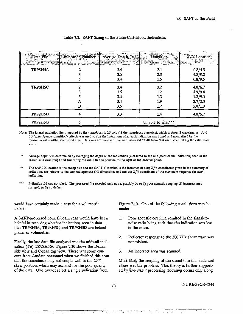
7.0 SAFT in the Field
Table 7.1. SAFT Sizing of the Static-Cast-Elbow Indications
Data File
TR9SH5A
TR9SH5C
TR9SH5D
TR9SH5G
Indication Number
235
235AB
4
6
Average Depth, In.*
3.43.53.4
3.43.53.53.43.6
3.3
Length, in.
2.12.31.5
3.21.21.31.91.2
1.4
X/Y Location,in.**
0.8/5.34.8/9.20.8/9.5
4.0/6.74.9/9.41.2/9.52.7/2.05.0/1.0
4.0/6.7
Unable to size.***
Note: The lateral resolution limit imposed by the transducer is OS inch (V4 the transducer diameter), which is about 2 wavelengths. A -6dB (green/yellow transition) criteria was used to size the indications after each indication was boxed and normalized by themaximum value within the boxed area. Data was acquired with the gain increased 12 dB from that used when taking the calibration
Average depth was determined by averaging the depth of the indications (measured to the mid-point of the indication) seen in theB-scan side view image and truncating the value to one position to the right of the decimal point.
The SAFT X location is the sweep axis and the SAFT Y location is the incremental axis; X/Y coordinates given in the summary ofindications are relative to the scanned aperture OD dimensions and are the X/Y coordinate of the maximum response for eachindication.
Indication #6 was not sized. The processed file revealed only noise, possibly do to 1) poor acoustic coupling, 2) incorrect areascanned, or 3) no defect.
would have certainly made a case for a volumetricdefect.
Figure 7.10. One of the following conclusions may bemade:
A SAFT-processed normal-beam scan would have beenhelpful in resolving whether indications seen in datafiles TR9SH5A, TR9SH5C, and TR9SH5D are indeedplanar or volumetric.
Finally, the last data file analyzed was the midwall indi-cation (#6) TR9SH5G. Figure 7.10 shows the B-scanside view and C-scan top view. There was some con-cern from Amdata personnel when we finished this scanthat the transducer may not couple well in the 270°skew position, which may account for the poor qualityof the data. One cannot select a single indication from
1. Poor acoustic coupling resulted in the signal-to-noise ratio being such that the indication was lostin the noise.
2. Reflector response to the 500-leHz shear wave wasnonexistent.
3. An incorrect area was scanned.
Most likely the coupling of the sound into the static-castelbow was the problem. This theory is further support-ed by line-SAFT processing (focusing occurs only along
7.7 NUREG/CR-6344
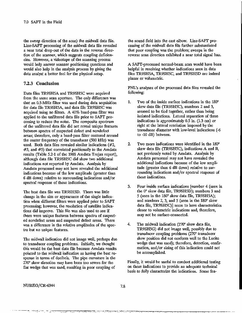
7.0 SAFT in the Field
the sweep direction of the scan) the midwall data file.Line-SAFT processing of the midwall data file revealeda near total drop-out of the data in the reverse direc-tion of the scanner, which suggests coupling deficien-cies. However, a videotape of the scanning processwould help answer scanner positioning questions andwould also help in the analysis process by giving thedata analyst a better feel for the physical setup.
7.2.3 Conclusion
Data files TR9SH5A and TR9SH5C were acquiredfrom the same scan aperture. The only difference wasthat an 0.5-MHz filter was used during data acquisitionfor data file TR9SH5A, and data file TR9SH5C wasacquired using no filters. A 40% band-pass filter wasapplied to the unfiltered data file prior to SAFT pro-cessing to reduce the noise. The composite spectrumof the unfiltered data file did not reveal unique featuresbetween spectra of suspected defect and nondefectareas; therefore, only a band-pass filter centered aroundthe center frequency of the transducer (500 kHz) wasused. Both data files revealed similar indications (#2,#3, and #5) that correlated positionally to the Amdataresults (Table 5.2-1 of the 1988 Amdata Trojan report),although data file TR9SH5C did show two additionalindications not reported by Amdata. Analysis byAmdata personnel may not have revealed the additionalindications because of the low amplitude (greater than6 dB down) relative to surrounding indications and/orspectral response of these indications.
The best data file was TR9SH5D. There was littlechange hi the size or appearance of the single indica-tion when different filters were applied prior to SAFTprocessing; however, the resolution of satellite indica-tions did improve. This file was also used to see ifthere were unique features between spectra of suspect-ed nondefect areas and suspected defect areas. Therewas a difference hi the relative amplitudes of the spec-tra but no unique features.
The midwall indication did not image well, perhaps dueto transducer coupling problems. Initially, we thoughtthis would be the best data file because Amdata resultspointed to the midwall indication as having the best re-sponse in terms of decibels. The pipe curvature in the270° skew direction may have been too severe for theflat wedge that was used, resulting in poor coupling of
the sound field into the cast elbow. Line-SAFT pro-cessing of the midwall data file further substantiatedthat poor coupling was the problem; sweeps in thereverse scan direction exhibited a near total signal loss.
A SAFT-processed normal-beam scan would have beenhelpful hi resolving whether indications seen hi datafiles TR9SH5A, TR9SH5C, and TR9SH5D are indeedplanar or volumetric.
PNL's analyses of the processed data files revealed thefollowing:
1. Two of the inside surface indications hi the 180°skew data file (TR9SH5C), numbers 2 and 3,seemed to be tied together, rather than beingisolated indications. Lateral separation of theseindications is approximately 0.5 in. (1.3 cm) orright at the lateral resolution imposed by thetransducer diameter with low-level indications (-6to -10 dB) between.
2. Two more indications were identified hi the 180°skew data file (TR9SH5C), indications A and B,not previously noted by Amdata. Analysis byAmdata personnel may not have revealed theadditional indications because of the low ampli-tude (greater than 6 dB down) relative to sur-rounding indications and/or spectral response ofthese indications.
3. Four inside surface indications [number 4 (seen inthe 0° skew data file, TR9SH5D); numbers 3 and5 (seen in the 180° skew data file, TR9SH5A);and numbers 2, 3, and 5 (seen hi the 180° skewdata file, TR9SH5C)] seem to have characteristicscloser to volumetric indications and, therefore,may not be surface-connected.
4. The midwall indication (270° skew data file,TR9SH5G) did not image well, possibly due totransducer coupling problems (270° transducerskew position did not conform well to the Lucitewedge that was used); therefore, detection, confir-mation, and/or sizing of this indication could notbe accomplished.
Finally, it would be useful to conduct additional testingon these indications to provide an adequate technicalbasis to fully characterize the indications. Some fea-
NUREG/CR-6344 7.8
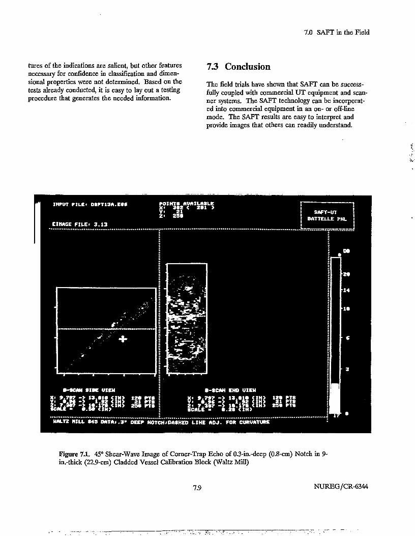
7.0 SAFT in the Field
tures of the indications are salient, but other featuresnecessary for confidence in classification and dimen-sional properties were not determined. Based on thetests already conducted, it is easy to lay out a testingprocedure that generates the needed information.
73 Conclusion
The field trials have shown that SAFT can be success-fully coupled with commercial UT equipment and scan-ner systems. The SAFT technology can be incorporat-ed into commercial equipment in an on- or off-linemode. The SAFT results are easy to interpret andprovide images that others can readily understand.
INPUT riLC> 0SFT13A.EM
CIIMGE FILE- 3.13
POINTS AVAILABLE
? 'If*? IfZ< 2SS
| SAFT-UT «> BATTELLE PHL '
m-*em I I K VIEW • - S O W CHO MXEM
NALTZ HILL *49 IMTA< .3- DEEP HOTCHiOASHEO LINE ADJ. FOR CUKUATUKE
Figure 7.1. 45° Shear-Wave Image of Corner-Trap Echo of 03-in.-deep (0.8-cm) Notch in 9-in.-thick (22.9-cm) Cladded Vessel Calibration Block (Waltz Mill)
7.9 NUREG/CR-6344
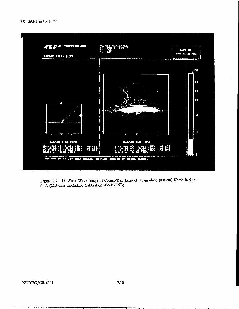
7.0 SAFT in the Field
Figure 7.2. 45° Shear-Wave Image of Corner-Trap Echo of 0.3-in.-deep (0.8-cm) Notch in 9-in.-thick (22.9-cm) Uncladded Calibration Block (PNL)
NUREG/CR-6344 7.10
7.0 SAFT in the Field
INPUT FILE' SMAUE2.E1Z
CIHAGE FILE' 3.73
I SAFT-UT }{ BATTELLE PHL j
»«_%,--,
•-•CAN END UXEH
' M H*i-F ><
Figure 7.3. 45° Shear-Wave Image (3-D Processed) of the Vessel Indication at Indian Point Unit II
7.11 NUREG/CR-6344
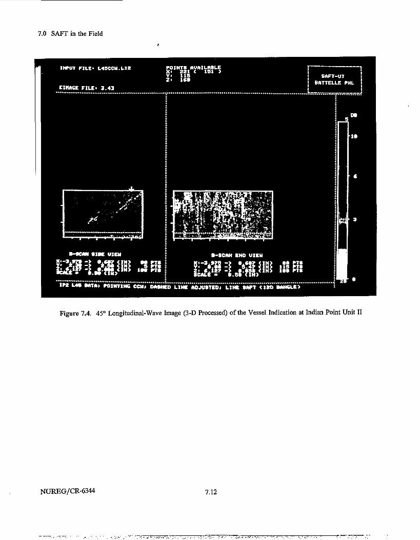
7.0 SAFT in the Field
Figure 7.4. 45° Longitudinal-Wave Image (3-D Processed) of the Vessel Indication at Indian Point Unit II
NUREG/CR-6344 7.12
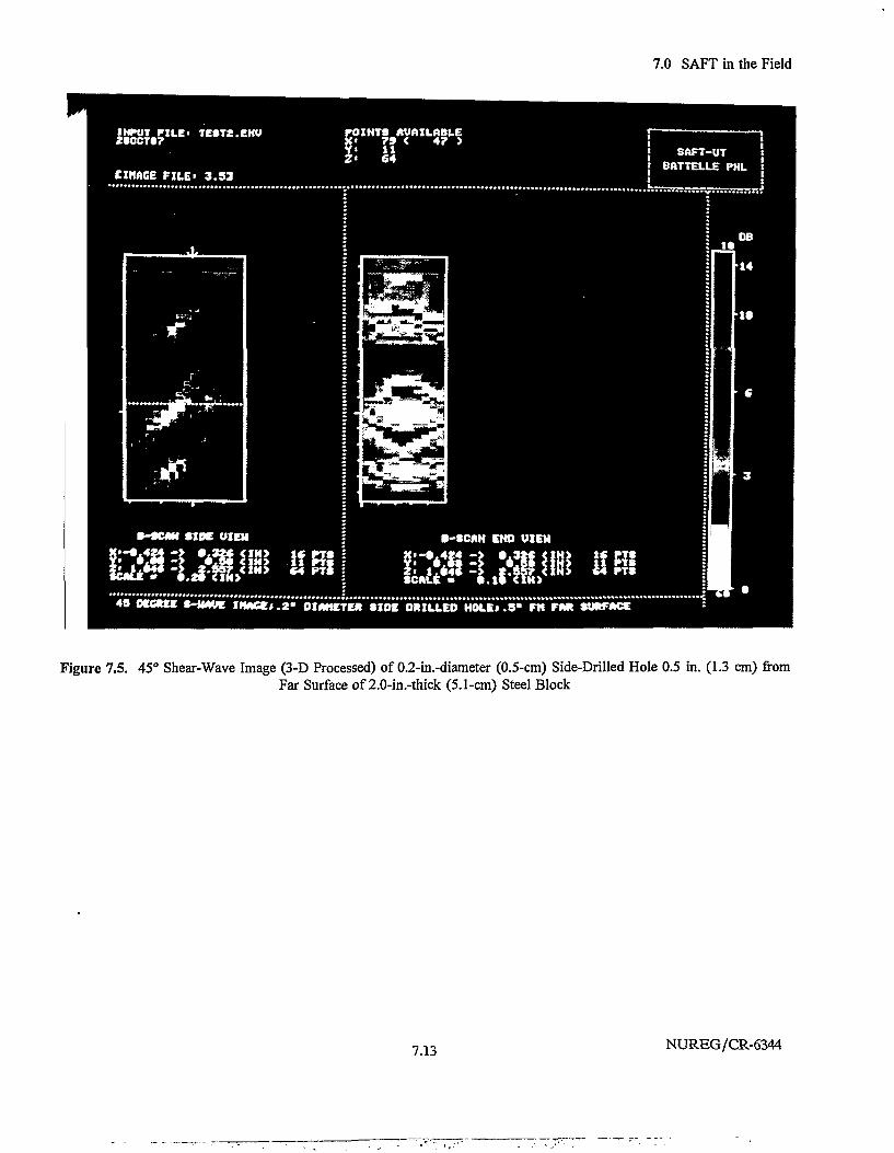
7.0 SAFT in the Field
Z« 6 4
CIHAGE FILE- 3 . S 3
| SAFT-UT 5} BftTTELLE PHL '
•-tcm «IDC VIEW •-SCAN END UIEH
Ufhl48 OCC«U t-IMUC i m c e « . 2 - OIAHETEK •iok" DlilLLED HOLEJ'.S" "r«"r*» «WF*CS
Figure 7.5. 45° Shear-Wave Image (3-D Processed) of 0.2-in.-diameter (0.5-cm) Side-Drilled Hole 0.5 in. (1.3 cm) fromFar Surface of 2.0-in.-thick (5.1-cm) Steel Block
7.13 NUREG/CR-6344
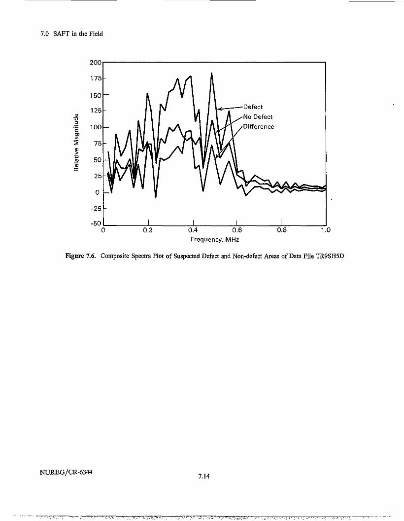
7.0 SAFT in the Field
CD•o
'ECO
CD
JOCD
CE
0 0.2 0.4 0.6Frequency, MHz
Figure 7.6. Composite Spectra Plot of Suspected Defect and Non-defect Areas of Data File TR9SH5D
NUREG/CR-63447.14
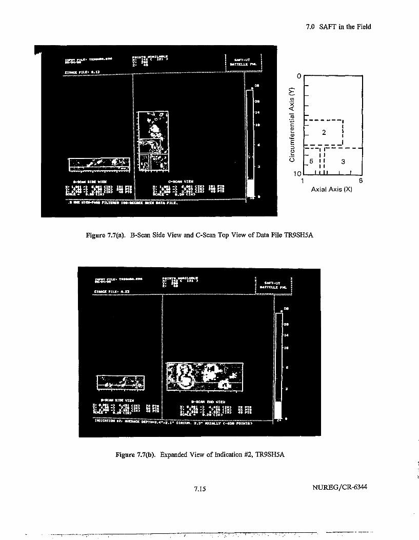
7.0 SAFT in the Field
SOFT-UTMTTCLLE PHL
CIIMCC r iU> ••130
'x
c03
03
Eoo
»-KM tIK Kit*
10
-
2
1 I--1 1
5 l 1
I i li
1
1
3
i i
1 6Axial Axis (X)
,• m inrnnw riLTnc* IW^CQMOC WXM MTA ritx.
Figure 7.7(a). B-Scan Side View and C-Scan Top View of Data File TR9SH5A
Figure 7.7(b). Expanded View of Indication #2, TR9SH5A
7.15 NUREG/CR-6344
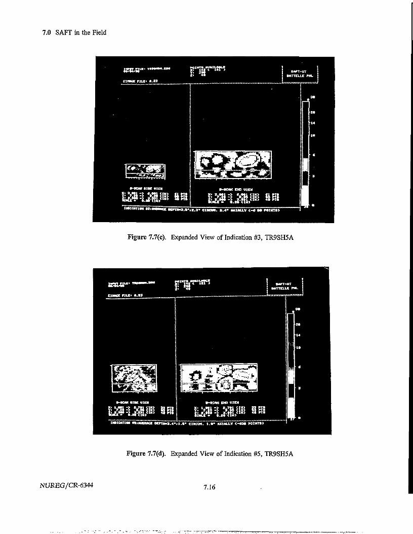
7.0 SAFT in the Field
Figure 7.7(c). Expanded View of Indication #3, TR9SH5A
Figure 7.7(d). Expanded View of Indication #5, TR9SH5A
NUREG/CR-6344 7.16
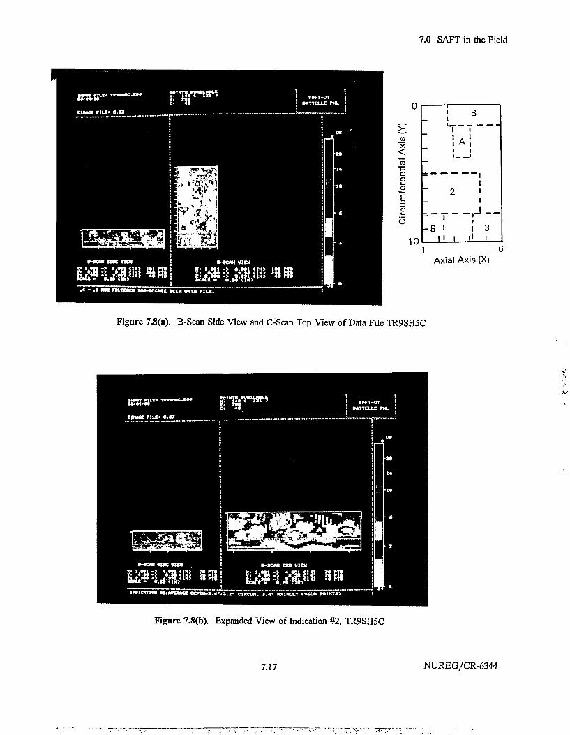
7.0 SAFT in the Field
c0)
3
o
O
10
11
-
- — —
- 5 1I I
T -
i
—
2
—
1
B
^ Ji
11I1
_,JiI
|l
- -
3i
1 6Axial Axis (X)
Figure 7.8(a). B-Scan Side View and C-Scan Top View of Data File TR9SH5C
Figure 7.8(b). Expanded View of Indication #2, TR9SH5C
7.17 NUREG/CR-6344
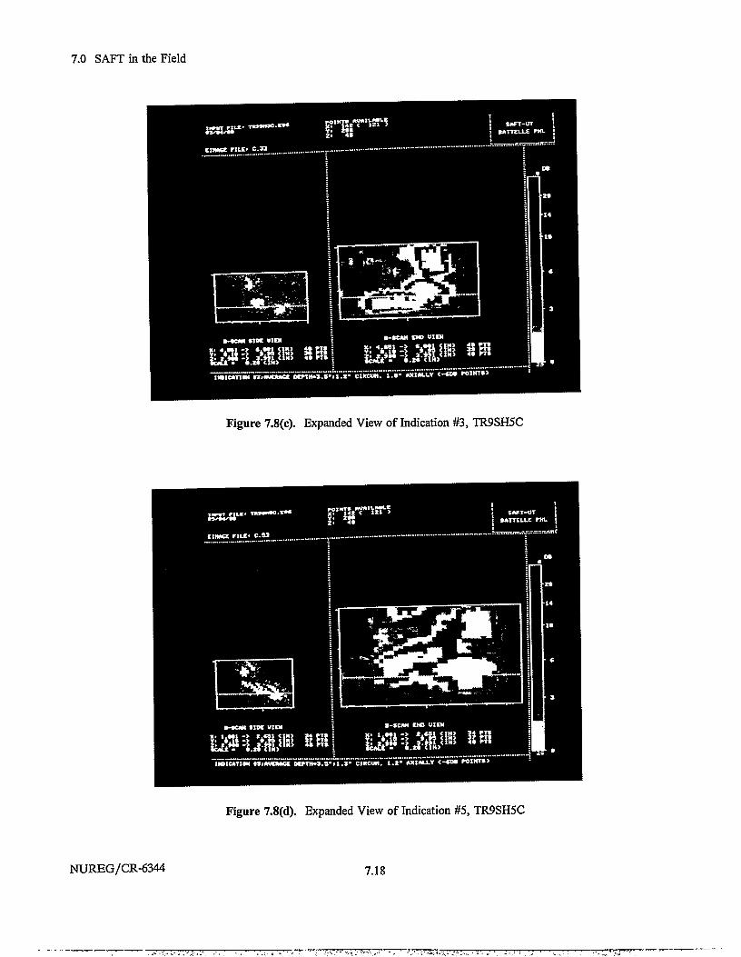
7.0 SAFT in the Field
Figure 7.8(c). Expanded View of Indication #3, TR9SH5C
Figure 7.8(d). Expanded View of Indication #5, TR9SH5C
NUREG/CR-6344 7.18
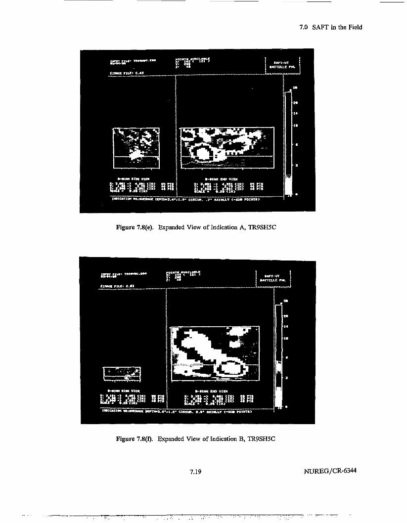
7.0 SAFT in the Field
Figure 7.8(e). Expanded View of Indication A, TR9SH5C
Figure 7.8(f). Expanded View of Indication B, TR9SH5C
7.19 NUREG/CR-6344
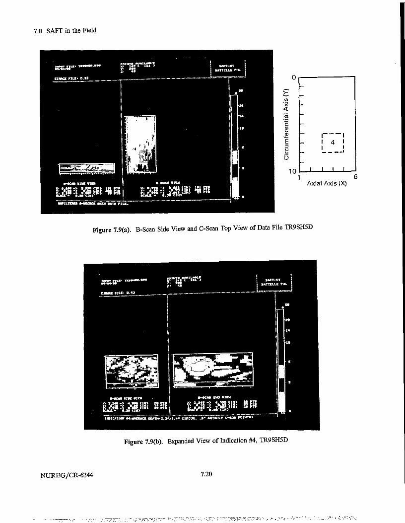
7.0 SAFT in the Field
1 6Axial Axis (X)
Figure 7.9(a). B-Scan Side View and C-Scan Top View of Data File TR9SH5D
Figure 7.9(b). Expanded View of Indication #4, TR9SH5D
NUREG/CR-6344 7.20
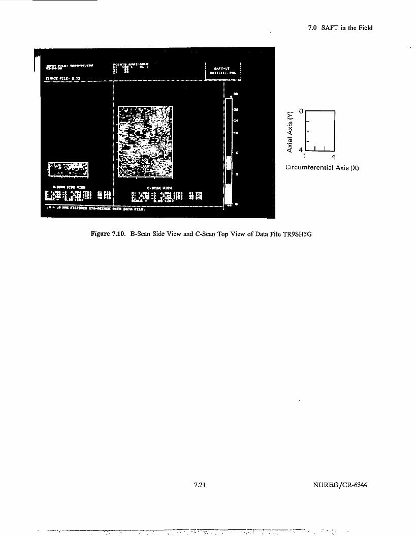
7.0 SAFT in the Field
to'x
< 41 4
Circumferential Axis (X)
Figure 7.10. B-Scan Side View and C-Scan Top View of Data File TR9SH5G
7.21 NUREG/CR-6344
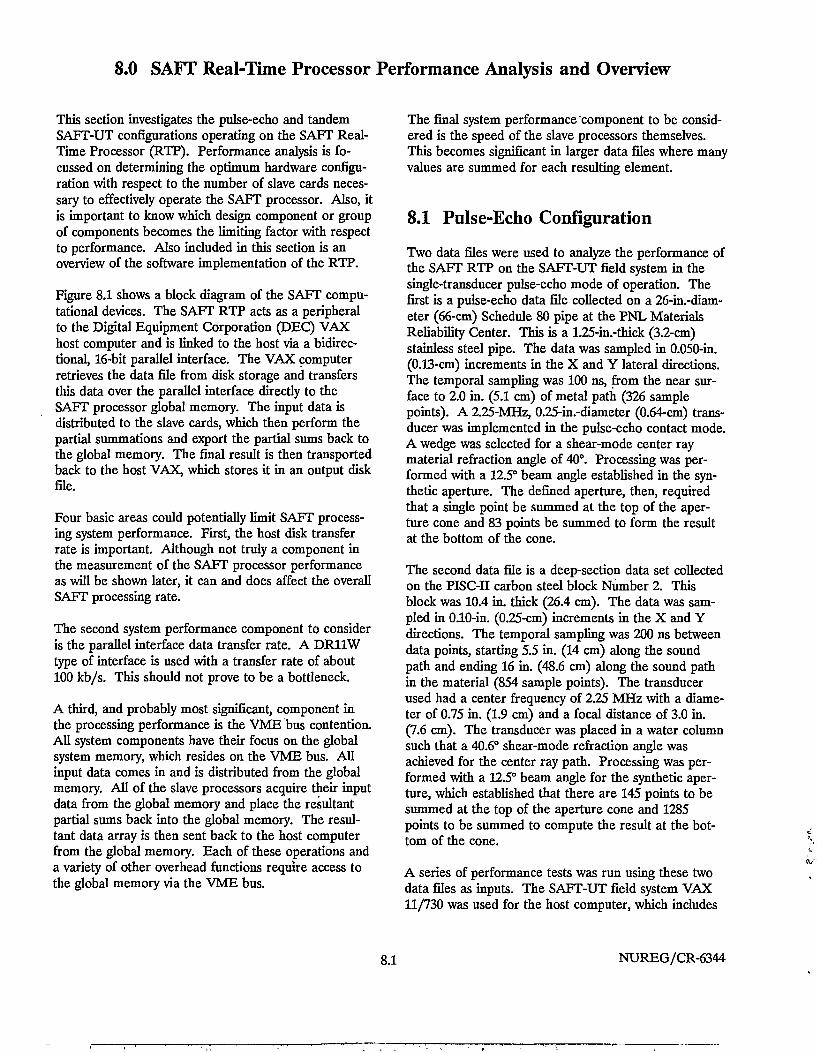
8.0 SAFT Real-Time Processor Performance Analysis and Overview
This section investigates the pulse-echo and tandemSAFT-UT configurations operating on the SAFT Real-Time Processor (RTP). Performance analysis is fo-cussed on determining the optimum hardware configu-ration with respect to the number of slave cards neces-sary to effectively operate the SAFT processor. Also, itis important to know which design component or groupof components becomes the limiting factor with respectto performance. Also included in this section is anoverview of the software implementation of the RTP.
Figure 8.1 shows a block diagram of the SAFT compu-tational devices. The SAFT RTP acts as a peripheralto the Digital Equipment Corporation (DEC) VAXhost computer and is linked to the host via a bidirec-tional, 16-bit parallel interface. The VAX computerretrieves the data file from disk storage and transfersthis data over the parallel interface directly to theSAFT processor global memory. The input data isdistributed to the slave cards, which then perform thepartial summations and export the partial sums back tothe global memory. The final result is then transportedback to the host VAX, which stores it in an output diskfile.
Four basic areas could potentially limit SAFT process-ing system performance. First, the host disk transferrate is important. Although not truly a component inthe measurement of the SAFT processor performanceas will be shown later, it can and does affect the overallSAFT processing rate.
The second system performance component to consideris the parallel interface data transfer rate. A DR11Wtype of interface is used with a transfer rate of about100 kb/s. This should not prove to be a bottleneck.
A third, and probably most significant, component inthe processing performance is the VME bus contention.All system components have their focus on the globalsystem memory, which resides on the VME bus. Allinput data comes in and is distributed from the globalmemory. All of the slave processors acquire their inputdata from the global memory and place the resultantpartial sums back into the global memory. The resul-tant data array is then sent back to the host computerfrom the global memory. Each of these operations anda variety of other overhead functions require access tothe global memory via the VME bus.
The final system performance "component to be consid-ered is the speed of the slave processors themselves.This becomes significant in larger data files where manyvalues are summed for each resulting element.
8.1 Pulse-Echo Configuration
Two data files were used to analyze the performance ofthe SAFT RTP on the SAFT-UT field system in thesingle-transducer pulse-echo mode of operation. Thefirst is a pulse-echo data file collected on a 26-in.-diam-eter (66-cm) Schedule 80 pipe at the PNL MaterialsReliability Center. This is a 1.25-in.-thick (3.2-cm)stainless steel pipe. The data was sampled in 0.050-in.(0.13-cm) increments in the X and Y lateral directions.The temporal sampling was 100 ns, from the near sur-face to 2.0 in. (5.1 cm) of metal path (326 samplepoints). A 2.25-MHz, 0.25-in.-diameter (0.64-cm) trans-ducer was implemented in the pulse-echo contact mode.A wedge was selected for a shear-mode center raymaterial refraction angle of 40°. Processing was per-formed with a 12.5° beam angle established in the syn-thetic aperture. The defined aperture, then, requiredthat a single point be summed at the top of the aper-ture cone and 83 points be summed to form the resultat the bottom of the cone.
The second data file is a deep-section data set collectedon the PISC-II carbon steel block Number 2. Thisblock was 10.4 in. thick (26.4 cm). The data was sam-pled in 0.10-in. (0.25-cm) increments in the X and Ydirections. The temporal sampling was 200 ns betweendata points, starting 5.5 in. (14 cm) along the soundpath and ending 16 in. (48.6 cm) along the sound pathin the material (854 sample points). The transducerused had a center frequency of 2.25 MHz with a diame-ter of 0.75 in. (1.9 cm) and a focal distance of 3.0 in.(7.6 cm). The transducer was placed in a water columnsuch that a 40.6° shear-mode refraction angle wasachieved for the center ray path. Processing was per-formed with a 12.5° beam angle for the synthetic aper-ture, which established that there are 145 points to besummed at the top of the aperture cone and 1285points to be summed to compute the result at the bot-tom of the cone.
A series of performance tests was run using these twodata files as inputs. The SAFT-UT field system VAX11/730 was used for the host computer, which includes
8.1 NUREG/CR-6344
8.0 Processor Performance
a DEC R80 disk drive for data storage. The focus ofthe tests was to determine the effects of adding slaveprocessors, to determine the benefit of specific pro-cessing options, and to observe the effects of the hostcomputer's disk output on the processing performance.The graphs shown in Figures 8.2 through 8.5 relate tothe pipe data file described earlier. Each figure showsthe processing speed of the overall system including theVAX 11/730 disk write (dashed line) and the perfor-mance when the disk input/output (I/O) is completelyremoved from the software during processing time.
Figure 8.2 shows the performance with selective pro-cessing disabled and with the output record size exactlythe same length as the input record size. With diskwrites, one can see that the performance is completelysaturated and that the rate of processing is totally de-termined by the host disk system. More interesting isthe solid line graph showing the response when the hostis free from the disk duties. One can see that parallelprocessing saturation occurs after installing more thanfive slaves in the system. Notice that a speed improve-ment of a factor of 2.1 is achieved by increasing thenumber of slaves from one to five. After five slavecards, there is no benefit in performance for this dataset.
Figure 8.3 shows the curves relating to selective pro-cessing disabled and an output record size compressionfactor of 5. Thus, the record being transmitted back tothe host computer and stored in the disk file is fivetimes smaller than the input data record length. Thiscompression is performed after envelope detection,when the frequency components of the signal are muchreduced; consequently, the sampling requirements ofthe signal are relaxed. This relates to about one datapoint per wavelength on the theoretical resolution lim-its. Furthermore, the data files are almost never dis-played one-to-one because there are many more pointsthan there are display pixels. Notice the level at whichperformance saturation of the dashed line has increasedas compared to Figure 8.2. This increase is directlyattributable to the fact that the amount of data-handlingis reduced and therefore the disk I/O- becomes lesssignificant. As expected, the solid line graph (no hostdisk activity) is identical to that shown in Figure 8.2.
Figure 8.4 shows the graphs related to a -20-dB thresh-old level in the selective processing option and no out-put record size compression selected. The chosen
threshold level resulted in 58% of the data points beingfully processed for this file. Remember that the other42% of the data points are retained but just not pro-cessed. Notice that the dashed curve is identical to thatshown in Figure 8.2. This is as expected, because thedisk output rate dominates the performance once again.The solid line saturates much quicker, however, thanthat shown in Figure 8.2. This is from the large reduc-tion in summations due to the selective processingalgorithm. Performance saturation occurs at three slaveprocessors for this file.
Figure 8.5 show the results of combining the options ofFigures 8.3 and 8.4. In this case, -20-dB selective pro-cessing was chosen and an output data record compres-sion factor of 5 was selected. As expected, the solidline (no host disk overhead) is identical to that shownin Figure 8.4, and the dashed line (disk output includ-ed) matches that shown in Figure 8.3.
The results for performing these tests on the largerPISC-II data set are shown in Figures 8.6 through 8.9.Because of the aperture size of this data set, the pro-cessing requires that at least three slaves be incorporat-ed in this test (adequate slave memory to store theentire aperture). Figure 8.6 represents the performanceobserved with selective processing disabled and nooutput record compression chosen. The dashed line(host disk activity) saturates at about the 5.3-A-scans/slevel, which corresponds to six slave processors. Thesolid line (no host disk activity) does not experiencesaturation; rather, a generally linear shape occurs. Ifone extrapolates the line back to a fictitious value for asingle slave processor (1.7 A-scans/s), then the additionof the number of slave cards to ten achieves a speedincrease of a factor of 3.9.
Figure 8.7 shows the graphs that result in choosing noselective processing and selecting an output record sizecompression factor of 5. The results are identical tothose in Figure 8.6, except the dashed line (with hostdisk activity) shows no saturation. In this case, the diskactivity has no limiting effect on the processing perfor-mance and is expected for large A-scans that requireextensive processing.
The results of choosing -20-dB selective processing withno output compression are shown in Figure 8.8. Theselective processing option in this data set dramaticallyaffects the amount of computations, because only 1% of
NUREG/CR-6344 8.2
8.0 Processor Performance
the data points are fully processed. This is due to thehigh signal-to-noise level of the data set and is typical ofpressure vessel steels. Both curves immediately achievesaturation levels and remain flat. The performance ofboth curves is dependent totally on the rate at whichthe data is transferred from device to device. The limitfor the dashed line is the disk transfer rate of the hostcomputer. The limit for the solid line is the throughputof the SAFT processor.
Figure 8.9 exhibits characteristics similar to those ofFigure 8.8. The output record size has been com-pressed by a factor of 5 so the amount of data to betransferred is correspondingly reduced.
This performance analysis has been helpful in determin-ing the benefit of adding slave processors and isolatingbottlenecks with respect to data throughput. It is ap-parent, for most applications, that five slaves are proba-bly sufficient. This is especially true if selective pro-cessing is used. Another important factor for systemperformance is the host disk I/O speed. It is importantto select a fast disk system when initially specifying theSAFT host computer for real-time analysis.
A very large data set was processed on the SAFT RTPto observe the corresponding execution performance.This file is a finely sampled scan of a resolution patternin an aluminum block. A 2.25-MHz transducer wasused with a diameter of 0.25 in. (0.6 cm). A wedge wasselected to provide shear mode illumination with arefraction angle of 43.7°. The X and Y lateral samplespacing was 0.025 in. (0.6 cm) (A/2), and the temporalsampling was 20 MHz (0.05 //.sec or about A/10).Digitization began 2 in. (5.1 cm) into the material alongthe center ray sound path and continued until 4.5 in.(11.4 cm). There were 806 data points in each A-scanrecord, and there was a total of 14,400 A-scan recordsin the data set.
Processing was performed on this data set with a syn-thetic aperture beam angle of 18.0°. With this angleselected, the number of off-center A-scans to sum atthe top of the aperture (2.0 in. [5.1 cm] into the materi-al) is 707; the number to be summed at the deepestpart of the defined aperture (4.5 in. [11.4 cm] into thematerial) is 3617.
This data set required at least nine slave processors be-cause of the immensity of the aperture size. The globalmemory had to be expanded to 3 Mbytes to performthis processing. Selective processing was not chosen,and an output record compression factor of 5 was im-plemented for this test. For this case, the host comput-er was the SAFT VAX/780.
The SAFT processor with ten slave processors success-fully processed this data set with statistics that are quiteimpressive. The total elapsed processing time was 64.2minutes, but the total central processing unit (CPU)time — the time required for the host computer to dowork - was 6.8 minutes. This means that the bulk ofthe processing is exported to the SAFT processor, andthat comparatively very little is required of the hostcomputer. This is the key to the success of the SAFTprocessor.
This file has not previously been processed withoutchoosing selective processing to reduce the number of
- summations required.. Processing of this data file withthese parameters was initiated on the VAX 11/780.However, practical completion of processing was notpossible. The program was submitted into a specialhigh-priority batch queue. After a connect time of 2.6days and an elapsed CPU time of 18.5 h, the processingwas only 7.1% complete so it was terminated. It wouldhave taken approximately 36 days and 260 CPU hoursto complete. This is a reduction in processing time bya factor of 250! The primary reason for the long timein execution is the number of page faults that occurredduring processing. There were 3 x 10⁶ page faults atthe point of termination, with approximately 42.2 x 10⁶
page faults required to complete the processing. TheVAX 11/780 has only 4.75 Mb of memory; thus, with afile this large and with an aperture of this size, it wasspending most of the time in a VMS page fault wait-state rather than actually computing the result.
As stated previously, an attractive feature of the SAFTRTP architecture is that it exports the CPU-intensivelabor required to execute the SAFT algorithm, thusdramatically increasing the speed of execution. This isespecially true for the very large data files as experi-enced here.
8.3 NUREG/CR-6344
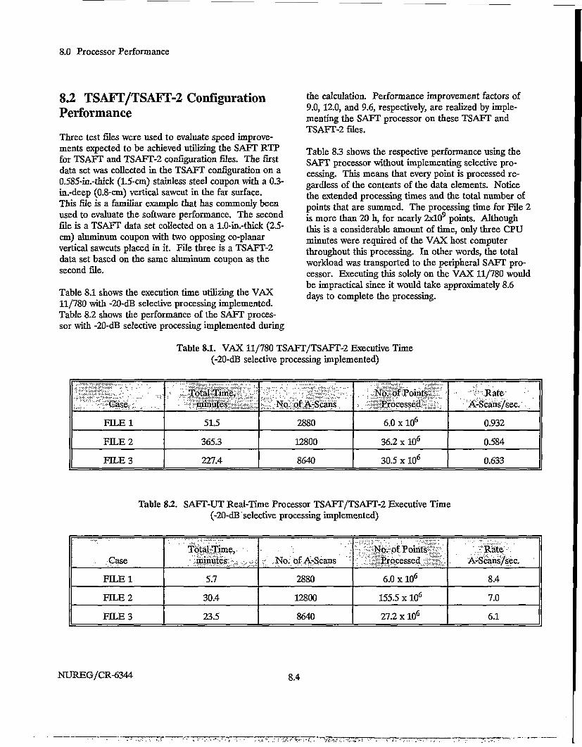
8.0 Processor Performance I8.2 TSAFT/TSAFT-2 ConfigurationPerformance
Three test files were used to evaluate speed improve-ments expected to be achieved utilizing the SAFT RTPfor TSAFT and TSAFT-2 configuration files. The firstdata set was collected in the TSAFT configuration on a0.585-in.-thick (1.5-cm) stainless steel coupon with a 0.3-in.-deep (0.8-cm) vertical sawcut in the far surface.This file is a familiar example that has commonly beenused to evaluate the software performance. The secondfile is a TSAFT data set collected on a 1.0-in.-thick (2.5-cm) aluminum coupon with two opposing co-planarvertical sawcuts placed in it. File three is a TSAFT-2data set based on the same aluminum coupon as thesecond file.
Table 8.1 shows the execution time utilizing the VAX11/780 with -20-dB selective processing implemented.Table 8.2 shows the performance of the SAFT proces-sor with -20-dB selective processing implemented during
the calculation. Performance improvement factors of9.0, 12.0, and 9.6, respectively, are realized by imple-menting the SAFT processor on these TSAFT andTSAPT-2 files.
Table 8.3 shows the respective performance using theSAFT processor without implementing selective pro-cessing. This means that every point is processed re-gardless of the contents of the data elements. Noticethe extended processing times and the total number ofpoints that are summed. The processing time for File 2is more than 20 h, for nearly 2xl09 points. Althoughthis is a considerable amount of time, only three CPUminutes were required of the VAX host computerthroughout this processing. In other words, the totalworkload was transported to the peripheral SAFT pro-cessor. Executing this solely on the VAX 11/780 wouldbe impractical since it would take approximately 8.6days to complete the processing.
Table 8.1. VAX 11/780 TSAFT/TSAFT-2 Executive Time(-20-dB selective processing implemented)
Case
FILE1
FILE 2
FILE 3
': Total Time,minutes
51.5
365.3
227.4
No. of A-Scans
2880
12800
8640
No. of PointsProcessed
6.0 x 10⁶
36.2 x 10⁶
30.5 x 10⁶
•KRate- ;
A^-Scaris/sec. .
0.932
0.584
0.633
Table $2. SAFT-UT Real-Time Processor TSAFT/TSAFT-2 Executive Time(-20-dB "selective processing implemented)
.-• *?ase
FILE1
FILE 2
FILE 3
Total Time,minutes
5.7
30.4
23.5
,No. bfA^Scans
2880
12800
8640
No. of PointsProcessed :
6.0 x 10⁶
155.5 x 10⁶
27.2 x 10⁶
..fRate/.A*Scans7sfee.
8.4
7.0
6.1
NUREG/CR-6344 8.4
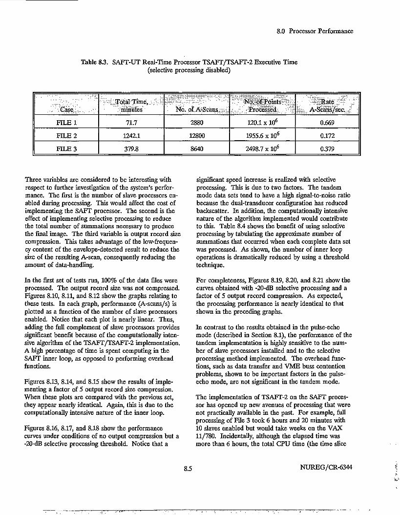
8.0 Processor Performance
Table 83. SAFT-UT Real-Time Processor TSAFT/TSAFT-2 Executive Time(selective processing disabled)
.... .Case,:.,.. .•••'•
FILE1
FILE 2
FILE 3
"minutes
71.7
1242.1
379.8
No. of A-Scans
2880
12800
8640
No. of PointsProcessed
120.1 x 10⁶
1955.6 x 106
2498.7 x 106
RateA-Scans/sec
0.669
0.172
0.379
Three variables are considered to be interesting withrespect to further investigation of the system's perfor-mance. The first is the number of slave processors en-abled during processing. This would affect the cost ofimplementing the SAFT processor. The second is theeffect of implementing selective processing to reducethe total number of summations necessary to producethe final image. The third variable is output record sizecompression. This takes advantage of the low-frequen-cy content of the envelope-detected result to reduce thesize of the resulting A-scan, consequently reducing theamount of data-handling.
In the first set of tests run, 100% of the data files wereprocessed. The output record size was not compressed.Figures 8.10, 8.11, and 8.12 show the graphs relating tothese tests. In each graph, performance (A-scans/s) isplotted as a function of the number of slave processorsenabled. Notice that each plot is nearly linear. Thus,adding the full complement of slave processors providessignificant benefit because of the computationally inten-sive algorithm of the TSAFT/TSAFT-2 implementation.A high percentage of time is spent computing in theSAFT inner loop, as opposed to performing overheadfunctions.
Figures 8.13, 8.14, and 8.15 show the results of imple-menting a factor of 5 output record size compression.When these plots are compared with the previous set,they appear nearly identical. Again, this is due to thecomputationally intensive nature of the inner loop.
Figures 8.16, 8.17, and 8.18 show the performancecurves under conditions of no output compression but a-20-dB selective processing threshold. Notice that a
significant speed increase is realized with selectiveprocessing. This is due to two factors. The tandemmode data sets tend to have a high signal-to-noise ratiobecause the dual-transducer configuration has reducedbackscatter. In addition, the computationally intensivenature of the algorithm implemented would contributeto this. Table 8.4 shows the benefit of using selectiveprocessing by tabulating the approximate number ofsummations that occurred when each complete data setwas processed. As shown, the number of inner loopoperations is dramatically reduced by using a thresholdtechnique.
For completeness, Figures 8.19, 8.20, and 8.21 show thecurves obtained with -20-dB selective processing and afactor of 5 output record compression. As expected,the processing performance is nearly identical to thatshown in the preceding graphs.
In contrast to the results obtained in the pulse-echomode (described in Section 8.1), the performance of thetandem implementation is highly sensitive to the num-ber of slave processors installed and to the selectiveprocessing method implemented. The overhead func-tions, such as data transfer and VME buss contentionproblems, shown to be important factors in the pulse-echo mode, are not significant in the tandem mode.
The implementation of TSAFT-2 on the SAFT proces-sor has opened up new avenues of processing that werenot practically available in the past. For example, fullprocessing of File 3 took 6 hours and 20 minutes with10 slaves enabled but would take weeks on the VAX11/780. Incidentally, although the elapsed time wasmore than 6 hours, the total CPU time (the time slice
8.5 NUREG/CR-6344
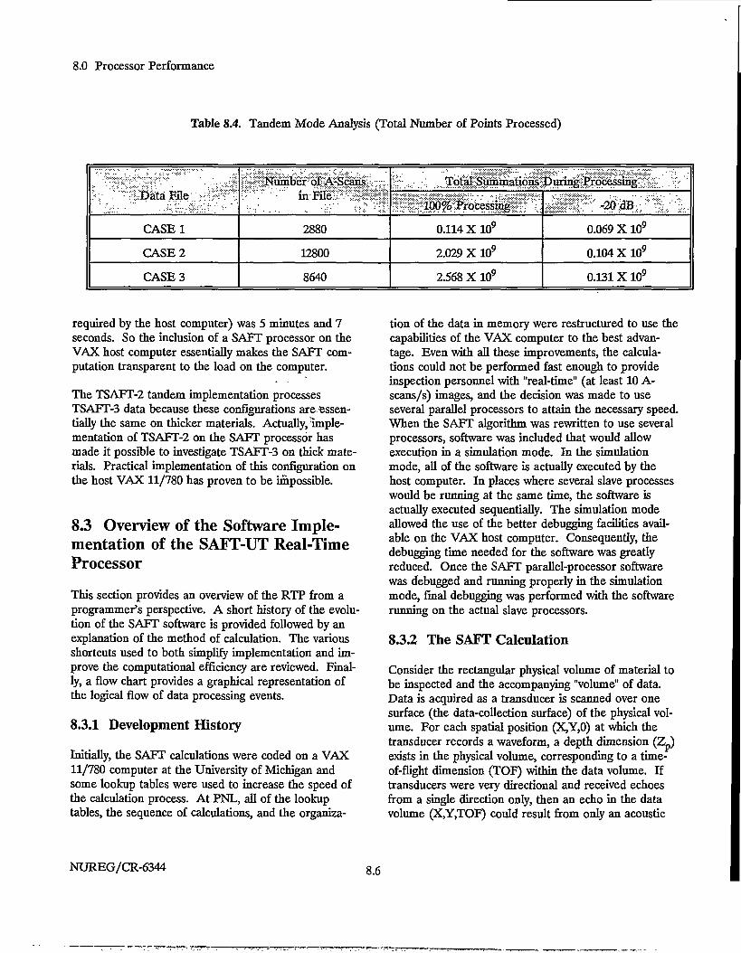
8.0 Processor Performance
Table 8.4. Tandem Mode Analysis (Total Number of Points Processed)
Data File
CASE1
CASE 2
CASE 3
Number of A-Scansin File
2880
12800
8640
Total Summations During Processing
100% Processing
0.114 X 10⁹
2.029 X 10⁹
2.568 X 10⁹
-20 dB
0.069 X 10⁹
0.104 X 10⁹
0.131 X 10⁹
required by the host computer) was 5 minutes and 7seconds. So the inclusion of a SAFT processor on theVAX host computer essentially makes the SAFT com-putation transparent to the load on the computer.
The TSAFT-2 tandem implementation processesTSAFT-3 data because these configurations are 'essen-tially the same on thicker materials. Actually, imple-mentation of TSAFT-2 on the SAFT processor hasmade it possible to investigate TSAFT-3 on thick mate-rials. Practical implementation of this configuration onthe host VAX 11/780 has proven to be impossible.
8.3 Overview of the Software Imple-mentation of the SAFT-UT Real-TimeProcessor
This section provides an overview of the RTP from aprogrammer's perspective. A short history of the evolu-tion of the SAFT software is provided followed by anexplanation of the method of calculation. The variousshortcuts used to both simplify implementation and im-prove the computational efficiency are reviewed. Final-ly, a flow chart provides a graphical representation ofthe logical flow of data processing events.
8.3.1 Development History
Initially, the SAFT calculations were coded on a VAX11/780 computer at the University of Michigan andsome lookup tables were used to increase the speed ofthe calculation process. At PNL, all of the lookuptables, the sequence of calculations, and the organiza-
tion of the data hi memory were restructured to use thecapabilities of the VAX computer to the best advan-tage. Even with all these improvements, the calcula-tions could not be performed fast enough to provideinspection personnel with "real-time" (at least 10 A-scans/s) images, and the decision was made to useseveral parallel processors to attain the necessary speed.When the SAFT algorithm was rewritten to use severalprocessors, software was included that would allowexecution in a simulation mode. In the simulationmode, all of the software is actually executed by thehost computer. In places where several slave processeswould be running at the same time, the software isactually executed sequentially. The simulation modeallowed the use of the better debugging facilities avail-able on the VAX host computer. Consequently, thedebugging tune needed for the software was greatlyreduced. Once the SAFT parallel-processor softwarewas debugged and running properly in the simulationmode, final debugging was performed with the softwarerunning on the actual slave processors.
8.3.2 The SAFT Calculation
Consider the rectangular physical volume of material tobe inspected and the accompanying "volume" of data.Data is acquired as a transducer is scanned over onesurface (the data-collection surface) of the physical vol-ume. For each spatial position (X,Y,0) at which thetransducer records a waveform, a depth dimension (2L)exists in the physical volume, corresponding to a time-of-flight dimension (TOF) within the data volume. Iftransducers were very directional and received echoesfrom a single direction only, then an echo hi the datavolume (X,Y,TOF) could result from only an acoustic
NUREG/CR-6344 8.6
8.0 Processor Performance
reflector located in the physical volume at (X,Y,Z ),where Z=TOF/2V and V is the material velocity.However, this is not the case.
Transducers "see" everything within some cone-shapedaperture; and, the best that can be said, when consider-ing a single waveform, is that an echo located at(X,Y,TOF) in the data volume may have resulted froman acoustic reflector at a distance d=TOF/2V (orfrom the transducer location (X,Y,0) and within thecone-shaped aperture. Of course, this is less than onewould like to know about the location and size of re-flectors within the physical volume. Clearly, some sortof focusing technique is needed.
Better results are achieved by reversing the scenario;i.e., consider a given point in the physical volume anddetermine where, within the data volume, the digitizedamplitude values would be stored if an acoustic reflec-tor were located at the point being considered. Severalbenefits arise from this approach. First, this approachwould enable one to average over a locus of echoes,determining the strength of the reflector at the pointbeing processed. All waveform data acquired at spatiallocations from which the transducer cannot "see" thepoint in question may be eliminated because the pointis outside the beam aperture. This leaves a set oftransducer locations on the data-collection surface thatcorrespond to a cone drawn from the point in the phys-ical volume, toward the surface, and with the same full-beam angle as the transducer aperture. For each spa-tial transducer location (X,Y,0) within the cone-shapedaperture, only the time dimension (t) need be deter-mined to locate the digitized amplitude value (withinthe data volume) corresponding to the echo producedby the point being processed. Since we know the dis-tance from the transducer (X,Y,0) to the point in ques-tion (X,Y,Z ) and the sound velocity, we may calculatethe TOF as twice the distance (sound path down andback) divided by the acoustic velocity; i.e.,
TOF = 2 * d
where: d = J[(X-Xpf * (Y-Ypf - (Z-Zp)2]
Therefore, from an elementary perspective, for everypoint in the physical volume
1. Determine which spatial transducer locations(X,Y,0) should receive an echo from the pointbeing processed.
2. Calculate the TOF between the point being pro-cessed and the transducer for each spatial trans-ducer location determined in step 1.
3. Sum the digitized values from the data volume forall (X,Y,TOF) locations determined in steps 1 and2.
The final summations are stored in a second data vol-ume at (X,Y,Z), and their amplitude should directlyrelate to the strength of the acoustic reflector at(X,Y,ZJ in the physical volume. If the acoustic reflec-tor at (X,Y,2L) is strong and correlates with a locus ofA-scan echoes, then the summation of the amplitudevalues by the SAFT calculation will produce a well-defined signal or high value. If the reflector is weak ornonexistent and does not correlate well with a locus ofA-scan echoes, the amplitude values digitized wouldmost likely be from random noise and the summationprocess would produce a spatial average of nearly zero.The SAFT algorithm is analogous to a spatial-temporalmatched filter in that the raw A-scans are time-shiftedby a predicted time delay and then averaged over anumber of positions. Constructive interference is pro-duced by coherent signals, and destructive interferenceis produced by incoherent signals.
The SAFT algorithm works well. However, when im-plemented in a straightforward or brute-force manner,there can be millions upon millions of calculations thatcan take hours, days, or even weeks to complete.Hence, the complexity of implementing the SAFT algo-rithm arises from measures taken to reduce the compu-tational time required.
A solution was twofold:
First, many alterations in the data collection and com-putational procedures were made to eliminate redun-dant calculations and take advantage of the computer'sabilities. Second, we divided the computational loadamong several processors.
8.7 NUREG/CR-6344
8.0 Processor Performance
Redundant calculations were eliminated in the determi-nation of which spatial transducer locations contain(within their beam aperture) the point in question. Ifthe data is acquired over an ordered grid pattern, thenthe qualifying transducer locations will always have thesame relative positions for all of the points (to be pro-cessed) at a given level (2L) in the physical volume.The problem is simplified from a series of complexgeometric calculations to one of constructing and keep-ing track of an orderly mapping in the computer memo-ry. However, this does impose a relatively minor con-straint on the data acquisition process: it must main-tain a constant X and Y increment throughout the dataacquisition scan.
Another, more important, benefit of the ordered griddata acquisition pattern is that the distance calculationsbetween each point in the physical volume and each ofthe associated transducer locations are the same for allpoints (to be processed) at the same depth (Z ) level inthe physical volume. Thus, the distance calculationsneed be computed only once for each depth (2L) levelin the volume and then subsequently stored in lookuptables to be used over and over again. Here again, theproblem is reduced from a series of quadratic equationcalculations to one of constructing and efficiently usinglookup tables. Still, this imposes yet another constrainton the data acquisition process: the data collectionsurface must be relatively flat over an area described bythe reverse projected cone. A study by Ganapathy etal. (1981) at the University of Michigan indicates thaterrors from surface variations are of minor significancefor most geometries because of the small apertureangles normally used (12° or less) and the inherentspatial averaging that occurs when the SAFT algorithmis employed. However, a complex and rapid change inthe surface curvature (such as sometimes observedwhen inspecting pressure vessel nozzles) may produce asignificant error, prompting the use of a correctionalgorithm.
The SAFT calculations are reduced to a series of mem-ory accesses into the lookup tables and data storage.The final computational modifications consisted oforganizing the lookup tables and data storage within thecomputer's RAM to further facilitate memory accesses.
A simplified example may illustrate how the distanceand time calculations, which describe the physical datavolume and transducer locations, are converted into a
memory offset lookup table that can subsequently beused to find the data stored in the computer's memory.Assume the transducer collects a waveform, consistingof 100 data points in time, at each location in an X,Ygrid consisting of 10 increments in Y and 10 incrementsin X. These data points are stored sequentially inmemory as follows:
1. the waveform taken at location (1,1,0); points(1,1,1) .... (1,1,100)
2. followed by the waveforms taken at (1,2,0) ....(1,10,0)
3. followed by waveforms taken at (2,1,0) .... (2,10,0),and so on.
Suppose that we are currently performing the SAFTcalculation for a point in the physical volume at(5,5,25). The center of the cone projected back fromthis point (in the data volume stored in that computer'smemory) is at storage location number 4401. That is 4complete rows of data with 1000 points each (10 x 100),plus four waveforms in the fifth row at 100 points each,plus one for the first data point, in the fifth waveform,in the fifth row. (In practice, the memory location ofthis data point is not recalculated each time but ratherincrementally changed as the point in the physical vol-ume is moved; e.g., if the physical point is changed to(5,6,25), then 100 is added to 4401 to get the correctposition of 4501). In addition to the position of thiswaveform in the computer memory, positions of wave-forms taken at adjacent transducer locations need to beknown. These may be located as follows:
1. For each increment in the X direction in the phys-ical volume, add (or subtract) 1000 storage loca-tions.
2. For each increment in the Y direction in the phys-ical volume, add or subtract 100 storage locations(of course, the software also needs to keep trackof when the transducer location is near the edgeof the physical volume and preclude summingpoints that would actually be off the edge).
Thus, the location in the computer memory of eachwaveform taken within the cone, projected backwardsfrom the point in the physical volume, may be found.
NUREG/CR-6344 8.8
8.0 Processor Performance
Having previously calculated and stored in a lookuptable the relative locations of the data from all of diespatial transducer locations in the backward projectedcone, one can easily locate in memory all waveformsthat should contain an echo from an acoustic reflectorlocated at any given point in the physical volume. Forexample, if five transducer locations are within thebackward projected cone and the memory address ofthe data from the point at the center of the backwardprojected cone is 4401, the data from the other fourpoints will be located at 4501, 4301, 5401, and 3401(Figure 8.22).
The relationship between the time, depth, and datastorage location works in a similar manner. Becauseeach waveform is digitized at a constant rate, movingone storage location is equivalent to moving the recip-rocal of the digitization rate in time; i.e., a 10-MHzdigitization rate would mean each storage locationwould be equivalent to 100 ns. The precalculated TOFbetween a point in the physical volume and each trans-ducer location, in its backward projected cone, is subse-quently stored in a lookup table as a memory offsetequal to the TOF/(time per data storage location).
Thus, the final SAFT algorithm consists of mathemati-cal calculations no more time-consuming than additionsand subtractions. A typical calculation would proceedas follows:
1. For every Z level in the physical volume, precalcu-late the positions of the points in the backwardprojected cone in terms of Y and Z offsets rela-tive to the center of the cone and the distance toeach of those points.
2. Convert the calculated relative positions and dis-tances to memory offsets and store them in twosets of lookup tables.
3. Now, for every point in the physical data volume,use the first lookup table to locate, in the comput-er memory, the position of the waveforms thatshould contain echoes from the point in question.
4. Use the second lookup table to locate the properdata point within each waveform and sum themall together.
8.3.3 Configuration Modifications
The SAFT algorithm lends itself to parallel processingbecause subsequent calculations do not depend uponthe results of previous calculations. However, becausethe SAFT algorithm is primarily a series of memoryaccesses (into the lookup tables and the data storagearea), parallel processors should not share the samememory for the lookup tables or data storage. If theydid, they would frequently be competing for access tothe same memory and performance would suffer. Eachof the parallel processors has a copy of the lookuptables hi its on-board memory. The handling of thedata storage memory is a bit more complicated becausethe basic SAFT algorithm requires access to all of thedata storage memory further, the massive size of thedata makes it prohibitive to have a copy for each of theparallel processors. The solution to this problem is todivide the data among the parallel processors, with eachprocessor storing every Nth Y plane (where N is thetotal number of parallel processors) of the data in on-board memory. Consequently, all of the lookup tablesand the SAFT algorithm were modified so that hi per-forming the summation process, each slave would auto-matically skip over the data planes it did not processbut still produce partial sums over the data it did havein its on-board memory, for every point in the totalphysical volume. Partial sums from each slave are thensummed into a common storage area. Finally, the rfcomponent of the processed data is removed using aprocedure called envelope detection.
The sequence of operations is as follows:
1. The host computer inputs raw data from disk orthe real-time data acquisition system.
2. The host calculates all of the lookup tables thatwill be used by the parallel processors.
3. One of the parallel processors is designated to bethe supervisor. It handles all of the communica-tions with the host and directs the operations ofthe other parallel processors, called slaves. Eachslave runs the exact same software.
4. The host downloads the lookup tables and otherparameters to the supervisor and starts to down-load the actual 'data.
8.9 NUREG/CR-6344
8.0 Processor Performance
5. Upon a system reset, each slave executes a shortstartup sequence stored in its ROM and thenwaits for the supervisor to give the "go" signal.
6. The supervisor places into each slave's memorythe code that the slave will execute, in performingits part of the SAFT algorithm, along with otherparameters and each slave's number. The slavenumber causes each slave to execute the slavecode in a slightly different sequence, compensatingfor the different sequence of data planes eachslave processes.
7. When the supervisor has received enough datafrom the host for processing to start, it tells eachslave in turn to begin executing the downloadedcode.
8. Each slave copies every Nth Y plane of data fromthe supervisor's shared memory into its privatememory.
9. Each slave commences to compute the SAFTsummations one Y plane at a time.
10. When a slave finishes a partial summation of eachY plane, it transfers its results to the supervisorwhere they are combined with the partial summa-tions from all the other slaves for the same Yplane.
11. The supervisor transfers back to the host the fullysummed Y plane.
8.3.4 Tandem SAFT
In all respects commented on thus far, tandem SAFT isthe same as pulse-echo SAFT. The exception is thatwhen the TOF is computed, the distance used is thedistance from the sending transducer to the point in thephysical volume plus the distance from the point in thevolume to the receiving transducer, rather than twicethe distance from the point in the physical volume tothe single pulse-echo transducer.
8.3.5 Flow Chart Commentary
Figure 8.23 shows the logical flow of events that occurduring SAFT processing of data; from the host comput-
er, to the real-time processor supervisor, to the slaveprocessors, and back. Each box has a number thatcorresponds to numbers listed below commenting onthe events that take place.
Host computer:
<1> Set up and receive data acquisition parame-ters.
<2> The VAX calculates all of the lookup tablesthat will be used by the slave processors.
<3> Initialize the supervisor. One of the parallelprocessors is designated to be the supervi-sor. It handles all of the communicationswith the VAX and directs the operations ofthe other parallel processors, called slaves.Each of the slaves runs the exact same soft-ware.
<4> The VAX downloads all of the lookup tables
to the supervisor.
<5> Is the raw data ready for input?
<6> Is supervisor ready for more raw data?
<7> Is the supervisor ready with processed data?
<8> Is SAFT processmg finished?
<9> Enter data from data acquisition system ordisk file.
<10> Download one plane of raw data to supervi-sor.
<11> Upload processed data from the supervisorand write to disk file.
<12> Close current files and exit.
Real-time processor supervisor:
<13> Wait for the VAX to initialize, downloadlookup tables, and so forth.
<14> Download slave software code and parame-ters to each slave. Give each slave the start-
NUREG/CR-6344 8.10
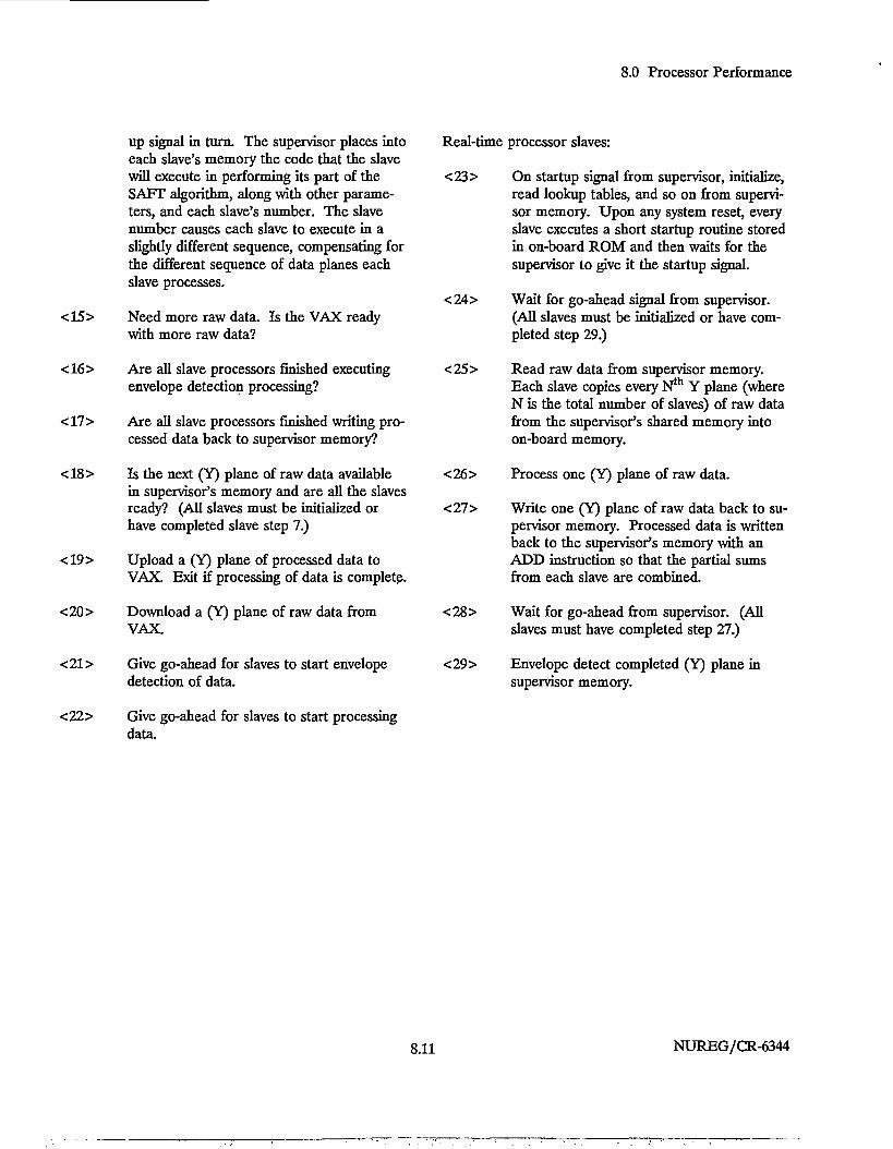
8.0 Processor Performance
<20>
<22>
up signal in turn. The supervisor places intoeach slave's memory the code that the slavewill execute in performing its part of theSAFT algorithm, along with other parame-ters, and each slave's number. The slavenumber causes each slave to execute in aslightly different sequence, compensating forthe different sequence of data planes eachslave processes.
Need more raw data. Is the VAX readywith more raw data?
Are all slave processors finished executingenvelope detection processing?
Are all slave processors finished writing pro-cessed data back to supervisor memory?
Is the next (Y) plane of raw data availablein supervisor's memory and are all the slavesready? (All slaves must be initialized orhave completed slave step 7.)
Upload a (Y) plane of processed data toVAX. Exit if processing of data is complete.
Download a (Y) plane of raw data fromVAX.
Give go-ahead for slaves to start envelopedetection of data.
Give go-ahead for slaves to start processingdata.
Real-time processor slaves:
<23> On startup signal from supervisor, initialize,read lookup tables, and so on from supervi-sor memory. Upon any system reset, everyslave executes a short startup routine storedin on-board ROM and then waits for thesupervisor to give it the startup signal.
<24> Wait for go-ahead signal from supervisor.(All slaves must be initialized or have com-pleted step 29.)
<25> Read raw data from supervisor memory.Each slave copies every Nth Y plane (whereN is the total number of slaves) of raw datafrom the supervisor's shared memory intoon-board memory.
<26> Process one (Y) plane of raw data.
<27> Write one (Y) plane of raw data back to su-pervisor memory. Processed data is writtenback to the supervisor's memory with anADD instruction so that the partial sumsfrom each slave are combined.
<28> Wait for go-ahead from supervisor. (Allslaves must have completed step 27.)
<29> Envelope detect completed (Y) plane insupervisor memory.
8.11 NUREG/CR-6344
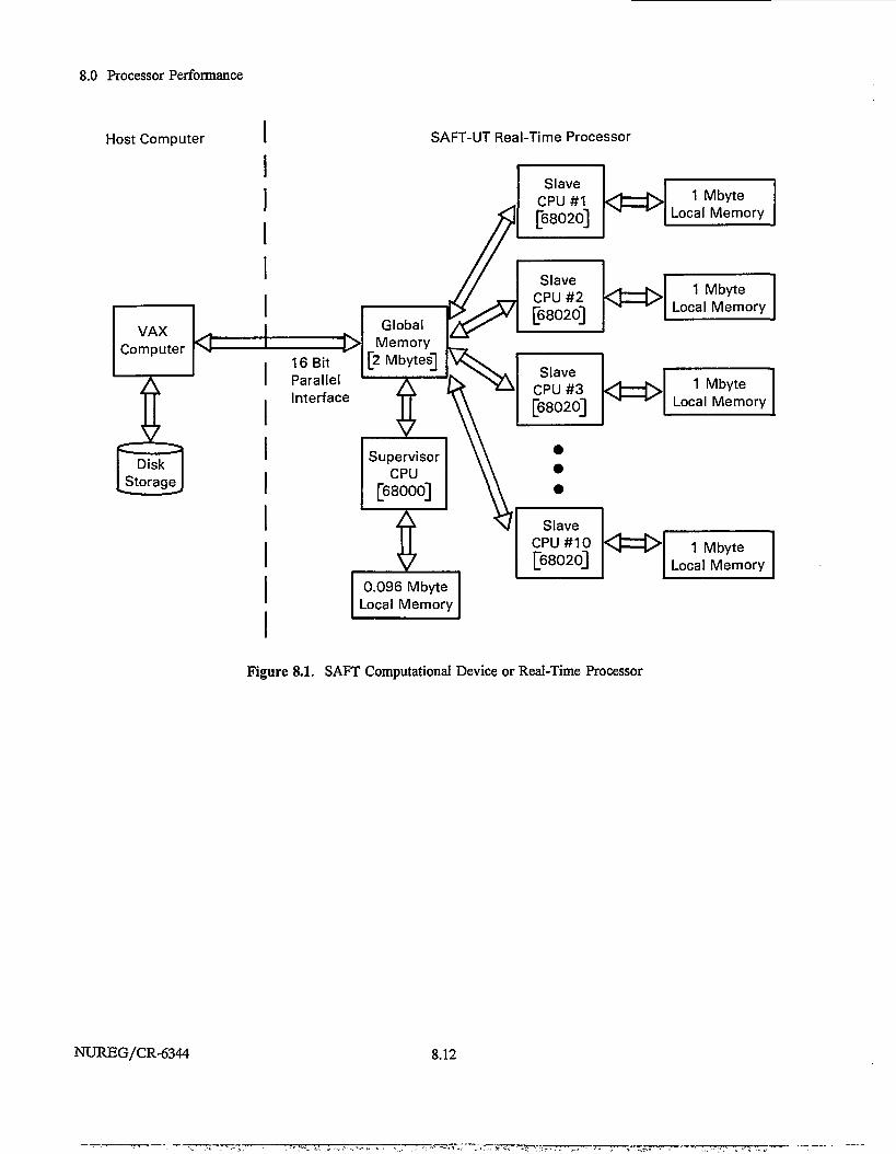
8.0 Processor Performance
Host Computer
DiskStorage
SAFT-UT Real-Time Processor
16 BitParallelInterface
0.096 MbyteLocal Memory
SlaveCPU #10[68020]
SlaveCPU#1[68020]
SlaveCPU #2[68020]
SlaveCPU #3[68020]
<]=t>
<t=t>
1 MbyteLocal Memory
1 MbyteLocal Memory
1 MbyteLocal Memory
1 MbyteLocal Memory
Figure 8.1. SAFT Computational Device or Real-Time Processor
NUREG/CR-6344 8.12
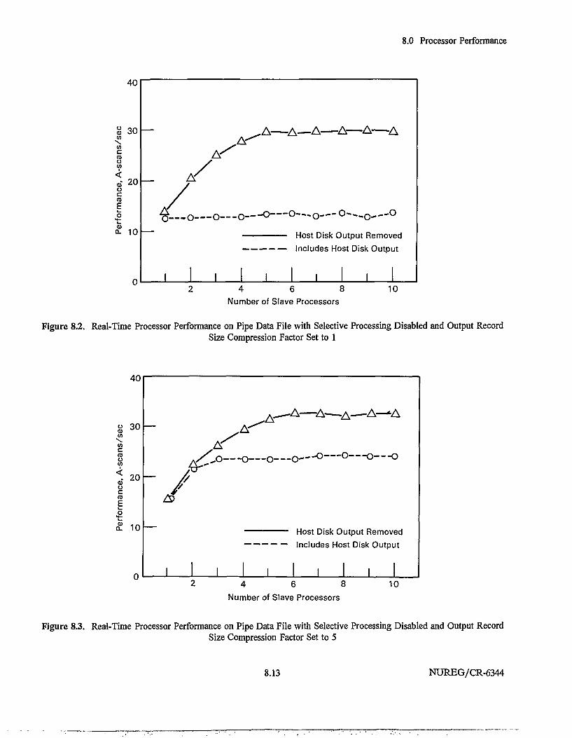
8.0 Processor Performance
40
g 30
inrooCO
I 20
10
A—A—A—A—A—A
Host Disk Output RemovedIncludes Host Disk Output
I4 6 8
Number of Slave Processors10
Figure 8.2. Real-Time Processor Performance on Pipe Data File with Selective Processing Disabled and Output RecordSize Compression Factor Set to 1
40
S 30
ininccoom
o
CD
E
S. 10
-A—A A—-A
—o—o—o—°—o—o—o
Host Disk Output RemovedIncludes Host Disk Output
I4 6 8
Number of Slave Processors10
Figure 8.3. Real-Time Processor Performance on Pipe Data File with Selective Processing Disabled and Output RecordSize Compression Factor Set to 5
8.13 NUREG/CR-6344
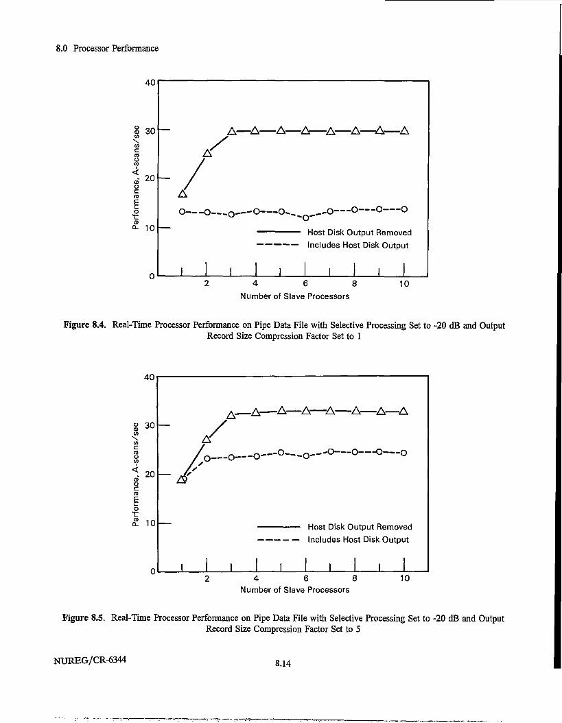
8.0 Processor Performance
40
S 30enCO
CO
o
ocCO
A—A—A—A—A—A—A—A
Ao—o—o—°— o^ _-o—o—o—o
10 Host Disk Output RemovedIncludes Host Disk Output
I4 6 8
Number of Slave Processors10
Figure 8.4. Real-Time Processor Performance on Pipe Data File with Selective Processing Set to -20 dB and OutputRecord Size Compression Factor Set to 1
40
g 30to<nccoon
^ 20CDocCO
E
CO 1 r iQ. 10
__A—A—A—A—A—A—A
Host Disk Output RemovedIncludes Host Disk Output
I4 6 8
Number of Slave Processors10
Figure 8.5. Real-Time Processor Performance on Pipe Data File with Selective Processing Set to -20 dB and OutputRecord Size Compression Factor Set to 5
NUREG/CR-6344 8.14
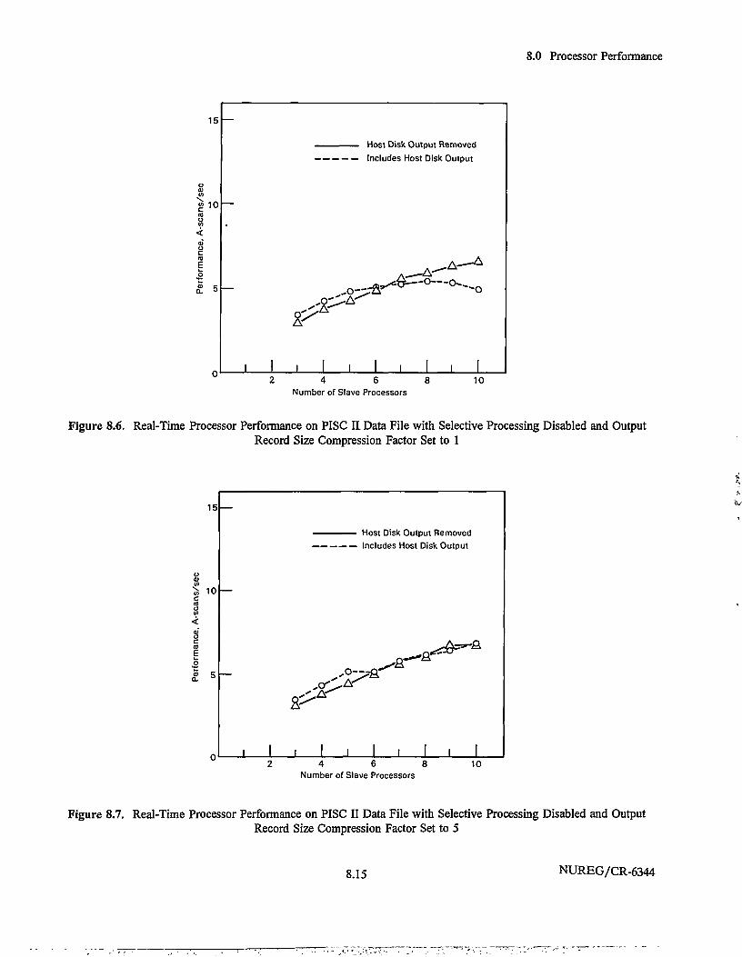
8.0 Processor Performance
15
Host Disk Output RemovedIncludes Host Disk Output
10
4 6Number of Slave Processors
10
Figure 8.6. Real-Time Processor Performance on PISC II Data File with Selective Processing Disabled and OutputRecord Size Compression Factor Set to 1
15
10
Host Disk Output RemovedIncludes Host Disk Output
4 6 8Number of Slave Processors
10
Figure 8.7. Real-Time Processor Performance on PISC II Data File with Selective Processing Disabled and OutputRecord Size Compression Factor Set to 5
8.15 NUREG/CR-6344
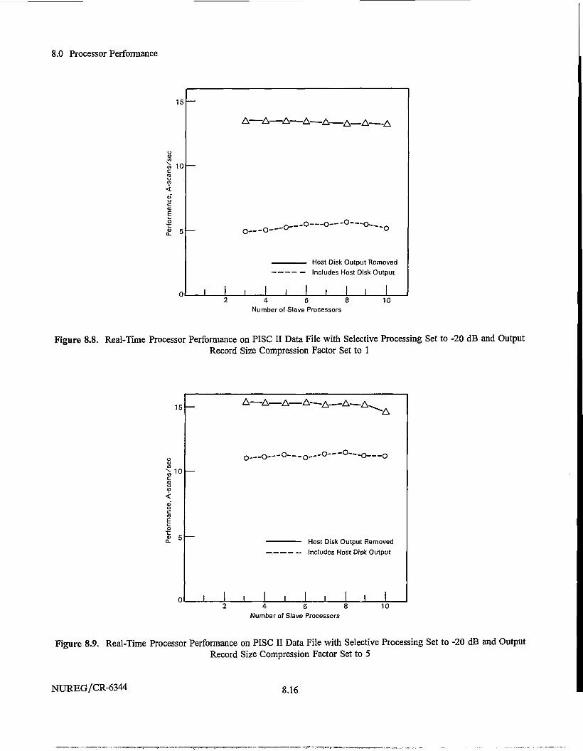
8.0 Processor Performance
15
10
A—A—A—A—A—A—A—A
—o— " - O
^ ^ — — Host Disk Output RemovedIncludes Host Disk Output
I I , I I I4 6 8
Number of Slave Processors10
Figure 8.8. Real-Time Processor Performance on PISC II Data File with Selective Processing Set to -20 dB and OutputRecord Size Compression Factor Set to 1
15A — A — A — A - — A — A —
3 O — O - — o O O o c
Host Disk Output RemovedIncludes Host Disk Output
4 6 8Number of Slave Processors
10
Figure 8.9. Real-Time Processor Performance on PISC II Data File with Selective Processing Set to -20 dB and OutputRecord Size Compression Factor Set to 5
NUREG/CR-6344 8.16
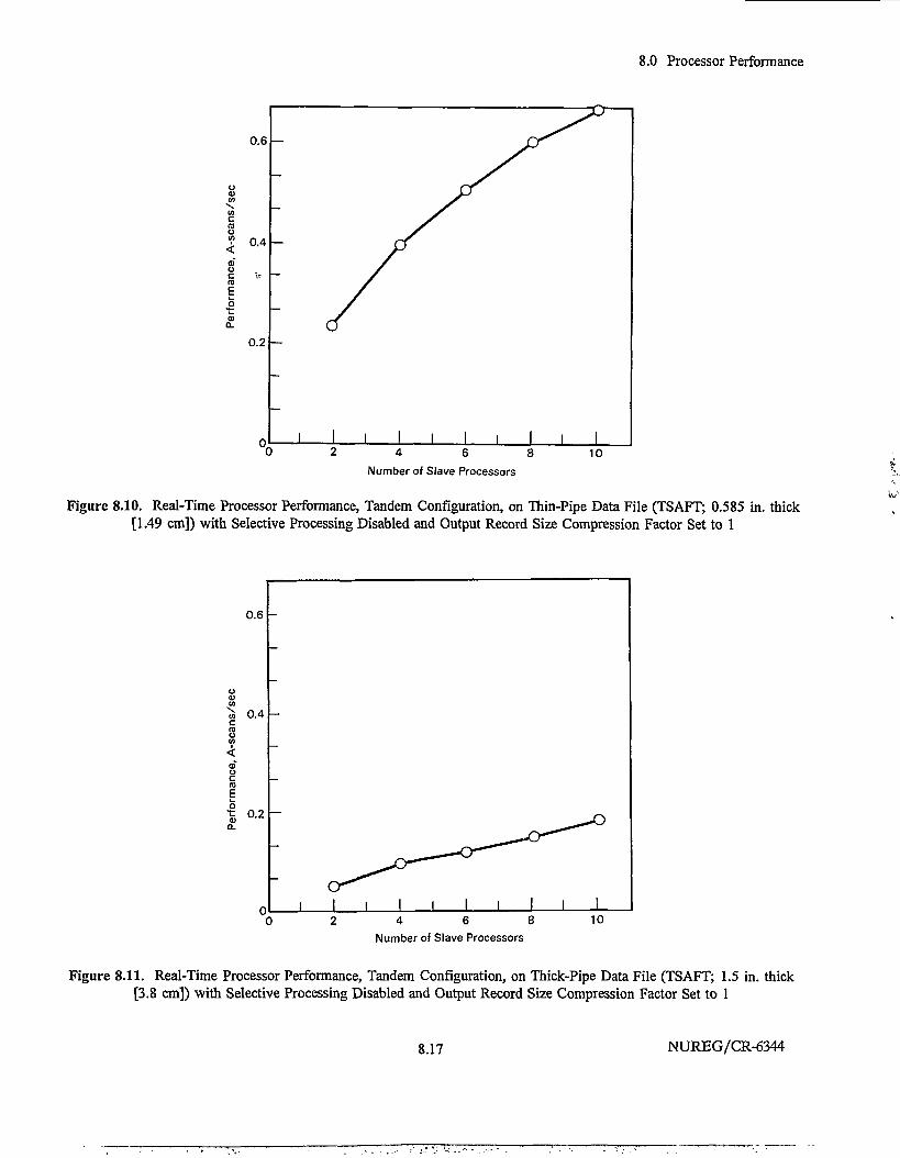
8.0 Processor Performance
0.6 —
4 6 8
Number of Slave Processors
10
Figure 8.10. Real-Time Processor Performance, Tandem Configuration, on Thin-Pipe Data File (TSAFT; 0.585 in. thick[1.49 cm]) with Selective Processing Disabled and Output Record Size Compression Factor Set to 1
0.6 -
4 6 8Number of Slave Processors
Figure 8.11. Real-Time Processor Performance, Tandem Configuration, on Thick-Pipe Data File (TSAFT; 1.5 in. thick[3.8 cm]) with Selective Processing Disabled and Output Record Size Compression Factor Set to 1
8.17 NUREG/CR-6344
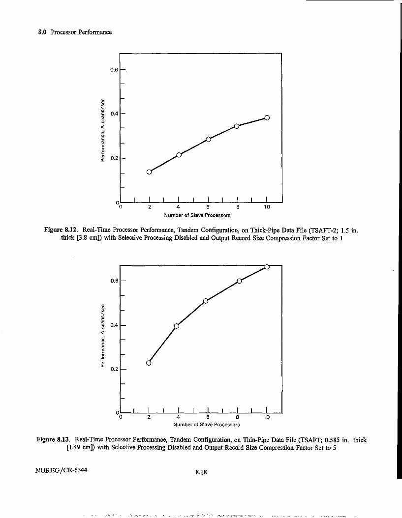
8.0 Processor Performance
4 6
Number of Slave Processors
10
Figure 8.12. Real-Time Processor Performance, Tandem Configuration, on Thick-Pipe Data File (TSAFT-2; 1.5 in.thick [3.8 cm]) with Selective Processing Disabled and Output Record Size Compression Factor Set to 1
cCO
ID
a.
4 6 8Number of Slave Processors
10
Figure 8.13. Real-Time Processor Performance, Tandem Configuration, on Thin-Pipe Data File (TSAFT; 0.585 in. thick[1.49 cm]) with Selective Processing Disabled and Output Record Size Compression Factor Set to 5
NUREG/CR-6344 8.18
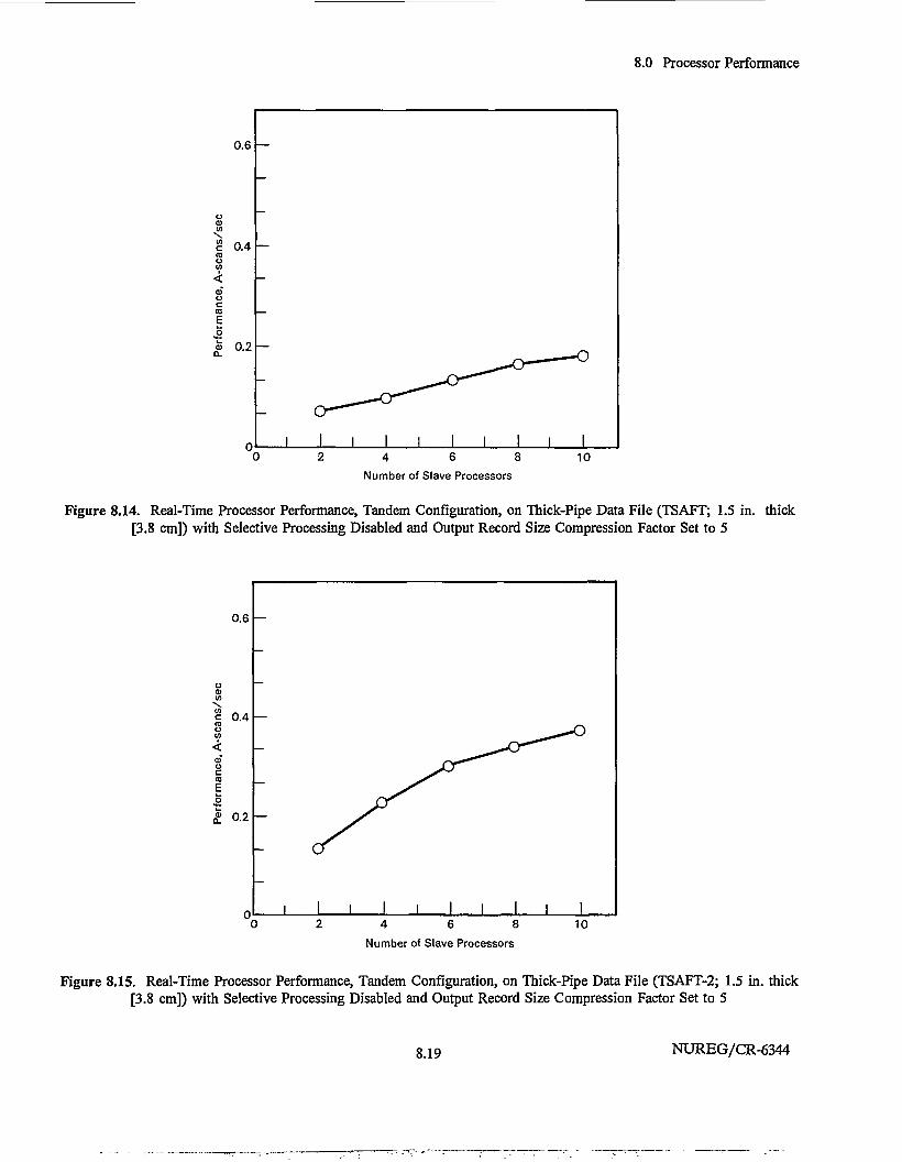
8.0 Processor Performance
4 6 8
Number of Slave Processors
10
Figure 8.14. Real-Time Processor Performance, Tandem Configuration, on Thick-Pipe Data File (TSAFT; 1.5 in. thick[3.8 cm]) with Selective Processing Disabled and Output Record Size Compression Factor Set to 5
S. 0.2 -
4 6 8
Number of Slave Processors
10
Figure 8.15. Real-Time Processor Performance, Tandem Configuration, on Thick-Pipe Data File (TSAFT-2; 1.5 in. thick[3.8 cm]) with Selective Processing Disabled and Output Record Size Compression Factor Set to 5
8.19 NUREG/CR-6344
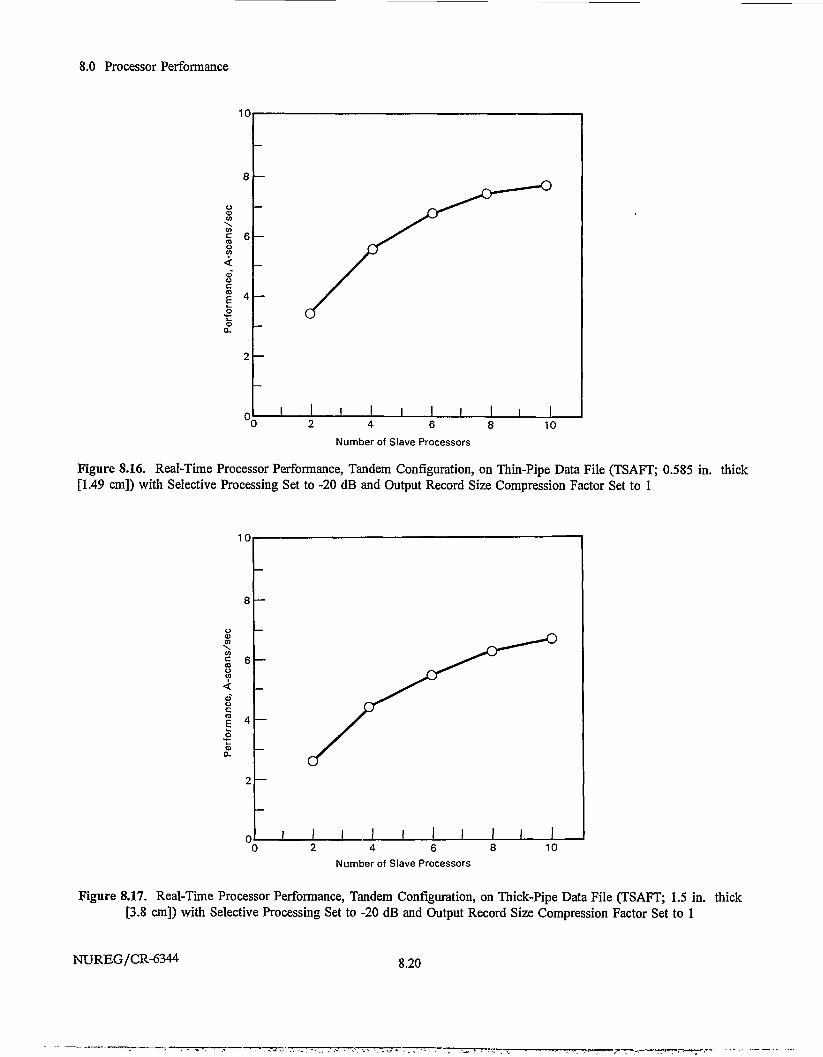
8.0 Processor Performance
4 6
Number of Slave Processors
10
Figure 8.16. Real-Time Processor Performance, Tandem Configuration, on Thin-Pipe Data File (TSAFT; 0.585 in. thick[1.49 cm]) with Selective Processing Set to -20 dB and Output Record Size Compression Factor Set to 1
4 6Number of Slave Processors
10
Figure 8.17. Real-Time Processor Performance, Tandem Configuration, on Thick-Pipe Data File (TSAFT; 1.5 in. thick[3.8 cm]) with Selective Processing Set to -20 dB and Output Record Size Compression Factor Set to 1
NUREG/CR-6344 8.20
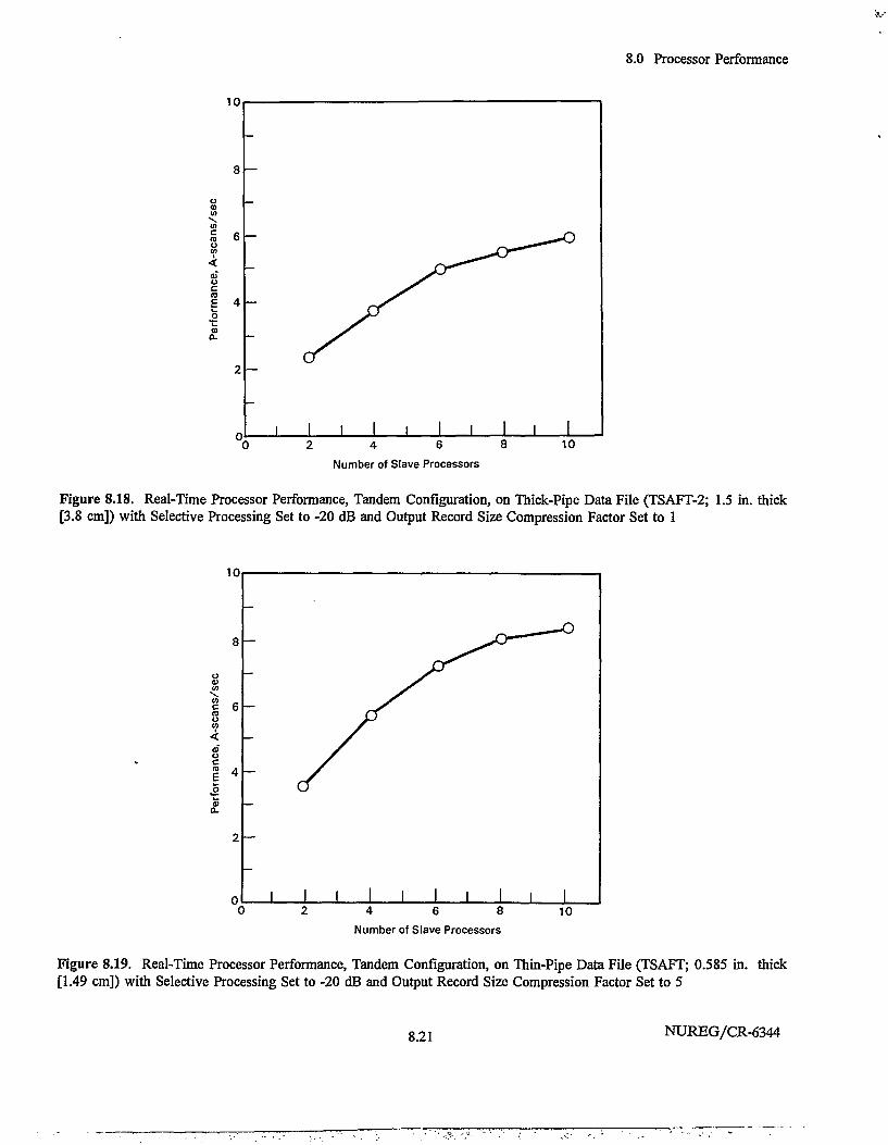
8.0 Processor Performance
oa.
I I I I I I I2 4 6 8
Number of Slave Processors
10
Figure 8.18. Real-Time Processor Performance, Tandem Configuration, on Thick-Pipe Data File (TSAFT-2; 1.5 in. thick[3.8 cm]) with Selective Processing Set to -20 dB and Output Record Size Compression Factor Set to 1
4 6 8
Number of Slave Processors
10
Figure 8.19. Real-Time Processor Performance, Tandem Configuration, on Thin-Pipe Data File (TSAFT; 0.585 in. thick[1.49 cm]) with Selective Processing Set to -20 dB and Output Record Size Compression Factor Set to 5
8.21 NUREG/CR-6344
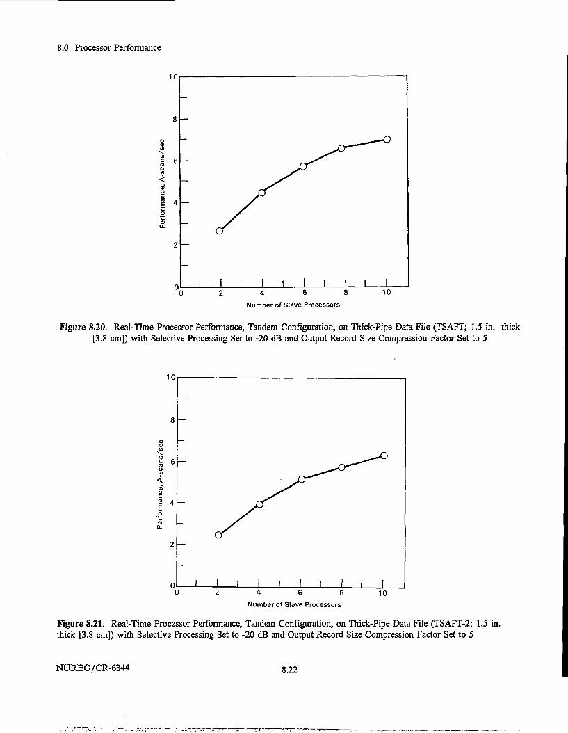
8.0 Processor Performance
4 6 8
Number of Slave Processors
Figure 8.20. Real-Time Processor Performance, Tandem Configuration, on Thick-Pipe Data File (TSAFT; 1.5 in. thick[3.8 cm]) with Selective Processing Set to -20 dB and Output Record Size Compression Factor Set to 5
4 6 8
Number of Slave Processors
10
Figure 8.21. Real-Time Processor Performance, Tandem Configuration, on Thick-Pipe Data File (TSAFT-2; 1.5 in.thick [3.8 cm]) with Selective Processing Set to -20 dB and Output Record Size Compression Factor Set to 5
NUREG/CR-6344 8.22
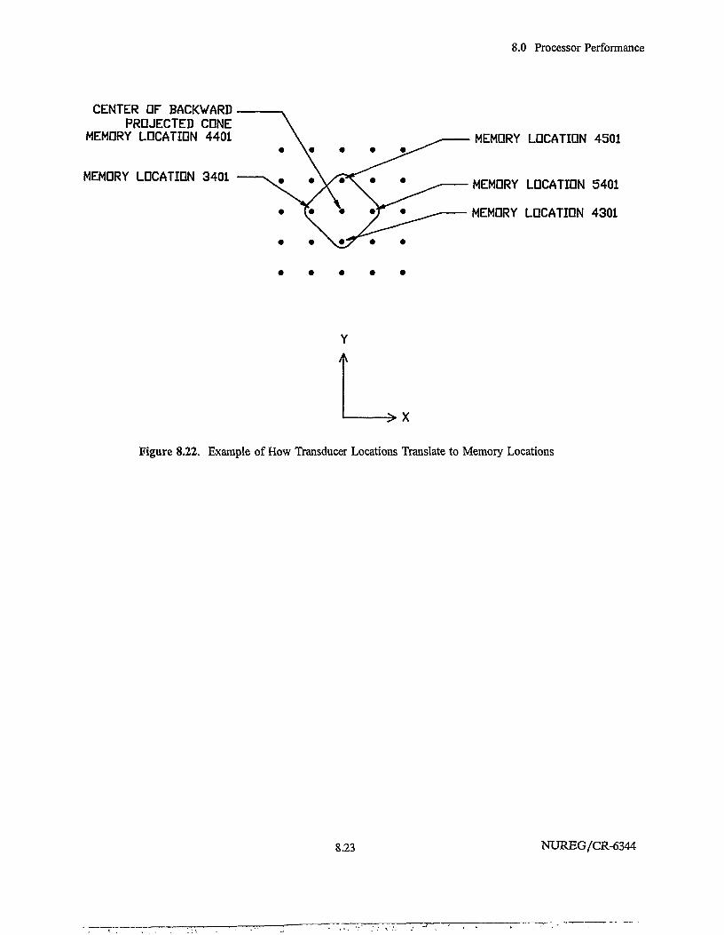
8.0 Processor Performance
CENTER DF BACKWARDPROJECTED CDNE
MEMORY LOCATION 4401
MEMORY LOCATION 3401
MEMORY LOCATION 4501
MEMORY LOCATION 5401
MEMORY LOCATION 4301
Figure 8.22. Example of How Transducer Locations Translate to Memory Locations
8.23 NUREG/CR-6344
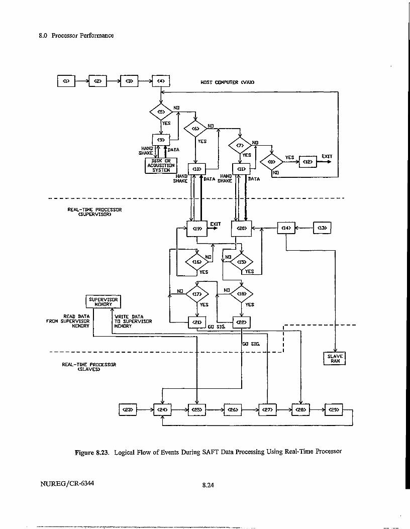
8.0 Processor Performance
REAU-TIME PROCESSOR<SUPERVISOR>
SUPERVISORMEMORY
READ DATAFRDK SUPERVISOR
MEMORY
<1> <2> <3> <4>
eHOST COMPUTER CVA»
HANDSHAKE
DISK ORACQUSITION
SYSTEM
VRITE DATATO SUPERVISORMEMORY
HAND 4 i t n . T J L i m m *
SHAKE I DATA S H A K E
EXIT
DATA
<20>
GO SIG.
REAL-TIME PROCESSOR<SLAVES>
<23>
GO SIG.
<25> <26> <27> <28>
EXIT
SLAVERAM
Figure 8.23. Logical Flow of Events During SAFT Data Processing Using Real-Time Processor
NUREG/CR-6344 8.24
9.0 Upgrading the SAFT-UT Field System
In the development and evaluation of the SAFT-UTtechnology, one of the important goals has been to im-prove the reliability of the inspection of reactor pres-sure vessels. In addition, another NRC program (JCNL1099) has as a goal to develop a data base on thedistribution of fabrication flaws (i.e., flaws that existedat the time of vessel fabrication) that exist in U.S. nu-clear reactor pressure vessels. SAFT-UT field inspec-tions of unused pressure vessel material are planned forthis project. The planned inspections require ultrasonictests with equipment best suited to providing fast andaccurate scans of the selected reactor pressure vesselareas. The SAFT-UT field data acquisition system hasbeen upgraded to better cope with the large volume ofdata that will result from this kind of inspection.
In this section, we discuss the hardware and softwaremethods used to achieve various rates of data collec-tion, processing, and display. This text is useful forduplicating the system and for planning the implemen-tation of SAFT-UT on other UT/ISI systems. Perfor-mance of the SAFT-UT system is measured using met-
rics: sustained data acquisition rate, SAFT processingrate, and the data display rate. Table 9.1 shows thechanges hi these three rates as the SAFT-UT systemwas improved.
9.1 SAFT System Architecture
The SAFT-UT system is composed of four functionalsubsystems as shown in Figure 9.1. The data acquisi-tion subsystem controls the scan of the part and collectsthe data for transfer to the host computer. The hostcomputer receives the data from the data acquisitionsubsystem, files the data, and transfers the data to theother subsystems for processing and display. The SAFTreal-time processor performs the computationally inten-sive SAFT calculations. Finally, the data display mod-ule provides the image display to the operator for inter-pretation.
Table 9.1. Performance for Upgrades to SAFT-UT System
Sustained Data Acquisition Rate(kBytes/sec)
PDPU and:.VAX-ll/730
5
• iPDPll-and MicroVax
20
PC and MicroVax::;,:;,..
200 500
Approximate Relative SAFT Processing Rate(for thick material)
VAX41/780
1
SAFT;RTP> J-.4:^
25
^-:M2foVAX:m - f e
3
. ,Sun Sparc 10, Model 30 ,:
25
Data Display Rate
.::- cyax-34^730 yath &ara
1 25
• . • • • : • . • - - . - - - : : : : . . . • „ . • : - - : - . - ;
Sun Sparc 10, MdalSf ,;:;
250
*RTP = real-time processor
9.1 NUREG/CR-6344
9.0 Upgrading the Field System
9.2 Installation of a MicroVAX IH
The host computer subsystem was upgraded from aVAX 11/730 to a MicroVAX 3400 computer. Thisupgrade improved the three functions of the host com-puter subsystem: 1) transfer of data from the dataacquisition module, 2) archive the data to a removabledisk platter instead of 9-track tape, and 3) transfer ofdata to the display module. A functional diagram ofthe subsystem is shown in Figure 9.2. The hardwarespecifications are the following:
• MicroVAX 3400 CPU with 12-slot backplane• 12-MB memory• 40-MB system disk• 300-MB removable cartridge tape drive
HP C1711A 600-MB removable rewritable opticaldisk drive
• SCSI interface adapter for the optical disk drive• two DR11 parallel interfaces• Ramtek interface• serial ports for eight users
VT 320 system terminal• printer• VMS operating system• 'C compiler.
In addition, a few changes were made to the SAFT-UTdata acquisition subsystem. The upgraded subsystem,shown in Figure 9.3, is divided into five components:mechanical scanner, acoustic subsystem, computer, diskdrive, and interface to the host computer subsystem.The upgrades included
• a new 100-MB disk drive - This permits the dataacquisition subsystem to operate better in thestand-alone mode.
• a joy-stick added to the scanner component tomore easily position the scanner before beginningthe inspection
• a DRV11-WA parallel interface added to morequickly transfer data to the host computer - Asoftware device driver was written for this inter-face because this software was not available fromthe manufacturer.
Using this upgraded system, the time required to per-form an inspection was decreased by a factor of 4 overthe previous system. This was accomplished by improv-ing the data transfer rate to the host computer from 5kBytes/s (kB/s) to 20 kB/s. The data acquisition rateto PDP11 memory was unchanged at 50 kB/s and limit-ed to a total of 128 kB per scan line with each A-scannot more than 1024 bytes in length.
The most dramatic improvement was made in the per-formance of data display calculations that routinelyoccur on the host CPU. The time required to performaxis transformations and image projections wasdecreased by a factor of 25 over the time requiredwhen using the VAX 11-730.
9.3 Other System Upgrades for theInspection of Nuclear Reactor Pres-sure Vessels
Additional system upgrades included a robotic ultrason-ic scanner, improvements to the SAFT-UT data fileheader, and a new data acquisition subsystem. A blockdiagram of the upgraded system is shown in Figure 9.4.The robotic scanner shown in Figure 9.5 uses a PUMA562 industrial robotic arm, an RTD probe holder, andthe existing SAFT-UT transducer gimbals. The PUMA562 is a six-axis robotic arm with a reach of 914 mm(36 in.) and a repeatability of better than 0.10 mm(0.004 in.).
The robot is blind in the sense that it must be taughtthe inspection surface. However, the robot permits thesystematic scanning of large complex objects, such asreactor pressure vessel nozzles, without moving a scan-ner track along the surface of the vessel. The SAFT-UT robotic scanner assumes that the contact methodwill be used. The transducers are attached to therobot's end effector and moved along the surface of thematerial, permitting data acquisition at appropriatelyspaced intervals. The robotic scanner queries the oper-ator about the location of the test material and asks theoperator to teach it how to find the test material if ithas no memory of the material's location in its workspace. Once this is done, the robot can position itselfanywhere on the surface of the test material that iswithin the robot's reach. The operator can move therobot's transducer along the surface of the test material
NUREG/CR-6344 9.2
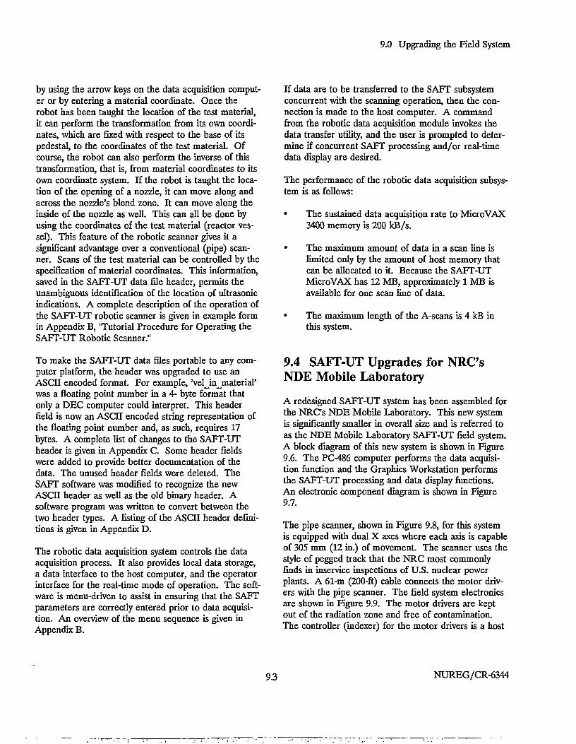
9.0 Upgrading the Field System
by using the arrow keys on the data acquisition comput-er or by entering a material coordinate. Once therobot has been taught the location of the test material,it can perform the transformation from its own coordi-nates, which are fixed with respect to the base of itspedestal, to the coordinates of the test material. Ofcourse, the robot can also perform the inverse of thistransformation, that is, from material coordinates to itsown coordinate system. If the robot is taught the loca-tion of the opening of a nozzle, it can move along andacross the nozzle's blend zone. It can move along theinside of the nozzle as well. This can all be done byusing the coordinates of the test material (reactor ves-sel). This feature of the robotic scanner gives it asignificant advantage over a conventional (pipe) scan-ner. Scans of the test material can be controlled by thespecification of material coordinates. This information,saved in the SAFT-UT data file header, permits theunambiguous identification of the location of ultrasonicindications. A complete description of the operation ofthe SAFT-UT robotic scanner is given in example formin Appendix B, "Tutorial Procedure for Operating theSAFT-UT Robotic Scanner."
To make the SAFT-UT data files portable to any com-puter platform, the header was upgraded to use anASCII encoded format. For example, 'vel_in_niaterial'was a floating point number in a 4- byte format thatonly a DEC computer could interpret. This headerfield is now an ASCII encoded string representation ofthe floating point number and, as such, requires 17bytes. A complete list of changes to the SAFT-UTheader is given hi Appendix C. Some header fieldswere added to provide better documentation of thedata. The unused header fields were deleted. TheSAFT software was modified to recognize the newASCII header as well as the old binary header. Asoftware program was written to convert between thetwo header types. A listing of the ASCII header defini-tions is given in Appendix D.
The robotic data acquisition system controls the dataacquisition process. It also provides local data storage,a data interface to the host computer, and the operatorinterface for the real-time mode of operation. The soft-ware is menu-driven to assist in ensuring that the SAFTparameters are correctly entered prior to data acquisi-tion. An overview of the menu sequence is given inAppendix B.
If data are to be transferred to the SAFT subsystemconcurrent with the scanning operation, then the con-nection is made to the host computer. A commandfrom the robotic data acquisition module invokes thedata transfer utility, and the user is prompted to deter-mine if concurrent SAFT processing and/or real-timedata display are desired.
The performance of the robotic data acquisition subsys-tem is as follows:
• The sustained data acquisition rate to MicroVAX3400 memory is 200 kB/s.
• The maximum amount of data in a scan line islimited only by the amount of host memory thatcan be allocated to it. Because the SAFT-UTMicroVAX has 12 MB, approximately 1 MB isavailable for one scan line of data.
• The maximum length of the A-scans is 4 kB inthis system.
9.4 SAFT-UT Upgrades for NRC'sNDE Mobile Laboratory
A redesigned SAFT-UT system has been assembled forthe NRC's NDE Mobile Laboratory. This new systemis significantly smaller in overall size and is referred toas the NDE Mobile Laboratory SAFT-UT field system.A block diagram of this new system is shown in Figure9.6. The PC-486 computer performs the data acquisi-tion function and the Graphics Workstation performsthe SAFT-UT processing and data display functions.An electronic component diagram is shown in Figure9.7.
The pipe scanner, shown in Figure 9.8, for this systemis equipped with dual X axes where each axis is capableof 305 mm (12 in.) of movement. The scanner uses thestyle of pegged track that the NRC most commonlyfinds in inservice inspections of U.S. nuclear powerplants. A 61-m (200-ft) cable connects the motor driv-ers with the pipe scanner. The field system electronicsare shown hi Figure 9.9. The motor drivers are keptout of the radiation zone and free of contamination.The controller (indexer) for the motor drivers is a host
9.3 NUREG/CR-6344
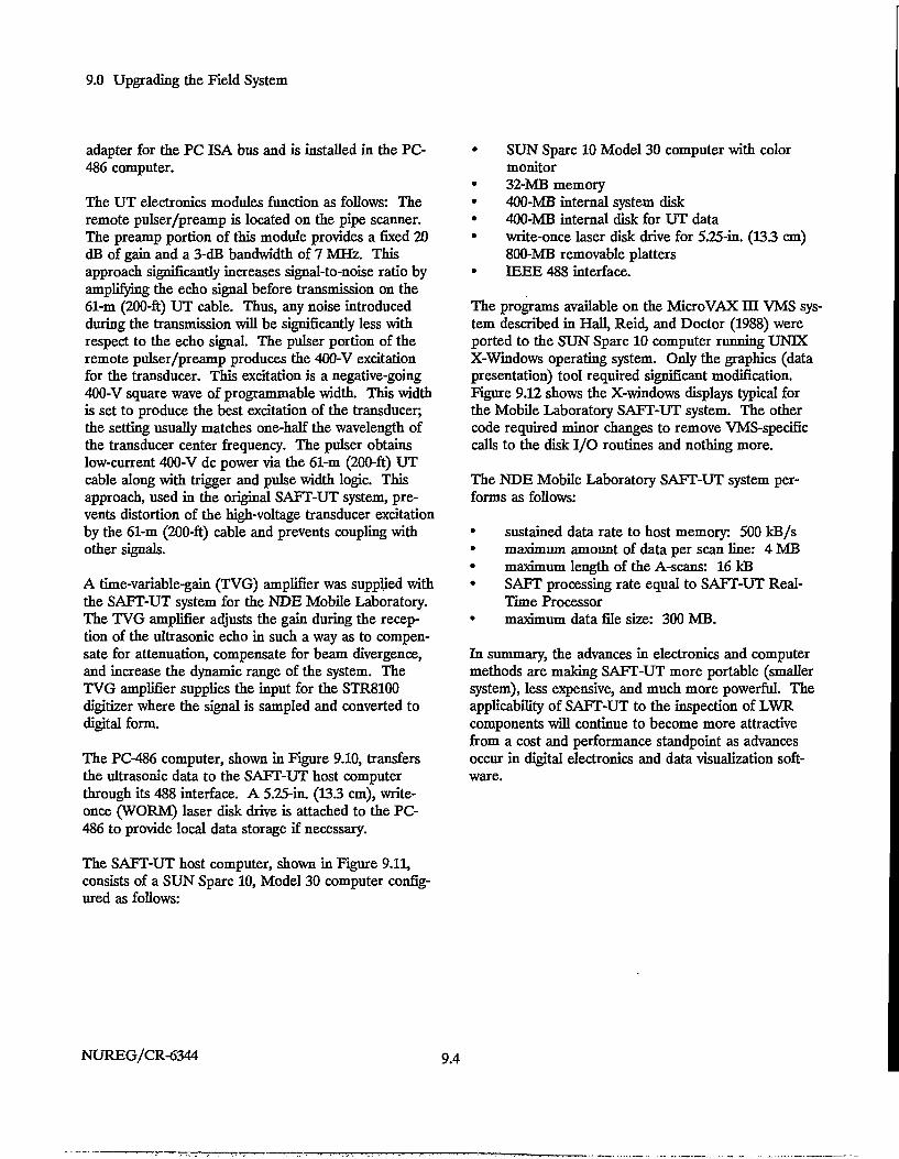
9.0 Upgrading the Field System
adapter for the PC ISA bus and is installed in the PC-486 computer.
The UT electronics modules function as follows: Theremote pulser/preamp is located on the pipe scanner.The preamp portion of this module provides a fixed 20dB of gain and a 3-dB bandwidth of 7 MHz. Thisapproach significantly increases signal-to-noise ratio byamplifying the echo signal before transmission on the61-m (200-ft) UT cable. Thus, any noise introducedduring the transmission will be significantly less withrespect to the echo signal. The pulser portion of theremote pulser/preamp produces the 400-V excitationfor the transducer. This excitation is a negative-going400-V square wave of programmable width. This widthis set to produce the best excitation of the transducer;the setting usually matches one-half the wavelength ofthe transducer center frequency. The pulser obtainslow-current 400-V dc power via the 61-m (200-ft) UTcable along with trigger and pulse width logic. Thisapproach, used in the original SAFT-UT system, pre-vents distortion of the high-voltage transducer excitationby the 61-m (200-ft) cable and prevents coupling withother signals.
A time-variable-gain (TVG) amplifier was supplied withthe SAFT-UT system for the NDE Mobile Laboratory.The TVG amplifier adjusts the gam during the recep-tion of the ultrasonic echo in such a way as to compen-sate for attenuation, compensate for beam divergence,and increase the dynamic range of the system. TheTVG amplifier supplies the input for the STR8100digitizer where the signal is sampled and converted todigital form.
The PC-486 computer, shown in Figure 9.10, transfersthe ultrasonic data to the SAFT-UT host computerthrough its 488 interface. A 5.25-in. (13.3 cm), write-once (WORM) laser disk drive is attached to the PC-486 to provide local data storage if necessary.
The SAFT-UT host computer, shown in Figure 9.11,consists of a SUN Sparc 10, Model 30 computer config-ured as follows:
• SUN Sparc 10 Model 30 computer with colormonitor
• 32-MB memory• 400-MB internal system disk• 400-MB internal disk for UT data• write-once laser disk drive for 5.25-in. (13.3 cm)
800-MB removable plattersIEEE 488 interface.
The programs available on the MicroVAX m VMS sys-tem described in Hall, Reid, and Doctor (1988) wereported to the SUN Sparc 10 computer running UNIXX-Windows operating system. Only the graphics (datapresentation) tool required significant modification.Figure 9.12 shows the X-windows displays typical forthe Mobile Laboratory SAFT-UT system. The othercode required minor changes to remove VMS-specificcalls to the disk I/O routines and nothing more.
The NDE Mobile Laboratory SAFT-UT system per-forms as follows:
• sustained data rate to host memory: 500 kB/s• maximum amount of data per scan line: 4 MB• maximum length of the A-scans: 16 kB
SAFT processing rate equal to SAFT-UT Real-Time Processor
• maximum data file size: 300 MB.
In summary, the advances in electronics and computermethods are making SAFT-UT more portable (smallersystem), less expensive, and much more powerful. Theapplicability of SAFT-UT to the inspection of LWRcomponents will continue to become more attractivefrom a cost and performance standpoint as advancesoccur in digital electronics and data visualization soft-ware.
NUREG/CR-6344 9.4
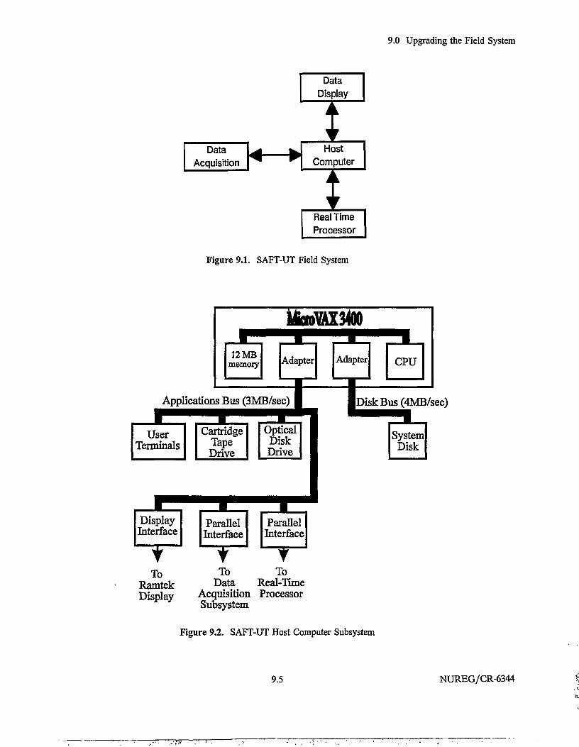
DataAcquisition
DataDisplay
iHost
Computer
IReal TimeProcessor
Figure 9.1. SAFT-UT Field System
9.0 Upgrading the Field System
ifaoYAXMOO
12 MBmemory Adapter
Applications Bus (3MB/sec)iUser
TerminalsCartridge
TapeDrive
OpticalDiskDrive
Adapter CPU
Disk Bus (4MB/sec)
DisplayInterface
ParallelInterface
ParallelInterface
To To ToRamtek Data Real-TimeDisplay Acquisition Processor
Subsystem
Figure 9.2. SAFT-UT Host Computer Subsystem
9.5 NUREG/CR-6344
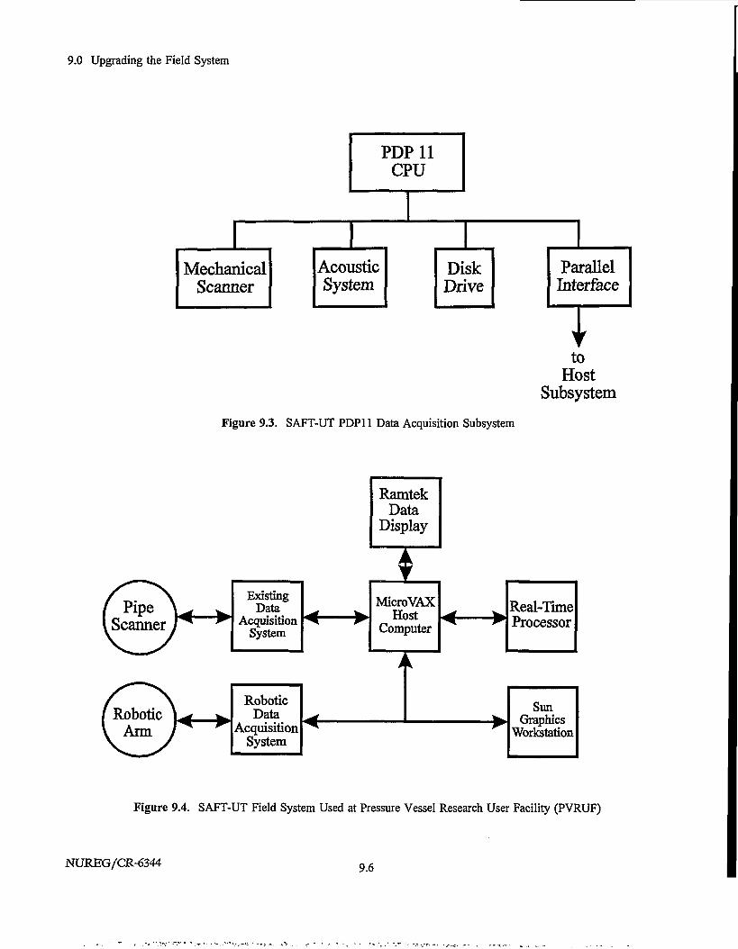
9.0 Upgrading the Field System
1Mechanical
Scanner
PDPllCPU
AcousticSystem
DiskDrive
ParallelInterface
toHost
Subsystem
Figure 9.3. SAFT-UT PDPll Data Acquisition Subsystem
ExistingData
AcquisitionSystem
RoboticData
AcquisitionSystem
RamtekData
Display
IMicroVAX
HostComputer
Real-TimeProcessor
SunGraphics
Workstation
Figure 9.4. SAFT-UT Field System Used at Pressure Vessel Research User Facility (PVRUF)
NUREG/CR-6344 9.6
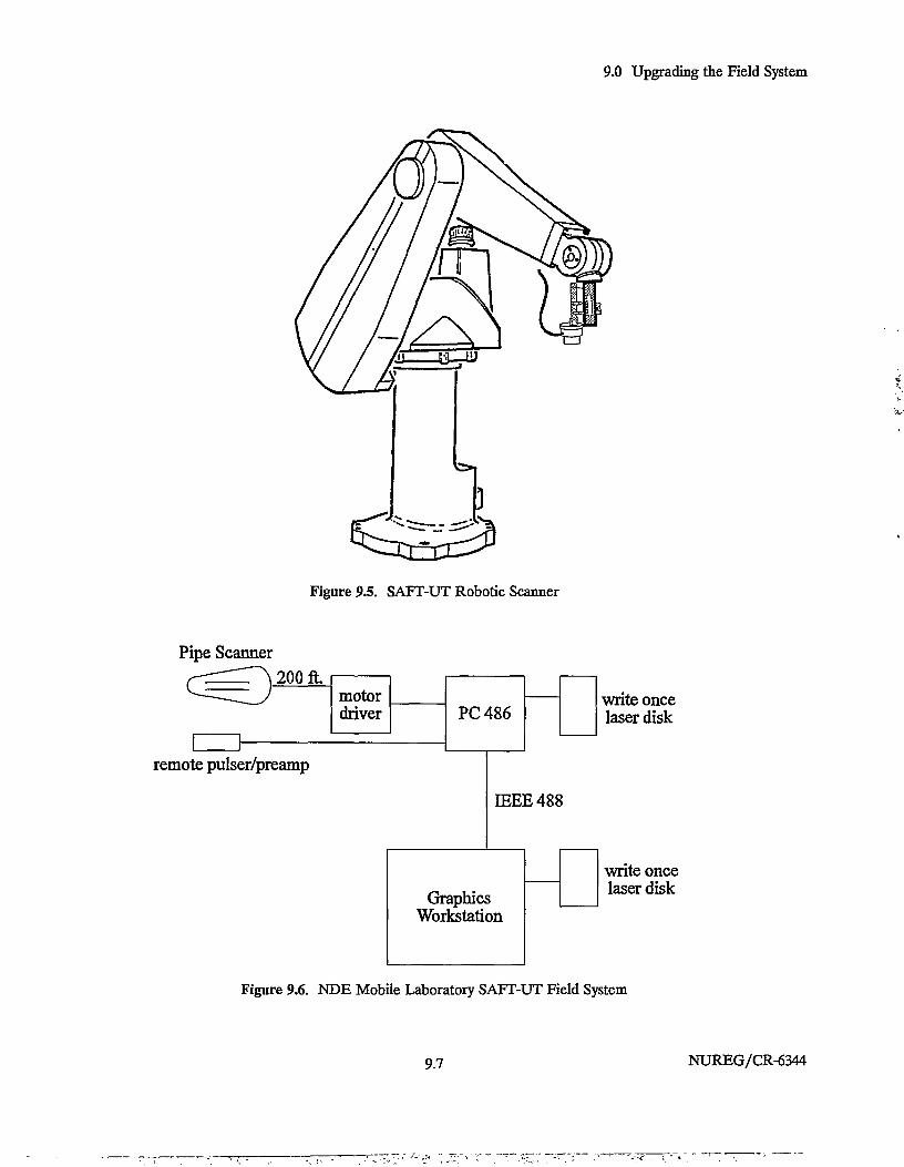
9.0 Upgrading the Field System
Figure 9.5. SAFT-UT Robotic Scanner
Pipe Scanner
r - — A 200 ftmotordriver
remote pulser/preamp
PC 486
ffiE]
GraphicsWorkstation
E48S
write oncelaser disk
write oncelaser disk
Figure 9.6. NDE Mobile Laboratory SAFT-UT Field System
9.7 NUREG/CR-6344
' - • • * - , ; ' *
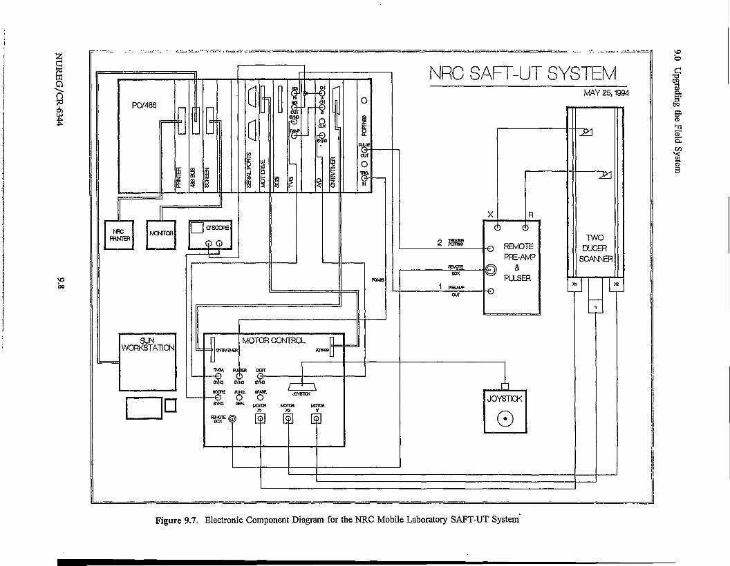
"g6>
NRC SAFT-UT SYSTEM
bo
MAY 25,1994
yoo
a.
I"
§:en
I
Figure 9.7. Electronic Component Diagram for the NRC Mobile Laboratory SAFT-UT System'
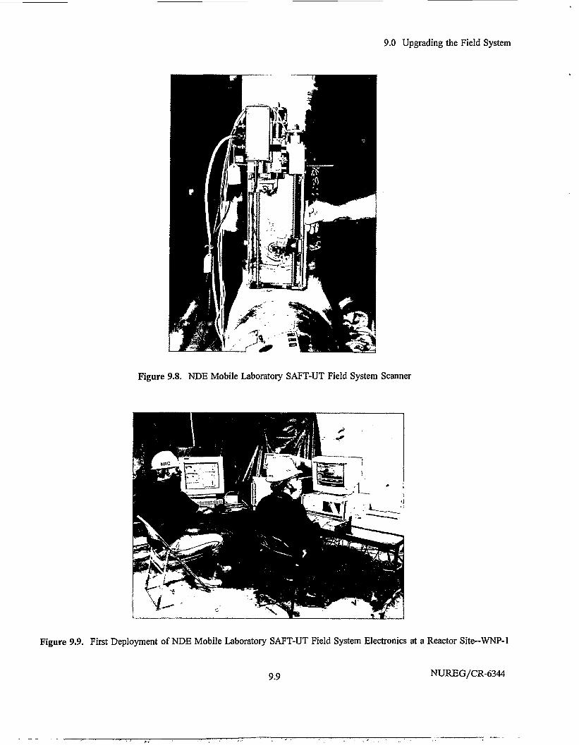
9.0 Upgrading the Field System
Figure 9.8. NDE Mobile Laboratory SAFT-UT Field System Scanner
Figure 9.9. First Deployment of NDE Mobile Laboratory SAFT-UT Field System Electronics at a Reactor Site-WNP-1
9.9 NUREG/CR-6344
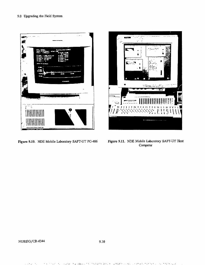
9.0 Upgrading the Field System
Figure 9.10. NDE Mobile Laboratory SAFT-UT PC-486 Figure 9.11. NDE Mobile Laboratory SAFT-UT HostComputer
NUREG/CR-6344 9.10
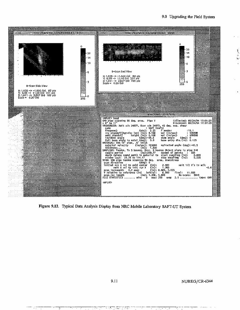
9.0 Upgrading the Field System
X: 1.02S - > -1.000 (.in) 82 ntsV: 8 .00-> 11.00 On) 201 stsZ: 1.011 - > 2.827 (In) 1S8 ptsScale » 0.20 (in)
X: 1 .025->-1.000 (in) 82 ptsY: 13.00 ~> 11.00 (in) 201 pisZ: 1.011 - > 2.827 (in) 168 ptsSea l * " 0.20 (In)
<APL0T> headSKA pipe scanning 90 deg. area.- 6" to 11"TRANSDUCER: Xnit s/n 24877, Rcvr s/n 24873. 45 deg. notn. shear
mode : SAFT t sa f t2
Col lected: 06/24/94 17:01:20Processed: 06/24/94 17:37:29
f nunbervel Cin/sec)vel Cin/sec)ske» angle
frequency Cmhz): 2.25rev standoff(hgt=foc len) ( i n ) : 0.150xnit standoff height Cin): 0.150incident angle Cdeg):-35.6fu l l bean angle in metal Cdeg): 3.0
MATERIAL: SHA 10" pipe, .6" thickMaterial velocity Cin/sec): 123000thickness... Cin): 1.930
SAMPLING: Tandem, Tx 5 bounce, Rcvr. 0 bounce Object plane is pipe X=0sample period Cns):239.77 number of points : 355depth Calong sound path) in material to start sampling Cin): 0.000Bindos Cus): 29.29 to 114.17 stop sampling Cin): 5.235
SCAN: SMA pipe tandem scanning 90 deg.scan direction Cdeg): 0i n i t i a l rev X rel to seld center Cin):
xmit X rel to i n i t rev X Cin):scan increment: X.Y axes Cin):V relative to reference Cin) i n i t i a l :scan.inc length Cin): 1.200,
FILE STATISTICS min: 0 oax:
19.11OEOOO10S0O00
bean entry dia.Cin): 0.125
refracted angle Cdeg):-42.5
area, donnstrean
xmit 1/2 V's to »cl :2.4001.200
0.025. 0.0256.000 f i n a l : 11.000
5.000 Ha-scans: 9843255 avg: 2.9 type: ENV
Figure 9.12. Typical Data Analysis Display from NRC Mobile Laboratory SAFT-UT System
9.11 NUREG/CR-6344
10.0 SAFT-UT Validation
The SAFT-UT technology has been under evaluationsince the program started a number of years ago.However, many of these evaluations- have been conduct-ed on small sample sets without objective and blindtesting conditions. In other cases, the defects detectedand characterized were not destructively validated and,thus, do not provide hard evidence of the technology'seffectiveness.
This section describes several such tests conducted tomore fully quantify SAFT-UT system performance.The testing included SAFT-UT participation in theMini-Round Robin (MRR) conducted at PNL, testingat the Electric Power Research Institute (EPRI) NDECenter, and testing conducted as part of the Pro-gramme for the Inspection of Steel Components Phase3 (PISC-III).
10.1 Validation of SAFT-UT in theMini-Round Robin
10.1.1 The Mini-Round Robin
The round robin study, conducted at PNL is completelydescribed in NUREG/CR-4908 (Heasler et al. 1990).The study was conducted to provide an engineeringdata base for UT/ISI that would help
• quantify the effect of training and performancedemonstration testing that resulted from IEB 83-02
• quantify the differences in capability between de-tecting long (greater than 76 mm [3 in.]) cracksversus short (less than 51 mm [2 in.]) cracks
• quantify the capability of UT/ISI inspectors to de-termine the length and depth of intergranularstress corrosion cracks (IGSCCs).
The round robin study involved six two-person manualinspector teams and three automated inspection teams.SAFT-UT was an add-on after the original testing hadbeen completed and before destructive testing. It wasdecided not to include the SAFT-UT results inNUREG/CR-4908 because its inclusion as part of theoriginal study had not been planned. It needs to benoted that the SAFT-UT inspections were conducted bya PNL staff member who was totally ignorant of the
MRR study and had no connection with the specimensin any way. The specimens used in this study containedlaboratory-produced IGSCC. Key features of the speci-mens used in the MRR are listed in Tables 10.1 and10.2.
The results were evaluated using the concept of gradingunits to define two performance parameters—probabilityof detection (POD) and false call probability (FCP).Each inspector's detection capabilities are estimatedusing these two statistics, which are defined by
PODNumber of Correct Detections
Number of Cracked Grading Units Inspected
pcp _ Number of Blank Grading Units Called CrackedNumber of Blank Grading Units Inspected
The round robin was constructed so these two statisticscould be estimated efficiently for different inspectionconditions. These statistics are employed in this sectionto examine inspection performance.
The POD and FCP statistics always refer to a unit ofmaterial of particular size, called a grading unit. There-fore, individual detection and false call statistics are al-ways associated with a unique grading unit. The detec-tion statistic for a particular grading unit is 1 if a crackwas called within the unit and 0 if no crack was called.Individual grading units were separated by a minimumof 25 mm (1 in.) of blank weld material in the circum-ferential direction with no separation axially for gradingunits on opposite sides of the weld; all the grading unitshave the same circumferential length. Grading unitsare randomly located within the test specimens but arenot actually marked on the outside of the specimen, sothe inspectors do not know their location. See Appen-dix E of Heasler et al. (1990), which shows all thegrading units on each MRR specimen.
Each grading unit was classified as defective if it con-tained a crack or as blank if it did not contain a crack.A true-state data base describing defective and blankgrading units was developed for each test specimenused in the MRR.
The 69 grading units were large enough to encompassthe cracks in the specimens. Because the cracks were
10.1 NUREG/CR-6344
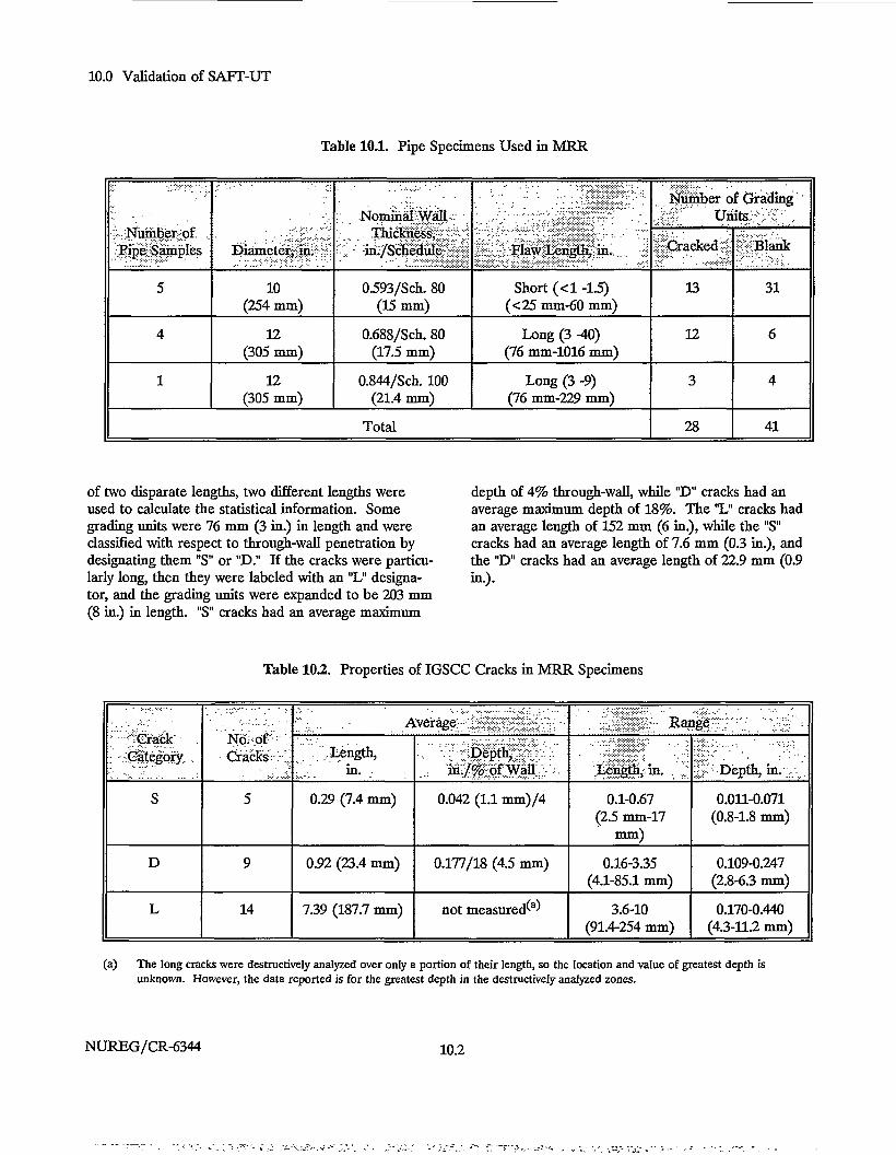
10.0 Validation of SAFT-UT
Table 10.1. Pipe Specimens Used in MRR
:.: ,:NumBet::of. ..;Bip#SampIes
5
4
1
Diameter, in.
10(254 mm)
12(305 mm)
12(305 mm)
Nominal WallThickness,
in./Schedu!e
0.593/Sch. 80(15 mm)
0.688/Sch. 80(17.5 mm)
0.844/Sch. 100(21.4 mm)
Flaw Length, in.
Short (<1 -1.5)(<25 mm-60 mm)
Long (3 -40)(76 mm-1016 mm)
Long (3 -9)(76 mm-229 mm)
Total
Number of GradingUnits
Cracked
13
12
3
28
Blank
31
6
4
41
of two disparate lengths, two different lengths wereused to calculate the statistical information. Somegrading units were 76 mm (3 in.) in length and wereclassified with respect to through-wall penetration bydesignating them "S" or "D." If the cracks were particu-larly long, then they were labeled with an "L" designa-tor, and the grading units were expanded to be 203 mm(8 in.) in length. "S" cracks had an average maximum
depth of 4% through-wall, while "D" cracks had anaverage maximum depth of 18%. The "L" cracks hadan average length of 152 mm (6 in.), while the "S"cracks had an average length of 7.6 mm (0.3 in.), andthe "D" cracks had an average length of 22.9 mm (0.9in.).
Table 10.2. Properties of IGSCC Cracks in MRR Specimens
;:; ffpack: • .: .Category..,
S
D
L
Cracks^'..;
5
9
14
.. .. . • Average
..Length,. ..; i n . •
0.29 (7.4 mm)
0.92 (23.4 mm)
7.39 (187.7 mm)
Depth,ia./% of Wall
0.042 (1.1 mm)/4
0.177/18 (4.5 mm)
not measured^
Range
Length, in.
0.1-0.67(2.5 mm-17
mm)
0.16-3.35(4.1-85.1 mm)
3.6-10(91.4-254 mm)
. Depth, in.
0.011-0.071(0.8-1.8 mm)
0.109-0.247(2.8-6.3 mm)
0.170-0.440(4.3-11.2 mm)
(a) The long cracks were destructively analyzed over only a portion of their length, so the location and value of greatest depth isunknown. However, the data reported is for the greatest depth in the destructively analyzed zones.
NUREG/CR-6344 10.2
10.0 Validation of SAFT-UT
Each specimen inspected by the SAFT-UT field systemwas first prepared by an MRR official; i.e., each speci-men was masked to expose only a specified area to bescanned. There were a total of 47 such areas averaging254 mm (10 in.) in length. The areas were dividedamong three different sizes of pipe; 14 were on 254-mm- (10-in.) diameter Schedule 80, 29 on 305-mm- (12-in.) diameter Schedule 80, and 4 areas on 305-mm- (12-in.) diameter Schedule 100 pipe specimens.
10.1.2 SAFT-UT Inspection Procedure
Three different transducer configurations were used oneach area scanned using SAFT-UT. A single transduc-er normal to the front surface was used for profiling thepipe inner surface to help identify geometrical condi-tions that may present crack-like indications. A singletransducer using angle beam was used for crack detec-tion and lateral location relative to the weld center, andtandem transducers using angle beam were used forcrack detection confirmation.
The normal beam transducer was chosen to providegood penetration through the weldment; for this appli-cation, the transducer was 6 mm (0.25 in.) in diameterand operated at 5 MHz. The transducers used for theangle beam inspection and the tandem inspection were6 mm (0.25 in.) in diameter but operated at 2.25 MHz.
Because the SAFT real-time processor was not operat-ing at this time, the scanning and data analysis tookmuch longer than the time required by the other MRRteams. In this sense, there was not a realistic compari-son with the manual or commercially available automat-ed systems. However, the effectiveness of the techniquewas still validated.
10.1.3 SAFT-UT Analysis Procedure
All three scanning configurations were used during thedata analysis. The -6-dB level was chosen to determinethe crack length. Each crack was isolated, and theimage color scale was adjusted by the maximum valueof the isolated crack. This avoided undersizing smallcracks or cracks that are not good acoustic reflectorsthat may be adjacent to a strong acoustic reflection.
At the time this data was collected, the SAFT real-timeprocessor did not exist. Thus, the sizes of the areas
scanned were minimized to make three-dimensionalSAFT processing practical on the data files. Indicationswere considered cracks only if they lay in a predeter-mined "crack zone." This region was approximatelyone-half the thickness of the pipe specimen plus theweld root width from the weld center. Naturally, indi-cations that lay close to the weld center presented thebiggest problem in interpretation because of possibleinterference from weld root indications in this area.Indications that lay on the outer edge of the crack zonewere generally noted but not classified as cracks be-cause the SAFT aperture was limited to make the filessmall for practical processing.
10.1.4 SAFT-UT Performance Results andDiscussion
Figures 10.1 through 10.6 show the relative operatingcharacteristic (ROC) curves of the SAFT team, manualteams, and advanced teams under various crack condi-tions. The ROC curve quantifies the relationship be-tween POD and FCP results based on the decisioncriteria employed. Five decision criteria were usedbased on the confidence level of the particular call.These ranged from "definitely not a crack" to "possibly acrack" to "definitely a crack." Each graph shows theROC curve displayed in the center of the graph; theupper and lower curves describe the upper and lowerconfidence limits of the ROC fit. The scattered lettersare the actual data points used for the ROC curve fit.A performance curve intersecting the area in the upperleft-hand corner of these plots is considered acceptable.
Figure 10.1 shows the ROC curves for "D" and "S"cracks for the SAFT team. The SAFT team perfor-mance is better for "D" cracks because of improvedsignal-to-noise ratio. Figure 10.2 shows the ROCcurves for "D" and "L" cracks. The SAFT team per-formed equally well for these cracks. Figures 10.3 and10.4 show the ROC curves for the manual teams' aver-age performance on "D," "S," and "L" cracks. Whenthese figures are compared with the previouslydescribed plots, they suggest that the SAFT team hadbetter performance in all three crack categories thanthe average of the manual teams. The final set of ROCcurves (Figures 10.5 and 10.6) shows the average per-formance of the advanced teams on "D," "S," and "L"cracks. A comparison of these plots to Figures 10.1and 10.2 suggests that the SAFT team's performance
10.3 NTJREG/CR-6344
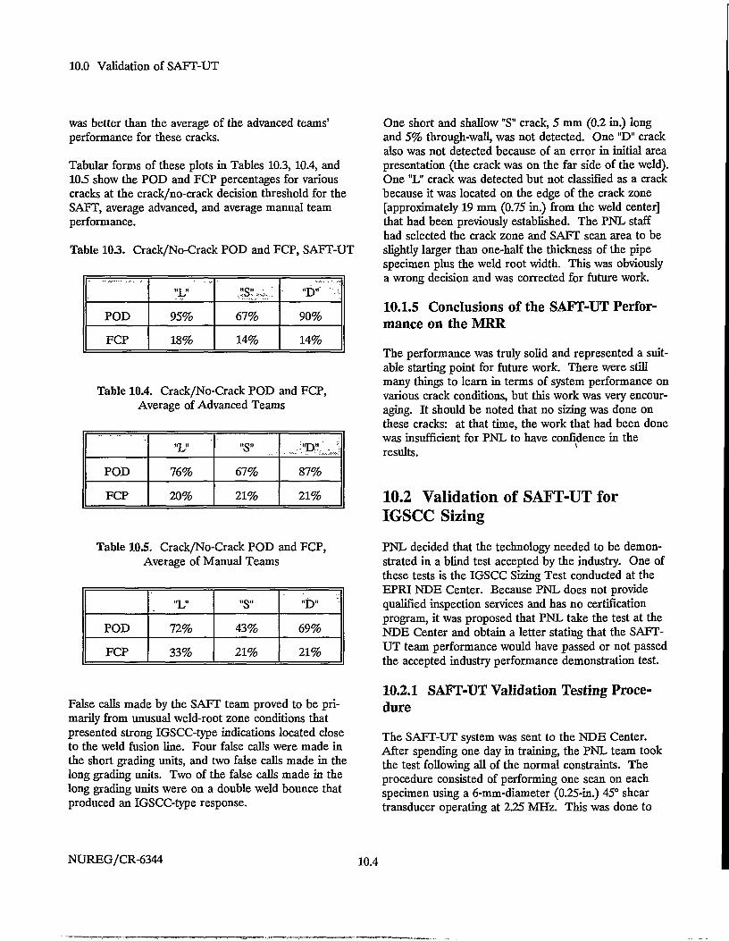
10.0 Validation of SAFT-UT
was better than the average of the advanced teams'performance for these cracks.
Tabular forms of these plots in Tables 10.3, 10.4, and10.5 show the POD and FCP percentages for variouscracks at the crack/no-crack decision threshold for theSAFT, average advanced, and average manual teamperformance.
Table 103. Crack/No-Crack POD and FCP, SAFT-UT
POD
FCP
"L"
95%
18%
,"S" :::.::/
67%
14%
"b" "•{
90%
14%
Table 10.4. Crack/No-Crack POD and FCP,Average of Advanced Teams
POD
FCP
"L"
76%
20%
"S"
67%
21%
.:"D?',.....:;
87%
21%
Table 10.5. Crack/No-Crack POD and FCP,Average of Manual Teams
POD
FCP
«L"
72%
33%
"S"
43%
21%
"b"69%
21%
False calls made by the SAFT team proved to be pri-marily from unusual weld-root zone conditions thatpresented strong IGSCC-type indications located closeto the weld fusion line. Four false calls were made inthe short grading units, and two false calls made in thelong grading units. Two of the false calls made in thelong grading units were on a double weld bounce thatproduced an IGSCC-type response.
One short and shallow "S" crack, 5 mm (0.2 in.) longand 5% through-wall, was not detected. One "D" crackalso was not detected because of an error in initial areapresentation (the crack was on the far side of the weld).One "L" crack was detected but not classified as a crackbecause it was located on the edge of the crack zone[approximately 19 mm (0.75 in.) from the weld center]that had been previously established. The PNL staffhad selected the crack zone and SAFT scan area to beslightly larger than one-half the thickness of the pipespecimen plus the weld root width. This was obviouslya wrong decision and was corrected for future work.
10.1.5 Conclusions of the SAFT-UT Perfor-mance on the MRR
The performance was truly solid and represented a suit-able starting point for future work. There were stillmany things to learn in terms of system performance onvarious crack conditions, but this work was very encour-aging. It should be noted that no sizing was done onthese cracks: at that time, the work that had been donewas insufficient for PNL to have confidence in theresults.
10.2 Validation of SAFT-UT forIGSCC Sizing
PNL decided that the technology needed to be demon-strated in a blind test accepted by the industry. One ofthese tests is the IGSCC Sizing Test conducted at theEPRI NDE Center. Because PNL does not providequalified inspection services and has no certificationprogram, it was proposed that PNL take the test at theNDE Center and obtain a letter stating that the SAFT-UT team performance would have passed or not passedthe accepted industry performance demonstration test.
10.2.1 SAFT-UT Validation Testing Proce-dure
The SAFT-UT system was sent to the NDE Center.After spending one day in training, the PNL team tookthe test following all of the normal constraints. Theprocedure consisted of performing one scan on eachspecimen using a 6-mm-diameter (0.25-in.) 45° sheartransducer operating at 2.25 MHz. This was done to
NUREG/CR-6344 10.4
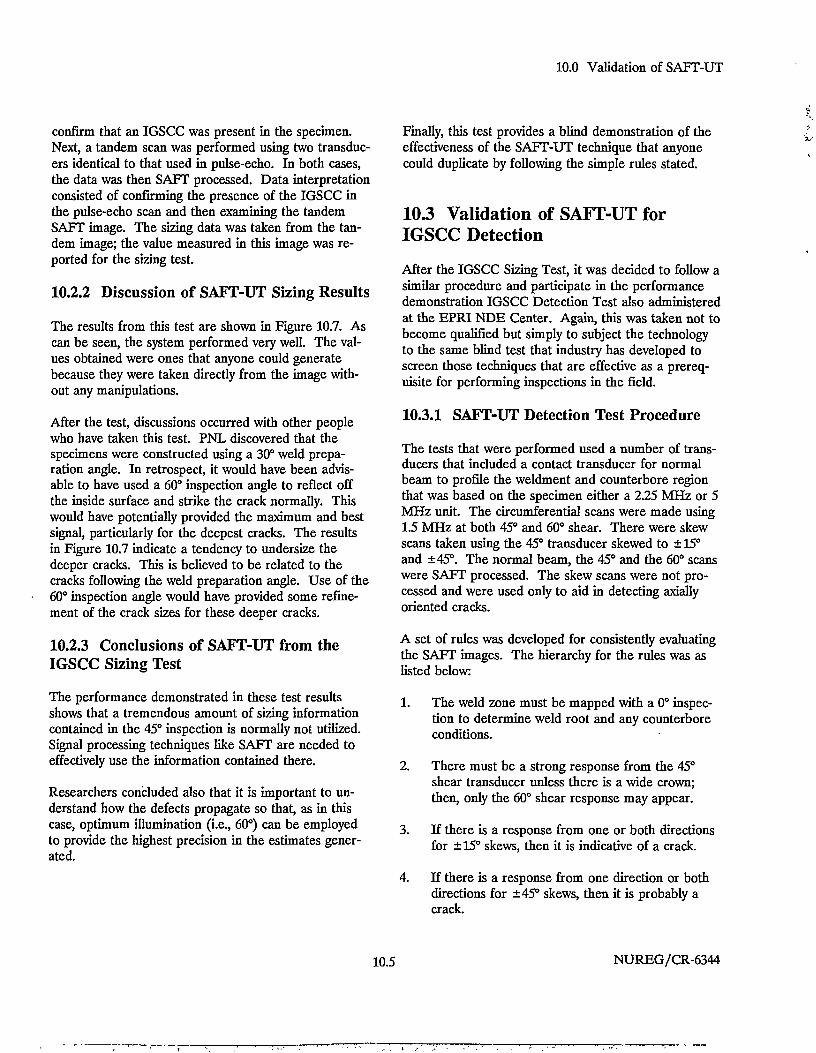
10.0 Validation of SAFT-UT
confirm that an IGSCC was present in the specimen.Next, a tandem scan was performed using two transduc-ers identical to that used in pulse-echo. In both cases,the data was then SAFT processed. Data interpretationconsisted of confirming the presence of the IGSCC inthe pulse-echo scan and then examining the tandemSAFT image. The sizing data was taken from the tan-dem image; the value measured in this image was re-ported for the sizing test.
10.2.2 Discussion of SAFT-UT Sizing Results
The results from this test are shown in Figure 10.7. Ascan be seen, the system performed very well. The val-ues obtained were ones that anyone could generatebecause they were taken directly from the image with-out any manipulations.
After the test, discussions occurred with other peoplewho have taken this test. PNL discovered that thespecimens were constructed using a 30° weld prepa-ration angle. In retrospect, it would have been advis-able to have used a 60° inspection angle to reflect offthe inside surface and strike the crack normally. Thiswould have potentially provided the maximum and bestsignal, particularly for the deepest cracks. The resultsin Figure 10.7 indicate a tendency to undersize thedeeper cracks. This is believed to be related to thecracks following the weld preparation angle. Use of the60° inspection angle would have provided some refine-ment of the crack sizes for these deeper cracks.
10.2.3 Conclusions of SAFT-UT from theIGSCC Sizing Test
The performance demonstrated in these test resultsshows that a tremendous amount of sizing informationcontained in the 45° inspection is normally not utilized.Signal processing techniques like SAFT are needed toeffectively use the information contained there.
Researchers concluded also that it is important to un-derstand how the defects propagate so that, as in thiscase, optimum illumination (i.e., 60°) can be employedto provide the highest precision in the estimates gener-ated.
Finally, this test provides a blind demonstration of theeffectiveness of the SAFT-UT technique that anyonecould duplicate by following the simple rules stated.
10.3 Validation of SAFT-UT forIGSCC Detection
After the IGSCC Sizing Test, it was decided to follow asimilar procedure and participate in the performancedemonstration IGSCC Detection Test also administeredat the EPRI NDE Center. Again, this was taken not tobecome qualified but simply to subject the technologyto the same blind test that industry has developed toscreen those techniques that are effective as a prereq-uisite for performing inspections in the field.
10.3.1 SAFT-UT Detection Test Procedure
The tests that were performed used a number of trans-ducers that included a contact transducer for normalbeam to profile the weldment and counterbore regionthat was based on the specimen either a 2.25 MHz or 5MHz unit. The circumferential scans were made using1.5 MHz at both 45° and 60° shear. There were skewscans taken using the 45° transducer skewed to ±15°and ±45°. The normal beam, the 45° and the 60° scanswere SAFT processed. The skew scans were not pro-cessed and were used only to aid in detecting axiallyoriented cracks.
A set of rules was developed for consistently evaluatingthe SAFT images. The hierarchy for the rules was aslisted below:
1. The weld zone must be mapped with a 0° inspec-tion to determine weld root and any counterboreconditions.
2. There must be a strong response from the 45°shear transducer unless there is a wide crown;then, only the 60° shear response may appear.
3. If there is a response from one or both directionsfor ±15° skews, then it is indicative of a crack.
4. If there is a response from one direction or bothdirections for ±45° skews, then it is probably acrack.
10.5 NUREG/CR-6344
10.0 Validation of SAFT-UT
5. Responses from skewed scans that are much larg-er than from the non-skewed scans are candidatesfor classification as axial cracks.
6. Weld roots tend to occur beyond the specimenback surface.
7. Counterbores tend to have very large responsesfrom non-skewed scans and will have virtually noresponse from the skewed scans unless they aremachined rough. In this latter case, they will tendto have similar properties when skewing in both +and - directions. If the counterbore is taperedand disappears, then the ends will tend to yield aresponse for the skewed scans.
8. If the response from the 60° is much less than theresponse from the 45°, then the indication is mostlikely a geometric condition.
10.3.2 SAFT-UT Detection Test Results andDiscussions
The test was first taken using the SAFT-UT systemcontaining the DEC VAX 11/730. This system severelylimited data collection, processing, and analysis. Conse-quently, the spatial sampling was reduced and the tem-poral zone was limited to the inner one-third of thepipe. A second test was taken when the system hadbeen upgraded to include the MicroVAX IH. This up-grade provided a significant increase in speed and im-proved the amount of information that could be taken.
Since that time, the technology has been implementedon a Sun Microsystems SPARCStation, greatly improv-ing the speed over that of the MicroVAX III. Thislater system would provide further improvements thatwould make taking this type of test much easier.
In the IGSCC test taken, seven of the cracks weredetected, and false calls were acceptably low. In re-viewing the reason for missing the three cracks, it waslearned that there were, in two of the cases, good datafrom the cracks that had been recorded. In one case,there was no data, believed to be a result of the factthat skews to angles of at least 70° would be required toobtain a suitable response from the crack. In one case,the response from the crack was classified as axialversus the true-state data that classified it as circumfer-
ential. The decision for this one can only be conjec-tured, because it is riot permissible to relook at the testdata. We believe that the judgement was based in parton the strength of the ultrasonic response from thecrack as well as its length in the image. This classifica-tion is a subjective decision and does not relate towhether the unit of material is determined to becracked. We believe that the detection grading schemeshould only consider calling a unit of material as eithercracked or blank. The classification of the cracks intoaxial or circumferential is related to a performance pa-rameter connected more closely with the false callperformance. We feel that this is a better way to judgeacceptable performance. Most IGSCCs have axialcomponents, and for long cracks there is no problemwith this. But for short cracks, a very subjective deci-sion has to be made.
The other crack missed in the test was one that wewere told was detected and correctly identified on theworksheets but not selected for reporting on the testforms. We do not know why it was not selected forreporting.
One major result of this exercise is that much waslearned about classification of signals in this test. TheSAFT-UT system provided good signals to be used foranalysis, and we were told that the cracks reportedcorrelated with high accuracy with the true state. Ourexperience with this exercise will result in modificationof the data collection and analysis rules. These changesare as follows:
1. Skew to much higher angle for detection ofmissed axial cracks.
2. Change the classification decision for axial cracksto one based solely on a length measure; ignoresignal strength.
3. Refine decision for indication'response from theends to classify those with a planar machined-typeresponse versus that from a more cloud-like orbranched crack response.
These changes should lead to correct detection of theIGSCC and proper classification.
NUREG/CR-6344 10.6
10.0 Validation of SAFT-UT
10.3.3 Conclusions Based on the IGSCCDetection Test
Although the IGSCC Detection Test was not successful-ly passed, the SAFT-UT system did provide informationon nearly all of the cracks in the test. The rules forsystematically evaluating the images have evolved withtime, and the testing demonstrated then- weaknessesand where improvements were needed. These webelieve have been identified and corrected and nowshould form a complete set that will allow proper iden-tification of all the signals.
10.4 Validation of the SAFT-UT onthe PISC-m Full-Scale Vessel Test
10.4.1 Overview of the FSV Test
Another blind test selected for evaluating the SAFT-UTtechnology was the PISC-HI Full-Scale Vessel (FSV)Test. Located in Stuttgart, Germany, at the Material-pruefungsanstalt (MPA) Laboratory, this test involvedthe characterization of 12 indications in a full-scalereactor pressure vessel.
During December 1990, three PNL staff traveled toStuttgart and spent 11 days performing inspections onthe FSV. Eight of the inspection zones were examinedfrom both the inside and the outside surfaces of thereactor vessel. In these examinations, more than 650MB of data were collected. The inspections included0°, ±45°, ±60°, ±70°, and tandem SAFT. The data wasnot analyzed in Germany but was shipped back to PNLfor this evaluation.
Field trip notes were developed during the testing atthe MPA site. These notes were recorded on a PC todocument the activities that occurred during the testing.This turned out to be very useful because a number ofconfusing points were later clarified with these detailednotes.
A number of things were learned in this exercise. TheSAFT-UT system, in general, performed very well; how-ever, several areas were found in which improvementswere needed. The most important of these was that theheader for the files needed to be changed to accommo-
date the sizes of numbers to cover the dimensions of afull-sized reactor pressure vessel.
10.4.2 FSV SAFT-UT Results
All 650 MB of data were methodically analyzed. Theanalysis was performed by first evaluating the data fromthe clad surface, followed by the data from the uncladsurface, and then all the data combined. This approachallowed us to learn more from the data evaluation andto determine optimum inspection combinations.
During the analysis, it became apparent that theamount of data to be analyzed was substantially morethan had been analyzed previously for any other inspec-tion. In other examinations, most of the scanned mate-rial is blank. However, in this case, every area scannedhad a substantial number of indications.
Another result from the data analysis was that the UTresponses obtained from the various directions andinspection conditions led to different conclusions abouthow to interpret the indication. Consequently, a deci-sion was needed as to which signals and interpretationto believe. Every attempt was made to follow the rulesthat had been established from previous work, but therewere many instances of ambiguity associated with theinterpretation. In these cases, a decision was reachedby looking at the strength of the signals (top tip signalamplitude versus bottom tip amplitude), or recognizingthat volumetric indications should be detected during anormal beam scan. The tandem scans were very usefulin determining if an indication was surface-connected orif two signal tips were from a single indication or twodifferent indications.
When the analysis was complete, several knowledgeablePNL staff reviewed the results to ensure that nothingwas overlooked in the evaluation and to confirm theflaw size estimates. The SAFT-UT inspection resultswere provided to the JRC at Ispra, Italy. Overall, theresults were felt to be good, but there were difficultiesin interpreting the data. This was due, in part, to thenumber of indications in each of the zones examinedand the fact that defects have a large range of scatter-ing properties. Some indications were easy to interpret,but others were exceedingly complex and did not fitsimple models.
10.7 NUREG/CR-6344
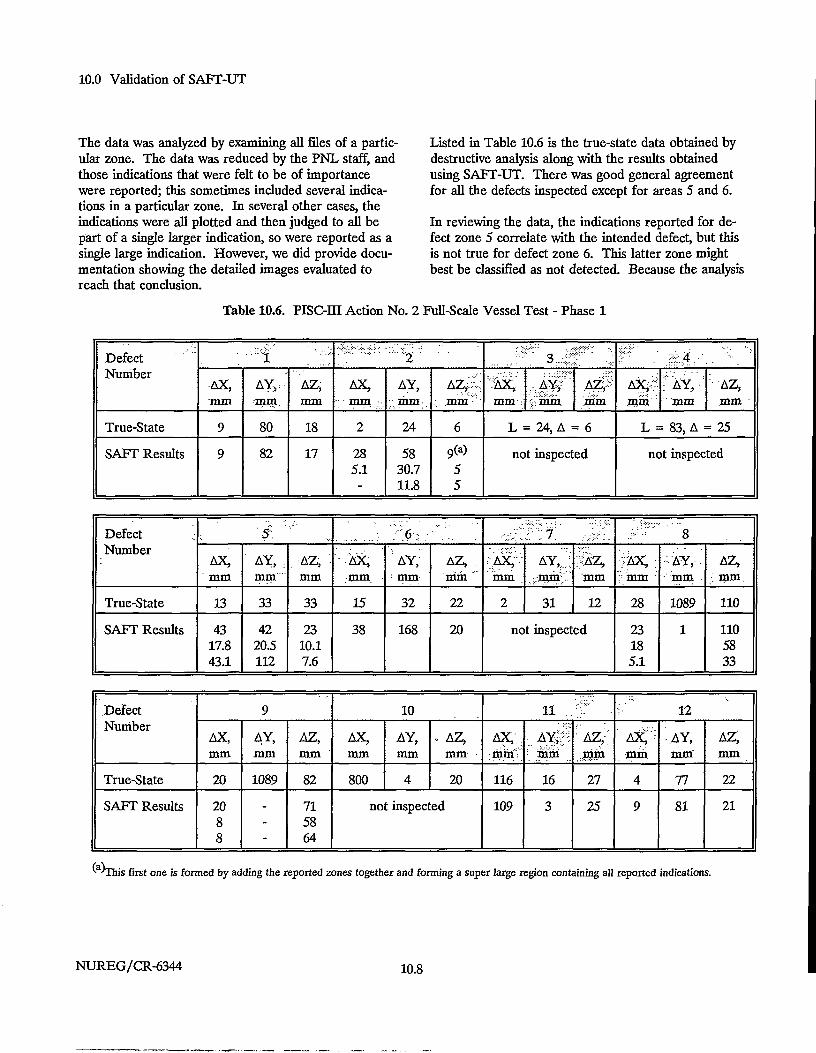
10.0 Validation of SAFT-UT
The data was analyzed by examining all files of a partic-ular zone. The data was reduced by the PNL staff, andthose indications that were felt to be of importancewere reported; this sometimes included several indica-tions in a particular zone. In several other cases, theindications were all plotted and then judged to all bepart of a single larger indication, so were reported as asingle large indication. However, we did provide docu-mentation showing the detailed images evaluated toreach that conclusion.
Listed in Table 10.6 is the true-state data obtained bydestructive analysis along with the results obtainedusing SAFT-UT. There was good general agreementfor all the defects inspected except for areas 5 and 6.
In reviewing the data, the indications reported for de-fect zone 5 correlate with the intended defect, but thisis not true for defect zone 6. This latter zone mightbest be classified as not detected. Because the analysis
Table 10.6. PISC-HI Action No. 2 Full-Scale Vessel Test - Phase 1
DefectNumber
True-State
SAFT Results
AX,mm
9
9
mm.
80
82
AZ,mm
18
17
AX,• m m . •
2
285.1
' "2 '
AY,mm
24
5830.711.8
.-.. mm '•"
6
9(a)55
3
lAX,mm •:
AY,mm
AZ;-Mm
L = 24, A = 6
not inspected
ffim :
fAY,- :
mm
L = 83, A =
: AZ,mm
= 25
not inspected
DefectNumber
True-State
SAFT Results
'5;:. ""'
AX,mm
13
4317.843.1
AY, :mm :
33
4220.5112
. AZ, :mm
33
2310.17.6
.,r.^ . . . . . .
• AX,
mm
15
38
' AY,:: mm
32
168
AZ, .mm
22
20
mm
2
AY, :-mm...
31
;Sz,mm
12
not inspected
>=•?'' ' "8
:: mm
28
23185.1
:.AY,'mm
1089
1
AZ,: mm
110
1105833
DefectNumber
True-State
SAFT Results
9
AX,mm
20
2088
AY,mm
1089
-
AZ,mm
82
715864
AX,mm
800
AY,mm
4
. AZ,mm
20
not inspected
11 ,/f" .
: m m V:
116
109
• A Y J: mm
16
3
: AZ,:;min
27
25
f 12
mm
4
9
.AY,mm
77
81
AZ,mm
22
21
^ -TTiis first one is formed by adding the reported zones together and forming a super large region containing all reported indications.
NUREG/CR-6344 10.8
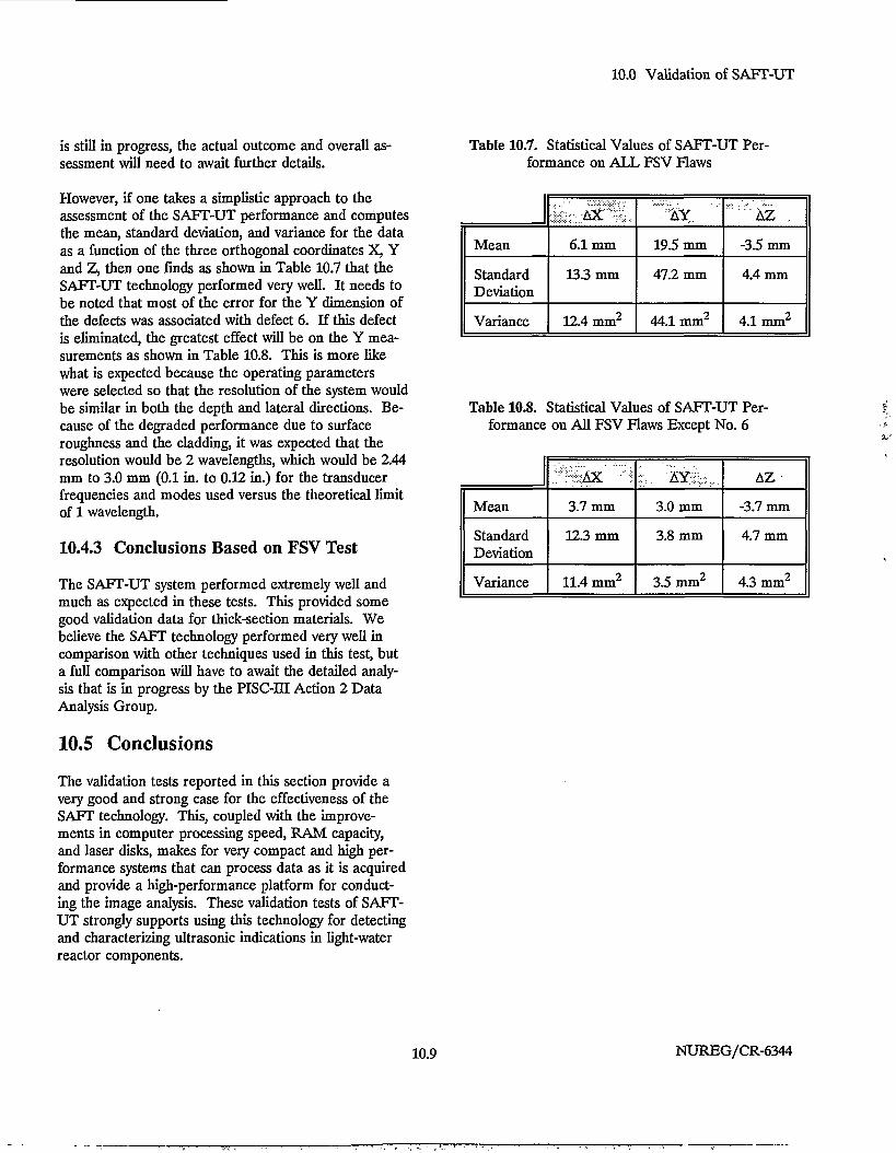
10.0 Validation of SAFT-UT
is still in progress, the actual outcome and overall as-sessment will need to await further details.
However, if one takes a simplistic approach to theassessment of the SAFT-UT performance and computesthe mean, standard deviation, and variance for the dataas a function of the three orthogonal coordinates X, Yand Z, then one finds as shown in Table 10.7 that theSAFT-UT technology performed very well. It needs tobe noted that most of the error for tie Y dimension ofthe defects was associated with defect 6. If this defectis eliminated, the greatest effect will be on the Y mea-surements as shown in Table 10.8. This is more likewhat is expected because the operating parameterswere selected so that the resolution of the system wouldbe similar in both the depth and lateral directions. Be-cause of the degraded performance due to surfaceroughness and the cladding, it was expected that theresolution would be 2 wavelengths, which would be 2.44mm to 3.0 mm (0.1 in. to 0.12 in.) for the transducerfrequencies and modes used versus the theoretical limitof 1 wavelength.
10.4.3 Conclusions Based on FSV Test
The SAFT-UT system performed extremely well andmuch as expected in these tests. This provided somegood validation data for thick-section materials. Webelieve the SAFT technology performed very well incomparison with other techniques used in this test, buta full comparison will have to await the detailed analy-sis that is in progress by the PISC-III Action 2 DataAnalysis Group.
10.5 Conclusions
The validation tests reported in this section provide avery good and strong case for the effectiveness of theSAFT technology. This, coupled with the improve-ments in computer processing speed, RAM capacity,and laser disks, makes for very compact and high per-formance systems that can process data as it is acquiredand provide a high-performance platform for conduct-ing the image analysis. These validation tests of SAFT-UT strongly supports using this technology for detectingand characterizing ultrasonic indications in light-waterreactor components.
Table 10.7. Statistical Values of SAFT-UT Per-formance on ALL FSV Flaws
Mean
StandardDeviation
Variance
6.1 mm
13.3 mm
12.4 mm2
' ::AY
19.5 mm
47.2 mm
44.1 mm2
: : : : f AZ .
-3.5 mm
4.4 mm
4.1 mm
Table 10.8. Statistical Values of SAFT-UT Per-formance on All FSV Flaws Except No. 6
Mean
StandardDeviation
Variance
AX
3.7 mm
12.3 mm
11.4 mm2
AYlb..
3.0 mm
3.8 mm
3.5 mm2
AZ
-3.7 mm
4.7 mm
4.3 mm2
10.9 NUREG/CR-6344
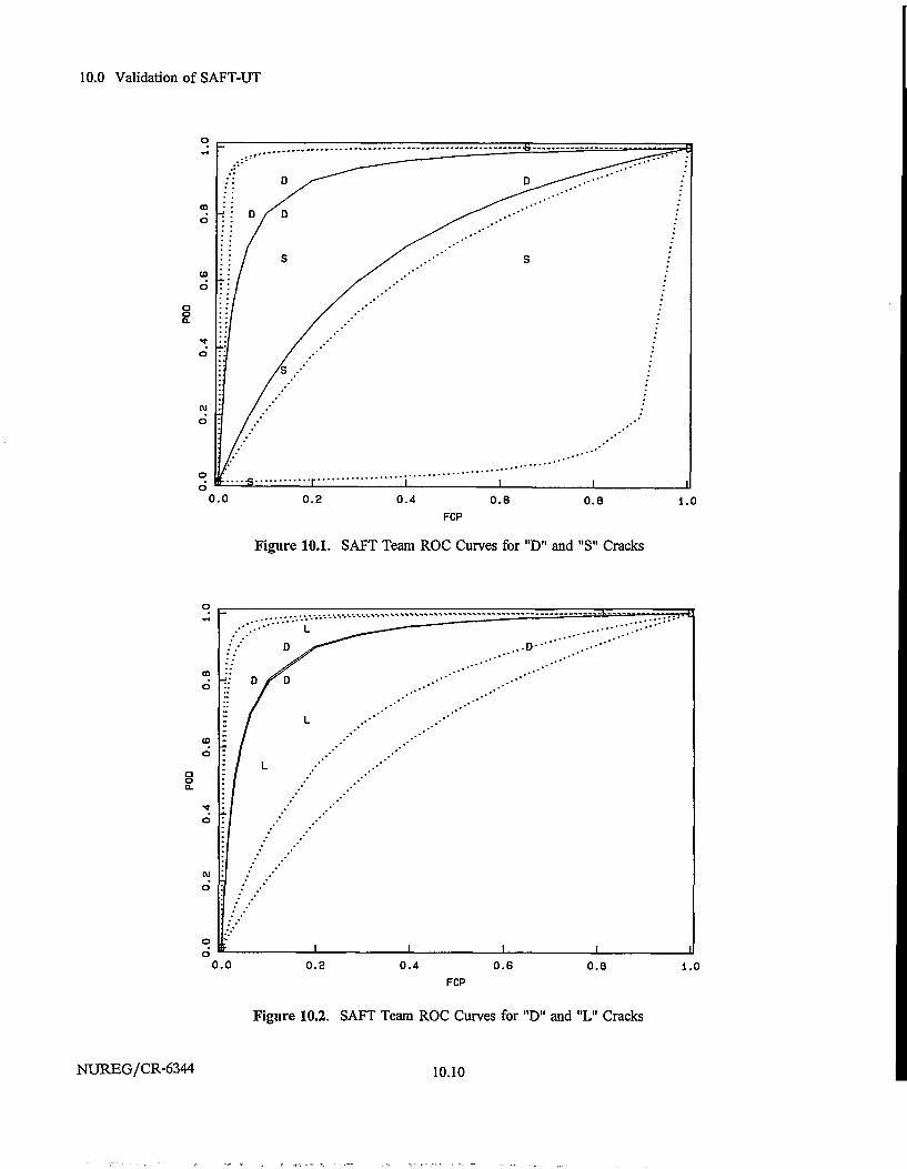
10.0 Validation of SAFT-UT
o.o 1.0
Figure 10.1. SAFT Team ROC Curves for "D" and "S" Cracks
o.o 1.0
Figure 10.2. SAFT Team ROC Curves for "D" and "L" Cracks
NUREG/CR-6344 10.10
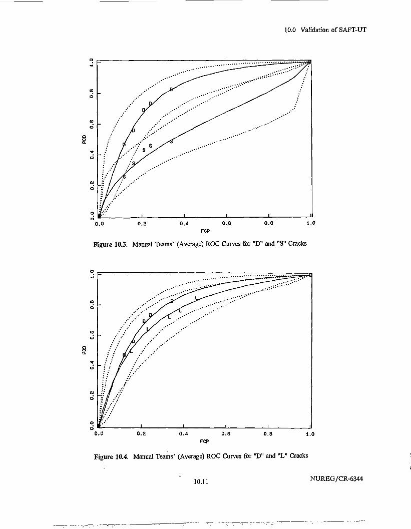
10.0 Validation of SAFT-UT
o.o
Figure 10.3. Manual Teams' (Average) ROC Curves for "D" and "S" Cracks
o.o
Figure 10.4. Manual Teams' (Average) ROC Curves for "D" and "L" Cracks
10.11 NUREG/CR-6344
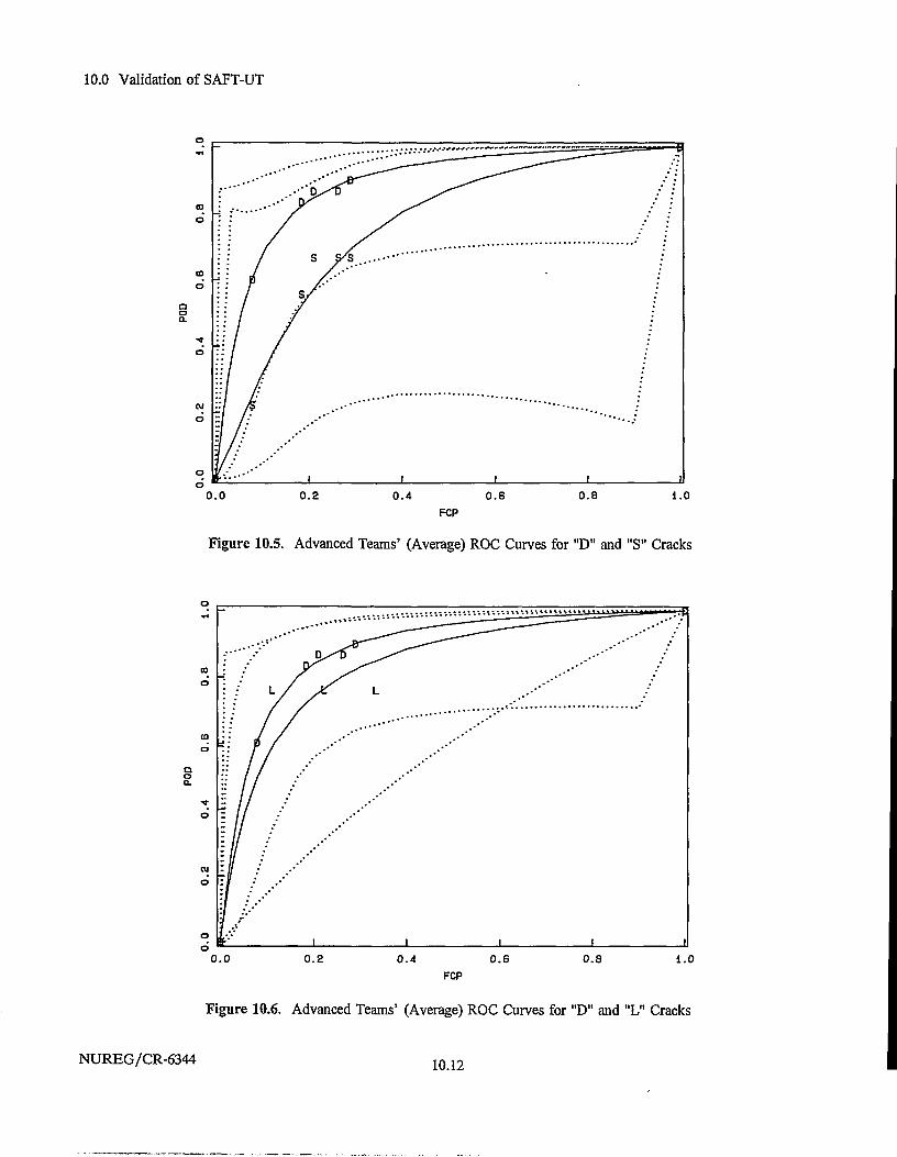
10.0 Validation of SAFT-UT
0.0 1.0
Figure 10.5. Advanced Teams' (Average) ROC Curves for "D" and "S" Cracks
0.0 1.0
Figure 10.6. Advanced Teams' (Average) ROC Curves for "D" and "L" Cracks
NUREG/CR-6344 10.12
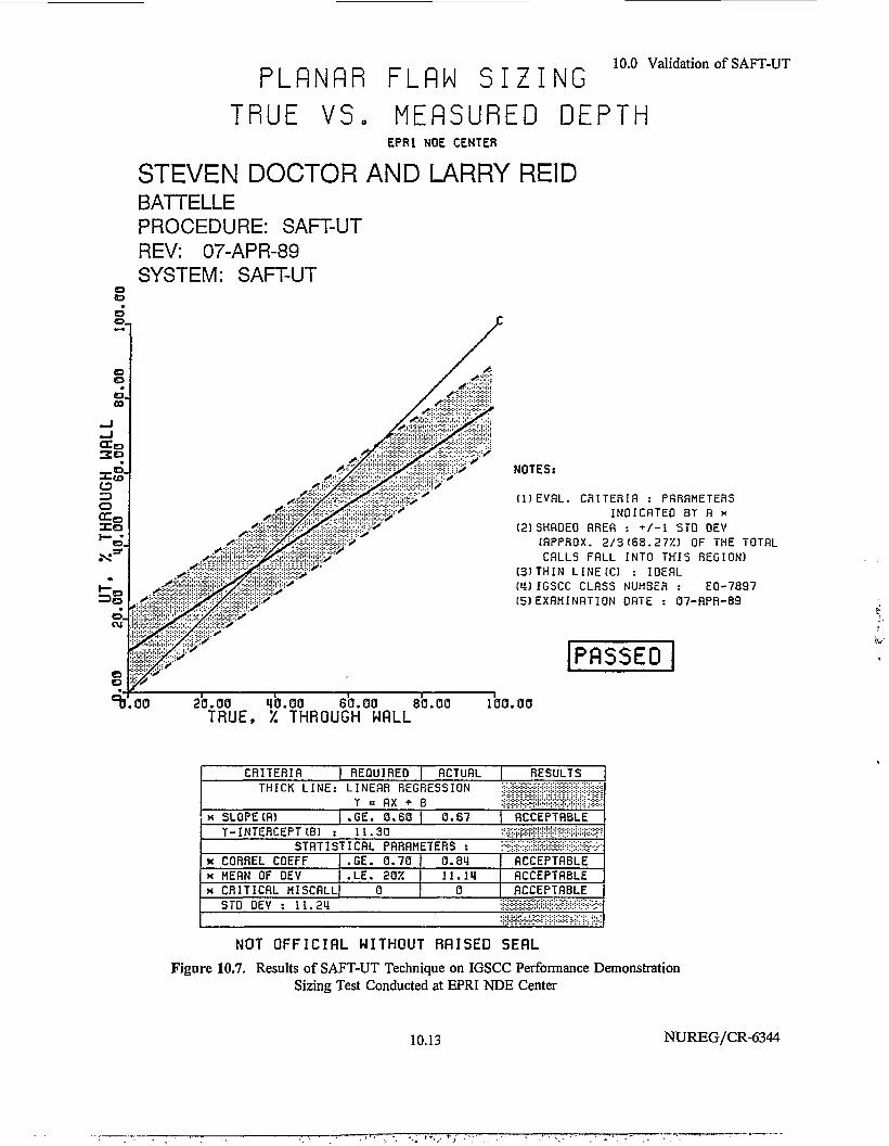
PLflNflR FLflN S IZ INGTRUE VS, MERSURED DEPTH
EPRI NDE CENTER
STEVEN DOCTOR AND LARRY REIDBATTELLEPROCEDURE: SAFT-UTREV: 07-APR-89SYSTEM: SAFT-UT
10.0 Validation of SAFT-UT
NOTES:
UJEVRL. CRITERIA : PRRRMETERSINDICflTED BT fl *
(2)SHRDED RRER : +/-1 STO OEV(FIPPROX. 2/3 168.27Z) OF THE TOTRLCRLLS FRLL INTO TKIS REGION)
(3) THIN LINE(C) : IOEflL(4)IGSCC CLflSS NUMBER : EO-7897C5)EXRMINRTI0N ORTE : 67-flPR-89
PASSED
00 20.00 40.00 80.00 80.00 100.00
TRUE, V. THROUGH WALL
CRITERIf)THICK LINE:
K SLOPECfl)Y-INTERCEPT(B) :
REQUIREO | RCTUflLLINERR REGRESSIONT = RX + B.GE. 0.60 | 0.6711.30
RESULTS
•
flCCEPTflBLE
STflTISTICflL PflRflMETERS :»t CORREL COEFFx HERN OF DEVx CRIT1CRL MISCRLL
STO OEV : 11.24
.GE. 0.70
.LE. 20/C
0
0.8411.14
0
flCCEPTRBLEflCCEPTflBLEflCCEPTflBLE
:*:':':':":':":":':':':"-":":":":':':":":"'"r':
NOT OFFICIflL WITHOUT RfllSED SEflLFigure 10.7. Results of SAFT-UT Technique on IGSCC Performance Demonstration
Sizing Test Conducted at EPRI NDE Center
10.13 NUREG/CR-6344
11.0 Conclusions
The SAFT technology has evolved into a practical anduseful tool for performing inservice inspections on lightwater reactor components. The SAFT algorithm hasbeen accelerated to process inspection data at the samerate at which the data is collected. The SAFT imagesare displayed in the true perspective that exists relativeto the inspected part and with uniform dimensions, thusmaking the images easy to interpret. Extensive labora-tory testing has shown the viability of the technology.Field trials have shown that SAFT can be applied in theadverse environment of light water reactors and thatthe resulting images are easy to interpret. A procedurebased on the SAFT-UT real-time field system has beenwritten for the SAFT technology.
Over the past 20 years, work has continued to improveSAFT-UT inspection systems for the field and thelaboratory. The following list summarizes the highlightsof work performed:
• Software from the University of Michigan wasmodified to reduce processing times.
• Software was developed to run on the host VAXthat would communicate with the data acquisitionsystem, graphics processor, and real-time proces-sor.
• The focusing properties of SAFT-UT were numer-ically analyzed. The point spread function ofSAFT was studied as a function of aperture size,pulse attenuation, pulse bandwidth, and horizontalsample intervals.
• Advanced data presentation techniques were ana-lyzed. Perspective contour plotting, grey scale,color plotting, and interactive displays were con-sidered. Finally, a RAMTEK high-resolutiongraphics imaging system was purchased and agraphics/analysis utility was written.
• Processing needs associated with performing real-time SAFT-UT were analyzed. Commerciallyavailable computer systems and array processorswere analyzed and found to be either inadequateor too expensive for performing real-time SAFT-UT. The concept of a special-purpose, hardwareimplementation, SAFT processor was proposedand developed. However, this also was inade-quate (variations of the SAFT algorithm could not
be easily implemented) and a second real-timeprocessor was developed using a parallel proces-sor architecture. This second real-time processorutilized commercially available hardware, and thesoftware could be easily modified to accommodatemodified SAFT algorithms.
Special-purpose scanning head hardware has beendeveloped. Such hardware allows for high-speedscanning of arbitrary surfaces and constant offsetof transducers. The scanning hardware was fur-ther modified to accommodate multiple transduc-er configurations such as TSAFT-2 and TSAFT-3.
Tandem SAFT configurations were developed toovercome the ambiguities inherent in pulse-echo,single-transducer configurations. Further, a spe-cial tandem configuration (TSAFT-3) was devel-oped for thick-section materials such as reactorpressure vessels.
Parametric studies were performed to study theeffects of errors in parameters used during SAFTprocessing. Included in these studies were effectsfrom assumptions made within the SAFT algo-rithm itself.
A SAFT-UT field data collection system was de-veloped and employed in the field during inserviceinspections of operating reactors (Dresden andVermont Yankee). Further, SAFT data was ac-quired using two different commercial dataacquisition systems and subsequently processedand analyzed to characterize real defects in areactor pressure vessel (Indian Point Unit II) anda static-cast stainless steel elbow in the hot-leg ofa reactor (Trojan Nuclear Power Plant).
Advanced preprocessing techniques were devel-oped for anisotropic materials such as centrifugal-ly cast stainless steels. Utilities were written todetermine the spectrum characteristics of defectsand nondefects in anisotropic materials. A filterutility could subsequently be used on raw data,prior to SAFT processing, to enhance defect re-sponses and diminish nondefect responses. Atime-derivative utility was developed to improvethe signal-to-noise ratio of wide-band data files.
11.1 NUREG/CR-6344
11.0 Conclusions
Installation of the SAFT utilities on a VAX11/750 owned by Combustion Engineering consti-tuted the first step in examining how to transferthe SAFT technology. Also, a real-time processorwas fabricated for use by Sandia National Labo-ratories, and the SAFT utilities were installed ona Micro VAX computer, which was designated asthe host computer in the Sandia SAFT-UT sys-tem.
The SAFT technology has been formally integrat-ed into ASME Code Section V, Article 4, Appen-dix E, which addresses computerized UT imagingsystems. This article contains general require-ments plus specific requirements covering calibra-tion, SAFT-UT, L-SAFT, broadband holography,and UT-phased arrays.
Because of the new computer products that havebecome available during the time that the SAFT-UT system was under development, we have seensignificant improvement in the system. Tremen-dous amounts of data generated by SAFT-UTinspections need efficient handling and effectivestorage. Particularly for the inspection of pres-sure vessels, SAFT-UT effectively uses advancingcomputer technology.
• The validation testing provides a very good andstrong case for the effectiveness of the SAFTtechnology. This, coupled with the improvementsin computer processing speed, RAM, capacity,and laser disks, makes for very compact and high-performance systems that can process data as it isacquired and provide a high-performance platformfor conducting the image analysis. This workprovides a powerful case for use of this technologyfor detecting and characterizing ultrasonic indica-tions in light water reactor components.
• Development, training, and delivery of a compactSAFT-UT field system based on the latest com-puter advances has been achieved through thesystem now used by the NRC NDE Mobile Labo-ratory staff.
To summarize, much developmental research work hasbeen performed over the past 20 years to develop andimplement SAFT-UT. Many of the basic questions re-garding the ultimate resolution and computational com-plexity associated with performing SAFT-UT have beenanswered. The SAFT program has resulted in a real-time SAFT-UT field system and hand-in-hand workwith commercial companies performing special inserviceinspections of operating reactors. Transfer of theSAFT technology to the nuclear industry has been agoal of the program, and PNL is continuing to worktoward achieving that goal.
NUREG/CR-6344 11.2
12.0 References
Bates, D. J., S. R. Doctor, and P. G. Heasler. 1987.Stainless Steel Round Robin Test Centrifugally CastStainless Steel Screening Phase, NUREG/CR-4970, U.S.Nuclear Regulatory Commission, Washington, D.C.
Bracewell, R. 1965 The Fourier Transform and ItsApplications. McGraw-Hill, NY.
Burckhardt, C. B., P. A. Grandchamp, and H. Hoff-mann. 1974. "Methods for Increasing the LateralResolution of B-Scan," in Acoustical Imaging, Vol. 5, ed.P. S. Green. Plenum Press, New York, NY.
Busse, L. J., H. D. Collins, and S. R. Doctor. 1984.Review and Discussion of the Development of SyntheticAperture Focusing Technique for Ultrasonic Testing(SAFT-UT), NUREG/CR-3625. U.S. Nuclear Regula-tory Commission, Washington, D.C.
Collins, H. D. and Gribble, R. P. 1986. Siamese Imag-ing Technique for Quasi-Vertical Type (QVT) Defects inNuclear Reactor Piping. NUREG/CR-4472. U.S. Nu-clear Regulatory Commission, Washington, D.C.
Doctor, S. R., L. J. Busse, S. L. Crawford, T. E. Hall,R. P. Gribble, A. J. Baldwin, and L. P. Van Houten.1986. Development and Validation of a Real-TimeSAFT-UT System for the Inspection of Light Water Reac-tor Components, Semi-annual Report, April 1984 toSeptember 1984, NUREG/CR-4583, Vol. 1. U.S. Nu-clear Regulatory Commission, Washington, D.C.
Doctor, S. R., T. E. Hall, L. D. Reid, S. L. Crawford,R. J. Littlefield, and R. W. Gilbert. 1987a. Develop-ment and Validation of a Real-Time SAFT-UT Systemfor the Inspection of Light Water Reactor Components,Annual Report, October 1984 to September 1985,NUREG/CR-4583, Vol. 2. U.S. Nuclear RegulatoryCommission, Washington, D.C.
Doctor, S. R., T. E. Hall, L. D. Reid, and G. A. Mart.1987b. Development and Validation of a Real-TimeSAFT-UT System for the Inspection of Light Water Reac-tor Components, Annual Report, October 1985 to Sep-tember 1986, NUREG/CR-4583, Vol. 3. U.S. NuclearRegulatory Commission, Washington, D.C.
Frederick, J. R., C. VandenBroek, S. Ganapathy, M.Elzinga, W. DeVries, D. Papworth, and N. Hamano.1979. Improved Ultrasonic Nondestructive Testing of
Pressure Vessels, NUREG/CR-0909. U.S. NuclearRegulatory Commission, Washington, D.C.
Frederick, J. R., R. C. Fairchild, and B. H. Anderson.1977. Improved Ultrasonic Nondestructive Testing ofPressure Vessels, NUREG-0007-2. U.S. Nuclear Regu-latory Commission, Washington, D.C.
Frederick, J. R., C. VandenBroek, R. C. Fairchild, andM. B. Elzinga. 1978. Improved Ultrasonic Nondestruc-tive Testing of Pressure Vessels, NUREG/CR-0135.U.S. Nuclear Regulatory Commission, Washington,D.C.
Frederick, J. R., C. VandenBroek, M. Elzinga, M.Dixon, D. Papworth, N. Hamano, and K. Ganapathy.1979. Improved Ultrasonic Nondestructive Testing ofPressure Vessels, NUREG/CR-0581. U.S. NuclearRegulatory Commission, Washington, D.C.
Frederick, J. R. Seydel, and R. C. Fairchild. 1976.Improved Ultrasonic Non-Destructive Testing of PressureVessels, NUREG-0007-1. U.S. Nuclear RegulatoryCommission, Washington, D.C.
Ganapathy, S., W. S. Wu, and B. Schmult. 1982."Analysis and Design Considerations for a Real-TimeSystem for Nondestructive Evaluation in the NuclearIndustry." Ultrasonics 20:249.
Ganapathy, S., B. Schmult, W. S. Wu, T. G. Dennehy,N. Moayeri, and P. Kelly. 1985. Design and Develop-ment of a Special Purpose SAFT System for Nondestruc-tive Evaluation of Nuclear Reactor Vessels and PipingComponents, NUREG/CR-4365. U.S. Nuclear Regula-tory Commission, Washington, D.C.
Ganapathy, S. N. Hamano, M. R. Bether, W. S. Wu, T.G. Dennehy, C. Purnaveja, M. M. Murray, M. B.Elzinga, and F. Raam. 1981. Ultrasonic Imaging Tech-niques for Real-time In-service Inspection of NuclearPower Reactors, NUREG/CR-2154. U.S. Nuclear Reg-ulatory Commission, Washington, D.C.
Ganapathy, S. and B. Schmult. 1982. "Design of aReal-time Inspection System for NDE of Reactor Ves-sels and Piping Components." Presented at IMECH EConference, London, England. I MECH E 1982-9.
12.1 NUREG/CR-6344
12.0 References
Ganapathy, S., B. Schmult, W. S. Wu, N. Hamano, andD. Bristor. 1983. Investigation of Special Purpose Pro-cessors for Real-Time Synthetic Aperture Focusing Tech-niques for Nondestructive Evaluation of Nuclear ReactorVessels and Piping Components, NUREG/CR-2703.U.S. Nuclear Regulatory Commission, Washington,D.C.
Hall, T. E., L. D. Reid, and S. R. Doctor. 1988. TheSAFT-UT Real-Time Inspection System-OperationalPrinciples and Implementation. NUREG/CR-5075.U.S. Nuclear Regulatory Commission, Washington,D.C.
Hamano, N. 1980. "Deconvolution of Ultrasonic Non-destructive Testing Data." PhD Dissertation, ElectricalEngineering Dept., University of Missouri, Columbia,Missouri.
Hamlin, D. R. 1985. Program for Field Validation ofthe Synthetic Aperture Focusing Technique for UltrasonicTesting (SAFT-UT), NUREG/CR-4078. U.S. NuclearRegulatory Commission, Washington, D.C.
Heasler, P. G., T. T. Taylor, J. C. Spanner, S. R. Doc-tor, and J. D. Deffenbaugh. 1990. Ultrasonic InspectionReliability for Intergranular Stress Corrosion Cracks -ARound Robin Study of the Effects of Personnel, Proce-dures, Equipment and Crack Characteristics, NUREG/CR-4908. U.S. Nuclear Regulatory Commission, Wash-ington, D.C.
Hildebrand, B. P. 1986. Investigation of AdvancedAcoustic and Optical Nondestructive Evaluation Tech-niques. Final Report NP-4897 for Research Project606-7. Sigma Research, Inc., Redmond, Washington,pp. 3-44 to 3-51.
Jackson, J. L. 1978a. Program for Field Validation ofthe Synthetic Aperture Focusing Technique for UltrasonicTesting (SAFT-UT) - Analysis Before Test, NU-REG/CR-0288. U.S. Nuclear Regulatory Commission,Washington, D.C.
Jackson, J. L. 1978b. Program for Field Validation ofthe Synthetic Aperture Focusing Technique for UltrasonicTesting (SAFT-UT) Midyear Progress Report. NUREG/CR-0290. U.S. Nuclear Regulatory Commission, Wash-ington, D.C.
Jackson, J. L. 1981. Program for Field Validation of theSynthetic Aperture Focusing Technique for UltrasonicTesting (SAFT-UT), NUREG/CR-1885, Vols. 1, 2, and3. U.S. Nuclear Regulatory Commission, Washington,D.C.
Johnson, S. A., J. F. Greenleaf, F. A. Duck, A. Chu, W.R. Samayou, and B. K. Gilbert. 1975. "Digital Com-puter Simulation Study of a Real-Time Collection, Post-Processing Synthetic Focusing Ultrasound CardiacCamera," in. Acoustical Holography, Vol. 6, ed. NewellBooth. Plenum Press, New York, NY.
Norton, S. J. 1976. Theory of Acoustic Imaging, Tech-nical Report No. 4956-2. Stanford University, Stanford,California.
Polky, J. N. 1986. Development of a Real-Time Num-ber Processor for SAFT Inspection, NUREG/CR-4634.U.S. Nuclear Regulatory Commission, Washington,D.C.
Polky, J. N. and D. D. Miller. 1985. An Ultra-HighSpeed Residue Processor for SAFT Image Enhancement,NUREG/CR-4170. U.S. Nuclear Regulatory Commis-sion, Washington, D.C.
Prine, D. W. 1972. "Synthetic Aperture UltrasonicImaging," in Proceedings of the Engineering Applicationsof Holography Symposium:287. Society of Photo-opticalInstrumentation Engineers.
Seydel, J. A. 1978. (Signal Processing) Methods Devel-opment, ed. J. R. Frederick, NUREG/CR-0135. U.S.Nuclear Regulatory Commission, Washington, D.C.
Thome, David K 1985. "Ultrasonic Image Analysis."in Proceedings for The World Conference on Nondestruc-tive Testing, Vol. 2. American Society for Nondestruc-tive Testing, Columbus, OH.
NUREG/CR-6344 12.2
Appendix A
Detailed Hardware Description of theSAFT-UT Field Inspection System
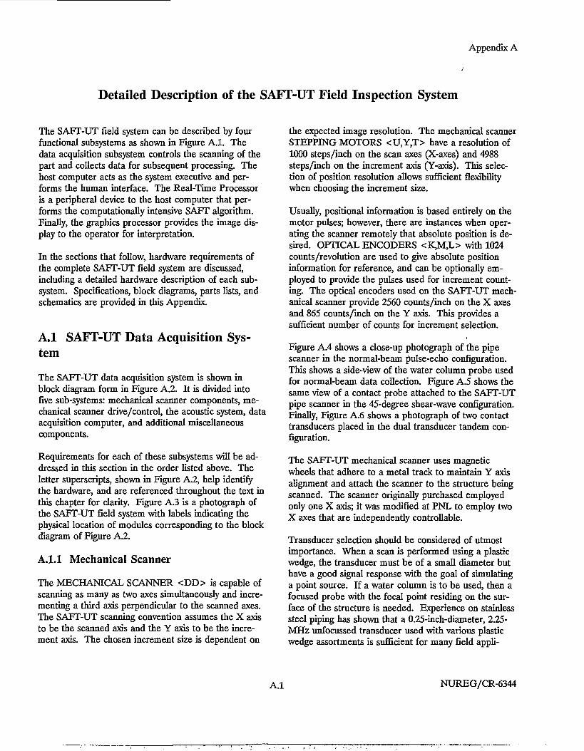
Appendix A
Detailed Description of the SAFT-UT Field Inspection System
The SAFT-UT field system can be described by fourfunctional subsystems as shown in Figure A.l. Thedata acquisition subsystem controls the scanning of thepart and collects data for subsequent processing. Thehost computer acts as the system executive and per-forms the human interface. The Real-Time Processoris a peripheral device to the host computer that per-forms the computationally intensive SAFT algorithm.Finally, the graphics processor provides the image dis-play to the operator for interpretation.
In the sections that follow, hardware requirements ofthe complete SAFT-UT field system are discussed,including a detailed hardware description of each sub-system. Specifications, block diagrams, parts lists, andschematics are provided in this Appendix.
A.1 SAFT-UT Data Acquisition Sys-tem
The SAFT-UT data acquisition system is shown inblock diagram form in Figure A.2. It is divided intofive sub-systems: mechanical scanner components, me-chanical scanner drive/control, the acoustic system, dataacquisition computer, and additional miscellaneouscomponents.
Requirements for each of these subsystems will be ad-dressed in this section in the order listed above. Theletter superscripts, shown in Figure A.2, help identifythe hardware, and are referenced throughout the text inthis chapter for clarity. Figure A.3 is a photograph ofthe SAFT-UT field system with labels indicating thephysical location of modules corresponding to the blockdiagram of Figure A.2.
A.1.1 Mechanical Scanner
The MECHANICAL SCANNER <DD> is capable ofscanning as many as two axes simultaneously and incre-menting a third axis perpendicular to the scanned axes.The SAFT-UT scanning convention assumes the X axisto be the scanned axis and the Y axis to be the incre-ment axis. The chosen increment size is dependent on
the expected image resolution. The mechanical scannerSTEPPING MOTORS <U,Y,T> have a resolution of1000 steps/inch on the scan axes (X-axes) and 4988steps/inch on the increment axis (Y-axis). This selec-tion of position resolution allows sufficient flexibilitywhen choosing the increment size.
Usually, positional information is based entirely on themotor pulses; however, there are instances when oper-ating the scanner remotely that absolute position is de-sired. OPTICAL ENCODERS <K,M,L> with 1024counts/revolution are used to give absolute positioninformation for reference, and can be optionally em-ployed to provide the pulses used for increment count-ing. The optical encoders used on the SAFT-UT mech-anical scanner provide 2560 counts/inch on the X axesand 865 counts/inch on the Y axis. This provides asufficient number of counts for increment selection.
Figure A.4 shows a close-up photograph of the pipescanner in the normal-beam pulse-echo configuration.This shows a side-view of the water column probe usedfor normal-beam data collection. Figure A.5 shows thesame view of a contact probe attached to the SAFT-UTpipe scanner hi the 45-degree shear-wave configuration.Finally, Figure A.6 shows a photograph of two contacttransducers placed hi the dual transducer tandem con-figuration.
The SAFT-UT mechanical scanner uses magneticwheels that adhere to a metal track to maintain Y axisalignment and attach the scanner to the structure beingscanned. The scanner originally purchased employedonly one X axis; it was modified at PNL to employ twoX axes that are independently controllable.
Transducer selection should be considered of utmostimportance. When a scan is performed using a plasticwedge, the transducer must be of a small diameter buthave a good signal response with the goal of simulatinga point source. If a water column is to be used, then afocused probe with the focal point residing on the sur-face of the structure is needed. Experience on stainlesssteel piping has shown that a 0.25-inch-diameter, 2.25-MHz unfocussed transducer used with various plasticwedge assortments is sufficient for many field appli-
A.1 NUREG/CR-6344
Appendix A
cations. A water column is normally used for far-sur-face profiling only. A 5-MHz, 3-inch focal length, and0.75-inch-diameter transducer has been used for far-surface profiling using a water column coupling device.
A number of considerations effected the design of theSAFT-UT pipe scanner. These are itemized as follows:
• It was designed to provide the capability for at-taching either a plastic wedge or water columncoupling device to the probes involved.
• Two independently controlled scan axes wereimplemented to accommodate theTSAFT/TSAFT-2 configurations. Also for theseconfigurations the source transducer was aligneddirectly behind the receive transducer.
• Sufficient tension was required to maintain cou-pling throughout the scan, overhead or under-neath an object such as a pipe.
• When using water columns for normal-beam orangle-beam data collection, the mechanical attach-ment was designed to be rigid enough to ensureaccurate tracking and maintaining the incident an-gles.
• The mechanical attachment was designed to allowthe transducer to be rotated 180-degrees for look-ing back towards the scanner with the transducer;i.e., reaching across a weld when it is not conve-nient to mount the scanner on the far side.
• To fully benefit from the ability to straddle aweld, it was necessary to be able to remotelyselect either transducer to be a source, receiver,or to operate in the pulse-echo or tandem mode.
• Strain reliefs were used on the cables to preventcable fatigue and to keep the cables out of thepathway of the scanner. Motor and encoder sig-nals utilized shielded pair cabling to ensure elec-trical isolation and a separate 75-ohm coaxialcable were used for preamplifier signals.
• Decontamination was considered since the scan-ner was to be used in a contaminated area duringinservice inspections. The scanner assembly was
designed to be easy to replace, low cost, and sim-ple to disassemble.
• Provision for mounting a remote pulser/preampon the mechanical scanner was needed. Themounting of the pulser/preamp was studied atlength so that the overall size of the scanner wasnot compromised and interference with the trans-ducer movement was minimized.
A.1.2 Scanner Drive/Control
Processing data using the SAFT algorithm requires reli-able positional information and the ability to accuratelyread the position of the mechanical scanner duringoperation. The stepper motor and driver combinationwas designed to provide sufficient torque to drive theloads that are be encountered, such as the transducerswhen they are used in conjunction with a water columnor when scanning curved surfaces such as horizontalpiping. The Y axis stepper motor and driver providesenough torque to transport the scanner mechanism on avertical surface. The mechanical scanner gear ratio,stepper motor, and driver combination used in theSAFT-UT field system provide adequate torque (53-oz.-in.) up to 2 inches per second, which is a sufficientscanning speed for the field application work that hasbeen performed.
Control of the mechanical scanner is accomplished bythe Data Acquisition System computer interfacing witha stepper motor controller. The STEPPER MOTORCONTROLLER <P,Q,R> has the following specifi-cations:
• The number of steps is defined by a number with23-bit resolution and an additional sign bit for di-rection.
• Adjustable linear acceleration and deceleration.
• Remote operating mode for connection to a joy-stick.
• Ability to stop and start a motor during a cyclewithout losing position information.
• Programmable control of speed and acceleration.
NUREG/CR-6344 A.2
Appendix A
• Half-step mode for improved torque and resolu-tion.
• Motor pulse and direction outputs.
The motor or encoder pulses are counted as the motoris in motion; when the increment size is reached, data isthen collected. Therefore, hardware is needed to countthe motor pulses or the optionally selectable encoderpulses. Two counters are used in the SAFT-UT system.The first counter, referred to as the PROGRAMMA-BLE DIVIDER <N>, shown in detail in Figure A.7,was designed and assembled at PNL on a CAMACprototype card and placed into the system. The counteris loaded with the desired increment count. When thecounter overflows, a sync pulse is generated that beginsthe data acquisition cycle. The counter is then reloadedto count the next scan increment. The counter has thefollowing specifications:
• 12-bit presettable up/down counter.
• Hardware selectable to use either the encoder ormotor pulses as the input.
• Software selectable to use the XI, X2, or the Yaxes as the input, latch and load a new incrementcount, set the pulser drive module to remote, andclear the counter.
The second counter is a four-channel UP/DOWN<O> CAMAC module, and is used to continuallycount the encoder pulses to provide the system with-absolute position information. This counter has the fol-lowing specifications:
• Four presettable 16-bit up/down counters.
• Separate up/down inputs.
• Counting rates from dc to 20 MHz.
• Capacity of 65,535 counts per channel.
• Overflow and underflow status bits for each chan-nel.
• Separate clear command for each channel.
A.1.3 Acoustic System
The Acoustic System is a critical component of theSAFT-UT field system. The quality of the data collect-ed is dependent on the quality of the hardware selected.The SAFT-UT field system incorporates a PNL-builtSQUARE WAVE PULSER <B>, which is detailed ina block diagram in Figure A.8, and a commerciallyavailable PREAMPLIFIER <B>, into one packagecalled the remote pulser/preamplifier. This unitmounts directly on the mechanical scanner. The func-tion of the remote pulser/preamplifier is to reduce thesignal degradation inherent in having 200 feet of cablelinking the mechanical scanner and transducers to theData Acquisition System main frame. The specifica-tions of the remote pulser /preamplifier are:
• TTL trigger input.
• Output pulse width controllable by trigger inputpulse width.
• Separate high voltage input.
• Two transducer hookups, each remotely selectableto be a source or receiver when operated in thetandem mode, or a pulser and receiver whenoperated in the pulse-echo mode.
• An output pulse amplitude is provided of up to350 volts with the duration of the pulse adjustablefrom 0.10 to 1.0 microseconds.
• Pulser output impedance is on the order of 2 to 4ohms.
• RF output drives 200 feet of 75-ohm coaxial cablewith no more than a -6 dB loss.
• Preamplifier input impedance is 500 ohms forsignal voltages less than the clamp voltage, andnot less than 100 ohms for signal voltages greaterthan the clamp voltage.
• The clamp circuit protects the preamplifier from apositive or negative 350-volt pulse of 1 microsec-ond duration.
A.3 NUREG/CR-6344
Appendix A
• Gain of the preamplifier is 20 dB when loadedinto 50 ohms.
-3 dB bandwidth is at least 0.5 to 7.5 MHz.
At times it is desirable to switch the identity of thetransducers that are attached to the remote mechanicalscanner. When collecting SAFT-UT data, this featureis desirable because of the tandem and pulse-echomodes that are used. One would like to be able toswitch between the two modes without having to physi-cally switch the cables, especially if one has to enter aradiation zone to do the switching. The MODE SE-LECT <A> module, as detailed in the block diagramin Figure A.9, was developed at PNL to accomplish theswitching task and has the following specifications:
• Inhibits pulser high voltage when switching out-puts.
• Selects any one of four transducer configurations;pulse-echo mode-front or rear transducer; tan-dem mode-rear transducer as the source, fronttransducer as the receiver, or the front transduceras the source and the rear transducer as the re-ceiver.
The PULSER DRIVER <G> module, as shown inFigure A.10, was developed at PNL and provides thesystem sync pulse, remote pulser trigger, and the re-mote pulser high voltage. The pulser driver has thefollowing specifications:
• Adjustable sync delay to compensate for the elec-trical time delay experienced in the 200 feet ofcable to the remote pulser/preamplifier.
• High voltage power supply adjustable from 150 to350 volts.
• Remote pulser trigger output with continuouslyadjustable pulse widths of 0.1 microsecond to 1microsecond.
• Remote select input - The pulser driver can pro-vide internal timing or the timing can be providedby an external source. External timing is providedby the programmable divider module on the com-pletion of an increment count. Local timing is
adjustable from 0.5 kHz to 2 kHz and is selectedfrom the front panel.
• Pulser inhibit input - Useful when remotelyswitching transducer sources and is controlled bythe Mode Select module.
After the RF signal has passed through the preamplifi-er, and the 200 feet of cable, it is received and ampli-fied by the TIME VARIABLE GAIN AMPLIFIER<C> (TVG Amplifier) which has the following specifi-cations:
• Total gam of at least 60 dB.
• At least 40 dB of voltage controlled gain that canchange in 20 microseconds without changing theoutput more than 10% of full scale with the am-plifier input terminated into 500 ohms and noinput signal.
• The -3 dB bandwidth is 0.5 to 7.5 MHz.
• An output swing is 10 volts peak to peak into 50ohms.
• At least 48 dB of dynamic range at the output be-tween the noise floor and the saturated outputlevel.
• The output stage is the first stage to saturateunder any gain setting.
• Transmit overload recovery is 25 microseconds. Itis defined as the time required for the output tosettle to the noise level after the leading edge ofthe transmit pulse at any gain setting and anytransmit pulse width from 1 microsecond to 67nanoseconds. This should be measured with a 50-ohm resistor connected to the transducer connec-tor.
• The overload recovery time, from 100% signaloverload, is less than the time required for onehalf of a cycle of the input signal after the end ofthe input signal. It is defined as the time requiredfor the output to settle to the noise level after aninput signal twice the amplitude required to satu-rate the output. The input signal should be a
NUREG/CR-6344 A.4
Appendix A
bipolar, single-cycle sine wave of any frequencybetween 0.5 and 7.5 MHz.
A block diagram of the TVG RAMP GENERATOR<D> module shown in Figure A.ll. It is needed todevelop the ramps that control the gain of the TVGamplifier. The ramp generator used in the SAFT-UTfield system is a PNL-built unit and has the followingspecifications:
• Minimum ramp time of 8 microseconds.
• Ramp start adjustable from 0 to 200 microsec-onds.
• Three slope end point adjustments - each slopeend point is settable from 0 to 20 microseconds.
• Five gain adjustments - starting gain, slope 1 gain,slope 2 gain, slope 3 gain, and the final gain.
A dual-trace Tektronix oscilloscope is used as MONI-TOR #1 <E> to observe the RF signal out of theTVG amplifier and the TVG ramps out of the TVGramp generator. It is necessary to ensure that signalsof interest are not saturating when collecting data to beprocessed using either the pulse-echo or tandem SAFTalgorithm and set up of the TVG ramps is simplifiedwhen the RF signal and the TVG ramps can be viewedat the same time.
The RF waveform is digitized for processing by theSAFT algorithm and provides a data base that can beprocessed in real time or at a later date. The SAFTalgorithm requires four samples per cycle as a temporalsampling minimum. A dual trace Tektronix oscillo-scope is used as MONITOR #2 <F> to observe thedigitized RF signal. The ANALOG-TO-DIGITALCONVERTER <I> module that is used in the SAFT-UT field system has the following specifications:
• 100-MHz analog bandwidth (-3 dB points) overentire input range.
• 8-bit resolution.
• Programmable internal clock with an externalclock input option. The internal clock rates are asMows: 0.5, 1, 2, 4, 8, 16, and 32 MHz.
• Conversion rates of dc to 32 MHz.
• Analog Input impedance to be 50 ohms with theDC offset adjustable from the front panel. Theinput must handle ±10 volts.
• Stop sampling input that stops sampling after aselected number of post-trigger samples have beenstored.
• Display output and trigger for monitor by an oscil-loscope.
• Memory capable of storing at least 1024 samplesand memory size programmable and readable bycomputer.
A PROGRAMMABLE DELAY <H> module is usedto trigger the stop sampling input of the analog-to-digital converter and is extremely useful when signals ofinterest are delayed in time from the initial pulse. Theprogrammable delay module has the following specifica-tions':
• Programmable delays from 100 nanoseconds to 10seconds.
• Delay readout on the front panel.
• Start delay input is TTL compatible.
An external PROGRAMMABLE CLOCK < J> mod-ule is used to provide the timing to the analog-to-digitalconverter because the analog-to-digital converter inter-nal clock rates did not provide the sampling multiplesthat were desired. With the option of using either theinternal clock or the external clock, the majority ofsampling rates can be obtained. The external program-mable clock has the following specifications:
• Programmable clock rates of 0.5, 1, 2, 5, 10, and20 MHz.
• Outputs are TTL compatible and will drive 50ohms.
A.5 NUREG/CR-6344
Appendix A
A.1.4 Data Acquisition Computer
The data acquisition computer subsystem provides anoperator interface and controls the SAFT-UT dataacquisition system. Data can be transferred to the hostVAX for processing and graphic display or stored di-rectly on the local disk drives. The ability to store datadirectly onto disk allows the data acquisition system toperform as a stand-alone unit. In the stand-alone modeprocessing and analysis of the data is then performed ata later date.
An LSI-11/23 <W> minicomputer is the heart of thedata acquisition computer system coupled with an RT-11 operating system and a FORTRAN IV compiler.The following is a list of specifications:
• Extended fixed point instruction set, floating pointinstruction set.
256 KB of RAM.
• 2 RS-232 asynchronous serial interface ports.
• Half-rack card cage with four slots.
To extend the usefulness of the LSI-11/23, a full quadEXPANSION BOX <X> was purchased that attaches,through a bus expansion cable, to the LSI-11/23. Thefollowing is a list of specifications:
120 volts AC input.
• Forced air cooling.
• Capable of accepting eight double or four quadsize LSI-11 compatible cards.
An LSI-11 BUS ADAPTER <X> plugs into the expan-sion box and interfaces the LSI-11/23 computer,through a ribbon cable, to the CAMAC CONTROL-LER <S> card. The CAMAC controller card super-vises the various cards housed in the CAMAC cardcage. The two cards will be treated as a set whichforms a dedicated interface with the following specifica-tions:
• Supports DMA block transfer mode.
• Fully buffered bus.
Transfer of data to the host VAX requires a high-speedserial or parallel interface. The SAFT-UT field systemuses a PRONET <X> high-speed serial interprocessorcommunications device which consists of two boardsthat plug into the LSI-11/23 bus expansion box. ThePRONET hardware has the following specifications:
• 10 Mbits per second throughput; no saturation.
• Low software interface burden on the host com-puter.
• Data links up to 300 meters.
• DMA interface to the Q-bus.
• Separate 2 KB packet buffers, plus control andstatus registers.
• Token arbitration, variable length data packet, andparity checking.
• Full duplex operation.
One of the RS-232 asynchronous serial lines from theLSI-11/23 connects to a VT-100 compatible TERMI-NAL <AA> and provides an operator interface. Thesecond RS-232 serial interface line is connected to thehost VAX computer which provides a virtual terminalinterface to allow the operator to directly communicatewith the VAX 11/730 host computer via the operatorterminal.
Finally the LSI-11/23 system must have a mass storagedevice. An 8-inch Winchester hard disk and 8-inchfloppy combination is used. The DISK DRIVE <Z>unit used in the SAFT-UT field system has the follow-ing specifications:
• 20 MByte capacity Winchester hard disk.
• 1 MB floppy disk capacity, RX02 format.
• Disk controller card interface is LSI-11 compati-ble.
NUREG/CR-6344 A.6
Appendix A
A.1.5 Additional Hardware
Two 24-volt power supplies provide the necessary cur-rent for the stepper motors and have the followingspecifications:
• Adjustable output voltage.
• Output rated at 24 volts and 10 amperes.
A CAMAC CRATE POWER SUPPLY AND MAIN-FRAME <BB> provides power and a card cage toplug the Camac modules into. The following is a list ofthe modules that plug into the Camac crate:
3 STEPPER MOTOR CONTROLLERS<P,Q,R>
PROGRAMMABLE DELAY <H>
ANALOG-TO-DIGITAL CONVERTER <I>
PROGRAMMABLE CLOCK <J>
UP/DOWN COUNTER <O>
PROGRAMMABLE DIVIDER <N> (PNLdesigned)
CAMAC CRATE BUS CONTROLLER < S>
The following is a list of specifications for the poweredCamac crate mainframe and power supply unit:
• Power supply provides ±24 volts @ 6 amperes,±12 volts @ 3 amperes, +6 volts @ 42 amperes,and -6 volts @ 25 amperes.
• 25 slots available for Camac modules.
• Metering for voltage and currents of the powersupply.
A TEKTRONIX POWER SUPPLY AND MAIN-FRAME <CC> provides the power for the analogmodules. The following is a list of the modules thatplug into the Tektronix mainframe:
MODE SELECT <A>
(PNL designed)TVG AMPLIFIER <C>TVG RAMP GENERATOR <D>
(PNL designed)MONITOR SCOPE #1 <E>PULSER DRIVER <G>
(PNL designed)
The following is a list of specifications for the Tektronixpower supply and mainframe:
• Six powered compartments with compartmentnumber six having a higher power rating than theother five.
• Forced air cooling.
• ±26 volts DC @ 1 ampere per compartment, +8volts DC @ 3 amperes per compartment, 25 voltsAC @ 1-ampere rms (2.5-ampere rms for the highpower compartment) - two per compartment, and17.5 volts @ 350 milliamperes per compartment.
• One NPN and PNP series pass transistor percompartment, 10-watts (30-watts for the highpower compartment) maximum dissipation each.
The data acquisition system includes a PULIZZI POW-ER CONTROLLER <EE> which provides 120 voltsAC for all the equipment within the Data Acquisitionrack. The Pulizzi power controller sequences the com-puter components on first and then the rest of theequipment all from a single front panel switch. Thefollowing is a list of specifications:
• Input power: 120 volts AC, 60 cycle, and 20 am-peres.
• Output power: 12 circuits total; four on theswitched 1 circuit, four on the switched 2 circuit,and four on the unswitched circuit.
• Remote I/O connection for on/off control.
In field applications, it is desirable to insure that onehas a clean AC source. The SOLA POWER CONDI-TIONER <FF> is used in the SAFT-UT field systemto provide both a regulated and filtered AC source.The following is a list of specifications:
A.7 NUREG/CR-6344
Appendix A
Input power: 95-130 volts AC, 60 cycle, and 20amperes.
Output power: 120 volts AC ±3% for an inputvariation of ±15%, 60 cycle, and 20 amperes.
85% efficiency at full load, common mode noiserejection >120 dB, and transverse noise rejection>60dB.
A.2 Host Computer
A Digital Equipment Corporation VAX-11/730 runningunder the VMS operating system was selected to be theSAFT-UT field system host computer. It functions as acentral controller funneling data to the SAFT-UT Real-Time Processor, communicating with the graphics gen-erator and data acquisition system, and doing the gener-al housekeeping tasks that are needed. Although aVAX-11/730 was used for the SAFT-UT field system,any VAX-class computer running the VMS operatingsystem could serve as the host computer; e.g., VAX-11/780, VAX-11/750, or a Micro VAX. The hardwarespecifications of the SAFT-UT field system host com-puter are the following:
VAX-11/730 with 5 MB of Random Access Mem-ory.
R80 121 MB hard disk.
• DMF32 communications controller
• LA120 printing terminal to act as the computerconsole.
• VTlOO-compatible terminal for user interaction.The SAFT-UT field system uses the Tektronix4105 for this terminal because of its graphicscapabilities. Software has been developed toallow use of this terminal as a backup graphicsdisplay unit should one have a need to use it inthis capacity.
VAX/VMS operating system with C and FOR-TRAN 77 compilers.
• Unibus expansion box with four slot backplane.
Tri-density tape system complete with unibusinterface board. The tape drive provides archivalstorage for the large data bases that can accrue.
DR11W parallel interface module that resides onthe unibus. This parallel interface provides a datalink to the SAFT-UT Real-Time Processor.
High-speed PRONET serial data link interfacecard that is unibus compatible with appropriateVMS software driver. The data acquisition systeminterfaces through this high-speed serial data linkto the host computer.
A.3 Graphics Processing and Display
The SAFT-UT field system uses a RAMTEK 9465graphics processor for image display and analysis. Ithas the following specifications:
• MC68000-based display generator with 50 feet ofinterface cable, 1280 x 1024 x 12 planes of refreshmemory, 240 KBytes of user RAM, and a joystickcursor controller.
• Vector throughput rates (under DMA control) of16,000 vectors per second and images (pixel ar-rays) transferred from the computer interface tothe memory control processor at rates up to892,000 pixels per second.
VAX/VMS driver and DEC/VAX interface card.
• 19 inch color RGB, long persistance phosphormonitor.
A.4 Real-Time Processor
SAFT processing is a highly intensive computationalprocess that can require a considerable amount of timeto complete for some data files. The host computerhas many tasks to perform (i.e., graphics control, dataI/O, etc.); and if one wishes to process data while thedata is being collected, an alternative peripheral devicemust exist to effectively implement the SAFT algorithm.The SAFT-UT Real-Time Processor was developed asa peripheral to the VAX host to compute the SAFT
NUREG/CR-6344 A.8
Appendix A
functions. Figure A.12 shows a simplified diagram ofthe hardware structure within the SAFT Processormodule. It performs on the VME bus structure in aparallel processing environment to expedite the compu-tational process. The following hardware specificationspertain to this module:
• 20 slot VME card cage having both Jl and J2backplanes.
• Each board referenced is a double high/singlewide VME-bus compatible board.
• ±12 volt power supply @ 6 amperes.
• +5 volt power supply @ 73 amperes at tempera-tures to 60°C.
68000 CPU card having the ROM versions ofPROBE and PSOS on board. Two RS232 asyn-chronous serial ports are required and full arbitra-tion capability of the bus is needed. This CPUcard performs the supervisor function.
• System controller board that provides general sys-tem utilities necessary for VME bus-compatibleboards to operate in a VME bus card cage. Itmust support all four levels of bus request andallocation; system reset generation and bus arbiteroptions (fixed priority/round-robin) must also besupported.
• Disk controller card that supports both hard andflexible disk drives with the appropriate on-boardROMS to be compatible with the CP/M operat-ing system.
• 10 MByte Winchester hard disk and 48 tracks perinch, double-sided floppy disk drive.
Two 1-MByte and one 256-KByte DRAM boardscapable of 8-, 16-, and 32-bit operations with user-selectable addressing.
• CP/M operating system with BIOS, C-compiler,68000 assembler, editor, and linker.
• VME bus high-speed parallel DMA interfaceboard, fully emulating the DEC DR11W.
Ten 68020 single-board computers that function asslave processors with 1 MByte of local RAM.Each of the slave boards must be capable of 32-bit data transfers and come complete withEPROM sockets on board.
A VT100 compatible terminal is used to commu-nicate with the supervisor CPU board and to bootthe Real-Time Processor when processing datafiles.
A.5 SAFT-UT Field System Per-formance Requirements
Certain requirements of the SAFT-UT field systemshould be emphasized. Experiences, primarily in fieldtests, have contributed to establishing the list that is asfollows:
• The host computer hard disk storage size is im-portant. When post analysis is performed, manydifferent data files or processed files are neededfor review before any conclusions can be reached.It is convenient if all the necessary files can resideon the hard disk. A disk with a capacity of 100Mbytes or greater is recommended and should beconsidered a minimum for nuclear applications.
• The mechanical scanner needs to have two inde-pendently controllable scan axes to make use ofthe tandem SAFT mode. Adequate resolution ofeach of the axes is defined as "having the capabili-ty to set the increment size small enough toachieve a spatial sampling of at least one wavelength."
• Temporal sampling is also a critical parameterwhen collecting data. The analog-to-digital con-verter that is used must be able to sample thetransducer center frequency at least four times percycle.
• A fully programmable delay gate is necessary inthicker materials to reduce the data file size sothat more reasonable data display and manipu-lation rates can be achieved. This delay gatedelays the sync pulse used to stop the digitizersampling, and allows one to digitize only the area
A.9 NUREG/CR-6344
Appendix A
of interest; the digitizer then stores each digitizedvalue which constitutes one A-scan.
The host computer should be a VAX-class com-puter running the VMS operating system. Be-cause of the larger files, the host computer anddisk writing rates become the bottleneck forachieving fast processing speeds. Therefore, thefaster VAX-class computer and disk writing speci-fications should be selected.
Development of the SAFT-UT Real-Time Proces-sor was a major milestone for the SAFT programand deviation from the hardware listed in TableA.4 may jeopardize the performance of this de-vice. Even subtle hardware differences can bedetrimental to the successful performance of theSAFT-UT Real-Time Processor due to the com-plex nature of a parallel processing environment.
A.6 SAFT-UT Complete HardwareListing
Comprehensive hardware listings in Tables A.1 throughA.4 are provided to facilitate duplication of the SAFT-UT field system. The bracketed letters identify theblock on the Data Acquisition System block diagram(Figure A.2), and the bracketed numbers refer to themanufacturer address list in Table A.5.
A.7 Mechanical and Electrical SystemDrawings
Figures A.13 through A.18 are electronic schematic dia-grams of the PNL custom designed electronic modules.Drawings of the mechanical scanner design are shownin Figures A.19 through A.23.
NUREG/CR-6344 A.10
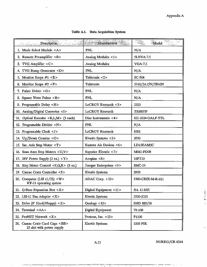
Table A.l. Data Acquisition System
Appendix A
...- •;:;..•;.:•...:..•;•.•;;; .:Description
1. Mode Select Module <A>
2. Remote Preamplifier <B>
3. TVG Amplifier <C>
4. TVG Ramp Generator <D>
5. Monitor Scope #1 <E>
6. Monitor Scope # 2 <F>
7. Pulser Driver <G>
8. Square Wave Pulser <B>
9. Programable Delay <H>
10. Analog/Digital Converter <I>
11. Optical Encoder <K,L,M> (3 each)
12. Programable Divider <N>
13. Programable Clock <J>
14. Up/Down Counter <O>
15. Inc. Axis Step Motor <T>
16. Scan Axes Step Motors <U,V>
17. 24V Power Supply (2 ea.) <Y>
18. Step Motor Control <P,Q,R> (3 ea.)
19. Camac Crate Controller <S>
20. Computer (LSI 11/23) <W>RT-11 operating system
21. Q-Buss Expansion Box <X>
22. LSI-11 Bus Adapter <X>
23. Drive (8" Hard/Floppy) <Z>
24. Terminal <AA>
25. ProNET Network <X>
26. Camac Crate Card Cage <BB>25 slot with power supply
Manufacturer
PNL
Analog Modules <1>
Analog Modules
PNL
Tektronix <2>
Tektronix
PNL
PNL
LeCROY Research <3>
LeCROY Research
Disc Instruments <4>
PNL
LeCROY Research
Kinetic Systems <5>
Eastern Air Devices <6>
Superior Electric <7>
Acopian <8>
Joerger Enterprises <9>
Kinetic Systems
ADACCorp. <10>
Digital Equipment <11>
Kinetic Systems
Qualogy <12>
Digital Equipment
Proteon, Inc. <13>
Kinetic Systems
iltodel '""?\%. r:
N/A
5LNVA-7.5
VGA-7.5
N/A
SC-504
5110/5A15N/5B10N
N/A
N/A
2323
TR8837F
821-1024-OALP-TTL
N/A
8501
3920
LD11EAM3C
M061-FD08
24PT10
SMC-24
3920
2200-CRIX-M-R-611
BA 11-ME
2920-Z1D
DSD 880/20
Vt-100
P1100
1500 PIK
A.11 NUREG/CR-6344
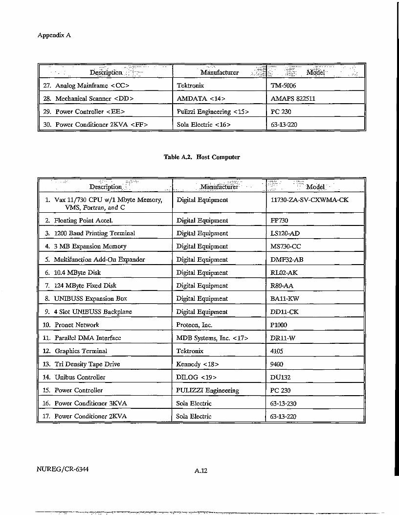
Appendix A
Description:.-:: :: ::- •
27. Analog Mainframe <CC>
28. Mechanical Scanner <DD>
29. Power Controller <EE>
30. Power Conditioner 2KVA <FF>
Manufacturer
Tektronix
AMDATA <14>
Pulizzi Engineering <15>
Sola Electric <16>
Model . ::;,:
TM-5006
AMAPS 822511
PC 230
63-13-220
Table A2.. Host Computer
Description.'.;•.:. .;
1. Vax 11/730 CPU w/1 Mbyte Memory,VMS, Fortran, and C
2. Floating Point Accel.
3. 1200 Baud Printing Terminal
4. 3 MB Expansion Memory
5. Multifunction Add-On Expander
6. 10.4 MByte Disk
7. 124 MByte Fixed Disk
8. UNIBUSS Expansion Box
9. 4 Slot UNIBUSS Backplane
10. Pronet Network
11. Parallel DMA Interface
12. Graphics Terminal
13. Tri Density Tape Drive
14. Unibus Controller
15. Power Controller
16. Power Conditioner 3KVA
17. Power Conditioner 2KVA
. .Maniifactufer: •
Digital Equipment
Digital Equipment
Digital Equipment
Digital Equipment
Digital Equipment
Digital Equipment
Digital Equipment
Digital Equipment
Digital Equipment
Proteon, Inc.
MDB Systems, Inc. <17>
Tektronix
Kennedy <18>
DILOG <19>
PULIZZI Engineering
Sola Electric
Sola Electric
:;|-""'. ~?" Model.; .
11730-ZA-SV-CXWMA-CK
FP730
LS120-AD
MS730-CC
DMF32-AB
RL02-AK
R80-AA
BA11-KW
DD11-CK
P1000
DR11-W
4105
9400
DU132
PC 230
63-13-230
63-13-220
NUREG/CR-6344 A.12
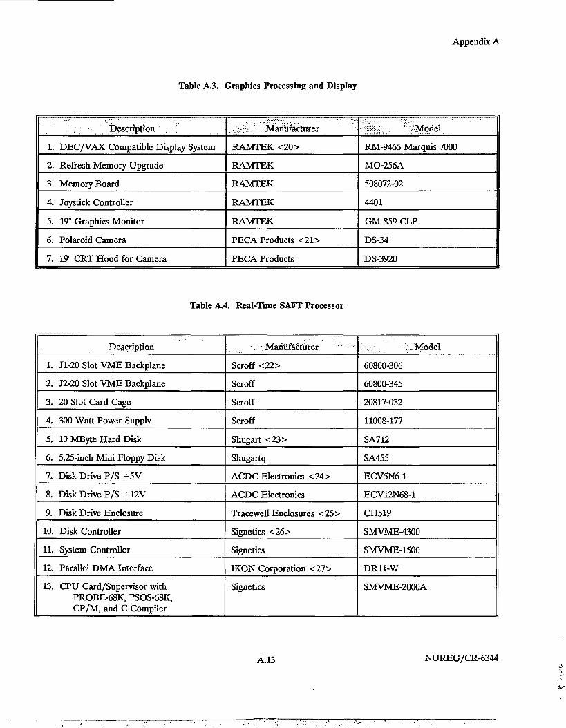
Appendix A
Table A3. Graphics Processing and Display
!:.. Descriptron . !
1. DEC/VAX Compatible Display System
2. Refresh Memory Upgrade
3. Memory Board
4. Joystick Controller
5. 19" Graphics Monitor
6. Polaroid Camera
7. 19" CRT Hood for Camera
,,;.;.:-K-: -_'•'•• Manufacturer
RAMTEK <20>
RAMTEK
RAMTEK
RAMTEK
RAMTEK
PECA Products <21>
PECA Products
Model
RM-9465 Marquis 7000
MQ-256A
508072-02
4401
GM-859-CLP
DS-34
DS-3920
Table A.4. Real-Time SAFT Processor
Description
1. Jl-20 Slot VME Backplane
2. J2-20 Slot VME Backplane
3. 20 Slot Card Cage
4. 300 Watt Power Supply
5. 10 MByte Hard Disk
6. 5.25-inch Mini Floppy Disk
7. Disk Drive P/S +5V
8. Disk Drive P/S +12V
9. Disk Drive Enclosure
10. Disk Controller
11. System Controller
12. Parallel DMA Interface
13. CPU Card/Supervisor withPROBE-68K, PSOS-68K,CP/M, and C-Compiler
Manufacturer ::
Scroff <22>
Scroff
Scroff
Scroff
Shugart <23>
Shugartq
ACDC Electronics <24>
ACDC Electronics
Tracewell Enclosures <25>
Signetics <26>
Signetics
IKON Corporation <27>
Signetics
-,.; : . :,::Model
60800-306
60800-345
20817-032
11008-177
SA712
SA455
ECV5N6-1
ECV12N68-1
CH519
SMVME-4300
SMVME-1500
DR11-W
SMVME-2000A
A.13 NUREG/CR-6344
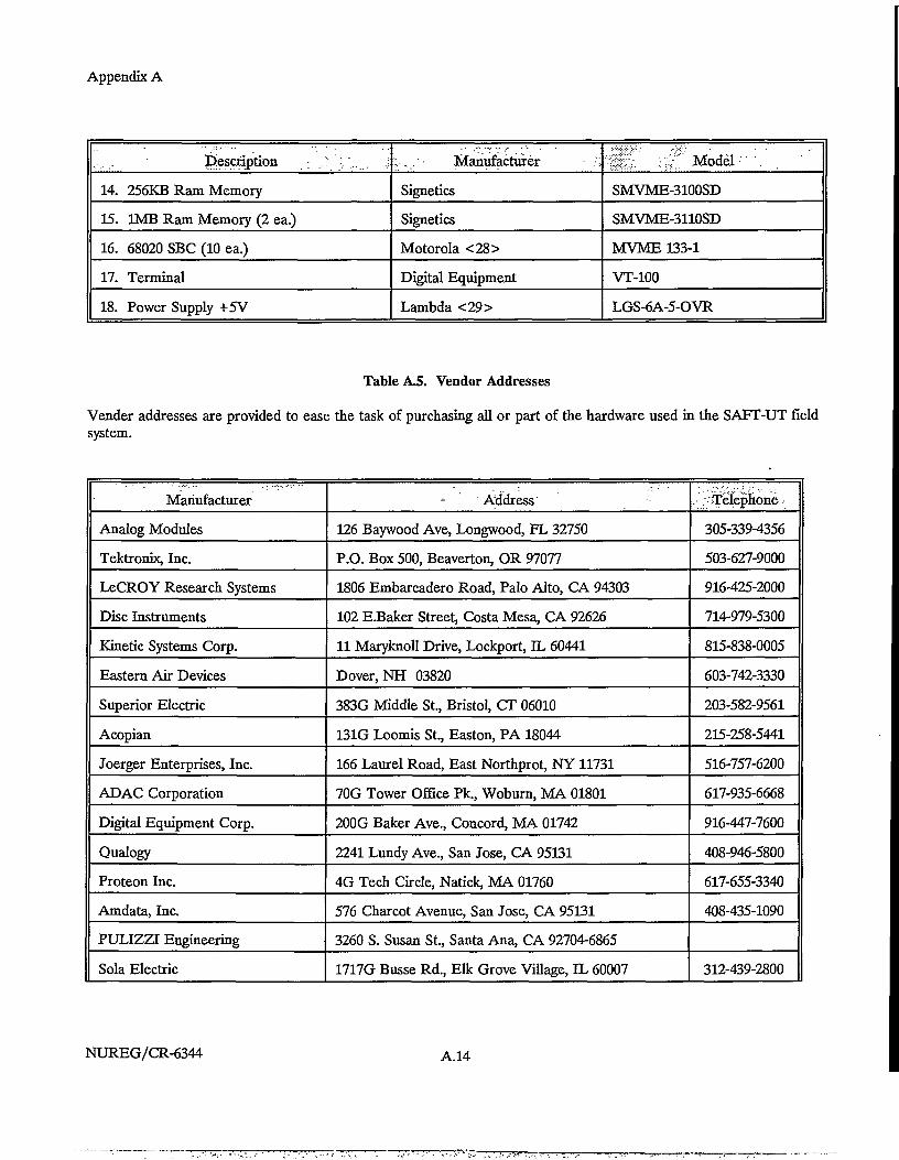
Appendix A
Prescription : ,.: [.... . j
14. 256KB Ram Memory
15. 1MB Ram Memory (2 ea.)
16. 68020 SBC (10 ea.)
17. Terminal
18. Power Supply +5V
:. :.. Manufacturer ':"•.
Signetics
Signetics
Motorola <28>
Digital Equipment
Lambda <29>
illf ::#" Model-' :. .SMVME-3100SD
SMVME-3110SD
MVME 133-1
VT-100
LGS-6A-5-OVR
Table A.5. Vendor Addresses
Vender addresses are provided to ease the task of purchasing all or part of the hardware used in the SAFT-UT fieldsystem.
Manufacturer
Analog Modules
Tektronix, Inc.
LeCROY Research Systems
Disc Instruments
Kinetic Systems Corp.
Eastern Air Devices
Superior Electric
Acopian
Joerger Enterprises, Inc.
ADAC Corporation
Digital Equipment Corp.
Qualogy
Proteon Inc.
Amdata, Inc.
PULIZZI Engineering
Sola Electric
Address
126 Baywood Ave, Longwood, FL 32750
P.O. Box 500, Beaverton, OR 97077
1806 Embarcadero Road, Palo Alto, CA 94303
102 EJBaker Street, Costa Mesa, CA 92626
11 Maryknoll Drive, Lockport, IL 60441
Dover, NH 03820
383G Middle St., Bristol, CT 06010
131G Loomis St., Easton, PA 18044
166 Laurel Road, East Northprot, NY 11731
70G Tower Office Pk., Woburn, MA 01801
200G Baker Ave., Concord, MA 01742
2241 Lundy Ave., San Jose, CA 95131
4G Tech Circle, Natick, MA 01760
576 Charcot Avenue, San Jose, CA 95131
3260 S. Susan St., Santa Ana, CA 92704-6865
1717G Busse Rd., Elk Grove Village, IL 60007
. . JTetepnone
305-339-4356
503-627-9000
916-425-2000
714-979-5300
815-838-0005
603-742-3330
203-582-9561
215-258-5441
516-757-6200
617-935-6668
916-447-7600
408-946-5800
617-655-3340
408-435-1090
312-439-2800
NUREG/CR-6344 A.14
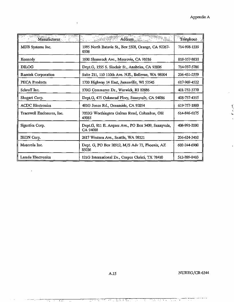
Appendix A
••::•••'•• • •'z:-':'r<&;.zz;.- •.-..-• ' • : . ; ••••••?:;™-.-
• • . . ManiMctarer .. •'.; ':••.
MDB Systems Inc.
Kennedy
DILOG
Ramtek Corporation
PECA Products
Schroff Inc.
Shugart Corp.
ACDC Electronics
Tracewell Enclosures, Inc.
Signetics Corp.
IKON Corp.
Motorola Inc.
Lamda Electronics
•••:•:. . . A d d r e s s
1995 North Batavia St., Box 5508, Orange, CA 92267-0508
1600 Shamrock Ave., Monrovia, CA 91016
Dept.G, 1555 S. Sinclair St., Anaheim, CA 92806
Suite 211, 110 110th Ave. N.E., Bellevue, WA 98004
1700 Highway 14 East, Jamesville, WI 53545
170G Commerce Dr., Warwick, RI 02886
Dept.G, 475 Oakmead Pkwy, Sunnyvale, CA 94086
401G Jones Rd., Oceanside, CA 92054
7032G Worthington Galena Road, Columbus, OH43085
DeptG, 811 E. Arques Ave., PO Box 3409, Sunnyvale,CA 94088
2617 Western Ave., Seattle, WA 98121
Dept. G, PO Box 20912, M/S Adv 72, Phoenix, AZ85036
121G International Dr., Corpus Christi, TX 78410
Telephone.,.;
714-998-1339
818-357-8831
714-937-5700
206-451-2559
617-969-4522
401-732-3770
408-737-4355
619-757-1880
614-846-6175
408-991-2000
206-624-3410
602-244-6900
512-289-0403
A.15 NUREG/CR-6344
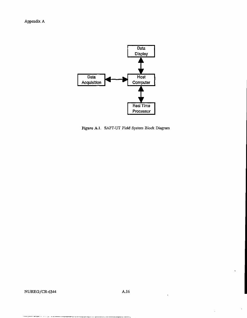
Appendix A
DataDisplay
DataAcquisition 4 • Host
Computer
IReal TimeProcessor
Figure A.l. SAFT-UT Field System Block Diagram
NUREG/CR-6344 A.16
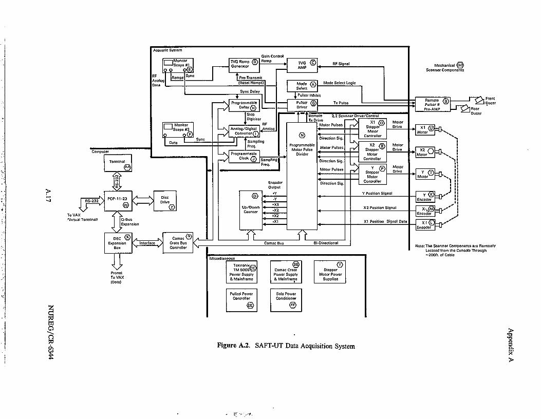
Remote 2.2 Scanner Drive/ControlTx Drive
Motor Pulses
To VAX'Virtual Terminal!
Noto: The Scanner Components are RemotelyLocated from the Console Through~200(t. of Coble
Figure A.2. SAFT-UT Data Acquisition Systemi8B*.
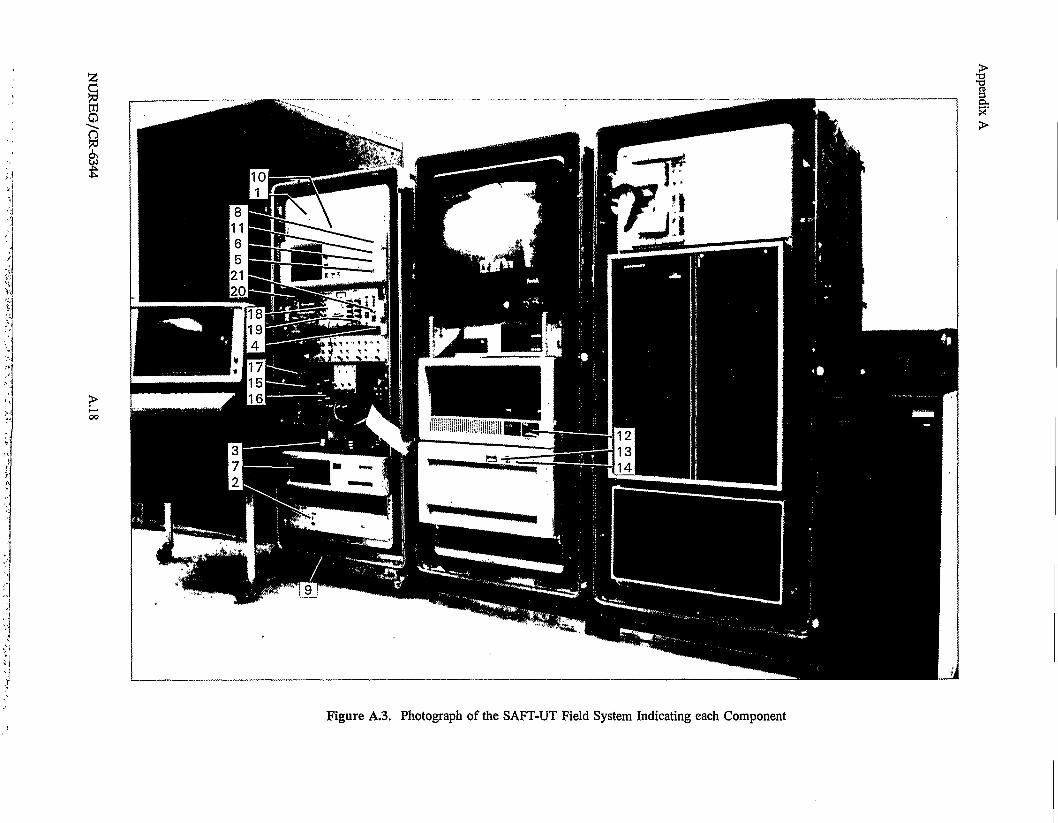
©
>oo
>
Figure A.3. Photograph of the SAFT-UT Field System Indicating each Component
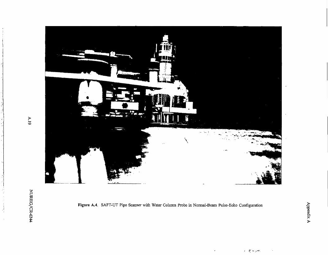
ao
O\
Figure A.4. SAFT-UT Pipe Scanner with Water Column Probe in Normal-Beam Pulse-Echo Configuration
§a.
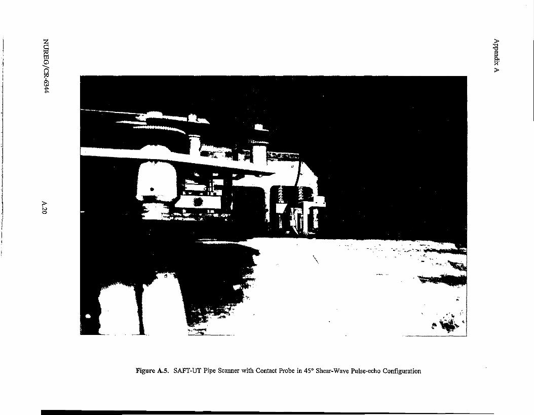
aCD
to©
Figure A.5. SAFT-UT Pipe Scanner with Contact Probe in 45° Shear-Wave Pulse-echo Configuration
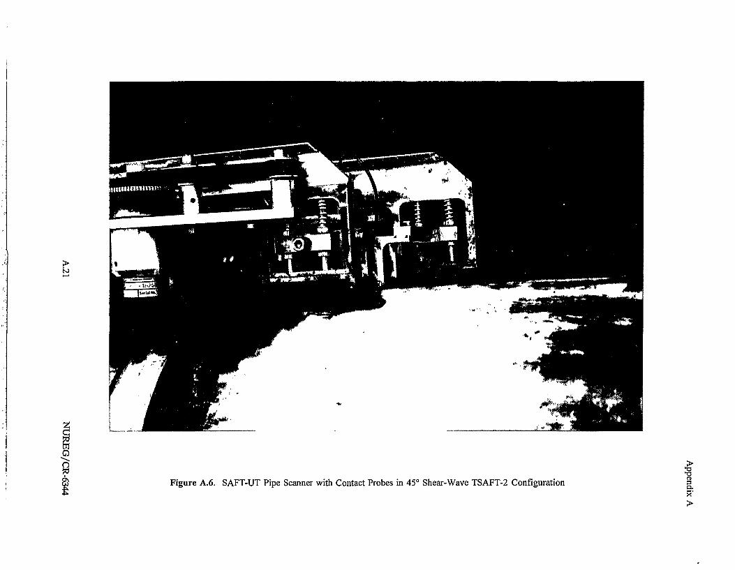
>to
IFigure A.6. SAFT-UT Pipe Scanner with Contact Probes in 45° Shear-Wave TSAFT-2 Configuration
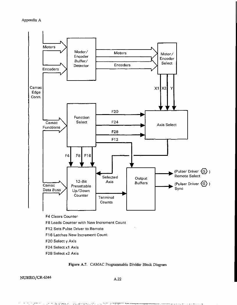
Appendix A
Modor/EncoderBuffer/Detector
CamacEdgeConn.
Motors
Encoders
Motor/EncoderSelect
X1
CamacFunctions
FunctionSelect
F4
CamacData Buss
F8 F16
F20
F24
F28
F12
X2
Axis Select
12-BitPresettableUp/DownCounter
SelectedAxis
TerminalCounts
OutputBuffers
(Pulser DriverRemote Select
(Pulser DriverSync
F4 Clears Counter
F8 Loads Counter with New Increment Count
F12 Sets Pulse Driver to Remote
F16 Latches New Increment Count
F20 Select y Axis
F24 Select x1 Axis
F28 Select x2 Axis
Figure A.7. CAMAC Programmable Divider Block Diagram
NUREG/CR-6344 A.22
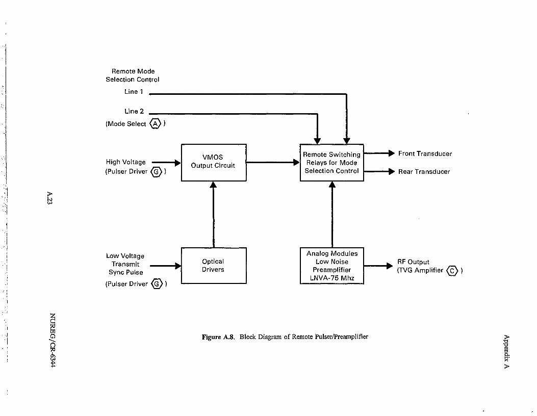
>to
Remote ModeSelection Control
Line 1
Line 2
(Mode Select <A>)
High Voltage(Pulser Driver
Low VoltageTransmit
Sync Pulse
(Pulser Driver
VMOSOutput Circuit
OpticalDrivers
Remote SwitchingRelays for ModeSelection Control
Analog ModulesLow Noise
PreamplifierLIWA-75 Mhz
• • Front Transducer
- • Rear Transducer
RF Output(TVG Amplifier
Figure A.8. Block Diagram of Remote Pulser/Preamplifier
a.
>
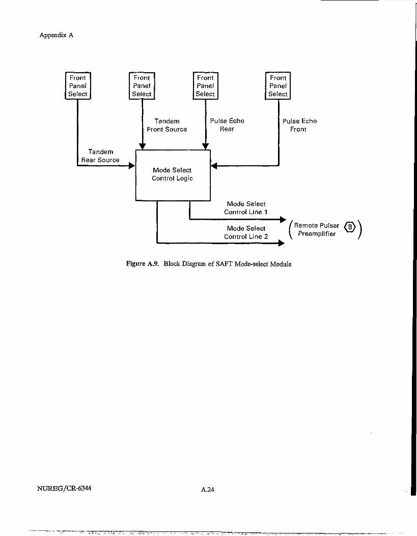
Appendix A
TandemRear Source
TandemFront Source
Pulse EchoRear
Mode SelectControl Logic
Pulse EchoFront
Mode SelectControl Line 1
Mode SelectControl Line 2
/Remote PulserI Preamplifier
Figure A.9. Block Diagram of SAFT Mode-select Module
NUREG/CR-6344 A.24
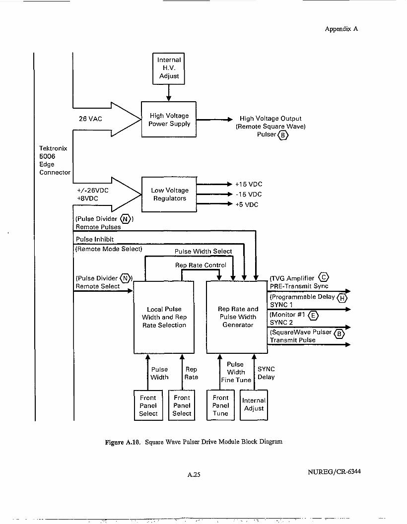
Appendix A
InternalH.V.
Adjust
26 VAC
Tektronix5006EdgeConnector
High VoltagePower Supply
•>. High Voltage Output(Remote Square Wave)
+/-26VDC+8VDC
(Pulse DividerRemote Pulses
Low VoltageRegulators
+15VDC
*• -15VDC
+5 VDC
Pulse Inhibit
(Remote Mode Select) Pulse Width Select
(Pulse Divider (Remote Select
Rep Rate Control
Local PulseWidth and RepRate Selection
Rep Rate andPulse WidthGenerator
PulseWidth
FrontPanelSelect
RepRate
FrontPanelSelect
PulseWidth
Fine Tune
FrontPanelTune
(TVG Amplifier \C)PRE-Transmit Sync
(Programmable DelaySYNC 1(Monitor #1SYNC 2(SquareWave Pulser / g \Transmit Pulse
SYNCDelay
InternalAdjust
Figure A.10. Square Wave Pulser Drive Module Block Diagram
A.25 NUREG/CR-6344
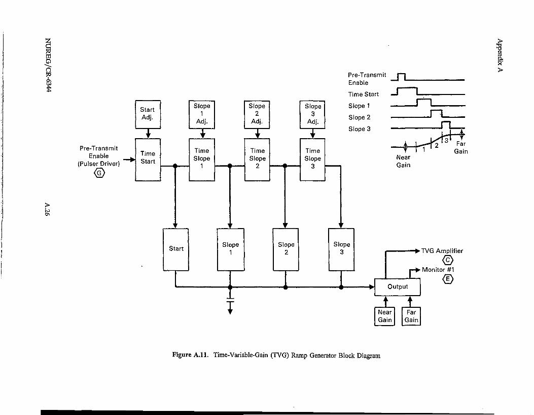
IsSix'
StartAdj.
Slope1
Adj.
Slope2
Adj.
Slope3
Adj.
Pre-TransmitEnable
(Puiser Driver)
Pre-TransmitEnable
Time Start
Slope 1
Slope 2
Slope 3
•TVG Amplifier
• Monitor #1
Output
ITJNearGain
FarGain
Figure A.11. Time-Variable-Gain (TVG) Ramp Generator Block Diagram
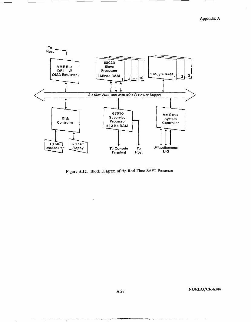
Appendix A
VME BusDR11-W
DMA Emulator
68020Slave
Processor
1 Mbyte RAM
1/4Winchester I Floppy
101 Mbyte RAM
20 Slot VME Bus with 400 W Power Supply
68010SupervisorProcessor
512Kb RAM
To Console ToTerminal Host
VME BusSystem
Controller
MiscellaneousI/O
Figure A.12. Block Diagram of the Real-Time SAFT Processor
A.27 NUREG/CR-6344
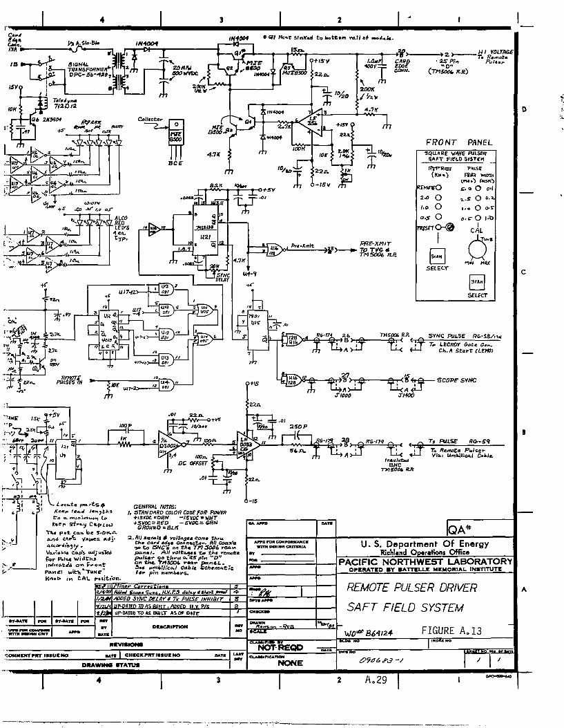
Vt A.SW>-Bto
S1ONALTRANSFORMER"DPC-Sb-Wy
+ QI tot SlnKtd to kott.m rail of i
BCE
• 2S Pin
(jMSOOb KR)
.HI VOLVt&£
P
FRONT PANEL
% alter*' +s 40 M- >.o or
fit
•tea.-Jifetft^
i.s.t
U2I
ih eJU\
^ L
. \TStNC^ »
•f.7/f
- * S >Ffie-xniT
• TO TVS- *TMS006 7t.f>
•.171
SQUARE- WAVE PlUSfRSAFT FI5LD SrSTFM
FSQ MOTH
S.t> O O'lerwrO2-0 O a.s O »•*•f.o O 1.. o »r
o * O o.s- O I-O
n t s s n O - ^ C / | L
Sc«H
SELECT"l« MlIX
SetECT
U i f
T?+IS
hs>Af%::2r^:"^fPUtS£ /?S.-S8/;->«
GateA Starr a
• scope SVNC
TIOOO TI400
T94a 25OP
54^1.ln*ulst>d
BNCTin SOOt RJl
T» PUI.SC gQ-g<>
7i RtmiSta P « / « pVia: Umbilical Co H i
Th« pot Can be
Va.r"abl< Cap's adjustedfor R>lM Width3
CAL
GENfB/li/. STANDARD COLOR COX FOR PM/tR
+IS1DC. 'ORN -ISVDC *VHT+SVOC = KeD -SVIX.-CRN
SROUMO =BLK
2 . All iitiKlt 4 voltages com* thruthm ctLrd «</«« Conn%£&a*. fill Coaltav> to BNCi an th* TIO5O0L reav>ptxnml. All volttuft -t» tit* mmet*ptAlsMr QO tU*u a. ZS ptn ̂ D"art the. TnBOOi f«av> p o n t L .it* umk'llcck.1 CaL/t Sc/nm«t/'cf«r pm numUrs.
-15
UP-P47ED TO /IS B l l t r . ADDf [> M V P/SUP-DATH) TO »S BUILT AS Of D<Tf
DCSCHIPTXXI
REVISIONSMi l I CHECK PitriMUI NO
DMWINO STATUS
WtTM DOIM ClIimiA
NOTREQD
""""IJONE
QA*U. S. Department Of Energy
Riehland Oprationi OfficaPACIFIC NORTHWEST LABORATORY
OPERATED BY BATTELLE MEMORIAL INSTITUTE
REMOTE PULSER DRIVER
SAFT FIELD SYSTEM
FIGURE AO13I.HOfaHO
? - / J
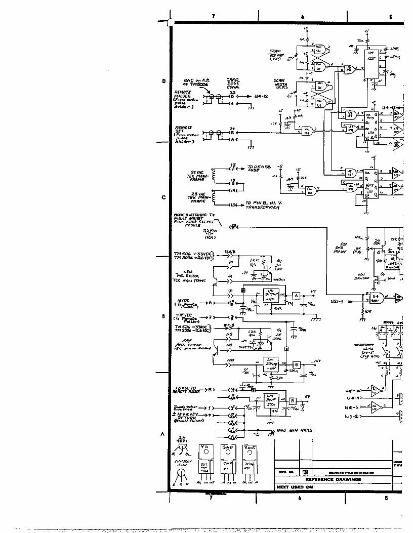
nooe autrcHiNPULSF MHIBITFrom nODC SSLtCT
r/5V0CIscr)
THSOk -33»OC"1TM5006 -S.b»OC\
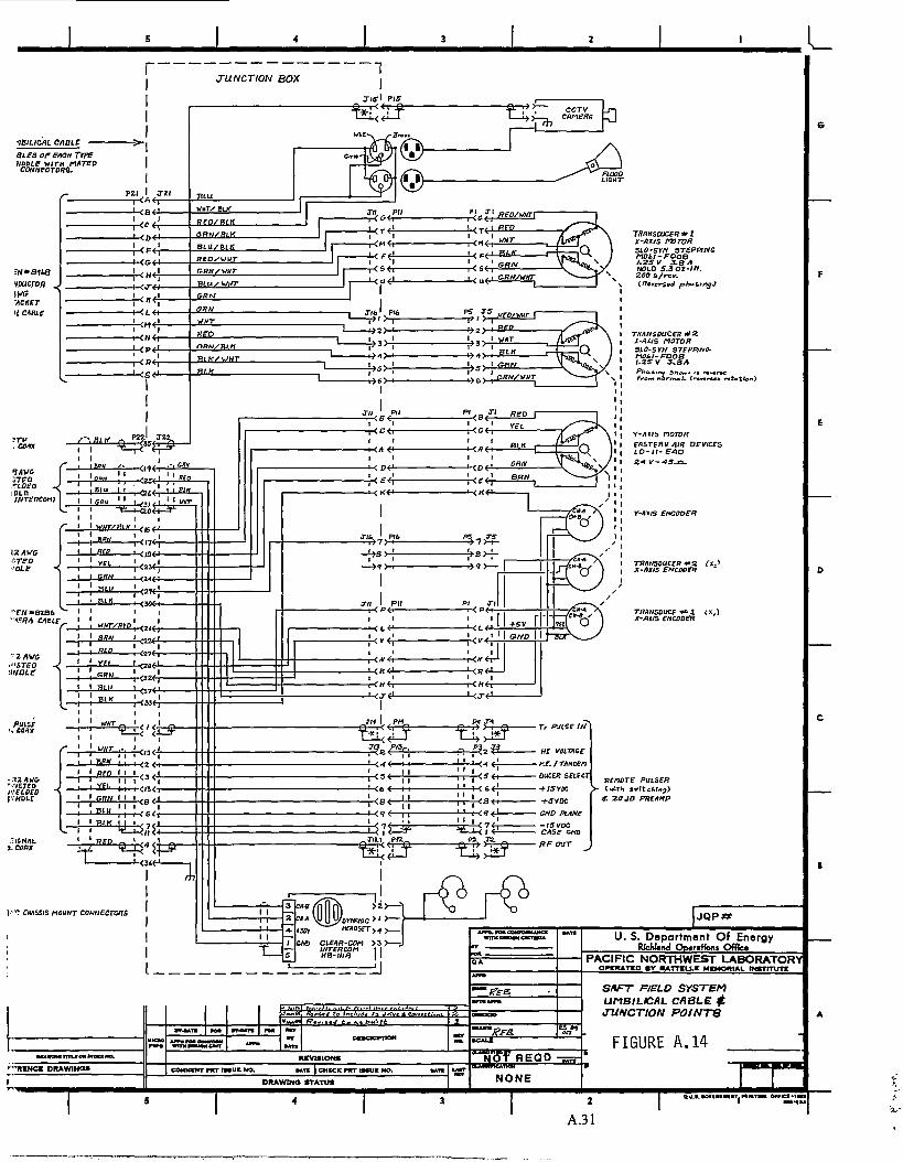
LJUNCTION BOX
TRANSDUCER* IX-AXIS MOTVftSIO-SM STtPPINSMObl-FDOQ1.35 V 3.3 AHOLD S.3O2-IH.ZOO s/rev.
TRANSDUCER *X-AXIS MOTORSIO-SYM STEPfWe-Mail- FDOBI.2SV
AIR DEVICESLO-II-EAD
TWNSOUCfRX-AXIS ENCOOttt
HI YOLTASE
RE./TANXn
DUCCK sneer•HSVK
+3V0C
GHD PLANS
HCHOTE PULSER
2 0 JS PREAHP
U. S. Department Of EnergyRicMwd O P T «fk>m Offic
PACIFIC NORTHWEST LABORATORY
FIELD SYSTEMUnBILICfIL CABLE $.JUNCTION POINTS
FIGURE A.14
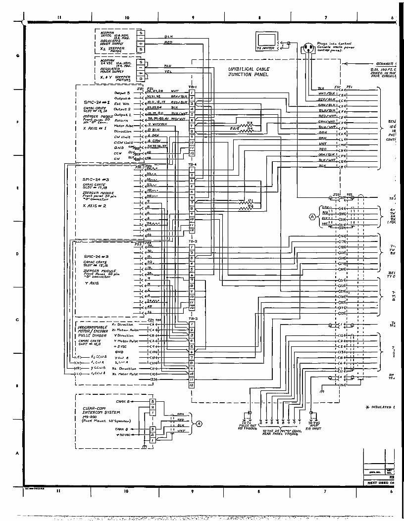
10
r
I Xz STEPPER| *• MOTOR
ICOPIAMZ4 VDC IOA.
HA. MAXREGULATED
•a SUPPLY CABLEJUNCTION PANEL
MOTOR/ENCODER "' "'to
| PULSE DIVIDER
I CHM4C CRATESLOT •*• 10,11
y Motor PU
e/vo
|
CLEAR-COMINTEHCOn SYSTEMMS-SOO(iB«K Mount
•X- INSULATCO t
TOTxPUlSEOur"
Re TMSOOt, V FP IHFVTTO THE 2 5 PH -D~ COHH.
PANEL TnSOOt
L A,
NCCT USED Of
10
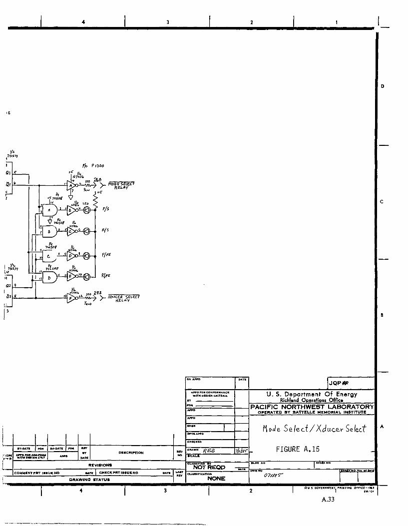
•r«OAT* PON
U. S. Department Of EnergyRichland OperaKont Office
PACIFIC NORTHWEST LABORATORYOPERATED BY BATTELLE MEMORIAL INSTITUTE
Select/Xduce.r Select
FIGURE A.15
REVISIONS
COMMENT TUT I I I U I N O BATS CHICK PRTISSUK NO
DRAWING STATUS
>...r.b. *r
NOT REQDI IMbCXNO
CLASSIfiCATIOH
NONE07ms-
I tru s GOveRMateNr HHHTIMG ornce-tmI I 696 I!
A.33
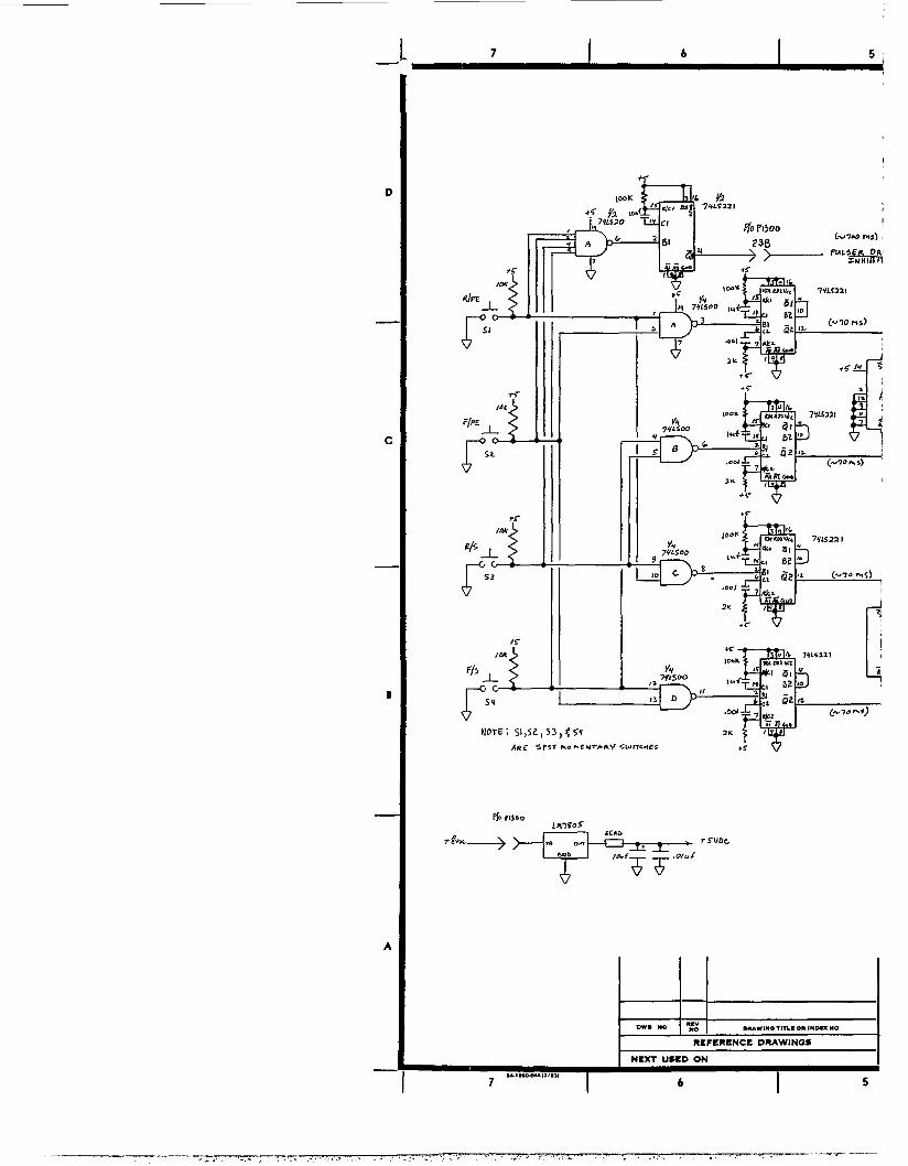
L
NOTE'. $ 1 , 5 2 , 5 3 , 4 S I
ARE spir ho».£»iTAny
J
S4-1MO-O44I3/B3]
MUWINO TIT1.SOR IHDO NO
REFERENCE DRAWINGS
NEXT USED ON
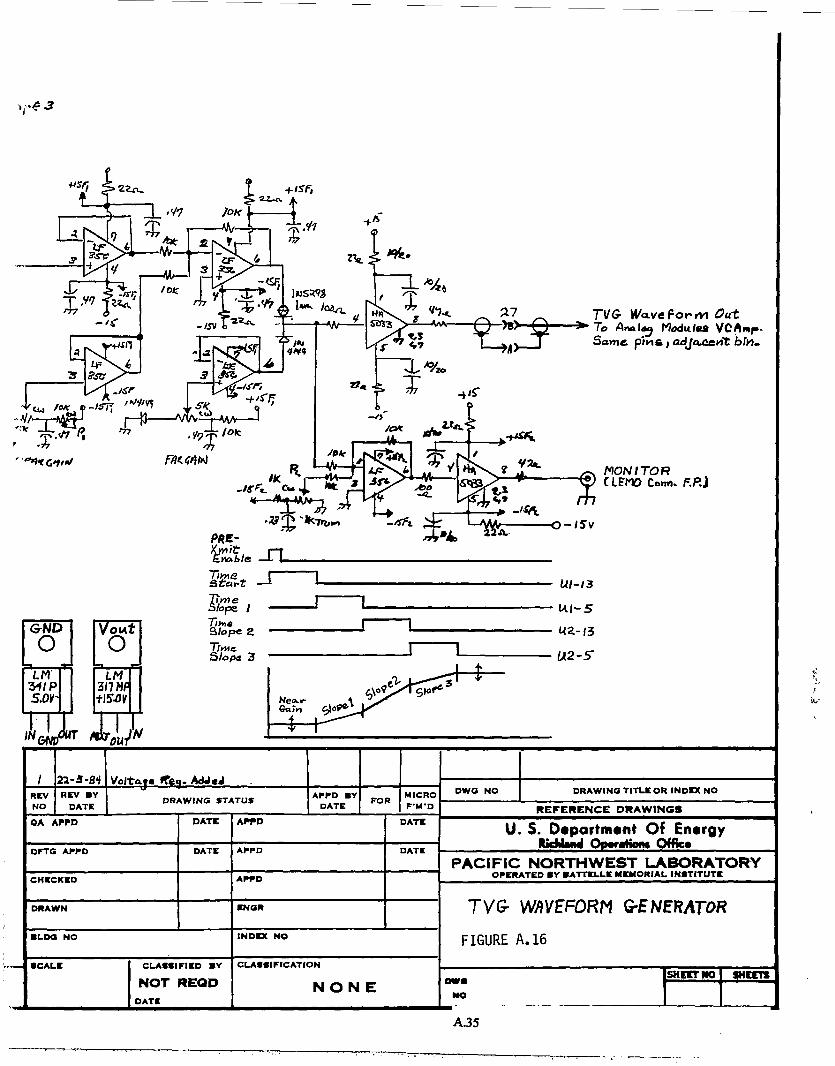
To Anal<3 Modutafi rSame pine, adjacent bin.
'""•XGf/*/ ^ MONITOR© CLFMO Com).
OLM'
5.0V-
out
REVNO
REV BYDATE
Voltaj*DRAWING STATUS APPD BY
DATE FORMICROF-M'D
DWG NO DRAWING TITLE OR INDEX NO
REFERENCE DRAWINGSQA APPD
DFTG APPD
CHECKED
DRAWN
DATE APPD
DATE
•LDO NO
•CALE CLASSIFIED BY
NOT REQDDATE
APPD
APPD
ENGR
DATE
DATE
U. S. Department Of EnergyK d U j OPT«4ioiH Offks
PACIFIC NORTHWEST LABORATORYOPERATED BY BATTELLE MEMORIAL INSTITUTE
INDEX NO
TVG- W/1VEF0RM GENERATOR
FIGURE A.16
CLASSIFICATION
NONE aw«SHEET WO WCTTt
A.35
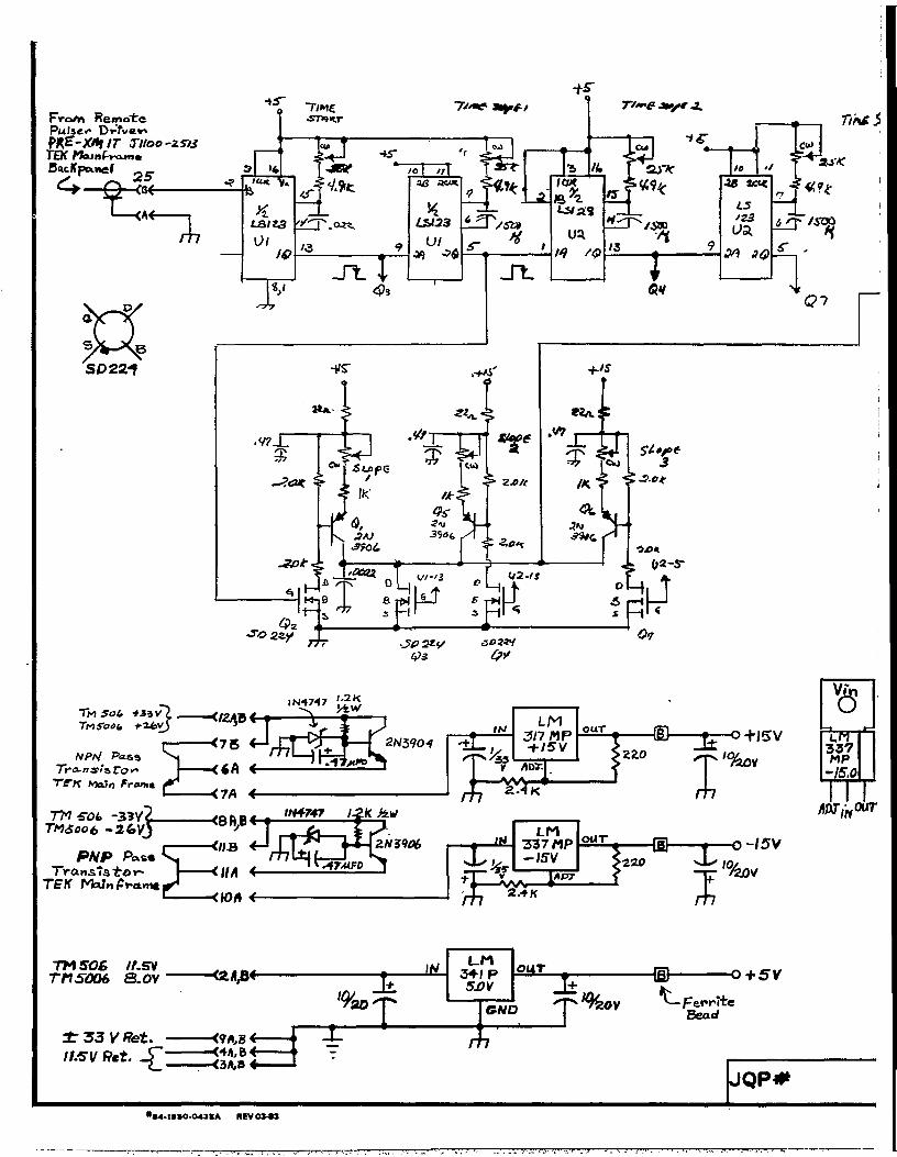
Pulse.*
TEK
RemoteTe**
Tlloo-zstS
O+J5V
O-/5V
vc5337MP
'15,0
ff
ir.svTHS006 8.OV
±- 33 V fet.II.XV Ret.
*«4-I»»O-O43KA REV 03^3
IIS/ LM34/P
5JOVour
T ov
•o+SV
Bead
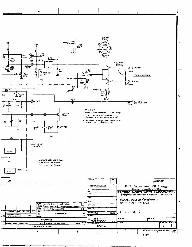
NOTES I/. KISK2 A™ Tcltdyna 713.012.
-I2V
~{ 1BLI2
79LIZ+ /2V
TiF OUT7 TV.G-.AmR)
BMC J"acKl a>-e Insulated fromCKutlf. Use RMPHENOLlf-ZI-IO.
3 . Fafe.-a.cate Or? ground p/om: SC8.Mounl Jw "Compac" box.
//V4733
ANflLOC MODULES INC.LOW noise PRE-AMP(Encapsulated Mojule)
J
Revised Duciv Stttct Belaysmodi*
ised t-o CMS b«»/ t
DMCRIPTTON
APTO rOR CONFORMANCKWITH OOf OM CltlTUUA U. S. Department Of Energy
RichUnd Operations OffioPACIFIC NORTHWEST LABORATORY
OPERATED BY BATTELLE MEMORIAL INSTITUTE
TtEMOTE PULSER/PRE-AMP5f\FT FIELD SYSTEM
. FIGURE A.17
REVISIONS
COMMENT PUT IStUCNO MTI CHICK PRTIHUE NO
DRAWINO STATUS
j&SiFBTfi
NOTREQDLASTRCV CLAMinCATION
NONEPICC-1M3
8M124
A.37
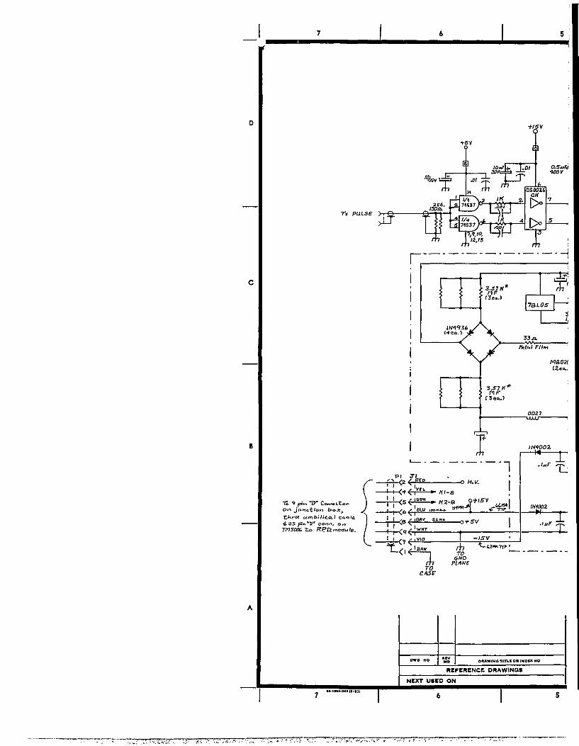
5 .
. «[ I
sagJ*r 0.5*%tOOY
Tt PULSE
"K <» pin -D* Co»«cto<-On JMtict'OM box>"thru. umbiliCQ-\ cablei-ZS p inV conn. onTIISDtX, Za f!l?D. madu Is.
DRAWIHa TIT1.K OH INDCX NO
REFERENCE DRAWINGS
NEXT USED ON
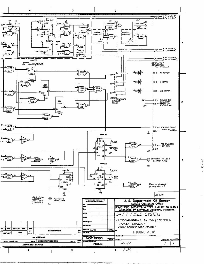
3..•# f .
a |UM
-sv
CtK FromLECROYY
IBR.P.)
CiD 7??
LS7474Q
C1KU23
X
DIV/OFO PULSES(LfMO HP.)
(S) KeyboardSelectable
mAFPD POd COHPOHMANCC
WITM M I W CXITtlUA U. S. Department Of EnergyR'lehUnd Opr«tiont Offio
PACIFIC NORTHWEST LABORATORYBY »ATTtLLt MEMORIAL IN»TITUTt
SAFT FIELD SYSTEMPROGRAMMABLE MOTOR I ENCODER
PULSE DIVIDERCAMAC DOUBLE VIDE M0DUL5
FIGURE A0I8WKVtSIOfM
T<rr IHUINO —n I CHECKP«TI»»U«NO
DRAWINO STATUS
LMTHV
sawnrtmNOTREQD
HU 46
IPICATION
NONE
AO39
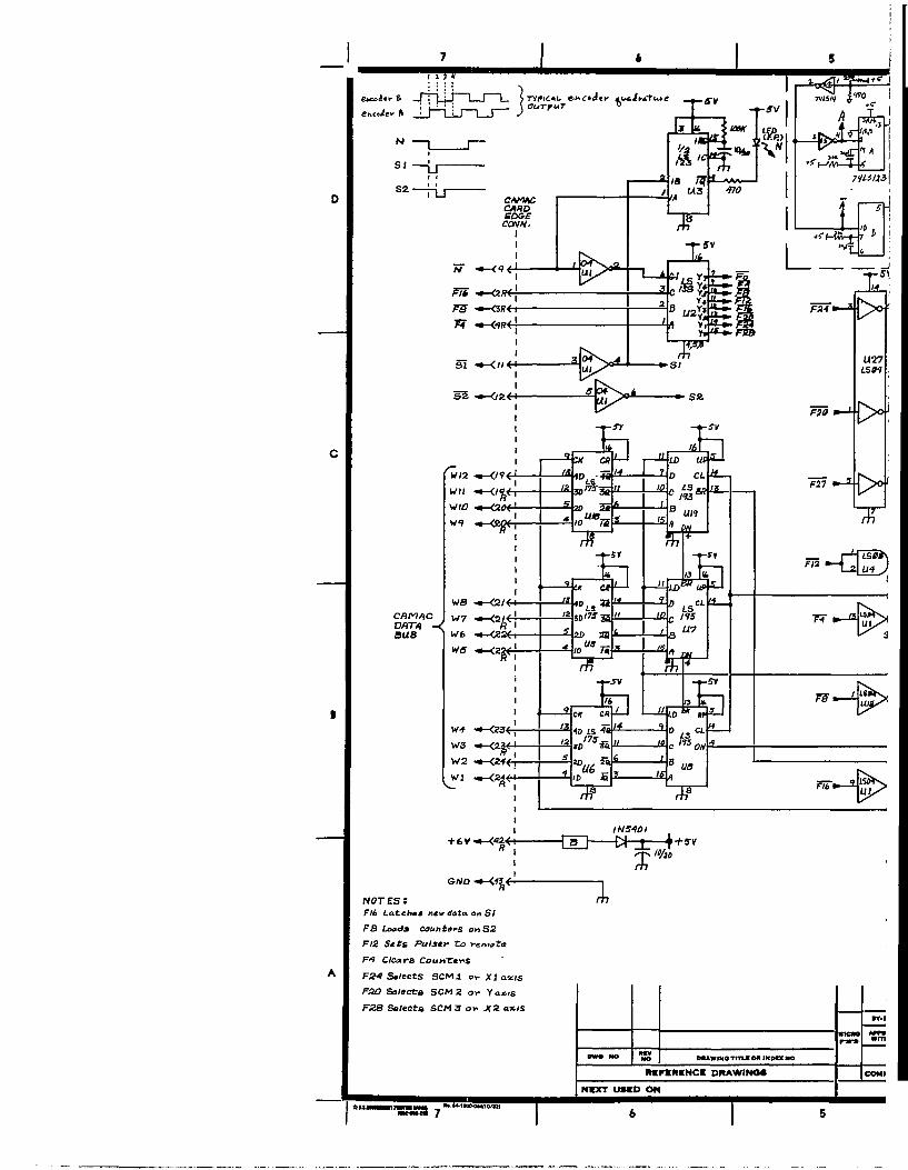
G/VO •-<•»:
NOT ES iFit Latch*! new data an SI
FB Loads Counters onS2
FI2 Stts Pullty Zo yvmata
F4 Clears Counters
F24 SmlectS SCMi o»- X I axis
FOO Sa/ecte SCM 2 ov Yaws
F2B Selects SCM 3 of JC2 a%/S
MIAWINO TTnM OH INDCX HO
RIFCRENCE DRAWING*
NEXT USED ON
STS7
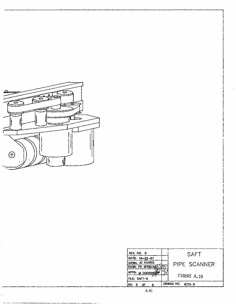
SAFT
PIPE SCANNER
FIGURE A.19
DRVflNG NO. 8710-5
A.41
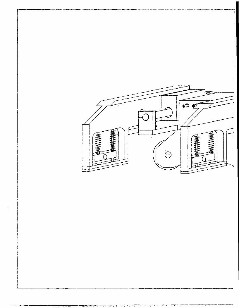
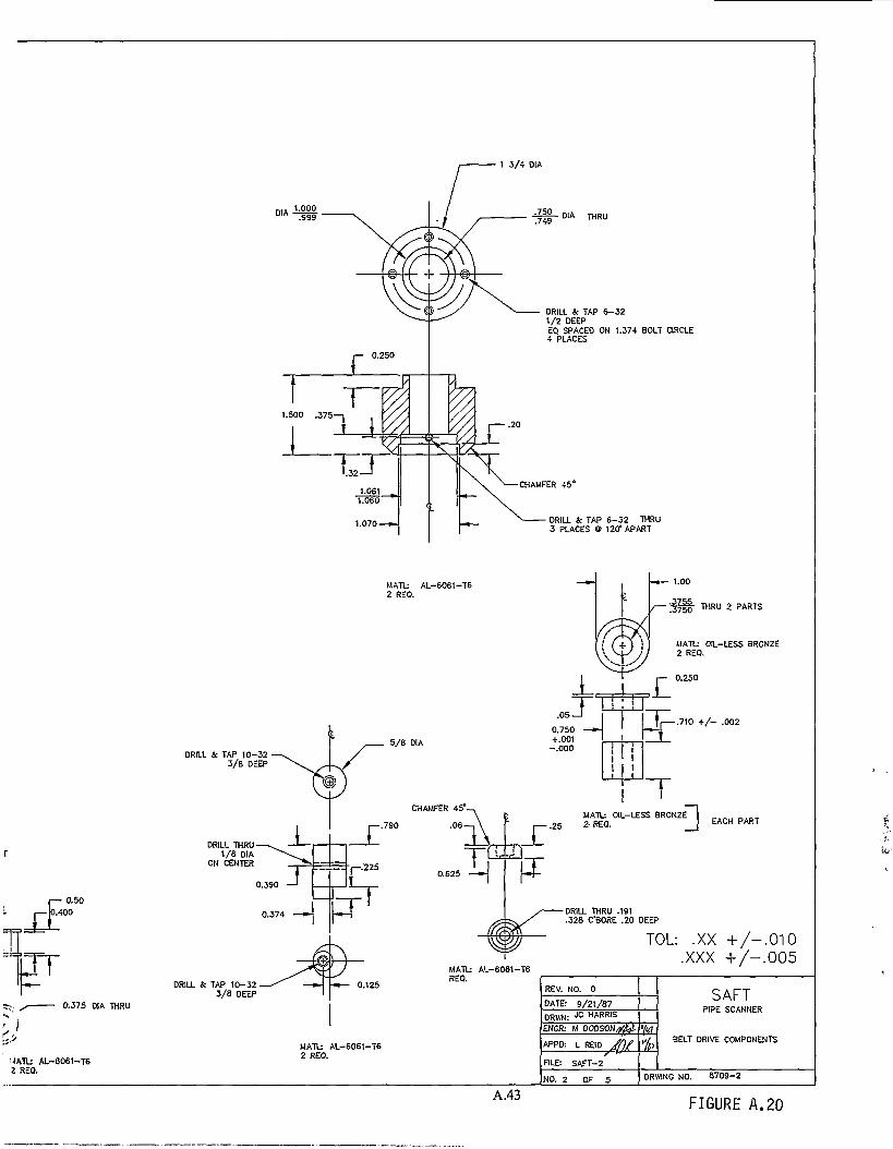
1 3 /4 DIA
1.500 .375
1.0611.060"
1.070-
THRU
DRILL & TAP 6 -321/2 DEEPEQ SPACED ON 1.374 BOLT CIRCLE4 PLACES
• DRILL & TAP 6 -32 THRU3 PLACES @ 120" APART
1
0.5010.400
orr~
DRILL & TAP 10-323/8 DEEP
MATU AL-6061-T62 REQ.
0.375 DIA THRU
5/8 DIA
CHAMFER 45°.
.790
13750" ™ R U 2 P A R T S
MATL- OIL-LESS BRONZE2 REQ.
EACH PART
-DRILL THRU .191.328 C'BORE .20 DEEP
DRILL & TAP 10-323/8 DEEP
MAUi AL-6061-T62 REQ.
0.125
MATU AL-6061-T62 REQ.
MAIL: AL-6061-T6REQ.
TOL: .XX +/-.010.XXX +/-.005
REV. NO. 0
PATE: 9/21/87D R W N . JC HARRIS
ENCR: M
APPD: L REID
RLE: SAFT-2
NO. 2 OF 5
SAFT
PIPE SCANNER
BELT DRIVE COMPONENTS
DRWING NO. 8709-2
A.43FIGURE A.20
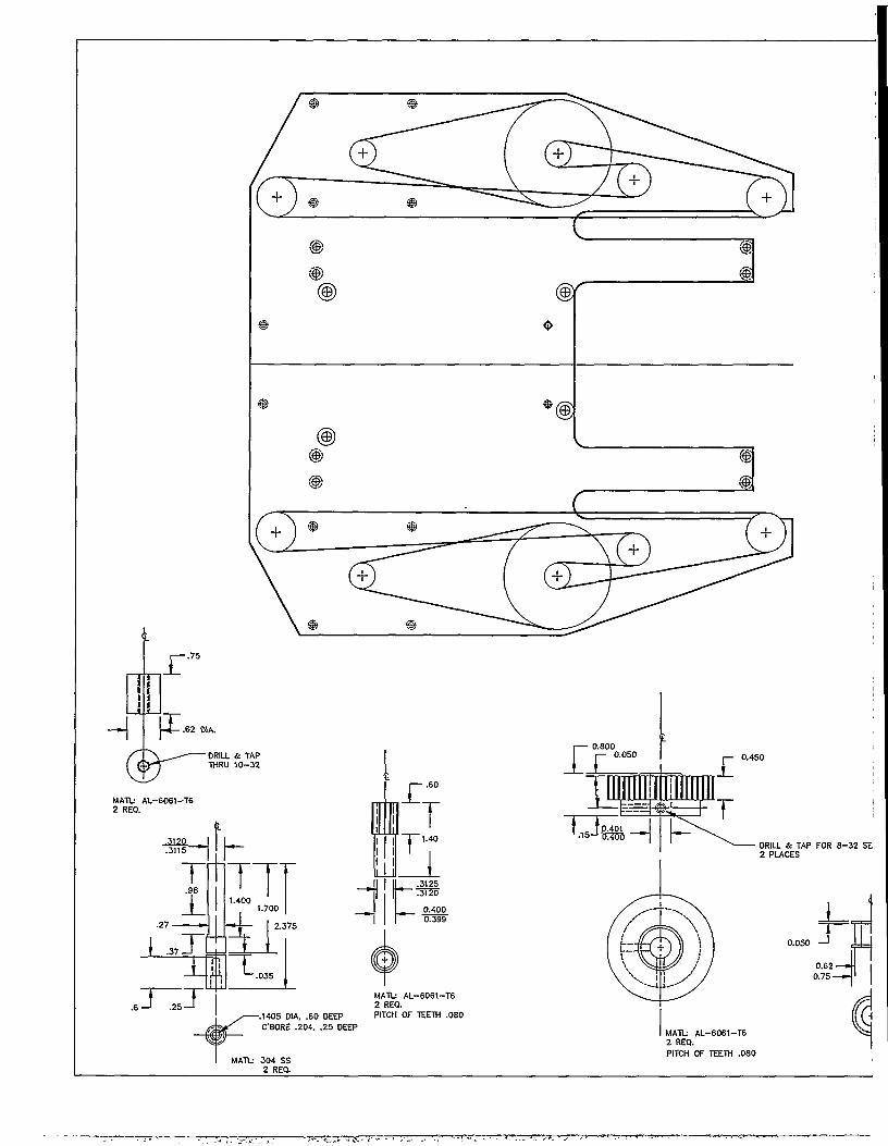
t
r- .62 DIA.
MATU AL-BO61-T62 REQ.
.»o
.27-
.6 —I .25J
TT1.400
ft1.700
Z375
I .035
T
.60
T1.40
.3125"3T20
0.4000.399
MATL: AL-6061-T62 REQ.
-.1405 DIA, .60 DEEP PITCH OF TEETH .080C'BORE .204. .25 DEEP
MATL: 304 SS2 REQ.
r
0.450
DRILL & TAP FOR 8-32 SE2 PLACES
0.050
I.62 — •7 5 — * - '
0.620.75
MATL: AL-6061-T62 REQ.PITCH OF TEETH .030
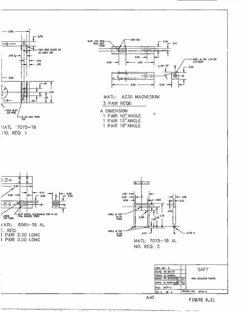
3/16
.062 WIDE SLOTS BY.07 DEEP TYP
- 6 - 3 2 UNC THRUTYP
MAIL 7075-T6
'110. REQ: 1
SLOT .144 WIDE-FULL RAD.
THRU
O.SO
.063 DIA
ET"
- \"t ^3.00 0.50
MATL: AZ30 MAGNESIUM
3 PAIR REQD
A DIMENSION1 PAIR 10° ANGLE1 PAIR 13° ANGLE1 PAIR 18° ANGLE
DRILL k. TAP 1 / 4 - 2 01/2 DEEP
2.30
O.SO
— -\£
0.37 _ J U_ as0.08 S. j — 0.
0.500.50
- .0625TYP THRU
OT WIDTH. CLEARANCE FOR 6 -32LL RADIUS, THRU
v'ATL: 6061 -T6 AL
C. REQ:I PAIR 2.30 LONGI PAIR 3.00 LONG
0.07
3 /32 R
MATL: 7075-T6 AL
NO. REQ: 2
REV. NO. 0
DATE: 10-20-87
DRWN: X HARRISENGR: PD SPERLIINGS.
APPD: M
FILE: SAFT-4
NO. 4 OF 5
SAFT
PIPE SCANNER PARTS
DRWING NO. 8710-4
A.45FIGURE A.21
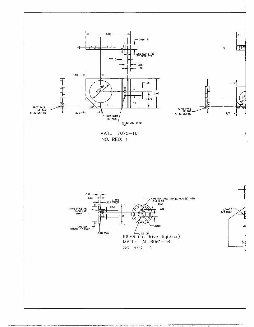
SPOT FACEAR FOR
6-32 SKT HD
6-32 UNC THRUTYP
MATL 7075-T6NO. REQ: 1
SPOT FACEAR FOR
6-32 SKT HD
SPOT FACE AR2-56 UNF
THRU
1.00 DIAC'BORE .17 DEEP
1.18 DIAM
.03 DIA THRU TYP (2 PLACES) WITH.010 SLOT
0.32
0.18
.1250
IDLER (to drive digitizer)MATL: AL 6061-T6NO. REQ: 1
1/4-203/4 DEEP
N(
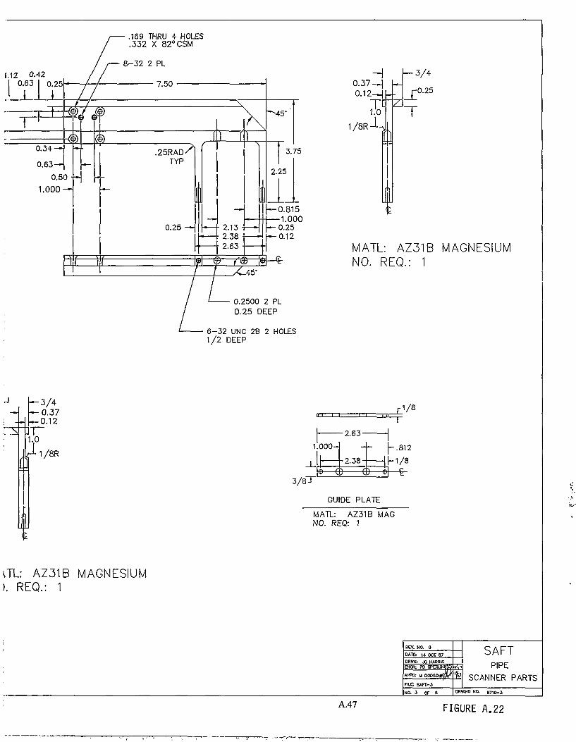
.169 THRU 4 HOLES.332 X 82°CSM
1,12 0.42
3.75
1.000
0.2500 2 PL0.25 DEEP
6-32 UNC 2B 2 HOLES1/2 DEEP
H0.37-^0 . ]
1/8R _L
[-3/4
r0.25
T
MATL: AZ31B MAGNESIUMNO. REQ.: 1
1.0
- 3 / 4— 0.37
0.12
1/8R
It l < t
j-1/8
GUIDE PLATE
MATL: AZ31B MAGNO. REQ: 1
\TL: AZ31B MAGNESIUM). REQ.: 1
DATE: u OCT 87
DRW: JC HARRIS
FILE: SAFT-3
SAFTPIPE
SCANNER PARTS
0RWNC HO. 8710-3
A.47 FIGURE A.22
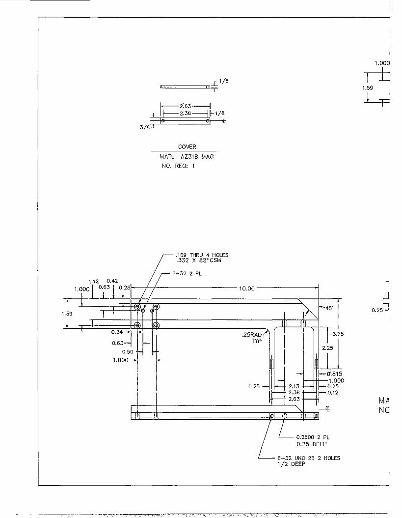
j . 1/8
1
3/8 -i
• 2:63
COVER
1
-1/8
MATL: AZ31B MAG
NO. REQ: 1
T1.59
I
1.000
1.12 0.42
1.000
t1.59
0.63
J__Li
0.34—]
0.63—|0.50
1.000—I•H
.169 THRU 4 HOLES
.332 X 82°CSM
8-32 2 PL
10.00
.25RAD'TYP
0.25 —j
I2.132.382.63
3a
I
-45'
3.75
2.25
11h-0'.815
-1.000•0.25
j - — 0.12
\—t
0.2500 2 PL0.25 DEEP
6-32 UNC 2B 2 HOLES1/2 DEEP
J0.25
NC
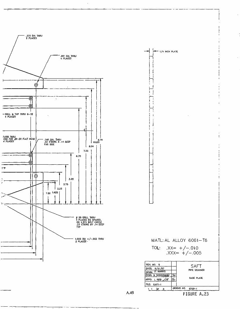
.375 DIA THRU2 PLACES
.191 OIA THRU4 PUCES
0,186 THRUCSK FOR #8-32 FLAT HEAD4 PLACES
-m
TV
.140 DIA. THRU
.23 C'BORE X .14 DEEPFAR SIDE
8.758.625
8.04
7.50
6.70
3.55
2.75
2.22
1.50
LLi
# 28 DRILL THRU4 PLACES EQ SPACED.ON 1.374 BOLT -CIRCLE.23 CBORE BY .14 DEEPTYP
1.005 DIA + / - . 003 THRU2 PLACES•
A.49
H 1/4 INCH PLATE
P
n!
u;! i
u
FIGURE A.23
MATLAL ALLOY 6061-T6
TOL: .XX= +/ - .010.XXX= + / - .005
REV. NO. 0
DATE: 9/21/87
DRWN: J C H A R R I S
ENGR: M DODSOW/©'
APPD: L REID ^ ? f
RLE: SAFT-1
1.1 OF 5
"ftl
In
SAFTPIPE SCANNER
BASE PLATE
DRWING NO. 8709-1
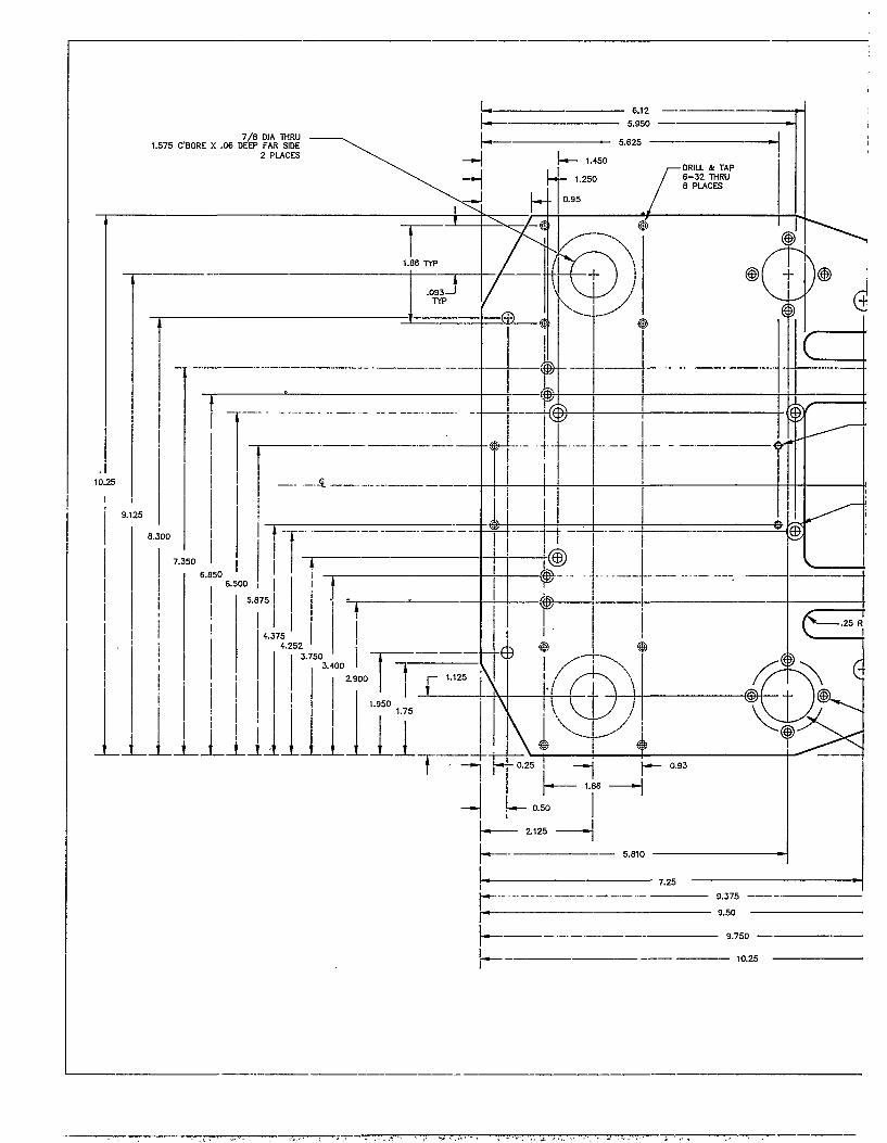
1.575 C'BORE X7/8 DIA THRU
.06 DEEP
C
JJ_±J__LLLLLL
Appendix B
Tutorial Procedure for Operatingthe SAFT-UT Robotic Scanner
NUREG/CR-6344
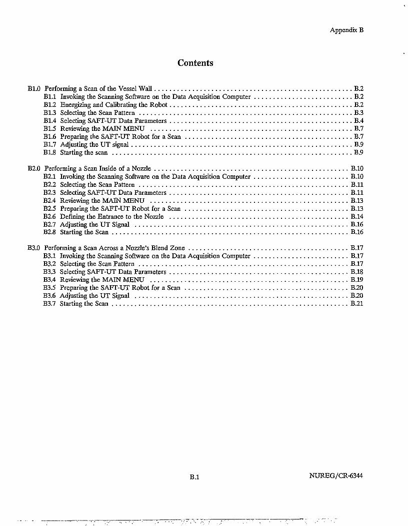
Appendix B
Contents
Bl.O Performing a Scan of the Vessel Wall B.2Bl.l Invoking the Scanning Software on the Data Acquisition Computer B.2B1.2 Energizing and Calibrating the Robot B.2B1.3 Selecting the Scan Pattern B.3B1.4 Selecting SAFT-UT Data Parameters B.4B1.5 Reviewing the MAIN MENU B.7B1.6 Preparing the SAFT-UT Robot for a Scan B.7B1.7 Adjusting the UT signal B.9B1.8 Starting the scan B.9
B2.0 Performing a Scan Inside of a Nozzle B.10B2.1 Invoking the Scanning Software on the Data Acquisition Computer B.10B2.2 Selecting the Scan Pattern B.llB2.3 Selecting SAFT-UT Data Parameters B.llB2.4 Reviewing the MAIN MENU B.13B2.5 Preparing the SAFT-UT Robot for a Scan B.13B2.6 Defining the Entrance to the Nozzle B.14B2.7 Adjusting the UT Signal B.16B2.8 Starting the Scan B.16
B3.0 Performing a Scan Across a Nozzle's Blend Zone B.17B3.1 Invoking the Scanning Software on the Data Acquisition Computer B.17B3.2 Selecting the Scan Pattern B.17B3.3 Selecting SAFT-UT Data Parameters B.18B3.4 Reviewing the MAIN MENU B.19B3.5 Preparing the SAFT-UT Robot for a Scan B.20B3.6 Adjusting the UT Signal B.20B3.7 Starting the Scan B.21
B.I NUREG/CR-6344
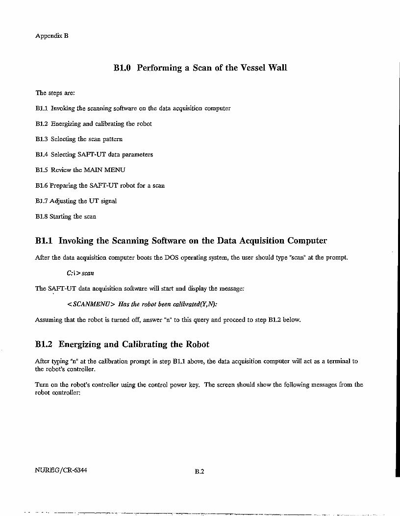
Appendix B
B1.0 Performing a Scan of the Vessel Wall
The steps are:
Bl.l Invoking the scanning software on the data acquisition computer
B1.2 Energizing and calibrating the robot
B1.3 Selecting the scan pattern
B1.4 Selecting SAFT-UT data parameters
B1.5 Review the MAIN MENU
B1.6 Preparing the SAFT-UT robot for a scan
B1.7 Adjusting the UT signal
B1.8 Starting the scan
Bl.l Invoking the Scanning Software on the Data Acquisition Computer
After the data acquisition computer boots the DOS operating system, the user should type "scan" at the prompt.
C:\>scan
The SAFT-UT data acquisition software will start and display the message:
<SCANMENU> Has the robot been calibrated(Y,N):
Assuming that the robot is turned off, answer "n" to this query and proceed to step B1.2 below.
B1.2 Energizing and Calibrating the Robot
After typing "n" at the calibration prompt in step Bl.l above, the data acquisition computer will act as a terminal tothe robot's controller.
Turn on the robot's controller using the control power key. The screen should show the following messages from therobot controller:
NUREG/CR-6344 B.2
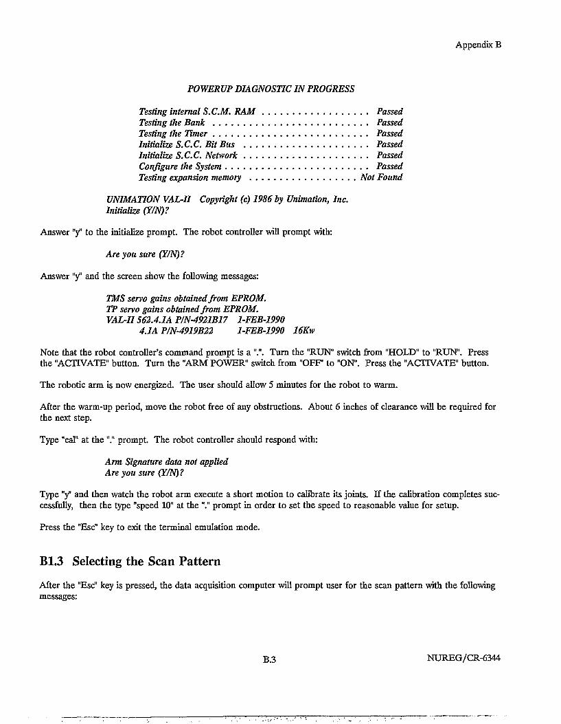
Appendix B
POWERUP DIAGNOSTIC IN PROGRESS
Testing internal S.C.M. RAM PassedTesting the Bank PassedTesting the Timer PassedInitialize S.C.C. Bit Bus PassedInitialize S.C.C. Network PassedConfigure the System PassedTesting expansion memory Not Found
UNIMATION VAL-II Copyright (c) 1986 by Unimation, Inc.Initialize (Y/N)?
Answer "y" to the initialize prompt. The robot controller will prompt with:
Are you sure (Y/N)?
Answer "y" and the screen show the following messages:
TMS servo gains obtained from EPROM.TP servo gains obtained from EPROM.VAL-II 562.4.1A P/N-4921B17 l-FEB-1990
4.1A P/N-4919B22 l-FEB-1990 16Kw
Note that the robot controller's command prompt is a ".". Turn the "RUN" switch from "HOLD" to "RUN". Pressthe "ACTIVATE" button. Turn the "ARM POWER" switch from "OFF1 to "ON". Press the "ACTIVATE" button.
The robotic arm is now energized. The user should allow 5 minutes for the robot to warm.
After the warm-up period, move the robot free of any obstructions. About 6 inches of clearance will be required forthe next step.
Type "cal" at the "." prompt. The robot controller should respond with:
Arm Signature data not appliedAre you sure (Y/N)?
Type "y" and then watch the robot arm execute a short motion to calibrate its joints. If the calibration completes suc-cessfully, then the type "speed 10" at the "." prompt in order to set the speed to reasonable value for setup.
Press the "Esc" key to exit the terminal emulation mode.
B1.3 Selecting the Scan Pattern
After the "Esc" key is pressed, the data acquisition computer will prompt user for the scan pattern with the followmgmessages:
B.3 NUREG/CR-6344
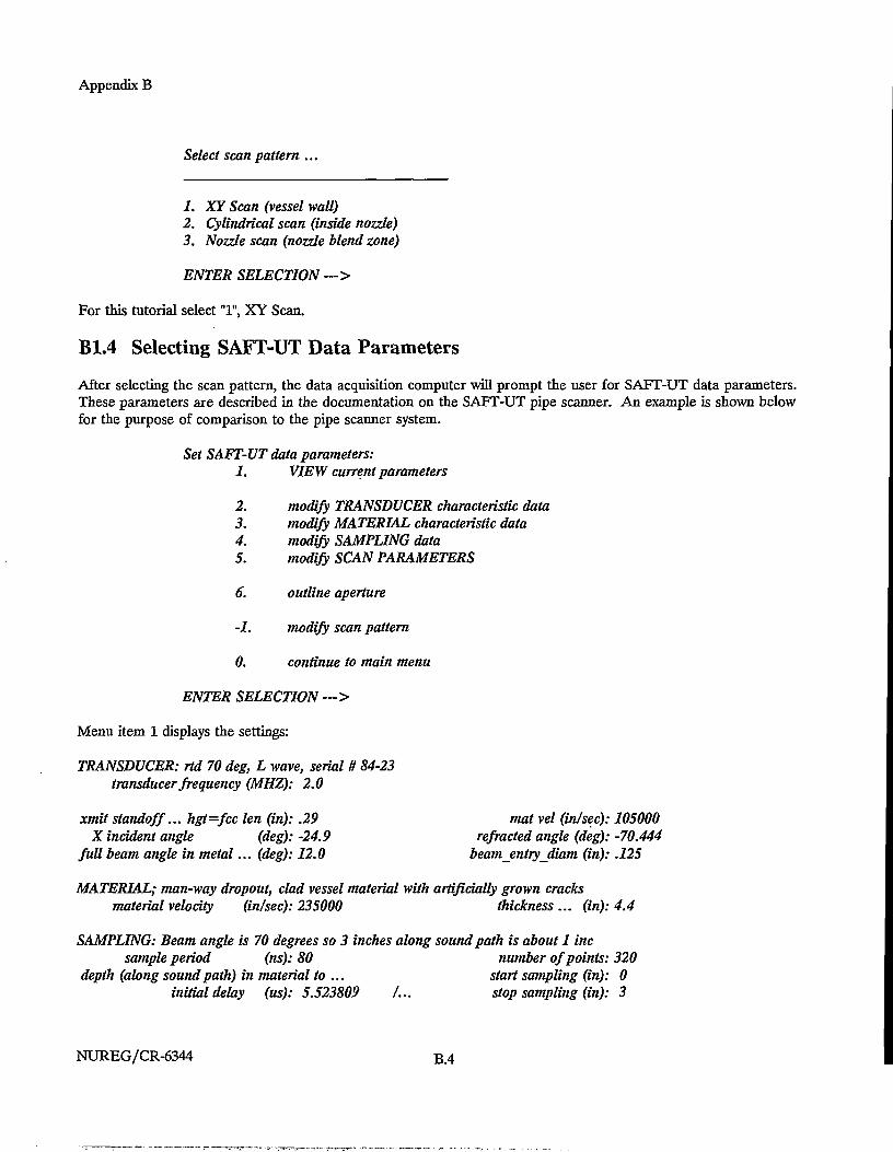
Appendix B
Select scan pattern ...
1. XY Scan (vessel wall)2. Cylindrical scan (inside nozzle)3. Nozzle scan (nozzle blend zone)
ENTER SELECTION —>
For this tutorial select "1", XY Scan.
B1.4 Selecting SAFT-UT Data Parameters
After selecting the scan pattern, the data acquisition computer will prompt the user for SAFT-UT data parameters.These parameters are described in the documentation on the SAFT-UT pipe scanner. An example is shown belowfor the purpose of comparison to the pipe scanner system.
Set SAFT-UT data parameters:1. VIEW current parameters
2. modify TRANSDUCER characteristic data3. modify MATERIAL characteristic data4. modify SAMPLING data
5. modify SCAN PARAMETERS
6. outline aperture
-1. modify scan pattern
0. continue to main menu
ENTER SELECTION—>
Menu item 1 displays the settings:TRANSDUCER: rtd 70 deg, L wave, serial # 84-23
transducer frequency (MHZ): 2.0
xmit standoff... hgt=fcc len (in): .29 mat vel (in/sec): 105000X incident angle (deg): -24.9 refracted angle (deg): -70.444
full beam angle in metal... (deg): 12.0 beamentrydiam (in): .125
MATERIAL; man-way dropout, clad vessel material with artificially grown cracksmaterial velocity (in/sec): 235000 thickness... (in): 4.4
SAMPLING: Beam angle is 70 degrees so 3 inches along sound path is about 1 incsample period (ns): 80 number of points: 320
depth (along sound path) in material to ... start sampling (in): 0initial delay (us): 5.523809 I... stop sampling (in): 3
NUREG/CR-6344 B.4
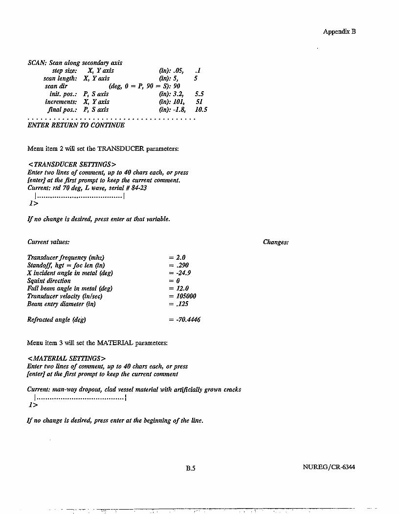
Appendix B
SCAN: Scan along secondary axisstep size: X, Y axis (in): .05, .1
scan length: X, Y axis (in): 5, 5scan dir (deg, 0 = P, 90 = S): 90
init. pos.: P, S axis (in): 3.2, 5.5increments: X, Y axis (in): 101, 51final pos.: P, S axis (in): -1.8, 10.5
ENTER RETURN TO CONTINUE
Menu item 2 will set the TRANSDUCER parameters:
<TRANSDUCER SETTINGS>Enter two lines of comment, up to 40 chars each, or press[enter] at the first prompt to keep the current comment.Current: rtd 70 deg, L wave, serial # 84-23
I I
If no change is desired, press enter at that variable.
Current values:
Transducer frequency (mhz)Standoff, hgt = foe len (in)X incident angle in metal (deg)Squint directionFull beam angle in metal (deg)Transducer velocity (in/sec)Beam entry diameter (in)
Refracted angle (deg)
Changes:
= 2.0= .290= -24.9= 0= 12.0= 105000= .125
= -70.4446
Menu item 3 will set the MATERIAL parameters:
< MATERIAL SETTINGS >Enter two lines of comment, up to 40 chars each, or press[enter] at the first prompt to keep the current comment
Current: man-way dropout, clad vessel material with artificially grown cracksI I
If no change is desired, press enter at the beginning of the line.
B.5 NUREG/CR-6344
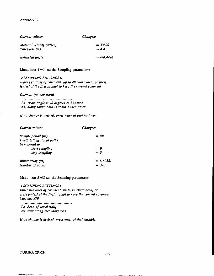
Appendix B
Current values: Changes:
Material velocity (in/sec) . = 23500Thickness (in) = 4.4
Refracted angle = -70.4446
Menu item 4 will set the Sampling parameters:
< SAMPLING SETTINGS >Enter two lines of comment, up to 40 chars each, or press[enter] at the first prompt to keep the current comment
Current: (no comment)i ii i
1 > Beam angle is 70 degrees so 3 inches2> along sound path is about I inch down
If no change is desired, press enter at that variable.
Current values: Changes:
Sample period (ns) = 80Depth (along sound path)in material to
start sampling = 0stop sampling = 3
Initial delay (us) = 5.52381Number of points = 320
Menu item 5 will set the Scanning parameters:
< SCANNING SETTINGS >Enter two lines of comment, up to 40 chars each, orpress [enter] at the first prompt to keep the current comment.Current: 270
1 > Scan of vessel wall,2> scan along secondary axis
If no change is desired, press enter at that variable.
NUREG/CR-6344 B.6
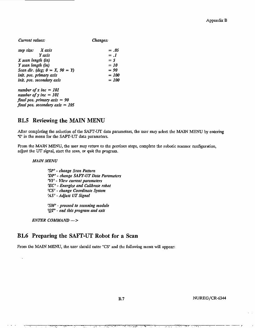
Appendix B
Current values:
step size: X axisY axis
X scan length (in)Y scan length (in)Scan dir. (deg; 0 = X, 90 = Y)init. pos. primary axisinit. pos. secondary axis
Changes:
= .05= .1= 5= 10= 90= 100= 100
number ofx inc = 101number o/y inc = 101final pos. primary axis = 90final pos. secondary axis = 105
B1.5 Reviewing the MAIN MENU
After completing the selection of the SAFT-UT data parameters, the user may select the MAIN MENU by entering"0" in the menu for the SAFT-UT data parameters.
From the MAIN MENU, the user may return to the previous steps, complete the robotic scanner configuration,adjust the UT signal, start the scan, or quit the program.
MAIN MENU
'SP' - change Scan Pattern'DP' - change SAFT-UT Data Parameters'VI' - View current parameters'EC - Energize and Calibrate robot'CS' - change Coordinate System'AS' - Adjust UT Signal
'SM' - proceed to scanning module'QT' - end this program and exit
ENTER COMMAND — >
B1.6 Preparing the SAFT-UT Robot for a Scan
From the MAIN MENU, the user should enter "CS" and the following menu will appear:
B.7 NUREG/CR-6344
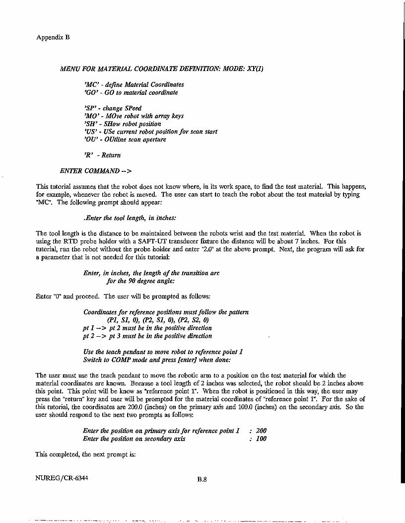
Appendix B
MENU FOR MATERIAL COORDINATE DEFINITION: MODE: XY(1)
'MC - define Material Coordinates'GO' - GO to material coordinate
'SP' - change SPeed'MO' - MOve robot with array keys'SH' - SHow robot position'US' - USe current robot position for scan start
'OU' - OUtline scan aperture
'R' -Return
ENTER COMMAND -->This tutorial assumes that the robot does not know where, in its work space, to find the test material. This happens,for example, whenever the robot is moved. The user can start to teach the robot about the test material by typing"MC". The following prompt should appear:
.Enter the tool length, in inches:
The tool length is the distance to be maintained between the robots wrist and the test material. When the robot isusing the RTD probe holder with a SAFT-UT transducer fixture the distance will be about 7 inches. For thistutorial, run the robot without the probe holder and enter "2.0" at the above prompt. Next, the program will ask fora parameter that is not needed for this tutorial:
Enter, in inches, the length of the transition arcfor the 90 degree angle:
Enter "0" and proceed. The user will be prompted as follows:
Coordinates for reference positions must follow the pattern(PI, SI, 0), (P2, SI, 0), (P2, S2, 0)
pt 1 --> pt 2 must be in the positive directionpt 2 ~> pt 3 must be in the positive direction
Use the teach pendant to move robot to reference point 1Switch to COMP mode and press [enter] when done:
The user must use the teach pendant to move the robotic arm to a position on the test material for which thematerial coordinates are known. Because a tool length of 2 inches was selected, the robot should be 2 inches abovethis point. This point will be know as "reference point 1". When the robot is positioned in this way, the user maypress the "return" key and user win be prompted for the material coordinates of "reference point 1". For the sake ofthis tutorial, the coordinates are 200.0 (inches) on the primary axis and 100.0 (inches) on the secondary axis. So theuser should respond to the next two prompts as follows:
Enter the position on primary axis for reference point 1 : 200Enter the position on secondary axis : 100
This completed, the next prompt is:
NUREG/CR-6344 B.8
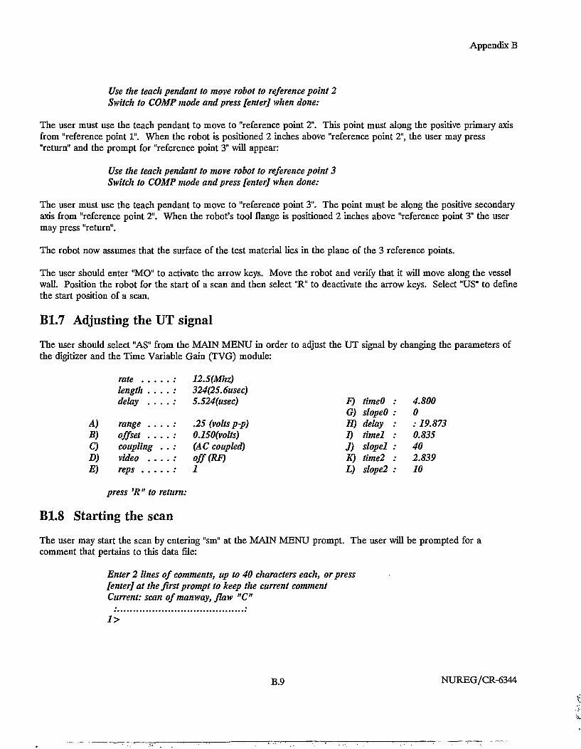
Appendix B
Use the teach pendant to move robot to reference point 2Switch to COMP mode and press [enter] when done:
The user must use the teach pendant to move to "reference point 2". This point must along the positive primary axisfrom "reference point 1". When the robot is positioned 2 inches above "reference point 2", the user may press"return" and the prompt for "reference point 3" will appear:
Use the teach pendant to move robot to reference point 3Switch to COMP mode and press [enter] when done:
The user must use the teach pendant to move to "reference point 3". The point must be along the positive secondaryaxis from "reference point 2". When the robot's tool flange is positioned 2 inches above "reference point 3" the usermay press "return".
The robot now assumes that the surface of the test material lies in the plane of the 3 reference points.
The user should enter "MO" to activate the arrow keys. Move the robot and verify that it will move along the vesselwall. Position the robot for the start of a scan and then select "R" to deactivate the arrow keys. Select "US" to definethe start position of a scan.
B1.7 Adjusting the UT signal
The user should select "AS" from the MAIN MENU in order to adjust the UT signal by changing the parameters ofthe digitizer and the Time Variable Gain (TVG) module:
rate : 12.5(Mhz)length . . . . : 324(25.6usec)delay . . . . : 5.524(usec)
A) range . . . . : .25 (volts p-p)B) offset : 0.150(volts)C) coupling . . : (AC coupled)D) video : off (RF)E) reps : 1
press 'R" to return:
B1.8 Starting the scan
The user may start the scan by entering "sm" at the MAIN MENU prompt. The user will be prompted for acomment that pertains to this data file:
Enter 2 lines of comments, up to 40 characters each, or press[enter] at the first prompt to keep the current commentCurrent: scan ofmanway, flaw "C"
F)G)H)I)J)K)L)
timeOslopeO .delaytimelslopeltime2slope2
• 4.800• 0
• : 19.873• 0.835• 40• 2.839• 10
1>
B.9 NUREG/CR-6344
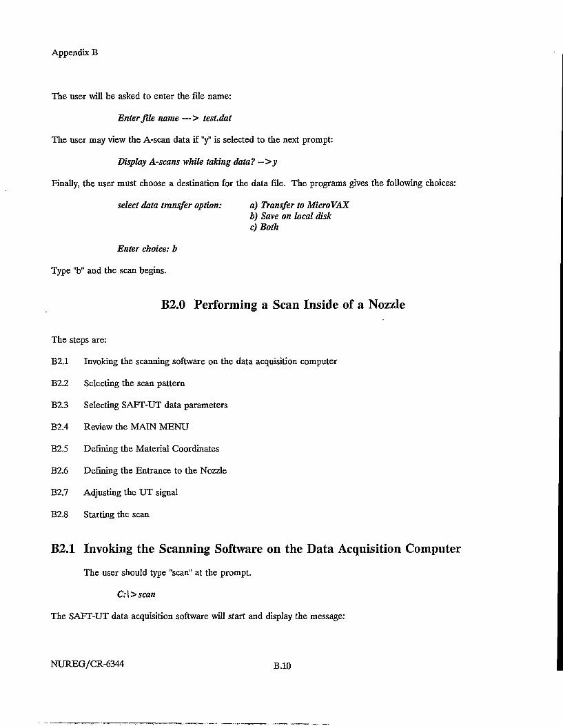
Appendix B
The user will be asked to enter the file name:
Enter file name —> test.dat
The user may view the A-scan data if "y" is selected to the next prompt:
Display A-scans while taking data? —>y
Finally, the user must choose a destination for the data file. The programs gives the following choices:
select data transfer option: a) Transfer to MicroVAXb) Save on local disk
c) Both
Enter choice: b
Type "b" and the scan begins.
B2.0 Performing a Scan Inside of a Nozzle
The steps are:
B2.1 Invoking the scanning software on the data acquisition computer
B2.2 Selecting the scan pattern
B2.3 Selecting SAFT-UT data parameters
B2.4 Review the MAIN MENU
B2.5 Defining the Material Coordinates
B2.6 Defining the Entrance to the Nozzle
B2.7 Adjusting the UT signal
B2.8 Starting the scan
B2.1 Invoking the Scanning Software on the Data Acquisition Computer
The user should type "scan" at the prompt.
C:\>scan
The SAFT-UT data acquisition software will start and display the message:
NUREG/CR-6344 B.10
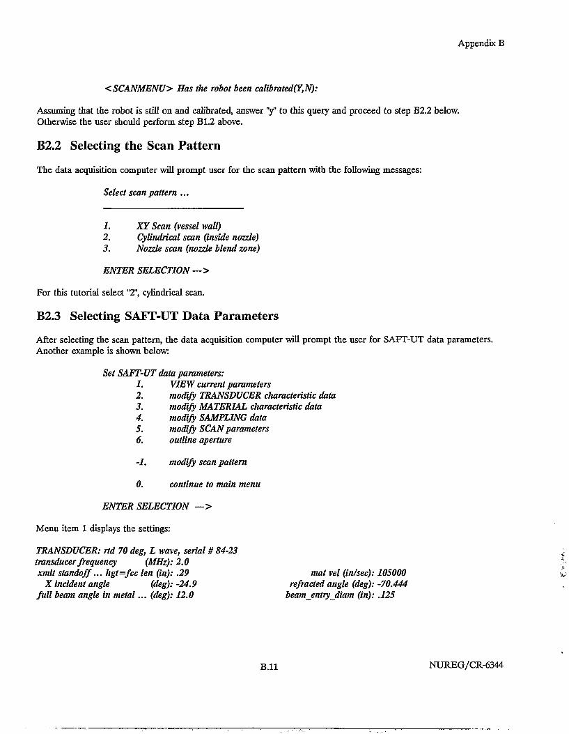
Appendix B
<SCANMENU> Has the robot been calibrated^,N):
Assuming that the robot is still on and calibrated, answer "y" to this query and proceed to step B2.2 below.Otherwise the user should perform step B1.2 above.
B2.2 Selecting the Scan Pattern
The data acquisition computer will prompt user for the scan pattern with the following messages:
Select scan pattern...
1. XY Scan (vessel wall)2. Cylindrical scan (inside nozzle)3. Nozzle scan (nozzle blend zone)
ENTER SELECTION --->
For this tutorial select "2", cylindrical scan.
B2.3 Selecting SAFT-UT Data Parameters
After selecting the scan pattern, the data acquisition computer will prompt the user for SAFT-UT data parameters.Another example is shown below:
Set SAFT-UT data parameters:1.2.3.4.5.6.
-1.
0.
VIEW current parametersmodify TRANSDUCER characteristic datamodify MATERIAL characteristic datamodify SAMPLING datamodify SCAN parametersoutline aperture
modify scan pattern
continue to main menu
ENTER SELECTION --->
Menu item 1 displays the settings:
TRANSDUCER: rtd 70 deg, L wave, serial # 84-23transducer frequency (MHz): 2.0xmit standoff... hgt=fcc len (in): .29 mat vel (in/sec): 105000
X incident angle (deg): -24.9 refracted angle (deg): -70.444full beam angle in metal... (deg): 12.0 beam_entry_diam (in): .125
B.11 NUREG/CR-6344
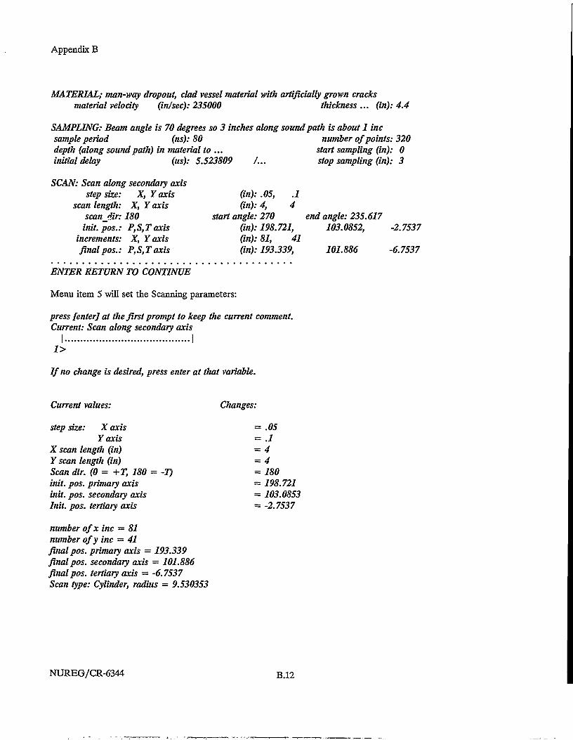
Appendix B
MATERIAL; man-way dropout, clad vessel material with artificially grown cracksmaterial velocity (in/sec): 235000 thickness... (in): 4.4
SAMPLING: Beam angle is 70 degrees so 3 inches along sound path is about 1 incsample period (ns): 80 number of points: 320depth (along sound path) in material to ... start sampling (in): 0initial delay (us): 5.523809 I... stop sampling (in): 3
SCAN: Scan along secondary axisstep size:
scan length:scanjfir:init. post-
increments:final pos.:
X, YaxisX, Yaxis
180P,S, TaxisX, Yaxis
P,S, Taxis
(in): .05, .1(in): 4, 4
start angle: 270(in): 198.721,(in): 81, 41(in): 193.339,
end angle: 235.617103.0852,
101.886
-2.7537
-6.7537
ENTER RETURN TO CONTINUE
Menu item 5 will set the Scanning parameters:
press [enter] at the first prompt to keep the current comment.Current: Scan along secondary axis
I !
If no change is desired, press enter at that variable.
Current values: Changes:
step size: X axis —.05Yaxis = .1
X scan length (in) = 4Y scan length (in) = 4Scan dir. (0 = +T, 180 = -T) = 180init. pos. primary axis = 198.721init. pos. secondary axis = 103.0853Init. pos. tertiary axis = -2.7537
number ofx inc = 81number ofy inc = 41final pos. primary axis = 193.339final pos. secondary axis = 101.886final pos. tertiary axis = -6.7537Scan type: Cylinder, radius = 9.530353
NUREG/CR-6344 B.12
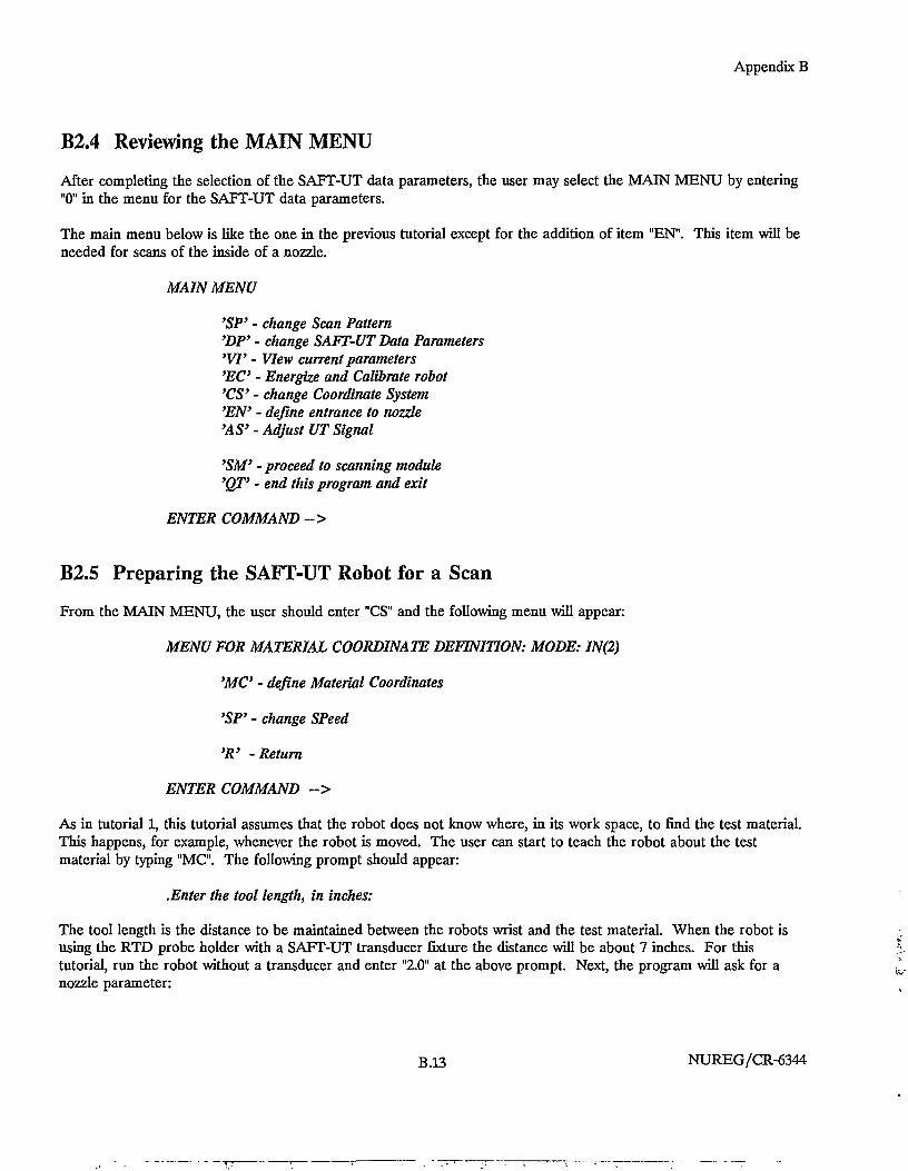
Appendix B
B2.4 Reviewing the MAIN MENU
After completing the selection of the SAFT-UT data parameters, the user may select the MAIN MENU by entering"0" in the menu for the SAFT-UT data parameters.
The main menu below is like the one in the previous tutorial except for the addition of item "EN". This item will beneeded for scans of the inside of a nozzle.
MAIN MENU
'SP' - change Scan Pattern'DP' - change SAFT-UT Data Parameters'VI' - View current parameters'EC - Energize and Calibrate robot'CS' - change Coordinate System'EN' - define entrance to nozzle'AS' - Adjust UT Signal
'SM' - proceed to scanning module'QT' - end this program and exit
ENTER COMMAND - >
B2.5 Preparing the SAFT-UT Robot for a Scan
From the MAIN MENU, the user should enter "CS" and the following menu will appear:
MENU FOR MATERIAL COORDINATE DEFINITION: MODE: IN(2)
'MC - define Material Coordinates
'SP' - change SPeed
'R' -Return
ENTER COMMAND ->
As in tutorial 1, this tutorial assumes that the robot does not know where, in its work space, to find the test material.This happens, for example, whenever the robot is moved. The user can start to teach the robot about the testmaterial by typing "MC". The following prompt should appear:
.Enter the tool length, in inches:
The tool length is the distance to be maintained between the robots wrist and the test material. When the robot isusing the RTD probe holder with a SAFT-UT transducer fixture the distance will be about 7 inches. For thistutorial, run the robot without a transducer and enter "2.0" at the above prompt. Next, the program will ask for anozzle parameter:
B.13 NUREG/CR-6344
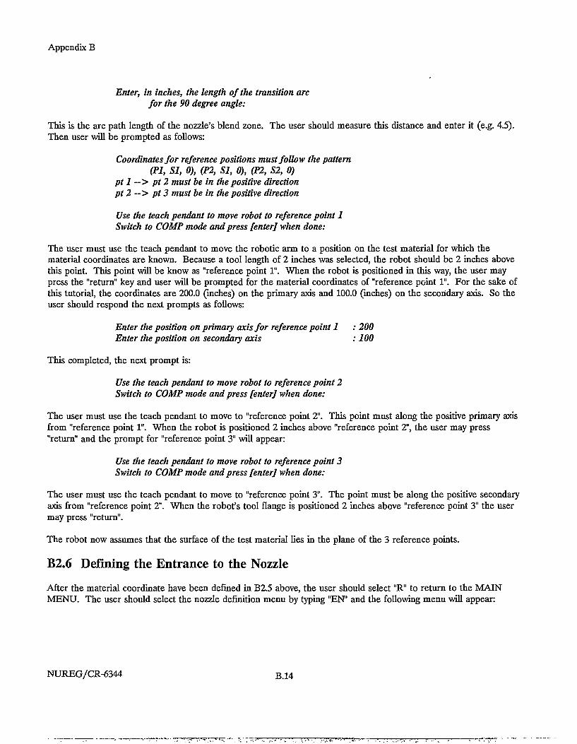
Appendix B
Enter, in inches, the length of the transition arcfor the 90 degree angle:
This is the arc path length of the nozzle's blend zone. The user should measure this distance and enter it (e.g. 4.5).Then user will be prompted as follows:
Coordinates for reference positions must follow the pattern(PI, SI, 0), (P2, SI, 0), (P2, S2, 0)
pt 1 — > pt 2 must be in the positive directionpt 2 --> pt 3 must be in the positive direction
Use the teach pendant to move robot to reference point 1Switch to COMP mode and press [enter] when done:
The user must use the teach pendant to move the robotic arm to a position on the test material for which thematerial coordinates are known. Because a tool length of 2 inches was selected, the robot should be 2 inches abovethis point. This point will be know as "reference point 1". When the robot is positioned in this way, the user maypress the "return" key and user will be prompted for the material coordinates of "reference point 1". For the sake ofthis tutorial, the coordinates are 200.0 (inches) on the primary axis and 100.0 (inches) on the secondary axis. So theuser should respond the next prompts as follows:
Enter the position on primary axis for reference point 1 : 200Enter the position on secondary axis : 100
This completed, the next prompt is:
Use the teach pendant to move robot to reference point 2Switch to COMP mode and press [enter] when done:
The user must use the teach pendant to move to "reference point 2". This point must along the positive primary axisfrom "reference point 1". When the robot is positioned 2 inches above "reference point 2", the user may press"return" and the prompt for "reference point 3" will appear:
Use the teach pendant to move robot to reference point 3Switch to COMP mode and press [enter] when done:
The user must use the teach pendant to move to "reference point 3". The point must be along the positive secondaryaxis from "reference point 2". When the robot's tool flange is positioned 2 inches above "reference point 3" the usermay press "return".
The robot now assumes that the surface of the test material lies in the plane of the 3 reference points.
B2.6 Defining the Entrance to the Nozzle
After the material coordinate have been defined in B2.5 above, the user should select "R" to return to the MAINMENU. The user should select the nozzle definition menu by typing "EN" and the following menu will appear:
NUREG/CR-6344 B.14
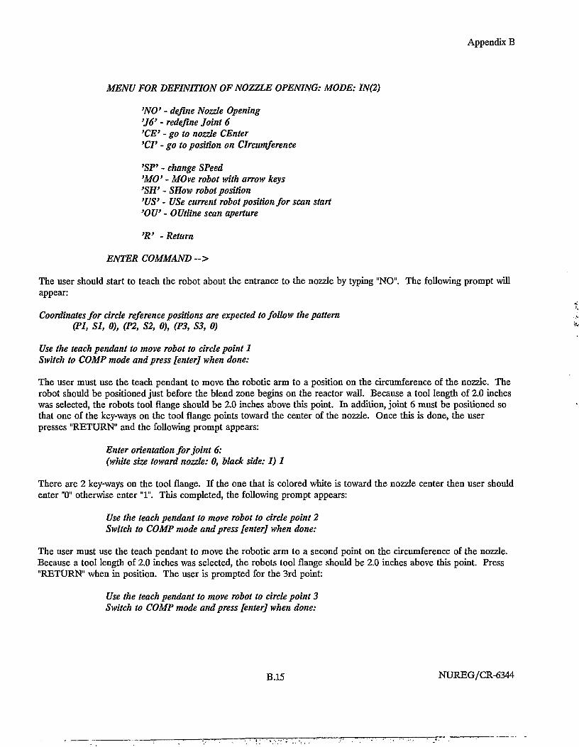
Appendix B
MENU FOR DEFINITION OF NOZZLE OPENING: MODE: IN(2)
'NO' - define Nozzle Opening'J6' - redefine Joint 6'CE' - go to nozzle CEnter'CI' - go to position on Circumference
'SP' - change SPeed'MO' - MOve robot with arrow keys'SH' - SHow robot position'US' - USe current robot position for scan start'OU' - Outline scan aperture
'R' -Return
ENTER COMMAND -->
The user should start to teach the robot about the entrance to the nozzle by typing "NO". The following prompt willappear:
Coordinates for circle reference positions are expected to follow the pattern(PI, SI, 0), (P2, S2, 0), (P3, S3, 0)
Use the teach pendant to move robot to circle point 1Switch to COMP mode and press [enter] when done:
The user must use the teach pendant to move the robotic arm to a position on the circumference of the nozzle. Therobot should be positioned just before the blend zone begins on the reactor wall. Because a tool length of 2.0 incheswas selected, the robots tool flange should be 2.0 inches above this point. In addition, joint 6 must be positioned sothat one of the key-ways on the tool flange points toward the center of the nozzle. Once this is done, the userpresses "RETURN" and the following prompt appears:
Enter orientation for joint 6:(white size toward nozzle: 0, black side: I) I
There are 2 key-ways on the tool flange. If the one that is colored white is toward the nozzle center then user shouldenter "0" otherwise enter "1". This completed, the following prompt appears:
Use the teach pendant to move robot to circle point 2Switch to COMP mode and press [enter] when done:
The user must use the teach pendant to move the robotic arm to a second point on the circumference of the nozzle.Because a tool length of 2.0 inches was selected, the robots tool flange should be 2.0 inches above this point. Press"RETURN" when in position. The user is prompted for the 3rd point:
Use the teach pendant to move robot to circle point 3Switch to COMP mode and press [enter] when done:
B.15 NUREG/CR-6344
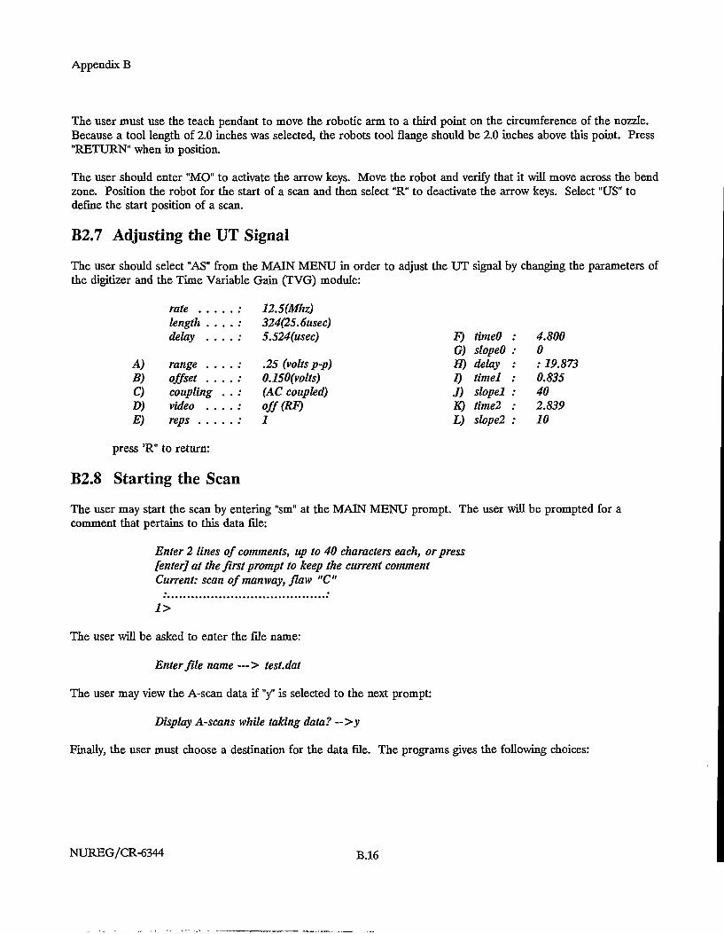
Appendix B
The user must use the teach pendant to move the robotic arm to a third point on the circumference of the nozzle.Because a tool length of 2.0 inches was selected, the robots tool flange should be 2.0 inches above this point. Press"RETURN" when in position.
The user should enter "MO" to activate the arrow keys. Move the robot and verify that it will move across the bendzone. Position the robot for the start of a scan and then select "R" to deactivate the arrow keys. Select "US" todefine the start position of a scan.
B2.7 Adjusting the UT Signal
The user should select "AS" from the MAIN MENU in order to adjust the UT signal by changing the parameters ofthe digitizer and the Time Variable Gain (TVG) module:
rate : 12.5(Mhz)length . . . . : 324(25.6usec)delay . . . . : 5.524(usec)
A) range . . . . : .25 (volts p-p)B) offset . . . . : 0.150(volts)C) coupling . . : (AC coupled)D) video . . . . : off(RF)E) reps : 1
press 'R" to return:
B2.8 Starting the Scan
The user may start the scan by entering "sm" at the MAIN MENU prompt. The user will be prompted for acomment that pertains to this data file:
Enter 2 lines of comments, up to 40 characters each, or press[enter] at the first prompt to keep the current commentCurrent: scan ofmanway, flaw "C"
F)G)H)DJ)K)L)
timeuslopeO .delaytimel .slopeltime2 .slope2
• 4.800• 0
: 19.873• 0.835• 40• 2.839• 10
The user will be asked to enter the file name:
Enter file name — > test.dat
The user may view the A-scan data if "y" is selected to the next prompt:
Display A-scans while taking data? —>y
Finally, the user must choose a destination for the data file. The programs gives the following choices:
NUREG/CR-6344 B . 1 6
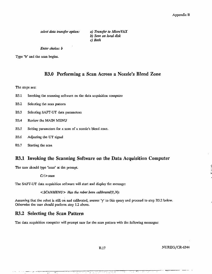
Appendix B
select data transfer option: a) Transfer to MicroVAXb) Save on local diskc) Both
Enter choice: b
Type "b" and the scan begins.
B3.0 Performing a Scan Across a Nozzle's Blend Zone
The steps are:
B3.1 Invoking the scanning software on the data acquisition computer
B3.2 Selecting the scan pattern
B3.3 Selecting SAFT-UT data parameters
B3.4 Review the MAIN MENU
B3.5 Setting parameters for a scan of a nozzle's blend zone.
B3.6 Adjusting the UT signal
B3.7 Starting the scan
B3.1 Invoking the Scanning Software on the Data Acquisition Computer
The user should type "scan" at the prompt.
C:\>scan
The SAFT-UT data acquisition software will start and display the message:
<SCANMENU> Has the robot been calibrated^,N):
Assuming that the robot is still on and calibrated, answer "y" to this query and proceed to step B3.2 below.Otherwise the user should perform step 1.2 above.
B3.2 Selecting the Scan Pattern
The data acquisition computer will prompt user for the scan pattern with the following messages:
B.17 NUREG/CR-6344
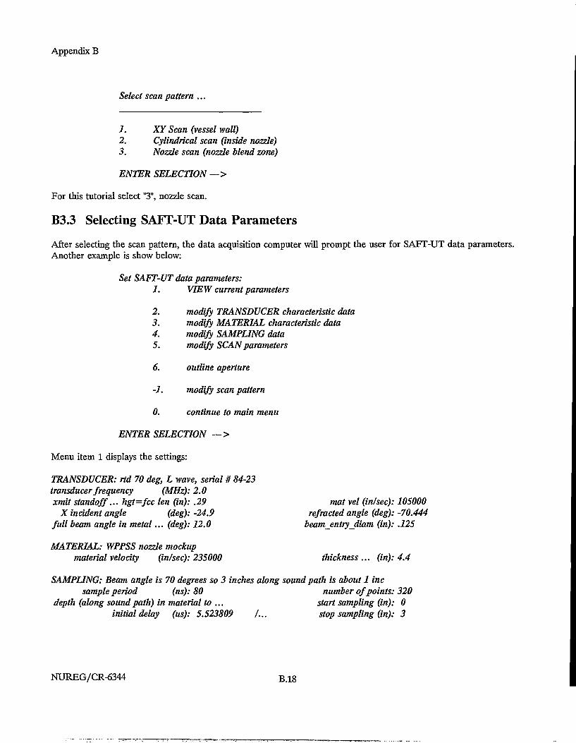
Appendix B
Select scan pattern ...
1. XY Scan (vessel wall)2. Cylindrical scan (inside nozzle)3. Nozzle scan (nozzle blend zone)
ENTER SELECTION — >
For this tutorial select "3", nozzle scan.
B3.3 Selecting SAFT-UT Data Parameters
After selecting the scan pattern, the data acquisition computer will prompt the user for SAFT-UT data parameters.Another example is show below:
Set SAFT-UT data parameters:1. VIEW current parameters
2. modify TRANSDUCER characteristic data3. modify MATERIAL characteristic data4. modify SAMPLING data
5. modify SCAN parameters
6. outline aperture
-1. modify scan pattern
0. continue to main menu
ENTER SELECTION — >
Menu item 1 displays the settings:TRANSDUCER: rtd 70 deg, L wave, serial # 84-23transducer frequency (MHz): 2.0xmit standoff... hgt=fcc len (in): .29 mat vel (in/sec): 105000
X incident angle (deg): -24.9 refracted angle (deg): -70.444full beam angle in metal... (deg): 12.0 beam_entry_diam (in): .125
MATERIAL: WPPSS nozzle mockupmaterial velocity (in/sec): 235000 thickness... (in): 4.4
SAMPLING: Beam angle is 70 degrees so 3 inches along sound path is about 1 incsample period (ns): 80 number of points: 320
depth (along sound path) in material to ... start sampling (in): 0initial delay (us): 5.523809 I... stop sampling (in): 3
NUREG/CR-6344 B.18
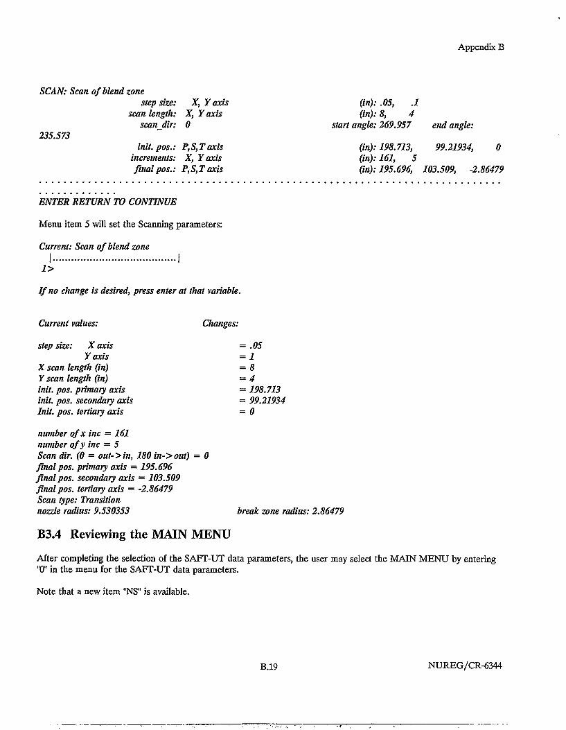
Appendix B
SCAN: Scan of blend zonestep size: X, Y axis (in): .05, .1
scan length: X, Y axis (in): 8, 4scan_dir: 0 start angle: 269.957 end angle:
235.573init.pos.: P,S,Taxis (in): 198.713, 99.21934, 0
increments: X, Y axis (in): 161, 5finalpos.: P,S,Taxis (in): 195.696, 103.509, -2.86479
ENTER RETURN TO CONTINUE
Menu item 5 will set the Scanning parameters:
Current: Scan of blend zone
I I
If no change is desired, press enter at that variable.
Current values: Changes:
step size: X axis =.05Yaxis =1
X scan length (in) = 8Y scan length (in) = 4init. pos. primary axis = 198.713init. pos. secondary axis = 99.21934Init. pos. tertiary axis = 0
number ofx inc = 161number ofy inc = 5Scan dir. (0 = out->in, 180 in->out) = 0final pos. primary axis = 195.696final pos. secondary axis = 103.509final pos. tertiary axis = -2.86479Scan type: Transitionnozzle radius: 9.530353
B3.4 Reviewing the MAIN MENU
break zone radius: 2.86479
After completing the selection of the SAFT-UT data parameters, the user may select the MAIN MENU by entering"0" in the menu for the SAFT-UT data parameters.
Note that a new item "NS" is available.
B.19 NUREG/CR-6344
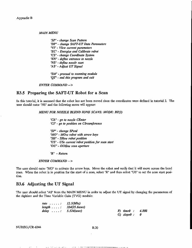
Appendix B
MAIN MENU
'SP' - change Scan Pattern'DP' - change SAFT-UT Data Parameters'VI' - View current parameters'EC - Energize and Calibrate robot'CS' - change Coordinate System'EN' - define entrance to nozzle'NS' - define nozzle scan'AS'- Adjust UT Signal
'SM' -proceed to scanning module'QT' - end this program and exit
ENTER COMMAND ->
B3.5 Preparing the SAFT-UT Robot for a Scan
In this tutorial, it is assumed that the robot has not been moved since the coordinates were defined in tutorial 2. Theuser should enter "NS" and the following menu will appear:
MENU FOR NOZZLE BLEND ZONE SCANS: MODE: BZ(3)
'CE' - go to nozzle CEnter'CI' - go to position on Circumference
'SP' - change SPeed'MO' - MOve robot with arrow keys'SH' - SHow robot position'US' - USe current robot position for scan start
'OU' - OUtline scan aperture
'R' -Return
ENTER COMMAND - >The user should enter "MO" to activate the arrow keys. Move the robot and verify that it will move across the bendzone. When the robot is in position for the start of a scan, select "R" and then select "US" to set the scan start posi-tion.
B3.6 Adjusting the UT Signal
The user should select "AS" from the MAIN MENU in order to adjust the UT signal by changing the parameters ofthe digitizer and the Time Variable Gain (TVG) module:
rate : 12.5(Mhz)length . . . . : 324(25.6usec)delay . . . . : 5.524(usec) F) timeO : 4.800
G) sloped : 0
NUREG/CR-6344 B.20
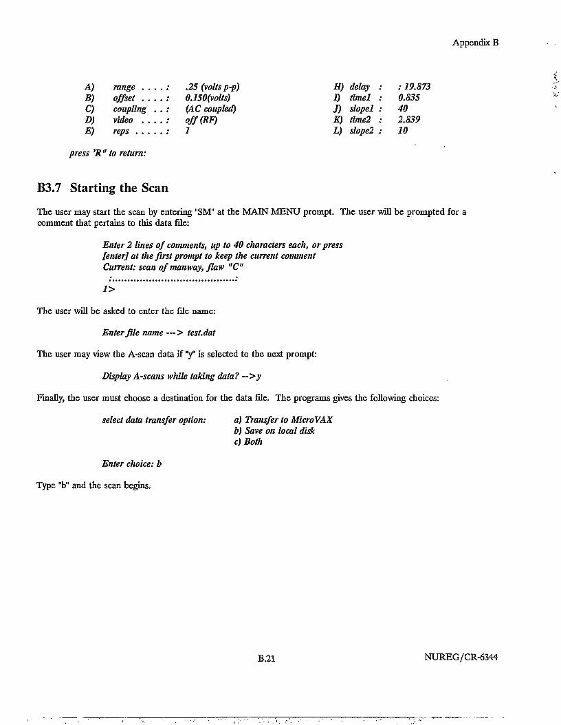
Appendix B
A) range . . . . : .25 (volts p-p) H) delay : : 1B) offset ; 0.150(volts) I) timel : 0.835C) coupling . . : (AC coupled) J) slopel : 40D) video : off(RF) K) time2 : 2.839E) reps : 1 L) slope2 : 10
press 'R" to return:
B3.7 Starting the Scan
The user may start the scan by entering "SM" at the MAIN MENU prompt. The user will be prompted for acomment that pertains to this data file:
Enter 2 lines of comments, up to 40 characters each, or press[enter] at the first prompt to keep the current commentCurrent: scan ofmanway, flaw "C"
The user will be asked to enter the file name:
Enter file name —> test.dat
The user may view the A-scan data if "y" is selected to the next prompt:
Display A-scans while taking data? —>y
Finally, the user must choose a destination for the data file. The programs gives the following choices:
select data transfer option: a) Transfer to MicroVAXb) Save on local disk
c) Both
Enter choice: b
Type "b" and the scan begins.
B.21 NUREG/CR-6344
Appendix C
Changes to the SAFT Header
NUREG/CR-6344
Appendix C
Changes to the SAFT Header
1) All fields are now represented as ASCII charac-ters. By way of example, in the old header,'vel_in_material' was a floating point number andas such required 4 bytes of header space. In thenew header, this is an ASCII character stringrepresentation of the floating point number and assuch requires 17 bytes. This change will make theSAFT data files portable to any computer.
2) The header size has been increased from 512bytes to 2048 bytes.
3) All unused fields have been deleted. They are:
num_sig_sumfocal_lengthpm_dampingpm_energypm_attenuationpm_gainlc_attenuationpipe_radiussm_flagpipe_flagsm_depthproc_modetransybandwidth
4) All header fields have been reorganized into oneof the following categories:
FILE_PROPERTIESTRANSDUCERPROPERTIESMATERIALPROPERTffiSSAMPLING_PROPERTIESSCANNING_PROPERTIESPROCESSINGPROPERTIES
5) Changes to FILE PROPERTIES
5.1) Added file_format_id. This is a flag that indicateswhat (header) format the file has.
6) Changes to TRANSDUCER PROPERTIES
6.1) Added transducer_comment.6.2) Renamed hgt_transd to recv_hgt_transd and
changed units to inches (from equivalent waterpath).
6.3) Changed units of xmit_hgt_transd to inches.6.4) Renamed beam_angle to beam_width_angle.6.5) Changed units of squint_dir to 0-360.0 degrees
(floating point) from x=0; and y=l.6.6) Renamed squint_angle to incident_angle and
changed units to shoe degrees (from equivalentwater angle).
7) Changes to MATERIAL PROPERTIES
7.1) Added material_comment.
7.2) Added refracted_angle.
8) Changes to SAMPLING PROPERTIES
8.1) Added sampling_comment.8.2) Changed delay_inc to floating point number.8.3) Deleted float_delay_increment.8.4) Changed init_delay to floating point number.9) Changes to SCANNING PROPERTIES
9.1) Added scanning_comment.9.2) Renamed scan_axis to scan_direction and changed
unit to 0-360.0 degrees (from xl,x2,y).9.3) Renamed init_x_pos to initjpos_primary_axis,
changed to floating point, and changed units toinches.
9.4) Added final_jposjprimary_axis.9.5) Renamed init_jjpos to init_pos_secondary_axis.9.6) Renamed final_y_pos to final_pos_secondary_axis.
10) Changes to PROCESSING PROPERTIES
10.1) Added processing_comment.
C.1 NUREG/CR-6344
Appendix D
Definition of SAFT-UT ASCII Header
NUREG/CR-6344
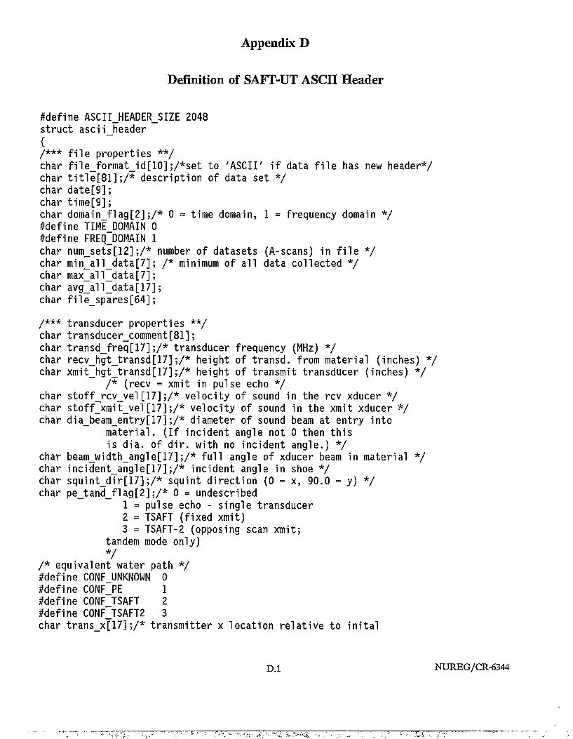
Appendix D
Definition of SAFT-UT ASCII Header
#define ASCII_HEADER_SIZE 2048struct ascii_header{/*** file properties **/char file_format_id[10];/*set to 'ASCII' if data file has new header*/char title[81];/* description of data set */char date[9];char time[9];char domain_flag[2];/* 0 = time domain, 1 = frequency domain */#define TIME_DOMAIN 0#define FREQ_DOMAIN 1char num_sets[12];/* number of datasets (A-scans) in file */char min_all_data[7]; /* minimum of all data collected */char max_all_data[7];char avg_all_data[17];char fi1e_spares[64];
/*** transducer properties **/char transducer_comment[81];char transd_freq[17];/* transducer frequency (MHz) */char recv_hgt_transd[17];/* height of transd. from material (inches) */char xmit_hgt_transd[17];/* height of transmit transducer (inches) */
/* (recv = xmit in pulse echo */char stoff_rcv_vel[17];/* velocity of sound in the rev xducer */char stoff_xmit_vel[17];/* velocity of sound in the xmit xducer */char dia_beam_entry[17];/* diameter of sound beam at entry into
material. (If incident angle not 0 then thisis dia. of dir. with no incident angle.) */
char beam_width_angle[17];/* full angle of xducer beam in material */char incident_angle[17];/* incident angle in shoe */char squint_dir[17];/* squint direction (0 = x, 90.0 = y) */char pe_tand_flag[2];/* 0 = undescribed
1 = pulse echo - single transducer2 = TSAFT (fixed xmit)3 = TSAFT-2 (opposing scan xmit;
tandem mode only)V
/* equivalent water path */#define CONFJJNKNOWN 0#define CONF_PE 1#define CONFJTSAFT 2#define CONF_TSAFT2 3char trans_x[17];/* transmitter x location relative to inital
D.I NUREG/CR-6344
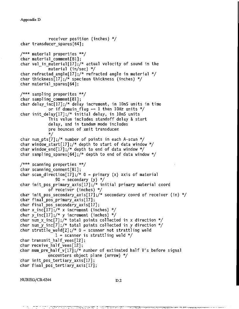
Appendix D
receiver position (inches) */char transducer_spares[64];
/*** material properties **/char material_comment[81];char ve"I_in_material [17];/* actual velocity of sound in the
material (in/sec) */char refracted_angle[17];/* refracted angle in material */char thickness[17];/* specimen thickness (inches) */char material_spares[64];
/*** sampling properites **/char sampling_comment[81];char delay_inc[17];/* delay increment, in lOnS units in time
or if domain_flag == 1 then lOHz units */char init_delay[17];/* initial delay, in lOnS units
This value includes standoff delay & startdelay, and in tandem mode includespre bounces of xmit transducerV
char num_pts[7];/* number of points in each A-scan */char window_start[17];/* depth to start of data window */char window_end[17];/* depth to end of data window */char sampling_spares[64];/* depth to end of data window */
/*** scanning properties **/char scanning_comment[81];char scan_direction[17];/* 0 = primary (x) axis of material
90 = secondary (y) */char init_pos_primary_axis[17];/* initial primary material coord
of receiver (inches) */char init_pos_secondary_axis[17];/* secondary coord of receiver (in) */char final_pos_primary_axis[17];char final_pos_secondary_axis[17];char x_inc[17];/* x increment (inches) */char y_inc[17];/* y increment (inches) */char num_x_inc[7];/* total points collected in x direction */char num_y_inc[7];/* total points collected in y direction */char strattle_weld[2];/* 0 = scanner not strattling weld
1 = scanner is strattling weld */char transmit_half_vees[12];char receive_half_vees[12];char num_pre_half_v[17];/* number of extimated half V's before signal
encounters object plane (arrow) */char init_pos_tertiary_axis[17];char final_pos_tertiary_axis[17];
NUREG/CR-6344 D.2
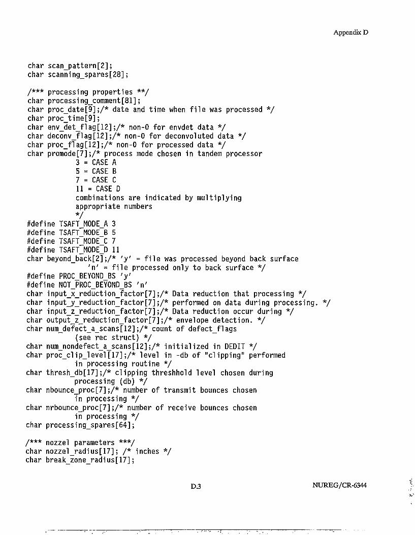
Appendix D
char scan_pattern[2];char scanning_spares[28];
/*** processing properties **/char processing_comment[81];char proc_date[9];/* date and time when file was processed */char proc_time[9];char env_det_flag[12];/* non-0 for envdet data */char deconv_flag[12];/* non-0 for deconvolved data */char proc_flag[12];/* non-0 for processed data */char promode[7];/* process mode chosen in tandem processor
3 = CASE A5 = CASE B7 = CASE C11 = CASE Dcombinations are indicated by multiplyingappropriate numbers*/
#define TSAFT_MODE_A 3#define TSAFT_MODE_B 5#define TSAFT_MODE_C 7#define TSAFT_MODE_D 11char beyond_back[2];/* 'y' = file was processed beyond back surface
'n' = file processed only to back surface */#define PROC_BEYOND_BS 'y'#define NOT_PROC_BEYOND_BS 'n'char input_x_reduction_factor[7];/* Data reduction that processing */char input_y_reduction_factor[7];/* performed on data during processing. */char input_z_reduction_factor[7];/* Data reduction occur during */char output_z_reduction_factor[7];/* envelope detection. */char num_defect_a_scans[12];/* count of defect_flags
(see rec struct) */char num_nondefect_a_scans[12];/* initialized in DEDIT */char proc_clip_level[17];/* level in -db of "clipping" performed
in processing routine */char thresh_db[17];/* clipping threshhold level chosen during
processing (db) */char nbounce_proc[7];/* number of transmit bounces chosen
in processing */char nrbounce_proc[7];/* number of receive bounces chosen
in processing */char processing_spares[64];
/*** nozzel parameters ***/char nozzel_radius[17]; /* inches */char break_zone_radius[17];
D.3 NUREG/CR-6344
Appendix D
char nozze!_center_primary[17];char nozzel_center_secondary[17];
char asci i_header_spares[2048-1648];} ah;
NUREG/CR-6344 D.4
NUREG/CR-6344PNL-10571
R5
DISTRIBUTION
No. ofCopies
J. MuscaraNRC/RESMail Stop T-10E10
D. NaujockNRC/NRRMail Stop 7 D4
J. StrosniderNRC/NRRMail Stop 7 D4
E. J. Sullivan, Jr.NRC/RESMail Stop 7 E23
M. VaginsNRC/RESMail Stop NS 217
E. H. GrayNRC/Region I
R. H. HarrisNRC/Region I
M. C. ModesNRC/Region I
P. M. PetersonNRC/Region I
A. R. HerdtNRC/Region II
J. J. BlakeNRC/Region II
J. JacobsonNRC/Region III
L. J. BusseTetrad Corporation12741 E. Caley AvenueUnit 126Englewood, CO 80111
S. L. Crawford1308 Brookwood Ave.Richland, WA 99352
R. A. HewesGeneral Electric CompanyBuilding KW, Room D243PO Box 8Schenectady, NY 12301
D. S. KuppermanMaterials Science CenterArgonne National Laboratory9700 S. Cass AvenueBuilding 212Argonne, IL 60439
J. LaReauABB Amdata1000 Prospect Hill RoadWindsor, CT 06095-0500
C. LittleNondestructive Testing
Technology DivisionSandia National LaboratoriesAlbuquerque, NM 87185
L. E. MullinsKnolls Atomic Power LaboratoryPO Box 1072Schenectady, N Y 12301-1072
Distr.l NUREG/CR-6344
Distribution
W. W. ShurtleffNondestructive Testing
Technology DivisionSandia National LaboratoriesAlbuquerque, NM 87185
J. H. TehruneGeneral Electric Company175 Curtner AvenueSan Jose, CA 95125
FOREIGN
S. CrutzenJoint Research CentrePO Box 21755 ZG PettenThe Netherlands
K. KussmaulMaterialpruefungsanstaltUniversitat StuttgartPfaffenwaldring 327000 Stuttgart 80 (Vaihingen)West Germany
A. RogersonAEA TechnologyRisleyWarringtonCheshire WA3 6ATUnited Kingdom
V. SchmitzIzfpUniversitat, Gerbaude 376600 Saarbrucken 11West Germany
J. R. TomlinsonNDT Application CentreNuclear Electric picTimpson RoadWythenshaweManchester M23 9LLUnited Kingdom
ONSITE
50 Pacific Northwest Laboratory
R. E. BoweyD. M. BoydS. H. BushA. A. DiazS. R. Doctor (36)T. E. HallR. V. HarrisL. D. ReidG. J. SchusterPublishing CoordinationTechnical Report Files (5)
NUREG/CR-6344 Distr.2
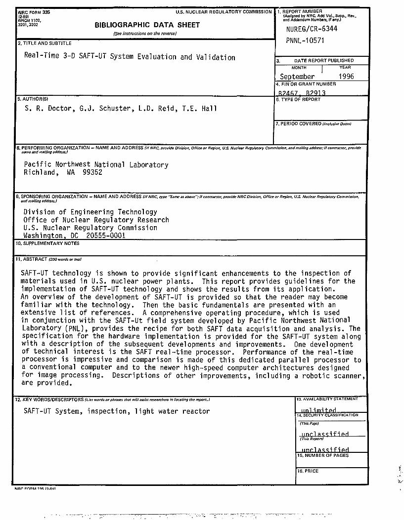
NRC FORM 335 U.S. NUCLEAR REGULATORY COMMISSION12-89)
» S ? BIBLIOGRAPHIC DATA SHEET(See instructions on the reverse)
2. TITLE AND SUBTITLE
Real-Time 3-D SAFT-UT System Evaluation and Validation
5. AUTHOR (S)
S. R. Doctor , G.J . Schuster , L.D. Re id , T .E . Hal l
1. REPORT NUMBER(Assigned by NRC. Add Vol., Supp., Rev.,and Addendum Numbers, If any.)
NUREG/CR-6344
PNNL-10571
3. DATE REPORT PUBLISHED
MONTH 1 YEAR
September 19964. FIN OR GRANT NUMBER
R?dfi7, R?Q136. TYPE OF REPORT
7. PERIOD COVERED (Inclusive Dates!
8, PERFORMING ORGANIZATION - NAME AND ADDRESS (If NRC, provide Division, Office or Region, U.S. Nuclear Regulatory Commission, and mailing address: if contractor, providename and mailing address.)
Pacific Northwest National LaboratoryRichland, WA 99352
9. SPONSORING ORGANIZATION - NAME AND ADDRESS (If NRC. type "Same as above"; if contractor, provide NRC Division. Office or Region. U.S. Nuclear Regulatory Commission,and mailing address.)
Division of Engineering TechnologyOffice of Nuclear Regulatory ResearchU.S. Nuclear Regulatory CommissionWashinqton, DC 20555-0001
10. SUPPLEMENTARY NOTES
11 . ABSTRACT (200 words or less)
SAFT-UT technology is shown to provide signif icant enhancements to the inspection ofmaterials used in U.S. nuclear power plants. This report provides guidelines for theimplementation of SAFT-UT technology and shows the results from i t s application.An overview of the development of SAFT-UT is provided so that the reader may becomefamiliar with the technology. Then the basic fundamentals are presented with anextensive l i s t of references. A comprehensive operating procedure, which is usedin conjunction with the SAFT-Ut f i e ld system developed by Pacific Northwest NationalLaboratory (PNL), provides the recipe for both SAFT data acquisition and analysis. Thespecification for the hardware implementation is provided for the SAFT-UT system alongwith a description of the subsequent developments and improvements. One developmentof technical interest is the SAFT real-time processor. Performance of the real-timeprocessor is impressive and comparison is made of this dedicated parallel processor toa conventional computer and to the newer high-speed computer architectures designedfor image processing. Descriptions of other improvements, including a robotic scanner,are provided.
12, KEY WORDS/DESCRIPTORS (List words or phrases that will assist researchers in locating the report.)
SAFT-UT System, inspection, l igh t water reactor
13. AVAILABILITY STATEMENT
nniinrn tpH14. SECURITY CLASSIFICATION
(This Page)
u p r l a<;<;Tf I P H(This Report)
nnrl a«;«;if ipH15. NUMBER OF PAGES
16. PRICE
Nflr CflOM I IS I9.BQI