re vie w - cepal
TRANSCRIPT

Rev
iew
economic commission foR
Latin ameRicaand the caRibbean


Rev
iew
economic commission foR
Latin ameRicaand the caRibbean
Osvaldo SunkelChairman of the Editorial Board
André HofmanDirector
Miguel TorresTechnical Editor
issn 0251-2920
105NO
DECEMBER • 2011
Alicia BárcenaExecutive Secretary
Antonio PradoDeputy Executive Secretary
The cepal Review was founded in 1976, along with the corresponding Spanish version, Revista de la cepal, and is published three times a year by the United Nations Economic Commission for Latin America and the Caribbean, which has its headquarters in Santiago, Chile. The Review, however, has full editorial independence and follows the usual academic procedures and criteria, including the review of articles by independent external referees. The purpose of the Review is to contribute to the discussion of socio-economic development issues in the region by offering analytical and policy approaches and articles by economists and other social scientists working both within and outside the United Nations. The Review is distributed to universities, research institutes and other international organizations, as well as to individual subscribers.
The opinions expressed in the signed articles are those of the authors and do not necessarily reflect the views of the organization. The designations employed and the way in which data are presented do not imply the expression of any opinion whatsoever on the part of the secretariat concerning the legal status of any country, territory, city or area or its authorities, or concerning the delimitation of its frontiers or boundaries.
A subscription to the cepal Review in Spanish costs US$ 30 for one year (three issues) and US$ 50 for two years. A subscription to the English version costs US$ 35 or US$ 60, respectively. The price of a single issue in either Spanish or English is US$ 15, including postage and handling.
The complete text of the Review can also be downloaded free of charge from the eclac web site (www.cepal.org).
United Nations publicationISSN 0251-2920ISBN 978-92-1-221058-2e-ISBN 978-92-1-1055359-9LC/G.2508-PCopyright © United Nations, December 2011. All rights reserved.Printed in Santiago, Chile
Requests for authorization to reproduce this work in whole or in part should be sent to the Secretary of the Publications Board. Member States and their governmental institutions may reproduce this work without prior authorization, but are requested to mention the source and to inform the United Nations of such reproduction. In all cases, the United Nations remains the owner of the copyright and should be identified as such in reproductions with the expression “© United Nations 2008” (or other year as appropriate).
This publication, entitled the cepal Review, is covered in the Social Sciences Citation Index (ssci), published by Thomson
Reuters, and in the Journal of Economic Literature (jel), published by the American Economic Association
To subscribe, please apply to eclac Publications, Casilla 179-D,Santiago, Chile, by fax to (562) 210-2069 or by e-mail to [email protected]. The subscription form may be requested by mail or e-mail or can be downloaded from the Review’s Web page:http://www.cepal.org/revista/noticias/paginas/5/20365/suscripcion.pdf.
C E P A L r E v i E w 1 0 5
D E C E M B E r 2 0 1 1
A r t i c l e s
The dynamics of industrial energy consumption in Latin Americaand their implications for sustainable development 7Hugo Altomonte, Nelson Correa, Diego Rivas and Giovanni Stumpo
income inequality and credit markets 37Adolfo Figueroa
Trinidad and Tobago: inter-industry wage differentials 53Allister Mounsey and Tracy Polius
Mexico: food price increases and growth constraints 73Moritz Cruz, Armando Sánchez and Edmund Amann
Dissecting the Chilean export boom 87Raphael Bergoeing, Alejandro Micco and Andrea Repetto
Chile: early retirement, impatience and risk aversion 103Jaime Ruiz-Tagle and Pablo Tapia
Profit margins, financing and investment in the Peruvian business sector (1998-2008) 123Germán Alarco T.
Do private schools in Argentina perform better because they are private? 141María Marta Formichella
Technology, trade and skills in Brazil: evidence from micro data 157Bruno César Araújo, Francesco Bogliacino and Marco Vivarelli
Brazil: structural change and balance-of-payments-constrained growth 173João Prates Romero, Fabrício Silveira and Frederico G. Jayme Jr.
cepal Review referees 2010 and January-August 2011 197
Guidelines for contributors to cepal Review 199

Explanatory notesThe following symbols are used in tables in the Review:… Three dots indicate that data are not available or are not separately reported.(–) A dash indicates that the amount is nil or negligible. A blank space in a table means that the item in question is not applicable.(-) A minus sign indicates a deficit or decrease, unless otherwise specified.(.) A point is used to indicate decimals.(/) A slash indicates a crop year or fiscal year; e.g., 2006/2007.(-) Use of a hyphen between years (e.g., 2006-2007) indicates reference to the complete period considered, including the beginning
and end years.The word “tons” means metric tons and the word “dollars” means United States dollars, unless otherwise stated. References to annual rates of growth or variation signify compound annual rates. Individual figures and percentages in tables do not necessarily add up to the corresponding totals because of rounding.

C E P A L R E V I E W 1 0 5 • D E C E M B E R 2 0 1 1
7
K E Y W O R D S
Industry
Energy consumption
Industrial production
Productivity
Sustainable development
Energy statistics
Industrial statistics
Latin America
Brazil
Chile
Colombia
Mexico
The dynamics of industrial energy consumption in Latin Americaand their implications for
sustainable development
Hugo Altomonte, Nelson Correa, Diego Rivas and Giovanni Stumpo
This article analyses the relationship between energy consumption
in industry and industrial productivity and the implications of this for
sustainable development. To this end, it presents a matrix characterizing
economies as: (i) converging or diverging in terms of energy consumption
per unit of value added, and (ii) catching up with or falling further behind
the productivity level of the international frontier (the United States). On the
basis of data from the industrial surveys of four Latin American countries
(Brazil, Chile, Colombia and Mexico), it concludes that the region’s evident
specialization in natural resource-intensive sectors has contributed to a
pattern of high energy consumption and slow productivity growth, and
that while there is no productive convergence, there is evidence of energy
sustainability in three of the four countries analysed.
Hugo Altomonte
Director, Natural Resources
and Infrastructure Division
eclac
Nelson Correa
Research assistant,
Division of Production, Productivity
and Management
eclac
Diego Rivas
Research assistant,
Division of Production, Productivity
and Management
eclac
Giovanni Stumpo
Chief, Unit on Investment
and Corporate Strategies,
Division of Production, Productivity
and Management
eclac
8
ThE DynAMiCs of inDusTriAL EnErGy ConsuMPTion in LATin AMEriCA AnD ThEir iMPLiCATions for sustAInABLE DEVELoPMEnt • Hugo ALtoMontE, nELson CoRREA, DIEgo RIVAs AnD gIoVAnnI stuMPo
C E P A L R E V I E W 1 0 5 • D E C E M B E R 2 0 1 1
A central theme in current economic development discussions is the growing energy demands of industrial production systems and the environmental consequences that ensue. In particular, it is argued that developing countries cannot replicate the industrial processes followed by the developed economies, and that a sustainable structural shift is therefore needed to generate a process of virtuous development, given the negative environmental impacts generated by the most polluting energy-intensive processes and the clear upward trend of long-run energy prices.
It is thus important to analyse a country’s industrial energy consumption in combination with the industrial structure prevailing there. While industrial energy consumption accounts for about 30% of the total in both the United States and Latin America, the importance of industry, with its traditional role in generating technical progress and spreading it to other sectors of the economy, makes it a crucial sector for the production of innovations that can offset environmental impacts and reduce energy consumption—both its own and that of other sectors.
The relationship between energy consumption in industry and the associated growth in industrial value added has been thoroughly discussed in the literature on the stages of the industrialization process in developed countries, and the issue is now becoming critical once again for developing economies as industry advances at the periphery.
The relationship between the amount of energy consumed and the development level attained by a society is neither unequivocal, one-directional nor universal. Disparities in timing and between different production spheres appear to be due, first, to technological choices that are critical to the sectoral structure of industry and, second, to the way resources are used. Thus, the technological choices of production agents affect both the amount of energy they consume and their levels of productivity and competitiveness. A twofold economic policy challenge thus arises, since the technological choices of individual countries’ production systems ought to be efficient in terms of productivity while ensuring rational energy use.
Productive efficiency reflects the degree of technical progress and is usually described using the dynamic of
labour productivity. The trend of energy consumption indicates the relationship between a country’s energy usage and its economic development over time. When the growth of energy consumption in the production structure is decomposed, the technological factor that measures energy intensity by sector provides information about the quantity of energy required, directly and indirectly, to produce a unit of industrial value added (iva). In turn, this relationship is affected by production scale and the different fuels used in the production process.
Although the energy industry reform and modernization processes that took place in the region subsequent to the debt crisis (starting in the mid-1980s in some cases and the 1990s in others) will not be analysed in detail for each country, it is necessary to be aware of them when seeking to explain decision-making by economic agents, and also when analysing the developments and processes involved in the substitution of energy sources. Thus, for the countries studied in this paper, the main reforms can be summarized as follows (olade/eclac/gtz, 2003; Altomonte, 2010):— There has been a complete restructuring of the
electricity chain, from generation to distribution, in Chile and Colombia, and the same is true to a lesser extent of generation in Brazil and Mexico, which has been partially opened up to the private sector.
— In Chile, while locally produced oil is used in the energy matrix, the oil industry has not been privatized, and this is also the case in Mexico. In Brazil, although Petrobras is still State-owned and is one of the leading “trans-Latins” in the region, different parts of the industry have been opened up to private-sector participation, and this has also happened in Colombia.This article aims to conduct a comparative analysis
of industrial energy consumption by sector and of productive efficiency in Brazil, Chile, Colombia and Mexico relative to the technology frontier, with a view to ascertaining whether these countries are catching up with global best practice or falling further behind. These four countries were chosen in view of the data available, since only a few countries collect information on energy consumption by manufacturing sector in their
Iintroduction

9
ThE DynAMiCs of inDusTriAL EnErGy ConsuMPTion in LATin AMEriCA AnD ThEir iMPLiCATions for sustAInABLE DEVELoPMEnt • Hugo ALtoMontE, nELson CoRREA, DIEgo RIVAs AnD gIoVAnnI stuMPo
C E P A L R E V I E W 1 0 5 • D E C E M B E R 2 0 1 1
industrial surveys.1 This dearth of data also limits the period of study, which will centre on the decade from 1997 to 2006.
This document is structured as follows. Section II presents a typology of productive development patterns by performance level and relationship with energy consumption, allowing the specific energy-
1 The industrial surveys that will be used are as follows. Brazil: the Annual Survey of Industrial Companies carried out by the Brazilian Geographical and Statistical Institute (ibge); Chile: the National Annual Manufacturing Industry Survey (ENIA) carried out by the National Institute of Statistics (INE); Colombia: the Annual Manufacturing Survey (EAM) of the National Administrative Department of Statistics (DANE); Mexico: the Annual Industrial Survey (eia) of the National Institute of Statistics and Geography (INEGI); United States: the Survey of Current Business conducted by the Bureau of Economic Analysis (BEA) of the Department of Commerce.
use and sectoral trajectories of the countries studied to be compared. It also specifies the decomposition methodology employed to explain the different factors influencing the evolution of energy consumption. Section III analyses the dynamic of the industrial sector in Brazil, Chile, Colombia and Mexico and in the United States, which is the frontier. Section IV provides a description of the general energy situation in the four countries discussed. It also establishes the contribution of the dominant energy sources to CO2 emissions. Section V carries out a more thorough analysis of the evolution of energy consumption in the industrial sector within the four Latin American countries, decomposing this sector into three groups of subsectors: engineering-intensive, natural resource-intensive, and labour-intensive. The final section sets out the general conclusions drawn from the analysis presented in the earlier sections.
IIGeneral development patterns: the productivity
gap and the energy gap
When the trajectory of Latin America is analysed from a long-run perspective, what emerges is that the region has not succeeded in reducing the per capita income differences separating it from the developed world. This has been a key concern at eclac from its earliest formulations right down to the most recent documents.
Increasing concern about the environment has thrown up new questions and challenges regarding the attainment of a more sustainable growth pattern. It has been argued that energy intensity ought to display a long-run evolution similar to a curve that is concave to the origin (an inverted U).
At the sectoral level, the basis for this evolution is that the industrialization process usually evolves from industries that are highly intensive in natural resources (such as the iron, steel and other metal industries) towards industries that are far more technology-intensive (the aeronautical industry, for example). Because of the technical characteristics of their production processes, natural resource-intensive industries are far more energy-intensive2 than technology-intensive
2 Basic iron, steel and other metal industries are a clear example, as high temperatures (caloric energy) are needed to forge metal, so
industries. Consequently, energy consumption ought to rise during the early stages of development (as natural resource-intensive industries prosper) before stabilizing and finally declining with the incorporation of more technology-intensive sectors, whereupon the industrialization process is complete.
At the level of agents, observation of the introduction of technological change in firms over the long term could also account for changes in energy intensity. Thus, the first wave of technological change would take the form of an automation process replacing labour by machinery (thus increasing energy consumption). Once automation of the stages in the production process was complete, however, the next technological leap would consist in digitalizing these and centralizing all information in a computer that improved the efficiency of the process. This improvement would be likely to yield energy savings as well. From this perspective, then, the pattern of innovation would also be associated with greater energy use in the early stages (automation) and lower (or at least not rising) use during the subsequent
that these industries consume a great deal of energy and count as energy-intensive.

10
ThE DynAMiCs of inDusTriAL EnErGy ConsuMPTion in LATin AMEriCA AnD ThEir iMPLiCATions for sustAInABLE DEVELoPMEnt • Hugo ALtoMontE, nELson CoRREA, DIEgo RIVAs AnD gIoVAnnI stuMPo
C E P A L R E V I E W 1 0 5 • D E C E M B E R 2 0 1 1
stages (digitalization) thanks to the optimization of production processes.
The production structure and the dynamic of productivity relative to the technology frontier is a recurring concern in the debate about the region’s development. By focusing on sustainable productive development, this line of inquiry opens up a broader debate. What type of transformation in the production structure accompanies or leads to energy convergence or divergence? To what extent does the predominant structure in the region’s economies tend to maintain not only the productivity gap relative to the frontier, but the energy gap too?
In relation to these questions, figure 1 distinguishes four situations:— A virtuous development model: closing of the
energy and productivity gap (catching up) (upper right-hand quadrant).
— Model in which the productivity gap narrows, but unsustainably: relative productivity catches up but with expanding energy consumption patterns (upper left-hand quadrant).
— Sustainable model with a widening productivity gap: this gap increases while energy consumption patterns converge (lower right-hand quadrant).
— Vicious development model: widening energy and productivity gaps (falling behind) (lower left-hand quadrant).The problem the Latin American economies face will
depend on where they are situated in these quadrants. To achieve a virtuous development pattern that is sustainable over time (upper right-hand quadrant of figure 1), there needs to be a process of structural change that narrows productivity differences (technical change) together with a path of lower energy consumption per unit of output. This structural change obviously does not always operate in the right direction, so that one of the other three possible trajectories may be followed instead.
The opposite situation to the virtuous pattern would involve a situation in which the production structure specializes in sectors that are technologically less dynamic, leading to a widening of the productivity gap and to higher energy consumption than in the developed economies (bottom left-hand quadrant). This creates the classic problem of productivity divergence with a pattern of energy consumption that is unsustainable over time.
A situation can also arise in which efforts are concentrated on modifying energy consumption patterns with a view to incorporating lower-intensity energies
FIGURE 1
Matrix of productive development and energy sustainability
Source: prepared by the authors.
ENERGY SUSTAINABILITY
PRO
DU
CT
IVIY
CO
NV
ER
GE
NC
E
Non-energy-sustainable productivity convergence
Energy-sustainable productivity convergence
Non-energy-sustainable productivity divergence
Energy-sustainable productivity divergence
11
ThE DynAMiCs of inDusTriAL EnErGy ConsuMPTion in LATin AMEriCA AnD ThEir iMPLiCATions for sustAInABLE DEVELoPMEnt • Hugo ALtoMontE, nELson CoRREA, DIEgo RIVAs AnD gIoVAnnI stuMPo
C E P A L R E V I E W 1 0 5 • D E C E M B E R 2 0 1 1
that are, however, less efficient in production terms, so that the productivity gap relative to the frontier widens (lower right-hand quadrant).
Lastly, there is the possibility of having a more technology-intensive specialization pattern that narrows the productivity gap but increases energy consumption (upper left-hand quadrant). An approach that is strongly geared towards production rather than energy goals results in this kind of trajectory. A situation of this type would call for higher spending on more energy-efficient
technologies (oriented towards efficient recycling of materials, lower-emission technologies or both), resulting in lower energy intensity.
Thus, the schema put forward implies different development trajectories associated with two indicators: the productivity gap and the energy gap. This schema will be used in the sections that follow as an analytical reference framework to describe the energy and production situation of industry in the Latin American countries selected.
IIIThe dynamic of the industrial sector
in Latin America
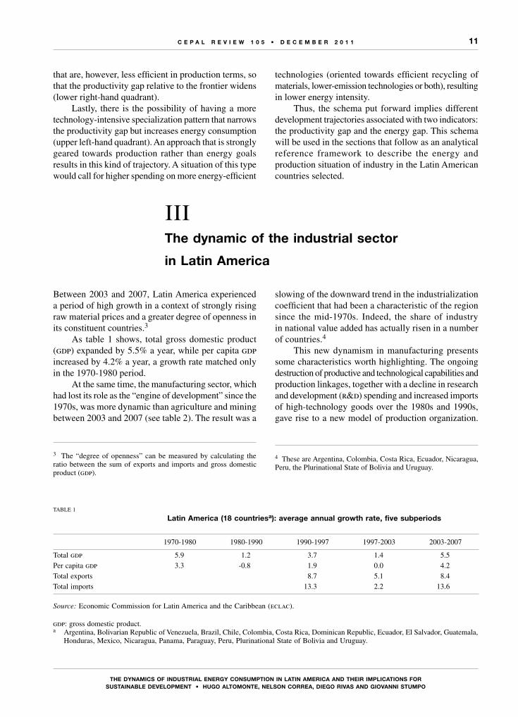
Between 2003 and 2007, Latin America experienced a period of high growth in a context of strongly rising raw material prices and a greater degree of openness in its constituent countries.3
As table 1 shows, total gross domestic product (gdp) expanded by 5.5% a year, while per capita gdp increased by 4.2% a year, a growth rate matched only in the 1970-1980 period.
At the same time, the manufacturing sector, which had lost its role as the “engine of development” since the 1970s, was more dynamic than agriculture and mining between 2003 and 2007 (see table 2). The result was a
3 The “degree of openness” can be measured by calculating the ratio between the sum of exports and imports and gross domestic product (gdp).
slowing of the downward trend in the industrialization coefficient that had been a characteristic of the region since the mid-1970s. Indeed, the share of industry in national value added has actually risen in a number of countries.4
This new dynamism in manufacturing presents some characteristics worth highlighting. The ongoing destruction of productive and technological capabilities and production linkages, together with a decline in research and development (r&d) spending and increased imports of high-technology goods over the 1980s and 1990s, gave rise to a new model of production organization.
4 These are Argentina, Colombia, Costa Rica, Ecuador, Nicaragua, Peru, the Plurinational State of Bolivia and Uruguay.
TABLE 1
Latin America (18 countriesa): average annual growth rate, five subperiods
1970-1980 1980-1990 1990-1997 1997-2003 2003-2007
Total gdp 5.9 1.2 3.7 1.4 5.5Per capita gdp 3.3 -0.8 1.9 0.0 4.2Total exports 8.7 5.1 8.4Total imports 13.3 2.2 13.6
Source: Economic Commission for Latin America and the Caribbean (eclac).
gdp: gross domestic product.a Argentina, Bolivarian Republic of Venezuela, Brazil, Chile, Colombia, Costa Rica, Dominican Republic, Ecuador, El Salvador, Guatemala,
Honduras, Mexico, Nicaragua, Panama, Paraguay, Peru, Plurinational State of Bolivia and Uruguay.
12
ThE DynAMiCs of inDusTriAL EnErGy ConsuMPTion in LATin AMEriCA AnD ThEir iMPLiCATions for sustAInABLE DEVELoPMEnt • Hugo ALtoMontE, nELson CoRREA, DIEgo RIVAs AnD gIoVAnnI stuMPo
C E P A L R E V I E W 1 0 5 • D E C E M B E R 2 0 1 1
The almost total absence of active industrial development policies5 in the stage of growth from 2003 to 2007, together with the profound transformation of the production base in earlier decades, meant that the rise in output achieved in technology-intensive sectors (and manufacturing more generally) was essentially quantitative, there being no true process of technological capacity-building.
The consequences of this situation can be appreciated in two quite different aspects. The first is a country’s position in the world economy and its industrial trade balance, and the second is the evolution of productivity.
The increasing importance of the external sector has been reflected by a rise in industrial export and import ratios. In particular, the increase in the latter between 2003 and 2007 reveals how much the industrial production system is struggling to compete in most sectors. This is especially evident in the case of technology-intensive sectors, but is also true of labour-intensive sectors exposed to competition from new producers, especially in the Asian countries.
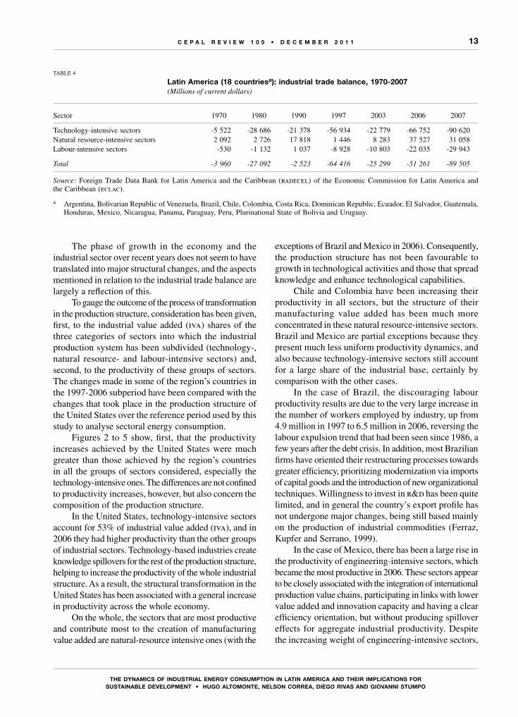
The result of this weakness is that, in a context of steadily rising domestic demand, industrial trade balances are presenting growing deficits or substantially lower surpluses (see table 4).
These deficits were offset in those years by high prices for the agricultural and mining products exported by the region. This situation is unlikely to be sustainable in the medium and long run, however, considering the openness of the region’s economies and the volatility of raw material prices, something that has been confirmed by the international crisis which broke out in September 2008.
5 The major exception in this case is Brazil.
TABLE 2
Latin America: gross domestic product (gdp), three subperiods(Average annual growth rate)
1990-1997 1997-2003 2003-2007
Total gdp 3.7 1.4 5.5
Agriculture 2.4 3.3 3.5
Mining 4.2 1.3 1.5
Industry 3.3 0.5 5.4
Electricity 4.8 2.3 5.2
Construction 4.0 -0.8 8.2
Commerce 3.7 0.8 6.9
Transport 5.9 4.2 8.1
Financial institutions 3.1 2.3 6.3
Community and social services 2.3 1.7 3.3
Source: Economic Commission for Latin America and the Caribbean (eclac).
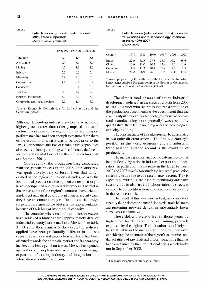
Although technology-intensive sectors have achieved higher growth rates than other groups of industrial sectors in a number of the region’s countries, this good performance has not been enough to restore their share of the economy to what it was in periods prior to the 1980s. Furthermore, this loss of technological capabilities also seems to have gone along with a dramatic decline in institutional capabilities within the public sector (Katz and Stumpo, 2001).
Consequently, the production base associated with the growth process in the 2003-2007 subperiod was qualitatively very different from that which existed in the region in previous decades, as was the institutional production development context that might have accompanied and guided that process. The fact is that when some of the region’s countries have tried to implement industrial development plans in recent years, they have encountered major difficulties at the design stage and insurmountable obstacles to implementation because of their loss of institutional capacity.
The countries where technology-intensive sectors have achieved a higher share (approximately 40% of industrial capacity) are Brazil and Mexico (see table 3). Despite their similarity, however, the policies applied have been profoundly different in the two cases: while industrial production in Brazil has been oriented towards the domestic market and its economy has become less open than it was, Mexico has opened up further and implemented a policy to encourage export manufacturing industry and integration into international production chains.
TABLE 3
Latin America (selected countries): industrial value added share of technology-intensive sectors, 1970-2007(Percentages)
Country 1970 1980 1990 1997 2003 2007
Brazil 22.0 32.3 27.8 33.7 33.2 39.6Chile 16.6 11.0 10.2 12.4 11.3 11.6Colombia 11.3 11.3 10.4 12.4 11.2 12.3Mexico 20.2 26.9 26.3 30.5 33.0 41.3
Source: prepared by the authors on the basis of the Industrial Performance Analysis Program (padi) of the Economic Commission for Latin America and the Caribbean (eclac).
13
ThE DynAMiCs of inDusTriAL EnErGy ConsuMPTion in LATin AMEriCA AnD ThEir iMPLiCATions for sustAInABLE DEVELoPMEnt • Hugo ALtoMontE, nELson CoRREA, DIEgo RIVAs AnD gIoVAnnI stuMPo
C E P A L R E V I E W 1 0 5 • D E C E M B E R 2 0 1 1
The phase of growth in the economy and the industrial sector over recent years does not seem to have translated into major structural changes, and the aspects mentioned in relation to the industrial trade balance are largely a reflection of this.
To gauge the outcome of the process of transformation in the production structure, consideration has been given, first, to the industrial value added (iva) shares of the three categories of sectors into which the industrial production system has been subdivided (technology-, natural resource- and labour-intensive sectors) and, second, to the productivity of these groups of sectors. The changes made in some of the region’s countries in the 1997-2006 subperiod have been compared with the changes that took place in the production structure of the United States over the reference period used by this study to analyse sectoral energy consumption.
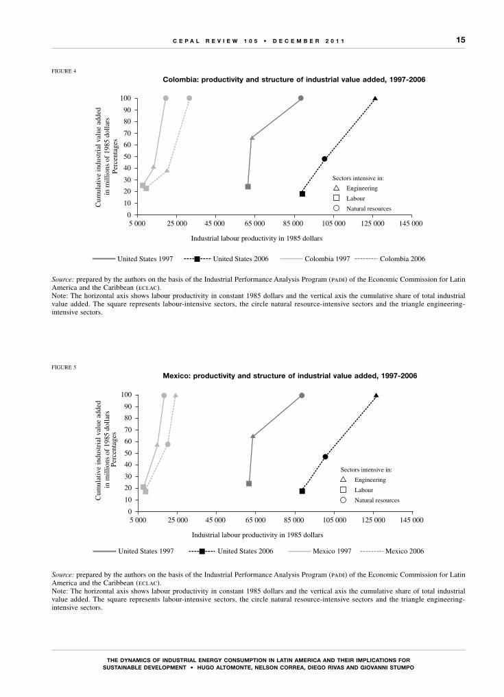
Figures 2 to 5 show, first, that the productivity increases achieved by the United States were much greater than those achieved by the region’s countries in all the groups of sectors considered, especially the technology-intensive ones. The differences are not confined to productivity increases, however, but also concern the composition of the production structure.
In the United States, technology-intensive sectors account for 53% of industrial value added (iva), and in 2006 they had higher productivity than the other groups of industrial sectors. Technology-based industries create knowledge spillovers for the rest of the production structure, helping to increase the productivity of the whole industrial structure. As a result, the structural transformation in the United States has been associated with a general increase in productivity across the whole economy.
On the whole, the sectors that are most productive and contribute most to the creation of manufacturing value added are natural-resource intensive ones (with the
exceptions of Brazil and Mexico in 2006). Consequently, the production structure has not been favourable to growth in technological activities and those that spread knowledge and enhance technological capabilities.
Chile and Colombia have been increasing their productivity in all sectors, but the structure of their manufacturing value added has been much more concentrated in these natural resource-intensive sectors. Brazil and Mexico are partial exceptions because they present much less uniform productivity dynamics, and also because technology-intensive sectors still account for a large share of the industrial base, certainly by comparison with the other cases.
In the case of Brazil, the discouraging labour productivity results are due to the very large increase in the number of workers employed by industry, up from 4.9 million in 1997 to 6.5 million in 2006, reversing the labour expulsion trend that had been seen since 1986, a few years after the debt crisis. In addition, most Brazilian firms have oriented their restructuring processes towards greater efficiency, prioritizing modernization via imports of capital goods and the introduction of new organizational techniques. Willingness to invest in r&d has been quite limited, and in general the country’s export profile has not undergone major changes, being still based mainly on the production of industrial commodities (Ferraz, Kupfer and Serrano, 1999).
In the case of Mexico, there has been a large rise in the productivity of engineering-intensive sectors, which became the most productive in 2006. These sectors appear to be closely associated with the integration of international production value chains, participating in links with lower value added and innovation capacity and having a clear efficiency orientation, but without producing spillover effects for aggregate industrial productivity. Despite the increasing weight of engineering-intensive sectors,
TABLE 4
Latin America (18 countriesa): industrial trade balance, 1970-2007(Millions of current dollars)
Sector 1970 1980 1990 1997 2003 2006 2007
Technology-intensive sectors -5 522 -28 686 -21 378 -56 934 -22 779 -66 752 -90 620Natural resource-intensive sectors 2 092 2 726 17 818 1 446 8 283 37 527 31 058Labour-intensive sectors -530 -1 132 1 037 -8 928 -10 803 -22 035 -29 943
Total -3 960 -27 092 -2 523 -64 416 -25 299 -51 261 -89 505
Source: Foreign Trade Data Bank for Latin America and the Caribbean (badecel) of the Economic Commission for Latin America and the Caribbean (eclac).
a Argentina, Bolivarian Republic of Venezuela, Brazil, Chile, Colombia, Costa Rica, Dominican Republic, Ecuador, El Salvador, Guatemala, Honduras, Mexico, Nicaragua, Panama, Paraguay, Peru, Plurinational State of Bolivia and Uruguay.

14
ThE DynAMiCs of inDusTriAL EnErGy ConsuMPTion in LATin AMEriCA AnD ThEir iMPLiCATions for sustAInABLE DEVELoPMEnt • Hugo ALtoMontE, nELson CoRREA, DIEgo RIVAs AnD gIoVAnnI stuMPo
C E P A L R E V I E W 1 0 5 • D E C E M B E R 2 0 1 1
FIGURE 2
Brazil: productivity and structure of industrial value added, 1997-2006
Source: prepared by the authors on the basis of the Industrial Performance Analysis Program (padi) of the Economic Commission for Latin America and the Caribbean (eclac).Note: The horizontal axis shows labour productivity in constant 1985 dollars and the vertical axis the cumulative share of total industrial value added. The square represents labour-intensive sectors, the circle natural resource-intensive sectors and the triangle engineering-intensive sectors.
FIGURE 3
Chile: productivity and structure of industrial value added, 1997-2006
Source: prepared by the authors on the basis of the Industrial Performance Analysis Program (padi) of the Economic Commission for Latin America and the Caribbean (eclac).Note: The horizontal axis shows labour productivity in constant 1985 dollars and the vertical axis the cumulative share of total industrial value added. The square represents labour-intensive sectors, the circle natural resource-intensive sectors and the triangle engineering-intensive sectors.
0
10
20
30
40
50
60
70
80
90
100
5 000 25 000 45 000 65 000 85 000 105 000 125 000 145 000
Industrial labour productivity in 1985 dollars
Cum
ulat
ive
indu
stri
al v
alue
add
ed
in m
illio
ns o
f 19
85 d
olla
rsPe
rcen
tage
s
United States 1997 Brazil 1997 Brazil 2006United States 2006
Sectors intensive in:
Engineering
Labour
Natural resources
United States 1997 Chile 1997 Chile 2006United States 2006
0
10
20
30
40
50
60
70
80
90
100
10 000 30 000 50 000 70 000 90 000 110 000 130 000 150 000
Industrial labour productivity in 1985 dollars
Cum
ulat
ive
indu
stri
al v
alue
add
ed
in m
illio
ns o
f 19
85 d
olla
rsPe
rcen
tage
s
Sectors intensive in:
Engineering
Labour
Natural resources
15
ThE DynAMiCs of inDusTriAL EnErGy ConsuMPTion in LATin AMEriCA AnD ThEir iMPLiCATions for sustAInABLE DEVELoPMEnt • Hugo ALtoMontE, nELson CoRREA, DIEgo RIVAs AnD gIoVAnnI stuMPo
C E P A L R E V I E W 1 0 5 • D E C E M B E R 2 0 1 1
FIGURE 4
Colombia: productivity and structure of industrial value added, 1997-2006
Source: prepared by the authors on the basis of the Industrial Performance Analysis Program (padi) of the Economic Commission for Latin America and the Caribbean (eclac).Note: The horizontal axis shows labour productivity in constant 1985 dollars and the vertical axis the cumulative share of total industrial value added. The square represents labour-intensive sectors, the circle natural resource-intensive sectors and the triangle engineering-intensive sectors.
FIGURE 5
Mexico: productivity and structure of industrial value added, 1997-2006
Source: prepared by the authors on the basis of the Industrial Performance Analysis Program (padi) of the Economic Commission for Latin America and the Caribbean (eclac).Note: The horizontal axis shows labour productivity in constant 1985 dollars and the vertical axis the cumulative share of total industrial value added. The square represents labour-intensive sectors, the circle natural resource-intensive sectors and the triangle engineering-intensive sectors.
United States 1997 Mexico 1997 Mexico 2006United States 2006
0
10
20
30
40
50
60
70
80
90
100
5 000 25 000 45 000 65 000 85 000 105 000 125 000 145 000
Industrial labour productivity in 1985 dollars
Cum
ulat
ive
indu
stri
al v
alue
add
ed
in m
illio
ns o
f 19
85 d
olla
rsPe
rcen
tage
s
Sectors intensive in:
Engineering
Labour
Natural resources
United States 1997 Colombia 1997 Colombia 2006United States 2006
0
10
20
30
40
50
60
70
80
90
100
5 000 25 000 45 000 65 000 85 000 105 000 125 000 145 000
Industrial labour productivity in 1985 dollars
Cum
ulat
ive
indu
stri
al v
alue
add
ed
in m
illio
ns o
f 19
85 d
olla
rsPe
rcen
tage
s
Sectors intensive in:
Engineering
Labour
Natural resources
16
ThE DynAMiCs of inDusTriAL EnErGy ConsuMPTion in LATin AMEriCA AnD ThEir iMPLiCATions for sustAInABLE DEVELoPMEnt • Hugo ALtoMontE, nELson CoRREA, DIEgo RIVAs AnD gIoVAnnI stuMPo
C E P A L R E V I E W 1 0 5 • D E C E M B E R 2 0 1 1
the industrial fabric still includes a large percentage of natural resource-intensive sectors.
The aspects mentioned make it clear that technological change in industry in these Latin American countries has been limited and inadequate when set against the need for a production structure that is more open and integrated into international trade. This situation could become even more difficult in an international context where, for a number of years now, technologies and production methods have been changing because of increasing incorporation of information and communication technologies (icts) into production processes.
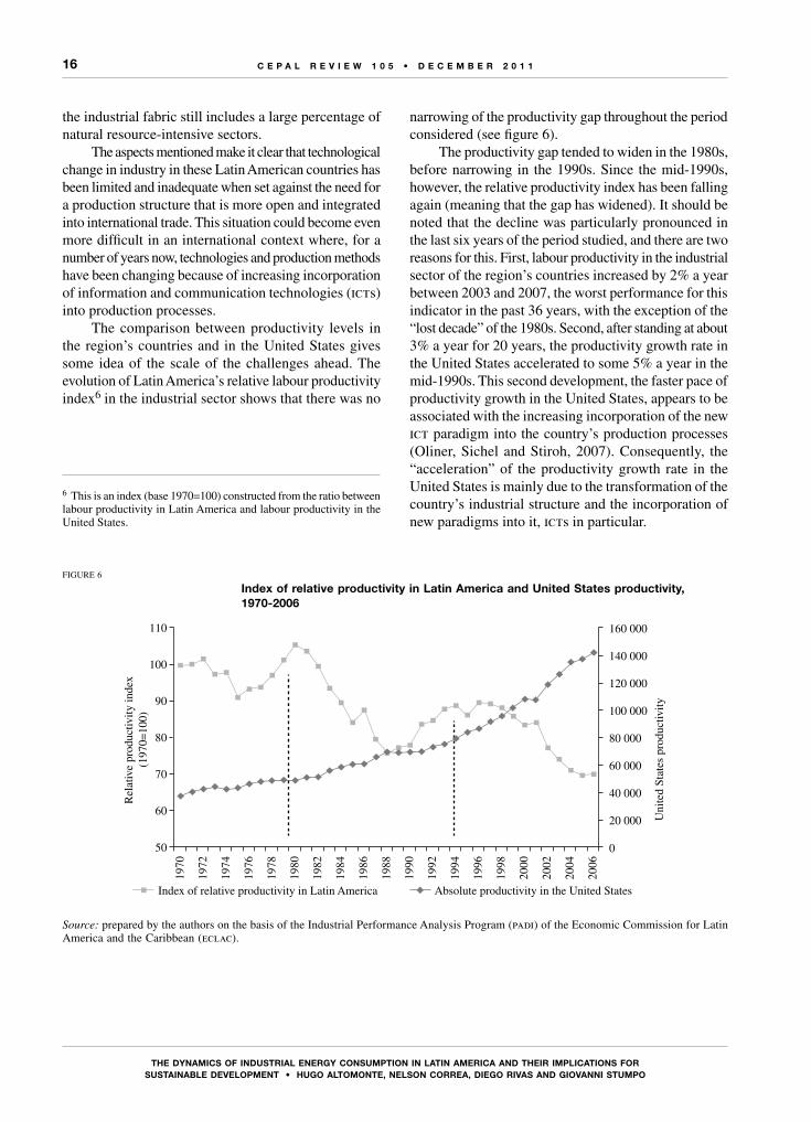
The comparison between productivity levels in the region’s countries and in the United States gives some idea of the scale of the challenges ahead. The evolution of Latin America’s relative labour productivity index6 in the industrial sector shows that there was no
6 This is an index (base 1970=100) constructed from the ratio between labour productivity in Latin America and labour productivity in the United States.
narrowing of the productivity gap throughout the period considered (see figure 6).
The productivity gap tended to widen in the 1980s, before narrowing in the 1990s. Since the mid-1990s, however, the relative productivity index has been falling again (meaning that the gap has widened). It should be noted that the decline was particularly pronounced in the last six years of the period studied, and there are two reasons for this. First, labour productivity in the industrial sector of the region’s countries increased by 2% a year between 2003 and 2007, the worst performance for this indicator in the past 36 years, with the exception of the “lost decade” of the 1980s. Second, after standing at about 3% a year for 20 years, the productivity growth rate in the United States accelerated to some 5% a year in the mid-1990s. This second development, the faster pace of productivity growth in the United States, appears to be associated with the increasing incorporation of the new ict paradigm into the country’s production processes (Oliner, Sichel and Stiroh, 2007). Consequently, the “acceleration” of the productivity growth rate in the United States is mainly due to the transformation of the country’s industrial structure and the incorporation of new paradigms into it, icts in particular.
FIGURE 6
index of relative productivity in Latin America and united states productivity, 1970-2006
Source: prepared by the authors on the basis of the Industrial Performance Analysis Program (padi) of the Economic Commission for Latin America and the Caribbean (eclac).
0
20 000
40 000
60 000
80 000
100 000
120 000
140 000
160 000
50
1970
1972
1974
1976
1978
1980
1982
1984
1986
1988
1990
1992
1994
1996
1998
2000
2002
2004
2006
60
70
80
90
100
110
Uni
ted
Stat
es p
rodu
ctiv
ity
Rel
ativ
e pr
oduc
tivity
inde
x(1
970=
100)
Absolute productivity in the United StatesIndex of relative productivity in Latin America
17
ThE DynAMiCs of inDusTriAL EnErGy ConsuMPTion in LATin AMEriCA AnD ThEir iMPLiCATions for sustAInABLE DEVELoPMEnt • Hugo ALtoMontE, nELson CoRREA, DIEgo RIVAs AnD gIoVAnnI stuMPo
C E P A L R E V I E W 1 0 5 • D E C E M B E R 2 0 1 1
the regional average, with transport taking a larger share. This is the case with Chile, Colombia and Mexico. Brazil is an example of the opposite, with industry exceeding the regional average and having the largest share of any sector of the economy.
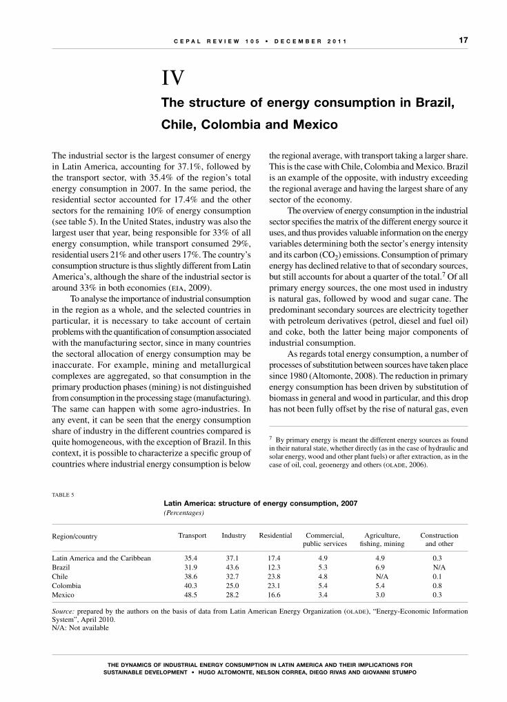
The overview of energy consumption in the industrial sector specifies the matrix of the different energy source it uses, and thus provides valuable information on the energy variables determining both the sector’s energy intensity and its carbon (CO2) emissions. Consumption of primary energy has declined relative to that of secondary sources, but still accounts for about a quarter of the total.7 Of all primary energy sources, the one most used in industry is natural gas, followed by wood and sugar cane. The predominant secondary sources are electricity together with petroleum derivatives (petrol, diesel and fuel oil) and coke, both the latter being major components of industrial consumption.
As regards total energy consumption, a number of processes of substitution between sources have taken place since 1980 (Altomonte, 2008). The reduction in primary energy consumption has been driven by substitution of biomass in general and wood in particular, and this drop has not been fully offset by the rise of natural gas, even
7 By primary energy is meant the different energy sources as found in their natural state, whether directly (as in the case of hydraulic and solar energy, wood and other plant fuels) or after extraction, as in the case of oil, coal, geoenergy and others (olade, 2006).
The industrial sector is the largest consumer of energy in Latin America, accounting for 37.1%, followed by the transport sector, with 35.4% of the region’s total energy consumption in 2007. In the same period, the residential sector accounted for 17.4% and the other sectors for the remaining 10% of energy consumption (see table 5). In the United States, industry was also the largest user that year, being responsible for 33% of all energy consumption, while transport consumed 29%, residential users 21% and other users 17%. The country’s consumption structure is thus slightly different from Latin America’s, although the share of the industrial sector is around 33% in both economies (eia, 2009).
To analyse the importance of industrial consumption in the region as a whole, and the selected countries in particular, it is necessary to take account of certain problems with the quantification of consumption associated with the manufacturing sector, since in many countries the sectoral allocation of energy consumption may be inaccurate. For example, mining and metallurgical complexes are aggregated, so that consumption in the primary production phases (mining) is not distinguished from consumption in the processing stage (manufacturing). The same can happen with some agro-industries. In any event, it can be seen that the energy consumption share of industry in the different countries compared is quite homogeneous, with the exception of Brazil. In this context, it is possible to characterize a specific group of countries where industrial energy consumption is below
IVThe structure of energy consumption in Brazil,
Chile, Colombia and Mexico
TABLE 5
Latin America: structure of energy consumption, 2007(Percentages)
Region/country Transport Industry Residential Commercial, public services
Agriculture, fishing, mining
Construction and other
Latin America and the Caribbean 35.4 37.1 17.4 4.9 4.9 0.3Brazil 31.9 43.6 12.3 5.3 6.9 N/AChile 38.6 32.7 23.8 4.8 N/A 0.1Colombia 40.3 25.0 23.1 5.4 5.4 0.8Mexico 48.5 28.2 16.6 3.4 3.0 0.3
Source: prepared by the authors on the basis of data from Latin American Energy Organization (olade), “Energy-Economic Information System”, April 2010.N/A: Not available
18
ThE DynAMiCs of inDusTriAL EnErGy ConsuMPTion in LATin AMEriCA AnD ThEir iMPLiCATions for sustAInABLE DEVELoPMEnt • Hugo ALtoMontE, nELson CoRREA, DIEgo RIVAs AnD gIoVAnnI stuMPo
C E P A L R E V I E W 1 0 5 • D E C E M B E R 2 0 1 1
though its share in the composition of final consumption has doubled (Altomonte, 2008). The expansion of natural gas has been due above all to the extensive substitution of fuel oil in the industrial sector and in electricity generation. It has also penetrated the residential sector, albeit to a lesser extent, owing to continuing urbanization and expansion of distribution networks.
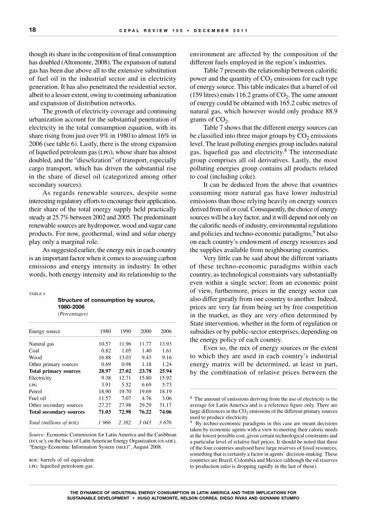
The growth of electricity coverage and continuing urbanization account for the substantial penetration of electricity in the total consumption equation, with its share rising from just over 9% in 1980 to almost 16% in 2006 (see table 6). Lastly, there is the strong expansion of liquefied petroleum gas (lpg), whose share has almost doubled, and the “dieselization” of transport, especially cargo transport, which has driven the substantial rise in the share of diesel oil (categorized among other secondary sources).
As regards renewable sources, despite some interesting regulatory efforts to encourage their application, their share of the total energy supply held practically steady at 25.7% between 2002 and 2005. The predominant renewable sources are hydropower, wood and sugar cane products. For now, geothermal, wind and solar energy play only a marginal role.
As suggested earlier, the energy mix in each country is an important factor when it comes to assessing carbon emissions and energy intensity in industry. In other words, both energy intensity and its relationship to the
environment are affected by the composition of the different fuels employed in the region’s industries.
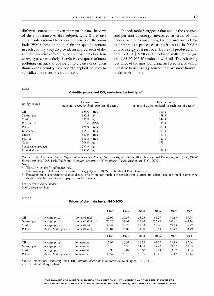
Table 7 presents the relationship between calorific power and the quantity of CO2 emissions for each type of energy source. This table indicates that a barrel of oil (159 litres) emits 116.2 grams of CO2. The same amount of energy could be obtained with 165.2 cubic metres of natural gas, which however would only produce 88.9 grams of CO2.
Table 7 shows that the different energy sources can be classified into three major groups by CO2 emissions level. The least polluting energies group includes natural gas, liquefied gas and electricity.8 The intermediate group comprises all oil derivatives. Lastly, the most polluting energies group contains all products related to coal (including coke).
It can be deduced from the above that countries consuming more natural gas have lower industrial emissions than those relying heavily on energy sources derived from oil or coal. Consequently, the choice of energy sources will be a key factor, and it will depend not only on the calorific needs of industry, environmental regulations and policies and techno-economic paradigms,9 but also on each country’s endowment of energy resources and the supplies available from neighbouring countries.
Very little can be said about the different variants of these techno-economic paradigms within each country, as technological constraints vary substantially even within a single sector; from an economic point of view, furthermore, prices in the energy sector can also differ greatly from one country to another. Indeed, prices are very far from being set by free competition in the market, as they are very often determined by State intervention, whether in the form of regulation or subsidies or by public-sector enterprises, depending on the energy policy of each country.
Even so, the mix of energy sources or the extent to which they are used in each country’s industrial energy matrix will be determined, at least in part, by the combination of relative prices between the
8 The amount of emissions deriving from the use of electricity is the average for Latin America and is a reference figure only. There are large differences in the CO2 emissions of the different primary sources used to produce electricity.9 By techno-economic paradigms in this case are meant decisions taken by economic agents with a view to meeting their caloric needs at the lowest possible cost, given certain technological constraints and a particular level of relative fuel prices. It should be noted that three of the four countries analysed have large reserves of fossil resources, something that is certainly a factor in agents’ decision-making. These countries are Brazil, Colombia and Mexico (although the oil reserves to production ratio is dropping rapidly in the last of these).
TABLE 6
structure of consumption by source, 1980-2006(Percentages)
Energy source 1980 1990 2000 2006
Natural gas 10.57 11.96 11.77 13.93Coal 0.82 1.05 1.40 1.61Wood 16.88 13.03 9.43 9.16Other primary sources 0.69 0.98 1.18 1.24Total primary sources 28.97 27.02 23.78 25.94Electricity 9.38 12.71 15.80 15.92lpg 3.91 5.52 6.69 5.73Petrol 18.90 19.70 19.69 18.19Fuel oil 11.57 7.07 4.76 3.06Other secondary sources 27.27 27.98 29.29 31.17Total secondary sources 71.03 72.98 76.22 74.06
Total (millions of boe) 1 966 2 382 3 043 3 676
Source: Economic Commission for Latin America and the Caribbean (eclac), on the basis of Latin American Energy Organization (olade), “Energy-Economic Information System (siee)”, August 2008.
boe: barrels of oil equivalent.lpg: liquefied petroleum gas.
19
ThE DynAMiCs of inDusTriAL EnErGy ConsuMPTion in LATin AMEriCA AnD ThEir iMPLiCATions for sustAInABLE DEVELoPMEnt • Hugo ALtoMontE, nELson CoRREA, DIEgo RIVAs AnD gIoVAnnI stuMPo
C E P A L R E V I E W 1 0 5 • D E C E M B E R 2 0 1 1
TABLE 7
Calorific power and Co2 emissions by fuel typea
Energy sourceCalorific power
(amount needed to obtain one boe of energy)CO2 emissions
(grams of carbon emitted for each boe of energy)
Oil 159.0 litres 116.2Natural gas 165.2 m3 88.9Coal 205.7 kg 149.9Electricityb 1.6 MWh 93.0Petrol 178.9 litres 109.8Kerosene 165.1 litres 113.3Diesel 152.6 litres 117.4Fuel oil 150.3 litres 122.6Coke 206.9 kg 173.1Sugar cane productsc 1 297.9 kg -Liquefied gas 131.0 kg 99.9
Source: Latin American Energy Organization (olade), Energy Statistics Report, Quito, 2006; International Energy Agency (iea), World Energy Outlook 2008, Paris, 2008; and Voluntary Reporting of Greenhouse Gases, Washington, D.C., 2007.Notes:a These figures are for reference only.b Information provided by the International Energy Agency (2007) for South and Central America.c Emissions from sugar cane production depend greatly on how much of this production is turned into ethanol and how much is employed
as pulp, which is used to make paper or to fuel boilers.
boe: barrel of oil equivalent.MWh: megawatt hour.
TABLE 8
Prices of the main fuels, 1990-2008
1990 1996 2000 2006 2007 2008
Oil (average price) (dollars/barrel) 22.99 20.37 28.23 64.27 71.13 97.04Natural gas (average price) (dollars/1,000 m3) 73.26 92.64 129.85 235.90 240.41 345.24Coal (average price) (dollars/ton) 38.42 38.25 27.32 59.01 67.43 136.27Petrol (United States price ) (dollars/barrel) 29.84 25.02 34.98 76.53 85.47 103.49
1990 1996 2000 2006 2007 2008
Oil (average price) dollars/boe 22.99 20.37 28.23 64.27 71.13 97.04Natural gas (average price) dollars/boe 12.10 15.30 21.45 38.97 39.72 57.03Coal (average price) dollars/boe 7.90 7.87 5.62 12.14 13.87 28.03Petrol (United States price) dollars/boe 33.57 28.16 39.35 86.11 96.17 116.44
Source: International Monetary Fund (imf), International Financial Statistics, Washington, D.C., 2010.boe: barrels of oil equivalent.
different sources at a given moment in time. In view of the importance of this subject, table 8 presents certain international trends in the prices of the main fuels. While these do not explain the specific context in each country, they do provide an appreciation of the general incentives affecting the employment of certain energy types, particularly the relative cheapness of more polluting energies as compared to cleaner ones, even though each country may operate explicit policies to subsidize the prices of certain fuels.
Indeed, table 8 suggests that coal is the cheapest fuel per unit of energy (measured in terms of final energy, without considering the performance of the equipment and processes using it), since in 2008 a unit of energy cost just over US$ 28 if produced with coal, but US$ 57.033 if produced with natural gas and US$ 97.035 if produced with oil. The relatively low price of the most polluting fuel type is a powerful incentive to use energy sources that are more harmful to the environment.
20
ThE DynAMiCs of inDusTriAL EnErGy ConsuMPTion in LATin AMEriCA AnD ThEir iMPLiCATions for sustAInABLE DEVELoPMEnt • Hugo ALtoMontE, nELson CoRREA, DIEgo RIVAs AnD gIoVAnnI stuMPo
C E P A L R E V I E W 1 0 5 • D E C E M B E R 2 0 1 1
Energy intensity is a commonly used indicator for measuring the relationship between energy use and a country’s economic development over time. The evolution of this indicator, measured as the ratio between the amount of energy consumed and the country’s gdp at a given time, provides information on the way energy is used, directly and indirectly, to produce a unit of output. Disparities in this indicator between different places and times reflect the structures of both energy systems and production systems, and thus can be seen to relate, first, to technological choices and, second, to differentiated forms of social and economic behaviour.
Energy analysts usually accept that energy intensity displays an upward evolution over time at the start of the early phases of development (mechanization of agriculture, development of energy-intensive industries such as chemicals, cement, metallurgy and paper) or when there is growth in energy-intensive primary sectors such as mining; then it levels off as these processes stabilize, before finally diminishing as technological innovations and know-how are introduced and as improvements are achieved in energy yields, transformation and consumption.
This concept can also be applied at the sectoral level. Thus, to take the industrial sector, the amount of energy consumed to produce a particular physical unit of output, such as kilocalories per ton of steel or cement, could be taken as an indicator of energy intensity. Given information availability and the need to analyse this indicator on a more disaggregated basis, this study will use two complementary methodologies:(i) First, a distinction will be drawn between the different “effects” explaining industrial energy consumption.10 Here, reference will be made to the energy intensity of the industrial sector in the aggregate, understood as the amount of physical energy (in calories) needed to produce a unit of value added, measured in constant money (calories/dollar of value added in constant 2000 dollars).(ii) Second, to conduct a more disaggregated analysis of the manufacturing sector, the structure of industrial
10 The methodology used to decompose the energy consumed in the industrial sector is set out in the Annex.
consumption will be examined using the taxonomy of Katz and Stumpo (2001). In this case, use will be made of industry surveys, the great majority of which publish data not on physical energy consumption but on monetary expenditure on energy. Thus, in this second part of the analysis of the energy dynamic, a proxy for energy intensity will be used, namely the energy spending needed to produce a unit of value added, both values being measured in constant 2000 dollars.
It should be noted that the evolution of energy consumption as measured in physical quantities (calories) could be very different from the evolution of energy consumption as measured by monetary expenditure (in pesos or dollars). This difference derives from the fact that increasing monetary expenditure does not necessary entail a rise in physical consumption, and thus higher spending per unit of value added does not necessarily represent an increase in energy intensity.11
1. The united states
The United States is not only an industrial power, given the modernization of its industrial base and its high productivity, but also has very high energy standards, given the reduction of its industrial energy consumption and its specialization in less energy-intensive activities with high value added. For this reason, the United States has been taken as a proxy for the frontier, as it gives an idea of the best practices possible in production terms and also presents a large reduction in industrial energy intensity.
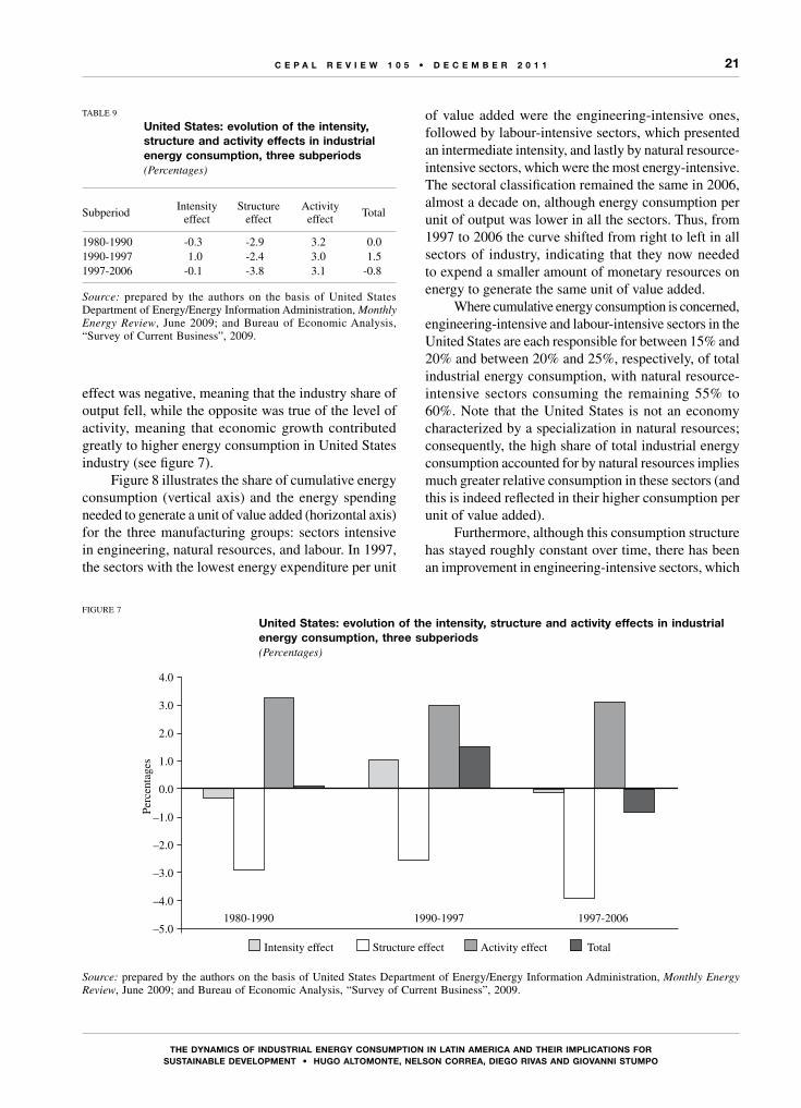
As table 9 shows, in the 1997-2006 subperiod there was a decline in both energy intensity (-0.1% a year) and in total energy consumption in the industrial sector (-0.8% a year). Taking a longer-term view, furthermore, in the three periods studied it can be seen that the structure
11 An example of this could arise in a company or sector that modernized its energy consumption by making use of cleaner sources, switching from cheaper but more contaminating sources (such as coal or oil) to more refined and higher-yielding but costlier ones (such as gas or electricity). The shift from cheaper, more polluting sources to higher-yielding ones would surely entail higher (monetary) expenditure on energy, but not necessarily greater physical consumption or higher energy intensity, precisely because of the higher yield of the new sources.
Vsectoral patterns of industrial energy
consumption in the region
21
ThE DynAMiCs of inDusTriAL EnErGy ConsuMPTion in LATin AMEriCA AnD ThEir iMPLiCATions for sustAInABLE DEVELoPMEnt • Hugo ALtoMontE, nELson CoRREA, DIEgo RIVAs AnD gIoVAnnI stuMPo
C E P A L R E V I E W 1 0 5 • D E C E M B E R 2 0 1 1
effect was negative, meaning that the industry share of output fell, while the opposite was true of the level of activity, meaning that economic growth contributed greatly to higher energy consumption in United States industry (see figure 7).
Figure 8 illustrates the share of cumulative energy consumption (vertical axis) and the energy spending needed to generate a unit of value added (horizontal axis) for the three manufacturing groups: sectors intensive in engineering, natural resources, and labour. In 1997, the sectors with the lowest energy expenditure per unit
of value added were the engineering-intensive ones, followed by labour-intensive sectors, which presented an intermediate intensity, and lastly by natural resource-intensive sectors, which were the most energy-intensive. The sectoral classification remained the same in 2006, almost a decade on, although energy consumption per unit of output was lower in all the sectors. Thus, from 1997 to 2006 the curve shifted from right to left in all sectors of industry, indicating that they now needed to expend a smaller amount of monetary resources on energy to generate the same unit of value added.
Where cumulative energy consumption is concerned, engineering-intensive and labour-intensive sectors in the United States are each responsible for between 15% and 20% and between 20% and 25%, respectively, of total industrial energy consumption, with natural resource-intensive sectors consuming the remaining 55% to 60%. Note that the United States is not an economy characterized by a specialization in natural resources; consequently, the high share of total industrial energy consumption accounted for by natural resources implies much greater relative consumption in these sectors (and this is indeed reflected in their higher consumption per unit of value added).
Furthermore, although this consumption structure has stayed roughly constant over time, there has been an improvement in engineering-intensive sectors, which
TABLE 9
united states: evolution of the intensity, structure and activity effects in industrial energy consumption, three subperiods(Percentages)
SubperiodIntensity
effectStructure
effectActivity
effectTotal
1980-1990 -0.3 -2.9 3.2 0.01990-1997 1.0 -2.4 3.0 1.51997-2006 -0.1 -3.8 3.1 -0.8
Source: prepared by the authors on the basis of United States Department of Energy/Energy Information Administration, Monthly Energy Review, June 2009; and Bureau of Economic Analysis, “Survey of Current Business”, 2009.
FIGURE 7
united states: evolution of the intensity, structure and activity effects in industrial energy consumption, three subperiods(Percentages)
Source: prepared by the authors on the basis of United States Department of Energy/Energy Information Administration, Monthly Energy Review, June 2009; and Bureau of Economic Analysis, “Survey of Current Business”, 2009.
–5.0
–4.0
–3.0
–2.0
–1.0
0.0
1.0
2.0
3.0
4.0
Perc
enta
ges
Intensity effect Structure effect Activity effect Total
1980-1990 1990-1997 1997-2006

22
ThE DynAMiCs of inDusTriAL EnErGy ConsuMPTion in LATin AMEriCA AnD ThEir iMPLiCATions for sustAInABLE DEVELoPMEnt • Hugo ALtoMontE, nELson CoRREA, DIEgo RIVAs AnD gIoVAnnI stuMPo
C E P A L R E V I E W 1 0 5 • D E C E M B E R 2 0 1 1
have succeeded in reducing their energy intensity sharply and decreasing their share of total energy consumption, this being a clear example of virtuous structural change. Thus, it can be seen that the reduction in energy intensity is explained not only by a fall in energy expenditure per unit of value added in all manufacturing sectors, but also by a shift in the composition of the production structure towards the least energy-intensive sectors, i.e., those that are engineering-intensive.
2. Brazil
The behaviour of energy consumption in the Brazilian industrial sector displays a worrying upward trend:
although consumption fell sharply in the 1980-1990 subperiod (-6.0%), it increased in the following subperiods (by 3.7% in 1990-1997 and by 3.5% in 1997-2006).
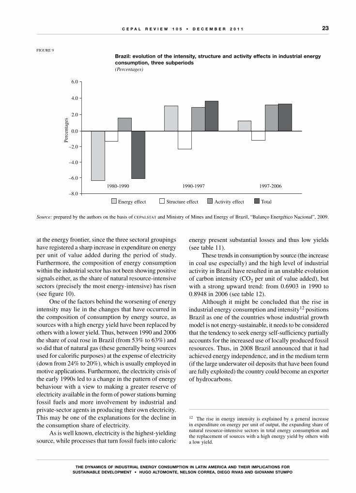
Much as in the United States, the structure effect has been systematically negative, while the activity effect has always contributed to higher energy consumption, a trend that can be attributed to the strong growth of the Brazilian economy over the past 15 years (see table 10 and figure 9).
In the case of Brazil, the rise in energy intensity can be seen both at the aggregate level, with a 1.2% annual increase in the 1997-2006 subperiod, and when the figures are disaggregated by groups of production sectors. In fact, the pattern in Brazil is the opposite of that
FIGURE 8
united states: cumulative energy consumption and expenditure on energy in industry per unit of value added, 1997-2006
Source: Economic Commission for Latin America and the Caribbean (eclac), on the basis of industrial surveys.Note: Expenditure on energy per unit of value added is calculated as the ratio between industrial energy consumption (in millions of 2000 dollars) and industrial value added (in millions of 2000 dollars).
0
10
20
30
40
50
60
70
80
90
100
0 0.01 0.02 0.040.03 0.05 0.06 0.07 0.08 0.09 0.1
Cum
ulat
ive
ener
gy c
onsu
mpt
ion
in m
illi
ons
of 2
000
doll
ars
Per
cent
ages
Expenditure on energy per unit of value added
United States 1997 United States 2006
Sectors intensive in:
Engineering
Labour
Natural resources
TABLE 10
Brazil: evolution of the intensity, structure and activity effects in industrial energy consumption, three subperiods(Percentages)
Subperiod Intensity effect Structure effect Activity effect Total
1980-1990 -6.2 -1.3 1.6 -6.01990-1997 3.1 -2.3 2.9 3.71997-2006 1.2 -1.1 3.3 3.5
Source: prepared by the authors on the basis of cepalstat and Ministry of Mines and Energy of Brazil, “Balanço Energético Nacional”, 2009.
23
ThE DynAMiCs of inDusTriAL EnErGy ConsuMPTion in LATin AMEriCA AnD ThEir iMPLiCATions for sustAInABLE DEVELoPMEnt • Hugo ALtoMontE, nELson CoRREA, DIEgo RIVAs AnD gIoVAnnI stuMPo
C E P A L R E V I E W 1 0 5 • D E C E M B E R 2 0 1 1
FIGURE 9
Brazil: evolution of the intensity, structure and activity effects in industrial energy consumption, three subperiods(Percentages)
Source: prepared by the authors on the basis of cepalstat and Ministry of Mines and Energy of Brazil, “Balanço Energético Nacional”, 2009.
–8.0
–6.0
–4.0
–2.0
0.0
2.0
4.0
6.0
Perc
enta
ges
Energy effect Structure effect Activity effect Total
1980-1990 1990-1997 1997-2006
at the energy frontier, since the three sectoral groupings have registered a sharp increase in expenditure on energy per unit of value added during the period of study. Furthermore, the composition of energy consumption within the industrial sector has not been showing positive signals either, as the share of natural resource-intensive sectors (precisely the most energy-intensive) has risen (see figure 10).
One of the factors behind the worsening of energy intensity may lie in the changes that have occurred in the composition of consumption by energy source, as sources with a high energy yield have been replaced by others with a lower yield. Thus, between 1990 and 2006 the share of coal rose in Brazil (from 53% to 63%) and so did that of natural gas (these generally being sources used for calorific purposes) at the expense of electricity (down from 24% to 20%), which is usually employed in motive applications. Furthermore, the electricity crisis of the early 1990s led to a change in the pattern of energy behaviour with a view to making a greater reserve of electricity available in the form of power stations burning fossil fuels and more involvement by industrial and private-sector agents in producing their own electricity. This may be one of the explanations for the decline in the consumption share of electricity.
As is well known, electricity is the highest-yielding source, while processes that turn fossil fuels into caloric
energy present substantial losses and thus low yields (see table 11).
These trends in consumption by source (the increase in coal use especially) and the high level of industrial activity in Brazil have resulted in an unstable evolution of carbon intensity (CO2 per unit of value added), but with a strong upward trend: from 0.6903 in 1990 to 0.8948 in 2006 (see table 12).
Although it might be concluded that the rise in industrial energy consumption and intensity12 positions Brazil as one of the countries whose industrial growth model is not energy-sustainable, it needs to be considered that the tendency to seek energy self-sufficiency partially accounts for the increased use of locally produced fossil resources. Thus, in 2008 Brazil announced that it had achieved energy independence, and in the medium term (if the large underwater oil deposits that have been found are fully exploited) the country could become an exporter of hydrocarbons.
12 The rise in energy intensity is explained by a general increase in expenditure on energy per unit of output, the expanding share of natural resource-intensive sectors in total energy consumption and the replacement of sources with a high energy yield by others with a low yield.

24
ThE DynAMiCs of inDusTriAL EnErGy ConsuMPTion in LATin AMEriCA AnD ThEir iMPLiCATions for sustAInABLE DEVELoPMEnt • Hugo ALtoMontE, nELson CoRREA, DIEgo RIVAs AnD gIoVAnnI stuMPo
C E P A L R E V I E W 1 0 5 • D E C E M B E R 2 0 1 1
FIGURE 10
Cumulative energy consumption and expenditure on energy per unit of value added in Brazilian and united states industry, 1997-2006
Source: Economic Commission for Latin America and the Caribbean (eclac), on the basis of industrial surveys.Note: Expenditure on energy per unit of value added is calculated as the ratio between industrial energy consumption (in millions of 2000 dollars) and industrial value added (in millions of 2000 dollars).
TABLE 11
Brazil: evolution of the industrial consumption structure, by source, 1990-2006(Millions of toe and percentages)
Brazil Electricity Natural gas Oil and derivatives Coal and other Total
1990 106 toe 9.66 2.45 6.85 21.20 40.15 Percentage 24.05 6.10 17.06 52.79 100.002000 106 toe 12.61 5.51 7.31 31.53 56.96 Percentage 22.14 9.68 12.83 55.35 100.002006 106 toe 15.60 9.65 3.96 49.27 78.48 Percentage 19.88 12.30 5.05 62.78 100.00
Source: prepared by the authors on the basis of Ministry of Mines and Energy of Brazil, “Balanço Energético Nacional”, 2009.
toe: tons of oil equivalent.
TABLE 12
Brazil: carbon intensity of industry, 1990-2006
1990 2000 2005 2006
Millions of tons of CO2 57.5 94.0 99.5 105iva (millions of 2000 dollars) 83 293 96 131 110 925 117 463Kg CO2/iva 0.6903 0.9778 0.8970 0.8948
Source: prepared by the authors on the basis of Energy Information Administration (2007), Voluntary Reporting of Greenhouse Gases, Washington, D.C., United States Department of Energy, 2010; and Economic Commission for Latin America and the Caribbean (eclac), Time for Equality: Closing Gaps, Opening Trails (LC/G.2432(SES.33/3)), Santiago, Chile, 2010.
iva: industrial value added.Kg CO2/iva: kilograms of carbon per unit of industrial value added.
0
10
20
30
40
50
60
70
80
90
100
0 0.01 0.02 0.03 0.04 0.05 0.06 0.07 0.08 0.09 0.1
Cum
ulat
ive
ener
gy c
onsu
mpt
ion
in m
illi
ons
of 2
000
doll
ars
Per
cent
ages
Expenditure on energy per unit of value added
United States 1997 United States 2006 Brazil 1997 Brazil 2006
Sectors intensive in:
Engineering
Labour
Natural resources
25
ThE DynAMiCs of inDusTriAL EnErGy ConsuMPTion in LATin AMEriCA AnD ThEir iMPLiCATions for sustAInABLE DEVELoPMEnt • Hugo ALtoMontE, nELson CoRREA, DIEgo RIVAs AnD gIoVAnnI stuMPo
C E P A L R E V I E W 1 0 5 • D E C E M B E R 2 0 1 1
3. Chile
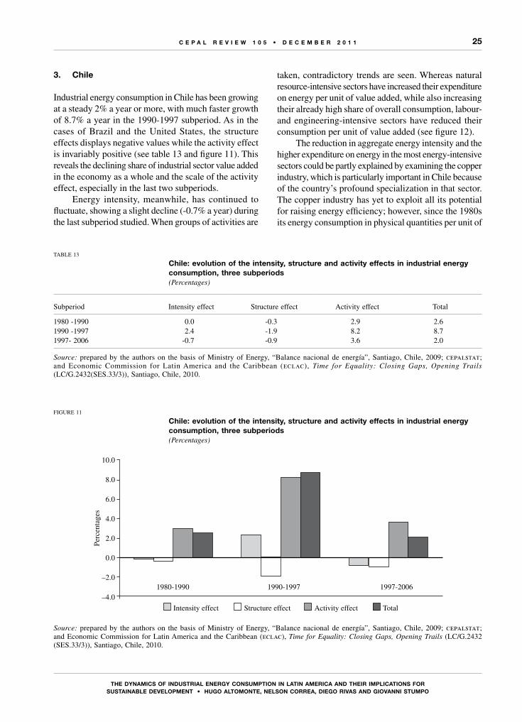
Industrial energy consumption in Chile has been growing at a steady 2% a year or more, with much faster growth of 8.7% a year in the 1990-1997 subperiod. As in the cases of Brazil and the United States, the structure effects displays negative values while the activity effect is invariably positive (see table 13 and figure 11). This reveals the declining share of industrial sector value added in the economy as a whole and the scale of the activity effect, especially in the last two subperiods.
Energy intensity, meanwhile, has continued to fluctuate, showing a slight decline (-0.7% a year) during the last subperiod studied. When groups of activities are
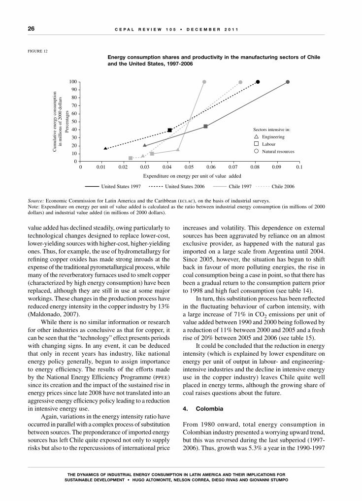
taken, contradictory trends are seen. Whereas natural resource-intensive sectors have increased their expenditure on energy per unit of value added, while also increasing their already high share of overall consumption, labour- and engineering-intensive sectors have reduced their consumption per unit of value added (see figure 12).
The reduction in aggregate energy intensity and the higher expenditure on energy in the most energy-intensive sectors could be partly explained by examining the copper industry, which is particularly important in Chile because of the country’s profound specialization in that sector. The copper industry has yet to exploit all its potential for raising energy efficiency; however, since the 1980s its energy consumption in physical quantities per unit of
FIGURE 11
Chile: evolution of the intensity, structure and activity effects in industrial energy consumption, three subperiods(Percentages)
Source: prepared by the authors on the basis of Ministry of Energy, “Balance nacional de energía”, Santiago, Chile, 2009; cepalstat; and Economic Commission for Latin America and the Caribbean (eclac), Time for Equality: Closing Gaps, Opening Trails (LC/G.2432 (SES.33/3)), Santiago, Chile, 2010.
TABLE 13
Chile: evolution of the intensity, structure and activity effects in industrial energy consumption, three subperiods(Percentages)
Subperiod Intensity effect Structure effect Activity effect Total
1980 -1990 0.0 -0.3 2.9 2.61990 -1997 2.4 -1.9 8.2 8.71997- 2006 -0.7 -0.9 3.6 2.0
Source: prepared by the authors on the basis of Ministry of Energy, “Balance nacional de energía”, Santiago, Chile, 2009; cepalstat; and Economic Commission for Latin America and the Caribbean (eclac), Time for Equality: Closing Gaps, Opening Trails (LC/G.2432(SES.33/3)), Santiago, Chile, 2010.
–4.0
–2.0
0.0
2.0
4.0
6.0
8.0
10.0
Perc
enta
ges
Intensity effect Structure effect Activity effect Total
1980-1990 1990-1997 1997-2006
26
ThE DynAMiCs of inDusTriAL EnErGy ConsuMPTion in LATin AMEriCA AnD ThEir iMPLiCATions for sustAInABLE DEVELoPMEnt • Hugo ALtoMontE, nELson CoRREA, DIEgo RIVAs AnD gIoVAnnI stuMPo
C E P A L R E V I E W 1 0 5 • D E C E M B E R 2 0 1 1
value added has declined steadily, owing particularly to technological changes designed to replace lower-cost, lower-yielding sources with higher-cost, higher-yielding ones. Thus, for example, the use of hydrometallurgy for refining copper oxides has made strong inroads at the expense of the traditional pyrometallurgical process, while many of the reverberatory furnaces used to smelt copper (characterized by high energy consumption) have been replaced, although they are still in use at some major workings. These changes in the production process have reduced energy intensity in the copper industry by 13% (Maldonado, 2007).
While there is no similar information or research for other industries as conclusive as that for copper, it can be seen that the “technology” effect presents periods with changing signs. In any event, it can be deduced that only in recent years has industry, like national energy policy generally, begun to assign importance to energy efficiency. The results of the efforts made by the National Energy Efficiency Programme (ppee) since its creation and the impact of the sustained rise in energy prices since late 2008 have not translated into an aggressive energy efficiency policy leading to a reduction in intensive energy use.
Again, variations in the energy intensity ratio have occurred in parallel with a complex process of substitution between sources. The preponderance of imported energy sources has left Chile quite exposed not only to supply risks but also to the repercussions of international price
increases and volatility. This dependence on external sources has been aggravated by reliance on an almost exclusive provider, as happened with the natural gas imported on a large scale from Argentina until 2004. Since 2005, however, the situation has begun to shift back in favour of more polluting energies, the rise in coal consumption being a case in point, so that there has been a gradual return to the consumption pattern prior to 1998 and high fuel consumption (see table 14).
In turn, this substitution process has been reflected in the fluctuating behaviour of carbon intensity, with a large increase of 71% in CO2 emissions per unit of value added between 1990 and 2000 being followed by a reduction of 11% between 2000 and 2005 and a fresh rise of 20% between 2005 and 2006 (see table 15).
It could be concluded that the reduction in energy intensity (which is explained by lower expenditure on energy per unit of output in labour- and engineering-intensive industries and the decline in intensive energy use in the copper industry) leaves Chile quite well placed in energy terms, although the growing share of coal raises questions about the future.
4. Colombia
From 1980 onward, total energy consumption in Colombian industry presented a worrying upward trend, but this was reversed during the last subperiod (1997-2006). Thus, growth was 5.3% a year in the 1990-1997
FIGURE 12
Energy consumption shares and productivity in the manufacturing sectors of Chile and the united states, 1997-2006
Source: Economic Commission for Latin America and the Caribbean (eclac), on the basis of industrial surveys.Note: Expenditure on energy per unit of value added is calculated as the ratio between industrial energy consumption (in millions of 2000 dollars) and industrial value added (in millions of 2000 dollars).
0
10
20
30
40
50
60
70
80
90
100
0 0.01 0.02 0.03 0.04 0.05 0.06 0.07 0.08 0.09 0.1
Cum
ulat
ive
ener
gy c
onsu
mpt
ion
in m
illi
ons
of 2
000
doll
ars
Per
cent
ages
Expenditure on energy per unit of value added
United States 1997 United States 2006 Chile 1997 Chile 2006
Sectors intensive in:
Engineering
Labour
Natural resources

27
ThE DynAMiCs of inDusTriAL EnErGy ConsuMPTion in LATin AMEriCA AnD ThEir iMPLiCATions for sustAInABLE DEVELoPMEnt • Hugo ALtoMontE, nELson CoRREA, DIEgo RIVAs AnD gIoVAnnI stuMPo
C E P A L R E V I E W 1 0 5 • D E C E M B E R 2 0 1 1
subperiod, followed by decline of -1.9% in the following one (see table 16 and figure 13). It is important to stress that while economic growth in Colombia is still contributing to higher energy consumption, the downward trend of the structure effect was also reversed in the last subperiod, implying a rise in the industry share of total national output and thus an increase in its energy consumption. The positive contribution of these two effects during the last subperiod (1997-2006) makes the reduction in total energy consumption even more striking, as it was only made possible by the fall in energy intensity (-5.1% a year), offsetting the 4.7% annual increase in the previous subperiod.
At a more disaggregated level, opposing trends can be seen. While natural resource-intensive and labour-intensive sectors have increased their expenditure on energy per unit of value added, energy-intensive sectors have dramatically lowered it, thus reducing yet further their already small share of Colombian industry’s total energy consumption (see figure 14).
The decline in energy intensity can largely be explained by the introduction of more efficient processes in Colombian manufacturing, such as the use of alternative energies (upme, 2008).
Certain industries underwent major changes, although by international standards they still seem to have scope to improve their performance in terms of specific consumption values for both energy and water.
Different industries made heavy use of coal, crude oil (known in Colombia as Castilla oil) and fuel oil, while the use of waste was low and that of gas fuels only incipient. In the paper industry, for example, comparative analysis of the findings reveals great potential for energy savings, depending on the technologies and production scales used: a special feature of non-integrated firms in the medium-sized industry sector is their use of rotating drum technology for forming sheets. Only one of the firms surveyed consumed thermal energy in the process; the others carried out the drying process with atmospheric air. The specific energy consumption of these industries is not comparable with international indices, given low production volumes and the type of technology used in Colombia.13
13 Average specific consumption for integrated firms is of the order of 0.9 megawatt hours per ton (MWh/ton), equivalent to 3.2 gigajoules per ton (GJ/ton), and 5,731.8 megacalories per ton (Mcal/ton), equivalent to 23.9 GJ/ton, for electrical and thermal
TABLE 14
Chile: evolution of the industrial consumption structure, by source, 1990-2007 (Millions of toe and percentages)
Electricity Natural gas Oil and derivatives Coal and other Total
1990 106 toe 0.88 0.18 1.43 1.39 3.87 Percentage 22.61 4.69 36.94 35.76 100.002000 106 toe 2.21 0.98 2.14 1.96 7.28 Percentage 30.32 13.45 29.37 26.86 100.002007 106 toe 1.39 0.47 2.95 2.16 6.96 Percentage 19.95 6.70 42.33 31.01 100.00
Source: Ministry of Energy, “Balance nacional de energía”, 2009, Santiago, Chile, 2009.
toe: tons of oil equivalent.
TABLE 15
Chile: carbon intensity of industry, 1990-2006
1990 2000 2005 2006
Millions of tons of CO2 8.62 14.78 15.75 17.78iva (millions of 2000 dollars) 7 811 12 131 14 560 15 135Kg CO2/dollar of iva 1.10 1.22 1.08 1.17
Source: prepared by the authors on the basis of International Energy Agency (iea) and Economic Commission for Latin America and the Caribbean (eclac).
iva: industrial value added.Kg CO2/iva: kilograms of carbon per unit of industrial value added.
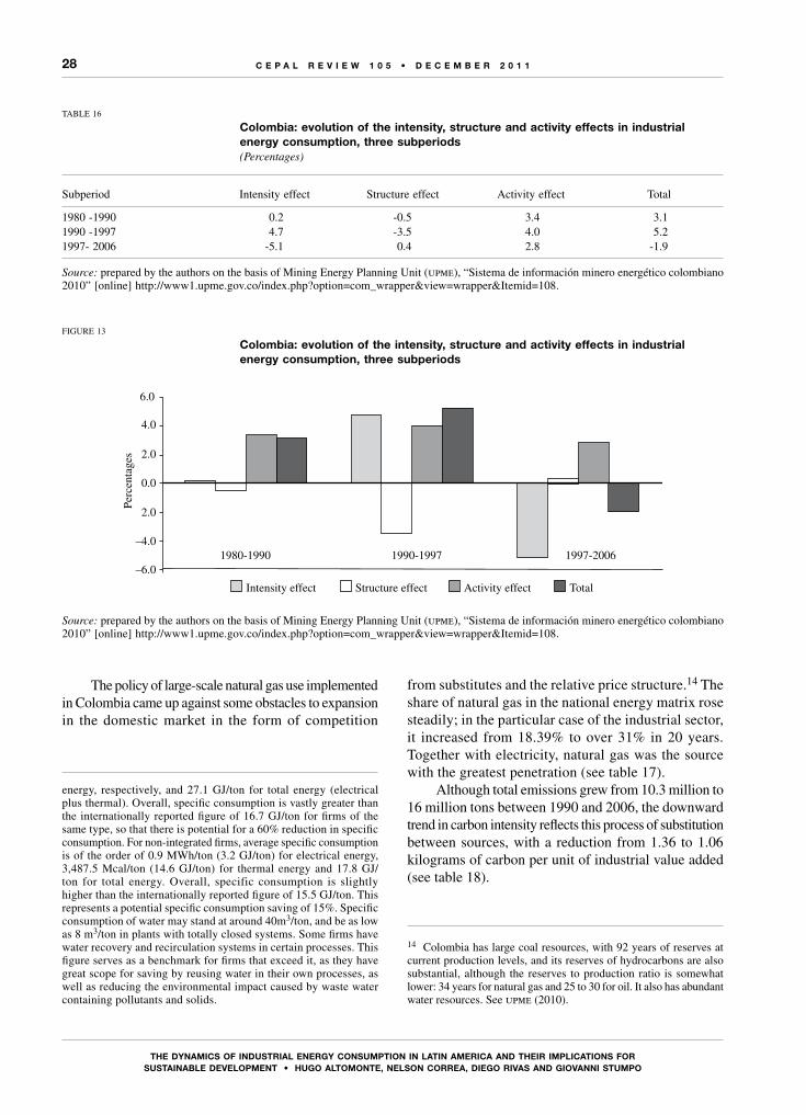
28
ThE DynAMiCs of inDusTriAL EnErGy ConsuMPTion in LATin AMEriCA AnD ThEir iMPLiCATions for sustAInABLE DEVELoPMEnt • Hugo ALtoMontE, nELson CoRREA, DIEgo RIVAs AnD gIoVAnnI stuMPo
C E P A L R E V I E W 1 0 5 • D E C E M B E R 2 0 1 1
TABLE 16
Colombia: evolution of the intensity, structure and activity effects in industrial energy consumption, three subperiods(Percentages)
Subperiod Intensity effect Structure effect Activity effect Total
1980 -1990 0.2 -0.5 3.4 3.11990 -1997 4.7 -3.5 4.0 5.21997- 2006 -5.1 0.4 2.8 -1.9
Source: prepared by the authors on the basis of Mining Energy Planning Unit (upme), “Sistema de información minero energético colombiano 2010” [online] http://www1.upme.gov.co/index.php?option=com_wrapper&view=wrapper&Itemid=108.
FIGURE 13
Colombia: evolution of the intensity, structure and activity effects in industrial energy consumption, three subperiods
Source: prepared by the authors on the basis of Mining Energy Planning Unit (upme), “Sistema de información minero energético colombiano 2010” [online] http://www1.upme.gov.co/index.php?option=com_wrapper&view=wrapper&Itemid=108.
Perc
enta
ges
Intensity effect Structure effect Activity effect Total
1980-1990 1990-1997 1997-2006–6.0
–4.0
2.0
0.0
2.0
4.0
6.0
The policy of large-scale natural gas use implemented in Colombia came up against some obstacles to expansion in the domestic market in the form of competition
energy, respectively, and 27.1 GJ/ton for total energy (electrical plus thermal). Overall, specific consumption is vastly greater than the internationally reported figure of 16.7 GJ/ton for firms of the same type, so that there is potential for a 60% reduction in specific consumption. For non-integrated firms, average specific consumption is of the order of 0.9 MWh/ton (3.2 GJ/ton) for electrical energy, 3,487.5 Mcal/ton (14.6 GJ/ton) for thermal energy and 17.8 GJ/ton for total energy. Overall, specific consumption is slightly higher than the internationally reported figure of 15.5 GJ/ton. This represents a potential specific consumption saving of 15%. Specific consumption of water may stand at around 40m3/ton, and be as low as 8 m3/ton in plants with totally closed systems. Some firms have water recovery and recirculation systems in certain processes. This figure serves as a benchmark for firms that exceed it, as they have great scope for saving by reusing water in their own processes, as well as reducing the environmental impact caused by waste water containing pollutants and solids.
from substitutes and the relative price structure.14 The share of natural gas in the national energy matrix rose steadily; in the particular case of the industrial sector, it increased from 18.39% to over 31% in 20 years. Together with electricity, natural gas was the source with the greatest penetration (see table 17).
Although total emissions grew from 10.3 million to 16 million tons between 1990 and 2006, the downward trend in carbon intensity reflects this process of substitution between sources, with a reduction from 1.36 to 1.06 kilograms of carbon per unit of industrial value added (see table 18).
14 Colombia has large coal resources, with 92 years of reserves at current production levels, and its reserves of hydrocarbons are also substantial, although the reserves to production ratio is somewhat lower: 34 years for natural gas and 25 to 30 for oil. It also has abundant water resources. See upme (2010).
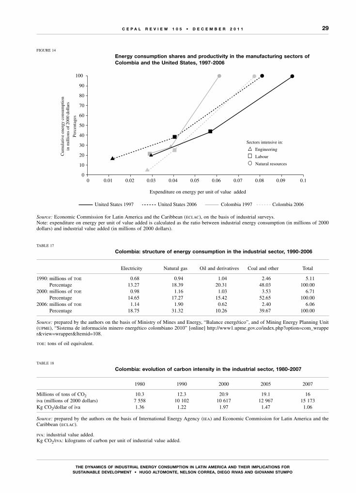
29
ThE DynAMiCs of inDusTriAL EnErGy ConsuMPTion in LATin AMEriCA AnD ThEir iMPLiCATions for sustAInABLE DEVELoPMEnt • Hugo ALtoMontE, nELson CoRREA, DIEgo RIVAs AnD gIoVAnnI stuMPo
C E P A L R E V I E W 1 0 5 • D E C E M B E R 2 0 1 1
FIGURE 14
Energy consumption shares and productivity in the manufacturing sectors of Colombia and the united states, 1997-2006
Source: Economic Commission for Latin America and the Caribbean (eclac), on the basis of industrial surveys.Note: expenditure on energy per unit of value added is calculated as the ratio between industrial energy consumption (in millions of 2000 dollars) and industrial value added (in millions of 2000 dollars).
0
10
20
30
40
50
60
70
80
90
100
0 0.01 0.02 0.03 0.04 0.05 0.06 0.07 0.08 0.09 0.1
Cum
ulat
ive
ener
gy c
onsu
mpt
ion
in m
illi
ons
of 2
000
doll
ars
Per
cent
ages
Expenditure on energy per unit of value added
United States 1997 United States 2006 Colombia 1997 Colombia 2006
Sectors intensive in:
Engineering
Labour
Natural resources
TABLE 17
Colombia: structure of energy consumption in the industrial sector, 1990-2006
Electricity Natural gas Oil and derivatives Coal and other Total
1990: millions of toe 0.68 0.94 1.04 2.46 5.11 Percentage 13.27 18.39 20.31 48.03 100.002000: millions of toe 0.98 1.16 1.03 3.53 6.71 Percentage 14.65 17.27 15.42 52.65 100.002006: millions of toe 1.14 1.90 0.62 2.40 6.06 Percentage 18.75 31.32 10.26 39.67 100.00
Source: prepared by the authors on the basis of Ministry of Mines and Energy, “Balance energético”, and of Mining Energy Planning Unit (upme), “Sistema de información minero energético colombiano 2010” [online] http://www1.upme.gov.co/index.php?option=com_wrapper&view=wrapper&Itemid=108.
toe: tons of oil equivalent.
TABLE 18
Colombia: evolution of carbon intensity in the industrial sector, 1980-2007
1980 1990 2000 2005 2007
Millions of tons of CO2 10.3 12.3 20.9 19.1 16iva (millions of 2000 dollars) 7 558 10 102 10 617 12 967 15 173Kg CO2/dollar of iva 1.36 1.22 1.97 1.47 1.06
Source: prepared by the authors on the basis of International Energy Agency (iea) and Economic Commission for Latin America and the Caribbean (eclac).
iva: industrial value added.Kg CO2/iva: kilograms of carbon per unit of industrial value added.
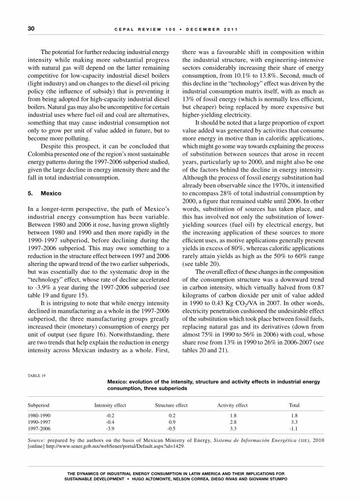
30
ThE DynAMiCs of inDusTriAL EnErGy ConsuMPTion in LATin AMEriCA AnD ThEir iMPLiCATions for sustAInABLE DEVELoPMEnt • Hugo ALtoMontE, nELson CoRREA, DIEgo RIVAs AnD gIoVAnnI stuMPo
C E P A L R E V I E W 1 0 5 • D E C E M B E R 2 0 1 1
The potential for further reducing industrial energy intensity while making more substantial progress with natural gas will depend on the latter remaining competitive for low-capacity industrial diesel boilers (light industry) and on changes to the diesel oil pricing policy (the influence of subsidy) that is preventing it from being adopted for high-capacity industrial diesel boilers. Natural gas may also be uncompetitive for certain industrial uses where fuel oil and coal are alternatives, something that may cause industrial consumption not only to grow per unit of value added in future, but to become more polluting.
Despite this prospect, it can be concluded that Colombia presented one of the region’s most sustainable energy patterns during the 1997-2006 subperiod studied, given the large decline in energy intensity there and the fall in total industrial consumption.
5. Mexico
In a longer-term perspective, the path of Mexico’s industrial energy consumption has been variable. Between 1980 and 2006 it rose, having grown slightly between 1980 and 1990 and then more rapidly in the 1990-1997 subperiod, before declining during the 1997-2006 subperiod. This may owe something to a reduction in the structure effect between 1997 and 2006 altering the upward trend of the two earlier subperiods, but was essentially due to the systematic drop in the “technology” effect, whose rate of decline accelerated to -3.9% a year during the 1997-2006 subperiod (see table 19 and figure 15).
It is intriguing to note that while energy intensity declined in manufacturing as a whole in the 1997-2006 subperiod, the three manufacturing groups greatly increased their (monetary) consumption of energy per unit of output (see figure 16). Notwithstanding, there are two trends that help explain the reduction in energy intensity across Mexican industry as a whole. First,
there was a favourable shift in composition within the industrial structure, with engineering-intensive sectors considerably increasing their share of energy consumption, from 10.1% to 13.8%. Second, much of this decline in the “technology” effect was driven by the industrial consumption matrix itself, with as much as 13% of fossil energy (which is normally less efficient, but cheaper) being replaced by more expensive but higher-yielding electricity.
It should be noted that a large proportion of export value added was generated by activities that consume more energy in motive than in calorific applications, which might go some way towards explaining the process of substitution between sources that arose in recent years, particularly up to 2000, and might also be one of the factors behind the decline in energy intensity. Although the process of fossil energy substitution had already been observable since the 1970s, it intensified to encompass 28% of total industrial consumption by 2000, a figure that remained stable until 2006. In other words, substitution of sources has taken place, and this has involved not only the substitution of lower-yielding sources (fuel oil) by electrical energy, but the increasing application of these sources to more efficient uses, as motive applications generally present yields in excess of 80%, whereas calorific applications rarely attain yields as high as the 50% to 60% range (see table 20).
The overall effect of these changes in the composition of the consumption structure was a downward trend in carbon intensity, which virtually halved from 0.87 kilograms of carbon dioxide per unit of value added in 1990 to 0.43 Kg CO2/VA in 2007. In other words, electricity penetration cushioned the undesirable effect of the substitution which took place between fossil fuels, replacing natural gas and its derivatives (down from almost 75% in 1990 to 56% in 2006) with coal, whose share rose from 13% in 1990 to 26% in 2006-2007 (see tables 20 and 21).
TABLE 19
Mexico: evolution of the intensity, structure and activity effects in industrial energy consumption, three subperiods
Subperiod Intensity effect Structure effect Activity effect Total
1980-1990 -0.2 0.2 1.8 1.81990-1997 -0.4 0.9 2.8 3.31997-2006 -3.9 -0.5 3.3 -1.1
Source: prepared by the authors on the basis of Mexican Ministry of Energy, Sistema de Información Energética (sie), 2010 [online] http://www.sener.gob.mx/webSener/portal/Default.aspx?id=1429.
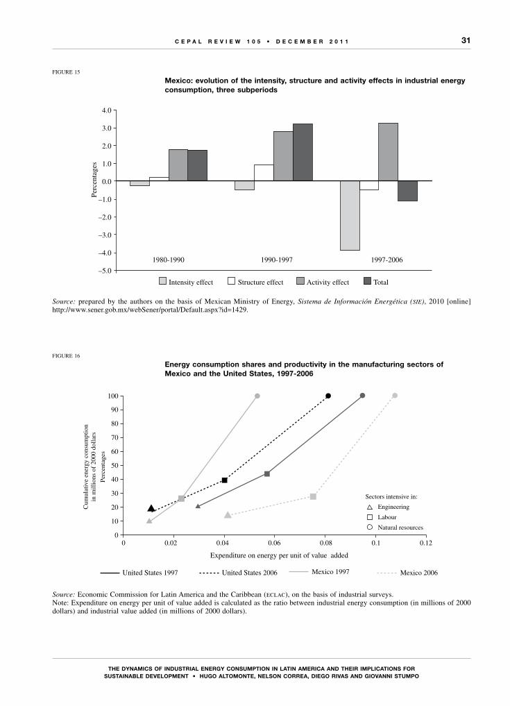
31
ThE DynAMiCs of inDusTriAL EnErGy ConsuMPTion in LATin AMEriCA AnD ThEir iMPLiCATions for sustAInABLE DEVELoPMEnt • Hugo ALtoMontE, nELson CoRREA, DIEgo RIVAs AnD gIoVAnnI stuMPo
C E P A L R E V I E W 1 0 5 • D E C E M B E R 2 0 1 1
FIGURE 16
Energy consumption shares and productivity in the manufacturing sectors of Mexico and the united states, 1997-2006
Source: Economic Commission for Latin America and the Caribbean (eclac), on the basis of industrial surveys.Note: Expenditure on energy per unit of value added is calculated as the ratio between industrial energy consumption (in millions of 2000 dollars) and industrial value added (in millions of 2000 dollars).
FIGURE 15
Mexico: evolution of the intensity, structure and activity effects in industrial energy consumption, three subperiods
Source: prepared by the authors on the basis of Mexican Ministry of Energy, Sistema de Información Energética (sie), 2010 [online] http://www.sener.gob.mx/webSener/portal/Default.aspx?id=1429.
–5.0
–4.0
–3.0
–2.0
–1.0
0.0
1.0
2.0
3.0
4.0
Perc
enta
ges
Intensity effect Structure effect Activity effect Total
1980-1990 1990-1997 1997-2006
0
10
20
30
40
50
60
70
80
90
100
0 0.02 0.04 0.06 0.08 0.1 0.12
Cum
ulat
ive
ener
gy c
onsu
mpt
ion
in m
illi
ons
of 2
000
doll
ars
Per
cent
ages
Expenditure on energy per unit of value added
United States 1997 United States 2006 Mexico 1997 Mexico 2006
Sectors intensive in:
Engineering
Labour
Natural resources
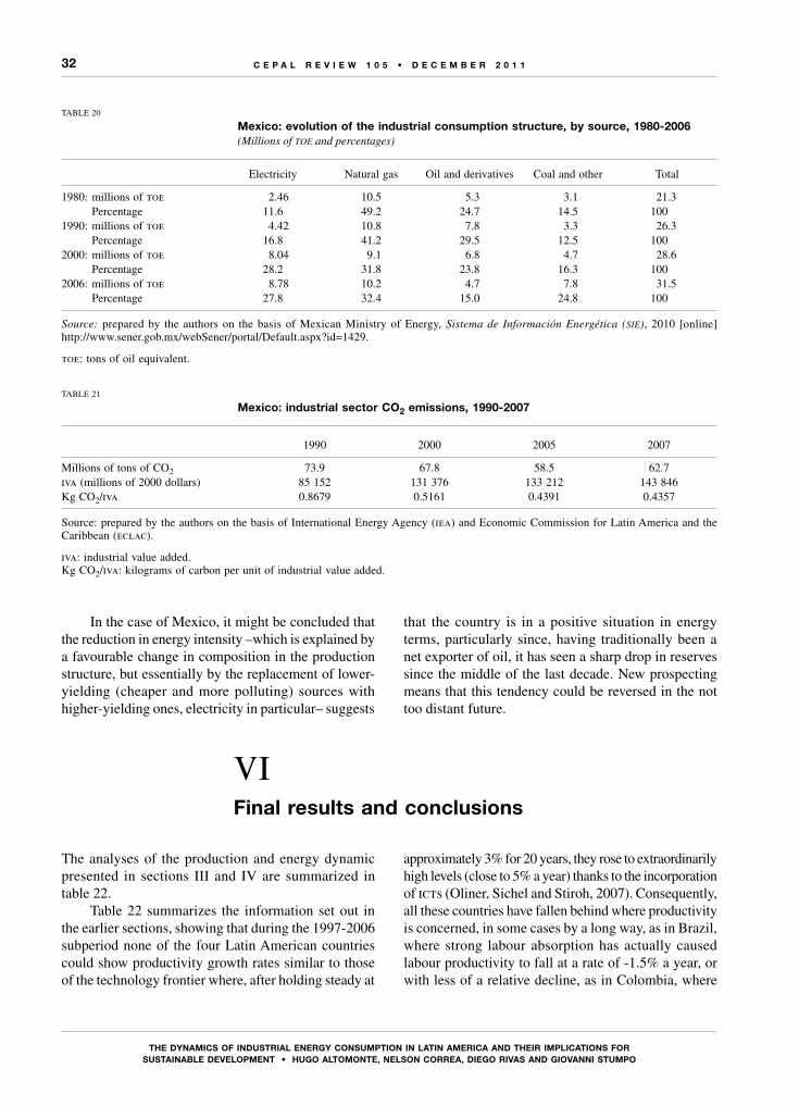
32
ThE DynAMiCs of inDusTriAL EnErGy ConsuMPTion in LATin AMEriCA AnD ThEir iMPLiCATions for sustAInABLE DEVELoPMEnt • Hugo ALtoMontE, nELson CoRREA, DIEgo RIVAs AnD gIoVAnnI stuMPo
C E P A L R E V I E W 1 0 5 • D E C E M B E R 2 0 1 1
TABLE 20
Mexico: evolution of the industrial consumption structure, by source, 1980-2006 (Millions of toe and percentages)
Electricity Natural gas Oil and derivatives Coal and other Total
1980: millions of toe 2.46 10.5 5.3 3.1 21.3 Percentage 11.6 49.2 24.7 14.5 1001990: millions of toe 4.42 10.8 7.8 3.3 26.3 Percentage 16.8 41.2 29.5 12.5 1002000: millions of toe 8.04 9.1 6.8 4.7 28.6 Percentage 28.2 31.8 23.8 16.3 1002006: millions of toe 8.78 10.2 4.7 7.8 31.5 Percentage 27.8 32.4 15.0 24.8 100
Source: prepared by the authors on the basis of Mexican Ministry of Energy, Sistema de Información Energética (sie), 2010 [online] http://www.sener.gob.mx/webSener/portal/Default.aspx?id=1429.
toe: tons of oil equivalent.
TABLE 21
Mexico: industrial sector Co2 emissions, 1990-2007
1990 2000 2005 2007
Millions of tons of CO2 73.9 67.8 58.5 62.7iva (millions of 2000 dollars) 85 152 131 376 133 212 143 846Kg CO2/iva 0.8679 0.5161 0.4391 0.4357
Source: prepared by the authors on the basis of International Energy Agency (iea) and Economic Commission for Latin America and the Caribbean (eclac).
iva: industrial value added.Kg CO2/iva: kilograms of carbon per unit of industrial value added.
In the case of Mexico, it might be concluded that the reduction in energy intensity –which is explained by a favourable change in composition in the production structure, but essentially by the replacement of lower-yielding (cheaper and more polluting) sources with higher-yielding ones, electricity in particular– suggests
that the country is in a positive situation in energy terms, particularly since, having traditionally been a net exporter of oil, it has seen a sharp drop in reserves since the middle of the last decade. New prospecting means that this tendency could be reversed in the not too distant future.
VIfinal results and conclusions
The analyses of the production and energy dynamic presented in sections III and IV are summarized in table 22.
Table 22 summarizes the information set out in the earlier sections, showing that during the 1997-2006 subperiod none of the four Latin American countries could show productivity growth rates similar to those of the technology frontier where, after holding steady at
approximately 3% for 20 years, they rose to extraordinarily high levels (close to 5% a year) thanks to the incorporation of icts (Oliner, Sichel and Stiroh, 2007). Consequently, all these countries have fallen behind where productivity is concerned, in some cases by a long way, as in Brazil, where strong labour absorption has actually caused labour productivity to fall at a rate of -1.5% a year, or with less of a relative decline, as in Colombia, where
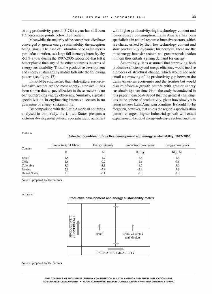
33
ThE DynAMiCs of inDusTriAL EnErGy ConsuMPTion in LATin AMEriCA AnD ThEir iMPLiCATions for sustAInABLE DEVELoPMEnt • Hugo ALtoMontE, nELson CoRREA, DIEgo RIVAs AnD gIoVAnnI stuMPo
C E P A L R E V I E W 1 0 5 • D E C E M B E R 2 0 1 1
strong productivity growth (3.7%) a year has still been 1.5 percentage points below the frontier.
Meanwhile, the majority of the countries studied have converged on greater energy sustainability, the exception being Brazil. The case of Colombia once again merits particular attention, as a large fall in energy intensity (by -5.1% a year during the 1997-2006 subperiod) has left it better placed than any of the other countries in terms of energy sustainability. Thus, the productive development and energy sustainability matrix falls into the following pattern (see figure 17).
It should be emphasized that while natural resource-intensive sectors are the most energy-intensive, it has been shown that a specialization in these sectors is no bar to improving energy efficiency. Similarly, a greater specialization in engineering-intensive sectors is no guarantee of energy sustainability.
By comparison with the Latin American countries analysed in this study, the United States presents a virtuous development pattern, specializing in activities
with higher productivity, high technology content and lower energy consumption. Latin America has been specializing in natural resource-intensive sectors, which are characterized by their low technology content and slow productivity dynamic; furthermore, these are the most energy-intensive sectors, and greater specialization in them thus entails a rising demand for energy.
Accordingly, it is assumed that improving both productive efficiency and energy efficiency would involve a process of structural change, which would not only entail a narrowing of the productivity gap between the Latin American economies and the frontier but would also reinforce a growth pattern with greater energy sustainability over time. From the analysis conducted in this paper it can be deduced that the greatest challenge lies in the sphere of productivity, given how slowly it is rising in these Latin American countries. It should not be forgotten, however, that unless the region’s specialization pattern changes, higher industrial growth will entail expansion of the most energy-intensive sectors, and thus
TABLE 22
selected countries: productive development and energy sustainability, 1997-2006
CountryProductivity of labour Energy intensity Productive convergence Energy convergence
Π EI Πi-ΠUS EIUS-EIi
Brazil -1.5 1.2 -6.8 -1.3Chile 2.6 -0.7 -2.6 0.6Colombia 3.7 -5.1 -1.5 5.0Mexico 2.8 -3.9 -2.4 3.8United States 5.3 -0.1 0.0 0.0
Source: prepared by the authors.
FIGURE 17
Productive development and energy sustainability matrix
Source: prepared by the authors.
Chile, Colombiaand Mexico
Brazil
ENERGY SUSTAINABILITY
PRO
DU
CT
IVIT
YC
ON
VE
RG
EN
CE

34
ThE DynAMiCs of inDusTriAL EnErGy ConsuMPTion in LATin AMEriCA AnD ThEir iMPLiCATions for sustAInABLE DEVELoPMEnt • Hugo ALtoMontE, nELson CoRREA, DIEgo RIVAs AnD gIoVAnnI stuMPo
C E P A L R E V I E W 1 0 5 • D E C E M B E R 2 0 1 1
increased energy consumption. To bring about sustainable structural development, in other words, it is necessary to shift the industrial structure towards the sectors that are the most knowledge-intensive and dynamic in terms
of productivity growth where these have the potential to replace other sectors that are less dynamic and more energy-intensive, thereby altering the region’s current specialization path.
(Original: Spanish)
Bibliography
Aguayo, F. and K.P. Gallagher (2003), “Economic reform, energy, and development: the case of Mexican manufacturing”, gdae Working Papers, No. 03-05, Tufts University.
Altomonte, H. (2010), “Mercados de energía eléctrica en América Latina: La regulación pública y las estrategias de las empresas”, América Latina y petróleo. Los desafíos políticos y económicos de cara al siglo XXI, Isabel Rousseau, Mexico City, El Colegio de México.
(coord.) (2008), “América Latina y el Caribe frente a la coyuntura energética internacional: Oportunidades para una nueva agenda de políticas”, Project Document (LC/W.220), Santiago, Chile, Economic Commission for Latin America and the Caribbean (eclac), September.
Cimoli, M. (ed.) (2005), “Brecha tecnológica y crecimiento en América Latina”, Heterogeneidad estructural, asimetrías tecnológicas y crecimiento en América Latina, Santiago, Chile, Inter-American Development Bank/Economic Commission for Latin America and the Caribbean (idb/eclac).
Cole, M.A., A.J. Rayner and J.M. Bates (1997), “The environmental Kuznets curve: An empirical analysis”, Environment and Development Economics, vol. 2, No. 4, Cambridge, Cambridge University Press.
De Bruyn, S.M., J.C.J.M. Van den Bergh and J.B. Opschoor (1998), “Economic growth and emissions: Reconsidering the empirical basis of environmental Kuznets curves”, Ecological Economics, vol. 25, No. 2, Amsterdam, Elsevier.
eclac (Economic Commission for Latin America and the Caribbean) (2010), Time for Equality: Closing Gaps, Opening Trails (LC/G.2432(SES.33/3)), Santiago, Chile.
eia (Energy Information Administration) (2009), Monthly Energy Review, Washington, D.C., Department of Energy, June.
Ferraz, J.C., D. Kupfer and F. Serrano (1999), “Productividad y heterogeneidad estructural en la industria brasileña”.
iea (International Energy Agency) (2008), World Energy Outlook 2008, Paris.
Katz, J. and G. Stumpo (2001), “Regímenes competitivos sectoriales, productividad y competitividad internacional”, Desarrollo productivo series, No. 103 (LC/L.1578-P), Santiago, Chile, Economic Commission for Latin America and the Caribbean (eclac). United Nations publication, Sales No. S.01.II.G.120.
Maldonado, P. (2007), “Estudio sobre empresas energo intensivas y su posible contribución a programas de eficiencia energética”, Santiago, Chile, Economic Commission for Latin America and the Caribbean (eclac).
Ministry of Energy/National Energy Commission (various years), “Balances energéticos” [online] http://www.cne.cl
Ministry of Mines and Energy, “Balance energético nacional de Brasil” [online] http://www.mme.gov.br
olade (Latin American Energy Organization) (2008), Energy Statistics Report, Quito.
(2006), Energy Statistics Report, Quito.olade/eclac/gtz (Latin American Energy Organization/Economic
Commission for Latin America and the Caribbean/German Agency for Technical Cooperation) (2003), Energía y desarrollo sustentable en América Latina y el Caribe: guía para la formulación de políticas energéticas (LC/G.2214-P), Santiago, Chile, December. United Nations publication, Sales No. S.03.II.G.160.
Oliner, S.D., D. Sichel and K. Stiroh (2007), “Explaining a productive decade” Journal of Policy Modeling, vol. 30, No. 4, Amsterdam, Elsevier.
Pasche, M. (2002), “Technical progress, structural change, and the environmental Kuznets curve”, Ecological Economics, vol. 42, No. 3, Amsterdam, Elsevier.
upme (Unidad de Planeación Minero Energética) (2010), Boletín estadístico de minas y energía 1990-2010, Bogota, Ministry of Mines and Energy.
(2008), “Programa estratégico nacional. Gestión integral de la energía en centros productivos, gie”, Bogota, Ministry of Mines and Energy.
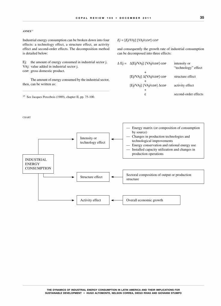
35
ThE DynAMiCs of inDusTriAL EnErGy ConsuMPTion in LATin AMEriCA AnD ThEir iMPLiCATions for sustAInABLE DEVELoPMEnt • Hugo ALtoMontE, nELson CoRREA, DIEgo RIVAs AnD gIoVAnnI stuMPo
C E P A L R E V I E W 1 0 5 • D E C E M B E R 2 0 1 1
AnnEx15
Industrial energy consumption can be broken down into four effects: a technology effect, a structure effect, an activity effect and second-order effects. The decomposition method is detailed below:
Ej: the amount of energy consumed in industrial sector j.VAj: value added in industrial sector j.gdp: gross domestic product.
The amount of energy consumed by the industrial sector, then, can be written as:
15 See Jacques Percebois (1989), chapter II, pp. 75-100.
Ej = [Ej/VAj] [VAj/gdp] gdp
and consequently the growth rate of industrial consumption can be decomposed into three effects:
∆ Ej = ∆[Ej/VAj] [VAj/gdp] gdp intensity or “technology” effect
+ [Ej/VAj] ∆[VAj/gdp] gdp structure effect + [Ej/VAj] [VAj/gdp] ∆gdp activity effect + ε second-order effects
CHART
INDUSTRIALENERGYCONSUMPTION
Intensity or technology effect
— Energy matrix (or composition of consumption by source)
— Changes in production technologies and technological improvements
— Energy conservation and rational energy use— Installed capacity utilization and changes in
production operations
Structure effectSectoral composition of output or production structure
Activity effect Overall economic growth


C E P A L R E V I E W 1 0 5 • D E C E M B E R 2 0 1 1
37
K E Y W O R D S
Income
Income distribution
Bank credit market
Bank deposits
Markets
Financial services
Banks
Financial institutions
Informal sector
Adolfo Figueroa, Ph.D.
Professor Emeritus of Economics
Centrum Business School
Catholic University of Peru
Income inequality and credit markets
Adolfo Figueroa
T hree empirical regularities have been identified in the financial
literature: bank credit markets operate with collateral, they operate with
excess demand and they coexist with other forms of credit provision. In
the particular case of less developed countries, the financial structure
comprises the banking industry, the formal non-banking industry and
the informal sector. This paper presents a theoretical model that explains
all three regularities together. According to the model, wealth inequality
in society is the essential factor that explains this dual-dual financial
structure. The model predicts market segmentation: the wealthy and the
banks constitute one market, the less wealthy and formal non-banking
organizations constitute another and the poorest groups and small lenders
constitute the informal sector; moreover, credit is more expensive in
the latter sectors. As long as wealth inequality remains unchanged, this
financial structure will prevail. The public policy implications of the model
are also presented.

38
InCoME InEquALIty AnD CREDIt MARkEts • ADoLfo fIguERoA
C E P A L R E V I E W 1 0 5 • D E C E M B E R 2 0 1 1
The author is grateful for the valuable comments of an anonymous cepal Review referee. The research assistance of Paola Lazarte and Erick Vila is also greatly appreciated.
Three empirical regularities in the workings of bank credit markets have been identified by the literature: (1) bank credit markets operate with collateral (Berger and Udell, 1995); (2) bank credit markets operate with demand rationing (Berger and Udell, 1992; Steijvers and Voordeckers, 2009); and (3) bank credit markets coexist with non-bank forms of credit provision, which operate with higher interest rates. The third regularity is particularly significant in less developed countries (Campion, Kiran-Ekka and Wenner, 2010; Banerjee, 2003). A review of the literature failed to identify any empirical studies testing theoretical models of bank credit markets.
These three facts can be interpreted as the equilibrium conditions under which the banking industry operates. Any particular values that equilibrium prices and quantities may take in the market will satisfy those conditions. Consequently, the simplest way to refute any theoretical model of a bank credit market is to show that its predictions about the observable equilibrium conditions are inconsistent with these regularities. This paper will present a theoretical model that is able to predict all three regularities together. Of course, a complete refutation also requires a set of empirical predictions about the relations between endogenous and exogenous variables in the theoretical model, which can then be compared statistically against empirical data. That task lies beyond the scope of this paper.
Standard economics has sought to explain facts (1) and (2) by the theory of asymmetric information. The model developed by Stiglitz and Weiss (1981) is the classic presentation of the theory. According to this model, credit markets operate with rationing. The interest rate does not clear the market because loan quality, insofar as it affects bank profits, is not independent of this rate. The model does not necessarily predict equilibrium with
excess demand, however; rationing could also take the form of excess supply. In other words, excess demand plays no role in the functioning of bank credit markets; i.e., it is not a necessity. Fact (2) implies the opposite.
At the same time, different views on the nature of credit market equilibrium coexist within the standard literature. While the credit market is treated as Walrasian in most macro-models (Barro, 1997; Krugman and Wells, 2006), it is treated as non-Walrasian by the Stiglitz-Weiss model and its followers. In his Nobel Lecture, Stiglitz (2002) even argued that equilibrium in the credit market may not exist.
What type of market is the bank credit market? This paper develops a partial equilibrium model of bank credit markets that will seek to answer this theoretical question. The assumptions of the model depart from the models utilized in standard economics in several ways in order to to explain the determination of prices and quantities as observed in bank credit markets. Without a sound theoretical basis, public policies run the risk of failure.
The paper is organized as follows. Section II presents a review of the literature on the empirical testing of partial equilibrium models of bank credit markets, which shows that this topic has been understudied. The nature of the bank credit market is presented in section III. Construction of the proposed partial equilibrium model starts in section IV, where a competitive model of bank credit is presented. The empirical predictions of the model are then developed. A non-competitive model may seem more appropriate for studying the banking industry, but we can invoke the theorem of equivalence: although competitive, monopoly and oligopoly models have different structural equations, under certain conditions they will qualitatively generate the same reduced form equations (same empirical predictions). The competitive model is the simplest; hence, bank credit markets can fruitfully be studied using a competitive market model. A dual model of credit markets that connects the banking and formal non-banking industries is presented in section V. Section VI introduces the informal credit sector and analyses its role in the functioning of the whole credit system. Section VII concludes.
Iintroduction
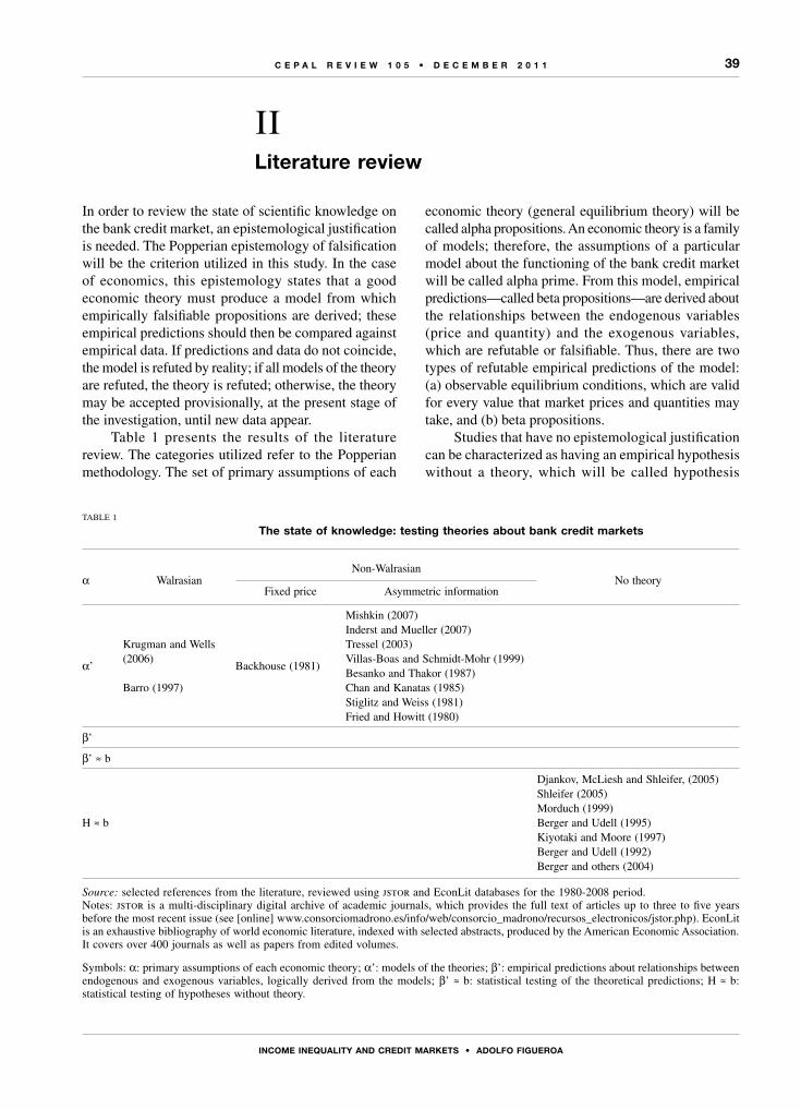
39
InCoME InEquALIty AnD CREDIt MARkEts • ADoLfo fIguERoA
C E P A L R E V I E W 1 0 5 • D E C E M B E R 2 0 1 1
In order to review the state of scientific knowledge on the bank credit market, an epistemological justification is needed. The Popperian epistemology of falsification will be the criterion utilized in this study. In the case of economics, this epistemology states that a good economic theory must produce a model from which empirically falsifiable propositions are derived; these empirical predictions should then be compared against empirical data. If predictions and data do not coincide, the model is refuted by reality; if all models of the theory are refuted, the theory is refuted; otherwise, the theory may be accepted provisionally, at the present stage of the investigation, until new data appear.
Table 1 presents the results of the literature review. The categories utilized refer to the Popperian methodology. The set of primary assumptions of each
economic theory (general equilibrium theory) will be called alpha propositions. An economic theory is a family of models; therefore, the assumptions of a particular model about the functioning of the bank credit market will be called alpha prime. From this model, empirical predictions—called beta propositions—are derived about the relationships between the endogenous variables (price and quantity) and the exogenous variables, which are refutable or falsifiable. Thus, there are two types of refutable empirical predictions of the model: (a) observable equilibrium conditions, which are valid for every value that market prices and quantities may take, and (b) beta propositions.
Studies that have no epistemological justification can be characterized as having an empirical hypothesis without a theory, which will be called hypothesis
IILiterature review
TABLE 1
The state of knowledge: testing theories about bank credit markets
α WalrasianNon-Walrasian
No theoryFixed price Asymmetric information
α’
Krugman and Wells (2006)
Barro (1997)
Backhouse (1981)
Mishkin (2007)Inderst and Mueller (2007)Tressel (2003)Villas-Boas and Schmidt-Mohr (1999)Besanko and Thakor (1987)Chan and Kanatas (1985)Stiglitz and Weiss (1981)Fried and Howitt (1980)
β’
β’ ≈ b
H ≈ b
Djankov, McLiesh and Shleifer, (2005)Shleifer (2005)Morduch (1999)Berger and Udell (1995)Kiyotaki and Moore (1997)Berger and Udell (1992)Berger and others (2004)
Source: selected references from the literature, reviewed using jstor and EconLit databases for the 1980-2008 period.Notes: jstor is a multi-disciplinary digital archive of academic journals, which provides the full text of articles up to three to five years before the most recent issue (see [online] www.consorciomadrono.es/info/web/consorcio_madrono/recursos_electronicos/jstor.php). EconLit is an exhaustive bibliography of world economic literature, indexed with selected abstracts, produced by the American Economic Association. It covers over 400 journals as well as papers from edited volumes.
Symbols: α: primary assumptions of each economic theory; α’: models of the theories; β’: empirical predictions about relationships between endogenous and exogenous variables, logically derived from the models; β’ ≈ b: statistical testing of the theoretical predictions; H ≈ b: statistical testing of hypotheses without theory.

40
InCoME InEquALIty AnD CREDIt MARkEts • ADoLfo fIguERoA
C E P A L R E V I E W 1 0 5 • D E C E M B E R 2 0 1 1
H. This hypothesis can be tested statistically. If it passes the test, it will corroborate the hypothesis and correlations, but there will not be causality. Causality —the relationship between endogenous and exogenous variables— can only be derived from a theoretical model. Causality takes the form of a beta proposition, as indicated in table 1.
Relevant and representative bibliographical references are shown in table 1. This indicates the existence of a vast literature on asymmetric information models, which predict that the bank credit market
operates with collateral and rationing. It also indicates the existence of a large literature applying statistical testing to hypotheses which lack a theoretical underpinning, the so-called “empirical approach”. The conclusion is clear: the cells corresponding to studies where theories have been subject to the falsification process are empty (the third row). Not even the set of beta propositions has been developed (the second row). This paper proposes to help fill the gap by presenting a set of falsifiable empirical predictions logically derived from the particular model developed here.
IIIThe nature of the credit market
What type of market is the bank credit market? Could excess demand play any role in the functioning of credit markets? The type of transaction that takes place in a credit market involves the exchange of a sum of money now for the promise to repay later at a given interest rate. This is the nature of the credit market. Hence, this market raises the principal-agent problem. Could it operate as a Walrasian market? If individuals could always obtain the credit they desired at the prevailing market interest rate, they would not have economic incentives to repay the loan. If individuals could get credit irrespective of the effort they made to repay the loan and of their repayment history, why should they bother to repay the loan or avoid risky projects? Borrowers would not incur any cost if they defaulted. In sum, the credit market cannot operate as a Walrasian market.
What devices might banks use to discipline borrowers? A possible one would be to set the interest rate below the Walrasian price. Excess demand would thus be generated. The cost of default would now be the exclusion of bad borrowers from the credit market. Thus, the credit market could operate on a non-Walrasian basis, with excess demand.
How could this market result be attained? Assume that banks use collateral on loans as a device to discipline borrowers. The cost of default is now the loss of the
collateral. Assume that the distribution of wealth in society is highly unequal. In addition, assume a financial technology that has economies of scale, so that large credits are more profitable for banks; then banks will have an incentive to do business with the wealthy segment of the market only. Total demand is now separated into two: those served by banks (the wealthy) and those excluded (the poor), who are served by the non-banking market, in which another financial technology will be used.
This is the model that will be formally developed in what follows. It will be shown that this model predicts the three empirical regularities stated above. Whether the empirical predictions of the model (relationships between endogenous and exogenous variables of the model) are refuted by data will require statistical testing.
The credit market is clearly influenced by and itself influences the rest of the economy. In order to reduce the second effect and justify the use of partial equilibrium analysis, this study will divide the bank credit market into several particular markets, which can then be analysed separately. More specifically, the partial equilibrium model is intended to explain the functioning of markets for short-term credit (for working capital) and long-run credit (for investment), in which the demand comes from firms alone. For simplicity, credit demand from households will not be part of this study.
41
InCoME InEquALIty AnD CREDIt MARkEts • ADoLfo fIguERoA
C E P A L R E V I E W 1 0 5 • D E C E M B E R 2 0 1 1
The particular model of the standard theory of credit markets that will be presented here seeks to explain the behaviour of prices and quantities in the banking industry. The basic assumptions of the model are the following: — agents operate in a capitalist society in which the
initial individual endowment of wealth, mainly physical capital, is significantly unequal;
— market lending transactions take place in a context of uncertainty, asymmetric information and significant transaction costs;
— technology in the banking industry is such that there are major economies of scale in transaction costs when loans are large;
— collateral is the device banks use to generate a disincentive for borrowers to default. How does the banking industry operate in such a
context? This is the question that the model will seek to answer.
The banking industry is composed of two markets, the credit market and the deposit market. Banks are the financial intermediaries. Prices and quantities in the banking industry will depend upon the market structure or degree of market power of buyers and sellers. The model will assume that the banking industry operates with a market structure of perfect competition, for the reasons given in the Introduction.
1. The behaviour of banks
The model assumes that banks set an amount of collateral sufficient to cover the loan and the interest to be repaid; that is, loans are fully covered by the collateral. It also assumes that the enforcement of loan contracts is costless; consequently, the problems of asymmetric information are reduced significantly. The implication of these assumptions is that all potential borrowers become homogeneous in terms of risk. Therefore, banks can seek to maximize profits in the manner that is common in standard demand-supply analysis.
In a situation of perfect competition, banks are price takers in both the credit market and the deposit market. They can supply the quantity of credit they desire at the prevailing market lending interest rate; they can also acquire the quantity of deposits they desire at the prevailing market deposit interest rate. In determining
the quantities they are willing to transact, banks will be guided by the desire to maximize profits.
The model then assumes the following behaviour for the case of a representative bank k in the short run:
∑
= − − −= > >≤ −
= ≥ ∀ =
Max P rS rD C FC (Profits function)s.t C f S f f
S e DS s such that s s j n
( ), ´ 0, ´ 0
(1 ), 1, 2,... ,
k rk rk k k
k rk
rk rk
rk kj kj k k
*
(1)
The first equation of system (1) is the bank’s profit equation, where P stands for nominal profits, r for the nominal lending interest rate, Sr for the nominal quantity of credit, r~ for the nominal deposit interest rate, D
~ r for
the nominal quantity of deposits, C for the total variable cost of intermediation and FC for the total fixed costs of the bank. The second equation is just the variable cost function. The third equation shows the restriction that the bank’s loanable fund is net of the reserve requirement, whose rate e is established by the monetary authority.
This last constraint indicates that banks set threshold values for the size of individual loanable funds by borrower (called s), which cannot be smaller than s*. This is due to the nature of the intermediation cost faced by banks. The intermediation cost includes transaction costs and the cost of intermediation proper. The model assumes that the transaction cost per borrower is constant; i.e., it is independent of loan size. Therefore, the unit cost per dollar of lending declines with loan size up to size s* and then becomes constant. The bank thus has no incentive to lend money to borrowers seeking loans smaller than s*.
In the short run, banks must determine the quantity of lending that maximizes profits. From the structural equations shown in system (1), the equilibrium condition can then be derived by differentiating the profit equation with respect to Sr. The equilibrium condition for bank k then becomes:
˜˜r r
ef S MC S r e
MC MC MC(1 )
’( ) ( , , ),
0, 0, 0
rk k rk
1 2 3
=−
+ =
> > > (2)
IVA competitive model of the bank credit market
42
InCoME InEquALIty AnD CREDIt MARkEts • ADoLfo fIguERoA
C E P A L R E V I E W 1 0 5 • D E C E M B E R 2 0 1 1
The individual bank will seek to maximize profits, which implies equalizing the market lending interest rate with the marginal cost of providing credit (MC). The latter is equal to the net marginal cost of acquiring the necessary bank deposits plus the marginal cost of intermediation.
The equilibrium condition in (2) is clearly stable; consequently, the static comparative method can be applied to this equilibrium condition to derive empirical predictions for the behaviour of the representative bank. The endogenous variables include the quantities of loans and deposits. The exogenous variables include lending and deposit interest rates and the reserve requirement ratio. The capital stock of the bank is also exogenously given, but changes in it will be ignored in this short-run model.
The effects of changes in the exogenous variables upon the endogenous variables can easily be derived from equation (2). The reduced form equations are then obtained as follows:
˜S F r r e( , , ), 0, 0, 0rkk k k k
1 2 3= > < <F F F (3a)
˜( )=
−
D
eS1
1rk rk (4a)
The equilibrium quantity of credit supplied by representative bank k depends upon the exogenous variables of the model, as shown in equation (3a). An increase in the lending interest rate has the effect of increasing the quantity of credit supplied because it increases marginal revenue; an increase in the deposit interest rate or in the reserve requirement ratio has the effect of reducing the quantity of credit supplied because the marginal cost increases.
The bank will determine the quantity of credit supplied on the basis of the values of the exogenous variables. The required quantity of deposits will then also be determined, as a derived demand for bank deposits. This is shown in equation (4a).
The aggregate behaviour of banks will be obtained by simple addition of the equations of the individual banks, as shown in system (3a)-(4a), across all banks in the industry. Thus, equation (3) represents the market supply function of bank credit and equation (4) the market derived demand function for bank deposits.
˜S S F r r e F F F( , , ), 0, 0, 0rk r 1 2 3∑ ≡ = > < < (3)
˜ ˜∑ ( )≡ =−
D D
eS1
1rk r r (4)
2. The behaviour of households and the supply of bank deposits
In a market economy that includes banks, the quantity of money will be equal to currency in circulation plus demand deposits. Both can be used as a means of payment. Households must choose not only the stock of money they want to hold, but also its allocation between bank deposits and cash balances.
A model of household behaviour will now be presented. There is a demand for money from households to cope with the transaction and precautionary needs that arise in a market economy. Holding cash has an opportunity cost, which is given by the deposit interest rate paid by banks. Households will therefore decide on a portfolio of cash and bank deposits to meet their demand for money.
The model will assume that households choose their portfolios on the basis of the mean return and risk of each asset, as suggested by the standard mean-variance theory. Cash may be considered an asset with no return and no risk, whereas bank deposits may be considered an asset with a positive mean return and risk. The risk includes the instability of individual banks and that of the banking system as a whole. The model also assumes the existence of a State regulatory policy involving State deposit insurance up to a certain deposit amount and the supervision of bank operations, such that the State is the lender of last resort. As far as households are concerned, all banks are thus homogeneous in terms of the risk of deposits not being returned (there are no high-risk banks and low-risk banks). Bank deposits entail risks due to the variability of interest rates, however.
An individual household’s portfolio will therefore depend on the deposit interest rate and the real income of the household. The higher the interest rate paid by banks, the larger the quantity of money deposited in them; the higher the household’s real income, the larger the quantities of both assets in its portfolio. If money endowment changes exogenously, households will revise their portfolios, and the effects on both cash and bank deposits will also be positive. Hence, for the representative household h it follows that:
˜ ˜S G r Y, , 0, 0rhh h h
1 2)(= > >G G (5a)
43
InCoME InEquALIty AnD CREDIt MARkEts • ADoLfo fIguERoA
C E P A L R E V I E W 1 0 5 • D E C E M B E R 2 0 1 1
The market supply function of bank deposits will be obtained by aggregating the individual household functions. Then:
˜ ˜h Srh ≡ Sr = G (r, Y, Sm), G1 > 0, G2 > 0, G3 > 0 ∑ ˜ (5)
The exogenous variables in function (5) include the deposit interest rate (r) and households’ income level (Y). In the aggregation of micro behaviour to market behaviour, one new exogenous variable will appear. This is the central bank’s money supply (Sm), which is determined by the monetary authority and which in equilibrium must be equal to the currency willingly held by households and by banks as required reserves. The larger the money supply, the higher the excess demand for money in the hands of households and the greater bank deposits will be.
3. The behaviour of production firms and the demand for bank credit
The demand for bank credit will come from production firms alone (lending to households will be ignored). Two types of credit demand will be considered: to finance working capital in the short run and to finance capital accumulation in the long run.
Firms are endowed with quantities of fixed capital (K). Assume that all firms produce a single good, called good B, which has a market price Pb. Also assume that only one set of labour skills is utilized in the production of good B in quantity Dh at the nominal market wage rate Ph.
Another factor of production will be introduced now: circulating or working capital. This production input is a financial fund, which firms take in the form of credit from banks and which is utilized in a fixed proportion of total output. Let Drj = vjPbQbj, where Dr is the nominal quantity of credit demanded and v is the technical coefficient of working capital per unit of output value.
Firms seek to maximize profits. The behaviour of the representative firm, which is now identified as firm t, can be summarized as follows:
Max P P Q P D rD
s.t Q g D K Dv P
, , 0, 0
t b bt h ht rt
btt
ht trt
t b
t t1 2)(
= − −
= = > >g g (6)
The first equation of system (6) shows the individual firm’s nominal profit (P), which is equal to the net value of output (net of physical capital replacement and net of working capital replacement or loan repayment) minus labour costs and minus the cost of the short-term loan. The constraint is given by the limitational production function, represented as a system of equations, which assumes that fixed capital and labour are substitutes for each other (function g) but neither is a substitute for working capital.
In the short run, firms must decide on the quantity of employment that maximizes profits. From the structural equations of system (6), the equilibrium condition can be derived by differentiating the first equation with respect to Dh. This condition is:
P g D K rv P, 1bt
ht h1 )( − =t t[ ] (7)
In order to maximize profits, the individual firm must hire labour until the net value of the marginal productivity of labour, net of the cost of working capital per unit of output that is required to realize this output, is equal to the nominal market wage rate Ph.
The equilibrium condition in (7) is clearly stable; therefore, comparative statics may be applied to derive the behaviour of the individual firm. The endogenous variables of the model include Dh, Qb and Dr , while the exogenous variables include Pb, K, r and Ph (the technological coefficient v is assumed to be invariant in the short run). The reduced form equation is obtained from equation (7). The labour demand function can be written as:
D L P K r P L
L L L, , , , 0,
0, 0, 0ht
tb t h
01
2 3 4
)(= >> < <
(8)
where equilibrium prices and quantities are marked with a superscript zero. The derived demand for short-run credit can then be written as:
D v P g D K
J r P K PJ J
,
( , , , ) 0, 0, 0, 0
rt t bt
ht j
tb t h
0 0
1 2 3 4
)(=
=< > > <J J
(9)
The quantity of bank credit demanded by firm j depends negatively upon the lending interest rate and upon the firm’s other exogenous variables, as shown in equation (9).
44
InCoME InEquALIty AnD CREDIt MARkEts • ADoLfo fIguERoA
C E P A L R E V I E W 1 0 5 • D E C E M B E R 2 0 1 1
The quantity of bank credit demanded in the market will be arrived at by aggregating individual equilibrium quantities across all firms. Then, for a given total of n firms in the bank credit market and a given distribution of capital endowments between firms such that m firms have capital equal to or higher than the threshold value s*,
…
D D J r P K P
J J J J JK K K s t
m m n
, , , , ,
0, 0, 0, 0, 0Such that y
1, 2, , and
rtt
m
r b h
t t
0
1
*
1 2 3 4 5
*
∑
∑
δ )(≡ =
< > > < >
<
=
∀ = = ≥ (10)
Equation (10) shows the aggregation of the quantity of bank credit demanded by production firms. But the aggregation includes only firms endowed with a large amount of capital, equal to or greater than the threshold loan size (s*) that banks require if firms are to be eligible for credit, as shown in system (1). The aggregate quantity of bank credit demanded Dr* may then be called the effective aggregate demand for bank credit. Let Dr represent the total demand for credit; then Dr > Dr*. Hence, small firms to the number of (n – m) will be excluded from the bank credit market.
In the process of aggregation, another exogenous variable appears in the credit demand function J: the degree of concentration of total physical capital among firms, the variable δ. The effect of this variable is positive. If the given total stock of capital in the economy is more concentrated in the highest percentiles, the demand for credit will be higher. The reason is simple: those high percentiles of the distribution, which are already eligible for bank credit, will now account for a larger share of the capital stock. The quantity of capital that is available as collateral will then be a larger proportion of the total capital stock. In the extreme case where the whole capital stock of the economy was in the hands of one firm, the proportion of total capital available as collateral and eligible for bank credit would be 100%. In the contrary extreme case where the capital stock of the economy was divided among many firms that were too small to be eligible for credit, there would be no effective demand for credit and no bank credit market.
In the long run, production firms need financing for their investment projects. Each project has an expected rate of return. Firms will take out loans to finance a project if and only if the interest rate is equal to or less than the expected rate of return. At lower market interest rates, the quantity of projects seeking financing will be
greater and the long-run quantity of bank credit demanded will be higher. The reason is very simple: there will be more projects with low returns than with high returns; thus, if the interest rate were lower, projects that were not profitable before would now become so, while those that were profitable before would continue to be so.
The behaviour of production firms seeking investment financing generates a downward-sloping demand curve. This is similar to the demand curve for short-run working capital. The prices, however, will be different, i.e., there will be a short-run interest rate and a long-run interest rate in the bank credit market. They constitute two separate bank credit markets, but the same demand function (10) can be utilized to represent either case.
4. Market equilibrium conditions
Market equilibrium conditions can be written as equality between quantities supplied and demanded in each market. Thus:
Credit market Sr r r*D D= < (11)
=Deposit market D Sr r˜ ˜ (12)
Equation (11) says that bank credit market equilibrium requires equality between the quantity of credit supplied (by banks) and the effective quantity of credit demanded (from eligible production firms, selected by banks). It is a Walrasian market in the sense that there is no excess demand in terms of the effective demand category (Dr*), but it is non-Walrasian in the sense that it operates with excess demand in terms of the total demand category (Dr). According to the first concept, effective demand and supply are not independent, as effective demand is influenced by bank behaviour. If banks changed the threshold values for eligibility, effective demand would change even though total demand remained constant. The bank credit market may thus be called a quasi-Walrasian market.
The Stiglitz-Weiss model assumes a relationship between expected returns to the bank and the lending interest rate, in the form of an inverted U. Thus, an optimal interest rate exists and banks choose this as the market price, which is independent of quantities, and in this way the credit market can operate with either excess demand or excess supply. Collateral is then introduced in a manner that does not fully protect the loan and interest, so that asymmetric information

45
InCoME InEquALIty AnD CREDIt MARkEts • ADoLfo fIguERoA
C E P A L R E V I E W 1 0 5 • D E C E M B E R 2 0 1 1
continues to be the main feature of the model. Collateral may, under certain conditions, reduce the expected rate of return for banks. The same argument is also found in Manove, Padilla and Pagano (2001). In the present paper, the model assumes full collateral, implying that the effective demand curve is one of the essential market relationships; hence, prices and quantities are determined simultaneously in the credit market.
Equation (12) shows the equilibrium condition of the bank deposit market. The quantity of deposits supplied (by households) must be equal to the quantity of deposits demanded (from banks). This is a Walrasian market.
The banking industry model thus has four structural equations: (3), (4), (5) and (10). They should be sufficient to solve for the four endogenous variables, two prices and two quantities: r, r, Q = Sr = Dr and Q = Sr = Dr
˜ ˜ . The equilibrium conditions shown in system (11)-(12) can then be rewritten as:
˜ δ=Credit market F r r e J r P P K ( , , ) ( , , ,b h, ) (13)
˜ =−
Deposit market Ye
S G(r, S , ) 11m r (14)
The first condition shows the transaction between banks and firms, the second the transaction between banks and households; in each case, the quantity supplied must be equal to the quantity demanded. The aggregate behaviour of production firms is represented by function J and that of households by function G.
The competitive market equilibrium is represented in figure 1. The structural equations are represented by the supply and demand curves in the credit and deposit markets. The parameters of each credit curve are fixed. Then the equilibrium condition determines the equilibrium values of the lending interest rate and the quantity of credit; the latter determines the equilibrium quantity of bank deposits, which will be forthcoming at a particular value for the deposit interest rate, which should be equal to the initial value for equilibrium to be attained in both markets. The two supply-demand curves are interdependent; hence, the equilibrium values of prices and quantities in the credit and deposit markets are determined simultaneously.
It will be most convenient for what follows to solve the system (11)-(12) using the corresponding inverse demand and supply functions, which are called demand and supply curves. Demand and supply functions are monotonic by assumption. This assumption is sufficient
for us now to use the inverse functions, which are also monotonic. Hence:
Credit market:
˜ )(=
> > >
Supply curve r F Q
F F F
´ , ,
´ 0, 0, 02´
3´
r e (15)
δ )(=
< > < > >
Demand curve r J Q P P K
J J J J J
´ , , , ,
0, 0, 0, 0, 0b h
1´
2´
3´
4´
5´
(16)
Deposit market:
˜ ˜ )(=
> < <
Supply curve G Q S Y
G G G
r ´ , ,
0, 0, 0m
1´
2´
3´
(17)
˜ =−
Derived demand Qe
Q11
(18)
FIGURE 1
supply-demand model: equilibrium conditions in bank credit and bank deposit markets
Source: Prepared by the author.
Symbols: S: bank credit supply curve; D: effective bank credit demand curve; S: effective bank deposit supply curve; D: derived demand for bank deposits; r: nominal lending interest rate; r : nominal deposit interest rate.
O QQº
D r º;e[ ]S r º;e[ ]
P P K, , ,D* b h δ[ ]
r ºY S,S m[ ]
Qº
%
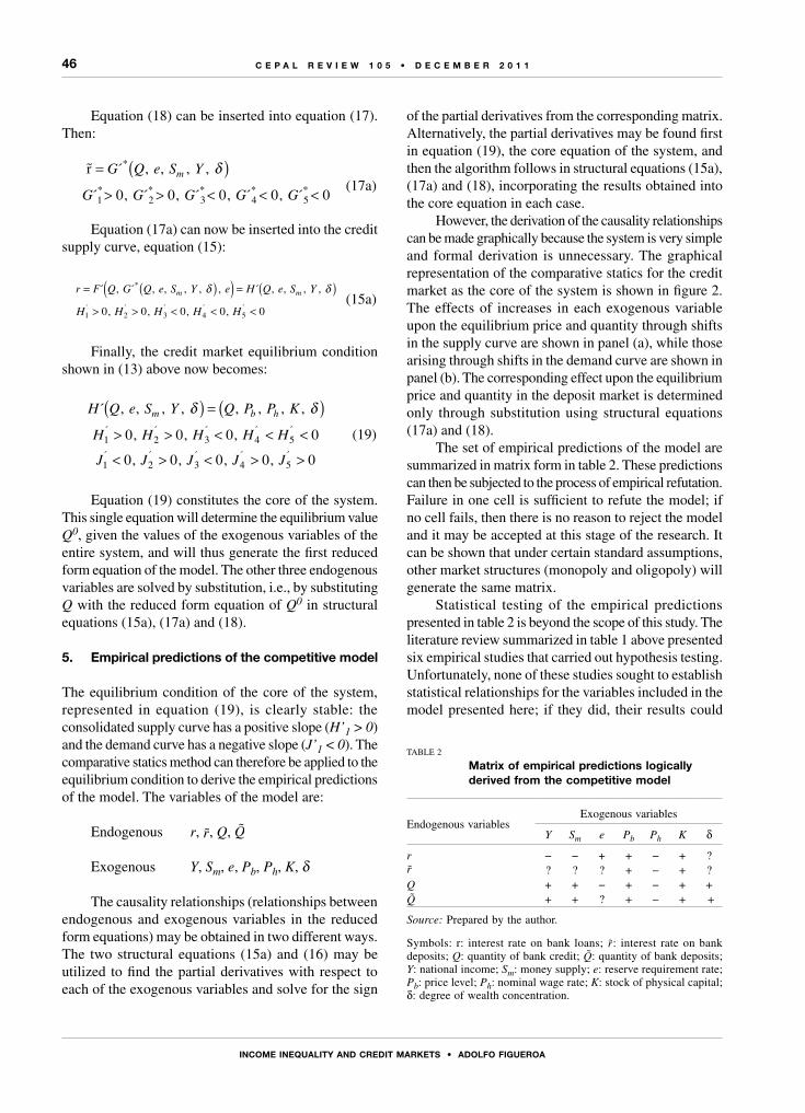
46
InCoME InEquALIty AnD CREDIt MARkEts • ADoLfo fIguERoA
C E P A L R E V I E W 1 0 5 • D E C E M B E R 2 0 1 1
Equation (18) can be inserted into equation (17). Then:
˜ δ )(=
> > < < <
G Q e S Y
G G G G G
r ´ , , , ,
´ 0, ´ 0, ´ 0, ´ 0, ´ 0m
*
1*
2*
3*
4*
5* (17a)
Equation (17a) can now be inserted into the credit supply curve, equation (15):
δδ )( )) (( ==
> > < < <
r F Q G Q e S Y e H Q e S Y
H H H H H
´ , ´ , , , , , ´ , , , ,
0, 0, 0, 0, 0mm
*
1´
2´
3´
4´
5´
(15a)
Finally, the credit market equilibrium condition shown in (13) above now becomes:
( ) =
> > < < <
< > < > >
H Q e S Y Q P P K
H H H H HJ J J J J
´ , , , , , , , ,
0, 0, 0, 00, 0, 0, 0, 0
h
1´
2´
3´
4´
5´
1´
2´
3´
4´
5´
δ δ( )m b
(19)
Equation (19) constitutes the core of the system. This single equation will determine the equilibrium value Q0, given the values of the exogenous variables of the entire system, and will thus generate the first reduced form equation of the model. The other three endogenous variables are solved by substitution, i.e., by substituting Q with the reduced form equation of Q0 in structural equations (15a), (17a) and (18).
5. Empirical predictions of the competitive model
The equilibrium condition of the core of the system, represented in equation (19), is clearly stable: the consolidated supply curve has a positive slope (H’1 > 0) and the demand curve has a negative slope (J’1 < 0). The comparative statics method can therefore be applied to the equilibrium condition to derive the empirical predictions of the model. The variables of the model are:
Endogenous r, r, Q, Q
Exogenous Y, Sm, e, Pb, Ph, K, δ
The causality relationships (relationships between endogenous and exogenous variables in the reduced form equations) may be obtained in two different ways. The two structural equations (15a) and (16) may be utilized to find the partial derivatives with respect to each of the exogenous variables and solve for the sign
of the partial derivatives from the corresponding matrix. Alternatively, the partial derivatives may be found first in equation (19), the core equation of the system, and then the algorithm follows in structural equations (15a), (17a) and (18), incorporating the results obtained into the core equation in each case.
However, the derivation of the causality relationships can be made graphically because the system is very simple and formal derivation is unnecessary. The graphical representation of the comparative statics for the credit market as the core of the system is shown in figure 2. The effects of increases in each exogenous variable upon the equilibrium price and quantity through shifts in the supply curve are shown in panel (a), while those arising through shifts in the demand curve are shown in panel (b). The corresponding effect upon the equilibrium price and quantity in the deposit market is determined only through substitution using structural equations (17a) and (18).
The set of empirical predictions of the model are summarized in matrix form in table 2. These predictions can then be subjected to the process of empirical refutation. Failure in one cell is sufficient to refute the model; if no cell fails, then there is no reason to reject the model and it may be accepted at this stage of the research. It can be shown that under certain standard assumptions, other market structures (monopoly and oligopoly) will generate the same matrix.
Statistical testing of the empirical predictions presented in table 2 is beyond the scope of this study. The literature review summarized in table 1 above presented six empirical studies that carried out hypothesis testing. Unfortunately, none of these studies sought to establish statistical relationships for the variables included in the model presented here; if they did, their results could
TABLE 2
Matrix of empirical predictions logically derived from the competitive model
Endogenous variablesExogenous variables
Y Sm e Pb Ph K δ
r − − + + − + ?r ? ? ? + − + ?Q + + − + − + +Q + + ? + − + +
Source: Prepared by the author.
Symbols: r: interest rate on bank loans; r: interest rate on bank deposits; Q: quantity of bank credit; Q: quantity of bank deposits; Y: national income; Sm: money supply; e: reserve requirement rate; Pb: price level; Ph: nominal wage rate; K: stock of physical capital; δ: degree of wealth concentration.

47
InCoME InEquALIty AnD CREDIt MARkEts • ADoLfo fIguERoA
C E P A L R E V I E W 1 0 5 • D E C E M B E R 2 0 1 1
have been used as first indicators of consistency or refutation of some of the signs shown in table 2. Those studies were interested in other variables, such as bank concentration, credit rationing, the direct impacts of micro-credit, macro-credit as a ratio to gross domestic
product (gdp), the role of the legal system and credit in macroeconomic cycles. Empirical research is therefore expected to be encouraged by the results presented in table 2, which constitute a set of hypotheses with theoretical backing.
FIGURE 2
Graphic representation of comparative statics from the competitive model
Source: Prepared by the author.
Notes: Graph (a): an increase in exogenous variable Y, Sm or δ shifts the consolidated bank credit supply curve outward, but an increase in e shifts the curve inward. Graph (b): an increase in exogenous variable Pb, K or δ shifts the bank credit demand curve outward, but an increase in Ph shifts the curve inward.
D*[Pb, K, Ph]
[e’]
[Y’, Sm’]
QQº QQº
S[Y, Sm, eδ]
(a) (b)
rº
r
S[Y, Sm, e]
[Pb’, K’, δ’]
D*[Pb, K, Ph, δ]
[Ph’]
rº
r
VA dual model
The banking industry model will now be extended to explain why the banking industry and formal non-banking financial organizations coexist. This new model will be called the dual model.
Non-banking organizations are small in size and are usually called micro-financial organizations, examples being cooperatives, credit unions and small State and private-sector financial organizations. They are also State-regulated.
Consider that prices and quantities in the banking industry have already been determined. The equilibrium in the bank credit market is with excess demand. Those excluded from the bank credit market are the less wealthy,
and they will seek loans in the non-banking credit market; therefore, the demand curve for non-banking organizations will also be determined. Non-banking organizations are also financial intermediaries and thus need to have deposits to make their loans. They will use several incentives. One is to establish a requirement for deposits to be made as a condition of eligibility for loans, so potential borrowers of small loans will have an incentive to deposit their funds in the non-banking organization instead of in the banking industry (the case of a cooperative is a clear example); another is to pay an interest rate higher than banks pay. The deposit supply curve in the non-banking organization will thus
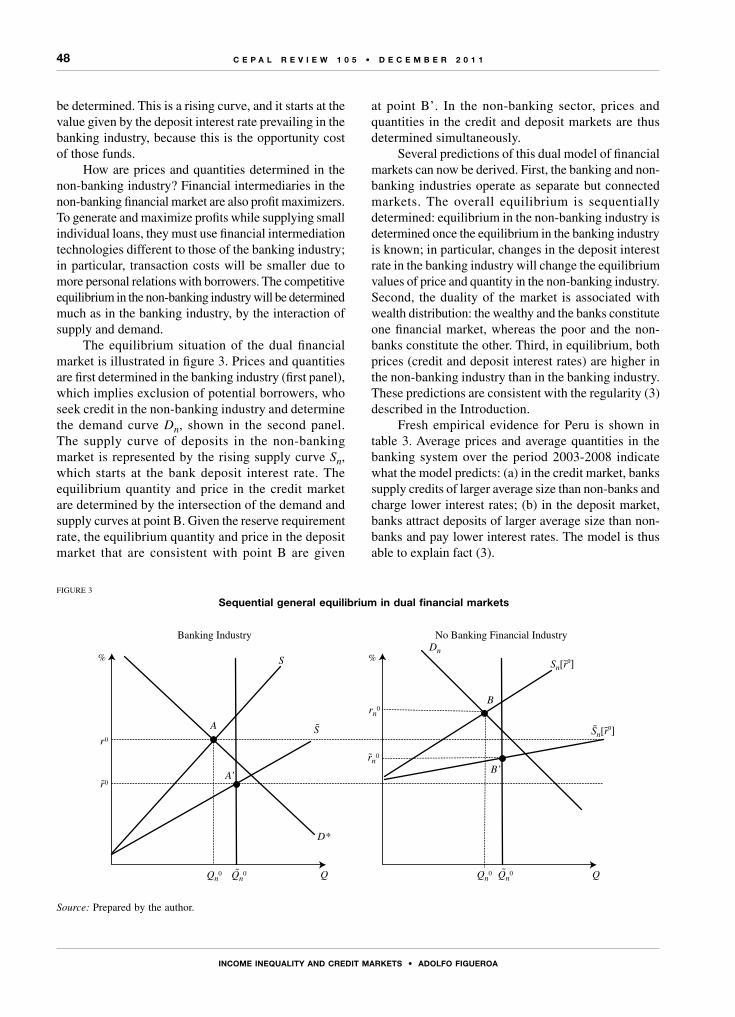
48
InCoME InEquALIty AnD CREDIt MARkEts • ADoLfo fIguERoA
C E P A L R E V I E W 1 0 5 • D E C E M B E R 2 0 1 1
be determined. This is a rising curve, and it starts at the value given by the deposit interest rate prevailing in the banking industry, because this is the opportunity cost of those funds.
How are prices and quantities determined in the non-banking industry? Financial intermediaries in the non-banking financial market are also profit maximizers. To generate and maximize profits while supplying small individual loans, they must use financial intermediation technologies different to those of the banking industry; in particular, transaction costs will be smaller due to more personal relations with borrowers. The competitive equilibrium in the non-banking industry will be determined much as in the banking industry, by the interaction of supply and demand.
The equilibrium situation of the dual financial market is illustrated in figure 3. Prices and quantities are first determined in the banking industry (first panel), which implies exclusion of potential borrowers, who seek credit in the non-banking industry and determine the demand curve Dn, shown in the second panel. The supply curve of deposits in the non-banking market is represented by the rising supply curve Sn, which starts at the bank deposit interest rate. The equilibrium quantity and price in the credit market are determined by the intersection of the demand and supply curves at point B. Given the reserve requirement rate, the equilibrium quantity and price in the deposit market that are consistent with point B are given
at point B’. In the non-banking sector, prices and quantities in the credit and deposit markets are thus determined simultaneously.
Several predictions of this dual model of financial markets can now be derived. First, the banking and non-banking industries operate as separate but connected markets. The overall equilibrium is sequentially determined: equilibrium in the non-banking industry is determined once the equilibrium in the banking industry is known; in particular, changes in the deposit interest rate in the banking industry will change the equilibrium values of price and quantity in the non-banking industry. Second, the duality of the market is associated with wealth distribution: the wealthy and the banks constitute one financial market, whereas the poor and the non-banks constitute the other. Third, in equilibrium, both prices (credit and deposit interest rates) are higher in the non-banking industry than in the banking industry. These predictions are consistent with the regularity (3) described in the Introduction.
Fresh empirical evidence for Peru is shown in table 3. Average prices and average quantities in the banking system over the period 2003-2008 indicate what the model predicts: (a) in the credit market, banks supply credits of larger average size than non-banks and charge lower interest rates; (b) in the deposit market, banks attract deposits of larger average size than non-banks and pay lower interest rates. The model is thus able to explain fact (3).
FIGURE 3
sequential general equilibrium in dual financial markets
Source: Prepared by the author.
Q
S
D*
Sn[r0]Dn
Sn[r0]˜ ˜SA
A’
B
B’
Banking Industry No Banking Financial Industry
% %
Qn0
rn0
r0
r0
rn0
Qn0QQn
0Qn0
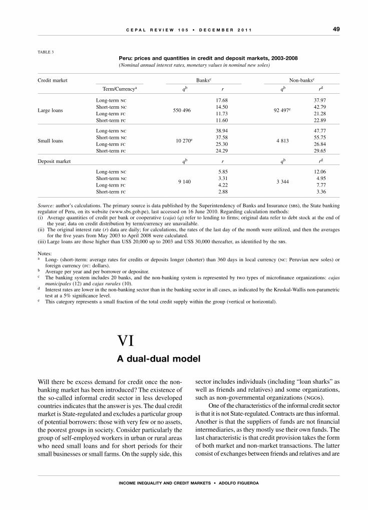
49
InCoME InEquALIty AnD CREDIt MARkEts • ADoLfo fIguERoA
C E P A L R E V I E W 1 0 5 • D E C E M B E R 2 0 1 1
VIA dual-dual model
sector includes individuals (including “loan sharks” as well as friends and relatives) and some organizations, such as non-governmental organizations (ngos).
One of the characteristics of the informal credit sector is that it is not State-regulated. Contracts are thus informal. Another is that the suppliers of funds are not financial intermediaries, as they mostly use their own funds. The last characteristic is that credit provision takes the form of both market and non-market transactions. The latter consist of exchanges between friends and relatives and are
TABLE 3
Peru: prices and quantities in credit and deposit markets, 2003-2008(Nominal annual interest rates, monetary values in nominal new soles)
Credit market Banksc Non-banksc
Term/Currencya qb r qb rd
Large loans
Long-term ncShort-term ncLong-term fcShort-term fc
550 496
17.6814.5011.7311.60
92 497e
37.9742.7921.2822.89
Small loans
Long-term ncShort-term ncLong-term fcShort-term fc
10 270e
38.9437.5825.3024.29
4 813
47.7755.7526.8429.65
Deposit market qb r qb rd
Long-term ncShort-term ncLong-term fcShort-term fc
9 140
5.853.314.222.88
3 344
12.064.957.773.36
Source: author’s calculations. The primary source is data published by the Superintendency of Banks and Insurance (sbs), the State banking regulator of Peru, on its website (www.sbs.gob.pe), last accessed on 16 June 2010. Regarding calculation methods: (i) Average quantities of credit per bank or cooperative (caja) (q) refer to lending to firms; original data refer to debt stock at the end of
the year; data on credit distribution by term/currency are unavailable. (ii) The original interest rate (r) data are daily; for calculations, the rates of the last day of the month were utilized, and then the averages
for the five years from May 2003 to April 2008 were calculated. (iii) Large loans are those higher than US$ 20,000 up to 2003 and US$ 30,000 thereafter, as identified by the sbs.
Notes:a Long- (short-)term: average rates for credits or deposits longer (shorter) than 360 days in local currency (nc: Peruvian new soles) or
foreign currency (fc: dollars). b Average per year and per borrower or depositor. c The banking system includes 20 banks, and the non-banking system is represented by two types of microfinance organizations: cajas
municipales (12) and cajas rurales (10). d Interest rates are lower in the non-banking sector than in the banking sector in all cases, as indicated by the Kruskal-Wallis non-parametric
test at a 5% significance level. e This category represents a small fraction of the total credit supply within the group (vertical or horizontal).
Will there be excess demand for credit once the non-banking market has been introduced? The existence of the so-called informal credit sector in less developed countries indicates that the answer is yes. The dual credit market is State-regulated and excludes a particular group of potential borrowers: those with very few or no assets, the poorest groups in society. Consider particularly the group of self-employed workers in urban or rural areas who need small loans and for short periods for their small businesses or small farms. On the supply side, this
50
InCoME InEquALIty AnD CREDIt MARkEts • ADoLfo fIguERoA
C E P A L R E V I E W 1 0 5 • D E C E M B E R 2 0 1 1
based on rules of reciprocity, social control mechanisms, social networks and family ties. The use of credit as part of multiple exchanges of goods is also common (credit provided to farmers by merchants, for example) and can be seen as a type of interlocking transactions that are hard to define as pure market transactions. For these reasons, it is more appropriate to call it the informal credit sector, rather than market. The construction of theoretical models for this very heterogeneous sector is something that needs to be done. After reviewing a large set of empirical surveys and studies on informal credit, Banerjee (2003) underscored “the significance of developing a proper theory” (p.10).
Empirical regularities are hard to establish for informal credit. These transactions are not usually registered. However, some studies have aggregated empirical surveys and case studies in particular regions to produce some empirical regularities. Hence, Banerjee (2003) finds that credit exchange does indeed take the form of market and non-market exchange. For Latin America, a study concludes that “a plethora of reports document that microfinance institutions charge far less than informal money lenders” and reports rates of 22% a year versus 120% (cited in Campion, Rashmi-Kiran and Wenner, 2010). These facts are consistent with the predictions of the dual-dual model.
VIIConclusions
A new model of the standard theory of bank credit markets has been developed in this paper. The model predicts that the equilibrium conditions under which the banking industry operates include: the use of collateral, equilibrium with excess demand and coexistence with a non-banking financial sector. The financial structure is thus composed of the banking industry, the formal non-banking industry and the informal sector. The equilibrium values of prices and quantities in the banking industry determine the prices and quantities of the formal non-banking industry, which in turn determine prices and quantities in the informal sector.
According to the model, wealth inequality in society is the essential factor explaining this dual-dual financial structure. The model then predicts market segmentation: the wealthy and the banks constitute one market, the less wealthy and formal non-banking organizations constitute another and the poorest groups and small lenders constitute the informal sector; prices are higher in the two latter sectors.
The bank credit market is quasi-Walrasian in its operation in the sense that the market clears, but for effective demand (from eligible borrowers, as determined by banks) rather than total demand. Those excluded from this market will seek credit in the regulated non-bank credit market. This second market is also quasi-Walrasian because it clears, but for effective demand (from eligible borrowers as determined by the non-banking organizations) rather than total demand. Those excluded from this second market, the residual, have the option of seeking credit in the informal sector, which operates
through both market and non-market transactions. In this dual-dual credit system, the poorest groups pay the highest price for credit. In sum, the three empirical regularities established at the beginning of this paper are all explained by the model.
There is now the dynamic equilibrium question. The study by Tressel (2003) is very helpful in this regard. It presents a dynamic macroeconomic model in a standard growth theory context to study the dynamics of the dual credit market over time. The basic assumptions of Tressel’s model are that banks operate with collateral (as in the model used here) and that the expansion of the banking industry over time depends upon the accumulation of assets by entrepreneurs, because those assets are needed as credit collateral; hence, in his model the level and distribution of wealth also play a significant role in the development of the banking industry.
This conclusion is consistent with what would emerge from the extension of the static model presented here to a dynamic one. If the poor could accumulate capital in significant amounts, the dual-dual credit system would tend to disappear; hence, the persistence of this system in less developed countries can be taken to be the result of a process of economic growth in which wealth inequality either increases or does not decrease significantly.
The public policy implications of the model can be stated in terms of the policies that have been most commonly applied, which have not been very effective in changing the dual-dual structure, given its persistence:
51
InCoME InEquALIty AnD CREDIt MARkEts • ADoLfo fIguERoA
C E P A L R E V I E W 1 0 5 • D E C E M B E R 2 0 1 1
(i) government policies concentrate on the banking industry, but neglect the indirect effects on the formal non-banking market and the informal sector;
(ii) the effect of State programmes of legal security for property rights has not been significant because they do not change the inequality of wealth in society;
(iii) the effect of banking industry liberalization (absence of financial repression) has not been significant because the dual-dual structure operates even under conditions of perfect competition in the banking industry, as shown by the model developed in this paper;
(iv) the current role of the State as regulator in the financial system has not had a significant effect because regulation does not impede the dual-dual credit system, as the model also shows. Changing the dual-dual system and the type of
economic growth that comes with it would require a State that was more developmental and innovative. Innovative ways of redistributing concentrated wealth and new rules and new forms of organization in the financial system are the public policies that derive from the theoretical model presented in this paper.
(Original: English)
Bibliography
Backhouse, Roger (1981), “Credit rationing in a general equilibrium model”, Economica, New Series, vol. 48, No. 190, London, London School of Economics and Political Science.
Banerjee, Abhijit (2003), “Contracting constraints, credit markets, and economic development”, Advances in Economics and Econometrics: Theory and Applications. Eight World Congress of the Econometric Society, Mathias Dewatripont, Lars Hansen and Stephen Turnovsky (eds.), vol. 3, Cambridge, Cambridge University Press.
Barro, Robert (1997), Macroeconomics, Cambridge, The mit Press.Berger, Allen and others (2004), “Bank concentration and competition:
an evolution in the making”, Journal of Money, Credit and Banking, vol. 36, No. 6, Blackwell Publishing.
Berger, Allen and Gregory Udell (1995), “Relationship lending and lines of credit in small firm finance”, The Journal of Business, vol. 68, No. 3, Chicago, The University of Chicago Press.
(1992), “Some evidence on the empirical significance of credit rationing”, The Journal of Political Economy, vol. 100, No. 5, Chicago, The University of Chicago Press.
Besanko, David and Thakor Anjan (1987), “Collateral and rationing: sorting equilibria in monopolistic and competitive credit markets”, International Economic Review, vol. 28, No. 3, Philadelphia, University of Pennsylvania/Osaka University Institute of Social and Economic Research Association.
Campion, Anita, Rashmi Kiran-Ekka and Mark Wenner (2010), “Interest rates and implications for microfinance in Latin America and the Caribbean”, Working Paper Series, No. 177, Washington, D.C., Inter-American Development Bank.
Chan, Yuk-Shee and George Kanatas (1985), “Asymmetric valuations and the role of collateral in loan agreements”, Journal of Money, Credit, and Banking, vol. 17, No. 1, Blackwell Publishing.
Djankov, Simeon, Caralee McLiesh and Andrei Shleifer (2005), “Private credit in 129 countries”, nber Working Papers, No. 11078, Cambridge, Massachusetts, National Bureau of Economic Research.
Fried, Joel and Peter Howitt (1980), “Credit rationing and implicit
contract theory”, Journal of Money, Credit, and Banking, vol. 12, No. 3, Blackwell Publishing.
Inderst, Roman and Holger Mueller (2007), “A lender based theory of collateral”, Journal of Finance Economics, vol. 84, No. 3, Amsterdam, Elsevier.
Kiyotaki, Nobuhiro and John Moore (1997), “Credit cycles”, Journal of Political Economy, vol. 105, No. 2, Chicago, University of Chicago Press.
Krugman, Paul and Robin Wells (2006), Macroeconomics, New York, Worth Publishers.
Manove, Michael, Jorge Padilla and Marco Pagano (2001), “Collateral versus project screening: a model of lazy banks”, rand Journal of Economics, vol. 32, No. 4, Santa Monica, The Rand Corporation.
Mishkin, Frederic (2007), The Economics of Money, Banking and Financial Markets, Boston, Pearson.
Morduch, Jonathan (1999), “The microfinance promise”, Journal of Economic Literature, vol. 37, No. 4, Nashville, Tennessee, American Economic Association.
Steijvers, Tensie and Wim Voordeckers (2009), “Collateral and credit rationing: a review of recent empirical studies as a guide for future research”, Journal of Economic Surveys, vol. 23, No. 5, Wiley-Blackwell.
Stiglitz, Joseph (2002), “Information and the change in the paradigm in economics”, The American Economic Review, vol. 92, No. 3, Nashville, Tennessee, American Economic Association.
Stiglitz, Joseph and Andrew Weiss (1981), “Credit rationing in markets with imperfect information”, American Economic Review, vol. 71, No. 3, Nashville, Tennessee, American Economic Association.
Tressel, Thierry (2003), “Dual financial systems and inequalities in economic development”, Journal of Economic Growth, vol. 8, No. 2, New York, Springer.
Villas-Boas, Miguel and Udo Schmidt-Mohr (1999), “Oligopoly with asymmetric information: differentiation in credit markets”, The rand Journal of Economics, vol. 30, No. 3, Santa Monica, The rand Corporation.

C E P A L R E V I E W 1 0 5 • D E C E M B E R 2 0 1 1
53
K E Y W O R D S
Wages
Equal pay
Labour market
Agribusiness
Industrial sector
Service industries
Statistical data
Case studies
Trinidad and Tobago
Trinidad and Tobago:Inter-industry wage
differentials
Allister Mounsey and Tracy Polius
Conventional labour economics argues that the typical firm is a
wage taker and that wages are determined by the interaction of labour
supply and the aggregate demand for labour. Under these conditions,
markets clear, and non-frictional unemployment cannot feature in the long
run. The persistently high levels of unemployment in the Caribbean present
a significant challenge to this critical prediction of neoclassical economics.
Efficiency wage theories argue that wages are endogenously determined
by firms, which pick wage levels that minimize the average per unit cost
of “efficiency labour”. Among the important conclusions of these theories
is the possibility of persistent non-frictional unemployment. This paper
presents evidence suggesting the existence of long-term inter-industry
wage differentials in Trinidad and Tobago. This is a possible indication of
the applicability of efficiency wage theories in explaining labour market
phenomena in the twin-island Republic.
Allister Mounsey
Manager of Planning and Research,
Tourism Development Company of
Trinidad and Tobago
Tracy Polius
Research Fellow, Caribbean Centre
for Money and Finance,
University of the West Indies,
St. Augustine

54
tRInIDAD AnD toBAgo: IntER-InDustRy WAgE DIffEREntIALs • ALLIstER MounsEy AnD tRACy PoLIus
C E P A L R E V I E W 1 0 5 • D E C E M B E R 2 0 1 1
Standard economic theory assumes that the typical firm is a wage taker, i.e., it takes the market-determined wage rate as given and proceeds to employ labour units until the marginal revenue product of labour (mrpl) equals the wage rate. This can, of course, be adjusted to accommodate the reality of heterogeneous labour, so that equation (1) represents the profit-maximizing behaviour of firm j as far as the employment of labour is concerned.
MRPlij = Wi j = 1, 2, 3… n (1)
where i denotes the category of worker skill/class/occupation.
Equation (1) implies that each firm will pay the same wage rate for the same category of labour. Therefore, according to textbook labour economics, any observed differences in wage rates for the same category of labour between firms or between industries must be transitory in nature and will be eroded in the long run by competitive market forces.
1. inter-industry wage differentials
Economists have noted stable inter-industry wage differentials since at least as far back as the early 1950s. Slichter (1950, as cited in Krueger and Summers, 1987) illustrates the time-invariant nature of inter-industry wage differentials. Slichter found an intertemporal rank correlation coefficient of 0.73 in industry wages using hourly wage data for unskilled male workers from the National Industrial Conference Board establishment surveys of 20 manufacturing industries in the United States from 1923 to 1946.
Many studies have since reconfirmed the presence of stable inter-industry wage differentials in the United States. Among them, Krueger and Summers (1987), using correlations of log annual earnings for full-time equivalent employees in nine major industries for selected years between 1900 and 1984, found stability in the United States inter-industry wage structure throughout the period from 1915 to 1984. Correlations with the wage structure of 1984 range from 0.76 to 0.98.
Inter-industry wage differences are not unique to the United States. In a study of 14 Organisation for Economic Co-operation and Development (oecd) countries for the period from 1970 to 1985, Gittleman and Wolff (1993) found that the rank order of industrial wages had been stable over the period for all countries studied and that industrial wage differentials were positively related to an industry’s productivity growth, output growth, capital intensity and export orientation. Arbache (2001) used microdata for Brazil to explain industrial wage differentials for the period from 1984 to 1998 and found that efficiency wage and unmeasured ability models were significant in explaining the wage structure.
2. Caribbean literature
The subject of labour market segmentation along industrial lines has received relatively little attention in the Caribbean literature. One notable exception is Scott (2005), who used a segmented (along industrial lines) labour market approach to estimate the distributional effects of trade in Jamaica. Anderson (1987) proposed that the Jamaican labour market should be analysed using six conceptually distinct categories (primary formal, central government, secondary formal, large-scale agriculture, small-scale agriculture and informal sectors). She further demonstrated that these sectors differed by average education level, average worker age, sex and average income.
This paper extends the literature on labour market segmentation in the Caribbean by demonstrating that a temporally stable inter-industry wage distribution exists in Trinidad and Tobago after fully accounting for occupational differences. Furthermore, accounting for compositional differences in labour quality does not significantly affect the industry distribution.
The remainder of the paper is divided into three sections. In section II, evidence is presented to support the hypothesis of a temporally stable wage hierarchy among industries. Theoretical explanations for inter-industry wage differentials are presented in section III, and section IV contains conclusions and recommendations.
Iintroduction
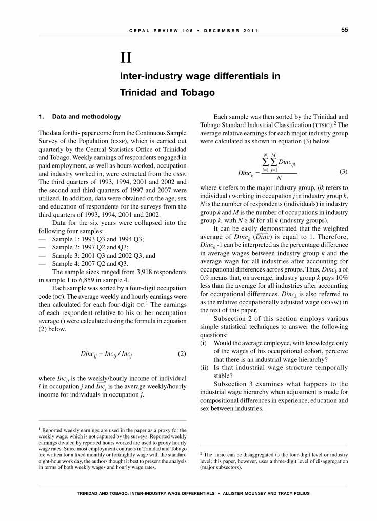
55
tRInIDAD AnD toBAgo: IntER-InDustRy WAgE DIffEREntIALs • ALLIstER MounsEy AnD tRACy PoLIus
C E P A L R E V I E W 1 0 5 • D E C E M B E R 2 0 1 1
1. Data and methodology
The data for this paper come from the Continuous Sample Survey of the Population (cssp), which is carried out quarterly by the Central Statistics Office of Trinidad and Tobago. Weekly earnings of respondents engaged in paid employment, as well as hours worked, occupation and industry worked in, were extracted from the cssp. The third quarters of 1993, 1994, 2001 and 2002 and the second and third quarters of 1997 and 2007 were utilized. In addition, data were obtained on the age, sex and education of respondents for the surveys from the third quarters of 1993, 1994, 2001 and 2002.
Data for the six years were collapsed into the following four samples: — Sample 1: 1993 Q3 and 1994 Q3; — Sample 2: 1997 Q2 and Q3; — Sample 3: 2001 Q3 and 2002 Q3; and — Sample 4: 2007 Q2 and Q3.
The sample sizes ranged from 3,918 respondents in sample 1 to 6,859 in sample 4.
Each sample was sorted by a four-digit occupation code (oc). The average weekly and hourly earnings were then calculated for each four-digit oc.1 The earnings of each respondent relative to his or her occupation average () were calculated using the formula in equation (2) below.
Dincij = Incij / Incj (2)
where Incij is the weekly/hourly income of individual i in occupation j and Incj is the average weekly/hourly income for individuals in occupation j.
1 Reported weekly earnings are used in the paper as a proxy for the weekly wage, which is not captured by the surveys. Reported weekly earnings divided by reported hours worked are used to proxy hourly wage rates. Since most employment contracts in Trinidad and Tobago are written for a fixed monthly or fortnightly wage with the standard eight-hour work day, the authors thought it best to present the analysis in terms of both weekly wages and hourly wage rates.
Each sample was then sorted by the Trinidad and Tobago Standard Industrial Classification (ttsic).2 The average relative earnings for each major industry group were calculated as shown in equation (3) below.
Dinc
Dinc
Nk
ijkj
M
i
N
= ==∑∑
11 (3)
where k refers to the major industry group, ijk refers to individual i working in occupation j in industry group k, N is the number of respondents (individuals) in industry group k and M is the number of occupations in industry group k, with N ≥ M for all k (industry groups).
It can be easily demonstrated that the weighted average of Dinck (Dinc) is equal to 1. Therefore, Dinck -1 can be interpreted as the percentage difference in average wages between industry group k and the average wage for all industries after accounting for occupational differences across groups. Thus, Dinck a of 0.9 means that, on average, industry group k pays 10% less than the average for all industries after accounting for occupational differences. Dinck is also referred to as the relative occupationally adjusted wage (roaw) in the text of this paper.
Subsection 2 of this section employs various simple statistical techniques to answer the following questions:(i) Would the average employee, with knowledge only
of the wages of his occupational cohort, perceive that there is an industrial wage hierarchy?
(ii) Is that industrial wage structure temporally stable?Subsection 3 examines what happens to the
industrial wage hierarchy when adjustment is made for compositional differences in experience, education and sex between industries.
2 The ttsic can be disaggregated to the four-digit level or industry level; this paper, however, uses a three-digit level of disaggregation (major subsectors).
IIinter-industry wage differentials in
Trinidad and Tobago
—
—
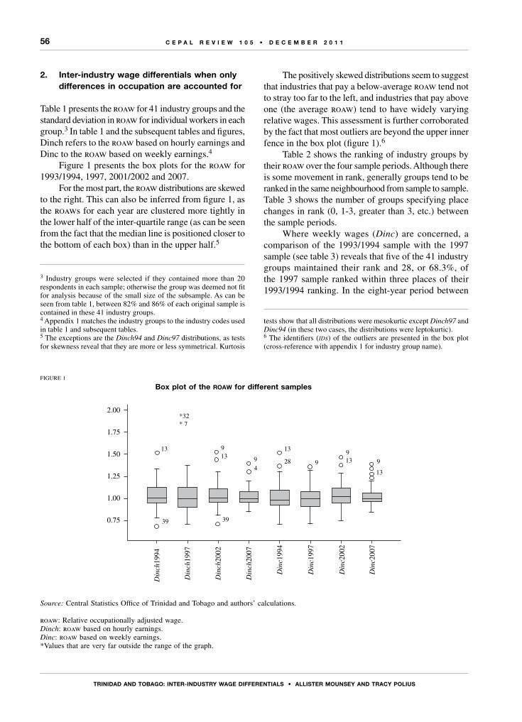
56
tRInIDAD AnD toBAgo: IntER-InDustRy WAgE DIffEREntIALs • ALLIstER MounsEy AnD tRACy PoLIus
C E P A L R E V I E W 1 0 5 • D E C E M B E R 2 0 1 1
2. inter-industry wage differentials when only differences in occupation are accounted for
Table 1 presents the roaw for 41 industry groups and the standard deviation in roaw for individual workers in each group.3 In table 1 and the subsequent tables and figures, Dinch refers to the roaw based on hourly earnings and Dinc to the roaw based on weekly earnings.4
Figure 1 presents the box plots for the roaw for 1993/1994, 1997, 2001/2002 and 2007.
For the most part, the roaw distributions are skewed to the right. This can also be inferred from figure 1, as the roaws for each year are clustered more tightly in the lower half of the inter-quartile range (as can be seen from the fact that the median line is positioned closer to the bottom of each box) than in the upper half.5
3 Industry groups were selected if they contained more than 20 respondents in each sample; otherwise the group was deemed not fit for analysis because of the small size of the subsample. As can be seen from table 1, between 82% and 86% of each original sample is contained in these 41 industry groups. 4 Appendix 1 matches the industry groups to the industry codes used in table 1 and subsequent tables.5 The exceptions are the Dinch94 and Dinc97 distributions, as tests for skewness reveal that they are more or less symmetrical. Kurtosis
The positively skewed distributions seem to suggest that industries that pay a below-average roaw tend not to stray too far to the left, and industries that pay above one (the average roaw) tend to have widely varying relative wages. This assessment is further corroborated by the fact that most outliers are beyond the upper inner fence in the box plot (figure 1).6
Table 2 shows the ranking of industry groups by their roaw over the four sample periods. Although there is some movement in rank, generally groups tend to be ranked in the same neighbourhood from sample to sample. Table 3 shows the number of groups specifying place changes in rank (0, 1-3, greater than 3, etc.) between the sample periods.
Where weekly wages (Dinc) are concerned, a comparison of the 1993/1994 sample with the 1997 sample (see table 3) reveals that five of the 41 industry groups maintained their rank and 28, or 68.3%, of the 1997 sample ranked within three places of their 1993/1994 ranking. In the eight-year period between
tests show that all distributions were mesokurtic except Dinch97 and Dinc94 (in these two cases, the distributions were leptokurtic).6 The identifiers (ids) of the outliers are presented in the box plot (cross-reference with appendix 1 for industry group name).
FIGURE 1
Box plot of the roaw for different samples
Source: Central Statistics Office of Trinidad and Tobago and authors’ calculations.
roaw: Relative occupationally adjusted wage.Dinch: roaw based on hourly earnings. Dinc: roaw based on weekly earnings.*Values that are very far outside the range of the graph.
Din
ch19
94
1313
*32* 7
13
13
13
39 39
9
94
28 9
99
2.00
1.75
1.50
1.25
1.00
0.75
Din
ch19
97
Din
ch20
02
Din
ch20
07
Din
c199
4
Din
c199
7
Din
c200
2
Din
c200
7

57
tRInIDAD AnD toBAgo: IntER-InDustRy WAgE DIffEREntIALs • ALLIstER MounsEy AnD tRACy PoLIus
C E P A L R E V I E W 1 0 5 • D E C E M B E R 2 0 1 1
TABLE 1.a
relative occupationally adjusted weekly wage (Dinc) across industry groups, four samples
IDSample 1: 1993/1994 Sample 2: 1997 Sample 3: 2001/2002 Sample 4: 2007
N Dinc S N Dinc S N Dinc S N Dinc S
Ind. 1 144 0.97 0.37 132 1.00 0.41 115 0.98 0.39 27 0.89 0.23Ind. 2 30 0.94 0.52 32 0.89 0.51 26 0.92 0.53 123 0.97 0.44Ind. 3 39 1.15 0.37 45 1.00 0.28 35 1.06 0.33 35 1.01 0.28Ind. 4 64 1.27 0.64 60 1.29 0.48 66 1.30 0.50 87 1.32 0.57Ind. 5 32 1.01 0.90 41 0.98 0.46 47 1.06 0.53 50 0.95 0.35Ind. 6 23 0.97 0.48 29 0.88 0.33 32 1.04 0.46 29 0.91 0.32Ind. 7 38 0.90 0.42 59 0.99 0.47 43 0.96 0.66 34 1.01 0.47Ind. 8 23 1.13 0.50 35 1.23 0.62 35 1.24 0.55 44 1.20 0.62Ind. 9 66 1.31 0.54 46 1.35 0.45 47 1.46 0.53 70 1.35 0.53Ind. 10 31 0.97 0.38 23 1.09 0.28 33 1.09 0.50 47 1.13 0.43Ind. 11 22 1.11 0.58 25 1.10 0.35 23 1.28 0.50 27 1.05 0.35Ind. 12 29 0.88 0.41 24 0.88 0.37 21 0.91 0.35 69 0.85 0.31Ind. 13 40 1.52 0.71 48 1.33 0.52 40 1.38 0.70 40 1.25 0.39Ind. 14 39 1.12 0.31 44 1.20 0.39 42 1.14 0.31 47 1.23 0.47Ind. 15 132 0.95 0.39 281 0.96 0.37 369 0.96 0.35 654 0.99 0.48Ind. 16 231 1.01 0.36 234 1.01 0.34 253 1.00 0.38 282 0.99 0.45Ind. 17 28 0.95 0.35 38 0.91 0.37 77 1.07 0.40 89 1.04 0.42Ind. 18 44 1.02 0.44 39 1.00 0.58 62 1.04 0.69 77 1.05 0.51Ind. 19 93 0.91 0.62 89 0.89 0.43 105 0.87 0.46 155 0.92 0.48Ind. 20 25 0.86 0.33 33 1.06 0.33 24 1.12 0.49 20 1.06 0.32Ind. 21 72 0.80 0.29 73 0.77 0.25 77 0.82 0.39 105 0.95 0.60Ind. 22 63 1.10 0.62 84 1.03 0.60 75 1.08 1.17 130 1.19 0.75Ind. 23 21 0.80 0.43 27 0.89 0.32 42 0.98 0.41 22 1.02 0.32Ind. 24 104 0.95 0.41 142 0.98 0.50 136 0.89 0.51 246 0.99 0.56Ind. 25 100 0.79 0.41 164 0.84 0.29 176 0.90 0.42 360 0.85 0.51Ind. 26 49 0.98 0.44 55 0.98 0.50 63 1.12 0.53 58 1.17 0.58Ind. 27 78 0.90 0.48 84 0.91 0.38 86 0.92 0.35 317 0.97 0.41Ind. 28 35 1.38 0.69 42 1.08 0.39 44 1.12 0.51 49 1.20 0.54Ind. 29 42 1.25 0.45 56 1.23 0.47 38 1.12 0.31 27 0.99 0.41Ind. 30 61 1.14 0.51 63 1.24 0.44 85 1.20 0.53 63 1.20 0.63Ind. 31 101 1.10 0.39 167 1.04 0.36 145 1.09 0.43 111 1.02 0.35Ind. 32 81 1.03 0.43 83 1.02 0.55 76 1.03 0.53 70 1.00 0.56Ind. 33 129 0.88 0.37 225 0.89 0.35 195 0.89 0.38 327 0.96 0.39Ind. 34 392 1.06 0.41 431 1.09 0.37 562 1.02 0.33 612 1.05 0.37Ind. 35 76 1.01 0.38 149 1.03 0.48 117 0.97 0.35 220 0.98 0.45Ind. 36 312 0.98 0.42 352 1.01 0.41 368 1.00 0.35 336 1.00 0.36Ind. 37 175 1.05 0.40 180 1.15 0.39 192 1.02 0.40 185 1.06 0.41Ind. 38 29 0.95 0.42 37 0.98 0.49 31 0.97 0.36 28 0.97 0.53Ind. 39 87 0.70 0.35 89 0.71 0.35 86 0.75 0.33 198 0.87 0.41Ind. 40 151 0.92 0.40 216 0.93 0.42 178 0.93 0.79 213 0.89 0.45Ind. 41 37 0.97 0.39 29 0.81 0.66 41 0.95 0.45 164 0.97 0.58
Total table (N>20)a 3 368 1.00 0.43 4 105 1.01 0.40 4 308 1.00 0.44 5 847 1.00 0.45
Total sample 3 918 1.00 0.48 4 937 1.00 0.43 5 250 1.00 0.46 6 860 1.00 0.47
Source: Central Statistics Office of Trinidad and Tobago and authors’ calculations.
a The weighted standard deviation is presented in this row.Ind.: Industry.roaw: Relative occupationally adjusted wage.Dinc: roaw based on weekly earnings.

58
tRInIDAD AnD toBAgo: IntER-InDustRy WAgE DIffEREntIALs • ALLIstER MounsEy AnD tRACy PoLIus
C E P A L R E V I E W 1 0 5 • D E C E M B E R 2 0 1 1
TABLE 1.b
relative occupationally adjusted hourly wage (Dinch) across industry groups, four samples
IDSample 1: 1993/1994 Sample 2: 1997 Sample 3: 2001/2002 Sample 4: 2007
N Dinch S N Dinch S N Dinch S N Dinch S
Ind. 1 139 0.94 0.37 129 0.99 0.43 114 0.97 0.36 27 0.92 0.23Ind. 2 29 1.26 1.35 32 0.93 0.40 25 0.96 0.62 121 1.00 0.55Ind. 3 38 1.13 0.36 45 1.05 0.38 34 1.07 0.35 35 1.00 0.30Ind. 4 63 1.31 0.72 60 1.35 0.53 66 1.31 0.52 87 1.30 0.59Ind. 5 31 0.95 0.82 41 0.93 0.40 47 1.07 0.57 49 0.95 0.37Ind. 6 22 0.97 0.52 29 0.90 0.33 32 1.05 0.54 29 0.88 0.29Ind. 7 37 0.87 0.41 58 1.88 6.48 40 0.98 0.58 34 0.96 0.43Ind. 8 23 1.09 0.49 35 1.19 0.58 35 1.24 0.50 43 1.19 0.65Ind. 9 60 1.34 0.54 46 1.38 0.48 45 1.51 0.61 70 1.38 0.53Ind. 10 29 0.97 0.39 23 1.07 0.37 33 1.11 0.52 45 1.12 0.47Ind. 11 18 1.20 0.57 25 1.11 0.41 23 1.28 0.52 27 1.08 0.38Ind. 12 29 1.25 0.89 24 0.82 0.37 20 0.89 0.39 69 0.85 0.27Ind. 13 39 1.52 0.80 46 1.35 0.57 37 1.40 0.74 39 1.30 0.47Ind. 14 38 1.03 0.34 41 1.19 0.43 41 1.12 0.28 44 1.20 0.44Ind. 15 130 1.04 0.66 279 0.99 0.42 364 0.97 0.44 641 0.99 0.50Ind. 16 226 1.01 0.38 231 0.99 0.33 250 1.00 0.42 276 1.03 0.75Ind. 17 26 1.07 0.62 38 0.94 0.36 76 1.07 0.39 89 1.02 0.40Ind. 18 43 0.95 0.43 39 1.02 0.65 57 1.08 0.70 77 1.05 0.52Ind. 19 93 0.98 0.71 89 0.89 0.47 104 0.87 0.48 154 0.90 0.46Ind. 20 24 0.88 0.38 32 1.04 0.30 22 1.11 0.37 20 1.05 0.30Ind. 21 71 0.80 0.34 73 0.76 0.24 77 0.84 0.43 105 0.97 0.70Ind. 22 63 1.07 0.62 84 1.00 0.58 75 1.12 1.23 129 1.20 0.75Ind. 23 21 0.80 0.45 27 0.88 0.35 42 0.97 0.43 21 0.99 0.33Ind. 24 102 0.95 0.43 141 0.95 0.51 135 0.88 0.49 245 0.98 0.53Ind. 25 99 0.78 0.38 159 0.81 0.30 171 0.89 0.42 355 0.85 0.48Ind. 26 48 0.96 0.54 54 0.92 0.48 62 1.05 0.47 57 1.09 0.51Ind. 27 77 0.91 0.49 83 0.90 0.43 85 0.91 0.41 310 0.96 0.39Ind. 28 35 1.25 0.58 41 1.11 0.49 41 1.17 0.63 48 1.20 0.53Ind. 29 41 1.19 0.43 56 1.24 0.48 38 1.15 0.37 26 0.97 0.46Ind. 30 60 1.12 0.49 62 1.24 0.44 83 1.22 0.55 61 1.19 0.65Ind. 31 95 1.08 0.41 163 1.04 0.39 141 1.10 0.45 109 1.03 0.35Ind. 32 77 0.99 0.42 82 1.95 8.43 75 1.00 0.52 70 1.00 0.53Ind. 33 126 0.86 0.40 224 0.88 0.38 184 0.86 0.37 322 0.96 0.41Ind. 34 376 1.04 0.41 414 1.23 3.28 545 1.01 0.32 603 1.06 0.39Ind. 35 72 1.00 0.35 141 1.02 0.47 115 0.99 0.33 213 0.97 0.43Ind. 36 205 1.17 5.22 287 0.87 0.46 269 0.81 0.37 274 0.85 0.46Ind. 37 171 1.30 3.75 177 1.13 0.39 188 1.01 0.38 182 1.04 0.39Ind. 38 29 0.95 0.47 37 1.01 0.49 30 0.97 0.53 27 0.99 0.55Ind. 39 86 0.68 0.31 89 0.70 0.35 85 0.71 0.34 196 0.86 0.42Ind. 40 149 1.01 0.48 214 0.99 0.49 175 0.97 0.76 210 0.92 0.40Ind. 41 37 1.01 0.49 27 0.81 0.60 40 0.91 0.39 160 1.01 0.59
Total table (N>20)a 3 177 1.03 0.96 3 977 1.04 0.98 4 121 0.99 0.45 5 699 1.00 0.48
Total sample 3 716 1.00 1.55 4 796 1.00 1.71 5 055 1.00 0.49 6 707 1.00 0.49
Source: Central Statistics Office of Trinidad and Tobago and authors’ calculations.
a The weighted standard deviation is presented in this row.Ind.: Industry.roaw: Relative occupationally adjusted wage.Dinch: roaw based on hourly earnings.
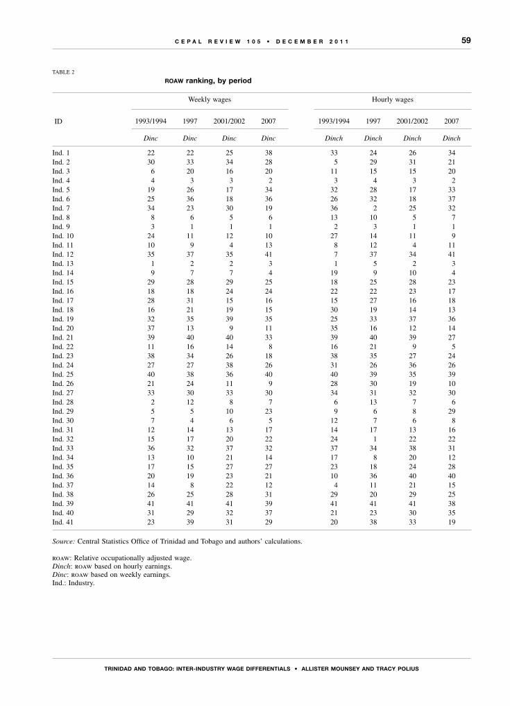
59
tRInIDAD AnD toBAgo: IntER-InDustRy WAgE DIffEREntIALs • ALLIstER MounsEy AnD tRACy PoLIus
C E P A L R E V I E W 1 0 5 • D E C E M B E R 2 0 1 1
TABLE 2
roaw ranking, by period
ID
Weekly wages Hourly wages
1993/1994 1997 2001/2002 2007 1993/1994 1997 2001/2002 2007
Dinc Dinc Dinc Dinc Dinch Dinch Dinch Dinch
Ind. 1 22 22 25 38 33 24 26 34Ind. 2 30 33 34 28 5 29 31 21Ind. 3 6 20 16 20 11 15 15 20Ind. 4 4 3 3 2 3 4 3 2Ind. 5 19 26 17 34 32 28 17 33Ind. 6 25 36 18 36 26 32 18 37Ind. 7 34 23 30 19 36 2 25 32Ind. 8 8 6 5 6 13 10 5 7Ind. 9 3 1 1 1 2 3 1 1Ind. 10 24 11 12 10 27 14 11 9Ind. 11 10 9 4 13 8 12 4 11Ind. 12 35 37 35 41 7 37 34 41Ind. 13 1 2 2 3 1 5 2 3Ind. 14 9 7 7 4 19 9 10 4Ind. 15 29 28 29 25 18 25 28 23Ind. 16 18 18 24 24 22 22 23 17Ind. 17 28 31 15 16 15 27 16 18Ind. 18 16 21 19 15 30 19 14 13Ind. 19 32 35 39 35 25 33 37 36Ind. 20 37 13 9 11 35 16 12 14Ind. 21 39 40 40 33 39 40 39 27Ind. 22 11 16 14 8 16 21 9 5Ind. 23 38 34 26 18 38 35 27 24Ind. 24 27 27 38 26 31 26 36 26Ind. 25 40 38 36 40 40 39 35 39Ind. 26 21 24 11 9 28 30 19 10Ind. 27 33 30 33 30 34 31 32 30Ind. 28 2 12 8 7 6 13 7 6Ind. 29 5 5 10 23 9 6 8 29Ind. 30 7 4 6 5 12 7 6 8Ind. 31 12 14 13 17 14 17 13 16Ind. 32 15 17 20 22 24 1 22 22Ind. 33 36 32 37 32 37 34 38 31Ind. 34 13 10 21 14 17 8 20 12Ind. 35 17 15 27 27 23 18 24 28Ind. 36 20 19 23 21 10 36 40 40Ind. 37 14 8 22 12 4 11 21 15Ind. 38 26 25 28 31 29 20 29 25Ind. 39 41 41 41 39 41 41 41 38Ind. 40 31 29 32 37 21 23 30 35Ind. 41 23 39 31 29 20 38 33 19
Source: Central Statistics Office of Trinidad and Tobago and authors’ calculations.
roaw: Relative occupationally adjusted wage.Dinch: roaw based on hourly earnings. Dinc: roaw based on weekly earnings.Ind.: Industry.
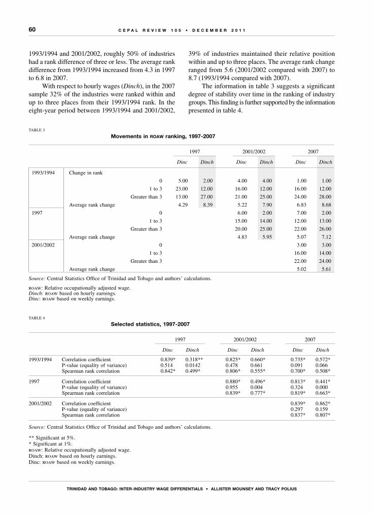
60
tRInIDAD AnD toBAgo: IntER-InDustRy WAgE DIffEREntIALs • ALLIstER MounsEy AnD tRACy PoLIus
C E P A L R E V I E W 1 0 5 • D E C E M B E R 2 0 1 1
1993/1994 and 2001/2002, roughly 50% of industries had a rank difference of three or less. The average rank difference from 1993/1994 increased from 4.3 in 1997 to 6.8 in 2007.
With respect to hourly wages (Dinch), in the 2007 sample 32% of the industries were ranked within and up to three places from their 1993/1994 rank. In the eight-year period between 1993/1994 and 2001/2002,
39% of industries maintained their relative position within and up to three places. The average rank change ranged from 5.6 (2001/2002 compared with 2007) to 8.7 (1993/1994 compared with 2007).
The information in table 3 suggests a significant degree of stability over time in the ranking of industry groups. This finding is further supported by the information presented in table 4.
TABLE 3
Movements in roaw ranking, 1997-2007
1997 2001/2002 2007
Dinc Dinch Dinc Dinch Dinc Dinch
1993/1994 Change in rank
0 5.00 2.00 4.00 4.00 1.00 1.00
1 to 3 23.00 12.00 16.00 12.00 16.00 12.00
Greater than 3 13.00 27.00 21.00 25.00 24.00 28.00
Average rank change 4.29 8.39 5.22 7.90 6.83 8.68
1997 0 6.00 2.00 7.00 2.00
1 to 3 15.00 14.00 12.00 13.00
Greater than 3 20.00 25.00 22.00 26.00
Average rank change 4.83 5.95 5.07 7.12
2001/2002 0 3.00 3.00
1 to 3 16.00 14.00
Greater than 3 22.00 24.00
Average rank change 5.02 5.61
Source: Central Statistics Office of Trinidad and Tobago and authors’ calculations.
roaw: Relative occupationally adjusted wage.Dinch: roaw based on hourly earnings. Dinc: roaw based on weekly earnings.
TABLE 4
selected statistics, 1997-2007
1997 2001/2002 2007
Dinc Dinch Dinc Dinch Dinc Dinch
1993/1994 Correlation coefficient 0.839* 0.318** 0.825* 0.660* 0.735* 0.572*P-value (equality of variance) 0.514 0.0142 0.478 0.661 0.091 0.066Spearman rank correlation 0.842* 0.499* 0.806* 0.555* 0.700* 0.508*
1997 Correlation coefficient 0.880* 0.496* 0.813* 0.441*P-value (equality of variance) 0.955 0.004 0.324 0.000Spearman rank correlation 0.839* 0.777* 0.819* 0.663*
2001/2002 Correlation coefficient 0.839* 0.862*P-value (equality of variance) 0.297 0.159Spearman rank correlation 0.837* 0.807*
Source: Central Statistics Office of Trinidad and Tobago and authors’ calculations.
** Significant at 5%.* Significant at 1%.roaw: Relative occupationally adjusted wage.Dinch: roaw based on hourly earnings. Dinc: roaw based on weekly earnings.

61
tRInIDAD AnD toBAgo: IntER-InDustRy WAgE DIffEREntIALs • ALLIstER MounsEy AnD tRACy PoLIus
C E P A L R E V I E W 1 0 5 • D E C E M B E R 2 0 1 1
Table 4 shows that there is a strong positive correlation between the roaw in each of the six possible pairs of samples.
With regard to weekly wages, the correlation coefficient ranges from 0.88 (1997-2001/2002) to 0.74 (1993/1994-2007). The Spearman rank correlation coefficient ranges from 0.84 (1993/1994-1997) to 0.70 (1993/1994-2007), suggesting that a group’s ranking in one sample is a fairly good indication of what its ranking would be in other samples.
With respect to hourly wages, the Pearson correlation coefficient ranges from 0.86 (2001/2002-2007) to 0.32 (1993/1994-1997). The Spearman rank correlation coefficient ranges from 0.81 (2001/2002-2007) to 0.5 (1993/1994-1997).
Table 4 also presents the p-values for the F-test of variances. For the most part, the null hypothesis of equality of variances cannot be rejected for Dinc (weekly wages) at conventional levels of significance, as the probability of type 1 error ranges from 0.30 (2001/2002 and 2007) to 0.51 (1993/1994 and 1997).7 This suggests that by and large, the ROAWs in the various samples have the same distributional spread.
The hypothesis of equality of variances between the various Dinch (hourly wages) is rejected for all sample pairs except the 1993/1994-2001/2002 and the 2001/2002-2007 pairs. The volatility in variances from sample to sample stems from temporal instability in the relative hours worked.
Table 5 presents the roaw for industry groups in each sample sorted into three tiers. The first tier consists of those industry groups whose roaw is greater than one and which have p-values (two-tailed) of less than 0.30 or, equivalently, 0.15 (one-tailed). The second tier consists of those groups whose roaw was found not to be significantly different from one in the two-tailed test (p-value > 0.30). The last tier comprises groups whose roaw is significantly less than one. Table 6a summarizes the findings of table 5 with respect to the first tier, while table 6b summarizes the last tier.
Analysis of the roaw based on weekly wages is presented in tables 5a, 6a and 6b. The size of tier 1 ranges from 12 groups (2007) to 14 groups (1997 and 2001/2002). Eight industry groups are found in each of the four tier 1 groupings, and 12 are common to at least three samples (see table 6a).
7 The sample pair 1993/1994 and 2007 is an exception, as the null hypothesis was rejected at the 10% level of significance; this result is consistent with the visual representation in figure 1.
An analysis of the third tier reveals that the number of groups in this tier ranges from 10 (2001/2002 and 2007) to 14 (1997). A total of seven industry groups were common to all four samples, and a further two groups were found in three of the sample periods (see table 6b).
With respect to the roaw based on Dinch (hourly wages) (see tables 5b, 6a and 6b), the size of tier 1 ranges from 12 (samples 1, 2 and 4) to 15 (sample 3). A total of seven industry groups were in tier 1 in each of the four samples, with a further five industry groups found in three of the four tier 1 groupings (see table 6a).
The size of tier 3 ranges from 10 industry groups (sample 1 and sample 4) to 15 (sample 2). A total of nine industry groups were found in this tier at least three times over the four samples, with four of them being common to all samples.
Tables 5 and 6 suggest that the average employee, with knowledge only of the weekly wages of his occupational cohort, will probably perceive that there are about eight to 12 industry groups that pay an above-average wage for a given occupation type. He will also perceive that there are seven to nine industry groups that pay less than the average wage for a given occupation. The remaining industry groups seemingly tend to pay wages that are about average.
If this employee also has knowledge of the hours worked by his occupational cohorts, he or she will probably conclude that of the 41 industry groups under consideration, seven to 12 of them pay above average for a given occupation type. He or she may also perceive that between four and nine industry groups consistently pay below average for a given occupation.
3. Adjusting for labour quality
Having established that there is a stable inter-industry wage distribution, it is important to determine whether these wage differentials disappear when other factors that influence wages are considered. Experience is one such factor, as are education and, as numerous studies show, gender.
Age is used as a proxy for experience, two dummy variables for secondary and tertiary education are used to capture the education effect, and a dummy variable “male” is used to capture the gender effect.
The following equation was estimated for the first and third samples:
Dincij = α + β1 Age + β2Tert + β3Sec + β4Male (4)

62
tRInIDAD AnD toBAgo: IntER-InDustRy WAgE DIffEREntIALs • ALLIstER MounsEy AnD tRACy PoLIus
C E P A L R E V I E W 1 0 5 • D E C E M B E R 2 0 1 1
TABLE 5.a
roaw (weekly wage) ranking of industry groups by their significance from 1, four samples
Sample 1: 1993/1994 Sample 2: 1997 Sample 3: 2001/2002 Sample 4: 2007
Code Dinc P-value Code Dinc P-value Code Dinc P-value Code Dinc P-value
Tie
r 1
Ind. 9 1.31 0.00 Ind. 34 1.09 0.00 Ind. 9 1.46 0.00 Ind. 9 1.35 0.00Ind. 13 1.52 0.00 Ind. 9 1.35 0.00 Ind. 4 1.30 0.00 Ind. 4 1.32 0.00Ind. 29 1.25 0.00 Ind. 37 1.15 0.00 Ind. 13 1.38 0.00 Ind. 13 1.25 0.00Ind. 4 1.27 0.00 Ind. 4 1.29 0.00 Ind. 30 1.20 0.00 Ind. 14 1.23 0.00Ind. 28 1.38 0.00 Ind. 30 1.24 0.00 Ind. 14 1.14 0.00 Ind. 34 1.05 0.00Ind. 34 1.06 0.00 Ind. 13 1.33 0.00 Ind. 11 1.28 0.01 Ind. 22 1.19 0.00Ind. 3 1.15 0.01 Ind. 29 1.23 0.00 Ind. 8 1.24 0.01 Ind. 28 1.20 0.01Ind. 31 1.10 0.01 Ind. 14 1.20 0.00 Ind. 31 1.09 0.01 Ind. 30 1.20 0.01Ind. 14 1.12 0.02 Ind. 8 1.23 0.03 Ind. 29 1.12 0.02 Ind. 26 1.17 0.03Ind. 30 1.14 0.03 Ind. 10 1.09 0.15 Ind. 26 1.12 0.08 Ind. 8 1.20 0.03Ind. 37 1.05 0.10 Ind. 11 1.10 0.16 Ind. 34 1.02 0.09 Ind. 37 1.06 0.04Ind. 22 1.10 0.19 Ind. 31 1.04 0.17 Ind. 28 1.12 0.11 Ind. 10 1.13 0.04Ind. 8 1.13 0.22 Ind. 28 1.08 0.21 Ind. 17 1.07 0.14 Ind. 20 1.06 0.28 Ind. 20 1.12 0.22 Ind. 3 1.06 0.30 Ind. 10 1.09 0.30
Tie
r 2
Ind. 1 0.97 0.35 Ind. 35 1.03 0.43 Ind. 35 0.97 0.33 Ind. 21 0.95 0.36Ind. 11 1.11 0.35 Ind. 24 0.98 0.68 Ind. 2 0.92 0.42 Ind. 20 1.06 0.37Ind. 36 0.98 0.41 Ind. 22 1.03 0.69 Ind. 37 1.02 0.42 Ind. 17 1.04 0.40Ind. 17 0.95 0.44 Ind. 16 1.01 0.69 Ind. 5 1.06 0.45 Ind. 18 1.05 0.41Ind. 2 0.94 0.50 Ind. 36 1.01 0.72 Ind. 41 0.95 0.51 Ind. 35 0.98 0.42Ind. 32 1.03 0.51 Ind. 32 1.02 0.73 Ind. 22 1.08 0.55 Ind. 11 1.05 0.44Ind. 38 0.95 0.56 Ind. 26 0.98 0.82 Ind. 38 0.97 0.60 Ind. 2 0.97 0.47Ind. 16 1.01 0.61 Ind. 5 0.98 0.82 Ind. 1 0.98 0.63 Ind. 41 0.97 0.51Ind. 41 0.97 0.62 Ind. 38 0.98 0.84 Ind. 6 1.04 0.64 Ind. 31 1.02 0.51Ind. 10 0.97 0.62 Ind. 1 1.00 0.92 Ind. 32 1.03 0.66 Ind. 15 0.99 0.60Ind. 26 0.98 0.71 Ind. 7 0.99 0.93 Ind. 18 1.04 0.67 Ind. 38 0.97 0.74Ind. 6 0.97 0.73 Ind. 3 1.00 0.96 Ind. 7 0.96 0.70 Ind. 16 0.99 0.75Ind. 18 1.02 0.73 Ind. 18 1.00 0.97 Ind. 23 0.98 0.72 Ind. 23 1.02 0.78Ind. 35 1.01 0.73 Ind. 36 1.00 0.85 Ind. 24 0.99 0.78Ind. 5 1.01 0.96 Ind. 16 1.00 0.99 Ind. 7 1.01 0.88 Ind. 3 1.01 0.90 Ind. 29 0.99 0.92 Ind. 32 1.00 0.94 Ind. 36 1.00 0.97
Tie
r 3
Ind. 39 0.70 0.00 Ind. 21 0.77 0.00 Ind. 39 0.75 0.00 Ind. 25 0.85 0.00Ind. 21 0.80 0.00 Ind. 39 0.71 0.00 Ind. 33 0.89 0.00 Ind. 39 0.87 0.00Ind. 25 0.79 0.00 Ind. 25 0.84 0.00 Ind. 21 0.82 0.00 Ind. 12 0.85 0.00Ind. 33 0.88 0.00 Ind. 33 0.89 0.00 Ind. 25 0.90 0.00 Ind. 40 0.89 0.00Ind. 40 0.92 0.02 Ind. 40 0.93 0.01 Ind. 19 0.87 0.00 Ind. 1 0.89 0.01Ind. 20 0.86 0.03 Ind. 19 0.89 0.01 Ind. 24 0.89 0.01 Ind. 19 0.92 0.03Ind. 23 0.80 0.04 Ind. 27 0.91 0.04 Ind. 27 0.92 0.03 Ind. 33 0.96 0.08Ind. 27 0.90 0.08 Ind. 6 0.88 0.05 Ind. 15 0.96 0.04 Ind. 6 0.91 0.12Ind. 15 0.95 0.11 Ind. 23 0.89 0.07 Ind. 12 0.91 0.25 Ind. 27 0.97 0.15Ind. 12 0.88 0.11 Ind. 15 0.96 0.10 Ind. 40 0.93 0.26 Ind. 5 0.95 0.27Ind. 7 0.90 0.13 Ind. 12 0.88 0.10 Ind. 19 0.91 0.17 Ind. 41 0.81 0.12 Ind. 24 0.95 0.24 Ind. 17 0.91 0.14 Ind. 2 0.89 0.23
Source: Central Statistics Office of Trinidad and Tobago and authors’ calculations.
roaw: Relative occupationally adjusted wage.Dinc: roaw based on weekly earnings.Ind.: Industry.
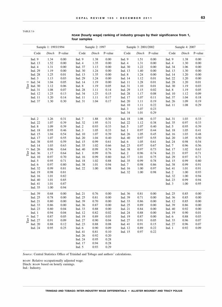
63
tRInIDAD AnD toBAgo: IntER-InDustRy WAgE DIffEREntIALs • ALLIstER MounsEy AnD tRACy PoLIus
C E P A L R E V I E W 1 0 5 • D E C E M B E R 2 0 1 1
TABLE 5.b
roaw (hourly wage) ranking of industry groups by their significance from 1, four samples
Sample 1: 1993/1994 Sample 2: 1997 Sample 3: 2001/2002 Sample 4: 2007
Code Dinch P-value Code Dinch P-value Code Dinch P-value Code Dinch P-value
Tie
r 1
Ind. 9 1.34 0.00 Ind. 9 1.38 0.00 Ind. 9 1.51 0.00 Ind. 9 1.38 0.00Ind. 13 1.52 0.00 Ind. 4 1.35 0.00 Ind. 4 1.31 0.00 Ind. 4 1.30 0.00Ind. 4 1.31 0.00 Ind. 37 1.13 0.00 Ind. 30 1.22 0.00 Ind. 34 1.06 0.00Ind. 29 1.19 0.00 Ind. 30 1.24 0.00 Ind. 13 1.40 0.00 Ind. 13 1.30 0.00Ind. 28 1.25 0.01 Ind. 13 1.35 0.00 Ind. 8 1.24 0.00 Ind. 14 1.20 0.00Ind. 3 1.13 0.03 Ind. 29 1.24 0.00 Ind. 14 1.12 0.01 Ind. 22 1.20 0.00Ind. 34 1.04 0.05 Ind. 14 1.19 0.00 Ind. 11 1.28 0.01 Ind. 28 1.20 0.01Ind. 30 1.12 0.06 Ind. 8 1.19 0.05 Ind. 31 1.10 0.01 Ind. 30 1.19 0.03Ind. 31 1.08 0.07 Ind. 28 1.11 0.14 Ind. 29 1.15 0.02 Ind. 8 1.19 0.05Ind. 12 1.25 0.13 Ind. 34 1.23 0.15 Ind. 28 1.17 0.08 Ind. 10 1.12 0.09Ind. 11 1.20 0.14 Ind. 11 1.11 0.17 Ind. 17 1.07 0.11 Ind. 37 1.04 0.18Ind. 37 1.30 0.30 Ind. 31 1.04 0.17 Ind. 20 1.11 0.19 Ind. 26 1.09 0.19 Ind. 10 1.11 0.22 Ind. 11 1.08 0.29 Ind. 3 1.07 0.23 Ind. 34 1.01 0.29
Tie
r 2
Ind. 2 1.26 0.31 Ind. 7 1.88 0.30 Ind. 18 1.08 0.37 Ind. 31 1.03 0.33Ind. 22 1.07 0.39 Ind. 32 1.95 0.31 Ind. 22 1.12 0.38 Ind. 35 0.97 0.33Ind. 8 1.09 0.39 Ind. 2 0.93 0.33 Ind. 5 1.07 0.40 Ind. 5 0.95 0.39Ind. 18 0.95 0.46 Ind. 3 1.05 0.33 Ind. 1 0.97 0.44 Ind. 18 1.05 0.41Ind. 15 1.04 0.54 Ind. 10 1.07 0.39 Ind. 26 1.05 0.45 Ind. 16 1.03 0.48Ind. 17 1.07 0.55 Ind. 20 1.04 0.40 Ind. 40 0.97 0.55 Ind. 20 1.05 0.50Ind. 38 0.95 0.59 Ind. 15 0.99 0.61 Ind. 6 1.05 0.61 Ind. 24 0.98 0.54Ind. 14 1.03 0.63 Ind. 35 1.02 0.66 Ind. 23 0.97 0.67 Ind. 7 0.96 0.56Ind. 26 0.96 0.64 Ind. 40 0.99 0.74 Ind. 38 0.97 0.73 Ind. 17 1.02 0.63Ind. 36 1.17 0.64 Ind. 1 0.99 0.76 Ind. 2 0.96 0.74 Ind. 21 0.97 0.71Ind. 10 0.97 0.70 Ind. 16 0.99 0.80 Ind. 37 1.01 0.75 Ind. 29 0.97 0.71Ind. 5 0.95 0.71 Ind. 18 1.02 0.88 Ind. 35 0.99 0.78 Ind. 15 0.99 0.80Ind. 6 0.97 0.80 Ind. 38 1.01 0.94 Ind. 7 0.98 0.86 Ind. 38 0.99 0.91Ind. 32 0.99 0.81 Ind. 22 1.00 0.98 Ind. 16 1.00 0.97 Ind. 41 1.01 0.91Ind. 19 0.98 0.81 Ind. 32 1.00 0.98 Ind. 2 1.00 0.93Ind. 16 1.01 0.82 Ind. 32 1.00 0.94Ind. 40 1.01 0.85 Ind. 23 0.99 0.94Ind. 41 1.01 0.87 Ind. 3 1.00 0.95Ind. 35 1.00 0.94
Tie
r 3
Ind. 39 0.68 0.00 Ind. 21 0.76 0.00 Ind. 36 0.81 0.00 Ind. 25 0.85 0.00Ind. 25 0.78 0.00 Ind. 25 0.81 0.00 Ind. 39 0.71 0.00 Ind. 36 0.85 0.00Ind. 21 0.80 0.00 Ind. 39 0.70 0.00 Ind. 33 0.86 0.00 Ind. 12 0.85 0.00Ind. 33 0.86 0.00 Ind. 36 0.87 0.00 Ind. 25 0.89 0.00 Ind. 39 0.86 0.00Ind. 23 0.80 0.04 Ind. 33 0.88 0.00 Ind. 21 0.84 0.00 Ind. 40 0.92 0.00Ind. 1 0.94 0.04 Ind. 12 0.82 0.02 Ind. 24 0.88 0.00 Ind. 19 0.90 0.01Ind. 7 0.87 0.05 Ind. 19 0.89 0.03 Ind. 19 0.87 0.00 Ind. 6 0.88 0.03Ind. 27 0.91 0.09 Ind. 27 0.90 0.04 Ind. 27 0.91 0.05 Ind. 33 0.96 0.07Ind. 20 0.88 0.12 Ind. 23 0.88 0.08 Ind. 41 0.91 0.15 Ind. 27 0.96 0.07Ind. 24 0.95 0.25 Ind. 6 0.90 0.09 Ind. 12 0.89 0.22 Ind. 1 0.92 0.09 Ind. 41 0.81 0.10 Ind. 15 0.97 0.22 Ind. 26 0.92 0.20 Ind. 24 0.95 0.28 Ind. 17 0.94 0.28 Ind. 5 0.93 0.29
Source: Central Statistics Office of Trinidad and Tobago and authors’ calculations.
roaw: Relative occupationally adjusted wage.Dinch: roaw based on hourly earnings. Ind.: Industry.
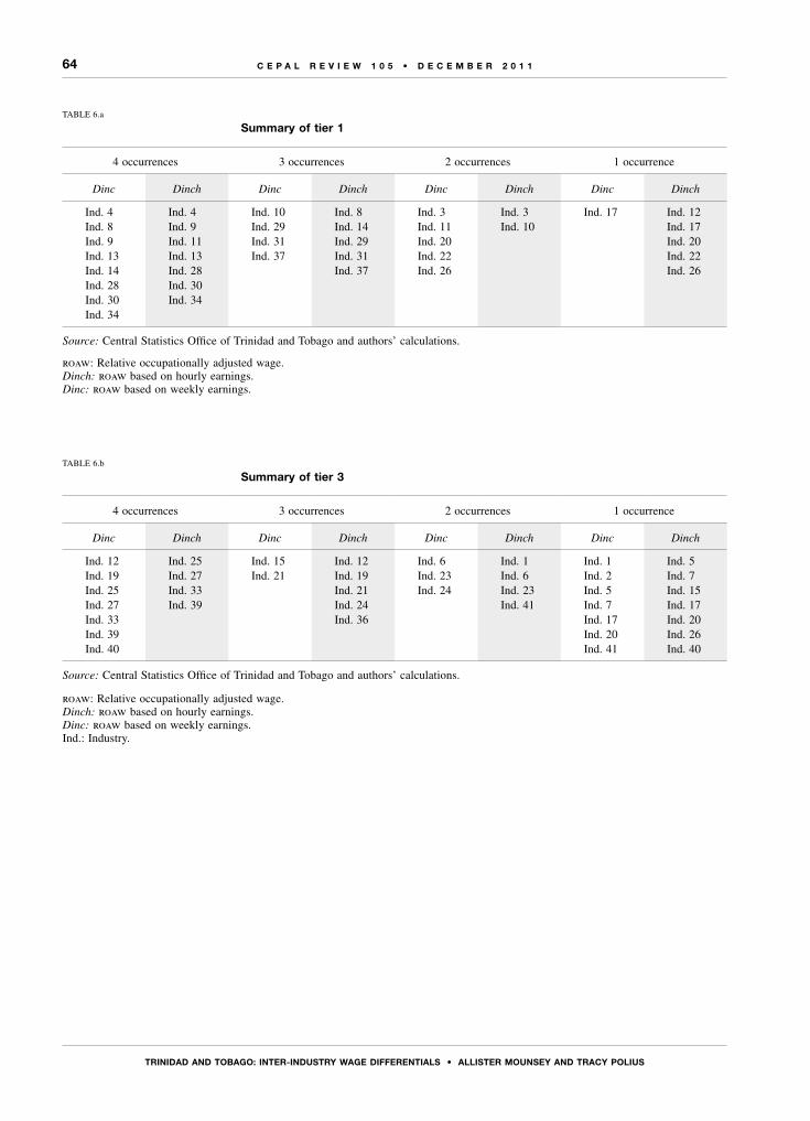
64
tRInIDAD AnD toBAgo: IntER-InDustRy WAgE DIffEREntIALs • ALLIstER MounsEy AnD tRACy PoLIus
C E P A L R E V I E W 1 0 5 • D E C E M B E R 2 0 1 1
TABLE 6.a
summary of tier 1
4 occurrences 3 occurrences 2 occurrences 1 occurrence
Dinc Dinch Dinc Dinch Dinc Dinch Dinc Dinch
Ind. 4 Ind. 4 Ind. 10 Ind. 8 Ind. 3 Ind. 3 Ind. 17 Ind. 12Ind. 8 Ind. 9 Ind. 29 Ind. 14 Ind. 11 Ind. 10 Ind. 17Ind. 9 Ind. 11 Ind. 31 Ind. 29 Ind. 20 Ind. 20Ind. 13 Ind. 13 Ind. 37 Ind. 31 Ind. 22 Ind. 22Ind. 14 Ind. 28 Ind. 37 Ind. 26 Ind. 26Ind. 28 Ind. 30 Ind. 30 Ind. 34 Ind. 34
Source: Central Statistics Office of Trinidad and Tobago and authors’ calculations.
roaw: Relative occupationally adjusted wage.Dinch: roaw based on hourly earnings. Dinc: roaw based on weekly earnings.
TABLE 6.b
summary of tier 3
4 occurrences 3 occurrences 2 occurrences 1 occurrence
Dinc Dinch Dinc Dinch Dinc Dinch Dinc Dinch
Ind. 12 Ind. 25 Ind. 15 Ind. 12 Ind. 6 Ind. 1 Ind. 1 Ind. 5Ind. 19 Ind. 27 Ind. 21 Ind. 19 Ind. 23 Ind. 6 Ind. 2 Ind. 7Ind. 25 Ind. 33 Ind. 21 Ind. 24 Ind. 23 Ind. 5 Ind. 15Ind. 27 Ind. 39 Ind. 24 Ind. 41 Ind. 7 Ind. 17Ind. 33 Ind. 36 Ind. 17 Ind. 20Ind. 39 Ind. 20 Ind. 26Ind. 40 Ind. 41 Ind. 40
Source: Central Statistics Office of Trinidad and Tobago and authors’ calculations.
roaw: Relative occupationally adjusted wage.Dinch: roaw based on hourly earnings. Dinc: roaw based on weekly earnings.Ind.: Industry.
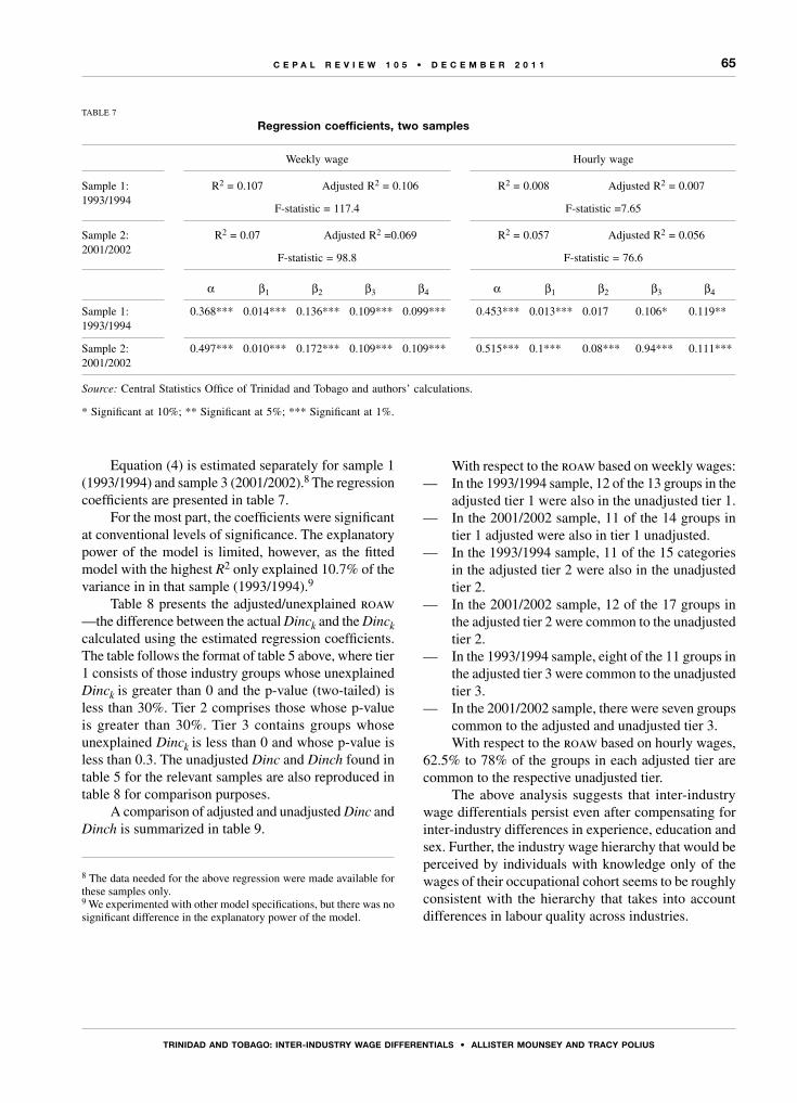
65
tRInIDAD AnD toBAgo: IntER-InDustRy WAgE DIffEREntIALs • ALLIstER MounsEy AnD tRACy PoLIus
C E P A L R E V I E W 1 0 5 • D E C E M B E R 2 0 1 1
TABLE 7
regression coefficients, two samples
Weekly wage Hourly wage
Sample 1: 1993/1994
R2 = 0.107 Adjusted R2 = 0.106 R2 = 0.008 Adjusted R2 = 0.007
F-statistic = 117.4 F-statistic =7.65
Sample 2: 2001/2002
R2 = 0.07 Adjusted R2 =0.069 R2 = 0.057 Adjusted R2 = 0.056
F-statistic = 98.8 F-statistic = 76.6
α β1 β2 β3 β4 α β1 β2 β3 β4
Sample 1: 1993/1994
0.368*** 0.014*** 0.136*** 0.109*** 0.099*** 0.453*** 0.013*** 0.017 0.106* 0.119**
Sample 2: 2001/2002
0.497*** 0.010*** 0.172*** 0.109*** 0.109*** 0.515*** 0.1*** 0.08*** 0.94*** 0.111***
Source: Central Statistics Office of Trinidad and Tobago and authors’ calculations.
* Significant at 10%; ** Significant at 5%; *** Significant at 1%.
Equation (4) is estimated separately for sample 1 (1993/1994) and sample 3 (2001/2002).8 The regression coefficients are presented in table 7.
For the most part, the coefficients were significant at conventional levels of significance. The explanatory power of the model is limited, however, as the fitted model with the highest R2 only explained 10.7% of the variance in in that sample (1993/1994).9
Table 8 presents the adjusted/unexplained roaw —the difference between the actual Dinck and the Dinck calculated using the estimated regression coefficients. The table follows the format of table 5 above, where tier 1 consists of those industry groups whose unexplained Dinck is greater than 0 and the p-value (two-tailed) is less than 30%. Tier 2 comprises those whose p-value is greater than 30%. Tier 3 contains groups whose unexplained Dinck is less than 0 and whose p-value is less than 0.3. The unadjusted Dinc and Dinch found in table 5 for the relevant samples are also reproduced in table 8 for comparison purposes.
A comparison of adjusted and unadjusted Dinc and Dinch is summarized in table 9.
8 The data needed for the above regression were made available for these samples only.9 We experimented with other model specifications, but there was no significant difference in the explanatory power of the model.
With respect to the roaw based on weekly wages:— In the 1993/1994 sample, 12 of the 13 groups in the
adjusted tier 1 were also in the unadjusted tier 1. — In the 2001/2002 sample, 11 of the 14 groups in
tier 1 adjusted were also in tier 1 unadjusted.— In the 1993/1994 sample, 11 of the 15 categories
in the adjusted tier 2 were also in the unadjusted tier 2.
— In the 2001/2002 sample, 12 of the 17 groups in the adjusted tier 2 were common to the unadjusted tier 2.
— In the 1993/1994 sample, eight of the 11 groups in the adjusted tier 3 were common to the unadjusted tier 3.
— In the 2001/2002 sample, there were seven groups common to the adjusted and unadjusted tier 3. With respect to the roaw based on hourly wages,
62.5% to 78% of the groups in each adjusted tier are common to the respective unadjusted tier.
The above analysis suggests that inter-industry wage differentials persist even after compensating for inter-industry differences in experience, education and sex. Further, the industry wage hierarchy that would be perceived by individuals with knowledge only of the wages of their occupational cohort seems to be roughly consistent with the hierarchy that takes into account differences in labour quality across industries.
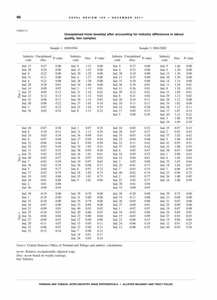
66
tRInIDAD AnD toBAgo: IntER-InDustRy WAgE DIffEREntIALs • ALLIstER MounsEy AnD tRACy PoLIus
C E P A L R E V I E W 1 0 5 • D E C E M B E R 2 0 1 1
TABLE 8.a
unexplained roaw (weekly) after accounting for industry differences in labour quality, two samples
Sample 1: 1993/1994 Sample 3: 2001/2002
Industry code
Unexplained Dinc
P-valueIndustry
codeDinc P-value
Industry code
Unexplained Dinc
P-valueIndustry
codeDinc P-value
Tie
r 1
Ind. 13 0.47 0.00 Ind. 9 1.31 0.00 Ind. 9 0.37 0.00 Ind. 9 1.46 0.00Ind. 29 0.24 0.00 Ind. 13 1.52 0.00 Ind. 4 0.23 0.00 Ind. 4 1.30 0.00Ind. 9 0.22 0.00 Ind. 29 1.25 0.00 Ind. 30 0.19 0.00 Ind. 13 1.38 0.00Ind. 31 0.11 0.00 Ind. 4 1.27 0.00 Ind. 13 0.32 0.00 Ind. 30 1.20 0.00Ind. 4 0.22 0.00 Ind. 28 1.38 0.00 Ind. 31 0.10 0.00 Ind. 14 1.14 0.00Ind. 28 0.28 0.01 Ind. 34 1.06 0.00 Ind. 26 0.18 0.01 Ind. 11 1.28 0.01Ind. 14 0.09 0.07 Ind. 3 1.15 0.01 Ind. 11 0.26 0.01 Ind. 8 1.24 0.01Ind. 37 0.05 0.12 Ind. 31 1.10 0.01 Ind. 29 0.12 0.01 Ind. 31 1.09 0.01Ind. 22 0.12 0.13 Ind. 14 1.12 0.02 Ind. 8 0.21 0.02 Ind. 29 1.12 0.02Ind. 41 0.08 0.17 Ind. 30 1.14 0.03 Ind. 20 0.16 0.11 Ind. 26 1.12 0.08Ind. 30 0.09 0.22 Ind. 37 1.05 0.10 Ind. 10 0.11 0.17 Ind. 34 1.02 0.09Ind. 3 0.07 0.23 Ind. 22 1.10 0.19 Ind. 14 0.06 0.20 Ind. 28 1.12 0.11Ind. 34 0.02 0.24 Ind. 8 1.13 0.22 Ind. 17 0.05 0.23 Ind. 17 1.07 0.14 Ind. 5 0.08 0.30 Ind. 20 1.12 0.22 Ind. 3 1.06 0.30 Ind. 10 1.09 0.30
Tie
r 2
Ind. 10 -0.07 0.30 Ind. 1 0.97 0.35 Ind. 16 -0.02 0.32 Ind. 35 0.97 0.33Ind. 8 0.10 0.31 Ind. 11 1.11 0.35 Ind. 28 0.07 0.37 Ind. 2 0.92 0.42Ind. 24 0.03 0.39 Ind. 36 0.98 0.41 Ind. 35 -0.03 0.38 Ind. 37 1.02 0.42Ind. 6 -0.07 0.40 Ind. 17 0.95 0.44 Ind. 19 -0.04 0.40 Ind. 5 1.06 0.45Ind. 12 -0.06 0.44 Ind. 2 0.94 0.50 Ind. 22 0.11 0.42 Ind. 41 0.95 0.51Ind. 35 -0.03 0.49 Ind. 32 1.03 0.51 Ind. 37 0.02 0.42 Ind. 22 1.08 0.55Ind. 11 0.07 0.52 Ind. 38 0.95 0.56 Ind. 6 0.05 0.47 Ind. 38 0.97 0.60Ind. 32 0.03 0.55 Ind. 16 1.01 0.61 Ind. 18 0.05 0.52 Ind. 1 0.98 0.63Ind. 40 -0.02 0.57 Ind. 41 0.97 0.62 Ind. 41 0.04 0.61 Ind. 6 1.04 0.64Ind. 7 -0.03 0.59 Ind. 10 0.97 0.62 Ind. 3 0.02 0.68 Ind. 32 1.03 0.66Ind. 38 0.02 0.76 Ind. 26 0.98 0.71 Ind. 25 -0.01 0.73 Ind. 18 1.04 0.67Ind. 5 0.04 0.77 Ind. 6 0.97 0.73 Ind. 7 -0.03 0.74 Ind. 7 0.96 0.70Ind. 17 -0.02 0.79 Ind. 18 1.02 0.73 Ind. 40 -0.02 0.74 Ind. 23 0.98 0.72Ind. 19 0.02 0.80 Ind. 35 1.01 0.73 Ind. 2 -0.03 0.77 Ind. 36 1.00 0.85Ind. 18 -0.01 0.88 Ind. 5 1.01 0.96 Ind. 23 0.02 0.77 Ind. 16 1.00 0.99Ind. 2 0.01 0.89 Ind. 38 0.01 0.94 Ind. 26 0.00 0.94 Ind. 32 0.00 0.95
Tie
r 3
Ind. 39 -0.19 0.00 Ind. 39 0.70 0.00 Ind. 39 -0.20 0.00 Ind. 39 0.75 0.00Ind. 1 -0.10 0.00 Ind. 21 0.80 0.00 Ind. 33 -0.11 0.00 Ind. 33 0.89 0.00Ind. 33 -0.10 0.00 Ind. 25 0.79 0.00 Ind. 36 -0.05 0.00 Ind. 21 0.82 0.00Ind. 36 -0.07 0.00 Ind. 33 0.88 0.00 Ind. 27 -0.09 0.01 Ind. 25 0.90 0.00Ind. 21 -0.09 0.01 Ind. 40 0.92 0.02 Ind. 1 -0.07 0.07 Ind. 19 0.87 0.00Ind. 25 -0.10 0.01 Ind. 20 0.86 0.03 Ind. 34 -0.02 0.08 Ind. 24 0.89 0.01Ind. 16 -0.04 0.04 Ind. 23 0.80 0.04 Ind. 15 -0.03 0.09 Ind. 27 0.92 0.03Ind. 27 -0.09 0.07 Ind. 27 0.90 0.08 Ind. 21 -0.06 0.15 Ind. 15 0.96 0.04Ind. 20 -0.11 0.07 Ind. 15 0.95 0.11 Ind. 24 -0.06 0.18 Ind. 12 0.91 0.25Ind. 15 -0.06 0.07 Ind. 12 0.88 0.11 Ind. 12 -0.08 0.25 Ind. 40 0.93 0.26Ind. 23 -0.13 0.16 Ind. 7 0.90 0.13 Ind. 19 0.91 0.17 Ind. 24 0.95 0.24
Source: Central Statistics Office of Trinidad and Tobago and authors’ calculations.
roaw: Relative occupationally adjusted wage.Dinc: roaw based on weekly earnings.Ind: Industry.
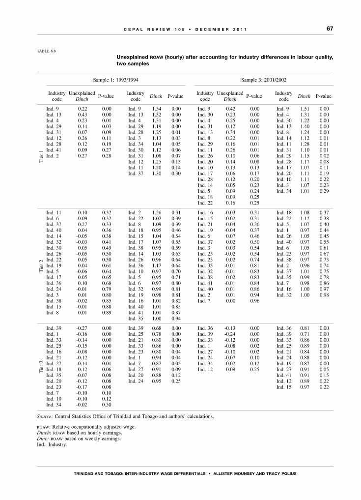
67
tRInIDAD AnD toBAgo: IntER-InDustRy WAgE DIffEREntIALs • ALLIstER MounsEy AnD tRACy PoLIus
C E P A L R E V I E W 1 0 5 • D E C E M B E R 2 0 1 1
TABLE 8.b
unexplained roaw (hourly) after accounting for industry differences in labour quality, two samples
Sample 1: 1993/1994 Sample 3: 2001/2002
Industry code
Unexplained Dinch
P-valueIndustry
codeDinch P-value
Industry code
Unexplained Dinch
P-valueIndustry
codeDinch P-value
Tie
r 1
Ind. 9 0.22 0.00 Ind. 9 1.34 0.00 Ind. 9 0.42 0.00 Ind. 9 1.51 0.00Ind. 13 0.43 0.00 Ind. 13 1.52 0.00 Ind. 30 0.23 0.00 Ind. 4 1.31 0.00Ind. 4 0.23 0.01 Ind. 4 1.31 0.00 Ind. 4 0.25 0.00 Ind. 30 1.22 0.00Ind. 29 0.14 0.03 Ind. 29 1.19 0.00 Ind. 31 0.12 0.00 Ind. 13 1.40 0.00Ind. 31 0.07 0.09 Ind. 28 1.25 0.01 Ind. 13 0.34 0.00 Ind. 8 1.24 0.00Ind. 12 0.26 0.11 Ind. 3 1.13 0.03 Ind. 8 0.22 0.01 Ind. 14 1.12 0.01Ind. 28 0.12 0.19 Ind. 34 1.04 0.05 Ind. 29 0.16 0.01 Ind. 11 1.28 0.01Ind. 41 0.09 0.27 Ind. 30 1.12 0.06 Ind. 11 0.26 0.01 Ind. 31 1.10 0.01Ind. 2 0.27 0.28 Ind. 31 1.08 0.07 Ind. 26 0.10 0.06 Ind. 29 1.15 0.02 Ind. 12 1.25 0.13 Ind. 20 0.14 0.08 Ind. 28 1.17 0.08 Ind. 11 1.20 0.14 Ind. 10 0.13 0.13 Ind. 17 1.07 0.11 Ind. 37 1.30 0.30 Ind. 17 0.06 0.17 Ind. 20 1.11 0.19 Ind. 28 0.12 0.20 Ind. 10 1.11 0.22 Ind. 14 0.05 0.23 Ind. 3 1.07 0.23 Ind. 5 0.09 0.24 Ind. 34 1.01 0.29 Ind. 18 0.09 0.25 Ind. 22 0.16 0.25
Tie
r 2
Ind. 11 0.10 0.32 Ind. 2 1.26 0.31 Ind. 16 -0.03 0.31 Ind. 18 1.08 0.37Ind. 6 -0.09 0.32 Ind. 22 1.07 0.39 Ind. 15 -0.02 0.31 Ind. 22 1.12 0.38Ind. 37 0.27 0.33 Ind. 8 1.09 0.39 Ind. 21 -0.04 0.36 Ind. 5 1.07 0.40Ind. 40 0.04 0.36 Ind. 18 0.95 0.46 Ind. 19 -0.04 0.37 Ind. 1 0.97 0.44Ind. 14 -0.05 0.38 Ind. 15 1.04 0.54 Ind. 6 0.07 0.46 Ind. 26 1.05 0.45Ind. 32 -0.03 0.41 Ind. 17 1.07 0.55 Ind. 37 0.02 0.50 Ind. 40 0.97 0.55Ind. 30 0.05 0.49 Ind. 38 0.95 0.59 Ind. 3 0.03 0.54 Ind. 6 1.05 0.61Ind. 26 -0.05 0.50 Ind. 14 1.03 0.63 Ind. 25 -0.02 0.54 Ind. 23 0.97 0.67Ind. 22 0.05 0.50 Ind. 26 0.96 0.64 Ind. 23 0.02 0.74 Ind. 38 0.97 0.73Ind. 19 0.04 0.61 Ind. 36 1.17 0.64 Ind. 35 -0.01 0.81 Ind. 2 0.96 0.74Ind. 5 -0.06 0.64 Ind. 10 0.97 0.70 Ind. 32 -0.01 0.83 Ind. 37 1.01 0.75Ind. 17 0.05 0.65 Ind. 5 0.95 0.71 Ind. 38 0.02 0.83 Ind. 35 0.99 0.78Ind. 36 0.10 0.68 Ind. 6 0.97 0.80 Ind. 41 -0.01 0.84 Ind. 7 0.98 0.86Ind. 24 -0.01 0.79 Ind. 32 0.99 0.81 Ind. 40 0.01 0.86 Ind. 16 1.00 0.97Ind. 3 0.01 0.80 Ind. 19 0.98 0.81 Ind. 2 0.01 0.94 Ind. 32 1.00 0.98Ind. 38 -0.02 0.85 Ind. 16 1.01 0.82 Ind. 7 0.00 0.96 Ind. 15 -0.01 0.88 Ind. 40 1.01 0.85 Ind. 8 0.01 0.89 Ind. 41 1.01 0.87 Ind. 35 1.00 0.94
Tie
r 3
Ind. 39 -0.27 0.00 Ind. 39 0.68 0.00 Ind. 36 -0.13 0.00 Ind. 36 0.81 0.00Ind. 1 -0.16 0.00 Ind. 25 0.78 0.00 Ind. 39 -0.24 0.00 Ind. 39 0.71 0.00Ind. 33 -0.14 0.00 Ind. 21 0.80 0.00 Ind. 33 -0.12 0.00 Ind. 33 0.86 0.00Ind. 25 -0.15 0.00 Ind. 33 0.86 0.00 Ind. 1 -0.08 0.02 Ind. 25 0.89 0.00Ind. 16 -0.08 0.00 Ind. 23 0.80 0.04 Ind. 27 -0.10 0.02 Ind. 21 0.84 0.00Ind. 21 -0.12 0.00 Ind. 1 0.94 0.04 Ind. 24 -0.07 0.10 Ind. 24 0.88 0.00Ind. 27 -0.14 0.01 Ind. 7 0.87 0.05 Ind. 34 -0.02 0.12 Ind. 19 0.87 0.00Ind. 18 -0.12 0.06 Ind. 27 0.91 0.09 Ind. 12 -0.09 0.25 Ind. 27 0.91 0.05Ind. 35 -0.07 0.08 Ind. 20 0.88 0.12 Ind. 41 0.91 0.15Ind. 20 -0.12 0.08 Ind. 24 0.95 0.25 Ind. 12 0.89 0.22Ind. 23 -0.17 0.08 Ind. 15 0.97 0.22Ind. 7 -0.10 0.10 Ind. 10 -0.10 0.12 Ind. 34 -0.02 0.30
Source: Central Statistics Office of Trinidad and Tobago and authors’ calculations.
roaw: Relative occupationally adjusted wage.Dinch: roaw based on hourly earnings. Dinc: roaw based on weekly earnings.Ind.: Industry.
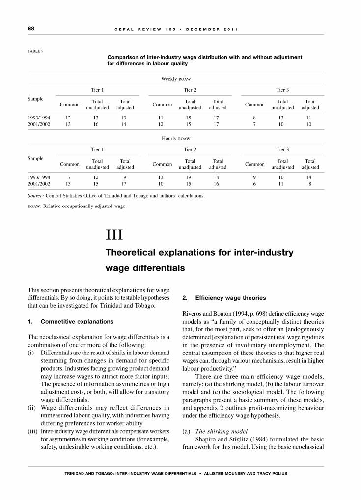
68
tRInIDAD AnD toBAgo: IntER-InDustRy WAgE DIffEREntIALs • ALLIstER MounsEy AnD tRACy PoLIus
C E P A L R E V I E W 1 0 5 • D E C E M B E R 2 0 1 1
IIITheoretical explanations for inter-industry
wage differentials
TABLE 9
Comparison of inter-industry wage distribution with and without adjustment for differences in labour quality
Weekly roaw
Sample
Tier 1 Tier 2 Tier 3
CommonTotal
unadjustedTotal
adjustedCommon
Total unadjusted
Total adjusted
CommonTotal
unadjustedTotal
adjusted
1993/1994 12 13 13 11 15 17 8 13 112001/2002 13 16 14 12 15 17 7 10 10
Hourly roaw
Sample
Tier 1 Tier 2 Tier 3
CommonTotal
unadjustedTotal
adjustedCommon
Total unadjusted
Total adjusted
CommonTotal
unadjustedTotal
adjusted
1993/1994 7 12 9 13 19 18 9 10 142001/2002 13 15 17 10 15 16 6 11 8
Source: Central Statistics Office of Trinidad and Tobago and authors’ calculations.
roaw: Relative occupationally adjusted wage.
This section presents theoretical explanations for wage differentials. By so doing, it points to testable hypotheses that can be investigated for Trinidad and Tobago.
1. Competitive explanations
The neoclassical explanation for wage differentials is a combination of one or more of the following:(i) Differentials are the result of shifts in labour demand
stemming from changes in demand for specific products. Industries facing growing product demand may increase wages to attract more factor inputs. The presence of information asymmetries or high adjustment costs, or both, will allow for transitory wage differentials.
(ii) Wage differentials may reflect differences in unmeasured labour quality, with industries having differing preferences for worker ability.
(iii) Inter-industry wage differentials compensate workers for asymmetries in working conditions (for example, safety, undesirable working conditions, etc.).
2. Efficiency wage theories
Riveros and Bouton (1994, p. 698) define efficiency wage models as “a family of conceptually distinct theories that, for the most part, seek to offer an [endogenously determined] explanation of persistent real wage rigidities in the presence of involuntary unemployment. The central assumption of these theories is that higher real wages can, through various mechanisms, result in higher labour productivity.”
There are three main efficiency wage models, namely: (a) the shirking model, (b) the labour turnover model and (c) the sociological model. The following paragraphs present a basic summary of these models, and appendix 2 outlines profit-maximizing behaviour under the efficiency wage hypothesis.
(a) The shirking modelShapiro and Stiglitz (1984) formulated the basic
framework for this model. Using the basic neoclassical
69
tRInIDAD AnD toBAgo: IntER-InDustRy WAgE DIffEREntIALs • ALLIstER MounsEy AnD tRACy PoLIus
C E P A L R E V I E W 1 0 5 • D E C E M B E R 2 0 1 1
competitive paradigm as their starting point, they showed that the typical employee, under conditions of imperfect monitoring, will have an inbuilt incentive to shirk. They argued that since labour markets clear, i.e., there is no involuntary unemployment, there is no cost associated with shirking since if a worker is caught shirking and is fired he will be immediately rehired at the going wage rate. Thus, at the market clearing rate, all workers will shirk.
To elicit greater effort from employees, the firm pays more than the market clearing wage, thereby instituting a penalty for an employee who is caught shirking and is fired.10 Assuming firms are identical, it would therefore be profitable for all firms to increase wages. What results is an equilibrium where the market wage is not market clearing. This market-produced unemployment is a worker discipline device of sorts, as it ensures that the worker who is fired for shirking will not immediately obtain another job.
Bulow and Summers (1986) extended the basic Shapiro-Stiglitz framework to show how equally productive workers can in equilibrium be arbitrarily allocated between a high-wage and a low-wage sector.11 They thereby provided a theoretical basis for explaining
10 The extent of the wage premium is obviously dependent on the cost of shirking to the firm.11 The high-wage sector pays a high-wage premium because shirking is more costly in that sector than in other sectors.
market equilibrium with both inter-industry wage differentials and involuntary unemployment.
(b) The labour turnover modelThis model postulates that when workers quit, firms
incur sunk costs associated with hiring replacements, training new workers and losing productivity as new workers move along the learning curve. Firms try to minimize these turnover costs by paying a wage premium (Salop, 1979). For any given occupation, turnover costs may vary from industry to industry, thereby creating different wage premiums. The model produces equilibria with involuntary unemployment and a distribution of wages for a given occupation.
(c) The sociological modelAkerloff (1982 and 1984) argues that social
conventions in the workplace, which he refers to as norms, have a strong effect on workers’ attitudes. Workers are motivated to work hard because they acquire sentiment for each other and for the firm. In return for their commitment, workers expect to be reciprocated with “fair” wages. This fair wage depends on the wages of workers in the workers’ reference group and past wages, among other things. According to the basic sociological model, “the loyalty of workers is exchanged for high wages, and this loyalty can be translated via effective management into high productivity” (Akerloff, 1984, p. 80). Inter-firm (inter-industry) wage differentials can be explained by the differing ability of firms (industries) to translate employee loyalty into higher productivity.
IVConclusion
Trinidad and Tobago seems to have a relatively temporally stable inter-industry wage distribution. Some industries at times pay as much as 52% more than average for a given occupation, while others sometimes pay as little as 25% below average. Even after accounting for measured differences in labour quality, disparities in industry wages still persist.
While the paper does not necessarily provide an explanation for these differentials, it has provided a
snapshot of current explanations for this phenomenon in the literature. Further work is needed to test the hypotheses put forward by these explanations. The importance of this work should not be underestimated. Knowledge of and explanations for these differentials should be important to researchers and policymakers, as the existence of wage differentials has distributional implications and may also point to a need to radically rethink our understanding of how labour markets function in the Caribbean.
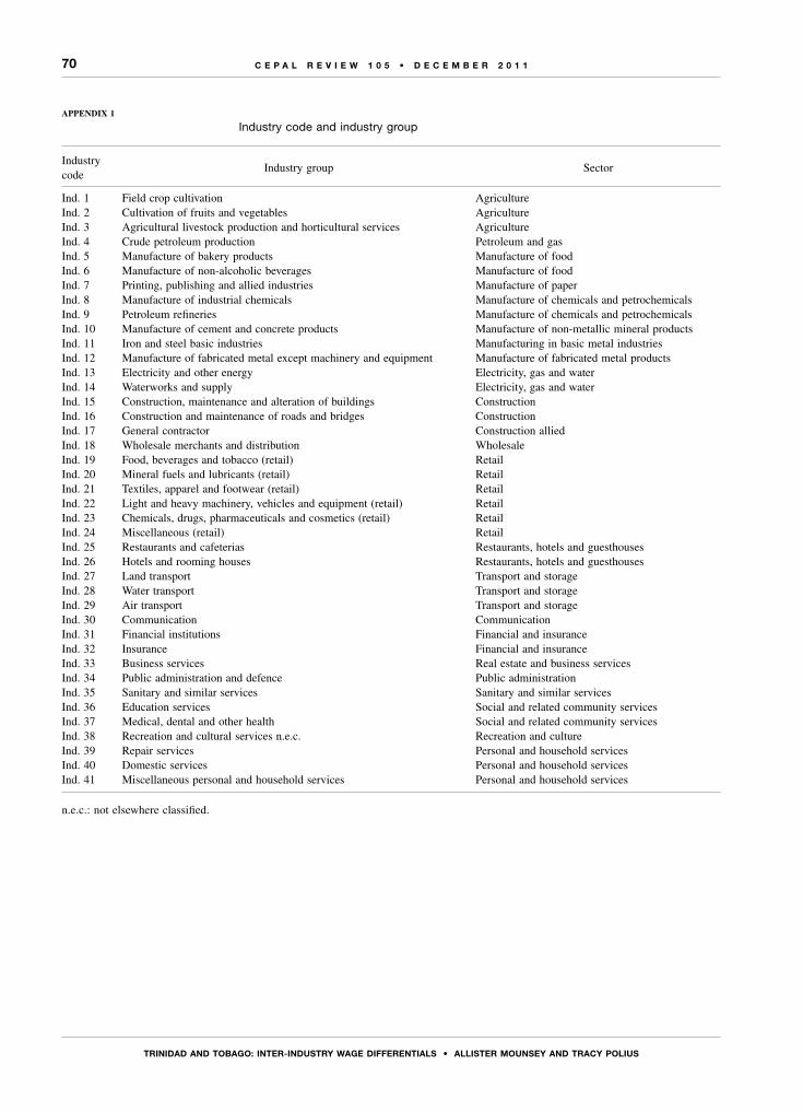
70
tRInIDAD AnD toBAgo: IntER-InDustRy WAgE DIffEREntIALs • ALLIstER MounsEy AnD tRACy PoLIus
C E P A L R E V I E W 1 0 5 • D E C E M B E R 2 0 1 1
AppEndix 1
Industry code and industry group
Industry code
Industry group Sector
Ind. 1 Field crop cultivation AgricultureInd. 2 Cultivation of fruits and vegetables AgricultureInd. 3 Agricultural livestock production and horticultural services AgricultureInd. 4 Crude petroleum production Petroleum and gasInd. 5 Manufacture of bakery products Manufacture of foodInd. 6 Manufacture of non-alcoholic beverages Manufacture of foodInd. 7 Printing, publishing and allied industries Manufacture of paperInd. 8 Manufacture of industrial chemicals Manufacture of chemicals and petrochemicalsInd. 9 Petroleum refineries Manufacture of chemicals and petrochemicalsInd. 10 Manufacture of cement and concrete products Manufacture of non-metallic mineral productsInd. 11 Iron and steel basic industries Manufacturing in basic metal industriesInd. 12 Manufacture of fabricated metal except machinery and equipment Manufacture of fabricated metal productsInd. 13 Electricity and other energy Electricity, gas and waterInd. 14 Waterworks and supply Electricity, gas and waterInd. 15 Construction, maintenance and alteration of buildings ConstructionInd. 16 Construction and maintenance of roads and bridges ConstructionInd. 17 General contractor Construction alliedInd. 18 Wholesale merchants and distribution Wholesale Ind. 19 Food, beverages and tobacco (retail) RetailInd. 20 Mineral fuels and lubricants (retail) RetailInd. 21 Textiles, apparel and footwear (retail) RetailInd. 22 Light and heavy machinery, vehicles and equipment (retail) RetailInd. 23 Chemicals, drugs, pharmaceuticals and cosmetics (retail) RetailInd. 24 Miscellaneous (retail) RetailInd. 25 Restaurants and cafeterias Restaurants, hotels and guesthousesInd. 26 Hotels and rooming houses Restaurants, hotels and guesthousesInd. 27 Land transport Transport and storageInd. 28 Water transport Transport and storageInd. 29 Air transport Transport and storageInd. 30 Communication CommunicationInd. 31 Financial institutions Financial and insuranceInd. 32 Insurance Financial and insuranceInd. 33 Business services Real estate and business servicesInd. 34 Public administration and defence Public administrationInd. 35 Sanitary and similar services Sanitary and similar servicesInd. 36 Education services Social and related community servicesInd. 37 Medical, dental and other health Social and related community servicesInd. 38 Recreation and cultural services n.e.c. Recreation and cultureInd. 39 Repair services Personal and household servicesInd. 40 Domestic services Personal and household servicesInd. 41 Miscellaneous personal and household services Personal and household services
n.e.c.: not elsewhere classified.
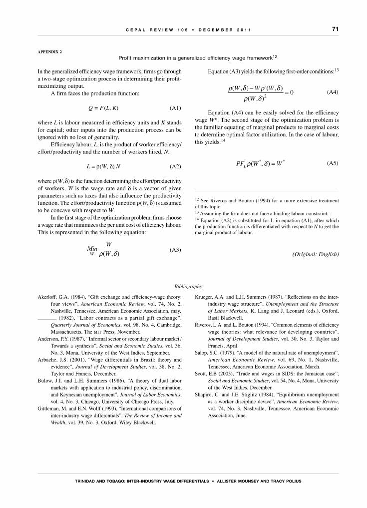
71
tRInIDAD AnD toBAgo: IntER-InDustRy WAgE DIffEREntIALs • ALLIstER MounsEy AnD tRACy PoLIus
C E P A L R E V I E W 1 0 5 • D E C E M B E R 2 0 1 1
In the generalized efficiency wage framework, firms go through a two-stage optimization process in determining their profit-maximizing output.
A firm faces the production function:
Q = F (L, K) (A1)
where L is labour measured in efficiency units and K stands for capital; other inputs into the production process can be ignored with no loss of generality.
Efficiency labour, L, is the product of worker efficiency/effort/productivity and the number of workers hired, N.
L = ρ(W, δ) N (A2)
where ρ(W, δ) is the function determining the effort/productivity of workers, W is the wage rate and δ is a vector of given parameters such as taxes that also influence the productivity function. The effort/productivity function ρ(W, δ) is assumed to be concave with respect to W.
In the first stage of the optimization problem, firms choose a wage rate that minimizes the per unit cost of efficiency labour. This is represented in the following equation:
MinW
WW ( , )ρ δ (A3)
AppEndix 2
Profit maximization in a generalized efficiency wage framework12
12 See Riveros and Bouton (1994) for a more extensive treatment of this topic.13 Assuming the firm does not face a binding labour constraint.14 Equation (A2) is substituted for L in equation (A1), after which the production function is differentiated with respect to N to get the marginal product of labour.
Equation (A3) yields the following first-order conditions:13
ρ δ ρ δ
ρ δ( , ) '( , )
( , )
W W W
W
− =2
0 (A4)
Equation (A4) can be easily solved for the efficiency wage W*. The second stage of the optimization problem is the familiar equating of marginal products to marginal costs to determine optimal factor utilization. In the case of labour, this yields:14
PFL' * *)ρ δ =W W( , (A5)
Bibliography
Akerloff, G.A. (1984), “Gift exchange and efficiency-wage theory: four views”, American Economic Review, vol. 74, No. 2, Nashville, Tennessee, American Economic Association, may.
(1982), “Labor contracts as a partial gift exchange”, Quarterly Journal of Economics, vol. 98, No. 4, Cambridge, Massachusetts, The mit Press, November.
Anderson, P.Y. (1987), “Informal sector or secondary labour market? Towards a synthesis”, Social and Economic Studies, vol. 36, No. 3, Mona, University of the West Indies, September.
Arbache, J.S. (2001), “Wage differentials in Brazil: theory and evidence”, Journal of Development Studies, vol. 38, No. 2, Taylor and Francis, December.
Bulow, J.I. and L.H. Summers (1986), “A theory of dual labor markets with application to industrial policy, discrimination, and Keynesian unemployment”, Journal of Labor Economics, vol. 4, No. 3, Chicago, University of Chicago Press, July.
Gittleman, M. and E.N. Wolff (1993), “International comparisons of inter-industry wage differentials”, The Review of Income and Wealth, vol. 39, No. 3, Oxford, Wiley Blackwell.
Krueger, A.A. and L.H. Summers (1987), “Reflections on the inter-industry wage structure”, Unemployment and the Structure of Labor Markets, K. Lang and J. Leonard (eds.), Oxford, Basil Blackwell.
Riveros, L.A. and L. Bouton (1994), “Common elements of efficiency wage theories: what relevance for developing countries”, Journal of Development Studies, vol. 30, No. 3, Taylor and Francis, April.
Salop, S.C. (1979), “A model of the natural rate of unemployment”, American Economic Review, vol. 69, No. 1, Nashville, Tennessee, American Economic Association, March.
Scott, E.B (2005), “Trade and wages in SIDS: the Jamaican case”, Social and Economic Studies, vol. 54, No. 4, Mona, University of the West Indies, December.
Shapiro, C. and J.E. Stiglitz (1984), “Equilibrium unemployment as a worker discipline device”, American Economic Review, vol. 74, No. 3, Nashville, Tennessee, American Economic Association, June.
(Original: English)


C E P A L R E V I E W 1 0 5 • D E C E M B E R 2 0 1 1
73
K E Y W O R D S
Food prices
Inflation
Food production
Price indices
Economic growth
Economic statistics
Mathematical analysis
Mexico
Mexico: food price increasesand growth constraints
Moritz Cruz, Armando Sánchez and Edmund Amann
This paper uses dynamic panel techniques to evaluate the extent
to which Mexico’s consumer price index will be affected by food price
inflation in the long term. We argue that sharp increases in international
food prices (of the type seen since 2001) are likely to persist and to
reinforce domestic growth constraints in Mexico. Our results suggest that
in an economy like Mexico’s that is highly dependent on imported food,
the consumer price index will be noticeably affected by international food
price increases. Conducting monetary policy without reference to the
structural issue of food price inflation is therefore likely to be ineffective
in controlling inflation and could be damaging in terms of its impact on
demand and growth. Thus, the revitalization of the Mexican agricultural
sector should be a centrepiece of future counter-inflationary policy.
Moritz Cruz
Researcher, National Autonomous
University of Mexico (unam),
Institute of Economic Research
Armando Sánchez
Researcher, National Autonomous
University of Mexico (unam),
Institute of Economic Research
Edmund Amann
Senior Lecturer, University of
Manchester, School of Social
Sciences
74
MExICo: fooD PRICE InCREAsEs AnD gRoWtH ConstRAInts • MoRItz CRuz, ARMAnDo sánCHEz AnD EDMunD AMAnn
C E P A L R E V I E W 1 0 5 • D E C E M B E R 2 0 1 1
International commodity prices increased by around 195% in real terms during the 2001-2008 period. Food prices, in particular, practically doubled during the period (imf, 2010; see also eclac, 2008), reaching unprecedented levels. Given the nature of the factors driving it, food price inflation cannot be viewed as a temporary phenomenon. On the demand side, pressure on food prices is stemming from the sustained and rapid growth of key emerging economies (mainly China and India) as well as from the generation of new sources of energy derived from basic food grains such as maize. On the supply side, global climate change and lags in technological development are adversely affecting efforts to increase production. In the near future therefore, the demand for food is expected to considerably outstrip supply. This, in turn, has led to predictions of rising international food prices for at least the next 10 years (oecd/fao, 2010). The era of cheap food, in other words, has come to an end (see The Economist, 2007, 2008, 2009).1
At the same time, the demand for food from net food importers will continue growing, according to Bruinsma (2003, p. 235): “The outlook to 2030 suggests that the agricultural trade deficit of developing countries will widen markedly, reaching an overall net import level of US$ 31 billion. Net imports of food will increase to about US$ 50 billion.” These two likely developments represent bad news for developing economies that are net importers of food. Food price inflation will increase poverty. According to the Inter-American Development Bank (idb, 2008), for example, in Latin America there is the risk that more than 26 million people will be pushed into extreme poverty due to food price inflation (see also fao, 2008, for a broader international view along the same lines).
Another important but rarely analysed negative effect of food price inflation and food dependency is their impact
The authors would like to thank Julio López, the editor of cepal Review and a cepal Review referee for their helpful suggestions. The usual disclaimers apply. The authors are also grateful for financial support received from the Programme to Support Research and Technological Innovation Projects (papiit) of the National Autonomous University of Mexico (unam), under the IN-306809 research project.1 The oecd-fao Agricultural Outlook, 2010-2019 (oecd/fao, 2010, p. 1) points out that average maize and coarse grain prices are projected to be nearly 15% to 40% higher in real terms over the next 10 years than in 1997-2006.
on demand growth constraints. Such constraints exist because in developing countries, unlike rich countries, food weighs heavily in the consumer price index (cpi).2 Thus, food price inflation is very likely to pass through to the cpi of developing economies that are net importers of food. Faced with rising domestic inflation, the authorities are likely to respond with conventional monetary and fiscal measures to tame inflationary pressures. If the source of inflationary pressure is structural, however, such efforts might well prove ineffective. The direct consequence of fighting inflation by conventional means will be to constrain growth by way of lower investment. In other words, international food price inflation might create (or at least reinforce) the so-called domestic demand growth constraint (see Kalecki, 1954; Noyola, 1956; Sunkel, 1958) in food-dependent developing economies.
In the same vein, food price inflation and food dependency might also exercise indirect upward pressure on inflation through the external accounts. This might occur in two different ways. First, when international food prices are soaring, more foreign exchange is needed to meet the demand for food imports. A shortage of foreign exchange coupled with an unsustainable current account deficit might generate expectations that the government will seek to devalue the currency in the near future in order to correct the external deficit. Expectations of a future devaluation will feed inflation expectations. This, in turn, will make the authorities tighten monetary and fiscal policy, restricting growth as a result. Second, if domestic inflation increased as a result of food price inflation, the real exchange rate would appreciate, causing the economy to lose international competitiveness. Exports would fall and imports, in all likelihood, would increase. This would lead to a deterioration of the external accounts. To rectify this disequilibrium, the authorities might decide to reduce aggregate demand, a decision that would inevitably have the effect of constraining growth further.
Against this background, the objective of this paper is to explore the growth-constraining effects of food price inflation. In particular, it seeks to illustrate the extent
2 Food generally accounts for about 10% of the cpi in developed countries. In developing economies, food can account for 50% to 60% of the cpi (The Economist, 2007).
Iintroduction
75
MExICo: fooD PRICE InCREAsEs AnD gRoWtH ConstRAInts • MoRItz CRuz, ARMAnDo sánCHEz AnD EDMunD AMAnn
C E P A L R E V I E W 1 0 5 • D E C E M B E R 2 0 1 1
to which food price inflation might affect domestic inflation and thus result in – or reinforce – the domestic growth constraint. The Mexican economy is used as a case study in this paper because its food dependency (particularly for imports of basic food grains) has been steadily growing since the mid-1980s, following trade liberalization policies sealed by the launch of the North American Free Trade Agreement (nafta). At the same time, the foodstuffs component still has a large weight in Mexico’s cpi. As a result, Mexico risks being caught in a dilemma, with international food price inflation causing domestic inflation to rise and the authorities finding it ever harder to keep inflation within its target range, so that they respond with growth-constraining
macroeconomic policies. To measure the extent to which food price inflation will affect Mexico’s cpi in the long term, we apply dynamic panel techniques.
The paper is organized as follows. Section II describes how food price inflation and food dependency can both give rise to and reinforce demand growth constraints. Our analysis employs structural inflation theory, but focuses on the case of an open developing economy with food dependency in a scenario where international food prices are rising. Section III presents evidence for Mexico’s high dependence on imported food and its influence on the country’s cpi. Section IV then presents the dynamic panel estimates. The final section sets out our concluding remarks.
IIThe macro effects of food price inflation
and food dependency: the materialization
of demand growth constraints
A primary objective in developing economies is to expand output (and employment) rapidly and sustainably.3 A sine qua non for achieving this goal, generally ignored by the literature, is the reduction (or if possible the elimination) of so-called growth constraints (see Sakar, 1988; Storm, 1997).
These constraints are associated with excessive inflation and balance-of-payments disequilibria, both the consequence of policies to expand aggregate demand. The former is generally identified, for obvious reasons, as the domestic demand growth constraint, whereas the latter is recognized as the external constraint. Much of the seminal theoretical literature on both these growth constraints ignores international food price inflation or food dependency, or both. However, the growing influence and importance of these phenomena in developing economies’ growth processes makes it clear that
3 As Wolf (2008) clearly puts it: “Growth is not everything. But it is the foundation for everything. The poorer the country the more important growth becomes, partly because it is impossible to redistribute nothing and partly because higher incomes make a huge difference to the welfare of the poorest.” Moreover, rapid and sustained growth implies increasing aggregate demand, which is the primary source of firms’ sales and profits.
they should be considered key sources of potential growth constraints.
One of the pioneers in drawing attention to how inflation could constrain growth was the Polish economist Michał Kalecki. The Kaleckian argument, developed in the early 1950s, was configured for a closed economy (perhaps because of the existence of domestic or international trade barriers, or both, at that time). Moreover, this closed economy is a developing one where food prices have a large weight in the cpi. In today’s context, only the large weighting of food in the cpi still holds, as most developing economies are engaged in the globalization process; thus, it is unrealistic to think in terms of a closed economy. As is pointed out below, however, the main result of Kalecki’s argument holds for an open developing economy (which we assume has a rigid domestic supply of food and is, therefore, food-dependent). By considering an open economy, furthermore, we are able to illustrate how the domestic growth constraint might be indirectly reinforced.
Kalecki put forward the idea that an economy that was expanding might face excessive inflationary pressures if supply in the primary sector, and that of foodstuffs in particular, was limited. More specifically, he argued that one important obstacle a developing economy might face
76
MExICo: fooD PRICE InCREAsEs AnD gRoWtH ConstRAInts • MoRItz CRuz, ARMAnDo sánCHEz AnD EDMunD AMAnn
C E P A L R E V I E W 1 0 5 • D E C E M B E R 2 0 1 1
when investment was increasing strongly was the difficulty of procuring an “adequate supply of necessities to cover the demand resulting from the increase in employment” (Kalecki, 1966, p. 16). If this supply is not adequate, inflationary pressures might be generated. In this sense, inflation, as Noyola (1956, p. 604) remarked, is chiefly “the result of real imbalances”.4 In other words, “the crucial point of whether a certain level of investment creates or does not create inflationary pressures is the possibility of expansion of supply of consumer goods in response to demand” (Kalecki, 1993b, pp. 25-26). If supply in the primary sector is indeed rigid, prices will increase, causing real wages to fall. Thereafter, “the reaction of workers to the reduction of real wages will be a demand for higher money wages, and thus a price-wage spiral will be initiated” (Kalecki, 1993b, p. 26). As can be seen, inflation for Kalecki is the result of a structural problem (a real imbalance), stemming from the limited productive capacity of the primary sector to satisfy a growing demand for food. An important point is that institutional and structural rigidities in the agricultural sector mean that relative and absolute rises in agricultural prices do not stimulate an adequate supply response.
The inflationary pressure resulting from a rigid food supply leads to constraints on growth via investment. Investment can be negatively affected through two different mechanisms. First, policymakers might decide to reduce aggregate demand in order to reduce the demand for food, with investment shrinking as a result (i.e., as a result of falling public investment, but also of shrinking public expenditure, which in turn reduces firms’ sales). Second, monetary authorities in developed and developing economies alike generally have a strong belief that inflation is exclusively a monetary problem. To fight inflationary pressures, therefore, they apply conventional policies in the form of fiscal and monetary tightening. Both types of policies act by reining in private investment through their impact on effective demand, thus reducing actual and potential growth.5
In a context where inflation arises from a real imbalance, the cost of taming it by shrinking demand (merely in order to reduce the quantity of money) will be very high, since this implies a loss of output (and thus employment). At the same time, it is important
4 See Sunkel (1958) for the classic reference work acknowledging and providing evidence for the structural origins of inflation. See also Cardoso (1981) for a more recent study of this phenomenon.5 Tight monetary policy entails higher interest rates, which might also have a negative effect on investment by increasing firms’ debt service.
to realize that the policy measures described are by no means guaranteed to put an end to inflation.6
In sum, under conditions where an economy is expanding and facing domestic supply shortages of food commodities, it is likely that growth will be constrained at some point. This outcome will be unavoidable when an economy is a net importer of food (that is, it is an open economy) and international food prices are rising (a scenario that, as we have emphasized, has been forecast to prevail for at least the next decade). Inflation occurs because food weighs heavily in the cpi in developing economies, as we have mentioned, making this very sensitive to international food price movements. Hence, any increase in international food prices will generate inflationary pressures (countries will in fact be “importing” inflation in this sense), inducing the authorities to tighten macroeconomic policy. In a scenario of food dependency and rising international food prices, therefore, any expansion of output will necessarily generate inflationary pressures (via higher employment, à la Kalecki, and via “imported” inflation) that give rise to a domestic growth constraint.7 The economy will be unable to grow sustainably in consequence.
It could also be the case that international food price inflation might reinforce or give rise to the domestic growth constraint in food-dependent economies that are, paradoxically, not growing (in this context, or even under conditions of low growth, the demand for food tends to be very stable, rising only in line with increasing population), because the economy will merely “import” inflation. If growth is stagnating (or, even worse, is negative), the sort of conventional macroeconomic policies applied to fight inflation will aggravate the deterioration of the real economy. Additionally, as mentioned, since the source of inflation is a real imbalance (reflected in this case in “imported” inflation), it is unlikely to be controlled.
Food price inflation (due to either economic expansion or imported inflation, or both) may not just give rise to or reinforce the domestic growth constraint
6 This was pointed out long ago by Kaldor, who remarked: “Western economists were slow to recognize this point [that fiscal and monetary policies had little to do with the persistence of inflation in some Latin American economies], with the result that the stabilization policies… urged by international organizations proved abortive in halting these inflations, though they frequently involved contractions in the level of production and employment” (1966, p. 61).7 Evidently, it could happen that international food prices decline at the same time as the food-dependent economy is expanding. In this case, the domestic growth constraint will not bite. Even if domestic food prices are declining, however, the current account could deteriorate as a result of the agricultural trade deficit. As we will see, this contributes to the materialization of the external demand growth constraint.
77
MExICo: fooD PRICE InCREAsEs AnD gRoWtH ConstRAInts • MoRItz CRuz, ARMAnDo sánCHEz AnD EDMunD AMAnn
C E P A L R E V I E W 1 0 5 • D E C E M B E R 2 0 1 1
directly, but may also do so indirectly, in two related ways. First, international food price inflation implies a larger foreign-exchange requirement to cover a given amount of food imports. If the economy in question maintains an unsustainable current account deficit8 and there is a shortage of foreign exchange, expectations of a future devaluation to correct the external imbalance will start growing. As is well known, expectations of currency depreciation feed inflation due to the expected increase in the cost of imported capital goods and other production inputs. In this scenario, workers will demand a nominal wage that takes into account not only the increase in food prices, but also other price increments. The resulting wage-price spiral could thus accelerate, producing much higher inflation, and the authorities might respond by applying tighter demand constraint measures, which affect output and growth accordingly.
Second, the increase in domestic inflation resulting from food price inflation will have a negative impact on the economy’s international competitiveness. In other words, rising domestic inflation, other things being equal, will strengthen the real exchange rate. Domestic currency appreciation will worsen the current account because exports will decrease while imports will increase. If the resulting external deficit is unsustainable, agents will expect the government to devalue in order to correct it.9 It is easy to deduce that this will trigger a process similar to the one just described, with severely constrained economic growth as the final outcome.
It is important to stress that food dependency has the potential to reinforce the external or balance-of-payments growth constraint, as initially proposed by Harrod (1933) and Prebisch (1982) but refined by Thirlwall (1979). The argument is that an economy will be compelled to correct an unsustainable current account deficit by shrinking domestic demand when such a deficit can no longer be externally financed or when exchange-rate adjustments do not suffice to rectify the external disequilibrium, or both. As is well known (see Keynes, 1936), and as we stressed earlier, changes in output (and employment) follow effective demand adjustments. An induced reduction in effective demand to correct the trade balance will therefore affect growth negatively. Likewise, an economy that is expanding faces a potential balance-of-payments growth constraint.
8 The agricultural trade deficits obviously run by net food importers contribute to a worsening of the current account.9 If the currency depreciates, domestic inflation will clearly increase, adding to the domestic growth constraint.
Much as with the domestic growth constraint theory, a key insight of the external demand growth constraint approach is that the current account deficit deteriorates as a consequence of economic expansion (assuming imports grow faster than exports).10 For an economy that is food-dependent, any output expansion will therefore lead to a deterioration of the agricultural trade balance, which will potentially worsen the current account. With the current account deteriorating, growth will be constrained when policies to reduce aggregate demand are applied at any point. This being so, it is clear that food dependency contributes directly to the emergence of the balance-of-payments growth constraint.
To sum up, international food price inflation and food dependency represent a negative combination for growth, since they are a potent source of domestic demand and external growth constraints. If any of these constraints materialize, economic growth cannot be long sustained. However, in practice policymakers frequently respond more quickly to inflationary pressures than to current account deficits. This is often because policymakers are bound by inflation targeting frameworks and tend not to worry about external deficits so long as they are relatively small and can be financed. Furthermore, they expect (often wrongly) that exchange-rate adjustments will rectify the external deficit.11 Given the predicted evolution of food price inflation over the coming decades, the question that naturally arises is how far this phenomenon will affect domestic inflation and thus give rise to the domestic growth constraint.
To shed light on this question, we use the Mexican economy as our case study. There are two reasons for this. First, Mexico is an economy in which food dependency has steadily increased since the mid-1980s, i.e., since the adoption of trade liberalization policies. Second, food still has a large weight in its cpi. Mexico’s central bank has accordingly recognized that domestic inflation has been subjected to upward pressures since international food prices started to soar. This is despite the fact that economic growth in Mexico since the early 1980s has been, on average, low and unstable. This being so, as we
10 Not all economies that expand will face a current account deficit (a remarkable recent example here being the Chinese economy). The net trade balance, we must recall, depends ultimately on the income elasticities of imports and exports.11 Even if the Marshall-Lerner condition holds, there is no guarantee that currency depreciation will improve the trade balance (see, for example, Thirlwall, 2003), at least in the short term (see Harberger, 1950; Laursen and Metzler, 1950). Even if it does, it might lead to a severe loss of real output (see Krugman and Taylor, 1978).
78
MExICo: fooD PRICE InCREAsEs AnD gRoWtH ConstRAInts • MoRItz CRuz, ARMAnDo sánCHEz AnD EDMunD AMAnn
C E P A L R E V I E W 1 0 5 • D E C E M B E R 2 0 1 1
argue above, the authorities’ decision to fight inflation has constrained the expansion of output in the recent past and will continue to do so, without succeeding in taming inflation. We argue that the Mexican experience indicates that when the source of inflation is a real imbalance, fighting inflation by conventional means
produces ineffective results and severe real costs in terms of output, employment.
We shall now estimate the expected long-term effects of food price inflation on Mexican inflation. First, though, we present a brief overview of Mexico’s food dependency.
IIIMexico’s dependency on imported food
and its consumer price index
Nothing in the growth literature suggests that governments should neglect the primary sector as economies climb the ladder of development, for example by removing trade protection and reducing technological and financial support. Nor should increasing development imply a shift from growing self-sufficiency in food production to food dependency.12 It is therefore surprising that Mexico’s dependence on imported food started to increase steadily just about the time its per capita income reached its highest-ever level (around US$ 7,400 in real terms in the early 1980s). Furthermore, and just as surprisingly, Mexico’s food dependency started to intensify even as per capita income stagnated over the course of the following decade.
Although it is not the main focus of this paper, it is important to mention that Mexico’s growing food dependency can be traced to both declining government support for the primary sector and trade liberalization policies, sealed with the launch of nafta. The combined outcome of decreasing government support and the nafta-driven trade liberalization strategy has been an ever-growing gap between domestic food production and demand (with demand growth having been driven essentially by the rise in population).13 This gap has
12 In fact, empirical evidence shows (and development theory implies, with the idea that primary sector exports should finance industrial imports during the early stages of development) that industrializing economies ought to deploy the necessary measures to guarantee food self-sufficiency and that, once industrialized, they should be able to continue exporting food commodities. In fact, Kaldor (1966) goes further in emphasizing the importance of the agricultural sector to the industrialization process by arguing that any successful industrialization strategy must be underpinned by the development and maintenance of an agricultural surplus, “…that is, the excess of food production over the food consumption of the food producers themselves” (p. 55).13 By contrast with other developing economies such as China and India, economic performance cannot explain Mexico’s rising demand
been filled by rising imports of food, which have steadily increased food dependency.
Part of the reason for the stagnation of domestic food production after trade opening lies in the inability of domestic producers to compete with imports. Another reason, however, is that many farmers have shifted production towards more profitable products (see Calva, 2007). Additionally, trade liberalization hastened the abandonment of government support for the primary sector, a process that started during the early 1980s with the debt crisis and the adoption of International Monetary Fund (imf) and World Bank stabilization and adjustment programmes. In effect, both public expenditure and investment to support the primary sector declined sharply: public expenditure of this type fell from 0.89% of gdp in 1990 to 0.57% in 1999, while public investment fell from 0.31% to 0.09% in the same period (Calva, 2001). Moreover, credit to the agricultural sector grew only weakly after 1990 even in nominal terms, and it has been decreasing since 1998.
Our earlier arguments are underscored by the fact that domestic production of five basic grains (beans, maize, wheat, sorghum and rice) increased by a negligible 4% from 1994 to 2005 while imports of these foodstuffs kept growing substantially (food imports increased by 66% from 1994 to 2005), and that Mexico has increasingly been an importer of food since the mid-1980s (see table 1).
for imported food. During the 1985-2007 period, for example, Mexico’s average output and per capita income growth rates were just 2.8% and 1.2%, respectively. The main explanation for Mexico’s growing imports of food commodities, therefore, has been population growth coupled with the stagnation of domestic production, particularly since the early 1990s.

79
MExICo: fooD PRICE InCREAsEs AnD gRoWtH ConstRAInts • MoRItz CRuz, ARMAnDo sánCHEz AnD EDMunD AMAnn
C E P A L R E V I E W 1 0 5 • D E C E M B E R 2 0 1 1
With domestic food output stagnant, little is being produced for external markets, whereas the demand for food imports has kept increasing. It is therefore not surprising that Mexico has been facing a chronic and ever
growing agricultural trade deficit (see figure 1). Periods in which this account has recovered, i.e., gone into surplus, have been the result of severe constraints on demand to deal with economic crises. The agricultural trade deficit
TABLE 1
Mexico: domestic production and imports of food, 1985-2005(Thousands of tonnes)
Year Food importsa Domestic food productiona Dependencyratio
1985 5 109.99 27 633.90 0.181986 2 889.23 23 144.90 0.121984 4 860.16 23 954.30 0.201988 5 683.10 21 469.90 0.261989 7 031.67 21 450.10 0.331990 7 783.27 26 226.30 0.301991 5 312.54 24 345.70 0.221992 7 368.63 27 015.60 0.271993 5 977.63 25 863.70 0.231994 7 987.05 27 825.60 0.291995 4 991.12 27 628.90 0.181996 10 283.33 29 953.80 0.341997 6 908.88 28 459.10 0.241998 11 402.73 29 883.40 0.381999 13 303.50 27 833.30 0.482000 13 796.98 28 131.70 0.492001 15 179.77 31 265.50 0.492002 15 278.69 29 516.20 0.522003 14 360.34 31 864.50 0.452004 12 999.98 32 453.30 0.402005 13 284.35 28 996.40 0.46
Source: eclac database (available at: www.eclac.cl).
a Includes five basic grains: beans, maize, wheat, sorghum and rice.
FIGURE 1
Mexico: agricultural trade balance, 1985-2005(Millions of dollars)
Source: eclac online database (available at: www.eclac.cl).
–4 000
–3 000
–2 000
–1 000
0
1 000
2 000
1985
1986
1987
1988
1989
1990
1991
1992
1993
1994
1995
1996
1997
1998
1999
2000
2001
2002
2003
2004
2005
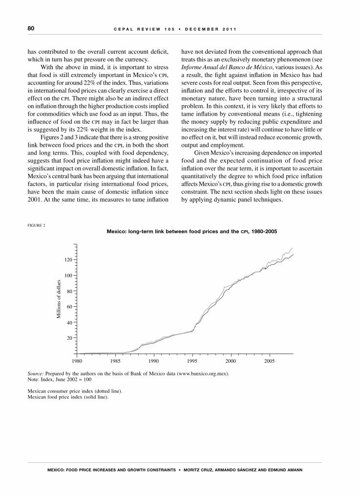
80
MExICo: fooD PRICE InCREAsEs AnD gRoWtH ConstRAInts • MoRItz CRuz, ARMAnDo sánCHEz AnD EDMunD AMAnn
C E P A L R E V I E W 1 0 5 • D E C E M B E R 2 0 1 1
has contributed to the overall current account deficit, which in turn has put pressure on the currency.
With the above in mind, it is important to stress that food is still extremely important in Mexico’s cpi, accounting for around 22% of the index. Thus, variations in international food prices can clearly exercise a direct effect on the cpi. There might also be an indirect effect on inflation through the higher production costs implied for commodities which use food as an input. Thus, the influence of food on the cpi may in fact be larger than is suggested by its 22% weight in the index.
Figures 2 and 3 indicate that there is a strong positive link between food prices and the cpi, in both the short and long terms. This, coupled with food dependency, suggests that food price inflation might indeed have a significant impact on overall domestic inflation. In fact, Mexico’s central bank has been arguing that international factors, in particular rising international food prices, have been the main cause of domestic inflation since 2001. At the same time, its measures to tame inflation
have not deviated from the conventional approach that treats this as an exclusively monetary phenomenon (see Informe Anual del Banco de México, various issues). As a result, the fight against inflation in Mexico has had severe costs for real output. Seen from this perspective, inflation and the efforts to control it, irrespective of its monetary nature, have been turning into a structural problem. In this context, it is very likely that efforts to tame inflation by conventional means (i.e., tightening the money supply by reducing public expenditure and increasing the interest rate) will continue to have little or no effect on it, but will instead reduce economic growth, output and employment.
Given Mexico’s increasing dependence on imported food and the expected continuation of food price inflation over the near term, it is important to ascertain quantitatively the degree to which food price inflation affects Mexico’s cpi, thus giving rise to a domestic growth constraint. The next section sheds light on these issues by applying dynamic panel techniques.
FIGURE 2
Mexico: long-term link between food prices and the cpi, 1980-2005
Source: Prepared by the authors on the basis of Bank of Mexico data (www.banxico.org.mex).Note: Index, June 2002 = 100
Mexican consumer price index (dotted line). Mexican food price index (solid line).
60
40
20
80
100
120
1980 1985 1990 1995 2000 2005
Mill
ions
of
dolla
rs
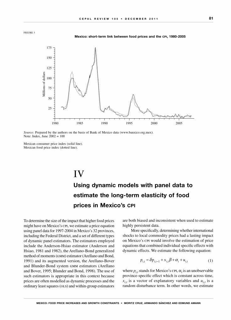
81
MExICo: fooD PRICE InCREAsEs AnD gRoWtH ConstRAInts • MoRItz CRuz, ARMAnDo sánCHEz AnD EDMunD AMAnn
C E P A L R E V I E W 1 0 5 • D E C E M B E R 2 0 1 1
To determine the size of the impact that higher food prices might have on Mexico’s cpi, we estimate a price equation using panel data for 1997-2004 in Mexico’s 32 provinces, including the Federal District, and a set of different types of dynamic panel estimators. The estimators employed include the Anderson-Hsiao estimator (Anderson and Hsiao, 1981 and 1982), the Arellano-Bond generalized method of moments (gmm) estimator (Arellano and Bond, 1991) and its augmented version, the Arellano-Bover and Blunder-Bond system gmm estimators (Arellano and Bover, 1995; Blunder and Bond, 1998). The use of such estimators is appropriate in this context because prices are often modelled as dynamic processes and the ordinary least squares (ols) and within-group estimators
are both biased and inconsistent when used to estimate highly persistent data.
More specifically, determining whether international shocks to local commodity prices had a lasting impact on Mexico’s cpi would involve the estimation of price equations that combined individual specific effects with dynamic effects. We estimate the following equation:
p pi t i t i t t, ,= + + +− α1 , ,x ui iδ β (1)
where pi,t stands for Mexico’s cpi, αi is an unobservable province-specific effect which is constant across time, xi,t is a vector of explanatory variables and ui,t is a random disturbance term. In other words, we estimate
FIGURE 3
Mexico: short-term link between food prices and the cpi, 1980-2005
Source: Prepared by the authors on the basis of Bank of Mexico data (www.banxico.org.mex).Note: Index, June 2002 = 100
Mexican consumer price index (solid line). Mexican food price index (dotted line).
IVusing dynamic models with panel data to
estimate the long-term elasticity of food
prices in Mexico’s cpi
75
50
25
100
125
150
175
1980 1985 1990 1995 2000 2005
Mill
ions
of
dolla
rs
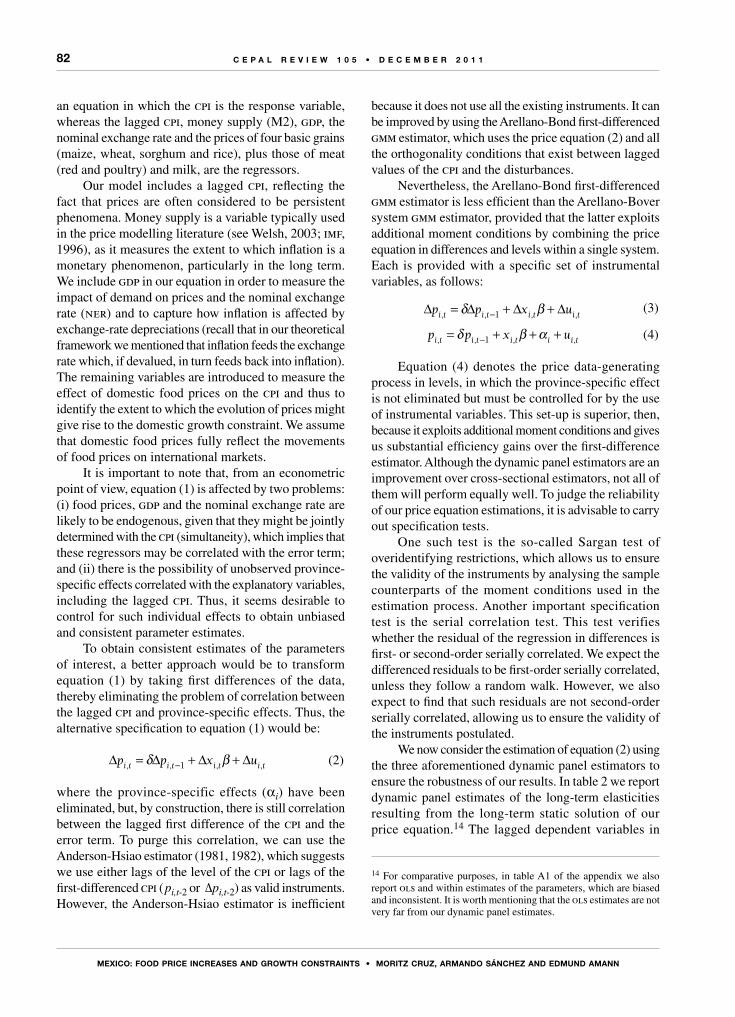
82
MExICo: fooD PRICE InCREAsEs AnD gRoWtH ConstRAInts • MoRItz CRuz, ARMAnDo sánCHEz AnD EDMunD AMAnn
C E P A L R E V I E W 1 0 5 • D E C E M B E R 2 0 1 1
an equation in which the cpi is the response variable, whereas the lagged cpi, money supply (M2), gdp, the nominal exchange rate and the prices of four basic grains (maize, wheat, sorghum and rice), plus those of meat (red and poultry) and milk, are the regressors.
Our model includes a lagged cpi, reflecting the fact that prices are often considered to be persistent phenomena. Money supply is a variable typically used in the price modelling literature (see Welsh, 2003; imf, 1996), as it measures the extent to which inflation is a monetary phenomenon, particularly in the long term. We include gdp in our equation in order to measure the impact of demand on prices and the nominal exchange rate (ner) and to capture how inflation is affected by exchange-rate depreciations (recall that in our theoretical framework we mentioned that inflation feeds the exchange rate which, if devalued, in turn feeds back into inflation). The remaining variables are introduced to measure the effect of domestic food prices on the cpi and thus to identify the extent to which the evolution of prices might give rise to the domestic growth constraint. We assume that domestic food prices fully reflect the movements of food prices on international markets.
It is important to note that, from an econometric point of view, equation (1) is affected by two problems: (i) food prices, gdp and the nominal exchange rate are likely to be endogenous, given that they might be jointly determined with the cpi (simultaneity), which implies that these regressors may be correlated with the error term; and (ii) there is the possibility of unobserved province-specific effects correlated with the explanatory variables, including the lagged cpi. Thus, it seems desirable to control for such individual effects to obtain unbiased and consistent parameter estimates.
To obtain consistent estimates of the parameters of interest, a better approach would be to transform equation (1) by taking first differences of the data, thereby eliminating the problem of correlation between the lagged cpi and province-specific effects. Thus, the alternative specification to equation (1) would be:
∆ ∆p pi t i t i t i t, ,= + +−1 , ,δ βx u∆ ∆ (2)
where the province-specific effects (αi) have been eliminated, but, by construction, there is still correlation between the lagged first difference of the cpi and the error term. To purge this correlation, we can use the Anderson-Hsiao estimator (1981, 1982), which suggests we use either lags of the level of the cpi or lags of the first-differenced cpi ( pi,t-2 or ∆pi,t-2) as valid instruments. However, the Anderson-Hsiao estimator is inefficient
because it does not use all the existing instruments. It can be improved by using the Arellano-Bond first-differenced gmm estimator, which uses the price equation (2) and all the orthogonality conditions that exist between lagged values of the cpi and the disturbances.
Nevertheless, the Arellano-Bond first-differenced gmm estimator is less efficient than the Arellano-Bover system gmm estimator, provided that the latter exploits additional moment conditions by combining the price equation in differences and levels within a single system. Each is provided with a specific set of instrumental variables, as follows:
∆ ∆p pi t i t i t i t, ,= + +−1 , ,δ βx u∆ ∆ (3)
p pi t i t i t t, ,= + + +− α1 , ,x ui iδ β (4)
Equation (4) denotes the price data-generating process in levels, in which the province-specific effect is not eliminated but must be controlled for by the use of instrumental variables. This set-up is superior, then, because it exploits additional moment conditions and gives us substantial efficiency gains over the first-difference estimator. Although the dynamic panel estimators are an improvement over cross-sectional estimators, not all of them will perform equally well. To judge the reliability of our price equation estimations, it is advisable to carry out specification tests.
One such test is the so-called Sargan test of overidentifying restrictions, which allows us to ensure the validity of the instruments by analysing the sample counterparts of the moment conditions used in the estimation process. Another important specification test is the serial correlation test. This test verifies whether the residual of the regression in differences is first- or second-order serially correlated. We expect the differenced residuals to be first-order serially correlated, unless they follow a random walk. However, we also expect to find that such residuals are not second-order serially correlated, allowing us to ensure the validity of the instruments postulated.
We now consider the estimation of equation (2) using the three aforementioned dynamic panel estimators to ensure the robustness of our results. In table 2 we report dynamic panel estimates of the long-term elasticities resulting from the long-term static solution of our price equation.14 The lagged dependent variables in
14 For comparative purposes, in table A1 of the appendix we also report ols and within estimates of the parameters, which are biased and inconsistent. It is worth mentioning that the ols estimates are not very far from our dynamic panel estimates.
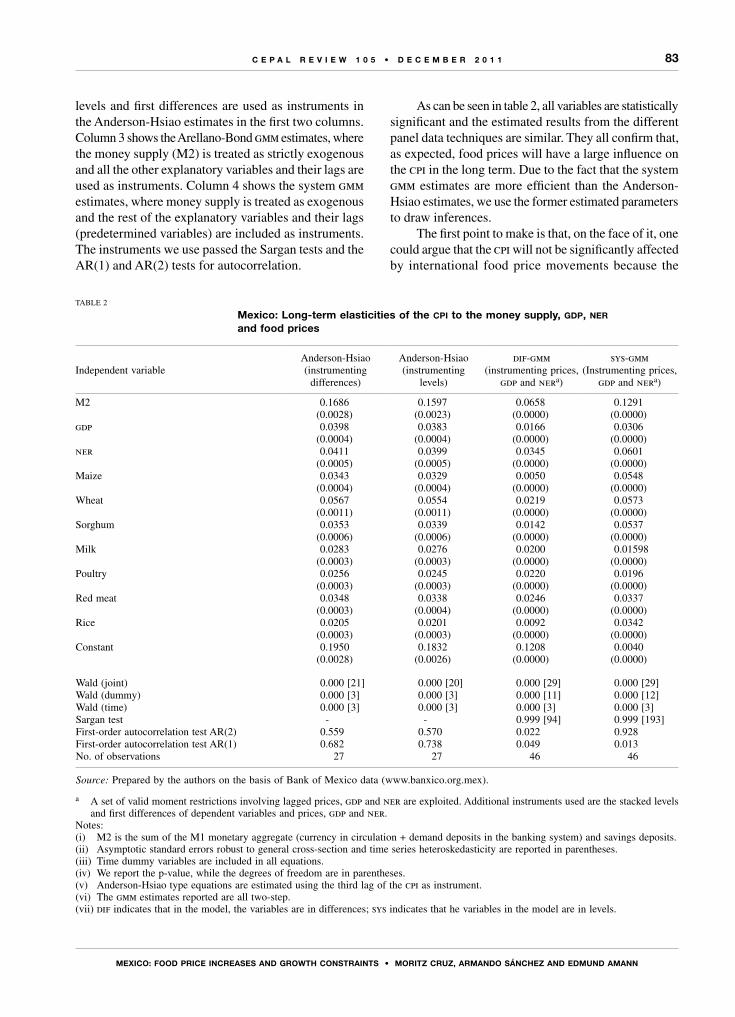
83
MExICo: fooD PRICE InCREAsEs AnD gRoWtH ConstRAInts • MoRItz CRuz, ARMAnDo sánCHEz AnD EDMunD AMAnn
C E P A L R E V I E W 1 0 5 • D E C E M B E R 2 0 1 1
levels and first differences are used as instruments in the Anderson-Hsiao estimates in the first two columns. Column 3 shows the Arellano-Bond gmm estimates, where the money supply (M2) is treated as strictly exogenous and all the other explanatory variables and their lags are used as instruments. Column 4 shows the system gmm estimates, where money supply is treated as exogenous and the rest of the explanatory variables and their lags (predetermined variables) are included as instruments. The instruments we use passed the Sargan tests and the AR(1) and AR(2) tests for autocorrelation.
As can be seen in table 2, all variables are statistically significant and the estimated results from the different panel data techniques are similar. They all confirm that, as expected, food prices will have a large influence on the cpi in the long term. Due to the fact that the system gmm estimates are more efficient than the Anderson-Hsiao estimates, we use the former estimated parameters to draw inferences.
The first point to make is that, on the face of it, one could argue that the cpi will not be significantly affected by international food price movements because the
TABLE 2
Mexico: Long-term elasticities of the cpi to the money supply, gdp, ner and food prices
Independent variableAnderson-Hsiao (instrumenting
differences)
Anderson-Hsiao (instrumenting
levels)
dif-gmm(instrumenting prices,
gdp and nera)
sys-gmm(Instrumenting prices,
gdp and nera)
M2 0.1686(0.0028)
0.1597(0.0023)
0.0658(0.0000)
0.1291(0.0000)
gdp 0.0398(0.0004)
0.0383(0.0004)
0.0166(0.0000)
0.0306(0.0000)
ner 0.0411(0.0005)
0.0399(0.0005)
0.0345(0.0000)
0.0601(0.0000)
Maize 0.0343(0.0004)
0.0329(0.0004)
0.0050(0.0000)
0.0548(0.0000)
Wheat 0.0567(0.0011)
0.0554(0.0011)
0.0219(0.0000)
0.0573(0.0000)
Sorghum 0.0353(0.0006)
0.0339(0.0006)
0.0142(0.0000)
0.0537(0.0000)
Milk 0.0283(0.0003)
0.0276(0.0003)
0.0200(0.0000)
0.01598(0.0000)
Poultry 0.0256(0.0003)
0.0245(0.0003)
0.0220(0.0000)
0.0196(0.0000)
Red meat 0.0348(0.0003)
0.0338(0.0004)
0.0246(0.0000)
0.0337(0.0000)
Rice 0.0205(0.0003)
0.0201(0.0003)
0.0092(0.0000)
0.0342(0.0000)
Constant 0.1950(0.0028)
0.1832(0.0026)
0.1208(0.0000)
0.0040(0.0000)
Wald (joint) 0.000 [21] 0.000 [20] 0.000 [29] 0.000 [29]Wald (dummy) 0.000 [3] 0.000 [3] 0.000 [11] 0.000 [12]Wald (time) 0.000 [3] 0.000 [3] 0.000 [3] 0.000 [3]Sargan test - - 0.999 [94] 0.999 [193]First-order autocorrelation test AR(2) 0.559 0.570 0.022 0.928First-order autocorrelation test AR(1) 0.682 0.738 0.049 0.013No. of observations 27 27 46 46
Source: Prepared by the authors on the basis of Bank of Mexico data (www.banxico.org.mex).
a A set of valid moment restrictions involving lagged prices, gdp and ner are exploited. Additional instruments used are the stacked levels and first differences of dependent variables and prices, gdp and ner.
Notes:(i) M2 is the sum of the M1 monetary aggregate (currency in circulation + demand deposits in the banking system) and savings deposits.(ii) Asymptotic standard errors robust to general cross-section and time series heteroskedasticity are reported in parentheses.(iii) Time dummy variables are included in all equations.(iv) We report the p-value, while the degrees of freedom are in parentheses.(v) Anderson-Hsiao type equations are estimated using the third lag of the cpi as instrument.(vi) The gmm estimates reported are all two-step.(vii) dif indicates that in the model, the variables are in differences; sys indicates that he variables in the model are in levels.
84
MExICo: fooD PRICE InCREAsEs AnD gRoWtH ConstRAInts • MoRItz CRuz, ARMAnDo sánCHEz AnD EDMunD AMAnn
C E P A L R E V I E W 1 0 5 • D E C E M B E R 2 0 1 1
VConclusions
International food prices have soared since 2001 to unprecedented levels. Food price inflation is expected to persist in the near future as demand for food continues to overwhelm supply. Countries which are highly dependent on imported food commodities and where foods weigh heavily in the cpi are and will continue to be adversely affected in terms of their domestic inflation. This, in turn, will give rise to an inescapable domestic growth constraint. Mexico is an economy that lacks food self-sufficiency. It
is also one in which food has a large weighting in the cpi (around 25%). Since the mid-1980s, food dependency has intensified, and domestic food production has stagnated. In this paper, we have used dynamic panel techniques to investigate the extent to which rising food prices influence Mexico’s cpi and how that affects the materialization of the domestic growth constraint .
Our estimated long-term elasticities indicate that domestic prices will be severely affected by food price
elasticities associated with each food item are relatively low. However, this conclusion might be misleading. If grain prices continuously increase, for example, as forecast by the Organisation for Economic Co-operation and Development (oecd) and the Food and Agriculture Organization of the United Nations (fao), then the sum of the elasticities of three basic grains (0.1658), namely, wheat, maize and sorghum (0.0573, 0.0548 and 0.0537, respectively), easily overwhelms the elasticity of the cpi with respect to changes in the money supply. This implies that an increase of 10% in the price of these food grains will push inflation up by 1.7%. This is by no means a negligible impact, and it shows that many of the inflationary pressures Mexico will face in future will be of a structural character. It means that inflation in Mexico is indeed quite sensitive to the prices of basic grains. Moreover, if the prices of several foodstuffs increase considerably at the same time then, in our case, the exercise of summing up the elasticities of our edible commodities more than doubles the response of the cpi to changes in the money supply. Thus, food prices will put considerable pressure on domestic inflation, and the domestic growth constraint is likely to materialize as a result. At the same time, other things being equal, the international competitiveness of exports is likely to be negatively affected by the rise in prices, leading to a deterioration in the current account that would feed back into inflationary pressures. If this occurs, policymakers are likely to fight inflation by conventional means, with a negative effect on growth.
Our findings, then, suggest that, given the country’s dependence on imported food, Mexican inflation will turn into a largely structural problem (a real imbalance). Under these circumstances, it is very likely that the authorities will find it difficult to tame inflation with
their conventional tools, and that these will negatively affect output and economic growth instead.
Another point worth noting is that the estimated long-term elasticity of the cpi to gdp is very low (0.0306), suggesting that expansionary policies can be applied without much risk of generating inflation. In particular, expansionary policies to support the primary sector and expand its production could be implemented without the risk of generating inflation.
The policy recommendation that derives from our estimates is that the best way to control inflation in the long term is to eliminate its structural component. Evidently, this cannot be done by imposing price controls or export restrictions or by further augmenting food imports. Neither can it be done by tightening the money supply or maintaining an overvalued exchange rate. These policy options, though real and feasible alternatives, will only solve the problem of food dependency and imported inflation on a short-term basis. The long-term policy solution to this problem consists in putting the primary sector on the agenda of national priorities, as developed nations have done (see Chang, 2009), providing support until a greater degree of food self-sufficiency is achieved. This can be done through several mechanisms, which include land (reform) policy; research, education and information policy; credit policy; inputs policy, such as canal irrigation, infrastructure, transport, marketing, processing and the use of price guarantees to maintain the stability of producers’ incomes; warehousing; trade protection; insurance; and so on (see Calva, 2002; Chang, 2009). Kalecki (1954, p. 30) advocates the adoption of the policies suggested, stating that “the expansion of food production… is of paramount importance in avoiding inflationary pressures”, particularly when economic expansion and industrial development are under way.

85
MExICo: fooD PRICE InCREAsEs AnD gRoWtH ConstRAInts • MoRItz CRuz, ARMAnDo sánCHEz AnD EDMunD AMAnn
C E P A L R E V I E W 1 0 5 • D E C E M B E R 2 0 1 1
inflation. In the long term, we have established that the responsiveness of the cpi to changes in food prices will be more than double its reaction to changes in the money supply. This indicates that the root of domestic inflation will be structural rather than monetary. In this context, monetary policy is likely to fail to control inflation if
the agricultural price issue is not taken into account, instead placing further constraints on economic growth. Effective control of inflation should therefore prioritize the primary sector with the aim of restoring its supply capacity and enhancing self-sufficiency.
(Original: English)
AppEndix
TABLE A1
Mexico: Long-term elasticities of the cpi to the money supply, gdp, ner and food prices
Independent variable(1)ols
(2)Within-group
M2 0.1190(0.0000)
0.7116(0.0000)
gdp 0.0081(0.0000)
0.5553(0.0000)
ner 0.0590(0.0000)
0.7377(0.0000)
Maize 0.1335(0.0000)
1.0338(0.0000)
Wheat 0.0328(0.0000)
0.9837(0.0000)
Sorghum 0.0435(0.0000)
0.1327(0.0000)
Milk 0.0057(0.0000)
0.6407(0.0000)
Poultry 0.0433(0.0000)
0.4607(0.0000)
Red meat 0.0219(0.0000)
-
Rice 0.0289(0.0000)
1.7810(0.0000)
Constant 0.0066(0.0000)
-
Wald (joint) 0.000 [23] 0.000 [18]Wald (dummy) 0.000 [14] 0.000 [6]Wald (time) 0.000 [4] 0.000 [6]First-order autocorrelation test AR(2) 0.003 0.964First-order autocorrelation test AR(1) 0.003 0.095No. of observations 46 65
Source: Prepared by the authors on the basis of Bank of Mexico data (www.banxico.org.mex).
Notes:(i) M2 is the sum of the M1 monetary aggregate (currency in circulation + demand deposits in the banking system) and savings deposits.(ii) Asymptotic standard errors robust to general cross-section and time series heteroskedasticity are reported in parentheses.(iii) Time dummies are included in all equations.(iv) We report the p-value, while the degrees of freedom are in parentheses.(v) Column (1) reports ols estimates of the equation in levels.(vi) Column (2) reports within-group estimates. These are ols estimates of the equation in deviations from time means.(vii) cpi: consumer price index.(viii) gdp: gross domestic product. (ix) ner: nominal exchange rate.
86
MExICo: fooD PRICE InCREAsEs AnD gRoWtH ConstRAInts • MoRItz CRuz, ARMAnDo sánCHEz AnD EDMunD AMAnn
C E P A L R E V I E W 1 0 5 • D E C E M B E R 2 0 1 1
Bibliography
Anderson, T.W. and C. Hsiao (1982), “Formulation and estimation of dynamic models using panel data”, Journal of Econometrics, vol. 18, No. 1, Amsterdam, Elsevier.
(1981), “Estimation of dynamic models with error components”, Journal of the American Statistical Association,
vol. 76, No. 375, Alexandria, American Statistical Association.Arellano, M. and O. Bover (1995), “Another look at the instrumental
variable estimation of error-components models”, Journal of Econometrics, vol. 68, No. 1, Amsterdam, Elsevier.
Arellano, M. and S. Bond (1991), “Some tests of specification for panel data: Monte Carlo evidence and application to employment equations”, Review of Economics Studies, vol. 58, No. 2, Wiley Blackwell.
Bank of Mexico (various issues), Annual Report [online] http://www.banxico.org.mx/publicaciones/JSP/informeAnual.jsp.
Blundell, R. and S. Bond (1998), “Initial conditions and moment restrictions in dynamic panel data models”, Journal of Econometrics, vol. 87, No. 1, Amsterdam, Elsevier.
Bruinsma, J. (2003), World Agriculture: Towards 2015/2030. An fao Study, London, Earthscan Publications Ltd.
Calva, J. (2007), “Políticas de desarrollo agropecuario”, Desarrollo agropecuario, forestal y pesquero. Agenda para el desarrollo, J. Calva (ed.), vol. 9, Mexico City, Miguel Ángel Porrúa.
(2001), México más allá del neoliberalismo. Opciones dentro del cambio global, Mexico City, Plaza y Janés.
Cardoso, A. (1981), “Food supply and inflation”, Journal of Development Economics, vol. 8, No. 3, Amsterdam, Elsevier.
Chang, H-J. (2009), “Rethinking public policy in agriculture: lessons from history, distant and recent”, Journal of Peasant Studies, vol. 36, No. 3, New York, Routledge.
eclac (Economic Commission for Latin America and the Caribbean) (2008), La volatilidad de los precios internacionales y los retos de política económica en América Latina y el Caribe (LC/L.2958), Santiago, Chile, September.
fao (Food and Agriculture Organization of the United Nations) (2008), The State of Food Insecurity in the World 2008. High Food Prices and Food Security – Threats and Opportunities, Rome.
Harberger, A. (1950), “Currency depreciation, income and the balance of trade”, Journal of Political Economy, vol. 58, No. 1, Chicago, The University of Chicago Press.
Harrod, R. (1933), International Economics, Cambridge, Cambridge University Press.
idb (Inter-American Development Bank) (2008), “Países necesitan invertir más para prevenir que la crisis alimentaria profundice la pobreza” [online] http://www.iadb.org/NEWS/detail.cfm?artid=4718&language=Sp&id=4718&CFID=4924426&CFTOKEN=96418290.
imf (International Monetary Fund) (2010), International Financial Statistics [online] http://www.imfstatistics.org/imf/logon.aspx
(1996), Annual Report 1995, Washington, D.C.Kaldor, N. (1966), Strategic Factors in Economic Development,
Ithaca, New York.Kalecki, M. (1993a), “The difference between crucial economic
problems of developed and underdeveloped non-socialist
economies”, Collected Works of Michal Kalecki, J. Osiatynsky (ed.), Oxford, Oxford University Press. Originally publilshed in 1966.
(1993b), “The problem of financing economic development”, Collected Works of Michal Kalecki, J. Osiatynsky (ed.), vol. 5, Oxford, Oxford University Press. Originally published in 1954.
Keynes, J. (1936), The General Theory of Employment, Interest and Money, New York, Harcourt Brace and Company.
Krugman, P. and L. Taylor (1978), “Contractionary effects of devaluation”, Journal of International Economics, vol. 8, No. 3, Amsterdam, Elsevier.
Laursen, S. and L. Metzler (1950), “Flexible exchange rate and the theory of employment”, Review of Economics and Statistics, vol. 32, Cambridge, Massachusetts, The mit Press.
Noyola, J. (1956), “El desarrollo económico y la inflación en México y otros países latinoamericanos”, Investigación económica, vol. 16, No. 4, Mexico City, National Autonomous University of Mexico.
oecd/fao (Organization for Economic Cooperation and Development/Food and Agriculture Organization of the United Nations) (2010), oecd-fao Agricultural Outlook, 2010-2019, Paris.
Prebisch, R. (1982), “Problemas teóricos y prácticos del crecimiento económico”, La obra de Prebisch en la cepal, A. Gurrieri (ed.), Mexico City, Fondo de Cultura Económica. Originally published in 1951.
Sakar, A. (1988), “Supply constraints, government subsidies and industrial employment”, Journal of Development Economics, vol. 28, No. 1, Amsterdam, Elsevier.
Storm, S. (1997), “Domestic constraints on export-led growth: a case-study of India”, Journal of Development Economics, vol. 52, No. 1, Amsterdam, Elsevier.
Sunkel, O. (1958), “La inflación chilena: un enfoque heterodoxo”, El trimestre económico, vol. 24, No. 4, Mexico City, Fondo de Cultura Económica.
The Economist (2009), “Whatever happened to the food crisis?”, 2 July [online] http://www.economist.com/world/international/displaystory.cfm?story_id=13944900].
(2008), “The new face of hunger”, 17 April [online] http://www.economist.com/world/international/displaystory.cfm?story_id=11049284.
(2007), “Cheap no more”, 6 December [online] http://www.economist.com/displaystory.cfm?story_id=10250420.
Thirlwall, A. (2003), Trade, the Balance of Payments and Exchange Rate Policy in Developing Countries, Edward Elgar, United Kingdom.
(1979), “The balance of payments constraint as an explanation of international growth rate differences”, Banca Nazionale del Lavoro Quartely Review, vol. 132, No. 128, Associazione Paolo Sylos Labini.
Walsh, C.E. (2003), Monetary Theory and Policy, Cambridge, Massachusetts, The mit Press.
Wolf, M. (2008), “Useful dos and don’ts for fast economic growth”, Financial Times, 3 June [online] http://www.ft.com/cms/s/0/616526bc-3178-11dd-b77c-0000779fd2ac.html#axzz1N8iQURhS.

C E P A L R E V I E W 1 0 5 • D E C E M B E R 2 0 1 1
87
K E Y W O R D S
Exports
Industry
Manufactures
Industrial productivity
Factories
Evaluation
Statistical data
Trade statistics
Chile
Dissecting the Chileanexport boom
Raphael Bergoeing, Alejandro Micco and Andrea Repetto
Chilean exports have boomed since 1975, growing at an average
annual rate of 6% per year in real terms. In this paper, we use Chilean
manufacturing data at the plant level for the years from 1990 to 2007
to investigate the relationship between exports, plant dynamics and
productivity. Our findings are consistent with the predictions of the new
theories of heterogeneous firms and trade. First, 64.4% of the total
increase in exports is accounted for by new exporters net of failed
exporters. This effect is a combination of a larger proportion of plants
exporting, a rising proportion of output sold abroad and a higher level of
total sales. Second, productivity and exports co-moved over the course
of the Chilean boom, exports being positively correlated with both within-
plant productivity growth and the productivity-enhancing reallocation of
output between plants.
Raphael Bergoeing
Academic, Department of
Economics, University of Chile
Alejandro Micco
Academic, Department of
Economics, University of Chile
Andrea Repetto
Academic, School of Government,
Adolfo Ibáñez University
88
DIssECtIng tHE CHILEAn ExPoRt BooM • RAPHAEL BERgoEIng, ALEjAnDRo MICCo AnD AnDREA REPEtto
C E P A L R E V I E W 1 0 5 • D E C E M B E R 2 0 1 1
Recent empirical research based on plant-level data has consistently shown that there is considerable heterogeneity in productivity across units even within narrowly defined sectors in any given period of time. Thus, as several studies document, the reallocation of inputs and factors of production is a crucial element of aggregate productivity gains and growth.1
New models based on firm heterogeneity have analysed these intra-industry effects in the context of international trade. Melitz (2003) and Bernard and others (2003) developed alternative models of international trade which predict that only the most productive firms export and that industry’s exposure to trade induces aggregate productivity gains through reallocation —an effect that is ignored by the standard representative firm framework. At the same time, a growing body of empirical literature has studied the extent and causes of productivity differentials between exporters and non-exporters.2 Little evidence exists on the importance of trade-driven reallocation effects.
In the light of these new theoretical developments, this paper analyses the sources of the Chilean export boom and its relationship to productivity heterogeneity at the microeconomic level. Using a sample of Chilean manufacturing plants for the years from 1990 to 2007, we decompose observed aggregate export growth into two complementary sets of margins: net entry into foreign markets versus resource reallocation effects, and export intensity changes versus sales growth. We also consider
We are grateful to the National Institute of Statistics (ine) for providing the manufacturing plant-level data used in this paper. We are also grateful to the cepal Review referee and to participants at a number of seminars for helpful comments and suggestions. Excellent research assistance was provided by Pablo Muñoz. We acknowledge financial support from the Inter-American Development Bank (idb) and from the National Fund for Scientific and Technological Development (fondecyt) (grant no. 1070805).1 For Chile, see Bergoeing, Hernando and Repetto (2010).2 See Wagner (2007 and 2008) and Eaton, Kortum and Kramarz (2008) for recent surveys. The evidence indicates that the most productive firms self-select as export market entrants. Although there is mixed evidence on export-driven learning effects, Álvarez and López (2005) confirm this hypothesis using plant-level data for Chile.
the role of efficiency by correlating export growth with both within-plant productivity growth and between-plant productivity-enhancing reallocation effects.
The Chilean experience is interesting for several reasons. First, the economy underwent a deep and far-reaching trade liberalization reform starting in the mid-1970s. During the 30 years that followed, Chilean exports grew at an average real annual rate of 6%. This export boom dramatically changed the level of trade as well as its composition and the productive structure of the economy. Although there was a partial reversal of the unilateral tariff reduction process after the early 1980s crisis, trade liberalization continued after 1985. Since 1992, furthermore, trade policy has moved towards bilateral agreements. In fact, Chile has signed trade agreements with more than 50 countries over the last two decades, including the United States, Canada, Mexico, the European Union, China and the Republic of Korea. Thus, the data considered in this study cover a period that came after more than a decade of major reforms, but that was also characterized by active negotiation of preferential trade agreements. Consequently, this time period provides a rich environment for research in pursuit of a better understanding of the link between trade and industrial and plant dynamics.
Our findings are consistent with the predictions of the new theories of heterogeneous firms and trade. First, 64.4% of the increase in exports came from larger and highly intensive new exporters, rather than being the result of rising export intensity at existing exporters. Second, productivity and exports have co-moved over the Chilean boom. Finally, the export expansion has been associated with a productivity-enhancing reallocation of resources towards more efficient plants.
The remainder of the paper is organized as follows. Section II provides an overview of trade reforms and the recent trade boom in Chile. Section III describes the data we use and presents a number of plant-level facts that characterize manufacturing exports. Section IV dissects exports to explore the main sources of growth. We also study the link between export growth and productivity. The final section concludes.
Iintroduction
89
DIssECtIng tHE CHILEAn ExPoRt BooM • RAPHAEL BERgoEIng, ALEjAnDRo MICCo AnD AnDREA REPEtto
C E P A L R E V I E W 1 0 5 • D E C E M B E R 2 0 1 1
In June 2002, Chile signed a free trade agreement with the European Union; a year later, a similar agreement was signed with the United States. These negotiations marked the culmination of three decades of free-trade policies that have consolidated Chile’s position as one of the most open economies in the world.
Today, few question the significance of the trade liberalization programme initiated in the mid-1970s in shaping the economic transformation of Chile.3 The situation was very different four decades ago, however. By the late 1960s, trade restrictions had practically isolated the Chilean economy from the rest of the world, exacerbating its dependence on copper exports and confining imports to intermediate and capital goods. The structure of relative prices was drastically distorted in favour of industrial goods at the expense of agricultural, mining and other tradable activities. Differential import duties exempted capital goods, and high taxes were levied on final goods, creating a generally inefficient capital-intensive industrial sector. Import tariffs ranged from 0% for capital goods to 750% for luxury goods, a 90-day non-interest-bearing deposit of 10,000% of the cif value of imported goods was required, and all import operations required administrative approval. In addition, a system of multiple exchange rates was in operation, with a 52 to 1 ratio having been reached by the time the economy collapsed in 1973.
In the years that followed the 1973 crisis, trade liberalization policies were to be the cornerstone of the transformation of the inward-oriented Chilean economy into a dynamic export-oriented one. The initial set of trade reforms were intended to simplify the structure of the economy. Consistently, exchange markets were unified, most non-tariff barriers (quotas and prohibitions) were eliminated, and tariffs were drastically reduced to a uniform 10% by 1979.
The economy recovered at great speed during the years from 1976 to 1980, with gross domestic product
3 The Chilean economic transformation has been extensively documented by Edwards and Edwards (1992) and Corbo and Fischer (1994), among others.
(gdp) growing at an annual rate of 7%. Moreover, the availability of foreign goods expanded markedly and the government deficit turned into a surplus. In addition, a large number of reforms were initiated to complement and reinforce the change in relative prices induced by trade deregulation. Among them, a large number of public enterprises were privatized, labour markets were deregulated, a defined contribution social security system was set up to replace the pay-as-you-go system, and health and public education responsibilities were transferred from the ministries to the municipality level.
Although reforms advanced on several fronts, two major problems remained unsolved: unemployment did not decline significantly, and inflation remained stubbornly high. Among the instruments used to control inflation, the fixing of the nominal exchange rate in June 1979 proved devastating in its effects. The highly indexed nature of the economy, in combination with the fixed exchange rate, induced an increasing real overvaluation of the currency, fostering imports and discouraging exports, and leading to large current account deficits. In 1981, the external deficit reached 14.5% of gdp. Large amounts of foreign loans entered the country to finance the trade imbalance and, as a consequence, the foreign debt increased from US$ 6 billion in 1977 to US$ 14.8 billion in 1981. Two additional elements also helped induce the observed rise in indebtedness: the resistance of the real interest rate to convergence on world levels and the deregulation of the financial market in 1981. The former induced a continuous flow of short-term lending; the lack of adequate supervision of bank portfolio quality in the latter led to a general miscalculation of risk levels and imprudent domestic lending (Barandiarán and Hernández, 1999).
With such a large trade imbalance, confidence in the Chilean economy faltered, and foreign lending ceased. In June 1982 the authorities were forced to devalue the peso by 19%, but “it was too little and too late” (Edwards and Edwards, 1992). The economy fell into a deep recession as gdp dropped by 13.4% in 1982 and a further 3.5% in 1983; unemployment, already high, skyrocketed to 34% of the labour force (including emergency employment programmes). The government
IITrade reforms and the Chilean export boom:
an overview
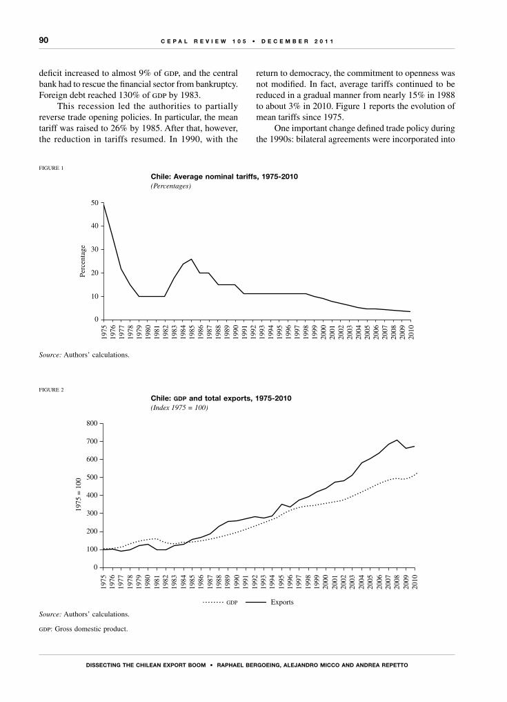
90
DIssECtIng tHE CHILEAn ExPoRt BooM • RAPHAEL BERgoEIng, ALEjAnDRo MICCo AnD AnDREA REPEtto
C E P A L R E V I E W 1 0 5 • D E C E M B E R 2 0 1 1
deficit increased to almost 9% of gdp, and the central bank had to rescue the financial sector from bankruptcy. Foreign debt reached 130% of gdp by 1983.
This recession led the authorities to partially reverse trade opening policies. In particular, the mean tariff was raised to 26% by 1985. After that, however, the reduction in tariffs resumed. In 1990, with the
return to democracy, the commitment to openness was not modified. In fact, average tariffs continued to be reduced in a gradual manner from nearly 15% in 1988 to about 3% in 2010. Figure 1 reports the evolution of mean tariffs since 1975.
One important change defined trade policy during the 1990s: bilateral agreements were incorporated into
FIGURE 1
Chile: Average nominal tariffs, 1975-2010(Percentages)
Source: Authors’ calculations.
0
10
20
30
40
50
1975
1976
1977
1978
1979
1980
1981
1982
1983
1984
1985
1986
1987
1988
1989
1990
1991
1992
1993
1994
1995
1996
1997
1998
1999
2000
2001
2002
2003
2004
2005
2006
2007
2008
2009
2010
Perc
enta
ge
FIGURE 2
Chile: gdp and total exports, 1975-2010(Index 1975 = 100)
Source: Authors’ calculations.
gdp: Gross domestic product.
0
100
200
300
400
500
600
700
800
1975
1976
1977
1978
1979
1980
1981
1982
1983
1984
1985
1986
1987
1988
1989
1990
1991
1992
1993
1994
1995
1996
1997
1998
1999
2000
2001
2002
2003
2004
2005
2006
2007
2008
2009
2010
1975
= 1
00
GDP Exports
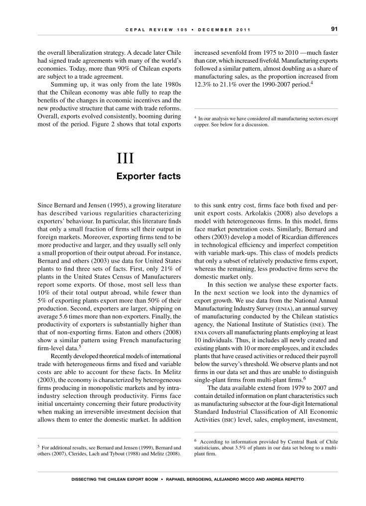
91
DIssECtIng tHE CHILEAn ExPoRt BooM • RAPHAEL BERgoEIng, ALEjAnDRo MICCo AnD AnDREA REPEtto
C E P A L R E V I E W 1 0 5 • D E C E M B E R 2 0 1 1
Since Bernard and Jensen (1995), a growing literature has described various regularities characterizing exporters’ behaviour. In particular, this literature finds that only a small fraction of firms sell their output in foreign markets. Moreover, exporting firms tend to be more productive and larger, and they usually sell only a small proportion of their output abroad. For instance, Bernard and others (2003) use data for United States plants to find three sets of facts. First, only 21% of plants in the United States Census of Manufacturers report some exports. Of those, most sell less than 10% of their total output abroad, while fewer than 5% of exporting plants export more than 50% of their production. Second, exporters are larger, shipping on average 5.6 times more than non-exporters. Finally, the productivity of exporters is substantially higher than that of non-exporting firms. Eaton and others (2008) show a similar pattern using French manufacturing firm-level data.5
Recently developed theoretical models of international trade with heterogeneous firms and fixed and variable costs are able to account for these facts. In Melitz (2003), the economy is characterized by heterogeneous firms producing in monopolistic markets and by intra-industry selection through productivity. Firms face initial uncertainty concerning their future productivity when making an irreversible investment decision that allows them to enter the domestic market. In addition
5 For additional results, see Bernard and Jensen (1999), Bernard and others (2007), Clerides, Lach and Tybout (1988) and Melitz (2008).
to this sunk entry cost, firms face both fixed and per-unit export costs. Arkolakis (2008) also develops a model with heterogeneous firms. In this model, firms face market penetration costs. Similarly, Bernard and others (2003) develop a model of Ricardian differences in technological efficiency and imperfect competition with variable mark-ups. This class of models predicts that only a subset of relatively productive firms export, whereas the remaining, less productive firms serve the domestic market only.
In this section we analyse these exporter facts. In the next section we look into the dynamics of export growth. We use data from the National Annual Manufacturing Industry Survey (enia), an annual survey of manufacturing conducted by the Chilean statistics agency, the National Institute of Statistics (ine). The enia covers all manufacturing plants employing at least 10 individuals. Thus, it includes all newly created and existing plants with 10 or more employees, and it excludes plants that have ceased activities or reduced their payroll below the survey’s threshold. We observe plants and not firms in our data set and thus are unable to distinguish single-plant firms from multi-plant firms.6
The data available extend from 1979 to 2007 and contain detailed information on plant characteristics such as manufacturing subsector at the four-digit International Standard Industrial Classification of All Economic Activities (isic) level, sales, employment, investment,
6 According to information provided by Central Bank of Chile statisticians, about 3.5% of plants in our data set belong to a multi-plant firm.
IIIExporter facts
the overall liberalization strategy. A decade later Chile had signed trade agreements with many of the world’s economies. Today, more than 90% of Chilean exports are subject to a trade agreement.
Summing up, it was only from the late 1980s that the Chilean economy was able fully to reap the benefits of the changes in economic incentives and the new productive structure that came with trade reforms. Overall, exports evolved consistently, booming during most of the period. Figure 2 shows that total exports
increased sevenfold from 1975 to 2010 —much faster than gdp, which increased fivefold. Manufacturing exports followed a similar pattern, almost doubling as a share of manufacturing sales, as the proportion increased from 12.3% to 21.1% over the 1990-2007 period.4
4 In our analysis we have considered all manufacturing sectors except copper. See below for a discussion.
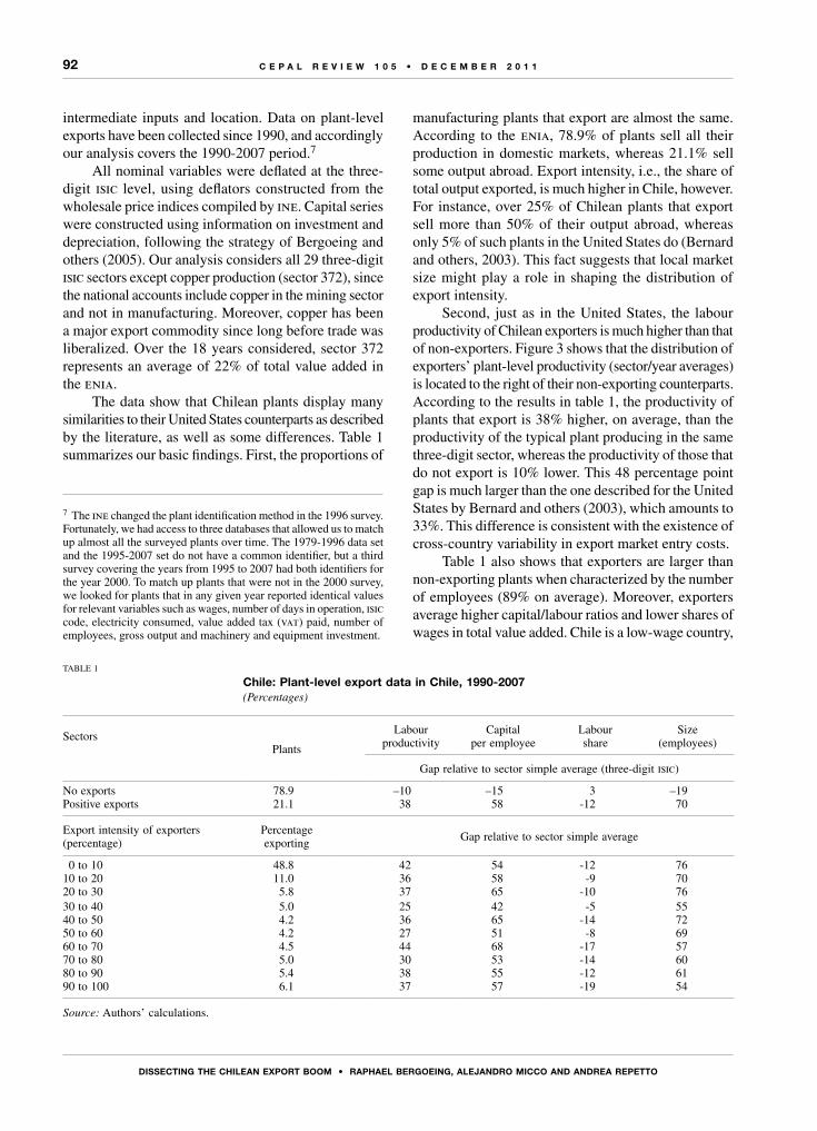
92
DIssECtIng tHE CHILEAn ExPoRt BooM • RAPHAEL BERgoEIng, ALEjAnDRo MICCo AnD AnDREA REPEtto
C E P A L R E V I E W 1 0 5 • D E C E M B E R 2 0 1 1
intermediate inputs and location. Data on plant-level exports have been collected since 1990, and accordingly our analysis covers the 1990-2007 period.7
All nominal variables were deflated at the three-digit isic level, using deflators constructed from the wholesale price indices compiled by ine. Capital series were constructed using information on investment and depreciation, following the strategy of Bergoeing and others (2005). Our analysis considers all 29 three-digit isic sectors except copper production (sector 372), since the national accounts include copper in the mining sector and not in manufacturing. Moreover, copper has been a major export commodity since long before trade was liberalized. Over the 18 years considered, sector 372 represents an average of 22% of total value added in the enia.
The data show that Chilean plants display many similarities to their United States counterparts as described by the literature, as well as some differences. Table 1 summarizes our basic findings. First, the proportions of
7 The ine changed the plant identification method in the 1996 survey. Fortunately, we had access to three databases that allowed us to match up almost all the surveyed plants over time. The 1979-1996 data set and the 1995-2007 set do not have a common identifier, but a third survey covering the years from 1995 to 2007 had both identifiers for the year 2000. To match up plants that were not in the 2000 survey, we looked for plants that in any given year reported identical values for relevant variables such as wages, number of days in operation, isic code, electricity consumed, value added tax (vat) paid, number of employees, gross output and machinery and equipment investment.
manufacturing plants that export are almost the same. According to the enia, 78.9% of plants sell all their production in domestic markets, whereas 21.1% sell some output abroad. Export intensity, i.e., the share of total output exported, is much higher in Chile, however. For instance, over 25% of Chilean plants that export sell more than 50% of their output abroad, whereas only 5% of such plants in the United States do (Bernard and others, 2003). This fact suggests that local market size might play a role in shaping the distribution of export intensity.
Second, just as in the United States, the labour productivity of Chilean exporters is much higher than that of non-exporters. Figure 3 shows that the distribution of exporters’ plant-level productivity (sector/year averages) is located to the right of their non-exporting counterparts. According to the results in table 1, the productivity of plants that export is 38% higher, on average, than the productivity of the typical plant producing in the same three-digit sector, whereas the productivity of those that do not export is 10% lower. This 48 percentage point gap is much larger than the one described for the United States by Bernard and others (2003), which amounts to 33%. This difference is consistent with the existence of cross-country variability in export market entry costs.
Table 1 also shows that exporters are larger than non-exporting plants when characterized by the number of employees (89% on average). Moreover, exporters average higher capital/labour ratios and lower shares of wages in total value added. Chile is a low-wage country,
TABLE 1
Chile: Plant-level export data in Chile, 1990-2007 (Percentages)
Sectors Plants
Labourproductivity
Capitalper employee
Labourshare
Size(employees)
Gap relative to sector simple average (three-digit isic)
No exports 78.9 –10 –15 3 –19Positive exports 21.1 38 58 -12 70
Export intensity of exporters (percentage)
Percentageexporting
Gap relative to sector simple average
0 to 10 48.8 42 54 -12 7610 to 20 11.0 36 58 -9 7020 to 30 5.8 37 65 -10 7630 to 40 5.0 25 42 -5 5540 to 50 4.2 36 65 -14 7250 to 60 4.2 27 51 -8 6960 to 70 4.5 44 68 -17 5770 to 80 5.0 30 53 -14 6080 to 90 5.4 38 55 -12 6190 to 100 6.1 37 57 -19 54
Source: Authors’ calculations.
93
DIssECtIng tHE CHILEAn ExPoRt BooM • RAPHAEL BERgoEIng, ALEjAnDRo MICCo AnD AnDREA REPEtto
C E P A L R E V I E W 1 0 5 • D E C E M B E R 2 0 1 1
and one would thus expect exporters to be more labour-intensive. Several explanations may account for this seeming anomaly. First, manufactured goods are sold mostly to other Latin American countries. Therefore, it is not necessarily the case that Chile can be defined as a labour-abundant country in this context. Second, non-exporters are more likely to be liquidity-constrained and thus might face higher capital costs. Third, as explained by Trefler (1993), labour should be measured in effective units. If not, human capital, a scarce resource
in Chile relative to developed economies, is included in total labour.
Finally, the table shows that these characteristics are not necessarily correlated with plant export intensity, i.e., there is no clear tendency for plants that export a larger share of their sales to be more productive, larger or more capital-intensive.
In what follows, we further analyse the role of plant-level heterogeneity on exports and productivity, this time looking at the mechanisms underlying their dynamics.
FIGURE 3
Chile: Distribution of plant-level productivity(Percentages)
Source: Authors’ calculations.
0-0.
25
0.25
-0.3
0.3-
0.35
0.35
-0.4
2
0.42
-0.5
0.5-
0.59
0.59
-0.7
1
0.71
-0.8
4
0.84
-1
1-1.
2
1.2-
1.4
1.4-
1.7
1.7-
2
2-2.
4
2.4-
2.8
2.8-
3.4
3.4-
4
4-00
Average productivity range, by sector and year
Perc
enta
ge
0
2
4
6
8
10
12
14
16
Non-exporter Exporter
IVThe microdynamics of Chilean exports
Recent international trade theories predict that increasing exposure to foreign markets due, for instance, to a fall in transport costs leads to a reallocation of inputs and production towards the most productive firms. As the cost of entering export markets falls, firms that used to sell their output in domestic markets only now find it profitable to pay the costs of selling abroad. If variable costs fall, then old exporters increase their export intensity, whereas if fixed costs fall, these firms do not change their sales patterns. In any case, the least productive firms
are forced to exit as the increased demand for domestic inputs bids up real production costs. The reallocation driven by the increased exposure to trade delivers gains in terms of aggregate productivity growth.
A number of recent papers have looked at the effects of trade on productivity dynamics. Bernard and others (2007) show that productivity growth is faster in industries with falling trade costs. Low-productivity plants in these industries are more likely to exit, whereas high-productivity non-exporters are more likely to
94
DIssECtIng tHE CHILEAn ExPoRt BooM • RAPHAEL BERgoEIng, ALEjAnDRo MICCo AnD AnDREA REPEtto
C E P A L R E V I E W 1 0 5 • D E C E M B E R 2 0 1 1
start selling abroad. In the aggregate, their results are consistent with productivity-enhancing reallocation effects associated with trade growth.8
Bernard and Jensen (2004) study the recent export boom in the United States by examining the role of entry, firm expansion and export intensity. The paper finds that most of the increase in manufacturing exports came from rising export intensity at existing exporters rather than from new entrants into exporting. They also find that changes in exchange rates and rises in foreign income drove most of the export boom, while within-plant productivity increases played a smaller role.
Other papers suggest a major role for entry into exporting, however. For example, Kehoe and Ruhl (2009) examine the bilateral trade patterns by commodity of countries involved in significant trade liberalization processes, finding a striking relationship between a good’s pre-liberalization share of trade and its subsequent growth. The goods that were traded the least before liberalization account for a disproportionate share of trade following the reduction of trade barriers. They interpret this evidence as supporting the role of the new goods margin as a source of trade expansion.
Plant-level data for Chile have also been used to study the connection between trade liberalization and firm dynamics by Pavcnik (2002), Irarrázabal and Opromolla (2007) and Álvarez and Vergara (2010). Using a difference-in-differences approach and data for the 1979-1986 period, Pavcnik (2002) shows that plants in export-oriented and import-competing sectors became more productive by the end of the sample period. An important caveat of this work is that, as figure 1 shows, tariffs were much higher in 1986 than in 1979: the actual direction of trade openness is opposite to that assumed by the study.
Irarrázabal and Opromolla (2007) use the Bernard and others (2003) model to simulate the effects of the Chilean liberalization. The model predicts that a 50% reduction in trade barriers leads to a 24% change in aggregate productivity. About 72% of the gains are due to within-plant gains and 26% to the exit of less efficient plants. Reallocation and entry effects are quantitatively unimportant. Their simulation results do not single out the effects due to entry into export markets, however, or reallocation towards the most productive exporters; they focus on aggregate market effects without distinguishing
8 It is worth noting that Bernard and others (2007) use United States import cost measures rather than export cost measures in their analysis. The correlation between these trade cost measures is not necessarily positive.
exporter from non-exporter behaviour. Thus, one of the predicted channels of productivity gains, entry into export markets, cannot be accounted for from their results.9 Álvarez and Vergara (2010) do study how trade liberalization, among other market reforms, could affect exit decisions. Using data for Chilean manufacturing plants during the period from 1979 to 2000, they find that exit is more likely in export-oriented industries.
Table 2 suggests that heterogeneity has in fact played a major role in Chile’s export boom. The table shows that 78.5% of the total change in the real level of exports is accounted for by new exporters. That is, plants that were either not in the market or not exporting in 1990 contributed greatly to the total increase in exports. By way of comparison, Bernard and Jensen (2004) report that entry accounted for a 67% share of the United States export boom.10 Continuing plants contributed the remaining 35.6% of this increase. Finally, since exiting plants reduced the rise in exports by 14.1%, net entry contributed 64.4% of total growth, a larger share than reported for the United States (39%).
In this section, we use Chilean plant data to further analyse the role of this micro level heterogeneity in explaining the recent export boom. We perform three main exercises, each focusing on different aspects of plant behaviour and its consequences for aggregate growth. In the first, we ask whether the aggregate export boom is mostly explained by changes in export intensity (the fraction of total output that is sold abroad) or by a growing fraction of plants exporting. Second, we examine whether there are differences in this export intensity across new, continuing and failing exporters that can account for the aggregate dynamics. In the third and final exercise we look into aggregate productivity behaviour and how it correlates with the evolution of exports.
9 Moreover, the model is calibrated for exporter facts as of 1992 (productivity and sales advantage of exporters relative to non-exporters). Thus, it is implicitly assumed that the 1992 productivity structure is representative of the pre-liberalization structure. The model is then simulated to study the effects of reducing trade barriers, mimicking falling trade costs between 1975 and early 1980, so their results might underestimate the true gains from the reallocation of resources among firms that was driven by the liberalization of Chilean trade. The authors had to calibrate the model on the basis of 1990s data, as the enia covers export behaviour only since then.10 Bernard and Jensen (2004) report that the United States export boom is mostly explained by existing exporters rather than by entry. However, the paper defines new exporters as plants that were exporting in 1992 and were not producing in 1987, even for the domestic market. We believe that classifying new exporters that were previously producing as continuers understates the scale of entry into export markets. Once we relax this restriction, entry accounts for 67% of the United States export boom, instead of 29% as reported in the paper.
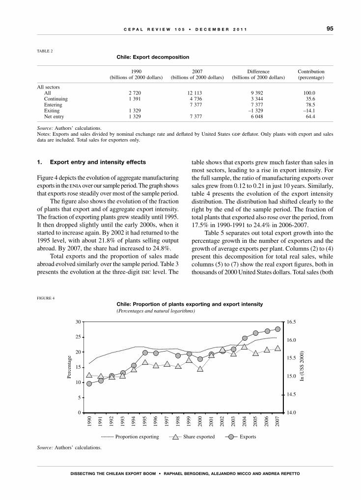
95
DIssECtIng tHE CHILEAn ExPoRt BooM • RAPHAEL BERgoEIng, ALEjAnDRo MICCo AnD AnDREA REPEtto
C E P A L R E V I E W 1 0 5 • D E C E M B E R 2 0 1 1
1. Export entry and intensity effects
Figure 4 depicts the evolution of aggregate manufacturing exports in the enia over our sample period. The graph shows that exports rose steadily over most of the sample period.
The figure also shows the evolution of the fraction of plants that export and of aggregate export intensity. The fraction of exporting plants grew steadily until 1995. It then dropped slightly until the early 2000s, when it started to increase again. By 2002 it had returned to the 1995 level, with about 21.8% of plants selling output abroad. By 2007, the share had increased to 24.8%.
Total exports and the proportion of sales made abroad evolved similarly over the sample period. Table 3 presents the evolution at the three-digit isic level. The
table shows that exports grew much faster than sales in most sectors, leading to a rise in export intensity. For the full sample, the ratio of manufacturing exports over sales grew from 0.12 to 0.21 in just 10 years. Similarly, table 4 presents the evolution of the export intensity distribution. The distribution had shifted clearly to the right by the end of the sample period. The fraction of total plants that exported also rose over the period, from 17.5% in 1990-1991 to 24.4% in 2006-2007.
Table 5 separates out total export growth into the percentage growth in the number of exporters and the growth of average exports per plant. Columns (2) to (4) present this decomposition for total real sales, while columns (5) to (7) show the real export figures, both in thousands of 2000 United States dollars. Total sales (both
TABLE 2
Chile: Export decomposition
1990(billions of 2000 dollars)
2007(billions of 2000 dollars)
Difference(billions of 2000 dollars)
Contribution (percentage)
All sectors All 2 720 12 113 9 392 100.0 Continuing 1 391 4 736 3 344 35.6 Entering 7 377 7 377 78.5 Exiting 1 329 –1 329 –14.1 Net entry 1 329 7 377 6 048 64.4
Source: Authors’ calculations.Notes: Exports and sales divided by nominal exchange rate and deflated by United States gdp deflator. Only plants with export and sales data are included. Total sales for exporters only.
FIGURE 4
Chile: Proportion of plants exporting and export intensity(Percentages and natural logarithms)
Source: Authors’ calculations.
Proportion exporting
0
5
10
15
20
25
30
1990
1991
1992
1993
1994
1995
1996
1997
1998
1999
2000
2001
2002
2003
2004
2005
2006
2007
Perc
enta
ge
14.0
14.5
15.0
15.5
16.0
16.5
In (
US$
200
0)
Share exported Exports

96
DIssECtIng tHE CHILEAn ExPoRt BooM • RAPHAEL BERgoEIng, ALEjAnDRo MICCo AnD AnDREA REPEtto
C E P A L R E V I E W 1 0 5 • D E C E M B E R 2 0 1 1
TABLE 3
Chile: Dynamics of total exports and export intensity
SITC code
Export growth(annual rate)a
Export intensity
Percentage of sales exported Difference
1990/1991-2006/2007 1990-1991 2006-2007 Percentage points Percentage
311 1.78 18.81 28.28 9.47 50.3312 3.45 3.16 4.85 1.68 53.2313 8.39 7.95 21.34 13.39 168.4314 –1.00 3.15 0.00 –3.15 –100.0321 0.49 4.85 13.15 8.30 171.1322 –0.49 5.73 2.35 –3.38 –59.0323 18.84 1.08 26.13 25.05 2 329.0324 –0.93 9.27 0.81 –8.46 –91.3331 3.61 30.14 46.07 15.93 52.9332 –0.37 6.33 5.19 –1.14 –18.0341 3.77 29.88 53.71 23.82 79.7342 0.18 3.41 3.06 –0.35 –10.3351 6.58 34.63 12.90 –21.73 –62.8352 1.10 6.49 8.02 1.53 23.6353 –1.00 3.26 0.00 –3.26 –100.0354 –0.89 2.62 0.49 –2.14 –81.4355 2.80 13.52 29.54 16.02 118.5356 13.35 1.47 7.40 5.94 405.2361 3.66 14.20 24.36 10.16 71.6362 9.11 2.14 7.15 5.01 234.3369 1.94 1.23 1.35 0.12 9.5371 5.81 31.39 45.48 14.09 44.9381 2.74 2.71 4.88 2.17 80.3382 12.34 1.33 9.44 8.12 611.6383 8.63 1.87 9.31 7.43 396.8384 3.33 5.82 15.43 9.62 165.3385 30.17 2.90 15.75 12.84 442.5390 13.10 2.65 13.17 10.52 396.4All 3.17 12.26 21.08 8.81 71.9
Mean 5.4 9.0 14.6 5.6 62.525th percentile 0.4 2.6 4.4 1.8 66.350th percentile 3.4 4.1 9.4 5.2 126.975th percentile 8.5 10.3 22.1 11.8 113.8
Source: Authors’ calculations.
a Nominal Chilean pesos were converted into 2000 dollars deflated by the annual average nominal exchange rate and the United States gdp deflator.
domestic and foreign) grew by 96% over the period. This growth is mostly explained by changes in average sales per plant, as the number of plants decreased during the period. Interestingly, the results for export growth are significantly different. First, total exports grew by much more, with a rise of 149%. Second, more than 80% of this growth is explained by the expansion of exports per plant, whereas less than 20% is due to the number of plants exporting. The rapid growth of exports per plant relative to sales per plant confirms the fact that exporters are much larger than average.
These figures, however, do not reveal differences across plants in terms of their export status (new, old and failing exporters). To estimate their relative contribution, we measure the significance of each margin by plant type as a source of the export boom. That is, we look not only at the number of plants and the fraction of sales exported, but also at the contribution of continuers, exiters and new exporters. For instance, if new exporters export a larger share of their sales than existing exporters, even a small entry of plants may end up contributing greatly to export growth. To examine
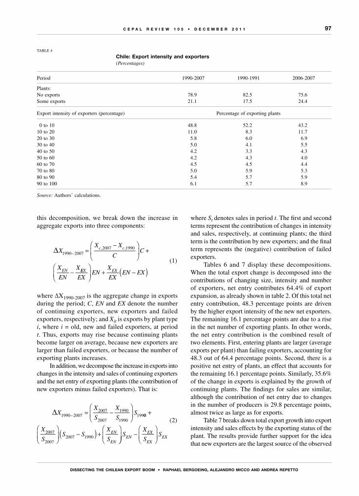
97
DIssECtIng tHE CHILEAn ExPoRt BooM • RAPHAEL BERgoEIng, ALEjAnDRo MICCo AnD AnDREA REPEtto
C E P A L R E V I E W 1 0 5 • D E C E M B E R 2 0 1 1
TABLE 4
Chile: Export intensity and exporters(Percentages)
Period 1990-2007 1990-1991 2006-2007
Plants:No exports 78.9 82.5 75.6Some exports 21.1 17.5 24.4
Export intensity of exporters (percentage) Percentage of exporting plants
0 to 10 48.8 52.2 43.210 to 20 11.0 8.3 11.720 to 30 5.8 6.0 6.930 to 40 5.0 4.1 5.540 to 50 4.2 3.3 4.350 to 60 4.2 4.3 4.060 to 70 4.5 4.5 4.470 to 80 5.0 5.9 5.380 to 90 5.4 5.7 5.990 to 100 6.1 5.7 8.9
Source: Authors’ calculations.
this decomposition, we break down the increase in aggregate exports into three components:
∆XX X
CC
X
EN
X
c c
EN
1990 20072007 1990
− =−
+
−
, ,
EEX EX
EXEN
X
EXEN EX
( )+ −
(1)
where ∆X1990-2007 is the aggregate change in exports during the period; C, EN and EX denote the number of continuing exporters, new exporters and failed exporters, respectively; and Xit is exports by plant type i, where i = old, new and failed exporters, at period t. Thus, exports may rise because continuing plants become larger on average, because new exporters are larger than failed exporters, or because the number of exporting plants increases.
In addition, we decompose the increase in exports into changes in the intensity and sales of continuing exporters and the net entry of exporting plants (the contribution of new exporters minus failed exporters). That is:
∆X
X
S
X
SS1990 2007
2007
2007
1990
1990199− = −
00
2007
20072007 1990
+
−( ) +
X
SS S
X
SEN
EN −
S
X
SSEN
EX
EXEX
(2)
where St denotes sales in period t. The first and second terms represent the contribution of changes in intensity and sales, respectively, at continuing plants; the third term is the contribution by new exporters; and the final term represents the (negative) contribution of failed exporters.
Tables 6 and 7 display these decompositions. When the total export change is decomposed into the contributions of changing size, intensity and number of exporters, net entry contributes 64.4% of export expansion, as already shown in table 2. Of this total net entry contribution, 48.3 percentage points are driven by the higher export intensity of the new net exporters. The remaining 16.1 percentage points are due to a rise in the net number of exporting plants. In other words, the net entry contribution is the combined result of two elements. First, entering plants are larger (average exports per plant) than failing exporters, accounting for 48.3 out of 64.4 percentage points. Second, there is a positive net entry of plants, an effect that accounts for the remaining 16.1 percentage points. Similarly, 35.6% of the change in exports is explained by the growth of continuing plants. The findings for sales are similar, although the contribution of net entry due to changes in the number of producers is 29.8 percentage points, almost twice as large as for exports.
Table 7 breaks down total export growth into export intensity and sales effects by the exporting status of the plant. The results provide further support for the idea that new exporters are the largest source of the observed
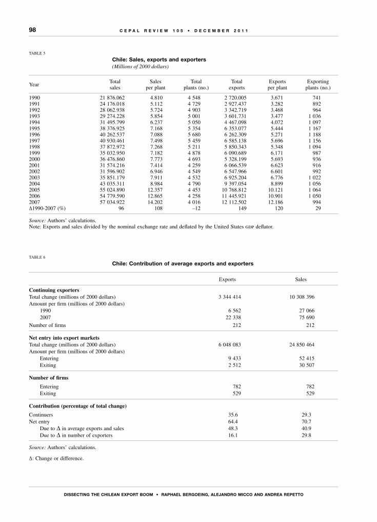
98
DIssECtIng tHE CHILEAn ExPoRt BooM • RAPHAEL BERgoEIng, ALEjAnDRo MICCo AnD AnDREA REPEtto
C E P A L R E V I E W 1 0 5 • D E C E M B E R 2 0 1 1
TABLE 5
Chile: sales, exports and exporters(Millions of 2000 dollars)
YearTotal sales
Salesper plant
Totalplants (no.)
Totalexports
Exportsper plant
Exporting plants (no.)
1990 21 876.062 4.810 4 548 2 720.005 3.671 7411991 24 176.018 5.112 4 729 2 927.437 3.282 8921992 28 062.938 5.724 4 903 3 342.719 3.468 9641993 29 274.228 5.854 5 001 3 601.731 3.477 1 0361994 31 495.799 6.237 5 050 4 467.098 4.072 1 0971995 38 376.925 7.168 5 354 6 353.077 5.444 1 1671996 40 262.537 7.088 5 680 6 262.309 5.271 1 1881997 40 930.461 7.498 5 459 6 585.138 5.696 1 1561998 37 872.972 7.268 5 211 5 850.343 5.348 1 0941999 35 032.950 7.182 4 878 6 090.689 6.171 9872000 36 476.860 7.773 4 693 5 328.199 5.693 9362001 31 574.216 7.414 4 259 6 066.539 6.623 9162002 31 596.902 6.946 4 549 6 547.966 6.601 9922003 35 851.179 7.911 4 532 6 925.204 6.776 1 0222004 43 035.311 8.984 4 790 9 397.054 8.899 1 0562005 55 024.890 12.357 4 453 10 768.812 10.121 1 0642006 54 779.590 12.865 4 258 11 445.921 10.901 1 0502007 57 034.922 14.202 4 016 12 112.502 12.186 994∆1990-2007 (%) 96 108 –12 149 120 29
Source: Authors’ calculations.Note: Exports and sales divided by the nominal exchange rate and deflated by the United States gdp deflator.
TABLE 6
Chile: Contribution of average exports and exporters
Exports Sales
Continuing exportersTotal change (millions of 2000 dollars) 3 344 414 10 308 396Amount per firm (millions of 2000 dollars) 1990 6 562 27 066 2007 22 338 75 690
Number of firms 212 212
net entry into export marketsTotal change (millions of 2000 dollars) 6 048 083 24 850 464Amount per firm (millions of 2000 dollars) Entering 9 433 52 415 Exiting 2 512 30 507
number of firms
Entering 782 782 Exiting 529 529
Contribution (percentage of total change)
Continuers 35.6 29.3Net entry 64.4 70.7 Due to ∆ in average exports and sales 48.3 40.9 Due to ∆ in number of exporters 16.1 29.8
Source: Authors’ calculations.
∆: Change or difference.
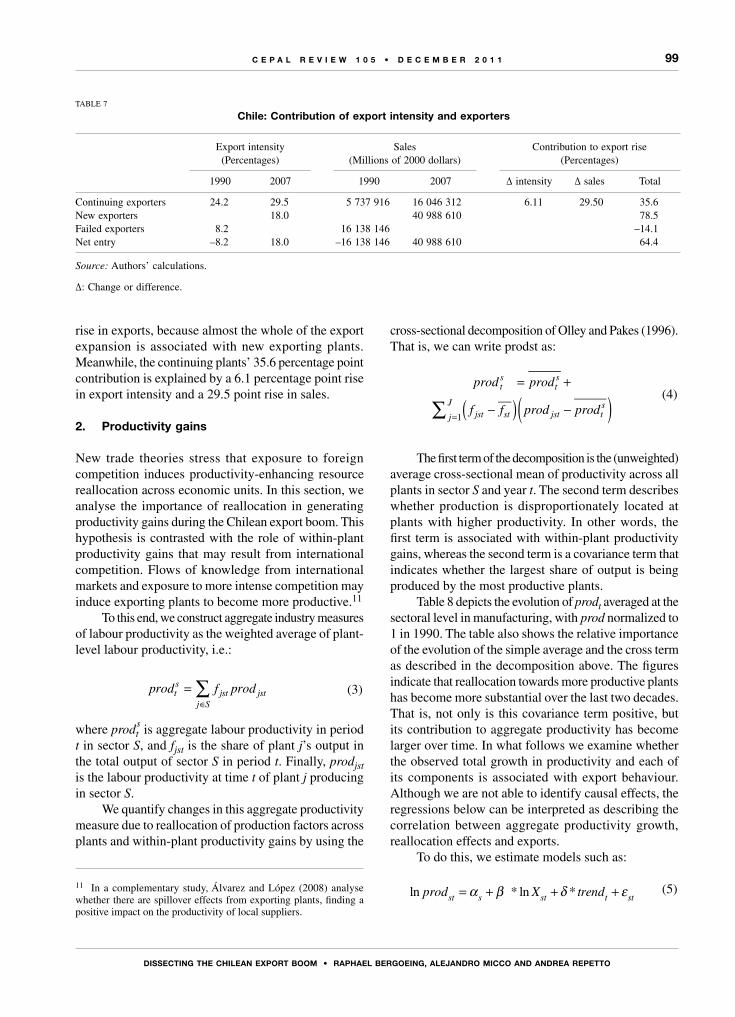
99
DIssECtIng tHE CHILEAn ExPoRt BooM • RAPHAEL BERgoEIng, ALEjAnDRo MICCo AnD AnDREA REPEtto
C E P A L R E V I E W 1 0 5 • D E C E M B E R 2 0 1 1
rise in exports, because almost the whole of the export expansion is associated with new exporting plants. Meanwhile, the continuing plants’ 35.6 percentage point contribution is explained by a 6.1 percentage point rise in export intensity and a 29.5 point rise in sales.
2. Productivity gains
New trade theories stress that exposure to foreign competition induces productivity-enhancing resource reallocation across economic units. In this section, we analyse the importance of reallocation in generating productivity gains during the Chilean export boom. This hypothesis is contrasted with the role of within-plant productivity gains that may result from international competition. Flows of knowledge from international markets and exposure to more intense competition may induce exporting plants to become more productive.11
To this end, we construct aggregate industry measures of labour productivity as the weighted average of plant-level labour productivity, i.e.:
∑=∈
prod f prodts
jstj S
jst (3)
where prodts is aggregate labour productivity in period
t in sector S, and fjst is the share of plant j’s output in the total output of sector S in period t. Finally, prodjst is the labour productivity at time t of plant j producing in sector S.
We quantify changes in this aggregate productivity measure due to reallocation of production factors across plants and within-plant productivity gains by using the
11 In a complementary study, Álvarez and López (2008) analyse whether there are spillover effects from exporting plants, finding a positive impact on the productivity of local suppliers.
cross-sectional decomposition of Olley and Pakes (1996). That is, we can write prodst as:
prod prod
f f prod prod
s s
jst st jst ts
j
J
1∑ ( )= ( )− −
= +t t (4)
The first term of the decomposition is the (unweighted) average cross-sectional mean of productivity across all plants in sector S and year t. The second term describes whether production is disproportionately located at plants with higher productivity. In other words, the first term is associated with within-plant productivity gains, whereas the second term is a covariance term that indicates whether the largest share of output is being produced by the most productive plants.
Table 8 depicts the evolution of prodt averaged at the sectoral level in manufacturing, with prod normalized to 1 in 1990. The table also shows the relative importance of the evolution of the simple average and the cross term as described in the decomposition above. The figures indicate that reallocation towards more productive plants has become more substantial over the last two decades. That is, not only is this covariance term positive, but its contribution to aggregate productivity has become larger over time. In what follows we examine whether the observed total growth in productivity and each of its components is associated with export behaviour. Although we are not able to identify causal effects, the regressions below can be interpreted as describing the correlation between aggregate productivity growth, reallocation effects and exports.
To do this, we estimate models such as:
ln * ln *prod X trendst s s st= +α β δ ε+ +t t (5)
TABLE 7
Chile: Contribution of export intensity and exporters
Export intensity (Percentages)
Sales (Millions of 2000 dollars)
Contribution to export rise (Percentages)
1990 2007 1990 2007 ∆ intensity ∆ sales Total
Continuing exporters 24.2 29.5 5 737 916 16 046 312 6.11 29.50 35.6New exporters 18.0 40 988 610 78.5Failed exporters 8.2 16 138 146 –14.1Net entry –8.2 18.0 –16 138 146 40 988 610 64.4
Source: Authors’ calculations.
∆: Change or difference.
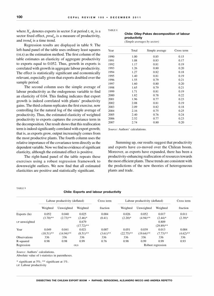
100
DIssECtIng tHE CHILEAn ExPoRt BooM • RAPHAEL BERgoEIng, ALEjAnDRo MICCo AnD AnDREA REPEtto
C E P A L R E V I E W 1 0 5 • D E C E M B E R 2 0 1 1
where Xst denotes exports in sector S at period t, αs is a sector fixed effect, prodst is a measure of productivity, and trendt is a time trend.
Regression results are displayed in table 9. The left-hand panel of the table uses ordinary least squares (ols) as the estimation method. The first column of the table estimates an elasticity of aggregate productivity to exports equal to 0.052. Thus, growth in exports is correlated with growth in aggregate labour productivity. The effect is statistically significant and economically relevant, especially given that exports doubled over the sample period.
The second column uses the simple average of labour productivity as the endogenous variable to find an elasticity of 0.04. This finding indicates that export growth is indeed correlated with plants’ productivity gains. The third column replicates the first exercise, now controlling for the natural log of the simple average of productivity. Thus, the estimated elasticity of weighted productivity to exports captures the covariance term in the decomposition. Our result shows that this reallocation term is indeed significantly correlated with export growth; that is, as exports grow, output increasingly comes from the most productive plants. The fourth column uses the relative importance of the covariance term directly as the dependent variable. Now we find no evidence of significant elasticity, although the estimated effect is positive.
The right-hand panel of the table repeats these exercises using a robust regression framework to downweight outliers. We now find that all estimated elasticities are positive and statistically significant.
TABLE 8
Chile: olley-Pakes decomposition of labour productivity (Simple averages by sector)
Year Total Simple average Cross term
1990 1.00 0.85 0.151991 1.08 0.83 0.171992 1.17 0.81 0.191993 1.26 0.80 0.201994 1.27 0.82 0.181995 1.40 0.81 0.191996 1.55 0.79 0.211997 1.60 0.80 0.201998 1.65 0.79 0.211999 1.71 0.81 0.192000 1.82 0.78 0.222001 1.96 0.77 0.232002 2.08 0.81 0.192003 2.09 0.82 0.182004 2.16 0.75 0.252005 2.40 0.76 0.242006 2.52 0.77 0.232007 2.74 0.80 0.20
Source: Authors’ calculations.
TABLE 9
Chile: Exports and labour productivity
Labour productivity (deflated) Cross term Labour productivity (deflated) Cross term
Weighted Unweighted Weighted fraction Weighted Unweighted Weighted fraction
Exports (ln) 0.052 0.040 0.025 0.004 0.026 0.052 0.017 0.011(3.70)** (2.73)** (2.46)* (0.41) (2.20)* (4.94)** (2.44)* (2.39)*
lp unweighted 0.679 0.809(17.72)** (29.89)**
Year 0.049 0.041 0.021 0.007 0.051 0.039 0.013 0.004 (18.51)** (14.94)** (8.51)** (3.61)** (22.75)** (19.64)** (7.73)** (4.62)**Observations 336 336 336 336 336 336 336 336R-squared 0.98 0.98 0.99 0.76 0.98 0.99 0.99 0.93Regression ols Robust regression
Source: Authors’ calculations.Absolute value of t-statistics in parentheses.
* significant at 5%; ** significant at 1%.lp: Labour productivity
Summing up, our results suggest that productivity and exports have co-moved over the Chilean boom. Moreover, as exports have expanded, there has been a productivity-enhancing reallocation of resources towards the most efficient plants. These trends are consistent with the predictions of the new theories of heterogeneous plants and trade.

101
DIssECtIng tHE CHILEAn ExPoRt BooM • RAPHAEL BERgoEIng, ALEjAnDRo MICCo AnD AnDREA REPEtto
C E P A L R E V I E W 1 0 5 • D E C E M B E R 2 0 1 1
This paper uses almost two decades of Chilean plant-level manufacturing data to empirically investigate the relationship between exports, plant dynamics and productivity. We find that 64.4% of the increase in exports over the years from 1990 to 2007 was due to the net entry of new exporters. About two thirds of this net entry contribution is associated with the larger size (average exports per plant) of new exporters; only a third is related to the increase in the number of exporters. Additionally, the export intensity (exports over sales) of new exporters was more than double that of failing exporters. Overall, even though exporters in Chile remain a minority among domestic producers and usually sell only a small fraction of their output abroad, as reported by Bernard and Jensen (1995) for developed economies, figures have increased during the last two decades. The bilateral trade agreements that came to supplement the previous unilateral liberalization strategy in the early 1990s may have favoured new and more intensive exporters by reducing foreign market penetration costs.
We also show that productivity and exports have co-moved over the Chilean boom. Moreover, the export expansion has been associated with a productivity-enhancing reallocation of resources towards more efficient plants.
The aggregate effect on productivity is a topic that requires further research, however, as other margins not analysed here may be affected. For instance, Atkenson and Burstein (2010) suggest that there may be countervailing effects, since increases in exporters’ innovative activity might diminish productivity innovation undertaken by smaller companies primarily serving domestic markets.
Finally, future research should address the role of natural resources as a driver of Chile’s export boom. Although non-copper exports have shown increasing diversification in terms of markets and products (Berthelon, 2011), natural resources still predominate in Chile’s export expansion as compared to other liberalization experiences.
(Original: English)
VConcluding remarks
Bibliography
Arkolakis, C. (2008), “Market penetration costs and the new consumers margin in international trade”, nber Working Paper, No. 14214, Cambridge, Massachusetts.
Álvarez, R. and R.A. López (2008), “Is exporting a source of productivity spillovers?”, Review of World Economics (Weltwirtschaftliches Archiv), vol. 144, No. 4, New York, Springer.
(2005), “Exporting and performance: evidence from Chilean plants”, Canadian Journal of Economics, vol. 38, No. 4, Quebec, Canadian Economics Association.
Álvarez, R. and S. Vergara (2010), “Exit in developing countries: economic reforms and plant heterogeneity”, Economic Development and Cultural Change, vol. 58, No. 3, Chicago, Chicago University Press.
Atkenson, A. and A. Burstein (2010), “Innovation, firm dynamics, and international trade”, Journal of Political Economy, vol. 118, No. 3, Chicago, University of Chicago Press.
Barandiarán, E. and L. Hernández (1999), “Origins and resolution of a banking crisis: Chile 1982-86”, Working Paper, No. 57, Santiago, Chile, Central Bank of Chile.
Bergoeing, R., A. Hernando and A. Repetto (2010), “Market reforms and efficiency gains in Chile”, Estudios de Economía, vol. 37, No. 2, Santiago, Chile, University of Chile.
(2005), “Deflators and capital series in the enia: technical appendix”, Santiago, Chile, Center of Applied Economics, University of Chile, unpublished.
Bernard, A.B. and J.B. Jensen (2004), “Entry, expansion, and intensity in the U.S. export boom, 1987-1992”, Review of International Economics, vol. 12, No. 4, Wiley Blackwell.
(1999), “Exceptional exporter performance: cause, effect, or both?”, Journal of International Economics, vol. 47, No. 1, Amsterdam, Elsevier.
(1995), “Exporters, jobs and wages in U.S. manufacturing: 1976-1987”, Brookings Papers on Economic Activity, Microeconomics 1995, Washington, D.C., Brookings Institution.
Bernard, A.B. and others (2007), “Firms in international trade”, Journal of Economic Perspectives, vol. 21, No. 3, Nashville, Tennessee, American Economic Association.
(2003), “Plants and productivity in international trade”, American Economic Review, vol. 93, No. 4, Nashville, Tennessee.
Berthelon, M. (2011), “Chilean export performance: the role of intensive and extensive margins”, Working Paper, No. 615, Santiago, Chile, Central Bank of Chile.
Clerides, S., S. Lach and J. Tybout (1988), “Is learning-by-exporting important?”, Quarterly Journal of Economics, vol. 113, No. 3, Cambridge, Massachusetts, The mit Press.
Corbo, V. and S. Fischer (1994), “Lessons from the Chilean stabilization and recovery”, The Chilean Economy: Policy Lessons and Challenges, B. Bosworth, R. Dornbusch and R. Labán (eds.), Washington, D.C., The Brookings Institution.
102
DIssECtIng tHE CHILEAn ExPoRt BooM • RAPHAEL BERgoEIng, ALEjAnDRo MICCo AnD AnDREA REPEtto
C E P A L R E V I E W 1 0 5 • D E C E M B E R 2 0 1 1
Eaton, J., S. Kortum and F. Kramarz (2008), “An anatomy of international trade: evidence from French firms”, nber Working Papers, No. 14610, Cambridge, Massachusetts, National Bureau of Economic Research.
Edwards, A. and S. Edwards (1992), Monetarismo y liberalización: el experimento chileno, Santiago, Chile, Fondo de Cultura Económica.
Irarrázabal, A. and L.D. Opromolla (2007), “Trade reforms in a global competition model: the case of Chile”, Lisbon, Bank of Portugal, unpublished.
Kehoe, T. and K. Ruhl (2009), “How important is the new goods margin in international trade?”, Staff Report, No. 324, Minneapolis, Federal Reserve Bank of Minneapolis,.
Melitz, M.J. (2008), “International trade and heterogeneous firms”, The New Palgrave Dictionary of Economics, S.N. Durlauf and L.E. Blume (eds.), Palgrave Macmillan.
(2003), “The impact of trade on intra-industry reallocations
and aggregate industry productivity”, Econometrica, vol. 71, No. 6, New York, Econometric Society.
Olley, S. and A. Pakes (1996), “The dynamics of productivity in the telecommunication equipment industry”, Econometrica, vol. 64, New York, Econometric Society.
Pavcnik, N. (2002), “Trade liberalization, exit, and productivity improvements: evidence from Chilean plants”, The Review of Economic Dynamics, vol. 69, No. 1, Wiley Blackwell.
Trefler, D. (1993), “International factor price differences: Leontief was right!”, Journal of Political Economy, vol. 101, No. 6, Chicago, University of Chicago Press.
Wagner, J. (2008), “Exports, imports, and productivity at the firm level: an international perspective: introduction by guest editor”, Review of World Economics, vol. 144, No. 44, Springer.
(2007), “Exports and productivity: a survey of the evidence from firm level data”, The World Economy, vol. 30, No. 1, Wiley Blackwell.
C E P A L R E V I E W 1 0 5 • D E C E M B E R 2 0 1 1
103
K E Y W O R D S
Pensions
Retirement
Age
Quality of life
Life expectancy
Risk
Statistical data
Comparative analysis
Chile
Chile: early retirement,impatience and risk aversion
Jaime Ruiz-Tagle and Pablo Tapia
About one third of all Chileans take early retirement. As retirement
age approaches, people become more aware of the health issues
associated with that stage of life. This reduces their uncertainty about their
future quality of life and may lead to a relative increase in impatience. This
article offers a theoretical examination of how future life expectancy affects
relative levels of impatience in ways that may increase the probability of
early retirement. The empirical findings for Chile show that the greater
people’s future life expectancy is, the less likely they will be to take early
retirement. The article also looks at how risk aversion increases relative
impatience as a consequence of people’s uncertainty as to whether or
not they will enjoy a good quality of life in the years ahead. The empirical
findings point to a positive correlation between risk aversion and early
retirement via the mechanism of life expectancy.
Jaime Ruiz-Tagle
Assistant Professor, Department of
Economics and Microdata Centre
University of Chile
Pablo Tapia
Assistant Professor of Statistical
Analysis, Department of
Administration
University of Chile
104
CHILE: EARLy REtIREMEnt, IMPAtIEnCE AnD RIsk AVERsIon • jAIME RuIz-tAgLE AnD PABLo tAPIA
C E P A L R E V I E W 1 0 5 • D E C E M B E R 2 0 1 1
Although the current tendency in pension policy is to raise the retirement age, early retirement is fairly common in Chile. Of all those who retired in 2006, 35% did so early.1 According to data from the country’s pension fund management companies (afps), people who opt to start drawing their pensions early are doing so at age 55, on average. From a public policy standpoint, the reasons behind these retirement decisions therefore merit examination. This article offers a new perspective on the important role which impatience and risk aversion may play in early retirement decisions.
People who retire early receive smaller pensions than they would if they retired at the age established by law, and they have to use those pensions to cover their living expenses over a greater number of years, on average (Nalebuff and Zeckhauser, 1985). Given that the number of pensioners is rising every year and that 35% are retiring early, it is important to understand how risk aversion influences the decision to retire early.2
In Chile, in order to take early retirement,3 a person must have belonged to the new pension system for at least five years and must have accumulated pension funds equal to or greater than 62%4 of the taxable income declared over the past 10 years. Requirements such as these may have little impact on the impatience factor at the individual level, however.
A person who has reached an age at which he or she must decide whether to retire early or to wait until the legally mandated age is more aware of the loss of
The authors are grateful for valuable comments received from José Luis Ruiz and the participants in the Meeting of the Economics Society of Chile and the Microdata Centre. Professor Ruiz-Tagle wishes to express his gratitude for the funding provided to the Microdata Centre under the Millennium Science Initiative within the framework of project P07S-023-F.1 Pensions Oversight Agency, Chile.2 According to the results of the Social Protection Survey (eps), the percentage of pensioners rose from 13.3% in 2004 to 14.5% in 2006.3 Act No. 19.943.4 Under Act No. 19.943, this percentage was raised to 70% on 19 August 2010.
cognitive and motor abilities that can occur as people grow older. Accordingly, the value placed on the years that they have left to live (future life expectancy) can generate differences in relative levels of impatience. Uncertainty about the quality of life that they may enjoy in the future can lead risk-averse individuals to prioritize present consumption over future consumption. This article offers evidence that the higher an individual’s level of risk aversion is, the greater that person’s relative level of impatience will be.
In this analysis, a person’s decision as to when to retire is represented by an aggregate utility model over two periods, such that a social-security contributor who retires at the beginning of the first period is doing so early, whereas one who retires at the start of the second period is doing so at the legally established age. Thus, the legally mandated age defines the break between the two periods. The estimation procedure used here involves a discrete choice model which distinguishes only between whether or not the individual takes early retirement. This procedure follows the structure suggested by the theoretical model, with the aim being to identify the impact that the perception of future quality of life, based on future life expectancy (Bleichrodt and Quiggin, 1999), has in terms of the level of impatience that leads people to retire early.
The results show that those who retire early are using a higher intertemporal discount rate, which could be attributable to their perceived future life expectancy. Some evidence is also found that the higher the level of risk aversion, the greater the degree of impatience to take early retirement, which may reflect uncertainty about future quality of life.
The rest of this article is structured as follows: after this introduction, section II offers a brief review of the regulatory context and the existing data and literature. Section III sets forth the theoretical framework and the estimation model used. Section IV presents the empirical analysis, description of variables and empirical findings, as well as some possible extensions of the model and other considerations. Section V concludes.
Iintroduction
105
CHILE: EARLy REtIREMEnt, IMPAtIEnCE AnD RIsk AVERsIon • jAIME RuIz-tAgLE AnD PABLo tAPIA
C E P A L R E V I E W 1 0 5 • D E C E M B E R 2 0 1 1
Prior to 1980, Chile had a pay-as-you-go pension system. At that point, however, it consolidated its structural pension-system reform programme.5 This reform allowed it to phase out the pay-as-you-go system and to replace it with a fully funded system based on individual accounts. Unlike its predecessor, this financing mechanism relies on market returns.
Part of the literature on pensions focuses on examining the factors that may lead people to start drawing their pensions before the legally mandated age. Some authors have posited that the likelihood that people will decide to take early retirement increases as their social security benefits rise (Mitchell and Phillips, 2000), as their level of additional savings increases (Au, Mitchell and Phillips, 2005) and as their perception of their own health status diminishes (Hammitt, Haninger and Treich, 2005). Some studies use simulations to work out the reasons for this kind of retirement decision. For example, Poterba, Rauh and Venti (2005) maintain that the future marginal utility could be quite high even for a low-risk household if its members succeed in diversifying their investments in such a way as to permit them to take early retirement. Taking a different approach, Diamond and Köszegi (2003) propose a quasi-hyperbolic model as a basis for arguing that a lack of self-control influences retirement behaviour and, in particular, the decision to retire early.
5 Decree-Law No. 3500.
Early retirement decisions may also be influenced by the business cycle. For example, a period of high unemployment may further diminish the chances that people nearing retirement age have of finding a job and thereby prompt them to retire early (Hairault, Langot and Sopraseuth, 2010). Another possibility is that a recessionary phase of the business cycle may depress wages to such an extent that it increases the likelihood of early retirement in the presence of an endogenous labour supply (Chai and others, 2009). On the other hand, a downswing in the business cycle may drive down the rates of return at which future pension payments can be calculated, thereby making the prospect of drawing on retirement pensions ahead of time less attractive and thus encouraging people to delay their retirement.
People’s perception of their health and future life expectancy are very closely related. French (2005) finds evidence that people’s state of health, or their uncertainty as to the likelihood that they will remain healthy in the future, influences their decision about when to retire. Guiso and Paiella (2006) find that the level of risk aversion provides a basis for predicting a series of household decisions, including the decision to take early retirement. Risk tolerance is also positively correlated with people’s perception of their own state of health and future life expectancy (Hammitt, Haninger and Treich, 2005). This study will therefore seek to arrive at a formal expression of the integration of risk aversion into early retirement decisions, together with people’s perceptions of their state of health and life expectancy, based on their assessment of their future quality of life.
IIreview of the literature on pensions
IIITheoretical model and empirical strategy
A model that provides a formal expression of the influence that impatience and risk aversion exert on early retirement decisions is presented below. This represents an analytical formalization of the decision to retire early or to wait until the legally mandated
age based on a simple two-stage life-cycle model. In this model, then, if a person takes early retirement, he or she does so during the first of these time periods; if not, then the person retires during the second time period.
106
CHILE: EARLy REtIREMEnt, IMPAtIEnCE AnD RIsk AVERsIon • jAIME RuIz-tAgLE AnD PABLo tAPIA
C E P A L R E V I E W 1 0 5 • D E C E M B E R 2 0 1 1
Let us take U(∙) to represent the aggregate utility under conditions of linear separability, while u(∙)6 will represent the utility in a given period, such that u'(Ct) > 0 and u''(Ct) < 0. It is also assumed that the utility function for each period is isoelastic (constant relative risk aversion, or crra), such that σ represents the crra, ρ is the intertemporal discount rate, which will be written as the discount factor β(H,σ) and is linked to risk aversion σ and life expectancy H.
The maximization of individual welfare consists of:
max ( , , , , )
( , ) ( , )
,C C t t
t
t t
U C
u C H u+
+ =
+ ⋅1
1 σ ρ
σ β σ ( )Ct+1 σ
C H
( , (1)
Subject to: C At t t+ ≤ λY B+ ⋅
C r A s B A(1 ) (1 )(1t t t1 λ≤ + ⋅ + + −+ ) 0⋅ ≥
where r represents the market interest rate and s represents the rate of return offered by afps. B corresponds to the amount of pension funds that a person has accumulated, while λ is the portion that a person receives when he or she retires, which may vary depending on how early an age the person retires at. If a person waits until the legally mandated age, λ will be zero (0). Finally, At represents the initial level of assets.
In order to incorporate the value placed on life expectancy and risk aversion into the measurement of relative impatience, the discount factor is defined as β(H,σ) = δ.Ø(H,σ). The parameter δ is a constant that represents the distortion in the discount factor generated by the difference between the values that different individuals place on their quality of life. In the case of the function Ø(H,σ), it is assumed that, for a given level of risk aversion lim ( , )H H→ =0 0φ σ , which means that if a person does not expect to live much longer, his or her only chance to have a better quality of life is in the present. In addition, it is assumed that lim ( , )H H→∞ =φ σ 1, which indicates that future quality of life does not compete with present quality of life.
Proposition 1. The function Ø(H,σ) is defined as increasing
and convex in H, ∂∂ >φH
0 and ∂∂
<2
2 0φH
. It is also defined
as decreasing and concave in σ, ∂∂ <φσ 0 and,
∂∂
<2
2 0φσ
.
In view of how tight the credit market is at present, it is assumed that individuals in this economy are faced with liquidity constraints.
6 It is assumed that the function satisfies the Inada conditions lim ( )C u C→∞ ′ = 0 and lim ( )C u C→ ′ = ∞0 .
Some of the factors mentioned in the literature that could account for a decline in future marginal utility are the non-contributory element in the social security system, financial risks and a person’s state of health. Social security and the financial market are not under any one person’s control. Nonetheless, a person’s perception of his or her state of health is used as a basis for calculating future life expectancy. In fact, Engen, Gale and Uccello (1999) show that a failure to take this element into account places serious limitations on estimates for temporal consumption models. Alternatively, it may be that this condition is attributable to different people’s psychological make-up as reflected in their attitude about the years to come.
In the proposed model, Ø(H,σ) represents the future value that an individual places on his or her future life expectancy, which is similar to the concept of longevity as a probability of living for a given period of time as described in Bleichrodt and Quiggin (1999), or to the incorporation of a person’s state of health into the intertemporal discount factor as described by Nordhaus (2002). The idea is to establish the future discount rate that people will use based on their assessment of their future psychological and physical state.
The constraints expressed in the model for equation (1) can be summed up as:
C C Y B Bt r t ts r
r+ ≤ + ++ +
−+
11 1 1
1( )( )
λ( )− ⋅
For the sake of simplicity, we will call this R = 1+r. It is assumed that people will use up all of their assets by the time that they die. On the other hand, if s < r, then everyone —regardless of their degree of risk aversion or impatience— will take early retirement, since the model will be offering them a better financial option, no matter what they decide to do with their assets after retirement. Thus, the decision to take early retirement is relevant only if the rate of return on the person’s individual account is higher or equal to the market rate.7
The condition for equilibrium in the problem shown in equation (1) thus comes down to:
7 Business cycles have an impact on both the rate of return for an individual’s account and the market rate of return, mainly via a levelling effect which may also alter rate differentials. Nonetheless, downswings in the business cycle that lead to a drop in the rates of return used to calculate future pensions may discourage people from retiring either at the legally mandated age or earlier. This presupposes that they expect rates of return to increase in the short term, however, and does not affect people’s propensity to retire based on the difference between market rates and the rates for individual accounts.

107
CHILE: EARLy REtIREMEnt, IMPAtIEnCE AnD RIsk AVERsIon • jAIME RuIz-tAgLE AnD PABLo tAPIA
C E P A L R E V I E W 1 0 5 • D E C E M B E R 2 0 1 1
TMS = –(1 + r) = –R
TMSU C
U C
u C
H u Ct
t
t
t
= −∂ ∂
∂ ∂= −
′⋅ ⋅ ′+
/
/
( , )
( , ) (1
σδ φ σ ++
= −1, )σ
R (2)
′
⋅ ⋅ ′=
+
u C
H u CRt
t
( , )
( , ) ( , )
σδ φ 1σ σ
At the same time, the ratio between future and present consumption must be lower for people who decide to take early retirement, A, than it is for those who decide to wait until the legally mandated age, L. This occurs because the former are substituting a higher level of present consumption for a lower level of future consumption. This is expressed in equation (3).
C
C
C
CtA
tA
tL
tL<1 1+ + (3)
Thus, if the utility function is isoelastic,8 as in u C Ct t( , σ−1 1σ σ= −( )) / , and consumption levels are greater than unity and the risk-aversion index is σ > 1, then:
′
′
′
′<u C
u C
u C
u CtA
tA
tL
tL
( , )
( , )
( , )
)
σ
σ
σ
σ1 1+ +( , (4)
However, equation (2) should hold both for people who retire early and for those who wait until the legally mandated age:
u C
H u C
u C
H u CR
( , )
( , ) ( , )
( , )
( , ) ( , )
tA
AA A
tA
tL
LL L
tL
1
1
=
=
σδ φ
σδ φ
′⋅ ⋅ ′
′⋅ ⋅ ′
+
+
σ σ
σ σ
(5)
Thus < < <φ σAA A
LL L( , ) ( , )0 1H Hφ σ , which
indicates that people who take early retirement are more impatient and so tend to discount future revenues more heavily. This difference in discounting may occur because of: (i) a difference in the value ascribed to the remaining years of life expectancy;9 (ii) differences in life expectancy; or (iii) a difference in the level of risk aversion.
8 Constant Relative Risk Aversion (crra).9 This difference is probably due to the fact that persons who retire early would presumably enjoy the first years of their remaining years of life more than the people who wait until the legally mandated age would.
If equally risk-averse individuals (σA = σL = σ) have the same perceived life expectancy (HA = HL = H), then, if some of them decide to take early retirement, it follows that they value their remaining years of life differently (ØA(H,σ) < ØL(H,σ)). Since life expectancy equates to a person’s remaining years of life, then the idea of enjoying a better quality of life in the present than in the future is equivalent to a lower future valuation of life expectancy (a lower discount factor). On the other hand, a person might be setting an equal value on the years that remain to him or her (Ø(HA,σ) = Ø(HL,σ)), in which case, if the person wishes to take early retirement, then that person must believe that he or she has fewer years left to live (HA < HL).
If we assume that two people have the same future life expectancy (HA = HL = H) and risk-aversion coefficients of σ0 and σ1, respectively, then they will be risk averse if σ0 > 1 and σ1 > 1. However, if σ0 < σ1, then the first person will be less risk-averse tan the second. Thus, from equations (3) and (4), it follows that:
L,u C
u C
u C
u C
( , )
( , )
( , )
( , )tj
tj
tj
tj
1
1 1
0
1 0< ∀ =
σσ
σσ
′′
′′+ +
j A (6)
This new condition is shown in equation (7), where (b) and (c) represent the equilibrium condition set up in (5), while (a) represents the equilibrium condition for an individual who decides to take early retirement but who is more risk averse than the level defined in (b).
R
u C
H u C
a
u C
H u C
b
u C
H u C
c
( , )
( , ) ( , )
( )
( , )
( , ) ( , )
( )
( , )
( , ) ( , )
( )
tA
AA
tA
tA
AA
tA
tL
LL
tL
1
1 1 1
0
0
0
0 1 0=
σδ φ σ σ
σδ φ
σδ φ σ σ
′⋅ ⋅ ′
′⋅ ⋅ ′
′⋅ ⋅ ′ +
= =+ + σ σ0 1
(7)
In order for equation (7) to hold, it is necessary that:
φ σA AA( , ) (H Hφ σA0 , )< <1 0
L ( , )LHφ σ< <10
Thus, if a person retires early, it is because he or she discounts the future more heavily. The smaller discount factor is due to the difference in the present value placed on future life expectancy. This difference is heightened by a greater degree of risk aversion owing to the level of uncertainty as to whether the person will have a good quality of life in the future.
108
CHILE: EARLy REtIREMEnt, IMPAtIEnCE AnD RIsk AVERsIon • jAIME RuIz-tAgLE AnD PABLo tAPIA
C E P A L R E V I E W 1 0 5 • D E C E M B E R 2 0 1 1
While the theoretical model tells us something about the expected behaviour of people when the time comes to decide when to retire, taking into account their future life expectancy and degree of risk aversion, the hypotheses derived from that model are not directly measureable by econometric means. The following empirical strategy is designed to provide a simple, estimable way of incorporating the characteristics of the theoretical model.
The decision as to whether to retire early or at the legally mandated age can be presented as a discrete choice, with a rational individual opting for the alternative that will provide a greater level of utility. It is generally agreed that indirect utility should be taken into account in analysing discrete choices, since this internalizes the constraints associated with income and other restrictions (Deaton and Muellbauer, 1980; Hensher, Barnard and Truong, 1988).
Using an empirical approach, we take the dichotomous variable Y, which represents the retirement decision and is equal to 1 if the person decides to take early retirement. This will be the case if the latent, indirect utility of retiring early, U *A, is greater than it would be if the person waits until the legally mandated age, U *L. Otherwise, the retirement decision variable will be zero (0), as shown here:
YA L
=>
≤
1
0
si
si
* *A L* *
U U
U U (8)
Equation (8) shows the conditions under which a person decides to take early retirement or to wait until the legally mandated age, bearing in mind that one of the parameters for the utility function is risk aversion.
Taking the utility function defined in equation (1), we introduce a latent variable to represent the indirect utility function for individual i and decision j:
U u C H u Cij ij t i j i i ij t
*,
*,
*( ) ( , ) ( , ) (⋅ = + ⋅ ⋅ +σ δ φ σ 1,, )
,..., ; ,
σ i
i n j A L∀ = =1 (9)
where the intertemporal discount rate is represented by β σ δ φ σ( , = ⋅H H , )) ( , as explained in detail in section III.
It is assumed that both groups have the same future life expectancy. Using that as a basis, an ad hoc assumption is made concerning the valuation of life expectancy, such that:
φ σ φ σ σ
j i i i i j ia
H H
i n
( , ) ( , | )
,..., ;
/−
∀ =
−1
1 jj A L aj, ; 0
= =a H j i
= > (10)
It will also be assumed that the members of both groups believe that they will live the same number of years, and the difference in their discount factors will therefore stem from the difference in their valuations of their remaining years of life, as represented by the parameter aj in equation (10).
The function described in equation (10) fulfils Proposition No. 1, such that, at a constant level of risk aversion, people will behave as shown in figure 1. Parameter aj stands for the value that they place on the years remaining to them, which could be interpreted as the value ascribed to their future quality of life; thus: aA < aL.
If the same assessment of future life expectancy H is maintained but the level of risk aversion changes from σ0 to a less risk-averse σ1, i.e., σ0 < σ1, then a higher value is placed on future years of life. This is shown in figure 2.
Now, if (10) is substituted for (9), a broader expression of indirect utility is obtained.
U u C u Cij ij t i ij
I
*,
*,
*
( )
( ) ( , ) (⋅ = + ⋅ +σ δ σ1
−
⋅ −+
σH u Ci
aij t i
II
j i/,
*
( )
( , )1
δ σ
t i, )
(11)
Component (I) gives the classic discount model for two periods of time. Component (II) is an additional term for the “loss” of utility of future consumption due to the assessment of the present vis-à-vis future life expectancy.
IVAn empirical strategy for identifying the
determinants of early retirement

109
CHILE: EARLy REtIREMEnt, IMPAtIEnCE AnD RIsk AVERsIon • jAIME RuIz-tAgLE AnD PABLo tAPIA
C E P A L R E V I E W 1 0 5 • D E C E M B E R 2 0 1 1
FIGURE 1
relationship between valuation of future life expectancy and degree of impatience
Source: Original calculations.
FIGURE 2
Lower valuation of future life expectancy due to uncertain future
Source: Original calculations.
0.0
0 5 10 15 20
0.2
0.4
0.6
0.8
1.0
Life expectancy (years)
Futu
re v
aluat
ion o
f li
fe e
xpec
tancy
(non-u
nit
ary)
φ(H|aL)
φ(H|aA)
φ(H0|aA) < φ(H0|aL)
H0
aA < aL
Early retirement Retirement at mandated age
Life expectancy (years)
φ(H|σ0)
H0
φ(H|σ1)
σ0 < σ1
Intermediate risk aversion High risk aversion
0.0
0.2
0.4
0.6
0.8
1.0
Futu
re v
aluat
ion o
f li
fe e
xpec
tancy
(non-u
nit
ary)
φ(H0|σ0) > φ(H0|σ1)
0 2 4 6 8 10 12 14 16 18 20
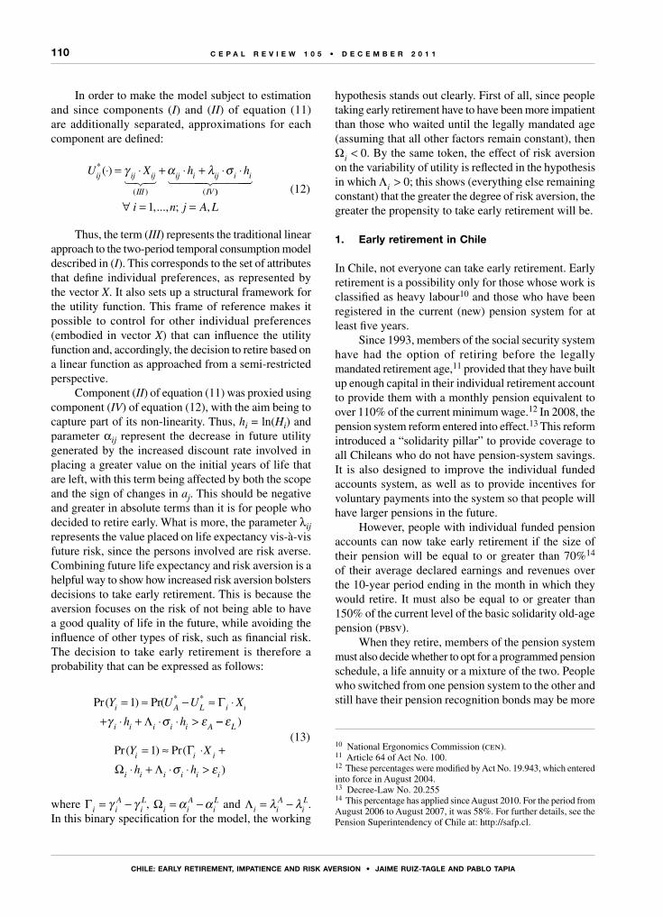
110
CHILE: EARLy REtIREMEnt, IMPAtIEnCE AnD RIsk AVERsIon • jAIME RuIz-tAgLE AnD PABLo tAPIA
C E P A L R E V I E W 1 0 5 • D E C E M B E R 2 0 1 1
In order to make the model subject to estimation and since components (I) and (II) of equation (11) are additionally separated, approximations for each component are defined:
U Xij ij ij
III
ij i ij i i
IV
*
( ) (
( )⋅ = ⋅ + ⋅ +γ α λ σ
))
,..., ; ,
∀ = =i n j A L1
h h
⋅ ⋅ (12)
Thus, the term (III) represents the traditional linear approach to the two-period temporal consumption model described in (I). This corresponds to the set of attributes that define individual preferences, as represented by the vector X. It also sets up a structural framework for the utility function. This frame of reference makes it possible to control for other individual preferences (embodied in vector X) that can influence the utility function and, accordingly, the decision to retire based on a linear function as approached from a semi-restricted perspective.
Component (II) of equation (11) was proxied using component (IV) of equation (12), with the aim being to capture part of its non-linearity. Thus, hi = ln(Hi) and parameter αij represent the decrease in future utility generated by the increased discount rate involved in placing a greater value on the initial years of life that are left, with this term being affected by both the scope and the sign of changes in aj. This should be negative and greater in absolute terms than it is for people who decided to retire early. What is more, the parameter λij represents the value placed on life expectancy vis-à-vis future risk, since the persons involved are risk averse. Combining future life expectancy and risk aversion is a helpful way to show how increased risk aversion bolsters decisions to take early retirement. This is because the aversion focuses on the risk of not being able to have a good quality of life in the future, while avoiding the influence of other types of risk, such as financial risk. The decision to take early retirement is therefore a probability that can be expressed as follows:
Pr( ) Pr( * *Y U
h hi A i
i i i i i A
= ≈ − ≈ ⋅+ ⋅ + ⋅ ⋅ >
1 ΓΛγ σ ε −− εL )
U XL i (13)
Pr( ) Pr(
)i
i i i i
= ≈⋅ + ⋅ ⋅ >
1 ΓΩ Λ
Y Xi i
σ εh hi i
⋅ +
where Γi iA
iLγ γ= − , Ωi i
AiLα α= − and Λi i
AiLλ λ= − .
In this binary specification for the model, the working
hypothesis stands out clearly. First of all, since people taking early retirement have to have been more impatient than those who waited until the legally mandated age (assuming that all other factors remain constant), then Ωi < 0. By the same token, the effect of risk aversion on the variability of utility is reflected in the hypothesis in which Λi > 0; this shows (everything else remaining constant) that the greater the degree of risk aversion, the greater the propensity to take early retirement will be.
1. Early retirement in Chile
In Chile, not everyone can take early retirement. Early retirement is a possibility only for those whose work is classified as heavy labour10 and those who have been registered in the current (new) pension system for at least five years.
Since 1993, members of the social security system have had the option of retiring before the legally mandated retirement age,11 provided that they have built up enough capital in their individual retirement account to provide them with a monthly pension equivalent to over 110% of the current minimum wage.12 In 2008, the pension system reform entered into effect.13 This reform introduced a “solidarity pillar” to provide coverage to all Chileans who do not have pension-system savings. It is also designed to improve the individual funded accounts system, as well as to provide incentives for voluntary payments into the system so that people will have larger pensions in the future.
However, people with individual funded pension accounts can now take early retirement if the size of their pension will be equal to or greater than 70%14 of their average declared earnings and revenues over the 10-year period ending in the month in which they would retire. It must also be equal to or greater than 150% of the current level of the basic solidarity old-age pension (pbsv).
When they retire, members of the pension system must also decide whether to opt for a programmed pension schedule, a life annuity or a mixture of the two. People who switched from one pension system to the other and still have their pension recognition bonds may be more
10 National Ergonomics Commission (cen).11 Article 64 of Act No. 100.12 These percentages were modified by Act No. 19.943, which entered into force in August 2004.13 Decree-Law No. 20.25514 This percentage has applied since August 2010. For the period from August 2006 to August 2007, it was 58%. For further details, see the Pension Superintendency of Chile at: http://safp.cl.

111
CHILE: EARLy REtIREMEnt, IMPAtIEnCE AnD RIsk AVERsIon • jAIME RuIz-tAgLE AnD PABLo tAPIA
C E P A L R E V I E W 1 0 5 • D E C E M B E R 2 0 1 1
inclined to wait until the legally mandated retirement age, which is when these bonds reach their full value.
On the other hand, people who have a voluntary pension account (apv) may be more inclined to take early retirement, since this will increase their chances of meeting future requirements.
Because greater restrictions on early retirement15 are being phased in, people may also be more likely to retire early, since, if they wait until the following year, they may no longer meet the requirements for doing so.
The only available source of information for a detailed analysis of the empirical evidence for Chile concerning retirees and those eligible for early retirement is the Social Protection Survey (eps). The 2006 version of this survey covers people aged 18 and over (a total population of 12,426,437 – 50.9% of whom are women and 49.1% of whom are men). At the time of the survey, 12.6% of this population reported that they were unemployed, 57% said that they were working, and the remaining 30.4% were classified as economically inactive.16
15 Act No. 19.943.16 The way the question about occupational status is phrased in the eps differs from the wording used in employment surveys taken by the National Statistics Institute (ine) or the occupational survey administered by the University of Chile. In the eps, respondents classify their own occupational status, whereas in the other employment surveys, it is the poll-taker who does so. Because of this difference, in the eps a large number of individuals self-report themselves as unemployed, whereas many of those same people would have been classified as
The results of the 2006 eps indicate that average monetary income begins to decline at age 50, as shown in figure 3. This decline begins at just around the time that people begin to decide to take early retirement.
The number of people deciding to take early retirement has fluctuated over time (see figure 4), and there seems to be some correlation between this number and the rate of return on pension funds. When that rate is lower, fewer people would appear to choose to retire early, although this effect is lagged somewhat. The impact of the 2008 financial crisis is clearly reflected in the rate of return on pension funds and in the level of early retirements, which did not rebound to their pre-crisis levels until 2010.
The figures compiled by the National Statistics Institute (ine) indicate that the potential number of retirees is rising sharply and could reach about 20% of the population by 2016.
In 2006, 9.2% of respondents “self-reported” themselves to have retired for a given reason, and slightly over one fifth of those people (20.7%) said that they had done so because of a disability. For this latter group, the decision to retire is exogenous, and they are therefore not taken into consideration in the following analysis.
economically inactive by the poll-takers of the other employment surveys. This leads to an overestimation of the unemployment rate and of the labour participation rate, especially in the case of women.
FIGURE 3
Mean monetary income, by age(Thousands of pesos)
Source: Original calculations based on the Social Protection Survey of 2006.
50
100
150
200
250
300
10 20 30 40 50 60 70 80 90 100
Inco
me
in t
housa
nds
of
pes
os
Age (years)
Under 55 years of age
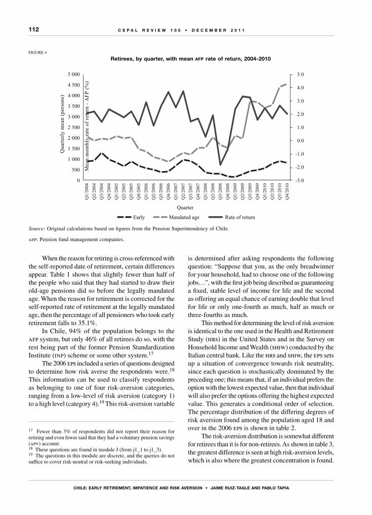
112
CHILE: EARLy REtIREMEnt, IMPAtIEnCE AnD RIsk AVERsIon • jAIME RuIz-tAgLE AnD PABLo tAPIA
C E P A L R E V I E W 1 0 5 • D E C E M B E R 2 0 1 1
When the reason for retiring is cross-referenced with the self-reported date of retirement, certain differences appear. Table 1 shows that slightly fewer than half of the people who said that they had started to draw their old-age pensions did so before the legally mandated age. When the reason for retirement is corrected for the self-reported rate of retirement at the legally mandated age, then the percentage of all pensioners who took early retirement falls to 35.1%.
In Chile, 94% of the population belongs to the afp system, but only 46% of all retirees do so, with the rest being part of the former Pension Standardization Institute (inp) scheme or some other system.17
The 2006 eps included a series of questions designed to determine how risk averse the respondents were.18 This information can be used to classify respondents as belonging to one of four risk-aversion categories, ranging from a low-level of risk aversion (category 1) to a high level (category 4).19 This risk-aversion variable
17 Fewer than 3% of respondents did not report their reason for retiring and even fewer said that they had a voluntary pension savings (apv) account.18 These questions are found in module J (from j1_1 to j1_3).19 The questions in this module are discrete, and the queries do not suffice to cover risk-neutral or risk-seeking individuals.
is determined after asking respondents the following question: “Suppose that you, as the only breadwinner for your household, had to choose one of the following jobs…”, with the first job being described as guaranteeing a fixed, stable level of income for life and the second as offering an equal chance of earning double that level for life or only one-fourth as much, half as much or three-fourths as much.
This method for determining the level of risk aversion is identical to the one used in the Health and Retirement Study (hrs) in the United States and in the Survey on Household Income and Wealth (shiw) conducted by the Italian central bank. Like the hrs and shiw, the eps sets up a situation of convergence towards risk neutrality, since each question is stochastically dominated by the preceding one; this means that, if an individual prefers the option with the lowest expected value, then that individual will also prefer the options offering the highest expected value. This generates a conditional order of selection. The percentage distribution of the differing degrees of risk aversion found among the population aged 18 and over in the 2006 eps is shown in table 2.
The risk-aversion distribution is somewhat different for retirees than it is for non-retirees. As shown in table 3, the greatest difference is seen at high risk-aversion levels, which is also where the greatest concentration is found.
FIGURE 4
retirees, by quarter, with mean afp rate of return, 2004-2010
Source: Original calculations based on figures from the Pension Superintendency of Chile.
afp: Pension fund management companies.
-3.0
-2.0
-1.0
0.0
1.0
2.0
3.0
4.0
5.0
0
500
1 000
1 500
2 000
2 500
3 000
3 500
4 000
4 500
5 000
Q1
/2004
Q2
/2004
Q3
/2004
Q4
/2004
Q1
/2005
Q2
/2005
Q3
/2005
Q4
/2005
Q1
/2006
Q2
/2006
Q3
/2006
Q4
/2006
Q1
/2007
Q2
/2007
Q3
/2007
Q4
/2007
Q1
/2008
Q2
/2008
Q3
/2008
Q4
/2008
Q1
/2009
Q2
/2009
Q3
/2009
Q4
/2009
Q1
/2010
Q2
/2010
Q3
/2010
Q4
/2010
Mean
mo
nth
ly r
ate
of
retu
rn -
AF
P (
%)
Qu
art
erl
y m
ean
(p
ers
on
s)
Quarter
Early Mandated age Rate of return
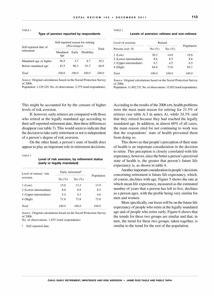
113
CHILE: EARLy REtIREMEnt, IMPAtIEnCE AnD RIsk AVERsIon • jAIME RuIz-tAgLE AnD PABLo tAPIA
C E P A L R E V I E W 1 0 5 • D E C E M B E R 2 0 1 1
This might be accounted for by the censure of higher levels of risk aversion.
If, however, early retirees are compared with those who retired at the legally mandated age according to their self-reported retirement date, then these differences disappear (see table 3). This would seem to indicate that the decision to take early retirement or not is independent of a person’s degree of risk aversion.
On the other hand, a person’s state of health does appear to play an important role in retirement decisions.
TABLE 1
Type of pension reported by respondents
Self-reported date of retirement
Self-reported reason for retiring (Percentages)
TotalMandated
ageEarly Disability
Mandated age or higher 56.5 3.7 8.7 35.1
Before mandated age 43.5 96.3 91.3 64.9
Total 100.0 100.0 100.0 100.0
Source: Original calculations based on the Social Protection Survey of 2006.Population: 1,129.325; No. of observations: 2,375 (total respondents).
TABLE 2
Levels of aversion: retirees and non-retirees
Level of aversion RetiredPopulation
Persons over 18 No (%) Yes (%)
1 (Low) 20.3 14.0 19.82 (Lower-intermediate) 8.6 8.5 8.63 (Upper-intermediate) 6.7 4.5 6.54 (High) 64.4 73.0 65.1
Total 100.0 100.0 100.0
Source: Original calculations based on the Social Protection Survey of 2006.Population: 11,492,732. No. of observations: 15,052 (total respondents).
TABLE 3
Level of risk aversion, by retirement status (early or legally mandated)
Level of retirees’ risk aversion
Early retirementa
PopulationNo (%) Yes (%)
1 (Low) 15.0 13.2 13.9
2 (Lower-intermediate) 8.0 8.8 8.5
3 (Upper-intermediate) 5.4 4.2 4.6
4 (High) 71.6 73.8 73.0
Total 100.0 100.0 100.0
Source: Original calculations based on the Social Protection Survey of 2006.No. of observations: 1,875 (total respondents).
a Self-reported date.
According to the results of the 2006 eps, health problems were the most main reason for retiring for 21.5% of retirees (see table A.3 in annex A), while 24.3% said that they retired because they had reached the legally mandated age. In addition, in almost 60% of all cases, the main reason cited for not continuing to work was that the respondents’ state of health prevented them from doing so.
This shows us that people’s perception of their state of health is an important consideration in the decision to retire. This perception is closely correlated with life expectancy, however, since the better a person’s perceived state of health is, the greater that person’s future life expectancy is, as shown in table 4.
Another important consideration in people’s decisions concerning retirement is future life expectancy, which, of course, declines with age. Figure 5 shows the rate at which mean life expectancy, measured as the estimated number of years that a person has left to live, declines as a person ages, with the profile being very similar for men and women.
More specifically, our focus will be on the future life expectancy of people who retire at the legally mandated age and of people who retire early. Figure 6 shows that the trends for these two groups are similar and that, in turn, the trend for these two groups, taken together, is similar to the trend for the rest of the population.
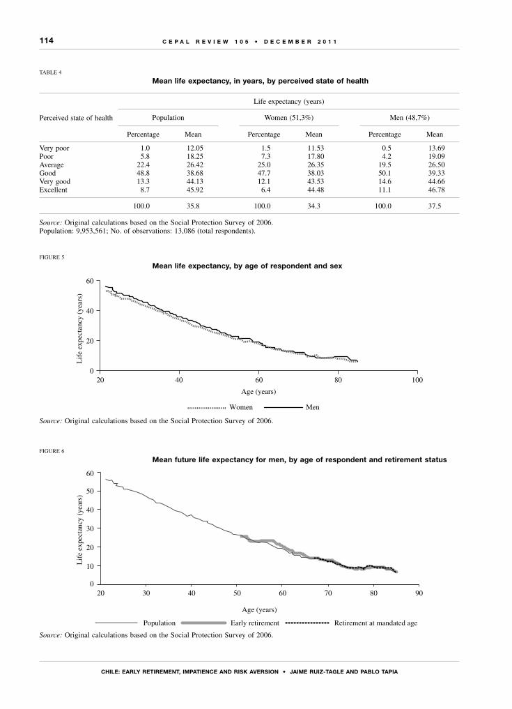
114
CHILE: EARLy REtIREMEnt, IMPAtIEnCE AnD RIsk AVERsIon • jAIME RuIz-tAgLE AnD PABLo tAPIA
C E P A L R E V I E W 1 0 5 • D E C E M B E R 2 0 1 1
TABLE 4
Mean life expectancy, in years, by perceived state of health
Perceived state of health
Life expectancy (years)
Population Women (51,3%) Men (48,7%)
Percentage Mean Percentage Mean Percentage Mean
Very poor 1.0 12.05 1.5 11.53 0.5 13.69Poor 5.8 18.25 7.3 17.80 4.2 19.09Average 22.4 26.42 25.0 26.35 19.5 26.50Good 48.8 38.68 47.7 38.03 50.1 39.33Very good 13.3 44.13 12.1 43.53 14.6 44.66Excellent 8.7 45.92 6.4 44.48 11.1 46.78
100.0 35.8 100.0 34.3 100.0 37.5
Source: Original calculations based on the Social Protection Survey of 2006.Population: 9,953,561; No. of observations: 13,086 (total respondents).
FIGURE 5
Mean life expectancy, by age of respondent and sex
Source: Original calculations based on the Social Protection Survey of 2006.
FIGURE 6
Mean future life expectancy for men, by age of respondent and retirement status
Source: Original calculations based on the Social Protection Survey of 2006.
0
20
40
60
20 40 60 80 100
Age (years)
Lif
e ex
pect
ancy
(ye
ars)
Women Men
20 30 40 50 60 70 80 900
10
20
30
40
50
60
Age (years)
Lif
e ex
pect
ancy
(ye
ars)
Population Early retirement Retirement at mandated age

115
CHILE: EARLy REtIREMEnt, IMPAtIEnCE AnD RIsk AVERsIon • jAIME RuIz-tAgLE AnD PABLo tAPIA
C E P A L R E V I E W 1 0 5 • D E C E M B E R 2 0 1 1
and low level of risk aversion (27% of the sample) (see table 3).
The information that can be used to predict the degree of uncertainty surrounding a given event will influence what action a risk-averse person will take. The extent of a person’s knowledge about the financial market and pensions schemes was therefore taken into account.
Information on the geographical area in which respondents reside was also included, with the categories being northern zones (regions I-IV), central areas (regions V-VII) and southern areas (regions VIII-XII). The responses from these zones were then compared with those given in the Metropolitan Region.
The descriptive statistic for the variables to be used for the estimates is shown in table 6. When the average age of respondents and their expectation regarding future years of life are examined, it turns out that both the group of people who retired at the legally mandated age and the group of early retirees believe that they will live until nearly 80 years of age.
The descriptive statistic also indicates that a majority of early retirees are men (see table 6). The early retirees have lower monetary incomes, which could have to do with the fact that the percentage of the members of this group who are economically active is also lower, as is their lower average level of education.
The retirees in the sample belong to the afp pension scheme. Their level of knowledge concerning the afp system and the relevant pension plan is slightly lower than is the case for those who choose to retire at the legally mandated age. The level of knowledge concerning the financial market is similar in the two groups of retirees, however (see table 6).
2. Estimating the determinants of early retirement
Before examining these estimates, we should first review the features of the sample and the variables to be used. The sample is pared down on the basis of a series of considerations that need to be taken into account in order to arrive at these estimates. First of all, the requirements that must be met under Chilean law in order to be eligible for early retirement,20 the way in which this situation works out in practice, and the fact that respondents have in fact answered the questionnaire are all factors that restrict the number of observations.21 In addition, age ranges of 60-65 for women and 65-70 for men were set.
The variables that were used have to do with the determinants of the utility function. In this case, a vector is defined of variables representing traits of individuals, households and the labour market, along with those having to do with the pension system as such. This set of variables is shown in table 5.
Risk aversion is an intrinsic trait of each individual, and it was therefore defined as a parameter whose influence on early retirement decisions needed to be established. Because the risk-aversion variable exhibits little continuity, it had to be grouped into two categories: a high level of risk aversion (approximately 73% of the sample) and an upper-intermediate, lower-intermediate
20 Act No. 19.943.21 The 2006 eps covered 12,426,437 individuals based on 16,443 respondents, of whom 8.5% did not respond to the question regarding risk aversion.
TABLE 5
variables to be taken into consideration
Individual characteristics Household characteristics Other
Gender Head of household Knowledge about afp systemAge Marital status Knowledge about pension systemYears of schooling Number of children Knowledge about financial marketPerceived state of health Number of grandchildren Region of residence, by zonePerceived life expectancy Monetary income Years in labour marketLevel of risk aversion Assets Age at entry into labour market Home ownership Economically active
Source: Original calculations.

116
CHILE: EARLy REtIREMEnt, IMPAtIEnCE AnD RIsk AVERsIon • jAIME RuIz-tAgLE AnD PABLo tAPIA
C E P A L R E V I E W 1 0 5 • D E C E M B E R 2 0 1 1
TABLE 6
Characteristics of retirees at mandated age and early retirees in sample(Percentages)
Population: 134 934; Sample: 314 observations Retirees Women [38%] Men [62%]
VariablesMandated age
(34%)Early (66%)
Mandated age (54%)
Early (46%)
Mandated age (22%)
Early (78%)
Gender (male = 1) 0.40 0.73 Years of schooling 7.1 8.1 7.9 10.9 6.0 7.1Age (years) 65.3 66.1 63.4 62.4 68.1 67.4Perceived state of health (poor = 1 to excellent = 6) 3.4 3.4 3.3 3.4 3.5 3.4Perceived life expectancy (years) 14.7 12.4 16.5 14.9 11.9 11.5Level of aversion (high = 1) 0.7 0.8 0.8 0.8 0.7 0.8Head of household (yes = 1) 0.72 0.91 0.56 0.80 0.95 0.95
Marital status (partner present = 1) 0.48 0.64 0.43 0.18 0.54 0.81Number of children 0.22 0.36 0.32 0.42 0.08 0.34Number of grandchildren 2.1 2.2 2.0 1.6 2.3 2.4Monetary income (M$ / 2006) $ 287 $ 270 $ 333 $ 238 $ 217 $ 282Assets (MM$ / 2006) $ 19.85 $ 25.05 $ 21.88 $ 20.02 $ 16.75 $ 26.90Debts (MM$ / 2006) $ 0.54 $ 0.86 $ 0.84 $ 1.87 $ 0.08 $ 0.49Home ownership (yes = 1) 0.87 0.88 0.88 0.81 0.87 0.91
Knowledge of afp system (<%>) 0.35 0.40 0.37 0.45 0.31 0.38Knowledge of pension system (<%>) 0.29 0.40 0.29 0.36 0.28 0.42Knowledge of financial market (yes = 1) 0.06 0.05 0.06 0.05 0.06 0.06Northern zone 0.11 0.12 0.15 0.11 0.05 0.13Central zone 0.30 0.17 0.24 0.13 0.38 0.19Southern zone 0.19 0.17 0.13 0.10 0.29 0.20Years in labour market 43.3 39.4 40.1 33.9 48.1 41.5Age at entry into labour market 19.0 17.4 19.9 21.2 17.5 16.1Economically active (yes = 1) 0.35 0.43 0.35 0.33 0.36 0.46
Source: Original calculations based on the Social Protection Survey of 2006.
Men: 65 - 70 years; women: 60 - 65 years.Note: M$ = Thousands of pesos; MM$ = Millions of pesos.
(a) The estimatesIn order to arrive at an estimate for the model
proposed in equation (13), it will be assumed that the errors follow a normal distribution based on a normal equivalent deviation (probit). The results, with different specifications, are shown in table 7.
The estimates of the marginal effects for the model given in table 7 are shown in table 8.
The estimates indicate that the effect of future life expectancy on the probability of taking early retirement (parameter Ωi) is negative and significant, with a stable value for all the models (values of between -0.38 and -0.46). The effect of the combined component of life expectancy and risk aversion (parameter Λi) is positive, but its significance changes if the life expectancy variable is not included. This may be because the proxy is unsatisfactory or because risk aversion is also affected by other factors, such as financial exposure.
Other variables, such as years of schooling completed, gender (male) and being economically active, increase the utility of early retirement and have a positive influence on the probability of taking early retirement
(see table 7). Similar results are reported by Gustman and Steinmeier (2005).22 As people grow older, however, they become less likely to take early retirement. This finding is corroborated by the estimates arrived at here and by other studies (Mitchell and Phillips, 2000).
If people place greater value on their present quality of life than on their future quality of life, and if this translates into spending more time with their loved ones, then having children and being married should increase the probability of taking early retirement. The estimates corroborate this hypothesis, since the variables of marital status (being in a conjugal union) and of having children23 are positive and significant, as shown in tables 7 and 8. This finding is also reported by Mitchell and Phillips (2000).
22 Their estimates are focused on how the social security system and other factors influence retirement decisions, rather than early retirement decisions, but their findings also support the estimates calculated in this study.23 When the presence of children (regardless of origin) is the variable that is used, the level of significance is greater than when it is restricted to children within the household.
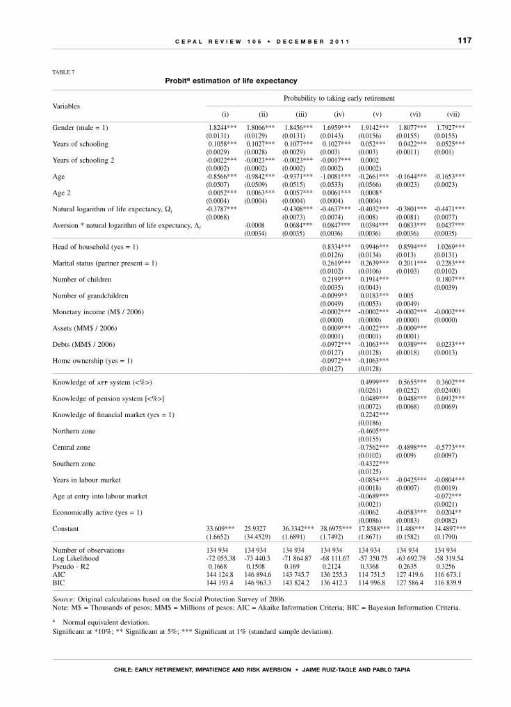
117
CHILE: EARLy REtIREMEnt, IMPAtIEnCE AnD RIsk AVERsIon • jAIME RuIz-tAgLE AnD PABLo tAPIA
C E P A L R E V I E W 1 0 5 • D E C E M B E R 2 0 1 1
TABLE 7
Probita estimation of life expectancy
VariablesProbability to taking early retirement
(i) (ii) (iii) (iv) (v) (vi) (vii)
Gender (male = 1) 1.8244*** (0.0131)
1.8066*** (0.0129)
1.8456*** (0.0131)
1.6959*** (0.0143)
1.9142*** (0.0156)
1.8077*** (0.0155)
1.7927*** (0.0155)
Years of schooling 0.1058*** (0.0029)
0.1027*** (0.0028)
0.1077*** (0.0029)
0.1027*** (0.003)
0.052*** (0.003)
0.0422*** (0.0011)
0.0525*** (0.001)
Years of schooling 2 -0.0022*** (0.0002)
-0.0023*** (0.0002)
-0.0023*** (0.0002)
-0.0017*** (0.0002)
0.0002 (0.0002)
Age -0.8566*** (0.0507)
-0.9842*** (0.0509)
-0.9371*** (0.0515)
-1.0081*** (0.0533)
-0.2661*** (0.0566)
-0.1644*** (0.0023)
-0.1653*** (0.0023)
Age 2 0.0052*** (0.0004)
0.0063*** (0.0004)
0.0057*** (0.0004)
0.0061*** (0.0004)
0.0008* (0.0004)
Natural logarithm of life expectancy, Ωi -0.3787*** (0.0068)
-0.4308*** (0.0073)
-0.4637*** (0.0074)
-0.4032*** (0.008)
-0.3801*** (0.0081)
-0.4471*** (0.0077)
Aversion * natural logarithm of life expectancy, Λi -0.0008 (0.0034)
0.0684*** (0.0035)
0.0847*** (0.0036)
0.0394*** (0.0036)
0.0833*** (0.0036)
0.0437*** (0.0035)
Head of household (yes = 1) 0.8334*** (0.0126)
0.9946*** (0.0134)
0.8594*** (0.013)
1.0269*** (0.0131)
Marital status (partner present = 1) 0.2619*** (0.0102)
0.2639*** (0.0106)
0.2011*** (0.0103)
0.2283*** (0.0102)
Number of children 0.2199*** (0.0035)
0.1914*** (0.0043)
0.1807*** (0.0039)
Number of grandchildren -0.0099** (0.0049)
0.0183*** (0.0053)
0.005 (0.0049)
Monetary income (M$ / 2006) -0.0002*** (0.0000)
-0.0002*** (0.0000)
-0.0002*** (0.0000)
-0.0002*** (0.0000)
Assets (MM$ / 2006) 0.0009*** (0.0001)
-0.0022*** (0.0001)
-0.0009*** (0.0001)
Debts (MM$ / 2006) -0.0972*** (0.0127)
-0.1063*** (0.0128)
0.0389*** (0.0018)
0.0233*** (0.0013)
Home ownership (yes = 1) -0.0972*** (0.0127)
-0.1063*** (0.0128)
Knowledge of afp system (<%>) 0.4999*** (0.0261)
0.5655*** (0.0252)
0.3602*** (0.02400)
Knowledge of pension system [<%>] 0.0489*** (0.0072)
0.0488*** (0.0068)
0.0932*** (0.0069)
Knowledge of financial market (yes = 1) 0.2242*** (0.0186)
Northern zone -0.4605*** (0.0155)
Central zone -0.7562*** (0.0102)
-0.4898*** (0.009)
-0.5773*** (0.0097)
Southern zone -0.4322*** (0.0125)
Years in labour market -0.0854*** (0.0018)
-0.0425*** (0.0007)
-0.0804*** (0.0019)
Age at entry into labour market -0.0689*** (0.0021)
-0.072*** (0.0021)
Economically active (yes = 1) -0.0062 (0.0086)
-0.0583*** (0.0083)
0.0204** (0.0082)
Constant 33.609*** (1.6652)
25.9327 (34.4529)
36.3342*** (1.6891)
38.6975*** (1.7492)
17.8588*** (1.8671)
11.488*** (0.1582)
14.4897*** (0.1790)
Number of observations 134 934 134 934 134 934 134 934 134 934 134 934 134 934Log Likelihood -72 055.38 -73 440.3 -71 864.87 -68 111.67 -57 350.75 -63 692.79 -58 319.54Pseudo - R2 0.1668 0.1508 0.169 0.2124 0.3368 0.2635 0.3256AIC 144 124.8 146 894.6 143 745.7 136 255.3 114 751.5 127 419.6 116 673.1BIC 144 193.4 146 963.3 143 824.2 136 412.3 114 996.8 127 586.4 116 839.9
Source: Original calculations based on the Social Protection Survey of 2006.Note: M$ = Thousands of pesos; MM$ = Millions of pesos; AIC = Akaike Information Criteria; BIC = Bayesian Information Criteria.
a Normal equivalent deviation.Significant at *10%; ** Significant at 5%; *** Significant at 1% (standard sample deviation).
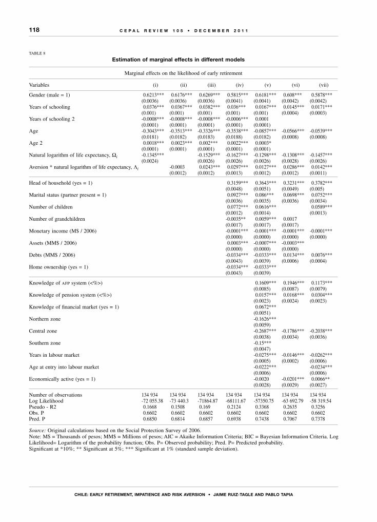
118
CHILE: EARLy REtIREMEnt, IMPAtIEnCE AnD RIsk AVERsIon • jAIME RuIz-tAgLE AnD PABLo tAPIA
C E P A L R E V I E W 1 0 5 • D E C E M B E R 2 0 1 1
TABLE 8
Estimation of marginal effects in different models
Marginal effects on the likelihood of early retirement
Variables (i) (ii) (iii) (iv) (v) (vi) (vii)
Gender (male = 1) 0.6213*** (0.0036)
0.6176*** (0.0036)
0.6269*** (0.0036)
0.5815*** (0.0041)
0.6181*** (0.0041)
0.608*** (0.0042)
0.5878*** (0.0042)
Years of schooling 0.0376*** (0.001)
0.0367*** (0.001)
0.0382*** (0.001)
0.036*** (0.001)
0.0167*** (0.001)
0.0145*** (0.0004)
0.0171*** (0.0003)
Years of schooling 2 -0.0008*** (0.0001)
-0.0008*** (0.0001)
-0.0008*** (0.0001)
-0.0006*** (0.0001)
0.0001 (0.0001)
Age -0.3043*** (0.0181)
-0.3513*** (0.0182)
-0.3326*** (0.0183)
-0.3538*** (0.0188)
-0.0857*** (0.0182)
-0.0566*** (0.0008)
-0.0539*** (0.0008)
Age 2 0.0018*** (0.0001)
0.0023*** (0.0001)
0.002*** (0.0001)
0.0022*** (0.0001)
0.0003* (0.0001)
Natural logarithm of life expectancy, Ωi -0.1345*** (0.0024)
-0.1529*** (0.0026)
-0.1627*** (0.0026)
-0.1298*** (0.0026)
-0.1308*** (0.0028)
-0.1457*** (0.0026)
Aversion * natural logarithm of life expectancy, Λi -0.0003 (0.0012)
0.0243*** (0.0012)
0.0297*** (0.0013)
0.0127*** (0.0012)
0.0286*** (0.0012)
0.0142*** (0.0011)
Head of household (yes = 1) 0.3159*** (0.0048)
0.3643*** (0.0051)
0.3231*** (0.0049)
0.3782*** (0.005)
Marital status (partner present = 1) 0.0927*** (0.0036)
0.086*** (0.0035)
0.0698*** (0.0036)
0.0752*** (0.0034)
Number of children 0.0772*** (0.0012)
0.0616*** (0.0014)
0.0589*** (0.0013)
Number of grandchildren -0.0035** (0.0017)
0.0059*** (0.0017)
0.0017 (0.0017)
Monetary income (M$ / 2006) -0.0001*** (0.0000)
-0.0001*** (0.0000)
-0.0001*** (0.0000)
-0.0001*** (0.0000)
Assets (MM$ / 2006) 0.0003*** (0.0000)
-0.0007*** (0.0000)
-0.0003*** (0.0000)
Debts (MM$ / 2006) -0.0334*** (0.0043)
-0.0333*** (0.0039)
0.0134*** (0.0006)
0.0076*** (0.0004)
Home ownership (yes = 1) -0.0334*** (0.0043)
-0.0333*** (0.0039)
Knowledge of afp system (<%>) 0.1609*** (0.0085)
0.1946*** (0.0087)
0.1173*** (0.0079)
Knowledge of pension system (<%>) 0.0157*** (0.0023)
0.0168*** (0.0024)
0.0304*** (0.0023)
Knowledge of financial market (yes = 1) 0.0672*** (0.0051)
Northern zone -0.1626*** (0.0059)
Central zone -0.2687*** (0.0038)
-0.1786*** (0.0034)
-0.2038*** (0.0036)
Southern zone -0.15*** (0.0047)
Years in labour market -0.0275*** (0.0005)
-0.0146*** (0.0002)
-0.0262*** (0.0006)
Age at entry into labour market -0.0222*** (0.0006)
-0.0234*** (0.0006)
Economically active (yes = 1) -0.0020 (0.0028)
-0.0201*** (0.0029)
0.0066** (0.0027)
Number of observations 134 934 134 934 134 934 134 934 134 934 134 934 134 934Log Likelihood -72 055.38 -73 440.3 -71864.87 -68111.67 -57350.75 -63 692.79 -58 319.54Pseudo - R2 0.1668 0.1508 0.169 0.2124 0.3368 0.2635 0.3256Obs. P 0.6602 0.6602 0.6602 0.6602 0.6602 0.6602 0.6602Pred. P 0.6850 0.6814 0.6857 0.6938 0.7438 0.7067 0.7378
Source: Original calculations based on the Social Protection Survey of 2006.Note: M$ = Thousands of pesos; MM$ = Millions of pesos; AIC = Akaike Information Criteria; BIC = Bayesian Information Criteria. Log Likelihood= Logarithm of the probability function; Obs. P= Observed probability; Pred. P= Predicted probability.Significant at *10%; ** Significant at 5%; *** Significant at 1% (standard sample deviation).
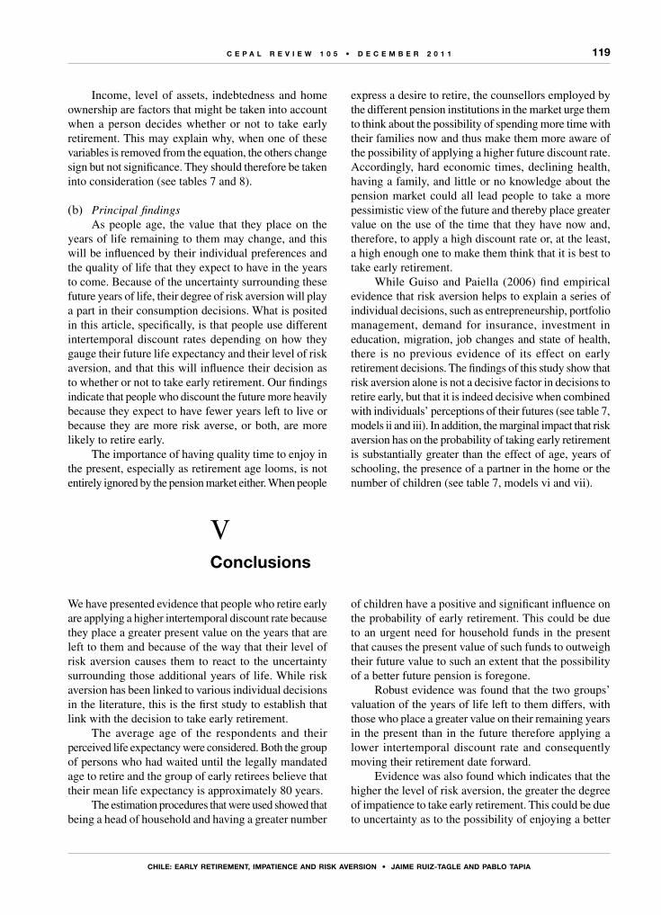
119
CHILE: EARLy REtIREMEnt, IMPAtIEnCE AnD RIsk AVERsIon • jAIME RuIz-tAgLE AnD PABLo tAPIA
C E P A L R E V I E W 1 0 5 • D E C E M B E R 2 0 1 1
Income, level of assets, indebtedness and home ownership are factors that might be taken into account when a person decides whether or not to take early retirement. This may explain why, when one of these variables is removed from the equation, the others change sign but not significance. They should therefore be taken into consideration (see tables 7 and 8).
(b) Principal findingsAs people age, the value that they place on the
years of life remaining to them may change, and this will be influenced by their individual preferences and the quality of life that they expect to have in the years to come. Because of the uncertainty surrounding these future years of life, their degree of risk aversion will play a part in their consumption decisions. What is posited in this article, specifically, is that people use different intertemporal discount rates depending on how they gauge their future life expectancy and their level of risk aversion, and that this will influence their decision as to whether or not to take early retirement. Our findings indicate that people who discount the future more heavily because they expect to have fewer years left to live or because they are more risk averse, or both, are more likely to retire early.
The importance of having quality time to enjoy in the present, especially as retirement age looms, is not entirely ignored by the pension market either. When people
express a desire to retire, the counsellors employed by the different pension institutions in the market urge them to think about the possibility of spending more time with their families now and thus make them more aware of the possibility of applying a higher future discount rate. Accordingly, hard economic times, declining health, having a family, and little or no knowledge about the pension market could all lead people to take a more pessimistic view of the future and thereby place greater value on the use of the time that they have now and, therefore, to apply a high discount rate or, at the least, a high enough one to make them think that it is best to take early retirement.
While Guiso and Paiella (2006) find empirical evidence that risk aversion helps to explain a series of individual decisions, such as entrepreneurship, portfolio management, demand for insurance, investment in education, migration, job changes and state of health, there is no previous evidence of its effect on early retirement decisions. The findings of this study show that risk aversion alone is not a decisive factor in decisions to retire early, but that it is indeed decisive when combined with individuals’ perceptions of their futures (see table 7, models ii and iii). In addition, the marginal impact that risk aversion has on the probability of taking early retirement is substantially greater than the effect of age, years of schooling, the presence of a partner in the home or the number of children (see table 7, models vi and vii).
VConclusions
We have presented evidence that people who retire early are applying a higher intertemporal discount rate because they place a greater present value on the years that are left to them and because of the way that their level of risk aversion causes them to react to the uncertainty surrounding those additional years of life. While risk aversion has been linked to various individual decisions in the literature, this is the first study to establish that link with the decision to take early retirement.
The average age of the respondents and their perceived life expectancy were considered. Both the group of persons who had waited until the legally mandated age to retire and the group of early retirees believe that their mean life expectancy is approximately 80 years.
The estimation procedures that were used showed that being a head of household and having a greater number
of children have a positive and significant influence on the probability of early retirement. This could be due to an urgent need for household funds in the present that causes the present value of such funds to outweigh their future value to such an extent that the possibility of a better future pension is foregone.
Robust evidence was found that the two groups’ valuation of the years of life left to them differs, with those who place a greater value on their remaining years in the present than in the future therefore applying a lower intertemporal discount rate and consequently moving their retirement date forward.
Evidence was also found which indicates that the higher the level of risk aversion, the greater the degree of impatience to take early retirement. This could be due to uncertainty as to the possibility of enjoying a better

120
CHILE: EARLy REtIREMEnt, IMPAtIEnCE AnD RIsk AVERsIon • jAIME RuIz-tAgLE AnD PABLo tAPIA
C E P A L R E V I E W 1 0 5 • D E C E M B E R 2 0 1 1
AnnEx A
Supplementary tables
Module J of the 2006 Social Protection Survey (eps) contains three questions (j1_1 - j1_3) that are used to place the respondents at one of four different levels of risk aversion, ranging from the lowest (1) to the highest level of aversion (4).
TABLE A.1
Population distribution, by sex, economic activity status and level of risk aversion
Level of aversionPopulationdistribution
Sex Working Retired
Women Men No Yes No Yes
1 (Low) 2 278 115 964 894 1 313 221 871 829 1 406 286 2 146 101 132 0142 (Lower-intermediate) 985 508 464 222 521 286 398 050 587 458 905 571 79 9373 (Upper-intermediate) 750 826 361 057 389 769 327 635 423 191 708 212 42 6144 (Alto) 7 478 283 3 975 611 3 502 672 3 360 807 4 117 476 6 789 315 688 968
Total 11 492 732 5 765 784 5 726 948 4 958 321 6 534 411 10 549 199 943 533
Source: Original calculations based on the Social Protection Survey (eps) of 2006.
TABLE A.2
Membership in pension systems
Pension System
Population Retirees
System No. Percentage No. Percentage
afp 7 550 278 88.5 338 274 41.3inp 849 219 10.0 421 799 51.5capredena 25 260 0.3 9 123 1.1dipreca 26 228 0.3 5 173 0.6Other 81 157 1.0 44 543 5.4
Total 8 532 142 100.0 818 912 100.0
Source: Original calculations based on the Social Protection Survey (eps) of 2006. Respondents self-reported their pension system membership.
afp: Pension fund management companies.inp: Pension Standardization Institute.capredena: National Defence Pension Fund.dipreca: Carabineros Pension Administration.
quality of life in the future. It would therefore be more beneficial to discount future utility more heavily and to prefer to enjoy a better present quality of life. These effects overshadow other variables such as age, years of schooling and household structure.
This analysis thus offers evidence that supports the hypothesis of heterogeneity in intertemporal discount rates
linked to future life expectancy, which is heightened by uncertainty about future quality of life. As an extrapolation from these conclusions, it can be posited that situations such as economic crises, increased uncertainty as to the possibility of enjoying quality time in the future and small monetary shocks can increase the probability of early retirement as well.
(Original: Spanish)

121
CHILE: EARLy REtIREMEnt, IMPAtIEnCE AnD RIsk AVERsIon • jAIME RuIz-tAgLE AnD PABLo tAPIA
C E P A L R E V I E W 1 0 5 • D E C E M B E R 2 0 1 1
TABLE A.3
retirees in the afp system: retirees at the legally mandated age and early retirees
Reasons for retiring
Retired population (Percentages)
Total Mandated age [No. = 34,929]
Early [No. = 51,556]
To increase income by undertaking new income-generating activities 24.9 8.5 36.0To use disposable funds or surpluses 4.8 3.1 6.0Convinced to do so by a sales agent 1.1 0.0 1.8Health problems 21.5 24.3 19.5To devote time to other, non-occupational activities 6.0 3.6 7.6Completed years of service (inp, dipreca or capredena) 8.7 15.4 4.2The company offered a buy-out 3.8 3.7 3.9Because was performing heavy labour 0.5 0.0 0.7Became unemployed and little time remained until retirement age 5.9 0.2 9.3Received a gift or money from a sales agent 0.0 0.0 0.0Reached legally mandated retirement age 20.0 40.4 6.2Other 2.9 0.0 4.9
Total 100.0 100.0 100.0
Source: Original calculations based on the Social Protection Survey (eps) of 2006.
inp: Pension Standardization Institute.capredena: National Defence Pension Fund.dipreca: Carabineros Pension Administration.
Bibliography
Au, A., O. Mitchell and J. Phillips (2005), “Saving shortfalls and delayed retirement”, Working Paper, No. WP-094, Michigan, Michigan Retirement Research Center, University of Michigan.
Bleichrodt, H. and J. Quiggin (1999), “Life-cycle preferences over consumption and health: when is cost-effectiveness analysis equivalent to cost-benefit analysis?”, Journal of Health Economics, vol. 18, No. 6, Amsterdam, Elsevier.
Chai, J. and others (2009), “Extending life cycle models of optimal portfolio choice: integrating flexible work, endogenous retirement, and investment decisions with lifetime payouts”, nber Working Paper, No. 15079, Cambridge, Massachusetts, National Bureau of Economic Research.
Deaton, A. and J. Muellbauer (1980), “An almost ideal demand system”, American Economic Review, vol. 70, No. 3, Nashville, Tennessee, American Economic Association.
Diamond, P. and B. Köszegi (2003), “Quasi-hyperbolic discounting and retirement”, Journal of Public Economics, vol. 87, No. 9-10, Amsterdam, Elsevier.
Engen, E.M, W.G. Gale and C. Uccello (1999), “The adequacy of retirement saving”, Brookings Papers en Economic Activity, vol. 30, No. 2, Washington, D.C., The Brookings Institution.
French, E. (2005), “The effects of health, wealth, and wages on labour supply and retirement behavior”, Review of Economic Studies, vol. 72, No. 2, John Wiley & Sons.
Guiso, L. and M. Paiella (2008), “Risk aversion, wealth, and background risk”, Journal of the European Economic Association, vol. 6, No. 6, Cambridge, Massachusetts, mit Press.
(2006), “The role of risk aversion in predicting individual behavior”, Insurance: Theoretical Analysis and Policy Implications, P. Chiappori and C. Gollier (eds.), cesifo.
Gustman, A. and T. Steinmeier (2005), “The social security early entitlement age in a structural model of retirement and wealth”, Journal of Public Economics, vol. 89, No. 2-3, Amsterdam, Elsevier.
Hairault, J-O., F. Langot and T. Sopraseuth (2010), “Distance to retirement and older workers’ employment: the case for delaying the retirement age”, Journal of the European Economic Association, vol. 8, No. 5, Cambridge, Massachusetts, mit Press, September.
Hammitt, J., K. Haninger and N. Treich (2005), “The effects of health and longevity on risk tolerance”, Boston, Harvard Center for Risk Analysis.
Hensher, D., P. Barnard and P. Truong (1988), “The role of stated preference methods in studies of travel choice”, Journal of Transport Economics and Policy, vol. 22, No. 1, Bath, University of Bath.
Mitchell, O. and J. Phillips (2000), “Retirement responses to early social security benefit reductions”, Working Paper, No. WP-006, Michigan, Michigan Retirement Research Center, University of Michigan.
Nalebuff, B. and R. Zeckhauser (1985), “Pensions and the retirement decision”, Pensions, Labor, and Individual Choice, David A. Wise (comp.), Cambridge, Massachusetts, National Bureau of Economic Research.
Nordhaus, W.D. (2002), “The health of nations: the contribution of improved health to living standars”, nber Working Paper, No. 8818, Cambridge, Massachusetts, National Bureau of Economic Research.
Poterba, J., J. Rauh and S. Venti (2005), “Utility evaluation of risk in retirement saving accounts”, Analyses in the Economics of Aging, Chicago, University of Chicago Press.

C E P A L R E V I E W 1 0 5 • D E C E M B E R 2 0 1 1
123
K E Y W O R D S
Business enterprises
Industrial enterprises
Corporate financing
Investment
Profit
Corporate debt
Statistical data
Peru
Profit margins, financing and investment in the Peruvianbusiness sector (1998-2008)
Germán Alarco T.
This paper develops a model and explains the determinants of profit
margins in the Peruvian business sector in the 1998-2008 period. These
are established in a fixed-price scenario, with reference to a set of variables
such as the price elasticity of demand, the behaviour of possible industry
entrants and any regulatory intervention by government. In addition,
there is a direct relationship between profit margins and self-financing
of investment. Profit margins and profit ratios in the business sector are
rising and exceed international norms. The paper also identifies a trend
towards lower levels of debt and leverage. It does not reject the hypothesis
of linkage between profit margins and investment at the aggregate and
sectoral level. The output-to-capital ratio or sales-to-assets ratio is directly
linked to profit margins. Most investment is self-financed.
Germán Alarco T.
Principal Research Fellow and
Professor at centrum Católica
Catholic University of Peru
124
PRofIt MARgIns, fInAnCIng AnD InVEstMEnt In tHE PERuVIAn BusInEss sECtoR (1998-2008) • gERMán ALARCo t.
C E P A L R E V I E W 1 0 5 • D E C E M B E R 2 0 1 1
The economic performance of Peru has been positive over the last decade. The average annual rate of gross domestic product (gdp) growth up to 2009, including the negative effects of the international financial crisis, was 5.3%. Inflation in the same period was low, averaging 2.5% a year. A positive trade balance resulted in the build-up of a substantial quantity of international reserves. The public finances were kept in reasonable balance. Both pay and the operating surplus grew in real terms. However, these positive macroeconomic results went together with greater inequality in the functional distribution of income, with the operating surplus gaining at the expense of remuneration as a share of output.
Between 2000 and 2009, remunerations as a share of gdp fell from 24.4% to 22%, while in the same period the operating surplus rose from 59.1% to 62.8% of national output (inei, 2011). In no other Latin American economy are remunerations such a small share of gdp as in Peru (Lindenboim, 2008). Drawing on long-term statistical information, we find that remunerations fell from just under 40% of output in the mid-1950s to just over half this level in 2009 (Alarco, 2010b). The labour market factors that might have contributed to this are various, but one important point is that the increasing share of income represented by the operating surplus has been matched by an increase in profit margins in a substantial number of economic activities.
The fact that profit margins are high by international standards is due to the predominance of market structures closer to imperfect competition than more competitive ones with a greater presence of activities that yield substantial economic rents, such as mining and hydrocarbons. In the first group of sectors, these higher margins mean higher domestic prices and lower real remunerations, negatively impacting demand and gdp unless accompanied by higher levels of exports and private-sector investment. Investment as a proportion of gdp rose from 19.6% in 2000 to 23.7% in 2009, having peaked at 29.2% in 2008. In other circumstances, the
I am grateful for the assistance of Paul Durand Villarroel as general project assistant, to Patricia Del Hierro Carrillo for her suggestions, and to the anonymous referees who commented on this paper.
combination of greater inequality and lower exports or lower investment or both would not be a good recipe for economic growth.
This paper will use information from businesses to illustrate the evolution of the operating surplus in the main production sectors and the evolution of profit margins in the Peruvian economy as a whole and the main economic activities between 1998 and 2008. It will employ a post-Keynesian approach to establish the determinants of profit margins, focusing exclusively on fixed-price scenarios. Lastly, it will assess the relationship between profit margins and investment.
Formally, this article contains the following sections. Section II presents the theoretical discussion on profit margins. Section III introduces the basic model relating profit margins to microeconomic and then macroeconomic price-setting. Section IV deals with sources, information processing and the main results of the aggregate information and that furnished by businesses. It analyses the compatibility of the theoretical framework with the statistical information available. Lastly, some final considerations are offered.
This article does not analyse modes of price-setting or profit determination other than the post-Keynesian one. It does not consider the effects on profit margins of competition between firms, or the effects of trade opening. Nor does it evaluate the likely reaction of government competition authorities, which would be expected to act if profit margins became very high. There is no analysis of growth and concentration processes as in Alarco (2010a), or of technical change, corporate behaviour in the presence of higher profit margins, or the appearance of new barriers to entry. Nor does the paper discuss all the problems associated with the fact that the operating surplus in Peru encompasses company earnings, rents and self-employed workers’ income, among other elements.1
1 The Central Reserve Bank of Peru (bcrp) published the details of the operating surplus from 1960 to the mid-1970s. Subsequently, the National Institute of Statistics and Informatics (inei) integrated all the earlier concepts, but currently only presents homogeneous series from 1991 onward.
Iintroduction
125
PRofIt MARgIns, fInAnCIng AnD InVEstMEnt In tHE PERuVIAn BusInEss sECtoR (1998-2008) • gERMán ALARCo t.
C E P A L R E V I E W 1 0 5 • D E C E M B E R 2 0 1 1
Kalecki (1956, pp. 11-12) focuses on products determined mainly by changes in production costs, as opposed to those explained by changes in demand (especially agricultural products). In the first group of products, supply is elastic because there is spare installed capacity. It is also assumed that costs per unit produced do not alter when production rises. Higher demand is responded to by a rising volume of output, without any tendency for prices to change. The other component dealt with in passing by Kalecki is the presence of uncertainty in the pricing process, so that firms seek to maximize profits but do so in an imprecise way.
Under these conditions, any firm’s prices reflect its prime costs (cost of raw materials and payment of direct wages) and its degree of monopoly, which covers general costs (these being more or less fixed over time) and includes profits. The same author identifies at least four determinants of variations in the degree of monopoly: processes of concentration, sales promotion through advertising, protection of profits in depressed periods and the activity of labour unions, in some degree preventing monopoly power from increasing.
The more that concentration in an industry leads to the formation of larger firms, the greater the degree of monopoly will be. Prices will be higher in relation to prime costs when the structure of the market is less competitive. Likewise, the existence of more or less formal cartel-type agreements between producers will tend to increase the degree of monopoly. In another area, a rise in general costs may increase the degree of monopoly, particularly at times of recession and still more so when there is a tacit agreement between firms in the same industry to protect profits. Lastly, greater union action will prevent the degree of monopoly from increasing. If firms tend to increase their prices in the wake of wage adjustments, unions will apply renewed pressure, raising costs (Kalecki, 1956, pp. 17-19).
These markets subsequently came to be called “fixed-price” markets and monopoly was replaced by mark-up, which would likewise be applied to unit production costs (labour and raw materials). Ocampo (1988, p. 20) argues that theoretical analysis has led to the identification of two fundamental determinants of profit margins: competition conditions and corporate demand for investment funding. For Sylos Labini (1966), conversely, profit margins are set with the goal of limiting
the entry of new firms into the market. Markets contain firms of different sizes, large, medium-sized and small, with the largest firms generally taking the lead in price-setting but potentially being affected by the reactions and performance of smaller ones.
Sylos Labini (1969) argues that if the firm or firms with pricing power wish to prevent the entry of new firms of a particular type, they must undercut the price these firms need to charge to obtain the minimum rate of profit. If the firms with pricing power wish to force out firms already operating, they need to set the price at a level that undercuts the direct costs of the firms they are seeking to force out.
Steindl (1988) links firms’ profit margins to their investment funding requirements. Firms with higher profit margins accumulate funds internally, and the greater their differential advantage, the more they accumulate. For Steindl, an increase in an industry’s profit margin will lead to a rise in the internal accumulation rate, and this in turn will result in an increase in production capacity. If this increase is greater than the growth in the industry’s sales, it will lead to greater concentration benefiting the firm with the highest profit margin and level of accumulation. Ocampo (1988) comments that the existence of an oligopolistic or monopolistic context, with high entry barriers, makes the appearance of new firms in the sector unlikely, within certain limits.
Eichner (1988) then notes that profit margins depend on the demand for and supply of additional investment funding on the part of the firm or group of firms with pricing power in their industry. Firms can increase their margin over costs to obtain more internally generated funding, although they are constrained by: (i) the substitution effect, as higher margins make customers more likely to opt for a substitute product, (ii) the entry factor, with new firms overcoming the barriers to entry in the industry, and (iii) significant government intervention in response to increasing evidence of uncompetitive practices in the marketplace.
Eichner (1988, pp. 213-217) argues that the reduction in cash flow resulting from factors (i) and (ii) above is analogous to the reduction in financial flows resulting from the higher interest that would be payable on external financing. There is an implied rate of interest on additional funding generated internally. An increase in the margin over costs will increase the
IIDeterminants of profit margins

126
PRofIt MARgIns, fInAnCIng AnD InVEstMEnt In tHE PERuVIAn BusInEss sECtoR (1998-2008) • gERMán ALARCo t.
C E P A L R E V I E W 1 0 5 • D E C E M B E R 2 0 1 1
implied cost of additional investment funding. As the margin increases, the substitution effect and the entry factor would be expected to grow disproportionately, so that the implied interest rate would also rise at an increasing pace. When demand for investment is greater than can be financed internally whilst avoiding the substitution effect or the entry factor, use will be made of supplementary external financing.
Along the same lines, Wood (1988) argues that firms have to cope with two frontiers: a finance frontier and an opportunity frontier. The first of these concerns the relationship between a firm’s internal funding and its investment needs. The opportunity frontier, meanwhile, expresses the ratio between the profit margin, sales and the marginal investment-to-output ratio. As a firm’s profit margin rises, it generates more resources for growth but has to contend with a smaller increase in sales.
Harcourt and Kenyon (1988) argue that a firm has a twofold objective in setting its profit margin. First, pricing needs to be compatible with expectations of demand for what it produces. Second, it needs to be high enough to generate retained earnings sufficient to finance the firm’s investment plans. When firms succeed in setting sufficient retained earnings margins for them to expand capacity in line with demand growth in the market, the conditions are created for investment to maintain capacity growth that keeps up with demand in the context of a stable market share (Harcourt and Kenyon, 1988).
In this fixed-price scenario, neither temporary changes in variable costs nor temporary changes in product demand directly influence the price of the product. What happens is that the level of output adjusts to the level of demand in accordance with the business cycle. As Harcourt and Kenyon (1988, pp. 233 and 238) note, however, as demand and cost conditions change, the firm will realize that its plant capacity is inadequate
and new investment is required. In these circumstances, the firm will decide whether the flow of investment funding is appropriate to the current price level. If not, the price and investment decision-making process will have to be reopened.
Vargas (2007, p. 192) revisits the proposals of Eichner and Kregel and argues that, for post-Keynesians, the generation of internal funding to finance investment is the rule, while external financing is the exception when the implied interest rate is distinguished from the market interest rate. If the implied rate is lower than the market rate, the firm will increase its financing by raising prices. If not, the firm will prefer to finance itself through the money market. However, the authors conclude that nobody could calculate the point at which the demand for and supply of internal funding intercept.
For Vargas (2007, pp. 177 and 202), both the level of and changes in profit margins depend on a set of variables such as the substitution effect2 (price elasticity of demand), the behaviour and reaction of any entrants into the industry, any government intervention, the growth rate of the industry and the increase in the output-to-capital ratio relative to other industries. These last two variables are the counterpart of the firm’s investment decisions. In this regard, the main decisions for any firm’s managers are: (i) the targeted rate of return on investment, (ii) the new investment projects to be included in the annual capital budget, (iii) the profit margin required for their investment plans, (iv) the annual increase in salaries, wages and dividends, and (v) changes in the company’s debt level.
2 According to neoclassical microeconomics, the profit margin relative to price is equivalent to the inverse of the price elasticity of demand (Urzúa, 2009, p. 94) (P – cmg) / p = 1/η.
IIIThe basic model
The explanatory factors and determinants of profit margins are an issue that can be addressed in two spheres: at the microeconomic level and at the macroeconomic level. As noted earlier, a post-Keynesian approach which assumes a fixed-price scenario is followed in both cases for simplicity’s sake. Under this condition, the identity of
total revenue (tr), equivalent to prices (p) by quantities produced (x) in equation (1), becomes total expenditure (e) by one, plus the profit margin (z) of equation (2). Equation (3) then incorporates the traditional financial ratio relating to total sales turnover, which expresses the proportion of sales to the value of total assets (a)
127
PRofIt MARgIns, fInAnCIng AnD InVEstMEnt In tHE PERuVIAn BusInEss sECtoR (1998-2008) • gERMán ALARCo t.
C E P A L R E V I E W 1 0 5 • D E C E M B E R 2 0 1 1
in any firm, this being a proxy for the output-to-capital ratio. Likewise, equation (5) defines both total assets as the sum of liabilities (l), and equity: capital or partners’ investments (c). Likewise, the proportion of liabilities to equity must be as determined by k in equation (6).
TR = PX (1)
TR = E(1 + z) (2)
R = ITA
(3)
RAE
= 1+ z( ) (4)
A = L + C (5)
PC
= k (6)
A = C(1 + k) (7)
When equation (6) is substituted into (5), we get equation (7), which is then substituted into (4) to determine equation (8). This last equation shows that the profit margin of a firm, a sector or all firms in any economy is directly proportional to the turnover of total assets, partners’ investments (equity) and debt levels (liabilities), and inversely related to total expenditure. A higher sales-to-assets ratio would be matched by higher profit levels. Underlying the decision to raise the profit margin, again, is an explicit policy to self-finance productive investment. Increased third-party financing would be on a scale such as to maintain the proportions determined by the market to be acceptable.
RC 1+ k( )E
= 1+ z( ) (8)
At the aggregate level, the assumptions used, which are also those of Taylor (1986), have been a simple economy with a single production sector; two social groups, namely wage earners and recipients of profits (owners of the means of production); and a single production input, namely labour. Total expenditure (E) is the product of average remuneration (w) and labour content per unit of output (lX), as indicated by equation
(9). When these are substituted into equation (8), we get an expression equivalent to the previous one, where the profit margin z rises as a result of the components set out in equation (8) and because of the reduction in average wages or in labour content per unit of output.
E = wlX (9)
RC(1+ k)
wlX= 1+ z( ) (10)
RC 1+ k( )wlX
1 100 = z (11)
Equation (12) is equivalent to (2) if labour is treated as the only production input. Equation (13) determines the level of real production on the basis of consumption and investment. For the purposes of this study, there is no government and no external sector. Equations (14) and (15) deal with nominal demand for consumer goods from the owners of the means of production and from wage earners. They depend on the respective propensity of these to consume (γi), on the mass of remunerations (wlX) and, in the case of the owners of the means of production, on the profit margin z. Real private-sector consumption as expressed in equation (16) is equivalent to the sum of nominal demand for consumer goods deflated by the price level. Substituting this last equation into (12), we get the reduced form of real output observed in equation (18).
P = wl(1 + z) (12)
X = C + I (13)
Dz = γz zwlX (14)
Dw = γw wlX (15)
CP
=+z wD D
(16)
XzwlX wlX
PI
γ γ=
++z w (17)
Real output is determined by multiplying the autonomous spending component, which in this case would only be nominal private-sector investment, by

128
PRofIt MARgIns, fInAnCIng AnD InVEstMEnt In tHE PERuVIAn BusInEss sECtoR (1998-2008) • gERMán ALARCo t.
C E P A L R E V I E W 1 0 5 • D E C E M B E R 2 0 1 1
the spending multiplier, which incorporates the different propensities of owners and wage earners, the profit margin and the level of real remunerations. If private-sector investment is greater, output will be higher. Similarly, if there is an increase in the profit margin, a corollary of which is a reduction in the output share accruing to labour, then income will become more concentrated in favour of the owners of the means of production, to the detriment of wage earners. Then, the lesser propensity to consume of owners as compared to wage earners reduces the spending multiplier and output tends to grow by less. One effect that might counteract this fall would be higher investment, owing to the positive (direct) effect this has on demand, or a rise in exports, if an open economy model is worked with.
X IPzz
l wp11
=−
+−z wγ γ
(18)
Equation (19) presents the equality between saving and investment in nominal terms. In aggregate terms, total saving is broken down between that carried out by the owners of the means of production and that carried out by wage earners. What is considered in the first case
is the propensity to save (Si = 1 – γ1i) multiplied by the profit margin z and the mass of remunerations that is the only production input. In the second case, it is the saving carried out by wage earners that is considered.
A = IP (19)
SzzwlX + SwwlX = (1 + z)wlI (20)
s
zS
I
Xw
zI
X
=−
− (21)
Equation (21) explains the profit margin of the economy by the investment-to-output ratio and propensity to save. As Taylor (1986) comments, z will be positive as long as there is a positive difference between the respective propensities to save of owners and wage
earners. When Sz > Sw, the share IX
of needs to have
an intermediate value for there to be macroeconomic equilibrium. The proportion between the profit margin and the investment-to-output ratio must be positive, as discussed in the microeconomic analysis.
IVinformation processing and results
Before beginning the processing and analysis of information from firms, we should consider table 1. Based on all the information available from inei (2011), this shows that the operating surplus had a clear upward tendency between 1991 and 2009, rising from 52.7% of gdp to close to 62.8%. A review of this series reveals that the largest increases took place between 1991 and 1993, the time of the adjustment and stabilization programme in the early part of the Fujimori Government. The other jump was between 2003 and 2008, and was associated both with the increased output share of mining and with higher international prices for the sector’s export products.
Manufacturing now accounts for a little under 13% of the operating surplus generated in the Peruvian economy, this share having peaked at over 16% at the beginning of the period under analysis. The commerce and services sector now makes a smaller contribution to the
surplus than formerly. The contribution of the agriculture, hunting, forestry and fishing sector to the total surplus has also been declining. Conversely, the contribution of mining and electricity, water and construction to the surplus more than doubled between 1991 and 2009. This statistical information does not convey the increased contributions of the transport and communication sector in relation to the financial sector, as these are part of the commerce and services sector. Here, there has been a drop in the contributions of commerce, restaurants and hotels, and other services.
Profit margins are assessed from information provided by businesses, specifically an annual report on the performance of the country’s 10,000 leading firms. Unlike the official information, this presents records of total sales or revenues, total assets, liabilities, equity and net after-tax earnings, which are useful for the present analysis. This study has considered all the
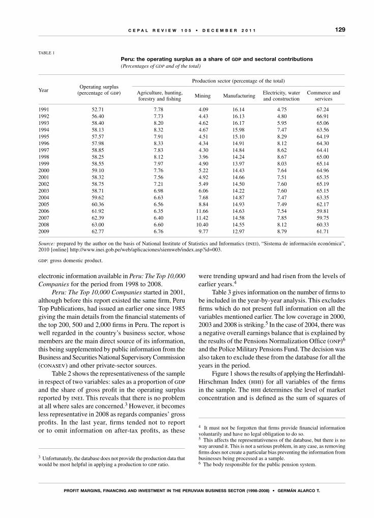
129
PRofIt MARgIns, fInAnCIng AnD InVEstMEnt In tHE PERuVIAn BusInEss sECtoR (1998-2008) • gERMán ALARCo t.
C E P A L R E V I E W 1 0 5 • D E C E M B E R 2 0 1 1
electronic information available in Peru: The Top 10,000 Companies for the period from 1998 to 2008.
Peru: The Top 10,000 Companies started in 2001, although before this report existed the same firm, Peru Top Publications, had issued an earlier one since 1985 giving the main details from the financial statements of the top 200, 500 and 2,000 firms in Peru. The report is well regarded in the country’s business sector, whose members are the main direct source of its information, this being supplemented by public information from the Business and Securities National Supervisory Commission (conasev) and other private-sector sources.
Table 2 shows the representativeness of the sample in respect of two variables: sales as a proportion of gdp and the share of gross profit in the operating surplus reported by inei. This reveals that there is no problem at all where sales are concerned.3 However, it becomes less representative in 2008 as regards companies’ gross profits. In the last year, firms tended not to report or to omit information on after-tax profits, as these
3 Unfortunately, the database does not provide the production data that would be most helpful in applying a production to gdp ratio.
were trending upward and had risen from the levels of earlier years.4
Table 3 gives information on the number of firms to be included in the year-by-year analysis. This excludes firms which do not present full information on all the variables mentioned earlier. The low coverage in 2000, 2003 and 2008 is striking.5 In the case of 2004, there was a negative overall earnings balance that is explained by the results of the Pensions Normalization Office (onp)6 and the Police Military Pensions Fund. The decision was also taken to exclude these from the database for all the years in the period.
Figure 1 shows the results of applying the Herfindahl-Hirschman Index (hhi) for all variables of the firms in the sample. The hhi determines the level of market concentration and is defined as the sum of squares of
4 It must not be forgotten that firms provide financial information voluntarily and have no legal obligation to do so.5 This affects the representativeness of the database, but there is no way around it. This is not a serious problem, in any case, as removing firms does not create a particular bias preventing the information from businesses being processed as a sample.6 The body responsible for the public pension system.
TABLE 1
Peru: the operating surplus as a share of gdp and sectoral contributions (Percentages of gdp and of the total)
Year Operating surplus
(percentage of gdp)
Production sector (percentage of the total)
Agriculture, hunting, forestry and fishing
Mining ManufacturingElectricity, water and construction
Commerce and services
1991 52.71 7.78 4.09 16.14 4.75 67.241992 56.40 7.73 4.43 16.13 4.80 66.911993 58.40 8.20 4.62 16.17 5.95 65.061994 58.13 8.32 4.67 15.98 7.47 63.561995 57.57 7.91 4.51 15.10 8.29 64.191996 57.98 8.33 4.34 14.91 8.12 64.301997 58.85 7.83 4.30 14.84 8.62 64.411998 58.25 8.12 3.96 14.24 8.67 65.001999 58.55 7.97 4.90 13.97 8.03 65.142000 59.10 7.76 5.22 14.43 7.64 64.962001 58.32 7.56 4.92 14.66 7.51 65.352002 58.75 7.21 5.49 14.50 7.60 65.192003 58.71 6.98 6.06 14.22 7.60 65.152004 59.62 6.63 7.68 14.87 7.47 63.352005 60.36 6.56 8.84 14.93 7.49 62.172006 61.92 6.35 11.66 14.63 7.54 59.812007 62.39 6.40 11.42 14.58 7.85 59.752008 63.00 6.60 10.40 14.55 8.12 60.332009 62.77 6.76 9.77 12.97 8.79 61.71
Source: prepared by the author on the basis of National Institute of Statistics and Informatics (inei), “Sistema de información económica”, 2010 [online] http://www.inei.gob.pe/web/aplicaciones/siemweb/index.asp?id=003.
gdp: gross domestic product.

130
PRofIt MARgIns, fInAnCIng AnD InVEstMEnt In tHE PERuVIAn BusInEss sECtoR (1998-2008) • gERMán ALARCo t.
C E P A L R E V I E W 1 0 5 • D E C E M B E R 2 0 1 1
TABLE 2
representativeness of the sample in Peru: The Top 10,000 Companies in relation to gdp and the operating surplus, 1998-2008(Percentages)
Year Number of firmsa Sales-to-gdp ratio Gross profits
1998 4 951 73.96 1.671999 3 249 72.71 3.352000 2 271 61.34 8.792001 2 391 55.07 3.152002 10 000 98.00 4.502003 9 354 93.84 2.812004 2 375 52.99 4.262005 2 475 63.69 9.602006 7 104 102.97 21.872007 8 477 100.96 21.272008 7 946 102.87 4.14
Source: prepared by the author on the basis of data from the National Institute of Statistics and Informatics (inei) and from Peru: The Top 10,000 Companies, various years.
a Number of firms that at least report sales.gdp: gross domestic product.
TABLE 3
Peru: The Top 10,000 Companies: adjusted database with full information,a 1998-2008
Year of data processed Source Number of firms in the year’s sample
1998 Peru: The Top 10,000 2001 2 9621999 Peru: The Top 10,000 2001 2 1492000 Peru: The Top 10,000 2002 5002001 Peru: The Top 10,000 2003 1 1782002 Peru: The Top 10,000 2004 7652003 Peru: The Top 10,000 2005 5572004 Peru: The Top 10,000 2006 6772005 Peru: The Top 10,000 2007 9102006 Peru: The Top 10,000 2009 1 1652007 Peru: The Top 10,000 2009 1 0682008 Peru: The Top 10,000 2010 496
Source: prepared by the author on the basis of data from the National Institute of Statistics and Informatics (inei) and from Peru: The Top 10,000 Companies, various years.
a Firms that did not report any sales, assets, liabilities, equity or net profits were removed from the database.
the market shares of each firm in the industry.7 The use of squares is justified because greater weighting is being given to firms with a larger market share, so that the index measures the relative size of firms depending on whether there are just a few firms with high market
7 IHi
n
:1i2= ∑H S ,where Si is each firm’s share of the market concerned.
The maximum value of the hhi is 10,000 when a firm has 100% of the market. According to the United States Department of Justice (http://www.usdoj.gov/atr/hmerger/11247.htm), markets can be classed as unconcentrated (if hhi < 1,000), moderately concentrated (if 1,000 < hhi < 1,800) or highly concentrated (if hhi > 1,800).
shares (which would give an index with a high value) or numerous small firms with small market shares, whereupon we would have a low index value. Figure 1 reveals a tendency towards greater concentration of after-tax profits and of liabilities in 2005, after which there is a gradual decline. A restricted group of firms accounts for the bulk of profits and liabilities. Concentration levels are low in the case of sales, assets and equity in an analysis of a general type.
Figure 2 shows the sales, assets, liabilities and equity shares of the top 10 and 100 firms in the sample. The contribution of these subgroups is important for the
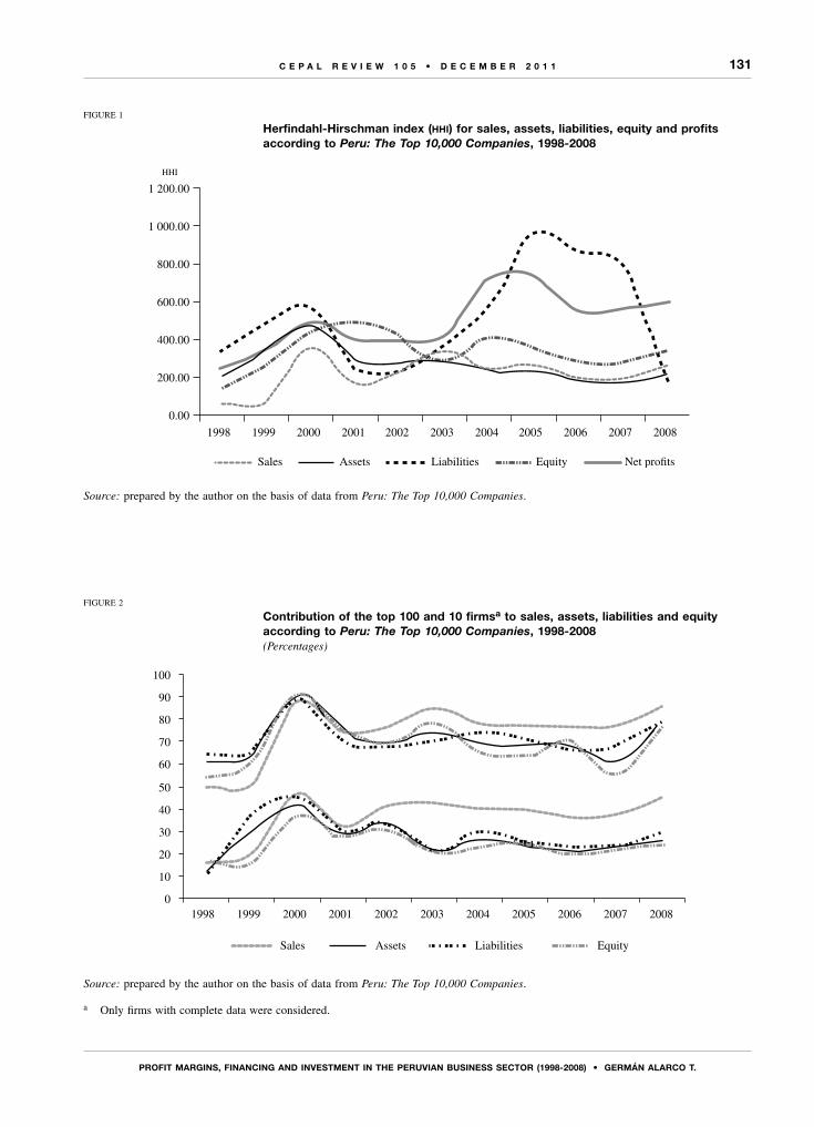
131
PRofIt MARgIns, fInAnCIng AnD InVEstMEnt In tHE PERuVIAn BusInEss sECtoR (1998-2008) • gERMán ALARCo t.
C E P A L R E V I E W 1 0 5 • D E C E M B E R 2 0 1 1
FIGURE 1
herfindahl-hirschman index (hhi) for sales, assets, liabilities, equity and profits according to Peru: The Top 10,000 Companies, 1998-2008
Source: prepared by the author on the basis of data from Peru: The Top 10,000 Companies.
FIGURE 2
Contribution of the top 100 and 10 firmsa to sales, assets, liabilities and equity according to Peru: The Top 10,000 Companies, 1998-2008(Percentages)
Source: prepared by the author on the basis of data from Peru: The Top 10,000 Companies.
a Only firms with complete data were considered.
0.00
200.00
400.00
600.00
800.00
1 000.00
1 200.00
1998 1999 2000 2001 2002 2003 2004 2005 2006 2007 2008
HHI
Sales Assets Liabilities Equity Net prots
Sales Assets Liabilities Equity
0
10
20
30
40
50
60
70
80
90
100
1998 1999 2000 2001 2002 2003 2004 2005 2006 2007 2008
132
PRofIt MARgIns, fInAnCIng AnD InVEstMEnt In tHE PERuVIAn BusInEss sECtoR (1998-2008) • gERMán ALARCo t.
C E P A L R E V I E W 1 0 5 • D E C E M B E R 2 0 1 1
whole, as the top 10 firms account for somewhat over 40% of sales and just over 20% of assets, liabilities and equity, while the group of the 100 largest firms accounts for just over 80% of sales and over 75% of the other variables analysed. In both subgroups there is a rising trend between 1998 and 2008, although a cyclical pattern can be observed, with peaks in 2000 and 2003 in the case of the subgroup of the country’s 100 largest firms.
To analyse the information for all the leading Peruvian firms and by production sector, both traditional financial ratios and some complementary ones have been used. These ratios include, in particular, the sales-to-assets ratio, which is the ratio of sales or total revenue (tr) to assets (a), this being a proxy for the output-to-capital ratio mentioned in the theoretical discussion. Other financial ratios are equity turnover, equating to total revenue (tr) over equity (c). Equity is the sum of capital plus retained earnings. The level of debt is measured as the ratio of total liabilities (l) over total assets (a). Only total liabilities are considered here because there is not enough information available to discriminate between short- and long-term liabilities, or between banking system and non-banking system liabilities. Another indicator is the level of leverage, which expresses the ratio between third-party investments and those made by the partners in a firm: the liabilities-to-equity ratio.
Firms’ profitability is measured by four indicators: net after-tax profits relative to sales, which are equivalent to the net return on sales; net profits relative to total assets, which is the return on assets; and net profits relative to equity (return on equity). Because there is a lack of detailed information on costs and spending, whether fixed or variable, the profit margin8 is obtained
as: SalesExpenditure
1 100
−
∗
In addition, two investment-related ratios have been considered, investment being understood as the difference between total assets in the current period and the previous one. This investment in current and fixed assets is expressed in relative terms with respect, firstly, to sales or total revenues and, secondly, to net after-tax profits.
Table 4 shows that, taking the whole sample, there has been a relative reduction in levels of indebtedness and leverage among the country’s main firms. These were highest at the start of the period and lowest at
8 Expenditure is obtained as the difference of sales minus profits, taking an income tax rate of 30% for the whole period in question, which is why the profit margin is pre-income tax.
the end. The counterpart of lower debt levels was an increase in equity as a share of firms’ total assets from 32.92% to 59.51%. This is important, as it indicates that the growth of firms’ total assets has been due more to internally generated resources than to outside resources. Hypotheses explaining this dynamic may be sought both in the behaviour of the banking system and other lenders and in corporate behaviour that became averse to the greater risk involved in growing on the basis of outside financing in response to the external shocks of the Asian crisis and the events of 2001.
All indicators of returns and profit margins show a trajectory similar to the performance of the operating surplus observed in table 1, being lowest at the start of the period and highest towards the end. However, the highest rates of return and margin were obtained in 2006, with lower levels seen in 2007 and 2008. This is because, in accordance with the calculation protocol, all firms not submitting full financial information were removed, and there were more and more of these. The 2006 profit margin was over 30% of total expenditure and returns on sales exceeded 16%. These results were 2.6 and 2.9 times as great as those of the world’s 500 largest companies as reported by Fortune (2011), also for 2006.9
The increased importance of investment self-financing or internally generated funding in Peruvian firms can also be observed in the financial ratio of investment to net after-tax profits. This is very high at the start of the period, and incorporates the other sources of investment financing other than net after-tax profits, after which it declines. No conclusion can be drawn from the ratio of investment to sales. Another cause reflected in the increase in investment self-financing is the reduced value of equity turnover, which peaked in 1998 before gradually declining and plateauing at between 1.10 and 1.14 from 2002, owing to higher growth in investment by partners in firms (equity).
The sales-to-assets ratio serves to demonstrate how productively assets are used. This encompasses both an adequate performance of the markets that firms’ goods and services are sold in and the effectiveness with which assets (both current and fixed) are used to generate greater output and sales. Implicitly, it captures both capital intensity and capital to labour ratios, and also manufacturing processes. Furthermore, according
9 The return on sales of the world’s 500 largest companies in 2005, 2006, 2007 and 2008 was 6.4%, 7.3%, 6.7% and 3.3%, respectively. The profit margin was 10.9%, 12.7%, 11.6% and 5.3%, respectively, assuming an average tax rate of 35%.
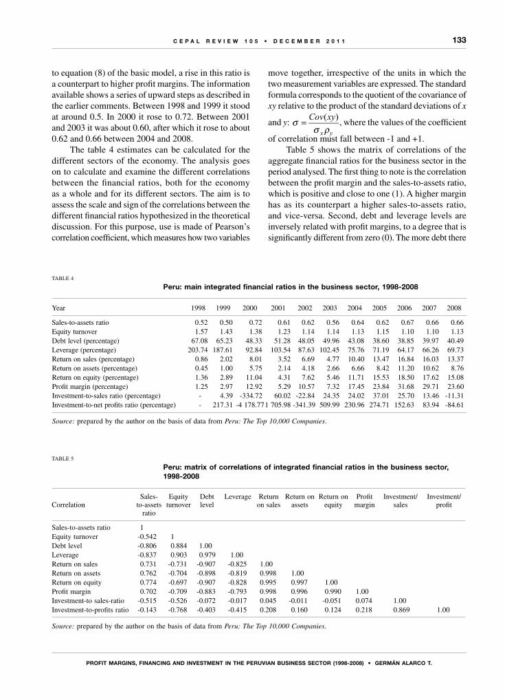
133
PRofIt MARgIns, fInAnCIng AnD InVEstMEnt In tHE PERuVIAn BusInEss sECtoR (1998-2008) • gERMán ALARCo t.
C E P A L R E V I E W 1 0 5 • D E C E M B E R 2 0 1 1
move together, irrespective of the units in which the two measurement variables are expressed. The standard formula corresponds to the quotient of the covariance of xy relative to the product of the standard deviations of x
and y: Cov xy
x yσ
σ ρ= ( )
, where the values of the coefficient
of correlation must fall between -1 and +1.Table 5 shows the matrix of correlations of the
aggregate financial ratios for the business sector in the period analysed. The first thing to note is the correlation between the profit margin and the sales-to-assets ratio, which is positive and close to one (1). A higher margin has as its counterpart a higher sales-to-assets ratio, and vice-versa. Second, debt and leverage levels are inversely related with profit margins, to a degree that is significantly different from zero (0). The more debt there
to equation (8) of the basic model, a rise in this ratio is a counterpart to higher profit margins. The information available shows a series of upward steps as described in the earlier comments. Between 1998 and 1999 it stood at around 0.5. In 2000 it rose to 0.72. Between 2001 and 2003 it was about 0.60, after which it rose to about 0.62 and 0.66 between 2004 and 2008.
The table 4 estimates can be calculated for the different sectors of the economy. The analysis goes on to calculate and examine the different correlations between the financial ratios, both for the economy as a whole and for its different sectors. The aim is to assess the scale and sign of the correlations between the different financial ratios hypothesized in the theoretical discussion. For this purpose, use is made of Pearson’s correlation coefficient, which measures how two variables
TABLE 4
Peru: main integrated financial ratios in the business sector, 1998-2008
Year 1998 1999 2000 2001 2002 2003 2004 2005 2006 2007 2008
Sales-to-assets ratio 0.52 0.50 0.72 0.61 0.62 0.56 0.64 0.62 0.67 0.66 0.66Equity turnover 1.57 1.43 1.38 1.23 1.14 1.14 1.13 1.15 1.10 1.10 1.13Debt level (percentage) 67.08 65.23 48.33 51.28 48.05 49.96 43.08 38.60 38.85 39.97 40.49Leverage (percentage) 203.74 187.61 92.84 103.54 87.63 102.45 75.76 71.19 64.17 66.26 69.73Return on sales (percentage) 0.86 2.02 8.01 3.52 6.69 4.77 10.40 13.47 16.84 16.03 13.37Return on assets (percentage) 0.45 1.00 5.75 2.14 4.18 2.66 6.66 8.42 11.20 10.62 8.76Return on equity (percentage) 1.36 2.89 11.04 4.31 7.62 5.46 11.71 15.53 18.50 17.62 15.08Profit margin (percentage) 1.25 2.97 12.92 5.29 10.57 7.32 17.45 23.84 31.68 29.71 23.60Investment-to-sales ratio (percentage) - 4.39 -334.72 60.02 -22.84 24.35 24.02 37.01 25.70 13.46 -11.31Investment-to-net profits ratio (percentage) - 217.31 -4 178.771 705.98 -341.39 509.99 230.96 274.71 152.63 83.94 -84.61
Source: prepared by the author on the basis of data from Peru: The Top 10,000 Companies.
TABLE 5
Peru: matrix of correlations of integrated financial ratios in the business sector, 1998-2008
Correlation Sales-
to-assets ratio
Equity turnover
Debt level
Leverage Return on sales
Return on assets
Return on equity
Profit margin
Investment/sales
Investment/profit
Sales-to-assets ratio 1 Equity turnover -0.542 1 Debt level -0.806 0.884 1.00 Leverage -0.837 0.903 0.979 1.00 Return on sales 0.731 -0.731 -0.907 -0.825 1.00 Return on assets 0.762 -0.704 -0.898 -0.819 0.998 1.00 Return on equity 0.774 -0.697 -0.907 -0.828 0.995 0.997 1.00 Profit margin 0.702 -0.709 -0.883 -0.793 0.998 0.996 0.990 1.00 Investment-to sales-ratio -0.515 -0.526 -0.072 -0.017 0.045 -0.011 -0.051 0.074 1.00 Investment-to-profits ratio -0.143 -0.768 -0.403 -0.415 0.208 0.160 0.124 0.218 0.869 1.00
Source: prepared by the author on the basis of data from Peru: The Top 10,000 Companies.
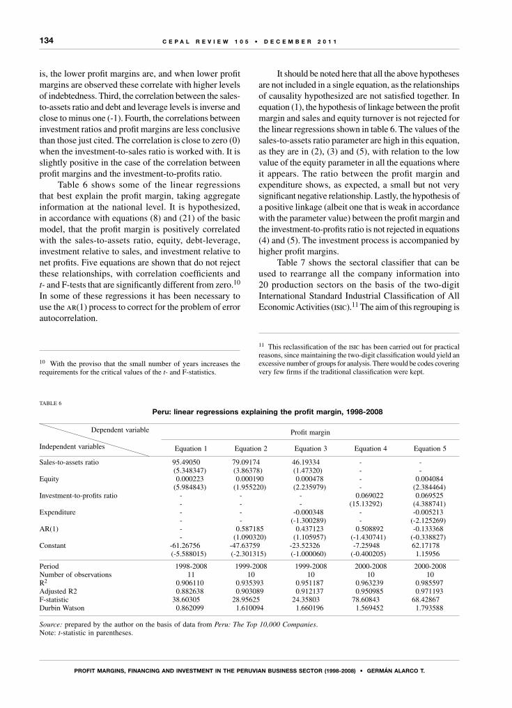
134
PRofIt MARgIns, fInAnCIng AnD InVEstMEnt In tHE PERuVIAn BusInEss sECtoR (1998-2008) • gERMán ALARCo t.
C E P A L R E V I E W 1 0 5 • D E C E M B E R 2 0 1 1
is, the lower profit margins are, and when lower profit margins are observed these correlate with higher levels of indebtedness. Third, the correlation between the sales-to-assets ratio and debt and leverage levels is inverse and close to minus one (-1). Fourth, the correlations between investment ratios and profit margins are less conclusive than those just cited. The correlation is close to zero (0) when the investment-to-sales ratio is worked with. It is slightly positive in the case of the correlation between profit margins and the investment-to-profits ratio.
Table 6 shows some of the linear regressions that best explain the profit margin, taking aggregate information at the national level. It is hypothesized, in accordance with equations (8) and (21) of the basic model, that the profit margin is positively correlated with the sales-to-assets ratio, equity, debt-leverage, investment relative to sales, and investment relative to net profits. Five equations are shown that do not reject these relationships, with correlation coefficients and t- and F-tests that are significantly different from zero.10 In some of these regressions it has been necessary to use the ar(1) process to correct for the problem of error autocorrelation.
10 With the proviso that the small number of years increases the requirements for the critical values of the t- and F-statistics.
It should be noted here that all the above hypotheses are not included in a single equation, as the relationships of causality hypothesized are not satisfied together. In equation (1), the hypothesis of linkage between the profit margin and sales and equity turnover is not rejected for the linear regressions shown in table 6. The values of the sales-to-assets ratio parameter are high in this equation, as they are in (2), (3) and (5), with relation to the low value of the equity parameter in all the equations where it appears. The ratio between the profit margin and expenditure shows, as expected, a small but not very significant negative relationship. Lastly, the hypothesis of a positive linkage (albeit one that is weak in accordance with the parameter value) between the profit margin and the investment-to-profits ratio is not rejected in equations (4) and (5). The investment process is accompanied by higher profit margins.
Table 7 shows the sectoral classifier that can be used to rearrange all the company information into 20 production sectors on the basis of the two-digit International Standard Industrial Classification of All Economic Activities (isic).11 The aim of this regrouping is
11 This reclassification of the isic has been carried out for practical reasons, since maintaining the two-digit classification would yield an excessive number of groups for analysis. There would be codes covering very few firms if the traditional classification were kept.
TABLE 6
Peru: linear regressions explaining the profit margin, 1998-2008
Dependent variable
Independent variables
Profit margin
Equation 1 Equation 2 Equation 3 Equation 4 Equation 5
Sales-to-assets ratio 95.49050 79.09174 46.19334 - - (5.348347) (3.86378) (1.47320) - -Equity 0.000223 0.000190 0.000478 - 0.004084 (5.984843) (1.955220) (2.235979) - (2.384464)Investment-to-profits ratio - - - 0.069022 0.069525 - - - (15.13292) (4.388741)Expenditure - - -0.000348 - -0.005213 - - (-1.300289) - (-2.125269)AR(1) - 0.587185 0.437123 0.508892 -0.133368 - (1.090320) (1.105957) (-1.430741) (-0.338827)Constant -61.26756 -47.63759 -23.52326 -7.25948 62.17178 (-5.588015) (-2.301315) (-1.000060) (-0.400205) 1.15956
Period 1998-2008 1999-2008 1999-2008 2000-2008 2000-2008Number of observations 11 10 10 10 10R2 0.906110 0.935393 0.951187 0.963239 0.985597Adjusted R2 0.882638 0.903089 0.912137 0.950985 0.971193F-statistic 38.60305 28.95625 24.35803 78.60843 68.42867Durbin Watson 0.862099 1.610094 1.660196 1.569452 1.793588
Source: prepared by the author on the basis of data from Peru: The Top 10,000 Companies.Note: t-statistic in parentheses.
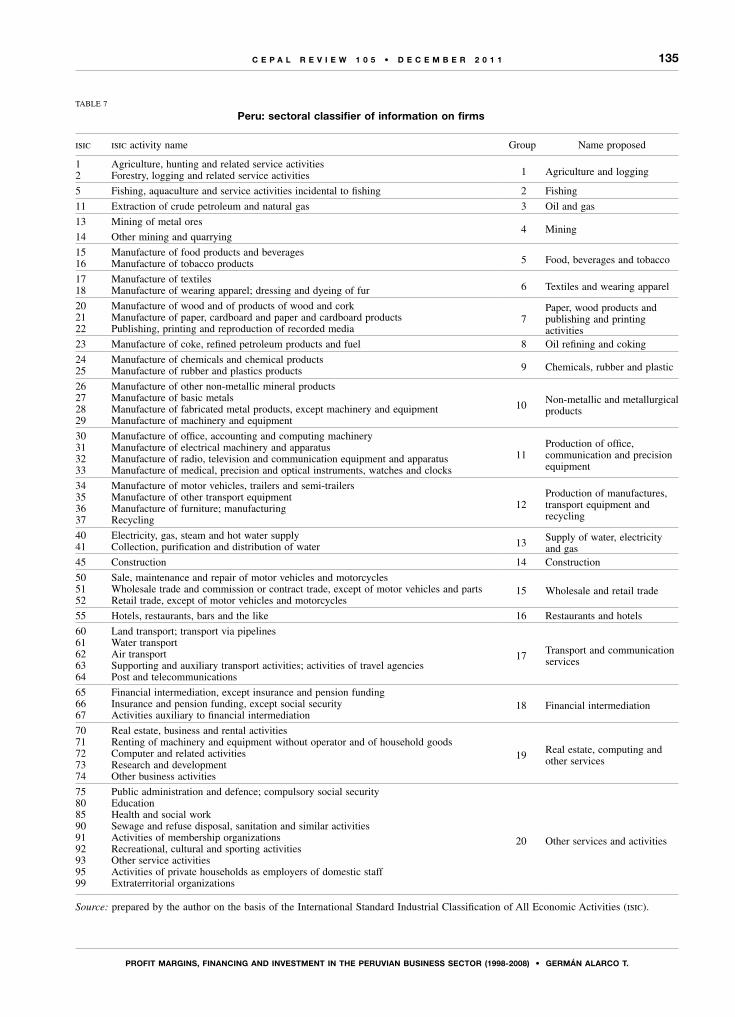
135
PRofIt MARgIns, fInAnCIng AnD InVEstMEnt In tHE PERuVIAn BusInEss sECtoR (1998-2008) • gERMán ALARCo t.
C E P A L R E V I E W 1 0 5 • D E C E M B E R 2 0 1 1
TABLE 7
Peru: sectoral classifier of information on firms
isic isic activity name Group Name proposed
1 Agriculture, hunting and related service activities1 Agriculture and logging2 Forestry, logging and related service activities
5 Fishing, aquaculture and service activities incidental to fishing 2 Fishing
11 Extraction of crude petroleum and natural gas 3 Oil and gas
13 Mining of metal ores4 Mining
14 Other mining and quarrying
15 Manufacture of food products and beverages5 Food, beverages and tobacco16 Manufacture of tobacco products
17 Manufacture of textiles6 Textiles and wearing apparel18 Manufacture of wearing apparel; dressing and dyeing of fur
20 Manufacture of wood and of products of wood and cork7
Paper, wood products and publishing and printing activities
21 Manufacture of paper, cardboard and paper and cardboard products22 Publishing, printing and reproduction of recorded media
23 Manufacture of coke, refined petroleum products and fuel 8 Oil refining and coking
24 Manufacture of chemicals and chemical products9 Chemicals, rubber and plastic25 Manufacture of rubber and plastics products
26 Manufacture of other non-metallic mineral products
10 Non-metallic and metallurgical products
27 Manufacture of basic metals28 Manufacture of fabricated metal products, except machinery and equipment29 Manufacture of machinery and equipment
30 Manufacture of office, accounting and computing machinery
11Production of office, communication and precision equipment
31 Manufacture of electrical machinery and apparatus32 Manufacture of radio, television and communication equipment and apparatus33 Manufacture of medical, precision and optical instruments, watches and clocks
34 Manufacture of motor vehicles, trailers and semi-trailers
12Production of manufactures, transport equipment and recycling
35 Manufacture of other transport equipment36 Manufacture of furniture; manufacturing37 Recycling
40 Electricity, gas, steam and hot water supply13 Supply of water, electricity
and gas41 Collection, purification and distribution of water
45 Construction 14 Construction
50 Sale, maintenance and repair of motor vehicles and motorcycles15 Wholesale and retail trade51 Wholesale trade and commission or contract trade, except of motor vehicles and parts
52 Retail trade, except of motor vehicles and motorcycles
55 Hotels, restaurants, bars and the like 16 Restaurants and hotels
60 Land transport; transport via pipelines
17 Transport and communication services
61 Water transport62 Air transport63 Supporting and auxiliary transport activities; activities of travel agencies64 Post and telecommunications
65 Financial intermediation, except insurance and pension funding18 Financial intermediation66 Insurance and pension funding, except social security
67 Activities auxiliary to financial intermediation
70 Real estate, business and rental activities
19 Real estate, computing and other services
71 Renting of machinery and equipment without operator and of household goods72 Computer and related activities73 Research and development74 Other business activities
75 Public administration and defence; compulsory social security
20 Other services and activities
80 Education85 Health and social work90 Sewage and refuse disposal, sanitation and similar activities91 Activities of membership organizations92 Recreational, cultural and sporting activities93 Other service activities95 Activities of private households as employers of domestic staff99 Extraterritorial organizations
Source: prepared by the author on the basis of the International Standard Industrial Classification of All Economic Activities (isic).
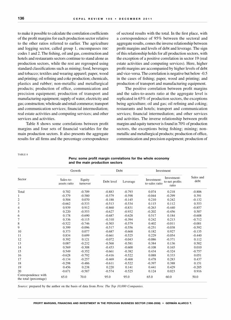
136
PRofIt MARgIns, fInAnCIng AnD InVEstMEnt In tHE PERuVIAn BusInEss sECtoR (1998-2008) • gERMán ALARCo t.
C E P A L R E V I E W 1 0 5 • D E C E M B E R 2 0 1 1
to make it possible to calculate the correlation coefficients of the profit margins for each production sector relative to the other ratios referred to earlier. The agriculture and logging sector, called group 1, encompasses isic codes 1 and 2. The fishing, oil and gas, construction and hotels and restaurants sectors continue to stand alone as production sectors, while the rest are regrouped using standard classifications such as mining; food, beverages and tobacco; textiles and wearing apparel; paper, wood and printing; oil refining and coke production; chemicals, plastics and rubber; non-metallic and metallurgical products; production of office, communication and precision equipment; production of transport and manufacturing equipment; supply of water, electricity and gas; construction; wholesale and retail commerce; transport and communication services; financial intermediation; real estate activities and computing services; and other services and activities.
Table 8 shows some correlations between profit margins and four sets of financial variables for the main production sectors. It also presents the aggregate results for all firms and the percentage correspondence
of sectoral results with the total. In the first place, with a correspondence of 95% between the sectoral and aggregate results, comes the inverse relationship between profit margins and levels of debt and leverage. The sign of this relationship holds for all production sectors, with the exception of a positive correlation in sector 19 (real estate activities and computing services). Here, higher profit margins are accompanied by higher levels of debt and vice-versa. The correlation is negative but below -0.5 in the cases of fishing; paper, wood and printing; and production of transport and manufacturing equipment.
The positive correlation between profit margins and the sales-to-assets ratio at the aggregate level is replicated in 65% of production sectors, the exceptions being agriculture; oil and gas; oil refining and coking; restaurants and hotels; transport and communication services; financial intermediation; and other services and activities. The inverse relationship between profit margins and equity turnover is found in 70% of production sectors, the exceptions being fishing; mining; non-metallic and metallurgical products; production of office, communication and precision equipment; production of
TABLE 8
Peru: some profit margin correlations for the whole economy and the main production sectors
Sector
Growth Debt Investment
Sales and debtSales-to-
assets ratioEquity
turnoverDebt level Leverage
Investment-to-sales ratio
Investment-to-net profits
ratio
Total 0.702 -0.709 -0.883 -0.793 0.074 0.218 -0.8061 -0.379 -0.580 -0.579 -0.598 -0.044 -0.299 0.3912 0.504 0.070 -0.188 -0.145 0.210 0.242 -0.1323 -0.662 -0.533 -0.513 -0.534 0.115 0.112 0.5534 0.939 0.912 -0.860 -0.831 -0.263 -0.440 -0.8575 0.220 -0.553 -0.627 -0.932 -0.202 -0.456 0.5076 0.178 -0.690 -0.687 -0.628 0.517 0.184 -0.6087 0.336 -0.115 -0.310 -0.394 0.242 0.213 -0.7128 -0.522 -0.746 -0.503 -0.579 0.402 -0.011 -0.0019 0.399 -0.096 -0.517 -0.556 -0.251 -0.038 -0.59210 0.373 0.077 -0.687 -0.668 0.182 0.927 -0.13511 0.834 0.699 -0.661 -0.525 0.229 -0.054 -0.44012 0.392 0.121 -0.072 -0.043 -0.086 -0.371 0.11213 0.087 -0.232 -0.568 -0.581 0.384 0.136 0.50214 0.569 -0.308 -0.453 -0.600 -0.108 0.165 0.01015 0.549 -0.352 -0.661 -0.382 0.434 -0.324 -0.75716 -0.628 -0.792 -0.416 -0.522 0.088 0.333 0.05117 -0.134 -0.257 -0.469 -0.468 0.478 0.283 0.43718 -0.298 -0.486 -0.611 -0.522 -0.397 0.388 0.15119 0.456 0.238 0.220 0.141 0.441 0.429 -0.20520 -0.671 -0.587 -0.574 -0.525 0.124 0.023 0.916Correspondence with the total (percentage)
65.0 70.0 95.0 95.0 65.0 60.0 50.0
Source: prepared by the author on the basis of data from Peru: The Top 10,000 Companies.
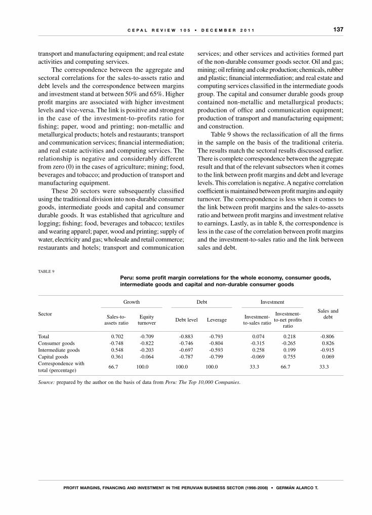
137
PRofIt MARgIns, fInAnCIng AnD InVEstMEnt In tHE PERuVIAn BusInEss sECtoR (1998-2008) • gERMán ALARCo t.
C E P A L R E V I E W 1 0 5 • D E C E M B E R 2 0 1 1
transport and manufacturing equipment; and real estate activities and computing services.
The correspondence between the aggregate and sectoral correlations for the sales-to-assets ratio and debt levels and the correspondence between margins and investment stand at between 50% and 65%. Higher profit margins are associated with higher investment levels and vice-versa. The link is positive and strongest in the case of the investment-to-profits ratio for fishing; paper, wood and printing; non-metallic and metallurgical products; hotels and restaurants; transport and communication services; financial intermediation; and real estate activities and computing services. The relationship is negative and considerably different from zero (0) in the cases of agriculture; mining; food, beverages and tobacco; and production of transport and manufacturing equipment.
These 20 sectors were subsequently classified using the traditional division into non-durable consumer goods, intermediate goods and capital and consumer durable goods. It was established that agriculture and logging; fishing; food, beverages and tobacco; textiles and wearing apparel; paper, wood and printing; supply of water, electricity and gas; wholesale and retail commerce; restaurants and hotels; transport and communication
services; and other services and activities formed part of the non-durable consumer goods sector. Oil and gas; mining; oil refining and coke production; chemicals, rubber and plastic; financial intermediation; and real estate and computing services classified in the intermediate goods group. The capital and consumer durable goods group contained non-metallic and metallurgical products; production of office and communication equipment; production of transport and manufacturing equipment; and construction.
Table 9 shows the reclassification of all the firms in the sample on the basis of the traditional criteria. The results match the sectoral results discussed earlier. There is complete correspondence between the aggregate result and that of the relevant subsectors when it comes to the link between profit margins and debt and leverage levels. This correlation is negative. A negative correlation coefficient is maintained between profit margins and equity turnover. The correspondence is less when it comes to the link between profit margins and the sales-to-assets ratio and between profit margins and investment relative to earnings. Lastly, as in table 8, the correspondence is less in the case of the correlation between profit margins and the investment-to-sales ratio and the link between sales and debt.
TABLE 9
Peru: some profit margin correlations for the whole economy, consumer goods, intermediate goods and capital and non-durable consumer goods
Sector
Growth Debt Investment
Sales and debtSales-to-
assets ratioEquity
turnoverDebt level Leverage
Investment-to-sales ratio
Investment-to-net profits
ratio
Total 0.702 -0.709 -0.883 -0.793 0.074 0.218 -0.806Consumer goods -0.748 -0.822 -0.746 -0.804 -0.315 -0.265 0.826Intermediate goods 0.548 -0.203 -0.697 -0.593 0.258 0.199 -0.915Capital goods 0.361 -0.064 -0.787 -0.799 -0.069 0.755 0.069Correspondence with total (percentage)
66.7 100.0 100.0 100.0 33.3 66.7 33.3
Source: prepared by the author on the basis of data from Peru: The Top 10,000 Companies.
138
PRofIt MARgIns, fInAnCIng AnD InVEstMEnt In tHE PERuVIAn BusInEss sECtoR (1998-2008) • gERMán ALARCo t.
C E P A L R E V I E W 1 0 5 • D E C E M B E R 2 0 1 1
In the post-Keynesian school, the level of and changes in the profit margins of fixed-price sectors are held to depend on a set of factors such as the price elasticity of demand, the behaviour and reactions of possible entrants into the industry and the minimization of possible regulatory reactions by the authorities. Also important are the industry’s growth rate and the output-to-capital ratio, which are the counterpart of any firm’s investment decisions. Profit margins rise when these last variables grow more strongly, owing to investment self-financing needs.
These theories seem to be helpful in explaining the behaviour of profit margins, investment and financing in the Peruvian business sector between 1998 and 2008. There are a number of grey areas, however, owing both to the lack of detailed statistical information and to the need for a supplementary theoretical framework to account for the evolution of profit margins in production sectors other than manufacturing. The lack of longer time series and more detailed information limits the scope for analysis. The greatest limitation of the aggregate information concerns the use of the operating surplus variable, as unfortunately this aggregates the rents and income of self-employed people in urban and rural areas with company profits. It is essential for specific information to be presented for each sector.
The gdp share of the operating surplus has grown over time, and within this the greatest contribution has been made by commerce and services, although the mining sector and hydrocarbons have increased their contribution to the surplus because of their greater dynamism and high international prices. Electricity, water and construction have also registered a growing contribution to the operating surplus, although the growth of these profit margins would seem to be due to the same factors as have operated in manufacturing.
Information from firms is useful for the analysis because it allows basic financial ratios to be estimated at both the aggregate and sectoral levels. When the representativeness of the sample is compared with the national total, furthermore, it transpires that these are adequately representative of the aggregate for the period under analysis. Because a ranking of the country’s largest firms is used, however, smaller businesses are omitted, as are those operating in sectors dominated by what
are probably the most competitive smaller production units. The aggregate analysis does not determine high levels of concentration, but when it is carried out for the 10 and 100 largest firms in the annual surveys, these subgroups of firms account for a substantial proportion of net profits, liabilities, assets, sales and equity.
The evolution of profit margins and of all the profitability indicators estimated on the basis of the sample of firms analysed displays a rising trajectory similar to that of the operating surplus. This correspondence was less in 2007 and 2008, however, owing to the fall-off in reporting of after-tax earnings by private firms. In 2006, profit margins and after-tax profits relative to net sales were equivalent to 2.6 and 2.9 times the same ratios, respectively, for the world’s 500 largest firms as reported by Fortune magazine.
The aggregate information shows that there has been a relative reduction in debt and leverage levels in the Peruvian business sector. The counterpart of these lower debt levels has been an increase in the share of equity in total corporate assets. Unfortunately, there is not the information available to ascertain whether this reduction in the debt level was due to the behaviour of the banking system and other lenders or to corporate behaviour that became adverse to the greater risk involved in growing on the basis of outside financing in response to the external shock of the Asian crisis and the events in the international economy in 2001.
At the level of both the aggregate sample and the sectoral subgroups, what stands out is the positive correlation of close to one (1) between profit margins and the sales-to-assets ratio. A higher margin is matched by a higher sales-to-assets ratio (a proxy for the output-to-capital ratio) and vice-versa. Second, debt and leverage maintained a relationship with profit margins that was inverse and significantly different from zero (0). The higher the debt, the lower the profit margins, and when lower profit margins are observed these correlate with higher levels of debt. Third, the correlation between the sales-to-assets ratio and debt and leverage levels is inverse and close to minus one (-1). Fourth, the correlations between investment ratios and profit margins are less conclusive than the previous ones, although they are positive in the case of the correlation between profit margins and the investment-to-profits ratio. The investment process is
Vfinal considerations
139
PRofIt MARgIns, fInAnCIng AnD InVEstMEnt In tHE PERuVIAn BusInEss sECtoR (1998-2008) • gERMán ALARCo t.
C E P A L R E V I E W 1 0 5 • D E C E M B E R 2 0 1 1
accompanied by higher profit margins. Peruvian firms tend to self-finance their investment decisions. The two decision-making processes are linked.
The lesser correlation of profit margins and investment relative to sales would seem to demonstrate, at the microeconomic level, that higher profit margins can be generated without the need for higher investment. Higher margins may simply be the result of a policy
designed to obtain greater returns on investment or higher dividends. This is a subject that ought to be incorporated into theories for determining profit margins. The factors underlying today’s lower borrowing also need to be explored in more detail, as does the question of whether or not investment self-financing is related in some way to the behaviour of the financial sector.
(Original: Spanish)
Bibliography
Alarco, G. (2010a), “Growth and concentration among the leading business groups in Mexico”, cepal Review, No. 101 (LC/G.2455-P), Santiago, Chile, August.
(2010b), “Crisis financiera internacional y patrón de crecimiento de una economía mediana y dependiente: el caso del Perú”, Convergencia, vol. 17, No. 54, Mexico City, Autonomous University of Mexico State, September-December.
Eichner, A. (1988), “Una teoría de la determinación del margen de ganancia en el oligopolio”, Economía postkeynesiana, J. Ocampo (ed.), Mexico City, Fondo de Cultura Económica.
Feiwel, G. (1981), Michal Kalecki: contribuciones a la teoría de la política económica, Mexico City, Fondo de Cultura Económica.
Fortune (2011), “Global 500 annual ranking of the world’s largest corporations” [online] http://money.cnn.com/magazines/fortune/global500/2010/index.html.
Harcourt, C. and P. Kenyon (1988), “La fijación de precios y la decisión de inversión”, Economía postkeynesiana, J.A. Ocampo (ed.), Mexico City, Fondo de Cultura Económica.
inei (National Institute of Statistics and Informatics) (2011), “Sistema de información económica” [online] http://www.inei.gob.pe/web/aplicaciones/siemweb/index.asp?id=003
Kalecki, M. (1954), Theory of Economic Dynamics, London, George Allen and Unwin.
Lindenboim, J. (2008), “Distribución funcional del ingreso, un tema olvidado que reclama atención”, Problemas del desarrollo, vol. 39, No. 153, Mexico City, Institute of Economics Research, National Autonomous University of Mexico, April.
Ocampo, J. (1988), “De Keynes al análisis postkeynesiano”, Economía postkeynesiana, J.A. Ocampo (ed.), Mexico City, Fondo de Cultura Económica.
Peru Top Publications (2010), Peru: The Top 10,000 Companies [online] http://www.perutop10000.com.pe/.
(2008), Peru: The Top 10,000 Companies [online] http://www.perutop10000.com.pe/.
(2007), Peru: The Top 10,000 Companies [online] http://www.perutop10000.com.pe/.
(2006), Peru: The Top 10,000 Companies [online] http://www.perutop10000.com.pe/.
(2005), Peru: The Top 10,000 Companies [online] http://www.perutop10000.com.pe/. (2005).
(2004), Peru: The Top 10,000 Companies [online] http://www.perutop10000.com.pe/.
(2002), Peru: The Top 10,000 Companies [online] http://www.perutop10000.com.pe/.
(2001), Peru: The Top 10,000 Companies [online] http://www.perutop10000.com.pe/.
Steindl, J. (1988), “Precios, costos y márgenes de ganancia”, Economía postkeynesiana, J.A. Ocampo (ed.), Mexico City, Fondo de Cultura Económica.
Sylos Labini, P. (1969), Oligopoly and Technical Progress, Cambridge, MA, Harvard University Press.
Taylor, L. (1986), Modelos macroeconómicos para los países en desarrollo, Mexico City, Fondo de Cultura Económica.
United Nations (2002), International Standard Industrial Classification of All Economic Activities (isic). Revision 3.1 (ST/ESA/STAT/SER.M/4/Rev.3.1), New York [online] http://documents-dds-ny.un.org/doc/UNDOC/GEN/N02/764/15/pdf/N0276415.pdf?OpenElement.
Urzúa, C. (2009), “Efectos sobre el bienestar social de las empresas con poder de mercado en México”, Finanzas públicas, vol. 1, No. 1, Mexico City, Centro de Estudios de las Finanzas Públicas.
Vargas, G. (2007), “La nueva microeconomía dinámica”, Investigación económica, vol. 66, No. 162, Mexico City, National Autonomous University of Mexico.
Wood, A. (1988), “El margen de ganancia a largo plazo”, Economía postkeynesiana, J.A. Ocampo (ed.), Mexico City, Fondo de Cultura Económica.

C E P A L R E V I E W 1 0 5 • D E C E M B E R 2 0 1 1
141
K E Y W O R D S
Quality of education
Academic performance
Measurement
Private schools
Public schools
Social aspects
Argentina
Do private schools in Argentina perform betterbecause they are private?
María Marta Formichella
The objective of this study is to analyse the determinants of the
quality of education in Argentina and, in particular, to look at what influence
a school’s ownership structure has. A multilevel regression model and
2006 data from the Programme for International Student Assessment
(pisa) were used for this purpose. One of the main findings is that the
correlation between a school’s administrative structure (public or private)
and its students’ scholastic performance fades when the socioeconomic
school environment is taken into consideration.
María Marta Formichella
Assistant Professor for the
Seminar on Economic Accounting
and Fundamental Principles
of Economics, Department of
Economics, Universidad Nacional
del Sur (uns)
142
Do PRIVAtE sCHooLs In ARgEntInA PERfoRM BEttER BECAusE tHEy ARE PRIVAtE? • MARíA MARtA foRMICHELLA
C E P A L R E V I E W 1 0 5 • D E C E M B E R 2 0 1 1
Countless research projects have shown how important education is as a determinant of socioeconomic development. The beneficial effects of education have been shown to range from employment-related advantages to less tangible ones having to do with the fact that educated persons may have a better quality of life than uneducated ones (Formichella, 2010).
One of the relevant considerations in this connection is the differing levels of scholastic achievement, in terms of both quantity and quality, that a given individual can attain. In quantitative terms, 51% of the people between the ages of 25 and 65 do not have a high school diploma, and the educational Gini coefficient, calculated on the basis of completed years of schooling, is 0.21. In qualitative terms, the rating on the Theil index –calculated on the basis of scores on the 2006 pisa science test–is 0.059, with 41% of this difference being accounted for by differences between schools (Formichella, 2010).
The existing literature on determinants of scholastic performance in Argentina indicates that qualitative differences in achievement can be accounted for by the traits of individuals and their households, characteristics of the schools that they attend, and, according to many of these papers, the socioeconomic background of a student’s classmates.
While these studies agree on many points, there is one issue about which they differ, and that is how the type of administrative structure influences academic
achievement. This divergence is also seen in the findings of empirical studies conducted in other countries.1
As we will see, some empirical studies focusing on education in Argentina have found that students’ performance is strongly influenced by whether the school is privately or publicly run, while others have found that this correlation is eclipsed by the socioeconomic environment of the students enrolled in each type of school.
The aim of this study is therefore to find evidence to settle this difference of opinion. Its working hypothesis tends to favour the second of these positions (i.e. that the influence that the form of school administration appears to have on students’ performance is actually attributable to the effect that the socioeconomic school environment has on scholastic achievement).
The sections that follow this introduction will explore different aspects of this question. Section II presents a review of the major studies that have focused on the determinants of scholastic performance in Argentina. Section III examines the data sources used for this study. Section IV covers the methodology, while section V outlines the proposed models and their results. The conclusions are presented in section VI.
1 For a review of these studies, see Calero and Escardíbul (2007).
Iintroduction
IIBackground information about the education
system in Argentina
Various empirical studies have explored the determinants of scholastic performance in Argentina. Cervini (1999) analyses the performance (as measured by scores on mathematics tests) of students in the seventh year of the basic general education track using qualitative information from the National Evaluation Campaign (one) of 1997. Using a hierarchical methodology applied at two different levels (schools and students), he finds that the socioeconomic level of the household and of the school
environment have a significant impact. In addition, the following factors were identified as having a negative impact on achievement: (i) if a student is over-age;2 (ii) if a student has repeated a grade; (iii) if a student
2 “Over-age students” are defined as students who are two or more years behind. This factor is measured by the number of students in different age groups who are attending grade levels below those that would usually correspond to their age group.
143
Do PRIVAtE sCHooLs In ARgEntInA PERfoRM BEttER BECAusE tHEy ARE PRIVAtE? • MARíA MARtA foRMICHELLA
C E P A L R E V I E W 1 0 5 • D E C E M B E R 2 0 1 1
has changed schools; (iv) if a student lives far away from the school; and (v) if the student is female. This author also finds that self-motivation, personal effort and the student’s view of how much help he or she receives from family members have a positive impact. Finally, he finds evidence that better school infrastructure and better-quality educational resources have positive effects on performance, but he does not conclude that the fact that a school is privately or publicly run has any significant explanatory value.
In 2002, Cervini used 1997 one data to study scholastic achievement at the primary level. For this study, he used a three-level hierarchical methodology based on provinces, schools and students. He found that differences among students and, after that, schools were the most powerful explanations for the differences in achievement, while differences at the provincial level were of virtually no importance. His main conclusion is that the theory of cultural reproduction holds true for Argentina, with scholastic performance being largely accounted for by households’ cultural and economic capital. He also finds that the influence of socioeconomic factors varies a great deal across schools. He concludes that this variance is attributable to different schools’ varying abilities to offset underlying inequalities. His ultimate conclusion is that, of all the various factors that have an influence on performance, the one that has the greatest impact of all is the socioeconomic status of students’ classmates.
Cervini (2002a) analyses the determinants of scholastic performance at the middle-school level using data from the national secondary-school completion survey conducted in 1998. He uses the same tri-level (provinces, schools and students) analytical methodology as in the preceding study and, here again, finds that inequalities in outcomes are primarily found at the individual student level, although a significant percentage of the existing inequalities can also be accounted for by inter-school differences. As in the preceding case, he found that inter-province differences had very little explanatory power. He also found that there was a negative correlation between being female (male) and performance in mathematics (reading) and that the economic assets of a household were a determining factor for access to middle school, while a household’s cultural assets had a positive effect on performance. Here again, he found that schools differ in their ability to offset inequalities in the students’ backgrounds.
Fernández Aguerre (2002) uses one data from the year 2000 and a logistic regression methodology to study the determinants of success in school for sixth-grade students in Argentina. Like Cervini, he finds evidence
of a positive correlation between the socioeconomic status of students’ households and their performance. He also finds that a school’s sociocultural environment has more of an impact on student outcomes than their households’ economic status does. His results indicate that students who attend private schools outperform those who attend public schools and that men perform better than women.
Wößmann and Fuchs (2005) also study scholastic performance at the primary-school level in Argentina using clustering-robust linear regressions (crlrs) and data from the Progress in International Reading Literacy Study (pirls) of 2001. These authors identify household characteristics and family background as the most influential factors in determining a student’s scholastic performance. They do not find convincing evidence of a correlation between academic achievement and how well-funded a school is or other school characteristics. They do find, however, that a school that uses a centralized curriculum or that uses a skills-building approach has a positive effect on performance.
Cervini (2005a and 2006) then took his 2002 middle-school study on math performance to another level. He found that being a female, having repeated a grade or working longer hours all have an adverse effect on scholastic performance and that the degree of institutional selectivity based on students’ socioeconomic status was quite high. He also found evidence of a positive correlation between the school environment and performance. In addition, his findings indicate that schools’ capacity to offset household-based differences varies and that inequities related to inter-school inequalities of effect diminish when schools of a similar make-up are compared to one another.
Cervini (2005b) has also studied non-cognitive (as well as cognitive) educational outcomes linked to general socio-educational attitudes, which he measures using other variables gleaned from the student questionnaire that he then uses to capture related subjective factors. He uses a tripartite (students, schools, provinces) hierarchical model for this purpose together with data from the national secondary-school completion survey conducted in 1998. His comparison of the determinants of these two types of results leads him to the following conclusions: (i) individuals’ traits have a greater impact on cognitive than on non-cognitive outcomes; (ii) schools’ ability to offset inequalities of origin relative to cognitive and non-cognitive outcomes differ; and (iii) schools’ performance in terms of their students’ outcomes are inconsistent (i.e. there is no strong correlation between cognitive and non-cognitive outcomes).
144
Do PRIVAtE sCHooLs In ARgEntInA PERfoRM BEttER BECAusE tHEy ARE PRIVAtE? • MARíA MARtA foRMICHELLA
C E P A L R E V I E W 1 0 5 • D E C E M B E R 2 0 1 1
Gertel and others (2006) have also used one data (mathematics and reading test results at the primary school level for 2000), together with a dual-level (students and classrooms) hierarchical model, to study the determinants of academic performance in Argentina. Their findings underscore the importance of grade-repetition and gender variables: having repeated a grade lowers performance and being a male improves it (lowers it) in mathematics (reading). Their results in terms of household-related variables indicate that having siblings who have dropped out of school or who never attended in the first place depresses student performance, while there is a positive, although fairly weak, correlation between socioeconomic status and educational outcomes. They also find that a number of school-related variables, including the quality of infrastructure, teacher experience and training, and the type of school administration, have a significant impact (with students attending private schools scoring higher).
In view of their results concerning the impact of the private/public school variable, Gertel and others (2007a) followed up with a tripartite model (students, grades and schools) in which the third level (schools) is represented by all the different variables linked to the public/private differential. Their findings corroborate the conclusion that the school’s ownership structure has a greater influence on actual learning outcomes.
These same researchers (Gertel and others, 2007b) later looked at scholastic performance using not only one data, but also 1997 scores of primary-school students on the international Latin American Laboratory for Assessment of the Quality of Education (llece). They use a hierarchical data methodology and the same three levels as before. One of their main findings is that the public/private school variable has a strong explanatory value in terms of scholastic performance in Argentina.
Santos (2007) has also studied the determinants of educational quality in Argentina at the middle-school level, but uses pisa scores from 2000 on mathematics and reading tests and quantile regressions to do so. She found that gender is an influential variable, with females scoring higher on reading tests and males higher on mathematics tests. She also finds that class size should be limited to a maximum of 32 students in order to achieve positive learning outcomes and that the quality of a school’s educational resources has a major impact on performance. She also finds that, after controlling for other features, private schools actually do not have better results than public schools, and she posits that the differences in scores may be attributable to the fact
that the private-school students come from a higher socioeconomic stratum. She also concludes that the presence or absence of educational resources in students’ homes has a highly significant effect.
Abdul-Hamid (2007) also analyses the determinants of educational quality in Argentina using quantile regressions and 2000 pisa scores. He finds that the factors that have a positive influence on scholastic achievement include the following: (i) the school learning environment; (ii) the geographic location of the school (schools in larger cities perform more successfully); (iii) the academic guidance and encouragement provided to students; (iv) the type of school administration (private-school students outperform public-school students); (v) a majority of women in the student body; (vi) whether or not the student has education resources in the home; and (vii) whether or not the student’s mother has an above-average level of education.
Finally, Cervini conducted two studies in which he compares the educational levels of primary and secondary students in Argentina using one (2000) data, the results of the 1998 national secondary-school completion survey and a multilevel methodology.
In the first of these studies (Cervini, 2009), he uses three levels of analysis: students (level 1), schools (level 2) and provinces (level 3). His objective is to compare the pattern of (in)equity in the distribution of scores on reading and mathematics tests. He finds that schools differ markedly in terms of their students’ performance in the evaluations conducted at the two different grade levels and that the intra-school variance was greater at the primary education level. He therefore concludes that the characteristics of a student’s household are more influential during the primary education cycle. He also finds that, in general, all the variables associated with the students’ socioeconomic status influence their test scores at both grade levels and that the variables associated with the school environment are also significant factors at both levels, although the economic status of classmates exerts a greater influence in the primary education cycle, whereas the students’ educational environment, proxied by the level of education of their parents, has a greater impact in the secondary cycle.
In the second study (2010), Cervini uses various models to disaggregate information at different levels (in which he considers, alternatively, three of the following variables: students, classrooms, schools, municipalities and provinces) and focuses on an analysis of a comparison of the “school effect” across primary and secondary grade levels. He concludes that the results are determined by the methodology that is employed, that the school effect

145
Do PRIVAtE sCHooLs In ARgEntInA PERfoRM BEttER BECAusE tHEy ARE PRIVAtE? • MARíA MARtA foRMICHELLA
C E P A L R E V I E W 1 0 5 • D E C E M B E R 2 0 1 1
in Argentina is close to what it is in developed countries, and that no significant differences can be detected between the primary and secondary levels of education.
In drawing this section to a close, we can synthesize some of the results as follows: the studies discussed above appear to represent a consensus view as to the impact of the household’s socioeconomic environment on academic performance, as well as the school environment. As for the variable that, based on our stated objective, is of the greatest interest to us here, some of the authors use the
form of school administration (public/private) as an explanatory value, whereas others do not, and even among those who do use this variable, a consensus is lacking. Some reach the conclusion that it is an important variable in explaining scholastic achievement (Fernández Aguerre, 2002; Gertel and others, 2007a and 2007b; Abdul-Hamid, 2007), whereas others conclude that it loses explanatory value and actually becomes irrelevant when the model is controlled for school-related socioeconomic variables (Cervini, 2010; Santos, 2007).
III The data
The regression analysis employed in this study3 was performed on data from the 2006 pisa tests administered by the Organization of Economic Cooperation and Development (oecd), which are designed to measure the knowledge and skills of 15-year-olds in different countries in order to determine how well prepared they are to participate fully in society as adults. The assessment is composed of a series of mathematics, science and reading tests. It is conducted once every three years, with a particular area being given priority each time. The 2006 pisa emphasized knowledge and skills in the field of science (oecd, 2006a).
The pisa assessments are supplemented with information on the characteristics of each student’s household and school. The household data are collected by means of a questionnaire that the students fill out at the time that they take the tests. In some countries, parents also answer a questionnaire. Information on the schools is gathered by interviewing their directors.
Scores on the pisa test go from 0 to 1,000 and are grouped into six brackets. The cut-off scores for each bracket vary from one skill set to the next (oecd, 2006a).
The results of these assessments are presented using “plausible values” (pvs), which represent the sum total of a student’s proficiencies. Arriving at pvs based on this type of evaluation entails extrapolating a continuum from a group of discontinuous variables (the test scores) (oecd, 2003).
3 This econometric regression methodology is explained in section IV.
Martínez Arias (2006) explains that the problem which the pisa programme has to deal with is that each individual answers only a limited number of questions, so it becomes necessary to estimate how he or she would have answered all the others. These responses are predicted on the basis of the answers to the questions to which the individual did respond and of what are known as “conditioning” variables, which are gleaned from the background questionnaire. Thus, rather than making just one prediction, a distribution of values is generated a posteriori for each student, along with the probabilities associated with each of those values. Five values are taken from this distribution at random; these are the pvs. This approach avoids the bias that would be generated if a (non-observable) proficiency were to be predicted on the basis of a limited number of observable data. The pisa team uses tailor-made software to estimate these values.
The population statistics and the parameters for the regression models have to be estimated using each of the pvs separately. The value of each population statistic will be equal to the mean of the estimates for that population statistic using each of the five pvs generated from the pisa test. The same is true of the model parameters: the value of each parameter will be equal to the mean of the estimates for that parameter arrived at using each of the five pvs (oecd, 2003).
Although the countries that take part in the pisa programme are not always exactly the same ones from one test to the next, they are always in one of two groups: oecd member countries and oecd partner countries. Argentina, which falls into the second group, participated in the pisa assessments for 2000, 2006 and 2009.
146
Do PRIVAtE sCHooLs In ARgEntInA PERfoRM BEttER BECAusE tHEy ARE PRIVAtE? • MARíA MARtA foRMICHELLA
C E P A L R E V I E W 1 0 5 • D E C E M B E R 2 0 1 1
At the time of writing, the latest available data are from the 2006 pisa assessment, and this is therefore the database used here. In Argentina, the 2006 pisa test was administered between 14 and 16 August 2006. A total of 4,339 students of 15 years of age in 179 different schools took part. The sample used for this study was reduced to 3,860 observations owing to data losses. According to oecd (2003), this does not distort the results, however, since the reduction in data amounts to somewhat less than 10%.4
4 In order to avoid having to dispense with a larger number of observations, some variables have not been used in this analysis. To this end, complex imputation techniques have not been used, since they would make it necessary to estimate the value of the missing variables using regression analyses that would make use of the rest of the explanatory variables. In the case of a number of the observations,
It should also be pointed out that the sample for the pisa programme in each country is constructed using a two-stage procedure: first the schools are selected and, then, the students within those schools are chosen. This is why, as we will see in the following section, it is best to use multilevel models for analysing scholastic performance.
data for more than one variable were missing. Santos (2007) explains that this can cause more problems than it solves. In these cases, a simple imputation technique (whereby the missing datum would be replaced with the mean value for the sample) was not used either because, since a very large percentage of data were missing, failing to use an imputation technique based on the characteristics of the observation may distort the results. However, as we will see later on, in some cases (the cultposs, scmatedu and clsize variables), the simple imputation technique is used because the percentage of missing data was small.
IVMethodology
This study uses multilevel regression techniques to arrive at its findings. Cervini (1999) characterizes this as an appropriate correlation technique for examining variations in the characteristics of individual members of a group (e.g., in the case, schools).
In multilevel regression analyses, sample units are nested within larger units. Rather than calculating a regression equation for the entire dataset, a regression equation is calculated for each of these larger units (oecd, 2003). Therefore, these models are the most suitable ones to use when the data are grouped together, since they incorporate information about the nesting structure of the data.
In addition, when the population sample is selected in stages, we are dealing with a hierarchical multilevel analysis, and the observations within each group are therefore not independent (Hox, 1995). In other words, when we first select a larger structure and, then, select specific cases within it, we have created a multilevel structure. One advantage of using a multilevel analysis in this case is that it makes it possible to study the effects that both the group variables and the individual variables have on the individual results at the same time. It also incorporates the intra-group dependence of the observations (Diez Roux, 2002).
Thus, the use of multilevel models allows us to obtain better estimators of the regression coefficients and
their variance than we could achieve using traditional models such as ordinary least squares regressions (De la Cruz, 2008). Moreover, the standard statistical tests rely heavily on the assumption that the observations are independent, and if this assumption is violated (as occurs in multilevel structures), the estimates of standard errors on conventional statistical tests are much smaller and their “significant” results are spurious (Hox, 1995).
One example of such a multilevel structure is the case of schools composed of different classes which are in turn made up of different groups of students. This is why this type of analysis is suitable for studying the determinants of scholastic performance (Hox, 1995; Bryk and Raudenbusch, 1988, cited in Calero, Choi and Waisgrais, 2009). When information on all three of these levels is available, then we have a tri-level hierarchical model, and when information is available only on the schools and the students involved, then we have a dual-level hierarchical model.
Multilevel models may incorporate fixed and random effects. In its simplest form, this occurs when inter-group variance (random effects) appears only in the intercept; more complex forms emerge when this variance is present in the coefficients of explanatory variables. In the first case, there is a straight regression line for each group and all the lines are parallel. In the second case, the lines will also have different slopes.
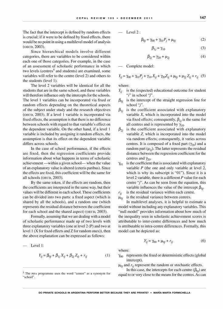
147
Do PRIVAtE sCHooLs In ARgEntInA PERfoRM BEttER BECAusE tHEy ARE PRIVAtE? • MARíA MARtA foRMICHELLA
C E P A L R E V I E W 1 0 5 • D E C E M B E R 2 0 1 1
The fact that the intercept is defined by random effects is crucial; if it were to be defined by fixed effects, there would be no point in using a multilevel model of analysis (oecd, 2003).
Since hierarchical models involve different categories, there are variables to be considered within each one of those categories. For example, in the case of an assessment of scholastic performance in which two levels (centres5 and students) are examined, some variables will refer to the centre (level 2) and others to the students (level 1).
The level 2 variables will be identical for all the students that are in the same school, and these variables will therefore influence only the intercepts for the schools. The level 1 variables can be incorporated via fixed or random effects depending on the theoretical aspects of the subject under study and the research objectives (oecd, 2003). If a level 1 variable is incorporated via fixed effects, the assumption is that there is no difference between schools with regard to that variable’s effect on the dependent variable. On the other hand, if a level 1 variable is included by assigning it random effects, the assumption is that its effect on the dependent variable differs across schools.
In the case of school performance, if the effects are fixed, then the regression coefficients provide information about what happens in terms of scholastic achievement —within a given school— when the value of an explanatory value is altered (ceteris paribus). Since the effects are fixed, this coefficient will be the same for all schools (oecd, 2003).
By the same token, if the effects are random, then the coefficients are interpreted in the same way, but their values will be different in each school. These coefficients can be divided into two parts: a fixed aspect (which is shared by all the schools), and a random one (which represents the residual distance between the coefficient for each school and the shared aspect) (oecd, 2003).
Formally, assuming that we are dealing with a model of scholastic performance made up of two levels with three explanatory variables (one at level 2 (P) and two at level 1 (X for fixed effects and Z for random ones)), then the above explanation can be expressed as follows:
— Level 1:
Yij = β0j + β1j Xij + β2j Zij + rij (1)
5 The pisa programme uses the word “centre” as a synonym for “school”.
— Level 2 :
β0j = γ00 + γ01Pj + µ0j (2)
β1j = γ10 (3)
β2j = γ20 + µ2j (4)
— Complete model:
Yij = γ00 + γ01Pj + γ10 Xij + γ20Zij + µ0j + µ2j Zij + rij (5)
where: Yij is the (expected) educational outcome for student
“i” in school “j”.β0j is the intercept of the straight regression line for
school “j”. β1j is the coefficient associated with explanatory
variable X, which is incorporated into the model via fixed effects; consequently, β1j is the same for all centres and is represented by γ10.
β2j is the coefficient associated with explanatory variable Z, which is incorporated into the model via random effects; consequently, it varies across centres. It is composed of a fixed part (γ20) and a random part (µ2j). The latter represents the residual distance between the regression coefficient for the centres and γ20.
γ01 is the coefficient that is associated with explanatory variable P (the one and only variable at level 2, which is why its subscript is “01”). Since it is a level 2 variable, there is a different P value for each centre “j”. As can be seen from the equation, this variable influences the value of the intercept β0j.
rij is the residual variance within each centre.µ0j is the residual variance between centres.
In multilevel analyses, it is helpful to estimate a model without including any explanatory variables. This “null model” provides information about how much of the inequality seen in scholastic achievement scores is attributable to inter-centre differences and how much is attributable to intra-centre differences. Formally, this model can be depicted as:
Yij = γ00 + µ0j + rij (6)
where: γ00 represents the fixed or deterministic effects (global
intercept).µ0j and rij represent the random or stochastic effects.
In this case, the intercepts for each centre (β0j) are equal to or very close to the means for the centres. As can

148
Do PRIVAtE sCHooLs In ARgEntInA PERfoRM BEttER BECAusE tHEy ARE PRIVAtE? • MARíA MARtA foRMICHELLA
C E P A L R E V I E W 1 0 5 • D E C E M B E R 2 0 1 1
be seen, β0j is made up of a fixed component, which is the same for all schools (γ00), and a random component (µ0j), which represents the deviation of school “j” from γ00, with γ00 being the result for the schools as a group (the mean), i.e. the “global intercept”. Thus, µ0j is the deviation of school “j” from the global intercept and represents the variance across the different centres.
For its part, rij is the deviation of the result for individual student “i” from the mean for school “j” (the school that the student attends). Since, in this model, each student is assigned the mean value for his or her school as a predicted score, rij is equal to the variance within each school.
Therefore, when there are no explanatory variables in the model, the residual and estimated intra- and inter-centre variances are equal to each other (oecd, 2003).
In sum, there are generally two types of relevant indices in multilevel analyses: regression coefficients and the decomposition of the variance between the different levels. A frequently used indicator, known as the “intraclass correlation coefficient” (ρ), can be derived from the second of these indices. This coefficient represents the proportion of the residual variance that is explained by inter-school differences (ρ = µ0j/ (µ0j + rij). In the null model, it represents the proportion of the variance in educational outcomes between schools. If this value were zero (0), then there would be no point in using a multilevel model.
When the models include explanatory variables, multilevel analyses usually provide information about the variance in the residual, i.e. the variance in the results that is not explained by the predictor variables that have been included in the model. However, it is interesting to look at the proportion of the variance that is explained. This can be obtained by comparing the proposed model with the null model at each level and overall. The way that this variance can be calculated is detailed in table 1:
TABLE 1
Percentage of variance accounted for by variables over the null model
Total 1 – (µ0j + rij) Proposed model/(µ0j + rij) Null model
Level 1 (students)
1 – (rij) Proposed model/(rij) Null model
Level 2 (schools)
1 – (µ0j) Proposed model/(µ0j) Null model
Source: Author’s original calculations based on Organization for Economic Cooperation and Development (oecd), El programa pisa de la ocde. ¿Qué es y para qué sirve?, Paris, 2003.
It will be helpful to provide a general description of the econometric models used in this study. As noted in the preceding section, data at the classroom level are not available, and a two-level hierarchical model (students and schools) is therefore used. In addition, variance between schools is permitted in the constant term and the slope coefficients. In other words, there can be variance not only in the intercepts of the straight regression lines for each school, but also in the coefficients associated with some of the level 1 explanatory variables The formal expression of these models is as follows:
Level 1
mj∑ ∑β γ β= +Y Xij j kk
K
kijm
M
mi j0 0 + +Z rj i1 1= =
(7)
Level 2
∑β γ γ= + +=f
F
0 00 01
0j f j jP u (8)
β γ umj j0m m= + (9)
where: K is the number of level 1 explanatory variables which are incorporated into the model via fixed effects (X); M is the number of level 1 explanatory variables which are incorporated into the model via random effects (Z); and F is the number of level 2 explanatory values (P). (The rest of the nomenclature has already been defined above.)
The Hierarchical Linear and Nonlinear Modeling for Windows (vhlm) programme was used to calculate the parameters for the above equations, which are estimated using simultaneous iteration methods that maximize the probability function.
In all of the models discussed here, observations are weighted using the w_fstuwt 6 weighting variable provided in the pisa database, and the weightings are standardized using the specific option offered by the vhlm software. The five plausible values for the “score on science test” variable (since this was the area emphasized in the 2006 pisa assessment) are used as the dependent variable, and the programme generates the final mean result for the population estimators. Finally, in order to preclude any problems in the significance tests in the event of heteroskedasticity, the parameters calculated for the equations and their corresponding standard errors are robust to heteroskedasticity.
6 “Weights are therefore inversely proportional to the probability of selection.” (oecd, 2003).
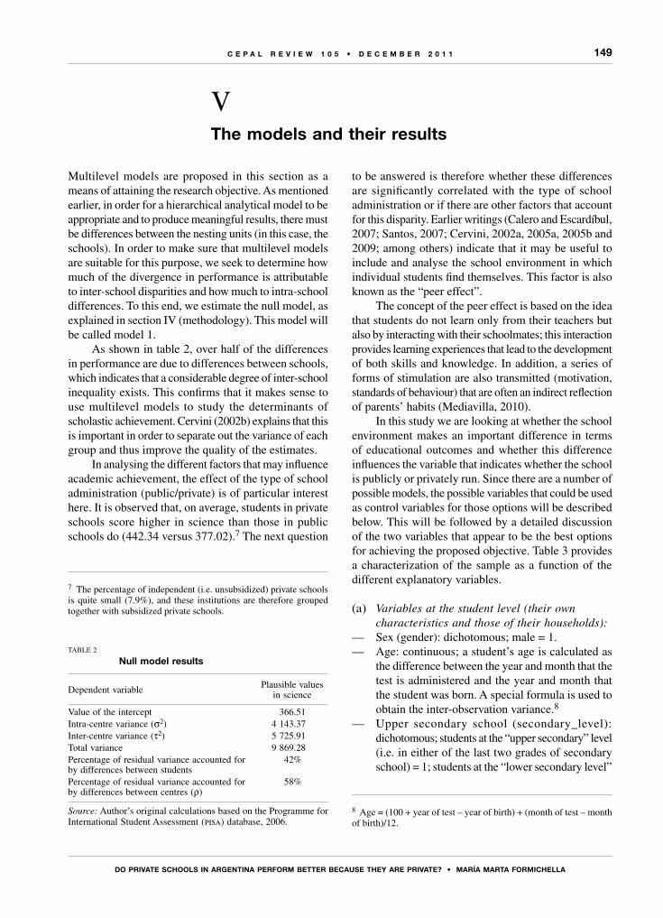
149
Do PRIVAtE sCHooLs In ARgEntInA PERfoRM BEttER BECAusE tHEy ARE PRIVAtE? • MARíA MARtA foRMICHELLA
C E P A L R E V I E W 1 0 5 • D E C E M B E R 2 0 1 1
Multilevel models are proposed in this section as a means of attaining the research objective. As mentioned earlier, in order for a hierarchical analytical model to be appropriate and to produce meaningful results, there must be differences between the nesting units (in this case, the schools). In order to make sure that multilevel models are suitable for this purpose, we seek to determine how much of the divergence in performance is attributable to inter-school disparities and how much to intra-school differences. To this end, we estimate the null model, as explained in section IV (methodology). This model will be called model 1.
As shown in table 2, over half of the differences in performance are due to differences between schools, which indicates that a considerable degree of inter-school inequality exists. This confirms that it makes sense to use multilevel models to study the determinants of scholastic achievement. Cervini (2002b) explains that this is important in order to separate out the variance of each group and thus improve the quality of the estimates.
In analysing the different factors that may influence academic achievement, the effect of the type of school administration (public/private) is of particular interest here. It is observed that, on average, students in private schools score higher in science than those in public schools do (442.34 versus 377.02).7 The next question
7 The percentage of independent (i.e. unsubsidized) private schools is quite small (7.9%), and these institutions are therefore grouped together with subsidized private schools.
to be answered is therefore whether these differences are significantly correlated with the type of school administration or if there are other factors that account for this disparity. Earlier writings (Calero and Escardíbul, 2007; Santos, 2007; Cervini, 2002a, 2005a, 2005b and 2009; among others) indicate that it may be useful to include and analyse the school environment in which individual students find themselves. This factor is also known as the “peer effect”.
The concept of the peer effect is based on the idea that students do not learn only from their teachers but also by interacting with their schoolmates; this interaction provides learning experiences that lead to the development of both skills and knowledge. In addition, a series of forms of stimulation are also transmitted (motivation, standards of behaviour) that are often an indirect reflection of parents’ habits (Mediavilla, 2010).
In this study we are looking at whether the school environment makes an important difference in terms of educational outcomes and whether this difference influences the variable that indicates whether the school is publicly or privately run. Since there are a number of possible models, the possible variables that could be used as control variables for those options will be described below. This will be followed by a detailed discussion of the two variables that appear to be the best options for achieving the proposed objective. Table 3 provides a characterization of the sample as a function of the different explanatory variables.
(a) Variables at the student level (their own characteristics and those of their households):
— Sex (gender): dichotomous; male = 1. — Age: continuous; a student’s age is calculated as
the difference between the year and month that the test is administered and the year and month that the student was born. A special formula is used to obtain the inter-observation variance.8
— Upper secondary school (secondary_level): dichotomous; students at the “upper secondary” level (i.e. in either of the last two grades of secondary school) = 1; students at the “lower secondary level”
8 Age = (100 + year of test – year of birth) + (month of test – month of birth)/12.
VThe models and their results
TABLE 2
null model results
Dependent variable Plausible values in science
Value of the intercept 366.51Intra-centre variance (σ2) 4 143.37Inter-centre variance (τ2) 5 725.91Total variance 9 869.28Percentage of residual variance accounted for by differences between students
42%
Percentage of residual variance accounted for by differences between centres (ρ)
58%
Source: Author’s original calculations based on the Programme for International Student Assessment (pisa) database, 2006.
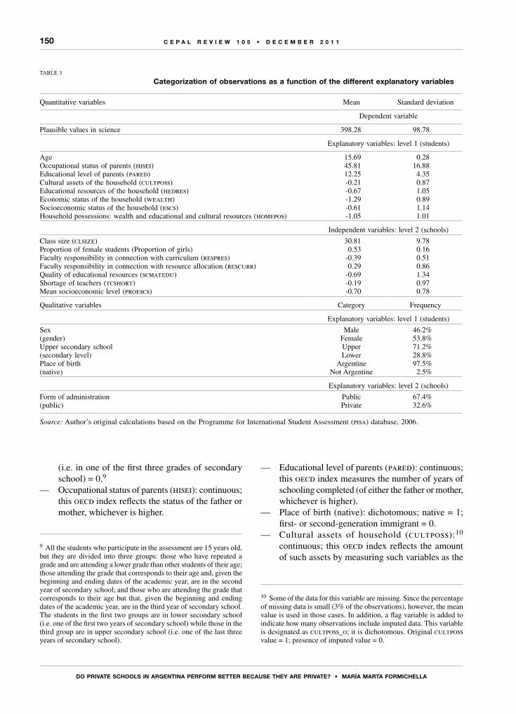
150
Do PRIVAtE sCHooLs In ARgEntInA PERfoRM BEttER BECAusE tHEy ARE PRIVAtE? • MARíA MARtA foRMICHELLA
C E P A L R E V I E W 1 0 5 • D E C E M B E R 2 0 1 1
TABLE 3
Categorization of observations as a function of the different explanatory variables
Quantitative variables Mean Standard deviation
Dependent variable
Plausible values in science 398.28 98.78
Explanatory variables: level 1 (students)
Age 15.69 0.28Occupational status of parents (hisei) 45.81 16.88Educational level of parents (pared) 12.25 4.35Cultural assets of the household (cultposs) -0.21 0.87Educational resources of the household (hedres) -0.67 1.05Economic status of the household (wealth) -1.29 0.89Socioeconomic status of the household (escs) -0.61 1.14Household possessions: wealth and educational and cultural resources (homepos) -1.05 1.01
Independent variables: level 2 (schools)
Class size (clsize) 30.81 9.78Proportion of female students (Proportion of girls) 0.53 0.16Faculty responsibility in connection with curriculum (respres) -0.39 0.51Faculty responsibility in connection with resource allocation (rescurr) 0.29 0.86Quality of educational resources (scmatedu) -0.69 1.34Shortage of teachers (tcshort) -0.19 0.97Mean socioeconomic level (proescs) -0.70 0.78
Qualitative variables Category Frequency
Explanatory variables: level 1 (students)
Sex(gender)
Male 46.2%Female 53.8%
Upper secondary school(secondary level)
Upper 71.2%Lower 28.8%
Place of birth(native)
Argentine 97.5%Not Argentine 2.5%
Explanatory variables: level 2 (schools)
Form of administration(public)
Public 67.4%Private 32.6%
Source: Author’s original calculations based on the Programme for International Student Assessment (pisa) database, 2006.
(i.e. in one of the first three grades of secondary school) = 0.9
— Occupational status of parents (hisei): continuous; this oecd index reflects the status of the father or mother, whichever is higher.
9 All the students who participate in the assessment are 15 years old, but they are divided into three groups: those who have repeated a grade and are attending a lower grade than other students of their age; those attending the grade that corresponds to their age and, given the beginning and ending dates of the academic year, are in the second year of secondary school; and those who are attending the grade that corresponds to their age but that, given the beginning and ending dates of the academic year, are in the third year of secondary school. The students in the first two groups are in lower secondary school (i.e. one of the first two years of secondary school) while those in the third group are in upper secondary school (i.e. one of the last three years of secondary school).
— Educational level of parents (pared): continuous; this oecd index measures the number of years of schooling completed (of either the father or mother, whichever is higher).
— Place of birth (native): dichotomous; native = 1; first- or second-generation immigrant = 0.
— Cultural assets of household (cultposs):10 continuous; this oecd index reflects the amount of such assets by measuring such variables as the
10 Some of the data for this variable are missing. Since the percentage of missing data is small (3% of the observations), however, the mean value is used in those cases. In addition, a flag variable is added to indicate how many observations include imputed data. This variable is designated as cultposs_o; it is dichotomous. Original cultposs value = 1; presence of imputed value = 0.

151
Do PRIVAtE sCHooLs In ARgEntInA PERfoRM BEttER BECAusE tHEy ARE PRIVAtE? • MARíA MARtA foRMICHELLA
C E P A L R E V I E W 1 0 5 • D E C E M B E R 2 0 1 1
availability of books (classic literature and poetry) in the home and the presence or absence of works of art. The higher the ranking on this index, the higher the household’s cultural level.
— Educational resources of the household (hedres): continuous; this oecd index reflects the amount of such resources (e.g., whether there is a desk and a quiet place to study, if a computer is available for schoolwork, if it is loaded with an educational computer programme, and if reference books and a dictionary are present). The higher the ranking on this index, the higher the level of educational resources in the household.
— Economic status of household (wealth): continuous; this oecd index measures the possessions present in the student’s household (e.g., whether or not the student has his or her own room and whether the household has an Internet connection, washing machine, dvd player, refrigerator with freezer, landline telephone and cable television). It also registers the number of mobile phones, televisions sets, computers and motor vehicles owned by the household. The higher the value of the index, the higher the household’s economic status.
(b) Variables at the school level:— Class size (clsize):11 indicates the average number
of students per class.— Proportion of female students: indicates the
percentage of females students in the school.— Faculty responsibility in connection with the
curriculum (respres): this oecd index reflects the degree of responsibility that the teaching staff has in regard to curricular issues. Higher rankings indicate greater levels of responsibility.
— Faculty responsibility in connection with resources (rescurr): this oecd index reflects the degree of responsibility that the teaching staff has in regard to resource allocation. Higher rankings indicate greater levels of responsibility.
— Quality of educational resources (scmatedu): this oecd index represents the quantity and quality of the school’s educational resources. (It includes measurements of laboratory equipment, books, computers, Internet connections, audiovisuals, etc.)
11 There are some (a few) data missing for this variable and for scmatedu. Where information is not available, the mean value is imputed. There are also two flag variables (clzise_o and scmatedu_o) which, as in the case of cultposs_o, show whether the observation includes an imputed datum or not.
Positive values indicate that the school provides good conditions in terms of educational resources; negative values indicate the opposite. Higher positive values signal a greater stock of educational resources.
— Shortage of teachers (tcshort): this oecd index measures any teacher shortages. Higher values indicate that a more serious problem exists owing to a lack of qualified teachers.Variables relating to the prior individual performance
of students are not included here. This is because academic performance is usually recurrent, and using past individual performance to account for current performance may not be appropriate (Viego, 2006).
Among the main variables considered in this study, the information available on the type of ownership structure is represented by a dichotomous variable that has been labeled “public”; thus public schools = 1 and private schools = 0. The characteristics of the student body at the school level are used to gauge the school environment, since the 2006 pisa does not report information at the classroom level. This environment is represented by the variable “Socioeconomic level of the school”. In order to quantify it, the mean escs indicator for the school is used.
The escs indicator is constructed by the pisa oecd team and sums up the information provided by the hisei, pared and homepos indices. hisei and pared have been explained above. homepos amalgamates the information supplied by the wealth, hedres and cultposs indices, together with the number of books in the home. In short, escs represents the household’s socioeconomic status. This index is designed in such a way that a positive value indicates that the household’s socioeconomic status exceeds the mean for oecd countries, while a negative value indicates the opposite. The higher the value of the index, the higher the household’s socioeconomic status.
The results of the estimated models will now be explored. As noted earlier, model 1 includes only the constant term. In contrast, explanatory variables have gradually been incorporated into the other models (first, variables relating to the students and, later, variables relating to the schools).
Consequently, we now propose that all the level 1 variables be incorporated as independent variables. These are first incorporated with fixed effects (model 2). Later, another model is proposed (model 3)12 that includes
12 No problems of multicollinearity arise in models 2 or 3; the mean result for the variance inflation factor (vif) is 1.2 and does not surpass 5 for any of the variables. The value of 5 is taken as a benchmark in line with Calero and Escardíbul (2007).
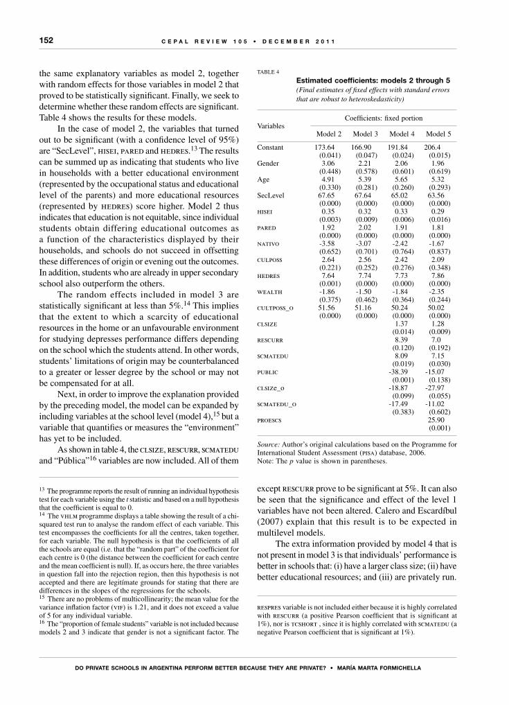
152
Do PRIVAtE sCHooLs In ARgEntInA PERfoRM BEttER BECAusE tHEy ARE PRIVAtE? • MARíA MARtA foRMICHELLA
C E P A L R E V I E W 1 0 5 • D E C E M B E R 2 0 1 1
the same explanatory variables as model 2, together with random effects for those variables in model 2 that proved to be statistically significant. Finally, we seek to determine whether these random effects are significant. Table 4 shows the results for these models.
In the case of model 2, the variables that turned out to be significant (with a confidence level of 95%) are “SecLevel”, hisei, pared and hedres.13 The results can be summed up as indicating that students who live in households with a better educational environment (represented by the occupational status and educational level of the parents) and more educational resources (represented by hedres) score higher. Model 2 thus indicates that education is not equitable, since individual students obtain differing educational outcomes as a function of the characteristics displayed by their households, and schools do not succeed in offsetting these differences of origin or evening out the outcomes. In addition, students who are already in upper secondary school also outperform the others.
The random effects included in model 3 are statistically significant at less than 5%.14 This implies that the extent to which a scarcity of educational resources in the home or an unfavourable environment for studying depresses performance differs depending on the school which the students attend. In other words, students’ limitations of origin may be counterbalanced to a greater or lesser degree by the school or may not be compensated for at all.
Next, in order to improve the explanation provided by the preceding model, the model can be expanded by including variables at the school level (model 4),15 but a variable that quantifies or measures the “environment” has yet to be included.
As shown in table 4, the clsize, rescurr, scmatedu and “Pública”16 variables are now included. All of them
13 The programme reports the result of running an individual hypothesis test for each variable using the t statistic and based on a null hypothesis that the coefficient is equal to 0. 14 The vhlm programme displays a table showing the result of a chi-squared test run to analyse the random effect of each variable. This test encompasses the coefficients for all the centres, taken together, for each variable. The null hypothesis is that the coefficients of all the schools are equal (i.e. that the “random part” of the coefficient for each centre is 0 (the distance between the coefficient for each centre and the mean coefficient is null). If, as occurs here, the three variables in question fall into the rejection region, then this hypothesis is not accepted and there are legitímate grounds for stating that there are differences in the slopes of the regressions for the schools. 15 There are no problems of multicollinearity; the mean value for the variance inflation factor (vif) is 1.21, and it does not exceed a value of 5 for any individual variable.16 The “proportion of female students” variable is not included because models 2 and 3 indicate that gender is not a significant factor. The
except rescurr prove to be significant at 5%. It can also be seen that the significance and effect of the level 1 variables have not been altered. Calero and Escardíbul (2007) explain that this result is to be expected in multilevel models.
The extra information provided by model 4 that is not present in model 3 is that individuals’ performance is better in schools that: (i) have a larger class size; (ii) have better educational resources; and (iii) are privately run.
respres variable is not included either because it is highly correlated with rescurr (a positive Pearson coefficient that is significant at 1%), nor is tcshort , since it is highly correlated with scmatedu (a negative Pearson coefficient that is significant at 1%).
TABLE 4
Estimated coefficients: models 2 through 5(Final estimates of fixed effects with standard errors that are robust to heteroskedasticity)
VariablesCoefficients: fixed portion
Model 2 Model 3 Model 4 Model 5
Constant 173.64(0.041)
166.90(0.047)
191.84(0.024)
206.4(0.015)
Gender 3.06(0.448)
2.21(0.578)
2.06(0.601)
1.96(0.619)
Age 4.91(0.330)
5.39(0.281)
5.65(0.260)
5.32(0.293)
SecLevel 67.65(0.000)
67.64(0.000)
65.02(0.000)
63.56(0.000)
hisei 0.35(0.003)
0.32(0.009)
0.33(0.006)
0.29(0.016)
pared 1.92(0.000)
2.02(0.000)
1.91(0.000)
1.81(0.000)
nativo -3.58(0.652)
-3.07(0.701)
-2.42(0.764)
-1.67(0.837)
culposs 2.64(0.221)
2.56(0.252)
2.42(0.276)
2.09(0.348)
hedres 7.64(0.001)
7.74(0.000)
7.73(0.000)
7.86(0.000)
wealth -1.86(0.375)
-1.50(0.462)
-1.84(0.364)
-2.35(0.244)
cultposs_o 51.56(0.000)
51.16(0.000)
50.24(0.000)
50.02(0.000)
clsize 1.37(0.014)
1.28(0.009)
rescurr 8.39(0.120)
7.0(0.192)
scmatedu 8.09(0.019)
7.15(0.030)
public -38.39(0.001)
-15.07(0.138)
clsize_o -18.87(0.099)
-27.97(0.055)
scmatedu_o -17.49(0.383)
-11.02(0.602)
proescs 25.90(0.001)
Source: Author’s original calculations based on the Programme for International Student Assessment (pisa) database, 2006.Note: The p value is shown in parentheses.
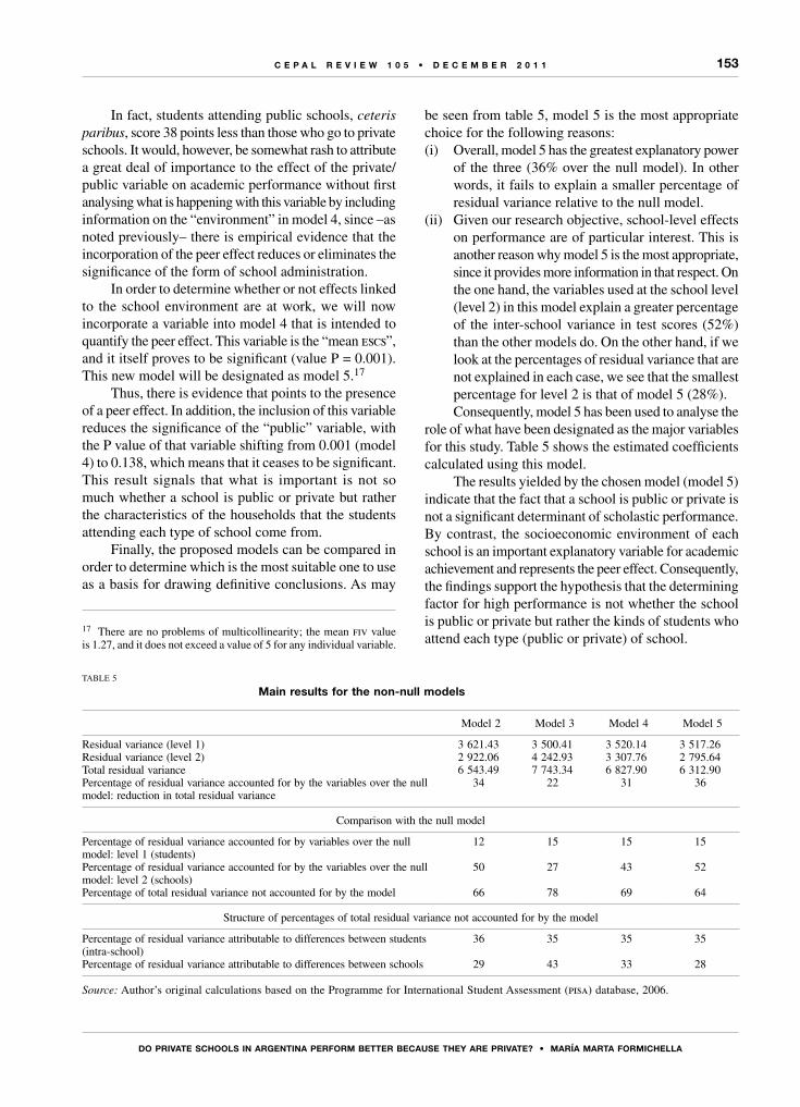
153
Do PRIVAtE sCHooLs In ARgEntInA PERfoRM BEttER BECAusE tHEy ARE PRIVAtE? • MARíA MARtA foRMICHELLA
C E P A L R E V I E W 1 0 5 • D E C E M B E R 2 0 1 1
In fact, students attending public schools, ceteris paribus, score 38 points less than those who go to private schools. It would, however, be somewhat rash to attribute a great deal of importance to the effect of the private/public variable on academic performance without first analysing what is happening with this variable by including information on the “environment” in model 4, since –as noted previously– there is empirical evidence that the incorporation of the peer effect reduces or eliminates the significance of the form of school administration.
In order to determine whether or not effects linked to the school environment are at work, we will now incorporate a variable into model 4 that is intended to quantify the peer effect. This variable is the “mean escs”, and it itself proves to be significant (value P = 0.001). This new model will be designated as model 5.17
Thus, there is evidence that points to the presence of a peer effect. In addition, the inclusion of this variable reduces the significance of the “public” variable, with the P value of that variable shifting from 0.001 (model 4) to 0.138, which means that it ceases to be significant. This result signals that what is important is not so much whether a school is public or private but rather the characteristics of the households that the students attending each type of school come from.
Finally, the proposed models can be compared in order to determine which is the most suitable one to use as a basis for drawing definitive conclusions. As may
17 There are no problems of multicollinearity; the mean fiv value is 1.27, and it does not exceed a value of 5 for any individual variable.
be seen from table 5, model 5 is the most appropriate choice for the following reasons: (i) Overall, model 5 has the greatest explanatory power
of the three (36% over the null model). In other words, it fails to explain a smaller percentage of residual variance relative to the null model.
(ii) Given our research objective, school-level effects on performance are of particular interest. This is another reason why model 5 is the most appropriate, since it provides more information in that respect. On the one hand, the variables used at the school level (level 2) in this model explain a greater percentage of the inter-school variance in test scores (52%) than the other models do. On the other hand, if we look at the percentages of residual variance that are not explained in each case, we see that the smallest percentage for level 2 is that of model 5 (28%).Consequently, model 5 has been used to analyse the
role of what have been designated as the major variables for this study. Table 5 shows the estimated coefficients calculated using this model.
The results yielded by the chosen model (model 5) indicate that the fact that a school is public or private is not a significant determinant of scholastic performance. By contrast, the socioeconomic environment of each school is an important explanatory variable for academic achievement and represents the peer effect. Consequently, the findings support the hypothesis that the determining factor for high performance is not whether the school is public or private but rather the kinds of students who attend each type (public or private) of school.
TABLE 5
Main results for the non-null models
Model 2 Model 3 Model 4 Model 5
Residual variance (level 1) 3 621.43 3 500.41 3 520.14 3 517.26Residual variance (level 2) 2 922.06 4 242.93 3 307.76 2 795.64Total residual variance 6 543.49 7 743.34 6 827.90 6 312.90Percentage of residual variance accounted for by the variables over the null model: reduction in total residual variance
34 22 31 36
Comparison with the null model
Percentage of residual variance accounted for by variables over the null model: level 1 (students)
12 15 15 15
Percentage of residual variance accounted for by the variables over the null model: level 2 (schools)
50 27 43 52
Percentage of total residual variance not accounted for by the model 66 78 69 64
Structure of percentages of total residual variance not accounted for by the model
Percentage of residual variance attributable to differences between students (intra-school)
36 35 35 35
Percentage of residual variance attributable to differences between schools 29 43 33 28
Source: Author’s original calculations based on the Programme for International Student Assessment (pisa) database, 2006.
154
Do PRIVAtE sCHooLs In ARgEntInA PERfoRM BEttER BECAusE tHEy ARE PRIVAtE? • MARíA MARtA foRMICHELLA
C E P A L R E V I E W 1 0 5 • D E C E M B E R 2 0 1 1
Throughout this study we have been examining the determinants of secondary-school students’ scholastic achievement in Argentina based on data from the 2006 pisa test. The aim of this exercise is to answer the following question: Is the fact that a school is public or private a significant factor in accounting for educational outcomes?
The evidence presented here supports the hypothesis put forward in the introduction, according to which the correlation between the type of school administration (public/private) and scholastic performance fades when the socioeconomic environment of the school is brought into the picture. This appears to indicate that private schools provide a better education than public schools do, but not because of their ownership structure. Instead, this is due to the fact that their students are better-placed, because of their background, to study and attain a high level of performance.
This raises an interesting question for further research: although the way in which private schools are organized does not appear to be a decisive factor in terms of performance, it is nonetheless true that such schools provide some sort of signal that causes individuals of a certain socioeconomic status to choose to attend them. In other words, the reasons why families choose this type of school (and, frequently, why these schools choose their students) may account for the favourable learning environment that is provided for students.
The considerations that we have explored here furnish grounds for stating that education policies need to go beyond the scope of the educational environment as such
because socioeconomic status appears to be an extremely influential determinant of scholastic performance. The results also show, however, that schools differ in their ability to offset inequalities of origin. This shows that there is indeed scope for education policy. In other words, since some schools perform better than others, there is scope for improvements that will, at the very least, bring the lower-performing schools up to the level of the better-performing ones.
As to the question of what kinds of education policies should be put in place, the information presented here would seem to indicate that one aspect to be taken into account is the quality of each school’s educational resources. A more detailed study will be needed in order to pinpoint exactly which aspects should be given priority, however. Future research efforts should incorporate more level 2 (school-level) variables into the analysis in order to fine-tune the related policy considerations.
Finally, it should be noted that many governments may be seeking to achieve a basic minimum of educational services for their students. In order to assess the extent to which this goal is achieved and the conditions that lead to success or failure in school, the specific factors that determine the likelihood that a given student will fail need to be explored.18 Further research will also need to be done in this area.
(Original: Spanish)
18 This can be done thanks to the development of software that allows logistic regression models to be used in multilevel analyses.
VI Conclusions
155
Do PRIVAtE sCHooLs In ARgEntInA PERfoRM BEttER BECAusE tHEy ARE PRIVAtE? • MARíA MARtA foRMICHELLA
C E P A L R E V I E W 1 0 5 • D E C E M B E R 2 0 1 1
Abdul-Hamid, H. (2007), “Evaluación de lo preparada que está Argentina para la economía del conocimiento: Medición del conocimiento y las habilidades de los alumnos en matemáticas y ciencias con resultados de pisa 2000”, Bienestar y política social, vol. 3, No. 2, Mexico City, Inter-American Conference on Social Security/Ibero-American University.
Calero, J., A. Choi and S. Waisgrais (2010), “¿Qué determina el fracaso escolar en España? Un estudio a través de pisa-2006” [online] http://www.um.es/dp-hacienda/eep2010/comunicaciones/eep2010-6.pdf.
(2009), “Determinantes del rendimiento educativo del alumnado de origen nacional e inmigrante en pisa-2006”, Cuadernos económicos, No. 77, Madrid, Información Comercial Española, Ministry of Industry, Tourism and Trade.
Calero, J. and J.O. Escardibul (2007), “Evaluación de servicios educativos: El rendimiento en los centros públicos y privados medido en Pisa-2003”, Hacienda pública española, vol. 183, No. 4, Madrid, Institute of Fiscal Studies.
Cervini, R. (2010), “El ‘efecto escuela’ en la educación primaria y secundaria: El caso de Argentina”, Revista electrónica iberoamericana sobre calidad, eficiencia y cambio en educación (reice), vol. 8, No. 1, Madrid, Red Iberoamericana de Investigación sobre Cambio y Eficacia Escolar.
(2009), “Comparando la inequidad en los logros escolares de la educación primaria y secundaria en Argentina: Un estudio multinivel”, Revista electrónica iberoamericana sobre calidad, eficiencia y cambio en la educación (reice), vol. 7, No. 1, Madrid, Red Iberoamericana de Investigación sobre Cambio y Eficacia Escolar.
(2006), “Los efectos de la escuela y del aula sobre el logro en matemáticas y en lengua de la educación secundaria. Un modelo multinivel”, Perfiles educativos, vol. 28, No. 112, Mexico City, National Autonomous University of Mexico.
(2005a), “Nivel y variación de la equidad en la educación media de Argentina”, Revista iberoamericana de educación, Madrid, Organization of Ibero-American States for Education, Science and Culture.
(2005b), “Variación de la equidad en resultados cognitivos y no cognitivos de la educación media de Argentina”, Revista electrónica de investigación educativa, vol. 7, No. 1 [online] http://redie.uabc.mx/vol7no1/contenido-cervini3.html.
(2002a), “Desigualdades socioculturales en el aprendizaje de matemática y lengua de la educación secundaria en argentina: un modelo de tres niveles”, Revista electrónica de investigación y evaluación educativa (relieve), vol. 8, No. 2, Valencia, University of Valencia.
(2002b), “Desigualdades en el logro académico y reproducción cultural en Argentina. Un modelo de tres niveles”, Revista mexicana de investigación educativa, vol. 7, No. 16, Mexico City, Consejo Mexicano de Investigación Educativa.
(1999), Calidad y equidad en la educación básica en la Argentina, Buenos Aires, Ministerio de Cultura y Educación de la Nación.
De La Cruz, F. (2008), “Modelos multinivel” [online] http://rpe.epiredperu.net/rpe_ediciones/v12_n03_2008/AR1.pdf
Diez Roux, A. (2002), “A glossary for multilevel analysis”, Journal of Epidemiology and Community Health, vol. 56, No. 8, bmj Publishing Group.
Fernández Aguerre, T. (2002), “Determinantes sociales e institucionales de la desigualdad educativa en sexto año de educación primaria de Argentina y Uruguay, 1999. Una aproximación mediante un modelo de regresión logística”, Revista mexicana de investigación educativa, vol. 7, No. 16, Mexico City, Consejo Mexicano de Investigación Educativa.
Formichella, M. (2010), “Educación y desarrollo: análisis desde la perspectiva de la equidad educativa interna y del mercado laboral”, thesis, Buenos Aires, Universidad Nacional del Sur.
Gertel, H. and others (2007a), “El rendimiento escolar de la población de estudiantes de la educación básica en Argentina: ¿cómo contribuye la gestión de la escuela?”, IX Jornadas Argentinas de Estudios de Población, Cordoba, Argentine Association of Population Studies.
(2007b), “Incidencia de la gestión sobre el rendimiento escolar en la escuela argentina. El mensaje de las pruebas internacionales y nacionales” [online] http://www.aaep.org.ar.
(2007c), “Los factores determinantes del rendimiento escolar al término de la educación básica en Argentina. Una aplicación de técnicas de análisis jerárquico de datos”, Anales de las XVI Jornadas de la Asociación de Economía de la Educación.
(2006), “Análisis multinivel del rendimiento escolar al término de la educación básica en Argentina”, document presented at the Annual meeting of the Argentine Association of Political Economy [online] http://www.aaep.org.ar/espa/anales/works06/Gertel_Giuliodori_Herrero.pdf
Hox, J.J (1995), Applied Multilevel Analysis, Amsterdam, tt-Publikaties.
Martínez Arias, R. (2006), “La metodología de los estudios pisa”, Revista de educación, Madrid, Complutense University of Madrid.
Mediavilla, M. (2010), “Las becas y ayudas al estudio como elemento determinante de la continuidad escolar en el nivel secundario post-obligatorio. Un análisis de sensibilidad a partir de la aplicación del Propensity Score Matching”, Investigaciones de economía de la educación, Asociación de Economía de la Educación.
oecd (Organization for Economic Cooperation and Development) (2006a), El programa pisa de la ocde. ¿Qué es y para qué sirve?, Paris.
(2006b), pisa 2006: Science Competencies for Tomorrow’s World, Paris.
(2006c), pisa Data Analysis Manual. spss, Second Edition, Paris.
(2003), pisa 2003. Data Analysis Manual, Paris.Santos, M. (2007), “Quality of education in Argentina: determinants
and distribution using pisa 2000 test scores”, Well-being and Social Policy, vol. 3, No. 1, Mexico City, Inter-American Conference on Social Security/Ibero-American University.
Viego, V. (2006), “Comentario al trabajo ‘Análisis multinivel del rendimiento escolar al término de la educación básica en Argentina’” [online] www.aaep.org.ar.
Wößmann, L. and T. Fuchs (2005), “Families, schools, and primary-school learning: evidence for Argentina and Colombia in an international perspective”, Policy Research Working Paper Series, No. 3537, Washington, D.C., World Bank.
Bibliography

C E P A L R E V I E W 1 0 5 • D E C E M B E R 2 0 1 1
157
K E Y W O R D S
Trade liberalization
Exports
Imports
Technology transfer
Manpower needs
Skilled workers
Industrial sector
Manufacturing enterprises
Econometric models
Brazil
Technology, trade and skills in Brazil:evidence from micro data
Bruno César Araújo, Francesco Bogliacino and Marco Vivarelli
B razil was characterized by a rapid process of trade liberalization in
the 1990s, resulting in a dramatic increase in the volumes of exports and
imports since the year 2000. Over the same period, the relative demand
for skilled labour has increased substantially. To investigate whether these
two simultaneous phenomena are linked is the purpose of this paper.
More particularly, this study focuses on the possible impact of domestic
technology, capital complementarity and trade openness on the relative
demand for skilled labour in Brazilian manufacturing firms, using a unique
panel database of Brazilian manufacturing firms over the period from 1997
to 2005. The empirical evidence supports the hypothesis that technology
played a role in determining the skill upgrading of Brazilian manufacturing
firms. Indeed, the estimations show that domestic technology and capital
formation are complements for skilled workers and that imported capital
goods clearly act as a skill-enhancing component of trade.
Bruno César Araújo
Researcher, Institute of Applied
Economic Research (ipea)
Francesco Bogliacino
Academic and researcher,
Department of Economics and
rise Group, eafit University
Joint Research Centre (jrc)-
Institute for Prospective
Technological Studies (ipts),
European Commission
Marco Vivarelli
Professor of Economic Policy,
Faculty of Economics, Università
Cattolica del Sacro Cuore
158
tECHnoLogy, tRADE AnD skILLs In BRAzIL: EVIDEnCE fRoM MICRo DAtA •Bruno CésAr ArAúJo, frAnCEsCo BoGLiACino AnD MArCo vivArELLi
C E P A L R E V I E W 1 0 5 • D E C E M B E R 2 0 1 1
The views expressed herein are the authors’ alone and may not in any circumstances be construed as stating an official position of the European Commission.The authors acknowledge financial support from ipea and eafit and would like to thank Eric Jardim, Geovane Lopes, Gustavo Alvarenga and Calebe Figueiredo for their statistical assistance (while themselves taking full responsibility for any errors and omissions) and Luigi Benfratello, Carlos Medina, Cristian Posso and Andrea Vaona for
This paper deals with the relationship between trade openness, with particular reference to technology transfer, and the relative demand for skilled labour in Brazilian manufacturing firms.
Brazil was characterized by a rapid process of trade liberalization in the 1990s, resulting in a dramatic increase in export and import volumes since the year 2000. An important aspect of this process might be its effect on labour demand and, more specifically, its impact on the relative demand for skilled labour. And in fact, the relative demand for skilled labour has increased substantially over the period, affecting the equilibrium employment level in the presence of a significant increase in the supply of skilled labour. To investigate whether these two simultaneous phenomena are linked is the purpose of this paper.
The theoretical literature offers different predictions regarding the impact of trade liberalization on labour demand in middle-income developing countries. On the one hand, according to the central tenet of traditional trade theory, expressed in the Heckscher-Ohlin theorem and in its Stolper-Samuelson corollary (hoss hereafter), we might expect a relative decrease in the demand for skilled labour, since openness should benefit a country’s relatively abundant factor, which in the case of Brazil is unskilled labour. On the other hand, if the hoss assumption of homogeneous
production functions between countries (i.e., absence of technological differentials) is relaxed, international openness may facilitate technology transfer from richer countries to middle-income developing countries. In this context, trade may act as a stimulus for technological upgrading and shift the production function towards more skill-intensive technologies; in addition, if the dominant technological paradigm is skill-biased, trade may induce and foster both domestic and imported skill-biased technological change.
This paper contributes to the debate, presenting new empirical evidence. We estimate the impact of domestic technologies and trade openness on labour demand for skilled and unskilled workers, using a unique panel database (obtained by merging three different statistical sources) of Brazilian manufacturing firms over the period from 1997 to 2005.
The remainder of this paper is organized as follows: the next section reviews the theoretical and empirical literature on the interaction between trade openness and the relative demand for skilled labour, mainly focusing on developing countries. Section III introduces and describes the data. Section IV. is devoted to a closer investigation of recent economic trends in Brazil. In section V we explain our empirical strategy and present and discuss our econometric results. Finally, the last section offers some brief concluding remarks.
Iintroduction
helpful comments on some econometric issues. We would also like to thank all the participants in the third Conference on Micro Evidence on Innovation and Development (meide iii) in Rio de Janeiro, Brazil, and those who attended the seminars at the Bank of the Republic in Medellín, Colombia, and at La Salle University and the National Planning Department in Bogotá. Finally, useful suggestions were provided by Naubahar Sharif, a discussant of this paper at the eighth Globelics International Conference, and by an anonymous cepal Review referee.
159
tECHnoLogy, tRADE AnD skILLs In BRAzIL: EVIDEnCE fRoM MICRo DAtA •Bruno CésAr ArAúJo, frAnCEsCo BoGLiACino AnD MArCo vivArELLi
C E P A L R E V I E W 1 0 5 • D E C E M B E R 2 0 1 1
After more than two decades of an ongoing debate focusing on the competing explanations for the increase in inequality in developed countries,1 there has recently been a stream of literature on the determinants of inequality in low- and middle-income countries (lmics). The shift in focus from the former to the latter originated in the discussion of the role played by trade: simply put, if inequality is driven by a specialization effect (countries with a skill abundance will reallocate their production towards it), there should be simultaneously an increase in inequality in the advanced countries (abundant in skilled labour) and a reduction of inequality in lmics (abundant in unskilled labour).
However, this argument is proved invalid by the macroeconomic data (Acemoglu, 2003), which shows an increase in within-country income inequality in both developed and developing countries. This outcome can be ascribed to the various theoretical problems affecting the hypotheses of the Hecksher-Ohlin and Stolper-Samuelson (hoss) theorems (see Leontief, 1953; Trefler, 1995; Davis and others, 1996, for an overall discussion). The core of the matter, first, is that neither consumers’ preferences nor production functions can be assumed to be homogeneous.2 Indeed, richer countries and lmics are endowed with very different technological capabilities (Abramowitz, 1986; Lall, 2004), and trade may act as a pervasive channel of technology transfer.
From a microeconomic point of view, it is worth noting that, in a developing country, firms’ reactions to trade openness are usually very heterogeneous.
1 See Acemoglu (2002) for a discussion of the literature with a focus on the United States, where the debate started. The two competing explanations of inequality in developed countries are the one focusing on the role of trade (see Wood, 1994; Freeman, 1995) and the one identifying new technologies as the main drivers of a skill bias that in turn increases wage dispersion and inequality. Berman, Bound and Griliches (1994) were the first to point out the skill-biased nature of current information and communication technologies (icts). See also Katz and Autor (1999) and Machin and Van Reenen (1998) for an extension to the Organisation for Economic Co-operation and Development (oecd) countries and Caroli and Van Reenen (2001), Aguirregabiria and Alonso-Borrego (2001) and Piva, Santarelli and Vivarelli (2005) for analyses of individual European countries.2 The literature that has extended hoss, while weakening its basic assumptions, is very extensive. For instance, Dornbush (1980) extended the model to multiple goods, Wood (1994) added multiple skills, and Davis (1995 and 1996) introduced the concept of “cones of diversification”.
Some firms are simply crowded out by international competition and are eliminated from the market, others adapt their production processes to the new competitive environment (opting for technical or operational efficiency through outsourcing and imports of embodied technology), whilst others again rely on innovation and accumulation of domestic technological capabilities as their main competitive strategies. This process is well documented in De Negri and Turchi (2007) for Brazil and Argentina.
In this context, skill upgrading can be related to technology diffusion, either by way of complementarities with domestic research and development (r&d) and capital formation, or through the learning-by-doing or technology adoption effect connected with the implementation of imported technologies (Arrow, 1962; Nelson and Phelps, 1966), initially introduced in richer countries.
Where the first perspective is concerned, Berman and Machin (2000 and 2004) found strong evidence for an increased demand for skills in middle-income developing countries in the 1980s and related it to the diffusion of skill-biased technological change from the richer developed countries to middle-income ones. In this framework, a country like Brazil, characterized by a certain degree of indigenous innovation effort, might well exhibit a positive correlation between domestic technologies and skill upgrading. By the same token, domestic capital is also a vehicle of “embodied technological change” (see Salter, 1960; Solow, 1960) that can be skill-biased in nature; hence, capital/skills complementarity (see Griliches, 1969) may also have had an important role in the skill upgrading of the Brazilian labour force.
Where the second perspective is concerned, Robbins and Gindling (1999) and Robbins (2003) put forward the so-called skill-enhancing trade (set) hypothesis, pointing out the potential skill-biased effect of technologies flowing in as a result of trade liberalization. The idea is that trade liberalization accelerates flows of imported technologies embodied in capital goods (especially machinery), and the resulting technology transfer induces adaptation to the modern skill-intensive technologies currently used in the most advanced countries, involving a substantial increase in the demand for skilled labour within the developing countries receiving them (for
IILiterature

160
tECHnoLogy, tRADE AnD skILLs In BRAzIL: EVIDEnCE fRoM MICRo DAtA •Bruno CésAr ArAúJo, frAnCEsCo BoGLiACino AnD MArCo vivArELLi
C E P A L R E V I E W 1 0 5 • D E C E M B E R 2 0 1 1
more extensive analyses, see Lee and Vivarelli, 2004 and 2006; Almeida and Fernandes, 2008). Obviously, this technology-related effect may more than counterbalance the hoss predictions.3
Where the empirical literature is concerned, there is a growing body of studies associating trade with a rise in inequality in developing countries. For instance, Hanson and Harrison (1999) reported that trade liberalization was related to a rise in inequality in Mexico. Manacorda, Sanchez-Paramo and Schady (2006) found that the relative demand for skilled workers had risen in Argentina, Mexico, Chile and Colombia, with mixed results in Brazil.4
Following this line of research, Meschi and Vivarelli (2009), using a sample of 65 developing countries over the 1980-1999 period, found that trade with high-income countries made the income distribution more unequal in middle-income developing countries, by way of both imports and exports.5 Similarly, Meschi, Taymaz and Vivarelli (2008) showed that set was an important factor in explaining the rise of the skilled labour cost share in Turkey during the 1980-2001 period.6
Where Brazil is concerned, previous literature on the subject is scarce. According to Gonzaga, Menezes-Filho and Terra (2006), wage differentials between skilled and unskilled workers decreased during the 1988-1995
3 Interestingly enough, if the technological effect prevails over the hoss effect in developing countries, inequality rises in both developed and developing countries, which is what has been observed for the last two decades (see Feenstra and Hanson, 1996 and 1997). However, an increase in inequality as a consequence of economic growth in developing countries was predicted by Kuznets a long time ago (see Kuznets, 1955; Grimalda and Vivarelli, 2010).4 Similar results were found by Conte and Vivarelli (2011), using sectoral manufacturing data for 23 low- and middle-income countries over the 1980-1991 period.5 Similarly, Vivarelli (2004), using data for 45 developing countries in the 1990s, found that imports could entail an increase in the domestic income inequality of the recipient developing country, at least in the early stages of the opening process. 6 The authors show that the increase in the skilled labour cost share was mainly driven by the “within” effect (increase in the demand for skills within industrial sectors, due to new technologies) rather than by the “between” effect (reallocation of skilled labour between sectors, as a possible outcome of hoss specialization).
period, which is when trade liberalization started to be implemented in Brazil. The authors provided some evidence that hoss mechanisms may have had a role in this process.7
However, Menezes-Filho and Giovanetti (2006) analysed the evolution of skilled employment in Brazil over the subsequent 1990-1998 period. First, partially contradicting the findings of Gonzaga, Menezes-Filho and Terra (2006), they detected an increase in the skilled labour share; this increase was entirely due to the ‘within-industry’ effect, while the ‘between-industries’ effect was negative, in line with the hoss predictions. Then, inspired by Machin and Van Reenen (1998), they ran an econometric equation to test the trade-induced skill bias hypothesis. Their variable was input tariffs, the hypothesis being that the reduction of input tariffs should have induced the importation of technologically advanced inputs, in turn raising the demand for skilled labour. Consistently with their hypothesis, they found that tariffs were negatively related to skill upgrading, and that this effect was stronger in those sectors that used inputs more complementary to skills.
Relative to Menezes-Filho and Giovanetti (2006), our paper has three distinctive characteristics. Firstly, while that study analysed the most intensive period of trade opening, we cover the aftermath of this severe reshaping of industrial sectors in Brazil and part of the export boom triggered in 2002 (our data cover the period from 1997 to 2005). The second distinctive characteristic is that our dataset, which consists of firm-level micro data, comes from the merging of several databases.8 Finally, our data allow us to use a direct and precise indicator of the set effect (see below).
7 For instance, their decomposition analysis of the increase in the skilled labour share of total employment showed that there was a negative “between-industries” effect in Brazil and that this was consistent with the hoss predictions.8 Instead, Menezes-Filho and Giovanetti (2006) used a micro-aggregated database, in which each observational unit was a weighted average of three firms. For further details, see Menezes-Filho, Muendler and Ramey (2003).
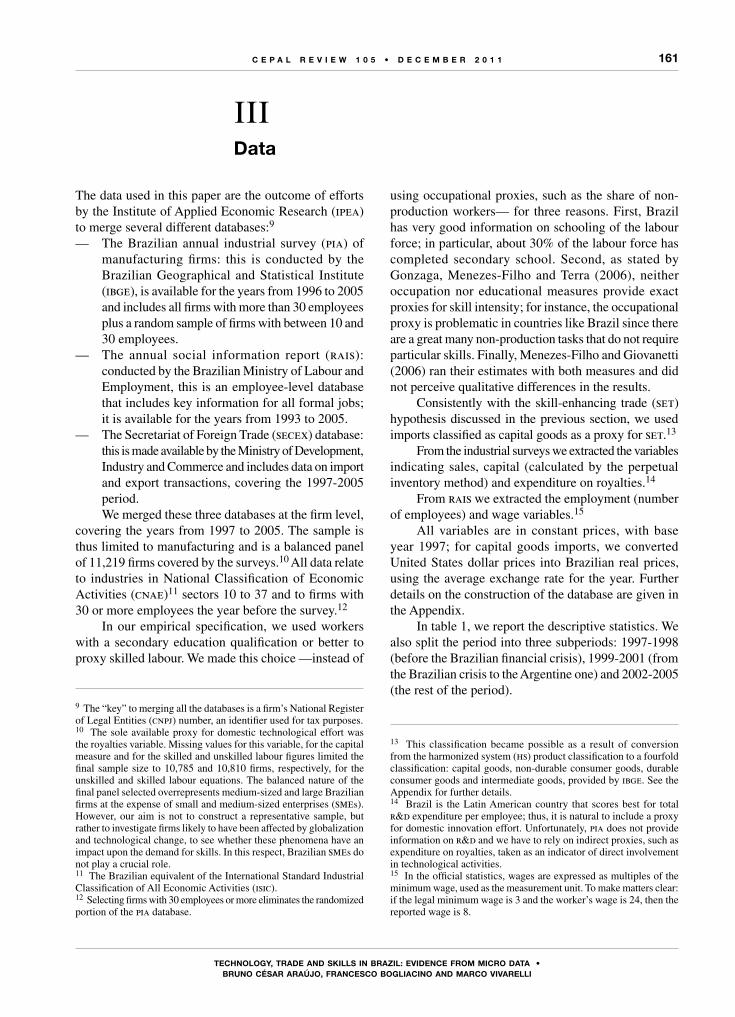
161
tECHnoLogy, tRADE AnD skILLs In BRAzIL: EVIDEnCE fRoM MICRo DAtA •Bruno CésAr ArAúJo, frAnCEsCo BoGLiACino AnD MArCo vivArELLi
C E P A L R E V I E W 1 0 5 • D E C E M B E R 2 0 1 1
The data used in this paper are the outcome of efforts by the Institute of Applied Economic Research (ipea) to merge several different databases:9
— The Brazilian annual industrial survey (pia) of manufacturing firms: this is conducted by the Brazilian Geographical and Statistical Institute (ibge), is available for the years from 1996 to 2005 and includes all firms with more than 30 employees plus a random sample of firms with between 10 and 30 employees.
— The annual social information report (rais): conducted by the Brazilian Ministry of Labour and Employment, this is an employee-level database that includes key information for all formal jobs; it is available for the years from 1993 to 2005.
— The Secretariat of Foreign Trade (secex) database: this is made available by the Ministry of Development, Industry and Commerce and includes data on import and export transactions, covering the 1997-2005 period.We merged these three databases at the firm level,
covering the years from 1997 to 2005. The sample is thus limited to manufacturing and is a balanced panel of 11,219 firms covered by the surveys.10 All data relate to industries in National Classification of Economic Activities (cnae)11 sectors 10 to 37 and to firms with 30 or more employees the year before the survey.12
In our empirical specification, we used workers with a secondary education qualification or better to proxy skilled labour. We made this choice —instead of
9 The “key” to merging all the databases is a firm’s National Register of Legal Entities (cnpj) number, an identifier used for tax purposes.10 The sole available proxy for domestic technological effort was the royalties variable. Missing values for this variable, for the capital measure and for the skilled and unskilled labour figures limited the final sample size to 10,785 and 10,810 firms, respectively, for the unskilled and skilled labour equations. The balanced nature of the final panel selected overrepresents medium-sized and large Brazilian firms at the expense of small and medium-sized enterprises (smes). However, our aim is not to construct a representative sample, but rather to investigate firms likely to have been affected by globalization and technological change, to see whether these phenomena have an impact upon the demand for skills. In this respect, Brazilian smes do not play a crucial role.11 The Brazilian equivalent of the International Standard Industrial Classification of All Economic Activities (isic).12 Selecting firms with 30 employees or more eliminates the randomized portion of the pia database.
using occupational proxies, such as the share of non-production workers— for three reasons. First, Brazil has very good information on schooling of the labour force; in particular, about 30% of the labour force has completed secondary school. Second, as stated by Gonzaga, Menezes-Filho and Terra (2006), neither occupation nor educational measures provide exact proxies for skill intensity; for instance, the occupational proxy is problematic in countries like Brazil since there are a great many non-production tasks that do not require particular skills. Finally, Menezes-Filho and Giovanetti (2006) ran their estimates with both measures and did not perceive qualitative differences in the results.
Consistently with the skill-enhancing trade (set) hypothesis discussed in the previous section, we used imports classified as capital goods as a proxy for set.13
From the industrial surveys we extracted the variables indicating sales, capital (calculated by the perpetual inventory method) and expenditure on royalties.14
From rais we extracted the employment (number of employees) and wage variables.15
All variables are in constant prices, with base year 1997; for capital goods imports, we converted United States dollar prices into Brazilian real prices, using the average exchange rate for the year. Further details on the construction of the database are given in the Appendix.
In table 1, we report the descriptive statistics. We also split the period into three subperiods: 1997-1998 (before the Brazilian financial crisis), 1999-2001 (from the Brazilian crisis to the Argentine one) and 2002-2005 (the rest of the period).
13 This classification became possible as a result of conversion from the harmonized system (hs) product classification to a fourfold classification: capital goods, non-durable consumer goods, durable consumer goods and intermediate goods, provided by ibge. See the Appendix for further details.14 Brazil is the Latin American country that scores best for total r&d expenditure per employee; thus, it is natural to include a proxy for domestic innovation effort. Unfortunately, pia does not provide information on r&d and we have to rely on indirect proxies, such as expenditure on royalties, taken as an indicator of direct involvement in technological activities.15 In the official statistics, wages are expressed as multiples of the minimum wage, used as the measurement unit. To make matters clear: if the legal minimum wage is 3 and the worker’s wage is 24, then the reported wage is 8.
IIIData
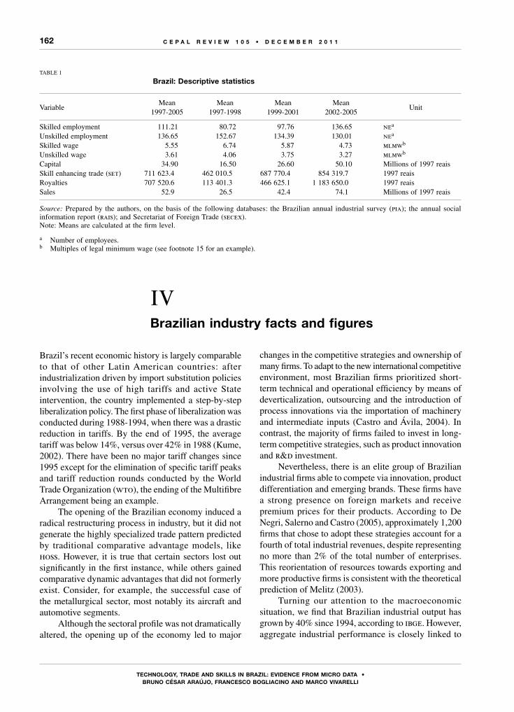
162
tECHnoLogy, tRADE AnD skILLs In BRAzIL: EVIDEnCE fRoM MICRo DAtA •Bruno CésAr ArAúJo, frAnCEsCo BoGLiACino AnD MArCo vivArELLi
C E P A L R E V I E W 1 0 5 • D E C E M B E R 2 0 1 1
Brazil’s recent economic history is largely comparable to that of other Latin American countries: after industrialization driven by import substitution policies involving the use of high tariffs and active State intervention, the country implemented a step-by-step liberalization policy. The first phase of liberalization was conducted during 1988-1994, when there was a drastic reduction in tariffs. By the end of 1995, the average tariff was below 14%, versus over 42% in 1988 (Kume, 2002). There have been no major tariff changes since 1995 except for the elimination of specific tariff peaks and tariff reduction rounds conducted by the World Trade Organization (wto), the ending of the Multifibre Arrangement being an example.
The opening of the Brazilian economy induced a radical restructuring process in industry, but it did not generate the highly specialized trade pattern predicted by traditional comparative advantage models, like hoss. However, it is true that certain sectors lost out significantly in the first instance, while others gained comparative dynamic advantages that did not formerly exist. Consider, for example, the successful case of the metallurgical sector, most notably its aircraft and automotive segments.
Although the sectoral profile was not dramatically altered, the opening up of the economy led to major
changes in the competitive strategies and ownership of many firms. To adapt to the new international competitive environment, most Brazilian firms prioritized short-term technical and operational efficiency by means of deverticalization, outsourcing and the introduction of process innovations via the importation of machinery and intermediate inputs (Castro and Ávila, 2004). In contrast, the majority of firms failed to invest in long-term competitive strategies, such as product innovation and r&d investment.
Nevertheless, there is an elite group of Brazilian industrial firms able to compete via innovation, product differentiation and emerging brands. These firms have a strong presence on foreign markets and receive premium prices for their products. According to De Negri, Salerno and Castro (2005), approximately 1,200 firms that chose to adopt these strategies account for a fourth of total industrial revenues, despite representing no more than 2% of the total number of enterprises. This reorientation of resources towards exporting and more productive firms is consistent with the theoretical prediction of Melitz (2003).
Turning our attention to the macroeconomic situation, we find that Brazilian industrial output has grown by 40% since 1994, according to ibge. However, aggregate industrial performance is closely linked to
TABLE 1
Brazil: Descriptive statistics
VariableMean
1997-2005Mean
1997-1998Mean
1999-2001Mean
2002-2005Unit
Skilled employment 111.21 80.72 97.76 136.65 nea
Unskilled employment 136.65 152.67 134.39 130.01 nea
Skilled wage 5.55 6.74 5.87 4.73 mlmwb
Unskilled wage 3.61 4.06 3.75 3.27 mlmwb
Capital 34.90 16.50 26.60 50.10 Millions of 1997 reaisSkill enhancing trade (set) 711 623.4 462 010.5 687 770.4 854 319.7 1997 reaisRoyalties 707 520.6 113 401.3 466 625.1 1 183 650.0 1997 reaisSales 52.9 26.5 42.4 74.1 Millions of 1997 reais
Source: Prepared by the authors, on the basis of the following databases: the Brazilian annual industrial survey (pia); the annual social information report (rais); and Secretariat of Foreign Trade (secex). Note: Means are calculated at the firm level.
a Number of employees.b Multiples of legal minimum wage (see footnote 15 for an example).
IVBrazilian industry facts and figures
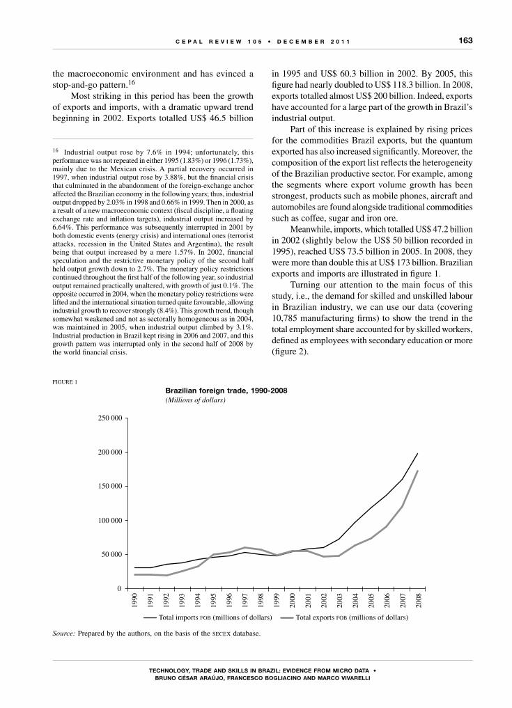
163
tECHnoLogy, tRADE AnD skILLs In BRAzIL: EVIDEnCE fRoM MICRo DAtA •Bruno CésAr ArAúJo, frAnCEsCo BoGLiACino AnD MArCo vivArELLi
C E P A L R E V I E W 1 0 5 • D E C E M B E R 2 0 1 1
the macroeconomic environment and has evinced a stop-and-go pattern.16
Most striking in this period has been the growth of exports and imports, with a dramatic upward trend beginning in 2002. Exports totalled US$ 46.5 billion
16 Industrial output rose by 7.6% in 1994; unfortunately, this performance was not repeated in either 1995 (1.83%) or 1996 (1.73%), mainly due to the Mexican crisis. A partial recovery occurred in 1997, when industrial output rose by 3.88%, but the financial crisis that culminated in the abandonment of the foreign-exchange anchor affected the Brazilian economy in the following years; thus, industrial output dropped by 2.03% in 1998 and 0.66% in 1999. Then in 2000, as a result of a new macroeconomic context (fiscal discipline, a floating exchange rate and inflation targets), industrial output increased by 6.64%. This performance was subsequently interrupted in 2001 by both domestic events (energy crisis) and international ones (terrorist attacks, recession in the United States and Argentina), the result being that output increased by a mere 1.57%. In 2002, financial speculation and the restrictive monetary policy of the second half held output growth down to 2.7%. The monetary policy restrictions continued throughout the first half of the following year, so industrial output remained practically unaltered, with growth of just 0.1%. The opposite occurred in 2004, when the monetary policy restrictions were lifted and the international situation turned quite favourable, allowing industrial growth to recover strongly (8.4%). This growth trend, though somewhat weakened and not as sectorally homogeneous as in 2004, was maintained in 2005, when industrial output climbed by 3.1%. Industrial production in Brazil kept rising in 2006 and 2007, and this growth pattern was interrupted only in the second half of 2008 by the world financial crisis.
in 1995 and US$ 60.3 billion in 2002. By 2005, this figure had nearly doubled to US$ 118.3 billion. In 2008, exports totalled almost US$ 200 billion. Indeed, exports have accounted for a large part of the growth in Brazil’s industrial output.
Part of this increase is explained by rising prices for the commodities Brazil exports, but the quantum exported has also increased significantly. Moreover, the composition of the export list reflects the heterogeneity of the Brazilian productive sector. For example, among the segments where export volume growth has been strongest, products such as mobile phones, aircraft and automobiles are found alongside traditional commodities such as coffee, sugar and iron ore.
Meanwhile, imports, which totalled US$ 47.2 billion in 2002 (slightly below the US$ 50 billion recorded in 1995), reached US$ 73.5 billion in 2005. In 2008, they were more than double this at US$ 173 billion. Brazilian exports and imports are illustrated in figure 1.
Turning our attention to the main focus of this study, i.e., the demand for skilled and unskilled labour in Brazilian industry, we can use our data (covering 10,785 manufacturing firms) to show the trend in the total employment share accounted for by skilled workers, defined as employees with secondary education or more (figure 2).
FIGURE 1
Brazilian foreign trade, 1990-2008(Millions of dollars)
Source: Prepared by the authors, on the basis of the secex database.
1990
1991
1992
1993
1994
1995
1996
1997
1998
1999
2000
2001
2002
2003
2004
2005
2006
2007
2008
0
50 000
100 000
150 000
200 000
250 000
Total imports FOB (millions of dollars) Total exports FOB (millions of dollars)

164
tECHnoLogy, tRADE AnD skILLs In BRAzIL: EVIDEnCE fRoM MICRo DAtA •Bruno CésAr ArAúJo, frAnCEsCo BoGLiACino AnD MArCo vivArELLi
C E P A L R E V I E W 1 0 5 • D E C E M B E R 2 0 1 1
Figure 2 clearly suggests a rising trend; indeed, by the end of the period considered, the share of skilled workers was close to half the firms’ workforce.
An initial attempt to determine the main forces behind skill upgrading can be made by splitting the revealed increase in the demand for skilled labour into its between- and within-industry components. The aggregate increase in the demand for skills may have been driven by — employment reallocation across industries (for a
number of reasons, such as trade shifts, structural change, evolving tastes or changes in economic policy) or
— skill upgrading within industries (mainly due to technological change). Therefore, we decompose the aggregate change in
the demand for skilled labour (∆SL) in the i = 1,…, N industries (with N going from sector 10 to sector 37) according to the following formula:
∆ ∆ ∆SL SL SLi ii
N
ii
N
i1 1= =
P P∑ ∑= + (1)
where SL is skilled labour (number of skilled workers) and Pi is industry i’s share of total employment.
The first term is the within-industry component of skill upgrading, weighted by
–Pi, the relative size of
industry i (i.e., industry i’s share of total employment), where the bar is a time mean. The second term measures the contribution of between-industry shifts, i.e., how much bigger or smaller an industry is becoming over time, weighted by time-averaged skill demand.
Table 2 shows that the increase in the demand for skilled labour was driven by the within-industry variation, which basically accounts for the whole of the overall change. This interesting preliminary evidence
FIGURE 2
Brazil: Average skilled share of employment in the labor market, 1996-2006(Percentages)
Source: Prepared by the authors, on the basis of the rais database.
1996 1998 2000 2002 2004 2006
25
30
35
40
45
Fitted valuesAverage skilled share
Ave
rage
ski
lled
shar
e
TABLE 2
Brazil: Decomposition of the skilled employment sharea
Within Between Overall Within/Between
1997-2005 0.23 -0.01 0.22 1.041997-1998 0.03 0.00 0.03 1.001999-2001 0.06 -0.01 0.05 1.202002-2005 0.08 0.00 0.08 1.00
Source: Prepared by the authors, on the basis of the pia, rais, and secex databases.
a The sum of rows 2, 3 and 4 does not add up to the row 1 total. The row 1 total is the sum of the three plus the changed occurred during the years 1998 and 2001. Both were years of financial crisis, so their effect is difficult to interpret.

165
tECHnoLogy, tRADE AnD skILLs In BRAzIL: EVIDEnCE fRoM MICRo DAtA •Bruno CésAr ArAúJo, frAnCEsCo BoGLiACino AnD MArCo vivArELLi
C E P A L R E V I E W 1 0 5 • D E C E M B E R 2 0 1 1
supports the hypothesis that technology (and in particular technology transfer from richer countries) may have played a crucial role as a determinant of skill upgrading in Brazilian manufacturing.
Other preliminary evidence is obtained by considering the density functions of skilled employment and the skilled
employment share in the subsample of firms that do not import capital goods and the subsample of those that do, respectively (figures 3 and 4). Since in both cases we can see that the distribution is more right-skewed for the subsample of technology adopters, we again find some empirical evidence in favour of the set hypothesis.
FIGURE 3
Brazil: Density of (log) skilled employment for non-importers of capital goods (left) and for capital-importing firms (right)
Source: Prepared by the authors, on the basis of the rais and secex databases.
Den
sity
–5 0
Capital importers
Log (skilled workers)
0
0.1
0.2
0.3
0.4
5 10
Den
sity
–2 2 40
Non-capital importers
Log (skilled workers)
0
0.1
0.2
0.3
0.4
6 8
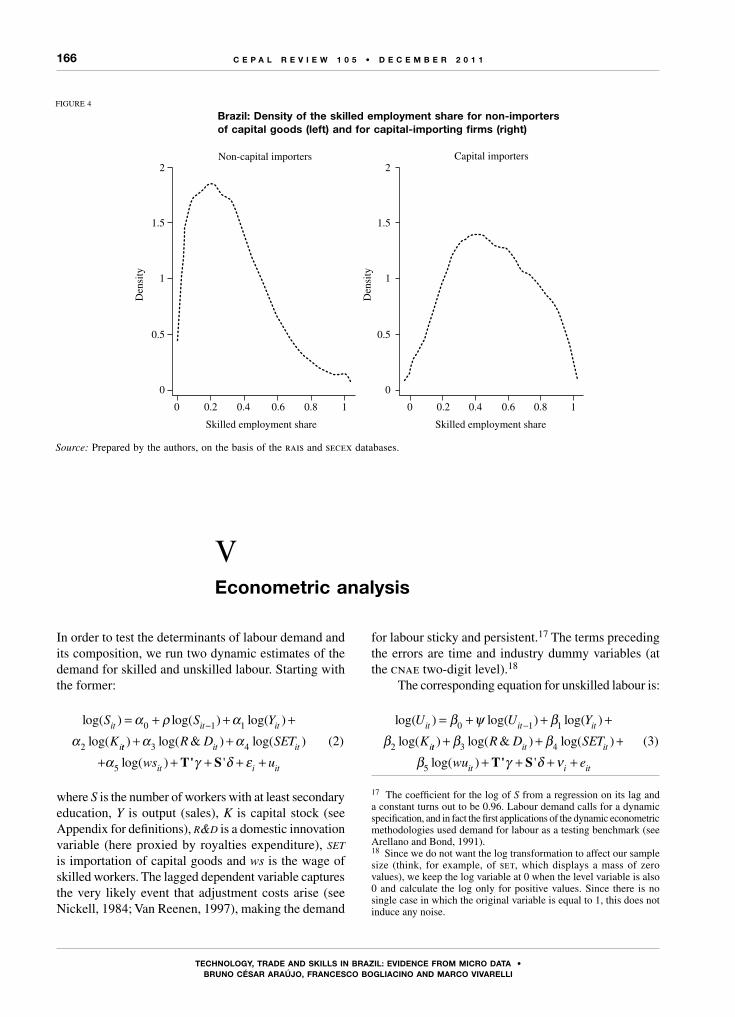
166
tECHnoLogy, tRADE AnD skILLs In BRAzIL: EVIDEnCE fRoM MICRo DAtA •Bruno CésAr ArAúJo, frAnCEsCo BoGLiACino AnD MArCo vivArELLi
C E P A L R E V I E W 1 0 5 • D E C E M B E R 2 0 1 1
In order to test the determinants of labour demand and its composition, we run two dynamic estimates of the demand for skilled and unskilled labour. Starting with the former:
log( ) log( ) log( )
log(
S S Y
Kit it it
i
= + −α ρ αα
0 1 1
2 tt i t
it
R D SET
ws
) log( & ) log( )
log( )+ +α5 T '' 'γ δ ε+ + +S i itut i
+ +
3 4α α+ + (2)
where S is the number of workers with at least secondary education, Y is output (sales), K is capital stock (see Appendix for definitions), r&d is a domestic innovation variable (here proxied by royalties expenditure), set is importation of capital goods and ws is the wage of skilled workers. The lagged dependent variable captures the very likely event that adjustment costs arise (see Nickell, 1984; Van Reenen, 1997), making the demand
for labour sticky and persistent.17 The terms preceding the errors are time and industry dummy variables (at the cnae two-digit level).18
The corresponding equation for unskilled labour is:
log( ) log( ) log( )
log(
U U Y
Kit it it
i
= + −β ψ ββ
0 1 1
2 tt i t
it
R D SET
wu
) log( & ) log( )
log( )
++β5 T '' 'γ δ ν+ + +S i ite
t i
+ +
3 4β β+ + (3)
17 The coefficient for the log of S from a regression on its lag and a constant turns out to be 0.96. Labour demand calls for a dynamic specification, and in fact the first applications of the dynamic econometric methodologies used demand for labour as a testing benchmark (see Arellano and Bond, 1991). 18 Since we do not want the log transformation to affect our sample size (think, for example, of set, which displays a mass of zero values), we keep the log variable at 0 when the level variable is also 0 and calculate the log only for positive values. Since there is no single case in which the original variable is equal to 1, this does not induce any noise.
FIGURE 4
Brazil: Density of the skilled employment share for non-importers of capital goods (left) and for capital-importing firms (right)
Source: Prepared by the authors, on the basis of the rais and secex databases.
Den
sity
0 0.2
Capital importers
Skilled employment share
0
0.5
1
1.5
2
0.4 0.6 0.8 1
Den
sity
0 0.4 0.60.2
Non-capital importers
Skilled employment share
0
0.5
1
1.5
2
0.8 1
VEconometric analysis
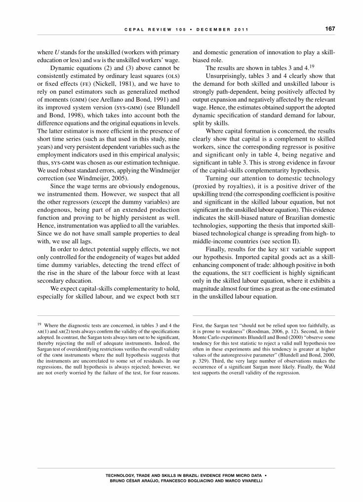
167
tECHnoLogy, tRADE AnD skILLs In BRAzIL: EVIDEnCE fRoM MICRo DAtA •Bruno CésAr ArAúJo, frAnCEsCo BoGLiACino AnD MArCo vivArELLi
C E P A L R E V I E W 1 0 5 • D E C E M B E R 2 0 1 1
where U stands for the unskilled (workers with primary education or less) and wu is the unskilled workers’ wage.
Dynamic equations (2) and (3) above cannot be consistently estimated by ordinary least squares (ols) or fixed effects (fe) (Nickell, 1981), and we have to rely on panel estimators such as generalized method of moments (gmm) (see Arellano and Bond, 1991) and its improved system version (sys-gmm) (see Blundell and Bond, 1998), which takes into account both the difference equations and the original equations in levels. The latter estimator is more efficient in the presence of short time series (such as that used in this study, nine years) and very persistent dependent variables such as the employment indicators used in this empirical analysis; thus, sys-gmm was chosen as our estimation technique. We used robust standard errors, applying the Windmeijer correction (see Windmeijer, 2005).
Since the wage terms are obviously endogenous, we instrumented them. However, we suspect that all the other regressors (except the dummy variables) are endogenous, being part of an extended production function and proving to be highly persistent as well. Hence, instrumentation was applied to all the variables. Since we do not have small sample properties to deal with, we use all lags.
In order to detect potential supply effects, we not only controlled for the endogeneity of wages but added time dummy variables, detecting the trend effect of the rise in the share of the labour force with at least secondary education.
We expect capital-skills complementarity to hold, especially for skilled labour, and we expect both set
and domestic generation of innovation to play a skill-biased role.
The results are shown in tables 3 and 4.19
Unsurprisingly, tables 3 and 4 clearly show that the demand for both skilled and unskilled labour is strongly path-dependent, being positively affected by output expansion and negatively affected by the relevant wage. Hence, the estimates obtained support the adopted dynamic specification of standard demand for labour, split by skills.
Where capital formation is concerned, the results clearly show that capital is a complement to skilled workers, since the corresponding regressor is positive and significant only in table 4, being negative and significant in table 3. This is strong evidence in favour of the capital-skills complementarity hypothesis.
Turning our attention to domestic technology (proxied by royalties), it is a positive driver of the upskilling trend (the corresponding coefficient is positive and significant in the skilled labour equation, but not significant in the unskilled labour equation). This evidence indicates the skill-biased nature of Brazilian domestic technologies, supporting the thesis that imported skill-biased technological change is spreading from high- to middle-income countries (see section II).
Finally, results for the key set variable support our hypothesis. Imported capital goods act as a skill-enhancing component of trade: although positive in both the equations, the set coefficient is highly significant only in the skilled labour equation, where it exhibits a magnitude almost four times as great as the one estimated in the unskilled labour equation.
19 Where the diagnostic tests are concerned, in tables 3 and 4 the ar(1) and ar(2) tests always confirm the validity of the specifications adopted. In contrast, the Sargan tests always turn out to be significant, thereby rejecting the null of adequate instruments. Indeed, the Sargan test of overidentifying restrictions verifies the overall validity of the gmm instruments where the null hypothesis suggests that the instruments are uncorrelated to some set of residuals. In our regressions, the null hypothesis is always rejected; however, we are not overly worried by the failure of the test, for four reasons.
First, the Sargan test “should not be relied upon too faithfully, as it is prone to weakness” (Roodman, 2006, p. 12). Second, in their Monte Carlo experiments Blundell and Bond (2000) “observe some tendency for this test statistic to reject a valid null hypothesis too often in these experiments and this tendency is greater at higher values of the autoregressive parameter” (Blundell and Bond, 2000, p. 329). Third, the very large number of observations makes the occurrence of a significant Sargan more likely. Finally, the Wald test supports the overall validity of the regression.
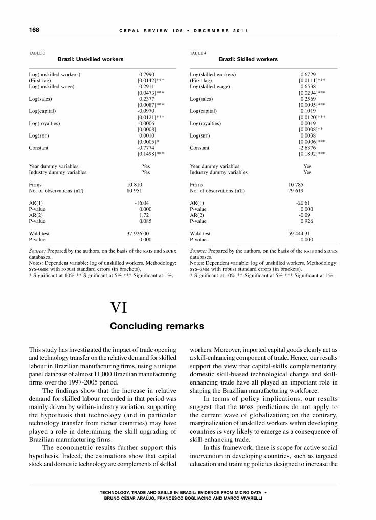
168
tECHnoLogy, tRADE AnD skILLs In BRAzIL: EVIDEnCE fRoM MICRo DAtA •Bruno CésAr ArAúJo, frAnCEsCo BoGLiACino AnD MArCo vivArELLi
C E P A L R E V I E W 1 0 5 • D E C E M B E R 2 0 1 1
This study has investigated the impact of trade opening and technology transfer on the relative demand for skilled labour in Brazilian manufacturing firms, using a unique panel database of almost 11,000 Brazilian manufacturing firms over the 1997-2005 period.
The findings show that the increase in relative demand for skilled labour recorded in that period was mainly driven by within-industry variation, supporting the hypothesis that technology (and in particular technology transfer from richer countries) may have played a role in determining the skill upgrading of Brazilian manufacturing firms.
The econometric results further support this hypothesis. Indeed, the estimations show that capital stock and domestic technology are complements of skilled
workers. Moreover, imported capital goods clearly act as a skill-enhancing component of trade. Hence, our results support the view that capital-skills complementarity, domestic skill-biased technological change and skill-enhancing trade have all played an important role in shaping the Brazilian manufacturing workforce.
In terms of policy implications, our results suggest that the hoss predictions do not apply to the current wave of globalization; on the contrary, marginalization of unskilled workers within developing countries is very likely to emerge as a consequence of skill-enhancing trade.
In this framework, there is scope for active social intervention in developing countries, such as targeted education and training policies designed to increase the
TABLE 4
Brazil: skilled workers
Log(skilled workers)(First lag)
0.6729[0.0111]***
Log(skilled wage) -0.6538[0.0294]***
Log(sales) 0.2569[0.0095]***
Log(capital) 0.1019[0.0120]***
Log(royalties) 0.0019[0.0008]**
Log(set) 0.0038[0.0006]***
Constant -2.6376[0.1892]***
Year dummy variables YesIndustry dummy variables Yes
Firms 10 785No. of observations (nT) 79 619
AR(1) -20.61P-value 0.000AR(2) -0.09P-value 0.926
Wald test 59 444.31P-value 0.000
Source: Prepared by the authors, on the basis of the rais and secex databases.Notes: Dependent variable: log of unskilled workers. Methodology: sys-gmm with robust standard errors (in brackets). * Significant at 10% ** Significant at 5% *** Significant at 1%.
TABLE 3
Brazil: unskilled workers
Log(unskilled workers)(First lag)
0.7990[0.0142]***
Log(unskilled wage) -0.2911[0.0473]***
Log(sales) 0.2377[0.0087]***
Log(capital) -0.0970[0.0121]***
Log(royalties) -0.0006[0.0008]
Log(set) 0.0010[0.0005]*
Constant -0.7774[0.1498]***
Year dummy variables YesIndustry dummy variables Yes
Firms 10 810No. of observations (nT) 80 951
AR(1) -16.04P-value 0.000AR(2) 1.72P-value 0.085
Wald test 37 926.00P-value 0.000
Source: Prepared by the authors, on the basis of the rais and secex databases.Notes: Dependent variable: log of unskilled workers. Methodology: sys-gmm with robust standard errors (in brackets). * Significant at 10% ** Significant at 5% *** Significant at 1%.
VIConcluding remarks
169
tECHnoLogy, tRADE AnD skILLs In BRAzIL: EVIDEnCE fRoM MICRo DAtA •Bruno CésAr ArAúJo, frAnCEsCo BoGLiACino AnD MArCo vivArELLi
C E P A L R E V I E W 1 0 5 • D E C E M B E R 2 0 1 1
domestic supply of skilled labour. At the same time, the construction of a welfare system able to create safety nets and insurance schemes for the possible victims of globalization would also be advisable. In this context,
domestic industrial and labour policies in developing countries might be severely limited by government budget constraints, with international organizations instead playing a pivotal role (see, for instance, ilo, 2004).
AppEndix
Sample and variables
We chose to build a large balanced panel of 11,219 manufacturing firms, observed for nine years: this is the largest panel obtainable by merging the original pia, rais and secex databases. After purging it of unreliable observations and obvious outliers, we ended up with 10,785 firms for which we have information on skilled employment and 10,810 for which we have information on unskilled employment.
We deflated expenditure variables by the Extended National Consumer Price Index (ipca), published by ibge, with base year 1997. Since import data are provided in United States dollars, we converted them into Brazilian reais using the average exchange rate for the year of reference.
We used secex to construct a set variable capturing imported capital goods embodying technology. ibge makes available a classification of products into four categories, in accordance with the harmonized system (hs) code for foreign trade. These four macro categories are: capital goods, non-durable consumer goods, durable consumer goods and intermediate goods. This classification underwent some minor changes in 2002, and it is not possible to carry out a one-to-one mapping from the old to the new categories. However, the unclassified import transactions are less than 5% of the total, so we simply used the updated taxonomy and left out unclassifiable imports.
Since secex is a registry database, we can legitimately assume that missing values for imports are actually zeros. Given our use of log scale data, the log transformation of zero values would have dropped a significant portion of the sample; thus, we constructed log(set) as 0 if capital goods imports were 0 and we applied the log transformation only to positive values (the absence of values equal to 1 makes this exercise meaningful).
Regarding pia, we used a capital measure obtained from ibge that employs the perpetual inventory methodology applied to investment data.
From pia we also took total sales and expenditure on royalties (in Section C5 of the pia questionnaire there is in fact a specific question about expenditure on royalties and technical assistance) (see ibge, 2004).
With regard to employment, we used a firm-level database extracted from rais, which is provided by the Ministry of Labour and Employment. We deemed workers with secondary or tertiary education to be skilled and those with primary education or below to be unskilled. Wages are at firm level for both categories and are expressed as multiples of the minimum wage.
(Original: English)
Bibliography
Abramovitz, M. (1986), “Catching-up, forging ahead and falling behind”, Journal of Economic History, vol. 46, No. 2, Cambridge, Cambridge University Press.
Acemoglu, D. (2003), “Patterns of skill premia”, Review of Economic Studies, vol. 70, No. 2, Oxford, Oxford University Press.
(2002), “Technical change, inequality and the labor market”, Journal of Economic Literature, vol. 40, No. 1, Nashville, Tennessee, American Economic Association.
Aguirregabiria, V. and C. Alonso-Borrego (2001), “Occupational structure, technological innovation and reorganisation of production”, Labour Economics, vol. 8, No. 1, Amsterdam, Elsevier.
Almeida, R. and A.M. Fernandes (2008), “Openness and technological innovations in developing countries: evidence from firm-level surveys”, Journal of Development Studies, vol. 44, No. 5, London, Taylor and Francis.
Arellano, M. and S. Bond (1991), “Some tests of specification for panel data: Monte Carlo evidence and an application to employment equations”, Review of Economic Studies, vol. 58, No. 2, Oxford, Oxford University Press.
Arrow, K. (1962), “The economic implications of learning by doing”, Review of Economic Studies, vol. 29, No. 3, Oxford, Oxford University Press.
Berman, E., J. Bound and Z. Griliches (1994), “Changes in the demand for skilled labor within U.S. manufacturing industries: evidence from the Annual Survey of Manufacturing”, Quarterly Journal of Economics, vol. 109, No. 2, Cambridge, Massachusetts, mit Press.
Berman, E. and S. Machin (2004), “Globalization, skill-biased technological change and labour demand”, Understanding Globalization, Employment and Poverty Reduction, E. Lee and M. Vivarelli (eds.), New York, Palgrave Macmillan.
(2000), “Skill-biased technology transfer around the world”, Oxford Review of Economic Policy, vol. 16, Oxford, Oxford University Press.
Blundell, R. and S. Bond (2000), “gmm estimation with persistent panel data: an application to production functions”, Econometric Reviews, vol. 19, No. 3, London, Taylor and Francis.
(1998), “Initial conditions and moment restrictions in dynamic panel data models”, Journal of Econometrics, vol. 87, No. 1, Amsterdam, Elsevier.
170
tECHnoLogy, tRADE AnD skILLs In BRAzIL: EVIDEnCE fRoM MICRo DAtA •Bruno CésAr ArAúJo, frAnCEsCo BoGLiACino AnD MArCo vivArELLi
C E P A L R E V I E W 1 0 5 • D E C E M B E R 2 0 1 1
Caroli, E. and J. Van Reenen (2001), “Skill biased organizational change? Evidence from a panel of British and French establishments”, Quarterly Journal of Economics, vol. 116, No. 4, Cambridge, Massachusetts, mit Press.
Castro, A.B. and J. Ávila (2004), “Uma política industrial e tecnológica voltada para o potencial das empresas”, document presented at the 16th National Forum, Rio de Janeiro.
Conte, A. and M. Vivarelli (2011), “Imported skill biased technological change in developing countries”, The Developing Economies, vol. 49, Wiley Blackwell, forthcoming.
Davis, D.R. (1996), “Trade liberalization and income distribution”, nber Working Paper, No. 5693, Cambridge, Massachusetts, National Bureau of Economic Research.
(1995), “Intra-industry trade: a Heckscher-Ohlin-Ricardo approach”, Journal of International Economics, vol. 39, No. 3-4, Amsterdam, Elsevier.
Davis, D.R. and others (1996), “The Heckscher-Ohlin-Vanek model of trade: why does it fail? When does it work?”, nber Working Paper, No. 5625, Cambridge, Massachusetts, National Bureau of Economic Research.
De Negri, J.A. and L. Turchi (eds.) (2007), Technological Innovation in Brazilian and Argentine Firms, Brasilia, Institute of Applied Economic Research (ipea).
De Negri, J.A., M. Salerno and A.B. Castro (2005), “Inovações, padrões tecnológicos e desempenho das firmas industriais brasileiras”, Inovações, padrões tecnológicos e desempenho das firmas industriais brasileiras, J.A. de Negri and M. Salerno (orgs.), Brasilia, Institute of Applied Economic Research (ipea).
Dornbusch, R. (1980), Open Economy Macroeconomics, New York, Basic Books.
Feenstra, R. and G. Hanson (1997), “Foreign direct investment and relative wages: evidence from Mexico’s maquiladoras”, Journal of International Economics, vol. 42, No. 3-4, Amsterdam, Elsevier.
(1996), “Globalization, outsourcing, and wage inequality”, American Economic Review, vol. 86, No. 2, Nashville, Tennessee, American Economic Association.
Freeman, R. (1995), “Are your wages set in Beijing?”, Journal of Economic Perspectives, vol. 9, No. 3, Nashville, Tennessee, American Economic Association.
Gonzaga, G., N. Menezes-Filho and C. Terra (2006), “Trade liberalization and evolution of skill earnings differentials in Brazil”, Journal of International Economics, vol. 68, Amsterdam, Elsevier.
Griliches, Z. (1969), “Capital-skill complementarity”, Review of Economics and Statistics, vol. 51, Cambridge, Massachusetts, mit Press.
Grimalda, G. and M. Vivarelli (2010), “Is inequality the price to pay for higher growth in middle-income countries?”, Journal of Evolutionary Economics, vol. 20, No. 4, Springer.
Hanson, G. and A. Harrison (1999), “Trade liberalization and wage inequality in Mexico”, Industrial and Labor Relations Review, vol. 52, No. 2, Ithaca, Cornell University.
ibge (Brazilian Geographical and Statitical Institute) (2004), Pesquisa industrial 2004, vol, 23, No. 1, Rio de Janeiro.
ilo (International Labour Organization) (2004), A Fair Globalization: Creating Opportunities for All, Geneva, World Commission on the Social Dimension of Globalization.
Katz, L.F. and D.H. Autor (1999), “Changes in the wage structure and earning inequality”, Handbook of Labor Economics, Amsterdam, Elsevier.
Kume, H. (2002), “A política brasileira de importação no período 1987-99: descrição e avaliação”, May, unpublished.
Kuznets, S. (1955), “Economic growth and income inequality”, American Economic Review, vol. 45, No. 1, Nashville, Tennessee, American Economic Association.
Lall, S. (2004), “The employment impact of gobalization in developing countries”, Understanding Globalization, Employment and Poverty Reduction, E. Lee and M. Vivarelli (eds.), New York, Palgrave Macmillan.
Lee, E. and M. Vivarelli (2006), “The social impact of globalization in the developing countries”, International Labour Review, vol. 145, No. 3, Geneva, International Labour Organization.
(eds.) (2004), Understanding Globalization, Employment and Poverty Reduction, New York, Palgrave Macmillan.
Leontief, W. (1953), “Domestic production and foreign trade: the American capital position re-examined”, Proceedings of the American Philosophical Society, vol. 97, Philadelphia, American Philosophical Society.
Machin, S. and J. Van Reenen (1998), “Technology and changes in skill structure: evidence from seven oecd countries”, Quarterly Journal of Economics, vol. 113, No. 4, Cambridge, Massachusetts, mit Press.
Manacorda, M., C. Sanchez-Paramo and N. Schady (2006), “Changes in returns to education in Latin America: the role of demand and supply of skills”, Washington, D.C., World Bank, unpublished.
Melitz, M.J. (2003), “The impact of trade on intra-industry reallocations and aggregate industry productivity”, Econometrica, vol. 71, No. 6, Econometric Society.
Menezes-Filho, N. and B. Giovanetti (2006), “Trade liberalization and demand for skills in Brazil”, ibmec Working Paper, No. 9, São Paulo, Instituto Brasileiro de Mercado de Capitais (ibmec).
Menezes-Filho, N., M. Mundler and G. Ramey (2003), “Trade liberalization and worker displacement from Brazilian manufacturing, 1990-1998: request for data match and tabulations”, unpublished.
Meschi, E. and M. Vivarelli (2009), “Trade and income inequality in developing countries”, World Development, vol. 37, No. 2, Amsterdam, Elsevier.
Meschi, E., E. Taymaz and M. Vivarelli (2008), “Trade openness and the demand for skills: evidence from Turkish microdata”, iza Discussion Papers, No. 3887, Bonn, Institute for the Study of Labor.
Nelson, R. and E. Phelps (1966), “Investment in humans, technological diffusion, and economic growth”, American Economic Review, vol. 56, Nashville, Tennessee, American Economic Association.
Nickell, S. (1984), “An investigation of the determinants of manufacturing employment in the United Kingdom”, Review of Economic Studies, vol. 51, No. 4, Oxford, Oxford University Press.
(1981), “Biases in dynamic models with fixed effects”, Econometrica, vol. 49, No. 6, Econometric Society.
Piva, M., E. Santarelli and M. Vivarelli (2005), “The skill bias effect of technological and organisational change: evidence and policy implications”, Research Policy, vol. 34, No. 2, Amsterdam, Elsevier.

171
tECHnoLogy, tRADE AnD skILLs In BRAzIL: EVIDEnCE fRoM MICRo DAtA •Bruno CésAr ArAúJo, frAnCEsCo BoGLiACino AnD MArCo vivArELLi
C E P A L R E V I E W 1 0 5 • D E C E M B E R 2 0 1 1
Robbins, D. (2003), “The impact of trade liberalization upon inequality in developing countries: a review of theory and evidence”, ilo Working Paper, No. 13, Geneva, International Labour Organization (ilo).
Robbins, D. and T.H. Gindling (1999), “Trade liberalization and the relative wages for more-skilled workers in Costa Rica”, Review of Development Economics, vol. 3, No. 2, Wiley Blackwell.
Roodman, D. (2006), “How to do xtabond2: an introduction to “difference” and “system” gmm in Stata”, cgd Working Papers, No. 103, Washington, D.C., Center for Global Development.
Salter, W.E.G. (1960), Productivity and Technical Change, Cambridge, Cambridge University Press.
Solow, R.M. (1960), “Investment and technical progress”, Mathematical Methods in the Social Sciences, K.J. Arrow, S. Karlin and P. Suppes (eds.), Stanford, Stanford University Press.
Trefler, D. (1995), “International factor prices differences: Leontief was right!”, Journal of Political Economy, vol. 101, No. 6, Chicago, University of Chicago Press.
Van Reenen, J. (1997), “Employment and technological innovation: evidence from UK manufacturing firms”, Journal of Labor Economics, vol. 15, No. 2, Chicago, University of Chicago Press.
Vivarelli, M. (2004), “Globalization, skills and within-country income inequality in developing countries”, Understanding Globalization, Employment and Poverty Reduction, E. Lee and M. Vivarelli (eds.), New York, Palgrave Macmillan.
Windmeijer, F. (2005), “A finite sample correction for the variance of linear efficient two-step gmm estimators”, Journal of Econometrics, vol. 126, No. 1, Amsterdam, Elsevier.
Wood, A. (1994), North-South Trade, Employment, and Inequality: Changing Fortunes in a Skill-driven World, Oxford, Clarendon Press.

C E P A L R E V I E W 1 0 5 • D E C E M B E R 2 0 1 1
173
K E Y W O R D S
Economic growth
Gross domestic product
Balance of payments
Exports
Imports
Technological change
Production
Economic analysis
Brazil
Brazil: structural changeand balance-of-payments-constrained growth
João Prates Romero, Fabrício Silveira and Frederico G. Jayme Jr.
This article argues that differences in gdp growth rates are related
to differences in income-elasticities; and that these, in turn, depend
on the technological intensity of domestic production. Statistical tests
were conducted to verify this hypothesis; and the following hypothetical
elasticities were estimated to demonstrate its validity for the Brazilian
economy: (i) basic; (ii) expanded with capital flows; and (iii) implicit.
Co-integration techniques were used in conjunction with vector
error correction, to estimate real elasticities for each technological
category of output in the Brazilian trade matrix. The results obtained
were corroborated by analysing impulse-response functions and the
decomposition of the forecast error variance, which confirmed that goods
of higher technological intensity have higher income-elasticities. Thus,
according to Thirlwall’s Law, increasing the domestic production of such
goods should promote growth.
João Prates Romero
PhD student at the Land
Economy Department, University
of Cambridge, United Kingdom;
holder of a scholarship awarded
by the Coordination for the
Improvement of Higher Education,
Brazil, in partnership with the
Cambridge Overseas Trust
(capes-cot scholarship).
Fabrício Silveira
Internal consultant at Instituto
Euvaldo Lodi iel/fiemg and
assistant teacher at face/ufmg,
Federal University of Minas Gerais,
Brazil.
Frederico G. Jayme Jr.
Professor at the Department of
Economics and Centre for Regional
Development and Planning at the
Federal University of Minas Gerais.
174
BRAzIL: stRuCtuRAL CHAngE AnD BALAnCE-of-PAyMEnts-ConstRAInED gRoWtH • joão PRAtEs RoMERo, fABRíCIo sILVEIRA AnD fREDERICo g. jAyME jR.
C E P A L R E V I E W 1 0 5 • D E C E M B E R 2 0 1 1
There is a vast literature that highlights the key role of foreign-trade elasticities in determining Brazil’s gross domestic product (gdp) (Jayme Jr., 2003; Santos, Lima and Carvalho, 2005; Porcile and Lima, 2006; Vieira and Holland, 2006; Carvalho and Lima, 2008). Although these studies have all acknowledged the external constraint on the country’s growth, as proposed in Thirlwall’s Law (Thirlwall, 1979), little progress has been made thus far in understanding the mechanisms that determine the elasticities in question. Nonetheless, several recent studies have shown that the productive structure has a major influence (Gouvêa and Lima, 2009; Araujo and Lima, 2007).1 This article argues that differences in gdp growth rates are related to differences in income-elasticities, which in turn, depend on the technological intensity of domestic output. The article propounds the thesis that structural change, in other words variations in sector gdp shares, also helps ease the external constraint on growth, since the changes are reflected in the country’s foreign-trade specialization pattern. Implicit in this argument is the hypothesis that the different sectors produce goods with different elasticities, thereby validating a multi-sector
1 This result was obtained by considering a multi-sector model of Thirlwall’s Law, in which each sector’s specific production faces a different income-elasticity of demand. The total income-elasticity of the economy is calculated as the sum of the elasticities of the different sectors, weighted by their share of national output. Changes in the composition of the productive structure thus also affect the economy’s total income-elasticity of demand.
version of Thirlwall’s Law, such that changes in their output shares are reflected in national elasticity.2
A variety of statistical tests were performed to corroborate these hypotheses. Firstly, the following hypothetical elasticities were estimated using different databases: (i) basic (McCombie, 1997); (ii) expanded with capital flows (Moreno-Brid, 2003), and (iii) implicit (Atesoglu, 1997). Co-integration techniques were used along with vector error correction (vec) to estimate real elasticities for each technological category of production in Brazil’s trade matrix. These categories were constructed from a classification of products by technological level, following Lall (2001). The results of the analyses are corroborated by analysing innovations in the model, through impulse-response functions and the decomposition of the forecast error variance. Lastly, an attempt was made to identify the trend of Brazil’s trade elasticities, using the methodology proposed by Gouvêa and Lima (2009).
Following this introduction, the article has another four sections. Section II discusses the Kaldorian-Keynesian theory of balance-of-payments-constrained growth. Section III outlines the recent specialization of Brazil’s productive structure in low-technology products, as revealed by the pattern of its trade matrix. Section IV describes the methodology used to test Brazilian data and the results of the estimations; and section V presents the conclusions.
2 Theoretically, each country’s productive structure determines its pattern of international trade.
Iintroduction
IITheoretical framework
Understanding the causes of unequal economic growth was always one of the major topics of study in the Kaldorian-Keynesian theoretical framework (Kaldor, 1966; Thirlwall, 1979; McCombie and Thirlwall, 1994). The cited studies all view demand as driving the economic system, so growth-rate differences between countries are
interpreted as the outcome of different rates of growth of demand, which vary from one country to another according to the constraints they face. Thirlwall (1979) stresses the role of the balance-of-payments constraint in economic performance, given the need for long-term external equilibrium. The fact that balance-of-payments
175
BRAzIL: stRuCtuRAL CHAngE AnD BALAnCE-of-PAyMEnts-ConstRAInED gRoWtH • joão PRAtEs RoMERo, fABRíCIo sILVEIRA AnD fREDERICo g. jAyME jR.
C E P A L R E V I E W 1 0 5 • D E C E M B E R 2 0 1 1
deficits cannot be financed indefinitely means that aggregate demand eventually has to be adjusted. As a result, “…Investment is discouraged; technological progress is slowed down, and a country’s goods compared with foreign goods become less desirable so worsening the balance of payment still further, and so on. A vicious cycle is started. By contrast, if a country is able to expand demand up to the level of existing productive capacity, without balance-of-payment difficulties arising, the pressure of demand upon capacity may well raise the capacity growth rate by encouraging investment, technological progress and productivity…” (McCombie and Thirlwall, 1994).
This framework envisages demand incentives triggering a virtuous circle of growth that would raise the economy’s overall productivity, as factors migrate towards higher-productivity sectors (manufactures), and learning-by-doing intensifies (Kaldor, 1966). Demand growth alters the sectoral mix of incentives in the economy, promoting certain sectors to the detriment of others. The benefited sectors mainly have higher income-elasticities of demand (which, according to the hypothesis of this query, reflects greater technological content). These sectors also tend to display increasing returns, such that an increase in their share of gdp, with a consequent shift of productive factors towards them, raises the productivity of the economy as a whole. Investment is seen as the key variable in propelling growth; while the importance of the balance of payments stems from the scale of the incentive, or disincentive, it provides to investment growth.
This analytical approach led to the formulation of export-led growth theories, in which exports are the only means of raising the growth rate without a deterioration in the balance of payments.
1. The balance-of-payments-constrained growth model
Bearing in mind the key importance of external balance for the growth of demand and output, Thirlwall’s original 1979 paper developed a growth model under an external constraint in which economic growth is intrinsically related to the income-elasticities of exports and imports.
In this model, balance-of-payments equilibrium in local currency is given by:
PdX=Pf ME (1)
where E is the exchange rate. Imports (M) are a function of the ratio between prices weighted by the price-elasticity
of demand for imports (Ψ<0) and the income-elasticity of demand for imports (π>0), as shown in the following equation:3
M aP E
PYf
d
=
ψπ
(2)
Similarly, exports are a function of the real exchange rate and external income, in which the income-elasticity of demand for exports is denoted by ε >0, and the price-elasticity of demand for exports is η <0, both expressed in foreign currency:
X bP
P EZd
f
=
ηε (3)
A linear transformation of the equations, subject to the initial balance-of-payments-equilibrium condition, gives the rate of growth of domestic income that is consistent with balance-of-payments equilibrium (McCombie and Thirlwall, 1994, pp. 234 y 235):
yp p
Bd f=
+ + − − +( )1 η ψ επ
( )e z (4)
Equation (4) has several implications: (i) if domestic inflation is higher than foreign inflation, the balance-of-payments-equilibrium growth rate falls, if |Ψ + η| > 1; (ii) exchange-rate depreciation (e >0) tends to raise the balance-of-payments-equilibrium growth rate, if
|Ψ + η| > 1 (this is the Marshall-Lerner condition); (iii) a higher rate of growth of world income raises the balance-of-payments-equilibrium growth rate; and (iv) the higher the income-elasticity of demand for imports (π), the lower will be the balance-of-payments-equilibrium growth rate.
Nonetheless, if purchasing-power-parity (ppp) is accepted as valid in the long run, which means no change in relative prices and domestic inflation equal to international inflation ( pdt - pft - et = 0), then equation (4) can be reduced to the one initially proposed by Thirlwall (1979), which is equivalent to the growth rule proposed by Harrod (1933):
yz x
B
επ π
= = (5)
3 The price-elasticities of demand for imports and for exports are assumed equal to their cross price-elasticity, namely Ψ = Ø and η = τ respectively.
176
BRAzIL: stRuCtuRAL CHAngE AnD BALAnCE-of-PAyMEnts-ConstRAInED gRoWtH • joão PRAtEs RoMERo, fABRíCIo sILVEIRA AnD fREDERICo g. jAyME jR.
C E P A L R E V I E W 1 0 5 • D E C E M B E R 2 0 1 1
The empirical evidence presented in McCombie and Thirlwall (1994) confirms this relation, and shows that a pre-requisite for raising a country’s growth rate is overcoming the balance-of-payments constraint. This is achieved through policies to stimulate an increase in the income-elasticities of exports and reduce those of imports. Nonetheless, to bring that paradigm closer to the reality prevailing in developing countries, new explanatory factors need to be considered, such as capital flows, exchange-rate variations, and changes in debt-service payments (Thirlwall and Hussain, 1982; McCombie and Thirlwall, 1997).
Firstly, capital flows are very important in developing countries, because they make it possible to run temporary current-account deficits. This means that countries with trade deficits can keep growing provided they can finance the deficit through the capital account. Nonetheless, capital inflows also generate a liability that may depress gdp growth, since they have to be amortized. The model also needs to take account of interest payments abroad, because, at some point, a trade surplus will be needed to service the debt. In other words, an accumulation of external debt can itself generate the need for a contraction in domestic demand (income), to generate a balance-of-payments surplus to pay debt service, which will thus reduce the growth rate (Moreno-Brid, 2003; Barbosa-Filho, 2001).
Moreno-Brid (2003) incorporate these components to obtain the following balance-of-payments-equilibrium condition:
Pd Xt + Pd F + Pd R = Pf Mt Et (6)
where F represents capital flows, and R is the real value of capital services. Weighting factors are also included: θ1 for the share of exports in income, and θ2= (1-θ1) for the income-share of capital. Expressed as growth rates:
m p e p x pt ft t dt dt+ + = +θ θ( ) r( ) +1 2− +
dt− −θ θ1 1 2 ( ++ f )p( ) (7)
where r is the variation in net interest payments, f is the variation in capital flows, and θ1 and θ2 are the following ratios measured in the initial period:
θ1 =P X
P EMd
f (8)
θ2 =P R
P EMd
f
(9)
Lastly, a sustainable borrowing constraint, F/Y = k, is also introduced, which in terms of growth rates is given by:
f + pd = y + pd (10)
Substituting this constraint in (7) and using the same export and import functions, the balance-of-payments-equilibrium growth rate in the presence of capital flows is given by:
yp p e z r
Bd f*
( )( )
( )=
+ + − −
− − +
θ η ε θπ θ θ
1 1
1 1 2
ψ θ1 2+ + (11)
The first term represents the effect of changes in the terms of trade; the second shows the effect of export demand; the third, the effect of interest payments; and the fourth, by subtracting in the denominator, the effect of capital flows. In the absence of capital flows, θ1 = 1, which returns us to the initial result of the Harrod (1933) growth rule.
2. Productive structure and its effect on elasticities
The fact that elasticities are important for growth calls for deeper research into their determinants.4 Although an economy’s potential output is determined by the rate of growth of demand, the balance-of-payments-constrained growth approach reiterates the importance of the supply characteristics of goods (non-price competitiveness). Thus, if one assumes a country that produces a variety of goods with different elasticities, in which the total income-elasticity of the economy is calculated as the average of the sector elasticities, weighted by each sector’s share in the productive structure, then a change in the economy’s productive structure will affect the income-elasticity of imports and exports, since different sector-demand growth rates result in different growth rates for the economy as a whole.
Based on this rationale, Araujo and Lima (2007) develop a multi-sector model and reach what the authors
4 The model developed in the foregoing section implicitly assumes a country that produces a single good with given and unchangeable elasticities.

177
BRAzIL: stRuCtuRAL CHAngE AnD BALAnCE-of-PAyMEnts-ConstRAInED gRoWtH • joão PRAtEs RoMERo, fABRíCIo sILVEIRA AnD fREDERICo g. jAyME jR.
C E P A L R E V I E W 1 0 5 • D E C E M B E R 2 0 1 1
refer to as the Multi-sector Thirlwall’s Law (mstl). The chief implication of this model is that changes in sector shares in the economy, in other words changes the structure of production, have repercussions on the overall economic growth rate. As a result, “a country can still raise its growth rate even when such a rise in growth of world income does not occur, provided it is able to change the sectoral composition of exports and/or imports accordingly” (Gouvêa and Lima, 2009).
According to Thirlwall’s traditional approach, the final equation of the Araujo and Lima (2007) model shows that each country’s growth rate is directly proportional to the rate of growth of exports. This proportionality is related inversely to the sector income-elasticity of demand for imports and directly to the sector income-elasticity of demand for exports. In short, the growth rate depends on the sector composition of the economy.
In seeking empirical validity for this sector-formulation of Thirlwall’s Law, the aforementioned authors estimate the mstl elasticities for several Latin
American and Asian countries and find that the most technology-intensive sectors have a higher income-elasticity, with smaller differences for imports than for exports. They also conclude that both the original version of Thirlwall’s law, and its multi-sector formulation, adequately represent the economy’s growth rate. Lastly, with sector income-elasticities estimated as relative weightings, the authors use each sector’s foreign-trade share to calculate a weighted average of the annual changes in the elasticities, thus indicating the process of structural change.
This evidence shows that, as industrialization deepens, and, in particular, as higher-technology-intensive sectors gain a larger share of gdp, the elasticities of exports and imports also change, directly affecting output growth rates. Using this framework, this article seeks to identify the relation between the elasticities and the technological content of the goods that comprise the Brazilian trade balance, for the purpose of analysing the effects of structural changes on the country’s growth rate.
IIIExternal constraint and productive structure
in Brazil: 1962-2010
In an empirical study for a group of countries, McCombie and Thirlwall (1994) concluded that terms-of-trade deterioration is a reality for developing countries (although the real effect of this may be very small), whereas capital flows tend to ease the constraint marginally, albeit temporarily. These results are broadly consistent with the structuralist approach adopted by Prebisch (2000a and 2000b), which explains the phenomenon by stressing that: (i) the goods produced in developing countries have a lower income-elasticity of demand; and (ii) the goods produced by central countries have a high income-elasticity of demand.
In an analysis of the Brazilian case, Carvalho and Lima (2008) found that the growth achieved between 1930 and 2004 was compatible with balance-of-payments equilibrium.5 Moreover, by estimating the share of each of the components considered important in determining
5 See also Holland, Vieira and Canuto (2004); Ferreira (2001); Bértola, Higachi and Porcile (2002); López and Cruz (2000); Santos, Lima and Carvalho (2005).
the growth rate, they concluded that the real exchange rate is statistically insignificant for observed growth, and also that capital flows do not raise the growth rate in the long run. The ratio of elasticities (Thirlwall’s Law) accounted for most of the growth during the period, followed by the terms of trade. In the same study, a structural-break test showed that —in a subsample for the period 1930-1993— the ratio of elasticities fell from 7% to just 1.3% between 1994 and 2004, indicating that the growth slowdown in the Brazilian economy during that period reflected a productive structure that was overly reliant on goods with low income-elasticities of demand (or low-technology products, as will be shown) at a time when world trade patterns were reorganizing (Jayme Jr. and Resende, 2009). Between 1930 and 1993 the terms of trade deteriorated, making a negative contribution to output growth (-0.7%). Thereafter the pattern reverses, and the terms of trade generate average output growth of 1.7%, probably caused by stronger growth in the global economy and the consequent rise in commodity prices.
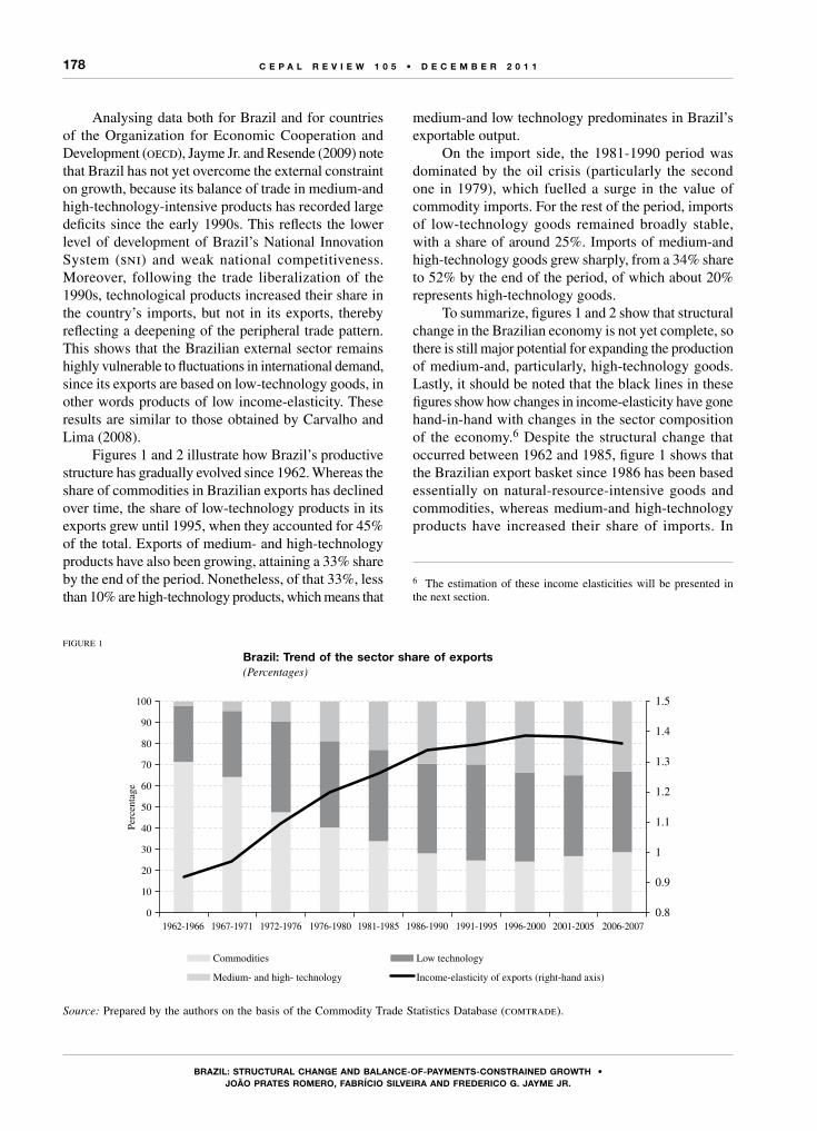
178
BRAzIL: stRuCtuRAL CHAngE AnD BALAnCE-of-PAyMEnts-ConstRAInED gRoWtH • joão PRAtEs RoMERo, fABRíCIo sILVEIRA AnD fREDERICo g. jAyME jR.
C E P A L R E V I E W 1 0 5 • D E C E M B E R 2 0 1 1
Analysing data both for Brazil and for countries of the Organization for Economic Cooperation and Development (oecd), Jayme Jr. and Resende (2009) note that Brazil has not yet overcome the external constraint on growth, because its balance of trade in medium-and high-technology-intensive products has recorded large deficits since the early 1990s. This reflects the lower level of development of Brazil’s National Innovation System (sni) and weak national competitiveness. Moreover, following the trade liberalization of the 1990s, technological products increased their share in the country’s imports, but not in its exports, thereby reflecting a deepening of the peripheral trade pattern. This shows that the Brazilian external sector remains highly vulnerable to fluctuations in international demand, since its exports are based on low-technology goods, in other words products of low income-elasticity. These results are similar to those obtained by Carvalho and Lima (2008).
Figures 1 and 2 illustrate how Brazil’s productive structure has gradually evolved since 1962. Whereas the share of commodities in Brazilian exports has declined over time, the share of low-technology products in its exports grew until 1995, when they accounted for 45% of the total. Exports of medium- and high-technology products have also been growing, attaining a 33% share by the end of the period. Nonetheless, of that 33%, less than 10% are high-technology products, which means that
medium-and low technology predominates in Brazil’s exportable output.
On the import side, the 1981-1990 period was dominated by the oil crisis (particularly the second one in 1979), which fuelled a surge in the value of commodity imports. For the rest of the period, imports of low-technology goods remained broadly stable, with a share of around 25%. Imports of medium-and high-technology goods grew sharply, from a 34% share to 52% by the end of the period, of which about 20% represents high-technology goods.
To summarize, figures 1 and 2 show that structural change in the Brazilian economy is not yet complete, so there is still major potential for expanding the production of medium-and, particularly, high-technology goods. Lastly, it should be noted that the black lines in these figures show how changes in income-elasticity have gone hand-in-hand with changes in the sector composition of the economy.6 Despite the structural change that occurred between 1962 and 1985, figure 1 shows that the Brazilian export basket since 1986 has been based essentially on natural-resource-intensive goods and commodities, whereas medium-and high-technology products have increased their share of imports. In
6 The estimation of these income elasticities will be presented in the next section.
FIGURE 1
Brazil: Trend of the sector share of exports(Percentages)
Source: Prepared by the authors on the basis of the Commodity Trade Statistics Database (comtrade).
0
10
20
30
40
50
60
70
80
90
100
1962-1966 1967-1971 1972-1976 1976-1980 1981-1985 1986-1990 1991-1995 1996-2000 2001-2005 2006-20070.8
0.9
1
1.1
1.2
1.3
1.4
1.5
Commodities
Perc
enta
ge
Low technology
Medium- and high- technology Income-elasticity of exports (right-hand axis)

179
BRAzIL: stRuCtuRAL CHAngE AnD BALAnCE-of-PAyMEnts-ConstRAInED gRoWtH • joão PRAtEs RoMERo, fABRíCIo sILVEIRA AnD fREDERICo g. jAyME jR.
C E P A L R E V I E W 1 0 5 • D E C E M B E R 2 0 1 1
short, the productive modernization and diversification process that has been unfolding in Brazil since the 1950s and is reflected in the trade pattern, came to a halt in the late 1980s, since when commodity and natural-resource-intensive goods have continued to
account for over 50% of total exports. The opposite is true of imports, where high- and medium-technology-intensive products have accounted for over 50% of the total volume imported between 1989 and 2009 (Jayme Jr. and Resende, 2009).
FIGURE 2
Brazil: Trend of the sector share of imports (Percentages)
Source: Prepared by the authors on the basis of the Commodity Trade Statistics Database (comtrade).
0
10
20
30
40
50
60
70
80
90
100 1.4
1.35
1.3
1.25
1.2
1.15
1.1
1.05
1
Commodities
Per
cent
age
Low technology
Medium- and high- technology Income-elasticity of exports (right-hand axis)
1962-1966 1967-1971 1972-1976 1976-1980 1981-1985 1986-1990 1991-1995 1996-2000 2001-2005 2006-2007
IVEmpirical analysis
1. Calculation of hypothetical elasticities
In the economic literature, real elasticities have been estimated empirically using various alternative methods. As data relating to certain economies and periods are often incompatible, some studies suggest substitutes for these elasticities, which are also known as hypothetical elasticities. The most frequently used definition is presented by McCombie (1997), who defines “hypothetical income-elasticity” as that which equalizes the observed and theoretical growth rates: π' ≡ x/y.7 A
7 From this specification, it follows that if and the estimation of are not statistically different, it is impossible to reject the hypothesis that the country’s growth rate is balance-of-payments constrained (Santos, Lima and Carvalho, 2005). The estimation of will, in turn, be illustrated in the next subsection.
second substitute for the elasticities can be obtained in the same way, although following the specifications of the model proposed by Moreno-Brid (2003). Jayme Jr. (2003), estimates an “implicit elasticity”, π'', which is obtained from the co-integration coefficient estimated from the relation lnYt = (1/π'') lnXt.
Hypothetical elasticities can thus be expressed as follows:
1) 1 = x / yπ (Original model)
2) π θ θ2 1 1 2= − + +−
( )y
tx r1 2θ θ
(Moreno-Brid model)
3) 3 = 1 / βπ obtained by the co-integration of lnYt = βln Xt
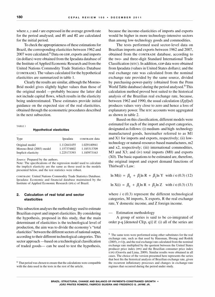
180
BRAzIL: stRuCtuRAL CHAngE AnD BALAnCE-of-PAyMEnts-ConstRAInED gRoWtH • joão PRAtEs RoMERo, fABRíCIo sILVEIRA AnD fREDERICo g. jAyME jR.
C E P A L R E V I E W 1 0 5 • D E C E M B E R 2 0 1 1
where x, y and r are expressed in the average growth rate for the period analysed; and θ1 and θ2 are calculated for the initial period.
To check the appropriateness of these estimations for Brazil, the corresponding elasticities between 1962 and 2007 were calculated.8 Data on gdp, exports and imports (in dollars) were obtained from the Ipeadata database of the Institute of Applied Economic Research and from the United Nations Commodity Trade Statistics Database (comtrade). The values calculated for the hypothetical elasticities are summarized in table 1.
Clearly the results are similar, although the Moreno-Brid model gives slightly higher values than those of the original model —probably because the latter did not include capital flows, which results in the elasticity being underestimated. These estimates provide initial guidance on the expected size of the real elasticities, obtained through the econometric procedures described in the next subsection.
TABLE 1
hypothetical elasticities
Type Ipeadata comtrade data
Original model 1.112641455 1.029140941Moreno-Brid (2003) model 1.157374802 1.185313709Implicit elasticity 1.225173393 1.185973163
Source: Prepared by the authors.Note: The specifications of the regression model used to calculate the implicit elasticity are the same as those used in the models presented below, and the test statistics were robust.
comtrade: United Nations Commodity Trade Statistics Database.Ipeadata: Economic and financial database maintained by the Institute of Applied Economic Research (ipea) of Brazil.
2. Calculation of real total and sector elasticities
This subsection analyses the methodology used to estimate Brazilian export and import elasticities. By considering the hypothesis, proposed in this study, that the main determinant of elasticities is the technological level of production, the aim was to divide the economy’s “total elasticities” between the different sectors of national output, according to their different technological categories. This sector approach —based on a technological classification of traded goods— can be used to test the hypothesis,
8 That period was chosen to ensure that the calculations were compatible with the data used in the tests in the rest of the article.
because the income-elasticities of imports and exports would be higher in more technology-intensive sectors than among low-technology goods and commodities.
The tests performed used sector-level data on Brazilian imports and exports between 1962 and 2007, obtained from the comtrade database, according to the two- and three-digit Standard International Trade Classification (sitc). In addition, gdp data were obtained from Ipeadata (values in United States dollars); and the real exchange rate was calculated from the nominal exchange rate provided by the same source, divided by purchasing-power-parity (obtained from the Penn World Table database) during the period analysed.9 This calculation method proved best suited to the historical analysis of the Brazilian real exchange rate, because, between 1962 and 1990, the usual calculation (Epf/pd) produces values very close to zero and hence a loss of explanatory power. The sitc accounts were aggregated as shown in table 2.
Based on this classification, different models were estimated for each of the import and export categories, designated as follows: (i) medium- and high- technology manufactured goods, hereinafter referred to as M1 and X1 for imports and exports, respectively; (ii) low-technology or natural-resource-based manufactures, m2 and x2, respectively; (iii) international commodities, M3 and X3; and (iv) total imports (M0) and exports (X0). The basic equations to be estimated are, therefore, the original import and export demand functions of Thirlwall’s Law:
ln M(i) ln n Y0 1 2= + +β β βR l with i ∈(0.3) (12)
ln X(i) ln0 1 2= + +β β βR ln Z with i ∈(0.3) (13)
where i ∈(0.3) represent the different technological categories, M imports, X exports, R the real exchange rate, Y domestic income, and Z foreign income.
— Estimation methodologyA group of series is said to be co-integrated of
order p-q [denoted CI(p, q)] if: (i) all of the series are
9 The same tests were performed using other substitutes for the real exchange rate, such as that used by Hausman, Hwang and Rodrik (2005), r=1/p, and the real exchange rate calculated from the nominal exchange rate multiplied by the quotient between the United States producer price index (ppi) and the Brazilian consumer price index (cpi) (Gouvêa and Lima, 2009). Similar results were obtained in all cases. The choice of the version presented here represents the series that best fits the historical analysis of Brazilian exchange rate, given the recurrent inflationary processes and changes in exchange-rate regimes that occurred during the period under study.
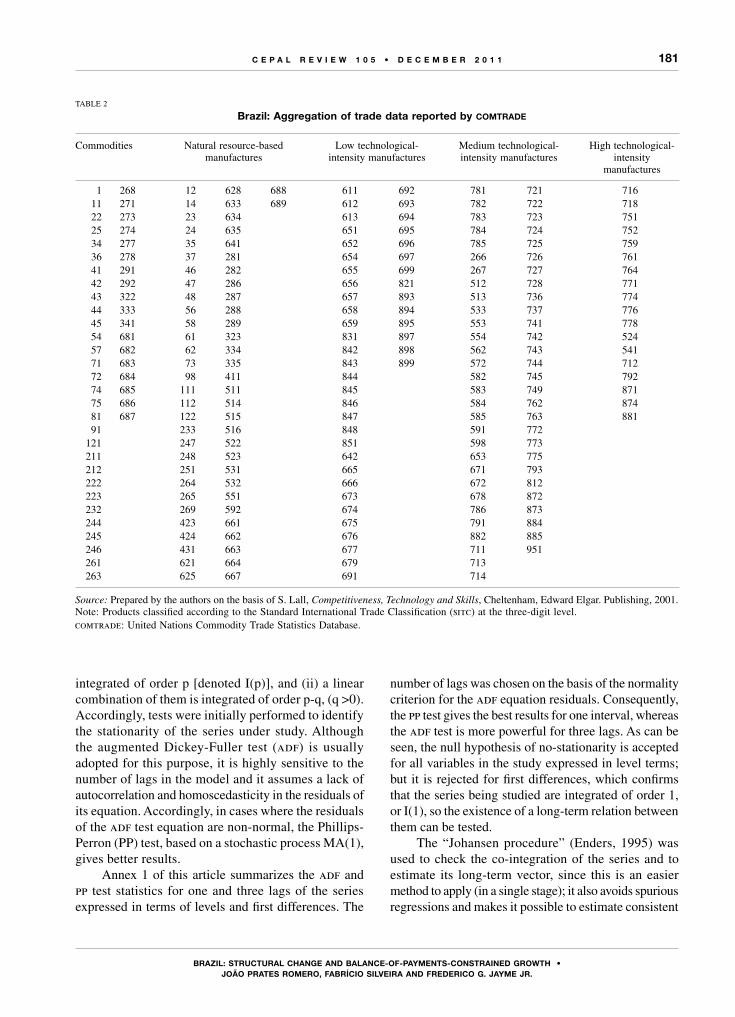
181
BRAzIL: stRuCtuRAL CHAngE AnD BALAnCE-of-PAyMEnts-ConstRAInED gRoWtH • joão PRAtEs RoMERo, fABRíCIo sILVEIRA AnD fREDERICo g. jAyME jR.
C E P A L R E V I E W 1 0 5 • D E C E M B E R 2 0 1 1
integrated of order p [denoted I(p)], and (ii) a linear combination of them is integrated of order p-q, (q >0). Accordingly, tests were initially performed to identify the stationarity of the series under study. Although the augmented Dickey-Fuller test (adf) is usually adopted for this purpose, it is highly sensitive to the number of lags in the model and it assumes a lack of autocorrelation and homoscedasticity in the residuals of its equation. Accordingly, in cases where the residuals of the adf test equation are non-normal, the Phillips-Perron (PP) test, based on a stochastic process MA(1), gives better results.
Annex 1 of this article summarizes the adf and pp test statistics for one and three lags of the series expressed in terms of levels and first differences. The
number of lags was chosen on the basis of the normality criterion for the adf equation residuals. Consequently, the pp test gives the best results for one interval, whereas the adf test is more powerful for three lags. As can be seen, the null hypothesis of no-stationarity is accepted for all variables in the study expressed in level terms; but it is rejected for first differences, which confirms that the series being studied are integrated of order 1, or I(1), so the existence of a long-term relation between them can be tested.
The “Johansen procedure” (Enders, 1995) was used to check the co-integration of the series and to estimate its long-term vector, since this is an easier method to apply (in a single stage); it also avoids spurious regressions and makes it possible to estimate consistent
TABLE 2
Brazil: Aggregation of trade data reported by comtrade
Commodities Natural resource-based manufactures
Low technological-intensity manufactures
Medium technological-intensity manufactures
High technological-intensity
manufactures
1 268 12 628 688 611 692 781 721 71611 271 14 633 689 612 693 782 722 71822 273 23 634 613 694 783 723 75125 274 24 635 651 695 784 724 75234 277 35 641 652 696 785 725 75936 278 37 281 654 697 266 726 76141 291 46 282 655 699 267 727 76442 292 47 286 656 821 512 728 77143 322 48 287 657 893 513 736 77444 333 56 288 658 894 533 737 77645 341 58 289 659 895 553 741 77854 681 61 323 831 897 554 742 52457 682 62 334 842 898 562 743 54171 683 73 335 843 899 572 744 71272 684 98 411 844 582 745 79274 685 111 511 845 583 749 87175 686 112 514 846 584 762 87481 687 122 515 847 585 763 88191 233 516 848 591 772
121 247 522 851 598 773211 248 523 642 653 775212 251 531 665 671 793222 264 532 666 672 812223 265 551 673 678 872232 269 592 674 786 873244 423 661 675 791 884245 424 662 676 882 885246 431 663 677 711 951261 621 664 679 713263 625 667 691 714
Source: Prepared by the authors on the basis of S. Lall, Competitiveness, Technology and Skills, Cheltenham, Edward Elgar. Publishing, 2001.Note: Products classified according to the Standard International Trade Classification (sitc) at the three-digit level. comtrade: United Nations Commodity Trade Statistics Database.
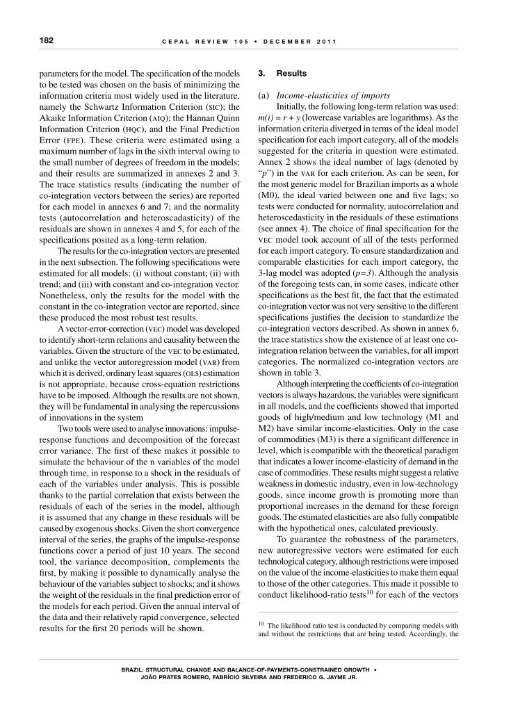
182
BRAzIL: stRuCtuRAL CHAngE AnD BALAnCE-of-PAyMEnts-ConstRAInED gRoWtH • joão PRAtEs RoMERo, fABRíCIo sILVEIRA AnD fREDERICo g. jAyME jR.
C E P A L R E V I E W 1 0 5 • D E C E M B E R 2 0 1 1
parameters for the model. The specification of the models to be tested was chosen on the basis of minimizing the information criteria most widely used in the literature, namely the Schwartz Information Criterion (sic); the Akaike Information Criterion (aiq); the Hannan Quinn Information Criterion (hqc), and the Final Prediction Error (fpe). These criteria were estimated using a maximum number of lags in the sixth interval owing to the small number of degrees of freedom in the models; and their results are summarized in annexes 2 and 3. The trace statistics results (indicating the number of co-integration vectors between the series) are reported for each model in annexes 6 and 7; and the normality tests (autocorrelation and heteroscadasticity) of the residuals are shown in annexes 4 and 5, for each of the specifications posited as a long-term relation.
The results for the co-integration vectors are presented in the next subsection. The following specifications were estimated for all models: (i) without constant; (ii) with trend; and (iii) with constant and co-integration vector. Nonetheless, only the results for the model with the constant in the co-integration vector are reported, since these produced the most robust test results.
A vector-error-correction (vec) model was developed to identify short-term relations and causality between the variables. Given the structure of the vec to be estimated, and unlike the vector autoregression model (var) from which it is derived, ordinary least squares (ols) estimation is not appropriate, because cross-equation restrictions have to be imposed. Although the results are not shown, they will be fundamental in analysing the repercussions of innovations in the system
Two tools were used to analyse innovations: impulse-response functions and decomposition of the forecast error variance. The first of these makes it possible to simulate the behaviour of the n variables of the model through time, in response to a shock in the residuals of each of the variables under analysis. This is possible thanks to the partial correlation that exists between the residuals of each of the series in the model, although it is assumed that any change in these residuals will be caused by exogenous shocks. Given the short convergence interval of the series, the graphs of the impulse-response functions cover a period of just 10 years. The second tool, the variance decomposition, complements the first, by making it possible to dynamically analyse the behaviour of the variables subject to shocks; and it shows the weight of the residuals in the final prediction error of the models for each period. Given the annual interval of the data and their relatively rapid convergence, selected results for the first 20 periods will be shown.
3. results
(a) Income-elasticities of importsInitially, the following long-term relation was used:
m(i) = r + y (lowercase variables are logarithms). As the information criteria diverged in terms of the ideal model specification for each import category, all of the models suggested for the criteria in question were estimated. Annex 2 shows the ideal number of lags (denoted by “p”) in the var for each criterion. As can be seen, for the most generic model for Brazilian imports as a whole (M0), the ideal varied between one and five lags; so tests were conducted for normality, autocorrelation and heteroscedasticity in the residuals of these estimations (see annex 4). The choice of final specification for the vec model took account of all of the tests performed for each import category. To ensure standardization and comparable elasticities for each import category, the 3-lag model was adopted (p=3). Although the analysis of the foregoing tests can, in some cases, indicate other specifications as the best fit, the fact that the estimated co-integration vector was not very sensitive to the different specifications justifies the decision to standardize the co-integration vectors described. As shown in annex 6, the trace statistics show the existence of at least one co-integration relation between the variables, for all import categories. The normalized co-integration vectors are shown in table 3.
Although interpreting the coefficients of co-integration vectors is always hazardous, the variables were significant in all models, and the coefficients showed that imported goods of high/medium and low technology (M1 and M2) have similar income-elasticities. Only in the case of commodities (M3) is there a significant difference in level, which is compatible with the theoretical paradigm that indicates a lower income-elasticity of demand in the case of commodities. These results might suggest a relative weakness in domestic industry, even in low-technology goods, since income growth is promoting more than proportional increases in the demand for these foreign goods. The estimated elasticities are also fully compatible with the hypothetical ones, calculated previously.
To guarantee the robustness of the parameters, new autoregressive vectors were estimated for each technological category, although restrictions were imposed on the value of the income-elasticities to make them equal to those of the other categories. This made it possible to conduct likelihood-ratio tests10 for each of the vectors
10 The likelihood ratio test is conducted by comparing models with and without the restrictions that are being tested. Accordingly, the
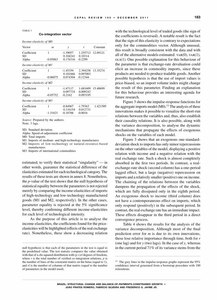
183
BRAzIL: stRuCtuRAL CHAngE AnD BALAnCE-of-PAyMEnts-ConstRAInED gRoWtH • joão PRAtEs RoMERo, fABRíCIo sILVEIRA AnD fREDERICo g. jAyME jR.
C E P A L R E V I E W 1 0 5 • D E C E M B E R 2 0 1 1
estimated, to verify their statistical “singularity” — in other words, guarantee the statistical difference of the elasticities estimated for each technological category. The results of these tests are shown in annex 8. Nonetheless, the p-value of the test shows that the null hypothesis of statistical equality between the parameters is not rejected merely by comparing the income-elasticities of imports of high-technology and low-technology manufactured goods (M1 and M2, respectively). In the other cases, parameter equality is rejected at the 5% significance level, thereby confirming different income-elasticities for each level of technological intensity.
As the purpose of this article is to analyse the income-elasticities, the coefficients found for the price-elasticities will be highlighted (effects of the real exchange rate). Nonetheless, these show a decreasing relation
null hypothesis is that each of the parameters in the test is equal to the predefined value. The test statistic compares the value obtained with that of a chi-squared distribution with (p-r)rl degrees of freedom, where r is the total number of verified co-integration relations, p is the number of lines of the constraint matrix on the betas (equal to 1), and rl is the number of columns of that matrix (equal to the number of parameters in the model used).
with the technological level of traded goods (the sign of the coefficients is reversed). A notable result is the fact that the sign of this elasticity is contrary to expectations only for the commodities vector. Although unusual, this result is broadly consistent with the data and with all of the alternative models estimated: var(0), var(1), ols(1). One possible explanation for this behaviour of the parameter is that exchange-rate devaluation could elicit an increase in commodity imports, since these products are needed to produce tradable goods. Another possible hypothesis is that the use of import values is price-biased, so an import volume index might change the result of this parameter. Finding an explanation for this behaviour provides an interesting agenda for future research.
Figure 3 shows the impulse-response functions for the aggregate imports model (M0).11 The analysis of these innovations makes it possible to visualize the short-run relations between the variables and, thus, also establish their causality relations. It is also possible, along with the variance decomposition, to analyse the dynamic mechanisms that propagate the effects of exogenous shocks on the variables of each model.
Figure 3 shows that an exogenous one-standard-deviation shock to imports has only minor repercussions on the other variables of the model, displaying a positive relation with income and a negative relation with the real exchange rate. Such a shock is almost completely absorbed in the first two periods. In contrast, a real-exchange-rate shock (second column) has a one-period lagged effect, but a large (negative) repercussion on imports and a relatively smaller (positive) one on income. The chaining of the relations between the variables dampens the propagation of the effects of the shock, which are fully dissipated only in the eighth period. An exogenous shock to income (third column) does not have a contemporaneous effect on imports, which only respond (positively) in the subsequent period. In contrast, the real exchange rate has an immediate impact. These effects disappear in the third period in a direct convergence process.
Table 4 shows the results for the analysis of the variance decomposition. Although most of the final prediction error for m is due to its own innovations, these lose relative importance through time, both for r (one lag) and for y (two lags). In the case of y, whereas in the current period 71% of its variance stems from the
11 The grey lines in the impulse-response graphs represent the 95% confidence interval generated from a bootstrap procedure with 100 reiterations.
TABLE 3
Co-integration vector
Income-elasticity of M0
Vector m y r Constant
Coefficient 1 -1.39057 1.255712 12.09121SD 0.104241 0.10314Alpha -0.05863 0.176316 -0.2299
Income-elasticity of M1
Coefficient 1 -1.45359 2.394258 13.35274SD 0.101666 0.097003Alpha -0.06075 0.074304 -0.12344
Income-elasticity of M2
Coefficient 1 -1.47117 1.681609 15.40699SD 0.097724 0.009242Alpha -0.05752 -0.2162 0.093195
Income-elasticity of M3
Coefficient 1 -0.84967 -1.79363 1.421589SD 0.116154 0.012731Alpha -1.31621 -0.18706 -0.0016
Source: Prepared by the authors.Note: 3 lags.
SD: Standard deviation.Alpha: Speed-of-adjustment coefficientM0: Total imports M1: Imports of medium- and high-technology manufactures M2: Imports of low-technology or natural-resource-based
manufacturesM3: Imports of international commodities
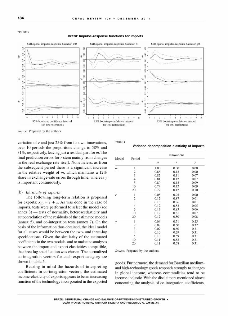
184
BRAzIL: stRuCtuRAL CHAngE AnD BALAnCE-of-PAyMEnts-ConstRAInED gRoWtH • joão PRAtEs RoMERo, fABRíCIo sILVEIRA AnD fREDERICo g. jAyME jR.
C E P A L R E V I E W 1 0 5 • D E C E M B E R 2 0 1 1
variation of r and just 25% from its own innovations, over 10 periods the proportions change to 58% and 31%, respectively, leaving just a residual part for m. The final prediction errors for r stem mainly from changes in the real exchange rate itself. Nonetheless, as from the subsequent period there is a significant increase in the relative weight of m, which maintains a 12% share in exchange-rate errors through time, whereas y is important continuously.
(b) Elasticity of exportsThe following long-term relation is proposed
for exports: x(i) = r + z. As was done in the case of imports, tests were performed to select the model (see annex 3) — tests of normality, heteroscedasticity and autocorrelation of the residuals of the estimated models (annex 5), and co-integration tests (annex 7). On the basis of the information thus obtained, the ideal model for all cases would be between the two- and three-lag specifications. Given the similarity of the estimated coefficients in the two models, and to make the analyses between the import and export elasticities compatible, the three-lag specification was chosen. The normalized co-integration vectors for each export category are shown in table 5.
Bearing in mind the hazards of interpreting coefficients in co-integration vectors, the estimated income-elasticity of exports appears to be an increasing function of the technology incorporated in the exported
FIGURE 3
Brazil: impulse-response functions for imports
Source: Prepared by the authors.
–0.0
5 0.
05
0.15
0.
25
0 1 2 3 4 5 6 7 8 9 10 0 1 2 3 4 5 6 7 8 9 10 0 1 2 3 4 5 6 7 8 9 10
–0.
05
0.05
0.
15
0.25
–0.
05
0.05
0.
15
0.25
95% bootstrap confidence interval for 100 reiterations
95% bootstrap confidence interval for 100 reiterations
95% bootstrap confidence interval for 100 reiterations
Orthogonal impulse-response based on m0 Orthogonal impulse-response based on r0 Orthogonal impulse-response based on y0
r0y0
m0
r0y0
m0
r0y0
m0
–0.0
5 0.
05
0.15
0.
25 –
0.05
0.
05
0.15
0.
25 –
0.05
0.
05
0.15
0.
25
–0.0
5 0.
05
0.15
0.
25 –
0.05
0.
05
0.15
0.
25 –
0.05
0.
05
0.15
0.
25
TABLE 4
variance decomposition-elasticity of imports
Model PeriodInnovations
m r y
m 1 1.00 0.00 0.002 0.88 0.12 0.003 0.82 0.11 0.074 0.81 0.12 0.075 0.80 0.12 0.09
10 0.79 0.12 0.0920 0.79 0.12 0.10
r 1 0.05 0.95 0.002 0.12 0.87 0.013 0.13 0.86 0.014 0.12 0.83 0.055 0.12 0.83 0.06
10 0.12 0.81 0.0720 0.12 0.80 0.08
y 1 0.04 0.71 0.252 0.08 0.60 0.323 0.09 0.60 0.314 0.10 0.59 0.315 0.10 0.59 0.31
10 0.11 0.58 0.3120 0.11 0.58 0.31
Source: Prepared by the authors.
goods. Furthermore, the demand for Brazilian medium-and high-technology goods responds strongly to changes in global income, whereas commodities tend to be income-inelastic. With the disclaimers mentioned above concerning the analysis of co-integration coefficients,

185
BRAzIL: stRuCtuRAL CHAngE AnD BALAnCE-of-PAyMEnts-ConstRAInED gRoWtH • joão PRAtEs RoMERo, fABRíCIo sILVEIRA AnD fREDERICo g. jAyME jR.
C E P A L R E V I E W 1 0 5 • D E C E M B E R 2 0 1 1
in particular because the co-integration vector does not define a causality relation between the variables, this result raises important issues, especially in view of the large differences found between the elasticities of each category of goods. Annex 9 contains the results of the likelihood-ratio tests for the income-elasticities of exports, which show that the elasticity levels for each sector are statistically different: the null hypothesis that the coefficients are equal is rejected (in the case low-technology manufactured goods (X2), the income-elasticity differs from the others only at a 10% significance level).
The estimated results suggest that, if the external constraint posited by Thirlwall’s Law in any of its versions is valid, an export basket that is biased towards goods with higher technological content could support higher gdp growth rates than one based particularly on commodities, as is the case in Brazil.
In relation to the price-elasticities of demand for exports, the same pattern is seen as in the case of imports: the elasticities in question are directly proportional to the level of technology incorporated in the products. This result stands in contrast to the different income-elasticities of imports and exports. The impulse-response functions for aggregate exports (X0) are shown in figure 4.
Figure 4 shows that an exogenous shock to exports has an immediate, but relatively insignificant, effect both on external income (positive) and the real exchange rate
TABLE 5
Co-integration vector
Income-elasticity of X0
Vector x r z Constant
Coefficient 1 -0.68115 -1.14414 18.33868SD 0.084565 0.035604Alpha -0.02912 0.672952 0.047245
Income-elasticity of X1
Coefficient 1 -2.01321 -1.9767 46.47997SD 0.084257 0.036008Alpha 0.047675 0.213471 0.020072
Income-elasticity of X2
Coefficient 1 -0.96508 -1.28721 23.97728SD 0.0869 0.00141Alpha 0.002171 0.297678 0.045457
Income-elasticity of X3
Coefficient 1 -0.80188 -0.74934 7.619842SD 0.082212 0.033953Alpha 0.062179 0.599276 0.020581
Source: Prepared by the authors.Note: 3 lags.
SD: standard deviation.Alpha: Speed-of-adjustment coefficientX0: Total exportsX1: Exports of medium- and high-technology manufacturesX2: Exports of low technology or natural-resource-based
manufacturesX3: Exports of international commodities
FIGURE 4
Brazil: impulse-response functions for exports
Source: Prepared by the authors.
0 1 2 3 4 5 6 7 8 9 10
95% bootstrap condenceinterval for 100 reiterations
0 1 2 3 4 5 6 7 8 9 10
95% bootstrap condenceinterval for 100 reiterations
0 1 2 3 4 5 6 7 8 9 10
95% bootstrap condenceinterval for 100 reiterations
Orthogonal impulse-response based on x0 Orthogonal impulse-response based on r0 Orthogonal impulse-response based on z0
r0z0
x0
r0z0
x0
r0z0
x0
–0,0
5 0,
00
0,05
0,
10 –
0,05
0,
00
0,05
0,
10 –
0,05
0,
00
0,05
0,
10
–0,0
5 0,
00
0,05
0,
10 –
0,05
0,
00
0,05
0,
10 –
0,05
0,
00
0,05
0,
10
–0,0
5 0,
00
0,05
0,
10 –
0,05
0,
00
0,05
0,
10 –
0,05
0,
00
0,05
0,
10
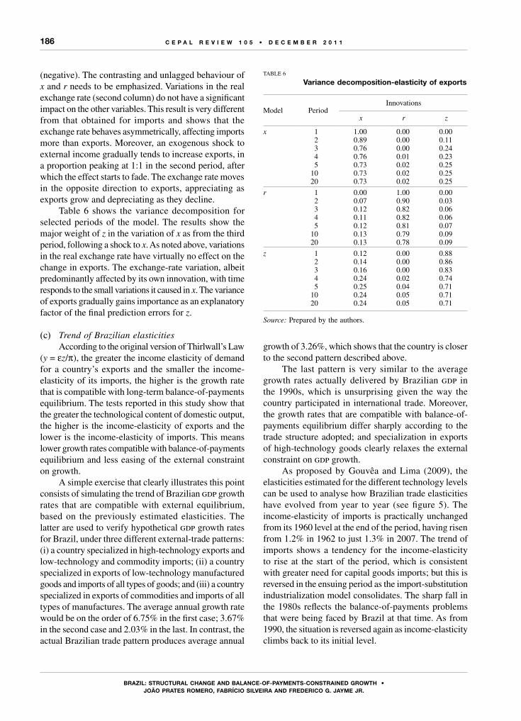
186
BRAzIL: stRuCtuRAL CHAngE AnD BALAnCE-of-PAyMEnts-ConstRAInED gRoWtH • joão PRAtEs RoMERo, fABRíCIo sILVEIRA AnD fREDERICo g. jAyME jR.
C E P A L R E V I E W 1 0 5 • D E C E M B E R 2 0 1 1
(negative). The contrasting and unlagged behaviour of x and r needs to be emphasized. Variations in the real exchange rate (second column) do not have a significant impact on the other variables. This result is very different from that obtained for imports and shows that the exchange rate behaves asymmetrically, affecting imports more than exports. Moreover, an exogenous shock to external income gradually tends to increase exports, in a proportion peaking at 1:1 in the second period, after which the effect starts to fade. The exchange rate moves in the opposite direction to exports, appreciating as exports grow and depreciating as they decline.
Table 6 shows the variance decomposition for selected periods of the model. The results show the major weight of z in the variation of x as from the third period, following a shock to x. As noted above, variations in the real exchange rate have virtually no effect on the change in exports. The exchange-rate variation, albeit predominantly affected by its own innovation, with time responds to the small variations it caused in x. The variance of exports gradually gains importance as an explanatory factor of the final prediction errors for z.
(c) Trend of Brazilian elasticitiesAccording to the original version of Thirlwall’s Law
(y = εz/π), the greater the income elasticity of demand for a country’s exports and the smaller the income-elasticity of its imports, the higher is the growth rate that is compatible with long-term balance-of-payments equilibrium. The tests reported in this study show that the greater the technological content of domestic output, the higher is the income-elasticity of exports and the lower is the income-elasticity of imports. This means lower growth rates compatible with balance-of-payments equilibrium and less easing of the external constraint on growth.
A simple exercise that clearly illustrates this point consists of simulating the trend of Brazilian gdp growth rates that are compatible with external equilibrium, based on the previously estimated elasticities. The latter are used to verify hypothetical gdp growth rates for Brazil, under three different external-trade patterns: (i) a country specialized in high-technology exports and low-technology and commodity imports; (ii) a country specialized in exports of low-technology manufactured goods and imports of all types of goods; and (iii) a country specialized in exports of commodities and imports of all types of manufactures. The average annual growth rate would be on the order of 6.75% in the first case; 3.67% in the second case and 2.03% in the last. In contrast, the actual Brazilian trade pattern produces average annual
growth of 3.26%, which shows that the country is closer to the second pattern described above.
The last pattern is very similar to the average growth rates actually delivered by Brazilian gdp in the 1990s, which is unsurprising given the way the country participated in international trade. Moreover, the growth rates that are compatible with balance-of-payments equilibrium differ sharply according to the trade structure adopted; and specialization in exports of high-technology goods clearly relaxes the external constraint on gdp growth.
As proposed by Gouvêa and Lima (2009), the elasticities estimated for the different technology levels can be used to analyse how Brazilian trade elasticities have evolved from year to year (see figure 5). The income-elasticity of imports is practically unchanged from its 1960 level at the end of the period, having risen from 1.2% in 1962 to just 1.3% in 2007. The trend of imports shows a tendency for the income-elasticity to rise at the start of the period, which is consistent with greater need for capital goods imports; but this is reversed in the ensuing period as the import-substitution industrialization model consolidates. The sharp fall in the 1980s reflects the balance-of-payments problems that were being faced by Brazil at that time. As from 1990, the situation is reversed again as income-elasticity climbs back to its initial level.
TABLE 6
variance decomposition-elasticity of exports
Model PeriodInnovations
x r z
x 1 1.00 0.00 0.002 0.89 0.00 0.113 0.76 0.00 0.244 0.76 0.01 0.235 0.73 0.02 0.25
10 0.73 0.02 0.2520 0.73 0.02 0.25
r 1 0.00 1.00 0.002 0.07 0.90 0.033 0.12 0.82 0.064 0.11 0.82 0.065 0.12 0.81 0.07
10 0.13 0.79 0.0920 0.13 0.78 0.09
z 1 0.12 0.00 0.882 0.14 0.00 0.863 0.16 0.00 0.834 0.24 0.02 0.745 0.25 0.04 0.71
10 0.24 0.05 0.7120 0.24 0.05 0.71
Source: Prepared by the authors.
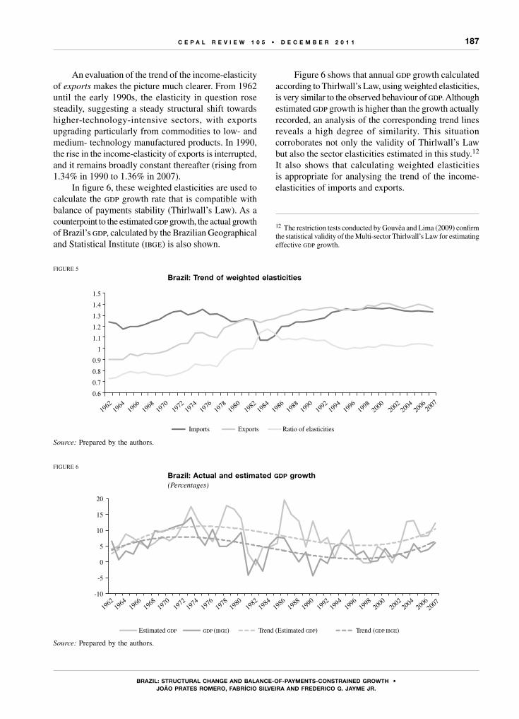
187
BRAzIL: stRuCtuRAL CHAngE AnD BALAnCE-of-PAyMEnts-ConstRAInED gRoWtH • joão PRAtEs RoMERo, fABRíCIo sILVEIRA AnD fREDERICo g. jAyME jR.
C E P A L R E V I E W 1 0 5 • D E C E M B E R 2 0 1 1
An evaluation of the trend of the income-elasticity of exports makes the picture much clearer. From 1962 until the early 1990s, the elasticity in question rose steadily, suggesting a steady structural shift towards higher-technology-intensive sectors, with exports upgrading particularly from commodities to low- and medium- technology manufactured products. In 1990, the rise in the income-elasticity of exports is interrupted, and it remains broadly constant thereafter (rising from 1.34% in 1990 to 1.36% in 2007).
In figure 6, these weighted elasticities are used to calculate the gdp growth rate that is compatible with balance of payments stability (Thirlwall’s Law). As a counterpoint to the estimated gdp growth, the actual growth of Brazil’s gdp, calculated by the Brazilian Geographical and Statistical Institute (ibge) is also shown.
Figure 6 shows that annual gdp growth calculated according to Thirlwall’s Law, using weighted elasticities, is very similar to the observed behaviour of gdp. Although estimated gdp growth is higher than the growth actually recorded, an analysis of the corresponding trend lines reveals a high degree of similarity. This situation corroborates not only the validity of Thirlwall’s Law but also the sector elasticities estimated in this study.12 It also shows that calculating weighted elasticities is appropriate for analysing the trend of the income-elasticities of imports and exports.
12 The restriction tests conducted by Gouvêa and Lima (2009) confirm the statistical validity of the Multi-sector Thirlwall’s Law for estimating effective gdp growth.
FIGURE 5
Brazil: Trend of weighted elasticities
Source: Prepared by the authors.
1962
1964
1966
1968
1970
1972
1974
1976
1978
1980
1982
1984
1986
1988
1990
1992
1994
1996
1998
2000
2002
2004
2006 20
070.6
0.7
0.8
0.9
1
1.1
1.2
1.3
1.4
1.5
Imports Exports Ratio of elasticities
FIGURE 6
Brazil: Actual and estimated gdp growth (Percentages)
Source: Prepared by the authors.
1962
1964
1966
1968
1970
1972
1974
1976
1978
1980
1982
1984
1986
1988
1990
1992
1994
1996
1998
2000
2002
2004
2006
-10
-5
0
5
10
15
20
Estimated GDP GDP (IBGE) Trend (Estimated GDP) Trend (GDP IBGE)
2007
188
BRAzIL: stRuCtuRAL CHAngE AnD BALAnCE-of-PAyMEnts-ConstRAInED gRoWtH • joão PRAtEs RoMERo, fABRíCIo sILVEIRA AnD fREDERICo g. jAyME jR.
C E P A L R E V I E W 1 0 5 • D E C E M B E R 2 0 1 1
This article has attempted to show that structural change favouring sectors that produce technology-intensive goods eases the external constraint on growth by changing the income-elasticities of imports and exports.
Thirlwall’s Law is used to show that the growth rate of the domestic economy is ultimately determined by the income-elasticities of demand for imports and for exports. Higher growth rates are associated with a low income-elasticity of imports and a high income-elasticity of exports. Nonetheless, the literature usually treats these variables as exogenous. Araujo and Lima (2007) and Gouvêa and Lima (2009) show that changes in the productive structure of the economy cause changes in the elasticities, which are directly determined via the level of technological development embodied in domestic production. According to Jayme Jr. and Resende (2009), developed countries tend to participate in international trade as exporters of medium- and high-technology manufactured goods and as importers of commodities and low-technology manufactures —the opposite trade pattern to that seen in peripheral countries such as Brazil.
To corroborate that analysis, this study conducted a series of empirical tests to estimate the income-elasticities of technologically different categories of Brazilian tradable goods, based on an adaptation of the classification proposed by Lall (2001), in which the data were reclassified in three groups: (i) commodities; (ii) goods of low technological content and natural-resource-based manufactures; and (iii) medium- and high-technology goods.
VConclusions
The test results corroborate the theoretical framework presented, confirming the existence of an increasing positive relation between the technological level of exports and income-elasticity, and the same for imports. This shows that higher growth rates are obtained by participating in world trade as an exporter of medium- and high-technology goods (high income-elasticity) and as an importer of low-technology goods (commodities, low income-elasticity) which is precisely the pattern identified for oecd countries by Jayme Jr. and Resende (2009). Accordingly, a structural shift is needed to increase the gdp share of sectors producing goods with high technological content.
A separate analysis of the trend of Brazilian elasticities showed the pattern of imports remaining broadly constant, whereas the profile of exports evolved continuously until 1990 (reflecting an increase in the income-elasticity of exports) but not afterwards. The subsequent stagnation of the income-elasticity of exports poses an obstacle to the structural change needed to maintain higher growth rates.
The conclusions stress the importance of technological development as a way to influence the elasticities and thus ease the external constraint. Taking as a basic premise the need to keep demand growing to fuel faster output growth, it was shown that the incorporation of technology in production (or an increase in the share of higher-technology sectors in national output) is essential for sustaining this process and breaking free from balance-of-payments problems.
(Original: Portuguese)
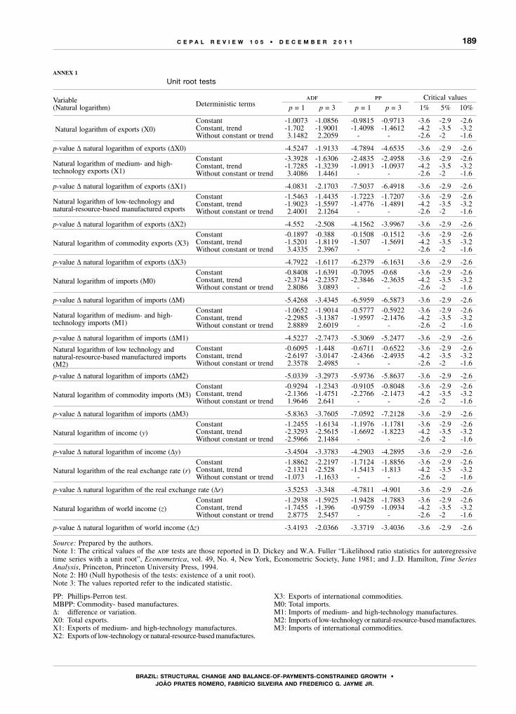
189
BRAzIL: stRuCtuRAL CHAngE AnD BALAnCE-of-PAyMEnts-ConstRAInED gRoWtH • joão PRAtEs RoMERo, fABRíCIo sILVEIRA AnD fREDERICo g. jAyME jR.
C E P A L R E V I E W 1 0 5 • D E C E M B E R 2 0 1 1
AnnEx 1
Unit root tests
Variable(Natural logarithm) Deterministic terms
adf pp Critical valuesp = 1 p = 3 p = 1 p = 3 1% 5% 10%
Natural logarithm of exports (X0)Constant -1.0073 -1.0856 -0.9815 -0.9713 -3.6 -2.9 -2.6Constant, trend -1.702 -1.9001 -1.4098 -1.4612 -4.2 -3.5 -3.2Without constant or trend 3.1482 2.2059 - - -2.6 -2 -1.6
p-value ∆ natural logarithm of exports (∆X0) -4.5247 -1.9133 -4.7894 -4.6535 -3.6 -2.9 -2.6
Natural logarithm of medium- and high- technology exports (X1)
Constant -3.3928 -1.6306 -2.4835 -2.4958 -3.6 -2.9 -2.6Constant, trend -1.7285 -1.3239 -1.0913 -1.0937 -4.2 -3.5 -3.2Without constant or trend 3.4086 1.4461 - - -2.6 -2 -1.6
p-value ∆ natural logarithm of exports (∆X1) -4.0831 -2.1703 -7.5037 -6.4918 -3.6 -2.9 -2.6
Natural logarithm of low-technology and natural-resource-based manufactured exports
Constant -1.5463 -1.4435 -1.7223 -1.7207 -3.6 -2.9 -2.6Constant, trend -1.9023 -1.5597 -1.4776 -1.4891 -4.2 -3.5 -3.2Without constant or trend 2.4001 2.1264 - - -2.6 -2 -1.6
p-value ∆ natural logarithm of exports (∆X2) -4.552 -2.508 -4.1562 -3.9967 -3.6 -2.9 -2.6
Natural logarithm of commodity exports (X3)Constant -0.1897 -0.388 -0.1508 -0.1512 -3.6 -2.9 -2.6Constant, trend -1.5201 -1.8119 -1.507 -1.5691 -4.2 -3.5 -3.2Without constant or trend 3.4335 2.3967 - - -2.6 -2 -1.6
p-value ∆ natural logarithm of exports (∆X3) -4.7922 -1.6117 -6.2379 -6.1631 -3.6 -2.9 -2.6
Natural logarithm of imports (M0)Constant -0.8408 -1.6391 -0.7095 -0.68 -3.6 -2.9 -2.6Constant, trend -2.3734 -2.2357 -2.3846 -2.3635 -4.2 -3.5 -3.2Without constant or trend 2.8086 3.0893 - - -2.6 -2 -1.6
p-value ∆ natural logarithm of imports (∆M) -5.4268 -3.4345 -6.5959 -6.5873 -3.6 -2.9 -2.6
Natural logarithm of medium- and high- technology imports (M1)
Constant -1.0652 -1.9014 -0.5777 -0.5922 -3.6 -2.9 -2.6Constant, trend -2.2985 -3.1387 -1.9597 -2.1476 -4.2 -3.5 -3.2Without constant or trend 2.8889 2.6019 - - -2.6 -2 -1.6
p-value ∆ natural logarithm of imports (∆M1) -4.5227 -2.7473 -5.3069 -5.2477 -3.6 -2.9 -2.6
Natural logarithm of low technology and natural-resource-based manufactured imports (M2)
Constant -0.6095 -1.448 -0.6711 -0.6522 -3.6 -2.9 -2.6Constant, trend -2.6197 -3.0147 -2.4366 -2.4935 -4.2 -3.5 -3.2Without constant or trend 2.3578 2.4985 - - -2.6 -2 -1.6
p-value ∆ natural logarithm of imports (∆M2) -5.0339 -3.2973 -5.9736 -5.8637 -3.6 -2.9 -2.6
Natural logarithm of commodity imports (M3)Constant -0.9294 -1.2343 -0.9105 -0.8048 -3.6 -2.9 -2.6Constant, trend -2.1366 -1.4751 -2.2766 -2.1473 -4.2 -3.5 -3.2Without constant or trend 1.9646 2.641 - - -2.6 -2 -1.6
p-value ∆ natural logarithm of imports (∆M3) -5.8363 -3.7605 -7.0592 -7.2128 -3.6 -2.9 -2.6
Natural logarithm of income (y)
Constant -1.2455 -1.6134 -1.1976 -1.1781 -3.6 -2.9 -2.6Constant, trend -2.3293 -2.5615 -1.6692 -1.8223 -4.2 -3.5 -3.2Without constant or trend -2.5966 2.1484 - - -2.6 -2 -1.6
p-value ∆ natural logarithm of income (∆y) -3.4504 -3.3783 -4.2903 -4.2895 -3.6 -2.9 -2.6
Natural logarithm of the real exchange rate (r)
Constant -1.8862 -2.2197 -1.7124 -1.8856 -3.6 -2.9 -2.6Constant, trend -2.1321 -2.528 -1.5413 -1.813 -4.2 -3.5 -3.2Without constant or trend -1.073 -1.1633 - - -2.6 -2 -1.6
p-value ∆ natural logarithm of the real exchange rate (∆r) -3.5253 -3.348 -4.7811 -4.901 -3.6 -2.9 -2.6
Natural logarithm of world income (z)
Constant -1.2938 -1.5925 -1.9428 -1.7883 -3.6 -2.9 -2.6Constant, trend -1.7455 -1.396 -0.9759 -1.0934 -4.2 -3.5 -3.2Without constant or trend 2.8775 2.5457 - - -2.6 -2 -1.6
p-value ∆ natural logarithm of world income (∆z) -3.4193 -2.0366 -3.3719 -3.4036 -3.6 -2.9 -2.6
Source: Prepared by the authors.Note 1: The critical values of the adf tests are those reported in D. Dickey and W.A. Fuller “Likelihood ratio statistics for autoregressive time series with a unit root”, Econometrica, vol. 49, No. 4, New York, Econometric Society, June 1981; and J..D. Hamilton, Time Series Analysis, Princeton, Princeton University Press, 1994.Note 2: H0 (Null hypothesis of the tests: existence of a unit root).Note 3: The values reported refer to the indicated statistic.
PP: Phillips-Perron test.MBPP: Commodity- based manufactures.∆: difference or variation.X0: Total exports. X1: Exports of medium- and high-technology manufactures.X2: Exports of low-technology or natural-resource-based manufactures.
X3: Exports of international commodities.M0: Total imports.M1: Imports of medium- and high-technology manufactures.M2: Imports of low-technology or natural-resource-based manufactures.M3: Imports of international commodities.
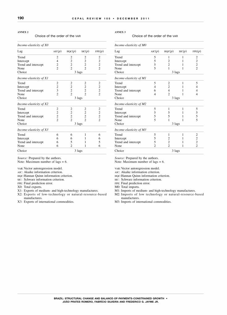
190
BRAzIL: stRuCtuRAL CHAngE AnD BALAnCE-of-PAyMEnts-ConstRAInED gRoWtH • joão PRAtEs RoMERo, fABRíCIo sILVEIRA AnD fREDERICo g. jAyME jR.
C E P A L R E V I E W 1 0 5 • D E C E M B E R 2 0 1 1
AnnEx 2
Choice of the order of the var
Income-elasticity of X0
Lag aic(p) hqc(p) sic(p) fpe(p)
Trend 2 2 2 2Intercept 4 2 2 2Trend and intercept 2 2 2 2None 2 2 2 2Choice 3 lags
Income-elasticity of X1
Trend 2 2 2 2Intercept 2 2 2 2Trend and intercept 3 2 2 2None 2 2 2 2Choice 3 lags
Income-elasticity of X2
Trend 2 2 2 2Intercept 2 2 2 2Trend and intercept 2 2 2 2None 2 2 2 2Choice 3 lags
Income-elasticity of X3
Trend 6 6 1 6Intercept 6 6 1 6Trend and intercept 6 5 1 5None 6 2 1 6
Choice 3 lags
Source: Prepared by the authors.Note: Maximum number of lags = 6.
var: Vector autoregression model.aic: Akaike information criterion.hqc: Hannan Quinn information criterion.sic: Schwarz information criterion.fpe: Final prediction error.X0: Total exports.X1: Exports of medium- and high-technology manufactures.X2: Exports of low-technology or natural-resource-based
manufactures.X3: Exports of international commodities.
AnnEx 3
Choice of the order of the var
Income-elasticity of M0
Lag aic(p) hqc(p) sic(p) fpe(p)
Trend 5 1 1 2Intercept 5 2 1 2Trend and intercept 5 2 1 2None 5 1 1 2Choice 3 lags
Income-elasticity of M1
Trend 5 2 1 5Intercept 4 2 1 4Trend and intercept 6 4 1 4None 4 2 1 4Choice 3 lags
Income-elasticity of M2
Trend 5 1 1 5Intercept 5 5 1 5Trend and intercept 5 5 1 5None 5 1 1 5Choice 3 lags
Income-elasticity of M3
Trend 5 1 1 2Intercept 5 2 1 2Trend and intercept 5 2 1 2None 2 2 1 2
Choice 3 lags
Source: Prepared by the authors.Note: Maximum number of lags = 6.
var: Vector autoregression model.aic: Akaike information criterion. hqc: Hannan Quinn information criterion.sic: Schwarz information criterion.fpe: Final prediction error. M0: Total imports.M1: Imports of medium- and high-technology manufactures.M2: Imports of low technology or natural-resource-based
manufactures.M3: Imports of international commodities.

191
BRAzIL: stRuCtuRAL CHAngE AnD BALAnCE-of-PAyMEnts-ConstRAInED gRoWtH • joão PRAtEs RoMERo, fABRíCIo sILVEIRA AnD fREDERICo g. jAyME jR.
C E P A L R E V I E W 1 0 5 • D E C E M B E R 2 0 1 1
AnnEx 4
Diagnostic evaluation of the residuals
Diagnosis of residuals of income-elasticity of M0
Model jb p-value Q p-value arch p-value
p = 3 24.2956 0.0004607 101.818 0.7221 82.0855 0.1951p = 2 19.1771 2.51x-104 99.842 0.9096 95.4263 0.03381p = 1 38.7853 7.89x-107 107.595 0.915 100.0163 0.01617
Income-elasticity of M1
p = 3 14.1097 0.02843 91.0622 0.9166 62.7236 0.7742p = 2 18.8462 4.43x10³ 103.18 0.8638 69.9512 0.5464p = 1 25.1554 3.20x10⁴ 116.412 0.779 73.3348 0.4341
Income-elasticity of M2
p = 3 6.0231 0.4206 103.307 0.6857 89.8549 0.0757p = 2 12.7499 0.04718 101.144 0.8932 95.6307 0.03276p = 1 21.5636 0.001452 110.03 0.8854 106.9891 0.004691
Income-elasticity of M3
p = 3 24.9692 0.000346 111.948 0.4569 86.4326 0.1179p = 2 29.839 4.22x10⁵ 109.363 0.7469 120.7874 0.000281p = 1 58.9255 7.44x10¹¹ 104.191 0.9468 118.1968 0.000493
Source: Prepared by the authors.Note: The results refer to the best model with intercept in the co-integration vector.
Jarque-Bera (JB): Jarque-Bera test of normality of the residuals (H0: Normal residuals).Portmanteau (Q): Test for autocorrelation in the residuals (H0: No autocorrelation).arch: Test for autoregressive conditional heteroscedasticity in the
residuals (H0: homoscedasticity).M0: Total imports.M1: Imports of medium- and high-technology manufactures.M2: Imports of low-technology or natural-resource-based
manufactures.M3: Imports of international commodities.
AnnEx 5
Diagnostic of the residuals
Income-elasticity of X0
Model jb p-value p-value arch p-value
p = 3 6.2999 0.3904 105.107 0.6397 76.529 0.3354p = 2 10.8343 0.09364 98.5533 0.924 59.0846 0.8626p = 1 9.5393 1.45x101 104.955 0.9406 82.9702 0.1771
Income-elasticity of X1
p = 3 1.7535 0.941 90.9865 0.9175 59.843 0.8461p = 2 3.8717 0.694 96.6295 0.9424 51.5521 0.9672p = 1 9.4118 1.52x101 83.0726 0.9994 78.4628 0.2815
Income-elasticity of X2
p = 3 5.3618 0.4983 109.938 0.5107 72.3643 0.4658p = 2 11.212 0.08204 90.9576 0.9777 68.3158 0.6012p = 1 8.7636 0.1873 90.6287 0.9958 86.4695 0.1174
Income-elasticity of X3
p = 6 3.0402 0.8038 99.9439 0.113 65.6792 0.6869p = 3 2.4965 0.8689 101.418 0.7316 67.873 0.616p = 2 7.6678 0.2635 99.2726 0.9162 82.3719 0.1892
Source: Prepared by the authors.Note: The results refer to the best model with intercept in the co-integration vector.
Jarque-Bera (JB): Jarque-Bera test got normality of the residuals (H0: Normal residuals).Portmanteau (Q): Test for autocorrelation in the residuals (H0: No autocorrelation).arch: Test for autoregressive conditional heteroscedasticity in the
residuals (H0: homoscedasticity)X0: Total exports. X1: Exports of medium- and high-technology manufactures.X2: Exports of low-technology or natural-resource-based
manufactures.X3: Exports of international commodities.

192
BRAzIL: stRuCtuRAL CHAngE AnD BALAnCE-of-PAyMEnts-ConstRAInED gRoWtH • joão PRAtEs RoMERo, fABRíCIo sILVEIRA AnD fREDERICo g. jAyME jR.
C E P A L R E V I E W 1 0 5 • D E C E M B E R 2 0 1 1
AnnEx 6
Co-integration test
Income-elasticity of M0
h0Test statistics Critical values
p = 1 p = 2 p = 3 90% 95% 99%
r = 0 39.07 34.12 36.75 32 34.91 41.07r = 1 16.86 17.67 17.73 17.85 19.96 24.6r = 2 6.52 4.14 6.12 7.52 9.24 12.97
Income-elasticity of M1
r = 0 35.81 36.47 46.42 32 34.91 41.07r = 1 15.37 17.59 20.99 17.85 19.96 24.6r = 2 4.79 2.35 6.07 7.52 9.24 12.97
Income-elasticity of M2
r = 0 39.83 40.01 42.37 32 34.91 41.07r = 1 17.59 21.14 20.41 17.85 19.96 24.6r = 2 7.72 4.45 7.51 7.52 9.24 12.97
Income-elasticity of M3
r = 0 44.47 39.56 35.67 32 34.91 41.07r = 1 18.55 19.34 15.69 17.85 19.96 24.6r = 2 5.05 8.44 6.87 7.52 9.24 12.97
Source: Prepared by the authors.Note 1: The results refer to the best model with intercept in the co-integration vector.Note 2: The results refer to the trace of statistics.Note 3: The critical values of the trace of statistics referred to those found in S. Johansen, Likelihood-Based Inference in Cointegrated Vector Autorregresive Models, New York, Oxford University Press, 1995.
H0: the null hypothesis is that there are r co-integration vectors.M0: Total imports.M1: Imports of medium- and high-technology manufactures.M2: Imports of low-technology or natural-resource-based
manufactures.M3: Imports of international commodities.
AnnEx 7
Co-integration test
Income-elasticity of X0
h0
Test statistics Critical values
p = 1 p = 2 p = 3 90% 95% 99%
r = 0 36.44 40.27 48.21 32 34.91 41.07r = 1 9.7 11.87 16.46 17.85 19.96 24.6r = 2 2.98 2.17 4.79 7.52 9.24 12.97
Income-elasticity of X1
r = 0 45.69 61.08 51.54 32 34.91 41.07r = 1 20.41 29.3 20.8 17.85 19.96 24.6r = 2 6.53 7.21 4.47 7.52 9.24 12.97
Income-elasticity of X2
r = 0 40.84 41.87 40.64 32 34.91 41.07r = 1 12.19 13.65 15.28 17.85 19.96 24.6r = 2 5.28 5.33 5.31 7.52 9.24 12.97
Income-elasticity of X3
r = 0 34.02 49.86 80.43 32 34.91 41.07r = 1 9.59 14.75 36.36 17.85 19.96 24.6r = 2 1.55 2.33 17.59 7.52 9.24 12.97
Source: Prepared by the authors.Note 1: The results refer to the model with an intercept in the co-integration vector.Note 2: The results refer to the trace of statistic.Note 3: The critical values of the trace statistic are those found in S. Johansen, Likelihood-Based Inference in Cointegrated Vector Autorregresive Models, New York, Oxford University Press, 1995.
H0: Null hypothesis.X0: Total exports.X1: Exports of medium- and high-technology manufactures.X2: Exports of low-technology or natural-resource-based
manufactures.X3: Exports of international commodities.
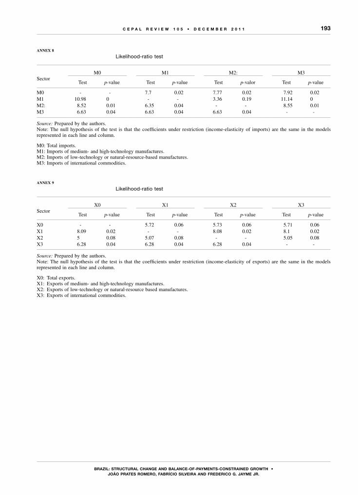
193
BRAzIL: stRuCtuRAL CHAngE AnD BALAnCE-of-PAyMEnts-ConstRAInED gRoWtH • joão PRAtEs RoMERo, fABRíCIo sILVEIRA AnD fREDERICo g. jAyME jR.
C E P A L R E V I E W 1 0 5 • D E C E M B E R 2 0 1 1
AnnEx 8
Likelihood-ratio test
SectorM0 M1 M2: M3
Test p-value Test p-value Test p-valor Test p-value
M0 - - 7.7 0.02 7.77 0.02 7.92 0.02M1 10.98 0 - - 3.36 0.19 11.14 0M2: 8.52 0.01 6.35 0.04 - - 8.55 0.01M3 6.63 0.04 6.63 0.04 6.63 0.04 - -
Source: Prepared by the authors.Note: The null hypothesis of the test is that the coefficients under restriction (income-elasticity of imports) are the same in the models represented in each line and column.
M0: Total imports.M1: Imports of medium- and high-technology manufactures.M2: Imports of low-technology or natural-resource-based manufactures.M3: Imports of international commodities.
AnnEx 9
Likelihood-ratio test
SectorX0 X1 X2 X3
Test p-value Test p-value Test p-value Test p-value
X0 - - 5.72 0.06 5.73 0.06 5.71 0.06X1 8.09 0.02 - - 8.08 0.02 8.1 0.02X2 5 0.08 5.07 0.08 - - 5.05 0.08X3 6.28 0.04 6.28 0.04 6.28 0.04 - -
Source: Prepared by the authors.Note: The null hypothesis of the test is that the coefficients under restriction (income-elasticity of exports) are the same in the models represented in each line and column.
X0: Total exports.X1: Exports of medium- and high-technology manufactures.X2: Exports of low-technology or natural-resource based manufactures.X3: Exports of international commodities.

194
BRAzIL: stRuCtuRAL CHAngE AnD BALAnCE-of-PAyMEnts-ConstRAInED gRoWtH • joão PRAtEs RoMERo, fABRíCIo sILVEIRA AnD fREDERICo g. jAyME jR.
C E P A L R E V I E W 1 0 5 • D E C E M B E R 2 0 1 1
Bibliography
Abramovitz, M. (1986), “Catching up, forging ahead, and falling behind”, The Journal of Economic History, vol. 46, No. 2, New York, Cambridge University Press.
Albuquerque, E.M. (1999), “National systems of innovation and non-oecd countries: notes about a rudimentary and tentative ‘typology’”, Brazilian Journal of Political Economy, vol. 19, No. 4, São Paulo.
Araujo, R.A. and G.T. Lima (2007), “A structural economic dynamics approach to balance-of-payments-constrained growth”, Cambridge Journal of Economics, vol. 31, No. 5, Oxford, Oxford University Press.
Atesoglu, H.S. (1997), “Balance of payments constrained growth model and its implications for the United States”, Journal of Post Keynesian Economics, vol. 19, No. 3, Armonk, M.E. Sharpe.
Barbosa-Filho, N.H. (2001), “Balance-of-payments constraint: from balanced trade to sustainable debt”, Banca Nazionale del Lavoro Quarterly Review, No. 219, Rome, Banca Nazionale del Lavoro.
Bertola, L., H. Higachi and G. Porcile (2002), “Balance-of-payments constrained growth in Brazil: a test of Thirlwall’s law, 1980-1973”, Journal of Post Keynesian Economics, vol. 25, No. 1, Armonk, M.E. Sharpe.
Carvalho, V.R. and G.T. Lima (2008), “A restrição externa e a perda de dinamismo da economia brasileira: investigando relações entre estrutura produtiva e crescimento econômico”, Anais do XXXV Encontro Nacional de Economia, Niterói, National Association of Centers for Post-graduation in Economics (anpec).
Dickey, D. and W.A. Fuller (1981), “Likelihood ratio statistics for autoregressive time series with a unit root”, Econometrica, vol. 49, No. 4, New York, Econometric Society, June.
Enders, W. (1995), Applied Econometric Time Series, New York, John Wiley & Sons.
Fajnzylber, R.F. (2000), “Da caixa-preta ao conjunto vazio”, Cinqüenta anos de pensamento na cepal, R. Bielschowsky (org.), Rio de Janeiro, Record.
(1983), La industrialización trunca de América Latina, Mexico City, Nueva Imagen.
Ferreira, A. (2001), “A lei de crescimento de Thirlwall”, dissertation, Campinas, Institute of Economics/State University at Campinas.
Freeman, C. (2004), “The ‘National System of Innovation’ in historical perspective”, Revista brasileira de inovação, vol. 3, No. 1, Finance Company for the Study of Programs and Projects (finep).
Gouvêa, R.R. and G.T. Lima (2009), “Structural change, balance-of-payments constraint and economic growth: evidence from the multi-sectoral Thirlwall’s Law”, Anais do XXXVII Encontro Nacional de Economia da anpec, Niterói, National Association of Centers for Post-graduation in Economics (anpec).
Hamilton, J.D. (1994), Time Series Analysis, Princeton, Princeton University Press.
Harrod, R. (1933), International Economics, Cambridge, Cambridge University Press.
Hausman, R., J. Hwang and D. Rodrik (2005), “What you export matters”, nber Working Papers, No. 11905, Cambridge, Massachusetts, National Bureau of Economic Research.
Holland, M., F. Vieira and O. Canuto (2004), “Economic growth and the balance-of-payments constraint in Latin America”, Investigación económica, vol. 63, Mexico City, National Autonomous University of Mexico.
Jayme Jr., F.G. (2003) “Balance-of-payments constrained economic growth in Brazil”, Revista de economia política, vol. 23, São Paulo.
Jayme Jr., F.G. and M.F.C. Resende (2009), “Crescimento econômico e restrição externa: teoria e a experiência brasileira”, Crescimento econômico: setor externo e inflação, R. Michel and L. Carvalho (orgs.), Rio de Janeiro, Institute of Applied Economic Research (ipea).
Johansen, S. (1995), Likelihood-Based Inference in Cointegrated Vector Autoregressive Models, New York, Oxford University Press.
Kaldor, N. (1966), Causes of the Slow Rate of Economic Growth of the United Kingdom, London, Cambridge University Press.
Lall, S. (2001), Competitiveness, Technology and Skills, Cheltenham, Edward Elgar Publishing.
López, J. and A. Cruz (2000), “Thirlwall’s law and beyond: the Latin American experience”, Journal of Post Keynesian Economics, vol. 22, No. 3, Armonk, M.E. Sharpe.
Lundvall, B. (ed.) (1992), National Systems of Innovation: Towards a Theory of Innovation and Interactive Learning, London, Pinter.
McCombie, J.S.L. (1997), “On the empirics of balance-of-payments constrained growth”, Journal of Post Keynesian Economics, vol. 19, No. 3, Armonk, M.E. Sharpe.
McCombie, J.S.L. and A.P. Thirlwall (1999), “Growth in an international context: a post Keynesian view”, Foundations of International Economics: Post Keynesian Perspectives, J. Deprez and J.T. Harvey (orgs.), London, Routledge.
(1997), “Economic growth and balance-of-payments constraint revisited”, Markets, Unemployment and Economic Policy, P. Arestis, G. Palma and M. Sawyer (eds.), vol. 2, London, Routledge.
(1994), Economic Growth and the Balance-of-Payments Constraint, New York, St. Martin’s Press.
Moreno-Brid, J. (2003), “Capital flows, interest payments and the balance-of-payments constrained growth model: a theoretical and empirical analysis”, Metroeconomica, vol. 54, No. 2-3, Wiley Blackwell.
Nelson, R.R. (ed.) (1993), National Innovation Systems: A Comparative Analysis, Oxford, Oxford University Press.
(1964), “Aggregate production functions and medium-range growth projections”, American Economic Review, vol. 54, No. 5, Nashville, Tennessee, American Economic Association.
Pérez, C. and L. Soete (1988), “Catching up in technology: entry barriers and windows of opportunity”, Technical Change and Economic Theory, Dosi and others (eds.), London, Macmillan.
Porcile, G. and G.T. Lima (2006), “Tipo de cambio, empleo y crecimiento en un modelo con restricción externa”, Investigación económica, vol. 65, No. 257, Mexico City, National Autonomous University of Mexico.
Prebisch, R. (2000a), “O desenvolvimento da economia da América Latina e alguns de seus problemas principais”, Cinqüenta

195
BRAzIL: stRuCtuRAL CHAngE AnD BALAnCE-of-PAyMEnts-ConstRAInED gRoWtH • joão PRAtEs RoMERo, fABRíCIo sILVEIRA AnD fREDERICo g. jAyME jR.
C E P A L R E V I E W 1 0 5 • D E C E M B E R 2 0 1 1
anos de pensamento na cepal, R. Bielschowsky (org.), Rio de Janeiro, Record.
(2000b), “Problemas teóricos e práticos do crescimento econômico”, Cinqüenta anos de pensamento na cepal, R. Bielschowsky (org.), Rio de Janeiro, Record.
Resende, M.F.C. and D.R. Torres (2008), “National Innovation System, trade elasticities and economic growth”, Anais do XXXVI Encontro Nacional de Economia, Niterói, National Association of Centers for Post-graduation in Economics (anpec).
Santos, A.T., G.T. Lima and V.R.S. Carvalho (2005), “A restrição externa como fator limitante do crescimento econômico brasileiro: um teste empírico”, Anais do XXXIII Encontro Nacional de Economia, Natal [online] http://www.anpec.org.br.
Thirlwall, A.P. (1979), “The balance of payments constraint as an explanation of international growth rates differences”, Banca Nazionale del Lavoro Quarterly Review, No. 128, Rome, Banca Nazionale del Lavoro.
Thirlwall, A.P. and M. Hussain (1982), “The balance of payments constraint, capital flows and growth rates differences between developing countries”, Oxford Economic Papers, No. 10, Oxford, Oxford University Press.
Vieira, F.A. and M. Holland (2006), “Crescimento econômico secular no Brasil, modelo de Thirlwall e termos de troca”, Anais do XXXIV Encontro Nacional de Economia da anpec, Niterói, National Association of Centers for Post-graduation in Economics (anpec), December.


197C E P A L R E V I E W 1 0 5 • D E C E M B E R 2 0 1 1
Mario AbuhadbaManuel AgosinDillon AlleyneIrma ArriagadaReynaldo BajrajOmar BelloRudolf BuitelaarFernando CantúPablo CarvalloPablo CelhayNelson CorreaLuiz Fernando de PaulaArmando Di FilippoErnesto EspíndolaEduardo FajnzylberFernando FerrariGuillermo FuentesMarcela GajardoSarah GammageElisa GiulianiCarlos Guerrero de Lizardi
cepal Review referees 2010and January-August 2011
During this period, the following academics and researchers acted as referees for the cepal Review
Joaquim GuilhotoKarla HernándezRené HernándezRicardo InfanteLuis Felipe JiménezBernardo KosacoffMarcelo La FleurOscar LanderretcheXavier ManceroSandra ManuelitoAndrés MarinakisJorge MattarFrancisco MenesesLeonardo MonasterioSonia MontañoMichael MortimoreOscar MuñozCarlos MussiLucas NavarroJose Luis OreiroRamón Padilla
Mauricio PereiraEsteban PérezRamón PinedaGabriel PorcileJuan Carlos RamírezAndrea RepettoDiego RivasLuis RiverosMônica RodriguesAdrián RodríguezPilar RomagueraJaime RosClaudio SotoRaquel SzalachmanAndras UthoffRodrigo ValdésHugo VenturaSebastián VergaraFrancisco VillarrealJürgen WellerWilly Zapata
cepal Review is grateful for their invaluable assistance.

C E P A L r E v i E w 1 0 5
D E C E M B E r 2 0 1 1
199
Guidelinesfor contributorsto CePal Review
In order to facilitate the submission, consideration and publication of articles, the editorial board of the cepal Review has prepared the following information and suggestions to serve as a guide for future contributors.
The submission of an article implies an undertaking by the author not to submit it simultaneously to other publications. The copyright to all articles published in the Review shall be owned by the United Nations.
All articles will be submitted to external referees.
Papers should be submitted in the original language (English, French, Portuguese or Spanish). They will be translated into the appropriate language by the relevant eclac services.
Each article must be accompanied by a summary, no more than 150 words in length, giving a brief description of its subject matter and main conclusions.
Papers should be no longer than 10,000 words, including the summary, notes and bibliography. Shorter papers will also be considered.
Articles should be sent either by e-mail (to [email protected]) or by regular mail, on cd or diskette, to: cepal Review, Casilla 179-D, Santiago, Chile. They should not be submitted in pdf format.
style guide:
Titles should not be excessively long.
Footnotes
– It is recommended that footnotes be kept to a minimum.
– It is recommended that footnotes not be used to cite bibliographical references; such references should preferably be incorporated into the text.
– Footnotes should be numbered consecutively using superscript Arabic numerals.
Tables and figures
– It is recommended that tables and figures be kept to a minimum, avoiding any redundancy with the text.
– Tables, figures and other elements should be inserted at the end of the text in the format in which they were designed; they should not be inserted as “pictures”. Figures in Excel should include the corresponding worksheets.
– The location of tables and figures in the body of the article should be indicated in the appropriate place as follows:
Insert figure 1Insert table 1
– Tables and figures should include an explicit and complete reference to their sources.
– Tables should indicate the period covered at the end of the title, and should indicate the units in which the data are expressed in a subtitle (in italics and between brackets).
– The symbols referred to in the “Explanatory notes” which appear on the page preceding the table of contents should be taken into account in the preparation of tables and figures.
– Footnotes to tables and figures should be ordered consecutively using superscript lower-case letters.
– Figures should be prepared bearing in mind that they will be printed in black and white.
Acronyms and abbreviations
– Acronyms and abbreviations should not be used unless absolutely necessary, in which case the full name should be written out the first time it occurs in the article.
Bibliography
– Bibliographical references should be directly related to the content of the article and should not be excessively long.
– At the end of the article, under the title “Bibliography”, all the necessary information should be included accurately and in alphabetical order by author: name of author(s), year of publication, full name of article (if any) and publication (including any subtitle), city of publication, publisher and, in the case of a periodical, month of publication.
The editorial board of the Review reserves the right to make any necessary editorial changes in the articles, including their titles.
Authors will receive a one-year courtesy subscription to the Review, plus 30 offprints of their article in Spanish and 30 in English, at the time of publication in each language.
Publicaciones de la CEPAL / ECLAC publications Comisión Económica para América Latina y el Caribe / Economic Commission for Latin America and the Caribbean
Casilla 179-D, Santiago de Chile. E-mail: [email protected] Véalas en: www.cepal.org/publicaciones
Publications may be accessed at: www.eclac.org
Revista CEPAL / CEPAL Review La Revista se inició en 1976 como parte del Programa de Publicaciones de la Comisión Económica para América Latina y el Caribe, con el propósito de contribuir al examen de los problemas del desarrollo socioeconómico de la región. Las opiniones expresadas en los artículos firmados, incluidas las colaboraciones de los funcionarios de la Secretaría, son las de los autores y, por lo tanto, no reflejan necesariamente los puntos de vista de la Organización.
La Revista CEPAL se publica en español e inglés tres veces por año. Los precios de suscripción anual vigentes son de US$ 30 para la versión en español y US$ 35 para la versión en inglés. El precio por
ejemplar suelto es de US$ 15 para ambas versiones. Los precios de suscripción por dos años son de US$ 50 para la versión en español y US$ 60 para la versión en inglés. CEPAL Review first appeared in 1976 as part of the Publications Programme of the Economic Commission for Latin America and the Caribbean, its aim being to make a contribution to the study of the economic and social development problems of the region. The views expressed in signed articles, including those by Secretariat staff members, are those of the authors and therefore do not necessarily reflect the point of view of the Organization.
CEPAL Review is published in Spanish and English versions three times a year. Annual subscription costs are US$ 30 for the Spanish version and US$ 35 for the English version. The price of single issues is US$ 15 for
both versions. The cost of a two-year subscription is US$ 50 for the Spanish version and US$ 60 for the English version.
Informes periódicos institucionales / Annual reports Todos disponibles para años anteriores / Issues for previous years also available • Balance preliminar de las economías de América Latina y el Caribe, 2010, 176 p. Preliminary Overview of the Economies of Latin America and the Caribbean, 2010, 160 p. • Estudio económico de América Latina y el Caribe 2010-2011, 344 p. Economic Survey of Latin America and the Caribbean 2010-2011, 334 p. • Panorama de la inserción internacional de América Latina y el Caribe, 2010-2011, 140 p. Latin America and the Caribbean in the World Economy, 2010-2011, 168 p. • Panorama social de América Latina, 2010, 266 p. Social Panorama of Latin America, 2010, 256 p. • La inversión extranjera directa en América Latina y el Caribe, 2010, 216 p. Foreign Direct Investment of Latin America and the Caribbean, 2010, 204 p. • Anuario estadístico de América Latina y el Caribe / Statistical Yearbook for Latin America and the Caribbean, 2010, 310 p.
Libros de la CEPAL 112 El desarrollo inclusivo en América Latina y el Caribe. Ensayos sobre políticas de convergencia productiva para la igualdad, Ricardo
Infante (editor), 384 p. 111 Protección social inclusiva en América Latina. Una mirada integral, un enfoque de derechos, Simone Cecchini y Rodrigo Martínez,
284 p. 110 Envejecimiento en América Latina. Sistema de pensiones y protección social integral, Antonio Prado y Ana Sojo (eds.), 304 p. 109 Modeling Public Policies in Latin America and the Caribbean, Carlos de Miguel, José Durán Lima, Paolo Giordiano, Julio
Guzmán, Andrés Schuschny and Masazaku Watanuki (eds.), 322 p.
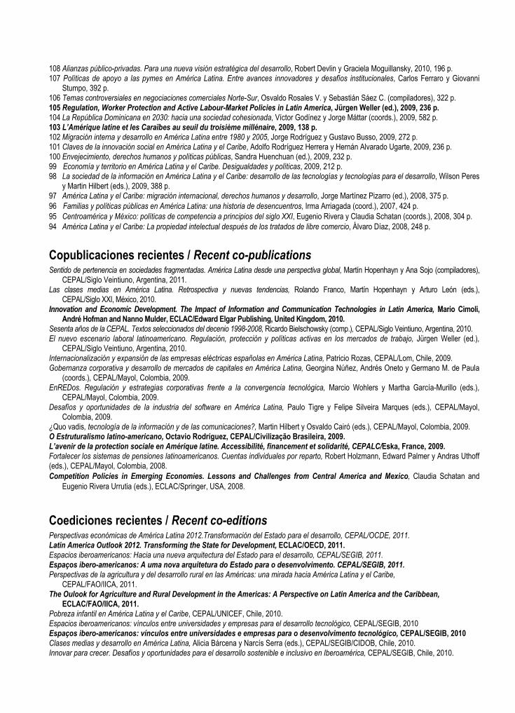
108 Alianzas público-privadas. Para una nueva visión estratégica del desarrollo, Robert Devlin y Graciela Moguillansky, 2010, 196 p. 107 Políticas de apoyo a las pymes en América Latina. Entre avances innovadores y desafíos institucionales, Carlos Ferraro y Giovanni
Stumpo, 392 p. 106 Temas controversiales en negociaciones comerciales Norte-Sur, Osvaldo Rosales V. y Sebastián Sáez C. (compiladores), 322 p. 105 Regulation, Worker Protection and Active Labour-Market Policies in Latin America, Jürgen Weller (ed.), 2009, 236 p. 104 La República Dominicana en 2030: hacia una sociedad cohesionada, Víctor Godínez y Jorge Máttar (coords.), 2009, 582 p. 103 L’Amérique latine et les Caraïbes au seuil du troisième millénaire, 2009, 138 p. 102 Migración interna y desarrollo en América Latina entre 1980 y 2005, Jorge Rodríguez y Gustavo Busso, 2009, 272 p. 101 Claves de la innovación social en América Latina y el Caribe, Adolfo Rodríguez Herrera y Hernán Alvarado Ugarte, 2009, 236 p. 100 Envejecimiento, derechos humanos y políticas públicas, Sandra Huenchuan (ed.), 2009, 232 p. 99 Economía y territorio en América Latina y el Caribe. Desigualdades y políticas, 2009, 212 p. 98 La sociedad de la información en América Latina y el Caribe: desarrollo de las tecnologías y tecnologías para el desarrollo, Wilson Peres
y Martin Hilbert (eds.), 2009, 388 p. 97 América Latina y el Caribe: migración internacional, derechos humanos y desarrollo, Jorge Martínez Pizarro (ed.), 2008, 375 p. 96 Familias y políticas públicas en América Latina: una historia de desencuentros, Irma Arriagada (coord.), 2007, 424 p. 95 Centroamérica y México: políticas de competencia a principios del siglo XXI, Eugenio Rivera y Claudia Schatan (coords.), 2008, 304 p. 94 América Latina y el Caribe: La propiedad intelectual después de los tratados de libre comercio, Álvaro Díaz, 2008, 248 p.
Copublicaciones recientes / Recent co-publications Sentido de pertenencia en sociedades fragmentadas. América Latina desde una perspectiva global, Martín Hopenhayn y Ana Sojo (compiladores),
CEPAL/Siglo Veintiuno, Argentina, 2011. Las clases medias en América Latina. Retrospectiva y nuevas tendencias, Rolando Franco, Martín Hopenhayn y Arturo León (eds.),
CEPAL/Siglo XXI, México, 2010. Innovation and Economic Development. The Impact of Information and Communication Technologies in Latin America, Mario Cimoli,
André Hofman and Nanno Mulder, ECLAC/Edward Elgar Publishing, United Kingdom, 2010. Sesenta años de la CEPAL. Textos seleccionados del decenio 1998-2008, Ricardo Bielschowsky (comp.), CEPAL/Siglo Veintiuno, Argentina, 2010. El nuevo escenario laboral latinoamericano. Regulación, protección y políticas activas en los mercados de trabajo, Jürgen Weller (ed.),
CEPAL/Siglo Veintiuno, Argentina, 2010. Internacionalización y expansión de las empresas eléctricas españolas en América Latina, Patricio Rozas, CEPAL/Lom, Chile, 2009. Gobernanza corporativa y desarrollo de mercados de capitales en América Latina, Georgina Núñez, Andrés Oneto y Germano M. de Paula
(coords.), CEPAL/Mayol, Colombia, 2009. EnREDos. Regulación y estrategias corporativas frente a la convergencia tecnológica, Marcio Wohlers y Martha García-Murillo (eds.),
CEPAL/Mayol, Colombia, 2009. Desafíos y oportunidades de la industria del software en América Latina, Paulo Tigre y Felipe Silveira Marques (eds.), CEPAL/Mayol,
Colombia, 2009. ¿Quo vadis, tecnología de la información y de las comunicaciones?, Martin Hilbert y Osvaldo Cairó (eds.), CEPAL/Mayol, Colombia, 2009. O Estruturalismo latino-americano, Octavio Rodríguez, CEPAL/Civilização Brasileira, 2009. L’avenir de la protection sociale en Amérique latine. Accessibilité, financement et solidarité, CEPALC/Eska, France, 2009. Fortalecer los sistemas de pensiones latinoamericanos. Cuentas individuales por reparto, Robert Holzmann, Edward Palmer y Andras Uthoff (eds.), CEPAL/Mayol, Colombia, 2008. Competition Policies in Emerging Economies. Lessons and Challenges from Central America and Mexico, Claudia Schatan and
Eugenio Rivera Urrutia (eds.), ECLAC/Springer, USA, 2008.
Coediciones recientes / Recent co-editions Perspectivas económicas de América Latina 2012.Transformación del Estado para el desarrollo, CEPAL/OCDE, 2011. Latin America Outlook 2012. Transforming the State for Development, ECLAC/OECD, 2011. Espacios iberoamericanos: Hacia una nueva arquitectura del Estado para el desarrollo, CEPAL/SEGIB, 2011. Espaços ibero-americanos: A uma nova arquitetura do Estado para o desenvolvimento. CEPAL/SEGIB, 2011. Perspectivas de la agricultura y del desarrollo rural en las Américas: una mirada hacia América Latina y el Caribe,
CEPAL/FAO/IICA, 2011. The Oulook for Agriculture and Rural Development in the Americas: A Perspective on Latin America and the Caribbean,
ECLAC/FAO/IICA, 2011. Pobreza infantil en América Latina y el Caribe, CEPAL/UNICEF, Chile, 2010. Espacios iberoamericanos: vínculos entre universidades y empresas para el desarrollo tecnológico, CEPAL/SEGIB, 2010 Espaços ibero-americanos: vínculos entre universidades e empresas para o desenvolvimento tecnológico, CEPAL/SEGIB, 2010 Clases medias y desarrollo en América Latina, Alicia Bárcena y Narcís Serra (eds.), CEPAL/SEGIB/CIDOB, Chile, 2010. Innovar para crecer. Desafíos y oportunidades para el desarrollo sostenible e inclusivo en Iberoamérica, CEPAL/SEGIB, Chile, 2010.
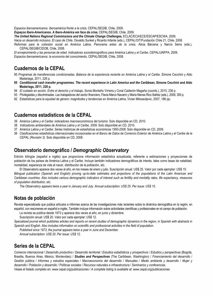
Espacios iberoamericanos. Iberoamérica frente a la crisis, CEPAL/SEGIB, Chile, 2009. Espaços Ibero-Americanos. A Ibero-América em face da crise, CEPAL/SEGIB, Chile, 2009. The United Nations Regional Commissions and the Climate Change Challenges, ECLAC/ECA/ECE/ESCAP/ESCWA, 2009. Hacia un desarrollo inclusivo. El caso de Chile, Osvaldo Sunkel y Ricardo Infante (eds.), CEPAL/OIT/Fundación Chile 21, Chile, 2008. Reformas para la cohesión social en América Latina. Panorama antes de la crisis, Alicia Bárcena y Narcís Serra (eds.),
CEPAL/SEGIB/CIDOB, Chile, 2008. El envejecimiento y las personas de edad. Indicadores sociodemográficos para América Latina y el Caribe, CEPAL/UNFPA, 2009. Espacios iberoamericanos: la economía del conocimiento, CEPAL/SEGIB, Chile, 2008.
Cuadernos de la CEPAL 95 Programas de transferencias condicionadas. Balance de la experiencia reciente en América Latina y el Caribe, Simone Cecchini y Aldo
Madariaga, 2011, 226 p. 95 Conditionnal cash transfer programmes. The recent experience in Latin America and the Caribbean, Simone Cecchini and Aldo
Madariaga, 2011, 220 p. 94 El cuidado en acción. Entre el derecho y el trabajo, Sonia Montaño Virreira y Coral Calderón Magaña (coords.), 2010, 236 p. 93 Privilegiadas y discriminadas. Las trabajadoras del sector financiero, Flavia Marco Navarro y María Nieves Rico Ibáñez (eds.), 2009, 300 p. 92 Estadísticas para la equidad de género: magnitudes y tendencias en América Latina, Vivian Milosavljevic, 2007, 186 pp.
Cuadernos estadísticos de la CEPAL 39 América Latina y el Caribe: indicadores macroeconómicos del turismo. Solo disponible en CD, 2010. 38 Indicadores ambientales de América Latina y el Caribe, 2009. Solo disponible en CD, 2010. 37 América Latina y el Caribe: Series históricas de estadísticas económicas 1950-2008. Solo disponible en CD, 2009. 36 Clasificaciones estadísticas internacionales incorporadas en el Banco de Datos de Comercio Exterior de América Latina y el Caribe de la
CEPAL (Revisión 3). Solo disponible en CD, 2008.
Observatorio demográfico / Demographic Observatory Edición bilingüe (español e inglés) que proporciona información estadística actualizada, referente a estimaciones y proyecciones de población de los países de América Latina y el Caribe. Incluye también indicadores demográficos de interés, tales como tasas de natalidad, mortalidad, esperanza de vida al nacer, distribución de la población, etc.
El Observatorio aparece dos veces al año, en los meses de enero y julio. Suscripción anual: US$ 25. Valor por cada ejemplar: US$ 15. Bilingual publication (Spanish and English) proving up-to-date estimates and projections of the populations of the Latin American and Caribbean countries. Also includes various demographic indicators of interest such as fertility and mortality rates, life expectancy, measures of population distribution, etc.
The Observatory appears twice a year in January and July. Annual subscription: US$ 25. Per issue: US$ 15.
Notas de población Revista especializada que publica artículos e informes acerca de las investigaciones más recientes sobre la dinámica demográfica en la región, en español, con resúmenes en español e inglés. También incluye información sobre actividades científicas y profesionales en el campo de población.
La revista se publica desde 1973 y aparece dos veces al año, en junio y diciembre. Suscripción anual: US$ 20. Valor por cada ejemplar: US$ 12.
Specialized journal which publishes articles and reports on recent studies of demographic dynamics in the region, in Spanish with abstracts in Spanish and English. Also includes information on scientific and professional activities in the field of population.
Published since 1973, the journal appears twice a year in June and December. Annual subscription: US$ 20. Per issue: US$ 12.
Series de la CEPAL Comercio internacional / Desarrollo productivo / Desarrollo territorial / Estudios estadísticos y prospectivos / Estudios y perspectivas (Bogotá, Brasilia, Buenos Aires, México, Montevideo) / Studies and Perspectives (The Caribbean, Washington) / Financiamiento del desarrollo / Gestión pública / Informes y estudios especiales / Macroeconomía del desarrollo / Manuales / Medio ambiente y desarrollo / Mujer y desarrollo / Población y desarrollo / Políticas sociales / Recursos naturales e infraestructura / Seminarios y conferencias. Véase el listado completo en: www.cepal.org/publicaciones / A complete listing is available at: www.cepal.org/publicaciones
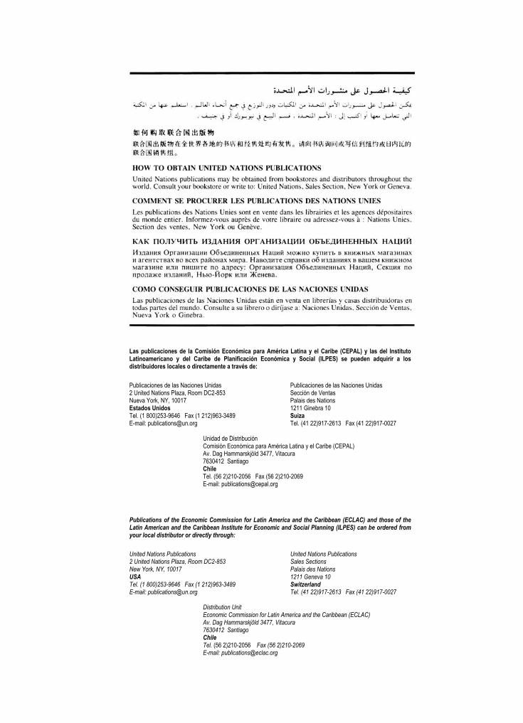
Las publicaciones de la Comisión Económica para América Latina y el Caribe (CEPAL) y las del Instituto Latinoamericano y del Caribe de Planificación Económica y Social (ILPES) se pueden adquirir a los distribuidores locales o directamente a través de:
Publicaciones de las Naciones Unidas Publicaciones de las Naciones Unidas 2 United Nations Plaza, Room DC2-853 Sección de Ventas Nueva York, NY, 10017 Palais des Nations Estados Unidos 1211 Ginebra 10 Tel. (1 800)253-9646 Fax (1 212)963-3489 Suiza E-mail: [email protected] Tel. (41 22)917-2613 Fax (41 22)917-0027 Unidad de Distribución Comisión Económica para América Latina y el Caribe (CEPAL) Av. Dag Hammarskjöld 3477, Vitacura 7630412 Santiago Chile Tel. (56 2)210-2056 Fax (56 2)210-2069 E-mail: [email protected]
Publications of the Economic Commission for Latin America and the Caribbean (ECLAC) and those of the Latin American and the Caribbean Institute for Economic and Social Planning (ILPES) can be ordered from your local distributor or directly through:
United Nations Publications United Nations Publications 2 United Nations Plaza, Room DC2-853 Sales Sections New York, NY, 10017 Palais des Nations USA 1211 Geneva 10 Tel. (1 800)253-9646 Fax (1 212)963-3489 Switzerland E-mail: [email protected] Tel. (41 22)917-2613 Fax (41 22)917-0027 Distribution Unit Economic Commission for Latin America and the Caribbean (ECLAC) Av. Dag Hammarskjöld 3477, Vitacura 7630412 Santiago Chile Tel. (56 2)210-2056 Fax (56 2)210-2069 E-mail: [email protected]
