arX

iv:h

ep-p

h/06

0906

9v2

17

Oct

200

6CUMQ/HEP 142

RARE DECAY OF THE TOP t→ cll AND SINGLE

TOP PRODUCTION AT ILC

Mariana Frank∗ and Ismail Turan†

Department of Physics, Concordia University,

7141 Sherbrooke Street West, Montreal, Quebec, CANADA H4B 1R6

(Dated: February 2, 2008)

Abstract

We perform a complete and detailed analysis of the flavor changing neutral current rare top

quark decays t → cl+l− and t → cνiνi at one-loop level in the Standard Model, Two Higgs Doublet

Models (I and II) and in MSSM. The branching ratios are very small in all models, O(10−14),

except for the case of the unconstrained MSSM, where they can reach O(10−6) for e+e− and νiνi,

and O(10−5) for τ+τ−. This branching ratio is comparable to the ones for t → cV, cH. We also

study the production rates of single top and the forward-backward asymmetry in e+e− → tc and

comment on the observability of such a signal at the International Linear Collider.

PACS numbers: 12.15.-y, 12.15.Ji, 14.65.Ha

Keywords: Rare Top Decays, Standard Model, Flavor Changing Neutral Currents, MSSM

∗mfrank@alcor.concordia.ca†ituran@physics.concordia.ca

1

I. INTRODUCTION

With the advent of the CERN Large Hadron Collider (LHC) [1], 80 million top quark

pairs will be produced per year [2]. This number will increase by one order of magnitude

with the high luminosity option. Therefore, the properties of top quarks can be examined

with significant precision at LHC. Thus top quark physics will be a testing ground for new

phenomena, be it electroweak symmetry breaking, or the existence of interactions forbidden

in the Standard Model (SM). Flavor Changing Neutral Currents (FCNC) in general, and of

the top quark in particular, play an important role for validation of the SM and for New

Physics (NP) signals. In the SM, there are no FCNC mediated by the γ, Z, g or H-boson at

tree level, and FCNC induced by radiative effects are highly suppressed [3, 4]. Higher order

contributions are proportional to (m2i −m2

j )/M2W , with mi, mj the masses of the quarks in

the loop diagrams and MW the W -boson mass. Thus all top-quark induced FCNC in SM

are highly suppressed. Their branching ratios predicted in the SM are of the order of 10−11

to 10−14 [3, 4], far away from present and even future reaches of either the Large Hadron

Collider (LHC) [5, 6] or the International Linear Collider (ILC) [7].

There are many models of NP in which the branching ratios for the two-body FCNC

decays are much larger than those obtained in the SM, and rare top decays might be enhanced

to reach detectable levels [8]. Rare FCNC two-body processes t → cg, γ, Z,H have been

extensively studied in the two-Higgs Doublet Model (2HDM)[9, 10, 11, 12], Alternative Left-

Right Symmetric Models [13] , Constrained [14, 15, 16, 17, 18] and Unconstrained [19, 20]

Minimal Supersymmetric Standard Model (MSSM), Left-Right Supersymmetric Models [21],

Supersymmetric Model with R-parity violation [22], top-assisted technicolor models [23, 24]

as well as models with extra singlet quarks [25].

In addition to the two-body rare decays of top quark, some of its rare three-body decays

e.g., t→ cWW, cZZ, bWZ have been considered in the literature within the SM [26, 27, 28]

and for NP [28, 29]. These three body decays are suppressed with respect to two-body

decays in the SM but some of them get comparably larger within models of NP, such as

two-Higgs-Doublet [29], especially after including finite-width effects [28]. In addition, it has

been shown that the branching ratio for three-body decay t → cgg can exceed that of the

two body decay t→ cg in both SM [30] and MSSM [31]. The three body decay t→ cqq has

also been analyzed [31, 32], and while the branching ratio is smaller than that of t → cgg,

2

it is competitive with t→ cV .

The above facts strengthens the case for investigating top quark physics further in three

body decays. The goal of the present paper is to analyze another three-body rare decay,

namely t → cll in several frameworks and compare it to both t → cγ and t → cqq, q = u.

This decay was previously analyzed in [34] in the framework of topcolor assisted technicolor

models, and in [35] as induced by scalar leptoquarks in a Pati-Salam model. For b quarks, it

is known that under certain circumstances, b → sl+l− can be more significant than b → sγ

in restricting the parameter space, i.e., in supersymmetry in the large tan β region [33].

The remainder of the paper is organized as follows: In Section II we present the calculation

of t→ cl+l− in the SM and in Section III we present the same decay in the Two Higgs Doublet

Model. Section IV is dedicated to presenting the formalism and calculation of t→ cl+l− in

the MSSM (in both constrained and unconstrained versions). In each section, we present the

Feynman diagrams and analyze the results obtained within the given model. We include,

for completeness, the related decay t → cνiνi in Section V. Finally, we analyze the related

production of the single top quark in e+e− → tc+ tc at the ILC in Section VI. We conclude

and discuss experimental observation in Section VII.

II. t → cll IN THE SM

In the SM, since FCNC are forbidden, the decay t → cl+l− is induced at one-loop level

through charged currents, involving vertices for Wqq′ in the loop. The Feynman diagrams

for this process are depicted in Fig. 1. For our numerical evaluation, we used the following

parameters:

α(mt) = 1/132.5605 , MW = 80.45 GeV , MZ = 91.1875 GeV , s2W = 1 −M2

W/M2Z ,

mt = 172.5 GeV, mb = 2.85 GeV, mc = 0.63 GeV, αs(mt) ≈ 0.1068. (2.1)

We obtained:

BR(t→ ce+e−) = 8.48 × 10−15,

BR(t→ cµ+µ−) = 9.55 × 10−15,

BR(t→ cτ+τ−) = 1.91 × 10−14,

BR(t→ c∑

i

νiνi) = 2.99 × 10−14. (2.2)

3

1

t

c

ei

ej

h0

G

dk

dk

2

t

c

ei

ej

G0

G

dk

dk

3

t

c

ei

ej

h0

dk

G

G

4

t

c

ei

ej

h0

W

dk

dk

5

t

c

ei

ej

G0

W

dk

dk

6

t

c

ei

ej

h0

dk

G

W

7

t

c

ei

ej

G0

dk

G

W

8

t

c

ei

ej

h0

dk

W

G

9

t

c

ei

ej

G0

dk

W

G

10

t

c

ei

ej

h0

dk

W

W

11

t

c

ei

ej

γ

G

dk

dk

12

t

c

ei

ej

Z

G

dk

dk

13

t

c

ei

ej

γ

dk

G

G

14

t

c

ei

ej

Z

dk

G

G

15

t

c

ei

ej

γ

W

dk

dk

16

t

c

ei

ej

Z

W

dk

dk

17

t

c

ei

ej

γ

dk

G

W

18

t

c

ei

ej

Z

dk

G

W

19

t

c

ei

ej

γ

dk

W

G

20

t

c

ei

ej

Z

dk

W

G

21

t

c

ei

ej

γ

dk

W

W

22

t

c

ei

ej

Z

dk

W

W

23

t

c

ei

ej

dk

G

G

ν l

24

t

c

ei

ej

dk

G

W

ν l

25

t

c

ei

ej

dk

W

G

ν l

26

t

c

ei

ej

dk

W

W

ν l

27

t

c

ei

ej

h0

t

dk

G

28

t

c

ei

ej

G0

t

dk

G

29

t

c

ei

ej

h0

t

dk

W

30

t

c

ei

ej

G0

t

dk

W

31

t

c

ei

ej

γt

dk

G

32

t

c

ei

ej

Z

t

dk

G

33

t

c

ei

ej

γt

dk

W

34

t

c

ei

ej

Z

t

dk

W

35

t

c

ei

ej

h0

c

dk

G

36

t

c

ei

ej

G0

c

dk

G

37

t

c

ei

ej

h0

c

dk

W

38

t

c

ei

ej

G0

c

dk

W

39

t

c

ei

ej

γ

c

dk

G

40

t

c

ei

ej

Z

c

dk

G

41

t

c

ei

ej

γ

c

dk

W

42

t

c

ei

ej

Z

c

dk

W

FIG. 1: The one-loop SM contributions to t → cl+l− in the ’t Hooft-Feynman gauge.

As expected, the branching ratios are very small since even at one loop, the process is

suppressed by the Glashow-Iliopoulos-Maiani (GIM) mechanism.1 The SM signal cannot be

detected in current or future high energy collider experiments; thus any signal would be an

indication of New Physics.

III. THE TWO-HIGGS-DOUBLET MODELS

The Two Higgs Doublet Models (2HDM) are simple extensions of the SM, formed by

adding an extra complex SU(2)L⊗U(1)Y scalar doublet to the SM Lagrangian. Motivations

1 Though BR(t → ce+e−) is small, it is of same order of magnitude as BR(t → cZ), and BR(t → cτ+τ−)

is of same order of magnitude as BR(t → cγ) [2].

4

1

t

c

ei

ej

h0

H

dk

dk

2

t

c

ei

ej

H0

H

dk

dk

3

t

c

ei

ej

H0

G

dk

dk

4

t

c

ei

ej

A0

H

dk

dk

5

t

c

ei

ej

A0

G

dk

dk

6

t

c

ei

ej

G0

H

dk

dk

7

t

c

ei

ej

h0

dk

H

H

8

t

c

ei

ej

h0

dk

H

G

9

t

c

ei

ej

h0

dk

G

H

10

t

c

ei

ej

H0

dk

H

H

11

t

c

ei

ej

H0

dk

H

G

12

t

c

ei

ej

H0

dk

G

H

13

t

c

ei

ej

H0

dk

G

G

14

t

c

ei

ej

A0

dk

H

G

15

t

c

ei

ej

A0

dk

G

H

16

t

c

ei

ej

H0

W

dk

dk

17

t

c

ei

ej

A0

W

dk

dk

18

t

c

ei

ej

h0

dk

H

W

19

t

c

ei

ej

H0

dk

H

W

20

t

c

ei

ej

H0

dk

G

W

21

t

c

ei

ej

A0

dk

H

W

22

t

c

ei

ej

h0

dk

W

H

23

t

c

ei

ej

H0

dk

W

H

24

t

c

ei

ej

H0

dk

W

G

25

t

c

ei

ej

A0

dk

W

H

26

t

c

ei

ej

H0

dk

W

W

27

t

c

ei

ej

γ

H

dk

dk

28

t

c

ei

ej

Z

H

dk

dk

29

t

c

ei

ej

γ

dk

H

H

30

t

c

ei

ej

Z

dk

H

H

31

t

c

ei

ej

dk

H

H

ν l

32

t

c

ei

ej

dk

H

G

ν l

33

t

c

ei

ej

dk

G

H

ν l

34

t

c

ei

ej

dk

H

W

ν l

35

t

c

ei

ej

dk

W

H

ν l

36

t

c

ei

ej

h0

t

dk

H

37

t

c

ei

ej

H0

t

dk

H

38

t

c

ei

ej

H0

t

dk

G

39

t

c

ei

ej

A0

t

dk

H

40

t

c

ei

ej

A0

t

dk

G

41

t

c

ei

ej

G0

t

dk

H

42

t

c

ei

ej

H0

t

dk

W

43

t

c

ei

ej

A0

t

dk

W

44

t

c

ei

ej

γt

dk

H

45

t

c

ei

ej

Z

t

dk

H

46

t

c

ei

ej

h0

c

dk

H

47

t

c

ei

ej

H0

c

dk

H

48

t

c

ei

ej

H0

c

dk

G

49

t

c

ei

ej

A0

c

dk

H

50

t

c

ei

ej

A0

c

dk

G

51

t

c

ei

ej

G0

c

dk

H

52

t

c

ei

ej

H0

c

dk

W

53

t

c

ei

ej

A0

c

dk

W

54

t

c

ei

ej

γ

c

dk

H

55

t

c

ei

ej

Z

c

dk

H

FIG. 2: The one-loop 2HDM contributions to t → cl+l− in the ’t Hooft-Feynman gauge.

for such a extension include the possibility of having CP–violation in the Higgs sector, and

the fact that some models of dynamical electroweak symmetry breaking yield the 2HDM

as their low-energy effective theory [36]. There are three popular versions of this model in

the literature, depending on how the two doublets couple to the fermion sector. Models

I and II (2HDM-I, 2HDM-II) include natural flavor conservation [37, 38], while model III

5

(2HDM-III) has the simplest extended Higgs sector that naturally introduces FCNC at the

tree level [39, 40, 41].

The most general 2HDM scalar potential which is both SU(2)L⊗U(1)Y and CP invariant

is given by [38]:

V (Φ1,Φ2) = λ1(|Φ1|2 − v21)

2 + λ2(|Φ2|2 − v22)

2 + λ3((|Φ1|2 − v21) + (|Φ2|2 − v2

2))2 +

λ4(|Φ1|2|Φ2|2 − |Φ+1 Φ2|2) + λ5(ℜ(Φ+

1 Φ2) − v1v2)2 + λ6[ℑ(Φ+

1 Φ2)]2 , (3.1)

where Φ1 and Φ2 have weak hypercharge Y=1, v1 and v2 are respectively the vacuum expec-

tation values of Φ1 and Φ2 and the λi are real–valued parameters. Note that this potential

violates softly the discrete symmetry Φ1 → −Φ1, Φ2 → Φ2 by the dimension two term

λ5ℜ(Φ+1 Φ2). The above scalar potential has 8 independent parameters (λi)i=1,...,6, v1 and v2.

After the electroweak symmetry breaks, three of the original eight degrees of freedom

associated to Φ1 and Φ2 correspond to the three Goldstone bosons (G±, Go), while the other

five degrees of freedom reduce to five physical Higgs bosons: h0, H0 (both CP-even), A0 (CP-

odd), and H±. Their masses are obtained as usual by diagonalizing the scalar mass matrix.

The combination v21 + v2

2 is fixed by the electroweak scale through v21 + v2

2 = (2√

2GF )−1.

Seven independent parameters are left, which are given in terms of four physical scalar masses

(mh0 , mH0 , mA0, mH±), two mixing angles (tanβ = v1/v2 and α) and the soft breaking term

λ5.

In this analysis, we impose that, when the independent parameters are varied, the con-

tributions to the δρ parameter from the Higgs scalars should not exceed the current limits

from precision measurements [43]: |δρ| ≤ 0.001.

The Feynman rules in the general 2HDM are given in [38]. The Feynman diagrams which

contribute to t → cl+l− are given in Fig. 2. The full one-loop calculation presented here

is done in the ’t Hooft gauge with the help of FormCalc [44]. The parameters used are the

same as for the standard model. We have tested analyticity for the independent parameters

of the model and restricted the parameter space accordingly. The parameter space of the

models are severely constrained by the perturbativity constraints (|λi| ≤ 8π). The situation

becomes even more severe if one takes into account the unitarity bounds. The branching

ratios for t → cl+l− obtained running the 2HDM parameters over their allowed values are

all negligibly small (same order as the SM and often numerically indistinguishible), and

thus not likely to show up at the present or future colliders. There are few points in the

6

parameter space where t→ cl+l− becomes enhanced (around 1-2 orders of magnitude) with

respect to the SM predictions but this usually requires very small tan β values (≤ 0.1)

which are excluded [42]. It is also possible to get some deviation from the SM values if the

Higgs bosons (h0, H0, A0 and H±) are very light (around 100-200 GeV). Overall we do not

obtain significant deviations from the SM results and for this reason we do not graph them

separately.

IV. THE MINIMAL SUPERSYMMETRIC STANDARD MODEL

The MSSM constitutes the minimal supersymmetric extension of the SM. It includes

all SM fields, as well as two Higgs doublets needed to keep anomaly cancellation. One

Higgs doublet, H1, gives mass to the d-type fermions (with weak isospin -1/2), the other

doublet, H2, gives mass to the u-type fermions (with weak isospin +1/2). All SM multiplets,

including the two Higgs doublets, are extended to supersymmetric multiplets, resulting in

scalar partners for quarks and leptons (squarks and sleptons) and fermionic partners for the

SM gauge bosons and the Higgs bosons (gauginos and higgsinos). We do not consider effects

of complex phases here, i.e. we treat all MSSM parameters as real.

The superpotential of the MSSM Lagrangian is

W = µH1H2 + Y ijl H

1LiejR + Y ij

d H1Qidj

R + Y iju H

2QiujR, (4.1)

while the part of the soft-SUSY-breaking Lagrangian responsible for the non-minimal squark

family mixing is given by

Lsquarksoft = −Qi†(M2

Q)ijQ

j − ui†(M2U)ij u

j − di†(M2D)ij d

j + Y iuA

iju QiH

2uj + Y idA

ijd QiH

1dj. (4.2)

In the above expressions Q is the SU(2) scalar doublet, u, d are the up- and down-quark

SU(2) singlets (Q, u, d represent scalar quarks), respectively, Yu,d are the Yukawa couplings

and i, j are generation indices. Here Aij are the trilinear scalar couplings and H1,2 represent

two SU(2) Higgs doublets with vacuum expectation values

〈H1〉 =

v1√2

0

≡

v cos β√2

0

, 〈H2〉 =

0

v2√2

≡

0

v sin β√2

, (4.3)

where v = (√

2GF )−1/2 = 246 GeV, and the angle β is defined by tanβ ≡ v2/v1, the ratio

of the vacuum expectation values of the two Higgs doublets; and µ is the Higgs mixing

parameter.

7

The squark mass term of the MSSM Lagrangian is given by

Lfmass = −1

2

(

f †L, f

†R

)

M2f

fL

fR

, (4.4)

where we assume the following form of M2f

M2u{d} =

M2Lu{d} 0 0 mu{d}Au{d} 0 0

0 M2Lc{s} (M2

U{D})LL 0 mc{s}Ac{s} (M2U{D})LR

0 (M2U{D})LL M2

Lt{b} 0 (M2U{D})RL mt{b}At{b}

mu{d}Au,{d} 0 0 M2Ru{d} 0 0

0 mc{s}Ac{s} (M2U{D})RL 0 M2

Rc{s} (M2U{D})RR

0 (M2U{D})LR mt{b}At{b} 0 (M2

U{D})RR M2Rt{b}

(4.5)

with

M2Lq

= M2Q,q

+m2q + cos 2β(Tq −Qqs

2W )M2

Z ,

M2R{u,c,t} = M2

U ,{u,c,t} +m2u,c,t + cos 2βQts

2WM

2Z ,

M2R{d,s,b} = M2

D,{d,s,b} +m2d,s,b + cos 2βQbs

2WM

2Z , (4.6)

Au,c,t = Au,c,t − µ cotβ , Ad,s,b = Ad,s,b − µ tanβ ,

with mq, Tq, Qq the mass, isospin, and electric charge of the quark q, MZ the Z-boson mass,

sW ≡ sin θW and θW the electroweak mixing angle. Since we are concerned with top quark

physics, we assume that the squark mixing is significant only for transitions between the

squarks of the second and third generations. These mixings are expected to be the largest

in Grand Unified Models and are also experimentally the least constrained. The most

stringent bounds on these transitions come from b → sγ. In contrast, there exist strong

experimental bounds involving the first squark generation, based on data from K0–K0 and

D0–D0 mixing [45].

We define the dimensionless flavor-changing parameters (δ23U,D)AB (A,B = L,R) from

the flavor off-diagonal elements of the squark mass matrices in the following way. First, to

simplify the calculation we assume that all diagonal entries M2Q,q

and M2U(D),q

are set equal

to the common value M2SUSY, and then we normalize the off-diagonal elements to M2

SUSY

8

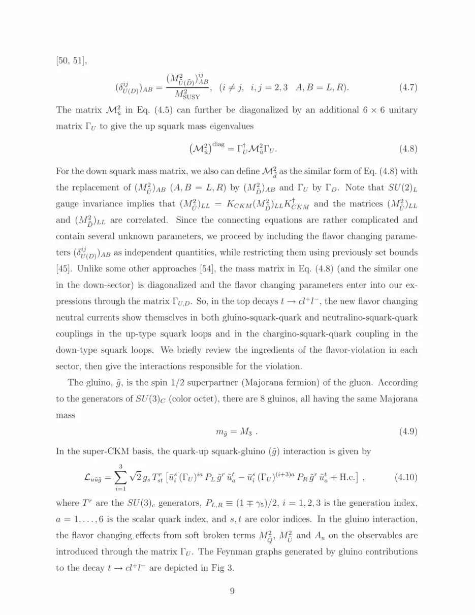
[50, 51],

(δijU(D))AB =

(M2U (D)

)ijAB

M2SUSY

, (i 6= j, i, j = 2, 3 A,B = L,R). (4.7)

The matrix M2u in Eq. (4.5) can further be diagonalized by an additional 6 × 6 unitary

matrix ΓU to give the up squark mass eigenvalues

(

M2u

)diag= Γ†

UM2uΓU . (4.8)

For the down squark mass matrix, we also can define M2das the similar form of Eq. (4.8) with

the replacement of (M2U)AB (A,B = L,R) by (M2

D)AB and ΓU by ΓD. Note that SU(2)L

gauge invariance implies that (M2U)LL = KCKM(M2

D)LLK

†CKM and the matrices (M2

U)LL

and (M2D)LL are correlated. Since the connecting equations are rather complicated and

contain several unknown parameters, we proceed by including the flavor changing parame-

ters (δijU(D))AB as independent quantities, while restricting them using previously set bounds

[45]. Unlike some other approaches [54], the mass matrix in Eq. (4.8) (and the similar one

in the down-sector) is diagonalized and the flavor changing parameters enter into our ex-

pressions through the matrix ΓU,D. So, in the top decays t→ cl+l−, the new flavor changing

neutral currents show themselves in both gluino-squark-quark and neutralino-squark-quark

couplings in the up-type squark loops and in the chargino-squark-quark coupling in the

down-type squark loops. We briefly review the ingredients of the flavor-violation in each

sector, then give the interactions responsible for the violation.

The gluino, g, is the spin 1/2 superpartner (Majorana fermion) of the gluon. According

to the generators of SU(3)C (color octet), there are 8 gluinos, all having the same Majorana

mass

mg = M3 . (4.9)

In the super-CKM basis, the quark-up squark-gluino (g) interaction is given by

Luug =3

∑

i=1

√2 gs T

rst

[

usi (ΓU)ia PL g

r uta − us

i (ΓU)(i+3)a PR gr ut

a + H.c.]

, (4.10)

where T r are the SU(3)c generators, PL,R ≡ (1 ∓ γ5)/2, i = 1, 2, 3 is the generation index,

a = 1, . . . , 6 is the scalar quark index, and s, t are color indices. In the gluino interaction,

the flavor changing effects from soft broken terms M2Q, M2

Uand Au on the observables are

introduced through the matrix ΓU . The Feynman graphs generated by gluino contributions

to the decay t→ cl+l− are depicted in Fig 3.

9

1

t

c

ei

ej

h0

g

ua˜

ub˜

2

t

c

ei

ej

H0

g

ua˜

ub˜

3

t

c

ei

ej

A0

g

ua˜

ub˜

4

t

c

ei

ej

G0

g

ua˜

ub˜

5

t

c

ei

ej

γ

g

ua˜

ua˜

6

t

c

ei

ej

Z

g

ua˜

ub˜

7

t

c

ei

ej

h0

t

g

ua˜

8

t

c

ei

ej

H0

t

g

ua˜

9

t

c

ei

ej

A0

t

g

ua˜

10

t

c

ei

ej

G0

t

g

ua˜

11

t

c

ei

ej

γt

g

ua˜

12

t

c

ei

ej

Z

t

g

ua˜

13

t

c

ei

ej

h0

c

g

ua˜

14

t

c

ei

ej

H0

c

g

ua˜

15

t

c

ei

ej

A0

c

g

ua˜

16

t

c

ei

ej

G0

c

g

ua˜

17

t

c

ei

ej

γ

c

g

ua˜

18

t

c

ei

ej

Z

c

g

ua˜

FIG. 3: The one-loop gluino contributions to t → cl+l− in MSSM in the ’t Hooft-Feynman gauge.

The charginos χ+i (i = 1, 2) are four component Dirac fermions. The mass eigenstates

are obtained from the winos W± and the charged higgsinos H−1 , H+

2 :

W+ =

−iλ+

iλ−

; W− =

+iλ−

iλ−

; H+2 =

ψ+H2

ψ−H1

; H−1 =

ψ−H1

ψ+H2

. (4.11)

The chargino masses are defined as mass eigenvalues of the diagonalized mass matrix,

Lχ+

mass = −1

2

(

ψ+, ψ−)

0 XT

X 0

ψ+

ψ−

+ H.c. (4.12)

or given in terms of two-component fields

ψ+ = (−iλ+, ψ+H2

), ψ− = (−iλ−, ψ−H1

) , (4.13)

where X is given by

X =

M2

√2MW sin β

√2MW cosβ µ

. (4.14)

In the mass matrix, M2 is the soft SUSY-breaking parameter for the Majorana mass term.

and µ is the Higgsino mass parameter from the Higgs potential.

The physical (two-component) mass eigenstates are obtained via unitary (2×2) matrices

U and V :

χ+i = Vij ψ

+j , χ−

i = Uij ψ−j

i, j = 1, 2 . (4.15)

10

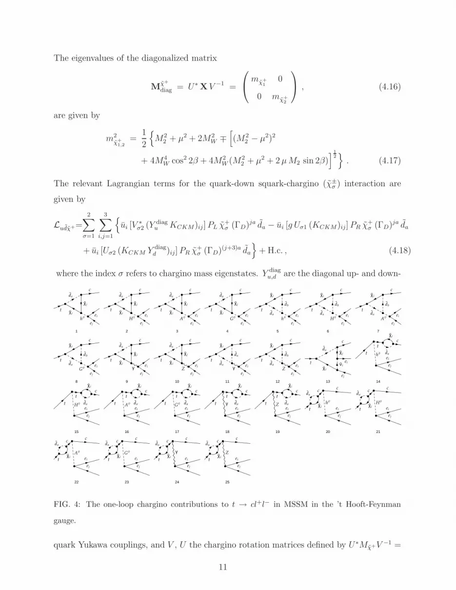
The eigenvalues of the diagonalized matrix

Mχ+

diag = U∗X V −1 =

mχ+1

0

0 mχ+2

, (4.16)

are given by

m2χ+

1,2=

1

2

{

M22 + µ2 + 2M2

W ∓[

(M22 − µ2)2

+ 4M4W cos2 2β + 4M2

W (M22 + µ2 + 2µM2 sin 2β)

]12}

. (4.17)

The relevant Lagrangian terms for the quark-down squark-chargino (χ±σ ) interaction are

given by

Ludχ+=

2∑

σ=1

3∑

i,j=1

{

ui [V∗σ2 (Y diag

u KCKM)ij ]PL χ+σ (ΓD)ja da − ui [g Uσ1 (KCKM)ij]PR χ

+σ (ΓD)ja da

+ ui [Uσ2 (KCKM Y diagd )ij]PR χ

+σ (ΓD)(j+3)a da

}

+ H.c. , (4.18)

where the index σ refers to chargino mass eigenstates. Y diagu,d are the diagonal up- and down-

1

t

c

ei

ej

h0

da˜

χ i˜

χ j˜

2

t

c

ei

ej

H0

da˜

χ i˜

χ j˜

3

t

c

ei

ej

A0

da˜

χ i˜

χ j˜

4

t

c

ei

ej

G0

da˜

χ i˜

χ j˜

5

t

c

ei

ej

h0

χ i˜

da˜

db˜

6

t

c

ei

ej

H0

χ i˜

da˜

db˜

7

t

c

ei

ej

A0

χ i˜

da˜

db˜

8

t

c

ei

ej

G0

χ i˜

da˜

db˜

9

t

c

ei

ej

γ

da˜

χ i˜

χ i˜

10

t

c

ei

ej

Z

da˜

χ i˜

χ j˜

11

t

c

ei

ej

γ

χ i˜

da˜

da˜

12

t

c

ei

ej

Z

χ i˜

da˜

db˜

13

t

c

ei

ej

da˜

χ i˜

χ j˜

ν i˜

14

t

c

ei

ej

h0

t

χ i˜

da˜

15

t

c

ei

ej

H0

t

χ i˜

da˜

16

t

c

ei

ej

A0

t

χ i˜

da˜

17

t

c

ei

ej

G0

t

χ i˜

da˜

18

t

c

ei

ej

γt

χ i˜

da˜

19

t

c

ei

ej

Z

t

χ i˜

da˜

20

t

c

ei

ej

h0

c

χ i˜

da˜

21

t

c

ei

ej

H0

c

χ i˜

da˜

22

t

c

ei

ej

A0

c

χ i˜

da˜

23

t

c

ei

ej

G0

c

χ i˜

da˜

24

t

c

ei

ej

γ

c

χ i˜

da˜

25

t

c

ei

ej

Z

c

χ i˜

da˜

FIG. 4: The one-loop chargino contributions to t → cl+l− in MSSM in the ’t Hooft-Feynman

gauge.

quark Yukawa couplings, and V , U the chargino rotation matrices defined by U∗Mχ+V −1 =

11

diag(mχ+1, mχ+

2). The flavor changing effects arise from both the off-diagonal elements in the

CKM matrix KCKM and from the soft supersymmetry breaking terms in ΓD. The Feynman

graphs generated by chargino contributions to the decay t→ cl+l− are shown in Fig 4.

1

t

c

ei

ej

h0

ua˜

χ i0˜

χ j0˜

2

t

c

ei

ej

H0

ua˜

χ i0˜

χ j0˜

3

t

c

ei

ej

A0

ua˜

χ i0˜

χ j0˜

4

t

c

ei

ej

G0

ua˜

χ i0˜

χ j0˜

5

t

c

ei

ej

h0

χ i0˜

ua˜

ub˜

6

t

c

ei

ej

H0

χ i0˜

ua˜

ub˜

7

t

c

ei

ej

A0

χ i0˜

ua˜

ub˜

8

t

c

ei

ej

G0

χ i0˜

ua˜

ub˜

9

t

c

ei

ej

Z

ua˜

χ i0˜

χ j0˜

10

t

c

ei

ej

γ

χ i0˜

ua˜

ua˜

11

t

c

ei

ej

Z

χ i0˜

ua˜

ub˜

12

t

c

eiej

ua˜

χ i0˜

χ j0˜

eis˜

13

t

c

ei

ej

ua˜

χ i0˜

χ j0˜

eis˜

14

t

c

ei

ej

h0

t

χ i0˜

ua˜

15

t

c

ei

ej

H0

t

χ i0˜

ua˜

16

t

c

ei

ej

A0

t

χ i0˜

ua˜

17

t

c

ei

ej

G0

t

χ i0˜

ua˜

18

t

c

ei

ej

γt

χ i0˜

ua˜

19

t

c

ei

ej

Z

t

χ i0˜

ua˜

20

t

c

ei

ej

h0

c

χ i0˜

ua˜

21

t

c

ei

ej

H0

c

χ i0˜

ua˜

22

t

c

ei

ej

A0

c

χ i0˜

ua˜

23

t

c

ei

ej

G0

c

χ i0˜

ua˜

24

t

c

ei

ej

γ

c

χ i0˜

ua˜

25

t

c

ei

ej

Z

c

χ i0˜

ua˜

FIG. 5: The one-loop neutralino contributions to t → cl+l− in MSSM in the ’t Hooft-Feynman

gauge.

Neutralinos χ0i (i = 1, 2, 3, 4) are four-component Majorana fermions. They are the mass

eigenstates of the photino, γ, the zino, Z, and the neutral higgsinos, H01 and H0

2 , with

γ =

−iλγ

iλγ

; Z =

−iλZ

iλZ

; H01 =

ψ0H1

ψ0H1

; H02 =

ψ0H2

ψ0H2

. (4.19)

The mass term in the Lagrangian density is given by

Lχ0,mass = −1

2(ψ0)T

Y ψ0 + H.c. (4.20)

with the two-component fermion fields

(ψ0)T = (−iλ′,−iλ3, ψ0H1, ψ0

H2) . (4.21)

12

The mass matrix Y is given by

Y =

M1 0 −MZ sin θW cosβ MZ sin θW sin β

0 M2 MZ cos θW cosβ −MZ cos θW sin β

−MZ sin θW cosβ MZ cos θW cosβ 0 −µ

MZ sin θW sin β −MZ cos θW sin β −µ 0

. (4.22)

The physical neutralino mass eigenstates are obtained with the unitary transformation ma-

trix N :

χ0i = Nij ψ

0j i, j = 1, . . . , 4, (4.23)

The diagonal mass matrix is then given by

Mχ0

diag = N∗YN−1 . (4.24)

the relevant Lagrangian terms for the quark-up squark neutralino (χ0n) interaction are

Luuχ0 =

4∑

n=1

3∑

i=1

{

uiN∗n1

4

3

g√2

tan θW PL χ0n (ΓU)(i+3)a ua − uiN

∗n4 Y

diagu PL χ

0n (ΓU)ia ua

− uig√2

(

Nn2 +1

3Nn1 tan θW

)

PR χ0n (ΓU)ia ua − uiNn4 Y

diagu PR χ

0n (ΓU)(i+3)a ua

}

,

(4.25)

where N is the rotation matrix which diagonalizes the neutralino mass matrix Mχ0 ,

N∗Mχ0N−1 = diag(mχ01, mχ0

2, mχ0

3, mχ0

4). As in the gluino case, FCNC terms arise only

from supersymmetric parameters in ΓU . The Feynman graphs generated by neutralino con-

tributions to the decay t→ cl+l− are given in Fig 5.

Note that MSSM can be studied as a model in itself, or as a low energy realization of a

supersymmetric grand unified scenario (SUSY GUT). In SUSY GUTs M1, M2 and M3 are

not independent but connected via

mg = M3 =g23

g22

M2 =αs

αem

sin θ2W M2, M1 =

5

3

sin θ2W

cos θ2W

M2 . (4.26)

which results in a reduction of the number of independent parameters. We shall refer to this

as the mSUGRA scenario and label the figures accordingly.

In the unconstrained MSSM no specific assumptions are made about the underlying

SUSY-breaking mechanism, and a parametrization of all possible soft SUSY-breaking terms

13

is used that does not alter the relation between the dimensionless couplings (which ensures

that the absence of quadratic divergences is maintained). This parametrization has the

advantage of being very general, but the disadvantage of introducing more than 100 new

parameters in addition to the SM. While in principle these parameters (masses, mixing an-

gles, complex phases) could be chosen independently of each other, experimental constraints

from flavour-changing neutral currents, electric dipole moments, etc. seem to favour a certain

degree of universality among the soft SUSY-breaking parameters.

We now proceed to investigate the dependence of the branching ratio of t→ cl+l− on the

parameters of the supersymmetric model. In the case of flavor violating MSSM, only the

mixing between the second and the third generations is turned on, and the dimensionless

parameters δ’s run over as much of the interval (0,1) as allowed. The allowed upper limits of

δ’s are constrained by the requirement that mui,di> 0 and consistent with the experimental

lower bounds (depending on the chosen values ofMSUSY, A, tanβ, and µ). We assume a lower

bound of 96 GeV for all up squark masses and 90 GeV for the down squark masses [53].

The Higgs masses are calculated with FeynHiggs version 2.3 [52], with the requirement

that the lightest neutral Higgs mass is larger than 114 GeV. Other experimental bounds

included are [53]: 96 GeV for the lightest chargino, 46 GeV the lightest neutralino, and 195

GeV for the gluino. We did not include the possible constraints coming from b → sγ or

Bs − Bs mixing. The reason is the following: the most stringent constraints of these arise

from the gluino contributions, and they restrict (δ23D )AB. Constraints on (δ23

U )AB are obtained

under certain assumptions only. For instance, Cao et. al. in [31], allow two flavor-violating

parameters, (δ23U )LL and (δ23

U )LR, to be non-zero at the same time. This permits (δ23U )LR to

be of order one, but restricts (δ23U )LL to be 0.5 or less.

As in the case of the 2HDM, the constrained MSSM contribution to t → cl+l− is very

small, often below the SM contribution. Thus, the only signals likely to be observed at

the colliders would come from the unconstrained MSSM, which we investigate in detail. In

Fig. 6 we plot the dependence of the branching ratio of t → ce+e− on the flavor-changing

parameter δ23U,D. The δ23

U parameter drives the contributions from the gluino and neutralino

sectors, while δ23D affects the chargino contribution only. The constrained MSSM values for

the branching ratio correspond to δ23U,D = 0.2 The first graph is obtained by allowing free

2 The branching ratio is calculated by taking the top quark total decay width as 1.55 GeV.

14

SM

chargino

//

neutralino

//

gluinoRR

LL

RR

LL

NO GUT

(δ23

U)AA

BR

(t→

ce

+e−)

0.70.60.50.40.30.20.10

10−6

10−7

10−8

10−9

10−10

10−11

10−12

10−13

10−14

10−15

10−16

SM

chargino

//

neutralino

//

gluino

RR

LL

RR

LLmSUGRA

(δ23

U)AA

BR

(t→

ce

+e−)

0.70.60.50.40.30.20.10

10−7

10−8

10−9

10−10

10−11

10−12

10−13

10−14

10−15

10−16

SM

chargino

mSUGRA

No GUT

mSUGRA

No GUT

χ0

χ0

g

g

(δ23U )LR

BR

(t→

ce

+e−)

0.70.60.50.40.30.20.10

10−6

10−7

10−8

10−9

10−10

10−11

10−12

10−13

10−14

10−15

10−16

SM

(δ23D )RR

(δ23D )LR

(δ23D )LL

(δ23D )AB

BR

(t→

ce

+e−)

10.90.80.70.60.50.40.30.20.10

10−8

10−9

10−10

10−11

10−12

10−13

10−14

10−15

FIG. 6: Upper left panel: BR’s of t → ce+e− decay as function of (δ23U )AA without the GUT

relations (mg = 250 GeV). Upper right panel: BR’s as function of (δ23U )AA under the same condi-

tions in mSUGRA scenarios. Lower left panel: BR’s of t → ce+e− decay as function of (δ23U )LR.

Lower right panel: BR’s as function of (δ23D )AB , A,B = L,R. The parameters are chosen as

tan β = 10, mA0 = MSUSY = 500 GeV, M2 = µ = 200 GeV, and At = 1.2 TeV.

values for the gaugino masses (no-GUT scenario); in practice this allows the gluino mass to be

relatively light and the gluino contribution large. Taking only one (δ23U )AB 6= 0, A,B = L,R

at a time, the LL and RR contribution from the gluino are almost the same (as the gluino

couplings are helicity blind, the only difference comes from the squark masses in the loop).

15

SM

No GUT-(δ23U )LR = 0.5

(δ23U )LR = 0.5

(δ23U )LR = 0.0

MSUSY

BR

(t→

ce

+e−)

1000900800700600500

10−6

10−7

10−8

10−9

10−10

10−11

10−12

10−13

10−14

10−15

SM

No GUT-(δ23U )LR = 0.5

(δ23U )LR = 0.5

(δ23U )LR = 0

tan β

BR

(t→

ce

+e−)

302520151050

10−6

10−7

10−8

10−9

10−10

10−11

10−12

10−13

10−14

10−15

FIG. 7: Left panel: BR’s of t → ce+e− decay as function of MSUSY for various values of (δ23U )LR

with tan β = 10. Right panel: BR’s as function of tan β under the same conditions with MSUSY =

500 GeV. The common parameters are chosen as mA0 = 500 GeV, M2 = µ = 200 GeV, and

At = 1.2 TeV. mg = 250 GeV for without GUT cases.

For the neutralino, the LL contribution is larger than the RR one by one order of magnitude

or more. The total branching ratio can reach 10−7 or so, for large allowed values of (δ23U )LL.

Once gaugino mass relations are imposed in accordance with the mSUGRA scenario, the

gluino masses are forced to be larger and the gluino contributions are reduced by an order of

magnitude, while the neutralino contributions are practically unaffected (upper right-sided

panel). Throughout both scenarios, the chargino contribution, induced by the CKM matrix,

is very small but non-zero. We give, in all graphs, the value of the SM branching ratio, for

comparison; but not the value of the branching ration for 2HDM, which is indistinguishable

numerically from that of the SM. In the lower left-sided panel we graph the branching ratio

of t→ ce+e− as a function of the flavor- and helicity-changing parameter (δ23U )LR. As in the

case of t → cV [21], this dependence is somewhat stronger than for the helicity-conserving

parameter and the branching ratio can reach 10−6 for the no-GUT scenario. Finally in

the lower right-sided panel, we show the dependence of he branching ratio of t → ce+e−

as a function of the parameter (δ23D )AB in the down squark sector. This parameter affects

the chargino contributions only. The branching ratio can reach at most 10−9 from the

chargino contributions alone; in this case (δ23U )AB is set to zero and the gluino and neutralino

16

SM

chargino

//

neutralino

//

gluinoRR

LL

RR

LL

NO GUT

(δ23

U)AA

BR

(t→

cτ

+τ−)

0.70.60.50.40.30.20.10

10−5

10−6

10−7

10−8

10−9

10−10

10−11

10−12

10−13

10−14

10−15

SM

chargino

//

neutralino

//

gluinoRR

LLRR

LL

mSUGRA

(δ23

U)AA

BR

(t→

cτ

+τ−)

0.70.60.50.40.30.20.10

10−6

10−7

10−8

10−9

10−10

10−11

10−12

10−13

10−14

10−15

10−16

SM

chargino

mSUGRA

No GUT

mSUGRA

No GUT

χ0

χ0

g

g

(δ23U )LR

BR

(t→

cτ

+τ−)

0.70.60.50.40.30.20.10

10−4

10−6

10−8

10−10

10−12

10−14

10−16

SM

(δ23D )RR

(δ23D )LR

(δ23D )LL

(δ23D )AB

BR

(t→

cτ

+τ−)

10.90.80.70.60.50.40.30.20.10

10−7

10−8

10−9

10−10

10−11

10−12

10−13

10−14

FIG. 8: Upper left panel: BR’s of t → cτ+τ− decay as function of (δ23U )AA without the GUT

relations (mg = 250 GeV). Upper right panel: BR’s as a function of (δ23U )AA under the same

conditions in mSUGRA scenario. Lower left panel: BR’s as function of (δ23U )LR. Lower right panel:

BR’s as function of (δ23D )AB , A,B = L,R. The parameters are chosen as tan β = 10, mA0 =

MSUSY = 500 GeV, M2 = µ = 200 GeV, and At = 1.2 TeV.

contributions are zero. Should the flavor violation come from the down squark sector only,

the branching ratio would be one-to-two orders of magnitude smaller than if it originated in

the up squark sector.

In Fig. 7 we plot the dependence of the branching ratio of t→ ce+e− on the scalar mass

17

SM

chargino

No GUT-(δ23U )LR = 0.5

(δ23U )LR = 0.5

(δ23U )LR = 0

MSUSY

BR

(t→

cτ

+τ−)

1000900800700600500

10−5

10−6

10−7

10−8

10−9

10−10

10−11

10−12

10−13

10−14

SM

chargino

No GUT-(δ23U )LR = 0.5

(δ23U )LR = 0.5

(δ23U )LR = 0

tanβ

BR

(t→

cτ

+τ−)

302520151050

10−5

10−6

10−7

10−8

10−9

10−10

10−11

10−12

10−13

10−14

10−15

FIG. 9: Left panel: BR’s of t → cτ+τ− decay as function of MSUSY for various values of (δ23U )LR

with tan β = 10. Right panel: BR’s as function of MSUSY for various values of (δ23U )LR with

tan β = 10. The common parameters are chosen as mA0 = 500 GeV, M2 = µ = 200 GeV, and

At = 1.2 TeV. Mg = 250GeV for without GUT cases.

MSUSY and tan β. MSUSY affects scalar quark masses; one can see from the left-handed

panel in Fig. 7 that the dependence is very weak, less than one order of magnitude change

in going from 500 GeV to 1 TeV. The same is true for the tanβ dependence which affects

scalar quark masses and mixings, and the chargino/neutralino contribution: except for very

low tanβ’s, between 0 and 5 when the branching ratio increases dramatically from 0, the

branching ratio is insensitive to variations in intermediate values of tanβ between 7 and 30.

We investigated the same dependence for the decay t → cµ+µ− and the results are

practically identical, so we do not show them here. However, as expected, the branching

ratio for t → cτ+τ− differs numerically, though not in its general variation pattern, from

t→ ce+e− and we show it in Fig. 8. While the differences between the behavior of different

curves are insignificant, the branching ratio for t → cτ+τ− is consistently one order of

magnitude larger than either t → ce+e− or t → cµ+µ−. Plotting the branching ratio of

t → cτ+τ− with respect to MSUSY and tan β, in Fig. 9, one can see the effects of the τ

lepton coupling to Higgs. In this, we assume flavor-violation in the up squark sector only,

thus only the gluino and neutralino graphs are important. Looking at the diagrams, the

decays proceed mostly though the penguins t → cγ∗, t → cZ∗ and t → cH∗ followed by

18

γ∗, Z∗, H∗ → τ+τ−. If the Higgs exchange was dominant, one would expect an enhancement

in ττ with respect to ee final state, of the order of (mτ/me)2, while no change would be

expected if the dominant exchange would be through the γ or Z.3 The enhancement shows

that there is some interference between the Higgs and vector boson graphs.

V. t → cνiνi

The transition t→ cνiνi is generated at one-loop by the same operators as t→ cl+l−. Of

course, in this case, the experimental search for this rare decay is harder than for t→ cl+l−

(the signal will be a quark jet plus missing energy instead of a quark jet plus a lepton pair).

As one cannot distinguish neutrino species, we sum over all three light families, which in

principle could result in a rate for t → c∑

νiνi a factor of 3-4 larger than the rate for

t → cl+l−. The Feynman diagrams which contribute to this decay in the SM are given in

Fig. 10; for the 2HDM in Fig 11; and for the gluino, chargino and neutralino contributions

in MSSM in Figs. 12, 13 and 14 respectively.

1

t

c

ν i

ν j

Z

G

dk

dk

2

t

c

ν i

ν j

Z

dk

G

G

3

t

c

ν i

ν j

Z

W

dk

dk

4

t

c

ν i

ν j

Z

dk

G

W

5

t

c

ν i

ν j

Z

dk

W

G

6

t

c

ν i

ν j

Z

dk

W

W

7

t

c

ν iν j

dk

G

G

el

8

t

c

ν iν j

dk

G

W

el

9

t

c

ν iν j

dk

W

G

el

10

t

c

ν iν j

dk

W

W

el

11

t

c

ν i

ν j

Z

t

dk

G

12

t

c

ν i

ν j

Z

t

dk

W

13

t

c

ν i

ν j

Z

c

dk

G

14

t

c

ν i

ν j

Z

c

dk

W

FIG. 10: The one-loop SM contributions to t → cνiνi in the ’t Hooft-Feynman gauge.

Fig. 15 is dedicated to the investigation of the branching ratio of t → c∑

νiνi. For the

case in which the gluino mass is allowed to be relatively light (no GUT scenario), the largest

contribution comes from the flavor- and helicity-changing parameter in the up squark sector

(δ23U )LR, though the contributions from the LL and RR parameters are comparable. We

recover here the features from the decay t → cl+l−, while summing over neutrino flavors

results in a larger overall branching ratio than t → ce+e− (The factor is slightly bigger

3 Note that in the ττ case there is an additional phase space supression.

19

1

t

c

ν i

ν j

Z

H

dk

dk

2

t

c

ν i

ν j

Z

dk

H

H

3

t

c

ν iν j

dk

H

H

el

4

t

c

ν iν j

dk

H

G

el

5

t

c

ν iν j

dk

G

H

el

6

t

c

ν iν j

dk

H

W

el

7

t

c

ν iν j

dk

W

H

el

8

t

c

ν i

ν j

Z

t

dk

H

9

t

c

ν i

ν j

Z

c

dk

H

FIG. 11: The one-loop 2HDM contributions to t → cνiνi in the ’t Hooft-Feynman gauge.

1

t

c

ν i

ν j

Z

g

ua˜

ub˜

2

t

c

ν i

ν j

Z

t

g

ua˜

3

t

c

ν i

ν j

Z

c

g

ua˜

FIG. 12: The one-loop gluino contributions to t → cνiνi in MSSM in the ’t Hooft-Feynman gauge.

than three). The down sector parameters (δ23D )AD contribute much less, especially (δ23

D )RR

as there are no right-handed gauginos. At best, the branching ratio for t → c∑

νiνi can

reach 10−6. This decreases somewhat for the case where we impose GUT relations between

gaugino masses (upper right-handed panel). We plot the variation with (δ23U )AB parameters

only, for comparison, as they are dominant and the pattern of variation remains the same.

The variation with the scalar mass MSUSY and tan β are shown in the lower right-had panel.

As for t → cl+l−, the variation with MSUSY is weak, the branching ratio decreasing by

1

t

c

ν i

ν j

Z

da˜

χ i˜

χ j˜

2

t

c

ν i

ν j

Z

χ i˜

da˜

db˜

3

t

c

ν iν j

da˜

χ i˜

χ j˜

eks˜

4

t

c

ν i

ν j

Z

t

χ i˜

da˜

5

t

c

ν i

ν j

Z

c

χ i˜

da˜

FIG. 13: The one-loop chargino contributions to t → cνiνi in MSSM in the ’t Hooft-Feynman

gauge.

20

1

t

c

ν i

ν j

Z

ua˜

χ i0˜

χ j0˜

2

t

c

ν i

ν j

Z

χ i0˜

ua˜

ub˜

3

t

c

ν iν j

ua˜

χ i0˜

χ j0˜

νk˜

4

t

c

ν i

ν j

ua˜

χ i0˜

χ j0˜

νk˜

5

t

c

ν i

ν j

Z

t

χ i0˜

ua˜

6

t

c

ν i

ν j

Z

c

χ i0˜

ua˜

FIG. 14: The one-loop neutralino contributions to t → cνiνi in MSSM in the ’t Hooft-Feynman

gauge.

less than one order of magnitude when varying MSUSY from 500 GeV to 1 TeV. Also, the

variation with tanβ is very pronounced for low tanβ (between 0 and 5) but the branching

ratio is insensitive to variations in intermediate values of tan β between 10 and 30.

VI. PRODUCTION OF SINGLE TOP IN e+e− → tc AT THE ILC

While the LHC as a factory of top quarks would allow to search for FCNC top quark

decays, the single top quark production is also likely to be overwhelmed by the large back-

ground. At the ILC at√s ≤ 500 GeV, the signal e+e− → tc is likely to be observed as a

clear signal at relatively low energy, ≤ 2mt. At such energies a single top quark production

would present a clear signal, with the c being essentially a massless jet [55]. This produc-

tion process has been considered by Chang et al [56] in the SM and its extensions, then by

Huang et al [57] in the SM, and later by Li et al [58] in MSSM including SUSY-QCD correc-

tions only. Lately, the process has been reconsidered by Cao et al [59] in the unconstrained

MSSM (SUSY QCD) with a nonzero mixing (δ23U )LL. The conclusion is that the production

in SM is impossible to observe but it could be observable in models beyond the SM. Our

results agree with [59] for the same parameter values. Here, the charm associated top quark

production at ILC, e+e− → tc, is discussed in both constrained and unconstrained MSSM

frameworks including gluino, chargino, neutralino and charged Higgs contributions, allowing

flavor violation in both up and down squark sectors between second and third generation.

Additionally, we calculate the forward-backward asymmetry. We assume that the electrons

and positrons are unpolarized.

The Feynman diagrams contributing to e+e− → tc process in MSSM can be easily read

from the diagrams presented for the decay t→ cl+l− in the previous sections. So, we don’t

repeat them here. Throughout this section the final state of the process is represented as tc

21

even though we symmetrize the final state by adding the charged conjugated part as well (tc

+tc). The ultra-violet convergence of the process has been checked not only numerically but

also analytically. After taking into account of the unitarity properties of the CKM matrix,

the 6× 6 matrix ΓU in the gluino sector, the 2× 2 matrices U and V in the chargino sector,

and 4× 4 matrix N in the neutralino sector, we have shown analytically that the amplitude

of the process is ultra-violet divergent free. A similar analysis was carried out for the decay

t→ cl+l− discussed in the previous sections. In this section we adopt the same experimental

bounds as in t → cl+l− decay. We also apply an angular cut (10◦) in the center of mass

frame. In addition to the cross section, the forward-backward asymmetry (AFB)

AFB =σ(θ < 90◦) − σ(θ > 90◦)

σ(θ < 90◦) + σ(θ > 90◦)(6.1)

in e+e− → tc as observable is calculated.

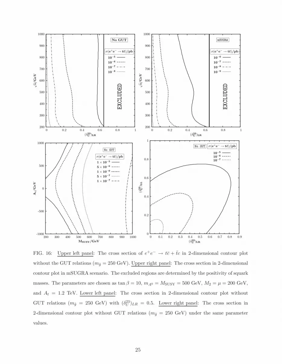
In Fig. 16, the cross section σ(e+e− → tc) is presented in two-dimensional contour plots

for various parameters. In the upper diagrams, σ(e+e− → tc) in ((δ23U )LR,

√s) plane is

shown with and without GUT relations. The cross section can reach 10−5 pb only for large

flavor-violating parameter values. The enhancement is about 3-4 orders of magnitude with

respect to the unconstrainted MSSM results. In the lower diagrams, the contour diagram in

(MSUSY, At) shows that a small MSUSY with At > 500 GeV favors a cross section of the order

of 10−5 pb. The contours in ((δ23U )LR, (δ

23U )LL) plane show that a large cross section can be

achieved by either assuming only one or both of the flavor-violating parameters large. The

cross section can still get as large as 10−5 pb. We further analyzed the dependence of the

cross section with tan β and M2 and found no significant change.

In Fig. 17 we present a best case scenario for intermediate tan β values as a function of

the gluino mass mg at the center of mass energies 500 and 1000 GeV, respectively. The cross

section can become only few times 10−5 pb for a very light gluino and is less than 10−9 pb

for the constrained MSSM case.

The last figure of the section, Fig. 18, shows how the forward-backward asymmetry

changes as a function of various MSSM parameters. The upper two diagrams show that the

asymmetry AFB can be as large as 30% for moderate values of (δ23U )LR at center of mass

energies less than tt threshold. It is also seen that AFB is not too sensitive to the gluino

mass. As shown in the lower diagrams, AFB can become even larger if MSUSY < 300 GeV

with |At| > 500 GeV. For MSUSY > 500 GeV, the asymmetry is always smaller than 20%,

22

independent of the value of At. Note that the sign of AFB shows the differences between

right-handed versus left-handed couplings.

We would like to end this section by commenting on the observibility of both the decay

t → cl+l− and the production e+e− → tc + tc at ILC. In the case where the center of mass

energy is less than 2mt ∼ 350 GeV, we shouldn’t expect any tt background so that we can

assume the signal as top quark plus almost a massless c-jet. If we further assume that the

integrated luminosity 500fb−1 is reached, one should expect to have more than 10 events at√s = 300 GeV, mg = 250 GeV with a large flavor violation (σ ∼ 0.025fb). This could still

be an observable signal after including detector efficiency factors since the background is

very clear. If the center of mass energy is higher than the 2mt threshold, then background

cuts will be required due to the tt production and the situation becomes worse than in

the below threshold case. For the decay t → cl+l−, ILC might not be the best place to

look. Assuming√s < 2mt, one can consider e+e− → tc → ccl+l− where l should be taken

either as electron or muon. Due to its short life-time, l = τ case is much more challenging.

Without doubt, this wouldn’t give any observable signal (considering the two top channel

not feasible). For√s > 500 GeV, e+e− → tt → bWcl+l−, which yields more events but

a more complicated background. For σ(e+e− → tt) ∼ 1 pb, the number of events for the

decay at integrated luminosity 500fb−1 becomes around 1.1× 105 ×BR(t→ cl+l−).4 Since

BR(t → cl+l−) , l = e, µ can reach at most 10−6, we get less than one event. Further cuts

needed will make t→ cl+l− not possible to be observed. However, if one looked at this decay

at LHC, one can have 1.8 × 107 × BR(t → cl+l−) number of events at 100fb−1 integrated

limunosity. A total efficiency of 10% is enough to get roughly 1.8 events.

4 W boson is assumed to decay leptonically. In this case, further cuts are necessary to distinguish the lepton

from W decay with the signal.

23

SM

(δ23D )RR

(δ23D )LL

(δ23D )LR

(δ23U )RR

(δ23U )LL

(δ23U )LR

NO GUT

(δ23U(D))AB

BR

(t→

c∑

iνiν

i)

10.90.80.70.60.50.40.30.20.10

10−5

10−6

10−7

10−8

10−9

10−10

10−11

10−12

10−13

10−14

SM

chargino

(δ23U )RR

(δ23U )LL

(δ23U )LR

mSUGRA

(δ23U )AB

BR

(t→

c∑

iνiν

i)

0.70.60.50.40.30.20.10

10−6

10−7

10−8

10−9

10−10

10−11

10−12

10−13

10−14

SM

No GUT-(δ23U )LR = 0.5

(δ23U )LR = 0.5

(δ23U )LR = 0

MSUSY

BR

(t→

c∑

iνiν

i)

1000900800700600500

10−5

10−6

10−7

10−8

10−9

10−10

10−11

10−12

10−13

10−14

SM

No GUT-(δ23U )LR = 0.5

(δ23U )LR = 0.5

(δ23U )LR = 0

tan β

BR

(t→

c∑

iνiν

i)

302520151050

10−5

10−6

10−7

10−8

10−9

10−10

10−11

10−12

10−13

10−14

10−15

10−16

FIG. 15: Upper left panel: BR’s of t → c∑

i νiνi decay as function of (δ23U(D))AB without the

GUT relations (mg = 250 GeV). Upper right panel: BR’s as function of (δ23U )AB under the same

conditions in mSUGRA scenario. The parameters are chosen as tan β = 10, mA0 = MSUSY = 500

GeV, M2 = µ = 200 GeV, and At = 1.2 TeV. Lower left panel: BR’s as function of MSUSY for

various values of (δ23U )LR for various values of (δ23

U )LR with tan β = 10. Lower right panel: BR’s as

a function of tan β under the same conditions with MSUSY = 500 GeV.

24

10−8

10−7

10−6

10−5

EXCLUDED

No GUT

σ(e+e− → tc)/pb

(δ23U )LR

√s/

GeV

10.80.60.40.20

1000

900

800

700

600

500

400

300

200

10−9

10−8

10−7

10−6

EXCLUDED

mSUGRA

σ(e+e− → tc)/pb

(δ23U )LR

√s/

GeV

10.80.60.40.20

1000

900

800

700

600

500

400

300

200

1 × 10−7

5 × 10−7

1 × 10−6

5 × 10−6

1 × 10−5

No GUT

σ(e+e− → tc)/pb

MSUSY/GeV

At/G

eV

1000900800700600500400300200

1000

500

0

-500

-1000

10−710−610−5

No GUT σ(e+e− → tc)/pb

(δ23U )LR

(δ23

U) L

L

0.90.80.70.60.50.40.30.20.10

1

0.8

0.6

0.4

0.2

0

FIG. 16: Upper left panel: The cross section of e+e− → tc + tc in 2-dimensional contour plot

without the GUT relations (mg = 250 GeV). Upper right panel: The cross section in 2-dimensional

contour plot in mSUGRA scenario. The excluded regions are determined by the positivity of squark

masses. The parameters are chosen as tan β = 10, mA0 = MSUSY = 500 GeV, M2 = µ = 200 GeV,

and At = 1.2 TeV. Lower left panel: The cross section in 2-dimensional contour plot without

GUT relations (mg = 250 GeV) with (δ23U )LR = 0.5. Lower right panel: The cross section in

2-dimensional contour plot without GUT relations (mg = 250 GeV) under the same parameter

values.

25

(δ23U )LR = 0.00

(δ23U )LR = 0.30

(δ23U )LR = 0.50

(δ23U )LR = 0.65

√s = 500 GeV

mg/GeV

σ(e

+e−→

tc)/

pb

1000900800700600500400300200

10−4

10−5

10−6

10−7

10−8

10−9

10−10

(δ23U )LR = 0.00

(δ23U )LR = 0.30

(δ23U )LR = 0.50

(δ23U )LR = 0.65

√s = 1000 GeV

mg/GeV

σ(e

+e−→

tc)/

pb

1000900800700600500400300200

10−4

10−5

10−6

10−7

10−8

10−9

10−10

FIG. 17: Left panel: The cross section of e+e− → tc + tc as a function of mg at√

s = 500 GeV.

Right panel: The cross section as a function of mg at√

s = 1000 GeV. The parameters are chosen

as tan β = 10,M2 = µ = 200 GeV, MSUSY = 250 GeV, and At = 400 GeV.

26

-0.1

0.0

0.1

0.2

0.3

EXCLUDED

No GUT

AFB(e+e− → tc)

(δ23U )LR

√s/

GeV

10.80.60.40.20

1000

900

800

700

600

500

400

300

200

-0.1

0.0

0.1

0.2

0.3

EXCLUDED

mSUGRA

AFB(e+e− → tc)

(δ23U )LR

√s/

GeV

10.80.60.40.20

1000

900

800

700

600

500

400

300

200

0.0

0.1

0.2

0.3

0.4

0.5

No GUT

AFB(e+e− → tc)

MSUSY/GeV

At/G

eV

1000900800700600500400300200

1000

500

0

-500

-1000

-0.1

0.0

0.1

0.2

0.3

0.4

0.5

No GUT

AFB(e+e− → tc)

(δ23U )LR

(δ23

U) L

L

10.90.80.70.60.50.40.30.20.10

1

0.9

0.8

0.7

0.6

0.5

0.4

0.3

0.2

0.1

0

FIG. 18: Upper left panel: The forward-backward asyymetry, AFB, for the process e+e− → tc in

2-dimensional contour plot without the GUT relations (mg = 250 GeV). Upper right panel: AFB in

2-dimensional contour plot in mSUGRA scenario. The parameters are chosen as tan β = 10, mA0 =

MSUSY = 500 GeV, M2 = µ = 200 GeV, and At = 1.2 TeV. Lower left panel: AFB in 2-dimensional

contour plot without GUT relations (mg = 250 GeV) with (δ23U )LR = 0.5. Lower right panel: AFB

in 2-dimensional contour plot without GUT relations (mg = 250 GeV).

27

VII. SUMMARY AND CONCLUSION

In the next few years, combined studies from the hadron (LHC) and linear (ILC) colliders,

with their ability to produce large number of top quarks, should be able to test FCNC in its

decays. Nonexistent at tree level, and very suppressed at one loop level in the SM, a signal

of these processes will most certainly be a sign of New Physics. The dominant and most

studied of these decays are the penguin ones: t→ cγ, cg, cZ and cH . But a complete study

of rare decays is likely to unravel more about FCNC phenomenology. We have concentrated

here on the rare decays t→ cl+l− and t→ cνiνi. While the dominant contribution to these

decays comes from the penguin diagrams, followed by the decays γ, Z,H → l+l−, these

decays can proceed even in the case in which the two-body decays are forbidden, through

box diagrams. Additionally, one can study the associated production cross section at ILC,

e+e− → tc, which is likely to provide a striking and almost background-free signal for single

top quark production.

Evaluation of the branching ratio for the decays t→ cl+l− and t→ cνiνi has shown that

they are strongly suppressed in SM and 2HDM; the branching ratios are expected to be of

O(10−15) for e+e− and µ+µ− and O(10−14) for τ+τ− and νiνi. These values, while small,

are of the same order of magnitude, or only one order smaller, than the two body decays.

Though at this level neither are possible to observe at present or future colliders, it gives

credence to the study of the rare decays t → cl+l− and t → cνiνi in beyond SM scenarios.

In the constrained MSSM the branching ratios are of the same order, or even smaller than

in the SM. However, in the unconstrained MSSM branching ratios of O(10−7) for e+e− and

µ+µ− and O(10−6) for τ+τ− and νiνi can be obtained in the mSUGRA scenario; and these

branching ratios can be one order of magnitude larger if one relaxes the GUT requirement

on gaugino masses. The values obtained are comparable to the values for branching ratios

obtained for t→ cγ, cZ and cH [8].

We also investigated the single top quark production in e+e− → tc + tc in the MSSM

with and without GUT scenarios. The cross section can get as large as a few times 10−5 pb

for the light gluino case with large flavor violation at√s = 500 GeV. This represents more

than 5 orders of magnitude enhancement with respect to unconstrained MSSM prediction

(δ′s = 0). In addition to the cross section, we calculated the forward-backward asymmetry

and found large asymmetries in certain parts of the parameter space (it can become 50%)

28

so that such a measurement would be a better alternative to measuring cross sections for

observing this channel. We commented on the observibility of both the decay and the

production processes at the ILC. Lower energies (less than tt threshold) are favorable for

the process e+e− → tc and we predicted roughly more than 10 events for certain parameter

values. At energies larger than the tt threshold, the background becomes more challenging.

For the decay t → cl+l− , l = e, µ, LHC would be a better alternative for observing a signal

than ILC, and could give an observable event rate if the total efficiency is around 10%.

[1] M. Beneke, I. Efthymipopulos, M. L. Mangano, J. Womersley (conveners) et al.,

hep-ph/0003033.

[2] J.A. Aguilar-Saavedra, Acta Phys. Pol. B35, 2695 (2004); Phys. Rev. D67, 035003 (2003);

ibid. D69, 099901 (2004); J.A. Aguilar-Saavedra and B.M. Nobre, Phys. Lett. B553, 251

(2003); J.A. Aguilar-Saavedra and G.C. Branco, Phys. Lett. B495, 347 (2000); J.A. Aguilar-

Saavedra, Phys. Lett. B502, 115 (2001).

[3] G. Eilam, J. L. Hewett and A. Soni, Phys. Rev. D44, 1473 (1991) [Erratum-ibid. D59, 039901

(1999)].

[4] B. Mele, S. Petrarca and A. Soddu, Phys. Lett. B435, 401 (1998).

[5] M. Beneke et al., hep-ph/0003033.

[6] J. Carvalho, N. Castro, A. Onofre and F. Velosco (ATLAS Collaboration), “Study of ATLAS

sensitivity to FCNC top decays”, ATLAS internal note, ATL-PHYS-PUB-2005-009, May 2005.

[7] M. Cobal, AIP Conf. Proc. 753, 234 (2005).

[8] W. Wagner, Rept. Prog. Phys. 68, 2409 (2005); A. Juste et al., hep-ph/0601112; J.M. Yang,

Ann. Phys. (N.Y.) 316, 529 (2005); D. Chakraborty, J. Konigsberg, D. Rainwater, Ann. Rev.

Nucl. Part. Sci. 53, 301 (2003); M. Beneke et al., hep-ph/0003033. F. Larios, R. Martinez and

M. A. Perez, hep-ph/0605003.

[9] A. Arhrib, Phys. Rev. D72, 075016 (2005).

[10] S. Bejar, J. Guasch, J. Sola, Nucl. Phys. B675, 270 (2003).

[11] E.O. Iltan, Phys. Rev. D65, 075017 (2002); E.O. Iltan and I. Turan, Phys. Rev. D67, 015004

(2003); W.S. Hou, Phys. Lett. B296, 179 (1992).

[12] J.L. Dıaz-Cruz, M.A. Perez, G. Tavares-Velasco and J.J. Toscano, Phys. Rev. D60, 115014

29

(1999); R. A. Dıaz, R. Martınez and J. Alexis Rodrıguez, hep-ph/0103307.

[13] R. Gaitan, O. G. Miranda and L. G. Cabral-Rosetti, hep-ph/0604170.

[14] C.S. Li, R.J. Oakes and J.M. Yang, Phys. Rev. D49, 293 (1994); Erratum-ibid. D56, 3156

(1997).

[15] G. Couture, C. Hamzaoui and H. Konig, Phys. Rev. D52, 1713 (1995); G. Couture, M. Frank

and H. Konig, Phys. Rev. D56, 4213 (1997).

[16] J.L. Lopez, D.V. Nanopoulos and R. Rangarajan, Phys. Rev. D56, 3100 (1997).

[17] G.M. de Divitiis, R. Petronzio and L. Silvestrini, Nucl. Phys. B504, 45 (1997).

[18] J. Guasch and J. Sola, Nucl. Phys. B562, 3 (1999); S. Bejar, J. Guasch and J. Sola,

hep-ph/0101294.

[19] M. Misiak, S. Pokorski and J. Rosiek, Adv. Ser. Direct. High Energy Phys. 15, 798 (1997);

also in hep-ph/9703442.

[20] J.J. Liu, C.S. Li, L.L. Yang and L.G. Jin, Phys. Lett. B599, 92 (2004).

[21] M. Frank and I. Turan, Phys. Rev. D72, 035008 (2005).

[22] J.M. Yang, B.-L. Young and X. Zhang, Phys. Rev. D58, 055001 (1998).

[23] X. Wang et al., Phys. Rev. D50, 5781 (1994); J. Phys. G20, 291 (1994); G. Lu, C. Yue and

J. Huang, J. Phys. G22, 305 (1996); Phys. Rev. D57, 1755 (1998).

[24] G. Lu et al., Phys. Rev. D68, 015002 (2003); C.X. Yue et al., Phys. Rev. D64, 095004 (2001);

G. Burdman, Phys. Rev. Lett. 83, 2888 (1999).

[25] A. Arhrib and W.S. Hou, hep-ph/0602035.

[26] E. Jenkins, Phys. Rev. D56, 458 (1997).

[27] G. Altarelli, L. Conti and V. Lubicz, Phys. Lett. B502, 125 (2001).

[28] S. Bar-Shalom, G. Eilam, M. Frank and I. Turan, Phys. Rev. D72, 055018 (2005).

[29] S. Bar-Shalom, G. Eilam, A. Soni and J. Wudka, Phys. Rev. D57, 2957 (1998).

[30] G. Eilam, M. Frank and I. Turan, Phys. Rev. D73, 053011 (2006).

[31] G. Eilam, M. Frank and I. Turan, Phys. Rev. D74, 035012 (2006); J. Cao, G. Eilam,

K. I. Hikasa and J. M. Yang, Phys. Rev. D 74, 031701(R) (2006).

[32] A. Cordero-Cid, J. M. Hernandez, G. Tavares-Velasco and J. J. Toscano, Phys. Rev. D73,

094005 (2006).

[33] C. S. Huang, W. Liao, Q. S. Yan and S. H. Zhu, Phys. Rev. D63, 114021 (2001) [Erratum-

ibid. D64, 059902 (2001)]; E. Lunghi, A. Masiero, I. Scimemi and L. Silvestrini, Nucl. Phys.

30

B568, 120 (2000); E. Gabrielli and S. Khalil, Phys. Lett. B530, 133 (2002).

[34] C. Yue, L. Wang and D. Yu, Phys. Rev. D70, 054011 (2004).

[35] P. Y. Popov and A. D. Smirnov, “Rare T-Quark Decays T → C L+(J) L-(K) And T → C

Sneutrino(J) Nu(K) Induced By Doublets Of Scalar Leptoquarks Within The Minimal Phys.

Atom. Nucl. 69, 977 (2006) [Yad. Fiz. 69, 1006 (2006)]; P. Y. Popov, A. V. Povarov and

A. D. Smirnov, “Fermionic decays of scalar leptoquarks and scalar gluons in the minimal

Mod. Phys. Lett. A 20, 3003 (2005)

[36] H. J. He, C. T. Hill and T. M. P. Tait, Phys. Rev. D65, 055006 (2002).

[37] D. Atwood, L. Reina and A. Soni, Phys. Rev. D55, 3156 (1997).

[38] For a review see e.g. J. F. Gunion, H. E. Haber, G. L. Kane and S. Dawson, “The Higgs

Hunter’s Guide” SCIPP-89/13 and ERRATA, hep-ph/9302272.

[39] T.P. Cheng and M. Sher, Phys. Rev. D35, 3484 (1987); M. Sher and Y. Yuan, Phys. Rev.

D44, 1461 (1991); J.L. Dıaz-Cruz and G. Lopez-Castro, Phys. Lett. B301, 405 (1993).

[40] A. Antaramian, L.J. Hall and A. Rasin, Phys. Rev. Lett. 69, 1871 (1992); L.Hall and S.

Weinberg, Phys. Rev. D48, R979 (1993); M.J. Savage, Phys. Lett. B266, 135 (1991); M.

Luke and M.J. Savage, Phys. Lett. B307, 387 (1993).

[41] D. Atwood, L. Reina and A. Soni, Phys. Rev. D53, 1199 (1996); Phys. Rev. Lett. 75, 3800

(1975); Phys. Rev. D55, 3156 (1997); B. Grzadowski, J.F. Gunion and P. Krawczyk, Phys.

Lett. B268, 106 (1991).

[42] V. Barger, J. L. Hewett and R. J. N. Phillips, Phys. Rev. D41, 3421 (1990).

[43] K. Hagiwara et al. [Particle Data Group Collaboration], Phys. Rev. D66 (2002) 010001.

[44] T. Hahn and M. Perez-Victoria, Comput. Phys. Commun. 118, 153 (1999); T. Hahn,

Nucl. Phys. Proc. Suppl. 89, 231 (2000); T. Hahn, Comput. Phys. Commun. 140, 418

(2001); T. Hahn, C. Schappacher, Comput. Phys. Commun. bf 143, 54 (2002); T. Hahn,

hep-ph/0506201.

[45] F. Gabbiani, E. Gabrielli, A. Masiero and L. Silvestrini, Nucl. Phys. B477, 321 (1996);

M. Misiak, S. Pokorski and J. Rosiek, Adv. Ser. Direct. High Energy Phys. 15, 795 (1998);

M. Ciuchini, E. Franco, A. Masiero, L. Silvestrini, Phys. Rev. D67, 075016 (2003) [Erratum

ibid. D68, 079901 (2003).

[46] M. Sher, Phys. Rept. 179, 273 (1989). S. Kanemura, T. Kasai and Y. Okada, Phys. Lett.

B471, 182 (1999).

31

[47] J. F. Gunion and H. E. Haber, Phys. Rev. D67, 075019 (2003). L. Brucher and R. Santos,

Eur. Phys. J. C12, 87 (2000).

[48] A. G. Akeroyd, A. Arhrib and E. Naimi, Eur. Phys. J. C20, 51 (2001). A. Arhrib and G. Moul-

taka, Nucl. Phys. B558, 3 (1999).

[49] A. Barroso, P. M. Ferreira and R. Santos, hep-ph/0507329. P. M. Ferreira, R. Santos and

A. Barroso, Phys. Lett. B603, 219 (2004).

[50] R. Harnik, D. T. Larson, H. Murayama and A. Pierce, Phys. Rev. D69, 094024 (2004).

[51] T. Besmer, C. Greub and T. Hurth, Nucl. Phys. B609, 359 (2001); D. A. Demir, Phys. Lett.

B571, 193 (2003); A. M. Curiel, M. J. Herrero and D. Temes, Phys. Rev. D67, 075008 (2003);

J. J. Liu, C. S. Li, L. L. Yang and L. G. Jin, Nucl. Phys. B705, 3 (2005).

[52] S. Heinemeyer, W. Hollik and G. Weiglein, Comput. Phys. Comm. 124, 76 (2000),

hep-ph/9812320; S. Heinemeyer, W. Hollik and G. Weiglein, Eur. Phys. J. C9, 343 (1999);

G. Degrassi, S. Heinemeyer, W. Hollik, P. Slavich and G. Weiglein, Eur. Phys. J. C28, 133

(2003); T. Hahn, S. Heinemeyer, W. Hollik and G. Weiglein, hep-ph/0507009.

[53] S. Eidelman et al. [Particle Data Group], Phys. Lett. B592, 1 (2004).

[54] L. J. Hall, V. A. Kostelecky and S. Raby, Nucl. Phys. B267, 415 (1986); A. Masiero and L. Sil-

vestrini, in Perspectives on Supersymmetry, edited by G. Kane (World Scientific, Singapore,

1998).

[55] K. Agashe, G. Perez and A. Soni, hep-ph/0606293.

[56] C. H. Chang, X. Q. Li, J. X. Wang and M. Z. Yang, Phys. Lett. B 313, 389 (1993).

[57] C. S. Huang, X. H. Wu and S. H. Zhu, Phys. Lett. B452, 143 (1999).

[58] C. S. Li, X. Zhang and S. H. Zhu, Phys. Rev. D 60, 077702 (1999).

[59] J. j. Cao, Z. h. Xiong and J. M. Yang, Nucl. Phys. B 651, 87 (2003).

32