querying large collections of music for similarity
TRANSCRIPT
Querying Large Collections of Music for Similarity
Matt Welsh, Nikita Borisov, Jason Hill, Robert von Behren, and Alec WooComputer Science Division
University of California, BerkeleyBerkeley, CA 94720, USA mdw,nikitab,jhill,jrvb,[email protected]
Abstract
We present a system capable of performing similarityqueries against a large archive of digital music. Users areable to search for songs which “sound similar” to a givenquery song, thereby aiding the navigation and discoveryof new music in such an archive. Our technique is basedon reduction of the music data to a feature space of rela-tively small dimensionality (1248 feature dimensions persong); this is accomplished using a set of feature extrac-tors which derive frequency, amplitude, and tempo datafrom the encoded music data. Queries are then per-formed using a k-nearest neighbor search in the featurespace. Our system allows subsets of the feature spaceto be selected on a per-query basis.
We have integrated the music query engine into an
online MP3 music archive consisting of over 7000 songs.
We present an evaluation of our feature extraction and
query results against this archive.
1 Introduction
Digital music archives are an increasingly popu-lar Internet resource, supported by a surging mar-ket for personal digital music devices, an increase ofbandwidth to the home, and the emergence of thepopular MP3 digital audio format. Music archivesites such as mp3.com and search engines such asmp3.lycos.com are changing the face of music dis-tribution by archiving and indexing a vast array ofdigital audio files on the Internet. Users of thesesites need a way to navigate and discover music filesbased on a variety of factors. Many archive sitesoffer text-based searching of artist, song/album ti-tle, and genre. However, discovering music basedon textual indexing alone can be difficult; for exam-ple, mp3.com categorizes its 208,000 songs into 215separate genres. Discovering new music amounts to
This research was sponsored by the Advanced ResearchProjects Agency under grant DABT63-98-C-0038, and anequipment grant from Intel Corporation.
downloading (and listening to!) an arbitrary num-ber of songs which match a particular text search,which could potentially number into the thousands.
In this paper, we present a system enabling sim-ilarity queries against a database of digital music.Our system allows a user to submit a query which,given a particular song in the database, returns auser-supplied number of other songs which “soundsimilar” to the query song. Our technique is basedon a set of feature extractors which preprocess themusic archive, distilling each song’s content downto a small set of values (currently, 1248 floating-point values per song). Similarity queries can thenbe performed using a k-nearest-neighbor search inthe feature space.
We have developed a number of domain-specificfeature extractors, described in Section 3, whichprocess audio data stored in MP3 format. Theseextract data from the music such as frequency his-tograms, volume, noise, tempo, and tonal transi-tions. The choice of feature extractors is essentialfor music similarity matching to work effectively.We have found that certain combinations of features(for example, low-frequency plus tempo data) arehighly selective for certain types of music. Classicaland soul music are particularly well-selected by ourfeature extractors, as detailed in Section 5.
We have incorporated our query engine into theNinja Jukebox [6], a scalable, online repository ofover 7000 songs totalling over 30 gigabytes of MP3data. The Jukebox client application, described inSection 4, allows the user to select, listen to, andperform queries on the entire database. An addi-tional feature provided by our system is the abil-ity to select subsets of the feature space on whichto perform queries, thus facilitating the investiga-tion of individual feature extractors. The queryengine performs well, with a response time of lessthan 1 second for a music database consisting of10000 songs and 1248 feature dimensions per song.
This paper makes three major contributions.
First, we present a full-featured search facility fordigital music based on acoustic properties alone.Second, we present a number of novel feature ex-traction techniques for digital music, specifically tai-lored for performing similarity queries. Third, weevaluate our results against a reasonably large musicarchive containing a diverse assortment of genres.
2 Design Overview
The music query engine operates in two stages.The first stage consists of a relatively expensive pre-processing phase, wherein each song in is passedover by a number of independent feature extractors.Each feature extractor reduces the information con-tent in the raw music data to a vector in a smallnumber of dimensions (typically one or two, but oneextractor produces as many as 306 dimensions persong). The music data is stored in MP3 [10] for-mat, however, the feature extractors generally op-erate on raw audio samples produced by decodingthe MP3 file. The features associated with each songare stored in a simple text database for later pro-cessing by the query engine. Each feature extractorhas its own database file associated with it, allowingthe extractors to run independently and in parallel.
While the preprocessing step is expensive, it mustbe executed just once for each song; when new songsare added, the preprocessor is capable of only pro-cessing new entries rather than rerunning across theentire set. Each feature extractor takes approxi-mately 30-45 seconds to run against a 5-minute songon a 500 MHz Pentium III system; the longest runtime (for tempo extraction) is about 5 minutes.
The query engine reads the set of featuredatabases into main memory, storing each featurevector as an array of floating-point values. The setof vectors for a particular song treated as a point inan n-dimensional Euclidean space. The basic querymodel assumes that two songs S1 and S2 sound sim-ilar if their feature sets v1 and v2, respectively, arewithin distance ε as computed by the Euclidean dis-tance:
d =√∑
i
(vi1 − vi
2
)2
where vi1 denotes the ith component of v1, i ranges
over (0 . . . |v1|), and |v1| = |v2|.While it would be interesting to explore other
similarity metrics for music, Euclidean distance isattractive for our feature extractors because it is in-tuitive both when implementing a feature extractorsand when querying the database. One concern with
this approach is that the magnitude of feature vec-tors must be normalized to prevent one feature from“weighting” the distance function more than others.For the results presented here, all features were nor-malized in the range (0.0 . . . 1.0). However, it maybe desirable for the user to assign scalar weights togiven feature vectors, in essence assigning them rel-ative priorities in terms of computing the Euclideandistance between two songs. We have not yet ex-plored this possibility in our prototype.
Rather than have the user specify the desiredclustering distance ε, the query application allowsthe user to specify a value k indicating the numberof similar songs to return for a given query. Givena query song Q and a value for k > 2, the similarityquery is performed by a k-nearest-neighbor searchin the n-dimensional space of song features. Vari-ous algorithms for computing nearest neighbors ex-ist; our prototype uses a straightforward algorithmwith early rejection. Section 4 discusses our imple-mentation in more detail.
Because one of the goals of our system is to fa-cilitate investigation of different feature extractors,the query engine allows the user to perform queriesacross a subset of the feature space. Each vec-tor can be independently indexed by a text stringidentifying that feature; for example, tempo data isstored with a tag of “av_tempo”. The query appli-cation allows the user to select the features used inthe nearest-neighbor matching by specifying one ormore of these feature tags. This allows the user tocompare queries using different subsets of the fea-ture space, in order to better understand the effectof each feature on the results of a query.
3 Feature Extraction
To be able to search through a collection of manygigabytes worth of music, we reduce each song to acollection of features. A feature is a small vector,which captures some aspect of a song which can beused to determine similarity. This is somewhat dif-ficult because of the large amount of detail presentin a given song. A key challenge is to remove ex-traneous detail that might overshadow similaritiesbetween songs, while retaining enough detail to ef-fectively discriminate between qualitatively differ-ent songs. We achieve this by ensuring that eachfeature is very simple. It is more useful if a featuremistakenly classifies dissimilar songs as similar, thanvice versa, since using a combination of features willallow us to eliminate these false matches.
This section describes the features we chose to ex-
0
0.05
0.1
0.15
0.2
0.25
0.3
0 500 1000 1500 2000 2500
Am
litud
e
Frequency, Hz
Amplitude dataDerived normalization function
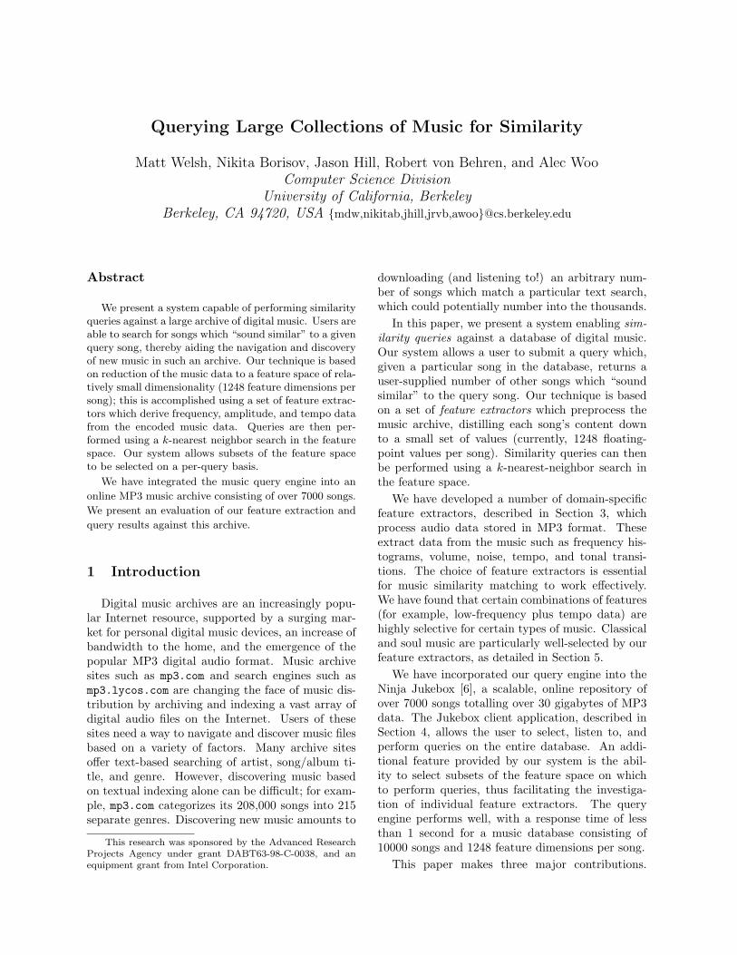
Figure 1: Derivation of normalization function νbased on frequency averages.
tract, as well as the mechanisms for extracting them.The types of data captured are tonal histograms,tonal transitions, noise, volume, and tempo.
3.1 Tonal histograms
The first feature extractor produces a histogramof frequency amplitudes across the notes of theWestern music scale. Each bucket of the histogramcorresponds to the average amplitude of a particularnote (e.g., C sharp) across 5 octaves. This informa-tion can be used to help determine the key that themusic was played in, as well as any dominant chords.It also has the property of determining how manydifferent frequencies were active in the sample.
Frequency analysis of this sort should compen-sate for the characteristics of the human ear, whichis more sensitive to high frequencies than to lowones. As such, music tends to exhibit greater am-plitudes in the low frequency range. Therefore, wemust attenuate the energy levels of the music be-fore performing frequency analysis, in order to per-form comparisons using the perceived frequenciesthat a human would hear. Otherwise, low noteswould dominate the amplitudes in the frequency his-togram.
The tonal feature extractor determines frequencyamplitudes by performing an FFT on 0.1 sec sam-ples for 16 sec in the middle of the song. The fre-quency amplitudes A are then normalized using thefunction:
A′φ =
Aφ
ν(φ)
where the normalization factor ν is
ν(φ) =43.066
75.366 + φ+ 0.015
0.6
0.8
1
1.2
1.4
250 500 750 1000 1250 1500 1750 2000 2250 2500
Am
litud
e
Frequency, Hz
Amplitude dataDerived normalization function
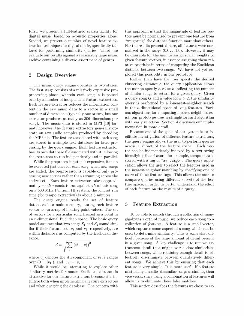
Figure 2: Normalized frequency amplitudes and thenotes of the Western scale.
which is parameterized by φ, the frequency ofthe sample being normalized. ν was determinedby applying an inverse linear regression againstamplitude-versus-frequency data averaged across100 random songs, as shown in Figure 1. Anotherway to determine ν would be to use establishedmodels of frequency sensitivity in the human ear,as in [8]. However, determining this function em-pirically allows us to adapt it to actual music char-acteristics, which often exhibit some compensationfor recording and amplification technology.
Figure 2 shows a plot of normalized frequencyranges across the same set of 100 songs used to de-termine ν. Superimposed onto this figure are thefrequencies of notes in the Western musical scale;we can see that frequency peaks occur clearly atthe corresponding notes.
Two types of information are extracted from thenormalized frequency data. The first is the low fre-quency average, which is the average amplitude ofnormalized frequencies from 40Hz to 1KHz. Thisfeature is meant to distinguish “bass-heavy” music(such as rock and rap) from “lighter” music such asclassical and jazz. This value is again normalized tocompensate for differences in volume levels betweenrecordings.
The second type of feature is a histogram of tonalamplitudes across multiple octaves, as describedearlier. Each bucket of the histogram correspondsto the average frequency amplitude of a given noteacross 5 octaves, ranging from 130Hz to 4.16KHz,with middle C being 260 Hz. If a measured fre-quency is within 1/2 of a Hz of a note in the mu-sical scale, it is counted as that note. We ignorefrequencies less that 130 Hz because the precisionof the FFT below that frequency range is not ac-
curate enough to distinguish between two adjacentnotes. Each interval of the FFT is 10Hz, yet at100Hz, only 5Hz separates the musical notes.
3.2 Tonal transitions
Music, to some approximation, can be summa-rized as a collection of frequency transitions overtime. Gibson [5] has investigated the use of fre-quency transitions to identify individual songs givena short sample; applying these techniques for simi-larity matching is the focus of our tonal transitionfeature extractor. This extractor produces a set of306 values, each of which corresponds to the to-tal number of tonal transitions in a given frequencyrange for a 10-second sample of the song. Five suchfeature vectors, corresponding to a 50-second sam-ple, are extracted for each song.
The tonal feature extractor works as follows. Leta song be modeled as a finite sequence of samplesSt. A parameter s can be used to skip s samplesfrom the beginning of the song. The actual imple-mentation sets s to correspond to 20 seconds. St+s
is then segmented into a sequence of blocks Bk withblock size b where 0 ≤ k ≤ b |S|−s
b c. FFT is appliedto each block and only the amplitude component isused. Thus, Bk = |FFT (Bk)|
The frequency amplitudes from the FFT aremapped onto the Western musical scale for 6 oc-taves ranging from 53.8Hz (A 3 octaves below mid-dle C) to 3.43kHz (A 3 octaves above middle C).This range was chosen as it captures the majorityof the frequencies emitted by acoustic instrumentsas well as the human voice, ignoring high-order har-monics [9].
Tonal transitions are determined by compar-ing frequency amplitudes between two consecutiveblocks, namely from Bk to Bk+1. Let fφ(k) equalthe amplitude of frequency φ in Bk. If
fφ(k + 1)fρ(k)fρ(k + 1)fφ(k)
> 1 (1)
there exists a frequency transition from φ to ρ fromblock Bk to block Bk+1. Since a relative value isused for determining frequency transition, effectsfrom white noise and band filtering can be avoided.
A large block size b corresponds to high resolutionin the frequency domain. However, a large b will notcapture tonal transitions at short time scales. Wechoose b = 8192 which corresponds to 0.18 sec ata sampling rate of 44.1kHz. As a result, frequencytransitions faster than 0.18 sec will not be captured.However, we believe that this resolution is adequateto capture the primary tonal properties of music.
Let n be the number of notes that can be cap-tured per octave and o be the number of octaves tobe examined. Across the o octaves, the number ofall possible tonal transitions is
d = o× n× (o× n− 1)
Let TT be a function that applies the tonal transi-tion equation given in Equation (1) d times over allpossible tonal transitions and stores each occurrenceon a bit vector ~v with length d. That is,
TT (Bk,Bk+1) → ~v ∈ 0, 1d
Since d = O((o × n)2), it is desirable to maken smaller, in order to reduce the dimensionality inthe feature space. In our case, each octave is dividedinto 3 segments each, yielding 18 tones. As a result,d = 18× 17 = 306.
By applying TT to the entire sequence Bi, a se-quence ~V of bit vectors is generated. If two songsare similar, the ~V of the two songs should also besimilar using a metric like hamming distance. How-ever, this approach is not effective since it requiresa pairwise comparison and is prone to phase errors.
One naive method is to count the number of tonaltransitions over a fixed period T . If two songs aresimilar, they should have similar number of tonaltransitions over T . The tradeoff is that temporalinformation is lost due to summation.
Let FT be the feature extractor function whichperforms vector summation over a sequence of vec-tors and ~F be a sequence of feature vectors.
~FK = FT (~VK×T ...(K+1)×T−1)
where 0 ≤ K ≤ b |S|−sb c.
Since error due to summation approximation iscumulative, error increases as T increases. Thus,T should be tuned by experiment. In our case, Tis chosen to correspond to 10-second samples of asong, and F contains at most five feature vectorswhich correspond to 50-second samples of a song.
3.3 Noise
Another good measure of how similar two songsare is their relative noise level. It’s unlikely thata person will characterize a song with pure soundsimilar to one with a lot of noise. To convert this toan objective metric, though, it is necessary to definewhat is meant by a “noisy” or a “pure” sound. Asensible definition should recognize a pure tone (i.e.a perfect sine
wave) as pure, and random noise (e.g.
random samples) as highly noisy.
Examining these two extremes, we notice thata pure tone can be identified by a highly regularFourier transform. In the ideal case, it consists ofa single spike at the corresponding frequency. TheFourier transform of random samples, on the otherhand, should exhibit no visible structure. In gen-eral, we can define a pure sound as one where only afew dominant frequencies are present in the Fouriertransform, and a noisy one where a large number offrequencies are present.
Now we are faced with the task of using this def-inition to algorithmically reduce a sound sample toa real number representing its noise level. Simplycounting the number dominant frequencies is prob-lematic, since it’s not always clear which frequenciesare dominant, and which are not. For example, adiscrete Fourier transform of an instrument such asa violin playing a single tone will produce a peak atthe frequency of the tone, as well as smaller peaksat several nearby frequencies. Similar difficultiesarise in examining a Fourier transform of a sam-ple with several instruments playing distinct notes,some louder than others.
We decided to count peak frequencies by weight-ing each frequency by the magnitude of the corre-sponding Fourier coefficient; for example, one loudtone and two quieter ones with half the magnitudewill count as a total of two peaks. Mathematically,we simply compute the sum of the magnitudes ofthe coefficients corresponding to each dominant fre-quency. A useful observation is that a non-dominantfrequency would have a nearly negligible contribu-tion to such a sum, since its magnitude is muchsmaller than that of a dominant frequency. Becauseof this, we do not perform thresholding to select thedominant frequencies, and add up all the Fouriercoefficients instead. We then normalize the sum ac-cording to the maximum Fourier coefficient, so thatsongs which are recorded at a louder volume will notappear more noisy. Therefore,
noise(f) =∑n
i=1 |f(i)|maxn
i=1 |f(i)|
where n is the highest coefficient calculated by thediscrete Fourier transform. This metric applied toa pure tone will return 1, and applied to a randomset of Fourier coefficients will return approximately1/2n. A loud pure tone combined with some ran-dom noise at a half the volume will result in 1/4n— more noisy than a pure tone, but less noisy thanjust random noise. In general, the behavior of thismetric closely approximates the subjective notion ofhow noisy a sound is.
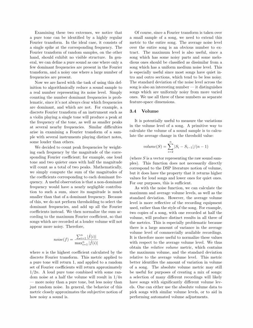
Of course, since a Fourier transform is taken overa small sample of a song, we need to extend thismetric to the entire song. The average noise levelover the entire song is an obvious number to ex-tract. The maximum level is also useful, since asong which has some noisy parts and some melo-dious ones should be classified as dissimilar from asong which has a uniform medium noise level. Thisis especially useful since most songs have quiet in-tro and outro sections, which tend to be less noisy.The standard deviation of the noise level across thesong is also an interesting number — it distinguishessongs which are uniformly noisy from more variedones. We use all three of these numbers as separatefeature-space dimensions.
3.4 Volume
It is potentially useful to measure the variationsin the volume level of a song. A primitive way tocalculate the volume of a sound sample is to calcu-late the average change in the threshold value:
volume(S) =n∑
i=2
|Si − Si−1|/(n− 1)
(where S is a vector representing the raw sound sam-ples). This function does not necessarily directlycorrespond to the DSP literature notion of volume,but it does have the property that it returns highervalues for loud songs and lower ones for quiet ones.For our purposes, this is sufficient.
As with the noise function, we can calculate themaximum and average volume levels, as well as thestandard deviation. However, the average volumelevel is more reflective of the recording equipmentused, rather than the style of the song. For example,two copies of a song, with one recorded at half thevolume, will produce distinct results in all three ofthe metrics. This is especially problematic becausethere is a large amount of variance in the averagevolume level of commercially available recordings.It is therefore more useful to normalize these valueswith respect to the average volume level. We thusobtain the relative volume metric, which containsthe maximum volume, and the standard deviationrelative to the average volume level. This metricbetter identifies the amount of variation in volumeof a song. The absolute volume metric may stillbe useful for purposes of creating a mix of songs:a selection of many different recordings will likelyhave songs with significantly different volume lev-els. One can either use the absolute volume data topick songs with similar volume levels, or to aid inperforming automated volume adjustments.
3.5 Tempo and Rhythm
The specific rhythmic qualities of a piece of mu-sic have a good deal of influence on how humansexperience it. Fast songs are often upbeat and en-ergetic, while slower songs are often more peaceful.The syncopated rhythms of jazz songs feel very dif-ferent from the more straightforward even temposof rock.
Extracting rhythmic information from raw soundsamples is a difficult task. Several studies have fo-cused on extracting rhythmic information from digi-tal music representations such as MIDI, or with ref-erence to a musical score [16]. Neither approachis suitable for analyzing raw sound data. For thepurposes of our analysis, we adopted the algorithmproposed by Scheirer [17]. This technique breaks aninput signal into several bands, each representingone-octave ranges. The algorithm then uses banksof resonators on each input to settle in on the posi-tion of the downbeat over time.
The output of this algorithm allows us to extractseveral interesting features from a music sample.First, we can determine the average tempo of a song.Additionally, we can examine how the tempo variesthroughout the song. Finally, as a measure of therhythmic complexity of the song, we track how wellthe algorithm was able to settle down to a particulartempo.
The tempo feature extractor determines thetempo of the song from three 10-second samples,at 60, 120, and 180 seconds into the song.1 It thenoutputs 4 numbers: the average tempo of the 3 sam-ples, the spread and deviation of the tempo acrosssamples, and the fraction of samples for which thetempo extraction appeared not to work well, as in-dicated by the inability of the algorithm to settlein on a steady beat by the end of the 10-secondsample. Note that it is impossible to measure theactual effectiveness of the algorithm for every sam-ple, since this involves listening to the sample anddeducing the tempo manually. In the samples thatwe listened to, however, a wide variation in the out-put of the tempo algorithm typically coincided withthe failure of the algorithm, often due to complexrhythms or noisy music.
1For shorter songs, additional samples are chosen by halv-ing the start position of the sample until chosen start pointis at least 10 seconds from the end of the song.
4 The Jukebox Query Engine
In order to study the effectiveness of our fea-ture extraction and similarity-matching algorithms,we have integrated the query engine into the NinjaJukebox [6], a scalable online digital music reposi-tory consisting of nearly 7000 songs stored in MP3format. The Ninja Jukebox consists of a cluster ofworkstations each hosting a collection of music dataon local disk, as well as a Java-based scalable serviceplatform, the MultiSpace [7], which manages clus-ter resources and facilitates application constructionand composability. The Jukebox service itself is en-tirely coded in Java, using Java Remote MethodInvocation (RMI) for communication between dis-tributed components (e.g., the music locator serviceon each node of the cluster).
The Jukebox user interface is a Java applicationwhich establishes a connection to a centralized Juke-box directory service to select songs, and which re-ceives MP3 audio data streaming over HTTP to anexternal player application. Access to both the mu-sic directory and each song in the Jukebox requiresaccess controls based on client authentication usingpublic key certificates. The Jukebox also includes asimple collaborative-filtering feature allowing usersto express song preferences.
Integrating the query engine into the Ninja Juke-box consisted of two steps: first, adding the similar-ity query functionality to the Jukebox service itself,and second, enhancing the Jukebox user interface toaccept queries and return results.
The Jukebox Query Engine is implemented inJava and runs alongside the other Jukebox subser-vices in the MultiSpace cluster environment. Whenthe engine is started, it reads the feature database(stored as a collection of text files) and exports aJava RMI interface with a number of methods whichcan be invoked by a client application. These meth-ods are:
• int numSongs() — return the number of songsin the database;
• String[] getFeatures() — return a list of fea-ture tags;
• String[] getSongNames() — return a list ofsongs;
• getSong(String name) — return the Song datastructure for a given song;
• Song[] query(Song query, int k) — returnthe k nearest songs which match the querysong;
• Song[] query(Song query, String features[],
int k) — return the k nearest songs whichmatch the query song, using only the givenfeatures.
Having the Query Engine export a simple RMI in-terface allows multiple client applications to be builtwhich are able to perform remote queries on the en-tire Ninja Jukebox.
Feature extraction from the Ninja Jukebox is per-formed in parallel, with each node of the Jukeboxrunning each of the feature extractors against thesubset of the music database stored on that node.The scripts performing the feature extraction areengineered to be highly resilient to failures in thefeature extractors themselves, as well as in the un-derlying system software. The feature extractionscripts perform checkpointing so that they may bestopped and restarted at any time without loss ofdata. This functionality is vital considering the ex-pense of losing feature data (i.e., re-running the fea-ture extractors, which are slow).
4.1 Query algorithm
The Query Engine performs similarity matcheson the database using a brute-force k-nearest neigh-bor algorithm. Our nearest-neighbor algorithmkeeps track of the current result set of size k, andis optimized to quickly reject points which have adistance exceeding the maximal distance of pointsin this set. This early rejection prevents the n-dimensional distance from being fully computed foreach point.
This algorithm requires at most O(n · d) op-erations where n is the number of songs in thedatabase and d is the number of feature dimen-sions stored per song. Clearly there are more ef-ficient algorithms for computing nearest neighbors.Most deterministic algorithms have a query time ofat least Ω(exp(d) · log(n)) [4, 1], while Kleinberg’sε-approximate algorithm [12] has a query time ofO((d log2 d)(d + log n)) and a preprocessing stepwhich requires O((n log d)2d) storage.
However, we feel that our use of a brute-forcetechnique is reasonable for two reasons. First, itperforms very well given the size of the Ninja Juke-box, with a query time of less than 1 second in mostcases. Secondly, our algorithm allows queries onsubsets of the feature space. Many of the approx-imate nearest-neighbor algorithms require prepro-cessing of the data set which lose information whichis needed to independently identify feature dimen-sions for such subset queries. Subset queries are animportant tool for studying the effectiveness of our
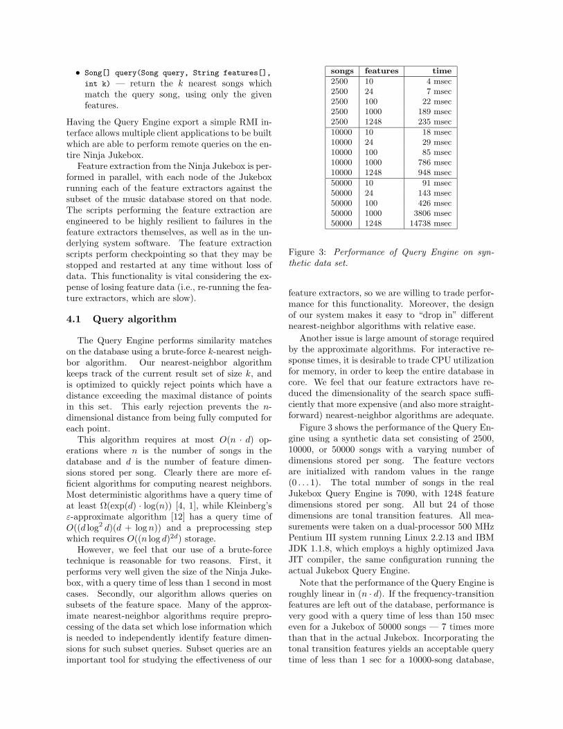
songs features time
2500 10 4 msec2500 24 7 msec2500 100 22 msec2500 1000 189 msec2500 1248 235 msec
10000 10 18 msec10000 24 29 msec10000 100 85 msec10000 1000 786 msec10000 1248 948 msec
50000 10 91 msec50000 24 143 msec50000 100 426 msec50000 1000 3806 msec50000 1248 14738 msec
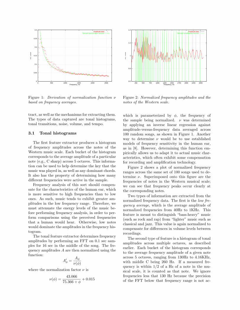
Figure 3: Performance of Query Engine on syn-thetic data set.
feature extractors, so we are willing to trade perfor-mance for this functionality. Moreover, the designof our system makes it easy to “drop in” differentnearest-neighbor algorithms with relative ease.
Another issue is large amount of storage requiredby the approximate algorithms. For interactive re-sponse times, it is desirable to trade CPU utilizationfor memory, in order to keep the entire database incore. We feel that our feature extractors have re-duced the dimensionality of the search space suffi-ciently that more expensive (and also more straight-forward) nearest-neighbor algorithms are adequate.
Figure 3 shows the performance of the Query En-gine using a synthetic data set consisting of 2500,10000, or 50000 songs with a varying number ofdimensions stored per song. The feature vectorsare initialized with random values in the range(0 . . . 1). The total number of songs in the realJukebox Query Engine is 7090, with 1248 featuredimensions stored per song. All but 24 of thosedimensions are tonal transition features. All mea-surements were taken on a dual-processor 500 MHzPentium III system running Linux 2.2.13 and IBMJDK 1.1.8, which employs a highly optimized JavaJIT compiler, the same configuration running theactual Jukebox Query Engine.
Note that the performance of the Query Engine isroughly linear in (n · d). If the frequency-transitionfeatures are left out of the database, performance isvery good with a query time of less than 150 mseceven for a Jukebox of 50000 songs — 7 times morethan that in the actual Jukebox. Incorporating thetonal transition features yields an acceptable querytime of less than 1 sec for a 10000-song database,
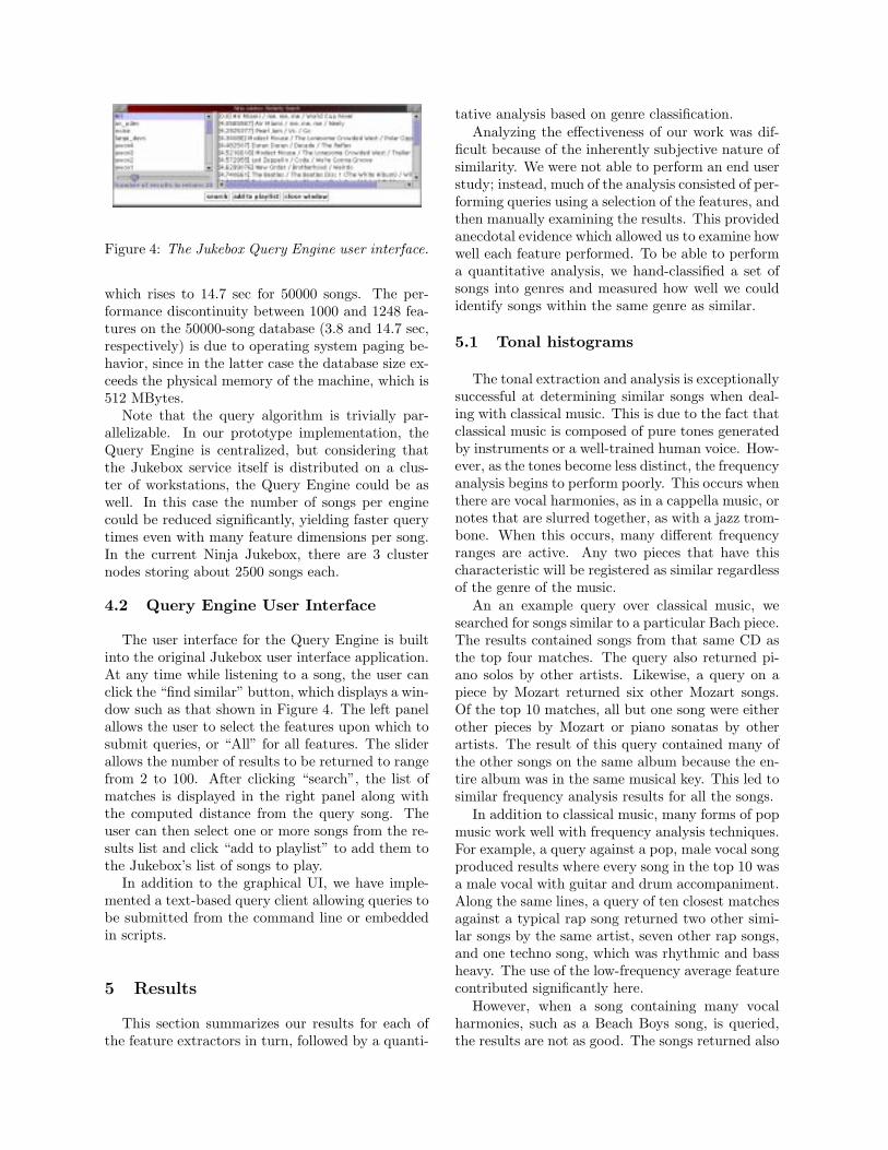
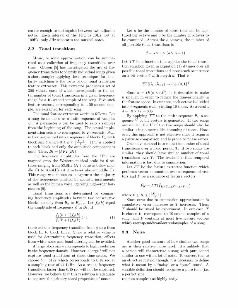
Figure 4: The Jukebox Query Engine user interface.
which rises to 14.7 sec for 50000 songs. The per-formance discontinuity between 1000 and 1248 fea-tures on the 50000-song database (3.8 and 14.7 sec,respectively) is due to operating system paging be-havior, since in the latter case the database size ex-ceeds the physical memory of the machine, which is512 MBytes.
Note that the query algorithm is trivially par-allelizable. In our prototype implementation, theQuery Engine is centralized, but considering thatthe Jukebox service itself is distributed on a clus-ter of workstations, the Query Engine could be aswell. In this case the number of songs per enginecould be reduced significantly, yielding faster querytimes even with many feature dimensions per song.In the current Ninja Jukebox, there are 3 clusternodes storing about 2500 songs each.
4.2 Query Engine User Interface
The user interface for the Query Engine is builtinto the original Jukebox user interface application.At any time while listening to a song, the user canclick the “find similar” button, which displays a win-dow such as that shown in Figure 4. The left panelallows the user to select the features upon which tosubmit queries, or “All” for all features. The sliderallows the number of results to be returned to rangefrom 2 to 100. After clicking “search”, the list ofmatches is displayed in the right panel along withthe computed distance from the query song. Theuser can then select one or more songs from the re-sults list and click “add to playlist” to add them tothe Jukebox’s list of songs to play.
In addition to the graphical UI, we have imple-mented a text-based query client allowing queries tobe submitted from the command line or embeddedin scripts.
5 Results
This section summarizes our results for each ofthe feature extractors in turn, followed by a quanti-
tative analysis based on genre classification.Analyzing the effectiveness of our work was dif-
ficult because of the inherently subjective nature ofsimilarity. We were not able to perform an end userstudy; instead, much of the analysis consisted of per-forming queries using a selection of the features, andthen manually examining the results. This providedanecdotal evidence which allowed us to examine howwell each feature performed. To be able to performa quantitative analysis, we hand-classified a set ofsongs into genres and measured how well we couldidentify songs within the same genre as similar.
5.1 Tonal histograms
The tonal extraction and analysis is exceptionallysuccessful at determining similar songs when deal-ing with classical music. This is due to the fact thatclassical music is composed of pure tones generatedby instruments or a well-trained human voice. How-ever, as the tones become less distinct, the frequencyanalysis begins to perform poorly. This occurs whenthere are vocal harmonies, as in a cappella music, ornotes that are slurred together, as with a jazz trom-bone. When this occurs, many different frequencyranges are active. Any two pieces that have thischaracteristic will be registered as similar regardlessof the genre of the music.
An an example query over classical music, wesearched for songs similar to a particular Bach piece.The results contained songs from that same CD asthe top four matches. The query also returned pi-ano solos by other artists. Likewise, a query on apiece by Mozart returned six other Mozart songs.Of the top 10 matches, all but one song were eitherother pieces by Mozart or piano sonatas by otherartists. The result of this query contained many ofthe other songs on the same album because the en-tire album was in the same musical key. This led tosimilar frequency analysis results for all the songs.
In addition to classical music, many forms of popmusic work well with frequency analysis techniques.For example, a query against a pop, male vocal songproduced results where every song in the top 10 wasa male vocal with guitar and drum accompaniment.Along the same lines, a query of ten closest matchesagainst a typical rap song returned two other simi-lar songs by the same artist, seven other rap songs,and one techno song, which was rhythmic and bassheavy. The use of the low-frequency average featurecontributed significantly here.
However, when a song containing many vocalharmonies, such as a Beach Boys song, is queried,the results are not as good. The songs returned also
contain many harmonies, but they span many differ-ent genres. When the music contains certain instru-ments, such as harmonicas, a similar effect occurs— the closest matches don’t exhibit much similar-ity, but they all tend to contain harmonicas. This isbecause many different frequency ranges are activein this type of music, regardless of the exact style.
5.2 Tonal transitions
Query results against tonal transition data forclassical, folk, and pop songs are quite promising.That is, they return songs in the same categorywhich share a similar tonal structure.
A query of a classical cello piece by Bach per-forms very well. The two most similar songs re-turned are cello pieces by Bach. A number of classi-cal and soft guitar pieces are also in the list. A newage and a techno song are also returned. Despitethe fact that different instruments are used, songsthat contain similar tonal transitions should be con-sidered similar. This, in fact, is observed from theresult.
A query of a folk song also gives promising re-sults. In one such query, all the songs returned arecan be classified as folk. Since we are counting thenumber of tonal transitions over a fixed time period,it is expected that songs with similar temporal andtonal transitions should also be considered similarby this feature.
Pop and new-age songs are often complex andcontain different streams of tonal transitions concur-rently. The “noisiness” of the tonal transition datameans that results for these genres are not very spe-cific; however, other features could be used to helprestrict the search within a particular genre.
Electronic and rock music often share similartonal transitions. Therefore, it is difficult for thisfeature extractor to find songs specific to these gen-res, although the tonal transitions are matched well.Also, these genres tend to involve a great amountof noise in the frequency domain, which introduceserrors into tonal extraction. It should be possibleto couple the use of tonal transitions with the noiseextractor for better results.
The limitation of not being able to capture tonaltransitions faster than 0.18 seconds does not seemimpose significant errors. Nonetheless, it may beinteresting to explore the tradeoff between resolu-tion within the frequency domain and the ability todetect faster tonal transitions.
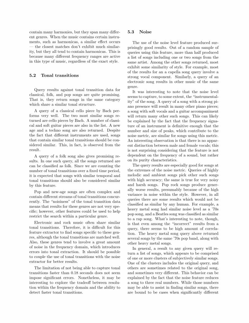
5.3 Noise
The use of the noise level feature produced sur-prisingly good results. Out of a random sample ofqueries using this feature, more than half produceda list of songs including one or two songs from thesame artist. Among the other songs returned, mostexhibit some similarity of style. For example, mostof the results for an a capella song query involve astrong vocal component. Similarly, a query of anelectronic song results in other music of the samegenre.
It was interesting to note that the noise levelseems to capture, to some extent, the “instrumental-ity” of the song. A query of a song with a strong pi-ano presence will result in many other piano pieces;a song with soft vocals and a guitar accompanimentwill return many other such songs. This can likelybe explained by the fact that the frequency signa-ture of an instrument is definitive enough that thenumber and size of peaks, which contribute to thenoise metric, are similar for songs using this metric.An interesting observation is that there is no appar-ent distinction between male and female vocals; thisis not surprising considering that the feature is notdependent on the frequency of a sound, but ratheron its purity characteristics.
The query results are especially good for songs atthe extremes of the noise metric. Queries of highlymelodic and ambient songs pick other such songswith high accuracy; the same is true for very noisyand harsh songs. Pop rock songs produce gener-ally worse results, presumably because of the highvariance in noise within the style. However, in allqueries there are some results which would not beclassified as similar by any human. For example, aheavy metal song had similar noise level as a ’70spop song, and a Beatles song was classified as similarto a rap song. What’s interesting to note, though,is that even among the “incorrect” results from aquery, there seems to be high amount of correla-tion. The heavy metal song query above returnedseveral songs by the same ’70s pop band, along withother heavy metal songs.
In general, a result to any given query will re-turn a list of songs, which appears to be comprisedof one or more clusters of subjectively similar songs.One of the clusters includes the original query, andothers are sometimes related to the original song,and sometimes very different. This behavior can beexplained by the fact that the noise feature reducesa song to three real numbers. While those numbersmay be able to assist in finding similar songs, thereare bound to be cases when significantly different
styles of music will result in similar noise feature.This means that the noise feature can be used toidentify subclasses of songs, but it is unable to dis-tinguish between certain subclasses. However, thisis still a useful result, since we can use other featuresto separate these subclasses, hopefully leaving onlytruly similar songs.
5.4 Volume
The volume level feature produced mixed results.From experiments, there appears to be some corre-lation between the queries and the results. In par-ticular, the number of songs selected which are bythe same artist is higher than that expected in a ran-dom distribution. However, the correlation is smallenough that it is difficult to analyze the rest of theresults from a query. There are many results whichare highly dissimilar from the original query, and itis difficult to judge how similar the rest are, due tothe subjective nature of similarity.
These results are perhaps not surprising. Thevariation in volume level, unlike some of the otherfeatures, is not something that is very noticeable ormemorable to a human; it is difficult to identify astyle of music with high or low volume variation.Furthermore, there is a large amount of variance inthe feature based on the recording. For example,a live and a studio recording of the same song arebound to have different values for the volume levelfeature. It may still be possible, however, to exploitthe small amount of correlation exhibited by thisfeature, if it is used in the similarity search but witha low weight relative to other features.
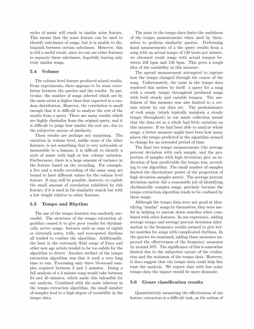
5.5 Tempo and Rhythm
The use of the tempo features was modestly suc-cessful. The structure of the tempo extraction al-gorithm caused it to give poor results for rhythmi-cally active songs: features such as runs of eighthor sixteenth notes, trills, and syncopated rhythmsall tended to confuse the algorithm. Additionally,the beat in the extremely fluid songs of Enya andother new age artists tended to be too subtle for thealgorithm to detect. Another artifact of the tempoextraction algorithm was that it took a very longtime to run. Processing only three 10-second sam-ples required between 3 and 5 minutes. Doing afull analysis of a 4 minute song would take between24 and 40 minutes, which made this infeasible forour analysis. Combined with the noise inherent inthe tempo extraction algorithm, the small numberof samples lead to a high degree of variability in thetempo data.
The noise in the tempo data limits the usefulnessof the tempo measurements when used by them-selves to perform similarity queries. Performinghand measurements of a the query results from asong with an actual tempo of 138 beats per minute,we obtained result songs with actual tempos be-tween 102 bpm and 156 bpm. This gives a roughidea of the variability in this measure.
The spread measurement attempted to capturehow the tempo changed through the course of thesong. Unfortunately, the noise in the tempo datarendered this useless by itself: a query for a songwith a steady tempo throughout produced songswith both steady and variable tempos. The use-fulness of this measure was also limited to a cer-tain extent by our data set. The predominanceof rock songs (which typically maintain a steadytempo throughout) in our music collection meantthat the data set as a whole had little variation onthis measure. If we had been able to analyze wholesongs, a better measure might have been how manyplaces the tempo predicted in the algorithm seemedto change for an extended period of time.
The final two tempo measurements (the averagepercent deviation with each sample, and the pro-portion of samples with high deviation) give an in-dication of how predictable the tempo was, accord-ing to our algorithm. The small number of sampleslimited the discrimitave power of the proportion ofhigh deviation samples metric. The average percentdeviation metric did a reasonable job of identifyingrhythmically complex songs, precisely because thetempo extraction algorithm tends to be confused bythese songs.
Although the tempo data were not good at iden-tifying “similar” songs by themselves, they were use-ful in helping to narrow down searches when com-bined with other features. In our experience, addingaverage tempo and average percent deviation infor-mation to the frequency results seemed to give bet-ter matches for songs with complicated rhythms. Inthe queries we examined, adding these measures im-proved the effectiveness of the frequency measuresby around 10%. The significance of this is somewhatlimited due to the subjective nature of the evalua-tion and the noisiness of the tempo data. However,it does suggest that the tempo data could help finetune the analysis. We expect that with less noisytempo data the impact would be more dramatic.
5.6 Genre classification results
Quantitatively measuring the effectiveness of ourfeature extractors is a difficult task, as the notion of
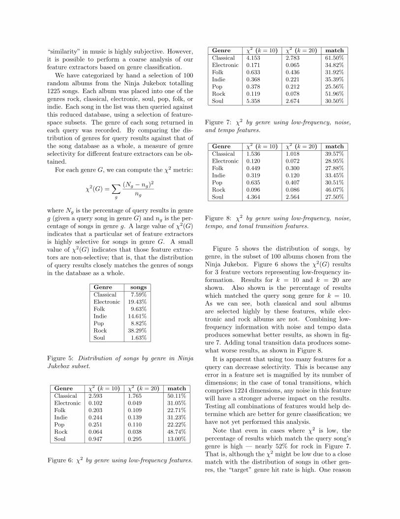
“similarity” in music is highly subjective. However,it is possible to perform a coarse analysis of ourfeature extractors based on genre classification.
We have categorized by hand a selection of 100random albums from the Ninja Jukebox totalling1225 songs. Each album was placed into one of thegenres rock, classical, electronic, soul, pop, folk, orindie. Each song in the list was then queried againstthis reduced database, using a selection of feature-space subsets. The genre of each song returned ineach query was recorded. By comparing the dis-tribution of genres for query results against that ofthe song database as a whole, a measure of genreselectivity for different feature extractors can be ob-tained.
For each genre G, we can compute the χ2 metric:
χ2(G) =∑
g
(Ng − ng)2
ng
where Ng is the percentage of query results in genreg (given a query song in genre G) and ng is the per-centage of songs in genre g. A large value of χ2(G)indicates that a particular set of feature extractorsis highly selective for songs in genre G. A smallvalue of χ2(G) indicates that those feature extrac-tors are non-selective; that is, that the distributionof query results closely matches the genres of songsin the database as a whole.
Genre songs
Classical 7.59%Electronic 19.43%Folk 9.63%Indie 14.61%Pop 8.82%Rock 38.29%Soul 1.63%
Figure 5: Distribution of songs by genre in NinjaJukebox subset.
Genre χ2 (k = 10) χ2 (k = 20) match
Classical 2.593 1.765 50.11%Electronic 0.102 0.049 31.05%Folk 0.203 0.109 22.71%Indie 0.244 0.139 31.23%Pop 0.251 0.110 22.22%Rock 0.064 0.038 48.74%Soul 0.947 0.295 13.00%
Figure 6: χ2 by genre using low-frequency features.
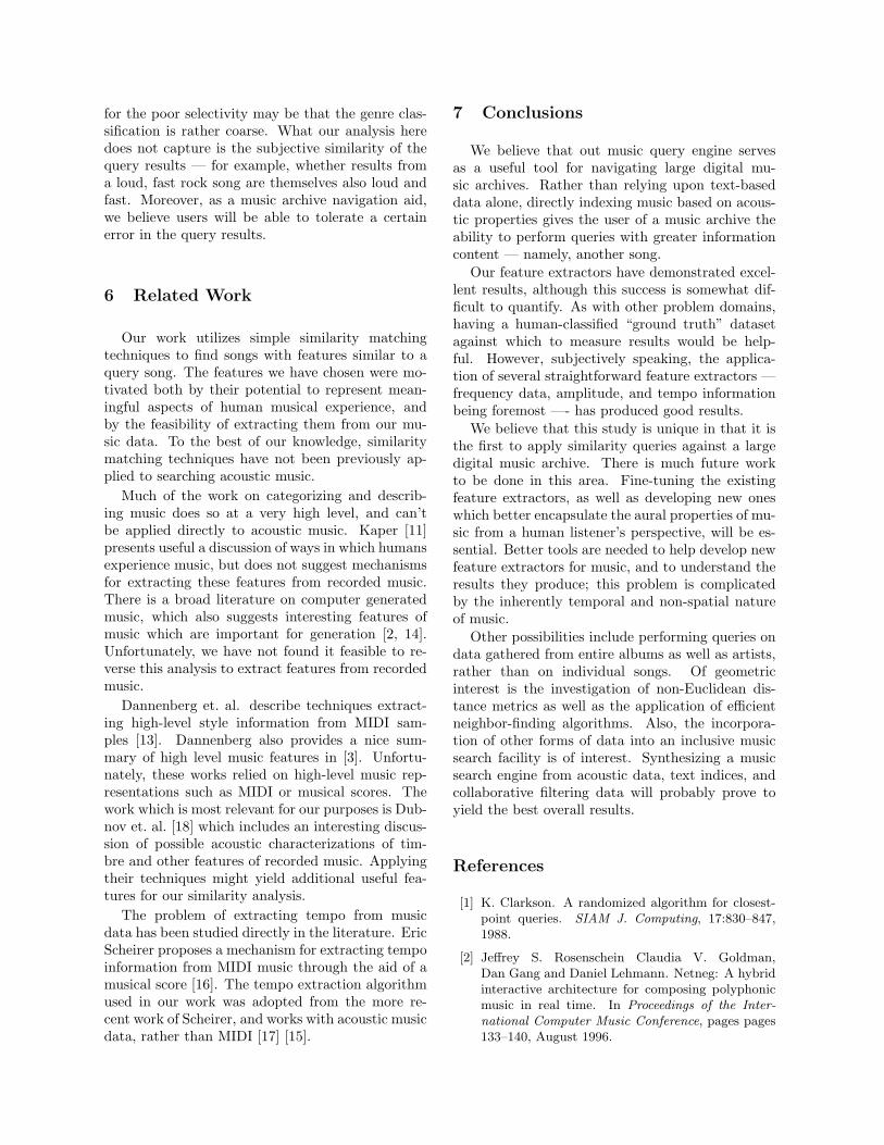
Genre χ2 (k = 10) χ2 (k = 20) match
Classical 4.153 2.783 61.50%Electronic 0.171 0.065 34.82%Folk 0.633 0.436 31.92%Indie 0.368 0.221 35.39%Pop 0.378 0.212 25.56%Rock 0.119 0.078 51.96%Soul 5.358 2.674 30.50%
Figure 7: χ2 by genre using low-frequency, noise,and tempo features.
Genre χ2 (k = 10) χ2 (k = 20) match
Classical 1.536 1.018 39.57%Electronic 0.120 0.072 28.95%Folk 0.449 0.300 27.88%Indie 0.319 0.120 33.45%Pop 0.635 0.407 30.51%Rock 0.096 0.086 46.07%Soul 4.364 2.564 27.50%
Figure 8: χ2 by genre using low-frequency, noise,tempo, and tonal transition features.
Figure 5 shows the distribution of songs, bygenre, in the subset of 100 albums chosen from theNinja Jukebox. Figure 6 shows the χ2(G) resultsfor 3 feature vectors representing low-frequency in-formation. Results for k = 10 and k = 20 areshown. Also shown is the percentage of resultswhich matched the query song genre for k = 10.As we can see, both classical and soul albumsare selected highly by these features, while elec-tronic and rock albums are not. Combining low-frequency information with noise and tempo dataproduces somewhat better results, as shown in fig-ure 7. Adding tonal transition data produces some-what worse results, as shown in Figure 8.
It is apparent that using too many features for aquery can decrease selectivity. This is because anyerror in a feature set is magnified by its number ofdimensions; in the case of tonal transitions, whichcomprises 1224 dimensions, any noise in this featurewill have a stronger adverse impact on the results.Testing all combinations of features would help de-termine which are better for genre classification; wehave not yet performed this analysis.
Note that even in cases where χ2 is low, thepercentage of results which match the query song’sgenre is high — nearly 52% for rock in Figure 7.That is, although the χ2 might be low due to a closematch with the distribution of songs in other gen-res, the “target” genre hit rate is high. One reason
for the poor selectivity may be that the genre clas-sification is rather coarse. What our analysis heredoes not capture is the subjective similarity of thequery results — for example, whether results froma loud, fast rock song are themselves also loud andfast. Moreover, as a music archive navigation aid,we believe users will be able to tolerate a certainerror in the query results.
6 Related Work
Our work utilizes simple similarity matchingtechniques to find songs with features similar to aquery song. The features we have chosen were mo-tivated both by their potential to represent mean-ingful aspects of human musical experience, andby the feasibility of extracting them from our mu-sic data. To the best of our knowledge, similaritymatching techniques have not been previously ap-plied to searching acoustic music.
Much of the work on categorizing and describ-ing music does so at a very high level, and can’tbe applied directly to acoustic music. Kaper [11]presents useful a discussion of ways in which humansexperience music, but does not suggest mechanismsfor extracting these features from recorded music.There is a broad literature on computer generatedmusic, which also suggests interesting features ofmusic which are important for generation [2, 14].Unfortunately, we have not found it feasible to re-verse this analysis to extract features from recordedmusic.
Dannenberg et. al. describe techniques extract-ing high-level style information from MIDI sam-ples [13]. Dannenberg also provides a nice sum-mary of high level music features in [3]. Unfortu-nately, these works relied on high-level music rep-resentations such as MIDI or musical scores. Thework which is most relevant for our purposes is Dub-nov et. al. [18] which includes an interesting discus-sion of possible acoustic characterizations of tim-bre and other features of recorded music. Applyingtheir techniques might yield additional useful fea-tures for our similarity analysis.
The problem of extracting tempo from musicdata has been studied directly in the literature. EricScheirer proposes a mechanism for extracting tempoinformation from MIDI music through the aid of amusical score [16]. The tempo extraction algorithmused in our work was adopted from the more re-cent work of Scheirer, and works with acoustic musicdata, rather than MIDI [17] [15].
7 Conclusions
We believe that out music query engine servesas a useful tool for navigating large digital mu-sic archives. Rather than relying upon text-baseddata alone, directly indexing music based on acous-tic properties gives the user of a music archive theability to perform queries with greater informationcontent — namely, another song.
Our feature extractors have demonstrated excel-lent results, although this success is somewhat dif-ficult to quantify. As with other problem domains,having a human-classified “ground truth” datasetagainst which to measure results would be help-ful. However, subjectively speaking, the applica-tion of several straightforward feature extractors —frequency data, amplitude, and tempo informationbeing foremost —- has produced good results.
We believe that this study is unique in that it isthe first to apply similarity queries against a largedigital music archive. There is much future workto be done in this area. Fine-tuning the existingfeature extractors, as well as developing new oneswhich better encapsulate the aural properties of mu-sic from a human listener’s perspective, will be es-sential. Better tools are needed to help develop newfeature extractors for music, and to understand theresults they produce; this problem is complicatedby the inherently temporal and non-spatial natureof music.
Other possibilities include performing queries ondata gathered from entire albums as well as artists,rather than on individual songs. Of geometricinterest is the investigation of non-Euclidean dis-tance metrics as well as the application of efficientneighbor-finding algorithms. Also, the incorpora-tion of other forms of data into an inclusive musicsearch facility is of interest. Synthesizing a musicsearch engine from acoustic data, text indices, andcollaborative filtering data will probably prove toyield the best overall results.
References
[1] K. Clarkson. A randomized algorithm for closest-point queries. SIAM J. Computing, 17:830–847,1988.
[2] Jeffrey S. Rosenschein Claudia V. Goldman,Dan Gang and Daniel Lehmann. Netneg: A hybridinteractive architecture for composing polyphonicmusic in real time. In Proceedings of the Inter-national Computer Music Conference, pages pages133–140, August 1996.
[3] Roger B. Dannenberg. Recent work in music under-standing. In Proceedings of the 11th Annual Sympo-sium on Small Computers in the Arts, pages pages9–14, November 1991.
[4] D. Dobkin and R. Lipton. Multidimensional searchproblems. SIAM J. Computing, 5:181–186, 1976.
[5] David Gibson. Name That Clip:Content-based music retrieval.http://www.cs.berkeley.edu/~dag/NameThat-
Clip/, 1999.
[6] I. Goldberg, S. Gribble, D. Wagner, and E. Brewer.The ninja jukebox. In 2nd USENIX Symposium onInternet Technologies and Systems, October 1999.
[7] S. Gribble, M. Welsh, D. Culler, and E. Brewer.Multispace: An evolutionary platform for infras-tructural services. In Proceedings of the 16thUSENIX Annual Technical Conference, Monterey,California, 1999.
[8] Gebeshuber I.C. and Rattay F. Modelled humanhearing threshold curve, 1998.
[9] PSB Speakers International. The frequencies- and sound - of music. http://www.psb-
speakers.com/frequenciesOfMusic.html.
[10] ISO/IEC 13818-3. Information Technology:Generic coding of moving pictures and associatedaudio - audio part. International Standard, 1995.
[11] H. G. Kaper and S. Tipei. Abstract approach tomusic. In Preprint ANL/MCS-P748-0399, March1999.
[12] J. Kleinberg. Two algorithms for nearest-neighborsearch in high dimensions. In Proc. 29th ACM Sym-posium on Theory of Computing, 1997.
[13] Belinda Thom Roger B. Dannenberg and DavidWatson. A machine learning approach to musicalstyle recognition. In International Computer MusicConference, pages pages 344–347, September 1997.
[14] B. J. Ross. A process algebrafor stochastic music composition.http://www.cosc.brocku.ca/Research/TechRep/,February 1995.
[15] Eric D. Scheirer. Pulse tracking with a pitchtracker. In Proc 1997 IEEE Workshop on Applica-tions of Signal Processing to Audio and Acoustics,October 1997.
[16] Eric D. Scheirer. Using Musical Knowledge toExtract Expressive Performance Information fromAudio Recordings. 1997.
[17] Eric D. Scheirer. Tempo and beat analysis of acous-tic musical signals. In J. Acoust. Soc. Am. 103:1,pages pages 588–601, January 1998.
[18] Naftali Tishby Shlomo Dubnov and Dalia Cohen.Hearing beyond the spectrum. In Journal of NewMusic Research, Vol. 25, 1996.