arX

iv:1

304.

5095

v2 [

gr-q

c] 1

3 Ju

n 20

13

Quasi-dilaton non-linear massive gravity: Investigations of background

cosmological dynamics

Radouane Gannouji,1 Md. Wali Hossain,2 M. Sami,3, 2 and Emmanuel N. Saridakis4, 5

1Astrophysics and Cosmology Research Unit, School of Mathematics,Statistics and Computer Sciences, Univ. of KwaZulu-Natal,

Private Bag X54001, Durban 4000, South Africa2Centre for Theoretical Physics, Jamia Millia Islamia, New Delhi-110025, India

3Department of Physics, Nagoya University, Nagoya 464-8602, Japan4Physics Division, National Technical University of Athens, 15780 Zografou Campus, Athens, Greece5Instituto de Fısica, Pontificia Universidad de Catolica de Valparaıso, Casilla 4950, Valparaıso, Chile

We investigate cosmological behavior in the quasi-Dilaton non-linear massive gravity. We performa detailed dynamical analysis and examine the stable late-time solutions relevant to late time cosmicacceleration. We demonstrate that a dark-energy dominated, cosmological-constant-like solution isa late attractor of the dynamics. We also analyze the evolution of the universe at intermediate times,showing that the observed epoch sequence can be easily obtained in the model under consideration.Furthermore, we study the non-singular bounce and the cosmological turnaround which can berealized for a region of the parameter space. Last but not least, we use observational data from TypeIa Supernovae (SNIa), Baryon Acoustic Oscillations (BAO) and Cosmic Microwave Background(CMB), in order to constrain the parameters of the theory.

PACS numbers: 98.80.-k, 95.36.+x, 04.50.Kd

I. INTRODUCTION

It is widely believed that an elementary particleof mass m and spin s is described by a field whichtransforms according to a particular representation ofPoincare group. In field theory, formulated in Minkowskispace-time, mass can either be introduced by hand orvia spontaneous symmetry breaking. The spin-2 fieldhµν is supposed to be relevant to gravity as it sharesan important property of universality with Einstein gen-eral relativity(GR) a la Weinberg theorem and GR canbe thought as an interacting theory of hµν . It is there-fore natural to first formulate the field theory of hµν inMinkowski space-time and then extend the concept tonon-linear background.The first formulation of a linear massive theory of grav-

ity was given by Fierz and Pauli [1] with a motivation towrite down the consistent relativistic equations for higherspin fields including spin-2 field. The linear theory ofFierz-Pauli, however, suffers from van Dam, Veltman,Zakharov (vDVZ) discontinuity [2, 3]: in the zero-masslimit, the theory is at finite difference from GR. The un-derlying reason of the (vDVZ) discontinuity is related tothe fact the longitudinal degree of freedom of massivegraviton does not decouple in the said limit; it is rathercoupled to the source with the strength of the universalcoupling at par with the massless mode.It was pointed out by Vainshtein that linear approxi-

mation in the neighborhood of a massive source breaksdown below certain distance dubbed Vainshtein radiusand by incorporating non-linearities one could remove thediscontinuity [4] present in the linear theory. However,the sixth degree of freedom, suppressed in Pauli-Fierztheory, which is essentially a ghost known as Boulware-Deser (BD) ghost [5], becomes alive in the non-linear

background.

Efforts were then made to find out the non-linear ana-log of Fierz-Pauli mass term requiring the ghost to besystematically removed. The authors of Ref.[6, 7] dis-covered a specific nonlinear extension of massive gravity(dRGT ) that is BD-ghost free in the decoupling limit(see[8] for a review). Subsequently, it was demonstrated[9] that the Hamiltonian constraint is maintained at thenon-linear order along with the associated secondary con-straint, which implies the absence of the BD ghost. Apartfrom the field theoretic interests of such a construction,there is a cosmological motivation to study massive grav-ity. This formulation provides a new class of (Infra-Red)gravity modification which can give rise to late-time cos-mic acceleration and it is therefore not surprising thatmassive gravity has recently generated enormous inter-est in cosmology [9–71].

In spite of the the successes of the framework, ithas challenging problems to be resolved, namely, themodel does not admit spatially flat FLRW backgroundwhereas isotropic and homogeneous cosmological solu-tions (K = ±1) are perturbatively unstable [72]. Thelatter speaks of some inherent difficulty of dRGT . Thisled the authors of [73, 74] to abandon isotropy whereas inRef.[75], effort was made to address the problem by mak-ing the graviton mass a field dependent quantity througha more radical approach, namely by extending the the-ory to a varying graviton mass driven by a scalar field[76, 77]. A similar approach was followed in [78], wherethe framework of massive gravity was extended by in-troducing a quasi-dilaton field. It was pointed that themodel could rise to a healthy cosmology in the FLRW

2

background1.

In this work we carry out detailed dynamical investi-gations of cosmological behaviors in the aforementionedquasi-Dilaton non-linear massive gravity. In particular,we perform dynamical analysis relevant to late time cos-mic acceleration, and moreover we examine the realiza-tion of non-singular bouncing solutions. Finally, we useobservational data in order to constrain the model pa-rameters.

The plan of the paper is as follows: In section II wereview the quasi-dilaton non-linear massive gravity andits cosmological implications. In section III, we performa detailed dynamical analysis and obtain the late-timestable solutions, while in section IV we investigate theuniverse evolution focusing on bouncing and turnaroundsolutions. In section V we use observations in order toconstrain the model parameters and finally in section VI,we summarize the results of our analysis.

II. QUASI-DILATON NON-LINEAR MASSIVE

GRAVITY AND COSMOLOGY

In this section we briefly review the quasi-dilaton non-linear massive gravitational formulation following [78].In the first subsection we present the gravitational the-ory itself, while in the next subsection we examine itscosmological implications in presence of matter and ra-diation.

A. Massive gravity with quasi-dilaton

Let us consider the following action of non-linear mas-sive gravity with dilaton

Sgr = SEH + Smass + Sσ, (1)

with

SEH =M2

Pl

2

∫

d4x√−g R (2)

the usual Einstein-Hilbert action,

Smass =m2M2

Pl

8

∫

d4x√−g

[

U2 + α3U3 + α4U4

]

(3)

1 During the finalization of the present work, a perturbation anal-ysis of the stability of the model was performed in [79, 80], whereit was shown that the de Sitter solution of the model may havea ghost instability for short wavelength modes, shorter than cos-mological scales. The calculations were performed at the linearorder of perturbations, or equivalently at second order in the ac-tion. It will be interesting to see whether the ghost exists in anon-linear approach of the stability analysis.

the action corresponding to non-linear massive term,along with the action of a massless dilaton σ

Sσ = −ω

2

∫

d4x (∂σ)2. (4)

In action (3), α3, α4 are two arbitrary parameters andUi are specific polynomials of the matrix

Kµν = δµν − eσ/MP l

√

gµα∂αφa∂νφbηab, (5)

given by

U2 = 4([K]2 − [K2]) (6)

U3 = [K]3 − 3[K][K2] + 2[K3] (7)

U4 = [K]4 − 6[K]2[K2] + 3[K2]2 + 8[K][K3]− 6[K4]. (8)

In (5), ηab (Minkowski metric) is a fiducial metric, andφa(x) are the Stuckelberg scalars introduced to restoregeneral covariance [81].

B. Cosmology

In order to apply the above gravitational theory in cos-mological frameworks, we also have to incorporate thematter and radiations sectors. Thus, the total action weconsider is as follows

S = SEH + Smass + Sσ + Sm + Sr, (9)

in which Sm and Sr denote the standard matter and ra-diation actions, corresponding to ideal fluids with energydensities ρm, ρr and pressures pm, pr respectively. Insummary, we consider a scenario of usual nonlinear mas-sive gravity [6, 7] coupled with a dilaton field σ, wherethe coupling is introduced through (5) [78].Next, we consider a flat Friedmann-Lemaıtre-

Robertson-Walker (FLRW) metric of the form

ds2 = gµνdxµdxν = −N(t)2dt2 + a2(t)δijdx

idxj , (10)

while for the Stuckelberg scalars we consider the ansatz

φ0 = f(t), φi = xi. (11)

In this case the actions (2)-(4) become:

SEH = −3M2Pl

∫

dt[aa2

N

]

(12)

Smass = 3m2M2Pl

∫

dta3[

NG1(ξ)− faG2(ξ)]

(13)

Sσ =ω

2

∫

dt a3[ σ2

N

]

, (14)

where we have defined

G1(ξ) = (1 − ξ)[

2− ξ +α3

4(1− ξ)(4 − ξ) + α4(1 − ξ)2

]

(15)

G2(ξ) = ξ(1 − ξ)[

1 +3

4α3(1− ξ) + α4(1− ξ)2

]

(16)

3

being functions of the introduced dilaton-variable

ξ =eσ/MPl

a. (17)

Variation with respect to f gives the constraint equa-tion (as an essential feature of any model of non-linearmassive gravity)

G2(ξ) =C

a4, (18)

where C is a constant of integration.Variation with respect to the lapse function N and

setting N = 1 at the end, leads to the first Friedmannequation

3M2PlH

2 =ρm + ρr − 3m2M2

PlG1

1− ω6

(

1− 4 G2

ξG′

2

)2 , (19)

where primes in G’s denote derivatives with respect totheir argument ξ. Similarly, variation with respect to σprovides the dilaton evolution equation

ω

a3d

Ndt(a3σ) + 3MPlm

2[

F1(ξ) + afF2(ξ)]

= 0, (20)

where

F1(ξ) = 3(1 +3

4α3 + α4)ξ − 2(1 +

3

2α3 + 3α4)ξ

2

+3

4(α3 + 4α4)ξ

3 (21)

F2(ξ) = (1 +3

4α3 + α4)ξ − 2(1 +

3

2α3 + 3α4)ξ

2

+9

4(α3 + 4α4)ξ

3 − 4α4ξ4. (22)

Finally, the evolution equations close by consider-ing the continuity equations for matter and radiation,namely ρm+3H(ρm+pm) = 0 and ρr +3H(ρr+pr) = 0respectively.Before proceeding to the detailed analysis of the model,

let us make a few comments. Firstly, as it was first no-ticed for a similar model in [67], the Friedmann equation(19) can exhibit singularities when the denominator goesto zero. However, as we will show in the next section,these singularities separate the phase space in discon-nected branches, that is the universe cannot evolve fromone to the other.As a second remark we mention that in the case where

C 6= 0, in the constraint equation (18) it appears a func-tion of 1/a4 which plays, in the early Universe, a rolesimilar to “Dark Matter” or “Dark Radiation”. In par-ticular, when α4 6= 0, in the early Universe (a → 0) rela-tion (17) gives ξ → ∞. This implies G2 ≃ −α4ξ

4 = C/a4

leading the Friedmann equation (19) to be

3M2PlH

2 ≃ ρm + ρr + 3m2M2Pl

(

α4 +α3

4

)(

− C

α4

)3/4

a−3,

(23)

that is an effective dark-matter term appears. Similarly,when α4 = 0 we acquire

3(

1− ω

54

)

M2PlH

2 ≃ ρm + ρr +m2M2PlCa−4, (24)

that is we get an effective dark radiation term.

Finally, we mention that in the particular case C = 0,(18) leads to a constant ξ, and the Friedmann equation(19) becomes

3M2PlH

2 = ρm + ρr − αΛ + βH2 , (25)

where αΛ, β are constants. It is interesting to notice thatthis relation appears as a particular case of Holographicmodels where the IR cut-off is fixed at the Hubble scale.In fact in the aforementioned theories the number of de-grees of freedom in a finite volume should be finite andrelated to the area of its boundary. This gives an upperbound on the entropy contained in the visible Universe.Following an idea suggested by [82, 83] where a long dis-tance cut-off is related to a short distance cut-off, in [84]it was suggested to take the largest distance as the Hub-ble scale or the event horizon. Later these models weredubbed holographic dark energy [85].

All these particular cases reveal the richness and thecapabilities of the scenario. In what follows we shall castthe evolution equations in the autonomous form and in-vestigate their implications for late time cosmology.

III. DYNAMICAL BEHAVIOR

In this section we perform a dynamical analysis of thescenario at hand, which allows us to bypass the com-plexities of the equations and obtain information for thelate-time, asymptotic, cosmological behavior [86–88]. Wemention here that in [78] the authors investigated the cos-mological implications in a specific setting allowing themto obtain simple analytical solutions. However, in thiswork we are interested in the full dynamical investiga-tions of evolution equations.

A. Phase-space analysis

In order to perform a phase-space analysis, we firsttransform the involved cosmological equations into theirautonomous form introducing suitable auxiliary vari-ables. We extract the critical points of the dynamicalsystem under consideration, perturb the system aroundthem and analyze their stability by examining the eigen-values of the corresponding perturbation matrix.

4

Let us first introduce the density parameters

Ωm =ρm

3M2PlH

2(26)

Ωr =ρr

3M2PlH

2(27)

ΩΛ = −m2 G1

H2(28)

Ωσ =ω

6

(

1− 4G2

ξG′2

)2

, (29)

with which we can re-write the Friedmann equation (19)as

Ωm +Ωr +ΩΛ +Ωσ = 1. (30)

Thus, we can now transform the above cosmological sys-tem into its autonomous form, using only the dimension-less variables Ωr, ΩΛ and ξ, while (30) will be used toeliminate Ωm. Doing so we obtain

dΩr

d ln a= −2Ωr

(

2 +H

H2

)

(31)

dΩΛ

d ln a= −2ΩΛ

(

2G2G

′1

G1G′2

+H

H2

)

(32)

dξ

d ln a= −4

G2

G′2

, (33)

where the combination HH2 can be acquired differentiating

the first Friedmann equation (19) as

H

H2=

−9Ωm − 12Ωr − 12G2

G′

2

[

G′

1

G1

ΩΛ + ω6

ddξ (1 − 4 G2

ξG′

2

)2]

6− ω[

1− 4 G2

ξG′

2

]2 .

(34)

A comment about the role of dilaton in the scenario un-der consideration is in order. The dilaton role is twofold,first, it has an effect through its impact on the gravitonmass, since in the above equations m appears multipliedby a function of ξ, that is of the exponential of the dila-ton field. This is what we call ΩΛ. Secondly, the dilatonhas an effect through its kinetic term in (14), which is ofcourse proportional to the parameter ω. This is what wecall Ωσ. Therefore, strictly speaking, in the present sce-nario the effective dark energy sector includes both ΩΛ

and Ωσ, since these two contributions cannot be distin-guished observationally (we write them separately onlyfor clarity). Thus:

ΩDE ≡ ΩΛ +Ωσ = 1− Ωm − Ωr. (35)

Finally, note that in terms of the auxiliary variablesΩr, ΩΛ and ξ, we can express the physically interest-ing observables such as the total (effective) equation-of-state parameter weff , the deceleration parameter q andthe dark energy equation-of-state parameter wDE respec-tively as

weff = −1− 2

3

H

H2(36)

q = −1− H

H2=

1

2+

3

2weff . (37)

wDE =weff − wmΩm − wrΩr

ΩΛ +Ωσ, (38)

where the combination H/H2 is given by (34). Lastly, inthe following for simplicity we focus on the usual casesof standard dust matter wm = 0 and standard radiationwr = 1/3.The critical points of the above autonomous system are

extracted setting the left hand sides of equations (31)-(33) to zero. In particular, equation (33) implies thatat the critical points G2(ξ) = 0, which according to (16)gives ξ = 0, ξ = 1 and

ξ± = 1 +3α3 ±

√

9α23 − 64α4

8α4. (39)

In order for the critical points to be physical they have topossess 0 ≤ Ωr ≤ 1, 0 ≤ ΩΛ+Ωσ ≤ 1, 0 ≤ ξ and of courseξ ∈ R. Now, in order for ξ± ∈ R we require 9α2

3−64α4 ≥0 while 0 ≤ ξ leads to the necessary conditions for α’susing (39).The real and physically meaningful critical points

(Ωr,ΩΛ, ξ) of the autonomous system (31)-(33) are pre-sented in Table I, along with their existence conditions.We mention here that there is an additional existencecondition, namely the obtained H2 from (19) must bealways positive, a condition which constrains the allowedα3 and α4 values. We will come back to this later on.For each critical point we calculate the 3× 3 perturba-

tion matrix of the corresponding linearized perturbationequations, and examining the sign of the real part of itseigenvalues we determine the type and stability of thispoint (positive real parts correspond to unstable point,negative real parts correspond to stable point, and realparts with different signs correspond to saddle point).The eigenvalues and the stability results are summarizedin Table I.Finally, for completeness, in the same Table we present

the corresponding values of the rest density parametersΩm and Ωσ, as well as the calculated values for the ob-servables such as the deceleration parameter q, the totalequation-of-state parameter weff , and the dark energyequation-of-state parameter wDE . These results are inagreement with the general analysis of nonlinear massivegravity of [89].Before proceeding to the discussion of the physical im-

plications of these results, we make a remark concerningthe structure of the phase space. As we mentioned in theIntroduction, the Friedmann equation (19) exhibits sin-gularities when the denominator goes to zero. In particu-lar, in the scenario at hand we obtain various singularities

localized at the roots of 1−ω6

(

1−4 G2

ξG′

2

)2

, which, for every

parameter ω, is a function of the rescaled field-variable ξonly. Since ω must be relatively small in order to satisfyobservations (this will be confirmed later on), assuming

5

Cr.P. Ωr ΩΛ ξ Ωm Ωσ q weff wDE Existence conditions Stability EigenvaluesA 0 0 0 1− 3ω/2 3ω/2 1/2 0 0 0 ≤ ω ≤ 2/3 Saddle point -4, 3, -1B 0 1− 3ω/2 0 0 3ω/2 −1 -1 -1 0 ≤ ω ≤ 2/3 Attractor -4, -4, -3C 1− 3ω/2 0 0 0 3ω/2 1 1/3 1/3 0 ≤ ω ≤ 2/3 Saddle point -4, 4, 1D 0 0 1 1− ω/6 ω/6 1/2 0 0 0 ≤ ω ≤ 6 Attractor -4, -1, -1E± 0 0 ξ± 1− ω/6 ω/6 1/2 0 0 0 ≤ ω ≤ 6, 0 ≤ ξ±, ξ± ∈ R Saddle point -4,-1, 3F± 1− ω/6 0 ξ± 0 ω/6 1 1/3 1/3 0 ≤ ω ≤ 6, 0 ≤ ξ±, ξ± ∈ R Saddle point -4,4,1G± 0 1− ω/6 ξ± 0 ω/6 −1 -1 -1 0 ≤ ω ≤ 6, 0 ≤ ξ±, ξ± ∈ R Attractor -4,-4,-3I Ωr 1− ω/6− Ωr 1 0 ω/6 1 1/3 1/3 0 ≤ ω ≤ 6 Saddle -4,1,0

TABLE I: The real and physically meaningful critical points of the autonomous system (31)-(33), their existence conditions,the eigenvalues of the perturbation matrix, and the deduced stability conditions. We also present the corresponding values ofthe various density parameters, and the values of the observables: deceleration parameter q, total equation-of-state parameterweff and dark energy equation-of-state parameter wDE.

ω ≪ 1 the zeros of the previous function nearly coincidewith the roots of G′

2(ξ). But as we mentioned above, thecritical points correspond to G2(ξ) = 0. Thus, using theRolle’s theorem, we conclude that each cosmological late-time solution (G2(ξ) = 0) and the corresponding region,is disconnected from the others by a singularity (G′

2 = 0).In other words, during its evolution, the universe cannottransit from one of these regions to another.

B. Physical implications

In the previous subsection we performed a completephase-space analysis of the scenario at hand, we ex-tracted the late-time stable solutions (attractors) and wecalculated the corresponding observables. Here we dis-cuss their cosmological implications.As we observe from Table I, there exist four stable crit-

ical points, that can attract the universe at late times,namely B, D and the two points G±. Points B andG± correspond to a dark-energy dominated, accelerat-ing universe, where dark energy behaves like cosmologi-cal constant (de Sitter solutions). These features makethese points very good candidates for the description oflate-time universe. On the other hand, point D corre-sponds to a non-accelerating universe, with dark energyand matter density parameters of the same order (thatis it can alleviate the coincidence problem), but the darkenergy has a stiff equation of state. Therefore, this pointis disfavored by observations.Apart from the above stable late-time solutions, the

scenario of quasi-Dilaton non-linear massive gravitypossesses the non-accelerating, stiff dark-energy pointsA,C,E±,F±, and the critical curve I. These points aresaddle (I is non-hyperbolic curve with saddle behavior)and thus they cannot be the late time states of the uni-verse, and moreover their cosmological features are notfavored by observations.Let us make a comment here on the appearance of

more than one stable critical points, which for some pa-rameter choices can exist simultaneously. Although thebi-stability and multi-stability is usual in complicated dy-

namical systems [90, 91], with each critical point attract-ing orbits initially starting inside its basin of attraction,in the present scenario the case is simpler, since thesepoints usually lie in the disconnected regions we men-tioned in the previous subsection, separated by the ξ val-ues that make the denominator of (19) zero, and thus toBig-Rip-type divergences [92–95]. Finally, note that forω > 6 there are not stable late-time solutions, that is thecorresponding cosmology is not interesting.

0.0 0.2 0.4 0.6 0.8 1.00.0

0.2

0.4

0.6

0.8

1.0

Wm

WD

E

matter phase

radiation era

de Sitter

FIG. 1: Trajectories in the ΩDE-Ωm plane of the cosmologicalscenario of quasi-Dilaton non-linear massive gravity, for theparameter choice α3 = 1,α4 = 1 and ω = 0.01. In this spe-cific example the universe at late times is led to the de Sittersolution.

Finally, as we previously mentioned, the α3-α4 param-eter subspace is constrained by the condition the ob-tained H2 from (19) to be always positive. The cor-responding constraints are complicated and we do notpresent them here, however they do get a very simpleform when the universe evolves towards its interestingstable late-time states B and G± (where Ωr and Ωm be-come smaller and smaller). In particular, for the point B

6

we obtain 2 + α3 + α4 < 0, for the point G+ we acquire

α3 > 0, 0 < α4 <α2

3

8 and for the point G− we obtain

α3 < 0 and 0 < α4 <α2

3

8 .In order to present the cosmological behavior more

transparently, we numerically evolve the autonomous sys-tem (31)-(33) for the the parameter choice α3 = 1,α4 = 1and ω = 0.01, and in Fig. 1 we depict the correspondingphase-space behavior in the ΩDE-Ωm plane.

IV. COSMOLOGICAL EVOLUTION

In the previous section we performed a dynamical anal-ysis of quasi-Dilaton non-linear massive gravity, that iswe focused on its asymptotic behavior at late times, thatis on solutions that are going to attract the universe in-dependently of the initial conditions and of the specificcosmological evolution towards them. In this section weinvestigate the behavior of the universe at intermediatetimes, which obviously does depend on the initial condi-tions, but it can be very interesting. In particular, weare interested in obtaining a evolution of the universe inagreement with the observed epoch sequence. Further-more, we examine the possibility of obtaining bouncingbehavior. In the following subsections we discuss thesetwo cosmological behaviors separately.

A. Epoch sequence and late-time acceleration

Let us first examine the universe evolution, focusingon the various density parameters and the dark-energyequation of state. Observing the Friedmann equation(19), as well as the evolution equations for the densityparameters and for ξ (31)-(33), we deduce that the ob-served post-inflationary thermal history of the universecan be easily obtained by suitably choosing the modelparameters.In order to present this behavior more transparently,

we numerically evolve the system for α3 = 1, α4 = 0.115and ω = 0.01, starting with initial conditions correspond-ing to Ωr ≈ 1, and imposing the current values to beΩm ≈ 0.28 and ΩDE ≈ 0.72. In Fig. 2 we depict theresulting evolution for the density parameters using, in-stead of the scale factor, the redshift z as the indepen-dent variable (1 + z = a0/a with a0 = 1 the presentscale-factor value). As we observe, the thermal historyof the universe can be reproduced, namely we obtain thesuccessive sequence of radiation, matter and dark energyepochs.Similarly, in Fig. 3 we present the corresponding evo-

lution of the total equation-of-state parameter weff aswell as of the dark-energy one wDE . As we observe,dark energy starts from a dust-like behavior, resultingin a cosmological-constant-like one at the current uni-verse, driving the observed acceleration. Note that, asexpected, in the future, where dark energy completely

-1 0 1 2 3 4 5 60.0

0.2

0.4

0.6

0.8

1.0

Log10 @1+ zD

W

Wm

Wr

WDE

FIG. 2: Cosmological evolution of the radiation (Ωr), matter(Ωm) and dark energy (ΩDE ≡ ΩΛ +Ωσ) density parameters,as a function of the redshift z, for the parameter choice α3 =1, α4 = 0.115 and ω = 0.01. In this specific example theobserved universe epoch sequence is reproduced.

-1 0 1 2 3 4 5 6-1.0

-0.8

-0.6

-0.4

-0.2

0.0

0.2

Log10 @1+ zD

ww eff

w DE

FIG. 3: Cosmological evolution of the total (weff ) and of thedark-energy (wDE) equation-of-state parameters, as a func-tion of the redshift z, for the parameter choice α3 = 1, α4 =0.115 and ω = 0.01. In this specific example, dark energystarts from a dust-like behavior, resulting in a cosmological-constant-like one at the current epoch, which drives the ob-served universe acceleration.

dominates, both weff and wDE coincide at the cosmo-logical constant value.

B. Bouncing and turnaround solutions

In this subsection we examine the bounce realizationin the scenario at hand. Bouncing cosmologies in gen-eral have gained significant interest, since they offer analternative paradigm free of the “Big-Bang singularity”,as well as of the horizon, flatness and monopole problems[96]. The basic condition for the bounce is the Hubbleparameter to change sign from negative to positive, while

7

its time-derivative to be positive. Additionally, whenthe Hubble parameter changes from positive to nega-tive, while its time-derivative is negative, we have therealization of a cosmological turnaround. Such a behav-ior implies the Null Energy Condition (NEC) violationaround the bounce (or the turnaround), which is non-trivial in the context of General Relativity [97], leadingin general to ghost degrees of freedom [98, 99]. How-ever, a safe bounce evolution, free of ghosts and instabil-ities, is possible in various modified gravity constructions[100, 101]. Clearly, observing the Friedmann equation(19) of the present scenario of quasi-Dilaton non-linearmassive gravity, we deduce that the basic bounce (orturnaround) realization condition can be easily fulfilled.In order to quantify the above discussion, and assum-

ing standard dust matter and standard radiation, werewrite the Friedmann equation (19) in the followingform:

H2

H20

=Ωm0a

−3 +Ωr,0a−4 − m2

H2

0

G1

1− ω6

(

1− 4 G2

ξG′

2

)2 , (40)

where Ωm0 and Ωr,0 are the values of the correspond-ing density parameters at present (a0 = 1), and H0 thecurrent Hubble parameter. Furthermore, since the con-straint equation (18) provides ξ as a function of the scalefactor, we can finally write (40) as

H2

H20

= V (a), (41)

with C,α3, α4, ω,m and Ωm0,Ωr,0 as parameters. Insummary, examining the behavior of the above knownV (a), we can find possible bouncing points at a = aB(when V (aB) = 0 and H−1

0ddt

√

V (aB) > 0), or possi-ble turnaround points at a = aT (when V (aT ) = 0 and

H−10

ddt

√

V (aT ) < 0). This procedure is straightforward,and thus we deduce that both bounce and turnaround arepossible in the scenario of quasi-Dilaton non-linear mas-sive gravity. Although one can apply it in full generality,obtaining exact results, since the involved expressions foraB and aT are lengthy in the following we explicitly applyit in a specific simple example, where simple expressionscan be easily obtained.First of all, since a bounce occurs in the early universe,

that is at small scale factors (a ≪ a0 = 1), from (18) wededuce that at the bounce ξ ≫ 1. On the other hand,since a turnaround occurs in the late universe, that is ata ≫ a0 = 1, from (18) we deduce that at the turnaroundG2(ξ) = 0.Let us for simplicity investigate the simplest case α3 =

α4 = 0. At the bounce region from (15) we obtain G1 ≈ξ2 and G2 ≈ −ξ2 = C/a4, which implies that C < 0.Therefore, from (40) we deduce that

H2

H20

≈Ωm0

(

1− aB

a

)

a−3

1− ω/6, (42)

with

aB = −Ωr,0 +

Cm2

H2

0

Ωm0, (43)

and therefore

H

H20

≈ −3Ωm0a

−3(

3− 4aB

a

)

6− ω. (44)

From the above relations we easily acquire that H(aB) =0 and moreover for ω < 6, which is always the case in in-teresting cosmology as we discussed in section III, wehave H(aB) > 0. Thus, we immediately see that thebounce is obtained at a = aB. Finally, note that ob-viously we require aB > 0, which gives an additionalconstraint on the parameters, namely Cm2/H2

0 < −Ωr,0.Let us now see whether a turnaround can occur in this

simplest case α3 = α4 = 0. For a ≫ 1, that is for G2 = 0,we have ξ = 0 or ξ = 1. Obviously, since ξ varies, theabove conditions are quite difficult to be obtained, andthus contrary to the bounce, the turnaround is harderto be acquired. In the ξ = 0 case from (15) we acquireG1 = 2, and therefore from (40) we obtain

H2

H20

≈Ωm0

(

a−3 − a−3T

)

1− 3ω2

(45)

with

aT =

(

H20Ωm0

2m2

)1/3

, (46)

where for simplicity we neglected the radiation term sinceat large scale factors the matter term will dominate ingeneral. Thus,

H

H20

≈ −32Ωm0a

−3

1− 3ω2

. (47)

From these relations we deduce that H(aT ) = 0, while

H(aT ) < 0 for ω < 2/3, which is the turnaround condi-tion (note that in this case aT > 0 always). Concerningthe second case ξ = 1, from (15) we acquire G1 = 0,and thus H2 ∝ Ωm0a

−3 + Ωr,0a−4 which has no roots,

and hence we deduce that in this case the turnaround isimpossible.Finally, note that for ω < 2/3 and Cm2/H2

0 < −Ωr,0,in the above simplest example we obtain both a bounceand a turnaround, which is the realization of cyclic cos-mology [96]. In Fig. 4, we present such a behavior, bynumerically evolving the exact cosmological equations forparameter choices that satisfy the above conditions.One can straightforwardly perform the above analysis

for general α3 and α4, extracting the corresponding con-ditions for a bounce and turnaround, or for their simul-taneous realization, that is for cyclic cosmology. In sum-mary, as we can see, in the scenario of quasi-Dilaton non-linear massive gravity the above alternative cosmologicalevolutions can be easily obtained, in agreement with thegeneral case of extended non-linear massive gravity [77].

8

10.110-210-310-4

0

102

104

106

-102

-104

-106

aa0

h

FIG. 4: The rescaled Hubble function h = H/H0 as a functionof a/a0, for α3 = α4 = 0, Ωm = 0.3, Ωr = 10−4, C =−1.1×10−4 and m = H0. In this case we obtain two evolutionbranches, one corresponding to a cyclic Universe (blue line)and a second branch corresponding to a Universe with a pastbounce (red dashed curve). The dotted line corresponds toΛCDM scenario with the same cosmological parameters.

V. OBSERVATIONAL CONSTRAINTS

Having analyzed the cosmological behavior in the sce-nario of quasi-Dilaton non-linear massive gravity, wenow proceed to investigate the observational constraintson the model parameters. We use observational datafrom Type Ia Supernovae (SNIa), Baryon Acoustic Os-cillations (BAO), and Cosmic Microwave Background(CMB), and as usual we work in the standard unitssuitable for observational comparisons, namely setting8πG = c = 1.In order to perform the analysis, and assuming stan-

dard dust matter and standard radiation (wr = 1/3),we re-write the Friedmann equation (19) in the formof (40), and we use the redshift z instead of the scalefactor. Thus, the scenario at hand has the parametersC,α3, α4, ω,m and Ωm0 or ΩDE0 (we fix H0 by its 7-yearWMAP best-fit value [103]). The details of the combinedSNIa+CMB+BAO analysis are given in the Appendix,and here we present the constructed likelihood contours,discussing their structure.Let us first examine the constraints on α3 and α4. In

Fig. 5 we depict the 1σ and 2σ α3 −Ωm0 and α4 −Ωm0

contours respectively. As we observe, the parameters α3

and α4 are not constrained by the observational data,that is they only slightly affect the cosmological evolu-tion. This behavior verifies the results obtained in sectionIII, where the stable late-time solutions were found to beindependent of α3,α4, as well as those obtained in sectionIV, where at intermediate times different values of α3,α4

lead to nearly the same cosmology. This is in agreement

-100 - 50 0 50 1000.22

0.24

0.26

0.28

0.30

0.32

0.34

Α3

Wm

0

-100 - 50 0 50 1000.22

0.24

0.26

0.28

0.30

0.32

0.34

Α4

Wm

0

FIG. 5: Top: The 1σ (dark) and 2σ (light) likelihood contoursin the α3 −Ωm0 plane, using SNIa, BAO and CMB data, forα4 = 1. Bottom: The 1σ (dark) and 2σ (light) likelihoodcontours in the α4 − Ωm0 plane using SNIa, BAO and CMBdata, for α3 = 1. Both graphs are for ω = 0.01.

with the analysis of [57] for the simple non-linear mas-sive gravity. Finally, concerning Ωm0 we obtain a best fitvalue approximately at 0.284 for both α3 and α4.

In order to extract the constraints on the quasi-dilatonparameter ω, and knowing the above results on the in-significant role of α3 and α4, we fix them to α3 = 1,α4 =0.115 (alternatively we could consider them as free pa-rameters, marginalizing with flat priors, but the resultswould be almost the same). In Fig. 6 we depict the 1σand 2σ likelihood contours in the ω − Ωm0 plane. Aswe observe ω is significantly constrained by observations,with its best-fit value being ω = 0.0878. Note also thatnegative ω values are also allowed, leading the dilatonto behave as a phantom field. This strong constrainingbehavior verifies the results of the dynamical analysis ofsection III, where in the case of interesting late-time cos-mology ω was bounded. Finally, we mention that apart

9

- 0.2 0.0 0.2 0.40.22

0.24

0.26

0.28

0.30

0.32

0.34

Ω

Wm

0

FIG. 6: The 1σ (dark) and 2σ (light) likelihood contours in theω − Ωm0 plane using SNIa, BAO and CMB data, for α3 = 1and α4 = 0.115.

from the above late-time observational data, we coulduse Big Bang Nucleosynthesis arguments [104] in orderto impose constraints on ΩDE , that is to ω, however thesewould be weaker than the ones obtained above.

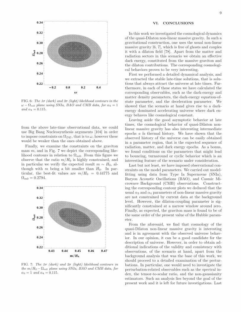
Finally, we examine the constraints on the gravitonmass m, and in Fig. 7 we depict the corresponding like-lihood contours in relation to Ωm0. From this figure weobserve that the ratio m/H0 is highly constrained, andin particular we verify the expected result m ∼ H0, al-though with m being a bit smaller than H0. In par-ticular, the best-fit values are m/H0 = 0.44775 andΩm0 = 0.2794.

0.43 0.44 0.45 0.46 0.470.22

0.24

0.26

0.28

0.30

0.32

0.34

m H0

Wm

0

FIG. 7: The 1σ (dark) and 2σ (light) likelihood contours inthe m/H0 −Ωm0 plane using SNIa, BAO and CMB data, forα3 = 1 and α4 = 0.115.

VI. CONCLUSIONS

In this work we investigated the cosmological dynamicsof the quasi-Dilaton non-linear massive gravity. In such agravitational construction, one uses the usual non-linearmassive gravity [6, 7], which is free of ghosts and couplesit with a dilaton field [78]. Apart from the matter andradiation sectors in this scenario we obtain an effectivedark energy, constituted from the massive graviton andthe dilaton contributions. The corresponding cosmologi-cal behaviors proves to be very interesting.First we performed a detailed dynamical analysis, and

we extracted the stable late-time solutions, that is solu-tions that always attract the universe at late times. Fur-thermore, in each of these states we have calculated thecorresponding observables, such as the dark-energy andmatter density parameters, the dark-energy equation-of-state parameter, and the deceleration parameter. Weshowed that the scenario at hand gives rise to a dark-energy dominated accelerating universe where dark en-ergy behaves like cosmological constant.Leaving aside the good asymptotic behavior at late

times, the cosmological behavior of quasi-Dilaton non-linear massive gravity has also interesting intermediateepochs a la thermal history. We have shown that theobserved history of the universe can be easily obtainedin a parameter region, that is the expected sequence ofradiation, matter, and dark energy epochs. As a bonus,we found conditions on the parameters that might leadto bouncing, turnaround or cyclic behavior which is aninteresting feature of the scenario under consideration.Last but not least, we have imposed observational con-

straints on the model parameters. We carried out model-fitting using data from Type Ia Supernovae (SNIa),Baryon Acoustic Oscillations (BAO), and Cosmic Mi-crowave Background (CMB) observations. Construct-ing the corresponding contour plots we deduced that theusual α3 and α4 parameters of non-linear massive gravityare not constrained by current data at the backgroundlevel. However, the dilaton-coupling parameter is sig-nificantly constrained at a narrow window around zero.Finally, as expected, the graviton mass is found to be ofthe same order of the present value of the Hubble param-eter.From the aforesaid, we find that cosmology of the

quasi-Dilaton non-linear massive gravity is interestingand is in agreement with the observed universe behav-ior. In our opinion, it can be a good candidate for thedescription of universe. However, in order to obtain ad-ditional indications of the validity and consistency withobservations, of the scenario at hand, apart from thebackground analysis that was the base of this work, weshould proceed to a detailed examination of the pertur-bations. In particular, one would need to investigate theperturbation-related observables such as the spectral in-dex, the tensor-to-scalar ratio, and the non-gaussianityestimators. Such an analysis lies beyond the goal of thepresent work and it is left for future investigations. Last

10

but not least we should comment on the issue of super-luminality in the model under consideration. As pointedout by Deser and Waldron [102], superluminal behavior isan essential feature of dRGT. In the quasi-Dilaton model,in the decoupling limit, we have a standard scalar field σin addition to the galileon which is plagued with super-luminality. Since σ has canonical kinetic term, it looksless likely that it would affect the superluminal behaviorof the model. However, the problem requires separateinvestigations to address the issue which we defer to ourfuture work.

Acknowledgments

The authors wish to thank G. Leon for useful com-ments. M.W.H acknowledges the funding from CSIR,Govt of India. MS thanks G. Gabadadze for a brief andfruitful discussion on the subject during Kyoto meeting.MS is also thankful to K. Bamba and S. Nojiri for use-ful discussions on the related theme. The research ofE.N.S. is implemented within the framework of the Oper-ational Program “Education and Lifelong Learning” (Ac-tions Beneficiary: General Secretariat for Research andTechnology), and is co-financed by the European SocialFund (ESF) and the Greek State.

Appendix: Observational data and constraints

Here we briefly review the sources of observational con-straints used in this manuscript, namely Type Ia Super-novae constraints, Baryon Acoustic Oscillations (BAO)and Cosmic Microwave Background (CMB). The totalχ2 defined as

χ2 = χ2SN + χ2

BAO + χ2CMB, (A.1)

where the individual χ2i for every data set is calculated

as follows.

a. Type Ia Supernovae constraints

In order to incorporate Type Ia constraints we use theUnion2.1 data compilation [105] of 580 data points. Therelevant observable is the distance modulus µ which is de-fined as µ = m−M = 5 logDL+µ0, where m and M arethe apparent and absolute magnitudes of the Supernovae,

DL(z) is the luminosity distanceDL(z) = (1+z)∫ z

0H0dz

′

H(z′)

and µ0 = 5 log(

H−1

0

Mpc

)

+ 25 is a nuisance parameter that

should be marginalized. The corresponding χ2 writes as

χ2SN (µ0, θ) =

580∑

i=1

[µth(zi, µ0, θ)− µobs(zi)]2

σµ(zi)2, (A.2)

where µobs denotes the observed distance modulus whileµth the theoretical one, and σµ is the uncertainty in thedistance modulus. Additionally, θ denotes any parameterof the specific model at hand. Finally, marginalizing µ0

following [106] we obtain

χ2SN (θ) = A(θ) − B(θ)2

C(θ), (A.3)

with

A(θ) =

580∑

i=1

[µth(zi, µ0 = 0, θ)− µobs(zi)]2

σµ(zi)2(A.4)

B(θ) =

580∑

i=1

µth(zi, µ0 = 0, θ)− µobs(zi)

σµ(zi)2(A.5)

C(θ) =

580∑

i=1

1

σµ(zi)2. (A.6)

b. Baryon Acoustic Oscillation constraints

We use BAO data from [107–110], that is of dA(z⋆)DV (ZBAO) ,

where z⋆ is the decoupling time given by z⋆ ≈ 1091, the

co-moving angular-diameter distance dA(z) =∫ z

0dz′

H(z′)

and DV (z) =(

dA(z)2 zH(z)

)1

3

is the dilation scale [111].

th required data are depicted in Table II.

In order to calculate χ2BAO for BAO data we follow the

procedure described in [112], where it is defined as,

χ2BAO = XT

BAOC−1BAOXBAO, (A.7)

with

XBAO =

dA(z⋆)DV (0.106) − 30.95dA(z⋆)DV (0.2) − 17.55dA(z⋆)

DV (0.35) − 10.11dA(z⋆)

DV (0.44) − 8.44dA(z⋆)DV (0.6) − 6.69dA(z⋆)

DV (0.73) − 5.45

(A.8)

and the inverse covariance matrix reads as

11

zBAO 0.106 0.2 0.35 0.44 0.6 0.73dA(z⋆)

DV (ZBAO)30.95 ± 1.46 17.55 ± 0.60 10.11 ± 0.37 8.44 ± 0.67 6.69± 0.33 5.45 ± 0.31

TABLE II: Values of dA(z⋆)DV (ZBAO)

for different values of zBAO.

C−1 =

0.48435 −0.101383 −0.164945 −0.0305703 −0.097874 −0.106738−0.101383 3.2882 −2.45497 −0.0787898 −0.252254 −0.2751−0.164945 −2.45499 9.55916 −0.128187 −0.410404 −0.447574−0.0305703 −0.0787898 −0.128187 2.78728 −2.75632 1.16437−0.097874 −0.252254 −0.410404 −2.75632 14.9245 −7.32441−0.106738 −0.2751 −0.447574 1.16437 −7.32441 14.5022

. (A.9)

c. CMB constraints

We use the CMB shift parameter

R = H0

√

Ωm0

∫ 1089

0

dz′

H(z′)(A.10)

following [103]. The corresponding χ2CMB is defined as,

χ2CMB(θ) =

(R(θ)−R0)2

σ2, (A.11)

with R0 = 1.725± 0.018 and R(θ) [103].

[1] M. Fierz, W. Pauli, Proc. Roy. Soc. Lond. A173, 211(1939).

[2] H. van Dam and M. J. G. Veltman, Nucl. Phys. B 22,397 (1970).

[3] V. I. Zakharov, JETP Lett. 12, 312 (1970) [Pisma Zh.Eksp. Teor. Fiz. 12, 447 (1970)].

[4] A. I. Vainshtein, Phys. Lett. B 39, 393 (1972).[5] D. G. Boulware, S. Deser, Phys. Rev. D6, 3368 (1972).[6] C. de Rham and G. Gabadadze, Phys. Rev. D 82,

044020 (2010) [arXiv:1007.0443 [hep-th]].[7] C. de Rham, G. Gabadadze and A. J. Tolley, Phys. Rev.

Lett. 106, 231101 (2011) [arXiv:1011.1232 [hep-th]].[8] K. Hinterbichler, Rev. Mod. Phys. 84, 671 (2012)

[arXiv:1105.3735 [hep-th]].[9] S. F. Hassan and R. A. Rosen, Phys. Rev. Lett. 108,

041101 (2012) [arXiv:1106.3344 [hep-th]].[10] K. Koyama, G. Niz and G. Tasinato, Phys. Rev. D 84,

064033 (2011) [arXiv:1104.2143 [hep-th]].[11] C. de Rham, G. Gabadadze and A. J. Tolley, Phys. Lett.

B 711, 190 (2012) [arXiv:1107.3820 [hep-th]].[12] B. Cuadros-Melgar, E. Papantonopoulos, M. Tsoukalas

and V. Zamarias, Phys. Rev. D 85, 124035 (2012)[arXiv:1108.3771 [hep-th]].

[13] S. F. Hassan and R. A. Rosen, JHEP 1202, 126 (2012)[arXiv:1109.3515 [hep-th]].

[14] J. Kluson, JHEP 1201, 013 (2012) [arXiv:1109.3052[hep-th]].

[15] A. E. Gumrukcuoglu, C. Lin and S. Mukohyama, JCAP

1111, 030 (2011) [arXiv:1109.3845 [hep-th]].[16] M. S. Volkov, JHEP 1201, 035 (2012) [arXiv:1110.6153

[hep-th]].[17] M. von Strauss, A. Schmidt-May, J. Enander, E. Mort-

sell and S. F. Hassan, JCAP 1203, 042 (2012)[arXiv:1111.1655 [gr-qc]].Y. Akrami, T. S. Koivisto and M. Sandstad, JHEP1303, 099 (2013) [arXiv:1209.0457 [astro-ph.CO]].

[18] D. Comelli, M. Crisostomi, F. Nesti and L. Pilo, JHEP1203, 067 (2012) [Erratum-ibid. 1206, 020 (2012)][arXiv:1111.1983 [hep-th]].

[19] S. F. Hassan and R. A. Rosen, JHEP 1204, 123 (2012)[arXiv:1111.2070 [hep-th]].

[20] L. Berezhiani, G. Chkareuli, C. de Rham, G. Gabadadzeand A. J. Tolley, Phys. Rev. D 85, 044024 (2012)[arXiv:1111.3613 [hep-th]].

[21] A. E. Gumrukcuoglu, C. Lin and S. Mukohyama, JCAP1203, 006 (2012) [arXiv:1111.4107 [hep-th]].

[22] N. Khosravi, N. Rahmanpour, H. R. Sepangi andS. Shahidi, Phys. Rev. D 85, 024049 (2012)[arXiv:1111.5346 [hep-th]].

[23] Y. Brihaye and Y. Verbin, Phys. Rev. D 86, 024031(2012) [arXiv:1112.1901 [gr-qc]].

[24] I. L. Buchbinder, D. D. Pereira and I. L. Shapiro, Phys.Lett. B 712, 104 (2012) [arXiv:1201.3145 [hep-th]].

[25] H. Ahmedov and A. N. Aliev, Phys. Lett. B 711, 117(2012) [arXiv:1201.5724 [hep-th]].

[26] E. A. Bergshoeff, J. J. Fernandez-Melgarejo, J. Rosseel

12

and P. K. Townsend, JHEP 1204, 070 (2012)[arXiv:1202.1501 [hep-th]].

[27] D. Comelli, M. Crisostomi and L. Pilo, JHEP 1206, 085(2012) [arXiv:1202.1986 [hep-th]].

[28] M. F. Paulos and A. J. Tolley, JHEP 1209, 002 (2012)[arXiv:1203.4268 [hep-th]].

[29] S. F. Hassan, A. Schmidt-May and M. von Strauss,Phys. Lett. B 715, 335 (2012) [arXiv:1203.5283 [hep-th]].

[30] D. Comelli, M. Crisostomi, F. Nesti and L. Pilo, Phys.Rev. D 86, 101502 (2012) [arXiv:1204.1027 [hep-th]].

[31] F. Sbisa, G. Niz, K. Koyama and G. Tasinato, Phys.Rev. D 86, 024033 (2012) [arXiv:1204.1193 [hep-th]].

[32] J. Kluson, Phys. Rev. D 86, 044024 (2012)[arXiv:1204.2957 [hep-th]].

[33] G. Tasinato, K. Koyama and G. Niz, JHEP 1207, 062(2012) [arXiv:1204.5880 [hep-th]].

[34] K. Morand and S. N. Solodukhin, Phys. Lett. B 715,260 (2012) [arXiv:1204.6224 [hep-th]].

[35] V. F. Cardone, N. Radicella and L. Parisi, Phys. Rev.D 85, 124005 (2012) [arXiv:1205.1613 [astro-ph.CO]].

[36] V. Baccetti, P. Martin-Moruno and M. Visser, Class.Quant. Grav. 30, 015004 (2013) [arXiv:1205.2158 [gr-qc]].

[37] P. Gratia, W. Hu and M. Wyman, Phys. Rev. D 86,061504 (2012) [arXiv:1205.4241 [hep-th]].

[38] M. S. Volkov, Phys. Rev. D 86, 061502 (2012)[arXiv:1205.5713 [hep-th]].

[39] C. de Rham and S. Renaux-Petel, JCAP 1301, 035(2013) [arXiv:1206.3482 [hep-th]].

[40] M. Berg, I. Buchberger, J. Enander, E. Mortsell andS. Sjors, JCAP 1212, 021 (2012) [arXiv:1206.3496 [gr-qc]].

[41] G. D’Amico, Phys. Rev. D 86, 124019 (2012)[arXiv:1206.3617 [hep-th]].

[42] M. Fasiello and A. J. Tolley, JCAP 1211, 035 (2012)[arXiv:1206.3852 [hep-th]].

[43] V. Baccetti, P. Martin-Moruno and M. Visser, JHEP1208, 108 (2012) [arXiv:1206.4720 [gr-qc]].

[44] Y. Gong, Commun. Theor. Phys. 59, 319 (2013)[arXiv:1207.2726 [gr-qc]].

[45] S. ’i. Nojiri and S. D. Odintsov, Phys. Lett. B 716, 377(2012) [arXiv:1207.5106 [hep-th]].

[46] C. Deffayet, J. Mourad and G. Zahariade, JCAP 1301,032 (2013) [arXiv:1207.6338 [hep-th]].

[47] C. -IChiang, K. Izumi and P. Chen, JCAP 1212, 025(2012) [arXiv:1208.1222 [hep-th]].

[48] S. F. Hassan, A. Schmidt-May and M. von Strauss,arXiv:1208.1515 [hep-th].

[49] F. Kuhnel, arXiv:1208.1764 [gr-qc].[50] H. Motohashi and T. Suyama, Phys. Rev. D 86, 081502

(2012) [arXiv:1208.3019 [hep-th]].[51] C. Deffayet, J. Mourad and G. Zahariade,

arXiv:1208.4493 [gr-qc].[52] G. Lambiase, JCAP 1210, 028 (2012) [arXiv:1208.5512

[gr-qc]].[53] A. E. Gumrukcuoglu, S. Kuroyanagi, C. Lin, S. Muko-

hyama and N. Tanahashi, Class. Quant. Grav. 29,235026 (2012) [arXiv:1208.5975 [hep-th]].

[54] G. Gabadadze, K. Hinterbichler, J. Khoury, D. Pirt-skhalava and M. Trodden, Phys. Rev. D 86, 124004(2012) [arXiv:1208.5773 [hep-th]].

[55] J. Kluson, arXiv:1209.3612 [hep-th].[56] G. Tasinato, K. Koyama and G. Niz, arXiv:1210.3627

[hep-th].[57] Y. Gong, arXiv:1210.5396 [gr-qc].[58] Y. -l. Zhang, R. Saito and M. Sasaki, JCAP 1302, 029

(2013) [arXiv:1210.6224 [hep-th]].[59] M. Park and L. Sorbo, JHEP 1301, 043 (2013)

[arXiv:1210.7733 [hep-th]].[60] Y. -F. Cai, D. A. Easson, C. Gao and E. N. Saridakis,

Phys. Rev. D 87, 064001 (2013) [arXiv:1211.0563 [hep-th]].

[61] M. Wyman, W. Hu and P. Gratia, arXiv:1211.4576[hep-th].

[62] C. Burrage, N. Kaloper and A. Padilla, arXiv:1211.6001[hep-th].

[63] S. ’i. Nojiri, S. D. Odintsov and N. Shirai,arXiv:1212.2079 [hep-th].

[64] M. Park and L. Sorbo, Phys. Rev. D 87, 024041 (2013)[arXiv:1212.2691 [hep-th]].

[65] S. Alexandrov, K. Krasnov and S. Speziale,arXiv:1212.3614 [hep-th].

[66] C. de Rham, G. Gabadadze, L. Heisenberg and D. Pirt-skhalava, arXiv:1212.4128 [hep-th].

[67] K. Hinterbichler, J. Stokes and M. Trodden,arXiv:1301.4993 [astro-ph.CO].

[68] D. Langlois and A. Naruko, Class. Quant. Grav. 29,202001 (2012) [arXiv:1206.6810 [hep-th]].

[69] K. Zhang, P. Wu, H. Yu and , Phys. Rev. D 87, 063513(2013) [arXiv:1302.6407 [gr-qc]].

[70] Z. Haghani, H. R. Sepangi, S. Shahidi and , gravity,”arXiv:1303.2843 [gr-qc].

[71] A. De Felice, A. E. Gumrukcuoglu, C. Lin, S. Muko-hyama and , arXiv:1303.4154 [hep-th].

[72] A. De Felice, A. E. Gumrukcuoglu and S. Mukohyama,Phys. Rev. Lett. 109, 171101 (2012) [arXiv:1206.2080[hep-th]].

[73] G. D’Amico, C. de Rham, S. Dubovsky, G. Gabadadze,D. Pirtskhalava and A. J. Tolley, Phys. Rev. D 84,124046 (2011) [arXiv:1108.5231 [hep-th]].

[74] A. E. Gumrukcuoglu, C. Lin and S. Mukohyama, Phys.Lett. B 717, 295 (2012) [arXiv:1206.2723 [hep-th]].

[75] Q. -G. Huang, Y. -S. Piao and S. -Y. Zhou, Phys. Rev.D 86, 124014 (2012) [arXiv:1206.5678 [hep-th]].

[76] E. N. Saridakis, Class. Quant. Grav. 30, 075003 (2013)[arXiv:1207.1800 [gr-qc]].

[77] Y. -F. Cai, C. Gao and E. N. Saridakis, JCAP 1210,048 (2012) [arXiv:1207.3786 [astro-ph.CO]].

[78] G. D’Amico, G. Gabadadze, L. Hui and D. Pirtskhalava,arXiv:1206.4253 [hep-th].

[79] A. De Felice, A. E. Gumrukcuoglu, C. Lin and S. Muko-hyama, arXiv:1304.0484 [hep-th].

[80] G. D’Amico, G. Gabadadze, L. Hui and D. Pirtskhalava,arXiv:1304.0723 [hep-th].

[81] N. Arkani-Hamed, H. Georgi and M. D. Schwartz, An-nals Phys. 305, 96 (2003) [hep-th/0210184].

[82] A. G. Cohen, D. B. Kaplan and A. E. Nelson, Phys.Rev. Lett. 82 (1999) 4971 [hep-th/9803132].

[83] P. Horava and D. Minic, Phys. Rev. Lett. 85 (2000)1610 [hep-th/0001145].

[84] S. D. H. Hsu, Phys. Lett. B 594 (2004) 13 [hep-th/0403052].

[85] M. Li, Phys. Lett. B 603 (2004) 1 [hep-th/0403127].[86] E. J. Copeland, A. RLiddle and D. Wands, Phys. Rev.

D 57, 4686 (1998) [gr-qc/9711068].[87] P. G. Ferreira and M. Joyce, Phys. Rev. Lett. 79, 4740

(1997) [astro-ph/9707286].

13

[88] X. -m. Chen, Y. -g. Gong and E. N. Saridakis, JCAP0904, 001 (2009) [arXiv:0812.1117 [gr-qc]].

[89] G. Leon, J. Saavedra and E. N. Saridakis,arXiv:1301.7419 [astro-ph.CO].

[90] S., Lynch, Dynamical Systems with Applications usingMathematica, Birkhauser, Boston (2007).

[91] G. Leon and C. R. Fadragas, Cosmological Dynam-ical Systems, LAP LAMBERT Academic Publishing,(2011).

[92] E. J. Copeland, M. Sami and S. Tsujikawa, Int. J. Mod.Phys. D 15, 1753 (2006) [hep-th/0603057].

[93] K. Bamba, S. ’i. Nojiri and S. D. Odintsov, JCAP 0810,045 (2008) [arXiv:0807.2575 [hep-th]].

[94] S. Capozziello, M. De Laurentis, S. Nojiri andS. D. Odintsov, Phys. Rev. D 79, 124007 (2009)[arXiv:0903.2753 [hep-th]].

[95] E. N. Saridakis and J. M. Weller, Phys. Rev. D 81,123523 (2010) [arXiv:0912.5304 [hep-th]].

[96] M. Novello and S. E. P. Bergliaffa, Phys. Rept. 463, 127(2008) [arXiv:0802.1634 [astro-ph]].

[97] S. ’i. Nojiri and E. N. Saridakis, arXiv:1301.2686 [hep-th].

[98] S. M. Carroll, M. Hoffman and M. Trodden, Phys. Rev.D 68, 023509 (2003) [astro-ph/0301273].

[99] J. M. Cline, S. Jeon and G. D. Moore, Phys. Rev. D 70,043543 (2004) [hep-ph/0311312].

[100] Y. -F. Cai and E. N. Saridakis, J. Cosmol. 17, 7238(2011) [arXiv:1108.6052 [gr-qc]].

[101] S. Capozziello and M. De Laurentis, Phys. Rept. 509,167 (2011) [arXiv:1108.6266 [gr-qc]].

[102] S. Deser and A. Waldron, Phys. Rev. Lett. 110, 111101(2013) [arXiv:1212.5835 [hep-th]].

[103] E. Komatsu et al. [WMAP Collaboration], Astrophys. J.Suppl. 192, 18 (2011) [arXiv:1001.4538 [astro-ph.CO]].

[104] K. A. Olive, G. Steigman and T. P. Walker, Phys. Rept.333, 389 (2000) [arXiv:astro-ph/9905320].

[105] N. Suzuki, D. Rubin, C. Lidman, G. Aldering, R. Aman-ullah, K. Barbary, L. F. Barrientos and J. Botyanszkiet al., Astrophys. J. 746, 85 (2012) [arXiv:1105.3470[astro-ph.CO]].

[106] R. Lazkoz, S. Nesseris and L. Perivolaropoulos, JCAP0511, 010 (2005) [astro-ph/0503230].

[107] C. Blake, E. Kazin, F. Beutler, T. Davis, D. Parkinson,S. Brough, M. Colless and C. Contreras et al., Mon. Not.Roy. Astron. Soc. 418, 1707 (2011) [arXiv:1108.2635[astro-ph.CO]].

[108] W. J. Percival et al. [SDSS Collaboration], Mon. Not.Roy. Astron. Soc. 401, 2148 (2010) [arXiv:0907.1660[astro-ph.CO]].

[109] F. Beutler, C. Blake, M. Colless, D. H. Jones,L. Staveley-Smith, L. Campbell, Q. Parker andW. Saunders et al., Mon. Not. Roy. Astron. Soc. 416,3017 (2011) [arXiv:1106.3366 [astro-ph.CO]].

[110] N. Jarosik, C. L. Bennett, J. Dunkley, B. Gold,M. R. Greason, M. Halpern, R. S. Hill and G. Hin-shaw et al., Astrophys. J. Suppl. 192, 14 (2011)[arXiv:1001.4744 [astro-ph.CO]].

[111] D. J. Eisenstein et al. [SDSS Collaboration], Astrophys.J. 633, 560 (2005) [astro-ph/0501171].

[112] R. Giostri, M. V. d. Santos, I. Waga, R. R. R. Reis,M. O. Calvao and B. L. Lago, JCAP 1203, 027 (2012)[arXiv:1203.3213 [astro-ph.CO]].