Quantum Perceptrons

Francisco Horta Ferreira da Silva

Thesis to obtain the Master of Science Degree in

Engineering Physics

Supervisor(s): Prof. João Carlos Carvalho de Sá SeixasProf. Yasser Rashid Revez Omar

Examination CommitteeChairperson: Prof. Jorge Manuel Rodrigues Crispim Romão

Supervisor: Prof. João Carlos Carvalho de Sá SeixasMember of the Committee: Prof. Luís Henrique Martins Borges de Almeida

November 2018

ii

“Que otros se jacten de las paginas que han escrito; a mı me enorgullecen las que he leıdo.”Jorge Luis Borges

iii

iv

Acknowledgments

This work was supported in part by a New Talents in Quantum Technologies scholarship from theCalouste Gulbenkian Foundation.

I would like to thank my advisors Professor Joao Seixas and Professor Yasser Omar for theirguidance. They were the ones who introduced me to scientific research, and any capabilitythat I might now have of producing original work, I owe to them.

Special thanks are also in order to Dr. Mikel Sanz, for his unwavering patience for the barrageof questions that inevitably came to me whenever I was trying to grasp a new paper, as well asfor all the time spent reading and rereading my first attempt at a paper of my own.

On a more personal level, I must thank my family. My father, for setting a standard of char-acter and work ethic that I will always aim for and hope to one day reach. My mother, for herattentive ear and sage advice regarding whatever existential matter I confided in her. My sisters,for putting up with me.

Last but not least, the denizens of the P10 study room, as well as its regular visitors, that attimes had to endure some hostility to be there with me. During the past 5 years they’ve gonefrom study group to friend group to support group. If it were not for their incessant motivationdisguised as nagging this thesis would probably not be done on time and, at least as importantly,if it were not for their intolerance of my less-than-stellar jokes, the quality of my humour wouldhave long ago dropped below acceptable levels.

v

vi

Resumo

A recente adicao de memristors quanticos as ferramentas disponıveis em circuitos quanticosabriu um novo mundo de possiblidades em computacao neuromorfica quantica. Por outrolado, houve uma explosao de interesse em redes neuronais quanticas (RNQ). Este trabalhotem como objectivo combinar estas areas propondo uma abordagem completamente orig-inal as RNQs baseada em memristors quanticos. Nesse sentido, propomos modelos paraperceptroes classicos de uma e varias camadas baseados exclusivamente em memristorsclassicos, preenchendo uma lacuna na literatura de memristors no contexto de computacaoneuromorfica. Desenvolvemos algoritmos de treino baseados no algoritmo de backpropaga-tion. Efectuamos simulacoes de ambos os modelos e dos algoritmos. Estas mostram que temum bom desempenho e estao de acordo com o teorema de Minsky-Papert, motivando a pos-sibilidade de construir redes neuronais fısicas baseadas em memristors. Este trabalho resultounum artigo submetido para publicacao. Passando para a quantizacao destes modelos, temosque memristors quanticos sao sistemas quanticos abertos e canais quanticos sao uma estruturamatematica extensivamente estudada que descreve o comportamento desses sistemas. Por-tanto, para estudar RNQs no contexto de sistemas quanticos abertos, propomos um modelode uma RNQ baseada em canais quanticos, bem como um metodo de treino baseado emoptimizacao em variedades de Stiefel. Mostramos que a rede e universal no sentido de portaslogicas classicas, sendo capaz de implementar padroes nao linearmente separaveis tais comoo XOR. Isto implica que a RNQ e mais poderosa do que o seu equivalente classico e que naose lhe aplica uma versao quantica do teorema de Minsky-Papert.

Palavras-chave: redes neuronais quanticas, memristors, redes neuronais, canais quanticos,sistemas quanticos abertos.

vii

viii

Abstract

The recent addition of quantum memristors to the quantum circuit toolbox has opened up anew world of possibilities in neuromorphic quantum computing. On the other hand, interest inquantum neural networks (QNN) has boomed. We aim to combine these areas by launching acompletely original approach to QNNs based on quantum memristors. To this end, we proposemodels for classical single and multilayer perceptrons based exclusively on classical memristors,filling a gap in the literature of memristors for neuromorphic computation. We develop trainingalgorithms based on the backpropagation algorithm. We run simulations of both the modelsand the algorithms. These show that both perform well and in accordance with Minsky-Papert’stheorem, motivating the possibility of building memristor-based hardware for physical neural net-works. This work resulted in a paper that is currently submitted for publication. Moving towardsquantizing these models, we have that quantum memristors are open quantum systems, andthat quantum channels are a widely studied framework that describes the behaviour of suchsystems. Therefore, in order to study QNNs in the context of open quantum systems, we proposea model for QNNs based on quantum channels, as well as a training method relying on opti-mization over Stiefel manifolds. We show that the network is universal in the classical logic gatesense, being capable of implementing non-linearly separable patterns such as the XOR gate.This implies that the QNN is more powerful than its classical equivalent and that it is not subjectto a quantum version of Minsky-Papert’s theorem.

Keywords: quantum neural networks (QNNs), memristors, neural networks (NNs), quan-tum channels, open quantum systems.

ix

x

Contents

Acknowledgments . . . . . . . . . . . . . . . . . . . . . . . . . . . . . . . . . . . . . . . . . . vResumo . . . . . . . . . . . . . . . . . . . . . . . . . . . . . . . . . . . . . . . . . . . . . . . . . viiAbstract . . . . . . . . . . . . . . . . . . . . . . . . . . . . . . . . . . . . . . . . . . . . . . . . ixList of Tables . . . . . . . . . . . . . . . . . . . . . . . . . . . . . . . . . . . . . . . . . . . . . . xiiiList of Figures . . . . . . . . . . . . . . . . . . . . . . . . . . . . . . . . . . . . . . . . . . . . . . xvAcronyms . . . . . . . . . . . . . . . . . . . . . . . . . . . . . . . . . . . . . . . . . . . . . . . xvii

1 Introduction 11.1 Motivation . . . . . . . . . . . . . . . . . . . . . . . . . . . . . . . . . . . . . . . . . . . . 11.2 Topic Overview . . . . . . . . . . . . . . . . . . . . . . . . . . . . . . . . . . . . . . . . . 2

1.2.1 Quantum Computing . . . . . . . . . . . . . . . . . . . . . . . . . . . . . . . . . 21.2.2 Perceptrons . . . . . . . . . . . . . . . . . . . . . . . . . . . . . . . . . . . . . . . 21.2.3 Memristors . . . . . . . . . . . . . . . . . . . . . . . . . . . . . . . . . . . . . . . . 31.2.4 Quantum Memristors . . . . . . . . . . . . . . . . . . . . . . . . . . . . . . . . . . 41.2.5 Quantum Channels . . . . . . . . . . . . . . . . . . . . . . . . . . . . . . . . . . 5

1.3 State of the art . . . . . . . . . . . . . . . . . . . . . . . . . . . . . . . . . . . . . . . . . 61.3.1 Memristors in learning systems . . . . . . . . . . . . . . . . . . . . . . . . . . . . 61.3.2 Quantum neural networks . . . . . . . . . . . . . . . . . . . . . . . . . . . . . . 6

1.4 Objectives . . . . . . . . . . . . . . . . . . . . . . . . . . . . . . . . . . . . . . . . . . . . 9

2 Perceptrons from Memristors 112.1 Memristor-based Perceptrons . . . . . . . . . . . . . . . . . . . . . . . . . . . . . . . . . 11

2.1.1 Memristor-based Single-Layer Perceptron . . . . . . . . . . . . . . . . . . . . . 112.1.2 Memristor-based Multilayer Perceptron . . . . . . . . . . . . . . . . . . . . . . . 13

2.2 Simulation results . . . . . . . . . . . . . . . . . . . . . . . . . . . . . . . . . . . . . . . . 152.2.1 Single-Layer Perceptron Simulation Results . . . . . . . . . . . . . . . . . . . . . 172.2.2 Multilayer Perceptron Simulation Results . . . . . . . . . . . . . . . . . . . . . . 172.2.3 Receiver Operating Characteristic Curves . . . . . . . . . . . . . . . . . . . . . 18

2.3 Concluding Remarks . . . . . . . . . . . . . . . . . . . . . . . . . . . . . . . . . . . . . . 19

3 Quantum Neural Network 213.1 Classical Network as a Stochastic Matrix . . . . . . . . . . . . . . . . . . . . . . . . . . 21

xi

3.1.1 Stochastic Learning . . . . . . . . . . . . . . . . . . . . . . . . . . . . . . . . . . 233.1.2 Simulation Results . . . . . . . . . . . . . . . . . . . . . . . . . . . . . . . . . . . . 24

3.2 Quantum Neural Network . . . . . . . . . . . . . . . . . . . . . . . . . . . . . . . . . . . 273.2.1 Quantum-classical Equivalence . . . . . . . . . . . . . . . . . . . . . . . . . . . 273.2.2 Generalization . . . . . . . . . . . . . . . . . . . . . . . . . . . . . . . . . . . . . 293.2.3 Capabilities of the QNN . . . . . . . . . . . . . . . . . . . . . . . . . . . . . . . . 323.2.4 Training the QNN . . . . . . . . . . . . . . . . . . . . . . . . . . . . . . . . . . . . 333.2.5 Scaling . . . . . . . . . . . . . . . . . . . . . . . . . . . . . . . . . . . . . . . . . . 363.2.6 Dimensionality Reduction . . . . . . . . . . . . . . . . . . . . . . . . . . . . . . . 38

3.3 Concluding Remarks . . . . . . . . . . . . . . . . . . . . . . . . . . . . . . . . . . . . . . 39

4 Conclusions 41

Bibliography 45

A Encoding Neural Network in Stochastic Matrix 51

B QNN capabilities 53

xii

List of Tables

3.1 Encoding of the inputs. . . . . . . . . . . . . . . . . . . . . . . . . . . . . . . . . . . . . 223.2 Encoding of the output. . . . . . . . . . . . . . . . . . . . . . . . . . . . . . . . . . . . . 223.3 Outputs of the network in terms of the network’s weights. . . . . . . . . . . . . . . . . 253.4 Correspondence between input bits x0, x1 and input diagonal density matrix ρ. . . 273.5 Correspondence between result of measuring ρout and network output. . . . . . . 283.6 Diagonal entries of ρ′ for each of the possible input pairs, which are encoded ac-

cording to table 3.4. . . . . . . . . . . . . . . . . . . . . . . . . . . . . . . . . . . . . . . 303.7 Correspondence between total state and states of system and environment. . . . 313.8 Diagonal entries of ρ′ for each of the possible input pairs. . . . . . . . . . . . . . . . 323.9 The sixteen 2-input, 1-output classical logic gates. . . . . . . . . . . . . . . . . . . . . 32

xiii

xiv

List of Figures

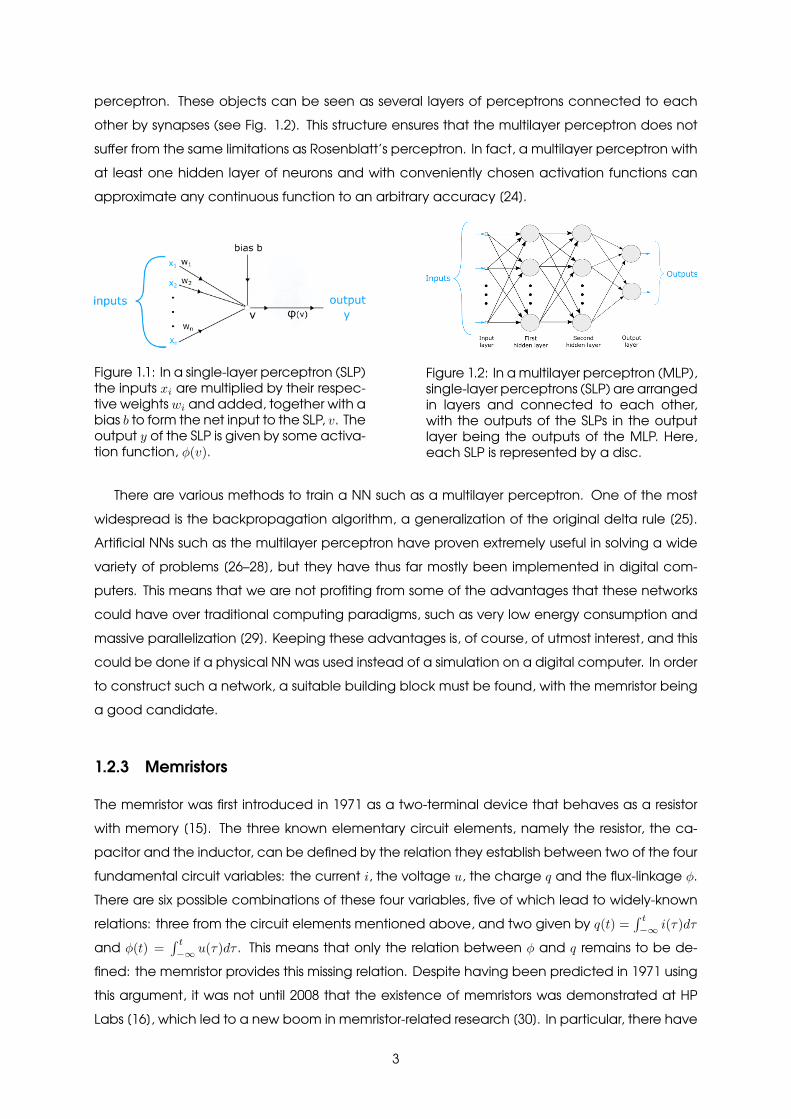
1.1 In a single-layer perceptron (SLP) the inputs xi are multiplied by their respectiveweights wi and added, together with a bias b to form the net input to the SLP, v.The output y of the SLP is given by some activation function, φ(v). . . . . . . . . . . 3

1.2 In a multilayer perceptron (MLP), single-layer perceptrons (SLP) are arranged inlayers and connected to each other, with the outputs of the SLPs in the outputlayer being the outputs of the MLP. Here, each SLP is represented by a disc. . . . . 3

2.1 Evolution of the learning progress of our single-layer perceptron (SLP), quantifiedby its total error, given by Equation (2.19), for the OR, AND and XOR gates over1000 epochs. The total error of our SLP for the OR and AND gates goes to 0 veryquickly, indicating that our SLP successfully learns these gates. The same is nottrue for the XOR gate, which our SLP is incapable of learning, in accordance withMinksy-Papert’s theorem [23]. . . . . . . . . . . . . . . . . . . . . . . . . . . . . . . . . 17

2.2 Evolution of the learning progress of our multilayer perceptron (MLP), quantified byits total error, given by Equation (2.19) for the OR, AND and XOR gates over 1000

epochs. As can be seen, the total error of our MLP for the these gates approaches0, indicating that it successfully learns all three gates. . . . . . . . . . . . . . . . . . . 18

2.3 ROC curves obtained with the SLP for the OR and XOR gates, and with the MLP forthe XOR gate. The thresholds used were t = 0.3, 0.5 and 0.7 We can see that the SLPcorrectly classifies the inputs for the OR gate every time, but it does not performbetter than random guessing for the XOR gate, as expected. On the other hand,the MLP correctly classifies the XOR gate inputs every time. . . . . . . . . . . . . . . 19

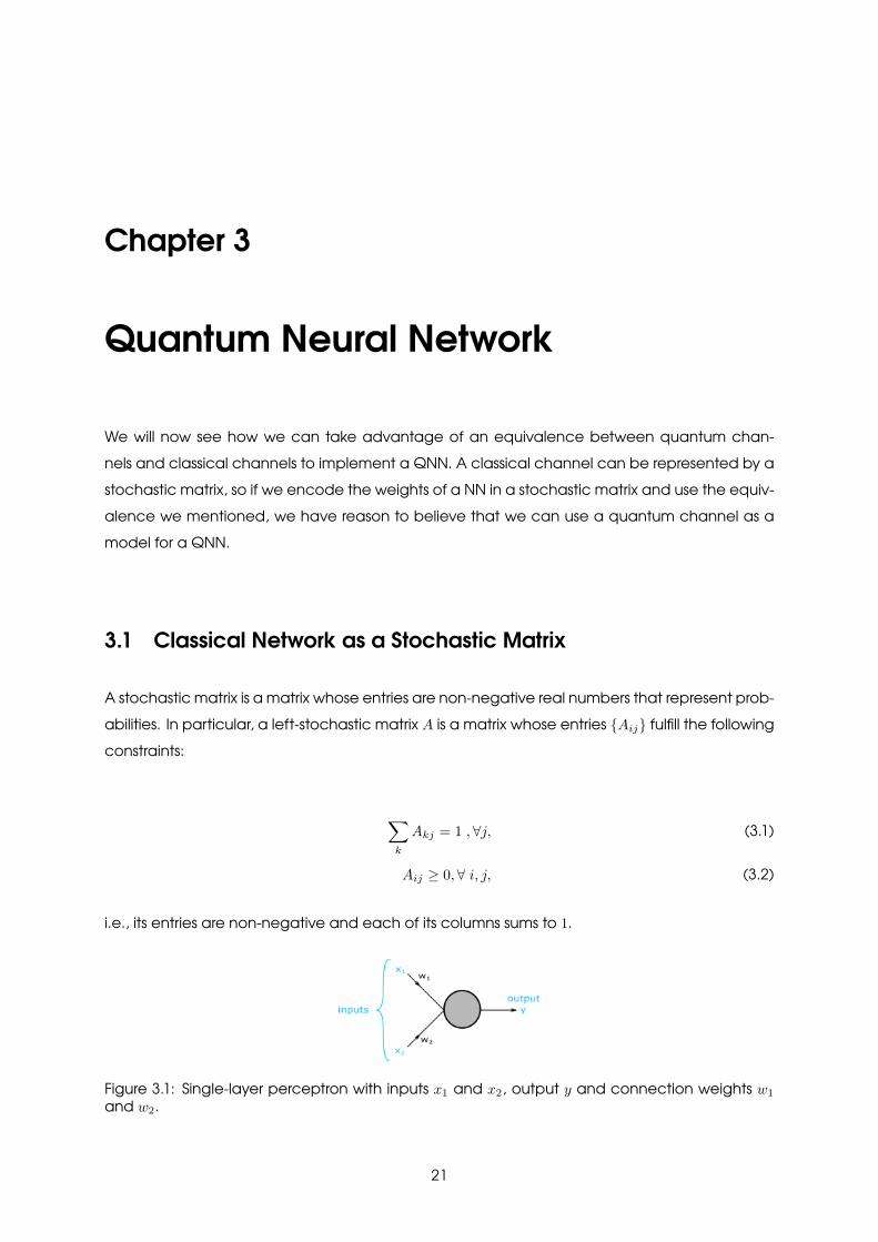
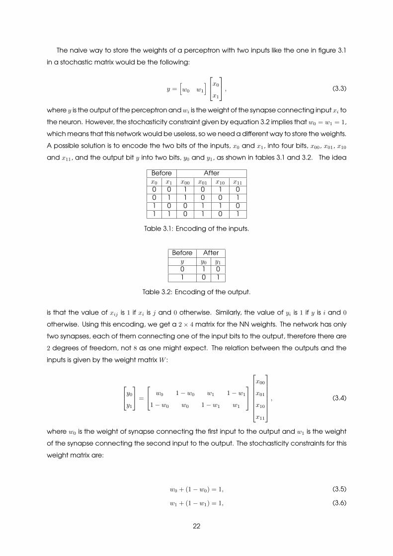
3.1 Single-layer perceptron with inputs x1 and x2, output y and connection weights w1

and w2. . . . . . . . . . . . . . . . . . . . . . . . . . . . . . . . . . . . . . . . . . . . . . . 21

3.2 Learning progress of the network on the OR gate, quantified by the cost functionover 30 epochs and averaged over 1000 different randomly chosen starting points.The blue line is the median of the 1000 realizations, the top limit is the 95th percentileand the bottom limit is the 5th percentile. As we can see, the value of the costfunction goes to zero, indicating that the network is capable of learning the ORgate. . . . . . . . . . . . . . . . . . . . . . . . . . . . . . . . . . . . . . . . . . . . . . . . 26

xv

3.3 Learning progress of our QNN on the XOR gate using a steepest descent algorithmin a complex Stiefel manifold, quantified by the cost function over 20 iterations andaveraged over 1000 different randomly chosen starting points. The blue line is themedian of the 1000 realizations, the top limit is the 95th percentile and the bottomlimit is the 5th percentile. As we can see, the value of the cost function goes tozero very quickly, indicating that the network is capable of learning the XOR gate. 35

xvi

Acronyms

CPTP Completely Positive and Trace-Preserving.

MLP Multilayer Perceptron.

NN Neural Network.

POVM Positive-Operator Valued Measure.

QC Quantum Computing.

QNN Quantum Neural Network.

SLP Single-layer Perceptron.

xvii

xviii

Chapter 1

Introduction

1.1 Motivation

The introduction of Shor’s algorithm in 1994 [1] showed that quantum computing is not just a fieldof theoretical interest, but can in fact have extraordinary advantages over traditional paradigmsof computation. Since then, interest in quantum computing research has boomed and it iswidely believed that the next years will bring about a quantum revolution.

On the other hand, machine learning has had tremendous impact in the past couple ofdecades, performing remarkably well on tasks as diverse as image recognition, medical diag-nosis and natural language processing [2–4]. In particular, NNs, a subset of machine learning,have found many applications in a wide range of disciplines.

Taking into account the massive impact that NNs have had, and the exciting possibilitiesbrought by quantum computing, it is natural to wonder if it is possible to combine the two in aQNN, and if this can result in faster algorithms. The concept of QNNs has been around since the1990s [5] and since then several proposals claiming that name have been put forward [6–9].These vary wildly in scope, but none of these earlier models can be said to be the definitivemodel of a QNN, either because they fail to incorporate neural computing mechanisms or be-cause they violate quantum theory in some way. Recent proposals [10–14] seem to introducemore adequate QNN models, but it is safe to say that there is not yet a standard model thatis widely accepted in the field. There has also been a growing interest in memristors, deviceswith history-dependent resistance which provide memory effects in form of a resistive hystere-sis. Although the first theoretical prediction of memristive behaviour came in 1971 [15], it wasnot until 2008 that the existence of memristors was demonstrated, at HP Labs [16]. This discov-ery reignited interest in memristor research, and their intrinsic memory features suggest that theymight be suitable building blocks for neural computing. Recently, memristors have been addedto the quantum circuit toolbox [17], constituting a building block for quantum neural computing,so one might wonder if they can be used in the context of QNNs.

1

1.2 Topic Overview

1.2.1 Quantum Computing

Quantum computing is a non-traditional paradigm of computation that uses quantum systemsto process information. The unique properties of these systems, such as superposition and en-tanglement, allow for speedups over classical computing in some tasks [18].

The time evolution of a closed quantum system is deterministic and reversible in time. Fortime-independent Hamiltonians, we can represent the time evolution of the system by an uni-tary operator, which is known as a quantum gate. The notable exception to the unitarity ofquantum computing is that of measurement - when a quantum system in a superposition ismeasured it collapses into one of the states of the superposition, with probability determined bythe amplitude of said state. The outcome of a quantum measurement is then probabilistic and,consequently, so is the output of a quantum algorithm.

The advantage of quantum computing over classical computing lies in the fact that quan-tum bits, unlike classical bits, can be in a state of superposition of 0 and 1. In the standard, digitalmodel of quantum computing, quantum algorithms aim to employ quantum gates in such away that interference effects maximize the amplitude of the desired result and minimize theamplitude of all others. Along these lines, quantum algorithms that are believed to be more effi-cient than their classical counterparts have been proposed in tasks such as database searching,solving systems of linear equations and, most notably due to its impact on cryptography andthe exponential speedup it is believed to provide, integer factorization [1, 19, 20].

1.2.2 Perceptrons

NNs are a computational model vaguely inspired by our understanding of how the brain pro-cesses information and, in particular, perceptrons are a class of NNs. The perceptron, introducedby Rosenblatt in 1958 [21], was one of the first models for supervised learning. In a perceptron,the inputs x1...xn are linearly combined with coefficients given by the weights w1...wn, as wellas with a bias b to form the input v to the neuron (see Fig. 1.1). v is then fed into a nonlinearfunction whose output is either 0 or 1. The goal of the perceptron is thus to find a set of weights{wi} and bias b that correctly assigns inputs {xi} to one of two predetermined binary classes.Geometrically, the perceptron tries to find a boundary that correctly splits the data into the twoclasses, with the weights changing the slope of the boundary and the bias its position. Lookingat the task this way, it becomes obvious that the bias is fundamental to successful training inmany problems, since there are data sets that require moving the boundary to be properly split.The correct parameters for the task of classifying the inputs are found by an iterative trainingprocess, such as the delta rule [22]. However, the perceptron is only capable of learning linearlyseparable patterns, as was shown in 1969 by Minksy and Papert [23]. These limitations triggereda search for more capable models, which eventually resulted in the proposal of the multilayer

2

perceptron. These objects can be seen as several layers of perceptrons connected to eachother by synapses (see Fig. 1.2). This structure ensures that the multilayer perceptron does notsuffer from the same limitations as Rosenblatt’s perceptron. In fact, a multilayer perceptron withat least one hidden layer of neurons and with conveniently chosen activation functions canapproximate any continuous function to an arbitrary accuracy [24].

Figure 1.1: In a single-layer perceptron (SLP)the inputs xi are multiplied by their respec-tive weights wi and added, together with abias b to form the net input to the SLP, v. Theoutput y of the SLP is given by some activa-tion function, φ(v).

Figure 1.2: In a multilayer perceptron (MLP),single-layer perceptrons (SLP) are arrangedin layers and connected to each other,with the outputs of the SLPs in the outputlayer being the outputs of the MLP. Here,each SLP is represented by a disc.

There are various methods to train a NN such as a multilayer perceptron. One of the mostwidespread is the backpropagation algorithm, a generalization of the original delta rule [25].Artificial NNs such as the multilayer perceptron have proven extremely useful in solving a widevariety of problems [26–28], but they have thus far mostly been implemented in digital com-puters. This means that we are not profiting from some of the advantages that these networkscould have over traditional computing paradigms, such as very low energy consumption andmassive parallelization [29]. Keeping these advantages is, of course, of utmost interest, and thiscould be done if a physical NN was used instead of a simulation on a digital computer. In orderto construct such a network, a suitable building block must be found, with the memristor beinga good candidate.

1.2.3 Memristors

The memristor was first introduced in 1971 as a two-terminal device that behaves as a resistorwith memory [15]. The three known elementary circuit elements, namely the resistor, the ca-pacitor and the inductor, can be defined by the relation they establish between two of the fourfundamental circuit variables: the current i, the voltage u, the charge q and the flux-linkage φ.There are six possible combinations of these four variables, five of which lead to widely-knownrelations: three from the circuit elements mentioned above, and two given by q(t) =

∫ t−∞ i(τ)dτ

and φ(t) =∫ t−∞ u(τ)dτ . This means that only the relation between φ and q remains to be de-

fined: the memristor provides this missing relation. Despite having been predicted in 1971 usingthis argument, it was not until 2008 that the existence of memristors was demonstrated at HPLabs [16], which led to a new boom in memristor-related research [30]. In particular, there have

3

been proposals of how memristors could be used in Hebbian learning systems [31–33], in thesimulation of fluid-like integro-differential equations [34], in the construction of digital quantumcomputers [35] and of how they could be used to implement non-volatile memories [36].

The pinched current-voltage hysteresis loop inherent to memristors endows them with intrinsicmemory capabilities, leading to the belief that they might be used as a building block in neuralcomputing architectures [37–39].

1.2.4 Quantum Memristors

As was shown in [17], a quantum memristor can be modelled as an open quantum system con-sisting of a Markovian tunable dissipative environment [40], a weak-measurement protocol [41],and a classical feedback controlling the coupling of the system to the dissipative environment.The evolution of the circuit quantum state ρ is then given by:

dρ = dρH + dρmeas + dρ(µ)damp, (1.1)

where dρH is the Hamiltonian term that describes the circuit evolution by itself, with no interac-tion with the environment, dρmeas is the term due to the presence of weak measurements anddρ

(µ)damp contains the dissipative contribution, which depends on the state variable µ. This equa-

tion of state is the quantum analogue of Ohm’s law. If the interaction with the state variable µ

is done via a measurement scheme, the records of the voltage MV (t) govern the state variabledynamics:

µ(t) = f(µ(t),MV (t)). (1.2)

If we shunt an LC circuit with a quantum memristor, the description of the Hamiltonian partrequires only one degree of freedom, the top node flux φ, and its conjugate momentum q, whichcorresponds to the charge on the capacitor connected to the top node. The time evolution ofthe Hamiltonian part is then given by:

dρH = − i~

[H(φ, q), ρ(t)]dt. (1.3)

Measuring the voltage applied to the quantum memristor implies monitoring the node chargeq, since the charge on the capacitor is determined by the voltage and the capacitance C, i.e.,q = CV . Therefore, as follows from the theory of continuous measurements, the state updateand the measurement output have the following form, respectively [41]:

dρmeas = − τ

q20[q, [q, ρ(t)]]dt+

√2τ

q20({q, ρ(t)} − 2〈q〉ρ(t))dW, (1.4)

MV (t) =1

C

(〈q(t)〉+

q208τζ(t)

). (1.5)

4

A numerical analysis of the evolution of this quantum memristor reveals that it in fact showshysteretic behaviour. This implies that the system has memory, which hints at the possibility ofusing quantum memristors as a building block for quantum neural computing.

1.2.5 Quantum Channels

As we mentioned in 1.2.1, the operations on a closed quantum system must be unitary, withthe exception of measurement. However, if we are studying an open quantum system, i.e., aquantum system that interacts with its environment, there are three effects that must be takeninto account: the unitary time evolution of the system given by Schrodinger’s equation, theinteractions with the environment and measurement. It turns out that there is a mathematicalformalism that can be used to describe all three effects simultaneously: quantum channels. Aquantum channel is a completely positive trace-preserving (CPTP) map acting on the space ofdensity matrices. Suppose that the initial state of our quantum system A is ρA and that the initialstate of its environment E is |0〉E . The initial state of the joint system AE is thus ρA ⊗ |0〉 〈0|E . Let’ssay that the interaction between these two systems is given by a unitary operator UAE actingon both systems and that we only have access to A after the interaction. We then obtain thestate of the system A, σA, by taking the partial trace over the environment:

σA = TrE

[UAE(ρA |0〉 〈0|E)U†AE

]. (1.6)

This is known as the physical representation of a quantum channel. It can be shown that thisevolution is equivalent to that of a CPTP map given by the following Kraus operators [42]:

Bi = {(IA ⊗ 〈i|E)UAE (IA ⊗ |0〉E)}i. (1.7)

This equivalence is formalized in the Choi-Kraus representation theorem.

Theorem 1.2.1 (Choi-Kraus representation theorem). Let |HA| denote the dimension of the Hilbertspace HA and let L(HA) denote the set of linear operators in HA. Let the map N : L(HA) →

L(HB) be denoted by NA→B . NA→B is linear and CPTP if and only if it has a Choi-Kraus decom-position of the following type:

NA→B(XA) =

d−1∑l=0

VlXAV†l , (1.8)

where XA ∈ L(HA), Vl ∈ L(HA,HB) for all l ∈ {0, ..., d− 1},

d−1∑l=0

V †l Vl = 1A, (1.9)

where 1A is the identity matrix in HA and d is at most |HA| × |HB |.

A proof of this result can be found in [43]. We thus have that any operation on a quantum

5

system, including unitary time-evolution, measurement and interaction with environment, canbe represented by Kraus operators using equation 1.8. These operators are subject only to theconstraint given by equation 1.9.

1.3 State of the art

1.3.1 Memristors in learning systems

There have been proposals of how memristors can be used in learning systems [31–33], but onlyregarding Hebbian learning and spike-timing-dependent plasticity (STDP). Hebbian learning isan unsupervised learning rule inspired by Hebbian theory, which proposes an explanation forsynaptic plasticity. In simple terms, the theory states that the connection between two neuronsstrengthens if they fire together and weakens if they fire separately. The process of training anetwork through Hebbian learning consists of feeding it inputs and increasing the weights of theconnections between neurons that have the same output and decreasing the weights betweenthose who do not. STDP is an extension of Hebbian learning that takes causality into account. Iftwo neurons fire at exactly the same time, one cannot have influenced the firing of the other, soin STDP the strength of a connection only increases if the pre-synaptic neuron fires immediatelybefore the post-synaptic neuron. Furthermore, the papers using memristors in the context of STDPare more focused on replicating biological effects than obtaining algorithmical advantages.

This being said, as far as we know, there is as of yet no model for how a NN based exclusivelyon memristors can be used to perform supervised learning. Such a model is thus the first mainresult of this thesis and its presentation here is based on work submitted for publication by theauthor in IEEE Transactions on Neural Networks and Learning Systems. This work is also availableonline as an arXiv preprint [44].

1.3.2 Quantum neural networks

The main difficulty in introducing a QNN lies in the fact that it tries to combine two fundamentallydifferent areas: quantum mechanics, which is unitary and therefore linear and NNs, which mustcontain nonlinearities in order to be universal [24]. In an extensive review article [45], the authorsintroduced the following criteria that a meaningful QNN proposal should fulfill:

1. The initial state of the quantum system encodes any binary string of lengthN . The QNN pro-duces a stable output configuration encoding the one state of 2M possible output binarystrings of length M which is closest to the input by some distance measure.

2. The QNN reflects one or more basic neural computing mechanisms (attractor dynamics,synaptic connections, integrate and fire, training rules, structure of a NN).

3. The evolution is based on quantum effects, such as superposition, entanglement and in-terference, and it is fully consistent with quantum theory.

6

Most attempts made so far failed in conciliating the need for nonlinear activation functionswith the linear nature of quantum theory, which means they did not fulfill either 2 or 3. However,models proposed mainly in the last two years seem to be of higher quality, in the sense that theydo not violate the above criteria in any obvious way. We will now review the most promising ofthese models one by one.

In [12], the authors introduce a QNN that can represent labeled data, classical or quantum,and be trained by supervised learning, through a process similar to gradient descent. They de-rive an expression for the number of two qubit unitaries needed to represent any label function,which can be seen as a quantum representation result analogous to the classical representa-tion theorem by Cybenko [24]. In general, the number of unitaries needed to represent the labelfunction grows exponentially, so there is no advantage over the classical case. As the authorsstate, it may be that certain functions can be represented more efficiently, but that is still anopen problem.

In [10], the authors propose a quantum neuron as follows: let the inputs x1, . . . , xn ∈ {0, 1}be linearly combined to form an input θ = w1x1 + . . . wnxn + b. Use the state |x〉 = |x1 . . . xn〉 asa control state and apply Ry(2w1), a rotation of w1 generated by the Pauli Y operator, onto anancilla qubit conditioned on the i-th qubit, followed by Ry(2b) on the same ancilla qubit. Thesecond step is to perform a rotation by Ry(2σ(θ)) where σ is a sigmoid function. This rotation canbe approximated by a repeat-until-success (RUS) circuit [46]. By recursively applying the RUScircuit k times a rotation Ry(2q◦k(θ) can be performed, where q◦k is the self-composition of q ktimes. This results in a threshold behaviour on θ: if θ > π/4 then we want the output qubit to beas close to |1〉 as possible. This threshold behaviour is key in neural computing and up until thispoint no QNN model had been successful in implementing it.

In [11], the authors propose a quantum perceptron intimately related to this quantum neuron.Here, a quantum perceptron is introduced as a two-level system that exists in a superposition ofresting and active states, as a nonlinear reaction to a classical or quantum field, i.e.:

Uj(xj ; f) |0j〉 =√

1− f(xj) |0j〉+√f(xj) |1j〉 . (1.10)

This transformation can be implemented as a SU(2) rotation parameterized by a general inputfield xj :

Uj(xj ; f) = exp{if(xj)σ

yj

}(1.11)

The unitary operator Uj(xj ; f) is fully defined by an activation function f(xj), the weights wjkand the thresholds θj . The rotation angle f(xj) = arcsin

(f(xj)

1/2)

depends nonlinearly on theinput field xj . in a feed-forward network setup, the perceptron gate depends on the field xj

generated by neurons in earlier layers, in analogy with what happens in a classical NN. Theauthors use this fact and go on to prove that a network based on this perceptron is a universalfunction approximator.

Although these two proposals use different mechanisms to implement their quantum neu-

7

rons, namely RUS circuits in the first case and rotations in the second, the underlying idea isvery similar. Both of them aim to find a way of embedding a classical perceptron in a quantumframework. This is made evident, for instance, in the proof of universality of the quantum percep-tron given in [11]. The proof is done by first determining the parameters of the classical networkthat approximates a given function and then encoding those parameters in a qubit circuit. Be-cause of this, a function that can be approximated with an accuracy of ε classically with M+Nε

neurons, needs k ×M + Nε quantum neurons for an approximation of the same quality. Thereis actually a decrease in efficiency when moving the network to the quantum realm, which isdue to the fact that these models consist of blueprints of how to encode classical networks inquantum settings, not in actual quantum networks.

In [47], the authors propose how the quantum memristor model introduced in [17] can beused to quantize a simplified version of the Hodgkin-Huxley neuron with one ionic channel in aquantum circuit. The main result is that the area of the hysteresis curve of the quantum neuronis bigger for quantum inputs and, in particular, for entangled quantum inputs. This indicatesthat there is an advantage in terms of memory for the quantum neuron versus the classicalneuron. The main drawback is the difficulty in scaling up the network. Using just one memristor,the network is limited to just one neuron with one ionic channel, i.e., one output, so being ableto add more neurons and enrich them is of utmost importance. However, the equations thatdescribe the behaviour of the quantum memristor used for the neurons are extremely compli-cated, which makes expanding the network unfeasible until these equations are in some waysimplified.

In [13], the authors aim to train near-term quantum circuits to distinguish between non-orthogonal quantum states, i.e., to perform quantum state discrimination [48]. This is achievedby iterative interactions between a classical device and a quantum processor to discover theparameters of an unknown non-unitary quantum circuit. Numerical simulations show that shal-low quantum circuits can be trained to discriminate among various pure and quantum states.The authors establish an analogy between this circuit and a QNN: the unitary evolution of thestates in the circuit can be considered as a layer of symmetric fully-connected neurons, andthe multiple layers of POVMs provide the necessary nonlinearities. This approach consists of aquantum circuit learning approach for discrimination and classification of quantum data, andit is successful in this sense. However, it is not, nor does it claim to be, a a universal QNN, i.e., aquantum version of a NN that can be applied to all the tasks a classical NN can.

In [49], the authors propose an architecture for NNs unique to quantum optical systems, aquantum optical neural network (QONN). The authors argue that the main features of classi-cal NNs can be directly translated to quantum optical systems. The architecture of the QONNconsists of photonic quantum states as inputs, linear optical unitaries as linear transformationsand nonlinear layers that act on single sites by adding a constant phase. This network is ap-plied to several problems, such as quantum state generation, quantum gate implementation,hamiltonian simulation, quantum optical autoenconding and quantum reinforcement learning.

8

It constitutes a powerful simulation tool for the design of quantum optical systems as well as anexperimental platform.

In [14], the authors propose how a QNN can be created by building a quantum circuit ina continuous-variable architecture, which is based on encoding quantum information in con-tinuous degrees of freedom such as the amplitudes of the electromagnetic field [50]. Thiscircuit contains a layered structure of continuously parameterized gates which is universal forcontinuous-variable QC. The introduction of non-Gaussian gates provides both the nonlinearityand universality of the network. They also allow it to encode highly nonlinear transformationswhile remaining completely unitary. The authors go on how to show how to embed a classi-cal network into their quantum formalism and propose quantum versions of various machinelearning models. Finally, they apply their model to several different problems with good results,namely the fitting of 1D functions, the generation of quantum states to encode images, dataclassification and autoencoding. These last two problems were done using a hybrid quantum-classical network.

1.4 Objectives

Having surveyed the current state of the field of quantum machine learning and, in particular,of QNNs, we can see that despite the increase in quantity and quality of attempts in recentyears, a standard model that is widely accepted in this field does not yet exist. The goal ofthis work is thus to take a completely original approach to this problem by proposing a QNNbased on quantum memristors. However, as we saw in section 1.2.4, the equations describingthe behaviour of the quantum memristors put forward in [17] are extremely complicated, andbecome even more so when several quantum memristors are allowed to interact. We then havethat the task of putting several quantum memristors together to form a network looks daunting.The plan is thus to split it into smaller, more tractable parts.

First, we will propose and validate a model of a classical perceptron made exclusively withclassical memristors and adapt a learning algorithm for its training. Taking into account the factthat quantum memristors are open quantum systems, we would like to learn more about QNNs inthe context of open quantum systems before proceeding with the quantization of the classicalmodel. Quantum channels constitute a formalism to describe open quantum systems that hasbeen extensively studied in the past couple of decades, so the wealth of results that has beenaccumulated about them is immediately available to any construction based on this formalism.The second goal of this thesis is thus to propose a model for a QNN based on quantum channels,as well as a training algorithm for it. A detailed study of this model will be performed in order tounderstand what implications for the QNN come from known results about quantum channelsand to determine if there are any mechanisms that may limit the QNN at a fundamental level,such as a quantum generalization of Misnky-Papert’s theorem. Hopefully, the knowledge thestudy of this model brings about QNNs in the context of open quantum systems will be of use in

9

the future when trying to use quantum memristors for neuromorphic quantum computation.

10

Chapter 2

Perceptrons from Memristors

This chapter is based on work submitted for publication by the author in IEEE Transactions onNeural Networks and Learning Systems: ”Francisco Silva, Mikel Sanz, Joao Seixas, Enrique Solano,and Yasser Omar - Perceptrons from Memristors”. It is also available online as an arXiv preprint[44].

In general, a current-controlled memristor is a dynamical system whose evolution is describedby the following pair of equations [15]:

{V = R(~γ, I)I, (2.1a)

~γ = ~f(~γ, I). (2.1b)

The first one is Ohm’s law and relates the voltage output of the memristor V with the current inputI through the memristance R(~γ, I), which is a scalar function depending both on I and on theset of the memristor’s internal variables ~γ. This dependence of the memristance on the internalvariables induces the memristor’s output dependence on past inputs, i.e., this is the mechanismthat endows the memristor with memory. The second equation describes the time-evolution ofthe memristor’s internal variables by relating their time derivative, ~γ, to an n-dimensional vectorfunction ~f(~γ, I), depending on both previous values of the internal variables and the input of thememristor. The internal variables can, in practice, be any physical memristor characteristic overwhich we have some control. For instance, in [16], the internal variable specifies the distributionof dopants in the device.

2.1 Memristor-based Perceptrons

2.1.1 Memristor-based Single-Layer Perceptron

Our goal is to implement a perceptron and an adaptation of the delta rule to train it using only amemristor. To this end, we use the memristor’s internal variables to store the SLP’s weights. Equa-tion (2.1b) allows us to control the evolution of the memristor’s internal variables and implement

11

a learning rule. If, for example, we want to implement a SLP with two inputs we need a mem-ristor with three internal variables, two of them to store the weights of the connections betweenthe inputs and the SLP and the other one to store the SLP’s bias weight.

Let us then consider a memristor with three internal state variables, from now on labeledby ~γ = (γ1, γ2, γ3) and in which ~f = (f1, f2, f3). It could be difficult to externally control multi-ple internal variables. However, a possible solution is to use several memristors with the chosenrequirements and with an externally controlled internal variable each.

In order to understand the form of these functions, we must remember that we expect dif-ferent behaviours from the perceptron depending on the stage of the algorithm. In the forwardpropagation stage, the weights must remain constant to obtain the output for a given input. Inthis phase the internal variables must not change. On the other hand, in the backpropagationstage, we want to update the perceptron’s weights by changing the internal variables. How-ever, it may happen that the update is different for each of the weights, so we need to be ableto change only one of the internal variables without affecting the others.

There are thus three different possible scenarios in the backpropagation stage: we want toupdate γ1, while γ2 and γ3 should not change; we want to update γ2, while γ1 and γ3 should notchange, and we want to update γ3, while γ1 and γ2 should not change. To conciliate this withthe fact that a memristor takes only one input, we propose the use of threshold-based functions,as well as a bias current Ib, for the evolution of the internal variables

V (t) = g(I, γ1, γ2, γ3), (2.2)

γi = (I − Ib) (θ(I − Iγi)− θ(I − (Iγi + a))) + (I + Ib) (θ(−I − Iγi)− θ(−I − (Iγi + a))) , (2.3)

where g is an activation function, θ is the Heaviside function function, Iγi is the threshold for theinternal variable γi and a is a parameter that determines the dimension of the threshold, i.e., therange of current values for which the internal variables are updated. The first term of the updatefunction can only be non-zero if the input current is positive, whereas the second term can onlybe non-zero if the input current is negative. If Iγ1 , Iγ2 and Iγ3 are sufficiently different from eachother and from zero, we can reach the correct behaviour by choosing the memristor’s inputappropriately. We thus have that the thresholds and the a paramater are hyperparametersthat must be calibrated for each problem. In the aforementioned construction in which ourmemristor with three internal variables is constructed as an equivalent memristor, we can alsouse an external current or voltage control to keep the internal variable fixed. In fact, this is how itis usually addressed experimentally [39, 51–53]. Therefore, we can assume that this constructionis possible. It is important to note that, in an experimental implementation, this threshold systemdoes not need to be based on the input currents’ intensities. It can, for instance, be based onthe use of signals of different frequencies for each of the internal variables or in the codificationof the signals meant for each of the internal variables in AC voltage signals. We are now ready topresent a learning algorithm for our SLP based on the delta rule, which is described in Algorithm 1.

12

Algorithm 1 Delta rule for Single-layer PerceptronInitializationSet the bias current Ib to 0.Initialize the weights w1, w2, wb.Set the internal state variables γ1, γ2, γ3 to w1, w2 and wb, respectively.for d in data do

Forward PassCompute the net input to the perceptron:

I = w1x1 + w2x2. (2.4)

Compute the perceptron’s output:

V = g(I, γ1, γ2, γ3). (2.5)

Backward PassCompute the difference ∆ between the target output and the actual output:

∆ = T − V. (2.6)

Compute the derivative of the activation function with respect to the net input, g′.for i in internal variables do

if ∆ ≥ 0 thenSet the bias Ib = Iγi .

elseSet the bias Ib = −Iγi .

Update γi by inputting I = ∆xig′ + Ib.

Update the weights by setting them to the updated values of the internal state variables.Set the bias Ib = 0.

In case one wants to generalize this procedure to an arbitrary number of inputs n, this can betrivially achieved by using a memristor with n + 1 internal variables and adapting Algorithm 1accordingly.

2.1.2 Memristor-based Multilayer Perceptron

In this model, memristors are used to emulate both the connections and the nodes of a MLP.In principle, the nodes could be emulated by non-linear resistors, but using memristors allows usto take advantage of their internal variable to implement a bias weight, which in some casesproves fundamental for a successful network training.

The equations describing the evolution of the memristor at each node in this model are thesame as in the seminal HP Labs paper [16]. We have chosen the experimentally tested set

V (t) =

(RON

γ(t)

D+ROFF

(1− γ(t)

D

))I(t), (2.7)

γ =

(µV

ROND

I(t)− Iγ)θ

(µV

ROND

I(t)− Iγ). (2.8)

Here, RON and ROFF are, respectively, the doped and undoped resistances of the memristor, Dand µV are physical memristor parameters, namely the thickness of its semiconductor film andits average ion mobility, and Iγ is a threshold current playing the same role as the I~γ in the model

13

for the memristor-based SLP introduced above. Equation (2.7) can be approximated by

V (t) = ROFF

(1− γ(t)

D

)I(t), (2.9)

since we have that RONROFF

≈ 1100 , as seen in [16]. If, for instance, we impose a constant current

input I to the memristor for a time t, the output is given by

V (t) ∝ −I2t. (2.10)

This can be achieved in practice by using a current integrator. It is then possible to implementnon-linear activation functions starting from Equation (2.7), which is an important condition forthe universality of NNs [54].

Looking now at synaptic memristors, their evolution is described by

V (t) = γ(t)I(t), (2.11)

with the evolution of the internal variable being given by equation (2.8).

In synaptic memristors, the internal variable γ is used to store the weight of the respectiveconnection, whereas in node memristors the internal variable is used to store the node’s biasweight.

As explained before, the node memristors are chosen to operate in a non-linear regime,which allows us to implement non-linear activation functions. On the other hand, we choose alinear regime for synaptic memristors, which allows us to emulate the multiplication of weightsby signals.

It must be mentioned that Equation (2.8) is only valid for γ ∈ [0, D], due to reasons relatedto the physical memristor device, as detailed in [16]. If we were to store the network weights inthe internal variables using only a rescaling constant A, i.e., w = Aγ, then the weights would allhave the same sign. Although convergence of the standard backpropagation algorithm is stillpossible in this case [55], it is usually slower and more difficult, so it is convenient to redefine thevariable [16] D → D′ so that the interval of the internal variable in which Equation (2.8) is validbecomes [−D′/2, D′2]. Using a rescaling constant B, the network weights can then be in theinterval [−BD′/2, BD′/2].

The new learning algorithm is an adaptation of the backpropagation algorithm, chosen dueto its widespread use and robustness. In our case, the activation function of the neurons is thefunction that relates the output of a node memristor with its input, as seen in Equation (2.7). The

14

local gradients of the output layer and hidden layer neurons are respectively given by:

Output: δk = Tkφ

′

(∑i

Vik

), (2.12)

Hidden: δk = φ′

(∑i

Vik

)∑l

δlwkl. (2.13)

In Equation (2.12), Tk denotes the target output for neuron k in the output layer. In Equa-tions (2.12) and (2.13), φ′ is the derivative of the neuron’s activation function with respect tothe input to the neuron

∑i Vik. Finally, in Equation (2.13), the sum

∑l δlwkl is taken over the gra-

dients of all neurons l in the layer to the right of the neuron that are connected to it by weightswkl. The update to the bias weight of a node memristor is given by:

∆wk = ηδk, (2.14)

where η is the learning rate. The connection weight wij is updated using ∆wij = ηδjVi, whereδj is the local gradient of the neuron to the right of the connection, and Vi is the output of theneuron to the left of the connection.

We count now with all necessary elements to adapt the backpropagation algorithm for ourmemristor-based MLP, as described in Algorithm 2.

2.2 Simulation results

In order to test the validity of our SLP and MLP, we tested their performance on three logicalgates: OR, AND and XOR. The first two are simple problems which should be successfully learntby SLP and MLP, whereas only the MLP should be able to learn the XOR gate, due to Minsky-Papert’s theorem.

The Glorot weight initialization scheme [56] was used for all simulations, as it has been shownto bring faster convergence in some problems when compared to other initialization schemes.In this scheme the weights are initialized according to a uniform distribution with extremal values−1 and 1, weighed by

√6

nin+nout, where nin and nout are the number of neurons in the previous

and following layers, respectively. The data sets used contain 100 randomly generated labeledelements, which were shuffled for each epoch, and the cost function is:

E =1

2(T −O)2, (2.18)

where T is the target output and O the actual output.

15

Algorithm 2 Backpropagation for Multilayer PerceptronInitializationSet the bias current Ib to 0.Initialize the weights {wij} and {wbk}.Set the internal variable γij of each connection memristor ij to the respective connectionweight wij .Set the internal variable γk of each connection memristor k to the respective bias weight wbk .for d in data do

Forward Passfor l in layers do

Compute the output of each connection memristor ij in layer l:

Vij(wij , I) = wijI. (2.15)

Sum the outputs of the connection memristors connected to each node memristor k inlayer l

ink =∑

Iik (2.16)

Compute the node memristor’s output:

Vk = ROFF

(1− γbk

D+RONROFF

γbkD

)ink.

Backward Passfor k in output layer do

Compute the difference ∆ between the target output and the actual output of thenode memristor:

∆k = Tk − Vk. (2.17)Compute the local gradient of the node memristor using Equation (2.12).

for layer in hidden layers dofor node in layer do

Compute the local gradient of node memristor l in layer using Equation (2.13).for connection in connections do

Compute the weight update.Set the bias current: Ib = Iγij .Update the connection memristor’s internal variable by inputting I = ∆wij + Ib to it.Update the connection’s weight by setting it to the updated value of the respective

internal variable.for node in nodes do

Compute the bias weight update according to Equation (2.14).Set the bias current: Ib = Iγb .Update the node memristor’s internal variable by inputting I = ∆wk + Ib.Update the bias weight by setting it to the updated value of the respective internal

variable.

16

2.2.1 Single-Layer Perceptron Simulation Results

For the SLP, a learning rate of 0.1 was used for all tested gates, a value set by trial and error. Themetric we used to evaluate the evolution of the network’s performance on a given problem wasits total error over an epoch, which is given by Equation (2.19).

Etotal =∑j

Ej =1

2

∑j

(Tj −Oj)2, (2.19)

where the sum is taken over all elements in the training set. In Fig. 2.1, the evolution of the totalerror over 1000 epochs, averaged over 100 different realizations of the starting weights, is plotted.

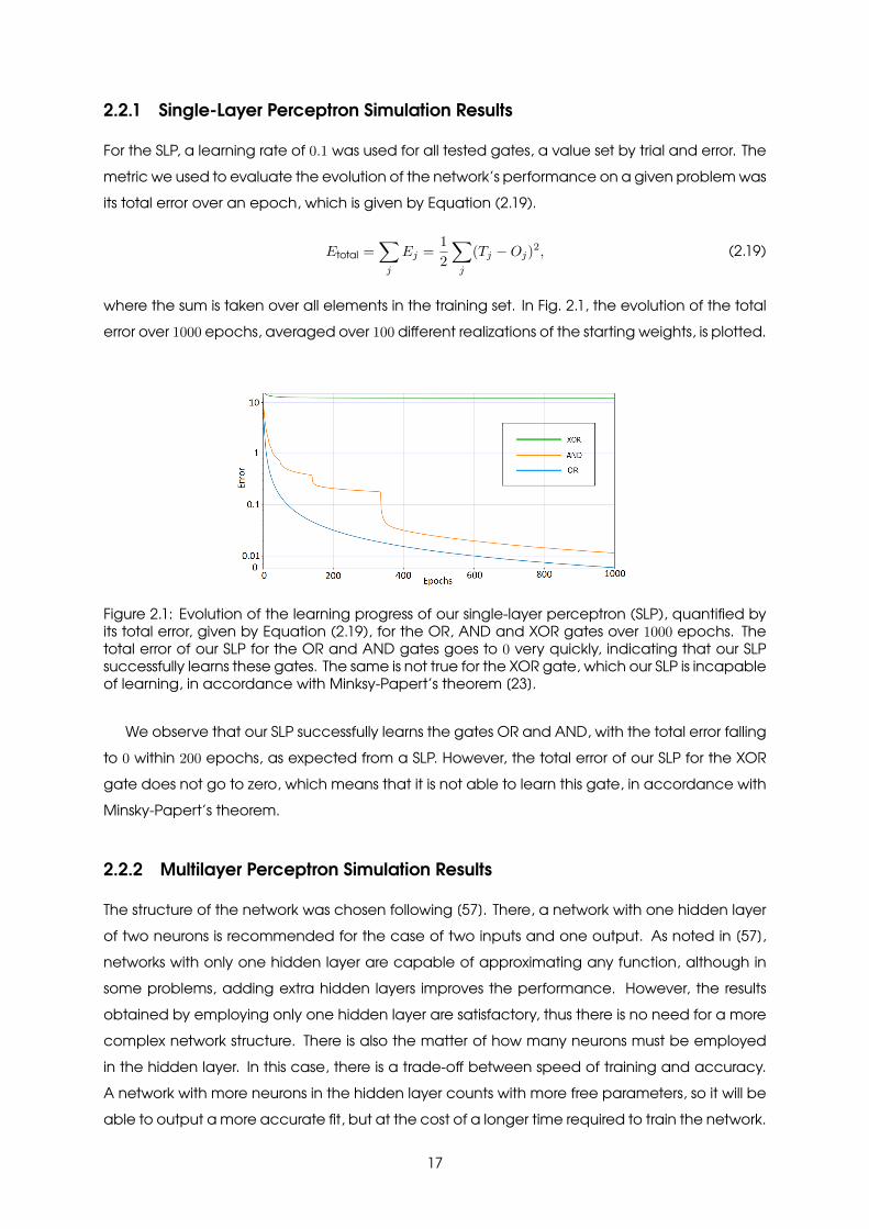
Figure 2.1: Evolution of the learning progress of our single-layer perceptron (SLP), quantified byits total error, given by Equation (2.19), for the OR, AND and XOR gates over 1000 epochs. Thetotal error of our SLP for the OR and AND gates goes to 0 very quickly, indicating that our SLPsuccessfully learns these gates. The same is not true for the XOR gate, which our SLP is incapableof learning, in accordance with Minksy-Papert’s theorem [23].

We observe that our SLP successfully learns the gates OR and AND, with the total error fallingto 0 within 200 epochs, as expected from a SLP. However, the total error of our SLP for the XORgate does not go to zero, which means that it is not able to learn this gate, in accordance withMinsky-Papert’s theorem.

2.2.2 Multilayer Perceptron Simulation Results

The structure of the network was chosen following [57]. There, a network with one hidden layerof two neurons is recommended for the case of two inputs and one output. As noted in [57],networks with only one hidden layer are capable of approximating any function, although insome problems, adding extra hidden layers improves the performance. However, the resultsobtained by employing only one hidden layer are satisfactory, thus there is no need for a morecomplex network structure. There is also the matter of how many neurons must be employedin the hidden layer. In this case, there is a trade-off between speed of training and accuracy.A network with more neurons in the hidden layer counts with more free parameters, so it will beable to output a more accurate fit, but at the cost of a longer time required to train the network.

17

A rule of thumb for choosing the number of neurons in the hidden layer is to start with an amountthat is between the number of inputs and the number of outputs and adjust according to theresults obtained. This leads to two neurons for the hidden layer and, similarly to what happenedwith the number of hidden layers, the results obtained using two neurons in the hidden layer aresufficiently accurate, so there was no need to try other structures. The learning rates used, whichwe have chosen through trial and error, are 0.1 for the OR and AND gates, and 0.01 for the XORgate. In Fig. 2.2, the evolution of the total error over 1000 epochs, averaged over 100 differentrealizations of the starting weights, is plotted.

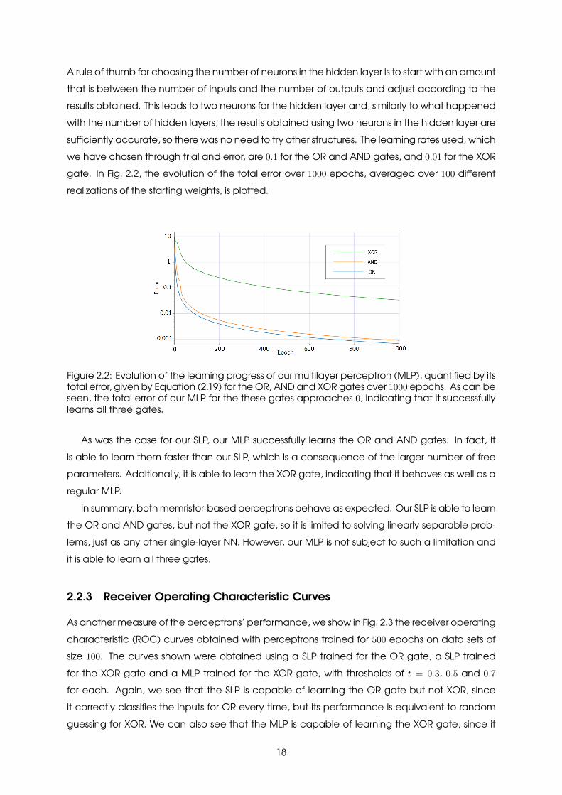
Figure 2.2: Evolution of the learning progress of our multilayer perceptron (MLP), quantified by itstotal error, given by Equation (2.19) for the OR, AND and XOR gates over 1000 epochs. As can beseen, the total error of our MLP for the these gates approaches 0, indicating that it successfullylearns all three gates.

As was the case for our SLP, our MLP successfully learns the OR and AND gates. In fact, itis able to learn them faster than our SLP, which is a consequence of the larger number of freeparameters. Additionally, it is able to learn the XOR gate, indicating that it behaves as well as aregular MLP.

In summary, both memristor-based perceptrons behave as expected. Our SLP is able to learnthe OR and AND gates, but not the XOR gate, so it is limited to solving linearly separable prob-lems, just as any other single-layer NN. However, our MLP is not subject to such a limitation andit is able to learn all three gates.

2.2.3 Receiver Operating Characteristic Curves

As another measure of the perceptrons’ performance, we show in Fig. 2.3 the receiver operatingcharacteristic (ROC) curves obtained with perceptrons trained for 500 epochs on data sets ofsize 100. The curves shown were obtained using a SLP trained for the OR gate, a SLP trainedfor the XOR gate and a MLP trained for the XOR gate, with thresholds of t = 0.3, 0.5 and 0.7

for each. Again, we see that the SLP is capable of learning the OR gate but not XOR, sinceit correctly classifies the inputs for OR every time, but its performance is equivalent to randomguessing for XOR. We can also see that the MLP is capable of learning the XOR gate, since it

18

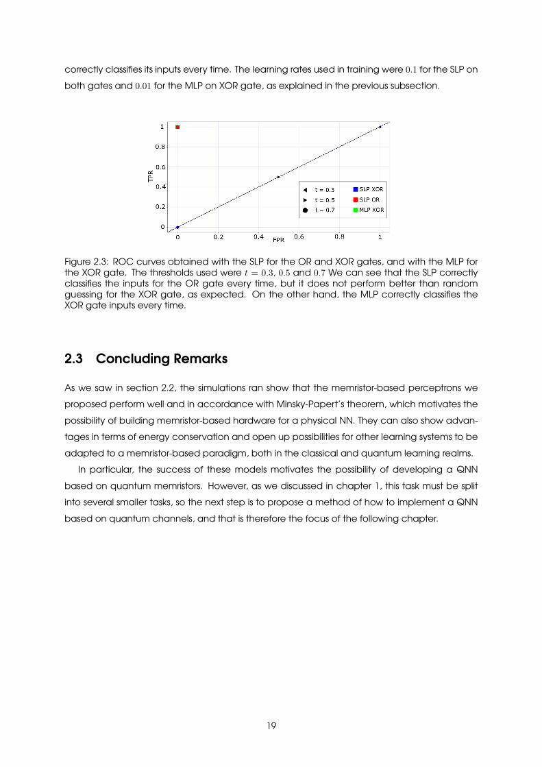
correctly classifies its inputs every time. The learning rates used in training were 0.1 for the SLP onboth gates and 0.01 for the MLP on XOR gate, as explained in the previous subsection.

Figure 2.3: ROC curves obtained with the SLP for the OR and XOR gates, and with the MLP forthe XOR gate. The thresholds used were t = 0.3, 0.5 and 0.7 We can see that the SLP correctlyclassifies the inputs for the OR gate every time, but it does not perform better than randomguessing for the XOR gate, as expected. On the other hand, the MLP correctly classifies theXOR gate inputs every time.

2.3 Concluding Remarks

As we saw in section 2.2, the simulations ran show that the memristor-based perceptrons weproposed perform well and in accordance with Minsky-Papert’s theorem, which motivates thepossibility of building memristor-based hardware for a physical NN. They can also show advan-tages in terms of energy conservation and open up possibilities for other learning systems to beadapted to a memristor-based paradigm, both in the classical and quantum learning realms.

In particular, the success of these models motivates the possibility of developing a QNNbased on quantum memristors. However, as we discussed in chapter 1, this task must be splitinto several smaller tasks, so the next step is to propose a method of how to implement a QNNbased on quantum channels, and that is therefore the focus of the following chapter.

19

20

Chapter 3

Quantum Neural Network

We will now see how we can take advantage of an equivalence between quantum chan-nels and classical channels to implement a QNN. A classical channel can be represented by astochastic matrix, so if we encode the weights of a NN in a stochastic matrix and use the equiv-alence we mentioned, we have reason to believe that we can use a quantum channel as amodel for a QNN.

3.1 Classical Network as a Stochastic Matrix

A stochastic matrix is a matrix whose entries are non-negative real numbers that represent prob-abilities. In particular, a left-stochastic matrix A is a matrix whose entries {Aij} fulfill the followingconstraints:

∑k

Akj = 1 ,∀j, (3.1)

Aij ≥ 0,∀ i, j, (3.2)

i.e., its entries are non-negative and each of its columns sums to 1.

Figure 3.1: Single-layer perceptron with inputs x1 and x2, output y and connection weights w1

and w2.

21

The naive way to store the weights of a perceptron with two inputs like the one in figure 3.1in a stochastic matrix would be the following:

y =[w0 w1

]x0x1

, (3.3)

where y is the output of the perceptron andwi is the weight of the synapse connecting input xi tothe neuron. However, the stochasticity constraint given by equation 3.2 implies that w0 = w1 = 1,which means that this network would be useless, so we need a different way to store the weights.A possible solution is to encode the two bits of the inputs, x0 and x1, into four bits, x00, x01, x10and x11, and the output bit y into two bits, y0 and y1, as shown in tables 3.1 and 3.2. The idea

Before Afterx0 x1 x00 x01 x10 x110 0 1 0 1 00 1 1 0 0 11 0 0 1 1 01 1 0 1 0 1

Table 3.1: Encoding of the inputs.

Before Aftery y0 y10 1 01 0 1

Table 3.2: Encoding of the output.

is that the value of xij is 1 if xi is j and 0 otherwise. Similarly, the value of yi is 1 if y is i and 0

otherwise. Using this encoding, we get a 2 × 4 matrix for the NN weights. The network has onlytwo synapses, each of them connecting one of the input bits to the output, therefore there are2 degrees of freedom, not 8 as one might expect. The relation between the outputs and theinputs is given by the weight matrix W :

y0y1

=

w0 1− w0 w1 1− w1

1− w0 w0 1− w1 w1

x00

x01

x10

x11

, (3.4)

where w0 is the weight of synapse connecting the first input to the output and w1 is the weightof the synapse connecting the second input to the output. The stochasticity constraints for thisweight matrix are:

w0 + (1− w0) = 1, (3.5)

w1 + (1− w1) = 1, (3.6)

22

which result in

w0,1 ∈ [0, 1]. (3.7)

This is the most freedom we can have in choosing the parameters of a stochastic matrix.

3.1.1 Stochastic Learning

Now that we have established how the weights of the network should be stored in a stochasticmatrix, we must find a way to train them, that is, we must find an algorithm to update the weightswith the goal of minimizing some cost function J in such a way that the stochasticity constraintsremain fulfilled. Typically, in the context of supervised learning, a gradient descent-based al-gorithm is used to solve problems like this. However, this method imposes no restriction on thevalues that the weights can take. This means that even if we start with a stochastic matrix, up-dating the weights with a gradient descent-based method will violate the stochasticity, both bymaking entries negative and by making it so that the columns no longer add to 1. We thereforeneed to go about this in a different way.

The multiplicative update rule is a rule on which a set of algorithms for optimizing cost func-tions with respect to matrices are based. If we are optimizing a cost function J with respect toa matrix W , the update rule is given by [58]:

W ′ij = Wij

∇−ij∇+ij

, (3.8)

in which ∇ = ∂J∂W = ∇+ −∇−. ∇+ is the positive part of the gradient and ∇− the absolute value

of its negative part. The cost function is non-increasing under this update rule and it is invariantif and only if W is at a stationary point of the cost function [58]. This rule also guarantees that theentries of the matrix remain non-negative. It does not, however, guarantee that the columnssum to 1. The naive solution would be to normalize the columns at the end of each iterationof the learning process, but this has been shown to raise convergence issues [59], so we needa more sophisticated solution. One such solution is to use the reparameterization method [59].Reparameterization is a method for learning with stochastic matrices that imposes stochasticityas a hard requirement, as we will now see. Again, let W be the stochastic matrix that stores theweights of our network:

W =

w0 1− w0 w1 1− w1

1− w0 w0 1− w1 w1

. (3.9)

W is reparameterized as a non-stochastic matrix U in the following manner:

Wij =Uij∑k Ukj

. (3.10)

23

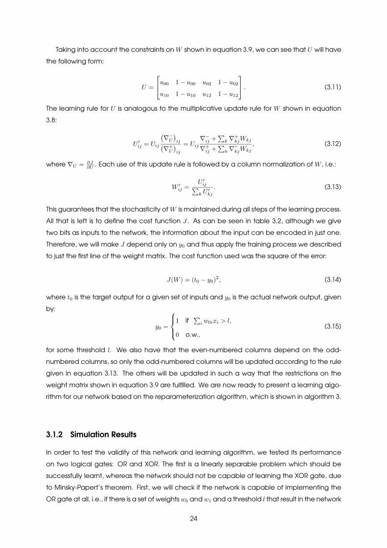
Taking into account the constraints on W shown in equation 3.9, we can see that U will havethe following form:

U =

u00 1− u00 u02 1− u02u10 1− u10 u12 1− u12

. (3.11)

The learning rule for U is analogous to the multiplicative update rule for W shown in equation3.8:

U ′ij = Uij

(∇−U)ij(

∇+U

)ij

= Uij∇−ij +

∑k∇

+kjWkj

∇+ij +

∑k∇−kjWkj

, (3.12)

where ∇U = ∂J∂U . Each use of this update rule is followed by a column normalization of W , i.e.:

W ′ij =U ′ij∑k U′kj

. (3.13)

This guarantees that the stochasticity of W is maintained during all steps of the learning process.All that is left is to define the cost function J . As can be seen in table 3.2, although we givetwo bits as inputs to the network, the information about the input can be encoded in just one.Therefore, we will make J depend only on y0 and thus apply the training process we describedto just the first line of the weight matrix. The cost function used was the square of the error:

J(W ) = (t0 − y0)2, (3.14)

where t0 is the target output for a given set of inputs and y0 is the actual network output, givenby:

y0 =

1 if∑i w0ixi > l,

0 o.w.,(3.15)

for some threshold l. We also have that the even-numbered columns depend on the odd-numbered columns, so only the odd-numbered columns will be updated according to the rulegiven in equation 3.13. The others will be updated in such a way that the restrictions on theweight matrix shown in equation 3.9 are fulfilled. We are now ready to present a learning algo-rithm for our network based on the reparameterization algorithm, which is shown in algorithm 3.

3.1.2 Simulation Results

In order to test the validity of this network and learning algorithm, we tested its performanceon two logical gates: OR and XOR. The first is a linearly separable problem which should besuccessfully learnt, whereas the network should not be capable of learning the XOR gate, dueto Minsky-Papert’s theorem. First, we will check if the network is capable of implementing theOR gate at all, i.e., if there is a set of weights w0 and w1 and a threshold l that result in the network

24

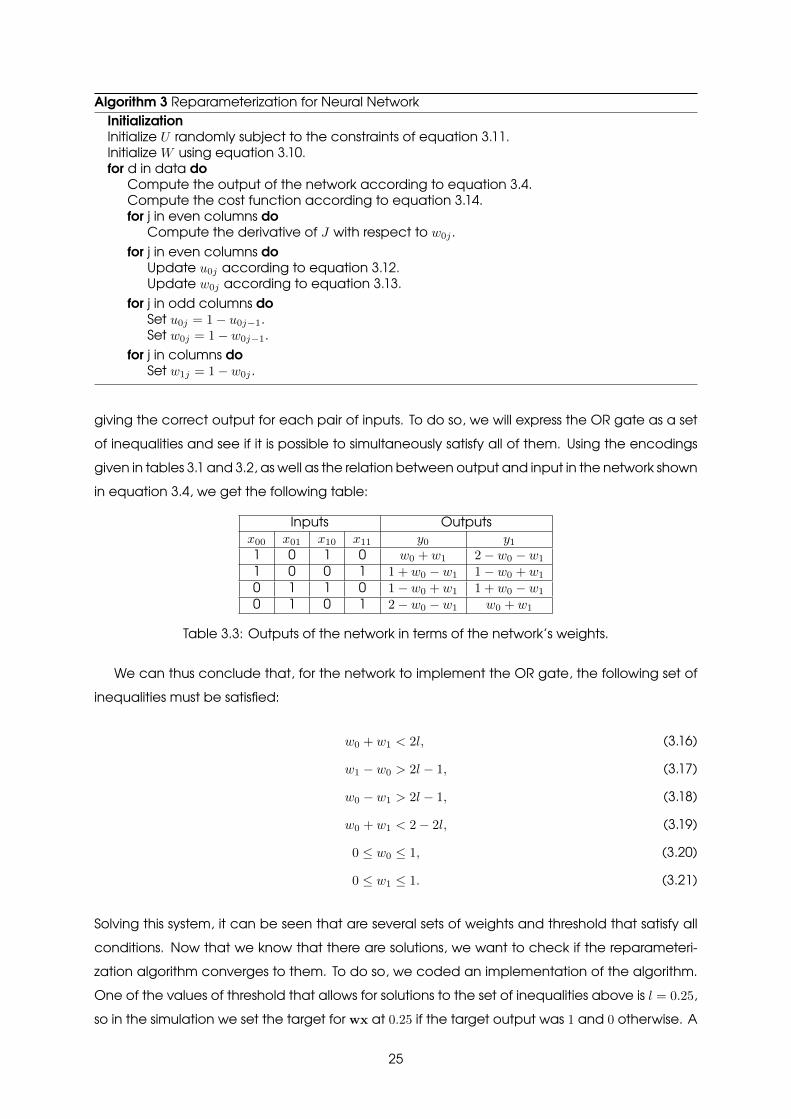
Algorithm 3 Reparameterization for Neural NetworkInitializationInitialize U randomly subject to the constraints of equation 3.11.Initialize W using equation 3.10.for d in data do

Compute the output of the network according to equation 3.4.Compute the cost function according to equation 3.14.for j in even columns do

Compute the derivative of J with respect to w0j .for j in even columns do

Update u0j according to equation 3.12.Update w0j according to equation 3.13.

for j in odd columns doSet u0j = 1− u0j−1.Set w0j = 1− w0j−1.

for j in columns doSet w1j = 1− w0j .

giving the correct output for each pair of inputs. To do so, we will express the OR gate as a setof inequalities and see if it is possible to simultaneously satisfy all of them. Using the encodingsgiven in tables 3.1 and 3.2, as well as the relation between output and input in the network shownin equation 3.4, we get the following table:

Inputs Outputsx00 x01 x10 x11 y0 y1

1 0 1 0 w0 + w1 2− w0 − w1

1 0 0 1 1 + w0 − w1 1− w0 + w1

0 1 1 0 1− w0 + w1 1 + w0 − w1

0 1 0 1 2− w0 − w1 w0 + w1

Table 3.3: Outputs of the network in terms of the network’s weights.

We can thus conclude that, for the network to implement the OR gate, the following set ofinequalities must be satisfied:

w0 + w1 < 2l, (3.16)

w1 − w0 > 2l − 1, (3.17)

w0 − w1 > 2l − 1, (3.18)

w0 + w1 < 2− 2l, (3.19)

0 ≤ w0 ≤ 1, (3.20)

0 ≤ w1 ≤ 1. (3.21)

Solving this system, it can be seen that are several sets of weights and threshold that satisfy allconditions. Now that we know that there are solutions, we want to check if the reparameteri-zation algorithm converges to them. To do so, we coded an implementation of the algorithm.One of the values of threshold that allows for solutions to the set of inequalities above is l = 0.25,so in the simulation we set the target for wx at 0.25 if the target output was 1 and 0 otherwise. A

25

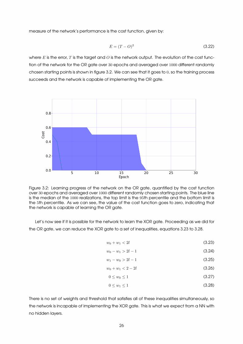
measure of the network’s performance is the cost function, given by:

E = (T −O)2 (3.22)

where E is the error, T is the target and O is the network output. The evolution of the cost func-tion of the network for the OR gate over 30 epochs and averaged over 1000 different randomlychosen starting points is shown in figure 3.2. We can see that it goes to 0, so the training processsucceeds and the network is capable of implementing the OR gate.

Figure 3.2: Learning progress of the network on the OR gate, quantified by the cost functionover 30 epochs and averaged over 1000 different randomly chosen starting points. The blue lineis the median of the 1000 realizations, the top limit is the 95th percentile and the bottom limit isthe 5th percentile. As we can see, the value of the cost function goes to zero, indicating thatthe network is capable of learning the OR gate.

Let’s now see if it is possible for the network to learn the XOR gate. Proceeding as we did forthe OR gate, we can reduce the XOR gate to a set of inequalities, equations 3.23 to 3.28.

w0 + w1 < 2l (3.23)

w0 − w1 > 2l − 1 (3.24)

w1 − w0 > 2l − 1 (3.25)

w0 + w1 < 2− 2l (3.26)

0 ≤ w0 ≤ 1 (3.27)

0 ≤ w1 ≤ 1 (3.28)

There is no set of weights and threshold that satisfies all of these inequalities simultaneously, sothe network is incapable of implementing the XOR gate. This is what we expect from a NN withno hidden layers.

26

In summary, the network does not seem to lose capabilities by having its weights encodedinto a stochastic matrix. It can learn linearly separable problems, but is incapable of learningnon-linearly separable ones, just as a regular NN with no hidden layers.

3.2 Quantum Neural Network

3.2.1 Quantum-classical Equivalence

We will now use the correspondence between quantum and classical channels the authorsshow in [60] to lay the foundations for our QNN. Let W = (aij) be a left-stochastic matrix, i.e.:

dim∑k=1

akj = 1 ∀j ∈ [1, dim], (3.29)

aij ≥ 0∀ i, j. (3.30)

Let the action of the quantum channel EA be given by the Kraus operators:

Ai,j =√ai,j |i〉 〈j| . (3.31)

Let ρ be a diagonal density operator with entries ρi,j = δi,jpi ≥ 0. The fact that ρ is a densityoperator implies that pi are real numbers with 0 ≤ pi ≤ 1 and

∑i pi = 1. For such an operator, EA

has the property that ρ′ := EA(ρ) is also diagonal with ρ′i,j = δi,jp′i and p′ = Wp, i.e., the quantum

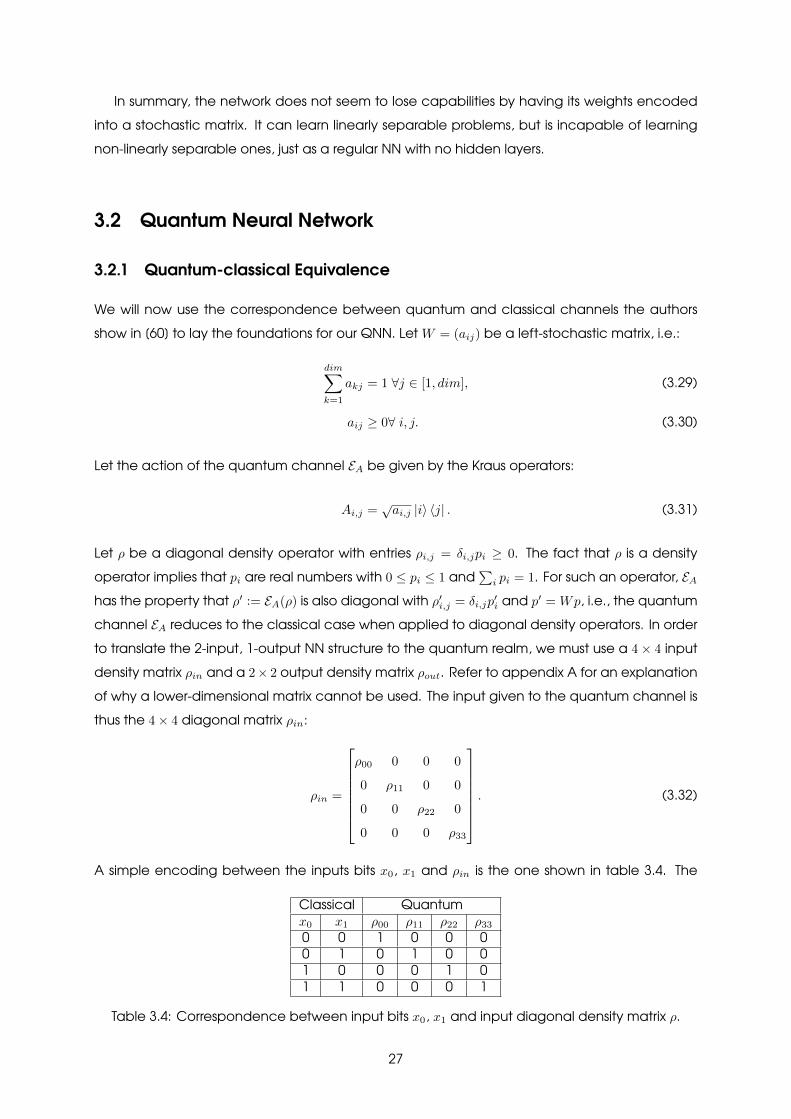
channel EA reduces to the classical case when applied to diagonal density operators. In orderto translate the 2-input, 1-output NN structure to the quantum realm, we must use a 4× 4 inputdensity matrix ρin and a 2× 2 output density matrix ρout. Refer to appendix A for an explanationof why a lower-dimensional matrix cannot be used. The input given to the quantum channel isthus the 4× 4 diagonal matrix ρin:

ρin =

ρ00 0 0 0

0 ρ11 0 0

0 0 ρ22 0

0 0 0 ρ33

. (3.32)

A simple encoding between the inputs bits x0, x1 and ρin is the one shown in table 3.4. The

Classical Quantumx0 x1 ρ00 ρ11 ρ22 ρ330 0 1 0 0 00 1 0 1 0 01 0 0 0 1 01 1 0 0 0 1

Table 3.4: Correspondence between input bits x0, x1 and input diagonal density matrix ρ.

27

output of the network, ρout, is given by:

ρout = EA(ρin) =∑i,j

Ai,jρinA†i,j =

ρ′00 0

0 ρ′11

, (3.33)

where: ρ′00ρ′11

=

ρ00w0 + ρ11(1− w0) + ρ22w1 + ρ33(1− w1)

ρ00(1− w0) + ρ11w0 + ρ22(1− w1) + ρ33w1

. (3.34)

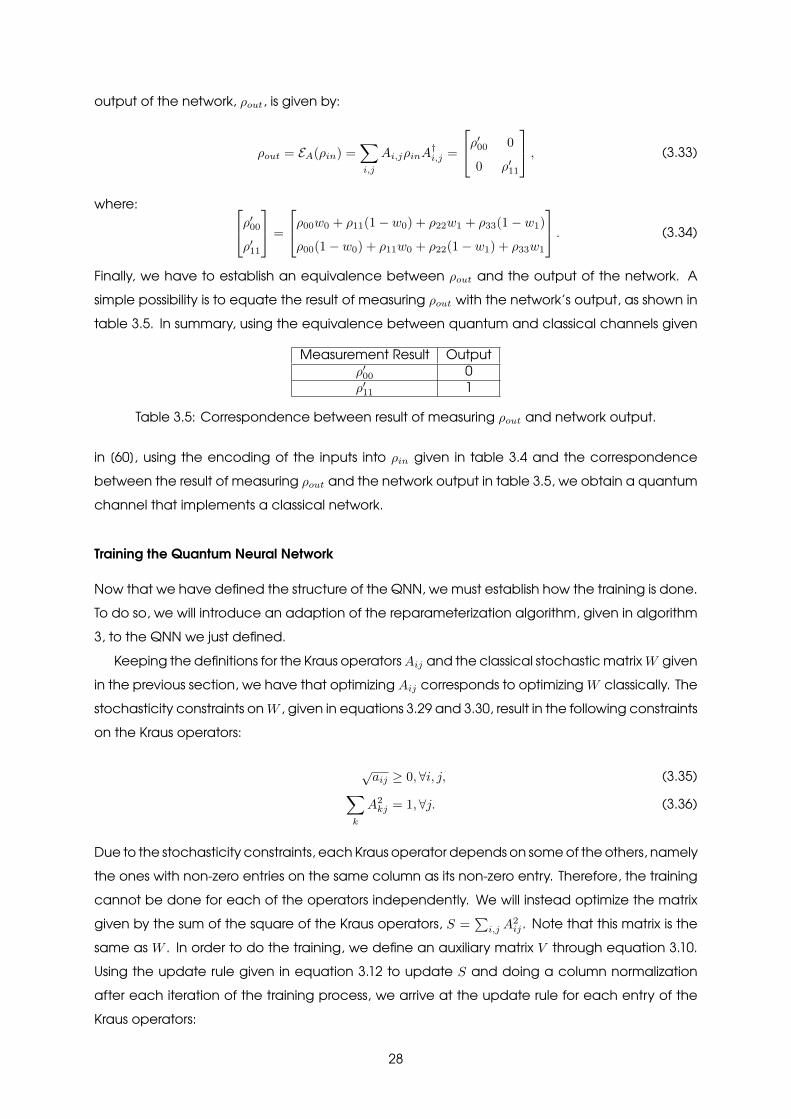
Finally, we have to establish an equivalence between ρout and the output of the network. Asimple possibility is to equate the result of measuring ρout with the network’s output, as shown intable 3.5. In summary, using the equivalence between quantum and classical channels given

Measurement Result Outputρ′00 0ρ′11 1

Table 3.5: Correspondence between result of measuring ρout and network output.

in [60], using the encoding of the inputs into ρin given in table 3.4 and the correspondencebetween the result of measuring ρout and the network output in table 3.5, we obtain a quantumchannel that implements a classical network.

Training the Quantum Neural Network

Now that we have defined the structure of the QNN, we must establish how the training is done.To do so, we will introduce an adaption of the reparameterization algorithm, given in algorithm3, to the QNN we just defined.

Keeping the definitions for the Kraus operatorsAij and the classical stochastic matrixW givenin the previous section, we have that optimizing Aij corresponds to optimizing W classically. Thestochasticity constraints on W , given in equations 3.29 and 3.30, result in the following constraintson the Kraus operators:

√aij ≥ 0,∀i, j, (3.35)∑

k

A2kj = 1,∀j. (3.36)

Due to the stochasticity constraints, each Kraus operator depends on some of the others, namelythe ones with non-zero entries on the same column as its non-zero entry. Therefore, the trainingcannot be done for each of the operators independently. We will instead optimize the matrixgiven by the sum of the square of the Kraus operators, S =

∑i,j A

2ij . Note that this matrix is the

same as W . In order to do the training, we define an auxiliary matrix V through equation 3.10.Using the update rule given in equation 3.12 to update S and doing a column normalizationafter each iteration of the training process, we arrive at the update rule for each entry of theKraus operators:

28

A′ij =√S′ij =

√V ′ij∑k V′kj

(3.37)

This learning algorithm is a direct adaptation of the algorithm shown in algorithm 3, with justan extra step to update the Kraus operators, so the performance of this QNN should be identicalto that of the classical network we saw in section 3.1.

3.2.2 Generalization

We will now remove the stochasticity restriction we had imposed on the Kraus operators to obtainthe link between classical and quantum channels and we will consider a completely generalquantum channel. This channel maps a density matrix in C4 to a density matrix in C2, so, as aresult of theorem 1.2.1, it is defined by a maximum of 8 Kraus operators, A0 through A7:

A0 =

a00 a01 a02 a03

a10 a11 a12 a13

, A7 =

h00 h01 h02 h03

h10 h11 h12 h13

. (3.38)

A quantum channel is a CPTP map so, again in accordance with theorem 1.2.1, these operatorsare subject to the following constraint:

∑k

A†kAk = 14, (3.39)

where 14 is the identity matrix of dimension 4. Besides this constraint, the operators will alsobe subject to conditions analogous to the ones in the classical network, which arise from thefact that the input is 4-dimensional, the output is 2-dimensional, but the network has only twosynapses. Essentially, we want to translate the restrictions on the weight matrix made evident inequation 3.9 to the Kraus operators. To do this, it is useful to gain an intuition of the effect thisquantum channel has on its input. The action of a quantum channel on an input density matrixρ is given, in terms of its Kraus operators, by:

ρ′ = EA(ρ) =∑k

AkρA†k, (3.40)

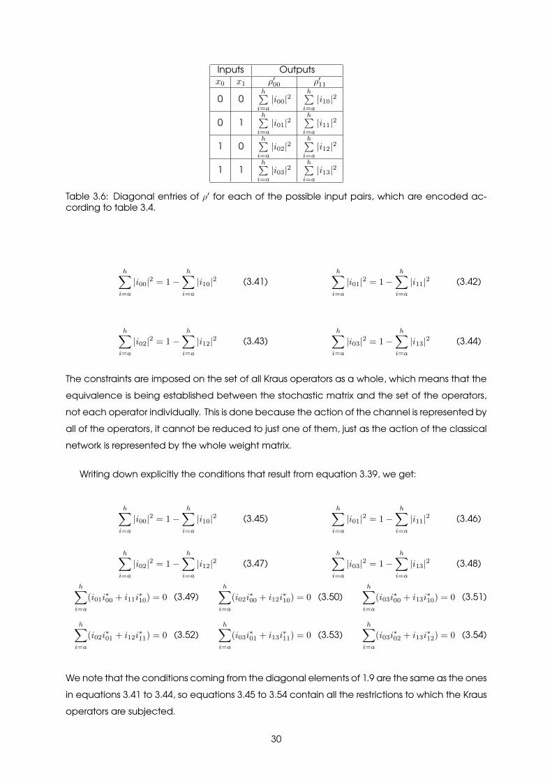
where ρ′ is the output density matrix. We will establish an equivalence between the result ofmeasuring ρ′ and the network output just as we did for the ’classical’ quantum case (see table3.5). If we encode the inputs according to table 3.4, the values of each entry in the maindiagonal of ρ′ for each possible combination of inputs are given in table 3.6.

Comparing equation 3.4 with table 3.6, we can establish a correspondence between theweights of the classical stochastic and the Kraus operators of the generalized quantum channel.In doing so, we find conditions for the operators that are analogous to the conditions for theclassical weights given in equations 3.5 and 3.6. The set of conditions for the Kraus operatorsemerging from this analysis are given in equations 3.41 to 3.44.

29

Inputs Outputsx0 x1 ρ′00 ρ′11

0 0h∑i=a

|i00|2h∑i=a

|i10|2

0 1h∑i=a

|i01|2h∑i=a

|i11|2

1 0h∑i=a

|i02|2h∑i=a

|i12|2

1 1h∑i=a

|i03|2h∑i=a

|i13|2

Table 3.6: Diagonal entries of ρ′ for each of the possible input pairs, which are encoded ac-cording to table 3.4.

h∑i=a

|i00|2 = 1−h∑i=a

|i10|2 (3.41)h∑i=a

|i01|2 = 1−h∑i=a

|i11|2 (3.42)

h∑i=a

|i02|2 = 1−h∑i=a

|i12|2 (3.43)h∑i=a

|i03|2 = 1−h∑i=a

|i13|2 (3.44)

The constraints are imposed on the set of all Kraus operators as a whole, which means that theequivalence is being established between the stochastic matrix and the set of the operators,not each operator individually. This is done because the action of the channel is represented byall of the operators, it cannot be reduced to just one of them, just as the action of the classicalnetwork is represented by the whole weight matrix.

Writing down explicitly the conditions that result from equation 3.39, we get:

h∑i=a

|i00|2 = 1−h∑i=a

|i10|2 (3.45)h∑i=a

|i01|2 = 1−h∑i=a

|i11|2 (3.46)

h∑i=a

|i02|2 = 1−h∑i=a

|i12|2 (3.47)h∑i=a

|i03|2 = 1−h∑i=a

|i13|2 (3.48)

h∑i=a

(i01i∗00 + i11i

∗10) = 0 (3.49)

h∑i=a

(i02i∗00 + i12i

∗10) = 0 (3.50)

h∑i=a

(i03i∗00 + i13i

∗10) = 0 (3.51)

h∑i=a

(i02i∗01 + i12i

∗11) = 0 (3.52)

h∑i=a

(i03i∗01 + i13i

∗11) = 0 (3.53)

h∑i=a

(i03i∗02 + i13i

∗12) = 0 (3.54)

We note that the conditions coming from the diagonal elements of 1.9 are the same as the onesin equations 3.41 to 3.44, so equations 3.45 to 3.54 contain all the restrictions to which the Krausoperators are subjected.

30

Unitary representation

We would also like to know the restrictions on the unitary representation of the quantum channel,i.e., the unitary operator that acts on the closed composite system consisting of the system ofstudy and the environment. In this framework, the action of the quantum channel is given by:

ρ′ = E(ρ) = Trenv[U(ρ0 ⊗ |j〉 〈j|)U†

], (3.55)

where ρ0 is the initial state of the system, |j〉 〈j| is the initial state of the environment, ρ′ is the finalstate of the system and U is the unitary that acts on the composite system. Writing the traceover the environment explicitly, equation 3.55 becomes:

ρ′ =∑i

〈i|U |j〉 ρ0 〈j|U†|i〉 , (3.56)

where {|i〉} is an orthonormal basis of the environment. We want to write out ρ′ in terms of theelements of U . ρ, the initial state of the composite system is given by:

ρ = ρ0 ⊗ |j〉 〈j| . (3.57)

It is, in our case, a 4 × 4 diagonal density matrix. The correspondence between the input bitsx0, x1 and the diagonal entries of ρ is the same as the one used in the Kraus representation (seetable 3.4). We need to figure out which combinations of ρ0 and |j〉 〈j| result in the desired initialstates ρ. Writing down ρ0 as follows:

ρ0 =

ρ000 ρ001

ρ010 ρ011

, (3.58)

we obtain the desired combinations, as shown in table 3.7. In order to write down the output of

System Environment Totalρ000 ρ011 |j〉 ρ00 ρ11 ρ22 ρ33

1 0 |0〉 1 0 0 00 1 |0〉 0 1 0 01 0 |1〉 0 0 1 00 1 |1〉 0 0 0 1

Table 3.7: Correspondence between total state and states of system and environment.

the quantum channel, we write the elements of the unitary U explicitly:

U =

u0 u1 u2 u3

u4 u5 u6 u7

u8 u9 u10 u11

u12 u13 u14 u15

, (3.59)

31

where u0 through u15 are complex numbers that are subject to restrictions coming from theunitarity of U . Taking all of this into account, the diagonal entries of ρ′ are given by:

Inputs Outputsx0 x0 ρ′00 ρ′110 0 |u0|2 + |u4|2 |u8|2 + |u12|20 1 |u2|2 + |u6|2 |u10|2 + |u14|21 0 |u1|2 + |u5|2 |u9|2 + |u13|21 1 |u3|2 + |u7|2 |u11|2 + |u15|2

Table 3.8: Diagonal entries of ρ′ for each of the possible input pairs.

3.2.3 Capabilities of the QNN

Now that we have some understanding of how the network behaves, the next step is to lookinto its capabilities and limitations. One natural question to ask is if it is universal in the classicalsense, i.e., if it is capable of implementing every classical 2-input, 1-output logic gate. There aresixteen of them, as shown in table 3.9. We start by checking if there is a set of Kraus operators

Inputs Outputx1 x2 y1 y2 y3 y4 y5 y6 y7 y8 y9 y10 y11 y12 y13 y14 y15 y160 0 0 0 0 0 0 0 0 0 1 1 1 1 1 1 1 10 1 0 0 0 0 1 1 1 1 0 0 0 0 1 1 1 11 0 0 0 1 1 0 0 1 1 0 0 1 1 0 0 1 11 1 0 1 0 1 0 1 0 1 0 1 0 1 0 1 0 1

Table 3.9: The sixteen 2-input, 1-output classical logic gates.

that implements each of these gates, starting with gate 7, because it corresponds to the XORgate. If there is a set of Kraus operators that implements it, we have that there is no quantumversion of Minsky-Papert’s theorem, which means that our QNN is, in a sense, more powerfulthan a classical NN with no hidden layers.

Using the correspondence between measurement result and output given in table 3.5 andthe values of the diagonal entries of the output density matrix given in table 3.6, we get thefollowing conditions for successful implementation of gate 7:

h∑i=a

|i00|2 = 1, (3.60)h∑i=a

|i10|2 = 0, (3.61)h∑i=a

|i01|2 = 0, (3.62)h∑i=a

|i11|2 = 1, (3.63)

h∑i=a

|i02|2 = 0, (3.64)h∑i=a

|i12|2 = 1, (3.65)h∑i=a

|i03|2 = 1, (3.66)h∑i=a

|i13|2 = 0. (3.67)

32

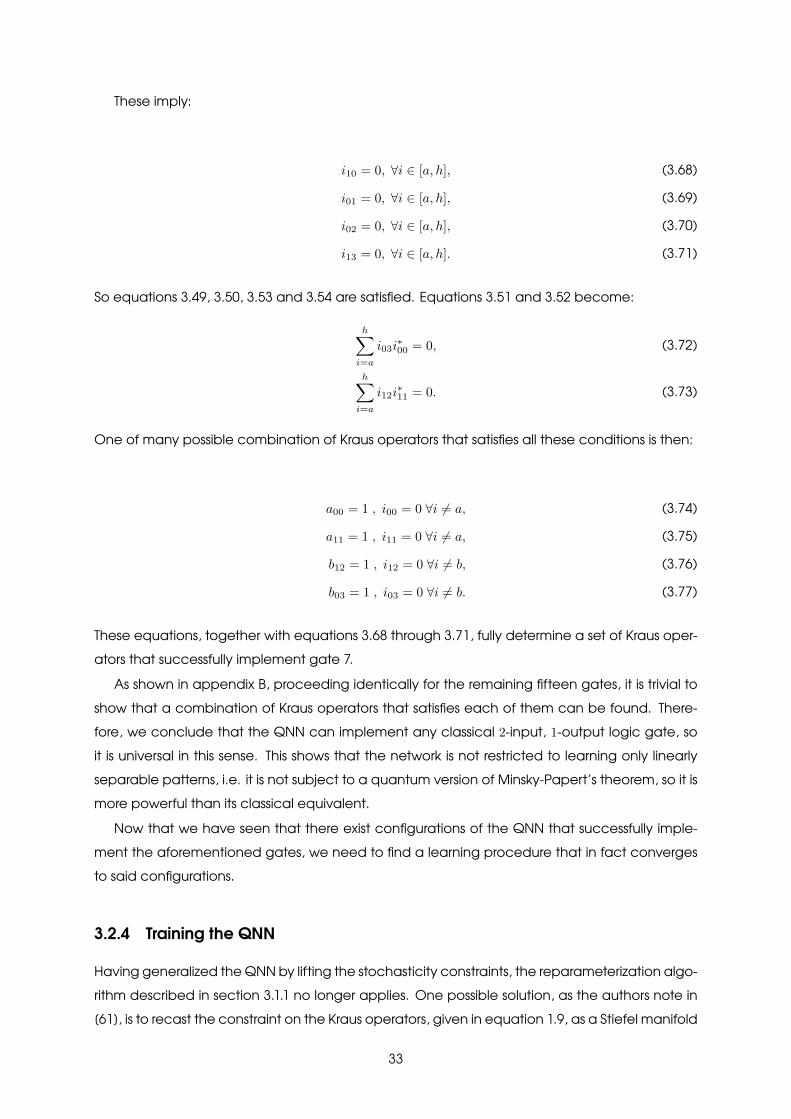
These imply:

i10 = 0, ∀i ∈ [a, h], (3.68)

i01 = 0, ∀i ∈ [a, h], (3.69)

i02 = 0, ∀i ∈ [a, h], (3.70)

i13 = 0, ∀i ∈ [a, h]. (3.71)

So equations 3.49, 3.50, 3.53 and 3.54 are satisfied. Equations 3.51 and 3.52 become:

h∑i=a

i03i∗00 = 0, (3.72)

h∑i=a

i12i∗11 = 0. (3.73)

One of many possible combination of Kraus operators that satisfies all these conditions is then:

a00 = 1 , i00 = 0 ∀i 6= a, (3.74)

a11 = 1 , i11 = 0 ∀i 6= a, (3.75)

b12 = 1 , i12 = 0 ∀i 6= b, (3.76)

b03 = 1 , i03 = 0 ∀i 6= b. (3.77)

These equations, together with equations 3.68 through 3.71, fully determine a set of Kraus oper-ators that successfully implement gate 7.

As shown in appendix B, proceeding identically for the remaining fifteen gates, it is trivial toshow that a combination of Kraus operators that satisfies each of them can be found. There-fore, we conclude that the QNN can implement any classical 2-input, 1-output logic gate, soit is universal in this sense. This shows that the network is not restricted to learning only linearlyseparable patterns, i.e. it is not subject to a quantum version of Minsky-Papert’s theorem, so it ismore powerful than its classical equivalent.

Now that we have seen that there exist configurations of the QNN that successfully imple-ment the aforementioned gates, we need to find a learning procedure that in fact convergesto said configurations.

3.2.4 Training the QNN

Having generalized the QNN by lifting the stochasticity constraints, the reparameterization algo-rithm described in section 3.1.1 no longer applies. One possible solution, as the authors note in[61], is to recast the constraint on the Kraus operators, given in equation 1.9, as a Stiefel manifold

33

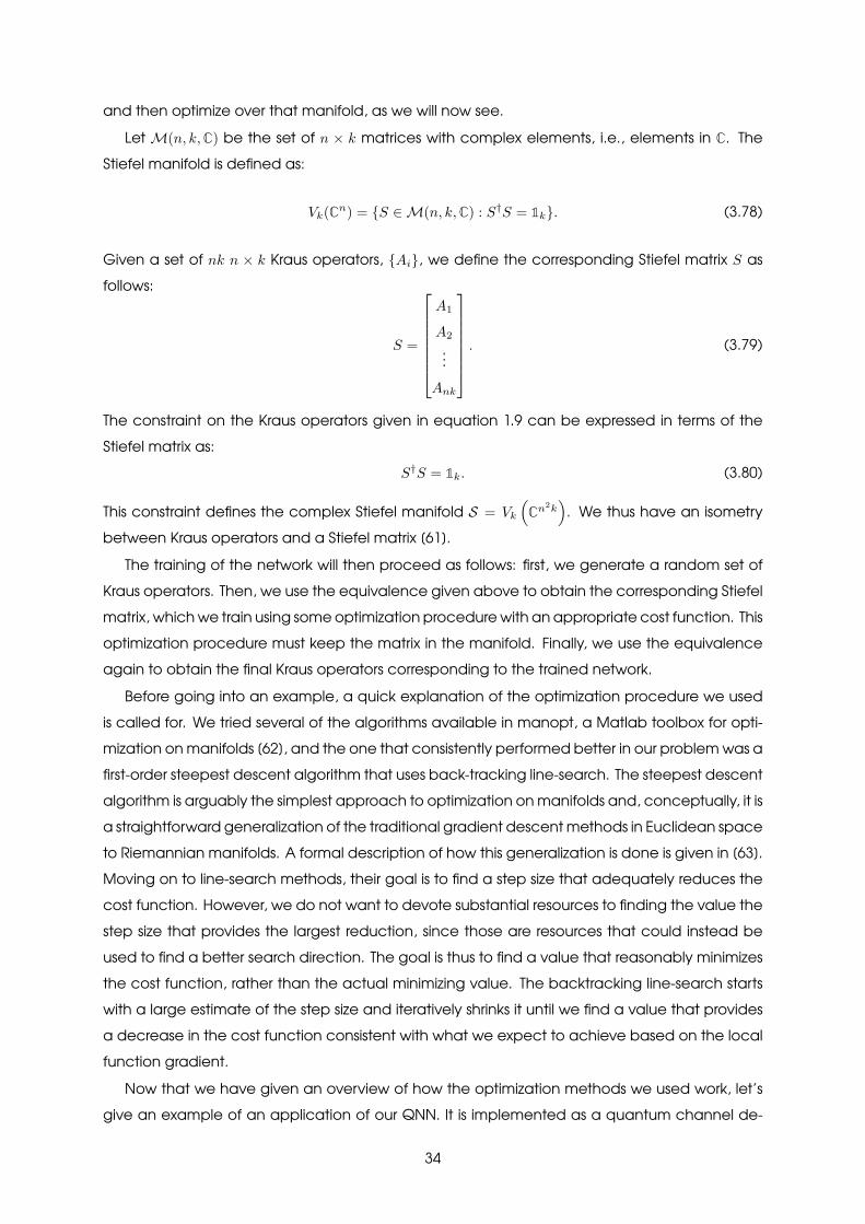
and then optimize over that manifold, as we will now see.

Let M(n, k,C) be the set of n × k matrices with complex elements, i.e., elements in C. TheStiefel manifold is defined as:

Vk(Cn) = {S ∈M(n, k,C) : S†S = 1k}. (3.78)

Given a set of nk n × k Kraus operators, {Ai}, we define the corresponding Stiefel matrix S asfollows:

S =

A1

A2

...Ank

. (3.79)

The constraint on the Kraus operators given in equation 1.9 can be expressed in terms of theStiefel matrix as:

S†S = 1k. (3.80)

This constraint defines the complex Stiefel manifold S = Vk

(Cn

2k)

. We thus have an isometrybetween Kraus operators and a Stiefel matrix [61].

The training of the network will then proceed as follows: first, we generate a random set ofKraus operators. Then, we use the equivalence given above to obtain the corresponding Stiefelmatrix, which we train using some optimization procedure with an appropriate cost function. Thisoptimization procedure must keep the matrix in the manifold. Finally, we use the equivalenceagain to obtain the final Kraus operators corresponding to the trained network.

Before going into an example, a quick explanation of the optimization procedure we usedis called for. We tried several of the algorithms available in manopt, a Matlab toolbox for opti-mization on manifolds [62], and the one that consistently performed better in our problem was afirst-order steepest descent algorithm that uses back-tracking line-search. The steepest descentalgorithm is arguably the simplest approach to optimization on manifolds and, conceptually, it isa straightforward generalization of the traditional gradient descent methods in Euclidean spaceto Riemannian manifolds. A formal description of how this generalization is done is given in [63].Moving on to line-search methods, their goal is to find a step size that adequately reduces thecost function. However, we do not want to devote substantial resources to finding the value thestep size that provides the largest reduction, since those are resources that could instead beused to find a better search direction. The goal is thus to find a value that reasonably minimizesthe cost function, rather than the actual minimizing value. The backtracking line-search startswith a large estimate of the step size and iteratively shrinks it until we find a value that providesa decrease in the cost function consistent with what we expect to achieve based on the localfunction gradient.

Now that we have given an overview of how the optimization methods we used work, let’sgive an example of an application of our QNN. It is implemented as a quantum channel de-

34

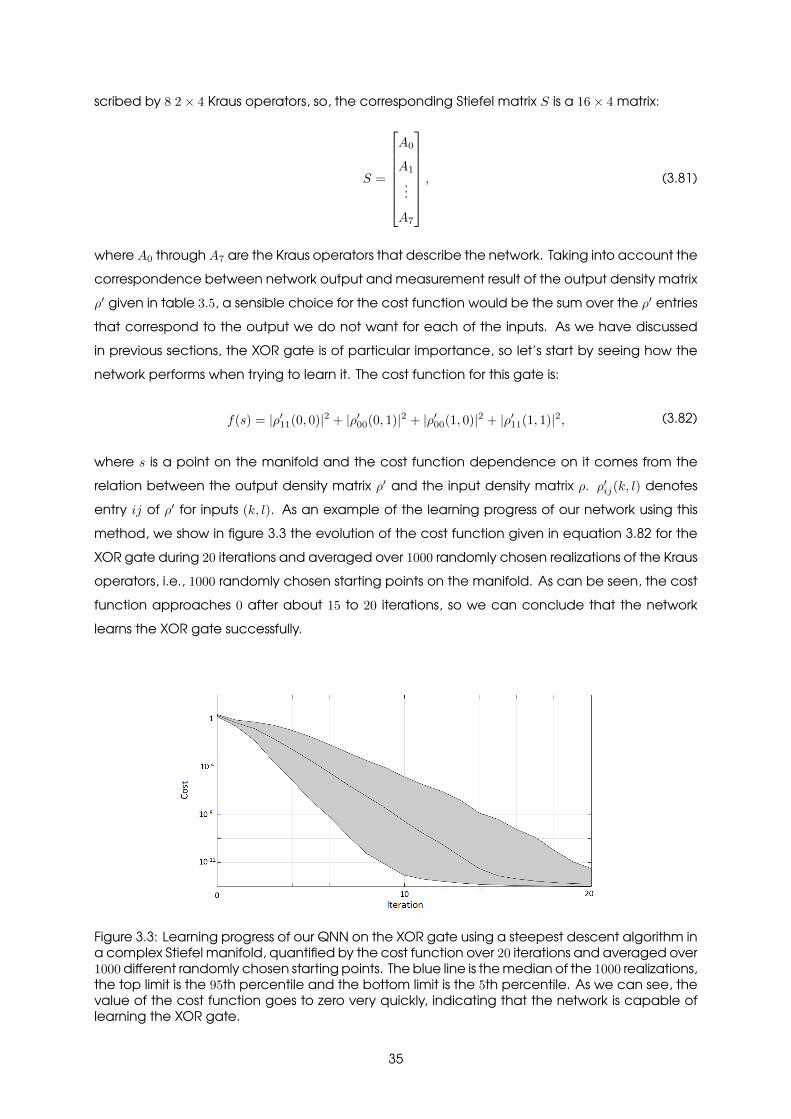
scribed by 8 2× 4 Kraus operators, so, the corresponding Stiefel matrix S is a 16× 4 matrix:

S =

A0

A1

...A7

, (3.81)

where A0 through A7 are the Kraus operators that describe the network. Taking into account thecorrespondence between network output and measurement result of the output density matrixρ′ given in table 3.5, a sensible choice for the cost function would be the sum over the ρ′ entriesthat correspond to the output we do not want for each of the inputs. As we have discussedin previous sections, the XOR gate is of particular importance, so let’s start by seeing how thenetwork performs when trying to learn it. The cost function for this gate is:

f(s) = |ρ′11(0, 0)|2 + |ρ′00(0, 1)|2 + |ρ′00(1, 0)|2 + |ρ′11(1, 1)|2, (3.82)

where s is a point on the manifold and the cost function dependence on it comes from therelation between the output density matrix ρ′ and the input density matrix ρ. ρ′ij(k, l) denotesentry ij of ρ′ for inputs (k, l). As an example of the learning progress of our network using thismethod, we show in figure 3.3 the evolution of the cost function given in equation 3.82 for theXOR gate during 20 iterations and averaged over 1000 randomly chosen realizations of the Krausoperators, i.e., 1000 randomly chosen starting points on the manifold. As can be seen, the costfunction approaches 0 after about 15 to 20 iterations, so we can conclude that the networklearns the XOR gate successfully.

Figure 3.3: Learning progress of our QNN on the XOR gate using a steepest descent algorithm ina complex Stiefel manifold, quantified by the cost function over 20 iterations and averaged over1000 different randomly chosen starting points. The blue line is the median of the 1000 realizations,the top limit is the 95th percentile and the bottom limit is the 5th percentile. As we can see, thevalue of the cost function goes to zero very quickly, indicating that the network is capable oflearning the XOR gate.

35

By redefining the cost function appropriately and performing the training process again, sim-ilar results can be obtained for any of the fifteen other gates, showing that the QNN is capableof learning these gates.

3.2.5 Scaling

We have seen some properties of the simplest unit of our QNN and how to perform its training.However, in order for the network to be applicable to practical problems, we need to increase itsdimension, both by adding hidden layers and increasing the size of the input and output layers.We are thus interested in studying how increasing the size of the network affects the trainingprocess. In more concrete terms, we want to know how the dimension of the Stiefel manifold inwhich we perform the optimization grows with the number of neurons and layers in the network.To this end, the following result on quantum channels is useful:

Proposition. Let H be a separable Hilbert space and let L1, L2 be two quantum channels onL1(H) with Kraus decompositions:

L1(T ) =∑i

AiTA†i and L2(T ) =

∑j

BjTB†j . (3.83)

The composition L2 ◦L1 is a quantum channel on L1(H). It admits a Kraus decomposition givenby:

L2 ◦ L1(T ) =∑i,j

BjAiTA†iB†j .

Proof. L1 and L2 are quantum channels on L1(H) so, by definition, for i = 1, 2 there exist Hilbertspaces Ki, states ωi on Ki and unitary operators Ui on Ki such that:

Li = TrKi(Ui(ρ⊗ ωi)U†i ), (3.84)

for all T ∈ L1(H).Let us now consider the Hilbert space K = K1 ⊗ K2 and the quantum state ω = ω1 ⊗ ω2. We

consider the natural extensions Ui of Ui to H ⊗ K by taking the tensor product of Ui with theidentity operator on the space Kj for i 6= j. We thus have that U = U2U1 is a unitary operator onH⊗K. Using the properties of partial traces, we have:

TrK(U(T ⊗ ω)U†) = TrK1⊗K2

(U2U1(T ⊗ ω1ω2)U†1 U

†2

)(3.85)

= TrK2

(TrK1

(U2(U1(T ⊗ ω1)U†1 ⊗ ω2)U†2

))(3.86)

= TrK2

(U2(TrK1

(U1(T ⊗ ω1)U†1 )⊗ ω2)U†2

)(3.87)

= TrK2(U2(L1(T )⊗ ω2)U†2 ) (3.88)

= L2(L1(T )). (3.89)

We have expressed L2 ⊗ L1 as the partial trace T → TrK(U(T ⊗ ω)U†). This is, by definition,

36

a quantum channel, so the composition of two quantum channels is also a quantum channel.We now want to find the Kraus representation of this quantum channel.

The unitary dilations of L1 and L2 can be chosen in such a way that ω1 and ω2 are pure states|ψi〉 〈ψi| [64]. Let (ei)i∈N and (fj)j∈N be orthonormal bases of K1 and K2, respectively. It can beshown [64] that the coefficients of a Kraus representation of L1 can be obtained as:

Ai = K1〈ei|U1|ψ1〉K1, (3.90)

and similarly for L2:Bj = K2

〈ej |U1|ψ1〉K2. (3.91)

Now if we compute the coefficients of L2 ◦ L1 we get:

Mij = K1⊗K2〈ei ⊗ fj |U |ψ1 ⊗ ψ2〉K1⊗K2

(3.92)

= K2〈fj | 〈ei|U2U1|ψ1〉|ψ2〉K2

(3.93)

= K2〈fj |U2K1

〈ei|U1|ψ1〉K1|ψ2〉K2

(3.94)

= K2〈fj |U2|ψ2〉K2

K1〈ei|U1|ψ1〉K1

(3.95)

= BjAi. (3.96)

This gives the expected Kraus representation.

Just as our single-layer QNN can be seen as a quantum channel, a QNN with several layerscan be seen as a composition of quantum channels, so it follows from the above proposition thata QNN can always be reduced to a single quantum channel of higher dimension. Therefore,adding layers and neurons to the QNN corresponds to increasing the maximum number of Krausoperators that describe the quantum channel.

If the input to the network is an n-dimensional density matrix and the output is anm-dimensionaldensity matrix then the Kraus operators of the quantum channel that implements the networkhave dimension m× n. If there are k layers in the network, each with jk neurons, then the maxi-mum number of Kraus operators is NKraus = j1j2...jk. Therefore, the Stiefel matrix of a k-layer QNNwith n-dimensional input, m-dimensional output and ji neurons in the ith layer is given by:

S =

A1

A2

...Aj1j2jk

.

{Ai} is a set of j1j2...jk Kraus operators of dimension n×m. The Stiefel matrix S thus has dimensionj1j2...jkn ×m ≈ jkavn ×m, jav being the average number of neurons in a layer. This means thatthe dimension of the matrix, and thus the dimension of the search space, grows exponentially

37

with the number of layers in the QNN. This presents a problem that must be overcome beforethis QNN can be useful in practice, since the exponential scaling implies that the search spacewill be far too big for problems with more than a few tens of neurons.

3.2.6 Dimensionality Reduction

As we just discussed, we would like to find a way of avoiding the exponential scaling of thenetwork. One possibility would be to approximate the quantum channel that implements ourQNN by a lower-dimensional quantum channel. In [65], the authors show that any quantumchannel mapping states on some input Hilbert spaceHA to states on some output Hilbert spaceHB can be compressed into one with order d log(d) Kraus operators, where d = max(|HA|, |HB |),which is much less than the usual |HA|×|HB |. More formally, the main result of [65] is the followingproposition:

Proposition. Fix 0 < ε < 1 and let N : L(HA) → L(HB) be a CPTP map with Kraus rank |HE | ≥|HA|, |HB |. Then, there exists a CP map N : L(HA)→ L(HB) with Kraus rank at most

C max(|HA|, |HB |)1

ε2log

(|HE |ε

), (3.97)

where C > 0 is a universal constant and such that:

∀ρ ∈ D(HA), −ε(N (ρ)− 1

|HB |

)≤ N (ρ)−N(ρ) ≤ ε

(N (ρ) +

1|HB |

). (3.98)

In particular,

∀ρ ∈ D(HA), ‖N (ρ)−N (ρ)‖1 ≤ 2ε, (3.99)

where N (ρ) is strictly trace preserving.

A proof of this result can be found in the article. Now that we know that an approximationN to the quantum channel that implements the network, N , exists, it is natural to ask how it isconstructed. We write N in the physical form:

N (ρ) = TrE(UρU†). (3.100)

For any given unit vector φ in the environment E define the CP map Nφ : L(A)→ L(B) by:

Nφ(ρ) = |E|TrE((1⊗ φ)UρU†(1⊗ φ)

). (3.101)

For φ1...φn independent uniformly distributed unit vectors in E, set Nφ(n) = 1n

∑ni=1Nφi

. Finally, wehave that for n ≤ C max (|HA|, |HB |) log

(|HE |ε

)1ε2 :

‖Nφ(ρ)−N (ρ)‖1 ≤ 2ε. (3.102)

38

The implications of this result to our QNN are clear: the number of layers and hidden layerneurons in the network does not significantly affect its capabilities, since we can always finda quantum channel with small Kraus rank that approximately implements the QNN. Moreover,this Kraus rank depends only on the dimension of the input and output Hilbert spaces. Thisdependence is linear, but, since the dimension of the Hilbert spaces scales exponentially withthe number of bits, the same is true for the Kraus rank of the approximate QNN. This meansthat for networks with a large number of inputs, say of the order of 100, the training process willstill be intractable, because this network will be implemented by about 2100 Kraus operators. Anumber of inputs of this order is not unusual, so our network cannot be used for a sizable amountof problems unless the training process is in some way simplified.

3.3 Concluding Remarks

We have introduced a QNN based on quantum channels by taking advantage of a connectionbetween classical and quantum channels. We have performed an analysis of its capabilitiesand concluded that it is universal in the classical logic gate sense, and that it is not subjectto a quantum version of Minsky-Papert’s theorem. It is thus, in a sense, more powerful thanits classical equivalent. By using an isometry between Kraus operators and Stiefel matrices, wehave introduced a training procedure for our QNN based on optimization on manifolds. Throughthe use of a result on the approximation of quantum channels by lower-dimensional ones, wehave seen that enriching the network by adding hidden layers is feasible.

As we mentioned in the previous section, the main question that remains to be addressed isthe matter of the exponential scaling of the search space with the size of the input and outputlayers. Possible paths towards solving this problem will be discussed in the final chapter.

39

40

Chapter 4

Conclusions

The goal of this thesis was to begin making headway with a completely original approach toquantum neural networks (QNN) based on quantum memristors. Due to its complexity, we splitthis task into smaller steps. First, develop models for memristor-based classical neural networks(NN). Then, develop a QNN based on quantum channels to gain knowledge about QNNs inthe context of open quantum systems, and in particular, of quantum memristors. The next stepwould be to use the knowledge we gained with this QNN model to help quantize the classicalmemristor-based perceptrons we proposed. We will use this final chapter to summarize the mainresults of this thesis, clarify its place in the field of quantum machine learning and go over thework that lies ahead.

We introduced models for classical single and multilayer perceptrons based on classicalmemristors. We provided learning algorithms for both, based on the delta rule and on the back-propagation algorithm, respectively. Using a threshold-based system, our models are able touse the internal variables of memristors to store and update the perceptron’s weights. We alsoran simulations of both models, which revealed that they behaved as expected and in accor-dance with Minsky-Papert’s theorem. Our memristor-based perceptrons have the same capa-bilities and are subject to the same limitations of regular perceptrons and thus show the feasibilityand power of a memristor-based NN.

Moving on to the quantum realm, we found a way to go from classical NNs to QNNs basedon quantum channels by taking advantage of an equivalence between classical and quantumchannels. An analysis of the capabilities of the resulting quantum network revealed that it canimplement any 2-input, 1-output classical logic gate, so it is universal in this sense. In particular, itcan implement the XOR gate, which means that there is no quantum version of Minsky-Papert’stheorem, so the QNN is not subject to the same limitations as its classical equivalent. By usingan isometry between Kraus operators and Stiefel matrices, we defined a training procedure forthe QNN based on optimization over Stiefel manifolds. Taking advantage of a result on the ap-proximation of quantum channels by completely positive maps with low Kraus rank, we showedthat the complexity of the learning process does not increase with the number of layers or the

41

number of hidden layer neurons.

Now that we have recapitulated the main results we have obtained, we will move on towhat is left to be done. As we have already mentioned, since the experimental demonstrationof memristors in 2008 there has been a boom in memristor-related research. There have beenproposals of how memristors could be used in Hebbian learning systems, in the simulation offluid-like integro-differential equations, in the construction of digital quantum computers and ofhow they could be used to implement non-volatile memories, among others. Despite all this, ourmodels are the first ones in which memristors are used as both the nodes and the synapses in thecontext of supervised learning, thus paving the way for other NN architectures and algorithmsbased exclusively on memristors.

Although the idea of QNNs has been around since the 1990s, the growing interest in quantummachine learning that has been going for a few years has led to an increase in both the amountand overall quality of QNN proposals lately. Despite this, it is safe to say that it is not yet clear whatthe standard model of a QNN is, or even if any of the models proposed so far can eventuallytake that place. The goal of this thesis was to launch a completely original approach to thisproblem in the form of a quantum memristor based QNN. To this end, we have introduced amapping between classical and quantum networks, a fully quantum framework for a NN, wehave shown that our model is more powerful than its classical equivalent, we have proposed atraining algorithm for the network and we have shown that scaling it by adding hidden layers isfeasible.

However, there is still work to be done; the main issue that remains to be solved is related tothe scaling of the input and output layers. For several problems, there will be a large amountof features and a large amount of outputs, so our network must have large input and outputlayers in order to be applicable. However, as we saw in section 3.2.5, the dimension of thesearch space in which the training is done grows exponentially with the size of the input andoutput layers. This means that having more than a handful of neurons in these layers makes thetraining process too slow to be practical. The reason why this is a problem for our QNN but notfor classical networks is that classically the training is done locally, meaning that the parametersof each neuron are updated independently of the others and therefore the time needed totrain the network scales linearly with its size. On the other hand, our QNN is trained globally, withall parameters being dependent on one another, which leads to the exponential scaling. Wewould thus like to find a method that allows us to optimize locally, node by node, instead ofoptimizing the whole network at once. This would result in a reduction of the effective degreesof freedom, solving the problem of the exponential scaling, similar to what happens with thedensity matrix renormalization group in quantum many-body physics [66] and, more generally,with renormalization group methods [67]. In conclusion, the issue of the exponential scaling ofthe search space must be addressed before the QNN can be applied to real-world problems.

After the issues with the scaling of the QNN are addressed, the question that inspired thiswork remains: how to use quantum memristors, and their implementation in different quantum

42

technologies, such as superconducting circuits [68] or quantum photonics [69], to implementa QNN. This is not an easy task due to the complexity of the behaviour of quantum memris-tors, as was explained in section 1.2.4, but we hope that the results we have obtained aboutQNNs in the context of open quantum systems can serve as a guide. The most obvious pathtowards the connection between quantum channels and quantum memristors would be to ex-press the quantum memristor as a quantum channel and use the resulting channel to implementa network in the way we described in this work. However, the matter of the classical feedbackcontrolling the strength of the coupling between the system and the environment, which is inte-gral to endow the quantum memristor with memory, is one that, as far as we know, has not yetbeen studied in the context of quantum channels, so that is a challenge that must be overcomebefore this connection can be made.

Moving on to future work in a broader sense, outside of the scope of our model and ofquantum memristors, there is also a lot to be done. In this work, we have looked at QNNs froma supervised learning perspective, but there are other machine learning paradigms, such asreinforcement learning and unsupervised learning that might be transported to the quantumrealm. There has been work done in these fields in the past couple of years [70–73], but thereare still plenty of promising avenues of research that remain to be explored.

43

44

Bibliography

[1] Peter W Shor. Algorithms for quantum computation: Discrete logarithms and factoring. InFoundations of Computer Science, 1994 Proceedings., 35th Annual Symposium on, pages124–134. Ieee, 1994.

[2] Karen Simonyan and Andrew Zisserman. Very deep convolutional networks for large-scaleimage recognition. arXiv preprint arXiv:1409.1556, 2014.

[3] Qeethara Kadhim Al-Shayea. Artificial neural networks in medical diagnosis. InternationalJournal of Computer Science Issues, 8(2):150–154, 2011.

[4] Ronan Collobert and Jason Weston. A unified architecture for natural language process-ing: Deep neural networks with multitask learning. In Proceedings of the 25th internationalconference on Machine learning, pages 160–167. ACM, 2008.

[5] Subhash Kak. On quantum neural computing. Information Sciences, 83(3-4):143–160, 1995.

[6] MV Altaisky. Quantum neural network. arXiv preprint quant-ph/0107012, 2001.

[7] Alaa Sagheer and Mohammed Zidan. Autonomous quantum perceptron neural network.arXiv preprint arXiv:1312.4149, 2013.

[8] Kok-Leong Seow, Elizabeth Behrman, and James Steck. Efficient learning algorithm forquantum perceptron unitary weights. arXiv preprint arXiv:1512.00522, 2015.

[9] Noriaki Kouda, Nobuyuki Matsui, Haruhiko Nishimura, and Ferdinand Peper. Qubit neuralnetwork and its learning efficiency. Neural Computing & Applications, 14(2):114–121, 2005.

[10] Yudong Cao, Gian Giacomo Guerreschi, and Alan Aspuru-Guzik. Quantum neuron: anelementary building block for machine learning on quantum computers. arXiv preprintarXiv:1711.11240, 2017.

[11] Eric Torrontegui and Juan Jose Garcia-Ripoll. Universal quantum perceptron as efficientunitary approximators. arXiv preprint arXiv:1801.00934, 2018.

[12] Edward Farhi and Hartmut Neven. Classification with quantum neural networks on nearterm processors. arXiv preprint arXiv:1802.06002, 2018.

45

[13] Hongxiang Chen, Leonard Wossnig, Simone Severini, Hartmut Neven, and MasoudMohseni. Universal discriminative quantum neural networks. arXiv preprint arXiv:1805.08654,2018.

[14] Nathan Killoran, Thomas R Bromley, Juan Miguel Arrazola, Maria Schuld, Nicolas Que-sada, and Seth Lloyd. Continuous-variable quantum neural networks. arXiv preprintarXiv:1806.06871, 2018.

[15] Leon Chua. Memristor-the missing circuit element. IEEE Transactions on circuit theory, 18(5):507–519, 1971.

[16] Dmitri B Strukov, Gregory S Snider, Duncan R Stewart, and R Stanley Williams. The missingmemristor found. Nature, 453(7191):80, 2008.

[17] Paul Pfeiffer, IL Egusquiza, M Di Ventra, M Sanz, and E Solano. Quantum memristors. Scientificreports, 6:29507, 2016.

[18] Michael A Nielsen and Isaac Chuang. Quantum computation and quantum information,2002.

[19] Lov K Grover. A fast quantum mechanical algorithm for database search. In Proceedings ofthe twenty-eighth annual ACM symposium on Theory of computing, pages 212–219. ACM,1996.

[20] Aram W Harrow, Avinatan Hassidim, and Seth Lloyd. Quantum algorithm for linear systemsof equations. Physical review letters, 103(15):150502, 2009.

[21] Frank Rosenblatt. The perceptron: a probabilistic model for information storage and orga-nization in the brain. Psychological review, 65(6):386, 1958.

[22] Bernard Widrow and Marcian E Hoff. Adaptive switching circuits. Technical report, StanfordUniv Ca Stanford Electronics Labs, 1960.

[23] Marvin Minsky and Seymour A Papert. Perceptrons: An introduction to computational ge-ometry. MIT press, 2017.

[24] George Cybenko. Approximation by superpositions of a sigmoidal function. Mathematicsof control, signals and systems, 2(4):303–314, 1989.

[25] David E Rumelhart, Geoffrey E Hinton, and Ronald J Williams. Learning representations byback-propagating errors. nature, 323(6088):533, 1986.

[26] Henry A Rowley, Shumeet Baluja, and Takeo Kanade. Neural network-based face detec-tion. IEEE Transactions on pattern analysis and machine intelligence, 20(1):23–38, 1998.

[27] Jacob Devlin, Rabih Zbib, Zhongqiang Huang, Thomas Lamar, Richard Schwartz, and JohnMakhoul. Fast and robust neural network joint models for statistical machine translation. In

46

Proceedings of the 52nd Annual Meeting of the Association for Computational Linguistics(Volume 1: Long Papers), volume 1, pages 1370–1380, 2014.

[28] Fikret Ercal, Anurag Chawla, William V Stoecker, Hsi-Chieh Lee, and Randy H Moss. Neuralnetwork diagnosis of malignant melanoma from color images. IEEE Transactions on biomed-ical engineering, 41(9):837–845, 1994.

[29] Anil K Jain, Jianchang Mao, and K Moidin Mohiuddin. Artificial neural networks: A tutorial.Computer, 29(3):31–44, 1996.

[30] Themistoklis Prodromakis and Chris Toumazou. A review on memristive devices and applica-tions. In Electronics, Circuits, and Systems (ICECS), 2010 17th IEEE International Conferenceon, pages 934–937. IEEE, 2010.

[31] Daniel Soudry, Dotan Di Castro, Asaf Gal, Avinoam Kolodny, and Shahar Kvatinsky. Hebbianlearning rules with memristors. Israel Institute of Technology: Haifa, Israel, 2013.

[32] Kurtis D Cantley, Anand Subramaniam, Harvey J Stiegler, Richard A Chapman, Eric M Vo-gel, et al. Hebbian learning in spiking neural networks with nanocrystalline silicon tfts andmemristive synapses. IEEE Transactions on Nanotechnology, 10(5):1066–1073, 2011.

[33] Wei He, Kejie Huang, Ning Ning, Kiruthika Ramanathan, Guoqi Li, Yu Jiang, JiaYin Sze, Lup-ing Shi, Rong Zhao, and Jing Pei. Enabling an integrated rate-temporal learning schemeon memristor. Scientific reports, 4:4755, 2014.

[34] G Alvarado Barrios, JC Retamal, E Solano, and M Sanz. Analog simulator of integro-differential equations with classical memristors. arXiv preprint arXiv:1803.05945, 2018.

[35] Yuriy V Pershin and Massimiliano Di Ventra. Neuromorphic, digital, and quantum compu-tation with memory circuit elements. Proceedings of the IEEE, 100(6):2071–2080, 2012.

[36] Yenpo Ho, Garng M Huang, and Peng Li. Nonvolatile memristor memory: device char-acteristics and design implications. In Computer-Aided Design-Digest of Technical Papers,2009. ICCAD 2009. IEEE/ACM International Conference on, pages 485–490. IEEE, 2009.

[37] Fabio Lorenzo Traversa and Massimiliano Di Ventra. Universal memcomputing machines.IEEE transactions on neural networks and learning systems, 26(11):2702–2715, 2015.

[38] Yuriy V Pershin and Massimiliano Di Ventra. Experimental demonstration of associativememory with memristive neural networks. Neural Networks, 23(7):881–886, 2010.

[39] J Joshua Yang, Dmitri B Strukov, and Duncan R Stewart. Memristive devices for computing.Nature nanotechnology, 8(1):13, 2013.

[40] Amir O Caldeira and Anthony J Leggett. Influence of dissipation on quantum tunneling inmacroscopic systems. Physical Review Letters, 46(4):211, 1981.

47

[41] Kurt Jacobs and Daniel A Steck. A straightforward introduction to continuous quantummeasurement. Contemporary Physics, 47(5):279–303, 2006.

[42] Mark M Wilde. From classical to quantum shannon theory. arXiv preprint arXiv:1106.1445,2011.

[43] Man-Duen Choi. Completely positive linear maps on complex matrices. Linear algebraand its applications, 10(3):285–290, 1975.

[44] Francisco Silva, Mikel Sanz, Joao Seixas, Enrique Solano, and Yasser Omar. Perceptrons frommemristors. arXiv preprint arXiv:1807.04912, 2018.

[45] Maria Schuld, Ilya Sinayskiy, and Francesco Petruccione. The quest for a quantum neuralnetwork. Quantum Information Processing, 13(11):2567–2586, 2014.

[46] Nathan Wiebe and Vadym Kliuchnikov. Floating point representations in quantum circuitsynthesis. New Journal of Physics, 15(9):093041, 2013.

[47] Xiao-Hang Cheng, Tasio Gonzalez-Raya, Xi Chen, Mikel Sanz, and Enrique Solano. Quan-tized hodgkin-huxley model for quantum neurons. arXiv preprint arXiv:1807.10698, 2018.

[48] Stephen M Barnett and Sarah Croke. Quantum state discrimination. Advances in Opticsand Photonics, 1(2):238–278, 2009.

[49] Gregory R Steinbrecher, Jonathan P Olson, Dirk Englund, and Jacques Carolan. Quantumoptical neural networks. arXiv preprint arXiv:1808.10047, 2018.

[50] Seth Lloyd and Samuel L Braunstein. Quantum computation over continuous variables. InQuantum Information with Continuous Variables, pages 9–17. Springer, 1999.

[51] Qiangfei Xia, Warren Robinett, Michael W Cumbie, Neel Banerjee, Thomas J Cardinali,J Joshua Yang, Wei Wu, Xuema Li, William M Tong, Dmitri B Strukov, et al. Memristor- cmoshybrid integrated circuits for reconfigurable logic. Nano letters, 9(10):3640–3645, 2009.

[52] Dongsheng Yu, Herbert Ho-Ching Iu, Yan Liang, Tyrone Fernando, and Leon O Chua. Dy-namic behavior of coupled memristor circuits. IEEE Transactions on Circuits and Systems I:Regular Papers, 62(6):1607–1616, 2015.

[53] Ram Kaji Budhathoki, Maheshwar Pd Sah, Shyam Prasad Adhikari, Hyongsuk Kim, and LeonChua. Composite behavior of multiple memristor circuits. IEEE Transactions on Circuits andSystems I: Regular Papers, 60(10):2688–2700, 2013.

[54] Kurt Hornik. Approximation capabilities of multilayer feedforward networks. Neural net-works, 4(2):251–257, 1991.

[55] FM Dickey and JM DeLaurentis. Optical neural networks with unipolar weights. Optics com-munications, 101(5-6):303–305, 1993.

48

[56] Xavier Glorot and Yoshua Bengio. Understanding the difficulty of training deep feedforwardneural networks. In Proceedings of the thirteenth international conference on artificial in-telligence and statistics, pages 249–256, 2010.

[57] Steven Walczak and Narciso Cerpa. Heuristic principles for the design of artificial neuralnetworks. Information and software technology, 41(2):107–117, 1999.

[58] Daniel D Lee and H Sebastian Seung. Algorithms for non-negative matrix factorization. InAdvances in neural information processing systems, pages 556–562, 2001.

[59] Zhanxing Zhu, Zhirong Yang, and Erkki Oja. Multiplicative updates for learning with stochas-tic matrices. In Scandinavian Conference on Image Analysis, pages 143–152. Springer,2013.

[60] Mikel Sanz, David Perez-Garcıa, Michael M Wolf, and Juan I Cirac. A quantum version ofwielandt’s inequality. IEEE Transactions on Information Theory, 56(9):4668–4673, 2010.

[61] Anand Oza, Alexander Pechen, Jason Dominy, Vincent Beltrani, Katharine Moore, and Her-schel Rabitz. Optimization search effort over the control landscapes for open quantumsystems with kraus-map evolution. Journal of Physics A: Mathematical and Theoretical, 42(20):205305, 2009.

[62] N. Boumal, B. Mishra, P.-A. Absil, and R. Sepulchre. Manopt, a Matlab toolbox for opti-mization on manifolds. Journal of Machine Learning Research, 15:1455–1459, 2014. URLhttp://www.manopt.org.

[63] P-A Absil, Robert Mahony, and Rodolphe Sepulchre. Optimization algorithms on matrixmanifolds. Princeton University Press, 2009.

[64] John Preskill. Lecture notes for ph219/cs219: Quantum information. Accesible viahttp://www. theory. caltech. edu/people/preskill/ph229, 2015, 1997.

[65] Cecilia Lancien and Andreas Winter. Approximating quantum channels by completelypositive maps with small kraus rank. arXiv preprint arXiv:1711.00697, 2017.

[66] Steven R White. Density matrix renormalization group algorithms with a single center site.Physical Review B, 72(18):180403, 2005.

[67] Kenneth G. Wilson. The renormalization group: Critical phenomena and the kondo prob-lem. Rev. Mod. Phys., 47:773–840, Oct 1975. doi: 10.1103/RevModPhys.47.773. URLhttps://link.aps.org/doi/10.1103/RevModPhys.47.773.

[68] Juha Salmilehto, F Deppe, Massimiliano Di Ventra, M Sanz, and E Solano. Quantum mem-ristors with superconducting circuits. Scientific reports, 7:42044, 2017.

[69] M. Sanz, L. Lamata, and E. Solano. Invited article: Quantum memristors in quantum pho-tonics. APL Photonics, 3(8):080801, 2018. doi: 10.1063/1.5036596.

49

[70] Daoyi Dong, Chunlin Chen, Hanxiong Li, and Tzyh-Jong Tarn. Quantum reinforcementlearning. IEEE Transactions on Systems, Man, and Cybernetics, Part B (Cybernetics), 38(5):1207–1220, 2008.

[71] JS Otterbach, R Manenti, N Alidoust, A Bestwick, M Block, B Bloom, S Caldwell, N Didier,E Schuyler Fried, S Hong, et al. Unsupervised machine learning on a hybrid quantum com-puter. arXiv preprint arXiv:1712.05771, 2017.

[72] Seth Lloyd, Masoud Mohseni, and Patrick Rebentrost. Quantum algorithms for supervisedand unsupervised machine learning. arXiv preprint arXiv:1307.0411, 2013.

[73] Seth Lloyd, Masoud Mohseni, and Patrick Rebentrost. Quantum principal component anal-ysis. Nature Physics, 10(9):631, 2014.

50

Appendix A

Encoding Neural Network inStochastic Matrix

We claimed in section 3.2 that in order to encode the weights of a 2-input 1-output neural net-work in a stochastic matrix, a 2× 4 matrix must be used. We will now show that it is not possibleto use a lower dimensional matrix. A left-stochastic matrix A is a matrix whose entries {Aij} fulfillthe following constraints:

∑k

Akj = 1 ,∀j, (A.1)

Aij ≥ 0,∀ i, j. (A.2)

We want to encode the weights of a simple perceptron with two inputs in a stochastic matrix.The naive way to do it would be something like:

y =[w0 w1

]x0x1

, (A.3)

where y is the output of the perceptron and wi is the weight of the synapse connecting input i tothe neuron. However, the stochasticity constraint given by equation A.2 implies thatw0 = w1 = 1,which means that learning cannot happen, so we clearly need a different way to store theweights of the connections in a stochastic matrix. A natural solution would be to add a secondoutput neuron, and two corresponding extra synapses, which results in:

y0y1

=

w00 w01

w10 w11

x0x1

, (A.4)

where y0 and y1 are the outputs and wij are the weights of the synapses connecting output yito input xj . In this encoding, we’d set the second line of the weight matrix to:

51

w1i = 1− w0i, (A.5)

which means that the weights in the first line can take any value between 0 and 1, which is asmuch freedom we’re going to get using a stochastic matrix. However, when making the transi-tion to the quantum case, we have that the input to the QNN is a density matrix. A 2D densitymatrix has, of course, two eigenvalues, i.e., two possible measurement outcomes. However, weare including four different bit combinations, that can be mapped to four different states, so weneed a higher-dimensional solution.

Having excluded these alternatives, the natural step to take next is to use 4 bits for the inputsand 2 for the outputs, as was done in the main text.

52

Appendix B

QNN capabilities

All 2-input, 1-output classical logic gates are shown in table 3.9. We’ve seen in section 3.2 thatour QNN is capable of learning the XOR gate, gate 7 in this table. We will now see if it can alsolearn the remaining gates.

Gate 1

Using the correspondence between measurement result and output mentioned in table 3.5and the values of the diagonal entries of the output density matrix given in table 3.6, we get thefollowing conditions for successful implementation of gate 1:

h∑i=a

|i00|2 = 1, (B.1)h∑i=a

|i10|2 = 0, (B.2)h∑i=a

|i01|2 = 1, (B.3)h∑i=a

|i11|2 = 0, (B.4)

h∑i=a

|i02|2 = 1, (B.5)h∑i=a

|i12|2 = 0, (B.6)h∑i=a

|i03|2 = 1, (B.7)h∑i=a

|i13|2 = 0. (B.8)

These imply:

i10 = 0, ∀i ∈ [a, h], (B.9)

i11 = 0, ∀i ∈ [a, h], (B.10)

i12 = 0, ∀i ∈ [a, h], (B.11)

i13 = 0, ∀i ∈ [a, h]. (B.12)

53

Equations 3.49 through 3.54 become:

h∑i=a

i01i∗00 = 0, (B.13)

h∑i=a

i02i∗00 = 0, (B.14)

h∑i=a

i03i∗00 = 0, (B.15)

h∑i=a

i02i∗01 = 0, (B.16)

h∑i=a

i03i∗01 = 0, (B.17)

h∑i=a

i03i∗02 = 0. (B.18)

One of many possible combination of Kraus operators that satisfies all these conditions is then:

a00 = 1 , i00 = 0 ∀i 6= a, (B.19)

b01 = 1 , i01 = 0 ∀i 6= b, (B.20)

c02 = 1 , i02 = 0 ∀i 6= c, (B.21)

d03 = 1 , i03 = 0 ∀i 6= d. (B.22)

These equations, together with equations B.9 through B.12, fully determine a set of Kraus opera-tors that successfully implement gate 1.

Gate 2

Conditions for successful implementation of gate 2:

h∑i=a

|i00|2 = 1, (B.23)h∑i=a

|i10|2 = 0, (B.24)h∑i=a

|i01|2 = 1, (B.25)h∑i=a

|i11|2 = 0, (B.26)

h∑i=a

|i02|2 = 1, (B.27)h∑i=a

|i12|2 = 0, (B.28)h∑i=a

|i03|2 = 0, (B.29)h∑i=a

|i13|2 = 1. (B.30)

These imply:

i10 = 0, ∀i ∈ [a, h], (B.31)

i11 = 0, ∀i ∈ [a, h], (B.32)

i12 = 0, ∀i ∈ [a, h], (B.33)

i03 = 0, ∀i ∈ [a, h]. (B.34)

54

So equations 3.51, 3.53 and 3.54 are satisfied. Equations 3.49, 3.50 and 3.52 become:

h∑i=a

i01i∗00 = 0, (B.35)

h∑i=a

i02i∗00 = 0, (B.36)

h∑i=a

i02i∗01 = 0. (B.37)

One of many possible combination of Kraus operators that satisfies all these conditions is then:

a00 = 1 , i00 = 0 ∀i 6= a, (B.38)

b01 = 1 , i01 = 0 ∀i 6= b, (B.39)

c02 = 1 , i02 = 0 ∀i 6= c, (B.40)

a13 = 1 , i13 = 0 ∀i 6= a. (B.41)

These equations, together with equations B.31 through B.34, fully determine a set of Kraus oper-ators that successfully implement gate 2.

Gate 3

Conditions for successful implementation of gate 3:

h∑i=a

|i00|2 = 1, (B.42)h∑i=a

|i10|2 = 0, (B.43)h∑i=a

|i01|2 = 1, (B.44)h∑i=a

|i11|2 = 0, (B.45)

h∑i=a

|i02|2 = 0, (B.46)h∑i=a

|i12|2 = 1, (B.47)h∑i=a

|i03|2 = 1, (B.48)h∑i=a

|i13|2 = 0. (B.49)

These imply:

i10 = 0, ∀i ∈ [a, h], (B.50)

i11 = 0, ∀i ∈ [a, h], (B.51)

i02 = 0, ∀i ∈ [a, h], (B.52)

i13 = 0, ∀i ∈ [a, h]. (B.53)

55

So equations 3.50, 3.52 and 3.54 are satisfied. Equations 3.49, 3.51 and 3.53 become:

h∑i=a

i01i∗00 = 0, (B.54)

h∑i=a

i03i∗00 = 0, (B.55)

h∑i=a

i03i∗01 = 0. (B.56)

One of many possible combination of Kraus operators that satisfies all these conditions is then:

a00 = 1 , i00 = 0 ∀i 6= a, (B.57)

b01 = 1 , i01 = 0 ∀i 6= b, (B.58)

c03 = 1 , i03 = 0 ∀i 6= c, (B.59)

a12 = 1 , i12 = 0 ∀i 6= a. (B.60)

These equations, together with equations B.50 through B.53, fully determine a set of Kraus oper-ators that successfully implement gate 3.

Gate 4

Conditions for successful implementation of gate 4:

h∑i=a

|i00|2 = 1, (B.61)h∑i=a

|i10|2 = 0, (B.62)h∑i=a

|i01|2 = 1, (B.63)h∑i=a

|i11|2 = 0, (B.64)

h∑i=a

|i02|2 = 0, (B.65)h∑i=a

|i12|2 = 1, (B.66)h∑i=a

|i03|2 = 0, (B.67)h∑i=a

|i13|2 = 1. (B.68)

These imply:

i10 = 0, ∀i ∈ [a, h], (B.69)

i11 = 0, ∀i ∈ [a, h], (B.70)

i02 = 0, ∀i ∈ [a, h], (B.71)

i03 = 0, ∀i ∈ [a, h]. (B.72)

So equations 3.50, 3.51, 3.52 and 3.53 are satisfied. Equations 3.49 and 3.54 become:

h∑i=a

i01i∗00 = 0, (B.73)

h∑i=a

i13i∗12 = 0. (B.74)

56

One of many possible combination of Kraus operators that satisfies all these conditions is then:

a00 = 1 , i00 = 0 ∀i 6= a, (B.75)

b01 = 1 , i01 = 0 ∀i 6= b, (B.76)

b12 = 1 , i12 = 0 ∀i 6= b, (B.77)

a13 = 1 , i13 = 0 ∀i 6= a. (B.78)

These equations, together with equations B.69 through B.72, fully determine a set of Kraus oper-ators that successfully implement gate 4.

Gate 5

Conditions for successful implementation of gate 5:

h∑i=a

|i00|2 = 1, (B.79)h∑i=a

|i10|2 = 0, (B.80)h∑i=a

|i01|2 = 0, (B.81)h∑i=a

|i11|2 = 1, (B.82)

h∑i=a

|i02|2 = 1, (B.83)h∑i=a

|i12|2 = 0, (B.84)h∑i=a

|i03|2 = 1, (B.85)h∑i=a

|i13|2 = 0. (B.86)

These imply:

i10 = 0, ∀i ∈ [a, h], (B.87)

i01 = 0, ∀i ∈ [a, h], (B.88)

i12 = 0, ∀i ∈ [a, h], (B.89)

i13 = 0, ∀i ∈ [a, h]. (B.90)

So equations 3.49, 3.52 and 3.53 are satisfied. Equations 3.50, 3.51 and 3.54 become:

h∑i=a

i02i∗00 = 0, (B.91)

h∑i=a

i03i∗00 = 0, (B.92)

h∑i=a

i03i∗02 = 0. (B.93)

One of many possible combination of Kraus operators that satisfies all these conditions is then:

57

a00 = 1 , i00 = 0 ∀i 6= a, (B.94)

b02 = 1 , i01 = 0 ∀i 6= b, (B.95)

c03 = 1 , i03 = 0 ∀i 6= c, (B.96)

a11 = 1 , i12 = 0 ∀i 6= a. (B.97)

These equations, together with equations B.87 through B.90, fully determine a set of Kraus oper-ators that successfully implement gate 5.

Gate 6Conditions for successful implementation of gate 6:

h∑i=a

|i00|2 = 1, (B.98)h∑i=a

|i10|2 = 0, (B.99)h∑i=a

|i01|2 = 0, (B.100)h∑i=a

|i11|2 = 1, (B.101)

h∑i=a

|i02|2 = 1, (B.102)h∑i=a

|i12|2 = 0, (B.103)h∑i=a

|i03|2 = 0, (B.104)h∑i=a

|i13|2 = 1. (B.105)

These imply:

i10 = 0, ∀i ∈ [a, h], (B.106)

i01 = 0, ∀i ∈ [a, h], (B.107)

i12 = 0, ∀i ∈ [a, h], (B.108)

i03 = 0, ∀i ∈ [a, h]. (B.109)

So equations 3.49, 3.51, 3.52 and 3.54 are satisfied. Equation 3.50 and 3.53 become:

h∑i=a

i02i∗00 = 0, (B.110)

h∑i=a

i13i∗11 = 0. (B.111)

One of many possible combination of Kraus operators that satisfies all these conditions is then:

a00 = 1 , i00 = 0 ∀i 6= a, (B.112)

a11 = 1 , i11 = 0 ∀i 6= a, (B.113)

b02 = 1 , i02 = 0 ∀i 6= b. (B.114)

b13 = 1 , i11 = 0 ∀i 6= b. (B.115)

These equations, together with equations B.106 through B.109, fully determine a set of Kraus

58

operators that successfully implement gate 6.

Gate 8

Conditions for successful implementation of gate 8:

h∑i=a

|i00|2 = 1, (B.116)h∑i=a

|i10|2 = 0, (B.117)h∑i=a

|i01|2 = 0, (B.118)h∑i=a

|i11|2 = 1, (B.119)

h∑i=a

|i02|2 = 0, (B.120)h∑i=a

|i12|2 = 1, (B.121)h∑i=a

|i03|2 = 0, (B.122)h∑i=a

|i13|2 = 1. (B.123)

These imply:

i10 = 0, ∀i ∈ [a, h], (B.124)

i01 = 0, ∀i ∈ [a, h], (B.125)

i02 = 0, ∀i ∈ [a, h], (B.126)

i03 = 0, ∀i ∈ [a, h]. (B.127)

So equations 3.49, 3.50 and 3.51 are satisfied. Equations 3.52, 3.53 and 3.54 become:

h∑i=a

i12i∗11 = 0, (B.128)

h∑i=a

i13i∗11 = 0, (B.129)

h∑i=a

i13i∗12 = 0. (B.130)

One of many possible combination of Kraus operators that satisfies all these conditions is then:

a00 = 1 , i00 = 0 ∀i 6= a, (B.131)

a11 = 1 , i11 = 0 ∀i 6= a, (B.132)

b12 = 1 , i12 = 0 ∀i 6= b, (B.133)

c13 = 1 , i13 = 0 ∀i 6= c. (B.134)

These equations, together with equations B.124 through B.127, fully determine a set of Krausoperators that successfully implement gate 8.

Gate 9

Conditions for successful implementation of gate 9:

h∑i=a

|i00|2 = 0, (B.135)h∑i=a

|i10|2 = 1, (B.136)h∑i=a

|i01|2 = 1, (B.137)h∑i=a

|i11|2 = 0, (B.138)

59

h∑i=a

|i02|2 = 1, (B.139)h∑i=a

|i12|2 = 0, (B.140)h∑i=a

|i03|2 = 1, (B.141)h∑i=a

|i13|2 = 0. (B.142)

These imply:

i00 = 0, ∀i ∈ [a, h], (B.143)

i11 = 0, ∀i ∈ [a, h], (B.144)

i12 = 0, ∀i ∈ [a, h], (B.145)

i13 = 0, ∀i ∈ [a, h]. (B.146)

So equations 3.49, 3.50 and 3.51 are satisfied. Equations 3.52, 3.53 and 3.54 become:

h∑i=a

i02i∗01 = 0, (B.147)

h∑i=a

i03i∗01 = 0, (B.148)

h∑i=a

i03i∗02 = 0. (B.149)

One of many possible combination of Kraus operators that satisfies all these conditions is then:

a10 = 1 , i10 = 0 ∀i 6= a, (B.150)

a01 = 1 , i01 = 0 ∀i 6= a, (B.151)

b02 = 1 , i02 = 0 ∀i 6= b, (B.152)

c03 = 1 , i13 = 0 ∀i 6= c. (B.153)

These equations, together with equations B.143 through B.146, fully determine a set of Krausoperators that successfully implement gate 9.

Gate 10

Conditions for successful implementation of gate 10:

h∑i=a

|i00|2 = 0, (B.154)h∑i=a

|i10|2 = 1, (B.155)h∑i=a

|i01|2 = 1, (B.156)h∑i=a

|i11|2 = 0, (B.157)

h∑i=a

|i02|2 = 1, (B.158)h∑i=a

|i12|2 = 0, (B.159)h∑i=a

|i03|2 = 0, (B.160)h∑i=a

|i13|2 = 1. (B.161)

These imply:

60

i00 = 0, ∀i ∈ [a, h], (B.162)

i11 = 0, ∀i ∈ [a, h], (B.163)

i12 = 0, ∀i ∈ [a, h], (B.164)

i03 = 0, ∀i ∈ [a, h]. (B.165)

So equations 3.49, 3.50, 3.53 and 3.54 are satisfied. Equations 3.51 and 3.52 become:

h∑i=a

i13i∗10 = 0, (B.166)

h∑i=a

i02i∗01 = 0. (B.167)

One of many possible combination of Kraus operators that satisfies all these conditions is then:

a10 = 1 , i10 = 0 ∀i 6= a, (B.168)

a01 = 1 , i01 = 0 ∀i 6= a, (B.169)

b02 = 1 , i02 = 0 ∀i 6= b, (B.170)

b13 = 1 , i13 = 0 ∀i 6= b. (B.171)

These equations, together with equations B.162 through B.165, fully determine a set of Krausoperators that successfully implement gate 10.

Gate 11

Conditions for successful implementation of gate 11:

h∑i=a

|i00|2 = 0, (B.172)h∑i=a

|i10|2 = 1, (B.173)h∑i=a

|i01|2 = 1, (B.174)h∑i=a

|i11|2 = 0, (B.175)

h∑i=a

|i02|2 = 0, (B.176)h∑i=a

|i12|2 = 1, (B.177)h∑i=a

|i03|2 = 1, (B.178)h∑i=a

|i13|2 = 0. (B.179)

These imply:

i00 = 0, ∀i ∈ [a, h], (B.180)

i11 = 0, ∀i ∈ [a, h], (B.181)

i02 = 0, ∀i ∈ [a, h], (B.182)

i13 = 0, ∀i ∈ [a, h]. (B.183)

61

So equations 3.49, 3.51, 3.52 and 3.54 are satisfied. Equations 3.50 and 3.53 become:

h∑i=a

i12i∗10 = 0, (B.184)

h∑i=a

i03i∗01 = 0. (B.185)

One of many possible combinations of Kraus operators that satisfies all these conditions is then:

a10 = 1 , i10 = 0 ∀i 6= a, (B.186)

a01 = 1 , i01 = 0 ∀i 6= a, (B.187)

b12 = 1 , i12 = 0 ∀i 6= b, (B.188)

b03 = 1 , i03 = 0 ∀i 6= b. (B.189)

These equations, together with equations B.180 through B.183, fully determine a set of Krausoperators that successfully implement gate 11.

Gate 12

Conditions for successful implementation of gate 12:

h∑i=a

|i00|2 = 0, (B.190)h∑i=a

|i10|2 = 1, (B.191)h∑i=a

|i01|2 = 1, (B.192)h∑i=a

|i11|2 = 0, (B.193)

h∑i=a

|i02|2 = 0, (B.194)h∑i=a

|i12|2 = 1, (B.195)h∑i=a

|i03|2 = 0, (B.196)h∑i=a

|i13|2 = 1. (B.197)

These imply:

i00 = 0, ∀i ∈ [a, h], (B.198)

i11 = 0, ∀i ∈ [a, h], (B.199)

i02 = 0, ∀i ∈ [a, h], (B.200)

i03 = 0, ∀i ∈ [a, h]. (B.201)

So equations 3.49, 3.52 and 3.53 are satisfied. Equations 3.50, 3.51 and 3.54 become:

h∑i=a

i12i∗10 = 0, (B.202)

h∑i=a

i13i∗10 = 0, (B.203)

h∑i=a

i13i∗12 = 0. (B.204)

62

One of many possible combination of Kraus operators that satisfies all these conditions is then:

a10 = 1 , i10 = 0 ∀i 6= a, (B.205)

a01 = 1 , i01 = 0 ∀i 6= a, (B.206)

b12 = 1 , i12 = 0 ∀i 6= b, (B.207)

c13 = 1 , i13 = 0 ∀i 6= c. (B.208)

These equations, together with equations B.198 through B.201, fully determine a set of Krausoperators that successfully implement gate 12.

Gate 13

Conditions for successful implementation of gate 13:

h∑i=a

|i00|2 = 0, (B.209)h∑i=a

|i10|2 = 1, (B.210)h∑i=a

|i01|2 = 0, (B.211)h∑i=a

|i11|2 = 1, (B.212)

h∑i=a

|i02|2 = 1, (B.213)h∑i=a

|i12|2 = 0, (B.214)h∑i=a

|i03|2 = 1, (B.215)h∑i=a

|i13|2 = 0. (B.216)

These imply:

i00 = 0, ∀i ∈ [a, h], (B.217)

i01 = 0, ∀i ∈ [a, h], (B.218)

i12 = 0, ∀i ∈ [a, h], (B.219)

i13 = 0, ∀i ∈ [a, h]. (B.220)

So equations 3.50, 3.51, 3.52 and 3.53 are satisfied. Equations 3.49 and 3.54 become:

h∑i=a

i11i∗10 = 0, (B.221)

h∑i=a

i03i∗02 = 0. (B.222)

One of many possible combinations of Kraus operators that satisfies all these conditions is then:

a10 = 1 , i10 = 0 ∀i 6= a, (B.223)

b11 = 1 , i11 = 0 ∀i 6= b, (B.224)

a02 = 1 , i02 = 0 ∀i 6= a, (B.225)

b03 = 1 , i03 = 0 ∀i 6= b. (B.226)

63

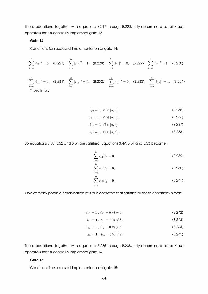
These equations, together with equations B.217 through B.220, fully determine a set of Krausoperators that successfully implement gate 13.

Gate 14

Conditions for successful implementation of gate 14:

h∑i=a

|i00|2 = 0, (B.227)h∑i=a

|i10|2 = 1, (B.228)h∑i=a

|i01|2 = 0, (B.229)h∑i=a

|i11|2 = 1, (B.230)

h∑i=a

|i02|2 = 1, (B.231)h∑i=a

|i12|2 = 0, (B.232)h∑i=a

|i03|2 = 0, (B.233)h∑i=a

|i13|2 = 1. (B.234)

These imply:

i00 = 0, ∀i ∈ [a, h], (B.235)

i01 = 0, ∀i ∈ [a, h], (B.236)

i12 = 0, ∀i ∈ [a, h], (B.237)

i03 = 0, ∀i ∈ [a, h]. (B.238)

So equations 3.50, 3.52 and 3.54 are satisfied. Equations 3.49, 3.51 and 3.53 become:

h∑i=a

i11i∗10 = 0, (B.239)

h∑i=a

i13i∗10 = 0, (B.240)

h∑i=a

i13i∗11 = 0. (B.241)

One of many possible combination of Kraus operators that satisfies all these conditions is then:

a10 = 1 , i10 = 0 ∀i 6= a, (B.242)

b11 = 1 , i11 = 0 ∀i 6= b, (B.243)

a02 = 1 , i02 = 0 ∀i 6= a, (B.244)

c13 = 1 , i13 = 0 ∀i 6= c. (B.245)

These equations, together with equations B.235 through B.238, fully determine a set of Krausoperators that successfully implement gate 14.

Gate 15

Conditions for successful implementation of gate 15:

64

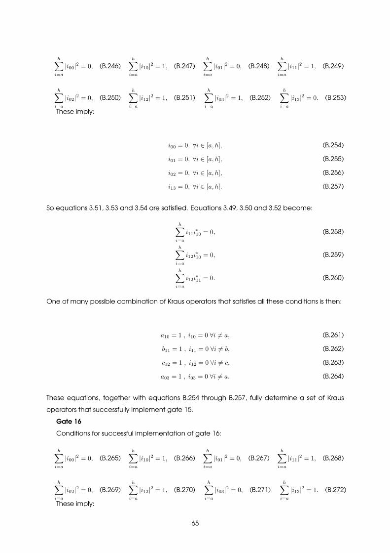
h∑i=a

|i00|2 = 0, (B.246)h∑i=a

|i10|2 = 1, (B.247)h∑i=a

|i01|2 = 0, (B.248)h∑i=a

|i11|2 = 1, (B.249)

h∑i=a

|i02|2 = 0, (B.250)h∑i=a

|i12|2 = 1, (B.251)h∑i=a

|i03|2 = 1, (B.252)h∑i=a

|i13|2 = 0. (B.253)

These imply:

i00 = 0, ∀i ∈ [a, h], (B.254)

i01 = 0, ∀i ∈ [a, h], (B.255)

i02 = 0, ∀i ∈ [a, h], (B.256)

i13 = 0, ∀i ∈ [a, h]. (B.257)

So equations 3.51, 3.53 and 3.54 are satisfied. Equations 3.49, 3.50 and 3.52 become:

h∑i=a

i11i∗10 = 0, (B.258)

h∑i=a

i12i∗10 = 0, (B.259)

h∑i=a

i12i∗11 = 0. (B.260)

One of many possible combination of Kraus operators that satisfies all these conditions is then:

a10 = 1 , i10 = 0 ∀i 6= a, (B.261)

b11 = 1 , i11 = 0 ∀i 6= b, (B.262)

c12 = 1 , i12 = 0 ∀i 6= c, (B.263)

a03 = 1 , i03 = 0 ∀i 6= a. (B.264)

These equations, together with equations B.254 through B.257, fully determine a set of Krausoperators that successfully implement gate 15.

Gate 16Conditions for successful implementation of gate 16:

h∑i=a

|i00|2 = 0, (B.265)h∑i=a

|i10|2 = 1, (B.266)h∑i=a

|i01|2 = 0, (B.267)h∑i=a

|i11|2 = 1, (B.268)

h∑i=a

|i02|2 = 0, (B.269)h∑i=a

|i12|2 = 1, (B.270)h∑i=a

|i03|2 = 0, (B.271)h∑i=a

|i13|2 = 1. (B.272)

These imply:

65

i00 = 0, ∀i ∈ [a, h], (B.273)

i01 = 0, ∀i ∈ [a, h], (B.274)

i02 = 0, ∀i ∈ [a, h], (B.275)

i03 = 0, ∀i ∈ [a, h]. (B.276)

Equations 3.49 through 3.54 become:

h∑i=a

i11i∗10 = 0, (B.277)

h∑i=a

i12i∗10 = 0, (B.278)

h∑i=a

i13i∗10 = 0, (B.279)

h∑i=a

i12i∗11 = 0, (B.280)

h∑i=a

i13i∗11 = 0, (B.281)

h∑i=a

i13i∗12 = 0. (B.282)

One of many possible combination of Kraus operators that satisfies all these conditions is then:

a10 = 1 , i10 = 0 ∀i 6= a, (B.283)

b11 = 1 , i11 = 0 ∀i 6= b, (B.284)

c12 = 1 , i12 = 0 ∀i 6= c, (B.285)

d13 = 1 , i13 = 0 ∀i 6= d. (B.286)

These equations, together with equations B.273 through B.276, fully determine a set of Krausoperators that successfully implement gate 16.

66