arX

iv:0

909.

4098

v3 [

quan

t-ph

] 1

7 Ju

n 20

10

Pure Phase Decoherence in a Ring Geometry

Z. Zhu,1 A. Aharony,2, 3, ∗ O. Entin-Wohlman,2, 3, ∗ and P.C.E. Stamp1, 3

1Department of Physics and Astronomy, University of British Columbia,

6224 Agricultural Rd., Vancouver, B.C., Canada V6T 1Z12Department of Physics and the Ilse Katz Center for Meso- and Nano-Scale Science and Technology,

Ben Gurion University, Beer Sheva 84105, Israel3Pacific Institute of Theoretical Physics, University of British Columbia,

6224 Agricultural Rd., Vancouver, B.C., Canada V6T 1Z1

(Dated: June 18, 2010)

We study the dynamics of pure phase decoherence for a particle hopping around an N-site ring,coupled both to a spin bath and to an Aharonov-Bohm flux which threads the ring. Analytic resultsare found for the dynamics of the influence functional and of the reduced density matrix of theparticle, both for initial single wave-packet states, and for states split initially into 2 separate wave-packets moving at different velocities. We also give results for the dynamics of the current as afunction of time.

PACS numbers: 03.65.Yz

I. INTRODUCTION

The dynamics of phase decoherence is central to ourunderstanding of those physical systems whose propertiesdepend on interference. This is particularly evident whenparticles are forced to propagate around closed paths;phase coherence then makes all physical properties de-pend on the topology of these paths.1 For this reasonthe quantum dynamics of particles on rings has beenextremely important in our understanding of quantumphase coherence. Examples at the microscopic level in-clude the energetics and response to magnetic fields ofmolecules,2 as well as charge transfer dynamics in a vastarray of solid-state and biochemical systems. There isevidence now for coherent transport around ring struc-tures even in some large biomolecules.3 At the nanoscopicand mesoscopic scale many ring-like structures, both con-ducting and superconducting,4 show coherent transportaround the rings, along with interesting Aharonov-Bohmstyle interference phenomena. We also note the impor-tance of closed loop structures in quantum informationprocessing.5

The interference around loops in all of these systems isvery sensitive to phase decoherence. Questions about themechanisms and dynamics of this decoherence are sub-tle, and have led to major controversies, notably in thediscussion of mesoscopic conductors.6 A quantitative un-derstanding of decoherence processes in metallic systemsand in superconducting ”qubits” has yet to be attained(in both cases local defect modes clearly make the ma-jor contribution to phase decoherence at low temperatureT ).7,8 These controversies are examples of a wider prob-lem: typically in solid-state systems, low T decoherencerates are far higher in experiments than theoretical esti-mates based on the dissipation rates in these systems.

These problems are complex because both decoher-ence and dissipation rates depend strongly on whichenvironmental modes are causing the decoherence.9,10

Delocalized modes (electrons, phonons, photons, spin

waves, etc.) can typically be modeled as ”oscillatorbath” modes.11–13 In such models, decoherence goeshand-in-hand with dissipation,14,15 in accordance withthe fluctuation-dissipation theorem. However localizedmodes (defects, dislocations, dangling bonds, nuclear andparamagnetic impurity spins, etc.), which can be mappedto a ”spin bath” representation of the environment,9,10

behave quite differently; indeed they often give decoher-ence with almost no dissipation. This is because althoughtheir low characteristic energy scale means they can causelittle dissipation, nevertheless their phase dynamics canbe strongly affected when they couple to some collec-tive coordinate - this then causes strong decoherence inthe dynamics of this coordinate.10,16 The fluctuation-dissipation theorem is then not obeyed,9 and often theselocalized modes are rather far from equilibrium.

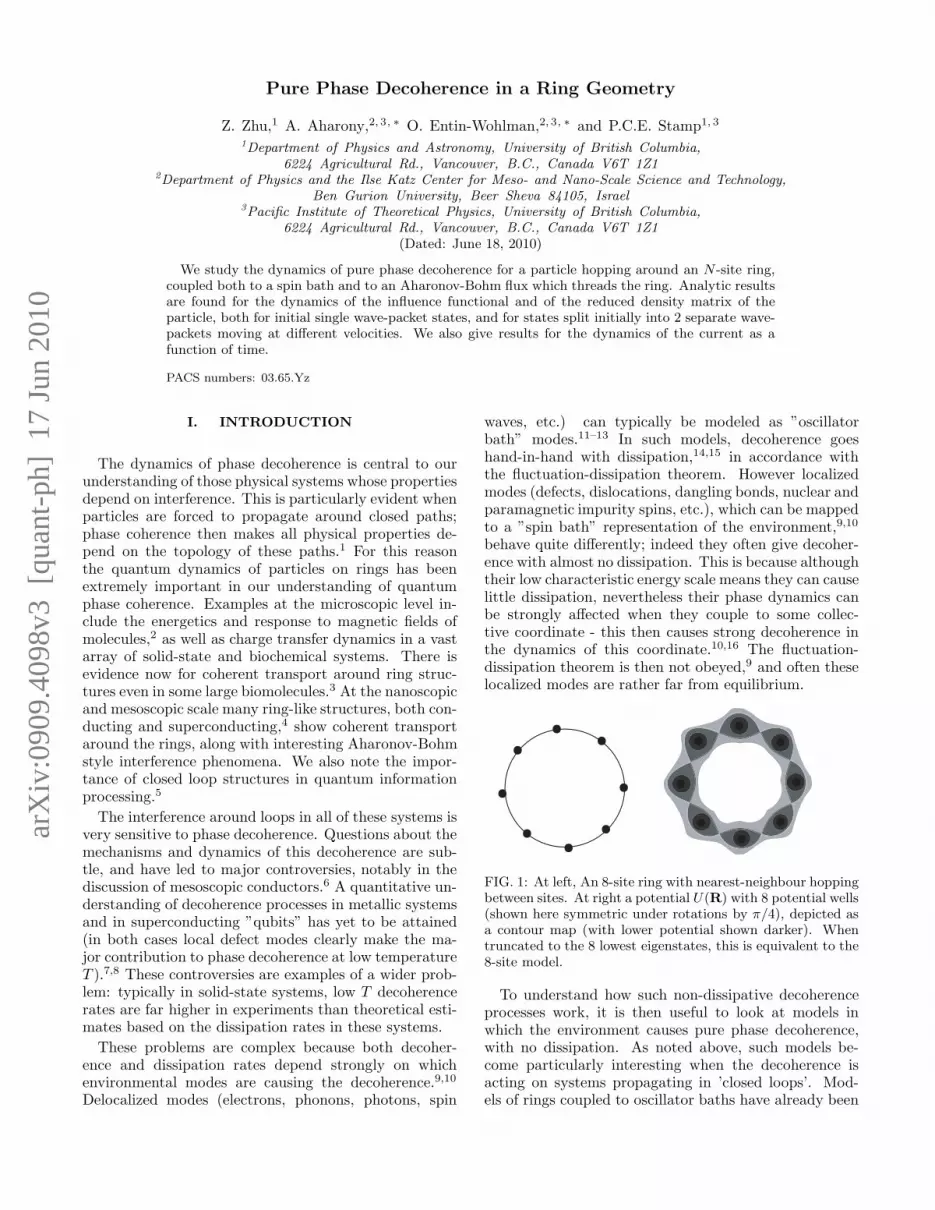
FIG. 1: At left, An 8-site ring with nearest-neighbour hoppingbetween sites. At right a potential U(R) with 8 potential wells(shown here symmetric under rotations by π/4), depicted asa contour map (with lower potential shown darker). Whentruncated to the 8 lowest eigenstates, this is equivalent to the8-site model.

To understand how such non-dissipative decoherenceprocesses work, it is then useful to look at models inwhich the environment causes pure phase decoherence,with no dissipation. As noted above, such models be-come particularly interesting when the decoherence isacting on systems propagating in ’closed loops’. Mod-els of rings coupled to oscillator baths have already been

2

studied.17 However such models, in which decoherenceis inextricably linked to dissipation, do not capture thelargely non-dissipative decoherence processes that domi-nate many solids at low T . On the the other hand purephase decoherence has been studied in many papers,18–20

but not, as far as we know, the rather unique phenomenaoccurring on a ring.In this paper we study a model which embodies in a

simple way both the ’closed path’ propagation which isgeneric to quantum interference processes, and which in-volves pure phase decoherence coming from a spin bath.The model describes a particle propagating around a ringof N discrete sites, while coupled to a spin bath; we as-sume hopping between nearest neighbors. The modelbecomes particularly interesting if we also have a flux Φthreading the ring (see Fig. 1). The spin bath variablesare assumed to be Two-Level Systems (TLS); these areubiquitous in solid-state systems, and are the main causeof decoherence at low T in these systems.One can also study the problem of a continuous ring,

but the discrete model is simpler, and is easily re-lated to diverse problems like quantum walks with phasedecoherence,21,22 or the dynamics of electrons in rings ofquantum dots.23 The Hamiltonian we will study has thegeneral form

Hφ =∑

<ij>

[∆oc†i cje

i(Aoij+

∑kα

ij

k·σk) +H.c.] (1)

The operator c†j creates a particle at site j; we assume a

single particle only. The phase factors Aoij result from

the flux Φ threading the ring. In writing (1), we haveassumed a symmetric ring, with N sites, and assumedthat the hopping matrix elements tij between sites i andj have simplified to a nearest-neighbour amplitude ∆o

(here∑

<ij> denotes a sum over nearest neighbours).This also means we can ignore any diagonal site ener-gies, since symmetry under rotations by angles 2π/Nmeans these energies are all the same. The spin bathvariables σk are Pauli spin-1/2 operators for the TLS,with k = 1, 2, ....Ns. We emphasize immediately thatthese bath spins are, in real situations, often not spins,but instead the 2 lowest levels of localized modes in asolid (for example, as noted above, they could be defectsor dangling bonds).The paper is organized as follows. In section II we dis-

cuss the derivation of model Hamiltonians like (1) frommore microscopic models, and the approximations whichallow us to drop other terms that can also appear in thecoupling of a ring particle to a spin bath. In section III wediscuss the dynamics of the particle in the absence of thebath - this establishes a number of useful mathematicalresults. In section IV we show how the dynamics of thereduced density matrix for the particle is derived in thepresence of the bath, and give some results for this dy-namics. In section V we analyze the dynamics of a pair ofinterfering wave-packets moving around the ring, show-ing how pure phase decoherence destroys the interference

between them. Finally, in section VI, we summarize ourconclusions - since some of the calculations are quite ex-tensive, readers may want to look first at this section fora guide to the main results. The more technical detailsof the derivations in sections III and IV are given in anAppendix.

II. DERIVATION OF MODEL

Consider first an N -site ring system without a bath.In site representation, this typically has a ”bare ring”model Hamiltonian

Ho =∑

<ij>

[

tijc†i cj e

iAoij +H.c.

]

+∑

j

εjc†jcj (2)

This ”1-band” Hamiltonian is the result of truncating, tolow energies, a high-energy Hamiltonian of form:

HV =1

2M(P−A(R))2 + U(R) (3)

where a particle of mass M moves in a potential U(R)characterized by N potential wells in a ring array (seeagain Fig. 1). Then εj is the energy of the loweststate in the j-th well, and tij is the tunneling ampli-tude between the i-th and j-th wells (which we take hereto be nearest neighbours). In path integral language,this tunneling is over a semiclassical ”instanton” trajec-tory Rins(τ), occurring over a timescale τB ∼ 1/Ω0 (the”bounce time”).24 Here Ω0 (the ”bounce frequency”) isroughly the small oscillation frequency of the particle inthe potential wells. In a semiclassical calculation, thephase Ao

ij is that incurred along the semiclassical tra-jectory by the particle, moving in the gauge field A(R).For a symmetric ring the site energy εj → ε0, ∀j, and wehenceforth ignore it.Consider now what happens when we couple the par-

ticle to a spin bath. The spin bath itself, independent ofthe ring particle, has the Hamiltonian

HSB =∑

k

hk · σk +∑

k,k′

V αβkk′ σ

αk σ

βk′ (4)

in which each TLS has some local field hk acting on

it, and the interactions V αβkk′ are typically rather small

because the TLS represent localized modes in the envi-ronment. The most general coupling between the ringparticle and the bath has the form

Hint =∑Ns

k [∑

j

F kj (σk)c

†j cj

+∑

<ij>

(Gkij(σk)c

†i cj +H.c.)] (5)

in which both the diagonal coupling F kj and the non-

diagonal coupling Gkij are vectors in the Hilbert space of

the k-th bath spin. We shall see below, when considering

3

the origin of these terms from microscopic models, thatvery often we can write the total Hamiltonian as

H = Hband +HSB (6)

where Hband = Ho +Hint takes the form

Hband =∑

ij [tijc†icje

iAoij+i

∑k(φij

k+αij

k·σk) +H.c.]

+∑

j(εj +∑

k γjk · σk)c

†jcj (7)

in which the diagonal couplings to the spin bath assume a”Zeeman” form, of strength |γj

k|, linear in the σk, andthe non-diagonal couplings appear in the form of extraphase factors in the hopping amplitude between sites.Before we consider the microscopic origins of this

model, let us note how it simplifies when we assume thesymmetry under rotations by 2π/N noted above (so thatthe site energy εj is dropped, and tij → ∆o, with nearest-neighbour hopping only). It is then natural to write Ao

ij

as

Aoij =

e

2H ·Ri ×Rj = Φ/N (8)

for j = i + 1 (we now use MKS units, and put ~ = 1).Here, H is the magnetic field, and Ri is the radius-vectorto the ith site; in cylindrical coordinates

Rj = (Ro,Θj)

Θj = 2πj/N (9)

for a ring of radius Ro. Fourier transforming from the sitebasis to a momentum basis for the couplings, we definequasi-momenta kn = 2πn/N , with n = 0, 1, 2, ..., N − 1,for the particle on the ring, and define operators

c†j =

√

1

N

∑

kn

eiknjc†kn,

c†kn=

√

1

N

∑

ℓ

e−iknℓc†ℓ ,

kn =2πn

N, n = 0, 1, . . . , N − 1 . (10)

We can write the free particle Hamiltonian as

Ho =∑

n

ǫoknc†kn

ckn

= 2∆o

∑

n

cos(kn − Φ/N)c†knckn

(11)

Then in this basis we can write:

Vint =

Ns∑

k

∑

n

[

F kn(σk)ρ(kn) + Gk

n(σk)c†knckn

]

(12)

where ρ(kn) =∑

n′ c†kn+kn′

ckn′ is the density operator

in momentum space for the particle, and the Fourier-transformed interaction functions are

Gkn(σk) =

∑

ij

eikn(i−j)Gkij(σk)

F kn(σk) =

∑

j

eiknjF kj (σk) (13)

In this basis the band HamiltonianHband has a dispersionwhich is a functional of the bath spin distribution:

Hband =∑

k

∑

n

ǫkn[σk]c

†knckn

+∑

n,n′

vn[σk]c†kn+kn′

ckn′ (14)

and in which the ’band energy’ ǫkn[σk] and the ’scatter-

ing potential’ vn[σk] are now both functionals over thespin bath coordinates σk:

ǫkn[σk] = ǫokn

+∑

k

Gkn(σk)

vn[σk] =∑

k

F kn(σk) (15)

Under many circumstances one can assume that thissymmetry under rotations also applies to the bath cou-plings, so these no longer depend on site variables, ie.,F k

j → F k, and Gkij → Gk. The results then simplify a

great deal; Gkn(σk) → 2Gk(σk) cos kn, and F k

n → F k.Now let us consider the microscopic origin of this model

(ie., before truncation to the lowest band). The mostobvious interaction between the particle moving aroundthe ring and a set of bath spins has the local form25:

Hint(R,σk) =∑

k

F (R− rk) · σk

≡∑

k

Hkint(R,σk) (16)

where F (r) is some vector function, and rk is the position

at the k-th bath spin. The diagonal coupling F kj , or its

linearized form γjk, is then easily obtained from (16) when

we truncate to the single band form. But the term (16)must also generate a non-diagonal term, which is moresubtle. We can see this by defining the operator

T kij = exp [−i/~

∫ τf (Rj)

τin(Ri)

dτ Hkint(R,σk)] (17)

where the particle is assumed to start in the i-th potentialwell centered at position Ri, at the initial time τin, andfinish at position Rj in the adjacent j-th well at timeτf ; the intervening trajectory is the instanton trajectory(which in general is modified somewhat by the coupling

to the spin bath). Now we operate on σk with T kij , to get

|σfk〉 = T k

ij |σink 〉 = ei(φ

ij

k+αij

k·σk)|σin

k 〉 (18)

where we note that both the phase φijk multiplying the

unit Pauli matrix σ0k, and the vector αij

k multiplying theother 3 Pauli matrices σx

k , σyk , σ

zk, are in general com-

plex. In this way the instanton trajectory of the par-ticle acts as an operator in the Hilbert space of the k-thbath spin.10,26 Note that one important implication of

4

this derivation is that typically |αijk | ≪ 1, in fact expo-

nentially small, since the interaction energy scale set by|F (R − rk)| is usually much smaller than the ”bounceenergy” scale ~Ωo set by the potential U(R), ie., thetunneling of the particle between wells is a sudden per-turbation on the bath spins.10 Detailed calculations inspecific cases10,26,27 show that |αij

k | ∼ π|ωijk |/2Ωo in this

’sudden’ regime, where ωijk = γ

jk − γi

k is the change inthe diagonal coupling acting between the particle and thek-th bath spin when the particle hops from site i to sitej (this result can be found directly from time-dependentperturbation theory in the sudden approximation).From these considerations we see that, starting from a

ring with the particle-bath interaction given in (16), wewill end up with an effective Hamiltonian for the lowestband of the form given in (7), in which the non-diagonal

interaction Gkij(σk) in (5) has assumed a rather special

form.One can in fact have a more general form for Gk

ij(σk)in the lowest-band approximation, provided one also in-troduces in the microscopic Hamiltonian a coupling

Hint(P,σk) =∑

k

G(P ,σk) (19)

to the momentum of the particle. This can include var-ious terms, including functions of P × σk and P · σk; adetailed analysis is fairly lengthy. The main new effect ofthese is to generate terms in the band Hamiltonian whichcouple the spins to the amplitude of tij as well as to itsphase; these do not appear in (7).In any case, if we know U(R), F (R − rk), and

G(P ,σk), we can clearly then calculate all the param-eters in the generic model Hamiltonian, using variousmethods.10,27 However we are not interested here in thegeneric case, since our main object is to study the dy-namics of decoherence in a ring model which containsonly phase decoherence. We therefore make the follow-ing approximations:

(i) We drop the interaction V αβkk′ , between bath spins

(often a very good approximation, since interactions be-tween defects or nuclear spins are often very weak), andalso neglect the local fields hk acting on the σk. Thuswe make HSB = 0.(ii) We drop the momentum coupling G(P ,σk) en-

tirely, and in the band Hamiltonian (7) we drop the di-

agonal interaction γjk. This implies that the energy of

the k-th bath spin does not depend on whether the j-thsite is occupied. We make this approximation (in manycases not physically reasonable) only because we wishto study phase decoherence without the complication ofenergy relaxation.(iii) We assume a symmetric ring, so that εj → 0 and

tij → ∆o as before; and we absorb the phases φijk → φkinto a renormalization of ∆o (from

∑

k Im φk), and ofAo

ij (from∑

k Re φk).The resulting model Hφ is then just that given in (1).

This turns out to be explicitly solvable, and reveals some

important properties of phase decoherence. We will usu-ally assume the parameters αij

k are small, in line with theremarks above (although the net effect of all of them maybe very large), and we will also usually specialize to the

case αijk → αk, consistent with a completely symmetric

ring.Finally, let us briefly compare with the kind of Hamil-

tonian one would expect for a particle on a ring coupledto an oscillator bath. Let us assume a set of oscillatorswith Hamiltonian Ho + Hosc + Hint, where Ho is againthe free particle hopping Hamiltonian, coupling to a setof No oscillators with Hamiltonian

Hosc =

No∑

q=1

1

2(p2qmq

+mqω2qx

2q) (20)

In general there will be diagonal couplings Vj(q)and non-diagonal couplings Uij(q) between particleand oscillators. We could also have a coupling tothe oscillator momenta - however in this case one canmake a canonical transformation28 which transformsthis back into a coupling to the xq. Typically the

couplings Vj(q), Uij(q) ∼ O(N−1/2o ). We note here

that in many microscopic models of this kind, thecouplings Vj(q), Uij(q) are actually also strong func-tions of temperature, either because the underlying ef-fective Hamiltonian is strongly T -dependent (eg., in asuperconductor),29 or because the coupling to the oscil-lators is non-linear (eg., in the coupling to a soliton).30

If we restrict the problem to rotationally invariant cou-plings on the ring, then we can write

Hint =∑

q

∑

<ij>

(Uq c†i cj +H.c.) +

∑

j

Vq c†j cj

xq (21)

where Uij(q) → Uq, Vj(q) → Vq, and the sum∑

<ij> isover nearest neighbours. It is then straightforward to gothrough the same manipulations as in (12)-(15), to get arenormalised band which is a functional of the xq.In these results there is no connection between the ring

sites and the space in which the oscillators are supposedto exist. However in many cases the oscillator displace-ment field xj can be defined at each site j of the ring;the coupling then reduces to

V =∑

q

∑

j

vqc†j cje

iq·Rjxq

≡∑

jj′

v(Rj − rj′ )c†j cjx(rj′ ) (22)

in which Rj , rj′ are site vectors on the ring, and xq isnow the Fourier transform of xj .

III. FREE BAND PARTICLE DYNAMICS

We first consider the dynamics of a free particle insome initial state moving on the symmetric N -site ringdescribed by Ho in (11), with no bath.

5

For this free particle the dynamics is entirely describedin terms of the bare 1-particle Green function

Gojj′ (t) ≡ 〈j|Go(t)|j′〉 ≡ 〈j|e−iHot|j′〉

=1

N

∑

n

e−i2∆0t cos(kn−Φ/N)eikn(j′−j) , (23)

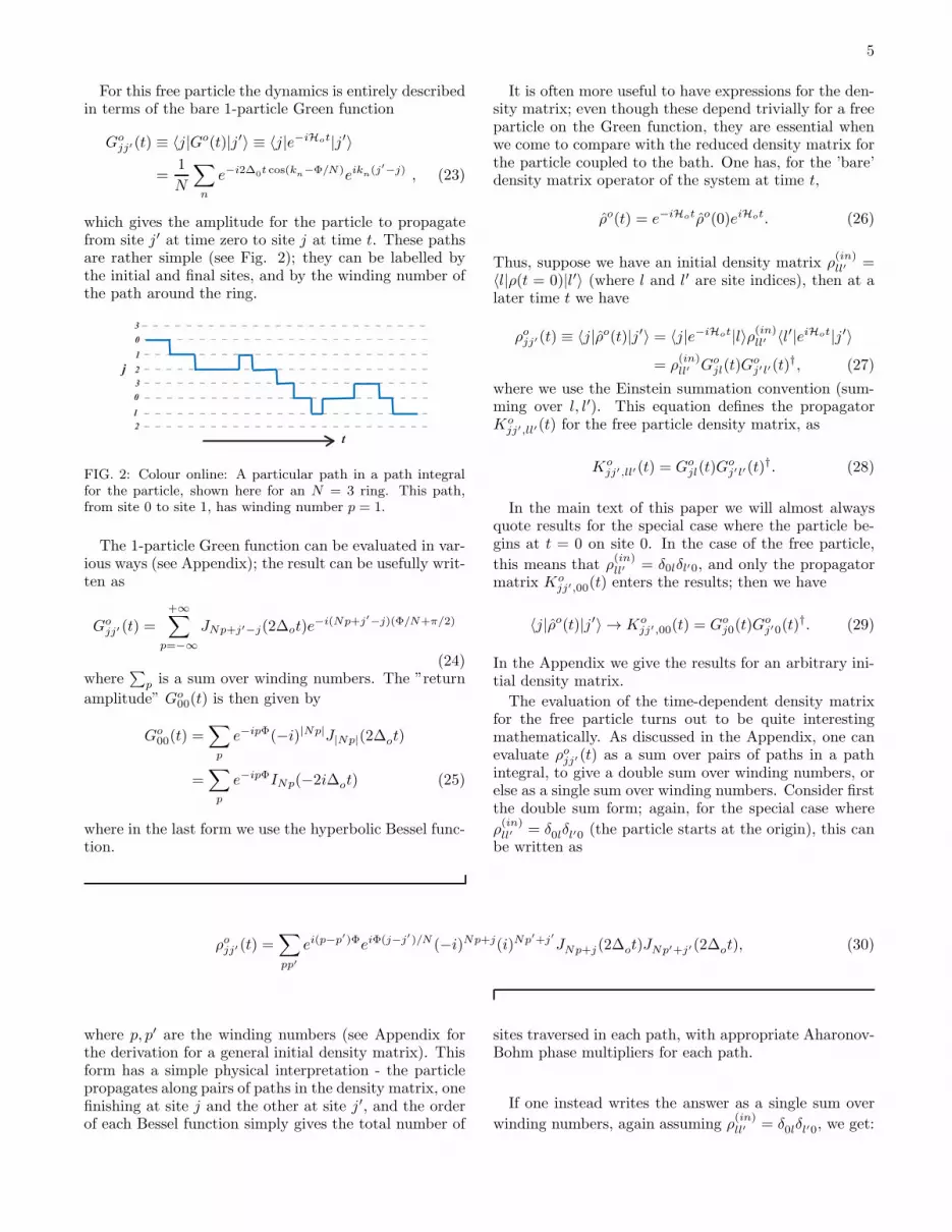
which gives the amplitude for the particle to propagatefrom site j′ at time zero to site j at time t. These pathsare rather simple (see Fig. 2); they can be labelled bythe initial and final sites, and by the winding number ofthe path around the ring.

t

j

3

0

0

2

1

3

2

1

FIG. 2: Colour online: A particular path in a path integralfor the particle, shown here for an N = 3 ring. This path,from site 0 to site 1, has winding number p = 1.

The 1-particle Green function can be evaluated in var-ious ways (see Appendix); the result can be usefully writ-ten as

Gojj′ (t) =

+∞∑

p=−∞

JNp+j′−j(2∆ot)e−i(Np+j′−j)(Φ/N+π/2)

(24)where

∑

p is a sum over winding numbers. The ”return

amplitude” Go00(t) is then given by

Go00(t) =

∑

p

e−ipΦ(−i)|Np|J|Np|(2∆ot)

=∑

p

e−ipΦINp(−2i∆ot) (25)

where in the last form we use the hyperbolic Bessel func-tion.

It is often more useful to have expressions for the den-sity matrix; even though these depend trivially for a freeparticle on the Green function, they are essential whenwe come to compare with the reduced density matrix forthe particle coupled to the bath. One has, for the ’bare’density matrix operator of the system at time t,

ρo(t) = e−iHotρo(0)eiHot. (26)

Thus, suppose we have an initial density matrix ρ(in)ll′ =

〈l|ρ(t = 0)|l′〉 (where l and l′ are site indices), then at alater time t we have

ρojj′ (t) ≡ 〈j|ρo(t)|j′〉 = 〈j|e−iHot|l〉ρ(in)ll′ 〈l′|eiHot|j′〉= ρ

(in)ll′ Go

jl(t)Goj′l′(t)

†, (27)

where we use the Einstein summation convention (sum-ming over l, l′). This equation defines the propagatorKo

jj′,ll′(t) for the free particle density matrix, as

Kojj′,ll′(t) = Go

jl(t)Goj′l′(t)

†. (28)

In the main text of this paper we will almost alwaysquote results for the special case where the particle be-gins at t = 0 on site 0. In the case of the free particle,

this means that ρ(in)ll′ = δ0lδl′0, and only the propagator

matrix Kojj′,00(t) enters the results; then we have

〈j|ρo(t)|j′〉 → Kojj′,00(t) = Go

j0(t)Goj′0(t)

†. (29)

In the Appendix we give the results for an arbitrary ini-tial density matrix.

The evaluation of the time-dependent density matrixfor the free particle turns out to be quite interestingmathematically. As discussed in the Appendix, one canevaluate ρojj′ (t) as a sum over pairs of paths in a pathintegral, to give a double sum over winding numbers, orelse as a single sum over winding numbers. Consider firstthe double sum form; again, for the special case where

ρ(in)ll′ = δ0lδl′0 (the particle starts at the origin), this can

be written as

ρojj′ (t) =∑

pp′

ei(p−p′)ΦeiΦ(j−j′)/N (−i)Np+j(i)Np′+j′JNp+j(2∆ot)JNp′+j′ (2∆ot), (30)

where p, p′ are the winding numbers (see Appendix forthe derivation for a general initial density matrix). Thisform has a simple physical interpretation - the particlepropagates along pairs of paths in the density matrix, onefinishing at site j and the other at site j′, and the orderof each Bessel function simply gives the total number of

sites traversed in each path, with appropriate Aharonov-Bohm phase multipliers for each path.

If one instead writes the answer as a single sum over

winding numbers, again assuming ρ(in)ll′ = δ0lδl′0, we get:

6

ρojj′ (t) =1

N

N−1∑

m=0

∞∑

p′=−∞

JNp′+j′−j [4∆ot sin(km/2)]eiΦ[p′+(j′−j)/N ]−ikm(j+j′−Np′)/2 (31)

where as before the km are the momenta of the par-ticle eigenfunctions. The physical interpretation of thisform is less obvious, but the sums are much easier toevaluate since they only contain single Bessel functionsinstead of pairs of them. Thus wherever possible we re-duce double sum forms to single sums. Notice that forthese finite rings, the bare density matrix is of coursestrictly periodic in time. Notice also that the diagonalelements of ρ(t) are generally periodic in Φ. However, theoff-diagonal elements are only periodic in Φ/N . In con-

trast, eiΦ(j−j′)/N 〈j|ρ(t)|j′〉 is periodic in Φ, with period2π. This latter is the quantity needed for calculating thecurrents, as we will see below.From either Go

jj′ (t) or ρojj′ (t) we may immediatelycompute two useful physical quantities. First, the prob-ability P o

j0(t) to find the particle at time t at site j, as-suming it starts at the origin; and second, the currentIoj,j+1(t) between adjacent sites as a function of time.Looking first at the probability P o

j0(t), one has

P oj0(t) = 〈j|ρo(t)|j〉 = |Go

j0(t)|2 (32)

which from above can be written in double sum form as

P oj0(t) =

∑

pp′

JNp+j(2∆ot)JNp′+j(2∆ot)

× e−iN(p′−p)(Φ/N+ π2 ) (33)

or in single sum form as

P oj0(t) =

1

N

N−1∑

m=0

∞∑

p=−∞

eip(Φ+Nkm/2)

× JNp[4∆ot sin(km/2)] . (34)

One may also compute moments of these probabilities.These are not terribly meaningful for a small ring, be-cause any wave-packet will be spread around the ring.However for a large ring they can be useful- for example,the 2nd moment

∑

j j2P o

j0(t) tells us the rate at which aninitial density matrix spreads in time, provided the spa-tial extent of the density matrix is much smaller thanthe ring circumference. Coherent dynamics will thenmanifest itself as ballistic propagation of an initial wave-packet.

From these general expressions it is hard to see whatis going on. To give some idea of how the probabilitydensity behaves, it is useful to then look at these resultsfor a small 3-site ring, where the oscillation periods arequite short. One then has, for the case where the particlestarts at the origin, that

P oj0(t) =

1

3

(

1 + (3δj,0 − 1)[

J0(2∆o

√3t)

+ 2

∞∑

p=1

J6p(2∆o

√3t) cos(2pΦ)

]

+ (δj,1 − δj,2)2√3

∞∑

p=1

J6p−3(2∆o

√3t) sin((2p− 1)Φ)

)

.

(35)

In Fig. 3 the return probability P o00(t) is plotted for the

case N = 3, using (35). From the results one strikingfeature immediately emerges - we see that the periodicbehaviour depends strongly on the flux Φ. This flux de-pendence illustrates the way in which the flux controlsthe particle dynamics, by acting directly on the particlephase. In section V we will see how this also happenswhen one looks at interference between 2 wave-packets;and in sections IV and V we will see how decoherencewashes out the flux dependence of the particle dynamics.Thus the flux dependence of the particle dynamics veryeffectively measures how coherent its dynamics may be.

Turning now to the current Ioj,j+1(t) from site j and sitej + 1, this is given from elementary quantum mechanicsby

Ioj,j+1(t) = 2 Im [∆oe−iΦ/Nρoj,j+1(t)]

= i∆o

(

eiΦ/Nρoj+1,j(t)− e−iΦ/Nρoj,j+1(t))

(36)

where the flux per link appears in each contribution.Again, one can write this expression as either a doublesum over pairs of winding numbers, or as a single sum(see Appendix for the general results and derivation). Forthe case where the particle starts from the origin, theseexpressions reduce to

7

Ioj+1,j = 2∆o

∑

pp′

JNp+j(2∆ot)JNp′+j+1(2∆ot) cos[(π

2N +Φ)(p′ − p)]

=2∆o

N

N−1∑

m=0

∑

p

JNp+1(4∆ot sinkm2

)e−ikm(Np+12 +j)iNp+1 cos[(

π

2N +Φ)p] (37)

for the double and single sum forms respectively.

5 10 15D0t

13

23

1P j

5 10 15D0t

-0.4

0.4

IH1®2LD0

5 10 15D0t

13

23

1P j

5 10 15D0t

-0.4

0.4

0.8

IH1®2LD0

FIG. 3: Colour online: Results for the free particle for N = 3and for a particle initially on site 1. Left: The probabilities tooccupy site 1 (full line), 2 (large dashes), and 3 (small dashes).Right: the current from site 1 to site 2. Top: Φ = 0. Bottom:Φ = π/2.

Again, the currents across any links must be strictlyperiodic in time for this free particle system; and again,it is useful to show the results for a 3-site system. Forthis case N = 3, and assuming that the particle beginsat the origin, we find

Io0,1 =2∆o

3Im

2∑

m=1

∑

p

J3p+1(4∆ot sinmπ

3)

× e−imπ(3p+1)/3i3p+1 cos[(3π

2+ Φ)p]

(38)

which we can also write in the form

Io0,1 =2∆o

3Im

∑

p

J3p+1(2√3∆ot) cos[(

3π

2+ Φ)p]

× i3p+12

∑

m=1

(e−iπ(3p+1)/3 + e−i2π(3p+1)/3) (39)

Now let us write (e−iπ(3p+1)/3 + e−i2π(3p+1)/3) =

(−1)pe−iπ/3 + e−2iπ/3. If p is even, this becomes −i√3

and cos[(3π2 + Φ)p] = (−1)3p/2 cos(Φp); If p is odd, it

becomes −1 and cos[(3π2 + Φ)p] = (−1)3(p−1)/2 sin(Φp).

Therefore, we have

Io0,1 =2

3∆o

∞∑

p=−∞

J3p+1(2∆o

√3t)K(p,Φ) ,

K(p,Φ) = sin(pΦ) if p = odd ,

K(p,Φ) =√3 cos(pΦ) if p = even . (40)

These results are also shown in Fig. 3. Notice that inthis special case the result is periodic in Φ; this is not

however true for a general initial density matrix ρ(in)ll′ ,

when the result is periodic in Φ/N .

IV. RING PLUS BATH: PHASE AVERAGING

We now wish to solve for the dynamics of the particleonce it is coupled to the bath, via the Hamiltonian (1).This is done in general by integrating out the bath spins,to produce expressions for the reduced density matrixof the particle. In this section we first show how this isdone, and then give results for physical quantities (in par-ticular, the probability Pj0(t) and the current Ij,j+1(t)).Finally, we briefly compare the results to the behaviourone expects for a ring coupled to an oscillator bath.

A. General results

As shown in the Appendix, the reduced density matrixfor the particle obeys the equation of motion

ρjj′ (t) =∑

l,l′

Kjj′,ll′(t)ρ(in)l,l′ (41)

where Kjj′ ,ll′(t) is the propagator for the reduced densitymatrix. This latter can be written in the form of a doublesum over winding numbers

Kjj′,ll′(t) =∑

pp′

Kojj′,ll′(p, p

′; t)F ll′

jj′ (p, p′) (42)

where the function Kojj′,ll′(p, p

′; t) is the free particle

propagator for fixed winding numbers p, p′ (so thatKo

jj′,ll′(t) =∑

pp′ Kojj′,ll′(p, p

′; t); see the Appendix,

eqtn. (A8) et seq.). All effects from the spin bath are

then contained in F ll′

jj′ (p, p′), which we will call the ”in-

fluence function”. The remarkable thing is that this func-tion depends only on the initial and final states, and on

8

the winding numbers - all other aspects of the two pathsinvolved in the density matrix propagation have disap-peared. As explained in the appendix, this is a particularfeature of the pure phase decoherence being treated here.The form the influence function takes depends on what

kind of averaging we do over the bath. To discuss this,let us first discriminate between two different ways ofaveraging over the bath, as follows:(i) The first and most obvious case is where the αmn

kare considered to be a set of fixed couplings, for a specificsingle ring. In this case the average is only over the bathstates; we will denote this bath average by< .... >. Oftenit will only involve a thermal average over the bath states.(ii) However it is often the case that one is either in-

terested in an ensemble of rings, all having the same freeparticle Hamiltonian but with the αk possibly varyingfrom one ring to another, or a single ring in which thevalues of the couplings αk are indeterminate. In this caseit makes sense to define a probability distribution P (α)over a coupling variable α. One then must average notonly over the bath states themselves, but also over thebath couplings. We will denote this double average by<< ..... >>, to signify the average over both the bathstates and the probability distribution; and the influencefunction for this case will be written as F ll′

jj′ (p, p′), with

the bar over the F signifying that an average over cou-plings is being done as well.In general the results for the dynamics of the density

matrix and the current, and their dependence on the in-fluence function, may be quite complicated. Thus, beforewe begin quoting results, it is useful to note what are theimportant parameters in the problem. We will only con-sider here the simplest completely symmetric case whereαmn

k → αk for all links mn; and we will assume that|αk| ≪ 1 for all k, as discussed in section II. Now in theprevious literature for this case of pure phase decoher-ence, it has been usual to define a ’topological decoher-ence’ parameter10,26

λ =1

2

∑

k

|αk|2 (43)

which provides a measure of the strength of the purephase decoherence.10 If the number Ns of bath spins islarge, then we can have λ≫ 1; this is the limit of strongphase decoherence.However we shall see in what follows that on a ring

it is often more useful to define a parameter F0(p) thatalso depends on a winding number p. The form of thisparameter depends on which of the two bath averages isperformed. In the case where only an average over thebath states is performed, we have

F0(p) =∏

k

cos(Np|αk|) (44)

which defines a rather complicated function of the fixedbath couplings. The strong decoherence limit for thiscase is defined by the parameter λ defined above.

In the case where we also perform an average over thebath couplings, we have

F0(p) =∏

k

∫

dαkP (αk) cos(Np|αk|) (45)

The result then depends on what form one has for thedistribution function P (αk). In what follows we will use,as an example, a Gaussian distribution, given by

P (|αk|) = e−|αk|2/2λo/

√

2πλo (46)

so that

F0(p) = e−λN2p2/2, λ = Nsλo (47)

The limit λ → ∞ is the “strong decoherence” limit forthis distribution, where we have F0(p) → δp,0. How-ever we will see below that it is convenient to think ofthe strong decoherence regime for the present problemas that for which the particle dynamics is independentof flux - we will see that this happens already for quitesmall values of λ.We can see why these functions enter by considering

the forms for F ll′

jj′ (p, p′) and F ll′

jj′ (p, p′) that enter into

physical quantities. In the appendix the full expressionsfor these are derived; but here we will again only use

them for the case where ρ(in)l,l′ = δ0lδl′0, ie., the particle

starts at the origin, and so only the function Fjj′ (p, p′) ≡

F 00jj′ (p, p

′) comes in. We will also again assume the purely

symmetric case where αijk → αk for every link.

Let us first consider the case of fixed bath couplings.In this case the form of the influence function reduces to(see Appendix):

Fjj′ (p, p′) = 〈e−iN [(p−p′)+(j−j′)]

∑k αk·σk〉 (48)

Notice that Fjj′ (p, p′) is a function only of the distance

j− j′ between initial and final sites, and of the differencep = p − p′ in winding numbers. Writing this now asFjj′ (p), let us evaluate it by assuming the usual thermalinitial bath spin distribution. Since all the bath statesare degenerate, then at any finite T all states are equallypopulated; we then get:

Fjj′ (p) =∏

k

cos((Np+ j − j′)|αk|) (49)

Other initial non-thermal distributions for the spin bathstates are also easily evaluated from (48).

B. Physical Quantities

From expressions like (49) one can now write downexpectation values of physical quantities as a function oftime. The simplest example is the probability for theparticle to end up at some site after a time t, having

9

started at another. Thus, eg., the probability Pj0(t) tomove to site j from the origin in time t is now given by

Pj0(t) = ρjj(t)

=∑

pp′

JNp+j(2∆ot)JNp′+j(2∆ot)

× e−iN(p′−p)(Φ/N+ π2 ) F0(p, p

′) (50)

which is a simple generalization of the free particle resultin (33); we note that only the term

F0(p, p′) =

∏

k

cos(N(p− p′)|αk|) (51)

in the influence function survives in this expression. Sincethis function depends only on the difference p − p′, itis identical to the function F0(p) defined in (44) above(letting p = p). We shall see below that the ring currentis also controlled by this same function. Note that ithas a complex multiperiodicity, as a function of the Ns

different parameters Np|αk|; we do not have space hereto examine the rich variety of behaviour found in thesystem dynamics as we vary these parameters.Now let us consider the case where we also average over

the bath couplings. One then finds (see appendix) that

Fjj′ (p) =∏

k

∫

dαkP (αk)〈e−iN [p+(j−j′)]αk·σk〉 (52)

In the symmetric case we can treat each bath spin in thesame way, and simply use a distribution function P (|α|),the same for all the different σk. Then we can treateverything in terms of this single average, over a singlerepresentative spin σ from the bath. Then, eg., for aninitial thermal ensemble for the bath spins, this gives

Fjj′ (p) = [

∫

dαP (α) cos((Np+ j − j′)|α|)]Ns (53)

To give something of the flavour of this case, we usethe Gaussian distribution for the P (|α|), given by (46)above. Then, for the thermal ensemble just given, wehave

Fjj′ (p) = exp[−λ(Np+ j′ − j)2/2] (54)

It is then immediately obvious that the result for theprobability for the particle to go from site 0 to site j intime t is the same expression as (50) above, but now withF0(p) instead of F0(p).To see how this behaves, let us take the specific case

where N = 3 again. Then for this 3-site ring one has, forexample, that

P10(t) =1

3

(

1 + 2[J0(2∆o

√3t)

+ 2

∞∑

p=1

J6p(2∆o

√3t) cos(2pΦ)F0(6p)]

)

.

(55)

5 10 15D0t

13

23

1P j

5 10 15D0t

-0.4

0.4

IH1®2LD0

5 10 15D0t

13

23

1P j

5 10 15D0t

-0.4

0.4

IH1®2LD0

FIG. 4: Colour online: Plot of Pj0(t) for a 3-site ring, fora particle initially on site 1, in the intermediate decoherencelimit, with λ = .02. Left: The probability to occupy site 0(full line), 1 (large dashes), and 2 (small dashes). Right: thecurrent from site 0 to site 1. Top: Φ = 0. Bottom: Φ = π/2 .

To analyse this result, note that for x ≫ (6p)2, we can

use J6p(x) ≈ (−1)p√

2/(πx) cos(x − π/4). The function

F0(p) decays with p, and becomes negligible for largeenough p. For example, Eqtn. (47) implies that F0(6p) <

e−10 for p > pmax, with pmax =√

5/9λ. Neglectingthese terms in the sum in Eq. (55) we conclude that for

2∆o

√3t≫ (6pmax)

2 we have e.g.

P10(t) ≈1

3

[

1 +2A

√

π∆o

√3t

cos(2∆o

√3t− π/4)

]

,

A = 1 + 2

∞∑

p=1

(−1)p cos(2pΦ)F0(6p) . (56)

The sum in the amplitude A reduces to∑

(−1)pF0(6p),for Φ = 0, and to

∑

F0(6p), for Φ = π/2. Clearly, switch-ing from Φ = 0 to Φ = π/2 causes a large increase in A.Notice that the inverse Fourier transform of the ampli-tude A(φ) can be used to measure the decoherence func-tion F0(6p). Results for this low decoherence regime areshown in Fig. 4.

As λ increases, pmax decreases, and Eq. (56) applies atshorter times. Remarkably, if λ > 0.1 the whole sum be-comes negligible, and we have already reached the strongdecoherence result where the result is Φ−independent.The result is shown in Fig. 5. Thus, if we define the’strong decoherence’ regime as that where all results areflux-independent, then it is reached for very low valuesof λ. We emphasize here that the detailed form of theresults, as well as the decoherence strength required forflux-independent dynamics, depends strongly on the formwe adopt for either F0(p) or F (p); we do not have spaceto explore this question here.

Turning now to the current through the ring, we gen-eralize the free particle results in the same way as above.

10

5 10 15D0t

13

23

1P j

5 10 15D0t

-0.4

0.4IH1®2LD0

FIG. 5: Colour online: Plot of Pj0(t) for a 3-site ring, fora particle initially on site 1, in the strong decoherence limit.Left: The probability to occupy site 0 (full line), 1 (largedashes), and 2 (small dashes). Right: the current from site 0to site 1 (compare Fig. 3). The results do not depend on Φ.

Quite generally one has

Ij,j+1(t) = i〈∆j,j+1ρj+1,j(t)− ∆j+1,jρj,j+1(t)〉 (57)

where we average the operator

∆j,j+1 = ∆oeiΦ/Nei

∑kαj,j+1

k·σk (58)

over bath states, with fixed bath couplings - the casewhere one also averages over an ensemble of bath cou-plings is a by now obvious generalization of this. This ex-pression is evaluated in detail in the Appendix; as notedthere, the result is more complicated than it seems, be-cause the density matrix depends implicitly on both theinitial state, and on the full details of the propagator forthe density matrix. Here we consider only the specialcase where the particle starts from the origin, and thefully symmetric case α

ijk → αk. Then one has, for the

case of a bath state average only, that

Ij,j+1(t) =2∆o

N

N−1∑

m=0

∑

p

JNp+1(4∆ot sinkm2)e−ikm(Np+1

2 +j)iNp+1F0(p) cos[(π

2N +Φ)p] (59)

with a similar result for the current Ij,j+1(t) arising inthe case where one also averages over bath couplings,with F0(p) then replaced by F0(p). One can also analyzethis result as a function of time, and of the decoherencestrength, the ring size, and the flux - there is no spacefor this here. To nevertheless give some flavour for theresults, consider again the 3-site ring, for the couplingaveraged case, in the strong decoherence limit. Currentthen only flows in regions where the initial density matrixis inhomogeneous; for some general initial density matrixone finds

Ij,j+1(t) →2√3

3∆o(ρ

(in)j,j − ρ

(in)j+1,j+1)J1(2∆o

√3t) ,

(60)

where ρ(in)ll′ is the initial density matrix. Again we see

that the result is completely independent of the flux.

C. Comparison with Oscillator Bath

To gain some perspective on the results just given, it isuseful to compare with what one might expect for a ringparticle coupled to an oscillator bath. The differencesare both formal and physical, and both are important.Here we simply sketch these - a more detailed study ofthis rather complex problem will appear elsewhere.31 Tospecify the formal problem completely, one needs first todefine ’spectral functions’ for the couplings between theoscillator bath and the ring particle.12 These couplingswere defined earlier, in (21); Fourier transforming them

in the same way as we did for the spin bath couplings,we then define the spectral functions as:

J⊥p (ω) =

π

2

∑

q

U2q (p)

ωqδ(ω − ωq)

J‖p(ω) =

π

2

∑

q

V 2q (p)

ωqδ(ω − ωq) (61)

In many cases the non-diagonal function J⊥p (ω) can be

neglected compared to the diagonal J‖p(ω), and we will

assume this here. J‖p(ω) can take many forms; the

most commonly analysed is the ”Ohmic form”, where

J‖p(ω) = ηω at low frequency, but this form is very useful

for systems coupled to an itinerant electron bath, it isinappropriate for insulating systems (where a more accu-

rate low-ω form is the ”superOhmic” form J‖p(ω) ∼ ωk,

with k > 1). In addition, there is often significant low-

energy structure in J‖p(ω), not describable by a simple

power-law form; and in many cases J‖p(ω) also depends

strongly on temperature T .Defining the influence functional F [Θ,Θ′] in the usual

way for general paths Θ(t),Θ′(t) (cf. eqtn. (A19) of theAppendix), we can write

F [Θ,Θ′] = expiN2

~

∫

dt1

∫

dt2 ×

[ϕ(t1)Dp(t1 − t2)ϕ(t2) + iΓp(t1 − t2)ϕ(t1)ψ(t1)] (62)

where we have defined the sum and difference angular

11

variables

ψ(t) = (Θ(t) + Θ′(t))/2

ϕ(t) = (Θ(t)−Θ′(t))/2 (63)

and the oscillator propagator Dp(t) = Dp(t) + iΓp(t),with

Dp(t) =4

N2

∫

dωJ‖p(ω)

ω2(1 − cosωt) coth(

β~ω

2)

Γp(t) =4

N2

∫

dωJ‖p(ω)

ω2sinωt (64)

The behaviour in time ofDp(t) can be quite complex, andvaries strongly with the form of Jp(ω), and with temper-ature; the details of this behaviour have been reviewedextensively.13,32

In the same way as for the spin bath, we may nowconstruct expressions for the reduced density matrix, andphysical correlation functions derived therefrom, by sum-ming over all paths; this is done in a simple general-isation of methods developed for the spin-boson32 andSchmid33,34 models. For example, the probability Pn0(t)takes the form

Pn0(t) =

∞∑

p=−∞

∞∑

l=|n+Np|

(−1)l−n−NpeiΦ(p+n/N)∆2lo

∫ t

0

dt2l

∫ t2l

0

...

∫ t1

0

∑

qr

∑

σr

F (qr, σr; tl) (65)

written as a sum over winding numbers p and the num-ber of intersite hops l. In this expression the influencefunctional has now become a function F (ξr, χr; tl)of the times tl at which the particle hops, and of two setsof ’charges’ qr = ±1, σr = ±1. These charges aredefined in terms of the sum and difference paths by

ψ(t) =π

N

l∑

r=1

qrθ(t− tr)

ϕ(t) =π

N

l∑

r=1

σrθ(t− tr) (66)

so that the qr describe hops in the ’centre of mass’ partof the density matrix, and the σr are hops in the ’differ-ence’ or off-diagonal elements of the density matrix. Thegeneral form of F (ξr, χr; tl) is

F (ξr, χr; tl) = δ(2n−2l∑

r=1

qr) δ(

2l∑

r=1

σr)

× expi

~

∑

r′<r

[Dp(tr − tr′)qrσr′ + iΓ(tr − tr′)σrσr′ ]

(67)

and we get the well-known oscillator-mediated interac-tions between the charges, familiar from the spin-bosonand Kondo problems. Thus from the formal point ofview, for a ring particle coupled to either an oscillator orspin bath, the principal difference between the two casesis the existence, in the oscillator bath case, of retarded in-teractions between particle hops at different times, whose

form depends on J‖p(ω) and on T . Just as in the spin-

boson and Schmid models, the interactions between thecharges in the Ohmic case eventually cause a zero tem-perature Kosterlitz-Thouless binding transition between

the charges, which localizes the particle at one site in thering. This happens at a critical Ohmic coupling strengthη → ηc = ~/2π, independent of the ring size.31 Whenη < ηc, the particle dynamics is strongly diffusive - wedo not go here into the details of how the dynamics varieswith η, with N , and with temperature T . In the super-Ohmic case there is no localization transition, no matterhow strong the coupling; the analysis of this case is verylengthy.31

None of these features has any formal counterpart inthe coupling to a spin bath. In the present case the spinbath results are entirely independent of T , because allbath levels are degenerate. Even when this is not the case(ie., when we add back the local fields hk, so that thedecoherence becomes temperature dependent), the onlyway that interactions can be generated between differentbath spins is through their coupling to the particle itself- there is no analogue to the propagator Dp(t).

The key physical difference between this ring-oscillatorbath model, and the ring coupled to a spin bath, is thatin the oscillator bath system, decoherence is in a certainsense a mere side effect of the dissipation taking placeeach time the particle excites an oscillator. On the otherhand in the spin bath model, no such dissipation occurs,only phase decoherence. This difference is most obvi-ously seen in the centre of mass dynamics of a particlewave-packet - for the oscillator bath model a wave-packetinitially moving around the ring will dissipate centre ofmass momentum (formally this happens via the interac-tions between qr and σr′ in the influence function), slowlybringing it to rest. However, as we see in the next sec-tion, for a ring particle coupled to a spin bath, the centreof mass momentum of a wave-packet is completely con-served, even in the strong decoherence limit, providedthe spin bath dynamics is governed by its coupling tothe ring particle (the typical case). This leads to some

12

counter-intuitive features, as we now see.

V. WAVE-PACKET INTERFERENCE

It is interesting to now turn to the situation where twosignals are launched at t = 0 from 2 different points inthe ring. The idea is to see how the spin bath affectstheir mutual interference, and how, by effectively cou-pling to the momentum of the particle, it destroys thecoherence between states with different momenta. Wedo not give complete results here, but only enough toshow how things work.We therefore start with two-wave-packets which will

initially be in a pure state, and will then gradually bedephased by the bath. In the absence of a bath, we willassume the wave function of this state to be the symmet-ric superposition

Ψ(t) =1√2(ψ1(t) + ψ2(t)) (68)

where the two wave-packets are assumed to have Gaus-sian form:

|ψ1(t)〉 = 1Z

N−1∑

n=0

e−(kn−π/2)2D/2

× e−ij0kn−i2∆0t cos(kn−Φ/N)|kn〉 (69)

|ψ2(t)〉 = 1Z

N−1∑

n=0

e−(kn−π/2)2D/2

× e−i2∆0t cos(kn−Φ/N)|2π − kn〉 (70)

where we assume the usual symmetric ring with flux Φ,

and Z =√

∑N−1n=0 e

−(kn−π/2)2D is the wave-function nor-

malization factor. At t = 0, one of the packets is centredat the origin, and the other at site jo, and they both havewidth D. Note that the velocity of each wave-packet isconserved, and at times such that ∆ot = 2n, they crosseach other. From (69) we see that the main effect ofthe flux is to shift the relative momentum of the wave-packets. It also affects the rate at which the wave-packetsdisperse in real space - this dispersion rate is at a mini-mum when Φ/N = π

2 .

The free-particle wave function in real space is then

|Ψj(t)〉 =1

Z√2N

N−1∑

n=0

e−(kn−π/2)2D/2

× (ei(j−j0)kne−2i∆ot cos (kn+Φ/N)

+ e−ijkne−2i∆ot cos (kn−Φ/N))|j〉

(71)

so that the probability to find a particle at time t on sitej is P (j) = |Ψj(t)|2.Let us now consider the effect of phase decoherence

from the spin bath. Using the results for Pjj′ (t) from thelast section, with an initial reduced density matrix

ρ(in)jj′ = |Ψj(t = 0)〉〈Ψj′(t = 0)| (72)

we find a rather lengthy result for the probability thatthe site j is occupied at time t:

Pj(t) =1

2NZ2

N−1∑

n,n′=0

+∞∑

m=−∞

e−((kn−π/2)2+(kn′−π/2)2)D/2F0(m)

×ei(j−j0)(kn−kn′ )Jm(4∆ot sin ((kn − kn′)/2))eim((kn+kn′)/2+Φ/N)+

+ e−i(kn−kn′)jJm(4∆ot sin ((kn − kn′)/2))eim((kn+kn′)/2−Φ/N)+

+ [ei((j−j0)kn+jkn′ )Jm(4∆ot sin ((kn + kn′)/2))eim((kn−kn′)−Φ/N) +H.c.]

(73)

One can also, in the same way, derive results for the current in the situation where we start with 2 wave-packets.We see that expressions like (73) are too unwieldy for simple analysis. However in the strong decoherence limit (73)simplifies to:

Pj(t) =1

2NZ2

N−1∑

n,n′=0

e−((kn−π/2)2+(kn′−π/2)2)D/2ei(j−j0)(kn−kn′ )J0(4∆t sin ((kn − kn′)/2))+

+ e−ij(kn−kn′)J0(4∆t sin ((kn − kn′)/2)) + [ei((j−j0)kn+jkn′ )J0(4∆t sin ((kn + kn′)/2)) +H.c.] (74)

and again we see that the flux has disappeared from this equation.

13

FIG. 6: Colour online: Plot for Pj(t) as a function of both jand ∆ot in the strong decoherence limit. jo = 50 and N =100. The relative velocity is π

2, in phase units. Top: global

view. Bottom: a particular peak

This result is shown in Fig. 6. As one might ex-pect, the interference between the two wave-packets iscompletely washed out in this strong decoherence limit.However there is also a more unexpected feature - eachwave-packet now has portions moving in opposite direc-tions to each other. The explanation is to be found bynoticing that as the particle hops, at the same time caus-ing the bath spins to make transitions, the topologicalphase it exchanges with the spins also changes the to-tal phase around the ring seen by the particle. Thus,from the point of view of the particle, these transitionsare forcing the total flux through the ring to fluctuate,in a way which depends on the trajectory followed bythe particle. This dependence, such that the changingphase is conditional on the particle path, is of coursewhy we get decoherence. Now the changing effective fluxchanges the particle momentum and velocity, and in thecase of the pair of wave-packets here, it also changes theirrelative momentum. Indeed, given that the transforma-tion Φ → Φ + π completely reverses the momentum, wesee that a strong coupling to the bath spins can evencause a part of the initial wave-packets to reverse its di-rection. However we emphasize that the centre of massmomentum for the combined wave-packet system has notchanged - the average momentum imparted to the ringparticle is zero. Thus, as noted in the last section, thedecoherence caused by the bath is not accompanied byany net dissipation of the particle momentum, or of itsenergy. Indeed, if a wave-packet starts off with a net an-gular momentum around the ring, this will be conserved,

long after all coherence has been lost.Note that these results are not the same as one would

get by just adding a fluctuating noise δΦ(t) to the staticflux. Such an external noise term will also cause ’noise’decoherence, but of a quite different form from that of thespin bath decoherence discussed here, since there is nocorrelation between the noise and the particle dynamics.In fact, as we will discuss elsewhere, a fluctuating fluxnoise acting on the particle causes exponential decay intime of the particle correlation functions, quite differentfrom the power law decay typical for the present case.

VI. SUMMARY & CONCLUSIONS

Let us first recall the main results derived in sectionsII-V. In section II we show how the basic Hamiltonian (1)we have studied can be derived, including the fairly severeapproximations that are involved. No attempt is madeto connect the model with any specific physical system,since the main focus of this paper is to study pure phasedecoherence in a solvable model. The most importantfeatures of the model are that (i) the spin bath whichcouples to the model can cause severe phase decoherencewith no dissipation, and (ii) the phase interference in thering (including Aharonov-Bohm oscillations) is affectedin a rather fascinating way by the decoherence; and (iii)the model can be solved exactly. The main tasks we setourselves in this paper were to set up a formal apparatusto solve this model, and to study some aspects of thedecoherence dynamics in it.Before studying the decoherence, it turns out to be

important to develop the detailed solution for the dy-namics of the N -site ring without the bath, in sectionIII - to our surprise, this does not seem to have beendone before. It is convenient to develop the free particledensity matrix ρo(t) and its propagator Ko(t) as doublesums over winding numbers around the ring (see eqtn.(A9) for the propagator); but we also show how this canbe rewritten as a single sum over winding numbers (seeeqtn. (A10), a form more useful for numerical work onlarge rings.The importance of the work on the free particle prob-

lem is seen in the result (42) for the propagator K(t)of the reduced density matrix once one integrates outthe spin bath - we can find this by summing over wind-ing numbers an expression involving matrix elements ofKo(t) and a weighting function F ll′

jj′ (p, p′), the influence

function. The influence function can be found exactly(Appendix A.2); we do this both for the case where thecouplings between the particle and the bath spins arefixed, and the case where we make an ensemble averageover these couplings. This allows us to derive a wholeseries of exact expressions for the propagator K(t) (seeAppendix A.2, eqtns. (A26) and (A30)), and thence forthe time evolution of the reduced density matrix, theprobability density, and the current (section IV). In de-riving results for these physical quantities, one finds that

14

the full details of F ll′

jj′ (p, p′) are not required, but only

certain matrix elements (often only the element F0(p),produced by letting µ = j− j′+ l− l′ = 0, and p′−p = p;see (44) et seq.). The characteristics of the decoherenceare controlled by these.It turns out that the decoherence dynamics, and how it

affects different physical quantities, depends on the ringsizeN , the flux Φ, and the form of the function F0(p); andalso on the initial state of the system. A full explorationof this large parameter space would take a lot of space,so we have focussed on certain questions. One of theseis the flux dependence of the various physical quantities,and how phase decoherence affects these - how this worksis shown in section IV, with details given for a 3-site ring.We also look at the interference of 2 wave-packets on alarge ring, in section V. This of course depends cruciallyon the flux, and as we switch on decoherence, this flux de-pendence disappears, even though the wave-packets stillpropagate (although the coupling to the spin bath alsostrongly distorts the shape of the wave-packets). In allcases we find that the detailed dynamics is quite differentfrom what one would get if the decoherence was simu-lated by adding flux noise to the problem - in particular,all coherence properties show power law decay in time,instead of exponential decay.Because of the size of the parameter space, there is

much that is unexplored in this paper - in particular, weexpect the decoherence dynamics, and its dependence onflux, to depend very dramatically on the form of F0(p);and we have hardly explored the dependence on ring size.Nor have we attempted any connection to experiment.The main reason for this is that for a detailed compar-ison with experiments on most real systems one has toadd two crucial ingredients, viz. (i) we must add backthe local fields hk acting on the bath spins, and the di-

agonal couplings γjk (compare eqtns. (4) and (7)); and

(ii) in many physical applications there are also impor-tant couplings to delocalised modes like phonons, whichare modeled using oscillator bath interactions. Actuallyone can also solve the problem when these couplings areadded, in certain parameter ranges - this will be the sub-ject of future papers.31

Acknowledgments

AA, OE-W, and PCES acknowledge the support ofPITP for this work. ZZ and PCES were also supportedby NSERC, and PCES by CIFAR, in Canada, and AAand OE-W by the German-Israeli project cooperation(DIP) and the US-Israel binational foundation.

Appendix A

In this Appendix we derive some of the expressions forGreen functions and density matrices that are used in the

text, and also explain some of the mathematical trans-formations required to go from single sums over windingnumber to double sums.

1. Free Particle

We consider first the free particle for the N -site sym-metric ring, with Hamiltonian

Ho =∑

<ij>

[

∆oc†icj e

iΦ/N +H.c.]

(A1)

and band dispersion ǫkn= 2∆o cos(kn − Φ/N).

For this free particle the dynamics is entirely describedin terms of the bare 1-particle Green function

Gojj′ (t) ≡ 〈j|Go(t)|j′〉 ≡ 〈j|e−iHot|j′〉

=1

N

∑

n

e−i2∆0t cos(kn−Φ/N)eikn(j′−j) . (A2)

which gives the amplitude for the particle to propagatefrom site j′ at time zero to site j at time t. This can bewritten as a sum over winding numbers m, viz.,

Gojj′ (t) =

∞∑

ℓ=0

ℓ∑

m=0

(−i∆ot)ℓ

m!(ℓ −m)!eiΦ/N(ℓ−2m)

× 1

N

N−1∑

n=0

e−i 2πn(ℓ−2m−j+j′)N (A3)

This sum may be evaluated in various forms, the mostuseful being in terms of Bessel functions:

Gojj′ (t)

=1

N

N−1∑

n=0

+∞∑

m=−∞

Jm(2∆ot)(−i)meim(kn−Φ/N)+ikn(j−j′)

=+∞∑

m=−∞

Jm(2∆ot)(−i)me−imΦ/NδNp,m+j−j′

=+∞∑

p=−∞

JNp+j′−j(2∆ot)e−i(Np+j′−j)(Φ/N+π/2)

(A4)

(this last form, where we have eliminated the sum overwinding numbers, is also of course directly derivable from(A2)). We can also write this last form as

Gojj′ (t) =

∑

p

eipΦ+i ΦN

(j−j′)INp+j−j′ (−2i∆ot) , (A5)

where we use the hyperbolic Bessel function Iα(x), de-fined as Iα(x) = (i)−αJα(ix).Consider now the free particle density matrix. As dis-

cussed in the main text, we have in general some initial

density matrix ρ(in)l,l′ = 〈l|ρo(t = 0)|l′〉 at time t = 0

15

(where l and l′ are site indices). Then at a later time twe have

ρojj′ (t) =∑

l,l′

Kojj′,ll′(t)ρ

(in)l,l′ (A6)

where Kojj′,ll′(t) is the propagator for the free particle

density matrix. Its form follows directly from the defini-tion of this density matrix as ρo(t) = |ψ(t)〉〈ψ(t)|, where|ψ(t)〉 is the particle state vector at time t. One thus has

Kojj′,ll′(t) = Go

jl(t)Goj′l′(t)

†. (A7)

An obvious way of writing this propagator is then:

Kojj′,ll′(t) =

∑

pp′

Kojj′,ll′(p, p

′; t) (A8)

where we have a double sum over winding numbers p, p′.The explicit form for Ko

jj′,ll′(p, p′; t) is then given from

(A4) as

Kojj′,ll′(t) =

∑

pp′

ei(p−p′)ΦeiΦ(j−j′+l−l′)/N i−Np−j+liNp′+j′−l′JNp+j−l(2∆ot)JNp′+j′−l′(2∆ot)

=∑

pp′

ei(p−p′)ΦeiΦ(j−j′+l−l′)/NINp+j−l(−2i∆ot)INp′+j′−l′(2i∆ot) . (A9)

However this expression is somewhat unwieldy, particularly for numerical evaluation, because of the sum over pairs ofBessel functions. It is then useful to notice that we can also derive the answer as a single sum over winding numbers,as follows:

Kojj′,ll′(t) =

1

N2

N−1∑

n,n′=0

e−i(kn(j−l)−kn′ (j

′−l′))+4i∆ot sin[Φ/N−(kn+kn′)/2] sin[(kn−k

n′)/2]

=1

N2

N−1∑

n,m=0

∞∑

p=−∞

Jp[4∆ot sin(km/2)]eip(Φ/N−kn+km/2)−ikn(j−l)+i(kn−km)(j′−l′)

=1

N

∞∑

p′=−∞

N−1∑

m=0

(

JNp′+j′−j+l−l′ [4∆ot sin(km/2)]eikm(l+l′−j−j′+Np′)/2

)

eiΦ/N(Np′+j′−j+l−l′) . (A10)

In the second step we replaced n′ = m − n. In the

third step we also used the identity∑N−1

n′=0 eik

n′ ℓ ≡∑∞

p′=−∞Nδℓ,Np′ .The result for the density matrix then depends on what

is the initial density matrix, according to (A6). If westart with ρ(in) = |0〉〈0|, the density matrix is then justρojj′ (t) = Ko

jj′,00(t). One then gets a much simpler ex-pression; the density matrix at time t is:

ρojj′ (t) =1

N

N−1∑

m=0

∞∑

p′=−∞

JNp′+j′−j[4∆ot sin(km/2)]

× eiφ(Np′+j′−j)−ikm(j+j′−Np′)/2

(A11)

It is useful and important to show that the double- andsingle-sum expressions (A9) and (A10) are equivalent toeach other. To do this we use Graf’s summation theoremfor Bessel functions,35 in the form:

Jν(2x sinθ

2)(−e−iθ)

ν2 =

+∞∑

µ=−∞

Jν+µ(x)Jµ(x)eiµθ (A12)

We set θ = 0, 2πN , ... 2πmN , ... 2π(N−1)N , which is the km in

(A10) and multiply by e−iθj on each side. We then have

Jν(2x sinkm2

)e−i(km+π) ν2 e−ikmj

=+∞∑

µ=−∞

Jν+µ(x)Jµ(x)ei(µ−j)km (A13)

Noticing then that∑N−1

m=0 eikmn = N

∑

p δNp,n we thendo the sum over m; only µ− j = Np survives, and thus

1

N

N−1∑

m=0

Jν(2x sinkm2)e−i(km+π) ν

2 e−ikmj

=1

N

∑

p

JNp+j+ν(x)JNp+j(x) (A14)

Setting ν = Np′+ j′−Np− j+ l− l′, x = 2∆ot, we thensubstitute back into (A9), to get

16

Kojj′,ll′(t) =

∑

pp′

ei(Φ/N+π/2)(Np′−Np+j′−j+l−l′)JNp+j−l(2∆ot)JNp′+j′−l′(2∆ot)

=1

N

∑

p

e+i(Np+j′−j+l−l′)( ΦN

+π2 )

N−1∑

m=0

JNp+j′−j+l−l′ (4∆ot sinkm2)e−i(km+π)Np+j′−j+l−l′

2 e−ikmj

=1

N

∑

p

N−1∑

m=0

JNp+j′−j+l−l′ (4∆ot sinkm2

)ei(Np+j′−j) ΦN

−ikm(j+j′−l−l′+Np)/2 (A15)

The propagator ρ is Hermitian, ie., Kojj′,ll′(t) = Ko

j′j,l′l(t)∗; setting p′ = −p, we then have

Kojj′,ll′(t) =

1

N

∑

p′

N−1∑

m=0

J−Np′+j−j′+l′−l(4∆ot sinkm2

)ei(Np′+j′−j+l−l′) ΦN

+ikm(j+j′−l−l′−Np′)/2

=1

N

N−1∑

m=0

∞∑

p′=−∞

JNp′+j′−j+l−l′ [4∆ot sin(km/2)]eiφ(Np′+j′−j+l−l′)−ikm(j+j′−l−l′−Np′)/2 (A16)

where in the last line, we set km → −km, and use the fact that for integer order n, Jn(−x) = J−n(x). Thus we havedemonstrated the equivalence of the single and double sum forms for the density matrix.

2. Including Phase Decoherence

To calculate the reduced density matrix for the par-ticle in the presence of the spin bath, we need to av-erage over the spin bath degrees of freedom. We willdo this in a path integral technique, adapting the usualFeynman-Vernon11 theory for oscillator baths to a spinbath; the following is a generalization of the method dis-cussed previously.10 We can parametrize a path for theangular coordinate Θ(t) which includes m transitions be-tween sites in the form

Θ(m)(qi, t) = Θ(t = 0) +

m∑

i=1

qiθ(t− ti) (A17)

where θ(x) is the step-function; we have transitions eitherclockwise (with qj = +1) or anticlockwise (with qj = −1)at times t1, t2, . . . , tm. The propagator K(1, 2) for theparticle reduced density matrix between times τ1 and τ2is then

K(1, 2) =

∫ Θ2

Θ1

dΘ

∫ Θ′2

Θ′1

dΘ′ e−i~(So[Θ]−So[Θ

′])F [Θ,Θ′]

(A18)where So[Θ] is the free particle action, and F [Θ,Θ′] isthe “influence functional”,11 defined by

F [Θ,Θ′] =∏

k

〈Uk(Θ, t)U†k(Θ

′, t)〉 (A19)

Here the unitary operator Uk(Θ, t) describes the evo-lution of the k-th environmental mode, given that thecentral system follows the path Θ(t) on its ”outward”voyage, and Θ′(t) on its ”return” voyage. Thus F [Θ,Θ′]acts as a weighting function, over different possible paths

(Θ(t),Θ′(t)). The average 〈...〉 is performed over environ-mental modes - its form depends on what constraints weapply to the initial full density matrix. In what followswe will assume an initial product state for the full parti-cle/environment density matrix.

For the general Hamiltonian in eqtns. (6)-(4), the en-vironmental average is a generalisation of the form thatappears10,21 when we average over a spin bath for a cen-tral 2-level system, or ”qubit”. The essential result isthat we can calculate the reduced density matrix for acentral system by performing a set of averages over thebare density matrix. For a spin bath these can be re-duced to phase averages and energy averages; and forthe present case it reduces to a simple phase average.

To see this, notice that the sole effect of the pure phasecoupling to the spin bath is simply to accumulate an ad-ditional phase in the path integral each time the particlehops. Just as for the free particle, we can then classifythe paths by their winding number; for a path with wind-ing number p which starts at site l (the initial state) andends at site j, the additional phase factor can then bewritten as

exp−ip∑

k

〈N0〉∑

〈mn〉=〈01〉

−〈j−1,j〉∑

〈mn〉=〈l,l+1〉

(αmnk · σk)

(A20)and for fixed initial and final sites, this additional phaseonly depends on the winding number.

Consider now the form this implies for the reduceddensity matrix of the particle, once the bath has beenaveraged out. The equation of motion for the reduced

17

density matrix will be written as

ρjj′ (t) =∑

l,l′

Kjj′,ll′(t)ρ(in)l,l′ (A21)

where Kjj′ ,ll′(t) is the propagator for the reduced densitymatrix. Now the key result is that

Kjj′ ,ll′(t) =∑

pp′

Kojj′,ll′(p, p

′; t)F ll′

jj′ (p, p′) (A22)

where the function Kojj′,ll′(p, p

′; t) is the free particle

propagator for fixed winding numbers p, p′ (see eqtn.(A8) above). This form follows from the argument just

given, viz., that the only effect of the spin bath is to addthe extra phase factor (A20) in each path in the path in-tegral for the propagator. Thus the influence functional,initially over the entire pair of paths for the reduced den-sity matrix, has now reduced to the much simpler weight-ing function F ll′

jj′ (p, p′), which we will henceforth call the

”influence function”. To evaluate this influence function,we must specify what kind of bath average we wish totake. We consider here the two cases discussed in thetext, viz., (i) a simple average < ... > over bath states,and (ii) an average << .... >> over both the bath statesand over a distribution P (αmn

k ) of couplings to the bathspins. The results are obtained as follows:

(i) In the case of fixed bath couplings αmnk , the average is obtained by simply inserting the phase factors (A20)

from above into the paths of different winding number. We then get:

F ll′

jj′ (p, p′) = 〈e−i(p−p′)

∑k

∑〈N−1,N〉

〈mn〉=〈0,1〉αmn

k ·σke−i

∑k

∑〈l−1,l〉

〈mn〉=〈l′,l′+1〉αmn

k ·σk e−i

∑k

∑〈j−1,j〉

〈mn〉=〈j′,j′+1〉αmn

k ·σk〉 (A23)

In the symmetric coupling case where αmnk → αk, this expression reduces to a much simpler result:

F ll′

jj′ (p, p′) = 〈ei(µ+Np)

∑kαk·σk〉 (A24)

where we define

µ = j′ − j + l′ − l , p = p′ − p. (A25)

If the particle is launched from the origin, this gives the even simpler result (48) quoted in the main text.We can now give the explicit result for the propagator of the reduced density matrix in double sum form as

Kll′

jj′ (t) =∑

pp′

〈ei(µ+Np)∑

kαk·σk〉 e−ip)Φe−iΦµ/N iNp+µJNp+j−l(2∆ot)JNp′+j′−l′(2∆ot) (A26)

Typically the average < ... > here will be over a set of thermally weighted states, but this is not required - in principleone could average with a non-thermal state of the bath (or even a definite bath state, eg., one which had been polarizedbeforehand - in this case no bath averaging is required at all). If we do assume a thermal state, then since all bathstates are degenerate, and hence equally populated at any finite T , eqtn. (A24) reduces to

F ll′

jj′ (p, p′) = 〈ei(µ+Np)

∑kαk·σk〉 →

∏

k

cos((Np+ µ)|α|) (A27)

These results can also be written in single sum form - we do not go through the details here. Both forms are fairlyeasily summed numerically, even for rather large rings.

(ii) In the case where we must also average over the distribution of bath couplings, the same phase factors appear,but now we must average over the bath spin couplings; this gives instead

F ll′

jj′ (p, p′) =

∏

k

∫

dαmnk P (αmn

k )

× 〈e−i(p−p′)∑〈N−1,N〉

〈mn〉=〈0,1〉αmn

k ·σke−i

∑〈l−1,l〉

〈mn〉=〈l′,l′+1〉αmn

k ·σk e−i

∑〈j−1,j〉

〈mn〉=〈j′,j′+1〉αmn

k ·σk〉 (A28)

where we put a bar over the influence function to signify an extra average over bath couplings; again < ... > signifiesthe average over bath states, and P (αmn

k ) is the probability weighting for the different bath couplings. Typicallyit makes little sense, in this ensemble average, to have any dependence of the P (αmn

k ) on the link mn, so that thisreduces to

F ll′

jj′ (p, p′) ≡

∏

k

〈〈ei(µ+Np)αk·σk〉〉 =∏

k

∫

dαkP (αk) 〈ei(µ+Np)αk·σk〉 (A29)

18

where µ = j′ − j + l′ − l, and p = p′ − p as above, and where we use the fact that the distribution P (αk), definedfor the individual bath couplings, reduces in an ensemble average to a simple average over some coupling strength α,with weighting P (α), acting on some representative spin σ (see main text, section IV.B). Thus our explicit result forthe propagator of the reduced density matrix is now

Kll′

jj′ (t) =∑

pp′

〈〈ei(µ+Np)α·σ〉〉Ns e−ipΦe−iΦµ/N iNp+µJNp+j−l(2∆ot)JNp′+j′−l′(2∆ot) (A30)

To make this result more specific, let us assume the Gaussian distribution of couplings given in the text (eqtn.(45)). If we again assume a thermal average then we can easily evaluate this average, in the same way as in the maintext, to get

〈〈ei(µ+Np)α·σ〉〉Ns → exp[−λ(Np+ µ)2/2] (A31)

As before, the result (A30) can be rewritten as a single sum, and this is again fairly easily summed numerically. Wenote that the effect of the influence function is now to rapidly suppress paths in which |Np+ µ| is non-zero.

Now consider the current Ij,j+1(t). Again we may dis-tinguish between the case where we average only overthe bath states, and the case where we average over boththe bath states and the bath couplings. In the case of asingle average over bath states, with fixed couplings, thecurrent is given by Eqs. (57) and (58), with the brack-ets in (57) replaced by double brackets when we averageover the bath couplings as well. We see that formally ev-erything depends only on the phase between sites j and

j + 1, via the bath-generated phase-dependent coupling∆j,j+1, and on the density matrix element ρj,j+1(t) andits conjugate at time t. However this apparent simplicityis deceptive, because the density matrix depends itself on

the form of the initial density matrix ρ(in)ll′ at time t = 0,

and on the propagation of this density matrix in the in-terim; thus (57) contains implicitly the full propagator

K ll′

jj′ (p, p′).

Using the results derived above for this propagator, we can now derive expressions for Ij,j+1(t). In what follows weonly quote the results of the case of a bath average with fixed couplings - the case where one also does an ensembleaverage over the couplings is easily deduced from these expressions, following the same manoeuvres as above. Theresults can be found in both single and double winding number forms. The double Bessel function form is

Ij,j+1(t) = 2∆o

∑

pp′

JNp+j−l(2∆ot)JNp′+j+1−l′(2∆ot)

× Re〈ρ(in)ll′ iN(p−p′)ei[(p−p′)+ 1N

]Φ e−i(p−p′)

∑k

∑〈N0〉

〈mn〉=〈01〉αmn

k ·σke2i

∑k

∑〈j−1,j〉

〈mn〉=〈j′,j′+1〉αj,j+1

k·σk〉 (A32)

Again, let us make the assumption of a completely ring-symmetric bath, so that αijk → αk. Then we get

Ij,j+1(t) = 2∆o

∑

pp′

∑

l,l′

JNp+j−l(2∆ot)JNp′+j+1−l′ (2∆ot)Fl,l′(p′, p)× Re[ρ

(in)ll′ eiΦ[p′−p+(l−l′)/N)]] (A33)

From this we can derive the single Bessel Function summation form as follows. Using the equation

∑

p

JNp+n−l(x)JNp+n−l+ν (x) =1

N

N−1∑

m=0

Jk(2x sinkm2)e−i(n−l)km−i(km−π)ν/2 (A34)

which is another form of Graf’s identity,35 we set ν = N(p′ − p) + 1 + l − l′, x = 2∆ot; then

Ij,j+1(t) =2∆o

N

N−1∑

m=0

∑

p

∑

l,l′

JNp+1+l−l′ (4∆ot sinkm2)

× e−ikm[Np+12 +n−(l+l′)/2]iNp+1+l−l′Fll′(p)Re[ρ

(in)ll′ eiΦ[(p′−p+l−l′)/N)]] (A35)

where we define Fll′ (p, 0) ≡ Fll′ (p).

19

If we make the assumption that the particle starts at the origin, these results simplify considerably; one gets

Ij,j+1(t) = 2∆o

∑

pp′

JNp+j(2∆ot)JNp′+j+1(2∆ot)F0(p′, p) cos[(

π

2N +Φ)(p′ − p)]

=2∆o

N

N−1∑

m=0

∑

p

JNp+1(4∆ot sinkm2

)e−ikm(Np+12 +j)iNp+1F0(p) cos[(

π

2N +Φ)p] (A36)

for the double and single sums over winding numbers,respectively; and F0(p) ≡ Fjj(p, 0). The latter expression

is used in the text for practical analysis.

∗ Also at Tel Aviv University, Tel Aviv 69978, Israel1 D.J. Thouless, ”Topological Quantum numbers in non-

relativisitc physics”, World Scientific (1998)2 L. Pauling, J. Chem. Phys. 4, 673 (1936); F. London, J.Phys. Radium 8, 397 (1937)

3 H. Lee, Y.-C. Cheng, G.R. Fleming, Science 316,1462 (2007); see also A. Damjanovic, I. Kosztin, U.Kleinekathofer, K. Schulten, Phys. Rev. E65, 031919(2002), and X. Hu, K. Schulten, Phys. Today 50 (8), 28(1997)

4 Y. Imry, ”Introduction to Mesoscopic Physics”, OxfordUniversity Press (1997)

5 The earliest quantum ideas for quantum computation in-volved ’control loops’ (see, eg., R.P. Feynman, Found.Phys. 16, 507 (1986); or D. de Falco, D. Tamascelli, J. PhysA37, 909 (2004)). The role of loops in modern quantuminformation processing is most clearly seen in the quan-tum walk formulation - see E. Farhi, S. Gutmann, Phys.Rev. A58, 915 (1998); J. Kempe, Contemp. Phys. 44, 307(2003); A.P. Hines, P.C.E. Stamp, Phys. Rev. A75, 062321(2007); and also refs.21,22 below.

6 P. Mohanty, E. M. Q. Jariwala, R. A. Webb, Phys. Rev.Lett. 78, 3366 (1997); J. von Delft, pp. 115-138 in ”Funda-mental Problems of Mesoscopic Physics”, ed. I.V. Lerner,B.L. Altshuler, Y. Gefen (Kluwer, 2004); and refs. therein.

7 F. Pierre, N.O. Birge, Phys. Rev. Lett. 89, 206804 (2002);F.Pierre et al., Phys. Rev. B68, 085413 (2003)

8 J.M. Martinis et al., Phys.Rev. Lett. 95, 210503 (2005)9 P.C.E. Stamp, Stud. Hist. Phil. Mod. Phys. 37, 467 (2006)

10 N.V. Prokof’ev, P.C.E. Stamp, Rep. Prog. Phys. 63, 669(2000)

11 R.P. Feynman, F.L. Vernon, Ann. Phys. (NY) 24, 118(1963)

12 A.O. Caldeira, A.J. Leggett, Ann. Phys. (NY), 149, 374(1983)

13 U.Weiss, ”Quantum Dissipative Systems”, World Scientific(1999)

14 A.J. Leggett, Phys. Rev. B30, 1208 (1984)

15 A.O. Caldeira, A.J. Leggett, Physica 121A, 587 (1983)16 P.C.E. Stamp, A. Gaita-Arino, J. Mat. Chem. 19, 1718

(2009)17 See F. Guinea, Phys. Rev B65, 205317 (2002); D. Cohen,

B. Horovitz, Europhys. Lett. 81, 30001 (2008); and refs.therein.

18 W.G. Unruh, Phys. Rev. A51, 992 (1995)19 G.M. Palma, K-A. Suominen, A. Ekert, Proc. Roy. Soc.

A452, 567 (1996)20 C.M. Dawson, A.P. Hines, R.H. McKenzie, G.J. Milburn,

Phys. Rev. A71, 052321 (2005)21 N.V. Prokof’ev, P.C.E. Stamp, Phys. Rev.A74, 020102(R)

(2006)22 V. Kendon, Math. Struct. Comp. Sci. 17, 1169 (2006)23 O. Entin-Wohlman, Y. Imry, A. G. Aronov, and Y. Levin-

son, Phys. Rev. B51, 11584 (1995).24 C. G. Callan, S. Coleman, Phys. Rev. D16, 1762 (1977)25 M. Dube, P.C.E. Stamp, J. Low. Temp. Phys. 110, 779-840

(1998).26 N.V. Prokof’ev, P.C.E. Stamp, J. Phys. CM 5, L663 (1993)27 I.S. Tupitsyn, N.V. Prokof’ev, P.C.E. Stamp, Int. J. Mod.

Phys. B11, 2901-2926 (1997).28 A.J. Leggett, Phys. Rev. B30, 1208 (1984)29 V. Ambegaokar, U. Eckern, G. Schon, Phys. Rev. Lett. 48,

1745 (1982).30 Y. Wada, J.R. Schrieffer, Phys. Rev. B18, 3897 (1978);

P.C.E. Stamp, Phys. Rev. Lett. 66, 2802 (1991); A.H.Castro-Neto and A.O.Caldeira, Phys. Rev. E48, 4037(1993); and ref..25

31 Z. Zhu, P.C.E. Stamp, to be published32 A.J. Leggett, S. Chakravarty, A.T. Dorsey, M.P.A. Fisher,

A. Garg, W. Zwerger, Rev. Mod. Phys. 59, 1 (1987)33 A. Schmid, Phys. Rev. Lett. 51, 1506 (1983)34 M.P.A. Fisher, W. Zwerger, Phys. Rev. B32, 6190 (1985)35 G.N. Watson, ”A Treatise on the Theory of Bessel Func-

tions”, section 11.3, pp. 359-361 (Merchant books, 2008).