proportionality in multi-winner elections and participatory

Choosing Fair Committees and Budgets:Proportionality in Multi-Winner Elections

and Participatory Budgeting

M.D. Los

University of Groningen

Choosing Fair Committees and Budgets:Proportionality in Multi-Winner Elections and Participatory Budgeting

Master’s Thesis

To fulfill the requirements for the degree ofMaster of Science in Artificial Intelligence

at the University of Groningen

under the supervision ofProf. Dr. D. Grossi

andDr. Z. Christoff

M.D. Loss2995263

July 2, 2021

3

ContentsPage

Abstract 5

1 Introduction 61.1 Theoretical framework . . . . . . . . . . . . . . . . . . . . . . . . . . . . . . . . . 71.2 Contributions of this thesis . . . . . . . . . . . . . . . . . . . . . . . . . . . . . . . 81.3 Outline of Thesis . . . . . . . . . . . . . . . . . . . . . . . . . . . . . . . . . . . . 91.4 Preliminaries . . . . . . . . . . . . . . . . . . . . . . . . . . . . . . . . . . . . . . 9

2 Multi-Winner Voting 122.1 Definitions . . . . . . . . . . . . . . . . . . . . . . . . . . . . . . . . . . . . . . . . 12

2.1.1 Rules . . . . . . . . . . . . . . . . . . . . . . . . . . . . . . . . . . . . . . 122.1.2 Axioms . . . . . . . . . . . . . . . . . . . . . . . . . . . . . . . . . . . . . 13

2.2 Properties of rules . . . . . . . . . . . . . . . . . . . . . . . . . . . . . . . . . . . . 182.3 Relations between axioms . . . . . . . . . . . . . . . . . . . . . . . . . . . . . . . 21

2.3.1 The relation between laminar proportionality and priceability in MWV . . . 212.3.2 Priceability’s and laminar proportionality’s relation with PJR, EJR, and the

core in multi-winner elections . . . . . . . . . . . . . . . . . . . . . . . . . 262.3.3 FJR . . . . . . . . . . . . . . . . . . . . . . . . . . . . . . . . . . . . . . . 28

2.4 Future work . . . . . . . . . . . . . . . . . . . . . . . . . . . . . . . . . . . . . . . 28

3 Participatory Budgeting 303.1 Definitions . . . . . . . . . . . . . . . . . . . . . . . . . . . . . . . . . . . . . . . . 30

3.1.1 Rules . . . . . . . . . . . . . . . . . . . . . . . . . . . . . . . . . . . . . . 303.1.2 PB Axioms from the literature . . . . . . . . . . . . . . . . . . . . . . . . . 323.1.3 PJR in Participatory Budgeting . . . . . . . . . . . . . . . . . . . . . . . . . 343.1.4 Laminar Proportionality in Participatory Budgeting . . . . . . . . . . . . . . 36

3.2 Properties of rules . . . . . . . . . . . . . . . . . . . . . . . . . . . . . . . . . . . . 393.3 Relations between axioms . . . . . . . . . . . . . . . . . . . . . . . . . . . . . . . 44

3.3.1 The relation between priceability, PJR, and EJR in PB . . . . . . . . . . . . 453.3.2 Laminar proportionality and priceability of laminar election instances in PB . 463.3.3 Laminar proportional profiles and the core in approval based PB . . . . . . . 503.3.4 Summary about the relations between laminar proportionality, priceability,

PJR, EJR, and the core in PB . . . . . . . . . . . . . . . . . . . . . . . . . . 513.3.5 FJR . . . . . . . . . . . . . . . . . . . . . . . . . . . . . . . . . . . . . . . 51

3.4 Future work . . . . . . . . . . . . . . . . . . . . . . . . . . . . . . . . . . . . . . . 51

4 Restrictions in MWV and PB 544.1 Restrictions for SBA . . . . . . . . . . . . . . . . . . . . . . . . . . . . . . . . . . 55

4.1.1 SBA and fairness axioms . . . . . . . . . . . . . . . . . . . . . . . . . . . . 554.1.2 SBA and strategyproofness . . . . . . . . . . . . . . . . . . . . . . . . . . . 55

4.2 Restrictions for Rule X . . . . . . . . . . . . . . . . . . . . . . . . . . . . . . . . . 564.2.1 A restriction under which Rule X satisfies the core in PB . . . . . . . . . . . 564.2.2 Rule X and Nash welfare . . . . . . . . . . . . . . . . . . . . . . . . . . . . 58

4.3 Restrictions regarding laminar proportionality . . . . . . . . . . . . . . . . . . . . . 59

4 CONTENTS

4.3.1 A restriction under which priceability implies laminar proportionality in MWV 594.3.2 A restriction under which laminar proportional committees satisfy the core in

PB . . . . . . . . . . . . . . . . . . . . . . . . . . . . . . . . . . . . . . . . 604.4 Party-list profiles in MWV . . . . . . . . . . . . . . . . . . . . . . . . . . . . . . . 63

5 Computational Experiments: The influence of polarisation on proportionality 665.1 Introduction . . . . . . . . . . . . . . . . . . . . . . . . . . . . . . . . . . . . . . . 665.2 Methods . . . . . . . . . . . . . . . . . . . . . . . . . . . . . . . . . . . . . . . . . 665.3 Results . . . . . . . . . . . . . . . . . . . . . . . . . . . . . . . . . . . . . . . . . . 675.4 Discussion . . . . . . . . . . . . . . . . . . . . . . . . . . . . . . . . . . . . . . . . 68

6 Conclusion 71

Bibliography 74

Appendix 77A Non-proportionality axioms that PAV, Phragmen’s rule and Rule X satisfy . . . . . . 77

A.1 Axioms . . . . . . . . . . . . . . . . . . . . . . . . . . . . . . . . . . . . . 77A.2 Properties of rules . . . . . . . . . . . . . . . . . . . . . . . . . . . . . . . 78

5

AbstractParticipatory budgeting is a way to allow citizens to have a say in deciding how to spend public funds.It is a generalisation of multi-winner voting, where a committee is to be elected based on the prefer-ences of multiple voters. An important topic in both multi-winner voting and participatory budgetingis fairness of committees or budgets. One way of expressing fairness and increasing the influence ofminorities in a participatory budgeting project or multi-winner election, is requiring proportionalityof a voting rule. But what is proportionality? Proportionality, although somewhat intuitive, is a com-plex concept, and can be defined in many different ways. We bring more structure in the landscape ofproportionality axioms, and show the existence or non-existence of logical relations between differentaxioms. Furthermore, we investigate the axiomatic properties of some of the most important existingand some promising new rules for computing proportional committees or budgets and we systemati-cally identify which axioms are satisfied by which voting rules, both in the multi-winner voting andthe participatory budgeting setting.

6 Chapter 1 INTRODUCTION

1 Introduction

First introduced in Porto Alegre, Brazil in 1988, Participatory Budgeting (PB) is a growing field, bothin research and application. In increasingly more cities and municipalities, citizens can have theirsay in the allocation of the government budgets [1]. By giving the residents of a city a vote, thecommunity can decide over which projects will be funded by the government.However, ‘giving the people a vote’ may seem easier than it is in practice. Many different voting sys-tems have been proposed, with different forms of preference elicitation, different aggregation rules,and different output forms. Consider the input format. On one hand, we would like as much infor-mation as possible from the voters, so we could let them all define a utility function that shows theutility they would get from every single project when it is implemented. On the other hand, for thevoter himself the mental load of giving such utilities is much higher than that of just denoting some‘good’ projects that he likes, and this may influence the willingness of citizens to participate. Evenmore dilemmas arise when we look at the axioms a voting rule can satisfy. There are many desirableproperties for voting rules, and since some of them are incompatible, it may not be easy to choose theappropriate voting system. We would want a rule to give a division of the available budget over theprojects in such a way that it represents the voters preferences. We would like to spend the budget ef-ficiently, so that no money is used unwisely, we would like all voters to be happy in the end, we wouldlike to be able to compute the solution in reasonable time, we would like all voters to be encouragedto give their true preferences and not to lie about them, and we could formulate a lot of other desir-able requirements. Unfortunately, there is no known rule that satisfies all of these characteristics, andsome of these properties even have been shown to be incompatible (take e.g. Arrow’s theorem andthe Gibbard–Satterthwaite theorem, or more recently the incompatibility between efficiency, strate-gyproofness and a form of fairness [2]). On first sight it may seem that optimising welfare is one ofthe most important properties a rule should have. In a utilitarian view, we should fund the projectsthat give the greatest amount of happiness to as many people as possible, i.e. that maximises the totalutility. However, such a utilitarian viewpoint may in some situations end up in a budget division thatis intuitively not fair.As an example, imagine we have a fictional village of 100 people of which 55 are elderly and 45are young. Suppose the elderly people really want the sidewalk to be made broader and they want anew park to be build, and the young people do not care about sidewalks and parks, but want a newskating rink and a new festival site. Unfortunately, the public budget is such that only two of thesefour projects can be afforded. Suppose that every citizen gets a happiness of 1 for every project thathe likes if that project is implemented, and no happiness at all from the other projects. If welfareis to be maximised, we should implement the park and the broader sidewalk, since that will give amaximal total happiness (2×55 = 110). However, intuitively it seems much fairer that one of theseprojects and one of the projects that the younger people like is chosen, even though that will onlygive a total happiness of 55+ 45 = 100. This example shows that proportionality is a property ofPB-algorithms that can be desirable over utilitarian welfare. We do not only want the majority todecide everything, minority groups should have a vote as well. This is a reason to define axioms thatdescribe proportionality in PB, and to design rules that satisfy those axioms.In the above example, a proportional budget would intuitively give all groups a utility that is insome way proportional to the size of the group. However, how exactly to define proportionality isnot trivial. In a setting with strictly divided groups of voters, we could give all groups of voters anamount of the total budget that is proportional to the size of the group. Many situations however,are not so easily separable. People might belong to several groups, or approve different types ofprojects without forming clear groups. To deal with such more abstract situations, we could say that

Chapter 1 INTRODUCTION 7

a solution is proportional if all possible groups of agents are sufficiently happy. However, there aremany possible ways of defining when a group is ‘sufficiently happy’. Some of them are more strictand hence demand in some way ‘more proportional’ solutions, but those are also harder to satisfy.Others are easier to satisfy, but also are less demanding on the fairness of the solution. In this thesis,we will thoroughly study different notions of proportionality and try to bring structure in this broadlandscape of definitions.

1.1 Theoretical frameworkMany existing voting systems use approval voting, where each voter has to specify for each projectwhether he approves it or not. The set of elected projects is determined based on the number ofapproval votes each project gets. A well-known, easy to understand, and often used method that usesapproval voting is Knapsack voting, as described in [3]. In Knapsack voting, each voter forms asubset of the projects such that the cost of this subset is at most the budget limit. The outcome is thendetermined by choosing one by one the projects that are approved by most voters, until the budgetlimit is reached.Approval voting is only one way of preference elicitation, and although easy to use, not the mostinformative. Instead of only asking a set of approved projects from every voter, one could also askfor more elaborate utility functions. This may give more workload to the voters, but also gives muchmore information that can be used to decide on which projects to elect.In many existing rules, indeed utility functions rather than approval sets are used to decide on thewinning set of projects. For example, [4] introduce a fair version of the Knapsack rule, that maximisesthe Nash product ∏i∈N(∑c∈W ui(c)), where N is the set of voters, W the set of elected projects andui(c) the utility that voter i gets when project c is implemented. This method takes into account thevote of minorities (because a voter that does not yet have many elected projects he approves will addmore to the Nash product than a voter who already has a lot of approved elected projects), but it is acomputationally complex rule and hence it can take too much time to compute for real applications.An example of an algorithm that is relatively easy to compute (and in fact can be computed in poly-nomial time) is SBA [5], which computes a Condorcet-winning budget if it exists, and else findsa member of the Smith set (the minimal set of which each member beats each non-member). BothKnapsack voting and SBA are welfarist algorithms: they maximise some function of the utility vectorsof the voters.Although the field of PB is still relatively small, it is closely related to the field of multi-winner voting(MWV), of which participatory budgeting is a generalisation. In MWV, a committee of candidateshas to be elected based on the preferences of the voters. In short, MWV is PB with a unit cost as-sumption and approval voting. The literature on MWV is much more elaborate than that on PB,which allows us to study proportionality in MWV and try to generalise it to PB. Studies of propor-tionality in multi-winner elections describe for example the axiom of Justified Representation (JR)[6] and the related concepts of Proportional Justified Representation (PJR) [7] or Extended JustifiedRepresentation (EJR) [6]. In short, JR requires that if a large enough group of voters agrees about acertain candidate, there is at least one candidate in the chosen committee that at least one of the groupmembers approves. PJR and EJR are generalisations of JR and add a proportionality aspect to it: ifa larger group agrees about more candidates, they should be represented by more candidates in theoutcome. In [7], these concepts from multi-winner elections are generalised to concepts for PB withapproval voting.A related fairness concept is the core [8; 9; 10], and, related to that, the Lindahl equilibrium [8; 9].A PB solution is in a Lindahl equilibrium when the costs are divided over all participants in a way


that is proportional to the utility they gain by the solution. A solution is a core solution if there is nosubset of agents that can afford a different solution (with their own share of the total budget) whereevery agent in that subset gets more utility than in the chosen solution. Lindahl equilibria are alwaysin the core [9]. Although the core is is a good proportionality concept, it is not known whether therealways exists an outcome in the core [11].In [10], two multi-winner election rules that both claim to enhance proportionality (Proportional Ap-proval Voting (PAV) and Phragmen’s rule) are analysed, and shown to focus on different types ofproportionality. PAV induces a fair distribution of welfare, so every group of agents should get autility proportional to the size of their group, while Phragmen’s rule can be seen as inducing a fairdistribution of power: every group of agents should have an influence on the proposed budget propor-tional to their group’s size. This can for example be expressed in giving all agents the same amountof money to spend. Related to this difference in concepts of proportionality, the authors introducetwo new axioms of proportionality for the field of multi-winner elections: priceability and laminarproportionality, and a new rule (Rule X) that is similar to both PAV and Phragmen’s rule, and satisfiesthe two new axioms, as well as EJR.The relations between different axioms can give interesting insights to their meaning. Peters andSkowron [10] show that rules that maximise welfare always fail priceability and laminar propor-tionality, and never satisfy the core. In [12] it is shown that the core implies EJR, PJR, and JR formulti-winner elections. These findings raise the question whether the axioms, rules, and concepts ofmulti-winner voting can be generalised to similar concepts for participatory budgeting, and whetherthe same relations hold in PB.In [11], Rule X and EJR are generalised from the context of multi-winner voting to PB, and it is shownthat even in this context, Rule X satisfies EJR. The PB variant of Rule X satisfies an approximationof the core. It satisfies priceability but not exhaustiveness, an axiom that requires that once a set ofprojects is chosen, there is no unelected project for which there is still enough remaining money. Infact it is shown that priceability is incompatible with exhaustiveness. A stronger variant of EJR, FJR,is proposed, and a rule, Greedy Cohesive Rule (GCR), that satisfies it. PAV is also generalised forPB, and shown to fail EJR without unit cost assumption.

1.2 Contributions of this thesisAlthough PB is a topical subject of research and the literature on it is growing, there are still a lot ofgaps in the knowledge of proportionality axioms in PB. We aim to give a clear overview of a couple ofpromising rules and the fairness axioms that they satisfy, and to study the relations between differentfairness axioms. We do not claim to give a complete overview of all axioms and rules, but aim tostudy some promising and relevant rules.

Proportionality of rules In Table 1, we give an overview of the axioms that four rules satisfy inMWV and PB. Phragmen’s rule and PAV are well known proportional voting rules, Rule X and SBA,as mentioned above, are promising new rules. The core, PJR, EJR, FJR are all related proportionalityaxioms that demand that any group of voters that has certain properties gets sufficient utility from thewinning budget. Priceability is another fairness axiom that ensures that the power is equally spreadover the voters, laminar proportionality ensures that groups of voters get equal numbers of approvedprojects in the winning budget, Nash welfare is a way to spread utilities more egalitarian. We willgive exact definitions of these properties in Sections 2.1 and 3.1. Purple entries in the table indicateresults from the literature, green entries indicate new results. MWV indicates the multi-winner votingsetting with unit costs and approval voting, PB indicates the participatory budgeting setting without


the unit cost assumption, and with ordinal utilities for SBA, approval votes for PAV and Phragmen’srule (because they are only defined for approval votes), and cardinal utilities for Rule X. Note thatSBA does not have a column for MWV, because it is not well-defined in that setting: although MWVis a special case of PB, in MWV we use approval voting. However, SBA’s input consists of ordinalballots. If we would use approval ballots instead, the algorithm would have not enough informationto give a sensible outcome, and depend too much on tie-breaking decisions.Proofs and explanations of the new results will be given in Chapters 2 and 3.

SBA PAV Phragmen Rule XPB MWV PB MWV PB MWV PB

core 7 7[10] 7 7 7 7[10] 7[11]EJR 7 X[10] 7[11] 7[10] 7 X[10] X[11]PJR 7 X[13] 7 X[10] X X[10] X

priceability 7 7[10] 7 X[10] X X[10] X[11]laminar proportionality 7 7[10] 7 X[10] 7 X[10] 7

Table 1: Different rules and the properties they satisfy, purple entries in the table indicate results fromthe literature, green entries indicate new results.

Logical relations between axioms Different entries in the table give rise to the conjecture thatbetween some of the axioms there is a logical relationship. Some of these are already known, weknow for example from [11] that the core implies FJR, which implies EJR, in PB, and that in MWV,EJR implies PJR, which implies JR. We study the logical relationships between PJR, EJR, the core,priceability, and laminar proportionality, both in MWV as in PB, and in this thesis will show that thereare implications between them as shown in Figure 1. The arrows indicate an implicational relation,and the absence of an arrow indicates that there is no implicational relation between the axioms.The blue arrows indicate implications in PB, while the red arrows indicate implications in MWV. Asmentioned in the figure, some implications only hold under certain restrictions.

1.3 Outline of Thesis

In Chapter 2 we will study different rules and axioms and their relations in multi-winner voting. Then,in Chapter 3, we will try to generalise those to participatory budgeting. In Chapter 4, we will look athow certain restrictions on the domain of profiles or on the definitions of axioms can make negativeresults positive, and in Chapter 5, we will use experimental simulations to study the influence ofpolarisation on proportionality.

1.4 Preliminaries

In the main part of this thesis, we will distinguish two settings. The first setting is that of multi-winnervoting (MWV). In this setting, each voter gives a set of projects (or candidates) she approves. As isdone a lot in the literature (e.g. [11], [9], [4]), we assume that a voter gets a utility of one from anapproved project and a utility of zero from a non-approved project. Furthermore, every project hasthe same (unit) cost.


PJR

EJR

priceability

corelaminar proportionality

[10]

Corollary

4.2.2

Corollary 4.2.2

Corollary 4.2.2

The

orem

2.2

[13]

[11]

(onl

yfo

r lam

inar

inst

ance

s)

(only for laminar instances)(only

for laminar

instances

)

(only for laminar instances)

The

orem

3.4

The

orem

4.1

for b

alan

ced

pric

esy

stem

s

[11]

The

orem

3.3

subject to Pu−afford

Corollary 4.2.1

subject to

P u−affo

rd

Corollary

4.2.1


Corollary 4.2.1

Figure 1: The relations between laminar proportionality, priceability, PJR, EJR, and the core in themulti-winner voting setting (red) and in the participatory budgeting setting (blue). Along the arrowsare references to the theorems or papers in which the corresponding result is explained. Some of theimplications only hold under certain conditions or restrictions: laminar instances (Definition 2.10),balanced price systems (Section 4.3.1), and unanimity affordability (Pu−afford) (Definition 4.3).

Secondly, we have the more general participatory budgeting (PB) setting, which is a generalisationof MWV. In this setting, projects can have different costs, and voters can have arbitrary utilities forthe different projects. Nevertheless, there are some voting rules that require approval voting. In thesecases we will use the term ‘participatory budgeting’ for the setting with approval voting but withoutthe unit cost assumption.In both MWV and PB, we denote the set of projects or candidates by C = {c1,c2, ...,cm} and the setof voters by N = {v1,v2,v3, ...,vn}. The outcome of a voting rule, i.e. the winning set of projects orcandidates is called W . Each voter has a utility function ui : C→ {0,1} in MWV or ui : C→ [0,1] inPB, that assigns a utility to all projects. Utilities are assumed to be additive, so the utility of a set ofprojects T for a set of voters S is defined as S⊆ N: uS(T ) = ∑i∈S ∑c∈T ui(c).In MWV, each voter i has an approval set Ai := {c ∈ C : ui(c) = 1}. A profile P is a vector of theapproval sets of all voters: P = (A1, ...,An). We call the desired committee size k. Hence, with abudget limit of 1, each candidate has a cost of 1

k , and |W | ≤ k. The set of voters that approves a set ofcandidates C is denoted as N(C), and the set of voters that approves a candidate c as N(c). The set ofall voters that occur in a profile P is called N(P), but we will sometimes abuse notation and use theprofile P itself for the set of voters in it, so that |P|= n is the number of voters in P, and we can have avoter i ∈ P. We will use C(P) for the set of projects that occur in a profile P, i.e. that are approved byat least one voter in P, and we assume that |C(P)| ≥ k. The sum of two profiles P1 and P2 is defined asthe concatenation of lists P1 and P2. When we want to look at a profile P without a certain candidate c,


we write P−c = (A1\{c}, ...,An\{c}). A unanimous profile is a profile in which every voter approvesthe same projects: for all i, j ∈ N: Ai = A j. In MWV, an election instance E = (N,C,P,k) consists ofa set of voters N, a set of projects C, a profile P, and a desired committee size k. Since N and C canbe deducted from the profile P, an election instance is often denoted just as E = (P,k).In PB, there is a cost function that assigns a cost to every project: cost: C→Q+. The cost of a set ofprojects T is determined by cost(T ) = ∑c∈T cost(c). The total budget limit is denoted by l. If l is notmentioned, it is equal to 1. A profile P is a vector of the utility functions of all voters: P = (u1, ...,un).Hence, in PB, an election instance E = (N,C,cost,P, l) consists of a set of voters N, a set of projectsC, a cost function that assigns a cost to every project, a profile P, and a budget limit l. If all else isclear from the context we will sometimes abbreviate this to E = (P, l).

12 Chapter 2 MULTI-WINNER VOTING

2 Multi-Winner Voting

In this chapter, we will study three promising MWV rules and a couple of proportionality axiomsthat they may or may not satisfy. Furthermore, we will investigate the relations between the differentaxioms. As a reminder: since we use the MWV setting, in this chapter we assume that every projector candidate has the same cost and we use approval voting.

Outline of chapter In Section 2.1 we will give definitions of the rules and axioms used in MWV.Then in Section 2.2 we will study which axioms are satisfied by the different rules, and in Section2.3 we will study the relations between the different axioms. Finally in Section 2.4, we will mentionsome directions for future work.

2.1 Definitions

2.1.1 Rules

In [10], two well known voting rules are studied, Proportional Approval Votal (PAV) and Phragmen’srule, that both claim to be proportional. However, [10] shows that – while both being proportional – ,the proportional representation they guarantee is of a different type.PAV is introduced by the Danish mathematician Thorvald Thiele [14]. It chooses a subset of projectsthat maximises the sum of the ui-th harmonic numbers, where ui is the utility that voter i gets fromthat set. Formally, we can define it as follows:

Definition 2.1 (PAV). The outcome W of PAV is the committee with |W | ≤ k that maximises the score

PAV-score(W ) = ∑i∈N

(1+

12+

13+ · · ·+ 1

|W ∩Ai|

).

The intuition behind the proportionality of this rule is that the more projects that a voter approvesare chosen, the less those projects count in the sum to be maximised. In this way, a project that isapproved by a voter who approves not many other elected projects is more likely to be chosen thana project approved by a voter who already approves a lot of projects in the winning committee. In away, PAV can be considered as a rule that distributes welfare proportionally over voters.Competing to PAV as a proportional voting rule is Phragmen’s rule [15; 16; 10], which was, asits name suggests, designed by Edvard Phragmen, who was also a Scandinavian mathematician.Phragmen’s rule is a sequential rule 1, it gives each voter virtual money at a constant rate and buys aproject from that money as soon as it is affordable. More formally, its definition is as follows:

Definition 2.2 (Phragmen’s rule [10]). Every voter continuously receives one unit of currency pertime unit. At the first moment in time t when there is a group of voters S who all approve a not-yet-selected candidate c, and who have n

k units of currency in total, the rule adds c to the committeeand asks the voters from S to pay the total amount of n

k for c (i.e., the rule resets the balance of eachvoter from S); the other voters keep their so-far earned money. The rule stops when k candidates areselected.

1Phragmen (and later researchers) constructed many versions of his rule, but the version that is commonly named‘Phragmen’s rule’, which is the version that we are using here, is his sequential rule.

Chapter 2 MULTI-WINNER VOTING 13

Instead of distributing welfare proportionally over voters, Phragmen’s rule can be seen as distributingvoting power fairly over the voters, by giving every voter the same amount of money.Peters and Skowron [10] introduce a new rule, which they call Rule X, that satisfies some proportion-ality axioms that are satisfied by either PAV or Phragmen’s rule, but not by both. Rule X is similarto Phragmen’s rule, but instead of giving the voters money continuously, it gives each voter a certainbudget from the beginning. It is defined as follows:

Definition 2.3 (Rule X [10]). Each voter gets an initial budget of one unit of money, which they canspend on buying projects. The price of a project is p = n

k . The rule starts with an empty committeeW = /0 and adds projects each step. Let bi(t) be the amount of money that voter i is left with justbefore the start of the t-th iteration. In the t-th step, the rule selects the project that should be addedto W as follows. For a value q≥ 0, we say that a project c /∈W is q-affordable at round t if

∑t∈N(c)

min(q,bi(t))≥ p.

If no project c /∈W is q-affordable for any q, the rule stops and returns W . Otherwise, the rule selectsa project c /∈W which is q-affordable for a minimum q, and adds c to the committee W . Note thatby minimality of q, inequality (1) holds with equality. For each voter i ∈ N(c), we set their budgetto bi(t + 1) = bi(t)−min(q,bi(t)). (So each of these voters pays either q or their entire remainingbudget for c.) For each i /∈ N(c) we set bi(t +1) = bi(t).

2.1.2 Axioms

In this section, we give the definitions of the main axioms that will be used later on in the chapter, andof some specific types of profiles.The first four definitions are closely related, and ordered here in decreasing degree of strictness. Themost demanding axiom of the four is the core. If a committee is in the core, there is no group of votersthat can block it, i.e. that can afford a different committee that they all prefer to the chosen committee2.

Definition 2.4 (Core for MWV (derived from [8])). A rule R satisfies the core property if for everyelection instance E, the committee W =R (E) is in the core, i.e. there is no group of agents S⊆N suchthat there is a committee T ⊆C that they can afford given their share of the budget, i.e. |S| ≥ |T | · n

k ,with |Ai∩T |> |Ai∩W | for all agents i ∈ S.

Example 2.1. In Figure 2 is an example election instance (taken from [11]) of a committee thatdoes not satisfy the core. The columns represent the approval votes of the voters (v1, · · · ,v6), a crossindicates that the voter approves that candidate and an empty cell indicates that a voter does notapprove that candidate. In this example, k = 12, and the elected committee W is marked in blue. Theset of voters S = {v1,v2,v3} (marked green) can block the core with committee T = {c1, · · · ,c6}: theirshare of the budget is 3 · 12

6 = 6, which is the size of T , and they all have four approved candidates inT while they have only three approved candidates in W .

A slightly less demanding axiom than the core is fully justified representation, which restricts thegroups of agents that can block the outcome by demanding that such a group must be cohesive insome degree, and which weakens the requirement that some voter must prefer the elected outcomeover T by only demanding that there must be enough representatives of this voter in the electedcommittee.

2Note that although the core is the most strict axiom of this kind, even committees that are intuitively not fair can bein the core, as is shown in [12].


c15 xc14 xc13 xc12 xc11 xc10 xc9 xc8 xc7 x

T

c6 xc5 xc4 xc3 x x xc2 x x xc1 x x x

v1 v2 v3 v4 v5 v6︸︷︷︸S

Table 2: Example of a committee that does not satisfy the core and FJR but does satisfy EJR. Thecolumns represent the approval votes of the voters (v1, · · · ,v6), a cross indicates that the voter approvesthat candidate and an empty cell indicates that a voter does not approve that candidate. The committeesize k = 12.

Definition 2.5 (Fully Justified Representation (FJR) for MWV [11]). Let S be a group of voters, andsuppose that each member of S approves at least β candidates from some set T ⊆ C with |T | ≤ `,and let |S| ≥ `

k · n. Then at least one voter from S must have at least β representatives in the electedcommittee W .

Although FJR is less demanding than the core, the committee in Example 2.1 still does not satisfy it,which we can show by taking β = 4 and ` = 6: each member of S approves four candidates from T ,|T | ≤ 6, and |S| = 3 ≥ 6

12 ·6. However, none of the voters from S has at least four representatives inW .FJR is not easily satisfied, an even weaker and more often used proportionality axiom is that ofextended justified representation, which is equivalent to FJR with β = `. Extended justified represen-tation requires that in every group that agrees about a certain number of candidates, which they canalso afford given their own share of the total budget, there is a voter who approves at least that numberof candidates in the winning committee.

Definition 2.6 (Extended justified representation (EJR) for MWV [13]). An approval based votingrule R satisfies EJR if for every ballot profile P and committee size k, the rule outputs a committeeW = R ((P,k)) that satisfies:For every `≤ k and `-cohesive set of voters S ∈ N, there is a voter i ∈ S such that |W ∩Ai| ≥ `, wherea set S is `-cohesive if |S| ≥ ` · n

k and |∩i∈S Ai| ≥ `.


The committee in Example 2.1 does satisfy EJR: there is no group of voters that agrees about fouror more candidates, so for `≥ 4 there is no `-cohesive group of voters. Furthermore, every voter hasthree approved candidates in the winning committee W , so for `≤ 3 the requirement that |W ∩Ai| ≥ `is true for all voters.Hence, the committee in blue is proportional in some sense (EJR) but not in other, more strict, senses(FJR or the core). In fact, W is the committee that is returned by PAV in the given instance.The requirement that there must be a voter who approves at least ` candidates in the winning com-mittee is relaxed further in proportional justified representation, here it is only required that for atleast ` candidates in the winning committee, there must be some voter in the group that approves it(which may be a different voter for each candidate, while in EJR it had to be the same voter for all `candidates).

Definition 2.7 (Proportional justified representation (PJR) for MWV [13]). An approval based votingrule R satisfies PJR if for every ballot profile P and committee size k, the rule outputs a committeeW = R (P,k) that satisfies:For every `≤ k and every `-cohesive set of voters S⊆ N, it holds that |W ∩ (∪i∈SAi) | ≥ `.

The following example illustrates the difference between EJR and PJR.

Example 2.2. In the instance as shown in Table 3 (which should be read in the same way as Table2), the group of voters S witnesses that the committee W = {c1,c2,c3} as indicated in blue doesnot satisfy EJR. S is 2-cohesive (it is large enough to afford two candidates and agrees about c4 andc6), but there is no agent in S who approves two or more candidates from W . Nevertheless, W doessatisfy PJR. Indeed for the 2-cohesive group S it holds that |W ∩ (∪i∈SAi) |= 3≥ 2, there are no other`-cohesive groups for ` ≥ 2, and since every voter has at least one representative in W , for every1-cohesive group the requirement is also fulfilled.

c6 x x xc5 x x xc4 x x x xc3 x x xc2 x x x xc1 x x

v1 v2 v3 v4 v5 v6︸︷︷︸S

Table 3: Example of a committee (in blue) that does not satisfy EJR but does satisfy PJR. The columnsrepresent the approval votes of the voters (v1, · · · ,v6), a cross indicates that the voter approves thatcandidate and an empty cell indicates that a voter does not approve that candidate. The committeesize k = 3.

In [10], a different kind of proportionality is proposed. By giving all voters the same amount ofmoney, and designing a system in which they can pay for candidates they approve, each voter is giventhe same amount of ‘voting power’. Such a price system is defined as follows:


Definition 2.8 (Price systems for MWV [10]). A price system is defined as a pair ps = (p,〈pi〉i≤n)where p > 0 is a price and for each voter i ∈ N, there is a payment function pi : C→ [0,1] such that

1. a voter can only pay for candidates she approves of: if pi(c)> 0, then c ∈ Ai, and

2. a voter can spend at most one unit of money: ∑c∈C pi(c)≤ 1.

Now we can argue that a committee is fair or proportional if there is a price system in which all votersspend their money such that that committee is bought. The notion of priceability requires this:

Definition 2.9 (Priceability for MWV [10]). A rule R is priceable if for all election instances E,the output committee R (E) is priceable. A committee W is priceable if there exists a price systemps = (p,〈pi〉i∈N) that supports W , i.e.

1. for each c ∈W , the sum of the payments for c equals its price: ∑i∈N pi(c) = p;

2. no candidate outside of the committee gets any payment: for all c /∈W,∑i∈N pi(c) = 0; and

3. There exists no unelected candidate whose supporters in total have a remaining unspent budgetof more than the price: for all c /∈W,∑i∈N for which c∈Ai(1−∑c′∈W pi(c′))≤ p.

Example 2.1 can serve as an illustration for priceable committees. As indicated by [10], in the in-stance from Example 2.1, the blue committee as elected by PAV is not priceable. Voters v1,v2,and v3 together have only three candidates in the winning committee that at least one of them ap-proves, while voters v4,v5, and v6 together have nine approved candidates in W . Hence, if bothgroups get the same amount of money, this committee will not be elected. Instead, the committeeW ′ = {c1,c2,c3,c4,c5,c6,c7,c8,c10,c11,c13,c14} returned by Phragmen’s rule is priceable since vot-ers v1,v2, and v3 can work together and share the cost of c1,c2, and c3, and now both groups have sixapproved candidates in W ′.In some election instances, a profile is structured in a special, non-random way. Examples of suchinstances are laminar election instances, in which voters can be divided in parties and sub-parties.

Definition 2.10 (Laminar election instances for MWV [10]). An election instance (P,k) is laminar ifeither:

1. P is unanimous and |C(P)| ≥ k.

2. There is a candidate c ∈C(P) such that c ∈ Ai for all Ai ∈ P, the profile P−c is not unanimousand the instance (P−c,k−1) is laminar (with P−c = (A1\{c}, ...,An\{c})).

3. There are two laminar instances (P1,k1) and (P2,k2) with C(P1)∩C(P2) = /0 and |P1| · k2 =|P2| · k1

3 such that P = P1 +P2 and k = k1 + k2.

In these laminar election instances, we could say that a committee is proportional if the candidatesare equally distributed over the parties and sub-parties, proportionally to the number of voters in eachparty.

Definition 2.11 (Laminar proportionality for MWV [10]). A rule R satisfies laminar proportionalityif for every laminar election instance with ballot profile P and committee size k, R (P,k) =W whereW is a laminar proportional committee, i.e.

3In the original definition in [10], this requirement is written as |P1|k1

= |P2|k2

. However, in that case k is not allowed to bezero. We do not often consider empty committees, nevertheless we will need the possibility for k to be zero in some casesto build a laminar election instance.


1. If P is unanimous, then W ⊆ Ai for some i ∈ N (if everyone agrees, then part of the candidatesthey agree on is chosen.

2. If there is a unanimously approved candidate c s.t. (P−c,k−1) is laminar, then W =W ′∪{c}where W ′ is a committee which is laminar proportional for (P−c,k−1).

3. If P is the sum of laminar instances (P1,k1) and (P2,k2), then W =W1∪W2 where W1 is laminarproportional for (P1,k1) and W2 is laminar proportional for (P2,k2).

Example 2.3. Table 4 shows an example of a laminar election instance (P,k) with k = 4. Namely:there is a unanimous candidate c6, the instance (P′,k′) without c6 and with k′ = 3 consists of twoinstances (P1,k1) and (P2,k2), where P1 consists of the approval sets of v1 and v2 and k1 = 2, and P2consists of the approval set of v3, with k2 = 1, so |P1| · k2 = 2 ·1 = 1 ·2 = |P2| · k1. Then (P1,k1) and(P2,k2) are both unanimous instances with a number of candidates larger than k1 resp k2, so (P,k) isindeed laminar. The committee W as indicated in green is a laminar proportional committee: {c1,c2}is a laminar proportional committee for (P1,k1), {c4} is a laminar proportional committee for (P2,k2)so {c1,c2,c4} is a laminar proportional committee for (P′,k′). Since c6 is unanimously approved, thenW = {c1,c2,c4,c6} is laminar proportional for (P,k). On the contrary, if we would elect candidatec3 instead of candidate c6, as in the committee in Table 7, the committee is not laminar proportionalanymore.

c3

c2 c5

c1 c4

c6

v1 v2 v3

Table 4: An example of a laminar proportional committee W (in green) in a laminar election instance.Each column represents the approval set of a voter (written beneath it), and each box represents acandidate. For example, voter v2 approves c6,c1,c2, andc3

A specific instance of laminar election instances are party-list profiles, in which there are no sub-parties. In party-list profiles, many of the proportionality axioms become equivalent, as we will showin Chapter 4.

Definition 2.12 (party-list profiles for MWV [10]). A profile P = (A1, ...,An) is a party-list profile iffor all i, j ∈ N, either Ai = A j or Ai∩A j = /0

A very different form of proportionality is obtained by maximising the Nash welfare. Nash welfaretries to combine maximising welfare with some form of fairness, by giving more weight to the votersthat obtain a small utility from the committee compared to voters that are already more satisfied.

Definition 2.13 (Nash welfare [4]). A rule satisfies Nash welfare if it elects a committee W with|W | ≤ k that maximises the Nash product

Nash(W ) = ∏i∈N

(1+ |W ∩Ai|).


c3 x xc2 x xc1 x x x

v1 v2 v3 v4

Table 5: The profile mentioned in Example 2.4. The columns represent the approval votes of thevoters (v1, · · · ,v4), a cross indicates that the voter approves that candidate and an empty cell indicatesthat a voter does not approve that candidate. The desired committee size k = 2.

Example 2.4. In the simple election instance in Table 5, the committees W = {c1,c2} and W ′ ={c1,c3} would lead to the same cumulative welfare: both have in total five approval votes. However,voters v1,v2 and v4 already get utility from c1, while c3 does not. Hence a rule satisfying the Nashwelfare axiom would compensate v3 for that and elect W (since 2 ·2 ·2 ·3 = 24 > 3 ·3 ·1 ·2 = 18).

Given this list of desirable axioms that voting rules can satisfy, we will in the following sectioninvestigate some promising MWV rules and study which of these axioms they indeed satisfy, andwhich they do not satisfy.

2.2 Properties of rules

In this section, we study which axioms are satisfied by three MWV rules from the literature: Propor-tional Approval Voting (PAV), Phragmen’s rule, and Rule X (which are all three introduced in Section2.1.1).

PAV Phragmen Rule Xcore 7[10] 7(Prop. 2.1) 7[10]EJR X[10] 7[10] X[10]PJR X[13] X[10] X[10]priceability 7[10] X[10] X[10]laminar proportionality 7[10] X[10] X[10]

Nash welfare 7(Prop. 2.4) 7(Prop. 2.2) 7(Prop. 2.4)FJR 7[11] 7(Prop. 2.5) 7[11]

Table 6: Different rules and the properties they satisfy, purple entries in the table indicate results fromthe literature, green entries indicate new results.

In Table 6 is shown for the three mentioned rules which axioms they satisfy and which they do notsatisfy. In the top of the table are the fairness axioms that are focused on in this thesis, the bottom ofthe table contains other relevant axioms. Purple entries in the table indicate results from the literature,green entries indicate new results. As we see, most of the results for the five axioms in the focus ofthis thesis are already established in the literature. Only the fact that Phragmen’s rule does not satisfythe core was missing, but is very easy to see:

Proposition 2.1. Phragmen’s rule fails the core.


Proof. The core implies EJR, so because Phragmen’s rule does not satisfy EJR, it also does not satisfythe core.

However, as far as we know it was not shown yet whether or not the three rules maximise Nashwelfare. We show that neither of them does:

Proposition 2.2. Phragmen does not maximise Nash welfare.

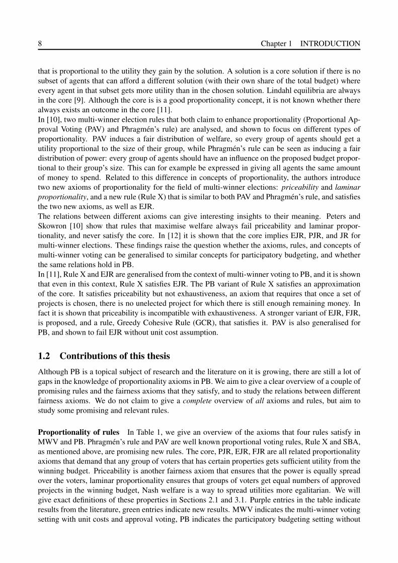
Proof. Because Phragmen’s rule is build to have a fair distribution of power and maximising the Nashwelfare can be considered a way to get a fair distribution of welfare, it is obvious that Phragmen’s ruledoes not necessarily maximise the Nash welfare. We can show this by the example given in [10], asshown in Figure 2 where the difference between Phragmen’s rule (which distributes power fairly) andPAV (which distributes welfare fairly) is demonstrated. The Nash score for the committee returned

Figure 2: An example of a laminar election instance and the results of Phragmen’s rule and PAV [10].

by Phragmen’s rule here is 53 · 33 = 3375, and the Nash score for the committee returned by PAVis 46 = 4096. Even without knowing whether the Nash score for the PAV-committee is the highestpossible, it is clear that the score for Phragmen’s committee is not maximal.

Proposition 2.3. PAV does not maximise Nash welfare.

Proof. The counterexample from Proposition 3.9 (in Chapter 3) showing that PAV does not alwaysmaximise the Nash product obviously does not work in a multi-winner voting setting where everyproject has unit cost. In fact, the two functions are very similar, and therefore it is not trivial to findand example where their maxima are different. Both PAV and Nash are a sum over the agents of acertain value that for each agent is based on the number of projects that they approve of, that are inthe elected committee. For PAV, this value per agent is determined by g(x) = ∑

xk=1

1k , the harmonic

numbers, and for Nash, this value is determined by f (x) = ln(1+ x). As [4] already mention, theharmonic numbers can be considered a discrete version of the logarithm. Both functions are plottedin Figure 3. Because we are interested in finding the maximum of a sum over these functions, wewant to investigate their change on adding or removing a project for an agent, hence we look at theirderivatives. For f (x), the derivative is just f ′(x) = 1

1+x . For g(x), this is a bit more involved, becauseg(x) is not a continuous function. However, if we look at how g(x) changes if we add or removeone from x, we observe that if we increase x by one, g(x) increases by 1

x+1 , and if we decrease x byone, g(x) decreases by 1

x . Thus, on one side, the ‘derivative’ is the same as for f (x), on the otherside it is slightly different. If we would change it into a continuous function somehow, it might verywell have the same derivative as f (x). However, because they are not exactly the same, probablythere is a situation where the maximum of their sums over agents are different. We try to find such a


Figure 3: The functions g(x) used for PAV and f (x) used for Nash, where x is the number of projectsthat an agent approves that are elected.

counterexample by trial and error.Let us take a small set of projects, say {w1, ...,w5}, and a large group of agents X that all approvethose five projects in order to make sure that they are all in the winning committee. We can chooseX arbitrarily large in order to make sure that indeed {w1, ...,w5} ⊆W . Now let there be two otherprojects, say c1 and c2, such that for c1 there is a small group of voters Y 6⊆X that approve only c1, andthat for c2 there is a subgroup X ′ ⊆ X such that all i ∈ X ′ approve c2 (and because they are in X , theyalso approve {w1, ...,w5}). Let k = 6, so that we can either add c1 to the winning committee or c2,but not both. The idea behind this counterexample is that in order to get a different maximum, theremust be a difference in the functions in whether we add one project that is the first approved electedproject for some voters, or we add one project that is approved for a group of voters that is alreadysomewhat happy. Suppose we add c1 to the winning committee. Then the PAV score increases with|Y |, and the Nash score increases with ln(2) · |Y |. If we add c2 to the committee instead, the PAV scoreincreases by |X

′|6 , and the Nash score increases by |X ′| ln(7)−|X ′| ln(6). We now look for values of

|Y | and |X ′| such that the PAV score increases more for adding c1 and the Nash score increases morefor adding c2 or vice versa. The system |Y |> |X ′|

6 and ln(2)×|Y |< |X ′|× ln(7)−|X ′|× ln(6) gives ussome possible solutions, for example |X ′|= 5, |Y |= 1, so if a group of five agents from X approve c2and one agent not from X approves c1, adding c1 to W will increase the PAV score more than addingc2, but adding c1 to W will increase the Nash score less than adding c2. We only have to choose Xlarge enough such that {w1, ...,w5} are elected, and then we have found a situation where the winningcommittee for PAV is not the committee that maximises the Nash product.

It seems that for small numbers of agents and projects, those maxima will be the same, so an interest-ing question for future research is what is the minimum number of voters and projects for which theycan differ.

Open Question 2.1. What is the minimal number of voters and projects for which the Nash scoreand the PAV score have a different maximum?

Proposition 2.4. Rule X does not maximise Nash welfare.

This will be shown in Section 4.2.


Finally, for Phragmen’s rule it was not established whether or not it satisfied FJR, but in the sameway we saw it did not satisfy the core, it is very easy to see that it does not satisfy FJR either.

Proposition 2.5. Phragmen’s rule fails FJR.

Proof. As shown by [10], the outcome of Phragmen’s rule does not necessarily satisfy EJR. We knowfrom [11] that FJR implies EJR, so Phragmen’s rule does also not satisfy FJR.

2.3 Relations between axiomsWe study the relations between proportionality axioms in this thesis, and quite some of them arealready shown in the literature, or become immediately clear from the definition of the axioms. From[11] and [13], we know that the core implies FJR, which implies EJR, which implies PJR, and from[10], we know that priceability implies PJR.In some of the following sections we will study new relations between axioms. A summary of thefindings is given here, with references to the corresponding theorems:

• Priceability does not imply laminar proportionality in MWV: Theorem 2.1.

• Laminar proportionality implies priceability of laminar election instances in MWV: Theorem2.2.

• Laminar proportionality implies PJR, EJR, and the core in MWV: Corollary 4.2.2.

• PJR does not imply laminar proportionality in MWV: Theorem 2.3.

• PJR does not imply priceability in MWV, not even in laminar election instances: Theorem 2.4and Corollary 2.4.1.

• Priceability does not imply EJR or the core in MWV: Theorem 2.5 and Corollary 2.5.1.

• Neither EJR nor the core implies priceability or laminar proportionality in MWV: Theorem 2.6and Corollary 2.6.1.

2.3.1 The relation between laminar proportionality and priceability in MWV

In Table 6 we saw that a lot of rules satisfy both priceability and laminar proportionality or neither ofthem, which gives rise to the question whether there is a logical relation between the two axioms. Inthis section we will try to answer this question.First of all, note that laminar proportionality cannot say anything about priceability in general becauseit is only defined on laminar instances, while priceability is defined on all profiles. We can howeverstudy whether laminar proportionality implies priceability in laminar election instances, and whetherpriceability implies laminar proportionality.

Theorem 2.1. In MWV, priceability does not imply laminar proportionality

Proof. In order to show that priceability does not imply laminar proportionality, we construct a coun-terexample. Consider a profile P as in Table 7.We have 3 voters, v1,v2, and v3, and 6 candidates c1, ...,c6. Candidates c1,c2, and c3 are approvedby voters v1 and v2, candidates c4 and c5 are approved by voter v3, and candidate c6 is approvedby all three voters. This profile is laminar for k = 4, we can construct it according to the inductive


c3

c2 c5

c1 c4

c6

v1 v2 v3

Table 7: A counterexample that shows that priceability does not imply laminar proportionality: ProfileP with committee W (in green). It should be read in the same way as Table 4.

Definition 2.10 by first concatenating {c1,c2,c3} (k = 2) and {c4,c5} (k = 1) by Definition 2.10.3 andthen adding c6 by Definition 2.10.2, which results in k = 2+1+1 = 4.The elected committee W , as indicated in green, is not laminar proportional, because in order to belaminar proportional, c6 would have to be included in W . It is, however, priceable: we can construct aprice system with price p = 0.65: v1 and v2 together pay for c1,c2, and c3 and have 2−3 ·0.65 = 0.05left over, and v3 pays for c4 and has 1−0.65 = 0.35 left over. Hence, v3 cannot pay for c5 anymore,and all voters together have an unspent budget of 0.4, so they cannot pay for c6.

Although priceable committees in laminar election instances need not be laminar proportional, wecan show that the converse is true: in laminar election instances, laminar proportional committeesare priceable. In order to show this, we show that we can construct a price system with price n

k forlaminar proportional committees in laminar election instances.

Theorem 2.2. Laminar proportionality implies priceability on laminar election instances.

Proof. We construct an inductive proof on the structure of laminar election instances to prove that forevery committee W that is laminar proportional for a laminar election instance (P,k), there exists aprice system ps = (p,〈pi〉i∈N) where p = |P|

k .Basis: If P is unanimous with |C(P)| ≥ k and W is laminar proportional for (P,k), then W ⊆C(P), sothe voters can just divide their budget over the candidates in W . If we set the price p to p = n

k , wecan let every voter pay 1

k to every candidate. Then every voter will have in total spent k · 1k = 1 unit of

money, so have nothing left to spend on other candidates, and every candidate in W will have receivedn · 1

k = p units of money, so can exactly be afforded.Inductive Hypothesis (IH): Suppose that (P′,k′), (P1,k1), and (P2,k2) are laminar election instances,committees W ′,W1, and W2 are laminar proportional for respectively (P′,k′), (P1,k1), and (P2,k2), andsuppose that for W ′ there exists a price system with price p′ = |P′|

k′ , for W1 there exists a price systemwith price p1 =

|P1|k1

, and for W2 there exists a price system with price p2 =|P2|k2

. Furthermore, supposethat P′ is not unanimous, that C(P1)∩C(P2) = /0 and that |P1| · k2 = |P2| · k1.Inductive step:

• Case 1: There is a unanimously approved candidate c such that P = P′+c, where P′+c = (A1 ∪{c}, ...An∪{c}). Suppose that W is laminar proportional for P,k = k′+1, then W =W ′∪{c}.By the inductive hypothesis, there exists a price system ps′ for W ′ with price p′ = |P′|

k′ . Becausec is unanimously approved, in theory all voters can pay for c. We know that in ps′, there wasno candidate that was not in W ′ for which its supporters together had enough (more than p′)unspent budget. If we would give every voter 1

k′ more budget, which we let them spend entirelyon c, c will get enough money and no voter will have more unspent budged than they had before.We then only have to rescale the system so that every voter has 1 unit of currency to start with


again. Every voter now has 1+ 1k′ units of money, so we divide everything by 1+ 1

k′ in order to

get a per voter budget of 1. The price p now becomesnk′

1+ 1k′= n

k′ ·k′

k′+1 = nk′+1 = n

k and all the

individual payment functions are divided by 1+ 1k′ as well. Because for every candidate in W

the sum of the individual payments was equal to the price, when we divide both the individualpayments and the price by the same constant, this equality will continue to hold.

Formally we define the price system ps for the instance (P,k) as follows: ps = (p,〈pi〉i∈N) with

p = p′

1+ 1k′= n

k , and pi : C→ [0,1] such that pi(c) =1k′

1+ 1k−1

=1

k−11+ 1

(k−1)= 1

k and pi(d) =p′i(d)

1+ 1(k−1)

for

all other candidates d ∈C(P), where p′i is the payment function of voter i in the price systemps′.

To show that this is indeed a valid price system that supports W , we look at the five points ofthe definition of a price system that supports a committee:

1. Voters only pay for candidates they approve of, because they did so in ps′, and the onlycandidate which they now pay for that they did not pay for before is c, which is unani-mously approved.

2.

∑d∈C(P)

pi(d) = ∑d∈C(P)

p′i(d)1+ 1

k−1

+1k

=1

1+ 1k−1

∑d∈C(P)

p′i(d)+1k

IH≤ 1

1+ 1k−1

+1k

=k−1

k+

1k= 1

3. For each elected candidate d ∈W , if d 6= c the sum of the payments is

∑i∈N

pi(d) = ∑i∈N

p′i(d)1+ 1

k−1

=1

1+ 1k−1

∑i∈N

p′i(d)

IH=

11+ 1

k−1

· p′

=1

1+ 1k−1

· nk−1

=n

(1+ 1k−1) · (k−1)

=nk= p.

For c, ∑i∈N pi(c) = n · 1k = n

k=p


4. For any candidate outside of the committee d /∈W ,

∑i∈N

pi(d) = ∑i∈N

p′i(d)1+ 1

k−1

=1

1+ 1k−1

∑i∈N

p′i(d)

IH=

11+ 1

k−1

·0 = 0.

5. For any candidate outside of the committee d /∈W , its supporters do not have a remainingunspent budget of more than p:

∑i∈N for which d∈Ai

(1− ∑e∈W=W ′∪{c}

pi(e))

= ∑i∈N:d∈Ai

(1− pi(c)− ∑e∈W ′

pi(e))

= ∑i∈N:d∈Ai

(1− 1k− ∑

e∈W ′pi(e))

= ∑i∈N:d∈Ai

(k−1

k− ∑

e∈W ′pi(e))

= ∑i∈N:d∈Ai

(k−1

k− k−1

k ∑e∈W ′

(pi(e)k

k−1))

=k−1

k ∑i∈N:d∈Ai

(1− ∑e∈W ′

(pi(e)k

k−1))

=k−1

k ∑i∈N:d∈Ai

(1− ∑e∈W ′

p′i(e))

IH≤ k−1

k· p′

=k−1

k· n

k−1=

nk= p,

so there is no unelected candidate whose supporters in total have a remaining unspentbudget of more than p.

Hence, ps is indeed a valid price system that supports committee W .

• Case 2: P = P1 + P2 and k = k1 + k2. Take W = W1 ∪W2, which is by definition laminarproportional for (P,k). We have to show that W is priceable for this election instance. Note thatthere are no overlapping candidates between P1 and P2, there is no voter in P1 that approves acandidate from C(P2), and no voter in P2 that approves a candidate from C(P1). By the inductivehypothesis, there exists a price system ps1 = (p1,{p1,i}i∈N) for W1 with price p1 = |P1|

k1, and

for W2 there exists a price system ps2 = (p2,{p2,i}i∈N) with p2 =|P2|k2

. Also by the inductivehypothesis, |P1| · k2 = |P2| · k1, so p1 = p2. We can now define a price system ps that supportsW as follows: ps = (p,〈pi〉i∈N) with p = p1 = p2, and for all voters i ∈ N,

pi(c) = p′1,i(c)+ p′2,i(c),


where p′1,i and p′2,i are extended versions of respectively p1,i and p2,i that yield zero for thecandididates that those are not defined for:

p′1,i(c) =

{p1,i(c) if c ∈C(P1) and i ∈ P1;0 if c ∈C(P2) or i ∈ P2.

p′2,i(c) =

{0 if c ∈C(P1) or i ∈ P1;p2,i(c) if c ∈C(P2) and i ∈ P2.

Again, we show that this is a valid price system that supports W by looking at the five points ofthe definition:

1. We know that ps1 is a valid price system that supports W1, so for voters i ∈ P1 and can-didates c ∈W1, if p1,i(c) > 0, then c ∈ Ai. Analogously, for voters i ∈ P2 and c ∈W2 ifp2,i(c)> 0, then c∈ Ai. Suppose pi(c)> 0. If c∈C(P1), then pi(c) = p1,i(c), so i∈ P1 be-cause there is no voter in P2 that approves a candidate from C(P1) and vice versa. Hence,for c ∈ C(P1), if pi(c) > 0, then p1,i(c) > 0 and then c ∈ Ai. Similarly, we can arguethat for c ∈ C(P2), if pi(c) > 0, then p2,i(c) > 0 and then c ∈ Ai. Because P = P1 +P2,C(P) =C(P1)∪C(P2), so for all c ∈C(P), if pi(c)> 0 then c ∈ Ai.

2. ∑c∈C(P) pi(c) = ∑c∈C(P) p′1,i(c) + p′2,i(c). We already saw that voters from P1 do notpay for candidates from C(P2) and vice versa. Hence, if i ∈ P1, then ∑c∈C(P) pi(c) =

∑c∈C(P) p′1,i(c)IH≤ 1, and if i ∈ P2, then ∑c∈C(P) pi(c) = ∑c∈C(P) p′2,i(c)

IH≤ 1

3. For each elected candidate c ∈W , the sum of its payments is ∑i∈N pi(c) = ∑i∈N p′1,i(c)+

p′2,i(c). For c ∈C(Px) (with x ∈ {1,2}) this is ∑i∈N p′x,i(c)IH= px = p.

4. Because W =W1∪W2, any candidate that is not elected in the new committee, c /∈W , wasnot elected in W1 or W2, so did not get any payment there: for c ∈C(Px), ∑i∈N px,i(c) = 0.Hence, it also does not get any payment in the new system: for c ∈C(Px), ∑i∈N pi(c) =∑i∈N p′x,i(c) = ∑i∈N px,i(c) = 0 (for x ∈ {1,2}).

5. All unelected candidates are only supported by voters from their own ‘old’ system, whodid not have in total a remaining unspent budget of more than the price there, so neitherwill they have it now:Without loss of generality, assume that an unelected candidate c /∈W is part of C(P1).Then because c /∈W , we also have c /∈W1, because if it was in W1, it would also have beenin W . Because ps1 is a price system that supports W1, we know that ∑i∈N for which c∈Ai(1−∑e∈W1 p1,i(e))≤ p1. However, for all voters i ∈ N for which c ∈ Ai, we have i ∈ P1, so forall e ∈W1, p1,i(e) = pi(e), and for all e ∈W2, pi(e) = 0. This implies that

∑i∈N for which c∈Ai

(1− ∑e∈W1

p1,i(e)) ≤ p1

⇔∑

i∈N:c∈Ai

(1− ∑e∈W=W1∪W2

pi(e)) ≤ p1 = p.

We can analogously show the same for c ∈ C(P2), so conclude that for all c ∈ C(P) =C(P1)∪C(P2), if c /∈W ,

∑i∈N:c∈Ai

(1− ∑e∈W

pi(e))≤ p


By these five points, we have shown that ps is indeed a valid price system that supports com-mittee W .

We have shown by induction over laminar election instances that, if a committee W is laminar pro-portional in a laminar election instance (P,k), it is also supported by a price system with price |P|k .Hence we can conclude that laminar proportionality implies priceability in laminar election instancesin multi-winner approval based election settings.

2.3.2 Priceability’s and laminar proportionality’s relation with PJR, EJR, and the core inmulti-winner elections

In the previous section we examined the relationship between priceability and laminar proportionality.In this section, we will study the logical relations between those two axioms on one hand, and theaxioms of the core, EJR, and PJR on the other hand.As is shown in [10], a committee that is priceable also satisfies PJR. Hence, we can deduce that PJRdoes not imply laminar proportionality.

Theorem 2.3. PJR does not imply laminar proportionality in MWV.

Proof. Take the example from Section 2.3.1 (Table 7). This profile is laminar, and committee Windicated in green is priceable. Hence, it satisfies PJR. It does however not satisfy laminar propor-tionality, because candidate c6 is not elected. Therefore we can conclude that PJR does not implylaminar proportionality.

PJR also does not imply priceability, as we can show by the following counterexample (visualized inTable 8):

Theorem 2.4. PJR does not imply priceability in laminar election instances in MWV.

Proof. We give a counterexample that shows that a committee W in a laminar profile can satisfyPJR without being priceable. Suppose we have 3 voters, v1,v2, and v3, and 5 candidates c1, ...,c5.Candidates c1 and c2 are approved by voters v1 and v2, candidates c3 and c4 are approved by voter v3,and candidate c5 is approved by all three voters. This election instance is laminar, as can easily bechecked, and the elected committee W , as indicated in green in Table 8 satisfies PJR: for all `≤ 4 andall `-cohesive group of voters S, it holds that |W ∩∪i∈SAi| ≥ `. It is, however, not priceable: suppose,for a contradiction, that there is a price system ps that supports W . The price p of this system has tobe such that v3 can pay for both c3 and c4 (because no other voter can pay for these candidates), sop ≤ 0.5. However, v1 and v2 together have a budget of 2, which they must spend only on c1 and c2.Hence, p > 2

3 , because otherwise v1 and v2 together have enough unspent budget to pay for c5 whichis not in W . Hence p ≤ 0.5 and p > 2

3 , which is a contradiction. Therefore, there is no price systemthat supports W .

Since laminar election instances are a specific type of approval elections, the same result holds forMWV elections in general.

Corollary 2.4.1. PJR does not imply priceability in MWV.

Proof. This follows directly from theorem 2.4.


c2 c4

c1 c3

c5

v1 v2 v3

Table 8: Profile P with committee W indicated in green. It should be read in the same manner asTable 4 and Table 7.

In [10], it is shown that in the multi-winner election setting, priceability implies PJR. We studywhether it is also the case that all priceable committees must satisfy the stronger axiom of EJR.Note that we only have to look at cases where the unit cost assumption is satisfied, in PB, we havethat priceable committees do not necessarily satisfy PJR, so they also cannot necessarily satisfy thestronger EJR. We see that pricable committees need not satisfy EJR. In party-list profiles however,priceable committees do satisfy EJR.The following counterexample shows that in general, pricable committees need not satisfy EJR:

Theorem 2.5. Priceability does not imply EJR in MWV.

Proof. Take an election instance E with 3 voters N = {v1,v2,v3} and 6 candidates C = {c1, ...c6}, andlet k = 3. Let every voter approve four projects, namely one that only that voter approves and threethat all three voters approve: Ai = {ci,c4,c5,c6}. Suppose the winning committee of the election isW = {c1,c2,c3}. For this committee, there is a price system with p = 1 in which every voter i paysthe price of candidate i and nothing else. The group S = N is 3-cohesive, because |S| = 3 = 3n

k , andall three voters agree on the projects {c4,c5,c6}. However, there is no voter in S who approves 3 ormore projects in W , so W does not satisfy EJR.

Since the core implies EJR, this example also shows that priceable committees are not necessarily inthe core.

Corollary 2.5.1. Priceability does not imply the core in MWV.

The implication in the other direction does not hold either, EJR does not imply priceability or laminarproportionality.

Theorem 2.6. Neither EJR nor the core implies priceability or laminar proportionality in laminarelection instances in MWV.

Proof. The counterexample for Theorem 2.4 also shows that a committee that satisfies EJR or is inthe core does not necessarily have to be priceable or laminar proportional. The committee in Table 8does satisfy EJR and it is in the core, as can easily be checked, but it is neither priceable nor laminarproportional.

Again, since laminar election instances are a specific type of multi-winner approval elections, thesame result holds for MWV in general.

Corollary 2.6.1. Neither EJR nor the core implies priceability in MWV.

Proof. This follows directly from theorem 2.6.

In Section 4.3.2 (Corollary 4.2.2), we will show that in MWV, laminar proportionality implies allthree axioms of the core, EJR, and PJR.


2.3.3 FJR

So far, we did not really study the FJR axiom. However, it can be easily fitted in our landscapeof proportionality axioms, since we know that FJR is ‘in between’ EJR and the core (that the coreimplies FJR and FJR implies EJR). We have not studied it’s relation to laminar proportionality andpriceability yet. However, since laminar proportionality implies the core (Corollary 4.2.2), it alsoimplies FJR, and since priceability does not imply EJR (Theorem 2.5), pricability does not implyFJR. Furthermore, since the core does not imply priceability or laminar proportionality (Theorem 2.6,Corollary 2.6.1), FJR does not imply priceability or laminar proportionality either (since otherwisethe core would implicitly imply them as well).

In multi-winner voting, we now have the relations as shown in Figure 4. We have shown that theseare the only implicational relations between the four properties, the absence of arrows indicate thereis a counterexample that shows there is no implication between the properties.As we will show in Chapter 4, under certain conditions there are more relations. For example, we willshow in Section 4.4 that in party-list profiles (Definition 2.12) all axioms from Figure 4 are equivalent.

PJR

EJR

priceability


[10]

Corollary

4.2.2

Corollary 4.2.2

Corollary 4.2.2

The

orem

2.2

[13]

[11]

(onl

yfo

r lam

inar

inst

ance

s)


for laminar

instances

)


Figure 4: The implicational relations between laminar proportionality, priceability, PJR, EJR, and thecore in multi-winner approval voting

2.4 Future workIn the beginning of this Chapter, we also looked at the proportionality axiom of Nash welfare, and sawthat neither of the rules we studied satisfied it. PAV, however, seems to output a committee that has annearly maximal Nash score. We found a counterexample that shows that PAV does not always max-imise the Nash score (Proposition ), but for small numbers of voters and projects, the maximum Nashproduct and maximum PAV score seem to be produced by the same committee. It could be interestingto study what is the minimum number of voters and projects for which the maximum PAV score andmaximum Nash product are different (Open Question 2.1). Another interesting topic of research is the


relation between the Nash welfare axiom and the other axioms. We have not included Nash welfarein Figure 4 as the question remains what are the relations between Nash welfare and the axioms thathad our main focus, it is not entirely clear yet how it fits into the landscape of proportionality axioms.In Section 3.4, we will see that in the PB setting, a committee maximising the Nash product does notnecessarily satisfy EJR or the core. We have no such result for the MWV setting, but that result leadsto the conjecture that also in MWV Nash welfare does not imply EJR or the core. Investigating this,as well as studying the relation between Nash welfare and priceability, laminar proportionality, andPJR, remain topics for future research:

Open Question 2.2. Is there a logical relation in MWV between Nash welfare on the one hand, andthe core, EJR, PJR, priceability, and laminar proportionality on the other hand?

30 Chapter 3 PARTICIPATORY BUDGETING

3 Participatory BudgetingAs we already mentioned, participatory budgeting is a generalisation of multi-winner voting, with arelaxation of the unit cost assumption and utility based voting instead of approval voting. Hence, theresults that are obtained in the field of MWV can help a lot in understanding the behavior of rulesand axioms in PB. The rules that we studied in the previous chapter can each be generalised to aPB version (although some of them are only defined for approval voting), and for the axioms this ispossible as well. We will also study a new rule that is especially designed for PB, namely the Smith-consistent Budgeting Algorithm (SBA), which is a promising algorithm because it is computablein polynomial time and always returns a Condorcet-winning budget if it exists. As we will show,however, it performs poorly on the different fairness axioms.

Outline of chapter This chapter is structured very similar to Chapter 2. Just like in the previouschapter, we will start by giving the definitions of the rules and axioms used in PB in Section 3.1.Section 3.2 studies which axioms are satisfied by the different rules in PB, and in Section 3.3 wewill study the relations between the different axioms. Finally in Section 3.4, we will mention somedirections for future work.

3.1 Definitions3.1.1 Rules

In order for a rule to be generalisable from approval voting to utility voting, we must be able to useutility scores that can have any real value between 0 and 1. However, for both PAV and Phragmen’srule, there is no trivial way to do this. In computing the PAV-score, we use the harmonic numbers,which are only defined on integers (e.g. we cannot have an 0.345-th harmonic number). We coulddefine a continuous function that approximates the harmonic numbers4, but instead we chose to keepusing approval voting in the PB setting. Hence, the only generalization for PAV from MWV to PB isthe relaxation of the unit cost assumption, and the definition is as follows:

Definition 3.1 (PAV for PB). The outcome W of PAV is the committee with cost(W ) ≤ l that max-imises the score


(1+

12+

13+ · · ·+ 1

|W ∩Ai|

).

A similar problem arises in the generalisation of Phragmen’s rule. In Phragmen’s rule, whether or nota voter has to pay for a candidate is determined by whether or not the voter approves that candidate.The amount every approving agent has to pay may differ. However, having to pay or not is a binaryvariable, so we need a binary value to determine this. We could require that the amount a voter needsto pay is proportional to the utility they get from it, but as [11] show, this will make Phragmen’s ruleelect very inefficient outcomes. However, we can generalise the rule very naturally to non-unit costs.The PB definition of Phragmen’s rule then is as follows:

Definition 3.2 (Phragmen’s rule for PB [11]). Every voter gets continuously one unit of currency pertime unit. At the first moment in time t when there is a group of voters S who all approve a not-yet-selected candidate c, and who have cost(c) units of currency in total, the rule adds c to the committee

4In fact, the Nash score is a fairly close approximation of the PAV score, as noticed in the proof of Proposition 2.4 andin [4].

Chapter 3 PARTICIPATORY BUDGETING 31

and asks the voters from S to pay the cost of c (i.e., the rule resets the balance of each voter from S);the other voters keep their so-far earned money. The rule stops when it would select a project which,when implemented, would overshoot the budget limit.

In contrast to PAV and Phragmen’s rule, Rule X is very well generalisable to PB, as is shown in [11].This is done by letting the voters pay for a project proportionally to the utility they get from it. Unlikewith Phragmen’s rule, with Rule X this requirement does not cause inefficiency. Just as Phragmen’srule, Rule X is naturally extendable to non-unit costs. Each voter is now asked to pay for a project anamount proportional to their utility for that project if they can, namely ρ units of money per unit ofutility, and if they do not have this amount anymore they have to pay all the money they have left.

Definition 3.3 (Rule X for PB [11]). The rule starts by giving each voter an equal fraction of thebudget. In case of a budget limit of 1, each voter gets 1

n units of currency. We start with an emptyoutcome W = /0 and sequentially add projects to W . To add a project c to W , the voters have to payfor c. Write pi(c) for the amount that voter i pays for c; we will need that ∑i∈N pi(c) = cost(c). Letpi(W ) = ∑c∈W pi(c)≤ 1

n be the total amount voter i has paid so far. For ρ≥ 0, we say that a projectc /∈W is ρ-affordable if

∑i∈N

min(1n− pi(W ),ui(c) ·ρ) = cost(c).

If no project is ρ-affordable for any ρ, Rule X terminates and returns W . Otherwise it selects a projectc /∈W that is ρ-affordable for a minimum ρ. Individual payments are given by pi(c) = min(1

n −pi(W ),ui(c) ·ρ).The new rule SBA is introduced in [5]. Since SBA needs as input a ranking of projects from eachvoter, it is not generalisable to approval voting and hence not discussed in the chapter about MWV.(If we would transfer the ordinal ballots to approval ballots using some kind of approval threshold,the algorithm would depend largely on tie-breaking decisions.) For the total pseudo-code we refer tothe original paper, here we will give a textual definition.

Definition 3.4 (SBA [5]). The rule starts by generating a majority graph G of the profile, which is agraph that has all projects as vertices and an arc between two projects c and c′ if more than half ofthe voters rank c′ higher than c. Next, the rule continues with the ranking procedure: it creates anordered partition V of the set of projects C. V starts empty, and in every iteration the rule identifiesthe Schwartz set5 of the majority graph G, adds the projects in it as a new component of V andremoves them from G. This is done until the G is empty, at which point V is an ordered partition of C.Now the rule starts in the pruning procedure to fill the set of elected projects W by iterating over thecomponents C1, · · ·Cz of V and choosing the subset with maximal cost Bi of the current component Cisuch that the cost of Bi∪W is still within the budget limit. If there are more such subsets with equalcost, the previous budget (for example last year’s budget) is used as a tie-breaker: the one closest(minimal cost of symmetric distance) to the previous budget is chosen. This subset of Ci is added toW . After having considered all components of V, the rule stops.

Example 3.1. In Figure 5, an example of the SBA procedure is displayed. The input consists of autility profile, which is translated into a profile of ordinal ballots (of course, the input can also be anordinal profile directly). Then the majority graph G is constructed and the Ranking procedure starts:the Schwartz-set is computed and G is adjusted until G is empty, which leaves us with an orderedpartition V . Then in the Pruning procedure the output set B is formed by going over the items from Vand adding affordable projects to B.

5A Schwartz component X of a graph G with vertices A is a minimal set of vertices such that for any b ∈ A\X there isno a ∈ X such that there is an arc in G from b to a. The Schwartz set is the union of all Schwartz components.


Figure 5: Example of the SBA-algorithm

In the following subsections, we will give the definitions of several (fairness) axioms in PB. Theseare the same axioms as we used in MWV (Section 2.1.2), but generalised to the PB setting.

3.1.2 PB Axioms from the literature

Just as in MWV, we have the related axioms of core, FJR, and EJR. The core naturally extends to PB,by requiring that there is no group of agents that can afford a set of projects they strictly prefer to thewinning set of projects. The formal definition is then as follows:

Definition 3.5 (Core for PB [11]). For a given election instance E = (N,C,cost,P, l), we say that anoutcome W is in the core, if for every S ⊆ N and T ⊆C with |S| ≥ cost(T ) ·n there exists i ∈ S suchthat ui(W ) ≥ ui(T ). We say that an election rule R satisfies the core property if for each electioninstance E the winning outcome R (E) is in the core.

It is clear that this is a generalisation of the MWV variant of the core and that applying it in the MWVsetting will make it equivalent to Definition 2.4.In [11], the definition of FJR is given, which was originally designed for PB. The MWV version wegave in Definition 2.5 is a specific variant of it, proven by the authors to be a MWV variant of thesame axiom.

Definition 3.6 (Full Justified Representation (FJR) for PB [11]). We say that a group of voters S isweakly (β,T )-cohesive for β∈R≥0

6 and T ⊆C, if |S|> cost(T )l ·n and ui(T )> β for every voter i∈ S.

A rule R satisfies FJR if for each election instance E and each weakly (β,T )-cohesive group of votersS there exists a voter i ∈ S such that ui(R (E))> β.

6In the original definition, there is no constraint that β≥ 0, but as for negative β every S is (β,T )-cohesive for any T ,we added it.


A generalisation of the MWV axiom of EJR was also given by [11], and is proven to be indeed ageneralisation of that axiom.

Definition 3.7 (Extended justified representation (EJR) for PB [11]). A group of voters S is (α,T )-cohesive for α : C→ [0;1] and T ⊆ C, if |S| ≥ cost(T )

l · n and if it holds that ui(c) ≥ α(c) for everyvoter i ∈ S and each candidate c ∈ T . A rule R satisfies EJR if for each election instance E and each(α,T )-cohesive group of voters S, there is a voter i ∈ S such that ui(R (E))≥ ∑c∈T α(c). 7

In [11], also the idea of price systems and priceability is generalized to PB. The generalisation tonon-unit costs is very natural, we can just give each project its own price in the system instead oftaking one general price. The generalisation from approval votes to arbitrary utilities is a bit moreinvolved, but Peters et al. solve that by regarding every agent that gets some utility from a project asapproving that project. The new definitions then are as follows:

Definition 3.8 (Price systems for PB [11]). A price system is a pair ps = (b,〈pi〉i∈N) where b≥ 1 isthe initial budget, and for each voter i ∈ N, there is a payment function pi : C→ R such that

1. a voter can only pay for candidates she gets at least some utility from: if ui(c)= 0, then pi(c)= 0for each i ∈ N and c ∈C, and

2. each voter can spend the same budget of bn units of money: ∑c∈C pi(c)≤ b

n for each i ∈ N.

Definition 3.9 (Priceability for PB [11]). A rule R is priceable if for all election instances E, thereexists a price system ps = (b,〈pi〉i∈N) that supports R (E), i.e.

1. for each c ∈ R (E), the sum of the payments for c equals its price: ∑i∈N pi(c) = cost(c);

2. no candidate outside of the committee gets any payment: for all c /∈ R (E),∑i∈N pi(c) = 0; and

3. there exists no unelected candidate whose supporters in total have a remaining unspent budgetof more than its cost: for all c /∈ R (E),

∑i∈N for which ui(c)>0

(bn− ∑

c′∈R (E)pi(c′))≤ cost(c).

It is easy to see that every MWV rule that satisfies the MWV version of priceability also satisfies thePB version when approved projects are regarded having a utility of 1 and non-approved projects ashaving a utility of 0, and that any MWV satisfying the PB version also satisfies the MWV version.Hence, this is indeed a generalisation of the concept of priceability as introduced in [10].The concept of Nash welfare can trivially be extended to the PB setting, by replacing the total com-mittee size k by a budget limit l and the cost of a project from 1 to its actual cost, and measuring theutility an agent gets from a set of elected projects by the sum of the actual utilities of each electedproject, instead of by the number of approved elected projects.

Definition 3.10 (Nash welfare [4]). A rule satisfies Nash welfare if for every election instance it re-turns the committee W with cost(W )≤ l that maximises the Nash product Nash-prod(W ) =∏i∈N(1+ui(W )).

Two rules from the previous chapter are left over without a proper generalisation to the PB setting:PJR and laminar proportionality. In the following subsections, we will give generalisations to the PBsetting for those axioms.

7In the original definition in [11], there is an alternative condition to simplify the reasoning for rules that do notnecessarily spend the total budget. This extra condition relaxes EJR to hold up to one project, and allows a rule to alsosatisfy EJR if for some a ∈C it holds that ui(R (E)∪{a})> ∑c∈T α(c).


3.1.3 PJR in Participatory Budgeting

Sanchez-Fernandez et al. [13] define PJR as a measure of proportionality for multi-winner approvalbased voting rules. We give a generalisation of PJR to the context of participatory budgeting (beyondthe assumptions of unit cost and approval-based elections) based on the generalisation of EJR as in[11]. Two steps of generalisation are involved. One is that candidates do not have to have equalcosts anymore as in multi-winner voting. The second generalisation is that from approval ballots toutilities: in approval voting the utility of voter i for candidate c can be either 1 or 0: ui(c) ∈ {0,1},in utility based voting, the utility can be any real value in a range from 0 to 1: ui(c) ∈ [0,1]. To ourknowledge, no generalisation of PJR to the PB context has been proposed in the literature except forthe one by Aziz, Lee, and Talmon [7]. They define an axiom called Strong-BPJR-L that requires thefollowing: For a budget limit l, a budget W satisfies Strong-BPJR-L if for all ` ∈ [1, l] there doesnot exist a set of voters S ⊆ N with |S| ≥ `n

l , such that cost(∩i∈SAi) ≥ ` but cost((∪i∈SAi)∩W ) < `.This generalisation still uses approval votes rather than arbitrary utilities, so we could generalise iteven further to be applicable to election instances with arbitrary utilities. However, note that therequirement in this definition is not that for every `-cohesive S the utility of the projects they allapprove that are elected is at least `, but rather the cost of this set of projects. Although this indeed ageneralisation of PJR, as is shown in [7], we think the aim of PJR in MWV is to ensure a certain levelof utility for every group of voters, rather than a certain cost. Only if one assumes that the cost of aproject is directly proportional to a voter’s utility from that project, this property is transferred in thedefinition of Strong-BPJR-L. We give a generalisation of PJR that does not depend on this assumptionand in which utilities can be arbitrary, independent of the cost of a project. For cohesiveness, we usethe notion of (α,T )-cohesive groups as defined in Definition 3.7.

Definition 3.11 (PB-PJR). A rule R satisfies proportional justified representation (PB-PJR) if foreach election instance E and each (α,T )-cohesive group of voters S,

∑c∈R (E)

(maxi∈S

ui(c))≥ ∑c∈T

α(c). (1)

The intuition behind this is that in the solution for each cohesive group S (cohesive in that S agrees toa certain degree about the set of projects T ) there should be enough candidates to which at least onevoter in S assigns enough utility.

Example 3.2. As an example, consider the profile displayed in Table 9. Suppose that the total budgetlimit l = 1, and that the W = {c1,c3,c4} is the set of projects elected by some voting rule (note thatthis is, for example, the set of projects that maximises total utility). Then consider the group of votersS = {v1,v2}. Probably both voters in S are happy that c4 is elected, but they would both get muchmore utility from c2 than from the elected c1 or c3. Also, if they both would get their share of the totalbudget (1

6 ), they could together afford the set T = {c2,c4}. Intuitively then, W is not a fair outcomeconsidering voters v1 and v2. Let us look at it in the formal definition. S is (α,T )-cohesive forα(c2) = 7,α(c4) = 6 (and α(c1) and α(c3) arbitrary: as we already noticed, the voters in S can affordT with their share of the budget, and for both of them u(c2) ≥ α(c2) and u(c4) ≥ α(c4). However,Equation 1 is not satisfied: ∑c∈W (maxi∈S ui(c)) = 3+2+7 = 12, while ∑c∈T α(c) = 7+6 = 13. Thisshows that in the given election instance, the outcome W does not satisfy PB-PJR.

PB-PJR is a generalisation of PJR in MWV elections In order to show that given definition isindeed a generalisation of the PJR for multi-winner voting as defined in [13], we apply it to the multi-winner voting setting and show that PJR and PB-PJR are equivalent for approval based multi-winnervoting rules.


cost candidate utilities0.1 c4 0.7 0.6 0.6 0.8 0.4 0.70.7 c3 0.2 0.2 0.8 0.7 0.6 0.80.2 c2 0.7 0.9 0.1 0.2 0.1 0.30.2 c1 0.3 0.1 0.9 0.3 0.9 1

v1 v2 v3 v4 v5 v6

Table 9: Example profile used in Example 3.2. Each column contains the utilities per candidate of avoter. The cost of the candidates is indicated in the leftmost column. The budget limit l = 1.

Theorem 3.1. PJR and PB-PJR are equivalent in approval-based multi-winner elections.

In the proof of Theorem 3.1, we make use of the following Lemma:

Lemma 3.1.1. Let N be a set of agents, C a set of alternatives, let each candidate c have a costcost(c) = 1

k , and let each voter i have a utility ui(c) ∈ {0,1} for candidate c. Define the approval setAi of voter i as Ai = {c ∈C : ui(c) = 1}. Then

(a) for given α : C→ [0,1] and T ⊆C, any group of voters S that is (α,T )-cohesive is also `-cohesivefor `= |T ′| with T ′ = {c ∈ T : α(c)> 0}, and

(b) for every group S that is `-cohesive there are T ⊆C with |T |= ` and α : C→ [0,1] with α(c) = 1for all c ∈C, such that S is (α,T )-cohesive.

Proof of of Lemma 3.1.1. (a): Assume that S ⊆ N is (α,T )-cohesive for some α : C → [0,1] andT ⊆C. By definition, in the approval based multi-winner setting this means that |S| ≥ |T | · n

k and thatfor all i ∈ S and all c ∈ T , ui(c) ≥ α(c). Now take a subset T ′ from T of all the candidates in T thathave at least some utility for all voters in S: T ′ = {c ∈ T : α(c) > 0}. Because ui(c) ∈ {0,1} (i.e.voting is approval based), α(c)> 0 and ui(c)≥ α(c) imply that ui(c) = 1. Hence, for all i ∈ S and allc ∈ T ′,ui(c) = 1. We can rewrite this as T ′ ⊆ ∩i∈SAi, so |T ′| ≤ |∩i∈S Ai|. Now if we call |T ′|= `, wehave `≤ |T |, so |S| ≥ ` · n

k and |∩i∈S Aαi | ≥ ` , so S is `-cohesive.

(b): Assume that S ⊆ N is `-cohesive for some ` ≤ k. This means that |S| ≥ ` · nk and | ∩i∈S Ai| ≥ `.

We take T ⊆ ∩i∈SAi with |T | = ` (which we can do because ` ≤ |∩i∈S Ai|). Now take α : C→ [0,1]such that α(c) = 1 for all c ∈C. Then |S| ≥ |T | · n

k and for all i ∈ S and all c ∈ T,ui(c) = 1 = α(c), soS is (α,T )-cohesive.

Proof of Theorem 3.1. We show that a rule that satisfies the new definition of PB-PJR also satisfiesthe old PJR for every approval based multi-winner election instance.PB-PJR⇒PJR: Assume that a rule R satisfies PB-PJR. Now take an arbitrary multi-winner electioninstance E where all projects have unit cost, and voting is approval based: the utility of a project fora voter is either 0 (when the voter does not approve the project) or 1 (when the voter does approvethe project). According to PB-PJR, it is true that for all S, α : C → [0,1] , and T with T ⊆ C, ifS is (α,T )-cohesive (|S| ≥ cost(T ) · n and it holds that ui(c) ≥ α(c) for every voter i ∈ S and eachcandidate c ∈ T ), then

∑c∈R (E)

(maxi∈S

ui(c))≥ ∑c∈T

α(c).


Because E satisfies the assumptions of unit cost and approval based voting, this boils down to thefollowing: for all S,α : C→ [0,1], and T ⊆C with |S| ≥ |T | · n

k and for which ui(c)≥ α(c) for all i∈ Sand for all c ∈ T , it is the case that

|R (E)∩ (∪i∈SAi)| ≥ ∑c∈T

α(c). (2)

In order to show that R satisfies PJR, we have to prove that for all S and `≤ k where S is `-cohesive(|S| ≥ ` · n

k and |∩i∈S Ai| ≥ l),|R (E)∩ (∪i∈SAi)| ≥ `.

Take arbitrary S ⊆ N and ` ≤ k and suppose that S is `-cohesive. According to Lemma 1(b), thereare T ⊆C with |T |= ` and α : C→ [0,1] with α(c) = 1 for all c ∈C, such that S is (α,T )-cohesive.Because R satisfies PB-PJR, this implies that |R (E)∩ (∪i∈SAi)| ≥ ∑c∈T α(c). However, because ofour choice of T and α, we know that ∑c∈T α(c) = |T | = `, so |R (E)∩ (∪i∈SAi)| ≥ `, which is whatwe had to prove.

We still have to prove that a rule that satisfies PJR also satisfies the newly defined PB-PJR in ap-proval based multi-winner elections:PJR⇒PB-PJR: Assume that a rule R satisfies PJR: in every election instance E, for every `-cohesivegroup of voters S, |R (E)∩(∪i∈SAi)| ≥ `. We want to prove that in every approval based multi-winnerelection instance, any (α,T )-cohesive group S satisfies |R (E)∩(∪i∈SAi)| ≥∑c∈T α(c). Take arbitrarysuch election instance E, and suppose that a group S is (α,T )-cohesive. Then according to Lemma1(a), when we take T ′ = {c ∈ T : α(c) > 0}, S is `-cohesive for ` = |T ′|. Because R satisfies PJR,it follows that |R (E)∩ (∪i∈SAi)| ≥ ` = |T ′|. By definition of T ′, |T ′| ≥ ∑c∈T ′ α(c) = ∑c∈T α(c), so|R (E)∩ (∪i∈SAi)| ≥ ∑c∈T α(c), which is what we had to prove.

We introduced PB-PJR, a generalisation of the axiom Proportional Justified Representation to beapplied in the context of participatory budgeting. We showed that in approval based multi-winnerelections with a unit cost assumption, PB-PJR is equivalent to the existing multi-winner PJR.

3.1.4 Laminar Proportionality in Participatory Budgeting

Laminar election instances in PB In this section, we will generalise the definition of laminarelection instances and the axiom of laminar proportionality from MWV to PB. For a moment, wekeep the notion of unit costs and try to generalise the definition of laminar election instances fromapproval voting to voting with utilities.The basic idea of laminar proportionality is that if we know about a strict separation between differentparties, we can divide the number of chosen candidates proportionally over the parties (with a bitmore elaborate rules about unanimous candidates and subparties). So actually we only say thingsabout situations in which it is very clear how to divide the committee seats fairly (situations we call‘laminar’). The point here is that if a voter that belongs to one group also votes for a candidate ofanother group, the interests get more complex, and that the laminar proportionality axiom only isabout those situations in which the interests are clearly separated. This is slightly contradictory tothe idea of utility voting. If we switch from approval voting to utility voting, voters can express theirpreferences more detailed, and we get more focus exactly on those cases that are ignored when werestrict the scope to laminar election instances. However, we will still explore the idea of laminarelection instances in utility voting.


Laminar election instances require that if one candidate is approved by two voters, it is not possiblethat another candidate is approved by yet another voter and only one of the first two voters. This islike the notion of laminarity in set theory: the sets of voters that approve a candidate should be eitherdisjoint or subsets of each other. Hence, in utility voting we could say that we do not want a voterfrom one party to get any utility from another party.What we could do is define a kind of approval threshold in utility based voting, in order to transfer theutilities to approval votes, and then just use the old definition of laminar election instances. However,if we do that, we cause small utilities not to have any influence anymore, and we ‘throw away’ a lotof information (although the latter may not be insurmountable). Furthermore, we want to retain theidea of voters not getting any utility if candidates from other parties are selected. Therefore, it mightbe a solution to set this approval threshold to zero: if a voter even has the tiniest amount of utilityfor a candidate, we define him to approve that candidate, and only if a voter has no utility at all fora candidate, he does not approve that candidate. The problem with such an approval threshold at 0is that we disregard the information gotten from the utility voting (all utilities above 0 are regardedequal), and that there is now a big difference between a utility 0 and a utility of 0.1, while there is nodifference between a utility of 0.1 and one of 0.2. Nevertheless, when asking utility functions fromthe voters, they should expect these differences to be equal. For this reason, we do not see this as aproper way to define laminar instances for utility profiles. Note, however, that in the generalisationof priceability to PB given in [11] (Definitions 3.8 and 3.9), the exact same problem arises: the exactvalue of the utilities is never used, only whether or not it is positive.What we could do in order to let utilities make a difference is to look how much different voters agreeabout different candidates. Suppose that in an approval voting instance we have two candidates, andthree voters such that both candidates have two votes, and one voter votes for both candidates. Thisis not allowed in laminar election instances. However, it would be allowed if one of the voters thatonly votes one candidate would also vote for the other candidate. Hence, in utility voting, we wantthis voter to vote at least as much for this other candidate (have a utility at least as high) as the othervoter does. We can capture this intuition by subtracting that part of utility from a voter’s utility thatis shared by the other voters. We could define unanimity in utility profiles as follows: a candidate isvoted unanimously if all voters give it the same utility (> 0). Now we could say an election instanceE is laminar if either E is unanimous, or E consists of two laminar instances E1 and E2 (just as inDefinition 2.10.3), or there is some candidate c that gives all voters some utility and the instance E ′,where we subtract the utility of the voter with minimum utility for c from all voter’s utilities for c, islaminar. The problem remains what to do with the committee size k when subtracting utilities in thislast case. In approval voting, we could just take k−1, because we could assume that the unanimouslyapproved candidate would be chosen anyway. However, with utility voting, it depends on the votingrule whether or not a candidate for which every voter has some utility is actually elected or not. Wecould choose to decrease k with the amount of utility that we subtract from every voter (for that isthe amount for which that candidate is ‘chosen’, but then we would have to round off in some wayor another in the end in order to get integer numbers again 8. Depending on the voting rule, otheroptions could be used, but we cannot find a solution that works properly for every voting rule.In conclusion, the main problem with generalizing the definition of laminar election instances fromapproval voting to utility voting is that in approval voting, we can say: “If it is clear how we shoulddivide the seats of the committee fairly among the voters, we should divide them that way”, but thatin utility voting, the cases where it is really clear how we should divide the seats are very rare, andalmost always the extra nuance that is provided by giving utilities rather than approval votes causes

8k has to be integer because we cannot elect half candidates. However in settings where projects can be partiallybudgeted, this can be an interesting option.


the profile to not be that clear anymore.

Laminar election instances for approval based PB As shown above, the idea of laminar electioninstances is problematic for utility voting. What we can do however, is define laminar election in-stances and laminar proportionality for participatory budgeting with approval voting, i.e. releasingonly the unit cost assumption, just as is done in the definition of Strong-BPJR-L in [7]. In order todo so, we take the budget limit l instead of the committee size k, and use the cost of each candidateinstead of the unit cost. We get the following definitions:

Definition 3.12 (Laminar election instances for PB). An election instance (P, l) (where P is a profile,i.e. a list of approval sets Ai, and l is the budget limit) is PB-laminar if either:

1. P is unanimous and cost(C(P))≥ l.

2. There is a candidate c ∈C(P) such that c ∈ Ai for all Ai ∈ P, the profile P−c is not unanimousand the instance (P−c, l− cost(c) is laminar (with P−c = (A1\{c}, ...,An\{c})).

3. There are two laminar instances (P1, l1) and (P2, l2) with C(P1)∩C(P2) = /0 and |P1| · l2 = |P2| · l1such that P = P1 +P2 and l = l1 + l2.

Example 3.3. The instance P in Table 4 associated with the cost function cost(c1) = 2, cost(c2) = 3,cost(c3) = 3, cost(c4) = 4, cost(c5) = 2, and cost(c6) = 1 and budget limit l = 10 is laminar in PB.The instance P1 with v1 and v2 and projects c1,c2, and c3 with limit l1 = 6 satisfies Definition 3.12.1,as does the instance P2 with only voter v3 and candidates c4 and c5, and limit l2 = 3. Those twoinstances can be added by Definition 3.12.3 since |P1| · l2 = 2 · 3 = 1 · 6 = |P2| · l1. Then c6 can beadded by Definition 3.13.2 to get P with limit l = 6+3+ cost(c6) = 10.

Definition 3.13 (Laminar proportionality in PB). A rule R satisfies PB-laminar proportionality if forevery laminar election instance E with ballot profile P and budget limit l, R (E) = W where W is alaminar proportional committee, i.e.

1. If P is unanimous, then W ⊆C(P) (if everyone agrees, then part of the candidates they agreeon is chosen).

2. If there is a unanimously approved candidate c s.t. (P−c, l − cost(c)) is laminar, then W =W ′∪{c} where W ′ is a committee which is laminar proportional for (P−c, l− cost(c)).

3. If P is the sum of laminar instances (P1, l1) and (P2, l2), then W =W1∪W2 where W1 is laminarproportional for (P1, l1) and W2 is laminar proportional for (P2, l2).

The total cost of the committee W designed in this way fits in the limit l. In (1), W can just be chosensmall enough. In (2), because cost(W ) = cost(W ′)+cost(c) and cost(W )′ ≤ l−cost(c), we also havethat cost(W ) ≤ l. In (3), cost(W ) ≤ cost(W1)+ cost(W2) ≤ l1 + l2 = l It is trivial that in case of unitcost and budget limit k, these definitions are equivalent to the corresponding multi-winner electiondefinitions.

Example 3.4. Elaborating on Example 3.3, the committee W = {c1,c2,c4,c6} as indicated in greenin Table 4 is laminar proportional in that instance with a budget limit of l = 10. In (P1, l1), {c1,c2} islaminar proportional, as is {c4} in (P2, l2). Hence, {c1,c2,c4} is laminar proportional in (P1+P2, l1+l2), and {c1,c2,c4,c6} is laminar proportional in (P, l).


3.2 Properties of rulesNow that we have defined the different rules and proportionality axioms in the PB setting, we canstudy which axioms are satisfied by which rules. Table 10 is an extension of Table 6, with the re-sults for PB added. For the approval based rules PAV and Phragmen, the PB setting just releases theunit cost assumption, for Rule X, PB also releases the approval voting setting (we use utility basedvoting), and for SBA, the votes consist of rankings of the alternatives. Just like in Table 6, purpleentries in the table indicate results from the literature, green entries indicate new results. Referencesto either previous research or the corresponding propositions are given in the table. Explanations for


core 7(Prop. 3.1) 7[10] 7(Prop. 3.16) 7(Prop. 2.1) 7(Prop. 3.16) 7[10] 7[11]EJR 7(Prop. 3.2) X[10] 7[11] 7[10] 7(Prop. 3.16) X[10] X[11]PJR 7(Prop. 3.3) X[13] 7(Prop. 3.8) X[10] X(Prop. 3.12) X[10] X(Prop. 3.14)priceability 7(Prop. 3.4) 7[10] 7(Prop. 3.16) X[10] X(Prop. 3.11) X[10] X[11]laminar proportionality 7(Prop. 3.5) 7[10] 7(Prop. 3.16) X[10] 7(Prop. 3.13) X[10] 7(Prop. 3.13)

Nash welfare 7(Prop. 3.6) 7(Prop. 2.4) 7(Prop. 3.9) 7(Prop. 2.2) 7(Prop. 3.10) 7(Prop. 2.4) 7(Prop. 3.15)FJR 7(Prop. 3.7) 7[11] 7[11] 7(Prop. 2.5) x (Prop. 3.16) 7[11] 7[11]

Table 10: Different rules and the properties they satisfy, purple entries in the table indicate resultsfrom the literature, green entries indicate new results. References to propositions or literature areincluded for each entry.

new results are given below. All propositions in this section are about the PB setting, with no unitcost assumption and utility voting, unless the rule itself requires approval voting.

We start by giving a set of propositions about SBA [5].

Proposition 3.1. There exist election instances where the output of SBA is not in the core.

Proof. The outcome of the SBA algorithm is not always in the core (Definition 3.5), as can be shownby the following example: Take an election instance with C = {w, t}, cost(w)=1=l, cost(t)=ε > 0 forsome small ε and n > 29. Assume that for one voter, s, us(t)> us(w), so s prefers t to w, and that forall other voters i, ui(w) > ui(t), to those voters prefer w to t. When applying SBA to this situation,the majority graph will contain only one arc, from w to t because more than half of the voters prefersw to t, hence the first Schwartz set will contain only w. In the pruning step of the algorithm, w will beadded to the budget because its cost fits in the limit, but after that t cannot be added anymore, becausethe total amount of money is spent on w. Hence, the outcome of SBA is W = {w}. There exists anS ⊆ N and T ⊆ C, namely S = {s} and T = {t} with |S| ≥ cost(T )

l · n: 1 ≥ ε · n if n is not too large.However, there does not exist i ∈ S with ui(W )≥ ui(T ), because S only contains s and us(t)> us(w)so us(T )> us(W ). Hence the SBA outcome {w} is not in the core.

The idea behind this counterexample is that if there is a very small project that only few people like,this is already enough to ruin the core. SBA however only looks at majorities > 1

2n, so those smallprojects will be overlooked by the algorithm.

9For n= 2 the argument still works, the Schwartz set will consist of b and w together but because the algorithm choosesthe maximal subset of the Schwartz set, w will still be chosen first.


Proposition 3.2. SBA does not satisfy EJR.

Proof. With the generalisation of EJR to PB settings that [11] introduce (Definition 3.7) we canuse the same counterexample as for the core to show that SBA does not satisfy EJR, even if weallow the extra condition for EJR from [11]: Take an election instance with C = {w, t}, cost(w)=1=l,cost(t)=ε > 0 for some small ε, n > 2. Assume that for one voter, s, us(t) = 1 and us(w) = 0, andthat for all other voters i, ui(w) = 1 and ui(t) = 0. As shown above, the SBA outcome of this electioninstance is W = {w}. If we take S = {s} and T = {t}, we have |S| = 1 ≥ ε · n = cost(T ) · n (if nis not too large). We have that for every i ∈ S (which is only s), and every c ∈ T (which is only t),ui(c)≥ α(c), because us(t) = 1 = α(t). Hence, S is (α,T )-cohesive. However, there is no voter i ∈ Ssuch that ui(W ) ≥ ∑c∈T α(c) or for some a ∈ C it holds that ui(W ∪{a}) > ∑c∈T α(c), because theonly voter in S is s and the only a ∈C that is not yet in W is t, and us(W ) = 0 < 1 = ∑c∈T α(c) andus(W ∪{t}) = 1 = ∑c∈T α(c).

Proposition 3.3. SBA does not satisfy PB-PJR.

Proof. Using the example from the proof of proposition 3.2 where we showed that SBA fails EJR, itis easy to see that SBA also fails PJR. Because the group S in the example exists of only one voter s,the prerequisite that there should be one voter in the group whose utility is high enough is equal tothe prerequisite that the maximum utility over the voters in the group is high enough. Therefore, SBAfails PJR.

Proposition 3.4. SBA does not satisfy priceability.

Proof. According to [10], all priceable committees satisfy PJR, so if SBA fails PJR (Proposition 3.3),it fails priceability as well.

Proposition 3.5. SBA does not satisfy laminar proportionality.

Proof. Since laminar election instances per definition use approval profiles, SBA is not a properalgorithm for such election instances. We could however see the approval ballots as very roughrankings: obviously a voter ranks all her approved ballots higher than her non-approved ballots. Theoutcome of the SBA depends on the majority graph of the candidates. However, in a laminar electioninstance, it may very well be the case that there is no majority for any project, because the parties arenot large enough. Take Example 2.1. There are n = 6 voters, m = 15 candidates and k = 12 seats, theapproval votes are as shown in Table 2. In this example, no project has a majority of votes, projectsc1,c2, and c3 have 3 votes which is exactly half of the votes, and the others all have one vote. Hence,the majority graph of this profile will have no arcs at all, and the Schwartz-set of it will contain allcandidates. This means that in the Pruning step of the SBA procedure, the selected outcome willcompletely depend on the previous outcome (as tie-breaker), and by no means need to be laminarproportional.

Proposition 3.6. SBA does not maximise the Nash product.

Proof. As can be shown with a counterexample, SBA does not maximise the Nash product. Takean election instance with three voters and three projects, where each project has unit cost and thebudget limit is one so there is one project affordable. If the utilities are as shown in Table 11, the SBAoutcome is {c}, while the outcome that would maximise the Nash welfare is {b}.

Proposition 3.7. SBA does not satisfy FJR.


project a 1 1 50project b 25 50 1project c 49 1 25

voter v1 voter v2 voter v3

Table 11: Counterexample that shows that SBA does not maximise the Nash product.

Proof. As shown in proposition 3.2, the SBA outcome does not necessarily satisfy EJR. We knowfrom [11] that FJR implies EJR, so the SBA outcome does also not necessarily satisfy FJR.

The next set of propositions is about proportional approval voting (PAV), which maximises the sumof the x-th harmonic numbers, where x is the number of elected projects that a voter approves.

Proposition 3.8. In PB, PAV does not satisfy PB-PJR.

Proof. As [11] show by the example of Onetown, PAV does guarantee proportional representation, soin specific it does not satisfy PJR. Because PAV uses approval voting, we should use Definition 3.15for PJR here. The group of voters that live in Leftside are T -cohesive for T = {L1,L2,L3}: they canwith their share of the money afford all projects in T and do all approve all projects in T . However,the amount of projects in the committee W that PAV returns that at least one of the voters in Leftside(S) approves of is |W ∩i∈S Ai|= 2, which is less than the number of projects in T .

Proposition 3.9. In PB, PAV does not maximise Nash welfare.

Proof. PAV chooses W that maximises the score


(1+

12+

13+ · · ·+ 1

|W ∩Ai|

).

In order to satisfy Nash welfare, W should also maximise the Nash product

Nash-product = ∏i∈N

(1+ ∑

a∈Cui(a)

).

Note that at the maximum of this product, the sum of the logarithm of the utilities will also be maxi-mal. Hence, instead of maximising this product, we can also maximise the sum of its logarithm:

Nash-product-log = ∑i∈N

log

(1+ ∑

a∈Cui(a)

).

We will use this logarithm instead of the Nash product itself because it is more comparable to thePAV-score. As mentioned in the preliminaries, we define the utilities in approval voting to be 1 for aproject if the voter if the project is approved by that voter, and 0 otherwise. Then the Nash-product-logboils down to

Nash-product-log(W ) = ∑i∈N

log(1+ |W ∩Ai|) .

As we will show by giving a counterexample, these two sums do not always have the same max-imum. Take a setting with budget limit l = 2, and 4 projects: C = {a,b,c,d}, with cost(a)=0,


cost(b)=cost(c)=1, and cost(d)=2, so the maximal feasible outcomes are W1 = {a,b,c} and W2 ={a,d}. Suppose N = 19, 7 voters approve projects a, b, and c, and the other 12 voters approveprojects a and d. The PAV-score of W1 is PAV-score(W1) = ∑i∈N

(1+ 1

2 +13 + · · ·+

1|W∩Ai|

)= 7 · (1+

12 +

13)+ 12 · 1 = 365

6 and the PAV-score of W2 is PAV-score(W2) = 7 · 1+ 12 · (1+ 12) = 25, so PAV

will select W1. The Nash product (logarithmic version) however for W1 is Nash-product-log(W1) =

∑i∈N log(1+ |W1∩Ai|) = 7 · log(1 + 3) + 12 · log(1 + 1) ≈ 7.827, and the Nash product of W2 isNash-product-log(W2) = 7 · log(1+1)+12 · log(1+2)≈ 7.833. Hence, W1, although chosen by PAV,does not maximise the Nash product. This example shows that PAV does not satisfy Nash welfare.

The following propositions are about Phragmen’s rule [17].

Proposition 3.10. In PB, Phragmen’s rule does not maximise Nash welfare.

Proof. We can use the Onetown example from [11] to show that Phragmen’s rule does not maximiseNash welfare. As is shown in the abovementioned paper, Phragmen’s rule will implement all threeL-projects in Onetown, but as shown in Proposition 3.17, the Nash product is maximised with two L-projects and the R-project. Hence, Phragmen’s rule does not always maximise the Nash product.

Proposition 3.11. In PB, Phragmen’s rule is priceable.

Proof. As [11] mention, there is no obvious generalization of Phragmen’s rule to non-approval voting.For non-unit costs, it is however directly applicable. We can easily see that Phragmen’s rule for non-unit costs is still priceable (with the PB definition of priceability). We can construct a price system asfollows: If the rule stopped at time t, let the initial budget of every voter be t, so the total initial budgetis b = t ·n. Then every time that a candidate is elected by Phragmen’s rule and added to the winningcommittee W , add the amount of money that a voter i pays for it to pi(c). Clearly, in the price systemconstructed in this way, the cost for every candidate c ∈W is paid, every voter has spend at most b

nunits of money and pays only for voters she approves, and for each non-elected candidate c /∈W , itssupporters do not have enough money to buy it, because if they would have, c would have been addedto W already.

In [11] it is mentioned that it is “easy to see” that Phragmen gives proportional outcomes on instanceswith a district structure. However, the question remains whether this proportionality also holds forother instances. We will prove that the output of Phragmen’s sequential rule will always satisfy PJR,even in the PB setting. Because Phragmen’s rule uses approval voting, we should use the definition ofPJR as in Section 3.3.3 here (Definition 3.15). In order to satisfy PJR for approval based participatorybudgeting, the outcome W of the rule should satisfy |W ∩∪i∈SAi| ≥ |T | for every T -cohesive groupof voters S.

Proposition 3.12. In PB, Phragmen’s rule satisfies PJR.

Proof. Assume for a contradiction that there is a group of voters S⊆ N and a group of projects T ⊆Csuch that S is T -cohesive, i.e. |S| ≥ cost(T ) · n (the budget limit is 1) and T ⊆ ∩i∈SAi, and that forthis S and T , the outcome W of Phragmen’s rule does not contain enough projects that voters fromS like: |W ∩∪i∈sAi| < |T |. Intuitively, voters in S will get their own share of the money, and as theyare T -cohesive, they should be able to buy enough projects from T . They might also pay for projectsother than in T , but that will only increase |W ∩∪i∈sAi|, because they can only pay for projects thatthey approve of. However, we are looking at the number of projects in the outcome rather than attheir cost, so it might be possible that in T there are many small projects, and that they gave their


money to larger projects not in T . But, if we follow Phragmen’s rule, the amount they pay for any ofthose other projects should be smaller than the cost of something in T , because otherwise they wouldalready have been able to pay for the project in T . Let us rewrite this intuition as a proof.Let t be the moment in time when the rule stops. At this moment, a project is reached (its supportershave enough virtual money to buy it) that would overshoot the budget limit if it would be implemented.We call this project c, so we have cost(W )+ cost(c)> 1, but cost(W )≤ 1. Let x be the total amountof virtual money that all voters together have earned so far, so

t ·n = x = cost(W )+ cost(c)+ y, (3)

where y ≥ 0 is the money that voters that do not support c have earned in the mean time. Because|W ∩∪i∈sAi| < |T |, there must be some project in T that is not in W (because all projects in T aresupported by all voters in S). The voters in S together have earned x

n · |S| units of money in total, andbecause S is T -cohesive, |S| ≥ cost(T ) ·n, so

xn· |S| ≥ cost(T ) ·n · x

n= cost(T ) · x. (4)

From 3 and from the fact that cost(W )+ cost(c) > 1, it follows that x > 1+ y, and because y ≥ 0,x > 1. From 4, it now follows that the voters in S together have earned enough money at time t tobuy all projects from T , but as we noted, they have not done so. Hence, either they have also paid forprojects other than in T , or, if they did only spend their money on projects in T , c must be a projectfrom T , i.e. they do have the virtual money to buy T but it would overshoot the total budget limit. Inthe first case, for every project not in T that a voter or group of voters from S pays for, |W ∩∪i∈sAi|grows by one (since they can only pay for projects they approve). In order to keep |W ∩∪i∈sAi|< |T |,the mean amount of money they have paid at time t for such a project must be greater than the meancost of projects in T , otherwise the number of projects that they pay for (that they approve of and areelected) is greater than the number of projects in T . However, for every individual project not in Tthat the voters from S pay for, they should (as a group) pay less than the cost of any project from Tthat is not yet elected, because otherwise they would rather (or actually: earlier) buy a cheaper projectfrom T , since they all approve all projects in T . This is a contradiction. Hence, the voters from S onlyspent their money on projects from T , and c ∈ T . Let us assume that c is the last project from T thatis not yet elected10. Because the rule stops exactly when c can be paid by its supporters, we know thatat that point in time, the voters in S have earned exactly cost(T ) units of money, so t · |S| = cost(T ).Hence, the total amount of money earned at time t is x = t ·n = cost(T ) · n

|S| . Because S is T -cohesive,we know that cost(T )≤ n

|S| , so

x = cost(T ) · n|S|≤ |S|

nn|S|

= 1. (5)

However, we also had that x > 1+ y > 1. This is a contradiction with (5), which proves our initialstatement that W satisfies PJR.

Phragmen’s rule does in the PB model not satisfy laminar proportionality according to Definition3.13. Laminar proportionality still requires any affordable unanimously approved candidates to beelected, but Phragmen’s rule does not necessarily elect those, if their cost is high enough compared tothe other candidates. The same holds for Rule X.

10Just for clarity, if there are more projects from T not yet elected, we get that x≤ cost(T ) · n|S| , so x≤ 1 still holds.


Proposition 3.13. In PB, Pragmen’s rule and Rule X do not satisfy laminar proportionality.

Proof. As a concrete counterexample, we can use Table 7 again: Suppose the approval votes are asshown in Table 7, candidates c1, ...,c5 have a cost of 0.1 and candidate c6 has a cost of 0.7, and thetotal budget is 1. The profile is still a laminar election instance according to Definition 3.12. In thissituation, Phragmen’s rule will return {c1, ...,c5}: at time t = 0.05, v1 and v2 can buy c1, then att = 0.1, they can buy c2 and v3 can buy c4, at t = 0.15, v1 and v2 can buy c3 and at t = 0.2, v3 canbuy c5. The remaining amount of budget is 0.5, so c6 is not affordable anymore, and W = {c1, ...,c5}is returned. The same committee will be returned for Rule X: each voter starts with a budget of 1

3 .c1,c2, and c3 are ρ-affordable for ρ = 0.05, c4 and c5 are ρ-affordable for ρ = 0.1 (whereas c6 wouldonly be ρ-affordable for ρ≥ 0.7

3 in the beginning), the remaining budget is not enough to buy c6, so Wwill be returned. A laminar proportional committee, however, would consist of c6, two of {c1,c2,c3}and one of {c4,c5}.

Proposition 3.14. In PB, Rule X satisfies PB-PJR.

Proof. In [11] Rule X was shown to satisfy EJR in the PB model. In Theorem 3.3, we will show thatEJR implies PB-PJR in the PB model. Hence Rule X also satisfies PB-PJR.

Proposition 3.15. In PB, Rule X does not maximise Nash welfare.

Proof. Let us consider Rule X in Onetown: Each person gets 1 unit of currency. W is empty. AnL-project is ρ-affordable for ρ = 1

3 and is chosen. Then the people from Leftside all have 23 of a unit

of currency left over, and the people from Rightside still have 1 unit of currency. In the next step,again an L-project is ρ-affordable for ρ = 1

3 and is chosen, and in the step after that again, so just aswith Phragmen’s rule, all three L-projects will be chosen. Hence, Rule X does not always maximisethe Nash product.

Proposition 3.16. In PB, the PAV outcome is not necessarily in the core, and it does not necessarilysatisfy priceability or laminar proportionality, and the outcome of Phragmen’s rule is not necessarilyin the core and does not necessarily satisfy EJR or FJR.

Proof. These negative results can be derived in two steps: the corresponding result in MWV is nega-tive and the PB versions of the axiom and rule are proper generalisations from MWV to PB. The firstis shown either in the literature or in Chapter 2 of this paper, see Table 10 for the references, the latteris shown in Section 3.1. As an example, in Proposition 2.1 we saw that in MWV there are electioninstances where Phragmen’s rule yields a committee that is not in the core. Since these instances arespecific instances of PB, Definition 3.5 is a generalisation of Definition 2.4, and Definition 3.2 is ageneralisation of Definition 3.2 (i.e. for MWV instances the definitions are equivalent), in these PBinstances, the outcome of Phragmen’s rule is not in the core.

3.3 Relations between axiomsFrom Table 10, some questions arise about relations between different axioms. We see that SBA andPAV often fail or satisfy the same axioms, and Phragmen’s rule and Rule X also often fail or satisfythe same axioms but different from SBA and PAV. These observations lead to the question which(implication/exclusion) relations exist between the different axioms. Some relations are already clearfrom the literature, but not as many as in the MWV setting. In PB, we have only found (regarding theaxioms we study) that the core implies FJR, which implies EJR [11].In some of the following sections we will study new relations between axioms. A summary of thefindings is given here, with references to the corresponding theorems, corollaries, and propositions:


• In PB, priceability does not imply PB-PJR: Theorem 3.2.

• In PB, Priceability does not imply EJR or the core: Corollary 3.2.1

• In PB, EJR implies PJR: Theorem 3.3.

• Laminar proportionality implies priceability in laminar election instances in approval based PB:Theorem 3.4.

• In PB, laminar proportional committees are not necessarily in the core and do not necessarilysatisfy EJR or PJR: Theorem 3.5 and Theorem 3.6.

• In PB, Nash welfare does not imply EJR or the core: Propositions 3.17 and 3.18.

3.3.1 The relation between priceability, PJR, and EJR in PB

As shown in Section 2.3.2, PJR does not imply priceability in multi-winner approval voting. Becausethis is a specific instance of participatory budgeting, PJR does also not imply priceability in participa-tory budgeting. In multi-winner approval voting, every priceable committee satisfies PJR, as is shownby [10] (Proposition 1 in their paper). This raises the question whether this relation is also present inthe participatory budgeting setting. We will show that this is not the case.

Theorem 3.2. In PB, priceability does not imply PB-PJR.

Proof. To get an intuition: the PB version of PJR is based on the utility of the voters being higherthan some threshold α(c), while the PB version of priceability only discriminates between utilities of0 and utilities above zero. Which value above zero a utility has does not make any difference in theproperty of being priceable. Therefore, it is not the case that in participatory budgeting all priceablecommittees also satisfy PJR. We show this by giving a counterexample:Take a PB election instance E with N = {s1,s2,v1,v2,v3}, C = {t1, t2,c1,c2,c3}, the cost of all projectsis 0.2, α(t1)=α(t2)= 0.4, voters s1 and s2 have some utility only for the t-projects: us1(t1)= us1(t2)=0.6,us1(c) = 0 for c ∈ {c1,c2,c3}, us2 = us1 , and voters v1,v2, and v3 only have utility for the c-projects: for v∈ {v1,v2,v3}, uv(t1) = uv(t2) = 0 and uv(c)> 0 for c∈ {c1,c2,c3}. Furthermore, definea pricesystem ps with b = 1 and ps(c) = 0 for c ∈ {c1,c2,c3, t1}, and ps(t2) = 0.1 for s ∈ {s1,s2}, andwith pv(t) = 0 and pv(c) = 0.2

3 for v ∈ {v1,v2,v3}, t ∈ {t1, t2}, and c ∈ {c1,c2,c3}.Now, let committee W = {t2,c1,c2,c3} be the outcome of some election rule. We have:

(1) A voter can only pay for candidates she gets at least some utility form: if ui(c) = 0, then pi(c) = 0for each i ∈ N and c ∈C;

(2) Each voter can spend the same budget of bn units of money: ∑c∈C pi(c)≤ 1

n for each i ∈ N;

(3) for each c ∈W , the sum of the payments for c equals its price: ∑i∈N pi(c) = cost(c);

(4) no candidate outside of the committee gets any payment: for all c /∈W,∑i∈N pi(c) = 0;

(5) there exists no unelected candidate whose supporters in total have a remaining unspent budget ofmore than its cost: for all c /∈W,∑i∈N for which ui(c)>0(b−∑c′∈W pi(c′))≤ cost(c).


Hence, W is a priceable committee. However, if we take S = {s1,s2} and T = {t1, t2}, we have|S| = 2 = cost(T ) · n and ui(c) ≥ α(c) for all i ∈ S,c ∈ T , so S is (α,T )-cohesive. Nevertheless,∑c∈W (maxi∈S ui(c)) = 0.6 < 0.8 = ∑c∈T α(c), sW does not satisfy PB-PJR. Therefore, this coun-terexample shows that it is not the case that in PB (like in MWV), all priceable committees satisfyPJR.

From this result, it follows that priceability also neither implies EJR nor the core in the PB setting.For if that would have been the case, pricability would also imply PB-PJR, since the core impliesEJR, and EJR implies PB-PJR (Theorem 3.3).

Corollary 3.2.1. In PB, pricability does not imply EJR or the core.

We already mentioned the following theorem a few times: Just like in multi-winner elections EJRimplies PJR, in the PB setting EJR implies PB-PJR.

Theorem 3.3. In PB, EJR implies PB-PJR.

Proof. Suppose that rule R satisfies EJR and take an (α,T )-cohesive group of voters S for someα : T → [0,1],T ⊆C. Because R satisfies EJR, there is a voter i ∈ S such that ui(R (E))≥∑c∈T α(c)11 For this voter i, ∑c∈R (E)(ui(c))≥∑c∈T α(c). From this, it is obvious that ∑c∈R (E)(maxi∈S ui(c))≥∑c∈T α(c), so R satisfies PB-PJR.

3.3.2 Laminar proportionality and priceability of laminar election instances in PB

In Section 2.3.1, we saw that in multi-winner approval voting, priceability did not imply laminarproportionality, but that laminar proportionality did imply priceability on laminar election instances.Now that we have defined laminar proportionality in the participatory budgeting setting, this raisesthe question whether this implication still holds without the unit cost assumption.Because laminar proportionality, and laminar election instances in general, are not defined for utilityvoting, we look at a PB setting with approval voting. We use the definition of priceability from [11](Definition 3.9), and we assume that a voter has a utility greater than zero for projects he approvesand a utility of zero for projects he does not approve.

Theorem 3.4. In laminar election instances, laminar proportionality implies priceability.

Proof. We construct an inductive proof on the structure of laminar election instances, very similar tothe proof for the unit cost case, to prove that for every committee W that is laminar proportional fora laminar election instance (P, l), where P is the list of approval sets of the voters and l is the budgetlimit, there exists a price system ps = (b,〈pi〉i∈N) where b = cost(W ).Basis: If P is unanimous with cost(C(P))≥ l and W is laminar proportional for (P, l) (with cost(W )≤l), then W ⊆C(P), so the voters can just divide their budget over the candidates in W . If we set theinitial budget to be b = cost(W ), every voter can spend b

n = cost(W )n . We can now let every voter spend

cost(c)n on every candidate c ∈W , so every candidate c ∈W gets exactly cost(c). Then every voter

spends in total ∑c∈Wcost(c)

n = cost(W )n , so does not have anything left to spend on other candidates.

Inductive Hypothesis: Suppose that (P′, l′), (P1, l1), and (P2, l2) are laminar election instances, com-mittees W ′,W1, and W2 are laminar proportional for respectively (P′, l′), (P1, l1), and (P2, l2), and

11As mentioned the definition of [11], there is a weakening condition for situations where a rule does not utilise thewhole budget, EJR up to one budget, where the definition is extended by ”or for some a∈C it holds that ui(R (E)∩{a})>∑c∈T α(c)”. We could alter our definition of PB-PJR in a similar way, and it is easy to show that this weakened version ofPB-PJR is implied bu the weak version of EJR.


suppose that for W ′ there exists a price system ps′ with initial budget b′ = cost(W ′), for W1 there ex-ists a price system ps1 with initial budget b1 = cost(W1) and for W2 there exists a price system ps2 withinitial budget b2 = cost(W2). Furthermore, suppose that P′ is not unanimous, that C(P1)∩C(P2) = /0

and that |P1| · l2 = |P2| · l1.Inductive step:

• There is a unanimously approved candidate c such that P = P′+c, where P′+c = (A1∪{c}, ...An∪{c}) (case 2 of Definition 3.12). Suppose that W is laminar proportional for (P, l′+ cost(c)),then W = W ′ ∪{c}. By the inductive hypothesis, there exists a price system ps′ for W ′ withinitial budget b′ = cost(W ′). Because c is unanimously approved, in theory all voters can payfor c. We know that in ps′, there was no candidate that was not in W ′ for which its supporterstogether had enough (more than its cost) unspent budget. If we would give every voter cost(c)

nmore budget, which we let them spend entirely on c, c will get enough money and no voter willhave more unspent budget than they had before. Also, the initial budget of every voter is nowb′n + cost(c)

n = cost(W ′)+cost(c)n = cost(W )

n = bn units of money, and the initial budget is b = cost(W )

and all the individual payment functions stay the same. Because for every candidate c in W ′ thesum of the individual payments was equal to cost(c), this is also the case for every candidate inW .

Formally we define the price system ps for the instance (P, l) as follows: ps = (b,〈pi〉i∈N)

with b = cost(W ) and pi : C→ [0,1] such that pi(c) =cost(c)

n and pi(d) = p′i(d) for all othercandidates d ∈C(P), where p′i is the payment function of voter i in the price system ps′.To show that this is indeed a valid price system that supports W , we look at the five points ofthe definition of a price system that supports a committee:

1. Voters only pay for candidates they get at least some utility from because they did so inps′, and the only candidate which they now pay for that they did not pay for before is c,which is unanimously approved, so has some utility for all i ∈ N.

2. All voters i ∈ N have an initial budget of bn :

∑d∈C

pi(d) = ∑d∈C

p′i(d)+cost(c)

n(6)

≤ b′

n+

cost(c)n

(7)

=bn, (8)

where (7) follows from the inductive hypothesis: because ps′ is a price system that sup-ports W ′, the sum of the payments of voter i for the items in W ′ is smaller than orequal to b

n . Equation 8 holds because the new budget b is defined as b = cost(W ) =cost(W ′∩{c}) = b′+ cost(c).

3. For each elected candidate d ∈W , if d 6= c the sum of the payments is

∑i∈N

pi(d) = ∑i∈N

p′i(d) (9)

= cost(d). (10)

This follows from the inductive hypothesis: because ps′ is a price system that supports W ′,the sum of the payments of all voters for d equals its cost. For c, ∑i∈N pi(c) = n · cost(c)

n =cost(c).


4. For any non-elected candidate d /∈W , ∑i∈N pi(d) = ∑i∈N p′i(d) = 0.

5. For any candidate outside of the committee d /∈W , its supporters do not have a remainingunspent budget of more than cost(c):

∑i∈N for which ui(d)>0

(b− ∑e∈W=W ′∪{c}

pi(e)) (11)

= ∑i∈N:ui(d)>0

(b− pi(c)− ∑e∈W ′

pi(e)) (12)

= ∑i∈N:ui(d)>0

(cost(W )

n− cost(c)

n− ∑

e∈W ′p′i(e)) (13)

= ∑i∈N:ui(d)>0

(cost(W ′)

n− ∑

e∈W ′p′i(e)) (14)

= ∑i∈N:ui(d)>0

(b′− ∑e∈W ′

p′i(e)) (15)

≤ cost(d), (16)

so there is no unelected candidate whose supporters in total have a remaining unspentbudget of more than its cost. Equation (15) follows from the inductive hypothesis becauseps′ is a price system that supports W ′, so satisfies Definition 3.9.5, the other equations arejust rewritings of the formula.

Hence, ps is indeed a valid price system that supports committee W .

• P= P1+P2 and l = l1+ l2 (case 3 of Definition 3.12). Take W =W1∪W2, which is by definitionlaminar proportional for (P, l). We have to show that W is priceable for this election instance.Note that there are no overlapping candidates between P1 and P2, there is no voter in P1 that getsany utility from a candidate from C(P2), and no voter in P2 that gets any utility from a candidatefrom C(P1). By the inductive hypothesis, there exists a price system ps1 =(b1,{p1,i}i∈N) for W1with initial budget b1 = cost(W1), and for W2 there exists a price system ps2 = (b2,{p2,i}i∈N)with b2 = cost(W2). Also by the inductive hypothesis, |P1| · l2 = |P2| · l1.

We can now define a price system ps that supports W as follows: ps = (b,〈pi〉i∈N) with b =cost(W ) = b1 +b2, and for all voters i ∈ N,

pi(c) = p′1,i(c)+ p′2,i(c),

where p′1,i and p′2,i are extended versions of respectively p1,i and p2,i that yield zero for thecandididates that those are not defined for:

p′1,i(c) =

{p1,i(c) if c ∈C(P1) and i ∈ P1;0 if c ∈C(P2) or i ∈ P2.

p′2,i(c) =

{0 if c ∈C(P1) or i ∈ P1;p2,i(c) if c ∈C(P2) and i ∈ P2.

Again, we show that this is a valid price system that supports W by looking at the five points ofthe definition:


1. We know that ps1 is a valid price system that supports W1, so for voters i ∈ P1 and candi-dates c ∈W1, if p1,i(c) > 0, then ui(c) > 0, so c ∈ Ai. Analogously, for voters i ∈ P2 andc ∈W2 if p2,i(c) > 0, then ui(c) > 0, so c ∈ Ai. Suppose pi(c) > 0. If c ∈ C(P1), thenpi(c) = p1,i(c), so i ∈ P1 because there is no voter in P2 that approves a candidate fromC(P1) and vice versa. Hence, for c ∈C(P1), if pi(c)> 0, then p1,i(c)> 0 and then c ∈ Ai.Similarly, we can argue that for c ∈C(P2), if pi(c) > 0, then p2,i(c) > 0 and then c ∈ Ai.Because P = P1 +P2, C(P) =C(P1)∪C(P2), so for all c ∈C(P), if pi(c)> 0 then c ∈ Ai,so ui(c)> 0.

2. ∑c∈C(P) pi(c) = ∑c∈C(P) p′1,i(c) + p′2,i(c). We already saw that voters from P1 do notpay for candidates from C(P2) and vice versa. Hence, if i ∈ P1, then ∑c∈C(P) pi(c) =

∑c∈C(P) p′1,i(c)≤b1n by the inductive hypothesis (because ps1 is a valid price system with

initial budget b1). Furthermore, we have b1n ≤

b1+b2n = b

n , so ∑c∈C(P) pi(c) ≤ bn . If i ∈ P2,

then ∑c∈C(P) pi(c) = ∑c∈C(P) p′2,i(c)≤bn , in the same way.

3. For each elected candidate c ∈W , the sum of its payments is ∑i∈N pi(c) = ∑i∈N(p′1,i(c)+p′2,i(c)). For c ∈C(Px) (with x ∈ {1,2}) this is ∑i∈N p′x,i(c) = cost(c). This follows fromthe inductive hypothesis that ps1 and ps2 are price systems that support W1 and W2, so thesum of payments of all voters in these systems for an elected candidate is equal to the costof the candidate.

4. Because W =W1∪W2, any candidate that is not elected in the new committee, c /∈W , wasnot elected in W1 or W2, so did not get any payment there: for c ∈C(Px), ∑i∈N px,i(c) = 0.Hence, it also does not get any payment in the new system: for c ∈C(Px), ∑i∈N pi(c) =∑i∈N p′x,i(c) = ∑i∈N px,i(c) = 0 (for x ∈ {1,2}).

5. All unelected candidates are only supported by voters from their own ‘old’ system, whodid not have in total a remaining unspent budget of more than its cost there, so neither willthey have it now:Without loss of generality, assume that an unelected candidate c /∈W is part of C(P1). Thenbecause c /∈W , we also have c /∈W1, because if it was in W1, it would also have been inW . Because ps1 is a price system that supports W1, we know that ∑i∈N for which ui(c)>0(1−∑e∈W1 p1,i(e)) ≤ cost(c). However, for all voters i ∈ N for which c ∈ Ai, we have i ∈ P1,so for all e ∈W1, p1,i(e) = pi(e), and for all e ∈W2, pi(e) = 0. This implies that

∑i∈N for which ui(c)>0

(1− ∑e∈W1

p1,i(e)) ≤ cost(c)

⇔∑

i∈N:ui(c)>0(1− ∑

e∈W=W1∪W2

pi(e)) ≤ cost(c).

We can analogously show the same for c ∈ C(P2), so conclude that for all c ∈ C(P) =C(P1)∪C(P2), if c /∈W ,

∑i∈N:ui(c)>0

(1− ∑e∈W

pi(e))≤ cost(c)

By these five points, we have shown that ps is indeed a valid price system that supports com-mittee W .


We have shown by induction over laminar election instances that, if a committee W is laminar propor-tional in a laminar election instance (P, l), it is also supported by a price system with with b= cost(W ).Hence we can conclude that laminar proportionality implies priceability in laminar election instancesin approval based participatory budgeting settings.

3.3.3 Laminar proportional profiles and the core in approval based PB

Because laminar proportionality seems such a promising axiom, we will study its relation with otherfairness axioms, starting with the core. We use Definition 3.5 of the core for approval based elections,where we measure the utility an agent receives from a set of projects by counting the number ofprojects she approves in the set. Because laminar proportionality is solely defined on laminar electioninstances, we will restrict our domain of profiles to those, and we will follow their inductive structurein our analysis. Starting with unanimous profiles as in 3.12.1, any laminar proportional set of projectswill consist of candidates that are approved by every voter, so in such instances clearly a laminarproportional committee is in the core. However, in profiles with one unanimously approved candidate,as defined in Definition 3.12.2, we can have a set of voters that can afford a set of projects in whichthe unanimously approved candidate is not present, and of which all voters prefer this set of projectsto the elected set of projects. This can happen even though the elected set is laminar proportional, aswe show in Theorem 3.5.

Theorem 3.5. In PB, there exist laminar proportional election outcomes that are not in the core.

Proof. We will prove this theorem by giving a counterexample. Consider a situation with N ={v1,v2,v3,v4}, a unanimously approved project c with cost(c) = 1, a set of 8 projects T = {t1, ..., t8}that cost 1

3 each and are all approved by v1,v2, and v3, and a set of 2 projects {x1,x2,x3,x4} that alsocost 1

3 and are approved by v4. This profile is shown in Figure 6. The committee W = {c, t1, ..., t6,x1,x2}

Figure 6: A laminar election instance with a laminar proportional committee W (indicated in green),and a set of projects T (indicated with a red border)

as indicated in green in the figure is laminar proportional for limit l = 113 (which is also its cost). How-

ever, S = {v1,v2,v3} is a blocking coalition. S can afford T : |S|= 3 >83113·4 = cost(T )

l ·n, and for any

voter i ∈ S, ui(T ) = 8 > 7 = ui(W ). Therefore, W is not in the core.

In [11], a definition of EJR for approval based elections is given:


Definition 3.14 (EJR for approval based PB). A group of voters S is T -cohesive for T ⊆ C if T isaffordable with their share of the budget and they all approve all projects in T : |S| ≥ cost(T )

l · n andT ⊆ ∪i∈SAi. A committee W satisfies EJR if for all T -cohesive groups S ⊆ N, there is a voter i in Swho approves at least as many projects in W as in T : |W ∩Ai| ≥ |T |.

We construct a similar definition for PJR:

Definition 3.15 (PJR for approval based PB). A committee W satisfies PJR if for all T -cohesivegroups S⊆ N, the number of projects in W that is approved by at least one of the voters in S is largerthan the number of projects in T : |W ∩∪i∈SAi| ≥ |T |.

Using these definitions for EJR and PJR, we see that in the counterexample in Figure 12, the group Sis T -cohesive for given T , and there is no voter i∈ S such that |W ∩Ai| ≥ |T |, neither is |W ∩∪i∈SAi| ≥|T |. This proves the following theorem:

Theorem 3.6. In PB, laminar proportional election outcomes do not necessarily satisfy EJR or PJR.

Note however, that it is a quite specific example. In Section 4.3.2, we will show that with certainrestrictions, laminar proportional election outcomes are in the core (and hence also satisfy EJR andPJR).

3.3.4 Summary about the relations between laminar proportionality, priceability, PJR, EJR,and the core in PB

When comparing to the results in multi-winner approval voting, we see that some of the results stillhold in the participatory budgeting setting, however, in this setting priceabile committees need notsatisfy PJR and laminar proportionality does not imply either of PJR, EJR, and the core. Neverthelessas we will show in Chapter 4, under some conditions these implications do hold and there is a re-striction over price systems under which priceability implies laminar proportionality. In Figure 7, allrelations between the fairness axioms we discussed so far are visualised. Note that the relations withlaminar proportionality involved only apply to laminar election instances and approval based voting.

3.3.5 FJR

Just as in Chapter 2, the question remains what is the relation between FJR and the five axioms thathad our main focus. We know that also in PB, FJR is ‘in between’ EJR and the core (that the coreimplies FJR and FJR implies EJR) from [11]. We can deduce from Corollary 3.2.1 and Theorem3.6 that laminar proportionality and priceability do not imply FJR (since they do not imply EJR,and FJR implies EJR), and from Theorem 2.6 and Corollary 2.6.1 that the FJR does not imply LP andpriceability (since the core does not imply them in MWV, so also not in PB, and the core implies FJR).

3.4 Future workJust as in Chapter 2, we have regarded the axiom of Nash welfare in the beginning of this chapter andfound that neither of the rules we studied satisfied it. And just as in MWV, the question remains whatare the relations between Nash welfare and the other axioms. We can show that in PB Nash welfaredoes not imply EJR or the core:

Proposition 3.17. A committee that maximises Nash welfare does not necessarily satisfy EJR in PB.


PJR

EJR

priceability


[10]

Corollary

4.2.2

Corollary 4.2.2

Corollary 4.2.2

The

orem

2.2

[13]

[11]

(onl

yfo

r lam

inar

inst

ance

s)


for laminar

instances

)


The

orem

3.4

[11]

The

orem

3.3

Figure 7: The relations between laminar proportionality, priceability, PJR, EJR, and the core in themulti-winner voting setting (red) and in the participatory budgeting setting (blue).

Proof. As a counterexample, we take the city of Onetown ([11], p.4): The Nash product of the com-mittee {L1,L2,R} is Nash({L1,L2,R}) = 360 ·230 ≈ 4.6e37, while Nash({L1,L2,L3}) = 460 ·130 ≈1.3e36, so the Nash product is maximised with the set {L1,L2,R} (obviously there are no other setswith a higher Nash score). This outcome however does not satisfy EJR: if we take S as the pop-ulation of Leftside, α(L1) = α(L2) = α(L3) = 1,α(R) = 0 and T = {L1,L2,L3}, we have |S| =60 ≥ 60

90 · 90 = cost(T )limit · n, ui(c) = 1 = α(c) for every i ∈ S and every c ∈ T . But for every voter

ui({L1,L2,R}) = 2 < 3 = ∑c∈T α(c), and there is no a ∈C such that ui(W ∪{a})> ∑c∈T α(c) (if L3is added to W , the utility is still 3, which is not greater than 3).

In general, [11] show that every rule that does not take into account the cost of the projects (but onlydepends on utilities and the collection of budget-feasible sets) fails proportionality.

Proposition 3.18. A committee that maximises Nash welfare is not necessarily in the core in PB.

Proof. For the same reason as for which SBA outcomes are not always in the core (Proposition 3.1),a rule that maximises the Nash product does not always yield outcomes that are in the core. With thesame example as for the SBA, it can be shown that when there are small projects that are supportedby only a few voters, those can ‘screw up’ the core.

The relation between Nash welfare and PJR, laminar proportionality, and priceability in PB is some-thing that remains open for further research:

Open Question 3.1. Is there a logical relation in PB between Nash welfare on the one hand, and PJR,priceability, and laminar proportionality on the other hand?

Something else that has popped up during the writing of this chapter is that although PAV is so faronly defined for approval voting (hence its name), we could probably think of a variant that is alsoapplicable to utility ballots. Since the harmonic numbers are not defined for non-natural numbers, we


could either define a function that uses the logarithm, which can be seen as a continuous version ofthe harmonic numbers, or use some sort of approximation algorithm that counts units of utility anduses those as input for the PAV algorithm.

Open Question 3.2. Is there a natural way to generalise PAV such that it is applicable to electioninstances with arbitrary utilities?

54 Chapter 4 RESTRICTIONS IN MWV AND PB

4 Restrictions in MWV and PB

In the previous sections, we studied various rules and axioms for multi-winner elections and forparticipatory budgeting. We found relations between axioms and rules that satisfy certain axioms.However, we also showed that certain rules do not satisfy certain axioms, and that some axioms haveno implicational relations to some other axioms, by finding a counterexample. These counterexamplesdo not show that there is no relation at all between certain axioms, only that in the general (MWVor PB) setting there is no relation. In some cases, the counterexample is of a rather specific kind,and one could argue that in real life applications, such an example will rarely occur. Hence, we canstudy the relations between axioms and the axioms that rules satisfy under certain restrictions of thedomain of profiles, or under restrictions of the definition of an axiom. The domain of laminar profileswe discussed earlier is an example of a restricted domain, and we can find more examples in theliterature. One idea is that in many situations, the projects or candidates can be viewed as points in a(Euclidean) space, and that voters that like some candidate are supposed to also like candidates thatlie close to it. This idea gives rise to the notion of single-peaked preferences. [18] and [19] showthat in single winner voting, there always is a Condorcet winner in single-peaked profiles, and that insuch profiles the rule that elects the Condorcet winner is strategyproof (while without the assumptionof single-peakedness, the only reasonable strategyproof voting rule is dictatorship). Variations tonormal single-peakedness are proposed in [20] and [21]. When voters do not give their preferences asutilities or rankings of the alternatives, but rather as approval sets, [18] define the notion of ‘possiblesingle-peaked’, which means that an approval profile can be extended to a profile of linear orders thatis single peaked. This notion is similar to the Candidate Interval (CI) domain [22; 23], to which aprofile A belongs if there exists a linear order of candidates such that for each voter i ∈ N, the set Aiappears contiguously on the linear order. Note that in PB settings it is not very likely that preferencesare single-peaked or in the CI domain, because different projects can be about completely differenttopics. There is no clear way to measure the distance between, say, a school to be built, a charityproject, and an improvement of the road from one city to another. However, there could occur PBsettings where such a natural ordering does exist, when the physical location of the projects matters alot, or when projects can be placed on a political left-to-right scale.

Instead of demanding that the projects or candidates are in a linear order, we can also demand thatthe voters are ordered, which leads to the domain of single-crossing preferences [18]. In approvalvoting, we have the notion of ‘possible single-crossing’ [24; 25], which is similar to the Voter Interval(VI) domain [23], to which a profile A belongs if there exists a linear order of voters such that foreach candidate c ∈C, the set N(c) appears contiguously on the linear order (note that laminar elec-tion instances are in the VI domain). The studies of single-peaked and single-crossed preferences,respectively CI and VI domain, are mainly about computational complexity and not that much aboutaxiomatic properties. Nevertheless, some literature exists about restrictions that improve axiomaticproperties of rules. In the general setting, Rule X is not exhaustive, and does not satisfy the core.[11] propose a domain restriction to make Rule X exhaustive in the participatory budgeting setting.When every voter assigns at least some utility to every project, Rule X indeed satisfies exhaustiveness(Proposition 1 in that paper). As for the core, in MWV, Rule X satisfies core subject to priceabilitywith equal payments: whenever Rule X fails the core, the output committee can only be blocked byproposals that are “unfair” to members of the blocking coalition. [10]. In the same way, the restrictionof cohesiveness (which requires that every voter approves all candidates in the outcome), ensures thatthe core and EJR are equivalent [10].

Chapter 4 RESTRICTIONS IN MWV AND PB 55

Outline of chapter In this chapter we will study whether under certain restrictions, negative entriesin Table 10 or absent implications in Figure 7 may become positive, either by restricting the domainof profiles or restricting the definition of an axiom or rule. In the first two sections we will look atrestrictions for specific rules, in Section 4.1 for SBA and in Section 4.2 for Rule X. Then in Section4.3 we will look at two restrictions regarding laminar proportionality: Section 4.3.1 will deal with arestriction under which priceability implies laminar proportionality in MWV, in Section 4.3.2 we willlook at a restriction under which laminar proportionality implies the core in PB. Finally, in Section4.4, we will study party-list profiles.

4.1 Restrictions for SBAIn this section, we will try to find restrictions that can make some of the negative results for SBApositive, and under which SBA does satisfy some of the proportionality axioms. However, we willsee that it is difficult to find such, since SBA is not designed to be proportional.

4.1.1 SBA and fairness axioms

In general, because SBA is based on majority, it is not a rule that gives a fair or proportional outcome.Hence, it is clear that SBA does not satisfy any of the fairness axioms (PJR / EJR / FJR / Core / Nash),and we cannot restrict the domain in a non-trivial way such that it does satisfy any of these axioms.However, something to be mentioned about the results in Propositions 3.1 and 3.2 (where we showthat the SBA outcome is not necessarily in the core and does not satisfy EJR) is that the used exampleis an artificial example. In real situations, the smaller projects defined in the example have a muchlarger chance to be chosen. In the example, the small project was not in the final budget becausethe larger project fitted exactly in the budget limit. However, in reality, there is more chance that thelarger project(s) will not exactly fit in the limit, and therefore there will be some spare money leftover for the small projects. The non-core outcomes might be seen as a result of the inseparability ofprojects rather than pointing out unfairness of the voting algorithms. If we take arbitrary real costs,there is smaller chance that the large projects will exactly use up the budget, so larger chance thatthe small projects can still be funded. Or, if we take as a domain restriction that the costs of projectscannot differ too much, projects cannot be so small that |S| is large enough. We leave as an openresearch direction to work this out in further detail.

4.1.2 SBA and strategyproofness

As [18; 19] show, for single-peaked preferences there is a strategyproof rule that selects the Condorcetwinner. SBA is a Condorcet-consistent algorithm [5], so it will select the Condorcet winner whenthere is one. We could therefore expect that SBA is strategyproof for single-peaked domains. How-ever, we will show that this is not the case. Take a situation with three voters: v1,v2, and v3, and threeprojects, a,b, and c, where the preferences are as follows: v1 : a� b� c,v2 : b� a� c,v3 : c� b� a,and suppose that the previous budget B−1 = {a}, i.e. last year project a was implemented. This profileis single-peaked for the ordering aB bB c. In the majority graph corresponding to this profile, {b}is the Schwartz set, so b will be chosen first. Suppose only one of the three projects can be afforded,then for this profile b will be elected. However, if voter v1 misrepresents his preferences and insteadgives the ballot v′1 : a� c� b, the majority graph will be a cycle, so the Schwartz set will be {a,b,c},and because a was the only project in the previous budget, a will be elected, which is preferred by v1over the outcome that would be elected with his true ballot. Note that v1’s fake ballot is not single-peaked within the order specified above, so it would be interesting to study the strategyproofness of


SBA when only single-peaked preferences are allowed (but then the ordering of the projects shouldalready be defined).

4.2 Restrictions for Rule X

In this section we will study restrictions under which Rule X might satisfy the core and Nash welfare.

4.2.1 A restriction under which Rule X satisfies the core in PB

The restriction studied in this section is a restriction to an axiom rather than to the domain of electioninstances: we restrict the definition of the core. Peters and Skowron [10] show that in MWV, Rule Xsatisfies the core subject to priceability with equal payments. We know that in PB, Rule X does notsatisfy the core but does satisfy an approximation to the core [11]. However, the question remainsopen whether Rule X also satisfies the core subject to priceability with equal payments in the PBsetting. At the same time it is debatable whether equal payments do make sense in the PB setting.It would not really be fair if every voter had to pay the same amount for a candidate, because somevoters get more utility from a candidate than others. In the MWV setting, voters either approve ordisapprove of a candidate, so equal payments make more sense. In MWV, Rule X induces priceabilitywith equal payments in the winning committee. In PB, Rule X requires an equal price/utility ratio,see the proof of Theorem 2 on page 10 of [11]. Hence, for the PB setting, we want voters that getmore utility to pay more, and we will define priceability with an equal ratio of price/utility, analogousto priceability with equal payment.

Definition 4.1 (Priceability with equal ratios of price/utility). An election instance E with commit-tee T satisfies priceability with equal ratios of price/utility (Peq-price/utility) if there exists a family ofpayment functions {pi}i∈N with

1. ∑c∈T pi(c)≤ 1n for each i ∈ N,

2. ∑i∈N pi(c) = cost(c) for each c ∈ T , and

3. for each i, j ∈ N(c) we have pi(c)ui(c)

=p j(c)u j(c)

.

Note that our new definition of priceability with equal ratios of price/utility is very similar to [10]’sdefinition of Pprice-eq. In fact, it is a generalisation of it to the participatory budgeting setting, as wewill show here.

Proposition 4.1. Priceability with equal ratios of price/utility is a generalization of priceability withequal payments for the PB setting.

Proof. Note that priceability in MWV has a slightly different definition than it has in PB. In MWV,each voter has a budget of one unit of currency, while in PB, the initial budget is b≥ 1, and each voterhas an initial budget of b

n . We show what constraints the points of the definition of Peq-price/utility areequivalent to in the MWV setting:

1. ∑c∈T pi(c)≤ 1n for each i∈N, where the total initial budget is 1. In the definition of priceability

and of Pprice-eq in the MWV model, each voter has a total initial budget of 1 rather than 1n , to get

a total initial budget of n. Hence, in that situation this requirement translates to ∑c∈T pi(c)≤ 1.


2. ∑i∈N pi(c) = cost(c) for each c ∈ T . In the MWV model, each candidate c has the same cost,the number of candidates that can be elected is k, and the total budget is n, as mentioned above,so the cost of each candidate is n

k . Hence, the second requirement of Peq-price/utility translates to∑i∈N pi(c) = n

k .

3. For each i, j ∈ N(c) we have pi(c)ui(c)

=p j(c)u j(c)

. Since the utility of a voter for projects she approvesis 1, and both i and j approve c (since they are in N(c)), ui(c) = u j(c) = 1, so this requirementin the MWV setting is pi(c) = p j(c) for each i, j ∈ N(c).

We see that the three requirements of Peq-price/utility boil down to the three requirements of Pprice-eqwhen applied in a MWV setting, so a MWV election instance (P,k) and a committee W satisfyPeq-price/utility if and only if they satisfy Pprice-eq. This shows that indeed Peq-price/utility is a general-ization of Pprice-eq to the PB setting.

We define an allowed deviation from the core in PB as follows:

Definition 4.2. A pair (S,T ), with S⊆ N and T ⊆C is an allowed deviation from W if

(i) cost(T )≤ |s|n

(ii) for each i ∈ S we have that ui(T )> ui(W ), and

(iii) T has property P when E is restricted to voters in S.

Now we can prove that in the PB setting, Rule X satisfies the core subject to priceability with equalratios of price/utility (very analogous to the proof of Theorem 9 on page 21 of [10]).

Proposition 4.2. Rule X satisfies the core subject to priceability with equal ratios of price/utility.

Proof. Assume that there exists an instance E where Rule X returns committee W , and that there isan allowed deviation (S,T ). Take a pricesystem ps that shows that T is priceable with equal ratios ofprice/utility for the instance E restricted to voters in S. Let ρc be the payment per unit of utility thateach voter pays for a candidate c ∈ T in ps, and let Wt be the set of candidates selected by Rule X upto the t-th iteration. We will first prove the following invariant: For each t, in the t-th iteration RuleX selects a candidate for which each voter pays per unit of utility at most minc∈T\Wt ρc. For the sakeof contradiction assume this is not the case and let t be the first iteration in which Rule X selects acandidate ct for which some voter pays more than minc∈T\Wt ρc. Let c′t = argminc∈T\Wt

ρc. We willargue that Rule X would rather select c′t than ct . T is an allowed deviation of the core, so accordingto (ii), up to the t-th iteration, for each voter i, ui(Wt) < ui(T ). Further, up to the t-th iteration eachvoter pays on average less per unit of utility for her representatives in Wt than in T , so each voter paysless for Wt than for T . Thus, each voter who pays for c′t in ps can also pay for c′t now. Since Rule Xalways selects a candidate who is affordable and who minimizes the per-voter payment-per-utility, itwould rather select c′t than ct , which is a contradiction that proves our invariant.By the invariant, each voter pays less per unit of utility for her representatives in W than she wouldpay per utility for her representatives in T according to ps. Each voter in S also has a lower utilityfor W than for T (because of (ii)), so would have some money left to buy a not-yet selected candidatefrom T . This gives a contradiction and completes the proof.


4.2.2 Rule X and Nash welfare

In the proof of proposition 3.15, we used the situation in Onetown to show that in PB, Rule X does notmaximise Nash welfare: Rule X will choose W = {L1,L2,L3}, while the Nash welfare is maximisedwith W = {L1,L2,R}. However, if we look at the situation in Twotown, where all projects have thesame cost, Rule X will select the projects W = {L1,L2,R} and hence maximise the Nash equilibrium.This raises the question whether in situations with unit cost, Rule X will always select the set ofprojects that maximises Nash welfare.We first look at a situation like Twotown from [11], with unit cost and approval voting. We will provethat in such situations with two strictly separated parties, the outcome of Rule X does not differ morethan 1 from the outcome that maximises the Nash welfare.

Proposition 4.3. In MWV, in a setting where there are exactly two disjoint parties, the outcome ofRule X is always within a bound of 1 from optimal Nash welfare.

Proof. Suppose we have two strictly separated parties, Left and Right, where the number of voters inLeft (who only vote on Left projects) is L and the number of voters in Right (who only vote on Rightprojects) is R. Suppose all projects have unit cost, and we have a budget limit of l. If we apply Rule Xin this situation, then each voter starts with a budget of l

n , each Left project is ρ-affordable for ρ = 1L ,

and each Right project is ρ-affordable for ρ = 1R . Because voters from Left will only approve Left

projects and therefore only spend their money on Left projects, and in the same way voters from Rightwill only spend their money on Right projects, the total number of projects from the Left side that willbe selected is j = l

n ·L− ( ln ·L mod 1) (the number of whole projects that fits into the total budget of

Left), and the total number of projects from the Right side that will be selected is jr = ln ·R− ( l

n ·Rmod 1), i.e., in such a profile the outcome of Rule X will be proportional to the size of the parties.Now we look at the Nash welfare of such an outcome. Note that

Nash(W ) = ∏i∈N

(1+ |Ai∩W |) = (1+ j)L · (1+ jr)R.

For the committee that maximises this, we should find an allocation for which the derivative is 0. Ifwe write jr = l− j, we have

Nash′(W ) = L · (1+ j)L−1 · (1+ l− j)R− (1+ j)L ·R · (1+ l− j)R−1.

If we set this to be equal to zero, we can divide by some terms on both sides and get

L(1+ l− j)−R(1+ j) = 0L+ lL−R = j(L+R)L+ lL−R

L+R= j,

so if the outcome of Rule X is to maximise the Nash welfare in this situation, the number of Leftprojects j should be equal to this j that maximises the Nash welfare:

j =ln·L− (

ln·L mod 1) =

L+ lL−RL+R

.

Note that at j =−1 and at j = l+1, Nash(W ) = 0, and that−1 < L+lL−RL+R < l+1, and that at L+lL−R

L+R ,Nash(W ) is positive, so this is indeed a maximum. In general, those will be different, but when the


projects exactly fit into the budget ( ln ·L mod 1 = 0), the difference is only L−R

L+R . Because L and Rare positive numbers, the absolute value of this difference is always smaller than or equal to 1, so theoutcome of Rule X does not differ more than 1 from the outcome that maximises the Nash welfare(and it does exactly maximise the Nash welfare if L = R).

The discussion above raises the question whether Nash welfare is actually a good axiom to measureproportionality for minority groups, since it seems to focus especially on separate voters with a lowutility.

Open Question 4.1. To what extend are outcomes with maximal Nash welfare conducive to minoritygroups?

4.3 Restrictions regarding laminar proportionality4.3.1 A restriction under which priceability implies laminar proportionality in MWV

Note that the counterexample in Table 7 that shows that priceability does not imply laminar pro-portionality (in Section 2.3.1) is not efficient. By electing c6 instead of c3 no agent’s utility woulddecrease, but v3’s utility would increase. Maybe making it efficient would make it laminar propor-tional, because then unanimous candidates have to be elected. Note however that electing c6 insteadof c4 would make it efficient and still keep it priceable (v3 could just spend her money on c6 insteadof on c4), but still it is not laminar proportional because the instance without c6 is not laminar propor-tional.However, if the payments would have been equally divided over the voters that approve a candidate,it would have been laminar proportional. In [12], a property that demands exactly this is defined:Balanced Stable Priceability (BSP). This property demands that a price system is balanced: votersthat get utility from a candidate must all pay the same price for this candidate, and that the system isstable: there is no coalition of voters that wants to change their payments so that they get more utility(or pay less). As [12] show, the committees that satisfy BSP for a price p are the same as the com-mittees elected by a variant of Rule X, and because Rule X returns laminar proportional committeesin laminar profiles, probably BSP implies laminar proportionality. We can show easily by inductionover laminar profiles that this is indeed the case.

Theorem 4.1. Balanced Stable Priceability implies laminar proportionality in MWV.

Proof. We will give an inductive proof to show this.Basis: for unanimous profiles with |C(P)| ≥ k, any candidate c that is in W gets at least some paymentin the price system that supports W , and hence is in Ai for some voter i, and because P is unanimous,c ∈ Ai for all voters i, so W ⊆C(P).Inductive Hypothesis: Assume laminar profiles (P′,k′), (P1,k1) and (P2,k2) are laminar and re-spective committees W ′, W1, and W2 are laminar proportional if they satisfy BSP, where P′ is notunanimous.Inductive Step:

• Suppose c is a unanimously approved candidate, such that the instance (P′,k′) = (P−{c},k−1) and that W satisfies BSP in the instance (P,k). Then, by stability, c ∈W . Assume for acontradiction that c would not be elected, then all voters together would rather pay for c and allgive up one of the candidates they now pay for: then they would all get the same utility because


they all approve c, and would have to pay less because they can divide the price for c over themall. Hence c is elected in W . Now the committee W without c, which we call to be the W ′

from the inductive hypothesis, still satisfies BSP, because every voter pays the same amount forc (because the price system is balanced), and hence we can just subtract the price they all payfor c from the total budget every voter gets. Then, by the inductive hypothesis, W ′ is laminarproportional, so W itself is laminar proportional as well.

• Suppose (P,k) consists of two separate laminar election instances (P1,k1) and (P2,k2). DefineW1 as the set of candidates in W from P1, and W2 as the set of candidates in W from P2, soW = W1 ∪W2. If W satisfies BSP, then in the price system that witnesses this, voters fromP1 can only vote and pay for candidates in P1, and voters from P2 can only vote and pay forcandidates in P2, so we can split the price system to get a price system for both instances, whichshows that both W1 and W2 satisfy BSP. According to the inductive hypothesis, then W1 and W2are laminar proportional, so W is laminar proportional.

We have thus shown by induction over laminar profiles that if a winning committee in a laminarprofile satisfies BSP, it also satisfies laminar proportionality.

4.3.2 A restriction under which laminar proportional committees satisfy the core in PB

As shown in Section 3.3.3, laminar proportional committees in PB are not necessarily core com-mittees. However, with certain constraints on the sets of projects that can block the core, laminarproportional election outcomes are in the core. In general, a set of projects is in the core if for everygroup of voters S⊆N and set of projects T ⊆C such that S can afford T with their share of the budget(i.e. |S| ≥ cost(T )

l · n) there is a voter i ∈ S such that i does not prefer T over W : ui(W ) ≥ ui(T ). Wewill show that if for any unanimously approved candidate c in W either c is part of T or if there issome project in T that costs at least as much as c, then there is such a voter i ∈ S with ui(W )≥ ui(T ).We define a property of committees Pu−afford called unanimity-affordability:

Definition 4.3. ((P, l),T )∈ Pu−afford if for any unanimously approved candidate c∈C(P) there existst ∈ T with cost(t)≥ cost(c).

Since cost(c) ≥ cost(c), the definition is also satisfied if c ∈ T . Using Definition 4.2 (allowed de-viations), we will show that in any laminar election instance, for any laminar proportional electionoutcome there exists no allowed deviation, so a laminar proportional outcome satisfies the core subjectto Pu−afford.

Theorem 4.2. In PB, laminar proportional committees satisfy the core subject to Pu−afford.

Proof. We will prove this by induction over the structure of laminar profiles.Basis: For unanimous profiles P (Definition 3.12.1), W will consist of candidates that are approvedby every voter, so clearly for every group of voters S ⊆ N and T ⊆ C with |S| ≥ cost(T )

l · n, there issome voter in S (namely all voters in S) who approves at least as many projects in W as in T . This istrue even in the general situation, without the restriction of Pu−afford.Inductive hypothesis: Suppose that W ′,W1, and W2 are arbitrary committees in respective laminarinstances (P′, l′),(P1, l1), and (P2, l2) with C(P1)∩C(P2) = /0 and |P1| · l2 = |P2| · l1, that W ′,W1, andW2 are laminar proportional and are in the core subject to Pu−afford.Inductive step:


• Suppose there is a unanimously approved candidate c and (P−c, l−cost(c)) = (P′, l′) is laminar,W ′ is a laminar proportional committee for (P′, l′), and W =W ′∪{c} (Definition 3.12.2).Assume for a contradiction that W is not in the core. Then there must exist a group of votersS and a set of projects T such that |S| ≥ cost(T )·n

l , with ui(T ) > ui(W ) for all voters i ∈ S.Because utilities are assumed to be additive and everyone approves candidate c, we know thatfor all voters i ∈ S, ui(T\{c}) = ui(T )− ui(c) if c ∈ T and ui(T\{c}) = ui(T ) otherwise, andui(W ′) = ui(W )−ui(c), so for all i ∈ S

ui(T\{c})> ui(W ′) (17)

We distinguish two cases, with either c ∈ T or c /∈ T , and show that in both cases W is in thecore.

1. c ∈ T :Because we have chosen S and T such that |S|n ≥

cost(T )l and because cost(T )≤ l (since by

definition |S| ≤ n), we find that

cost(T\{c})l′

=cost(T )− cost(c)

l− cost(c)≤ cost(T )

l≤ |S|

n, (18)

However, from the inductive hypothesis we know that W ′ is in the core (subject to Pu−afford)in the election instance (P′, l′), so for all S′ ⊆ N′,T ′ ⊆C′ with |S′| ≥ cost(T ′)·n

l′ , there is avoter i′ ∈ S′ with ui′(W )≥ ui′(T ). In this instance, we can take T ′ = T\{c} and S′ = S. Asshown above, S can afford T ′ (|S| ≥ cost(T ′)·n

l′ ), so there is a voter i′ ∈ S′ with u′i(W )≥ u′i(T ).This is a contradiction with 17, which proves that W is indeed in the core (subject toPu−afford) if c ∈ T .

2. c /∈ T :In this case, equation 18 does not hold anymore, because not necessarily cost(T )

l−cost(c) ≤cost(T )

l ,in fact the first fraction is greater because c has a positive cost. Now suppose that S canafford T and that every voter in S prefers T to W . Then, since c is unanimously preferred,all voters in S prefer T to W\{c}, and even all voters in S prefer T\{t}, where t is anarbitrary project in T , to W\{c}, because we are in an approval voting setting (where theutility of a project a voter approves is 1 and the utility of all projects a voter does notapprove is 0). However, according to our inductive hypothesis, if the voters in S togethercould afford T\{t} in the situation where the budget limit is l− cost(c), there would be avoter in i ∈ S with ui(W\{c}) ≥ ui(T\{t}), since W\{c} = W ′ is in the core (subject toPu−afford) there. Hence, S cannot afford T\{t} in the instance (P′, l− cost(c)). We nowhave that

cost(T )l

≤ |S|n

<cost(T )− cost(t)

l− cost(c), (19)

where t was an arbitrary project in T , so all t ∈ T must have a lower cost than c. Hence,under our restriction that there exists t ∈ T with cost(t) ≥ cost(c), there is no S that canblock the outcome. Hence, if c /∈ T , W is in the core subject to Pu−afford.

• Suppose that (P, l) is the sum of (P1, l1) and (P2, l2), i.e.that P = P1 +P2 and l = l1 + l2, andthat W = W1 ∪W2 (Definition 3.12.3). Assume for a contradiction that W is not in the core.Then there must exist a group of voters S and a set of projects T such that |S| ≥ cost(T )·n

l , withui(T )> ui(W ) for all voters i ∈ S. Because P1 and P2 are strictly separated and voters can only


approve projects from their own election instances, each voter only gets utility from the electedcandidates from his own instance, so we can divide S into S1 and S2, and T into T1 and T2 suchthat all voters from S1 and projects from T1 only occur in P1 and all voters from S2 and projectsfrom T2 only occur in P2. Then we have that for all voters i ∈ S1, ui(T1) > ui(W ), and for allvoters i ∈ S2, ui(T2)> ui(W ). From |S| ≥ cost(T )·n

l follows that

|S1|+ |S2| ≥(cost(T1)+ cost(T2)) · (n1 +n2)

l1 + l2. (20)

Now, assume for a contradiction that both |S1| < cost(T1)·(n1)l1

and |S2| < cost(T2)·(n2)l2

. Then fromEquation 20 and the fact that n1

l1= n2

l2(from the inductive hypothesis) we have that:

cost(T1) ·n1

l1+

cost(T2) ·n2

l2> |S1|+ |S2|

cost(T1) ·n1

l1+ cost(T2) ·

n2

l2≥ (cost(T1)+ cost(T2)) · (n1 +n2)

l1 + l2

(cost(T1)+ cost(T2)) ·n2

l2>

(cost(T1)+ cost(T2)) · (n1 +n2)

l1 + l2n2

l2>

n1 +n2

l1 + l2n2 · (l1 + l2)l2 · (l1 + l2)

>(n1 +n2) · l2(l1 + l2) · l2

l1 ·n2 + l2 ·n2 > l2 ·n1 + l2 ·n2

l1 ·n2 > l2 ·n1 = l2 ·n2 · l1

l2= n2 · l1,

which is clearly a contradiction. Hence, at least one of |S1| ≥ cost(T1)·(n1)l1

and |S2| ≥ cost(T2)·(n2)l2

must be true. Without loss of generality, assume that |S1| ≥ cost(T1)·(n1)l1

. Then, since W1 is acore solution in the instance (P1, l1), there exists i ∈ S1 such that ui(W1) ≥ ui(T1). However,we already knew that for all voters i ∈ S1, ui(T1)> ui(W ). Since for voters i from S1 ui(W1) =ui(W ), this is a contradiction, that shows that W is in the core in the election instance (P, l).

This completes the proof.

Since the core implies EJR and PJR (as showed in [11] and Theorem 3.3), any laminar profile alsosatisfies EJR and PJR under the same restrictions.

Corollary 4.2.1. In PB, laminar proportional committees satisfy EJR and PJR subject to Pu−afford.

Note that in multi-winner elections, where all candidates have the same cost, there always is a candi-date in T that has a cost that is at least the cost of c, so our restriction is always met. Hence in MWV,laminar committees are in the core, and therefore also satisfy EJR and PJR.

Corollary 4.2.2. In MWV, laminar proportionality implies PJR, EJR, and the core.

Proof. This follows directly from Theorem 4.2, Corollary 4.2.1, and the unit cost assumption.

Since Phragmen’s rule satisfies laminar proportionality in MWV, on laminar election instances theoutcome of Phragmen’s rule will also satisfy the core (and hence also FJR) and EJR.

Corollary 4.2.3. In MWV, in laminar election instances, Phragmen’s rule satisfies the core, FJR, andEJR.


4.4 Party-list profiles in MWVParty-list profiles (Definition 2.12) are an interesting subset of approval profiles. Although they maybe improbable to arise arbitrarily, their use may be natural in some situations. And because of theirsimplicity, axioms that in general are different turn out to be equivalent in these profiles.

Proposition 4.4. In MWV, in party-list profiles, priceability implies EJR.

Proof. Suppose we have a party-list election instance E with a winning committee W that is priceable,which is shown by the price system ps= (p,〈pi〉i∈N). Suppose the group of voters S∈N is `-cohesive:|S| ≥ ` · n

k and | ∩i∈S Ai| ≥ `. Note that if ` 6= 0, this implies that all i ∈ S vote for the same party, i.e.for all i, j ∈ S,Ai = A j. Assume for a contradiction that for all voters i ∈ S, |W ∩Ai|< `. One cannotapprove or elect negative or null amounts of projects, so ` must be greater than zero, so all voters inS vote for the same party (have the same approval set). Now of all those projects that all voters in Sagree about ∩i∈SAi, there can only be less than ` in the winning committee W . Let’s say there are `−xprojects from the set ∩i∈SAi in the winning committee W , where 1 ≤ x ≤ `. Then there are at leastx projects left over that all voters in S agree on, but of which they cannot pay the price p (becauseotherwise those projects would also be elected) so the voters in S together do not have enough moneyleft over to pay them: x · p > |S|− (`− x) · p. We also know that the size of S is large enough to be`-cohesive: |S| ≥ ` · n

k . We can now rewrite the former to obtain a restriction on the price p:

x · p > |S|− (`− x) · p (21)

x · p > ` · nk− (`− x) · p (22)

0 > ` · nk− p` (23)

p` > ` · nk

(24)

p >nk

(25)

If nobody from S approves any of the other candidates in W , the other voters must pay fully for theother projects: (k−(`−x)) · p≤ n−|S|, so p≤ n−|S|

k−`+x . Combining this with the knowledge that p > nk

yields

nk< p ≤ n−|S|

k− `+ x(26)

n(k− `+ x)k

< n−|S| (27)

(`− x)nk

> |S| ≥ `nk

(28)

`− x > `, (29)

which is a contradiction because x is a positive number. Hence, someone from S must also pay forsome of the other candidates in W (except from the candidates that were in W and approved by allvoters in S), but since voters can only pay for projects they approve, and a project approved by onevoter in S is approved by all voters in S, this is not possible.Hence, in a party-list profile, priceable committees indeed satisfy EJR.

Proposition 4.5. In MWV, in party-list profiles, PJR and EJR are equivalent.


Proof. We already know that EJR implies PJR, so we only have to show that in party-list profiles,PJR implies EJR.Suppose an elected committee W in a party-list profile satisfies PJR. Take an arbitrary ` and `-cohesivegroup of voters S. Because S is `-cohesive, we have that |∩i∈S Ai| ≥ `, which implies if ` > 0 that alli ∈ S vote for the same party, so for all i, j ∈ S,Ai = A j. Then |W ∩ (∪i∈SAi)| is the number of electedcandidates from their party. According to PJR, this number is greater than or equal to `, so there isalso some i ∈ S for which |W ∩Ai| ≥ `. In the situation that ` = 0, obviously |W ∩Ai| ≥ ` is true forall i ∈ S. Hence, W satisfies EJR.

Proposition 4.6. In MWV, in party-list profiles EJR implies laminar proportionality.

We will give a proof over the structure of laminar profiles. Note that party-list profiles are laminar bydefinition. We will give a definition of party-list profiles equivalent to Definition 2.12 that is similarto Definition 2.10, in order to make the proof more smooth. We will restrict the definition of laminarproportionality to party-list instances, which means that we will drop Definition 2.11.2. Furthermore,for convenience we will rewrite Definition 2.11.3 such that P is the sum of two or more unanimousinstances instead of the sum of two laminar instances. Note that this does not change the meaningof the definition, it only takes a few of the inductive steps at once. Our new definitions of party-listprofiles and laminar proportionality for party-list profiles are now as follows:

Definition 4.4 (Party-list election instances as laminar profiles). An election instance (P,k) is a party-list instance if either:

1. P is unanimous and |C(P)| ≥ k.

2. There are two or more unanimous instances 〈(P1,k1), · · · ,(Pq,kq)〉 (q ∈ N>1 is the number ofparties) with |C(Pi)| ≥ ki for all i≤ q, C(Pi)∩C(Pj) = /0 for all i, j≤ q, and k1

|P1| = · · ·=kq|Pq| (we

assume that there are no parties without voters, if they would exist we could ignore them) suchthat P = P1 + · · ·+Pq and k = k1 + · · ·+ kq.

Definition 4.4 is equivalent to Definition 2.12, but written more like the definition of laminar electioninstances (Definition 2.10), with some inductive steps taken at once in part 2.

Definition 4.5 (Laminar proportionality for party-list profiles). A rule R satisfies laminar proportion-ality for party-list profiles if for every party-list election instance with ballot profile P and committeesize k, R ((P,k)) =W where W is a laminar proportional committee, i.e.

1. If P is unanimous, then W ⊆ Ai for some i ∈ N (if everyone agrees, then part of the candidatesthey agree on is chosen).

2. If P is the sum of unanimous instances 〈(P1,k1), · · · ,(Pq,kq)〉, then W = W1 ∪ ·· · ∪Wq whereWj is laminar proportional for (Pj,k j).

Note that on party-list profiles Definition 4.5 is equivalent to Definition 2.11.

Proof of proposition 4.6. For unanimous instances (P,k) that consist of one party (Definition 4.4.1),the group of all voters N(P) is k-cohesive (since |N(P)| = k · N(P)

k and all voters agree on all candi-dates), so if W satisfies EJR in this instance, |W ∩ (∪i∈N(P)Ai)| ≥ k, hence W ⊆ Ai for all i ∈ N(P).Suppose that P = P1+ · · ·+Pq and that k = k1+ · · ·+kq such that (P1,k1), · · · ,(Pq,kq) are unanimousinstances as in Definition 4.4.1 with C(Pi)∩C(Pj) = /0 for all i, j ≤ q, and k1

|P1| = · · ·=kq|Pq| (Definition


4.4.2). Also suppose that a committee W which is elected in the instance (P,k) satisfies EJR. Notethat the voters within each party Pj have the same approval sets, and the voters between parties haveno overlap in approval sets. Since |P| = |P1|+ · · ·+ |Pq|, k = k1 + · · ·+ kq, and k1

|P1| = · · · =kq|Pq| , we

also have that k1|P1| = · · · =

kq|Pq| =

k|P| . This implies that each party Pj is k j-cohesive: |Pj| = k j · |P|k

and | ∩i∈Pj Ai| ≥ k j. Since W satisfies EJR, for each of these parties Pj we have that there is avoter i ∈ Pj such that |W ∩Ai| ≥ k j. Hence, W contains at least k j candidates from party Pj. Since|W |= k = k1 + · · ·+ kq, W contains exactly k j candidates from every party Pj. Call the k j candidatesfrom party Pj Wj, so W =W1∪·· ·∪Wq. For every instance (Pj,k j), the committee Wj is clearly lam-inar proportional, since it is a unanimous instance and Wj ⊆ Ai for all i ∈ Pj. Hence, in the instance(P,k), W is laminar proportional.

From Proposition 4.6 and Theorem 2.2, the following corollary follows:

Corollary 4.2.4. In MWV, in party-list election instances, EJR implies priceability.

Theorem 4.3. In party-list profiles in MWV, EJR, PJR, laminar proportionality, priceability, and thecore are equivalent.

Proof. This follows directly from Corollary 4.2.2, Propositions 4.4, 4.5, 4.6, and Corollary 4.2.4

Since PAV satisfies EJR [10] and PJR [13], Theorem 4.3 implies that in party-list profiles in MWV, theoutcome of PAV also satisfies the core (and hence also FJR), priceability and laminar proportionality.

Corollary 4.3.1. In party-list profiles in MWV, PAV satisfies the core, FJR, priceability, and laminarproportionality.

The equivalence in Theorem 4.3 is only proven to hold with unit costs. Since it is a rather strongresult, this raises the question whether the equivalence (or part of it) also holds in the PB situation.

Open Question 4.2. To what extend do the equivalence relations from Theorem 4.3 keep to hold inPB, that is, without the unit cost assumption?

66Chapter 5 COMPUTATIONAL EXPERIMENTS: THE INFLUENCE OF POLARISATION ON

PROPORTIONALITY

5 Computational Experiments: The influence of polarisation onproportionality

5.1 IntroductionIn welfare-maximising voting systems, proportionality is not easily guaranteed. In a polarised settingwith different groups of voters with different opinions, the largest groups will get their way, becausethe projects that they approve will give the maximal total utility. However, when the profile is less po-larised, the opinions of different agents will have much more overlap, and therefore underrepresentedminority groups will be rarer.Although some welfare-maximising algorithms have proven to fail fairness axioms, the committeesthey calculate might in real life situations be not that unfair, if the profile is not polarised. After all,most fairness axioms only check whether a rule always outputs a fair committee, and not how often itwould do so. Hence, we will use an experimental approach to study the influence of polarisation orclustering on how often several rules satisfy several axioms (with a focus on proportionality axioms).Since polarisation does not have one single definition, we will first need to define what we mean bypolarisation. 12

In this experiment we will use a simple and intuitive measure. We can argue that party-list profiles(Definition 2.12) are more polarised than random approval profiles. In particular, party-list profilescan be seen as strictly clustered profiles, while more random profiles are less clustered. We willtherefore start from a party-list profile and adjust it according to two parameters: j is the number ofvoters whose ballot will be altered, and k is the number of votes that is adjusted for such a voter. Avote for a project is adjusted by changing it to ‘non-approved’ if the voter approved that project, andchanging it to ‘approved’ if the voter did not approve that project. Hence, in total the resulting profilewill differ by j× k votes from the original profile. Note that it is possible that the resulting profileis again a party-list profile or is closer to another party-list profile than to the party-list profile fromwhich it originated. However, since our aim is only to perform a simple experiment and it is rathertime and computation consuming to check this, we assume that with a large enough sample size thiswill not occur too often. For these to a greater or lesser extent party-list-like profiles, we will computetheir performance on different propportionality axioms.Note that in Section 4.4, we found that in party-list profiles in MWV, the core, EJR, PJR, laminarproportionality and priceability are equivalent (Theorem 4.3). We will take one of these axioms,namely the core, and furthermore the axiom of Nash welfare, to measure the proportionality of PAVand Phragmen’s rule. The other axioms and rules are left as future work.

5.2 MethodsThe experiment consists of a number of epochs, each of which consists of the following steps:

1. Generate a random party-list profile: pick a number of parties smaller than m, divide the projectsand voters over these parties, a budget limit l such that m≤ l ≤m ·n in the PB setting and l < m

12Polarisation can be based on the content of the policies of different political parties, or based on the distribution ofvoters’ preferences [26]. In [26], a manner to measure polarisation capturing both notions is defined, however the paperonly deals with a system with two candidates (Republican or Democrat), and makes use of real election data, to which wedo not have access.

We could also base our polarisation measure on the tendency of voters to form clusters, and use for example the Hopkinsstatistic [27], which is a statistical test that measures how likely the data is to contain clusters against it being uniformlyrandomly distributed (generated by a Poisson point process).

Chapter 5 COMPUTATIONAL EXPERIMENTS: THE INFLUENCE OF POLARISATION ONPROPORTIONALITY 67

in the MWV setting, and generate a random cost function (which gives every project a cost of1 in the MWV setting and a random cost below l in the PB setting).

2. Adjust the party-list profile: pick j voters arbitrarily and of each of those j voters, change karbitrary votes.

3. Calculate the output committee W of the current rule for that profile.

4. Check whether the winning committee W satisfies Nash welfare and the core.

We perform the above mentioned steps for m = 10, n = 10 for every combination of 0 ≤ j ≤ n and0 ≤ k ≤ m multiple times for PAV and Phragmen’s rule. The number of epochs (1 epoch runs overall possible combinations of j and k so consists of 100 generated profiles) differs per combination ofrule and axiom, due to computational resources and time constraints, and lies between the 118 and500 for every combination of rule and axiom. Note that for either j = 0 or k = 0 the value of the otherparameter does not make any difference, since no votes are changed and the profile stays party-list.

5.3 ResultsIn Table 12, the average percentage of profiles in which the rules gave an outcome that satisfiedrespectively the core and Nash is shown.

PAV PhragmenMWV PB MWV PB

core 100 97.57 100 100Nash 91.65 94.92 0 0

Table 12: Average percentage of satisfactions of the axioms for PAV and Phragmen’s rule in MWVand PB.

The core Surprisingly, both the result of PAV and Phragmen’s rule are in MWV always in the corein our experiment (140 epochs for PAV, 222 epochs for Phragmen’s rule). In PB, Phragmen’s rule stillin all cases (118 epochs) returns an outcome that is in the core , however PAV does not. In Figure 8the percentage of runs in which the PAV outcome satisfies the core for all combinations of j and k isdisplayed in a heatmap.

Nash welfare Phragmen’s rule in our experiment never returns a committee that satisfies Nashwelfare, neither in MWV nor in PB (both 500 epochs).The committee for PAV on the other hand, does satisfy Nash welfare sometimes. In Figure 9, thepercentage of Nash welfare satisfactions of the committee returned by PAV in MWV is displayed,and in Figure 10 the percentage in PB.

EJR and PJR For reference, we calculated how often the committee returned by Phragmen’s rulein MWV satisfied EJR and PJR, and indeed, this outcome always satisfies EJR and PJR (500 epochs),as suggested by the fact that it always satisfies the core (and for PJR also by the theoretical results in[10]).


PROPORTIONALITY

Figure 8: Percentage of times that the outcome of PAV satisfies the core in PB, for different values ofj and k.

5.4 DiscussionAlthough in [10] and in Proposition 2.1 we saw that PAV and Phragmen’s rule do not necessarilyreturn a committee in the core in MWV, and in Proposition 3.16 that Phragmen’s rule does not neces-sarily have an outcome in the core in PB, apparently with such a small number of voters and projectsthese rules do satisfy the core very often. This suggests that the corresponding propositions do notreach the examples generated in the above way, and leads to Open Question 5.1:

Open Question 5.1. Is there a maximal number of voters or projects under which PAV and Phragmen’srule always return a committee in the core in MWV or Phragmen’s rule returns a committee in thecore in PB?

More specific, the result that PAV satisfies the core in MWV in 100% of the profiles in our experimentsuggests that Corollary 4.3.1 can be generalised even further, that not only party-list profiles but alsoprofiles that are close enough to them satisfy the core.In Corollary 4.2.3, we saw that in laminar election instances in MWV, Phragmen’s rule satisfies thecore. Hence, the score of 100% core committees of Phragmen’s rule in MWV could point to a highpercentage of laminar instances in the profiles in our experiment, which is left as a question for furtherresearch:

Open Question 5.2. Does the process of adjusting party-list profiles as described above generatelaminar election instances with a high probability?

The fact that Phragmen’s rule does not give an outcome that satisfies Nash welfare (neither in MWV,nor in PB) shows that Proposition 2.2 and 3.10 are provable via a large range of examples, not only the

Chapter 5 COMPUTATIONAL EXPERIMENTS: THE INFLUENCE OF POLARISATION ONPROPORTIONALITY 69

Figure 9: Percentage of times that the outcome of PAV satisfies Nash welfare in the MWV setting fordifferent values of j and k.

counterexample given in their respective proofs. It raises the question whether (with certain settings)it is impossible for the outcome of Phragmen’s rule to maximise the Nash product:

Open Question 5.3. In which settings (with which numbers of voters and projects) can Phragmen’srule return a committee that satisfies Nash welfare?

We have similar results for PAV regarding the core in PB compared to PAV regarding Nash welfarein MWV. We can observe a trend that with small numbers of j and k, so with profiles that are closerto party-list profiles, the percentage of times PAV satisfies Nash in MWV and the percentage of timesPAV satisfies the core in PB is less than with more arbitrary profiles. Interestingly, this result doesnot keep to hold for Nash in PB, as can be seen in Figure 10, where the percentage of satisfactionsdoes not seem to exhibit any trend with respect to j and k. The fact that in more random profiles PAVsatisfies the core (PB) and Nash welfare (MWV) more than in profiles closer to party-list profilesconfirms our hypothesis that in less polarised profiles, the outcome is more proportional. Hence, eventhough certain rules may not satisfy proportionality axioms in general, in more realistic situationstheir proportionality performance may not be very bad. A more concrete measure of the extent towhich PAV behaves in more or less polarised profiles, and a more exact relation between j, k, and thepercentage of times PAV satisfies the proportionality axioms is left as a question for further studies.Note that in all cases except that of Phragmen satisfying Nash welfare, the axiom (core resp. Nashwelfare) is satisfied most of the times (more than 84%). This and the fact that PAV in the MWV settingand Phragmen’s rule both in the MWV and PB setting always satisfy the core in our simulation areinteresting and hopeful observations: although they have been proven to not always return an outcomethat is in the core, they seem to do return a core solution most of the time. This leaves us with thequestion whether we can define a restriction on the domain of profiles, in which they do always return


PROPORTIONALITY

Figure 10: Percentage of times that the outcome of PAV satisfies Nash welfare in the PB setting fordifferent values of j and k.

a committee in the core, or in what type of profiles they do not return a committee in the core (OpenQuestion 5.1). For all abovementioned open questions, a good starting point in finding an answercould be to run similar computational simulations with different numbers of voters n and projects m(note that we only regarded the case with m = n = 10), with more well-considered cost functions andbudget limits, and with more epochs.Furthermore, it would be interesting to run similar experiments for SBA and Rule X, and also con-sider priceability and laminar proportionality. Since we have proven that in party-list instances, allproportionality axioms discussed except for Nash welfare are equivalent, we expect that the furthera profile deviates from a party-list profile, the larger the difference in performance on the differentaxioms is.

Chapter 6 CONCLUSION 71

6 Conclusion

In this thesis, we studied different proportionality axioms for computing fair committees in the settingof MWV, and fair budgets in the setting of PB. We considered the performance of different votingrules with regard to these axioms, and investigated the relations between the different axioms. In thisway, we provided novel insights into the structure of the broad landscape of proportionality axiomsin multi-winner elections and participatory budgeting. We first studied rules and axioms in MWV,and then generalised those results where possible to PB. We considered different restrictions to thedomain of elections or to the definitions of axioms or rules, and showed that with these restrictedsettings some previously negative results, in specific many results in MWV, become positive. Finally,we performed a small computational experiment to study the proportionality performance of somerules on profiles with different degrees of polarisation, viewed as a random relaxation of the party-listrestriction.

Summary of results Our main results are displayed in Table 13 and Figure 11. In Table 10, wecan see which rules satisfy which proportionality axioms, some of which only hold under certainrestrictions as is indicated in the table. In Figure 11, which was already given in the introductory


core 7(Prop. 3.1) Xin party-list p. (Cor. 4.3.1) 7(Prop. 3.16) Xin laminar p. (Cor. 4.2.3) 7(Prop. 3.16) Xif Pprice-eq [10] Xif Peq-price/utility (Prop. 4.2)EJR 7(Prop. 3.2) Xin party-list p. (Cor. 4.3.1) 7[11] Xin laminar p. (Cor. 4.2.3) 7(Prop. 3.16) X[10] X[11]PJR 7(Prop. 3.3) X[13] 7(Prop. 3.8) X[10] X(Prop. 3.12) X[10] X(Prop. 3.14)priceability 7(Prop. 3.4) Xin party-list p. (Cor. 4.3.1) 7(Prop. 3.16) X[10] X(Prop. 3.11) X[10] X[11]lam. prop. 7(Prop. 3.5) Xin party-list p. (Cor. 4.3.1) 7(Prop. 3.16) X[10] 7(Prop. 3.13) X[10] 7(Prop. 3.13)

Nash 7(Prop. 3.6) 7(Prop. 2.4) 7(Prop. 3.9) 7(Prop. 2.2) 7(Prop. 3.10) 7(Prop. 2.4) 7(Prop. 3.15)FJR 7(Prop. 3.7) Xin party-list p. (Cor. 4.3.1) 7[11] Xin laminar p. (Cor. 4.2.3) x (Prop. 3.16) 7[11] 7[11]

Table 13: Different rules and the properties they satisfy, purple entries in the table indicate resultsfrom the literature, green entries indicate new results. References to propositions or literature areincluded for each entry.

chapter but is repeated here for ease of reading, all relations between the fairness axioms we studiedare shown. The arrows indicate implications, some of which only hold under certain restrictions,which are written along the arrows. Each implication has a reference to either the literature or atheorem in this paper, where the result is shown. Since in party-list election instances (Section 4.4) allaxioms are equivalent, all axioms imply all other axioms under that restriction. To enhance readabilitywe excluded these implications from the figure.How can we fit these technical results in our intuition about proportionality in MWV and PB? Can wetranslate our technical landscape of definitions to a more semantic one? First of all, a clear observationis that laminar proportionality implies the other axioms in MWV, and that in PB it implies priceabilityand under some constraints also the core, EJR, and PJR. This shows that laminar proportionality is arelatively strong proportionality axiom. However, note that it is only defined for laminar instances,which are of a specific type. In such nicely structured instances, it is intuitively clear how to divide thecommittee members or elected projects over the parties or sub-parties in a fair way, and this intuitiveallocation is exactly the one that laminar proportionality requires. It is not surprising that if we candivide the projects or candidates neatly over pre-defined groups, the other proportionality axioms alsohold.

72 Chapter 6 CONCLUSION

PJR

EJR

priceability


[10]

Corollary

4.2.2

Corollary 4.2.2

Corollary 4.2.2

The

orem

2.2

[13]

[11]

(onl

yfo

r lam

inar

inst

ance

s)


for laminar

instances

)


The

orem

3.4

The

orem

4.1

for b

alan

ced

pric

esy

stem

s

[11]

The

orem

3.3


Corollary 4.2.1

subject to

P u−affo

rd

Corollary

4.2.1


Corollary 4.2.1

Figure 11: The relations between laminar proportionality, priceability, PJR, EJR, and the core inthe multi-winner voting setting (red) and in the participatory budgeting setting (blue), including therelations in certain restricted domains.

In more arbitrary election instances (where laminar proportionality is out of the picture), the conceptof priceability has little connection to the concepts of the core, EJR, and PJR. Although in MWV,priceability still implies the least strict of the three, PJR, in PB even this connection is lost. One ofthe reasons for this lack of correspondence between the axioms is that in PJR, EJR, and the core,the exact utilities of the voters are taken into consideration, while in priceability only a difference ismade between zero and non-zero utilities. However, we have the conjecture that when the utilitieswould be taken into consideration in priceability, there might be a connection to the ‘JR’-axioms. InProposition 4.2, we showed that Rule X, a rule designed to be priceable, satisfies the core subjectto priceability with equal rations of price/utility. Hence, if we would redefine priceability so that avoter’s payment is proportional to her gained utility, this might be a proportionality axiom that is evenstronger than the core, EJR, and PJR. This would however be an axiom even more demanding thanpriceability, so the question remains how often it would be satisfied in real situations. This, as well asthe exact definition and proofs of potential relations to other axioms we leave as an open question:

Open Question 6.1. Can we define a version of priceability that takes into account the level of utilityof the voters for the projects, and if so, what is its relation to the other proportionality axioms?

Although a lot of the axioms are not satisfied by the rules we studied (see Table 10), we saw in Chapter5 that in many cases, the output of a rule will satisfy the fairness axioms even though the rule is provento not always return an outcome that satisfies the axiom. It remains as a question for further researchhow often and to what extent these rules that do not strictly satisfy an axiom will nevertheless returna committee that does satisfy the axiom, but this is a hopeful message. After all, the rules we studiedturn out to be not that ‘disproportional’.

Chapter 6 CONCLUSION 73

Future work In Sections 2.4 and 3.4, we already mentioned some interesting topics for furtherstudies in this field. Because the PB is still a relatively small topic in the literature of computationalsocial choice, there is a broad range of questions that are still open to be investigated. We will mentiona few of the open problems that we encountered in this project.

• To be able to have a laminar proportional committee, the election instance needs to be laminar.We can argue that in the way politics is structured, election instances are in some sense likelyto be laminar. However, this is still an intuitive conjecture. How likely are laminar electioninstances to occur, either when we look at real election data or when we look at election datasampled from certain realistic distributions?

• Another rule that is claimed to be proportional is minimal transfers over costs (MTC), intro-duced in [28], as a cumulative version of the single transferable vote (STV). Since the pro-portionality notions used in [28] differ from the ones we studied, we did not include it in ourstudy. Nevertheless, since the authors claim it to satisfy a strong notion of proportionality, aninteresting question is whether MTC satisfies the proportionality axioms studied here.

• We can to a larger extent discuss the practical meaning of the different types of proportionality.An example of this is Open Question 4.1: is Nash welfare actually a good axiom for minoritygroups? Or is it only favouring separate voters with a low utility?

• We showed in section 4.4 that in MWV, in party-list instances all discussed fairness axioms areequivalent. A remaining question (Open Question 4.2) is whether this equivalence still holdsin the PB setting, i.e. when projects can have different costs. Also: are there other, maybe lessstrict, restrictions in which the axioms are equivalent?

• We can add a lot of different nuances to the PB setting. How do the fairness axioms behavewhen we add diversity constraints [29; 30; 31], project groups [32], the possibility to expressnegative feelings [33], or several different resource types [34]?

• Although SBA is not properly defined for approval voting and therefore we only studied it inthe PB setting, it would be interesting to see which axioms it satisfies if the unit cost assumptionholds (so in a kind of MWV with ordinal ballots).

• The results of our computational simulation in Chapter 5 raise quite some questions for furtherresearch: Open Questions 5.1, 5.2, and 5.3, as well as the question what further simulationswith different numbers of voters n and projects m, with different cost functions and budgetlimits, with more epochs, with axioms like priceability and laminar proportionality, and withSBA and Rule X will reveal.

• Can we define overarching proportionality axioms like the one suggested in Open Question 6.1,and if so, are they still satisfiable by reasonable rules?

We hope to contribute to the study of these questions in future work.

74 BIBLIOGRAPHY

Bibliography

[1] H. Aziz and N. Shah, “Participatory budgeting: Models and approaches,” in Pathways be-tween Social Science and Computational Social Science: Theories, Methods and Interpretations(T. Rudas and P. Gabor, eds.), pp. 215–236, Springer, 2021.

[2] F. Brandl, F. Brandt, D. Peters, and C. Stricker, “Distribution rules under dichotomous prefer-ences: Two out of three ain’t bad,” in Proceedings of the 22nd ACM Conference on Economicsand Computation, ACM-EC, 2021. Forthcoming.

[3] A. Goel, A. Krishnaswamy, S. Sakshuwong, and T. Aitamurto, “Knapsack voting for participa-tory budgeting,” ACM Transactions on Economics and Computation, vol. 7, pp. 1–27, 2019.

[4] T. Fluschnik, P. Skowron, M. Triphaus, and K. Wilker, “Fair knapsack,” Proceedings of the AAAIConference on Artificial Intelligence, vol. 33, pp. 1941–1948, 2019.

[5] E. Shapiro and N. Talmon, “A participatory democratic budgeting algorithm,” CoRR,vol. abs/1709.05839, 2017.

[6] H. Aziz, M. Brill, V. Conitzer, E. Elkind, R. Freeman, and T. Walsh, “Justified representation inapproval-based committee voting,” Social Choice and Welfare, vol. 48, pp. 461–485, 2017.

[7] H. Aziz, B. E. Lee, and N. Talmon, “Proportionally representative participatory budgeting: Ax-ioms and algorithms,” in Proceedings of the 17th International Conference on AutonomousAgents and MultiAgent Systems, AAMAS ’18, (Richland, SC), p. 23–31, International Foun-dation for Autonomous Agents and Multiagent Systems, 2018.

[8] B. Fain, A. Goel, and K. Munagala, “The core of the participatory budgeting problem,” in Weband Internet Economics (Y. Cai and A. Vetta, eds.), (Berlin, Heidelberg), pp. 384–399, SpringerBerlin Heidelberg, 2016.

[9] F. Brandl, F. Brandt, D. Peters, C. Stricker, and W. Suksompong, “Funding public projects: Acase for the nash product rule,” CoRR, vol. abs/2005.07997, 2020.

[10] D. Peters and P. Skowron, “Proportionality and the limits of welfarism,” in Proceedings ofthe 21st ACM Conference on Economics and Computation, EC ’20, (New York, NY, USA),p. 793–794, Association for Computing Machinery, 2020.

[11] D. Peters, G. Pierczynski, and P. Skowron, “Proportional participatory budgeting with cardinalutilities,” CoRR, vol. abs/2008.13276, 2020.

[12] D. Peters, G. Pierczynski, N. Shah, and P. Skowron, “Market-based explanations of collec-tive decisions,” Proceedings of the AAAI Conference on Artificial Intelligence, vol. 35, no. 6,pp. 5656–5663, 2021.

[13] L. Sanchez-Fernandez, E. Elkind, M. Lackner, N. Fernandez, J. A. Fisteus, P. B. Val, andP. Skowron, “Proportional justified representation,” in Proceedings of the Thirty-First AAAIConference on Artificial Intelligence, AAAI’17, p. 670–676, AAAI Press, 2017.

BIBLIOGRAPHY 75

[14] K. D. videnskabernes selskab., Oversigt over det Kongelige Danske vidensk-abernes selskabs forhandlinger = Bulletin de l’Academie royale des scienceset des lettres de Danemark., vol. 1814-1836. København :A.F. Høst., 1814.https://www.biodiversitylibrary.org/bibliography/42570.

[15] E. Phragmen, “Sure une methode nouvelle pour realiser, dans les elections, la representationproportionelle des partis,” Ofversigt av Kongl. Vetenskaps-Akademiens Forhandlingar, vol. 3,pp. 133–137, 1894.

[16] S. Janson, “Phragmen’s and thiele’s election methods,” CoRR, vol. abs/1611.08826, 2016.

[17] M. Brill, R. Freeman, S. Janson, and M. Lackner, “Phragmen’s voting methods and justifiedrepresentation,” in Proceedings of the Thirty-First AAAI Conference on Artificial Intelligence,AAAI’17, p. 406–413, AAAI Press, 2017.

[18] E. Elkind, M. Lackner, and D. Peters, “Structured preferences,” Trends in computational socialchoice, pp. 187–207, 2017.

[19] H. Moulin, Axioms of Cooperative Decision Making, ch. 10 - Strategyproofness and core stabil-ity, p. 256–282. Econometric Society Monographs, Cambridge: Cambridge University Press,1988.

[20] D. Peters, L. Yu, H. Chan, and E. Elkind, “Preferences single-peaked on a tree: Multiwinnerelections and structural results,” CoRR, vol. abs/2007.06549, 2020.

[21] D. Peters and M. Lackner, “Preferences single-peaked on a circle,” Journal of Artificial Intelli-gence Research (JAIR), vol. 68, pp. 463–502, 2020.

[22] D. Peters, Fair division of the commons. PhD thesis, University of Oxford, 2019.

[23] M. Lackner and P. Skowron, “Approval-based committee voting: Axioms, algorithms, and ap-plications,” CoRR, vol. abs/2007.01795, 2020.

[24] E. Elkind and M. Lackner, “Structure in dichotomous preferences,” in Proceedings of the 24thInternational Conference on Artificial Intelligence, IJCAI’15, p. 2019–2025, AAAI Press, 2015.

[25] P. Skowron, L. Yu, P. Faliszewski, and E. Elkind, “The complexity of fully proportional repre-sentation for single-crossing electorates,” Theoretical Computer Science, vol. 569, pp. 43 – 57,2015.

[26] S. Krasa and M. Polborn, “Policy divergence and voter polarization in a structural model ofelections,” The Journal of Law Economics, vol. 57, no. 1, pp. 31–76, 2014.

[27] B. Hopkins and J. G. Skellam, “A New Method for determining the Type of Distribution of PlantIndividuals,” Annals of Botany, vol. 18, no. 2, pp. 213–227, 1954.

[28] P. Skowron, A. Slinko, S. Szufa, and N. Talmon, “Participatory budgeting with cumulativevotes,” CoRR, vol. abs/2009.02690, 2020.

76 BIBLIOGRAPHY

[29] R. Bredereck, P. Faliszewski, A. Igarashi, M. Lackner, and P. Skowron, “Multiwinner electionswith diversity constraints,” in Proceedings of the Thirty-Second AAAI Conference on ArtificialIntelligence, (AAAI-18), the 30th innovative Applications of Artificial Intelligence (IAAI-18),and the 8th AAAI Symposium on Educational Advances in Artificial Intelligence (EAAI-18),New Orleans, Louisiana, USA, February 2-7, 2018 (S. A. McIlraith and K. Q. Weinberger,eds.), pp. 933–940, AAAI Press, 2018.

[30] J. Lang and P. Skowron, “Multi-attribute proportional representation,” Artificial Intelligence,vol. 263, pp. 74–106, 2018.

[31] H. Aziz, “A Rule for Committee Selection with Soft Diversity Constraints,” Group Decisionand Negotiation, vol. 28, no. 6, pp. 1193–1200, 2019.

[32] P. Jain, K. Sornat, N. Talmon, and M. Zehavi, “Participatory budgeting with project groups,”CoRR, vol. abs/2012.05213, 2020.

[33] N. Talmon and R. Page, “Proportionality in committee selection with negative feelings,” CoRR,vol. abs/2101.01435, 2021.

[34] H. Aziz and N. Shah, Participatory Budgeting: Models and Approaches, pp. 215–236. SpringerInternational Publishing, 2021.

APPENDIX 77

Appendix

A Non-proportionality axioms that PAV, Phragmen’s rule and Rule X satisfyExcept from just being fair, there are a lot of other desirable properties a committee or budget canhave. In this section, we will shortly mention a few of those and show whether or not the rulesdiscussed in this thesis satisfy them or not.

A.1 Axioms

One very intuitive requirement is that of increasing the total utility. We want rules to select commit-tees that increase the utility, or happiness, of the voters as much as possible. Even when the utilityfunctions of all voters are given, the total welfare can be measured in different ways. When there issome function of the utility vectors of the voters that is maximised by a rule, we call it a welfaristrule:

Definition A.1 (Welfarist rules for MWV [10]). A rule R is called welfarist if for each k there is afunction gk mapping welfare vectors wE(R (E)) = (|A1∩R (E)|, ..., |An∩R (E)|) to real values suchthat for each election instance E with committee size k we have:

R (E,k) = argmaxW⊆C:|W |=kgk(wE(W )).

In many situations, we do not want there to be money left over that is not spend while there are stillaffordable candidates that are not elected. Hence, the axiom of exhaustiveness is defined:

Definition A.2 (Exhaustiveness for MWV). A rule R is called exhaustive if for every election in-stance E with committee size k, it holds that |R (E)|= k.

Another important axiom worth mentioning is that of strategy-proofness, which requires that it is notlucrative for voters to misreport their preferences.

Definition A.3 (Strategy-proofness in MWV). A rule R is strategy-proof if no agent has any incentiveto misrepresent his approval set: for all election instances E, for all i ∈ N, the elected committee Wshould satisfy |W ∩Ai|> |W ′∩Ai| where W ′ is the outcome of the rule for an election instance E ′ isequal to E except for the approval set of agent i, which is true in E but misrepresented in E ′.

The concepts of Welfarist rules, exhaustiveness, and strategyproofness can trivially be extended to thePB situation, by replacing the total committee size k by a budget limit l and the cost of a project from1 to its actual cost, and measuring the utility an agent gets from a set of elected projects by the sumof the actual utilities of each elected project, instead of by the number of approved elected projects.

Definition A.4 (Welfarist rules for PB). A rule R is called welfarist if for each budget limit l thereis a function gl mapping welfare vectors wE(R (E)) = (u1(R (E)), ...,un(R (E))) to real values suchthat for each election instance E with budget limit l we have:

R (E, l) = argmaxW⊆C:cost(W )≤lgl(wE(W )).

Definition A.5 (Exhaustiveness for PB [7]). A rule R is called exhaustive if for every election in-stance E with budget limit l, it holds that for each c /∈ R (E), cost(R (E)∪ c)> l.

78 APPENDIX

Definition A.6 (Strategy-proofness for PB). A rule R is strategy-proof if no agent has any incentiveto misrepresent his utilities: for all election instances E, for all i ∈ N,ui(R (E)) > ui(R (E ′)) whereE ′ is equal to E except for the utilities of agent i, which are true in E but misrepresented in E ′.

Some (negative) relations between these axioms and the proportionality axioms in the main part ofthis thesis have been shown in the literature. Peters [22] shows that proportional rules (already in aweak sense of proportionality) are not strategy-proof. In [10], it is shown that in MWV, welfarist rulesare not priceable, not laminar proportional and not in the core. Also, priceability is incompatible withexhaustiveness [11].

A.2 Properties of rules

In Table 14, we show whether or not SBA, PAV, Phragmen’s rule and Rule X satisfy these threeaxioms, both in the MWV and the PB situation. References of explanations and proofs are given foreach entry in the table, the corresponding propositions are given below.


welfarist X[13] X[10] X(Prop. A.6) 7[10] 7(Prop. A.7) 7[10] 7(Prop. A.7)

exhaustiveness X(Prop. A.3) X(Prop. A.1) X(Prop. A.5) 7[10] 7(Prop. A.7) 7[11] 7[11]

strategy-proof 7(Prop. A.4) 7(Prop. A.2) 7(Prop. A.7) 7(Prop. A.2) 7(Prop. A.7) 7(Prop. A.2) 7(Prop. A.7)

Table 14: Results for PAV, Phragmen’s rule, and Rule X that are not directly related to proportionality.Purple entries in the table indicate results from the literature, green entries indicate new results.

Proposition A.1. In MWV, PAV is exhaustive.

Proof. PAV is exhaustive in PB (see propositionA.5), so since MWV is a generalisation of PB it isalso exhaustive in MWV.

Proposition A.2. In MWV, PAV, Phragmen, and Rule X are not strategyproof.

Proof. These three rules are proportional approval based rules, and as [22] shows, no proportionalapproval based multi-winner voting rule is strategy proof

.

Proposition A.3. SBA is exhaustive.

Proof. In SBA, when all the projects are ranked in the Ranking procedure, for every group of equallyranked projects, a maximal subset such that the total cost is not exceeding the limit is added to thefinal outcome in the Pruning procedure. Hence, there are no projects that still fit into the budget butare not selected, for if this would be the case, the subset selected would not be maximal. Therefore,SBA is an exhaustive algorithm.

Proposition A.4. SBA fails strategyproofness.

APPENDIX 79

Proof. Because SBA is based on the majority graph, in which there need not be a Condorcet win-ner (explain why that matters), the outcome of the SBA may depend solely on the previous budget(tiebreaking), which makes SBA non-strategy-proof. Take as a counterexample a situation with threevoters, V = {v1,v2,v3}, and three alternatives C = {a,b,c}, with equal costs such that only one of thealternatives can be selected. Assume that the previous budget was {a} and that the preferences of thevoters are as follows: v1 : a � b � c, v2 : b � c � a, and v3 : c � a � b. Then a wins from b, b winsfrom c, and c wins from a, and the first Schwartz set consists of a, b, and c together. The outcomeof the SBA will therefore depend on the previous budget {a}. For voter v2, it is better to submit theuntruthful ballot v2∗ : c� b� a such that c will win from b, the first Schwartz set consists of only c,and c is selected by the SBA procedure. Hence, SBA is not strategy-proof.

Proposition A.5. In PB, PAV is exhaustive.

Proof. In Proportional Approval Voting, a committee is selected such that the PAV-score


(1+

12+

13+ · · ·+ 1

|W ∩Ai|

)is maximised. Suppose that PAV is not exhaustive, and that in some scenario it selects a committee Wsuch that there is a non-selected candidate c /∈W with cost(W ∪{c})<= 1. Then if c is not approvedby any voter, the final terms of the PAV-score are equal for W and W ∪{c}: 1

|W∩Ai| =1

|(W∪{c})∩Ai| forevery voter i, so PAV-score(W )=PAV-score(W ∪{c}). If c is approved by one or more voters, then|W ∩Ai| < |(W ∪{c})∩Ai| for those voters (and they are equal for all other voters). Hence PAV-score(W ) < PAV-score(W ∪{c}), which is a contradiction because W was the outcome selected byPAV. This shows that under the assumption that every candidate is approved by at least one voter,PAV is exhaustive (and without this assumption, it can be made exhaustive by using the right type oftie-breaking).

Proposition A.6. In PB, PAV is welfarist.

Proof. In the PB setting, PAV still maximises the score PAV-score(W )=∑i∈N

(1+ 1

2 +13 + · · ·+

1|W∩Ai|

).

Under the assumption that in approval voting a voter’s utility for a project is 1 if she approvesthat project and 0 otherwise, the welfare vector for election E is given as wE(R (E)) = (R (E)∩A1, ...,R (E)∩An). Then the welfare function g(wE(R (E))) = PAV-score(R (E)) clearly is a functionmapping the welfare vectors to real values, that is maximised by the winning committee R (E).

Proposition A.7. In PB, the PAV outcome is not necessarily strategy-proof, Phragmen’s rule is notwelfarist, not exhaustive and not strategy-proof, and Rule X is not welfarist or strategy-proof.

Proof. These negative results can be derived in two steps: the corresponding result in MWV is nega-tive and the PB versions of the axiom and rule are proper generalisations from MWV to PB, just likein Proposition 3.16.

proportionality in multi-winner elections and participatory

Documents