Found Phys (2011) 41: 883–904DOI 10.1007/s10701-011-9534-7

Parity Proofs of the Bell-Kochen-Specker TheoremBased on the 600-cell

Mordecai Waegell · P.K. Aravind · NormanD. Megill · Mladen Pavicic

Received: 21 October 2010 / Accepted: 4 January 2011 / Published online: 15 January 2011© Springer Science+Business Media, LLC 2011

Abstract The set of 60 real rays in four dimensions derived from the vertices of a600-cell is shown to possess numerous subsets of rays and bases that provide basis-critical parity proofs of the Bell-Kochen-Specker (BKS) theorem (a basis-criticalproof is one that fails if even a single basis is deleted from it). The proofs vary con-siderably in size, with the smallest having 26 rays and 13 bases and the largest 60rays and 41 bases. There are at least 90 basic types of proofs, with each coming ina number of geometrically distinct varieties. The replicas of all the proofs under thesymmetries of the 600-cell yield a total of almost a hundred million parity proofs ofthe BKS theorem. The proofs are all very transparent and take no more than simplecounting to verify. A few of the proofs are exhibited, both in tabular form as well asin the form of MMP hypergraphs that assist in their visualization. A survey of theproofs is given, simple procedures for generating some of them are described andtheir applications are discussed. It is shown that all four-dimensional parity proofs ofthe BKS theorem can be turned into experimental disproofs of noncontextuality.

M. Waegell · P.K. Aravind (�)Physics Department, Worcester Polytechnic Institute, Worcester, MA 01609, USAe-mail: paravind@wpi.edu

M. Waegelle-mail: caiw@wpi.edu

N.D. MegillBoston Information Group, 19 Locke Ln., Lexington, MA 02420, USA

M. PavicicInstitute for Theoretical Atomic, Molecular and Optical Physics at Physics Department at HarvardUniversity and Harvard-Smithsonian Center for Astrophysics, Cambridge, MA 02138, USAe-mail: mpavicic@grad.hr

M. PavicicChair of Physics, Faculty of Civil Engineering, University of Zagreb, Zagreb, Croatia

884 Found Phys (2011) 41: 883–904

Keywords Bell-Kochen-Specker theorem · 600-cell · Quantum noncontextuality ·Quantum cryptography

1 Introduction

In a recent paper ([1], the suggestion that the 600-cell could be used to prove theBKS theorem was first made in [39]) two of us showed that the system of 60 raysderived from the vertices of a 600-cell could be used to give two new proofs of theBell-Kochen-Specker (BKS) theorem [2, 3] ruling out the existence of noncontextualhidden variables theories. A later work [4] presented several additional proofs basedon the same set of rays. The purpose of this paper is to add to the store of proofs in [4],but, even more than that, to convey a feeling for the variety and flavor of the proofs(both through the examples presented here and the far more extensive listing on thewebsite1) and to show interested readers how many of the proofs can be obtained bysimple constructions based on the geometry of the 600-cell. There are two aspectsof the present proofs that make them noteworthy. The first is that they are all “parityproofs” (this term is explained in Sect. 2) whose validity can be checked by simplecounting. And the second is that there are about a hundred million of them in this60-ray system. While many of the proofs are just replicas of each other under thesymmetries of the 600-cell, the number of distinct proofs, in terms of size and othercharacteristics, is still fairly large (we used a random exhaustive generation of proofsto obtain over 8,000 proofs, most of which turned out to be parity proofs [5]). Thesheer profusion and variety of parity proofs contained in the 600-cell is unmatchedby that in any other system we are aware of and motivated us to study this system indetail, both for its geometric interest as well as for its possible applications.

A brief survey of earlier proofs of the BKS theorem may be helpful in settingthe present work in context. After Kochen and Specker [3] first gave a finitary proofof their theorem using 117 directions in ordinary three-dimensional space, a numberof authors gave alternative proofs in three [6–10], four [6, 11–17] and higher [18–21] dimensions. Some of the proofs in higher dimensions are much simpler than thethree-dimensional proofs and, in fact, are examples of the “parity proofs” we discussthroughout this paper. In recent years there has been a resurgence of interest in theBKS theorem as a result of the fruitful suggestion by Cabello [22, 23] of how it mightbe experimentally tested. Cabello’s basic observation is that many proof of the BKStheorem based on a finite set of rays and bases can be converted into an inequality thatmust be obeyed by a noncontextual hidden variables theory but is violated by quan-tum mechanics. Experimental tests of Cabello-like inequalities have been carried outin four-level systems realized by ions [24], neutrons [25], photons [26] and nuclearspins [27], and violations of the inequalities have been observed in all the cases.Still other inequalities, some state-dependent and others not, that must be satisfiedby noncontextual theories have been derived for qutrits [28], n-qubit systems [29]

1http://users.wpi.edu/~paravind/BKS600-cellDisplay.html (this site has a link to an excel file that listsmany examples of the parity proofs in Table 3 and also a link to a Web Application that shows many ofthese proofs in an easily visualized tabular form).

Found Phys (2011) 41: 883–904 885

and hypergraph models [30]. It has been argued in [31] that contextuality is the keyfeature underlying quantum nonlocality. A wide ranging discussion of the Kochen-Specker and other no-go theorems, as well as the subtle interplay between the notionsof contextuality, nonlocality and complementarity, can be found in [32]. Aside fromtheir foundational interest, proofs of the BKS theorem are useful in connection withprotocols such as quantum cryptography [33], random number generation [34] andparity oblivious transfer [35].

This paper is organized as follows. Section 2 reviews the BKS theorem and ex-plains what is meant by a “parity proof” of it. An explanation is also given of thenotion of a “basis-critical” parity proof, since only such proofs are presented in thispaper. Section 3 introduces the system of 60 rays and 75 bases derived from the 600-cell that is the source of all the proofs presented in this paper. A notation is introducedfor the ray-basis sets underlying the parity proofs, and an overview is given of all theparity proofs we were able to find in the 600-cell. The algorithm we used to search forthe proofs is described, and a few of the proofs are displayed in a tabular form so thatthe reader can see how they work. An equivalent McKay-Megill-Pavicic (MMP) hy-pergraph representation [4, 15, 36] is used to give the reader a graphical visualizationof some of the proofs. In an MMP hypergraph vertices correspond to rays and edgesto tetrads of mutually orthogonal rays (see Figs. 1 and 2). Section 4 summarizes thegeneral features of the parity proofs and also points out their relevance for quantumkey distribution and experimental disproofs of noncontextuality. The Appendix re-views some basic geometrical facts about the 600-cell and shows how they can beused to give simple constructions for some of the parity proofs in Table 3. Spaceprevents us from discussing more than a handful of examples, but the ones chosenmay help to convey some feeling for the rest. Some virtues of the treatment in theAppendix are (a) that it allows many of the proofs to be constructed “by hand” with-out the need to look up a compilation, (b) that it allows the number of replicas of aparticular proof under the symmetries of the 600-cell to be determined, and (c) that itreveals close connections between different proofs that might otherwise appear to beunrelated. However the treatment in the Appendix is not needed for an understandingof the main results of this paper and can be omitted by those not interested in it.

This paper is written to be self-contained and can be read without any knowledgeof our earlier work [1, 4] on this problem.

2 Parity Proofs of the BKS Theorem; Basis Critical Sets

The BKS theorem asserts that in any Hilbert space of dimension d ≥ 3 it is alwayspossible to find a finite set of rays2 that cannot each be assigned the value 0 or 1 in

2We explain some aspects of our terminology for readers unfamiliar with the BKS theorem. By a “ray”we mean an equivalence class of quantum states that differ from each other only by an overall phase. Onlyorthogonalities between states play a role in the BKS theorem, and since orthogonalities are unaffectedby a change of phase, it is rays rather than states that are of relevance for the BKS theorem. The basesare related to the projective measurements that one can carry out on the system. The projectors on to therays in a basis form a set of commuting operators, and a joint measurement of these projectors causesthe system to collapse into the ray associated with one of them, with the eigenvalue 1 being returned for

886 Found Phys (2011) 41: 883–904

such a way that (i) no two orthogonal rays are both assigned the value 1, and (ii) notall members of a basis, i.e. a set of d mutually orthogonal rays, are assigned thevalue 0. The proof of the theorem becomes trivial if one can find a set of R rays in d

dimensions that form an odd number, B , of bases in such a way that each ray occursan even number of times among those bases. Then the assignment of 0’s and 1’s tothe rays in accordance with rules (i) and (ii) is seen to be impossible because the totalnumber of 1’s over all the bases is required to be both odd (because each basis musthave exactly one ray labeled 1 in it) and even (because each ray labeled 1 is repeatedan even number of times). Any set of R rays and B bases that gives this even-oddcontradiction furnishes what we call a “parity proof” of the BKS theorem.

Let us denote a set of R rays that forms B bases a R-B set. A R-B set that yieldsa parity proof of the BKS theorem will be said to be basis-critical (or simply critical)if dropping even a single basis from it causes the BKS proof to fail. Basis-criticalityis not to be confused with ray-criticality, which takes all orthogonalities betweenrays into account and not just those in the limited set of bases considered. We focuson basis-criticality because it is more relevant to experimental tests of the Kochen-Specker theorem. Such tests typically involve projective measurements that pick outwhole sets of bases, and performing a test that corresponds to a basis-critical set is anefficient strategy because it involves no superfluous measurements. The only parityproofs exhibited in this paper are those that correspond to basis-critical sets.

3 Overview of Parity Proofs Contained in the 600-cell

Table 1 shows the 60 rays derived from the vertices of the 600-cell and Table 2 the 75bases (of four rays each) formed by them. Each ray occurs in exactly five bases, withits 15 companions in these bases being the only other rays it is orthogonal to. ThusTable 2 (or the “basis table”) captures all the orthogonalities between the rays and iscompletely equivalent to their Kochen-Specker diagram.

The rays and bases of the 600-cell make up a 60-75 set ( i.e., one with 60 raysand 75 bases). This set does not give a parity proof, but contains a large number ofsubsets that do. A R-B subset of the 60-75 set that yields a parity proof must haveeach of its rays occur either twice or four times among its bases (these being the onlypossibilities for the 600-cell). It is easy to see that the number of rays that occur fourtimes is 2B − R, while the number that occur twice is 2R − 2B .

Table 3 gives an overview of all the parity proofs we have found in the 600-cell.The smallest proof is provided by a 26-13 set (in which all 26 rays occur twice eachamong the bases) and the largest by a 60-41 set (in which 38 rays occur twice eachand 22 rays four times each among the bases). Moving one step to the left in any rowof Table 3 causes the number of rays that occur four times to go up by one and thenumber that occur twice to go down by two.

this projector and 0 for the others. This explains why a hidden variables theory attempting to simulatequantum mechanics is required to assign a 1 to one projector and 0’s to the others. The rays and bases inour theoretical discussion correspond to states and compatible sets of projective measurements in an actualexperiment.

Found Phys (2011) 41: 883–904 887

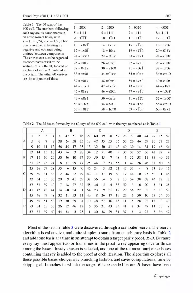
Table 1 The 60 rays of the600-cell. The numbers followingeach ray are its components inan orthonormal basis, withτ = (1 + √

5)/2, κ = 1/τ , a barover a number indicating itsnegative and commas beingomitted between components.The entries can also be regardedas coordinates of 60 of thevertices of a 600-cell, located ona sphere of radius 2 centered atthe origin. The other 60 verticesare the antipodes of these

1 = 2000 2 = 0200 3 = 0020 4 = 0002

5 = 1111 6 = 1111 7 = 1111 8 = 1111

9 = 1111 10 = 1111 11 = 1111 12 = 1111

13 = κ0τ1 14 = 0κ1τ 15 = τ1κ0 16 = 1τ0κ

17 = τκ01 18 = 10κτ 19 = κτ10 20 = 01τκ

21 = 1κτ0 22 = τ01κ 23 = 0τκ1 24 = κ10τ

25 = τ01κ 26 = 0τκ1 27 = 1κτ0 28 = κ10τ

29 = 0κ1τ 30 = τ1κ0 31 = κ0τ1 32 = 1τ0κ

33 = τκ01 34 = 01τκ 35 = 10κτ 36 = κτ10

37 = τ01κ 38 = 0τκ1 39 = 1κτ0 40 = κ10τ

41 = τ1κ0 42 = 0κ1τ 43 = 1τ0κ 44 = κ0τ1

45 = 01τκ 46 = τκ01 47 = κτ10 48 = 10κτ

49 = κ0τ1 50 = 0κ1τ 51 = τ1κ0 52 = 1τ0κ

53 = 10κτ 54 = τκ01 55 = 01τκ 56 = κτ10

57 = τ01κ 58 = 1κτ0 59 = κ10τ 60 = 0τκ1

Table 2 The 75 bases formed by the 60 rays of the 600-cell, with the rays numbered as in Table 1

A B C D E

A′1 2 3 4 31 42 51 16 22 60 39 28 57 23 27 40 44 29 15 52

5 6 7 8 38 24 58 25 18 47 33 55 36 53 20 46 59 26 37 21

9 10 11 12 56 45 17 35 13 32 50 41 43 49 30 14 34 19 48 54

B′13 14 15 16 43 54 3 28 34 12 51 40 9 35 39 52 56 41 27 4

17 18 19 20 50 36 10 37 30 59 45 7 48 5 32 58 11 38 49 33

21 22 23 24 8 57 29 47 25 44 2 53 55 1 42 26 46 31 60 6

C′25 26 27 28 55 6 15 40 46 24 3 52 21 47 51 4 8 53 39 16

29 30 31 32 2 48 22 49 42 11 57 19 60 17 44 10 23 50 1 45

33 34 35 36 20 9 41 59 37 56 14 5 7 13 54 38 58 43 12 18

D′37 38 39 40 7 18 27 52 58 36 15 4 33 59 3 16 20 5 51 28

41 42 43 44 14 60 34 1 54 23 9 31 12 29 56 22 35 2 13 57

45 46 47 48 32 21 53 11 49 8 26 17 19 25 6 50 10 55 24 30

E′49 50 51 52 19 30 39 4 10 48 27 16 45 11 15 28 32 17 3 40

53 54 55 56 26 12 46 13 6 35 21 43 24 41 8 34 47 14 25 9

57 58 59 60 44 33 5 23 1 20 38 29 31 37 18 2 22 7 36 42

Most of the sets in Table 3 were discovered through a computer search. The searchalgorithm is exhaustive, and quite simple: it starts from an arbitrary basis in Table 2and adds one basis at a time in an attempt to obtain a target parity proof, R-B . Becauseevery ray must appear two or four times in the proof, a ray appearing once or thriceamong the bases already chosen is selected, and one of the (at most four) other basescontaining that ray is added to the proof at each iteration. The algorithm explores allthese possible bases-choices in a branching fashion, and saves computational time byskipping all branches in which the target R is exceeded before B bases have been

888 Found Phys (2011) 41: 883–904

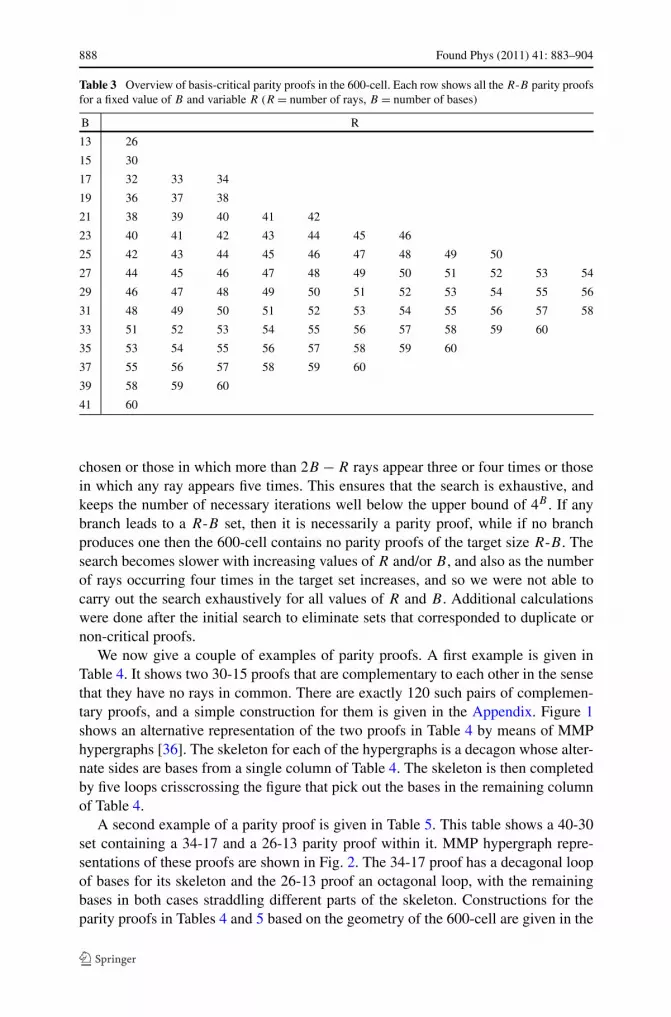
Table 3 Overview of basis-critical parity proofs in the 600-cell. Each row shows all the R-B parity proofsfor a fixed value of B and variable R (R = number of rays, B = number of bases)

B R

13 26

15 30

17 32 33 34

19 36 37 38

21 38 39 40 41 42

23 40 41 42 43 44 45 46

25 42 43 44 45 46 47 48 49 50

27 44 45 46 47 48 49 50 51 52 53 54

29 46 47 48 49 50 51 52 53 54 55 56

31 48 49 50 51 52 53 54 55 56 57 58

33 51 52 53 54 55 56 57 58 59 60

35 53 54 55 56 57 58 59 60

37 55 56 57 58 59 60

39 58 59 60

41 60

chosen or those in which more than 2B − R rays appear three or four times or thosein which any ray appears five times. This ensures that the search is exhaustive, andkeeps the number of necessary iterations well below the upper bound of 4B . If anybranch leads to a R-B set, then it is necessarily a parity proof, while if no branchproduces one then the 600-cell contains no parity proofs of the target size R-B . Thesearch becomes slower with increasing values of R and/or B , and also as the numberof rays occurring four times in the target set increases, and so we were not able tocarry out the search exhaustively for all values of R and B . Additional calculationswere done after the initial search to eliminate sets that corresponded to duplicate ornon-critical proofs.

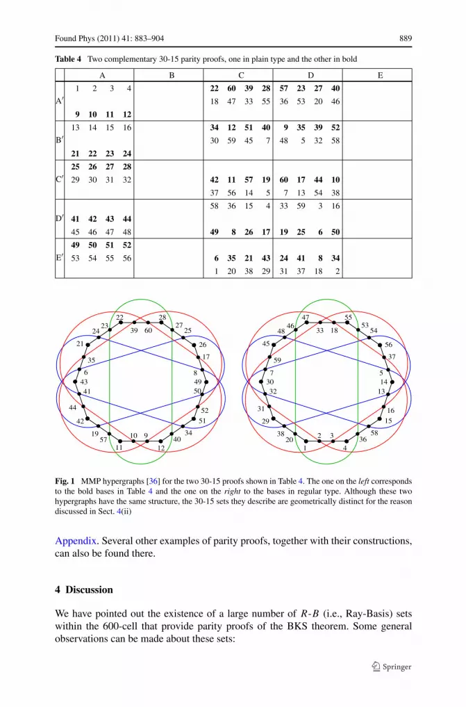
We now give a couple of examples of parity proofs. A first example is given inTable 4. It shows two 30-15 proofs that are complementary to each other in the sensethat they have no rays in common. There are exactly 120 such pairs of complemen-tary proofs, and a simple construction for them is given in the Appendix. Figure 1shows an alternative representation of the two proofs in Table 4 by means of MMPhypergraphs [36]. The skeleton for each of the hypergraphs is a decagon whose alter-nate sides are bases from a single column of Table 4. The skeleton is then completedby five loops crisscrossing the figure that pick out the bases in the remaining columnof Table 4.

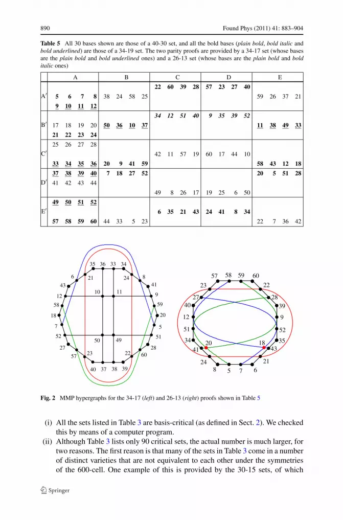
A second example of a parity proof is given in Table 5. This table shows a 40-30set containing a 34-17 and a 26-13 parity proof within it. MMP hypergraph repre-sentations of these proofs are shown in Fig. 2. The 34-17 proof has a decagonal loopof bases for its skeleton and the 26-13 proof an octagonal loop, with the remainingbases in both cases straddling different parts of the skeleton. Constructions for theparity proofs in Tables 4 and 5 based on the geometry of the 600-cell are given in the

Found Phys (2011) 41: 883–904 889

Table 4 Two complementary 30-15 parity proofs, one in plain type and the other in bold

A B C D E

A′1 2 3 4 22 60 39 28 57 23 27 40

18 47 33 55 36 53 20 46

9 10 11 12

B′13 14 15 16 34 12 51 40 9 35 39 52

30 59 45 7 48 5 32 58

21 22 23 24

C′25 26 27 28

29 30 31 32 42 11 57 19 60 17 44 10

37 56 14 5 7 13 54 38

D′58 36 15 4 33 59 3 16

41 42 43 44

45 46 47 48 49 8 26 17 19 25 6 50

E′49 50 51 52

53 54 55 56 6 35 21 43 24 41 8 34

1 20 38 29 31 37 18 2

Fig. 1 MMP hypergraphs [36] for the two 30-15 proofs shown in Table 4. The one on the left correspondsto the bold bases in Table 4 and the one on the right to the bases in regular type. Although these twohypergraphs have the same structure, the 30-15 sets they describe are geometrically distinct for the reasondiscussed in Sect. 4(ii)

Appendix. Several other examples of parity proofs, together with their constructions,can also be found there.

4 Discussion

We have pointed out the existence of a large number of R-B (i.e., Ray-Basis) setswithin the 600-cell that provide parity proofs of the BKS theorem. Some generalobservations can be made about these sets:

890 Found Phys (2011) 41: 883–904

Table 5 All 30 bases shown are those of a 40-30 set, and all the bold bases (plain bold, bold italic andbold underlined) are those of a 34-19 set. The two parity proofs are provided by a 34-17 set (whose basesare the plain bold and bold underlined ones) and a 26-13 set (whose bases are the plain bold and bolditalic ones)

A B C D E

A′22 60 39 28 57 23 27 40

5 6 7 8 38 24 58 25 59 26 37 21

9 10 11 12

B′34 12 51 40 9 35 39 52

17 18 19 20 50 36 10 37 11 38 49 33

21 22 23 24

C′25 26 27 28

42 11 57 19 60 17 44 10

33 34 35 36 20 9 41 59 58 43 12 18

D′37 38 39 40 7 18 27 52 20 5 51 28

41 42 43 44

49 8 26 17 19 25 6 50

E′49 50 51 52

6 35 21 43 24 41 8 34

57 58 59 60 44 33 5 23 22 7 36 42

Fig. 2 MMP hypergraphs for the 34-17 (left) and 26-13 (right) proofs shown in Table 5

(i) All the sets listed in Table 3 are basis-critical (as defined in Sect. 2). We checkedthis by means of a computer program.

(ii) Although Table 3 lists only 90 critical sets, the actual number is much larger, fortwo reasons. The first reason is that many of the sets in Table 3 come in a numberof distinct varieties that are not equivalent to each other under the symmetriesof the 600-cell. One example of this is provided by the 30-15 sets, of which

Found Phys (2011) 41: 883–904 891

there are six different varieties. In addition to the two different varieties shownin Table 4 (which are really different, despite their structurally identical MMPdiagrams), a third type is shown in Table 6 and there are three further types thatwe have not exhibited here. The differences between these types can be broughtout by calculating the inner products of vectors in each of them, whereupon itwill be found that the patterns of the inner products are not the same. Thesedifferences are experimentally significant, because the unitary transformationsneeded to transform the standard basis into the bases of each of these types aredifferent. A few sets, such as the 26-13 set, come in only one variety, but the vastmajority come in a number of different varieties. The second reason is that eachof the geometrically distinct critical sets for a particular set of R and B valueshas many replicas (typically in the thousands) under the symmetries of the 600-cell. The combined effect of both these factors is to increase the total number ofdistinct parity proofs to somewhere in the vicinity of a hundred million.

(iii) We have limited our discussion in this paper only to critical sets that provideparity proofs of the BKS theorem. However the 600-cell has a large numberof critical sets that provide non-parity proofs of the theorem. These proofs arenot as transparent as the parity proofs, but they are just as conclusive. We ex-plored them in part in Ref. [4] and will analyze and generate them extensivelyin Ref. [5].

(iv) The parity proofs of this paper can be used to devise experimental tests of non-contextuality of the sort proposed by Cabello [22, 23]. We recall how sucha test works. For a R-B set yielding a parity proof, let Ai

j = 2|ψij 〉〈ψi

j | − 1

(i = 1, . . . ,B, j = 1, . . . ,4), where |ψij 〉 is the normalized column vector corre-

sponding to the j -th ray of the i-th basis (note that two or more of the ψij with

different values of i and/or j can be identical because the same ray generallyoccurs in several different bases). Each observable Ai

j has only the eigenvalues+1 or −1. Cabello’s argument implies that any noncontextual hidden variablestheory (NHVT) obeys the inequality

B∑

i=1

−〈Ai1A

i2A

i3A

i4〉 ≤ M, (1)

where the averages 〈〉 above are to be taken over an ensemble of runs and M isan upper bound. Quantum mechanics predicts that (1) holds as an equality withM = B , but NHVTs predict (see next paragraph) that the above inequality holdswith M equal to B − 2 at most. This is the contradiction between a NHVT andquantum mechanics that can be put to experimental test.

We now give the argument leading to the maximum value of M , namely,B − 2. According to a NHVT, each observable Ai

j has the definite value of +1or −1 in any quantum state, independent of the other observables with whichit is measured. Consider the expression on the left side of (1), but without theaveraging 〈〉 over many runs, and denote it by F . The maximum value of F inany run is B , and it is achieved when each term in it has the value of +1. Letus see how the values of the various Ai

j can be chosen so that this maximum is

892 Found Phys (2011) 41: 883–904

achieved. Clearly, one or three of the Aij ’s in each term of F must be equal to

−1 for this to happen. Let the number of terms with one Aij equal to −1 be n

and the number with three Aij ’s equal to −1 be m. Then, if we choose the values

of the Aij ’s in such a way that n + m = B , we can guarantee that F = B . But

an obstacle looms that prevents us from reaching this goal. The total number of−1’s occurring over all the bases is n + 3m = B + 2m (since n + m = B). Thedifficulty now is that B + 2m is required to be both odd and even (odd becauseB is odd, and even because the number of −1’s in all the bases is required tobe even for the parity proof to be valid). This contradiction shows that a NHVTtheory cannot make the value of F equal to B . The best it can do is to make allbut one of the terms in F equal to +1, and this limits the maximum value of F

to B − 2. Averaging the value of F over a large number of runs could make thequantity on the left side of (1) dip below the upper bound of B − 2, according toa NHVT.

For any basis-critical parity proof, quantum mechanics predicts that (1) holdsas an equality with M = B whereas a NHVT predicts that M = B − 2 (sincevalue assignments can always be found that make B − 1 of the terms on the leftof (1) equal to 1 and one term equal to −1). A 18-9 parity proof thus leads to theratio of 7/9 for the bounds due to NHVTs and quantum mechanics. This boundcan be improved slightly by considering all 1800 26-13 parity proofs within the60-75 set. Of the 75 terms on the left side of (1), at least 9 must then contribute−1 to the sum, causing the previous ratio to dip to 57/75, which is very slightlyless than 7/9. Whether a further improvement can be effected by simultaneousconsideration of a larger number of parity proofs is an open question.

It is worth stressing that the contradiction we have demonstrated betweenNHVTs and quantum mechanics generalizes in a straightforward manner to anyparity proof in any even dimension greater than or equal to 4. Parity proofs of thetype we are considering are not possible in odd dimensions, so a similar conflictcannot be demonstrated in this case.

(v) Any parity proof of the BKS theorem (or even a non-parity proof) can be turnedinto a scheme for quantum key distribution, as pointed out in [33]. The ideais simple: since there are no hidden variables that model the observables in aBKS proof, there is no data in the transmitted particles to be stolen while thekey is being established; the key comes into being only after sender and receiverexchange messages to determine the cases in which they used the same bases toencode and decode their particles. The preferred bases in such a scheme, whenthey exist, are a maximal set of mutually unbiased bases. A maximal set of fivemutually unbiased bases does indeed exist in four dimensions, and has beenproposed for use in key distribution schemes based on four-state systems [37].However, any set of bases leading to a BKS proof, such as the ones in this paper,can also be used. They may not be as efficient as schemes based on mutuallyunbiased bases, but they may be advantageous in some situations and wouldtherefore seem to be worth exploring further.

Found Phys (2011) 41: 883–904 893

Appendix A

The purpose of this Appendix is to show how special geometrical features of the 600-cell can be exploited to give simple rules for generating many of the parity proofs inTable 3. We first review some basic geometrical facts about the 600-cell and thenshow how they can be used to arrive at the rules. Readers wanting a more detailed ac-count of the geometrical properties of the 600-cell can consult the classic monographby Coxeter [38].

The 600-cell is a regular polytope with 120 vertices distributed symmetrically onthe surface of a four-dimensional sphere. The vertices come in antipodal pairs, andthe 60 rays are the unoriented directions passing through antipodal pairs of vertices.If the vertices are taken to lie on a sphere of radius 2 centered at the origin, thenthe coordinates of 60 of the vertices can be chosen as in Table 1 and the remainingvertices are the antipodes of these.

A.1 Facets of the 600-cell

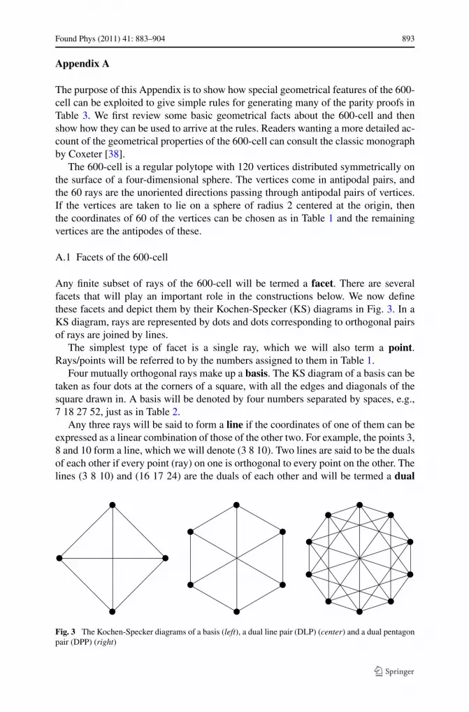
Any finite subset of rays of the 600-cell will be termed a facet. There are severalfacets that will play an important role in the constructions below. We now definethese facets and depict them by their Kochen-Specker (KS) diagrams in Fig. 3. In aKS diagram, rays are represented by dots and dots corresponding to orthogonal pairsof rays are joined by lines.

The simplest type of facet is a single ray, which we will also term a point.Rays/points will be referred to by the numbers assigned to them in Table 1.

Four mutually orthogonal rays make up a basis. The KS diagram of a basis can betaken as four dots at the corners of a square, with all the edges and diagonals of thesquare drawn in. A basis will be denoted by four numbers separated by spaces, e.g.,7 18 27 52, just as in Table 2.

Any three rays will be said to form a line if the coordinates of one of them can beexpressed as a linear combination of those of the other two. For example, the points 3,8 and 10 form a line, which we will denote (3 8 10). Two lines are said to be the dualsof each other if every point (ray) on one is orthogonal to every point on the other. Thelines (3 8 10) and (16 17 24) are the duals of each other and will be termed a dual

Fig. 3 The Kochen-Specker diagrams of a basis (left), a dual line pair (DLP) (center) and a dual pentagonpair (DPP) (right)

894 Found Phys (2011) 41: 883–904

line pair (DLP) and denoted (3 8 10) + (16 17 24). The KS diagram of a DLP takeson a simple form if the points of the dual lines are arranged at the alternate vertices ofa hexagon; then the orthogonalities between the rays are represented by the six edgesand three diameters of the hexagon. The geometry of the 600-cell is such that any setof six points having this KS diagram represents a dual line pair; the requirement thatthe points at the alternate vertices satisfy the conditions for a line need not be addedbecause it turns out to be satisfied automatically.

A pentagon is any set of five rays with the property that five pairs among themhave an absolute inner product of τ and the remaining five an absolute inner prod-uct of κ . The points 1, 15, 30, 47 and 56 form a pentagon, which we will denote(1 15 30 47 56). Two pentagons will be said to be the duals of one another if everypoint of one is orthogonal to every point of the other. The pentagons (1 15 30 47 56)and (4 14 29 45 55) are the duals of each other and will be said to be a dual pen-tagon pair (DPP). A symbol for a DPP will be introduced in the next subsection.If the points corresponding to a dual pair of pentagons are arranged at the alternatevertices of a decagon, then the KS diagram of the DPP takes on a very simple form:it consists of the ten edges and five diameters of the decagon, together with ten of itsdiagonals (see Fig. 3). Again, it turns out that any set of ten points possessing this KSdiagram constitutes a DPP, with the conditions for the points at alternate vertices toform pentagons being automatically satisfied.

The most complex facet of interest to us is a Reye’s configuration (RC), which isa set of 12 “points” and 16 “lines” with the property that three “points” lie on every“line” and four “lines” pass through every “point”. If the terms “points” and “lines”in this definition are taken to be identical with the points and lines defined above, itis easy to check that points 1 through 12 form a RC with the 16 lines being given by(1 5 9), (1 6 10), (1 7 11), (1 8 12), (2 5 10), (2 6 9), (2 7 12), (2 8 11), (3 5 11),(3 6 12), (3 7 9), (3 8 10), (4 5 12), (4 6 11), (4 7 10) and (4 8 9). An equivalentdefinition of a RC is that it consists of the rays in three mutually unbiased bases (i.e.bases with the property that the magnitude of the inner product of any normalized rayof one with any normalized ray of the other is always the same). In the case of the600-cell this latter definition guarantees that the 12 rays in the three bases form 16lines, with one point of each line coming from each of the three bases. In the exampleof the RC just given, the three (mutually unbiased) bases are 1 2 3 4, 5 6 7 8 and 9 1011 12.

The above discussion has been carried out in projective or ray space. However,many of the facets correspond to familiar figures in four-dimensional Euclidean spaceif one recalls that each point in projective space corresponds to a pair of mutuallyinverse points in Euclidean space. Then a basis corresponds to a 16-cell (or crosspolytope), a pair of mutually unbiased bases to a 8-cell (or hypercube), and threemutually unbiased bases (or a RC) to a 24-cell. These three figures are all convexregular polytopes in four dimensions (just like the 600-cell), and their bounding cellsconsist of 16 tetrahedra, 8 cubes and 24 octahedra, respectively.

A.2 Tilings of the 600-cell by Its Facets

A particular type of facet (e.g. bases) will be said to tile the 600-cell if the union ofseveral mutually disjoint specimens of that type yields all 60 rays of the 600-cell. The

Found Phys (2011) 41: 883–904 895

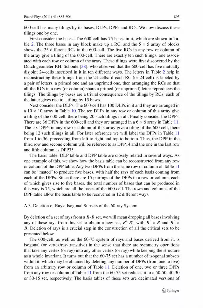
600-cell has many tilings by its bases, DLPs, DPPs and RCs. We now discuss thesetilings one by one.

First consider the bases. The 600-cell has 75 bases in it, which are shown in Ta-ble 2. The three bases in any block make up a RC, and the 5 × 5 array of blocksshows the 25 different RCs in the 600-cell. The five RCs in any row or column ofthe array give a tiling of the 600-cell. There are exactly ten such tilings, one associ-ated with each row or column of the array. These tilings were first discovered by theDutch geometer P.H. Schoute [38], who observed that the 600-cell has five mutuallydisjoint 24-cells inscribed in it in ten different ways. The letters in Table 2 help inreconstructing these tilings from the 24-cells: if each RC (or 24-cell) is labeled bya pair of letters, a primed one and an unprimed one, then arranging the RCs so thatall the RCs in a row (or column) share a primed (or unprimed) letter reproduces thetilings. The tilings by bases are a trivial consequence of the tilings by RCs: each ofthe latter gives rise to a tiling by 15 bases.

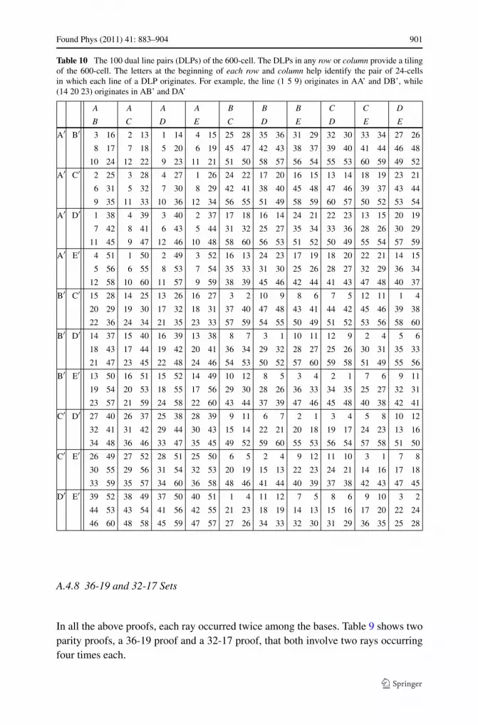
Next consider the DLPs. The 600-cell has 100 DLPs in it and they are arranged ina 10 × 10 array in Table 10. The ten DLPs in any row or column of this array givea tiling of the 600-cell, there being 20 such tilings in all. Finally consider the DPPs.There are 36 DPPs in the 600-cell and they are arranged in a 6 × 6 array in Table 11.The six DPPs in any row or column of this array give a tiling of the 600-cell, therebeing 12 such tilings in all. For later reference we will label the DPPs in Table 11from 1 to 36, proceeding from left to right and top to bottom. Thus, the DPP in thethird row and second column will be referred to as DPP14 and the one in the last rowand fifth column as DPP35.

The basis table, DLP table and DPP table are closely related in several ways. Asone example of this, we show how the basis table can be reconstructed from any rowor column of the DPP table. Any two DPPs from the same row or column of Table 11can be “mated” to produce five bases, with half the rays of each basis coming fromeach of the DPPs. Since there are 15 pairings of the DPPs in a row or column, eachof which gives rise to five bases, the total number of bases that can be produced inthis way is 75, which are all the bases of the 600-cell. The rows and columns of theDPP table allow the basis table to be recovered in 12 different ways.

A.3 Deletion of Rays; Isogonal Subsets of the 60-ray System

By deletion of a set of rays from a R-B set, we will mean dropping all bases involvingany of these rays from this set to obtain a new set, R′-B ′, with R′ < R and B ′ <

B . Deletion of rays is a crucial step in the construction of all the critical sets to bepresented below.

The 600-cell, as well as the 60-75 system of rays and bases derived from it, isisogonal (or vertex/ray-transitive) in the sense that there are symmetry operationsthat take any vertex (or ray) into any other vertex (or ray) while keeping the structureas a whole invariant. It turns out that the 60-75 set has a number of isogonal subsetswithin it, which may be obtained by deleting any number of DPPs (from one to five)from an arbitrary row or column of Table 11. Deletion of one, two or three DPPsfrom any row or column of Table 11 from the 60-75 set reduces it to a 50-50, 40-30or 30-15 set, respectively. The basis tables of these sets are decimated versions of

896 Found Phys (2011) 41: 883–904

Table 2, with 25, 35 or 45 bases dropped, respectively. The number of different 50-50, 40-30 and 30-15 sets is 36, 180 and 240, respectively. These smaller isogonal setsare interesting because they each contain a large number of critical sets and can besearched far more easily for these sets than the full 60-75 set. We will ignore the setsobtained by deleting four or more DPPs from a row or column of Table 11 becausethey do not contain any critical sets.

A.4 Constructions for some Critical Sets

We now use the ideas and tools developed in the previous subsections to give con-structions for some of the parity proofs in Table 3.

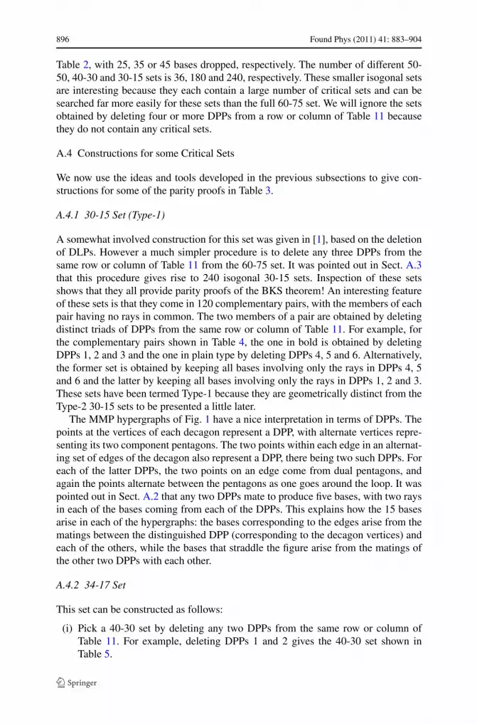
A.4.1 30-15 Set (Type-1)

A somewhat involved construction for this set was given in [1], based on the deletionof DLPs. However a much simpler procedure is to delete any three DPPs from thesame row or column of Table 11 from the 60-75 set. It was pointed out in Sect. A.3that this procedure gives rise to 240 isogonal 30-15 sets. Inspection of these setsshows that they all provide parity proofs of the BKS theorem! An interesting featureof these sets is that they come in 120 complementary pairs, with the members of eachpair having no rays in common. The two members of a pair are obtained by deletingdistinct triads of DPPs from the same row or column of Table 11. For example, forthe complementary pairs shown in Table 4, the one in bold is obtained by deletingDPPs 1, 2 and 3 and the one in plain type by deleting DPPs 4, 5 and 6. Alternatively,the former set is obtained by keeping all bases involving only the rays in DPPs 4, 5and 6 and the latter by keeping all bases involving only the rays in DPPs 1, 2 and 3.These sets have been termed Type-1 because they are geometrically distinct from theType-2 30-15 sets to be presented a little later.

The MMP hypergraphs of Fig. 1 have a nice interpretation in terms of DPPs. Thepoints at the vertices of each decagon represent a DPP, with alternate vertices repre-senting its two component pentagons. The two points within each edge in an alternat-ing set of edges of the decagon also represent a DPP, there being two such DPPs. Foreach of the latter DPPs, the two points on an edge come from dual pentagons, andagain the points alternate between the pentagons as one goes around the loop. It waspointed out in Sect. A.2 that any two DPPs mate to produce five bases, with two raysin each of the bases coming from each of the DPPs. This explains how the 15 basesarise in each of the hypergraphs: the bases corresponding to the edges arise from thematings between the distinguished DPP (corresponding to the decagon vertices) andeach of the others, while the bases that straddle the figure arise from the matings ofthe other two DPPs with each other.

A.4.2 34-17 Set

This set can be constructed as follows:

(i) Pick a 40-30 set by deleting any two DPPs from the same row or column ofTable 11. For example, deleting DPPs 1 and 2 gives the 40-30 set shown inTable 5.

Found Phys (2011) 41: 883–904 897

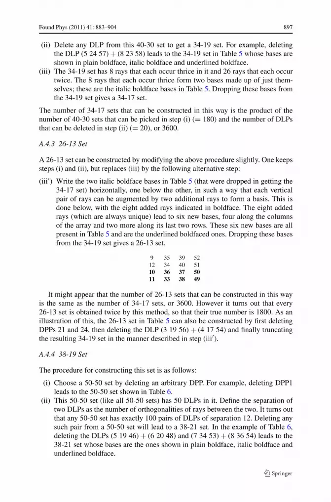
(ii) Delete any DLP from this 40-30 set to get a 34-19 set. For example, deletingthe DLP (5 24 57) + (8 23 58) leads to the 34-19 set in Table 5 whose bases areshown in plain boldface, italic boldface and underlined boldface.

(iii) The 34-19 set has 8 rays that each occur thrice in it and 26 rays that each occurtwice. The 8 rays that each occur thrice form two bases made up of just them-selves; these are the italic boldface bases in Table 5. Dropping these bases fromthe 34-19 set gives a 34-17 set.

The number of 34-17 sets that can be constructed in this way is the product of thenumber of 40-30 sets that can be picked in step (i) (= 180) and the number of DLPsthat can be deleted in step (ii) (= 20), or 3600.

A.4.3 26-13 Set

A 26-13 set can be constructed by modifying the above procedure slightly. One keepssteps (i) and (ii), but replaces (iii) by the following alternative step:

(iii′) Write the two italic boldface bases in Table 5 (that were dropped in getting the34-17 set) horizontally, one below the other, in such a way that each verticalpair of rays can be augmented by two additional rays to form a basis. This isdone below, with the eight added rays indicated in boldface. The eight addedrays (which are always unique) lead to six new bases, four along the columnsof the array and two more along its last two rows. These six new bases are allpresent in Table 5 and are the underlined boldfaced ones. Dropping these basesfrom the 34-19 set gives a 26-13 set.

9 35 39 5212 34 40 5110 36 37 5011 33 38 49

It might appear that the number of 26-13 sets that can be constructed in this wayis the same as the number of 34-17 sets, or 3600. However it turns out that every26-13 set is obtained twice by this method, so that their true number is 1800. As anillustration of this, the 26-13 set in Table 5 can also be constructed by first deletingDPPs 21 and 24, then deleting the DLP (3 19 56) + (4 17 54) and finally truncatingthe resulting 34-19 set in the manner described in step (iii′).

A.4.4 38-19 Set

The procedure for constructing this set is as follows:

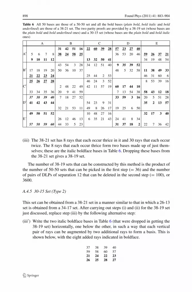
(i) Choose a 50-50 set by deleting an arbitrary DPP. For example, deleting DPP1leads to the 50-50 set shown in Table 6.

(ii) This 50-50 set (like all 50-50 sets) has 50 DLPs in it. Define the separation oftwo DLPs as the number of orthogonalities of rays between the two. It turns outthat any 50-50 set has exactly 100 pairs of DLPs of separation 12. Deleting anysuch pair from a 50-50 set will lead to a 38-21 set. In the example of Table 6,deleting the DLPs (5 19 46) + (6 20 48) and (7 34 53) + (8 36 54) leads to the38-21 set whose bases are the ones shown in plain boldface, italic boldface andunderlined boldface.

898 Found Phys (2011) 41: 883–904

Table 6 All 50 bases are those of a 50-50 set and all the bold bases (plain bold, bold italic and boldunderlined) are those of a 38-21 set. The two parity proofs are provided by a 38-19 set (whose bases arethe plain bold and bold underlined ones) and a 30-15 set (whose bases are the plain bold and bold italicones)

A B C D E

A′31 42 51 16 22 60 39 28 57 23 27 40

5 6 7 8 38 24 58 25 36 53 20 46 59 26 37 21

9 10 11 12 13 32 50 41 34 19 48 54

B′43 54 3 28 34 12 51 40 9 35 39 52

17 18 19 20 50 36 10 37 48 5 32 58 11 38 49 33

21 22 23 24 25 44 2 53 46 31 60 6

C′25 26 27 28 46 24 3 52 8 53 39 16

2 48 22 49 42 11 57 19 60 17 44 10

33 34 35 36 20 9 41 59 7 13 54 38 58 43 12 18

D′37 38 39 40 7 18 27 52 33 59 3 16 20 5 51 28

41 42 43 44 54 23 9 31 35 2 13 57

32 21 53 11 49 8 26 17 19 25 6 50

E´

49 50 51 52 10 48 27 16 32 17 3 40

26 12 46 13 6 35 21 43 24 41 8 34

57 58 59 60 44 33 5 23 31 37 18 2 22 7 36 42

(iii) The 38-21 set has 8 rays that each occur thrice in it and 30 rays that each occurtwice. The 8 rays that each occur thrice form two bases made up of just them-selves; these are the italic boldface bases in Table 6. Dropping these bases fromthe 38-21 set gives a 38-19 set.

The number of 38-19 sets that can be constructed by this method is the product ofthe number of 50-50 sets that can be picked in the first step (= 36) and the numberof pairs of DLPs of separation 12 that can be deleted in the second step (= 100), or3600.

A.4.5 30-15 Set (Type 2)

This set can be obtained from a 38-21 set in a manner similar to that in which a 26-13set is obtained from a 34-17 set. After carrying out steps (i) and (ii) for the 38-19 setjust discussed, replace step (iii) by the following alternative step:

(iii′) Write the two italic boldface bases in Table 6 (that were dropped in getting the38-19 set) horizontally, one below the other, in such a way that each verticalpair of rays can be augmented by two additional rays to form a basis. This isshown below, with the eight added rays indicated in boldface.

37 38 39 4059 58 60 5721 24 22 2326 25 28 27

Found Phys (2011) 41: 883–904 899

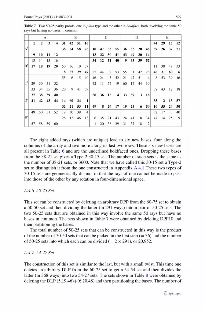
Table 7 Two 50-25 parity proofs, one in plain type and the other in boldface, both involving the same 50rays but having no bases in common

A B C D E

A′1 2 3 4 31 42 51 16 44 29 15 52

38 24 58 25 18 47 33 55 36 53 20 46 59 26 37 21

9 10 11 12 13 32 50 41 43 49 30 14

B′13 14 15 16 34 12 51 40 9 35 39 52

17 18 19 20 50 36 10 37 11 38 49 33

8 57 29 47 25 44 2 53 55 1 42 26 46 31 60 6

C′55 6 15 40 46 24 3 52 21 47 51 4 8 53 39 16

29 30 31 32 42 11 57 19 60 17 44 10

33 34 35 36 20 9 41 59 58 43 12 18

D′37 38 39 40 58 36 15 4 33 59 3 16

41 42 43 44 14 60 34 1 35 2 13 57

32 21 53 11 49 8 26 17 19 25 6 50 10 55 24 30

E′49 50 51 52 19 30 39 4 32 17 3 40

26 12 46 13 6 35 21 43 24 41 8 34 47 14 25 9

57 58 59 60 1 20 38 29 31 37 18 2

The eight added rays (which are unique) lead to six new bases, four along thecolumns of the array and two more along its last two rows. These six new bases areall present in Table 6 and are the underlined boldfaced ones. Dropping these basesfrom the 38-21 set gives a Type-2 30-15 set. The number of such sets is the same asthe number of 38-21 sets, or 3600. Note that we have called this 30-15 set a Type-2set to distinguish it from the one constructed in Appendix A.4.1 These two types of30-15 sets are geometrically distinct in that the rays of one cannot be made to passinto those of the other by any rotation in four-dimensional space.

A.4.6 50-25 Set

This set can be constructed by deleting an arbitrary DPP from the 60-75 set to obtaina 50-50 set and then dividing the latter (in 291 ways) into a pair of 50-25 sets. Thetwo 50-25 sets that are obtained in this way involve the same 50 rays but have nobases in common. The sets shown in Table 7 were obtained by deleting DPP10 andthen partitioning the bases.

The total number of 50-25 sets that can be constructed in this way is the productof the number of 50-50 sets that can be picked in the first step (= 36) and the numberof 50-25 sets into which each can be divided (= 2 × 291), or 20,952.

A.4.7 54-27 Set

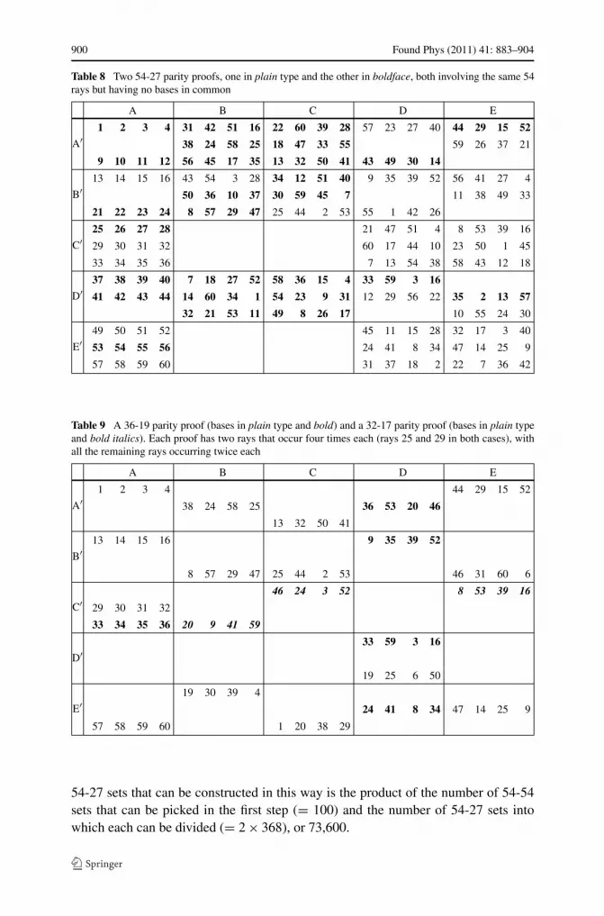
The construction of this set is similar to the last, but with a small twist. This time onedeletes an arbitrary DLP from the 60-75 set to get a 54-54 set and then divides thelatter (in 368 ways) into two 54-27 sets. The sets shown in Table 8 were obtained bydeleting the DLP (5,19,46)+(6,20,48) and then partitioning the bases. The number of

900 Found Phys (2011) 41: 883–904

Table 8 Two 54-27 parity proofs, one in plain type and the other in boldface, both involving the same 54rays but having no bases in common

A B C D E

A′1 2 3 4 31 42 51 16 22 60 39 28 57 23 27 40 44 29 15 52

38 24 58 25 18 47 33 55 59 26 37 21

9 10 11 12 56 45 17 35 13 32 50 41 43 49 30 14

B′13 14 15 16 43 54 3 28 34 12 51 40 9 35 39 52 56 41 27 4

50 36 10 37 30 59 45 7 11 38 49 33

21 22 23 24 8 57 29 47 25 44 2 53 55 1 42 26

C′25 26 27 28 21 47 51 4 8 53 39 16

29 30 31 32 60 17 44 10 23 50 1 45

33 34 35 36 7 13 54 38 58 43 12 18

D′37 38 39 40 7 18 27 52 58 36 15 4 33 59 3 16

41 42 43 44 14 60 34 1 54 23 9 31 12 29 56 22 35 2 13 57

32 21 53 11 49 8 26 17 10 55 24 30

E′49 50 51 52 45 11 15 28 32 17 3 40

53 54 55 56 24 41 8 34 47 14 25 9

57 58 59 60 31 37 18 2 22 7 36 42

Table 9 A 36-19 parity proof (bases in plain type and bold) and a 32-17 parity proof (bases in plain typeand bold italics). Each proof has two rays that occur four times each (rays 25 and 29 in both cases), withall the remaining rays occurring twice each

A B C D E

A′1 2 3 4 44 29 15 52

38 24 58 25 36 53 20 46

13 32 50 41

B′13 14 15 16 9 35 39 52

8 57 29 47 25 44 2 53 46 31 60 6

C′46 24 3 52 8 53 39 16

29 30 31 32

33 34 35 36 20 9 41 59

D′33 59 3 16

19 25 6 50

E′19 30 39 4

24 41 8 34 47 14 25 9

57 58 59 60 1 20 38 29

54-27 sets that can be constructed in this way is the product of the number of 54-54sets that can be picked in the first step (= 100) and the number of 54-27 sets intowhich each can be divided (= 2 × 368), or 73,600.

Found Phys (2011) 41: 883–904 901

Table 10 The 100 dual line pairs (DLPs) of the 600-cell. The DLPs in any row or column provide a tilingof the 600-cell. The letters at the beginning of each row and column help identify the pair of 24-cellsin which each line of a DLP originates. For example, the line (1 5 9) originates in AA’ and DB’, while(14 20 23) originates in AB’ and DA’

A A A A B B B C C D

B C D E C D E D E E

A′ B′ 3 16 2 13 1 14 4 15 25 28 35 36 31 29 32 30 33 34 27 26

8 17 7 18 5 20 6 19 45 47 42 43 38 37 39 40 41 44 46 48

10 24 12 22 9 23 11 21 51 50 58 57 56 54 55 53 60 59 49 52

A′ C′ 2 25 3 28 4 27 1 26 24 22 17 20 16 15 13 14 18 19 23 21

6 31 5 32 7 30 8 29 42 41 38 40 45 48 47 46 39 37 43 44

9 35 11 33 10 36 12 34 56 55 51 49 58 59 60 57 50 52 53 54

A′ D′ 1 38 4 39 3 40 2 37 17 18 16 14 24 21 22 23 13 15 20 19

7 42 8 41 6 43 5 44 31 32 25 27 35 34 33 36 28 26 30 29

11 45 9 47 12 46 10 48 58 60 56 53 51 52 50 49 55 54 57 59

A′ E′ 4 51 1 50 2 49 3 52 16 13 24 23 17 19 18 20 22 21 14 15

5 56 6 55 8 53 7 54 35 33 31 30 25 26 28 27 32 29 36 34

12 58 10 60 11 57 9 59 38 39 45 46 42 44 41 43 47 48 40 37

B′ C′ 15 28 14 25 13 26 16 27 3 2 10 9 8 6 7 5 12 11 1 4

20 29 19 30 17 32 18 31 37 40 47 48 43 41 44 42 45 46 39 38

22 36 24 34 21 35 23 33 57 59 54 55 50 49 51 52 53 56 58 60

B′ D′ 14 37 15 40 16 39 13 38 8 7 3 1 10 11 12 9 2 4 5 6

18 43 17 44 19 42 20 41 36 34 29 32 28 27 25 26 30 31 35 33

21 47 23 45 22 48 24 46 54 53 50 52 57 60 59 58 51 49 55 56

B′ E′ 13 50 16 51 15 52 14 49 10 12 8 5 3 4 2 1 7 6 9 11

19 54 20 53 18 55 17 56 29 30 28 26 36 33 34 35 25 27 32 31

23 57 21 59 24 58 22 60 43 44 37 39 47 46 45 48 40 38 42 41

C′ D′ 27 40 26 37 25 38 28 39 9 11 6 7 2 1 3 4 5 8 10 12

32 41 31 42 29 44 30 43 15 14 22 21 20 18 19 17 24 23 13 16

34 48 36 46 33 47 35 45 49 52 59 60 55 53 56 54 57 58 51 50

C′ E′ 26 49 27 52 28 51 25 50 6 5 2 4 9 12 11 10 3 1 7 8

30 55 29 56 31 54 32 53 20 19 15 13 22 23 24 21 14 16 17 18

33 59 35 57 34 60 36 58 48 46 41 44 40 39 37 38 42 43 47 45

D′ E′ 39 52 38 49 37 50 40 51 1 4 11 12 7 5 8 6 9 10 3 2

44 53 43 54 41 56 42 55 21 23 18 19 14 13 15 16 17 20 22 24

46 60 48 58 45 59 47 57 27 26 34 33 32 30 31 29 36 35 25 28

A.4.8 36-19 and 32-17 Sets

In all the above proofs, each ray occurred twice among the bases. Table 9 shows twoparity proofs, a 36-19 proof and a 32-17 proof, that both involve two rays occurringfour times each.

902 Found Phys (2011) 41: 883–904

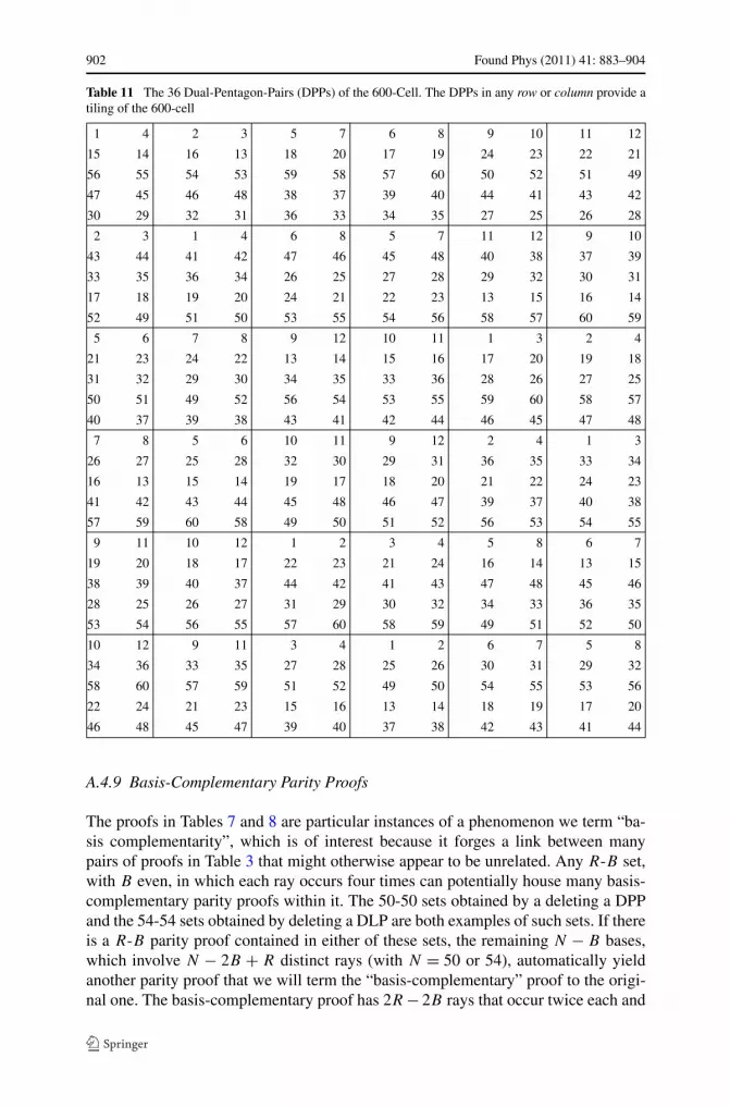
Table 11 The 36 Dual-Pentagon-Pairs (DPPs) of the 600-Cell. The DPPs in any row or column provide atiling of the 600-cell

1 4 2 3 5 7 6 8 9 10 11 12

15 14 16 13 18 20 17 19 24 23 22 21

56 55 54 53 59 58 57 60 50 52 51 49

47 45 46 48 38 37 39 40 44 41 43 42

30 29 32 31 36 33 34 35 27 25 26 28

2 3 1 4 6 8 5 7 11 12 9 10

43 44 41 42 47 46 45 48 40 38 37 39

33 35 36 34 26 25 27 28 29 32 30 31

17 18 19 20 24 21 22 23 13 15 16 14

52 49 51 50 53 55 54 56 58 57 60 59

5 6 7 8 9 12 10 11 1 3 2 4

21 23 24 22 13 14 15 16 17 20 19 18

31 32 29 30 34 35 33 36 28 26 27 25

50 51 49 52 56 54 53 55 59 60 58 57

40 37 39 38 43 41 42 44 46 45 47 48

7 8 5 6 10 11 9 12 2 4 1 3

26 27 25 28 32 30 29 31 36 35 33 34

16 13 15 14 19 17 18 20 21 22 24 23

41 42 43 44 45 48 46 47 39 37 40 38

57 59 60 58 49 50 51 52 56 53 54 55

9 11 10 12 1 2 3 4 5 8 6 7

19 20 18 17 22 23 21 24 16 14 13 15

38 39 40 37 44 42 41 43 47 48 45 46

28 25 26 27 31 29 30 32 34 33 36 35

53 54 56 55 57 60 58 59 49 51 52 50

10 12 9 11 3 4 1 2 6 7 5 8

34 36 33 35 27 28 25 26 30 31 29 32

58 60 57 59 51 52 49 50 54 55 53 56

22 24 21 23 15 16 13 14 18 19 17 20

46 48 45 47 39 40 37 38 42 43 41 44

A.4.9 Basis-Complementary Parity Proofs

The proofs in Tables 7 and 8 are particular instances of a phenomenon we term “ba-sis complementarity”, which is of interest because it forges a link between manypairs of proofs in Table 3 that might otherwise appear to be unrelated. Any R-B set,with B even, in which each ray occurs four times can potentially house many basis-complementary parity proofs within it. The 50-50 sets obtained by a deleting a DPPand the 54-54 sets obtained by deleting a DLP are both examples of such sets. If thereis a R-B parity proof contained in either of these sets, the remaining N − B bases,which involve N − 2B + R distinct rays (with N = 50 or 54), automatically yieldanother parity proof that we will term the “basis-complementary” proof to the origi-nal one. The basis-complementary proof has 2R − 2B rays that occur twice each and

Found Phys (2011) 41: 883–904 903

N −R rays that occur four times each. In general the proof complementary to a givenproof might not be basis-critical, in which case it would be left out of Table 3. Onlyif both members of a basis-complementary pair are basis-critical would they bothbe included in Table 3. Three examples of basis-complementary (and basis-critical)parity proofs within a 50-50 set are 36-19/48-31, 39-21/47-29, and 42-21/50-29 andthree examples within a 54-54 set are 37-19/53-35, 41-21/53-33 and 44-23/52-31.We hope to make several examples of such proofs available on the interactive web-site (see footnote 1).

Acknowledgements One of us (M. P.) would like to thank his host Hossein Sadeghpour at ITAMP. M.P.’s stay at ITAMP was Supported by the US National Science Foundation through a grant for the Institutefor Theoretical Atomic, Molecular, and Optical Physics (ITAMP) at Harvard University and SmithsonianAstrophysical Observatory and Ministry of Science, Education, and Sport of Croatia through the projectNo. 082-0982562-3160. M. P. carried out his part of the computation on the cluster Isabella of the Univer-sity Computing Centre of the University of Zagreb and on the Croatian National Grid Infrastructure.

References

1. Waegell, M., Aravind, P.K.: J. Phys. A 43, 105304 (2010)2. Bell, J.S.: Rev. Mod. Phys. 38, 447 (1966). Reprinted in J.S. Bell, Speakable and Unspeakable in

Quantum Mechanics. Cambridge University Press, Cambridge (1987)3. Kochen, S., Specker, E.P.: J. Math. Mech. 17, 59 (1967)4. Pavicic, M., Megill, N.D., Aravind, P.K.: arXiv:1004.1433 (2010)5. Pavicic, M., Megill, N.D., Aravind, P.K., Waegell, M.: Unpublished (2010)6. Peres, A.: J. Phys. A 24, L175 (1991)7. Kochen, S., Conway, J.H.: Quantum Theory: Concepts and Methods. Kluwer Academic, Dordrecht

(1993). As quoted in A. Peres8. Bub, J.: Found. Phys. 26, 787 (1996)9. Bub, J.: Interpreting the Quantum World. Cambridge University Press, Cambridge (1997), Chap. 3

10. Penrose, R.: In: Ellis, J., Amati, D. (eds.) Quantum Reflections, pp. 1–27. Cambridge University Press,Cambridge (2000)

11. Cabello, A., Estebaranz, J.M., García-Alcaine, G.: Phys. Lett. A 212, 183 (1996)12. Kernaghan, M.: J. Phys. A 27, L829 (1994)13. Zimba, J., Penrose, R.: Stud. Hist. Philos. Sci. 24, 697 (1993)14. Penrose, R.: Shadows of the Mind. Oxford University Press, Oxford (1994), Chap. 515. Pavicic, M., Merlet, J.P., McKay, B.D., Megill, N.D.: J. Phys. A 38, 1577 (2005)16. Pavicic, M., Merlet, J.P., Megill, N.D.: The French National Institute for Research in Computer Sci-

ence and Control Research Reports RR-5388 (2004)17. Pavicic, M., Megill, N.D., Merlet, J.P.: Phys. Lett. A 374, 2122 (2010)18. Kernaghan, M., Peres, A.: Phys. Lett. A 198, 1 (1995)19. Conway, J.H., Kochen, S.B.: In: Bertlmann, R.A., Zeilinger, A. (eds.) Quantum [Un]speakables: From

Bell to Quantum Information, pp. 257–269. Springer, Berlin (2002)20. DiVincenzo, D., Peres, A.: Phys. Rev. A 55, 4089 (1997)21. Ruuge, A.E., Van Oystaeyen, F.: J. Math. Phys. 46, 052109 (2005)22. Cabello, A.: Phys. Rev. Lett. 101, 210401 (2008)23. Badziag, P., Bengtsson, I., Cabello, A., Pitowsky, I.: Phys. Rev. Lett. 103, 050401 (2009)24. Kirchmair, G., Zähringer, F., Gerritsma, R., Kleinmann, M., Gühne, O., Cabello, A., Blatt, R., Roos,

C.F.: Nature 460, 494 (2009)25. Bartosik, H., Klep, J., Schmitzer, C., Sponar, S., Cabello, A., Rauch, H., Hasegawa, Y.: Phys. Rev.

Lett. 103, 040403 (2009)26. Amselem, E., Rådmark, M., Bourennane, M., Cabello, A.: Phys. Rev. Lett. 103, 160405 (2009)27. Moussa, O., Ryan, C.A., Cory, D.G., Laflamme, R.: Phys. Rev. Lett. 104, 160501 (2010)28. Klyashko, A.A., Can, M.A., Binicioglu, S., Shumovsky, A.S.: Phys. Rev. Lett. 101, 020403 (2008)29. Cabello, A.: Phys. Rev. A 82, 032110 (2010)

904 Found Phys (2011) 41: 883–904

30. Cabello, A., Severini, S., Winter, A.: arXiv:1010.2163v1 (2010)31. Cabello, A.: Phys. Rev. Lett. 104, 2210401 (2010)32. Liang, Y.C., Spekkens, R.W., Wiseman, H.M.: arXiv:1010.1273v1 (2010)33. Bechmann-Pasquinucci, H., Peres, A.: Phys. Rev. Lett. 85, 3313 (2000)34. Svozil, K.: Phys. Rev. A 79, 054306 (2009)35. Spekkens, R.W., Buzacott, D.H., Keehn, A.J., Toner, B., Pryde, G.: Phys. Rev. Lett. 102, 010401

(2010)36. Pavicic, M., McKay, B.D., Megill, N.D., Fresl, K.: J. Math. Phys. 51, 102103 (2010)37. Gisin, N., Ribordy, G., Tittel, W., Zbinden, H.: Rev. Mod. Phys. 74, 145 (2002)38. Coxeter, H.: Regular Polytopes. Dover, New York (1973). Images of several different three-

dimensional projections of the 600-cell can be viewed at the following website maintained by DavidRichter: http://homepages.wmich.edu/~drichter/

39. Aravind, P.K., Lee-Elkin, F.: J. Phys. A 31, 9829 (1998)