profile guided hybrid compilation
TRANSCRIPT
HAL Id: tel-01428425https://tel.archives-ouvertes.fr/tel-01428425v2
Submitted on 11 Jan 2018
HAL is a multi-disciplinary open accessarchive for the deposit and dissemination of sci-entific research documents, whether they are pub-lished or not. The documents may come fromteaching and research institutions in France orabroad, or from public or private research centers.
L’archive ouverte pluridisciplinaire HAL, estdestinée au dépôt et à la diffusion de documentsscientifiques de niveau recherche, publiés ou non,émanant des établissements d’enseignement et derecherche français ou étrangers, des laboratoirespublics ou privés.
Profile guided hybrid compilationDiogo Nunes Sampaio
To cite this version:Diogo Nunes Sampaio. Profile guided hybrid compilation. Automatic Control Engineering. UniversitéGrenoble Alpes, 2016. English. �NNT : 2016GREAM082�. �tel-01428425v2�
THÈSEPour obtenir le grade de
DOCTEUR DE L’UNIVERSITÉ DE GRENOBLESpécialité : Informatique
Arrêté ministérial : 25 mai 2016
Présentée par
Diogo Nunes Sampaio
Thèse dirigée par Fabrice Rastello
préparée au sein du INRIAdans l’École Doctorale Mathématiques, Sciences et technologies del’information, Informatique
Profile Guided Hybrid Compilation
Thèse soutenue publiquement le 14/12/2016,devant le jury composé de :
Steven DERRIENProfessor, IRISA, Rennes, France, Rapporteur, PrésidentAyal ZAKSSoftware Engineer Manager, Intel, Haifa, Israel, RapporteurAlexandra JIMBOREANAssistant Professor Uppsala University, Sweden, ExaminatriceChristophe GUILLONSenior Compiler Architect, STMicro, Grenoble, France, ExaminateurLouis-Noel POUCHETAssistant Professor Colorado State University, Fort Collins, USA, ExaminateurFabrice RASTELLOResearch Director, Inria, Directeur de thèse

2
Contents
Chapter Page
1 Introduction 15
1.1 Challenges after the free lunch era . . . . . . . . . . . . . . . . . . . . . . . . . . . . . 15
1.2 Motivation . . . . . . . . . . . . . . . . . . . . . . . . . . . . . . . . . . . . . . . . . . 16
1.3 Contributions . . . . . . . . . . . . . . . . . . . . . . . . . . . . . . . . . . . . . . . . 18
2 Framework 21
2.1 Theoretical Foundations . . . . . . . . . . . . . . . . . . . . . . . . . . . . . . . . . . 22
2.2 Application profiling . . . . . . . . . . . . . . . . . . . . . . . . . . . . . . . . . . . . 24
2.3 Dynamic Dependence Graph (DDG) . . . . . . . . . . . . . . . . . . . . . . . . . . . . 27
2.4 Retrieving profitable optimizations . . . . . . . . . . . . . . . . . . . . . . . . . . . . . 27
2.5 Obtaining optimizations . . . . . . . . . . . . . . . . . . . . . . . . . . . . . . . . . . . 31
2.6 Building the run-time test . . . . . . . . . . . . . . . . . . . . . . . . . . . . . . . . . . 32
2.6.1 Precise dependence violation tests . . . . . . . . . . . . . . . . . . . . . . . . . 34
2.7 Simplifying the generated test . . . . . . . . . . . . . . . . . . . . . . . . . . . . . . . 37
2.7.1 Precision increase . . . . . . . . . . . . . . . . . . . . . . . . . . . . . . . . . . 38
2.7.2 Variable elimination . . . . . . . . . . . . . . . . . . . . . . . . . . . . . . . . 43
2.7.3 Redundancy removal . . . . . . . . . . . . . . . . . . . . . . . . . . . . . . . . 47
2.8 Current state . . . . . . . . . . . . . . . . . . . . . . . . . . . . . . . . . . . . . . . . . 49
2.9 Summary . . . . . . . . . . . . . . . . . . . . . . . . . . . . . . . . . . . . . . . . . . 49
3 Related work 51
3.1 Code optimization using quantifier-elimination . . . . . . . . . . . . . . . . . . . . . . 51
3.2 Extended data dependence analysis . . . . . . . . . . . . . . . . . . . . . . . . . . . . . 51
3.3 Handling polynomials . . . . . . . . . . . . . . . . . . . . . . . . . . . . . . . . . . . . 52
3.4 Array delinearization . . . . . . . . . . . . . . . . . . . . . . . . . . . . . . . . . . . . 52
3.5 Code versioning with run-time guards . . . . . . . . . . . . . . . . . . . . . . . . . . . 53
3
4 CONTENTS
3.6 Hybrid, speculative, polyhedral optimization . . . . . . . . . . . . . . . . . . . . . . . . 53
4 Experimental results 55
4.1 Test-bench . . . . . . . . . . . . . . . . . . . . . . . . . . . . . . . . . . . . . . . . . . 55
4.2 Quantifier elimination . . . . . . . . . . . . . . . . . . . . . . . . . . . . . . . . . . . . 56
5 On the details of the quantifier elimination 63
5.1 Sign detection . . . . . . . . . . . . . . . . . . . . . . . . . . . . . . . . . . . . . . . . 65
5.2 false detection . . . . . . . . . . . . . . . . . . . . . . . . . . . . . . . . . . . . . . . 65
5.3 Expression factorization . . . . . . . . . . . . . . . . . . . . . . . . . . . . . . . . . . 66
5.4 Equality normalization . . . . . . . . . . . . . . . . . . . . . . . . . . . . . . . . . . . 67
5.5 “A little randomness is always good” . . . . . . . . . . . . . . . . . . . . . . . . . . . . 67
6 On the details of the DDG 71
6.1 Technical details . . . . . . . . . . . . . . . . . . . . . . . . . . . . . . . . . . . . . . 72
6.2 Traced Events . . . . . . . . . . . . . . . . . . . . . . . . . . . . . . . . . . . . . . . . 73
6.2.1 ddg_start_trace . . . . . . . . . . . . . . . . . . . . . . . . . . . . . . . 73
6.2.2 ddg_alive_in . . . . . . . . . . . . . . . . . . . . . . . . . . . . . . . . . . 74
6.2.3 ddg_basic_block . . . . . . . . . . . . . . . . . . . . . . . . . . . . . . . 74
6.2.4 ddg_load/ddg_store . . . . . . . . . . . . . . . . . . . . . . . . . . . . . 74
6.2.5 ddg_loop_begin/ddg_loop_end . . . . . . . . . . . . . . . . . . . . . . 75
6.2.6 ddg_loop_iteration . . . . . . . . . . . . . . . . . . . . . . . . . . . . . 75
6.2.7 stop_trace . . . . . . . . . . . . . . . . . . . . . . . . . . . . . . . . . . . 75
6.3 Modeling . . . . . . . . . . . . . . . . . . . . . . . . . . . . . . . . . . . . . . . . . . 80
7 Conclusion 81
7.1 Future work . . . . . . . . . . . . . . . . . . . . . . . . . . . . . . . . . . . . . . . . . 82
7.2 Closing thoughts . . . . . . . . . . . . . . . . . . . . . . . . . . . . . . . . . . . . . . 85

Dedicado a José e Maria

Abstract
Heat dissipation limitations caused a paradigm change in how computational capacity of chips arescaled, from clock frequency increasing to building hardware with more parallelism. Computer applica-tions must be adapted to explore such parallelism, a hard job left to software developers. To aid in thisprocess many optimizing compilers and frameworks have been developed. In order to apply a transforma-tion to a code, required to better utilize hardware characteristics, compilers must prove that the originalprograms semantics is preserved. One possible way to do so is by ensuring that the relative executionorder between instructions in dependence are preserved in the transformed code. Two instructions are independence if both access the same memory cell and at least one is a write instruction. However precisedependence information is very difficult to retrieve.
Code containing memory base pointers that references regions which might overlap, depending oninput values, or that contain statements with polynomial memory access expressions, limit the capacityof static analysis to determinate existence, or not, of dependence between pairs of instructions. In suchscenario many valid transformations cannot be proven correct, rendering the compiler incapable of per-forming good optimizations. Dynamic compilers, that realize code analyses and transformation duringthe program execution, have access to much preciser dependence information, but suffer from limitedresources, such as memory and time usage. Hybrid compilers retrieve run-time information from pre-liminary executions of the program and perform optimizations based on information from both run-timeand source-code, but must deal with the fact that run-time behavior is input dependent and the chosentransformation might be invalid to different program inputs.
This works presents a new hybrid compiling technique for optimizing loop nest regions. It staticallyperforms complex loop transformations, guided by instruction dependence information obtained from thesource-code and from run-time. For all pairs of instructions in may-dependence, a run-time test verifies ifactually the dependence exists, and if the applied transformation changes relative execution order of thetwo instructions of the original program. If at least one dependence is violated the original version of theloop must be executed, else it is safe to use the optimized code, that is, they express required and sufficientconditions for which the transformation is invalid. However, such tests are extremely costly, if the loopexecutes O(n) iterations, the test must performs O(n2) evaluations. Such complex tests are convertedinto a simpler test, with constant number of expressions to be evaluated, that express required conditionsfor which the transformation is invalid. This simplification process uses a quantifier elimination scheme,based on Fourier-Motzkin Elimination. Developed techniques remove, as much as possible, imprecisiondue the use of reals algebra on integer systems.
The proposed quantifier elimination technique produces less imprecise simplifications of integer sys-tems, than other existing tools. The soundness of the framework is demonstrated over 26 kernels usingloops with polynomial memory access expressions and pointers in may-alias. Performing complex looptransformations, our framework generates tests that correctly allows the execution of valid transforma-tions and blocks invalid ones, in all performed tests.
7


KeywordsCode optimization, Compilers, Data dependence, Hybrid Analyses, May-alias, May-dependence,
Profiling, Polyhedral compilation, Quantifier Elimination, Symbolic Computation
9

List of Figures
2.1 perf time sampling by function . . . . . . . . . . . . . . . . . . . . . . . . . . . . . . 25
2.2 perf time sampling by line of source-code . . . . . . . . . . . . . . . . . . . . . . . . 25
2.3 Clang Abstract Syntax Tree . . . . . . . . . . . . . . . . . . . . . . . . . . . . . . . . . 25
2.4 Partial view of the Dynamic Dependence Graph (DDG) . . . . . . . . . . . . . . . . . 26
2.5 Abstract Syntax Tree (AST) generated from DDG . . . . . . . . . . . . . . . . . . . . . 29
2.6 Graphical view of the simplified representation. . . . . . . . . . . . . . . . . . . . . . . 30
2.7 FW-tri program transformation described in asteroid directives . . . . . . . . . . . 31
2.8 Domain space figure . . . . . . . . . . . . . . . . . . . . . . . . . . . . . . . . . . . . 32
2.9 Schedule space figure . . . . . . . . . . . . . . . . . . . . . . . . . . . . . . . . . . . . 33
2.10 Transformed schedule figure . . . . . . . . . . . . . . . . . . . . . . . . . . . . . . . . 33
2.11 Proposed quantifier elimination diagram . . . . . . . . . . . . . . . . . . . . . . . . . . 39
5.1 Object projection image . . . . . . . . . . . . . . . . . . . . . . . . . . . . . . . . . . . 63
5.2 Loose constraint example. . . . . . . . . . . . . . . . . . . . . . . . . . . . . . . . . . 64
6.1 Textual DDG example to be used as input to performance debugging tools . . . . . . . . 77
6.2 DDG example when not using clamping . . . . . . . . . . . . . . . . . . . . . . . . . . 78
6.3 DDG example when using clamping . . . . . . . . . . . . . . . . . . . . . . . . . . . . 79
6.4 Lattice to combine distance vectors . . . . . . . . . . . . . . . . . . . . . . . . . . . . . 80
7.1 iscc polynomial upper and lower bond over an parametric polyhedron . . . . . . . . . . 83
11

12 LIST OF FIGURES
List of Tables
2.1 Constraints that are added in the process of normalization of a parametric expression. . . 42
4.1 Table comparing the implemented FME and QEPCAD-B . . . . . . . . . . . . . . . . . 60
4.2 Table with applied transformations and speed-up . . . . . . . . . . . . . . . . . . . . . 61
13

14 LIST OF TABLES
Chapter 1
Introduction
Many compiler tools have been developed allowing exposition of parallelism and locality so as tobetter use modern computer resources. However, many difficulties are faced when trying to use thesetechniques in legacy code where it is not possible to statically obtain accurate instructions dependence in-formation. Whenever applying a code transformation the compiler must prove that the original programsemantics is preserved. To do so, it relies on accurate information of dependencies between instruc-tions to prove that changing their original order of execution (schedule) there is no dependence violation.Dependencies represent a producer consumer relationship, where the existence of dependence betweentwo instructions implies that one instruction produces information consumed or overwritten by the otherone. The original execution order between two instructions in dependency cannot be changed in order topreserve semantics. Whenever static dependence analysis are inaccurate, the compiler most act conserva-tively and assume existence of dependencies wherever their nonexistence is not proven, highly limitingthe possible code transformations applicable. This work relies on run-time information to overcomesuch limitation when optimizing loops. It presents a new compiler toolkit that statically applies complexloop transformations using dependencies information obtained from run-time. To assure semantics ispreserved, lightweight run-time checks guard the optimized region validating if the applied transforma-tion does not violate any dependencies for the given inputs, choosing between the original or optimizedversion of the code accordingly.
1.1 Challenges after the free lunch era
For decades CPUs1 frequency, consequently processing capacity, had grown exponentially. Invest-ments in developing good programming methodologies and compiler optimizations were mostly restrictedto academia researchers and a few centers of high performance processing. As for the market, obtainingbetter performance was only a matter of waiting for the next generation of computers. Known as the "freelunch era" (Sutter, 2005), this growth came to a halt around the year of 2005, when heat dissipation lim-ited further frequency scaling. As transistor scaling did not come to a halt, to continue the computationalcapacity growth, chip manufacturers went parallel, embedding multiple independent processing units ina single chip. The problem with this new trend is that it moved the responsibility of performance increasefrom chip manufacturers to software developers. From a world where productivity was the main concernin the software development industry, the new reality required production of efficient and parallel code.
1Central Processing Units
15
16 CHAPTER 1. INTRODUCTION
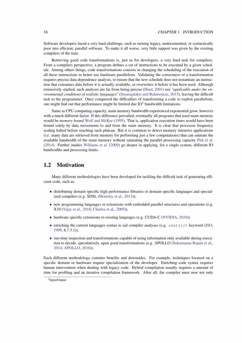
Software developers faced a very hard challenge, such as turning legacy, undocumented, or syntacticallypoor into efficient, parallel software. To make it all worse, very little support was given by the existingcompilers of the time.
Retrieving good code transformations is, just as for developers, a very hard task for compilers.From a compilers perspective, a program defines a set of instructions to be executed by a given sched-ule. Among others things, code transformations consists in changing the scheduling of the execution ofall these instructions to better use hardware parallelism. Validating the correctness of a transformationrequires precise data dependence analysis, to ensure that the new schedule does not instantiate an instruc-tion that consumes data before it is actually available, or overwrites it before it has been used. Althoughextensively studied, such analyses are far from being precise (Hind, 2001) nor "applicable under the en-vironmental conditions of realistic languages" (Smaragdakis and Balatsouras, 2015), leaving the difficulttask to the programmer. Once conquered the difficulties of transforming a code to exploit parallelism,one might find out that performance might be limited due IO2 bandwidth limitations.
Same as CPU computing capacity, main memory bandwidth experienced exponential grow, howeverwith a much different factor. If this difference prevailed, eventually all programs that used main memorywould be memory bound Wulf and McKee (1995). That is, application execution times would have beenbound solely by data movements to and from the main memory. It is clear that processor frequencyscaling halted before reaching such plateau. But it is common to detect memory intensive applications(i.e. many data are retrieved from memory for performing just a few computations) that can saturate theavailable bandwidth of the main memory without saturating the parallel processing capacity Pirk et al.(2014). Further studies Williams et al. (2009) go deeper in applying, for a single system, different IObandwidths and processing limits.
1.2 Motivation
Many different methodologies have been developed for tackling the difficult task of generating effi-cient code, such as:
• distributing domain specific high performance libraries or domain specific languages and special-ized compilers (e.g. SDSL (Henretty et al., 2013)),
• new programming languages or extensions with embedded parallel structures and operations (e.g.X10 (Vijay et al., 2016; Charles et al., 2005)),
• hardware specific extensions to existing languages (e.g. CUDA-C (NVIDIA, 2016))
• enriching the current languages syntax to aid compiler analyses (e.g. restrict keyword (ISO,1999, 6.7.3.1)),
• run-time inspection and transformations capable of using information only available during execu-tion to decide, speculatively, upon good transformations (e.g. APOLLO (Sukumaran-Rajam et al.,2014; APOLLO, 2016)).
Each different methodology contains benefits and downsides. For example, techniques focused on aspecific domain or hardware require specialization of the developer. Enriching code syntax requireshuman intervention when dealing with legacy code. Hybrid compilation usually requires a amount oftime for profiling and an iterative compilation framework. After all, the compiler must now not only
2Input/Output
1.2. MOTIVATION 17
know about the underlying hardware. But it must as well know which technique better suits the problembeing implemented, and must also have a deep comprehension of the code being optimized.
The Polytope model (Feautrier, 1992a,b; Bondhugula, 2008) underlying theory can be tracked backto late 60’s (Karp et al., 1967). It was built up over two decades (Lamport, 1974; Cousot and Halbwachs,1978; Feautrier, 1988a,b; Irigoin and Triolet, 1988; Pugh, 1991; Feautrier, 1992b). It consists of a soundformalism that allows to abstract, in an algebraic way, the iteration space of multi-dimensional loops andschedules for its iterations and instructions. In this framework, memory accesses must appear as affineexpressions in terms of the loop counters, allowing effective detection of dependencies between them.Proof of concepts of such techniques were initially applied to Fortran or restricted C code, in the contextof high performance computing.
Over a decade associated tools had been implemented and matured. Some examples are CLooG (Bas-toul, 2004), PluTo (Bondhugula, 2008), ISL (Verdoolaege, 2010) and PoCC (Pouchet, 2010). Achievingpromising performance results using automated source-to-source optimizers until the point when embed-ding developed techniques in main stream compilers became the next natural step: Projects such as GCCGraphite (Pop et al., 2006) and LLVM Polly (Grosser et al., 2012) vanguard the efforts of expanding poly-hedral optimizations usage beyond small scientific kernels and controlled source-to-source environments.However effectuating this step has demonstrated to be very hard.
Obstacles for applying the polyhedral model grew from inherent problems of compiler interme-diate representation (IR) lowering, e.g array linearisation and type erasure, from the use of pointerswith possibly multiple indirections, and the existence of dynamic parts that static analyses cannot copewith (Trifunovic et al., 2010). The fact is that, the closer a code representation is to the binary, the lesssemantic it holds, and thus the more imprecise the results static analysis become. Much work has beendone to overcome these problems, from high level semantic reconstruction out of IR (Grosser et al.,2015b), use of suitable code approximations (Benabderrahmane et al., 2008), to extending the polyhe-dral model (Grös̈linger, 2009; Venkat et al., 2014a). Speculative code transformations (Jimborean, 2012;Sukumaran-Rajam et al., 2014) demonstrate how run-time analyses can enable the use of polyhedral toolsto applications that, during execution, present a behavior that fits to the polyhedral model, not retrievedstatically. However, it imposes a online validation overhead with procedures to perform bookkeeping androllback.
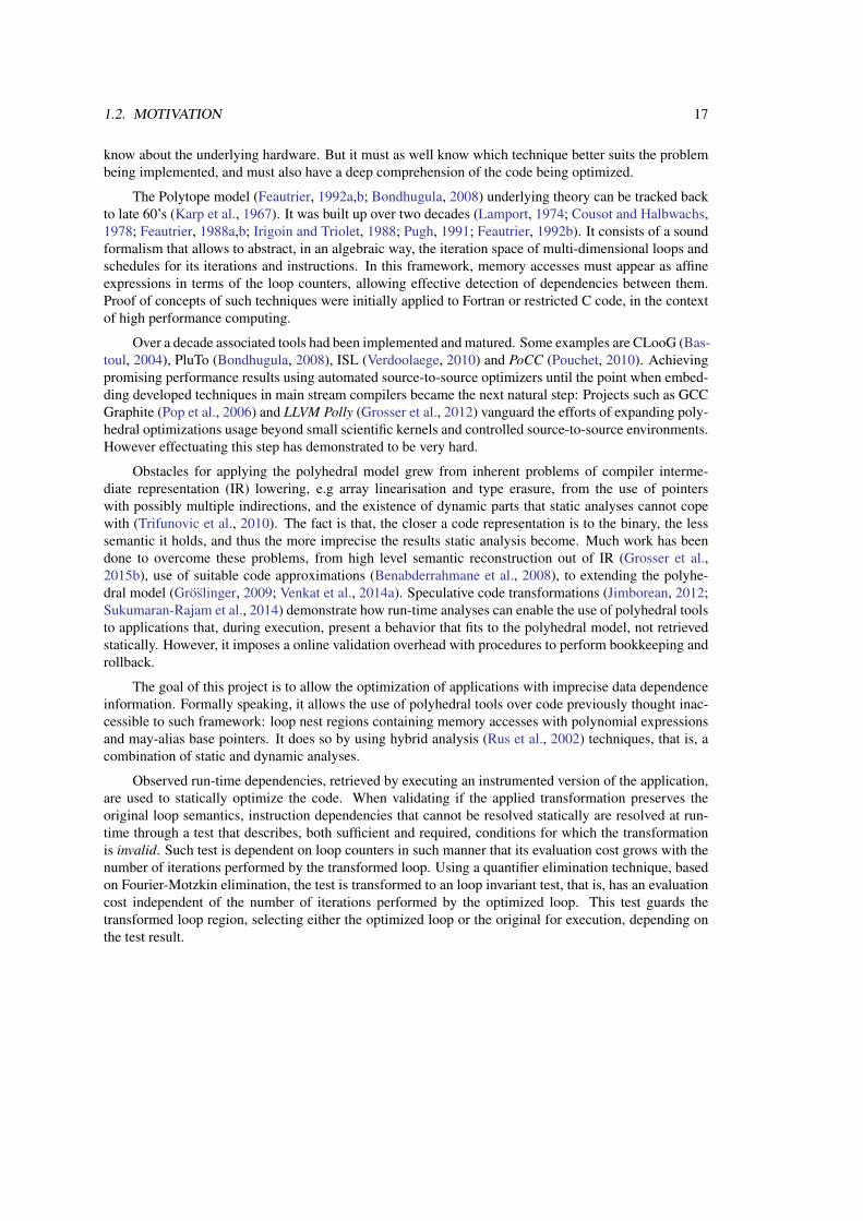
The goal of this project is to allow the optimization of applications with imprecise data dependenceinformation. Formally speaking, it allows the use of polyhedral tools over code previously thought inac-cessible to such framework: loop nest regions containing memory accesses with polynomial expressionsand may-alias base pointers. It does so by using hybrid analysis (Rus et al., 2002) techniques, that is, acombination of static and dynamic analyses.
Observed run-time dependencies, retrieved by executing an instrumented version of the application,are used to statically optimize the code. When validating if the applied transformation preserves theoriginal loop semantics, instruction dependencies that cannot be resolved statically are resolved at run-time through a test that describes, both sufficient and required, conditions for which the transformationis invalid. Such test is dependent on loop counters in such manner that its evaluation cost grows with thenumber of iterations performed by the transformed loop. Using a quantifier elimination technique, basedon Fourier-Motzkin elimination, the test is transformed to an loop invariant test, that is, has an evaluationcost independent of the number of iterations performed by the optimized loop. This test guards thetransformed loop region, selecting either the optimized loop or the original for execution, depending onthe test result.
18 CHAPTER 1. INTRODUCTION
1.3 Contributions
This work presents a novel methodology for using application execution profiling to statically gen-erate safe, yet complex, loop optimizations. Its contributions can be summarized as:
Lightweight dependence profiling: Our hybrid analysis uses information captured from run-time tohelp filling the gaps that cannot be solved by static dependence analysis. It retrieves run-time depen-dencies by instrumenting memory access instructions, that is, inserting operations into the program tomonitor and dump into a trace file, memory positions accessed during execution. In possession of thetrace file and the source-code our framework builds the dynamic dependence graph (DDG – described in§2.3), with observed dependence among dynamic instructions.
Two problems emerge when working with DDGs: First, tracking dependence among all instructionsmight generate spurious dependencies, that can prevent the optimizer to perform good transformations.For example, tracking dependencies of loop trip counter variables (also called induction variables) wouldtell the optimizer that there always exists dependencies among two consecutive iterations of any loop.These dependencies would prevent transformations that change execution order between two loop itera-tions. Second, the number of nodes in the graphs is proportional to the analyzed program complexity andoperating over them is both memory and time consuming.
Our framework relies in Scalar Evolution (Pop et al., 2005) analyses to avoid tracking variableswith a static known regression formula that expands to expressions affine in induction variables, ignoringspurious dependencies. To reduce generated graph sizes our framework allows limiting the number ofloop iterations traced. To preserve important dependencies a presented clamping technique unites non-traced instructions in a single graph node.
Optimizing loops with inaccurate dependence information: Code optimizers require precise depen-dence information to retrieve profitable transformations and to validate that a given transformation pre-serves the program semantics. However, evaluating existence of dependencies might only be solvableat run-time. Examples of such code is the use of may-alias base pointers3 and memory accesses withpolynomial expressions, as existing analysis avoid handling polynomials due their complexity. In suchscenarios, static dependence analysis provide inaccurate information, classifying many pairs of statementsas may-dependent and preventing optimizers to perform complex transformations.
To overcome the problem of retrieving complex loop transformations, our framework uses observedrun-time information as the absolute truth for instructions in may-dependence. It requires that the moni-tored execution describes the usual behavior of the application, and that a profitable optimization for thatexecution is also profitable in most cases.
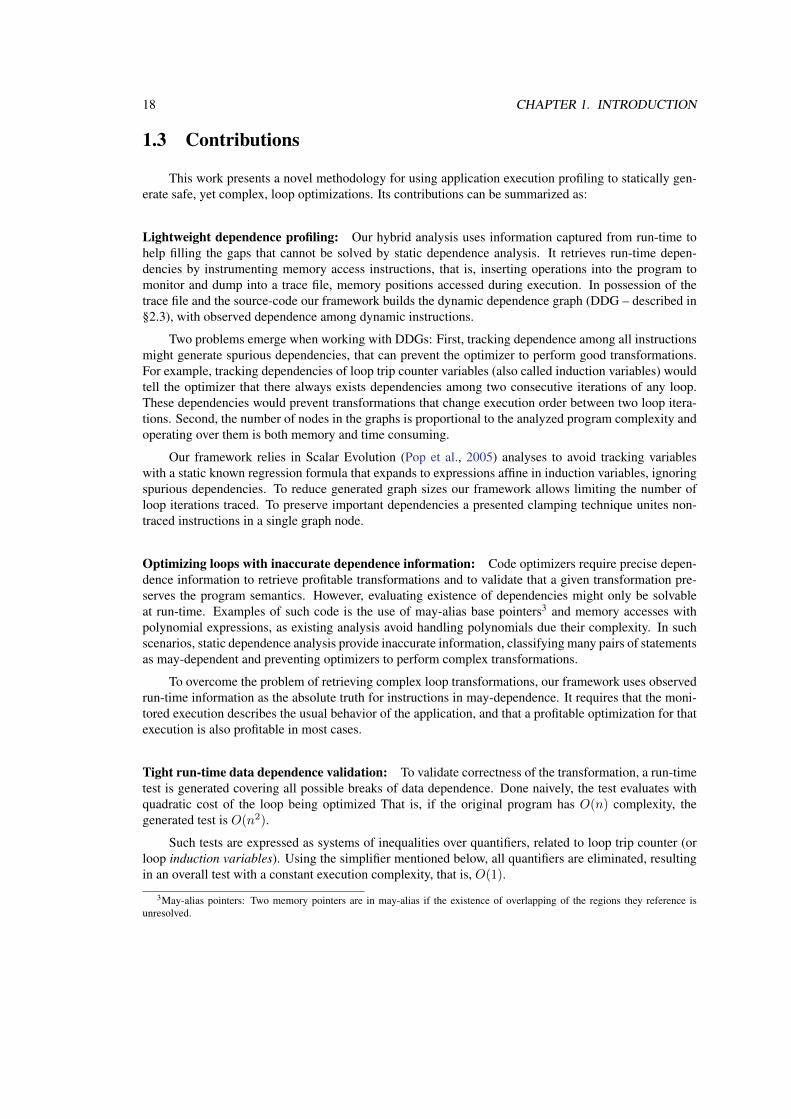
Tight run-time data dependence validation: To validate correctness of the transformation, a run-timetest is generated covering all possible breaks of data dependence. Done naively, the test evaluates withquadratic cost of the loop being optimized That is, if the original program has O(n) complexity, thegenerated test is O(n2).
Such tests are expressed as systems of inequalities over quantifiers, related to loop trip counter (orloop induction variables). Using the simplifier mentioned below, all quantifiers are eliminated, resultingin an overall test with a constant execution complexity, that is, O(1).
3May-alias pointers: Two memory pointers are in may-alias if the existence of overlapping of the regions they reference isunresolved.
1.3. CONTRIBUTIONS 19
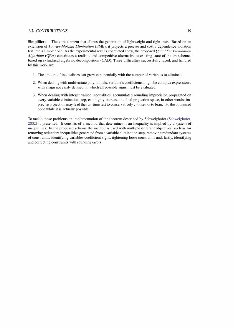
Simplifier: The core element that allows the generation of lightweight and tight tests. Based on anextension of Fourier-Motzkin Elimination (FME), it projects a precise and costly dependence violationtest into a simpler one. As the experimental results conducted show, the proposed Quantifier EliminationAlgorithm (QEA) constitutes a realistic and competitive alternative to existing state of the art schemesbased on cylindrical algebraic decomposition (CAD). Three difficulties successfully faced, and handledby this work are:
1. The amount of inequalities can grow exponentially with the number of variables to eliminate.
2. When dealing with multivariate polynomials, variable’s coefficients might be complex expressions,with a sign not easily defined, in which all possible signs must be evaluated.
3. When dealing with integer valued inequalities, accumulated rounding imprecision propagated onevery variable elimination step, can highly increase the final projection space, in other words, im-precise projection may lead the run-time test to conservatively choose not to branch to the optimizedcode while it is actually possible.
To tackle those problems an implementation of the theorem described by Schweighofer (Schweighofer,2002) is presented. It consists of a method that determines if an inequality is implied by a system ofinequalities. In the proposed scheme the method is used with multiple different objectives, such as forremoving redundant inequalities generated from a variable elimination step, removing redundant systemsof constraints, identifying variables coefficient signs, tightening loose constraints and, lastly, identifyingand correcting constraints with rounding errors.

20 CHAPTER 1. INTRODUCTION
Chapter 2
Framework
This work advocates the use of run-time information for a static loop optimizer. It proposes a frame-work, that allows to apply complex polyhedral transformations on any loop, as long the memory accessescan be statically written as polynomial expressions in loop induction variables and parameters. The pro-posed framework functions is composed of the following phases:
1. Profiling of the application: With the use of known tools such as perf, the profiling of the appli-cation uses hardware counters, in addition to debug information, to detect loop regions responsiblefor most of the execution time. For such hot regions, lightweight instrumentation is performed soas to build multiple execution traces and retrieve existing dependencies information.
2. Retrieving profitable optimizations: If the code has affine memory accesses, polyhedral source-to-source optimizers can be used for obtaining desired optimizations. If memory accesses arepolynomials, application execution is traced, using code instrumentation, and an affine representa-tion of the program’s data-flow is generated. This model holds some of the dependencies observedfrom run-time. Polyhedral optimizers are then used to obtain desirable transformations.
3. Building the run-time test: From the applied sequence of transformations and the original pro-gram source code, a precise run-time test for validating the correctness of the transformation isbuilt. Two operations are data-dependent with one-another if they access the same storage posi-tion, and at least one is a write. If the execution order between those two instructions is changed,the program result will possibly not be preserved. A may-dependence is when it is, statically, notpossible to determine if there exists a dependence between two operations. The generated test ver-ifies, for all possible pairs of operations that are in may-dependence and turn out to be dependentat run-time, if their execution order on the original program is preserved by the transformation.Effectively, the test is performed on the Cartesian product of all operations, so if the applicationhas complexity O(n), the test has complexity O(n2).
4. Simplifying the generated test: Validity checks can be viewed as testing the emptiness of a para-metric geometric region in a multi-dimensional space: The existence of an (integral) point in thisregion means that the transformation is non-valid. Algebraically, this region is defined as a systemof polynomial inequalities in terms of induction variables (loop counters), and loop-invariant vari-ables (parameters). Simplifying the generated test corresponds to “eliminating” induction variablesfrom the system, by computing a system of inequalities that is an over-approximation of the originalone, but made-up only of parameter variables. Using the geometric representation, this elimination
21
22 CHAPTER 2. FRAMEWORK
corresponds to a projection of the “forbidden” region to the sub-space of parameters. To this end,we developed a new quantifier-elimination scheme, an extension of the Fourier-Motzkin algorithm.The simplified tests are systems of inequalities between parameters (thus O(1) test). Going back tothe geometric representation, it corresponds to testing emptiness of the (over-approximated) pro-jected region: If empty, the transformation is safe. If statically proven the projected system is notempty, then the transformation will always be considered unsafe and is discarded.
5. Code versioning: For the transformations not discarded in the previous step, along with the originalcode, a decision tree is build to select which version of the code is to be executed.
This chapter describes the proposed framework functionality and components. §3 compares theadopted methodology to related works. §4 provides experimental results that demonstrate soundness ofthe claim that our proposed technique allows more loops to be safely optimized by the generation of safe,tight, run-time tests. §5 and §6 provide technical implementation details of the Quantifier Eliminationand the Dynamic Dependence Graph processes. For last §7 concludes and provide future work directions.
2.1 Theoretical Foundations
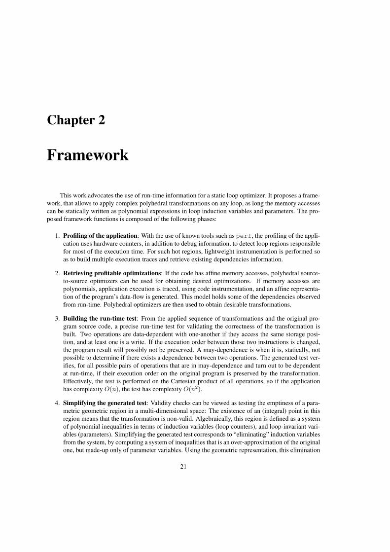
function FW-tri(*T){for(k=0;k<n;k++)for (i=0;i<k;i++)for (j=0;j<i;j++)S1: T[i*(i-1)/2+j] min= T[k*(k-1)/2+i]+T[k*(k-1)/2+j]
for (k=0;k<n;k++)for (i=0;i<k;i++)for (j=k+1;j< n;j++)S2: T[j*(j-1)/2+i] min= T[k*(k-1)/2+i]+T[j*(j-1)/2+k]
}
Algorithm 1: FW-tri: Part of a Floyd-Warshall algorithm for a non directional distance graph storedin a packed lower triangular matrix.
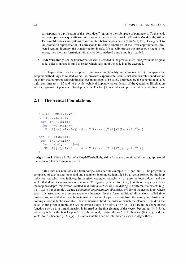
To illustrate our notations and terminology, consider the example of Algorithm 1. The program iscomposed of two nested loops and any statement is uniquely identified by a vector formed by the loopinduction variables (loop indices). In the given example, variables k,i,j are the loop indices, and thevector that identifies an instance of statement S1 is given by the vector (k, i, j). With as many elements asthe loop nest depth, this vector is called an iteration vector ( ~iv ). To distinguish different statements (e.g.S1, S2 in our example), we use a canonical representation (Feautrier, 1992b) of the nested loop, whereeach ~iv is associated to a unique statement instance. In this form, additional dimensions, called timedimensions, are added to disambiguate instructions and loops, spawning from the same point. Instead ofholding a loop induction variable, these dimensions hold the order on which the element is held on thecode. In the given example, the two outermost loops (for(k=0;k<n;k++))) are in the scope of thefunction FW-tri: a time dimension is inserted as the first element of the vector, becoming (t0, k, i, j),where t0 is 0 for the first loop and 1 for the second, making the ~iv / of S1 become (0, k, i, j) and thevector for S2 become (1, k, i, j). This representation can be interpreted as seen in Algorithm 2.
2.1. THEORETICAL FOUNDATIONS 23
function FW-tri(*T){for(t0=0;t0<2;t++)if(t0==0) {for(k=0;k<n;k++)for (i=0;i<k;i++)for (j=0;j<i;j++)S1: T[i*(i-1)/2+j] min= T[k*(k-1)/2+i]+T[k*(k-1)/2+j]
} else if(t0==1) {for (k=0;k<n;k++)for (i=0;i<k;i++)for (j=k+1;j< n;j++)S2: T[j*(j-1)/2+i] min= T[k*(k-1)/2+i]+T[j*(j-1)/2+k]
}
Algorithm 2: How the canonical ~iv representation can be interpreted for the FW-tri example.
A schedule is expressed as a function (written TS1 for statement S1) from the iteration spaceD to thescheduling space D′. Both D and D′ are affine spaces of possibly different dimension.TS1(0, k, i, j) = TS1(0, k′, i′, j′) means that S10,k,i,j and S10,k′,i′,j′ are executed in parallel. Using≺lex notation to represent the lexicographical order, TS1(0, k, i, j) ≺lex TS1(0, k′, i′, j′) means thatS10,k,i,j is executed before S10,k′,i′,j′ . A loop transformation is expressed as a schedule (also calledscattering) function, and most compositions of loop transformations can be represented as affine sched-ules (Feautrier, 1992b). Consider the case where we want to exchange the order in which the countersi and j are iterated for the loop nest encapsulating S1, a transformation called loop interchange. Thecorresponding schedule function for S1 would write TS1(0, k, i, j) = (0, k, j, i). The canonical formallows expressing the schedule of the original code as the identity function from D to itself (D′ can bethe same as D).
A data dependence between two statement instances expresses an ordering constraint (representedas <d) on their respective executions. A data dependence is induced by read and write accesses tothe same memory location. Here S10,k,i,j writes to location W1(0, k, i, j) = T + i(i − 1)/2 + j andreads from locations R2(0, k, i, j) = T + i(i − 1)/2 + j, R3(0, k, i, j) = T + k(k − 1)/2 + i, andR4(0, k, i, j) = T + k(k− 1)/2 + j. There is a read-after-write dependence (also known as flow or RAWdependence) between S10,k,i,j and S10,k′,i′,j′ from W1 to R2 as soon as:
1. (0, k, i, j) ∈ D strictly precedes (0, k′, i′, j′) ∈ D in the original schedule; which is written as(0, k, i, j) ≺lex (0, k′, i′, j′), where ≺lex denotes a lexicographic comparison;
2. read/write locations overlap; which is written as W1(0, k, i, j) = R2(0, k′, i′, j′).
For example S10,3,2,1 <d S10,4,2,1 as W1(0, 3, 2, 1) = R2(0, 4, 2, 1) ≡ T + 2.
The other kinds of data dependencies we care about are write-after-write dependencies, also calledoutput or WAW dependence and write-after-read dependencies, also known as anti or WAR dependence.A read-after-read, or RAR, usually is not considered a data dependency.
For any new schedule to be valid it must preserve all such dependencies. As an example, for the pre-viously considered loop interchange TS1(0, k, i, j) = (0, k, j, i), the dependence S10,3,2,1 <d S10,4,2,1is preserved since TS1(0, 3, 2, 1) = (0, 3, 1, 2) ≺lex TS1(0, 4, 2, 1) = (0, 4, 1, 2).
In the given example, the variable T is a base pointer, received as parameter of the function FW-tri.For the compiler, its value is unknown, but constant (invariant), inside this function. If in our example
24 CHAPTER 2. FRAMEWORK
multiple base pointers were received as parameters, without any pointer disambiguation information (e.g.through restrict annotation or inter-procedural analysis) the compiler would not be able to deter-mine dependencies between instructions accessing memory addresses derived from those different basepointers. A second problem comes from the use of polynomial memory accesses. Existing compileranalysis consider polynomial expressions as uninterpreted functions, usually leading to the inability toperform any optimizing transformation. The proposed framework leverages all these steps to overcomethe outlined problems based on a model built from profiling the run-time behavior of an application.
2.2 Application profiling
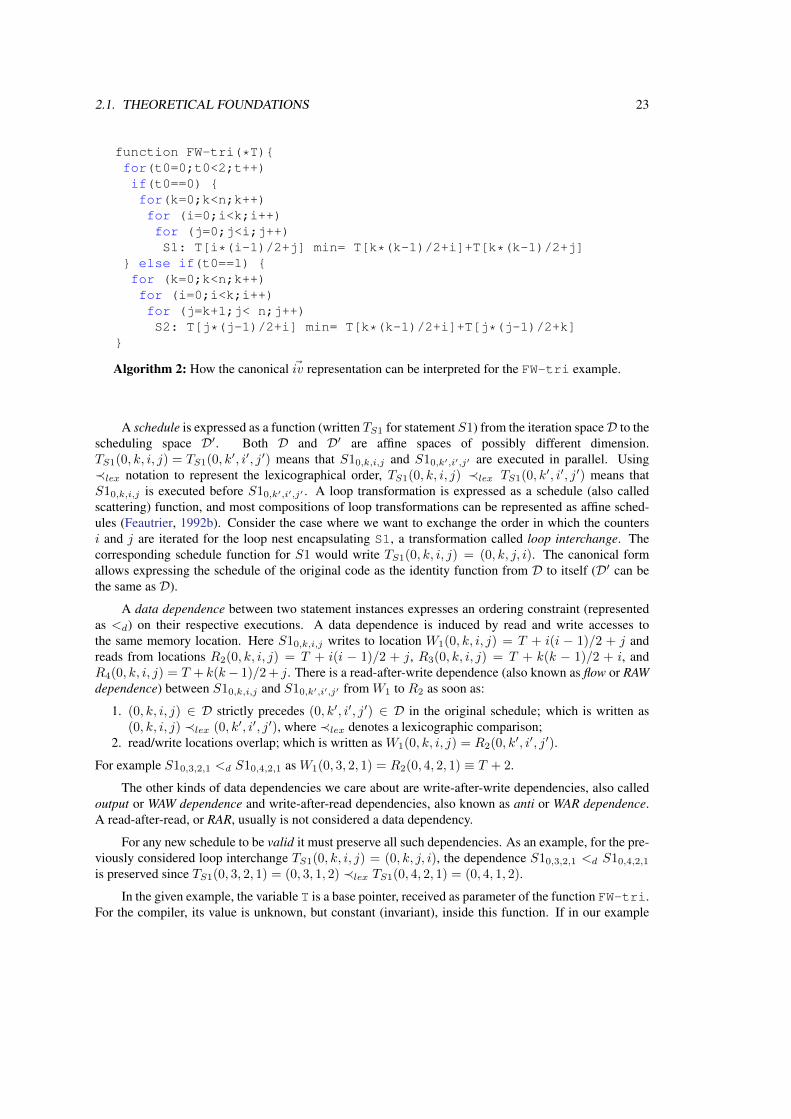
This work focus on optimizing loops in which memory accesses can be statically formulated bypolynomial expressions of the ~iv and loop invariant variables (parameters). Algorithms 1 and 3 will serveas reference along this chapter. The latter one is an alternative implementation of the dspmv routine,present in BLAS/LAPACK (www.netlib.org, 1992) 1.
52 void kernel_dspmv(int ni, int nj, double alpha,53 double beta, double *X, double *AP, double *Y){54 int i, j, k;55 double temp2;56
57 for (i = 0; i < ni; i++){58 for (j = 0; j < nj; j++ ){59 S1: temp2 = 0;60 for (k = 0; k < i; k++) {61 S2: Y[k*ni+j] += alpha * X[i*ni+j] *62 AP[i*(i+1)/2+k];63 S3: temp2 += X[k*ni+j] * AP[i*(i+1)/2+k];64 }65 S4: Y[i*ni+j] = beta * Y[i*ni+j]+alpha*X[i*ni+j] *66 AP[i*(i+1)/2+i] + alpha * temp2;
Algorithm 3: An alternative C implementation of the same of the dspmv routine obtained fromBLAS2, using a packed lower matrix AP and x, y steps equal to 1.
Since pointers X, AP and Y are parameters, in practice compilers have very limited information aboutthem, preventing static resolution of memory dependencies, and consequently disallowing the use of com-plex loop transformations. Source-to-source optimizers, using polyhedral techniques, were developed tobe used when the programmer can assure the independence of memory addresses accessed from eachbase pointer, but neither source-to-source compilers, nor embedded compiler tools such as Polly (Grosseret al., 2012) or Graphite (Pop et al., 2006) can handle memory accesses with polynomial expressions,such as AP[i*(i+1)/2+i].
This work relies in loop cloning which involves code size expansion. To avoid huge size expansions,it focuses on optimizing only critical parts of the program, so called hot-spots. We use perf, a wellknown performance debugging tool, to obtain a sampled distribution of time spent in each part of the
1The original application is hand optimized using temporary variables in a form that applying new transformations is not trivial.For simplicity, the example implements only the case of a lower triangular matrix AP and x and y strides of 1.
2.3. DYNAMIC DEPENDENCE GRAPH (DDG) 25
# Overhead Command Shared Object Symbol# ........ ....... ............. ......................
99.89% sample sample [.] kernel_dspmv.constprop0.11% sample sample [.] init_array.constprop.20.00% sample libc-2.23.so [.] _dl_addr
Figure 2.1: Distribution of samples among a programs functions reported by perf
Sorted summary for file dspmv/sample----------------------------------------------65.00 dspmv.l.c:6329.75 dspmv.l.c:624.92 dspmv.l.c:61
Figure 2.2: distribution of samples among source lines reported by perf
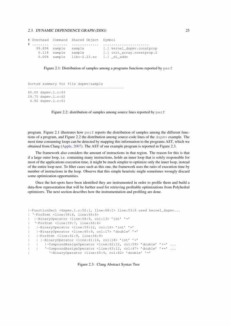
program. Figure 2.1 illustrates how perf reports the distribution of samples among the different func-tions of a program, and Figure 2.2 the distribution among source-code lines of the dspmv example. Themost time consuming loops can be detected by mapping this information to the programs AST, which weobtained from Clang (Apple, 2007). The AST of our example program is reported in Figure 2.3.
The framework also considers the amount of instructions in that region. The reason for this is thatif a large outer loop, i.e. containing many instructions, holds an inner loop that is solely responsible formost of the applications execution time, it might be much simpler to optimize only the inner loop, insteadof the entire loop nest. To filter cases such as this one, the framework uses the ratio of execution time bynumber of instructions in the loop. Observe that this simple heuristic might sometimes wrongly discardsome optimization opportunities.
Once the hot-spots have been identified they are instrumented in order to profile them and build adata-flow representation that will be further used for retrieving profitable optimizations from Polyhedraloptimizers. The next section describes how the instrumentation and profiling are done.
|-FunctionDecl <dspmv.l.c:52:1, line:68:1> line:53:6 used kernel_dspmv...| ‘-ForStmt <line:58:4, line:66:6>| |-BinaryOperator <line:58:9, col:13> ’int’ ’=’| ‘-ForStmt <line:59:7, line:66:6>| |-BinaryOperator <line:59:12, col:16> ’int’ ’=’| |-BinaryOperator <line:60:9, col:17> ’double’ ’=’| |-ForStmt <line:61:9, line:64:9>| | |-BinaryOperator <line:61:14, col:18> ’int’ ’=’| | |-CompoundAssignOperator <line:62:12, col:59> ’double’ ’+=’ ...| | ‘-CompoundAssignOperator <line:63:12, col:47> ’double’ ’+=’ ...| ‘-BinaryOperator <line:65:9, col:82> ’double’ ’=’
Figure 2.3: Clang Abstract Syntax Tree

26 CHAPTER 2. FRAMEWORK
471(3,2,1)13; line:64; column:21
LD
140(1,2)22; line:66; column:75
+
135(1,2)17; line:66; column:21
LD
136(1,2)18; line:66; column:31
*
142(1,2)24; line:66; column:38
+
141(1,2)23; line:66; column:45
*
143(1,2)25; line:66; column:19
ST
278(2,2,1)10; line:63; column:22
LD
280(2,2,1)12; line:63; column:22
ST
261(2,2,0)6; line:63; column:33
LD
742,2,1); line:63; column:33
LD
; column:21LD
275(2,2,1)7; line:63; column:31
*
277(2,2,1)9; line:63; column:43
*
279(2,2,1)11; line:63; column:22
+
468(3,2,1)10; line:63; column:22
LD
470(3,2,1)12; line:63; column:22
ST
336(3)1; line:66; column:69
/
337(3)2; line:66; column:71
+
388(3,0)20; line:66; column:59
LD
43); line:66; column:59
LD
375(3,0,2)8; line:63; column:45
LD
381(3,0,2)14; line:64; column:33
LD
427(3,1,2)8; line:63; column:45
LD
433(3,1,2)14; line:64; column:33
LD
479(3,2,2)8; line:63; column:45
LD
485(3,2,2)14; line:64; column:33
LD
537(3,3,2)14; line:64; column:33
LD
449(3,2,0)
i32 0
461(3,2,0)16; line:64; column:18
+
3; column:33LD
460(3,2,0)15; line:64; column:31
*
474(3,2,1)16; line:64; column:18
+
465(3,2,1)7; line:63; column:31
*
467(3,2,1)9; line:63; column:43
*
469(3,2,1)11; line:63; column:22
+
473(3,2,1)15; line:64; column:31
*
olumn:21
olumn:31
543(3,3)19; l
546(3,3)22; line:66; column:75
+
541(3,3)17; line:66; column:21
LD
542(3,3)18; line:66; column:31
*
548(3,3)24; line:66; column:38
+
545(3,3)21; line:66; column:57
*
547(3,3)23; line:66; column:45
*
549(3,3)25; line:66; column:19
ST
Figure 2.4: Partial view of the DDG combined with the Dynamic Reuse Graph (DRG) for dspmv. Eachnode represents a dynamic instruction, described by a unique node counter, the iteration vector, the staticinstruction identifier, the position (line and column )of the instruction in the source code. Green edgesconnect instructions that consumed the same data, that is, form a RAR. We differentiate data flow de-pendencies between scalar variables (visible through def-use chains in the compiler IR), and data flowdependencies between memory locations: Memory RAW are represented in orange and WAW are in red.Scalar RAW are in black. Scalar WAW are ignored as they can be removed using renaming.
2.3. DYNAMIC DEPENDENCE GRAPH (DDG) 27
2.3 Dynamic Dependence Graph (DDG)
Once the hot-spot regions have been selected, we can profile them. The goal of the profiling phaseis to build a DDG: a Directed Acyclic Graph (DAG) where each node represents a dynamic instance ofan IR instruction, and each edge represents a data-dependence, that is, a producer–consumer relationship.The construction of the DDG is done in two phases: the first phase is based on instrumentation of thecode at the LLVM IR level; The instrumented code is executed, gathering run-time information into atrace file; The second phase uses the collected information so as to simulate the execution and effectivelybuild the DDG.
Collected (chronologically) data during the first phase are: Accessed memory addresses; Alive val-ues in the region entry-point; Base pointers; Loop entries; Loop iteration counters; Loop exits.
Using generated trace files along with the compiler IR of the program, the simulation replays theexecution. So as to capture dependencies among memory instruction, a shadow-memory (Nethercote andSeward, 2007) is used. It consists of storing for every memory address used by the application the lastnode that wrote to it. Next, whenever a memory read or write operation is performed, a dependenceedge is inserted from the last writer to the current reader/writer node. We also build a Data Reuse Graph(DRG) that also contains read-after-read dependencies. In practice, for each write, a set of all nodes thatread since this write is built. Observe that write-after-read dependencies could be computed afterward bytransitivity from WAW and RAW links.
To identify the operation performed by each node, they receive a label associating it with the staticprogram instruction id that generated them. Merging all nodes of identical instruction-label-id allows toidentify dependencies between static elements of the code. As it comes to dynamic dependencies, theyare labeled by a distance vector: During the simulation, loop entry and exit events control a dynamiciteration vector. This vector, initially empty, has one new element (set to 0) inserted at its end every timea loop-entry event is detected. This last element is also removed by its corresponding loop-exit event, andin between incremented by one at every loop-iteration event. Whenever a node is created, it is labeledwith the current vector, which can be interpreted as an ~iv (not in canonical form here), as explained in§2.1. Figure 2.4 provides an illustrative example of the DDG.
Once dependencies between instructions have been retrieved, the following question is: how to usethis information to select code transformations? The next section describes how this graph is used togenerate a representation that can be used by existing loop optimizers.
2.4 Retrieving profitable optimizations
Once obtained, the dependencies between operations can be used as an input to existing loop opti-mizers. The goal is to find new schedules that better exploit machine resources, by e.g. improving datalocality or exposing parallelism. However, most existing tools operate on a tree-based representation ofloop nests and instructions. They also require a canonical iteration vector to distinguish specific instancesof each instruction. The DDG, that can be seen as an ocean of nodes, does not hold either qualifications.However the static instruction-id, together with the dynamic iteration vector can be used to map nodesinto an AST so as to fulfill those two prerequisites.
Using the compiler’s knowledge of the program semantic, the region Control Flow Graph (CFG),and the loop forest, a program AST is rebuilt. The constructed AST holds two kinds of nodes: instructionsand loops. The hierarchy on the tree represents, from parent node to children, the loop hierarchy fromoutermost loop to innermost. Instructions are always leaf nodes. Each node is given a unique canonical
28 CHAPTER 2. FRAMEWORK
iteration vector as described in 2.1. This vector is created by traversing the AST from top to bottomand by: using the induction variables of loops for actual loop dimensions; using static enumerations foradditional time dimensions. Lastly, each instruction node in the AST also receives the same static idgiven to its corresponding node in the DDG.
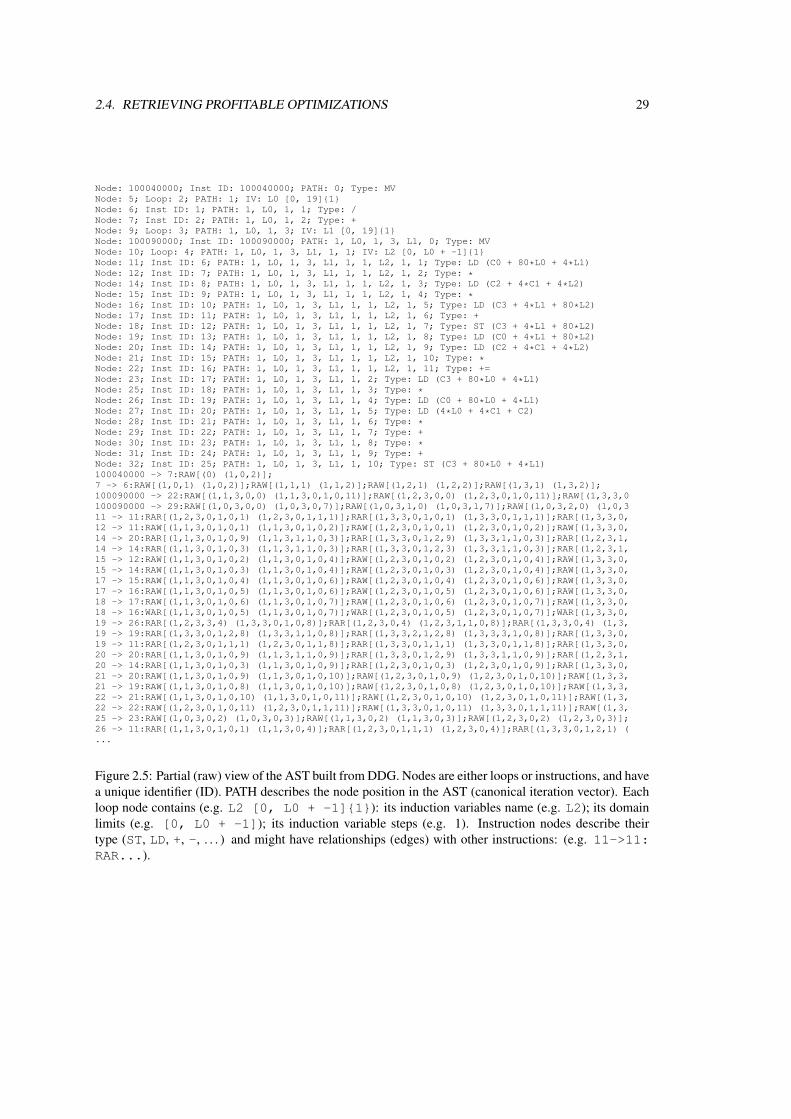
The mapping of DDG nodes to their respective nodes on the AST is done by filling the inductionvariables in the canonical iteration vector of the AST, with the dynamic time stamp from the DDG node,giving each node a unique position in the “canonical” iteration space. Each edge is labeled with a distancevector, computed by subtraction of the two nodes consumer− producer. This distance vector tells howfar apart in the execution the two nodes of the dependence relationship are. Observe that the directionof distance vector is the inverse of the orientation of the producer–consumer relationship. Finally, thisrepresentation is then either written into a text file to be used with the loop optimizers or into a graphicalrepresentation that can be analyzed by the user (see figures 2.5 and 2.6 respectively).
2.4. RETRIEVING PROFITABLE OPTIMIZATIONS 29
Node: 100040000; Inst ID: 100040000; PATH: 0; Type: MVNode: 5; Loop: 2; PATH: 1; IV: L0 [0, 19]{1}Node: 6; Inst ID: 1; PATH: 1, L0, 1, 1; Type: /Node: 7; Inst ID: 2; PATH: 1, L0, 1, 2; Type: +Node: 9; Loop: 3; PATH: 1, L0, 1, 3; IV: L1 [0, 19]{1}Node: 100090000; Inst ID: 100090000; PATH: 1, L0, 1, 3, L1, 0; Type: MVNode: 10; Loop: 4; PATH: 1, L0, 1, 3, L1, 1, 1; IV: L2 [0, L0 + -1]{1}Node: 11; Inst ID: 6; PATH: 1, L0, 1, 3, L1, 1, 1, L2, 1, 1; Type: LD (C0 + 80*L0 + 4*L1)Node: 12; Inst ID: 7; PATH: 1, L0, 1, 3, L1, 1, 1, L2, 1, 2; Type: *Node: 14; Inst ID: 8; PATH: 1, L0, 1, 3, L1, 1, 1, L2, 1, 3; Type: LD (C2 + 4*C1 + 4*L2)Node: 15; Inst ID: 9; PATH: 1, L0, 1, 3, L1, 1, 1, L2, 1, 4; Type: *Node: 16; Inst ID: 10; PATH: 1, L0, 1, 3, L1, 1, 1, L2, 1, 5; Type: LD (C3 + 4*L1 + 80*L2)Node: 17; Inst ID: 11; PATH: 1, L0, 1, 3, L1, 1, 1, L2, 1, 6; Type: +Node: 18; Inst ID: 12; PATH: 1, L0, 1, 3, L1, 1, 1, L2, 1, 7; Type: ST (C3 + 4*L1 + 80*L2)Node: 19; Inst ID: 13; PATH: 1, L0, 1, 3, L1, 1, 1, L2, 1, 8; Type: LD (C0 + 4*L1 + 80*L2)Node: 20; Inst ID: 14; PATH: 1, L0, 1, 3, L1, 1, 1, L2, 1, 9; Type: LD (C2 + 4*C1 + 4*L2)Node: 21; Inst ID: 15; PATH: 1, L0, 1, 3, L1, 1, 1, L2, 1, 10; Type: *Node: 22; Inst ID: 16; PATH: 1, L0, 1, 3, L1, 1, 1, L2, 1, 11; Type: +=Node: 23; Inst ID: 17; PATH: 1, L0, 1, 3, L1, 1, 2; Type: LD (C3 + 80*L0 + 4*L1)Node: 25; Inst ID: 18; PATH: 1, L0, 1, 3, L1, 1, 3; Type: *Node: 26; Inst ID: 19; PATH: 1, L0, 1, 3, L1, 1, 4; Type: LD (C0 + 80*L0 + 4*L1)Node: 27; Inst ID: 20; PATH: 1, L0, 1, 3, L1, 1, 5; Type: LD (4*L0 + 4*C1 + C2)Node: 28; Inst ID: 21; PATH: 1, L0, 1, 3, L1, 1, 6; Type: *Node: 29; Inst ID: 22; PATH: 1, L0, 1, 3, L1, 1, 7; Type: +Node: 30; Inst ID: 23; PATH: 1, L0, 1, 3, L1, 1, 8; Type: *Node: 31; Inst ID: 24; PATH: 1, L0, 1, 3, L1, 1, 9; Type: +Node: 32; Inst ID: 25; PATH: 1, L0, 1, 3, L1, 1, 10; Type: ST (C3 + 80*L0 + 4*L1)100040000 -> 7:RAW[(0) (1,0,2)];7 -> 6:RAW[(1,0,1) (1,0,2)];RAW[(1,1,1) (1,1,2)];RAW[(1,2,1) (1,2,2)];RAW[(1,3,1) (1,3,2)];100090000 -> 22:RAW[(1,1,3,0,0) (1,1,3,0,1,0,11)];RAW[(1,2,3,0,0) (1,2,3,0,1,0,11)];RAW[(1,3,3,0100090000 -> 29:RAW[(1,0,3,0,0) (1,0,3,0,7)];RAW[(1,0,3,1,0) (1,0,3,1,7)];RAW[(1,0,3,2,0) (1,0,311 -> 11:RAR[(1,2,3,0,1,0,1) (1,2,3,0,1,1,1)];RAR[(1,3,3,0,1,0,1) (1,3,3,0,1,1,1)];RAR[(1,3,3,0,12 -> 11:RAW[(1,1,3,0,1,0,1) (1,1,3,0,1,0,2)];RAW[(1,2,3,0,1,0,1) (1,2,3,0,1,0,2)];RAW[(1,3,3,0,14 -> 20:RAR[(1,1,3,0,1,0,9) (1,1,3,1,1,0,3)];RAR[(1,3,3,0,1,2,9) (1,3,3,1,1,0,3)];RAR[(1,2,3,1,14 -> 14:RAR[(1,1,3,0,1,0,3) (1,1,3,1,1,0,3)];RAR[(1,3,3,0,1,2,3) (1,3,3,1,1,0,3)];RAR[(1,2,3,1,15 -> 12:RAW[(1,1,3,0,1,0,2) (1,1,3,0,1,0,4)];RAW[(1,2,3,0,1,0,2) (1,2,3,0,1,0,4)];RAW[(1,3,3,0,15 -> 14:RAW[(1,1,3,0,1,0,3) (1,1,3,0,1,0,4)];RAW[(1,2,3,0,1,0,3) (1,2,3,0,1,0,4)];RAW[(1,3,3,0,17 -> 15:RAW[(1,1,3,0,1,0,4) (1,1,3,0,1,0,6)];RAW[(1,2,3,0,1,0,4) (1,2,3,0,1,0,6)];RAW[(1,3,3,0,17 -> 16:RAW[(1,1,3,0,1,0,5) (1,1,3,0,1,0,6)];RAW[(1,2,3,0,1,0,5) (1,2,3,0,1,0,6)];RAW[(1,3,3,0,18 -> 17:RAW[(1,1,3,0,1,0,6) (1,1,3,0,1,0,7)];RAW[(1,2,3,0,1,0,6) (1,2,3,0,1,0,7)];RAW[(1,3,3,0,18 -> 16:WAR[(1,1,3,0,1,0,5) (1,1,3,0,1,0,7)];WAR[(1,2,3,0,1,0,5) (1,2,3,0,1,0,7)];WAR[(1,3,3,0,19 -> 26:RAR[(1,2,3,3,4) (1,3,3,0,1,0,8)];RAR[(1,2,3,0,4) (1,2,3,1,1,0,8)];RAR[(1,3,3,0,4) (1,3,19 -> 19:RAR[(1,3,3,0,1,2,8) (1,3,3,1,1,0,8)];RAR[(1,3,3,2,1,2,8) (1,3,3,3,1,0,8)];RAR[(1,3,3,0,19 -> 11:RAR[(1,2,3,0,1,1,1) (1,2,3,0,1,1,8)];RAR[(1,3,3,0,1,1,1) (1,3,3,0,1,1,8)];RAR[(1,3,3,0,20 -> 20:RAR[(1,1,3,0,1,0,9) (1,1,3,1,1,0,9)];RAR[(1,3,3,0,1,2,9) (1,3,3,1,1,0,9)];RAR[(1,2,3,1,20 -> 14:RAR[(1,1,3,0,1,0,3) (1,1,3,0,1,0,9)];RAR[(1,2,3,0,1,0,3) (1,2,3,0,1,0,9)];RAR[(1,3,3,0,21 -> 20:RAW[(1,1,3,0,1,0,9) (1,1,3,0,1,0,10)];RAW[(1,2,3,0,1,0,9) (1,2,3,0,1,0,10)];RAW[(1,3,3,21 -> 19:RAW[(1,1,3,0,1,0,8) (1,1,3,0,1,0,10)];RAW[(1,2,3,0,1,0,8) (1,2,3,0,1,0,10)];RAW[(1,3,3,22 -> 21:RAW[(1,1,3,0,1,0,10) (1,1,3,0,1,0,11)];RAW[(1,2,3,0,1,0,10) (1,2,3,0,1,0,11)];RAW[(1,3,22 -> 22:RAW[(1,2,3,0,1,0,11) (1,2,3,0,1,1,11)];RAW[(1,3,3,0,1,0,11) (1,3,3,0,1,1,11)];RAW[(1,3,25 -> 23:RAW[(1,0,3,0,2) (1,0,3,0,3)];RAW[(1,1,3,0,2) (1,1,3,0,3)];RAW[(1,2,3,0,2) (1,2,3,0,3)];26 -> 11:RAR[(1,1,3,0,1,0,1) (1,1,3,0,4)];RAR[(1,2,3,0,1,1,1) (1,2,3,0,4)];RAR[(1,3,3,0,1,2,1) (...
Figure 2.5: Partial (raw) view of the AST built from DDG. Nodes are either loops or instructions, and havea unique identifier (ID). PATH describes the node position in the AST (canonical iteration vector). Eachloop node contains (e.g. L2 [0, L0 + -1]{1}): its induction variables name (e.g. L2); its domainlimits (e.g. [0, L0 + -1]); its induction variable steps (e.g. 1). Instruction nodes describe theirtype (ST, LD, +, -, . . . ) and might have relationships (edges) with other instructions: (e.g. 11->11:RAR...).

30C
HA
PTE
R2.
FRA
ME
WO
RK
ROOT
i64 0 L0[0, 19]{1}
+
RAW(1)
/ L1[0, 19]{1}
RAW(0, 0, 1) RAW(0, 0, 1)
L2[0, L0 + -1]{1} LD (C3 + 80*L0 + 4*L1) * LD (C0 + 80*L0 + 4*L1) LD (4*L0 + 4*C1 + C2)
RAW(0, 0, 0, 0, 1)
RAW(0, 0, 0, 0, 7)
ST (C3 + 4*L1 + 80*L2) LD (C0 + 4*L1 + 80*L2) LD (C2 + 4*C1 + 4*L2) *
RAR(0, 0, 0, 0, 3) RAW(0, 0, 0, 0, 6)
0, 0, 0, 2)
0, 0, 0, 0, 1)RAR(0, 0+, 0, *)
RAW(0, 0, 0, 0, 0, 0, 2)
RAR(0, 0, 0, 0+, 0, *)RAW(0, 0, 0, 0, 0, 0, 1)
RAW(0, 0, 0, 0, 1)
WAR(0, 0, 0, 0, 8)RAW(0, 0, 0, 0, 6)RAR(0, 0+, 0, *) RAW(0, 0, 0, 0, 2)
RAR(0, 0, 0, 1, 0)RAW(0, 0, 0, 0, 1)
Figure 2.6: Partial view of the graphical representation generated for the dspmv example. Elliptical nodes represent loop structures, containing theirinduction variable counter (e.g. L0, L1, L2), their maximum and minimum values and step size. Squares represent instructions. Red and orangeedges represent dependencies between instructions and green edges represent reuses. For easier comprehension, the distance vector directions areinverted to preserve the data flow sense.
2.5. OBTAINING OPTIMIZATIONS 31
#pragma parallelize (*)#pragma schedule S1 (k,i,j)#pragma tilable () 3
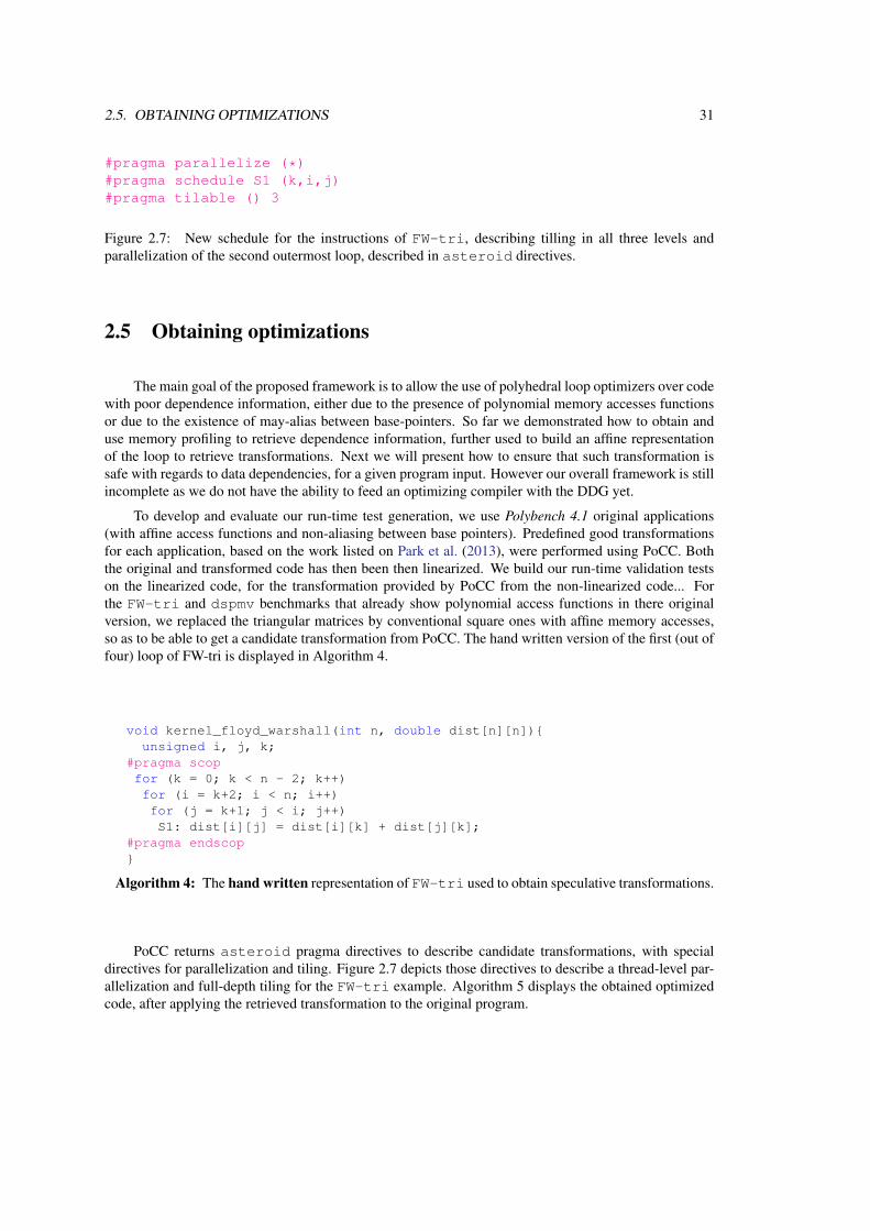
Figure 2.7: New schedule for the instructions of FW-tri, describing tilling in all three levels andparallelization of the second outermost loop, described in asteroid directives.
2.5 Obtaining optimizations
The main goal of the proposed framework is to allow the use of polyhedral loop optimizers over codewith poor dependence information, either due to the presence of polynomial memory accesses functionsor due to the existence of may-alias between base-pointers. So far we demonstrated how to obtain anduse memory profiling to retrieve dependence information, further used to build an affine representationof the loop to retrieve transformations. Next we will present how to ensure that such transformation issafe with regards to data dependencies, for a given program input. However our overall framework is stillincomplete as we do not have the ability to feed an optimizing compiler with the DDG yet.
To develop and evaluate our run-time test generation, we use Polybench 4.1 original applications(with affine access functions and non-aliasing between base pointers). Predefined good transformationsfor each application, based on the work listed on Park et al. (2013), were performed using PoCC. Boththe original and transformed code has then been then linearized. We build our run-time validation testson the linearized code, for the transformation provided by PoCC from the non-linearized code... Forthe FW-tri and dspmv benchmarks that already show polynomial access functions in there originalversion, we replaced the triangular matrices by conventional square ones with affine memory accesses,so as to be able to get a candidate transformation from PoCC. The hand written version of the first (out offour) loop of FW-tri is displayed in Algorithm 4.
void kernel_floyd_warshall(int n, double dist[n][n]){unsigned i, j, k;
#pragma scopfor (k = 0; k < n - 2; k++)for (i = k+2; i < n; i++)for (j = k+1; j < i; j++)S1: dist[i][j] = dist[i][k] + dist[j][k];
#pragma endscop}
Algorithm 4: The hand written representation of FW-tri used to obtain speculative transformations.
PoCC returns asteroid pragma directives to describe candidate transformations, with specialdirectives for parallelization and tiling. Figure 2.7 depicts those directives to describe a thread-level par-allelization and full-depth tiling for the FW-tri example. Algorithm 5 displays the obtained optimizedcode, after applying the retrieved transformation to the original program.
32 CHAPTER 2. FRAMEWORK
#pragma scopif (n >= 3) {for (k = 0; k <= floord(((33 * n)-97), 32); k++) {lb1 = ceild((k-29), 33);ub1 = min(floord((n-1), 32), k);
#pragma omp parallel for private(j, I, J) firstprivate(lb1, ub1)for (i = lb1; i <= ub1; i++) {for (j = ceild(((k-i)-30), 32); j <= min(floord((n-2), 32), i); j++) {for(I=max(max((32*i),((32*j)+1)),((k-i)+2));I<=min(((32*i)+31),(n-1));I++){
#pragma ivdep#pragma vector always#pragma simd
for (J = max((32 * j), (k-i+1)); J <= min(((32 * j) + 31), (I-1)); J++) {if(dist[I*(I-1)/2+J] > dist[I*(I-1)/2+k-i] + dist[J*(J-1)/2+k-i])dist[I*(I-1)/2+J] = dist[I*(I-1)/2+k-i] + dist[J*(J-1)/2+k-i]
}}}}}}#pragma endscop
Algorithm 5: FW-tri optimized: parallel execution of loop i and tiling of all three loops.
2.6 Building the run-time test
Our run-time tests consist of a set of systems of inequalities over variables and parameters. Systemvariables correspond to loop induction variables; System parameters correspond to program scalar vari-ables unknown at compile time, and constant along the code region being optimized: Such parametersare usually associated to memory pointers and loop boundaries. Each system of inequalities describesthe necessary conditions for a given may-dependence between two statements to be violated by the ap-plied transformation. In other words, if this condition is not fulfilled, then it is safe to use the appliedtransformation.
Our test description heavily depends on polyhedral loop representation concepts. To refresh theterminology consider the simple loop presented below, in Algorithm 6.
stencil(int m, int n, int H, int* t, int* a)for ( j = 1; j < m; j++ )for ( i = 1; i < n; i++ )S1: t[H*i+j] = ( t[H*(i-1)+j] + t[H*i+j-1] ) * a[j];
Algorithm 6: Stencil toy example.
j
i
(m,n)
(j,i)
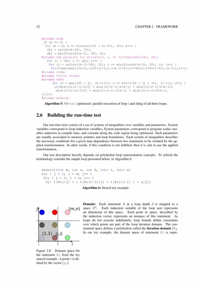
Figure 2.8: Domain space forthe statement S1 from the toystencil example. A point v is de-fined by the vector (j, i)
Domain: Each statement A at a loop depth d is mapped to aspace Zd. Each induction variable of the loop nest representsan dimension of this space. Each point in space, described bythe induction vector, represents an instance of this statement. Asloops do not execute indefinitely, loop bounds define constraintsover which points are part of the loop iteration domain. The con-strained space defines a polyhedron called the iteration domain DA.In our toy example, the domain space of statement S1 is repre-
2.6. BUILDING THE RUN-TIME TEST 33
sented by the gray region in Figure 2.8, defined by the constraints:
j
i
(m,n)
(1,1)
(j',i')(j,i)
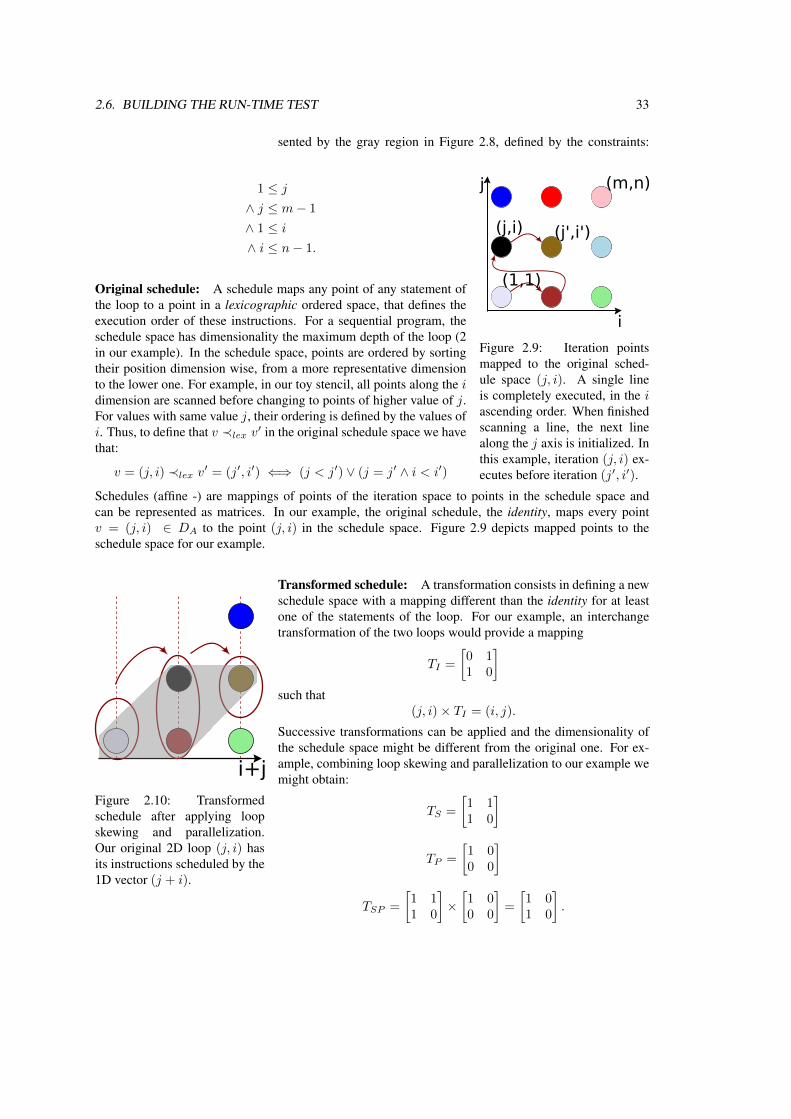
Figure 2.9: Iteration pointsmapped to the original sched-ule space (j, i). A single lineis completely executed, in the iascending order. When finishedscanning a line, the next linealong the j axis is initialized. Inthis example, iteration (j, i) ex-ecutes before iteration (j′, i′).
1 ≤ j∧ j ≤ m− 1
∧ 1 ≤ i∧ i ≤ n− 1.
Original schedule: A schedule maps any point of any statement ofthe loop to a point in a lexicographic ordered space, that defines theexecution order of these instructions. For a sequential program, theschedule space has dimensionality the maximum depth of the loop (2in our example). In the schedule space, points are ordered by sortingtheir position dimension wise, from a more representative dimensionto the lower one. For example, in our toy stencil, all points along the idimension are scanned before changing to points of higher value of j.For values with same value j, their ordering is defined by the values ofi. Thus, to define that v ≺lex v′ in the original schedule space we havethat:
v = (j, i) ≺lex v′ = (j′, i′) ⇐⇒ (j < j′) ∨ (j = j′ ∧ i < i′)
Schedules (affine -) are mappings of points of the iteration space to points in the schedule space andcan be represented as matrices. In our example, the original schedule, the identity, maps every pointv = (j, i) ∈ DA to the point (j, i) in the schedule space. Figure 2.9 depicts mapped points to theschedule space for our example.
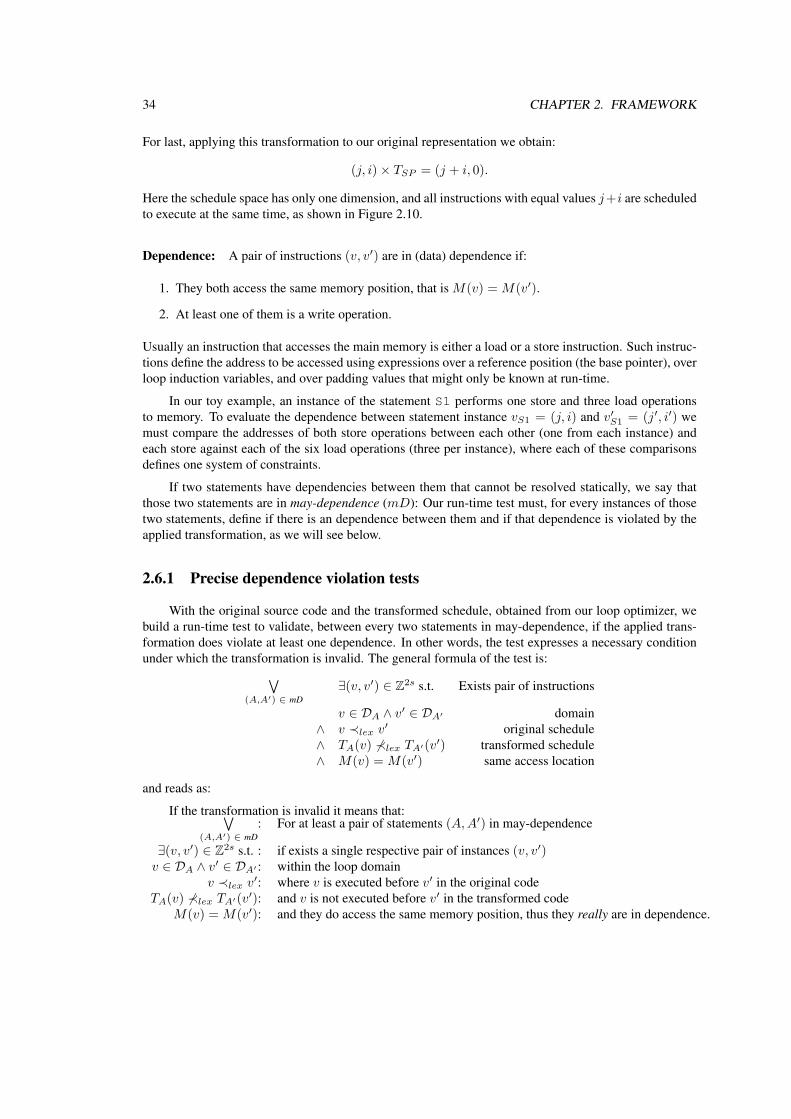
i+jFigure 2.10: Transformedschedule after applying loopskewing and parallelization.Our original 2D loop (j, i) hasits instructions scheduled by the1D vector (j + i).
Transformed schedule: A transformation consists in defining a newschedule space with a mapping different than the identity for at leastone of the statements of the loop. For our example, an interchangetransformation of the two loops would provide a mapping
TI =
[0 11 0
]such that
(j, i)× TI = (i, j).
Successive transformations can be applied and the dimensionality ofthe schedule space might be different from the original one. For ex-ample, combining loop skewing and parallelization to our example wemight obtain:
TS =
[1 11 0
]
TP =
[1 00 0
]
TSP =
[1 11 0
]×[1 00 0
]=
[1 01 0
].
34 CHAPTER 2. FRAMEWORK
For last, applying this transformation to our original representation we obtain:
(j, i)× TSP = (j + i, 0).
Here the schedule space has only one dimension, and all instructions with equal values j+i are scheduledto execute at the same time, as shown in Figure 2.10.
Dependence: A pair of instructions (v, v′) are in (data) dependence if:
1. They both access the same memory position, that is M(v) = M(v′).
2. At least one of them is a write operation.
Usually an instruction that accesses the main memory is either a load or a store instruction. Such instruc-tions define the address to be accessed using expressions over a reference position (the base pointer), overloop induction variables, and over padding values that might only be known at run-time.
In our toy example, an instance of the statement S1 performs one store and three load operationsto memory. To evaluate the dependence between statement instance vS1 = (j, i) and v′S1 = (j′, i′) wemust compare the addresses of both store operations between each other (one from each instance) andeach store against each of the six load operations (three per instance), where each of these comparisonsdefines one system of constraints.
If two statements have dependencies between them that cannot be resolved statically, we say thatthose two statements are in may-dependence (mD): Our run-time test must, for every instances of thosetwo statements, define if there is an dependence between them and if that dependence is violated by theapplied transformation, as we will see below.
2.6.1 Precise dependence violation tests
With the original source code and the transformed schedule, obtained from our loop optimizer, webuild a run-time test to validate, between every two statements in may-dependence, if the applied trans-formation does violate at least one dependence. In other words, the test expresses a necessary conditionunder which the transformation is invalid. The general formula of the test is:∨
(A,A′) ∈ mD∃(v, v′) ∈ Z2s s.t. Exists pair of instructions
v ∈ DA ∧ v′ ∈ DA′ domain∧ v ≺lex v′ original schedule∧ TA(v) 6≺lex TA′(v′) transformed schedule∧ M(v) = M(v′) same access location
and reads as:
If the transformation is invalid it means that:∨(A,A′) ∈ mD
: For at least a pair of statements (A,A′) in may-dependence
∃(v, v′) ∈ Z2s s.t. : if exists a single respective pair of instances (v, v′)v ∈ DA ∧ v′ ∈ DA′ : within the loop domain
v ≺lex v′: where v is executed before v′ in the original codeTA(v) 6≺lex TA′(v′): and v is not executed before v′ in the transformed code
M(v) = M(v′): and they do access the same memory position, thus they really are in dependence.
2.6. BUILDING THE RUN-TIME TEST 35
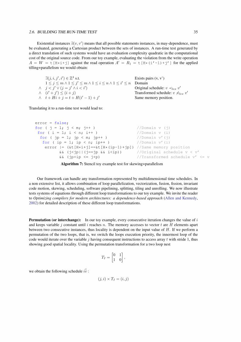
Existential instances ∃(v, v′) means that all possible statements instances, in may-dependence, mustbe evaluated, generating a Cartesian product between the sets of instances. A run-time test generated bya direct translation of such systems would have an evaluation complexity quadratic in the computationalcost of the original source code. From our toy example, evaluating the violation from the write operationA = W = t[H*i+j] against the read operation A′ = R1 = t[H*(i’-1)+j’] for the appliedtilling+parallelism we would obtain:
∃(j, i, j′, i′) ∈ Z4 s.t. Exists pairs (v, v’)1 ≤ j ≤ m ∧ 1 ≤ j′ ≤ m ∧ 1 ≤ i ≤ n ∧ 1 ≤ i′ ≤ n Domain
∧ j < j′ ∨ (j = j′ ∧ i < i′) Original schedule: v ≺lex v′∧ (i′ + j′) ≤ (i+ j) Transformed schedule: v 6≺lex v′∧ t+Hi+ j = t+H(i′ − 1) + j′ Same memory position.
Translating it to a run-time test would lead to:
error = false;for ( j = 1; j < m; j++ ) //Domain v (j)for ( i = 1; i < n; i++ ) //Domain v (i)for ( jp = 1; jp < m; jp++ ) //Domain v’(j)for ( ip = 1; ip < n; ip++ ) //Domain v’(i)error |= (&t[H*i+j]==&t[H*(ip-1)+jp]) //Same memory position
&& (j<jp||(j==jp && i<ip)) //Original schedule v < v’&& (jp+ip <= j+p) //Transformed schedule v’ <= v
Algorithm 7: Stencil toy example test for skewing+parallelism
Our framework can handle any transformation represented by multidimensional time schedules. Ina non extensive list, it allows combination of loop parallelization, vectorization, fusion, fission, invariantcode motion, skewing, scheduling, software pipelining, splitting, tiling and unrolling. We now illustratetests systems of equations through different loop transformations to our toy example. We invite the readerto Optimizing compilers for modern architectures: a dependence-based approach (Allen and Kennedy,2002) for detailed description of these different loop transformations.
Permutation (or interchange): In our toy example, every consecutive iteration changes the value of iand keeps variable j constant until i reaches n. The memory accesses to vector t are H elements apartbetween two consecutive instances, thus locality is dependent on the input value of H . If we perform apermutation of the two loops, that is, we switch the loops execution priority, the innermost loop of thecode would iterate over the variable j having consequent instructions to access array t with stride 1, thusshowing good spatial locality. Using the permutation transformation for a two loop nest
TI =
[0 11 0
],
we obtain the following schedule ~iv :
(j, i)× TI = (i, j)
36 CHAPTER 2. FRAMEWORK
For accesses W and R1, our test becomes:
∃(j, i, j′, i′) ∈ Z4 s.t.1 ≤ j ≤ m ∧ 1 ≤ j′ ≤ m ∧ 1 ≤ i ≤ n ∧ 1 ≤ i′ ≤ n
∧ j < j′ ∨ (j = j′ ∧ i < i′)∧ ¬(i < i′ ∨ (i = i′ ∧ j ≤ j′))∧ t+Hi+ j = t+H(i′ − 1) + j′
Skewing: In our toy example, every consecutive iteration along the i axis depends on the iterationbefore and every consecutive iteration along j axis also depends on its iteration before: in other words(i, j) depends on (i−1, j) and (i, j−1). Such dependence configuration forbids executing either of theseloops in parallel. However, skewing the j axis to the i positive direction, described by the transformation
TS =
[1 10 1
],
our obtained schedule holds(j, i)× TS = (j, j + i)
Such transformation would allow all points with a same (j+ i) value to be executed in parallel. Obtainedschedule would become D : (j, i) → (j + i). For accesses W and R1, our test for such transformationbecomes:
∃(j, i, j′, i′) ∈ Z4 s.t.1 ≤ j ≤ m ∧ 1 ≤ j′ ≤ m ∧ 1 ≤ i ≤ n ∧ 1 ≤ i′ ≤ n
∧ j < j′ ∨ (j = j′ ∧ i < i′)∧ ¬(j < j′ ∨ (j = j′ ∧ j + i < j′ + i′))∧ t+Hi+ j = t+H(i′ − 1) + j′.
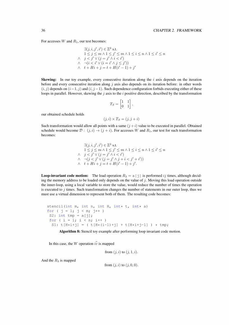
Loop-invariant code motion: The load operation R3 = a[j] is performed ij times, although decid-ing the memory address to be loaded only depends on the value of j. Moving this load operation outsidethe inner-loop, using a local variable to store the value, would reduce the number of times the operationis executed to j times. Such transformation changes the number of statements in our outer loop, thus wemust use a virtual dimension to represent both of them. The resulting code becomes:
stencil(int m, int n, int H, int* t, int* a)for ( j = 1; j < m; j++ )S2: int tmp = a[j];for ( i = 1; i < n; i++ )S1: t[H*i+j] = ( t[H*(i-1)+j] + t[H*i+j-1] ) * tmp;
Algorithm 8: Stencil toy example after performing loop invariant code motion.
In this case, the W operation ~iv is mapped
from (j, i) to (j, 1, i).
And the R3 is mappedfrom (j, i) to (j, 0, 0).
2.7. SIMPLIFYING THE GENERATED TEST 37
The test to detect broken dependencies writes as:
∃(j, i, j′, i′) ∈ Z4 s.t.1 ≤ j ≤ m ∧ 1 ≤ j′ ≤ m ∧ 1 ≤ i ≤ n ∧ 1 ≤ i′ ≤ n
∧ j < j′ ∨ (j = j′ ∧ i < i′)∧ ¬(j < j′)∧ t+Hi+ j = a+ j′.
Each system S of constraints describes violation conditions between a pair of statements in may-alias. Each one of these systems is transformed to a disjunction of conjunctive systems describing allconditions for which at least one dependence is violated. Each of these systems describe required andsufficient conditions to detect dependence violation, meaning that, if a system evaluates to true for agiven input, then there is at least one dependence violation and the optimization is incorrect. If all systemsevaluates to false, then there are no violations, and the optimized code can be safely used.
The next section describes how quantifier elimination is used to reduce our run-time test evaluationcosts, reducing from O(n2), where n is the number of iterations of our loop, to a O(1) test. Suchsimplification produces systems that define required conditions for a dependence violation.
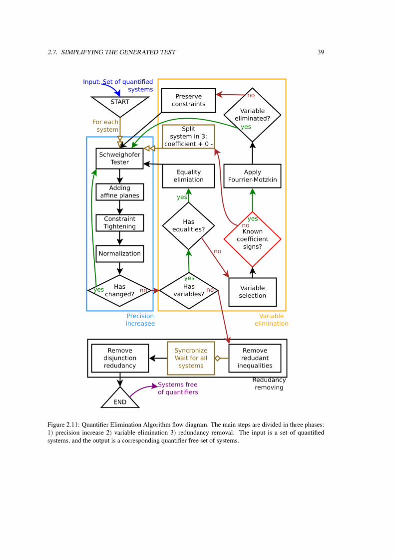
2.7 Simplifying the generated test
In our generated run-time tests, quantified variables require loops to explore all their possible values.Eliminating these quantifiers eliminates the need for loops, providing a massive gain in the run-time checkspeed. We developed a QEA that extends the FME technique. The first step to use FME requires oursystems to be in conjunctive form, that is, we rewrite our test as a disjunction of conjunctive systems,given by the formula:
S0 ∨ S1 ∨ S2 · · ·Sn−1 ∨ Snwhere each system Si is in a conjunctive form of inequality constraints given by the formula
Si = {E0 ≥ 0 ∧ E1 ≥ 0 ∧ E2 ≥ 0 · · ·Em−1 ≥ 0 ∧ Em ≥ 0}
The FME process was developed to be used with linear systems of constraints in R. Our systemshold multivariate polynomials over Z, thus we face three difficulties: First, FME requires to determinecoefficient signs of the variables being eliminated. Retrieving the sign of symbolic coefficient expressionsis not a trivial task. The second problem rises from the fact that constraint limits on reals are looser than onintegers. Loose limits generate rounding errors that accumulate at every step when eliminating variables.In practice obtained system using QEA on reals is usually so loose that the generated test forbids tochose the otherwise valid optimizing transformation. The third problem rises from the fact that FME wasdeveloped to be used with linear systems of inequalities. When applied over linear systems, every iterationof FME eliminates one quantifier. Our polynomial implementation might not eliminate a quantifier at agiven step, if it would also be present in it’s own coefficient. Naively eliminating constraints of lowerdegrees might generate unbounded variables leading to precision loss.
To tackle the first problem, our QEA depends on a positiveness expression test (which we call asSchweighofer tester), based on (Schweighofer, 2002, theorem 5). The Schweighofer tester is capableto determine if a given system of non-negative inequality constraints implies the positiveness of anotherexpression. The Schweighofer tester is the core of our QEA and is used to detect variables coefficientsigns, so that inequalities can be correctly positioned as lower or upper bounds for a the variable beingeliminated. It also allows to decide correlations between expressions such that normalization (Pugh,
38 CHAPTER 2. FRAMEWORK
1991) techniques can be applied, removing rounding errors due to loose system boundaries. For last, weimplement our FME in such a form that when a quantifier is not eliminated in a step of FME, we preserveconstraints on that variable in a manner that we prevent unbounded variables.
Our proposed QEA processes each disjunctive system separately, eliminating variables and furtherremoving redundant constraints generated by the FME process. Eventually, when all systems have beenindividually processes, the Schweighofer tester is again used to, between the resulting systems, eliminatethose that impose redundant constraints. Our QEA for each system is divided in three main steps:
• Increase precision: During this process the Schweighofer tester is built for the given system.Constraints are tightened whenever possible. If new affine constraints can be detected, they areadded to the system.
• Variable elimination: Say a quantified variable x is selected for elimination. If it is possible todetermine the coefficient sign of x in every inequality of the system, then the standard FME stepis applied. If not possible to determine the coefficient c of one of the inequality (say cx ≥ 0), thesystem S is split into three systems, such that
S → Sc≥1 ∨ Sc=0 ∨ Sc≤−1,
one where c ≥ 1, one where c = 0 and another where c ≤ −1. The three new systems are insertedto the conjunction of all other systems and processed individually.
• Redundancy removal: Once all variables of the simplified system S′i have been eliminated, theSchweighofer tester is used to detect, withing S′i, redundant constraints, where the least constrain-ing ones are removed. Hence, once all n systems of
S0 ∨ S1 ∨ S2 · · ·Sn−1 ∨ Sn
have been individual processed, generating
S′0 ∨ S′1 ∨ S′2 · · ·S′m−1 ∨ S′msimplified systems, the Schweighofer tester is again used to detect if
S′i =⇒ S′j ,
removing S′i as it defines a subspace of S′j .
We now describe the most important components of our QEA. For further technical details pleaserefer to §5.
2.7.1 Precision increase
Schweighofer tester
The first component of the proposed QEA is the Schweighofer tester, a tool used in almost everyother procedure for different means, such as removing redundant constraints and redundant systems, de-termining expressions signs or expressions relationships. The core of this utility is the algorithm describedby Schweighofer 2 to evaluate expressions signs under a system of constraints. The basic concept of it isthe following: Given a system of inequalities
S = {E1 ≥ 0, E2 ≥ 0 . . . En ≥ 0},2 We actually use the technique in a more general context where we do not enforce variables to live in a compact polytope.
2.7. SIMPLIFYING THE GENERATED TEST 39
Addingaffine planes
Equalityelimiation
Hasequalities?
Hasvariables?
Removedisjunctionredudancy
START
END
For eachsystem
Input: Set of quantifiedsystems
ConstraintTightening
Haschanged?
SchweighoferTester
yes
Precisionincreasee
no
yes
yes
Variableselection
Knowncoefficient
signs?
no
ApplyFourrier-Motzkin
Removeredudant
inequalities
SyncronizeWait for allsystems
Systems freeof quantifiers
Variableeliminated?
noPreserveconstraints
Splitsystem in 3:
coefficient + 0 -
yes
yes
no
Variableelimination
Normalization
Redudancyremoving
no
Figure 2.11: Quantifier Elimination Algorithm flow diagram. The main steps are divided in three phases:1) precision increase 2) variable elimination 3) redundancy removal. The input is a set of quantifiedsystems, and the output is a corresponding quantifier free set of systems.
40 CHAPTER 2. FRAMEWORK
Schweighofer provides an algorithm to evaluate if
S =⇒ E ≥ 0.
If E can be written as the sum of the product of any power of the inequalities of S multiplied by non-negative factors, then S implies E ≥ 0, that is
E =∑
αi · Ei where αi ≥ 0, Ei ∈ SD, D ∈ Z∗.
However, applying such algorithm requires to solve a linear system of constraints with size expo-nential in the size of the expression |S|D, where D is the maximum exponent S is raised to and |S| isthe cardinality of S. To tackle this exponential evaluation growth we empirically limited the maximumvalue of D. Instead of raising the entire system S to the power D, obtaining |S|D expressions, we usesubset constraints S′ ⊂ S, and we evaluate if any S′D can be used to prove if S′ =⇒ E ≥ 0. We alsoperform expressions pattern matching to quickly detect obvious signs, such as positive powers that arealways non-negative. We also perform expressions factorization and operator recursion to handle biggerexpressions, as detailed in §5.
Adding affine planes
The cost of the Schweighofer tester algorithm grows with |S|D, where |S| is the number of inequali-ties in the system and D the maximum power we raise the system. Due its exponential behavior, we limitthe maximum value D used to 2 or 3, depending on the number of constraints of S. Further, instead ofcombining all constraints of S to try to write the inequality we use distinct subsets S′ ⊂ S, limiting thenumber of constraints of S′ to four inequalities. To evaluate if S =⇒ E ≥ 0 we evaluate if any of thesubsets S′ =⇒ E ≥ 0.
Such limitations highly limits the capacity of the Schweighofer tester, as it is restricted to onlyconsider a small set of inequalities at a time. To bypass this limitation a set of simple affine constraints(of the form ±i ± j ≤ c), that the Schweighofer tester can prove to be implied by the system, is addedto the system. Enriching the system allows to generate more subsystems S′, thus increasing the capacityto write more expressions. The decision of increasing the number of constraints, over increasing themaximum exponent is a consequence of empirical observations:
1. Most observed systems have polynomials of absolute degree lower or equals to 3: Raising S to ahigh degree usually generates many unused inequalities.
2. Adding simple constraints, that are affine and are made up of one or two variables, allows thecreation of almost all monomials up to an absolute degree of 4, when D is limited to 3.
For our use cases, it was observed that, the increased capacity of the Schweighofer tester for provingexpressions signs reduced the overall execution time of the QEA. This is due to the fact that, as describedin §2.7.2, when the coefficient of a variable being eliminated is unknown, the system resolution is splitinto the resolution of three systems, identical to the original one, but each with an additional constraintthat defined the sign of the unknown coefficient. Improving the capacity of detecting signs also increasedthe quality of the final generated test.
Constraint tightening
This step relies on the Schweighofer tester to detect loose constraints and moves them to a positioncloser to the system boundaries. Reasoning geometrically, each inequality constraint (En ≥ 0) ∈ S
2.7. SIMPLIFYING THE GENERATED TEST 41
defines a plane, or curve, dividing the space and limiting the system boundaries. If a plane is not touchingthe convex-hull formed by the remaining constraints it is considered loose. When the Schweighofer testerproves that a constraint is implied by other constraints of S, it also determines how loose this constraintis. In fact it gives a distance that can be used to displace this inequality without changing the set definedby the system. As discussed in more details in §5, the “distance” returned by the Schweighofer testeris not necessarily the maximum possible one (the tester should be expressed as a more costly linearprogramming problem, which is not the case in our implementation). As illustrated here, to circumventthis limitation, Schweighofer tester is heuristically invoked with a more constraining test.
In our implementation, verifying if
S =⇒ En ≥ 0 where [En ≥ 0] ∈ S
will always detect that the distance of this plane has to the convex-hull is zero. To circumvent thisproblem, we request the Schweighofer tester to verify if
S =⇒ En − 1 ≥ 0,
that is, if S implies a more constraining boundary. To exemplify this technique, let
S = {x+ 1 ≥ 0 ∧ 2x− 6 ≥ 0},
where the first constraint is implied by the second. If the Schweighofer tester is requested to test if
S =⇒ x+ 1 ≥ 0,
it will respond with yes, by returning
x+ 1 = 1 ∗ (x+ 1) + 0,
using the first found inequality. However, if requested to verify if
S =⇒ x ≥ 0,
it would also say yes, but using the second inequality, returning
x = 0.5 ∗ (2x− 6) + 3. 3
This results describes that the system implies x−3 ≥ 0. As a consequence, this last inequality can safelyreplace the original x+ 1 ≥ 0 in the system.
Normalization
When using FME, we are manipulating integer constraints using reals algebra. As Z ⊂ R, con-straints that do not define integer limits might be a source of precision loss. If this error is to high, itcan generate a projection that represent a much bigger space than the actual one, generating quantifierfree tests that never allow the use of the desired transformation. To understand the source of these errors,consider the following example:
i ≤ 100t ≤ 100j − 1.
The elimination of t, as explained below in §2.7.2, would lead to
i ≤ 100j − 1.
3Observe that our systems being in Z do not restrain the Schweighofer tester to obtain only integer coefficients.
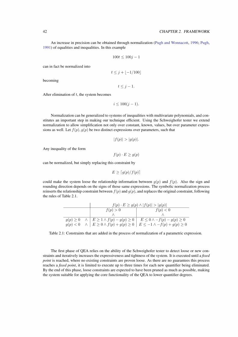
42 CHAPTER 2. FRAMEWORK
An increase in precision can be obtained through normalization (Pugh and Wonnacott, 1996; Pugh,1991) of equalities and inequalities. In this example
100t ≤ 100j − 1
can in fact be normalized intot ≤ j + b−1/100c
becomingt ≤ j − 1.
After elimination of t, the system becomes
i ≤ 100(j − 1).
Normalization can be generalized to systems of inequalities with multivariate polynomials, and con-stitutes an important step in making our technique efficient. Using the Schweighofer tester we extendnormalization to allow simplification not only over constant, known, values, but over parameter expres-sions as well. Let f(p), g(p) be two distinct expressions over parameters, such that
|f(p)| > |g(p)|.
Any inequality of the formf(p) · E ≥ g(p)
can be normalized, but simply replacing this constraint by
E ≥ dg(p)/f(p)e
could make the system loose the relationship information between g(p) and f(p). Also the sign androunding direction depends on the signs of those same expressions. The symbolic normalization processreinserts the relationship constraint between f(p) and g(p), and replaces the original constraint, followingthe rules of Table 2.1.
f(p) · E ≥ g(p) ∧ |f(p)| > |g(p)|f(p) > 0 f(p) < 0∧ ∧
g(p) ≥ 0 ∧ E ≥ 1 ∧ f(p)− g(p) ≥ 0 E ≤ 0 ∧ −f(p)− g(p) ≥ 0g(p) < 0 ∧ E ≥ 0 ∧ f(p) + g(p) ≥ 0 E ≤ −1 ∧ −f(p) + g(p) ≥ 0
Table 2.1: Constraints that are added in the process of normalization of a parametric expression.
The first phase of QEA relies on the ability of the Schweighofer tester to detect loose or new con-straints and iteratively increases the expressiveness and tightness of the system. It is executed until a fixedpoint is reached, where no existing constraints are proven loose. As there are no guarantees this processreaches a fixed point, it is limited to execute up to three times for each new quantifier being eliminated.By the end of this phase, loose constraints are expected to have been pruned as much as possible, makingthe system suitable for applying the core functionality of the QEA to lower quantifier degrees.
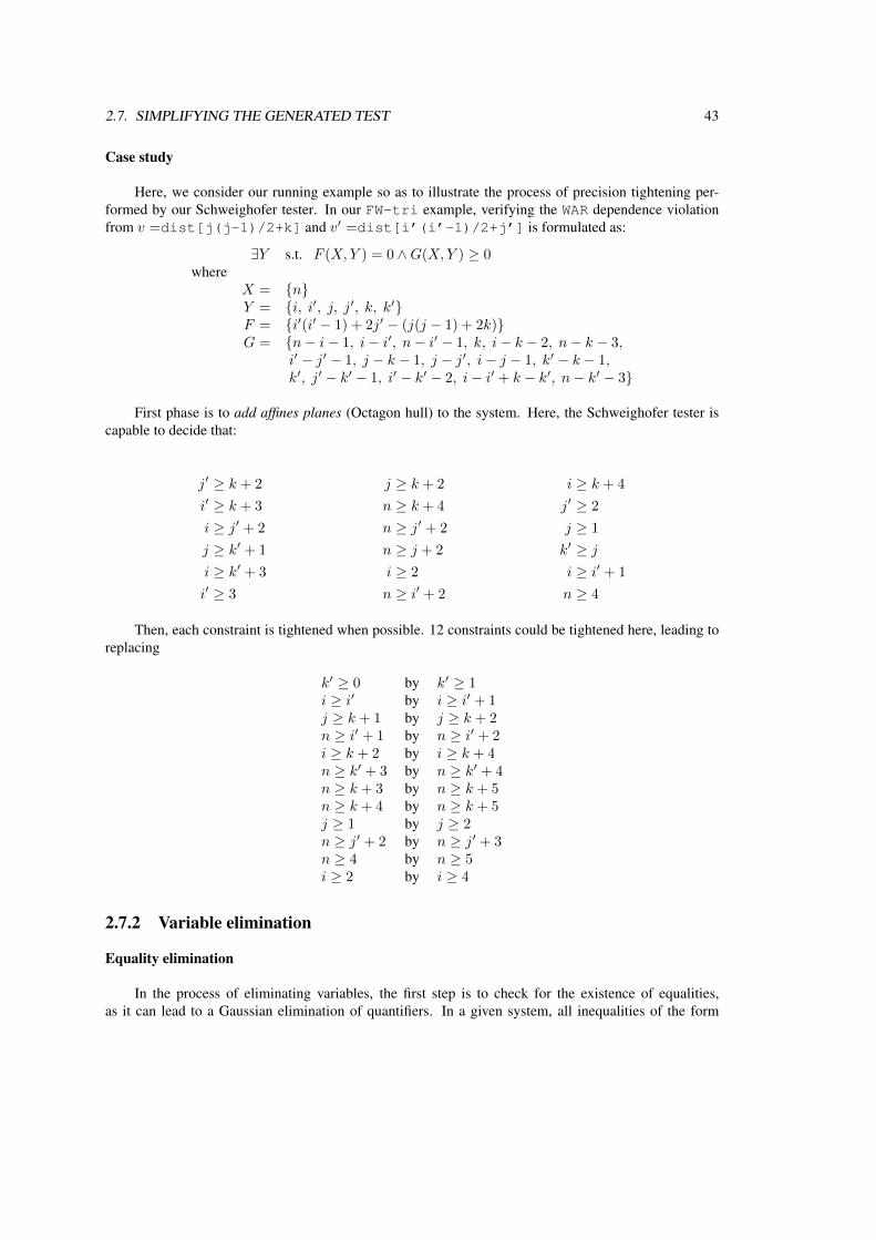
2.7. SIMPLIFYING THE GENERATED TEST 43
Case study
Here, we consider our running example so as to illustrate the process of precision tightening per-formed by our Schweighofer tester. In our FW-tri example, verifying the WAR dependence violationfrom v =dist[j(j-1)/2+k] and v′ =dist[i’(i’-1)/2+j’] is formulated as:
∃Y s.t. F (X,Y ) = 0 ∧G(X,Y ) ≥ 0where
X = {n}Y = {i, i′, j, j′, k, k′}F = {i′(i′ − 1) + 2j′ − (j(j − 1) + 2k)}G = {n− i− 1, i− i′, n− i′ − 1, k, i− k − 2, n− k − 3,
i′ − j′ − 1, j − k − 1, j − j′, i− j − 1, k′ − k − 1,k′, j′ − k′ − 1, i′ − k′ − 2, i− i′ + k − k′, n− k′ − 3}
First phase is to add affines planes (Octagon hull) to the system. Here, the Schweighofer tester iscapable to decide that:
j′ ≥ k + 2 j ≥ k + 2 i ≥ k + 4
i′ ≥ k + 3 n ≥ k + 4 j′ ≥ 2
i ≥ j′ + 2 n ≥ j′ + 2 j ≥ 1
j ≥ k′ + 1 n ≥ j + 2 k′ ≥ ji ≥ k′ + 3 i ≥ 2 i ≥ i′ + 1
i′ ≥ 3 n ≥ i′ + 2 n ≥ 4
Then, each constraint is tightened when possible. 12 constraints could be tightened here, leading toreplacing
k′ ≥ 0 by k′ ≥ 1i ≥ i′ by i ≥ i′ + 1j ≥ k + 1 by j ≥ k + 2n ≥ i′ + 1 by n ≥ i′ + 2i ≥ k + 2 by i ≥ k + 4n ≥ k′ + 3 by n ≥ k′ + 4n ≥ k + 3 by n ≥ k + 5n ≥ k + 4 by n ≥ k + 5j ≥ 1 by j ≥ 2n ≥ j′ + 2 by n ≥ j′ + 3n ≥ 4 by n ≥ 5i ≥ 2 by i ≥ 4
2.7.2 Variable elimination
Equality elimination
In the process of eliminating variables, the first step is to check for the existence of equalities,as it can lead to a Gaussian elimination of quantifiers. In a given system, all inequalities of the form
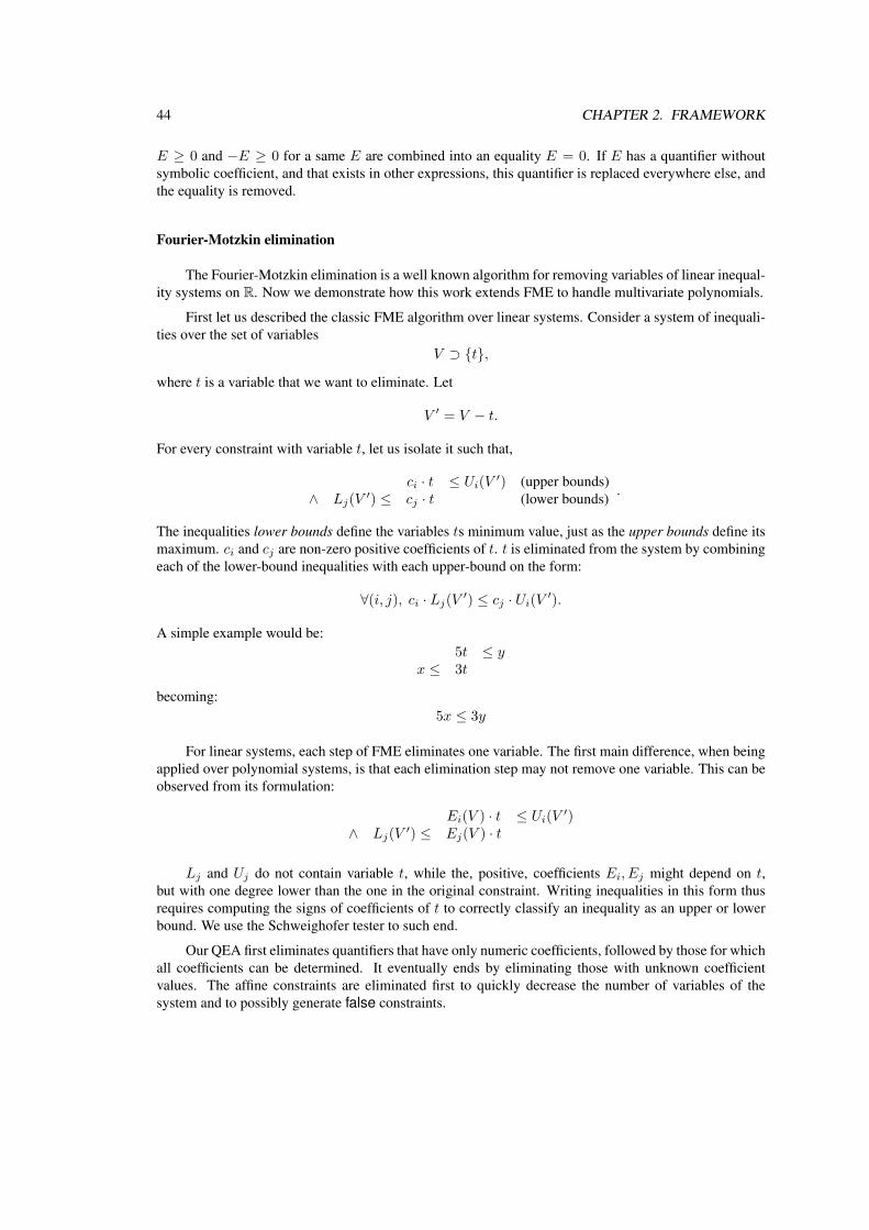
44 CHAPTER 2. FRAMEWORK
E ≥ 0 and −E ≥ 0 for a same E are combined into an equality E = 0. If E has a quantifier withoutsymbolic coefficient, and that exists in other expressions, this quantifier is replaced everywhere else, andthe equality is removed.
Fourier-Motzkin elimination
The Fourier-Motzkin elimination is a well known algorithm for removing variables of linear inequal-ity systems on R. Now we demonstrate how this work extends FME to handle multivariate polynomials.
First let us described the classic FME algorithm over linear systems. Consider a system of inequali-ties over the set of variables
V ⊃ {t},
where t is a variable that we want to eliminate. Let
V ′ = V − t.
For every constraint with variable t, let us isolate it such that,
ci · t ≤ Ui(V ′) (upper bounds)∧ Lj(V
′) ≤ cj · t (lower bounds) .
The inequalities lower bounds define the variables ts minimum value, just as the upper bounds define itsmaximum. ci and cj are non-zero positive coefficients of t. t is eliminated from the system by combiningeach of the lower-bound inequalities with each upper-bound on the form:
∀(i, j), ci · Lj(V ′) ≤ cj · Ui(V ′).
A simple example would be:5t ≤ y
x ≤ 3t
becoming:5x ≤ 3y
For linear systems, each step of FME eliminates one variable. The first main difference, when beingapplied over polynomial systems, is that each elimination step may not remove one variable. This can beobserved from its formulation:
Ei(V ) · t ≤ Ui(V ′)∧ Lj(V
′) ≤ Ej(V ) · t
Lj and Uj do not contain variable t, while the, positive, coefficients Ei, Ej might depend on t,but with one degree lower than the one in the original constraint. Writing inequalities in this form thusrequires computing the signs of coefficients of t to correctly classify an inequality as an upper or lowerbound. We use the Schweighofer tester to such end.
Our QEA first eliminates quantifiers that have only numeric coefficients, followed by those for whichall coefficients can be determined. It eventually ends by eliminating those with unknown coefficientvalues. The affine constraints are eliminated first to quickly decrease the number of variables of thesystem and to possibly generate false constraints.
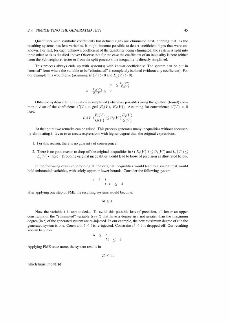
2.7. SIMPLIFYING THE GENERATED TEST 45
Quantifiers with symbolic coefficients but defined signs are eliminated next, hopping that, as theresulting systems has less variables, it might become possible to detect coefficient signs that were un-known. For last, for each unknown coefficient of the quantifier being eliminated, the system is split intothree other ones as detailed above: Observe that for the case the coefficient of an inequality is zero (eitherfrom the Schweighofer tester or from the split process), the inequality is directly simplified.
This process always ends up with system(s) with known coefficients: The system can be put in“normal” form where the variable to be “eliminated” is completely isolated (without any coefficient). Forour example this would give (assuming Ei(V ) > 0 and Ej(V ) > 0):
t ≤ Ui(V′)
Ei(V )
∧ Lj(V′)
Ej(V ) ≤ t
Obtained system after elimination is simplified (whenever possible) using the greatest (found) com-mon divisor of the coefficients G(V ) = gcd (Ei(V ), Ej(V )). Assuming for convenience G(V ) > 0here:
Lj(V′)Ei(V )
G(V )≤ Ui(V ′)
Ej(V )
G(V )
At that point two remarks can be raised. This process generates many inequalities without necessar-ily eliminating t. It can even create expressions with higher degree than the original expressions.
1. For this reason, there is no guaranty of convergence.
2. There is no good reason to drop-off the original inequalities in t (Ei(V )·t ≤ Ui(V ′) and Lj(V ′) ≤Ej(V ) ·t here). Dropping original inequalities would lead to loose of precision as illustrated below.
In the following example, dropping all the original inequalities would lead to a system that wouldhold unbounded variables, with solely upper or lower bounds. Consider the following system:
5 ≤ tt · t ≤ 4
after applying one step of FME the resulting systems would become:
5t ≤ 4.
Now the variable t is unbounded... To avoid this possible loss of precision, all lower an upperconstraints of the “eliminated” variable (say t) that have a degree in t not greater than the maximumdegree (in t) of the generated system are re-injected. In our example, the new maximum degree of t in thegenerated system is one. Constraint 5 ≤ t is re-injected. Constraint t2 ≤ 4 is dropped-off. Our resultingsystem becomes
5 ≤ t5t ≤ 4.
Applying FME once more, the system results in
25 ≤ 4,
which turns into false.
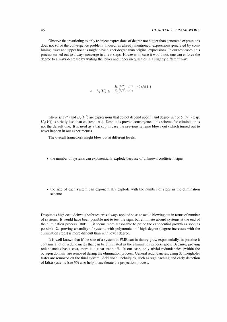
46 CHAPTER 2. FRAMEWORK
Observe that restricting to only re-inject expressions of degree not bigger than generated expressionsdoes not solve the convergence problem. Indeed, as already mentioned, expressions generated by com-bining lower and upper bounds might have higher degree than original expressions. In our test cases, thisprocess turned out to always converge in a few steps. However, in case it would not, one can enforce thedegree to always decrease by writing the lower and upper inequalities in a slightly different way:
Ei(V′) · tαi ≤ Ui(V )
∧ Lj(V ) ≤ Ej(V′) · tαj
whereEi(V ′) andEj(V ′) are expressions that do not depend upon t, and degree in t of Ui(V ) (resp.Uj(V )) is strictly less than αi (resp. αj). Despite is proven convergence, this scheme for elimination isnot the default one. It is used as a backup in case the previous scheme blows out (which turned out tonever happen in our experiments).
The overall framework might blow out at different levels:
• the number of systems can exponentially explode because of unknown coefficient signs
• the size of each system can exponentially explode with the number of steps in the eliminationscheme
Despite its high cost, Schweighofer tester is always applied so as to avoid blowing out in terms of numberof systems. It would have been possible not to test the sign, but eliminate absurd systems at the end ofthe elimination process. But: 1. it seems more reasonable to prune the exponential growth as soon aspossible; 2. proving absurdity of systems with polynomials of high degree (degree increases with theelimination steps) is more difficult than with lower degree.
It is well known that if the size of a system in FME can in theory grow exponentially, in practice itcontains a lot of redundancies that can be eliminated as the elimination process goes. Because, provingredundancies has a cost, there is a clear trade-off. In our case, only trivial redundancies (within theoctagon domain) are removed during the elimination process. General redundancies, using Schweighofertester are removed on the final system. Additional techniques, such as sign caching and early detectionof false systems (see §5) also help to accelerate the projection process.
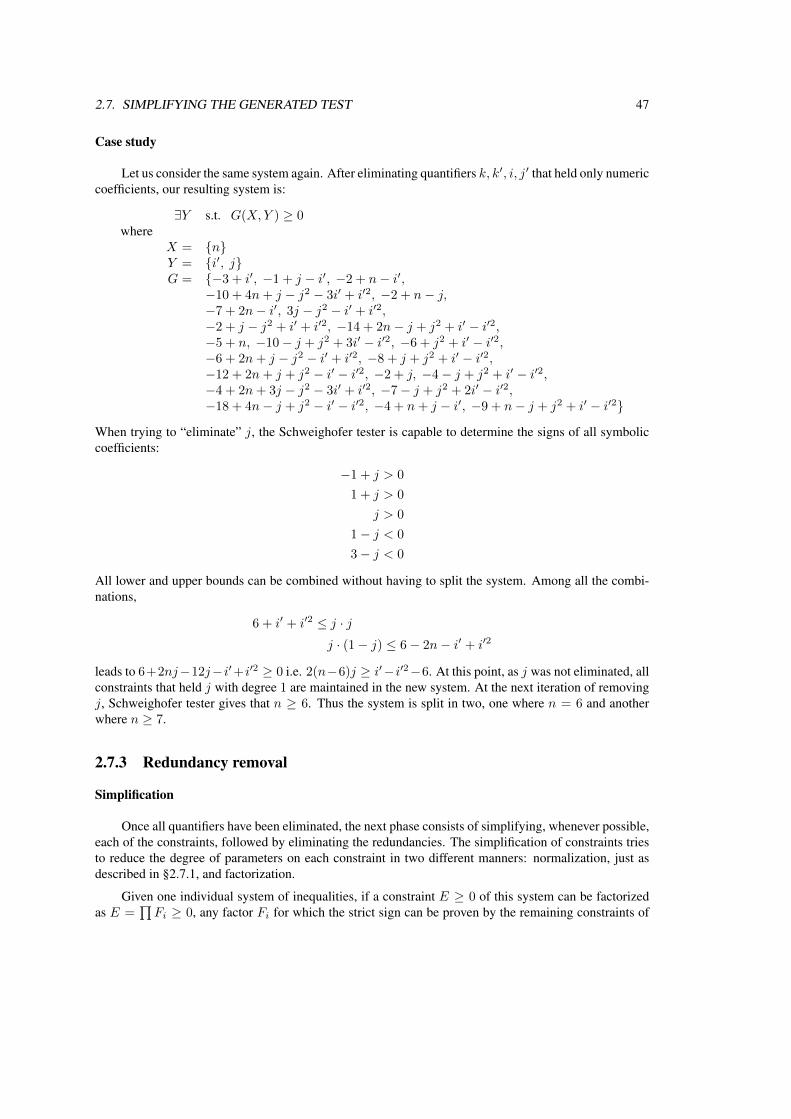
2.7. SIMPLIFYING THE GENERATED TEST 47
Case study
Let us consider the same system again. After eliminating quantifiers k, k′, i, j′ that held only numericcoefficients, our resulting system is:
∃Y s.t. G(X,Y ) ≥ 0where
X = {n}Y = {i′, j}G = {−3 + i′, −1 + j − i′, −2 + n− i′,
−10 + 4n+ j − j2 − 3i′ + i′2, −2 + n− j,−7 + 2n− i′, 3j − j2 − i′ + i′2,−2 + j − j2 + i′ + i′2, −14 + 2n− j + j2 + i′ − i′2,−5 + n, −10− j + j2 + 3i′ − i′2, −6 + j2 + i′ − i′2,−6 + 2n+ j − j2 − i′ + i′2, −8 + j + j2 + i′ − i′2,−12 + 2n+ j + j2 − i′ − i′2, −2 + j, −4− j + j2 + i′ − i′2,−4 + 2n+ 3j − j2 − 3i′ + i′2, −7− j + j2 + 2i′ − i′2,−18 + 4n− j + j2 − i′ − i′2, −4 + n+ j − i′, −9 + n− j + j2 + i′ − i′2}
When trying to “eliminate” j, the Schweighofer tester is capable to determine the signs of all symboliccoefficients:
−1 + j > 0
1 + j > 0
j > 0
1− j < 0
3− j < 0
All lower and upper bounds can be combined without having to split the system. Among all the combi-nations,
6 + i′ + i′2 ≤ j · jj · (1− j) ≤ 6− 2n− i′ + i′2
leads to 6+2nj−12j−i′+i′2 ≥ 0 i.e. 2(n−6)j ≥ i′−i′2−6. At this point, as j was not eliminated, allconstraints that held j with degree 1 are maintained in the new system. At the next iteration of removingj, Schweighofer tester gives that n ≥ 6. Thus the system is split in two, one where n = 6 and anotherwhere n ≥ 7.
2.7.3 Redundancy removal
Simplification
Once all quantifiers have been eliminated, the next phase consists of simplifying, whenever possible,each of the constraints, followed by eliminating the redundancies. The simplification of constraints triesto reduce the degree of parameters on each constraint in two different manners: normalization, just asdescribed in §2.7.1, and factorization.
Given one individual system of inequalities, if a constraint E ≥ 0 of this system can be factorizedas E =
∏Fi ≥ 0, any factor Fi for which the strict sign can be proven by the remaining constraints of
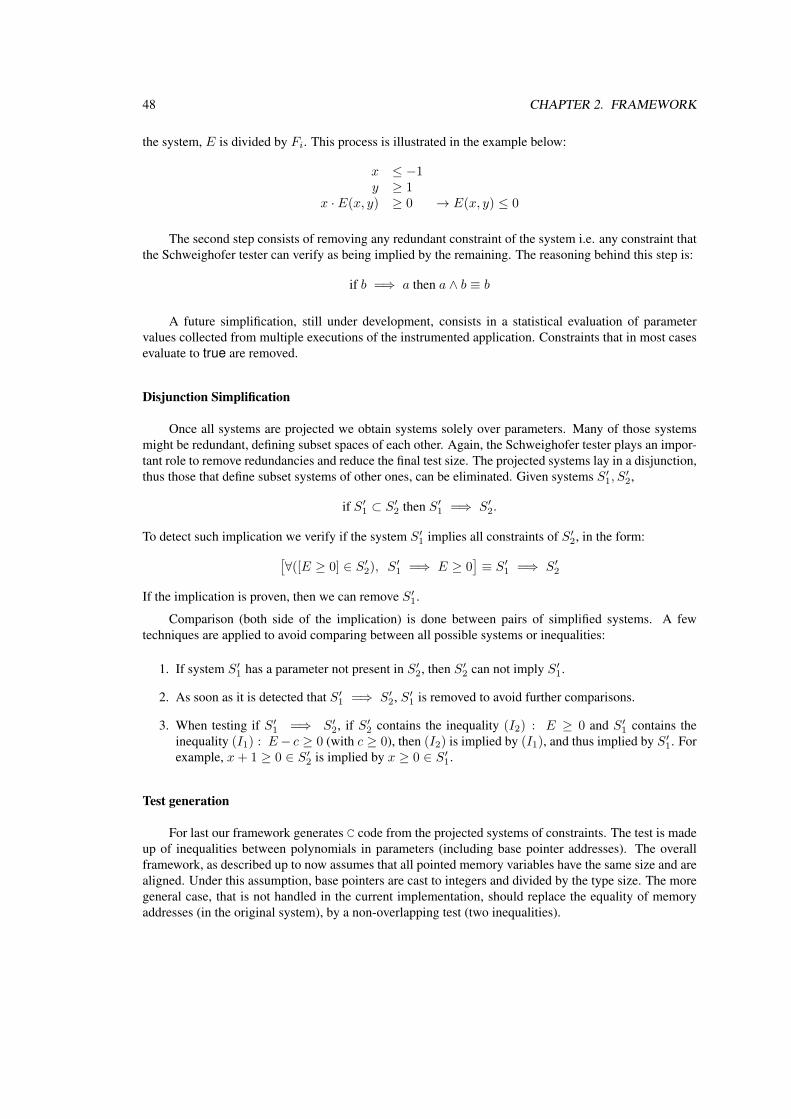
48 CHAPTER 2. FRAMEWORK
the system, E is divided by Fi. This process is illustrated in the example below:
x ≤ −1y ≥ 1
x · E(x, y) ≥ 0 → E(x, y) ≤ 0
The second step consists of removing any redundant constraint of the system i.e. any constraint thatthe Schweighofer tester can verify as being implied by the remaining. The reasoning behind this step is:
if b =⇒ a then a ∧ b ≡ b
A future simplification, still under development, consists in a statistical evaluation of parametervalues collected from multiple executions of the instrumented application. Constraints that in most casesevaluate to true are removed.
Disjunction Simplification
Once all systems are projected we obtain systems solely over parameters. Many of those systemsmight be redundant, defining subset spaces of each other. Again, the Schweighofer tester plays an impor-tant role to remove redundancies and reduce the final test size. The projected systems lay in a disjunction,thus those that define subset systems of other ones, can be eliminated. Given systems S′1, S
′2,
if S′1 ⊂ S′2 then S′1 =⇒ S′2.
To detect such implication we verify if the system S′1 implies all constraints of S′2, in the form:[∀([E ≥ 0] ∈ S′2), S′1 =⇒ E ≥ 0
]≡ S′1 =⇒ S′2
If the implication is proven, then we can remove S′1.
Comparison (both side of the implication) is done between pairs of simplified systems. A fewtechniques are applied to avoid comparing between all possible systems or inequalities:
1. If system S′1 has a parameter not present in S′2, then S′2 can not imply S′1.
2. As soon as it is detected that S′1 =⇒ S′2, S′1 is removed to avoid further comparisons.
3. When testing if S′1 =⇒ S′2, if S′2 contains the inequality (I2) : E ≥ 0 and S′1 contains theinequality (I1) : E− c ≥ 0 (with c ≥ 0), then (I2) is implied by (I1), and thus implied by S′1. Forexample, x+ 1 ≥ 0 ∈ S′2 is implied by x ≥ 0 ∈ S′1.
Test generation
For last our framework generates C code from the projected systems of constraints. The test is madeup of inequalities between polynomials in parameters (including base pointer addresses). The overallframework, as described up to now assumes that all pointed memory variables have the same size and arealigned. Under this assumption, base pointers are cast to integers and divided by the type size. The moregeneral case, that is not handled in the current implementation, should replace the equality of memoryaddresses (in the original system), by a non-overlapping test (two inequalities).
2.8. CURRENT STATE 49
2.8 Current state
The different components of the tool chain were developed in parallel as proofs of concept proto-types, were we experimented: 1. different techniques to overcome precision loss, and processing costs ofthe quantifier elimination technique. 2. trace analysis and compression in the instrumentation and profil-ing part. The current state of the framework is still far from being user friendly or applicable to generalloops as we intend it to be. The future work section in §7 describes what must be currently addressedsuch that our tools can be used by the public.
2.9 Summary
The proposed framework does not develop new transformations to better optimize loops, but extendsthe number of loops that can be safely optimized by existing compiler tools. Formally, our frameworkallows complex loop transformations even in the presence of may-dependencies. May-dependenciesappear from the presence of memory accesses with polynomial expressions, or from memory pointers thatmay-alias. They impose two problems to optimizing tools: First, deciding what is a good transformationmight be impossible statically in the presence of may-dependencies, as locality optimizations require dataaccess patterns. Second, when validating that a transformation preserves semantics, compilers must beconservative and cannot not perform any rescheduling between instructions in may-dependence.
Our solution uses profiling to obtain dependencies observed during the execution of a instrumentedversion of an application. This information is used as an absolute truth to resolve may-dependencies andobtain profitable transformations from existing loop optimizers. Validity of the obtained transformationsare dependent in how representative the observed dependencies are to all existing dependencies.
To ensure the applied transformation is valid, we build constraints that describe required and suf-ficient conditions for a dependence to be violated. For every pair of instructions in may-dependence, adisjunctive system of conjunctive constraints, inequalities, describe those conditions over loop inductionvariables and parameters. Those tests contains quantifiers, as many as twice the loop depth of the originalcode. They can easily (but not very efficiently) be evaluated at run-time with a cost quadratic in the sizeof the original iteration space.
Using a quantifier elimination technique, we simplify these tests by removing loop variants, such thatthe tests can be evaluated at run-time with a constant cost. To this end, we developed and implementeda new quantifier elimination algorithm that extends Fourier-Motzkin Elimination scheme so as to handlepolynomial constraints over the integers. The Schweighofer tester is the most important component ofthe QEA, a powerful algorithm that allows to obtain symbolic expressions signs under the space definedby a system of inequality constraints. This technique allows the classification of inequalities as upper orlower bound constraints for a given variable being eliminated, required to apply FME. It is also used todetect relationship between expressions, what allows integer normalization techniques to rewrite looseconstraints into tighter ones.
The next chapter, related works, describes other techniques developed to handle polynomial mem-ory expressions. We also mention similar published works, which are focused to consider more restrictedtransformations. In existing contexts considered systems of constraints mostly consist in conditions thatexpress the detection of memory regions overlapping. Further §4 provides results of our framework,demonstrating that it is capable to generate tighter tests than any other existing tool, allowing valid com-plex loop transformations to be safely used over code with polynomial memory access expressions andmay-alias pointers. Following, §5: On the details of the quantifier elimination and §6: On the details ofthe DDG provide technical details of the framework before concluding with §7.

50 CHAPTER 2. FRAMEWORK
Chapter 3
Related work
3.1 Code optimization using quantifier-elimination
Work has already been done in attempting to use quantifier-elimination techniques to optimize loopswith non-linear memory expressions. The Challenges of Non-linear Parameters and Variables in Auto-matic Loop Parallelisation (Grös̈linger, 2009, Section 5.1) is the one that resembles the most to this work,as it uses quantifier elimination to obtain dependence validation expressions. In that work the authors statethat, in the process of performing the dependence validation test, the most important step is to solve thememory access equality in the integers. From the possible integer solutions they use QEPCAD-B (Hong,1992; Brown, 2003), a software that performs quantifier elimination on R, to generate their test. Thework presented here improves the test generation process in many different points such as allowing poly-nomial expressions as coefficient of existential quantifier. With a customized FME process we constantlyrealize normalization and affine convex hull detection, which helps in obtaining tighter tests. We also arecapable of always eliminating all quantifiers, which allows to move our tests outside of the loops. Finally,their work was focused on allowing parametric parallelization, while our work allows any combinationof affine transformations with tiling.
More recently, on the work Fourier-Motzkin with Non-linear Symbolic Constant Coefficients (Suri-ana, 2016), an extension to the FME was developed to handle parameter coefficients so as to produceloop boundaries. Limited to systems with a single symbolic coefficient, they perform normalization asdescribed on (Pugh, 1991). In our work, we can also realize normalization over symbolic coefficients,as our Schweighofer tester can prove relationships between symbolic expressions. Without a techniqueto determine the sign of parametric coefficient they always evaluate all possibilities, except when deter-mined in the environment cache, while our work, many times, can retrieve symbolic coefficient signsfrom implications of the existing constraints.
3.2 Extended data dependence analysis
There is a large variety of studies on extending data dependence analysis beyond the affine poly-hedral model. In Non-Linear Array Dependence Analysis by Pugh and Wonnacott (1996), non-affineterms are treated as uninterpreted function symbols. A symbolic analysis combines and simplifies thesefunction symbols, sometimes leading to run-time tests. This technique cannot eliminate quantifiers with
51
52 CHAPTER 3. RELATED WORK
polynomial expressions and the generated tests would require loops to validate all possible values. Forcomparison our work is capable of generating run-time checks constant on the input data size.
In the Hybrid Analysis: Static and Dynamic Memory Reference Analysis by Rus et al. (2002), andlater the Logical Inference Techniques for Loop Parallelization by Oancea and Rauchwerger (2012), a“uniform set representation” is used along with appropriate inference rules to reason about data depen-dencies. They also present an associated predicate language for efficient run-time tests.
The A Unified Framework for Nonlinear Dependence Testing and Symbolic Analysis by van Engelenet al. (2004) represents symbolic information in the form of chains of recurrence, and covers inductionvariable detection and substitution as well as dependence analysis as a variation of value-range analysis.
As mentioned later, all those works are actually restricted to proving non-aliasing of points-to sets,which is simpler than array dependence analysis.
3.3 Handling polynomials
Polynomials have long been recognized as an important class of functions for loop analysis. In Sym-bolic Polynomial Maximization over Convex Sets and its Application to Memory Requirement Estimation,by Clauss et al. (2009), Bernstein basis decomposition is used to perform maximization of multivariatepolynomials in a given integer polyhedron. The authors use this to estimate applications memory usage.As described in §7.1: Bernstein expansion:, we intend to use this technique as a preliminary run-time testgeneration method, by determining if two instructions in may-dependence might access the same memoryposition inside the space where possible dependence violation might occur. If the results does detect thatthe distance is always different than zero, there is no need to use the costly QEA.
Recently, The Power of Polynomials by Feautrier (2015), has drawn attention to two polynomialpositiveness theorems by Handelman and Schweighofer (2002). It also describes potential applicationsand the exponential cost growth, limiting their use. The process of the Schweighofer tester developed inthis work is fundamentally based on it, and tries to address the question of usability of such complex al-gorithms for may-dependency resolution, such as using a random evaluation to define which sub-systemsto use and how adding an affine convex-hull helps the positiveness test generation.
3.4 Array delinearization
Another topic that is related to polynomial memory access expressions is delinearization, where aset of loop bounds are used to reconstruct multi-dimensional arrays in order to obtain affine memory ac-cesses from linearized data structures. The oldest approach for delinearization dates back to the work ofDelinearization: An Efficient Way to Break Multiloop Dependence Equations by Maslov (1992), but re-cent advances have been made allowing access functions with parametric coefficients, as described in Onrecovering multi-dimensional arrays in Polly by Grosser et al. (2015a) and in Optimistic Delinearizationof Parametrically Sized Arrays by Grosser et al. (2015c). Whereas delinearization consists of recon-structing affine array accesses to compute or apply a transformation, they work cannot handle cases withnon-constant strides, such as linearized triangular matrices. They do also assume no aliasing between thebase pointers and their run-time tests only validates the correctness of the predicted data structure. Thiswork generates a run-time test that is specialized by the performed transformation, but does not have toassume that any base-pointers received as parameters do not alias.
3.5. CODE VERSIONING WITH RUN-TIME GUARDS 53
3.5 Code versioning with run-time guards
Code versioning is not a new idea, by no means, and is now routinely used by compilers. GCC iscapable of performing auto-vectorization (Nuzman et al., 2003) using aliasing and interval overlappingtests, as described by Bik (2004). Regarding aliasing tests like the ones produced by our technique,recent works include Run-Time Pointer Disambiguation by Alves et al. (2015), which uses run-timeguards derived by static analysis to ensure non-overlapping of arrays. The analysis they use is restrictedto affine accesses, but the same paper also presents a purely dynamic approach to disambiguate pointers.However, they cannot resolve dependencies between the same base pointer, which is important whenapplying automatic loop parallelization. Another point is that they generate strict disambiguation tests toallow the compiler to do more optimizations, but the applied transformation might require a much lessrestrictive test. The proposed work generates a complete data-dependence safety test, allowing automaticparallelization and vectorization to be applied. The test is particular to a given transformation and mightbe much less restrictive, thus being more successful in applying the transformation.
3.6 Hybrid, speculative, polyhedral optimization
In the work Adapting the Polytope Model for Dynamic and Speculative Parallelization by Jimborean(2012) (later improved by Sukumaran-Rajam (2015); Martinez Caamaño (2016), a predefined set of poly-hedral transformations that expose thread level parallelism can be applied, speculatively and just-in-time,once linear memory accesses patterns are observed during execution. The idea is to instrument memoryaccesses during execution; if a linear pattern is observed, then an optimizing transformation is applied,expecting the access pattern to hold. Without guaranties that the memory access prediction would hold, aroll-back to a safe point must be done if a misprediction is detected. The main limitation of this approachis the overhead due to memory instrumentation and backtracking support. Our work based on hybridanalysis allows to avoid speculation as the validity of the transformation is checked before executing theoptimized code in an inspector/executor manner.
Our work based on hybrid analysis allows to avoid speculation as the validity of the transformationis checked before executing the optimized code in an inspector/executor manner. In the approaches ad-vocated by Venkat et al. (2014b), the inspector corresponds to loops that actually inspect the data (i.e.the test complexity is not O(1)). This approach is motivated as it focuses on indirect indexes throughread-only indexing arrays.
In previous paragraphs, we mentioned works that already perform hybrid analysis with O(1) run-time checks Alves et al. (2015); Kaplansky (2006); Rus et al. (2002); Grös̈linger (2009); Pugh and Won-nacott (1996), but they turn-out to be always restricted to testing non-overlapping of intervals. This isuseful in testing if a loop is fully parallel (or could be vectorized) but cannot serve as testing the validityof arbitrary loop transformation (such as loop-interchange). Hence, Alves et al. (2015) only tackles themay-aliasing problem while GCC is capable of performing auto-vectorization Kaplansky (2006) usingaliasing and interval overlap tests. Rus et al. Rus et al. (2002), and later Oancea and Rauchwerger Oanceaand Rauchwerger (2012) use “uniform set representation” along with appropriate inference rules to rea-son about data dependence, and an associated predicate language for efficient run-time tests that validateloop parallelization.

54 CHAPTER 3. RELATED WORK
Chapter 4
Experimental results
This chapter is dedicated to evaluating the proposed framework, first by comparing the proposedQEA against QEPCAD Version B 1.69 (Brown, 2003) an publicly available 1 package to perform quanti-fier elimination. Using applications taken from the Polybench 4.1 benchmark suite, we demonstrate thatour framework is precise, generating run-time tests that can actually allow optimizations to be used whenvalid, and that safely block invalid transformations. To exercise the polynomial capacities of our work,we linearized all evaluated applications, and particularly the FW-tri implements Floyd-Warshall minimaldistance for symmetric weights, using a packed triangular matrix which generates memory accesses thatare squares in the loop induction variables.
4.1 Test-bench
We used two different machine configurations. As every system of constraints can be processedindependently of one another, the platform used to benchmark the quantifier elimination processes, i.e.for comparing our QEA against QEPCAD-B, has large parallel computation capacities. To measure theoverhead of generated tests, a smaller platform was used, for minimizing time measurement variationsdue to clock frequency scaling and multiple-chips communication. The two experimental environmentsare:
Quantifier elimination: machine: uv2000.ujf-grenoble.fre (a.k.a idchire), 24 socked, 192 cores IntelXeon E5-4640 @ 2.4GHz with a total of 768GB of memory running a 64-bit openSUSE Linux withkernel 3.0.101-0.47.71 and gcc 5.3.0. We measure the proposed QEA against QEPCAD-B, allowing itto use as much as 1073741822 memory cells, the higher amount we could allow without it failing dueto allocation problems. Both solvers are set up with a time-limit of 60 minutes per system. We alsoprovide preliminary results on using the polynomial lower and upper bounds technique implemented iniscc, which uses Bernstein expansion to describe polynomials.
Tests overhead: machine: dracula.inrialpes.fr, 4 cores Intel Core i5-4590 @ 3.3GHz with a total of16GB of memory running a 64-bit Fedora 24 Linux with kernel 4.9. We compare binaries compiled
1https://www.usna.edu/CS/qepcadweb/B/QEPCAD.html
55
56 CHAPTER 4. EXPERIMENTAL RESULTS
with with gcc2 6.3.1 and icc 3 Version 17.0.2.174 Build 20170213. We use Polybench 4.1 internal timemeasuring functions to determine kernels execution times. For a given benchmark we generate twodifferent binaries:
1. Original/Reference: A simple linearized version of the application.
2. Versioned: Combine the generated test with the original and optimized code.
When compiling with gcc we use flags
-g0 -O3 -march=native -mtune=native -fopenmp.
When compiling with icc we use flags
-g0 -xHost -O3 -parallel -qopenmp.
Polybench flags used are:
-DPOLYBENCH_TIME -DPOLYBENCH_DUMP_ARRAYS -DDATA_TYPE_IS_DOUBLE-DPOLYBENCH_USE_C99_PROTO -UPOLYBENCH_USE_SCALAR_LB.
Displayed values are average over 20 executions.
4.2 Quantifier elimination
FW-tri: FW-tri implements a minimal distance algorithm between all nodes. Considering that dis-tances are symmetric, that is, traveling between two positions hold the same cost in both directions, wecan represent distances between two nodes only once. The implemented version uses the standard packedrepresentation: a compact upper triangle representation that discards the diagonal, as we consider thedistance from a node to itself being always zero.
The algorithm consists in four loop nests of depth 3 each, where one of them, as well the appliedtransformation to be validated, is presented below in Algorithm 9. The corresponding optimized code isshown further down in Algorithm 10. The applied transformation, that skews the outer loop and paral-lelizes the middle one, generates 385 dependence violation tests. Our QEA can statically prove that allthese systems are false, allowing the transformation of all loops. For this example, as one can see onTable 4.1, QEPCAD-B failed to process any of the systems.
One of the systems, verifying the WAR: dist[j(j-1)/2+k] = dist[i’(i’-1)/2+j’] is for-mulated as:
∃Y s.t. F (X,Y ) = 0 ∧G(X,Y ) ≥ 0where
X = {n}Y = {i, i′, j, j′, k, k′}F = {i′(i′ − 1) + 2j′ − (j(j − 1) + 2k)}G = {n− i− 1, i− i′, n− i′ − 1, k, i− k − 2, n− k − 3,
i′ − j′ − 1, j − k − 1, j − j′, i− j − 1, k′ − k − 1,k′, j′ − k′ − 1, i′ − k′ − 2, i− i′ + k − k′, n− k′ − 3}
2GCC, the GNU Compiler Collection3Intel C/C++ compiler
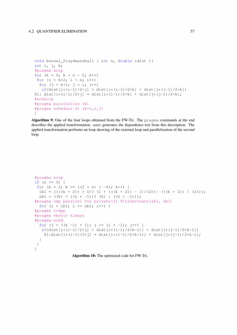
4.2. QUANTIFIER ELIMINATION 57
void kernel_floydwarshall ( int n, double *dist ){int i, j, k;#pragma scopfor (k = 0; k < n - 2; k++)for (i = k+2; i < n; i++)for (j = k+1; j < i; j++)if(dist[i*(i-1)/2+j] > dist[i*(i-1)/2+k] + dist[j*(j-1)/2+k])
S1: dist[i*(i-1)/2+j] = dist[i*(i-1)/2+k] + dist[j*(j-1)/2+k];#endscop#pragma parallelize (k)#pragma schedule S1 (k+i,i,j)}
Algorithm 9: One of the four loops obtained from the FW-Tri. The pragma commands at the enddescribes the applied transformation. aster generates the dependence test from this description. Theapplied transformation performs an loop skewing of the external loop and parallelization of the secondloop.
#pragma scopif (n >= 3) {for (k = 2; k <= ((2 * n) + -4); k++) {lb1 = ((((k + 2)) > 0)? (1 + (((k + 2)) - 1)/(2)): (((k + 2)) / (2)));ub1 = ((k) < ((n + -1))? (k) : ((n + -1)));
#pragma omp parallel for private(j) firstprivate(lb1, ub1)for (i = lb1; i <= ub1; i++) {
#pragma ivdep#pragma vector always#pragma simd
for (j = ((k -i) + 1); j <= (i + -1); j++) {if(dist[i*(i-1)/2+j] > dist[i*(i-1)/2+k-i)] + dist[j*(j-1)/2+k-i])S1:dist[i*(i-1)/2+j] = dist[i*(i-1)/2+k-i)] + dist[j*(j-1)/2+k-i];
}}}
Algorithm 10: The optimized code for FW-Tri.
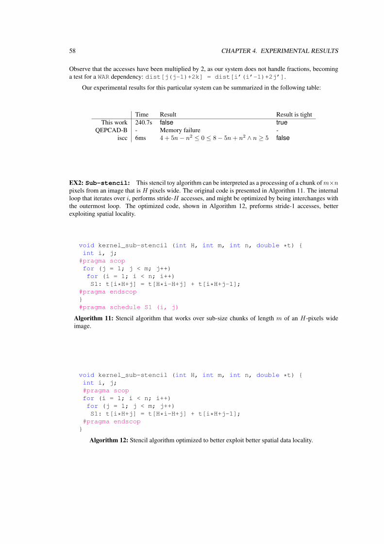
58 CHAPTER 4. EXPERIMENTAL RESULTS
Observe that the accesses have been multiplied by 2, as our system does not handle fractions, becominga test for a WAR dependency: dist[j(j-1)+2k] = dist[i’(i’-1)+2j’].
Our experimental results for this particular system can be summarized in the following table:
Time Result Result is tightThis work 240.7s false true
QEPCAD-B - Memory failure -iscc 6ms 4 + 5n− n2 ≤ 0 ≤ 8− 5n+ n2 ∧ n ≥ 5 false
EX2: Sub-stencil: This stencil toy algorithm can be interpreted as a processing of a chunk ofm×npixels from an image that is H pixels wide. The original code is presented in Algorithm 11. The internalloop that iterates over i, performs stride-H accesses, and might be optimized by being interchanges withthe outermost loop. The optimized code, shown in Algorithm 12, preforms stride-1 accesses, betterexploiting spatial locality.
void kernel_sub-stencil (int H, int m, int n, double *t) {int i, j;#pragma scopfor (j = 1; j < m; j++)for (i = 1; i < n; i++)S1: t[i*H+j] = t[H*i-H+j] + t[i*H+j-1];
#pragma endscop}#pragma schedule S1 (i, j)
Algorithm 11: Stencil algorithm that works over sub-size chunks of length m of an H-pixels wideimage.
void kernel_sub-stencil (int H, int m, int n, double *t) {int i, j;#pragma scopfor (i = 1; i < n; i++)for (j = 1; j < m; j++)S1: t[i*H+j] = t[H*i-H+j] + t[i*H+j-1];
#pragma endscop}
Algorithm 12: Stencil algorithm optimized to better exploit better spatial data locality.
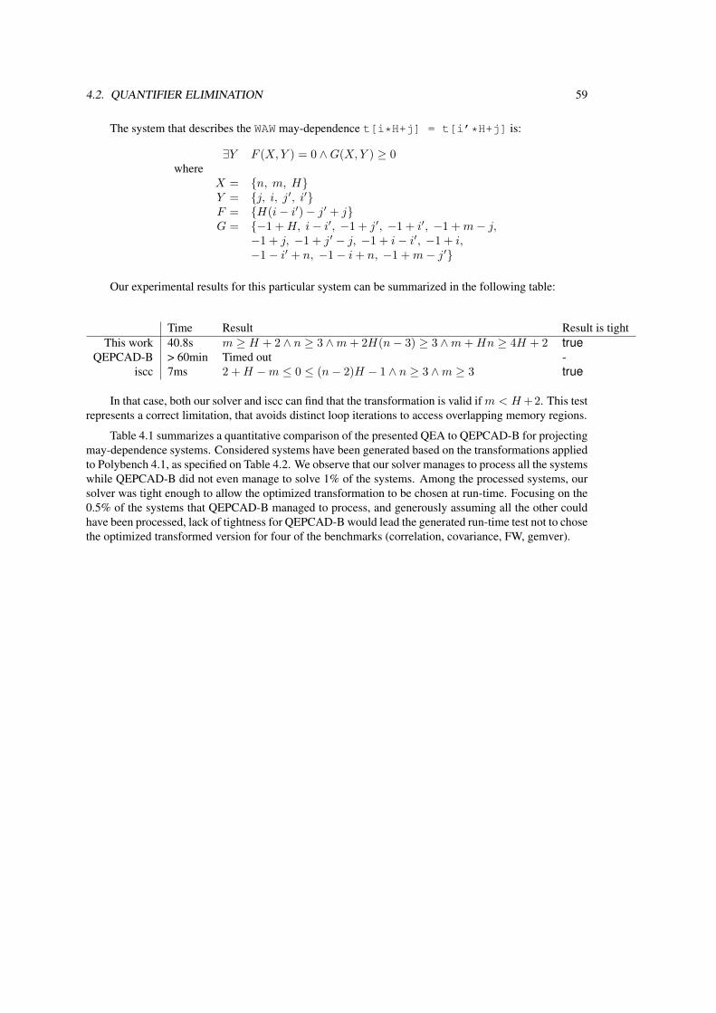
4.2. QUANTIFIER ELIMINATION 59
The system that describes the WAW may-dependence t[i*H+j] = t[i’*H+j] is:
∃Y F (X,Y ) = 0 ∧G(X,Y ) ≥ 0where
X = {n, m, H}Y = {j, i, j′, i′}F = {H(i− i′)− j′ + j}G = {−1 +H, i− i′, −1 + j′, −1 + i′, −1 +m− j,
−1 + j, −1 + j′ − j, −1 + i− i′, −1 + i,−1− i′ + n, −1− i+ n, −1 +m− j′}
Our experimental results for this particular system can be summarized in the following table:
Time Result Result is tightThis work 40.8s m ≥ H + 2 ∧ n ≥ 3 ∧m+ 2H(n− 3) ≥ 3 ∧m+Hn ≥ 4H + 2 true
QEPCAD-B > 60min Timed out -iscc 7ms 2 +H −m ≤ 0 ≤ (n− 2)H − 1 ∧ n ≥ 3 ∧m ≥ 3 true
In that case, both our solver and iscc can find that the transformation is valid ifm < H+2. This testrepresents a correct limitation, that avoids distinct loop iterations to access overlapping memory regions.
Table 4.1 summarizes a quantitative comparison of the presented QEA to QEPCAD-B for projectingmay-dependence systems. Considered systems have been generated based on the transformations appliedto Polybench 4.1, as specified on Table 4.2. We observe that our solver manages to process all the systemswhile QEPCAD-B did not even manage to solve 1% of the systems. Among the processed systems, oursolver was tight enough to allow the optimized transformation to be chosen at run-time. Focusing on the0.5% of the systems that QEPCAD-B managed to process, and generously assuming all the other couldhave been processed, lack of tightness for QEPCAD-B would lead the generated run-time test not to chosethe optimized transformed version for four of the benchmarks (correlation, covariance, FW, gemver).
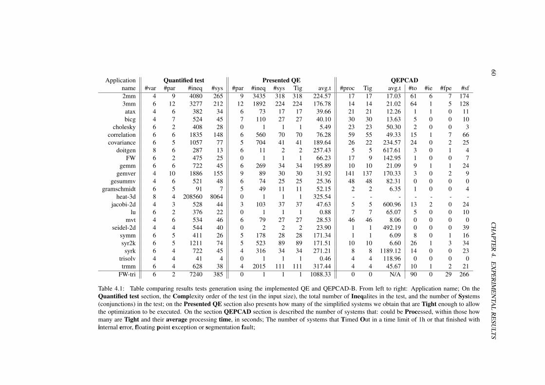
60C
HA
PTE
R4.
EX
PER
IME
NTA
LR
ESU
LTS
Application Quantified test Presented QE QEPCADname #var #par #ineq #sys #par #ineq #sys Tig avg.t #proc Tig avg.t #to #ie #fpe #sf2mm 4 9 4080 265 9 3435 318 318 224.57 17 17 17.03 61 6 7 1743mm 6 12 3277 212 12 1892 224 224 176.78 14 14 21.02 64 1 5 128atax 4 6 382 34 6 73 17 17 39.66 21 21 12.26 1 1 0 11bicg 4 7 524 45 7 110 27 27 40.10 30 30 13.63 5 0 0 10
cholesky 6 2 408 28 0 1 1 1 5.49 23 23 50.30 2 0 0 3correlation 6 6 1835 148 6 560 70 70 76.28 59 55 49.33 15 1 7 66covariance 6 5 1057 77 5 704 41 41 189.64 26 22 234.57 24 0 2 25
doitgen 8 6 287 13 6 11 2 2 257.43 5 5 617.61 3 0 1 4FW 6 2 475 25 0 1 1 1 66.23 17 9 142.95 1 0 0 7
gemm 6 6 722 45 6 269 34 34 195.89 10 10 21.09 9 1 1 24gemver 4 10 1886 155 9 89 30 30 31.92 141 137 170.33 3 0 2 9
gesummv 4 6 521 48 6 74 25 25 25.36 48 48 82.31 0 0 0 0gramschmidt 6 5 91 7 5 49 11 11 52.15 2 2 6.35 1 0 0 4
heat-3d 8 4 208560 8064 0 1 1 1 325.54 - - - - - - -jacobi-2d 4 3 528 44 3 103 37 37 47.63 5 5 600.96 13 2 0 24
lu 6 2 376 22 0 1 1 1 0.88 7 7 65.07 5 0 0 10mvt 4 6 534 46 6 79 27 27 28.53 46 46 8.06 0 0 0 0
seidel-2d 4 4 544 40 0 2 2 2 23.90 1 1 492.19 0 0 0 39symm 6 5 411 26 5 178 28 28 171.34 1 1 6.09 8 0 1 16syr2k 6 5 1211 74 5 523 89 89 171.51 10 10 6.60 26 1 3 34syrk 6 4 722 45 4 316 34 34 271.21 8 8 1189.12 14 0 0 23
trisolv 4 4 41 4 0 1 1 1 0.46 4 4 118.96 0 0 0 0trmm 6 4 628 38 4 2015 111 111 317.44 4 4 45.67 10 1 2 21
FW-tri 6 2 7240 385 0 1 1 1 1088.33 0 0 N/A 90 0 29 266
Table 4.1: Table comparing results tests generation using the implemented QE and QEPCAD-B. From left to right: Application name; On theQuantified test section, the Complexity order of the test (in the input size), the total number of Ineqalites in the test, and the number of Systems(conjunctions) in the test; on the Presented QE section also presents how many of the simplified systems we obtain that are Tight enough to allowthe optimization to be executed. On the section QEPCAD section is described the number of systems that: could be Processed, within those howmany are Tight and their average processing time, in seconds; The number of systems that Timed Out in a time limit of 1h or that finished withinternal error, floating point exception or segmentation fault;
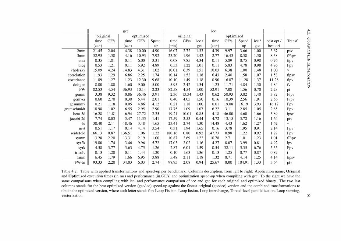
4.2.Q
UA
NT
IFIER
EL
IMIN
AT
ION
61gcc icc
ori.ginal opt.imized ori.ginal opt.imizedtime GF/s time GF/s Speed time GF/s icc / time GF/s Speed icc / best opt / Transf
(ms) (ms) -up (ms) gcc (ms) -up gcc best ori2mm 21.45 2.04 4.38 10.00 4.90 16.07 2.72 1.33 4.39 9.97 3.66 1.00 3.67 psv3mm 32.95 1.38 4.16 10.93 7.92 23.20 1.96 1.42 2.77 16.43 8.38 1.50 8.38 fFipvatax 0.35 1.81 0.11 6.00 3.31 0.08 7.85 4.34 0.11 5.89 0.75 0.98 0.76 fipvbicg 0.53 1.21 0.11 5.92 4.89 0.53 1.22 1.01 0.11 5.83 4.78 0.98 4.86 Fpv
cholesky 15.09 4.24 14.83 4.31 1.02 10.01 6.39 1.51 10.03 6.38 1.00 1.48 1.00 vcorrelation 11.93 1.29 6.86 2.25 1.74 10.14 1.52 1.18 6.43 2.40 1.58 1.07 1.58 fipsvcovariance 11.89 1.27 1.23 12.30 9.68 10.10 1.49 1.18 0.90 16.87 11.28 1.37 11.28 fipv
doitgen 8.00 1.80 1.60 9.00 5.00 5.95 2.42 1.34 1.23 11.71 4.84 1.30 4.84 fvFW 82.53 4.54 36.93 10.14 2.23 82.58 4.54 1.00 52.91 7.08 1.56 0.70 2.23 pt
gemm 3.38 9.32 0.86 36.46 3.91 2.36 13.34 1.43 0.62 50.93 3.82 1.40 3.82 Fipvgemver 0.60 2.70 0.30 5.44 2.01 0.40 4.05 1.50 0.16 10.39 2.56 1.91 2.56 Fipv
gesummv 0.21 1.18 0.05 4.86 4.12 0.21 1.18 1.00 0.01 19.08 16.19 3.93 16.17 Fpvgramschmidt 18.98 1.02 6.55 2.95 2.90 17.75 1.09 1.07 6.22 3.11 2.85 1.05 2.85 Fpv
heat-3d 16.28 11.81 6.94 27.72 2.35 19.21 10.01 0.85 4.18 46.00 4.60 1.66 3.89 ipsvjacobi-2d 7.74 8.03 5.47 11.35 1.41 17.59 3.53 0.44 4.72 13.15 3.72 1.16 1.64 ptv
lu 30.40 2.11 18.46 3.48 1.65 23.41 2.74 1.30 14.48 4.43 1.62 1.27 1.62 vmvt 0.51 1.17 0.14 4.14 3.54 0.31 1.94 1.65 0.16 3.78 1.95 0.91 2.14 Fpv
seidel-2d 166.13 0.87 136.51 1.06 1.22 180.16 0.80 0.92 147.73 0.98 1.22 0.92 1.22 Fpvsymm 13.28 2.20 13.31 2.19 1.00 10.87 2.69 1.22 10.78 2.71 1.01 1.23 1.01 fFipvsyr2k 19.80 1.74 3.46 9.96 5.72 17.03 2.02 1.16 4.27 8.07 3.99 0.81 4.92 ipv
syrk 4.58 3.77 3.63 4.75 1.26 2.87 6.01 1.59 0.54 32.11 5.35 6.76 5.35 Fpvtrisolv 0.13 1.20 0.11 1.44 1.20 0.10 1.63 1.36 0.13 1.25 0.77 0.87 0.89 ttrmm 6.45 1.79 1.66 6.95 3.88 5.48 2.11 1.18 1.32 8.71 4.14 1.25 4.14 fipsv
FW-tri 93.33 2.20 34.03 6.03 2.74 98.95 2.08 0.94 25.67 8.00 104.91 1.33 3.64 ptv
Table 4.2: Table with applied transformations and speed-up per benchmark. Columns description, from left to right: Application name; Originaland Optimized execution times (in ms) and performance (in GF/s) and optimization speed-up when compiling with gcc. To the right we have thesame comparisons when compiling with icc, and performance comparison of icc and gcc for each original and optimized binary. The two lastcolumns stands for the best optimized version (gcc/icc) speed-up against the fastest original (gcc/icc) version and the combined transformations toobtain the optimized version, where each letter stands for: Loop Fission, Loop fusion, Loop interchange, Thread-level parallelization, Loop skewing,vectorization.

62 CHAPTER 4. EXPERIMENTAL RESULTS
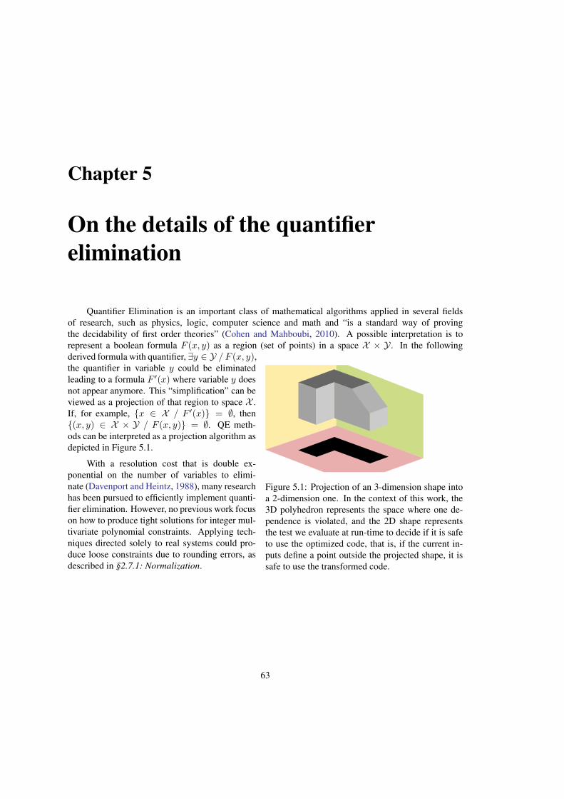
Chapter 5
On the details of the quantifierelimination
Quantifier Elimination is an important class of mathematical algorithms applied in several fieldsof research, such as physics, logic, computer science and math and “is a standard way of provingthe decidability of first order theories” (Cohen and Mahboubi, 2010). A possible interpretation is torepresent a boolean formula F (x, y) as a region (set of points) in a space X × Y . In the following
Figure 5.1: Projection of an 3-dimension shape intoa 2-dimension one. In the context of this work, the3D polyhedron represents the space where one de-pendence is violated, and the 2D shape representsthe test we evaluate at run-time to decide if it is safeto use the optimized code, that is, if the current in-puts define a point outside the projected shape, it issafe to use the transformed code.
derived formula with quantifier, ∃y ∈ Y / F (x, y),the quantifier in variable y could be eliminatedleading to a formula F ′(x) where variable y doesnot appear anymore. This “simplification” can beviewed as a projection of that region to space X .If, for example, {x ∈ X / F ′(x)} = ∅, then{(x, y) ∈ X × Y / F (x, y)} = ∅. QE meth-ods can be interpreted as a projection algorithm asdepicted in Figure 5.1.
With a resolution cost that is double ex-ponential on the number of variables to elimi-nate (Davenport and Heintz, 1988), many researchhas been pursued to efficiently implement quanti-fier elimination. However, no previous work focuson how to produce tight solutions for integer mul-tivariate polynomial constraints. Applying tech-niques directed solely to real systems could pro-duce loose constraints due to rounding errors, asdescribed in §2.7.1: Normalization.
63
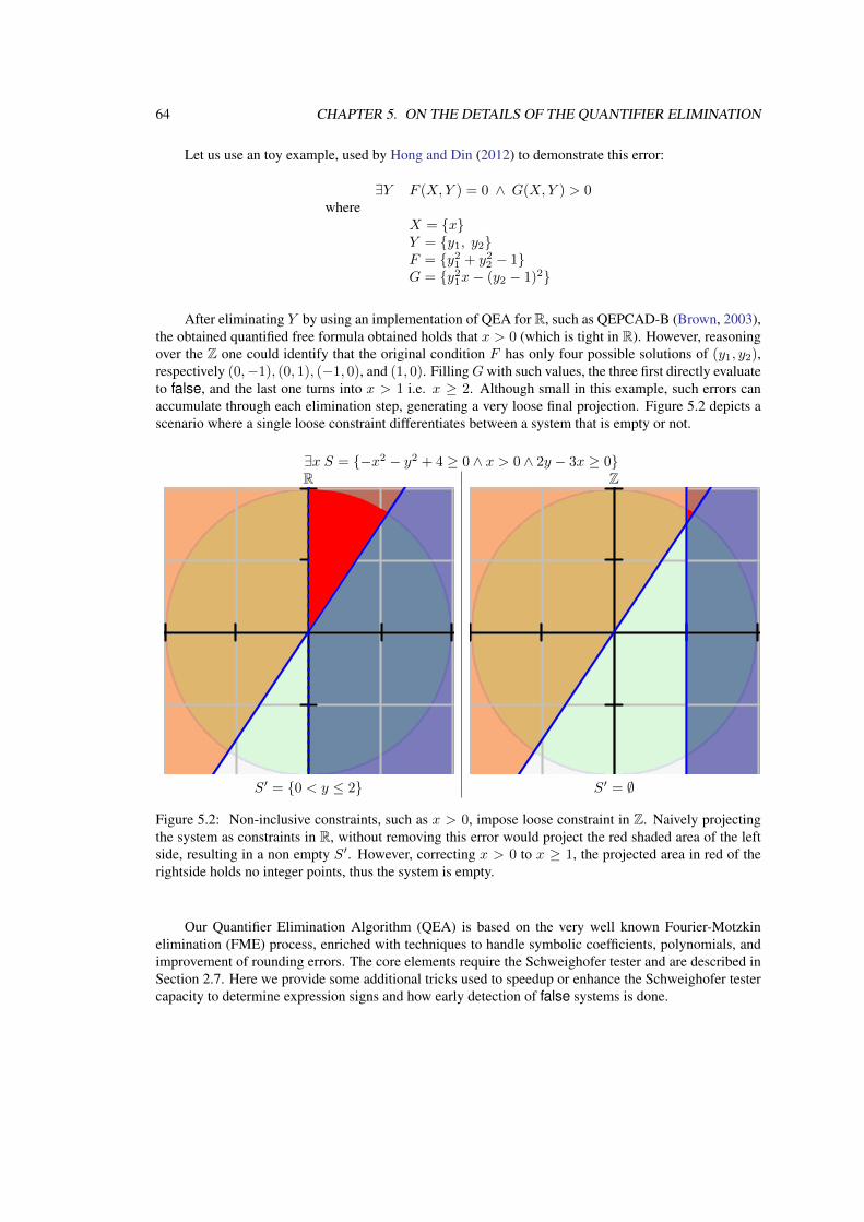
64 CHAPTER 5. ON THE DETAILS OF THE QUANTIFIER ELIMINATION
Let us use an toy example, used by Hong and Din (2012) to demonstrate this error:
∃Y F (X,Y ) = 0 ∧ G(X,Y ) > 0where
X = {x}Y = {y1, y2}F = {y21 + y22 − 1}G = {y21x− (y2 − 1)2}
After eliminating Y by using an implementation of QEA for R, such as QEPCAD-B (Brown, 2003),the obtained quantified free formula obtained holds that x > 0 (which is tight in R). However, reasoningover the Z one could identify that the original condition F has only four possible solutions of (y1, y2),respectively (0,−1), (0, 1), (−1, 0), and (1, 0). FillingGwith such values, the three first directly evaluateto false, and the last one turns into x > 1 i.e. x ≥ 2. Although small in this example, such errors canaccumulate through each elimination step, generating a very loose final projection. Figure 5.2 depicts ascenario where a single loose constraint differentiates between a system that is empty or not.
∃x S = {−x2 − y2 + 4 ≥ 0 ∧ x > 0 ∧ 2y − 3x ≥ 0}R Z
S′ = {0 < y ≤ 2} S′ = ∅
Figure 5.2: Non-inclusive constraints, such as x > 0, impose loose constraint in Z. Naively projectingthe system as constraints in R, without removing this error would project the red shaded area of the leftside, resulting in a non empty S′. However, correcting x > 0 to x ≥ 1, the projected area in red of therightside holds no integer points, thus the system is empty.
Our Quantifier Elimination Algorithm (QEA) is based on the very well known Fourier-Motzkinelimination (FME) process, enriched with techniques to handle symbolic coefficients, polynomials, andimprovement of rounding errors. The core elements require the Schweighofer tester and are described inSection 2.7. Here we provide some additional tricks used to speedup or enhance the Schweighofer testercapacity to determine expression signs and how early detection of false systems is done.
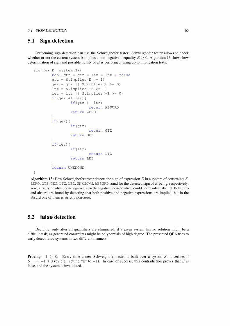
5.1. SIGN DETECTION 65
5.1 Sign detection
Performing sign detection can use the Schweighofer tester: Schweighofer tester allows to checkwhether or not the current system S implies a non-negative inequality E ≥ 0. Algorithm 13 shows howdetermination of sign and possible nullity of E is performed, using up to implication tests.
sign(ex E, system S){bool gtz = gez = lez = ltz = falsegtz = S.implies(E >= 1)gez = gtz || S.implies(E >= 0)ltz = S.implies(-E >= 1)lez = ltz || S.implies(-E >= 0)if(gez && lez){
if(gtz || ltz)return ABSURD
return ZERO}if(gez){
if(gtz)return GTZ
return GEZ}if(lez){
if(ltz)return LTZ
return LEZ}return UNKNOWN
}
Algorithm 13: How Schweighofer tester detects the sign of expression E in a system of constraints S.ZERO, GTZ, GEZ, LTZ, LEZ, UNKNOWN, ABSURD stand for the detected sign of E being, respectively:zero, strictly positive, non-negative, strictly negative, non-positive, could not resolve, absurd. Both zeroand absurd are found by detecting that both positive and negative expressions are implied, but in theabsurd one of them is strictly non-zero.
5.2 false detection
Deciding, only after all quantifiers are eliminated, if a given system has no solution might be adifficult task, as generated constraints might be polynomials of high degree. The presented QEA tries toearly detect false systems in two different manners:
Proving −1 ≥ 0: Every time a new Schweighofer tester is built over a system S, it verifies ifS =⇒ −1 ≥ 0 (by e.g. setting “E” to −1). In case of success, this contradiction proves that S isfalse, and the system is invalidated.
66 CHAPTER 5. ON THE DETAILS OF THE QUANTIFIER ELIMINATION
Proving E ∧ ¬E: Every time the Schweighofer tester is used to determine the sign of an expression Eunder a system S, it persistently tries to detect both if S =⇒ E ≥ 0 and if S =⇒ E ≤ 0. In the casewhere both are implied, and at least one is proved to be exclusively non-zero, then E holds an ABSURDsign, and the system is detected as false.
5.3 Expression factorization
Whenever the sign of an expression E can’t be resolved directly by the Schweighofer tester, arecursive technique tries to factorizeE and each operand sign is evaluated separately. To avoid testing thesame expressions multiple times, a sign cache is created, and whenever an expression is evaluated once,the returning sign is cached and not evaluated again. When factorized, these algebraic rules are applied:
Even powers are always non-negative ((E′)2n ≥ 0): If the expression being tested is an exponent ofeven power, it is first verified if the base has known sign. If it does and is not equal to zero, it is returnedas strictly positive. Otherwise, it is returned as greater or equals to zero.
Odd powers hold the same sign of the base (sign(E′)2n+1 ≡ sign(E′)): If the expression being
tested is an exponent of even power and the sign of the base is known, then the same sign is returned.
Sum sign rules If an expression E is a sum of expressions E′ + E′′ the rules when combining thesub-expressions signs are:
1. ABSURD prevails over any other sign.
2. UNKNOWN prevails over the remaining signs.
3. ZERO sign does not change the other sign.
4. If signs are in different directions, the result is UNKNOWN.
5. If both E′ and E′′ hold the same sign, the sum is the same.
6. Strict signs prevail over non-strict.
Multiplication sign rules If an expression E is a multiplication of expressions E′ · E′′ the rules whencombining the sub-expressions signs are:
1. ABSURD prevails over any other signs.
2. ZERO and right after UNKNOWN prevail over all other signs.
3. Non-strict signs prevail over strict signs (GEZ, LEZ).
4. Non-positive and negative inverts the sign (LEZ, LTZ).
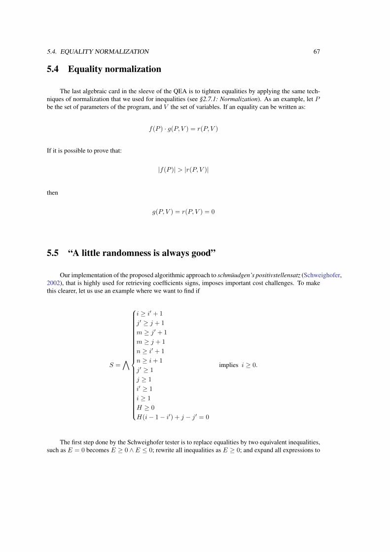
5.4. EQUALITY NORMALIZATION 67
5.4 Equality normalization
The last algebraic card in the sleeve of the QEA is to tighten equalities by applying the same tech-niques of normalization that we used for inequalities (see §2.7.1: Normalization). As an example, let Pbe the set of parameters of the program, and V the set of variables. If an equality can be written as:
f(P ) · g(P, V ) = r(P, V )
If it is possible to prove that:
|f(P )| > |r(P, V )|
then
g(P, V ) = r(P, V ) = 0
5.5 “A little randomness is always good”
Our implementation of the proposed algorithmic approach to schmüudgen’s positivstellensatz (Schweighofer,2002), that is highly used for retrieving coefficients signs, imposes important cost challenges. To makethis clearer, let us use an example where we want to find if
S =∧
i ≥ i′ + 1
j′ ≥ j + 1
m ≥ j′ + 1
m ≥ j + 1
n ≥ i′ + 1
n ≥ i+ 1
j′ ≥ 1
j ≥ 1
i′ ≥ 1
i ≥ 1
H ≥ 0
H(i− 1− i′) + j − j′ = 0
implies i ≥ 0.
The first step done by the Schweighofer tester is to replace equalities by two equivalent inequalities,such as E = 0 becomes E ≥ 0 ∧E ≤ 0; rewrite all inequalities as E ≥ 0; and expand all expressions to
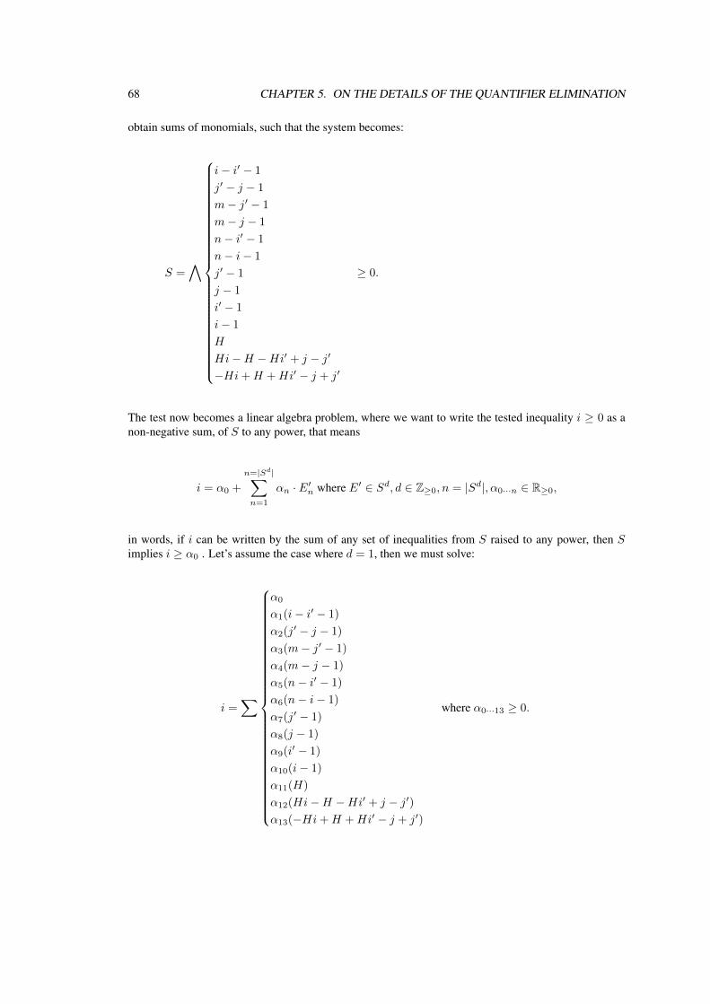
68 CHAPTER 5. ON THE DETAILS OF THE QUANTIFIER ELIMINATION
obtain sums of monomials, such that the system becomes:
S =∧
i− i′ − 1
j′ − j − 1
m− j′ − 1
m− j − 1
n− i′ − 1
n− i− 1
j′ − 1
j − 1
i′ − 1
i− 1
H
Hi−H −Hi′ + j − j′
−Hi+H +Hi′ − j + j′
≥ 0.
The test now becomes a linear algebra problem, where we want to write the tested inequality i ≥ 0 as anon-negative sum, of S to any power, that means
i = α0 +
n=|Sd|∑n=1
αn · E′n where E′ ∈ Sd, d ∈ Z≥0, n = |Sd|, α0···n ∈ R≥0,
in words, if i can be written by the sum of any set of inequalities from S raised to any power, then Simplies i ≥ α0 . Let’s assume the case where d = 1, then we must solve:
i =∑
α0
α1(i− i′ − 1)
α2(j′ − j − 1)
α3(m− j′ − 1)
α4(m− j − 1)
α5(n− i′ − 1)
α6(n− i− 1)
α7(j′ − 1)
α8(j − 1)
α9(i′ − 1)
α10(i− 1)
α11(H)
α12(Hi−H −Hi′ + j − j′)α13(−Hi+H +Hi′ − j + j′)
where α0···13 ≥ 0.
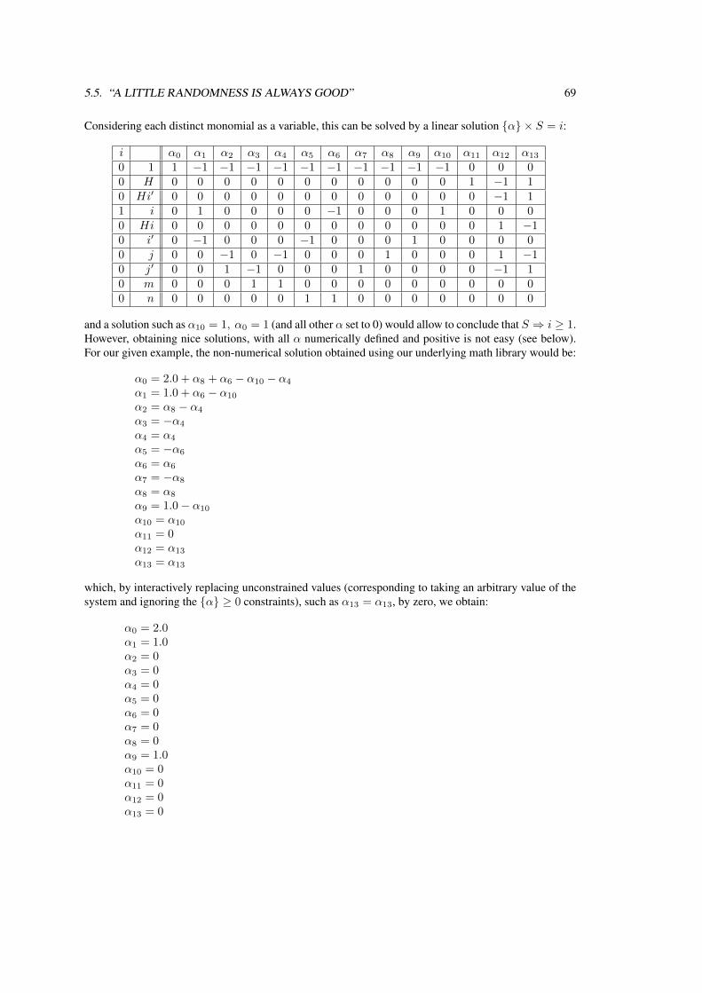
5.5. “A LITTLE RANDOMNESS IS ALWAYS GOOD” 69
Considering each distinct monomial as a variable, this can be solved by a linear solution {α} × S = i:
i α0 α1 α2 α3 α4 α5 α6 α7 α8 α9 α10 α11 α12 α13
0 1 1 −1 −1 −1 −1 −1 −1 −1 −1 −1 −1 0 0 00 H 0 0 0 0 0 0 0 0 0 0 0 1 −1 10 Hi′ 0 0 0 0 0 0 0 0 0 0 0 0 −1 11 i 0 1 0 0 0 0 −1 0 0 0 1 0 0 00 Hi 0 0 0 0 0 0 0 0 0 0 0 0 1 −10 i′ 0 −1 0 0 0 −1 0 0 0 1 0 0 0 00 j 0 0 −1 0 −1 0 0 0 1 0 0 0 1 −10 j′ 0 0 1 −1 0 0 0 1 0 0 0 0 −1 10 m 0 0 0 1 1 0 0 0 0 0 0 0 0 00 n 0 0 0 0 0 1 1 0 0 0 0 0 0 0
and a solution such as α10 = 1, α0 = 1 (and all other α set to 0) would allow to conclude that S ⇒ i ≥ 1.However, obtaining nice solutions, with all α numerically defined and positive is not easy (see below).For our given example, the non-numerical solution obtained using our underlying math library would be:
α0 = 2.0 + α8 + α6 − α10 − α4
α1 = 1.0 + α6 − α10
α2 = α8 − α4
α3 = −α4
α4 = α4
α5 = −α6
α6 = α6
α7 = −α8
α8 = α8
α9 = 1.0− α10
α10 = α10
α11 = 0α12 = α13
α13 = α13
which, by interactively replacing unconstrained values (corresponding to taking an arbitrary value of thesystem and ignoring the {α} ≥ 0 constraints), such as α13 = α13, by zero, we obtain:
α0 = 2.0α1 = 1.0α2 = 0α3 = 0α4 = 0α5 = 0α6 = 0α7 = 0α8 = 0α9 = 1.0α10 = 0α11 = 0α12 = 0α13 = 0
70 CHAPTER 5. ON THE DETAILS OF THE QUANTIFIER ELIMINATION
which for last proves it is implied. On the current implementation one problem is that the replacement byzero might invalidate an undetermined answer, as one of the resulting expressions can be
αx = αy + αz − 1.0 ∧ αy = αy ∧ αz = αz
and the final solution would be invalidated after replacing αy, αz by zero. As briefly discussed in §7, abetter (but more expensive) solution would express the problem as a linear programming problem: addthe {α} ≥ 0 linear constraints to the system and maximize α0.
A second problem lies in the fact that systems size to be solved grows exponentially with d. In ourexample, when d is set to 2, distinct monomials count grows from 10 to 80, and 14 to 170 expressions.Empirically, it was observed that most implications were solved by combination of up to 3 expressionsand that most of our problems would not have a polynomial of degree higher than 3. From the latterobservation, an empirical limit of the maximum power of S was imposed. From the former observation,it was decided to build subsets of system, with up to three inequalities, and evaluate if at least one ofthese subsets would imply the inequality being tested. However, the total number of possible subsets iscombinatorial, and testing each one of ended taking more time than the original evaluation. The problemnow became, how to select those promising subsets to test?
Let f(X) and g(X) be two inequalities where f(X)⇒ g(X). Then, for any value of X , if g(X) isfalse, then necessarily f(X) is also false. Suppose g(X) corresponds to the positiveness of E(X) andf(X) to a subsystem. Consider a random value to be assigned to the system variables (X here). If g,i.e. the inequality being tested, evaluates to false with that value X , all subsystems that evaluate to trueare discarded as they cannot involve g (thus cannot be used to prove g). The overall process iterates ond with a time-out for each iteration. It starts with all subsystems of S1 and tries to slim it using manygenerated random values. Denoting the slimmed version of S1, S′, it then considers S′2 and tries to slimthis new bigger system with the same mechanism. Say we obtain S′′. It finally slims S′′ × S and stops.
Chapter 6
On the details of the DDG
Recent works (Fauzia et al., 2013; Elango et al., 2015a,b) use DDG graphs to characterize thedata-movement complexity of a program. Performing transformations that preserve dependencies, theyreschedule the original program execution order, and try to identify code regions that hold potential foroptimizations with respect to data locality. Such works, used as performance debugging, might generateschedules that cannot be converted back into structured loop-oriented code. Different from those, thiswork uses DDG to resolve may-dependence information, required by loop optimizers to retrieve prof-itable code changes.
If applied naively using a shadow memory on any scalar/memory variable, the constructed DDGmight be polluted by many control/data dependencies stemming from iterators. As an example, enforcingto follow the dependencies related to the scan of the iteration space (that uses loop index increments andjumps) would impose exactly the same execution order as the instrumented program. A simple but tooapproximate approach used by Fauzia et al. (2013) to get around this problem, consists in instrumentingonly floating-point variables and ignoring all dependencies related to integer arithmetic. Our solution ismore robust and simply consists in ignoring any instruction for which the SCEV/ analysis (of LLVM)provides a closed static formula, dependent solely on canonical induction variables and loop invariantvalues.
Another possible problem when working with DDG graphs is related with the cost of manipulat-ing such graphs. As each node in the graph represents an dynamic instruction, applications that executefor just a tenth of a second might hold millions of dynamic instructions, making their analyses costlyin memory and time. As our work is focused on optimizing loop nests, we exploit the fact that in mostcases, dependencies observed in just a chunk of consecutive loop iterations are representative to the en-tire iteration domain. At that point, one should outline that our approach does not impose the DDG to beaccurate. As the program behavior (and the observed dependencies) might already depend on the inputdata, focusing on chunks of consecutive loop iterations, instead of considering the whole loop, is yetanother approximation. The challenge is to find tricks (such as the clamping technique described further)that makes the profiling as representative as possible with the important trade-off in mind: tightness ver-sus size/cost. So we limit the number of iterations a loop is tracked, from the time it is entered. Usingan environment variable to control the number of traced instructions, we can easily build graphs withrepresentative dependence information and limited number of nodes. This iteration limit can be disableby defining the limit to zero. The applied cut-off technique, that just ignores instructions outside themonitoring limits, might too optimistically loose important loop intra-iterations dependencies, that wouldprevent some transformations, such as loops interchange. To still build a small graph but preserving such
71
72 CHAPTER 6. ON THE DETAILS OF THE DDG
constraining dependencies this work proposes a clamping technique, where the otherwise ignored mem-ory accesses from consecutive iterations of a loop are instead clamped into a single virtual instruction,representing a single node on the DDG.
Loop optimizers, such as PLuTo (Bondhugula et al., 2008), require data producer and consumerinformation not only to guarantee that a given transformation is valid, but also to improve locality byscheduling close together instructions that use the same data (temporal locality). Our work allows toenhance the DDG with data reuse edges. If one wants to extend the shadow memory so as to online-buildRAR vectors, this will turn-out to be extremely expensive as it would require to store all the consumersof a given storage location in the shadow. Alternatively, we chose to build RAW and WAW informationusing the standard technique and offline-compute all the WAR and RAR hyper-edges by applying a simpletransitive closure.
Technical details on how we build the DDG and how we use results is presented below.
6.1 Technical details
It is important to highlight that the implementation of the process of generating the DDG, and using itto retrieve profitable transformations is an ongoing work. It falls into four steps: instrumentation, tracing(or run-time), trace analysis (or simulation) and optimization. The first three steps can be executed in ansemi-automated fashion while the modeling is still in preliminary stages. Semi-automated meaning thatthe user must define the region of code to be instrumented.
Instrumentation: Our instrumentation is done at the LLVM IR level. Function calls to our tracinglibrary are inserted in the program without changing its semantics.
Defining the instrumented region: Currently the instrumented region must be manually defined bythe user by inserting a call to
ddg_trace_start()
at the beginning of the region of interest and, at the end, inserting a call to
ddg_trace_stop().
During the instrumentation process, each instruction, basic block and loop receive a unique identifier, ina deterministic manner. This is important to map information in the trace file back into the code. List offunction calls and their meanings will be explained ahead in this chapter.
Instrumenting the code: The first step of the instrumentation process generates an LLVM IR sourcecode to be used as reference. From this file the instrumented version is generated, using the opt commandfrom the LLVM infrastructure:
opt -S -load ddg.so -ddg-instrument original.ll -o instrumented.ll
Run-Time: Two different C/C++ run-time libraries that have the same interface are presented. Thefirst, called cut run-time library (CRL), implements the cut-off technique, that stops tracing after a givennumber of loop iterations. The second one, the full run-time library (FLR), traces the entire execution, toeither produce a complete or clamped DDG, where the clamping process is done during the simulationstep.
6.2. TRACED EVENTS 73
Once instrumented, compiled and linked to our run-time library, executing the generated binary willproduce an trace file (that can be piped to the next phase) called
ddg.trace
containing sequences of execution of basic-blocks, induction variables values, and accesses memorypositions at instruction level. The environment variable
DDG_LIMIT
defines size of traced chunks within each loop dimension.
Simulation: The produced trace file contains basic-blocks execution order. To retrieve instruction leveldependencies our framework simulates the execution of every basic-block in the order they are found inthe trace file: Memory accesses are reported at the instruction level and the correctness of the simulationis guaranteed by matching the instruction identifier in both the reference code and the trace file.
Dependencies between memory accesses are built during this phase, using the shadow memorytechnique as described in section §2.3. Observe that there would have been no particular difficultiesin integrating the construction of the DDG in LLVM itself, thus merging it with the run-time. Thisdesign choice (that can be discussed) just allows to decouple all the developments related to the DDGconstruction (shadowing, clamping, folding, etc.) to the compilation of the program. As for the interface,the simulation phase uses the opt command from LLVM to load our analysis:
opt -load ddg.so -ddg-cdag .
6.2 Traced Events
This section will describe, for each different traced events:
• What is done during instrumentation
• The information stored in the trace file
• How the simulator acts when handling an event of that kind
6.2.1 ddg_start_trace
This defines the start of an instrumented region.
Instrumentation: Manually inserted by user, this function call defines a point of entering a given regionof interest.
Run-Time: Opens the trace file in append mode and clears the run-time state structures.
Simulation: The iteration vector is cleared, as are any other state structures, including the shadowmemory. It is expected that the next operation is either a basic block execution or a loop entry.
74 CHAPTER 6. ON THE DETAILS OF THE DDG
6.2.2 ddg_alive_in
Instrumentation: When a call to ddg_start_trace is detected, every variable that is alive duringthis point of the program has its identifier and value stored in the trace file using an ddg_alive_infunction call.
Run-Time: Add alive-in token to the trace file, followed by variable identifier and value.
Simulation: Obtain live-in information, including loop invariant values, such as memory base pointers.
6.2.3 ddg_basic_block
A basic block defines the smallest sequence of operations that necessarily execute in sequence. Ourinstrumentation gives, in a deterministic manner, a unique identifier to each basic block of the originalprogram.
Instrumentation: At the beginning of every basic block, that is not a loop header, insert a call tobasic_block that provides the unique static block identifier.
Run-Time: Add the basic block token to the trace and its corresponding identifier. The CRL only actsif the tracking flag is true.
Simulation: For each basic-block token seen in the trace (identified thanks to its static identifier), its listof instructions is traversed. Special treatment is necessary for φ-functions as only one of the operands (theone corresponding to the incoming edge) is used at a time. Identifier of the basic-block is kept so as to findthe matching operand. As any φ-function has the semantic of a register-to-register copy, simple dynamiccopy-propagation is (optionally) performed. As an example, assume the φ-function x1 = φ(x2, x3) isprocessed and the used operand is identified to be x3, then the shadow value of x3 that corresponds tothe producers’ identifier of x3 (instruction id & iteration vector) is copied to the shadow of x1. Forinstructions that do more than just a copy, a new node corresponding to the produced data is created. Thecurrent iteration vector is used to stamp the newly created node. The shadow memory is updated with theid of this new node. Note that memory load/store instructions are treated differently.
6.2.4 ddg_load/ddg_store
Just as with basic-blocks, every instruction of the original program receives a unique, deterministic,identifier that is used to map information from the trace file to the source-code, to the DDG graph and,for last, into the AST model of the program.
Instrumentation: Every load and store instructions is prefixed by a function call with the unique in-struction identifier and the memory address variable.
Run-Time: Adds a read/write token and the received/stored memory position.
6.2. TRACED EVENTS 75
Simulation: When traversing a basic-block, whenever a load/store instruction is reached, the sim-ulator reads the trace file to verify the existence of that memory operation, comparing the token type andinstruction identifier from the reference source-file and the trace file. The accessed memory position,obtained from the trace file, is used to populate the shadow memory (Nethercote and Seward, 2007) todetermine dependencies.
The shadow memory technique consists in a one-to-one map of all accessed memory positions andthe last dynamic instruction that wrote to that memory position. Any instruction that loads a mappedmemory position is RAW dependent on the instruction that wrote it, and an instruction that rewrites anmemory position is WAW dependent on the previous writer. To also obtain reuse information, that is RARedges between dynamic instructions, our implemented shadow memory also keeps a list of all dynamicinstructions that read a memory position before it is rewritten by a store operation.
6.2.5 ddg_loop_begin/ddg_loop_end
The ~iv , that defines an loop instance, has length equals to the depth of the loop being executed. Theddg_loop_begin and ddg_loop_end events are responsible to control this depth.
Instrumentation: Every loop header is split in two basic blocks, right at its beginning. The fist exe-cuting one defines a loop pre-header, an single entry point to the loop that is outside the loop it self. Itreceives all possible entry edges, except the fallback edge, that defines an loop iteration, that goes intothe second basic block. At the end of the pre-header the ddg_loop_begin function call is insertedregistering the entrance to the loop. In the same fashion all exit edges of the loop point to a single createdfooter, holding the ddg_loop_end function call.
Run-Time: A new position in the iteration vector is pushed/popped. The CRL only adds the event if ina traced region.
Simulation: It pushes a new position onto the back of the iteration vector.
6.2.6 ddg_loop_iteration
Instrumentation: Every loop header has an associated function call inserted at the beginning of theheader basic-block. The loop identifier is the same as its header basic-block. LLVM IR loop nest infor-mation does not detect irreducible loops, so we do ignore such cases.
Run-Time: Stores the current loop identifier and trip counts. The CRL also verifies if the current tripcounts exceeds the tracking limit, and updates the iteration vector as well the active tracking flag.
Simulation: Updates the iteration vector vector values and traverses the loop header basic block just asa ddg_basic_block.
6.2.7 stop_trace
Defines the end of an instrumented region.

76 CHAPTER 6. ON THE DETAILS OF THE DDG
Instrumentation: This function is inserted into the source code of the original program by the user.
Run-Time: Writes finish token, closes trace file and clears iteration vector.
Simulation: Verifies that the iteration vector is zeroed, and generates the output files, if requested.
The resulting DDG from which we extract dependence vectors can be exported for the user to view inGraphviz dot format. Figures 6.2 and 6.3 depicted respectively, graphs build with the cut-off and clampingtechniques, for the dspmv application, limiting in four the number of loop iterations to be traced. Thesame graph can be exported in text format, depicted in Figure 6.1, to be used with the debugging toolsprovides by Elango et al. (2015a).
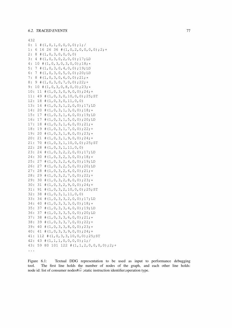
6.2. TRACED EVENTS 77
4320: 1 #(1,0,1,0,0,0,0);1;/1: 6 16 26 36 #(1,0,2,0,0,0,0);2;+2: 8 #(1,0,3,0,0,0,0)3: 4 #(1,0,3,0,2,0,0);17;LD4: 10 #(1,0,3,0,3,0,0);18;*5: 7 #(1,0,3,0,4,0,0);19;LD6: 7 #(1,0,3,0,5,0,0);20;LD7: 8 #(1,0,3,0,6,0,0);21;*8: 9 #(1,0,3,0,7,0,0);22;+9: 10 #(1,0,3,0,8,0,0);23;*10: 11 #(1,0,3,0,9,0,0);24;+11: 49 #(1,0,3,0,10,0,0);25;ST12: 18 #(1,0,3,0,11,0,0)13: 14 #(1,0,3,1,2,0,0);17;LD14: 20 #(1,0,3,1,3,0,0);18;*15: 17 #(1,0,3,1,4,0,0);19;LD16: 17 #(1,0,3,1,5,0,0);20;LD17: 18 #(1,0,3,1,6,0,0);21;*18: 19 #(1,0,3,1,7,0,0);22;+19: 20 #(1,0,3,1,8,0,0);23;*20: 21 #(1,0,3,1,9,0,0);24;+21: 70 #(1,0,3,1,10,0,0);25;ST22: 28 #(1,0,3,1,11,0,0)23: 24 #(1,0,3,2,2,0,0);17;LD24: 30 #(1,0,3,2,3,0,0);18;*25: 27 #(1,0,3,2,4,0,0);19;LD26: 27 #(1,0,3,2,5,0,0);20;LD27: 28 #(1,0,3,2,6,0,0);21;*28: 29 #(1,0,3,2,7,0,0);22;+29: 30 #(1,0,3,2,8,0,0);23;*30: 31 #(1,0,3,2,9,0,0);24;+31: 91 #(1,0,3,2,10,0,0);25;ST32: 38 #(1,0,3,1,11,0,0)33: 34 #(1,0,3,3,2,0,0);17;LD34: 40 #(1,0,3,3,3,0,0);18;*35: 37 #(1,0,3,3,4,0,0);19;LD36: 37 #(1,0,3,3,5,0,0);20;LD37: 38 #(1,0,3,3,6,0,0);21;*38: 39 #(1,0,3,3,7,0,0);22;+39: 40 #(1,0,3,3,8,0,0);23;*40: 41 #(1,0,3,3,9,0,0);24;+41: 112 #(1,0,3,3,10,0,0);25;ST42: 43 #(1,1,1,0,0,0,0);1;/43: 59 80 101 122 #(1,1,2,0,0,0,0);2;+...
Figure 6.1: Textual DDG representation to be used as input to performance debuggingtool. The first line holds the number of nodes of the graph, and each other line holds:node id: list of consumer nodes#~iv ;static instruction identifier;operation type.
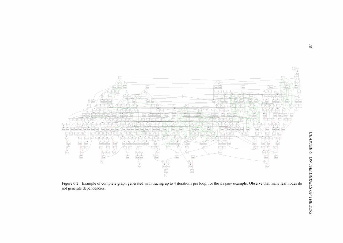
78C
HA
PTE
R6.
ON
TH
ED
ETA
ILS
OF
TH
ED
DG
0(0)
i64 0
2(0)
i32 0
4(0)1; line:66; column:69
/
5(0)2; line:66; column:71
+
16(0,0)20; line:66; column:59
LD
28(0,1)20; line:66; column:59
LD
40(0,2)20; line:66; column:59
LD
52(0,3)20; line:66; column:59
LD
11(0,0)
i32 0
18(0,0)22; line:66; column:75
+
13(0,0)17; line:66; column:21
LD
14(0,0)18; line:66; column:31
*
20(0,0)24; line:66; column:38
+
15(0,0)19; line:66; column:47
LD
17(0,0)21; line:66; column:57
*
78(1,0,0)13; line:64; column:21
LD
190(2,0,0)13; line:64; column:21
LD
354(3,0,0)13; line:64; column:21
LD
19(0,0)23; line:66; column:45
*
21(0,0)25; line:66; column:19
ST
75(1,0,0)10; line:63; column:22
LD
77(1,0,0)12; line:63; column:22
ST
23(0,1)
i32 0
30(0,1)22; line:66; column:75
+
25(0,1)17; line:66; column:21
LD
26(0,1)18; line:66; column:31
*
32(0,1)24; line:66; column:38
+
27(0,1)19; line:66; column:47
LD
29(0,1)21; line:66; column:57
*
104(1,1,0)13; line:64; column:21
LD
229(2,1,0)13; line:64; column:21
LD
406(3,1,0)13; line:64; column:21
LD
31(0,1)23; line:66; column:45
*
33(0,1)25; line:66; column:19
ST
101(1,1,0)10; line:63; column:22
LD
103(1,1,0)12; line:63; column:22
ST
35(0,2)
i32 0
42(0,2)22; line:66; column:75
+
37(0,2)17; line:66; column:21
LD
38(0,2)18; line:66; column:31
*
44(0,2)24; line:66; column:38
+
39(0,2)19; line:66; column:47
LD
41(0,2)21; line:66; column:57
*
130(1,2,0)13; line:64; column:21
LD
268(2,2,0)13; line:64; column:21
LD
458(3,2,0)13; line:64; column:21
LD
43(0,2)23; line:66; column:45
*
45(0,2)25; line:66; column:19
ST
127(1,2,0)10; line:63; column:22
LD
129(1,2,0)12; line:63; column:22
ST
47(0,3)
i32 0
54(0,3)22; line:66; column:75
+
49(0,3)17; line:66; column:21
LD
50(0,3)18; line:66; column:31
*
56(0,3)24; line:66; column:38
+
51(0,3)19; line:66; column:47
LD
53(0,3)21; line:66; column:57
*
156(1,3,0)13; line:64; column:21
LD
307(2,3,0)13; line:64; column:21
LD
510(3,3,0)13; line:64; column:21
LD
55(0,3)23; line:66; column:45
*
57(0,3)25; line:66; column:19
ST
153(1,3,0)10; line:63; column:22
LD
155(1,3,0)12; line:63; column:22
ST
60(1)1; line:66; column:69
/
61(1)2; line:66; column:71
+
86(1,0)20; line:66; column:59
LD
112(1,1)20; line:66; column:59
LD
138(1,2)20; line:66; column:59
LD
164(1,3)20; line:66; column:59
LD
69(1,0,0)
i32 0
81(1,0,0)16; line:64; column:18
+
71(1,0,0)6; line:63; column:33
LD
72(1,0,0)7; line:63; column:31
*
85(1,0)19; line:66; column:47
LD
203(2,0,1)13; line:64; column:21
LD
367(3,0,1)13; line:64; column:21
LD
74(1,0,0)9; line:63; column:43
*
73(1,0,0)8; line:63; column:45
LD
79(1,0,0)14; line:64; column:33
LD
99(1,1,0)8; line:63; column:45
LD
105(1,1,0)14; line:64; column:33
LD
125(1,2,0)8; line:63; column:45
LD
131(1,2,0)14; line:64; column:33
LD
151(1,3,0)8; line:63; column:45
LD
157(1,3,0)14; line:64; column:33
LD
76(1,0,0)11; line:63; column:22
+
187(2,0,0)10; line:63; column:22
LD
189(2,0,0)12; line:63; column:22
ST
80(1,0,0)15; line:64; column:31
*
88(1,0)22; line:66; column:75
+
83(1,0)17; line:66; column:21
LD
84(1,0)18; line:66; column:31
*
90(1,0)24; line:66; column:38
+
87(1,0)21; line:66; column:57
*
89(1,0)23; line:66; column:45
*
91(1,0)25; line:66; column:19
ST
200(2,0,1)10; line:63; column:22
LD
202(2,0,1)12; line:63; column:22
ST
95(1,1,0)
i32 0
107(1,1,0)16; line:64; column:18
+
97(1,1,0)6; line:63; column:33
LD
98(1,1,0)7; line:63; column:31
*
111(1,1)19; line:66; column:47
LD
242(2,1,1)13; line:64; column:21
LD
419(3,1,1)13; line:64; column:21
LD
100(1,1,0)9; line:63; column:43
*
102(1,1,0)11; line:63; column:22
+
226(2,1,0)10; line:63; column:22
LD
228(2,1,0)12; line:63; column:22
ST
106(1,1,0)15; line:64; column:31
*
114(1,1)22; line:66; column:75
+
109(1,1)17; line:66; column:21
LD
110(1,1)18; line:66; column:31
*
116(1,1)24; line:66; column:38
+
113(1,1)21; line:66; column:57
*
115(1,1)23; line:66; column:45
*
117(1,1)25; line:66; column:19
ST
239(2,1,1)10; line:63; column:22
LD
241(2,1,1)12; line:63; column:22
ST
121(1,2,0)
i32 0
133(1,2,0)16; line:64; column:18
+
123(1,2,0)6; line:63; column:33
LD
124(1,2,0)7; line:63; column:31
*
137(1,2)19; line:66; column:47
LD
281(2,2,1)13; line:64; column:21
LD
471(3,2,1)13; line:64; column:21
LD
126(1,2,0)9; line:63; column:43
*
128(1,2,0)11; line:63; column:22
+
265(2,2,0)10; line:63; column:22
LD
267(2,2,0)12; line:63; column:22
ST
132(1,2,0)15; line:64; column:31
*
140(1,2)22; line:66; column:75
+
135(1,2)17; line:66; column:21
LD
136(1,2)18; line:66; column:31
*
142(1,2)24; line:66; column:38
+
139(1,2)21; line:66; column:57
*
141(1,2)23; line:66; column:45
*
143(1,2)25; line:66; column:19
ST
278(2,2,1)10; line:63; column:22
LD
280(2,2,1)12; line:63; column:22
ST
147(1,3,0)
i32 0
159(1,3,0)16; line:64; column:18
+
149(1,3,0)6; line:63; column:33
LD
150(1,3,0)7; line:63; column:31
*
163(1,3)19; line:66; column:47
LD
320(2,3,1)13; line:64; column:21
LD
523(3,3,1)13; line:64; column:21
LD
152(1,3,0)9; line:63; column:43
*
154(1,3,0)11; line:63; column:22
+
304(2,3,0)10; line:63; column:22
LD
306(2,3,0)12; line:63; column:22
ST
158(1,3,0)15; line:64; column:31
*
166(1,3)22; line:66; column:75
+
161(1,3)17; line:66; column:21
LD
162(1,3)18; line:66; column:31
*
168(1,3)24; line:66; column:38
+
165(1,3)21; line:66; column:57
*
167(1,3)23; line:66; column:45
*
169(1,3)25; line:66; column:19
ST
317(2,3,1)10; line:63; column:22
LD
319(2,3,1)12; line:63; column:22
ST
172(2)1; line:66; column:69
/
173(2)2; line:66; column:71
+
211(2,0)20; line:66; column:59
LD
250(2,1)20; line:66; column:59
LD
289(2,2)20; line:66; column:59
LD
328(2,3)20; line:66; column:59
LD
181(2,0,0)
i32 0
193(2,0,0)16; line:64; column:18
+
183(2,0,0)6; line:63; column:33
LD
184(2,0,0)7; line:63; column:31
*
196(2,0,1)6; line:63; column:33
LD
210(2,0)19; line:66; column:47
LD
380(3,0,2)13; line:64; column:21
LD
186(2,0,0)9; line:63; column:43
*
185(2,0,0)8; line:63; column:45
LD
191(2,0,0)14; line:64; column:33
LD
224(2,1,0)8; line:63; column:45
LD
230(2,1,0)14; line:64; column:33
LD
263(2,2,0)8; line:63; column:45
LD
269(2,2,0)14; line:64; column:33
LD
302(2,3,0)8; line:63; column:45
LD
308(2,3,0)14; line:64; column:33
LD
188(2,0,0)11; line:63; column:22
+
351(3,0,0)10; line:63; column:22
LD
353(3,0,0)12; line:63; column:22
ST
192(2,0,0)15; line:64; column:31
*
206(2,0,1)16; line:64; column:18
+
197(2,0,1)7; line:63; column:31
*
199(2,0,1)9; line:63; column:43
*
198(2,0,1)8; line:63; column:45
LD
204(2,0,1)14; line:64; column:33
LD
237(2,1,1)8; line:63; column:45
LD
243(2,1,1)14; line:64; column:33
LD
276(2,2,1)8; line:63; column:45
LD
282(2,2,1)14; line:64; column:33
LD
315(2,3,1)8; line:63; column:45
LD
321(2,3,1)14; line:64; column:33
LD
201(2,0,1)11; line:63; column:22
+
364(3,0,1)10; line:63; column:22
LD
366(3,0,1)12; line:63; column:22
ST
205(2,0,1)15; line:64; column:31
*
213(2,0)22; line:66; column:75
+
208(2,0)17; line:66; column:21
LD
209(2,0)18; line:66; column:31
*
215(2,0)24; line:66; column:38
+
212(2,0)21; line:66; column:57
*
214(2,0)23; line:66; column:45
*
216(2,0)25; line:66; column:19
ST
377(3,0,2)10; line:63; column:22
LD
379(3,0,2)12; line:63; column:22
ST
220(2,1,0)
i32 0
232(2,1,0)16; line:64; column:18
+
222(2,1,0)6; line:63; column:33
LD
223(2,1,0)7; line:63; column:31
*
235(2,1,1)6; line:63; column:33
LD
249(2,1)19; line:66; column:47
LD
432(3,1,2)13; line:64; column:21
LD
225(2,1,0)9; line:63; column:43
*
227(2,1,0)11; line:63; column:22
+
403(3,1,0)10; line:63; column:22
LD
405(3,1,0)12; line:63; column:22
ST
231(2,1,0)15; line:64; column:31
*
245(2,1,1)16; line:64; column:18
+
236(2,1,1)7; line:63; column:31
*
238(2,1,1)9; line:63; column:43
*
240(2,1,1)11; line:63; column:22
+
416(3,1,1)10; line:63; column:22
LD
418(3,1,1)12; line:63; column:22
ST
244(2,1,1)15; line:64; column:31
*
252(2,1)22; line:66; column:75
+
247(2,1)17; line:66; column:21
LD
248(2,1)18; line:66; column:31
*
254(2,1)24; line:66; column:38
+
251(2,1)21; line:66; column:57
*
253(2,1)23; line:66; column:45
*
255(2,1)25; line:66; column:19
ST
429(3,1,2)10; line:63; column:22
LD
431(3,1,2)12; line:63; column:22
ST
259(2,2,0)
i32 0
271(2,2,0)16; line:64; column:18
+
261(2,2,0)6; line:63; column:33
LD
262(2,2,0)7; line:63; column:31
*
274(2,2,1)6; line:63; column:33
LD
288(2,2)19; line:66; column:47
LD
484(3,2,2)13; line:64; column:21
LD
264(2,2,0)9; line:63; column:43
*
266(2,2,0)11; line:63; column:22
+
455(3,2,0)10; line:63; column:22
LD
457(3,2,0)12; line:63; column:22
ST
270(2,2,0)15; line:64; column:31
*
284(2,2,1)16; line:64; column:18
+
275(2,2,1)7; line:63; column:31
*
277(2,2,1)9; line:63; column:43
*
279(2,2,1)11; line:63; column:22
+
468(3,2,1)10; line:63; column:22
LD
470(3,2,1)12; line:63; column:22
ST
283(2,2,1)15; line:64; column:31
*
291(2,2)22; line:66; column:75
+
286(2,2)17; line:66; column:21
LD
287(2,2)18; line:66; column:31
*
293(2,2)24; line:66; column:38
+
290(2,2)21; line:66; column:57
*
292(2,2)23; line:66; column:45
*
294(2,2)25; line:66; column:19
ST
481(3,2,2)10; line:63; column:22
LD
483(3,2,2)12; line:63; column:22
ST
298(2,3,0)
i32 0
310(2,3,0)16; line:64; column:18
+
300(2,3,0)6; line:63; column:33
LD
301(2,3,0)7; line:63; column:31
*
313(2,3,1)6; line:63; column:33
LD
327(2,3)19; line:66; column:47
LD
536(3,3,2)13; line:64; column:21
LD
303(2,3,0)9; line:63; column:43
*
305(2,3,0)11; line:63; column:22
+
507(3,3,0)10; line:63; column:22
LD
509(3,3,0)12; line:63; column:22
ST
309(2,3,0)15; line:64; column:31
*
323(2,3,1)16; line:64; column:18
+
314(2,3,1)7; line:63; column:31
*
316(2,3,1)9; line:63; column:43
*
318(2,3,1)11; line:63; column:22
+
520(3,3,1)10; line:63; column:22
LD
522(3,3,1)12; line:63; column:22
ST
322(2,3,1)15; line:64; column:31
*
330(2,3)22; line:66; column:75
+
325(2,3)17; line:66; column:21
LD
326(2,3)18; line:66; column:31
*
332(2,3)24; line:66; column:38
+
329(2,3)21; line:66; column:57
*
331(2,3)23; line:66; column:45
*
333(2,3)25; line:66; column:19
ST
533(3,3,2)10; line:63; column:22
LD
535(3,3,2)12; line:63; column:22
ST
336(3)1; line:66; column:69
/
337(3)2; line:66; column:71
+
388(3,0)20; line:66; column:59
LD
440(3,1)20; line:66; column:59
LD
492(3,2)20; line:66; column:59
LD
544(3,3)20; line:66; column:59
LD
345(3,0,0)
i32 0
357(3,0,0)16; line:64; column:18
+
347(3,0,0)6; line:63; column:33
LD
348(3,0,0)7; line:63; column:31
*
360(3,0,1)6; line:63; column:33
LD
373(3,0,2)6; line:63; column:33
LD
387(3,0)19; line:66; column:47
LD
350(3,0,0)9; line:63; column:43
*
349(3,0,0)8; line:63; column:45
LD
355(3,0,0)14; line:64; column:33
LD
401(3,1,0)8; line:63; column:45
LD
407(3,1,0)14; line:64; column:33
LD
453(3,2,0)8; line:63; column:45
LD
459(3,2,0)14; line:64; column:33
LD
505(3,3,0)8; line:63; column:45
LD
511(3,3,0)14; line:64; column:33
LD
352(3,0,0)11; line:63; column:22
+
356(3,0,0)15; line:64; column:31
*
370(3,0,1)16; line:64; column:18
+
361(3,0,1)7; line:63; column:31
*
363(3,0,1)9; line:63; column:43
*
362(3,0,1)8; line:63; column:45
LD
368(3,0,1)14; line:64; column:33
LD
414(3,1,1)8; line:63; column:45
LD
420(3,1,1)14; line:64; column:33
LD
466(3,2,1)8; line:63; column:45
LD
472(3,2,1)14; line:64; column:33
LD
518(3,3,1)8; line:63; column:45
LD
524(3,3,1)14; line:64; column:33
LD
365(3,0,1)11; line:63; column:22
+
369(3,0,1)15; line:64; column:31
*
383(3,0,2)16; line:64; column:18
+
374(3,0,2)7; line:63; column:31
*
376(3,0,2)9; line:63; column:43
*
375(3,0,2)8; line:63; column:45
LD
381(3,0,2)14; line:64; column:33
LD
427(3,1,2)8; line:63; column:45
LD
433(3,1,2)14; line:64; column:33
LD
479(3,2,2)8; line:63; column:45
LD
485(3,2,2)14; line:64; column:33
LD
531(3,3,2)8; line:63; column:45
LD
537(3,3,2)14; line:64; column:33
LD
378(3,0,2)11; line:63; column:22
+
382(3,0,2)15; line:64; column:31
*
390(3,0)22; line:66; column:75
+
385(3,0)17; line:66; column:21
LD
386(3,0)18; line:66; column:31
*
392(3,0)24; line:66; column:38
+
389(3,0)21; line:66; column:57
*
391(3,0)23; line:66; column:45
*
393(3,0)25; line:66; column:19
ST
397(3,1,0)
i32 0
409(3,1,0)16; line:64; column:18
+
399(3,1,0)6; line:63; column:33
LD
400(3,1,0)7; line:63; column:31
*
412(3,1,1)6; line:63; column:33
LD
425(3,1,2)6; line:63; column:33
LD
439(3,1)19; line:66; column:47
LD
402(3,1,0)9; line:63; column:43
*
404(3,1,0)11; line:63; column:22
+
408(3,1,0)15; line:64; column:31
*
422(3,1,1)16; line:64; column:18
+
413(3,1,1)7; line:63; column:31
*
415(3,1,1)9; line:63; column:43
*
417(3,1,1)11; line:63; column:22
+
421(3,1,1)15; line:64; column:31
*
435(3,1,2)16; line:64; column:18
+
426(3,1,2)7; line:63; column:31
*
428(3,1,2)9; line:63; column:43
*
430(3,1,2)11; line:63; column:22
+
434(3,1,2)15; line:64; column:31
*
442(3,1)22; line:66; column:75
+
437(3,1)17; line:66; column:21
LD
438(3,1)18; line:66; column:31
*
444(3,1)24; line:66; column:38
+
441(3,1)21; line:66; column:57
*
443(3,1)23; line:66; column:45
*
445(3,1)25; line:66; column:19
ST
449(3,2,0)
i32 0
461(3,2,0)16; line:64; column:18
+
451(3,2,0)6; line:63; column:33
LD
452(3,2,0)7; line:63; column:31
*
464(3,2,1)6; line:63; column:33
LD
477(3,2,2)6; line:63; column:33
LD
491(3,2)19; line:66; column:47
LD
454(3,2,0)9; line:63; column:43
*
456(3,2,0)11; line:63; column:22
+
460(3,2,0)15; line:64; column:31
*
474(3,2,1)16; line:64; column:18
+
465(3,2,1)7; line:63; column:31
*
467(3,2,1)9; line:63; column:43
*
469(3,2,1)11; line:63; column:22
+
473(3,2,1)15; line:64; column:31
*
487(3,2,2)16; line:64; column:18
+
478(3,2,2)7; line:63; column:31
*
480(3,2,2)9; line:63; column:43
*
482(3,2,2)11; line:63; column:22
+
486(3,2,2)15; line:64; column:31
*
494(3,2)22; line:66; column:75
+
489(3,2)17; line:66; column:21
LD
490(3,2)18; line:66; column:31
*
496(3,2)24; line:66; column:38
+
493(3,2)21; line:66; column:57
*
495(3,2)23; line:66; column:45
*
497(3,2)25; line:66; column:19
ST
501(3,3,0)
i32 0
513(3,3,0)16; line:64; column:18
+
503(3,3,0)6; line:63; column:33
LD
504(3,3,0)7; line:63; column:31
*
516(3,3,1)6; line:63; column:33
LD
529(3,3,2)6; line:63; column:33
LD
543(3,3)19; line:66; column:47
LD
506(3,3,0)9; line:63; column:43
*
508(3,3,0)11; line:63; column:22
+
512(3,3,0)15; line:64; column:31
*
526(3,3,1)16; line:64; column:18
+
517(3,3,1)7; line:63; column:31
*
519(3,3,1)9; line:63; column:43
*
521(3,3,1)11; line:63; column:22
+
525(3,3,1)15; line:64; column:31
*
539(3,3,2)16; line:64; column:18
+
530(3,3,2)7; line:63; column:31
*
532(3,3,2)9; line:63; column:43
*
534(3,3,2)11; line:63; column:22
+
538(3,3,2)15; line:64; column:31
*
546(3,3)22; line:66; column:75
+
541(3,3)17; line:66; column:21
LD
542(3,3)18; line:66; column:31
*
548(3,3)24; line:66; column:38
+
545(3,3)21; line:66; column:57
*
547(3,3)23; line:66; column:45
*
549(3,3)25; line:66; column:19
ST
Figure 6.2: Example of complete graph generated with tracing up to 4 iterations per loop, for the dspmv example. Observe that many leaf nodes donot generate dependencies.
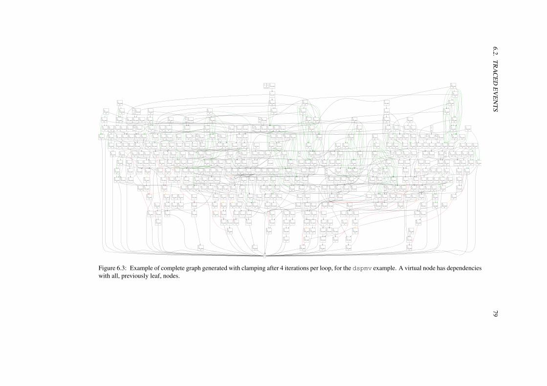
6.2.T
RA
CE
DE
VE
NT
S79
0(0)
i64 0
2(0)
i32 0
4(0)1; line:66; column:69
/
5(0)2; line:66; column:71
+
16(0,0)20; line:66; column:59
LD
28(0,1)20; line:66; column:59
LD
40(0,2)20; line:66; column:59
LD
52(0,3)20; line:66; column:59
LD
58(1,0,3,4,0)
11(0,0)
i32 0
18(0,0)22; line:66; column:75
+
13(0,0)17; line:66; column:21
LD
14(0,0)18; line:66; column:31
*
20(0,0)24; line:66; column:38
+
15(0,0)19; line:66; column:47
LD
17(0,0)21; line:66; column:57
*
79(1,0,0)13; line:64; column:21
LD
192(2,0,0)13; line:64; column:21
LD
357(3,0,0)13; line:64; column:21
LD
19(0,0)23; line:66; column:45
*
21(0,0)25; line:66; column:19
ST
76(1,0,0)10; line:63; column:22
LD
78(1,0,0)12; line:63; column:22
ST
23(0,1)
i32 0
30(0,1)22; line:66; column:75
+
25(0,1)17; line:66; column:21
LD
26(0,1)18; line:66; column:31
*
32(0,1)24; line:66; column:38
+
27(0,1)19; line:66; column:47
LD
29(0,1)21; line:66; column:57
*
105(1,1,0)13; line:64; column:21
LD
231(2,1,0)13; line:64; column:21
LD
409(3,1,0)13; line:64; column:21
LD
31(0,1)23; line:66; column:45
*
33(0,1)25; line:66; column:19
ST
102(1,1,0)10; line:63; column:22
LD
104(1,1,0)12; line:63; column:22
ST
35(0,2)
i32 0
42(0,2)22; line:66; column:75
+
37(0,2)17; line:66; column:21
LD
38(0,2)18; line:66; column:31
*
44(0,2)24; line:66; column:38
+
39(0,2)19; line:66; column:47
LD
41(0,2)21; line:66; column:57
*
131(1,2,0)13; line:64; column:21
LD
270(2,2,0)13; line:64; column:21
LD
461(3,2,0)13; line:64; column:21
LD
43(0,2)23; line:66; column:45
*
45(0,2)25; line:66; column:19
ST
128(1,2,0)10; line:63; column:22
LD
130(1,2,0)12; line:63; column:22
ST
47(0,3)
i32 0
54(0,3)22; line:66; column:75
+
49(0,3)17; line:66; column:21
LD
50(0,3)18; line:66; column:31
*
56(0,3)24; line:66; column:38
+
51(0,3)19; line:66; column:47
LD
53(0,3)21; line:66; column:57
*
157(1,3,0)13; line:64; column:21
LD
309(2,3,0)13; line:64; column:21
LD
513(3,3,0)13; line:64; column:21
LD
55(0,3)23; line:66; column:45
*
57(0,3)25; line:66; column:19
ST
154(1,3,0)10; line:63; column:22
LD
156(1,3,0)12; line:63; column:22
ST
171(1,1,3,4,0)
61(1)1; line:66; column:69
/
62(1)2; line:66; column:71
+
87(1,0)20; line:66; column:59
LD
113(1,1)20; line:66; column:59
LD
139(1,2)20; line:66; column:59
LD
165(1,3)20; line:66; column:59
LD
70(1,0,0)
i32 0
82(1,0,0)16; line:64; column:18
+
72(1,0,0)6; line:63; column:33
LD
73(1,0,0)7; line:63; column:31
*
86(1,0)19; line:66; column:47
LD
205(2,0,1)13; line:64; column:21
LD
370(3,0,1)13; line:64; column:21
LD
75(1,0,0)9; line:63; column:43
*
74(1,0,0)8; line:63; column:45
LD
80(1,0,0)14; line:64; column:33
LD
100(1,1,0)8; line:63; column:45
LD
106(1,1,0)14; line:64; column:33
LD
126(1,2,0)8; line:63; column:45
LD
132(1,2,0)14; line:64; column:33
LD
152(1,3,0)8; line:63; column:45
LD
158(1,3,0)14; line:64; column:33
LD
77(1,0,0)11; line:63; column:22
+
189(2,0,0)10; line:63; column:22
LD
191(2,0,0)12; line:63; column:22
ST
81(1,0,0)15; line:64; column:31
*
89(1,0)22; line:66; column:75
+
84(1,0)17; line:66; column:21
LD
85(1,0)18; line:66; column:31
*
91(1,0)24; line:66; column:38
+
88(1,0)21; line:66; column:57
*
90(1,0)23; line:66; column:45
*
92(1,0)25; line:66; column:19
ST
202(2,0,1)10; line:63; column:22
LD
204(2,0,1)12; line:63; column:22
ST
96(1,1,0)
i32 0
108(1,1,0)16; line:64; column:18
+
98(1,1,0)6; line:63; column:33
LD
99(1,1,0)7; line:63; column:31
*
112(1,1)19; line:66; column:47
LD
244(2,1,1)13; line:64; column:21
LD
422(3,1,1)13; line:64; column:21
LD
101(1,1,0)9; line:63; column:43
*
103(1,1,0)11; line:63; column:22
+
228(2,1,0)10; line:63; column:22
LD
230(2,1,0)12; line:63; column:22
ST
107(1,1,0)15; line:64; column:31
*
115(1,1)22; line:66; column:75
+
110(1,1)17; line:66; column:21
LD
111(1,1)18; line:66; column:31
*
117(1,1)24; line:66; column:38
+
114(1,1)21; line:66; column:57
*
116(1,1)23; line:66; column:45
*
118(1,1)25; line:66; column:19
ST
241(2,1,1)10; line:63; column:22
LD
243(2,1,1)12; line:63; column:22
ST
122(1,2,0)
i32 0
134(1,2,0)16; line:64; column:18
+
124(1,2,0)6; line:63; column:33
LD
125(1,2,0)7; line:63; column:31
*
138(1,2)19; line:66; column:47
LD
283(2,2,1)13; line:64; column:21
LD
474(3,2,1)13; line:64; column:21
LD
127(1,2,0)9; line:63; column:43
*
129(1,2,0)11; line:63; column:22
+
267(2,2,0)10; line:63; column:22
LD
269(2,2,0)12; line:63; column:22
ST
133(1,2,0)15; line:64; column:31
*
141(1,2)22; line:66; column:75
+
136(1,2)17; line:66; column:21
LD
137(1,2)18; line:66; column:31
*
143(1,2)24; line:66; column:38
+
140(1,2)21; line:66; column:57
*
142(1,2)23; line:66; column:45
*
144(1,2)25; line:66; column:19
ST
280(2,2,1)10; line:63; column:22
LD
282(2,2,1)12; line:63; column:22
ST
148(1,3,0)
i32 0
160(1,3,0)16; line:64; column:18
+
150(1,3,0)6; line:63; column:33
LD
151(1,3,0)7; line:63; column:31
*
164(1,3)19; line:66; column:47
LD
322(2,3,1)13; line:64; column:21
LD
526(3,3,1)13; line:64; column:21
LD
153(1,3,0)9; line:63; column:43
*
155(1,3,0)11; line:63; column:22
+
306(2,3,0)10; line:63; column:22
LD
308(2,3,0)12; line:63; column:22
ST
159(1,3,0)15; line:64; column:31
*
167(1,3)22; line:66; column:75
+
162(1,3)17; line:66; column:21
LD
163(1,3)18; line:66; column:31
*
169(1,3)24; line:66; column:38
+
166(1,3)21; line:66; column:57
*
168(1,3)23; line:66; column:45
*
170(1,3)25; line:66; column:19
ST
319(2,3,1)10; line:63; column:22
LD
321(2,3,1)12; line:63; column:22
ST
336(1,2,3,4,0)
174(2)1; line:66; column:69
/
175(2)2; line:66; column:71
+
213(2,0)20; line:66; column:59
LD
252(2,1)20; line:66; column:59
LD
291(2,2)20; line:66; column:59
LD
330(2,3)20; line:66; column:59
LD
183(2,0,0)
i32 0
195(2,0,0)16; line:64; column:18
+
185(2,0,0)6; line:63; column:33
LD
186(2,0,0)7; line:63; column:31
*
198(2,0,1)6; line:63; column:33
LD
212(2,0)19; line:66; column:47
LD
383(3,0,2)13; line:64; column:21
LD
188(2,0,0)9; line:63; column:43
*
187(2,0,0)8; line:63; column:45
LD
193(2,0,0)14; line:64; column:33
LD
226(2,1,0)8; line:63; column:45
LD
232(2,1,0)14; line:64; column:33
LD
265(2,2,0)8; line:63; column:45
LD
271(2,2,0)14; line:64; column:33
LD
304(2,3,0)8; line:63; column:45
LD
310(2,3,0)14; line:64; column:33
LD
190(2,0,0)11; line:63; column:22
+
354(3,0,0)10; line:63; column:22
LD
356(3,0,0)12; line:63; column:22
ST
194(2,0,0)15; line:64; column:31
*
208(2,0,1)16; line:64; column:18
+
199(2,0,1)7; line:63; column:31
*
201(2,0,1)9; line:63; column:43
*
200(2,0,1)8; line:63; column:45
LD
206(2,0,1)14; line:64; column:33
LD
239(2,1,1)8; line:63; column:45
LD
245(2,1,1)14; line:64; column:33
LD
278(2,2,1)8; line:63; column:45
LD
284(2,2,1)14; line:64; column:33
LD
317(2,3,1)8; line:63; column:45
LD
323(2,3,1)14; line:64; column:33
LD
203(2,0,1)11; line:63; column:22
+
367(3,0,1)10; line:63; column:22
LD
369(3,0,1)12; line:63; column:22
ST
207(2,0,1)15; line:64; column:31
*
215(2,0)22; line:66; column:75
+
210(2,0)17; line:66; column:21
LD
211(2,0)18; line:66; column:31
*
217(2,0)24; line:66; column:38
+
214(2,0)21; line:66; column:57
*
216(2,0)23; line:66; column:45
*
218(2,0)25; line:66; column:19
ST
380(3,0,2)10; line:63; column:22
LD
382(3,0,2)12; line:63; column:22
ST
222(2,1,0)
i32 0
234(2,1,0)16; line:64; column:18
+
224(2,1,0)6; line:63; column:33
LD
225(2,1,0)7; line:63; column:31
*
237(2,1,1)6; line:63; column:33
LD
251(2,1)19; line:66; column:47
LD
435(3,1,2)13; line:64; column:21
LD
227(2,1,0)9; line:63; column:43
*
229(2,1,0)11; line:63; column:22
+
406(3,1,0)10; line:63; column:22
LD
408(3,1,0)12; line:63; column:22
ST
233(2,1,0)15; line:64; column:31
*
247(2,1,1)16; line:64; column:18
+
238(2,1,1)7; line:63; column:31
*
240(2,1,1)9; line:63; column:43
*
242(2,1,1)11; line:63; column:22
+
419(3,1,1)10; line:63; column:22
LD
421(3,1,1)12; line:63; column:22
ST
246(2,1,1)15; line:64; column:31
*
254(2,1)22; line:66; column:75
+
249(2,1)17; line:66; column:21
LD
250(2,1)18; line:66; column:31
*
256(2,1)24; line:66; column:38
+
253(2,1)21; line:66; column:57
*
255(2,1)23; line:66; column:45
*
257(2,1)25; line:66; column:19
ST
432(3,1,2)10; line:63; column:22
LD
434(3,1,2)12; line:63; column:22
ST
261(2,2,0)
i32 0
273(2,2,0)16; line:64; column:18
+
263(2,2,0)6; line:63; column:33
LD
264(2,2,0)7; line:63; column:31
*
276(2,2,1)6; line:63; column:33
LD
290(2,2)19; line:66; column:47
LD
487(3,2,2)13; line:64; column:21
LD
266(2,2,0)9; line:63; column:43
*
268(2,2,0)11; line:63; column:22
+
458(3,2,0)10; line:63; column:22
LD
460(3,2,0)12; line:63; column:22
ST
272(2,2,0)15; line:64; column:31
*
286(2,2,1)16; line:64; column:18
+
277(2,2,1)7; line:63; column:31
*
279(2,2,1)9; line:63; column:43
*
281(2,2,1)11; line:63; column:22
+
471(3,2,1)10; line:63; column:22
LD
473(3,2,1)12; line:63; column:22
ST
285(2,2,1)15; line:64; column:31
*
293(2,2)22; line:66; column:75
+
288(2,2)17; line:66; column:21
LD
289(2,2)18; line:66; column:31
*
295(2,2)24; line:66; column:38
+
292(2,2)21; line:66; column:57
*
294(2,2)23; line:66; column:45
*
296(2,2)25; line:66; column:19
ST
484(3,2,2)10; line:63; column:22
LD
486(3,2,2)12; line:63; column:22
ST
300(2,3,0)
i32 0
312(2,3,0)16; line:64; column:18
+
302(2,3,0)6; line:63; column:33
LD
303(2,3,0)7; line:63; column:31
*
315(2,3,1)6; line:63; column:33
LD
329(2,3)19; line:66; column:47
LD
539(3,3,2)13; line:64; column:21
LD
305(2,3,0)9; line:63; column:43
*
307(2,3,0)11; line:63; column:22
+
510(3,3,0)10; line:63; column:22
LD
512(3,3,0)12; line:63; column:22
ST
311(2,3,0)15; line:64; column:31
*
325(2,3,1)16; line:64; column:18
+
316(2,3,1)7; line:63; column:31
*
318(2,3,1)9; line:63; column:43
*
320(2,3,1)11; line:63; column:22
+
523(3,3,1)10; line:63; column:22
LD
525(3,3,1)12; line:63; column:22
ST
324(2,3,1)15; line:64; column:31
*
332(2,3)22; line:66; column:75
+
327(2,3)17; line:66; column:21
LD
328(2,3)18; line:66; column:31
*
334(2,3)24; line:66; column:38
+
331(2,3)21; line:66; column:57
*
333(2,3)23; line:66; column:45
*
335(2,3)25; line:66; column:19
ST
536(3,3,2)10; line:63; column:22
LD
538(3,3,2)12; line:63; column:22
ST
553(1,3,3,4,0)
339(3)1; line:66; column:69
/
340(3)2; line:66; column:71
+
391(3,0)20; line:66; column:59
LD
443(3,1)20; line:66; column:59
LD
495(3,2)20; line:66; column:59
LD
547(3,3)20; line:66; column:59
LD
348(3,0,0)
i32 0
360(3,0,0)16; line:64; column:18
+
350(3,0,0)6; line:63; column:33
LD
351(3,0,0)7; line:63; column:31
*
363(3,0,1)6; line:63; column:33
LD
376(3,0,2)6; line:63; column:33
LD
390(3,0)19; line:66; column:47
LD
353(3,0,0)9; line:63; column:43
*
352(3,0,0)8; line:63; column:45
LD
358(3,0,0)14; line:64; column:33
LD
404(3,1,0)8; line:63; column:45
LD
410(3,1,0)14; line:64; column:33
LD
456(3,2,0)8; line:63; column:45
LD
462(3,2,0)14; line:64; column:33
LD
508(3,3,0)8; line:63; column:45
LD
514(3,3,0)14; line:64; column:33
LD
355(3,0,0)11; line:63; column:22
+
554(1,4,0)
359(3,0,0)15; line:64; column:31
*
373(3,0,1)16; line:64; column:18
+
364(3,0,1)7; line:63; column:31
*
366(3,0,1)9; line:63; column:43
*
365(3,0,1)8; line:63; column:45
LD
371(3,0,1)14; line:64; column:33
LD
417(3,1,1)8; line:63; column:45
LD
423(3,1,1)14; line:64; column:33
LD
469(3,2,1)8; line:63; column:45
LD
475(3,2,1)14; line:64; column:33
LD
521(3,3,1)8; line:63; column:45
LD
527(3,3,1)14; line:64; column:33
LD
368(3,0,1)11; line:63; column:22
+
372(3,0,1)15; line:64; column:31
*
386(3,0,2)16; line:64; column:18
+
377(3,0,2)7; line:63; column:31
*
379(3,0,2)9; line:63; column:43
*
378(3,0,2)8; line:63; column:45
LD
384(3,0,2)14; line:64; column:33
LD
430(3,1,2)8; line:63; column:45
LD
436(3,1,2)14; line:64; column:33
LD
482(3,2,2)8; line:63; column:45
LD
488(3,2,2)14; line:64; column:33
LD
534(3,3,2)8; line:63; column:45
LD
540(3,3,2)14; line:64; column:33
LD
381(3,0,2)11; line:63; column:22
+
385(3,0,2)15; line:64; column:31
*
393(3,0)22; line:66; column:75
+
388(3,0)17; line:66; column:21
LD
389(3,0)18; line:66; column:31
*
395(3,0)24; line:66; column:38
+
392(3,0)21; line:66; column:57
*
394(3,0)23; line:66; column:45
*
396(3,0)25; line:66; column:19
ST
400(3,1,0)
i32 0
412(3,1,0)16; line:64; column:18
+
402(3,1,0)6; line:63; column:33
LD
403(3,1,0)7; line:63; column:31
*
415(3,1,1)6; line:63; column:33
LD
428(3,1,2)6; line:63; column:33
LD
442(3,1)19; line:66; column:47
LD
405(3,1,0)9; line:63; column:43
*
407(3,1,0)11; line:63; column:22
+
411(3,1,0)15; line:64; column:31
*
425(3,1,1)16; line:64; column:18
+
416(3,1,1)7; line:63; column:31
*
418(3,1,1)9; line:63; column:43
*
420(3,1,1)11; line:63; column:22
+
424(3,1,1)15; line:64; column:31
*
438(3,1,2)16; line:64; column:18
+
429(3,1,2)7; line:63; column:31
*
431(3,1,2)9; line:63; column:43
*
433(3,1,2)11; line:63; column:22
+
437(3,1,2)15; line:64; column:31
*
445(3,1)22; line:66; column:75
+
440(3,1)17; line:66; column:21
LD
441(3,1)18; line:66; column:31
*
447(3,1)24; line:66; column:38
+
444(3,1)21; line:66; column:57
*
446(3,1)23; line:66; column:45
*
448(3,1)25; line:66; column:19
ST
452(3,2,0)
i32 0
464(3,2,0)16; line:64; column:18
+
454(3,2,0)6; line:63; column:33
LD
455(3,2,0)7; line:63; column:31
*
467(3,2,1)6; line:63; column:33
LD
480(3,2,2)6; line:63; column:33
LD
494(3,2)19; line:66; column:47
LD
457(3,2,0)9; line:63; column:43
*
459(3,2,0)11; line:63; column:22
+
463(3,2,0)15; line:64; column:31
*
477(3,2,1)16; line:64; column:18
+
468(3,2,1)7; line:63; column:31
*
470(3,2,1)9; line:63; column:43
*
472(3,2,1)11; line:63; column:22
+
476(3,2,1)15; line:64; column:31
*
490(3,2,2)16; line:64; column:18
+
481(3,2,2)7; line:63; column:31
*
483(3,2,2)9; line:63; column:43
*
485(3,2,2)11; line:63; column:22
+
489(3,2,2)15; line:64; column:31
*
497(3,2)22; line:66; column:75
+
492(3,2)17; line:66; column:21
LD
493(3,2)18; line:66; column:31
*
499(3,2)24; line:66; column:38
+
496(3,2)21; line:66; column:57
*
498(3,2)23; line:66; column:45
*
500(3,2)25; line:66; column:19
ST
504(3,3,0)
i32 0
516(3,3,0)16; line:64; column:18
+
506(3,3,0)6; line:63; column:33
LD
507(3,3,0)7; line:63; column:31
*
519(3,3,1)6; line:63; column:33
LD
532(3,3,2)6; line:63; column:33
LD
546(3,3)19; line:66; column:47
LD
509(3,3,0)9; line:63; column:43
*
511(3,3,0)11; line:63; column:22
+
515(3,3,0)15; line:64; column:31
*
529(3,3,1)16; line:64; column:18
+
520(3,3,1)7; line:63; column:31
*
522(3,3,1)9; line:63; column:43
*
524(3,3,1)11; line:63; column:22
+
528(3,3,1)15; line:64; column:31
*
542(3,3,2)16; line:64; column:18
+
533(3,3,2)7; line:63; column:31
*
535(3,3,2)9; line:63; column:43
*
537(3,3,2)11; line:63; column:22
+
541(3,3,2)15; line:64; column:31
*
549(3,3)22; line:66; column:75
+
544(3,3)17; line:66; column:21
LD
545(3,3)18; line:66; column:31
*
551(3,3)24; line:66; column:38
+
548(3,3)21; line:66; column:57
*
550(3,3)23; line:66; column:45
*
552(3,3)25; line:66; column:19
ST
Figure 6.3: Example of complete graph generated with clamping after 4 iterations per loop, for the dspmv example. A virtual node has dependencieswith all, previously leaf, nodes.
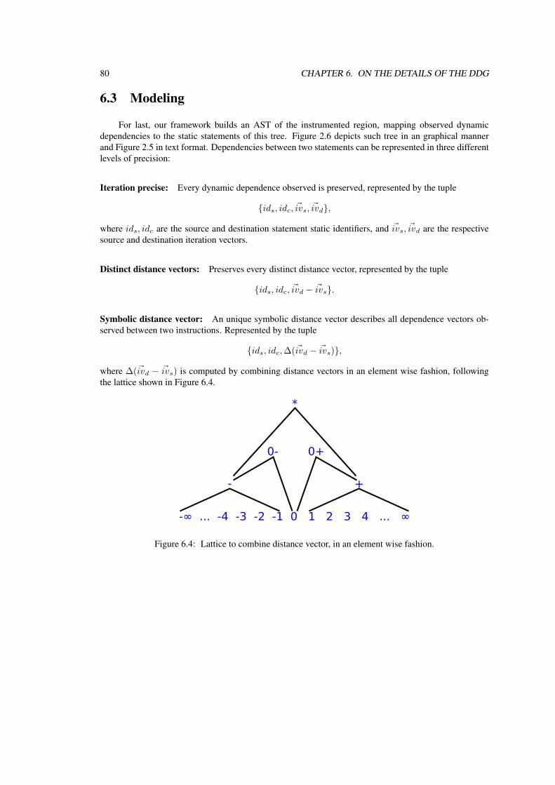
80 CHAPTER 6. ON THE DETAILS OF THE DDG
6.3 Modeling
For last, our framework builds an AST of the instrumented region, mapping observed dynamicdependencies to the static statements of this tree. Figure 2.6 depicts such tree in an graphical mannerand Figure 2.5 in text format. Dependencies between two statements can be represented in three differentlevels of precision:
Iteration precise: Every dynamic dependence observed is preserved, represented by the tuple
{ids, idc, ~ivs, ~ivd},
where ids, idc are the source and destination statement static identifiers, and ~ivs, ~ivd are the respectivesource and destination iteration vectors.
Distinct distance vectors: Preserves every distinct distance vector, represented by the tuple
{ids, idc, ~ivd − ~ivs}.
Symbolic distance vector: An unique symbolic distance vector describes all dependence vectors ob-served between two instructions. Represented by the tuple
{ids, idc,∆(~ivd − ~ivs)},
where ∆(~ivd − ~ivs) is computed by combining distance vectors in an element wise fashion, followingthe lattice shown in Figure 6.4.
-∞ ... -4 -3 -2 -1 0 1 2 3 4 ... ∞
- +
*
0- 0+
Figure 6.4: Lattice to combine distance vector, in an element wise fashion.
Chapter 7
Conclusion
When dependence analysis fail to provide precise information, it prejudices the compilers to re-trieve profitable code transformations or even to ensure that a given, valid, optimization preserves syntax.May-alias base pointers and memory accesses described by polynomial expressions over loop inductionvariables are two factors that limit existing dependence analysis precision addressed by this work. May-alias conditions appear from unrestrained memory pointers received as function arguments. Memoryaccesses using polynomial expressions over loop induction variables can appear as result of compilerslinearization process of data structures or use of data symmetries to preserve memory, such as symmetricmatrices used in LAPACK (www.netlib.org, 1992).
By performing memory accesses profiling the proposed framework uses dependencies observed atrun-time to resolve dependencies not solved statically. Using Scalar Evolution (Pop et al., 2005) anal-yses, spurious dependencies are ignoring computations of values that described statically by a closedformula. To avoid the expensive costs of analyzing all dynamic instructions, techniques such as cut-offand clamping limit the number of loop iterations analyzed. Cut-off, and optimistic approach, ignoresdependencies occurred outside the observed space while clamping preserves such dependencies but witha much lighter, and imprecise, method that compresses instructions outside the observed space into sin-gle fake instruction. Observed dependencies are used as ground truth information when retrieving looptransformations. Once retrieved a new loop schedule the framework builds a test that defines sufficient,and required, conditions for which the retrieve transformation is invalid.
Such test consists in validating, for every pair of distinct dynamic instructions in may-dependence, ifthey both accesses the same memory position and if their original relative execution order, is not preservedwhen applied the optimization. Evaluated at run-time the generated test would only return true if at leastone dependence is violated. However, the cost of evaluating such test grows quadratically in the numberof dynamic instructions in the transformed region. This means that evaluating such test would, probably,take a longer time than just executing the original program without any optimization. To transform suchcomplex test into a much lighter one the proposed work uses a quantifier elimination scheme.
The generated test consists in systems of equalities and inequalities over loop induction variables andmemory base pointers. Induction variables, coming from dynamic instruction identifiers (the inductionvectors), define existential variables for which all possible values must be evaluated. Using quantifierelimination these existential variables are eliminated generating systems that can be evaluated in O(1),in regard of the number of dynamic instructions, but might be more constraining than the original test.Based on Fourier-Motzking Elimination (FME), a quantifier elimination technique developed for linearsystems of inequalities over the R, new extensions were generated for handling multivariate polynomials
81
82 CHAPTER 7. CONCLUSION
on the Z. Writing all expressions as non-negative inequalities, the Schweighofer tester implements anpositiveness test algorithm based on Schweighofer’s work (Schweighofer, 2002, Theorem 5?) and isthe core tool of the proposed simplifier. The Schweighofer tester allows detection of coefficient signs,required to classify if a given inequality defines an upper or lower bound, prerequisite to perform FME.It allows extending normalization (Pugh, 1991) to symbolic expressions, minimizing rounding errors ofinteger systems. Although the test is evaluated in O(1) in regard of dynamic instructions, the numberof expressions inside each system, validating a may-dependence violation among two statements, mightgrow exponentially with the number of variables eliminated. The number of systems to be evaluatedmight also grow with the number of statements in may-dependence. Once again the Schweighofer testerplays an important role in simplifying the system, by allowing to detect and remove redundant constraintsfrom within each system, and redundant systems among all systems. Compared to existing quantifierelimination tools, such as QEPCAD-B (Brown, 2003), our quantifier elimination technique demonstratescompetitive time and memory costs and yields preciser results, required to successfully allow executionof the optimized code.
For last the simplified test guards the execution of the optimized region. If evaluated, at run-time, tofalse, the test directs to the execution of the optimized code and directs to the original, not optimized codeotherwise. We demonstrated that such tests impose very low overhead, even with very small load works,that take less then a second to execute. Our work allows any affine rescheduling of loop regions, as far allmemory accesses in the optimized region contain a static closed formula. Different than works that onlyperform may-alias overlapping tests (Rus et al., 2002; Kaplansky, 2006; Grös̈linger, 2009; Alves et al.,2015) or speculative systems that impose costly and complex run-time validations (Jimborean, 2012;Sukumaran-Rajam et al., 2014). The soundness and precision of the proposed technique is demonstratedover 24 kernels retrieved from the Polybench 4.1 (Pouchet and Yuki, 2015) and even in code with packedtriangular matrices, such as the implemented triangular Floyd-Warshall, for which lightweight and precisetests where generated.
The presented framework demonstrates promising results when it comes to validate complex looptransformations in code with poor dependence information, obtaining less constraining and still valid.Still under development the framework holds many room from improvements in test precision and exe-cution time cost.
7.1 Future work
Although the existing framework presents promising results, some factor currently limit its use: Theamount of time to generate run-time tests and to simplify them are in the range of minutes, when dealingwith small kernels, making it impossible to use with larger code. The process is not yet automated,requiring human intervention to handle non-affine code. The validation test is simplified regardless ifthe simplified test is too constraining and would always prevent the optimization to be used. The currentimplementation cannot handle code with function calls or double indirection. Addressing these flaws arecrucial to turn this framework competitive with existing techniques. Some guides on how to do so areprovided below:
Bernstein expansion: By using Bernstein expansion it is possible to bound the range of a multivariatepolynomial over a parametric polyhedra, as described by Phillipe Clauss on (Clauss and Tchoupaeva,2004). On that work their motivation was also dependence resolution among memory accesses describedby polynomial expressions. Just as in our systems that describe may-dependencies violations, to definethe dependence actually exists the memory positions accesses by two instructions in may-dependence
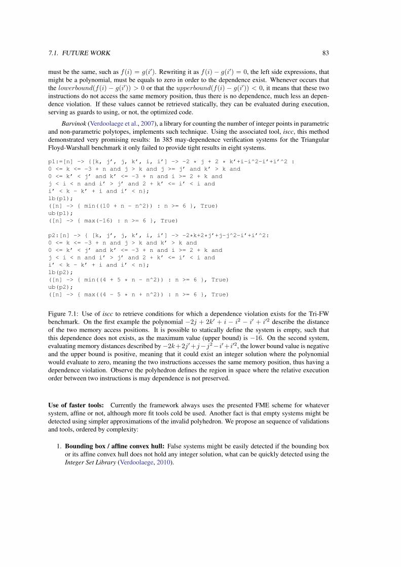
7.1. FUTURE WORK 83
must be the same, such as f(i) = g(i′). Rewriting it as f(i) − g(i′) = 0, the left side expressions, thatmight be a polynomial, must be equals to zero in order to the dependence exist. Whenever occurs thatthe lowerbound(f(i) − g(i′)) > 0 or that the upperbound(f(i) − g(i′)) < 0, it means that these twoinstructions do not access the same memory position, thus there is no dependence, much less an depen-dence violation. If these values cannot be retrieved statically, they can be evaluated during execution,serving as guards to using, or not, the optimized code.
Barvinok (Verdoolaege et al., 2007), a library for counting the number of integer points in parametricand non-parametric polytopes, implements such technique. Using the associated tool, iscc, this methoddemonstrated very promising results: In 385 may-dependence verification systems for the TriangularFloyd-Warshall benchmark it only failed to provide tight results in eight systems.
p1:=[n] -> {[k, j’, j, k’, i, i’] -> -2 * j + 2 * k’+i-i^2-i’+i’^2 :0 <= k <= -3 + n and j > k and j >= j’ and k’ > k and0 <= k’ < j’ and k’ <= -3 + n and i >= 2 + k andj < i < n and i’ > j’ and 2 + k’ <= i’ < i andi’ < k - k’ + i and i’ < n};lb(p1);([n] -> { min((10 + n - n^2)) : n >= 6 }, True)ub(p1);([n] -> { max(-16) : n >= 6 }, True)
p2:[n] -> { [k, j’, j, k’, i, i’] -> -2*k+2*j’+j-j^2-i’+i’^2:0 <= k <= -3 + n and j > k and k’ > k and0 <= k’ < j’ and k’ <= -3 + n and i >= 2 + k andj < i < n and i’ > j’ and 2 + k’ <= i’ < i andi’ < k - k’ + i and i’ < n};lb(p2);([n] -> { min((4 + 5 * n - n^2)) : n >= 6 }, True)ub(p2);([n] -> { max((4 - 5 * n + n^2)) : n >= 6 }, True)
Figure 7.1: Use of iscc to retrieve conditions for which a dependence violation exists for the Tri-FWbenchmark. On the first example the polynomial −2j + 2k′ + i − i2 − i′ + i′2 describe the distanceof the two memory access positions. It is possible to statically define the system is empty, such thatthis dependence does not exists, as the maximum value (upper bound) is −16. On the second system,evaluating memory distances described by−2k+2j′+j−j2− i′+ i′2, the lower bound value is negativeand the upper bound is positive, meaning that it could exist an integer solution where the polynomialwould evaluate to zero, meaning the two instructions accesses the same memory position, thus having adependence violation. Observe the polyhedron defines the region in space where the relative executionorder between two instructions is may dependence is not preserved.
Use of faster tools: Currently the framework always uses the presented FME scheme for whateversystem, affine or not, although more fit tools cold be used. Another fact is that empty systems might bedetected using simpler approximations of the invalid polyhedron. We propose an sequence of validationsand tools, ordered by complexity:
1. Bounding box / affine convex hull: False systems might be easily detected if the bounding boxor its affine convex hull does not hold any integer solution, what can be quickly detected using theInteger Set Library (Verdoolaege, 2010).
84 CHAPTER 7. CONCLUSION
2. Affine systems using existing FME: Affine systems can use existing FME implementation in theISL. If the systems holds polynomial constraints FME can be applied to its affine convex hull. Theresult can be evaluated against profiled values to determinate if it is tight enough.
3. Bernstein expansion: For systems defined by affine constraints, and a single polynomial equality,the technique described on the previous item can be used to retrieve parametric conditions to beused as the transformation validations. Systems containing multiple polynomial equalities can betransformed into multiple systems with a single polynomial equality. The obtained conditions canbe evaluated using profiled values to determine if they are tight enough.
4. Faster quantifier elimination: For systems with polynomial constraints faster quantifier elimi-nation implementations, such as Redlog (Dolzmann and Sturm, 1997; WEISPFENNING, 1997),might be capable to detect systems that are empty even when working over constraints in R.
Improve sign detection: Many can be done to speed-up or increase the capacity of the Schweighofertester to decide upon expressions signs. Such improvements might increase the number of coefficientsigns detected, reducing the number of systems to be evaluated, possible also reducing the final test sizeand increasing their precision, as normalization highly depends on the Schweighofer tester.
1. Bernstein expansion: Using only the affine constraints of an system to build a polyhedron, poly-nomial expressions that are exclusively positive, or negative, in such polyhedron hold the samesign in the original one. Once again, the Bernstein technique could be used to retrieve polynomialbounds.
2. Static Schweighofer tester: Our current heuristic to determinate which sub-set from a system ofconstraints should be used to build the Schweighofer tester if very costly, requiring to evaluate ahuge number of systems. Perhaps using the original system and eliminating constraints that areunique in holding monomials not present in the evaluated expression and that cannot be furthergenerated by higher order combination might be sufficient to avoid memory explosions.
3. More flexible linear solver: Our current Schweighofer tester implementation uses the linear solverdelivered in the GiNaC library, however this solver does not allow imposing positiveness con-straints, and many the algorithm failed to retrieve existing implications due the solver returningsolutions with negative factors.
Profile guided QE: This work only focused on complete elimination of quantifiers in test expressions.Perhaps, using run-time information, one could validate that eliminating a certain variable might generatea test that always fails, and try to eliminate other ones, or even generate a test with loops. The prob-lem with these tests containing loops is that validating that the complexity of the generated guard doesnot outweigh the optimization gains. For last, profiled values can be used to simplify the final test byremoving constraints that, in multiple executions traces, always evaluate to true.
Interleaved memory accesses: Can interleaved memory accesses, such as vectors of multi-elementstructures or two independent sub-images of a bigger picture, be represented in a form that quantifierelimination can preserve, which would help in validating distinct interleaved accesses? Perhaps by deter-mining expressions limited by modular values. For example, an matrix F [NxN ], and two sub-matricesA[MxM ] and B[LxL]. If the accesses to sub-matrices A and B module N would give non-overlappingsets, it means that A and B do not overlap.
7.2. CLOSING THOUGHTS 85
Code with function calls: This work does not allow function calls inside the optimized region, since itdoes not know how to fit them into an affine program representation to be given to a polyhedral optimizer.However, one might think on functions as statements in an outer, “global” loop. Each time a function callor return executes, it is as if a new iteration of this external loop had started. All the functions can then bethought of as residing in a global if-then-else chain where each element is assigned a unique timedimension id. In such a representation, all canonical iteration vector would have two more fields in frontof them. The first would hold how many times function calls and return instructions where executed. Thesecond holds a unique identifier per function.
Inspector / executor: Currently the framework only supports code with a single layer of indirection,such as A[f(~iv)] += ··, where f(~iv) is an statically known function over canonical induction variables.It can be extended to handle memory accesses with double indirection, such as A[B[f(~iv)]] += ··, aninspector / executor loop can verify that B[f(~iv)] defines an one-to-one memory to ~iv map, treatingA[B] as an common pointer AB, constant along the loop and treated as an parameter in our dependenceviolation systems.
Byte precise / lengthened instrumentation: The current instrumentation and test generation assumedata sizes are all equals, such that distinct memory accesses cannot overlap, even if the amount of loadeddata is different.
7.2 Closing thoughts
This work demonstrates how to statically optimize some loops with inaccurate dependence infor-mation using existing optimizing tools. Run-time behavior, retrieved by profiling, guide the optimizerproviding concrete dependence information not resolved statically. A run-time validation test, repre-senting the space where the applied transformation violates at least one dependence, is simplified to amuch simpler test using quantifier elimination. We believe this is an comprehensive method to resolvedependencies, including aliasing, allowing more loops to be optimized by polyhedron tools.
Apart from shortcomings that must be addresses, cited on the previous section, the current frame-work has no guaranties that the chosen transformation is actually profitable or if the run-time test wouldblock valid transformations in most cases. Further research could address these limitations by performingan incremental profiling information, where the success ration of the generate test is accumulated acrossmultiple executions. If the current test usually fails, a more complex instrumentation could retrieve moredependencies, used when retrieving the optimization, replacing the current test and transformed codes.Hardware counters could be used to determine if the applied optimization actually performs better thanthe original code by using hardware counters to evaluate both codes, and decide if the applied transfor-mation is better than the original code.
Other possibility to address the two limitations could be by combining speculative systems with thecurrent framework, such as Apollo. The first time an application is executed the speculative system runsthe its usual way. If it finished the program execution using an optimized code, this optimized code canbe exported to generate, statically, an lightweight run-time test, using the techniques here proposed. Justas described above, this could be part of an incremental profiling framework to decide upon the test ortransformation quality.
We hope the presented work will be useful to further research.

86 CHAPTER 7. CONCLUSION
Bibliography
Allen, R. and Kennedy, K. (2002). Optimizing compilers for modern architectures: a dependence-basedapproach, volume 289. Morgan Kaufmann. On page 35
Alves, P., Gruber, F., Doerfert, J., Lamprineas, A., Grosser, T., Rastello, F., and Pereira, F. M. Q. a.(2015). Runtime pointer disambiguation. In Proceedings of the 2015 ACM SIGPLAN InternationalConference on Object-Oriented Programming, Systems, Languages, and Applications, OOPSLA 2015,pages 589–606, New York, NY, USA. ACM. On pages 53 and 82
APOLLO (2016). Apollo. http://apollo.gforge.inria.fr. On page 16
Apple (2007). clang: a c language family frontend for llvm. On page 25
Bastoul, C. (2004). Code generation in the polyhedral model is easier than you think. In PACT’13 IEEEInternational Conference on Parallel Architecture and Compilation Techniques, pages 7–16, Juan-les-Pins, France. On page 17
Benabderrahmane, M.-W., Bastoul, C., Pouchet, L.-N., and Cohen, A. (2008). A Conservative Approachto Handle Full Functions in the Polyhedral Model. Research Report RR-6814, INRIA. On page 17
Bik, A. J. C. (2004). Software Vectorization Handbook, The: Applying Intel Multimedia Extensions forMaximum Performance. Intel Press. On page 53
Bondhugula, U., Hartono, A., Ramanujam, J., and Sadayappan, P. (2008). Pluto: A practical and fullyautomatic polyhedral program optimization system. In Proceedings of the ACM SIGPLAN 2008 Con-ference on Programming Language Design and Implementation (PLDI 08), Tucson, AZ (June 2008).On page 72
Bondhugula, U. K. R. (2008). Effective Automatic Parallelization and Locality Optimization Using thePolyhedral Model. PhD thesis, Ohio State University, Columbus, OH, USA. AAI3325799. On page 17
Brown, C. W. (2003). Qepcad b: A program for computing with semi-algebraic sets using cads. SIGSAMBull., 37(4):97–108. On pages 51, 55, 64, and 82
Charles, P., Grothoff, C., Saraswat, V., Donawa, C., Kielstra, A., Ebcioglu, K., von Praun, C., and Sarkar,V. (2005). X10: An object-oriented approach to non-uniform cluster computing. In Proceedings of the20th Annual ACM SIGPLAN Conference on Object-oriented Programming, Systems, Languages, andApplications, OOPSLA ’05, pages 519–538, New York, NY, USA. ACM. On page 16
Clauss, P., Fernandez, F., Garbervetsky, D., and Verdoolaege, S. (2009). Symbolic polynomial maxi-mization over convex sets and its application to memory requirement estimation. Very Large ScaleIntegration (VLSI) Systems, IEEE Transactions on, 17(8):983–996. On page 52
87
88 BIBLIOGRAPHY
Clauss, P. and Tchoupaeva, I. (2004). A Symbolic Approach to Bernstein Expansion for Program Analysisand Optimization, pages 120–133. Springer Berlin Heidelberg, Berlin, Heidelberg. On page 82
Cohen, C. and Mahboubi, A. (2010). A Formal Quantifier Elimination for Algebraically Closed Fields,pages 189–203. Springer Berlin Heidelberg, Berlin, Heidelberg. On page 63
Cousot, P. and Halbwachs, N. (1978). Automatic discovery of linear restraints among variables ofa program. In 5th ACM SIGACT-SIGPLAN Symposium on Principles of Programming Languages(POPL’78), pages 84–96, Tucson, Arizona. ACM. On page 17
Davenport, J. H. and Heintz, J. (1988). Real quantifier elimination is doubly exponential. Journal ofSymbolic Computation, 5(1):29 – 35. On page 63
Dolzmann, A. and Sturm, T. (1997). Redlog: Computer algebra meets computer logic. SIGSAM Bull.,31(2):2–9. On page 84
Elango, V., Rastello, F., Pouchet, L.-N., Ramanujam, J., and Sadayappan, P. (2015a). On characterizingthe data access complexity of programs. In Proceedings of the 42Nd Annual ACM SIGPLAN-SIGACTSymposium on Principles of Programming Languages, POPL ’15, pages 567–580, New York, NY,USA. ACM. On pages 71 and 76
Elango, V., Sedaghati, N., Rastello, F., Pouchet, L.-N., Ramanujam, J., Teodorescu, R., and Sadayappan,P. (2015b). On using the roofline model with lower bounds on data movement. ACM Trans. Archit.Code Optim., 11(4):67:1–67:23. On page 71
Fauzia, N., Elango, V., Ravishankar, M., Ramanujam, J., Rastello, F., Rountev, A., Pouchet, L.-N., andSadayappan, P. (2013). Beyond reuse distance analysis: Dynamic analysis for characterization of datalocality potential. ACM Transactions on Architecture and Code Optimization (TACO), 10(4):53. Onpage 71
Feautrier, P. (1988a). Array expansion. In 2nd International Conference on Supercomputing (ICS’88),pages 429–441. ACM. On page 17
Feautrier, P. (1988b). Parametric integer programming. RAIRO Recherche opérationnelle, 22(3):243–268.On page 17
Feautrier, P. (1992a). Some efficient solutions to the affine scheduling problem. i. one-dimensional time.International Journal of Parallel Programming, 21(5):313–347. On page 17
Feautrier, P. (1992b). Some efficient solutions to the affine scheduling problem. part ii. multidimensionaltime. International Journal of Parallel Programming, 21(6):389–420. On pages 17, 22, and 23
Feautrier, P. (2015). The power of polynomials. In 5th International Workshop on Polyhedral CompilationTechniques. http://impact.gforge.inria.fr/impact2015/. On page 52
Grös̈linger, A. (2009). The Challenges of Non-linear Parameters and Variables in Automatic Loop Par-allelisation. PhD thesis, Universität Passau. On pages 17, 51, 53, and 82
Grosser, T., Groesllinger, A., and Lengauer, C. (2012). Polly - performing polyhedral optimizations on alow-level intermediate representation. Parallel Processing Letters, 04(22):X. On pages 17 and 24
Grosser, T., Pop, S., Ramanujam, J., and Sadayappan, P. (2015a). On recovering multi-dimensional arraysin polly. In 5th International Workshop on Polyhedral Compilation Techniques. http://impact.gforge.inria.fr/impact2015/. On page 52
BIBLIOGRAPHY 89
Grosser, T., Ramanujam, J., Pouchet, L.-N., Sadayappan, P., and Pop, S. (2015b). Optimistic delineariza-tion of parametrically sized arrays. In Proceedings of the 29th ACM on International Conference onSupercomputing, ICS ’15, pages 351–360, New York, NY, USA. ACM. On page 17
Grosser, T., Ramanujam, J., Pouchet, L.-N., Sadayappan, P., and Pop, S. (2015c). Optimistic delineariza-tion of parametrically sized arrays. In Proceedings of the 29th ACM on International Conference onSupercomputing, ICS ’15, pages 351–360, New York, NY, USA. ACM. On page 52
Henretty, T., Veras, R., Franchetti, F., Pouchet, L.-N., Ramanujam, J., and Sadayappan, P. (2013). Astencil compiler for short-vector simd architectures. In Proceedings of the 27th International ACMConference on International Conference on Supercomputing, ICS ’13, pages 13–24, New York, NY,USA. ACM. On page 16
Hind, M. (2001). Pointer analysis: haven’t we solved this problem yet? In Proceedings of the 2001 ACMSIGPLAN-SIGSOFT workshop on Program analysis for software tools and engineering, pages 54–61.ACM. On page 16
Hong, H. (1992). Simple solution formula construction in cylindrical algebraic decomposition basedquantifier elimination. In Papers from the International Symposium on Symbolic and Algebraic Com-putation, ISSAC ’92, pages 177–188, New York, NY, USA. ACM. On page 51
Hong, H. and Din, M. S. E. (2012). Variant quantifier elimination. Journal of Symbolic Computation,47(7):883 – 901. On page 64
Irigoin, F. and Triolet, R. (1988). Supernode partitioning. In Symposium on Principles of ProgrammingLanguages (POPL’88), pages 319–328, San Diego, CA. On page 17
ISO (1999). The ANSI C standard (C99). Technical Report WG14 N1124, ISO/IEC. On page 16
Jimborean, A. (2012). Adapting the Polytope Model for Dynamic and Speculative Parallelization. Theses,Université de Strasbourg. On pages 17, 53, and 82
Kaplansky, V. (2006). Gcc patch: implementation of alias versioning in vectorizer. https://gcc.gnu.org/ml/gcc-patches/2006-05/msg00266.html. On pages 53 and 82
Karp, R. M., Miller, R. E., and Winograd, S. (1967). The organization of computations for uniformrecurrence equations. Journal of the ACM, 14(3):563–590. On page 17
Lamport, L. (1974). The parallel execution of DO loops. Communications of the ACM, 17(2):83–93. Onpage 17
Martinez Caamaño, J. M. (2016). Fast and Flexible Compilation Techniques for Effective SpeculativePolyhedral Parallelization. Theses, Université de Strasbourg. On page 53
Maslov, V. (1992). Delinearization: An efficient way to break multiloop dependence equations. InProceedings of the ACM SIGPLAN 1992 Conference on Programming Language Design and Imple-mentation, PLDI ’92, pages 152–161, New York, NY, USA. ACM. On page 52
Nethercote, N. and Seward, J. (2007). How to shadow every byte of memory used by a program. InProceedings of the 3rd International Conference on Virtual Execution Environments, VEE ’07, pages65–74, New York, NY, USA. ACM. On pages 27 and 75
Nuzman, D., Eres, R., Guenther, R., Jelinek, J., Matz, M., Sandiford, R., and Rosen, I. (2003). Auto-vectorization in gcc. https://gcc.gnu.org/projects/tree-ssa/vectorization.html. On page 53
90 BIBLIOGRAPHY
NVIDIA (2016). NVIDIA CUDA C programming guide. http://docs.nvidia.com/cuda/pdf/CUDA_C_Programming_Guide.pdf. Version 8.0. On page 16
Oancea, C. E. and Rauchwerger, L. (2012). Logical inference techniques for loop parallelization. InProceedings of the 33rd ACM SIGPLAN Conference on Programming Language Design and Imple-mentation, PLDI ’12, pages 509–520, New York, NY, USA. ACM. On pages 52 and 53
Park, E., Cavazos, J., Pouchet, L.-N., Bastoul, C., Cohen, A., and Sadayappan, P. (2013). Predictive mod-eling in a polyhedral optimization space. International journal of parallel programming, 41(5):704–750. On page 31
Pirk, H., Petraki, E., Idreos, S., Manegold, S., and Kersten, M. L. (2014). Database cracking: fancyscan, not poor man’s sort! In Tenth International Workshop on Data Management on New Hardware,DaMoN 2014, Snowbird, UT, USA, June 23, 2014, pages 4:1–4:8. On page 16
Pop, S., Cohen, A., Bastoul, C., Girbal, S., andré Silber, G., and Vasilache, N. (2006). Graphite: Polyhe-dral analyses and optimizations for gcc. In In Proceedings of the 2006 GCC Developers Summit, page2006. On pages 17 and 24
Pop, S., Cohen, A., and Silber, G.-A. (2005). Induction variable analysis with delayed abstractions. InHigh Performance Embedded Architectures and Compilers, pages 218–232. Springer. On pages 18and 81
Pouchet, L.-N. (2010). PoCC, the Polyhedral Compiler Collection, version 1.3. http://pocc.sourceforge.net. On page 17
Pouchet, L.-N. and Yuki, T. (2015). PolyBench/C 4.1. http://polybench.sourceforge.net.On page 82
Pugh, W. (1991). The omega test: A fast and practical integer programming algorithm for dependenceanalysis. In Proceedings of the 1991 ACM/IEEE Conference on Supercomputing, Supercomputing ’91,pages 4–13, New York, NY, USA. ACM. On pages 17, 37, 42, 51, and 82
Pugh, W. and Wonnacott, D. (1996). Non-linear array dependence analysis. In Szymanski, B. andSinharoy, B., editors, Languages, Compilers and Run-Time Systems for Scalable Computers, pages1–14. Springer US. On pages 42, 51, and 53
Rus, S., Rauchwerger, L., and Hoeflinger, J. (2002). Hybrid analysis: Static and dynamic memoryreference analysis. In ICS, pages 251–283. IEEE Computer Society. On pages 17, 52, 53, and 82
Schweighofer, M. (2002). An algorithmic approach to schmüdgen’s positivstellensatz. Journal of Pureand Applied Algebra, 166(3):307 – 319. On pages 19, 37, 38, 52, 67, and 82
Smaragdakis, Y. and Balatsouras, G. (2015). Pointer analysis. Found. Trends Program. Lang., 2(1):1–69.On page 16
Sukumaran-Rajam, A. (2015). Beyond the Realm of the Polyhedral Model: Combining Speculative Pro-gram Parallelization with Polyhedral Compilation. Theses, Université de Strasbourg. On page 53
Sukumaran-Rajam, A., Martinez, J. M., Wolff, W., Jimborean, A., and Clauss, P. (2014). SpeculativeProgram Parallelization with Scalable and Decentralized Runtime Verification. In Bonakdarpour, B.and Smolka, S. A., editors, Runtime Verification, volume 8734, pages 124–139, Toronto, Canada.Springer. On pages 16, 17, and 82
BIBLIOGRAPHY 91
Suriana, P. A. (2016). Fourier-motzkin with non-linear symbolic constant coefficients. Master’s thesis,Massachusetts Institute of Technology. On page 51
Sutter, H. (2005). The free lunch is over: A fundamental turn toward concurrency in software. http://www.gotw.ca/publications/concurrency-ddj.htm. On page 15
Trifunovic, K., Cohen, A., Edelsohn, D., Li, F., Grosser, T., Jagasia, H., Ladelsky, R., Pop, S., Sjödin, J.,and Upadrasta, R. (2010). Graphite two years after: First lessons learned from real-world polyhedralcompilation. In GCC Research Opportunities Workshop (GROW’10). On page 17
van Engelen, R. A., Birch, J., Shou, Y., Walsh, B., and Gallivan, K. A. (2004). A unified framework fornonlinear dependence testing and symbolic analysis. In Proceedings of the 18th Annual InternationalConference on Supercomputing, ICS ’04, pages 106–115, New York, NY, USA. ACM. On page 52
Venkat, A., Shantharam, M., Hall, M., and Strout, M. M. (2014a). Non-affine extensions to polyhedralcode generation. In Proceedings of Annual IEEE/ACM International Symposium on Code Generationand Optimization, CGO ’14, pages 185:185–185:194, New York, NY, USA. ACM. On page 17
Venkat, A., Shantharam, M., Hall, M., and Strout, M. M. (2014b). Non-affine extensions to polyhedralcode generation. In Proceedings of Annual IEEE/ACM International Symposium on Code Generationand Optimization, CGO ’14, pages 185:185–185:194, New York, NY, USA. ACM. On page 53
Verdoolaege, S. (2010). isl: An integer set library for the polyhedral model. In Mathematical Software–ICMS 2010, pages 299–302. Springer. On pages 17 and 83
Verdoolaege, S., Seghir, R., Beyls, K., Loechner, V., and Bruynooghe, M. (2007). Counting integer pointsin parametric polytopes using barvinok’s rational functions. Algorithmica, 48(1):37–66. On page 83
Vijay, S., Bard, B., Igor, P., Olivier, T., and David, G. (2016). X10 language specification. http://x10.sourceforge.net/documentation/languagespec/x10-latest.pdf. Ver-sion 2.6. On page 16
WEISPFENNING, V. (1997). Simulation and optimization by quantifier elimination. Journal of SymbolicComputation, 24(2):189 – 208. On page 84
Williams, S., Waterman, A., and Patterson, D. A. (2009). Roofline: an insightful visual performancemodel for multicore architectures. Commun. ACM, 52(4):65–76. On page 16
Wulf, W. A. and McKee, S. A. (1995). Hitting the memory wall: Implications of the obvious. SIGARCHComput. Archit. News, 23(1):20–24. On page 16
www.netlib.org (1992). Linear algebra package. http://www.netlib.org/lapack/. Onpages 24 and 81