proceedings of the 13th international conference on mobile

Nikolaos Kofinas, Emmanouil Orfanoudakis and Michail Lagoudakis Nikolaos Kofinas, EmmanouilOrfanoudakis and Michail Lagoudakis Nikolaos Kofinas, Emmanouil Orfanoudakis and Michail LagoudakisNikolaos Kofinas, Emmanouil Orfanoudakis and Michail Lagoudakis Nikolaos Kofinas, EmmanouilOrfanoudakis and Michail Lagoudakis Nikolaos Kofinas, Emmanouil Orfanoudakis and Michail Lagoudakis

Proceedings of the 13th International Conference on MobileRobots and Competitions

Edited by

João M. F. Calado, Luís Paulo Reis and Rui Paulo Rocha

24th April, 2013

Instituto Superior de Engenharia de Lisboa

Polytechnic Institute of Lisbon

Portugal

ISBN: 978 989 97531 2 9

© 2013 IEEE. Personal use of this material is permitted. Permission from IEEE must be obtained for allother uses, in any current or future media, including reprinting/republishing this material foradvertising or promotional purposes, creating new collective works, for resale or redistribution toservers or lists, or reuse of any copyrighted component of this work in other works.

Proceedings of the 13th International Conference on Mobile Robots and Competitions © 2013 IEEE

Robotica 2013 was organized under the IEEE Robotics & Automation Society Technical Co Sponsorship978 989 97531 2 9 ii

Organizers:

Sponsors:

Patrons:


Robotica 2013 was organized under the IEEE Robotics & Automation Society Technical Co Sponsorship978 989 97531 2 9 iii

Hosted:

Cover Design:

Catarina Sampaio

Secretariat:

Maria da Conceição Ribeiro

Website Design:

Sérgio Fernandes Palma

Website:

http://www.dem.isel.pt/Robotica2013


Robotica 2013 was organized under the IEEE Robotics & Automation Society Technical Co Sponsorship978 989 97531 2 9 iv

Organizing CommitteeJoão M. Ferreira [email protected]

Instituto Superior de Engenharia deLisboa

Área Departamental de EngenhariaMecânica

Luís Paulo [email protected] do Minho

Dep. Sistemas de informaçãoLab. Inteligência Artificial e Ciência

de Computadores

Rui Paulo [email protected]

Universidade de CoimbraDep. de Engenharia Eletrotécnica e

de ComputadoresInstituto de Sistemas e Robótica

Steering CommitteeAlexandro De Luca (URoma IT)Bruno Siciliano (UNINA IT)Toshio Fukuda (UNagoya JP)

Alicia Casals (UPC SP)Hideki Hashimoto (UTokyo JP)

International Program Committee

A. Fernando Ribeiro (UMinho PT)Alexandre Simões (UNESP BR)Alicia Casals (UPC SP)Alexandro De Luca (URoma IT)André Marcato (UJuizFora BR)Andreas BirK (UJacobs D)Angel Sappa (UAB SP)Aníbal Matos (FEUP PT)António Bandera (UM SP)António P. Moreira (FEUP PT)António Pascoal (IST PT)Armando Sousa (FEUP PT)Bernardo Cunha (UAveiro PT)Bruno Siciliano (UNIMA IT)Carlos Cardeira (IST PT)Carlos Carreto (IPG PT)Danilo Tardioli (UZaragoza SP)Denis Wolf (USão Paulo BR)Dimos Dimarogonas (KTH S)Enric Cervera (UJaume I SP)Estela Bicho (UMinho PT)Fernando Melício (ISEL PT)Fernando Pereira (FEUP PT)Flavio Tonidandel (CUFEI BR)Gabriel Oliver (UIB SP)G. Kratzschmar (UBonn Rhein D)Gil Lopes (UMinho PT)

Hans Du Buf (UAlgarve PT)Helder Araújo (UCoimbra PT)Hideki Hashimoto (Utokyo JP)Hugo Costelha (IPLeiria PT)Isabel Ribeiro (IST PT)João Calado (ISEL PT)João Palma (ISEL PT)João Pinto (IST PT)João Sequeira (IST PT)Jorge Dias (UCoimbra PT)Jorge Ferreira (UAveiro PT)Jorge Lobo (UCoimbra PT)Jorge Pais (ISEL PT)José Igreja (ISEL PT)José Lima (IPBragança PT)José Luís Azevedo (UAveiro PT)José Sá da Costa (IST PT)José Tenreiro Machado (ISEP PT)Jun Ota (UTokyo JP)Luca Locchi (URome IT)Lucia Pallottino (UPisa IT)Luís Almeida (FEUP PT)Luís Gomes (UNINOVA PT)Luís Louro (UMinho PT)Luís Merino (UPOlavide SP)Luís Mota (ISCTE PT)Luís Paulo Reis (UMinho PT)

Luís S. Lopes (UAveiro PT)Luiz Chaimowicz (UFMG BR)Manuel Lopes (INRIA FR)Manuel Silva (ISEP PT)Mário Mendes (ISEL PT)Nuno Lau (UAveiro PT)Nuno Ferreira (ISEC PT)Norberto Pires (UCoimbra PT)Patrícia Vargas (UHeriot Watt UK)Patrício Nebot (UJaume I SP)Paulo Costa (FEUP PT)Paulo Fiorini (UNIVR IT)Paulo Gonçalves (IPCB PT)Paulo Menezes (UCoimbra PT)Paulo Oliveira (IST PT)Pedro U. Lima (IST PT)René van de Molengraft (TUE NL)Reinaldo Bianchi (FEI BR)Rodrigo Braga (USCatarina BR)Rodrigo Ventura (IST PT)Rui Cortesão (UCoimbra PT)Rui P. Rocha (UCoimbra PT)Sérgio Monteiro (UMinho PT)Toshio Fukuda (UNagova JP)Urbano Nunes (UCoimbra PT)Vicente Matellan (ULeon SP)Vítor Santos (UAveiro PT)

Additional ReviewersAamir Ahmad (IST/ISR PT)R. Auzuir Alexandria (UFCeará BR)José Carlos Castillo (UTrier D)Eliana Costa e Silva (UPT PT)Jonathan Grizou (EPFL CH)

Yanjiang Huang UTokyo JP)Simone Martini (UBologna IT)E. Montijano (CUDZaragoza SP)Gustavo Pessin (USão Paulo BR)Cristiano Premebida (UC/ISR PT)

João Quintas (UC/ISR PT)Nima Shafii (FEUP PT)Pedro Torres (IPCB PT)Joaquín Sospedra (UJaume I SP)

mailto:[email protected]




Robotica 2013 was organized under the IEEE Robotics & Automation Society Technical Co Sponsorship978 989 97531 2 9 v

Welcome Message

Welcome to the 13th International Conference on Autonomous Robot Systems and Competitions.Welcome to ISEL – Instituto Superior de Engenharia de Lisboa, which is the Engineering School of thePolytechnic Institute of Lisbon, Lisbon, Portugal.

This is the 2013’s edition of the international scientific meeting of the Portuguese National Festival ofRobotics (ROBOTICA 2013). It aims to disseminate the most advanced knowledge and to promotediscussion of theories, methods and experiences in areas of relevance to the knowledge domains ofMobile Robotics and Robotic Competitions.

A total of 37 papers were submitted in response to the call for contributions. After a double blind reviewprocess, 13 papers have been accepted as regular papers for oral presentation and 9 papers have beenaccepted for short presentation plus poster presentation. The best papers will be selected to bepublished as an extended version in the Journal of Intelligent & Robotic Systems from Springer, indexedby Thomson ISI Web of Knowledge (IF=0.83). All accepted contributions are included in the proceedingsbook. The conference program also includes a keynote speaker, Prof. Dr. Wolfram Burgard, from theDepartment of Computer Science of Freiburg University, Germany, being also the Head of the ResearchLab for Autonomous Intelligent Systems.

The conference is kindly sponsored by the SPR Sociedade Portuguesa de Robótica, IEEE Robotics andAutomation Society, Portugal Section RA Chapter and Instituto Politécnico de Lisboa.

We would like to thank the invaluable contribution of the Conference Patrons, Caixa Geral de Depósitosand Festo Portugal, as well as Sponsors, Steering Committee Members, International ProgramCommittee Members, External Reviewers, Keynote Speaker, Sessions Chairs and Authors. We also thankand appreciate the collaboration of Sofia Duarte from Polytechnic Institute of Lisbon in managing theregistrations and the corresponding fees payment, the collaboration of Maria da Conceição Ribeiro fromISEL in managing all administrative matters and some other local arrangements and the collaboration ofSérgio Fernandes Palma from ISEL in supporting the web site development and update. Thank you all forparticipating in this conference hoping you enjoy and feel it as a highly productive and sociable event.

João M. Ferreira Calado

Luís Paulo Reis

Rui Paulo Rocha


Robotica 2013 was organized under the IEEE Robotics & Automation Society Technical Co Sponsorship978 989 97531 2 9 vi

Conference Program

Venue: Main Auditorium, ISEL – Instituto Superior de Engenharia de Lisboa

Wednesday 24th April 2013

08:15 – 08:45 Registration08:45 – 09:00 Welcome Session09:00 – 10:00 Session 1: Keynote Speaker

Chair: Luís Paulo Reis

09:00 – 10:00 Prof. Dr. Wolfram Burgard

Probabilistic Techniques for Mobile Robot Navigation10:00 – 11:15 Session 2: Perception / Educational Robotics

Chair: João Calado

10:00 – 10:25 Kai Häussermann, Oliver Zweigle and Paul Levi. A Framework for Anomaly Detection ofRobot Behaviors.

10:25 – 10:50 André Araújo, David Portugal, Micael Couceiro and Rui P. Rocha. Integrating Arduinobased Educational Mobile Robots in ROS.

10:50 – 11:15 Arthur Miranda Neto, Alessandro Correa Victorino, Isabelle Fantoni, Douglas EduardoZampieri and Janito Vaqueiro Ferreira. Image Processing Using Pearson’s CorrelationCoefficient: Applications on Autonomous Robotics.

11:15 – 11:30 Coffee Break

11:30 – 13:10 Session 3: Humanoid Robotics / Human Robot InteractionChair: Pedro Lima

11:30 – 11:55 Koichi Koganezawa and Takumi Tamamoto.Multi Joint Gripper with Stiffness Adjuster.11:55 – 12:20 Brígida Mónica Faria, Luís Paulo Reis and Nuno Lau. Manual, Automatic and Shared

Methods for Controlling an Intelligent Wheelchair: Adaptation to Cerebral Palsy Users.12:20 – 12:45 Nikolaos Kofinas, Emmanouil Orfanoudakis and Michail Lagoudakis. Complete Analytical

Inverse Kinematics for NAO.12:45 – 13:10 Paulo Gonçalves, Pedro Torres, Fábio Santos, Ruben António, Nuno Catarino and Jorge

Martins. On the Development and Simulation of a Robotic Ultrasound Guided System forOrthopedic Surgical Procedures.

13:10 – 14:30 Lunch

14:30 – 15:45 Session 4: Localization, Mapping, and Navigation (Part I)Chair: Rui P. Rocha

14:30 – 14:55 Francisco Mateus Campos, Luís Correia and João Calado. An Evaluation of Local FeatureCombiners for Robot Visual Localization.


Robotica 2013 was organized under the IEEE Robotics & Automation Society Technical Co Sponsorship978 989 97531 2 9 vii

14:55 – 15:20 Hugo Silva, Alexandre Bernardino and Eduardo Silva. Combining Sparse and DenseMethods in 6D Visual Odometry.

15:20 – 15:45 Fernando Carreira, João Calado, Carlos Cardeira and Paulo Oliveira. Enhanced PCA BasedLocalization Using Depth Maps with Missing Data.

15:45 – 16:30 Session 5: Posters Short PresentationsChair: Luís Paulo Reis

15:45 – 15:50 Gustavo Corrente, João Cunha, Ricardo Sequeira and Nuno Lau. Cooperative Robotics:Passes in Robotic Soccer.

15:50 – 15:55 Anže Troppan, Eduardo Guerreiro, Francesco Celiberti, Gonçalo Santos, Aamir Ahmadand Pedro U. Lima. Unknown Color Spherical Object Detection and Tracking.

15:55 – 16:00 Rui Ferreira, Nima Shafii, Nuno Lau, Luís Paulo Reis and Abbas Abdolmaleki. DiagonalWalk Reference Generator based on Fourier Approximation of ZMP Trajectory.

16:00 – 16:05 Frank Hoeller, Timo Röhling and Dirk Schulz. Collective Motion Pattern Scaling forImproved Open Loop Off Road Navigation.

16:05 – 16:10 Paulo Alves, Hugo Costelha and Carlos Neves. Localization and Navigation of a MobileRobot in an Office like Environment.

16:10 – 16:15 Zhenli Lu. Design of a 3DOF Passive Rotating Platform for the Adaptive Motion Planningof a Single Legged Robot

16:15 – 16:20 João Ribeiro, Rui Serra, Nuno Nunes, Hugo Silva and José Almeida. EKF based Visual SelfCalibration Tool for Robots with Rotating Directional Cameras.

16:20 – 16:25 Pedro Pinto, Ana Tomé and Vitor Santos. Visual Detection of Vehicles Using a Bag ofFeatures Approach.

16:25 – 16:30 Daniel Di Marco, Oliver Zweigle and Paul Levi. Base Pose Correction using SharedReachability Maps for Manipulation Tasks.

16:30 – 17:15 Coffee Break and Poster Session17:15 – 18:30 Session 6: Localization, Mapping, and Navigation (Part II)

Chair: Carlos Cardeira

17:15 – 17:40 Alfredo Martins, Guilherme Amaral, André Dias, Carlos Almeida, José Almeida andEduardo Silva. TIGRE: An Autonomous Ground Robot for Outdoor Exploration.

17:40 – 18:05 Andry Pinto, António P. Moreira and Paulo Costa. Robot@Factory: Localization MethodBased on Map Matching and Particle Swarm Optimization.

18:05 – 18:30 André Dias, José Almeida, Pedro Lima and Eduardo Silva. Multi Robot Cooperative Stereofor Outdoor Scenarios.

18:30 – 18:45 Closing Session

20:00 – 22:30 Conference Dinner / Award Ceremony

Notes: 25min are allocated per oral presentation for regular papers, including Q&A. 5min are allocated per oralshort presentation for posters.


Robotica 2013 was organized under the IEEE Robotics & Automation Society Technical Co Sponsorship978 989 97531 2 9 viii

Table of Contents

Cover ............................................................................................................................... ............................... i

Organizers/Sponsors/Patrons ....................................................................................................................... ii

Committees ............................................................................................................................... ................... iv

Welcome Message ............................................................................................................................... ......... v

Conference Program ............................................................................................................................... ..... vi

Table of Contents ............................................................................................................................... ........ viii

KEYNOTE – Probabilistic Techniques for Mobile Robot Navigation..............................................................1Wolfram Burgard

A Framework for Anomaly Detection of Robot Behaviors............................................................................2Kai Häussermann, Oliver Zweigle and Paul Levi

Integrating Arduino based Educational Mobile Robots in ROS ....................................................................8André Araújo, David Portugal, Micael Couceiro and Rui P. Rocha

Image Processing Using Pearson’s Correlation Coefficient: Applications on Autonomous Robotics .........14Arthur Miranda Neto, Alessandro Correa Victorino, Isabelle Fantoni, Douglas Eduardo Zampieri andJanito Vaqueiro Ferreira

Multi Joint Gripper with Stiffness Adjuster................................................................................................. 20Koichi Koganezawa and Takumi Tamamoto

Manual, Automatic and Shared Methods for Controlling an Intelligent Wheelchair: Adaptation toCerebral Palsy Users ............................................................................................................................... .....26

Brígida Mónica Faria, Luís Paulo Reis and Nuno Lau

Complete Analytical Inverse Kinematics for NAO ....................................................................................... 32Nikolaos Kofinas, Emmanouil Orfanoudakis and Michail Lagoudakis

On the Development and Simulation of a Robotic Ultrasound Guided System for Orthopedic SurgicalProcedures ............................................................................................................................... ...................38

Paulo Gonçalves, Pedro Torres, Fábio Santos, Ruben António, Nuno Catarino and Jorge Martins

An Evaluation of Local Feature Combiners for Robot Visual Localization ..................................................44Francisco Mateus Campos, Luís Correia and João Calado

Combining Sparse and Dense Methods in 6D Visual Odometry .................................................................50Hugo Silva, Alexandre Bernardino and Eduardo Silva

Enhanced PCA Based Localization Using Depth Maps with Missing Data ..................................................56Fernando Carreira, João Calado, Carlos Cardeira and Paulo Oliveira


Robotica 2013 was organized under the IEEE Robotics & Automation Society Technical Co Sponsorship978 989 97531 2 9 ix

TIGRE: An Autonomous Ground Robot for Outdoor Exploration ...............................................................64Alfredo Martins, Guilherme Amaral, André Dias, Carlos Almeida, José Almeida and Eduardo Silva

Robot@Factory: Localization Method Based on Map Matching and Particle Swarm Optimization..........70Andry Pinto, António P. Moreira and Paulo Costa

Multi Robot Cooperative Stereo for Outdoor Scenarios ............................................................................76André Dias, José Almeida, Pedro Lima and Eduardo Silva

Cooperative Robotics: Passes in Robotic Soccer......................................................................................... 82Gustavo Corrente, João Cunha, Ricardo Sequeira and Nuno Lau

Unknown Color Spherical Object Detection and Tracking..........................................................................88Anže Troppan, Eduardo Guerreiro, Francesco Celiberti, Gonçalo Santos, Aamir Ahmad and Pedro U.Lima

Diagonal Walk Reference Generator based on Fourier Approximation of ZMP Trajectory .......................94Rui Ferreira, Nima Shafii, Nuno Lau, Luís Paulo Reis and Abbas Abdolmaleki

Collective Motion Pattern Scaling for Improved Open Loop Off Road Navigation ..................................100Frank Hoeller, Timo Röhling and Dirk Schulz

Localization and Navigation of a Mobile Robot in an Office like Environment ........................................106Paulo Alves, Hugo Costelha and Carlos Neves

Design of a 3DOF Passive Rotating Platform for the Adaptive Motion Planning of a Single Legged Robot.................................................................................................................................. ....................................112

Zhenli Lu

EKF based Visual Self Calibration Tool for Robots with Rotating Directional Cameras............................118João Ribeiro, Rui Serra, Nuno Nunes, Hugo Silva and José Almeida

Visual Detection of Vehicles Using a Bag of Features Approach..............................................................124Pedro Pinto, Ana Tomé and Vitor Santos

Base Pose Correction using Shared Reachability Maps for Manipulation Tasks ......................................128Daniel Di Marco, Oliver Zweigle and Paul Levi


Robotica 2013 was organized under the IEEE Robotics & Automation Society Technical Co Sponsorship978 989 97531 2 9 1

Probabilistic Techniques for Mobile Robot Navigation

Wolfram BurgardInstitut für InformatikTechnische Fakultät

Albert Ludwigs Universität FreiburgGeorges Köhler Allee, Geb. 079D 79110 Freiburg, Germany

[email protected] freiburg.de

Abstract

Probabilistic approaches have been discovered as one of the most powerful approaches to highlyrelevant problems in mobile robotics including perception and robot state estimation. Major challengesin the context of probabilistic algorithms for mobile robot navigation lie in the questions of how to dealwith highly complex state estimation problems and how to control the robot so that it efficiently carriesout its task. In this talk, I will present recently developed techniques for efficiently learning a map of anunknown environment with a mobile robot. I will also describe how this state estimation problem can besolved more effectively by actively controlling the robot. For all algorithms I will present experimentalresults that have been obtained with mobile robots in real world environments.

Curriculum Vitae

Wolfram Burgard is a professor for computer science at the University of Freiburg, Germany where heheads the Laboratory for Autonomous Intelligent Systems. He studied Computer Science at theUniversity of Dortmund and received his Ph.D. degree in computer science from the University of Bonnin 1991. His areas of interest lie in artificial intelligence and mobile robots. In the past, Wolfram Burgardand his group developed several innovative probabilistic techniques for robot navigation and control.They cover different aspects including localization, map building, path planning, and exploration. He receivedthe prestigious Gottfried Wilhelm Leibniz Price in 2009 and an advanced ERC grant in 2010. He is fellow of the AAAIand of the ECCAI.

A Framework for Anomaly Detection of RobotBehaviors

Kai Haussermann, Oliver Zweigle, Paul LeviIPVS - Department of Image Understanding, University of Stuttgart, Universitatsstr. 38, 70569 Stuttgart, Germany

email: haeussermann |zweigle |[email protected]

Abstract—Autonomous mobile robots are designed to behaveappropriately in changing real-world environments without hu-man intervention. In order to satisfy the requirements of auton-omy, the robots have to cope with unknown settings and issuesof uncertainties in dynamic and complex environments. A firststep is to provide a robot with cognitive capabilities and theability of self-examination to detect behavioral abnormalities.Unfortunately, most existing anomaly recognition systems areneither suitable for the domain of robotic behavior nor wellgeneralizable. In this work a novel spatial-temporal anomalydetection framework for robotic behaviors is introduced whichis characterized by its high level of generalization, the semi-unsupervised manner and its high flexibility in application.

I. INTRODUCTION

Independent of the field of robotic application, e.g. domestic-,

military-, or space-robots, successful operations require robust

control algorithms and behaviors. Due to the high dynamics

and the unstructured nature of real-world environments, it

is nearly impossible to pre-program all potential plans or

consider all possible exceptions. Because of this impracticality,

autonomous robots that interact in real-world environments

urgently require cognitive skills to manage and detect hardware

failures [1]. For instance, assume a six-wheeled mobile robot

that got stuck because of a broken wheel. Instead of ending

up in a failure state, the robot could adapt the motor control

behavior to substitute the damaged wheel and to get out of

the situation [2]. But first of all, the robot has to detect the

unexpected situation and the behavioral abnormality. In this

work we define behavioral abnormalities (or short anomalies)

as patterns in observed data that do not fit to the common

behaviors. The goal of the anomaly detection framework

is a spatial-temporal comparison of the observation with

behavioral models to check whether something has gone wrong

during the execution. In contrast to the common domain of

anomaly detection systems, as credit card fraud or cyber-

intrusion, the proposed framework has to cope with several

factors that result in uncertainty. The most typical reason for

uncertainty in robotics is a noisy observation based on low-

quality, contaminated or broken sensors. Further uncertainties

arise due to imperfect or limited world-modeling, occlusions

or in-motion unsharpness during the visual observation of

a movement. In order to respect the underlying uncertainty,

the framework employs probabilistic reasoning and obtains

traceable conclusions.

To achieve a highly general anomaly detection framework,

which is able to cope with uncertainties adequately and which

is independent of the underlying robot platform and the number

and kinds of sensors, we propose to couple Kohonen-Feature

Maps (SOM) [3] with the concepts of Probabilistic Graphical

Models (PGM) [4].

A. Related Work

All existing anomaly detection methods can be classified into

three subclasses. Supervised anomaly detection methods assume

the availability of pre-labeled training data tagged as normal

or abnormal classes [5], [6]. This class of methods is not able

to detect unforeseen faults and it is often impossible to obtain

abnormal training-data for robots (since it would be extremely

costly). Thus, semi-supervised anomaly detection techniqueshave been developed, assuming a pre-labeled training set for

the normal data. The goal is to classify all observations as

anomaly which deviate from the normal model [7]. In contrary,

the class of unsupervised anomaly detection methods does not

require any training data. The key idea is the assumption that

normal instances are statistically more frequent than anomalies

in the observation. Thus, the goal is to identify individual

outliers as an anomaly [1], [8]. In respect to this definition, our

proposed framework is currently trained semi-unsupervised,

i.e. the spatial context is trained fully unsupervised, while

strictly speaking, the temporal context is trained in a semi-

supervised manner. In [9] the authors propose an anomaly-

detection system for surveillance tasks to find spatial anomalies

in the environment. Here, an autonomous mobile robot follows

a predefined path and is equipped with a monocular panoramic

camera. During navigation the robot detects visual differences

between captured and reference images. A similar scenario is

proposed in [10], where the authors use discriminative CRF

and MEMM to recognize human motions. [11] propose a

technique to recognize two levels of actions using shared-

structure hierarchical HMMs and a Rao-Blackwell particle

filter. Unfortunately, most existing approaches are limited to

their origin problem-domain and do not cope well with high

dimensional input spaces. In contrary, our proposed framework

will be able, in consequence of the SOM approach, to cope

with high-level input spaces. An approach with a similar high

degree of generalization as our approach was introduced by

[12], proposing SVM classifier [13]. Unfortunately, SVM is

not well suited to represent temporal context explicitly. Instead,

the authors include the temporal information of the optical flow

in form of an additional input feature to the SVM classifier.

Although there exist similar extrinsic methods for SOM (e.g.

Proceedings of the 13th International Conference on Mobile Robots and Competitions April 24, 2013. Lisbon, Portugal

© 2013 IEEE

Robotica 2013 was organized under the IEEE Robotics & Automation Society Technical Co-Sponsorship 978-989-97531-2-9

2

TDNN [14]) we decided to model the temporal context

explicitly with PGM. This provides a statistical methodology

with a flexible trade-off between computational complexity and

detection robustness.

For the sake of completeness, following works base on a

similar idea of combining SOMs and explicit probabilistic

models and therefore have to be mentioned. The authors in

[15] introduce a method for hand gesture recognition applying

the Levenstein distance to find the spatial similarity of the

gestures. In [16] the authors utilize a recurrent Kohonen

Map and a Markov Model to predict the next position of

the user and provide him with location based services. All

related approaches which combine SOM with some explicit

temporal modeling are specifically tailored to their application.

In contrast, our method will be able to provide a general

framework for anomaly detection, independent of the number

of dimensions of the input space and the kind of underlying

sensors spanning the input space.

II. METHODS

A. SOM-Algorithm

A SOM [3] is a popular method to extract characteristics

of observed data and to classify data into clusters without

supervision. The classical SOM algorithm provides a nonlinear

mapping from an input space Rn to an output space Uk, where

n � k is usually true. The output space consists of a set

of units U = {u1, .., um} which are regularly arranged in

a k-dimensional fix structure, e.g. lattice- or cube-structure.

Beside the lateral connections of adjacent units, each unit ui

is also connected with the elements of the input vector v,

represented by a weight vector wi ∈ Rn. The unit ui which

has the minimum (euclidean) distance d(v, ui) = ‖v − wi‖between its weight vector wi and the current input vector

v will be called best matching unit (bmu), calculated by

bmu(v) = argminu{d(v, ui)}∀i ∈ U.Each bmu represents a prototypical subspace of the input space.

During the training-phase (unfolding-stage) the weight vectors

of the bmu and its neighbors are adapted according to the input

vector v, to maximize the similarity (see Eq.1).

wu(t+ 1) = wu(t) + α(t) · h(bmu(v), u) · d(v, ui) (1)

Here, the learning rate α(t) is a monotonically decreasing

function over time. In consequence, the weights of the units

will converge. Furthermore, h(bmu(v), u) represents the neigh-

borhood kernel which defines the influence-factor in respect

to the distance. Formally:

h(c, j) = exp(−‖uc − uj‖22σ(t)2

) (2)

where uc and uj correspond to the vectorial location of the

units on the map and σ(t) corresponds to the width of the

neighborhood radius, which is decreasing monotonically in

time. A too small influence-radius means that units can not

adapt properly, resulting in topological defects.

To estimate the quality of a output space the average

quantization error, topographic product [17], or the SOM

Distortion Measure [18] can be used.

B. Temporal Graph

To find temporal anomalies, causal dependencies of the

observation sequence need to be considered. We assume the

Markov-condition and follow the concept of PGM [4] to exploit

well-studied graph analysis tools and to enable probabilistic

reasoning. Therefore, a temporal graph is introduced which

is represented by a directed graph TG = (S,E) that consists

of temporal states s ∈ S and directed edges eij ∈ E. An edge

eij ∈ E represents a causal dependency of state si ∈ S and

the successive state sj . States which are not connected by an

edge are conditionally independent of each other. Each edge

eij is equipped with a single weight value, which describes the

corresponding conditional probability Pij , i.e. the probability

to traverse from state si to sj in the following time step:

Pij : P (sj |si) = P (si∩sj)P (si)

, si, sj ∈ S.

For calculating the causal probability between non-adjacent

states S1:T = (s1, ..., sT ) the joint distribution is applied by

multiplying the conditional probabilities.

Formally: P (S1:T ) =∏T

i=1 P (si|CP(si)).Hereby, CP(x) represents the set of causal previous states

of the state x. Note, that CP(x) is not limited to the first-

order Markov-condition. Instead, it can model all arbitrary nth

ordered Markov processes. Keeping the recursive manner of

the joint distribution in mind, the logic behind the temporal

context is represented by a path between states in a graph

following a set of probability distributions.

III. FRAMEWORK

In order to keep a clear separation, we classify anomalies

into two types: spatial anomalies and temporal anomalies.

Spatial anomalies are classical out-liner in the observed data,

e.g. data that exceed the predefined input-space. Temporalanomalies are defined as unusual observations in respect to

the causal context. Based on this separation, the proposed

framework uses SOM and a spatial-level to map the spatial

context in combination with a generative probabilistic model

to represent the temporal context.

Spatial-Training:In order to collect sufficient training-data, we propose an

autonomous robot that observes itself during execution of

pre-programmed behavior primitives randomly. This self-

monitoring allows a high degree of autonomy since there

is no previous labeling by an expert necessary. The self-

monitored training-set consists of several sequences ai ∈ A of

samples v ∈ Rn. Accordingly, the training-sequence can be

described as ai = (vt1, vt2, ..., vm), under the causal ordering

vt1 � vt2 � ... � vm and ai ∈ A. To become more robust, we

extend the distance-function d by an extra modulus-vector mto dm in order to handle the cyclic components of the input-

vector which usually ’wrap-around’, e.g. angular values. The

unfolding-process of the spatial level is done as described in

Section II. Two remarkable characteristics are the consequence


© 2013 IEEE


3

of the nonlinear transformation of the spatial-level: First, the

distribution density of the units on the spatial-level is an

approximation of the distribution density of the input space.

Specifically, this means that denser sampled areas in the input

space (e.g. the relevant working area of a robot arm) have a

higher resolution in the output space than irrelevant areas in

the input space. Second, despite the different dimensionality of

the spaces, the topological order of the input space is preserved

on the spatial-level. This allows a generalization of the high

dimensional input space. Despite the loss of information due

to the dimensional reduction, the resulting spatial-level is still

sufficient to detect similar samples.

Temporal-Training:In order to create the temporal graph, the spatial-

level is extended by an additional list of tuples

ψu which contain the observed successive units.

Formally, ψui= {..., (uj , cij), ...} =

⋃uj∈hui

(uj , cij). Here,

the tuple (uj , cij) is used as an occurrence counter measuring

the number of visits of uj after ui, i.e. cij = ‖uti ∧ ut+1

j ‖.

Similar to Eq. 2, hs defines a spatial neighborhood kernel

to increase the generalization of the detection. For temporal

training, we assume a set of valid training sequence ai, that

is executed sequentially. Each sample vn of ai is projected

onto the best matching spatial-unit uv = bmu(v). Applying

this projection to the whole sequence ai, a new sequence

a∗i is created. Furthermore, we apply a pre-filter step on

a∗i by removing all identical units following one another.

Typically the resulting sequence a∗i is smaller than the

original input sequence ai. Although the temporal aspects

get lost, the shorter input sequence increases the training

and recognition speed. For constructing the temporal-graph

the updated list ψu, ∀u ∈ U is used. According to section

II-B we define the temporal-graph TG = (S,E), where

S = s1, ..., sm is constructed by applying a bijective function

to the spatial-level U = {u1, ..., um}. Formally: S → U ,

where si → ui. Since the structure of the spatial-level is fix

and discrete, the temporal-graph has a well defined state set,

too. The transition probabilities are calculated considering

a statistical approximation based on the list ψui, ∀ui ∈ U .

Accordingly, the transition probability is calculated by

Ptrans(ui|uj) =cij∑

uk∈ψuicik

. In consequence of S → U , we

are able to put Ptrans(ui|uj) directly on the level with the

transition probability of the temporal graph Ptrans(si|sj).Although the current temporal graph is able to cope with

temporal and spatial uncertainties, it is not fully sufficient for a

reliable modeling and a robust recognition. This is based on the

exclusive inclusion of the bmus of the spatial-level: In spite of

the advantages of the quantization and generalization aspects

of the SOM, the probabilistic modeling of the temporal graph

shows the disadvantage of the binary winner-takes-all-decision:

Even if there are several similar (or equal) probable units, the

winner-takes-all-decision returns only one (the most probable)

unit and drops out the others.

To increase the detection robustness the temporal graph is

extended by introducing so called path-states and affinity-states.

A path-state λi ∈ Λ ⊂ S is a state on the estimated path of

activated bmus on the spatial-level during time. In respect to

S → U , it is essential: (λi, ..., λN ) → (bmui, ..., bmuN ).Affinity-states φi ∈ Φ ⊂ S are states, whose equivalent

spatial-units have similar weights to the corresponding spatial

bmu. Further, an affinity-state φ ∈ Φ is generated by the

corresponding path-state λ ∈ Λ under an a priori unknown

stochastic process, same as the concept of Hidden Markov

Models.

To find the corresponding spatial-unit u of the affinity-state

φ, the mapping S → U is exploited. We consider the spatial-

level and define SMUδ(v) as the set of similar matching units,

i.e. these spatial-units whose difference between their weight-

vector and the weight-vector of the bmu(v) is under a predefined

threshold δ. SMU are formally calculated by:

SMUδ(v) = {smud(v) : dm(ud(v), bmu(v)) < δ}.

In respect to S → U , Φ = (φ, ..., φN ) is mapped to

(smui, ..., smuN ). In order to estimate the conditional proba-

bility of affinity-state φi under path-state λj , i.e. Paff (φi|λj),we take advantage of the implicit available quantization error

between the weight-vectors of the corresponding spatial-units

ui and uj :

Paff(φi|λj) =1

Zexp(−(σ · dm(ui, uj)

2)) (3)

Here, σ represents a decay-parameter of the influence-

factor and Z represents the normalization constant. Due to

the exponential function and the distance-function dm ≥ 0, it

is guaranteed that Paff will be in the interval [0,1]. Furthermore,

the conditional probability of that unit u with the minimum

error distance, here u = bmu, becomes the maximum

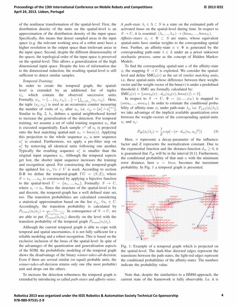
probability. In Fig. 1 a temporal graph is presented.

1 2 3 4 5 6 7 8 9 10 11 12 13 14 15 16 17 18 19 20 21 22 23 24 25

26 27 28 29 30 31 32 33 34 35 36 37 38 39 40 41 42 43 44 45 46 47 48 49 50

51 52 53 54 55 56 57 58 59 60 61 62 63 64 65 66 67 68 69 70 71 72 73 74 75

76 77 78 79 80 81 82 83 84 85 86 87 88 89 90 91 92 93 94 95 96 97 98 99 100

101 102 103 104 105 106 107 108 109 110 111 112 113 114 115 116 117 118 119 120 121 122 123 124 125

126 127 128 129 130 131 132 133 134 135 136 137 138 139 140 141 142 143 144 145 146 147 148 149 150

151 152 153 154 155 156 157 158 159 160 161 162 163 164 165 166 167 168 169 170 171 172 173 174 175

176 177 178 179 180 181 182 183 184 185 186 187 188 189 190 191 192 193 194 195 196 197 198 199 200

201 202 203 204 205 206 207 208 209 210 211 212 213 214 215 216 217 218 219 220 221 222 223 224 225

226 227 228 229 230 231 232 233 234 235 236 237 238 239 240 241 242 243 244 245 246 247 248 249 250

251 252 253 254 255 256 257 258 259 260 261 262 263 264 265 266 267 268 269 270 271 272 273 274 275

276 277 278 279 280 281 282 283 284 285 286 287 288 289 290 291 292 293 294 295 296 297 298 299 300

301 302 303 304 305 306 307 308 309 310 311 312 313 314 315 316 317 318 319 320 321 322 323 324 325

326 327 328 329 330 331 332 333 334 335 336 337 338 339 340 341 342 343 344 345 346 347 348 349 350

351 352 353 354 355 356 357 358 359 360 361 362 363 364 365 366 367 368 369 370 371 372 373 374 375

376 377 378 379 380 381 382 383 384 385 386 387 388 389 390 391 392 393 394 395 396 397 398 399 400

401 402 403 404 405 406 407 408 409 410 411 412 413 414 415 416 417 418 419 420 421 422 423 424 425

426 427 428 429 430 431 432 433 434 435 436 437 438 439 440 441 442 443 444 445 446 447 448 449 450

451 452 453 454 455 456 457 458 459 460 461 462 463 464 465 466 467 468 469 470 471 472 473 474 475

476 477 478 479 480 481 482 483 484 485 486 487 488 489 490 491 492 493 494 495 496 497 498 499 500

501 502 503 504 505 506 507 508 509 510 511 512 513 514 515 516 517 518 519 520 521 522 523 524 525

526 527 528 529 530 531 532 533 534 535 536 537 538 539 540 541 542 543 544 545 546 547 548 549 550

551 552 553 554 555 556 557 558 559 560 561 562 563 564 565 566 567 568 569 570 571 572 573 574 575

576 577 578 579 580 581 582 583 584 585 586 587 588 589 590 591 592 593 594 595 596 597 598 599 600

601 602 603 604 605 606 607 608 609 610 611 612 613 614 615 616 617 618 619 620 621 622 623 624 625

0.0460.0380.030.0220.0110.0080.003 0.005

0.0480.0470.0350.0290.0220.0120.010.0060.0010.0050.0130.008

0.0370.0380.0230.0190.0110.0060.0070.0110.0120.0140.0160.01

0.0260.0310.0210.020.013 0.0040.0110.0140.0170.0150.009

0.0190.0240.020.0170.008 0.0010.0050.0090.0120.003 0

0.0020.020.0180.006

0.0020.001

0.015

0.0290.05

0.0110.0410.066

0.0060.0290.077

0.0280.0440.060.047

0.0090.0460.0570.0520.038

0.0090.0430.0420.0330.025

0.0270.0080.0060.002

0.0080.001

0.0040.024

0.0320.0540.0520.018

0.0130.0630.085 0.0790.041

0.0240.0570.0870.062

0 0.0220.050.0530.02

0.0130.0160.021

0.0330.046

0.1270.1570.021

0.188

0.1020.041

0.025 0.058

0.157

0.1790.119

0.0880.110.0910.095

0.058

0.001

0.0040.007 0

0.002

0 0.0040.002

0.0010.0150.020.0090.0070.0040.001

0.0170.0440.0290.0280.0160.0190.008

0.0120.0430.050.0540.0430.0170.0140.006

0.0030.0410.059 0.0450.0250.015

0.020.0530.0490.0390.036

0.0180.041

0.004

0.03

0.068

0.262

0.019

0.5

0.5

0.25

0.5

0.25

0.5

0.5

Fig. 1: Example of a temporal graph which is projected on

the spatial-level. The dark-blue directed edges represent the

transitions between the path-states, the light-red edges represent

the conditional probabilities of the affinity-states. The numbers

indicate the probability value.

Note that, despite the similarities to a HMM-approach, the

current state of the framework is fully observable. I.e. it is


© 2013 IEEE


4

not required to distinguish between latent and observable

states. This allows a simplified and faster creation of the

models. A drawback of this approach is the vast size of the

resulting models. Accordingly, it should be mentioned that if

the path-states will be clustered to decrease the size of the

resulting model, then the classical HMM learning process

(e.g. using EM-methods as the Baum-Welch algorithm),

can be used without any modification of the overall framework.

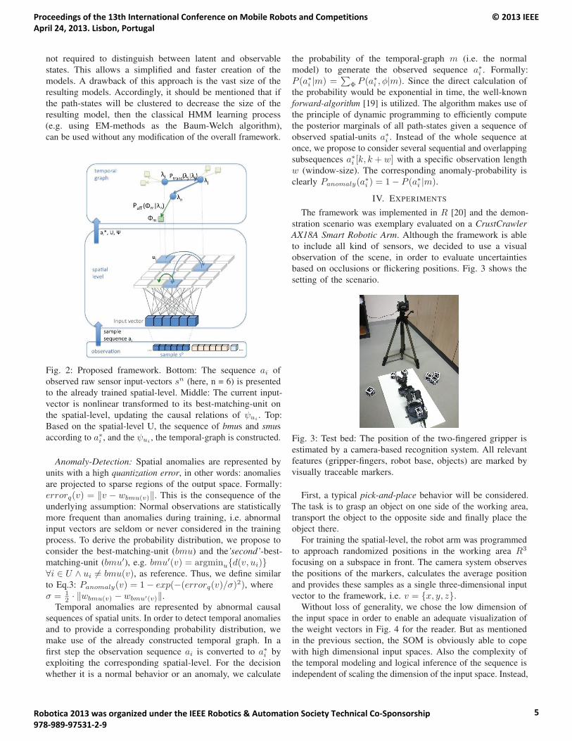
Fig. 2: Proposed framework. Bottom: The sequence ai of

observed raw sensor input-vectors sn (here, n = 6) is presented

to the already trained spatial-level. Middle: The current input-

vector is nonlinear transformed to its best-matching-unit on

the spatial-level, updating the causal relations of ψui. Top:

Based on the spatial-level U, the sequence of bmus and smus

according to a∗i , and the ψui, the temporal-graph is constructed.

Anomaly-Detection: Spatial anomalies are represented by

units with a high quantization error, in other words: anomalies

are projected to sparse regions of the output space. Formally:

errorq(v) = ‖v − wbmu(v)‖. This is the consequence of the

underlying assumption: Normal observations are statistically

more frequent than anomalies during training, i.e. abnormal

input vectors are seldom or never considered in the training

process. To derive the probability distribution, we propose to

consider the best-matching-unit (bmu) and the’second’-best-

matching-unit (bmu′), e.g. bmu′(v) = argminu{d(v, ui)}∀i ∈ U ∧ ui �= bmu(v), as reference. Thus, we define similar

to Eq.3: Panomaly(v) = 1− exp(−(errorq(v)/σ)2), where

σ = 12 · ‖wbmu(v) − wbmu′(v)‖.

Temporal anomalies are represented by abnormal causal

sequences of spatial units. In order to detect temporal anomalies

and to provide a corresponding probability distribution, we

make use of the already constructed temporal graph. In a

first step the observation sequence ai is converted to a∗i by

exploiting the corresponding spatial-level. For the decision

whether it is a normal behavior or an anomaly, we calculate

the probability of the temporal-graph m (i.e. the normal

model) to generate the observed sequence a∗i . Formally:

P (a∗i |m) =∑

Φ P (a∗i , φ|m). Since the direct calculation of

the probability would be exponential in time, the well-known

forward-algorithm [19] is utilized. The algorithm makes use of

the principle of dynamic programming to efficiently compute

the posterior marginals of all path-states given a sequence of

observed spatial-units a∗i . Instead of the whole sequence at

once, we propose to consider several sequential and overlapping

subsequences a∗i [k, k + w] with a specific observation length

w (window-size). The corresponding anomaly-probability is

clearly Panomaly(a∗i ) = 1− P (a∗i |m).

IV. EXPERIMENTS

The framework was implemented in R [20] and the demon-

stration scenario was exemplary evaluated on a CrustCrawlerAX18A Smart Robotic Arm. Although the framework is able

to include all kind of sensors, we decided to use a visual

observation of the scene, in order to evaluate uncertainties

based on occlusions or flickering positions. Fig. 3 shows the

setting of the scenario.

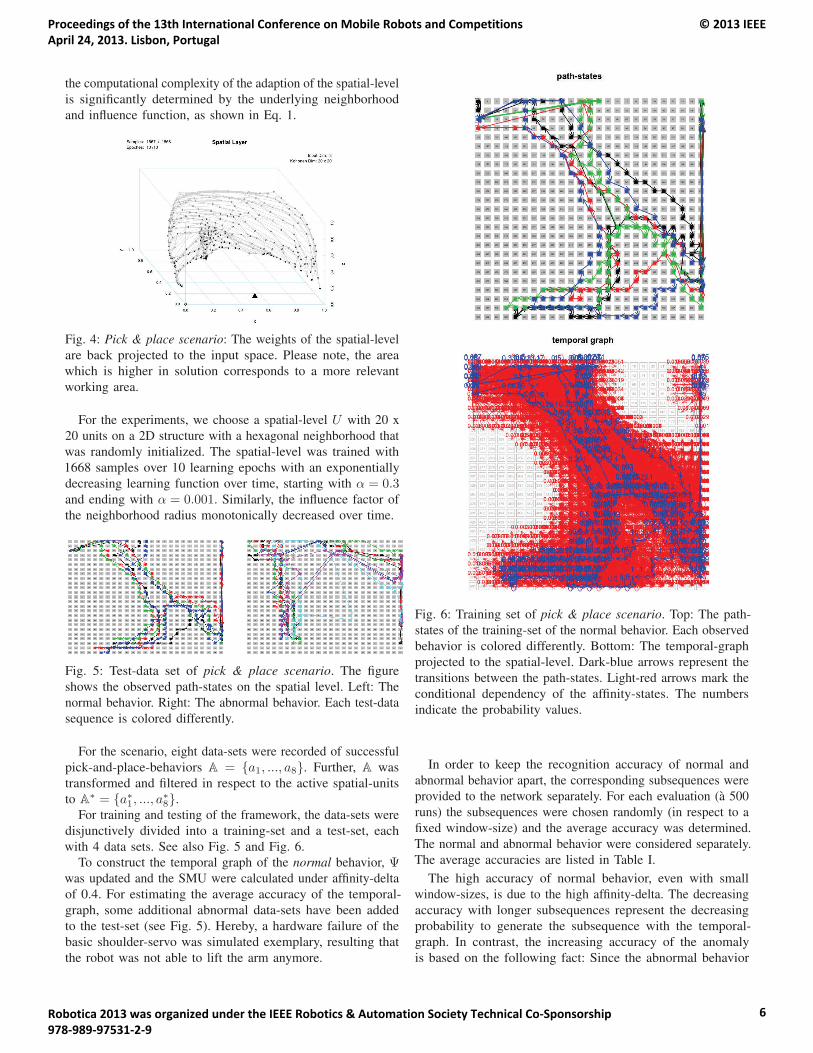
Fig. 3: Test bed: The position of the two-fingered gripper is

estimated by a camera-based recognition system. All relevant

features (gripper-fingers, robot base, objects) are marked by

visually traceable markers.

First, a typical pick-and-place behavior will be considered.

The task is to grasp an object on one side of the working area,

transport the object to the opposite side and finally place the

object there.

For training the spatial-level, the robot arm was programmed

to approach randomized positions in the working area R3

focusing on a subspace in front. The camera system observes

the positions of the markers, calculates the average position

and provides these samples as a single three-dimensional input

vector to the framework, i.e. v = {x, y, z}.Without loss of generality, we chose the low dimension of

the input space in order to enable an adequate visualization of

the weight vectors in Fig. 4 for the reader. But as mentioned

in the previous section, the SOM is obviously able to cope

with high dimensional input spaces. Also the complexity of

the temporal modeling and logical inference of the sequence is

independent of scaling the dimension of the input space. Instead,


© 2013 IEEE


5

the computational complexity of the adaption of the spatial-level

is significantly determined by the underlying neighborhood

and influence function, as shown in Eq. 1.

Fig. 4: Pick & place scenario: The weights of the spatial-level

are back projected to the input space. Please note, the area

which is higher in solution corresponds to a more relevant

working area.

For the experiments, we choose a spatial-level U with 20 x

20 units on a 2D structure with a hexagonal neighborhood that

was randomly initialized. The spatial-level was trained with

1668 samples over 10 learning epochs with an exponentially

decreasing learning function over time, starting with α = 0.3and ending with α = 0.001. Similarly, the influence factor of

the neighborhood radius monotonically decreased over time.

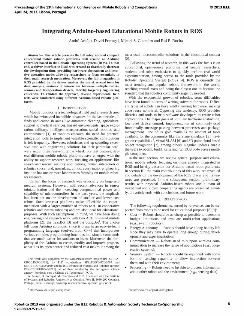
Fig. 5: Test-data set of pick & place scenario. The figure

shows the observed path-states on the spatial level. Left: The

normal behavior. Right: The abnormal behavior. Each test-data

sequence is colored differently.

For the scenario, eight data-sets were recorded of successful

pick-and-place-behaviors A = {a1, ..., a8}. Further, A was

transformed and filtered in respect to the active spatial-units

to A∗ = {a∗1, ..., a∗8}.

For training and testing of the framework, the data-sets were

disjunctively divided into a training-set and a test-set, each

with 4 data sets. See also Fig. 5 and Fig. 6.

To construct the temporal graph of the normal behavior, Ψwas updated and the SMU were calculated under affinity-delta

of 0.4. For estimating the average accuracy of the temporal-

graph, some additional abnormal data-sets have been added

to the test-set (see Fig. 5). Hereby, a hardware failure of the

basic shoulder-servo was simulated exemplary, resulting that

the robot was not able to lift the arm anymore.

Fig. 6: Training set of pick & place scenario. Top: The path-

states of the training-set of the normal behavior. Each observed

behavior is colored differently. Bottom: The temporal-graph

projected to the spatial-level. Dark-blue arrows represent the

transitions between the path-states. Light-red arrows mark the

conditional dependency of the affinity-states. The numbers

indicate the probability values.

In order to keep the recognition accuracy of normal and

abnormal behavior apart, the corresponding subsequences were

provided to the network separately. For each evaluation (a 500

runs) the subsequences were chosen randomly (in respect to a

fixed window-size) and the average accuracy was determined.

The normal and abnormal behavior were considered separately.

The average accuracies are listed in Table I.

The high accuracy of normal behavior, even with small

window-sizes, is due to the high affinity-delta. The decreasing

accuracy with longer subsequences represent the decreasing

probability to generate the subsequence with the temporal-

graph. In contrast, the increasing accuracy of the anomaly

is based on the following fact: Since the abnormal behavior


© 2013 IEEE


6

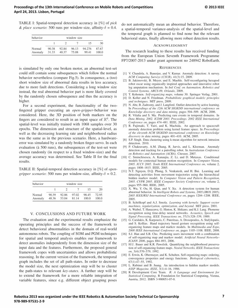
TABLE I: Spatial-temporal detection accuracy in [%] of pick& place scenario: 500 runs per window-size, affinity-δ = 0.4.

behavior window size

1 2 7 15 30

Normal 90.38 92.84 96.13 94.276 87.67Anomaly 31.33 40.37 75.08 99.41 100.0

is simulated by only one broken motor, an abnormal test-set

could still contain some subsequences which follow the normal

behavior nevertheless (compare Fig.5). In consequence, a (too)

short window size of abnormal data results in less accuracy,

due to more fault detections. Considering a long window size

instead, the real abnormal behavior part is more likely covered

by the randomly chosen subsequence and thus the accuracy is

higher.

For a second experiment, the functionality of the two-

fingered gripper executing an open-gripper-behavior was

considered. Here, the 3D position of both markers on the

fingers are considered to result in an input space of R6. The

spatial-level was initially trained with 1068 samples over 30

epochs. The dimension and structure of the spatial-level, as

well as the decreasing learning rate and neighborhood radius

was the same as in the previous scenario. Here, a hardware-

error was simulated by a randomly broken finger-servo. In each

evaluation (a 500 runs), the subsequences of the test-set were

chosen randomly (in respect to a fixed window-size) and the

average accuracy was determined. See Table II for the final

results.

TABLE II: Spatial-temporal detection accuracy in [%] of open-gripper scenario: 500 runs per window-size, affinity-δ = 0.2.

behavior window size

1 2 7 15 20

Normal 90.39 92.86 97.02 98.45 72.95Anomaly 48.36 53.04 81.14 100.0 100.0

V. CONCLUSIONS AND FUTURE WORK

The evaluation and the experimental results emphasize the

operating principles and the success of the framework to

detect behavioral abnormalities in the domain of real-world

autonomous robots. The coupling of SOM and PGM techniques

for spatial and temporal analysis enables our framework to

detect anomalies independently from the dimension size of the

input data and the features. Furthermore, the proposed general

framework copes with uncertainties and allows probabilistic

reasoning. In the current version of the framework, the temporal

graph includes the set of all path-states. In order to decrease

the model size, the next optimization step will be to cluster

the path-states to relevant key-states. A further step will be

to extend the framework for a more reliable integration of

variable features, since e.g. different object grasping poses

do not automatically mean an abnormal behavior. Therefore,

a spatial-temporal variance-analysis of the spatial-level and

the temporal graph is planned to find none but the relevant

behavioral states, finally allowing more robust detection results.

ACKNOWLEDGMENT

The research leading to these results has received funding

from the European Union Seventh Framework Programme

FP7/2007-2013 under grant agreement no 248942 RoboEarth.

REFERENCES

[1] V. Chandola, A. Banerjee, and V. Kumar. Anomaly detection: A survey.ACM Computing Surveys (CSUR), 41(3):15, 2009.

[2] B. Jakimovski, B. Meyer, and E. Maehle. Self-reconfiguring hexapodrobot oscar using organically inspired approaches and innovative robotleg amputation mechanism. In Intl Conf. on Automation, Robotics andControl Systems, ARCS-09, Orlando, 2009.

[3] T. Kohonen. Self-organizing maps, volume 30. Springer Verlag, 2001.[4] D. Koller and N. Friedman. Probabilistic graphical models: principles

and techniques. MIT press, 2009.[5] N. Abe, B. Zadrozny, and J. Langford. Outlier detection by active learning.

In Proceedings of the 12th ACM SIGKDD international conference onKnowledge discovery and data mining, pages 504–509. ACM, 2006.

[6] R. Vilalta and S. Ma. Predicting rare events in temporal domains. InData Mining, 2002. ICDM 2003. Proceedings. 2002 IEEE InternationalConference on, pages 474–481. IEEE, 2002.

[7] R. Fujimaki, T. Yairi, and K. Machida. An approach to spacecraftanomaly detection problem using kernel feature space. In Proceedingsof the eleventh ACM SIGKDD international conference on Knowledgediscovery in data mining, pages 401–410. ACM, 2005.

[8] S.P. Singh. Data clustering using k-mean algorithm for network intrusiondetection. 2010.

[9] P. Chakravarty, A.M. Zhang, R. Jarvis, and L. Kleeman. Anomalydetection and tracking for a patrolling robot. In Australasian Conferenceon Robotics and Automation (ACRA). Citeseer, 2007.

[10] C. Sminchisescu, A. Kanaujia, Z. Li, and D. Metaxas. Conditionalmodels for contextual human motion recognition. In Computer Vision,2005. ICCV 2005. Tenth IEEE International Conference on, volume 2,pages 1808–1815. IEEE, 2005.

[11] N.T. Nguyen, D.Q. Phung, S. Venkatesh, and H. Bui. Learning anddetecting activities from movement trajectories using the hierarchicalhidden markov model. In Computer Vision and Pattern Recognition,2005. CVPR 2005. IEEE Computer Society Conference on, volume 2,pages 955–960. IEEE, 2005.

[12] X. Wu, Y. Ou, H. Qian, and Y. Xu. A detection system for humanabnormal behavior. In Intelligent Robots and Systems, 2005.(IROS 2005).2005 IEEE/RSJ International Conference on, pages 1204–1208. IEEE,2005.

[13] B. Scholkopf and A.J. Smola. Learning with kernels: Support vectormachines, regularization, optimization, and beyond. MIT press, 2001.

[14] A. Waibel, T. Hanazawa, G. Hinton, K. Shikano, and K.J. Lang. Phonemerecognition using time-delay neural networks. Acoustics, Speech andSignal Processing, IEEE Transactions on, 37(3):328–339, 1989.

[15] G. Caridakis, K. Karpouzis, C. Pateritsas, A. Drosopoulos, A. Stafylopatis,and S. Kollias. Hand trajectory based gesture recognition using self-organizing feature maps and markov models. In Multimedia and Expo,2008 IEEE International Conference on, pages 1105–1108. IEEE, 2008.

[16] S.J. Han and S.B. Cho. Predicting users movement with a combinationof self-organizing map and markov model. Artificial Neural Networks–ICANN 2006, pages 884–893, 2006.

[17] H.U. Bauer and K.R. Pawelzik. Quantifying the neighborhood preserva-tion of self-organizing feature maps. Neural Networks, IEEE Transactionson, 3(4):570–579, 1992.

[18] E. Erwin, K. Obermayer, and K. Schulten. Self-organizing maps: ordering,convergence properties and energy functions. Biological cybernetics,67(1):47–55, 1992.

[19] L. Rabiner and B. Juang. An introduction to hidden markov models.ASSP Magazine, IEEE, 3(1):4–16, 1986.

[20] R Development Core Team. R: A Language and Environment forStatistical Computing. R Foundation for Statistical Computing, Vienna,Austria, 2012. ISBN 3-900051-07-0.


© 2013 IEEE


7

Abstract— This article presents the full integration of compact educational mobile robotic platforms built around an Arduino controller board in the Robotic Operating System (ROS). To that end, a driver interface in ROS was created to drastically decrease the development time, providing hardware abstraction and intui-tive operation mode, allowing researchers to focus essentially in their main research motivation. Moreover, the full integration in ROS provided by the driver enables the use of several tools for data analysis, easiness of interaction between multiple robots, sensors and teleoperation devices, thereby targeting engineering education. To validate the approach, diverse experimental field tests were conducted using different Arduino-based robotic plat-forms.

I. INTRODUCTIONMobile robotics is a technological field and a research area

which has witnessed incredible advances for the last decades. It finds application in areas like automatic cleaning, agriculture, support to medical services, hazard environments, space explo-ration, military, intelligent transportation, social robotics, and entertainment [1]. In robotics research, the need for practical integration tools to implement valuable scientific contributions is felt frequently. However, roboticists end up spending exces-sive time with engineering solutions for their particular hard-ware setup, often reinventing the wheel. For that purpose, sev-eral different mobile robotic platforms have emerged with the ability to support research work focusing on applications like search and rescue, security applications, human interaction or robotics soccer and, nowadays, almost every major engineering institute has one or more laboratories focusing on mobile robot-ics research.

Earlier, the focus of research was especially on large and medium systems. However, with recent advances in sensor miniaturization and the increasing computational power and capability of microcontrollers in the past years, the emphasis has been put on the development of smaller and lower cost robots. Such low-cost platforms make affordable the experi-mentation with a larger number of robots (e.g., in cooperative robotics and swarm robotics) and are also ideal for educational purposes. With such assumptions in mind, we have been doing engineering and research work with two Arduino-based mobile platforms [2]: the TraxBot [3] and the StingBot1. The choice fell upon Arduino solutions, since it presents an easy-to-learnprogramming language (derived from C++) that incorporates various complex programming functions into simple commands that are much easier for students to learn. Moreover, the sim-plicity of the Arduino to create, modify and improve projects, as well as its open-source and reduced cost makes it among the

This work was supported by the CHOPIN research project (PTDC/EEA-CRO/119000/2010), by PhD scholarships SFRH/BD/64426/2009 and SFRH/BD /73382/2010, and by ISR-Institute of Systems and Robotics (project PEst-C/EEI/UI0048/2011), all of them funded by the Portuguese science agency "Fundação para a Ciência e a Tecnologia" (FCT).

A. Araújo, D. Portugal, M. Couceiro and R. P. Rocha are with the Institute of Systems and Robotics, University of Coimbra, Pólo II, 3030-290 Coimbra, Portugal, email: {aaraujo, davidbsp, micaelcouceiro, rprocha}@isr.uc.pt.

1 http://www.isr.uc.pt/~aaraujo/doc

most used microcontroller solutions in the educational context [2].

Following the trend of research, in this work the focus is on educational, open-source platforms that enable researchers, students and robot enthusiasts to quickly perform real world experimentation, having access to the tools provided by the Robotic Operating System (ROS) [4]. ROS is currently the most trending and popular robotic framework in the world, reaching critical mass and being the closest one to become the standard that the robotics community urgently needed.

With the exponential growth of robotics, some difficulties have been found in terms of writing software for robots. Differ-ent types of robots can have wildly varying hardware, making code reuse nontrivial. Opposing this tendency, ROS provides libraries and tools to help software developers to create robot applications. The major goals of ROS are hardware abstraction, low-level device control, implementation of commonly-used functionally, message-passing between processes and package management. One of its gold marks is the amount of tools available for the community like the Stage simulator [5], navi-gation capabilities 2, visual SLAM [6] and 3D point cloud based object recognition [7], among others. Regular updates enable the users to obtain, build, write and run ROS code across multi-ple computers.

In the next section, we review general purpose and educa-tional mobile robots, focusing on those already integrated in ROS and briefly describe our Arduino-based robot platforms. In section III, the main contributions of this work are revealed and details on the development of the ROS driver and its fea-tures are presented. In the subsequent section, preliminary results with physical Arduino-based robots and a team of mixed real and virtual cooperating agents are presented. Final-ly, the article ends with conclusions and future work.

II. RELATED WORK

The following requirements, sorted by relevance, can be ex-pected from robots to be used for educational purposes [8][9]:

Cost — Robots should be as cheap as possible to overcome budget limitations and evaluate multi-robot applications (e.g., swarm robotics); Energy Autonomy — Robots should have a long battery life since they may have to operate long enough during devel-opment and experimentation; Communication — Robots need to support wireless com-munication to increase the range of applications (e.g., coop-erative systems); Sensory System — Robots should be equipped with some form of sensing capability to allow interaction between them and with their environment; Processing — Robots need to be able to process information about other robots and the environment (e.g., sensing data).

2 http://www.ros.org/wiki/navigation

Integrating Arduino-based Educational Mobile Robots in ROSAndré Araújo, David Portugal, Micael S. Couceiro and Rui P. Rocha


© 2013 IEEE


8

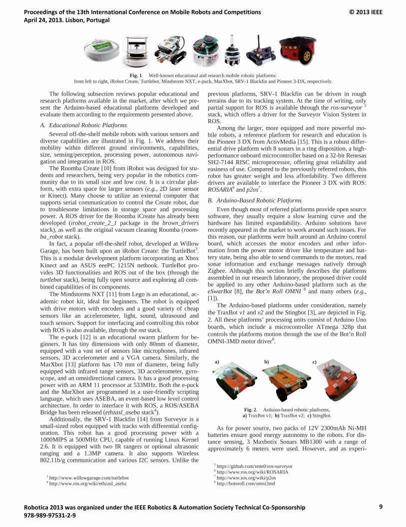
Fig. 1. Well-known educational and research mobile robotic platforms: from left to right, iRobot Create, Turtlebot, Mindstorm NXT, e-puck, MarXbot, SRV-1 Blackfin and Pioneer 3-DX, respectively.

The following subsection reviews popular educational and research platforms available in the market, after which we pre-sent the Arduino-based educational platforms developed and evaluate them according to the requirements presented above.

A. Educational Robotic Platforms Several off-the-shelf mobile robots with various sensors and

diverse capabilities are illustrated in Fig. 1. We address their mobility within different ground environments, capabilities, size, sensing/perception, processing power, autonomous navi-gation and integration in ROS.

The Roomba Create [10] from iRobot was designed for stu-dents and researchers, being very popular in the robotics com-munity due to its small size and low cost. It is a circular plat-form, with extra space for larger sensors (e.g., 2D laser sensor or Kinect). Many choose to utilize an external computer that supports serial communication to control the Create robot, due to troublesome limitations in storage space and processing power. A ROS driver for the Roomba iCreate has already been developed (irobot_create_2_1 package in the brown_drivers stack), as well as the original vacuum cleaning Roomba (room-ba_robot stack).

In fact, a popular off-the-shelf robot, developed at Willow Garage, has been built upon an iRobot Create: the TurtleBot3. This is a modular development platform incorporating an Xbox Kinect and an ASUS eeePC 1215N netbook. TurtleBot pro-vides 3D functionalities and ROS out of the box (through the turtlebot stack), being fully open source and exploring all com-bined capabilities of its components.

The Mindstorms NXT [11] from Lego is an educational, ac-ademic robot kit, ideal for beginners. The robot is equipped with drive motors with encoders and a good variety of cheap sensors like an accelerometer, light, sound, ultrasound and touch sensors. Support for interfacing and controlling this robot with ROS is also available, through the nxt stack.

The e-puck [12] is an educational swarm platform for be-ginners. It has tiny dimensions with only 80mm of diameter, equipped with a vast set of sensors like microphones, infrared sensors, 3D accelerometer and a VGA camera. Similarly, the MarXbot [13] platform has 170 mm of diameter, being fully equipped with infrared range sensors, 3D accelerometer, gyro-scope, and an omnidirectional camera. It has a good processing power with an ARM 11 processor at 533MHz. Both the e-puck and the MarXbot are programmed in a user-friendly scripting language, which uses ASEBA, an event-based low level control architecture. In order to interface it with ROS, a ROS/ASEBA Bridge has been released (ethzasl_aseba stack4).

Additionally, the SRV-1 Blackfin [14] from Surveyor is a small-sized robot equipped with tracks with differential config-uration. This robot has a good processing power with a 1000MIPS at 500MHz CPU, capable of running Linux Kernel 2.6. It is equipped with two IR rangers or optional ultrasonic ranging and a 1.3MP camera. It also supports Wireless 802.11b/g communication and various I2C sensors. Unlike the

3 http://www.willowgarage.com/turtlebot4 http://www.ros.org/wiki/ethzasl_aseba

previous platforms, SRV-1 Blackfin can be driven in rough terrains due to its tracking system. At the time of writing, only partial support for ROS is available through the ros-surveyor 5

stack, which offers a driver for the Surveyor Vision System in ROS.

Among the larger, more equipped and more powerful mo-bile robots, a reference platform for research and education is the Pioneer 3 DX from ActivMedia [15]. This is a robust differ-ential drive platform with 8 sonars in a ring disposition, a high-performance onboard microcontroller based on a 32-bit Renesas SH2-7144 RISC microprocessor, offering great reliability and easiness of use. Compared to the previously referred robots, this robot has greater weight and less affordability. Two different drivers are available to interface the Pioneer 3 DX with ROS: ROSARIA6 and p2os7.

B. Arduino-Based Robotic Platforms Even though most of referred platforms provide open source

software, they usually require a slow learning curve and the hardware has limited expandability. Arduino solutions have recently appeared in the market to work around such issues. For this reason, our platforms were built around an Arduino control board, which accesses the motor encoders and other infor-mation from the power motor driver like temperature and bat-tery state, being also able to send commands to the motors, read sonar information and exchange messages natively through Zigbee. Although this section briefly describes the platforms assembled in our research laboratory, the proposed driver could be applied to any other Arduino-based platform such as the eSwarBot [8], the Bot’n Roll OMNI 8 and many others (e.g.,[1]).

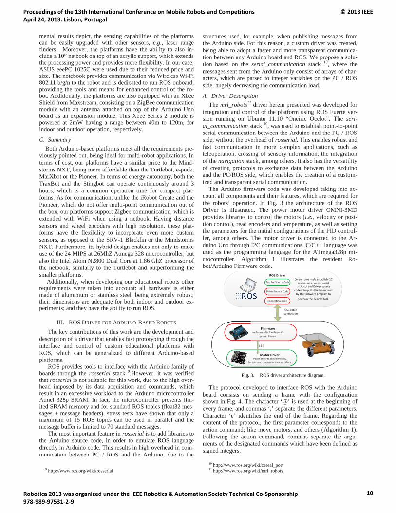
The Arduino-based platforms under consideration, namely the TraxBot v1 and v2 and the Stingbot [3], are depicted in Fig.2. All these platforms’ processing units consist of Arduino Uno boards, which include a microcontroller ATmega 328p that controls the platforms motion through the use of the Bot’n Roll OMNI-3MD motor driver8.

Fig. 2. Arduino-based robotic platforms,a) TraxBot v1; b) TraxBot v2; c) StingBot.

As for power source, two packs of 12V 2300mAh Ni-MH batteries ensure good energy autonomy to the robots. For dis-tance sensing, 3 Maxbotix Sonars MB1300 with a range of approximately 6 meters were used. However, and as experi-

5 https://github.com/rene0/ros-surveyor6 http://www.ros.org/wiki/ROSARIA7 http://www.ros.org/wiki/p2os8 http://botnroll.com/omni3md

a) b) c)


© 2013 IEEE


9

mental results depict, the sensing capabilities of the platforms can be easily upgraded with other sensors, e.g., laser range finders. Moreover, the platforms have the ability to also in-clude a 10” netbook on top of an acrylic support, which extends the processing power and provides more flexibility. In our case, ASUS eeePC 1025C were used due to their reduced price and size. The notebook provides communication via Wireless Wi-Fi802.11 b/g/n to the robot and is dedicated to run ROS onboard, providing the tools and means for enhanced control of the ro-bot. Additionally, the platforms are also equipped with an Xbee Shield from Maxstream, consisting on a ZigBee communication module with an antenna attached on top of the Arduino Uno board as an expansion module. This Xbee Series 2 module is powered at 2mW having a range between 40m to 120m, for indoor and outdoor operation, respectively.

C. SummaryBoth Arduino-based platforms meet all the requirements pre-

viously pointed out, being ideal for multi-robot applications. In terms of cost, our platforms have a similar price to the Mind-storms NXT, being more affordable than the Turtlebot, e-puck, MarXbot or the Pioneer. In terms of energy autonomy, both the TraxBot and the Stingbot can operate continuously around 3 hours, which is a common operation time for compact plat-forms. As for communication, unlike the iRobot Create and the Pioneer, which do not offer multi-point communication out of the box, our platforms support Zigbee communication, which isextended with WiFi when using a netbook. Having distance sensors and wheel encoders with high resolution, these plat-forms have the flexibility to incorporate even more custom sensors, as opposed to the SRV-1 Blackfin or the Mindstorms NXT. Furthermore, its hybrid design enables not only to make use of the 24 MIPS at 26MhZ Atmega 328 microcontroller, but also the Intel Atom N2800 Dual Core at 1.86 GhZ processor of the netbook, similarly to the Turtlebot and outperforming the smaller platforms.

Additionally, when developing our educational robots other requirements were taken into account: all hardware is either made of aluminium or stainless steel, being extremely robust; their dimensions are adequate for both indoor and outdoor ex-periments; and they have the ability to run ROS.

III. ROS DRIVER FOR ARDUINO-BASED ROBOTS

The key contributions of this work are the development and description of a driver that enables fast prototyping through the interface and control of custom educational platforms with ROS, which can be generalized to different Arduino-based platforms.

ROS provides tools to interface with the Arduino family of boards through the rosserial stack 9.However, it was verified that rosserial is not suitable for this work, due to the high over-head imposed by its data acquisition and commands, which result in an excessive workload to the Arduino microcontroller Atmel 328p SRAM. In fact, the microcontroller presents lim-ited SRAM memory and for standard ROS topics (float32 mes-sages + message headers), stress tests have shown that only a maximum of 15 ROS topics can be used in parallel and the message bu er is limited to 70 standard messages.

The most important feature in rosserial is to add libraries tothe Arduino source code, in order to emulate ROS language directly in Arduino code. This results in high overhead in com-munication between PC / ROS and the Arduino, due to the

9 http://www.ros.org/wiki/rosserial

structures used, for example, when publishing messages from the Arduino side. For this reason, a custom driver was created, being able to adopt a faster and more transparent communica-tion between any Arduino board and ROS. We propose a solu-tion based on the serial_communication stack 10, where the messages sent from the Arduino only consist of arrays of char-acters, which are parsed to integer variables on the PC / ROS side, hugely decreasing the communication load.

A. Driver Description The mrl_robots11 driver herein presented was developed for

integration and control of the platform using ROS Fuerte ver-sion running on Ubuntu 11.10 “Oneiric Ocelot”. The seri-al_communication stack 10, was used to establish point-to-point serial communication between the Arduino and the PC / ROS side, without the overhead of rosserial. This enables robust and fast communication in more complex applications, such as teleoperation, crossing of sensory information, the integration of the navigation stack, among others. It also has the versatility of creating protocols to exchange data between the Arduino and the PC/ROS side, which enables the creation of a custom-ized and transparent serial communication.

The Arduino firmware code was developed taking into ac-count all components and their features, which are required for the robots’ operation. In Fig. 3 the architecture of the ROS Driver is illustrated. The power motor driver OMNI-3MD provides libraries to control the motors (i.e., velocity or posi-tion control), read encoders and temperature, as well as setting the parameters for the initial configurations of the PID control-ler, among others. The motor driver is connected to the Ar-duino Uno through I2C communications. C/C++ language was used as the programming language for the ATmega328p mi-crocontroller. Algorithm 1 illustrates the resident Ro-bot/Arduino Firmware code.

ROS Driver

Connection node

TraxBot Source CodeCereal_port node establish I2C

communication via serial protocol and Driver source

code interprets the frame sent by the firmware program to

perform the desired task.

Driver Source Code

USB cable connection

Firmware Implemented in C with specific

protocol frame

Motor Driver Power driver to control motors,

Encoders and temperature among others.

I2C

Fig. 3. ROS driver architecture diagram.

The protocol developed to interface ROS with the Arduino board consists on sending a frame with the configuration shown in Fig. 4. The character ‘@’ is used at the beginning of every frame, and commas ‘,’ separate the different parameters. Character ‘e’ identifies the end of the frame. Regarding the content of the protocol, the first parameter corresponds to the action command; like move motors, and others (Algorithm 1).Following the action command, commas separate the argu-ments of the designated commands which have been defined as signed integers.

10 http://www.ros.org/wiki/cereal_port11 http://www.ros.org/wiki/mrl_robots


© 2013 IEEE


10

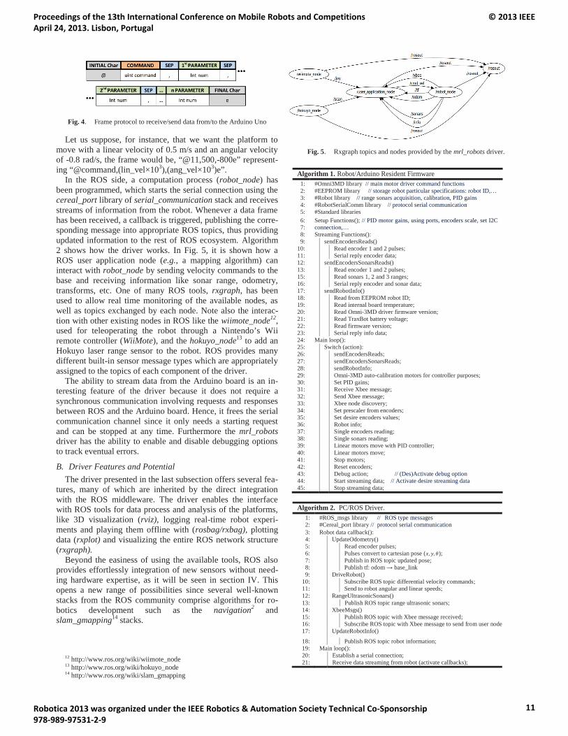
Fig. 4. Frame protocol to receive/send data from/to the Arduino Uno

Let us suppose, for instance, that we want the platform to move with a linear velocity of 0.5 m/s and an angular velocity of -0.8 rad/s, the frame would be, “@11,500,-800e” represent-ing “@command,(lin_vel×103),(ang_vel×103)e”.

In the ROS side, a computation process (robot_node) has been programmed, which starts the serial connection using the cereal_port library of serial_communication stack and receives streams of information from the robot. Whenever a data frame has been received, a callback is triggered, publishing the corre-sponding message into appropriate ROS topics, thus providing updated information to the rest of ROS ecosystem. Algorithm 2 shows how the driver works. In Fig. 5, it is shown how a ROS user application node (e.g., a mapping algorithm) can interact with robot_node by sending velocity commands to the base and receiving information like sonar range, odometry, transforms, etc. One of many ROS tools, rxgraph, has been used to allow real time monitoring of the available nodes, as well as topics exchanged by each node. Note also the interac-tion with other existing nodes in ROS like the wiimote_node12,used for teleoperating the robot through a Nintendo’s Wii remote controller (WiiMote), and the hokuyo_node13 to add an Hokuyo laser range sensor to the robot. ROS provides many different built-in sensor message types which are appropriately assigned to the topics of each component of the driver.

The ability to stream data from the Arduino board is an in-teresting feature of the driver because it does not require a synchronous communication involving requests and responses between ROS and the Arduino board. Hence, it frees the serial communication channel since it only needs a starting request and can be stopped at any time. Furthermore the mrl_robotsdriver has the ability to enable and disable debugging options to track eventual errors.

B. Driver Features and Potential The driver presented in the last subsection offers several fea-

tures, many of which are inherited by the direct integration with the ROS middleware. The driver enables the interface with ROS tools for data process and analysis of the platforms, like 3D visualization (rviz), logging real-time robot experi-ments and playing them offline with (rosbag/rxbag), plotting data (rxplot) and visualizing the entire ROS network structure (rxgraph).

Beyond the easiness of using the available tools, ROS also provides effortlessly integration of new sensors without need-ing hardware expertise, as it will be seen in section IV. This opens a new range of possibilities since several well-known stacks from the ROS community comprise algorithms for ro-botics development such as the navigation2 and slam_gmapping14 stacks.

12 http://www.ros.org/wiki/wiimote_node13 http://www.ros.org/wiki/hokuyo_node 14 http://www.ros.org/wiki/slam_gmapping

Fig. 5. Rxgraph topics and nodes provided by the mrl_robots driver.

Algorithm 1. Robot/Arduino Resident Firmware1:2:3:4:5:

#Omni3MD library // main motor driver command functions #EEPROM library // storage robot particular specifications: robot ID,… #Robot library // range sonars acquisition, calibration, PID gains#RobotSerialComm library // protocol serial communication#Standard libraries

6:7:

Setup Functions(); // PID motor gains, using ports, encoders scale, set I2C connection,…

8: Streaming Functions(): 9: sendEncodersReads()

10:11:

Read encoder 1 and 2 pulses;Serial reply encoder data;

12: sendEncodersSonarsReads()13:15:16:

Read encoder 1 and 2 pulses;Read sonars 1, 2 and 3 ranges;Serial reply encoder and sonar data;

17: sendRobotInfo()18:19:20:21:22:23:

Read from EEPROM robot ID;Read internal board temperature;Read Omni-3MD driver firmware version;Read TraxBot battery voltage;Read firmware version;Serial reply info data;

24: Main loop(): 25: Switch (action):26:27:28:29:30:31:32:33:34:35:36:37:38:39:40:41:42:43:44:45:

sendEncodersReads;sendEncodersSonarsReads;sendRobotInfo;Omni-3MD auto-calibration motors for controller purposes;Set PID gains;Receive Xbee message;Send Xbee message;Xbee node discovery;Set prescaler from encoders;Set desire encoders values;Robot info;Single encoders reading;Single sonars reading;Linear motors move with PID controller;Linear motors move;Stop motors;Reset encoders;Debug action; // (Des)Activate debug option Start streaming data; // Activate desire streaming dataStop streaming data;

Algorithm 2. PC/ROS Driver.1:2:

#ROS_msgs library // ROS type messages#Cereal_port library // protocol serial communication

3: Robot data callback(): 4: UpdateOdometry()5:6:7:8:

Read encoder pulses;Pulses convert to cartesian pose ( );Publish in ROS topic updated pose;Publish tf: odom → base_link

9: DriveRobot()10:11:

Subscribe ROS topic differential velocity commands;Send to robot angular and linear speeds;

12: RangeUltrasonicSonars()13: Publish ROS topic range ultrasonic sonars;14: XbeeMsgs()15:16:

Publish ROS topic with Xbee message received;Subscribe ROS topic with Xbee message to send from user node

17: UpdateRobotInfo()

18: Publish ROS topic robot information;19: Main loop(): 20: Establish a serial connection;21: Receive data streaming from robot (activate callbacks);


© 2013 IEEE


11

As a result, the overall time spent in robotics research is greatly reduced due to code reuse and therefore the driver represents a valuable tool that enables fast prototyping and opens a gateway into the world of ROS.

Another interesting feature of the driver is the simplicity for enabling heterogeneous multi-robot coordination and coopera-tion. Running the same hardware abstraction layer in the team of robots, ROS takes care of the communication messaging system using a publish/subscribe method, which enables all kinds of interaction between members of the same team, as seen in Fig. 6, where an example of a ROS network is depic-ted.

ROS Gazebo

ROS Gazebo Node

Driver Node Stingbot ...Robot N

Driver Node Traxbot v2 Robot 2

Driver Node Traxbot v1Robot 1

Computer

Multi Virtual robots in Stage Nodes

Main Algorithm

Node

Add specific task

NodeHokoyo Laser Node

Kinect Node

Wii Remote Controller Node...

Navigation Stack

Fig. 6. Network topology example with multiple robots, sensors, tele-operation devices and applications.

ROS also has the potential to integrate mixed real and virtu-al robot teams. With the use of the driver herein presented, together with the Stage15 multi-robot simulator, the same code can be used to drive either real robots or virtual agents running on Stage. Therefore, the developed ROS driver allows the integration of virtual robots with different sizes and driving characteristics, as seen later on. In addition, the communica-tion between real and virtual agents is completely transparent since they are both operating in the same ROS network. This major feature is ideal to perform multi-robot tasks, allowing the use of a large population of robots, when no extra physical robots are available, being cheaper and promoting safer test scenarios by making interactions between physical and virtual world objects.

Fig. 7. Evaluation of the ROS driver in Traxbot v1 with different sensors. a)Ultrassound Range Sensors integration; b) Hokuyo URG-04LX Laser Range Finder integration.

IV. RESULTS AND DISCUSSION

In order to experimentally evaluate the ROS driver, some tests were conducted using physical Arduino-based robots and

15 http://www.ros.org/wiki/stage

stage15, which provides essential options like the information about the ground truth pose and odometry of virtual robots.

We present experimental tests that validate the aforemen-tioned claims and we also show cooperative behaviors with real multi-robot systems, as well as mixed real and virtual robotic teams 16. Therefore, the experiments will allow to eval-uate the driver flexibility to different sensors, the driver porta-bility to different robotic platforms and the driver expandabil-ity and integration with the existent ROS tools.

The first experiment aims to demonstrate the driver flexibility to integration of different sensors. The TraxBot v1platform was equipped with a laser range finder (LFR) and its performance was compared against the native ultrasonic range sonars on a simple mapping task. The Hokuyo URG-04LX is a LRF classified as an Amplitude Modulated Continuous Wave (AMCW) sensor. In order to test the sonars performance, an L-shaped scenario of 2 m by 1.6 m was set up, with a 1 m width (Fig. 7). To perform this test, two lateral sonars placed at ±45 degrees were used.

In this test, the robot movement relies solely on odometry. In Fig. 7a it can be seen in the first rectilinear motion, that the sonars readings are stable (red dots) and coincident with the ground truth scenario limits (blue line). Green dots represent the midpoint of sonars acoustic beam while turning. Some issues arise during the 90 degrees rotation, since the sonar beam cone has an opening of approximately 36 degrees, thus presenting a much poorer resolution than the LRF, as illustrated in Fig. 7a. In the case of Fig. 7b, the Hokuyo LRF was used to perform the same test. The overture of the laser was set to 180 degrees with a rate of 512 samples per reading. It is possible to observe some discrepancy in some readings especially at the end of the movement due the odometry position error accumulated during motion.

In the second experiment, the main goal is to demonstrate the portability of the driver to different robots and sensors, which enables testing in our Arduino-based robots the existent algorithms in ROS. Hence, a mapping task with the incorporation and interaction of drivers for different sensors like LRF and a joystick controller was performed. Along these lines, this time the Traxbot v2 platform was equipped with an Hokuyo LRF and teleoperated with a WiiMote for a mapping task using Hector Mapping [16], which is available in the hector_slam stack17.

Fig. 8. Map generated by the Traxbot v2 with hector mapping.

16 A video of the experiments is available at:http://www.isr.uc.pt/~aaraujo/videos/Robotica2013

17 http://www.ros.org/wiki/hector_slam

a) b)

Position x [mm]Position x [mm]

Posi

tion

y [m

m]

Posi

tion

y [m

m]


© 2013 IEEE


12

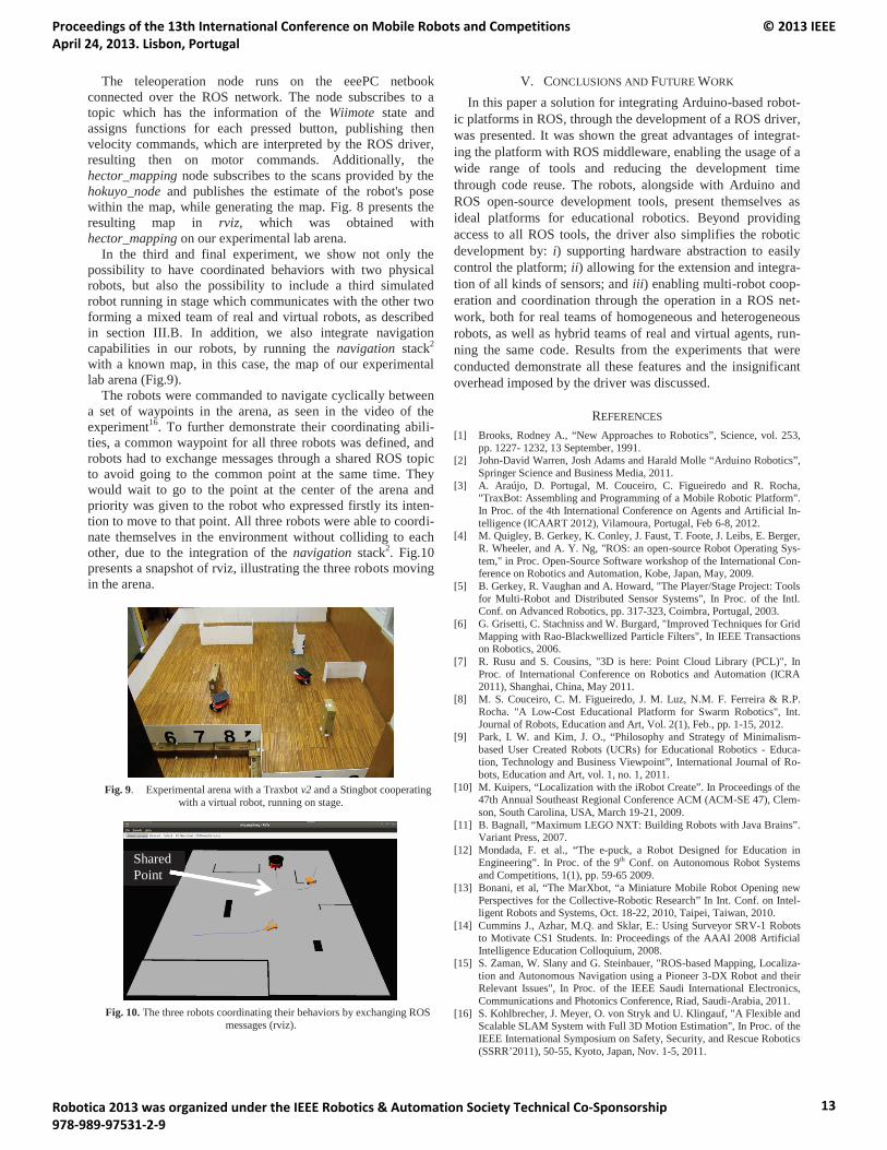
The teleoperation node runs on the eeePC netbook connected over the ROS network. The node subscribes to a topic which has the information of the Wiimote state and assigns functions for each pressed button, publishing then velocity commands, which are interpreted by the ROS driver, resulting then on motor commands. Additionally, the hector_mapping node subscribes to the scans provided by the hokuyo_node and publishes the estimate of the robot's pose within the map, while generating the map. Fig. 8 presents the resulting map in rviz, which was obtained with hector_mapping on our experimental lab arena.

In the third and final experiment, we show not only the possibility to have coordinated behaviors with two physical robots, but also the possibility to include a third simulated robot running in stage which communicates with the other two forming a mixed team of real and virtual robots, as described in section III.B. In addition, we also integrate navigation capabilities in our robots, by running the navigation stack2

with a known map, in this case, the map of our experimental lab arena (Fig.9).

The robots were commanded to navigate cyclically between a set of waypoints in the arena, as seen in the video of the experiment16. To further demonstrate their coordinating abili-ties, a common waypoint for all three robots was defined, and robots had to exchange messages through a shared ROS topic to avoid going to the common point at the same time. They would wait to go to the point at the center of the arena and priority was given to the robot who expressed firstly its inten-tion to move to that point. All three robots were able to coordi-nate themselves in the environment without colliding to each other, due to the integration of the navigation stack2. Fig.10presents a snapshot of rviz, illustrating the three robots moving in the arena.

Fig. 9. Experimental arena with a Traxbot v2 and a Stingbot cooperating with a virtual robot, running on stage.

Fig. 10. The three robots coordinating their behaviors by exchanging ROS messages (rviz).


In this paper a solution for integrating Arduino-based robot-ic platforms in ROS, through the development of a ROS driver,was presented. It was shown the great advantages of integrat-ing the platform with ROS middleware, enabling the usage of a wide range of tools and reducing the development time through code reuse. The robots, alongside with Arduino and ROS open-source development tools, present themselves as ideal platforms for educational robotics. Beyond providing access to all ROS tools, the driver also simplifies the robotic development by: i) supporting hardware abstraction to easily control the platform; ii) allowing for the extension and integra-tion of all kinds of sensors; and iii) enabling multi-robot coop-eration and coordination through the operation in a ROS net-work, both for real teams of homogeneous and heterogeneous robots, as well as hybrid teams of real and virtual agents, run-ning the same code. Results from the experiments that wereconducted demonstrate all these features and the insignificant overhead imposed by the driver was discussed.

REFERENCES

[1] Brooks, Rodney A., “New Approaches to Robotics”, Science, vol. 253, pp. 1227- 1232, 13 September, 1991.

[2] John-David Warren, Josh Adams and Harald Molle “Arduino Robotics”, Springer Science and Business Media, 2011.

[3] A. Araújo, D. Portugal, M. Couceiro, C. Figueiredo and R. Rocha, "TraxBot: Assembling and Programming of a Mobile Robotic Platform". In Proc. of the 4th International Conference on Agents and Artificial In-telligence (ICAART 2012), Vilamoura, Portugal, Feb 6-8, 2012.

[4] M. Quigley, B. Gerkey, K. Conley, J. Faust, T. Foote, J. Leibs, E. Berger, R. Wheeler, and A. Y. Ng, "ROS: an open-source Robot Operating Sys-tem," in Proc. Open-Source Software workshop of the International Con-ference on Robotics and Automation, Kobe, Japan, May, 2009.

[5] B. Gerkey, R. Vaughan and A. Howard, "The Player/Stage Project: Tools for Multi-Robot and Distributed Sensor Systems", In Proc. of the Intl. Conf. on Advanced Robotics, pp. 317-323, Coimbra, Portugal, 2003.

[6] G. Grisetti, C. Stachniss and W. Burgard, "Improved Techniques for Grid Mapping with Rao-Blackwellized Particle Filters", In IEEE Transactions on Robotics, 2006.

[7] R. Rusu and S. Cousins, "3D is here: Point Cloud Library (PCL)", In Proc. of International Conference on Robotics and Automation (ICRA 2011), Shanghai, China, May 2011.

[8] M. S. Couceiro, C. M. Figueiredo, J. M. Luz, N.M. F. Ferreira & R.P. Rocha. "A Low-Cost Educational Platform for Swarm Robotics", Int.Journal of Robots, Education and Art, Vol. 2(1), Feb., pp. 1-15, 2012.

[9] Park, I. W. and Kim, J. O., “Philosophy and Strategy of Minimalism-based User Created Robots (UCRs) for Educational Robotics - Educa-tion, Technology and Business Viewpoint”, International Journal of Ro-bots, Education and Art, vol. 1, no. 1, 2011.

[10] M. Kuipers, “Localization with the iRobot Create”. In Proceedings of the 47th Annual Southeast Regional Conference ACM (ACM-SE 47), Clem-son, South Carolina, USA, March 19-21, 2009.

[11] B. Bagnall, “Maximum LEGO NXT: Building Robots with Java Brains”. Variant Press, 2007.

[12] Mondada, F. et al., “The e-puck, a Robot Designed for Education in Engineering”. In Proc. of the 9th Conf. on Autonomous Robot Systems and Competitions, 1(1), pp. 59-65 2009.

[13] Bonani, et al, “The MarXbot, “a Miniature Mobile Robot Opening new Perspectives for the Collective-Robotic Research” In Int. Conf. on Intel-ligent Robots and Systems, Oct. 18-22, 2010, Taipei, Taiwan, 2010.

[14] Cummins J., Azhar, M.Q. and Sklar, E.: Using Surveyor SRV-1 Robots to Motivate CS1 Students. In: Proceedings of the AAAI 2008 Artificial Intelligence Education Colloquium, 2008.

[15] S. Zaman, W. Slany and G. Steinbauer, "ROS-based Mapping, Localiza-tion and Autonomous Navigation using a Pioneer 3-DX Robot and their Relevant Issues", In Proc. of the IEEE Saudi International Electronics, Communications and Photonics Conference, Riad, Saudi-Arabia, 2011.

[16] S. Kohlbrecher, J. Meyer, O. von Stryk and U. Klingauf, "A Flexible and Scalable SLAM System with Full 3D Motion Estimation", In Proc. of the IEEE International Symposium on Safety, Security, and Rescue Robotics (SSRR’2011), 50-55, Kyoto, Japan, Nov. 1-5, 2011.

Shared Point


© 2013 IEEE


13

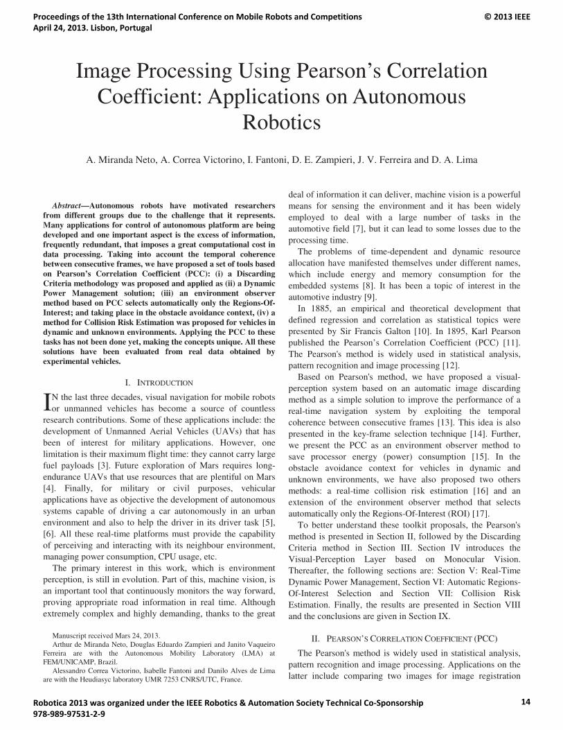
Abstract—Autonomous robots have motivated researchers

from different groups due to the challenge that it represents. Many applications for control of autonomous platform are being developed and one important aspect is the excess of information, frequently redundant, that imposes a great computational cost in data processing. Taking into account the temporal coherence between consecutive frames, we have proposed a set of tools based on Pearson’s Correlation Coefficient (PCC): (i) a Discarding Criteria methodology was proposed and applied as (ii) a Dynamic Power Management solution; (iii) an environment observer method based on PCC selects automatically only the Regions-Of-Interest; and taking place in the obstacle avoidance context, (iv) a method for Collision Risk Estimation was proposed for vehicles in dynamic and unknown environments. Applying the PCC to these tasks has not been done yet, making the concepts unique. All these solutions have been evaluated from real data obtained by experimental vehicles.

I. INTRODUCTION

N the last three decades, visual navigation for mobile robots or unmanned vehicles has become a source of countless

research contributions. Some of these applications include: the development of Unmanned Aerial Vehicles (UAVs) that has been of interest for military applications. However, one limitation is their maximum flight time: they cannot carry large fuel payloads [3]. Future exploration of Mars requires long-endurance UAVs that use resources that are plentiful on Mars [4]. Finally, for military or civil purposes, vehicular applications have as objective the development of autonomous systems capable of driving a car autonomously in an urban environment and also to help the driver in its driver task [5], [6]. All these real-time platforms must provide the capability of perceiving and interacting with its neighbour environment, managing power consumption, CPU usage, etc.

The primary interest in this work, which is environment perception, is still in evolution. Part of this, machine vision, is an important tool that continuously monitors the way forward, proving appropriate road information in real time. Although extremely complex and highly demanding, thanks to the great

Manuscript received Mars 24, 2013. Arthur de Miranda Neto, Douglas Eduardo Zampieri and Janito Vaqueiro

Ferreira are with the Autonomous Mobility Laboratory (LMA) at FEM/UNICAMP, Brazil.

Alessandro Correa Victorino, Isabelle Fantoni and Danilo Alves de Lima are with the Heudiasyc laboratory UMR 7253 CNRS/UTC, France.

deal of information it can deliver, machine vision is a powerful means for sensing the environment and it has been widely employed to deal with a large number of tasks in the automotive field [7], but it can lead to some losses due to the processing time.

The problems of time-dependent and dynamic resource allocation have manifested themselves under different names, which include energy and memory consumption for the embedded systems [8]. It has been a topic of interest in the automotive industry [9].

In 1885, an empirical and theoretical development that defined regression and correlation as statistical topics were presented by Sir Francis Galton [10]. In 1895, Karl Pearson published the Pearson’s Correlation Coefficient (PCC) [11]. The Pearson's method is widely used in statistical analysis, pattern recognition and image processing [12].

Based on Pearson's method, we have proposed a visual-perception system based on an automatic image discarding method as a simple solution to improve the performance of a real-time navigation system by exploiting the temporal coherence between consecutive frames [13]. This idea is also presented in the key-frame selection technique [14]. Further, we present the PCC as an environment observer method to save processor energy (power) consumption [15]. In the obstacle avoidance context for vehicles in dynamic and unknown environments, we have also proposed two others methods: a real-time collision risk estimation [16] and an extension of the environment observer method that selects automatically only the Regions-Of-Interest (ROI) [17].

To better understand these toolkit proposals, the Pearson's method is presented in Section II, followed by the Discarding Criteria method in Section III. Section IV introduces the Visual-Perception Layer based on Monocular Vision. Thereafter, the following sections are: Section V: Real-Time Dynamic Power Management, Section VI: Automatic Regions-Of-Interest Selection and Section VII: Collision Risk Estimation. Finally, the results are presented in Section VIII and the conclusions are given in Section IX.

II. PEARSON’S CORRELATION COEFFICIENT (PCC)

The Pearson's method is widely used in statistical analysis, pattern recognition and image processing. Applications on the latter include comparing two images for image registration

Image Processing Using Pearson’s Correlation Coefficient: Applications on Autonomous

Robotics

A. Miranda Neto, A. Correa Victorino, I. Fantoni, D. E. Zampieri, J. V. Ferreira and D. A. Lima

I


© 2013 IEEE


14

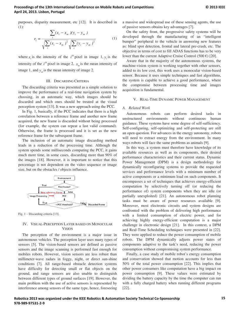
purposes, disparity measurement, etc [12]. It is described in (1):

−−

−−

imi

imi

imimi

)y(y)x(x

)y)(yx(x=r

221 (1)

where ix is the intensity of the thi pixel in image 1,iy is the

intensity of the thi pixel in image 2, mx is the mean intensity of

image 1, andmy is the mean intensity of image 2.

III. DISCARDING CRITERIA

The discarding criteria was presented as a simple solution to improve the performance of a real-time navigation system by choosing, in an automatic way, which images should be discarded and which ones should be treated at the visual perception system [13]. It was a new approach using the PCC.

In Fig. 1, basically, if the PCC indicates that there is a high correlation between a reference frame and another new frame acquired, the new frame is discarded without being processed (for example, the system can repeat a last valid command). Otherwise, the frame is processed and it is set as the new reference frame for the subsequent frame.

The inclusion of an automatic image discarding method leads in a reduction of the processing time. Although the system spends some milliseconds computing the PCC, it gains much more time, in some cases, discarding more than 90% of the images [18]. However, it is important to notice that this percentage is not dependent on the video sequence or image size, but on the obstacles / objects influence.

Fig. 1 – Discarding criteria [13].

IV. VISUAL-PERCEPTION LAYER BASED ON MONOCULAR

VISION

The perception of the environment is a major issue in autonomous vehicles. The perception layer uses many types of sensors [5]. The vision-based sensors are defined as passive sensors and the image scanning is performed fast enough for mobiles robots. However, vision sensors are less robust than millimeter-wave radars in foggy, night, or direct sun-shine conditions [7]. All range-based obstacle detection systems have difficulty for detecting small or flat objects on the ground, and range sensors are also unable to distinguish between different types of ground surfaces [19]. However, the main problem with the use of active sensors is represented by interference among sensors of the same type, hence, foreseeing

a massive and widespread use of these sensing agents, the use of passive sensors obtains key advantages [7].

On the safety front, the progressive safety systems will be developed through the manufacturing of an “intelligent bumper” peripheral to the vehicle in answering new features as: blind spot detection, frontal and lateral pre-crash, etc. The objective in terms of cost to fill ADAS functions has to be very lower than the current Adaptive Cruise Control (500 €) [20].

Aware that in the majority of the autonomous systems, the machine-vision system is working together with other sensors, added to its low cost, this work uses a monocular vision-based sensor. Because it uses simple techniques and fast algorithms, the system is capable to achieve a good performance, where the compromise between processing time and images acquisition is fundamental.

V. REAL-TIME DYNAMIC POWER MANAGEMENT

A. Related Work

Autonomous robots can perform desired tasks in unstructured environments without continuous human guidance. These systems have some degree of self-sufficiency. Self-configuring, self-optimizing and self-protecting are still an open question. For advances in the energy autonomy, robots will need to extract energy from the environment. In many ways robots will face the same problems as animals [9].

In this way, a system must therefore have knowledge of its available resources as well as its components, their desired performance characteristics and their current status. Dynamic Power Management (DPM) is a design methodology for dynamically reconfiguring systems to provide the requested services and performance levels with a minimum number of active components or a minimum load on such components. It encompasses a set of techniques that achieves energy-efficient computation by selectively turning off (or reducing the performance of) system components when they are idle (or partially unexploited) [21]. An autonomous robot planning tasks must be aware of power resources available [9]. Moreover, most electronic circuits and system designs are confronted with the problem of delivering high performance with a limited consumption of electric power, and for achieving highly energy-efficient computation is a major challenge in electronic design [21]. In this context, a DPM and Real-Time Scheduling techniques were presented in [22]. They were applied to reduce the power consumption of mobile robots. The DPM dynamically adjusts power states of components adaptive to the task’s need, reducing the power consumption without compromising system performance.

Finally, a case study of mobile robot’s energy consumption and conservation showed that motion accounts for less than 50% of the total power consumption [22]. This implies that other power consumers like computation have a big impact on power consumption [9]. These values were estimated by dividing the battery capacity by the time the computer can run with a fully charged battery when running different programs [22].


© 2013 IEEE


15

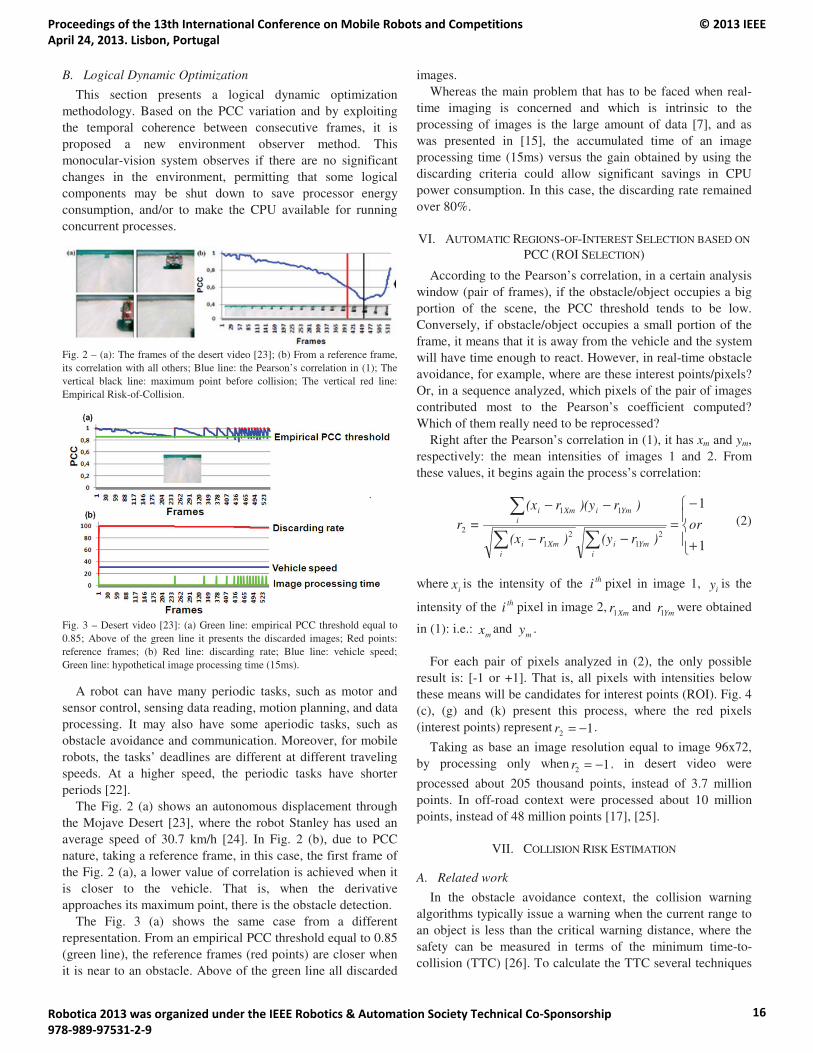
B. Logical Dynamic Optimization

This section presents a logical dynamic optimization methodology. Based on the PCC variation and by exploiting the temporal coherence between consecutive frames, it is proposed a new environment observer method. This monocular-vision system observes if there are no significant changes in the environment, permitting that some logical components may be shut down to save processor energy consumption, and/or to make the CPU available for running concurrent processes.

Fig. 2 – (a): The frames of the desert video [23]; (b) From a reference frame, its correlation with all others; Blue line: the Pearson’s correlation in (1); The vertical black line: maximum point before collision; The vertical red line: Empirical Risk-of-Collision.

Fig. 3 – Desert video [23]: (a) Green line: empirical PCC threshold equal to 0.85; Above of the green line it presents the discarded images; Red points: reference frames; (b) Red line: discarding rate; Blue line: vehicle speed; Green line: hypothetical image processing time (15ms).

A robot can have many periodic tasks, such as motor and sensor control, sensing data reading, motion planning, and data processing. It may also have some aperiodic tasks, such as obstacle avoidance and communication. Moreover, for mobile robots, the tasks’ deadlines are different at different traveling speeds. At a higher speed, the periodic tasks have shorter periods [22].

The Fig. 2 (a) shows an autonomous displacement through the Mojave Desert [23], where the robot Stanley has used an average speed of 30.7 km/h [24]. In Fig. 2 (b), due to PCC nature, taking a reference frame, in this case, the first frame of the Fig. 2 (a), a lower value of correlation is achieved when it is closer to the vehicle. That is, when the derivative approaches its maximum point, there is the obstacle detection.

The Fig. 3 (a) shows the same case from a different representation. From an empirical PCC threshold equal to 0.85 (green line), the reference frames (red points) are closer when it is near to an obstacle. Above of the green line all discarded

images. Whereas the main problem that has to be faced when real-

time imaging is concerned and which is intrinsic to the processing of images is the large amount of data [7], and as was presented in [15], the accumulated time of an image processing time (15ms) versus the gain obtained by using the discarding criteria could allow significant savings in CPU power consumption. In this case, the discarding rate remained over 80%.

VI. AUTOMATIC REGIONS-OF-INTEREST SELECTION BASED ON

PCC (ROI SELECTION)

According to the Pearson’s correlation, in a certain analysis window (pair of frames), if the obstacle/object occupies a big portion of the scene, the PCC threshold tends to be low. Conversely, if obstacle/object occupies a small portion of the frame, it means that it is away from the vehicle and the system will have time enough to react. However, in real-time obstacle avoidance, for example, where are these interest points/pixels? Or, in a sequence analyzed, which pixels of the pair of images contributed most to the Pearson’s coefficient computed? Which of them really need to be reprocessed?

Right after the Pearson’s correlation in (1), it has xm and ym, respectively: the mean intensities of images 1 and 2. From these values, it begins again the process’s correlation:

+

−

=−−

−−

1

1

21

21

11

2 or)r(y)r(x

)r)(yr(x

=r

iYmi

iXmi

iYmiXmi

(2)

whereix is the intensity of the thi pixel in image 1,

iy is the

intensity of the thi pixel in image 2, Xmr1 and Ymr1 were obtained

in (1): i.e.: mx and

my .

For each pair of pixels analyzed in (2), the only possible result is: [-1 or +1]. That is, all pixels with intensities below these means will be candidates for interest points (ROI). Fig. 4 (c), (g) and (k) present this process, where the red pixels (interest points) represent 12 −=r .

Taking as base an image resolution equal to image 96x72, by processing only when 12 −=r , in desert video were

processed about 205 thousand points, instead of 3.7 million points. In off-road context were processed about 10 million points, instead of 48 million points [17], [25].

VII. COLLISION RISK ESTIMATION

A. Related work

In the obstacle avoidance context, the collision warning algorithms typically issue a warning when the current range to an object is less than the critical warning distance, where the safety can be measured in terms of the minimum time-to-collision (TTC) [26]. To calculate the TTC several techniques


© 2013 IEEE


16

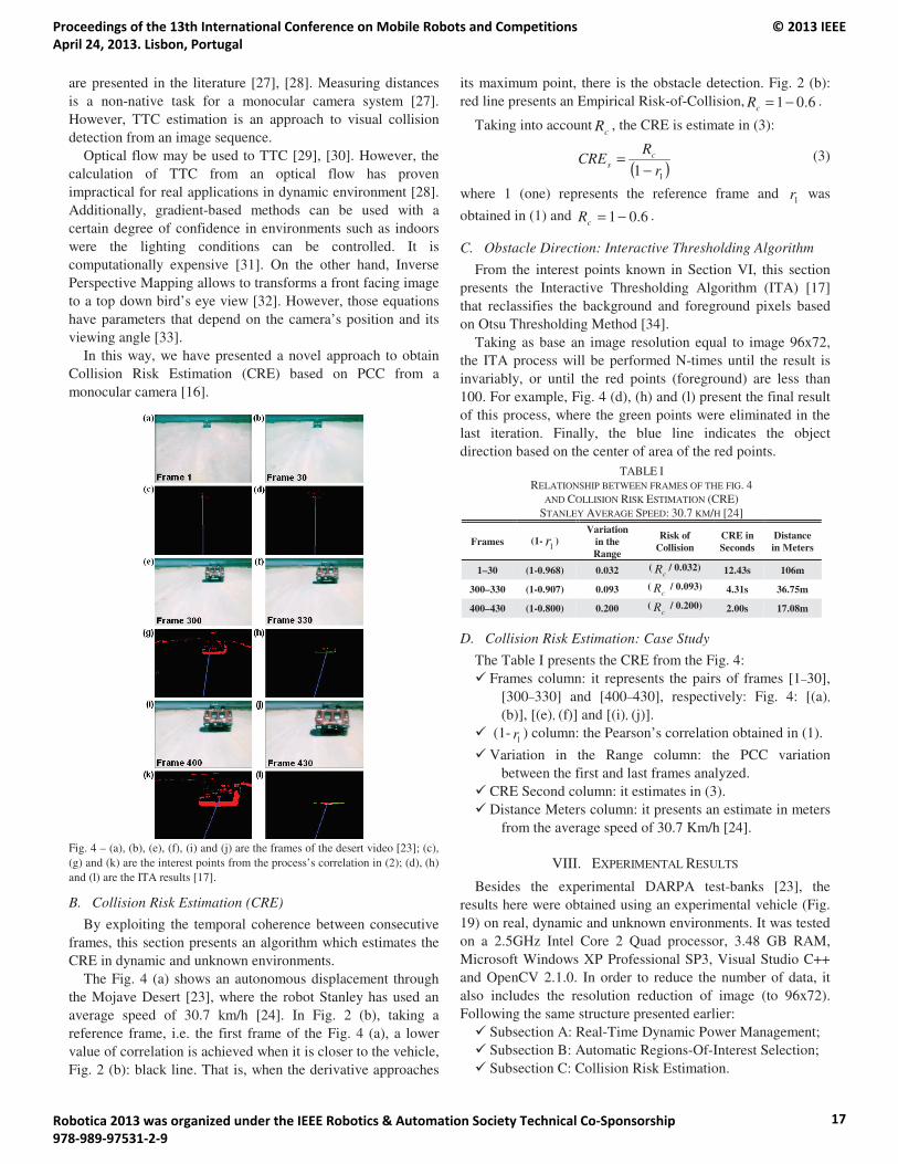
are presented in the literature [27], [28]. Measuring distances is a non-native task for a monocular camera system [27]. However, TTC estimation is an approach to visual collision detection from an image sequence.

Optical flow may be used to TTC [29], [30]. However, the calculation of TTC from an optical flow has proven impractical for real applications in dynamic environment [28]. Additionally, gradient-based methods can be used with a certain degree of confidence in environments such as indoors were the lighting conditions can be controlled. It is computationally expensive [31]. On the other hand, Inverse Perspective Mapping allows to transforms a front facing image to a top down bird’s eye view [32]. However, those equations have parameters that depend on the camera’s position and its viewing angle [33].

In this way, we have presented a novel approach to obtain Collision Risk Estimation (CRE) based on PCC from a monocular camera [16].

Fig. 4 – (a), (b), (e), (f), (i) and (j) are the frames of the desert video [23]; (c), (g) and (k) are the interest points from the process’s correlation in (2); (d), (h) and (l) are the ITA results [17].

B. Collision Risk Estimation (CRE)

By exploiting the temporal coherence between consecutive frames, this section presents an algorithm which estimates the CRE in dynamic and unknown environments.

The Fig. 4 (a) shows an autonomous displacement through the Mojave Desert [23], where the robot Stanley has used an average speed of 30.7 km/h [24]. In Fig. 2 (b), taking a reference frame, i.e. the first frame of the Fig. 4 (a), a lower value of correlation is achieved when it is closer to the vehicle, Fig. 2 (b): black line. That is, when the derivative approaches

its maximum point, there is the obstacle detection. Fig. 2 (b): red line presents an Empirical Risk-of-Collision, 6.01−=cR .

Taking into accountcR , the CRE is estimate in (3):

( )11 r

RCRE c

s−

= (3)

where 1 (one) represents the reference frame and 1r was

obtained in (1) and 6.01−=cR .

C. Obstacle Direction: Interactive Thresholding Algorithm

From the interest points known in Section VI, this section presents the Interactive Thresholding Algorithm (ITA) [17] that reclassifies the background and foreground pixels based on Otsu Thresholding Method [34].

Taking as base an image resolution equal to image 96x72, the ITA process will be performed N-times until the result is invariably, or until the red points (foreground) are less than 100. For example, Fig. 4 (d), (h) and (l) present the final result of this process, where the green points were eliminated in the last iteration. Finally, the blue line indicates the object direction based on the center of area of the red points.

D. Collision Risk Estimation: Case Study

The Table I presents the CRE from the Fig. 4: Frames column: it represents the pairs of frames [1–30],

[300–330] and [400–430], respectively: Fig. 4: [(a),

(b)], [(e), (f)] and [(i), (j)]. (1-

1r ) column: the Pearson’s correlation obtained in (1).

Variation in the Range column: the PCC variation between the first and last frames analyzed.

CRE Second column: it estimates in (3). Distance Meters column: it presents an estimate in meters

from the average speed of 30.7 Km/h [24].

VIII. EXPERIMENTAL RESULTS

Besides the experimental DARPA test-banks [23], the results here were obtained using an experimental vehicle (Fig. 19) on real, dynamic and unknown environments. It was tested on a 2.5GHz Intel Core 2 Quad processor, 3.48 GB RAM, Microsoft Windows XP Professional SP3, Visual Studio C++ and OpenCV 2.1.0. In order to reduce the number of data, it also includes the resolution reduction of image (to 96x72). Following the same structure presented earlier:

Subsection A: Real-Time Dynamic Power Management; Subsection B: Automatic Regions-Of-Interest Selection; Subsection C: Collision Risk Estimation.

TABLE I RELATIONSHIP BETWEEN FRAMES OF THE FIG. 4

AND COLLISION RISK ESTIMATION (CRE) STANLEY AVERAGE SPEED: 30.7 KM/H [24]

Frames

(1-

1r ) Variation

in the Range

Risk of Collision

CRE in Seconds

Distance in Meters

1–30 (1-0.968) 0.032 (cR / 0.032) 12.43s 106m

300–330 (1-0.907) 0.093 (cR / 0.093) 4.31s 36.75m

400–430 (1-0.800) 0.200 (cR / 0.200) 2.00s 17.08m


© 2013 IEEE


17

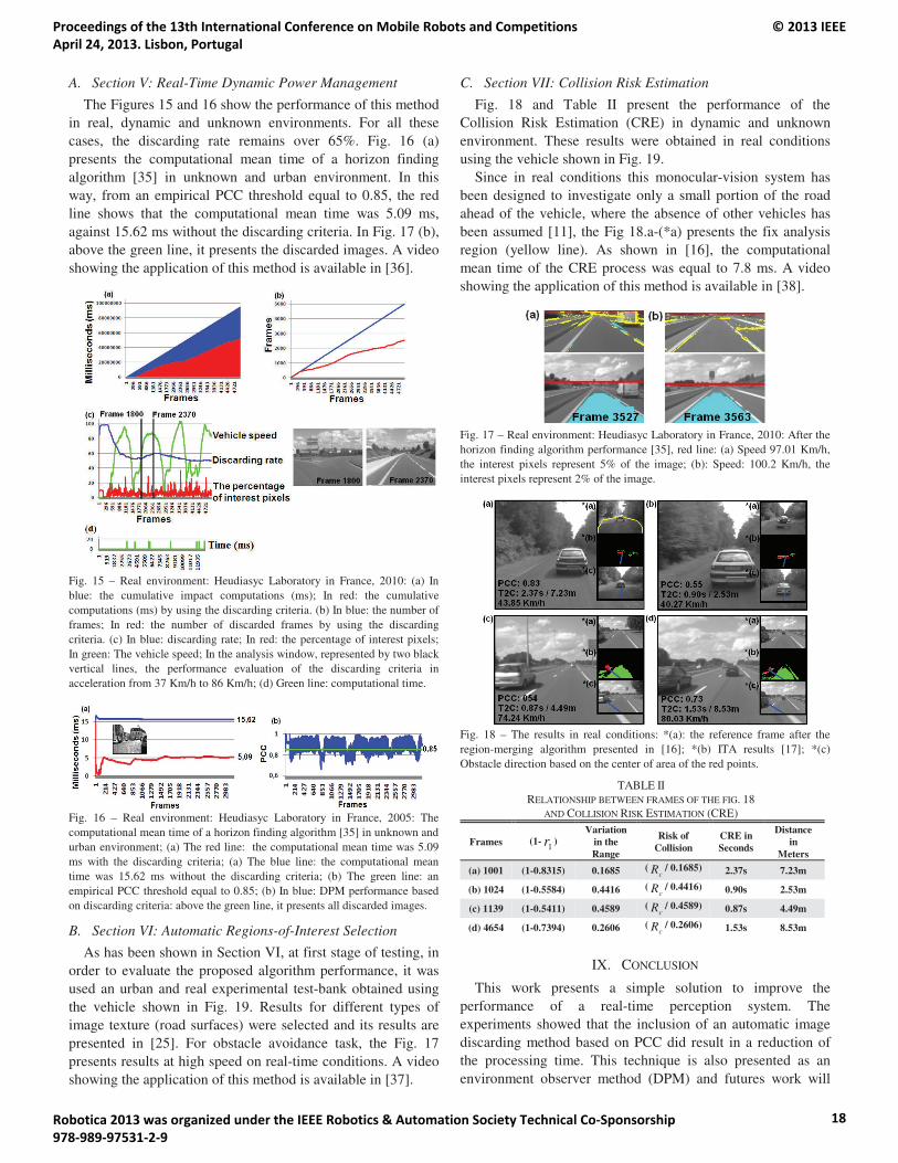
A. Section V: Real-Time Dynamic Power Management

The Figures 15 and 16 show the performance of this method in real, dynamic and unknown environments. For all these cases, the discarding rate remains over 65%. Fig. 16 (a) presents the computational mean time of a horizon finding algorithm [35] in unknown and urban environment. In this way, from an empirical PCC threshold equal to 0.85, the red line shows that the computational mean time was 5.09 ms, against 15.62 ms without the discarding criteria. In Fig. 17 (b), above the green line, it presents the discarded images. A video showing the application of this method is available in [36].

Fig. 15 – Real environment: Heudiasyc Laboratory in France, 2010: (a) In blue: the cumulative impact computations (ms); In red: the cumulative computations (ms) by using the discarding criteria. (b) In blue: the number of frames; In red: the number of discarded frames by using the discarding criteria. (c) In blue: discarding rate; In red: the percentage of interest pixels; In green: The vehicle speed; In the analysis window, represented by two black vertical lines, the performance evaluation of the discarding criteria in acceleration from 37 Km/h to 86 Km/h; (d) Green line: computational time.

Fig. 16 – Real environment: Heudiasyc Laboratory in France, 2005: The computational mean time of a horizon finding algorithm [35] in unknown and urban environment; (a) The red line: the computational mean time was 5.09 ms with the discarding criteria; (a) The blue line: the computational mean time was 15.62 ms without the discarding criteria; (b) The green line: an empirical PCC threshold equal to 0.85; (b) In blue: DPM performance based on discarding criteria: above the green line, it presents all discarded images.

B. Section VI: Automatic Regions-of-Interest Selection

As has been shown in Section VI, at first stage of testing, in order to evaluate the proposed algorithm performance, it was used an urban and real experimental test-bank obtained using the vehicle shown in Fig. 19. Results for different types of image texture (road surfaces) were selected and its results are presented in [25]. For obstacle avoidance task, the Fig. 17 presents results at high speed on real-time conditions. A video showing the application of this method is available in [37].

C. Section VII: Collision Risk Estimation

Fig. 18 and Table II present the performance of the Collision Risk Estimation (CRE) in dynamic and unknown environment. These results were obtained in real conditions using the vehicle shown in Fig. 19.

Since in real conditions this monocular-vision system has been designed to investigate only a small portion of the road ahead of the vehicle, where the absence of other vehicles has been assumed [11], the Fig 18.a-(*a) presents the fix analysis region (yellow line). As shown in [16], the computational mean time of the CRE process was equal to 7.8 ms. A video showing the application of this method is available in [38].

Fig. 17 – Real environment: Heudiasyc Laboratory in France, 2010: After the horizon finding algorithm performance [35], red line: (a) Speed 97.01 Km/h, the interest pixels represent 5% of the image; (b): Speed: 100.2 Km/h, the interest pixels represent 2% of the image.

Fig. 18 – The results in real conditions: *(a): the reference frame after the region-merging algorithm presented in [16]; *(b) ITA results [17]; *(c) Obstacle direction based on the center of area of the red points.

IX. CONCLUSION

This work presents a simple solution to improve the performance of a real-time perception system. The experiments showed that the inclusion of an automatic image discarding method based on PCC did result in a reduction of the processing time. This technique is also presented as an environment observer method (DPM) and futures work will

TABLE II RELATIONSHIP BETWEEN FRAMES OF THE FIG. 18

AND COLLISION RISK ESTIMATION (CRE)

Frames (1-1r )

Variation in the Range

Risk of Collision

CRE in Seconds

Distance in

Meters

(a) 1001 (1-0.8315) 0.1685 (cR / 0.1685) 2.37s 7.23m

(b) 1024 (1-0.5584) 0.4416 (cR / 0.4416) 0.90s 2.53m

(c) 1139 (1-0.5411) 0.4589 (cR / 0.4589) 0.87s 4.49m

(d) 4654 (1-0.7394) 0.2606 (cR / 0.2606) 1.53s 8.53m


© 2013 IEEE


18

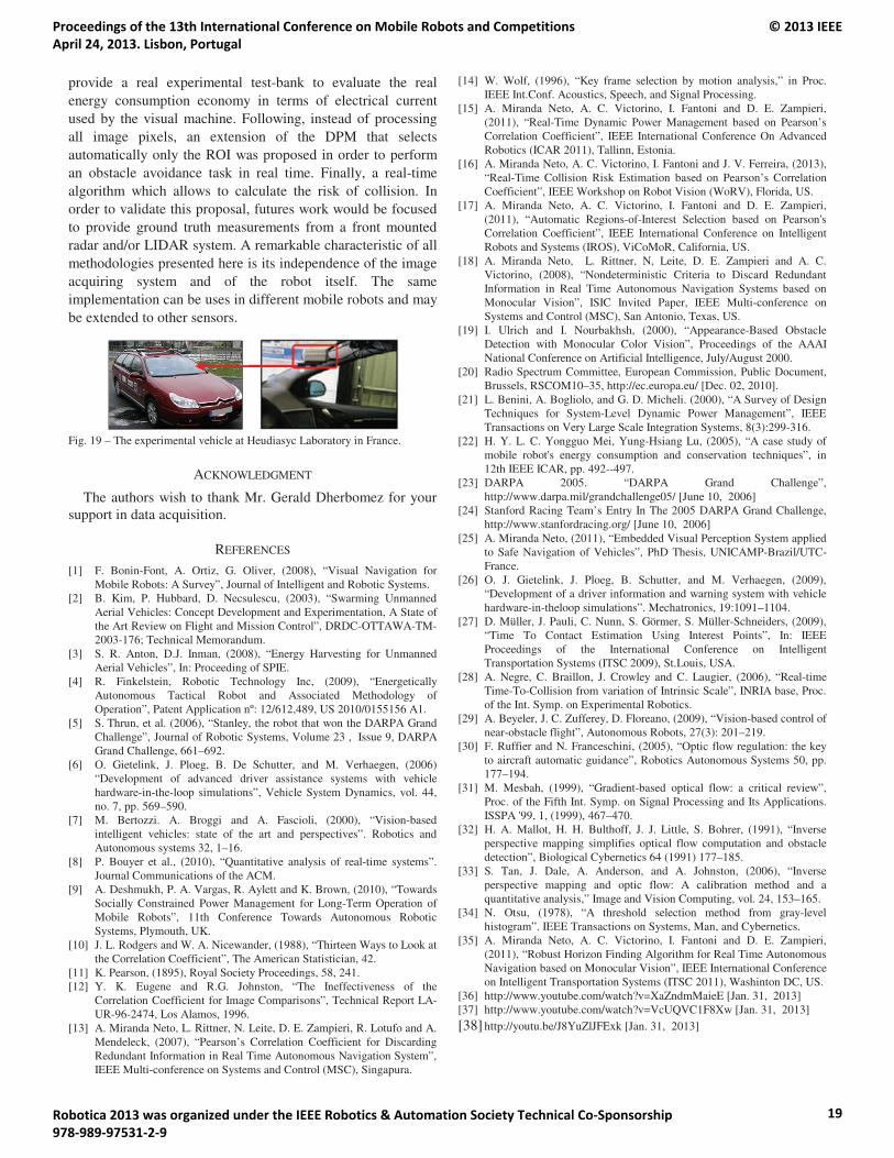
provide a real experimental test-bank to evaluate the real energy consumption economy in terms of electrical current used by the visual machine. Following, instead of processing all image pixels, an extension of the DPM that selects automatically only the ROI was proposed in order to perform an obstacle avoidance task in real time. Finally, a real-time algorithm which allows to calculate the risk of collision. In order to validate this proposal, futures work would be focused to provide ground truth measurements from a front mounted radar and/or LIDAR system. A remarkable characteristic of all methodologies presented here is its independence of the image acquiring system and of the robot itself. The same implementation can be uses in different mobile robots and may be extended to other sensors.

Fig. 19 – The experimental vehicle at Heudiasyc Laboratory in France.

ACKNOWLEDGMENT

The authors wish to thank Mr. Gerald Dherbomez for your support in data acquisition.

REFERENCES

[1] F. Bonin-Font, A. Ortiz, G. Oliver, (2008), “Visual Navigation for Mobile Robots: A Survey”, Journal of Intelligent and Robotic Systems.

[2] B. Kim, P. Hubbard, D. Necsulescu, (2003), “Swarming Unmanned Aerial Vehicles: Concept Development and Experimentation, A State of the Art Review on Flight and Mission Control”, DRDC-OTTAWA-TM-2003-176; Technical Memorandum.

[3] S. R. Anton, D.J. Inman, (2008), “Energy Harvesting for Unmanned Aerial Vehicles”, In: Proceeding of SPIE.

[4] R. Finkelstein, Robotic Technology Inc, (2009), “Energetically Autonomous Tactical Robot and Associated Methodology of Operation”, Patent Application nº: 12/612,489, US 2010/0155156 A1.

[5] S. Thrun, et al. (2006), “Stanley, the robot that won the DARPA Grand Challenge”, Journal of Robotic Systems, Volume 23 , Issue 9, DARPA Grand Challenge, 661–692.

[6] O. Gietelink, J. Ploeg, B. De Schutter, and M. Verhaegen, (2006) “Development of advanced driver assistance systems with vehicle hardware-in-the-loop simulations”, Vehicle System Dynamics, vol. 44, no. 7, pp. 569–590.

[7] M. Bertozzi. A. Broggi and A. Fascioli, (2000), “Vision-based intelligent vehicles: state of the art and perspectives”. Robotics and Autonomous systems 32, 1–16.

[8] P. Bouyer et al., (2010), “Quantitative analysis of real-time systems”. Journal Communications of the ACM.

[9] A. Deshmukh, P. A. Vargas, R. Aylett and K. Brown, (2010), “Towards Socially Constrained Power Management for Long-Term Operation of Mobile Robots”, 11th Conference Towards Autonomous Robotic Systems, Plymouth, UK.

[10] J. L. Rodgers and W. A. Nicewander, (1988), “Thirteen Ways to Look at the Correlation Coefficient”, The American Statistician, 42.

[11] K. Pearson, (1895), Royal Society Proceedings, 58, 241. [12] Y. K. Eugene and R.G. Johnston, “The Ineffectiveness of the

Correlation Coefficient for Image Comparisons”, Technical Report LA-UR-96-2474, Los Alamos, 1996.

[13] A. Miranda Neto, L. Rittner, N. Leite, D. E. Zampieri, R. Lotufo and A. Mendeleck, (2007), “Pearson’s Correlation Coefficient for Discarding Redundant Information in Real Time Autonomous Navigation System”, IEEE Multi-conference on Systems and Control (MSC), Singapura.

[14] W. Wolf, (1996), “Key frame selection by motion analysis,” in Proc. IEEE Int.Conf. Acoustics, Speech, and Signal Processing.

[15] A. Miranda Neto, A. C. Victorino, I. Fantoni and D. E. Zampieri, (2011), “Real-Time Dynamic Power Management based on Pearson’s Correlation Coefficient”, IEEE International Conference On Advanced Robotics (ICAR 2011), Tallinn, Estonia.

[16] A. Miranda Neto, A. C. Victorino, I. Fantoni and J. V. Ferreira, (2013), “Real-Time Collision Risk Estimation based on Pearson’s Correlation Coefficient”, IEEE Workshop on Robot Vision (WoRV), Florida, US.

[17] A. Miranda Neto, A. C. Victorino, I. Fantoni and D. E. Zampieri, (2011), “Automatic Regions-of-Interest Selection based on Pearson's Correlation Coefficient”, IEEE International Conference on Intelligent Robots and Systems (IROS), ViCoMoR, California, US.

[18] A. Miranda Neto, L. Rittner, N, Leite, D. E. Zampieri and A. C. Victorino, (2008), “Nondeterministic Criteria to Discard Redundant Information in Real Time Autonomous Navigation Systems based on Monocular Vision”, ISIC Invited Paper, IEEE Multi-conference on Systems and Control (MSC), San Antonio, Texas, US.

[19] I. Ulrich and I. Nourbakhsh, (2000), “Appearance-Based Obstacle Detection with Monocular Color Vision”, Proceedings of the AAAI National Conference on Artificial Intelligence, July/August 2000.

[20] Radio Spectrum Committee, European Commission, Public Document, Brussels, RSCOM10–35, http://ec.europa.eu/ [Dec. 02, 2010].

[21] L. Benini, A. Bogliolo, and G. D. Micheli. (2000), “A Survey of Design Techniques for System-Level Dynamic Power Management”, IEEE Transactions on Very Large Scale Integration Systems, 8(3):299-316.

[22] H. Y. L. C. Yongguo Mei, Yung-Hsiang Lu, (2005), “A case study of mobile robot's energy consumption and conservation techniques”, in 12th IEEE ICAR, pp. 492--497.

[23] DARPA 2005. “DARPA Grand Challenge”, http://www.darpa.mil/grandchallenge05/ [June 10, 2006]

[24] Stanford Racing Team’s Entry In The 2005 DARPA Grand Challenge, http://www.stanfordracing.org/ [June 10, 2006]

[25] A. Miranda Neto, (2011), “Embedded Visual Perception System applied to Safe Navigation of Vehicles”, PhD Thesis, UNICAMP-Brazil/UTC-France.

[26] O. J. Gietelink, J. Ploeg, B. Schutter, and M. Verhaegen, (2009), “Development of a driver information and warning system with vehicle hardware-in-theloop simulations”. Mechatronics, 19:1091–1104.

[27] D. Müller, J. Pauli, C. Nunn, S. Görmer, S. Müller-Schneiders, (2009), “Time To Contact Estimation Using Interest Points”, In: IEEE Proceedings of the International Conference on Intelligent Transportation Systems (ITSC 2009), St.Louis, USA.

[28] A. Negre, C. Braillon, J. Crowley and C. Laugier, (2006), “Real-time Time-To-Collision from variation of Intrinsic Scale”, INRIA base, Proc. of the Int. Symp. on Experimental Robotics.

[29] A. Beyeler, J. C. Zufferey, D. Floreano, (2009), “Vision-based control of near-obstacle flight”, Autonomous Robots, 27(3): 201–219.

[30] F. Ruffier and N. Franceschini, (2005), “Optic flow regulation: the key to aircraft automatic guidance”, Robotics Autonomous Systems 50, pp. 177–194.

[31] M. Mesbah, (1999), “Gradient-based optical flow: a critical review”, Proc. of the Fifth Int. Symp. on Signal Processing and Its Applications. ISSPA '99, 1, (1999), 467–470.

[32] H. A. Mallot, H. H. Bulthoff, J. J. Little, S. Bohrer, (1991), “Inverse perspective mapping simplifies optical flow computation and obstacle detection”, Biological Cybernetics 64 (1991) 177–185.

[33] S. Tan, J. Dale, A. Anderson, and A. Johnston, (2006), “Inverse perspective mapping and optic flow: A calibration method and a quantitative analysis,” Image and Vision Computing, vol. 24, 153–165.

[34] N. Otsu, (1978), “A threshold selection method from gray-level histogram”. IEEE Transactions on Systems, Man, and Cybernetics.

[35] A. Miranda Neto, A. C. Victorino, I. Fantoni and D. E. Zampieri, (2011), “Robust Horizon Finding Algorithm for Real Time Autonomous Navigation based on Monocular Vision”, IEEE International Conference on Intelligent Transportation Systems (ITSC 2011), Washinton DC, US.

[36] http://www.youtube.com/watch?v=XaZndmMaieE [Jan. 31, 2013] [37] http://www.youtube.com/watch?v=VcUQVC1F8Xw [Jan. 31, 2013]

[38] http://youtu.be/J8YuZlJFExk [Jan. 31, 2013]


© 2013 IEEE


19

Multi-Joint Gripper with Stiffness Adjuster Koichi Koganezawa

Dep. of Mechanical Engineering Tokai University

Hiratsuka, Kanagawa, Japan [email protected]

Takumi Tamamoto Dep. of Mechanical Engineering

Tokai University Hiratsuka, Kanagawa, Japan

Abstract— This paper proposes a multi-joint-gripper that achieves envelope grasping of unknown shape objects. Proposed mechanism is based on a chain of Planetary Gear Systems (PGS) controlled by only one motor. It also has a Variable Stiffness Mechanism (VSM) that controls joint stiffness to relieve interfering effects suffered from external or internal force/torque and to achieve a dexterous grasping. The experiments elucidate that the developed gripper achieves envelop grasping; the posture of the gripper automatically fits the shape of the object with no sensory feedback. And they also show that the VSM effectively works to relieve external interfering. This paper shows the detail of the mechanism and the experiments of its motion.

Keywords—Envelope Grasping; Multi-Joint-Gripper; Variable-Stiffness

I. INTRODUCTION The fatal disaster of the Fukushima nuclear plant being

brought about by the earthquake and subsequently assaulting tsunami on March 11 in 2011 revealed the disability for the current robot technology to work around when it faced with such disastrous environments. The disaster also prompts to develop a new type of autonomous robot that should have tough and effective hand or gripper. The forthcoming robots used in an ultimate environment should satisfy the following requirements. Back-drivability (BD): End-effectors always interact with

external environment, of which effect should not be expected to be predictable. This fact requires the end-effecter to have some “resiliency” to external interaction, which is interpreted as “back-drivability” of the joints in the technical point of view. Inherently safe design (ISD): This property is much related

to the BD in the sense that the end-effecter is never harmful to external environment (especially to human). In addition to the BD, ISD requires some items as follows. (a) Any electric/electronic devices or sensors should not be

equipped on the portions that directly contact with external objects. Since the robots have to cope with expected severe environments, such as electromagnetic or radio-active fields.

(b) According to (a) the controller cannot much rely on the feedback from sensors such as tactile or pressure sensors.

ISD does not completely deny using sensory feedback, which might be helpful to accomplish some dexterous and precise motion of the end-effector if a measure against radio active noise is satisfactory. Therefore ISD requires that some primitive motions of the end-effecter should be provided

without sensory feedback, in other words, mechanically, but it allows using the sensory feedback as subsidiary measures. Simple Control (SC): The control should be as simple as

possible. This requirement will be achieved along with pursuing the above BD and ISD requirements. BD will reduce the control burden to determine the end-effector’s motion when they interact with external objects. ISD also provides a simple control that does not much rely on the sensory feedback. But most of all, the SC requirement prompts us to reduce the end-effector’s DOF as far as possible. In this paper, we propose a multi-joint gripper that achieves envelope grasping for unknown-shape object under fulfilling the BD, ISD and SC requirements described above. The pioneering work in this field will be the “soft gripper” developed by Hirose and Umetani[1]. Since then the wire driven series of joint became the most typical mechanical architecture that has been followed by a lot of subsequent studies[2-6]. The mechanisms proposed in these studies will satisfy the BD, ISD and SC requirements or a part of them, but the most crucial problem of these studies resides in using much number of wires for driving series of joints, which gives rise to the following troubles on actual assembling and controlling. (a) Elasticity of the wire combined with the friction with pulleys sometimes causes unpredictable vibratory behavior of the gripper. (b) There exists singular posture of the gripper, especially of those having much number of serial joints. (c) Binding wires with appropriate tension is much cumbersome than one imagines and the tension is temperature dependent. So this paper proposes a novel mechanism without using wire

and pulley on its power transmission parts. It consists of a train of planetary gear system, of which fundamental function is the same as those of author’s another study [7]. We also propose a mechanism of adjusting stiffness of joints, which allows the gripper to vary the joint stiffness according to interactive conditions with grasping objects.

This paper is organized as follow. In the following section it shows a mechanism of the proposed gripper using planetary gear system, the principle of its motion and shape-fitting property to show it having the back-drivability. In the third section it shows the variable stiffness mechanism. The forth section is devoted to show the development of the machine


© 2013 IEEE


20

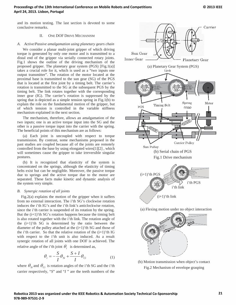
and its motion testing. The last section is devoted to some conclusive remarks.

II. ONE DOF DRIVE MECHANISM

A. Active/Passive amalgamation using planetary gears chain We consider a planar multi-joint gripper of which driving

torque is generated by only one motor and is transmitted to a distal end of the gripper via serially connected rotary joints. Fig.1 shows the outline of the driving mechanism of the proposed gripper. The planetary gear system (PGS) [Fig.1(a)] takes a crucial role for it, which is used as a “two inputs one output transmitter”. The rotation of the motor located at the proximal base is transmitted to the sun gear (SG) of the PGS that is located at the first joint by a timing belt. The carrier’s rotation is transmitted to the SG at the subsequent PGS by the timing belt. The link rotates together with the corresponding inner gear (IG). The carrier’s rotation is suppressed by the spring that is depicted as a simple tension spring in Fig.1(b) to explain the role on the fundamental motion of the gripper, but of which tension is controlled in the variable stiffness mechanism explained in the next section.

The mechanism, therefore, allows an amalgamation of the two inputs; one is an active torque input into the SG and the other is a passive torque input into the carrier with the spring. The beneficial points of this mechanism are as follows:

(a) Each joint is uncoupled with respect to torque transmission. By contrast, some mechanisms proposed in the past studies are coupled because all of the joints are remotely controlled from the base by using elongated wires[1][2] , which will sometimes cause the gripper to take irreversible singular postures.

(b) It is recognized that elasticity of the system is concentrated on the springs, although the elasticity of timing belts exist but can be negligible. Moreover, the passive torque due to springs and the active torque due to the motor are separated. These facts make kinetic and dynamic analysis of the system very simple.

B. Synergic rotation of all joints Fig.2(a) explains the motion of the gripper when it suffers

from no external interaction. The i’th SG’s clockwise rotation induces the i’th IG’s and the i’th link’s anticlockwise rotation, since the i’th carrier is suspended of its rotation by the spring. But the (i+1)’th SG’s rotation happens because the timing belt is also rotated together with the i’th link. The rotation angle of the (i+1)’th SG is determined by the ratio between the diameter of the pulley attached at the (i+1)’th SG and those of the i’th carrier. So that the relative rotation of the (i+1)’th IG with respect to the i’th unit is also induced. As a result synergic rotation of all joints with one DOF is achieved. The relative angle of the i’th joint i is determined as,

CiSii IIS

IS

(1)

where Si and Ci is rotation angles of the i’th SG and the i’th carrier respectively, “S” and “I ” are the teeth numbers of the

(a) Planetary Gear System (PGS)

(b) Serial chain of PGS Fig.1 Drive mechanism

(a) Flexing motion under no object interaction

(b) Motion transmission when object’s contact Fig.2 Mechanism of envelope grasping

i’th PGS i’th link

(i+1)’th PGS

(i+1)’th link


© 2013 IEEE


21

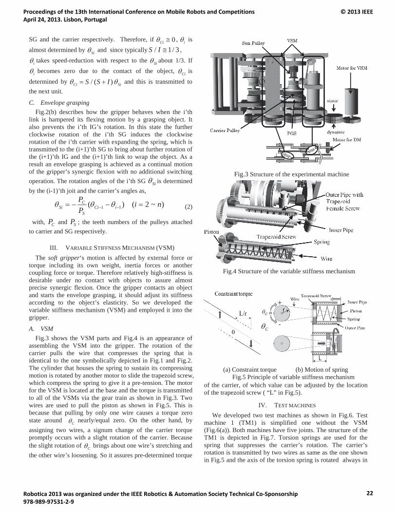
SG and the carrier respectively. Therefore, if 0Ci , i is almost determined by Si and since typically / 1/ 3S I ,

i takes speed-reduction with respect to the Si about 1/3. If

i becomes zero due to the contact of the object, Ci is

determined by / ( )Ci SiS S I and this is transmitted to the next unit.

C. Envelope grasping Fig.2(b) describes how the gripper behaves when the i’th

link is hampered its flexing motion by a grasping object. It also prevents the i’th IG’s rotation. In this state the further clockwise rotation of the i’th SG induces the clockwise rotation of the i’th carrier with expanding the spring, which is transmitted to the (i+1)’th SG to bring about further rotation of the (i+1)’th IG and the (i+1)’th link to wrap the object. As a result an envelope grasping is achieved as a continual motion of the gripper’s synergic flexion with no additional switching operation. The rotation angles of the i’th SG Si is determined by the (i-1)’th joit and the carrier’s angles as,

)~2()( 11 niPP

iCiS

CSi

(2)

with, CP and SP ; the teeth numbers of the pulleys attached to carrier and SG respectively.

III. VARIABLE STIFFNESS MECHANISM (VSM) The soft gripper‘s motion is affected by external force or

torque including its own weight, inertia forces or another coupling force or torque. Therefore relatively high-stiffness is desirable under no contact with objects to assure almost precise synergic flexion. Once the gripper contacts an object and starts the envelope grasping, it should adjust its stiffness according to the object’s elasticity. So we developed the variable stiffness mechanism (VSM) and employed it into the gripper.

A. VSM Fig.3 shows the VSM parts and Fig.4 is an appearance of

assembling the VSM into the gripper. The rotation of the carrier pulls the wire that compresses the spring that is identical to the one symbolically depicted in Fig.1 and Fig.2. The cylinder that houses the spring to sustain its compressing motion is rotated by another motor to slide the trapezoid screw, which compress the spring to give it a pre-tension. The motor for the VSM is located at the base and the torque is transmitted to all of the VSMs via the gear train as shown in Fig.3. Two wires are used to pull the piston as shown in Fig.5. This is because that pulling by only one wire causes a torque zero state around C nearly/equal zero. On the other hand, by assigning two wires, a signum change of the carrier torque promptly occurs with a slight rotation of the carrier. Because the slight rotation of C brings about one wire’s stretching and the other wire’s loosening. So it assures pre-determined torque

of the carrier, of which value can be adjusted by the location of the trapezoid screw ( “L” in Fig.5).

IV. TEST MACHINES We developed two test machines as shown in Fig.6. Test

machine 1 (TM1) is simplified one without the VSM (Fig.6(a)). Both machines have five joints. The structure of the TM1 is depicted in Fig.7. Torsion springs are used for the spring that suppresses the carrier’s rotation. The carrier’s rotation is transmitted by two wires as same as the one shown in Fig.5 and the axis of the torsion spring is rotated always in

Fig.3 Structure of the experimental machine

(a) Constraint torque (b) Motion of spring Fig.5 Principle of variable stiffness mechanism

C

Fig.4 Structure of the variable stiffness mechanism


© 2013 IEEE


22

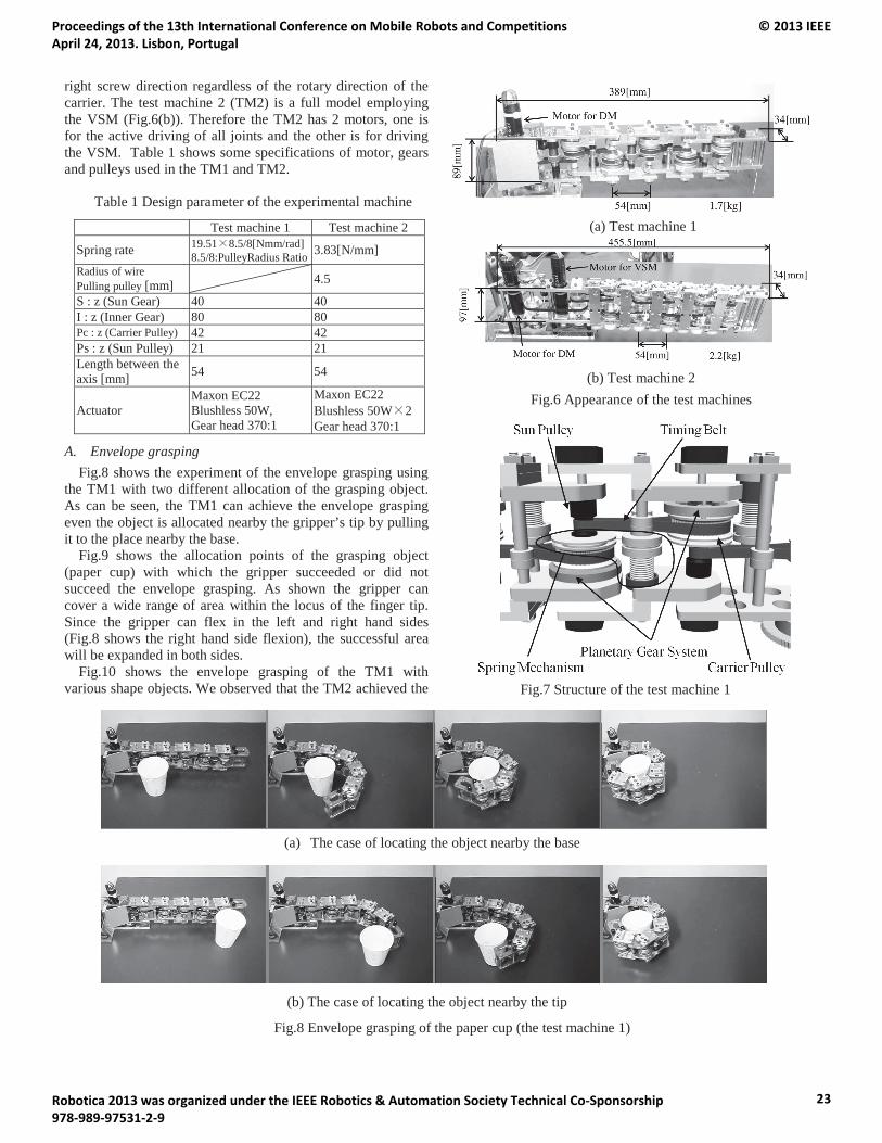
(a) The case of locating the object nearby the base

(b) The case of locating the object nearby the tip

Fig.8 Envelope grasping of the paper cup (the test machine 1)

right screw direction regardless of the rotary direction of the carrier. The test machine 2 (TM2) is a full model employing the VSM (Fig.6(b)). Therefore the TM2 has 2 motors, one is for the active driving of all joints and the other is for driving the VSM. Table 1 shows some specifications of motor, gears and pulleys used in the TM1 and TM2.

A. Envelope grasping Fig.8 shows the experiment of the envelope grasping using

the TM1 with two different allocation of the grasping object. As can be seen, the TM1 can achieve the envelope grasping even the object is allocated nearby the gripper’s tip by pulling it to the place nearby the base.

Fig.9 shows the allocation points of the grasping object (paper cup) with which the gripper succeeded or did not succeed the envelope grasping. As shown the gripper can cover a wide range of area within the locus of the finger tip. Since the gripper can flex in the left and right hand sides (Fig.8 shows the right hand side flexion), the successful area will be expanded in both sides.

Fig.10 shows the envelope grasping of the TM1 with various shape objects. We observed that the TM2 achieved the

Test machine 1 Test machine 2

Spring rate 19.51 8.5/8[Nmm/rad] 8.5/8:PulleyRadius Ratio 3.83[N/mm]

Radius of wire Pulling pulley [mm] 4.5

S : z (Sun Gear) 40 40 I : z (Inner Gear) 80 80 Pc : z (Carrier Pulley) 42 42 Ps : z (Sun Pulley) 21 21 Length between the axis [mm] 54 54

Actuator Maxon EC22 Blushless 50W, Gear head 370:1

Maxon EC22 Blushless 50W 2 Gear head 370:1

(a) Test machine 1

(b) Test machine 2 Fig.6 Appearance of the test machines

Fig.7 Structure of the test machine 1

Table 1 Design parameter of the experimental machine


© 2013 IEEE


23

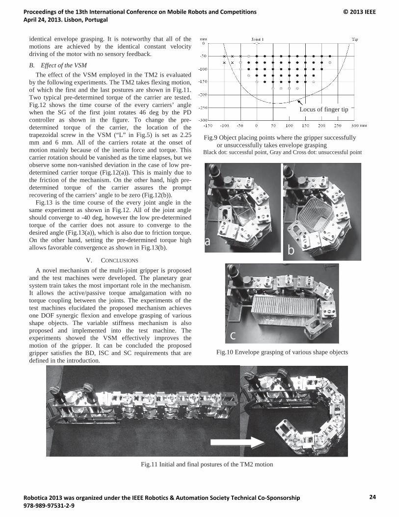
identical envelope grasping. It is noteworthy that all of the motions are achieved by the identical constant velocity driving of the motor with no sensory feedback.

B. Effect of the VSM The effect of the VSM employed in the TM2 is evaluated

by the following experiments. The TM2 takes flexing motion, of which the first and the last postures are shown in Fig.11. Two typical pre-determined torque of the carrier are tested. Fig.12 shows the time course of the every carriers’ angle when the SG of the first joint rotates 46 deg by the PD controller as shown in the figure. To change the pre-determined torque of the carrier, the location of the trapezoidal screw in the VSM (“L” in Fig.5) is set as 2.25 mm and 6 mm. All of the carriers rotate at the onset of motion mainly because of the inertia force and torque. This carrier rotation should be vanished as the time elapses, but we observe some non-vanished deviation in the case of low pre-determined carrier torque (Fig.12(a)). This is mainly due to the friction of the mechanism. On the other hand, high pre-determined torque of the carrier assures the prompt recovering of the carriers’ angle to be zero (Fig.12(b)).

Fig.13 is the time course of the every joint angle in the same experiment as shown in Fig.12. All of the joint angle should converge to -40 deg, however the low pre-determined torque of the carrier does not assure to converge to the desired angle (Fig.13(a)), which is also due to friction torque. On the other hand, setting the pre-determined torque high allows favorable convergence as shown in Fig.13(b).

V. CONCLUSIONS

A novel mechanism of the multi-joint gripper is proposed and the test machines were developed. The planetary gear system train takes the most important role in the mechanism. It allows the active/passive torque amalgamation with no torque coupling between the joints. The experiments of the test machines elucidated the proposed mechanism achieves one DOF synergic flexion and envelope grasping of various shape objects. The variable stiffness mechanism is also proposed and implemented into the test machine. The experiments showed the VSM effectively improves the motion of the gripper. It can be concluded the proposed gripper satisfies the BD, ISC and SC requirements that are defined in the introduction.

Fig.11 Initial and final postures of the TM2 motion

Fig.10 Envelope grasping of various shape objects

Fig.9 Object placing points where the gripper successfully or unsuccessfully takes envelope grasping

Black dot: successful point, Gray and Cross dot: unsuccessful point

Locus of finger tip


© 2013 IEEE


24

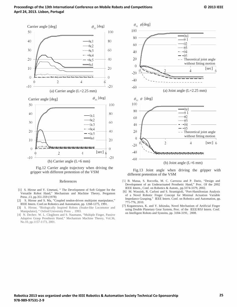
References [1] S. Hirose and Y. Umetani, “ The Development of Soft Gripper for the

Versatile Robot Hand,” Mechanism and Machine Theory, Pergamon Press ,13, pp.351-359 (1978)

[2] S. Hirose and S. Ma, ”Coupled tendon-driven multijoint manipulator,” IEEE Intern. Conf.on Robotics and Automation, pp. 1268-1275, 1991.

[3] S. Hirose, “Biologically Inspired Robots (Snake-like Locomotor and Manipulator), “ Oxford University Press , 1993.

[4] N. Dechev. W. L. Clegjhorn and S. Naumann, “Multiple Finger, Passive Adaptive Grasp Prosthesis Hand,” Mechanism Machine Theory, Vol.36, No.10, pp.1157-1173, 2001.

[5] B. Massa, S. Roccella, M. C. Carrozza and P. Dario, “Design and Development of an Underactuated Prosthetic Hand,” Proc. Of the 2002 IEEE Intern., Conf. on Robotics & Autom., pp.3374-3379, 2002.

[6] M. Wassink, R. Carloni and S. Stramigioli, “Port-Hamiltonian Analysis of a Novel Robotic Finger Concept for Minimal Actuation Variable Impedance Grasping,” IEEE Intern. Conf. on Robotics and Automation, pp. 771-776, 2010.

[7] Koganezawa, K. and Y. Ishizuka, Novel Mechanism of Artificial Finger using Double Planetary Gear System, Proc. of the IEEE/RSJ Intern. Conf. on Intelligent Robots and Systems, pp. 3184-3191, 2008.

[sec]

[deg] 1SCarrier angle [deg]

[sec]

(b) Carrier angle (L=6 mm)

Fig.12 Carrier angle trajectory when driving the gripper with different pretention of the VSM

[sec]

[deg] 1SCarrier angle [deg]

(a) Carrier angle (L=2.25 mm)

[deg] 1S

[deg] 1S

Theoretical joint angle without fitting motion

Theoretical joint angle without fitting motion

[sec]

[sec]

(a) Joint angle (L=2.25 mm)

(b) Joint angle (L=6 mm)

Fig.13 Joint angle when driving the gripper with different pretention of the VSM


© 2013 IEEE


25

Manual, Automatic and Shared Methods for Controlling an Intelligent Wheelchair

Adaptation to Cerebral Palsy Users

Brigida Monica Faria DETI/UA – Dep. Electrónica,

Telecomunicações e Informática/UA and ESTSP/IPP – Escola Superior de

Tecnologia da Saúde do Porto / Instituto Politécnico do Porto Aveiro and Porto, Portugal

[email protected]

Luis Paulo Reis EEUM – Escola de Engenharia da

Universidade do Minho, Departamento de Sistemas de

Informação and LIACC –Laboratório de Inteligência Artificial

e Ciência de Computadores, Univ. do Porto

Guimaraes and Porto [email protected]

Nuno Lau DETI/UA – Dep. de Electrónica, Telecomunicações e Informática /

Universidade de Aveiro and IEETA – Instituto de Engenharia

Electrónica e Telemática de Aveiro Aveiro

[email protected]

Abstract — The development of an intelligent wheelchair (IW) platform that may be easily adapted to any commercial wheelchair and aid any person with special mobility needs is the main objective of this project. To be able to achieve this main objective, three distinct control methods were implemented in the IW: manual, shared and automatic. Several manual, shared and automatic control algorithms were developed for this task. This paper presents three of the most significant of those algorithms with emphasis on the shared control method. Experiments were performed, using a realistic simulator, with real users suffering from cerebral palsy in order to validate the approach. These experiments enabled to conclude which were the best shared control methods to implement on the IW. The experiments also revealed the importance of using shared (aided) controls for users with severe disabilities. The patients still felt having complete control over the wheelchair movement when using a shared control at a 50% level and thus this control type was very well accepted and should be used in intelligent wheelchairs since it is able to correct the direction in case of involuntary movements of the user but still gives him a sense of complete control over the IW movement.

Keywords—intelligent wheelchair; automatic control; shared control; manual control; cerebral palsy

I. INTRODUCTION

Scientific research allowed the evolution and development of many technologies that are nowadays used in everyday life. In particular, innovations in the field of assistive technologies enabled increased autonomy and independence for human beings that, for some reason, have some kind of disability. Intelligent wheelchairs are an obvious application of the scientific work developed in the last decades on this area. Moreover, these assistive technologies still are object of research and the interaction between them and the user it is still an open research problem. The interaction between the Human and the IW is an important component to take in consideration.

The users’ opinions should also be integrated in the development process of the instruments which are to serve and fulfill a human necessity. An electric wheelchair is typically driven by two individually powered wheels which rotate around a horizontal axis, and another two non-powered caster wheels, which besides rotating around a horizontal axis, also have the ability to rotate around a vertical axis [1]. The mapping of joystick positions to individual wheel speeds can be performed in many ways and it is this mapping that will determine the manual control behavior. For that reason, several of these mappings were implemented tested with real users in a simulated environment and based on the users’ feedback some interesting conclusions about mappings were achieved [1].Nevertheless, an IW can also have a completely high level manner of control, for example an action such as “go to bedroom” can be performed autonomously by the IW. In shared control, the navigation process is divided between patient and machine. In this case, it is the machine which takes control when the navigation of the patient endangers its own safety, in situations such as potential collisions with objects [2].

This paper is organized in 5 sections. The first section is composed by this introduction. The second section reports the related work about Intelligent Wheelchairs including a briefly description about the IntellWheels project. The implementations of the proposed methods for manual, shared and automatic control are described in third section. Next, the experimental work and results are presented. Finally some conclusions and directions for future work conclude the paper.

II. INTELLIGENT WHEELCHAIRS

In the last years several prototypes of IW have been developed and many scientific works have been published [3-5] in this area. Next it is presented the state of art related to intelligent wheelchairs with special attention to the work developed in the IntellWheels project.


© 2013 IEEE


26

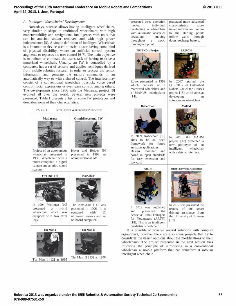
A. Intelligent Wheelchairs’ Developments Nowadays, science allows having intelligent wheelchairs,

very similar in shape to traditional wheelchairs, with high maneuverability and navigational intelligence, with units that can be attached and/or removed and with high power independence [5]. A simple definition of Intelligent Wheelchair is a locomotion device used to assist a user having some kind of physical disability, where an artificial control system augments or replaces the user control [6-7]. The main objective is to reduce or eliminate the user's task of having to drive a motorized wheelchair. Usually, an IW is controlled by a computer, has a set of sensors and applies techniques derived from mobile robotics research in order to process the sensor information and generate the motors commands in an automatically way or with a shared control. The interface may consist of a conventional wheelchair joystick, voice based control, facial expressions or even gaze control, among others. The developments since 1986 with the Madarasz project [8] evolved all over the world. Several new projects were presented. Table I presents a list of some IW prototypes and describes some of their characteristics.

TABLE I. INTELLIGENT WHEELCHAIRS’ PROJECTS

Madarasz

Project of an autonomous wheelchair presented in 1986. Wheelchair with a micro-computer, a digital camera and an ultra-sound scanner.

Omnidireccional IW

Hoyer and Holper [9] presented in 1993 an omnidirectional IW.

Two legs’ IW

In 1994 Wellman [10] presented a hybrid wheelchair which was equipped with two extra legs.

NavChair

The NavChair [11] was presented in 1996. It is equipped with 12 ultrasonic sensors and an on-board computer.

Tin Man I

Tin Man I [12] at 1995

Tin Man II

Tin Man II [13] at 1998

presented three operation modes: individual conducting a wheelchair with automatic obstacles deviation; moving throughout a track; moving to a point.

presented more advanced characteristics: store travel information; return to the starting point; follow walls; through doors; recharge battery.

FRIEND’s Project

Robot presented in 1999 which consists of a motorized wheelchair and a MANUS manipulator[14].

LURCH

In 2007 started the LURCH (Let Unleashed Robots Crawl the House) project [15] which aims at developing an autonomous wheelchair.

RoboChair

In 2009 Robochair [16] aims to be an open framework for future assistive applications.Design modular and based in open standards for easy extension and low cost.

VAHM

In 2010 the VAHM project [17] presented a new prototype of an intelligent wheelchair with a deictic interface.

ARTY

In 2012 was published and presented the Assistive Robot Transport for Youngsters (ARTY)[18]. This is an intelligent paediatric wheelchair.

Smart Driving Assistance

In 2012 was presented the results of the smart driving assistance from the University of Bremen[19].

It is possible to observe several solutions with complex ergonomics, however there are also some projects that try to considerer the users’ opinions about the modifications to their wheelchairs. The project presented in the next section tries following the principle of introducing in a conventional wheelchair a simple platform that can transform it into an intelligent wheelchair.

g

j

g


© 2013 IEEE


27

B. IntellWheelsProject The IntellWheels project aims developing an intelligent

wheelchair platform that may be easily adapted to any commercial wheelchair and aid any person with special mobility needs [20]. The project main focus is the research and design of a multi-agent platform, enabling easy integration of different sensors, actuators, devices for extended interaction with the user, navigation methods and planning techniques and methodologies for intelligent cooperation to solve problems associated with intelligent wheelchairs [21].

A real prototype (Fig. 1) was created by adapting a typical electric wheelchair. Two side bars with a total of 16 sonars, a laser range finder and two encoders were incorporated.

Fig. 1. Real prototype of the IW.

In the IntellWheels project it was also developed a simulator called IntellSim. The objective of this simulator is essentially to support the test of algorithms, analyze and test the modules of the platform and safely train users of the IW in a simulated environment [5] [22].

A multimodal interface was also developed that allows driving the wheelchair with several inputs such as joystick, head movements or more high level commands such as voice commands, facial expressions, and gamepad or even with a combination among them. For example it is possible to blink an eye and say “go” for the wheelchair to follow a right wall [23]. Therefore it is possible to drive the IW with a completely automatically way, with a shared or using the usual manual control.

III. MANUAL, AUTOMATIC AND SHARED CONTROLS

One initial objective of the IntellWheels project was to be able to control the wheelchair using three distinct methods: manual, shared and automatic. During the course of the project several manual and shared algorithms have been developed, but their comparative evaluation had never been performed. In the course of this work several experiments were performed, experiments to provide the best manual control, shared or automatic control adapted for the patients.

A. Manual Control The mapping of joystick positions to individual wheel

speed can be done in an infinite number of combinations, and it is this mapping that will determine the response behavior to manual control.

Considering that the joystick handle position is represented in a Cartesian coordinate system, with two axis, x and y, which vary between -1 and 1. These (x, y) coordinates can be used to determine the distance of the handle to the central (resting) position of the joystick (0, 0) and an angle relating to a reference vector (which is usually (0, 1)). The desired speed of the left wheel (L) or the right wheel (R) is represented by normalized values (between -1 and 1). With positive values the wheels rotate forward and with negative values the wheels rotate backward.

An intuitive mapping was implemented and the equations for R and L are:

nxyLnxyR

the value nx follows the Equation:

)(

)(

pointpoint1

point2pointpoint1

point2pointpoint1

cxcifxucxifucxcu

cxifucxcunx

where 1,0pointc ; 1,01u and 1,02u . The tested values were cpoint = 0.2; u1 = 0.5 and u2 = 0.25.The first slope u1allows a fast curve and the next slope u2 after the cut point (cpoint) should allow a slower curve.

B. Automatic Control The developed automatic control has as main objective

following a predefined circuit without the need of user intervention. The automatic control assumes full control over the navigation of the wheelchair and executes the navigating task following the circuit points without any user’s intervention. A predefined circuit can be specified by defining the relevant circuit points and the wheelchair can autonomously drive to the specified points.

The main reason to create an automatic control was concerned with the methodology used to achieve a shared driving algorithm for the intelligent wheelchair. The users in the study performed predetermined tasks such as collecting objects along a circuit. This automatic control assumes the self-localization problem solved and hence the IW always knows its position in the environment. Before this work, the IntellWheels IW was already capable of some forms of automatic control that did not rely on localization, such as “follow wall” or other high level actions like “go forward” [23]. However, it still missed an automatic driving algorithm based on the current position and orientation and the desired position and orientation.


© 2013 IEEE


28

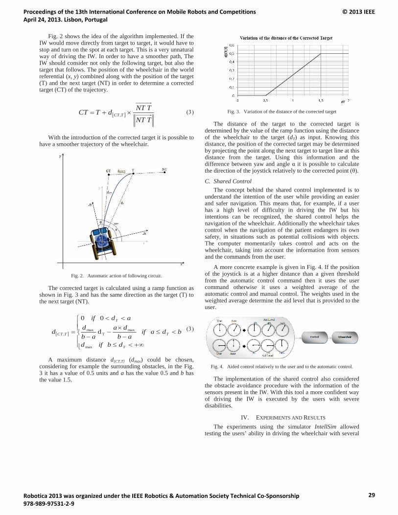
Fig. 2 shows the idea of the algorithm implemented. If the IW would move directly from target to target, it would have to stop and turn on the spot at each target. This is a very unnatural way of driving the IW. In order to have a smoother path, The IW should consider not only the following target, but also the target that follows. The position of the wheelchair in the world referential (x, y) combined along with the position of the target (T) and the next target (NT) in order to determine a corrected target (CT) of the trajectory.

TNT

TNTdTCT TCT ,

With the introduction of the corrected target it is possible to have a smoother trajectory of the wheelchair.

Fig. 2. Automatic action of following circuit.

The corrected target is calculated using a ramp function as shown in Fig. 3 and has the same direction as the target (T) to the next target (NT).

d

0 0

max

maxT

max,

T

T

T

TCT

dbifd

bdaifab

daab

dadif

d

A maximum distance d[CT,T] (dmax) could be chosen, considering for example the surrounding obstacles, in the Fig. 3 it has a value of 0.5 units and a has the value 0.5 and b has the value 1.5.

Fig. 3. Variation of the distance of the corrected target

The distance of the target to the corrected target is determined by the value of the ramp function using the distance of the wheelchair to the target (dT) as input. Knowing this distance, the position of the corrected target may be determinedby projecting the point along the next target to target line at this distance from the target. Using this information and the difference between yaw and angle α it is possible to calculate the direction of the joystick relatively to the corrected point (θ).

C. Shared Control The concept behind the shared control implemented is to

understand the intention of the user while providing an easier and safer navigation. This means that, for example, if a user has a high level of difficulty in driving the IW but his intentions can be recognized, the shared control helps the navigation of the wheelchair. Additionally the wheelchair takes control when the navigation of the patient endangers its own safety, in situations such as potential collisions with objects. The computer momentarily takes control and acts on the wheelchair, taking into account the information from sensors and the commands from the user.

A more concrete example is given in Fig. 4. If the position of the joystick is at a higher distance than a given threshold from the automatic control command then it uses the user command otherwise it uses a weighted average of the automatic control and manual control. The weights used in the weighted average determine the aid level that is provided to the user.

Fig. 4. Aided control relatively to the user and to the automatic control.

The implementation of the shared control also considered the obstacle avoidance procedure with the information of the sensors present in the IW. With this tool a more confident way of driving the IW is executed by the users with severe disabilities.

IV. EXPERIMENTS AND RESULTS

The experiments using the simulator IntellSim allowedtesting the users’ ability in driving the wheelchair with several


© 2013 IEEE


29

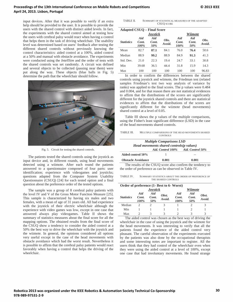
input devices. After that it was possible to verify if an extra help should be provided to the user. It is possible to provide the users with the shared control with distinct aided levels. In fact, the experiments with the shared control aimed at testing how the users with cerebral palsy would react when having a controlthat helps them in the task of driving wheelchair. The usability level was determined based on users’ feedback after testing the different shared controls without previously knowing the control characteristics: aided control at a 100%, aided control at a 50% and manual with obstacle avoidance. The experiments were conducted using the IntellSim and the order of tests with the shared controls was set randomly. A circuit was defined and several objects to be collected (passing near them) were put along the way. These objects (blue balls in Fig. 5)determine the path that the wheelchair should follow.

Fig. 5. Circuit for testing the shared controls.

The patients tested the shared controls using the joystick as input device and, in different rounds, using head movements detected using a wiimote. After each round the patients answered to a questionnaire composed of four parts: user identification; experience with videogames and joysticks; questions adapted from the Computer System Usability Questionnaire (CSUQ) [24] for each tested option and a final question about the preference order of the tested options.

The sample was a group of 8 cerebral palsy patients with the level IV and V of the Gross Motor Function Measure [25].This sample is characterized by having six males and two females, with a mean of age of 31 years old. All had experience with the joystick of their electric wheelchair although the experience with video games was low, except in one case that answered always play videogames. Table II shows the summary of statistics measures about the final score for all the mapping options. The obtained results from the final score of the CSUQ show a tendency to consider the aided control at a 50% the best way to drive the wheelchair with the joystick and the wiimote. In general, the opinions considered all options very useful except in the case of the head movements with obstacle avoidance which had the worst result. Nevertheless it is possible to affirm that the cerebral palsy patients would react favorably when having a control that helps the driving of the wheelchair.

TABLE II. SUMMARY OF STATISTICAL MEASURES OF THE ADAPTED CSUQ SCORE

Adapted CSUQ – Final ScoreJoystick Wiimote

StatisticsAid

Cont.100%

AidCont.50%

Obs.Avoid.

AidCont.100%

AidCont.50%

Obs.Avoid.

Mean 82.7 87.1 84.1 76.0 76.4 50.6Median 88.9 99.2 88.9 84.9 91.3 41.3Std. Dev. 21.0 22.3 19.4 24.7 33.1 30.8Min 39.68 36.5 44.4 31.8 15.9 14.3Max 100 100 100 100 100 96.83

In order to confirm the differences between the shared controls using joystick and wiimote, the Friedman test (related samples Friedman’s test two way analysis of variance by ranks) was applied to the final scores. The p values were 0.484 and 0.004, and for that reason there are not statistical evidences to affirm that the distributions of the scores are significantly different for the joystick shared controls and there are statistical evidences to affirm that the distributions of the scores are significantly different for the wiimote (head movements) shared control at a level of 0.05.

Table III shows the p values of the multiple comparisons, using the Fisher's least significant difference (LSD) in the case of the head movements shared controls.

TABLE III. MULTIPLE COMPARISONS OF THE HEAD MOVEMENTS SHARED CONTROLS

Multiple Comparisons LSD Head movements shared controls(p values)

Aid. Control 100% Aid. Control 50%Aided control 50% 1 --

Obstacle Avoidance 0.001 0.001The results of the CSUQ score also confirm the tendency to

the order of preference as can be observed in Table IV.

TABLE IV. SUMMARY STATISTICS ABOUT THE ORDER OF PREFERENCE OF THE SHARED CONTROLS

Order of preference (1- Best to 6- Worst)Joystick Wiimote

StatisticsAid

Cont.100%

AidCont.50%

Obst.Avoid.

AidCont.100%

AidCont.50%

Obst.Avoid.

Median 2 2 3 1 2 3Min 1 1 1 1 2 1Max 2 3 3 2 3 3The aided control was chosen as the best way of driving the

wheelchair in the case of using the joystick and the wiimote for the head movements. It was interesting to verify that all the patients found the experience of the aided control verypleasant. The careful observation of the experiments executed by the patients was also done by the occupational therapists and some interesting notes are important to register. All the users think that they had control of the wheelchair even when they were using the aided control at a level of 100%, except one case that had involuntary movements. He found strange


© 2013 IEEE


30

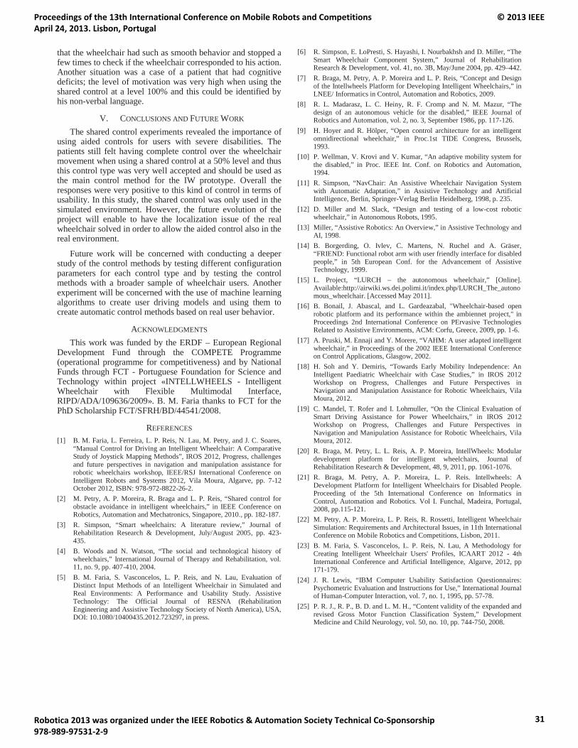
that the wheelchair had such as smooth behavior and stopped a few times to check if the wheelchair corresponded to his action. Another situation was a case of a patient that had cognitive deficits; the level of motivation was very high when using the shared control at a level 100% and this could be identified by his non-verbal language.


The shared control experiments revealed the importance of using aided controls for users with severe disabilities. The patients still felt having complete control over the wheelchair movement when using a shared control at a 50% level and thus this control type was very well accepted and should be used as the main control method for the IW prototype. Overall the responses were very positive to this kind of control in terms of usability. In this study, the shared control was only used in the simulated environment. However, the future evolution of the project will enable to have the localization issue of the real wheelchair solved in order to allow the aided control also in the real environment.

Future work will be concerned with conducting a deeper study of the control methods by testing different configuration parameters for each control type and by testing the control methods with a broader sample of wheelchair users. Another experiment will be concerned with the use of machine learning algorithms to create user driving models and using them to create automatic control methods based on real user behavior.

ACKNOWLEDGMENTS

This work was funded by the ERDF – European Regional Development Fund through the COMPETE Programme (operational programme for competitiveness) and by National Funds through FCT - Portuguese Foundation for Science and Technology within project «INTELLWHEELS - Intelligent Wheelchair with Flexible Multimodal Interface, RIPD/ADA/109636/2009». B. M. Faria thanks to FCT for the PhD Scholarship FCT/SFRH/BD/44541/2008.

REFERENCES

[1] B. M. Faria, L. Ferreira, L. P. Reis, N. Lau, M. Petry, and J. C. Soares, “Manual Control for Driving an Intelligent Wheelchair: A Comparative Study of Joystick Mapping Methods”, IROS 2012, Progress, challenges and future perspectives in navigation and manipulation assistance for robotic wheelchairs workshop, IEEE/RSJ International Conference on Intelligent Robots and Systems 2012, Vila Moura, Algarve, pp. 7-12October 2012, ISBN: 978-972-8822-26-2.

[2] M. Petry, A. P. Moreira, R. Braga and L. P. Reis, “Shared control for obstacle avoidance in intelligent wheelchairs,” in IEEE Conference on Robotics, Automation and Mechatronics, Singapore, 2010., pp. 182-187.

[3] R. Simpson, “Smart wheelchairs: A literature review,” Journal of Rehabilitation Research & Development, July/August 2005, pp. 423-435.

[4] B. Woods and N. Watson, “The social and technological history of wheelchairs,” International Journal of Therapy and Rehabilitation, vol. 11, no. 9, pp. 407-410, 2004.

[5] B. M. Faria, S. Vasconcelos, L. P. Reis, and N. Lau, Evaluation of Distinct Input Methods of an Intelligent Wheelchair in Simulated and Real Environments: A Performance and Usability Study. Assistive Technology: The Official Journal of RESNA (Rehabilitation Engineering and Assistive Technology Society of North America), USA, DOI: 10.1080/10400435.2012.723297, in press.

[6] R. Simpson, E. LoPresti, S. Hayashi, I. Nourbakhsh and D. Miller, “The Smart Wheelchair Component System,” Journal of Rehabilitation Research & Development, vol. 41, no. 3B, May/June 2004, pp. 429–442.

[7] R. Braga, M. Petry, A. P. Moreira and L. P. Reis, “Concept and Design of the Intellwheels Platform for Developing Intelligent Wheelchairs,” in LNEE/ Informatics in Control, Automation and Robotics, 2009.

[8] R. L. Madarasz, L. C. Heiny, R. F. Cromp and N. M. Mazur, “The design of an autonomous vehicle for the disabled,” IEEE Journal of Robotics and Automation, vol. 2, no. 3, September 1986, pp. 117-126.

[9] H. Hoyer and R. Hölper, “Open control architecture for an intelligent omnidirectional wheelchair,” in Proc.1st TIDE Congress, Brussels, 1993.

[10] P. Wellman, V. Krovi and V. Kumar, “An adaptive mobility system for the disabled,” in Proc. IEEE Int. Conf. on Robotics and Automation, 1994.

[11] R. Simpson, “NavChair: An Assistive Wheelchair Navigation System with Automatic Adaptation,” in Assistive Technology and Artificial Intelligence, Berlin, Springer-Verlag Berlin Heidelberg, 1998, p. 235.

[12] D. Miller and M. Slack, “Design and testing of a low-cost robotic wheelchair,” in Autonomous Robots, 1995.

[13] Miller, “Assistive Robotics: An Overview,” in Assistive Technology and AI, 1998.

[14] B. Borgerding, O. Ivlev, C. Martens, N. Ruchel and A. Gräser, “FRIEND: Functional robot arm with user friendly interface for disabled people,” in 5th European Conf. for the Advancement of Assistive Technology, 1999.

[15] L. Project, “LURCH – the autonomous wheelchair,” [Online]. Available:http://airwiki.ws.dei.polimi.it/index.php/LURCH_The_autonomous_wheelchair. [Accessed May 2011].

[16] B. Bonail, J. Abascal, and L. Gardeazabal, "Wheelchair-based open robotic platform and its performance within the ambiennet project," in Proceedings 2nd International Conference on PErvasive Technologies Related to Assistive Environments, ACM: Corfu, Greece, 2009, pp. 1-6.

[17] A. Pruski, M. Ennaji and Y. Morere, “VAHM: A user adapted intelligent wheelchair,” in Proceedings of the 2002 IEEE International Conference on Control Applications, Glasgow, 2002.

[18] H. Soh and Y. Demiris, “Towards Early Mobility Independence: An Intelligent Paediatric Wheelchair with Case Studies,” in IROS 2012 Workshop on Progress, Challenges and Future Perspectives in Navigation and Manipulation Assistance for Robotic Wheelchairs, Vila Moura, 2012.

[19] C. Mandel, T. Rofer and I. Lohmuller, “On the Clinical Evaluation of Smart Driving Assistance for Power Wheelchairs,” in IROS 2012Workshop on Progress, Challenges and Future Perspectives in Navigation and Manipulation Assistance for Robotic Wheelchairs, Vila Moura, 2012.

[20] R. Braga, M. Petry, L. L. Reis, A. P. Moreira, IntellWheels: Modular development platform for intelligent wheelchairs, Journal of Rehabilitation Research & Development, 48, 9, 2011, pp. 1061-1076.

[21] R. Braga, M. Petry, A. P. Moreira, L. P. Reis. Intellwheels: A Development Platform for Intelligent Wheelchairs for Disabled People. Proceeding of the 5th International Conference on Informatics in Control, Automation and Robotics. Vol I. Funchal, Madeira, Portugal, 2008, pp.115-121.

[22] M. Petry, A. P. Moreira, L. P. Reis, R. Rossetti, Intelligent Wheelchair Simulation: Requirements and Architectural Issues, in 11th International Conference on Mobile Robotics and Competitions, Lisbon, 2011.

[23] B. M. Faria, S. Vasconcelos, L. P. Reis, N. Lau, A Methodology for Creating Intelligent Wheelchair Users' Profiles, ICAART 2012 - 4th International Conference and Artificial Intelligence, Algarve, 2012, pp 171-179.

[24] J. R. Lewis, “IBM Computer Usability Satisfaction Questionnaires: Psychometric Evaluation and Instructions for Use,” International Journal of Human-Computer Interaction, vol. 7, no. 1, 1995, pp. 57-78.

[25] P. R. J., R. P., B. D. and L. M. H., “Content validity of the expanded and revised Gross Motor Function Classification System,” Development Medicine and Child Neurology, vol. 50, no. 10, pp. 744-750, 2008.


© 2013 IEEE


31

Complete Analytical Inverse Kinematics for NAO

Nikos Kofinas, Emmanouil Orfanoudakis, and Michail G. LagoudakisIntelligent Systems Laboratory, Department of Electronic and Computer Engineering

Technical University of Crete, Chania, Crete 73100, Greece

Email: {nikofinas, vosk, lagoudakis}@intelligence.tuc.gr

Abstract—The design of complex dynamic motions for hu-manoid robots is achievable only through the use of robotkinematics. In this paper, we study the problems of forwardand inverse kinematics for the Aldebaran NAO humanoid robotand present a complete, exact, analytical solution to bothproblems, including a software library implementation for real-time onboard execution. The forward kinematics allow NAOdevelopers to map any configuration of the robot from its ownjoint space to the three-dimensional physical space, whereasthe inverse kinematics provide closed-form solutions to findingjoint configurations that drive the end effectors of the robotto desired target positions in the three-dimensional physicalspace. The proposed solution was made feasible through adecomposition into five independent problems (head, two arms,two legs), the use of the Denavit-Hartenberg method, and theanalytical solution of a non-linear system of equations. Themain advantage of the proposed inverse kinematics solutioncompared to existing approaches is its accuracy, its efficiency,and the elimination of singularities. In addition, we suggest ageneric guideline for solving the inverse kinematics problemfor other humanoid robots. The implemented, freely-available,NAO kinematics library, which additionally offers center-of-masscalculations, is demonstrated in two motion design tasks: basiccenter-of-mass balancing and pointing to the ball.

I. INTRODUCTION

Articulated robots with multiple degrees of freedom, such

as humanoid robots, have become popular research platforms

in robotics and artificial intelligence. Our work focuses on

autonomous humanoid platforms with multiple manipulators

capable of performing complex motions, such as balancing,

walking, and kicking. These skills are required in the Standard

Platform League of the RoboCup robot soccer competition [1],

in which all teams compete using the Aldebaran NAO hu-

manoid robot [2], which is our target robot platform.

The design of complex dynamic motions is achievable only

through the use of robot kinematics, which is an application

of geometry to the study of arbitrary robotic chains. However,

past work [3]–[5] has not fully solved the inverse kinematics

problem for the NAO robot, since it focuses exclusively

on the robot legs. Furthermore, the widely-known analytical

solution [3] for the inverse kinematics of the legs is purely

geometric and cannot be generalized to other kinematic chains.

Also, existing numerical solutions [5] are inherently prone to

singularities and, therefore, lack in robustness.

In this paper, we present a complete and exact analytical

forward and inverse kinematics solution for all limbs of

the Aldebaran NAO humanoid robot, using the established

Denavit–Hartenberg convention [6], [7] for revolute joints. The

main advantage of the proposed solution is its accuracy, its

efficiency, and the elimination of singularities. In addition, we

contribute an implementation of the proposed NAO kinematics

as a freely-available software library1 for real-time execution

on the robot. This work enables NAO software developers

to make transformations between configurations in the joint

space and points in the three-dimensional physical space and

vice-versa, on-board in just microseconds, as the library is

designed for high-performance real-time execution on the lim-

ited embedded platform of the robot. The implemented NAO

kinematics library, which additionally offers center-of-mass

calculations, is demonstrated in two tasks2: basic center-of-

mass balancing and pointing to the ball. The library has been

integrated into the software architecture of our RoboCup team

Kouretes [www.kouretes.gr] and is currently being used in

various motion design problems, such as dynamic balancing,

trajectory following, dynamic kicking, and omnidirectional

walking. Extrapolating from our work on the NAO, we also

present some guidelines for finding analytical solutions to the

inverse kinematics problem for any humanoid with revolute

joints of up to 6 degrees of freedom (DOF) per manipulator.

II. BACKGROUND

A. The Aldebaran NAO Humanoid Robot

NAO (v3.3) is a 58cm, 5kg humanoid robot (Figure 1).

The NAO robot carries a fully capable computer on-board

with an x86 AMD Geode processor at 500 MHz, 256 MB

SDRAM, and 2 GB flash memory running an Embedded Linux

distribution. It is powered by a 6-cell Lithium-Ion battery

which provides about 30 minutes of continuous operation and

communicates with remote computers via an IEEE 802.11g

wireless or a wired Ethernet link. NAO RoboCup edition

has 21 degrees of freedom; 2 in the head, 4 in each arm,

5 in each leg and 1 in the pelvis (there are two pelvis

joints which are coupled together on one servo and cannot

move independently). All joints are position-controlled, using

closed-loop PID controllers and encoders. It also features a

variety of sensors: an Inertial Measurement Unit (IMU) in the

torso, Force Sensitive Resistors (FSR) on each foot, ultrasonic

range sensors on the chest, and two VGA cameras on the head.

B. Transformation Formalism

The translation and orientation of a joint j with respect to

an adjacent joint i in the three-dimensional space can be fully

1Library download link: www.github.com/kouretes/NAOKinematics2Video download link: www.intelligence.tuc.gr/kouretes/NAOKinematics


© 2013 IEEE


32

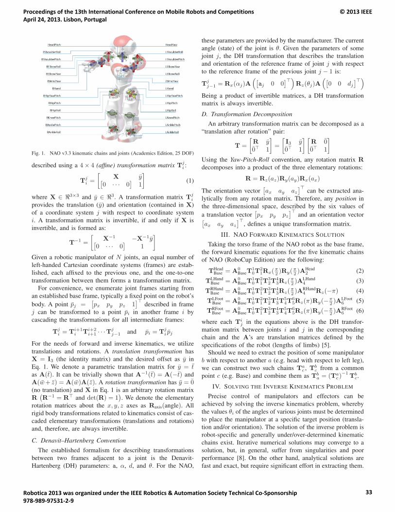
Fig. 1. NAO v3.3 kinematic chains and joints (Academics Edition, 25 DOF)

described using a 4× 4 (affine) transformation matrix Tji :

Tji =

[X y[

0 · · · 0]

1

](1)

where X ∈ �3×3 and y ∈ �3. A transformation matrix Tji

provides the translation (y) and orientation (contained in X)

of a coordinate system j with respect to coordinate system

i. A transformation matrix is invertible, if and only if X is

invertible, and is formed as:

T−1 =

[X−1 −X−1y[

0 · · · 0]

1

]Given a robotic manipulator of N joints, an equal number of

left-handed Cartesian coordinate systems (frames) are estab-

lished, each affixed to the previous one, and the one-to-one

transformation between them forms a transformation matrix.

For convenience, we enumerate joint frames starting from

an established base frame, typically a fixed point on the robot’s

body. A point pj =[px py pz 1

]�described in frame

j can be transformed to a point pi in another frame i by

cascading the transformations for all intermediate frames:

Tji = Ti+1

i Ti+2i+1 · · ·T

jj−1 and pi = Tj

i pj

For the needs of forward and inverse kinematics, we utilize

translations and rotations. A translation transformation has

X = I3 (the identity matrix) and the desired offset as y in

Eq. 1. We denote a parametric translation matrix for y = tas A(t). It can be trivially shown that A−1(t) = A(−t) and

A(w+ z) = A(w)A(z). A rotation transformation has y = 0(no translation) and X in Eq. 1 is an arbitrary rotation matrix

R(R−1 = R� and det(R) = 1

). We denote the elementary

rotation matrices about the x, y, z axes as Raxis(angle). All

rigid body transformations related to kinematics consist of cas-

caded elementary transformations (translations and rotations)

and, therefore, are always invertible.

C. Denavit–Hartenberg Convention

The established formalism for describing transformations

between two frames adjacent to a joint is the Denavit-

Hartenberg (DH) parameters: a, α, d, and θ. For the NAO,

these parameters are provided by the manufacturer. The current

angle (state) of the joint is θ. Given the parameters of some

joint j, the DH transformation that describes the translation

and orientation of the reference frame of joint j with respect

to the reference frame of the previous joint j − 1 is:

Tjj−1 = Rx(αj)A

([aj 0 0

]�)Rz(θj)A

([0 0 dj

]�)Being a product of invertible matrices, a DH transformation

matrix is always invertible.

D. Transformation DecompositionAn arbitrary transformation matrix can be decomposed as a

“translation after rotation” pair:

T =

[R y0� 1

]=

[I3 y0� 1

] [R 00� 1

]Using the Yaw-Pitch-Roll convention, any rotation matrix Rdecomposes into a product of the three elementary rotations:

R = Rz(az)Ry(ay)Rx(ax)

The orientation vector[ax ay az

]�can be extracted ana-

lytically from any rotation matrix. Therefore, any position in

the three-dimensional space, described by the six values of

a translation vector[px py pz

]�and an orientation vector[

ax ay az]�

, defines a unique transformation matrix.

III. NAO FORWARD KINEMATICS SOLUTION

Taking the torso frame of the NAO robot as the base frame,

the forward kinematic equations for the five kinematic chains

of NAO (RoboCup Edition) are the following:

THeadBase = A0

BaseT10T

21Rx(

π2 )Ry(

π2 )A

Head2 (2)

TLHandBase = A0

BaseT10T

21T

32T

43Rz(

π2 )A

LHand4 (3)

TRHandBase = A0

BaseT10T

21T

32T

43Rz(

π2 )A

RHand4 Rz(−π) (4)

TLFootBase = A0

BaseT10T

21T

32T

43T

54T

65Rz(π)Ry(−π

2 )ALFoot6 (5)

TRFootBase = A0

BaseT10T

21T

32T

43T

54T

65Rz(π)Ry(−π

2 )ARFoot6 (6)

where each Tij in the equations above is the DH transfor-

mation matrix between joints i and j in the corresponding

chain and the A’s are translation matrices defined by the

specifications of the robot (lengths of limbs) [5].Should we need to extract the position of some manipulator

b with respect to another a (e.g. head with respect to left leg),

we can construct two such chains Tac , Tb

c from a common

point c (e.g. Base) and combine them as Tba = (Ta

c )−1

Tbc.

IV. SOLVING THE INVERSE KINEMATICS PROBLEM

Precise control of manipulators and effectors can be

achieved by solving the inverse kinematics problem, whereby

the values θi of the angles of various joints must be determined

to place the manipulator at a specific target position (transla-

tion and/or orientation). The solution of the inverse problem is

robot-specific and generally under/over-determined kinematic

chains exist. Iterative numerical solutions may converge to a

solution, but, in general, suffer from singularities and poor

performance [8]. On the other hand, analytical solutions are

fast and exact, but require significant effort in extracting them.


© 2013 IEEE


33

A. Inverse Kinematics Methodology

The following seven steps were taken in order to find a

complete solution for the inverse kinematics problem for all

the kinematic chains of the NAO humanoid robot.

1) Construct the numeric transformation: Given a de-

sired target position, denoted by an orientation vector a =[ax ay az

]�and a translation vector p =

[px py pz

]�,

it is easy to reconstruct the target transformation matrix:

T = A(p)Rz(az)Ry(ay)Rx(ax)

2) Construct the symbolic transformation: Setting all θparameters as unknowns in the forward kinematics solution

of the target kinematic chain yields a symbolic matrix:

T0baseT

j0(θ0, . . . , θj)T

endj

3) Form a non-linear system: By equating the above ma-

trices, a non-linear system is formed, since the unknown

θ’s appear in transcendental trigonometric forms. Now, the

problem is to find values for the θ’s from 12 equations (the

upper 3× 4 block) of which only up to six are independent.

T = T0baseT

j0(θ0, . . . , θj)T

endj

4) Manipulate both sides: The chain can be simplified by

eliminating known terms. Such terms (e.g. the base and the

end transformations) can be removed by multiplying both sides

of the system with the appropriate inverse matrix:(T0

base

)−1T

(Tend

j

)−1= Tj

0(θ0, . . . , θj)

As soon as we find a solution for some θi, we can remove in a

similar way the corresponding joint i from the chain, because

the corresponding DH transformation matrix is now known;

this can occur if and only if this joint is the first or the last in

the kinematic chain.

Another way to manipulate the chain is to induce arbitrary

(known) constant transformations at the beginning or the end

of the chain, aiming at simplifying the non-linear system.

Tc(T0base)

−1T(Tendj )−1 = TcT

j0(θ0, . . . , θj)

In some kinematic chains we can decouple the orientation

and translation sub-problems. Quite often the target translation

vector can be expressed as a function of fewer joints in the

analytical equation of the kinematic chain or in the analytical

equation of the reverse kinematic chain.

5) Use geometry and trigonometry: It is possible to form

a closed-form solution for some θj using a geometric model

of the chain. For chains with up to two links (non-zero a

and d parameters) or “arm and wrist” chains commonly found

in humanoids, a geometric approach can easily determine the

values for the joints that lie between the links. These joints can

be modeled as an angle of the triangle formed by the links,

so the value of the joint can be obtained using trigonometry.

The kinematic arm chain of the NAO robot, for example,

has such a joint. Figure 2 shows the triangle formed by the

upper arm, the lower arm, and the line that connects the base

with the target point. Upper and lower arm lengths are known

Fig. 2. Triangle formed by the robot arm

and the third side of the triangle can be computed using the

Euclidean distance between the base of the chain and the end

of the chain. The law of cosines, yields a set of complementary

closed-form solutions for the angle θ.

6) Solve the non-linear system: The resulting equations

are combinations of sin θi and cos θi, thus, the closed-form

solution of these equations must utilize the inverse trigono-

metric functions (acos, asin). The transcendental nature of

the acos and asin trigonometric functions has the inherent

problem of producing multiple solutions in [−π, π]. Without

any restrictions on the valid range of a joint, we must examine

all candidate solutions for each joint and their combinations

for validity. To avoid this multiplicity, solutions that rely on

atan and acot are preferred, but forming them might not be

possible for a particular chain.

7) Validate through forward kinematics: Generally, there

are multiple candidate solutions for the joint values, due to

the existence of complementary and/or supplementary angles.

A validation step is taken to discard invalid candidates. This

validation is performed by feeding each candidate solution to

the forward kinematics of the chain and checking whether

the resulting position matches precisely the target position.

Choosing among the valid solutions, if more than one, can be

addressed independently of kinematics.

B. Applicability

The methodology presented above offers a generic guide-

line for solving the inverse kinematics problem on typical

humanoid robot kinematic chains that have the generic two-

link configuration (found in both the arms and legs). More

specifically, the kinematic chains must have up to five joints

or six joints with three consecutive ones having intersecting

axes [9], [10] to expect a possible solution.

V. NAO INVERSE KINEMATICS SOLUTION

Using the methodology presented above, we find the inverse

kinematics solution for all five kinematic chains of NAO

(RoboCup Edition): head (2 joints), left arm (4 joints), right

arm, left leg (6 joints), and right leg. The left chains are almost

identical to the right ones, thus the solutions are similar. Due

to space restrictions, the solutions for the the left part are

presented in detail, whereas the ones for the right part are

abbreviated. Full details may be found in a longer technical

report [11] .

A. Inverse Kinematics for the Head Chain

The head chain consists of only two joints (HeadYaw,

HeadPitch—in this order), therefore we can solve for either


© 2013 IEEE


34

θ2 = asin

(− pz + l3√l1

2 + l22

)− atan

(l1

l2

)+

π

2

θ2 = π − asin

(− pz + l3√l1

2 + l22

)− atan

(l1

l2

)+

π

2

θ1 = ±acos

(px

l2 cos(θ2 − π

2

)− l1 sin

(θ2 − π

2

))provided a target translation (px, py , pz), or

θ1 = az θ2 = ay

provided a target orientation (ax, ay , az)

Fig. 3. Head Inverse Kinematics Solution

the translation (p) or the orientation (a) of the target position

to obtain a solution. In the latter case, we can achieve the

desired target orientation simply by setting the HeadYaw and

HeadPitch joints to az and ay respectively, and assume ax = 0.

In the former case, we construct the symbolic matrix through

the forward kinematics solution (Eq. 2). Now, we can equate

the translation part from the symbolic matrix with p and

from these equations we can easily find the desired θ values.

Figure 3 shows the resulting analytical solution, in which l1and l2 are the x and the y part of the end translation and l3is the z part of the base translation.

B. Inverse Kinematics for the Left Arm Chain

The left arm chain consists of four joints (LShoulderPitch,

LShoulderRoll, LElbowYaw, LElbowRoll—in this order). Fol-

lowing our methodology, the first three steps are straight-

forward given the forward kinematics solution (Eq. 3). The

fourth step is not required, because the problem is not too

complicated. Using trigonometry, we find the value of θ4, as

shown in Figure 2. Next, the remaining three joint values are

easily extracted by solving the equations of the non-linear

system. Finally, we validate all candidate solutions through

the forward kinematics validation step. Figure 4 shows the

resulting analytical solution, in which s is the base translation

vector, l1 is the y part of the base translation, l3 is the length

of the upper arm, l4 is the length of the lower arm, and T(i,j)

is the (i, j) element of matrix T.

C. Inverse Kinematics for the Right Arm Chain

The right arm chain is almost identical to the left arm chain.

The only difference is in the forward kinematics solution, since

there is one more rotation at the end of the chain (Eq. 4). This

last rotation can be easily removed following the fourth step of

our methodology, by multiplying both sides of the equations

from the right with (Rz(−π))−1

. Besides this difference, all

other steps have similar results. The analytical solution is the

one shown in Figure 4 with the following differences: (a)

matrix T must be multiplied upfront by (Rz(−π))−1

from

the right, (b) there is no minus sign in the equation for θ4, (c)

there is a minus sign before T(2,4) in the equation for θ2, and

(d) all instances of (θ2 − π2 ) in the equations for θ3 and θ1

are changed to (θ2 +π2 ).

θ4 = −(π − acos

(l3

2 + l42 − ‖s− p‖22l3l4

))

θ2 = ±acos

⎛⎝T(2,4) − l1 −

(l4 sin θ4T(2,2)

cos θ4

)l3 + l4 cos θ4 + l4

sin2 θ4cos θ4

⎞⎠+

π

2

θ3 = asin

(T(2,3)

sin(θ2 − π

2

)) θ3 = π − asin

(T(2,3)

sin(θ2 − π

2

))

θ1 =

⎧⎪⎪⎪⎪⎪⎪⎪⎨⎪⎪⎪⎪⎪⎪⎪⎩

±acos

⎛⎜⎜⎝T(3,3) +

T(1,3) sin θ3 cos(θ2 − π

2

)cos θ3

cos θ3 +cos2

(θ2 − π

2

)sin2 θ3

cos θ3

⎞⎟⎟⎠ if θ3 �= π

2

±acos

(T(1,3)

cos(θ2 − π

2

)sin θ3

)if θ3 =

π

2

Fig. 4. Left Arm Inverse Kinematics Solution

T′ =(Rx(

π4)

((A0

Base

)−1T(AEnd

6

)−1))−1

θ4 = ±(π − acos

(l1

2 + l22 − ‖0− p‖22l1l2

))

θ6 =

{atan

(T′

(2,4)

T′(3,4)

)if (l2 cos θ5 + l1 cos (θ4 + θ5)) �= 0

undefined if (l2 cos θ5 + l1 cos (θ4 + θ5)) = 0

T′′ =((

T′)−1 (T6

5Rz (π)Ry(−π2))−1

)−1

θ5 = asin

(−T′′

(2,4)(l2 + l1 cos θ4) + l1T′′

(1,4)sin θ4

l12 sin2 θ4 + (l2 + l1 cos θ4)

2

)θ5 = π − asin

(−T′′

(2,4)(l2 + l1 cos θ4) + l1T′′

(1,4)sin θ4

l12 sin2 θ4 + (l2 + l1 cos θ4)

2

)T′′′ =

(T′′)−1 (

T43T

54

)−1

θ2 = ±acos(T′′′

(2,3)

)− π

4

θ3 = asin

(T′′′

(2,2)

sin(θ2 + π

4

)) θ3 = π − asin

(T′′′

(2,2)

sin(θ2 + π

4

))

θ1 = ±acos

(T′′′

(1,3)

sin(θ2 + π

4

))+π

2

Fig. 5. Left Leg Inverse Kinematics Solution

D. Inverse Kinematics for the Left Leg Chain

The kinematic chain of the left leg has six joints

(LHipYawPitch, LHipRoll, LHipPitch, LKneePitch, LAn-

klePitch, LAnkleRoll—in this order), but since the first three

joints have intersecting axes, the problem is possibly solv-

able [9], [10]. We construct both the numerical and symbolic

parts of the system with the help of forward kinematics (Eq. 5).

Following the fourth step, to make the problem easier, we

remove the known translations from the kinematic chain. Then,

to simplify the solution we induce a Rx(π4 ) transformation at

the start of the chain. In effect, we transform the first joint from

a yaw-pitch joint to a yaw joint, which is simpler to handle.

Close examination of the resulting kinematic chain reveals that


© 2013 IEEE


35

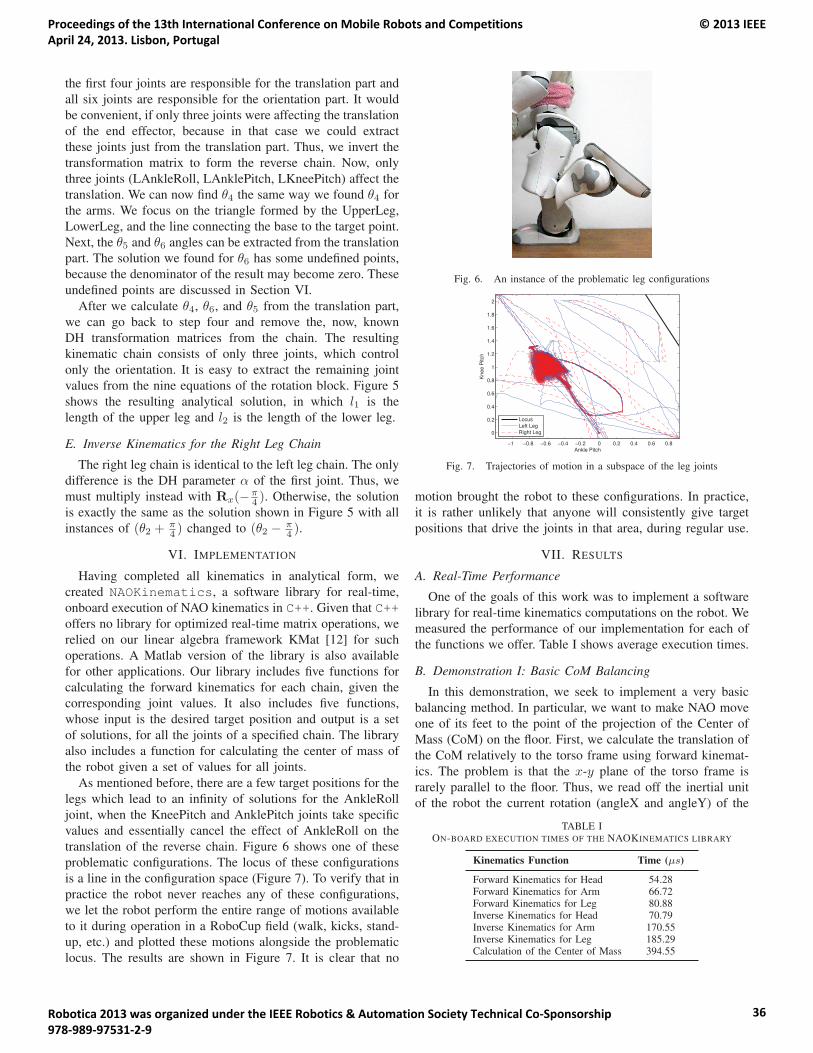
the first four joints are responsible for the translation part and

all six joints are responsible for the orientation part. It would

be convenient, if only three joints were affecting the translation

of the end effector, because in that case we could extract

these joints just from the translation part. Thus, we invert the

transformation matrix to form the reverse chain. Now, only

three joints (LAnkleRoll, LAnklePitch, LKneePitch) affect the

translation. We can now find θ4 the same way we found θ4 for

the arms. We focus on the triangle formed by the UpperLeg,

LowerLeg, and the line connecting the base to the target point.

Next, the θ5 and θ6 angles can be extracted from the translation

part. The solution we found for θ6 has some undefined points,

because the denominator of the result may become zero. These

undefined points are discussed in Section VI.

After we calculate θ4, θ6, and θ5 from the translation part,

we can go back to step four and remove the, now, known

DH transformation matrices from the chain. The resulting

kinematic chain consists of only three joints, which control

only the orientation. It is easy to extract the remaining joint

values from the nine equations of the rotation block. Figure 5

shows the resulting analytical solution, in which l1 is the

length of the upper leg and l2 is the length of the lower leg.

E. Inverse Kinematics for the Right Leg Chain

The right leg chain is identical to the left leg chain. The only

difference is the DH parameter α of the first joint. Thus, we

must multiply instead with Rx(−π4 ). Otherwise, the solution

is exactly the same as the solution shown in Figure 5 with all

instances of (θ2 +π4 ) changed to (θ2 − π

4 ).

VI. IMPLEMENTATION

Having completed all kinematics in analytical form, we

created NAOKinematics, a software library for real-time,

onboard execution of NAO kinematics in C++. Given that C++offers no library for optimized real-time matrix operations, we

relied on our linear algebra framework KMat [12] for such

operations. A Matlab version of the library is also available

for other applications. Our library includes five functions for

calculating the forward kinematics for each chain, given the

corresponding joint values. It also includes five functions,

whose input is the desired target position and output is a set

of solutions, for all the joints of a specified chain. The library

also includes a function for calculating the center of mass of

the robot given a set of values for all joints.

As mentioned before, there are a few target positions for the

legs which lead to an infinity of solutions for the AnkleRoll

joint, when the KneePitch and AnklePitch joints take specific

values and essentially cancel the effect of AnkleRoll on the

translation of the reverse chain. Figure 6 shows one of these

problematic configurations. The locus of these configurations

is a line in the configuration space (Figure 7). To verify that in

practice the robot never reaches any of these configurations,

we let the robot perform the entire range of motions available

to it during operation in a RoboCup field (walk, kicks, stand-

up, etc.) and plotted these motions alongside the problematic

locus. The results are shown in Figure 7. It is clear that no

Fig. 6. An instance of the problematic leg configurations

−1 −0.8 −0.6 −0.4 −0.2 0 0.2 0.4 0.6 0.8

0

0.2

0.4

0.6

0.8

1

1.2

1.4

1.6

1.8

2

Ankle Pitch

Kne

e P

itch

LocusLeft LegRight Leg

Fig. 7. Trajectories of motion in a subspace of the leg joints

motion brought the robot to these configurations. In practice,

it is rather unlikely that anyone will consistently give target

positions that drive the joints in that area, during regular use.

VII. RESULTS

A. Real-Time Performance

One of the goals of this work was to implement a software

library for real-time kinematics computations on the robot. We

measured the performance of our implementation for each of

the functions we offer. Table I shows average execution times.

B. Demonstration I: Basic CoM Balancing

In this demonstration, we seek to implement a very basic

balancing method. In particular, we want to make NAO move

one of its feet to the point of the projection of the Center of

Mass (CoM) on the floor. First, we calculate the translation of

the CoM relatively to the torso frame using forward kinemat-

ics. The problem is that the x-y plane of the torso frame is

rarely parallel to the floor. Thus, we read off the inertial unit

of the robot the current rotation (angleX and angleY) of the

TABLE ION-BOARD EXECUTION TIMES OF THE NAOKINEMATICS LIBRARY

Kinematics Function Time (μs)

Forward Kinematics for Head 54.28Forward Kinematics for Arm 66.72Forward Kinematics for Leg 80.88Inverse Kinematics for Head 70.79Inverse Kinematics for Arm 170.55Inverse Kinematics for Leg 185.29Calculation of the Center of Mass 394.55


© 2013 IEEE


36

torso plane. Now, we can calculate the translation of the CoM

relatively to the rotated torso:

Trotated = Ry(angleY)Rx(angleX)A(CoM)

Then, we assign a custom value to pz in T(4,3), which

represents the desired torso height from the floor and that

yields T′rotated. Now we must rotate back to the torso frame:

Tfinal =(Ry(angleY)Rx(angleX)

)−1T′

rotated

Finally, we extract px, py , and pz from Tfinal and we set[px py pz

]�as the target translation for inverse kine-

matics. The target orientation is set to[ax ay az

]�=[

−angleX −angleY 0]�

, because we do not care about the

rotation about the z-axis. Note that the foot is always parallel

to the floor, excluding any hardware precision errors.

C. Demonstration II: Pointing to the Ball

In this demonstration, our goal is to make the NAO point

to the ball with its stretched arms. Apart from the kinematics,

to realize this task we employed our vision module [12] for

ball recognition, along with the module that filters the belief

of the robot about the ball location. Initially, NAO scans for

the ball. When found, it points to it with the left, the right,

or both arms, depending on where the ball is located (left,

right, or front). The ball observation can be described as a

two-dimensional translation (px, py) on the floor. We add the

height of the torso (found through forward kinematics) as the

third coordinate pz to form the ball translation (px, py, pz) in

the three-dimensional space. We also set ax to zero, because

we are only rotating about the y-axis (up/down) and the z-axis

(right/left). To find the other two orientations, we focus on the

straight line that connects the location of the ball and the point

of the ShoulderPitch joint relatively to the torso frame. The

orientations ay, az are the angles between this line and the

corresponding axes. Additionally, the target point lies on this

line at a distance equal to the length of the stretched arm from

the ShoulderPitch joint. We run this procedure for both arms

and obtain the solution(s) from inverse kinematics. If both

solutions are returned, the robot raises both arms pointing to

the ball. If only one solution is returned, the robot raises only

one arm; the other arm cannot physically point to the ball.

VIII. CONCLUSION

In this paper, we presented a complete, exact, analytical

solution for the problems of forward and inverse kinematics

of the NAO robot. The main advantage of our solution is its

accuracy, its efficiency, and the elimination of singularities. In

addition, we contributed an implementation of the proposed

NAO kinematics as a freely-available software library for real-

time execution on the robot or for simulations.

Our approach to NAO kinematics is based on standard

principled methods for studying robot kinematic chains. No

complete analytical solution with full implementation for the

NAO robot has been published before. The currently widely-

known solution of team B-Human [3] applies only to the legs,

is purely geometric, and cannot be generalized to other kine-

matic chains. In addition, their work has not studied the effect

of the existing potentially problematic configurations. We have

tried to implement the other published analytical solution for

the legs by team MRL [4], but we were not able to reproduce

their results. Finally, the numerical solution [5] offered by the

manufacturer of the robot, Aldebaran Robotics, is a proprietary

implementation, which unfortunately is inherently prone to

singularities and, therefore, lacks in robustness. It should be

noted that none of the two demonstrations we presented in

this paper could be realized with the existing solutions and

implementations of NAO kinematics.

Since kinematics is the base for several applications related

to robot motion, we expect that our work will be useful not

only to RoboCup SPL teams, but also to any NAO software

developer. We believe that NAO developers can take advantage

of our off-the-shelf NAO kinematics library to work on omni-

directional walk algorithms, dynamic balancing methods, dy-

namic kick engines, etc. Our library can offer the basis for

following dynamic trajectories in real time for walking and

kicking or calculating the center of mass dynamically in real

time for balancing.

Finally, our methodology offers a generic guideline for

addressing the problem of inverse kinematics in humanoid

robots. Apart from extending our work to the Academic

Edition of NAO, which has four additional joints, one of our

future goals is to apply the same methodology to robots similar

to NAO, such as the Darwin-OP humanoid robot, which has

a maximum of six degrees of freedom per kinematic chain.

REFERENCES

[1] H. Kitano, M. Asada, Y. Kuniyoshi, I. Noda, E. Osawa, and H. Mat-subara, “Robocup: A challenge problem for AI,” AI Magazine, vol. 18,no. 1, pp. 73–85, 1997.

[2] D. Gouaillier and P. Blazevic, “A mechatronic platform, the AldebaranRobotics humanoid robot,” in Proceedings of the 32nd IEEE AnnualConference on Industrial Electronics (IECON), 2006, pp. 4049–4053.

[3] C. Graf, A. Hartl, T. Rofer, and T. Laue, “A robust closed-loop gait forthe Standard Platform League humanoid,” in Proceedings of the FourthWorkshop on Humanoid Soccer Robots, 2009, pp. 30–37.

[4] M. G. Jadidi, E. Hashemi, M. A. Z. Harandi, and H. Sadjadian,“Kinematic modeling improvement and trajectory planning of the NAObiped robot,” in Proceedings of the 1st Joint International Conferenceon Multibody System Dynamics, 2010.

[5] Aldebaran Robotics, “Nao documentation,” 2012, only available online:www.aldebaran-robotics.com/documentation.

[6] J. Denavit and R. S. Hartenberg, “A kinematic notation for lower-pairmechanisms based on matrices,” ASME Journal of Applied Mechanics,vol. 22, pp. 215–221, 1955.

[7] R. S. Hartenberg and J. Denavit, Kinematic Synthesis of Linkages. NewYork: McGraw-Hill, 1964.

[8] S. R. Buss, “Introduction to inverse kinematics with Jacobian transpose,pseudoinverse and damped least-squares methods,” 2009, available at:www.math.ucsd.edu/∼sbuss/ResearchWeb/ikmethods/iksurvey.pdf.

[9] D. Pieper and B. Roth, “The kinematics of manipulators under computercontrol,” in Proceedings of the 2nd International Congress on Theoryof Machines and Mechanisms, vol. 2, 1969, pp. 159–169.

[10] D. Pieper, “The kinematics of manipulators under computer control,”Ph.D. dissertation, Stanford University, U.S.A., 1968.

[11] N. Kofinas, “Forward and inverse kinematics for the NAO humanoidrobot,” Diploma Thesis, Technical University of Crete, Greece, 2012,available at: www.intelligence.tuc.gr/lib/downloadfile.php?id=430.

[12] E. Orfanoudakis, “Reliable object recognition for the RoboCup domain,”Diploma Thesis, Technical University of Crete, Greece, 2011.


© 2013 IEEE


37

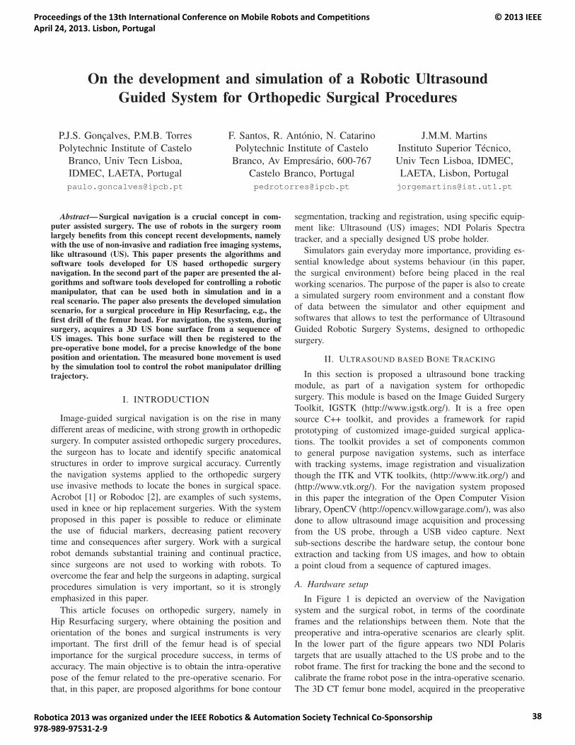
On the development and simulation of a Robotic UltrasoundGuided System for Orthopedic Surgical Procedures

P.J.S. Goncalves, P.M.B. Torres

Polytechnic Institute of Castelo

Branco, Univ Tecn Lisboa,

IDMEC, LAETA, Portugal

[email protected]

F. Santos, R. Antonio, N. Catarino

Polytechnic Institute of Castelo

Branco, Av Empresario, 600-767

Castelo Branco, Portugal

[email protected]

J.M.M. Martins

Instituto Superior Tecnico,

Univ Tecn Lisboa, IDMEC,

LAETA, Lisbon, Portugal

[email protected]

Abstract— Surgical navigation is a crucial concept in com-puter assisted surgery. The use of robots in the surgery roomlargely benefits from this concept recent developments, namelywith the use of non-invasive and radiation free imaging systems,like ultrasound (US). This paper presents the algorithms andsoftware tools developed for US based orthopedic surgerynavigation. In the second part of the paper are presented the al-gorithms and software tools developed for controlling a roboticmanipulator, that can be used both in simulation and in areal scenario. The paper also presents the developed simulationscenario, for a surgical procedure in Hip Resurfacing, e.g., thefirst drill of the femur head. For navigation, the system, duringsurgery, acquires a 3D US bone surface from a sequence ofUS images. This bone surface will then be registered to thepre-operative bone model, for a precise knowledge of the boneposition and orientation. The measured bone movement is usedby the simulation tool to control the robot manipulator drillingtrajectory.

I. INTRODUCTION

Image-guided surgical navigation is on the rise in many

different areas of medicine, with strong growth in orthopedic

surgery. In computer assisted orthopedic surgery procedures,

the surgeon has to locate and identify specific anatomical

structures in order to improve surgical accuracy. Currently

the navigation systems applied to the orthopedic surgery

use invasive methods to locate the bones in surgical space.

Acrobot [1] or Robodoc [2], are examples of such systems,

used in knee or hip replacement surgeries. With the system

proposed in this paper is possible to reduce or eliminate

the use of fiducial markers, decreasing patient recovery

time and consequences after surgery. Work with a surgical

robot demands substantial training and continual practice,

since surgeons are not used to working with robots. To

overcome the fear and help the surgeons in adapting, surgical

procedures simulation is very important, so it is strongly

emphasized in this paper.

This article focuses on orthopedic surgery, namely in

Hip Resurfacing surgery, where obtaining the position and

orientation of the bones and surgical instruments is very

important. The first drill of the femur head is of special

importance for the surgical procedure success, in terms of

accuracy. The main objective is to obtain the intra-operative

pose of the femur related to the pre-operative scenario. For

that, in this paper, are proposed algorithms for bone contour

segmentation, tracking and registration, using specific equip-

ment like: Ultrasound (US) images; NDI Polaris Spectra

tracker, and a specially designed US probe holder.

Simulators gain everyday more importance, providing es-

sential knowledge about systems behaviour (in this paper,

the surgical environment) before being placed in the real

working scenarios. The purpose of the paper is also to create

a simulated surgery room environment and a constant flow

of data between the simulator and other equipment and

softwares that allows to test the performance of Ultrasound

Guided Robotic Surgery Systems, designed to orthopedic

surgery.

II. ULTRASOUND BASED BONE TRACKING

In this section is proposed a ultrasound bone tracking

module, as part of a navigation system for orthopedic

surgery. This module is based on the Image Guided Surgery

Toolkit, IGSTK (http://www.igstk.org/). It is a free open

source C++ toolkit, and provides a framework for rapid

prototyping of customized image-guided surgical applica-

tions. The toolkit provides a set of components common

to general purpose navigation systems, such as interface

with tracking systems, image registration and visualization

though the ITK and VTK toolkits, (http://www.itk.org/) and

(http://www.vtk.org/). For the navigation system proposed

in this paper the integration of the Open Computer Vision

library, OpenCV (http://opencv.willowgarage.com/), was also

done to allow ultrasound image acquisition and processing

from the US probe, through a USB video capture. Next

sub-sections describe the hardware setup, the contour bone

extraction and tacking from US images, and how to obtain

a point cloud from a sequence of captured images.

A. Hardware setup

In Figure 1 is depicted an overview of the Navigation

system and the surgical robot, in terms of the coordinate

frames and the relationships between them. Note that the

preoperative and intra-operative scenarios are clearly split.

In the lower part of the figure appears two NDI Polaris

targets that are usually attached to the US probe and to the

robot frame. The first for tracking the bone and the second to

calibrate the frame robot pose in the intra-operative scenario.

The 3D CT femur bone model, acquired in the preoperative


© 2013 IEEE


38

scenario is the origin of the overall setup, because of the

model itself is more accurate, i.e., the data obtained from US

images is less accurate. All points in the model are referenced

to the CT. The relation between the 3D US points acquired in

the intraoperative scenario and 3D CT points from the bone

model is obtained from point cloud registration using the

methods later presented in section III. See the transformationCTTNDI , in figure 1 . The pose of the robot end-effector also

has to be referenced by the Navigation system to inform the

robot controller of its location. The relationship between the

Robot frame and the CT frame (CTTR), is determined during

the hardware setup, in the intra-operative scenario and once

obtained remains fixed, as long the robot base does not move

from its initial position.

Fig. 1. Overview of the hardware setup and frames transformations.

B. US based bone extraction and tracking

In this sub-section is proposed a method to extract and

track the femur bone in a sequence of US images. This work

appears in sequence of previous work of the authors [3],

where a comparative study for segmenting bones in US im-

ages was performed. The Threshold Level Set Segmentation(TLSS) [4] obtained the best results and will further tested

in this paper.

The algorithm is depicted in Figure 2 and comprises the

next steps:

1) Initialization - where the US probe, with the NDI

Polaris target, is correctly placed in the field of view

of the NDI Polaris cameras. Also the segmentation

process is initialised here, as seen below in the text.

2) Image Acquisition - where the US image is acquired

using the methods implemented in OpenCV.

3) NDI trigger - where a point within the bone in the US

image is chosen to start the NDI Polaris acquisition,

and synchronizes the tracking process. After, the same

point is used as the seed of the segmentation algorithm.

4) Segmentation and Tracking - where the bone surface

in the US image is extracted.

5) 3D points extraction - where the 3D points in the bone

surface are calculated, using the 2D data obtained in

Fig. 2. Ultrasound based Bone Tracking process.

the previous step.

6) UDP - where the 3D US point cloud for an image

(slice) is sent to the registration module.

This process is continuously repeated overtime to extract

a suitable number of slices to then obtain a 3D US bone

surface for registration, see Section III. The 4th step of the

algorithm, Segmentation and Tracking, is of special relevance

because of the image processing issues related to US images,

i.e., its high level of noise. Further, since the bone is a

rigidly anatomically structure, only the top surface of the

bone appearers in US images as can seen in figure 3, in the

red square. The main challenge of the segmentation method

is to identify where the bone is, in US images. To aid the

segmentation algorithm, i.e., to improve accuracy and also

to speed up the segmentation, a region of interest (ROI)

is defined in the first image, also in the first step of the

algorithm. The ROI is marked with a square around the

bone, as seen in figure 3. After this initialization, all images

that arrive through the video card are segmented using the

TLSS algorithm. Its goal is to define a range of intensity

values that classify the bone of interest and then base the

propagation term on the level set equation for that intensity

range. Using the level set approach [5], the smoothness of

the evolving surface can be constrained to prevent some of

the leaking that is common in connected-component schemes

[4]. The next iterations of the segmentation use the centroid

of the bone contour, extracted in the current step, that is also

responsible for the ROI update. The contour obtained in each

slice, properly referenced in the NDI frame is sent in packs

of 3D points by UDP to the registration process.

C. Point Cloud Extraction

The bone contours points extracted from US images,iP (u, v), using the US probe are converted to 3D points,

using the NDI Polaris Spectra pose measurement system.

This sensor measures the pose of the NDI Polaris target Mkrelated to its reference frame NDI , i.e., the transformation


© 2013 IEEE


39

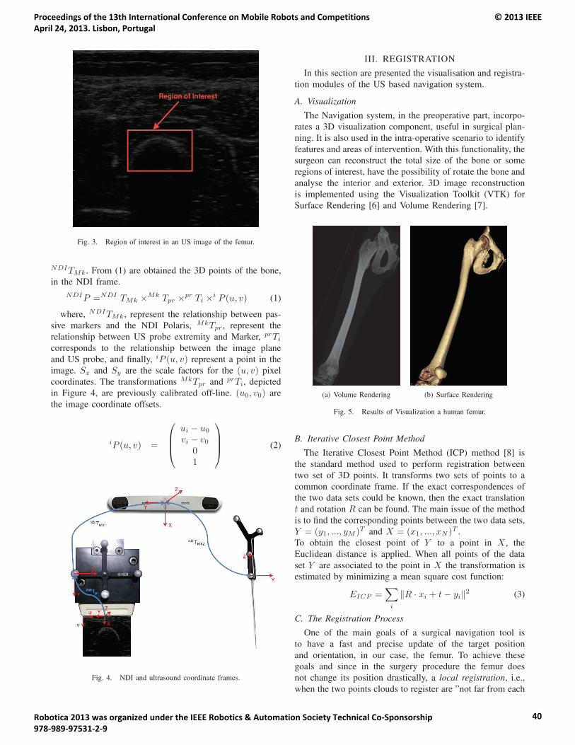
Fig. 3. Region of interest in an US image of the femur.

NDITMk. From (1) are obtained the 3D points of the bone,

in the NDI frame.

NDIP =NDI TMk ×Mk Tpr ×pr Ti ×i P (u, v) (1)

where, NDITMk, represent the relationship between pas-

sive markers and the NDI Polaris, MkTpr, represent the

relationship between US probe extremity and Marker, prTi

corresponds to the relationship between the image plane

and US probe, and finally, iP (u, v) represent a point in the

image. Sx and Sy are the scale factors for the (u, v) pixel

coordinates. The transformations MkTpr and prTi, depicted

in Figure 4, are previously calibrated off-line. (u0, v0) are

the image coordinate offsets.

iP (u, v) =

⎛⎜⎜⎝

ui − u0

vi − v001

⎞⎟⎟⎠ (2)

Fig. 4. NDI and ultrasound coordinate frames.

III. REGISTRATION

In this section are presented the visualisation and registra-

tion modules of the US based navigation system.

A. Visualization

The Navigation system, in the preoperative part, incorpo-

rates a 3D visualization component, useful in surgical plan-

ning. It is also used in the intra-operative scenario to identify

features and areas of intervention. With this functionality, the

surgeon can reconstruct the total size of the bone or some

regions of interest, have the possibility of rotate the bone and

analyse the interior and exterior. 3D image reconstruction

is implemented using the Visualization Toolkit (VTK) for

Surface Rendering [6] and Volume Rendering [7].

(a) Volume Rendering (b) Surface Rendering

Fig. 5. Results of Visualization a human femur.

B. Iterative Closest Point Method

The Iterative Closest Point Method (ICP) method [8] is

the standard method used to perform registration between

two set of 3D points. It transforms two sets of points to a

common coordinate frame. If the exact correspondences of

the two data sets could be known, then the exact translation

t and rotation R can be found. The main issue of the method

is to find the corresponding points between the two data sets,

Y = (y1, ..., yM )T and X = (x1, ..., xN )T .

To obtain the closest point of Y to a point in X , the

Euclidean distance is applied. When all points of the data

set Y are associated to the point in X the transformation is

estimated by minimizing a mean square cost function:

EICP =∑i

‖R · xi + t− yi‖2 (3)

C. The Registration Process

One of the main goals of a surgical navigation tool is

to have a fast and precise update of the target position

and orientation, in our case, the femur. To achieve these

goals and since in the surgery procedure the femur does

not change its position drastically, a local registration, i.e.,

when the two points clouds to register are ”not far from each


© 2013 IEEE


40

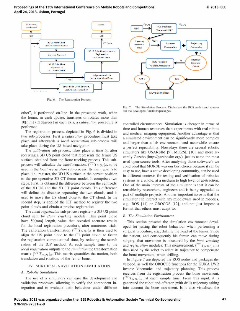
Fig. 6. The Registration Process.

other”, is performed on-line. In the presented work, when

the femur, in each update, translates or rotates more than

10[mm] / 3[degrees] in each axis, a calibration procedure is

performed.

The registration process, depicted in Fig. 6 is divided in

two sub-processes. First a calibration procedure must take

place and afterwards a local registration sub-process will

take place during the US based navigation.

The calibration sub-process, takes place at time t0, after

receiving a 3D US point cloud that represents the femur US

surface, obtained from the Bone tracking process. This sub-

process will calculate the transformation, (CTTNDI)0, to be

used in the local registration sub-process. Its main goal is to

place, i.e., register, the 3D US surface in the correct position

to the pre-operative 3D CT femur model. It comprises two

steps. First, is obtained the difference between the centroids,

of the 3D US and the 3D CT point clouds. This difference

will define the distance separating the two clouds, and is

used to move the US cloud close to the CT cloud. In the

second step, is applied the ICP method to register the two

point clouds and obtain a precise registration.

The local registration sub-process registers a 3D US point

cloud sent by Bone Tracking module. This point cloud

have 50[mm] length, value that revealed accurate results

for the local registration procedure, after numerous trials.

The calibration transformation (CTTNDI)0 is then used to

align the US point cloud to the CT point cloud, to fasten

the registration computational time, by reducing the search

radius of the ICP method. At each sample time tk the

local registration outputs to the simulation the transformation

matrix (CTTNDI)k. This matrix quantifies the motion, both

translation and rotation, of the femur bone.

IV. SURGICAL NAVIGATION SIMULATION

A. Robotic Simulation

The use of a simulators can ease the development and

validation processes, allowing to verify the component in-

tegration and to evaluate their behaviour under different

Fig. 7. The Simulation Process. Circles are the ROS nodes and squaresare the developed functions/packages.

controlled circumstances. Simulation is cheaper in terms of

time and human resources than experiments with real robots

and medical imaging equipment. Another advantage is that

a simulated environment can be significantly more complex

and larger than a lab environment, and meanwhile ensure

a perfect repeatability. Nowadays there are several robotic

simulators like USARSIM [9], MORSE [10], and more re-

cently Gazebo (http://gazebosim.org/), just to name the most

used open-source tools. After analysing those software’s we

concluded that MORSE was our best choice because it can be

easy to use, have a active developing community, can be used

in different contexts for testing and verification of robotics

systems as a whole, at a medium to high level of abstraction.

One of the main interests of the simulator is that it can be

reusable by researchers, engineers and is being upgraded as

part of multiple projects. Another important issue is that the

simulator can interact with any middleware used in robotics,

e.g., ROS [11] or OROCOS [12], and not just impose a

format that others must adapt to.

B. The Simulation Environment

This section presents the simulation environment devel-

oped for testing the robot behaviour when performing a

surgical procedure, e.g., drilling the head of the femur. Since

the patient, and consequently his femur, can move during

surgery, that movement is measured by the bone trackingand registration modules. This measurement, (CTTNDI)k, is

then used by the robot to adapt its trajectory to compensate

the bone movement, when drilling.

In Figure 7 are depicted the ROS nodes and packages de-

veloped, as well the OROCOS functions for the KUKA LWR

inverse kinematics and trajectory planning. This process

receives from the registration process the bone movement,

(CTTNDI)k, at each sample time. From this input, it is

generated the robot end-effector (with drill) trajectory taking

into account the bone movement. Is is also visualised the


© 2013 IEEE


41

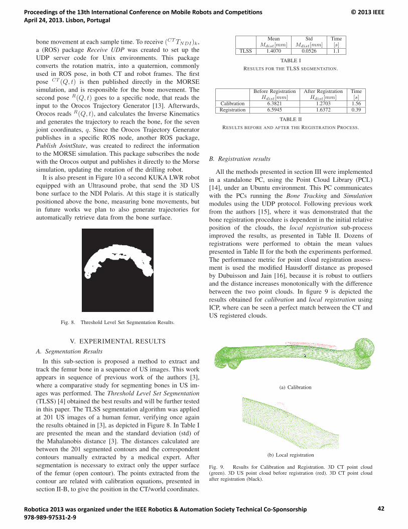
bone movement at each sample time. To receive (CTTNDI)k,

a (ROS) package Receive UDP was created to set up the

UDP server code for Unix environments. This package

converts the rotation matrix, into a quaternion, commonly

used in ROS pose, in both CT and robot frames. The first

pose CT (Q, t) is then published directly in the MORSE

simulation, and is responsible for the bone movement. The

second pose R(Q, t) goes to a specific node, that reads the

input to the Orocos Trajectory Generator [13]. Afterwards,

Orocos reads R(Q, t), and calculates the Inverse Kinematics

and generates the trajectory to reach the bone, for the seven

joint coordinates, q. Since the Orocos Trajectory Generator

publishes in a specific ROS node, another ROS package,

Publish JointState, was created to redirect the information

to the MORSE simulation. This package subscribes the node

with the Orocos output and publishes it directly to the Morse

simulation, updating the rotation of the drilling robot.

It is also present in Figure 10 a second KUKA LWR robot

equipped with an Ultrasound probe, that send the 3D US

bone surface to the NDI Polaris. At this stage it is statically

positioned above the bone, measuring bone movements, but

in future works we plan to also generate trajectories for

automatically retrieve data from the bone surface.

Fig. 8. Threshold Level Set Segmentation Results.

V. EXPERIMENTAL RESULTS

A. Segmentation Results

In this sub-section is proposed a method to extract and

track the femur bone in a sequence of US images. This work

appears in sequence of previous work of the authors [3],

where a comparative study for segmenting bones in US im-

ages was performed. The Threshold Level Set Segmentation(TLSS) [4] obtained the best results and will be further tested

in this paper. The TLSS segmentation algorithm was applied

at 201 US images of a human femur, verifying once again

the results obtained in [3], as depicted in Figure 8. In Table I

are presented the mean and the standard deviation (std) of

the Mahalanobis distance [3]. The distances calculated are

between the 201 segmented contours and the correspondent

contours manually extracted by a medical expert. After

segmentation is necessary to extract only the upper surface

of the femur (open contour). The points extracted from the

contour are related with calibration equations, presented in

section II-B, to give the position in the CT/world coordinates.

Mean Std TimeMdist[mm] Mdist[mm] [s]

TLSS 1.4070 0.0526 1.1

TABLE I

RESULTS FOR THE TLSS SEGMENTATION.

Before Registration After Registration TimeHdist[mm] Hdist[mm] [s]

Calibration 6.3821 1.2703 1.56Registration 6.5945 1.6372 0.39

TABLE II

RESULTS BEFORE AND AFTER THE REGISTRATION PROCESS.

B. Registration results

All the methods presented in section III were implemented

in a standalone PC, using the Point Cloud Library (PCL)

[14], under an Ubuntu environment. This PC communicates

with the PCs running the Bone Tracking and Simulationmodules using the UDP protocol. Following previous work

from the authors [15], where it was demonstrated that the

bone registration procedure is dependent in the initial relative

position of the clouds, the local registration sub-process

improved the results, as presented in Table II. Dozens of

registrations were performed to obtain the mean values

presented in Table II for the both the experiments performed.

The performance metric for point cloud registration assess-

ment is used the modified Hausdorff distance as proposed

by Dubuisson and Jain [16], because it is robust to outliers

and the distance increases monotonically with the difference

between the two point clouds. In figure 9 is depicted the

results obtained for calibration and local registration using

ICP, where can be seen a perfect match between the CT and

US registered clouds.

(a) Calibration

(b) Local registration

Fig. 9. Results for Calibration and Registration. 3D CT point cloud(green). 3D US point cloud before registration (red). 3D CT point cloudafter registration (black).


© 2013 IEEE


42

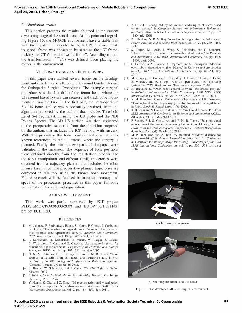
C. Simulation results

This section presents the results obtained at the current

developing stage of the simulations. At this point and regard-

ing Figure 10, the MORSE environment have a stable link

with the registration module. In the MORSE environment,

its global frame was chosen to be same as the CT frame,

making the CT frame the ”world frame”. According to this,

the transformation (CTTR) was defined when placing the

robots in the environment.

VI. CONCLUSIONS AND FUTURE WORK

In this paper were tackled several issues on the develop-

ment and simulation of a Robotic Ultrasound Guided System

for Orthopedic Surgical Procedures. The example surgical

procedure was the first drill of the femur head, where the

Ultrasound based system can measure and track bone move-

ments during the task. In the first part, the intra-operative

3D US bone surface was successfully obtained, from the

algorithm proposed by the authors that includes Threshold

Level Set Segmentation, using the US probe and the NDI

Polaris Spectra. The 3D US surface was then registered

to the preoperative scenario, from the algorithm proposed

by the authors that includes the ICP method, with success.

With this procedure the bone position and orientation is

known referenced to the CT frame, where the surgery is

planned. Finally, the previous two parts of the paper were

validated in the simulator. The sequence of bone positions

were obtained directly from the registration process and

the robot manipulator end-effector (drill) trajectories were

obtained from a trajectory planner that includes the robot

inverse kinematics. The preoperative planned trajectories are

corrected in this tool using the known bone movement.

Future research will be focused in increase accuracy and

speed of the procedures presented in this paper, for bone

segmentation, tracking and registration.

ACKNOWLEDGMENT

This work was partly supported by FCT project

PTDC/EME-CRO/099333/2008 and EU-FP7-ICT-231143,

project ECHORD.

REFERENCES

[1] M. Jakopec, F. Rodriguez y Baena, S. Harris, P. Gomes, J. Cobb, andB. Davies, “The hands-on orthopaedic robot ”acrobot”: Early clinicaltrials of total knee replacement surgery,” Robotics and Automation,IEEE Transactions on, vol. 19, pp. 902 – 911, oct. 2003.

[2] P. Kazanzides, B. Mittelstadt, B. Musits, W. Bargar, J. Zuhars,B. Williamson, P. Cain, and E. Carbone, “An integrated system forcementless hip replacement,” Engineering in Medicine and BiologyMagazine, IEEE, vol. 14, pp. 307 –313, may/jun 1995.

[3] N. M. M. Catarino, P. J. S. Goncalves, and P. M. B. Torres, “Bonecontour segmentation from us images a comparative study,” in Pro-ceedings of the 18th Portuguese Conference on Pattern Recognition,(Coimbra, Portugal), October 26 2012.

[4] L. Ibanez, W. Schroeder, and J. Cates, The ITK Software Guide.Kitware, 2005.

[5] J. Sethian, Level Set Methods and Fast Marching Methods. CambridgeUniversity Press, 1996.

[6] Y. Huang, Z. Qiu, and Z. Song, “3d reconstruction and visualizationfrom 2d ct images,” in IT in Medicine and Education (ITME), 2011International Symposium on, vol. 2, pp. 153 –157, dec. 2011.

[7] Z. Li and J. Zhang, “Study on volume rendering of ct slices basedon ray casting,” in Computer Science and Information Technology(ICCSIT), 2010 3rd IEEE International Conference on, vol. 7, pp. 157–160, july 2010.

[8] P. J. Besl and N. D. McKay, “A method for registration of 3-d shapes,”Pattern Analysis and Machine Intelligence, vol. 14(2), pp. 239 – 256,1992.

[9] S. Carpin, M. Lewis, J. Wang, S. Balakirsky, and C. Scrapper,“Usarsim: a robot simulator for research and education,” in Roboticsand Automation, 2007 IEEE International Conference on, pp. 1400–1405, april 2007.

[10] G. Echeverria, N. Lassabe, A. Degroote, and S. Lemaignan, “Modularopen robots simulation engine: Morse,” in Robotics and Automation(ICRA), 2011 IEEE International Conference on, pp. 46 –51, may2011.

[11] M. Quigley, K. Conley, B. P. Gerkey, J. Faust, T. Foote, J. Leibs,R. Wheeler, and A. Y. Ng, “Ros: an open-source robot operatingsystem,” in ICRA Workshop on Open Source Software, 2009.

[12] H. Bruyninckx, “Open robot control software: the orocos project,”in Robotics and Automation, 2001. Proceedings 2001 ICRA. IEEEInternational Conference on, vol. 3, pp. 2523 – 2528 vol.3, 2001.

[13] N. H. Francisco Ramos, Mohanarajah Gajamohan and R. DAndrea,“Time-optimal online trajectory generator for robotic manipulators,”in Robot Earth Technical Report, feb 2013.

[14] R. B. Rusu and S. Cousins, “3D is here: Point Cloud Library (PCL),” inIEEE International Conference on Robotics and Automation (ICRA),(Shanghai, China), May 9-13 2011.

[15] F. Santos, P. J. S. Goncalves, and P. M. B. Torres, “3d point cloudregistration of the femoral bone, using the point cloud library,” in Pro-ceedings of the 18th Portuguese Conference on Pattern Recognition,(Coimbra, Portugal), October 26 2012.

[16] M.-P. Dubuisson and A. Jain, “A modified hausdorff distance forobject matching,” in Pattern Recognition, 1994. Vol. 1 - ConferenceA: Computer Vision amp; Image Processing., Proceedings of the 12thIAPR International Conference on, vol. 1, pp. 566 –568 vol.1, oct1994.

(a) Full surgical scenario

(b) Zooming the robots and the femur

Fig. 10. The developed MORSE surgical environment.


© 2013 IEEE


43

An Evaluation of Local Feature Combiners for Robot Visual Localization

Francisco M. Campos LabMAg and the Mechanical Engineering Department

Instituto Superior de Engenharia de Lisboa Lisbon, Portugal

[email protected]

Luís Correia LabMAg, Computer Science Department

Universidade de Lisboa Lisbon, Portugal

[email protected]

João M. F. Calado IDMEC and the Mechanical Engineering Department

Instituto Superior de Engenharia de Lisboa Lisbon, Portugal

[email protected]

Abstract—In the last decade, local image features have been widely used in robot visual localization. To assess image similarity, a strategy exploiting these features compares raw descriptors extracted from the current image to those in the models of places. This paper addresses the ensuing step in this process, where a combining function must be used to aggregate results and assign each place a score. Casting the problem in the multiple classifier systems framework, we compare several candidate combiners with respect to their performance in the visual localization task. A deeper insight into the potential of the sum and product combiners is provided by testing two extensions of these algebraic rules: threshold and weighted modifications. In addition, a voting method, previously used in robot visual localization, is assessed. All combiners are tested on a visual localization task, carried out on a public dataset. It is experimentally demonstrated that the sum rule extensions globally achieve the best performance. The voting method, whilst competitive to the algebraic rules in their standard form, is shown to be outperformed by both their modified versions.

Keywords— robot visual localization; information fusion; multiple classifier systems.

I. INTRODUCTION

Currently, the most successful approach to vision-based robot localization relies on local image features, extracted from interest points detected in the image. The construction of appearance representations building on local features has followed two main paradigms: on the one hand, the descriptors are quantized onto a predefined visual vocabulary, being assigned corresponding visual words. Although this representation, denoted bag-of-words, is interesting due to the fast appearance comparison it offers, some limits to its descriptive power have been identified [1][2]. An alternative strategy is the exploitation of raw feature descriptors, thus avoiding approximations resulting from quantization. This approach involves direct comparison of the descriptors, extracted from the test image, to those comprising the models

of places in the environment. A central issue in using this method to compare appearances is the fusion of information obtained from multiple features. In [3][4] this issue is resolved through a voting scheme, which relies on a hard level comparison of features. An alternative approach is pursued in [5], where the continuous values resulting from the comparison are accumulated in a score function. In spite of the success of the two approaches, to the best of our knowledge no evaluation of information fusion methods, applied to raw feature descriptors, has ever been performed. In this paper, we perform such an evaluation, addressing the information fusion issue within the framework of multiple classifier systems. The choice of this framework arises naturally, given the similarities between local feature based recognition and multiple classifier systems. Yet, the specificities of the visual localization problem determine the type of tools, from multiple classifier systems, that are applicable here. At the localization stage it is not possible to predict either the quantity or the appearance of the features that will be extracted. This implies that one should not train classifiers to treat specific visual features, but should instead rely on a general classifier, suitable for any feature available to the recognizer. Hence, in this paper we consider a probabilistic model for local features that leads to a generic probabilistic base classifier. The aim of the paper is to provide an evaluation of classifier combiners, thus the two most popular non-trained combination methods are considered: the product and sum rules. Furthermore, two extensions of these rules, as well as a voting method previously used in robot localization, are assessed. In addition to addressing a localization task based on local features only, we assess performance in the situation where additional information is integrated, through Bayes fusion. For this purpose, we chose a global image feature, gist [6], since it is also extracted from image data, and provides information complementary to local features.

This paper is organized as follows: after reviewing related work in section 2, we outline the concepts used in our approach


© 2013 IEEE


44

to local feature based robot localization, in section 3; section 4 introduces the combination rules and their extensions, as well as the reliability estimation methods; results of our experiments are detailed in section 5 and, finally, section 6 draws the conclusions of the paper.

II. RELATED WORK

There is a wide range of well studied methods for the fusion of real-valued classifier outputs, including algebraic and statistical rules as well as trained combiners [7]. Among these methods, the sum rule and product rule have received considerable attention, due to their simplicity and good results. In practice, the sum rule has often been the preferred choice, due to its robustness. In spite of a solid theoretical foundation, it has been observed that the product rule is more sensitive to noise and to poor probability estimates of the base classifiers [8]. This drawback is addressed in [9], where the authors introduce a thresholding method that was shown to improve performance. Even though the sum rule behaves more reliably, in some cases there is room for improvement, by modulating the contributions of base classifiers. This approach has been successful in applications such as audio speech recognition [10] and person authentication [11], suggesting that weight adaptation is a viable solution to deal with noise, which may differently affect, at each time instance, the various information sources or, more generally, the various base classifiers. In studies where classifier contribution to the final decision is computed dynamically, the weighting of this contribution is usually associated to a reliability measure. In audio-based applications, researchers have derived the reliability measure from estimates of noise level in the input signal [11][12]. A more general approach, which is not limited to audio signals, relies on the analysis of base classifier scores for the extraction of the reliability measure. Along these lines, methods using the difference between the best two likelihood ratios [13], the dispersion of the class posterior probabilities [13] and maximum class posteriors [14] have been investigated. In the same category, another method that has gained considerable attention over the last years relies on the entropy of the posterior distribution [10]. This measure is adopted in this work, as it is claimed to be more powerful, for using all the information available in the posterior distribution [15]. Furthermore, in a study on audio-visual speech recognition [12], the entropy measure is shown to outperform the dispersion of posterior probabilities.

The traditional approach to mapping entropy to weights is to take the inverse entropy value, which reflects our intuition that low entropy distributions originate from reliable classifiers, which should receive greater weights, while classifiers producing close to flat distributions, with high entropy, should be weighted lower. In spite of agreement with these primary conditions, the inverse relation may not yield an optimal mapping, hence recently a number of studies proposed and assessed alternative functions [15][10]. In [10] a variation of the inverse entropy method is proposed, aiming at greatly reducing the contribution of higher entropy classifiers. This is achieved by computing the average entropy of classifiers and assigning a fixed small weight to classifiers with entropy above that value. In [15] the authors introduce an alternative mapping

function, defining the weights to be proportional to the negative entropy, and this outperformed the standard inverse relationship. In spite of the considerable attention feature combination has received in other research areas, an evaluation of combiners for visual robot localization has not been performed before.

Within the category of voting schemes, a few methods have been proposed for local feature based localization. In [3] the scale-invariant feature transform (SIFT) features extracted from the test image are matched against the descriptors from training images, through the matching rule proposed by Lowe [16]. Through this matching rule, a hard level decision is taken, simply indicating the presence or absence of the feature in a training image. A similar approach is provided in [4], where a dissimilarity measure is derived from the number of matches, the total number of features in the test and training images as well as a geometric alignment distance. Despite the success of the aforementioned voting schemes, these methods have not been assessed against the potentially more accurate approach that relies on continuous valued scores obtained from descriptor comparison.

III. ROBOT VISUAL LOCALIZATION

Robot localization can be addressed as a recognition problem, where the current sensor data is ascribed to a place from a map of the environment. When appearance representations rely on local image features, each feature may produce opinions for places, later to be aggregated in a final score. Within the framework of multiple classifier systems, fusion of opinions may be addressed by associating each feature with a base classifier. In this section we define the base classifiers of our approach, by describing how posterior estimates are obtained from a local feature. As one of the goals of this work is to assess the performance of combiners when their outcome is fused with additional visual information, in this section we also introduce a global image feature, gist, and describe how it is integrated with combiner outputs.

A. Base Classifiers

Let the current appearance I be described by a set of nf

visual feature descriptors {d1,d2,…, dnf} and L denote the robot location, defined over a map comprising np places: {l1,l2,...,lnp}. Models of places are constructed by dividing a training image sequence into subsequences so that each corresponds to a distinct place. The model of a place lj is therefore defined by

the collection of nlj descriptors, jnl

jj

jddd ,...,, 21 , extracted

during the training stage. In order to evaluate appearance similarity, the likelihood of a descriptor di may be estimated using a kernel density estimator:

( )( )=

=jnl

m

jmi

jji dddistK

nlldP

1

,1

)|( , (1)

where K(.) is the Gaussian Kernel function, with standard deviation σ, and dist is an appropriate distance function. The posterior distribution of the base classifier associated with feature di is obtained through Bayes rule, yielding


© 2013 IEEE


45

)(

)()|()|(

i

jjiij dP

lPldPdlP = (2)

Here a uniform prior for place distribution is applied, as we are considering the situation of having no previous knowledge about the robot location.

B. Fusion with Gist

For the purpose of our experiments in the fusion of local features with gist, this feature is extracted in all test and model images. Thus, descriptor g is obtained for the current image, while the model of a place j includes ngj descriptors,

jng

jj

jggg ,...,, 21 , each extracted from a training image of that

place. In the computation of likelihood P(g|lj), g is compared to all gist descriptors in the model of lj, through the Euclidean distance, and the minimum value is found. The likelihood of g is obtained by evaluating the zero-centered Gaussian function (standard deviation σg) at the minimum distance.

In order to perform localization exploiting both gist and local features, distribution P(lj|I,g) is estimated. Under the assumption of conditional independence of local features and gist, this estimate may be computed through Bayes rule as

),(

)()|()|(

),(

)()|,(),|(

gIP

lPlgPlIP

gIP

lPlgIPgIlP jjjjj

j == . (3)

However, the combiners we are considering output posterior distributions, rather than likelihoods. Hence, we expand the previous expression as

),(

)()|(

)(

)()|(),|(

gIP

lPlgP

lP

IPIlPgIlP jj

j

jj ×= , (4)

which may be rewritten in the form

)|()|(),|( jjj lgPIlPgIlP ∝ . (5)

IV. LOCAL FEATURE FUSION THROUGH CLASSIFIER

COMBINATION

A. Classifier Combination Methods

In local feature based localization, the ultimate goal is to arrive at an estimate of P(lj|I) derived from the outputs of individual base classifiers, P(lj|di). Below, we briefly review the two algebraic combination rules as well as the voting method to be assessed in this paper. Additionally, the extensions of the algebraic rules are outlined.

Sum rule - The sum rule may be expressed by the generalized form

=

=

nf

iijinfj dlPwddlP

11 )|(),...,|( , (6)

where wi is the weight that reflects reliability of classifier i. These weights are constrained to sum up to one and, in the standard form of the sum rule, are equally set to 1/nf.

Product rule - According to this rule, support for location lj is obtained by multiplying the outputs of base classifiers raised to the corresponding weights:

∏=

=

nf

i

wijnfj

idlPZ

ddlP1

1 )|(1

),...,|( (7)

In this expression, Z is a normalizing constant. As before, the standard rule is obtained by setting all weights to be equal, in this case with the value of 1.

Threshold rule - In [9] the authors introduce a modified product rule devised to alleviate the dominating effect of close to zero probabilities in this fusion method. This is accomplished by a mechanism that modifies classifiers outputs that fall below a predefined threshold. Thus, before applying the product rule, the probability estimate from each base classifier is modified according to

≥=

<=

ThdlPdlpdlP

ThdlPThdlP

oijoijij

oijij

)|(,)|()|(

)|(,)|( (8)

where the index o refers to the original probability estimates from the base classifiers and Th denotes the threshold value.

Voting method - Contrasting to the aforementioned methods, the voting scheme used in [3] performs an image-to-image rather than an image-to-model comparison. In effect, this method relies on the matching criterion of [16], which establishes feature correspondences between two images. In [3] the voting method is applied to visual localization by first finding, for each place, the training image with the highest number of matches with respect to the test image. Final scores assigned to places are the number of matches of the corresponding winning images. In this paper we use this implementation of the voting method and, where posterior probabilities are needed as the outcome of the combiner, the score distribution is converted to a probability distribution by normalization.

B. Reliability Estimation Methods

In this paper we evaluate the weighted combination rules with weights being derived from the posterior distribution entropy. To this end, the entropy of the posterior distribution output of a base classifier is computed, by

)|(log)|(1

ij

np

jiji dlPdlPH

=

−= (9)

In order to use this measure in a weighted combination scheme, the entropy is mapped onto weights by a suitable transformation. We consider four methods to perform this mapping: inverse entropy (IE) [10][15], negative entropy (NE)


© 2013 IEEE


46

[15], inverse entropy with average threshold (IEAT) [11], and negative entropy with average threshold (NEAT).

IE - In the inverse entropy method, each classifier weight is proportional to the inverse of the respective entropy:

ii Hw 1= (10)

NE - In the negative entropy method, weights are proportional to the negative entropy, being computed as

imaxi HHw −= (11)

In this expression Hmax is the maximum value the entropy can take. For a problem with np candidate locations it takes the value of log (np).

IEAT - The IEAT method [10] computes preliminary weights w'i in the same way as the IE method. Then, weights that fall below the mean of w’i are assigned a low value (10-4), while the remaining weights are kept unchanged. In practice this procedure corresponds to eliminating the contribution of higher entropy features.

NEAT – This method, which has not been tested in previous works, results from computing preliminary weights w'i as in NE and then applying the same rule as IEAT.

V. RESULTS

In this section we compare the classifier combination rules as well as the reliability estimation methods outlined in section 4, on an outdoor place recognition task. To this end, we resorted to the public FDF park dataset, used in past visual localization investigations [17][18]. This dataset describes the Frederick D. Fagg Park of the University of Southern California as a 9-location map, providing several video sequences for each location, gathered using a 8mm handheld camcorder carried by a person. The videos are organized in 8 sets used for testing and 7 sets used in training, each containing about 11000 frames. Strong lighting variation is the main source of variability in the data, since the videos were collected at different days and times of day. Considering the available test and training sets, several experimental conditions can be established. Our experiments showed that the difficulty of the localization task varies significantly with the differences in training and test lighting conditions, but the relative performance of the classifiers being tested is generally consistent. Hence, results for two representative training conditions, sets A and C, will be presented in the following analysis of results. These sets were chosen for posing challenging, yet distinctive scenarios to the place recognizer. The video sequences in the datasets are provided with the label of the corresponding place where they were captured. Thus, the localization task we consider aims at identifying the correct label for each image in a test set. Results presented in the next sections refer to the recognition rate obtained in this classification task.

For the purpose of our experiments, all images are processed for extraction of local features, as well as gist. Local

features are identified through the scale-space extrema detector and encoded in SIFT descriptors [16]. In gist extraction, steerable filters at 2 scales and 8 orientations are applied. Then, mean filter responses are averaged on a 4-by-4 grid, yielding gist descriptors of length 256. The parameters used in the experiments were empirically set for best performance, taking the values σ=100, σg=0.22, and Th=0.2.

A. Performance of the Combination Methods

Results for all combination methods are shown in tables 1 and 2, respectively obtained with training sets A and C. Results for the sum and the product rules are provided using the standard rules as well as the threshold and weighted (NEAT) versions. As we can see, the sum rule is clearly superior to the product rule, when the standard versions are considered. This was an expected outcome, as the product rule is more sensitive to noisy data, which is prevalent in difficult test scenarios. In the most discrepant situations, the difference in performance of the two rules is larger than 10%. In its threshold version, the product rule exhibits a substantial improvement, achieving levels of performance closer to the sum rule. Average recognition rate differences are now less than 1%. It is interesting to notice that the sum rule is also favoured by the threshold operation, which was originally developed to increase the product rule accuracy. By comparing the weighted with the standard rules, we can conclude that the weighting scheme also contributes to improve the recognition rate of both rules. The performance gains observed are similar to the threshold method; nevertheless, in this respect the weighting scheme is on average slightly more efficient with the sum rule.

Despite using a hard-level decision outcome of base classifiers, the voting method performs reasonably well. In particular, the comparison with the standard algebraic rules is favourable to voting, in the case of training set C. However, all the modifications of the standard rules are superior to the voting method, in the two training sets.

B. Evaluation of the Reliability Measures

In order to evaluate the reliability estimation methods, localization experiments were carried out with the schemes detailed in section 4. The corresponding results are shown in table 3 by the mean recognition rates obtained over all test sets. We observe that, with the product rule, the methods IEAT and NEAT generally surpass their non-eliminating feature counterparts, respectively IE and NE. This should be explained by the fact that high entropy features result in poor posterior distribution estimates, which are especially detrimental to the product rule. Thus, by strongly reducing the contribution of these features, the IEAT and NEAT methods achieve a performance gain. Smaller differences are observed when the same comparison is performed with respect to the sum rule. Yet, on average, IEAT and NEAT also perform better than IE and NE respectively. The comparison of methods using the inverse entropy function (IE and IEAT) with those using negative entropy function (NE and NEAT) shows consistent superiority of the latter in training set A. However, this relation is not observed in training set C, suggesting that none of these mappings is optimal.


© 2013 IEEE


47

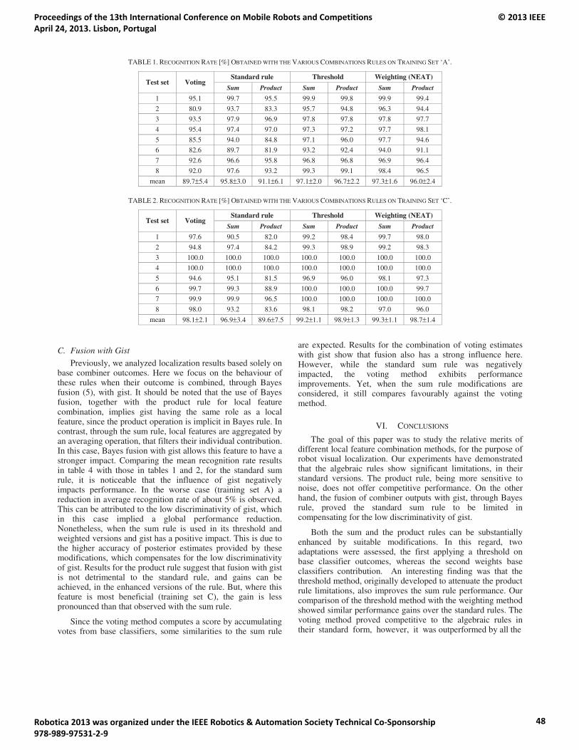
TABLE 1. RECOGNITION RATE [%] OBTAINED WITH THE VARIOUS COMBINATIONS RULES ON TRAINING SET ‘A’.

Standard rule Threshold Weighting (NEAT) Test set Voting

Sum Product Sum Product Sum Product

1 95.1 99.7 95.5 99.9 99.8 99.9 99.4

2 80.9 93.7 83.3 95.7 94.8 96.3 94.4

3 93.5 97.9 96.9 97.8 97.8 97.8 97.7

4 95.4 97.4 97.0 97.3 97.2 97.7 98.1

5 85.5 94.0 84.8 97.1 96.0 97.7 94.6

6 82.6 89.7 81.9 93.2 92.4 94.0 91.1

7 92.6 96.6 95.8 96.8 96.8 96.9 96.4

8 92.0 97.6 93.2 99.3 99.1 98.4 96.5

mean 89.7±5.4 95.8±3.0 91.1±6.1 97.1±2.0 96.7±2.2 97.3±1.6 96.0±2.4

TABLE 2. RECOGNITION RATE [%] OBTAINED WITH THE VARIOUS COMBINATIONS RULES ON TRAINING SET ‘C’.

Standard rule Threshold Weighting (NEAT) Test set Voting


1 97.6 90.5 82.0 99.2 98.4 99.7 98.0

2 94.8 97.4 84.2 99.3 98.9 99.2 98.3

3 100.0 100.0 100.0 100.0 100.0 100.0 100.0

4 100.0 100.0 100.0 100.0 100.0 100.0 100.0

5 94.6 95.1 81.5 96.9 96.0 98.1 97.3

6 99.7 99.3 88.9 100.0 100.0 100.0 99.7

7 99.9 99.9 96.5 100.0 100.0 100.0 100.0

8 98.0 93.2 83.6 98.1 98.2 97.0 96.0

mean 98.1±2.1 96.9±3.4 89.6±7.5 99.2±1.1 98.9±1.3 99.3±1.1 98.7±1.4

C. Fusion with Gist

Previously, we analyzed localization results based solely on base combiner outcomes. Here we focus on the behaviour of these rules when their outcome is combined, through Bayes fusion (5), with gist. It should be noted that the use of Bayes fusion, together with the product rule for local feature combination, implies gist having the same role as a local feature, since the product operation is implicit in Bayes rule. In contrast, through the sum rule, local features are aggregated by an averaging operation, that filters their individual contribution. In this case, Bayes fusion with gist allows this feature to have a stronger impact. Comparing the mean recognition rate results in table 4 with those in tables 1 and 2, for the standard sum rule, it is noticeable that the influence of gist negatively impacts performance. In the worse case (training set A) a reduction in average recognition rate of about 5% is observed. This can be attributed to the low discriminativity of gist, which in this case implied a global performance reduction. Nonetheless, when the sum rule is used in its threshold and weighted versions and gist has a positive impact. This is due to the higher accuracy of posterior estimates provided by these modifications, which compensates for the low discriminativity of gist. Results for the product rule suggest that fusion with gist is not detrimental to the standard rule, and gains can be achieved, in the enhanced versions of the rule. But, where this feature is most beneficial (training set C), the gain is less pronounced than that observed with the sum rule.

Since the voting method computes a score by accumulating votes from base classifiers, some similarities to the sum rule

are expected. Results for the combination of voting estimates with gist show that fusion also has a strong influence here. However, while the standard sum rule was negatively impacted, the voting method exhibits performance improvements. Yet, when the sum rule modifications are considered, it still compares favourably against the voting method.

VI. CONCLUSIONS

The goal of this paper was to study the relative merits of different local feature combination methods, for the purpose of robot visual localization. Our experiments have demonstrated that the algebraic rules show significant limitations, in their standard versions. The product rule, being more sensitive to noise, does not offer competitive performance. On the other hand, the fusion of combiner outputs with gist, through Bayes rule, proved the standard sum rule to be limited in compensating for the low discriminativity of gist.

Both the sum and the product rules can be substantially enhanced by suitable modifications. In this regard, two adaptations were assessed, the first applying a threshold on base classifier outcomes, whereas the second weights base classifiers contribution. An interesting finding was that the threshold method, originally developed to attenuate the product rule limitations, also improves the sum rule performance. Our comparison of the threshold method with the weighting method showed similar performance gains over the standard rules. The voting method proved competitive to the algebraic rules in their standard form, however, it was outperformed by all the


© 2013 IEEE


48

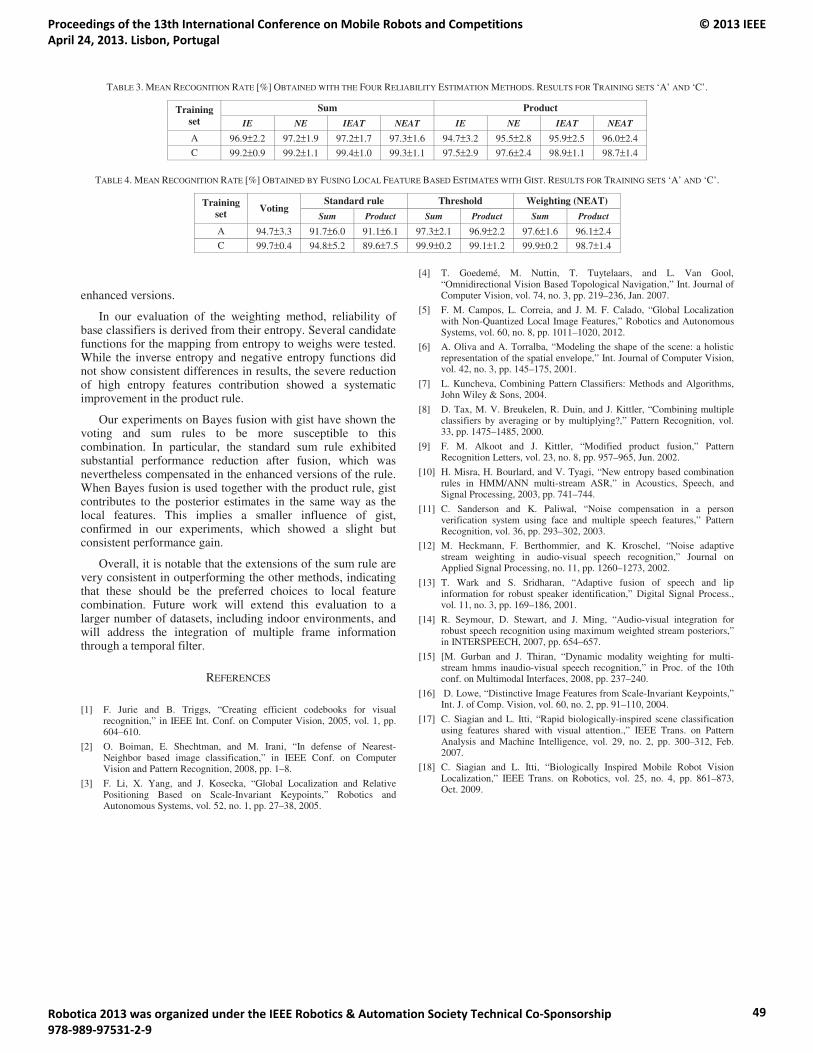
TABLE 3. MEAN RECOGNITION RATE [%] OBTAINED WITH THE FOUR RELIABILITY ESTIMATION METHODS. RESULTS FOR TRAINING SETS ‘A’ AND ‘C’.

Sum Product Training set IE NE IEAT NEAT IE NE IEAT NEAT

A 96.9±2.2 97.2±1.9 97.2±1.7 97.3±1.6 94.7±3.2 95.5±2.8 95.9±2.5 96.0±2.4

C 99.2±0.9 99.2±1.1 99.4±1.0 99.3±1.1 97.5±2.9 97.6±2.4 98.9±1.1 98.7±1.4

TABLE 4. MEAN RECOGNITION RATE [%] OBTAINED BY FUSING LOCAL FEATURE BASED ESTIMATES WITH GIST. RESULTS FOR TRAINING SETS ‘A’ AND ‘C’.

Standard rule Threshold Weighting (NEAT) Training set Voting


A 94.7±3.3 91.7±6.0 91.1±6.1 97.3±2.1 96.9±2.2 97.6±1.6 96.1±2.4

C 99.7±0.4 94.8±5.2 89.6±7.5 99.9±0.2 99.1±1.2 99.9±0.2 98.7±1.4

enhanced versions.

In our evaluation of the weighting method, reliability of base classifiers is derived from their entropy. Several candidate functions for the mapping from entropy to weighs were tested. While the inverse entropy and negative entropy functions did not show consistent differences in results, the severe reduction of high entropy features contribution showed a systematic improvement in the product rule.

Our experiments on Bayes fusion with gist have shown the voting and sum rules to be more susceptible to this combination. In particular, the standard sum rule exhibited substantial performance reduction after fusion, which was nevertheless compensated in the enhanced versions of the rule. When Bayes fusion is used together with the product rule, gist contributes to the posterior estimates in the same way as the local features. This implies a smaller influence of gist, confirmed in our experiments, which showed a slight but consistent performance gain.

Overall, it is notable that the extensions of the sum rule are very consistent in outperforming the other methods, indicating that these should be the preferred choices to local feature combination. Future work will extend this evaluation to a larger number of datasets, including indoor environments, and will address the integration of multiple frame information through a temporal filter.

REFERENCES

[1] F. Jurie and B. Triggs, “Creating efficient codebooks for visual

recognition,” in IEEE Int. Conf. on Computer Vision, 2005, vol. 1, pp. 604–610.

[2] O. Boiman, E. Shechtman, and M. Irani, “In defense of Nearest-Neighbor based image classification,” in IEEE Conf. on Computer Vision and Pattern Recognition, 2008, pp. 1–8.

[3] F. Li, X. Yang, and J. Kosecka, “Global Localization and Relative Positioning Based on Scale-Invariant Keypoints,” Robotics and Autonomous Systems, vol. 52, no. 1, pp. 27–38, 2005.

[4] T. Goedemé, M. Nuttin, T. Tuytelaars, and L. Van Gool, “Omnidirectional Vision Based Topological Navigation,” Int. Journal of Computer Vision, vol. 74, no. 3, pp. 219–236, Jan. 2007.

[5] F. M. Campos, L. Correia, and J. M. F. Calado, “Global Localization with Non-Quantized Local Image Features,” Robotics and Autonomous Systems, vol. 60, no. 8, pp. 1011–1020, 2012.

[6] A. Oliva and A. Torralba, “Modeling the shape of the scene: a holistic representation of the spatial envelope,” Int. Journal of Computer Vision, vol. 42, no. 3, pp. 145–175, 2001.

[7] L. Kuncheva, Combining Pattern Classifiers: Methods and Algorithms, John Wiley & Sons, 2004.

[8] D. Tax, M. V. Breukelen, R. Duin, and J. Kittler, “Combining multiple classifiers by averaging or by multiplying?,” Pattern Recognition, vol. 33, pp. 1475–1485, 2000.

[9] F. M. Alkoot and J. Kittler, “Modified product fusion,” Pattern Recognition Letters, vol. 23, no. 8, pp. 957–965, Jun. 2002.

[10] H. Misra, H. Bourlard, and V. Tyagi, “New entropy based combination rules in HMM/ANN multi-stream ASR,” in Acoustics, Speech, and Signal Processing, 2003, pp. 741–744.

[11] C. Sanderson and K. Paliwal, “Noise compensation in a person verification system using face and multiple speech features,” Pattern Recognition, vol. 36, pp. 293–302, 2003.

[12] M. Heckmann, F. Berthommier, and K. Kroschel, “Noise adaptive stream weighting in audio-visual speech recognition,” Journal on Applied Signal Processing, no. 11, pp. 1260–1273, 2002.

[13] T. Wark and S. Sridharan, “Adaptive fusion of speech and lip information for robust speaker identification,” Digital Signal Process., vol. 11, no. 3, pp. 169–186, 2001.

[14] R. Seymour, D. Stewart, and J. Ming, “Audio-visual integration for robust speech recognition using maximum weighted stream posteriors,” in INTERSPEECH, 2007, pp. 654–657.

[15] [M. Gurban and J. Thiran, “Dynamic modality weighting for multi-stream hmms inaudio-visual speech recognition,” in Proc. of the 10th conf. on Multimodal Interfaces, 2008, pp. 237–240.

[16] D. Lowe, “Distinctive Image Features from Scale-Invariant Keypoints,” Int. J. of Comp. Vision, vol. 60, no. 2, pp. 91–110, 2004.

[17] C. Siagian and L. Itti, “Rapid biologically-inspired scene classification using features shared with visual attention.,” IEEE Trans. on Pattern Analysis and Machine Intelligence, vol. 29, no. 2, pp. 300–312, Feb. 2007.

[18] C. Siagian and L. Itti, “Biologically Inspired Mobile Robot Vision Localization,” IEEE Trans. on Robotics, vol. 25, no. 4, pp. 861–873, Oct. 2009.


© 2013 IEEE


49

Combining sparse and dense methods in 6D visualodometry

Hugo Silva, Eduardo SilvaINESC TEC Robotics Unit

School of Engineering, Polytechnic Institute of Porto

Email:hsilva, [email protected]

Alexandre BernardinoInstitute of Systems and Robotics

IST Lisbon, Portugal

Email: [email protected]

Abstract—Visual Odometry is one of the most powerful, yetchallenging, means of estimating robot ego-motion. By groundingperception to the static features in the environment, vision isable, in principle, to prevent the estimation bias rather commonin other sensory modalities such as inertial measurement unitsor wheel odometers. We present a novel approach to ego-motionestimation of a mobile robot by using a 6D Visual OdometryProbabilistic Approach. Our approach exploits the complemen-tarity of dense optical flow methods and sparse feature basedmethods to achieve 6D estimation of vehicle motion. A denseprobabilistic method is used to robustly estimate the epipolargeometry between two consecutive stereo pairs; a sparse featurestereo approach to estimate feature depth; and an AbsoluteOrientation method like the Procrustes to estimate the globalscale factor.

We tested our proposed method on a known dataset and com-pared our 6D Visual Odometry Probabilistic Approach withoutfiltering techniques against a implementation that uses the wellknown 5-point RANSAC algorithm. Moreover, comparison withan Inertial Measurement Unit (RTK-GPS) is also performed,for providing a more detailed evaluation of the method againstground-truth information.

I. INTRODUCTION

Visual Navigation Systems have been increasingly used to

help improve robot’s ability to perceive and navigate through

out their environment. These systems are mainly built by

one or more low-cost sensors(cameras), and are becoming

ubiquituous, together with Inertial Measurement Units(IMU),

in modern mobile robots.An important component of such systems is the ability to

estimate the robot velocity. When vision cameras are used

as sensors, this capability is generically denoted as Visual

Odometry(VO). Usually such systems are based on computer

vision techniques such as deterministic optical-flow techniques

and/or appearance based matching.One of the main advantages of using VO techniques is their

ability to provide short term estimates of robot velocity to

feed higher levels of the robot navigation system, instead of

relying solely in constant angular and linear velocity motion

models. Constant velocity models are unable to cope with

camera/robot sudden movements and often conduct to tracking

failures. Some related work, performed by Alcantarilla et al

[1], used this method as prior for the prediction step of a robust

EKF-SLAM algorithm.VO has been a continuous topic of research over the past

years. These systems suffered a major outbreak due to the

outstanding work of [2] on NASA Mars Rover Program. Nister

et al ([3],[4]) developed a Visual Odometry system, based on

a 5-point algorithm, that became the standard algorithm for

comparison of Visual Odometry techniques. This algorithm

can be used either in stereo or monocular vision approaches

and consists on the use of several visual processing techniques,

namely: feature detection and matching, tracking, stereo trian-

gulation and RANSAC [5] for pose estimation with iterative

refinement.

Others, like Ni et al[6], use sparse flow separation of

features based on disparity together with two-point RANSAC

to recover rotation, while for the translation a one-point

RANSAC algorithm is used.

In [7] it is proposed a visual odometry estimation method

using stereo cameras. A closed form solution is derived

for the incremental movement of the cameras and combines

distinctive features (SIFT) [8] with sparse optical flow.

Notwithstanding the amount of research in Visual Odometry

during the past few years, almost all approaches employ

feature based methods. These methods have the advantage

of being fast, since only a subset of the image points is

processed, but depend critically on the features to track

between consecutive pairs of frames and are often sensitive

to noise. On the contrary, dense methods combined with

probabilistic approaches have demonstrated higher robustness

to noise and outliers. In Domke et al [9], a method for

estimating the epipolar geometry describing the motion of a

camera is proposed using dense probabilistic methods. Instead

of deterministically choosing matches between two images, a

probability distribution is computed over all possible corre-

spondences. By exploiting a larger amount of data, a better

performance is achieved under noisy measurements. However,

that method is more computationally expensive and does not

recover translational scale factor.

In our work, we propose the use of a dense probabilistic

method such as Domke et al [9] but with two important addi-

tions: (i) a sparse feature based method is used to estimate the

translational scale factor and (ii) a fast correspondence method

using a recursive ZNCC(Zero Normalized Cross Correlation)

implementation is provided for computational efficiency.

Our method, here on denoted (6DP) combines sparse feature

detection and tracking for stereo-based depth estimation, using

the well-known Harris corner detector[10] and a variant of the


© 2013 IEEE


50

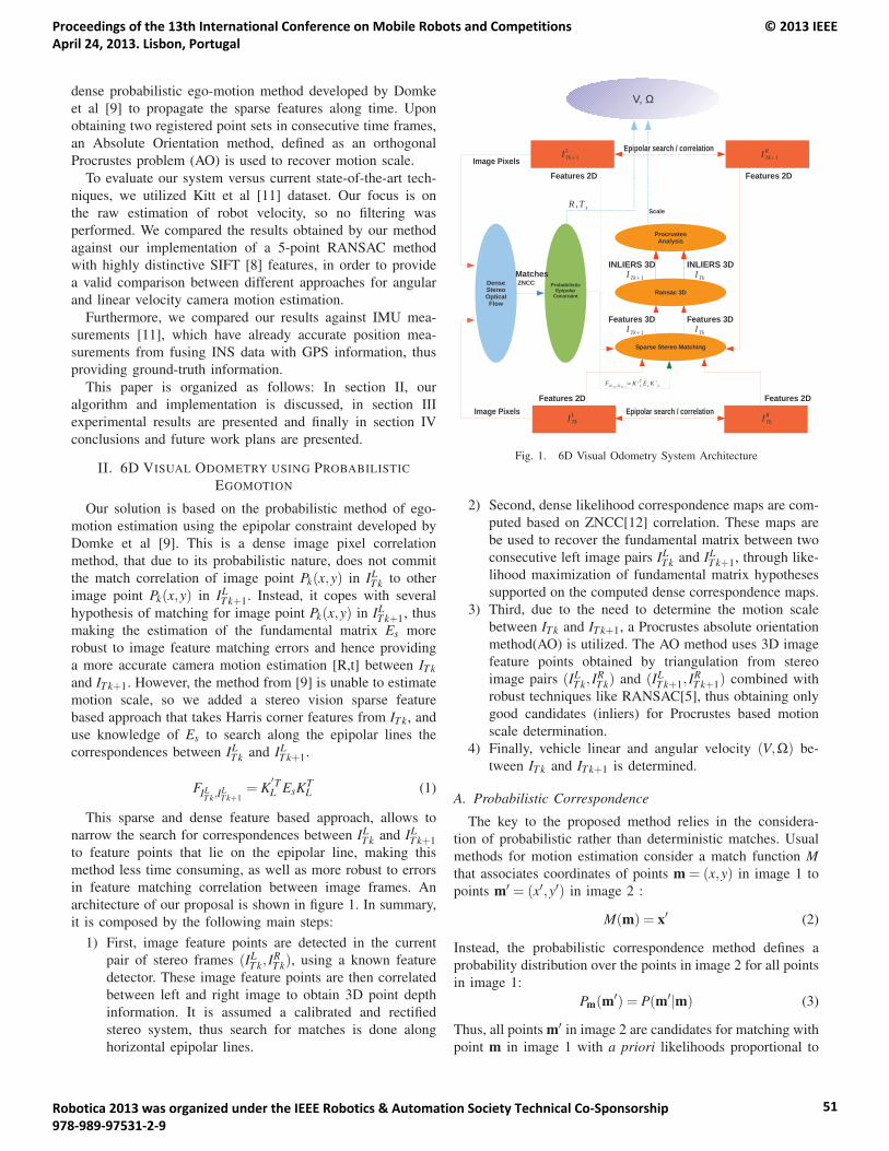
dense probabilistic ego-motion method developed by Domke

et al [9] to propagate the sparse features along time. Upon

obtaining two registered point sets in consecutive time frames,

an Absolute Orientation method, defined as an orthogonal

Procrustes problem (AO) is used to recover motion scale.

To evaluate our system versus current state-of-the-art tech-

niques, we utilized Kitt et al [11] dataset. Our focus is on

the raw estimation of robot velocity, so no filtering was

performed. We compared the results obtained by our method

against our implementation of a 5-point RANSAC method

with highly distinctive SIFT [8] features, in order to provide

a valid comparison between different approaches for angular

and linear velocity camera motion estimation.

Furthermore, we compared our results against IMU mea-

surements [11], which have already accurate position mea-

surements from fusing INS data with GPS information, thus

providing ground-truth information.

This paper is organized as follows: In section II, our

algorithm and implementation is discussed, in section III

experimental results are presented and finally in section IV

conclusions and future work plans are presented.

II. 6D VISUAL ODOMETRY USING PROBABILISTIC

EGOMOTION

Our solution is based on the probabilistic method of ego-

motion estimation using the epipolar constraint developed by

Domke et al [9]. This is a dense image pixel correlation

method, that due to its probabilistic nature, does not commit

the match correlation of image point Pk(x,y) in ILT k to other

image point Pk(x,y) in ILT k+1. Instead, it copes with several

hypothesis of matching for image point Pk(x,y) in ILT k+1, thus

making the estimation of the fundamental matrix Es more

robust to image feature matching errors and hence providing

a more accurate camera motion estimation [R,t] between IT kand IT k+1. However, the method from [9] is unable to estimate

motion scale, so we added a stereo vision sparse feature

based approach that takes Harris corner features from IT k, and

use knowledge of Es to search along the epipolar lines the

correspondences between ILT k and IL

T k+1.

FILT k,I

LT k+1

= K′TL EsKT

L (1)

This sparse and dense feature based approach, allows to

narrow the search for correspondences between ILT k and IL

T k+1

to feature points that lie on the epipolar line, making this

method less time consuming, as well as more robust to errors

in feature matching correlation between image frames. An

architecture of our proposal is shown in figure 1. In summary,

it is composed by the following main steps:

1) First, image feature points are detected in the current

pair of stereo frames (ILT k, I

RT k), using a known feature

detector. These image feature points are then correlated

between left and right image to obtain 3D point depth

information. It is assumed a calibrated and rectified

stereo system, thus search for matches is done along

horizontal epipolar lines.

Fig. 1. 6D Visual Odometry System Architecture

2) Second, dense likelihood correspondence maps are com-

puted based on ZNCC[12] correlation. These maps are

be used to recover the fundamental matrix between two

consecutive left image pairs ILT k and IL

T k+1, through like-

lihood maximization of fundamental matrix hypotheses

supported on the computed dense correspondence maps.

3) Third, due to the need to determine the motion scale

between IT k and IT k+1, a Procrustes absolute orientation

method(AO) is utilized. The AO method uses 3D image

feature points obtained by triangulation from stereo

image pairs (ILT k, I

RT k) and (IL

T k+1, IRT k+1) combined with

robust techniques like RANSAC[5], thus obtaining only

good candidates (inliers) for Procrustes based motion

scale determination.

4) Finally, vehicle linear and angular velocity (V,Ω) be-

tween IT k and IT k+1 is determined.

A. Probabilistic Correspondence

The key to the proposed method relies in the considera-

tion of probabilistic rather than deterministic matches. Usual

methods for motion estimation consider a match function Mthat associates coordinates of points m = (x,y) in image 1 to

points m′ = (x′,y′) in image 2 :

M(m) = x′ (2)

Instead, the probabilistic correspondence method defines a

probability distribution over the points in image 2 for all points

in image 1:

Pm(m′) = P(m′|m) (3)

Thus, all points m′ in image 2 are candidates for matching with

point m in image 1 with a priori likelihoods proportional to


© 2013 IEEE


51

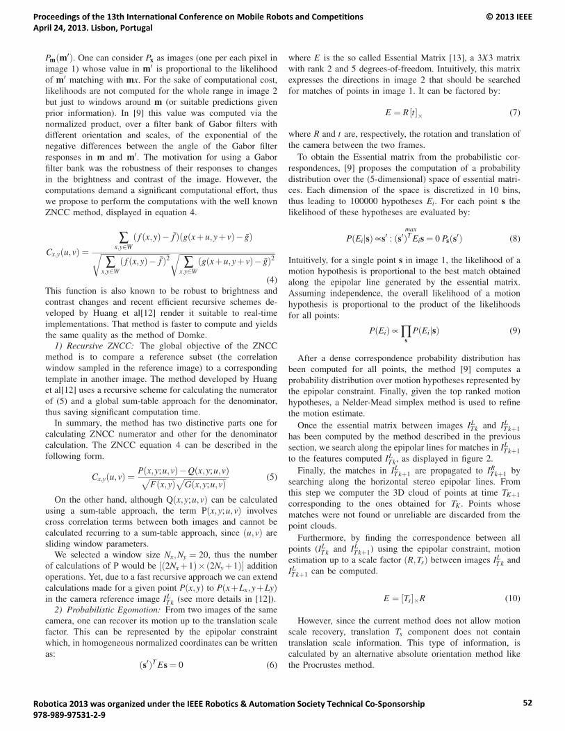
Pm(m′). One can consider Px as images (one per each pixel in

image 1) whose value in m′ is proportional to the likelihood

of m′ matching with mx. For the sake of computational cost,

likelihoods are not computed for the whole range in image 2

but just to windows around m (or suitable predictions given

prior information). In [9] this value was computed via the

normalized product, over a filter bank of Gabor filters with

different orientation and scales, of the exponential of the

negative differences between the angle of the Gabor filter

responses in m and m′. The motivation for using a Gabor

filter bank was the robustness of their responses to changes

in the brightness and contrast of the image. However, the

computations demand a significant computational effort, thus

we propose to perform the computations with the well known

ZNCC method, displayed in equation 4.

Cx,y(u,v) =∑

x,y∈W( f (x,y)− f )(g(x+u,y+ v)− g)√

∑x,y∈W

( f (x,y)− f )2√

∑x,y∈W

(g(x+u,y+ v)− g)2

(4)

This function is also known to be robust to brightness and

contrast changes and recent efficient recursive schemes de-

veloped by Huang et al[12] render it suitable to real-time

implementations. That method is faster to compute and yields

the same quality as the method of Domke.1) Recursive ZNCC: The global objective of the ZNCC

method is to compare a reference subset (the correlation

window sampled in the reference image) to a corresponding

template in another image. The method developed by Huang

et al[12] uses a recursive scheme for calculating the numerator

of (5) and a global sum-table approach for the denominator,

thus saving significant computation time.

In summary, the method has two distinctive parts one for

calculating ZNCC numerator and other for the denominator

calculation. The ZNCC equation 4 can be described in the

following form.

Cx,y(u,v) =P(x,y;u,v)−Q(x,y;u,v)√

F(x,y)√

G(x,y;u,v)(5)

On the other hand, although Q(x,y;u,v) can be calculated

using a sum-table approach, the term P(x,y;u,v) involves

cross correlation terms between both images and cannot be

calculated recurring to a sum-table approach, since (u,v) are

sliding window parameters.

We selected a window size Nx,Ny = 20, thus the number

of calculations of P would be [(2Nx +1)× (2Ny +1)] addition

operations. Yet, due to a fast recursive approach we can extend

calculations made for a given point P(x,y) to P(x+Lx,y+Ly)in the camera reference image IL

T k (see more details in [12]).2) Probabilistic Egomotion: From two images of the same

camera, one can recover its motion up to the translation scale

factor. This can be represented by the epipolar constraint

which, in homogeneous normalized coordinates can be written

as:

(s′)T Es = 0 (6)

where E is the so called Essential Matrix [13], a 3X3 matrix

with rank 2 and 5 degrees-of-freedom. Intuitively, this matrix

expresses the directions in image 2 that should be searched

for matches of points in image 1. It can be factored by:

E = R [t]× (7)

where R and t are, respectively, the rotation and translation of

the camera between the two frames.

To obtain the Essential matrix from the probabilistic cor-

respondences, [9] proposes the computation of a probability

distribution over the (5-dimensional) space of essential matri-

ces. Each dimension of the space is discretized in 10 bins,

thus leading to 100000 hypotheses Ei. For each point s the

likelihood of these hypotheses are evaluated by:

P(Ei|s) ∝max

s′ : (s′)T Eis = 0 Ps(s′) (8)

Intuitively, for a single point s in image 1, the likelihood of a

motion hypothesis is proportional to the best match obtained

along the epipolar line generated by the essential matrix.

Assuming independence, the overall likelihood of a motion

hypothesis is proportional to the product of the likelihoods

for all points:

P(Ei) ∝ ∏s

P(Ei|s) (9)

After a dense correspondence probability distribution has

been computed for all points, the method [9] computes a

probability distribution over motion hypotheses represented by

the epipolar constraint. Finally, given the top ranked motion

hypotheses, a Nelder-Mead simplex method is used to refine

the motion estimate.

Once the essential matrix between images ILT k and IL

T k+1

has been computed by the method described in the previous

section, we search along the epipolar lines for matches in ILT k+1

to the features computed ILT k, as displayed in figure 2.

Finally, the matches in ILT k+1 are propagated to IR

T k+1 by

searching along the horizontal stereo epipolar lines. From

this step we computer the 3D cloud of points at time TK+1

corresponding to the ones obtained for TK . Points whose

matches were not found or unreliable are discarded from the

point clouds.

Furthermore, by finding the correspondence between all

points (ILT k and IL

T k+1) using the epipolar constraint, motion

estimation up to a scale factor (R,Ts) between images ILT k and

ILT k+1 can be computed.

E = [Ts]×R (10)

However, since the current method does not allow motion

scale recovery, translation Ts component does not contain

translation scale information. This type of information, is

calculated by an alternative absolute orientation method like

the Procrustes method.


© 2013 IEEE


52

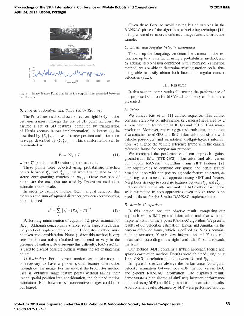
Image ILTk

Image ILTk+1

0 200 400 600 800 1000 1200 1400−1

−0.5

0

0.5

1

Image Width

Cor

rela

tion

scor

e

Correlation matching between line Es in IL

Tk+1 and Harris Feature in IL

Tk

Fig. 2. Image feature Point that lie in the epipolar line estimated betweenIT k to IT k+1

B. Procrustes Analysis and Scale Factor Recovery

The Procrustes method allows to recover rigid body motion

between frames, through the use of 3D point matches. We

assume a set of 3D features (computed by triangulation

of Harris corners in our implementation) in instant tT k be

described by {X ′i }T k, move to a new position and orientation

in tT k+1, described by {Y ′i }T k+1 . This transformation can be

represented as:

Y ′i = RX ′

i +T (11)

where Y ′i points, are 3D feature points in IT k+1.

These points were detected using probabilistic matched

points between ILT k and IL

T k+1, that were triangulated to their

stereo corresponding matches in IRT k+1. These two sets of

points are the ones that are used by Procrustes method to

estimate motion scale.

In order to estimate motion [R,T], a cost function that

measures the sum of squared distances between corresponding

points is used.

c2 =n

∑i

∥∥Y ′i − (RX ′

i +T )∥∥2

(12)

Performing minimization of equation 12, gives estimates of

[R,T ]. Although conceptually simple, some aspects regarding

the practical implementation of the Procrustes method must

be taken into consideration. Namely, since this method is very

sensible to data noise, obtained results tend to vary in the

presence of outliers. To overcome this difficulty, RANSAC [5]

is used to discard possible outliers within the set of matching

points.

1) Bucketing: For a correct motion scale estimation, it

is necessary to have a proper spatial feature distribution

through out the image. For instance, if the Procrustes method

uses all obtained image feature points without having their

image spatial position into consideration, the obtained motion

estimation [R,T] between two consecutive images could turn

out biased.

Given these facts, to avoid having biased samples in the

RANSAC phase of the algorithm, a bucketing technique [14]

is implemented to assure a unbiased image feature distribution

sample.

C. Linear and Angular Velocity Estimation

To sum up the foregoing, we determine camera motion es-

timation up to a scale factor using a probabilistic method, and

by adding stereo vision combined with Procrustes estimation

method, we are able to determine missing motion scale, thus

being able to easily obtain both linear and angular camera

velocities (V,Ω).

III. RESULTS

In this section, some results illustrating the performance of

our proposed solution for 6D Visual Odometry estimation are

presented.

A. Setup

We utilized Kitt et al [11] dataset sequence. This dataset

contains stereo vision information (2 cameras) separated by a

40 cm baseline, frame-rate at 10 fps and 391 × 1344 image

resolution. Moreover, regarding ground-truth data, the dataset

also contains fused GPS and IMU information consistent with

vehicle pose(x,y,z) and orientation (roll,pitch,yaw) informa-

tion. We aligned the vehicle reference frame with the camera

reference frame for comparison purposes.

We compared the performance of our approach against

ground-truth IMU (RTK-GPS) information and also versus

our 5-point RANSAC algorithm using SIFT features [8].

Our objective is to compare our sparse and dense feature

based solution with non-preserving scale feature detectors, as

opposing to a more direct approach using SIFT and Nearest

Neighbour strategy to correlate features between ILT k and IL

T k+1.

To validate our results, we used the AO method for motion

scale estimation in both approaches, even though there is no

need to do so for the 5-point RANSAC implementation.

B. Results Comparison

In this section, one can observe results comparing our

approach versus IMU ground-information and also with our

implementation of the 5-point RANSAC algorithm. We present

results of 6D velocities estimation (Linear and Angular) in the

camera reference frame, which is defined as: X axis contains

pitch information, Y axis yaw information and Z axis roll

information according to the right hand rule, Z points towards

the front.

Our method (6DP) contains a hybrid approach (dense and

sparse) correlation method. Results were obtained using only

1000 ZNCC correlation points between ILT k and IL

T k+1.

In figure 3, one can observe the performance for angular

velocity estimation between our 6DP method versus IMU

and 5-point RANSAC information. The displayed results

demonstrate a high degree of similarity between performance

obtained using 6DP and IMU ground-truth information results.

Additionally, results obtained by 6DP were performed without


© 2013 IEEE


53

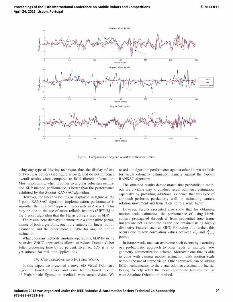
0 50 100 150 200 250 300−2

−1

0

1

2Angular Velocity Wx

Frame Index

Wx

degr

ees/

s

0 50 100 150 200 250 300−3

−2

−1

0

1

2Angular Velocity Wy

Frame Index

Wy

degr

ees/

s

0 50 100 150 200 250 300−2

−1

0

1

2Angular Velocity Wz

Frame Index

Wz

degr

ees/

s

6dpGT5−point

Fig. 3. Comparison of Angular velocities Estimation Results

using any type of filtering technique, thus the display of one

or two clear outliers (see figure arrows), that do not influence

overall results when compared to IMU filtered information.

Most importantly, when it comes to angular velocities estima-

tion 6DP method performance is better than the performance

exhibited by the 5-point RANSAC algorithm.

However, for linear velocities as displayed in figure 4, the

5-point RANSAC algorithm implementation performance is

smoother then our 6DP approach, especially in Z axis Tz. This

may be due to the use of more reliable features (SIFT)[8] in

the 5 point algorithm that the Harris corners used in 6DP.

The results here displayed demonstrate a compatible perfor-

mance of both algorithms, one more suitable for linear motion

estimation and the other more suitable for angular motion

estimation.

What concerns methods run-time operations, 6DP by using

recursive ZNCC approaches allows to reduce Domke Gabor

Filter processing time by 20 percent. Even so, 6DP it is not

yet suitable for real-time applications.

IV. CONCLUSIONS AND FUTURE WORK

In this paper, we presented a novel 6D Visual Odometry

algorithm based on sparse and dense feature based mixture

of Probabilistic Egomotion methods with stereo vision. We

tested our algorithm performance against other known methods

for visual odometry estimation, namely against the 5-point

RANSAC algorithm.

The obtained results demonstrated that probabilistic meth-

ods are a viable way to conduct visual odometry estimation,

especially by providing additional evidence that this type of

approach performs particularly well on estimating camera

rotation movement and translation up to a scale factor.

However, results presented also show that for obtaining

motion scale estimation, the performance of using Harris

corners propagated through E from sequential time frame

images are not as accurate as the one obtained using highly

distinctive features such as SIFT. Following this further, this

occurs due to low correlation values between ILT k and IL

T k+1

points.

In future work, one can overcome such events by extending

our probabilistic approach to other types of multiple view

geometry parametrization scheme. Moreover one that is able

to cope with camera motion estimation with motion scale

without the use of stereo vision. Other approach, can be adding

IMU mechanization to the visual odometry estimation(Inertial

Priors), to help select the more appropriate features for use

with Absolute Orientation method.


© 2013 IEEE


54

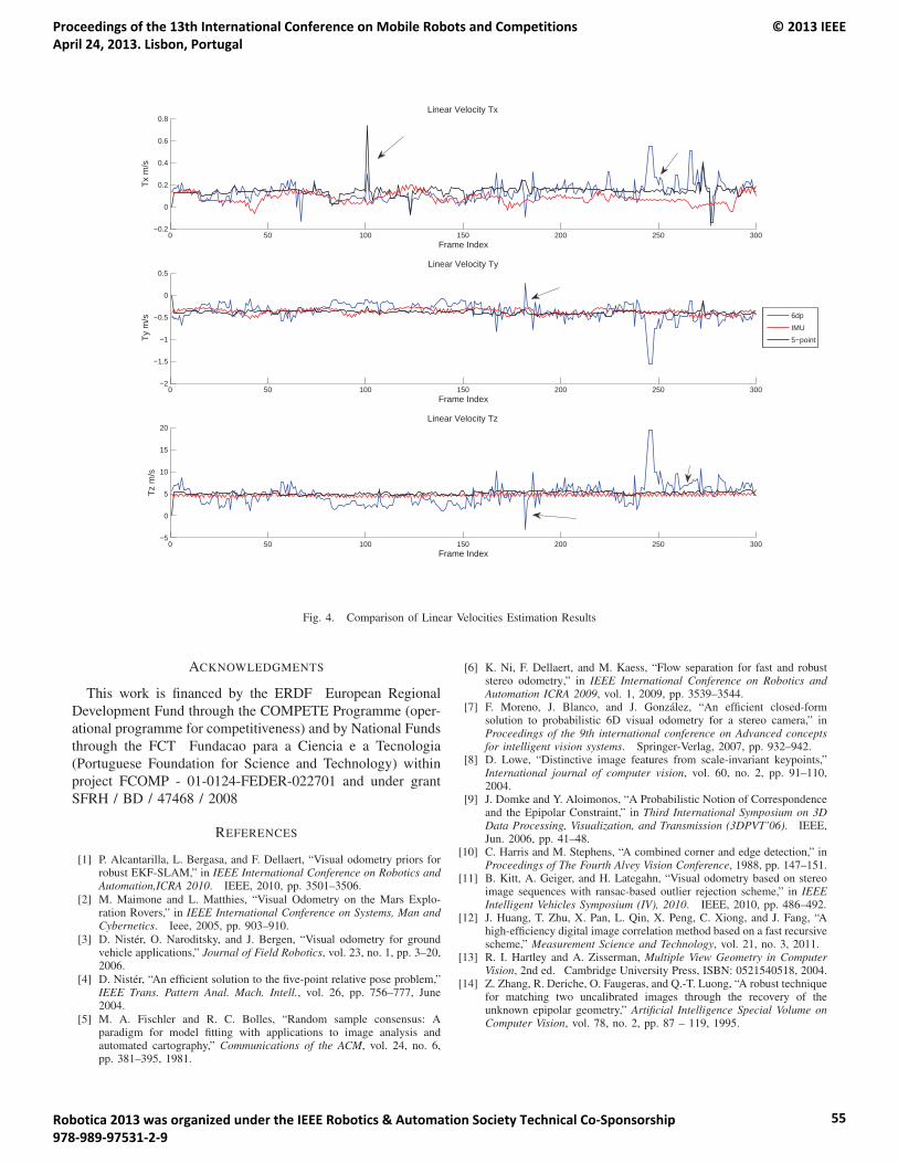
0 50 100 150 200 250 300−0.2

0

0.2

0.4

0.6

0.8Linear Velocity Tx

Frame Index

Tx m

/s

0 50 100 150 200 250 300−2

−1.5

−1

−0.5

0

0.5Linear Velocity Ty

Frame Index

Ty m

/s

0 50 100 150 200 250 300−5

0

5

10

15

20Linear Velocity Tz

Frame Index

Tz m

/s

6dpIMU5−point

Fig. 4. Comparison of Linear Velocities Estimation Results

ACKNOWLEDGMENTS

This work is financed by the ERDF European Regional

Development Fund through the COMPETE Programme (oper-

ational programme for competitiveness) and by National Funds

through the FCT Fundacao para a Ciencia e a Tecnologia

(Portuguese Foundation for Science and Technology) within

project FCOMP - 01-0124-FEDER-022701 and under grant

SFRH / BD / 47468 / 2008

REFERENCES

[1] P. Alcantarilla, L. Bergasa, and F. Dellaert, “Visual odometry priors forrobust EKF-SLAM,” in IEEE International Conference on Robotics andAutomation,ICRA 2010. IEEE, 2010, pp. 3501–3506.

[2] M. Maimone and L. Matthies, “Visual Odometry on the Mars Explo-ration Rovers,” in IEEE International Conference on Systems, Man andCybernetics. Ieee, 2005, pp. 903–910.

[3] D. Nister, O. Naroditsky, and J. Bergen, “Visual odometry for groundvehicle applications,” Journal of Field Robotics, vol. 23, no. 1, pp. 3–20,2006.

[4] D. Nister, “An efficient solution to the five-point relative pose problem,”IEEE Trans. Pattern Anal. Mach. Intell., vol. 26, pp. 756–777, June2004.

[5] M. A. Fischler and R. C. Bolles, “Random sample consensus: Aparadigm for model fitting with applications to image analysis andautomated cartography,” Communications of the ACM, vol. 24, no. 6,pp. 381–395, 1981.

[6] K. Ni, F. Dellaert, and M. Kaess, “Flow separation for fast and robuststereo odometry,” in IEEE International Conference on Robotics andAutomation ICRA 2009, vol. 1, 2009, pp. 3539–3544.

[7] F. Moreno, J. Blanco, and J. Gonzalez, “An efficient closed-formsolution to probabilistic 6D visual odometry for a stereo camera,” inProceedings of the 9th international conference on Advanced conceptsfor intelligent vision systems. Springer-Verlag, 2007, pp. 932–942.

[8] D. Lowe, “Distinctive image features from scale-invariant keypoints,”International journal of computer vision, vol. 60, no. 2, pp. 91–110,2004.

[9] J. Domke and Y. Aloimonos, “A Probabilistic Notion of Correspondenceand the Epipolar Constraint,” in Third International Symposium on 3DData Processing, Visualization, and Transmission (3DPVT’06). IEEE,Jun. 2006, pp. 41–48.

[10] C. Harris and M. Stephens, “A combined corner and edge detection,” inProceedings of The Fourth Alvey Vision Conference, 1988, pp. 147–151.

[11] B. Kitt, A. Geiger, and H. Lategahn, “Visual odometry based on stereoimage sequences with ransac-based outlier rejection scheme,” in IEEEIntelligent Vehicles Symposium (IV), 2010. IEEE, 2010, pp. 486–492.

[12] J. Huang, T. Zhu, X. Pan, L. Qin, X. Peng, C. Xiong, and J. Fang, “Ahigh-efficiency digital image correlation method based on a fast recursivescheme,” Measurement Science and Technology, vol. 21, no. 3, 2011.

[13] R. I. Hartley and A. Zisserman, Multiple View Geometry in ComputerVision, 2nd ed. Cambridge University Press, ISBN: 0521540518, 2004.

[14] Z. Zhang, R. Deriche, O. Faugeras, and Q.-T. Luong, “A robust techniquefor matching two uncalibrated images through the recovery of theunknown epipolar geometry,” Artificial Intelligence Special Volume onComputer Vision, vol. 78, no. 2, pp. 87 – 119, 1995.


© 2013 IEEE


55

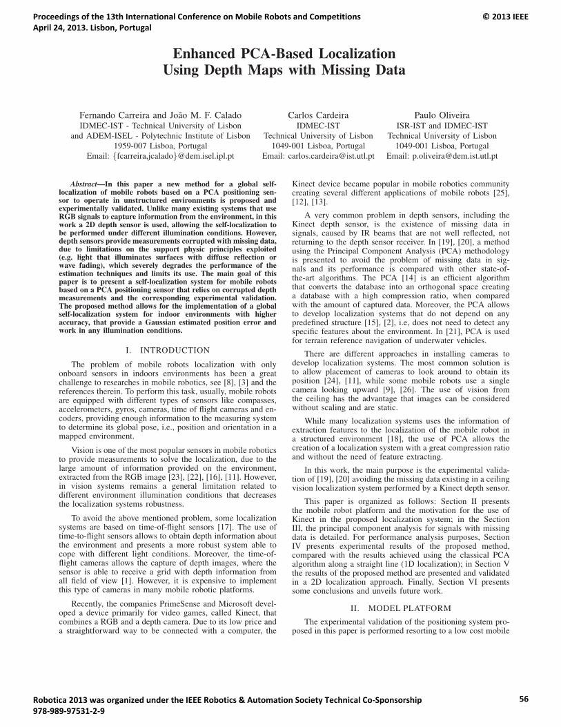
Enhanced PCA-Based LocalizationUsing Depth Maps with Missing Data

Fernando Carreira and Joao M. F. CaladoIDMEC-IST - Technical University of Lisbon

and ADEM-ISEL - Polytechnic Institute of Lisbon1959-007 Lisboa, Portugal

Email: {fcarreira,jcalado}@dem.isel.ipl.pt

Carlos CardeiraIDMEC-IST

Technical University of Lisbon1049-001 Lisboa, Portugal


Paulo OliveiraISR-IST and IDMEC-IST

Technical University of Lisbon1049-001 Lisboa, Portugal


Abstract—In this paper a new method for a global self-localization of mobile robots based on a PCA positioning sen-sor to operate in unstructured environments is proposed andexperimentally validated. Unlike many existing systems that useRGB signals to capture information from the environment, in thiswork a 2D depth sensor is used, allowing the self-localization tobe performed under different illumination conditions. However,depth sensors provide measurements corrupted with missing data,due to limitations on the support physic principles exploited(e.g. light that illuminates surfaces with diffuse reflection orwave fading), which severely degrades the performance of theestimation techniques and limits its use. The main goal of thispaper is to present a self-localization system for mobile robotsbased on a PCA positioning sensor that relies on corrupted depthmeasurements and the corresponding experimental validation.The proposed method allows for the implementation of a globalself-localization system for indoor environments with higheraccuracy, that provide a Gaussian estimated position error andwork in any illumination conditions.

I. INTRODUCTION

The problem of mobile robots localization with onlyonboard sensors in indoors environments has been a greatchallenge to researches in mobile robotics, see [8], [3] and thereferences therein. To perform this task, usually, mobile robotsare equipped with different types of sensors like compasses,accelerometers, gyros, cameras, time of flight cameras and en-coders, providing enough information to the measuring systemto determine its global pose, i.e., position and orientation in amapped environment.

Vision is one of the most popular sensors in mobile roboticsto provide measurements to solve the localization, due to thelarge amount of information provided on the environment,extracted from the RGB image [23], [22], [16], [11]. However,in vision systems remains a general limitation related todifferent environment illumination conditions that decreasesthe localization systems robustness.

To avoid the above mentioned problem, some localizationsystems are based on time-of-flight sensors [17]. The use oftime-to-flight sensors allows to obtain depth information aboutthe environment and presents a more robust system able tocope with different light conditions. Moreover, the time-of-flight cameras allows the capture of depth images, where thesensor is able to receive a grid with depth information fromall field of view [1]. However, it is expensive to implementthis type of cameras in many mobile robotic platforms.

Recently, the companies PrimeSense and Microsoft devel-oped a device primarily for video games, called Kinect, thatcombines a RGB and a depth camera. Due to its low price anda straightforward way to be connected with a computer, the

Kinect device became popular in mobile robotics communitycreating several different applications of mobile robots [25],[12], [13].

A very common problem in depth sensors, including theKinect depth sensor, is the existence of missing data insignals, caused by IR beams that are not well reflected, notreturning to the depth sensor receiver. In [19], [20], a methodusing the Principal Component Analysis (PCA) methodologyis presented to avoid the problem of missing data in sig-nals and its performance is compared with other state-of-the-art algorithms. The PCA [14] is an efficient algorithmthat converts the database into an orthogonal space creatinga database with a high compression ratio, when comparedwith the amount of captured data. Moreover, the PCA allowsto develop localization systems that do not depend on anypredefined structure [15], [2], i.e, does not need to detect anyspecific features about the environment. In [21], PCA is usedfor terrain reference navigation of underwater vehicles.

There are different approaches in installing cameras todevelop localization systems. The most common solution isto allow placement of cameras to look around to obtain itsposition [24], [11], while some mobile robots use a singlecamera looking upward [9], [26]. The use of vision fromthe ceiling has the advantage that images can be consideredwithout scaling and are static.

While many localization systems uses the information ofextraction features to the localization of the mobile robot ina structured environment [18], the use of PCA allows thecreation of a localization system with a great compression ratioand without the need of feature extracting.

In this work, the main purpose is the experimental valida-tion of [19], [20] avoiding the missing data existing in a ceilingvision localization system performed by a Kinect depth sensor.

This paper is organized as follows: Section II presentsthe mobile robot platform and the motivation for the use ofKinect in the proposed localization system; in the SectionIII, the principal component analysis for signals with missingdata is detailed. For performance analysis purposes, SectionIV presents experimental results of the proposed method,compared with the results achieved using the classical PCAalgorithm along a straight line (1D localization); in Section Vthe results of the proposed method are presented and validatedin a 2D localization approach. Finally, Section VI presentssome conclusions and unveils future work.

II. MODEL PLATFORM

The experimental validation of the positioning system pro-posed in this paper is performed resorting to a low cost mobile


© 2013 IEEE


56

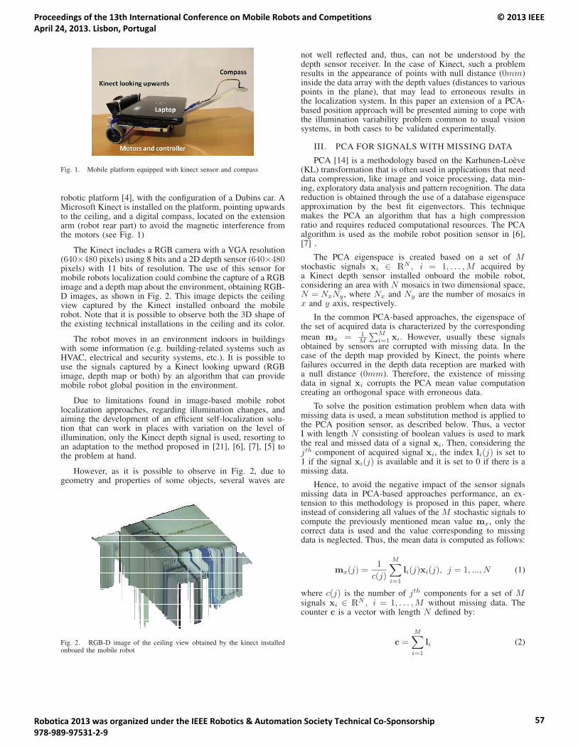
Fig. 1. Mobile platform equipped with kinect sensor and compass

robotic platform [4], with the configuration of a Dubins car. AMicrosoft Kinect is installed on the platform, pointing upwardsto the ceiling, and a digital compass, located on the extensionarm (robot rear part) to avoid the magnetic interference fromthe motors (see Fig. 1)

The Kinect includes a RGB camera with a VGA resolution(640×480 pixels) using 8 bits and a 2D depth sensor (640×480pixels) with 11 bits of resolution. The use of this sensor formobile robots localization could combine the capture of a RGBimage and a depth map about the environment, obtaining RGB-D images, as shown in Fig. 2. This image depicts the ceilingview captured by the Kinect installed onboard the mobilerobot. Note that it is possible to observe both the 3D shape ofthe existing technical installations in the ceiling and its color.

The robot moves in an environment indoors in buildingswith some information (e.g. building-related systems such asHVAC, electrical and security systems, etc.). It is possible touse the signals captured by a Kinect looking upward (RGBimage, depth map or both) by an algorithm that can providemobile robot global position in the environment.

Due to limitations found in image-based mobile robotlocalization approaches, regarding illumination changes, andaiming the development of an efficient self-localization solu-tion that can work in places with variation on the level ofillumination, only the Kinect depth signal is used, resorting toan adaptation to the method proposed in [21], [6], [7], [5] tothe problem at hand.

However, as it is possible to observe in Fig. 2, due togeometry and properties of some objects, several waves are

Fig. 2. RGB-D image of the ceiling view obtained by the kinect installedonboard the mobile robot

not well reflected and, thus, can not be understood by thedepth sensor receiver. In the case of Kinect, such a problemresults in the appearance of points with null distance (0mm)inside the data array with the depth values (distances to variouspoints in the plane), that may lead to erroneous results inthe localization system. In this paper an extension of a PCA-based position approach will be presented aiming to cope withthe illumination variability problem common to usual visionsystems, in both cases to be validated experimentally.

III. PCA FOR SIGNALS WITH MISSING DATA

PCA [14] is a methodology based on the Karhunen-Loeve(KL) transformation that is often used in applications that needdata compression, like image and voice processing, data min-ing, exploratory data analysis and pattern recognition. The datareduction is obtained through the use of a database eigenspaceapproximation by the best fit eigenvectors. This techniquemakes the PCA an algorithm that has a high compressionratio and requires reduced computational resources. The PCAalgorithm is used as the mobile robot position sensor in [6],[7] .

The PCA eigenspace is created based on a set of Mstochastic signals xi ∈ RN , i = 1, . . . ,M acquired bya Kinect depth sensor installed onboard the mobile robot,considering an area with N mosaics in two dimensional space,N = NxNy , where Nx and Ny are the number of mosaics inx and y axis, respectively.

In the common PCA-based approaches, the eigenspace ofthe set of acquired data is characterized by the corresponding

mean mx = 1M

∑Mi=1 xi. However, usually these signals

obtained by sensors are corrupted with missing data. In thecase of the depth map provided by Kinect, the points wherefailures occurred in the depth data reception are marked witha null distance (0mm). Therefore, the existence of missingdata in signal xi corrupts the PCA mean value computationcreating an orthogonal space with erroneous data.

To solve the position estimation problem when data withmissing data is used, a mean substitution method is applied tothe PCA position sensor, as described below. Thus, a vectorl with length N consisting of boolean values is used to markthe real and missed data of a signal xi. Then, considering thejth component of acquired signal xi, the index li(j) is set to1 if the signal xi(j) is available and it is set to 0 if there is amissing data.

Hence, to avoid the negative impact of the sensor signalsmissing data in PCA-based approaches performance, an ex-tension to this methodology is proposed in this paper, whereinstead of considering all values of the M stochastic signals tocompute the previously mentioned mean value mx, only thecorrect data is used and the value corresponding to missingdata is neglected. Thus, the mean data is computed as follows:

mx(j) =1

c(j)

M∑i=1

li(j)xi(j), j = 1, ..., N (1)

where c(j) is the number of jth components for a set of Msignals xi ∈ RN , i = 1, . . . ,M without missing data. Thecounter c is a vector with length N defined by:

c =

M∑i=1

li (2)


© 2013 IEEE


57

In order to apply the mean substitution method to the PCAalgorithm, all missing data presented in the acquired databaseis replaced by the mean value of the corresponding component,i.e., if there is a missing data in the jth component of the ith

signal, the missing value xi(j) is replaced with the value ofmx(j). After this substitution, the decomposition of the xi(j)into the orthogonal space follows the PCA algorithm classicalapproach, i.e. v = UT (x−mx). Matrix U = [u1 u2 . . . uN ]should be composed by the N orthogonal column vectors ofthe basis, verifying the eigenvalue problem

Rxxuj = λjuj , j = 1, ..., N, (3)

Assuming that the eigenvalues are ordered, i.e. λ1 ≥ λ2 ≥. . . ≥ λN , the choice of the first n � N principal compo-nents leads to stochastic signals approximation given by theratio on the covariances associated with the components, i.e.∑

n λn/∑

N λN .

During the mission, before the projection of the depthimage into the orthogonal space, the mean substitution shouldbe followed in order to eliminate the problem caused bymissing data in the signal x, i.e, all jth component of thesignal xi should be replaced by the corresponding mean valuemx(j).

The robot position x and y is obtained by finding a givenneighborhood δ, the mosaic whose eigenvector is nearest tothe acquired signal decomposed into the orthogonal space:

∀i‖[x y]T − [xi yi]T ‖2 < δ, rPCA = min

i‖v − vi‖2; (4)

Given the mosaic i that verifies this condition, its centercoordinates [xi yi]

T are selected as the robot position obtainedby the PCA-based sensor.

Then, the mean substitution approach is used when thereis missing data in the depth signals coming from the Kinectsensor. Just like during the creation of the PCA eigenspace,it must be done before the application of the PCA algorithm,i.e, all jth component of the signal xi should be replaced bythe corresponding mean value mx(j).

IV. EXPERIMENTAL RESULTS ALONG ASTRAIGHT LINE (1D LOCALIZATION)

As concept validation, the proposed self-localizationmethod is initially developed considering a straight line (1D),based on the model proposed in [6] and detailed in theappendix A. Thus, to create the PCA eigenspace, a set of 31depth images are captured along a straight line with 3 m oflength (sampling ratio of 0.1 m). Considering that the Kinectdepth sensor has a resolution of 640 by 480 points, and withthe purpose of reducing the amount of data stored in PCAeigenspace, the depth images are compressed with a ratioof 100 : 1, and transformed into vectors xi ∈ R3072, i =1, . . . , 31.

The mobile robot follows along a straight line with constantvelocity and the position estimation is obtained using themodel proposed in [6], see Appendix A for details. Theposition estimates are based on data obtained from the onboardsensors and the commands to the actuators, assuming constantvalues between sampling times (zero order hold assumption).

0 5 10 15 20 250

1

2

3Simulations with Kalman Filter − test 2

Time [s]

Posi

tion

[m]

Desired positionPCA analysisKalman result

0 5 10 15 20 25−0.6−0.4−0.2

00.20.40.6

Time [s]

Erro

r [m

]

0 5 10 15 200

5

10Ratio of missing data

Time [s]

Rat

io o

f mis

sing

dat

a [%

]

Fig. 3. Results of PCA-based positioning sensor and localization estimatesfrom Kalman filter

A. Monte Carlo Performance Tests

To assess the mobile robot self-localization methodologyproposed in this paper, a Monte Carlo test composed of10 experiments as described above is repeated. Images arecaptured with a frequency of 5 Hz to be processed by thePCA-based positioning sensor; Fig. 3 gives the localizationresults obtained in one of those experiments. The results showthat the PCA algorithm provides a reasonable approximationto the real robot localization. However, due to the existenceof missing data, the position obtained by the PCA algorithmoften gives incorrect results.

Analyzing Fig. 3, it is possible to see that the obtainedposition often reaches errors greater than 0.1 m (distanceat which the images are acquired to the eigenspace). Figure4 shows the results of three tests, where it is possible tosee the existence of large perturbations in the results of thePCA-based position sensor. Even the fusion of this resultswith the odometry, through a Kalman filter (KF), detailed

0 5 10 15 20−0.6

−0.4

−0.2

0

0.2

0.4

0.6Position error of PCA localization

Time [s]

Erro

r [m

]

Test 1Test 2Test 3

0 5 10 15 20

−0.4

−0.2

0

0.2

0.4

Position error of PCA localization with a Kalman Filter

Time [s]

Erro

r [m

]

Test 1Test 2Test 3

Fig. 4. Localization errors of tests along a straight line


© 2013 IEEE


58

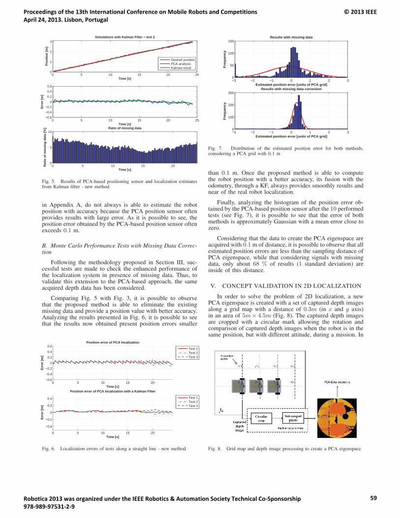
0 5 10 15 20 250

1

2

3Simulations with Kalman Filter − test 2

Time [s]

Posi

tion

[m]

Desired positionPCA analysisKalman result

0 5 10 15 20 25−0.6−0.4−0.2

00.20.40.6

Time [s]

Erro

r [m

]

0 5 10 15 200

5

10Ratio of missing data

Time [s]

Rat

io o

f mis

sing

dat

a [%

]

Fig. 5. Results of PCA-based positioning sensor and localization estimatesfrom Kalman filter - new method

in Appendix A, do not always is able to estimate the robotposition with accuracy because the PCA position sensor oftenprovides results with large error. As it is possible to see, theposition error obtained by the PCA-based position sensor oftenexceeds 0.1 m.

B. Monte Carlo Performance Tests with Missing Data Correc-tion

Following the methodology proposed in Section III, suc-cessful tests are made to check the enhanced performance ofthe localization system in presence of missing data. Thus, tovalidate this extension to the PCA-based approach, the sameacquired depth data has been considered.

Comparing Fig. 5 with Fig. 3, it is possible to observethat the proposed method is able to eliminate the existingmissing data and provide a position value with better accuracy.Analyzing the results presented in Fig. 6, it is possible to seethat the results now obtained present position errors smaller

0 5 10 15 20−0.6

−0.4

−0.2

0

0.2

0.4

0.6Position error of PCA localization

Time [s]

Erro

r [m

]

Test 1Test 2Test 3

0 5 10 15 20

−0.4

−0.2

0

0.2

0.4

Position error of PCA localization with a Kalman Filter

Time [s]

Erro

r [m

]

Test 1Test 2Test 3

Fig. 6. Localization errors of tests along a straight line - new method

−3 −2 −1 0 1 2 30

50

100

150Results with missing data

Freq

uenc

y

Estimated position error [units of PCA grid]

−3 −2 −1 0 1 2 30

100

200

300Results with missing data correction

Freq

uenc

y


Fig. 7. Distribution of the estimated position error for both methods,considering a PCA grid with 0.1 m

than 0.1 m. Once the proposed method is able to computethe robot position with a better accuracy, its fusion with theodometry, through a KF, always provides smoothly results andnear of the real robot localization.

Finally, analyzing the histogram of the position error ob-tained by the PCA-based position sensor after the 10 performedtests (see Fig. 7), it is possible to see that the error of bothmethods is approximately Gaussian with a mean error close tozero.

Considering that the data to create the PCA eigenspace areacquired with 0.1 m of distance, it is possible to observe that allestimated position errors are less than the sampling distance ofPCA eigenspace, while that considering signals with missingdata, only about 68 % of results (1 standard deviation) areinside of this distance.

V. CONCEPT VALIDATION IN 2D LOCALIZATION

In order to solve the problem of 2D localization, a newPCA eigenspace is created with a set of captured depth imagesalong a grid map with a distance of 0.3m (in x and y axis)in an area of 5m× 4.5m (Fig. 8). The captured depth imagesare cropped with a circular mark allowing the rotation andcomparison of captured depth images when the robot is in thesame position, but with different attitude, during a mission. In

Fig. 8. Grid map and depth image processing to create a PCA eigenspace


© 2013 IEEE


59

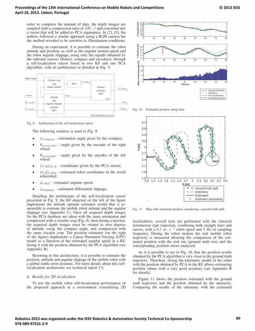
order to compress the amount of data, the depth images aresampled with a compression ratio of 100 : 1 and converted intoa vector that will be added to PCA eigenspace. In [7], [5], theauthors followed a similar approach using a RGB camera butthe method revealed to be sensitive to illumination conditions.

During an experiment, it is possible to estimate the robotattitude and position, as well as the angular motion speed andthe robot angular slippage, using only the signals obtained bythe onboard sensors (Kinect, compass and encoders), througha self-localization sensor based in two KF and one PCAalgorithm, with an architecture as detailed in Fig. 9.

Attitude

and

angular slippage

estimator

(KF)

Circular crop

and

image rotation

PCA

Position

estimator

(KF)

LPV

Self-localisation sensor

θlw encoder

θrw encoder

ψcompass

depth image

ωslippage

ψrobot

ωrobot

(x, y)PCA

(x, y)robot

Fig. 9. Architecture of the self-localization sensor

The following notation is used in Fig. 9:

• ψcompass - orientation angle given by the compass;

• θrwencoder - angle given by the encoder of the rightwheel;

• θlwencoder - angle given by the encoder of the leftwheel;

• (x, y)PCA - coordinates given by the PCA sensor;

• (x, y)robot - estimated robot coordinates in the worldreferential;

• ωrobot - estimated angular speed;

• ωslippage - estimated differential slippage.

Detailing the architecture of the self-localization sensorpresented in Fig. 9, the KF depicted on the left of the figureimplements the attitude optimal estimator model that is re-sponsible to estimate the mobile robot attitude and the angularslippage (see Appendix C). Once all acquired depth imagesfor the PCA database are taken with the same orientation andcompressed with a circular crop (Fig. 8), then during a mission,the acquired depth images must be rotated to zero degreesof attitude, using the compass angle, and compressed withthe same circular crop. The position estimator (on the rightof the figure) implements a Linear Parameter-Varying (LPV)model as a function of the estimated angular speed in a KF,fusing it with the position obtained by the PCA algorithm (seeAppendix B).

Resorting to this architecture, it is possible to estimate theposition, attitude and angular slippage of the mobile robot witha global stable error dynamic. For more details about this self-localization architecture see technical report [7].

A. Results for 2D localization

To test the mobile robot self-localization performance ofthe proposed approach in a environment (considering 2D

0 10 20 30 40 50 60 70 800

0.61.21.82.4

33.64.2

X Po

sitio

n [m

]

0 10 20 30 40 50 60 70 801.52.12.73.33.9

Y Po

sitio

n [m

]

0 10 20 30 40 50 60 70 800

5

10

15

Time [s]Rat

io o

f mis

sing

dat

a [%

]

Ground truth pathOdometryPCA localizationEstimated position

Fig. 10. Estimated position along time

0.9 1.2 1.5 1.8 2.1 2.4 2.7 3 3.3 3.6 3.9 4.2 4.51.5

1.8

2.1

2.4

2.7

3

3.3

3.6

3.9

4.2

X [m]

Y [m

]

startfinish

Ground truth pathOdometryEstimatedEstimator uncertainty

Fig. 11. Map with estimated position considering a ground truth path.

localization), several tests are performed with the classicallawnmower type trajectory, combining both straight lines andcurves, with a 0.1 m · s−1 robot speed and 5 Hz of samplingfrequency. During the robot motion the real mobile robottrajectory is measured allowing the comparison of the esti-mated position with the real one (ground truth test) and thecorresponding position errors analyzed.

As it is possible to see in Fig. 10, that the position resultsobtained by the PCA algorithm is very close to the ground truthtrajectory. Therefore, fusing the kinematic model of the robotwith the position obtained by PCA in the KF allows estimatingposition values with a very good accuracy (see Appendix Bfor details).

Figure 11 shows the position estimated with the groundtruth trajectory and the position obtained by the odometry.Comparing the results of the odometry with the estimated


© 2013 IEEE


60

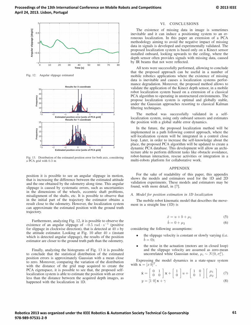
0 10 20 30 40 50 60 70 80−1

−0.5

0

0.5

1

Time [s]

Ang

ular

slip

page

[deg

/s]

Fig. 12. Angular slippage estimated

−3 −2 −1 0 1 2 30

10

20

30

40

50

Freq

uenc

y

Results for X coordinate


−3 −2 −1 0 1 2 30

5

10

15

20

25

Freq

uenc

y

Results for Y coordinate


Fig. 13. Distribution of the estimated position error for both axis, consideringa PCA grid with 0.3 m

position it is possible to see an angular slippage in motion,that is increasing the difference between the estimated attitudeand the one obtained by the odometry along time. This angularslippage is caused by systematic errors, such as uncertaintiesin the dimensions of the wheels, eccentric shaft problems,misalignment of the shafts, etc. It is possible to observe thatin the initial part of the trajectory the estimator obtains aresult close to the odometry. However, the localization systemcan approximate the estimated position with the ground truthtrajectory.

Furthermore, analyzing Fig. 12, it is possible to observe theexistence of an angular slippage of −0.5 rad · s−1 (positivefor slippage in clockwise direction), that is detected at 40 s bythe attitude estimator. Looking at Fig. 10 after 40 s (instantwhich is detected angular slippage), the results of the positionestimator are closer to the ground truth path than the odometry.

Finally, analyzing the histograms of Fig. 13 it is possibleto conclude that the statistical distribution of the estimatedposition errors is approximately Gaussian with a mean closeto zero. Moreover, comparing the variation of the distributionwith the distance of the grid map acquired to create thePCA eigenspace, it is possible to see that, the proposed self-localization system is able to estimate the position with an errorless than the distance between the acquired depth images, ashappened with the localization in 1D.

VI. CONCLUSIONS

The existence of missing data in image is sometimesinevitable and it can induce a positioning system to an er-roneous localization. In this paper an extension of a PCAmethodology aiming to avoid the negative impact of missingdata in signals is developed and experimentally validated. Theproposed localization system is based only on a Kinect sensorinstalled onboard, looking upwards to the ceiling, where thedepth sensor often provides signals with missing data, causedby IR beams that not were reflected.

All tests were successfully performed, allowing to concludethat the proposed approach can be useful in a number ofmobile robotics applications where the existence of missingdata is inevitable and causes a localization systems perfor-mance degradation. Moreover, the proposed method allows tovalidate the application of the Kinect depth sensor, in a mobilerobot localization system based on a extension of a classicalPCA algorithm to operating in unstructured environments. Thepropose localization system is optimal and globally stable,under the Gaussian approaches resorting to classical Kalmanfiltering techniques.

The method was successfully validated in a self-localization system, using only onboard sensors and estimatesthe position with a global stable error dynamics.

In the future, the proposed localization method will beimplemented in a path following control approach, where theself-localization system will be integrated in a control closeloop. Later, in order to increase the self-knowledge about theplace, the proposed PCA algorithm will be updated to create adynamic PCA database. This development will allow an archi-tecture able to perform different tasks like obstacle avoidance,robot-human interaction, rescue activities or integration in amulti-robots platform for collaborative work.

APPENDIX

For the sake of readability of this paper, this appendixshows the models and estimators used for the 1D and 2Dvalidation experiments. These models and estimators may befound, with more detail, in [7].

A. Model for position estimation in 1D localization

The mobile robot kinematic model that describes the move-ment in a straight line (1D) is

x = u+ b+ μ1 (5)

b = 0 + μ2 (6)

considering the following assumptions:

• the slippage velocity is constant or slowly varying (i.e.b = 0);

• the noise in the actuation (motors are in closed loop)and the slippage velocity are assumed as zero-meanuncorrelated white Gaussian noise, μi ∼ N(0, σ2

i ).

Expressing the model dynamics in a state-space systemwith x = [x b]T ,

x =

[0 10 0

]x+

[10

]u+

[1 00 1

] [μ1

μ2

](7)

y = [1 0]x+ γ (8)


© 2013 IEEE


61

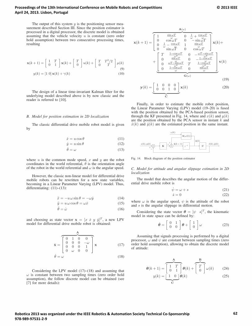
The output of this system y is the positioning sensor mea-surement described Section III. Since the position estimator isprocessed in a digital processor, the discrete model is obtainedassuming that the vehicle velocity u is constant (zero orderhold assumption) between two consecutive processing times,resulting

x(k + 1) =

[1 T0 1

]x(k) +

[T0

]u(k) +

[T T 2/20 T

]μ(k)

(9)

y(k) = [1 0]x(k) + γ(k) (10)

The design of a linear time-invariant Kalman filter for theunderlying model described above is by now classic and thereader is referred to [10].

B. Model for position estimation in 2D localization

The classic differential drive mobile robot model is givenby

x = u cos θ (11)

y = u sin θ (12)

θ = ω (13)

where u is the common mode speed, x and y are the robotcoordinates in the world referential, θ is the orientation angleof the robot in the world referential and ω is the angular speed.

However, the classic non-linear model for differential drivemobile robots can be rewritten for a new state variables,becoming in a Linear Parameter Varying (LPV) model. Thus,differentiating: (11)–(13):

x = −uω sin θ = −ωy (14)

y = uω cos θ = ωx (15)

θ = ω (16)

and choosing as state vector x = [x x y y]T , a new LPVmodel for differential drive mobile robot is obtained:

x =

A︷︸︸︷⎡⎢⎣

0 1 0 00 0 0 −ω0 0 0 10 ω 0 0

⎤⎥⎦x (17)

θ = ω (18)

Considering the LPV model (17)–(18) and assuming thatω is constant between two sampling times (zero order holdassumption), the follow discrete model can be obtained (see[7] for more details):

x(k + 1) =

A(ω)︷︸︸︷⎡⎢⎣

1 sinωTω 0 1

ω + cosωTω

0 cosωT 0 − sinωT0 1

ω − cosωTω 1 sinωT

ω0 sinωT 0 cosωT

⎤⎥⎦x(k)+

+

⎡⎢⎢⎣

T 1−cosωTω2 0 −ωT−sinωT

ω2

0 sinωTω 0 − 1−cosωT

ω0 ωT−sinωT

ω2 T 1−cosωTω2

0 1−cosωTω 0 sinωT

ω

⎤⎥⎥⎦

︸︷︷︸G(ω)

v(k)

(19)

y(k) =

[1 0 0 00 0 1 0

]︸︷︷︸

C

x(k) (20)

Finally, in order to estimate the mobile robot position,the Linear Parameter Varying (LPV) model (19–20) is fusedwith the position obtained by the PCA-based position sensor,through the KF presented in Fig. 14, where and x(k) and y(k)are the position obtained by the PCA sensor in instant k andx(k) and y(k) are the estimated position in the same instant.

K z−1 C

A(ω(k))

x(k), y(k)

+

+ x(k + 1)

x(k)

x(k), y(k)

−

+

ω(k)

Fig. 14. Block diagram of the position estimator

C. Model for attitude and angular slippage estimation in 2Dlocalization

The model that describes the angular motion of the differ-ential drive mobile robot is

ψ = ω + s (21)

s = 0 (22)

where ω is the angular speed, ψ is the attitude of the robotand s is the angular slippage in differential motion.

Considering the state vector θ = [ψ s]T , the kinematicmodel in state space can be defined by:

θ =

[0 10 0

]θ +

[10

]ω (23)

Assuming that signals processing is performed by a digitalprocessor, ω and ψ are constant between sampling times (zeroorder hold assumption), allowing to obtain the discrete modelof attitude:

θ(k + 1) =

A︷︸︸︷[1 T0 1

]θ(k) +

B︷︸︸︷[T0

]ω(k) (24)

y(k) = [ 1 0 ]︸︷︷︸C

θ(k) (25)


© 2013 IEEE


62

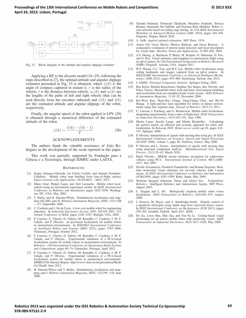
ψ(k)

+K2

+

s(k + 1)z−1 T

+ +

β(k + 1)z−1

β(k)

+

ψ(k)

αl(k)−

αr(k) + rL

Δψ0(k)

+

+ +

K1

+−

s(k)

Fig. 15. Block diagram of the attitude and angular slippage estimator

Applying a KF to the discrete model (24–25), following thesteps described in [7], the optimal attitude and angular slippageestimator presented in Fig. 15 is obtained, where ψ(k) is theangle of compass captured in instant k, r is the radius of thewheels, l is the distance between wheels, αr(k) and αl(k) arethe lengths of the paths of left and right wheels (that can beread directly from the encoders onboard) and ψ(k) and s(k)are the estimated attitude and angular slippage of the robot,respectively.

Finally, the angular speed of the robot applied in LPV (20)is obtained through a numerical difference of the estimatedattitude of the robot:

ω(k) =ψ(k)− ψ(k − 1)

T(26)

ACKNOWLEDGMENTS

The authors thank the valuable assistance of Joao Ro-drigues in the development of the work reported in this paper.

This work was partially supported by Fundacao para aCiencia e a Tecnologia, through IDMEC under LAETA.

REFERENCES

[1] Sergio Almansa-Valverde, Jos Carlos Castillo, and Antonio Fernndez-Caballero. Mobile robot map building from time-of-flight camera.Expert Systems with Applications, 39(10):8835 – 8843, 2012.

[2] Matej Artac, Matjaz Jogan, and Ales Leonardis. Mobile robot local-ization using an incremental eigenspace model. In IEEE InternationalConference on Robotics and Automation, pages 1025–1030, Washing-ton, DC, USA, May 2002.

[3] T. Bailey and H. Durrant-Whyte. Simultaneous localization and map-ping (SLAM): part II. Robotics Automation Magazine, IEEE, 13(3):108– 117, September 2006.

[4] C. Cardeira and J. Sa da Costa. A low cost mobile robot for engineeringeducation. In Industrial Electronics Society, 2005. IECON 2005. 31stAnnual Conference of IEEE, pages 2162–2167, Raleigh, USA, 2005.

[5] F. Carreira, C. Christo, D. Valerio, M. Ramalho, C. Cardeira, J. M. F.Calado, and P. Oliveira. 2d pca-based localization for mobile robotsin unstructured environments. In IEEE/RSJ International Conferenceon Intelligent Robots and Systems (IROS 2012), pages 3767–3868,Vilamoura, Portugal, October 2012.

[6] F. Carreira, C. Christo, D. Valerio, M. Ramalho, C. Cardeira, J. M. F.Calado, and P. Oliveira. Experimental validation of a PCA-basedlocalization system for mobile robots in unstructured environments. InRobotica - 12th International Conference on Autonomous Robot Systemsand Competitions, pages 69–74, Guimaraes, Portugal, April 2012.

[7] F. Carreira, C. Christo, D. Valerio, M. Ramalho, C. Cardeira, J. M. F.Calado, and P. Oliveira. Experimental validation of a PCA-basedlocalization system for mobile robots in unstructured environments.IDMEC/CSI Internal Report, http://www1.dem.ist.utl.pt/cardeira/Mesh/Ca12b.pdf, June 2012.

[8] H. Durrant-Whyte and T. Bailey. Simultaneous localization and map-ping: part I. Robotics Automation Magazine, IEEE, 13(2):99 –110, June2006.

[9] Yasuaki Fukutani, Tomoyuki Takahashi, Masahiro Iwahashi, TetsuyaKimura, Samsudin Siti Salbiah, and Norrima Binti Mokhtar. Robot vi-sion network based on ceiling map sharing. In 11th IEEE InternationalWorkshop on Advanced Motion Control (AMC 2010), pages 164–169,Nagaoka, Niigata, March 2010.

[10] A. Gelb. Applied optimal estimation. MIT Press, 1974.

[11] Arturo Gil, Oscar Mozos, Monica Ballesta, and Oscar Reinoso. Acomparative evaluation of interest point detectors and local descriptorsfor visual slam. Machine Vision and Applications, 21:905–920, 2010.

[12] A.S. Huang, A. Bachrach, P. Henry, M. Krainin, D. Maturana, D. Fox,and N. Roy. Visual odometry and mapping for autonomous flight usingan rgb-d camera. In 15th International Symposium on Robotics Research(ISRR), Flagstaff, Arizona, USA, August 2011.

[13] W.T. Huang, C.L. Tsai, and H.Y. Lin. Mobile robot localization usingceiling landmarks and images captured from an rgb-d camera. InIEEE/ASME International Conference on Advanced Intelligent Mecha-tronics (AIM 2012), pages 855–860, Kachsiung, Taiwan, July 2012.

[14] I. Jolliffe. Principal Component Analysis. Springer-Verlag, 2002.

[15] Ben Krose, Roland Bunschoten, Stephan Ten Hagen, Bas Terwijn, andNikos Vlassis. Household robots look and learn: environment modelingand localization from an omnidirectional vision system. IEEE Robotics& Automation Magazine, 11:45–52, December 2004.

[16] Bor-Woei Kuo, Hsun-Hao Chang, Yung-Chang Chen, and Shi-YuHuang. A light-and-fast slam algorithm for robots in indoor environ-ments using line segment map. Journal of Robotics, 2011:12, 2011.

[17] U. Larsson, J. Forsberg, and A. Wernersson. Mobile robot localization:integrating measurements from a time-of-flight laser. IEEE Transactionson Industrial Electronics, 43(3):422–431, June 1996.

[18] Martin Lauer, Sascha Lange, and Martin Riedmiller. Calculatingthe perfect match: an efficient and accurate approach for robot self-localization. In Robocup 2005: Robot soccer world cup IX, pages 142–153. Springer, 2006.

[19] P. Oliveira. Interpolation of signals with missing data using pca. In IEEEInternational Conference on Acoustics, Speech and Signal Processing(ICASSP 2006), volume 3, page III, Toulouse, France, May 2006.

[20] P. Oliveira and L. Gomes. Interpolation of signals with missing datausing principal component analysis. Multidimensional Syst. SignalProcess., 21(1):25–43, March 2010.

[21] Paulo Oliveira. MMAE terrain reference navigation for underwatervehicles using PCA. International Journal of Control, 80(7):1008–1017, July 2007.

[22] Davide Scaramuzza, Friedrich Fraundorfer, and Roland Siegwart. Real-time monocular visual odometry for on-road vehicles with 1-pointransac. In IEEE International Conference on Robotics and Automation(ICRA2009), pages 4293–4299, Kobe, Japan, May 2009.

[23] Wolfram Burgard Sebastian Thrun and Dieter Fox. ProbabilisticRobotics. Intelligent Robotics and Autonomous Agents. MIT Press,August 2005.

[24] C. Siagian and L. Itti. Biologically inspired mobile robot visionlocalization. IEEE Transactions on Robotics, 25(4):861–873, August2009.

[25] J. Stowers, M. Hayes, and A. Bainbridge-Smith. Altitude control ofa quadrotor helicopter using depth map from microsoft kinect sensor.In IEEE International Conference on Mechatronics (ICM 2011), pages358–362, Istanbul, Turkish, April 2011. IEEE.

[26] De Xu, Liwei Han, Min Tan, and You Fu Li. Ceiling-based visualpositioning for an indoor mobile robot with monocular vision. IEEETransactions on Industrial Electronics, 56(5):1617–1628, May 2009.


© 2013 IEEE


63

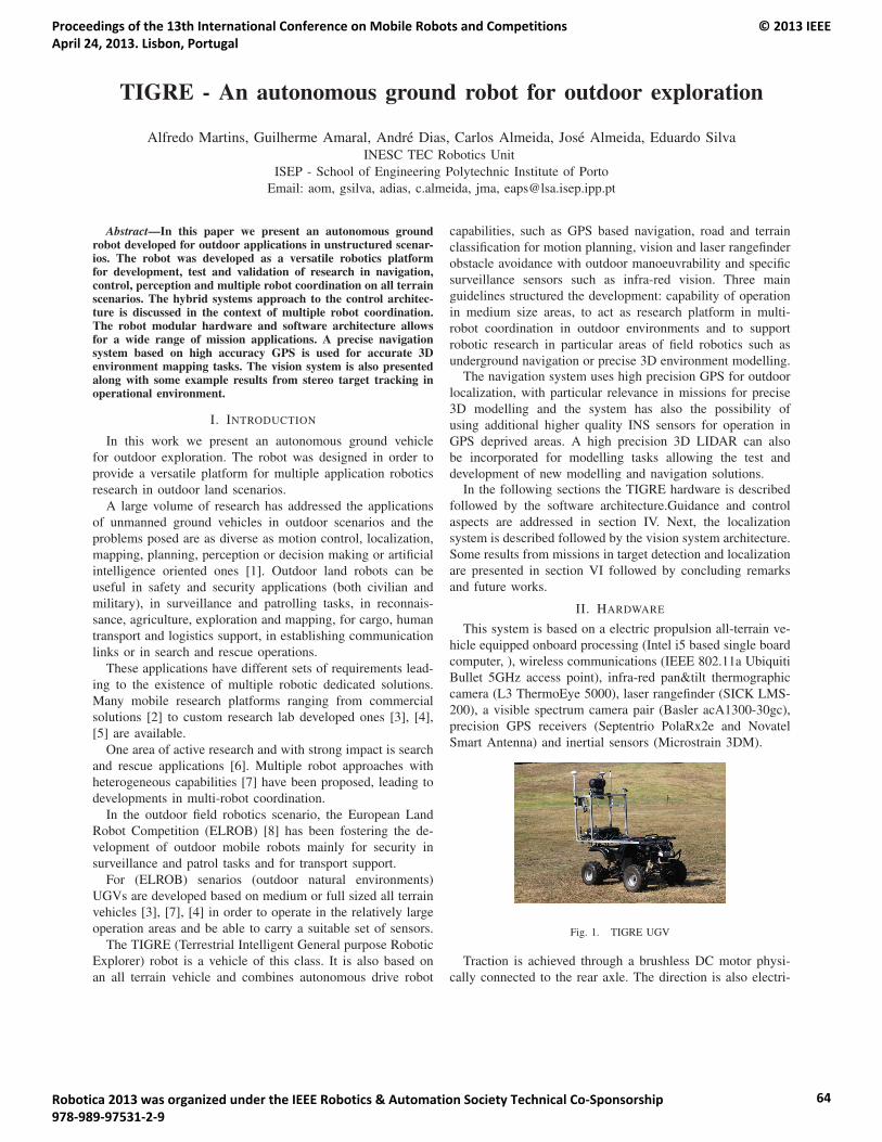
TIGRE - An autonomous ground robot for outdoor exploration

Alfredo Martins, Guilherme Amaral, Andre Dias, Carlos Almeida, Jose Almeida, Eduardo SilvaINESC TEC Robotics Unit

ISEP - School of Engineering Polytechnic Institute of Porto

Email: aom, gsilva, adias, c.almeida, jma, [email protected]

Abstract—In this paper we present an autonomous groundrobot developed for outdoor applications in unstructured scenar-ios. The robot was developed as a versatile robotics platformfor development, test and validation of research in navigation,control, perception and multiple robot coordination on all terrainscenarios. The hybrid systems approach to the control architec-ture is discussed in the context of multiple robot coordination.The robot modular hardware and software architecture allowsfor a wide range of mission applications. A precise navigationsystem based on high accuracy GPS is used for accurate 3Denvironment mapping tasks. The vision system is also presentedalong with some example results from stereo target tracking inoperational environment.

I. INTRODUCTION

In this work we present an autonomous ground vehicle

for outdoor exploration. The robot was designed in order to

provide a versatile platform for multiple application robotics

research in outdoor land scenarios.

A large volume of research has addressed the applications

of unmanned ground vehicles in outdoor scenarios and the

problems posed are as diverse as motion control, localization,

mapping, planning, perception or decision making or artificial

intelligence oriented ones [1]. Outdoor land robots can be

useful in safety and security applications (both civilian and

military), in surveillance and patrolling tasks, in reconnais-

sance, agriculture, exploration and mapping, for cargo, human

transport and logistics support, in establishing communication

links or in search and rescue operations.

These applications have different sets of requirements lead-

ing to the existence of multiple robotic dedicated solutions.

Many mobile research platforms ranging from commercial

solutions [2] to custom research lab developed ones [3], [4],

[5] are available.

One area of active research and with strong impact is search

and rescue applications [6]. Multiple robot approaches with

heterogeneous capabilities [7] have been proposed, leading to

developments in multi-robot coordination.

In the outdoor field robotics scenario, the European Land

Robot Competition (ELROB) [8] has been fostering the de-

velopment of outdoor mobile robots mainly for security in

surveillance and patrol tasks and for transport support.

For (ELROB) senarios (outdoor natural environments)

UGVs are developed based on medium or full sized all terrain

vehicles [3], [7], [4] in order to operate in the relatively large

operation areas and be able to carry a suitable set of sensors.

The TIGRE (Terrestrial Intelligent General purpose Robotic

Explorer) robot is a vehicle of this class. It is also based on

an all terrain vehicle and combines autonomous drive robot

capabilities, such as GPS based navigation, road and terrain

classification for motion planning, vision and laser rangefinder

obstacle avoidance with outdoor manoeuvrability and specific

surveillance sensors such as infra-red vision. Three main

guidelines structured the development: capability of operation

in medium size areas, to act as research platform in multi-

robot coordination in outdoor environments and to support

robotic research in particular areas of field robotics such as

underground navigation or precise 3D environment modelling.The navigation system uses high precision GPS for outdoor

localization, with particular relevance in missions for precise

3D modelling and the system has also the possibility of

using additional higher quality INS sensors for operation in

GPS deprived areas. A high precision 3D LIDAR can also

be incorporated for modelling tasks allowing the test and

development of new modelling and navigation solutions.In the following sections the TIGRE hardware is described

followed by the software architecture.Guidance and control

aspects are addressed in section IV. Next, the localization

system is described followed by the vision system architecture.

Some results from missions in target detection and localization

are presented in section VI followed by concluding remarks

and future works.

II. HARDWARE

This system is based on a electric propulsion all-terrain ve-

hicle equipped onboard processing (Intel i5 based single board

computer, ), wireless communications (IEEE 802.11a Ubiquiti

Bullet 5GHz access point), infra-red pan&tilt thermographic

camera (L3 ThermoEye 5000), laser rangefinder (SICK LMS-

200), a visible spectrum camera pair (Basler acA1300-30gc),

precision GPS receivers (Septentrio PolaRx2e and Novatel

Smart Antenna) and inertial sensors (Microstrain 3DM).

Fig. 1. TIGRE UGV

Traction is achieved through a brushless DC motor physi-

cally connected to the rear axle. The direction is also electri-


© 2013 IEEE


64

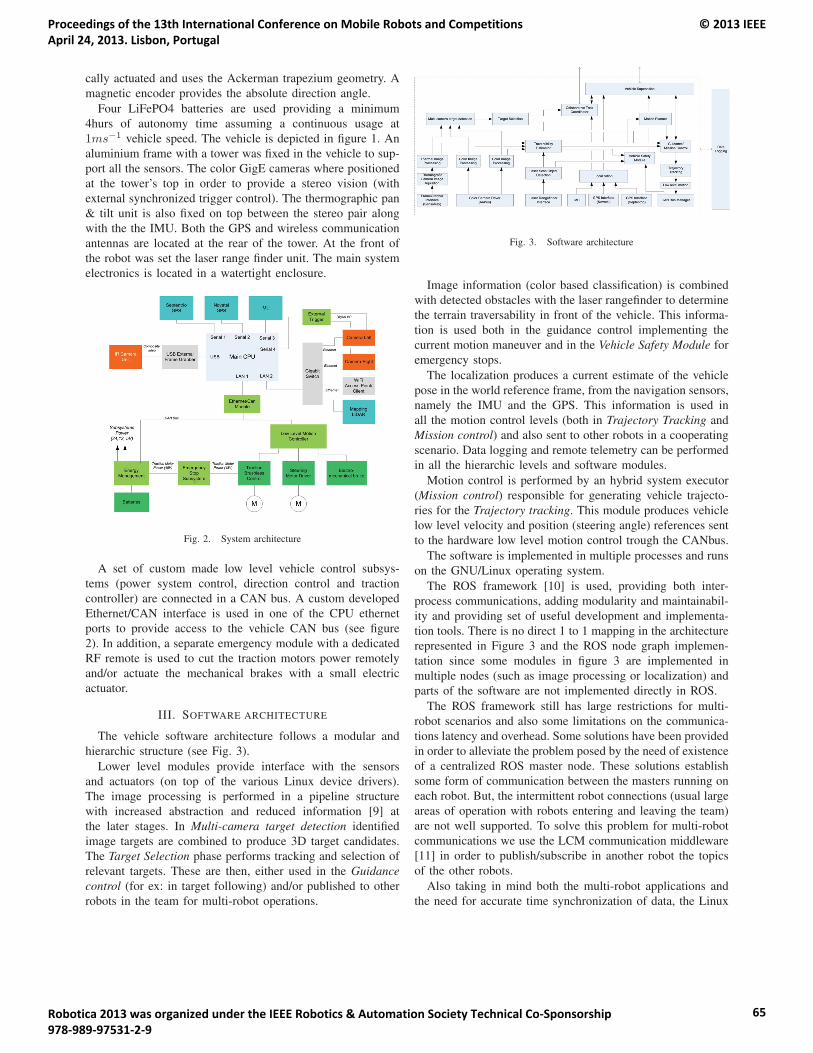
cally actuated and uses the Ackerman trapezium geometry. A

magnetic encoder provides the absolute direction angle.

Four LiFePO4 batteries are used providing a minimum

4hurs of autonomy time assuming a continuous usage at

1ms−1 vehicle speed. The vehicle is depicted in figure 1. An

aluminium frame with a tower was fixed in the vehicle to sup-

port all the sensors. The color GigE cameras where positioned

at the tower’s top in order to provide a stereo vision (with

external synchronized trigger control). The thermographic pan

& tilt unit is also fixed on top between the stereo pair along

with the the IMU. Both the GPS and wireless communication

antennas are located at the rear of the tower. At the front of

the robot was set the laser range finder unit. The main system

electronics is located in a watertight enclosure.

Fig. 2. System architecture

A set of custom made low level vehicle control subsys-

tems (power system control, direction control and traction

controller) are connected in a CAN bus. A custom developed

Ethernet/CAN interface is used in one of the CPU ethernet

ports to provide access to the vehicle CAN bus (see figure

2). In addition, a separate emergency module with a dedicated

RF remote is used to cut the traction motors power remotely

and/or actuate the mechanical brakes with a small electric

actuator.

III. SOFTWARE ARCHITECTURE

The vehicle software architecture follows a modular and

hierarchic structure (see Fig. 3).

Lower level modules provide interface with the sensors

and actuators (on top of the various Linux device drivers).

The image processing is performed in a pipeline structure

with increased abstraction and reduced information [9] at

the later stages. In Multi-camera target detection identified

image targets are combined to produce 3D target candidates.

The Target Selection phase performs tracking and selection of

relevant targets. These are then, either used in the Guidancecontrol (for ex: in target following) and/or published to other

robots in the team for multi-robot operations.

Fig. 3. Software architecture

Image information (color based classification) is combined

with detected obstacles with the laser rangefinder to determine

the terrain traversability in front of the vehicle. This informa-

tion is used both in the guidance control implementing the

current motion maneuver and in the Vehicle Safety Module for

emergency stops.

The localization produces a current estimate of the vehicle

pose in the world reference frame, from the navigation sensors,

namely the IMU and the GPS. This information is used in

all the motion control levels (both in Trajectory Tracking and

Mission control) and also sent to other robots in a cooperating

scenario. Data logging and remote telemetry can be performed

in all the hierarchic levels and software modules.

Motion control is performed by an hybrid system executor

(Mission control) responsible for generating vehicle trajecto-

ries for the Trajectory tracking. This module produces vehicle

low level velocity and position (steering angle) references sent

to the hardware low level motion control trough the CANbus.

The software is implemented in multiple processes and runs

on the GNU/Linux operating system.

The ROS framework [10] is used, providing both inter-

process communications, adding modularity and maintainabil-

ity and providing set of useful development and implementa-

tion tools. There is no direct 1 to 1 mapping in the architecture

represented in Figure 3 and the ROS node graph implemen-

tation since some modules in figure 3 are implemented in

multiple nodes (such as image processing or localization) and

parts of the software are not implemented directly in ROS.

The ROS framework still has large restrictions for multi-

robot scenarios and also some limitations on the communica-

tions latency and overhead. Some solutions have been provided

in order to alleviate the problem posed by the need of existence

of a centralized ROS master node. These solutions establish

some form of communication between the masters running on

each robot. But, the intermittent robot connections (usual large

areas of operation with robots entering and leaving the team)

are not well supported. To solve this problem for multi-robot

communications we use the LCM communication middleware

[11] in order to publish/subscribe in another robot the topics

of the other robots.

Also taking in mind both the multi-robot applications and

the need for accurate time synchronization of data, the Linux


© 2013 IEEE


65

Chrony clock-synchronization daemon is used with PPS (pulse

per second) information from GPS. This process allows to

synchronize the system clock to GPS time and in addition

provides multiple robot clock synchronization.Additionally video streaming (from any of the cameras) is

performed by the VLC streamer with MPEG4v codec.

IV. NAVIGATION GUIDANCE AND CONTROL

A. ControlThe vehicle control architecture follows an hybrid systems

approach [12] allowing both continuous time control with

discrete state evolution. The basic vehicle control maneuvers

can be defined as hybrid automata [13]. More complex mo-

tion control maneuvers can be obtained by the hierarchical

composition of simpler ones. Lower level reactive control can

be combined with higher level deliberative planning both in

continuous time and by the discrete state transition events

occurring (or generated) at the various levels of hierarchy in

the maneuvers.The path tracking used in the basic path following maneu-

vers (continuous time part) is a simple line of sight controller

and is the same used in [14]. The method is a nonlinear

feedback function of the cross track error ep measured from

the center of the front axle to the nearest path point (cx,cy).

δ

(cx, cy)v

θrobot

θαep

θpath

Fig. 4. Path tracking

The first term of the control law simply keeps the wheels

aligned with the given path by setting the steering angle δequal to the heading error.

eα = θrobot − θpath (1)

where θrobot is the heading of the vehicle and θpath is

the heading of the path at (cx, cy). In the presence of error

ep a second term adjusts δ such that the intended trajectory

intersects the path tangent from (cx, cy) at k v(t) units from the

front axle. The resulting of the steering control law is given

as

δ(t) = θe + tan−1

(kep(t)

vx(t)

)(2)

where k is a gain parameter.Rollover is a important concern in the vehicle locomotion

due to the vehicle characteristics and possible rough terrain.

The robot rollover detection is based on roll angle estimation

and on velocity and is prevented by limiting the velocity /

steering angle relation).

B. Cooperative mission control

In a multi vehicle cooperative setup each vehicle usually

provides a high level interface to the team coordination [15].

This can be done in a centralized [15] or distributed [16] ways.

Currently there is a strong effort in the research community

towards distributed approaches due to advantages in reliability

and scalability. In hierarchical coordination approaches [15]

higher layers of the vehicle sensing and control infrastructure

provide higher level of abstraction information for coordi-

nating purposes. These can be vehicle positions and discrete

vehicle states and high level commands.

In TIGRE architecture, multiple vehicle coordination can

occur at different levels of hierarchy. Explicit discrete event

coordination can occur in a multi-robot setup (such as with

other land based robots or with aerial robots) by exchange

of coordinating events. These events can be generated at all

vehicle control levels and by external entities as other robots.

In addition continuous variables (for ex: a particular sensor

reading) can be shared between multiple robots leading to

tighter multiple vehicle control loops.

Our architecture for multirobot coordination uses an hier-

archical approach similar to [15] considering 2 layers, one

representing local vehicle control and a multirobot controller.

We consider also a coordinating variable ξi = [ξc ξσ] and

a performance output for each vehicle zi = [zic ziσ ] but

for these variables we consider not only a continuous part

(ξc and zic ) but also an additional discrete part (ξσ and ziσ ).

In contrast to the two controllers solution proposed by Beard

with a discrete event system supervisor and a team formation

continuous controller, our architecture has both the multiple

robot coordination and the local vehicle controller as hybrid

systems allowing discrete and continuous control both locally

and for the robot team.

Each robotic vehicle is described in general as a non linear

dynamic system Si with states xi, inputs ui and outputs yi.The local vehicle controller eq.(3) can be viewed as an

hybrid system [12] with a set of continuous time flows for

each discrete state qi and generating the robot control inputs

ui.

Ci :

⎧⎪⎪⎪⎪⎨⎪⎪⎪⎪⎩

xqi = fqi (xqi , yi, ξc)ui = bqi(xqi , yi, ξc)zic = hqi(xqi , yi, ξc)

qi = φi(qi−, xqi , yi, σi, ξ)

zσ = ϕi(qi, xqi , yi, σi)

(3)

The discrete state update function φi depends not only on

the states, but also on the vehicle output yi, on local set of

events σi and on the coordinating variable ξ. The local set

of events are produced by guard conditions on discrete state

transitions and external events (such as user generated events).

M :

⎧⎪⎪⎨⎪⎪⎩

xqM = fqM (xqM , z1...zN )ξc = gqM (xqM , σM , z1...zN )

qM

= φM(q−

M, xqM , σ

M, z1...zN )

ξσ = ϕM(q

M, xqM , σ

M)

(4)


© 2013 IEEE


66

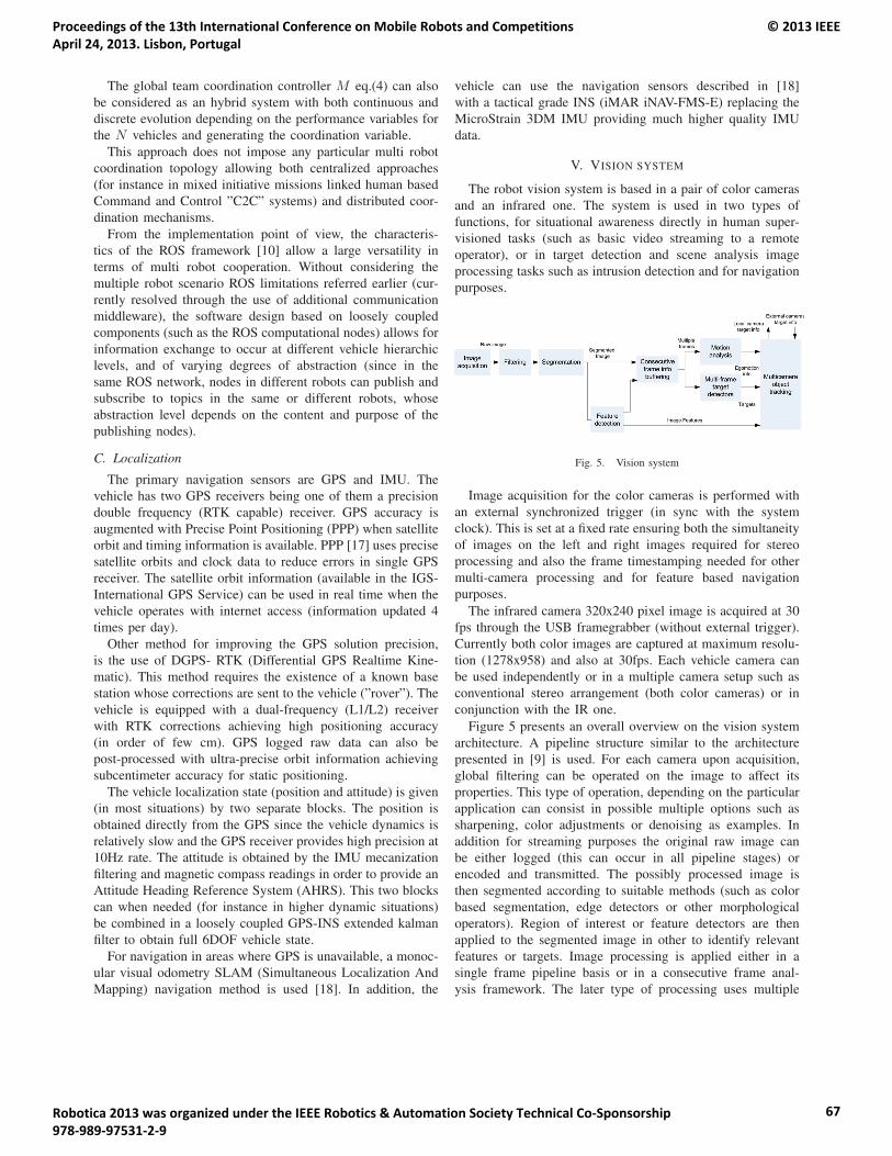
The global team coordination controller M eq.(4) can also

be considered as an hybrid system with both continuous and

discrete evolution depending on the performance variables for

the N vehicles and generating the coordination variable.

This approach does not impose any particular multi robot

coordination topology allowing both centralized approaches

(for instance in mixed initiative missions linked human based

Command and Control ”C2C” systems) and distributed coor-

dination mechanisms.

From the implementation point of view, the characteris-

tics of the ROS framework [10] allow a large versatility in

terms of multi robot cooperation. Without considering the

multiple robot scenario ROS limitations referred earlier (cur-

rently resolved through the use of additional communication

middleware), the software design based on loosely coupled

components (such as the ROS computational nodes) allows for

information exchange to occur at different vehicle hierarchic

levels, and of varying degrees of abstraction (since in the

same ROS network, nodes in different robots can publish and

subscribe to topics in the same or different robots, whose

abstraction level depends on the content and purpose of the

publishing nodes).

C. Localization

The primary navigation sensors are GPS and IMU. The

vehicle has two GPS receivers being one of them a precision

double frequency (RTK capable) receiver. GPS accuracy is

augmented with Precise Point Positioning (PPP) when satellite

orbit and timing information is available. PPP [17] uses precise

satellite orbits and clock data to reduce errors in single GPS

receiver. The satellite orbit information (available in the IGS-

International GPS Service) can be used in real time when the

vehicle operates with internet access (information updated 4

times per day).

Other method for improving the GPS solution precision,

is the use of DGPS- RTK (Differential GPS Realtime Kine-

matic). This method requires the existence of a known base

station whose corrections are sent to the vehicle (”rover”). The

vehicle is equipped with a dual-frequency (L1/L2) receiver

with RTK corrections achieving high positioning accuracy

(in order of few cm). GPS logged raw data can also be

post-processed with ultra-precise orbit information achieving

subcentimeter accuracy for static positioning.

The vehicle localization state (position and attitude) is given

(in most situations) by two separate blocks. The position is

obtained directly from the GPS since the vehicle dynamics is

relatively slow and the GPS receiver provides high precision at

10Hz rate. The attitude is obtained by the IMU mecanization

filtering and magnetic compass readings in order to provide an

Attitude Heading Reference System (AHRS). This two blocks

can when needed (for instance in higher dynamic situations)

be combined in a loosely coupled GPS-INS extended kalman

filter to obtain full 6DOF vehicle state.

For navigation in areas where GPS is unavailable, a monoc-

ular visual odometry SLAM (Simultaneous Localization And

Mapping) navigation method is used [18]. In addition, the

vehicle can use the navigation sensors described in [18]

with a tactical grade INS (iMAR iNAV-FMS-E) replacing the

MicroStrain 3DM IMU providing much higher quality IMU

data.

V. VISION SYSTEM

The robot vision system is based in a pair of color cameras

and an infrared one. The system is used in two types of

functions, for situational awareness directly in human super-

visioned tasks (such as basic video streaming to a remote

operator), or in target detection and scene analysis image

processing tasks such as intrusion detection and for navigation

purposes.

Fig. 5. Vision system

Image acquisition for the color cameras is performed with

an external synchronized trigger (in sync with the system

clock). This is set at a fixed rate ensuring both the simultaneity

of images on the left and right images required for stereo

processing and also the frame timestamping needed for other

multi-camera processing and for feature based navigation

purposes.

The infrared camera 320x240 pixel image is acquired at 30

fps through the USB framegrabber (without external trigger).

Currently both color images are captured at maximum resolu-

tion (1278x958) and also at 30fps. Each vehicle camera can

be used independently or in a multiple camera setup such as

conventional stereo arrangement (both color cameras) or in

conjunction with the IR one.

Figure 5 presents an overall overview on the vision system

architecture. A pipeline structure similar to the architecture

presented in [9] is used. For each camera upon acquisition,

global filtering can be operated on the image to affect its

properties. This type of operation, depending on the particular

application can consist in possible multiple options such as

sharpening, color adjustments or denoising as examples. In

addition for streaming purposes the original raw image can

be either logged (this can occur in all pipeline stages) or

encoded and transmitted. The possibly processed image is

then segmented according to suitable methods (such as color

based segmentation, edge detectors or other morphological

operators). Region of interest or feature detectors are then

applied to the segmented image in other to identify relevant

features or targets. Image processing is applied either in a

single frame pipeline basis or in a consecutive frame anal-

ysis framework. The later type of processing uses multiple


© 2013 IEEE


67

consecutive frames to extract information. Examples of this

type of processing are visual odometry computations where

the motion information is extracted, consecutive frame stereo

calculations or multiframe based target detectors. Target 3D

positioning can be determined from multi-camera information.

In our case, this can be done with images from the stereo

color pair or with one from the infrared camera and other

from the color (this can be extended to other cameras). Using

the standard pinhole camera model, the image points (for an

undistorted image) in homogeneous coordinates are given by:

x = K[R|t]X (5)

where K are the intrinsic parameters, [R|t] are the camera

extrinsic parameters and X is the 3D point in the world frame

(usually this is the vehicle body fixed frame).Each camera

provides a set of xi points. These, when corresponding to

the same real world point can be combined in a multi view

geometry to provide Xi.To determine the full 3D position

it is necessary to make the correspondence between same

target points in the different camera images. In classic dense

stereo all the image points are possible candidates and com-

putationally efficient methods like RANSAC [19] are applied

to determine point position in the epipolar line. The TIGRE

vision system assumes a sparse framework. In this case only

the relevant points in the image (for ex: target detected points)

are processed (also only for these is the distortion removed).

For each corresponding pair of target image points (x1,x2)on different cameras (for the same target) the relative 3D

positioning is determined by triangulation or by solving the

overdetermined system:{x1 = K1[R1|t1]Xx2 = K2[R2|t2]X (6)

The 3D target detection implementation in the ROS frame-

work is depicted in Figure 6. The offline extrinsic camera

parameter calibration is also included.

Fig. 6. Vision target detection implementation

VI. RESULTS

Field tests were performed with the robot in the Oporto City

Park. These tests were conducted in relatively easy terrain

(grass and earth) due to limitations in the allowed area of

operation. Human target tracking and following missions were

performed using the stereo color camera pair. The target

position was logged with a precision GPS receiver (identical

to the Septentrio one used on the robot).

In addition, a cooperative mission was performed with an

aerial autonomous robot (Ashtec’s Pelican UAV) where the

UAV detected the target and informed the ground vehicle to

follow it (for more information see [20]).

Fig. 7. Two frames from the color cameras with the detected target marked

In Figure 7 two images from the color camera taken during

the target tracking maneuver, are presented with the detected

target marked. Three images from the IR camera during the

same maneuver (but not at the same times) are also shown in

figure 8. The human target was wearing a red vest to facilitate

detection on the low powered UAV onboard processor. Al-

though this is not a realistic assumption, the detection on the

UGV can be performed by more advanced methods and also

on the thermographic camera [21], and for the UAV further

developments must be pursued in the implementation on the

limited resources of realistic vision human target detectors.

Fig. 8. Thermografic camera snapshots

In figure 9 the detected target positions (using the color

camera stereo pair), robot trajectory and real target trajectory

are indicated for a segment of the tracking maneuver when

the robot is approaching the target and stopping afterwards.

VII. CONCLUSIONS

In this work is presented the TIGRE autonomous ground

vehicle. The robot was developed for outdoor exploration

and to be a versatile robotics research platform. Applications

scenarios envision security tasks, precise mapping, cooperative

missions with other autonomous robots, and operation in

unstructured environments such as underground. The vehicle

hardware solutions are described along with the comprehen-

sive set of sensors. An hybrid systems approach was followed

in the vehicle control architecture. Basic motion control is

performed by hybrid (discrete and continuous) maneuvers.

These are composed in hierarchical finite (for the discrete

state) automata providing more complex motion functionali-

ties. The software implementation aspects were also addressed.

An overall overview for the vision system is presented along

with a particular use for stereo target tracking. The robot


© 2013 IEEE


68

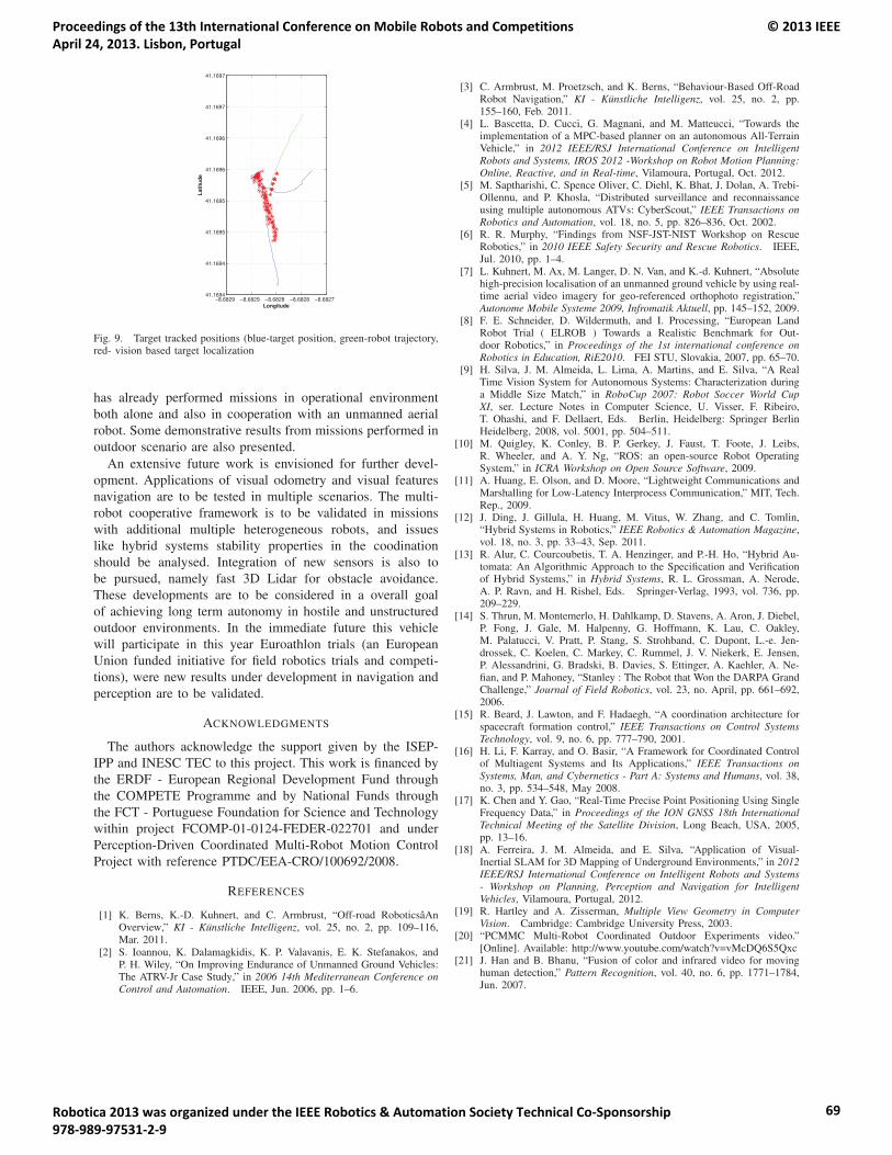
−8.6829 −8.6829 −8.6828 −8.6828 −8.682741.1694

41.1694

41.1695

41.1695

41.1696

41.1696

41.1697

41.1697

Longitude

Lat

itu

de

Fig. 9. Target tracked positions (blue-target position, green-robot trajectory,red- vision based target localization

has already performed missions in operational environment

both alone and also in cooperation with an unmanned aerial

robot. Some demonstrative results from missions performed in

outdoor scenario are also presented.

An extensive future work is envisioned for further devel-

opment. Applications of visual odometry and visual features

navigation are to be tested in multiple scenarios. The multi-

robot cooperative framework is to be validated in missions

with additional multiple heterogeneous robots, and issues

like hybrid systems stability properties in the coodination

should be analysed. Integration of new sensors is also to

be pursued, namely fast 3D Lidar for obstacle avoidance.

These developments are to be considered in a overall goal

of achieving long term autonomy in hostile and unstructured

outdoor environments. In the immediate future this vehicle

will participate in this year Euroathlon trials (an European

Union funded initiative for field robotics trials and competi-

tions), were new results under development in navigation and

perception are to be validated.

ACKNOWLEDGMENTS

The authors acknowledge the support given by the ISEP-

IPP and INESC TEC to this project. This work is financed by

the ERDF - European Regional Development Fund through

the COMPETE Programme and by National Funds through

the FCT - Portuguese Foundation for Science and Technology

within project FCOMP-01-0124-FEDER-022701 and under

Perception-Driven Coordinated Multi-Robot Motion Control

Project with reference PTDC/EEA-CRO/100692/2008.

REFERENCES

[1] K. Berns, K.-D. Kuhnert, and C. Armbrust, “Off-road RoboticsaAnOverview,” KI - Kunstliche Intelligenz, vol. 25, no. 2, pp. 109–116,Mar. 2011.

[2] S. Ioannou, K. Dalamagkidis, K. P. Valavanis, E. K. Stefanakos, andP. H. Wiley, “On Improving Endurance of Unmanned Ground Vehicles:The ATRV-Jr Case Study,” in 2006 14th Mediterranean Conference onControl and Automation. IEEE, Jun. 2006, pp. 1–6.

[3] C. Armbrust, M. Proetzsch, and K. Berns, “Behaviour-Based Off-RoadRobot Navigation,” KI - Kunstliche Intelligenz, vol. 25, no. 2, pp.155–160, Feb. 2011.

[4] L. Bascetta, D. Cucci, G. Magnani, and M. Matteucci, “Towards theimplementation of a MPC-based planner on an autonomous All-TerrainVehicle,” in 2012 IEEE/RSJ International Conference on IntelligentRobots and Systems, IROS 2012 -Workshop on Robot Motion Planning:Online, Reactive, and in Real-time, Vilamoura, Portugal, Oct. 2012.

[5] M. Saptharishi, C. Spence Oliver, C. Diehl, K. Bhat, J. Dolan, A. Trebi-Ollennu, and P. Khosla, “Distributed surveillance and reconnaissanceusing multiple autonomous ATVs: CyberScout,” IEEE Transactions onRobotics and Automation, vol. 18, no. 5, pp. 826–836, Oct. 2002.

[6] R. R. Murphy, “Findings from NSF-JST-NIST Workshop on RescueRobotics,” in 2010 IEEE Safety Security and Rescue Robotics. IEEE,Jul. 2010, pp. 1–4.

[7] L. Kuhnert, M. Ax, M. Langer, D. N. Van, and K.-d. Kuhnert, “Absolutehigh-precision localisation of an unmanned ground vehicle by using real-time aerial video imagery for geo-referenced orthophoto registration,”Autonome Mobile Systeme 2009, Infromatik Aktuell, pp. 145–152, 2009.

[8] F. E. Schneider, D. Wildermuth, and I. Processing, “European LandRobot Trial ( ELROB ) Towards a Realistic Benchmark for Out-door Robotics,” in Proceedings of the 1st international conference onRobotics in Education, RiE2010. FEI STU, Slovakia, 2007, pp. 65–70.

[9] H. Silva, J. M. Almeida, L. Lima, A. Martins, and E. Silva, “A RealTime Vision System for Autonomous Systems: Characterization duringa Middle Size Match,” in RoboCup 2007: Robot Soccer World CupXI, ser. Lecture Notes in Computer Science, U. Visser, F. Ribeiro,T. Ohashi, and F. Dellaert, Eds. Berlin, Heidelberg: Springer BerlinHeidelberg, 2008, vol. 5001, pp. 504–511.

[10] M. Quigley, K. Conley, B. P. Gerkey, J. Faust, T. Foote, J. Leibs,R. Wheeler, and A. Y. Ng, “ROS: an open-source Robot OperatingSystem,” in ICRA Workshop on Open Source Software, 2009.

[11] A. Huang, E. Olson, and D. Moore, “Lightweight Communications andMarshalling for Low-Latency Interprocess Communication,” MIT, Tech.Rep., 2009.

[12] J. Ding, J. Gillula, H. Huang, M. Vitus, W. Zhang, and C. Tomlin,“Hybrid Systems in Robotics,” IEEE Robotics & Automation Magazine,vol. 18, no. 3, pp. 33–43, Sep. 2011.

[13] R. Alur, C. Courcoubetis, T. A. Henzinger, and P.-H. Ho, “Hybrid Au-tomata: An Algorithmic Approach to the Specification and Verificationof Hybrid Systems,” in Hybrid Systems, R. L. Grossman, A. Nerode,A. P. Ravn, and H. Rishel, Eds. Springer-Verlag, 1993, vol. 736, pp.209–229.

[14] S. Thrun, M. Montemerlo, H. Dahlkamp, D. Stavens, A. Aron, J. Diebel,P. Fong, J. Gale, M. Halpenny, G. Hoffmann, K. Lau, C. Oakley,M. Palatucci, V. Pratt, P. Stang, S. Strohband, C. Dupont, L.-e. Jen-drossek, C. Koelen, C. Markey, C. Rummel, J. V. Niekerk, E. Jensen,P. Alessandrini, G. Bradski, B. Davies, S. Ettinger, A. Kaehler, A. Ne-fian, and P. Mahoney, “Stanley : The Robot that Won the DARPA GrandChallenge,” Journal of Field Robotics, vol. 23, no. April, pp. 661–692,2006.

[15] R. Beard, J. Lawton, and F. Hadaegh, “A coordination architecture forspacecraft formation control,” IEEE Transactions on Control SystemsTechnology, vol. 9, no. 6, pp. 777–790, 2001.

[16] H. Li, F. Karray, and O. Basir, “A Framework for Coordinated Controlof Multiagent Systems and Its Applications,” IEEE Transactions onSystems, Man, and Cybernetics - Part A: Systems and Humans, vol. 38,no. 3, pp. 534–548, May 2008.

[17] K. Chen and Y. Gao, “Real-Time Precise Point Positioning Using SingleFrequency Data,” in Proceedings of the ION GNSS 18th InternationalTechnical Meeting of the Satellite Division, Long Beach, USA, 2005,pp. 13–16.

[18] A. Ferreira, J. M. Almeida, and E. Silva, “Application of Visual-Inertial SLAM for 3D Mapping of Underground Environments,” in 2012IEEE/RSJ International Conference on Intelligent Robots and Systems- Workshop on Planning, Perception and Navigation for IntelligentVehicles, Vilamoura, Portugal, 2012.

[19] R. Hartley and A. Zisserman, Multiple View Geometry in ComputerVision. Cambridge: Cambridge University Press, 2003.

[20] “PCMMC Multi-Robot Coordinated Outdoor Experiments video.”[Online]. Available: http://www.youtube.com/watch?v=vMcDQ6S5Qxc

[21] J. Han and B. Bhanu, “Fusion of color and infrared video for movinghuman detection,” Pattern Recognition, vol. 40, no. 6, pp. 1771–1784,Jun. 2007.


© 2013 IEEE


69

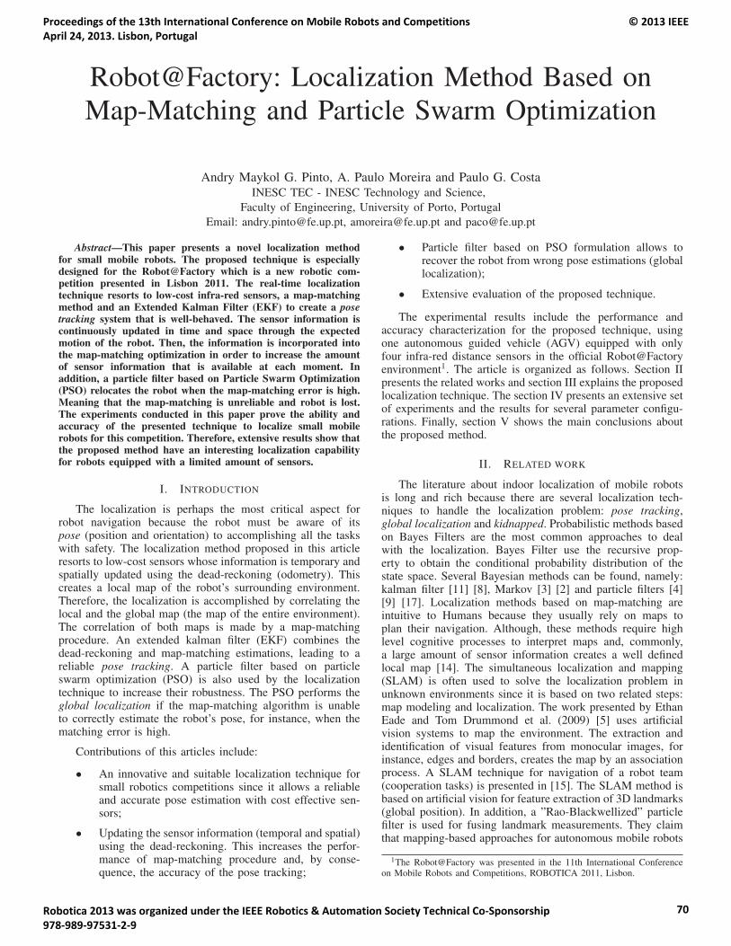
Robot@Factory: Localization Method Based onMap-Matching and Particle Swarm Optimization

Andry Maykol G. Pinto, A. Paulo Moreira and Paulo G. CostaINESC TEC - INESC Technology and Science,

Faculty of Engineering, University of Porto, Portugal

Email: [email protected], [email protected] and [email protected]

Abstract—This paper presents a novel localization methodfor small mobile robots. The proposed technique is especiallydesigned for the Robot@Factory which is a new robotic com-petition presented in Lisbon 2011. The real-time localizationtechnique resorts to low-cost infra-red sensors, a map-matchingmethod and an Extended Kalman Filter (EKF) to create a posetracking system that is well-behaved. The sensor information iscontinuously updated in time and space through the expectedmotion of the robot. Then, the information is incorporated intothe map-matching optimization in order to increase the amountof sensor information that is available at each moment. Inaddition, a particle filter based on Particle Swarm Optimization(PSO) relocates the robot when the map-matching error is high.Meaning that the map-matching is unreliable and robot is lost.The experiments conducted in this paper prove the ability andaccuracy of the presented technique to localize small mobilerobots for this competition. Therefore, extensive results show thatthe proposed method have an interesting localization capabilityfor robots equipped with a limited amount of sensors.

I. INTRODUCTION

The localization is perhaps the most critical aspect forrobot navigation because the robot must be aware of itspose (position and orientation) to accomplishing all the taskswith safety. The localization method proposed in this articleresorts to low-cost sensors whose information is temporary andspatially updated using the dead-reckoning (odometry). Thiscreates a local map of the robot’s surrounding environment.Therefore, the localization is accomplished by correlating thelocal and the global map (the map of the entire environment).The correlation of both maps is made by a map-matchingprocedure. An extended kalman filter (EKF) combines thedead-reckoning and map-matching estimations, leading to areliable pose tracking. A particle filter based on particleswarm optimization (PSO) is also used by the localizationtechnique to increase their robustness. The PSO performs theglobal localization if the map-matching algorithm is unableto correctly estimate the robot’s pose, for instance, when thematching error is high.

Contributions of this articles include:

• An innovative and suitable localization technique forsmall robotics competitions since it allows a reliableand accurate pose estimation with cost effective sen-sors;

• Updating the sensor information (temporal and spatial)using the dead-reckoning. This increases the perfor-mance of map-matching procedure and, by conse-quence, the accuracy of the pose tracking;

• Particle filter based on PSO formulation allows torecover the robot from wrong pose estimations (globallocalization);

• Extensive evaluation of the proposed technique.

The experimental results include the performance andaccuracy characterization for the proposed technique, usingone autonomous guided vehicle (AGV) equipped with onlyfour infra-red distance sensors in the official Robot@Factoryenvironment1. The article is organized as follows. Section IIpresents the related works and section III explains the proposedlocalization technique. The section IV presents an extensive setof experiments and the results for several parameter configu-rations. Finally, section V shows the main conclusions aboutthe proposed method.

II. RELATED WORK

The literature about indoor localization of mobile robotsis long and rich because there are several localization tech-niques to handle the localization problem: pose tracking,global localization and kidnapped. Probabilistic methods basedon Bayes Filters are the most common approaches to dealwith the localization. Bayes Filter use the recursive prop-erty to obtain the conditional probability distribution of thestate space. Several Bayesian methods can be found, namely:kalman filter [11] [8], Markov [3] [2] and particle filters [4][9] [17]. Localization methods based on map-matching areintuitive to Humans because they usually rely on maps toplan their navigation. Although, these methods require highlevel cognitive processes to interpret maps and, commonly,a large amount of sensor information creates a well definedlocal map [14]. The simultaneous localization and mapping(SLAM) is often used to solve the localization problem inunknown environments since it is based on two related steps:map modeling and localization. The work presented by EthanEade and Tom Drummond et al. (2009) [5] uses artificialvision systems to map the environment. The extraction andidentification of visual features from monocular images, forinstance, edges and borders, creates the map by an associationprocess. A SLAM technique for navigation of a robot team(cooperation tasks) is presented in [15]. The SLAM method isbased on artificial vision for feature extraction of 3D landmarks(global position). In addition, a ”Rao-Blackwellized” particlefilter is used for fusing landmark measurements. They claimthat mapping-based approaches for autonomous mobile robots

1The Robot@Factory was presented in the 11th International Conferenceon Mobile Robots and Competitions, ROBOTICA 2011, Lisbon.


© 2013 IEEE


70

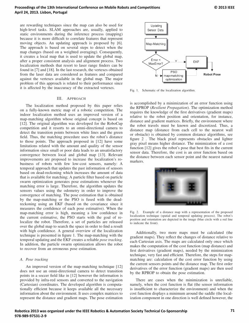
are rewarding techniques since the map can also be used forhigh-level tasks. SLAM approaches are, usually, applied tostatic environments during the inference process (mapping)because it is more difficult to correlate features that representmoving objects. An updating approach is proposed by [6].The approach is based on several steps to detect when themap changes (based on a weighted averaging). Consequently,it creates a local map that is used to update the global map,after a proper consistent analysis and alignment process. Twolocalization methods that resort to laser range finders can befound in [7] and [18]. In the last research, the vertexes obtainedfrom the laser data are considered as features and comparedagainst the vertexes available in the global map. The majorproblem of this approach is related to their performance sinceit is affected by the inaccuracy of the extracted vertexes.

III. APPROACH

The localization method proposed by this paper relieson a fully-known metric map of a robotic competition. Theindoor localization method uses an improved version of amap-matching algorithm whose original concept is based on[12]. The original algorithm was developed for the RoboCupcompetition and it resorts to an omni-directional camera todetect the transition points between white lines and the greenfield. Thus, the matching procedure uses the robot’s distanceto those points. The approach proposed in [12] have somelimitations related with the amount and quality of the sensorinformation since small or poor data leads to an unsatisfactoryconvergence between local and global map [13]. Relevantimprovements are proposed to increase the localization’s ro-bustness of robots with few low-cost sensors, namely: Atemporal approach that updates the past information of sensorsbased on dead-reckoning which increases the amount of datathat is available for matching; A particle filter based on particleswarm optimization generates pose estimations whenever thematching error is large. Therefore, the algorithm updates thesensors values using the odometry in order to improve theconvergence of matching. The pose estimation that is obtainedby the map-matching or the PSO is fused with the dead-reckoning using an EKF (based on the covariance since itmeasures the confidence of each pose estimative). When themap-matching error is high, meaning a low confidence inthe current estimative, the PSO starts with the goal of re-localize the robot. Therefore, a set of particles are releasedover the global map to search the space in order to find a resultwith high confidence. A general overview of the localizationtechnique is presented in figure 1. The map-matching with thetemporal updating and the EKF creates a reliable pose tracking.In addition, the particle swarm optimization allows the robotto recover from an erroneous pose estimation.

A. Pose tracking

An improved version of the map-matching technique [12]does not use an omni-directional camera to detect transitionpoints in a soccer field like in [12] however the information isprovided by infra-red sensors and converted to the navigation(Cartesian) coordinates. The developed algorithm is computa-tionally efficient because it keeps available all the necessaryinformation about the environment. It uses complex matrices torepresent the distance and gradient maps. The pose estimation

Fig. 1. Schematic of the localization algorithm.

is accomplished by a minimization of an error function usingthe RPROP (Resilient Propagation). The optimization methodrequires the knowledge of the first derivatives (gradient maps)relative to the robot position and orientation, for instance,distance and gradient matrices. Briefly, the environment wherethe robot travels must be known and discretized. Thus, adistance map (distance from each cell to the nearest wallor obstacle) is obtained by common distance algorithms, seefigure 2 . The black pixel represents obstacles and lightergray pixel means higher distance. The minimization of a costfunction [12] gives the robot’s pose that best fits in the currentsensor data. Therefore, the cost is an error function based onthe distance between each sensor point and the nearest naturalmarkers.

Fig. 2. Example of a distance map with a representation of the proposedlocalization technique (spatial and temporal updating process). The robot’sposition and orientation are depicted in the image (blue circle with a red lineto indicate the front).

Additionally, two more maps must be calculated (thegradient maps). They reflect the changes of distance relative toeach Cartesian axis. The maps are calculated only once whichmakes the computation of the cost function (map distance) andfirst derivatives (gradient maps), needed by the minimizationtechnique, very fast and efficient. Therefore, the steps for map-matching are: calculation of the cost error function by usingthe current sensors points and the distance map. The first orderderivatives of the error function (gradient maps) are then usedby the RPROP to obtain the pose estimation.

There are cases when the minimization is unreliable,namely, when the cost function is flat (the sensor informationis insufficient to characterize the environment) and when thecost function displays a minimum around the saddle (the local-ization component in one direction is well defined however, the


© 2013 IEEE


71

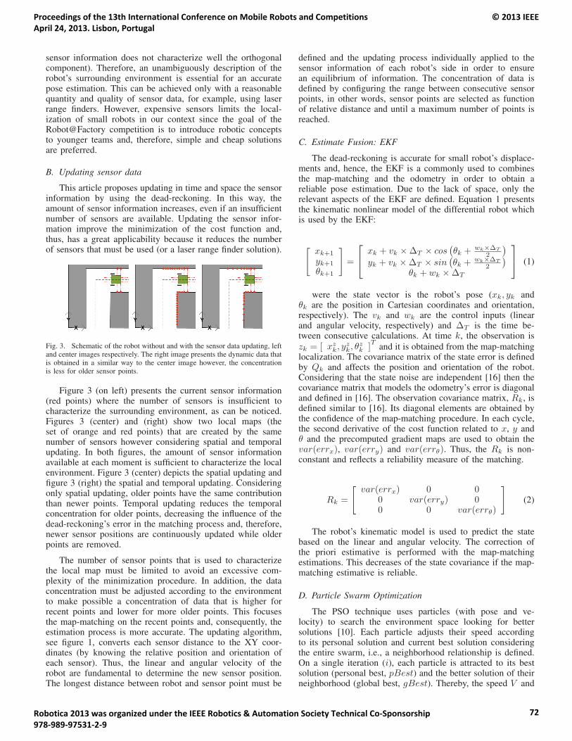
sensor information does not characterize well the orthogonalcomponent). Therefore, an unambiguously description of therobot’s surrounding environment is essential for an accuratepose estimation. This can be achieved only with a reasonablequantity and quality of sensor data, for example, using laserrange finders. However, expensive sensors limits the local-ization of small robots in our context since the goal of theRobot@Factory competition is to introduce robotic conceptsto younger teams and, therefore, simple and cheap solutionsare preferred.

B. Updating sensor data

This article proposes updating in time and space the sensorinformation by using the dead-reckoning. In this way, theamount of sensor information increases, even if an insufficientnumber of sensors are available. Updating the sensor infor-mation improve the minimization of the cost function and,thus, has a great applicability because it reduces the numberof sensors that must be used (or a laser range finder solution).

Fig. 3. Schematic of the robot without and with the sensor data updating, leftand center images respectively. The right image presents the dynamic data thatis obtained in a similar way to the center image however, the concentrationis less for older sensor points.

Figure 3 (on left) presents the current sensor information(red points) where the number of sensors is insufficient tocharacterize the surrounding environment, as can be noticed.Figures 3 (center) and (right) show two local maps (theset of orange and red points) that are created by the samenumber of sensors however considering spatial and temporalupdating. In both figures, the amount of sensor informationavailable at each moment is sufficient to characterize the localenvironment. Figure 3 (center) depicts the spatial updating andfigure 3 (right) the spatial and temporal updating. Consideringonly spatial updating, older points have the same contributionthan newer points. Temporal updating reduces the temporalconcentration for older points, decreasing the influence of thedead-reckoning’s error in the matching process and, therefore,newer sensor positions are continuously updated while olderpoints are removed.

The number of sensor points that is used to characterizethe local map must be limited to avoid an excessive com-plexity of the minimization procedure. In addition, the dataconcentration must be adjusted according to the environmentto make possible a concentration of data that is higher forrecent points and lower for more older points. This focusesthe map-matching on the recent points and, consequently, theestimation process is more accurate. The updating algorithm,see figure 1, converts each sensor distance to the XY coor-dinates (by knowing the relative position and orientation ofeach sensor). Thus, the linear and angular velocity of therobot are fundamental to determine the new sensor position.The longest distance between robot and sensor point must be

defined and the updating process individually applied to thesensor information of each robot’s side in order to ensurean equilibrium of information. The concentration of data isdefined by configuring the range between consecutive sensorpoints, in other words, sensor points are selected as functionof relative distance and until a maximum number of points isreached.

C. Estimate Fusion: EKF

The dead-reckoning is accurate for small robot’s displace-ments and, hence, the EKF is a commonly used to combinesthe map-matching and the odometry in order to obtain areliable pose estimation. Due to the lack of space, only therelevant aspects of the EKF are defined. Equation 1 presentsthe kinematic nonlinear model of the differential robot whichis used by the EKF:

[xk+1

yk+1

θk+1

]=

⎡⎣ xk + vk ×ΔT × cos

(θk + wk×ΔT

2

)yk + vk ×ΔT × sin

(θk + wk×ΔT

2

)θk + wk ×ΔT

⎤⎦ (1)

were the state vector is the robot’s pose (xk, yk andθk are the position in Cartesian coordinates and orientation,respectively). The vk and wk are the control inputs (linearand angular velocity, respectively) and ΔT is the time be-tween consecutive calculations. At time k, the observation iszk = [ xz

k, yzk, θ

zk ]

Tand it is obtained from the map-matching

localization. The covariance matrix of the state error is definedby Qk and affects the position and orientation of the robot.Considering that the state noise are independent [16] then thecovariance matrix that models the odometry’s error is diagonaland defined in [16]. The observation covariance matrix, Rk, isdefined similar to [16]. Its diagonal elements are obtained bythe confidence of the map-matching procedure. In each cycle,the second derivative of the cost function related to x, y andθ and the precomputed gradient maps are used to obtain thevar(errx), var(erry) and var(errθ). Thus, the Rk is non-constant and reflects a reliability measure of the matching.

Rk =

[var(errx) 0 0

0 var(erry) 00 0 var(errθ)

](2)

The robot’s kinematic model is used to predict the statebased on the linear and angular velocity. The correction ofthe priori estimative is performed with the map-matchingestimations. This decreases of the state covariance if the map-matching estimative is reliable.

D. Particle Swarm Optimization

The PSO technique uses particles (with pose and ve-locity) to search the environment space looking for bettersolutions [10]. Each particle adjusts their speed accordingto its personal solution and current best solution consideringthe entire swarm, i.e., a neighborhood relationship is defined.On a single iteration (i), each particle is attracted to its bestsolution (personal best, pBest) and the better solution of theirneighborhood (global best, gBest). Thereby, the speed V and


© 2013 IEEE


72

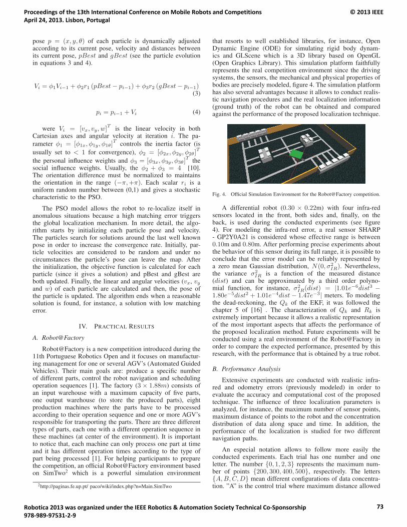
pose p = (x, y, θ) of each particle is dynamically adjustedaccording to its current pose, velocity and distances betweenits current pose, pBest and gBest (see the particle evolutionin equations 3 and 4).

Vi = φ1Vi−1 + φ2r1 (pBest− pi−1) + φ3r2 (gBest− pi−1)(3)

pi = pi−1 + Vi (4)

were Vi = [vx, vy, w]T

is the linear velocity in bothCartesian axes and angular velocity at iteration i. The pa-

rameter φ1 = [φ1x, φ1y, φ1θ]T

controls the inertia factor (is

usually set to < 1 for convergence), φ2 = [φ2x, φ2y, φ2θ]T

the personal influence weights and φ3 = [φ3x, φ3y, φ3θ]T

thesocial influence weights. Usually, the φ2 + φ3 = 4 [10].The orientation difference must be normalized to maintainsthe orientation in the range (−π,+π). Each scalar ri is auniform random number between (0,1) and gives a stochasticcharacteristic to the PSO.

The PSO model allows the robot to re-localize itself inanomalous situations because a high matching error triggersthe global localization mechanism. In more detail, the algo-rithm starts by initializing each particle pose and velocity.The particles search for solutions around the last well knownpose in order to increase the convergence rate. Initially, par-ticle velocities are considered to be random and under nocircumstances the particle’s pose can leave the map. Afterthe initialization, the objective function is calculated for eachparticle (since it gives a solution) and pBest and gBest areboth updated. Finally, the linear and angular velocities (vx, vyand w) of each particle are calculated and then, the pose ofthe particle is updated. The algorithm ends when a reasonablesolution is found, for instance, a solution with low matchingerror.

IV. PRACTICAL RESULTS

A. Robot@Factory

Robot@Factory is a new competition introduced during the11th Portuguese Robotics Open and it focuses on manufactur-ing management for one or several AGV’s (Automated GuidedVehicles). Their main goals are: produce a specific numberof different parts, control the robot navigation and schedulingoperation sequences [1]. The factory (3 × 1.88m) consists ofan input warehouse with a maximum capacity of five parts,one output warehouse (to store the produced parts), eightproduction machines where the parts have to be processedaccording to their operation sequence and one or more AGV’sresponsible for transporting the parts. There are three differenttypes of parts, each one with a different operation sequence inthese machines (at center of the environment). It is importantto notice that, each machine can only process one part at timeand it has different operation times according to the type ofpart being processed [1]. For helping participants to preparethe competition, an official Robot@Factory environment basedon SimTwo2 which is a powerful simulation environment

2http://paginas.fe.up.pt/ paco/wiki/index.php?n=Main.SimTwo

that resorts to well established libraries, for instance, OpenDynamic Engine (ODE) for simulating rigid body dynam-ics and GLScene which is a 3D library based on OpenGL(Open Graphics Library). This simulation platform faithfullyrepresents the real competition environment since the drivingsystems, the sensors, the mechanical and physical properties ofbodies are precisely modeled, figure 4. The simulation platformhas also several advantages because it allows to conduct realis-tic navigation procedures and the real localization information(ground truth) of the robot can be obtained and comparedagainst the performance of the proposed localization technique.

Fig. 4. Official Simulation Environment for the Robot@Factory competition.

A differential robot (0.30 × 0.22m) with four infra-redsensors located in the front, both sides and, finally, on theback, is used during the conducted experiments (see figure4). For modeling the infra-red error, a real sensor SHARP- GP2Y0A21 is considered whose effective range is between0.10m and 0.80m. After performing precise experiments aboutthe behavior of this sensor during its full range, it is possible toconclude that the error model can be reliably represented bya zero mean Gaussian distribution, N(0, σ2

IR). Nevertheless,the variance σ2

IR is a function of the measured distance(dist) and can be approximated by a third order polyno-mial function, for instance, σ2

IR(dist) = |1.01e−6dist3 −1.80e−5dist2 + 1.01e−4dist− 1.47e−3| meters. To modelingthe dead-reckoning, the Qk of the EKF, it was followed thechapter 5 of [16] . The characterization of Qk and Rk isextremely important because it allows a realistic representationof the most important aspects that affects the performance ofthe proposed localization method. Future experiments will beconducted using a real environment of the Robot@Factory inorder to compare the expected performance, presented by thisresearch, with the performance that is obtained by a true robot.

B. Performance Analysis

Extensive experiments are conducted with realistic infra-red and odometry errors (previously modeled) in order toevaluate the accuracy and computational cost of the proposedtechnique. The influence of three localization parameters isanalyzed, for instance, the maximum number of sensor points,maximum distance of points to the robot and the concentrationdistribution of data along space and time. In addition, theperformance of the localization is studied for two differentnavigation paths.

An especial notation allows to follow more easily theconducted experiments. Each trial has one number and oneletter. The number {0, 1, 2, 3} represents the maximum num-ber of points {200, 300, 400, 500}, respectively. The letters{A,B,C,D} mean different configurations of data concentra-tion. ”A” is the control trial where maximum distance allowed


© 2013 IEEE


73

is 1m and it has equal concentration of data for older andyounger points. ”B” represents the same than ”A” however,the maximum distance for the points is 1.5m. Experiments”C” and ”D” show the performance for different data concen-trations. Both represent higher concentration of younger sensorpoints than ”A” and ”B” however, the letter ”D” represents atrial with lower concentration for older data when comparedto ”C”.

Fig. 5. Experiment 2-C: Path 1 - direct movement between the top andbottom warehouses (top image). Path 2 - indirect movement (bottom image).The localization of the robot obtained by the proposed technique is representedin green and the ground truth in red.

Figure 5 shows the localization of the robot for twonavigation paths using the proposed technique with a 2-C con-figuration. Visually, the pose estimation (green) overrides theground truth (red) in almost the entire paths. Figure 2 depictsthe map-matching process using the updating process (sensorpoints are represented in blue). The robot is reaching the thirdstep according to the second path of the figure 5 (bottomimage). The updating procedure is extremely important for themap-matching because it allows a good characterization of thesurrounding environment with only four infra-red sensors.

Figure 6 shows quantitative results that were obtainedin both paths and for different configurations. The trial 3-B represents the worst case since the mean error is 0.07mand 4.8o with a standard deviation of 0.06m and 9o. Asexpected, there are differences between ”A”, ”B”, ”C and ”D”configurations. Experiments based on ’A” and ”B” usuallyhave position errors higher than ”C and ”D”. This is showin the graph of the position error. The reason for the higherperformance of configurations with less concentration of olderpoints is related to the dead-reckoning data that is used bythe updating process since more recent points are less affectedby the accumulation error. Large number of points or largemaximum distance lead to a higher accumulation of errorsbecause the estimation is highly influenced by distant and byolder points. This affects minimization process and decreasesthe matching accuracy. Thereby, parameters must be adjustedaccording to the environment topology.

Fig. 6. Graphical representation of the absolute mean (position and orienta-tion) error for several configurations and considering both paths.

Fig. 7. Longest cycle time for both paths and considering different trials(using a CPU Intel I3 M350, 2.75GHz).

The computational time in each conducted experiment isshown in figure 7. The localization of the robot is usuallyaccomplished in less than 40 milliseconds. Thus, the proposedlocalization technique reaches a real-time performance how-ever, the amount of sensor data used by the map-matchingincreases the time spent by the technique to estimate thelocalization of the robot. By increasing the concentration ofyounger and closer sensor points the processing time decreaseswithout a negative impact on the overall localization accuracy.Actually, the figure 6 shows lower errors in these situations(”C” and ”D”).

C. Particle Swarm Optimization

The PSO was not used in any circumstance during theprevious experiments and even for an additional free-pathnavigation experiment that was conducted for a large periodof time (2 hours). Therefore, a pose tracking error is simulatedin order to activate the re-localization mechanism. The errorconsists by adding 0.5m to the x-component, 0.8m to y-component and 90 degrees to the orientation of the currentpose. The symmetry of the Robot@Factory environment is amajor problem for the PSO formulation since there are at leasttwo possible matching solutions at each time. To avoid thisproblem, the particles’ searching space is initialized to an areaaround the last pose estimation with a low matching error. Thestopping criteria of the PSO is the number of iterations or themap-matching error being lower than a threshold.

The map-matching error is 1m and 90o around the second


© 2013 IEEE


74

Fig. 8. Distance error evolution (on the top) and orientation error evolution(on the bottom) of the map-matching in a kidnap situation. PSO configuredwith 15 particles, 30 iterations, φ1 = 1.2, φ2 = 1.5 and φ3 = 2.5.

33, see figure 8. This large error triggers the PSO which inless than 2 seconds reacquires one good pose estimation (thematching error decreases and the robot is relocated again). Thistwo seconds demonstrates the remarkable ability of the PSOto solve the global localization problem.

V. CONCLUSION

A real-time localization technique for the Robot@Factorycompetition is presented in this paper. It differs from othermethods since it combines a map-matching algorithm, spatialand temporal updating procedure and a particle filter based onparticle swarm optimization. The spatial and temporal updatingprocedure increases the amount of sensor information that isavailable and is used by the map-matching, avoiding the needfor many sensors or a laser range finder. The EKF combinesthe dead-reckoning with the map-matching pose estimation,leading to a reliable pose tracking. In addition, the PSO allowsto re-locate the robot when the map-matching returns an unreli-able pose estimation (the matching error is high) and, thereby,it is an important mechanism that searches the environmentlooking for a possible solution when the robot is completelylost. The conducted experiments prove the accuracy, flexibilityand robustness of the proposed technique since it achievesan error, usually, lower than 0.04m and 2degrees. Extensiveexperiments also prove the PSO capability to re-locate therobot in anomalous situations. Therefore, several importantimprovements are proposed in this article to increase theperformance of an efficient map-matching algorithm.

ACKNOWLEDGMENT

This work is partly funded by the Portuguese Governmentthrough FCT - Foundation for Science and Technology, SFRH-BD-70752-2010 and by the PRODUTECH PTI Project (no.13851) - New Processes and Innovative Technologies for theProduction Technologies Industry which is funded by the

Incentive System for Technology Research and Developmentin Companies, under the Competitive Factors Thematic Opera-tional Program of the Portuguese National Strategic ReferenceFramework and by the EU’s European Regional DevelopmentFund.

REFERENCES

[1] Andry Maykol Pinto and Luis F. Rocha and Antonio Paulo Moreiraand Paulo G. Costa. Shop Floor Scheduling in a Mobile RoboticEnvironment, In: EPIA 2011 - LNAI 7026 proceedings: Progress inArtificial Intelligence, Springer, 377-391, 2011

[2] Dieter Fox and Wolfram Burgard and Sebastian Thrun. Active MarkovLocalization for mobile robots. In: Robotics and Autonomous Systems,25:195-207, 1998.

[3] Dieter Fox and Sebastian Thrun and Wolfram Burgard. Markov Localiza-tion for Mobile Robots in Dynamic Environments. In: Elsevier Science:Journal of Artificial Intelligent Research, 11:391-427, 1999.

[4] Dieter Fox and Wolfram Burgard and Frank Dellaert e Sebastian Thrun.Monte carlo localization: Efficient position estimation for mobile robots.In: Sixteenth National Conference on Artificial Intelligence, 25:195-207,1999.

[5] Ethan Eade and Tom Drummond. Edge landmarks in monocular SLAM.In: Image and Vision Computing, 27:588-596, 2009.

[6] Fabrizio Abrate and Basilio Bona and Marina Indri and Stefano Rosa andF. Tibaldi. Map updating in dynamic environments. In: 41st InternationalSymposium on Robotics (ISR), 1-8, 2010.

[7] Fredy Tungadi, Wen L. Dennis Lui, Lindsay Kleeman and Ray Jarvis.Robust online map merging system using laser scan matching and omni-directional vision. In: IEEE/RSJ International Conference on IntelligentRobots and Systems (IROS), 7-14, 2010.

[8] J.J.Leonard and H.F. Durrant-White. A mobile robot localization bytracking geometric beacons. In: IEEE transactions on Robotics andAutomation, 3:376-382,1991.

[9] Jeong Woo and Young-Joong Kim and Jeong Lee and Myo-Taeg Lim.Localization of mobile robot using particle filter. In: SICEICASE Inter-national Joint Conference, 10:3031 - 3034, 2009.

[10] Kronfeld, Marcel and Weiss, Christian and Zell, Andreas. A DynamicSwarm for Visual Location Tracking. In: 6th International Conferenceon Ant Colony Optimization and Swarm Intelligence, 203-210, 2008

[11] L.Jetto and S.Longhi and D.Vitali. Localization of a wheeled mobilerobot by sensor data fusion based on a fuzzy logic adapted kalman filter.In: Elsevier Science: Control Engineering Practice, 7:763 - 771, 1999.

[12] M. Lauer, S. Lange and M. Riedmiller. Calculating the perfect match: anefficient and accurate approach for robot self-localization; Robot SoccerWorld, In RoboCup 2005, Cup IX , LNCS., Springer, 27:142153, 2005.

[13] Manuel Gouveia, A. Paulo Moreira, Paulo Costa, Luis P. Reis and Mar-cos Ferreira. Robustness and precision analysis in map-matching basedmobile robot self-localization. IRobot - 14th Portuguese Conference onArtificial Intelligent, EPIA 2009, Aveiro, 4:243-253, 2009

[14] Mohammed A. Quddus and Washington Y. Ochieng and Robert B.Noland. Current map-matching algorithms for transport applications:State-of-the art and future research directions. In: Elsevier Science:Transportation Research Part C: Emerging Technologies, 15:312-328,2007

[15] Monica Ballesta, Miguel Julia, Arturo Gil and Oscar Reinoso. Multi-robot visual slam using a Rao-blackwellized particle filter. In: ElsevierScience: Robotics and Autonomous Systems, 92:68-80, 2010.

[16] Sebastian Thrun and Wolfram Burgard and Dieter Fox. ProbabilisticRobotics, Cambridge (Mass.): MIT Press, first edition, 2005

[17] Sebastian Thrun and Dieter Fox and Wolfram Burgard and FrankDallaert. Robust Monte Carlo localization for mobile robots. In: ElsevierScience : Artificial Intelligent, 128:99-141, 2001

[18] Shung Han Cho and Sangjin Hong. Map Based Indoor Robot Nav-igation and Localization Using Laser Range Finder. In: InternationalConference on Control Automation, Robotics and Vision (ICARCV),1559 - 1564, 2010.


© 2013 IEEE


75

Multi-Robot Cooperative Stereo for OutdoorScenarios

A. Dias, J. Almeida, E. SilvaINESC TEC Robotics Unit

School of Engineering Polytechnic Institute of Porto

Email: adias, jma, [email protected]

P. LimaInstitute for Systems and Robotics

Instituto Superior Técnico (IST), Lisbon Portugal


Abstract—In this paper, we propose a cooperative perceptionframework for multi-robot real-time 3D high dynamic targetestimation in outdoor scenarios based on monocular cameraavailable on each robot. The relative position and orientationbetween robots establishes a flexible and dynamic stereo baseline.Overlap views subject to geometric constraints emerged from thestereo formulation, which allowed us to obtain a decentralizedcooperative perception layer. Epipolar constraints related to theglobal frame are applied both in image feature matching andto feature searching and detection optimization in the imageprocessing of robots with low computational capabilities. Incontrast to classic stereo, the proposed framework considersall sources of uncertainty (in localization, attitude and imagedetection from both robots) in the determination of the objectsbest 3D localization and its uncertainty. The proposed frameworkcan be later integrated in a decentralized data fusion (DDF)multi-target tracking approach where it can contribute to reducerumor propagation data association and track initialization issues.We demonstrate the advantages of this approach in real outdoorscenario. This is done by comparing a stereo rigid baseline stan-dalone target tracking with the proposed multi-robot cooperativestereo between a micro aerial vehicle (MAV) and an autonomousground vehicle (AGV).

I. INTRODUCTION

In recent years, we have seen a growing research effort on

novel multi-robot cooperative tasks for heterogeneous mobile

robotics applications. This ongoing development is driven by

a significant number of potential end-user applications, where

is necessary to reduce the human in the loop interaction

which includes large-scale sensing operations[12], cooperative

search and rescue tasks[5], surveillance[7], recognition recon-

naissance and border control[8]. Currently, mobile robots em-

ployed on these high-end user applications are equipped with

state-of-the art sensing equipment allowing them to navigate

and perceive their surrounding environment. One of the most

common and versatile means of perception in mobile robotics

applications is visual sensing with one or more cameras which

are able to acquire visual information[13] based on cooperative

approaches. Taking this a step further, here we address an

outdoor multi-robot scenario without localization issues, with

the surveillance task goal of detecting and estimating 3D high

dynamic targets positions behavior in a cooperative vision

flexible and dynamic stereo baseline framework.State of art approaches to enumerated end-user applications

can be organized according to cooperative tasks emerged from

local or cooperative perception.

In local perception approach, each robot is capable of

detecting and locating targets, sharing that information over

some communication middleware that can be later used to

some cooperative mechanism for task allocations[10].

Considering the proposal scenario, those approaches present

several limitations in any possible vision setups: monocular

or stereo rig baseline. In monocular vision, we have the

intrinsic difficulty in estimating depth and absolute scale[1],

so 3D target estimation without target known size is a re-

search challenge. Techniques like SFM(struture-from-motion)

or SLAM(Simultaneous localization and mapping) are able

to estimate depth from a monocular camera[6][3], but the

scene must have a large field of view and motion must not

occur along the optical axis and preferably parallax motion

to allow a fast uncertainty map convergence[1]. SLAM tech-

niques are able to obtain good results in depth estimation for

indoor and even in outdoor map building scenarios although

with constraints such as high computational requirements (not

available in most of the robots with low payload), lower

camera dynamic, preferably with features loop closing and

large field of view, but unable to track targets with high

dynamic behavior. Still with monocular vision and for a

particularly case of aerial vehicles depth estimation can be

obtained based on flat earth assumption[2]. Although it is

simple, its application is limited to tracking objects on the

ground with low accuracy and not applied to our addresses

scenario. Regarding stereo rig baseline, 3D target estimation

is a well known solution due to its relatively simple image

scale and depth estimation although with limited application

when the goal is to track targets whose depth distance greatly

exceeds the available stereo rig baseline, therefore reducing the

stereo setup to a bearing-only sensor[15]. The estimation error

grows quadratically with the depth[15][4], becoming even

more relevant this limitation when the robot majority tends to

decrease its scale factor and consequently smaller rig baseline.

The enumerated limitations strengthens our proposal by having

a multi-robot monocular approach with a flexible and dynamic

baseline between robots able estimate 3D information from

correlated detected targets.

Focusing now in cooperative perception approaches, char-

acterized by each robot, available at the multi-robot forma-

tion, builds its own local partial representation of the world,

described by the belief state and share in order to improve


© 2013 IEEE


76

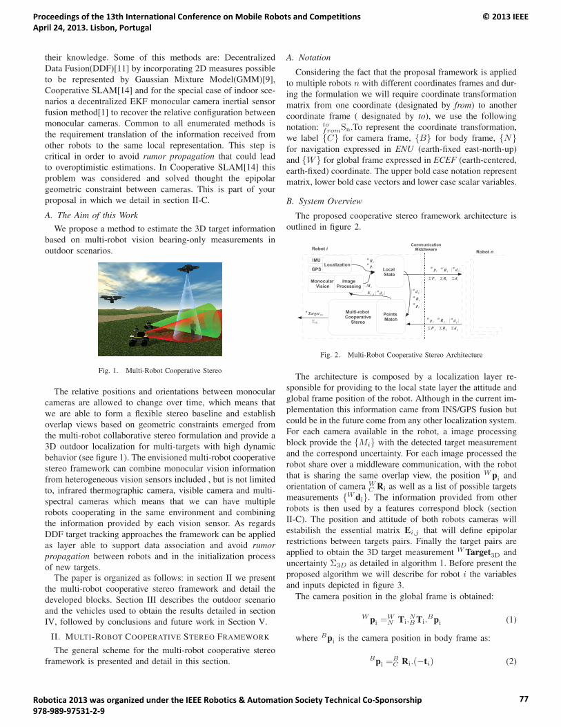
their knowledge. Some of this methods are: Decentralized

Data Fusion(DDF)[11] by incorporating 2D measures possible

to be represented by Gaussian Mixture Model(GMM)[9],

Cooperative SLAM[14] and for the special case of indoor sce-

narios a decentralized EKF monocular camera inertial sensor

fusion method[1] to recover the relative configuration between

monocular cameras. Common to all enumerated methods is

the requirement translation of the information received from

other robots to the same local representation. This step is

critical in order to avoid rumor propagation that could lead

to overoptimistic estimations. In Cooperative SLAM[14] this

problem was considered and solved thought the epipolar

geometric constraint between cameras. This is part of your

proposal in which we detail in section II-C.

A. The Aim of this WorkWe propose a method to estimate the 3D target information

based on multi-robot vision bearing-only measurements in

outdoor scenarios.

Fig. 1. Multi-Robot Cooperative Stereo

The relative positions and orientations between monocular

cameras are allowed to change over time, which means that

we are able to form a flexible stereo baseline and establish

overlap views based on geometric constraints emerged from

the multi-robot collaborative stereo formulation and provide a

3D outdoor localization for multi-targets with high dynamic

behavior (see figure 1). The envisioned multi-robot cooperative

stereo framework can combine monocular vision information

from heterogeneous vision sensors included , but is not limited

to, infrared thermographic camera, visible camera and multi-

spectral cameras which means that we can have multiple

robots cooperating in the same environment and combining

the information provided by each vision sensor. As regards

DDF target tracking approaches the framework can be applied

as layer able to support data association and avoid rumorpropagation between robots and in the initialization process

of new targets.The paper is organized as follows: in section II we present

the multi-robot cooperative stereo framework and detail the

developed blocks. Section III describes the outdoor scenario

and the vehicles used to obtain the results detailed in section

IV, followed by conclusions and future work in Section V.

II. MULTI-ROBOT COOPERATIVE STEREO FRAMEWORK

The general scheme for the multi-robot cooperative stereo

framework is presented and detail in this section.

A. Notation

Considering the fact that the proposal framework is applied

to multiple robots n with different coordinates frames and dur-

ing the formulation we will require coordinate transformation

matrix from one coordinate (designated by from) to another

coordinate frame ( designated by to), we use the following

notation: tofromSn.To represent the coordinate transformation,

we label {C} for camera frame, {B} for body frame, {N}for navigation expressed in ENU (earth-fixed east-north-up)

and {W} for global frame expressed in ECEF (earth-centered,

earth-fixed) coordinate. The upper bold case notation represent

matrix, lower bold case vectors and lower case scalar variables.

B. System Overview

The proposed cooperative stereo framework architecture is

outlined in figure 2.

Fig. 2. Multi-Robot Cooperative Stereo Architecture

The architecture is composed by a localization layer re-

sponsible for providing to the local state layer the attitude and

global frame position of the robot. Although in the current im-

plementation this information came from INS/GPS fusion but

could be in the future come from any other localization system.

For each camera available in the robot, a image processing

block provide the {Mi} with the detected target measurement

and the correspond uncertainty. For each image processed the

robot share over a middleware communication, with the robot

that is sharing the same overlap view, the position W pi and

orientation of camera WC Ri as well as a list of possible targets

measurements {W di}. The information provided from other

robots is then used by a features correspond block (section

II-C). The position and attitude of both robots cameras will

estabilish the essential matrix Ei,j that will define epipolar

restrictions between targets pairs. Finally the target pairs are

applied to obtain the 3D target measurement W Target3D and

uncertainty Σ3D as detailed in algorithm 1. Before present the

proposed algorithm we will describe for robot i the variables

and inputs depicted in figure 3.

The camera position in the global frame is obtained:

W pi =WN Ti.

NB Ti.

Bpi (1)

where Bpi is the camera position in body frame as:

Bpi =BC Ri.(−ti) (2)


© 2013 IEEE


77

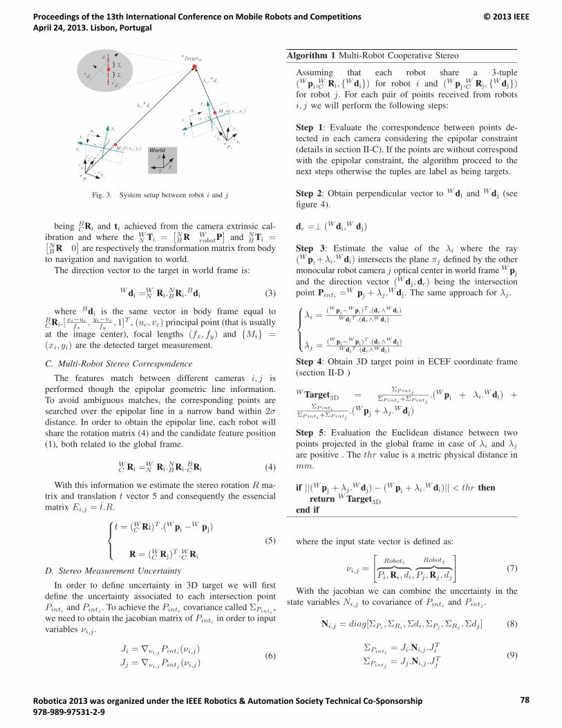
Fig. 3. System setup between robot i and j

being BCRi and ti achieved from the camera extrinsic cal-

ibration and where the WN Ti =

[NB R W

robotP]

and NB Ti =[

NB R 0

]are respectively the transformation matrix from body

to navigation and navigation to world.

The direction vector to the target in world frame is:

W di =WN Ri.

NB Ri.

Bdi (3)

where Bdi is the same vector in body frame equal toBCRi.[

xi−uc

fx, yi−vc

fy, 1]T , (uc, vc) principal point (that is usually

at the image center), focal lengths (fx, fy) and {Mi} =(xi, yi) are the detected target measurement.

C. Multi-Robot Stereo Correspondence

The features match between different cameras i, j is

performed though the epipolar geometric line information.

To avoid ambiguous matches, the corresponding points are

searched over the epipolar line in a narrow band within 2σdistance. In order to obtain the epipolar line, each robot will

share the rotation matrix (4) and the candidate feature position

(1), both related to the global frame.

WC Ri =

WN Ri.

NB Ri.

BCRi (4)

With this information we estimate the stereo rotation R ma-

trix and translation t vector 5 and consequently the essencial

matrix Ei,j = t.R.⎧⎪⎨⎪⎩t = (WC Ri)T .(W pi −W pj)

R = (WC Rj)T .WC Ri

(5)

D. Stereo Measurement Uncertainty

In order to define uncertainty in 3D target we will first

define the uncertainty associated to each intersection point

Pinti and Pintj . To achieve the Pinti covariance called ΣPinti,

we need to obtain the jacobian matrix of Pinti in order to input

variables νi,j .

Ji = ∇νi,jPinti(νi,j)

Jj = ∇νi,jPintj (νi,j)

(6)

Algorithm 1 Multi-Robot Cooperative Stereo

Assuming that each robot share a 3-tuple

(W pi,WC Ri, {W di}) for robot i and (W pj,

WC Rj, {W dj})

for robot j. For each pair of points received from robots

i, j we will perform the following steps:

Step 1: Evaluate the correspondence between points de-

tected in each camera considering the epipolar constraint

(details in section II-C). If the points are without correspond

with the epipolar constraint, the algorithm proceed to the

next steps otherwise the tuples are label as being targets.

Step 2: Obtain perpendicular vector to W di and W dj (see

figure 4).

dc =⊥ (W di,W dj)

Step 3: Estimate the value of the λi where the ray

(W pi+λi.W di) intersects the plane πj defined by the other

monocular robot camera j optical center in world frame W pj

and the direction vector (W dj, dc) being the intersection

point Pinti =W pj + λj .

W dj. The same approach for λj .⎧⎪⎪⎨⎪⎪⎩λi =

(W pj−W pi)T .(dc∧W di)

W diT .(dc∧W di)

λj =(W pi−W pi)

T .(dc∧W dj)W dj

T .(dc∧W dj)

Step 4: Obtain 3D target point in ECEF coordinate frame

(section II-D )

W Target3D =ΣPintj

ΣPinti+ΣPintj

.(W pi + λi.W di) +

ΣPinti

ΣPinti+ΣPintj

.(W pj + λj .W dj)

Step 5: Evaluation the Euclidean distance between two

points projected in the global frame in case of λi and λj

are positive . The thr value is a metric physical distance in

mm.

if ||(W pj + λj .W dj)− (W pi + λi.

W di)|| < thr thenreturn W Target3D

end if

where the input state vector is defined as:

νi,j =

[Roboti︷︸︸︷

Pi,Ri, di,

Robotj︷︸︸︷Pj ,Rj , dj

](7)

With the jacobian we can combine the uncertainty in the

state variables Ni,j to covariance of Pinti and Pintj .

Ni,j = diag[ΣPi ,ΣRi ,Σdi,ΣPj ,ΣRj ,Σdj ] (8)

ΣPinti= Ji.Ni,j .J

Ti

ΣPintj= Jj .Ni,j .J

Tj

(9)


© 2013 IEEE


78

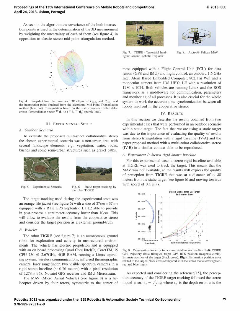
As seen in the algorithm the covariance of the both intersec-

tion points is used in the determination of the 3D measurement

by weighting the uncertainty of each of them (see figure 4) in

opposition to classic stereo mid-point triangulation method.

Fig. 4. Snapshot from the covariance 3D ellipse of Pinti and Pintj andthe intersection point obtained from the algorithm. Mid-Point Triangulationmethod (blue dot). Triangulation based on the state covariance value (bluecross). Perpendicular vector W dc to (W di,

W dj) (purple line).

III. EXPERIMENTAL SETUP

A. Outdoor Scenario

To evaluate the proposed multi-robot collaborative stereo

the chosen experimental scenario was a non-urban area with

several landscape elements, e.g., vegetation, water, rocks,

bushes and some semi-urban structures such as gravel paths.

Fig. 5. Experimental Scenario Fig. 6. Static target tracking bythe robot TIGRE

The target tracking used during the experimental tests was

an orange life jacket (see figure 6) with a size of 37cm×67cmequipped with a RTK GPS Septentrio L1 L2 able to provide

in post-process a centimeter-accuracy lower than 10cm. This

will allow to evaluate the results from the cooperative stereo

and consider the target position as a external ground-truth.

B. Vehicles

The robot TIGRE (see figure 7) is an autonomous ground

robot for exploration and activity in unstructured environ-

ments. The vehicle has electric propulsion and is equipped

with an on board processing Quad Core Intel(R) Core(TM) i5

CPU 750 @ 2.67GHz, 4GB RAM, running a Linux operat-

ing system, wireless communications, infra-red thermographic

camera, laser rangefinder, two visible spectrum cameras in a

rigid stereo baseline (∼ 0.76 meters) with a pixel resolution

of 1278× 958, Novatel GPS receiver and IMU Microstrain.

The MAV (Micro Aerial Vehicle) (see figure 8) is a he-

licopter driven by four rotors, symmetric to the center of

Fig. 7. TIGRE - Terrestrial Intel-ligent Ground Robotic Explorer

Fig. 8. Asctec@ Pelican MAV

mass equipped with a Flight Control Unit (FCU) for data

fusion (GPS and IMU) and flight control, an onboard 1.6 GHz

Intel Atom Based Embedded Computer, 802.11n Wifi and a

monocular camera from IDS UEYe LE with a resolution of

1280 × 1024. Both vehicles are running Linux and the ROS

framework as a middleware for communication, parameters

and monitoring of all processes. It is also crucial for the whole

system to work the accurate time synchronization between all

robots involved in the cooperative stereo.

IV. RESULTS

In this section we describe the results obtained from two

experimental cases that were performed in an outdoor scenario

with a static target. The fact that we are using a static target

was due to the importance of evaluating the quality of results

from stereo triangulation with a rigid baseline (IV-A) and the

paper proposal method with a multi-robot collaborative stereo

(IV-B) in a similar context able to be reproduced.

A. Experiment I: Stereo rigid known baseline

For this experimental case, a stereo rigid baseline available

at TIGRE was used to track the target. This means that the

MAV was not available, so the results will express the quality

of perception from TIGRE that was at a distance of ∼ 35meters from the static target (see figure 6) and moving towards

with speed of 0.4 m/s.

−8.6829−8.6829−8.682841.1693

41.1694

41.1695

41.1696

41.1697

41.1698

41.1699

Longitude

Lat

itu

de

5 10 15 20 25 30 350

2

4

6

8

10

12

14

Euclidean distance Target/TIGRE

Err

or

(met

ers)

Stereo Model error Vs Target Estimation Error

Fig. 9. Target estimation error for a stereo rigid known baseline. Left: TIGREGPS trajectory (blue triangle), target GPS RTK position (magenta circle).Estimate position of the target (black cross). Right: Estimation position errorrelated to the target (black cross) compared with the stereo model error (green,red and blue lines).

As expected and considering the reference[15], the percep-

tion accuracy of the TIGRE target tracking followed the stereo

model error: εz = z2

b.f .εd where εz is the depth error, z is the


© 2013 IEEE


79

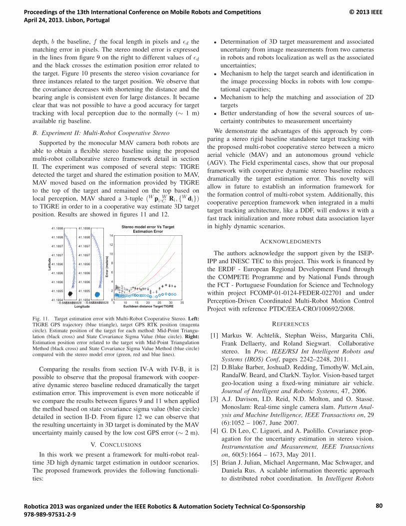
depth, b the baseline, f the focal length in pixels and εd the

matching error in pixels. The stereo model error is expressed

in the lines from figure 9 on the right to different values of εdand the black crosses the estimation position error related to

the target. Figure 10 presents the stereo vision covariance for

three instances related to the target position. We observe that

the covariance decreases with shortening the distance and the

bearing angle is consistent even for large distances. It became

clear that was not possible to have a good accuracy for target

tracking with local perception due to the normally (∼ 1 m)

available rig baseline.

B. Experiment II: Multi-Robot Cooperative Stereo

Supported by the monocular MAV camera both robots are

able to obtain a flexible stereo baseline using the proposed

multi-robot collaborative stereo framework detail in section

II. The experiment was composed of several steps: TIGRE

detected the target and shared the estimation position to MAV,

MAV moved based on the information provided by TIGRE

to the top of the target and remained on the top based on

local perception, MAV shared a 3-tuple (W pi,WC Ri, {W di})

to TIGRE in order to in a cooperative way estimate 3D target

position. Results are showed in figures 11 and 12.

−8.6829−8.6829−8.682841.1694

41.1695

41.1696

41.1696

41.1696

41.1697

41.1697

41.1698

41.1698

Longitude

Lat

itu

de

−8.6829−8.6829−8.682841.1694

41.1695

41.1696

41.1696

41.1696

41.1697

41.1697

41.1698

41.1698

5 10 15 20 25 30 350

2

4

6

8

10

12

14

Euclidean distance Target/TIGRE

Err

or

(met

ers)

Stereo model error Vs Target Estimation Error

Fig. 11. Target estimation error with Multi-Robot Cooperative Stereo. Left:TIGRE GPS trajectory (blue triangle), target GPS RTK position (magentacircle). Estimate position of the target for each method: Mid-Point Triangu-lation (black cross) and State Covariance Sigma Value (blue circle). Right:Estimation position error related to the target with Mid-Point TriangulationMethod (black cross) and State Covariance Sigma Value Method (blue circle)compared with the stereo model error (green, red and blue lines).

Comparing the results from section IV-A with IV-B, it is

possible to observe that the proposal framework with cooper-

ative dynamic stereo baseline reduced dramatically the target

estimation error. This improvement is even more noticeable if

we compare the results between figures 9 and 11 when applied

the method based on state covariance sigma value (blue circle)

detailed in section II-D. From figure 12 we can observe that

the resulting uncertainty in 3D target is dominated by the MAV

uncertainty mainly caused by the low cost GPS error (∼ 2 m).

V. CONCLUSIONS

In this work we present a framework for multi-robot real-

time 3D high dynamic target estimation in outdoor scenarios.

The proposed framework provides the following functionali-

ties:

• Determination of 3D target measurement and associated

uncertainty from image measurements from two cameras

in robots and robots localization as well as the associated

uncertainties;

• Mechanism to help the target search and identification in

the image processing blocks in robots with low compu-

tational capacities;

• Mechanism to help the matching and association of 2D

targets

• Better understanding of how the several sources of un-

certainty contributes to measurement uncertainty

We demonstrate the advantages of this approach by com-

paring a stereo rigid baseline standalone target tracking with

the proposed multi-robot cooperative stereo between a micro

aerial vehicle (MAV) and an autonomous ground vehicle

(AGV). The Field experimental cases, show that our proposal

framework with cooperative dynamic stereo baseline reduces

dramatically the target estimation error. This novelty will

allow in future to establish an information framework for

the formation control of multi-robot system. Additionally, this

cooperative perception framework when integrated in a multi

target tracking architecture, like a DDF, will endows it with a

fast track initialization and more robust data association layer

in highly dynamic scenarios.

ACKNOWLEDGMENTS

The authors acknowledge the support given by the ISEP-

IPP and INESC TEC to this project. This work is financed by

the ERDF - European Regional Development Fund through

the COMPETE Programme and by National Funds through

the FCT - Portuguese Foundation for Science and Technology

within project FCOMP-01-0124-FEDER-022701 and under

Perception-Driven Coordinated Multi-Robot Motion Control

Project with reference PTDC/EEA-CRO/100692/2008.

REFERENCES

[1] Markus W. Achtelik, Stephan Weiss, Margarita Chli,

Frank Dellaerty, and Roland Siegwart. Collaborative

stereo. In Proc. IEEE/RSJ Int Intelligent Robots andSystems (IROS) Conf, pages 2242–2248, 2011.

[2] D.Blake Barber, JoshuaD. Redding, TimothyW. McLain,

RandalW. Beard, and ClarkN. Taylor. Vision-based target

geo-location using a fixed-wing miniature air vehicle.

Journal of Intelligent and Robotic Systems, 47, 2006.

[3] A.J. Davison, I.D. Reid, N.D. Molton, and O. Stasse.

Monoslam: Real-time single camera slam. Pattern Anal-ysis and Machine Intelligence, IEEE Transactions on, 29

(6):1052 – 1067, June 2007.

[4] G. Di Leo, C. Liguori, and A. Paolillo. Covariance prop-

agation for the uncertainty estimation in stereo vision.

Instrumentation and Measurement, IEEE Transactionson, 60(5):1664 – 1673, May 2011.

[5] Brian J. Julian, Michael Angermann, Mac Schwager, and

Daniela Rus. A scalable information theoretic approach

to distributed robot coordination. In Intelligent Robots


© 2013 IEEE


80

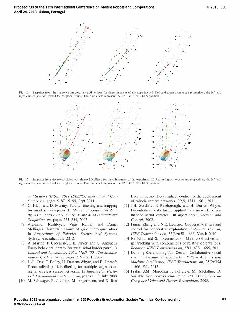
Fig. 10. Snapshot from the stereo vision covariance 3D ellipse for three instances of the experiment I. Red and green crosses are respectively the left andright camera position related to the global frame. The blue circle represent the TARGET RTK GPS position.

Fig. 12. Snapshot from the stereo vision covariance 3D ellipse for three instances of the experiment II. Red and green crosses are respectively the left andright camera position related to the global frame. The blue circle represent the TARGET RTK GPS position.

and Systems (IROS), 2011 IEEE/RSJ International Con-ference on, pages 5187 –5194, Sept 2011.

[6] G. Klein and D. Murray. Parallel tracking and mapping

for small ar workspaces. In Mixed and Augmented Real-ity, 2007. ISMAR 2007. 6th IEEE and ACM InternationalSymposium on, pages 225–234, 2007.

[7] Aleksandr Kushleyev, Vijay Kumar, and Daniel

Mellinger. Towards a swarm of agile micro quadrotors.

In Proceedings of Robotics: Science and Systems,

Sydney, Australia, July 2012.

[8] A. Marino, F. Caccavale, L.E. Parker, and G. Antonelli.

Fuzzy behavioral control for multi-robot border patrol. In

Control and Automation, 2009. MED ’09. 17th Mediter-ranean Conference on, pages 246 – 251, 2009.

[9] L.-L. Ong, T. Bailey, H. Durrant-Whyte, and B. Upcroft.

Decentralised particle filtering for multiple target track-

ing in wireless sensor networks. In Information Fusion11th International Conference on, pages 1 – 8, July 2008.

[10] M. Schwager, B. J. Julian, M. Angermann, and D. Rus.

Eyes in the sky: Decentralized control for the deployment

of robotic camera networks. 99(9):1541–1561, 2011.

[11] J.H. Sutcliffe, P. Riseborough, and H. Durrant-Whyte.

Decentralised data fusion applied to a network of un-

manned aerial vehicles. In Information, Decision andControl, 2002.

[12] Fumin Zhang and N.E. Leonard. Cooperative filters and

control for cooperative exploration. Automatic Control,IEEE Transactions on, 55(3):650 – 663, March 2010.

[13] Ke Zhou and S.I. Roumeliotis. Multirobot active tar-

get tracking with combinations of relative observations.

Robotics, IEEE Transactions on, 27(4):678 – 695, 2011.

[14] Danping Zou and Ping Tan. Coslam: Collaborative visual

slam in dynamic environments. Pattern Analysis andMachine Intelligence, IEEE Transactions on, 35(2):354

– 366, Feb. 2013.

[15] Frahm J.M. Mordohai P. Pollefeys M. ïz£Gallup, D.

Variable baseline/resolution stereo. IEEE Conference onComputer Vision and Pattern Recognition, 2008.


© 2013 IEEE


81

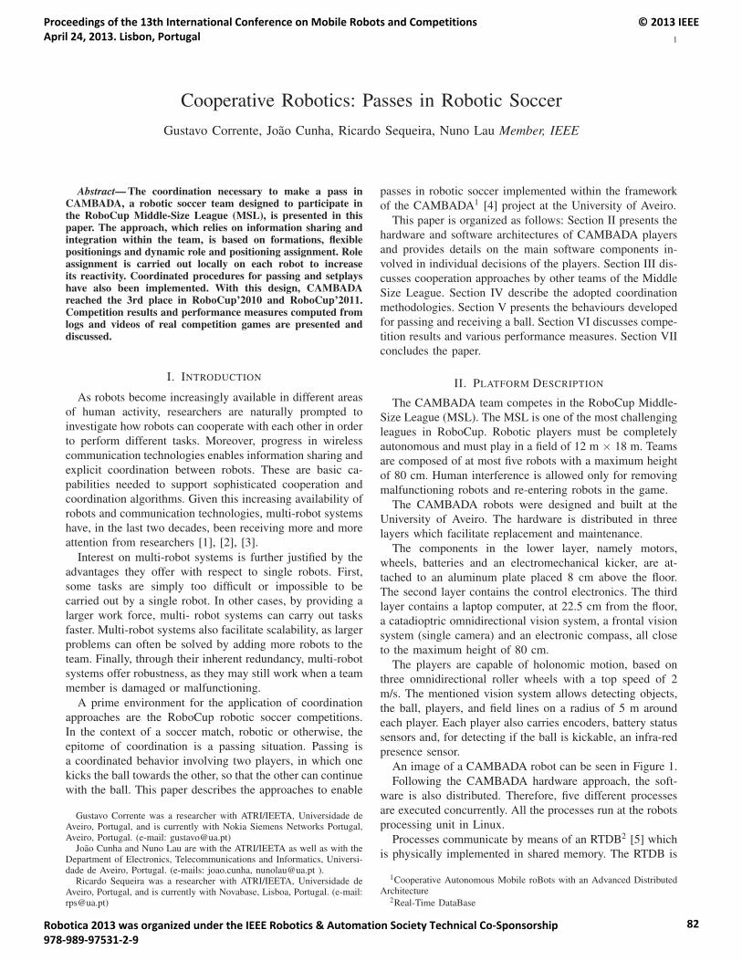
1

Cooperative Robotics: Passes in Robotic Soccer

Gustavo Corrente, Joao Cunha, Ricardo Sequeira, Nuno Lau Member, IEEE

Abstract— The coordination necessary to make a pass inCAMBADA, a robotic soccer team designed to participate inthe RoboCup Middle-Size League (MSL), is presented in thispaper. The approach, which relies on information sharing andintegration within the team, is based on formations, flexiblepositionings and dynamic role and positioning assignment. Roleassignment is carried out locally on each robot to increaseits reactivity. Coordinated procedures for passing and setplayshave also been implemented. With this design, CAMBADAreached the 3rd place in RoboCup’2010 and RoboCup’2011.Competition results and performance measures computed fromlogs and videos of real competition games are presented anddiscussed.

I. INTRODUCTION

As robots become increasingly available in different areas

of human activity, researchers are naturally prompted to

investigate how robots can cooperate with each other in order

to perform different tasks. Moreover, progress in wireless

communication technologies enables information sharing and

explicit coordination between robots. These are basic ca-

pabilities needed to support sophisticated cooperation and

coordination algorithms. Given this increasing availability of

robots and communication technologies, multi-robot systems

have, in the last two decades, been receiving more and more

attention from researchers [1], [2], [3].

Interest on multi-robot systems is further justified by the

advantages they offer with respect to single robots. First,

some tasks are simply too difficult or impossible to be

carried out by a single robot. In other cases, by providing a

larger work force, multi- robot systems can carry out tasks

faster. Multi-robot systems also facilitate scalability, as larger

problems can often be solved by adding more robots to the

team. Finally, through their inherent redundancy, multi-robot

systems offer robustness, as they may still work when a team

member is damaged or malfunctioning.

A prime environment for the application of coordination

approaches are the RoboCup robotic soccer competitions.

In the context of a soccer match, robotic or otherwise, the

epitome of coordination is a passing situation. Passing is

a coordinated behavior involving two players, in which one

kicks the ball towards the other, so that the other can continue

with the ball. This paper describes the approaches to enable

Gustavo Corrente was a researcher with ATRI/IEETA, Universidade deAveiro, Portugal, and is currently with Nokia Siemens Networks Portugal,Aveiro, Portugal. (e-mail: [email protected])

Joao Cunha and Nuno Lau are with the ATRI/IEETA as well as with theDepartment of Electronics, Telecommunications and Informatics, Universi-dade de Aveiro, Portugal. (e-mails: joao.cunha, [email protected] ).

Ricardo Sequeira was a researcher with ATRI/IEETA, Universidade deAveiro, Portugal, and is currently with Novabase, Lisboa, Portugal. (e-mail:[email protected])

passes in robotic soccer implemented within the framework

of the CAMBADA1 [4] project at the University of Aveiro.

This paper is organized as follows: Section II presents the

hardware and software architectures of CAMBADA players

and provides details on the main software components in-

volved in individual decisions of the players. Section III dis-

cusses cooperation approaches by other teams of the Middle

Size League. Section IV describe the adopted coordination

methodologies. Section V presents the behaviours developed

for passing and receiving a ball. Section VI discusses compe-

tition results and various performance measures. Section VII

concludes the paper.

II. PLATFORM DESCRIPTION

The CAMBADA team competes in the RoboCup Middle-

Size League (MSL). The MSL is one of the most challenging

leagues in RoboCup. Robotic players must be completely

autonomous and must play in a field of 12 m × 18 m. Teams

are composed of at most five robots with a maximum height

of 80 cm. Human interference is allowed only for removing

malfunctioning robots and re-entering robots in the game.

The CAMBADA robots were designed and built at the

University of Aveiro. The hardware is distributed in three

layers which facilitate replacement and maintenance.

The components in the lower layer, namely motors,

wheels, batteries and an electromechanical kicker, are at-

tached to an aluminum plate placed 8 cm above the floor.

The second layer contains the control electronics. The third

layer contains a laptop computer, at 22.5 cm from the floor,

a catadioptric omnidirectional vision system, a frontal vision

system (single camera) and an electronic compass, all close

to the maximum height of 80 cm.

The players are capable of holonomic motion, based on

three omnidirectional roller wheels with a top speed of 2

m/s. The mentioned vision system allows detecting objects,

the ball, players, and field lines on a radius of 5 m around

each player. Each player also carries encoders, battery status

sensors and, for detecting if the ball is kickable, an infra-red

presence sensor.

An image of a CAMBADA robot can be seen in Figure 1.

Following the CAMBADA hardware approach, the soft-

ware is also distributed. Therefore, five different processes

are executed concurrently. All the processes run at the robots

processing unit in Linux.

Processes communicate by means of an RTDB2 [5] which

is physically implemented in shared memory. The RTDB is

1Cooperative Autonomous Mobile roBots with an Advanced DistributedArchitecture

2Real-Time DataBase


© 2013 IEEE


82

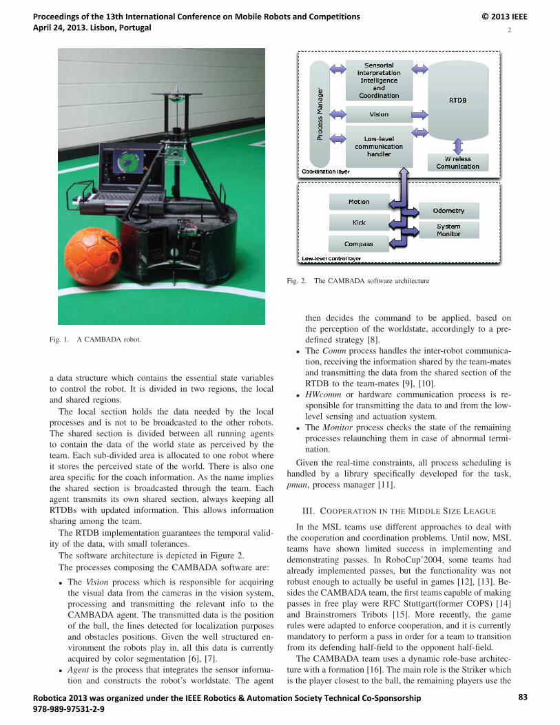
2

Fig. 1. A CAMBADA robot.

a data structure which contains the essential state variables

to control the robot. It is divided in two regions, the local

and shared regions.

The local section holds the data needed by the local

processes and is not to be broadcasted to the other robots.

The shared section is divided between all running agents

to contain the data of the world state as perceived by the

team. Each sub-divided area is allocated to one robot where

it stores the perceived state of the world. There is also one

area specific for the coach information. As the name implies

the shared section is broadcasted through the team. Each

agent transmits its own shared section, always keeping all

RTDBs with updated information. This allows information

sharing among the team.

The RTDB implementation guarantees the temporal valid-

ity of the data, with small tolerances.

The software architecture is depicted in Figure 2.

The processes composing the CAMBADA software are:

• The Vision process which is responsible for acquiring

the visual data from the cameras in the vision system,

processing and transmitting the relevant info to the

CAMBADA agent. The transmitted data is the position

of the ball, the lines detected for localization purposes

and obstacles positions. Given the well structured en-

vironment the robots play in, all this data is currently

acquired by color segmentation [6], [7].

• Agent is the process that integrates the sensor informa-

tion and constructs the robot’s worldstate. The agent

Fig. 2. The CAMBADA software architecture

then decides the command to be applied, based on

the perception of the worldstate, accordingly to a pre-

defined strategy [8].

• The Comm process handles the inter-robot communica-

tion, receiving the information shared by the team-mates

and transmitting the data from the shared section of the

RTDB to the team-mates [9], [10].

• HWcomm or hardware communication process is re-

sponsible for transmitting the data to and from the low-

level sensing and actuation system.

• The Monitor process checks the state of the remaining

processes relaunching them in case of abnormal termi-

nation.

Given the real-time constraints, all process scheduling is

handled by a library specifically developed for the task,

pman, process manager [11].

III. COOPERATION IN THE MIDDLE SIZE LEAGUE

In the MSL teams use different approaches to deal with

the cooperation and coordination problems. Until now, MSL

teams have shown limited success in implementing and

demonstrating passes. In RoboCup’2004, some teams had

already implemented passes, but the functionality was not

robust enough to actually be useful in games [12], [13]. Be-

sides the CAMBADA team, the first teams capable of making

passes in free play were RFC Stuttgart(former COPS) [14]

and Brainstromers Tribots [15]. More recently, the game

rules were adapted to enforce cooperation, and it is currently

mandatory to perform a pass in order for a team to transition

from its defending half-field to the opponent half-field.

The CAMBADA team uses a dynamic role-base architec-

ture with a formation [16]. The main role is the Striker which

is the player closest to the ball, the remaining players use the


© 2013 IEEE


83

3

role Midfielder. The strategic positions are assigned accord-

ing to the priority to the closest player available. In offensive

set pieces CAMBADA team already use passes, using the

role Replacer and Receiver achieving cooperation [16].

The Brainstormers Tribots roles are initially assigned by

the Teamcontroll which also decides what formation to use

depending on the number of robots in the field and robots

preferences [17]. Their coordination is based on centralized

decision. One robot is the master and decides which set play

to use. The master is usually the robot closer to the ball.

When deciding which robot to be master there is a possibility

to have an ambiguity. The first robot to request it to the

centralized Teamcontroll module gets it and if there is more

than one robot request at the same time the one with lower

shirt number gets it. In defensive plays they use a defensive

rotation. It is the master that evaluates the environment and

demands a rotation once they have been overplayed through

the sideline. This means that the first line of defense is no

longer between the ball and the goal. This rotation makes

the robots change their roles. When they have the ball the

master robot is the one with ball possession. It is the only

robot that can request a role exchange for itself and only the

master can start a set play like a pass. These decisions are

transmitted using keywords. In order to apply this approach

during a game all robots must know all possible actions and

associate them to keywords.

The RFC Stuttgart team uses dynamic role assignment

during the game with subroles so it is possible to have

two robots with the same role (Defender, Forward) but with

different subroles (Left Defender, Right Defender, etc) [18].

The list of roles is defined before each game. Cooperation

is achieved through a modified Interaction net.

Another team to use cooperation is the Tech United team.

Their approach is based on a dynamic role assigner [19]. A

module called Strategy Decider will pick a formation (e.g.

one keeper, two defenders, two attackers) and the roles based

on the information of the world state. Then the Role Assigner

will assign each role to the most suitable robot. This choice

is based on positions, of the entire team and of the ball, and if

the robot is fully operational or not. After the role is assigned

another module takes charge, the Behavior Executer. This

module will use the information of the world state in order

to act. The selection of strategy and role assignment is based

on weights defined before each game.

Another approach is taken by the Carpe Noctem team.

They have developed a new specification language, AL-

ICA3 [20]. Behaviors are modeled using this language. Each

robot will estimate the decisions of the teammates and will

act based on those [21]. Communication corrects any wrong

assumption. The language supports a degree of commitment

for strategies with several robots. A pass requires a higher

degree of commitment than deciding who attacks and who

defends. The path planning used to calculate the movements

of the robots uses shared information like teammates and

obstacles positions to achieve a more accurate path [22].

3A Language for Interactive Cooperative Agents

IV. COORDINATION FOR PASSING

The CAMBADA coordination model is based on sharing

the world state between all robots. Each robot has its own

world state, that integrates its own perception with the world

state broadcasted by the teammates [23], [16].

The Decision architecture is based on Roles, that provide a

way to perform high-level tasks. Each role is a combination

of Behaviors (ie: Move, Pass, Kick, ReceiveBall) that de-

compose the high-level tasks. The management of behaviors

in each role is made by using a finite state machine or an

utility function.

In free play, the CAMBADA team use four roles: Goalie,

Midfielder, Striker, Receiver. In a normal situation there are

five robots in the field: one Goalie, one Striker and three

Midfielders. The Goalie is used to defend the goal from

opponent shots, avoiding the team to suffer goals. The Striker

is the active role, that pursuits the ball and tries to dribble it

near to the opponent goal to perform a shot. The remaining

robots have the Midfielder role, that allow them to move

according to a strategic position model defined by our coach

agent [16].

The passing situation is a team task that involves two

robots, one with the role Striker and the other with the

role Receiver. Most of the opponent teams do not show

a distributed field occupation, rather following a swarm

strategy. Hence, to increase the success of a pass team

formations place a midfielder in areas of the field that we

expect to be free. Figure 3 shows two attacking situations

where the used formations place the Midfielder in a better

position to receive the pass.

Fig. 3. Two passing situations in free play. The CAMBADA robots arerepresented by the circular cyan robots and the opponents by the triangularmagenta robots.

Figure 4 shows which roles/behavior/messages are in-

volved in a passing situation. This situation is triggered when

the Striker has the ball engaged, the conditions to perform a

shot are not favorable and the dribble path is not free.

The Striker evaluates the best robot to pass the ball. His

choice is sent to all robots by setting a coordination flag

with TryingToPass [robotId] in the shared world state, where

robot id is the number receiver. When the chosen robot

realizes the flag is set, changes the role from Midfielder to


© 2013 IEEE


84

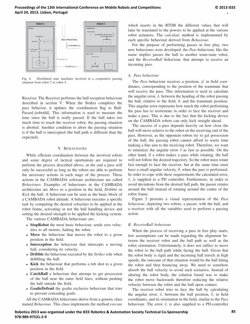
4

Fig. 4. Distributed state machines involved in a cooperative passingsituation from robot 2 to robot 5.

Receiver. The Receiver performs the ball reception behaviour

described in section V. When the Striker completes the

pass behavior, it updates the coordination flag to Ball-

Passed [robotId]. This information is used to measure the

time since the ball is really passed. If the ball takes too

much time to reach the receiver robot, the passing situation

is aborted. Another condition to abort the passing situation

is if the ball is intercepted (the ball path is different than the

expected).

V. BEHAVIOURS

While efficient coordination between the involved robots

and some degree of tactical oportunism are required to

perform the process described above, in the end a pass will

only be successful as long as the robots are able to perform

the necessary actions in each stage of the process. These

actions in the CAMBADA software architecture are called

Behaviours. Examples of behaviours in the CAMBADA

architecture are Move to a position in the field, Dribble or

Kick the ball. A behaviour can be seen as the basic block of

a CAMBADA robot attitude. A behaviour executes a specific

task by computing the desired velocities to be applied at the

robot frame, activating or not the ball handling device and

setting the desired strength to be applied the kicking system.

The various CAMBADA behaviours are:

• StopRobot the most basic behaviour, sends zero veloc-

ities to all motors, halting the robot.

• Move the behaviour that moves the robot to a given

position in the field.

• Interception the behaviour that intercepts a moving

ball, considering its velocity.

• Dribble the behaviour executed by the Striker role when

dribbling the ball.

• Kick the behaviour that performs a lob shot to a given

position in the field.

• CatchBall a behaviour that attemps to get possession

of the ball near the outer field lines, without pushing

the ball outside the field.

• GoalieDefend the goalie exclusive behaviour that tries

to prevent conceding goals.

All the CAMBADA behaviours derive from a generic class

named Behaviour. This class implements the method execute

which inserts in the RTDB the different values that will

later be translated to the powers to be applied at the various

robot actuators. The calculate method is implemented by

each specific behaviour derived from Behaviour.

For the purpose of performing passes in free play, two

new behaviours were developed: the Pass behaviour, like the

name implies passes the ball to another team-mate robot,

and the ReceiveBall behaviour, that attemps to receive an

incoming pass.

A. Pass behaviour

The Pass behaviour receives a position, �p, in field coor-

dinates, corresponding to the position of the teammate that

will receive the pass. This information is used to calculate

the angular error, δ, between the heading of the robot passing

the ball, relative to the field, θ, and the teammate position.

This angular error represents how much the robot performing

the pass has to reorientate in order to face the receiver and

make a pass. This is due to the fact that the kicking device

on the CAMBADA robots can only kick straight ahead.

The success of a pass depends heavily on how close the

ball will move relative to the robot on the receiving end of the

pass. However, as the opponent robots try to get possession

of the ball, the passing robot cannot afford to waste time

making a fine aim to the receiving robot. Therefore, we want

to minimize the angular error δ as fast as possible. On the

other hand, if a robot makes a pass while rotating, the ball

will not follow the desired trajectory. So the robot must rotate

fast enough to face the receiver, but at the same time must

have a small angular velocity, θ, when the pass is performed.

In order to cope with these requirements the calculated error,

δ, is supplied to a PD controller. Furthermore, in order to

avoid deviations from the desired ball path, the passer rotates

around the ball instead of rotating around the center of the

robot frame.

Figure 5 presents a visual representation of the Passbehaviour, depicting two robots, a passer, with the ball, and

a receiver with all the variables used to perform a passing

action.

B. ReceiveBall behaviour

When the process of receiving a pass in free play starts,

few assumptions can be made regarding the alignment be-

tween the receiver robot and the ball path as well as the

robot orientation. Unfortunately, it does not suffice to move

the robot to the ball path while facing the ball. Given that

the robot body is rigid and the incoming ball travels at high

speeds, the outcome of that situation would be the ball hiting

the robot and then bouncing away. We need to somehow

absorb the ball velocity to avoid such scenarios. Instead of

altering the robot body, the solution found was to make

the robot move backwards therefore reducing the relative

velocity between the robot and the ball upon contact.

The receiver robot tries to face the ball by calculating

the angular error, δ, between the ball position, �b, in field

coordinates, and its orientation in the field, similar to the Passbehaviour. The error δ, is also supplied to a PD-controller


© 2013 IEEE


85

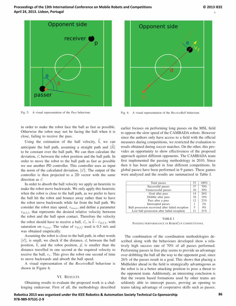
5

Fig. 5. A visual representation of the Pass behaviour.

in order to make the robot face the ball as fast as possible.

Otherwise the robot may not be facing the ball when it is

close, failing to receive the pass.

Using the estimation of the ball velocity, �b, we can

anticipate the ball path, assuming a straight path and ‖�b‖to be constant over the ball path. We can then calculate the

deviation, �e, between the robot position and the ball path. In

order to move the robot to the ball path as fast as possible

we use another PD controller. This controller uses as input

the norm of the calculated deviation, ‖�e‖. The output of the

controller is then projected to a 2D vector with the same

direction as �e.

In order to absorb the ball velocity we apply an heuristic to

make the robot move backwards. We only apply this heuristic

when the robot is close to the ball path, as we prefer to have

the ball hit the robot and bounce away rather than to have

the robot move backwards while far from the ball path. We

consider the robot max speed, vmax, and define a parameter

vdiff , that represents the desired relative velocity between

the robot and the ball upon contact. Therefore the velocity

the robot should have to receive a ball, �vr, is �b−vdiff , with

saturation on vmax. The value of vdiff used is 0.5 m/s and

was obtained empirically.

Assuming the robot is close to the ball path, in other words

‖�e‖, is small, we check if the distance, d, between the ball

position, �b, and the robot position, �p, is smaller than the

distance travelled in one second at the required velocity to

receive the ball, vr. This gives the robot one second of time

to move backwards and absorb the ball speed.

A visual representation of the ReceiveBall behaviour is

shown in Figure 6.

VI. RESULTS

Obtaining results to evaluate the proposed work is a chal-

lenging endeavour. First of all, the methodology described

Fig. 6. A visual representation of the ReceiveBall behaviour.

earlier focuses on performing long passes on the MSL field

to oppose the slow speed of the CAMBADA robots. However

since the authors only have access to a field with the official

measures during competitions, we restricted the evaluation to

resuls obtained during soccer matches. On the other, this pro-

vides an opportunity to show effectiveness of the proposed

approach against different opponents. The CAMBADA team

first implemented the passing methodology in 2010. Since

then it has been applied in four different competitions. In

global passes have been performed in 9 games. These games

were analyzed and the results are summarized in Table I.

Total passes 53 100%Successful passes 37 70%

Unsuccessful passes 16 30%Goal after pass 14 26%

Dribble after pass 10 19%Pass after a pass 12 23%

Intercepted passes 1 2%Ball possession recovered after failed reception 5 9%

Lost ball possession after failed reception 11 21%

TABLE I

PASSING PERFORMANCE IN ROBOCUP COMPETITIONS.

The combination of the coordination methodologies de-

scribed along with the behaviours developed show a rela-

tively high success rate of 70% of all passes performed.

Performing passes in free play seems to provide an advantage

over dribbling the ball all the way to the opponent goal, since

26% of the passes result in a goal. This shows that placing a

Midfielder ahead in the field is strategically advantageous as

the robot is in a better attacking position to pose a threat to

the opponent team. Additionaly, an interesting conclusion is

that the swarm based formations used by other teams are

seldomly able to intercept passes, proving an opening to

teams taking advantage of cooperative skills such as passes.


© 2013 IEEE


86

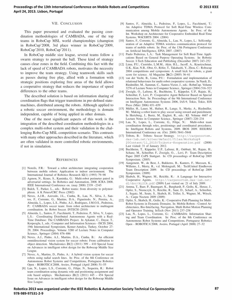
6

VII. CONCLUSION

This paper presented and evaluated the passing coor-

dination methodologies of CAMBADA, one of the top

teams in RoboCup MSL world championships (champion

in RoboCup’2008, 3rd place winner in RoboCup’2009,

RoboCup’2010, RoboCup’2011).

In RoboCup middle size league, several teams follow a

swarm strategy to pursuit the ball. These kind of strategy

causes clear zones in the field. Combining this fact with the

lack of speed of CAMBADA robots, motivates the necessity

to improve the team strategy. Using teamwork skills such

as passes during free play, allied with a formation with

strategic positions exploring free areas of the field allows

a cooperative strategy that reduces the importance of speed

differences to the other teams.

The described solution is based on information sharing of

coordination flags that trigger transitions in pre-defined state-

machines, distributed among the robots. Although applied to

a robotic soccer environment, the methodology is domain

independent, capable of being applied in other domais.

One of the most significant aspects of this work is the

integration of the described coordination methodologies in a

complex multi-robot system and their validation in the chal-

lenging Robo-Cup MSL competition scenario. This contrasts

with many other approaches described in the literature, which

are often validated in more controlled robotic environments,

if not in simulation.

REFERENCES

[1] Noreils, F.R.: Toward a robot architecture integrating cooperationbetween mobile robots: Application to indoor environment. TheInternational Journal of Robotics Research 12(1) (1993) 79–98

[2] Agmon, N., Kraus, S., Kaminka, G.: Multi-robot perimeter patrol inadversarial settings. In: Robotics and Automation, 2008. ICRA 2008.IEEE International Conference on. (may 2008) 2339 –2345

[3] Balch, T., Parker, L., eds.: Robot teams: from diversity to polymor-phism. A K Peters/CRC Press (2002)

[4] Neves, A.J.R., Azevedo, J.L., Cunha, B., Lau, N., Silva, J., San-tos, F., Corrente, G., Martins, D.A., Figueiredo, N., Pereira, A.,Almeida, L., Lopes, L.S., Pinho, A.J., Rodrigues, J.M.O.S., Pedreiras,P.: CAMBADA soccer team: from robot architecture to multiagentcoordination. In: Robot Soccer. INTECH (2010)

[5] Almeida, L., Santos, F., Facchinetti, T., Pedreiras, P., Silva, V., Lopes,L.S.: Coordinating Distributed Autonomous Agents with a Real-Time Database: The CAMBADA Project. In Aykanat, C., Dayar, T.,Korpeoglu, I., eds.: Computer and Information Sciences - ISCIS 2004,19th International Symposium, Kemer-Antalya, Turkey, October 27-29, 2004. Proceedings. Volume 3280 of Lecture Notes in ComputerScience., Springer (2004) 876–886

[6] Neves, A.J., Pinho, A.J., Martins, D.A., Cunha, B.: An efficientomnidirectional vision system for soccer robots: From calibration toobject detection. Mechatronics 21(2) (2011) 399 – 410 Special Issueon Advances in intelligent robot design for the Robocup Middle SizeLeague.

[7] Neves, A., Martins, D., Pinho, A.: A hybrid vision system for soccerrobots using radial search lines. In: Proc. of the 8th Conference onAutonomous Robot Systems and Competitions, Portuguese RoboticsOpen - ROBOTICA’2008, Aveiro, Portugal (April 2008) 51–55

[8] Lau, N., Lopes, L.S., Corrente, G., Filipe, N., Sequeira, R.: Robotteam coordination using dynamic role and positioning assignment androle based setplays. Mechatronics 21(2) (2011) 445 – 454 SpecialIssue on Advances in intelligent robot design for the Robocup MiddleSize League.

[9] Santos, F., Almeida, L., Pedreiras, P., Lopes, L., Facchinetti, T.:An Adaptive TDMA Protocol for Soft Real-Time Wireless Com-munication among Mobile Autonomous Agents. In: Proc. of theInt. Workshop on Architecture for Cooperative Embedded Real-TimeSystems, WACERTS 2004. (2004)

[10] Santos, F., Corrente, G., Almeida, L., Lau, N., Lopes, L.: Selfconfig-uration of an Adaptive TDMA wireless communication protocol forteams of mobile robots. In: Proc. of the 13th Portuguese Conferenceon Artificial Intelligence, EPIA 2007. (2007)

[11] Paulo Pedreiras, L.A.: Task Management for Soft Real-Time Appli-cations Based on General Purpose Operating Systems. In: RoboticSoccer. I-Tech Education and Publishing (December 2007) 243–252

[12] Lima, P.U., Custodio, L.M.M., Akin, H.L., Jacoff, A., Kraetzschmar,G.K., Kiat, N.B., Obst, O., Rofer, T., Takahashi, Y., Zhou, C.: Robocup2004 competitions and symposium: A small kick for robots, a giantscore for science. AI Magazine 26(2) (2005) 36–61

[13] van der Vecht, B., Lima, P.U.: Formulation and implementation ofrelational behaviours for multi-robot cooperative systems. In Nardi, D.,Riedmiller, M., Sammut, C., Santos-Victor, J., eds.: RobuCup. Volume3276 of Lecture Notes in Computer Science., Springer (2004) 516–523

[14] Zweigle, O., Lafrenz, R., Buchheim, T., Kappeler, U.P., Rajaie, H.,Schreiber, F., Levi, P.: Cooperative Agent Behavior Based on SpecialInteraction Nets. In: Proceedings of the 9th International Conferenceon Intelligent Autonomous Systems 2006, IAS-9, Tokio, Tokio, IOSPress (Marz 2006) 651–659

[15] Muller, H., Lauer, M., Hafner, R., Lange, S., Merke, A., Riedmiller,M.: Making a robot learn to play soccer using reward and punishment.In Hertzberg, J., Beetz, M., Englert, R., eds.: KI. Volume 4667 ofLecture Notes in Computer Science., Springer (2007) 220–234

[16] Lau, N., Lopes, L., Corrente, G., Filipe, N.: Multi-robot teamcoordination through roles, positionings and coordinated procedures.In: Intelligent Robots and Systems, 2009. IROS 2009. IEEE/RSJInternational Conference on. (Oct. 2009) 5841–5848

[17] Tribots, B.: Tribots: Soccer Strategy. http://carpenoctem.das-lab.net/sites/default/files/Workshop%20Content/11_2010/Tribots-Kooperation.pdf (2008)Last visited: 31 of January 2012.

[18] Buchheim, T., Kappeler, U.P., Lafrenz, R., Oubbati, M., Rajaie, H.,Schanz, M., Schreiber, F., Zweigle, O., , Levi, P.: Team DescriptionPaper 2005 CoPS Stuttgart. In: CD proceedings of RoboCup 2005Symposium. (2005)

[19] Aangenent, W., de Best, J., Bukkems, B., Kanters, F., Meessen, K.,Willems, J., Merry, R., v.d. Molengraft, M.: TechUnited EindhovenTeam Description 2009. In: CD proceedings of RoboCup 2009Symposium. (2009)

[20] Skubch, H., Wagner, M., Reichle, R.: A Language for InteractiveCooperative Agents. http://carpenoctem.das-lab.net/dl/doc/ALICA.pdf (2009) Last visited on: 21 of July 2009.

[21] Amma, T., Baer, P., Baumgart, K., Burghardt, P., Geihs, K., Henze, J.,Opfer, S., Niemczyk, S., Reichle, R., Saur, D., Scharf, A., Schreiber,J., Segatz, M., Seute, S., Skubch, H., Triller, S., Wagner, M., Witsch,A.: Carpe Noctem 2009 (2009)

[22] Opfer, S., Skubch, H., Geihs, K.: Cooperative Path Planning for Multi-Robot Systems in Dynamic Domains. In: Mobile Robots - Control Ar-chitectures, Bio-Interfacing, Navigation, Multi Robot Motion Planningand Operator Training. InTech (Nov 2011) 237–258

[23] Lau, N., Lopes, L., Corrente, G.: CAMBADA: Information Shar-ing and Team Coordination. In: Proc. of the 8th Conference onAutonomous Robot Systems and Competitions, Portuguese RoboticsOpen - ROBOTICA’2008, Aveiro, Portugal (April 2008) 27–32


© 2013 IEEE


87

1

Unknown-Color Spherical ObjectDetection and Tracking

Anze Troppan, Eduardo Guerreiro, Francesco Celiberti, Goncalo Santos, Aamir Ahmad and Pedro U. Lima

Institute for Systems and Robotics, Instituto Superior Tecnico, Lisboa, Portugal

Abstract—Detection and tracking of an unknown-color spher-ical object in a partially-known environment using a robot witha single camera is the core problem addressed in this article. Anovel color detection mechanism, which exploits the geometricalproperties of the spherical object’s projection onto the imageplane, precedes the object’s detection process. A Kalman filter-based tracker uses the object detection in its update step andtracks the spherical object. Real robot experimental evaluationof the proposed method is presented on soccer robots detectingand tracking an unknown-color ball.

I. INTRODUCTION

Detecting and tracking relevant objects in a known orunknown environment forms a vast area of research not onlyin the domain of image processing and computer vision [1][2] [3] [4], but also in that of mobile robotics [5] [6] [7] [8].Often the objective in the former is to classify complex objectsbased on their color and shape irregularities [1]. However,in mobile robotics the focus is more on computationally fastmethods for object tracking (including detection) and therebyusing the objects’ information to achieve other complex goals,e.g, robot’s self-localization [7] and high-level decision making[9]. The gain in an object tracker’s execution speed is dueto using the object’s shape as a prior knowledge and/orusing less-complex shaped objects, e.g, spheres. Although it isoften practical to assume the presence of less-complex shapedobjects in most environments, the same cannot be true withregard to the object’s color. Moreover, the lighting conditionsof the environment irregularly change the apparent colors ofthe objects over time rendering the prior knowledge of theobject’s color useless.

In this article we present a method to solve the problem ofdetecting and tracking spherical-shaped objects in a partially-known environment without the necessity of the object’scolor information as a prior knowledge of the tracker. Thepartially-known environment implies that the most dominantcolors contributing to the environment’s background are knownbeforehand. The method essentially consists of the followingthree modules:

• automatic color detection of a spherical-shaped object,• spherical object detection method and• a Kalman filter-based (KF) tracker that uses the spherical

object detection method in its update step.

The automatic color detection, which consists of a sweepover the HSV color space, is performed only once beforeinitiating the tracker. Therefore, the object should be in the

field of view of the camera at the beginning of the track-ing process. The detected color is subsequently used by thespherical object detection method which along with the KF-based tracker runs continuously to track the object. Since theautomatic color detection method itself is computationally fast,it can be scheduled to run intermittently without the needof manual intervention in environments where the lightingchanges frequently causing the apparent color of the objectto change. In order to experimentally validate our proposedmethod, the tracker was implemented on real soccer robots totrack an unknown-color soccer ball.

The rest of the article is organized as follows. In Section IIwe briefly overview the existing literature in the context ofobject detection and tracking. The novel contributions of thearticle concerning automatic color detection is presented inSection III along with the spherical object detection and theKF-based tracker’s theoretical details. Real robot experimentalresults are presented in Section IV, followed by Section Vwhere we conclude the article with comments on future work.

II. RELATED WORK

An extensive literature exists in the area of object detectionwhere researchers have explored concepts ranging from con-tour recognition, e.g., Hough transform (HT) [10] to structuretensor techniques [4]. While some of these assume a priorknowledge of the object’s color [8], innovative algorithms havebeen proposed recently to overcome this assumption, e.g, [5][6]. In [5] the authors present a color histogram mismatch-based method to distinguish a spherical object of knownsize from the background. This removes the dependency onthe prior color information and enables the spherical objectdetection in 3D space. However, since its accuracy dependson the number of pixels required to perform the histogrammismatch (the higher the number of pixels used, the better theaccuracy is) at every frame, the execution speed is adverselyaffected causing the method to be inefficient for real-timeapplications.

In [11] the authors present a circular HT-based method toidentify the circular projections of the spherical object to detectthem. Apart from being computationally expensive, the methodexplicitly requires a fine-tuning of the edge-detection system,required by the HT, every time the lighting condition of theenvironment changes. A possible solution to this problem isproposed in [12], where the image projection of the sphericalobject is an exact ellipse and radial and rotary scan lines areused to look for matching color variations to detect the outer


© 2013 IEEE


88

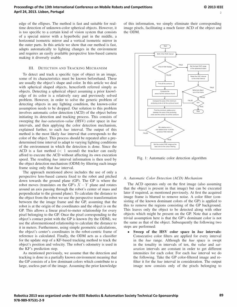
2

edge of the ellipses. The method is fast and suitable for real-time detection of unknown-color spherical objects. However, itis too specific to a certain kind of vision system that consistsof a special mirror with a hyperbolic part in the middle, ahorizontal isometric mirror and a vertical isometric mirror inthe outer parts. In this article we show that our method is fast,adapts automatically to lighting changes in the environmentand requires an easily available perspective lens-based cameramaking it diversely usable.

III. DETECTION AND TRACKING MECHANISM

To detect and track a specific type of object in an image,some of its characteristics must be known beforehand. Theseare usually the object’s shape and color. In this article we dealwith spherical shaped objects, henceforth referred simply asobjects. Detecting a spherical object assuming a prior knowl-edge of its color is a relatively easy and previously solvedproblem. However, in order to solve the generic problem ofdetecting objects in any lighting condition, the known-colorassumption needs to be dropped. Our solution to this probleminvolves automatic color detection (ACD) of the object beforeinitiating its detection and tracking process. This consists ofsweeping the hue-saturation-value (HSV) color space in hueintervals, and then applying the color detection mechanism,explained further, to each hue interval. The output of thismethod is the most likely hue interval that corresponds to thecolor of the object. This process should be repeated after a pre-determined time interval to adapt to varying lighting conditionsof the environment in which the detection is done. Since theACD is a fast method (< 1 second) the tracker can easilyafford to execute the ACD without affecting its own executionspeed. The resulting hue interval information is then used bythe object detection mechanism (ODM) by filtering each imageframe using only that hue interval.

The approach mentioned above includes the use of only aperspective lens-based camera fixed to the robot and pitcheddown towards the ground plane (GP). The GP is where therobot moves (translates on the GP’s X − Y plane and rotatesaround an axis passing through the robot’s center of mass andperpendicular to the ground plane). To calculate the distance tothe object from the robot we use the perspective transformationbetween the the image frame and the GP, assuming that therobot is at the origin of the coordinates and the object is on theGP. This allows a linear pixel-to-meter relationship for everypixel belonging to the GP. Once the pixel corresponding to theobject’s contact point with the GP is known (by the ODM), weuse the aforementioned relationship to calculate the distance toit in meters. Furthermore, using simple geometric calculations,the object’s center’s coordinates in the robot-centric frame ofreference is calculated. Finally, the ODM acts as a classifierfor the update step of a KF-based tracking method to track theobject’s position and velocity. The robot’s odometry is used inthe KF’s prediction step.

As mentioned previously, we assume that the detection andtracking is done in a partially known environment meaning thatthe GP consists of a few dominant colors which contribute to alarge, useless part of the image. Assuming the prior knowledge

of this information, we simply eliminate their correspondingimage pixels, facilitating a much faster ACD of the object andthe ODM.

Start

Shift of the HUE interval

End of HUE Sweep

Find all the contours

Compute thearea of all the contours found

Compute the area of the minimum enclosing circle of all the contours found

Find the minimum relative errorbetween the area of the enclosing

circle and the contour for all the contours

TRUE

FALSE

Min relative error <min relative error in all the

prevoius HUE intervals

Set the best HUE range of the sphereical object

Set the current HUE range as thebest one for the colour filtering

TRUE

FALSE

Spherical object out of the frame

TRUE

Exit

Reset the HUE intervalto the initial interval

FALSE

Stop

TRUE

FALSE

a

aa

a

Fig. 1: Automatic color detection algorithm

A. Automatic Color Detection (ACD) Mechanism

The ACD operates only on the first image (also assumingthat the object is present in that image) but can be executedlater if required, as mentioned previously. At first the acquiredimage frame is blurred to remove noise. A color filter (con-sisting of the known dominant colors of the GP) is applied tothis to remove the regions consisting of the GP background.This leaves only the object to be detected along with otherobjects which might be present on the GP. Note that a rathertrivial assumption here is that the GP’s dominant color is notthe same as that of the object. Subsequently the following twosteps are performed:

• Sweep of the HSV color space in hue intervals:Consecutive color filters are applied for every intervalin the hue range. Although the hue space is sweptin the tonality in intervals of ten, the value and sat-uration intervals are constant in order to get differentintensities for each color. For each hue interval we dothe following. Take the GP color-filtered image and re-filter it for the hue interval in consideration. The outputimage now consists only of the pixels belonging to


© 2013 IEEE


89

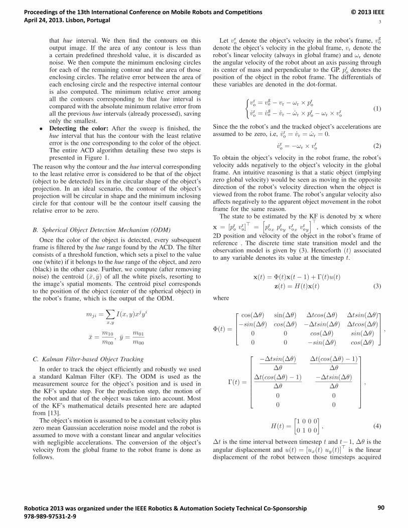
3

that hue interval. We then find the contours on thisoutput image. If the area of any contour is less thana certain predefined threshold value, it is discarded asnoise. We then compute the minimum enclosing circlesfor each of the remaining contour and the area of thoseenclosing circles. The relative error between the area ofeach enclosing circle and the respective internal contouris also computed. The minimum relative error amongall the contours corresponding to that hue interval iscompared with the absolute minimum relative error fromall the previous hue intervals (already processed), savingonly the smallest.

• Detecting the color: After the sweep is finished, thehue interval that has the contour with the least relativeerror is the one corresponding to the color of the object.The entire ACD algorithm detailing these two steps ispresented in Figure 1.

The reason why the contour and the hue interval correspondingto the least relative error is considered to be that of the object(object to be detected) lies in the circular shape of the object’sprojection. In an ideal scenario, the contour of the object’sprojection will be circular in shape and the minimum inclosingcircle for that contour will be the contour itself causing therelative error to be zero.

B. Spherical Object Detection Mechanism (ODM)

Once the color of the object is detected, every subsequentframe is filtered by the hue range found by the ACD. The filterconsists of a threshold function, which sets a pixel to the valueone (white) if it belongs to the hue range of the object, and zero(black) in the other case. Further, we compute (after removingnoise) the centroid (x, y) of all the white pixels, resorting tothe image’s spatial moments. The centroid pixel correspondsto the position of the object (center of the spherical object) inthe robot’s frame, which is the output of the ODM.

mji =∑x,y

I(x, y)xjyi

x =m10

m00, y =

m01

m00

C. Kalman Filter-based Object Tracking

In order to track the object efficiently and robustly we useda standard Kalman Filter (KF). The ODM is used as themeasurement source for the object’s position and is used inthe KF’s update step. For the prediction step, the motion ofthe robot and that of the object was taken into account. Mostof the KF’s mathematical details presented here are adaptedfrom [13].

The object’s motion is assumed to be a constant velocity pluszero mean Gaussian acceleration noise model and the robot isassumed to move with a constant linear and angular velocitieswith negligible accelerations. The conversion of the object’svelocity from the global frame to the robot frame is done asfollows.

Let vro denote the object’s velocity in the robot’s frame, vg

o

denote the object’s velocity in the global frame, vr denote therobot’s linear velocity (always in global frame) and ωr denotethe angular velocity of the robot about an axis passing throughits center of mass and perpendicular to the GP. pr

o denotes theposition of the object in the robot frame. The differentials ofthese variables are denoted in the dot-format.

{vr

o = vgo − vr − ωr × pr

o

vro = vg

o − vr − ωr × pro − ωr × vr

o

(1)

Since the the robot’s and the tracked object’s accelerations areassumed to be zero, i.e, vr

o = vr = ωr = 0.

vro = −ωr × vr

o (2)

To obtain the object’s velocity in the robot frame, the robot’svelocity adds negatively to the object’s velocity in the globalframe. An intuitive reasoning is that a static object (implyingzero global velocity) would be seen as moving in the oppositedirection of the robot’s velocity direction when the object isviewed from the robot frame. The robot’s angular velocity alsoaffects negatively to the apparent object movement in the robotframe for the same reason.

The state to be estimated by the KF is denoted by x where

x = [pro vr

o]�

=[pr

ox proy vr

ox vroy

]�, which consists of the

2D position and velocity of the object in the robot’s frame ofreference . The discrete time state transition model and theobservation model is given by (3). Henceforth (t) associatedto any variable denotes its value at the timestep t.

x(t) = Φ(t)x(t− 1) + Γ(t)u(t)

z(t) = H(t)x(t) (3)

where

Φ(t) =

⎡⎢⎢⎣

cos(Δθ) sin(Δθ) Δtcos(Δθ) Δtsin(Δθ)

−sin(Δθ) cos(Δθ) −Δtsin(Δθ) Δtcos(Δθ)

0 0 cos(Δθ) sin(Δθ)

0 0 −sin(Δθ) cos(Δθ)

⎤⎥⎥⎦ ,

Γ(t) =

⎡⎢⎢⎢⎢⎢⎢⎢⎣

−Δtsin(Δθ)

Δθ

Δt(cos(Δθ)− 1)

Δθ

Δt(cos(Δθ)− 1)

Δθ

−Δtsin(Δθ)

Δθ

0 0

0 0

⎤⎥⎥⎥⎥⎥⎥⎥⎦,

H(t) =

[1 0 0 0

0 1 0 0

], (4)

Δt is the time interval between timestep t and t−1, Δθ is the

angular displacement and u(t) = [ux(t) uy(t)]�

is the lineardisplacement of the robot between those timesteps acquired


© 2013 IEEE


90

4

Fig. 2: Perspective lens-based camera mounted on top of asoccer robot

from the robot’s odometry measurement. z(t) denotes theobject’s observation measurements obtained at the tth timestepfrom the ODM.

The KF’s prediction step and the update step are givenby (5) and (6), respectively. The prediction is performedwhenever new odometry readings are acquired and the updateis performed when the object’s measurements are obtained bythe ODM.

• Prediction Step

x(t) = Φ(t)x(t− 1) + Γ(t)u(t)

P(t) = Φ(t)P(t− 1)Φ(t)� +Q(t)(5)

• Update Step

K(t) = P(t)H(t)�(H(t)P(t)H(t)� +R(t)

)−1

x(t) = x(t) +K(t)(z(t)−H(t)x(t)

)P(t) =

(I−K(t)H(t)

)Φ(t)P(t)

(6)

The a priori and the a posteriori error covariance matricesare represented by P(t) and P(t) respectively. Both wereinitialized as identity matrices, whereas the process noise co-variance matrix, Q, and measurement noise covariance matrix,R, are based on the ODM’s measurement and odometry errors.K denotes the Kalman gain and I denotes an identity matrix.

IV. TESTBED, IMPLEMENTATION AND RESULTS

A. Testbed and ImplementationOur experimental testbed is the RoboCup Middle Sized

League (MSL) where one of the most important prerequisitesfor the soccer playing robots is to detect and track the soccerball which is a spherical object. As the official rules of theMSL have evolved, one of the major technical challengesin the recent years is to detect and track an unknown colorball. This makes MSL a suitable choice for implementing andevaluating the method proposed in this article. We used oneof our omnidirectional soccer robots for the implementationof the proposed algorithm. The robots acquire new odometryreadings every 30 milliseconds. To perform the ball’s detection,

a perspective lens-based camera (see Figure 2) was fixed ontop of the robot at a height of 80cm above the GP and pitcheddown at an angle of 40◦ w.r.t the GP. Images from this camerawere acquired at 30 frames per second (fps). All involveddistance computations are based on the perspective camera pro-jection model. An example of the distortion-corrected imagefrom this camera is presented in the Figure 3. All the robot’ssoftwares run on a Sony Vaio laptop, equipped with an IntelCore i3 2.2GHz (quad core) CPU and 4GB of RAM, which isconnected to the robot’s sensors and actuators through plug-and-play connections (USB and Firewire).

The ACD, ODM and the KF-based tracker were imple-mented using the robot operating system (ROS) and OpenCVlibraries for image processing related processes. Green andwhite were considered as the dominant color in the backgroundand were filtered out before the ACD was initiated.

Fig. 3: An example of the distortion-corrected image from theperspective camera.

B. resultsExperiments were conducted for various balls (note that

every ball was uniformly colored, meaning without any signif-icant patterns on it), each of a different color. The robot wasable to successfully detect and track the balls upto 6m fromitself. Table I shows the range in which the robot was ableto detect and track 2 different balls. In Figure 4 we show aseries of three images to demonstrate the ACD process. In thefirst image a red colored ball (color unknown to the detectionsystem) is place in the field of view of the robot’s camera.The second image shows result of filtering the backgrounddominant colors: green and white. The third image shows thecontours detected on the remaining image, the enclosing circleson those contours and eventually the chosen circle with theminimum relative error corresponding to the actual ball andits color (marked with fluorescent green color on the image).

We further present the statistical results of the KF-basedtracker’s implementation in case of the red ball for threeseparate experiments.

Experiment 1: In this experiment the ball was first placedin the field of view of the robot (as it is necessary for the ACD)


© 2013 IEEE


91

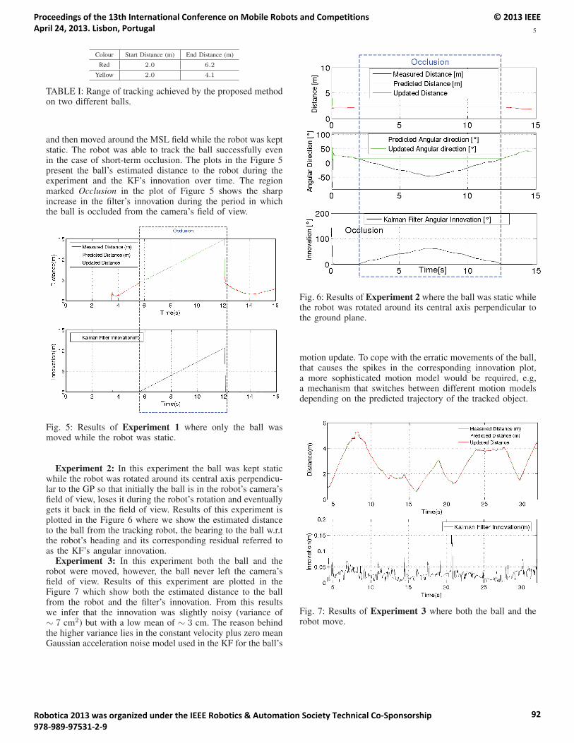
5

Colour Start Distance (m) End Distance (m)

Red 2.0 6.2

Yellow 2.0 4.1

TABLE I: Range of tracking achieved by the proposed methodon two different balls.

and then moved around the MSL field while the robot was keptstatic. The robot was able to track the ball successfully evenin the case of short-term occlusion. The plots in the Figure 5present the ball’s estimated distance to the robot during theexperiment and the KF’s innovation over time. The regionmarked Occlusion in the plot of Figure 5 shows the sharpincrease in the filter’s innovation during the period in whichthe ball is occluded from the camera’s field of view.

Fig. 5: Results of Experiment 1 where only the ball wasmoved while the robot was static.

Experiment 2: In this experiment the ball was kept staticwhile the robot was rotated around its central axis perpendicu-lar to the GP so that initially the ball is in the robot’s camera’sfield of view, loses it during the robot’s rotation and eventuallygets it back in the field of view. Results of this experiment isplotted in the Figure 6 where we show the estimated distanceto the ball from the tracking robot, the bearing to the ball w.r.tthe robot’s heading and its corresponding residual referred toas the KF’s angular innovation.

Experiment 3: In this experiment both the ball and therobot were moved, however, the ball never left the camera’sfield of view. Results of this experiment are plotted in theFigure 7 which show both the estimated distance to the ballfrom the robot and the filter’s innovation. From this resultswe infer that the innovation was slightly noisy (variance of∼ 7 cm2) but with a low mean of ∼ 3 cm. The reason behindthe higher variance lies in the constant velocity plus zero meanGaussian acceleration noise model used in the KF for the ball’s

Fig. 6: Results of Experiment 2 where the ball was static whilethe robot was rotated around its central axis perpendicular tothe ground plane.

motion update. To cope with the erratic movements of the ball,that causes the spikes in the corresponding innovation plot,a more sophisticated motion model would be required, e.g,a mechanism that switches between different motion modelsdepending on the predicted trajectory of the tracked object.

Fig. 7: Results of Experiment 3 where both the ball and therobot move.


© 2013 IEEE


92

6

a) Unknown-color ball in the robot’s view b) Background dominant colors filtered c) Ball color detected

(marked as fluorescent green)

Fig. 4: Demonstration of the automatic color detection (ACD) process.


In this article we presented a novel method to automaticallydetect the color of a spherical object before detecting and track-ing it using a Kalman filter-based tracker. The fast executionspeed of the color detection method enables it to be executedperiodically while running the tracker to cope with the changesin the lighting conditions of the environment. The method wasimplemented on the soccer playing robots to track unknown-color soccer balls with successful results. A few points thatcould be enumerated for the purpose of future work are asfollows.

• In order to deal better with occlusions and to have asmoother trajectory of the tracked object, cooperationamong multiple robots and innovative motion modelsare required, e.g, an alpha-beta filter [14]. It is a steady-state form of the nearly constant velocity filter. Since anerratically moving object is affected by random positive-mean acceleration, a good object motion model needs totake this effect into account.

• Although the camera is pitched down in our application,it still detects some irrelevant areas of the environment.A possible future improvement would be to choose aconfiguration where the camera’s field of view is betteroptimized to make use of the maximum possible imagespace.

ACKNOWLEDGMENT

This work was funded in part by Fundacao para a Cienciae a Tecnologia (ISR/IST pluriannual funding) through thePIDDAC Program funds.

REFERENCES

[1] C. Lemaitre, M. Perdoch, A. Rahmoune, J. Matas, and J. Miteran,“Detection and matching of curvilinear structures,” Pattern Recognition,vol. 44, no. 7, pp. 1514 – 1527, 2011. [Online]. Available:http://www.sciencedirect.com/science/article/pii/S0031320311000148

[2] O. Carmichael and M. Hebert, “Shape-based recognition of wiry ob-jects,” in Computer Vision and Pattern Recognition, 2003. Proceedings.2003 IEEE Computer Society Conference on, vol. 2, june 2003, pp. II– 401–8 vol.2.

[3] V. Ferrari, T. Tuytelaars, and L. V. Gool, “Object detection by contoursegment networks,” in Proceeding of the European Conference onComputer Vision, ser. LNCS, vol. 3953. Elsevier, June 2006, pp. 14–28.

[4] M. Donoser, S. Kluckner, and H. Bischof, “Object tracking by structuretensor analysis,” in Pattern Recognition (ICPR), 2010 20th InternationalConference on, aug. 2010, pp. 2600 –2603.

[5] M. Taiana, J. Santos, J. Gaspar, J. Nascimento, A. Bernardino, andP. U. Lima, “Tracking objects with generic calibrated sensors: Analgorithm based on color and 3d shape features,” Robot. Auton.Syst., vol. 58, no. 6, pp. 784–795, Jun. 2010. [Online]. Available:http://dx.doi.org/10.1016/j.robot.2010.02.010

[6] M. Wenig, K. Pang, and P. On, “Arbitrarily colored ball detectionusing the structure tensor technique,” Mechatronics, vol. 21, no. 2,pp. 367 – 372, 2011, ¡ce:title¿Special Issue on Advances inintelligent robot design for the Robocup Middle Size League¡/ce:title¿.[Online]. Available: http://www.sciencedirect.com/science/article/pii/S0957415810001297

[7] D. Gohring and H.-D. Burkhard, “Multi robot object tracking and selflocalization using visual percept relations,” in Intelligent Robots andSystems, 2006 IEEE/RSJ International Conference on, oct. 2006, pp.31 –36.

[8] A. Ahmad and P. U. Lima, “Multi-robot cooperative object trackingbased on particle filters,” in Proc. of the European Conference on MobileRobots (ECMR 2011), Orebro, Sweden, Sep 2011.

[9] J. Messias, M. Spaan, and P. Lima, “Multi-robot planning under un-certainty with communication: a case study,” in Multi-agent SequentialDecision Making in Uncertain Domains, 2010, workshop at AAMAS10.

[10] J. Matas, C. Galambos, and J. Kittler, “Progressive probabilistic houghtransform,” 1998.

[11] D. A. M. Antnio J. R. Neves and A. J. Pinho, “A hybrid vision systemfor soccer robots using radial search lines,” in Proc. of the 8th Con-ference on Autonomous Robot Systems and Competitions, PortugueseRobotics Open - ROBTICA’2008, Aveiro, Portugal, 2008.

[12] H. Lu, H. Zhang, J. Xiao, F. Liu, and Z. Zheng, “Arbitrary ballrecognition based on omni-directional vision for soccer robots,” inRoboCup 2008: Robot Soccer World Cup XII, ser. Lecture Notesin Computer Science, L. Iocchi, H. Matsubara, A. Weitzenfeld,and C. Zhou, Eds. Springer Berlin Heidelberg, 2009, vol.5399, pp. 133–144. [Online]. Available: http://dx.doi.org/10.1007/978-3-642-02921-9 12

[13] Z. Marinho, J. Messias, and P. U. Lima, “Multi-object tracking based onhistogram classifier and kalman filtering,” in ISR/IST Internal Report,2012.

[14] W. D. Blair, “Design of nearly constant velocity track filters for trackingmaneuvering targets.”


© 2013 IEEE


93

Diagonal Walk Reference Generator based on Fourier Approximation of ZMP Trajectory

Rui Ferreira1,3, Nima Shafii2,3, Nuno Lau1,4, Luis Paulo Reis2,5, Abbas Abdolmaleki1,2,4 1IEETA - Instituto de Engenharia Eletrónica e Telemática de Aveiro, Universidade de Aveiro

2LIACC - Laboratório de Inteligência Artificial e Ciência de Computadores, Universidade do Porto 3DEI/FEUP - Departamento de Engenharia Informática, Faculdade de Engenharia, Universidade do Porto

4DETI/UA - Departamento de Eletrónica, Telecomunicações e Informática, Universidade de Aveiro 5DSI/EEUM - Departamento de Sistemas de Informação, Escola de Engenharia da Universidade do Minho

[email protected], [email protected], [email protected], [email protected], [email protected] Abstract— Humanoid robots should be capable of adjusting their walking speed and walking direction. Due to the huge design space of the controller, it is very difficult to control the balance of humanoids walk. The position of the Zero Moment Point (ZMP) is widely used for dynamic stability measurement in biped locomotion. The reference trajectory of the Center of Mass (CoM) of a humanoid can be computed from a predefined ZMP trajectory. In order to generate the CoM trajectory, many researchers represent the ZMP equation using the motion equations of simple physical system, e.g. the cart-table model. A Fourier series approximation based method, which generates the CoM trajectory, was previously proposed for straight and curve walking. This paper extends these techniques to generate side and diagonal walking. In order to generate diagonal walking, straight and side walking are combined. The proposed CoM generation approach was tested on a simulated NAO robot. Experiments indicate that the method is successful in generating stable side and diagonal walking. Comparison results of the proposed method with ZMP preview control method show the benefits of the proposed technique.

Keywords— Biped Walking; Trajectory generation; diagonal walking;

I. INTRODUCTION

Humanoid robots are designed with high mobility capabilities. Wheeled locomotion is not appropriate for many human environments, such as stairs and areas littered by many obstacles. However, humanoid robots, due to a larger number of joints are able to avoid obstacles, and attain a wider variety of postures. Therefore, considering this advantage, humanoid robots can function and fulfill their tasks more easily than wheeled robots in domestic areas. In addition, due to the fact that biped locomotion is similar to human movement, people interact more easily with humanoid robots than with other types of robots.

Even though biped locomotion has advantages in many aspects, it is still not used in real common tasks, such as industrial and military activities. A humanoid robot contains many degrees of freedom which increase the dimension of the controller’s design space. Due to the huge controller design space, as well as being an inherently nonlinear system, it is very difficult to control the balance of the humanoid robot during walking. The ZMP [1] criterion is widely used as a stability measurement in the literature. For a given set of walking trajectories, if the ZMP trajectory keeps firmly inside the area covered by the foot of the support leg or the polygon

containing the support legs, the given biped locomotion will be physically feasible and the robot will not fall over during walking. Biped walking can be achieved by modelling the predefined ZMP references to the possible body swing or CoM trajectory. The possible CoM can be calculated by a simple model, approximating the bipedal robot dynamics, such as Cart-on-a-table or inverted pendulum model [2].

There is no straightforward way to compute CoM from ZMP by solving the differential equations of the cart-table model. The approaches presented previously, on how to tackle this issue, are organized into two major groups, optimal control approaches and analytical approaches. Kajita has presented an approach to find the proper CoM trajectory, based on the preview control of the ZMP reference, which makes the robot able to walk in any direction [3]. This is a dominant example of the optimal control approach. Some analytical approaches were also developed based on the Fourier series approximation technique, which can create straight walking reference [4] [5]. Recently this reference generation technique has been improved, and tested on the real humanoid robot to generate curve walking [6].

Although making a humanoid robot walk in a straight or curved line is very important and motivating for researchers, generating other types of walking such as side and diagonal walking can improve the ability of a humanoid robot to avoid obstacles. To the best of our knowledge, there is no method based on Fourier approximation to generate side and diagonal walking. Therefore, the contribution of this paper is to extend the Fourier based straight walking approach in [4] [5] into a side and diagonal walking generation approach. In order to create diagonal walking with desired speed, a combination of straight and side walking is required. The speeds on X and Y directions are varied according to user input, which allows the robot to change its walking direction. In order to test its performance, the proposed walking reference generation system is applied to the NAO simulated robot.

In this paper, the results are compared to another well-established method, the ZMP preview control approach. There are also no published studies which compare the outcome results of Fourier based approaches, with the results of the ZMP preview control approach. The experimental results outlined in this paper demonstrate that better side and diagonal walking can be achieved than has previously been achieved in the ZMP preview control approach. The reminder of paper is organized as follows. The next section outlines cart on the table


© 2013 IEEE


94

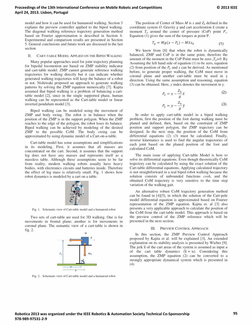
model and how it can be used for humanoid walking. Section 3 explains the preview controller applied to the biped walking. The diagonal walking reference trajectory generation method based on Fourier approximation is described in Section 4. Experimental and comparison results are presented in Section 5. General conclusions and future work are discussed in the last section

II. CART-TABLE MODEL APPLIED ON THE BIPED WALKING

Many popular approaches used for joint trajectory planning for bipedal locomotion are based on ZMP stability indicator and cart-table model. ZMP cannot generate reference walking trajectories for walking directly but it can indicate whether generated walking trajectories will keep the balance of a robot or not. Nishiwaki proposed an approach to generate walking patterns by solving the ZMP equation numerically [7]. Kajita assumed that biped walking is a problem of balancing a cart-table model [2], since in the single supported phase, human walking can be represented as the Cart-table model or linear inverted pendulum model [3].

Biped walking can be modeled using the movement of ZMP and body swing. The robot is in balance when the position of the ZMP is in the support polygon. When the ZMP reaches to the edge of the polygon, the robot loses its balance. Biped walking can be achieved by modeling of the desired ZMP to the possible CoM. The body swing can be approximated by using dynamic model of a Cart-on-a-table.

Cart-table model has some assumptions and simplifications in its modeling. First, it assumes that all masses are concentrated on the cart. Second, it assumes that the support leg does not have any masses and represents itself as a massless table. Although these assumptions seem to be far from reality, modern walking robots usually have heavy bodies, with electronics circuits and batteries inside. Therefore the effect of leg mass is relatively small. Fig. 1 shows how robot dynamics is modeled by a cart on a table.

Fig. 1. Schematic view of Cart-table model and a humanoid robot

Two sets of cart-table are used for 3D walking. One is for movements in frontal plane; another is for movements in coronal plane. The semantic view of a cart-table is shown in fig. 2.

Fig. 2. Schematic view of Cart-table model and a humanoid robot

The position of Center of Mass M is x and Zh defined in the coordinate system O. Gravity g and cart acceleration create a moment Tp around the center of pressure (CoP) point Px. Equation (1) gives the sum of the torques at point P.

We know from [8] that when the robot is dynamically balanced, ZMP and CoP is in the same point, therefore the amount of the moment in the CoP Point must be zero ,Tp=0. By Assuming the left hand side of equation (1) to be zero, equation (2) from position of the and x can be derived. As mentioned before, to generate proper walking, the CoM must move in coronal plane and another cart-table must be used in y direction. Using the same assumption and reasoning, equation (3) can be obtained. Here, y index denotes the movement in y.

In order to apply cart-table model in a biped walking problem, first the position of the foot during walking must be planed and defined, then, based on the constraint of ZMP position and support polygon, the ZMP trajectory can be designed. In the next step, the position of the CoM from differential equations (2) (3) must be calculated. Finally, inverse kinematics is used to find the angular trajectories of each joint based on the planed position of the foot and calculated CoM.

The main issue of applying Cart-table Model is how to solve its differential equations. Even though theoretically CoM trajectory can be calculated by using the exact solution of the Cart-table differential equations, Applying calculated trajectory is not straightforward in a real biped robot walking because the solution consists of unbounded functions cosh, and the obtained CoM trajectory is very sensitive to the time step variation of the walking gait.

An alternative robust CoM trajectory generation method can be found in [4][5], in which the solution of the Cart-pole model differential equation is approximated based on Fourier representation of the ZMP equation. Kajita et. al [3] also presents a very applicable approach to calculate the position of the CoM from the cart-table model. This approach is based on the preview control of the ZMP reference which will be presented in the next section.

III. PREVIEW CONTROL APPROACH

In this section, the ZMP Preview Control Approach proposed by Kajita et al. will be explained [3], An extended explanation on its stability analysis is presented by Wieber [9]. The jerk of the cart areas of the system is assumed as input u of the cart table dynamics ( ). Considering this assumption, the ZMP equation (2) can be converted to a strongly appropriate dynamical system which is presented in (4)


© 2013 IEEE


95

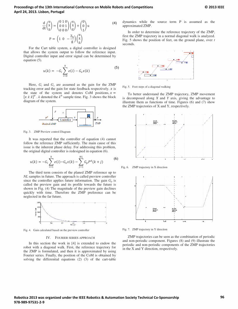
For the Cart table system, a digital controller is designed that allows the system output to follow the reference input. Digital controller input and error signal can be determined by equation (5).

Here, Gi and Gx are assumed as the gain for the ZMP tracking error and the gain for state feedback respectively. is the state of the system and denotes CoM positions,

. k denoted the kth sample time. Fig. 3 shows the block diagram of the system.

Fig. 3. ZMP Preview control Diagram

It was reported that the controller of equation (4) cannot follow the reference ZMP sufficiently. The main cause of this issue is the inherent phase delay. For addressing this problem, the original digital controller is redesigned in equation (6).

The third term consists of the planed ZMP reference up to NL samples in future. The approach is called preview controller since the controller applies future information. The gain Gp is called the preview gain and its profile towards the future is shown in Fig. (4) The magnitude of the preview gain declines quickly with time. Therefore the ZMP preference can be neglected in the far future.

Fig. 4. Gain calculated based on the preview controller

IV. FOURIER SERIES APPROACH

In this section the work in [4] is extended to endow the robot with a diagonal walk. First, the reference trajectory for the ZMP is formulated, and then it is approximated by using Fourier series. Finally, the position of the CoM is obtained by solving the differential equations (2) (3) of the cart-table

dynamics while the source term P is assumed as the approximated ZMP.

In order to determine the reference trajectory of the ZMP, first the ZMP trajectory in a normal diagonal walk is analyzed. Fig. 5 shows the position of feet, on the ground plane, over t seconds.

Fig. 5. Foot steps of a diagonal walking

To better understand the ZMP trajectory, ZMP movement is decomposed along X and Y axis, giving the advantage to illustrate them as functions of time. Figures (6) and (7) show the ZMP trajectories of X and Y, respectively.

Fig. 6. ZMP trajectory in X direction

Fig. 7. ZMP trajectory in Y direction

ZMP trajectories can be seen as the combination of periodic and non-periodic component. Figures (8) and (9) illustrate the periodic and non-periodic components of the ZMP trajectories in the X and Y direction, respectively.


© 2013 IEEE


96

Fig. 8. ZMP component in X direction

Fig. 9. ZMP component in Y direction

In order to employ Fourier series limited to a certain number of terms, continuous periodic functions are needed. Figures (8) and (9) are employed to determine the equations (7) and (12) for formulating the ZMP reference trajectory in X and Y direction respectively. The equations from (9) to (11) and from (14) to (23) formulate periodic components of the trajectory. The non-periodic component of the ZMP trajectories are presented in equations (8) (13).

This formulation design enhances the approach presented in [4] by adding a double support phase to formulate the ZMP trajectory, allowing to control the amount of double support phase using the parameter D. The parameters used in the ZMP trajectory formulation are listed in table (1) as well as a brief description of each one.

TABLE I. FORMULATION PARAMETERS

Parameter Description

T Period

A Amount of displacement in X direction

B Distance between both feet when walking straight

b Amount of displacement in Y direction

D Amount of time to be in double support phase

The next step is to determine the Fourier series of equations (7) and (12). For this we used the definition of the Fourier series given by (24).

The results are given by equations (25) and (26) which are approximated ZMP trajectories using Fourier series definition (24).


© 2013 IEEE


97

Where

Finally, it remains to solve the cart-table differential equations (2) and (3) using equations (25) and (26) as source term.

The value of the parameter N must be a positive integer. The solution will be of the form:

By substituting equations (30) and (31) to (29), the (32) is obtained.

This equality is true when:

Solving for Cn and substituting to (30) we get the particular solution for the second order differential equation:

To get the CoM equation all we have to do is to solve the differential equation (29) but changing the right side of the equation with the corresponding ZMP equations (25) and (26). The results are given by equations (35) and (36).

V. RESULTS AND DISCUSSIONS

According to section 2, the CoM reference trajectory is obtained by solving the Cart-Table model. Position trajectories of the swing foot are generated through Bézier curve based on predefined footsteps. The swing foot orientation is kept parallel to the ground to reduce the effect of the contact force. Joint angles are calculated based on swing foot positions and CoM references by using inverse kinematics, then joints are controlled by simple independent PID position controllers. The detailed explanation of the techniques, used for inverse kinematics and control of the swing foot positions, can be found in [10] [11].

In this study, a simulated NAO robot is used in order to test and verify the approach. The NAO model is a kid size humanoid robot which has 58 cm height and 21 degree of freedom (DoF). The link dimensions of the NAO robot can be found in [12]. The simulation is carried out by RoboCup soccer simulator, rcsssever3d, which is the official simulator released by the RoboCup community, in order to simulate humanoids soccer match. The simulator is based on Open Dynamic Engine and Simspark [13].

According to literature, there are no published studies to compare the performance of the Fourier based ZMP approximation approach and ZMP preview control approach. In order to test and compare the performance of aforementioned approaches, several robot walking scenarios were designed, in which the simulated NAO robot walks with different speeds from 0 to 0.6 m/s in different directions. The scenarios are designed for different speeds with 0.15 m/s increment in X and Y direction, while the overall speed should not exceed the maximum speed. Parameters used in the walking scenarios are presented in Table 2.

TABLE II. PARAMETERS OF WALKING SCENARIO

Parameters Value Step Period 0.2 s

Step Height of the swing foot 0.02 m

Step Size in X direction 3 ,6, 9 ,12 cm

Step Size in Y direction 3, 6, 9 ,12 cm

Percentage of the Double Support Phase (DSP) to the whole step time

15 %

Time of whole walking 4 s, 20 steps

Height of the inverted pendulum (Zh) 0.22 cm

All walking scenarios are simulated in the same machine with the same specification. Mean Absolute Error (MAE) of the predefined reference ZMP trajectory and computed ZMP using the two approaches are presented in table 3. The number of the Fourier terms denoted by N is assumed to be 8. The incremental times of the preview control loop denoted by dt are assumed to be 0.01, 0.001 and 0.0001.

In average, The MAE in X and Y direction are achieved by the proposed Fourier method are 25 and 3 times less, respectively, than achieved by the preview control approach.


© 2013 IEEE


98

Although by decreasing dt, the MAE of the preview control will be decreased, but achieving to the performance of the Fourier approach, practically, is not possible. Since the execution time of the algorithm will be increased dramatically. The average and variation of execution times for different specifications on the preview control and Fourier approach are presented in the table 4.

TABLE III. MAE OF COMPUTED ZMP AND REFERENCE ZMP TRAJECORY

Speed Mean Absolute Error (MAE in X direction, MAE in Y direction)

(SpeedX, SpeedY)

Fourier , N=8 Preview , dt=0.01

Preview , dt=0.001

Preview, dt=0.0001

(0.15,0) (0.0001167,0.0018) (0.0044,0.0061) (0.0031,0.0025) (0.0022,0.0014) (0.3 ,0) (0.0002335,0.0018) (0.0091,0.0061) (0.0058,0.0025) (0.0047,0.0014) (0.45,0) (0.0003503,0.0018) (0.0137,0.0061) (0.0087,0.0025) (0.0070,0.0014) (0.6 ,0) (0.0004671,0.0018) (0.0183,0.0061) (0.0116,0.0025) (0.0093,0.0014) (0, 0.15) (0, 0.0018) (0 ,0.0089) (0,0.0045) (0,0.0031)

(0.15, 0.15) (0.0001167,0.0018) (0.0046 ,0.0089) (0.0029,0.0045) (0.0023,0.0031) (0.3 , 0.15) (0.0002335,0.0018) (0.0091,0.0089) (0.0058,0.0045) (0.0047,0.0031) (0.45, 0.15) (0.0003503,0.0018) (0.0137 ,0.0089) (0.0087,0.0045) (0.0070,0.0031) (0 , 0.3) (0, 0.0018) (0, 0.0117) (0, 0.0065) (0, 0.0049) (0.15 , 0.3) (0.0001167,0.0018) (0.0046, 0.0117) (0.0029, 0.0065) (0.0023, 0.0049) (0 .3 , 0.3) (0.0002335,0.0018) (0.0091, 0.0117) (0.0058, 0.0065) (0.0047, 0.0049)

(0, 0.45) (0 , 0.0019) (0 , 0.0145) (0 , 0.0085) (0 , 0.0066) (0.15, 0.45) (0.0001167,0.0019) (0.0046 , 0.0145) ( 0.029, 0.0085) (0.0023 , 0.0066)

(0, 0.6) (0 , 0.0020) (0 , 0.0174) (0 , 0.00105) (0 , 0.0083)

TABLE IV. THE AVERAGE (VAR) EXECUTION TIMES OF THE METHODS

Fourier , N=8 Preview , dt=0.01 Preview , dt=0.001

Preview , dt=0.0001

0.0458(1.8482e-006) 0.3013(5.9957e-005) 0.6306(0.0015) 16.5349(0.0014)

After executing the methods for each walking scenarios on the machine, the average execution times for approximating ZMP and generating CoM trajectories, by using the Fourier based approach, was 0.0458 second. It is 15 times faster than the best computation time that could be achieved by using the preview control approach. For a humanoid robot that has limited computational resources, performing a real time task, such as controlling the walking, requires an algorithm with low time complexity like Fourier based approach. CoM reference and CoM position projection on the ground plane for the walking scenario, which has 15 cm/s speed in X direction and 15 cm/s in Y direction, are shown in fig. 10. The generated reference CoM trajectory and executed CoM trajectory by the robot are shown in blue and red lines respectively.

Fig. 10. COM (lines) for the diagonal walk

VI. CONCLUSIONS AND FUTURE WORK

In this paper an approach to generate the CoM reference trajectory of a diagonal and side walking is proposed. It is the

first time that, by using the Fourier approximation on the predefine ZMP reference, CoM trajectories of diagonal and side walking is achieved. In order to test and validate the results, walking scenarios for the simulated NAO robot with different speeds were presented. The comparison results show that the accuracy and time computation complexity of the proposed method is better compared to the previous approach.

In future work, the proposed method will be tested and implemented on a real humanoid robot. Our aim will be creating an omni-directional walking. Although the experimental results show that the robot can perform forward, side and diagonal walking successfully, extending the approach to make the robot able to do turn in place or curved walking, is also needed, to have a proper omni-directional walking. Following our previous work [14, 15, 16], future work will also be concerned with the application of optimization and machine learning algorithms to improve the results achieved.

REFERENCES [1] M. Vukobratovi , D. Jurici , “Contribution to the synthesis of biped

gait” IEEE Trans. Biomedical Engineering, vol. 16, no. 1, pp. 1–6, 1969. [2] S. Kajita, F. Kanehiro, K. Kaneko, K. Yokoi, and H. Hirukawa, “The 3D

linear inverted pendulum mode: a simple modeling for a biped walking pattern generation,” in IEEE/RSJ, IROS 2001, pp. 239–246.

[3] S. Kajita, F. Kanehiro, K. Kaneko, and K. Fujiwara, “Biped walking pattern generation by using preview control of zero-moment point,” in IEEE Int. Conf. Robotics and Automation, ICRA, 2003, pp. 1620–1626.

[4] K. Erbatur and O. Kurt, “Natural ZMP Trajectories for Biped Robot Reference Generation,” IEEE Transactions on Industrial Electronics, vol. 56, no. 3, pp. 835–845, Mar. 2009.

[5] Y. Choi, B. J. You, and S. R. Oh, “On the stability of indirect ZMP controller for biped robot systems,” in 2004 IEEE/RSJ Int. Conference on Intelligent Robots and Systems (IROS), 2004, pp. 1966–1971.

[6] M. Yilmaz, U. Seven, K. C. Fidan, T. Akbas, and K. Erbatur, “Circular arc-shaped walking trajectory generation for bipedal humanoid robots,” in 12th IEEE Int. Workshop on Advanced Motion Control, 2012, pp. 1–8.

[7] K. Nishiwaki, S. Kagami, Y. Kuniyoshi, M. Inaba, and H. Inoue, “Online generation of humanoid walking motion based on a fast generation method of motion pattern that follows desired ZMP,” in IEEE/RSJ Int. Conf.Intelligent Robots and System, 2002, pp. 2684–2689.

[8] A. Goswami, “Postural Stability of Biped Robots and the Foot-Rotation Indicator (FRI) Point,” The International Journal of Robotics Research, vol. 18, no. 6, pp. 523–533, Jun. 1999.

[9] P. Wieber, “Trajectory Free Linear Model Predictive Control for Stable Walking in the Presence of Strong Perturbations,” in 2006 6th IEEE-RAS International Conference on Humanoid Robots, 2006, pp. 137–142.

[10] R. Ferreira, L.P. Reis, A. P. Moreira, N. Lau, "Development of an Omnidirectional Kick For a NAO Humanoid Robot", 13th Ibero-American Conference on AI , LNAI 7637, pp 571-580 ,2012.

[11] E. Domingues, N. Lau, B. Pimentel, N. Shafii, L. P. Reis, A. J. R. Neves, "Humanoid Behaviors: From Simulation to a Real Robot", 15th Port. Conf. Artificial Intelligence, EPIA 2011, LNAI 7367, pp 352-364, 2011.

[12] D. Gouaillier, V. Hugel, P. Blazevic, C. Kilner, J. Monceaux, P. Lafourcade, B. Marnier, J. Serre, and B. Maisonnier, “Mechatronic design of NAO humanoid,” in Proceedings of the IEEE International Conference on Robotics and Automation (2009), 2009, pp. 769–774.

[13] J. Boedecker, M. Asada, “SimSpark – Concepts and Application in the RoboCup3D Soccer Sim. League,” Aut.Robots, pp. 174–181, 2008.

[14] H.Picado, M.Gestal, N.Lau, L.P.Reis, A.M.Tome,"Automatic generation of biped walk behavior using genetic algorithms" In: IWANN (1), Springer LNCS, vol. 5517, pp. 805-812. Springer (2009)

[15] N.Shafii, L.P.Reis, N.Lau, "Biped walking using coronal and sagittal movements based on truncated Fourier series", (2011) Springer LNAI, Vol. 6556, pp. 324-335.

[16] L.Cruz, L.P.Reis, N.Lau, A.Sousa, "Optimization Approach for the Development of Humanoid Robots’ Behaviors", IBERAMIA2012, Springer LNCS, Vol. 7637, pp 491-500, 2012


© 2013 IEEE


99

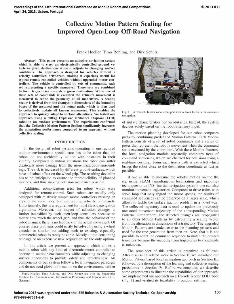
Collective Motion Pattern Scaling forImproved Open-Loop Off-Road Navigation

Frank Hoeller, Timo Rohling, and Dirk Schulz

Abstract—This paper presents an adaptive navigation systemwhich is able to steer an electronically controlled ground ve-hicle to given destinations while it adjusts to changing surfaceconditions. The approach is designed for vehicles without avelocity controlled drive-train, making it especially useful fortypical remote-controlled vehicles without upgraded motor con-trollers. The vehicle is controlled by sets of commands, eachset representing a specific maneuver. These sets are combinedto form trajectories towards a given destination. While one ofthese sets of commands is executed the vehicle’s movement ismeasured to refine the geometry of all maneuvers. A scalingvector is derived from the changes in dimensions of the boundingboxes of the assumed and the actual path, which is then usedto collectively update all known maneuvers. This enables theapproach to quickly adapt to surface alterations. We tested ourapproach using a 300 kg Explosive Ordnance Disposal (EOD)robot in an outdoor environment. The experiments confirmedthat the Collective Motion Pattern Scaling significantly increasesthe adaptation performance compared to an approach withoutcollective scaling.

I. INTRODUCTION

In the design of robot systems operating in unstructuredoutdoor environments special care has to be taken that therobots do not accidentally collide with obstacles in theirvicinity. Compared to indoor situations the robot can sufferdrastically more damage from the more hazardous surround-ings. The risk is increased by different ground surfaces, whichhave a distinct effect on the wheel grip. The resulting deviationhas to be anticipated to ensure the reproducibility of plannedmotions, and thus making collision avoidance possible.

Additional complications arise for robots which weredesigned for remote-control. Such robots are usually onlyequipped with relatively simple motor controllers missing anappropriate servo loop for interpreting velocity commands.Unfortunately, this is a requirement for most classic navigationalgorithms. Moreover, the impact of adhesion changes isfurther intensified by such open-loop controllers because nomatter how much the wheel grip, and thus the behavior of therobot changes, there is no feedback of the actual movement. Ofcourse, these problems could easily be solved by using a wheelencoder or similar, but adding such to existing, especiallycommercial robots is rarely possible. Mostly a time-consumingredesign or an expensive new acquisition are the only options.

In this article we present an approach, which allows amobile robot with any kind of electronic motor controller tooperate in outdoor environments while adjusting to changingsurface conditions to provide safety and effectiveness. Allcomponents of our system follow a local navigation paradigmand do not need global information on the environment, neither

Frank Hoeller, Timo Rohling, and Dirk Schulz are with the FraunhoferInstitute for Communication, Information Processing and Ergonomics FKIE,Germany

Fig. 1. A Telerob Teodor robot equipped with sensors for basic autonomousnavigation.

of surface characteristics nor on obstacles. Instead, the systemdecides solely based on the robot’s sensory input.

The motion planning developed for our robot composespaths by combining predefined Motion Patterns. Each MotionPattern consists of a set of robot commands and a series ofposes that represent the robot’s movement when the commandset is executed by the controllers. With these Motion Patterns,the local navigation module repeatedly computes trees ofcommand sequences, which are checked for collisions using areal-time costmap. From each tree a path is extracted whichbrings the robot close to the destination coordinate as fast aspossible.

If one is able to measure the robot’s motion on the fly,e.g using SLAM (simultaneous localization and mapping)techniques or an INS (inertial navigation system), one can alsomonitor movement trajectories. Compared to drive-trains withservo loop that only regard the motor speeds, the results ofcommand sequences can be observed on a larger scale, whichallows to tackle the surface traction problem in a novel way:The collected trajectory data is used to update the previouslymeasured movement trajectory of the corresponding MotionPatterns. Furthermore, the detected changes are propagatedto all other Motion Patterns by calculating a scaling vectorfrom the alteration in dimensions of a trajectory. The upgradedMotion Patterns are handed over to the planning process andused for the tree generation from then on. Note, that it is notpossible to adapt the command sequence to match the desiredtrajectory because the mapping from trajectories to commandsis unknown.

The remainder of this article is organized as follows:After discussing related work in Section II, we introduce ourMotion Pattern based local navigation approach in Section III,followed by a description of the learning and collective scalingprocedures in Section IV. Before we conclude, we describesome experiments to illustrate the capabilities of our approach.We implemented our approach on a Telerob Teodor EOD robot(Fig. 1) and verified its feasibility in outdoor settings.


© 2013 IEEE


100

II. RELATED WORK

In the field of outdoor robotics the terrain always is ofspecial interest. The analysis and classification of differentsurfaces regarding their traversability has been addressed bymany different authors. The classification of the differentsurface types using vibration sensors is very popular becausethis sensing mode is not vulnerable to lighting or perspectiveissues. Brooks et al. [1] attached this kind of sensor to axlearms and classified different terrains by traversing them. Theyused offline learning in combination with a voting mechanismto enable the system to identify a set of different surfaces.Unfortunately, classification approaches of this type can onlyidentify known terrains without deriving information concern-ing the behavior of a vehicle on the respective surface. Theidentified terrain type would have to be associated with aparameter set for the trajectory generator in an intermediatestep. Furthermore, this would make the navigation dependenton the a priori learned identification data, which would violatethe intended local navigation paradigm.

The DARPA Grand Challenge winning robot Stanley [13]also uses a vibration sensor to regulate its maximum speed.Unwilling to catalog every possible terrain type, Stavens etal. evaluate the occurring vibrations to limit Stanley’s speedaccording to observed human driving behaviors [11]. A similarapproach is presented by Castelnovi et al. [2], but instead ofsensing vibrations the authors used a 2D laser range finderaimed downwards to calculate a ruggedness grade. Based onthis result the robot’s top speed is reduced, resulting in adecreased number of terrain-related incidents. A combinedapproach was later proposed by Stavens et al. as an upgrade forStanley’s system [12]. Here a learning component associatesvibration intensities with surface profiles measured with aforward-facing 3D laser distance scanner. This way the systemcan automatically learn terrain-speed-associations. Thus themaximum speed can be adjusted before the vibration sensordetects a surface transition and the vehicle is exposed toless shock. These approaches show several similarities to thetechnique presented in this paper as the analysis of the grounddirectly affects the local navigation. Nevertheless, only themaximum translation velocity is altered. Rotation velocitiesare not addressed at all, which is not necessary for a robotlike Stanley.

Another interesting approach by Martinelli et al. [6] alsouses laser range finders, but in combination with SLAM andKalman filter techniques. The system is able to determinethe systematic component of the odometry error by using thewheel encoder readings and the estimated SLAM position.The non-systematic error, which is more interesting in outdoorapplications, can also be determined by a Kalman filter appliedon a history of robot states. These are provided by the formerKalman filter, making the estimation indirectly dependent onwheel encoders and closed-loop control.

Crusher, a six-wheeled robot for extreme outdoor environ-ments also suffered from trajectories differing from plannedpaths. Seegmiller at al. proposed an approach to automaticallycalibrate a dynamic model [10]. It linearizes the nominalvehicle model and then calibrates the dynamics to explainthe observed prediction residuals using a Kalman filter. Theirsystem, just as our system, takes advantage of the preciseshort-term localization sensors like GPS and INS. Although

results are impressive, their approach is again tailored to avelocity driven model which unfortunately is not applicable toour robot.

Instead of laser range finders, stereo cameras are alsowidely used. In [4] a planetary rover navigation suit is pre-sented which uses this type of camera to (besides handling thepath planning) classify the terrain and obstacles around therover. In addition, the system is able to predict wheel slippagebased on the same visual data. Again, the used algorithmcan only recognize differences to known surfaces, which isnegligible if the robot happens to be on a sparse planet.Furthermore, high velocities are not in the focus of planetaryrovers yet, thus most rover systems are not suited for otherapplications.

The combination of motion templates and learning hasbeen used widely in the area of walking robots. In this field,learning techniques are mostly applied to improve walkingpolicies that were derived from simulations [7] or observedfrom human walking [8]. Furthermore, due to the complexityof biped locomotion, every walking robot is equipped withmany sensors to determine its stance and to allow closed-loopcontrol.

Similarly, the concept of motion template based learninghas also been employed to simplify the learning of complexmotions [9]. In contrast to our approach the templates are pa-rameterized, so they can be adjusted to fit the desired trajectory.This implies a feasible correlation between parameter input anddrive-train behavior.

III. LOCAL NAVIGATION WITHMOTION PATTERNS

The core of the overall approach is a local navigationplanning component that directly controls the robot and steersit on a collision-free path from its current position to a givendestination in configuration space. For this purpose special pre-cautions for the open-loop motor controllers have to be taken.Since remote-controlled robots lack a velocity regulator circuit,the control commands influence the motor power directly. Thisinduces that their outcome depends on many factors and isfar too complex to compute in an online approach. To makemotion planning still possible, we introduce Motion Patterns.The first component of a Motion Pattern MP is a series ofrobot control commands U = (u1, . . . , uT ). A command ut

can be of any type and dimension: when used with a Teodorrobot they are motor power commands, when controlling acar they probably are throttle position and steering angle.A command sequence U is immutable, which implies thatMotion Patterns cannot be parameterized e.g. regarding theirvelocity. The second component of a Motion Pattern is anarray of oriented relative positions R = (Δr1, . . . ,ΔrT ). Itrepresents the trajectory on which the robot would theoreticallymove when the command series is sent to the robot, soeach pose Δrt describes the relative position of the robotafter it executed the command sequence from u1 to ut.The Motion Patterns can now be combined to form motionpaths P = (R1, . . . , Rk). Of course it has to be checkedif concatenated Motion Patterns fit together so that no harshvelocity change creates unexpected movement trajectories. Thecreated paths can then be checked for collisions e.g. by using


© 2013 IEEE


101

Fig. 2. A planning tree of collision free paths that has been build usingMotion Patterns in an 2-dimensional simulated environment.

an occupancy grid [5]. The corresponding sequence of seriesof commands CP = (U1, . . . , Uk) can be merged to a largearray of robot commands which can be executed by the robotsequentially. Notice that the number, shape, and complexity ofMotion Patterns are not restricted, but definitely have an impacton the planning process. In general, with fewer patterns a largerrange can be covered, while more patterns increase the qualityof the resulting paths. Since basic navigation capabilities weresufficient for the following learning algorithm, minimal a setof five Motion Patterns was used, which consisted of commandseries representing a forward, a left, and a right movement, anacceleration, and a deceleration.

Based on the model above, we can now also build acollision-free tree of Motion Patterns and extract the best pathtowards the destination. The path planning process is describedin detail in [5] and an example tree generated by this techniquecan be seen in Fig. 2. The theoretical principles of a verysimilar navigation approach are examined in [3] extensively.

IV. MOTION LEARNING USING COLLECTIVEMOTION PATTERN SCALING

A problem arising from our kind of local navigation isits sensitivity to surface and traction changes. Motion Patternsare created for specific surfaces only. And it is unlikely thatthe surface or the surface’s condition always remains constant,especially in outdoor scenarios. As a result, the driven and thepreviously recorded trajectories may differ.

To compensate for this, the local navigation has beenextended by a learning mechanism. While the command setof a selected Motion Pattern MP* is executed, the robot’sreactions are measured. For this purpose the robot’s movementtrajectory M, consisting of the x, y and ϕ deltas, is recorded.The saved trajectory RMP* inside the Motion Pattern MP*can directly be updated with this updated measurement. Thistechnique was combined with an exponential smoothing (seebelow) to form the first version of the learning Motion Patternbased local navigation. The potential of this basic systemhas been shown in [5]. Both learning approaches, the basicversion from [5] and the improved version discussed here,as well as the planning mechanism assume, that appliedMotion Patterns yield in similar trajectories repeatedly. Theexponential smoothing can cope with singular discontinuities,but it is not able to handle continuously changing results,i.e. occuring on slopes or rough terrain. Both methods arecomputationally simple and the calculation effort is negligiblecompared to the time needed for path planning.

Fig. 3. Evolution of a Motion Pattern set with three patterns: 1) Initial setbefore a Motion Pattern is chosen and executed. 2) After measuring a MotionPattern’s (MP*) result the bounding box changes are analyzed. 3) All MotionPatterns are scaled yielding to a new set.

The trajectory update inside the Motion Pattern can beregarded as information gain. We would like to propagate thisadditional knowledge to all other Motion Patterns as well toimprove the adaption speed considerably. For this purpose wecalculate a vector of scaling factors V = (xs, ys, ϕs)

T bycomparing the recently measured trajectory and the predictionRMP* saved inside the Motion Pattern MP*. xs and ys regardthe positions inside the trajectory, and ϕs the trajectory’syaw information. The first approach would be to comparethe final pose of the measured trajectory M and the predictedtrajectory from MP* to compute these factors. Unfortunately,this would decrease the robustness for trajectories which havea final lateral position close to its initial value (e.g. double-lane change maneuvers). In these cases, it is likely that themeasurement noise exceeds the position change, which wouldgenerate enormous scaling factors. A similar problem occursfor patterns which only include a movement in only onedimension, e.g. forward motions or in-place turns. Althoughthese patterns can be scaled, they cannot be used to calculatea reasonable scaling vector V because their movement in theunaddressed axes is only caused by noise and would againgenerate exaggerated scaling factors. For this reason, patternslike these are taken out of the learning process, because it isnot possible to gain information from something, that did notchange. To address the former case of this problem, the lengthand the width of the bounding boxes (BB) around the twoconsidered trajectories are used to calculate the scaling factorsxs and ys. The yaw scaling factor ϕs is calculated similarlyto the position factor: here the interval between the minimumand maximum of all recorded yaw angles is used. Now wecan compute a quotient for every dimension and compose thescaling vector V :

V (M,MP*) =

⎛⎜⎝

xs

ys

ϕs

⎞⎟⎠ =

⎛⎜⎜⎜⎝

LengthBB(M)LengthBB(MP∗)

WidthBB(M)WidthBB(MP∗)

|AngleInterval(M)||AngleInterval(MP∗)|

⎞⎟⎟⎟⎠ (1)

This vector can now be used to collectively scale all MotionPatterns making it possible to update even yet unregardedMotion Patterns. An example application is illustrated in Fig. 3.In this manner the knowledge of change of movement behavioris propagated without the need to wait for every Motion Patternto be chosen and executed, reducing the adoption time notably.

In both cases, without and with Collective Motion PatternScaling, the new predictions are integrated in the MotionsPatterns’ existing trajectory using a component-by-componentexponential smoothing function. This allows continuous learn-ing and at the same time smooths minor surface variations to


© 2013 IEEE


102

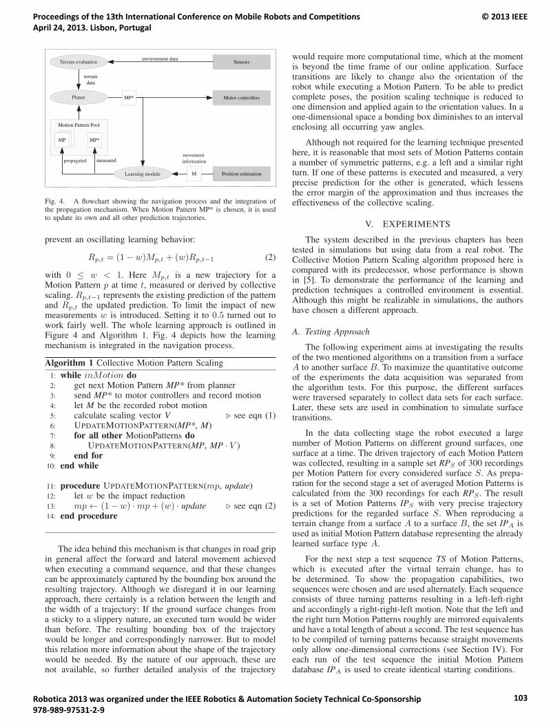
Motion Pattern Pool

MP2

Sensorsenvironment data

terrain

data

Motor controllers

Position estimation

MP*

MP*MP2MP

measuredpropagated

Terrain evaluation

Planer

Learning module

movement

information

M

Fig. 4. A flowchart showing the navigation process and the integration ofthe propagation mechanism. When Motion Pattern MP* is chosen, it is usedto update its own and all other prediction trajectories.

prevent an oscillating learning behavior:

Rp,t = (1− w)Mp,t + (w)Rp,t−1 (2)

with 0 ≤ w < 1. Here Mp,t is a new trajectory for aMotion Pattern p at time t, measured or derived by collectivescaling. Rp,t−1 represents the existing prediction of the patternand Rp,t the updated prediction. To limit the impact of newmeasurements w is introduced. Setting it to 0.5 turned out towork fairly well. The whole learning approach is outlined inFigure 4 and Algorithm 1. Fig. 4 depicts how the learningmechanism is integrated in the navigation process.

Algorithm 1 Collective Motion Pattern Scaling

1: while inMotion do2: get next Motion Pattern MP* from planner3: send MP* to motor controllers and record motion4: let M be the recorded robot motion5: calculate scaling vector V � see eqn (1)6: UPDATEMOTIONPATTERN(MP*, M)7: for all other MotionPatterns do8: UPDATEMOTIONPATTERN(MP, MP · V )9: end for

10: end while

11: procedure UPDATEMOTIONPATTERN(mp, update)12: let w be the impact reduction13: mp ← (1− w) ·mp+ (w) · update � see eqn (2)14: end procedure

The idea behind this mechanism is that changes in road gripin general affect the forward and lateral movement achievedwhen executing a command sequence, and that these changescan be approximately captured by the bounding box around theresulting trajectory. Although we disregard it in our learningapproach, there certainly is a relation between the length andthe width of a trajectory: If the ground surface changes froma sticky to a slippery nature, an executed turn would be widerthan before. The resulting bounding box of the trajectorywould be longer and correspondingly narrower. But to modelthis relation more information about the shape of the trajectorywould be needed. By the nature of our approach, these arenot available, so further detailed analysis of the trajectory

would require more computational time, which at the momentis beyond the time frame of our online application. Surfacetransitions are likely to change also the orientation of therobot while executing a Motion Pattern. To be able to predictcomplete poses, the position scaling technique is reduced toone dimension and applied again to the orientation values. In aone-dimensional space a bonding box diminishes to an intervalenclosing all occurring yaw angles.

Although not required for the learning technique presentedhere, it is reasonable that most sets of Motion Patterns containa number of symmetric patterns, e.g. a left and a similar rightturn. If one of these patterns is executed and measured, a veryprecise prediction for the other is generated, which lessensthe error margin of the approximation and thus increases theeffectiveness of the collective scaling.

V. EXPERIMENTS

The system described in the previous chapters has beentested in simulations but using data from a real robot. TheCollective Motion Pattern Scaling algorithm proposed here iscompared with its predecessor, whose performance is shownin [5]. To demonstrate the performance of the learning andprediction techniques a controlled environment is essential.Although this might be realizable in simulations, the authorshave chosen a different approach.

A. Testing Approach

The following experiment aims at investigating the resultsof the two mentioned algorithms on a transition from a surfaceA to another surface B. To maximize the quantitative outcomeof the experiments the data acquisition was separated fromthe algorithm tests. For this purpose, the different surfaceswere traversed separately to collect data sets for each surface.Later, these sets are used in combination to simulate surfacetransitions.

In the data collecting stage the robot executed a largenumber of Motion Patterns on different ground surfaces, onesurface at a time. The driven trajectory of each Motion Patternwas collected, resulting in a sample set RPS of 300 recordingsper Motion Pattern for every considered surface S. As prepa-ration for the second stage a set of averaged Motion Patterns iscalculated from the 300 recordings for each RPS . The resultis a set of Motion Patterns IPS with very precise trajectorypredictions for the regarded surface S. When reproducing aterrain change from a surface A to a surface B, the set IPA isused as initial Motion Pattern database representing the alreadylearned surface type A.

For the next step a test sequence TS of Motion Patterns,which is executed after the virtual terrain change, has tobe determined. To show the propagation capabilities, twosequences were chosen and are used alternately. Each sequenceconsists of three turning patterns resulting in a left-left-rightand accordingly a right-right-left motion. Note that the left andthe right turn Motion Patterns roughly are mirrored equivalentsand have a total length of about a second. The test sequence hasto be compiled of turning patterns because straight movementsonly allow one-dimensional corrections (see Section IV). Foreach run of the test sequence the initial Motion Patterndatabase IPA is used to create identical starting conditions.


© 2013 IEEE


103

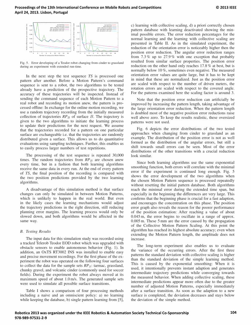
Fig. 5. Error developing of a Teodor robot changing from cinder to grasslandduring an experiment with extended run-time.

In the next step the test sequence TS is processed onepattern after another. Before a Motion Pattern’s commandsequence is sent to a robot, the two algorithms to be testedalready have a prediction of the prospective trajectory. Theaccuracy of these trajectories will be inspected. Instead ofsending the command sequence of each Motion Pattern to areal robot and recording its motion anew, the pattern is pro-cessed offline: In exchange for the online motion recording, weuse a random trajectory recording from the initially measuredcollection of trajectories RPB of surface B. The trajectory isgiven to the two algorithms to initiate the learning processto update their predictions for the next request. We assumethat the trajectories recorded for a pattern on one particularsurface are exchangeable i.e. that the trajectories are randomlydistributed given a surface. This allows us to do quantitativeevaluations using sampling techniques. Further, this enables usto easily process larger numbers of test repetitions.

The processing of the test sequence is repeated 30,000times. The random trajectories from RPB are chosen anewevery time, but in a fashion that both learning algorithmsreceive the same data in every run. At the end of every patternof TS, the final position of the recording is compared withthe two position predictions provided by the two learningalgorithms.

A disadvantage of this simulation method is that surfacechanges can only be simulated in between Motion Patterns,which is unlikely to happen in the real world. But evenin the likely cases the learning mechanisms would adjustthe trajectory predictions in the right direction, still reducingplanning error margins. The learning process would only beslowed down, and both algorithms would be affected in thesame way.

B. Testing Results

The input data for this simulation study was recorded usinga tracked Telerob Teodor EOD robot which was upgraded withobstacle sensors to enable autonomous behavior (Fig. 1). Inaddition, an OxTS RT3002 INS was installed to enable easyand precise movement recordings. For the first phase of the ex-periment the robot was operated on the following four surfacesto collect the data for the sample sets RPS : tarmac, grassland,chunky gravel, and volcanic cinder (commonly used for soccerfields). During the experiment the robot always moved at itsmaximum speed of about 1.0 m/s. The generated sample setswere used to simulate all possible surface transitions.

Table I shows a comparison of four processing methodsincluding a naive and an omniscient policy: a) no learningwhile keeping the database, b) single pattern learning from [5],

c) learning with collective scaling, d) a priori correctly chosenpattern database with learning deactivated showing the min-imal possible errors. The error reduction percentages for thenormal learning and the learning with collective scaling arepresented in Table II. As in the simulated experiment, thereduction of the orientation error is noticeably higher then theposition error reduction. The angular error reduction rangesfrom 7.3 % up to 27.9 % with one exception that probablyresulted from similar surface properties. The position errorreduction on the other hand only reaches 17.8 % at best, but isnormally below 10 %, sometimes even negative. The measuredorientation error values are quite large, but it has to be keptin mind that these are normalized. Just as the position errorare scaled with respect to the number of driven meters, therotation errors are scaled with respect to the covered angle.For the patterns examined here the scaling factor is around 3.

Note that the position error reduction can artificially beimproved by increasing the pattern length, taking advantage ofthe large orientation error reduction. When the pattern lengthis doubled most of the negative position error reductions raisewell above zero. To keep the results realistic, these oversizedpatterns were not used.

Fig. 6 depicts the error distributions of the two testedapproaches when changing from cinder to grassland as anexample. The distribution of the position error is not as wellformed as the distribution of the angular errors, but still ashift towards small errors can be seen. Most of the errordistributions of the other transitions with a crucial reductionlook similar.

Since both learning algorithms use the same exponentialsmoothing function, both errors will correlate with the minimalerror if the experiment is continued long enough. Fig. 5shows the error development of the two algorithms whenthe chosen Motion Pattern sequence is processed repeatedlywithout resetting the initial pattern database. Both algorithmsreach the minimal error during the extended time span, butespecially in the beginning the differences are very large. Thisconfirms that the beginning phase is crucial for a fast adaption,and encourages the concentration on this phase. The positionerror graph also reveals the reason for the poorer performanceof the position estimation: After reaching a value of about0.045 m, the error begins to oscillate in a range of approx.0.005 m. These 5 mm are the error caused by the propagationof the Collective Motion Pattern Scaling. At this point thealgorithm has reached its highest absolute accuracy; even whenextending the Motion Pattern length, the amplitude does notincrease.

The long-term experiment also enables us to evaluatethe variance of the occurring errors. After the first threepatterns the standard deviation with collective scaling is higherthan the standard deviation of the simple learning method.This is caused by the exponential smoothing: When it isused, it intentionally prevents instant adaption and generatesintermediate trajectory predictions while converging towardsthe measured behavior. When adding collective scaling, theseintermediate predictions appear more often due to the greaternumber of adjusted Motion Patterns, especially immediatelyafter a surface transition. As soon as the adaption to a newsurface is completed, the deviation decreases and stays belowthe deviation of the simple method.


© 2013 IEEE


104

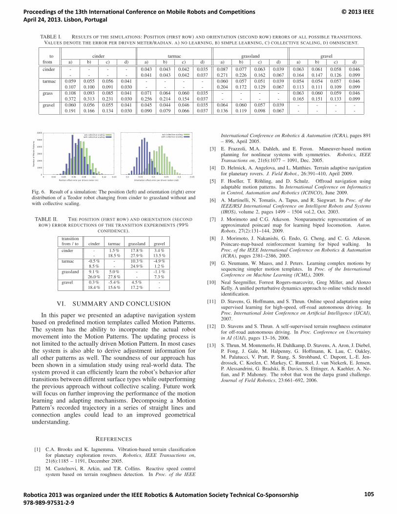
TABLE I. RESULTS OF THE SIMULATIONS: POSITION (FIRST ROW) AND ORIENTATION (SECOND ROW) ERRORS OF ALL POSSIBLE TRANSITIONS.VALUES DENOTE THE ERROR PER DRIVEN METER/RADIAN. A) NO LEARNING, B) SIMPLE LEARNING, C) COLLECTIVE SCALING, D) OMNISCIENT.

to cinder tarmac grassland gravel

from a) b) c) d) a) b) c) d) a) b) c) d) a) b) c) d)

cinder - - - - 0.043 0.043 0.042 0.035 0.087 0.077 0.063 0.039 0.063 0.061 0.058 0.046

- - - - 0.041 0.043 0.042 0.037 0.271 0.226 0.162 0.067 0.164 0.147 0.126 0.099

tarmac 0.059 0.055 0.056 0.041 - - - - 0.060 0.057 0.051 0.039 0.054 0.054 0.057 0.046

0.107 0.100 0.091 0.030 - - - - 0.204 0.172 0.129 0.067 0.113 0.111 0.109 0.099

grass 0.108 0.093 0.085 0.041 0.071 0.064 0.060 0.035 - - - - 0.063 0.060 0.059 0.046

0.372 0.313 0.231 0.030 0.256 0.214 0.154 0.037 - - - - 0.165 0.151 0.133 0.099

gravel 0.060 0.056 0.055 0.041 0.045 0.044 0.046 0.035 0.064 0.060 0.057 0.039 - - - -

0.191 0.166 0.134 0.030 0.090 0.079 0.066 0.037 0.136 0.119 0.098 0.067 - - - -

Fig. 6. Result of a simulation: The position (left) and orientation (right) errordistribution of a Teodor robot changing from cinder to grassland without andwith collective scaling.

TABLE II. THE POSITION (FIRST ROW) AND ORIENTATION (SECOND

ROW) ERROR REDUCTIONS OF THE TRANSITION EXPERIMENTS (99%CONFIDENCE).

transitionfrom / to cinder tarmac grassland gravel

cinder - 1.5 % 17.8 % 3.4 %- 18.5 % 27.9 % 13.5 %

tarmac -0.5 % - 10.3 % -4.9 %8.5 % - 24.9 % 1.2 %

grassland 9.1 % 5.0 % - -1.1 %26.0 % 27.8 % - 7.3 %

gravel 0.3 % -5.4 % 4.5 % -18.4 % 15.6 % 17.2 % -

VI. SUMMARY AND CONCLUSION

In this paper we presented an adaptive navigation systembased on predefined motion templates called Motion Patterns.The system has the ability to incorporate the actual robotmovement into the Motion Patterns. The updating process isnot limited to the actually driven Motion Pattern. In most casesthe system is also able to derive adjustment information forall other patterns as well. The soundness of our approach hasbeen shown in a simulation study using real-world data. Thesystem proved it can efficiently learn the robot’s behavior aftertransitions between different surface types while outperformingthe previous approach without collective scaling. Future workwill focus on further improving the performance of the motionlearning and adapting mechanisms. Decomposing a MotionPattern’s recorded trajectory in a series of straight lines andconnection angles could lead to an improved geometricalunderstanding.

REFERENCES

[1] C.A. Brooks and K. Iagnemma. Vibration-based terrain classificationfor planetary exploration rovers. Robotics, IEEE Transactions on,21(6):1185 – 1191, December 2005.

[2] M. Castelnovi, R. Arkin, and T.R. Collins. Reactive speed controlsystem based on terrain roughness detection. In Proc. of the IEEE

International Conference on Robotics & Automation (ICRA), pages 891– 896, April 2005.

[3] E. Frazzoli, M.A. Dahleh, and E. Feron. Maneuver-based motionplanning for nonlinear systems with symmetries. Robotics, IEEETransactions on, 21(6):1077 – 1091, Dec. 2005.

[4] D. Helmick, A. Angelova, and L. Matthies. Terrain adaptive navigationfor planetary rovers. J. Field Robot., 26:391–410, April 2009.

[5] F. Hoeller, T. Rohling, and D. Schulz. Offroad navigation usingadaptable motion patterns. In International Conference on Informaticsin Control, Automation and Robotics (ICINCO), June 2009.

[6] A. Martinelli, N. Tomatis, A. Tapus, and R. Siegwart. In Proc. of theIEEE/RSJ International Conference on Intelligent Robots and Systems(IROS), volume 2, pages 1499 – 1504 vol.2, Oct. 2003.

[7] J. Morimoto and C.G. Atkeson. Nonparametric representation of anapproximated poincare map for learning biped locomotion. Auton.Robots, 27(2):131–144, 2009.

[8] J. Morimoto, J. Nakanishi, G. Endo, G. Cheng, and C. G. Atkeson.Poincare-map-based reinforcement learning for biped walking. InProc. of the IEEE International Conference on Robotics & Automation(ICRA), pages 2381–2386, 2005.

[9] G. Neumann, W. Maass, and J. Peters. Learning complex motions bysequencing simpler motion templates. In Proc. of the InternationalConference on Machine Learning (ICML), 2009.

[10] Neal Seegmiller, Forrest Rogers-marcovitz, Greg Miller, and AlonzoKelly. A unified perturbative dynamics approach to online vehicle modelidentification.

[11] D. Stavens, G. Hoffmann, and S. Thrun. Online speed adaptation usingsupervised learning for high-speed, off-road autonomous driving. InProc. International Joint Conference on Artificial Intelligence (IJCAI),2007.

[12] D. Stavens and S. Thrun. A self-supervised terrain roughness estimatorfor off-road autonomous driving. In Proc. Conference on Uncertaintyin AI (UAI), pages 13–16, 2006.

[13] S. Thrun, M. Montemerlo, H. Dahlkamp, D. Stavens, A. Aron, J. Diebel,P. Fong, J. Gale, M. Halpenny, G. Hoffmann, K. Lau, C. Oakley,M. Palatucci, V. Pratt, P. Stang, S. Strohband, C. Dupont, L.-E. Jen-drossek, C. Koelen, C. Markey, C. Rummel, J. van Niekerk, E. Jensen,P. Alessandrini, G. Bradski, B. Davies, S. Ettinger, A. Kaehler, A. Ne-fian, and P. Mahoney. The robot that won the darpa grand challenge.Journal of Field Robotics, 23:661–692, 2006.


© 2013 IEEE


105

Localization and Navigation of a Mobile Robot in an Office-like Environment

Paulo Alves*, Hugo Costelha*†, Carlos Neves*‡ *Escola Superior de Tecnologia e Gestão de Leiria, Instituto Politécnico de Leiria, Leiria, Portugal

†Robis, INESCTEC, Porto, Portugal ‡INESCC, Coimbra, Portugal

[email protected], {hugo.costelha, cneves}@ipleiria.pt

Abstract - This article focuses on the localization and navigation of a mobile differential robot in an indoor office-like environment. These are fundamental issues to service robotics, which is a branch with a strong market growth. The work implements a vision tracking system, environment mapping, route planning and navigation for an autonomous robot application inside services buildings. One goal of the methodology is its application with low cost equipment. The test bed chosen was a Pioneer P3-DX robot [16] in a service building, with an attached USB webcam, pointed at the ceiling to take advantage of the position of the light fixtures as natural landmarks. The robot location is estimated through two distinct probabilistic methods: a particle filter, when there is no information about the starting location of the robot, and the Kalman filter, given the convergence of the particle filter. Both methods use the detection of light fixtures together with the robot kinematics as information to estimate the pose. The mapping of the environment and its obstacles is obtained from the localization estimates and the information gathered by ultrasound sensors, representing the entire navigation space discretized in the form of an occupation grid. Planning the navigation path is determined by a simple search algorithm, namely the Wavefront algorithm, based on the information contained in the occupancy grid. For a given path, navigation is performed with obstacle avoidance using the virtual forces method. Replanning is used to recover from local minima situations.

Keywords: Mobile Robots, Localization, Navigation, Mapping, Office Environment.

I. INTRODUCTION

Mobile robotics is currently considered a major area of interest, where there is a great willingness by the scientific community to develop its state of the art. Moreover, its interdisciplinary nature and the complexity of the associated problems make this advance depend on the development of mathematical tools, sensors, actuators and the materials themselves, which limit their progress. Whichever vehicle you want to use an autonomous behavior in, whether in health care, assistance at home, industry or even in an office environment, the basis of their performance includes localization and navigation tasks. In the particular case of offices, despite the circulation of a significant number of people, the environment is highly structured, with unique features which facilitate localization and navigation.

Mobile robots have unique capabilities to perform tasks requiring mobility that can be automated, freeing humans to other more creative activities [11]. Today there are several tasks already automated in different areas, such as the mapping and monitoring of land surface [1], large-scale agriculture [3], environmental monitoring [20] and industry [2]. On the other hand, there are high risk tasks or ones which are even impossible to accomplish by humans, such as the verification of explosive devices [5], the exploration and mapping of areas contaminated by biological or nuclear waste to assess the damage [15], or even space exploration of distant celestial bodies [13]. There are other emerging application areas, such as personal assistance [21],rehabilitation and entertainment. For this type of applications to be possible with some degree of autonomy, robots must be equipped with various types of sensors (force sensors, inertial sensors, GPS, odometry, distance sensors or vision), to feedback the work environment perception. The robot movement can be made either by wheels or tracks, on land robots, propellers or wings, for aerial robots, and control surfaces or propellers for aquatic robots. Whether on land, air or water, two fundamental problems coexist: localization and navigation. These two problems are interdependent and crucial for autonomous mobile robotic systems to interact with the physical world correctly by extended periods of time.

In [18] a filter of Simultaneous Localization and Map Building SLAM [12] is presented, which successfully exploited a low cost vision system, with means to improve dead reckoning pose estimate and maintain a correct estimate of the pose of a mobile robot for constructing a map of the environment. As in the present work, limited resources of hardware and low cost vision where used. These limitations impose the use of image processing algorithms involving low processing requirements. To avoid the computational complexity, the paper proposes a fast algorithm for feature extraction which includes the lens distortion model from the SLAM filter. In this methodology, as well as in the present work, the light fixtures positions were used as natural landmarks. Unlike the present work, in [18] the light fixture poses are not known a priori and will be mapped during navigation. Present work provides a better accuracy in pose estimate, since light fixture poses are known instead of calculated based in detection and pose estimation.


© 2013 IEEE


106

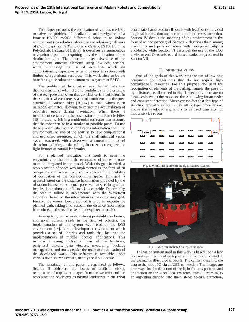
This paper proposes the application of various methods to solve the problem of localization and navigation of a Pioneer P3-DX mobile differential robot in an indoor environment (the robotics laboratory and adjoining hallways of Escola Superior de Tecnologia e Gestão, ESTG, from the Polytechnic Institute of Leiria). It describes an autonomous navigation algorithm, requiring only the indication of the destination point. The algorithm takes advantage of the environment structure elements using low cost sensors,while minimizing the use of techniques which are computationally expensive, so as to be used in systems with limited computational resources. This work aims to be the base for a guide robot or an autonomous system at ESTG.

The problem of localization was divided into two distinct situations: when there is confidence in the estimate of the real pose and when that confidence is insufficient. In the situation where there is a good confidence in the pose estimate, a Kalman filter [10][14] is used, which is an unimodal estimator, allowing to correct the accumulation of odometry errors during navigation. When there is insufficient certainty in the pose estimation, a Particle Filter [10] is used, which is a multimodal estimator that assumes that the robot can be in a number of possible poses. To use these probabilistic methods one needs information about the environment. As one of the goals is to save computational and economic resources, an off the shelf artificial vision system was used, with a video webcam mounted on top of the robot, pointing at the ceiling in order to recognize the light fixtures as natural landmarks.

For a planned navigation one needs to determine waypoints and, therefore, the occupation of the workspace must be integrated in the model. With this goal in mind, a representation of space was implemented in the form of an occupancy grid, where every cell represents the probability of occupation of the corresponding space. This grid is updated based on the distance information provided by the ultrasound sensors and actual pose estimate, as long as the localization estimate confidence is acceptable. Determining the path to follow is implemented with the Wavefront algorithm, based on the information in the occupancy grid. Finally, the virtual forces method is used to execute the planned path, taking into account the distance information from ultrasound sensors to avoid unexpected obstacles.

Aiming to give the work a strong portability and reuse, and given current trends in the field of robotics, the implementation of this system was based on the ROS environment [19]. It is a development environment which provides a set of libraries and tools that facilitate the implementation of mobile robotics applications. This includes a strong abstraction layer of the hardware, peripheral drivers, data viewers, messaging, package management, and makes easier the reuse and publication of the developed work. This software is available under various open source licenses, mainly the BSD license.

The remainder of this paper is organized as follows. Section II addresses the issues of artificial vision, recognition of objects in images from the webcam and the representation of objects as natural landmarks in the robot

coordinate frame. Section III deals with localization, divided in global localization and accumulation of errors correction. Section IV details the mapping of the environment in the form of an occupancy grid. Section V describes the planning algorithms and path execution with unexpected objects avoidance, while Section VI describes the use of the ROS environment. Conclusions and future works are presented in Section VII.

II. ARTIFICIAL VISION

One of the goals of this work was the use of low-cost equipment and algorithms that do not require high computational resources. For this purpose one used the recognition of elements of the ceiling, namely the pose of light fixtures, as illustrated in Fig. 1. Generally there are no obstacles between the robot and these, allowing for an easier and consistent detection. Moreover the fact that this type of structure typically exists in any office-type environment, allows the developed algorithms to be used generally for indoor service robots.

Fig. 1. Workspace plan with the light fixtures location.

Fig. 2. Webcam mounted on top of the robot.

The vision system used in this work is based upon a low cost webcam, mounted on top of a mobile robot, pointed at the ceiling, as illustrated in Fig. 2. The camera transmits the data to the robot PC via an USB connection. The images are processed for the detection of the light fixtures position and orientation on the robot local reference frame, according to an algorithm divided into three steps: feature extraction,


© 2013 IEEE


107

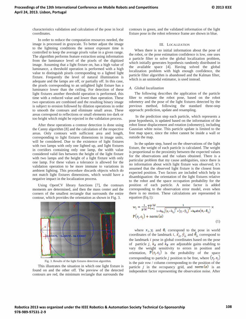
characteristics validation and calculation of the pose in local coordinates.

In order to reduce the computation resources needed, the image is processed in grayscale. To better adjust the image to the lightning conditions the sensor exposure time is controlled to keep the average pixels value in a given range. The algorithm performs feature extraction using information from the luminance level of the pixels of the digitized image. Assuming that a light fixture on, has a high value of luminance, a threshold operation is performed with a highvalue to distinguish pixels corresponding to a lighted light fixture. Frequently the level of natural illumination is adequate and the lamps are off, or partially off. In this case, the pixels corresponding to an unlighted light fixture has a luminance lower than the ceiling. For detection of these light fixtures another threshold operation is performed, this time with a reduced value and lower than operation. These two operations are combined and the resulting binary image is subject to erosion followed by dilation operations in order to smooth the contours and eliminate small areas. These areas correspond to reflections or small elements too dark or too bright which might be rejected in the validation process.

After these operations a contour detection is done using the Canny algorithm [8] and the calculation of the respective areas. Only contours with sufficient area and length, corresponding to light fixtures dimensions in image units, will be considered. Due to the existence of light fixtures with two lamps with only one lighted up, and light fixtures in corridors containing only one lamp, the width value considered valid lies between the height of the light fixture with two lamps and the height of a light fixture with only one lamp. For these values a tolerance is allowed for the validation operation to be more immune to variations in ambient lighting. This procedure discards objects which do not match light fixtures dimensions, which would have a negative impact in the localization process.

Using OpenCV library functions [7], the contours moments are determined, and then the mass center and the corners of the smallest rectangle that surrounds the entire contour, which provides the orientation as shown in Fig. 3.

Fig. 3. Results of the light fixtures detection algorithm.

This illustrates the situation in which one light fixture is found on and the other off. The preview of the detected contours are red, the minimum rectangle that surrounds the

contours in green, and the validated information of the light fixture pose in the robot reference frame are shown in blue.

III. LOCALIZATION

When there is no initial information about the pose of the robot, or the pose estimation confidence is low, one uses a particle filter to solve the global localization problem, which initially generates hypothesis randomly distributed in the available space [4]. Having solved the global localization problem with high enough confidence, the particle filter algorithm is abandoned and the Kalman filter, which is an unimodal estimator, is used instead.

A. Global localization The following describes the application of the particle

filter to estimate the robot pose, based on the robot odometry and the pose of the light fixtures detected by the previous method, following the standard three-step approach: prediction, update and resampling.

In the prediction step each particle, which represents a pose hypothesis, is updated based on the information of the robot linear displacement and rotation (odometry), including Gaussian white noise. This particle update is limited to the free map space, since the robot cannot be inside a wall or outside the map.

In the update step, based on the observations of the light fixture, the weight of each particle is calculated. The weight is proportional to the proximity between the expected values for the observations and the values obtained. There is a particular problem that my cause ambiguities, since there is no information about witch light fixture was observed; it’s assumed that the observed light fixture is the closest from expected position. Two factors are included which help in disambiguation: the orientation of the light fixtures relative to the robot and the space occupation probability for the position of each particle. A noise factor is added corresponding to the observation error model, even when there is no motion. These calculations are represented in equation (Eq.1):

(1)

where , and correspond to the pose in world coordinates of the landmark , , and

p correspond to

the landmark pose in global coordinates based on the pose of particle ,

p and

g are adjustable gains enabling to

vary the weight sensitivity to errors in position and orientation,

ggggg is the probability of the space

corresponding to particle position to be free, where is the pair row / column corresponding to the position of the particle in the occupancy grid, and

p is an

independent factor representing the observation noise. After


© 2013 IEEE


108

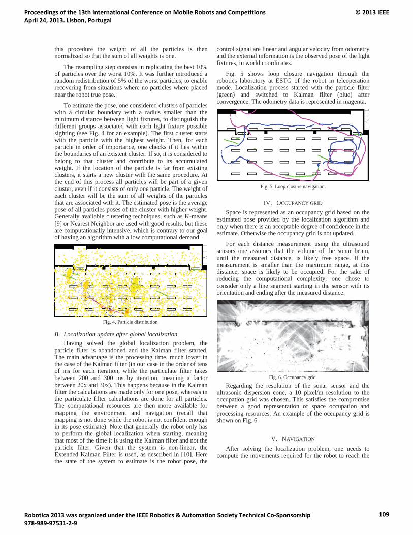
this procedure the weight of all the particles is then normalized so that the sum of all weights is one.

The resampling step consists in replicating the best 10% of particles over the worst 10%. It was further introduced a random redistribution of 5% of the worst particles, to enable recovering from situations where no particles where placed near the robot true pose.

To estimate the pose, one considered clusters of particles with a circular boundary with a radius smaller than the minimum distance between light fixtures, to distinguish the different groups associated with each light fixture possible sighting (see Fig. 4 for an example). The first cluster starts with the particle with the highest weight. Then, for each particle in order of importance, one checks if it lies within the boundaries of an existent cluster. If so, it is considered to belong to that cluster and contribute to its accumulated weight. If the location of the particle is far from existing clusters, it starts a new cluster with the same procedure. At the end of this process all particles will be part of a given cluster, even if it consists of only one particle. The weight of each cluster will be the sum of all weights of the particles that are associated with it. The estimated pose is the average pose of all particles poses of the cluster with higher weight. Generally available clustering techniques, such as K-means [9] or Nearest Neighbor are used with good results, but these are computationally intensive, which is contrary to our goal of having an algorithm with a low computational demand.

Fig. 4. Particle distribution.

B. Localization update after global localization Having solved the global localization problem, the

particle filter is abandoned and the Kalman filter started.The main advantage is the processing time, much lower in the case of the Kalman filter (in our case in the order of tens of ms for each iteration, while the particulate filter takes between 200 and 300 ms by iteration, meaning a factor between 20x and 30x). This happens because in the Kalman filter the calculations are made only for one pose, whereas in the particulate filter calculations are done for all particles. The computational resources are then more available for mapping the environment and navigation (recall that mapping is not done while the robot is not confident enough in its pose estimate). Note that generally the robot only has to perform the global localization when starting, meaning that most of the time it is using the Kalman filter and not the particle filter. Given that the system is non-linear, the Extended Kalman Filter is used, as described in [10]. Here the state of the system to estimate is the robot pose, the

control signal are linear and angular velocity from odometry and the external information is the observed pose of the light fixtures, in world coordinates.

Fig. 5 shows loop closure navigation through the robotics laboratory at ESTG of the robot in teleoperation mode. Localization process started with the particle filter (green) and switched to Kalman filter (blue) after convergence. The odometry data is represented in magenta.

Fig. 5. Loop closure navigation.

IV. OCCUPANCY GRID

Space is represented as an occupancy grid based on the estimated pose provided by the localization algorithm and only when there is an acceptable degree of confidence in the estimate. Otherwise the occupancy grid is not updated.

For each distance measurement using the ultrasound sensors one assumes that the volume of the sonar beam, until the measured distance, is likely free space. If the measurement is smaller than the maximum range, at this distance, space is likely to be occupied. For the sake of reducing the computational complexity, one chose to consider only a line segment starting in the sensor with its orientation and ending after the measured distance.

Fig. 6. Occupancy grid.

Regarding the resolution of the sonar sensor and the ultrasonic dispersion cone, a 10 pixel/m resolution to the occupation grid was chosen. This satisfies the compromise between a good representation of space occupation and processing resources. An example of the occupancy grid is shown on Fig. 6.

V. NAVIGATION

After solving the localization problem, one needs to compute the movements required for the robot to reach the


© 2013 IEEE


109

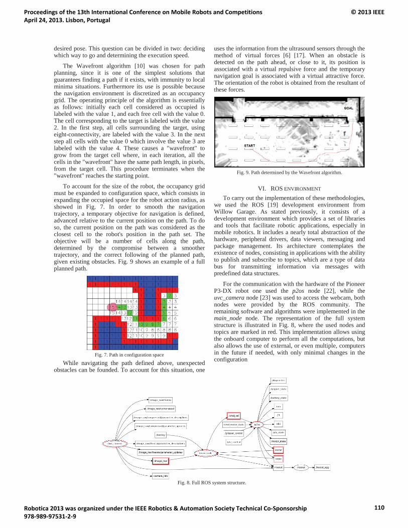
desired pose. This question can be divided in two: deciding which way to go and determining the execution speed.

The Wavefront algorithm [10] was chosen for path planning, since it is one of the simplest solutions that guarantees finding a path if it exists, with immunity to local minima situations. Furthermore its use is possible because the navigation environment is discretized as an occupancy grid. The operating principle of the algorithm is essentially as follows: initially each cell considered as occupied is labeled with the value 1, and each free cell with the value 0. The cell corresponding to the target is labeled with the value 2. In the first step, all cells surrounding the target, using eight-connectivity, are labeled with the value 3. In the next step all cells with the value 0 which involve the value 3 are labeled with the value 4. These causes a "wavefront" to grow from the target cell where, in each iteration, all the cells in the "wavefront" have the same path length, in pixels, from the target cell. This procedure terminates when the "wavefront" reaches the starting point.

To account for the size of the robot, the occupancy grid must be expanded to configuration space, which consists in expanding the occupied space for the robot action radius, as showed in Fig. 7. In order to smooth the navigation trajectory, a temporary objective for navigation is defined, advanced relative to the current position on the path. To do so, the current position on the path was considered as the closest cell to the robot's position in the path set. The objective will be a number of cells along the path, determined by the compromise between a smoother trajectory, and the correct following of the planned path, given existing obstacles. Fig. 9 shows an example of a full planned path.

Fig. 7. Path in configuration space

While navigating the path defined above, unexpected obstacles can be founded. To account for this situation, one

uses the information from the ultrasound sensors through the method of virtual forces [6] [17]. When an obstacle is detected on the path ahead, or close to it, its position is associated with a virtual repulsive force and the temporary navigation goal is associated with a virtual attractive force. The orientation of the robot is obtained from the resultant of these forces.

Fig. 9. Path determined by the Wavefront algorithm.

VI. ROS ENVIRONMENT

To carry out the implementation of these methodologies, we used the ROS [19] development environment from Willow Garage. As stated previously, it consists of a development environment which provides a set of libraries and tools that facilitate robotic applications, especially in mobile robotics. It includes a nearly total abstraction of the hardware, peripheral drivers, data viewers, messaging and package management. Its architecture contemplates the existence of nodes, consisting in applications with the ability to publish and subscribe to topics, which are a type of data bus for transmitting information via messages with predefined data structures.

For the communication with the hardware of the Pioneer P3-DX robot one used the p2os node [22], while the uvc_camera node [23] was used to access the webcam, both nodes were provided by the ROS community. The remaining software and algorithms were implemented in the main_node node. The representation of the full system structure is illustrated in Fig. 8, where the used nodes and topics are marked in red. This implementation allows using the onboard computer to perform all the computations, but also allows the use of external, or even multiple, computers in the future if needed, with only minimal changes in the configuration

Fig. 8. Full ROS system structure.


© 2013 IEEE


110

VII. CONCLUSIONS AND FUTURE WORK

A localization and navigation system was implemented to perform general tasks in office-like environments. This system maintains a correct estimate of the robot´s pose in real-time, being able to correct the error accumulation of intrinsic sensors and estimate its own pose if this information is not provided in advance.

Artificial vision is used with a common video camera for recognizing ceiling light fixture fixtures as external landmarks, whose poses are known a priori. However, given the similarity between the various fixtures and the symmetry of those poses, the determination between the real and the corresponding fixture detected is strongly dependent on the robot’s estimated pose. This may generate erroneous matches, leading to ambiguity and getting reasonable confidence in a pose that may not be real. Also, the ambient lighting conditions can lead to false detections that can compromise severely the location and hence the mapping of the environment. Nevertheless, the continuous movement of the robot combined with the particle filter used for global localization and the Kalman filter localization update, given the localization estimate confidence, allows the robot to recover when lost, and resume its normal operation.

For determining a safe and short path an occupancy grid was kept and updated with information of the space occupation likelihood. This map is updated based on the distance information of ultrasound sensors and pose estimate when this estimate has sufficiently high confidence. Based on the information of this occupancy grid the path to follow is determined with the Wavefront algorithm.

Finally, while performing the determined path, this system reacts to unexpected obstacles such as people or objects left in previously free space. To avoid these obstacles one used the virtual forces method for navigation, resuming the path whenever possible.

To speed up localization it would be interesting to explore matching techniques directly from the camera images or contours with a representation of the light fixtures and other ceiling elements, as air vents and fire detectors. This avoids significant movement without detection of landmarks, resulting in faster convergence for the particle filter and more accuracy for the Kalman filter and mapping. Furthermore, it is also expected to be more immune to erroneous detections caused by reflections, foreign objects or anomalous lighting conditions. This is difficult to combine with a high number of particles because it has to be done for each particle, which leads to a large consumption of processing resources, unavailable on the Pioneer P3-DXrobot standard platform.

As a follow up of the present work, one plans to use the developed work as a base for specific tasks, such as an autonomous guide or carrier robot.

REFERENCES

[1] Ahmad, A., & Samad, A. (2010). Aerial mapping using high resolution digital camera and unmanned aerial vehicle for Geographical Information System. Signal Processing and Its Applications (CSPA), 2010 6th International Colloquium on .

[2] Angerer, A., Hoffmann, A., Schierl, A., Vistein, M., & Reif, W. (2010). The Robotics API: An object-oriented framework for modeling industrial robotics applications. International Conference on Intelligent Robots and Systems (IROS), 2010 IEEE/RSJ.

[3] Arguenon, V., Bergues-Lagarde, A., Rosenberger, C., Bro, P., & Smari, W. (2006). Multi-Agent Based Prototyping of Agriculture Robots. International Symposium on Collaborative Technologies and Systems.

[4] Arulampalam, M. S., Maskell, S., & Gordon, N. (2002). A tutorial on particle filters for online nonlinear/non-Gaussian Bayesian tracking. IEEE Transactions on Signal Processing.

[5] Baumann, M., Hunter, J., Hannum, D., & Horton, R. (2004). Robohound™ remote explosives detection. Conference on Security Technology. 38th Annual 2004 International Carnahan.

[6] Borenstein, J. (1991). The Vector Field Histogram – Fast Obstacle Avoidance for Mobile Robots. IEEE Transactions on Robotics and Automation, Vol. 7, No.3.

[7] Bradsky, G. R.; Pisarevsky, V.; Bouguet, J. Learning OpenCV: Computer Vision with the OpenCV Library. Springer, 2006.

[8] Canny, J. (1986). A Computational Approach to Edge Detection. IEEE transactions on pattern analysis and machine intelligence, vol. Pami-8, no. 6.

[9] S. P. Lloyd, ªLeast Squares Quantization in PCM,º IEEE Trans. Information Theory, vol. 28, 129-137, 1982.

[10] Choset, H., Lynch, K. M., Hutchinson, S., Kantor, G., Burgard, W., Kavraky, L. E., et al. (2004). Principles of Robot Motion – Theory, Algorithms and Implementations. MIT Press.

[11] Couto, M. S. (2010). Localização e Navegação entre Robôs Móveis. Dissertação para a obtenção do Grau de Mestre em Engenharia Mecânica - Instituto Superior Técnico.

[12] Dissanayake, M. W., Newman, P., Clark, S., Whyte, H., & Csorba, M. (2001). A Solution to the Simultaneous Localization and Map Building (SLAM) Problem. IEEE Transactions on robotics and automation, Vol. 17, NO. 3, June 2001.

[13] Grotzinger, J. P., Ba, J. C., Blake, D. F., & all, e. (2011). Mars Science Laboratory Mission and Science. Space Sci Rev DOI 10.1007/s11214-012-9892-2.

[14] Kalman, R. E. (1960). A new approach to linear filtering and prediction problems. Journal of Basic Engineering 82 (1), 35–45.

[15] Manocha, K., Pernalete, N., & Dubey, R. (2001). Variable position mapping based assistance in teleoperation for nuclear cleanup . IEEE International Conference on Robotics and Automation. Proceedings 2001 ICRA.

[16] Mobile Robots, A. (2010). Pioneer 3 Operations Manual. [17] Neves, C. C. (1998). A Generalized Framework for the Analysis of

System Architectures in Automonomous Robots. Telford Research Institute Department of Electronic and Electric Engineering University of Salford, UK.

[18] Panzieri, S., Pascuci, F., & Ulivi, G. (2003). Vision based navigation using Kalman approach for SLAM. Proc. of the 11th International Conference on Advanced Robotics.

[19] Quigley, M., Gerkey, B., Conley, K., Faust, J., Foote, T., Leibs, J., et al. (2009). ROS: an open-source Robot Operating System. ICRA workshop.

[20] Rahimi, M., Pon, R., Kaiser, W., Sukhatme, G., Estrin, D., & Srivastava, M. (2004). Adaptive sampling for environmental robotics. IEEE International Conference on Robotics and Automation.

[21] Srinivasa, S. S., Ferguson, D., Helfrich, C. J., Berenson, D., Collet, A., Diankov, R., et al. (2009). HERB: a home exploring robotic butler. Springer Science+Business Media, LLC 2009.

[22] http://www.ros.org/wiki/p2os_driver[23] http://www.ros.org/wiki/uvc_camera


© 2013 IEEE


111

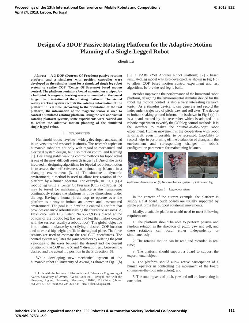
Abstract— A 3 DOF (Degrees Of Freedom) passive rotating platform and a simulator with position controller were developed as the stimulus input for a simulated single leg robot system to realize COP (Center Of Pressure) based motion control. The platform contains a board mounted on a tripod by a ball joint. A magnetic tracking sensor is mounted on the board to get the orientation of the rotating platform. The virtual reality tracking system records the rotating information of the platform in real time. According to the orientation of the real platform, the information of the magnetic sensor is used to control a simulated rotating platform. Using the real and virtual rotating platform systems, some experiments were carried out to realize the adaptive motion planning of the simulated single-legged robot.

I. INTRODUCTION

Humanoid robots have been widely developed and studied in universities and research institutes. The research topics on humanoid robot are not only with regard to mechanical and electrical system design, but also motion control and learning [1]. Designing stable walking control methods for biped robot is one of the most difficult research issues [2]. One of the tasks involved in designing algorithms for bipedal robot locomotion is to assess their effectiveness at maintaining balance in a changing environment [3, 4]. To simulate a dynamic environment, a method is used to allow free rotation of the platform by a human operator. For example, in Fig.1 (a) a robotic leg using a Center Of Pressure (COP) controller [5] may be tested for maintaining balance as the human-user continuously rotates the platform in three dimensions under the leg. Having a human-in-the-loop to operate over the platform is a way to imitate an uneven and unstructured environment. The goal is to develop a control algorithm that provides enhanced robustness using the four force sensors (i.e. FlexiForce with U.S. Patent No.6,272,936 ) placed at the bottom of the robotic leg (i.e. part of leg that makes contact with the surface, usually a robotic foot). The global objective is to maintain balance by specifying a desired COP location and a desired hip height profile in the sagittal plane. The force sensors are used to estimate the real COP coordinates. The control system regulates the joint actuators by relating the joint velocities to the error between the desired and the current position of the COP in the X and Y direction, and between the desired and the actual hip position in the Z direction [6].

While developing new mechanical system of the humanoid robot at University of Aveiro, as shown in Fig.1 (b)

Z. Lu is with the Institute of Electronics and Telematics Engineering of

Aveiro, University of Aveiro, Aveiro, 3810-193, Portugal, and with the Shenyang Ligong University, Shenyang, 110168, P.R.China (phone: 351-234-370-531; fax: 351-234-370-545; email: [email protected]).

[3], a YARP (Yet Another Robot Platform) [7] - based simulated leg model was also developed, as shown in Fig.1(c) to allow COP based motion control experiment and test algorithms before the real leg is built.

Besides improving the performance of the humanoid robot platform, designing the environmental stimulus device for the robot leg motion control is also a very interesting research topic. As a stimulus device, it can generate and record the independent trajectory of pitch, yaw and roll axes. The device to imitate shaking ground information is shown in Fig.1 (a). It is a board rotated by the researcher which is adopted in a robotic experiment to verify the COP leg control methods. It is the interface to realize the “human-in-the-loop” robot experiment. Human movement in the cooperation with robot is difficult, even impossible, to be recreated. Capability to record helps in performing offline evaluation of changes in the environment and corresponding changes in robot's configuration parameters for maintaining balance.

(a) Former demonstration (b) New mechanical system (c) Simulated leg

Figure 1. Leg robot system.

In the context of the current example, the platform is simply a flat board. Such boards are usually supported by stable platforms that support rotational movements.

Ideally, a suitable platform would need to meet following requirements:

1. The platform should be able to perform passive and random rotation in the direction of pitch, yaw and roll, and these rotations can occur either independently or simultaneously;

2. The rotating motion can be read and recorded in real time;

3. The platform should support a board to support the experimental object;

4. The platform should allow active participation of a human operator in controlling the movement of the board (human-in-the-loop interaction); and

5. The rotating axis of pitch, yaw and roll are interacting in one point.

Design of a 3DOF Passive Rotating Platform for the Adaptive Motion Planning of a Single-Legged Robot

Zhenli Lu


© 2013 IEEE


112

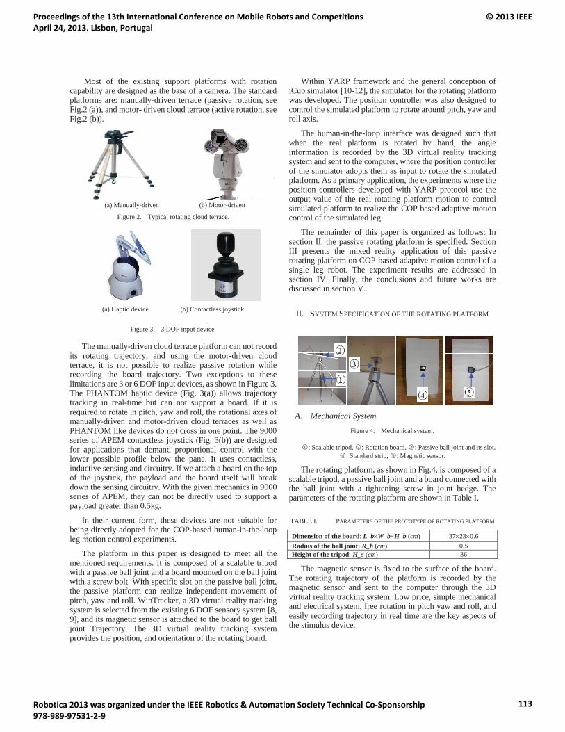
Most of the existing support platforms with rotation capability are designed as the base of a camera. The standard platforms are: manually-driven terrace (passive rotation, see Fig.2 (a)), and motor- driven cloud terrace (active rotation, see Fig.2 (b)).

(a) Manually-driven (b) Motor-driven

Figure 2. Typical rotating cloud terrace.

(a) Haptic device (b) Contactless joystick

Figure 3. 3 DOF input device.

The manually-driven cloud terrace platform can not record its rotating trajectory, and using the motor-driven cloud terrace, it is not possible to realize passive rotation while recording the board trajectory. Two exceptions to these limitations are 3 or 6 DOF input devices, as shown in Figure 3. The PHANTOM haptic device (Fig. 3(a)) allows trajectory tracking in real-time but can not support a board. If it is required to rotate in pitch, yaw and roll, the rotational axes of manually-driven and motor-driven cloud terraces as well as PHANTOM like devices do not cross in one point. The 9000 series of APEM contactless joystick (Fig. 3(b)) are designed for applications that demand proportional control with the lower possible profile below the pane. It uses contactless, inductive sensing and circuitry. If we attach a board on the top of the joystick, the payload and the board itself will break down the sensing circuitry. With the given mechanics in 9000 series of APEM, they can not be directly used to support a payload greater than 0.5kg.

In their current form, these devices are not suitable for being directly adopted for the COP-based human-in-the-loop leg motion control experiments.

The platform in this paper is designed to meet all the mentioned requirements. It is composed of a scalable tripod with a passive ball joint and a board mounted on the ball joint with a screw bolt. With specific slot on the passive ball joint, the passive platform can realize independent movement of pitch, yaw and roll. WinTracker, a 3D virtual reality tracking system is selected from the existing 6 DOF sensory system [8, 9], and its magnetic sensor is attached to the board to get ball joint Trajectory. The 3D virtual reality tracking system provides the position, and orientation of the rotating board.

Within YARP framework and the general conception of iCub simulator [10-12], the simulator for the rotating platform was developed. The position controller was also designed to control the simulated platform to rotate around pitch, yaw and roll axis.

The human-in-the-loop interface was designed such that when the real platform is rotated by hand, the angle information is recorded by the 3D virtual reality tracking system and sent to the computer, where the position controller of the simulator adopts them as input to rotate the simulated platform. As a primary application, the experiments where the position controllers developed with YARP protocol use the output value of the real rotating platform motion to control simulated platform to realize the COP based adaptive motion control of the simulated leg.

The remainder of this paper is organized as follows: In section II, the passive rotating platform is specified. Section III presents the mixed reality application of this passive rotating platform on COP-based adaptive motion control of a single leg robot. The experiment results are addressed in section IV. Finally, the conclusions and future works are discussed in section V.

II. SYSTEM SPECIFICATION OF THE ROTATING PLATFORM

A. Mechanical System

Figure 4. Mechanical system.

1 : Scalable tripod, 2 : Rotation board, 3 : Passive ball joint and its slot, 4 : Standard strip, 5 : Magnetic sensor.

The rotating platform, as shown in Fig.4, is composed of a scalable tripod, a passive ball joint and a board connected with the ball joint with a tightening screw in joint hedge. The parameters of the rotating platform are shown in Table I.

TABLE I. PARAMETERS OF THE PROTOTYPE OF ROTATING PLATFORM

Dimension of the board: L_b W_b H_b (cm) 37 23 0.6 Radius of the ball joint: R_b (cm) 0.5 Height of the tripod: H_s (cm) 36

The magnetic sensor is fixed to the surface of the board. The rotating trajectory of the platform is recorded by the magnetic sensor and sent to the computer through the 3D virtual reality tracking system. Low price, simple mechanical and electrical system, free rotation in pitch yaw and roll, and easily recording trajectory in real time are the key aspects of the stimulus device.


© 2013 IEEE


113

B. Control System

The hardware in the control system of the rotating platform is shown in Fig.5. The main component is Wintracker, a 3D virtual reality tracking system. Although Wintracker is a 6 DOF tracking system with three magnetic sensors, in this study, only the rotation information is being used to record the platform trajectory of pitch, yaw and roll axis. The position information can also be taken as a potential function of the rotating platform for robot motion control.

Figure 5. Control system hardware.

1 : Control box, 2 : Magnetic sensor transmitter, 3 : Magnetic sensor receiver, 4 : Power line, 5 : Computer connected by the USB line.

1) Hardware Specification of Wintracker Wintracker has three magnetic sensory receivers with

mounting clips. The magnetic sensor transmitter sends magnetic information. In this rotating platform, one magnetic sensor is put on the top of the board. When the platform is rotated, the origination relationship between the transmitter and the receiver can be recorded and sent to the computer.

The system parameters are listed in Table II. Since it is a magnetic tracker, the system signal can be influenced by metallic objects. Based on the application area and mechanical system integration requirements, similar devices, such as accelerometer-based tracking system, optical-based tracking system and potentiometer-based tracking system can also be adopted to record the trajectories of different passive rotating platforms. This design avoids the excessive use of complex mechanical and electrical parts.

TABLE II. SYSTEM PARAMETERS OF WINTRACKER

Weight : W (Kg) 4.6 Electronics unit : L_e W_e H_e (cm) 32 20 12 Transmitter : L_t W_t H_t (cm) 5.5 5.5 5.8 Cable length of transmitter: L_c (m) 4.5 Operating temperature: T (°C) 10~40 Update rate: R_u (outputs/second) 90(1),45(2),30(3) Operating Voltage: O_v (V) 85~264

2) Data Specification of Wintracker The data recorded by WinTracker is shown in Table III,

that contains the information for Cartesian coordinates of position, Euler angles, quaternion and orientation. In this research, we only use the information of azimuth, elevation and roll angles, as shown in Fig.6. In the rotating platform system, the pitch rotation means to rotate the X axis from +Y to +Z; the yaw rotation means to rotate the Y axis from +X to –Z; and the roll rotation means to rotate the Z axis from +X to +Y.

TABLE III. DATA SPECIFICATION OF WINTRACKER

Position X: X (m) Position Y: Y (m) Position

(accuracy in 0.0001 m) Position Z: Z (m) Azimuth Attitude: A (Deg) Elevation Attitude: E (Deg)

Attitude (accuracy in 0.01 Deg)

Roll Attitude: R (Deg) Qw : quaternion component W 10000Qx : quaternion component X 10000Qy : quaternion component Y 10000

Orientation

Qz : quaternion component Z 10000

Figure 6. Coordination system.

3) Interface Function Specification of Wintracker In this study, Wintracker is supplied with Windows

compatible data capture software. The sensor data can be saved in a file or as an input to other program in real time. As a functional demonstration, the platform is rotated by hand in one direction, from pitch, yaw to roll and then rotated in arbitrary direction to realize a complex behavior. The joint trajectory is recorded and sent to the computer, and the signal can be easily separated into independent axis data, as shown in Fig.7.The signal can be also recorded with a timer defined by world step size in ODE (Open Dynamic Engineering).

0 50 100 150 200 250 300-200

0200

Pitc

h (D

eg)

0 50 100 150 200 250 300-100

0100

Yaw

(Deg

)

0 50 100 150 200 250 300-200

0200

Time (Sec)

Roll

(Deg

)

Figure 7. Trajectory of rotating movement.

III. THE MIXED REALITY APPLICATION ON COP-BASED ADAPTIVE MOTION CONTROL OF A SINGLE LEG ROBOT

A. Development of the simulated rotating platform YARP is an open source middleware which contains a set

of software libraries, protocols, and tools to keep modules and devices clearly decoupled. The architecture of the simulator is realized as a set of YARP executables, and models are connected by the YARP port.


© 2013 IEEE


114

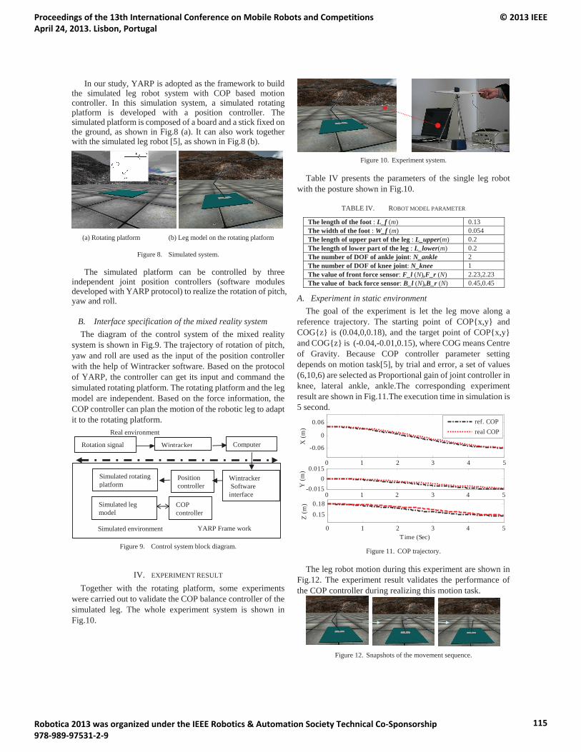
In our study, YARP is adopted as the framework to build the simulated leg robot system with COP based motion controller. In this simulation system, a simulated rotating platform is developed with a position controller. The simulated platform is composed of a board and a stick fixed on the ground, as shown in Fig.8 (a). It can also work together with the simulated leg robot [5], as shown in Fig.8 (b).

(a) Rotating platform (b) Leg model on the rotating platform

Figure 8. Simulated system.

The simulated platform can be controlled by three independent joint position controllers (software modules developed with YARP protocol) to realize the rotation of pitch, yaw and roll.

B. Interface specification of the mixed reality system The diagram of the control system of the mixed reality

system is shown in Fig.9. The trajectory of rotation of pitch, yaw and roll are used as the input of the position controller with the help of Wintracker software. Based on the protocol of YARP, the controller can get its input and command the simulated rotating platform. The rotating platform and the leg model are independent. Based on the force information, the COP controller can plan the motion of the robotic leg to adapt it to the rotating platform.

Figure 9. Control system block diagram.

IV. EXPERIMENT RESULT Together with the rotating platform, some experiments

were carried out to validate the COP balance controller of the simulated leg. The whole experiment system is shown in Fig.10.

Figure 10. Experiment system.

Table IV presents the parameters of the single leg robot with the posture shown in Fig.10.

TABLE IV. ROBOT MODEL PARAMETER

The length of the foot : L_f (m) 0.13 The width of the foot : W_f (m) 0.054 The length of upper part of the leg : L_upper(m) 0.2 The length of lower part of the leg : L_lower(m) 0.2 The number of DOF of ankle joint: N_ankle 2 The number of DOF of knee joint: N_knee 1 The value of front force sensor: F_l (N),F_r (N) 2.23,2.23 The value of back force sensor: B_l (N),B_r (N) 0.45,0.45

A. Experiment in static environment The goal of the experiment is let the leg move along a

reference trajectory. The starting point of COP{x,y} and COG{z} is (0.04,0,0.18), and the target point of COP{x,y} and COG{z} is (-0.04,-0.01,0.15), where COG means Centre of Gravity. Because COP controller parameter setting depends on motion task[5], by trial and error, a set of values (6,10,6) are selected as Proportional gain of joint controller in knee, lateral ankle, ankle.The corresponding experiment result are shown in Fig.11.The execution time in simulation is 5 second.

0 1 2 3 4 5

-0.06

0

0.06

X (m

)

ref. COPreal COP

0 1 2 3 4 5-0.015

00.015

Y (m

)

0 1 2 3 4 5

0.180.15

Time (Sec)

Z (m

)

Figure 11. COP trajectory.

The leg robot motion during this experiment are shown in Fig.12. The experiment result validates the performance of the COP controller during realizing this motion task.

Figure 12. Snapshots of the movement sequence.

Computer

Wintracker Software interface

Position controller

Simulated rotating platform

Real environment

WintrackerRotation signal

Simulated environment

Simulated leg model

YARP Frame work

COP controller


© 2013 IEEE


115

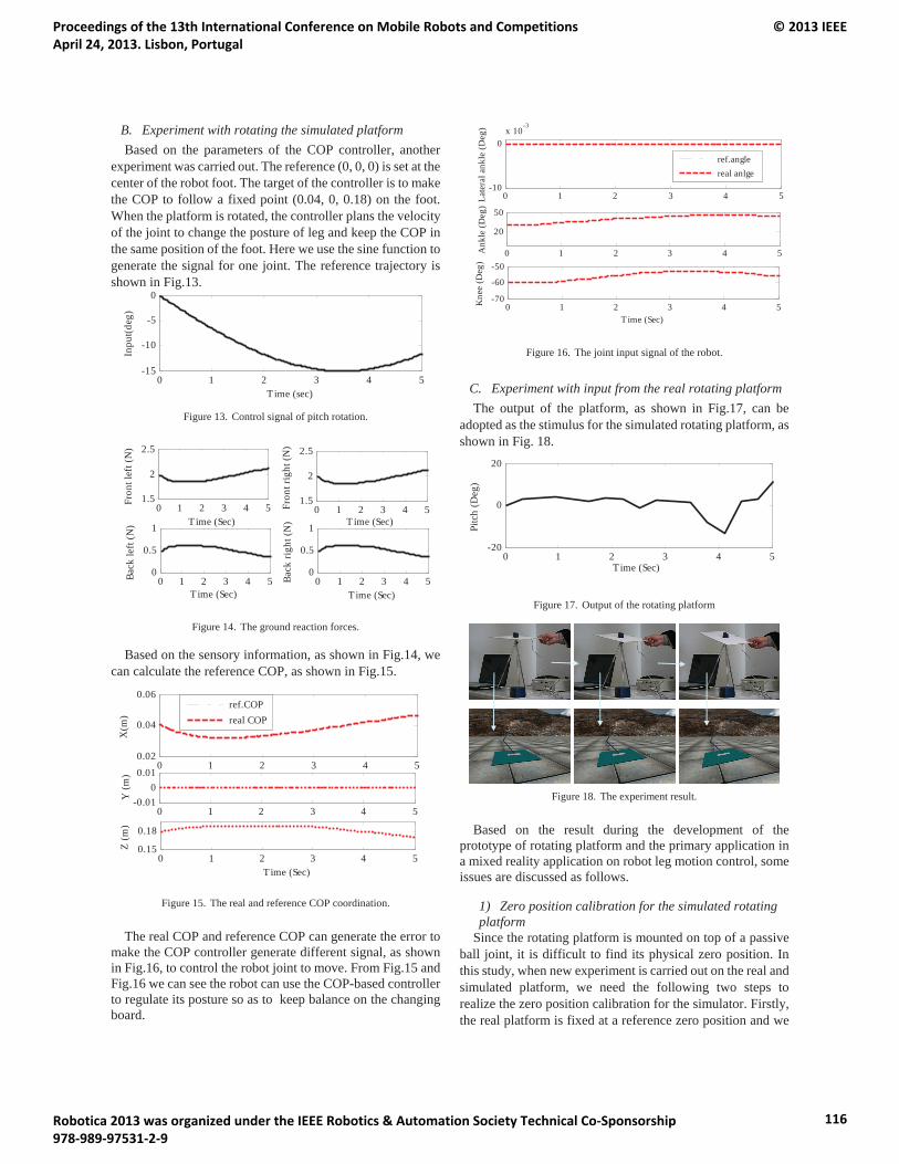
B. Experiment with rotating the simulated platform Based on the parameters of the COP controller, another

experiment was carried out. The reference (0, 0, 0) is set at the center of the robot foot. The target of the controller is to make the COP to follow a fixed point (0.04, 0, 0.18) on the foot. When the platform is rotated, the controller plans the velocity of the joint to change the posture of leg and keep the COP in the same position of the foot. Here we use the sine function to generate the signal for one joint. The reference trajectory is shown in Fig.13.

0 1 2 3 4 5-15

-10

-5

0

Time (sec)

Inpu

t(deg

)

Figure 13. Control signal of pitch rotation.

0 1 2 3 4 51.5

2

2.5

Time (Sec)

Fron

t lef

t (N

)

0 1 2 3 4 51.5

2

2.5

Time (Sec)

Fron

t rig

ht (N

)

0 1 2 3 4 50

0.5

1

Time (Sec)

Back

left

(N)

0 1 2 3 4 50

0.5

1

Time (Sec)

Back

righ

t (N

)

Figure 14. The ground reaction forces.

Based on the sensory information, as shown in Fig.14, we can calculate the reference COP, as shown in Fig.15.

0 1 2 3 4 50.02

0.04

0.06

X(m

)

ref.COPreal COP

0 1 2 3 4 5-0.01

00.01

Y (m

)

0 1 2 3 4 50.15

0.18

Time (Sec)

Z (m

)

Figure 15. The real and reference COP coordination.

The real COP and reference COP can generate the error to make the COP controller generate different signal, as shown in Fig.16, to control the robot joint to move. From Fig.15 and Fig.16 we can see the robot can use the COP-based controller to regulate its posture so as to keep balance on the changing board.

0 1 2 3 4 5-10

0x 10

-3

Late

ral a

nkle

(Deg

)

ref.anglereal anlge

0 1 2 3 4 5

20

50

Ank

le (D

eg)

0 1 2 3 4 5-70

-60

-50

Time (Sec)

Kne

e (D

eg)

Figure 16. The joint input signal of the robot.

C. Experiment with input from the real rotating platform The output of the platform, as shown in Fig.17, can be

adopted as the stimulus for the simulated rotating platform, as shown in Fig. 18.

0 1 2 3 4 5-20

0

20

Time (Sec)

Pitc

h (D

eg)

Figure 17. Output of the rotating platform

Figure 18. The experiment result.

Based on the result during the development of the prototype of rotating platform and the primary application in a mixed reality application on robot leg motion control, some issues are discussed as follows.

1) Zero position calibration for the simulated rotating platform

Since the rotating platform is mounted on top of a passive ball joint, it is difficult to find its physical zero position. In this study, when new experiment is carried out on the real and simulated platform, we need the following two steps to realize the zero position calibration for the simulator. Firstly, the real platform is fixed at a reference zero position and we


© 2013 IEEE


116

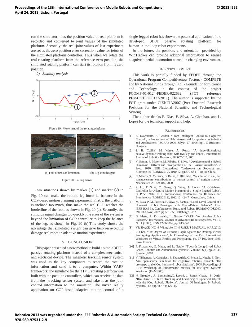
run the simulator, thus the position value of real platform is recorded and converted to joint values of the simulated platform. Secondly, the real joint values of last experiment are set as the zero position error correction value for joints of the simulated platform controller. Thus when we rotate the real rotating platform from the reference zero position, the simulated rotating platform can start its rotation from its zero position.

2) Stability analysis

Figure 19. Movement of the rotating platform.

(a) Foot dimension limitation (b) Big stimulus gain

Figure 20. Falling down.

Two situations shown by marker 1 and marker 2 in Fig. 19 can make the robotic leg loose its balance in the COP-based motion planning experiment. Firstly, the platform is inclined too much, thus make the real COP reaches the borderline of the foot, as shown in Fig. 20 (a). Secondly, the stimulus signal changes too quickly, the error of the system is beyond the limitation of COP controller to keep the balance of the leg, as shown in Fig. 20 (b).This study shows the advantage that simulated system can give help on avoiding damage real robot in adaptive motion experiment.

V. CONCLUSION This paper presented a new method to build a simple 3DOF

passive rotating platform instead of a complex mechanical and electrical device. The magnetic tracking sensor system was used as the key component to record the rotation information and send it to a computer. Within YARP framework, the simulator for the 3 DOF rotating platform was built with the position controllers, which can receive the data from the tracking sensor system and take it as the joint control information to the simulator. The mixed reality application on COP-based adaptive motion control of a

single-legged robot has shown the potential application of the developed 3DOF passive rotating platform for human-in-the-loop robot experiments.

In the future, the position, and orientation provided by WinTracker can provide addtional information to realize adaptive bipedal locomotion control in changing enviroment.

ACKNOWLEDGMENT This work is partially funded by FEDER through the

Operational Program Competitiveness Factors - COMPETE and by National Funds through FCT - Foundation for Science and Technology in the context of the project FCOMP-01-0124-FEDER-022682 (FCT reference PEst-C/EEI/UI0127/2011). The author is supported by the FCT grant under CIENCIA2007 (Post Doctoral Research Positions for the National Scientific and Technological System).

The author thanks P. Dias, F. Silva, A. Chauhan, and L. Lopes for the technical support and help.

REFERENCES [1] K. Kawamura, S. Gordon, “From Intelligent Control to Cognitive

Control”, in Proceedings of 11th International Symposium on Robotics and Applications (ISORA) 2006, July24-27, 2006, pp.1-9, Budapest, Hungary.

[2] S. H. Collins, M. Wisse, A. Ruina, “A three-dimensional passive-dynamic walking robot with two legs and knees”, International Journal of Robotics Research, 20, 607-615, 2001.

[3] V. Santos, R. Moreira, M. Ribeiro, F. Silva, “ Development of a Hybrid Humanoid Platform and Incorporation of the Passive Actuators”, in Proc. 2010 IEEE International Conference on Robotics and Biomimetics (ROBIO2010), 2010.12, pp.679-684 , Tianjin, China.

[4] C. Maurer, T. Mergner, B. Bolha, F. Hlavacka, “Vestibular, visual, and somatosensory contributions to human control of upright stance”, Neursci Let, 281:99-102, 2000.

[5] Z. Lu, F. Silva, Y. Zhang, Q. Wang, L. Lopes, “A COP-based Controller for Adaptive Motion Planning of a Single-Legged Robot”, in Proc. 2012 IEEE International Conference on Robotics and Biomimetics (ROBIO2012), 2012.12, 42-47 , Guangzhou, China.

[6] M. Ruas, P. M. Ferreira, F. Silva, V. Santos , “Local-Level Control of a Humanoid Robot Prototype with Force-Driven Balance”, Proc. IEEE-RAS Int. Conference on Humanoid Robots HUMANOIDS2007, 29 Out-1 Nov, 2007, pp.551-556, Pittsburgh, USA.

[7] G. Metta, P. Fitzpatrick, L. Natale, “YARP: Yet Another Robot Platform,” International Journal of Advanced Robotic Systems, Vol. 3, No. 1 (2006), ISSN 1729-8806, pp. 043-048.

[8] VR SPACE INC. ® Wintracker III ® USER’S MANUAL, MAR 2010. [9] E. Chen, “Six Degree-of-Freedom Haptic System for Desktop Virtual

Prototyping Applications”, In Proceedings of the First International Workshop on Virtual Reality and Prototyping, pp. 97-106, June 1999, Laval France.

[10] P. Fitzpatrick, G. Metta, and L. Natale, “Towards Long-Lived Robot Genes. Robotics and Autonomous Systems”, Volume 56(1), pp. 29-45, Elsevier ,2007.

[11] V. Tikhanoff, A. Cangelosi, P. Fitzpatrick, G. Metta, L. Natale, F. Nori, “An open-source simulator for cognitive robotics research: The prototype of the iCub humanoid robot simulator”, 2008, Proceedings of IEEE Workshop on Performance Metrics for Intelligent Systems Workshop (PerMIS08).

[12] N. Greggio , A. Bernardino,C. Laschi, J. Santos-Victor, P. Dario, “Real-Time 3D Stereo Tracking and Localizing of Spherical Objects with the iCub Robotic Platform”, Journal Of Intelligent & Robotic Systems - 63 : pp.417-446 (2011).

0 1 2 3 4 5-80

0

60

Time (Sec)

Pitc

h (D

eg)


© 2013 IEEE


117

EKF-based visual self-calibration tool for robotswith rotating directional cameras

Joao Ribeiro, Rui Serra, Nuno Nunes, Hugo Silva and Jose AlmeidaINESC TEC - INESC Technology and Science(formerly INESC Porto) and ISEP/IPP - Schoolof Engineering, Polytechnic Institute of Porto

Rua Dr Antonio Bernardino de Almeida, 431, Porto, PortugalEmail: {joao.ribeiro,nuno.nunes,ruiserra,hsilva,jma}@lsa.isep.ipp.pt

Abstract—Autonomous mobile robots perception systems arecomplex multi-sensors systems. Information from different sen-sors, placed in different parts of the platforms, need to berelated and fused into some representation of the world or robotstate. For that, the knowledge of the relative pose (positionand rotation) between sensors frames and the platform frameplays a critical role. The process to determine those is calledextrinsic calibration. This paper addresses the development ofautomatic robot calibration tool for Middle Size League Robotswith rotating directional cameras, such as the ISePorto teamrobots. The proposed solution consists on a robot navigating ina path, while acquiring visual information provided by a knowntarget positioned in a global reference frame. This informationis then combined with wheel odometry sensors, robot rotativeaxis encoders and gyro information within an Extend Kalmanfilter framework, that estimates all parameters required for thesensors angles and position determination related to the robotbody frame. We evaluated our solution, by performing severaltrials and obtaining similar results to the previous used manualcalibration procedure, but with a much less time consumingperformance and also without being susceptible to human error.

I. INTRODUCTION

In this paper, we present an EKF based solution, for the

development of a visual auto-calibration tool to fully calibrate

all rotative axis, angles and offsets of a ISePorto MSL Robot

[2].

Robot Calibration is an important and complex task, that

needs to be performed, in order for the robot to be able to

complete tasks in Robocup semi-structured environment. This

calibration procedure consists on defining sensors and active

mechanisms inter-relationships but also defines their relation

with a global robot body frame.

The ISePorto robots, are complex robots that pose an inter-

esting challenge for obtaining a well-established calibration

procedure, since it has many different sensors, namely: 2

cameras for visual perception, a low cost 3-axial Inertial

Measurement Unit (IMU), laser range sensor (only for the

goalkeeper) and odometry sensors(wheel encoders). The ISe-

Porto robot all possess two rotative axis one for the kicker

camera and kicking mechanism and other for the head camera.

The main objective, behind this type of rotation mechanism

is to facilitate cooperative play (passing) between robot team

members but also to artificially increase robot cameras field-

of-view(fov), to allow a better robot self-localization using

field landmarks and also a more efficient obstacle detection.There are several ways to perform specific calibration

procedures, such as the work of Ling [3], that allows to retrieve

camera extrinsic parameters through the use of vanishing lines,

thus being able to calibrate camera orientation, position and

focal length parameters.Others, like Zhang [8] or Shen and Wang [6] presented

algorithms to calibrate the extrinsic parameters of a camera

by minimizing total control-point errors. The algorithms min-

imized control-point errors of the pixels in the image plane and

also of the object points in the 3D physical space. Those papers

addressed the problem of determining the initial calibration

on a off-line procedure. However, for Robocup applications

where the extrinsic parameters can change during game-play

or as with the use of cameras in cars, the parameters must

be determined in real time. Examples of approaches in those

scenarios are the work of Martinelli [4] and Wu [7], but not

supporting rotating cameras in moving vehicles.Another developed special purpose robot calibration tool

supporting cameras that can change dynamically its config-

uration in the robot, is the one developed by Pradeep et al

[5] to calibrate a multi-arm multi-sensor PR2 robot, through

bundle adjustment. They estimated a set of system parameters

by acquiring poses of known targets in the world. However,

this approach is not applicable for on-line calibration.In the MSL scenario, the previous calibration method of

the ISePorto Robots consisted on a sequence of manual

procedures, see figure 1:

• First, concerning the imaging part of the procedure, cam-

era information measurements were acquired through out

a sequence of images that were processed off-line, in or-

der to obtain robot camera calibration parameters(intrinsic

and extrinsic parameters), this procedure was performed

using J.Y.Bouget [1] toolbox.

• Second, the robot is placed on a mechanical frame,

specially design to physically align all rotative robot axis,

so information regarding motor encoder position can be

acquired. The value read from the kicker axis encoder, is

defined as the initial bearing angle of the kicker device.

Where all camera (head and kicker) pose related angles

will be referenced to.

• Third, the one remaining angle to be estimated, is the


© 2013 IEEE


118

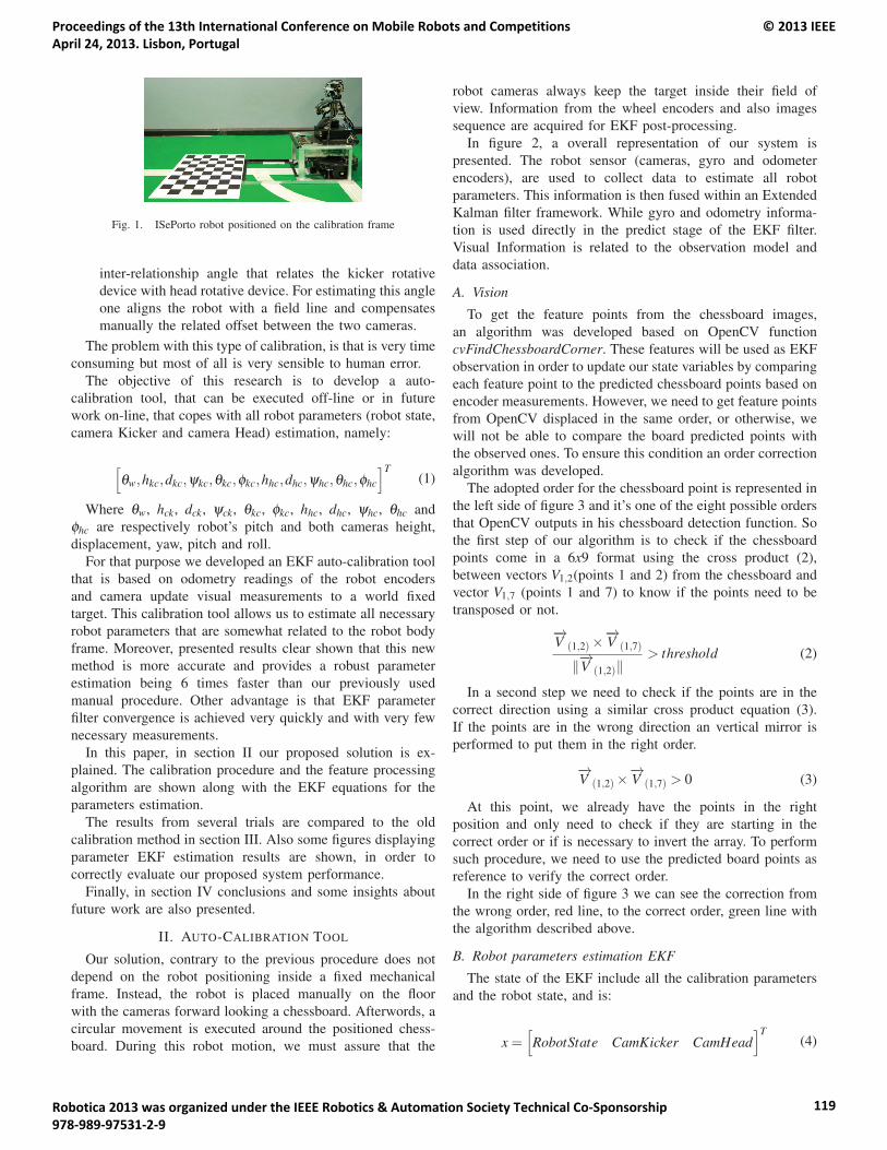
Fig. 1. ISePorto robot positioned on the calibration frame

inter-relationship angle that relates the kicker rotative

device with head rotative device. For estimating this angle

one aligns the robot with a field line and compensates

manually the related offset between the two cameras.

The problem with this type of calibration, is that is very time

consuming but most of all is very sensible to human error.

The objective of this research is to develop a auto-

calibration tool, that can be executed off-line or in future

work on-line, that copes with all robot parameters (robot state,

camera Kicker and camera Head) estimation, namely:

[θw,hkc,dkc,ψkc,θkc,φkc,hhc,dhc,ψhc,θhc,φhc

]T(1)

Where θw, hck, dck, ψck, θkc, φkc, hhc, dhc, ψhc, θhc and

φhc are respectively robot’s pitch and both cameras height,

displacement, yaw, pitch and roll.

For that purpose we developed an EKF auto-calibration tool

that is based on odometry readings of the robot encoders

and camera update visual measurements to a world fixed

target. This calibration tool allows us to estimate all necessary

robot parameters that are somewhat related to the robot body

frame. Moreover, presented results clear shown that this new

method is more accurate and provides a robust parameter

estimation being 6 times faster than our previously used

manual procedure. Other advantage is that EKF parameter

filter convergence is achieved very quickly and with very few

necessary measurements.

In this paper, in section II our proposed solution is ex-

plained. The calibration procedure and the feature processing

algorithm are shown along with the EKF equations for the

parameters estimation.

The results from several trials are compared to the old

calibration method in section III. Also some figures displaying

parameter EKF estimation results are shown, in order to

correctly evaluate our proposed system performance.

Finally, in section IV conclusions and some insights about

future work are also presented.

II. AUTO-CALIBRATION TOOL

Our solution, contrary to the previous procedure does not

depend on the robot positioning inside a fixed mechanical

frame. Instead, the robot is placed manually on the floor

with the cameras forward looking a chessboard. Afterwords, a

circular movement is executed around the positioned chess-

board. During this robot motion, we must assure that the

robot cameras always keep the target inside their field of

view. Information from the wheel encoders and also images

sequence are acquired for EKF post-processing.

In figure 2, a overall representation of our system is

presented. The robot sensor (cameras, gyro and odometer

encoders), are used to collect data to estimate all robot

parameters. This information is then fused within an Extended

Kalman filter framework. While gyro and odometry informa-

tion is used directly in the predict stage of the EKF filter.

Visual Information is related to the observation model and

data association.

A. Vision

To get the feature points from the chessboard images,

an algorithm was developed based on OpenCV function

cvFindChessboardCorner. These features will be used as EKF

observation in order to update our state variables by comparing

each feature point to the predicted chessboard points based on

encoder measurements. However, we need to get feature points

from OpenCV displaced in the same order, or otherwise, we

will not be able to compare the board predicted points with

the observed ones. To ensure this condition an order correction

algorithm was developed.

The adopted order for the chessboard point is represented in

the left side of figure 3 and it’s one of the eight possible orders

that OpenCV outputs in his chessboard detection function. So

the first step of our algorithm is to check if the chessboard

points come in a 6x9 format using the cross product (2),

between vectors V1,2(points 1 and 2) from the chessboard and

vector V1,7 (points 1 and 7) to know if the points need to be

transposed or not.

−→V (1,2)×

−→V (1,7)

‖−→V (1,2)‖> threshold (2)

In a second step we need to check if the points are in the

correct direction using a similar cross product equation (3).

If the points are in the wrong direction an vertical mirror is

performed to put them in the right order.

−→V (1,2)×

−→V (1,7) > 0 (3)

At this point, we already have the points in the right

position and only need to check if they are starting in the

correct order or if is necessary to invert the array. To perform

such procedure, we need to use the predicted board points as

reference to verify the correct order.

In the right side of figure 3 we can see the correction from

the wrong order, red line, to the correct order, green line with

the algorithm described above.

B. Robot parameters estimation EKF

The state of the EKF include all the calibration parameters

and the robot state, and is:

x =[RobotState CamKicker CamHead

]T(4)


© 2013 IEEE


119

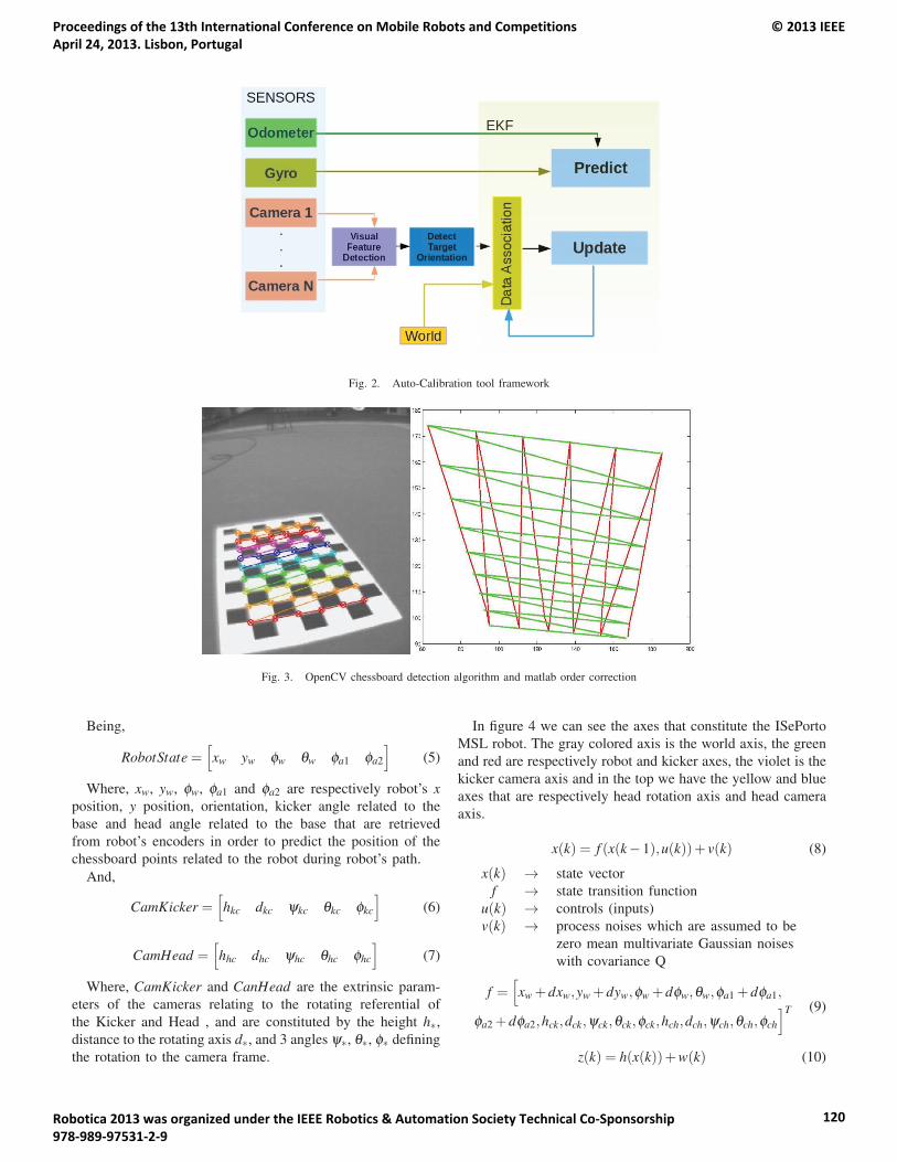
Fig. 2. Auto-Calibration tool framework

Fig. 3. OpenCV chessboard detection algorithm and matlab order correction

Being,

RobotState =[xw yw φw θw φa1 φa2

](5)

Where, xw, yw, φw, φa1 and φa2 are respectively robot’s xposition, y position, orientation, kicker angle related to the

base and head angle related to the base that are retrieved

from robot’s encoders in order to predict the position of the

chessboard points related to the robot during robot’s path.

And,

CamKicker =[hkc dkc ψkc θkc φkc

](6)

CamHead =[hhc dhc ψhc θhc φhc

](7)

Where, CamKicker and CanHead are the extrinsic param-

eters of the cameras relating to the rotating referential of

the Kicker and Head , and are constituted by the height h∗,

distance to the rotating axis d∗, and 3 angles ψ∗, θ∗, φ∗ defining

the rotation to the camera frame.

In figure 4 we can see the axes that constitute the ISePorto

MSL robot. The gray colored axis is the world axis, the green

and red are respectively robot and kicker axes, the violet is the

kicker camera axis and in the top we have the yellow and blue

axes that are respectively head rotation axis and head camera

axis.

x(k) = f (x(k−1),u(k))+ v(k) (8)

x(k) → state vector

f → state transition function

u(k) → controls (inputs)

v(k) → process noises which are assumed to be

zero mean multivariate Gaussian noises

with covariance Q

f =[xw +dxw,yw +dyw,φw +dφw,θw,φa1 +dφa1,

φa2 +dφa2,hck,dck,ψck,θck,φck,hch,dch,ψch,θch,φch

]T (9)

z(k) = h(x(k))+w(k) (10)


© 2013 IEEE


120

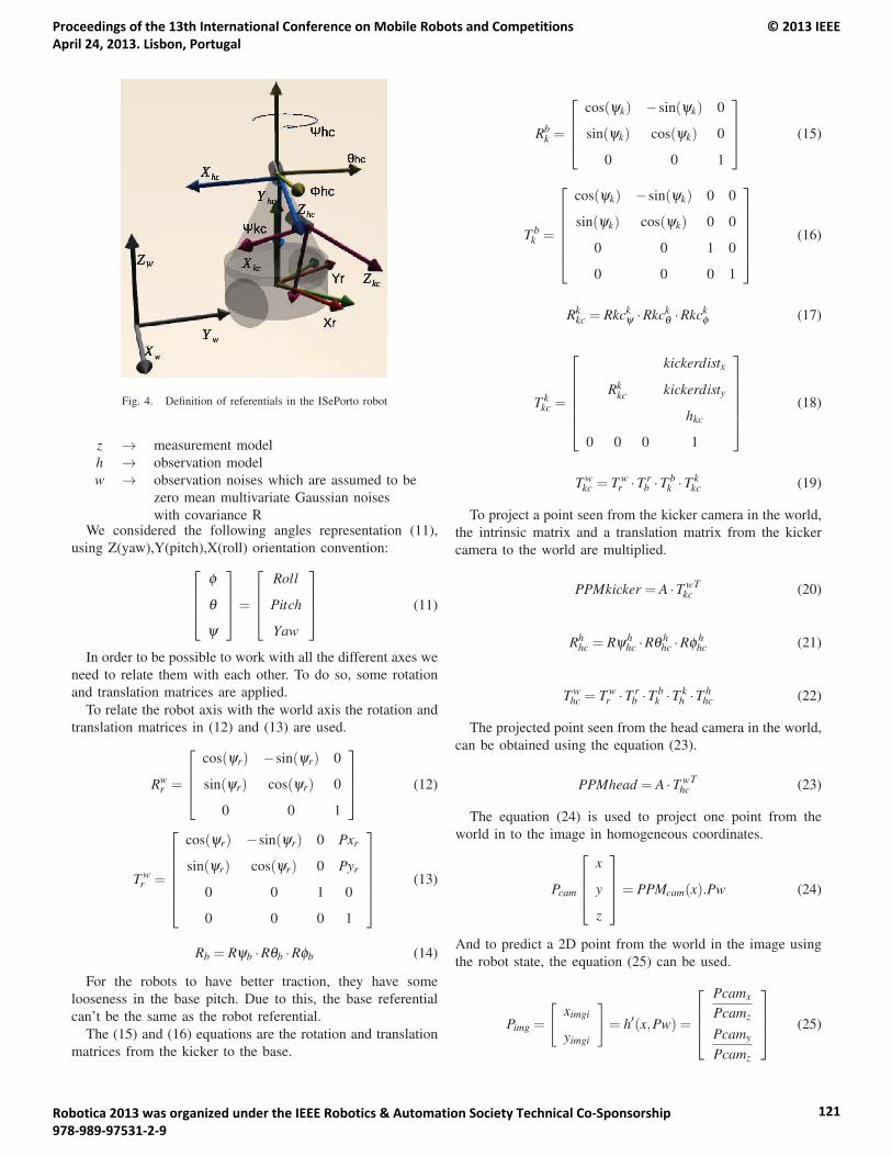
Fig. 4. Definition of referentials in the ISePorto robot

z → measurement model

h → observation model

w → observation noises which are assumed to be

zero mean multivariate Gaussian noises

with covariance RWe considered the following angles representation (11),

using Z(yaw),Y(pitch),X(roll) orientation convention:⎡⎢⎢⎣

φ

θ

ψ

⎤⎥⎥⎦=

⎡⎢⎢⎣

Roll

Pitch

Yaw

⎤⎥⎥⎦ (11)

In order to be possible to work with all the different axes we

need to relate them with each other. To do so, some rotation

and translation matrices are applied.

To relate the robot axis with the world axis the rotation and

translation matrices in (12) and (13) are used.

Rwr =

⎡⎢⎢⎣

cos(ψr) −sin(ψr) 0

sin(ψr) cos(ψr) 0

0 0 1

⎤⎥⎥⎦ (12)

T wr =

⎡⎢⎢⎢⎢⎢⎣

cos(ψr) −sin(ψr) 0 Pxr

sin(ψr) cos(ψr) 0 Pyr

0 0 1 0

0 0 0 1

⎤⎥⎥⎥⎥⎥⎦ (13)

Rb = Rψb ·Rθb ·Rφb (14)

For the robots to have better traction, they have some

looseness in the base pitch. Due to this, the base referential

can’t be the same as the robot referential.

The (15) and (16) equations are the rotation and translation

matrices from the kicker to the base.

Rbk =

⎡⎢⎢⎣

cos(ψk) −sin(ψk) 0

sin(ψk) cos(ψk) 0

0 0 1

⎤⎥⎥⎦ (15)

T bk =

⎡⎢⎢⎢⎢⎢⎣

cos(ψk) −sin(ψk) 0 0

sin(ψk) cos(ψk) 0 0

0 0 1 0

0 0 0 1

⎤⎥⎥⎥⎥⎥⎦ (16)

Rkkc = Rkck

ψ ·Rkckθ ·Rkck

φ (17)

T kkc =

⎡⎢⎢⎢⎢⎢⎣

kickerdistx

Rkkc kickerdisty

hkc

0 0 0 1

⎤⎥⎥⎥⎥⎥⎦ (18)

T wkc = T w

r ·T rb ·T b

k ·T kkc (19)

To project a point seen from the kicker camera in the world,

the intrinsic matrix and a translation matrix from the kicker

camera to the world are multiplied.

PPMkicker = A ·T wkc

T (20)

Rhhc = Rψh

hc ·Rθ hhc ·Rφ h

hc (21)

T whc = T w

r ·T rb ·T b

k ·T kh ·T h

hc (22)

The projected point seen from the head camera in the world,

can be obtained using the equation (23).

PPMhead = A ·T whc

T (23)

The equation (24) is used to project one point from the

world in to the image in homogeneous coordinates.

Pcam

⎡⎢⎢⎣

x

y

z

⎤⎥⎥⎦= PPMcam(x).Pw (24)

And to predict a 2D point from the world in the image using

the robot state, the equation (25) can be used.

Pimg =

[ximgi

yimgi

]= h′(x,Pw) =

⎡⎢⎢⎣

Pcamx

Pcamz

Pcamy

Pcamz

⎤⎥⎥⎦ (25)


© 2013 IEEE


121

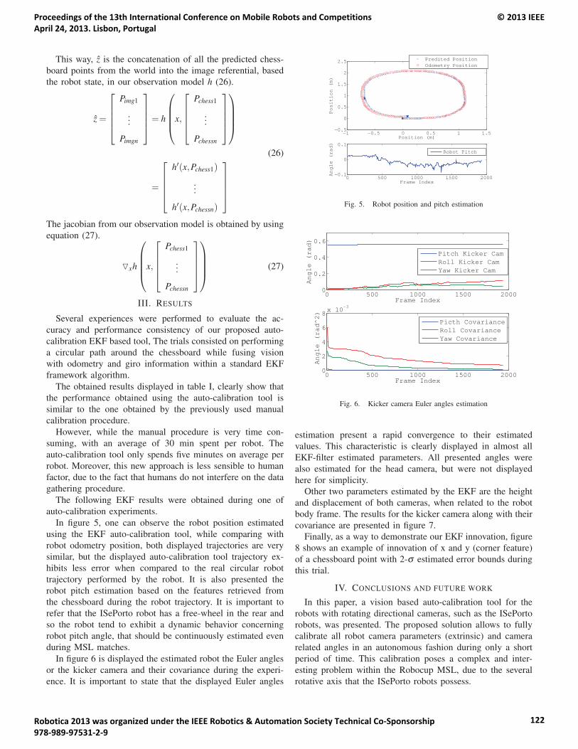
This way, z is the concatenation of all the predicted chess-

board points from the world into the image referential, based

the robot state, in our observation model h (26).

z =

⎡⎢⎢⎢⎣

Pimg1

...

Pimgn

⎤⎥⎥⎥⎦= h

⎛⎜⎜⎜⎝x,

⎡⎢⎢⎢⎣

Pchess1

...

Pchessn

⎤⎥⎥⎥⎦⎞⎟⎟⎟⎠

=

⎡⎢⎢⎢⎣

h′(x,Pchess1)

...

h′(x,Pchessn)

⎤⎥⎥⎥⎦

(26)

The jacobian from our observation model is obtained by using

equation (27).

�xh

⎛⎜⎜⎜⎝x,

⎡⎢⎢⎢⎣

Pchess1

...

Pchessn

⎤⎥⎥⎥⎦⎞⎟⎟⎟⎠ (27)

III. RESULTS

Several experiences were performed to evaluate the ac-

curacy and performance consistency of our proposed auto-

calibration EKF based tool, The trials consisted on performing

a circular path around the chessboard while fusing vision

with odometry and giro information within a standard EKF

framework algorithm.

The obtained results displayed in table I, clearly show that

the performance obtained using the auto-calibration tool is

similar to the one obtained by the previously used manual

calibration procedure.

However, while the manual procedure is very time con-

suming, with an average of 30 min spent per robot. The

auto-calibration tool only spends five minutes on average per

robot. Moreover, this new approach is less sensible to human

factor, due to the fact that humans do not interfere on the data

gathering procedure.

The following EKF results were obtained during one of

auto-calibration experiments.

In figure 5, one can observe the robot position estimated

using the EKF auto-calibration tool, while comparing with

robot odometry position, both displayed trajectories are very

similar, but the displayed auto-calibration tool trajectory ex-

hibits less error when compared to the real circular robot

trajectory performed by the robot. It is also presented the

robot pitch estimation based on the features retrieved from

the chessboard during the robot trajectory. It is important to

refer that the ISePorto robot has a free-wheel in the rear and

so the robot tend to exhibit a dynamic behavior concerning

robot pitch angle, that should be continuously estimated even

during MSL matches.

In figure 6 is displayed the estimated robot the Euler angles

or the kicker camera and their covariance during the experi-

ence. It is important to state that the displayed Euler angles

−1 −0.5 0 0.5 1 1.5−0.5

0

0.5

1

1.5

2

2.5

Position (m)

Position (m)

Predited PositionOdometry Position

0 500 1000 1500 2000−0.1

0

0.1

Frame Index

Angle (rad)

Robot Pitch

Fig. 5. Robot position and pitch estimation

0 500 1000 1500 20000

0.2

0.4

0.6

Frame IndexAngle (rad)

Pitch Kicker CamRoll Kicker CamYaw Kicker Cam

0 500 1000 1500 20000

2

4

6

8x 10

−3

Frame Index

Angle (rad^2)

Picth CovarianceRoll CovarianceYaw Covariance

Fig. 6. Kicker camera Euler angles estimation

estimation present a rapid convergence to their estimated

values. This characteristic is clearly displayed in almost all

EKF-filter estimated parameters. All presented angles were

also estimated for the head camera, but were not displayed

here for simplicity.

Other two parameters estimated by the EKF are the height

and displacement of both cameras, when related to the robot

body frame. The results for the kicker camera along with their

covariance are presented in figure 7.

Finally, as a way to demonstrate our EKF innovation, figure

8 shows an example of innovation of x and y (corner feature)

of a chessboard point with 2-σ estimated error bounds during

this trial.

IV. CONCLUSIONS AND FUTURE WORK

In this paper, a vision based auto-calibration tool for the

robots with rotating directional cameras, such as the ISePorto

robots, was presented. The proposed solution allows to fully

calibrate all robot camera parameters (extrinsic) and camera

related angles in an autonomous fashion during only a short

period of time. This calibration poses a complex and inter-

esting problem within the Robocup MSL, due to the several

rotative axis that the ISePorto robots possess.


© 2013 IEEE


122

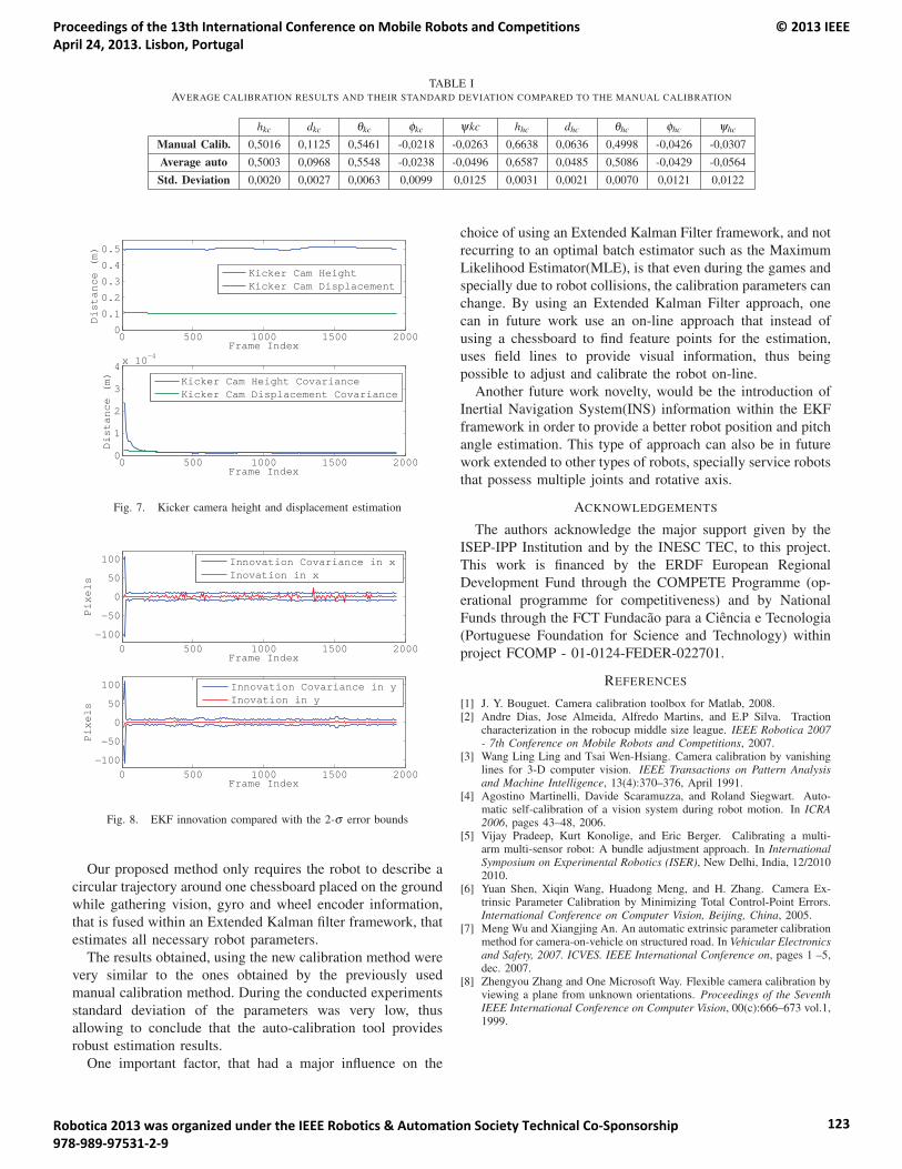
TABLE IAVERAGE CALIBRATION RESULTS AND THEIR STANDARD DEVIATION COMPARED TO THE MANUAL CALIBRATION

hkc dkc θkc φkc ψkc hhc dhc θhc φhc ψhc

Manual Calib. 0,5016 0,1125 0,5461 -0,0218 -0,0263 0,6638 0,0636 0,4998 -0,0426 -0,0307

Average auto 0,5003 0,0968 0,5548 -0,0238 -0,0496 0,6587 0,0485 0,5086 -0,0429 -0,0564

Std. Deviation 0,0020 0,0027 0,0063 0,0099 0,0125 0,0031 0,0021 0,0070 0,0121 0,0122

0 500 1000 1500 20000

0.1

0.2

0.3

0.4

0.5

Frame Index

Distance (m)

Kicker Cam HeightKicker Cam Displacement

0 500 1000 1500 20000

1

2

3

4x 10−4

Frame Index

Distance (m) Kicker Cam Height Covariance

Kicker Cam Displacement Covariance

Fig. 7. Kicker camera height and displacement estimation

0 500 1000 1500 2000−100

−50

0

50

100

Frame Index

Pixels

Innovation Covariance in xInovation in x

0 500 1000 1500 2000−100

−50

0

50

100

Frame Index

Pixels

Innovation Covariance in yInovation in y

Fig. 8. EKF innovation compared with the 2-σ error bounds

Our proposed method only requires the robot to describe a

circular trajectory around one chessboard placed on the ground

while gathering vision, gyro and wheel encoder information,

that is fused within an Extended Kalman filter framework, that

estimates all necessary robot parameters.

The results obtained, using the new calibration method were

very similar to the ones obtained by the previously used

manual calibration method. During the conducted experiments

standard deviation of the parameters was very low, thus

allowing to conclude that the auto-calibration tool provides

robust estimation results.

One important factor, that had a major influence on the

choice of using an Extended Kalman Filter framework, and not

recurring to an optimal batch estimator such as the Maximum

Likelihood Estimator(MLE), is that even during the games and

specially due to robot collisions, the calibration parameters can

change. By using an Extended Kalman Filter approach, one

can in future work use an on-line approach that instead of

using a chessboard to find feature points for the estimation,

uses field lines to provide visual information, thus being

possible to adjust and calibrate the robot on-line.

Another future work novelty, would be the introduction of

Inertial Navigation System(INS) information within the EKF

framework in order to provide a better robot position and pitch

angle estimation. This type of approach can also be in future

work extended to other types of robots, specially service robots

that possess multiple joints and rotative axis.

ACKNOWLEDGEMENTS

The authors acknowledge the major support given by the

ISEP-IPP Institution and by the INESC TEC, to this project.

This work is financed by the ERDF European Regional

Development Fund through the COMPETE Programme (op-

erational programme for competitiveness) and by National

Funds through the FCT Fundacao para a Ciencia e Tecnologia

(Portuguese Foundation for Science and Technology) within

project FCOMP - 01-0124-FEDER-022701.

REFERENCES

[1] J. Y. Bouguet. Camera calibration toolbox for Matlab, 2008.[2] Andre Dias, Jose Almeida, Alfredo Martins, and E.P Silva. Traction

characterization in the robocup middle size league. IEEE Robotica 2007- 7th Conference on Mobile Robots and Competitions, 2007.

[3] Wang Ling Ling and Tsai Wen-Hsiang. Camera calibration by vanishinglines for 3-D computer vision. IEEE Transactions on Pattern Analysisand Machine Intelligence, 13(4):370–376, April 1991.

[4] Agostino Martinelli, Davide Scaramuzza, and Roland Siegwart. Auto-matic self-calibration of a vision system during robot motion. In ICRA2006, pages 43–48, 2006.

[5] Vijay Pradeep, Kurt Konolige, and Eric Berger. Calibrating a multi-arm multi-sensor robot: A bundle adjustment approach. In InternationalSymposium on Experimental Robotics (ISER), New Delhi, India, 12/20102010.

[6] Yuan Shen, Xiqin Wang, Huadong Meng, and H. Zhang. Camera Ex-trinsic Parameter Calibration by Minimizing Total Control-Point Errors.International Conference on Computer Vision, Beijing, China, 2005.

[7] Meng Wu and Xiangjing An. An automatic extrinsic parameter calibrationmethod for camera-on-vehicle on structured road. In Vehicular Electronicsand Safety, 2007. ICVES. IEEE International Conference on, pages 1 –5,dec. 2007.

[8] Zhengyou Zhang and One Microsoft Way. Flexible camera calibration byviewing a plane from unknown orientations. Proceedings of the SeventhIEEE International Conference on Computer Vision, 00(c):666–673 vol.1,1999.


© 2013 IEEE


123

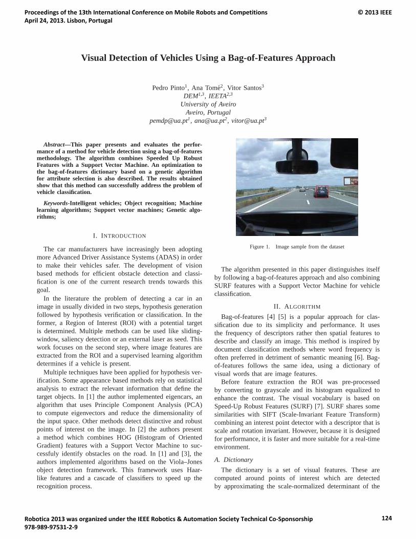
Visual Detection of Vehicles Using a Bag-of-Features Approach

Pedro Pinto1, Ana Tome2, Vitor Santos3

DEM1,3, IEETA2,3

University of AveiroAveiro, Portugal

[email protected], [email protected], [email protected]

Abstract—This paper presents and evaluates the perfor-mance of a method for vehicle detection using a bag-of-featuresmethodology. The algorithm combines Speeded Up RobustFeatures with a Support Vector Machine. An optimization tothe bag-of-features dictionary based on a genetic algorithmfor attribute selection is also described. The results obtainedshow that this method can successfully address the problem ofvehicle classification.

Keywords-Intelligent vehicles; Object recognition; Machinelearning algorithms; Support vector machines; Genetic algo-rithms;

I. INTRODUCTION

The car manufacturers have increasingly been adoptingmore Advanced Driver Assistance Systems (ADAS) in orderto make their vehicles safer. The development of visionbased methods for efficient obstacle detection and classi-fication is one of the current research trends towards thisgoal.

In the literature the problem of detecting a car in animage in usually divided in two steps, hypothesis generationfollowed by hypothesis verification or classification. In theformer, a Region of Interest (ROI) with a potential targetis determined. Multiple methods can be used like sliding-window, saliency detection or an external laser as seed. Thiswork focuses on the second step, where image features areextracted from the ROI and a supervised learning algorithmdetermines if a vehicle is present.

Multiple techniques have been applied for hypothesis ver-ification. Some appearance based methods rely on statisticalanalysis to extract the relevant information that define thetarget objects. In [1] the author implemented eigencars, analgorithm that uses Principle Component Analysis (PCA)to compute eigenvectors and reduce the dimensionality ofthe input space. Other methods detect distinctive and robustpoints of interest on the image. In [2] the authors presenta method which combines HOG (Histogram of OrientedGradient) features with a Support Vector Machine to suc-cessfuly identify obstacles on the road. In [1] and [3], theauthors implemented algorithms based on the Viola–Jonesobject detection framework. This framework uses Haar-like features and a cascade of classifiers to speed up therecognition process.

Figure 1. Image sample from the dataset

The algorithm presented in this paper distinguishes itselfby following a bag-of-features approach and also combiningSURF features with a Support Vector Machine for vehicleclassification.

II. ALGORITHM

Bag-of-features [4] [5] is a popular approach for clas-sification due to its simplicity and performance. It usesthe frequency of descriptors rather then spatial features todescribe and classify an image. This method is inspired bydocument classification methods where word frequency isoften preferred in detriment of semantic meaning [6]. Bag-of-features follows the same idea, using a dictionary ofvisual words that are image features.

Before feature extraction the ROI was pre-processedby converting to grayscale and its histogram equalized toenhance the contrast. The visual vocabulary is based onSpeed-Up Robust Features (SURF) [7]. SURF shares somesimilarities with SIFT (Scale-Invariant Feature Transform)combining an interest point detector with a descriptor that isscale and rotation invariant. However, because it is designedfor performance, it is faster and more suitable for a real-timeenvironment.

A. DictionaryThe dictionary is a set of visual features. These are

computed around points of interest which are detectedby approximating the scale-normalized determinant of the


© 2013 IEEE


124

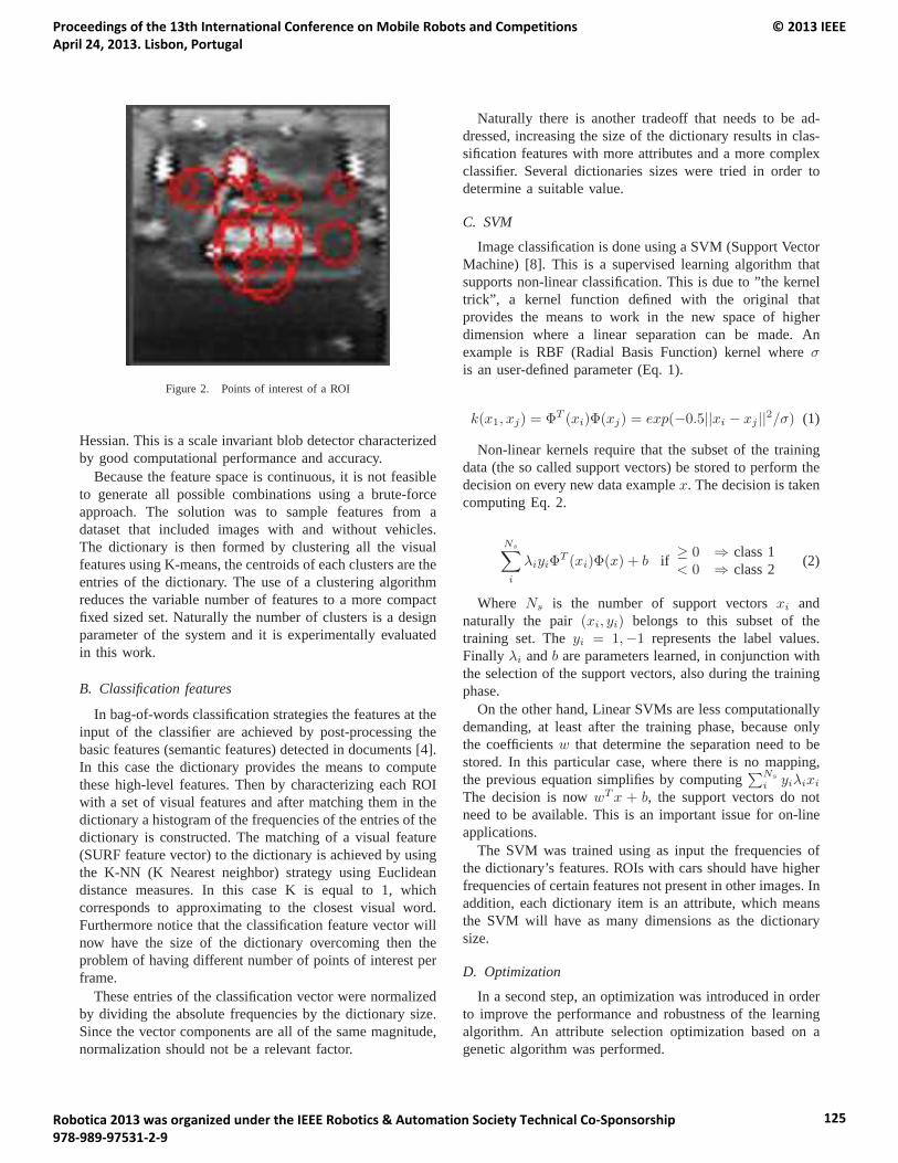
Figure 2. Points of interest of a ROI

Hessian. This is a scale invariant blob detector characterizedby good computational performance and accuracy.

Because the feature space is continuous, it is not feasibleto generate all possible combinations using a brute-forceapproach. The solution was to sample features from adataset that included images with and without vehicles.The dictionary is then formed by clustering all the visualfeatures using K-means, the centroids of each clusters are theentries of the dictionary. The use of a clustering algorithmreduces the variable number of features to a more compactfixed sized set. Naturally the number of clusters is a designparameter of the system and it is experimentally evaluatedin this work.

B. Classification features

In bag-of-words classification strategies the features at theinput of the classifier are achieved by post-processing thebasic features (semantic features) detected in documents [4].In this case the dictionary provides the means to computethese high-level features. Then by characterizing each ROIwith a set of visual features and after matching them in thedictionary a histogram of the frequencies of the entries of thedictionary is constructed. The matching of a visual feature(SURF feature vector) to the dictionary is achieved by usingthe K-NN (K Nearest neighbor) strategy using Euclideandistance measures. In this case K is equal to 1, whichcorresponds to approximating to the closest visual word.Furthermore notice that the classification feature vector willnow have the size of the dictionary overcoming then theproblem of having different number of points of interest perframe.

These entries of the classification vector were normalizedby dividing the absolute frequencies by the dictionary size.Since the vector components are all of the same magnitude,normalization should not be a relevant factor.

Naturally there is another tradeoff that needs to be ad-dressed, increasing the size of the dictionary results in clas-sification features with more attributes and a more complexclassifier. Several dictionaries sizes were tried in order todetermine a suitable value.

C. SVM

Image classification is done using a SVM (Support VectorMachine) [8]. This is a supervised learning algorithm thatsupports non-linear classification. This is due to ”the kerneltrick”, a kernel function defined with the original thatprovides the means to work in the new space of higherdimension where a linear separation can be made. Anexample is RBF (Radial Basis Function) kernel where σis an user-defined parameter (Eq. 1).

k(x1, xj) = ΦT (xi)Φ(xj) = exp(−0.5||xi − xj ||2/σ) (1)

Non-linear kernels require that the subset of the trainingdata (the so called support vectors) be stored to perform thedecision on every new data example x. The decision is takencomputing Eq. 2.

Ns∑i

λiyiΦT (xi)Φ(x) + b if ≥ 0 ⇒ class 1

< 0 ⇒ class 2 (2)

Where Ns is the number of support vectors xi andnaturally the pair (xi, yi) belongs to this subset of thetraining set. The yi = 1,−1 represents the label values.Finally λi and b are parameters learned, in conjunction withthe selection of the support vectors, also during the trainingphase.

On the other hand, Linear SVMs are less computationallydemanding, at least after the training phase, because onlythe coefficients w that determine the separation need to bestored. In this particular case, where there is no mapping,the previous equation simplifies by computing

∑Ns

i yiλixi

The decision is now wTx + b, the support vectors do notneed to be available. This is an important issue for on-lineapplications.

The SVM was trained using as input the frequencies ofthe dictionary’s features. ROIs with cars should have higherfrequencies of certain features not present in other images. Inaddition, each dictionary item is an attribute, which meansthe SVM will have as many dimensions as the dictionarysize.

D. Optimization

In a second step, an optimization was introduced in orderto improve the performance and robustness of the learningalgorithm. An attribute selection optimization based on agenetic algorithm was performed.


© 2013 IEEE


125

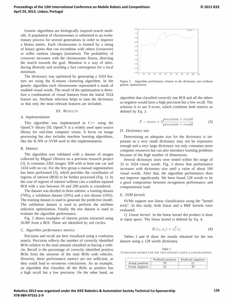
Genetic algorithms are biologically inspired search meth-ods. A population of chromosomes is submitted to an evolu-tionary process for several generations in order to improvea fitness metric. Each chromosome is formed by a stringof binary genes that can recombine with others (crossover)or suffer random changes (mutation). The probability ofcrossover increases with the chromosome fitness, directingthe search towards the goal. Mutation is a way of intro-ducing diversity and avoiding a fast convergence for a localminimum.

The dictionary was optimized by generating a 1024 fea-ture set using the K-means clustering algorithm. In thegenetic algorithm each chromosome represented a mask ofenabled visual words. The result of the optimization is there-fore a combination of visual features from the initial 1024feature set. Attribute selection helps to tune the dictionaryso that only the most relevant features are included.

III. RESULTS

A. ImplementationThis algorithm was implemented in C++ using the

OpenCV library [9]. OpenCV is a widely used open sourcelibrary for real-time computer vision. It focus on imageprocessing but also includes machine learning algorithms,like the K-NN or SVM used in this implementation.

B. DatasetThe algorithm was validated with a dataset of images

collected by Miguel Oliveira on a previous research project[3]. It constains 2265 images: 828 with at least one car and1434 with no car. For the first group a manual segmentationhas been performed [3], which provides the coordinates ofregions of interest (ROI) to be further processed (Fig. 1). Inthe case of regions of interest without cars a random squaredROI with a size between 50 and 200 pixels is considered.

The dataset was divided in three subsets: a training dataset(70%), a validation dataset (20%) and a test dataset (10%).The training dataset is used to generate the predictive model.The validation dataset is used to perform the attributeselection optimization. Finally the test dataset is used toevaluate the algorithm performance.

Fig. 2 shows examples of interest points extracted usingSURF from a ROI. These are identified by red circles.

C. Algorithm performance metricsPrecision and recall are best visualized using a confusion

matrix. Precision reflects the number of correctly identifiedROIs relative to the total amount classified as having a vehi-cle. Recall is the percentage of correctly identified positiveROIs from the universe of the total ROIs with vehicles.However, these performance metrics are not sufficient, asthey could lead to erroneous conclusions. As an example,an algorithm that classifies all the ROIs as positive hasa high recall but a low precision. On the other hand, an

0.72

0.74

0.76

0.78

0.8

0.82

0.84

0.86

0.88

0.9

0.92

0 100 200 300 400 500 600 700 800 900 1000 1100

F-Score

Figure 3. Algorithm performance relative to the dictionary size (withoutgenetic optimization)

algorithm that classified correctly one ROI and all the othersas negative would have a high precision but a low recall. Thesolution is to use F-score, which combines both metrics asdefined by Eq. 3.

F − score = 2precision× recall

precision+ recall(3)

D. Dictionary sizeDetermining an adequate size for the dictionary is im-

portant as a very small dictionary may not be expressiveenough and a very large dictionary not only consumes morecomputer resources but can also introduce learning problemsbecause of the high number of dimensions.

Several dictionary sizes were tested within the range of32 to 1024 visual words. Fig. 3 shows that performanceincreases with dictionary size until a value of about 100visual words. After that, the algorithm performance doesnot improve significantly. We have found 128 words to bea good compromise between recognition performance andcomputational load.

E. SVM kernelsSVMs support non linear classification using the ”kernel

trick”. In this study, both linear and a RBF kernels wereevaluated.

1) Linear kernel: In the linear kernel dot product is donein input space. The linear kernel is defined by Eq. 4.

K(xi, xj) = xTi xj (4)

Tables I and II show the results obtained for the testdataset using a 128 words dictionary.

Table ICONFUSION MATRIX FOR THE TEST DATASET USING A LINEAR KERNEL

Predicted positives Predicted negativesActual positives 70 12Actual negatives 22 39


© 2013 IEEE


126

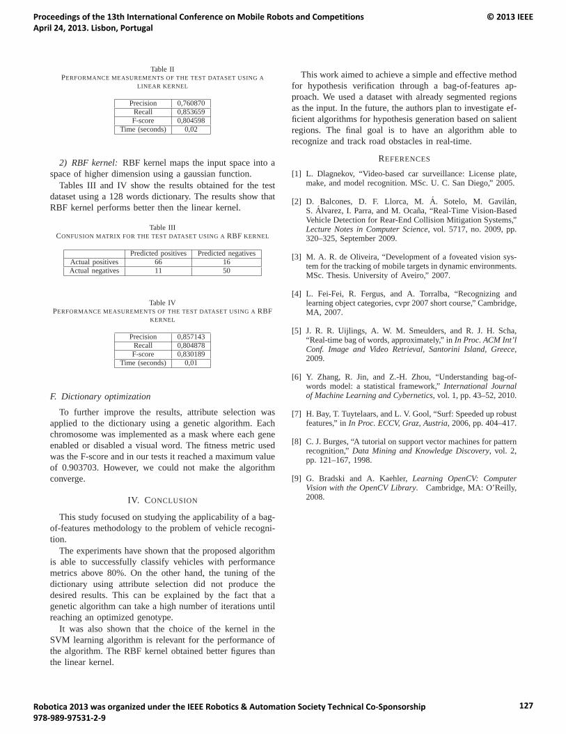
Table IIPERFORMANCE MEASUREMENTS OF THE TEST DATASET USING A

LINEAR KERNEL

Precision 0,760870Recall 0,853659F-score 0,804598

Time (seconds) 0,02

2) RBF kernel: RBF kernel maps the input space into aspace of higher dimension using a gaussian function.

Tables III and IV show the results obtained for the testdataset using a 128 words dictionary. The results show thatRBF kernel performs better then the linear kernel.

Table IIICONFUSION MATRIX FOR THE TEST DATASET USING A RBF KERNEL

Predicted positives Predicted negativesActual positives 66 16Actual negatives 11 50

Table IVPERFORMANCE MEASUREMENTS OF THE TEST DATASET USING A RBF

KERNEL

Precision 0,857143Recall 0,804878F-score 0,830189

Time (seconds) 0,01

F. Dictionary optimization

To further improve the results, attribute selection wasapplied to the dictionary using a genetic algorithm. Eachchromosome was implemented as a mask where each geneenabled or disabled a visual word. The fitness metric usedwas the F-score and in our tests it reached a maximum valueof 0.903703. However, we could not make the algorithmconverge.

IV. CONCLUSION

This study focused on studying the applicability of a bag-of-features methodology to the problem of vehicle recogni-tion.

The experiments have shown that the proposed algorithmis able to successfully classify vehicles with performancemetrics above 80%. On the other hand, the tuning of thedictionary using attribute selection did not produce thedesired results. This can be explained by the fact that agenetic algorithm can take a high number of iterations untilreaching an optimized genotype.

It was also shown that the choice of the kernel in theSVM learning algorithm is relevant for the performance ofthe algorithm. The RBF kernel obtained better figures thanthe linear kernel.

This work aimed to achieve a simple and effective methodfor hypothesis verification through a bag-of-features ap-proach. We used a dataset with already segmented regionsas the input. In the future, the authors plan to investigate ef-ficient algorithms for hypothesis generation based on salientregions. The final goal is to have an algorithm able torecognize and track road obstacles in real-time.

REFERENCES

[1] L. Dlagnekov, “Video-based car surveillance: License plate,make, and model recognition. MSc. U. C. San Diego,” 2005.

[2] D. Balcones, D. F. Llorca, M. A. Sotelo, M. Gavilan,S. Alvarez, I. Parra, and M. Ocana, “Real-Time Vision-BasedVehicle Detection for Rear-End Collision Mitigation Systems,”Lecture Notes in Computer Science, vol. 5717, no. 2009, pp.320–325, September 2009.

[3] M. A. R. de Oliveira, “Development of a foveated vision sys-tem for the tracking of mobile targets in dynamic environments.MSc. Thesis. University of Aveiro,” 2007.

[4] L. Fei-Fei, R. Fergus, and A. Torralba, “Recognizing andlearning object categories, cvpr 2007 short course,” Cambridge,MA, 2007.

[5] J. R. R. Uijlings, A. W. M. Smeulders, and R. J. H. Scha,“Real-time bag of words, approximately,” in In Proc. ACM Int’lConf. Image and Video Retrieval, Santorini Island, Greece,2009.

[6] Y. Zhang, R. Jin, and Z.-H. Zhou, “Understanding bag-of-words model: a statistical framework,” International Journalof Machine Learning and Cybernetics, vol. 1, pp. 43–52, 2010.

[7] H. Bay, T. Tuytelaars, and L. V. Gool, “Surf: Speeded up robustfeatures,” in In Proc. ECCV, Graz, Austria, 2006, pp. 404–417.

[8] C. J. Burges, “A tutorial on support vector machines for patternrecognition,” Data Mining and Knowledge Discovery, vol. 2,pp. 121–167, 1998.

[9] G. Bradski and A. Kaehler, Learning OpenCV: ComputerVision with the OpenCV Library. Cambridge, MA: O’Reilly,2008.


© 2013 IEEE


127

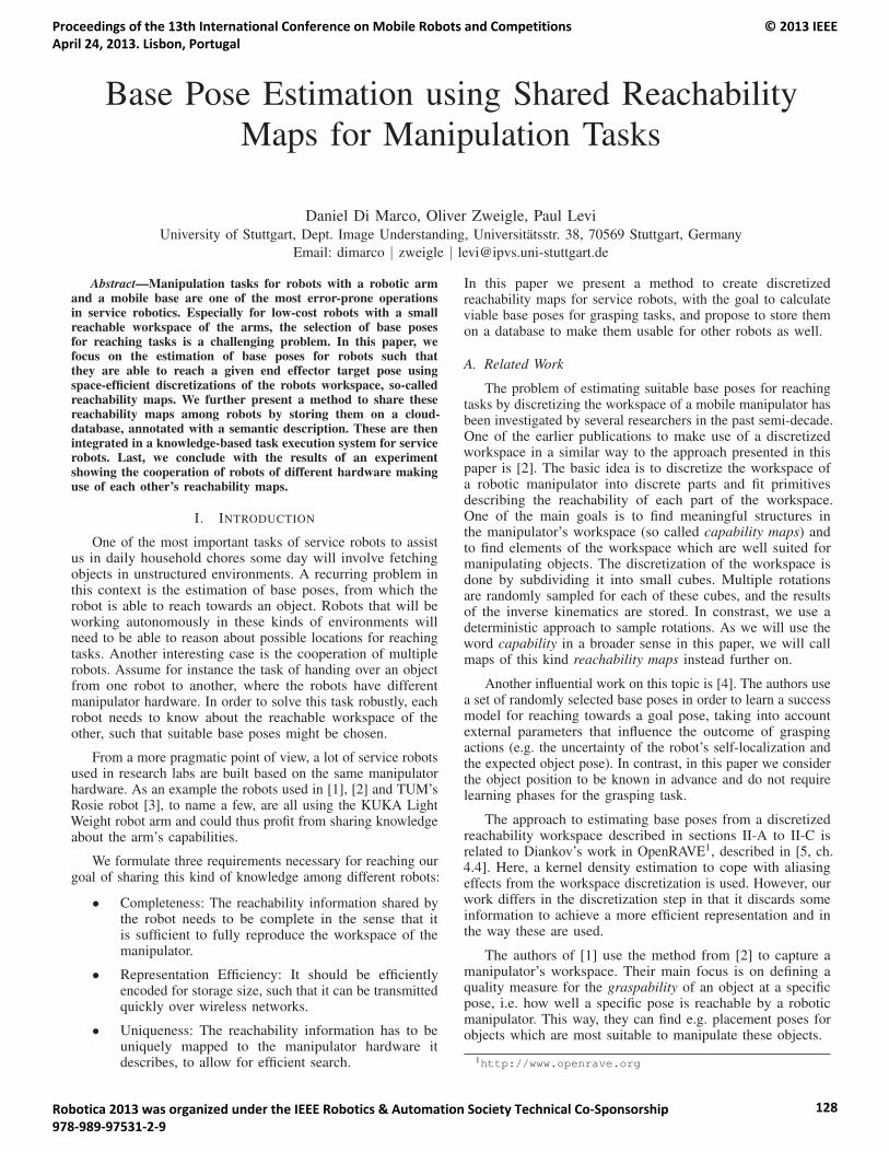
Base Pose Estimation using Shared ReachabilityMaps for Manipulation Tasks

Daniel Di Marco, Oliver Zweigle, Paul LeviUniversity of Stuttgart, Dept. Image Understanding, Universitatsstr. 38, 70569 Stuttgart, Germany

Email: dimarco | zweigle | [email protected]

Abstract—Manipulation tasks for robots with a robotic armand a mobile base are one of the most error-prone operationsin service robotics. Especially for low-cost robots with a smallreachable workspace of the arms, the selection of base posesfor reaching tasks is a challenging problem. In this paper, wefocus on the estimation of base poses for robots such thatthey are able to reach a given end effector target pose usingspace-efficient discretizations of the robots workspace, so-calledreachability maps. We further present a method to share thesereachability maps among robots by storing them on a cloud-database, annotated with a semantic description. These are thenintegrated in a knowledge-based task execution system for servicerobots. Last, we conclude with the results of an experimentshowing the cooperation of robots of different hardware makinguse of each other’s reachability maps.

I. INTRODUCTION

One of the most important tasks of service robots to assistus in daily household chores some day will involve fetchingobjects in unstructured environments. A recurring problem inthis context is the estimation of base poses, from which therobot is able to reach towards an object. Robots that will beworking autonomously in these kinds of environments willneed to be able to reason about possible locations for reachingtasks. Another interesting case is the cooperation of multiplerobots. Assume for instance the task of handing over an objectfrom one robot to another, where the robots have differentmanipulator hardware. In order to solve this task robustly, eachrobot needs to know about the reachable workspace of theother, such that suitable base poses might be chosen.

From a more pragmatic point of view, a lot of service robotsused in research labs are built based on the same manipulatorhardware. As an example the robots used in [1], [2] and TUM’sRosie robot [3], to name a few, are all using the KUKA LightWeight robot arm and could thus profit from sharing knowledgeabout the arm’s capabilities.

We formulate three requirements necessary for reaching ourgoal of sharing this kind of knowledge among different robots:

• Completeness: The reachability information shared bythe robot needs to be complete in the sense that itis sufficient to fully reproduce the workspace of themanipulator.

• Representation Efficiency: It should be efficientlyencoded for storage size, such that it can be transmittedquickly over wireless networks.

• Uniqueness: The reachability information has to beuniquely mapped to the manipulator hardware itdescribes, to allow for efficient search.

In this paper we present a method to create discretizedreachability maps for service robots, with the goal to calculateviable base poses for grasping tasks, and propose to store themon a database to make them usable for other robots as well.

A. Related Work

The problem of estimating suitable base poses for reachingtasks by discretizing the workspace of a mobile manipulator hasbeen investigated by several researchers in the past semi-decade.One of the earlier publications to make use of a discretizedworkspace in a similar way to the approach presented in thispaper is [2]. The basic idea is to discretize the workspace ofa robotic manipulator into discrete parts and fit primitivesdescribing the reachability of each part of the workspace.One of the main goals is to find meaningful structures inthe manipulator’s workspace (so called capability maps) andto find elements of the workspace which are well suited formanipulating objects. The discretization of the workspace isdone by subdividing it into small cubes. Multiple rotationsare randomly sampled for each of these cubes, and the resultsof the inverse kinematics are stored. In constrast, we use adeterministic approach to sample rotations. As we will use theword capability in a broader sense in this paper, we will callmaps of this kind reachability maps instead further on.

Another influential work on this topic is [4]. The authors usea set of randomly selected base poses in order to learn a successmodel for reaching towards a goal pose, taking into accountexternal parameters that influence the outcome of graspingactions (e.g. the uncertainty of the robot’s self-localization andthe expected object pose). In contrast, in this paper we considerthe object position to be known in advance and do not requirelearning phases for the grasping task.

The approach to estimating base poses from a discretizedreachability workspace described in sections II-A to II-C isrelated to Diankov’s work in OpenRAVE1, described in [5, ch.4.4]. Here, a kernel density estimation to cope with aliasingeffects from the workspace discretization is used. However, ourwork differs in the discretization step in that it discards someinformation to achieve a more efficient representation and inthe way these are used.

The authors of [1] use the method from [2] to capture amanipulator’s workspace. Their main focus is on defining aquality measure for the graspability of an object at a specificpose, i.e. how well a specific pose is reachable by a roboticmanipulator. This way, they can find e.g. placement poses forobjects which are most suitable to manipulate these objects.

1http://www.openrave.org


© 2013 IEEE


128

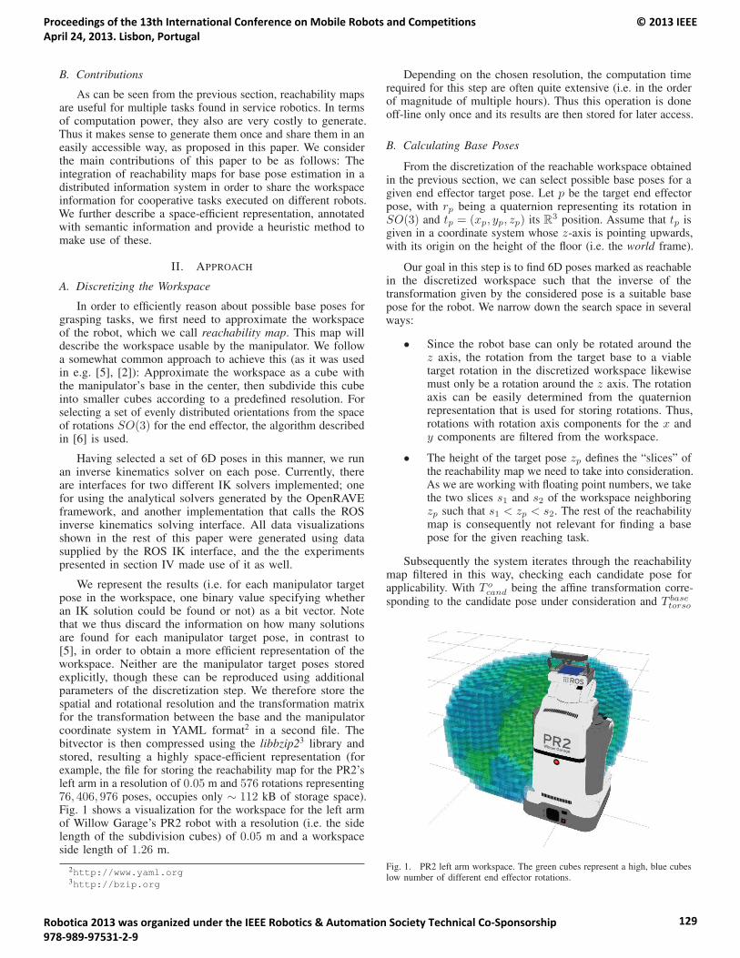
B. Contributions

As can be seen from the previous section, reachability mapsare useful for multiple tasks found in service robotics. In termsof computation power, they also are very costly to generate.Thus it makes sense to generate them once and share them in aneasily accessible way, as proposed in this paper. We considerthe main contributions of this paper to be as follows: Theintegration of reachability maps for base pose estimation in adistributed information system in order to share the workspaceinformation for cooperative tasks executed on different robots.We further describe a space-efficient representation, annotatedwith semantic information and provide a heuristic method tomake use of these.

II. APPROACH

A. Discretizing the Workspace

In order to efficiently reason about possible base poses forgrasping tasks, we first need to approximate the workspaceof the robot, which we call reachability map. This map willdescribe the workspace usable by the manipulator. We followa somewhat common approach to achieve this (as it was usedin e.g. [5], [2]): Approximate the workspace as a cube withthe manipulator’s base in the center, then subdivide this cubeinto smaller cubes according to a predefined resolution. Forselecting a set of evenly distributed orientations from the spaceof rotations SO(3) for the end effector, the algorithm describedin [6] is used.

Having selected a set of 6D poses in this manner, we runan inverse kinematics solver on each pose. Currently, thereare interfaces for two different IK solvers implemented; onefor using the analytical solvers generated by the OpenRAVEframework, and another implementation that calls the ROSinverse kinematics solving interface. All data visualizationsshown in the rest of this paper were generated using datasupplied by the ROS IK interface, and the the experimentspresented in section IV made use of it as well.

We represent the results (i.e. for each manipulator targetpose in the workspace, one binary value specifying whetheran IK solution could be found or not) as a bit vector. Notethat we thus discard the information on how many solutionsare found for each manipulator target pose, in contrast to[5], in order to obtain a more efficient representation of theworkspace. Neither are the manipulator target poses storedexplicitly, though these can be reproduced using additionalparameters of the discretization step. We therefore store thespatial and rotational resolution and the transformation matrixfor the transformation between the base and the manipulatorcoordinate system in YAML format2 in a second file. Thebitvector is then compressed using the libbzip23 library andstored, resulting a highly space-efficient representation (forexample, the file for storing the reachability map for the PR2’sleft arm in a resolution of 0.05 m and 576 rotations representing76, 406, 976 poses, occupies only ∼ 112 kB of storage space).Fig. 1 shows a visualization for the workspace for the left armof Willow Garage’s PR2 robot with a resolution (i.e. the sidelength of the subdivision cubes) of 0.05 m and a workspaceside length of 1.26 m.

2http://www.yaml.org3http://bzip.org

Depending on the chosen resolution, the computation timerequired for this step are often quite extensive (i.e. in the orderof magnitude of multiple hours). Thus this operation is doneoff-line only once and its results are then stored for later access.

B. Calculating Base Poses

From the discretization of the reachable workspace obtainedin the previous section, we can select possible base poses for agiven end effector target pose. Let p be the target end effectorpose, with rp being a quaternion representing its rotation inSO(3) and tp = (xp, yp, zp) its R

3 position. Assume that tp isgiven in a coordinate system whose z-axis is pointing upwards,with its origin on the height of the floor (i.e. the world frame).

Our goal in this step is to find 6D poses marked as reachablein the discretized workspace such that the inverse of thetransformation given by the considered pose is a suitable basepose for the robot. We narrow down the search space in severalways:

• Since the robot base can only be rotated around thez axis, the rotation from the target base to a viabletarget rotation in the discretized workspace likewisemust only be a rotation around the z axis. The rotationaxis can be easily determined from the quaternionrepresentation that is used for storing rotations. Thus,rotations with rotation axis components for the x andy components are filtered from the workspace.

• The height of the target pose zp defines the “slices” ofthe reachability map we need to take into consideration.As we are working with floating point numbers, we takethe two slices s1 and s2 of the workspace neighboringzp such that s1 < zp < s2. The rest of the reachabilitymap is consequently not relevant for finding a basepose for the given reaching task.

Subsequently the system iterates through the reachabilitymap filtered in this way, checking each candidate pose forapplicability. With T o

cand being the affine transformation corre-sponding to the candidate pose under consideration and T base

torso

Fig. 1. PR2 left arm workspace. The green cubes represent a high, blue cubeslow number of different end effector rotations.


© 2013 IEEE


129

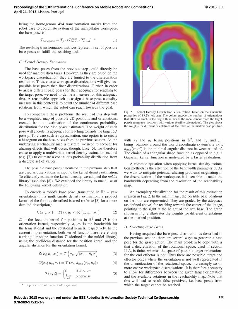
being the homogenous 4x4 transformation matrix from therobot base to coordinate system of the manipulator workspace,the base pose is:

Tbasepose = Tp · (T basetorso · T o

cand)−1 (1)

The resulting transformation matrices represent a set of possiblebase poses to fulfill the reaching task.

C. Kernel Density Estimation

The base poses from the previous step could directly beused for manipulation tasks. However, as they are based on theworkspace discretization, they are limited to the discretizationresolution. Thus, coarse workspace discretizations will give lesspossible base poses than finer discretizations. Further, in orderto assess different base poses for their adequacy for reaching tothe target pose, we need to define a measure for this adequacyfirst. A reasonable approach to assign a base pose a qualitymeasure in this context is to count the number of different baserotations from which the robot can reach towards the goal.

To compensate these problems, the result of this step willbe a weighted map of possible 2D positions and orientations,created from an estimation of the continuous probabilitydistribution for the base poses estimated. The weight of eachpose will encode its adequacy for reaching towards the target 6Dpose p. To create such a representation, one option is to createa histogram on the base poses from the previous section. As theunderlying reachability map is discrete, we need to account foraliasing effects that will occur, though. Like [5], we thereforechose to apply a multivariate kernel density estimation method(e.g. [7]) to estimate a continuous probability distribution froma discrete set of values.

The possible base poses calculated in the previous step II-Bare used as observations as input to the kernel density estimation.To efficiently estimate the kernel density, we adopted the nukleilibrary4 (see also [8]). We extended the library to make use ofthe following kernel definition.

To encode a robot’s base pose (translation in R2 + yaw

orientation) in a multivariate density estimation, a productkernel of the form as described is used (refer to [8] for a moredetailed description):

K(x;μ, σ) = L(xt;μt, σt)O(xt;μr, σr) (2)

L is the location kernel for positions in R2 and O is the

orientation kernel, respectively. σt, σr is the bandwidth forthe translational and the rotational kernels, respectively. In thecurrent implementation, both kernel functions are referencinga triangular shape function T (defined in the nuklei library)using the euclidean distance for the position kernel and theangular distance for the orientation kernel:

L(xt;μt, σt) = T(σt,

√(xt − μt)2

)(3)

O(xr;μr, σr) = T (σr, dang(xr, μr)) (4)

T (σ, d) =

{0 if d > 2σ1−d2σ otherwise

(5)

4http://nuklei.sourceforge.net

Fig. 2. Kernel Density Distribution Visualization, based on the kinematicproperties of PR2’s left arm. The colors encode the number of orientationsthat allow to reach to the origin (blue means the robot cannot reach the target,purple represents positions with various feasible orientations). The plot showsthe weights for different orientations of the robot at the marked base position.

with xt and μt being positions in R2, and xr and μr

being rotations around the world coordinate system’s z axis.dang(α, α

′) is the minimal angular distance between α and α′.The choice of a triangular shape function as opposed to e.g. aGaussian kernel function is motivated by a faster evaluation.

A common question when applying kernel density estima-tion methods is the selection of the bandwidth parameter σ. Aswe want to mitigate potential aliasing problems originating inthe discretization of the workspace, it is sensible to make thebandwidth depending from the resolution of the reachabilitymap.

An exemplary visualization for the result of this estimationis given in Fig. 2. In the main image, the possible base positionson the floor are represented. They are graded by the adequacy(as defined above) for reaching towards the center of the image,pointing to the right at the height of the arm base. The graphshown in Fig. 2 illustrates the weights for different orientationsat the marked position.

D. Selecting Base Poses

Having acquired the base pose distribution as described inthe previous section, there are several ways to generate a basepose for the grasp action. The main problem to cope with isthat a discretization of the rotational space, used in sectionII-A, is finite, whereas the space of possible target orientationsfor the end effector is not. Thus there are possible target endeffector poses where the orientation is not well represented inthe discretization of the rotational space, increasingly so onmore coarse workspace discretizations. It is therefore necessaryto allow for differences between the given target orientationand the available rotations in the reachability map. Note thatthis will lead to result false positives, i.e. base poses fromwhich the target cannot be reached.


© 2013 IEEE


130

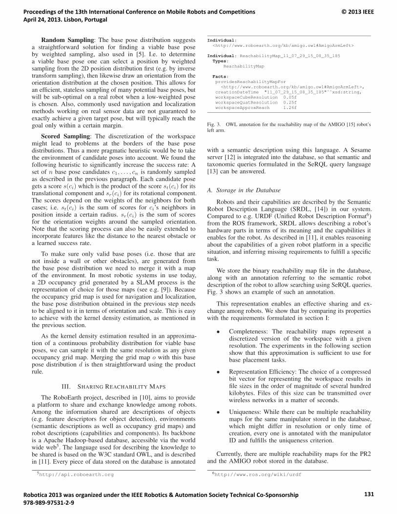
Random Sampling: The base pose distribution suggestsa straightforward solution for finding a viable base poseby weighted sampling, also used in [5]. I.e. to determinea viable base pose one can select a position by weightedsampling from the 2D position distribution first (e.g. by inversetransform sampling), then likewise draw an orientation from theorientation distribution at the chosen position. This allows foran efficient, stateless sampling of many potential base poses, butwill be sub-optimal on a real robot when a low-weighted poseis chosen. Also, commonly used navigation and localizationmethods working on real sensor data are not guaranteed toexactly achieve a given target pose, but will typically reach thegoal only within a certain margin.

Scored Sampling: The discretization of the workspacemight lead to problems at the borders of the base posedistributions. Thus a more pragmatic heuristic would be to takethe environment of candidate poses into account. We found thefollowing heuristic to significantly increase the success rate: Aset of n base pose candidates c1, . . . , cn is randomly sampledas described in the previous paragraph. Each candidate posegets a score s(ci) which is the product of the score st(ci) for itstranslational component and sr(ci) for its rotational component.The scores depend on the weights of the neighbors for bothcases; i.e. st(ci) is the sum of scores for ci’s neighbors inposition inside a certain radius. sr(ci) is the sum of scoresfor the orientation weights around the sampled orientation.Note that the scoring process can also be easily extended toincorporate features like the distance to the nearest obstacle ora learned success rate.

To make sure only valid base poses (i.e. those that arenot inside a wall or other obstacles), are generated fromthe base pose distribution we need to merge it with a mapof the environment. In most robotic systems in use today,a 2D occupancy grid generated by a SLAM process is therepresentation of choice for those maps (see e.g. [9]). Becausethe occupancy grid map is used for navigation and localization,the base pose distribution obtained in the previous step needsto be aligned to it in terms of orientation and scale. This is easyto achieve with the kernel density estimation, as mentioned inthe previous section.

As the kernel density estimation resulted in an approxima-tion of a continuous probability distribution for viable baseposes, we can sample it with the same resolution as any givenoccupancy grid map. Merging the grid map o with this basepose distribution d is then straightforward using the productrule.

III. SHARING REACHABILITY MAPS

The RoboEarth project, described in [10], aims to providea platform to share and exchange knowledge among robots.Among the information shared are descriptions of objects(e.g. feature descriptors for object detection), environments(semantic descriptions as well as occupancy grid maps) androbot descriptions (capabilities and components). Its backboneis a Apache Hadoop-based database, accessible via the worldwide web5. The language used for describing the knowledge tobe shared is based on the W3C standard OWL, and is describedin [11]. Every piece of data stored on the database is annotated

5http://api.roboearth.org

Individual:<http://www.roboearth.org/kb/amigo.owl#AmigoArmLeft>

Individual: ReachabilityMap_11_07_29_15_08_35_185Types:

ReachabilityMap

Facts:providesReachabilityMapFor<http://www.roboearth.org/kb/amigo.owl#AmigoArmLeft>,

creationDateTime "11_07_29_15_08_35_185"ˆˆxsd:string,workspaceCubeResolution 0.05fworkspaceQuatResolution 0.25fworkspaceApproxReach 1.26f

Fig. 3. OWL annotation for the reachability map of the AMIGO [15] robot’sleft arm.

with a semantic description using this language. A Sesameserver [12] is integrated into the database, so that semantic andtaxonomic queries formulated in the SeRQL query language[13] can be answered.

A. Storage in the Database

Robots and their capabilities are described by the SemanticRobot Description Language (SRDL, [14]) in our system.Compared to e.g. URDF (Unified Robot Description Format6)from the ROS framework, SRDL allows describing a robot’shardware parts in terms of its meaning and the capabilities itenables for the robot. As described in [11], it enables reasoningabout the capabilities of a given robot platform in a specificsituation, and inferring missing requirements to fulfill a specifictask.

We store the binary reachability map file in the database,along with an annotation referring to the semantic robotdescription of the robot to allow searching using SeRQL queries.Fig. 3 shows an example of such an annotation.

This representation enables an effective sharing and ex-change among robots. We show that by comparing its propertieswith the requirements formulated in section I:

• Completeness: The reachability maps represent adiscretized version of the workspace with a givenresolution. The experiments in the following sectionshow that this approximation is sufficient to use forbase placement tasks.

• Representation Efficiency: The choice of a compressedbit vector for representing the workspace results infile sizes in the order of magnitude of several hundredkilobytes. Files of this size can be transmitted overwireless networks in a matter of seconds.

• Uniqueness: While there can be multiple reachabilitymaps for the same manipulator stored in the database,which might differ in resolution or only time ofcreation, every one is annotated with the manipulatorID and fulfills the uniqueness criterion.

Currently, there are multiple reachability maps for the PR2and the AMIGO robot stored in the database.

6http://www.ros.org/wiki/urdf


© 2013 IEEE


131

B. Base Pose Correction for Manipulation Tasks

The small size of the workspace discretizations together withthe expressive semantic description in the database allows for anefficient retrieval on demand during run-time. We make use ofthis circumstance in the integration of a failure handling methodfor manipulation tasks in the execution framework described in[16]. To recap shortly, abstract task descriptions are describedin terms of OWL classes and instances which can refer tosemantic descriptions of objects, robot descriptions etc. Thetask descriptions are translated to an executable robot plan in therobot plan description language CPL [17], based on CommonLisp. During execution, the sub-actions forming the executionplan are annotated with the OWL identifiers of the objectsinvolved: e.g. the robot manipulator in manipulation actions,or the object class identifiers in object detection subtasks.

Manipulation tasks are prone to failure, in our experience,often due to an inability of the robot to reach to the target posebecause of localization or navigation issues. We implementeda straightforward failure handling method to compensate forthese problems making use of the database and the efficientworkspace representation described in the previous sections.

If during task execution an error condition is signaled thatrepresents an “cannot reach target pose” error, the implemen-tation poses a SeRQL query to the database using the robotmanipulator OWL id to retrieve a workspace discretizationfile. The query has the following form (namespaces have beenomitted for conciseness):

SELECT source FROM CONTEXT source {S}rdf:type {re:ReachabilityMap};re:providesReachabilityMapFor {amigo:AmigoArmLeft}

USING NAMESPACE re=..., amigo=...

If no suitable workspace file is found, the action fails.Otherwise, a base correction pose is selected with the scoredrandom sampling approach described in section II-D and themanipulation action is started again.

IV. EXPERIMENTS

A. Base Pose Estimation Method

This experiment tries to compare the base pose estimationmethod described in section II-D. The open source driverimplementations for Willow Garage’s PR2 robot were used tosimulate the robot during the trials. For each method, 1000base poses were selected, with a reaching target in the origin ofthe world coordinate system and a random height offset and arandom end effector orientation. After the robot was teleportedto one of these base poses, the inverse kinematics solver wascalled to move the manipulator to the reaching target. A trywas considered successful if the manipulator could be movedto the target pose.

Table I shows the results for both methods and severalworkspace resolutions. The resolution is given as the sidelength of the cubes and the number of sampled rotations (seesection II-A) It demonstrates that the voted sampling approachdescribed in section II-D has a significantly positive effecton the failure rate, when compared to the random samplingapproach. It also shows the impact of different resolutions forthe reachability maps; both the quality of the base estimationand the difference between random and voted sampling decreasewith lower resolution.

TABLE I. BASE POSE SELECTION FAILURE RATES FOR DIFFERENT

WORKSPACE RESOLUTIONS AND DIFFERENT BASE POSE ESTIMATION

METHODS FOR THE PR2 ROBOT.

method translational res. rotational res. failure rate

Random Sampling 0.05m 576 rot. 0.179Scored Sampling 0.05m 576 rot. 0.003

Random Sampling 0.10m 76 rot. 0.561Scored Sampling 0.10m 76 rot. 0.116

Fig. 4. Comparison of base pose distributions for PR2 (left) and AMIGO(right). Red stands for low, purple for a high density of base poses.

B. Use Case: Robotic Handover

In this section, the experiment for showing a use-case forthe approaches described in this paper is presented. Consideras a scenario two robots with different manipulators, whereone robot is handing over an object to the other. To do so, bothneed to move one of their manipulators to approximately thesame position. The problem is then to find base poses for bothrobots from which they can reach the handover position.

The two robot platforms used are the PR2 robot and theAMIGO prototype robot built by TU Eindhoven (described e.g.in [15]). Fig. 5 shows a visualization of both robots during asimulated handover. Because the AMIGO has a very limitedworkspace due to the fixed installation of the arms (see Fig. 4for a comparison), this combination is interesting for the taskat hand.

Fig. 5. PR2 (left) and AMIGO (right) during simulated handover with theirleft arm, respectively


© 2013 IEEE


132

As we do not have both robots in available for use, theexperiment is carried out in simulation. The experiment processis as follows:

• A handover height h is chosen randomly, such thatthere is at least one reachable pose in the workspaceof both PR2 and AMIGO at this height. The reachablepose for the AMIGO is selected as pamigo. The targetreaching pose for the PR2 ppr2 is defined as having anoffset of −0.05 m in z direction, while its orientationis rotated 180◦ around the z-axis.

• We generate base pose distribution maps for both targetposes, using the respective workspace discretizationfor each robot. In order to avoid selecting base posessuch that both robots stand on the same place, thedistribution map for the PR2 is subtracted from theone for the AMIGO and vice versa. For each robot,10 base poses are then estimated from the base posedistribution maps using the scored sampling approachfrom section II-D.

The process is repeated 100 times. In our experiment, thejoint failure rate was 14.5%, where the rate for the AMIGOwas 14.2% and for the PR2 0.3%. The difference between thefailure rates for both robots lies in the fact that the validityfor the pose estimated for AMIGO is checked first. If the firstcheck fails, the trial counts as failed.

V. CONCLUSIONS AND FURTHER WORK

We presented a system that efficiently discretizes theworkspace of a robotic manipulator, and shares them to beused by different robots. We also described methods makinguse of them for estimating suitable base poses for reachabilitytasks. Two experiments were provided to show the validity ofthe approach, one of which was showing a possible use casefor the work described in this paper. Overall, the system allowsto discretize the workspace of a robotic manipulator once andstore it in a space-efficient manner on a database, thus allowingan easy re-use for other robots or services.

A worthwhile idea for future work would be to integrateOpenRAVE’s powerful ikfast [5] module, which allows gen-erating analytical IK solvers from a manipulator’s URDFdescription, onto the database servers. Using this module, thesystem could discretize the robot’s workspace without requiringredundant information given by the user. To help with providingthe semantic information necessary for the database, there aretools that are able to convert a URDF robot specification to abasic SRDL description.

We also strive for a deeper integration of the system intothe knowledge representation framework, e.g. to be able toautomatically infer that downloading the reachability map isnecessary by integrating the system to make use of the capabilitymatching using semantic robot descriptions described in [11].

ACKNOWLEDGMENT

The research leading to these results has received fundingfrom the European Union Seventh Framework ProgrammeFP7/2007-2013 under grant agreement no 248942 RoboEarth.

REFERENCES

[1] S. Ruehl, A. Hermann, Z. Xue, T. Kerscher, and R. Dillmann,“Graspability: A description of work surfaces for planning of robotmanipulation sequences,” in Robotics and Automation (ICRA), 2011IEEE International Conference on. IEEE, 2011, pp. 496–502.

[2] F. Zacharias, C. Borst, and G. Hirzinger, “Capturing robot workspacestructure: representing robot capabilities,” in Intelligent Robots andSystems (IROS), 2007. IEEE/RSJ International Conference on. IEEE,2007, pp. 3229–3236.

[3] M. Beetz, U. Klank, A. Maldonado, D. Pangercic, and T. Ruhr,“Robotic roommates making pancakes-look into perception-manipulationloop,” in IEEE International Conference on Robotics and Automation(ICRA), Workshop on Mobile Manipulation: Integrating Perception andManipulation, 2011, pp. 9–13.

[4] F. Stulp, A. Fedrizzi, L. Mosenlechner, and M. Beetz, “Learning andreasoning with action-related places for robust mobile manipulation,”Journal of Artificial Intelligence Research (JAIR), vol. 43, pp. 1–42,2012.

[5] R. Diankov, “Automated construction of robotic manipulation programs,”Ph.D. dissertation, Carnegie Mellon University, Robotics Institute,August 2010. [Online]. Available: http://www.programmingvision.com/rosen diankov thesis.pdf

[6] A. Yershova, S. Jain, S. LaValle, and J. Mitchell, “Generating uniformincremental grids on so (3) using the hopf fibration,” The Internationaljournal of robotics research, vol. 29, no. 7, pp. 801–812, 2010.

[7] D. Scott, Multivariate density estimation: theory, practice, and visual-ization. New York: Wiley, 1992.

[8] R. Detry, D. Kraft, O. Kroemer, L. Bodenhagen, J. Peters, N. Kruger,and J. Piater, “Learning grasp affordance densities,” Paladyn. Journalof Behavioral Robotics, 2011.

[9] S. Thrun, W. Burgard, and D. Fox, Probabilistic Robotics (IntelligentRobotics and Autonomous Agents series), ser. Intelligent robotics andautonomous agents. The MIT Press, Aug. 2005.

[10] M. Waibel, M. Beetz, J. Civera, R. D’Andrea, J. Elfring, D. Galvez-Lopez, K. Haussermann, R. Janssen, J. Montiel, A. Perzylo et al.,“RoboEarth,” Robotics & Automation Magazine, IEEE, vol. 18, no. 2,pp. 69–82, 2011.

[11] M. Tenorth, A. Perzylo, R. Lafrenz, and M. Beetz, “The RoboEarthlanguage: Representing and Exchanging Knowledge about Actions,Objects, and Environments,” in Robotics and Automatic (ICRA), 2012,IEEE International Conference on, Saint Paul, USA, 2012.

[12] J. Broekstra, A. Kampman, and F. Van Harmelen, “Sesame: A genericarchitecture for storing and querying rdf and rdf schema,” The SemanticWebISWC 2002, pp. 54–68, 2002.

[13] J. Broekstra and A. Kampman, “SeRQL: a second generation RDF querylanguage,” in Proc. SWAD-Europe Workshop on Semantic Web Storageand Retrieval, 2003, pp. 13–14.

[14] L. Kunze, T. Roehm, and M. Beetz, “Towards semantic robot descrip-tion languages,” in IEEE International Conference on Robotics andAutomation (ICRA), Shanghai, China, May, 9–13 2011.

[15] J. Lunenburg, S. van den Dries, J. Elfring, R. Janssen, J. Sandee, andM. van de Molengraft, “Tech United Eindhoven Team Description 2012,”in RoboCup Team Description Papers 2012, 2012.

[16] D. Di Marco, M. Tenorth, K. Haussermann, O. Zweigle, and P. Levi,“Roboearth action recipe execution,” in 12th International Conferenceon Intelligent Autonomous Systems, 2012.

[17] M. Beetz, L. Mosenlechner, and M. Tenorth, “CRAM – a cognitive robotabstract machine for everyday manipulation in human environments,” inIEEE/RSJ International Conference on Intelligent Robots and Systems,2010.


© 2013 IEEE


133

proceedings of the 13th international conference on mobile

Documents