probing the reds and blues: sectionalism and voter location in the 2000 and 2004 u. s. presidential...

This article appeared in a journal published by Elsevier. The attachedcopy is furnished to the author for internal non-commercial researchand education use, including for instruction at the authors institution

and sharing with colleagues.

Other uses, including reproduction and distribution, or selling orlicensing copies, or posting to personal, institutional or third party

websites are prohibited.

In most cases authors are permitted to post their version of thearticle (e.g. in Word or Tex form) to their personal website orinstitutional repository. Authors requiring further information

regarding Elsevier’s archiving and manuscript policies areencouraged to visit:

http://www.elsevier.com/copyright

http://www.elsevier.com/copyright

Author's personal copy

Probing the reds and blues: Sectionalism and voter location in the 2000 and 2004U. S. presidential elections

Seth C. McKee a,*, Jeremy M. Teigen b,1

a University of South Florida, 140 7th Avenue South, DAV 258, St. Petersburg, FL 33701, USAb Ramapo College, 505 Ramapo Valley Road, Mahwah, NJ 07430, USA

Keywords:Regional votingU.S. presidential electionsPopulation densityPolarization

a b s t r a c t

The election outcomes of a place hinge largely on what is within its political boundaries: economic,social, cultural, and other compositional factors facing voters. Yet, it is also important to investigategeographic context, both within and between places. This study presents renewed emphasis on twogeographic factors that relate to electoral outcomes while controlling for compositional attributes:sectional distinctions and population density. Within different regions of the United States and acrossdifferent locations (urban, suburban, and rural residents), there exist notable differences in presidentialvoting. Using survey and county-level data on the 2000 and 2004 U.S. presidential elections, this studyevaluates the partisan preferences of voters from a regional perspective, and from a density perspective.The findings demonstrate independent relationships between section and voting, and location andvoting. A major consequence of the distinctiveness of section and location in the face of migration effects(as noted by others) is the increased spatial polarization of the electorate’s political preferences in theserecent presidential contests.

� 2009 Elsevier Ltd. All rights reserved.

The 2000 and 2004 presidential elections employed newbuzzwords in American politics defining the battle lines of the era:‘‘blue’’ and ‘‘red.’’ The extremely narrow margin of victory in thesetwo contests placed political observers’ attention squarely on theelectoral map of the United States and what it could reveal aboutthe dynamics shaping the fight for the world’s most influentialpolitical office. Indeed, between 2000 and 2004, at least at thestate-level, the stability of partisan divisions were remarkablebecause only three states changed allegiances – Iowa and NewMexico switched in favor of Bush and New Hampshire went forKerry, marking all of New England blue in 2004.

In this study, we move beyond the overly simplistic analyticdualism of red Republican and blue Democratic states in the 2000and 2004 presidential elections. We employ a research design thatemphasizes two components of political geography that influencepresidential voting behavior: sectionalism and location. First, in thecase of sectionalism we partition the United States into fivegeographic regions that show considerable differences in voter

preferences. Second, we evaluate the electoral significance oflocation – defined as urban, suburban, and rural settings for votersand measured in terms of population density for county-levelanalyses. With the expectation that sectionalism and location haveindependent as well as interdependent effects on presidential votechoice, our study proceeds in the following manner. First, weevaluate the independent relationship between sectionalism andlocation regarding presidential preferences. Next, we examinewhether the relationship between location and presidential votechoice remains when sectionalism is held constant, i.e. examiningwhether vote choice varies within a region depending on pop-ulation density. Finally, we assess whether section influences voterpreferences irrespective of location – for example, investigatingwhether rural voters’ preferences vary across regions.

The results of numerous multivariate analyses using indi-vidual- and county-level data reveal a consistent pattern: bothsection and location trend significantly with voter preferences inthe 2000 and 2004 presidential elections. Generally, the Southand Mountains/Plains are markedly more Republican than theMidwest, Pacific Coast, and Northeast sections of the UnitedStates. Both across and within these sections, vote choicefrequently varies according to location (population density)controlling for relevant correlates such as race and socioeconomicstatus. Furthermore, sectional differences remain even when

* Corresponding author. Tel.: þ1 (727) 873 4957; fax: þ1 (727) 873 4526.E-mail addresses: [email protected] (S.C. McKee), [email protected] (J.M.

Teigen).1 Tel.: þ1 (201) 684 6286; fax: þ1 (201) 684 7973.

Contents lists available at ScienceDirect

Political Geography

journal homepage: www.elsevier .com/locate/polgeo

0962-6298/$ – see front matter � 2009 Elsevier Ltd. All rights reserved.doi:10.1016/j.polgeo.2009.11.004

Political Geography 28 (2009) 484–495


location is held constant. For instance, compared to rural voters inthe Northeast, rural voters in the South are much more likely tovote Republican.

The now-familiar ‘‘red and blue’’ characterization from 2000and 2004 exists as a trope, reflecting the aggregating effect of state-based presidential election rules through the Electoral Collegesystem. But, relying on this dualistic conception of partisan pref-erences in the United States obfuscates two important geographicand exogenous phenomena: sectional differences reveal them-selves across states and location differences exist within states. Inshort, where voters call home matters. The results below join andsometimes contrast with past research that has also exploredpolitical geography and its relationship with election outcomes. Byinvestigating the role of sectional politics, we seek to contribute toan important debate on the changing nature of regional differencesin presidential preferences.

Our findings suggest that previous ways of looking at sectionaldistinctions may not help us understand the 2000 and 2004 pres-idential elections. For example, Bensel’s (1984) foundationalcontribution portrays section as an economically centered dualisticcore vs. periphery conception by viewing U.S. sectional conflictbetween a center (the Northeast and upper Midwest) and the rest.Yet, sectional vote differences can be found in five regions of theUnited States even after controlling for economic and educationaldifferences between places. And, with respect to location, weextend Morrill, Knopp, and Brown’s (2007) bivariate means ofcontradistinguishing Republican and Democratic counties, whichfocuses on the location of voters in terms of urban, suburban, andrural, by empirically demonstrating the role of density ceterisparibus.

The role of place in American politics

In this section, we discuss several reasons for the relevance ofplace in election outcomes. First, we note that presidentialcampaign strategies hinge on variability in state-level competi-tiveness. Next, we consider some explanations for how geographyrelates to voter preferences. Then we turn to a discussion of therelevance of sectionalism in shaping voting patterns, noting thatrealignment theory factors heavily in this approach. Finally, wediscuss the recent role of population mobility in contributing to there-sorting of voters into more politically distinct geographic loca-tions and what this has meant for contemporary presidentialpolitics.

It is too simplistic to state the obvious fact that geography iscrucial to understanding election outcomes. In the American case,with its federal system that makes states the decisive unit ofanalysis for determining who wins the Electoral College and thusthe presidency, modern campaigns obsess over targeting finiteresources in the so-called battlegrounds where the outcome isdecided (Shaw, 2006). Political geography matters because in anygiven election, there is considerable variability in state-levelcompetitiveness and this fact means that some states are moreinfluential than others are because they can potentially swing ineither the Democratic or the Republican direction. For instance, in2000 and 2004, back-to-back closely contested elections, one stateproved decisive in determining the winner: Florida in 2000 andOhio in 2004. Thus, campaign strategies are inextricably bound toplace because the spatial distribution of votes ensures that presi-dential candidates will focus their efforts (i.e., visits and televisionadvertising) on a subset of pivotal states (Gimpel, Kaufmann, andPearson-Merkowitz, 2007; Shaw, 1999).

If we take the examples of Florida and Ohio, the two decisivebattlegrounds in the 2000 and 2004 contests, respectively, it isapparent that these states are different. Florida, with its remarkable

rate of in-migration from outside the South (Black & Black, 1987),now appears only nominally southern. Over the decades, themassive influx of retirees, Yankees, Cubans, and Latinos from otherCaribbean countries, in addition to a changing economy basedheavily on service industries (with tourism leading the way), hastransformed the politics of the Sunshine State – making ita battleground since 1992. Ohio, on the other hand, is a swing statethat looks quite different from Florida. Economic vulnerabilitieshave not been spatially distributed evenly during the U.S. transitiontoward post-industrialism (Agnew, 1987a), and the Buckeye Statesuffered economically for years because of an ‘‘old economy’’industrial base that has been a net loser in the age of globalization.Declining economic opportunities has led to substantial out-migration, to states such as Florida. Hard times can lead to retro-spective voting that punishes the presidential nominee affiliatedwith the party of an unpopular incumbent (Fiorina, 1981).

Indeed, the characteristics of Iowa, New Hampshire, and NewMexico – the only three states that switched partisan support in the2004 election make it evident to even the most casual politicalobserver that these states are also different from each other. Thisfact brings up the second point we want to emphasize, and othershave made apparent (see Gimpel & Schuknecht, 2004), placematters because of marked differences in the composition of states’demographic characteristics of residents. To assess the changingculture within a region or state depends on ‘‘specific material anddemographic changes.within the region’’ (Mellow, 2008, p. 19).One of the reasons that Florida, Ohio, Iowa, New Hampshire, andNew Mexico are so different and yet were swing states in 2000/2004 stems from contrasting combinations of compositionalfeatures producing similarly narrow electoral margins. For instance,varying percentages of racial/ethnic groups, occupational groups,religious (or non-religious) groups, and age groups can aggregateinto close competition because of offsetting partisan preferencesamong individuals who comprise these groups.

Nonetheless, if compositional factors fail to account for all thevariance in electoral outcomes, some geographic contextual factorsmust therefore be in play. If one were to interpret a ‘‘finding’’ ofgeographic context ‘‘mattering’’ to political outcomes as a short-coming of political science as King (1996) does, then an interdis-ciplinary approach is warranted. Political geographers have longwrestled with clarifying a generalizable understanding of place as itrelates to politics. Agnew synthesizes scholarship on place, toforward a definition that comprises elements in the study of poli-tics and geography beyond the simplistic spatial boundaries of thestate or its federalized subdivisions. Place for Agnew (1987b, p. 230)is a structuralist process through and in which ‘‘social causes‘produce’ behavior’’. Place comprises three elements: locale,a setting for localized social interaction, location, the geographicsetting in which larger social and economic forces operate, andsense of place, the subjectively symbolic and perhaps unique linkresidents feel with their place.

Our analysis borrows this appreciation for the role of place notas a causal factor understood only ceteris paribus, but a channelthrough which our variable of interest, population density, relateswith electoral outcomes in the 2000 and 2004 U.S. presidentialelections. Additionally, as Johnston and Pattie (2006) have asserted,the compositional approach is not mutually exclusive to thecontextual one, and the analyses that follow use both lenses toexplain American electoral outcomes for two important elections.

First, within each state we expect voter location or place-of-residence (Gimpel & Karnes, 2006) to exhibit an independent effecton voter preferences. Shared experiences within similar settingssuch as an urban, suburban, or rural community produce contex-tual effects that translate into differences in voter preferencesacross locations. For example, despite a high rate of poverty in rural

S.C. McKee, J.M. Teigen / Political Geography 28 (2009) 484–495 485


locations, these residents are much more likely to oppose federalassistance than inner city dwellers because the former possessa more limited view of government – and a greater belief in self-reliance (see Gimpel & Karnes, 2006). Thus, consistent socializationpatterns in similar locations can vary voter preferences acrossdifferent locations to the extent that social networks emphasizecommon viewpoints on a broad range of political issues.

Likewise, because urbanites live in social milieus where diver-sity, in all its many varieties (racial, ethnic, religious, sexual, occu-pational, etc.) is prominently on display, it is conceivable that theseresidents are more likely to self-identify as liberals because toler-ance is a way of life as well as an effective coping mechanism whenliving in such a varied setting. Routine exposure to a variety ofpeople undoubtedly sets in motion a different socialization processthan the one present in a rural setting. Although perhaps overstated(see Oliver & Ha, 2007), suburban locales are often the mosthomogeneous in terms of physical features like the layout ofneighborhoods and shopping centers (Gainsborough, 2001; Oliver,2001) and this relatively high degree of geographic conformityattracts middle-to-high income voters who spatially and politically,live between the more traditional rural way of life and the morediverse urban lifestyle that many suburbanites chose to escape.Variation in the combination of compositional and contextualfeatures that impinge upon residents in these different types oflocations results in different presidential preferences.

We can also broaden the scope of place to understand votingbehavior in presidential elections. Moving beyond location, withone of its main components being the level of density – going fromthe city to the suburb to the countryside – there are distinctivepolitical regions or sections of states that exhibit similar votingbehavior in presidential elections (see Shelley, Archer, Davidson,and Brunn, 1996). Further, these sections have displayed similarelectoral preferences for long historical periods. Two of the mostenduring sectional cleavages in American politics are (1) Northversus South, sometimes referred to as battlefield sectionalismbecause the divide crystallized with the Civil War (Black & Black,2002) and (2) core versus periphery, which distinguishes the moreindustrialized east from the more agriculturally based southern andwestern parts of the nation (Bensel, 1984). While we believe there ismore lasting evidence for battlefield sectionalism than a coreversus periphery divide in American politics, the latter approachstill has empirical support (see Mellow & Trubowitz, 2005).

Although they have attracted criticism (e.g., Carmines & Stim-son, 1989; Mayhew, 2002), realignment explanations have factoredprominently in accounting for sectionalism in American politics.Sectionalism, according to Gimpel and Schuknecht (2004: p. 16),‘‘has usually been understood in straightforward partisan terms,and usually construed regionally, contrasting the states thatsupport Democrats with states that are more evenly matched, orelse support Republicans.’’ Despite its many variants (e.g. Bullock,Hoffman, and Gaddie, 2006; Mayhew, 2002), most realignmentapproaches attempt to explain sectional differences in Americanpolitics. For instance, in prominent accounts of realignment, criticalelections give rise to a fundamentally different set of political issuesthat define partisan eras, altering the balance of political compe-tition in sections of the United States (Burnham, 1970; Key, 1955).Realignments appear to manifest nationally when looking super-ficially at presidential election outcomes, but they are betterunderstood as an aggregation of sectional and parochial reactionsto crises or issues (Burnham, 1982).

Issues figure prominently in realignment explanations becausesome are salient and divisive enough to alter existing voter align-ments (Carmines & Stimson, 1989; Sundquist, 1983). Major histor-ical events leave lasting political imprints that vary by region in theUnited States. The historical legacy of slavery and the Civil War

continues to reverberate in the racial division of American politics.Many scholars contend that the 1896 election reinforced thesectional cleavage between the North and South (but see Bartels,1998), with the northern states becoming more Republican and thesouthern states remaining solidly Democratic (Black & Black, 1992;Miller & Schofield, 2003). In this historical period between 1896and 1932, racial liberals aligned with the northern Republican Partywhereas racial conservatives disproportionately remained in theDemocratic Party of the old Confederate states. Similarly, the nextcrisis of the Great Depression and its resulting partisan realignmentin the 1930s has left an enduring class division in voting behavior.The Democrats used trade liberalization policy as a way to unite itsregional factions during its dominance in the mid 20th century.

In many ways, the two major parties have ‘‘completely reversedtheir traditional regional bases’’ because of changes in how voterswithin regions react to crises and issues (Mellow, 2008, p. 35). Bythe 2000 presidential election, those states that were Democratic in1896 are more likely to be Republican in 2000 and vice versa forstates that were Republican in 1896 (Miller & Schofield, 2003). Thebehavior of political elites, candidates and party activists, essen-tially had the effect of rotating the issue positions of the parties(Miller & Schofield, 2003; Schofield, Miller, and Martin, 2003). Theonce racially and economically conservative southern DemocraticParty maintains strongholds in the Northeast and Pacific Coast,where it is viewed as a liberal party on racial and economic issues.By contrast, the once almost entirely northern Republican Party,known for being racially progressive and economically protec-tionist, attracts support in the racially and economically conserva-tive South and interior West (Webster, 1989). So, although the sametwo parties have dominated American politics since the Civil War,changes in the coalitions of groups that support Democrats andRepublicans (Petrocik, 1981) means that the parties now stand fordifferent things. Sundquist (1983, p. 10) reminds us that whilerealignments are frequently seen as nationalized transformations,the ‘‘patterns of political organization and competition have beenprofoundly different’’ between section. Because of differentmixtures of compositional, contextual, and historical effects, weexpect that certain regions of the United States exhibit distin-guishable presidential voting patterns.

Finally, an explanation for the stark electoral differences invarying shades of red and blue in 2000 and 2004 is that populationmobility has served to spatially polarize voter preferences. Lackinga temporal element and precise mobility measures, the data belowcannot empirically test this polarization theory that others haveelucidated, but the correlation between location and vote choicesupports the argument that spatial polarization of the electorateenables elite polarization through elections. As Gimpel and Schu-knecht (2004) and others have pointed out (see also Bishop, 2004;Oppenheimer, 2005), migration patterns are anything but random.Americans increasingly move into locations compatible with theirdemographic and political preferences. A consequence of thesemigratory patterns is greater spatial homogeneity, which in turnreinforces demographic and political similarities in shared loca-tions (e.g., rural areas) and at the same time magnifies politicaldifferences across places (e.g., rural versus urban locations, and theSouth versus the Northeast). By probing the reds and blues in thecontext of section and location while controlling for compositionalfactors, we can explicitly test the role of place in the 2000 and 2004presidential elections.

Data and methods

We rely on exit polls and county-level data to evaluate theeffects of section and location on voting behavior in the 2000 and2004 presidential elections. The individual-level data are from the

S.C. McKee, J.M. Teigen / Political Geography 28 (2009) 484–495486


2000 Voter News Service (VNS) and the 2004 National Election Pool(NEP). These data are confined to Election Day voters and thesample sizes for these polls are large (over 12,000 cases per elec-tion), giving us confidence in their representative accuracy of theentire voting public. It bears reminding that exit poll and surveydata suffer in varying degrees from respondent memory and socialdesirability biases, interviewer effects, and other concerns voicedelsewhere (see Biemer et al., 2003, for a specific evaluation of theexit polls), but there is little reason to suspect that these issueswould substantially influence the inferences drawn below. In theindividual- and county-level analyses, the respective dependentvariables are Republican presidential vote choice (1¼ Republicanvote, 0¼Democratic vote) and the Republican two-party share ofcounty-level returns.

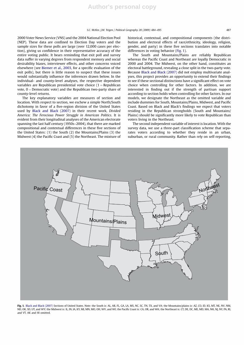
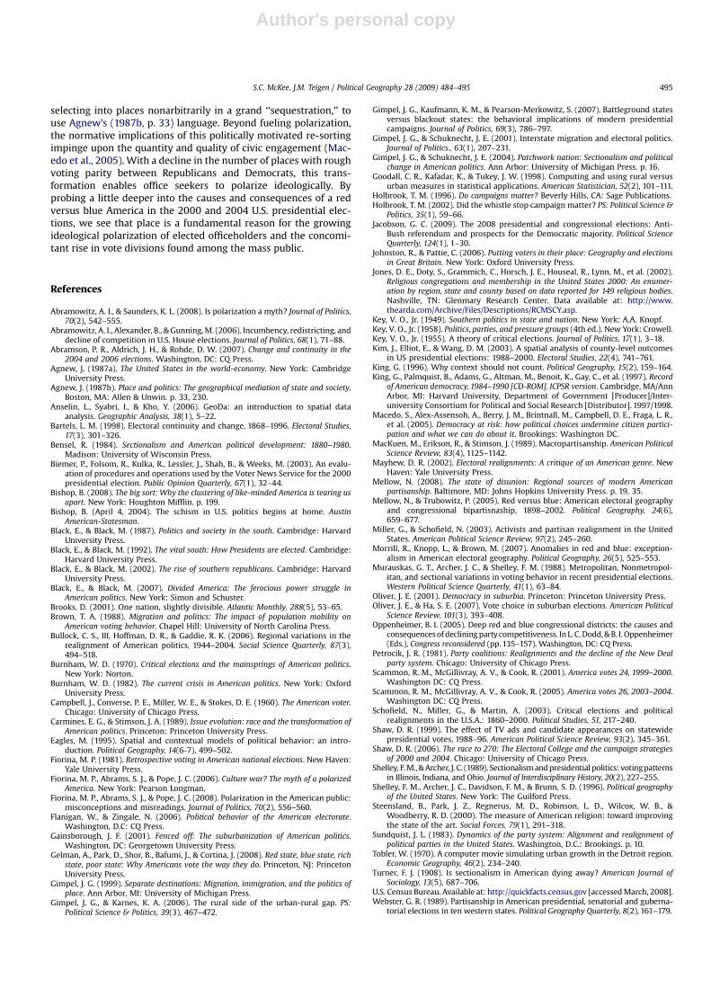
The key explanatory variables are measures of section andlocation. With respect to section, we eschew a simple North/Southdichotomy in favor of a five-region division of the United Statesused by Black and Black (2007) in their recent work, DividedAmerica: The Ferocious Power Struggle in American Politics. It isevident from their longitudinal analyses of the American electoratespanning the last half century (1950s–2004), that there are markedcompositional and contextual differences in these five sections ofthe United States: (1) the South (2) the Mountains/Plains (3) theMidwest (4) the Pacific Coast and (5) the Northeast. The mixture of

historical, contextual, and compositional components (the distri-bution and electoral effects of race/ethnicity, ideology, religion,gender, and party) in these five sections translates into notabledifferences in voting behavior (Fig. 1).

The South and Mountains/Plains are reliably Republicanwhereas the Pacific Coast and Northeast are loyally Democratic in2000 and 2004. The Midwest, on the other hand, constitutes anelectoral battleground, revealing a close split in the two-party vote.Because Black and Black (2007) did not employ multivariate anal-yses, this project provides an opportunity to extend their findingsto see if these sectional distinctions have a significant effect on votechoice when controlling for other factors. In addition, we areinterested in finding out if the strength of partisan supportaccording to section holds when controlling for other factors. In ourmodels, we designate the Northeast as the omitted variable andinclude dummies for South, Mountains/Plains, Midwest, and PacificCoast. Based on Black and Black’s findings we expect that votersresiding in the Republican strongholds (South and Mountains/Plains) should be significantly more likely to vote Republican thanvoters living in the Northeast.

The second independent variable of interest is location. With thesurvey data, we use a three-part classification scheme that sepa-rates voters according to whether they reside in an urban,suburban, or rural community. Rather than rely on self-reporting,

Mountains/Plains

Pacific Coast

Midwest

Northeast

South

Fig. 1. Black and Black (2007) Sections of United States. Note: the South is: AL, AR, FL, GA, LA, MS, NC, SC, TN, TX, and VA; the Mountains/plains is: AZ, CO, ID, KS, MT, NE, NV, NM,ND, OK, SD, UT, and WY; the Midwest is: IL, IN, IA, KY, MI, MN, MO, OH, WV, and WI; the Pacific Coast is: CA, OR, and WA; the Northeast is: CT, DE, DC, ME, MD, MA, NH, NJ, NY, PA, RI,and VT. AK and HI omitted.



the exit pollsters code respondents based on precinct zip codes’affiliation with a Metropolitan Statistical Area (MSA). The variable’sthree values indicate either urban (precinct within an MSA-desig-nated city exceeding 50,000 people), suburban (adjacent to but notwithin a city exceeding 50,000 people), or rural. This designation oflocation generally captures population density and we hypothesizethat the more dense the location the lower the support for theRepublican presidential candidate. Therefore, we expect that aftercontrolling for other factors, compared to urban voters (the omittedcategory in the regressions) rural and suburban voters are morelikely to vote Republican. We have a purer measure of location inthe county-level analyses in the form of population density. It isexpected that greater county-level population density negativelyassociates with the Republican share of the presidential vote.

In the individual-level presidential vote choice models for 2000and 2004, we use the following control variables: (1) Party Identi-fication (1¼Democrat, 2¼ Independent/other, 3¼ Republican) (2)Ideology (1¼ Liberal, 2¼Moderate, 3¼ Conservative) (3) Race(1¼African American, 0¼ otherwise) (4) Gender (1¼Male,0¼ Female) (5) Age (9 categories) (6) Family Income (6 categories)and (7) Religion (1¼ Protestant/other Christian, 0¼ otherwise).Similar to the exit poll analyses conducted by Gimpel and Schu-knecht (2004), we want to see if section and location show statis-tically significant effects on vote choice even after controlling forthe aforementioned compositional variables. To the extent possible,we have selected county-level control variables that are similar tothese individual-level controls.

We use U.S. counties in our aggregate-level analyses becausethey are the smallest geographic unit for which reliable demo-graphic and political data are available. The criteria for decidingwhich geographic unit to use include judging their size, mutability,and the prospects for data availability. Regarding size, the smallerthe geographic unit measured by population, the better. The use ofsmaller population units lessens the ecological inference problemsthat arise when inferring individual-level behavior from aggregatestatistics (Kim, Elliot, and Wang, 2003). Unit boundaries should alsobe stable across time as much as possible to allow researchers tocompare results across elections.

Multivariate analysis requires as much nonmissing data for eachcase on each variable as possible, so data availability is anotherimportant criterion. The unit that balances these three elements isthe county and county-equivalent units for the continental U.S.(county-equivalents include Louisiana’s parishes and some inde-pendent cities, largely in Virginia, that are de facto counties). Thereare political units smaller than counties and county-equivalents forwhich vote totals are measured, such as wards and precincts.Unfortunately, with few exceptions (King et al., 1997), electoral anddemographic data on the entire nation are unavailable for sub-county entities. Additionally, zip codes, legislative and congres-sional districts, wards, and precincts frequently undergo arbitraryand non-arbitrary boundary changes. Hence, county is the smallest,most static aggregate-level unit for which relevant control variabledata can be found in addition to our variables of interest.

Individual-level models and results

For the individual-level results we proceed as follows. First, wepresent descriptive data on the Republican vote based on regionand location within each region. Then we present logistic regres-sions of the Republican vote with region and location as keyexplanatory variables. Each region is also analyzed separately todetermine if location exhibits a significant effect on vote choice.Next, we present the predicted probabilities from the regressionmodels according to region and voter location. Lastly, we considerwhether region exhibits an independent effect on vote choice when

we hold location constant. We proceed in the same manner dis-cussed above – starting with a presentation of descriptive data,multivariate results, and a tabular display of predicted probabilities.

We begin with Table 1, which presents the Republicanpercentage of the two-party vote according to region and locationwithin each region. In addition, we present the Republican vote inthe nation and according to location. Both elections were extremelyclose at the national level, with Democrat Al Gore outpollingRepublican George W. Bush in 2000 by a half percent, and Bushbeating Democrat John Kerry by a slightly larger majority in 2004.The variation in the Republican vote according to location is quiterevealing of its effect on Republican support in the 2000 and 2004contests. In both elections, a majority of urban voters supported theDemocrat. Suburban voters narrowly favored the Republican andrural residents were firmly in the GOP column, with six out of 10preferring Bush in both years.

Looking down the columns in Table 1 and focusing on the voteby region, the pronounced Republican advantage in the South andMountains/Plains is apparent, as is the Democratic strength in thePacific Coast and Northeast. The Midwest is clearly the sectionalbattleground, registering 51% and 50% Republican in the 2000 and2004 elections, respectively. Notice however, the considerablevariation in the Republican vote within each region according tovoter location. With one exception, voters in the Northeast in 2004,it is always the case that regardless of region, rural voters are themost Republican while urban voters support the GOP the least. Inthe South and Mountains/Plains, with the exception of urban votersin 2000, all voters, whether urban, suburban, or rural, casta majority Republican vote. In the Democratic strongholds of thePacific Coast and Northeast, urban and suburban voters preferredthe Democratic candidates in 2000 and 2004. Except for ruralvoters in the Northeast in 2004, in both sections they preferred the

Table 1Republican presidential vote by region and voter location within each region of theUnited States (in percentages).

Region and Location 2000 2004 2000–2004

Nation (100%) 50 52 51Urban 40 47 44Suburban 51 53 52Rural 61 60 61

South (29%) 55 57 56Urban 47 56 52Suburban 59 57 58Rural 66 64 65

Mountains/Plains (10%) 57 61 59Urban 48 51 50Suburban 57 62 60Rural 69 75 72

Midwest (25%) 51 50 51Urban 38 40 39Suburban 53 55 54Rural 62 56 59

Pacific Coast (14%) 45 47 46Urban 34 46 41Suburban 48 46 47Rural 57 58 58

Northeast (22%) 41 44 43Urban 28 34 31Suburban 44 49 47Rural 51 38 47

Total cases 12,241 13,470 25,711

Note: data are from the Voter News Service (VNS) 2000 general election exit polland the National Election Pool (NEP) 2004 general election exit poll. Data show theRepublican percentage of the two-party presidential vote. Data are weighted.



Republican, but GOP support was much stronger among PacificCoast residents (57% in 2000 and 58% in 2004). Finally, in theMidwest, rural and suburban voters supported the Republican, buturban voters were strongly Democratic in 2000 and 2004.

In Table 2 we turn to multivariate analyses of Republican votechoice in order to see whether section and location exhibit signif-icant effects when controlling for other factors. With the sevencontrol variables included in all of the logistic regressions (but notshown in the table) presented in Table 2, we find evidence thatsection and location independently influence vote choice in 2000.With voters residing in the Northeast as the base category, voters inevery other region are more likely to vote Republican in 2000.Further, in terms of significance and the size of the effect, in keepingwith the descriptive findings in Table 1, in descending order themost Republican voters are in the South, the Mountains/Plains, theMidwest, the Pacific Coast, and finally the Northeast. Also, withrespect to location, both suburban and rural voters are moresupportive of the GOP than urban voters (the omitted category).Moreover, as we expected, rural voters are the most Republicanbased on the coefficient and level of statistical significance(p� 0.001). In the national model for 2004, only the South and

Mountains/Plains indicate a statistically significant difference inRepublican vote choice compared to Northeast voters. Againthough, we find that both suburban and rural voters are moresupportive of the GOP than urban voters, with rural voters the mostRepublican.

We now turn our attention to the models that evaluate the effectof location when region is held constant. In the South, only ruralvoters are significantly more Republican in their vote choicecompared to urban voters. Historically, white rural southernerswere the most loyal Democrats (Key, 1949). Likewise, it is the casethat rural voters are more Republican than urban voters are in 2000and 2004 in the Mountains/Plains and Midwest. Rural voters aremore Republican in vote choice than are urban voters in the PacificCoast in 2004 and the Northeast in 2000. Suburban voters are morelikely to vote Republican than urban voters in the Mountains/Plainsin 2000, the Midwest in 2004, and the Northeast in 2004. Overall,out of a total of 10 cases (each region multiplied by two for the 2000and 2004 elections) in eight instances rural voters were signifi-cantly more likely to vote Republican compared to urban voters. Bycomparison, there are only three instances out of 10 in whichsuburban voters were more Republican in their presidential pref-erences when compared to urban voters.

Table 3 presents the predicted probabilities of voting Republicanin the 2000 and 2004 elections, respectively. Holding the controlvariables from each of the region-specific models from Table 2 attheir mean values (and holding the national vote model controlvariables at their means for the national probabilities), the tabledisplays the Republican vote probability according to a voter’slocation (urban, suburban, or rural) and region (South, Mountains/Plains, Midwest, Pacific Coast, and Northeast). Moving down therows it is apparent that the likelihood of voting Republicanincreases according to location, urban to suburban to rural. Also,within each location Republican probabilities are markedly highermoving from right to left (from Northeast to South). In 2000 and2004, for voters who reside in the Republican strongholds of theSouth and Mountains/Plains, the likelihood of voting Republicanexceeds 0.5 in every location. In the Midwest, only suburban andrural voters in 2000 were more likely to vote Republican. In theDemocratic strongholds of the Pacific Coast and Northeast, with theexception of Pacific Coast rural voters in 2004, regardless of locationthese voters are more likely to vote Democratic in the 2000 and2004 presidential elections.

Finally, we can view these findings within each location for thetwo elections. Among urban voters, strong Democratic supportoutside the South and Mountains/Plains makes the national prob-ability of voting Republican below 0.5. Among suburban voters, themarkedly higher GOP support in the South and Mountains/Plains

Table 2Presidential vote choice regressions for region and voter location within each regionof the United States.

2000 2004 2000–2004

NationSouth 0.903 (0.088)*** 0.619 (0.085)*** 0.758 (0.061)***Mountains/plains 0.506 (0.112)*** 0.497 (0.112)*** 0.497 (0.079)***Midwest 0.371 (0.084)*** 0.007 (0.083) 0.184 (0.059)**Pacific coast 0.219 (0.100)* �0.038 (0.097) 0.087 (0.069)Suburban voter 0.168 (0.070)* 0.181 (0.066)** 0.182 (0.048)***Rural voter 0.682 (0.081)*** 0.532 (0.086)*** 0.615 (0.059)***Pseudo R2 0.49 0.51 0.50N 10,743 11,738 22,481

SouthSuburban voter 0.193 (0.132) �0.048 (0.127) 0.063 (0.091)Rural voter 0.918 (0.152)*** 0.689 (0.169)*** 0.810 (0.110)***Pseudo R2 0.51 0.57 0.54N 3017 3518 6535

Mountains/plainsSuburban voter 0.498 (0.248)* 0.130 (0.212) 0.264 (0.155)Rural voter 0.624 (0.203)** 0.916 (0.227)*** 0.776 (0.149)***Pseudo R2 0.49 0.48 0.48N 1180 1274 2454

MidwestSuburban voter 0.191 (0.141) 0.298 (0.130)* 0.234 (0.094)*Rural voter 0.834 (0.164)*** 0.372 (0.161)* 0.638 (0.114)***Pseudo R2 0.47 0.53 0.49N 2870 3097 5967

Pacific coastSuburban voter �0.008 (0.194) 0.198 (0.186) 0.116 (0.133)Rural voter 0.366 (0.298) 0.919 (0.262)*** 0.722 (0.192)***Pseudo R2 0.53 0.52 0.52N 1302 1368 2670

NortheastSuburban voter 0.188 (0.154) 0.295 (0.143)* 0.244 (0.104)*Rural voter 0.460 (0.185)* �0.054 (0.237) 0.269 (0.140)Pseudo R2 0.45 0.45 0.44N 2374 2481 4855

Note: logistic regression coefficients with standard errors in parentheses(***p� 0.001, **p� 0.01, *p� 0.05 two-tailed). Dependent variable is vote forpresident (1¼ Republican, 0¼Democrat). Omitted variables of interest are ‘‘UrbanVoter’’ and ‘‘Northeast’’ (for Nation model only). Control variables included in allmodels, but not shown are: party identification (1¼Democrat, 2¼ Independent/Other, 3¼ Republican), ideology (1¼ Liberal, 2¼Moderate, 3¼ Conservative), race(1¼African American, 0¼ otherwise), gender (1¼male, 0¼ female), age (9 cate-gories), family income (6 categories), and religion (1¼ Protestant/Other Christian,0¼ otherwise).

Table 3Republican presidential vote probabilities for the 2000 and 2004 elections accordingto voter location within each region of the United States.

South Mountains/plains

Midwest Pacificcoast

Northeast Nation

2000 ElectionUrban voters 0.50 0.57 0.45 0.36 0.31 0.44Suburban

voters0.61 0.74 0.54 0.37 0.37 0.52

Rural voters 0.73 0.72 0.67 0.45 0.43 0.62

2004 ElectionUrban voters 0.62 0.64 0.37 0.36 0.32 0.47Suburban

voters0.63 0.72 0.46 0.43 0.39 0.53

Rural voters 0.76 0.82 0.49 0.61 0.36 0.62

Note: probabilities were derived from the models in Table 2 with all the controlvariables set at their mean values.



results in slightly greater likelihood of voting Republican nationally.Indeed, with respect to location, suburbia is a presidential battle-ground in 2000 and 2004. The impressive Republican supportamong rural voters in the South and Mountains/Plains, coupledwith the relatively smaller drop-off in the other regions, makes thenational rural vote probability comfortably Republican (0.620 in2000 and 0.619 in 2004).

Another way to evaluate the effects of sectionalism and locationon vote choice is to consider whether there is regional variability invote choice when location is held constant. Referring back to Table1, in the 2000 election we see that the sectional pattern of presi-dential voting within each location holds – urban voters in theSouth and Mountains/Plains are more Republican than urban votersin the Midwest and the latter are more Republican than urbanvoters in the Pacific Coast and Northeast. This pattern is onlyslightly different in 2004. Even when location is held constant, it isevident that region and voter preferences present noteworthycorrelations.

Table 4 presents multiple logistic regressions to determinewhether region has a significant effect on presidential vote choicewhen location is held constant. Among urban voters, compared toNortheast voters (the baseline category), only those who reside inthe Republican strongholds of the South and Mountains/Plains aremore likely to vote Republican in the 2000 and 2004 elections. Inthe case of suburban voters, change between 2000 and 2004 isevident. In 2000, voters in the Republican strongholds and theMidwest were all more likely to cast Republican ballots ascompared to Northeast voters. But in 2004, we have furtherevidence that the battleground location in American politics issuburbia because only suburban southerners are more likely to voteRepublican compared to their Northeast counterparts. Given theprevious findings (see Table 3), it is not surprising that there areclear differences in the likelihood that rural residents vote

Republican according to region. In 2004, rural voters in everyregion outside the Northeast are more likely to vote Republican.

Table 5 presents the predicted Republican vote probabilitiesfrom Table 4 for each location according to section for 2000 and2004. Among urban voters, only among those in the South andMountains/Plains in 2004 does the Republican vote probabilityexceed 0.5. The vote probabilities for suburban residents providesfurther confirmation of their swing voter status, as the overalllikelihood of voting Republican centers around the 0.5 mark in2000 and 2004. The Republican vote probabilities for rural resi-dents provide a stark contrast to the data shown for urban andsuburban voters, because, with the exception of rural Northeastvoters, rural voters are overwhelmingly partial to voting Republicanin 2000 and 2004. When we hold location constant, it allows us toassess the variability in vote choice according to region. Despitelarge differences in the level of Republican voting depending on thelocation, within a given location it is clear presidential vote pref-erences differ meaningfully across region as GOP support declinesgoing from the South and Mountains/Plains to the Midwest to thePacific Coast and Northeast.

County-level spatial models and results

The individual-level analyses above provide empirical evidencein support of our conclusion that location matters in our under-standing of electoral outcomes and the context of populationdensity influences vote choice both nationally and within regions.In terms of both section and location, the individual-level datademonstrate geographic patterns beyond what is predicted bysolely compositional factors, like socioeconomic status, race, andethnicity. To bolster these findings, we also use aggregate-levelelectoral results. Rather than use exit poll respondents, we can usegeographic areas as the unit of analysis (Eagles, 1995) and runanalogous models to corroborate our findings with regard tosectionalism and location. Counties embody a balance betweenpopulation size, static boundaries, and data availability, so we drawparallels between our individual-level models in order to approx-imate closely the same logic when extrapolating to county-levelmultivariate analysis.

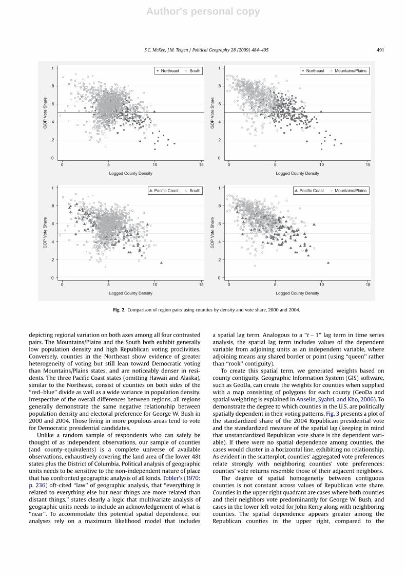
Fig. 2 depicts the bivariate relationship between populationdensity and Republican two-party vote share in the 2000 and 2004presidential elections among counties within contrasted pairs ofthe Black and Black (2007)-defined regions (the y-axes measure themean of 2000 and 2004). The horizontal line bisecting the plotrepresents the 0.5 line; cases above expressed more support forGeorge W. Bush than Al Gore/John Kerry. Clustering is evident,

Table 4Presidential vote choice regressions by voter location and according to region of theUnited States.

2000 2004 2000–2004

Urban voters by regionSouth 0.779 (0.160)*** 0.654 (0.153)*** 0.714 (0.111)***Mountains/plains 0.397 (0.183)* 0.423 (0.201)* 0.378 (0.135)**Midwest 0.300 (0.173) �0.038 (0.162) 0.123 (0.118)Pacific coast 0.127 (0.197) �0.143 (0.171) �0.012 (0.128)Pseudo R2 0.53 0.56 0.54N 3832 4681 8513

Suburban voters by regionSouth 0.777 (0.136)*** 0.364 (0.121)** 0.552 (0.089)***Mountains/plains 0.637 (0.232)** 0.274 (0.171) 0.418 (0.138)**Midwest 0.290 (0.119)* 0.019 (0.110) 0.132 (0.080)Pacific coast 0.118 (0.146) �0.184 (0.137) �0.049 (0.099)Pseudo R2 0.47 0.50 0.48N 4218 5300 9518

Rural voters by regionSouth 1.348 (0.177)*** 1.553 (0.257)*** 1.375 (0.144)***Mountains/Plains 0.648 (0.198)** 1.426 (0.271)*** 0.995 (0.156)***Midwest 0.706 (0.170)*** 0.476 (0.239)* 0.554 (0.135)***Pacific Coast 0.174 (0.247) 1.116 (0.288)*** 0.576 (0.179)**Pseudo R2 0.44 0.47 0.45N 2530 1749 4279

Note: logistic regression coefficients with standard errors in parentheses(***p� 0.001, **p� 0.01, *p� 0.05, two-tailed). Dependent variable is vote forpresident (1¼ Republican, 0¼Democrat). Omitted variable of interest is ‘‘North-east.’’ Control variables included in all models, but not shown are: party identifi-cation (1¼Democrat, 2¼ Independent/Other, 3¼ Republican), ideology(1¼ Liberal, 2¼Moderate, 3¼ Conservative), race (1¼African American,0¼ otherwise), gender (1¼male, 0¼ female), age (9 categories), family income (6categories), and religion (1¼ Protestant/Other Christian, 0¼ otherwise).

Table 5Republican presidential vote probabilities for the 2000 and 2004 elections accordingto region and voter location.

Urban voters Suburban voters Rural voters

2000 ElectionSouth 0.44 0.66 0.86Mountains/plains 0.40 0.66 0.80Midwest 0.38 0.56 0.80Pacific coast 0.35 0.54 0.73Northeast 0.24 0.44 0.53

2004 ElectionSouth 0.53 0.59 0.86Mountains/plains 0.52 0.58 0.86Midwest 0.42 0.52 0.73Pacific coast 0.40 0.48 0.85Northeast 0.36 0.50 0.43

Note: probabilities were derived from the models in Table 4 with all the controlvariables set at their mean values.



depicting regional variation on both axes among all four contrastedpairs. The Mountains/Plains and the South both exhibit generallylow population density and high Republican voting proclivities.Conversely, counties in the Northeast show evidence of greaterheterogeneity of voting but still lean toward Democratic votingthan Mountains/Plains states, and are noticeably denser in resi-dents. The three Pacific Coast states (omitting Hawaii and Alaska),similar to the Northeast, consist of counties on both sides of the‘‘red–blue’’ divide as well as a wide variance in population density.Irrespective of the overall differences between regions, all regionsgenerally demonstrate the same negative relationship betweenpopulation density and electoral preference for George W. Bush in2000 and 2004. Those living in more populous areas tend to votefor Democratic presidential candidates.

Unlike a random sample of respondents who can safely bethought of as independent observations, our sample of counties(and county-equivalents) is a complete universe of availableobservations, exhaustively covering the land area of the lower 48tstates plus the District of Columbia. Political analysis of geographicunits needs to be sensitive to the non-independent nature of placethat has confronted geographic analysis of all kinds. Tobler’s (1970:p. 236) oft-cited ‘‘law’’ of geographic analysis, that ‘‘everything isrelated to everything else but near things are more related thandistant things,’’ states clearly a logic that multivariate analysis ofgeographic units needs to include an acknowledgement of what is‘‘near’’. To accommodate this potential spatial dependence, ouranalyses rely on a maximum likelihood model that includes

a spatial lag term. Analogous to a ‘‘t� 1’’ lag term in time seriesanalysis, the spatial lag term includes values of the dependentvariable from adjoining units as an independent variable, whereadjoining means any shared border or point (using ‘‘queen’’ ratherthan ‘‘rook’’ contiguity).

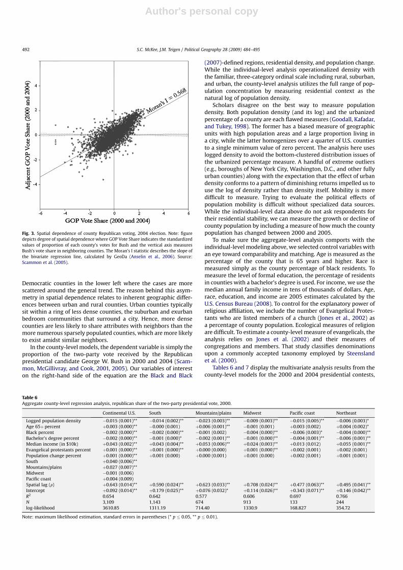
To create this spatial term, we generated weights based oncounty contiguity. Geographic Information System (GIS) software,such as GeoDa, can create the weights for counties when suppliedwith a map consisting of polygons for each county (GeoDa andspatial weighting is explained in Anselin, Syabri, and Kho, 2006). Todemonstrate the degree to which counties in the U.S. are politicallyspatially dependent in their voting patterns, Fig. 3 presents a plot ofthe standardized share of the 2004 Republican presidential voteand the standardized measure of the spatial lag (keeping in mindthat unstandardized Republican vote share is the dependent vari-able). If there were no spatial dependence among counties, thecases would cluster in a horizontal line, exhibiting no relationship.As evident in the scatterplot, counties’ aggregated vote preferencesrelate strongly with neighboring counties’ vote preferences:counties’ vote returns resemble those of their adjacent neighbors.

The degree of spatial homogeneity between contiguouscounties is not constant across values of Republican vote share.Counties in the upper right quadrant are cases where both countiesand their neighbors vote predominantly for George W. Bush, andcases in the lower left voted for John Kerry along with neighboringcounties. The spatial dependence appears greater among theRepublican counties in the upper right, compared to the

Fig. 2. Comparison of region pairs using counties by density and vote share, 2000 and 2004.



Democratic counties in the lower left where the cases are morescattered around the general trend. The reason behind this asym-metry in spatial dependence relates to inherent geographic differ-ences between urban and rural counties. Urban counties typicallysit within a ring of less dense counties, the suburban and exurbanbedroom communities that surround a city. Hence, more densecounties are less likely to share attributes with neighbors than themore numerous sparsely populated counties, which are more likelyto exist amidst similar neighbors.

In the county-level models, the dependent variable is simply theproportion of the two-party vote received by the Republicanpresidential candidate George W. Bush in 2000 and 2004 (Scam-mon, McGillivray, and Cook, 2001, 2005). Our variables of intereston the right-hand side of the equation are the Black and Black

(2007)-defined regions, residential density, and population change.While the individual-level analysis operationalized density withthe familiar, three-category ordinal scale including rural, suburban,and urban, the county-level analysis utilizes the full range of pop-ulation concentration by measuring residential context as thenatural log of population density.

Scholars disagree on the best way to measure populationdensity. Both population density (and its log) and the urbanizedpercentage of a county are each flawed measures (Goodall, Kafadar,and Tukey, 1998). The former has a biased measure of geographicunits with high population areas and a large proportion living ina city, while the latter homogenizes over a quarter of U.S. countiesto a single minimum value of zero percent. The analysis here useslogged density to avoid the bottom-clustered distribution issues ofthe urbanized percentage measure. A handful of extreme outliers(e.g., boroughs of New York City, Washington, D.C., and other fullyurban counties) along with the expectation that the effect of urbandensity conforms to a pattern of diminishing returns impelled us touse the log of density rather than density itself. Mobility is moredifficult to measure. Trying to evaluate the political effects ofpopulation mobility is difficult without specialized data sources.While the individual-level data above do not ask respondents fortheir residential stability, we can measure the growth or decline ofcounty population by including a measure of how much the countypopulation has changed between 2000 and 2005.

To make sure the aggregate-level analysis comports with theindividual-level modeling above, we selected control variables withan eye toward comparability and matching. Age is measured as thepercentage of the county that is 65 years and higher. Race ismeasured simply as the county percentage of black residents. Tomeasure the level of formal education, the percentage of residentsin counties with a bachelor’s degree is used. For income, we use themedian annual family income in tens of thousands of dollars. Age,race, education, and income are 2005 estimates calculated by theU.S. Census Bureau (2008). To control for the explanatory power ofreligious affiliation, we include the number of Evangelical Protes-tants who are listed members of a church (Jones et al., 2002) asa percentage of county population. Ecological measures of religionare difficult. To estimate a county-level measure of evangelicals, theanalysis relies on Jones et al. (2002) and their measures ofcongregations and members. That study classifies denominationsupon a commonly accepted taxonomy employed by Steenslandet al. (2000).

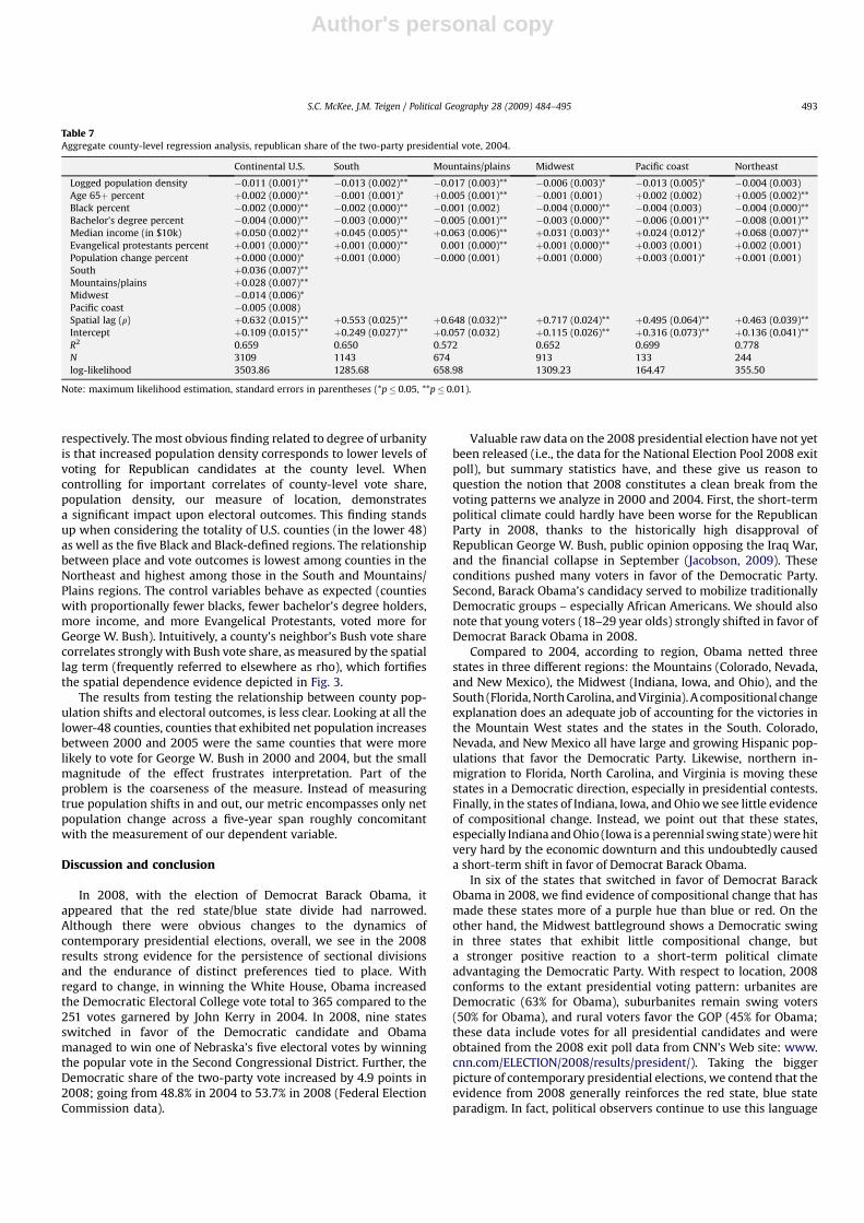
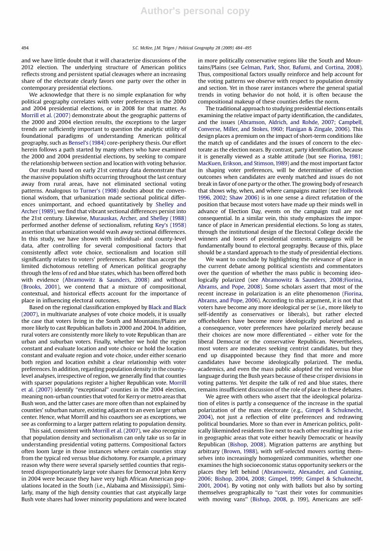
Tables 6 and 7 display the multivariate analysis results from thecounty-level models for the 2000 and 2004 presidential contests,

Fig. 3. Spatial dependence of county Republican voting, 2004 election. Note: figuredepicts degree of spatial dependence where GOP Vote Share indicates the standardizedvalues of proportion of each county’s votes for Bush and the vertical axis measuresBush’s vote share in neighboring counties. The Moran’s I statistic describes the slope ofthe bivariate regression line, calculated by GeoDa (Anselin et al., 2006). Source:Scammon et al. (2005).

Table 6Aggregate county-level regression analysis, republican share of the two-party presidential vote, 2000.

Continental U.S. South Mountains/plains Midwest Pacific coast Northeast

Logged population density �0.015 (0.001)** �0.014 (0.002)** �0.023 (0.003)** �0.009 (0.003)** �0.015 (0.005)** �0.006 (0.003)*Age 65þ percent þ0.003 (0.000)** �0.000 (0.001) þ0.006 (0.001)** �0.001 (0.001) þ0.003 (0.002) þ0.004 (0.002)*Black percent �0.002 (0.000)** �0.002 (0.000)** �0.001 (0.002) �0.004 (0.000)** �0.006 (0.003)* �0.004 (0.000)**Bachelor’s degree percent �0.002 (0.000)** �0.001 (0.000)* �0.002 (0.001)** �0.001 (0.000)** �0.004 (0.001)** �0.006 (0.001)**Median income (in $10k) þ0.043 (0.002)** þ0.043 (0.004)** þ0.053 (0.006)** þ0.024 (0.003)** þ0.013 (0.012) þ0.055 (0.001)**Evangelical protestants percent þ0.001 (0.000)** þ0.001 (0.000)** þ0.000 (0.000) þ0.001 (0.000)** þ0.002 (0.001) þ0.002 (0.001)Population change percent þ0.001 (0.000)** þ0.001 (0.000) þ0.000 (0.001) þ0.001 (0.000) þ0.002 (0.001) þ0.001 (0.001)South þ0.040 (0.006)**Mountains/plains þ0.027 (0.007)**Midwest �0.001 (0.006)Pacific coast þ0.004 (0.009)Spatial lag (r) þ0.643 (0.014)** þ0.590 (0.024)** þ0.623 (0.033)** þ0.708 (0.024)** þ0.477 (0.063)** þ0.495 (0.041)**Intercept þ0.092 (0.014)** þ0.179 (0.025)** þ0.076 (0.032)* þ0.114 (0.026)** þ0.343 (0.071)** þ0.146 (0.042)**R2 0.654 0.642 0.577 0.606 0.697 0.766N 3,109 1,143 674 913 133 244log-likelihood 3610.85 1311.19 714.40 1330.9 168.827 354.72

Note: maximum likelihood estimation, standard errors in parentheses (* p � 0.05, ** p � 0.01).



respectively. The most obvious finding related to degree of urbanityis that increased population density corresponds to lower levels ofvoting for Republican candidates at the county level. Whencontrolling for important correlates of county-level vote share,population density, our measure of location, demonstratesa significant impact upon electoral outcomes. This finding standsup when considering the totality of U.S. counties (in the lower 48)as well as the five Black and Black-defined regions. The relationshipbetween place and vote outcomes is lowest among counties in theNortheast and highest among those in the South and Mountains/Plains regions. The control variables behave as expected (countieswith proportionally fewer blacks, fewer bachelor’s degree holders,more income, and more Evangelical Protestants, voted more forGeorge W. Bush). Intuitively, a county’s neighbor’s Bush vote sharecorrelates strongly with Bush vote share, as measured by the spatiallag term (frequently referred to elsewhere as rho), which fortifiesthe spatial dependence evidence depicted in Fig. 3.

The results from testing the relationship between county pop-ulation shifts and electoral outcomes, is less clear. Looking at all thelower-48 counties, counties that exhibited net population increasesbetween 2000 and 2005 were the same counties that were morelikely to vote for George W. Bush in 2000 and 2004, but the smallmagnitude of the effect frustrates interpretation. Part of theproblem is the coarseness of the measure. Instead of measuringtrue population shifts in and out, our metric encompasses only netpopulation change across a five-year span roughly concomitantwith the measurement of our dependent variable.

Discussion and conclusion

In 2008, with the election of Democrat Barack Obama, itappeared that the red state/blue state divide had narrowed.Although there were obvious changes to the dynamics ofcontemporary presidential elections, overall, we see in the 2008results strong evidence for the persistence of sectional divisionsand the endurance of distinct preferences tied to place. Withregard to change, in winning the White House, Obama increasedthe Democratic Electoral College vote total to 365 compared to the251 votes garnered by John Kerry in 2004. In 2008, nine statesswitched in favor of the Democratic candidate and Obamamanaged to win one of Nebraska’s five electoral votes by winningthe popular vote in the Second Congressional District. Further, theDemocratic share of the two-party vote increased by 4.9 points in2008; going from 48.8% in 2004 to 53.7% in 2008 (Federal ElectionCommission data).

Valuable raw data on the 2008 presidential election have not yetbeen released (i.e., the data for the National Election Pool 2008 exitpoll), but summary statistics have, and these give us reason toquestion the notion that 2008 constitutes a clean break from thevoting patterns we analyze in 2000 and 2004. First, the short-termpolitical climate could hardly have been worse for the RepublicanParty in 2008, thanks to the historically high disapproval ofRepublican George W. Bush, public opinion opposing the Iraq War,and the financial collapse in September (Jacobson, 2009). Theseconditions pushed many voters in favor of the Democratic Party.Second, Barack Obama’s candidacy served to mobilize traditionallyDemocratic groups – especially African Americans. We should alsonote that young voters (18–29 year olds) strongly shifted in favor ofDemocrat Barack Obama in 2008.

Compared to 2004, according to region, Obama netted threestates in three different regions: the Mountains (Colorado, Nevada,and New Mexico), the Midwest (Indiana, Iowa, and Ohio), and theSouth (Florida, North Carolina, and Virginia). A compositional changeexplanation does an adequate job of accounting for the victories inthe Mountain West states and the states in the South. Colorado,Nevada, and New Mexico all have large and growing Hispanic pop-ulations that favor the Democratic Party. Likewise, northern in-migration to Florida, North Carolina, and Virginia is moving thesestates in a Democratic direction, especially in presidential contests.Finally, in the states of Indiana, Iowa, and Ohio we see little evidenceof compositional change. Instead, we point out that these states,especially Indiana and Ohio (Iowa is a perennial swing state) were hitvery hard by the economic downturn and this undoubtedly causeda short-term shift in favor of Democrat Barack Obama.

In six of the states that switched in favor of Democrat BarackObama in 2008, we find evidence of compositional change that hasmade these states more of a purple hue than blue or red. On theother hand, the Midwest battleground shows a Democratic swingin three states that exhibit little compositional change, buta stronger positive reaction to a short-term political climateadvantaging the Democratic Party. With respect to location, 2008conforms to the extant presidential voting pattern: urbanites areDemocratic (63% for Obama), suburbanites remain swing voters(50% for Obama), and rural voters favor the GOP (45% for Obama;these data include votes for all presidential candidates and wereobtained from the 2008 exit poll data from CNN’s Web site: www.cnn.com/ELECTION/2008/results/president/). Taking the biggerpicture of contemporary presidential elections, we contend that theevidence from 2008 generally reinforces the red state, blue stateparadigm. In fact, political observers continue to use this language

Table 7Aggregate county-level regression analysis, republican share of the two-party presidential vote, 2004.

Continental U.S. South Mountains/plains Midwest Pacific coast Northeast

Logged population density �0.011 (0.001)** �0.013 (0.002)** �0.017 (0.003)** �0.006 (0.003)* �0.013 (0.005)* �0.004 (0.003)Age 65þ percent þ0.002 (0.000)** �0.001 (0.001)* þ0.005 (0.001)** �0.001 (0.001) þ0.002 (0.002) þ0.005 (0.002)**Black percent �0.002 (0.000)** �0.002 (0.000)** �0.001 (0.002) �0.004 (0.000)** �0.004 (0.003) �0.004 (0.000)**Bachelor’s degree percent �0.004 (0.000)** �0.003 (0.000)** �0.005 (0.001)** �0.003 (0.000)** �0.006 (0.001)** �0.008 (0.001)**Median income (in $10k) þ0.050 (0.002)** þ0.045 (0.005)** þ0.063 (0.006)** þ0.031 (0.003)** þ0.024 (0.012)* þ0.068 (0.007)**Evangelical protestants percent þ0.001 (0.000)** þ0.001 (0.000)** 0.001 (0.000)** þ0.001 (0.000)** þ0.003 (0.001) þ0.002 (0.001)Population change percent þ0.000 (0.000)* þ0.001 (0.000) �0.000 (0.001) þ0.001 (0.000) þ0.003 (0.001)* þ0.001 (0.001)South þ0.036 (0.007)**Mountains/plains þ0.028 (0.007)**Midwest �0.014 (0.006)*Pacific coast �0.005 (0.008)Spatial lag (r) þ0.632 (0.015)** þ0.553 (0.025)** þ0.648 (0.032)** þ0.717 (0.024)** þ0.495 (0.064)** þ0.463 (0.039)**Intercept þ0.109 (0.015)** þ0.249 (0.027)** þ0.057 (0.032) þ0.115 (0.026)** þ0.316 (0.073)** þ0.136 (0.041)**R2 0.659 0.650 0.572 0.652 0.699 0.778N 3109 1143 674 913 133 244log-likelihood 3503.86 1285.68 658.98 1309.23 164.47 355.50

Note: maximum likelihood estimation, standard errors in parentheses (*p� 0.05, **p� 0.01).



and we have little doubt that it will characterize discussions of the2012 election. The underlying structure of American politicsreflects strong and persistent spatial cleavages where an increasingshare of the electorate clearly favors one party over the other incontemporary presidential elections.

We acknowledge that there is no simple explanation for whypolitical geography correlates with voter preferences in the 2000and 2004 presidential elections, or in 2008 for that matter. AsMorrill et al. (2007) demonstrate about the geographic patterns ofthe 2000 and 2004 election results, the exceptions to the largertrends are sufficiently important to question the analytic utility offoundational paradigms of understanding American politicalgeography, such as Bensel’s (1984) core-periphery thesis. Our effortherein follows a path started by many others who have examinedthe 2000 and 2004 presidential elections, by seeking to comparethe relationship between section and location with voting behavior.

Our results based on early 21st century data demonstrate thatthe massive population shifts occurring throughout the last centuryaway from rural areas, have not eliminated sectional votingpatterns. Analogous to Turner’s (1908) doubts about the conven-tional wisdom, that urbanization made sectional political differ-ences unimportant, and echoed quantitatively by Shelley andArcher (1989), we find that vibrant sectional differences persist intothe 21st century. Likewise, Murauskas, Archer, and Shelley (1988)performed another defense of sectionalism, refuting Key’s (1958)assertion that urbanization would wash away sectional differences.In this study, we have shown with individual- and county-leveldata, after controlling for several compositional factors thatconsistently affect vote choice, sectionalism and location stillsignificantly relates to voters’ preferences. Rather than accept thelimited dichotomous retelling of American political geographythrough the lens of red and blue states, which has been offered bothwith evidence (Abramowitz & Saunders, 2008) and without(Brooks, 2001), we contend that a mixture of compositional,contextual, and historical effects account for the importance ofplace in influencing electoral outcomes.

Based on the regional classification employed by Black and Black(2007), in multivariate analyses of vote choice models, it is usuallythe case that voters living in the South and Mountains/Plains aremore likely to cast Republican ballots in 2000 and 2004. In addition,rural voters are consistently more likely to vote Republican than areurban and suburban voters. Finally, whether we hold the regionconstant and evaluate location and vote choice or hold the locationconstant and evaluate region and vote choice, under either scenarioboth region and location exhibit a clear relationship with voterpreferences. In addition, regarding population density in the county-level analyses, irrespective of region, we generally find that countieswith sparser populations register a higher Republican vote. Morrillet al. (2007) identify ‘‘exceptional’’ counties in the 2004 election,meaning non-urban counties that voted for Kerry or metro areas thatBush won, and the latter cases are more often than not explained bycounties’ suburban nature, existing adjacent to an even larger urbancenter. Hence, what Morrill and his coauthors see as exceptions, wesee as conforming to a larger pattern relating to population density.

This said, consistent with Morrill et al. (2007), we also recognizethat population density and sectionalism can only take us so far inunderstanding presidential voting patterns. Compositional factorsoften loom large in those instances where certain counties strayfrom the typical red versus blue dichotomy. For example, a primaryreason why there were several sparsely settled counties that regis-tered disproportionately large vote shares for Democrat John Kerryin 2004 were because they have very high African American pop-ulations located in the South (i.e., Alabama and Mississippi). Simi-larly, many of the high density counties that cast atypically largeBush vote shares had lower minority populations and were located

in more politically conservative regions like the South and Moun-tains/Plains (see Gelman, Park, Shor, Bafumi, and Cortina, 2008).Thus, compositional factors usually reinforce and help account forthe voting patterns we observe with respect to population densityand section. Yet in those rarer instances where the general spatialtrends in voting behavior do not hold, it is often because thecompositional makeup of these counties defies the norm.

The traditional approach to studying presidential elections entailsexamining the relative impact of party identification, the candidates,and the issues (Abramson, Aldrich, and Rohde, 2007; Campbell,Converse, Miller, and Stokes, 1960; Flanigan & Zingale, 2006). Thisdesign places a premium on the impact of short-term conditions likethe match up of candidates and the issues of concern to the elec-torate as the election nears. By contrast, party identification, becauseit is generally viewed as a stable attitude (but see Fiorina, 1981;MacKuen, Erikson, and Stimson,1989) and the most important factorin shaping voter preferences, will be determinative of electionoutcomes when candidates are evenly matched and issues do notbreak in favor of one party or the other. The growing body of researchthat shows why, when, and where campaigns matter (see Holbrook1996, 2002; Shaw 2006) is in one sense a direct refutation of theposition that because most voters have made up their minds well inadvance of Election Day, events on the campaign trail are notconsequential. In a similar vein, this study emphasizes the impor-tance of place in American presidential elections. So long as states,through the institutional design of the Electoral College decide thewinners and losers of presidential contests, campaigns will befundamentally bound to electoral geography. Because of this, placeshould be a standard approach to the study of presidential elections.

We want to conclude by highlighting the relevance of place inthe current debate among political scientists and commentatorsover the question of whether the mass public is becoming ideo-logically polarized (see Abramowitz & Saunders, 2008;Fiorina,Abrams, and Pope, 2008). Some scholars assert that most of therecent increase in polarization is an elite phenomenon (Fiorina,Abrams, and Pope, 2006). According to this argument, it is not thatvoters have become any more ideological per se (i.e., more likely toself-identify as conservatives or liberals), but rather electedofficeholders have become more ideologically polarized and asa consequence, voter preferences have polarized merely becausetheir choices are now more differentiated – either vote for theliberal Democrat or the conservative Republican. Nevertheless,most voters are moderates seeking centrist candidates, but theyend up disappointed because they find that more and morecandidates have become ideologically polarized. The media,academics, and even the mass public adopted the red versus bluelanguage during the Bush years because of these crisper divisions invoting patterns. Yet despite the talk of red and blue states, thereremains insufficient discussion of the role of place in these debates.

We agree with others who assert that the ideological polariza-tion of elites is partly a consequence of the increase in the spatialpolarization of the mass electorate (e.g., Gimpel & Schuknecht,2004), not just a reflection of elite preferences and redrawingpolitical boundaries. More so than ever in American politics, polit-ically likeminded residents live next to each other resulting in a risein geographic areas that vote either heavily Democratic or heavilyRepublican (Bishop, 2008). Migration patterns are anything butarbitrary (Brown, 1988), with self-selected movers sorting them-selves into increasingly homogenized communities, whether oneexamines the high socioeconomic status opportunity seekers or theplaces they left behind (Abramowitz, Alexander, and Gunning,2006; Bishop, 2004, 2008; Gimpel, 1999; Gimpel & Schuknecht,2001, 2004). By voting not only with ballots but also by sortingthemselves geographically to ‘‘cast their votes for communitieswith moving vans’’ (Bishop, 2008, p. 199), Americans are self-



selecting into places nonarbitrarily in a grand ‘‘sequestration,’’ touse Agnew’s (1987b, p. 33) language. Beyond fueling polarization,the normative implications of this politically motivated re-sortingimpinge upon the quantity and quality of civic engagement (Mac-edo et al., 2005). With a decline in the number of places with roughvoting parity between Republicans and Democrats, this trans-formation enables office seekers to polarize ideologically. Byprobing a little deeper into the causes and consequences of a redversus blue America in the 2000 and 2004 U.S. presidential elec-tions, we see that place is a fundamental reason for the growingideological polarization of elected officeholders and the concomi-tant rise in vote divisions found among the mass public.

References

Abramowitz, A. I., & Saunders, K. L. (2008). Is polarization a myth? Journal of Politics,70(2), 542–555.

Abramowitz, A. I., Alexander, B., & Gunning, M. (2006). Incumbency, redistricting, anddecline of competition in U.S. House elections. Journal of Politics, 68(1), 71–88.

Abramson, P. R., Aldrich, J. H., & Rohde, D. W. (2007). Change and continuity in the2004 and 2006 elections. Washington, DC: CQ Press.

Agnew, J. (1987a). The United States in the world-economy. New York: CambridgeUniversity Press.

Agnew, J. (1987b). Place and politics: The geographical mediation of state and society.Boston, MA: Allen & Unwin. p. 33, 230.

Anselin, L., Syabri, I., & Kho, Y. (2006). GeoDa: an introduction to spatial dataanalysis. Geographic Analysis, 38(1), 5–22.

Bartels, L. M. (1998). Electoral continuity and change, 1868–1996. Electoral Studies,17(3), 301–326.

Bensel, R. (1984). Sectionalism and American political development: 1880–1980.Madison: University of Wisconsin Press.

Biemer, P., Folsom, R., Kulka, R., Lessler, J., Shah, B., & Weeks, M. (2003). An evalu-ation of procedures and operations used by the Voter News Service for the 2000presidential election. Public Opinion Quarterly, 67(1), 32–44.

Bishop, B. (2008). The big sort: Why the clustering of like-minded America is tearing usapart. New York: Houghton Mifflin. p. 199.

Bishop, B. (April 4, 2004). The schism in U.S. politics begins at home. AustinAmerican-Statesman.

Black, E., & Black, M. (1987). Politics and society in the south. Cambridge: HarvardUniversity Press.

Black, E., & Black, M. (1992). The vital south: How Presidents are elected. Cambridge:Harvard University Press.

Black, E., & Black, M. (2002). The rise of southern republicans. Cambridge: HarvardUniversity Press.

Black, E., & Black, M. (2007). Divided America: The ferocious power struggle inAmerican politics. New York: Simon and Schuster.

Brooks, D. (2001). One nation, slightly divisible. Atlantic Monthly, 288(5), 53–65.Brown, T. A. (1988). Migration and politics: The impact of population mobility on

American voting behavior. Chapel Hill: University of North Carolina Press.Bullock, C. S., III, Hoffman, D. R., & Gaddie, R. K. (2006). Regional variations in the

realignment of American politics, 1944–2004. Social Science Quarterly, 87(3),494–518.

Burnham, W. D. (1970). Critical elections and the mainsprings of American politics.New York: Norton.

Burnham, W. D. (1982). The current crisis in American politics. New York: OxfordUniversity Press.

Campbell, J., Converse, P. E., Miller, W. E., & Stokes, D. E. (1960). The American voter.Chicago: University of Chicago Press.

Carmines, E. G., & Stimson, J. A. (1989). Issue evolution: race and the transformation ofAmerican politics. Princeton: Princeton University Press.

Eagles, M. (1995). Spatial and contextual models of political behavior: an intro-duction. Political Geography, 14(6-7), 499–502.

Fiorina, M. P. (1981). Retrospective voting in American national elections. New Haven:Yale University Press.

Fiorina, M. P., Abrams, S. J., & Pope, J. C. (2006). Culture war? The myth of a polarizedAmerica. New York: Pearson Longman.

Fiorina, M. P., Abrams, S. J., & Pope, J. C. (2008). Polarization in the American public:misconceptions and misreadings. Journal of Politics, 70(2), 556–560.

Flanigan, W., & Zingale, N. (2006). Political behavior of the American electorate.Washington, D.C: CQ Press.

Gainsborough, J. F. (2001). Fenced off: The suburbanization of American politics.Washington, DC: Georgetown University Press.

Gelman, A., Park, D., Shor, B., Bafumi, J., & Cortina, J. (2008). Red state, blue state, richstate, poor state: Why Americans vote the way they do. Princeton, NJ: PrincetonUniversity Press.

Gimpel, J. G. (1999). Separate destinations: Migration, immigration, and the politics ofplace. Ann Arbor, MI: University of Michigan Press.

Gimpel, J. G., & Karnes, K. A. (2006). The rural side of the urban-rural gap. PS:Political Science & Politics, 39(3), 467–472.

Gimpel, J. G., Kaufmann, K. M., & Pearson-Merkowitz, S. (2007). Battleground statesversus blackout states: the behavioral implications of modern presidentialcampaigns. Journal of Politics, 69(3), 786–797.

Gimpel, J. G., & Schuknecht, J. E. (2001). Interstate migration and electoral politics.Journal of Politics., 63(1), 207–231.

Gimpel, J. G., & Schuknecht, J. E. (2004). Patchwork nation: Sectionalism and politicalchange in American politics. Ann Arbor: University of Michigan Press. p. 16.

Goodall, C. R., Kafadar, K., & Tukey, J. W. (1998). Computing and using rural versusurban measures in statistical applications. American Statistician, 52(2), 101–111.

Holbrook, T. M. (1996). Do campaigns matter? Beverly Hills, CA: Sage Publications.Holbrook, T. M. (2002). Did the whistle stop campaign matter? PS: Political Science &

Politics, 35(1), 59–66.Jacobson, G. C. (2009). The 2008 presidential and congressional elections: Anti-

Bush referendum and prospects for the Democratic majority. Political ScienceQuarterly, 124(1), 1–30.

Johnston, R., & Pattie, C. (2006). Putting voters in their place: Geography and electionsin Great Britain. New York: Oxford University Press.

Jones, D. E., Doty, S., Grammich, C., Horsch, J. E., Houseal, R., Lynn, M., et al. (2002).Religious congregations and membership in the United States 2000: An enumer-ation by region, state and county based on data reported for 149 religious bodies.Nashville, TN: Glenmary Research Center. Data available at: http://www.thearda.com/Archive/Files/Descriptions/RCMSCY.asp.

Key, V. O., Jr. (1949). Southern politics in state and nation. New York: A.A. Knopf.Key, V. O., Jr. (1958). Politics, parties, and pressure groups (4th ed.). New York: Crowell.Key, V. O., Jr. (1955). A theory of critical elections. Journal of Politics, 17(1), 3–18.Kim, J., Elliot, E., & Wang, D. M. (2003). A spatial analysis of county-level outcomes

in US presidential elections: 1988–2000. Electoral Studies, 22(4), 741–761.King, G. (1996). Why context should not count. Political Geography, 15(2), 159–164.King, G., Palmquist, B., Adams, G., Altman, M., Benoit, K., Gay, C., et al. (1997). Record

of American democracy, 1984–1990 [CD-ROM]. ICPSR version. Cambridge, MA/AnnArbor, MI: Harvard University, Department of Government [Producer]/Inter-university Consortium for Political and Social Research [Distributor]. 1997/1998.

Macedo, S., Alex-Assensoh, A., Berry, J. M., Brintnall, M., Campbell, D. E., Fraga, L. R.,et al. (2005). Democracy at risk: how political choices undermine citizen partici-pation and what we can do about it. Brookings: Washington DC.

MacKuen, M., Erikson, R., & Stimson, J. (1989). Macropartisanship. American PoliticalScience Review, 83(4), 1125–1142.

Mayhew, D. R. (2002). Electoral realignments: A critique of an American genre. NewHaven: Yale University Press.

Mellow, N. (2008). The state of disunion: Regional sources of modern Americanpartisanship. Baltimore, MD: Johns Hopkins University Press. p. 19, 35.

Mellow, N., & Trubowitz, P. (2005). Red versus blue: American electoral geographyand congressional bipartisnaship, 1898–2002. Political Geography, 24(6),659–677.

Miller, G., & Schofield, N. (2003). Activists and partisan realignment in the UnitedStates. American Political Science Review, 97(2), 245–260.

Morrill, R., Knopp, L., & Brown, M. (2007). Anomalies in red and blue: exception-alism in American electoral geography. Political Geography, 26(5), 525–553.

Murauskas, G. T., Archer, J. C., & Shelley, F. M. (1988). Metropolitan, Nonmetropol-itan, and sectional variations in voting behavior in recent presidential elections.Western Political Science Quarterly, 41(1), 63–84.

Oliver, J. E. (2001). Democracy in suburbia. Princeton: Princeton University Press.Oliver, J. E., & Ha, S. E. (2007). Vote choice in suburban elections. American Political

Science Review, 101(3), 393–408.Oppenheimer, B. I. (2005). Deep red and blue congressional districts: the causes and

consequences of declining party competitiveness. In L. C. Dodd, & B. I. Oppenheimer(Eds.), Congress reconsidered (pp. 135–157). Washington, DC: CQ Press.

Petrocik, J. R. (1981). Party coalitions: Realignments and the decline of the New Dealparty system. Chicago: University of Chicago Press.

Scammon, R. M., McGillivray, A. V., & Cook, R. (2001). America votes 24, 1999–2000.Washington DC: CQ Press.

Scammon, R. M., McGillivray, A. V., & Cook, R. (2005). America votes 26, 2003–2004.Washington DC: CQ Press.

Schofield, N., Miller, G., & Martin, A. (2003). Critical elections and politicalrealignments in the U.S.A.: 1860–2000. Political Studies, 51, 217–240.

Shaw, D. R. (1999). The effect of TV ads and candidate appearances on statewidepresidential votes, 1988–96. American Political Science Review, 93(2), 345–361.

Shaw, D. R. (2006). The race to 270: The Electoral College and the campaign strategiesof 2000 and 2004. Chicago: University of Chicago Press.

Shelley, F. M., & Archer, J. C. (1989). Sectionalism and presidential politics: voting patternsin Illinois, Indiana, and Ohio. Journal of Interdisciplinary History, 20(2), 227–255.

Shelley, F. M., Archer, J. C., Davidson, F. M., & Brunn, S. D. (1996). Political geographyof the United States. New York: The Guilford Press.

Steensland, B., Park, J. Z., Regnerus, M. D., Robinson, L. D., Wilcox, W. B., &Woodberry, R. D. (2000). The measure of American religion: toward improvingthe state of the art. Social Forces, 79(1), 291–318.

Sundquist, J. L. (1983). Dynamics of the party system: Alignment and realignment ofpolitical parties in the United States. Washington, D.C.: Brookings. p. 10.

Tobler, W. (1970). A computer movie simulating urban growth in the Detroit region.Economic Geography, 46(2), 234–240.

Turner, F. J. (1908). Is sectionalism in American dying away? American Journal ofSociology, 13(5), 687–706.

U.S. Census Bureau. Available at: http://quickfacts.census.gov [accessed March, 2008].Webster, G. R. (1989). Partisanship in American presidential, senatorial and guberna-

torial elections in ten western states. Political Geography Quarterly, 8(2), 161–179.


probing the reds and blues: sectionalism and voter location in the 2000 and 2004 u. s. presidential...

Documents