prime numbers– things long-known and things new-found
TRANSCRIPT
0
Karl-Heinz Kuhl
PRIME NUMBERS– THINGS LONG-KNOWN
AND THINGS NEW-FOUND
A JOURNE Y THR OUGH THE L ANDSCA PE OF THE PRIM E N UMB ERS
Amazing properties and insights – not from the perspective of a mathematician, but from that of a voyager who, pausing here and there in the landscape of the prime numbers, approaches their secrets in a spirit of playful adventure, eager to experiment and share their fascination with others who may be interested.
Third, revised and updated edition (2020)
1
Prime Numbers – things long-known and things new-found
A journey through the landscape of the prime numbers
Amazing properties and insights – not from the perspective of a mathematician, but
from that of a voyager who, pausing here and there in the landscape of the prime
numbers, approaches their secrets in a spirit of playful adventure, eager to experiment
and share their fascination with others who may be interested.
Dipl.-Phys. Karl-Heinz Kuhl
Parkstein, December 2020
1 + 2 + 3 + 4 +⋯ = −1
12
(Ramanujan)
Web:
https://yapps-arrgh.de
(Yet another promising prime number source:
amazing recent results from a guerrilla hobbyist)
Link to the latest online version https://yapps-arrgh.de/primes_Online.pdf
Some of the text and Mathematica programs have been removed from the free online version. The printed
and e-book versions, however, contain both the text and the programs in their entirety. Recent supple-
ments to the book can be found here: https://yapps-arrgh.de/data/Primenumbers_supplement.pdf
Please feel free to contact the author if you would like a deeper insight into the many Mathematica
programs.
Contact: [email protected]
2
For Michèle
ISBN 978-3-939247-93-7
Publishing house: Eckhard Bodner, Pressath, Germany - 2017
Third, revised edition – December 2020
Translation: Ewan Whyte
The illustration on the title page shows the graphic from Figure 82, Chapter 9.2.
Cover design: Karl-Heinz Kuhl
Copyright: this work and all embedded illustrations and computer programs are copyright protected. Any
commercial use that has not been expressly authorized by the author is prohibited. The new algorithms and
methods described in this book are protected by notarization (with an indication of the date).
The contents of this book (and of the free online version available for download) including all related files
may be used, distributed, published on the Internet and referred to by readers in their own publications in
each case for private and non-commercial purposes only and provided all contents are quoted correctly, in
full and in an unaltered form, accompanied by a description of the book, the name of the author and a link
to the website above. This applies to all texts, graphics and computer programs as well as other files.
Citations in particular from passages printed in blue should be accompanied by an indication that the
material in question is considered ‘new’.
Liability: the author is not responsible for damages of any kind that may result from use of the computer
program listings (whether in the Appendix, on the accompanying CD or in the body of the text).
Furthermore, the author gives no warranty that all programs are free from errors or that they will run in all
operating system environments.
3
1 Table of Contents
2 Introduction ................................................................................................................................................. 8
2.1 Mathematical notation used in this book .............................................................................. 10
3 Basics of prime numbers ...................................................................................................................... 14
3.1 Quick start: what do we know for certain? .......................................................................... 16
3.2 Quick start: what are our (unproven) conjectures? ......................................................... 17
3.3 Quick start: what is still unsolved? .......................................................................................... 18
3.4 Quick start: what is new? ............................................................................................................. 19
4 Special kinds of prime numbers ........................................................................................................ 20
4.1 Twin primes ...................................................................................................................................... 20
4.2 Prime triplets and quadruplets ................................................................................................. 23
4.3 Prime n-tuplets ............................................................................................................................... 25
4.4 Correlations of the last digits in the prime number sequence ..................................... 32
4.5 Mersenne prime numbers ........................................................................................................... 34
4.5.1 GIMPS – the Great Internet Mersenne Prime Search ................................................ 39
4.6 Fermat prime numbers................................................................................................................. 40
4.7 Lucky primes ..................................................................................................................................... 42
4.8 Perfect numbers .............................................................................................................................. 44
4.8.1 General issues and definition ............................................................................................. 44
4.8.2 Properties ................................................................................................................................... 45
4.9 Sophie Germain prime numbers ............................................................................................... 47
4.9.1 Computation and properties .............................................................................................. 48
4.10 Fibonacci numbers and other recursive sequences ......................................................... 49
4.10.1 Linear recursion: a mighty instrument .......................................................................... 52
4.10.2 Fibonacci prime and pseudoprime numbers ............................................................... 61
4.10.3 Meta-Fibonacci sequences ................................................................................................... 63
4.11 Carmichael and Knödel numbers ............................................................................................. 64
4.12 Emirp numbers ................................................................................................................................ 65
4.13 Wagstaff prime numbers ............................................................................................................. 65
4.14 Wieferich prime numbers ........................................................................................................... 67
4.15 Wilson prime numbers ................................................................................................................. 70
4.16 Wolstenholme prime numbers.................................................................................................. 71
4.17 RG numbers (= recursive Gödelized) ...................................................................................... 72
4.17.1 GOCRON type 6 (‘prime OCRONs‘) ................................................................................... 72
4
4.17.2 GOCRON type 4 (with the symbols ‚‘2’,‘*’,‘P’ and ‘^’) ................................................ 76
5 Digression: Riemann’s zeta function 휁(𝑠) ..................................................................................... 79
5.1 General ................................................................................................................................................ 79
5.2 The different representations of 휁(𝑠) ..................................................................................... 85
5.3 Product representation of 휁(𝑠) in the complex domain ................................................. 87
5.4 An unexpected product representation of a slightly different 휁(𝑠) ........................... 93
5.5 A counting function for the number of zeros ...................................................................... 96
5.6 The zeta function and quantum chaos: a gangway to physics...................................... 99
6 Digression: the Riemann function 𝑅(𝑠) ...................................................................................... 103
7 A few important arithmetical functions ...................................................................................... 104
7.1 Omega functions: number of prime factors ...................................................................... 104
7.2 The Liouville function ................................................................................................................ 106
7.3 The Chebyshev function ............................................................................................................ 108
7.4 The Euler phi function (totient function) ........................................................................... 111
7.4.1 Calculation and graphic representation of the phi function ............................... 111
7.4.2 Properties of the phi function ......................................................................................... 113
7.5 The sum-of-divisors function (sigma function) ............................................................... 115
7.5.1 Definition, properties ......................................................................................................... 115
7.5.2 Graphic representations of the sigma function ....................................................... 118
7.6 The Ramanujan tau function ................................................................................................... 122
7.7 The Mertens function ................................................................................................................. 126
7.8 The radical ...................................................................................................................................... 128
7.9 Ramanujan sums .......................................................................................................................... 129
7.9.1 Definition ................................................................................................................................. 130
7.9.2 Properties ................................................................................................................................ 134
7.9.3 Extension to ℝ ....................................................................................................................... 135
8 Functions for the calculation of prime numbers ..................................................................... 138
8.1 Functions that provide exactly all prime numbers ........................................................ 138
8.2 Functions that always return a prime number ................................................................ 139
8.3 Functions whose set of positive integers equates to the set of prime numbers .......... 139
8.4 Recursive formulae ..................................................................................................................... 140
8.5 Functions having zeros or minima at prime number positions................................ 141
8.5.1 A variant of the ℨ function ............................................................................................... 141
8.5.2 The Reed Jameson function ............................................................................................. 142
2 Introduction
5
8.5.3 Other arithmetical functions having zeros at prime number positions ........ 143
8.6 Formulae for calculating the number of primes ............................................................. 143
8.7 Formulae for calculating the nth prime number ............................................................. 150
8.8 Formulae for calculating the nth non-prime (composite number) ......................... 150
9 Now it gets interesting: four-dimensional spheres and prime numbers ...................... 152
9.1 The second dimension: circles and integer lattice points ........................................... 154
9.1.1 Formulae and properties .................................................................................................. 157
9.2 Third dimension: spheres and integer lattice points .................................................... 159
9.2.1 Formulae and properties .................................................................................................. 165
9.3 Fourth dimension: hyperspheres and integer lattice points on ‘glomes‘ ............. 166
9.3.1 Formulae and properties ...................................................................................................... 174
10 About OCRONs and GOCRONs: shades of Gödel ...................................................................... 175
10.1 What are OCRONs and GOCRONs? ........................................................................................ 175
10.1.1 Representation by sums in numeral systems ........................................................... 176
10.1.2 Product representation using prime factors............................................................. 178
10.2 OCRONs with prime operators ............................................................................................... 179
10.2.1 OCRONs with the prime “P” and “*” operators ........................................................ 180
10.2.2 OCRONs with the prime “P”, “*” and “^” operators ................................................ 182
10.2.3 OCRONs with the prime “P”, “*”, “^” and “Q” operators ....................................... 200
10.2.4 OCRONs with prime and non-prime operators ....................................................... 200
10.3 The world of OCRON beings and mathematical dynamite .......................................... 206
11 Prime numbers and the “Matrix” software: are there rules for primes? ....................... 212
11.1 Rules for differences of the nth order .................................................................................. 212
12 The abc conjecture ............................................................................................................................... 221
12.1 General ............................................................................................................................................. 221
12.2 The abc conjecture and GOCRONs: is there a connection? ......................................... 225
12.3 The set 𝑀𝑎𝑏𝑐 and its plane-equation .................................................................................. 230
13 Prime numbers in the natural sciences ....................................................................................... 234
13.1 Prime numbers in DNA code ................................................................................................... 234
13.2 Spectral characteristics of ‘prime number signals’ ........................................................ 237
14 Prime numbers and online banking ............................................................................................. 240
14.1 RSA encryption ............................................................................................................................. 240
14.2 The security of the RSA method ............................................................................................. 245
6
14.3 Computing examples of RSA encryption and decryption ............................................ 246
15 Prime numbers in music ................................................................................................................... 250
15.1 Euler’s theory of consonance and the Gradus Suavitatis ............................................. 250
15.1.1 Mathematical properties of the Gradus Suavitatis .................................................. 254
15.1.2 ‘Adjusted listening’ to complex or irrational intervals ......................................... 255
15.2 Prime numbers as rhythmic patterns .................................................................................. 256
16 Prime numbers in poetry .................................................................................................................. 259
16.1 Haikus and tankas ........................................................................................................................ 259
16.2 Sestinas............................................................................................................................................. 261
16.3 Matter for reflection.................................................................................................................... 265
17 Prime numbers and extraterrestrial life forms........................................................................ 267
17.1 The Arecibo message .................................................................................................................. 269
18 Miscellany ................................................................................................................................................ 271
18.1 The number 12 .............................................................................................................................. 271
18.2 The number 313 ........................................................................................................................... 272
18.3 Prime numbers and the arts .................................................................................................... 273
19 Conclusion ............................................................................................................................................... 274
20 Appendix .................................................................................................................................................. 275
20.1 Catalan’s conjecture .................................................................................................................... 275
20.2 Statistical anomalies of the last digits in the prime number sequence ................. 276
20.3 An interesting sequence: the Perrin sequence ................................................................ 278
20.4 More conjectures about prime numbers ............................................................................ 280
20.5 Prime n-tuplets: constellations of prime numbers ........................................................ 281
20.6 Explicit solutions from Chapter 4.10.1 ................................................................................ 283
20.7 More illustrations of RG sequences ...................................................................................... 284
20.8 Virtual OCRONs ............................................................................................................................. 287
20.9 More unsolved mathematical problems ............................................................................. 291
20.9.1 The Euclid-Mullin sequence ............................................................................................. 291
20.9.2 Aliquot sequences ................................................................................................................ 292
20.9.3 Factorization of integer numbers .................................................................................. 310
20.10 Tables ................................................................................................................................................ 316
20.10.1 Number of primes up to a given limit n: 𝜋(n) ........................................................... 316
20.10.2 Mersenne prime numbers ................................................................................................ 320
2 Introduction
7
20.10.3 Fermat prime numbers ...................................................................................................... 321
20.10.4 Degeneration of type 4 OCRONs and EOCRONs ...................................................... 322
20.10.5 Zeros of Ramanujan’s tau L function ............................................................................ 324
20.10.6 The abc conjecture: fit parameter and C3 values of the plane equations for
different Gödelization methods........................................................................................................ 326
20.10.7 Reed Jameson pseudo prime numbers ........................................................................ 329
20.11 Mathematica programs.............................................................................................................. 329
20.11.1 Comparison of the number of twin, cousin and sexy primes by the formula of
Hardy-Littlewood ................................................................................................................................... 330
20.11.2 RG sequences ......................................................................................................................... 330
20.11.3 Riemann’s zeta function .................................................................................................... 330
20.11.4 Reed Jameson and Perrin sequences ........................................................................... 331
20.11.5 Lattice points on n-spheres (n-dimensional spheres) .......................................... 331
20.11.6 Evaluation and statistics of differences of the prime sequence ........................ 335
20.11.7 The abc conjecture ............................................................................................................... 336
20.11.8 Other Mathematica programs ......................................................................................... 336
20.11.9 OCRONs and the abc conjecture: program library ................................................. 338
20.11.10 Sound routines ..................................................................................................................... 339
20.11.11 RSA encryption and decryption .................................................................................... 339
20.11.12 Aliquot sequences ............................................................................................................... 342
20.11.13 The Arecibo message ......................................................................................................... 343
20.11.14 Correlations of the last digits in the prime number sequence ......................... 344
20.11.15 Prime n-tuplets and maximal prime number density .......................................... 344
Bibliography ....................................................................................................................................................... 344
List of illustrations .......................................................................................................................................... 345
List of tables ....................................................................................................................................................... 351
Search index ....................................................................................................................................................... 352
The enclosed CD containing computer programs .............................................................................. 355
Animations ..................................................................................................................................................... 355
Mathematica notebooks ........................................................................................................................... 355
Sounds ............................................................................................................................................................. 355
Graphics .......................................................................................................................................................... 356
Acknowledgements ......................................................................................................................................... 357

8
2 INTRODUCTION
Prime numbers – scarcely any other concept in mathematics can have fascinated and
inspired so many people. Prime numbers seem devoid of the very properties usually
associated with mathematical ‘objects’: computability, neatness, order…
Prime numbers exhibit no discernible regularity; they just sit randomly and aimlessly
between the other natural numbers. One has the impression that God, when creating the
natural numbers, just scattered the primes in among them to grow wild like weeds.
Mathematicians have been known, of course, to use on occasion more positive and poetic
imagery when speaking of prime numbers and their related functions: instead of ‘weeds’,
one hears terms like ‘pearls’ or ‘gems’ (an allusion, perhaps, to the fact that very large
prime numbers are as hard to find as precious stones), and the zeta function, which is
closely related to prime numbers (see Chapter 1), is sometimes spoken of as a ‘landscape
crying out for exploration’.
This ‘unfathomability’ – this ‘quantum of chaos’, if you will – is the source of their
appeal; for although prime numbers have exercised a fascination over mankind for
hundreds of years, many of the questions surrounding them remain unresolved, despite
the best efforts of some of the greatest mathematicians who have ever lived or are alive
today!
The number of books devoted to prime numbers has grown considerably in recent years.
These fall for the most part into either of two categories: popular-scientific books, which
contain hardly any mathematical formulae, and academic treatises written in highly
technical language, which consist mainly of mathematical derivations, proofs and
formulae that even ambitious hobby-mathematicians find difficult to understand.
This book seeks to provide a different approach to mathematics. Wherever possible,
language has been used that is simple and easy to understand. The reader will find here
very few proofs. The author has made no attempt, though, to dispense with formulae and
graphs. To the contrary: the book contains an abundance of illustrations and formulae.
The reason for this is very simple: mathematical formulae have a certain aesthetic and
mysterious appeal, even if they are not always understood by the reader. This may awake
in readers a certain curiosity and inspire them to seek a more profound understanding of
some topics. It is the same with the many graphs and illustrations: a picture is worth a
thousand words. The author would even venture the hypothesis that it is possible to
appreciate the aesthetics of mathematics without subjecting oneself to the full rigours of
the discipline.
No effort has been made here to present formal mathematical proofs of the various
theorems discussed. The author regards mathematics – especially the mathematics of the
primes – rather as a giant playground to be explored at one’s leisure and within which to
experiment freely. Of course such experiments are not such as to satisfy the norms that
prevail in the mathematical community, and such a procedure may even make some
mathematicians uneasy. It is conceived, though, as a means of offering – even to those
with no formal education in the subject – a glimpse of the beauty of mathematics, just as
2 Introduction
9
one can enjoy a concerto by J.S. Bach without having previously analysed its structure
using the tools of the musicologist.
A constant source of astonishment is the way as one explores the galaxy of prime
numbers, wormholes suddenly appear linking supposedly remote areas of the
mathematical – and physical – universe with one another.
Without any mathematical knowledge whatever, it must be owned, readers are likely to
struggle. Those with high school or GCSE maths will certainly find it of assistance in the
understanding of certain chapters. On the other hand, it is possible to appreciate the results
(which are mostly presented in the form of illustrations and graphs) without necessarily
understanding the minutiae of the methods by which they were obtained…
The exploration of prime numbers was long categorized as ‘pure’ mathematical research
of little use to anyone in everyday life. But all that changed with the need in recent years
to develop secure methods of encrypting data flows over the Internet. These methods are
based on the characteristics of very large prime numbers (or on the characteristics of large
numbers composed of a very large prime numbers). More on this in the chapter “Prime
numbers and online banking”.
Naturally, this work does not cover all topics concerning prime numbers. Indeed certain
themes that might be thought relevant are not touched on at all. Instead, the author has
cherry-picked topics that seemed to him to be of particular interest and concentrated
exclusively upon them. Most of the themes discussed here can be found in the numerous
books devoted to the subject as well as in periodicals and on the Internet. This work is
therefore in large part a summary of well-known theorems and techniques of analysis that
are to some extent useful also for the understanding of the more detailed parts of the book.
These parts are in the nature of an ‘anthology of formulae’ and most of the selected topics
are dealt with in detail on websites such as https://en.wikipedia.org and
http://mathworld.wolfram.com.
This book would not have been possible without the software application ‘Mathematica’1
with the aid of which most of the many illustrations and formulae have been created.
Readers in possession of this software are encouraged to experiment with the many
programs presented here, which can be done simply by copying the program code into a
Mathematica notebook and then executing it or by loading the notebooks directly from
the CD enclosed with the book.
The author has endeavoured to cite as many sources as possible. However, to pre-empt
misunderstandings over any unattributed quotations or sources, the following convention
has been adopted: passages displayed or printed in black contain material that has already
been presented (by other authors) and published (whether on the Internet or in academic
books or periodicals). The material in black therefore constitutes for the most part a
summary or amalgam of texts the author considers especially interesting, sourced mainly
from well-known websites devoted to the subject. The author craves indulgence if every
last one of these sources is not mentioned, but in the age of the Internet, with its powerful
1 Mathematica: https://www.wolfram.com/mathematica
10
search engines, locating in any given case the source in question should only take a few
seconds.
Themes or formulae that (to the best of the author’s knowledge) have not yet been
dealt with in the specialist literature – including new conjectures and discoveries –
are presented in blue.
The author is aware that the term ‘new-found’ in the title of this work has a limited
shelf-life. What is still new today may, a few years from now, be ‘old hat’. Wherever
possible, therefore, the author has appended a ‘time stamp’ to important statements
and conjectures.
Readers wishing to delve more deeply into the subject will find a list of suitable material
in the Bibliography.
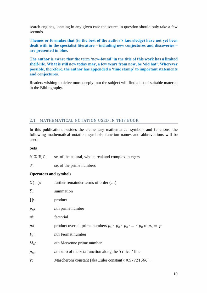
2.1 MATHEMATICAL NOTATION USED IN THIS BOOK
In this publication, besides the elementary mathematical symbols and functions, the
following mathematical notation, symbols, function names and abbreviations will be
used:
Sets
ℕ, ℤ, ℝ, ℂ: set of the natural, whole, real and complex integers
ℙ: set of the prime numbers
Operators and symbols
𝑂(…): further remainder terms of order (…)
∑: summation
∏: product
𝑝𝑛: nth prime number
𝑛!: factorial
𝑝#: product over all prime numbers 𝑝1 ⋅ 𝑝2 ⋅ 𝑝3 ⋅ … ⋅ 𝑝𝑛 to 𝑝𝑛 = 𝑝
𝐹𝑛: nth Fermat number
𝑀𝑛: nth Mersenne prime number
𝜌𝑛: nth zero of the zeta function along the ‘critical’ line
𝛾: Mascheroni constant (aka Euler constant): 0.57721566…
2 Introduction
11
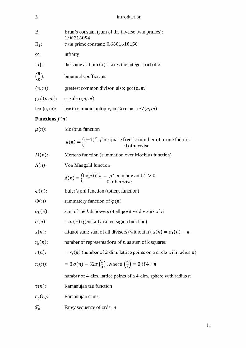
B: Brun’s constant (sum of the inverse twin primes):
1.90216054
Π2: twin prime constant: 0.6601618158
∞: infinity
⌊𝑥⌋: the same as floor(𝑥) : takes the integer part of 𝑥
(𝑛𝑘): binomial coefficients
(𝑛,𝑚): greatest common divisor, also: gcd(𝑛,𝑚)
gcd(𝑛,𝑚): see also (𝑛,𝑚)
lcm(n, m): least common multiple, in German: kgV(𝑛,𝑚)
Functions 𝒇(𝒏)
𝜇(𝑛): Moebius function
𝜇(𝑛) = {(−1)𝑘 𝑖𝑓 n square free, k: number of prime factors
0 otherwise
𝑀(𝑛): Mertens function (summation over Moebius function)
Λ(𝑛): Von Mangold function
Λ(𝑛) = {ln(𝑝) if 𝑛 = 𝑝𝑘, 𝑝 prime and 𝑘 > 0
0 otherwise
𝜑(𝑛): Euler’s phi function (totient function)
Φ(𝑛): summatory function of 𝜑(𝑛)
𝜎𝑘(𝑛): sum of the 𝑘th powers of all positive divisors of 𝑛
𝜎(𝑛): = 𝜎1(𝑛) (generally called sigma function)
𝑠(𝑛): aliquot sum: sum of all divisors (without n), 𝑠(𝑛) = 𝜎1(𝑛) − 𝑛
𝑟𝑘(𝑛): number of representations of 𝑛 as sum of k squares
𝑟(𝑛): = 𝑟2(𝑛) (number of 2-dim. lattice points on a circle with radius 𝑛)
𝑟4(𝑛): = 8 𝜎(𝑛) − 32𝜎 (𝑛
4) ,where (
𝑛
4) = 0, if 4 ∤ 𝑛
number of 4-dim. lattice points of a 4-dim. sphere with radius 𝑛
𝜏(𝑛): Ramanujan tau function
𝑐𝑞(𝑛): Ramanujan sums
ℱ𝑛: Farey sequence of order 𝑛

Mathematical notation used in this book
12
𝜔(𝑛): number of different prime factors of a number 𝑛
Ω(𝑛): number of prime factors of a number 𝑛
Functions 𝒇(𝒙)
𝜋(𝑥): counting function for prime numbers: gives the number of prime
numbers up to 𝑥.
𝜋2(𝑥): gives the number of twin primes up to 𝑥
𝜋3(𝑥), 𝜋4(𝑥): gives the number of prime triplets / quadruplets up to 𝑥
𝜋𝑛(𝑥): gives the number of prime n-tuplets up to 𝑥
𝜋´𝑛(𝑥): gives the number of prime pairs with difference n up to 𝑥
𝜋0(𝑥): same as 𝜋(𝑥), but different if x is a prime number:
𝜋0(𝑥) = lim𝜀→0
𝜋(𝑥−𝜀)+𝜋(𝑥+𝜀)
2 or: 𝜋0(𝑝) = 𝜋(𝑝) −
1
2
Θ(𝑥), 𝜗(𝑥): 1st Chebyshev function: = ∑ ln (𝑝)𝑝≤𝑥 (sum over log values
of all prime numbers ≤ 𝑛)
𝜓(𝑥): Chebyshev psi function: summatory function of Von Mangoldt function
𝜓(𝑥) = ∑ ln(𝑝) = ∑ Λ(𝑛)𝑛≤𝑥𝑝𝑘≤𝑥 (2nd Chebyshev func.)
𝜓0(𝑥): same as 𝜓(𝑥), but different if x is a prime number:
𝜓0(𝑥) = lim𝜀→0
𝜓(𝑥−𝜀)+𝜓(𝑥+𝜀)
2
휁(𝑠): Riemann’s zeta function
𝑃(𝑠): prime zeta function
𝜉(𝑠): variant of Riemann’s zeta function (has the same zeros along the critical
line as 휁(𝑠), but real function values)
Γ(𝑠): gamma function
𝑅(𝑥): Riemann function
ln(𝑥) , Li(𝑥): natural logarithm, integral logarithm
Ei(𝑥): integral exponential function
E𝑛(𝑥): exponential integral function of order n
𝑍(𝑡), 𝜗(𝑡): Riemann-Siegel functions
𝐿(𝑠): Ramanujan tau Dirichlet L function
2 Introduction
13
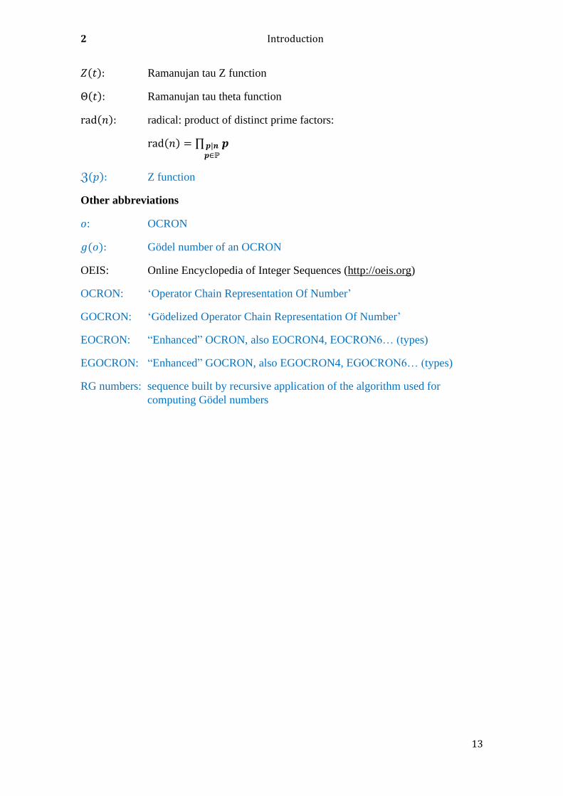
𝑍(𝑡): Ramanujan tau Z function
Θ(𝑡): Ramanujan tau theta function
rad(𝑛): radical: product of distinct prime factors:
rad(𝑛) = ∏ 𝒑𝒑|𝒏𝒑∈ℙ
ℨ(𝑝): Z function
Other abbreviations
𝑜: OCRON
𝑔(𝑜): Gödel number of an OCRON
OEIS: Online Encyclopedia of Integer Sequences (http://oeis.org)
OCRON: ‘Operator Chain Representation Of Number’
GOCRON: ‘Gödelized Operator Chain Representation Of Number’
EOCRON: “Enhanced” OCRON, also EOCRON4, EOCRON6… (types)
EGOCRON: “Enhanced” GOCRON, also EGOCRON4, EGOCRON6… (types)
RG numbers: sequence built by recursive application of the algorithm used for
computing Gödel numbers
14
3 BASICS OF PRIME NUMBERS
Let us begin, first of all, with some important fundamental statements about prime
numbers such as can be found in any handbook for mathematical beginners:
- A prime number is a natural number greater than 1 that has exactly two integer
divisors: ‘1’ and the number itself. Prime numbers are not divisible by any other
integers.
- The first prime numbers read: 2,3,5,7,11,13,17,19,… etc. The sequence of prime
numbers starts with 2 and not with 1.
- Prime numbers become rarer the further we ascend in the number region2. This
raises the question as to whether there exists a last, greatest prime number.
However, as the ancient Greek mathematician Euclid proved 2000 years ago:
- There are infinitely many prime numbers. Euclid’s proof is so easy to understand
that it can be stated in a few lines:
First, let us suppose the opposite of Euclid’s statement: that there exists a greatest prime
number 𝑝𝑛. Next build the product from all 𝑛 prime numbers and add 1:
𝑁 = 𝑝1 ⋅ 𝑝2 ⋅ 𝑝3 ⋅ … ⋅ 𝑝𝑛 + 1
Obviously, 𝑁 is much greater than 𝑝𝑛 and must be therefore be divisible, as we have
assumed a greatest prime number 𝑝𝑛 < 𝑁. After a moment’s reflection, it will be clear
that 𝑁 cannot be divisible by 2, nor by 3, 5 …It cannot be divisible by any of the primes
𝑝𝑛. Thus 𝑁 must be a prime number or must be divisible by a prime number 𝑝 > 𝑝𝑛.
This is, however, a contradiction to our assumption. Thus the assumption of the existence
of a greatest, last prime number 𝑝𝑛 is wrong!
The set ℙ of prime numbers can be easily extended to the Gaussian complex numbers,
leading to the set of ‘Gaussian primes’. ‘Primality’ can also be generalized and defined
for other sets of elements. These are commonly called ‘prime elements’.
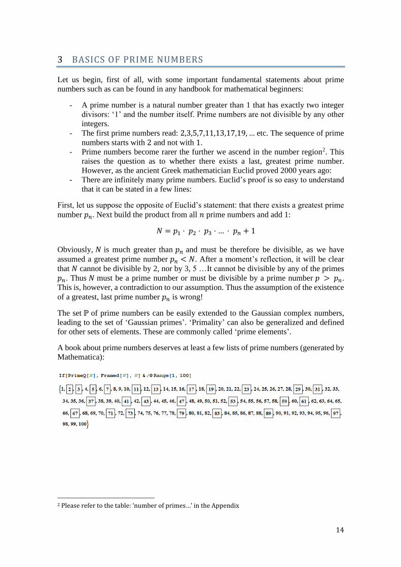
A book about prime numbers deserves at least a few lists of prime numbers (generated by
Mathematica):
2 Please refer to the table: ‘number of primes…’ in the Appendix
3 Basics of prime numbers
15
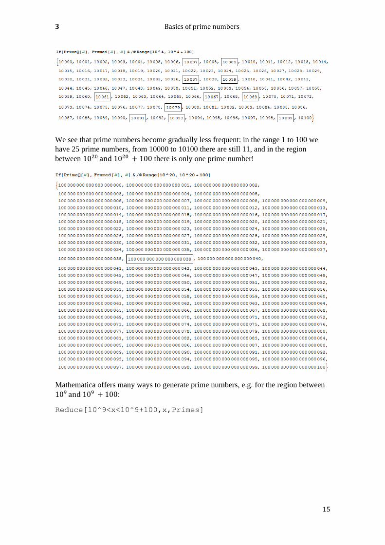
We see that prime numbers become gradually less frequent: in the range 1 to 100 we
have 25 prime numbers, from 10000 to 10100 there are still 11, and in the region
between 1020 and 1020 + 100 there is only one prime number!
Mathematica offers many ways to generate prime numbers, e.g. for the region between
109 and 109 + 100:
Reduce[10^9<x<10^9+100,x,Primes]
16
3.1 QUICK START: WHAT DO WE KNOW FOR CERTAIN?
Below, the reader will find a shortened description of the most important theorems about
prime numbers and arithmetical functions related to them that are proven (as of Nov.
2016):
1. There are infinitely many prime numbers.
2. Each integer that is composite (i.e. not a prime number) can be unambiguously
represented as a product of at least two prime numbers.
3. The number of primes 𝜋(𝑛) denotes the number of primes that exist up to a limit
𝑛 . For 𝜋(𝑛) there exist many (more or less precise) estimates that make it
possible to compute 𝜋(𝑛) approximately. There are also exact formulae for 𝜋 (𝑛) (see 8.6).
4. For computing the 𝑛th prime number, formulae also exist for an approximate
calculation, however, also exact formulae (see ‘Formulae for calculating the nth
prime number‘).
5. The ‘gaps’ between adjacent prime numbers can be of any size. The largest gap
currently known includes an area of 3.311.852 consecutive composite numbers
(as of Oct. 2015).
6. The sum of the reciprocals of all prime numbers diverges (goes towards infinity).
7. The largest currently known prime number is: 2𝟖𝟐𝟓𝟖𝟗𝟗𝟑𝟑 − 1. It has 24862047
digits if written in the decimal system (as of Dec. 2020).
8. There exists no arithmetic sequence of integer numbers that delivers only prime
numbers, such as for example Euler’s formula 𝑛2 + 𝑛 + 41, which generates
only prime numbers for 0 ≤ 𝑛 < 40 but not for 𝑛 = 40! However it remains
true that many arithmetic sequences create (among others) infinitely many prime
numbers.
9. Currently there are 51 known Mersenne prime numbers. The first Mersenne
prime exponents are:
2, 3, 5, 7, 13, 17, 19, 31 (sequence A000043 in OEIS) (as of Dec. 2020).
10. If 𝑀𝑝 is a prime, then 𝑝 is also a prime.
11. Currently there are 5 known Fermat primes 𝐹𝑛 = 22𝑛 + 1 (n = 0 … 4) These
are:
3, 5, 17, 257, 65537 (sequence A000215 in OEIS) (as of Nov. 2016).
𝐹5 to 𝐹32 are composite numbers. 𝐹33 is the first Fermat number of which it is not
known whether it is composite or prime (as of Nov. 2016).
12. Each even perfect number 𝑁 (i.e. the sum of its positive divisors without 𝑁 gives
𝑁) has the form 2𝑛−1(2𝑛 − 1)in which 2𝑛 − 1is prime, i.e. to each Mersenne
prime number belongs a perfect number!!
13. If 𝜙(𝑛) + 𝜎(𝑛) = 2 𝑛, 𝑛 ≥ 2 , then 𝑛 is a prime number, in which 𝜙(𝑛) is
Euler’s totient function and 𝜎(𝑛) the ‘sum-of-divisors function’.
14. If (𝑛 − 1𝑘) ≡ (−1)𝑘 (mod 𝑛), then 𝑛 is a prime number, of which (
𝑛𝑘) are the
binomial coefficients.
15. For each prime number 𝑝, the following relations to the 𝜎 function obtain:
𝜎0(𝑝) = 2 (Each prime number has only two divisors: itself and 1)
𝜎0(𝑝𝑛) = 𝑛 + 1
𝜎1(𝑝) = 𝑝 + 1
3 Basics of prime numbers
17
3.2 QUICK START: WHAT ARE OUR (UNPROVEN) CONJECTURES?
Here are (in shortened form) the most important statements and conjectures about prime
numbers and about the closely related zeta function that are probably true but still
unproved (as of Nov. 2016):
1. Each even natural number 𝑛 > 2 can be represented as the sum of two prime
numbers (strong Goldbach conjecture). This conjecture has been numerically
verified up to 𝑛 < 4 ⋅ 1018 (as of Apr. 2012).
2. Each odd natural number > 5 can be represented as the sum of three prime
numbers (weak Goldbach conjecture). This has been proved for 𝑛 > 1043000!
3. Between 𝑛2 and (𝑛 + 1)2 there exists at least 1 prime number (Oppermann’s
conjecture, 1882).
4. The ‘non-trivial’ zeros of the zeta function are all located in the Gaussian
complex plane on a straight line having a real part of 0.5. This is the famous
Riemann conjecture, which Riemann formulated in the year 1859, and which
remains unproved to this day (as of Nov. 2016). It ranks among the ‘Top Seven
unsolved mathematical problems’. A reward of one million US dollars has been
offered for its solution. The conjecture has been numerically verified up to the
first 1013 . Thus there is overwhelming numerical evidence for the truth of
Riemann’s conjecture.
5. There are infinitely many Mersenne prime numbers (numbers of the form 𝑀𝑝 =
2𝑝 − 1).
6. There are infinitely many composite Mersenne numbers.
7. There are only five Fermat prime numbers.
8. There are no odd perfect numbers (see above).
9. The ‘new Mersenne conjecture’:
if any two of the following conditions hold, then the third condition is also true:
- 𝑛 = 2𝑘 ± 1 or 𝑛 = 4𝑘 ± 3
- 2𝑛 − 1 is prime (obviously a Mersenne prime)
- (2𝑛+1)
3is prime
10. There are infinitely many twin prime numbers. Twin primes are prime numbers
having a difference of 2. It is known that the sum of the reciprocals of the twin
primes converges (Brun’s constant: 1.902160577783278, proved by Brun in
1919).
11. The number 𝑁𝑀𝑝of Mersenne prime numbers that are smaller than or equal to N
is given asymptotically by the formula: 𝑁𝑀𝑝(𝑁)~𝑒𝛾
ln(2)ln ln(𝑁).
12. The final digits of consecutive prime numbers show striking correlations.
18
3.3 QUICK START: WHAT IS STILL UNSOLVED?
Here are (in a shortened form) the most important unsolved questions about prime
numbers and related topics, of which we have no idea whether they are wrong or right:
1. Are all Mersenne numbers 𝑀𝑝 = 2𝑝 − 1 square-free, i.e. does their prime factor
decomposition contain each factor only once?
2. Are there infinitely many prime number 𝑁 -tuplets? (These are tuplets of 𝑛
consecutive prime numbers having minimal differences, as defined in Chapter
4.3).
3. Are there infinitely many ‘Wagstaff’ prime numbers, i.e. prime numbers of the
form (2𝑝+1)
3 (with 𝑝 being an odd prime number)?
4. Are there infinitely many ‘Sophie Germain’ prime numbers, i.e. prime numbers
of the form 2𝑝 + 1 (with 2𝑝 + 1 as a ‘safe prime’ and 𝑝 as the ‘Sophie Germain’
prime)?
5. Are there infinitely many ‘Fibonacci’ primes, i.e. prime numbers occurring in the
Fibonacci sequence?
6. Does the ‘Euclid-Mullin sequence’ contain all prime numbers?
7. Does there exist an efficient factorizing method for the prime factor
decomposition of large numbers, i.e. a procedure that accomplishes the
factorization process in ‘polynomial time’? Because no such a method is currently
known, it is still impossible to factorize large numbers (as the computing time
required would be astronomically high). Currently the fastest known methods of
factorization are the ‘number field sieve (Pomerance et. al.) and the method using
elliptic curves (as of Nov. 2016).

3 Basics of prime numbers
19
3.4 QUICK START: WHAT IS NEW?
1) A new property of the Fibonacci numbers (see 4.10).
2) Properties of the Reed Jameson sequence and its relation to prime numbers (see
4.10.1).
3) RG number sequences (recursive ‘Gödelized’) sequences (see 4.17).
4) ‘Fun and games’ with the product representation of the 휁(𝑠) in the complex
domain (see 5.3).
5) ℨ(𝑠): a ‘function’ having minima that are located at the prime positions (see 5.3).
6) The Reed Jameson function: zeros at the prime number positions (see 8.5.1).
7) Prime numbers and surfaces of 4-dimensional hyperspheres (glomes) (see 9.3).
8) Of OCRONs and GOCRONs (see Chapter 10).
9) Is it possible to find (typographic) prime number rules using the Matrix software?
(Chapter 11).
10) An equation for a plane as a link between GOCRONs and the abc conjecture (see
12.1).
11) Prime numbers as rhythmic patterns (Chapter 15.2).
12) Differences and quotients of aliquot sequences (Chapter 20.9.2.5).
20
4 SPECIAL KINDS OF PRIME NUMBERS
4.1 TWIN PRIMES
Twin primes are prime numbers having a difference of 2. The following applies: 𝑛 and
𝑛 + 2 are twin primes if and only if the following equation obtains:
𝟒[(𝒏 − 𝟏)! + 𝟏] + 𝒏 ≡ 𝟎 [𝐦𝐨𝐝 𝒏(𝒏 + 𝟐)] (1)
𝝓(𝒏)𝝈(𝒏) = (𝒏 − 𝟑)(𝒏 + 𝟏),𝐰𝐡𝐞𝐫𝐞 𝒏= 𝒑(𝒑 + 𝟐) (product of a twin prime pair)
(2)
(𝒏, 𝒏 + 𝟐) are twin primes if
∑𝒊𝒂 (⌊𝒏 + 𝟐
𝒊⌋ + ⌊
𝒏
𝒊⌋) = 𝟐 + 𝒏𝒂 +∑𝒊𝒂
𝒏
𝒊=𝟏
(⌊𝒏 + 𝟏
𝒊⌋ + ⌊
𝒏 − 𝟏
𝒊⌋)
𝒏
𝒊=𝟏
where 𝑎 ≥ 0 and ⌊ ⌋ is the floor() function.
(3)
Unfortunately these formulae are not practicable for the computation of twin prime
numbers.
Let 𝜋2(𝑥) be the number of twin primes up to a given limit 𝑥. Since the 19th century the following estimate has been accepted:
𝜋2(𝑥) ≤ 𝑐Π2𝑥
(ln 𝑥)2 (4)
Hardy and Littlewood have conjectured that c = 2 and
𝝅𝟐(𝒙)~𝟐𝚷𝟐∫𝒅𝒕
(𝐥𝐧 𝐭)𝟐
𝒙
𝟐
= 𝟐𝚷𝟐(𝐋𝐢(𝒙) −𝒙
𝐥𝐧(𝒙)− 𝑳𝒊(𝟐) +
𝟐
𝐥𝐧 (𝟐)) (5)
using the twin prime constant:
𝚷𝟐 =∏𝒑(𝒑 − 𝟐)
(𝒑 − 𝟏)𝟐𝒑≥𝟑
= 0.6601618158
𝟐𝚷𝟐 = 𝟏. 𝟑𝟐𝟎𝟑𝟐𝟑𝟔𝟑𝟏𝟔
The sum of the reciprocals of all twin primes converges (Brun’s constant, proved by Brun
in 1919).
4 Special kinds of prime numbers
21
𝐵 = ∑ (1
𝑝+
1
𝑝 + 2) = 1.90216054
𝑝=𝑡𝑤𝑖𝑛
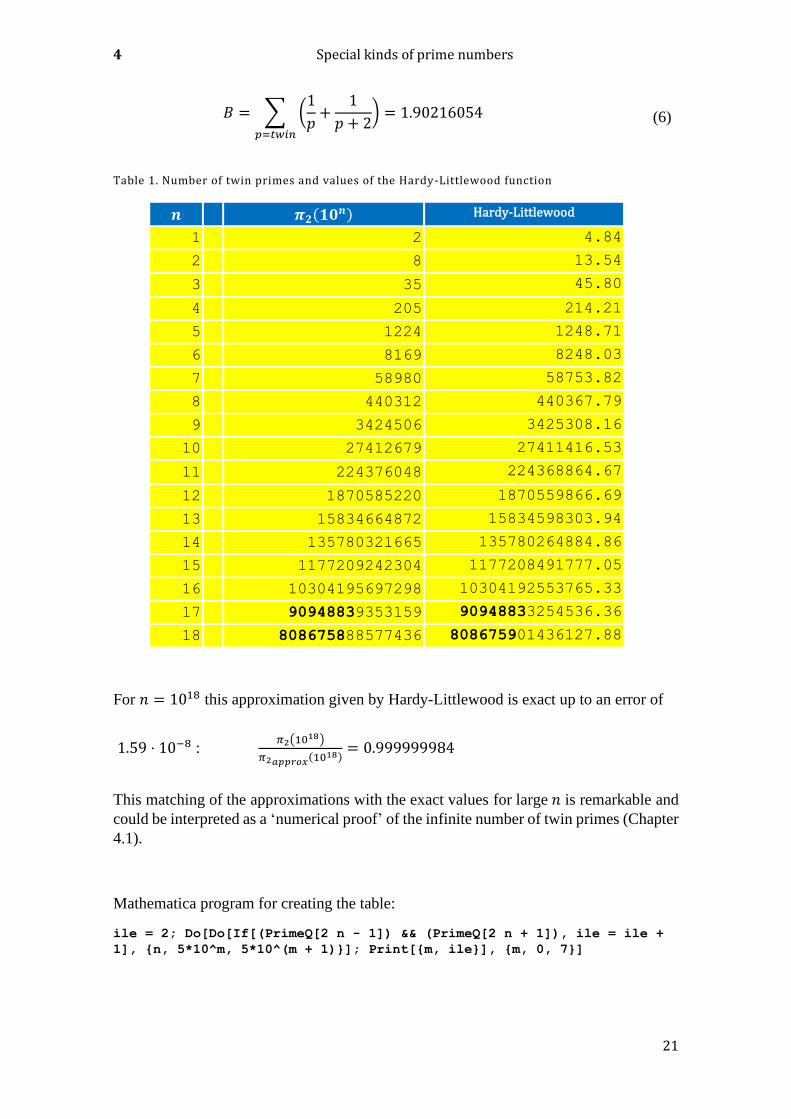
(6)
Table 1. Number of twin primes and values of the Hardy-Littlewood function
𝒏 𝝅𝟐(𝟏𝟎𝒏) Hardy-Littlewood
1 2 4.84
2 8 13.54
3 35 45.80
4 205 214.21
5 1224 1248.71
6 8169 8248.03
7 58980 58753.82
8 440312 440367.79
9 3424506 3425308.16
10 27412679 27411416.53
11 224376048 224368864.67
12 1870585220 1870559866.69
13 15834664872 15834598303.94
14 135780321665 135780264884.86
15 1177209242304 1177208491777.05
16 10304195697298 10304192553765.33
17 90948839353159 90948833254536.36
18 808675888577436 808675901436127.88
For 𝑛 = 1018 this approximation given by Hardy-Littlewood is exact up to an error of
1.59 ⋅ 10−8 : 𝜋2(10
18)
𝜋2𝑎𝑝𝑝𝑟𝑜𝑥(1018)= 0.999999984
This matching of the approximations with the exact values for large 𝑛 is remarkable and
could be interpreted as a ‘numerical proof’ of the infinite number of twin primes (Chapter
4.1).
Mathematica program for creating the table:
ile = 2; Do[Do[If[(PrimeQ[2 n - 1]) && (PrimeQ[2 n + 1]), ile = ile +
1], {n, 5*10^m, 5*10^(m + 1)}]; Print[{m, ile}], {m, 0, 7}]
Twin primes
22
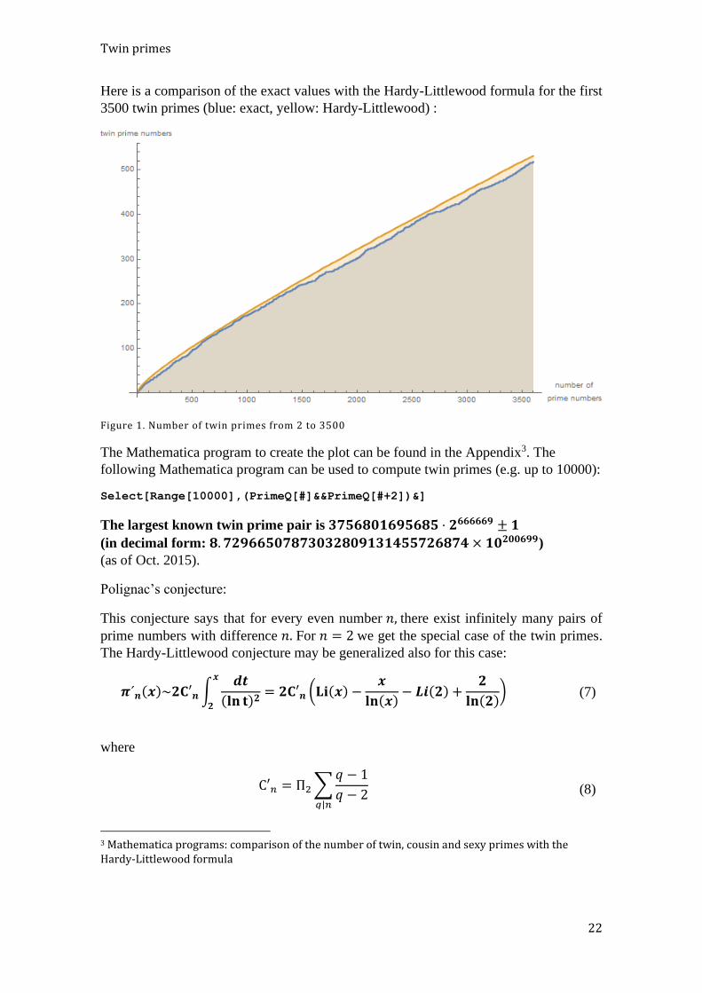
Here is a comparison of the exact values with the Hardy-Littlewood formula for the first
3500 twin primes (blue: exact, yellow: Hardy-Littlewood) :
Figure 1. Number of twin primes from 2 to 3500
The Mathematica program to create the plot can be found in the Appendix3. The
following Mathematica program can be used to compute twin primes (e.g. up to 10000):
Select[Range[10000],(PrimeQ[#]&&PrimeQ[#+2])&]
The largest known twin prime pair is 𝟑𝟕𝟓𝟔𝟖𝟎𝟏𝟔𝟗𝟓𝟔𝟖𝟓 ⋅ 𝟐𝟔𝟔𝟔𝟔𝟔𝟗 ± 𝟏
(in decimal form: 𝟖. 𝟕𝟐𝟗𝟔𝟔𝟓𝟎𝟕𝟖𝟕𝟑𝟎𝟑𝟐𝟖𝟎𝟗𝟏𝟑𝟏𝟒𝟓𝟓𝟕𝟐𝟔𝟖𝟕𝟒 × 𝟏𝟎𝟐𝟎𝟎𝟔𝟗𝟗)
(as of Oct. 2015).
Polignac’s conjecture:
This conjecture says that for every even number 𝑛, there exist infinitely many pairs of
prime numbers with difference 𝑛. For 𝑛 = 2 we get the special case of the twin primes.
The Hardy-Littlewood conjecture may be generalized also for this case:
𝝅´𝒏(𝒙)~𝟐𝐂′𝒏∫𝒅𝒕
(𝐥𝐧 𝐭)𝟐
𝒙
𝟐
= 𝟐𝐂′𝒏 (𝐋𝐢(𝒙) −𝒙
𝐥𝐧(𝒙)− 𝑳𝒊(𝟐) +
𝟐
𝐥𝐧(𝟐)) (7)
where
C′𝑛 = Π2∑𝑞− 1
𝑞 − 2𝑞|𝑛
(8)
3 Mathematica programs: comparison of the number of twin, cousin and sexy primes with the Hardy-Littlewood formula
4 Special kinds of prime numbers
23
Special cases:
𝑛 = 4: Cousin primes: here we have C′4 = C′2 = C2 primes (with difference 4) and twin
primes have the same asymptotic density. There exist the same number of instances of
both kinds!!
𝑛 = 6: Sexy primes: here we have C′6 = 2C′2primes (with difference 6) having an
asymptotic density twice as high as twin primes. There exist twice as many sexy primes
as twin primes!!
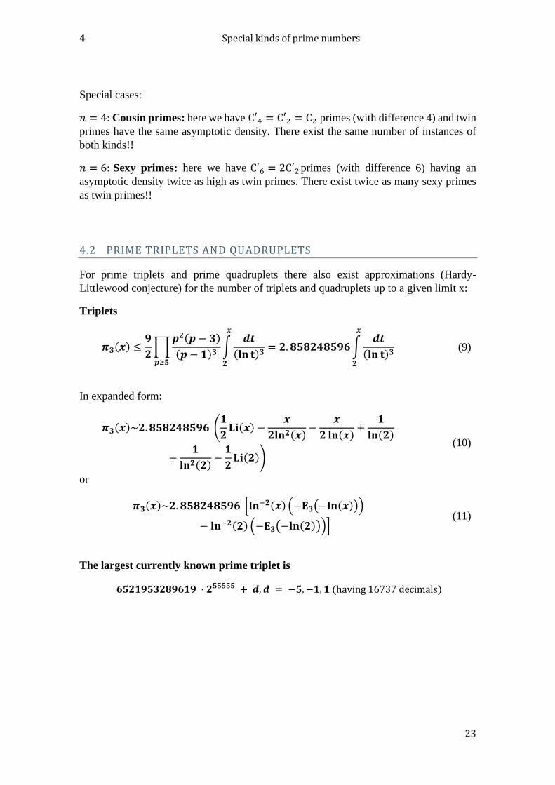
4.2 PRIME TRIPLETS AND QUADRUPLETS
For prime triplets and prime quadruplets there also exist approximations (Hardy-
Littlewood conjecture) for the number of triplets and quadruplets up to a given limit x:
Triplets
𝝅𝟑(𝒙) ≤𝟗
𝟐∏
𝒑𝟐(𝒑 − 𝟑)
(𝒑 − 𝟏)𝟑𝒑≥𝟓
∫𝒅𝒕
(𝐥𝐧 𝐭)𝟑
𝒙
𝟐
= 𝟐. 𝟖𝟓𝟖𝟐𝟒𝟖𝟓𝟗𝟔∫𝒅𝒕
(𝐥𝐧 𝐭)𝟑
𝒙
𝟐
(9)
In expanded form:
𝝅𝟑(𝒙)~𝟐. 𝟖𝟓𝟖𝟐𝟒𝟖𝟓𝟗𝟔 (𝟏
𝟐𝐋𝐢(𝒙) −
𝒙
𝟐𝐥𝐧𝟐(𝒙)−
𝒙
𝟐 𝐥𝐧(𝒙)+
𝟏
𝐥𝐧(𝟐)
+𝟏
𝐥𝐧𝟐(𝟐)−𝟏
𝟐𝐋𝐢(𝟐))
(10)
or
𝝅𝟑(𝒙)~𝟐. 𝟖𝟓𝟖𝟐𝟒𝟖𝟓𝟗𝟔 [𝐥𝐧−𝟐(𝒙) (−𝐄𝟑(−𝐥𝐧(𝒙)))
− 𝐥𝐧−𝟐(𝟐) (−𝐄𝟑(−𝐥𝐧(𝟐)))] (11)
The largest currently known prime triplet is
𝟔𝟓𝟐𝟏𝟗𝟓𝟑𝟐𝟖𝟗𝟔𝟏𝟗 ⋅ 𝟐𝟓𝟓𝟓𝟓𝟓 + 𝒅, 𝒅 = −𝟓,−𝟏, 𝟏 (having 16737 decimals)
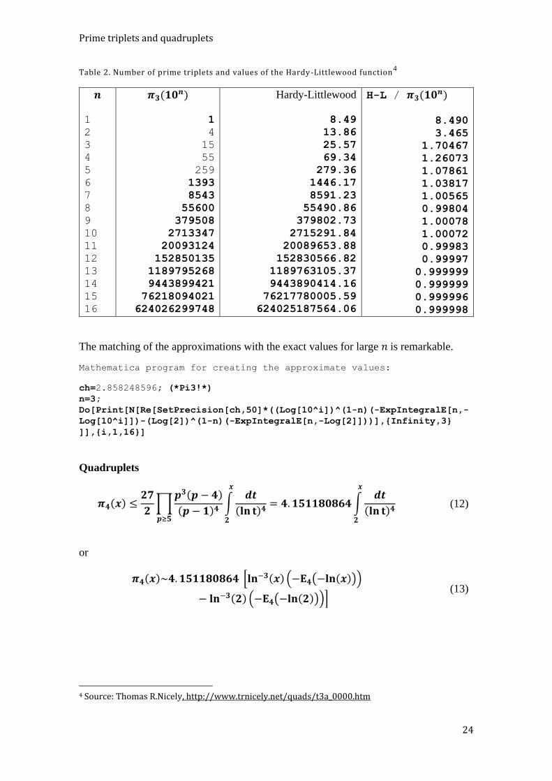
Prime triplets and quadruplets
24
Table 2. Number of prime triplets and values of the Hardy-Littlewood function4
𝒏
1
2
3
4
5
6
7
8
9
10
11
12
13
14
15
16
𝝅𝟑(𝟏𝟎𝒏)
1
4
15
55
259
1393
8543
55600
379508
2713347
20093124
152850135
1189795268
9443899421
76218094021
624026299748
Hardy-Littlewood
8.49
13.86
25.57
69.34
279.36
1446.17
8591.23
55490.86
379802.73
2715291.84
20089653.88
152830566.82
1189763105.37
9443890414.16
76217780005.59
624025187564.06
H-L / 𝝅𝟑(𝟏𝟎𝒏)
8.490
3.465
1.70467
1.26073
1.07861
1.03817
1.00565
0.99804
1.00078
1.00072
0.99983
0.99997 0.999999
0.999999
0.999996
0.999998
The matching of the approximations with the exact values for large 𝑛 is remarkable.
Mathematica program for creating the approximate values:
ch=2.858248596; (*Pi3!*)
n=3;
Do[Print[N[Re[SetPrecision[ch,50]*((Log[10^i])^(1-n)(-ExpIntegralE[n,-
Log[10^i]])-(Log[2])^(1-n)(-ExpIntegralE[n,-Log[2]]))],{Infinity,3}
]],{i,1,16}]
Quadruplets
𝝅𝟒(𝒙) ≤𝟐𝟕
𝟐∏
𝒑𝟑(𝒑 − 𝟒)
(𝒑 − 𝟏)𝟒𝒑≥𝟓
∫𝒅𝒕
(𝐥𝐧 𝐭)𝟒
𝒙
𝟐
= 𝟒. 𝟏𝟓𝟏𝟏𝟖𝟎𝟖𝟔𝟒∫𝒅𝒕
(𝐥𝐧 𝐭)𝟒
𝒙
𝟐
(12)
or
𝝅𝟒(𝒙)~𝟒. 𝟏𝟓𝟏𝟏𝟖𝟎𝟖𝟔𝟒 [𝐥𝐧−𝟑(𝒙) (−𝐄𝟒(−𝐥𝐧(𝒙)))
− 𝐥𝐧−𝟑(𝟐) (−𝐄𝟒(−𝐥𝐧(𝟐)))] (13)
4 Source: Thomas R.Nicely, http://www.trnicely.net/quads/t3a_0000.htm

4 Special kinds of prime numbers
25
Table 3. Number of prime quadruplets and values of the Hardy-Littlewood function5
𝒏
1
2
3
4
5
6
7
8
9
10
11
12
13
14
15
16
𝝅𝟒(𝟏𝟎𝒏)
1
2
5
12
38
166
899
4768
28388
180529
1209318
8398278
60070590
441296836
3314576487
25379433651
Hardy-Littlewood
11.29
13.60
16.49
24.17
52.88
183.68
862.95
4734.64
28396.84
181074.93
1209956.22
8394578.03
60075438.37
441290732.40
3314550290.38
25379441340.00
H-L / 𝝅𝟒(𝟏𝟎𝒏)
11.29
6.80
3.30
2.01
1.39
1.1065
0.9599
0.99300
1.00031
1.00302
1.00053
0.99956
1.00008
0.999986
0.999992
1.0000000
Here, too, the matching of the approximations with the exact values for large 𝑛 is
remarkable.
Mathematica program for creating the approximate values:
ch=4.151180864; (*Pi4!*)
n=4;
Do[Print[N[Re[SetPrecision[ch,50]*((Log[10^i])^(1-n)(-ExpIntegralE[n,-
Log[10^i]])-(Log[2])^(1-n)(-ExpIntegralE[n,-Log[2]]))],{Infinity,3}
]],{i,1,16}]
The largest prime quadruplet currently known is (Source: Thomas Forbes6)
𝟐𝟔𝟕𝟑𝟎𝟗𝟐𝟓𝟓𝟔𝟔𝟖𝟏 ⋅ 𝟏𝟓𝟑𝟎𝟒𝟖 + 𝒅, 𝒅 = −𝟒,−𝟐, 𝟐, 𝟒
= 𝟏. 𝟒𝟐𝟐𝟖𝟗𝟎𝟖𝟖𝟖𝟑𝟐𝟗𝟐𝟏𝟕𝟎𝟖𝟗𝟒𝟒𝟖𝟒𝟒𝟑𝟔𝟗𝟏𝟔𝟐 ⋅ 𝟏𝟎𝟑𝟓𝟗𝟕
(as of Oct. 2015).
4.3 PRIME N-TUPLETS
A prime n-tuplet is generally defined as a sequence of consecutive primes
(𝑝1, 𝑝2, 𝑝3, … 𝑝𝑛) with a fixed minimal value for the difference between the smallest and
the largest prime 𝑠(𝑛) = 𝑝𝑛 − 𝑝1 (see table below). For example, 𝑠(4) = 8 for
quadruplets or 𝑠(5) = 12 for quintuplets. Generally, there exist more solutions for the
5 Source: Thomas R.Nicely, http://www.trnicely.net/quads/t4_0000.htm 6 http://anthony.d.forbes.googlepages.com/ktuplets.htm
Prime n-tuplets
26
corresponding sequence for a given prime n-tuplet with a fixed 𝑠(𝑛). For example, prime
triplets can have two different forms: (𝑝, 𝑝 + 2, 𝑝 + 6) and (𝑝, 𝑝 + 4, 𝑝 + 6) . This
degeneration grows quite fast with the length 𝑛 of the 𝑛-tuplets. So, for 𝑛 = 13, the
degeneration is already 6; for 𝑛 = 25, we have a degeneration of 18 distinct ordering
possibilities for a prime number 25-tuplet where s(25) = 110.
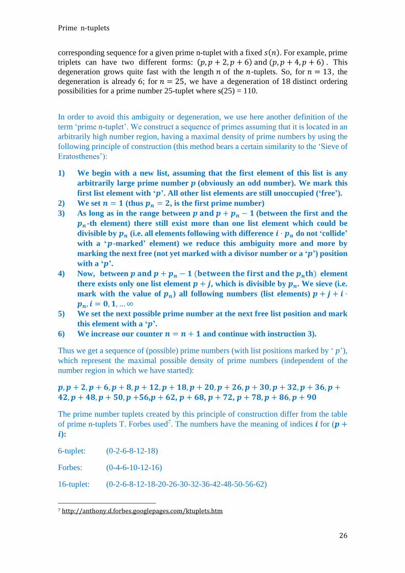
In order to avoid this ambiguity or degeneration, we use here another definition of the
term ‘prime n-tuplet’. We construct a sequence of primes assuming that it is located in an
arbitrarily high number region, having a maximal density of prime numbers by using the
following principle of construction (this method bears a certain similarity to the ‘Sieve of
Eratosthenes’):
1) We begin with a new list, assuming that the first element of this list is any
arbitrarily large prime number 𝒑 (obviously an odd number). We mark this
first list element with ‘𝒑’. All other list elements are still unoccupied (‘free’).
2) We set 𝒏 = 𝟏 (thus 𝒑𝒏 = 𝟐, is the first prime number)
3) As long as in the range between 𝒑 𝐚𝐧𝐝 𝒑 + 𝒑𝒏 − 𝟏 (between the first and the
𝒑𝒏 -th element) there still exist more than one list element which could be
divisible by 𝒑𝒏 (i.e. all elements following with difference 𝒊 ⋅ 𝒑𝒏 do not ‘collide’
with a ‘𝒑-marked’ element) we reduce this ambiguity more and more by
marking the next free (not yet marked with a divisor number or a ‘𝒑’) position
with a ‘𝒑’.
4) Now, between 𝒑 𝐚𝐧𝐝 𝒑 + 𝒑𝒏 − 𝟏 (𝐛𝐞𝐭𝐰𝐞𝐞𝐧 𝐭𝐡𝐞 𝐟𝐢𝐫𝐬𝐭 𝐚𝐧𝐝 𝐭𝐡𝐞 𝒑𝒏𝐭𝐡) element
there exists only one list element 𝒑 + 𝒋, which is divisible by 𝒑𝒏. We sieve (i.e.
mark with the value of 𝒑𝒏) all following numbers (list elements) 𝒑 + 𝒋 + 𝒊 ⋅𝒑𝒏, 𝒊 = 𝟎, 𝟏, …∞
5) We set the next possible prime number at the next free list position and mark
this element with a ‘𝒑’.
6) We increase our counter 𝒏 = 𝒏 + 𝟏 and continue with instruction 3).
Thus we get a sequence of (possible) prime numbers (with list positions marked by ‘ 𝑝’),
which represent the maximal possible density of prime numbers (independent of the
number region in which we have started):
𝒑, 𝒑 + 𝟐, 𝒑 + 𝟔, 𝒑 + 𝟖, 𝒑 + 𝟏𝟐, 𝒑 + 𝟏𝟖, 𝒑 + 𝟐𝟎, 𝒑 + 𝟐𝟔, 𝒑 + 𝟑𝟎, 𝒑 + 𝟑𝟐, 𝒑 + 𝟑𝟔, 𝒑 +𝟒𝟐, 𝒑 + 𝟒𝟖, 𝒑 + 𝟓𝟎, 𝒑 +56,𝒑 + 𝟔𝟐, 𝒑 + 𝟔𝟖, 𝒑 + 𝟕𝟐, 𝒑 + 𝟕𝟖, 𝒑 + 𝟖𝟔, 𝒑 + 𝟗𝟎
The prime number tuplets created by this principle of construction differ from the table
of prime n-tuplets T. Forbes used7. The numbers have the meaning of indices 𝒊 for (𝒑 +𝒊):
6-tuplet: (0-2-6-8-12-18)
Forbes: (0-4-6-10-12-16)
16-tuplet: (0-2-6-8-12-18-20-26-30-32-36-42-48-50-56-62)
7 http://anthony.d.forbes.googlepages.com/ktuplets.htm
4 Special kinds of prime numbers
27
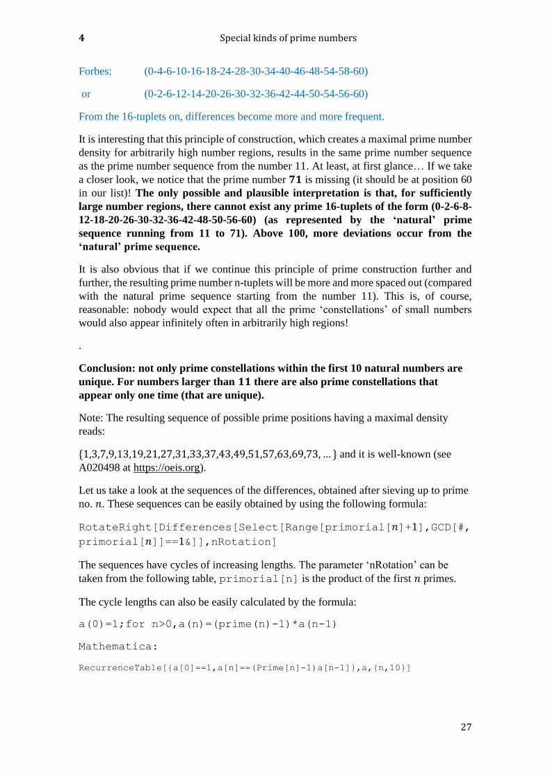
Forbes: (0-4-6-10-16-18-24-28-30-34-40-46-48-54-58-60)
or (0-2-6-12-14-20-26-30-32-36-42-44-50-54-56-60)
From the 16-tuplets on, differences become more and more frequent.
It is interesting that this principle of construction, which creates a maximal prime number
density for arbitrarily high number regions, results in the same prime number sequence
as the prime number sequence from the number 11. At least, at first glance… If we take
a closer look, we notice that the prime number 𝟕𝟏 is missing (it should be at position 60
in our list)! The only possible and plausible interpretation is that, for sufficiently
large number regions, there cannot exist any prime 16-tuplets of the form (0-2-6-8-
12-18-20-26-30-32-36-42-48-50-56-60) (as represented by the ‘natural’ prime
sequence running from 11 to 71). Above 100, more deviations occur from the
‘natural’ prime sequence.
It is also obvious that if we continue this principle of prime construction further and
further, the resulting prime number n-tuplets will be more and more spaced out (compared
with the natural prime sequence starting from the number 11). This is, of course,
reasonable: nobody would expect that all the prime ‘constellations’ of small numbers
would also appear infinitely often in arbitrarily high regions!
.
Conclusion: not only prime constellations within the first 10 natural numbers are
unique. For numbers larger than 𝟏𝟏 there are also prime constellations that
appear only one time (that are unique).
Note: The resulting sequence of possible prime positions having a maximal density
reads:
{1,3,7,9,13,19,21,27,31,33,37,43,49,51,57,63,69,73,… } and it is well-known (see
A020498 at https://oeis.org).
Let us take a look at the sequences of the differences, obtained after sieving up to prime
no. 𝑛. These sequences can be easily obtained by using the following formula:
RotateRight[Differences[Select[Range[primorial[𝑛]+1],GCD[#,
primorial[𝑛]]==1&]],nRotation]
The sequences have cycles of increasing lengths. The parameter ‘nRotation’ can be
taken from the following table, primorial[n] is the product of the first 𝑛 primes.
The cycle lengths can also be easily calculated by the formula:
a(0)=1;for n>0,a(n)=(prime(n)-1)*a(n-1)
Mathematica:
RecurrenceTable[{a[0]==1,a[n]==(Prime[n]-1)a[n-1]},a,{n,10}]
Prime n-tuplets
28
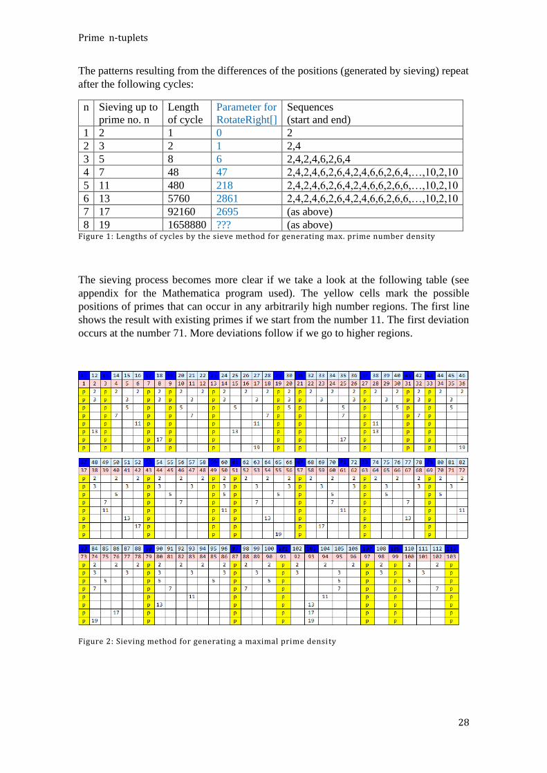
The patterns resulting from the differences of the positions (generated by sieving) repeat
after the following cycles:
n Sieving up to
prime no. n
Length
of cycle
Parameter for
RotateRight[]
Sequences
(start and end)
1 2 1 0 2
2 3 2 1 2,4
3 5 8 6 2,4,2,4,6,2,6,4
4 7 48 47 2,4,2,4,6,2,6,4,2,4,6,6,2,6,4,…,10,2,10
5 11 480 218 2,4,2,4,6,2,6,4,2,4,6,6,2,6,6,…,10,2,10
6 13 5760 2861 2,4,2,4,6,2,6,4,2,4,6,6,2,6,6,…,10,2,10
7 17 92160 2695 (as above)
8 19 1658880 ??? (as above) Figure 1: Lengths of cycles by the sieve method for generating max. prime number density
The sieving process becomes more clear if we take a look at the following table (see
appendix for the Mathematica program used). The yellow cells mark the possible
positions of primes that can occur in any arbitrarily high number regions. The first line
shows the result with existing primes if we start from the number 11. The first deviation
occurs at the number 71. More deviations follow if we go to higher regions.
Figure 2: Sieving method for generating a maximal prime densi ty
4 Special kinds of prime numbers
29
The web site of T. Forbes is a true treasure for this topic. The following formulae have
been taken in large part from his web site.
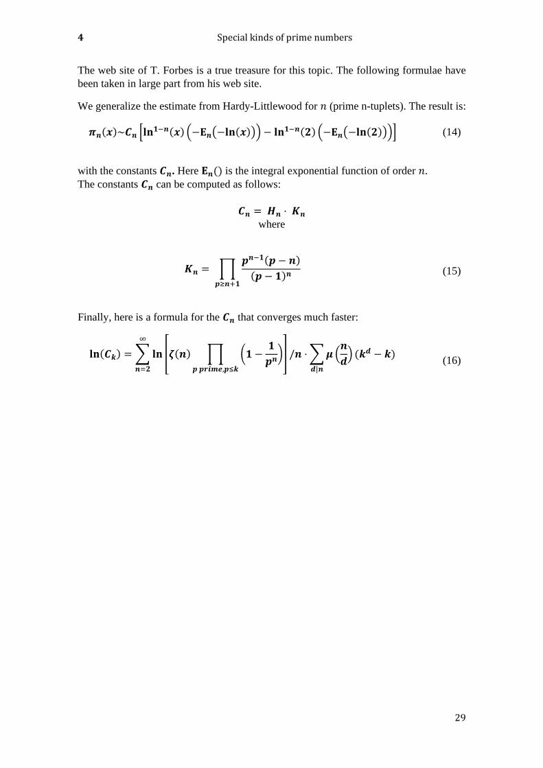
We generalize the estimate from Hardy-Littlewood for 𝑛 (prime n-tuplets). The result is:
𝝅𝒏(𝒙)~𝑪𝒏 [𝐥𝐧𝟏−𝒏(𝒙) (−𝐄𝒏(−𝐥𝐧(𝒙))) − 𝐥𝐧
𝟏−𝒏(𝟐) (−𝐄𝒏(−𝐥𝐧(𝟐)))] (14)
with the constants 𝑪𝒏. Here 𝐄𝒏() is the integral exponential function of order 𝑛.
The constants 𝑪𝒏 can be computed as follows:
𝑪𝒏 = 𝑯𝒏 ⋅ 𝑲𝒏
where
𝑲𝒏 = ∏𝒑𝒏−𝟏(𝒑 − 𝒏)
(𝒑 − 𝟏)𝒏𝒑≥𝒏+𝟏
(15)
Finally, here is a formula for the 𝑪𝒏 that converges much faster:
𝐥𝐧(𝑪𝒌) = ∑ 𝐥𝐧 [𝜻(𝒏) ∏ (𝟏 −𝟏
𝒑𝒏)
𝒑 𝒑𝒓𝒊𝒎𝒆,𝒑≤𝒌
]
∞
𝒏=𝟐
/𝒏 ⋅∑𝝁(𝒏
𝒅)
𝒅|𝒏
(𝒌𝒅 − 𝒌)
(16)
Prime n-tuplets
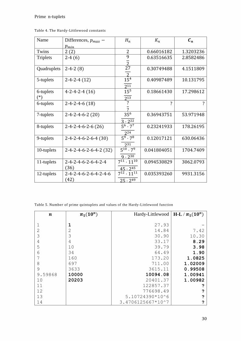
30
Table 4. The Hardy-Littlewood constants
Name Differences, 𝑝𝑚𝑎𝑥 −𝑝𝑚𝑖𝑛
𝐻𝑛 𝐾𝑛 𝑪𝒏
Twins 2 (2) 2 0.66016182 1.3203236 Triplets 2-4 (6) 9
2
0.63516635 2.8582486
Quadruplets 2-4-2 (8) 27
2
0.30749488 4.1511809
5-tuplets 2-4-2-4 (12) 154
211
0.40987489 10.131795
6-tuplets
(*) 4-2-4-2-4 (16) 155
213
0.18661430 17.298612
6-tuplets 2-4-2-4-6 (18) ?
?
? ?
7-tuplets 2-4-2-4-6-2 (20) 356
3 ⋅ 222
0.36943751 53.971948
8-tuplets 2-4-2-4-6-2-6 (26) 56 ⋅ 77
224
0.23241933 178.26195
9-tuplets 2-4-2-4-6-2-6-4 (30) 59 ⋅ 78
231
0.12017121 630.06436
10-tuplets 2-4-2-4-6-2-6-4-2 (32) 510 ⋅ 79
9 ⋅ 230
0.041804051 1704.7409
11-tuplets 2-4-2-4-6-2-6-4-2-4 (36)
711 ⋅ 1110
45 ⋅ 245
0.094530829 3062.0793
12-tuplets 2-4-2-4-6-2-6-4-2-4-6 (42)
712 ⋅ 1111
25 ⋅ 249
0.035393260 9931.3156
Table 5. Number of prime quintuplets and values of the Hardy-Littlewood function
𝒏
1
2
3
4
5
6
7
8
9
9.59868
10
11
12
13
14
𝝅𝟓(𝟏𝟎𝒏)
1
2
3
4
10
34
160
697
3633
10000
20203
Hardy-Littlewood
27.93
14.84
30.90
33.17
39.79
64.49
173.20
711.00
3615.11
10094.08
20401.37
122857.37
776698.49
5.10724390*10^6
3.4706125667*10^7
H-L / 𝝅𝟓(𝟏𝟎𝒏)
-
7.42
10.30
8.29
3.98
1.90
1.0825
1.02009
0.99508
1.00941
1.00982
?
?
?
?
4 Special kinds of prime numbers
31
15
16
2.42544985095*10^8
1.73651359676*10^9
?
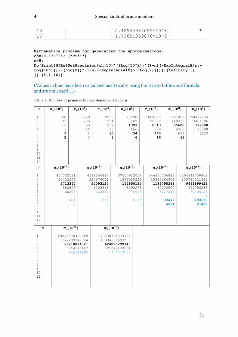
Mathematica program for generating the approximations:
ch=10.131795; (*Pi5!*)
n=5;
Do[Print[N[Re[SetPrecision[ch,50]*((Log[10^i])^(1-n)(-ExpIntegralE[n,-
Log[10^i]])-(Log[2])^(1-n)(-ExpIntegralE[n,-Log[2]]))],{Infinity,3}
]],{i,1,16}]
(Values in blue have been calculated analytically using the Hardy-Littlewood formula
and are not exact!…)
Table 6. Number of prime n-tuplets dependent upon n
𝒏
1
2
3
4
5
6
7
8
9
10
11
12
𝝅𝒏(𝟏𝟎𝟑)
168
35
15
5
3
2
𝝅𝒏(𝟏𝟎𝟒)
1229
205
55
12
4
3
𝝅𝒏(𝟏𝟎𝟓)
9592
1224
259
38
10
3
𝝅𝒏(𝟏𝟎𝟔)
78498
8169
1393
166
34
6
𝝅𝒏(𝟏𝟎𝟕)
664579
58980
8543
899
160
16
𝝅𝒏(𝟏𝟎𝟖)
5761455
440312
55600
4768
697
63
𝝅𝒏(𝟏𝟎𝟗)
50847534
3424506
379508
28388
3633
𝒏
1
2
3
4
5
6
7
8
9
10
11
12
𝝅𝒏(𝟏𝟎𝟏𝟎)
455052511
27412679
2713347
180529
20203
?
424
?
𝝅𝒏(𝟏𝟎𝟏𝟏)
4118054813
224376048
20093124
1209318
122857
?
1334
?
𝝅𝒏(𝟏𝟎𝟏𝟐)
37607912018
1870585220
152850135
8398278
776698
?
6185
?
𝝅𝒏(𝟏𝟎𝟏𝟑)
346065536839
15834664872
1189795268
60070590
5107243
?
33412
4601
𝝅𝒏(𝟏𝟎𝟏𝟒)
3204941750802
135780321665
9443899421
441296836
34706125
?
193160
21405
𝒏
1
2
3
4
5
6
7
8
9
10
11
𝝅𝒏(𝟏𝟎𝟏𝟓)
29844570422669
1177209242304
76218094021
3314576487
242544985
𝝅𝒏(𝟏𝟎𝟏𝟔)
279238341033925
10304195697298
624026299748
25379433651
1736513596
Correlations of the last digits in the prime number sequence
32
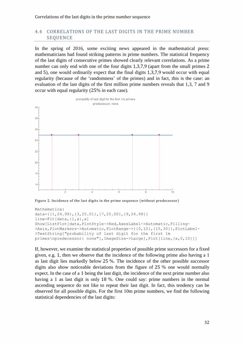
4.4 CORRELATIONS OF THE LAST DIGITS IN THE PRIME NUMBER SEQUENCE
In the spring of 2016, some exciting news appeared in the mathematical press:
mathematicians had found striking patterns in prime numbers. The statistical frequency
of the last digits of consecutive primes showed clearly relevant correlations. As a prime
number can only end with one of the four digits 1,3,7,9 (apart from the small primes 2
and 5), one would ordinarily expect that the final digits 1,3,7,9 would occur with equal
regularity (because of the ‘randomness’ of the primes) and in fact, this is the case: an
evaluation of the last digits of the first million prime numbers reveals that 1,3, 7 and 9
occur with equal regularity (25% in each case).
Figure 2. Incidence of the last digits in the prime sequence (without predecessor)
Mathematica:
data={{1,24.99},{3,25.01},{7,25.00},{9,24.99}}
line=Fit[data,{1,x},x]
Show[ListPlot[data,PlotStyle->Red,AxesLabel->Automatic,Filling-
>Axis,PlotMarkers->Automatic,PlotRange->{{0,10},{15,30}},PlotLabel-
>TextString["probability of last digit for the first 1m
primes\npredecessor: none"],ImageSize->Large],Plot[line,{x,0,10}]]
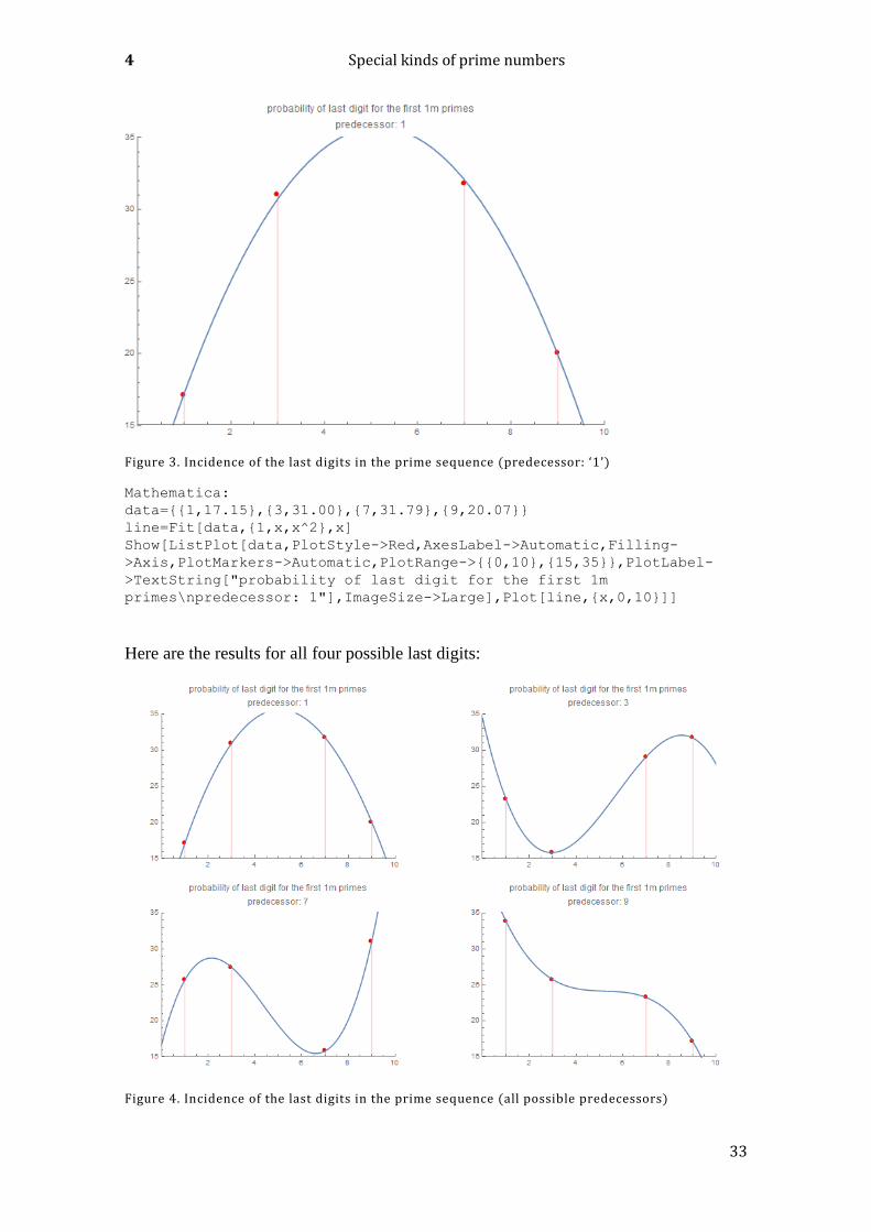
If, however, we examine the statistical properties of possible prime successors for a fixed
given, e.g. 1, then we observe that the incidence of the following prime also having a 1
as last digit lies markedly below 25 %. The incidence of the other possible successor
digits also show noticeable deviations from the figure of 25 % one would normally
expect. In the case of a 1 being the last digit, the incidence of the next prime number also
having a 1 as last digit is only 18 %. One could say: prime numbers in the normal
ascending sequence do not like to repeat their last digit. In fact, this tendency can be
observed for all possible digits. For the first 10m prime numbers, we find the following
statistical dependencies of the last digits:
4 Special kinds of prime numbers
33
Figure 3. Incidence of the last digits in the prime sequence (predecessor: ‘1’)
Mathematica:
data={{1,17.15},{3,31.00},{7,31.79},{9,20.07}}
line=Fit[data,{1,x,x^2},x]
Show[ListPlot[data,PlotStyle->Red,AxesLabel->Automatic,Filling-
>Axis,PlotMarkers->Automatic,PlotRange->{{0,10},{15,35}},PlotLabel-
>TextString["probability of last digit for the first 1m
primes\npredecessor: 1"],ImageSize->Large],Plot[line,{x,0,10}]]
Here are the results for all four possible last digits:
Figure 4. Incidence of the last digits in the prime sequence (all possible predecessors)

Mersenne prime numbers
34
Mathematica:
(programs see Appendix).
One may wonder what these statistical anomalies look like, if even more preceding primes
are included in this exploration. The results, if not only predecessors are included but also
pre-predecessors, can be found in the Appendix (Chapter 20.1).
These correlations of the last digits of consecutive primes do not appear exclusively in
the decimal system. They appear also in representations of systems having different
number bases (e.g. the binary system).
More refined examinations which have been carried out in the meantime have shown that
the observed correlations are a direct consequence of the (yet unproven) Hardy-
Littlewood formula (see Formula (14) in Chapter 4.3). The observation that these
correlations are becoming weaker if we examine prime sequences in very high regions is
also a consequence of the Hardy-Littlewood conjecture. Probably the anomalies will
steadily disappear if the tests are performed in arbitrarily high number regions. These
regions must, however, be very high – probably astronomically high – because the
anomalies tend to thin out only very gradually.
The slow pace of this thinning-out-process is actually the only strange thing in this story.
4.5 MERSENNE PRIME NUMBERS
There are a vast number of publications dealing with Mersenne prime numbers. In this
book, we will only mention some of the more important and interesting formulae and
statements:
Currently 51 Mersenne prime numbers are known (as of Dec. 2020). Many questions
about Mersenne primes still remain open (see 3.2 Basics of prime numbers).
Mersenne prime numbers have the form 𝑀𝑛 = 2𝑝 − 1 with 𝑝 necessarily being a prime
number. However, not every prime number 𝑝 in this term gives a Mersenne prime 𝑀𝑛.
Mersenne primes are very rare, and searching for them is a little bit like searching for
gems among the numbers. The largest known prime numbers are all Mersenne primes.
That is because for this type of prime there exists a very fast primality test that makes it
possible to test even gigantic numbers for primality. The largest currently known prime
number is the Mersenne prime number 282589933 -1. It has 24862048 digits when
expressed using the decimal number system (as of Dec. 2020).
The fastest test for Mersenne primes is the Lucas-Lehmer Test8, which is refined by
combination with other methods. A primality test for a number of this order of magnitude
needs approx. one month of computing time, if performed on a fast PC with 4 CPU
kernels (as of Oct. 2015). The Lucas-Lehmer test and the involved factorizing methods
8 https://de.wikipedia.org/wiki/Lucas-Lehmer-Test

4 Special kinds of prime numbers
35
(P1 test and trial factoring) have been documented and described many times in detail
and need not be explained here. 9
The 51 currently known Mersenne prime exponents are (as of Dec. 2020):
𝟐, 𝟑, 𝟓, 𝟕, 𝟏𝟑, 𝟏𝟕, 𝟏𝟗, 𝟑𝟏, 𝟔𝟏, 𝟖𝟗, 𝟏𝟎𝟕, 𝟏𝟐𝟕, 𝟓𝟐𝟏, 𝟔𝟎𝟕, 𝟏𝟐𝟕𝟗, 𝟐𝟐𝟎𝟑, 𝟐𝟐𝟖𝟏, 𝟑𝟐𝟏𝟕, 𝟒𝟐𝟓𝟑, 𝟒𝟒𝟐𝟑, 𝟗𝟔𝟖𝟗, 𝟗𝟗𝟒𝟏, 𝟏𝟏𝟐𝟏𝟑, 𝟏𝟗𝟗𝟑𝟕, 𝟐𝟏𝟕𝟎𝟏, 𝟐𝟑𝟐𝟎𝟗, 𝟒𝟒𝟒𝟗𝟕, 𝟖𝟔𝟐𝟒𝟑, 𝟏𝟏𝟎𝟓𝟎𝟑, 𝟏𝟑𝟐𝟎𝟒𝟗, 𝟐𝟏𝟔𝟎𝟗𝟏, 𝟕𝟓𝟔𝟖𝟑𝟗, 𝟖𝟓𝟗𝟒𝟑𝟑, 𝟏𝟐𝟓𝟕𝟕𝟖𝟕, 𝟏𝟑𝟗𝟖𝟐𝟔𝟗, 𝟐𝟗𝟕𝟔𝟐𝟐𝟏, 𝟑𝟎𝟐𝟏𝟑𝟕𝟕, 𝟔𝟗𝟕𝟐𝟓𝟗𝟑, 𝟏𝟑𝟒𝟔𝟔𝟗𝟏𝟕, 𝟐𝟎𝟗𝟗𝟔𝟎𝟏𝟏, 𝟐𝟒𝟎𝟑𝟔𝟓𝟖𝟑, 𝟐𝟓𝟗𝟔𝟒𝟗𝟓𝟏, 𝟑𝟎𝟒𝟎𝟐𝟒𝟓𝟕, 𝟑𝟐𝟓𝟖𝟐𝟔𝟓𝟕, 𝟑𝟕𝟏𝟓𝟔𝟔𝟔𝟕, 𝟒𝟐𝟔𝟒𝟑𝟖𝟎𝟏, 𝟒𝟑𝟏𝟏𝟐𝟔𝟎𝟗 𝟓𝟕𝟖𝟖𝟓𝟏𝟔𝟏, 𝟕𝟒𝟐𝟎𝟕𝟐𝟖𝟏, 𝟕𝟕𝟐𝟑𝟐𝟗𝟏𝟕, 𝟖𝟐𝟓𝟖𝟗𝟗𝟑𝟑 Mathematica program for creating Mersenne prime numbers:
Flatten[Position[EulerPhi[2^#-]+2==EulerPhi[2^#]&/@Range[1,100],True]-
1]
The range of the first 48 Mersenne prime numbers has been exhaustively tested. The
indices of the Four last numbers (49 to 51) are still uncertain, i.e. it may be possible that
in this region more Mersenne primes could be discovered.
(sequence A000043 in OEIS) (as of Dec. 2020)
Unresolved questions about Mersenne prime numbers
Are there infinitely many Mersenne prime numbers? Everything indicates that the answer
is ‘yes’.
Is the ‘new Mersenne conjecture’ true ‘?
This states that, if any two of the following conditions hold, then the third condition is
also true:
1) 𝑛 = 2𝑘 ± 1 or 𝑛 = 4𝑘 ± 3
2) 2𝑛 − 1 is a prime (obviously a Mersenne prime)
3) (2𝑛+1)
3is a prime
Are there infinitely many composite Mersenne numbers? Probably: yes.
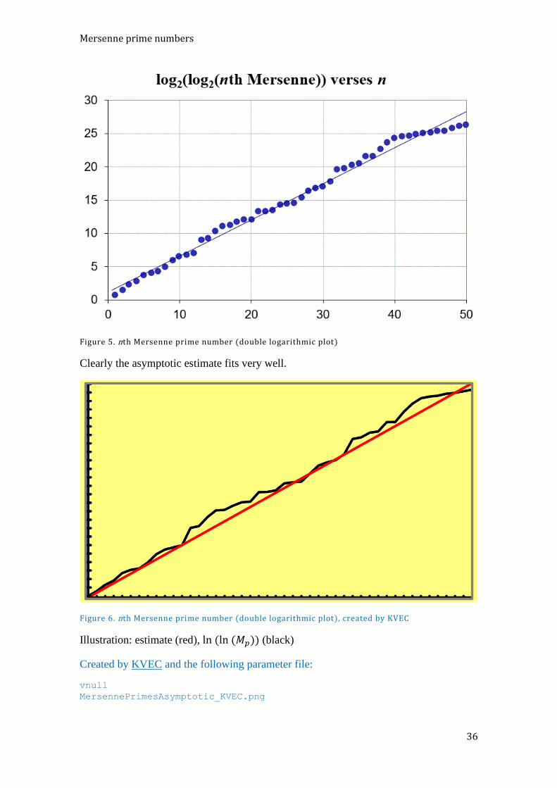
The number 𝑁𝑀𝑝 of Mersenne prime numbers that are less than or equal to 𝑁 is
asymptotically:
𝑵𝑴𝒑(𝑵) ~𝒆𝜸
𝐥𝐧 (𝟐)𝐥𝐧 𝐥𝐧 (𝑵) (17)
Graph:10
9 http://www.mersenne.org/various/math.php 10 http://primes.utm.edu/notes/faq/NextMersenne.html
Mersenne prime numbers
36
Figure 5. nth Mersenne prime number (double logarithmic plot)
Clearly the asymptotic estimate fits very well.
Figure 6. nth Mersenne prime number (double logarithmic plot), created by KVEC
Illustration: estimate (red), ln (ln (𝑀𝑝)) (black)
Created by KVEC and the following parameter file:
vnull
MersennePrimesAsymptotic_KVEC.png
4 Special kinds of prime numbers
37
-antialias 2 -dimension 1024 -xdim 1025 -ydim 576
-format png -xmin 0.000000 -xmax 45.000000
-drcolor 0 0 0 -bkcolor 255 255 128 -nstep 2000 -lwidth 200
-scmode 2 -mode aniso -reduce all -smooth on
function
imin 0; imax 51; drcolor 0 0 0;
f1(x)=log(KV_MPRIMES[x])/M_LN2;
drcolor 255 0 0;
f2(x)=exp(-M_G)*x+0.8255;
endfunc
The few things we know or assume about the analytic mathematics of the Mersenne prime
are documented in detail here: http://primes.utm.edu/notes/faq/
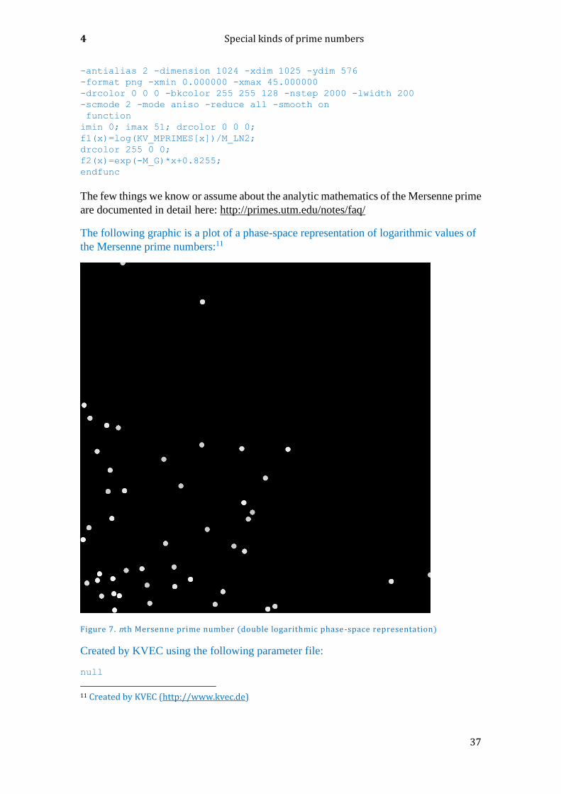
The following graphic is a plot of a phase-space representation of logarithmic values of
the Mersenne prime numbers:11
Figure 7. nth Mersenne prime number (double logarithmic phase-space representation)
Created by KVEC using the following parameter file:
null
11 Created by KVEC (http://www.kvec.de)
Mersenne prime numbers
38
Mersenne_Exponents_In_PhaseSpace.png
-antialias 2 -dimension 1024 -format png -mode aniso -random 24 703
Are there symmetric structures inside? What will this image look like if we take 100 or
1000 Mersenne primes instead of only 51 Mersenne primes?
KVEC-program for creating the first 50 Mersenne prime numbers:
vnull
(null).swf
-debug plot –function imax 51; f1(i)=KV_MPRIMES[i]; endfunc
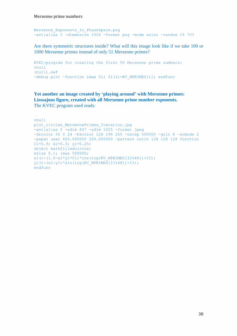
Yet another an image created by ‘playing around’ with Mersenne primes:
Lisssajous figure, created with all Mersenne prime number exponents.
The KVEC program used reads:
vnull
plot_circles_MersennePrimes_Iteration.jpg
-antialias 2 -xdim 847 -ydim 1025 -format jpeg
-drcolor 50 0 24 -bkcolor 128 196 255 -nstep 500000 -grit 8 -scmode 2
-paper user 600.000000 200.000000 -pattern outin 128 128 128 function
C1=0.9; x1=0.5; y1=0.25;
object markfilledcircle;
msize 0.1; imax 500000;
x1()=(1.0-x1*y1*C1)*cos(log(KV_MPRIMES[II%48])+II);
y1()=(x1-y1)*sin(log(KV_MPRIMES[II%48])-II);
endfunc
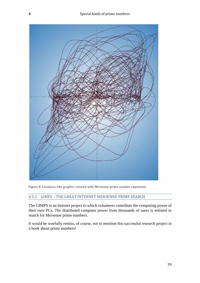
4 Special kinds of prime numbers
39
Figure 8. Lissajous-like graphic, created with Mersenne prime number exponents
4.5.1 GIMPS – THE GREAT INTERNET MERSENNE PRIME SEARCH
The GIMPS is an Internet project to which volunteers contribute the computing power of
their own PCs. The distributed computer power from thousands of users is enlisted to
search for Mersenne prime numbers.
It would be woefully remiss, of course, not to mention this successful research project in
a book about prime numbers!
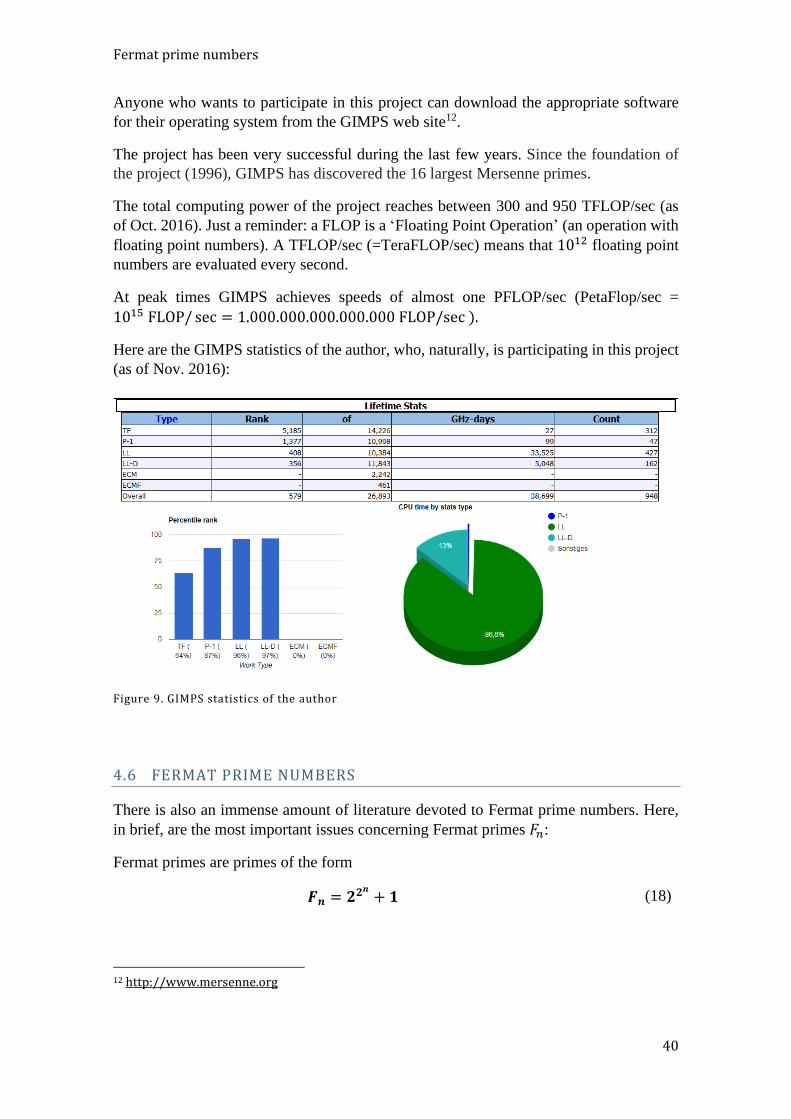
Fermat prime numbers
40
Anyone who wants to participate in this project can download the appropriate software
for their operating system from the GIMPS web site12.
The project has been very successful during the last few years. Since the foundation of
the project (1996), GIMPS has discovered the 16 largest Mersenne primes.
The total computing power of the project reaches between 300 and 950 TFLOP/sec (as
of Oct. 2016). Just a reminder: a FLOP is a ‘Floating Point Operation’ (an operation with
floating point numbers). A TFLOP/sec (=TeraFLOP/sec) means that 1012 floating point
numbers are evaluated every second.
At peak times GIMPS achieves speeds of almost one PFLOP/sec (PetaFlop/sec =
1015 FLOP/ sec = 1.000.000.000.000.000 FLOP/sec ).
Here are the GIMPS statistics of the author, who, naturally, is participating in this project
(as of Nov. 2016):
Figure 9. GIMPS statistics of the author
4.6 FERMAT PRIME NUMBERS
There is also an immense amount of literature devoted to Fermat prime numbers. Here,
in brief, are the most important issues concerning Fermat primes 𝐹𝑛:
Fermat primes are primes of the form
𝑭𝒏 = 𝟐𝟐𝒏 + 𝟏 (18)
12 http://www.mersenne.org
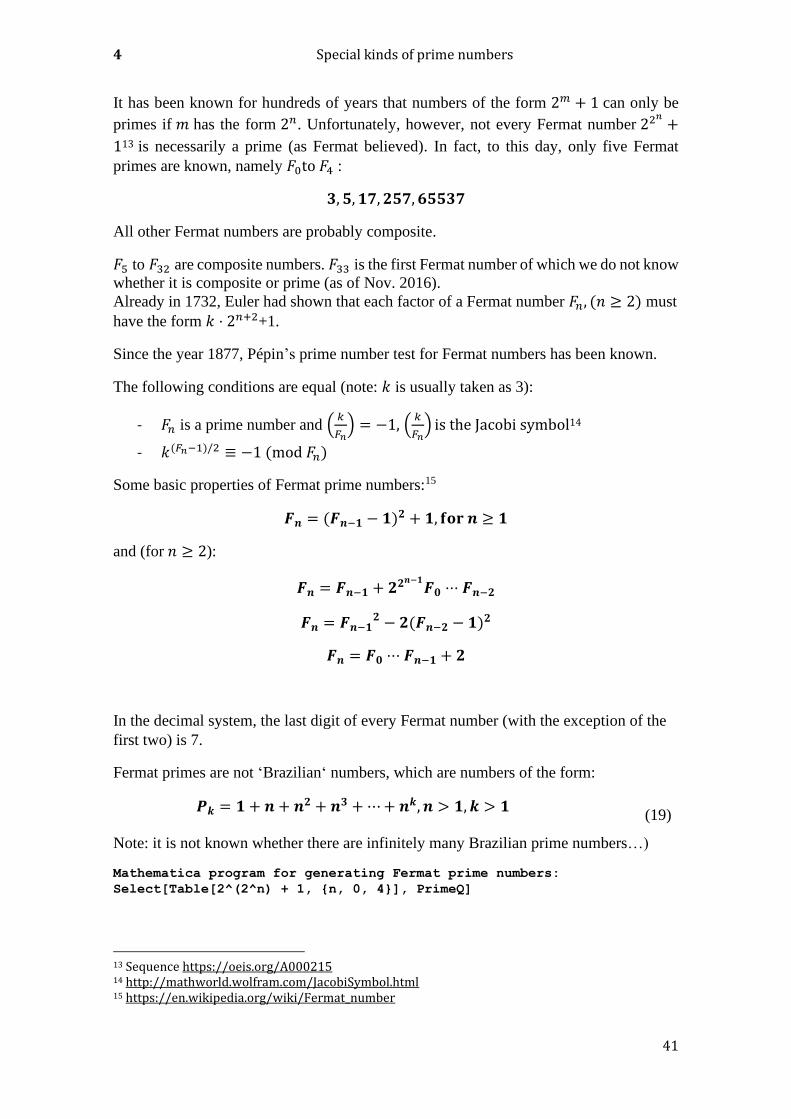
4 Special kinds of prime numbers
41
It has been known for hundreds of years that numbers of the form 2𝑚 + 1 can only be
primes if 𝑚 has the form 2𝑛. Unfortunately, however, not every Fermat number 22𝑛+
113 is necessarily a prime (as Fermat believed). In fact, to this day, only five Fermat
primes are known, namely 𝐹0to 𝐹4 :
𝟑, 𝟓, 𝟏𝟕, 𝟐𝟓𝟕, 𝟔𝟓𝟓𝟑𝟕
All other Fermat numbers are probably composite.
𝐹5 to 𝐹32 are composite numbers. 𝐹33 is the first Fermat number of which we do not know
whether it is composite or prime (as of Nov. 2016).
Already in 1732, Euler had shown that each factor of a Fermat number 𝐹𝑛, (𝑛 ≥ 2) must
have the form 𝑘 ⋅ 2𝑛+2+1.
Since the year 1877, Pépin’s prime number test for Fermat numbers has been known.
The following conditions are equal (note: 𝑘 is usually taken as 3):
- 𝐹𝑛 is a prime number and (𝑘
𝐹𝑛) = −1, (
𝑘
𝐹𝑛) is the Jacobi symbol14
- 𝑘(𝐹𝑛−1)/2 ≡ −1 (mod 𝐹𝑛)
Some basic properties of Fermat prime numbers:15
𝑭𝒏 = (𝑭𝒏−𝟏 − 𝟏)𝟐 + 𝟏, 𝐟𝐨𝐫 𝒏 ≥ 𝟏
and (for 𝑛 ≥ 2):
𝑭𝒏 = 𝑭𝒏−𝟏 + 𝟐𝟐𝒏−𝟏𝑭𝟎 ⋅⋅⋅ 𝑭𝒏−𝟐
𝑭𝒏 = 𝑭𝒏−𝟏𝟐 − 𝟐(𝑭𝒏−𝟐 − 𝟏)
𝟐
𝑭𝒏 = 𝑭𝟎 ⋅⋅⋅ 𝑭𝒏−𝟏 + 𝟐
In the decimal system, the last digit of every Fermat number (with the exception of the
first two) is 7.
Fermat primes are not ‘Brazilian‘ numbers, which are numbers of the form:
𝑷𝒌 = 𝟏 + 𝒏 + 𝒏𝟐 + 𝒏𝟑 +⋯+ 𝒏𝒌, 𝒏 > 𝟏, 𝒌 > 𝟏
(19)
Note: it is not known whether there are infinitely many Brazilian prime numbers…)
Mathematica program for generating Fermat prime numbers:
Select[Table[2^(2^n) + 1, {n, 0, 4}], PrimeQ]
13 Sequence https://oeis.org/A000215 14 http://mathworld.wolfram.com/JacobiSymbol.html 15 https://en.wikipedia.org/wiki/Fermat_number
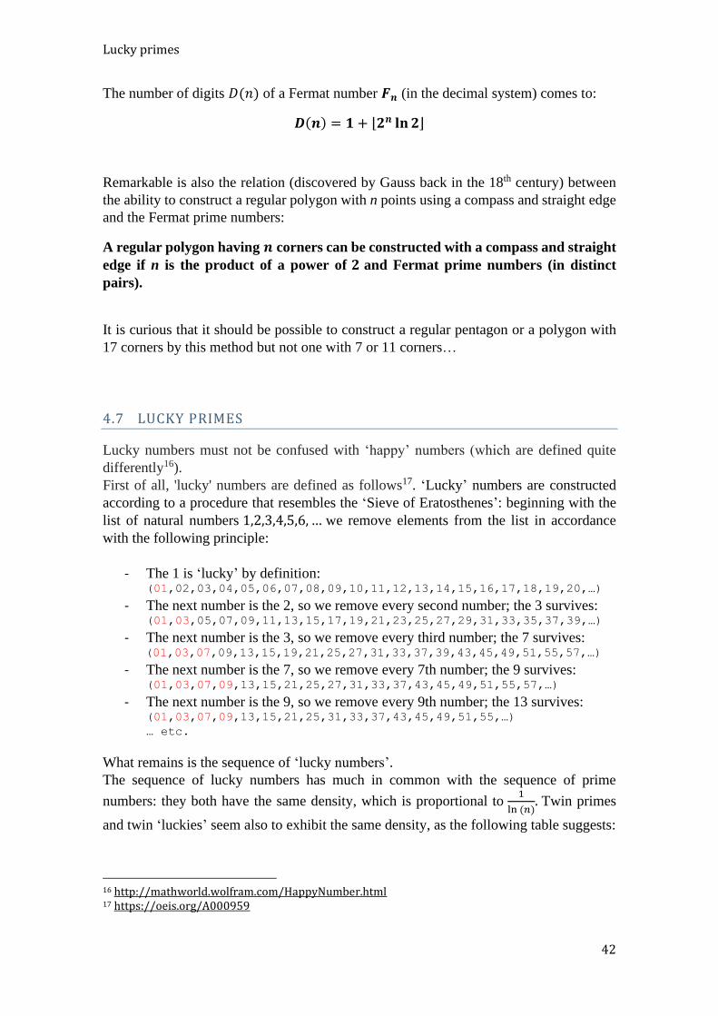
Lucky primes
42
The number of digits 𝐷(𝑛) of a Fermat number 𝑭𝒏 (in the decimal system) comes to:
𝑫(𝒏) = 𝟏 + ⌊𝟐𝒏 𝐥𝐧 𝟐⌋
Remarkable is also the relation (discovered by Gauss back in the 18th century) between
the ability to construct a regular polygon with n points using a compass and straight edge
and the Fermat prime numbers:
A regular polygon having 𝒏 corners can be constructed with a compass and straight
edge if n is the product of a power of 𝟐 and Fermat prime numbers (in distinct
pairs).
It is curious that it should be possible to construct a regular pentagon or a polygon with
17 corners by this method but not one with 7 or 11 corners…
4.7 LUCKY PRIMES
Lucky numbers must not be confused with ‘happy’ numbers (which are defined quite
differently16).
First of all, 'lucky' numbers are defined as follows17. ‘Lucky’ numbers are constructed
according to a procedure that resembles the ‘Sieve of Eratosthenes’: beginning with the
list of natural numbers 1,2,3,4,5,6, … we remove elements from the list in accordance
with the following principle:
- The 1 is ‘lucky’ by definition: (01,02,03,04,05,06,07,08,09,10,11,12,13,14,15,16,17,18,19,20,…)
- The next number is the 2, so we remove every second number; the 3 survives: (01,03,05,07,09,11,13,15,17,19,21,23,25,27,29,31,33,35,37,39,…)
- The next number is the 3, so we remove every third number; the 7 survives: (01,03,07,09,13,15,19,21,25,27,31,33,37,39,43,45,49,51,55,57,…)
- The next number is the 7, so we remove every 7th number; the 9 survives: (01,03,07,09,13,15,21,25,27,31,33,37,43,45,49,51,55,57,…)
- The next number is the 9, so we remove every 9th number; the 13 survives: (01,03,07,09,13,15,21,25,31,33,37,43,45,49,51,55,…)
… etc.
What remains is the sequence of ‘lucky numbers’.
The sequence of lucky numbers has much in common with the sequence of prime
numbers: they both have the same density, which is proportional to 1
ln (𝑛). Twin primes
and twin ‘luckies’ seem also to exhibit the same density, as the following table suggests:
16 http://mathworld.wolfram.com/HappyNumber.html 17 https://oeis.org/A000959
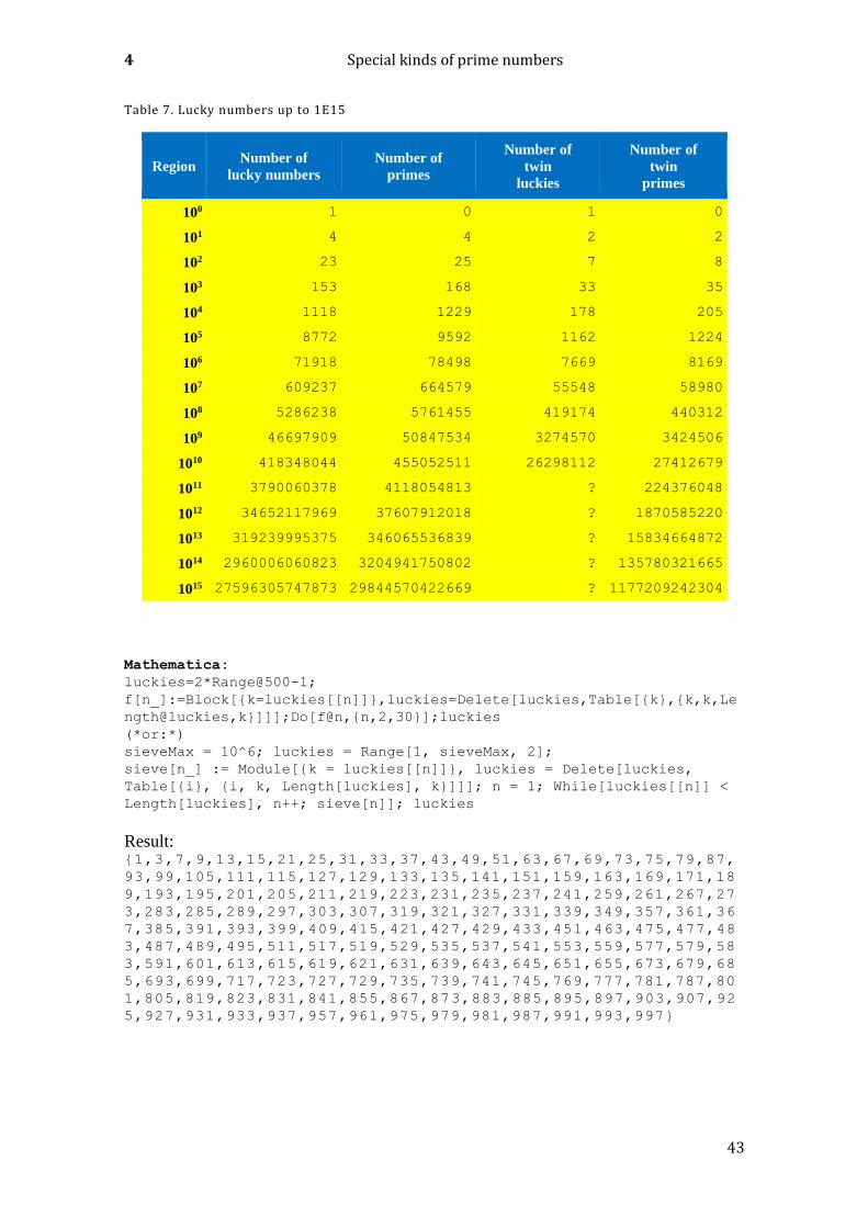
4 Special kinds of prime numbers
43
Table 7. Lucky numbers up to 1E15
Region Number of
lucky numbers
Number of
primes
Number of
twin
luckies
Number of
twin
primes
100 1 0 1 0
101 4 4 2 2
102 23 25 7 8
103 153 168 33 35
104 1118 1229 178 205
105 8772 9592 1162 1224
106 71918 78498 7669 8169
107 609237 664579 55548 58980
108 5286238 5761455 419174 440312
109 46697909 50847534 3274570 3424506
1010 418348044 455052511 26298112 27412679
1011 3790060378 4118054813 ? 224376048
1012 34652117969 37607912018 ? 1870585220
1013 319239995375 346065536839 ? 15834664872
1014 2960006060823 3204941750802 ? 135780321665
1015 27596305747873 29844570422669 ? 1177209242304
Mathematica:
luckies=2*Range@500-1;
f[n_]:=Block[{k=luckies[[n]]},luckies=Delete[luckies,Table[{k},{k,k,Le
ngth@luckies,k}]]];Do[f@n,{n,2,30}];luckies
(*or:*)
sieveMax = 10^6; luckies = Range[1, sieveMax, 2];
sieve[n_] := Module[{k = luckies[[n]]}, luckies = Delete[luckies,
Table[{i}, {i, k, Length[luckies], k}]]]; n = 1; While[luckies[[n]] <
Length[luckies], n++; sieve[n]]; luckies
Result: {1,3,7,9,13,15,21,25,31,33,37,43,49,51,63,67,69,73,75,79,87,
93,99,105,111,115,127,129,133,135,141,151,159,163,169,171,18
9,193,195,201,205,211,219,223,231,235,237,241,259,261,267,27
3,283,285,289,297,303,307,319,321,327,331,339,349,357,361,36
7,385,391,393,399,409,415,421,427,429,433,451,463,475,477,48
3,487,489,495,511,517,519,529,535,537,541,553,559,577,579,58
3,591,601,613,615,619,621,631,639,643,645,651,655,673,679,68
5,693,699,717,723,727,729,735,739,741,745,769,777,781,787,80
1,805,819,823,831,841,855,867,873,883,885,895,897,903,907,92
5,927,931,933,937,957,961,975,979,981,987,991,993,997}
Perfect numbers
44
Please note: this type of ‘lucky’ number must also not be confused with Euler’s ‘lucky’
numbers (prime numbers 𝑛 of the form 𝑚2 −𝑚 + 𝑛 such that 𝑚2 −𝑚 + 𝑛 gives a
prime number, for 𝑚 = 0,1,… , 𝑛 − 1).
The set of ‘lucky’ primes is simply the set of ‘lucky’ numbers that are prime.18 It is not
known if there are infinitely many ‘lucky’ prime numbers (as of Oct. 2015).
4.8 PERFECT NUMBERS
4.8.1 GENERAL ISSUES AND DEFINITION
Perfect numbers are closely related to Mersenne prime numbers (see Chapter 4.5).
Definition
A (positive whole) number is perfect if it is identical to the sum of its divisors (where the
number itself is excluded as a divisor). This sum of divisors is often called the aliquot
sum 𝑆(𝑛), in contrast to the complete sum of divisors 𝜎1(𝑛), for which the number itself
is also included in the sum. From this, it follows that:
a number is perfect if 𝑺(𝒏) = 𝒏 or 𝝈𝟏(𝒏) = 𝟐𝒏 (20)
Perfect numbers have been well known since antiquity (Nicomachus19, Philo Judaeus20)
(the four numbers 𝟔, 𝟐𝟖, 𝟒𝟗𝟔, 𝟖𝟏𝟐𝟖) and were already mentioned in the ‘Elements’ of
the ancient Greek mathematician Euclid. Probably the name comes from the idea that
God created the world in 6 days, as well as the fact that the moon’s orbit has a duration
of 28 days.
There are as many known perfect numbers as known Mersenne prime numbers (as of
Dec. 2020). The first 10 are21:
18 https://oeis.org/A031157 19 Nicomachus (60 – 120 n. Chr.), antique philosopher, musical theorist and mathematician 20 Philo Judaeus: (25-50 n. Chr.), Greek-Jewish philosopher, lived in Alexandria 21 https://en.wikipedia.org/wiki/Perfect_number

4 Special kinds of prime numbers
45
Table 8. The first 10 perfect numbers
n Perfect numbers
1 6
2 28
3 496
4 8128
5 33550336
6 8589869056
7 137438691328
8 2305843008139952128
9 2658455991569831744654692615953842176
10 191561942608236107294793378084303638130997321548169216
All known perfect numbers are related to the Mersenne prime numbers (the proof
originated from Euler, 18th century).
If 𝟐𝒑 − 𝟏 𝐢𝐬 𝐩𝐫𝐢𝐦𝐞, 𝐭𝐡𝐞𝐧 𝟐𝒑−𝟏(𝟐𝒑 − 𝟏) 𝐢𝐬 𝐚 𝐩𝐞𝐫𝐟𝐞𝐜𝐭 𝐧𝐮𝐦𝐛𝐞𝐫. (21)
All currently known perfect numbers are even. There are 51 perfect numbers known (as
of Dec. 2020). It is unknown if any odd perfect numbers exist. Probably there are
infinitely many perfect numbers (as there are also probably infinitely many Mersenne
primes).
Perfect numbers also occur in numerology and mysticism.
4.8.2 PROPERTIES
Each even perfect number can be represented as follows:
𝑛 = 1 +9
2𝑘(𝑘 + 1), (where 𝑘 = 8𝑗 + 2, 𝑗 > 0 and 𝑛 > 6) (22)
The converse does not apply! One does not obtain a perfect number for each 𝑗…
For j= 1, 2, … we obtain: 28, 496, 1540, 3160, 5356, 8128, 11476, 15400, 19900, …
Only the following 𝑗 will produce perfect numbers:
Mathematica-program for computing the indices that provide perfect
numbers:
MPrimeExp={2,3,5,7,13,17,19,31,61,89,107,127,521,607,1279,2203,2281,32
17,4253,4423,9689,9941,11213,19937,21701,23209,44497,86243,110503,1320
49,216091,756839,859433,1257787,1398269,2976221,3021377,6972593,134669
17,20996011,24036583,25964951,30402457,32582657}
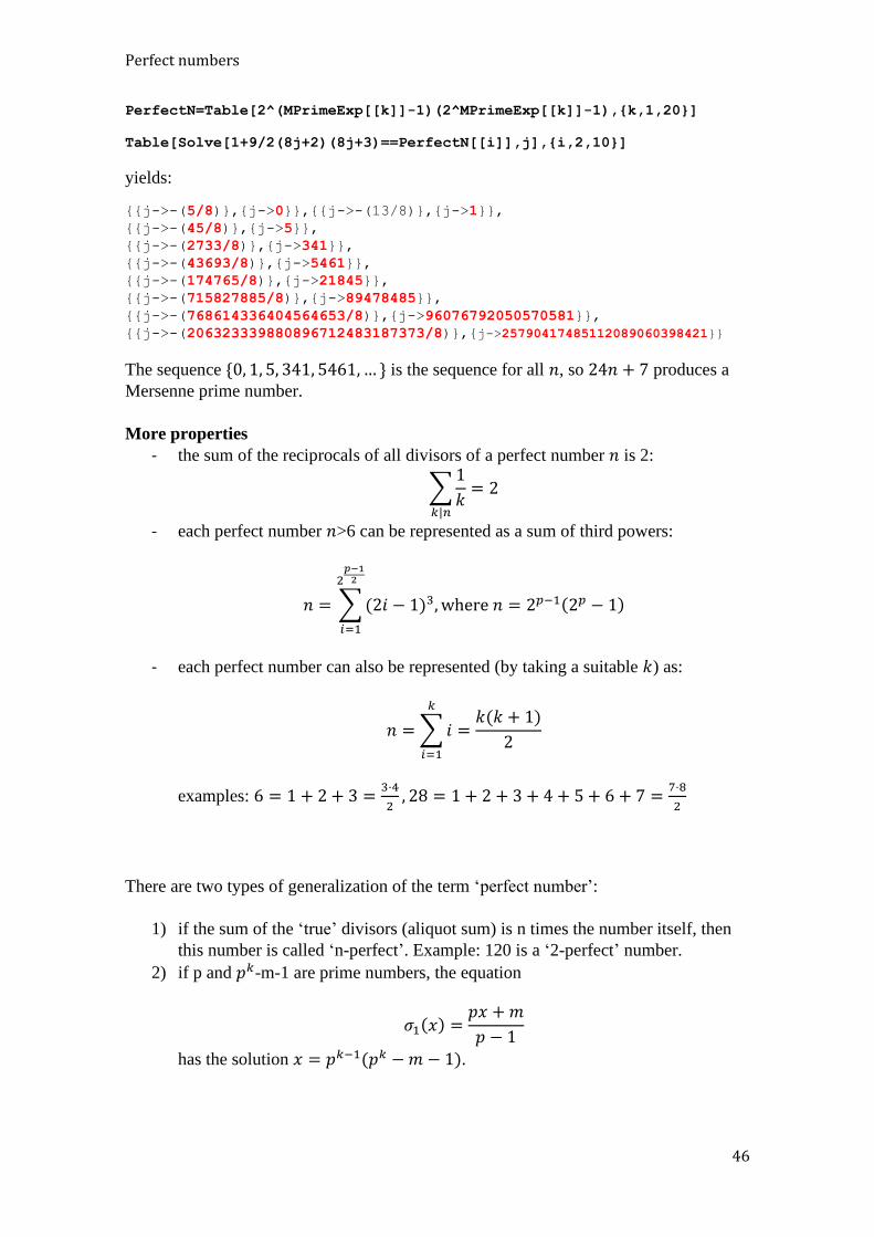
Perfect numbers
46
PerfectN=Table[2^(MPrimeExp[[k]]-1)(2^MPrimeExp[[k]]-1),{k,1,20}]
Table[Solve[1+9/2(8j+2)(8j+3)==PerfectN[[i]],j],{i,2,10}]
yields:
{{j->-(5/8)},{j->0}},{{j->-(13/8)},{j->1}},
{{j->-(45/8)},{j->5}},
{{j->-(2733/8)},{j->341}},
{{j->-(43693/8)},{j->5461}},
{{j->-(174765/8)},{j->21845}},
{{j->-(715827885/8)},{j->89478485}},
{{j->-(768614336404564653/8)},{j->96076792050570581}},
{{j->-(206323339880896712483187373/8)},{j->25790417485112089060398421}}
The sequence {0, 1, 5, 341, 5461,… } is the sequence for all 𝑛, so 24𝑛 + 7 produces a
Mersenne prime number.
More properties
- the sum of the reciprocals of all divisors of a perfect number 𝑛 is 2:
∑1
𝑘= 2
𝑘|𝑛
- each perfect number 𝑛>6 can be represented as a sum of third powers:
𝑛 = ∑(2𝑖 − 1)3, where 𝑛 = 2𝑝−1(2𝑝 − 1)
2𝑝−12
𝑖=1
- each perfect number can also be represented (by taking a suitable 𝑘) as:
𝑛 =∑𝑖
𝑘
𝑖=1
=𝑘(𝑘 + 1)
2
examples: 6 = 1 + 2 + 3 =3⋅4
2, 28 = 1 + 2 + 3 + 4 + 5 + 6 + 7 =
7⋅8
2
There are two types of generalization of the term ‘perfect number’:
1) if the sum of the ‘true’ divisors (aliquot sum) is n times the number itself, then
this number is called ‘n-perfect’. Example: 120 is a ‘2-perfect’ number.
2) if p and 𝑝𝑘-m-1 are prime numbers, the equation
𝜎1(𝑥) =𝑝𝑥 +𝑚
𝑝 − 1
has the solution 𝑥 = 𝑝𝑘−1(𝑝𝑘 −𝑚 − 1).
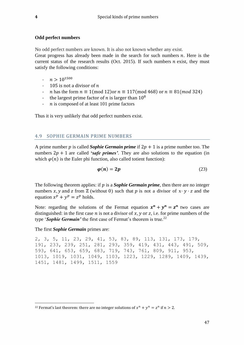
4 Special kinds of prime numbers
47
Odd perfect numbers
No odd perfect numbers are known. It is also not known whether any exist.
Great progress has already been made in the search for such numbers 𝑛. Here is the
current status of the research results (Oct. 2015). If such numbers 𝑛 exist, they must
satisfy the following conditions:
- 𝑛 > 101500 - 105 is not a divisor of 𝑛 - 𝑛 has the form 𝑛 ≡ 1(mod 12)or 𝑛 ≡ 117(mod 468) or 𝑛 ≡ 81(𝑚𝑜𝑑 324) - the largest prime factor of 𝑛 is larger than 108 - 𝑛 is composed of at least 101 prime factors
Thus it is very unlikely that odd perfect numbers exist.
4.9 SOPHIE GERMAIN PRIME NUMBERS
A prime number 𝑝 is called Sophie Germain prime if 2𝑝 + 1 is a prime number too. The
numbers 2𝑝 + 1 are called ‘safe primes’. They are also solutions to the equation (in
which 𝜑(𝑛) is the Euler phi function, also called totient function):
𝝋(𝒏) = 𝟐𝒑 (23)
The following theorem applies: if 𝑝 is a Sophie Germain prime, then there are no integer
numbers 𝑥, 𝑦 and 𝑧 from ℤ (without 0) such that 𝑝 is not a divisor of x⋅ 𝑦 ⋅ 𝑧 and the
equation 𝑥𝑝 + 𝑦𝑝 = 𝑧𝑝 holds.
Note: regarding the solutions of the Fermat equation 𝒙𝒏 + 𝒚𝒏 = 𝒛𝒏 two cases are
distinguished: in the first case 𝑛 is not a divisor of 𝑥, 𝑦 or 𝑧, i.e. for prime numbers of the
type ‘Sophie Germain’ the first case of Fermat’s theorem is true.22
The first Sophie Germain primes are:
2, 3, 5, 11, 23, 29, 41, 53, 83, 89, 113, 131, 173, 179,
191, 233, 239, 251, 281, 293, 359, 419, 431, 443, 491, 509,
593, 641, 653, 659, 683, 719, 743, 761, 809, 911, 953,
1013, 1019, 1031, 1049, 1103, 1223, 1229, 1289, 1409, 1439,
1451, 1481, 1499, 1511, 1559
22 Fermat’s last theorem: there are no integer solutions of 𝑥𝑛 + 𝑦𝑛 = 𝑧𝑛 if 𝑛 > 2.

Sophie Germain prime numbers
48
4.9.1 COMPUTATION AND PROPERTIES
Properties of Sophie Germain primes
1) If 𝑝 > 3 is a Sophie Germain prime and 𝑝 ≡ 3 (mod 4), then 2𝑝 + 1 is a divisor
of the 𝑝th Mersenne number.
2) For all Sophie Germain primes, the following obtains: 𝑝 ≡ 3 (mod 4). 3) If represented in the decimal system, Sophie Germain primes can never have a
last digit of 7.
4) 𝑝 and 2𝑝 + 1 are Sophie Germain primes, if and only if p is a prime and 22𝑝 ≡1(mod 2𝑝 + 1).
The following asymptotic estimate of the number of SG primes up to a limit 𝑁 obtains:
NumberOf𝑆𝐺 = 2𝐶2∫1
ln(𝑥) ln (2𝑥 + 1)𝑑𝑥 ≈
2𝐶2𝑁
ln2(𝑁)
𝑁
2
(24)
(with 𝐶2 = 0,6601618158 being the twin prime constant).
Computation by Mathematica: (e.g. in the interval 1 to 1000):
Select[Prime[Range[1000]], PrimeQ[2#+1]&]
Conjectures
1) There are infinitely many Sophie Germain primes.
2) Between 𝑛 and 2𝑛 there is always at least one Sophie Germain prime.
Record
Currently the largest SG prime has the value:
𝟏𝟖𝟓𝟒𝟑𝟔𝟑𝟕𝟗𝟎𝟎𝟓𝟏𝟓 · 𝟐𝟔𝟔𝟔𝟔𝟔𝟕 – 𝟏
– a number having 200.701 decimal digits (as of Nov. 2016).
Notes: in mathematical literature sequences of SG primes are called Cunningham chains
of the first kind.23
Number 𝑎(𝑛) of SG primes up to 10𝑛:
23 https://de.wikipedia.org/wiki/Cunningham-Kette
49
Table 9. Number of Sophie Germain primes up to 1E12
n a(n)
1 3
2 10
3 37
4 190
5 1171
6 7746
7 56032
8 423140
9 3308859
10 26569515
11 218116524
12 1822848478
Computation by Mathematica (example):
Accumulate[Table[Boole[PrimeQ[n]&&PrimeQ[2n+1]], {n, 1, 200}]]
4.10 FIBONACCI NUMBERS AND OTHER RECURSIVE SEQUENCES
There is an immense amount of literature concerning the Fibonacci numbers. An
overview is not given here. You can find interesting information on Michael Becker's
homepage.24
Only the following formulae are mentioned here (curiosities):
1
𝐹11=
1
89= 0.01123595 (the decimal expansion starts exactly with the Fibonacci
numbers)
(to be more precise, we should actually write):
1
𝐹11=∑
𝐹𝑘10𝑘+1
∞
𝑘=0
(25)
The quotient 𝐹𝑛+1
𝐹𝑛 of two consecutive Fibonacci numbers is the 𝑛th approximation of the
continued fraction:
1 +1
1 +1
1 +1
1 +⋯
(26)
24 http://www.ijon.de/mathe/fibonacci/node2.html#0002320

Fibonacci numbers and other recursive sequences
50
The limit is the number of the Golden Ratio: Φ = 1.618 =1+√5
2.
𝐹12 = 144 = 122
𝐹12 is the only square among the infinitely many Fibonacci numbers. The question arises
as to whether there is some more profound reason for this, because it cannot be the product
of chance… The reason for this actually exists. It appears as a ‘side-product’ in A. Wiles
proof of Fermat’s last theorem. But that is another story ☺…
The following formula is also a curiosity:
⌈𝑒𝑛−12 ⌉ , 𝑛 = 0,1,2…
It yields exactly the first 10 Fibonacci numbers, following each other for 𝑛 = 1, … ,10.
Mathematica: Table[Floor[Exp[(n-1)/2]]+1,{n,1,25}]
{1,1,2,3,5,8,13,21,34,55,91,149,245,404,666,1097,1809,2981,4915,8104,…
}
For practical purposes: the 𝑛th Fibonacci number can be calculated very easily:
𝐹𝑛 = Round (Φ𝑛
√5) (27)
Finally, J. P. Jones showed in the year 1975 that there exists a polynomial of degree 5
with two variables, whose positive integer values are exactly the set of the Fibonacci
numbers (using non-negative arguments). This remarkable fact seems to be more of
theoretical interest, at first glance. After all, the statement can be verified by using the
following Mathematica program:
numbersOfInstances=6;
polynom[x_,y_]:=2x*y^4+x^2*y^3-2x^3*y^2-y^5-x^4*y+2*y;
list=FindInstance[Reduce[polynom[x,y]>0&&x>=0&&y>=0,{x,y},Integers],{x
,y},Integers,numbersOfInstances,RandomSeed->112]
Table[polynom[list[[n]][[1]][[2]],list[[n]][[2]][[2]]],{n,1,Length[lis
t]}]
This strange property is not something the author has seen anywhere described, though
perhaps it has already been noticed.
If we have the following polynomial:
poly𝐹𝑖𝑏(𝑥, 𝑦) = 2𝑥𝑦4 + 𝑥2𝑦3 − 2𝑥3𝑦2 − 𝑦5 − 𝑥4𝑦 + 2𝑦 where 𝑥, 𝑦 ∈ ℕ0
Then
𝐩𝐨𝐥𝐲𝑭𝒊𝒃(𝑭𝒊, 𝑭𝒊+𝟏) = 𝑭𝒊+𝟏 (𝒊 ≥ 𝟎) (28)
i.e. the arguments for which the polynomial yields the (positive) Fibonacci numbers are
precisely the Fibonacci numbers themselves! From this, we get the following equation:
4 Special kinds of prime numbers
51
𝑭𝒊+𝟏 = 2𝑭𝒊𝑭𝒊+𝟏 4 + 𝑭𝒊
2𝑭𝒊+𝟏 3 − 2𝑭𝒊
3𝑭𝒊+𝟏 2 − 𝑭𝒊+𝟏
5 − 𝑭𝒊4𝑭𝒊+𝟏
+ 2𝑭𝒊+𝟏 (29)
Or, in other words, the ‘successor’ 𝑭𝒊+𝟏 in the Fibonacci sequence can be calculated from
the predecessor 𝑭𝒊 by calculating the positive, integer valued solution of this equation of
degree 4, and that all happens without knowing the index 𝑖:
−𝒚4 + 2𝑭𝒊𝒚3 + 𝑭𝒊
2𝒚2 − 2𝑭𝒊3𝒚 + 𝟏 − 𝑭𝒊
4 = 𝟎 (30)
Mathematica example: 𝑓 = 𝐹𝑖 = 8;
Solve[-y^4+2f y^3+f^2y^2-2f^3y+1-f^4==0,y,Integers]
{{y->-5},{y->13}}
The following conjecture is probably easily proved (if it is true…):
(30) always has real solutions for positive 𝑭𝒊. Integer solutions exist only if 𝑭𝒊 is a
Fibonacci number.
Note: this explicit formula can, of course, be used to calculate values of 𝑛 from 𝐹𝑛 (e.g.
using Mathematica) and, by taking 𝑛 + 1 for the explicit formula, the successor 𝐹𝑛+1 of
𝐹𝑛 can be determined (without knowing 𝑛 ). This procedure is, however, very
inconvenient and not as elegant as using the equation of 4th degree (30).
For practical use: the following formula is the fastest one (for 𝑛 > 1):
𝐹𝑛+1 = Round(𝐹𝑛Φ), Φ = 1.618 =1+√5
2 and Round(𝑥) = ⌊𝑥 + 0.5⌋ (31)
For the inverse process, it is also very easy to determine 𝑛:
𝑛 = Round(ln𝐹𝑛 +
ln52
lnΦ) (32)
A simple test to find out whether 𝑛 is a Fibonacci number or not:
𝒏 is a Fibonacci number, if 𝟓𝒏𝟐 + 𝟒 or 𝟓𝒏𝟐 − 𝟒 is a square (more precisely: only
if…).
Finally it should be mentioned that the last digit of the numbers in the Fibonacci sequence
repeats itself with a period of 60 (for the last n digits there also exist periods, whose
lengths grow by a factor of 5 for each additional digit).
The Fibonacci sequence was first mentioned in 450 B.C. in the Chandah-shāstra, a
document written in Sanskrit. It was only, however, through the publication in 1202 of
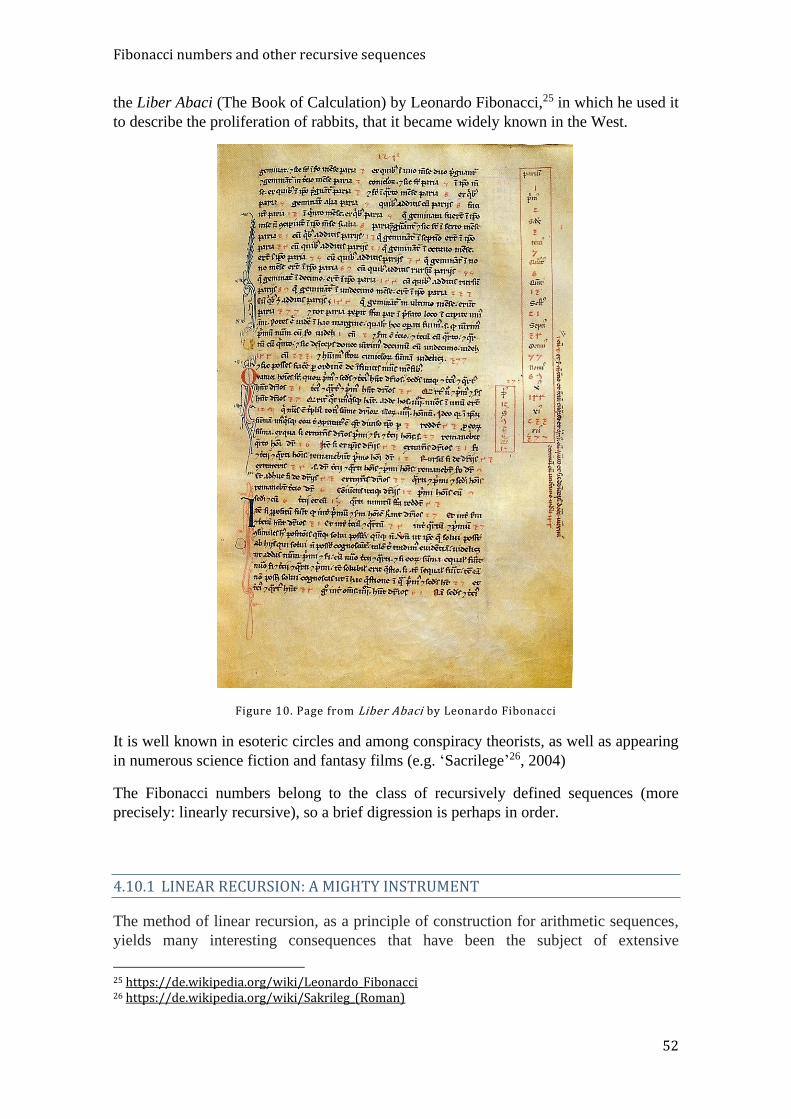
Fibonacci numbers and other recursive sequences
52
the Liber Abaci (The Book of Calculation) by Leonardo Fibonacci,25 in which he used it
to describe the proliferation of rabbits, that it became widely known in the West.
Figure 10. Page from Liber Abaci by Leonardo Fibonacci
It is well known in esoteric circles and among conspiracy theorists, as well as appearing
in numerous science fiction and fantasy films (e.g. ‘Sacrilege’26, 2004)
The Fibonacci numbers belong to the class of recursively defined sequences (more
precisely: linearly recursive), so a brief digression is perhaps in order.
4.10.1 LINEAR RECURSION: A MIGHTY INSTRUMENT
The method of linear recursion, as a principle of construction for arithmetic sequences,
yields many interesting consequences that have been the subject of extensive
25 https://de.wikipedia.org/wiki/Leonardo_Fibonacci 26 https://de.wikipedia.org/wiki/Sakrileg_(Roman)
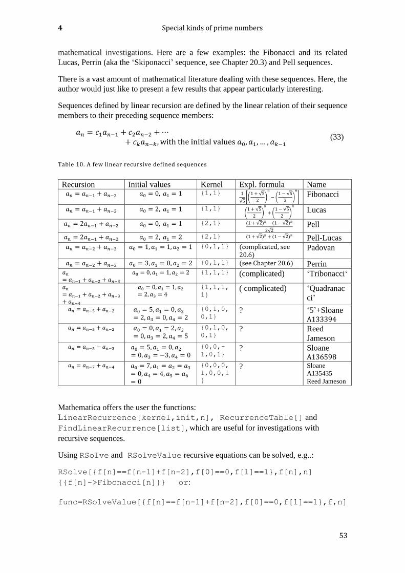
4 Special kinds of prime numbers
53
mathematical investigations. Here are a few examples: the Fibonacci and its related
Lucas, Perrin (aka the ‘Skiponacci’ sequence, see Chapter 20.3) and Pell sequences.
There is a vast amount of mathematical literature dealing with these sequences. Here, the
author would just like to present a few results that appear particularly interesting.
Sequences defined by linear recursion are defined by the linear relation of their sequence
members to their preceding sequence members:
𝑎𝑛 = 𝑐1𝑎𝑛−1 + 𝑐2𝑎𝑛−2 +⋯+ 𝑐𝑘𝑎𝑛−𝑘, with the initial values 𝑎0, 𝑎1, … , 𝑎𝑘−1
(33)
Table 10. A few linear recursive defined sequences
Mathematica offers the user the functions:
LinearRecurrence[kernel,init,n], RecurrenceTable[] and
FindLinearRecurrence[list], which are useful for investigations with
recursive sequences.
Using RSolve and RSolveValue recursive equations can be solved, e.g..:
RSolve[{f[n]==f[n-1]+f[n-2],f[0]==0,f[1]==1},f[n],n]
{{f[n]->Fibonacci[n]}} or:
func=RSolveValue[{f[n]==f[n-1]+f[n-2],f[0]==0,f[1]==1},f,n]
Recursion Initial values Kernel Expl. formula Name 𝑎𝑛 = 𝑎𝑛−1 + 𝑎𝑛−2 𝑎0 = 0, 𝑎1 = 1 {1,1} 1
√5[(1 + √5
2)
𝑛
− (1 − √5
2)
𝑛
] Fibonacci
𝑎𝑛 = 𝑎𝑛−1 + 𝑎𝑛−2 𝑎0 = 2, 𝑎1 = 1 {1,1} (1 + √5
2)
𝑛
+ (1 − √5
2)
𝑛
Lucas
𝑎𝑛 = 2𝑎𝑛−1 + 𝑎𝑛−2 𝑎0 = 0, 𝑎1 = 1 {2,1} (1 + √2)𝑛 − (1 − √2)𝑛
2√2 Pell
𝑎𝑛 = 2𝑎𝑛−1 + 𝑎𝑛−2 𝑎0 = 2, 𝑎1 = 2 {2,1} (1 + √2)𝑛 + (1 − √2)𝑛 Pell-Lucas 𝑎𝑛 = 𝑎𝑛−2 + 𝑎𝑛−3 𝑎0 = 1, 𝑎1 = 1, 𝑎2 = 1 {0,1,1} (complicated, see
20.6) Padovan
𝑎𝑛 = 𝑎𝑛−2 + 𝑎𝑛−3 𝑎0 = 3, 𝑎1 = 0, 𝑎2 = 2 {0,1,1} (see Chapter 20.6) Perrin 𝑎𝑛= 𝑎𝑛−1 + 𝑎𝑛−2 + 𝑎𝑛−3
𝑎0 = 0, 𝑎1 = 1, 𝑎2 = 2 {1,1,1} (complicated) ‘Tribonacci‘
𝑎𝑛= 𝑎𝑛−1 + 𝑎𝑛−2 + 𝑎𝑛−3+ 𝑎𝑛−4
𝑎0 = 0, 𝑎1 = 1, 𝑎2= 2, 𝑎3 = 4
{1,1,1,
1} ( complicated) ‘Quadranac
ci’
𝑎𝑛 = 𝑎𝑛−5 + 𝑎𝑛−2 𝑎0 = 5, 𝑎1 = 0, 𝑎2= 2, 𝑎3 = 0, 𝑎4 = 2
{0,1,0,
0,1} ? ‘5’+Sloane
A133394 𝑎𝑛 = 𝑎𝑛−5 + 𝑎𝑛−2 𝑎0 = 0, 𝑎1 = 2, 𝑎2
= 0, 𝑎3 = 2, 𝑎4 = 5
{0,1,0,
0,1} ? Reed
Jameson 𝑎𝑛 = 𝑎𝑛−5 − 𝑎𝑛−3 𝑎0 = 5, 𝑎1 = 0, 𝑎2
= 0, 𝑎3 = −3, 𝑎4 = 0 {0,0,-
1,0,1} ? Sloane
A136598 𝑎𝑛 = 𝑎𝑛−7 + 𝑎𝑛−4 𝑎0 = 7, 𝑎1 = 𝑎2 = 𝑎3
= 0, 𝑎4 = 4, 𝑎5 = 𝑎6= 0
{0,0,0,
1,0,0,1
}
? Sloane
A135435
Reed Jameson
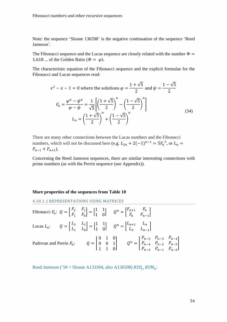
Fibonacci numbers and other recursive sequences
54
Note: the sequence ‘Sloane 136598’ is the negative continuation of the sequence ‘Reed
Jameson’.
The Fibonacci sequence and the Lucas sequence are closely related with the number Φ =1.618… of the Golden Ratio (Φ = 𝜑).
The characteristic equation of the Fibonacci sequence and the explicit formulae for the
Fibonacci and Lucas sequences read:
𝑥2 − 𝑥 − 1 = 0 where the solutions 𝜑 =1 + √5
2 and 𝜓 =
1 − √5
2
𝐹𝑛 =𝜑𝑛 − 𝜓𝑛
𝜑 − 𝜓=1
√5[(1 + √5
2)
𝑛
− (1 − √5
2)
𝑛
]
𝐿𝑛 = (1 + √5
2)
𝑛
+ (1 − √5
2)
𝑛
(34)
There are many other connections between the Lucas numbers and the Fibonacci
numbers, which will not be discussed here (e.g. 𝐿2𝑛 + 2(−1)𝑛−1 = 5𝐹𝑛
2, or 𝐿𝑛 =𝐹𝑛−1 + 𝐹𝑛+1).
Concerning the Reed Jameson sequences, there are similar interesting connections with
prime numbers (as with the Perrin sequence (see Appendix)).
More properties of the sequences from Table 10
4.10.1.1 REPRESENTATIONS USING MATRICES
Fibonacci 𝐹𝑛: 𝑄 = [ 𝐹2 𝐹1 𝐹1 𝐹0
] = [1 11 0
] 𝑄𝑛 = [𝐹𝑛+1 𝐹𝑛𝐹𝑛 𝐹𝑛−1
]
Lucas 𝐿𝑛: 𝑄 = [ 𝐿2 𝐿1 𝐿1 𝐿0
] = [1 11 0
] 𝑄𝑛 = [𝐿𝑛+1 𝐿𝑛𝐿𝑛 𝐿𝑛−1
]
Padovan and Perrin 𝑃𝑛: 𝑄 = [ 0 1 00 0 11 1 0
] 𝑄𝑛 = [ 𝑃𝑛−5 𝑃𝑛−3 𝑃𝑛−4𝑃𝑛−4 𝑃𝑛−2 𝑃𝑛−3𝑃𝑛−3 𝑃𝑛−1 𝑃𝑛−2
]
Reed Jameson (‘5# + Sloane A133394, also A136598) 𝑅𝑆𝑃𝑛, 𝑅𝑆𝑀𝑛:
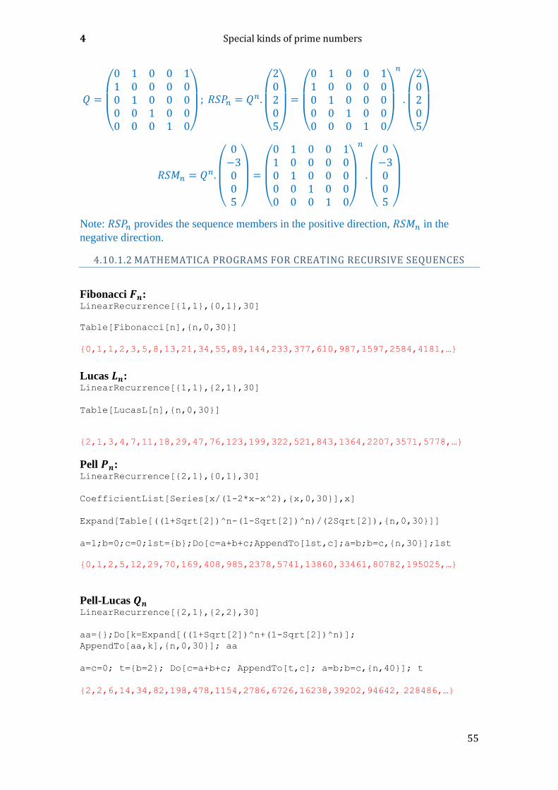
4 Special kinds of prime numbers
55
𝑄 =
(
0 1 0 0 11 0 0 0 00 1 0 0 00 0 1 0 00 0 0 1 0)
; 𝑅𝑆𝑃𝑛 = 𝑄
𝑛.
(
20205)
=
(
0 1 0 0 11 0 0 0 00 1 0 0 00 0 1 0 00 0 0 1 0)
𝑛
.
(
20205)
𝑅𝑆𝑀𝑛 = 𝑄𝑛.
(
0−3005 )
=
(
0 1 0 0 11 0 0 0 00 1 0 0 00 0 1 0 00 0 0 1 0)
𝑛
.
(
0−3005 )
Note: 𝑅𝑆𝑃𝑛 provides the sequence members in the positive direction, 𝑅𝑆𝑀𝑛 in the
negative direction.
4.10.1.2 MATHEMATICA PROGRAMS FOR CREATING RECURSIVE SEQUENCES
Fibonacci 𝑭𝒏: LinearRecurrence[{1,1},{0,1},30]
Table[Fibonacci[n],{n,0,30}]
{0,1,1,2,3,5,8,13,21,34,55,89,144,233,377,610,987,1597,2584,4181,…}
Lucas 𝑳𝒏: LinearRecurrence[{1,1},{2,1},30]
Table[LucasL[n],{n,0,30}]
{2,1,3,4,7,11,18,29,47,76,123,199,322,521,843,1364,2207,3571,5778,…}
Pell 𝑷𝒏: LinearRecurrence[{2,1},{0,1},30]
CoefficientList[Series[x/(1-2*x-x^2),{x,0,30}],x]
Expand[Table[((1+Sqrt[2])^n-(1-Sqrt[2])^n)/(2Sqrt[2]),{n,0,30}]]
a=1;b=0;c=0;lst={b};Do[c=a+b+c;AppendTo[lst,c];a=b;b=c,{n,30}];lst
{0,1,2,5,12,29,70,169,408,985,2378,5741,13860,33461,80782,195025,…}
Pell-Lucas 𝑸𝒏 LinearRecurrence[{2,1},{2,2},30]
aa={};Do[k=Expand[((1+Sqrt[2])^n+(1-Sqrt[2])^n)];
AppendTo[aa,k],{n,0,30}]; aa
a=c=0; t={b=2}; Do[c=a+b+c; AppendTo[t,c]; a=b;b=c,{n,40}]; t
{2,2,6,14,34,82,198,478,1154,2786,6726,16238,39202,94642, 228486,…}
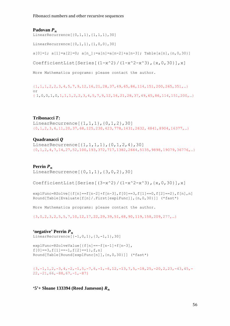
Fibonacci numbers and other recursive sequences
56
Padovan 𝑷𝒏 LinearRecurrence[{0,1,1},{1,1,1},30]
LinearRecurrence[{0,1,1},{1,0,0},30]
a[0]=1; a[1]=a[2]=0; a[n_]:=a[n]=a[n-2]+a[n-3]; Table[a[n],{n,0,30}]
CoefficientList[Series[(1-x^2)/(1-x^2-x^3),{x,0,30}],x]
More Mathematica programs: please contact the author.
{1,1,1,2,2,3,4,5,7,9,12,16,21,28,37,49,65,86,114,151,200,265,351,…} or
{ 1,0,0,1,0,1,1,1,2,2,3,4,5,7,9,12,16,21,28,37,49,65,86,114,151,200,…}
Tribonacci 𝑻: LinearRecurrence[{1,1,1},{0,1,2},30]
{0,1,2,3,6,11,20,37,68,125,230,423,778,1431,2632, 4841,8904,16377,…}
Quadranacci 𝑸 LinearRecurrence[{1,1,1,1},{0,1,2,4},30]
{0,1,2,4,7,14,27,52,100,193,372,717,1382,2664,5135,9898,19079,36776,…}
Perrin 𝑷𝒏 LinearRecurrence[{0,1,1},{3,0,2},30]
CoefficientList[Series[(3-x^2)/(1-x^2-x^3),{x,0,30}],x]
explFunc=RSolve[{f[n]==f[n-2]+f[n-3],f[0]==3,f[1]==0,f[2]==2},f[n],n]
Round[Table[Evaluate[f[n]/.First[explFunc]],{n,0,30}]] (*fast*)
More Mathematica programs: please contact the author.
{3,0,2,3,2,5,5,7,10,12,17,22,29,39,51,68,90,119,158,209,277,…}
‘negative’ Perrin 𝑷𝒏 LinearRecurrence[{-1,0,1},{3,-1,1},30]
explFunc=RSolveValue[{f[n]==-f[n-1]+f[n-3],
f[0]==3,f[1]==-1,f[2]==1},f,n]
Round[Table[Round[explFunc[n]],{n,0,30}]] (*fast*)
{3,-1,1,2,-3,4,-2,-1,5,-7,6,-1,-6,12,-13,7,5,-18,25,-20,2,23,-43,45,-
22,-21,66,-88,67,-1,-87}
‘5’+ Sloane 133394 (Reed Jameson) 𝑹𝒏

4 Special kinds of prime numbers
57
LinearRecurrence[{0,1,0,0,1},{5,0,2,0,2},30] or:
RecurrenceTable[{a[n]==a[n-2]
+a[n-5],a[1]==5,a[2]==0,a[3]==2,a[4]==0,a[5]==2},a,{n,1,30}]
reedJamesonMatrix={{0,1,0,0,1},{1,0,0,0,0},{0,1,0,0,0},{0,0,1,0,0},{0,
0,0,1,0}}; vect={{2},{0},{2},{0},{5}};
Flatten[Table[(MatrixPower[reedJamesonPlusMatrix,n].vect)[[1]],
{n,4-4,100-5}]]
More Mathematica programs: please contact the author.
identical
to{5,0,2,0,2,5,2,7,2,9,7,11,14,13,23,20,34,34,47,57,67,91,101,138,158,…
}
Sloane A136598: 𝑹𝒏∗
LinearRecurrence[{0,0,-1,0,1},{5,0,0,-3,0},30]
explFunc=RSolve[{f[n]==-f[n-3]+f[n-5],f[0]==5,f[1]==0,f[2]==0,f[3]==-
3,f[4]==0},f[n],n]//Simplify
Round[Table[Evaluate[f[n]/.First[explFunc]],{n,0,100}]]
{5,0,0,-3,0,5,3,0,-8,-3,5,11,3,-13,-14,2,24,17,-15,-38,-15,39,55,…}
Sloane A135435 LinearRecurrence[{0,0,0,1,0,0,1},{7,0,0,0,4,0,0},30]
explFunc=RSolve[{f[n]==f[n-4]+f[n-7],f[0]==7,f[1]==f[2]==f[3]==0,
f[4]==4,f[5]== f[6]==0},f[n],n]//Simplify
Round[Table[Evaluate[f[n]/.First[explFunc]],{n,0,100}]]
{7,0,0,0,4,0,0,7,4,0,0,11,4,0,7,15,4,0,18,19,4,7,33,23,4,25,52,27,11,5
8,75,31,36,110,102,42,94,185,133,78…}
(unknown,’negative A135435’) LinearRecurrence[{0,0,-1,0,0,0,1},{7,0,0,-3,0,0,3},30]
{7,0,0,-3,0,0,3,7,0,-3,-10,0,3,13,7,-3,-16,-17,3,19,30,4,-22,-46,-
21,25,65,51,-21,-87,-97,0,…}
4.10.1.3 COMPARISON OF THE DIFFERENT METHODS USED FOR CALCULATION
As you can see, there are a number of calculation methods that differ very much in
memory demands and computing speed.
1) LinearRecurrence[…]: best method for situation 1).
(alternatively: recurrenceTable[{a[n]==a[n-2]+…]; this function is
more flexible and has more options)
2) Method using matrices: 𝑀𝑛 ∗ initVec. Unbeatably fast for Situation 2). Perhaps
also suitable for Situation 1).

Fibonacci numbers and other recursive sequences
58
3) Computation with an explicit function (RSolveValue[]): this depends on
the complexity of the explicit solution of the recurrence equation. Not suitable
for Situation 1).
4) CoefficientList[…]
5) Computation by means of the zeros of the characteristic polynom: Solve[]…
6) Calculation by the definition (e.g. Do[c=a+b+c;AppendTo[lst,c];a=b;b=c,…):
slow, but in some cases quite practical!
7) Recursive method: (e.g. : a[0]=1; a[1]=a[2]=0; a[n_]:=a[n]=a[n-2]+a[n-
3];): impractical!
We distinguish between the following situations:
1) calculation of the recursive sequence from the beginning up to a limit 𝑁
2) calculation of single sequence members without knowing a predecessor (will be used
for very large indices). In this case mainly the matrix method or the calculation by explicit
formulae come into play.
Here is an example of case 2: the sequence ‘5+Reed Jameson’: f[n]==f[n-2]+f[n-5],f[0]==5,f[1]==0,f[2]==2,f[3]==0,f[4]==2
𝑁=10000000. The computation time for the 𝑛th sequence member is:
method 1: 476 seconds
method 2: 0.0156 seconds
method 3: 2964 seconds
(The explicit solution is complicated. It requires the calculation of the zeros of
polynomials of degree 5. The solution of the recursive equation, although simplified with
the Mathematica function ‘Simplify’, still covers 15 Mathematica Notebook pages …)
Peter Danzeglocke has come up with a method that uses a function
MatrixPowerMod[] instead of the function MatrixPower[] and that works only
with values modulo 𝑛. This method can be applied to all mentioned recursive sequences
and provides the sequence values modulo 𝑛 in unbeatably short computational times.
4.10.1.4 CONNECTION TO PRIME NUMBERS
Some of these linear recursively defined sequences show interesting relationships to
prime numbers. For a long time it was believed that the terms of the Perrin sequence
would always be divisible by prime numbers for prime indices:
𝑃𝑛 ≡ 0 (𝑚𝑜𝑑 n), if 𝑛 ∈ ℙ
This would be a method for checking prime numbers with a single modulus operation.
The computation of 𝑃𝑛 requires only additions, or additional powers and multiplications,
if an explicit formula is known for the 𝑛th term of the recursively defined sequence.
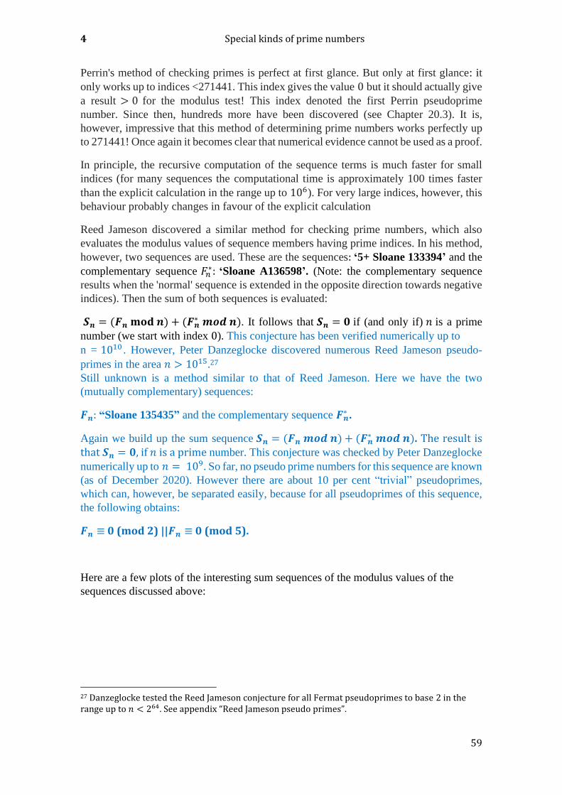
4 Special kinds of prime numbers
59
Perrin's method of checking primes is perfect at first glance. But only at first glance: it
only works up to indices <271441. This index gives the value 0 but it should actually give
a result > 0 for the modulus test! This index denoted the first Perrin pseudoprime
number. Since then, hundreds more have been discovered (see Chapter 20.3). It is,
however, impressive that this method of determining prime numbers works perfectly up
to 271441! Once again it becomes clear that numerical evidence cannot be used as a proof.
In principle, the recursive computation of the sequence terms is much faster for small
indices (for many sequences the computational time is approximately 100 times faster
than the explicit calculation in the range up to 106). For very large indices, however, this
behaviour probably changes in favour of the explicit calculation
Reed Jameson discovered a similar method for checking prime numbers, which also
evaluates the modulus values of sequence members having prime indices. In his method,
however, two sequences are used. These are the sequences: ‘5+ Sloane 133394’ and the
complementary sequence 𝐹𝑛∗: ‘Sloane A136598’. (Note: the complementary sequence
results when the 'normal' sequence is extended in the opposite direction towards negative
indices). Then the sum of both sequences is evaluated:
𝑺𝒏 = (𝑭𝒏 𝐦𝐨𝐝 𝒏) + (𝑭𝒏∗ 𝒎𝒐𝒅 𝒏). It follows that 𝑺𝒏 = 𝟎 if (and only if) 𝑛 is a prime
number (we start with index 0). This conjecture has been verified numerically up to
n = 1010 . However, Peter Danzeglocke discovered numerous Reed Jameson pseudo-
primes in the area 𝑛 > 1015.27
Still unknown is a method similar to that of Reed Jameson. Here we have the two
(mutually complementary) sequences:
𝑭𝒏: “Sloane 135435” and the complementary sequence 𝑭𝒏∗ .
Again we build up the sum sequence 𝑺𝒏 = (𝑭𝒏 𝒎𝒐𝒅 𝒏) + (𝑭𝒏∗ 𝒎𝒐𝒅 𝒏). The result is
that 𝑺𝒏 = 𝟎, if 𝑛 is a prime number. This conjecture was checked by Peter Danzeglocke
numerically up to 𝑛 = 109. So far, no pseudo prime numbers for this sequence are known
(as of December 2020). However there are about 10 per cent “trivial” pseudoprimes,
which can, however, be separated easily, because for all pseudoprimes of this sequence,
the following obtains:
𝑭𝒏 ≡ 0 (mod 2) ||𝑭𝒏 ≡ 0 (mod 5).
Here are a few plots of the interesting sum sequences of the modulus values of the
sequences discussed above:
27 Danzeglocke tested the Reed Jameson conjecture for all Fermat pseudoprimes to base 2 in the range up to 𝑛 < 264. See appendix “Reed Jameson pseudo primes”.
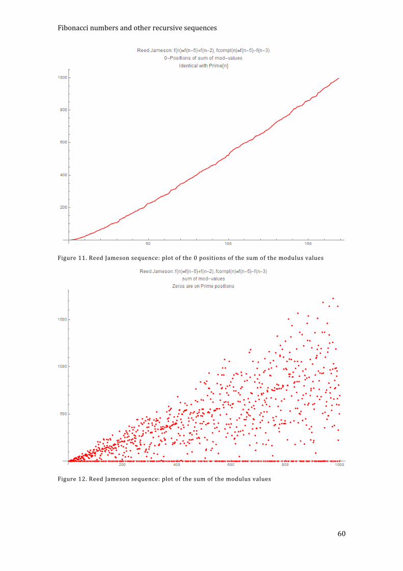
Fibonacci numbers and other recursive sequences
60
Figure 11. Reed Jameson sequence: plot of the 0 positions of the sum of the modulus values
Figure 12. Reed Jameson sequence: plot of the sum of the modulus values
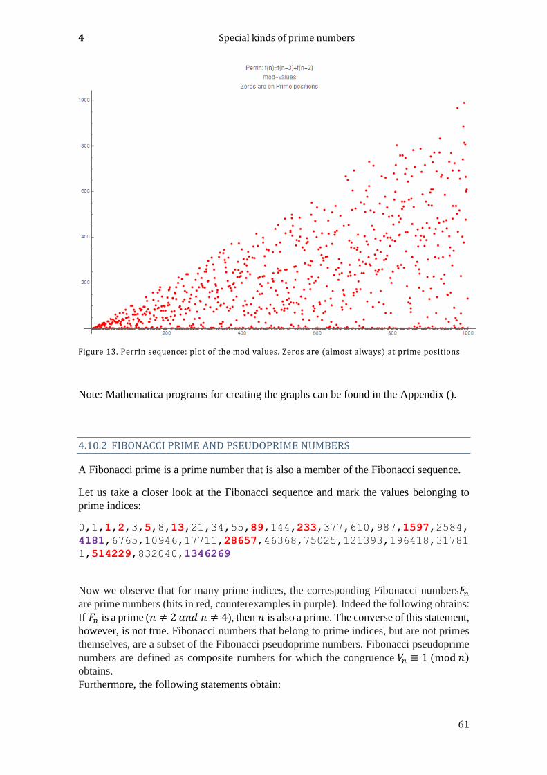
4 Special kinds of prime numbers
61
Figure 13. Perrin sequence: plot of the mod values. Zeros are (almost always) at prime positions
Note: Mathematica programs for creating the graphs can be found in the Appendix ().
4.10.2 FIBONACCI PRIME AND PSEUDOPRIME NUMBERS
A Fibonacci prime is a prime number that is also a member of the Fibonacci sequence.
Let us take a closer look at the Fibonacci sequence and mark the values belonging to
prime indices:
0,1,1,2,3,5,8,13,21,34,55,89,144,233,377,610,987,1597,2584,
4181,6765,10946,17711,28657,46368,75025,121393,196418,31781
1,514229,832040,1346269
Now we observe that for many prime indices, the corresponding Fibonacci numbers𝐹𝑛
are prime numbers (hits in red, counterexamples in purple). Indeed the following obtains:
If 𝐹𝑛 is a prime (𝑛 ≠ 2 𝑎𝑛𝑑 𝑛 ≠ 4), then 𝑛 is also a prime. The converse of this statement,
however, is not true. Fibonacci numbers that belong to prime indices, but are not primes
themselves, are a subset of the Fibonacci pseudoprime numbers. Fibonacci pseudoprime
numbers are defined as composite numbers for which the congruence 𝑉𝑛 ≡ 1 (mod 𝑛) obtains.
Furthermore, the following statements obtain:

Fibonacci numbers and other recursive sequences
62
If 𝑛 is a prime number, then:
𝐹𝑛 ≡ 0 (mod 𝑛) if 𝑛 ≡ 0 (mod 5) 𝐹𝑛−1 ≡ 0 (mod 𝑛) if 𝑛 ≡ ±1 (mod 5) 𝐹𝑛+1 ≡ 0 (mod 𝑛) if 𝑛 ≡ ±2 (mod 5)
The first condition only applies to 𝐹5: 𝐹5 (mod 5) ≡ 5(mod 5) ≡ 0
Here an example for the second condition: 𝑛 = 11; 𝑛 ≡ 1(mod 5) ⇒ 𝐹10 ≡0(mod 11)
An example for the third condition: 𝑛 = 13; 𝑛 ≡ −2(mod 5) ⇒ 𝐹14 ≡ 0(mod 13)
Record
The largest currently known Fibonacci prime number is 𝑭𝟏𝟎𝟒𝟗𝟏𝟏. It has 21925 decimal
digits. It is still unknown (as of Dec. 2015) whether there are infinitely many Fibonacci
prime numbers.
Mathematica:
Select[Fibonacci[Range[400]], PrimeQ]
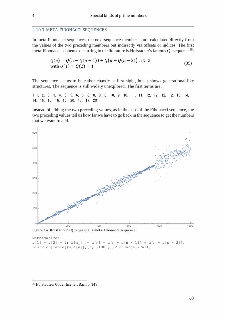
4 Special kinds of prime numbers
63
4.10.3 META-FIBONACCI SEQUENCES
In meta-Fibonacci sequences, the next sequence member is not calculated directly from
the values of the two preceding members but indirectly via offsets or indices. The first
meta-Fibonacci sequence occurring in the literature is Hofstadter's famous Q- sequence28:
𝑄(𝑛) = 𝑄(𝑛 − 𝑄(𝑛 − 1)) + 𝑄(𝑛 − 𝑄(𝑛 − 2)), 𝑛 > 2
with 𝑄(1) = 𝑄(2) = 1 (35)
The sequence seems to be rather chaotic at first sight, but it shows generational-like
structures. The sequence is still widely unexplored. The first terms are:
1 1, 2, 3, 3, 4, 5, 5, 6, 6, 6, 8, 8, 8, 10, 9, 10, 11, 11, 12, 12, 12, 12, 16, 14,
14, 16, 16, 16, 16, 20, 17, 17, 20
Instead of adding the two preceding values, as in the case of the Fibonacci sequence, the
two preceding values tell us how far we have to go back in the sequence to get the numbers
that we want to add.
Figure 14. Hofstadter’s Q sequence: a meta-Fibonacci sequence
Mathematica:
a[1] = a[2] = 1; a[n_] := a[n] = a[n - a[n - 1]] + a[n - a[n - 2]];
ListPlot[Table[{n,a[n]},{n,1,1000}],PlotRange->Full]
28 Hofstadter: Gödel, Escher, Bach p. 149
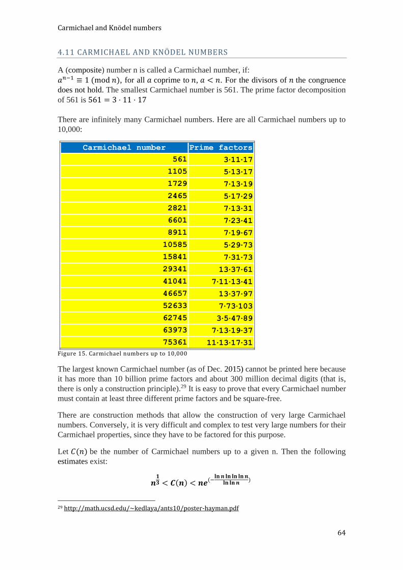
Carmichael and Knödel numbers
64
4.11 CARMICHAEL AND KNÖDEL NUMBERS
A (composite) number n is called a Carmichael number, if:
𝑎𝑛−1 ≡ 1 (mod 𝑛), for all 𝑎 coprime to 𝑛, 𝑎 < 𝑛. For the divisors of 𝑛 the congruence
does not hold. The smallest Carmichael number is 561. The prime factor decomposition
of 561 is 561 = 3 ⋅ 11 ⋅ 17
There are infinitely many Carmichael numbers. Here are all Carmichael numbers up to
10,000:
Carmichael number Prime factors
561 3⋅11⋅17
1105 5⋅13⋅17
1729 7⋅13⋅19
2465 5⋅17⋅29
2821 7⋅13⋅31
6601 7⋅23⋅41
8911 7⋅19⋅67
10585 5⋅29⋅73
15841 7⋅31⋅73
29341 13⋅37⋅61
41041 7⋅11⋅13⋅41
46657 13⋅37⋅97
52633 7⋅73⋅103
62745 3⋅5⋅47⋅89
63973 7⋅13⋅19⋅37
75361 11⋅13⋅17⋅31
Figure 15. Carmichael numbers up to 10,000
The largest known Carmichael number (as of Dec. 2015) cannot be printed here because
it has more than 10 billion prime factors and about 300 million decimal digits (that is,
there is only a construction principle).29 It is easy to prove that every Carmichael number
must contain at least three different prime factors and be square-free.
There are construction methods that allow the construction of very large Carmichael
numbers. Conversely, it is very difficult and complex to test very large numbers for their
Carmichael properties, since they have to be factored for this purpose.
Let 𝐶(𝑛) be the number of Carmichael numbers up to a given n. Then the following
estimates exist:
𝒏𝟏𝟑 < 𝑪(𝒏) < 𝒏𝒆(−
𝐥𝐧𝒏 𝐥𝐧 𝐥𝐧 𝐥𝐧𝒏𝐥𝐧 𝐥𝐧𝒏
)
29 http://math.ucsd.edu/~kedlaya/ants10/poster-hayman.pdf
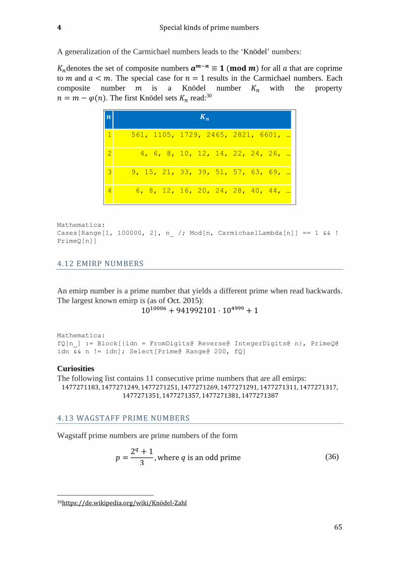
4 Special kinds of prime numbers
65
A generalization of the Carmichael numbers leads to the ‘Knödel’ numbers:
𝐾𝑛denotes the set of composite numbers 𝒂𝒎−𝒏 ≡ 𝟏 (𝐦𝐨𝐝 𝒎) for all 𝑎 that are coprime
to 𝑚 and 𝑎 < 𝑚. The special case for 𝑛 = 1 results in the Carmichael numbers. Each
composite number 𝑚 is a Knödel number 𝐾𝑛 with the property
𝑛 = 𝑚 − 𝜑(𝑛). The first Knödel sets 𝐾𝑛 read:30
𝒏 𝑲𝒏
1 561, 1105, 1729, 2465, 2821, 6601, …
2 4, 6, 8, 10, 12, 14, 22, 24, 26, …
3 9, 15, 21, 33, 39, 51, 57, 63, 69, …
4 6, 8, 12, 16, 20, 24, 28, 40, 44, …
Mathematica: Cases[Range[1, 100000, 2], n_ /; Mod[n, CarmichaelLambda[n]] == 1 && !
PrimeQ[n]]
4.12 EMIRP NUMBERS
An emirp number is a prime number that yields a different prime when read backwards.
The largest known emirp is (as of Oct. 2015):
1010006 + 941992101 ⋅ 104999 + 1
Mathematica:
fQ[n_] := Block[{idn = FromDigits@ Reverse@ IntegerDigits@ n}, PrimeQ@
idn && n != idn]; Select[Prime@ Range@ 200, fQ]
Curiosities
The following list contains 11 consecutive prime numbers that are all emirps: 1477271183, 1477271249, 1477271251, 1477271269, 1477271291, 1477271311, 1477271317,
1477271351, 1477271357, 1477271381, 1477271387
4.13 WAGSTAFF PRIME NUMBERS
Wagstaff prime numbers are prime numbers of the form
𝑝 =2𝑞 + 1
3,where 𝑞 is an odd prime (36)
30https://de.wikipedia.org/wiki/Knödel-Zahl

Wagstaff prime numbers
66
At present, 43 Wagstaff primes p are known (as of Oct. 2015). In red: PRP primes)31:
Table 11: Wagstaff prime numbers: exponent q
n q n q
1 3 22 2617
2 5 23 3539
3 7 24 5807
4 11 25 10501
5 13 26 10691
6 17 27 11279
7 19 28 12391
8 23 29 14479
9 31 30 42737
10 43 31 83339
11 61 32 95369
12 79 33 117239
13 101 34 127031
14 127 35 138937
15 167 36 141079
16 191 37 267017
17 199 38 269987
18 313 39 374321
19 347 40 986191
20 701 41 4031399
21 1709 42 13347311
43 13372531
Wagstaff primes can be calculated using the following Mathematica program:
Select[Array[(2^#+1)/3&,190],PrimeQ]
Output:
{3,11,43,683,2731,43691,174763,2796203,715827883,2932031007403, 768614336404564651,201487636602438195784363, 845100400152152934331135470251, 56713727820156410577229101238628035243, 62357403192785191176690552862561408838653121833643}
31 Pseudoprime tests provide PRPs (pseudoprime numbers) and work with probabilistic methods, but they provide reliable statements about primality
4 Special kinds of prime numbers
67
Finally, here is a Mathematica program for the prime exponents of the Wagstaff prime
numbers:
a= {}; Do[c = 1 + Sum[2^(2n - 1), {n, 1, x}]; If[PrimeQ[c],
AppendTo[a, c]], {x, 0, 100}]; a
4.14 WIEFERICH PRIME NUMBERS
A prime number satisfying the congruence 2𝑝−1 ≡ 1 (mod 𝑝2) is referred to in the
literature as a Wieferich prime. Wieferich, at the beginning of the last century, was the
first to explore these numbers. Let us remember the congruence relation of Fermat’s little
theorem: 2𝑝−1 ≡ 1 (mod 𝑝).
This is true for any odd prime. On the contrary, the above Wieferich congruence
relationship holds only for very few prime numbers (more precisely, only for two
numbers: 1093 and 3511). These are the only Wieferich primes currently known (as of
Dec. 2016). It is also known that no further Wieferich primes exist up to 4.968543 ⋅ 1017
(as of Dec. 2015).
The patterns in the binary representation of the value of Wieferich prime numbers (more
precisely, in the value reduced by 1) are remarkable:
𝟏𝟎𝟗𝟐 = 𝟏𝟎𝟎𝟎𝟏𝟎𝟎𝟎𝟏𝟎𝟎𝟐, 𝟑𝟓𝟏𝟎 = 𝟏𝟏𝟎𝟏𝟏𝟎𝟏𝟏𝟎𝟐
There is a close connection to the so-called 'powerful' numbers 𝑃𝑖, for which the
following conditions hold: 𝑝| 𝑃𝑖 and 𝑝2| 𝑃𝑖.
The first ‘powerful 'numbers are: 1,4,8,9,16,25,27,32,36,49… They are all of the form
𝑎2𝑏3 where 𝑎, 𝑏 ≥ 1. The sum of the reciprocal values of all powerful numbers is finite
and has the value:
∑1
𝑃𝑖𝑖
=휁(2)휁(3)
휁(6)= 1.9435964 (37)
Primes that do not satisfy the congruence condition 2𝑝 ≢ 1 (mod 𝑝2) are generally
referred to as non-Wieferich primes. Both are mutually complementary sets of numbers,
i.e. if one of them is finite, then the other must be infinite. There are interesting cross-
connections to the abc conjecture (Chapter 11.1). The literature about Wieferich primes
is very large. There are also many further surprising and interesting connections to
Mersenne and Fermat primes, as well as to other areas of number theory.32
Wieferich primes can be generalized to have any positive integer basis 𝑎 if they satisfy
the following congruence:
𝑎𝑝−1 ≡ 1 (mod 𝑝2) (38)
32 https://en.wikipedia.org/wiki/Wieferich_prime
Wieferich prime numbers
68
The assumption is that there are infinitely many base a Wieferich prime numbers for
every natural base 𝑎. Here an example: the following base 5 Wieferich primes are known
for 𝑎 = 5 (as of Oct. 2016):
2, 20771, 40487, 53471161, 1645333507, 6692367337, 188748146801
The quotient 𝑞𝑝(𝑎) =𝑎𝑝−1−1
𝑝 is generally denoted as the Fermat quotient of 𝑝 to the base
𝑎. The modulo residue of the Fermat quotient 𝑞𝑝(𝑎) has logarithmic properties. If 𝑝 is
not a divisor of 𝑎𝑏, then:
𝑞𝑝(𝑎𝑏) ≡ 𝑞𝑝(𝑎) + 𝑞𝑝(𝑏) (mod 𝑝) (39)
More properties:
𝑞𝑝(𝑝 − 1) ≡ 1 and 𝑞𝑝(𝑝 + 1) ≡ −1 (mod 𝑝) (40)
𝑞𝑝(2) =1
𝑝(1 −
1
2+1
3−1
4+⋯−
1
𝑝 − 1) (mod 𝑝) (41)
Mathematica programs for computing Wieferich primes:
Select[Prime[Range[50000]], Divisible[2^(#-1)-1, #^2]&]
Select[Prime[Range[50000]], PowerMod[2, #-1, #^2]==1&]
There are other interesting cross-links to other areas of number theory:
To Fermat’s theorem:
Let be 𝒌𝒑 + 𝒍𝒑 +𝒎𝒑 = 𝟎 (𝐰𝐡𝐞𝐫𝐞 𝒌, 𝒍,𝒎 ∈ ℤ 𝐚𝐧𝐝 𝒑 ∈ ℙ). Further we assume: 𝒑 is
not a divisor of the product 𝒌𝒍𝒎. Then 𝒑 is a Wieferich prime.
To Mersenne primes and Fermat primes:
Let 𝑴𝒒 be a Mersenne number with primal index q and p be a prime number
which is a divisor of 𝑴𝒒. If 𝒑𝟐 is also a divisor of 𝑴𝒒, then 𝑴𝒒 (and only then) p is a
Wieferich prime number.
Double Wieferich primes:
A pair of generalized Wieferich primes, for which
𝑞𝑝−1 ≡ 1 (mod 𝑝2) and 𝑝𝑞−1 ≡ 1 (mod 𝑞2) (42)
is called a ’double Wieferich prime’. Here is an example:
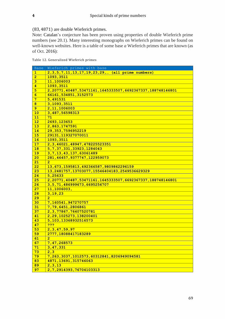
4 Special kinds of prime numbers
69
(83, 4871) are double Wieferich primes.
Note: Catalan’s conjecture has been proven using properties of double Wieferich prime
numbers (see 20.1). Many interesting monographs on Wieferich primes can be found on
well-known websites. Here is a table of some base a Wieferich primes that are known (as
of Oct. 2016):
Table 12. Generalized Wieferich primes
Base Wieferich primes with base
1 2,3,5,7,11,13,17,19,23,29,… (all prime numbers)
2 1093,3511
3 11,1006003
4 1093,3511
5 2,20771,40487,53471161,1645333507,6692367337,188748146801
6 66161,534851,3152573
7 5,491531
8 3,1093,3511
9 2,11,1006003
10 3,487,56598313
11 71
12 2693,123653
13 2,863,1747591
14 29,353,7596952219
15 29131,119327070011
16 1093,3511
17 2,3,46021,48947,478225523351
18 5,7,37,331,33923,1284043
19 3,7,13,43,137,63061489
20 281,46457,9377747,122959073
21 2
22 13,673,1595813,492366587,9809862296159
23 13,2481757,13703077,15546404183,2549536629329
24 5,25633
25 2,20771,40487,53471161,1645333507,6692367337,188748146801
26 3,5,71,486999673,6695256707
27 11,1006003,
28 3,19,23
29 2
30 7,160541,947270757
31 7,79,6451,2806861
37 2,3,77867,76407520781
41 2,29,1025273,138200401
43 5,103,13368932516573
47 ???
53 2,3,47,59,97
59 2777,18088417183289
61 2
67 7,47,268573
71 3,47,331
73 2,3
79 7,263,3037,1012573,60312841,8206949094581
83 4871,13691,315746063
89 2,3,13
97 2,7,2914393,76704103313
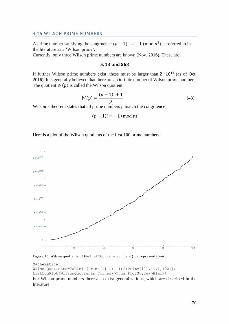
70
4.15 WILSON PRIME NUMBERS
A prime number satisfying the congruence (𝑝 − 1)! ≡ −1 (mod 𝑝2) is referred to in
the literature as a ‘Wilson prime’.
Currently, only three Wilson prime numbers are known (Nov. 2016). These are:
𝟓, 𝟏𝟑 𝐮𝐧𝐝 𝟓𝟔𝟑
If further Wilson prime numbers exist, these must be larger than 2 ⋅ 1013 (as of Oct.
2016). It is generally believed that there are an infinite number of Wilson prime numbers.
The quotient 𝑊(𝑝) is called the Wilson quotient:
𝑊(𝑝) =(𝑝 − 1)! + 1
𝑝 (43)
Wilson’s theorem states that all prime numbers p match the congruence
(𝑝 − 1)! ≡ −1 (mod 𝑝)
Here is a plot of the Wilson quotients of the first 100 prime numbers:
Figure 16. Wilson quotients of the first 100 prime numbers (log representation)
Mathematica:
WilsonQuotients=Table[((Prime[i]-1)!+1)/(Prime[i]),{i,1,100}];
ListLogPlot[WilsonQuotients,Joined->True,PlotStyle->Black]
For Wilson prime numbers there also exist generalizations, which are described in the
literature.
4 Special kinds of prime numbers
71
4.16 WOLSTENHOLME PRIME NUMBERS
A prime number satisfying the following congruence is called a Wolstenholme prime
number:
(2𝑝 − 1𝑝 − 1
) ≡ 1 (mod 𝑝4) (44)
Please note that according to the Wolstenholme theorem for each prime 𝑝 > 3 the
following obtains:
(2𝑝 − 1𝑝 − 1
) ≡ 1 (mod 𝑝3) (45)
The only currently known Wolstenholme prime numbers are (as of Oct. 2016):
𝟏𝟔𝟖𝟒𝟑 and 𝟐𝟏𝟐𝟒𝟔𝟕𝟗.
If there are further Wolstenholme prime numbers, these are greater than 109 . It is
assumed that there are infinitely many Wolstenholme prime numbers.
RG numbers (= recursive Gödelized)
72
4.17 RG NUMBERS (= RECURSIVE GÖDELIZED)
4.17.1 GOCRON TYPE 6 (‘PRIME OCRONS‘)
For this we need the definition of the GOCRON type 6 (Prime OCRON, with Gödel codes
‘*’=0 and ‘P’=1, see Chapter 10.2.4).
Let an RG sequence in the direction of positive indices be recursively defined as follows:
𝒂(𝟎) = 𝒎 (with any integer number 𝒎 >= 𝟏)
𝒂(𝒏 + 𝟏) = 𝐄𝐆𝐎𝐂𝐑𝐎𝐍𝟔(𝒂(𝒏))
The sequence can also be continued in the direction of negative indices:
𝒂(𝟎) = 𝒎 (with any integer number 𝒎 >= 𝟏)
𝒂(𝒏 − 𝟏) = 𝐈𝐍𝐕𝐄𝐆𝐎𝐂𝐑𝐎𝐍𝟔(𝒂(𝒏))
Here are a few examples: 0,1,2,4,8,14,9,19,67,401,409,1103,305999,210535619933…
3,3,3,3,3,3,3,3,3,3,3,3,3,3,3,3,3…
5,7,5,7,5,7,5,7,5,7,5,7,5,7,5,7,5…
6,6,6,6,6,6,6,6,6,6,6,6,6,6,6,6,6…
10,12,10,12,10,12,10,12,10,12,…
13,13,13,13,13,13,13,13,13,13,…
15,11,17,43,157,2833,3463,59723,4251697,97152271…
20,20,20,20,20,20,20,20,20,20,…
21,37,107,367,37217,363343,30612065639…
25,29,23,59,83,353,379,20719,448693727…
31,31,31,31,31,31,31,31,31,31,…
27,41,71,1153,769,349,8861,5065217,22920311…
33,79,2221,271003,680328533…
35,191, 15299,649093,50511459839…
39, 331,3559,1804973,50220857249
45,101,181,751,304553,627544381
91,547,4463,48266149
Here are a few examples in the direction of positive indices: 15,28,18,30,40,36,96,168,424,12544,6845104128,351820914765360116269056
21,26,22,16,24,56,72,84,122,928,108544,15903336184152064
25,48,64,208,656,1968,116992,30889404792832
27,60,34,58,100,352,3872,16016,73764,503296,360710432,2177877733799636238336
35,112,118,456,2368,6704,10250,25128,1001488,5575424,131365666816,
129617351244588913891122077503488
39, 120, 512, 4032, 6586368, 1065152675904
RG sequences of the 'Prime GOCRONs' have the following properties:
1) They are either periodic or they diverge to infinity in the case of positive and
negative indices.
2) An exception is the 9 sequence; it goes towards infinity for negative indices and
is not defined for positive indices.

4 Special kinds of prime numbers
73
3) Every non-periodic sequence has a 'centre' that lies in the neighbourhood of the
minimum. It is the only odd composite number in this sequence. Thus, the
sequences can be named after this single central odd number. These are the
numerical values marked in red.
4) In the direction of positive indices, there is a strong tendency to increase the
degree of 'compositeness'. Towards negative indices there is a tendency to
increase 'primality'. This is expressed by the fact that the ‘centre element’ (which
is composite and uneven) is the index at which a ‘turn over’ occurs, from the status
‘prime’ to the status ‘composite’ (or vice versa, depending upon the direction from
which one is coming).
5) The following RG sequences are periodic (classified according to the central odd
composite element):
3,5,6,7,10,12,13,20,31,61,97,250,457,41112
RG sequences of 'prime OCRONs' (if they are not periodic) come out from infinity as
prime numbers, 'hang around' a little bit among the 'finite' numbers, change (turn over) to
composite numbers at exactly one index, stay ‘even’ from there on and then disappear
again into the infinite. Here are a few plots of RG sequences (with the “transformation
point” marked in red, to the left of it: prime numbers, to the right of it: composite, even
numbers):
Figure 17. RG sequence ‘15’ (log plot)
Sequence: 97152271,4251697,59723,3463,2833,157,43,17,11,15,28,18,30,40,36,96,168
,424,12544,6845104128

RG numbers (= recursive Gödelized)
74
Figure 18. RG sequence ‘21’ (log plot) 30612065639,363343,37217,367,107,37,21,26,22,16,24,56,72,84,122,928,10
8544,15903336184152064
Figure 19. RG sequence ‘25’ (log plot) 448693727,20719,379,353,83,59,23,29,25,48,64,208,656,1968,116992,30889
404792832
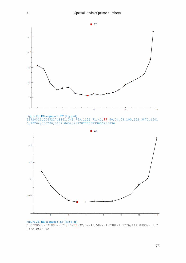
4 Special kinds of prime numbers
75
Figure 20. RG sequence ‘27’ (log plot) 22920311,5065217,8861,349,769,1153,71,41,27,60,34,58,100,352,3872,1601
6,73764,503296,360710432,2177877733799636238336
Figure 21. RG sequence ‘33’ (log plot) 680328533,271003,2221,79,33,32,52,42,50,224,2304,491776,14160388,70967
016210563072
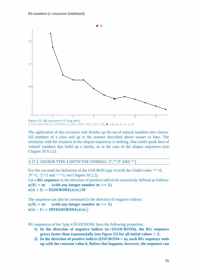
RG numbers (= recursive Gödelized)
76
Figure 22. RG sequence ‘9’ (log plot) 210535619933,305999,1103,409,401,67,19,9,14,8,4,2,1,0
The application of this recursive rule divides up the set of natural numbers into classes.
All numbers of a class end up in the manner described above sooner or later. The
similarity with the situation in the aliquot sequences is striking. One could speak here of
'related' numbers that build up a family, as in the case of the aliquot sequences (see
Chapter 20.9.2.2).
4.17.2 GOCRON TYPE 4 (WITH THE SYMBOLS ‚‘2’,‘*’,‘P’ AND ‘^’)
For this we need the definition of the GOCRON type 4 (with the Gödel codes ‘*’=0,
‘P’=1, ‘2’=2 and ‘^’=3, see Chapter 10.2.2).
Let a RG sequence in the direction of positive indices be recursively defined as follows:
𝒂(𝟎) = 𝒎 (with any integer number 𝒎 >= 𝟏)
𝒂(𝒏 + 𝟏) = 𝐄𝐆𝐎𝐂𝐑𝐎𝐍𝟒(𝒂(𝒏))10
The sequence can also be continued in the direction of negative indices:
𝒂(𝟎) = 𝒎 (with any integer number 𝒎 >= 𝟏)
𝒂(𝒏 − 𝟏) = 𝐈𝐍𝐕𝐄𝐆𝐎𝐂𝐑𝐎𝐍𝟒(𝒂(𝒏))
RG sequences of the 'type 4 EGOCRONs' have the following properties:
1) In the direction of negative indices (n->EGOCRON4), the RG sequence
grows faster than exponentially (see Figure 23) for all initial values > 𝟐.
2) In the direction of positive indices (EOCRON4-> n), each RG sequence ends
up with the constant value 6. Before this happens, however, the sequence can

4 Special kinds of prime numbers
77
attain astronomically high values before finally ending up on value 6. There
is an assumption that is based on the empirical data but it is as yet unproved.
3) There is always a ‘turn over’ value, from which point on all sequence
members remain even.
Here are a few plots of RG sequences in the direction of negative indices using different
initial values:
Figure 23. RG sequences in negative direction (type EGOCRON4)
Here are a few graphs of RG sequences in the direction of positive indices with different
initial values (value of ‘turn over’ index, from which all values remain straight, is
indicated):
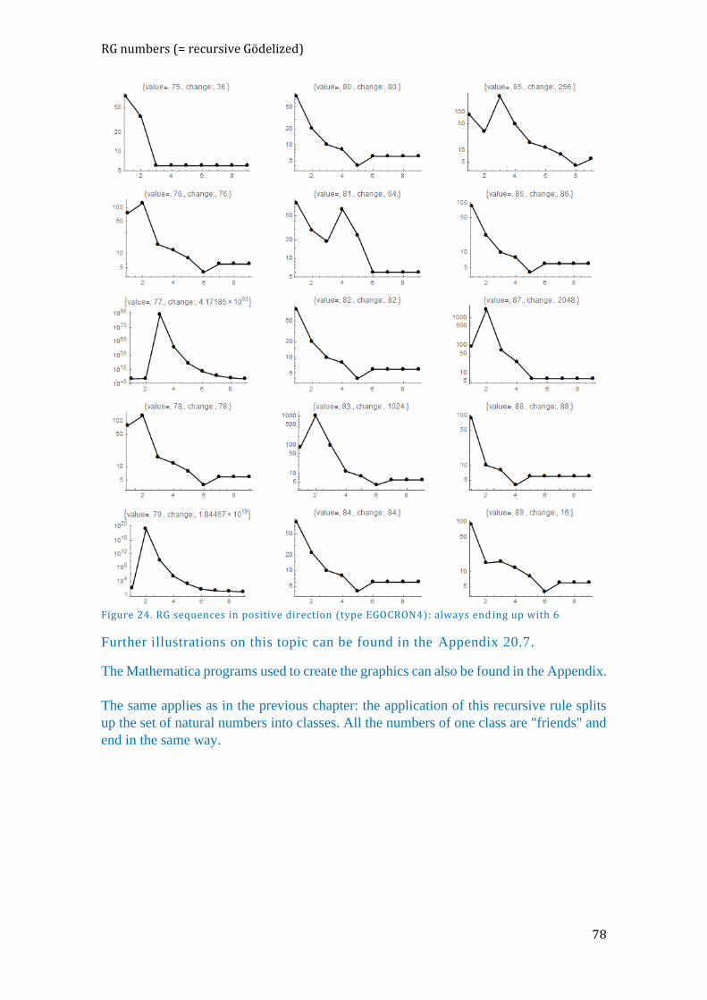
RG numbers (= recursive Gödelized)
78
Figure 24. RG sequences in positive direction (type EGOCRON4): always end ing up with 6
Further illustrations on this topic can be found in the Appendix 20.7.
The Mathematica programs used to create the graphics can also be found in the Appendix.
The same applies as in the previous chapter: the application of this recursive rule splits
up the set of natural numbers into classes. All the numbers of one class are "friends" and
end in the same way.
79
5 DIGRESSION: RIEMANN ’S ZETA FUNCTION 휁(𝑠)
5.1 GENERAL
The Riemann zeta function is one of the mysteries of mathematics. Its zeros are especially
puzzling. There are the so-called ‘trivial’ zeros in the real domain. These zeros all lie at
even negative integer values −2,−4,−6,… , (− 2𝑛). But there are infinitely many zeros
in the complex domain, all of which lie on the so-called 'critical' line Re (s) = 1/2. There
is no simple formula for the position of these zeros. They are seemingly chaotic and
randomly distributed and therefore possess similarly mysterious properties as the prime
numbers. In fact, the location of the non-trivial zeros is very closely related to the
distribution of the prime numbers (see e.g. Chapter 8.6, Formula (131)).
Entire books have been devoted to a discussion of the properties of the zeta function, so
we will not discuss them further here. In simple terms, one can say that from the
knowledge of the non-trivial zeros, the position (and distribution) of the prime numbers
can be calculated and vice versa. This relationship, however, is not a simple one-to-one
relationship between zeros and prime numbers but rather resembles a transformation
(such as the Fourier transform, which establishes the connection between the time domain
and the frequency domain). We could speak here of different domains such as the ‘prime
number domain’ and the 'zeta domain'.
We need to clarify here: the statement that all non-trivial zeros lie on the critical straight
line Re (s) = 1/2 (this is the famous Riemann conjecture) has neither been proved nor
disproved. However, it is probably true: the numerical evidence in its favour is
overwhelming. Although it is so easy to formulate, the 'Riemann conjecture' has so far
resisted all attempts (including those of the greatest mathematicians) at proof! For
example, it might theoretically happen that there are zeros in unimaginably high number
regions that lie apart from the critical line… The history of mathematics has taught us
that we cannot always trust in the numerical evidence. Just consider the fact that the
asymptotic formula for the prime counting function Li (x) ≈ π (x) always yields too large
values33. This is certainly true up to 1026, but it has been proved by Skewes (1933) that
𝐿𝑖(𝑥) < 𝜋(𝑥) can happen! Skewes showed that the sign of 𝐿𝑖(𝑥) − 𝜋(𝑥) changes
infinitely often, and he proved that the point of the first sign change is less than 10101034
!
This upper limit has now been considerably reduced to 𝑒727,95133.
Nevertheless, no mathematician believes that Riemann's conjecture is wrong! However,
the fact that it has not yet been proved, despite the enormous efforts that have been made,
leads many to suppose that Riemann’s conjecture belongs to the category of unprovable
mathematical propositions. It has been known, at least since the time of Gödel, that there
are mathematical propositions that are true but not provable, and Gödel, in fact, proved
this. This provides plenty of material for philosophical speculation. Why did God, when
he created mathematics and the numbers, also create rules such that something could be
'true' without a compelling reason? For if there were a compelling reason, there would
also be a proof…
33 https://en.wikipedia.org/wiki/Prime-counting_function
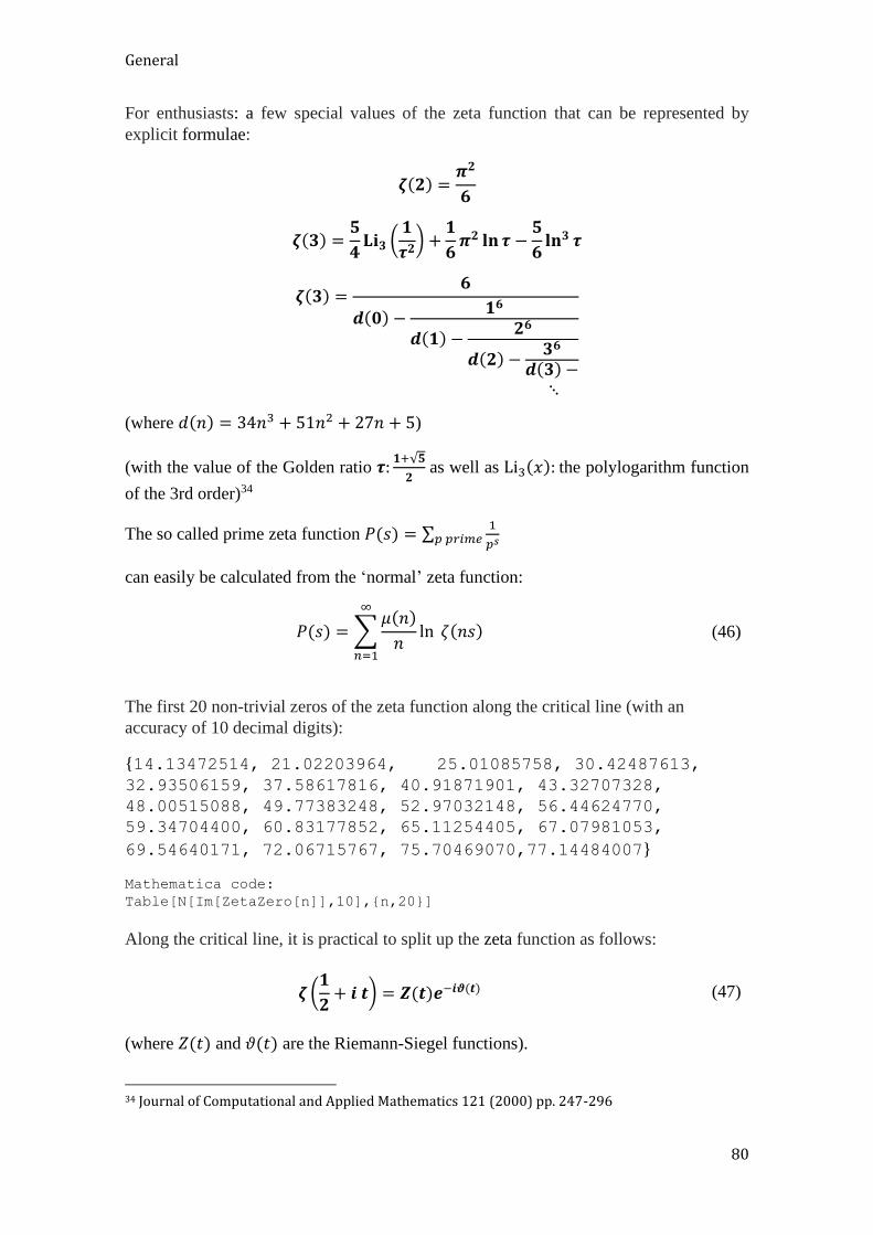
General
80
For enthusiasts: a few special values of the zeta function that can be represented by
explicit formulae:
𝜻(𝟐) =𝝅𝟐
𝟔
𝜻(𝟑) =𝟓
𝟒𝐋𝐢𝟑 (
𝟏
𝝉𝟐) +
𝟏
𝟔𝝅𝟐 𝐥𝐧 𝝉 −
𝟓
𝟔𝐥𝐧𝟑 𝝉
𝜻(𝟑) =𝟔
𝒅(𝟎) −𝟏𝟔
𝒅(𝟏) −𝟐𝟔
𝒅(𝟐) −𝟑𝟔
𝒅(𝟑) − ⋱
(where 𝑑(𝑛) = 34𝑛3 + 51𝑛2 + 27𝑛 + 5)
(with the value of the Golden ratio 𝝉:𝟏+√𝟓
𝟐 as well as Li3(𝑥): the polylogarithm function
of the 3rd order)34
The so called prime zeta function 𝑃(𝑠) = ∑1
𝑝𝑠𝑝 𝑝𝑟𝑖𝑚𝑒
can easily be calculated from the ‘normal’ zeta function:
𝑃(𝑠) = ∑𝜇(𝑛)
𝑛
∞
𝑛=1
ln 휁(𝑛𝑠) (46)
The first 20 non-trivial zeros of the zeta function along the critical line (with an
accuracy of 10 decimal digits):
{14.13472514, 21.02203964, 25.01085758, 30.42487613,
32.93506159, 37.58617816, 40.91871901, 43.32707328,
48.00515088, 49.77383248, 52.97032148, 56.44624770,
59.34704400, 60.83177852, 65.11254405, 67.07981053,
69.54640171, 72.06715767, 75.70469070,77.14484007}
Mathematica code:
Table[N[Im[ZetaZero[n]],10],{n,20}]
Along the critical line, it is practical to split up the zeta function as follows:
𝜻 (𝟏
𝟐+ 𝒊 𝒕) = 𝒁(𝒕)𝒆−𝒊𝝑(𝒕) (47)
(where 𝑍(𝑡) and 𝜗(𝑡) are the Riemann-Siegel functions).
34 Journal of Computational and Applied Mathematics 121 (2000) pp. 247-296
5 Digression: Riemann’s zeta function 𝜁(𝑠)
81
Many books have been written about the zeta function – see, for example, Edwards (1974)
and Sautoy (2004) in the Bibliography.
Note: the Riemann zeta function has generalizations (for example, the 'Hurwitz' or 'Lerch'
zeta functions, which are mostly named after their discoverers). Of these generalized zeta
functions, at least twelve versions are mentioned in the mathematical literature.
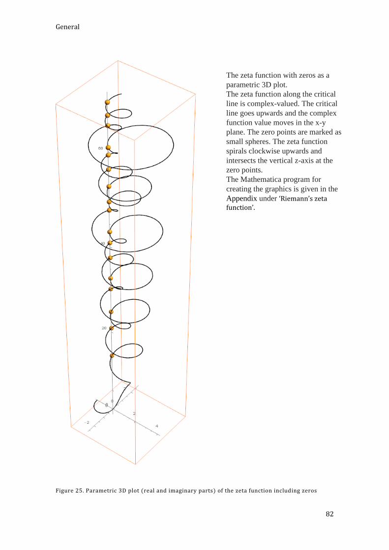
General
82
Figure 25. Parametric 3D plot (real and imaginary parts) of the zeta function including zeros
The zeta function with zeros as a
parametric 3D plot.
The zeta function along the critical
line is complex-valued. The critical
line goes upwards and the complex
function value moves in the x-y
plane. The zero points are marked as
small spheres. The zeta function
spirals clockwise upwards and
intersects the vertical z-axis at the
zero points.
The Mathematica program for
creating the graphics is given in the
Appendix under ‘Riemann’s zeta function’.

5 Digression: Riemann’s zeta function 𝜁(𝑠)
83
Figure 26. Parametric 3D plot (absolute and argument parts) of the zeta function including zeros
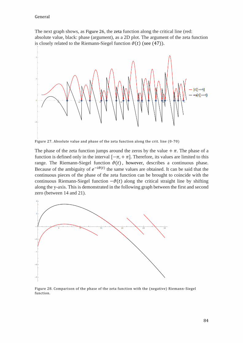
General
84
The next graph shows, as Figure 26, the zeta function along the critical line (red:
absolute value, black: phase (argument), as a 2D plot. The argument of the zeta function
is closely related to the Riemann-Siegel function 𝜗(𝑡) (see (47)).
Figure 27. Absolute value and phase of the zeta function along the crit. line (0-70)
The phase of the zeta function jumps around the zeros by the value + 𝜋. The phase of a
function is defined only in the interval [−𝜋,+ 𝜋]. Therefore, its values are limited to this
range. The Riemann-Siegel function 𝜗(𝑡) , however, describes a continuous phase.
Because of the ambiguity of 𝑒−𝑖𝜗(𝑡) the same values are obtained. It can be said that the
continuous pieces of the phase of the zeta function can be brought to coincide with the
continuous Riemann-Siegel function −𝜗(𝑡) along the critical straight line by shifting
along the y-axis. This is demonstrated in the following graph between the first and second
zero (between 14 and 21).
Figure 28. Comparison of the phase of the zeta function with the (negative) Riemann -Siegel function.
5 Digression: Riemann’s zeta function 𝜁(𝑠)
85
Surprisingly the Riemann-Siegel function 𝜗(𝑡) can be calculated without knowledge of
the zeta function, only with the aid of the gamma function. It is quite 'inconspicuous', but
it has jumps because the arguments can only have values between 𝜋 and – 𝜋:
𝜗(𝑡) = Im(ln (𝛤 (1
4+𝑖 𝑡
2))) −
𝑡
2ln 𝜋 =Arg (𝛤 (
1
4+𝑖 𝑡
2)) −
𝑡
2ln 𝜋 (48)
Note: for calculation with Mathematica, the normal Γ function should not be used to
calculate the term ln(𝛤(… )). This should be done by the function ‘LogGamma’. The
reason for this is that the branch structure in the complex domain is more complicated
for the normal gamma function, and only the main value of the logarithm would be
obtained. The LogGamma function overcomes this problem.
If we normalize the phase of 휁(1
2+ 𝑖𝑡) by the factor
1
𝜋, we get a jump of +1 at each zero.
If we do the same with −𝜗(𝑡) and subtract these two functions from each other (and add
1), we get a counting function for the zeros of the zeta function! More details can be
found in the Chapter 5.5.
5.2 THE DIFFERENT REPRESENTATIONS OF 휁(𝑠)
A book about primes must include the most important representations of the zeta
function.
First of all, the original definition of the zeta function is extremely simple, so people can
understand it without necessarily having read mathematics:
휁(𝑠) = 1 +1
2𝑠+1
3𝑠+⋯ =∑
1
𝑛𝑠
∞
𝑛=1
(Re(𝑠) > 1) (49)
Already Euler proved in the 18th century that 휁(2) = 1 +1
4+1
9+
1
16+⋯ =
𝜋2
6.
For all even positive arguments, there is the simple formula:
휁(2𝑛) = (−1)𝑛−1(2𝜋)2𝑛𝐵2𝑛
2(2𝑛)! (𝐵𝑛: Bernoulli − numbers, n = 1,2, … ) (50)
For the positive odd numbered arguments there are also formulae; these, however, are
somewhat more complex, e.g. :
휁(3) =7𝜋3
180− 2∑
1
𝑛3(𝑒2𝜋𝑛 − 1)
∞
𝑛=1
(51)
For negative integer arguments:
The different representations of 𝜁(𝑠)
86
휁(1 − 𝑛) = −𝐵𝑛𝑛
(52)
Some examples: 휁(0) = −1
2, 휁(−1) = −
1
12, 휁(−3) = −
1
120
The product formula (from which elementary methods (49) can be deduced) is also easy
to understand:
휁(𝑠) =1
(1 −12𝑠) (1 −
13𝑠) (1 −
15𝑠)…
=∏1
(1 −1𝑝𝑠)
∞
𝑝∈ℙ
(𝑅𝑒(𝑠) > 1) (53)
Most notable is a theorem proved by the Russian mathematician Voronin that the zeta
function can approximate any other function with arbitrary precision (more precisely,
every holomorphic complex function within an area with radius 1
4, without zeros).
Descriptively speaking: every complex-valued function, however chaotic and however
complicated its landscape may be, with all the 'hills' and 'valleys', will also appear
‘somewhere’ in the landscape of the complex zeta function, if one only searches far
enough in the infinite landscapes of the zeta function …
The derivative of the zeta function is closely connected with the Von Mangoldt function
Λ(𝑛):
−휁′(𝑠)
휁(𝑠)= ∑
Λ(𝑛)
𝑛𝑠
∞
𝑛=1
(54)
휁′(0) = −1
2ln 2𝜋 (55)
휁′(−2𝑛) = (−1)𝑛휁(2𝑛 + 1)(2𝑛)!
22𝑛+1𝜋2𝑛 (56)
More formulae:
1
휁(𝑠)= ∑
𝜇(𝑛)
𝑛𝑠
∞
𝑛=1
(with Moebius function 𝜇(𝑛)) (57)
Here a representation using integrals:
휁(𝑠) =1
Γ(𝑠)∫ 𝑥𝑠−1∑𝑒−𝑛𝑥𝑑𝑥 =
1
Γ(𝑠)∫𝑥𝑠−1
𝑒𝑥 − 1𝑑𝑥
∞
𝑛=0
∞
𝑛=1
∞
0
(58)
Further representations with products (Hadamard product):
5 Digression: Riemann’s zeta function 𝜁(𝑠)
87
휁(𝑠) =𝜋𝑠2
2(𝑠 − 1)Γ(1 +𝑠2)∏(1 −
𝑠
𝜌)
𝜌
(59)
Because of the conditional convergence of this formula (the evaluation of the product
over the terms with the zeros of the zeta function ρ must be done in pairs), one can also
write:
휁(𝑠) =𝜋𝑠2
2(𝑠 − 1)Γ(1 +𝑠2)
∏ (1 −𝑠
𝜌)
𝐼𝑚(𝜌)>0
(1 −𝑠
1 − 𝜌) (60)
5.3 PRODUCT REPRESENTATION OF 휁(𝑠) IN THE COMPLEX DOMAIN
Equation (53) describes the product representation of the zeta function. It also holds in
the complex domain, but converges only for 𝑅𝑒(𝑠) > 1. For this reason, it is better to
avoid using this formula in the region of the critical line in which the non-trivial zeros lie.
What happens if we do the 'forbidden' anyway? Do we then cross a boundary beyond
which the serious mathematician should not stray? Do we risk not being taken seriously?
In the spirit of mathematical adventure, let us look and see what happens if we do the
'forbidden' anyway:
We use Formula (53) to calculate the values along the critical line:
휁 (1
2+ 𝑡 ⋅ 𝑖) =∏
1
(1 − 𝑝−12−𝑡⋅𝑖)
∞
𝑝∈ℙ
where 𝑡 ≥ 0
The first thing to notice is that the term 1
(… ) in the infinite product can never be zero.
Nevertheless, 휁 (1
2+ 𝑡 ⋅ 𝑖) has infinitely often the value 0 along the critical line. How can
that happen? Let us look at the real part (black) and the imaginary part (red), as well as
the zeros (blue circles) in the range from 2 to 70:

Product representation of 𝜁(𝑠) in the complex domain
88
Figure 29. The zeta function (on crit. line, t=0-70, product formula with first 100 primes)
Mathematica:
cterm[n_,x_]:=1/(1-Prime[n]^(-1/2-x*I));
myFunc[x_]:=Product[cterm[n,x],{n,1,100}]
xmax=70;
Show[ListPlot[Table[{Im[ZetaZero[i]],0},{i,1,17}],PlotRange-
>{{0,71},{-3.5,5}},ImageSize-
>Large],Plot[{Im[myFunc[x]],Re[myFunc[x]]},{x,2,xmax},PlotStyle-
>{Red,Black},PlotRange->{{0,71},{-3.5,5}},
PlotLegends->{TraditionalForm[Im[Product[1/(1-Prime[n]^(-1/2-
x*I)),{n,1,N}]]],TraditionalForm[Re[Product[1/(1-Prime[n]^(-1/2-
x*I)),{n,1,N}]]]},ImageSize->Large]]
Looking at the absolute value of this function, we see clearly that the values calculated
with the product formula at the zeros (blue circles) of the zeta function have distinct
minima, but never become exactly 0 (which is clear from the formula). Somehow, the
infinitely many factors seem to work together in such a way that the infinite product at
the zeros nevertheless approaches arbitrarily close to the value 0 if the product is taken
over a sufficient number of factors.
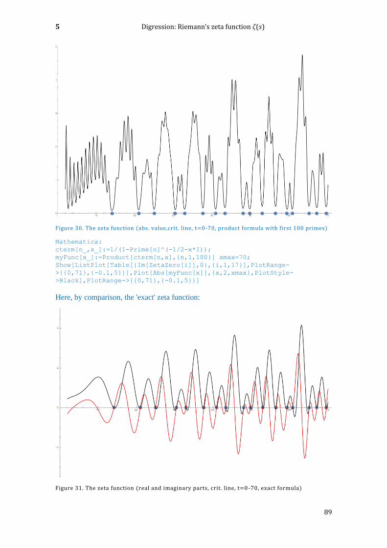
5 Digression: Riemann’s zeta function 𝜁(𝑠)
89
Figure 30. The zeta function (abs. value,crit. line, t=0-70, product formula with first 100 primes)
Mathematica:
cterm[n_,x_]:=1/(1-Prime[n]^(-1/2-x*I));
myFunc[x_]:=Product[cterm[n,x],{n,1,100}] xmax=70;
Show[ListPlot[Table[{Im[ZetaZero[i]],0},{i,1,17}],PlotRange-
>{{0,71},{-0.1,5}}],Plot[Abs[myFunc[x]],{x,2,xmax},PlotStyle-
>Black],PlotRange->{{0,71},{-0.1,5}}]
Here, by comparison, the 'exact' zeta function:
Figure 31. The zeta function (real and imaginary parts, crit. line, t=0 -70, exact formula)
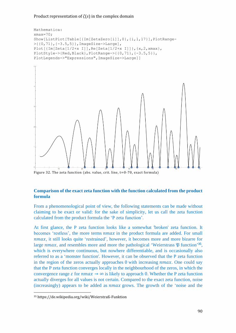
Product representation of 𝜁(𝑠) in the complex domain
90
Mathematica:
xmax=70;
Show[ListPlot[Table[{Im[ZetaZero[i]],0},{i,1,17}],PlotRange-
>{{0,71},{-3.5,5}},ImageSize->Large],
Plot[{Im[Zeta[1/2+x I]],Re[Zeta[1/2+x I]]},{x,2,xmax},
PlotStyle->{Red,Black},PlotRange->{{0,71},{-3.5,5}},
PlotLegends->"Expressions",ImageSize->Large]]
Figure 32. The zeta function (abs. value, crit. line, t=0-70, exact formula)
Comparison of the exact zeta function with the function calculated from the product
formula
From a phenomenological point of view, the following statements can be made without
claiming to be exact or valid: for the sake of simplicity, let us call the zeta function
calculated from the product formula the ‘P zeta function’.
At first glance, the P zeta function looks like a somewhat 'broken' zeta function. It
becomes ‘restless’, the more terms 𝑛𝑚𝑎𝑥 in the product formula are added. For small
𝑛𝑚𝑎𝑥, it still looks quite ‘restrained’, however, it becomes more and more bizarre for
large 𝑛𝑚𝑎𝑥, and resembles more and more the pathological ‘Weierstrass 𝔓 function’35,
which is everywhere continuous, but nowhere differentiable, and is occasionally also
referred to as a ‘monster function'. However, it can be observed that the P zeta function
in the region of the zeros actually approaches 0 with increasing 𝑛𝑚𝑎𝑥. One could say
that the P zeta function converges locally in the neighbourhood of the zeros, in which the
convergence range 휀 for 𝑛𝑚𝑎𝑥 → ∞ is likely to approach 0. Whether the P zeta function
actually diverges for all values is not certain. Compared to the exact zeta function, noise
(increasingly) appears to be added as 𝑛𝑚𝑎𝑥 grows. The growth of the ‘noise and the
35 https://de.wikipedia.org/wiki/Weierstraß-Funktion
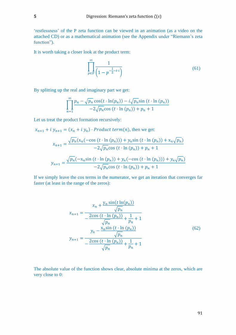
5 Digression: Riemann’s zeta function 𝜁(𝑠)
91
‘restlessness’ of the P zeta function can be viewed in an animation (as a video on the
attached CD) or as a mathematical animation (see the Appendix under “Riemann’s zeta
function”).
It is worth taking a closer look at the product term:
∏1
(1 − 𝑝−12−𝑡⋅𝑖)
∞
𝑝∈ℙ
(61)
By splitting up the real and imaginary part we get:
∏𝑝𝑛 −√𝑝𝑛 cos(𝑡 ⋅ ln(𝑝𝑛)) − 𝑖√𝑝𝑛sin (𝑡 ⋅ ln (𝑝𝑛))
−2√𝑝𝑛cos (𝑡 ⋅ ln (𝑝𝑛)) + 𝑝𝑛 + 1
∞
𝑛=1
Let us treat the product formation recursively:
𝑥𝑛+1 + 𝑖 𝑦𝑛+1 = (𝑥𝑛 + 𝑖 𝑦𝑛) ⋅ 𝑃𝑟𝑜𝑑𝑢𝑐𝑡 𝑡𝑒𝑟𝑚(𝑛), then we get:
𝑥𝑛+1 =√𝑝𝑛(x𝑛(−cos (𝑡 ⋅ ln (𝑝𝑛))) + 𝑦𝑛sin (𝑡 ⋅ ln (𝑝𝑛)) + x𝑛√𝑝𝑛)
−2√𝑝𝑛cos (𝑡 ⋅ ln (𝑝𝑛)) + 𝑝𝑛 + 1
𝑦𝑛+1 =√𝑝𝑛(−x𝑛sin (𝑡 ⋅ ln (𝑝𝑛)) + 𝑦𝑛(−cos (𝑡 ⋅ ln (𝑝𝑛))) + 𝑦𝑛√𝑝𝑛)
−2√𝑝𝑛cos (𝑡 ⋅ ln (𝑝𝑛)) + 𝑝𝑛 + 1
If we simply leave the cos terms in the numerator, we get an iteration that converges far
faster (at least in the range of the zeros):
𝑥𝑛+1 =
𝑥𝑛 +y𝑛 sin(𝑡 ln(𝑝𝑛))
√𝑝𝑛
−2cos (𝑡 ⋅ ln (𝑝𝑛))
√𝑝𝑛+1𝑝𝑛+ 1
𝑦𝑛+1 =
𝑦𝑛 −x𝑛sin (𝑡 ⋅ ln (𝑝𝑛))
√𝑝𝑛
−2cos (𝑡 ⋅ ln (𝑝𝑛))
√𝑝𝑛+1𝑝𝑛+ 1
(62)
The absolute value of the function shows clear, absolute minima at the zeros, which are
very close to 0:
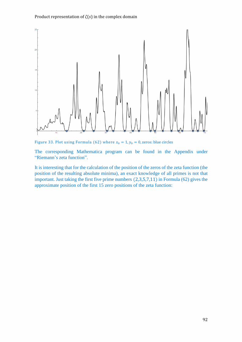
Product representation of 𝜁(𝑠) in the complex domain
92
Figure 33. Plot using Formula (62) where 𝑥0 = 1, 𝑦0 = 0, zeros: blue circles
The corresponding Mathematica program can be found in the Appendix under
“Riemann’s zeta function”.
It is interesting that for the calculation of the position of the zeros of the zeta function (the
position of the resulting absolute minima), an exact knowledge of all primes is not that
important. Just taking the first five prime numbers (2,3,5,7,11) in Formula (62) gives the
approximate position of the first 15 zero positions of the zeta function:
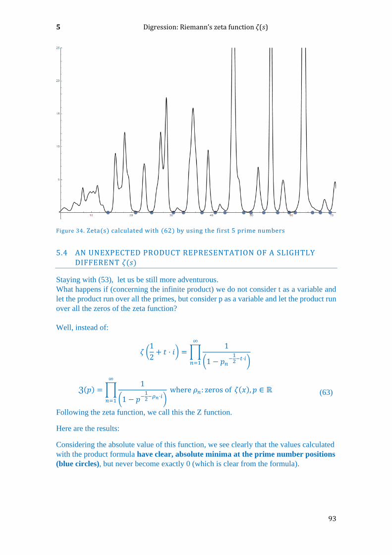
5 Digression: Riemann’s zeta function 𝜁(𝑠)
93
Figure 34. Zeta(s) calculated with (62) by using the first 5 prime numbers
5.4 AN UNEXPECTED PRODUCT REPRESENTATION OF A SLIGHTLY DIFFERENT 휁(𝑠)
Staying with (53), let us be still more adventurous.
What happens if (concerning the infinite product) we do not consider t as a variable and
let the product run over all the primes, but consider p as a variable and let the product run
over all the zeros of the zeta function?
Well, instead of:
휁 (1
2+ 𝑡 ⋅ 𝑖) =∏
1
(1 − 𝑝𝑛−12−𝑡⋅𝑖)
∞
𝑛=1
ℨ(𝑝) =∏1
(1 − 𝑝−12−𝜌𝑛⋅𝑖)
where 𝜌𝑛: zeros of
∞
𝑛=1
휁(𝑥), 𝑝 ∈ ℝ (63)
Following the zeta function, we call this the Z function.
Here are the results:
Considering the absolute value of this function, we see clearly that the values calculated
with the product formula have clear, absolute minima at the prime number positions
(blue circles), but never become exactly 0 (which is clear from the formula).
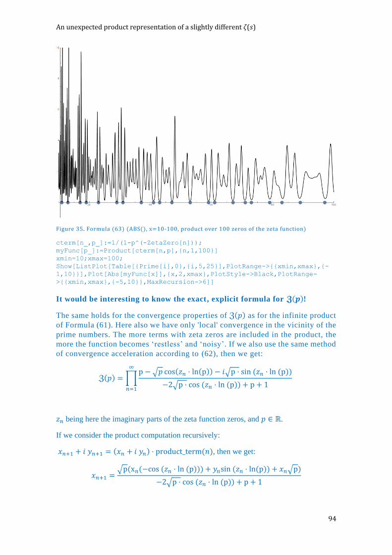
An unexpected product representation of a slightly different 𝜁(𝑠)
94
Figure 35. Formula (63) (ABS(), x=10-100, product over 100 zeros of the zeta function)
cterm[n_,p_]:=1/(1-p^(-ZetaZero[n]));
myFunc[p_]:=Product[cterm[n,p],{n,1,100}]
xmin=10;xmax=100;
Show[ListPlot[Table[{Prime[i],0},{i,5,25}],PlotRange->{{xmin,xmax},{-
1,10}}],Plot[Abs[myFunc[x]],{x,2,xmax},PlotStyle->Black,PlotRange-
>{{xmin,xmax},{-5,10}},MaxRecursion->6]]
It would be interesting to know the exact, explicit formula for 𝖅(𝒑)!
The same holds for the convergence properties of ℨ(𝑝) as for the infinite product
of Formula (61). Here also we have only 'local' convergence in the vicinity of the
prime numbers. The more terms with zeta zeros are included in the product, the
more the function becomes ‘restless’ and ‘noisy’. If we also use the same method
of convergence acceleration according to (62), then we get:
ℨ(𝑝) =∏p−√𝑝 cos(𝑧𝑛 ⋅ ln(p)) − 𝑖√p ⋅ sin (𝑧𝑛 ⋅ ln (p))
−2√p ⋅ cos (𝑧𝑛 ⋅ ln (p)) + p + 1
∞
𝑛=1
𝑧𝑛 being here the imaginary parts of the zeta function zeros, and 𝑝 ∈ ℝ.
If we consider the product computation recursively:
𝑥𝑛+1 + 𝑖 𝑦𝑛+1 = (𝑥𝑛 + 𝑖 𝑦𝑛) ⋅ product_term(𝑛), then we get:
𝑥𝑛+1 =√p(x𝑛(−cos (𝑧𝑛 ⋅ ln (p))) + 𝑦𝑛sin (𝑧𝑛 ⋅ ln(p)) + 𝑥𝑛√p)
−2√p ⋅ cos (𝑧𝑛 ⋅ ln (p)) + p + 1
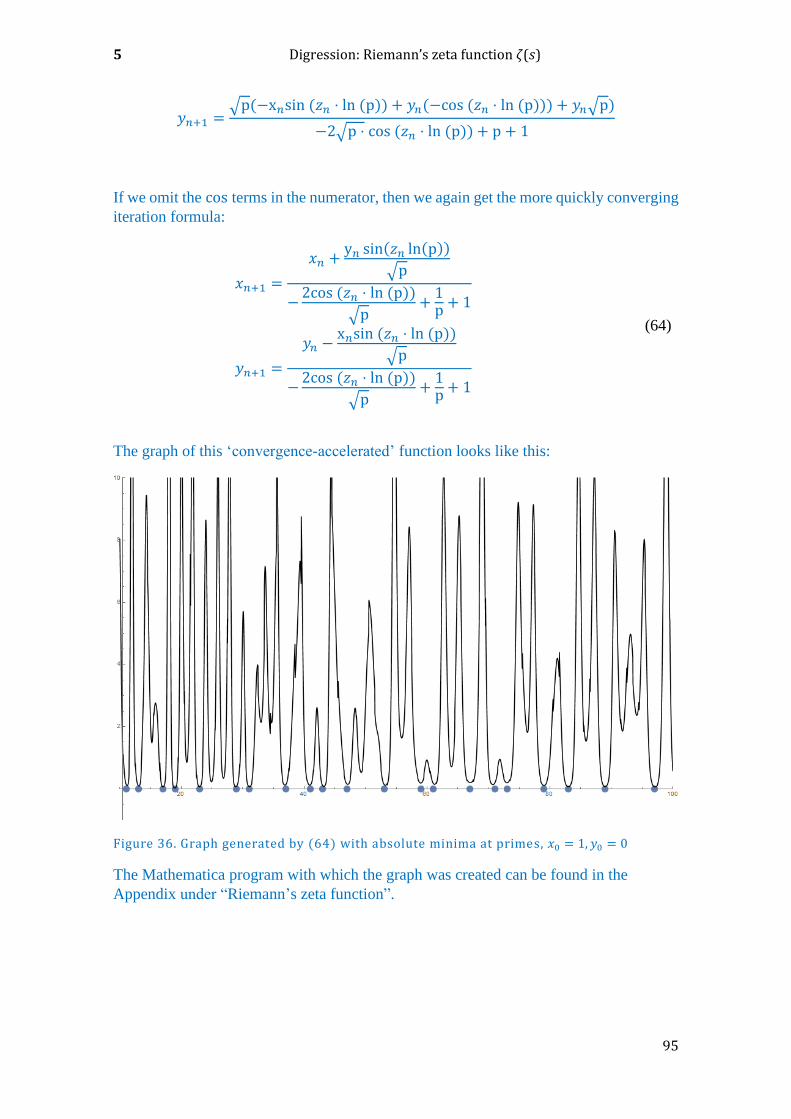
5 Digression: Riemann’s zeta function 𝜁(𝑠)
95
𝑦𝑛+1 =√p(−x𝑛sin (𝑧𝑛 ⋅ ln (p)) + 𝑦𝑛(−cos (𝑧𝑛 ⋅ ln (p))) + 𝑦𝑛√p)
−2√p ⋅ cos (𝑧𝑛 ⋅ ln (p)) + p + 1
If we omit the cos terms in the numerator, then we again get the more quickly converging
iteration formula:
𝑥𝑛+1 =
𝑥𝑛 +y𝑛 sin(𝑧𝑛 ln(p))
√p
−2cos (𝑧𝑛 ⋅ ln (p))
√p+1p + 1
𝑦𝑛+1 =
𝑦𝑛 −x𝑛sin (𝑧𝑛 ⋅ ln (p))
√p
−2cos (𝑧𝑛 ⋅ ln (p))
√p+1p + 1
(64)
The graph of this ‘convergence-accelerated’ function looks like this:
Figure 36. Graph generated by (64) with absolute minima at primes, 𝑥0 = 1, 𝑦0 = 0
The Mathematica program with which the graph was created can be found in the
Appendix under “Riemann’s zeta function”.
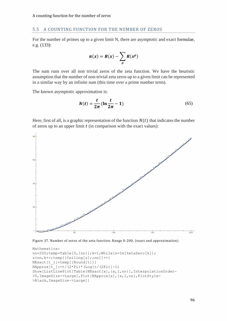
A counting function for the number of zeros
96
5.5 A COUNTING FUNCTION FOR THE NUMBER OF ZEROS
For the number of primes up to a given limit N, there are asymptotic and exact formulae,
e.g. (133):
𝝅(𝒙) = 𝑹(𝒙) −∑𝑹(𝒙𝝆)
𝝆
The sum runs over all non trivial zeros of the zeta function. We have the heuristic
assumption that the number of non-trivial zeta zeros up to a given limit can be represented
in a similar way by an infinite sum (this time over a prime number term).
The known asymptotic approximation is:
𝑵(𝒕) =𝒕
𝟐𝝅(𝐥𝐧
𝒕
𝟐𝝅− 𝟏) (65)
Here, first of all, is a graphic representation of the function 𝑁(𝑡) that indicates the number
of zeros up to an upper limit 𝑡 (in comparison with the exact values):
Figure 37. Number of zeros of the zeta function. Range 0-200, (exact and approximation)
Mathematica:
nn=200;temp=Table[0,{nn}];k=1;While[z=Im[ZetaZero[k]];
z<nn,k++;temp[[Ceiling[z];;nn]]++]
NExact[t_]:=temp[[Round[t]]]
NApprox[t_]:=t/(2*Pi)*(Log[t/(2Pi)]-1)
Show[ListLinePlot[Table[NExact[x],{x,1,nn}],InterpolationOrder-
>0,ImageSize->Large],Plot[NApprox[x],{x,1,nn},PlotStyle-
>Black,ImageSize->Large]]

5 Digression: Riemann’s zeta function 𝜁(𝑠)
97
However, exact formulae can be also found in the literature (for derivation, see above):
𝑁(𝑡) =1
𝜋 𝐼𝑚(ln(𝛤(
1
4 +𝑖𝑡
2)) −
𝑡
2𝜋 ln(𝜋) +
1
𝜋 𝐼𝑚(ln(휁(
1
2 + 𝑖𝑡)) + 1 (66)
Graph:
Figure 38. Number of zeros of the zeta function. Range: 0-200 (Formula (66) and approximation)
Mathematica:
countZero[t_]:=1/Pi*Im[LogGamma[1/4+I*t/2]]-
t/(2*Pi)Log[Pi]+1/Pi*Im[Log[Zeta[1/2+I*t]]]+1
NApprox[t_]:=t/(2*Pi)*(Log[t/(2Pi)]-1)
Show[ListLinePlot[Table[NApprox[n],{n,1,200}],
PlotRange->All],ListLinePlot[Table[countZero[n],{n,1,200}],
InterpolationOrder->0, PlotRange->All]]
Formula (66) seems to produce exactly the number of the zeros. (Verified by the author
up to 100000).
The duality between prime numbers and zeros of the zeta function is an essential theme
of this book. Of course, there is a temptation to find a representation for the number of
zeros, which consists of an approximation term (which describes the asymptotic
development), and an additional sum term, which takes into account all the details and
local nuances the more terms we include.
Thus the duality between prime numbers and zeros of the zeta function would be perfect.
We think, for example, of Formula (133) which gives the exact number of prime numbers:
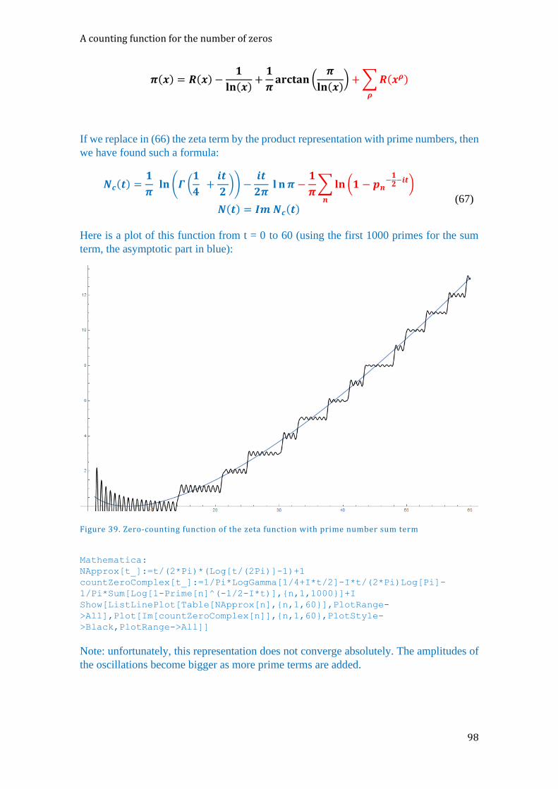
A counting function for the number of zeros
98
𝝅(𝒙) = 𝑹(𝒙) −𝟏
𝐥𝐧(𝒙)+𝟏
𝝅𝐚𝐫𝐜𝐭𝐚𝐧 (
𝝅
𝐥𝐧(𝒙)) +∑𝑹(𝒙𝝆)
𝝆
If we replace in (66) the zeta term by the product representation with prime numbers, then
we have found such a formula:
𝑵𝒄(𝒕) =𝟏
𝝅 𝐥𝐧 (𝜞 (
𝟏
𝟒 +𝒊𝒕
𝟐)) −
𝒊𝒕
𝟐𝝅 𝐥 𝐧𝝅 −
𝟏
𝝅∑𝐥𝐧(𝟏 − 𝒑𝒏
−𝟏𝟐−𝒊𝒕)
𝒏
𝑵(𝒕) = 𝑰𝒎 𝑵𝒄(𝒕)
(67)
Here is a plot of this function from t = 0 to 60 (using the first 1000 primes for the sum
term, the asymptotic part in blue):
Figure 39. Zero-counting function of the zeta function with prime number sum term
Mathematica:
NApprox[t_]:=t/(2*Pi)*(Log[t/(2Pi)]-1)+1
countZeroComplex[t_]:=1/Pi*LogGamma[1/4+I*t/2]-I*t/(2*Pi)Log[Pi]-
1/Pi*Sum[Log[1-Prime[n]^(-1/2-I*t)],{n,1,1000}]+I
Show[ListLinePlot[Table[NApprox[n],{n,1,60}],PlotRange-
>All],Plot[Im[countZeroComplex[n]],{n,1,60},PlotStyle-
>Black,PlotRange->All]]
Note: unfortunately, this representation does not converge absolutely. The amplitudes of
the oscillations become bigger as more prime terms are added.

5 Digression: Riemann’s zeta function 𝜁(𝑠)
99
5.6 THE ZETA FUNCTION AND QUANTUM CHAOS: A GANGWAY TO PHYSICS
Occasionally random coincidence lends a hand in mathematical discoveries. This was
probably the case in the 70s of the last century. By chance the mathematician H.
Montgomery and the physicist F. Dyson met and casually told each other about their
current research projects – poring, one assumes, over the odd diagram or formula at the
same time.
Montgomery was a mathematician, specializing in number theory and the zeta function
in particular, who had investigated the relationship between the complex zeros and prime
numbers. Dyson was one of the leading nuclear physicists in the field of the so-called
random matrices (a special mathematical field used in the treatment of the properties of
large and heavy atomic nuclei).
Perhaps Montgomery showed Dyson a diagram of the position of the zeros, because
Dyson quickly realized that a striking similarity existed between the distribution of the
zeros of the zeta function and certain physical spectra. Physically, these spectra describe
energy levels in heavy atomic nuclei; mathematically, such spectra are calculated from
the eigenvalues of so-called Gaussian random matrices (i.e. matrices occupied by random
values corresponding to a Gaussian normal distribution). Expressed in the language of
the physicists, this means that the spectral values are the 'eigenvalues' of a 'Hermitian'
operator36 . Hermitian (also called ‘self-adjoint’) operators play an important role in
quantum mechanics. Due to their symmetry properties, they always have real eigenvalues.
Now, the conjecture is that the complex zeros of the zeta function are nothing other than
the (real) eigenvalues of a mysterious Hermitian operator. This hypothesis is referred to
in the literature as the 'GUE' hypothesis ('GUE': Gaussian Unitary Ensemble).
Unfortunately this operator has not yet been found. There are, however, overwhelming
numerical indications that such an operator does exist (see below).
In fact, this conjecture goes much further back in time: the Hungarian mathematician
George Pólya expressed this conjecture more than 100 years ago (Hilbert-Pólya
conjecture). 37
Consider the differences of the complex zeros occurring along the critical line and
normalize these differences:
𝛿𝑛 =𝑧𝑛+1 − 𝑧𝑛2𝜋
ln𝑧𝑛2𝜋
From the theory, we know for sure that these 𝛿𝑛 have the mean value of
1.
(68)
36 https://de.wikipedia.org/wiki/Hermitescher_Operator 37 https://en.wikipedia.org/wiki/Hilbert-Pólya_conjecture
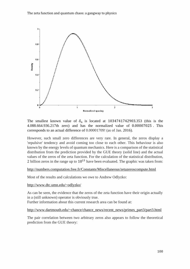
The zeta function and quantum chaos: a gangway to physics
100
The smallest known value of 𝛿𝑛 is located at 1034741742903.353 (this is the
4.088.664.936.217th zero) and has the normalized value of 0.00007025 . This
corresponds to an actual difference of 0.00001709! (as of Jan. 2016).
However, such small zero differences are very rare. In general, the zeros display a
'repulsive' tendency and avoid coming too close to each other. This behaviour is also
known by the energy levels of quantum mechanics. Here is a comparison of the statistical
distribution from the prediction provided by the GUE theory (solid line) and the actual
values of the zeros of the zeta function. For the calculation of the statistical distribution,
2 billion zeros in the range up to 1013 have been evaluated. The graphic was taken from:
http://numbers.computation.free.fr/Constants/Miscellaneous/zetazeroscompute.html
Most of the results and calculations we owe to Andrew Odlyzko:
http://www.dtc.umn.edu/~odlyzko/
As can be seen, the evidence that the zeros of the zeta function have their origin actually
in a (still unknown) operator is obviously true.
Further information about this current research area can be found at:
http://www.dartmouth.edu/~chance/chance_news/recent_news/primes_part3/part3.html
The pair correlation between two arbitrary zeros also appears to follow the theoretical
prediction from the GUE theory:
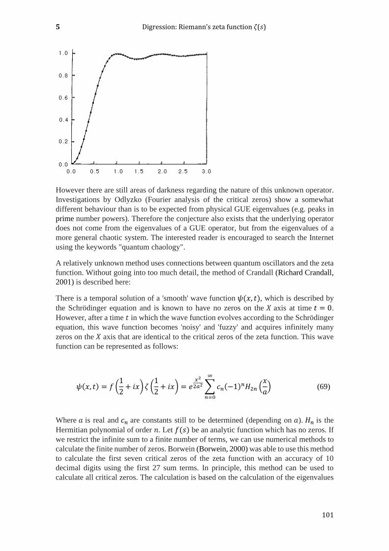
5 Digression: Riemann’s zeta function 𝜁(𝑠)
101
However there are still areas of darkness regarding the nature of this unknown operator.
Investigations by Odlyzko (Fourier analysis of the critical zeros) show a somewhat
different behaviour than is to be expected from physical GUE eigenvalues (e.g. peaks in
prime number powers). Therefore the conjecture also exists that the underlying operator
does not come from the eigenvalues of a GUE operator, but from the eigenvalues of a
more general chaotic system. The interested reader is encouraged to search the Internet
using the keywords "quantum chaology".
A relatively unknown method uses connections between quantum oscillators and the zeta
function. Without going into too much detail, the method of Crandall (Richard Crandall,
2001) is described here:
There is a temporal solution of a 'smooth' wave function 𝜓(𝑥, 𝑡), which is described by
the Schrödinger equation and is known to have no zeros on the 𝑋 axis at time 𝑡 = 0.
However, after a time 𝑡 in which the wave function evolves according to the Schrödinger
equation, this wave function becomes 'noisy' and 'fuzzy' and acquires infinitely many
zeros on the 𝑋 axis that are identical to the critical zeros of the zeta function. This wave
function can be represented as follows:
𝜓(𝑥, 𝑡) = 𝑓 (1
2+ 𝑖𝑥) 휁 (
1
2+ 𝑖𝑥) = 𝑒
𝑥2
2𝑎2∑𝑐𝑛(−1)𝑛𝐻2𝑛 (
𝑥
𝑎)
∞
𝑛=0
(69)
Where 𝑎 is real and 𝑐𝑛 are constants still to be determined (depending on 𝑎). 𝐻𝑛 is the
Hermitian polynomial of order 𝑛. Let 𝑓(𝑠) be an analytic function which has no zeros. If
we restrict the infinite sum to a finite number of terms, we can use numerical methods to
calculate the finite number of zeros. Borwein (Borwein, 2000) was able to use this method
to calculate the first seven critical zeros of the zeta function with an accuracy of 10
decimal digits using the first 27 sum terms. In principle, this method can be used to
calculate all critical zeros. The calculation is based on the calculation of the eigenvalues
The zeta function and quantum chaos: a gangway to physics
102
of a Hessenberg matrix, which ultimately leads to the calculation of the zeros of a
characteristic polynomial.
Here, further highly interesting contexts arise that are related to Riemann's conjecture.
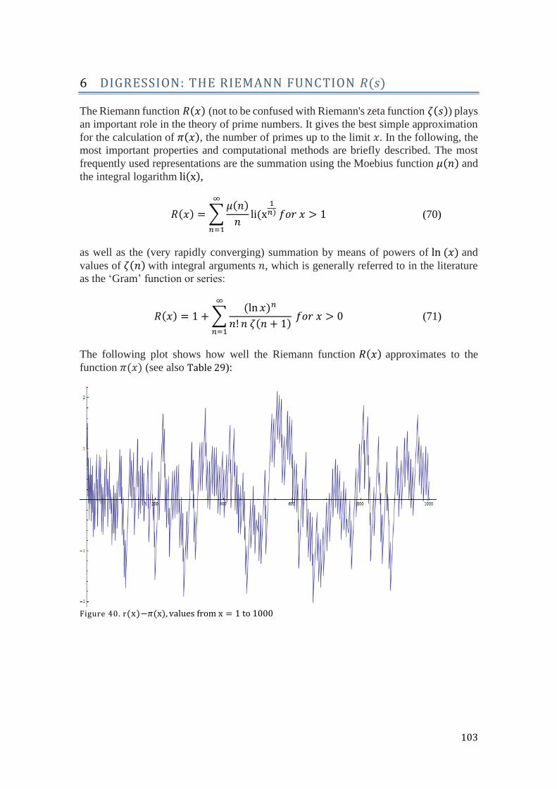
103
6 DIGRESSION: THE RIEMANN FUNCTION 𝑅(𝑠)
The Riemann function 𝑅(𝑥) (not to be confused with Riemann's zeta function 휁(𝑠)) plays
an important role in the theory of prime numbers. It gives the best simple approximation
for the calculation of 𝜋(𝑥), the number of primes up to the limit 𝑥. In the following, the
most important properties and computational methods are briefly described. The most
frequently used representations are the summation using the Moebius function 𝜇(𝑛) and
the integral logarithm li(x),
𝑅(𝑥) = ∑𝜇(𝑛)
𝑛
∞
𝑛=1
li(x1𝑛) 𝑓𝑜𝑟 𝑥 > 1 (70)
as well as the (very rapidly converging) summation by means of powers of ln (𝑥) and
values of 휁(𝑛) with integral arguments 𝑛, which is generally referred to in the literature
as the ‘Gram’ function or series:
𝑅(𝑥) = 1 +∑(ln 𝑥)𝑛
𝑛! 𝑛 휁(𝑛 + 1) 𝑓𝑜𝑟 𝑥 > 0
∞
𝑛=1
(71)
The following plot shows how well the Riemann function 𝑅(𝑥) approximates to the
function 𝜋(𝑥) (see also Table 29):
Figure 40. r(x)−𝜋(x), values from x = 1 to 1000

104
7 A FEW IMPORTANT ARITHMETICAL FUNCTIONS
7.1 OMEGA FUNCTIONS: NUMBER OF PRIME FACTORS
𝜔(𝑛) denotes the number of different prime factors of a positive integer 𝑛. Thus, 𝜔(𝑛) is
defined by the factorization of an integer as:
𝑛 = 𝑝1𝑒1𝑝2
𝑒2…𝑝𝜔(𝑛)𝑒𝜔(𝑛)
In contrast, Ω(𝑛) denotes the total number of prime factors of an integer 𝑛:
Ω(𝑛) = ∑ 𝑒𝑖
𝑒𝜔(𝑛)
𝑘=1
(72)
Clearly, Ω(𝑛) is simply the sum of the prime powers of 𝑛.
g 𝜔(𝑛) is defined by PrimeNu[n] and Ω(𝑛) by PrimeOmega[n].
Numbers that are composed only of different factors are identical to square-free numbers.
The asymptotic behaviour of 𝜔(𝑛) is given by:
𝜔(𝑛)~ ln ln 𝑛 + 𝐵1 +∑(−1 +∑𝛾𝑗
𝑗!
𝑘−1
𝑗=0
)(𝑘 − 1)!
(ln 𝑛)𝑘
∞
𝑘=1
where 𝐵1is the Mertens constant and 𝛾𝑗 are the Stieltjes constants.

7 A few important arithmetical functions
105
Figure 41. Function 𝜔(n), number of different prime factors (red: asymptotic)
Mathematica:
mertensB1=0.2614972128;
nmax=100000;
Show[ListLogLinearPlot[Table[PrimeNu[n],{n,2,nmax}],
PlotRange->All],ListLogLinearPlot[Table[Log[Log[n]]+mertensB1,
{n,2,nmax}],PlotRange->All,Joined->True,PlotStyle->Red]]
The asymptotic behaviour of Ω(𝑛) is also approximate:
Ω(𝑛)~ ln ln 𝑛 + 𝐵2, with 𝐵2 = 0.494906
Figure 42. Function Ω(n), total number of prime factors (red: asymptotic)
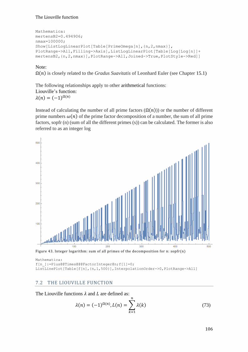
The Liouville function
106
Mathematica:
mertensB2=0.494906;
nmax=100000;
Show[ListLogLinearPlot[Table[PrimeOmega[n],{n,2,nmax}],
PlotRange->All,Filling->Axis],ListLogLinearPlot[Table[Log[Log[n]]+
mertensB2,{n,2,nmax}],PlotRange->All,Joined->True,PlotStyle->Red]]
Note:
Ω(𝑛) is closely related to the Gradus Suavitatis of Leonhard Euler (see Chapter 15.1)
The following relationships apply to other arithmetical functions:
Liouville’s function:
𝜆(𝑛) = (−1)Ω(n)
Instead of calculating the number of all prime factors (Ω(𝑛))) or the number of different
prime numbers 𝜔(𝑛) of the prime factor decomposition of a number, the sum of all prime
factors, sopfr (n) (sum of all the different primes (s)) can be calculated. The former is also
referred to as an integer log
Figure 43. Integer logarithm: sum of all primes of the decomposition for n: sopfr(n)
Mathematica:
f[n_]:=Plus@@Times@@@FactorInteger@n;f[1]=0;
ListLinePlot[Table[f[n],{n,1,500}],InterpolationOrder->0,PlotRange->All]
7.2 THE LIOUVILLE FUNCTION
The Liouville functions 𝜆 and 𝐿 are defined as:
𝜆(𝑛) = (−1)Ω(n), 𝐿(𝑛) = ∑𝜆(𝑘)
𝑛
𝑘=1
(73)
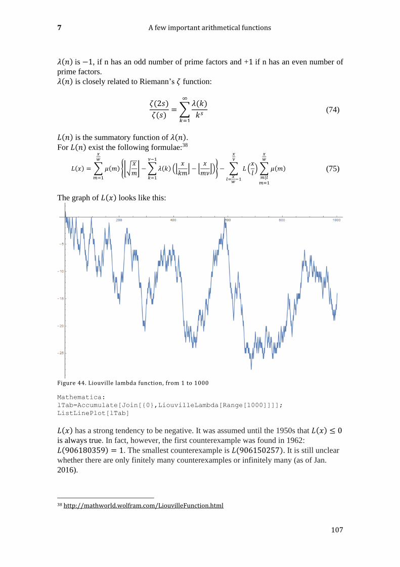
7 A few important arithmetical functions
107
𝜆(𝑛) is −1, if n has an odd number of prime factors and +1 if n has an even number of
prime factors.
𝜆(𝑛) is closely related to Riemann’s 휁 function:
휁(2𝑠)
휁(𝑠)= ∑
𝜆(𝑘)
𝑘𝑠
∞
𝑘=1
(74)
𝐿(𝑛) is the summatory function of 𝜆(𝑛). For 𝐿(𝑛) exist the following formulae:38
𝐿(𝑥) = ∑ 𝜇(𝑚) {⌊√𝑥
𝑚⌋ −∑𝜆(𝑘) (⌊
𝑥
𝑘𝑚⌋ − ⌊
𝑥
𝑚𝜈⌋)
𝜈−1
𝑘=1
} − ∑ 𝐿 (𝑥
𝑙) ∑ 𝜇(𝑚)
𝑥𝑤
𝑚|𝑙𝑚=1
𝑥𝜈
𝑙=𝑥𝑤−1
𝑥𝑤
𝑚=1
(75)
The graph of 𝐿(𝑥) looks like this:
Figure 44. Liouville lambda function, from 1 to 1000
Mathematica:
lTab=Accumulate[Join[{0},LiouvilleLambda[Range[1000]]]];
ListLinePlot[lTab]
𝐿(𝑥) has a strong tendency to be negative. It was assumed until the 1950s that 𝐿(𝑥) ≤ 0
is always true. In fact, however, the first counterexample was found in 1962:
𝐿(906180359) = 1. The smallest counterexample is 𝐿(906150257). It is still unclear
whether there are only finitely many counterexamples or infinitely many (as of Jan.
2016).
38 http://mathworld.wolfram.com/LiouvilleFunction.html
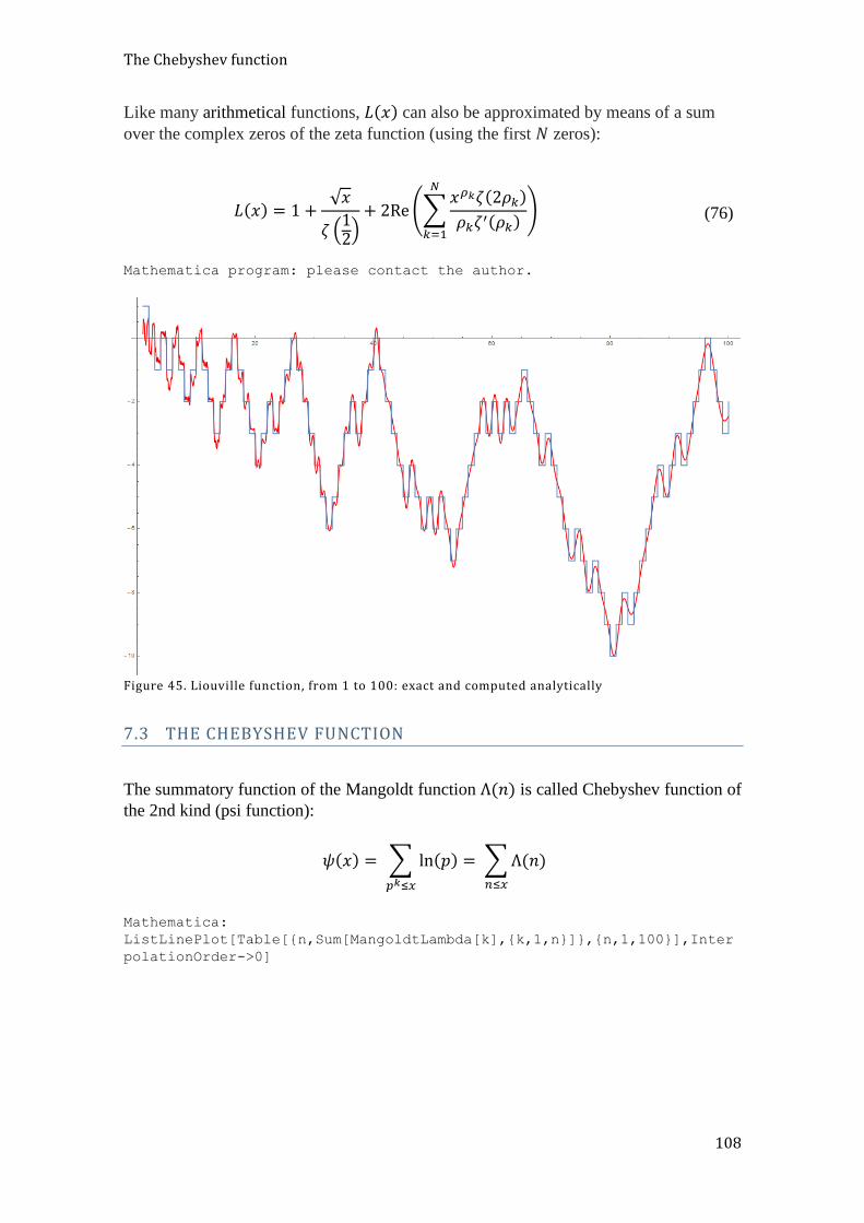
The Chebyshev function
108
Like many arithmetical functions, 𝐿(𝑥) can also be approximated by means of a sum
over the complex zeros of the zeta function (using the first 𝑁 zeros):
𝐿(𝑥) = 1 +√𝑥
휁 (12)+ 2Re(∑
𝑥𝜌𝑘휁(2𝜌𝑘)
𝜌𝑘휁′(𝜌𝑘)
𝑁
𝑘=1
) (76)
Mathematica program: please contact the author.
Figure 45. Liouville function, from 1 to 100: exact and computed analytically
7.3 THE CHEBYSHEV FUNCTION
The summatory function of the Mangoldt function Λ(𝑛) is called Chebyshev function of
the 2nd kind (psi function):
𝜓(𝑥) = ∑ ln(𝑝) = ∑Λ(𝑛)
𝑛≤𝑥𝑝𝑘≤𝑥
Mathematica:
ListLinePlot[Table[{n,Sum[MangoldtLambda[k],{k,1,n}]},{n,1,100}],Inter
polationOrder->0]
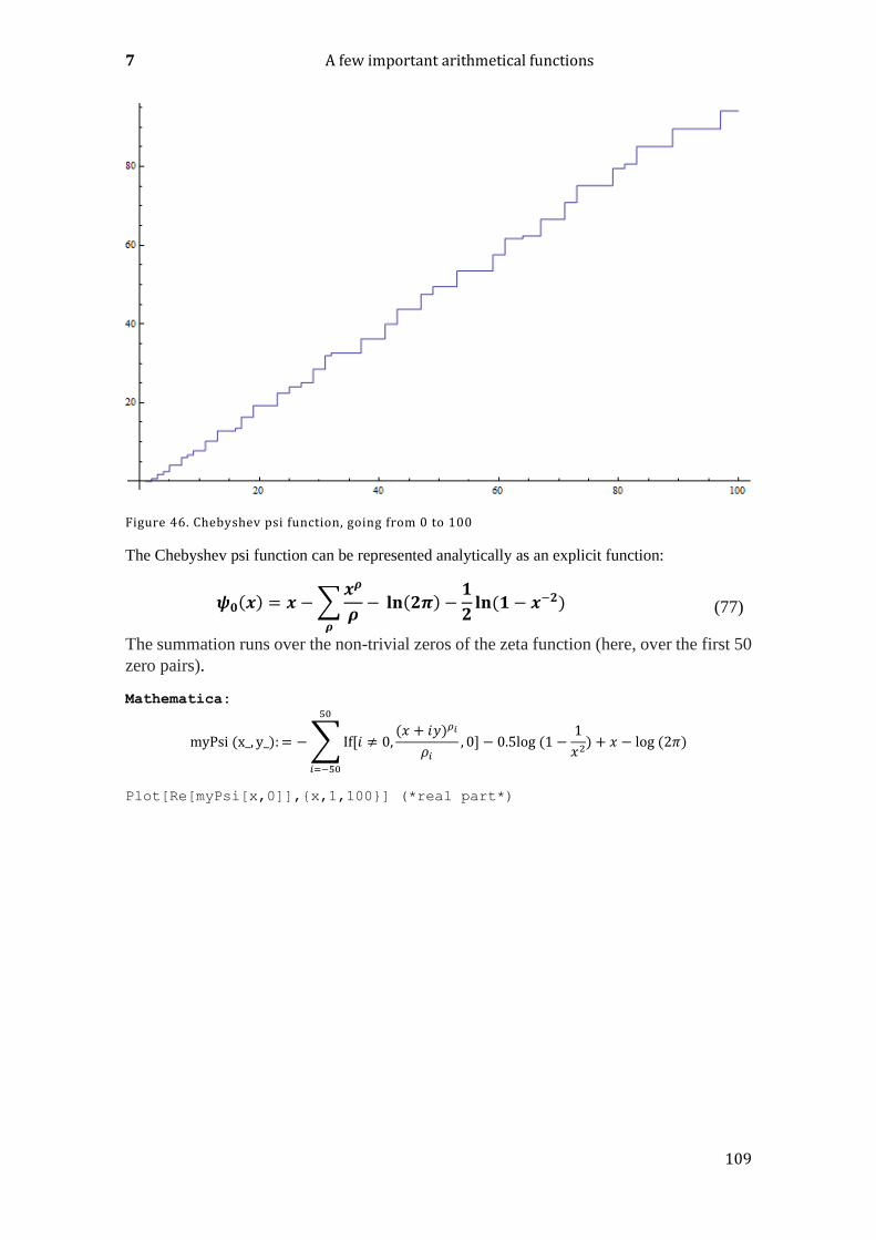
7 A few important arithmetical functions
109
Figure 46. Chebyshev psi function, going from 0 to 100
The Chebyshev psi function can be represented analytically as an explicit function:
𝝍𝟎(𝒙) = 𝒙 −∑𝒙𝝆
𝝆−
𝝆
𝐥𝐧(𝟐𝝅) −𝟏
𝟐𝐥𝐧(𝟏 − 𝒙−𝟐) (77)
The summation runs over the non-trivial zeros of the zeta function (here, over the first 50
zero pairs).
Mathematica:
myPsi (x_, y_):= −∑If[𝑖 ≠ 0,(𝑥 + 𝑖𝑦)𝜌𝑖
𝜌𝑖, 0]
50
𝑖=−50
− 0.5log (1 −1
𝑥2) + 𝑥 − log (2𝜋)
Plot[Re[myPsi[x,0]],{x,1,100}] (*real part*)

The Chebyshev function
110
Figure 47. Chebyshev psi function, computed analytically, plot from 0 to 100
Both functions in comparison (sum over the first 75 zero pairs):
Mathematica program: please contact the author.
Show[Plot[Re[myPsi[x, 0]], {x, 1, 100},PlotPoints->400,
PlotStyle->Red], ListLinePlot[Table[{n, Sum[MangoldtLambda[k], {k, 1,
n}]},{n, 1, 100}], InterpolationOrder->0]]
Figure 48. Chebyshev psi function; comparison of analytic and arithmetical method s of calculation
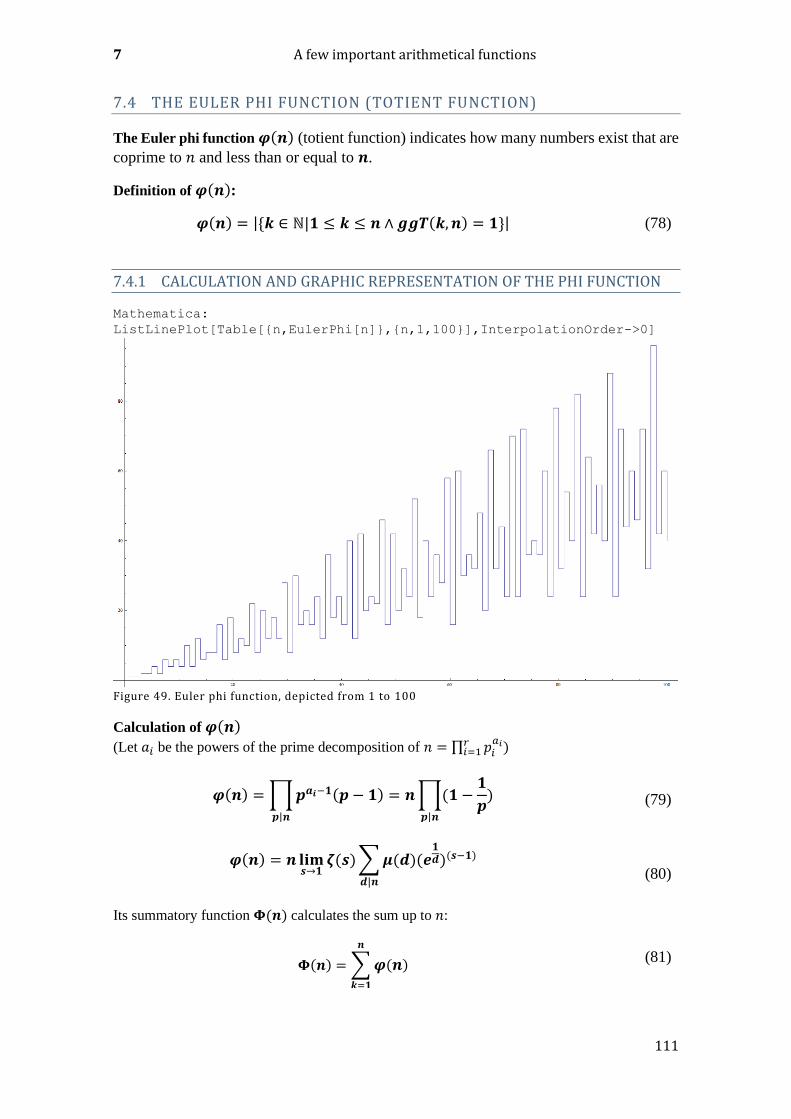
7 A few important arithmetical functions
111
7.4 THE EULER PHI FUNCTION (TOTIENT FUNCTION)
The Euler phi function 𝝋(𝒏) (totient function) indicates how many numbers exist that are
coprime to 𝑛 and less than or equal to 𝒏.
Definition of 𝝋(𝒏):
𝝋(𝒏) = |{𝒌 ∈ ℕ|𝟏 ≤ 𝒌 ≤ 𝒏 ∧ 𝒈𝒈𝑻(𝒌,𝒏) = 𝟏}| (78)
7.4.1 CALCULATION AND GRAPHIC REPRESENTATION OF THE PHI FUNCTION
Mathematica:
ListLinePlot[Table[{n,EulerPhi[n]},{n,1,100}],InterpolationOrder->0]
Figure 49. Euler phi function, depicted from 1 to 100
Calculation of 𝝋(𝒏) (Let 𝑎𝑖 be the powers of the prime decomposition of 𝑛 = ∏ 𝑝𝑖
𝑎𝑖𝑟𝑖=1 )
𝝋(𝒏) =∏𝒑𝒂𝒊−𝟏(𝒑 − 𝟏) = 𝒏
𝒑|𝒏
∏(𝟏−𝟏
𝒑)
𝒑|𝒏
(79)
𝝋(𝒏) = 𝒏 𝐥𝐢𝐦𝒔→𝟏
𝜻(𝒔)∑𝝁(𝒅)(𝒆𝟏𝒅)(𝒔−𝟏)
𝒅|𝒏
(80)
Its summatory function 𝚽(𝒏) calculates the sum up to 𝑛:
𝚽(𝒏) = ∑𝝋(𝒏)
𝒏
𝒌=𝟏
(81)
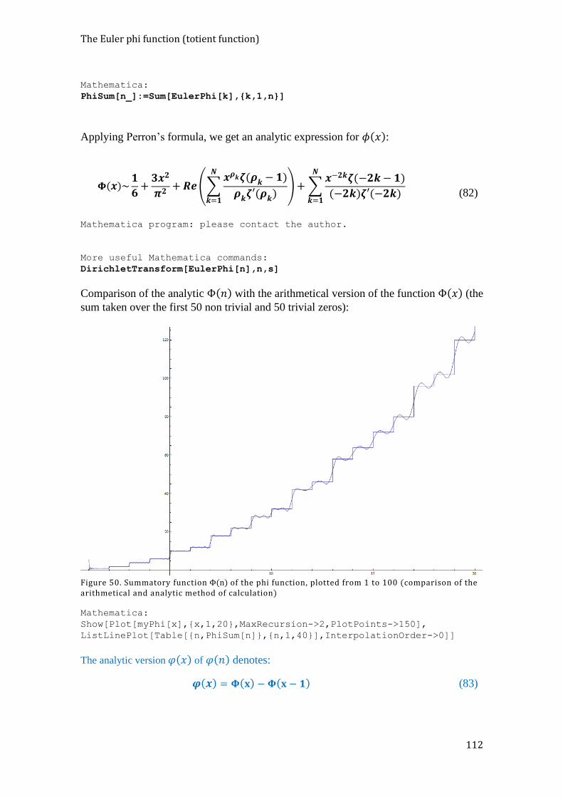
The Euler phi function (totient function)
112
Mathematica:
PhiSum[n_]:=Sum[EulerPhi[k],{k,1,n}]
Applying Perron’s formula, we get an analytic expression for 𝜙(𝑥):
𝚽(𝒙)~𝟏
𝟔+𝟑𝒙𝟐
𝝅𝟐+𝑹𝒆(∑
𝒙𝝆𝒌𝜻(𝝆𝒌 − 𝟏)
𝝆𝒌𝜻′(𝝆𝒌)
𝑵
𝒌=𝟏
)+∑𝒙−𝟐𝒌𝜻(−𝟐𝒌− 𝟏)
(−𝟐𝒌)𝜻′(−𝟐𝒌)
𝑵
𝒌=𝟏
(82)
Mathematica program: please contact the author.
More useful Mathematica commands:
DirichletTransform[EulerPhi[n],n,s]
Comparison of the analytic Φ(𝑛) with the arithmetical version of the function Φ(𝑥) (the
sum taken over the first 50 non trivial and 50 trivial zeros):
Figure 50. Summatory function Φ(n) of the phi function, plotted from 1 to 100 (comparison of the arithmetical and analytic method of calculation)
Mathematica:
Show[Plot[myPhi[x],{x,1,20},MaxRecursion->2,PlotPoints->150],
ListLinePlot[Table[{n,PhiSum[n]},{n,1,40}],InterpolationOrder->0]]
The analytic version 𝜑(𝑥) of 𝜑(𝑛) denotes:
𝝋(𝒙) = 𝚽(𝐱) −𝚽(𝐱 − 𝟏) (83)
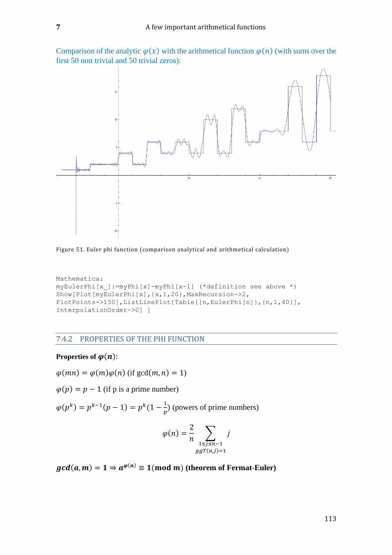
7 A few important arithmetical functions
113
Comparison of the analytic 𝜑(𝑥) with the arithmetical function 𝜑(𝑛) (with sums over the
first 50 non trivial and 50 trivial zeros):
Figure 51. Euler phi function (comparison analytical and arithmetical calculation)
Mathematica:
myEulerPhi[x_]:=myPhi[x]-myPhi[x-1] (*definition see above *)
Show[Plot[myEulerPhi[x],{x,1,20},MaxRecursion->2,
PlotPoints->150],ListLinePlot[Table[{n,EulerPhi[n]},{n,1,40}],
InterpolationOrder->0] ]
7.4.2 PROPERTIES OF THE PHI FUNCTION
Properties of 𝝋(𝒏):
𝜑(𝑚𝑛) = 𝜑(𝑚)𝜑(𝑛) (if gcd(𝑚, 𝑛) = 1)
𝜑(𝑝) = 𝑝 − 1 (if p is a prime number)
𝜑(𝑝𝑘) = 𝑝𝑘−1(𝑝 − 1) = 𝑝𝑘(1 −1
𝑝) (powers of prime numbers)
𝜑(𝑛) =2
𝑛∑ 𝑗
1≤𝑗≤𝑛−1
𝑔𝑔𝑇(𝑛,𝑗)=1
𝒈𝒄𝒅(𝒂,𝒎) = 𝟏 ⇒ 𝒂𝝋(𝒏) ≡ 𝟏(𝐦𝐨𝐝 𝒎) (theorem of Fermat-Euler)
The Euler phi function (totient function)
114
𝒑 ∤ 𝒂 ⇒ 𝒂𝒑−𝟏 ≡ 𝟏(𝐦𝐨𝐝 𝒑) (special case for prime numbers, ‘little Fermat
theorem’)
𝜑(𝑚𝑛) = 𝜑(𝑚)𝜑(𝑛)𝑑
𝜑(𝑑), where 𝑑 = 𝑔𝑐𝑑(𝑚, 𝑛)
𝜑(𝑛𝑚) = 𝑛𝑚−1𝜑(𝑛)
𝝋(𝒏)𝝈𝟎(𝒏) = ∑ 𝐠𝐠𝐓(𝒌 − 𝟏, 𝒏)𝟏≤𝒌≤𝟏
𝒈𝒈𝑻(𝒌,𝒏)=𝟏
(84)
∑𝝋(𝒏)
𝒏𝒔
∞
𝒏=𝟏
=𝜻(𝒔 − 𝟏)
𝜻(𝒔)
(85)
The Euler 𝜑 function has been generalized by Ramanujan (𝜑1(𝑛) = 𝜑(𝑛)):
𝝋𝒔(𝒏) = 𝒏𝒔∏(𝟏−
𝟏
𝒑𝒔)
𝒑|𝒏
(86)
Ramanujan determined 𝜑𝑠(𝑛) to be:
𝝋𝒔(𝒏) =𝝁(𝒏)𝒏𝒔
𝜻(𝒔)∑𝝁(𝒏𝒌)𝒌𝒔
∞𝒌=𝟏
(87)
𝝋(𝒏) =𝝁(𝒏)𝒏
𝜻(𝒔)∑𝝁(𝒏𝒌)𝒌
∞𝒌=𝟏
(88)
𝜑(𝑛) can also be calculated with a Ramanujan expansion:
𝝋(𝒏) =𝒏
𝜻(𝒔 + 𝟏)∑𝝁(𝒒)𝒄𝒒(𝒏)
𝝋𝟐(𝒒)
∞
𝒒=𝟏
This formula is, however, not practicable, because for the computation of 𝜑(𝑛), one also
needs 𝜑2(𝑘) (𝑘 = 1… ∞).

7 A few important arithmetical functions
115
7.5 THE SUM-OF-DIVISORS FUNCTION (SIGMA FUNCTION)
7.5.1 DEFINITION, PROPERTIES
The sum-of-divisors function 𝝈𝒌(𝒏) gives the sum of the 𝑘th powers of the positive
divisors of 𝑛 (including 𝑛).
Definition of 𝝈𝒌(𝒏):
𝝈𝒌(𝒏) =∑𝒅𝒌
𝒅|𝒏
(89)
Calculation of 𝝈𝒌(𝒏):
(let 𝑎𝑖 be the powers of the prime factor decomposition of 𝑛 = ∏ 𝑝𝑖𝑎𝑖𝑟
𝑖=1 )
𝝈𝒌(𝒏) =∏𝒑𝒊(𝒂𝒊+𝟏)𝒌 − 𝟏
𝒑𝒊𝒌 − 𝟏
𝒓
𝒊=𝟏
=∏∑𝒑𝒊𝒋𝒌
𝒂𝒊
𝒋=𝟎
𝒓
𝒊=𝟏
(90)
If 𝜎1(𝑛) is a prime number, so also is 𝜎0(𝑛). Here are the first 23 pairs:
(2,3) (3,7) (3,13) (5,31) (3,31) (7,127) (3,307) (7,1093)
(3,1723) (5,2801) (3,3541) (13,8191) (3,5113) (3,8011)
(3,10303) (7,19531) (3,17293) (3,28057) (5,30941) (3,30103)
(17,131071) (5,88741) (3,86143)
Mathematica:
For [i=1,i<100000,i++,If[PrimeQ[DivisorSigma[0,i]]==True&&
OddQ[DivisorSigma[0,i]],Print[DivisorSigma[0,i],",",
FactorInteger[DivisorSigma[1,i]]]]]
Odd prime values of 𝜎0(𝑛) are rare. Among the first 100000, 79 values (in ascending
order) can be found: {3,3,5,3,3,7,5,3,3,3,3,3,5,7,3,3,11,3,3,3,3,5,3,3,3,13,3,3,
3,3,3,3,3,3,3,3,3,3,5,7,3,3,3,3,3,3,3,3,3,5,3,3,3,3,3,3,3,3
,3,3,3,3,3,3,11,3,17,3,3,3,3,3,3,3,5,3,3,3,3}
Mathematica:
Select[Select[DivisorSigma[0,Range[100000]],OddQ],PrimeQ]
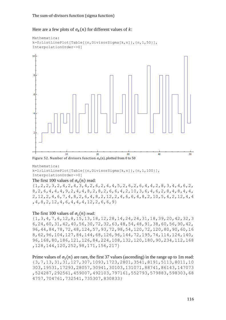
The sum-of-divisors function (sigma function)
116
Here are a few plots of 𝜎𝑘(𝑛) for different values of 𝑘:
Mathematica:
k=0;ListLinePlot[Table[{n,DivisorSigma[k,n]},{n,1,50}],
InterpolationOrder->0]
Figure 52. Number of divisors function 𝜎0(n), plotted from 0 to 50
Mathematica:
k=1;ListLinePlot[Table[{n,DivisorSigma[k,n]},{n,1,100}],
InterpolationOrder->0]
The first 100 values of 𝜎0(𝑛) read: {1,2,2,3,2,4,2,4,3,4,2,6,2,4,4,5,2,6,2,6,4,4,2,8,3,4,4,6,2,
8,2,6,4,4,4,9,2,4,4,8,2,8,2,6,6,4,2,10,3,6,4,6,2,8,4,8,4,4,
2,12,2,4,6,7,4,8,2,6,4,8,2,12,2,4,6,6,4,8,2,10,5,4,2,12,4,4
,4,8,2,12,4,6,4,4,4,12,2,6,6,9}
The first 100 values of 𝜎1(𝑛) read: {1,3,4,7,6,12,8,15,13,18,12,28,14,24,24,31,18,39,20,42,32,3
6,24,60,31,42,40,56,30,72,32,63,48,54,48,91,38,60,56,90,42,
96,44,84,78,72,48,124,57,93,72,98,54,120,72,120,80,90,60,16
8,62,96,104,127,84,144,68,126,96,144,72,195,74,114,124,140,
96,168,80,186,121,126,84,224,108,132,120,180,90,234,112,168
,128,144,120,252,98,171,156,217}
Prime values of 𝜎1(𝑛) are rare, the first 37 values (ascending) in the range up to 1m read: {3,7,13,31,31,127,307,1093,1723,2801,3541,8191,5113,8011,10
303,19531,17293,28057,30941,30103,131071,88741,86143,147073
,524287,292561,459007,492103,797161,552793,579883,598303,68
4757,704761,732541,735307,830833}
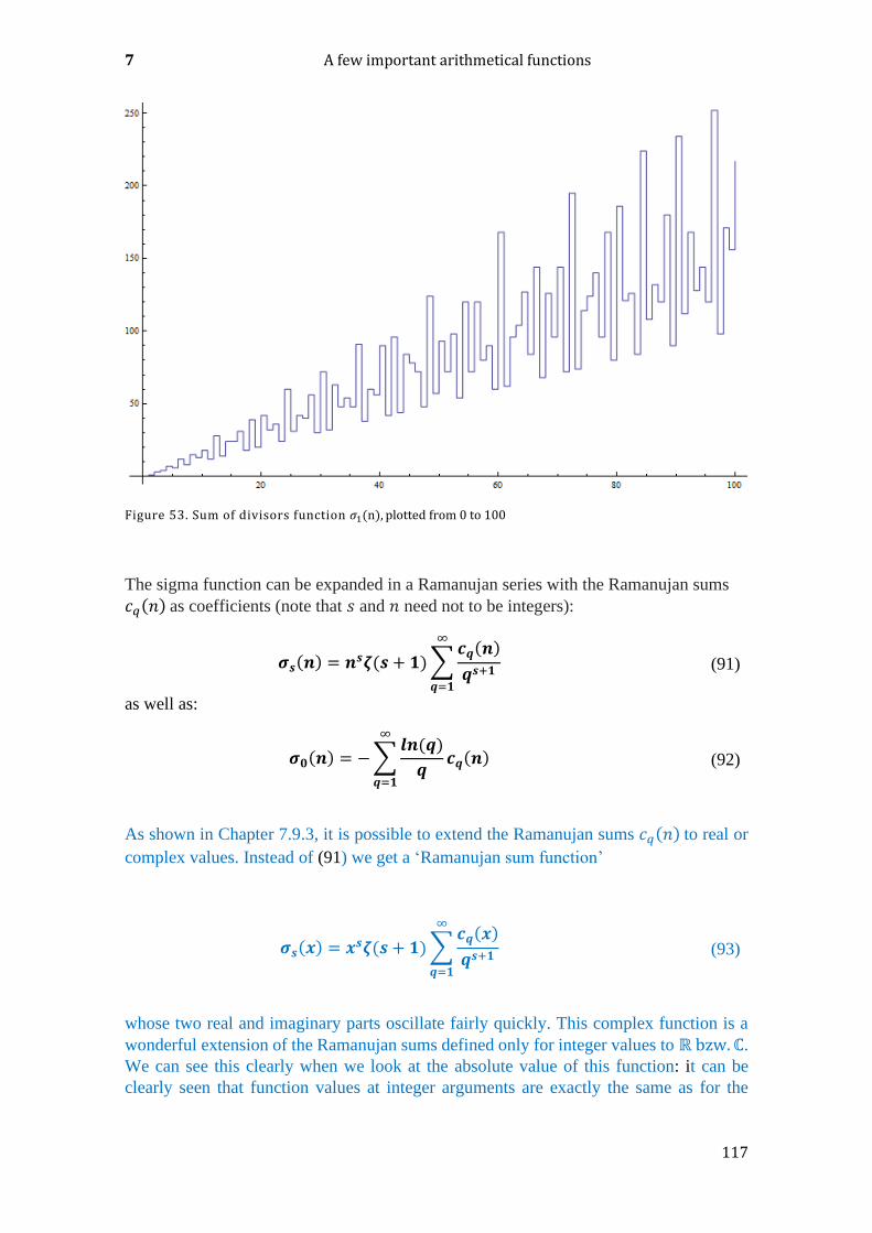
7 A few important arithmetical functions
117
Figure 53. Sum of divisors function 𝜎1(n), plotted from 0 to 100
The sigma function can be expanded in a Ramanujan series with the Ramanujan sums
𝑐𝑞(𝑛) as coefficients (note that 𝑠 and 𝑛 need not to be integers):
𝝈𝒔(𝒏) = 𝒏𝒔𝜻(𝒔 + 𝟏)∑
𝒄𝒒(𝒏)
𝒒𝒔+𝟏
∞
𝒒=𝟏
(91)
as well as:
𝝈𝟎(𝒏) = −∑𝒍𝒏(𝒒)
𝒒
∞
𝒒=𝟏
𝒄𝒒(𝒏) (92)
As shown in Chapter 7.9.3, it is possible to extend the Ramanujan sums 𝑐𝑞(𝑛) to real or
complex values. Instead of (91) we get a ‘Ramanujan sum function’
𝝈𝒔(𝒙) = 𝒙𝒔𝜻(𝒔 + 𝟏)∑
𝒄𝒒(𝒙)
𝒒𝒔+𝟏
∞
𝒒=𝟏
(93)
whose two real and imaginary parts oscillate fairly quickly. This complex function is a
wonderful extension of the Ramanujan sums defined only for integer values to ℝ bzw. ℂ.
We can see this clearly when we look at the absolute value of this function: it can be
clearly seen that function values at integer arguments are exactly the same as for the
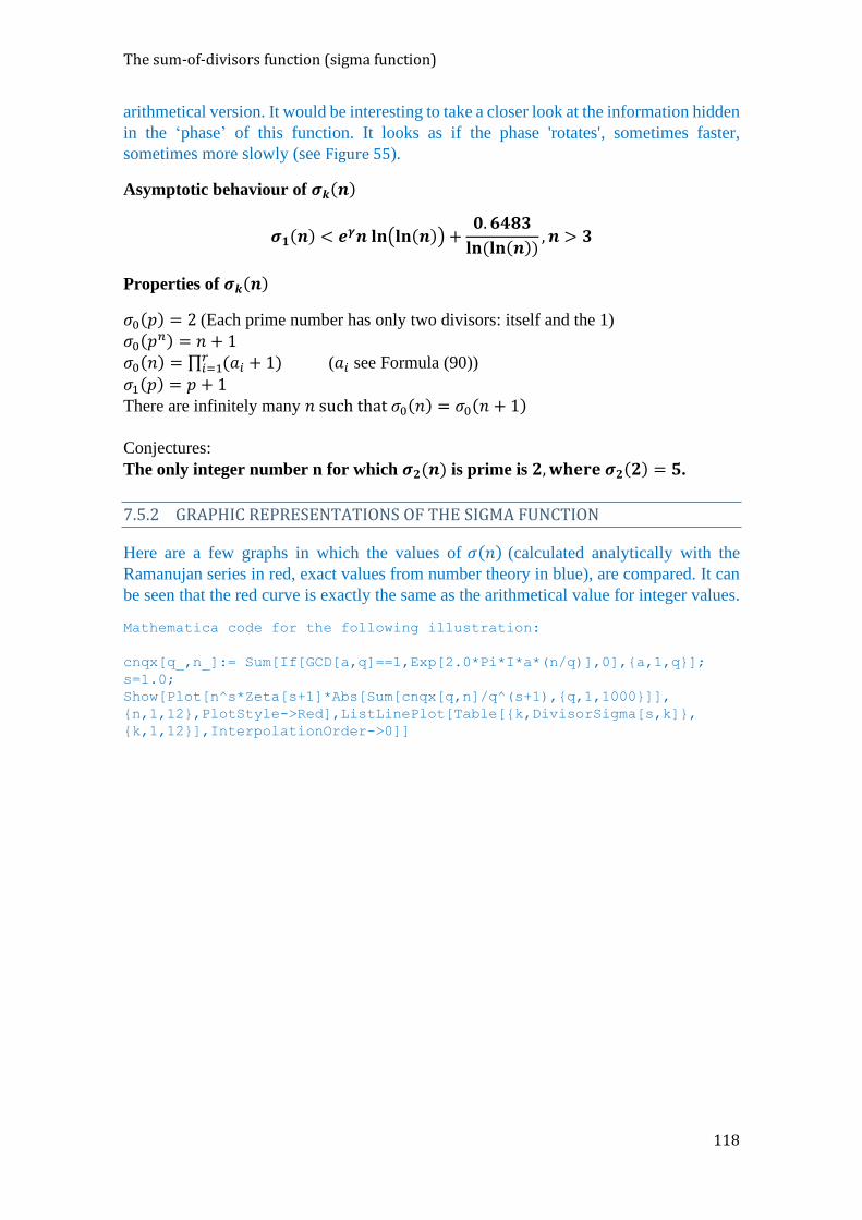
The sum-of-divisors function (sigma function)
118
arithmetical version. It would be interesting to take a closer look at the information hidden
in the ‘phase’ of this function. It looks as if the phase 'rotates', sometimes faster,
sometimes more slowly (see Figure 55).
Asymptotic behaviour of 𝝈𝒌(𝒏)
𝝈𝟏(𝒏) < 𝒆𝜸𝒏 𝐥𝐧(𝐥𝐧(𝒏)) +
𝟎. 𝟔𝟒𝟖𝟑
𝐥𝐧(𝐥𝐧(𝒏)), 𝒏 > 𝟑
Properties of 𝝈𝒌(𝒏)
𝜎0(𝑝) = 2 (Each prime number has only two divisors: itself and the 1)
𝜎0(𝑝𝑛) = 𝑛 + 1
𝜎0(𝑛) = ∏ (𝑎𝑖 + 1)𝑟𝑖=1 (𝑎𝑖 see Formula (90))
𝜎1(𝑝) = 𝑝 + 1
There are infinitely many 𝑛 such that 𝜎0(𝑛) = 𝜎0(𝑛 + 1)
Conjectures:
The only integer number n for which 𝝈𝟐(𝒏) is prime is 𝟐,𝐰𝐡𝐞𝐫𝐞 𝝈𝟐(𝟐) = 𝟓.
7.5.2 GRAPHIC REPRESENTATIONS OF THE SIGMA FUNCTION
Here are a few graphs in which the values of 𝜎(𝑛) (calculated analytically with the
Ramanujan series in red, exact values from number theory in blue), are compared. It can
be seen that the red curve is exactly the same as the arithmetical value for integer values.
Mathematica code for the following illustration:
cnqx[q_,n_]:= Sum[If[GCD[a,q]==1,Exp[2.0*Pi*I*a*(n/q)],0],{a,1,q}];
s=1.0;
Show[Plot[n^s*Zeta[s+1]*Abs[Sum[cnqx[q,n]/q^(s+1),{q,1,1000}]],
{n,1,12},PlotStyle->Red],ListLinePlot[Table[{k,DivisorSigma[s,k]},
{k,1,12}],InterpolationOrder->0]]
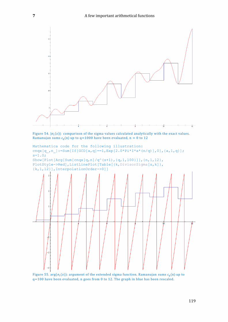
7 A few important arithmetical functions
119
Figure 54. |𝜎1(𝑥)|: comparison of the sigma values calculated analytically with the exact values. Ramanujan sums 𝑐𝑞(n) up to q=1000 have been evaluated, n = 0 to 12
Mathematica code for the following illustration:
cnqx[q_,n_]:=Sum[If[GCD[a,q]==1,Exp[2.0*Pi*I*a*(n/q)],0],{a,1,q}];
s=1.0;
Show[Plot[Arg[Sum[cnqx[q,n]/q^(s+1),{q,1,100}]],{n,1,12},
PlotStyle->Red],ListLinePlot[Table[{k,DivisorSigma[s,k]},
{k,1,12}],InterpolationOrder->0]]
Figure 55. arg(𝜎1(𝑥)): argument of the extended sigma function. Ramanujan sums 𝑐𝑞(n) up to
q=100 have been evaluated, n goes from 0 to 12. The graph in blue has been rescaled.
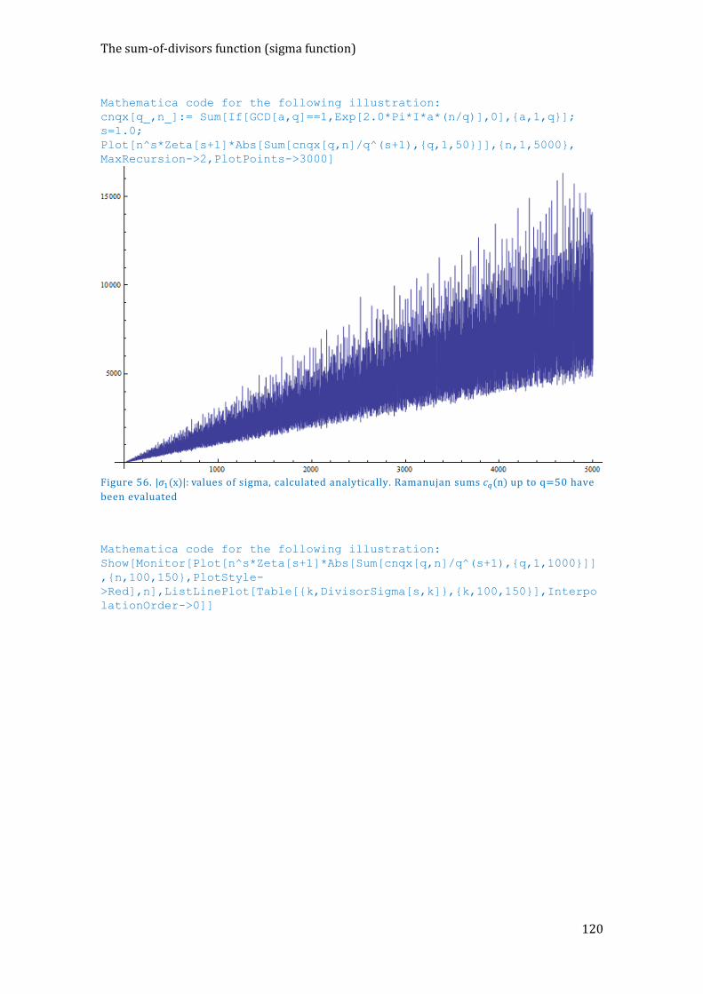
The sum-of-divisors function (sigma function)
120
Mathematica code for the following illustration:
cnqx[q_,n_]:= Sum[If[GCD[a,q]==1,Exp[2.0*Pi*I*a*(n/q)],0],{a,1,q}];
s=1.0;
Plot[n^s*Zeta[s+1]*Abs[Sum[cnqx[q,n]/q^(s+1),{q,1,50}]],{n,1,5000},
MaxRecursion->2,PlotPoints->3000]
Figure 56. |𝜎1(x)|: values of sigma, calculated analytically. Ramanujan sums 𝑐𝑞(n) up to q=50 have
been evaluated
Mathematica code for the following illustration:
Show[Monitor[Plot[n^s*Zeta[s+1]*Abs[Sum[cnqx[q,n]/q^(s+1),{q,1,1000}]]
,{n,100,150},PlotStyle-
>Red],n],ListLinePlot[Table[{k,DivisorSigma[s,k]},{k,100,150}],Interpo
lationOrder->0]]
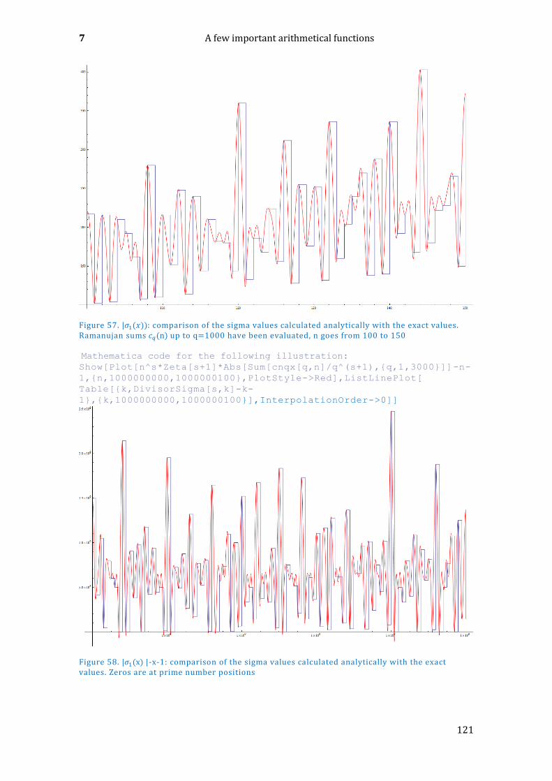
7 A few important arithmetical functions
121
Figure 57. |𝜎1(𝑥)): comparison of the sigma values calculated analytically with the exact values. Ramanujan sums 𝑐𝑞(n) up to q=1000 have been evaluated, n goes from 100 to 150
Mathematica code for the following illustration: Show[Plot[n^s*Zeta[s+1]*Abs[Sum[cnqx[q,n]/q^(s+1),{q,1,3000}]]-n-
1,{n,1000000000,1000000100},PlotStyle->Red],ListLinePlot[
Table[{k,DivisorSigma[s,k]-k-
1},{k,1000000000,1000000100}],InterpolationOrder->0]]
Figure 58. |𝜎1(x) |-x-1: comparison of the sigma values calculated analytically with the exact values. Zeros are at prime number positions
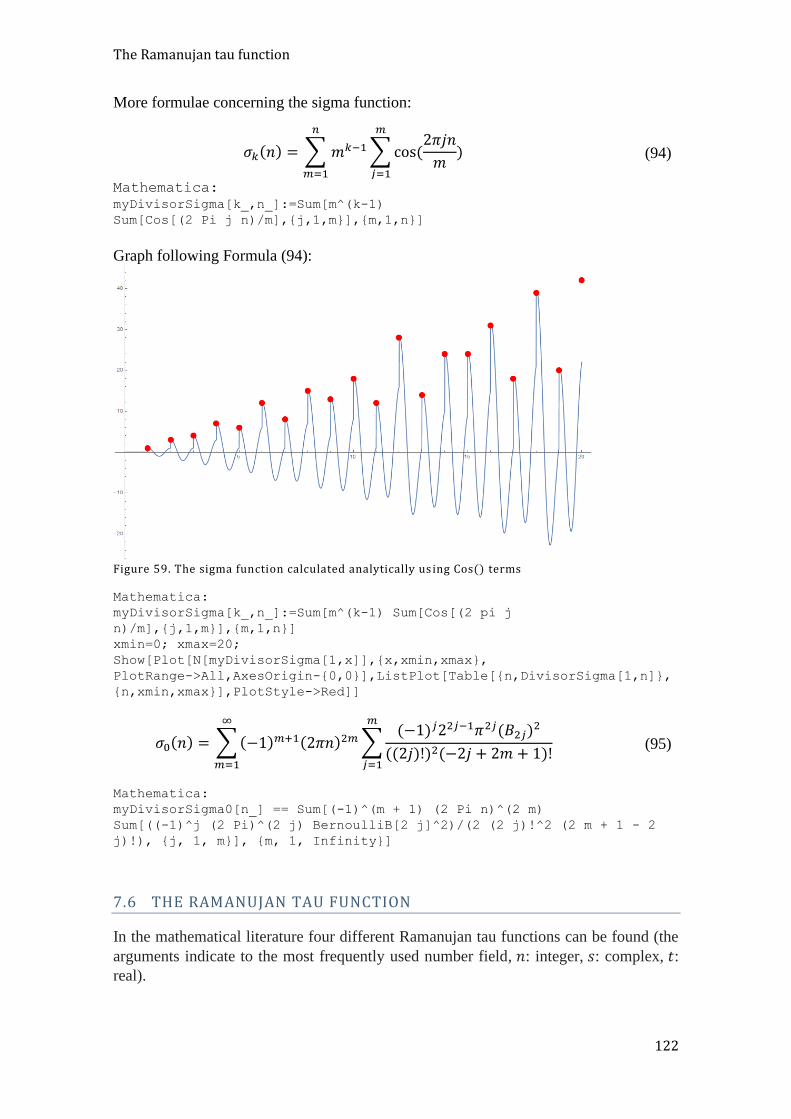
The Ramanujan tau function
122
More formulae concerning the sigma function:
𝜎𝑘(𝑛) = ∑ 𝑚𝑘−1∑cos(2𝜋𝑗𝑛
𝑚)
𝑚
𝑗=1
𝑛
𝑚=1
(94)
Mathematica:
myDivisorSigma[k_,n_]:=Sum[m^(k-1)
Sum[Cos[(2 Pi j n)/m],{j,1,m}],{m,1,n}]
Graph following Formula (94):
Figure 59. The sigma function calculated analytically us ing Cos() terms
Mathematica:
myDivisorSigma[k_,n_]:=Sum[m^(k-1) Sum[Cos[(2 pi j
n)/m],{j,1,m}],{m,1,n}]
xmin=0; xmax=20;
Show[Plot[N[myDivisorSigma[1,x]],{x,xmin,xmax},
PlotRange->All,AxesOrigin-{0,0}],ListPlot[Table[{n,DivisorSigma[1,n]},
{n,xmin,xmax}],PlotStyle->Red]]
𝜎0(𝑛) = ∑(−1)𝑚+1(2𝜋𝑛)2𝑚∑(−1)𝑗22𝑗−1𝜋2𝑗(𝐵2𝑗)
2
((2𝑗)!)2(−2𝑗 + 2𝑚 + 1)!
𝑚
𝑗=1
∞
𝑚=1
(95)
Mathematica:
myDivisorSigma0[n_] == Sum[(-1)^(m + 1) (2 Pi n)^(2 m)
Sum[((-1)^j (2 Pi)^(2 j) BernoulliB[2 j]^2)/(2 (2 j)!^2 (2 m + 1 - 2
j)!), {j, 1, m}], {m, 1, Infinity}]
7.6 THE RAMANUJAN TAU FUNCTION
In the mathematical literature four different Ramanujan tau functions can be found (the
arguments indicate to the most frequently used number field, 𝑛: integer, 𝑠: complex, 𝑡: real).

7 A few important arithmetical functions
123
𝜏(𝑛): Ramanujan tau function, Mathematica: RamanujanTau[n]
𝐿(𝑠): Ramanujan tau Dirichlet L function, Mathematica: RamanujanTauL[s]
𝑍(𝑡): Ramanujan tau Z function, Mathematica: RamanujanTauZ[n]
Θ(𝑡): Ramanujan tau theta function, Mathematica: RamanujanTauTheta[n]
The graph of 𝜏(𝑛) looks like:
Figure 60. Ramanujan 𝜏(N) (gray), in red: only 𝑛 for 𝑀𝑜𝑑(𝑛, 112) = 0
Mathematica:
Show[ListLogPlot[Table[{n,Abs[RamanujanTau[n]]},{n,1,10000}],Joined-
>True,PlotRange->{10^10,10^24},PlotStyle->Gray],
ListLogPlot[Table[{n,Abs[RamanujanTau[n]]},{n,121,10000,121}],Joined-
>True,PlotRange->{10^10,10^24},PlotStyle->Red,InterpolationOrder->1]]
The Ramanujan tau function has many representations (or definitions):
By its generating function 39 𝑮(𝒙)
𝐺(𝑥) = 𝑥∏(1 − 𝑥𝑛)24∞
𝑛=1
=∑ 𝜏(𝑛)𝑥𝑛∞
𝑛=1
= 𝑥 − 24𝑥2 + 252𝑥3 − 1472𝑥4 + 4830𝑥5
− 6048𝑥6 +⋯ = 𝑥(1 − 3𝑥 + 5𝑥3 − 7𝑥6 +⋯)8
(96)
(*Mathematica (the first 50 values):*)
CoefficientList[Take[Expand[Product[(1-x^k)^24,{k,1,50}]],50],x]:
39 A sequence a(n) can be defined by the coefficients of a power series expansion 𝑓(𝑥) = ∑ 𝑎𝑛𝑥
𝑛∞𝑛=0 .
𝑓(𝑥) is called the ‘generating function’ of 𝑎(𝑛)

The Ramanujan tau function
124
{1,-24,252,-1472,4830,-6048,-16744,84480,-113643,-115920,…}
(*From theory of modular forms:*)
max = 28; g[k_] := -BernoulliB[k]/(2k) + Sum[ DivisorSigma[k - 1, n -
1]*q^(n - 1), {n, 2, max + 1}]; CoefficientList[ Series[ 8000*g[4]^3 -
147*g[6]^2, {q, 0, max}], q] // Rest
Properties of 𝝉(𝒏)
𝜏(𝑝𝑟+1) = 𝜏(𝑝)𝜏(𝑝𝑟) − 𝑝11𝜏(𝑝𝑟−1), if 𝑝 ∈ ℙ 𝑎𝑛𝑑 𝑟 > 0 (97)
|𝜏(𝑝)| ≤ 2𝑝112 , if 𝑝 ∈ ℙ (98)
𝜏(𝑛) is a multiplicative function: 𝜏(𝑚𝑛) = 𝜏(𝑚)𝜏(𝑛), if gcd(𝑚, 𝑛) = 1
There are very many relationships between τ (n) and the sum-of-divisors functions
𝜎𝑘(𝑛).40
Here an example:
𝜏(𝑛) =65
756𝜎11(𝑛) +
691
756𝜎5(𝑛) −
691
3∑𝜎5(𝑘)𝜎5(𝑛 − 𝑘)
𝑛−1
𝑘=1
(99)
Ramanujan discovered the following recursive identities:
(𝑛 − 1)𝜏(𝑛) = ∑(−1)𝑚+1(2𝑚
𝑏𝑛
𝑚=1
+ 1)
× (𝑛 − 1 −9
2𝑚(𝑚 + 1)) 𝜏 (𝑛
−1
2𝑚(𝑚 + 1)) ,where 𝑏𝑛 =
1
2(√8𝑛 + 1 − 1)
(100)
𝜏(𝑝𝑛) =∑(−1)𝑗 (𝑛 − 𝑗𝑛 − 2𝑗
)
⌊𝑛2⌋
𝑗=0
𝑝11𝑗(𝜏(𝑝))𝑛−2𝑗
(101)
The Ramanujan tau L, tau theta and tau Z functions
𝑍(𝑡) = 𝑒𝑖𝜃(𝑡) 𝐿(𝑖𝑡 + 6) (102)
40 https://en.wikipedia.org/wiki/Ramanujan_Tau_function or: http://mathworld.wolfram.com/TauFunction.html
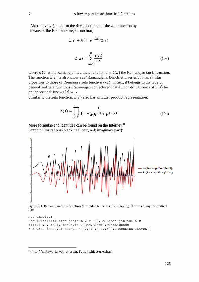
7 A few important arithmetical functions
125
Alternatively (similar to the decomposition of the zeta function by
means of the Riemann-Siegel function):
𝐿(𝑖𝑡 + 6) = 𝑒−𝑖𝜃(𝑡)𝑍(𝑡)
𝑳(𝒔) = ∑𝝉(𝒏)
𝒏𝒔
∞
𝒏=𝟏
(103)
where 휃(𝑡) is the Ramanujan tau theta function and 𝐿(𝑠) the Ramanujan tau L function.
The function 𝐿(𝑠) is also known as ‘Ramanujan's Dirichlet L series’. It has similar
properties to those of Riemann's zeta function 휁(𝑧). In fact, it belongs to the type of
generalized zeta functions. Ramanujan conjectured that all non-trivial zeros of 𝐿(𝑠) lie
on the 'critical' line 𝑅𝑒[𝑠] = 6.
Similar to the zeta function, 𝐿(𝑠) also has an Euler product representation:
𝑳(𝒔) =∏𝟏
𝟏 − 𝝉(𝒑)𝒑−𝒔 + 𝒑𝟏𝟏−𝟐𝒔
∞
𝒑𝝐ℙ
(104)
More formulae and identities can be found on the Internet.41
Graphic illustrations (black: real part, red: imaginary part):
Figure 61. Ramanujan tau L function (Dirichlet-L-series) 0-70, having 34 zeros along the critical line
Mathematica:
Show[Plot[{Im[RamanujanTauL[6+x I]],Re[RamanujanTauL[6+x
I]]},{x,0,xmax},PlotStyle->{Red,Black},PlotLegends-
>"Expressions",PlotRange->{{0,70},{-3.,4}},ImageSize->Large]]
41 http://mathworld.wolfram.com/TauDirichletSeries.html

The Mertens function
126
The density of the zeros of the Ramanujan tau L function 𝐿(𝑠) is about twice that of the
zeta function 휁(𝑠). In the range up to 70, the 휁 function 17 has zeros, while the tau L
function has 34 zeros.
A table with the first zeros of Ramanujan's tau L function is given in the Appendix
‘Zeros of Ramanujan’s tau L function’.
7.7 THE MERTENS FUNCTION
The Mertens function 𝑀(𝑛) is the summatory function of the Moebius function 𝜇(𝑛):
𝑀(𝑛) = ∑𝜇(𝑘)
𝑛
𝑘=1
(105)
Definition of 𝜇(𝑛) (for 𝑛 > 0):
𝜇(𝑛) = {
1, if 𝑛 square − free and having an even number of prime factors−1, if 𝑛 square − free and having an odd number of prime factors
0, if 𝑛 has a square prime factor }
𝜇(𝑛) can be calculated without knowledge of the prime factor decomposition of 𝑛
(however with the same complexity):
𝜇(𝑛) = ∑ 𝑒−2𝜋𝑖𝑘𝑛
1≤𝑘≤𝑛gcd(𝑘,𝑛)=1
(106)
Properties of the 𝜇 function:
∑𝜇(𝑘)
𝑘
∞
𝑘=1
= 0 (107)
Also interesting is the representation as a sum over Farey sequences:
𝑀(𝑛) = ∑ 𝑒−2𝜋𝑖𝑎
𝑎∈ℱ𝑛
(108)
Representation of the Moebius function:
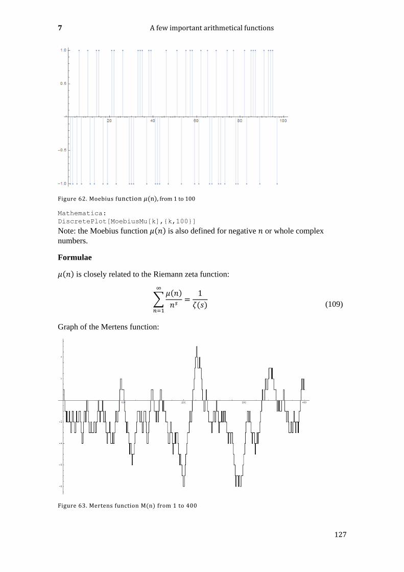
7 A few important arithmetical functions
127
Figure 62. Moebius function 𝜇(n), from 1 to 100
Mathematica:
DiscretePlot[MoebiusMu[k],{k,100}]
Note: the Moebius function 𝜇(𝑛) is also defined for negative 𝑛 or whole complex
numbers.
Formulae
𝜇(𝑛) is closely related to the Riemann zeta function:
∑𝜇(𝑛)
𝑛𝑠
∞
𝑛=1
=1
휁(𝑠)
(109)
Graph of the Mertens function:
Figure 63. Mertens function M(n) from 1 to 400
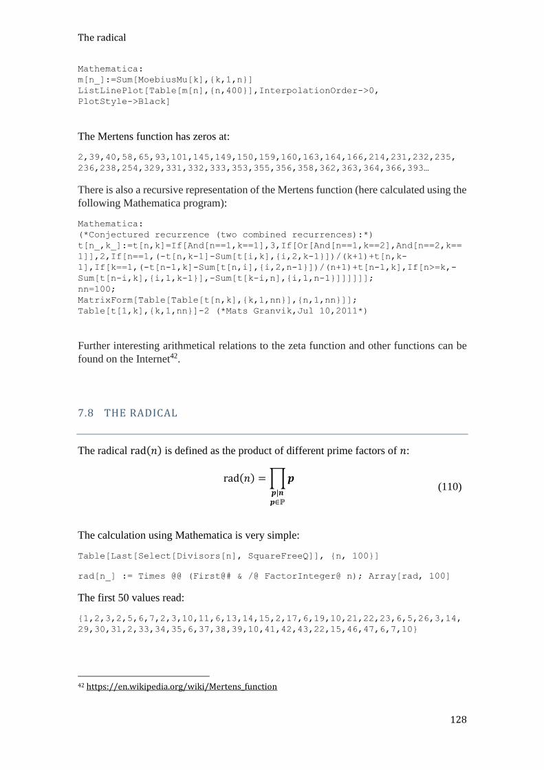
The radical
128
Mathematica:
m[n_]:=Sum[MoebiusMu[k],{k,1,n}]
ListLinePlot[Table[m[n],{n,400}],InterpolationOrder->0,
PlotStyle->Black]
The Mertens function has zeros at:
2,39,40,58,65,93,101,145,149,150,159,160,163,164,166,214,231,232,235,
236,238,254,329,331,332,333,353,355,356,358,362,363,364,366,393…
There is also a recursive representation of the Mertens function (here calculated using the
following Mathematica program):
Mathematica:
(*Conjectured recurrence (two combined recurrences):*)
t[n_,k_]:=t[n,k]=If[And[n==1,k==1],3,If[Or[And[n==1,k==2],And[n==2,k==
1]],2,If[n==1,(-t[n,k-1]-Sum[t[i,k],{i,2,k-1}])/(k+1)+t[n,k-
1],If[k==1,(-t[n-1,k]-Sum[t[n,i],{i,2,n-1}])/(n+1)+t[n-1,k],If[n>=k,-
Sum[t[n-i,k],{i,1,k-1}],-Sum[t[k-i,n],{i,1,n-1}]]]]]];
nn=100;
MatrixForm[Table[Table[t[n,k],{k,1,nn}],{n,1,nn}]];
Table[t[1,k],{k,1,nn}]-2 (*Mats Granvik,Jul 10,2011*)
Further interesting arithmetical relations to the zeta function and other functions can be
found on the Internet42.
7.8 THE RADICAL
The radical rad(𝑛) is defined as the product of different prime factors of 𝑛:
rad(𝑛) =∏𝒑𝒑|𝒏𝒑∈ℙ
(110)
The calculation using Mathematica is very simple:
Table[Last[Select[Divisors[n], SquareFreeQ]], {n, 100}]
rad[n_] := Times @@ (First@# & /@ FactorInteger@ n); Array[rad, 100]
The first 50 values read:
{1,2,3,2,5,6,7,2,3,10,11,6,13,14,15,2,17,6,19,10,21,22,23,6,5,26,3,14,
29,30,31,2,33,34,35,6,37,38,39,10,41,42,43,22,15,46,47,6,7,10}
42 https://en.wikipedia.org/wiki/Mertens_function
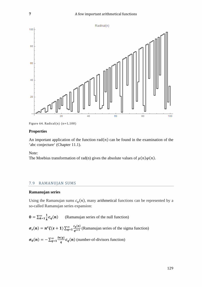
7 A few important arithmetical functions
129
Figure 64. Radical(n) (n=1,100)
Properties
An important application of the function rad(𝑛) can be found in the examination of the
‘abc conjecture‘ (Chapter 11.1).
Note:
The Moebius transformation of rad(n) gives the absolute values of 𝜇(𝑛)𝜑(𝑛).
7.9 RAMANUJAN SUMS
Ramanujan series
Using the Ramanujan sums 𝑐𝑞(𝑛), many arithmetical functions can be represented by a
so-called Ramanujan series expansion:
𝟎 = ∑𝟏
𝒌𝒄𝒒(𝒏)
∞𝒌=𝟏 (Ramanujan series of the null function)
𝝈𝒔(𝒏) = 𝒏𝒔𝜻(𝒔 + 𝟏)∑
𝒄𝒒(𝒏)
𝒒𝒔+𝟏∞𝒒=𝟏 (Ramanujan series of the sigma function)
𝝈𝟎(𝒏) = −∑𝒍𝒏(𝒒)
𝒒
∞𝒒=𝟏 𝒄𝒒(𝒏) (number-of-divisors function)
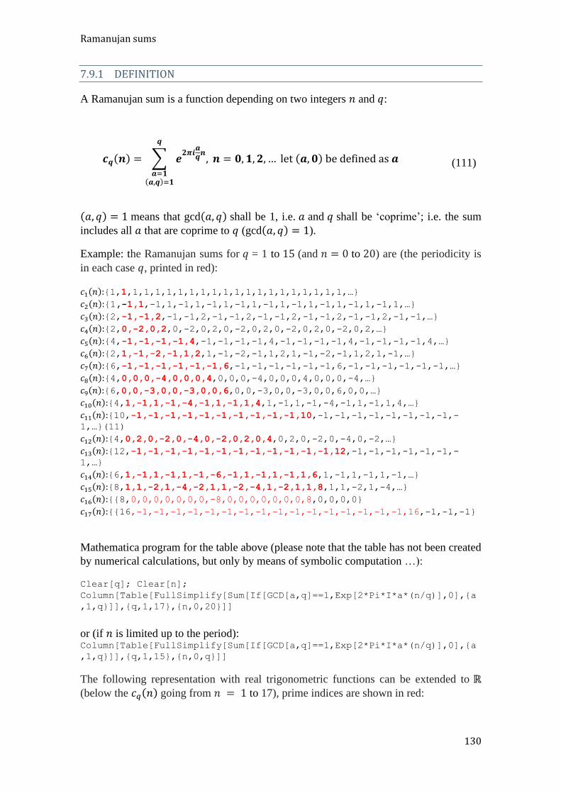
Ramanujan sums
130
7.9.1 DEFINITION
A Ramanujan sum is a function depending on two integers 𝑛 and 𝑞:
𝒄𝒒(𝒏) = ∑ 𝒆𝟐𝝅𝒊
𝒂𝒒𝒏,
𝒒
𝒂=𝟏(𝒂,𝒒)=𝟏
𝒏 = 𝟎, 𝟏, 𝟐, … let (𝒂, 𝟎) be defined as 𝒂 (111)
(𝑎, 𝑞) = 1 means that gcd(𝑎, 𝑞) shall be 1, i.e. 𝑎 and 𝑞 shall be ‘coprime’; i.e. the sum
includes all 𝑎 that are coprime to 𝑞 (gcd(𝑎, 𝑞) = 1).
Example: the Ramanujan sums for 𝑞 = 1 to 15 (and 𝑛 = 0 to 20) are (the periodicity is
in each case 𝑞, printed in red):
𝑐1(𝑛):{1,1,1,1,1,1,1,1,1,1,1,1,1,1,1,1,1,1,1,1,1,…}
𝑐2(𝑛):{1,-1,1,-1,1,-1,1,-1,1,-1,1,-1,1,-1,1,-1,1,-1,1,-1,1,…}
𝑐3(𝑛):{2,-1,-1,2,-1,-1,2,-1,-1,2,-1,-1,2,-1,-1,2,-1,-1,2,-1,-1,…}
𝑐4(𝑛):{2,0,-2,0,2,0,-2,0,2,0,-2,0,2,0,-2,0,2,0,-2,0,2,…}
𝑐5(𝑛):{4,-1,-1,-1,-1,4,-1,-1,-1,-1,4,-1,-1,-1,-1,4,-1,-1,-1,-1,4,…}
𝑐6(𝑛):{2,1,-1,-2,-1,1,2,1,-1,-2,-1,1,2,1,-1,-2,-1,1,2,1,-1,…}
𝑐7(𝑛):{6,-1,-1,-1,-1,-1,-1,6,-1,-1,-1,-1,-1,-1,6,-1,-1,-1,-1,-1,-1,…}
𝑐8(𝑛):{4,0,0,0,-4,0,0,0,4,0,0,0,-4,0,0,0,4,0,0,0,-4,…}
𝑐9(𝑛):{6,0,0,-3,0,0,-3,0,0,6,0,0,-3,0,0,-3,0,0,6,0,0,…}
𝑐10(𝑛):{4,1,-1,1,-1,-4,-1,1,-1,1,4,1,-1,1,-1,-4,-1,1,-1,1,4,…}
𝑐11(𝑛):{10,-1,-1,-1,-1,-1,-1,-1,-1,-1,-1,10,-1,-1,-1,-1,-1,-1,-1,-1,-1,…}(11)
𝑐12(𝑛):{4,0,2,0,-2,0,-4,0,-2,0,2,0,4,0,2,0,-2,0,-4,0,-2,…}
𝑐13(𝑛):{12,-1,-1,-1,-1,-1,-1,-1,-1,-1,-1,-1,-1,12,-1,-1,-1,-1,-1,-1,-1,…}
𝑐14(𝑛):{6,1,-1,1,-1,1,-1,-6,-1,1,-1,1,-1,1,6,1,-1,1,-1,1,-1,…}
𝑐15(𝑛):{8,1,1,-2,1,-4,-2,1,1,-2,-4,1,-2,1,1,8,1,1,-2,1,-4,…}
𝑐16(𝑛):{{8,0,0,0,0,0,0,0,-8,0,0,0,0,0,0,0,8,0,0,0,0}
𝑐17(𝑛):{{16,-1,-1,-1,-1,-1,-1,-1,-1,-1,-1,-1,-1,-1,-1,-1,-1,16,-1,-1,-1}
Mathematica program for the table above (please note that the table has not been created
by numerical calculations, but only by means of symbolic computation …):
Clear[q]; Clear[n];
Column[Table[FullSimplify[Sum[If[GCD[a,q]==1,Exp[2*Pi*I*a*(n/q)],0],{a
,1,q}]],{q,1,17},{n,0,20}]]
or (if 𝑛 is limited up to the period): Column[Table[FullSimplify[Sum[If[GCD[a,q]==1,Exp[2*Pi*I*a*(n/q)],0],{a
,1,q}]],{q,1,15},{n,0,q}]]
The following representation with real trigonometric functions can be extended to ℝ
(below the 𝑐𝑞(𝑛) going from 𝑛 = 1 to 17), prime indices are shown in red:

7 A few important arithmetical functions
131
Cos[2𝑛𝜋]
Cos[𝑛𝜋]
Cos[2𝑛𝜋
3] + Cos[
4𝑛𝜋
3]
Cos[𝑛𝜋
2] + Cos[
3𝑛𝜋
2]
Cos[2𝑛𝜋
5] + Cos[
4𝑛𝜋
5] + Cos[
6𝑛𝜋
5] + Cos[
8𝑛𝜋
5]
Cos[𝑛𝜋
3] + Cos[
5𝑛𝜋
3]
Cos[2𝑛𝜋
7] + Cos[
4𝑛𝜋
7] + Cos[
6𝑛𝜋
7] + Cos[
8𝑛𝜋
7] + Cos[
10𝑛𝜋
7] + Cos[
12𝑛𝜋
7]
Cos[𝑛𝜋
4] + Cos[
3𝑛𝜋
4] + Cos[
5𝑛𝜋
4] + Cos[
7𝑛𝜋
4]
Cos[2𝑛𝜋
9] + Cos[
4𝑛𝜋
9] + Cos[
8𝑛𝜋
9] + Cos[
10𝑛𝜋
9] + Cos[
14𝑛𝜋
9] + Cos[
16𝑛𝜋
9]
Cos[𝑛𝜋
5] + Cos[
3𝑛𝜋
5] + Cos[
7𝑛𝜋
5] + Cos[
9𝑛𝜋
5]
Cos [2𝑛𝜋
11] + Cos [
4𝑛𝜋
11] + Cos [
6𝑛𝜋
11] + Cos [
8𝑛𝜋
11] + Cos [
10𝑛𝜋
11] +
Cos[12𝑛𝜋
11] + Cos[
14𝑛𝜋
11] + Cos[
16𝑛𝜋
11] + Cos[
18𝑛𝜋
11] + Cos[
20𝑛𝜋
11]
Cos[𝑛𝜋
6] + Cos[
5𝑛𝜋
6] + Cos[
7𝑛𝜋
6] + Cos[
11𝑛𝜋
6]
Cos [2𝑛𝜋
13] + Cos [
4𝑛𝜋
13] + Cos [
6𝑛𝜋
13] + Cos [
8𝑛𝜋
13] + Cos [
10𝑛𝜋
13] + Cos [
12𝑛𝜋
13] +
Cos[14𝑛𝜋
13] + Cos[
16𝑛𝜋
13] + Cos[
18𝑛𝜋
13] + Cos[
20𝑛𝜋
13] + Cos[
22𝑛𝜋
13] + Cos[
24𝑛𝜋
13]
Cos[𝑛𝜋
7] + Cos[
3𝑛𝜋
7] + Cos[
5𝑛𝜋
7] + Cos[
9𝑛𝜋
7] + Cos[
11𝑛𝜋
7] + Cos[
13𝑛𝜋
7]
Cos[2𝑛𝜋
15] + Cos[
4𝑛𝜋
15] + Cos[
8𝑛𝜋
15] + Cos[
14𝑛𝜋
15] + Cos[
16𝑛𝜋
15] + Cos[
22𝑛𝜋
15] + Cos[
26𝑛𝜋
15] + Cos[
28𝑛𝜋
15]
Cos[𝑛𝜋
8] + Cos[
3𝑛𝜋
8] + Cos[
5𝑛𝜋
8] + Cos[
7𝑛𝜋
8] + Cos[
9𝑛𝜋
8] + Cos[
11𝑛𝜋
8] + Cos[
13𝑛𝜋
8] + Cos[
15𝑛𝜋
8]
Cos [2𝑛𝜋
17] + Cos [
4𝑛𝜋
17] + Cos [
6𝑛𝜋
17] + Cos [
8𝑛𝜋
17] + Cos [
10𝑛𝜋
17] + Cos [
12𝑛𝜋
17] + Cos [
14𝑛𝜋
17] + Cos [
16𝑛𝜋
17] +
Cos[18𝑛𝜋
17] + Cos[
20𝑛𝜋
17] + Cos[
22𝑛𝜋
17] + Cos[
24𝑛𝜋
17] + Cos[
26𝑛𝜋
17] + Cos[
28𝑛𝜋
17] + Cos[
30𝑛𝜋
17] + Cos[
32𝑛𝜋
17]
Table: Ramanujan sums 𝒄𝒒(𝑛) represented by cos() terms. This representation can be
extended from ℕ to ℝ or ℂ (see illustration below).
Mathematica program for the table above:
Clear[n];
Column[Table[FullSimplify[Sum[If[GCD[a,q]==1,Cos[2*Pi*a*(n/q)],0],{a,1
,q}]],{q,1,17}]]
For integers, the representation can be simplified (in each case the second half of a term
is the same as the first half, prime indices in red):

Ramanujan sums
132
1,Cos[𝑛𝜋],
2Cos [2𝑛𝜋
3] ,
2Cos [𝑛𝜋
2] ,
2 (Cos [2𝑛𝜋
5] + Cos [
4𝑛𝜋
5]) ,
Cos [𝑛𝜋
3] ,
2 (Cos [2𝑛𝜋
7] + Cos [
4𝑛𝜋
7] + Cos [
6𝑛𝜋
7]) ,
2 (Cos [𝑛𝜋
4] + Cos [
3𝑛𝜋
4]) ,
2 (Cos [2𝑛𝜋
9] + Cos [
4𝑛𝜋
9] + Cos [
8𝑛𝜋
9]) ,
2 (Cos [𝑛𝜋
5] + Cos [
3𝑛𝜋
5]) ,
2 (Cos [2𝑛𝜋
11] + Cos [
4𝑛𝜋
11] + Cos [
6𝑛𝜋
11] + Cos [
8𝑛𝜋
11] + Cos [
10𝑛𝜋
11]) ,
2 (Cos [𝑛𝜋
6] + Cos [
5𝑛𝜋
6]) ,
2 (Cos [2𝑛𝜋
13] + Cos [
4𝑛𝜋
13] + Cos [
6𝑛𝜋
13] + Cos [
8𝑛𝜋
13] + Cos [
10𝑛𝜋
13] + Cos [
12𝑛𝜋
13])
2 (Cos [𝑛𝜋
7] + Cos [
3𝑛𝜋
7] + Cos [
5𝑛𝜋
7]) ,
2 (Cos [2𝑛𝜋
15] + Cos [
4𝑛𝜋
15] + Cos [
8𝑛𝜋
15] + Cos [
14𝑛𝜋
15]) ,
2 (Cos [𝑛𝜋
8] + Cos [
3𝑛𝜋
8] + Cos [
5𝑛𝜋
8] + Cos [
7𝑛𝜋
8]) ,
2(Cos [
2𝑛𝜋
17] + Cos [
4𝑛𝜋
17] + Cos [
6𝑛𝜋
17] + Cos [
8𝑛𝜋
17] +
Cos [10𝑛𝜋
17] + Cos [
12𝑛𝜋
17] + Cos [
14𝑛𝜋
17] + Cos [
16𝑛𝜋
17]
)
Table: Ramanujan sums 𝑐𝑞(𝑛) represented by cos() terms, for integer numbers 𝑛.
There is an alternative method of calculating the Ramanujan sum, using the Moebius
function 𝜇(𝑛) and the Euler totient function 𝜑(𝑞):
𝒄𝒒(𝒏) = 𝝁(𝒒
(𝒒, 𝒏))
𝝋(𝒒)
𝝋(𝒒
(𝒒, 𝒏))
(112)
Mathematica:
nmax=14;cnq[q_,n_]:=EulerPhi[q]*(MoebiusMu[q/GCD[q,n]]/
EulerPhi[q/GCD[q,n]]);Column[Table[cnq[q,n],{q,1,nmax},{n,1,nmax}]]
Here are a few graphic illustrations of Ramanujan sums:

7 A few important arithmetical functions
133
Mathematica program: please contact the author.
Figure 65. Ramanujan sums 𝑐𝑞(n) from 𝑞 = 1 to 12 and 𝑛 going from 0 to 17
Mathematica programm: please contact the author.

Ramanujan sums
134
Figure 66. Ramanujan sums 𝑐𝑞(n) from 𝑞 = 1 to 24 and 𝑛 from 0 to 24
7.9.2 PROPERTIES
𝒄𝒒(𝒏) has a number of remarkable properties. The following ones can easily be checked
using the table above:
𝒄𝒒(𝒏) is always real and integer despite its complex definition.
𝒄𝒒(𝒏) = 𝒄𝒒(−𝒏)
𝒄𝒒(𝟎) = 𝝋(𝒒)
𝒄𝒒(𝟏) = 𝝁(𝒒)
𝒄𝒒𝒓(𝒏) = 𝒄𝒒(𝒏)𝒄𝒓(𝒏), 𝐢𝐟 (𝒒, 𝒓) = 𝟏 (multiplicativity)
𝒄𝒒(𝒏) = 𝒄𝒒((𝒒, 𝒏))
|𝒄𝒒(𝒏)| never becomes larger than 𝝋(𝒒), if 𝒒 is fixed)
|𝒄𝒒(𝒏)| never becomes larger than 𝒏 (if 𝒏 is fixed)

7 A few important arithmetical functions
135
𝒄𝒒(𝒏) = 0, if the natural number 𝒒
(𝒒,𝒏) has 𝒑𝟐 as a divisor, 𝒑 being prime
𝒄𝒒(𝒒) = 𝒄𝒒(𝒌𝒒) = 𝝋(𝒒), 𝒌 = 𝟎, 𝟏, 𝟐, …
𝒄𝒑(𝒏) = {−𝟏, 𝐢𝐟 𝒑 ∤ 𝒏
𝝋(𝒑), 𝐢𝐟 𝒑 | 𝒏}
𝒄𝒑𝒌(𝒏) = {
𝟎, 𝐢𝐟 𝒑𝒌−𝟏 ∤ 𝒏
−𝟏𝒑𝒌−𝟏, 𝐢𝐟 𝒑𝒌−𝟏 | 𝒏 𝐚𝐧𝐝 𝒑𝒌 ∤ 𝒏
𝝋(𝒑𝒌), 𝐢𝐟 𝒑𝒌 | 𝒏
}
∑ 𝒄𝒒(𝒏) = 𝟎𝒂+𝒒−𝟏𝒏=𝒂 (the sum over all terms of a period results in 0!)
𝟏
𝒎∑ 𝒄𝒎𝟏(𝒌)𝒄𝒎𝟐(𝒌) = {
𝝋(𝒎), 𝐢𝐟 𝒎𝟏 = 𝒎𝟐 = 𝒎𝟎, 𝐨𝐭𝐡𝐞𝐫𝐰𝐢𝐬𝐞
}𝒎𝒌=𝟏 (m = lcm(𝒎𝟏,𝒎𝟐))
(orthogonality)
7.9.3 EXTENSION TO ℝ
If we allow 𝑛 to have any real values 𝑥, then we get a real function that depends on an
integer parameter 𝑞:
𝒄𝒒(𝒙) = ∑ 𝒆𝟐𝝅𝒊
𝒂𝒒𝒙,
𝒒
𝒂=𝟏(𝒂,𝒒)=𝟏
(113)
Here are a few graphic illustrations of Ramanujan sums:
Mathematica program: please contact the author.
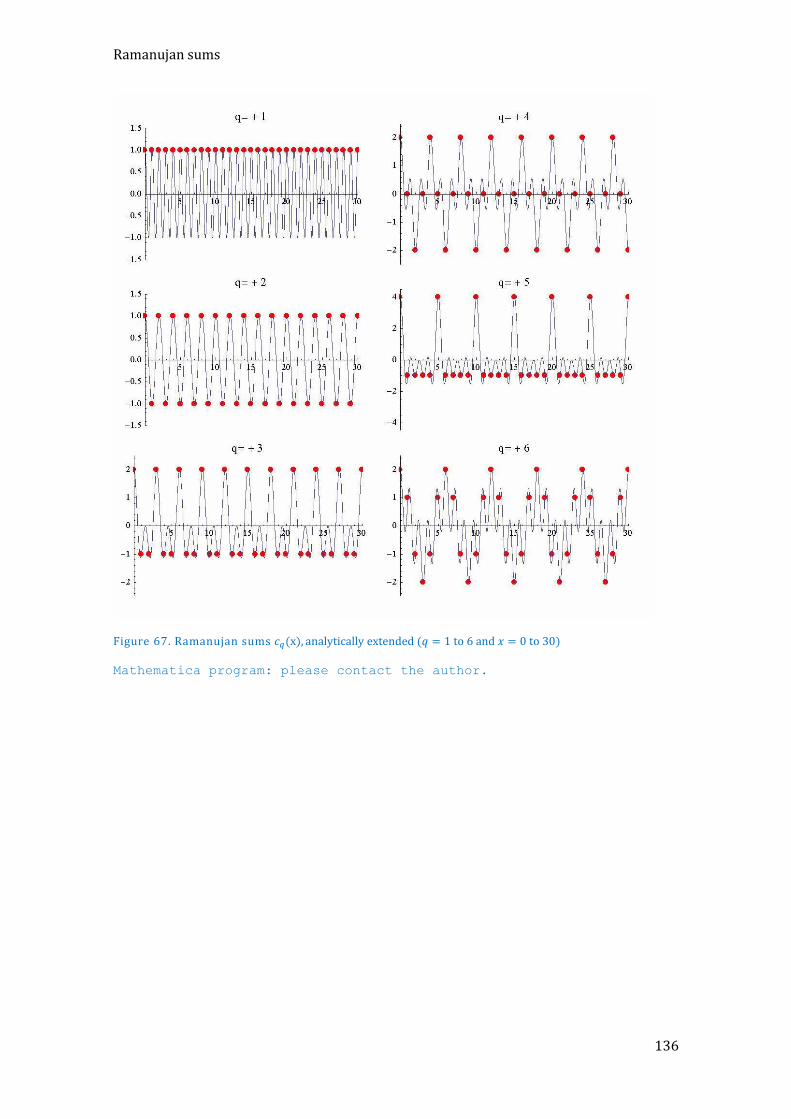
Ramanujan sums
136
Figure 67. Ramanujan sums 𝑐𝑞(x), analytically extended (𝑞 = 1 to 6 and 𝑥 = 0 to 30)
Mathematica program: please contact the author.

7 A few important arithmetical functions
137
Figure 68. Ramanujan sums 𝑐𝑞(x), analytically extended (𝑞 = 7 to 12 and 𝑥 = 0 to 30)
138
8 FUNCTIONS FOR THE CALCULATION OF PRIME NUMBERS
We distinguish between the following types of functions that can be used to compute
prime numbers:
- functions 𝑓(𝑛) that provide exactly all 𝑝𝑛
- functions 𝑓(𝑛) that always return a prime number
- functions 𝑓(𝑛) whose positive sets of integer values assumed by the function are
identical to the set of prime numbers
- functions that calculate the number of primes up to a given limit
8.1 FUNCTIONS THAT PROVIDE EXACTLY ALL PRIME NUMBERS
𝑝𝑛 = ⌊1 − log2(−1
2+ ∑
𝜇(𝑑)
2𝑑 − 1𝑑|𝑃𝑛−1
)⌋ (114)
With 𝑃𝑛 being the primorial function, which means 𝑝1𝑝2𝑝3…𝑝𝑛 (aka as 𝑃#). The identity was
discovered by J.M. Gandhi (1971).
The next formula comes from Williams (1964). For this he needs the prime counting
function 𝜋(𝑛) or the following function 𝐹(𝑗), which is defined as follows:
𝐹(𝑗) = [cos2 (𝜋(𝑗 − 1)! + 1
𝑗)]
𝑝𝑛 = 1+∑ [[𝑛
∑ 𝐹(𝑗)𝑚𝑗=1
]
1𝑛]
2𝑛
𝑚=1
(115)
or:
𝑝𝑛 = 1+∑ [[𝑛
1+ 𝜋(𝑚)]
1𝑛]
2𝑛
𝑚=1
(116)
𝑝𝑛 = [102𝑛𝛼] − 102
𝑛−1[102
𝑛−1 𝛼],where 𝛼 = ∑𝑝𝑚102
𝑚
∞
𝑚=1
(117)
All these formulae are very interesting theoretically, but they are not suitable for the
practical calculation of prime numbers.
8 Functions for the calculation of prime numbers
139
8.2 FUNCTIONS THAT ALWAYS RETURN A PRIME NUMBER
𝑝𝑛 = ⌊𝐴3𝑛⌋ (118)
𝐴 is called the ‘Mills constant‘ and has approximately a value of 1.3063778838. The
first six prime numbers generated by this formula (‘Mills’ prime numbers) read:
2, 11, 1361, 2521008887, 16022236204009818131831320183,
41131011492151048000305295379159531704861396235397599331359
49994882770404074832568499
So far, the first 11 ‘Mill’ primes of the form ⌊𝐴3𝑛⌋ have been calculated, the largest one
having more than 20000 decimal digits. The Mills constant 𝐴 has been calculated up to a
precision of 6850 decimal digits (as of Nov. 2015).
Wright (1951) found the following formula:
𝑝𝑛 = [2222...2𝜔
] (power tower from n exponents,𝜔 = 1.9287800) (119)
The first primes of this sequence read:
3,13,16381, … (the fourth already has more than 5000 decimal digits)
8.3 FUNCTIONS WHOSE SET OF POSITIVE INTEGERS EQUATES TO
THE SET OF PRIME NUMBERS
Since the year 1976, a polynomial of degree 25 with 26 variables has been known (Jones,
Sato, Wada & Wies)43 whose positive set of values coincides with the set of primes,
provided the 26 variables are integers.
Let us define the following constants:
𝐶0 = 𝑤𝑧 + ℎ + 𝑗 − 𝑞 𝐶1 = (𝑔𝑘 + 2𝑔 + 𝑘 + 1)(ℎ + 𝑗) + ℎ − 𝑧 𝐶2 = 2𝑛 + 𝑝 + 𝑞 + 𝑧 − 𝑒 𝐶3 = 16(𝑘 + 1)3(𝑘 + 2)(𝑛 + 1)2 + 1 − 𝑓2 𝐶4 = 𝑒3(𝑒 + 2)(𝑎 + 1)2 + 1 − 𝑜2 𝐶5 = (𝑎2 − 1)𝑦2 + 1 − 𝑥2 𝐶6 = 16𝑟2𝑦4(𝑎2 − 1) + 1 − 𝑢2
𝐶7 = ((𝑎 + 𝑢2(𝑢2 − 𝑎))2− 1) (𝑛 + 4𝑑𝑦)2 + 1 − (𝑥 + 𝑐𝑢)2
𝐶8 = 𝑛 + 𝑙 + 𝑣 − 𝑦 𝐶9 = (𝑎2 − 1)𝑙2 + 1 −𝑚2
43 https://www.maa.org/sites/default/files/pdf/upload_library/22/Ford/JonesSatoWadaWiens.pdf
Recursive formulae
140
𝐶10 = 𝑎𝑖 + 𝑘 + 1 − 𝑙 − 𝑖 𝐶11 = 𝑝 + 𝑙(𝑎 − 𝑛 − 1) + 𝑏(2𝑎𝑛 + 2𝑎 − 𝑛2 − 2𝑛 − 2) − 𝑚 𝐶12 = 𝑞 + 𝑦(𝑎 − 𝑝 − 1) + 𝑠(2𝑎𝑝 + 2𝑎 − 𝑝2 − 2𝑝 − 2) − 𝑥 𝐶13 = 𝑧 + 𝑝𝑙(𝑎 − 𝑝) + 𝑡(2𝑎𝑝 − 𝑝2 − 1) − 𝑝𝑚
Then there exists the following inequality whose positive integer solutions exactly
coincide with the set of all prime numbers:
(𝒌 + 𝟐)(𝟏 − 𝑪𝟎𝟐 − 𝑪𝟏𝟐 −⋯− 𝑪𝟏𝟑𝟐) > 𝟎 (120)
You can write a Mathematica program using this formula to search for prime numbers
(see Appendix). You can also run the program to find positive solutions for this
polynomial. But you will need a lot of patience: a Quad Core Pentium 3 GHz once
devoted an entire week to the search without finding a solution!
8.4 RECURSIVE FORMULAE
𝒑𝒏 = 𝒑𝒏−𝟏 +𝒈𝒈𝑻(𝒏, 𝒑𝒏−𝟏),𝑤ℎ𝑒𝑟𝑒 𝒑𝟏 = 𝟕 (121)
This sequence contains only primes or 1’s44. If we discard the 1’s we get:
{5,3,11,3,23,3,47,3,5,3,101,3,7,11,3,13,233,3,467,3,5,3,941
,3,7,1889,3,3779,3,7559,3,13,15131,3,53,3,7,30323,3,60647,3
,5,3,101,3,121403,3,242807,3,5,3,19,7,5,3,47,3,37,5,3,17,3,
199,53,3,29,3,486041,3,7,421,23,3,972533,3,577,7}
f[1] = 7; f[n_] := f[n] = f[n - 1] + GCD[n, f[n - 1]];
DeleteCases[Differences[Table[f[n], {n, 10^6}]], 1]
44 Eric S. Rowland, A simple prime-generating recurrence, Abstracts Amer. Math. Soc., 29 (No. 1, 2008),
p. 50
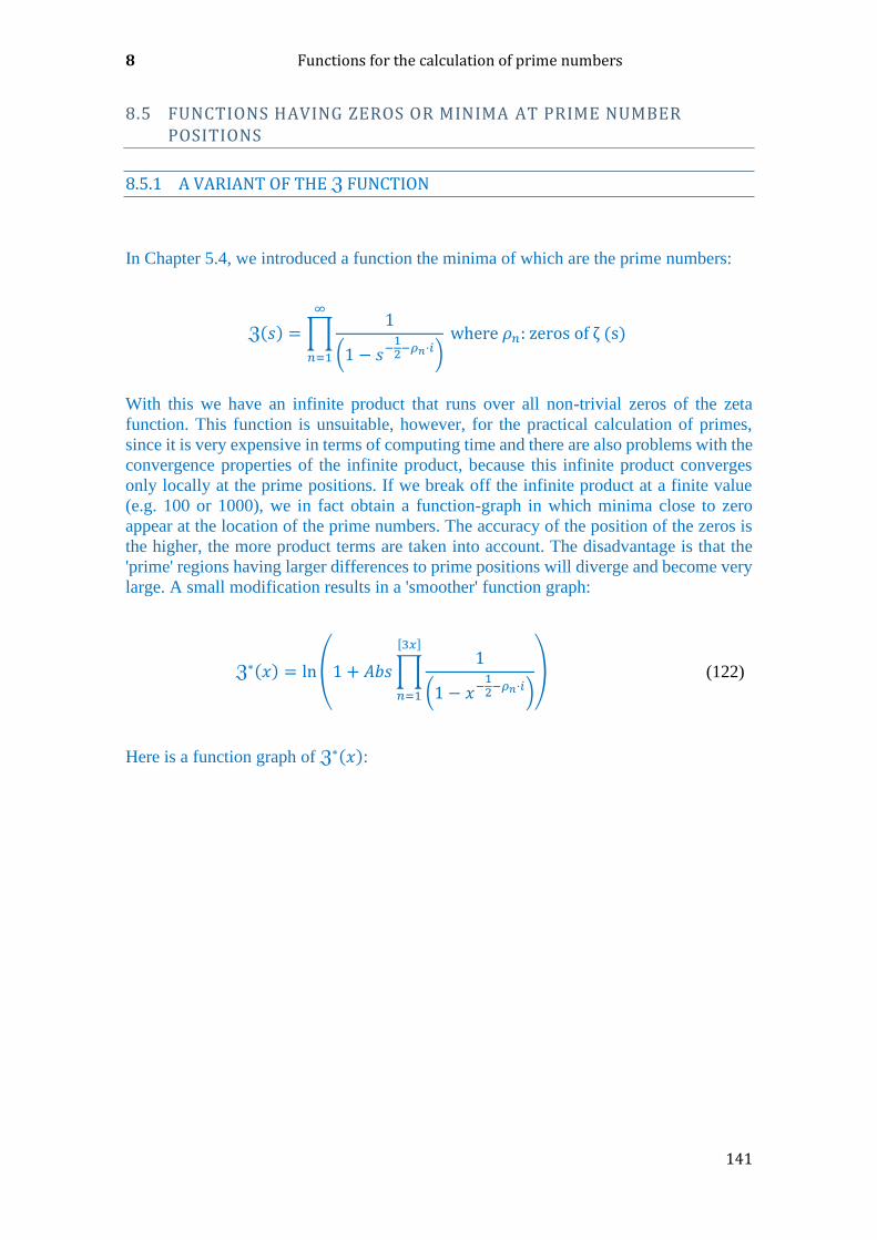
8 Functions for the calculation of prime numbers
141
8.5 FUNCTIONS HAVING ZEROS OR MINIMA AT PRIME NUMBER POSITIONS
8.5.1 A VARIANT OF THE ℨ FUNCTION
In Chapter 5.4, we introduced a function the minima of which are the prime numbers:
ℨ(𝑠) =∏1
(1 − 𝑠−12−𝜌𝑛⋅𝑖)
where 𝜌𝑛: zeros of ζ (s)
∞
𝑛=1
With this we have an infinite product that runs over all non-trivial zeros of the zeta
function. This function is unsuitable, however, for the practical calculation of primes,
since it is very expensive in terms of computing time and there are also problems with the
convergence properties of the infinite product, because this infinite product converges
only locally at the prime positions. If we break off the infinite product at a finite value
(e.g. 100 or 1000), we in fact obtain a function-graph in which minima close to zero
appear at the location of the prime numbers. The accuracy of the position of the zeros is
the higher, the more product terms are taken into account. The disadvantage is that the
'prime' regions having larger differences to prime positions will diverge and become very
large. A small modification results in a 'smoother' function graph:
ℨ∗(𝑥) = ln(1 + 𝐴𝑏𝑠∏1
(1 − 𝑥−12−𝜌𝑛⋅𝑖)
[3𝑥]
𝑛=1
) (122)
Here is a function graph of ℨ∗(𝑥):
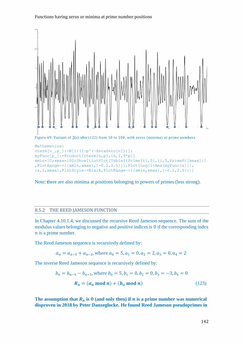
Functions having zeros or minima at prime number positions
142
Figure 69. Variant of ℨ(x) after (122) from 10 to 100, with zeros (minima) at prime numbers
Mathematica:
cterm[n_,p_]:=N[1/(1-p^(-ZetaZero[n]))];
myFunc[p_]:=Product[cterm[n,p],{n,1,3*p}]
xmin=10;xmax=100;Show[ListPlot[Table[{Prime[i],0},{i,5,PrimePi[xmax]}]
,PlotRange->{{xmin,xmax},{-0.2,2.5}}],Plot[Log[1+Abs[myFunc[x]]],
{x,2,xmax},PlotStyle->Black,PlotRange->{{xmin,xmax},{-0.2,2.5}}]]
Note: there are also minima at positions belonging to powers of primes (less strong).
8.5.2 THE REED JAMESON FUNCTION
In Chapter 4.10.1.4, we discussed the recursive Reed Jameson sequence. The sum of the
modulus values belonging to negative and positive indices is 0 if the corresponding index
𝑛 is a prime number.
The Reed Jameson sequence is recursively defined by:
𝑎𝑛 = 𝑎𝑛−5 + 𝑎𝑛−2, where 𝑎0 = 5, 𝑎1 = 0, 𝑎2 = 2, 𝑎3 = 0, 𝑎4 = 2
The inverse Reed Jameson sequence is recursively defined by:
𝑏𝑛 = 𝑏𝑛−5 − 𝑏𝑛−3, where 𝑏0 = 5, 𝑏1 = 0, 𝑏2 = 0, 𝑏3 = −3, 𝑏4 = 0
𝑹𝒏 = (𝒂𝒏 𝐦𝐨𝐝 𝒏) + (𝒃𝒏 𝐦𝐨𝐝 𝒏) (123)
The assumption that 𝑹𝒏 is 𝟎 (and only then) if 𝒏 is a prime number was numerical
disproven in 2018 by Peter Danzeglocke. He found Reed Jameson pseudoprimes in
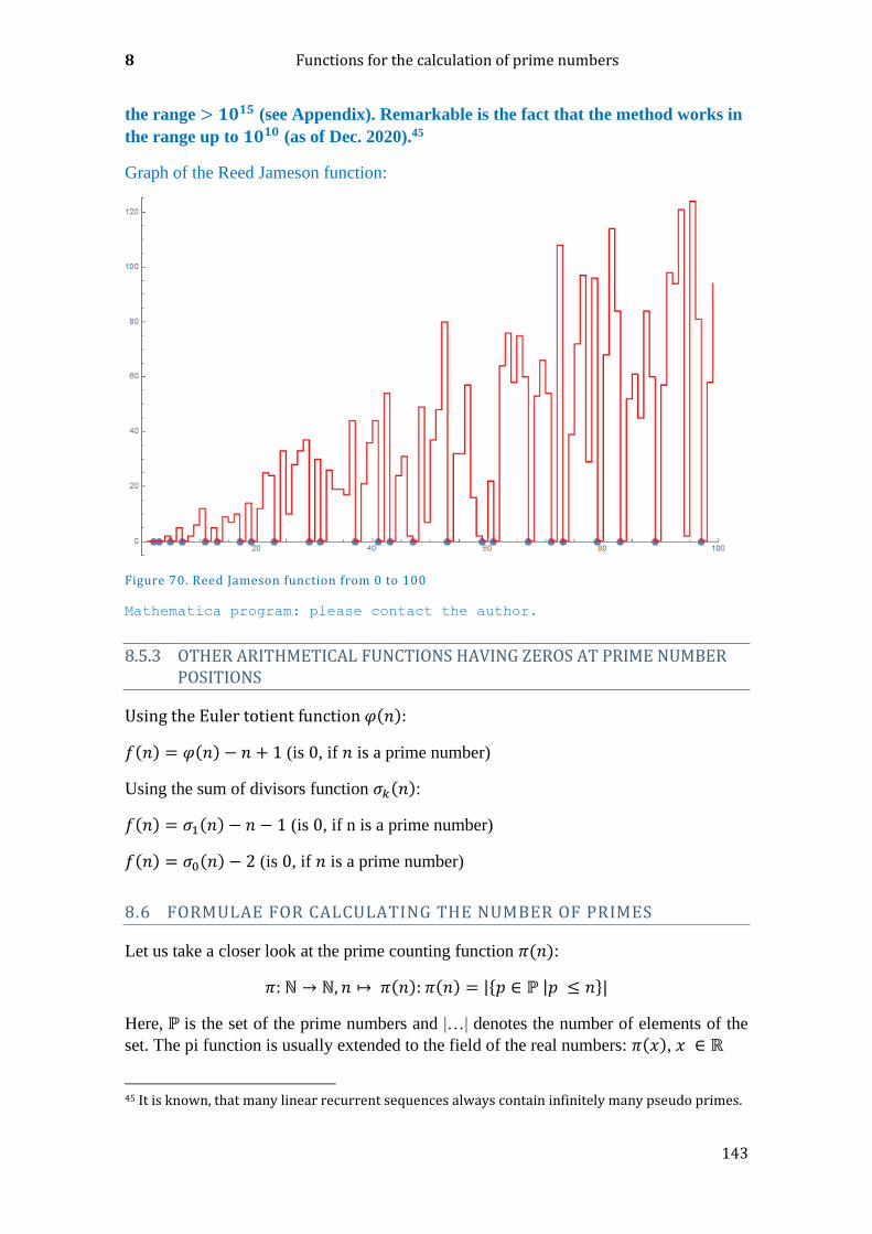
8 Functions for the calculation of prime numbers
143
the range > 𝟏𝟎𝟏𝟓 (see Appendix). Remarkable is the fact that the method works in
the range up to 𝟏𝟎𝟏𝟎 (as of Dec. 2020).45
Graph of the Reed Jameson function:
Figure 70. Reed Jameson function from 0 to 100
Mathematica program: please contact the author.
8.5.3 OTHER ARITHMETICAL FUNCTIONS HAVING ZEROS AT PRIME NUMBER POSITIONS
Using the Euler totient function 𝜑(𝑛):
𝑓(𝑛) = 𝜑(𝑛) − 𝑛 + 1 (is 0, if 𝑛 is a prime number)
Using the sum of divisors function 𝜎𝑘(𝑛):
𝑓(𝑛) = 𝜎1(𝑛) − 𝑛 − 1 (is 0, if n is a prime number)
𝑓(𝑛) = 𝜎0(𝑛) − 2 (is 0, if 𝑛 is a prime number)
8.6 FORMULAE FOR CALCULATING THE NUMBER OF PRIMES
Let us take a closer look at the prime counting function 𝜋(𝑛):
𝜋: ℕ → ℕ, 𝑛 ↦ 𝜋(𝑛): 𝜋(𝑛) = |{𝑝 ∈ ℙ |𝑝 ≤ 𝑛}|
Here, ℙ is the set of the prime numbers and |…| denotes the number of elements of the
set. The pi function is usually extended to the field of the real numbers: 𝜋(𝑥), 𝑥 ∈ ℝ
45 It is known, that many linear recurrent sequences always contain infinitely many pseudo primes.
Formulae for calculating the number of primes
144
Here are a few exact formulae:
Hardy and Wright (1979):
𝜋(𝑛) = −1 +∑[(𝑗 − 2)! − 𝑗 ⌊(𝑗 − 2!)
𝑗⌋]
𝑛
𝑗=3
(124)
Williams (1964):
𝜋(𝑛) = −1 +∑𝐹(𝑗),where 𝐹(𝑗) =
𝑛
𝑗=1
[cos2 (𝜋(𝑗 − 1)! + 1
𝑗)] (125)
or
𝜋(𝑛) = −1 +∑𝐻(𝑗),where 𝐻(𝑗) =
𝑛
𝑗=2
sin2(𝜋((𝑗 − 1)!)
2
𝑗 )
sin2𝜋𝑗
(126)
A similar formula originates from Mini:
𝜋(𝑛) =∑[(𝑗 − 1)! + 1
𝑗− [(𝑗 − 1)!
𝑗]]
𝑛
𝑗=2
(127)
The simplest formula has been well known since the 18th century (Legendre and Gauss,
1798):

8 Functions for the calculation of prime numbers
145
𝝅(𝒙) ≈ 𝒙
𝐥 𝐧(𝒙) − 𝟏. 𝟎𝟖𝟑𝟔𝟔 (128)
Figure 71. Comparison 𝜋(n) with Gauss approximation
Mathematica:
Plot[{x/(Log[x]-1.08366),PrimePi[x]},{x,1,1000},PlotRange-
>{{0,1000},{0,200}},PlotPoints->200,PlotLegends->"Expressions"]
A better approximation, also originating from C. F. Gauss:
𝝅(𝒙) = 𝑳𝒊(𝒙) + 𝑶(√𝒙 ⋅ 𝐥𝐧(𝒙))
with: 𝐿𝑖(𝑥) = ∫𝑑𝑡
ln (𝑡)
𝑥
2 (logarithmic integral function)
(129)
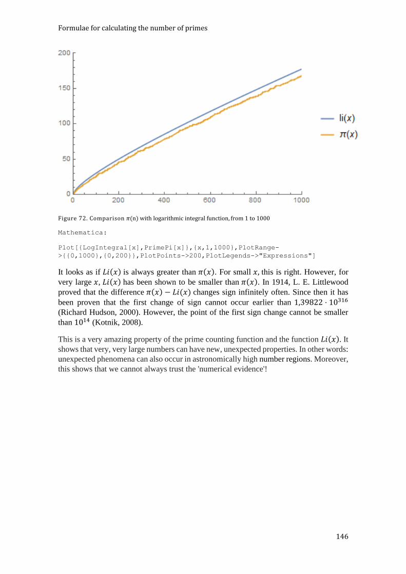
Formulae for calculating the number of primes
146
Figure 72. Comparison 𝜋(n) with logarithmic integral function, from 1 to 1000
Mathematica:
Plot[{LogIntegral[x],PrimePi[x]},{x,1,1000},PlotRange-
>{{0,1000},{0,200}},PlotPoints->200,PlotLegends->"Expressions"]
It looks as if 𝐿𝑖(𝑥) is always greater than 𝜋(𝑥). For small 𝑥, this is right. However, for
very large 𝑥, 𝐿𝑖(𝑥) has been shown to be smaller than 𝜋(𝑥). In 1914, L. E. Littlewood
proved that the difference 𝜋(𝑥) − 𝐿𝑖(𝑥) changes sign infinitely often. Since then it has
been proven that the first change of sign cannot occur earlier than 1,39822 ⋅ 10316
(Richard Hudson, 2000). However, the point of the first sign change cannot be smaller
than 1014 (Kotnik, 2008).
This is a very amazing property of the prime counting function and the function 𝐿𝑖(𝑥). It shows that very, very large numbers can have new, unexpected properties. In other words:
unexpected phenomena can also occur in astronomically high number regions. Moreover,
this shows that we cannot always trust the 'numerical evidence'!
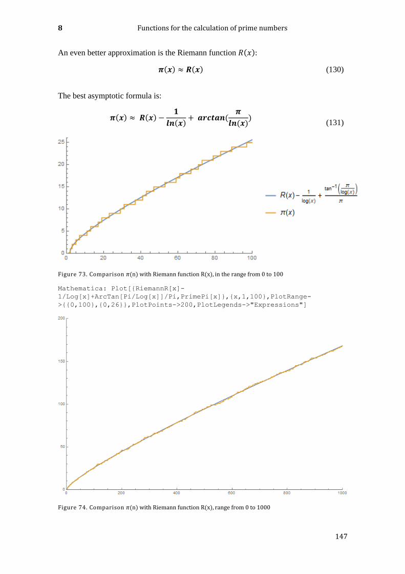
8 Functions for the calculation of prime numbers
147
An even better approximation is the Riemann function 𝑅(𝑥):
𝝅(𝒙) ≈ 𝑹(𝒙) (130)
The best asymptotic formula is:
𝝅(𝒙) ≈ 𝑹(𝒙) −𝟏
𝒍𝒏(𝒙)+ 𝒂𝒓𝒄𝒕𝒂𝒏(
𝝅
𝒍𝒏(𝒙))
(131)
Figure 73. Comparison 𝜋(n) with Riemann function R(x), in the range from 0 to 100
Mathematica: Plot[{RiemannR[x]-
1/Log[x]+ArcTan[Pi/Log[x]]/Pi,PrimePi[x]},{x,1,100},PlotRange-
>{{0,100},{0,26}},PlotPoints->200,PlotLegends->"Expressions"]
Figure 74. Comparison 𝜋(n) with Riemann function R(x), range from 0 to 1000

Formulae for calculating the number of primes
148
Mathematica:
Plot[{RiemannR[x]-
1/Log[x]+ArcTan[Pi/Log[x]]/Pi,PrimePi[x]},{x,1,1000},PlotRange-
>{{0,1000},{0,200}},PlotPoints->200,PlotLegends->"Expressions"]
And finally, here is the mysterious, exact formula found by Riemann:
𝝅(𝒙) = 𝑹(𝒙) −∑𝑹(𝒙𝝆)
𝝆
(132)
Using the Riemann function 𝑅(𝑥).
𝝅𝟎(𝒙) = 𝑹(𝒙) −∑𝑹(𝒙𝝆) −𝟏
𝒍𝒏(𝒙)+𝟏
𝝅𝝆
𝒂𝒓𝒄𝒕𝒂𝒏(𝝅
𝒍𝒏(𝒙)) (133)
The Riemann function is a very good approximation for 𝜋(𝑥), but Riemann's formula
(132) is much more precise. It also takes into account the small local fluctuations of 𝜋(𝑥) and finally fits (if enough zero terms of the zeta function are evaluated) to the exact integer
stairs function of the arithmetical calculation. Note: the summation over the zero terms
of the zeta function must occur in ascending order of increasing values of Im(𝜌), since
the sum is only conditionally convergent. The calculation of 𝑅(𝑥𝜌) requires the
calculation of Li(𝑥𝜌) and is not quite as simple because the complex logarithm of 𝑥𝜌 has
to be calculated. This function, in turn, is not injective and is not defined unambiguously
The calculation of the principal value using the ‘main branch’ of the complex logarithm46
would give incorrect results. In short, the problem lies in the fact that, for the complex
logarithm, the equation ln(𝑥𝜌) = 𝜌 ln(𝑥) does not always obtain. However, the problem
can be avoided by simply using Ei(𝜌 ln(𝑥)) instead of Li(𝑥𝜌), where Ei(𝑥) denotes the
complex integral exponential function ( Li(x) is the complex logarithmic integral
function). Ei(𝑥) is closely related to Li(𝑥), since 𝐋𝐢(𝒙) = 𝐄𝐢(𝐥𝐧 𝒙).
Note: the largest known values of 𝜋(𝑥) were obtained not by number theory but by the
methods of analytical number theory.
The following graphs show how the analytical formula approximates to the exact stair
function:
Mathematica program: please contact the author.
46 The logarithm of the kth branch is defined as 𝑤 = ln|𝑧| + 𝑖 (arg 𝑧 + 2𝑘𝜋), 𝑘 ∈ ℤ. For 𝑘 = 0 we have the main branch of the complex logarithm function.
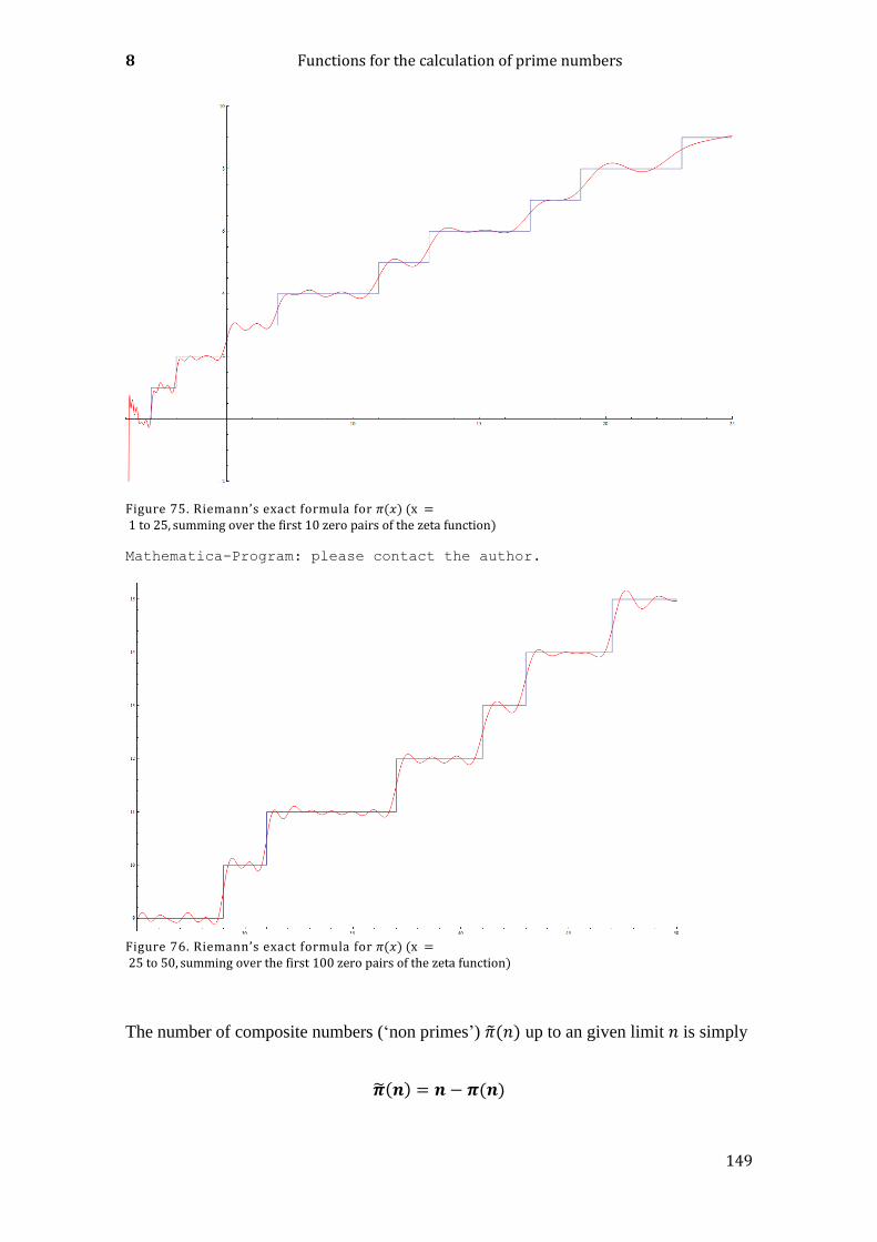
8 Functions for the calculation of prime numbers
149
Figure 75. Riemann’s exact formula for 𝜋(𝑥) (x = 1 to 25, summing over the first 10 zero pairs of the zeta function)
Mathematica-Program: please contact the author.
Figure 76. Riemann’s exact formula for 𝜋(𝑥) (x = 25 to 50, summing over the first 100 zero pairs of the zeta function)
The number of composite numbers (‘non primes’) �̃�(𝑛) up to an given limit 𝑛 is simply
�̃�(𝒏) = 𝒏 − 𝝅(𝒏)
Formulae for calculating the nth prime number
150
Mathematica:
n-PrimePi[n]
More formulae for 𝝅(𝒙)
𝝅(𝒙) ≈ 𝐥𝐢(𝒙) −√𝒙
𝐥𝐧 𝒙(𝟏 + 𝟐∑
𝐬𝐢𝐧(𝜸𝐥𝐧 𝒙)
𝜸𝜸
) ,𝐰𝐡𝐞𝐫𝐞 𝜸 = 𝐈𝐦(𝝆) (134)
Here, 𝜌 are the complex zeros of the zeta function.
8.7 FORMULAE FOR CALCULATING THE NTH PRIME NUMBER
Unlike in Chapter 8.1, here we want to look for analytical, asymptotic solutions.
The calculation of the nth prime is difficult. No explicit, simple formula is known for this
purpose.
The best asymptotic estimate currently known is (as of Dec. 2016):
𝒑𝒏 = 𝒏 (𝐥𝐧 𝒏 + 𝐥𝐧 𝐥𝐧 𝒏 − 𝟏 + (𝐥𝐧 𝐥𝐧 𝒏 − 𝟐)
𝐥𝐧 𝒏
−(𝐥𝐧 𝐥𝐧 𝒏)𝟐 − 𝟔 𝐥𝐧 𝐥𝐧 𝒏 + 𝟏𝟏)
𝟐(𝐥𝐧 𝒏)𝟐 )
Mathematica:
Table[Prime[n],{n,1,100}]
prime[n_]:=Block[{logn=N[Log[n],15],loglogn=N[Log[Log[n]],15]}
,
n(logn+loglogn-1+(loglogn-2)/logn-(loglogn^2-
6loglogn+11)/(2logn^2))]
(135
)
8.8 FORMULAE FOR CALCULATING THE NTH NON-PRIME (COMPOSITE NUMBER)
The nth non prime can be calculated using the following Mathematica program: (In this
example: from n= 1 to 1000)
Mathematica:
composite[n_Integer]:=FixedPoint[n+PrimePi[#]&,n+PrimePi[n]]
ListLinePlot[Table[{k,composite[k]},{k,0,1000,10}],Filling->Axis]
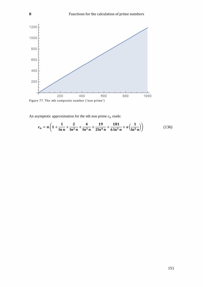
8 Functions for the calculation of prime numbers
151
Figure 77. The nth composite number (‘non prime’)
An asymptotic approximation for the nth non prime 𝑐𝑛 reads:
𝒄𝒏 = 𝒏(𝟏 +𝟏
𝐥𝐧𝒏+
𝟐
𝐥𝐧𝟐 𝒏+
𝟒
𝐥𝐧𝟑 𝒏+
𝟏𝟗
𝟐𝐥𝐧𝟒 𝒏+
𝟏𝟖𝟏
𝟔 𝐥𝐧𝟓 𝒏+ 𝒐(
𝟏
𝐥𝐧𝟓 𝒏)) (136)
152
9 NOW IT GETS INTERESTING: FOUR-DIMENSIONAL SPHERES AND PRIME NUMBERS
What have spheres – even four-dimensional spheres – to do with primes? We will pursue
this question in this chapter. In principle, the question arises as to how many integer lattice
points in the n-dimensional space have the same difference from the origin (i.e. lie on the
'surface' of an n-dimensional sphere). In mathematics the term 'n-sphere' is generally used
for an n-dimensional sphere. So, for example, a 1-sphere is the circumference of a circle,
a 2-sphere is the curved 2-dimensional surface of a sphere. A 3-sphere is the boundary of
a 4-dimensional sphere, i.e. a three-dimensional space bent into the fourth dimension,
which, for the sake of simplicity, we sometimes refer to as the ‘surface’ of the four-
dimensional sphere. The term 'glome' is also used for this. In this chapter, we are looking
for integer lattice points (of a Cartesian coordinate system) that ‘sit’ on n-spheres in two-
, three-, or four-dimensional space.
The Mathematica software provides three powerful tools for solving this problem:
FindInstance:
finds all points that lie on an n-sphere, here e.g. on a 2-sphere with radius √𝑛:
FindInstance[x^2+y^2+z^2==n,{x,y,z},Integers,numberOfInstances]
Since the solutions of FindInstance include many permutations and axis- and point-
symmetrically mirrored solutions due to the symmetry properties (the degree of symmetry
becomes higher as the number of dimensions increases), the following function is also
interesting, because it just computes the "core" of the solutions – that is to say, without
the ‘mirrored’ solutions from negative quadrants, octaves, etc., or which can be generated
by permutations:
PowersRepresentations:
Finds all (actually different, integer and positive) solutions of the equation
𝑥2 + 𝑦2 + 𝑧2 = 𝑛
Example: PowersRepresentations[n,3,2]
And finally the function SquaresR:
this provides (only) the number of solutions of FindInstance.
E.g.: SquaresR[3,n] gives the number of solutions of FindInstance[x^2+y^2+z^2==n,{x,y,z},Integers,Infinity]]
It will be shown that the spherical points on the n-spheres are not randomly distributed,
but, on the contrary, form very beautiful structures that become more interesting the
higher the dimensionality of the n-spheres. In the case of the 3-spheres ('surfaces' of four-
dimensional spheres), a remarkable relation exists between the number of spherical points
and the prime numbers. This connection is very simple and is anticipated here:

9 Now it gets interesting: four-dimensional spheres and prime numbers
153
If the square 𝑛 = 𝑟𝑎𝑑2 of the radius of a 4-dimensional sphere assumes the value of a
prime number, then (and only then) the following relation applies:
𝑟𝑎𝑑2 = 𝑛 =𝑟4(𝑛)
8− 1, if 𝑛 ∈ ℙ (137)
This relationship has long been known since the function 𝑟4(𝑛) can be easily calculated
from the sigma function 𝜎1(𝑛). However, there is no reference in the relevant literature
to the beautiful connection with the 3-spheres ('surfaces') of four-dimensional spheres and
primes.
Just a curiosity: the number 12 plays a special role in the sequence 𝑟4(𝑛), since it is the
only number for which
𝑛 =𝑟4(𝑛)
8, only if 𝑛 = 12 (138)
Since it is difficult to imagine four-dimensional objects, it is always a good idea to start
with the counterpart in one or two lower dimensions. Thus we begin with two-
dimensional spheres (1-spheres) – ‘circles’, in common parlance.

The second dimension: circles and integer lattice points
154
9.1 THE SECOND DIMENSION: CIRCLES AND INTEGER LATTICE POINTS
We are looking for the integer lattice points of our Cartesian coordinate system that can
lie along the circumference (we are not interested in any lattice points lying within the
circle, but only in lattice points that lie exactly on the circumference). If we assume that
the radius of the circle increases continuously, the circular line runs through the lattice
points of our coordinate system in order, which lie exactly on the circle line. The number
of these possible lattice points that are touched by the circumference, of course, depends
strongly on the radius of the circle. Let us suppose that we increase the circle radius
continuously, then the circumference will run through the grid points of our coordinate
system. We are interested in the grid points that lie exactly on the circumference. Here
are 6 examples for 𝑟2 = 8 to 13:
Figure 78. Lattice points on a 1-sphere, squared radius from 8 to 13
Mathematica program: please contact the author.
For some values with radius r, there are no integral solutions of the equation 𝑥2 + 𝑦2 =𝑟2, and therefore no corresponding lattice points either that are touched by the circle. The
"crossing" of the circular line through the two-dimensional grid points can be viewed in
an animation (as a video on the enclosed CD) or as a Mathematica animation (see
Appendix: “Lattice points on n-spheres (n-dimensional spheres)”).
The function which calculates the number of integer lattice points on a circumference in
2-dimensional space is called 𝑟2(𝑛). Its function values are all divisible by 4. The first
100 values are:
9 Now it gets interesting: four-dimensional spheres and prime numbers
155
{4,4,0,4,8,0,0,4,4,8,0,0,8,0,0,4,8,4,0,8,0,0,0,0,12,8,0,0,8,0,0,4,0,8,
0,4,8,0,0,8,8,0,0,0,8,0,0,0,4,12,0,8,8,0,0,0,0,8,0,0,8,0,0,4,16,0,0,8,
0,0,0,4,8,8,0,0,0,0,0,8,4,8,0,0,16,0,0,0,8,8,0,0,0,0,0,0,8,4,0,12}
Mathematica:
SquaresR[2,Range[100]]
Example: the 8 solutions 𝑟2 = 5 read:
{{-2,-1},{-2,1},{-1,-2},{-1,2},{1,-2},{1,2},{2,-1},{2,1}}
Mathematica:
FindInstance[x^2+y^2==5,{x,y},Integers,8]
These solutions can be created from each other mutually by permutations or symmetrical
mirroring. The number of genuinely different solutions is in this case 1:
{{1,2}}
Mathematica:
PowersRepresentations[5,2,2]
𝑟2(𝑛) is the number of lattice points in the 2-dimensional space lying on a circle with
radius √𝑛. We denote 𝑟2∗(𝑛) as the number of different, positive lattice points, such that
0 ≤ 𝑛1 ≤ 𝑛2 and 𝑛12 + 𝑛2
2 = 𝑛.
𝑟2(𝑛) has a value of 0 for many values of 𝑛. This means that not every natural number
can be written as the sum of 2 squares. Here is a list of the first values of these 'non-
representable' numbers:
{3,6,7,11,12,14,15,19,21,22,23,24,27,28,30,31,33,35,38,39,42,43,44,46,
47,48,51,54,55,56,57,59,60,62,63,66,67,69,70,71,75,76,77,78,79,83,84,
86,87, 88,91,92,93,94,95,96,99,…}
Mathematica:
Select[Range[199], Length[PowersRepresentations[ #, 2, 2]] == 0 &]
Here are two illustrations of 𝑟2(𝑛):

The second dimension: circles and integer lattice points
156
Figure 79. 𝑟2(𝑛): number/4 of possible representations of n as a sum of 2 squares. No simple relationship to prime numbers can be observed.
Figure 80. 𝑟2(𝑛): number/4 of possible representations of n as a sum of 2 squares (up to n=100000)
And finally a few plots of 𝑟2∗(𝑛) for different values of 𝑛:

9 Now it gets interesting: four-dimensional spheres and prime numbers
157
Figure 81. 𝑟2∗(bn): number of different representations of bn as the sum of two squares
Mathematica program (Figure 79): Show[ListLinePlot[Table[{n,SquaresR[2,n]/4},{n,1,150}],
InterpolationOrder->0],ListPlot[Table[{Prime[n],
SquaresR[2,Prime[n]]/4},{n,1,PrimePi[150]}],PlotStyle->Red]
]
Mathematica (Figure 80): Show[ListPlot[Table[{n,SquaresR[2,n]/4},{n,1,100000}],PlotRange->Full]
]
Mathematica (Figure 81): ListLinePlot[{Table[Length[PowersRepresentations[10^i,2,2]],{i,1,13}],
Table[Length[PowersRepresentations[14^i,2,2]],{i,1,13}],
Table[Length[PowersRepresentations[15^i,2,2]],{i,1,13}],
Table[Length[PowersRepresentations[16^i,2,2]],{i,1,13}],
Table[Length[PowersRepresentations[25^i,2,2]],{i,1,13}]
},PlotLegends->Automatic,PlotRange->All]
Note: integral solutions of 𝑥2 + 𝑦2 = 𝑟2 (where r is also an integer) are also referred to
as 'Pythagorean triplets'. These correspond to the lattice points on a circular line with an
integer radius r.
9.1.1 FORMULAE AND PROPERTIES
We restrict ourselves to the function 𝑟2(𝑛), which calculates the number of lattice points
in two-dimensional space lying on a circle with radius √𝑛. For the function 𝑟2∗(𝑛), which
The second dimension: circles and integer lattice points
158
calculates the number of different, positive grid points, such that: 0 ≤ 𝑛1 ≤ 𝑛2 and 𝑛12 +
𝑛22 = 𝑛, see note47.
The generating function of 𝑟2(𝑛) is the squared elliptic Jacobi 𝜗3(𝑛) function:
∑𝑟2(𝑛)𝑥𝑛 =
∞
𝑛=0
𝜗32(𝑥) = 1 + 4𝑥 + 4𝑥2 + 4𝑥4 + 8𝑥5 +⋯ (139)
Explicit formulae:
𝑟2(𝑛) = 4[𝑑1 − 𝑑3], 𝑑𝑘: number of divisors of 𝑛 of the form 4𝑚 + 𝑘 (140)
47 http://mathworld.wolfram.com/SumofSquaresFunction.html
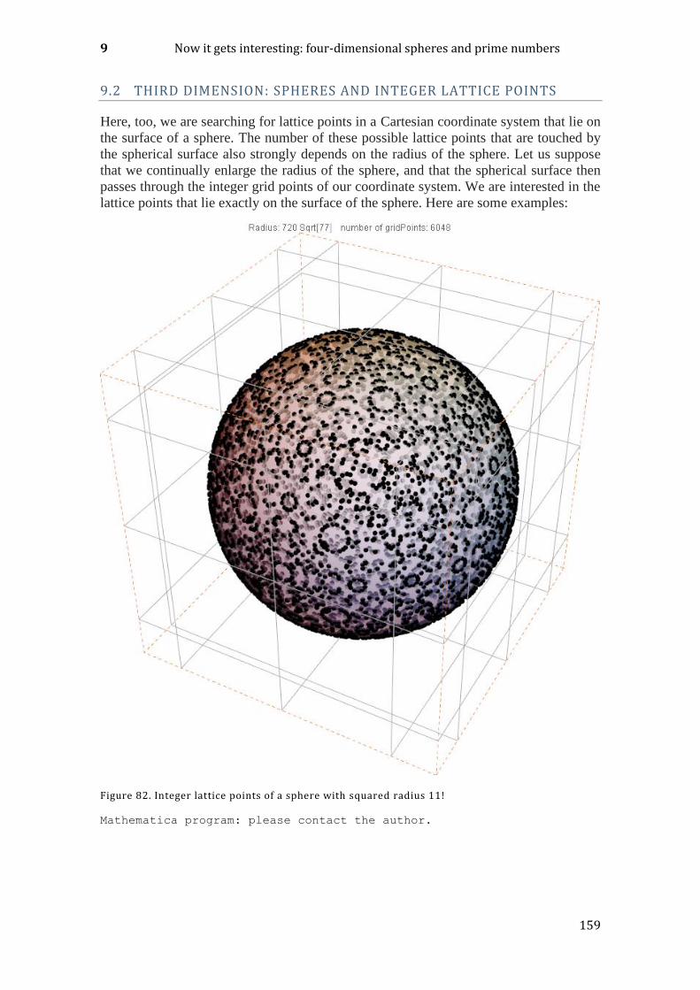
9 Now it gets interesting: four-dimensional spheres and prime numbers
159
9.2 THIRD DIMENSION: SPHERES AND INTEGER LATTICE POINTS
Here, too, we are searching for lattice points in a Cartesian coordinate system that lie on
the surface of a sphere. The number of these possible lattice points that are touched by
the spherical surface also strongly depends on the radius of the sphere. Let us suppose
that we continually enlarge the radius of the sphere, and that the spherical surface then
passes through the integer grid points of our coordinate system. We are interested in the
lattice points that lie exactly on the surface of the sphere. Here are some examples:
Figure 82. Integer lattice points of a sphere with squared radius 11!
Mathematica program: please contact the author.

Third dimension: spheres and integer lattice points
160
Figure 83. Integer lattice points of spheres (squared radius 999-102).
For some values with radius 𝑟 there are no integer solutions of the equation 𝑥2 + 𝑦2 +𝑧2 = 𝑟2 and therefore no corresponding lattice points either that are touched by the
spherical surface. Some structures are only visible when the spheres are viewed from
different viewing angles. This can be viewed in an animation (as a video on the enclosed
CD) or as a Mathematica animation (see Appendix). The function that calculates the
number of integer lattice points on the surface of a sphere in three-dimensional space is
denoted in mathematical literature by 𝑟3(𝑛). We define 𝑟3∗(𝑛) as the number of different,
positive lattice points, such that
0 ≤ 𝑛1 ≤ 𝑛2 ≤ 𝑛3 and 𝑛12 + 𝑛2
2 + 𝑛32 = 𝑛.

9 Now it gets interesting: four-dimensional spheres and prime numbers
161
Many (but not all) function values of 𝑟3(𝑛) are divisible by 6. The first 100 values are:
{6,12,8,6,24,24,0,12,30,24,24,8,24,48,0,6,48,36,24,24,48,24,0,24,30,72
,32,0,72,48,0,12,48,48,48,30,24,72,0,24,96,48,24,24,72,48,0,8,54,84,48
,24,72,96,0,48,48,24,72,0,72,96,0,6,96,96,24,48,96,48,0,36,48,120,56,2
4,96,48,0,24,102,48,72,48,48,120,0,24,144,120,48,0,48,96,0,24,48,108,7
2,30}
Mathematica:
SquaresR[3,Range[100]]
Example: the 8 solutions of 𝑟2 = 3 read:
{{-1,-1,-1},{-1,-1,1},{-1,1,-1},{-1,1,1},{1,-1,-1},{1,-1,1},{1,1,-1},{1,1,1}}
Mathematica:
FindInstance[x^2+y^2+z^2==3,{x,y,z},Integers,8]
These solutions can be created from each other mutually by permutations or symmetrical
mirroring. The number of genuinely different solutions in this case is 1: {{1,1,1}} Mathematica:
PowersRepresentations[3,3,2]
The first 100 values of 𝑟3∗(𝑛) read:
{1,1,1,1,1,1,0,1,2,1,1,1,1,1,0,1,2,2,1,1,1,1,0,1,2,2,2,0,2,1,0,1,2,2,1
,2,1,2,0,1,3,1,1,1,2,1,0,1,2,3,2,1,2,3,0,1,2,1,2,0,2,2,0,1,3,3,1,2,2,1
,0,2,2,3,2,1,2,1,0,1,4,2,2,1,2,3,0,1,4,3,1,0,1,2,0,1,2,3,3,2}
Mathematica:
Table[Length[PowersRepresentations[i,3,2]],{i,1,100}] or:
a[ n_] := If[ n < 0, 0, Sum[ Boole[ n == i^2 + j^2 + k^2], {i, 0,
Sqrt[n]}, {j, 0, i}, {k, 0, j}]];
As already mentioned above, 𝑟3(𝑛) has the value 0 for some 𝑛. This means that not every
natural number can be written as the sum of 3 squares. Here is a list of the first values of
these 'non-representable' numbers:
{7,15,23,28,31,39,47,55,60,63,71,79,87,92,95,103,111,112,119,124,127,1
35,143,151,156,159,167,175,183,188,191,199}
Mathematica:
Select[Range[199], Length[PowersRepresentations[ #, 3, 2]] == 0 &]
Here are two plots of 𝑟3(𝑛):

Third dimension: spheres and integer lattice points
162
Figure 84. 𝑟3(𝑛): number/6 of possible representations of n as the sum of 3 squares.
Mathematica:
Show[ListLinePlot[Table[{n,SquaresR[3,n]/6},{n,1,150}],InterpolationOrder-
>0],ListPlot[Table[{Prime[n],SquaresR[3,Prime[n]]/6},{n,1,PrimePi[150]}],PlotS
tyle->Red]]
Figure 85. Number/6 of possible representations of n as the sum of 3 squares (up to 100000)
Mathematica:
ListPlot[Table[{n,SquaresR[3,n]/6},{n,1,100000}],PlotRange-
>Full,PlotStyle->Black]

9 Now it gets interesting: four-dimensional spheres and prime numbers
163
Here are a few plots illustrating 𝑟3∗(𝑛):
Figure 86. 𝑟3
∗(𝑛): Number of different representations of n as the sum of 3 squares, (n=1 to 500)
Figure 87. 𝑟3
∗(𝑛): Number of different representations of n as the sumof 3 squares, (n=1 up to
100000)
ListPlot[Table[{n,Length[PowersRepresentations[n,3,2]]},{n,1,100000}],
PlotRange->Full,PlotStyle->Black]
Since everything happens on an n-sphere (here a 2-sphere or spherical surface), spherical
coordinates (𝑟, 𝜑, 휃), obviously, must be used rather than Cartesian ones (𝑥, 𝑦, 𝑧). The

Third dimension: spheres and integer lattice points
164
radius 𝑟 of the sphere remains constant in our investigations, therefore only two degrees
of freedom remain: the angles 𝜑 and 휃.
This leads to the tempting idea of interpreting 𝜑 and 휃 as 2-dimensional Cartesian
coordinates. All interesting patterns on the spherical surfaces can now be seen as two-
dimensional representations:
Figure 88. Lattice points of the surface of a sphere where 𝑟2 = 1001, angles of the spherical coordinates interpreted as 2-dimensional Cartesian coordinates (same colour indicates identical points with respect to mirror operations)
Figure 89. Same as above, however 𝑟2 = 11! (Mathematica programs in the Appendix)
9 Now it gets interesting: four-dimensional spheres and prime numbers
165
9.2.1 FORMULAE AND PROPERTIES
We restrict ourselves to the function 𝑟3(𝑛), which calculates the number of lattice points
in 3-dimensional space lying on the surface of a sphere with radius √𝑛. For the function
𝑟3∗(𝑛), which calculates the number of different, positive grid points, such that:
0 ≤ 𝑛1 ≤ 𝑛2 ≤ 𝑛3 and 𝑛12 + 𝑛2
2 + 𝑛32 = 𝑛, see e.g. note.48
The generating function of 𝑟3(𝑛) is the elliptic Jacobi 𝜗3(𝑛) function raised to a power
of 3:
∑𝑟3(𝑛)𝑥𝑛 =
∞
𝑛=0
𝜗33(𝑥) = 1 + 6𝑥 + 12𝑥2 + 8𝑥3 + 6𝑥4 + 24𝑥5 +⋯ (141)
Explicit formulae:
𝑟3(𝑛) = {24ℎ(−𝑛), if 𝑛 ≡ 3 (mod 8)
12ℎ(−4𝑛), if 𝑛 ≡ 1,2,5,6 (mod 8)0, if 𝑛 ≡ 7 (mod 8)
} (142)
(with ℎ(𝑛) being the ‘class number‘49 of 𝑛).
The ‘Three-squares theorem’ of C. F. Gauss is worth mentioning:
for each natural integer number 𝒏 that can be represented as a sum of 3 squares
(𝒙𝟐 + 𝒚𝟐 + 𝒛𝟐 = 𝒏,𝒏, 𝒙, 𝒚, 𝒛 ∈ ℕ), the following obtains:
𝒏 = 𝟒𝒌𝒎 where 𝟒 ∤ 𝒎 𝐚𝐧𝐝 𝒎 ≢ 𝟕 𝒎𝒐𝒅 𝟖
48 http://mathworld.wolfram.com/SumofSquaresFunction.html 49 https://en.wikipedia.org/wiki/Class_numberl
Fourth dimension: hyperspheres and integer lattice points on ‘glomes‘
166
9.3 FOURTH DIMENSION: HYPERSPHERES AND INTEGER LATTICE POINTS ON ‘GLOMES ‘
In the same way as in three-dimensional space, we are searching for lattice points in a
Cartesian coordinate system that lie on the ‘surface’ of a hypersphere. The number of
these possible lattice points that are touched by the surface of the hypersphere depends
heavily on the radius of the hypersphere. We will denote this ‘surface’ of the hypersphere
in the following as "glome" and thus stick to the general language usage. Let us suppose
that we increase the radius of the hypersphere continuously, then our glome will run
through the lattice points of our four-dimensional coordinate system. Our interest now is
directed to the lattice points that lie exactly on the glome. Here are a few examples:
(here, the author would have liked to have shown a few examples, but unfortunately it is
not so easy to visualize four-dimensional objects. There is, however, a trick to doing so,
see below).
Let us for the moment remain in the abstract, mathematical space.
In 3-dimensional space, some values 𝑟2 always existed for which the equation 𝑥2 + 𝑦2 +𝑧2 = 𝑟2 had no solutions (and therefore no corresponding lattice points). In the four-
dimensional domain, this is no longer the case: for every integer 𝑟2 (that is, every natural
number), the equation 𝑥2 + 𝑦2 + 𝑧2 + 𝑡2 = 𝑟2 has integer solutions! Each natural
number can be expressed as the sum of four squares. This is the famous theorem of
Lagrange from the year 1770.
The function that calculates the number of integer lattice points on a glome ('surface' of a
four-dimensional hypersphere) is in mathematical literature denoted as 𝑟4(𝑛). We denote
the number of different positive lattice points such that 0 ≤ 𝑛1 ≤ 𝑛2 ≤ 𝑛3 ≤ 𝑛4 and
𝑛12 + 𝑛2
2 + 𝑛32 + 𝑛4
2 = 𝑛
as 𝑟4∗(𝑛)
All function values of 𝑟4(𝑛) are divisible by 8. The first 50 values read:
{8,24,32,24,48,96,64,24,104,144,96,96,112,192,192,24,144,312,160,144,2
56,288,192,96,248,336,320,192,240,576,256,24,384,432,384,312,304,480,4
48,144,336,768,352,288,624,576,384,96,456,744}
Mathematica:
SquaresR[4,Range[50]]
The 8 solutions for 𝑟2 = 3 read:
{{1,-1,-1,0},{1,1,-1,0},{-1,0,-1,-1},{-1,-1,0,1},{1,1,0,1},{1,-
1,0,1},{-1,0,1,1},{0,1,-1,-1}}
Mathematica:
FindInstance[x^2+y^2+z^2+t^2==3,{x,y,z,t},Integers,8]
These solutions can be created from each other mutually by permutations or symmetrical
mirroring. The number of genuinely different solutions in this case is 1:
{{0,1,1,1}}
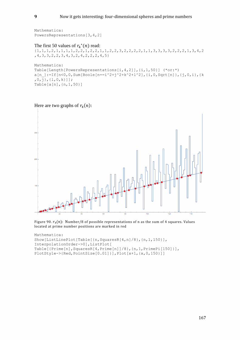
9 Now it gets interesting: four-dimensional spheres and prime numbers
167
Mathematica:
PowersRepresentations[3,4,2]
The first 50 values of 𝑟4∗(𝑛) read:
{1,1,1,2,1,1,1,1,2,2,1,2,2,1,1,2,2,3,2,2,2,2,1,1,3,3,3,3,2,2,2,1,3,4,2
,4,3,3,2,2,3,4,3,2,4,2,2,2,4,5}
Mathematica:
Table[Length[PowersRepresentations[i,4,2]],{i,1,50}] (*or:*)
a[n_]:=If[n<0,0,Sum[Boole[n==i^2+j^2+k^2+l^2],{i,0,Sqrt[n]},{j,0,i},{k
,0,j},{l,0,k}]];
Table[a[n],{n,1,50}]
Here are two graphs of 𝑟4(𝑛):
Figure 90. 𝑟4(𝑛): Number/8 of possible representations of n as the sum of 4 squares. Values
located at prime number positions are marked in red
Mathematica:
Show[ListLinePlot[Table[{n,SquaresR[4,n]/8},{n,1,150}],
InterpolationOrder->0],ListPlot[
Table[{Prime[n],SquaresR[4,Prime[n]]/8},{n,1,PrimePi[150]}],
PlotStyle->{Red,PointSize[0.01]}],Plot[x+1,{x,0,150}]]
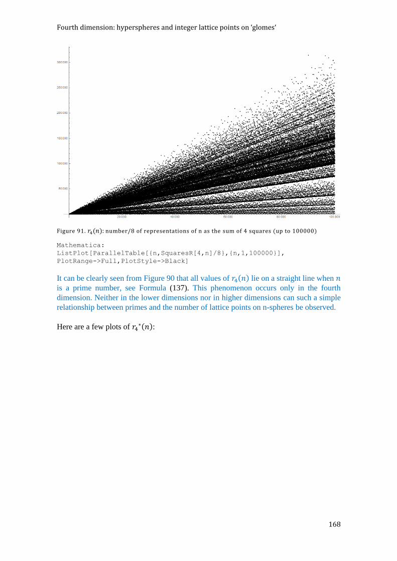
Fourth dimension: hyperspheres and integer lattice points on ‘glomes‘
168
Figure 91. 𝑟4(𝑛): number/8 of representations of n as the sum of 4 squares (up to 100000)
Mathematica:
ListPlot[ParallelTable[{n,SquaresR[4,n]/8},{n,1,100000}],
PlotRange->Full,PlotStyle->Black]
It can be clearly seen from Figure 90 that all values of 𝑟4(𝑛) lie on a straight line when 𝑛
is a prime number, see Formula (137). This phenomenon occurs only in the fourth
dimension. Neither in the lower dimensions nor in higher dimensions can such a simple
relationship between primes and the number of lattice points on n-spheres be observed.
Here are a few plots of 𝑟4∗(𝑛):
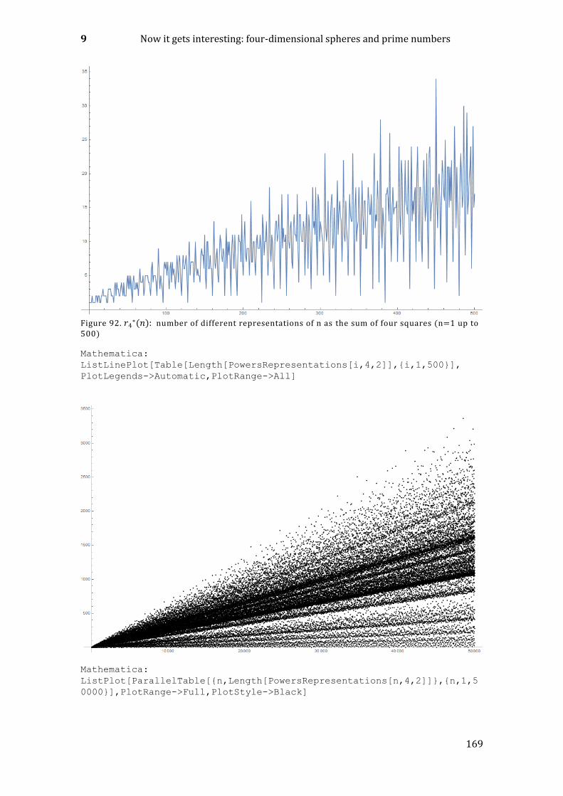
9 Now it gets interesting: four-dimensional spheres and prime numbers
169
Figure 92. 𝑟4
∗(𝑛): number of different representations of n as the sum of four squares (n=1 up to 500)
Mathematica:
ListLinePlot[Table[Length[PowersRepresentations[i,4,2]],{i,1,500}],
PlotLegends->Automatic,PlotRange->All]
Mathematica:
ListPlot[ParallelTable[{n,Length[PowersRepresentations[n,4,2]]},{n,1,5
0000}],PlotRange->Full,PlotStyle->Black]

Fourth dimension: hyperspheres and integer lattice points on ‘glomes‘
170
From the graphs for 𝑟4(𝑛) and 𝑟4∗(𝑛), we see that the asymptotic behavior of both
functions is linear.
As in the last section for three-dimensional spheres, we use a trick to reduce the number
of dimensions by one dimension by using hypersphere coordinates (𝑟, 𝜑, 휃, 𝜓) instead
of Cartesian coordinates(𝑥, 𝑦, 𝑧, 𝑡) The radius 𝑟 of the hypersphere remains constant and
only three degrees of freedom remain: the angles 𝜑, 휃 and 휃. 𝛷, 휃 and 𝜓 are interpreted
as three-dimensional Cartesian coordinates. Thus all interesting patterns on the hyper-
spherical surfaces can also be seen as a three-dimensional picture.
The colour representation was chosen such that the same (absolute) 𝑥, 𝑦, or 𝑧 coordinates of a point represent the same R G B triple in the RGB colour space.
Example 1: 𝑟2 =1001.
Example 2: 𝑟2 =10007
Animations (views on the surface of the 4-dimensional spheres) can be found on the
enclosed computer CD, or as a Mathematica program for the animations in the Appendix.
Figure 93. Example 1: lattice points on the 3-sphere of a 4 dim. sphere where r^2=1001
(Mathematica programs can be found in the Appendix).
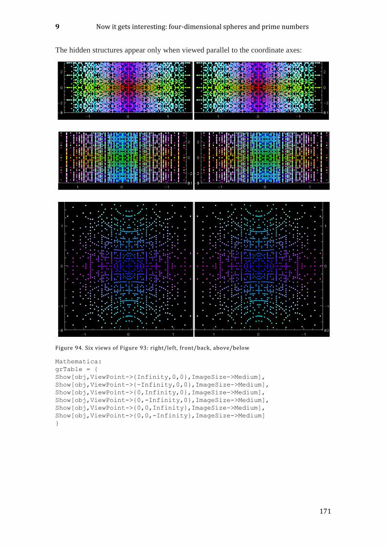
9 Now it gets interesting: four-dimensional spheres and prime numbers
171
The hidden structures appear only when viewed parallel to the coordinate axes:
Figure 94. Six views of Figure 93: right/left, front/back, above/below
Mathematica:
grTable = {
Show[obj,ViewPoint->{Infinity,0,0},ImageSize->Medium],
Show[obj,ViewPoint->{-Infinity,0,0},ImageSize->Medium],
Show[obj,ViewPoint->{0,Infinity,0},ImageSize->Medium],
Show[obj,ViewPoint->{0,-Infinity,0},ImageSize->Medium],
Show[obj,ViewPoint->{0,0,Infinity},ImageSize->Medium],
Show[obj,ViewPoint->{0,0,-Infinity},ImageSize->Medium]
}
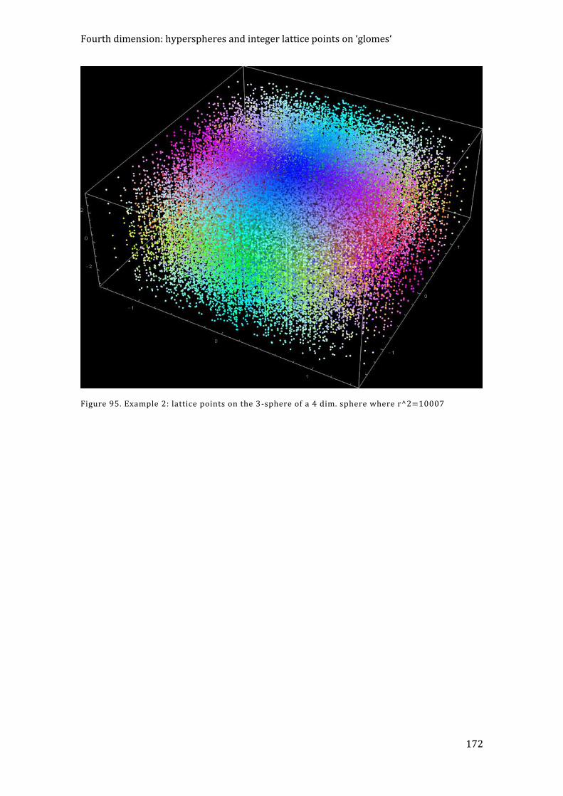
Fourth dimension: hyperspheres and integer lattice points on ‘glomes‘
172
Figure 95. Example 2: lattice points on the 3-sphere of a 4 dim. sphere where r^2=10007
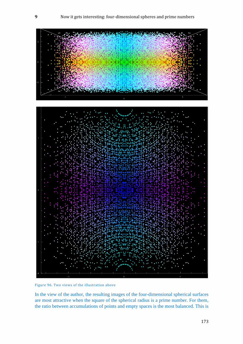
9 Now it gets interesting: four-dimensional spheres and prime numbers
173
Figure 96. Two views of the illustration above
In the view of the author, the resulting images of the four-dimensional spherical surfaces
are most attractive when the square of the spherical radius is a prime number. For them,
the ratio between accumulations of points and empty spaces is the most balanced. This is
Fourth dimension: hyperspheres and integer lattice points on ‘glomes‘
174
also demonstrated by Figure 90. The density of the spherical points on 3-spheres is for
primes always in the middle range.
9.3.1 FORMULAE AND PROPERTIES
As in the case of the lower dimensions, we restrict ourselves to the function 𝑟4(𝑛), which
calculates the number of lattice points in the 4-dimensional space that lie on a hypersphere
surface (glome) with radius √𝑛. For the function 𝑟4∗(𝑛), which calculates the number of
different positive grid points, such that: 0 ≤ 𝑛1 ≤ 𝑛2 ≤ 𝑛3 ≤ 𝑛4 and 𝑛12 + 𝑛2
2 + 𝑛32 +
𝑛42 = 𝑛, please refer to other relevant sources.
The generating function of 𝑟4(𝑛) is the elliptic Jacobi 𝜗3(𝑛) function raised to the 4th
power:
∑𝑟4(𝑛)𝑥𝑛 =
∞
𝑛=0
𝜗34(𝑥) = 1 + 8𝑥 + 24𝑥2 + 32𝑥3 + 24𝑥4 + 48𝑥5 +⋯ (143)
Explicit formulae:
𝑟4(𝑛) = {
8𝜎1(𝑛), if 𝑛 odd
24𝜎0(𝑛), if 𝑛 even,with 𝜎0(n) = ∑ 𝑑
2∤𝑑,𝑑|𝑛
(144)
This can be written somewhat more easily:
𝑟4(𝑛) = { 8𝜎1(𝑛), if 4 ∤ 𝑛 (𝑛 not divisable by 4)
8𝜎1(𝑛) − 32𝜎1 (𝑛
4) , otherwise (𝑛 divisable by 4)
(145)
or
𝑟4(𝑛) = 8 ∑ 𝑑
𝑑|𝑛,4∤𝑑
(146)

175
10 ABOUT OCRONS AND GOCRONS: SHADES OF GÖDEL
10.1 WHAT ARE OCRONS AND GOCRONS?
The acronym "OCRON" stands for "Operator Chain Representation Of Number". An
OCRON is a representation method for natural numbers 𝑛 > 0 that works procedurally
(similar to a small computer program written in a programming language with very simple
instructions) and operators that can be executed sequentially from left to right. For the
processing of the operator sequence (= OCRON), we use the so-called "Polish notation",
which works with a stack: numbers and basic symbols appearing in the list are simply
'pushed' onto the stack. Operators process the lowest two stack entries getting a single
value and let the stacked entries above slip down one position. The stack can become
arbitrarily large in the course of processing an OCRON, but in the end only one entry
should remain: the value of the OCRON. Thus, any number can be converted into an
OCRON. An OCRON, in contrast to a normal sum representation with number systems,
describes not only the value of the number but also the procedure by means of which the
number is generated.
Of course, the converse does not apply: not every string consisting of symbols from the
symbol stock is a number. The logicians speak of ‘well-formed’ and ‘non-well-formed’
character strings. For most types of OCRONs, there are more non-well-formed OCRONs
than well-formed OCRONs. Below, however, we will present methods that make possible
the interpretation non-well-formed OCRONs and the assignment of numbers to them.
There are also OCRON systems (see ‘prime OCRONs’) which, by their very nature,
always lead to well-formed operator sequences. These most interesting systems represent
a bijective mapping from the natural numbers onto a set of symbols that is unambiguously
reversible. We anticipate here (what is explained in detail below) that a GOCRON is a
‘Gödelized’ OCRON, freely following the method of the brilliant Austrian mathematician
Kurt Gödel, who invented this method (Gödel assigned mathematical assertions,
theorems, or formulae to natural numbers), we will assign a numerical value to each
OCRON chain. This process is called ‘Gödelization’. It describes a change in the ‘level
of meaning’: from a procedural meaning to an arithmetical meaning. In contrast to Gödel,
who used ‘Gödelization’ only hypothetically and theoretically (for the proof of his
‘theorem of incompleteness’), we will here work quite concretely with ‘Gödelized’
numbers.
First, we will repeat the simple number representations and show that they can also be
interpreted as OCRONs.
176
10.1.1 REPRESENTATION BY SUMS IN NUMERAL SYSTEMS
First, a brief overview of number representations is provided here. The usual methods
that are suitable for processing natural numbers in a computer are:
the sum representation in numeral systems with a suitable base: the base is typically 10
(decimal system), 2 (binary system), 16 (hexadecimal system), or 8 (octal system). Let 𝑏
be the base, 𝑧𝑖 < 𝑏 the 'digits', and 𝑁 the highest occurring power to the base 𝑏 of the
numeral representation. Then every natural number 𝑛 ≥ 0 can be written as:
𝑛 =∑𝑧𝑖
𝑁
𝑖=0
𝑏𝑖 , where 𝑁 = ⌊(𝑙𝑛 (𝑛))/𝑙𝑛 𝑏 ⌋ (147)
Both the digits 𝑧𝑖 and the exponents 𝑖 are represented in the same sum representation with
the same base 𝑏, so that we have a total representation with 𝑏 + 3 symbols (namely the 𝑏
numeral symbols as well as the three operator symbols ′+′,′∗′ and ′^′ (addition,
multiplication and exponentiation). This is a mixed representation, since all three
operators occur. Generally, the digits, base and exponents will also be represented in the
same system of numbers. We can, however, get a ‘pure’ representation, consisting only
of the operators ′+′ and ′^′ , by adding the terms 𝑧𝑖𝑏𝑖 as ( 𝑏𝑖 + 𝑏𝑖 + 𝑏𝑖 + …) and
discarding terms with ‘0’. This leads to a sum representation that uses only the two
operators ′+′ and ′^′. Here, we give the base its own symbol 𝑏. This has the advantage
that the symbol ′0′ no longer appears in the reduced representation, in which only the
individual digits and the operators actually occur.
The minimum number of different symbols for the sum representation with the
operators ′+′,′∗′ 𝐚𝐧𝐝 ′^′ is five (binary system), the maximum number 𝒃 + 𝟑 (in the
𝒃 system).
The minimum number of different symbols for the sum representation with the
operators ′+′𝐚𝐧𝐝 ′^′ is four (binary system), the maximum number 𝒃 + 𝟐 (in the 𝒃
system).
Example: the number 𝟏𝟐𝟖𝟎𝟎𝟎𝟎0=𝟏𝟏𝟎𝟎𝟎𝟎𝟏𝟏𝟎𝟏𝟎𝟏𝟎𝟎𝟎𝟎𝟎𝟎𝟎𝟎𝟎𝟎𝟎𝟎binary
(using the decimal system, with operators ′+′,′∗ ′ and ′^′):
𝟖 ∗ 𝟏𝟎𝟓 + 𝟐 ∗ 𝟏𝟎𝟔 + 𝟏𝟎𝟕 or in operator-notation (stack method50, b=10):
8b5^*2b6^*+b7^+
(decimal system, with operators ′+′ and ′^′):
𝟏𝟎𝟓 + 𝟏𝟎𝟓 + 𝟏𝟎𝟓 + 𝟏𝟎𝟓 + 𝟏𝟎𝟓 + 𝟏𝟎𝟓 + 𝟏𝟎𝟓 + 𝟏𝟎𝟓 + 𝟏𝟎𝟔 + 𝟏𝟎𝟔 + 𝟏𝟎𝟕 or in operator notation (stack method, b=10):
b5^b5^+b5^+b5^+b5^+b5^+b5^+b5^+b6^+b6^+b7^+
50 Stack method: inverse Polish notation, ‘b’ and ‘1’ will be pushed on the stack ‘+’ and ‘^’ evaluate and the two lowest stack values by applying the actual operator, write the result in to the lowest stack register and decrement the stack by 1.
10 About OCRONs and GOCRONs: shades of Gödel
177
(binary system, with operators ′+′,′∗ ′ and ′^′): 1 ∗ 212 + 1 ∗ 214 + 1 ∗ 216 + 1 ∗ 217 + 1 ∗ 222 + 1 ∗ 223 (𝑑𝑒𝑐𝑖𝑚𝑎𝑙)
= 1 ∗ 101∗1011+1∗1010 + 1 ∗ 101∗10
11+1∗1010+1∗101 + 1 ∗ 101∗10100+ 1 ∗ 101∗10
100+1 + 1
∗ 101∗10100+1∗1010+1∗101 + 1 ∗ 101∗10
100+1∗1010+1∗101+1(𝑏𝑖𝑛𝑎𝑟𝑦)
Obviously the multiplication by 1 is redundant, so we finally get:
(binary system, with operators ′+′ and ′^′):
𝟏𝟎𝟏𝟎𝟏𝟎+𝟏+ 𝟏𝟎𝟏𝟎 + 𝟏𝟎𝟏𝟎
𝟏𝟎+𝟏+ 𝟏𝟎𝟏𝟎+𝟏𝟎 + 𝟏𝟎𝟏𝟎𝟏𝟎𝟏𝟎 + 𝟏𝟎𝟏𝟎
𝟏𝟎𝟏𝟎+𝟏 + 𝟏𝟎𝟏𝟎𝟏𝟎𝟏𝟎+𝟏𝟎𝟏𝟎+𝟏𝟎 + 𝟏𝟎𝟏𝟎
𝟏𝟎𝟏𝟎+𝟏𝟎𝟏𝟎+𝟏𝟎+𝟏
or using the operator notation (stack method, b=10):
bbb1+^bb^+^bbb1+^bb^+b+^+bbbb^^^+bbbb^^1+^+bbbb^^bb^+b+^+bbbb^^bb^+b+1+^+
The method of reducing the description of a number to a small number of symbols (e.g.
1,2, ′+′,′∗ ′ and ′^′) was described back in 1944 by the British mathematician Reuben
Louis Goodstein51 when he was studying the ‘Goodstein sequence’52 (named after him).
This sequence has interesting properties, since its terms reach unimaginably large values
and (according to the theorem of Goodstein) returns to the value 0 after a finite number
of steps. Some mathematicians argue that this theorem belongs to Gödel's category of
unprovable statements: true, but not provable!
Note that in this example the 0 is no longer present, so that in the case of the binary system
we have a pure sum representation of a number with only two operators (, +’ and '^') and
the symbols 1 and b, thus only 4 symbols. This sum representation is, of course,
ambiguous: because of the commutativity of the operators, '+' and '*', the order can be
changed at many positions in the sequence. Let us summarize for the sake of
completeness, what is in any case trivial:
The sum representation within a numeral system with a base 𝒃 and its powers can
be written as a sequence of operators and symbols. The fewer the symbols used, the
longer the sequence and the smaller the base of the numeral system. Representations
with two (‘+' and '^') and three (, +', ’*’ and '^') operators are possible.
51 R.L. Goodstein(1945), „Function Theory in an Axiom-Free Equation Calculus". Proceedings of the London Mathematical Society 52 https://de.wikipedia.org/wiki/Goodstein-Folge
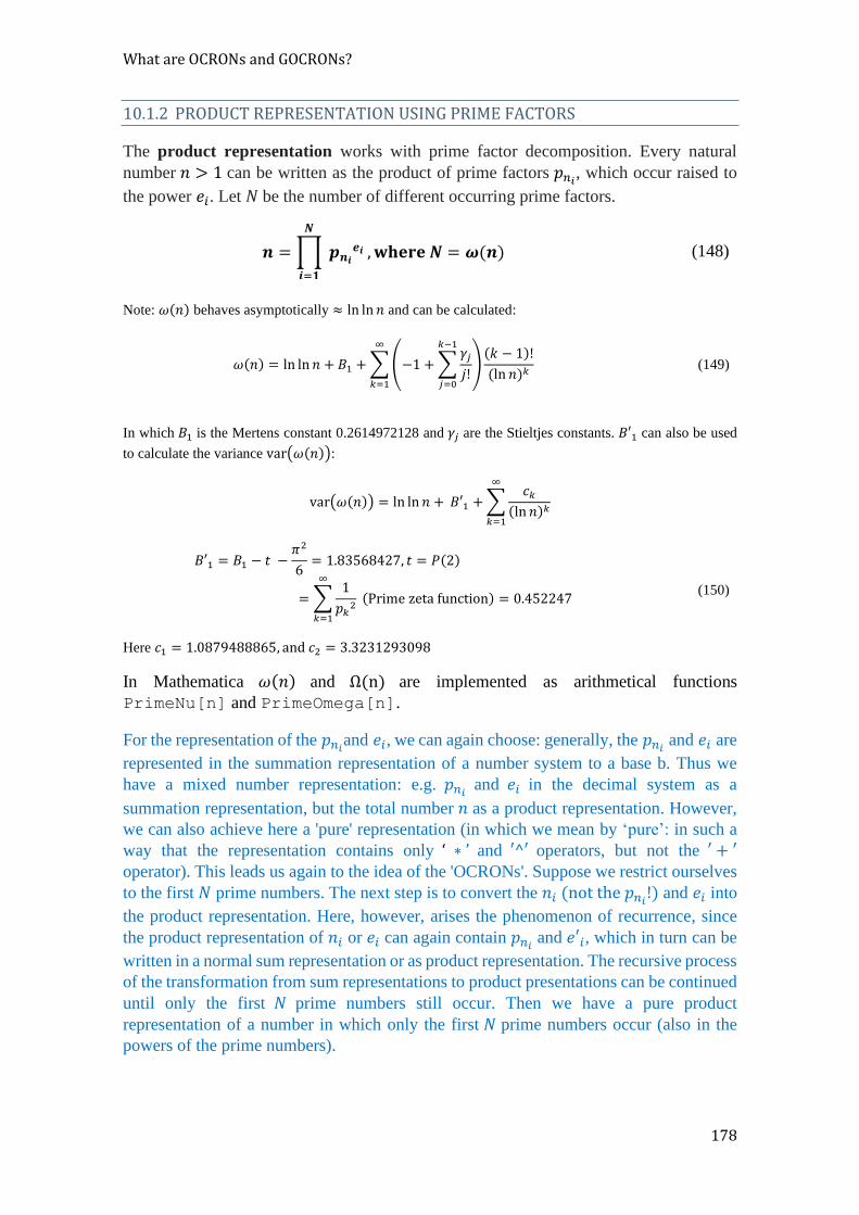
What are OCRONs and GOCRONs?
178
10.1.2 PRODUCT REPRESENTATION USING PRIME FACTORS
The product representation works with prime factor decomposition. Every natural
number 𝑛 > 1 can be written as the product of prime factors 𝑝𝑛𝑖, which occur raised to
the power 𝑒𝑖. Let 𝑁 be the number of different occurring prime factors.
𝒏 =∏ 𝒑𝒏𝒊𝒆𝒊
𝑵
𝒊=𝟏
, 𝐰𝐡𝐞𝐫𝐞 𝑵 = 𝝎(𝒏) (148)
Note: 𝜔(𝑛) behaves asymptotically ≈ ln ln 𝑛 and can be calculated:
𝜔(𝑛) = ln ln 𝑛 + 𝐵1 +∑(−1 +∑𝛾𝑗
𝑗!
𝑘−1
𝑗=0
)
∞
𝑘=1
(𝑘 − 1)!
(ln 𝑛)𝑘 (149)
In which 𝐵1 is the Mertens constant 0.2614972128 and 𝛾𝑗 are the Stieltjes constants. 𝐵′1 can also be used
to calculate the variance var(𝜔(𝑛)):
var(𝜔(𝑛)) = ln ln 𝑛 + 𝐵′1 +∑𝑐𝑘
(ln 𝑛)𝑘
∞
𝑘=1
𝐵′1 = 𝐵1 − 𝑡 −𝜋2
6= 1.83568427, 𝑡 = 𝑃(2)
= ∑1
𝑝𝑘2 (Prime zeta function) = 0.452247
∞
𝑘=1
(150)
Here 𝑐1 = 1.0879488865, and 𝑐2 = 3.3231293098
In Mathematica 𝜔(𝑛) and Ω(n) are implemented as arithmetical functions
PrimeNu[n] and PrimeOmega[n].
For the representation of the 𝑝𝑛𝑖and 𝑒𝑖, we can again choose: generally, the 𝑝𝑛𝑖 and 𝑒𝑖 are
represented in the summation representation of a number system to a base b. Thus we
have a mixed number representation: e.g. 𝑝𝑛𝑖 and 𝑒𝑖 in the decimal system as a
summation representation, but the total number 𝑛 as a product representation. However,
we can also achieve here a 'pure' representation (in which we mean by ‘pure’: in such a
way that the representation contains only ‘ ∗ ’ and ′^′ operators, but not the ′ + ′ operator). This leads us again to the idea of the 'OCRONs'. Suppose we restrict ourselves
to the first 𝑁 prime numbers. The next step is to convert the 𝑛𝑖 (not the 𝑝𝑛𝑖!) and 𝑒𝑖 into
the product representation. Here, however, arises the phenomenon of recurrence, since
the product representation of 𝑛𝑖 or 𝑒𝑖 can again contain 𝑝𝑛𝑖 and 𝑒′𝑖, which in turn can be
written in a normal sum representation or as product representation. The recursive process
of the transformation from sum representations to product presentations can be continued
until only the first 𝑁 prime numbers still occur. Then we have a pure product
representation of a number in which only the first 𝑁 prime numbers occur (also in the
powers of the prime numbers).
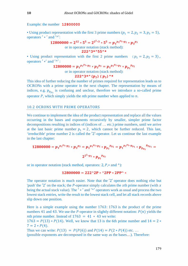
10 About OCRONs and GOCRONs: shades of Gödel
179
Example: the number 12800000
• Using product representation with the first 3 prime numbers (𝑝1 = 2, 𝑝2 = 3, 𝑝3 = 5), operators ′ ∗ ′ and ′^′:
𝟏𝟐𝟖𝟎𝟎𝟎𝟎𝟎 = 𝟐𝟏𝟐 ∗ 𝟓𝟓 = 𝟐𝟐𝟐∗𝟑 ∗ 𝟓𝟓 = 𝒑𝟏
𝒑𝟏𝒑𝟏∗𝒑𝟐 ∗ 𝒑𝟑
𝒑𝟑
or in operator notation (stack method): 222^3*^55^*
• Using product representation with the first 2 prime numbers (𝑝1 = 2, 𝑝2 = 3),
operators ′ ∗′ and ′^′ :
𝟏𝟐𝟖𝟎𝟎𝟎𝟎𝟎 = 𝒑𝟏𝒑𝟏𝒑𝟏∗𝒑𝟐 ∗ 𝒑𝟑
𝒑𝟑 = 𝒑𝟏𝒑𝟏𝒑𝟏∗𝒑𝟐 ∗ 𝒑𝒑𝟐
𝒑𝒑𝟐
or in operator notation (stack method):
222^3*^(𝒑𝟑)( 𝒑𝟑)^*
This idea of further reducing the number of primes required for representation leads us to
OCRONs with a prime operator in the next chapter. The representation by means of
indices, e.g. 𝑝𝑝𝑝3 is confusing and unclear, therefore we introduce a so-called prime
operator 𝑃, which simply yields the nth prime number when applied to 𝑛.
10.2 OCRONS WITH PRIME OPERATORS
We continue to implement the idea of the product representation and replace all the values
occurring in the bases and exponents recursively by smaller, simpler prime factor
decompositions resulting in indices of (indices of … etc.) prime numbers, until we arrive
at the last basic prime number 𝑝1 = 2 , which cannot be further reduced. This last,
‘irreducible' prime number 2 is called the ′2′-operator. Let us continue the last example
in the last chapter:
𝟏𝟐𝟖𝟎𝟎𝟎𝟎𝟎 = 𝒑𝟏𝒑𝟏𝒑𝟏∗𝒑𝟐 ∗ 𝒑𝟑
𝒑𝟑 = 𝒑𝟏𝒑𝟏𝒑𝟏∗𝒑𝟐 ∗ 𝒑𝒑𝟐
𝒑𝒑𝟐 = 𝒑𝟏𝒑𝟏𝒑𝟏∗𝒑𝒑𝟏 ∗ 𝒑𝒑𝒑𝟏
𝒑𝒑𝒑𝟏 =
𝟐𝟐𝟐∗𝒑𝟐 ∗ 𝒑𝒑𝟐
𝒑𝒑𝟐
or in operator notation (stack method, operators: 2, 𝑃,∗ and ^):
𝟏𝟐𝟖𝟎𝟎𝟎𝟎𝟎 = 𝟐𝟐𝟐^𝟐𝐏 ∗ ^𝟐𝐏𝐏 ∗ 𝟐𝐏𝐏^ ∗
The operator notation is much easier. Note that the ′2′ operator does nothing else but
'push' the ′2′ on the stack; the 𝑃-operator simply calculates the 𝑥th prime number (with 𝑥
being the actual stack value). The ′ ∗ ′ and ′^′ operators work as usual and process the two
lowest stack entries, write the result to the lowest stack cell, and let all stack records above
slip down one position.
Here is a simple example using the number 1763: 1763 is the product of the prime
numbers 41 and 43. We use the 𝑃-operator in slightly different notation: 𝑃(𝑛) yields the
𝑛th prime number. Instead of 1763 = 41 ∗ 43 we write:
1763 = 𝑃(13) ∗ 𝑃(14). Well, we know that 13 is the 6th prime number and 14 = 2 ∗7 = 2 ∗ 𝑃(4). Thus we can write: 𝑃(13) = 𝑃(𝑃(6)) and 𝑃(14) = 𝑃(2 ∗ 𝑃(4)) etc. …
(possible exponents are decomposed in the same way as the bases…). Therefore:
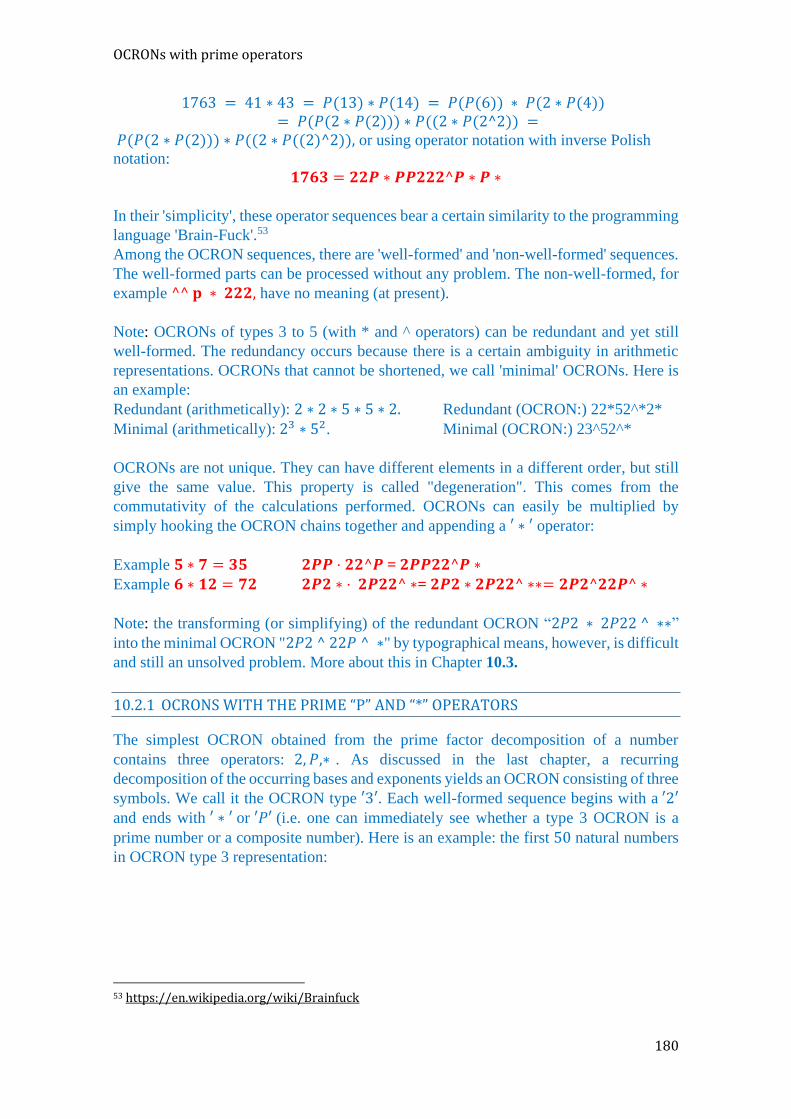
OCRONs with prime operators
180
1763 = 41 ∗ 43 = 𝑃(13) ∗ 𝑃(14) = 𝑃(𝑃(6)) ∗ 𝑃(2 ∗ 𝑃(4)) = 𝑃(𝑃(2 ∗ 𝑃(2))) ∗ 𝑃((2 ∗ 𝑃(2^2)) =
𝑃(𝑃(2 ∗ 𝑃(2))) ∗ 𝑃((2 ∗ 𝑃((2)^2)), or using operator notation with inverse Polish
notation:
𝟏𝟕𝟔𝟑 = 𝟐𝟐𝑷 ∗ 𝑷𝑷𝟐𝟐𝟐^𝑷 ∗ 𝑷 ∗
In their 'simplicity', these operator sequences bear a certain similarity to the programming
language 'Brain-Fuck'.53
Among the OCRON sequences, there are 'well-formed' and 'non-well-formed' sequences.
The well-formed parts can be processed without any problem. The non-well-formed, for
example ^^ 𝐩 ∗ 𝟐𝟐𝟐, have no meaning (at present).
Note: OCRONs of types 3 to 5 (with * and ^ operators) can be redundant and yet still
well-formed. The redundancy occurs because there is a certain ambiguity in arithmetic
representations. OCRONs that cannot be shortened, we call 'minimal' OCRONs. Here is
an example:
Redundant (arithmetically): 2 ∗ 2 ∗ 5 ∗ 5 ∗ 2. Redundant (OCRON:) 22*52^*2*
Minimal (arithmetically): 23 ∗ 52. Minimal (OCRON:) 23^52^*
OCRONs are not unique. They can have different elements in a different order, but still
give the same value. This property is called "degeneration". This comes from the
commutativity of the calculations performed. OCRONs can easily be multiplied by
simply hooking the OCRON chains together and appending a ′ ∗ ′ operator:
Example 𝟓 ∗ 𝟕 = 𝟑𝟓 𝟐𝑷𝑷 ⋅ 𝟐𝟐^𝑷 = 𝟐𝑷𝑷𝟐𝟐^𝑷 ∗ Example 𝟔 ∗ 𝟏𝟐 = 𝟕𝟐 𝟐𝑷𝟐 ∗ ⋅ 𝟐𝑷𝟐𝟐^ ∗= 𝟐𝑷𝟐 ∗ 𝟐𝑷𝟐𝟐^ ∗∗= 𝟐𝑷𝟐^𝟐𝟐𝑷^ ∗
Note: the transforming (or simplifying) of the redundant OCRON “2𝑃2 ∗ 2𝑃22 ^ ∗∗”
into the minimal OCRON "2𝑃2 ^ 22𝑃 ^ ∗" by typographical means, however, is difficult
and still an unsolved problem. More about this in Chapter 10.3.
10.2.1 OCRONS WITH THE PRIME “P” AND “*” OPERATORS
The simplest OCRON obtained from the prime factor decomposition of a number
contains three operators: 2, 𝑃,∗ . As discussed in the last chapter, a recurring
decomposition of the occurring bases and exponents yields an OCRON consisting of three
symbols. We call it the OCRON type ′3′. Each well-formed sequence begins with a ′2′ and ends with ′ ∗ ′ or ′𝑃′ (i.e. one can immediately see whether a type 3 OCRON is a
prime number or a composite number). Here is an example: the first 50 natural numbers
in OCRON type 3 representation:
53 https://en.wikipedia.org/wiki/Brainfuck

10 About OCRONs and GOCRONs: shades of Gödel
181
Table 13. Numbers 2 to 50 in OCRON type 3 format
n OCRON type 3 n OCRON type 3 1
2
3
4
5
6
7
8
9
10
11
12
13
14
15
16
17
18
19
20
21
22
23
24
25
-
2
2P
22*
2PP
2P2*
22*P
22*2*
2P2P*
2PP2*
2PPP
2P2*2*
2P2*P
22*P2*
2PP2P*
22*2*2*
22*PP
2P2P*2*
22*2*P
2PP2*2*
22*P2P*
2PPP2*
2P2P*P
2P2*2*2*
2PP2PP*
26
27
28
29
30
31
32
33
34
35
36
37
38
39
40
41
42
43
44
45
46
47
48
49
50
2P2*P2*
2P2P*2P*
22*P2*2*
2PP2*P
2PP2P*2*
2PPPP
22*2*2*2*
2PPP2P*
22*PP2*
22*P2PP*
2P2P*2*2*
2P2*2*P
22*2*P2*
2P2*P2P*
2PP2*2*2*
2P2*PP
22*P2P*2*
22*P2*P
2PPP2*2*
2PP2P*2P*
2P2P*P2*
2PP2P*P
2P2*2*2*2*
22*P22*P*
2PP2PP*2*
OCRONs of type 3 do not have a power operator and are therefore not as interesting. For
high powers, OCRONs of type 3 become unwieldy. Just think of large composite numbers
or powers of 2, such as 2𝟓𝟕𝟖𝟖𝟓𝟏𝟔𝟏, whose OCRON representation would then have a
length of millions of characters!
10.2.1.1 DEGENERATION OF TYPE 3 OCRONS
By ‘degeneration’ we understand the fact that there are generally several OCRON
representations for a unique number 𝑛. The converse does not apply, of course. To an
OCRON there is only one unique number 𝑛. This degeneration increases very fast with
𝑛, as the following graphic shows:
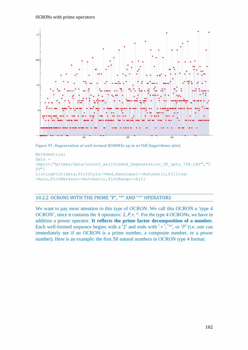
OCRONs with prime operators
182
Figure 97. Degeneration of well-formed OCRON3s up to n=768 (logarithmic plot)
Mathematica:
data =
Import["primes/data/ocron3_wellformed_Degeneration_OK_upto_768.txt","C
SV"]
ListLogPlot[data,PlotStyle->Red,AxesLabel->Automatic,Filling-
>Axis,PlotMarkers->Automatic,PlotRange->All]
10.2.2 OCRONS WITH THE PRIME “P”, “*” AND “^” OPERATORS
We want to pay most attention to this type of OCRON. We call this OCRON a ‘type 4
OCRON’, since it contains the 4 operators: 2, 𝑃,∗, ^. For the type 4 OCRONs, we have in
addition a power operator. It reflects the prime factor decomposition of a number.
Each well-formed sequence begins with a ′2′ and ends with ′ ∗ ′, ′^′, or ′𝑃′ (i.e. one can
immediately see if an OCRON is a prime number, a composite number, or a power
number). Here is an example: the first 50 natural numbers in OCRON type 4 format:

10 About OCRONs and GOCRONs: shades of Gödel
183
Table 14. The numbers 2 to 49 in OCRON type 4 format
n OCRON type 4 n OCRON type 4
2 3 4 5 6 7 8 9 10 11 12 13 14 15 16 17 18 19 20 21 22 23 24 25
2 2P 22^ 2PP 22P* 22^P 22P^ 2P2^ 22PP* 2PPP 22^2P* 22P*P 222^P* 2P2PP* 222^^ 22^PP 22P2^* 22P^P 22^2PP* 2P22^P* 22PPP* 2P2^P 22P^2P* 2PP2^
26 27 28 29 30 31 32 33 34 35 36 37 38 39 40 41 42 43 44 45 46 47 48 49
222P*P* 2P2P^ 22^22^P* 22PP*P 22P*2PP* 2PPPP 22PP^ 2P2PPP* 222^PP* 2PP22^P* 22^2P2^* 22^2P*P 222P^P* 2P22P*P* 22P^2PP* 22P*PP 22P*22^P* 222^P*P 22^2PPP* 2P2^2PP* 22P2^P* 2P2PP*P 222^^2P* 22^P2^
OCRONs of type 4 provide a compact representation of very large values. By way of
example, here is a table of the first Mersenne numbers:
Table 15. Mersenne numbers, as well as the exponents in OCRON type 4 representation
𝑛 Mersenne prime exponent p
Mersenne number 𝑀𝑝 = 2𝑃-1 OCRON4(p)
1 2 3 4 5 6 7 8 9 10 11 12 13 14 15 16
2 3 5 7 11 13 17 19 23 29 31 37 41 43 47 53
3 7 31 127 2047 8191 131071 524287 8388607 536870911 2147483647 137438953471 2199023255551 8796093022207 140737488355327 9007199254740991
2 2P 2PP 22^P 2PPP 22P*P 22^PP 22P^P 2P2^P 22PP*P 2PPPP 22^2P*P 22P*PP 222^P*P 2P2PP*P 222^^P
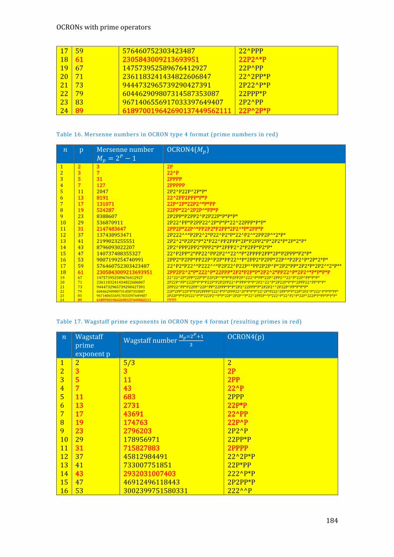
OCRONs with prime operators
184
17 18 19 20 21 22 23 24
59 61 67 71 73 79 83 89
576460752303423487 2305843009213693951 147573952589676412927 2361183241434822606847 9444732965739290427391 604462909807314587353087 9671406556917033397649407 618970019642690137449562111
22^PPP 22P2^*P 22P^PP 22^2PP*P 2P22^P*P 22PPP*P 2P2^PP 22P^2P*P
Table 16. Mersenne numbers in OCRON type 4 format (prime numbers in red)
𝑛 p Mersenne number 𝑀𝑝 = 2
𝑃 − 1 OCRON4(𝑀𝑝)
1 2 3 4 5 6 7 8 9 10 11 12 13 14 15 16 17 18 19 20 21 22 23 24
2 3 5 7 11 13 17 19 23 29 31 37 41 43 47 53 59 61 67 71 73 79 83 89
3 7 31 127 2047 8191 131071 524287 8388607 536870911 2147483647 137438953471 2199023255551 8796093022207 140737488355327 9007199254740991 576460752303423487 2305843009213693951 147573952589676412927 2361183241434822606847 9444732965739290427391 604462909807314587353087 9671406556917033397649407 618970019642690137449562111
2P 22^P 2PPPP 2PPPPP 2P2^P22P^2P*P* 22^2PP2PPP*P*P 22P^2P*22P2^*P*PP 22PP*22^2P2P^*PP*P 2P2PP*P2PP2^P2P22P*P*P*P* 2P22^PP*P2PP22^2P*P*P*22^22PPP*P*P* 2PP2P*22P^*PP2P2*P2PP*2P2^*P*2PP*P 2P222^^*P2P2^2*P22^P2*P*22^P2^*2PP2P^*2*P* 2P2^2*P2P2*P*2*P22^PP2PPP*2P*P2PP2*P*2P2*P*2P*2*P* 2P2^PPP2PP2*PPP2*P*2PPP2^2*P2PP*P2*P* 22^P2PP*2*PP22^PP2P2^*22^*P*2PPPP2PP*2P*P2PPP*P2*P* 2PP2*P2PP*PP22P^P2P*PP22^*P*2PP2*P2PP*22P^*P2P2^P*2P*2*P* 22^P2*P22^*P222^^*P2P22^P22P^*PP2P2P^P*2P2*PP*2P2*P*2P2^*2*P** 2PP2P2^2*P*222^P*22PPP*2P2*P2P*P*2P2^2*PP22^P*2P2^*P*P*P*P 22^22^2P*2PP*22P*P*22P2P^*P*P*P2PP2P^222^P*PP*22P^2PP2^*22^P*22P^PP*P*P* 2P22P^PP*222P*P*P*P22P*P2P2PP22^P*PPP*P*P*2P2^22^P*2P22P*P*P*2PPP22^PP*P*P* 2PP22^PP*P22PP^22P^PP*22PPP*P*P*2P2^22PPP*P*2P2P2^^2P22P^PP*P*P*P* 22P*2PP*22P*P*P2P2PPPP*222^P*P*2PPP22^2P*P*P*P*22^2P*P222^2PP*P*P*22P*2P2^P*222^P*P*P*PP* 2P22P*P*P2P222^P*P*222P2^*P*P*22P^2P2P^*P*22^2PP2P^*P*222^P*22^P2^P*22P^222P*P*PP*P*P*P* ??????
Table 17. Wagstaff prime exponents in OCRON type 4 format (resulting primes in red)
𝑛 Wagstaff prime exponent p
Wagstaff number 𝑀𝑝=2
𝑃+1
3
OCRON4(p)
1 2 3 4 5 6 7 8 9 10 11 12 13 14 15 16
2 3 5 7 11 13 17 19 23 29 31 37 41 43 47 53
5/3 3 11 43 683 2731 43691 174763 2796203 178956971 715827883 45812984491 733007751851 2932031007403 46912496118443 3002399751580331
2 2P 2PP 22^P 2PPP 22P*P 22^PP 22P^P 2P2^P 22PP*P 2PPPP 22^2P*P 22P*PP 222^P*P 2P2PP*P 222^^P

10 About OCRONs and GOCRONs: shades of Gödel
185
17 18 19 20 21 22
59 61 67 71 73 79
192153584101141163 768614336404564651 49191317529892137643 787061080478274202283 3148244321913096809131 201487636602438195784363
22^PPP 22P2^*P 22P^PP 22^2PP*P 2P22^P*P 22PPP*P
Table 18. Wagstaff numbers in OCRON type 4 format (prime numbers in red)
𝑛 Wagstaff prime exp. p
Wagstaff number 𝑊𝑝=2
𝑃+1
3
OCRON4(2𝑃+1
3)
1 2 3 4 5 6 7 8 9 10 11 12 13 14 15 16 17 18 19 20 21 22
2 3 5 7 11 13 17 19 23 29 31 37 41 43 47 53 59 61 67 71 73 79
5/3 3 11 43 683 2731 43691 174763 2796203 178956971 715827883 45812984491 733007751851 2932031007403 46912496118443 3002399751580331 192153584101141163 768614336404564651 49191317529892137643 787061080478274202283 3148244321913096809131 201487636602438195784363
- 2P 2PPP 222^P*P 22^2PPPP*P 2P22^P*22P^P*P 22P^22P^22P*P*P*P 222^22P2P^*P*P*P 2PP22^2P2^*P*2P22P^P*P*P 22^PPP222^^2P22^^*22P*P2^*P* 22^PPP22^22^P*2PPP*22^PP*PP*P 2PPP2*P2PP*PP2PPP*2P*2*P2PPP2PP2^*P* 222^^P2P*P2PPP2*P*2P2*P*22^P*2PP*2P*22^*P2P2^PP* 22^P2P^P2PP2P*P*P2P2*P22^*P2*P*2PPP*2*P 2PP2P2^*2*P2PP2*P*P2PPP2P*P2*P*2P2^2*P*2P*P2P2^2*PP* 2PP2P^2*P2P22^*P2P*P*2P*P22^PP2P*P22^P*2P*22^**P22^P22^*P* 22^P2^2PP2^*22P^*P22^PP*2P*PP2P2*PPP2PPP*2*P*2PPP2P*P2P*P* 22^222^PP*PP*222^PP*222^P*222^2P*22^2P*P*P*PP*P*P*PP 22PP*22^22P2P^P*P*P*P222^22P^PP*2P22P^P*222^P*PPP*P*P*PP* 22^2P*22^PP*2P2^P2P2^PP*P*P222^P*22PP*P*2PP22^PP*P*222^^22P22P*^*P*P*P* 2P22^P*22P*P*P22^2P*PP22P*222PP*2PPP*P*PP*P*2P2PP*22P2^P*2PP2PPP*P*P*P*P* ??????
The lengths of the OCRONs in Mersenne numbers grow approximately proportional to 𝑝:
Figure 98. Lengths of type 4 OCRONs of Mersenne numbers up to 𝑀83

OCRONs with prime operators
186
Mathematica:
data={{2,2},{3,4},{5,5},{7,6},{11,14},{13,14},{17,17},{19,18},{23,25},{29,35},{31,34},{37,42},{41,50},{43,37},{47,51},{53,57},{59,63},{61,62
},{67,72},{71,75},{73,66},{79,89},{83,88}}
line = Fit[data, {1,x},x]
Show[ListPlot[data,PlotStyle->Red, AxesLabel->Automatic,Filling-
>Axis,PlotMarkers->Automatic],Plot[line,{x,0,83}]]
If we extrapolate for high Mersenne primes, we expect OCRON lengths of some million
characters (about three times as long as in decimal representation, but much shorter than
in binary representation).
The lengths of the OCRONs in Wagstaff numbers also grow approximately proportional
to p:
Figure 99. Lengths of type 4 OCRONs of Wagstaff numbers up to 𝑊73
Mathematica: {{3,2},{5,4},{7,7},{11,10},{13,14},{17,17},{19,16},{23,24},{29,28},{31
,29},{37,36},{41,48},{43,39},{47,48},{53,58},{59,58},{61,52},{67,57},{
71,71},{73,73}}
line = Fit[data, {1,x},x]
Show[ListPlot[data,PlotStyle->Red, AxesLabel->Automatic,Filling-
>Axis,PlotMarkers->Automatic],Plot[line,{x,0,73}]]
If we extrapolate for high Wagstaff numbers to similarly high ranges as the largest
known Mersenne primes, we also expect OCRON lengths of some million characters.
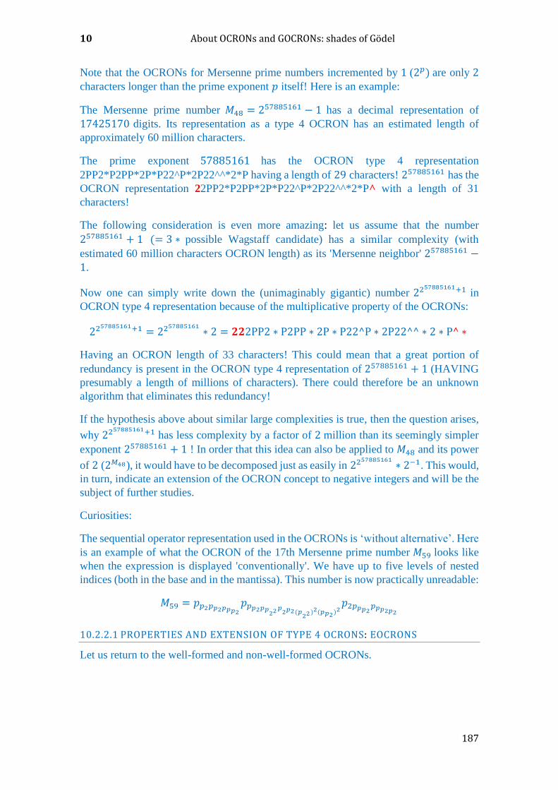
10 About OCRONs and GOCRONs: shades of Gödel
187
Note that the OCRONs for Mersenne prime numbers incremented by 1 (2𝑝) are only 2
characters longer than the prime exponent 𝑝 itself! Here is an example:
The Mersenne prime number 𝑀48 = 257885161 − 1 has a decimal representation of
17425170 digits. Its representation as a type 4 OCRON has an estimated length of
approximately 60 million characters.
The prime exponent 57885161 has the OCRON type 4 representation
2PP2*P2PP*2P*P22^P*2P22^^*2*P having a length of 29 characters! 257885161 has the
OCRON representation 22PP2*P2PP*2P*P22^P*2P22^^*2*P^ with a length of 31
characters!
The following consideration is even more amazing: let us assume that the number
257885161 + 1 (= 3 ∗ possible Wagstaff candidate) has a similar complexity (with
estimated 60 million characters OCRON length) as its 'Mersenne neighbor' 257885161 −1.
Now one can simply write down the (unimaginably gigantic) number 2257885161+1 in
OCRON type 4 representation because of the multiplicative property of the OCRONs:
2257885161+1 = 22
57885161∗ 2 = 𝟐𝟐2PP2 ∗ P2PP ∗ 2P ∗ P22^P ∗ 2P22^^ ∗ 2 ∗ P^ ∗
Having an OCRON length of 33 characters! This could mean that a great portion of
redundancy is present in the OCRON type 4 representation of 257885161 + 1 (HAVING
presumably a length of millions of characters). There could therefore be an unknown
algorithm that eliminates this redundancy!
If the hypothesis above about similar large complexities is true, then the question arises,
why 2257885161+1 has less complexity by a factor of 2 million than its seemingly simpler
exponent 257885161 + 1 ! In order that this idea can also be applied to 𝑀48 and its power
of 2 (2𝑀48), it would have to be decomposed just as easily in 2257885161
∗ 2−1. This would,
in turn, indicate an extension of the OCRON concept to negative integers and will be the
subject of further studies.
Curiosities:
The sequential operator representation used in the OCRONs is ‘without alternative’. Here
is an example of what the OCRON of the 17th Mersenne prime number 𝑀59 looks like
when the expression is displayed 'conventionally'. We have up to five levels of nested
indices (both in the base and in the mantissa). This number is now practically unreadable:
𝑀59 = 𝑝𝑝2𝑝𝑝2𝑝𝑝𝑝2𝑝𝑝𝑝2𝑝𝑝
22𝑝2𝑝2(𝑝
22)2(𝑝𝑝2)
2𝑝2𝑝𝑝𝑝2𝑝𝑝𝑝2𝑝2
10.2.2.1 PROPERTIES AND EXTENSION OF TYPE 4 OCRONS: EOCRONS
Let us return to the well-formed and non-well-formed OCRONs.

OCRONs with prime operators
188
Not all OCRONs that can be represented by the symbols′ ∗ ′, ′^′, ′2′ 𝑎𝑛𝑑 ′𝑃′ are 'well-
formed' and give meaning so that they can be processed (e.g. the sequence ^^ 𝒑 ∗ 𝟐𝟐𝟐
is not a well-formed OCRON).
There is now a possibility of assigning these degenerate OCRONs in a reasonable,
meaningful way also an indication and thus a numerical value. For the interpretation of
an OCRON, the symbols of the OCRON sequence must be 'pushed' onto the stack or
processed according to the rules of the 'Polish' notation.
- We ‘prime’ the stack with infinitely many virtual ′2′ symbols so that in the case
of 'unexpected', ‘ ∗ ’ or ‘^’ symbols (‘unexpected' here means that at the time of
the processing of an operator symbol, the stack has less than 2 values) the operator
can still applied.
- If there are still more than one stack entries at the end of the processing of an
OCRON, then we append virtual ′ ∗′ symbols, as many as needed (i.e.
multiplications with a virtual 2s) from left, until the stack has only one entry (the
final result).
Using these rules, non-well-formed OCRONs can be transformed into normal OCRONs.
Any OCRON (even if non-well-formed) is thereby given an unambiguous value.
Conversely, normal OCRONs can be shortened by discarding the leading ′2′, which is
always present, and removing all '*'s at the end, which would have eventually reduced
the stack to a single value.
This has the advantage that, at the end of the OCRON processing, as many stack entries
remain as factors are present, unless our number is a power number (number which can
be written as a power). The number of prime factors can also be ‘extracted’ from the
OCRONs without having to go to the meaning level of ‘numbers’. We can remain on the
formal typographic OCRON level of meaning without explicit decoding.
This means in practice that we simply remove the last ′ ∗ ′s (if the end of the OCRON
consists only of successive ′ ∗ ′𝑠 , so the stack remains unchanged). These 'erased'
multiplications can be added again afterwards (see above, 'virtual' ′ ∗ ′s), so that again a
well-formed OCRON arises.
Let us denote these non-well-formed OCRONs together with the set of well-formed
OCRONs ‘EOCRONs' (= Enhanced OCRONs). Either types may be converted into the
other. In order to make a well-formed OCRON from a non-well-formed EOCRON, it
must always be enlarged (to the left or to the right).
We distinguish three types of OCRONs: (well-formed OCRONs), standardized
EOCRONs, any EOCRONs.
Properties or transformation rules of (well-formed) OCRON4s
- An OCRON4 consists of an arbitrarily long string of OCRON4 symbols (2,
P, ^, *) which, when interpreted, yield a value.

10 About OCRONs and GOCRONs: shades of Gödel
189
- OCRON4s may be concatenated (that is, linked together, and finally
appended by a ′ ∗ ′). This concatenation is associative and commutative and
corresponds to a multiplication on the number significance level.
- Each OCRON4 (= well-formed) begins with a '2' and ends with a '*', '^' or
'P'. The only OCRON4 that can end with a '2' is '2' itself.
- Except for the concatenation rule, there are at present no further important
rules known (for example, addition rule, or transformation rules).
- The number 𝟏 has no representation by type 4 OCRONs
- The length of a type 4 OCRON typically increases proportional to the value
of the corresponding number.
- The difference between the maximum length and the minimum length of
OCRONs resulting in a set of degenerate OCRONs (i.e. having the same
numerical value) can be arbitrarily large.
Properties or transformation rules of (any) EOCRON4s
- An EOCRON4 consists of an arbitrarily long string of OCRON4 symbols (2,
P, ^, *) that can be arranged arbitrarily.
- For a non-well-formed EOCRON4 to be interpreted, it must be converted
into a well-formed OCRON4, resulting in an enlargement.
- There is an empty EOCRON4: by converting to an OCRON4 this is the '2'.
- There are EOCRONs, which result in the same numerical value as the
standard EOCRONs when interpreted, but are shorter.
Properties or transformation rules of (standardized) EOCRON4s
- A standardized EOCRON4 consists of an arbitrarily long string of OCRON4
symbols (2, P, ^, *).
- For a standardized EOCRON4 to be interpreted, it must be converted into a
well-formed OCRON4 (possibly by inserting '2' symbols at the beginning and
adding '*' symbols at the end). This results in an enlargement.
- There is an empty standardized EOCRON4: by converting to an OCRON4,
this is the '2'.
- The number of prime factors of an EOCRON4 is simply the number of stack
entries after interpretation of all standardized EOCRON symbols (with
insertion of the leading, ‘2’ before conversion into a well-formed OCRON).
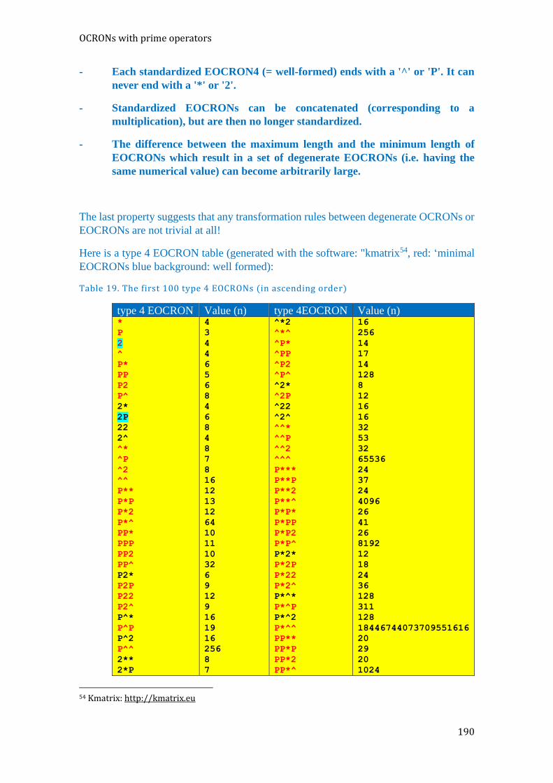
OCRONs with prime operators
190
- Each standardized EOCRON4 (= well-formed) ends with a '^' or 'P'. It can
never end with a '*' or '2'.
- Standardized EOCRONs can be concatenated (corresponding to a
multiplication), but are then no longer standardized.
- The difference between the maximum length and the minimum length of
EOCRONs which result in a set of degenerate EOCRONs (i.e. having the
same numerical value) can become arbitrarily large.
The last property suggests that any transformation rules between degenerate OCRONs or
EOCRONs are not trivial at all!
Here is a type 4 EOCRON table (generated with the software: "kmatrix54, red: ‘minimal
EOCRONs blue background: well formed):
Table 19. The first 100 type 4 EOCRONs (in ascending order)
type 4 EOCRON Value (n) type 4EOCRON Value (n) *
P
2
^
P*
PP
P2
P^
2*
2P
22
2^
^*
^P
^2
^^
P**
P*P
P*2
P*^
PP*
PPP
PP2
PP^
P2*
P2P
P22
P2^
P^*
P^P
P^2
P^^
2**
2*P
4
3
4
4
6
5
6
8
4
6
8
4
8
7
8
16
12
13
12
64
10
11
10
32
6
9
12
9
16
19
16
256
8
7
^*2
^*^
^P*
^PP
^P2
^P^
^2*
^2P
^22
^2^
^^*
^^P
^^2
^^^
P***
P**P
P**2
P**^
P*P*
P*PP
P*P2
P*P^
P*2*
P*2P
P*22
P*2^
P*^*
P*^P
P*^2
P*^^
PP**
PP*P
PP*2
PP*^
16
256
14
17
14
128
8
12
16
16
32
53
32
65536
24
37
24
4096
26
41
26
8192
12
18
24
36
128
311
128
18446744073709551616
20
29
20
1024
54 Kmatrix: http://kmatrix.eu
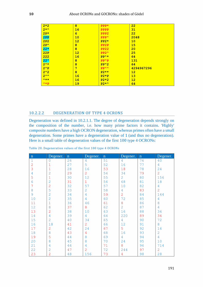
10 About OCRONs and GOCRONs: shades of Gödel
191
2*2
2*^
2P*
2PP
2P2
2P^
22*
22P
222
22^
2^*
2^P
2^2
2^^
^**
^*P
8
16
6
10
12
8
8
12
16
8
8
7
8
16
16
19
PPP*
PPPP
PPP2
PPP^
PP2*
PP2P
PP22
PP2^
PP^*
PP^P
PP^2
PP^^
P2**
P2*P
P2*2
P2*^
22
31
22
2048
10
15
20
25
64
131
64
4294967296
12
13
12
64
10.2.2.2 DEGENERATION OF TYPE 4 OCRONS
Degeneration was defined in 10.2.1.1. The degree of degeneration depends strongly on
the composition of the number, i.e. how many prime factors it contains. 'Highly'
composite numbers have a high OCRON degeneration, whereas primes often have a small
degeneration. Some primes have a degeneration value of 1 (and thus no degeneration).
Here is a small table of degeneration values of the first 100 type 4 OCRONs:
Table 20. Degeneration values of the first 100 type 4 OCRONs
n Degener. n Degener. n Degener. n Degener. 1
2
3
4
5
6
7
8
9
10
11
12
13
14
15
16
17
18
19
20
21
22
23
0
1
1
2
1
2
2
5
2
2
1
8
2
4
2
18
2
8
5
8
4
2
2
26
27
28
29
30
31
32
33
34
35
36
37
38
39
40
41
42
43
44
45
46
47
48
4
5
16
2
12
1
57
2
4
4
46
8
10
4
34
2
24
4
8
8
4
2
156
51
52
53
54
55
56
57
58
59
60
61
62
63
64
65
66
67
68
69
70
71
72
73
4
16
18
34
2
68
10
4
2
72
8
2
16
220
4
12
5
16
4
24
8
244
4
76
77
78
79
80
81
82
83
84
85
86
87
88
89
90
91
92
93
94
95
96
97
98
40
4
24
2
156
18
4
2
144
4
8
4
34
34
72
8
16
2
4
10
714
2
28
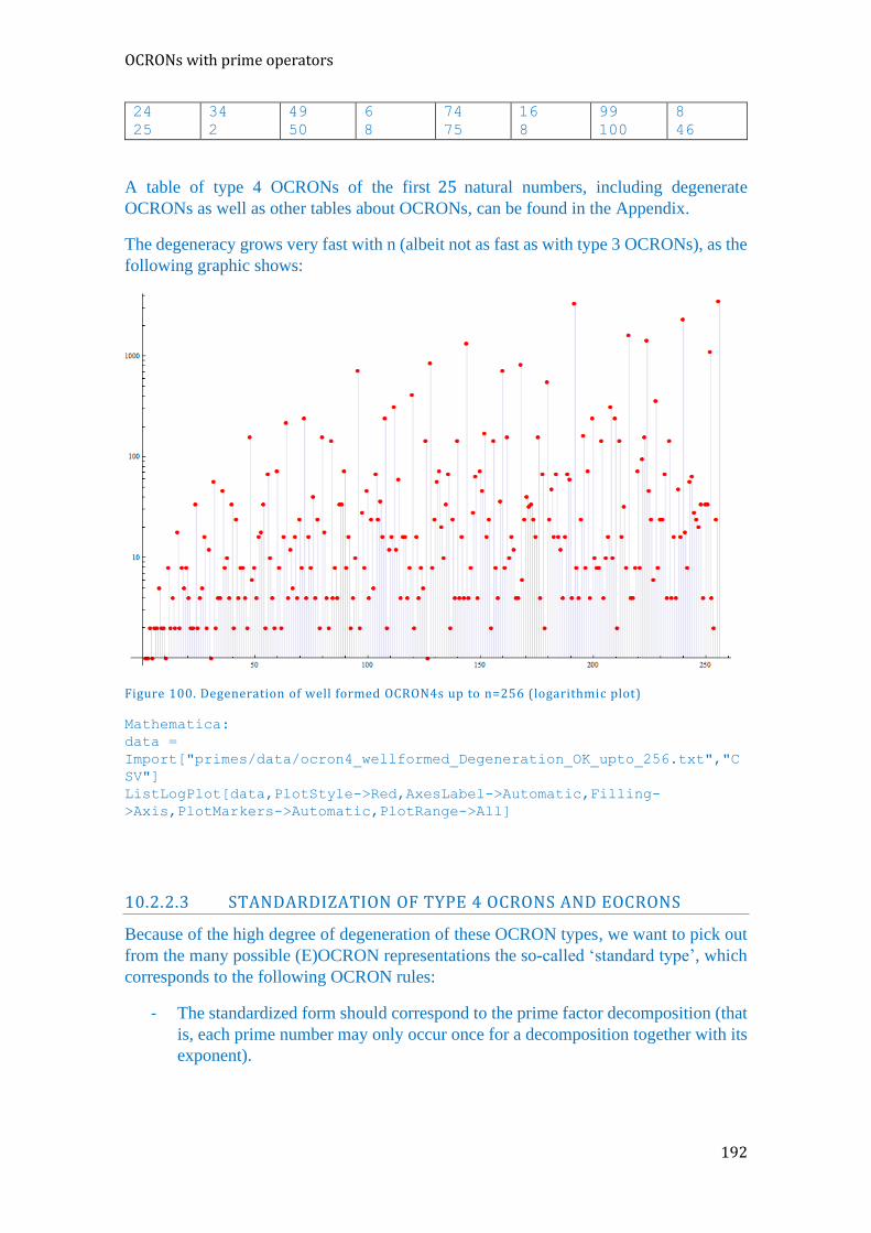
OCRONs with prime operators
192
24
25 34
2 49
50
6
8 74
75
16
8
99
100
8
46
A table of type 4 OCRONs of the first 25 natural numbers, including degenerate
OCRONs as well as other tables about OCRONs, can be found in the Appendix.
The degeneracy grows very fast with n (albeit not as fast as with type 3 OCRONs), as the
following graphic shows:
Figure 100. Degeneration of well formed OCRON4s up to n=256 (logarithmic plot)
Mathematica:
data =
Import["primes/data/ocron4_wellformed_Degeneration_OK_upto_256.txt","C
SV"]
ListLogPlot[data,PlotStyle->Red,AxesLabel->Automatic,Filling-
>Axis,PlotMarkers->Automatic,PlotRange->All]
10.2.2.3 STANDARDIZATION OF TYPE 4 OCRONS AND EOCRONS
Because of the high degree of degeneration of these OCRON types, we want to pick out
from the many possible (E)OCRON representations the so-called ‘standard type’, which
corresponds to the following OCRON rules:
- The standardized form should correspond to the prime factor decomposition (that
is, each prime number may only occur once for a decomposition together with its
exponent).
10 About OCRONs and GOCRONs: shades of Gödel
193
- Whenever products appear, the rule of ascending sorting (first the small factors,
then the large factors) applies.
- ‘ ^′ has a higher priority than the ′ ∗ ′ operator; that is, whenever possible, we take
the ‘ ^’ operator instead of the ′ ∗ ′ operator (for example, ‘ 22 ^′ instead of
‘ 22 ∗’). - The standardization should result in a reduced, minimal form (as a minimum
EOCRON), in which the prime factor assignment can simply be read off from the
stack values.
Before OCRONs are converted to EOCRONs, they should be converted into the
standardized form.
Note: the transformation of any type 4 OCRON into standardized type 4 OCRONs
only at the symbol level (without evaluation as a number) is a difficult and unsolved
problem!
10.2.2.4 THE GÖDELIZATION OF TYPE 4 OCRONS
By 'Gödelization' we mean a change in the level of meaning from a procedural point of
view (each OCRON represents a small computer program by means of which its value
can be calculated) into a static ‘value-defined’ interpretation. We assign a positive, integer
value 𝑛 to each OCRON (which initially consists only of a chain of formal symbols). This
approach was originally invented by the mathematician Kurt Gödel, who succeeded in
proving his famous ‘incompleteness theorem’ with this method.
This assignment is arbitrary and can be done in various ways. However, it is common to
all methods that the so-called ‘Gödel code’ is assigned to each OCRON symbol (e.g. the
‘^’ symbol gets the value of 3). The entire OCRON chain then results (when interpreted
by arithmetical processing of the individual OCRON symbols) in a total numerical value.
Here, we also have complete freedom with respect to the choice of a suitable algorithm
which combines the individual Gödel codes of the OCRON symbols into a total value.
We want to limit this freedom of choice by demanding that the resulting Gödel values
should become as small as possible, so that we can examine their possible arithmetic laws
as easily as possible. In the Gödelization used by Gödel himself, astronomically high
values arise that are useless for further arithmetic investigation.
More information can be found in Hofstadter's book 'Gödel-Escher-Bach' (Hofstadter,
1991/1985)55. The change of the level of meaning from formal symbols ('typographic')
into the world of numbers is amazing (we quote Hofstadter from his famous book):
“Stepping out of one purely typographical system into another isomorphic typographical
system is not a very exciting thing to do; whereas stepping out of the typographical
domain into an isomorphic part of number theory has some kind of unexplored potential.
It is as if somebody has known musical scores all his life, -but purely visually- and then,
all of a sudden, someone introduced him to the mapping between sounds a musical scores.
What a rich, new world! Then again, it is as if somebody has been familiar with string
55 p. 271: The Boomerang: Gödel-Numbering TNT
OCRONs with prime operators
194
figures all his life, but purely as string figures devoid of meaning - and then, all of a
sudden, someone introduced him the mapping between stories and strings. What a
revelation! The discovery of Gödel numbering has been likened to the discovery, by
Descartes, of the isomorphism between curves in a plane and equations in two variables;
incredibly simple, once you see it - and opening onto a vast new world.”
Here are a few conceivable possibilities of ‘Gödelizations’:
The simple prime number Gödelization56
For this purpose, for each OCRON 𝒐 of length 𝑙, we need the first 𝑙 prime numbers, e.g.
to ‘Gödelize’ the string ‘22^P2*P’ (of length 7), we need the first 7 prime numbers 𝑷𝒏 =2,3,5,7,11,13,17, as well as the Gödel codes 𝒈𝒄(𝐬𝐲𝐦𝐛𝐨𝐥) for the OCRON symbols (e.g.
1 for ‘ ∗ ’, 2 for ′2′, 3 for ′P′and 4 𝑓𝑜𝑟 ′^′).
The Gödel codes must have integer values > 0. The value 0 is not allowed. The total
value is then obtained by multiplying the factors 𝑷𝒏𝒈𝒄(𝐬𝐲𝐦𝐛𝐨𝐥)
by one another (where 𝑛
runs up to the OCRON length 𝑙 − 1):
Example: the OCRON ‘22^P2*P’ (corresponding to a value of 43) has
- in the first position, the value 𝑷𝟏𝒈𝒄(𝟐) = 𝟐𝟐 = 𝟒
- in the second position, the value 𝑷𝟐𝒈𝒄(𝟐) = 𝟑𝟐 = 𝟗
- in the third position, the value𝑷𝟑𝒈𝒄(^) = 𝟓𝟒 = 𝟔𝟐𝟓
- in the fourth position, the value 𝑷𝟒𝒈𝒄(𝑷) = 𝟕𝟑 = 𝟑𝟒𝟑
- in the fifth position, the value 𝑷𝟓𝒈𝒄(𝟐) = 𝟏𝟏𝟐 = 𝟏𝟐𝟏
- in the sixth position, the value 𝑷𝟔𝒈𝒄(∗) = 𝟏𝟑𝟏 = 𝟏𝟑
- in the seventh position, the value 𝑷𝟕𝒈𝒄(𝑷) = 𝟏𝟕𝟑 = 𝟒𝟗𝟏𝟑
The total value 𝑔(𝑜) (Gödel number of 22^P2*P) results in:
𝒈(𝒐) = 𝒈(22^P2*P) = 𝟒 ∗ 𝟗 ∗ 𝟔𝟐𝟓 ∗ 𝟑𝟒𝟑 ∗ 𝟏𝟐𝟏 ∗ 𝟏𝟑 ∗ 𝟒𝟗𝟏𝟑 = 𝟓𝟗𝟔𝟒𝟏𝟗𝟖𝟗𝟗𝟎𝟕𝟓𝟎𝟎
or generally (with 𝑙=length of the OCRON)
𝑔(𝑜) =∏𝑃𝑛𝑔𝑐(OCRON[𝑛−1])
𝑙
𝑛=1
(151)
From the prime factor decomposition of 59641989907500, it is possible to reconstruct
the OCRON ‘22 ^ P2 * P’', and finally the original number 43.
56 https://en.wikipedia.org/wiki/Gödel_numbering
10 About OCRONs and GOCRONs: shades of Gödel
195
The advantage of this method is the small number of 'degrees of freedom' (here 4 for the
choice of the Gödel codes of the OCRONs) and the independence in the representation
of any possible numeral system (for example, decimal system or binary system). The
disadvantage is clear: we get unwieldy large numbers for the Gödel numbers, which are
also difficult to decode.
The main drawback, however, is that there are a lot of numbers that do not correspond to
any Gödel number (and therefore cannot be converted into an OCRON), namely all
numbers having a prime factor decomposition that is not in the complete order of the first
numbers of 𝑛 prime numbers, or numbers whose prime factor decomposition contain a
prime power that is greater than all the occurring Gödel codes of our OCRONs. For
example 𝟑𝟐 = 𝟐𝟓 would not be a valid Gödel code.
The simple prime number Gödelization represents an injective mapping of the set of
OCRONs onto the set of positive natural numbers ℕ+.
The differential prime number Gödelization
In this method, we need more than the first 𝑙 prime numbers, where 𝑙 is the OCRON
length, as well as the fixed Gödel codes 1, 2, 3 and 4 for the symbols ‘*’, ‘2’, ’P’ (note
that the assignment is arbitrary, so that we have here also 4! = 24 possible code
assignments). With which algorithm is it now possible to construct from an arbitrarily
long OCRON chain (composed of the symbols, ‘*’, ’2’, ’P’, ’^' with the corresponding
Gödel codes (e.g. 1, 2, 3, 4)) a unique Gödel numbering?
By treating a Gödel code as an offset of indices in the prime number table. For the above
example, we therefore get:
The OCRON ‘22^P2*P’ has (using a slightly different Gödel code assignment ∗ −>0, 𝑃−> 1, 2−> 2, ^−> 3):
- in the first position, the value 𝑃0+𝑔𝑐(2) = 𝑃2 = 3
- in the second position, the value 𝑃2+𝑔𝑐(2) = 𝑃4 = 7
- in the third position, the value 𝑃4+𝑔𝑐(^) = 𝑃7 = 17
- in the fourth position, the value 𝑃7+𝑔𝑐(𝑃) = 𝑃8 = 19
- in the fifth position, the value 𝑃8+𝑔𝑐(2) = 𝑃10 = 29
- in the sixth position, the value 𝑃10+𝑔𝑐(∗) = 𝑃10 = 29
- in the seventh position, the value 𝑃10+𝑔𝑐(𝑃) = 𝑃11 = 31
The total value 𝑔(𝑜) (Gödel number of 22^P2*P) finally results in:
𝒈(𝒐) = 𝒈(22^P2*P) = 𝟑 ∗ 𝟕 ∗ 𝟏𝟕 ∗ 𝟏𝟗 ∗ 𝟐𝟗𝟐 ∗ 𝟑𝟏 = 𝟏𝟕𝟔𝟖𝟑𝟗𝟓𝟗𝟑
This looks quite a bit better, but this method still has the disadvantages described in the
last method.
Gödelization by using numeral systems
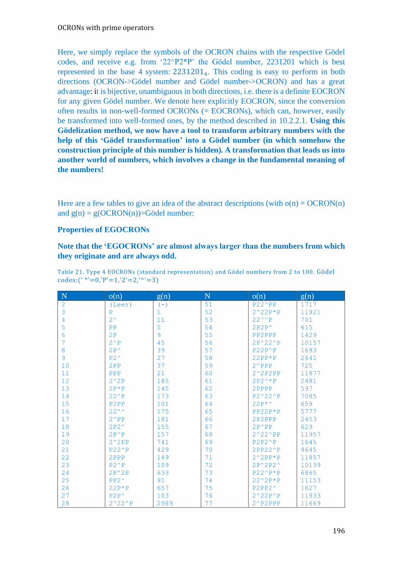
OCRONs with prime operators
196
Here, we simply replace the symbols of the OCRON chains with the respective Gödel
codes, and receive e.g. from ‘22^P2*P’ the Gödel number, 2231201 which is best
represented in the base 4 system: 22312014 . This coding is easy to perform in both
directions (OCRON->Gödel number and Gödel number->OCRON) and has a great
advantage: it is bijective, unambiguous in both directions, i.e. there is a definite EOCRON
for any given Gödel number. We denote here explicitly EOCRON, since the conversion
often results in non-well-formed OCRONs (= EOCRONs), which can, however, easily
be transformed into well-formed ones, by the method described in 10.2.2.1. Using this
Gödelization method, we now have a tool to transform arbitrary numbers with the
help of this ‘Gödel transformation’ into a Gödel number (in which somehow the
construction principle of this number is hidden). A transformation that leads us into
another world of numbers, which involves a change in the fundamental meaning of
the numbers!
Here are a few tables to give an idea of the abstract descriptions (with o(n) = OCRON(n)
and g(n) = g(OCRON(n))=Gödel number:
Properties of EGOCRONs
Note that the ‘EGOCRONs’ are almost always larger than the numbers from which
they originate and are always odd.
Table 21. Type 4 EOCRONs (standard representation) and Gödel numbers from 2 to 100. Gödel codes:(‘ *’=0,’P’=1,’2’=2,’^’=3)
N o(n) g(n) N o(n) g(n) 2
3
4
5
6
7
8
9
10
11
12
13
14
15
16
17
18
19
20
21
22
23
24
25
26
27
28
(Leer)
P
2^
PP
2P
2^P
2P^
P2^
2PP
PPP
2^2P
2P*P
22^P
P2PP
22^^
2^PP
2P2^
2P^P
2^2PP
P22^P
2PPP
P2^P
2P^2P
PP2^
22P*P
P2P^
2^22^P
(-)
1
11
5
9
45
39
27
37
21
185
145
173
101
175
181
155
157
741
429
149
109
633
91
657
103
2989
51
52
53
54
55
56
57
58
59
60
61
62
63
64
65
66
67
68
69
70
71
72
73
74
75
76
77
P22^PP
2^22P*P
22^^P
2P2P^
PP2PPP
2P^22^P
P22P^P
22PP*P
2^PPP
2^2P2PP
2P2^*P
2PPPP
P2^22^P
22P*^
PP22P*P
2P2PPP
2P^PP
2^22^PP
P2P2^P
2PP22^P
2^2PP*P
2P^2P2^
P22^P*P
22^2P*P
P2PP2^
2^22P^P
2^P2PPP
1717
11921
701
615
1429
10157
1693
2641
725
11877
2481
597
7085
659
5777
2453
629
11957
1645
9645
11857
10139
6865
11153
1627
11933
11669
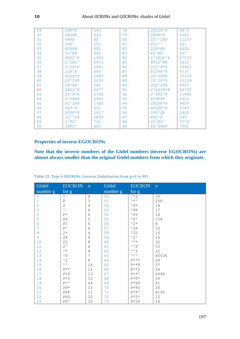
10 About OCRONs and GOCRONs: shades of Gödel
197
29
30
31
32
33
34
35
36
37
38
39
40
41
42
43
44
45
46
47
48
49
50
2PP*P
2P2PP
PPPP
2PP^
P2PPP
22^PP
PP22^P
2^2P2^
2^2P*P
22P^P
P22P*P
2P^2PP
2P*PP
2P22^P
22^P*P
2^2PPP
P2^2PP
2P2^P
P2PP*P
22^^2P
2^P2^
2PP2^
593
613
85
151
405
693
1453
2971
2961
669
1681
2533
581
2477
2769
2965
1765
621
1617
2809
731
603
78
79
80
81
82
83
84
85
86
87
88
89
90
91
92
93
94
95
96
97
98
99
2P22P*P
2PPP*P
22^^2PP
P22^^
22P*PP
P2^PP
2^2P22^P
PP22^PP
222^P*P
P22PP*P
2P^2PPP
2P^2P*P
2P2^2PP
2^P22P*P
2^2P2^P
P2PPPP
2P2PP*P
PP22P^P
2PP^2P
PP2^P
22^P2^
P2^2PPP
9873
2385
11237
431
2629
437
47533
5813
10961
6737
10133
10129
9957
46737
11885
1621
9809
5789
2425
365
2779
7061
Properties of inverse EGOCRONs
Note that the inverse numbers of the Gödel numbers (inverse EGOCRONs) are
almost always smaller than the original Gödel numbers from which they originate.
Table 22. Type 4 EOCRONs (inverse Gödelization from g=0 to 99)
Gödel
number g
EOCRON
for g
n Gödel
number g
EOCRON
for g
n
0
1
2
3
4
5
6
7
8
9
10
11
12
13
14
15
16
17
18
19
20
21
22
23
*
P
2
^
P*
PP
P2
P^
2*
2P
22
2^
^*
^P
^2
^^
P**
P*P
P*2
P*^
PP*
PPP
PP2
PP^
4
3
4
4
6
5
6
8
4
6
8
4
8
7
8
16
12
13
12
64
10
11
10
32
50
51
52
53
54
55
56
57
58
59
60
61
62
63
64
65
66
67
68
69
70
71
72
73
^*2
^*^
^P*
^PP
^P2
^P^
^2*
^2P
^22
^2^
^^*
^^P
^^2
^^^
P***
P**P
P**2
P**^
P*P*
P*PP
P*P2
P*P^
P*2*
P*2P
16
256
14
17
14
128
8
12
16
16
32
53
32
65536
24
37
24
4096
26
41
26
8192
12
18

OCRONs with prime operators
198
24
25
26
27
28
29
30
31
32
33
34
35
36
37
38
39
40
41
42
43
44
45
46
47
48
49
P2*
P2P
P22
P2^
P^*
P^P
P^2
P^^
2**
2*P
2*2
2*^
2P*
2PP
2P2
2P^
22*
22P
222
22^
2^*
2^P
2^2
2^^
^**
^*P
6
9
12
9
16
19
16
256
8
7
8
16
6
10
12
8
8
12
16
8
8
7
8
16
16
19
74
75
76
77
78
79
80
81
82
83
84
85
86
87
88
89
90
91
92
93
94
95
96
97
98
99
P*22
P*2^
P*^*
P*^P
P*^2
P*^^
PP**
PP*P
PP*2
PP*^
PPP*
PPPP
PPP2
PPP^
PP2*
PP2P
PP22
PP2^
PP^*
PP^P
PP^2
PP^^
P2**
P2*P
P2*2
P2*^
24
36
128
311
128
18446744073709551616
20
29
20
1024
22
31
22
2048
10
15
20
25
64
131
64
4294967296
12
13
12
64
One may wonder what the frequencies of the ‘*’, ’P’, ’2’ and ‘^’ symbols are. A statistical
evaluation of the EOCRONs of the type 4 for the natural numbers from 3 to 10000
yields the following frequencies:
Total number of symbols: 123952
of which P symbols: 52664 (42, 487 %)
of which 2 symbols: 42794 (34, 525 %)
of which ^ symbols: 16711 (13, 482 %)
of which * symbols: 11783 (9, 506 %)
The following illustration shows a logarithmic representation of the Gödel numbers for
the first 5,000 natural numbers using the Gödel codes ‘*’ = 0, ‘P’ = 1, ‘2’ = 2, and ‘^’ =
3. In the Gödelization, the base 4 numeral system was used. One can clearly see a striated
structure.
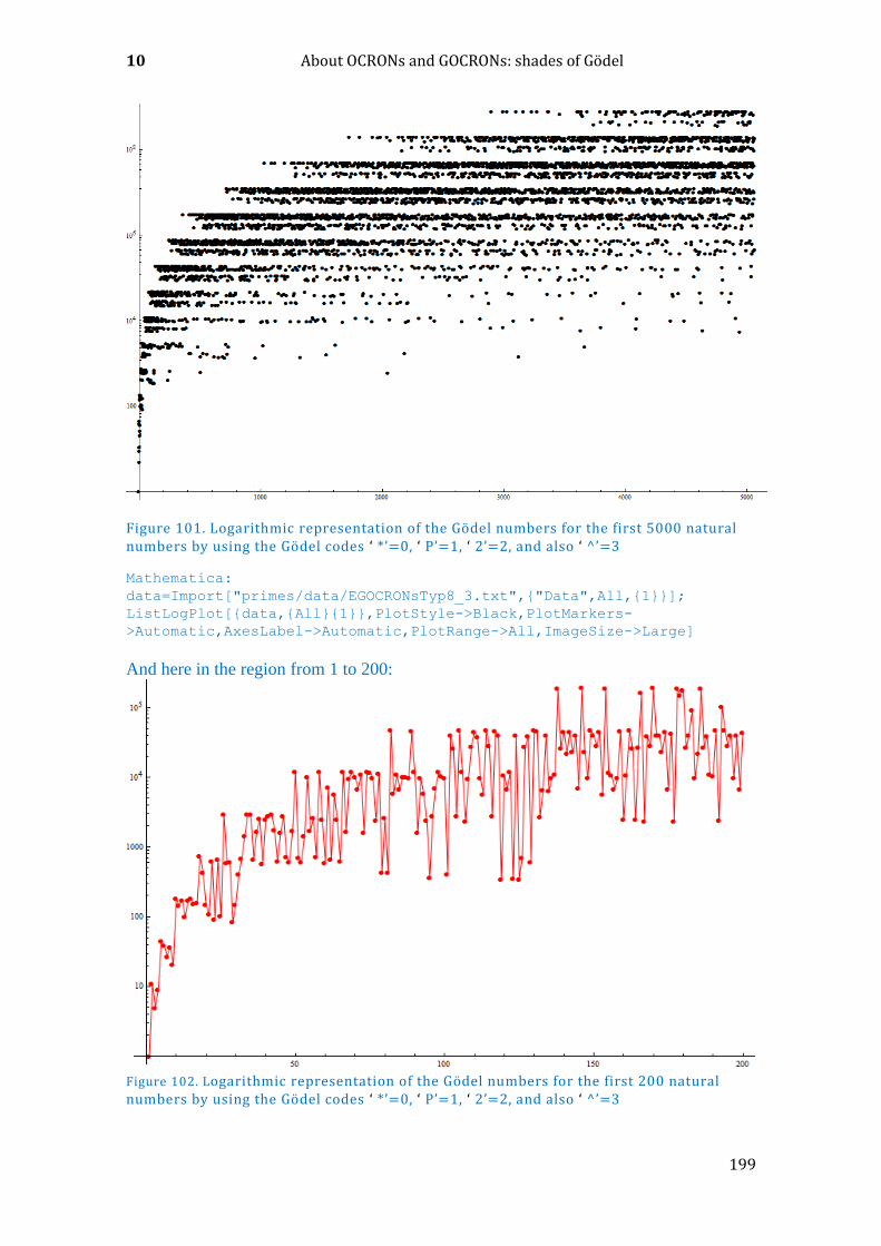
10 About OCRONs and GOCRONs: shades of Gödel
199
Figure 101. Logarithmic representation of the Gödel numbers for the first 5000 natural numbers by using the Gödel codes ‘ *’=0, ‘ P’=1, ‘ 2’=2, and also ‘ ^’=3
Mathematica:
data=Import["primes/data/EGOCRONsTyp8_3.txt",{"Data",All,{1}}];
ListLogPlot[{data,{All}{1}},PlotStyle->Black,PlotMarkers-
>Automatic,AxesLabel->Automatic,PlotRange->All,ImageSize->Large]
And here in the region from 1 to 200:
Figure 102. Logarithmic representation of the Gödel numbers for the first 200 natural numbers by using the Gödel codes ‘ *’=0, ‘ P’=1, ‘ 2’=2, and also ‘ ^’=3

OCRONs with prime operators
200
10.2.3 OCRONS WITH THE PRIME “P”, “*”, “^” AND “Q” OPERATORS
The Q operator replaces multiple consecutive ‘P’ operators by the sequence <𝑛>Q, where
𝑛 is represented in the corresponding OCRON coding and contains the number of
successive 𝑃's. All other operators are identical to the OCRON type 4. We call this type
OCRON type 5.
10.2.3.1 DEGENERATION OF TYPE 5 OCRONS
Degeneration was defined in 10.2.1.1. The degeneration increases very quickly with 𝑛
as shown in the following graph:
Figure 103. Degeneration of well-formed OCRONs of type 5 up to n=128
Mathematica:
data =
Import["primes/data/ocron5_wellformed_Degeneration_OK_upto_128.txt","C
SV"]
ListPlot[data,PlotStyle->Red,AxesLabel->Automatic,Filling-
>Axis,PlotMarkers->Automatic,PlotRange->All]
10.2.4 OCRONS WITH PRIME AND NON-PRIME OPERATORS
This type of OCRON has only two operators: the prime operator ‘𝑃’, and the non prime
operator, which for the sake of simplicity we may also refer to by ‘∗’ (not to be confused
with the multiplication operator used by the OCRON types 3 to 5. The interpretation of
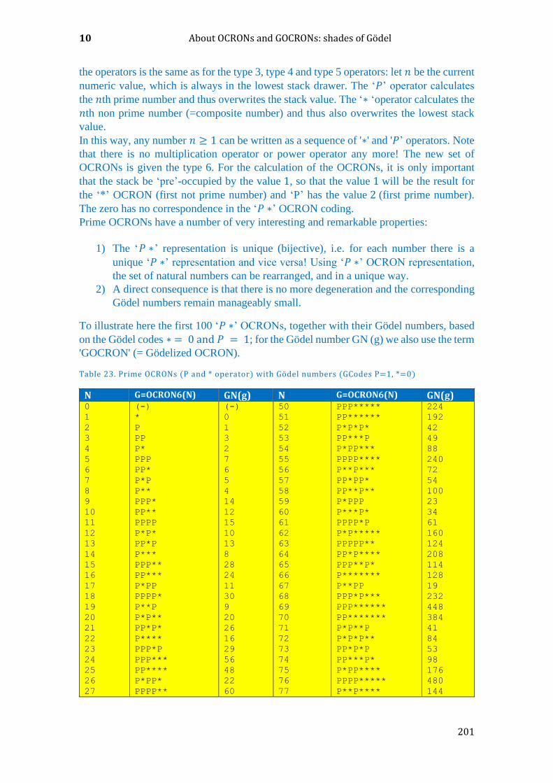
10 About OCRONs and GOCRONs: shades of Gödel
201
the operators is the same as for the type 3, type 4 and type 5 operators: let 𝑛 be the current
numeric value, which is always in the lowest stack drawer. The ‘𝑃’ operator calculates
the 𝑛th prime number and thus overwrites the stack value. The ‘∗ ‘operator calculates the
𝑛th non prime number (=composite number) and thus also overwrites the lowest stack
value.
In this way, any number 𝑛 ≥ 1 can be written as a sequence of '∗' and '𝑃’ operators. Note
that there is no multiplication operator or power operator any more! The new set of
OCRONs is given the type 6. For the calculation of the OCRONs, it is only important
that the stack be ‘pre’-occupied by the value 1, so that the value 1 will be the result for
the ‘*’ OCRON (first not prime number) and ‘P’ has the value 2 (first prime number).
The zero has no correspondence in the ‘𝑃 ∗’ OCRON coding.
Prime OCRONs have a number of very interesting and remarkable properties:
1) The ‘𝑃 ∗’ representation is unique (bijective), i.e. for each number there is a
unique ‘𝑃 ∗’ representation and vice versa! Using ‘𝑃 ∗’ OCRON representation,
the set of natural numbers can be rearranged, and in a unique way.
2) A direct consequence is that there is no more degeneration and the corresponding
Gödel numbers remain manageably small.
To illustrate here the first 100 ‘𝑃 ∗’ OCRONs, together with their Gödel numbers, based
on the Gödel codes ∗ = 0 and 𝑃 = 1; for the Gödel number GN (g) we also use the term
'GOCRON' (= Gödelized OCRON).
Table 23. Prime OCRONs (P and * operator) with Gödel numbers (GCodes P=1, *=0)
N G=OCRON6(N) GN(g) N G=OCRON6(N) GN(g) 0
1
2
3
4
5
6
7
8
9
10
11
12
13
14
15
16
17
18
19
20
21
22
23
24
25
26
27
(-)
*
P
PP
P*
PPP
PP*
P*P
P**
PPP*
PP**
PPPP
P*P*
PP*P
P***
PPP**
PP***
P*PP
PPPP*
P**P
P*P**
PP*P*
P****
PPP*P
PPP***
PP****
P*PP*
PPPP**
(-)
0
1
3
2
7
6
5
4
14
12
15
10
13
8
28
24
11
30
9
20
26
16
29
56
48
22
60
50
51
52
53
54
55
56
57
58
59
60
61
62
63
64
65
66
67
68
69
70
71
72
73
74
75
76
77
PPP*****
PP******
P*P*P*
PP***P
P*PP***
PPPP****
P**P***
PP*PP*
PP**P**
P*PPP
P***P*
PPPP*P
P*P*****
PPPPP**
PP*P****
PPP**P*
P*******
P**PP
PPP*P***
PPP******
PP*******
P*P**P
P*P*P**
PP*P*P
PP***P*
P*PP****
PPPP*****
P**P****
224
192
42
49
88
240
72
54
100
23
34
61
160
124
208
114
128
19
232
448
384
41
84
53
98
176
480
144
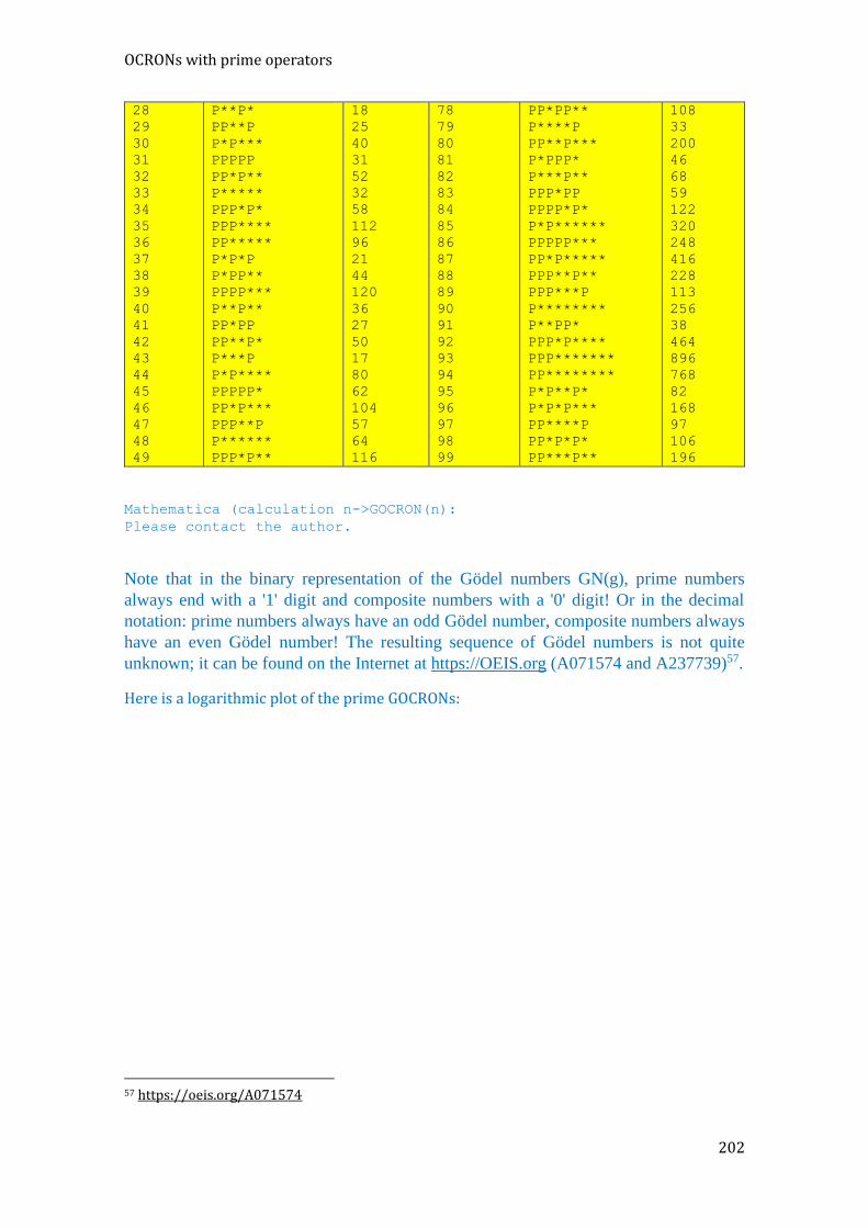
OCRONs with prime operators
202
28
29
30
31
32
33
34
35
36
37
38
39
40
41
42
43
44
45
46
47
48
49
P**P*
PP**P
P*P***
PPPPP
PP*P**
P*****
PPP*P*
PPP****
PP*****
P*P*P
P*PP**
PPPP***
P**P**
PP*PP
PP**P*
P***P
P*P****
PPPPP*
PP*P***
PPP**P
P******
PPP*P**
18
25
40
31
52
32
58
112
96
21
44
120
36
27
50
17
80
62
104
57
64
116
78
79
80
81
82
83
84
85
86
87
88
89
90
91
92
93
94
95
96
97
98
99
PP*PP**
P****P
PP**P***
P*PPP*
P***P**
PPP*PP
PPPP*P*
P*P******
PPPPP***
PP*P*****
PPP**P**
PPP***P
P********
P**PP*
PPP*P****
PPP*******
PP********
P*P**P*
P*P*P***
PP****P
PP*P*P*
PP***P**
108
33
200
46
68
59
122
320
248
416
228
113
256
38
464
896
768
82
168
97
106
196
Mathematica (calculation n->GOCRON(n):
Please contact the author.
Note that in the binary representation of the Gödel numbers GN(g), prime numbers
always end with a '1' digit and composite numbers with a '0' digit! Or in the decimal
notation: prime numbers always have an odd Gödel number, composite numbers always
have an even Gödel number! The resulting sequence of Gödel numbers is not quite
unknown; it can be found on the Internet at https://OEIS.org (A071574 and A237739)57.
Here is a logarithmic plot of the prime GOCRONs:
57 https://oeis.org/A071574
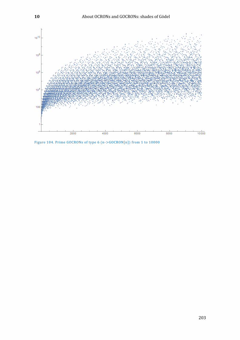
10 About OCRONs and GOCRONs: shades of Gödel
203
Figure 104. Prime GOCRONs of type 6 (n->GOCRON[n]) from 1 to 10000
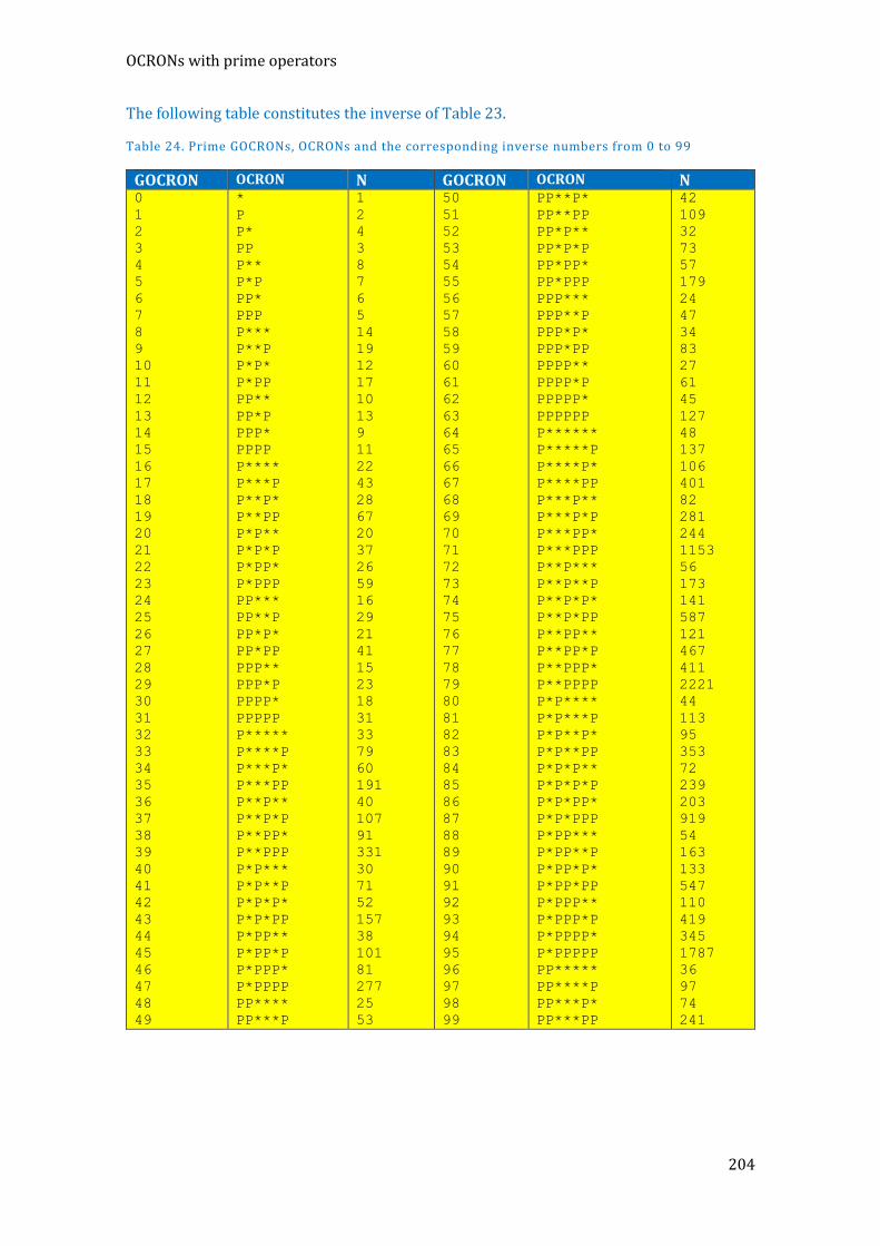
OCRONs with prime operators
204
The following table constitutes the inverse of Table 23.
Table 24. Prime GOCRONs, OCRONs and the corresponding inverse numbers from 0 to 99
GOCRON OCRON N GOCRON OCRON N 0
1
2
3
4
5
6
7
8
9
10
11
12
13
14
15
16
17
18
19
20
21
22
23
24
25
26
27
28
29
30
31
32
33
34
35
36
37
38
39
40
41
42
43
44
45
46
47
48
49
*
P
P*
PP
P**
P*P
PP*
PPP
P***
P**P
P*P*
P*PP
PP**
PP*P
PPP*
PPPP
P****
P***P
P**P*
P**PP
P*P**
P*P*P
P*PP*
P*PPP
PP***
PP**P
PP*P*
PP*PP
PPP**
PPP*P
PPPP*
PPPPP
P*****
P****P
P***P*
P***PP
P**P**
P**P*P
P**PP*
P**PPP
P*P***
P*P**P
P*P*P*
P*P*PP
P*PP**
P*PP*P
P*PPP*
P*PPPP
PP****
PP***P
1
2
4
3
8
7
6
5
14
19
12
17
10
13
9
11
22
43
28
67
20
37
26
59
16
29
21
41
15
23
18
31
33
79
60
191
40
107
91
331
30
71
52
157
38
101
81
277
25
53
50
51
52
53
54
55
56
57
58
59
60
61
62
63
64
65
66
67
68
69
70
71
72
73
74
75
76
77
78
79
80
81
82
83
84
85
86
87
88
89
90
91
92
93
94
95
96
97
98
99
PP**P*
PP**PP
PP*P**
PP*P*P
PP*PP*
PP*PPP
PPP***
PPP**P
PPP*P*
PPP*PP
PPPP**
PPPP*P
PPPPP*
PPPPPP
P******
P*****P
P****P*
P****PP
P***P**
P***P*P
P***PP*
P***PPP
P**P***
P**P**P
P**P*P*
P**P*PP
P**PP**
P**PP*P
P**PPP*
P**PPPP
P*P****
P*P***P
P*P**P*
P*P**PP
P*P*P**
P*P*P*P
P*P*PP*
P*P*PPP
P*PP***
P*PP**P
P*PP*P*
P*PP*PP
P*PPP**
P*PPP*P
P*PPPP*
P*PPPPP
PP*****
PP****P
PP***P*
PP***PP
42
109
32
73
57
179
24
47
34
83
27
61
45
127
48
137
106
401
82
281
244
1153
56
173
141
587
121
467
411
2221
44
113
95
353
72
239
203
919
54
163
133
547
110
419
345
1787
36
97
74
241
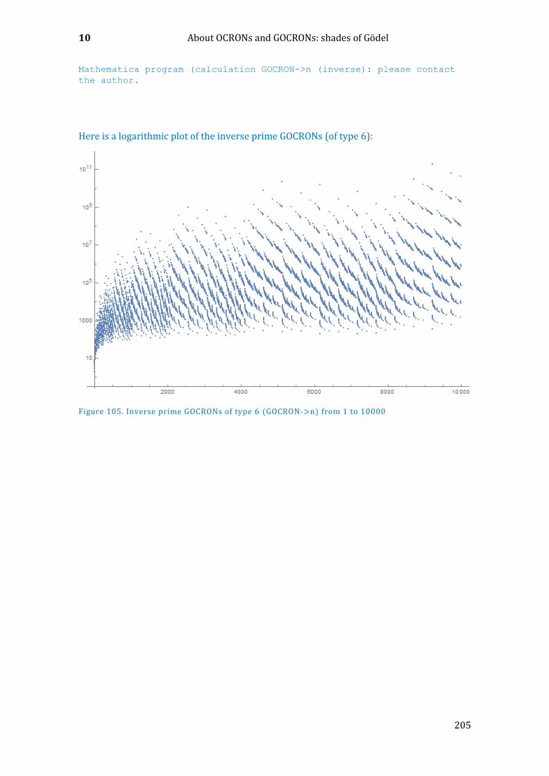
10 About OCRONs and GOCRONs: shades of Gödel
205
Mathematica program (calculation GOCRON->n (inverse): please contact
the author.
Here is a logarithmic plot of the inverse prime GOCRONs (of type 6):
Figure 105. Inverse prime GOCRONs of type 6 (GOCRON->n) from 1 to 10000
The world of OCRON beings and mathematical dynamite
206
10.3 THE WORLD OF OCRON BEINGS AND MATHEMATICAL DYNAMITE
Note: in order to understand this chapter properly, the reader should at least be a bit
familiar with the type 4 OCRONs (see Chapter 10.2.2).
We want to make an excursion into the world of OCRON beings. This is a thought
experiment, since we do not know for certain whether this world exists together with
its inhabitants, which we will call 'OCRONians'. Thought experiments are a
successful tool in science to make complex relations clearer. It is known that Einstein
had the decisive idea for his general theory of relativity by using thought experiments.
One of these thought experiments was that he imagined himself to be in a huge falling
elevator that is large enough to hold a whole physics laboratory with all possible
measuring instruments, and which would not have any contact with the environment
outside. He compared this situation with a closed room (also having all possible
measuring instruments and devices and also without contact to the outside world) that
is moving with constant velocity through space far away from any planets or other
space objects (today in the space age this is no longer hard to imagine). A physicist
who is in the first or in the second room can perform all the measurements and
experiments he wants. All types of measuring instruments are available in the two
rooms. However, the physicist cannot determine, solely by means of measurements
performed within the respective room, whether it is situated in a falling elevator (it
may also be said to be within reach of a gravitational field), or in a space ship moving
with constant velocity far away in space.
A similar thought experiment would be to put the first closed room, together with the
measuring instruments simply on the surface of the earth, to place the other room on
the top of a rocket that has turned its engines on, and which moves with a constant
acceleration through the universe. Again, a physicist cannot determine solely by
measurements performed within the respective rooms in which situation he is.
The logical conclusion was that the two respective situations do not only appear to
be identical, but are actually identical. A gangway can be constructed between the
respective situations using appropriate mathematical tools. In the case of the general
theory of relativity, it was the idea of a 'curved spacetime' that finally produced the
equivalence of the two situations.
Our thought experiment leads us into another world, a world that is so completely
different from ours that we can hardly imagine it. The cosmologists often speak of
other worlds. There is the concept of a multiverse, which includes many or even
infinitely many universes of a certain kind. The universe, in which we want to go
now originated in a multiverse, which has a name: in his book 'Our Mathematical
Universe', Max Tegmark58 calls it the ‘level IV' multiverse. Tegmark speaks of
different parallel universes that form a four-stage hierarchy, each multiverse being a
single element among many of the other ones existing one level higher. According to
his theory, level I and II universes emerged physically after the Big Bang in the so-
called ‘inflationary phase’. In level I, however, each universe has the same physical
natural laws and natural constants, the same mathematics, however different initial
conditions. In level II each universe has the same natural laws and the same
mathematics but different natural constants and different particles. This type of
multiverse can also have higher spatial dimension. The level III multiverse
corresponds to the level II multiverse, but it consists of infinitely many individual
58 Max Tegmark: Our mathematical universe, Ullstein Buchverlage GmbH, Berlin
10 About OCRONs and GOCRONs: shades of Gödel
207
universes that continuously split up by generating new universes, always when
anybody perceives something (or someone else). It takes account of the quantum
mechanical nature of our world.
By "perceiving" is meant the most general form of perception, including the
following situations: 'looking' or 'viewing', a physicist who measures a physical
quantity, but also any completely abstract interaction between a complex quantum
mechanical system and another.
At an atomic and subatomic scale, all physical processes are calculated by quantum
mechanics and by a wave function that describes the process spatial and temporal. It
only has the disadvantage that all potentially measurable quantities exist as an infinite
superposition of all possible discrete states. At least, as long as no measurement is
made – that is, as long as nobody ‘looks’ at the system, since in the case of a
measurement the quantum mechanical system has to decide for one of these infinitely
many possible states. The physicists call this the collapse of the wave function
following the 'Copenhagen interpretation' and are still not happy about it. One
conceivable alternative that avoids this collapse of the wave function is the ‘many
worlds’ hypothesis of quantum mechanics, which states that our entire universe splits
into several universes, depending on which process is considered (caused by a
measurement).
This leads to the level III multiverse. From a philosophical point of view it can be
said that in such a multiverse everything occurs (all possible events happen, in any
of the infinite many plane III universes), which can occur at any time.
In the level VI multiverse, the restriction of the uniform equations of physics also
fails. Each universe contains its own set of mathematical structures. Many of these
type VI universes will be uninteresting, but many will be complex and powerful
enough to create their own worlds within this level VI universe.
Why do we digress so far? In order to show that the world in which we want to go is
so unimaginably different to our own world, since it is a level VI world (after Max
Tegmark) in which there is a completely different mathematics to that of our world.
Now we finally come to our OCRON beings. Let us suppose that the world of
mathematics in this world is versatile and powerful enough to create a world with a
similar complexity and diversity to ours. There exists also life in this world: the
inhabitants are the OCRONians mentioned above.
They live there in communities, are intelligent, and they also pursue science,
including mathematics, out of curiosity. They can also construct machines, computers
and other devices for which they need mathematics as a tool. Their own mathematics
is fundamentally different from our mathematics.
The OCRONians cannot add, they can only multiply and raise to the power (and in
some mysterious way also calculate logarithms to the base 2). They also do not
calculate using numbers to which a unique value can be assigned, but they only
calculate using OCRONs: the four different formal symbols ‘ ∗ ’, ‘ 2’, ‘ ^’, and ‘ 𝑃’. They can not say how large a number is, the terms 'size' or value of a number (in our
sense) do not exist in their world.
The concept of addition is alien to them, not just alien, for it simply does not exist in
their world. They can multiply huge numbers effortlessly (in their world of course
OCRONs) from childhood onward. Not even prime factors are a problem for them:
they look at a number and can see in a fraction of a second whether it is a prime
The world of OCRON beings and mathematical dynamite
208
number, or of which prime factors it is composed.
Their computers also work without addition, since numbers are not stored in them as
sum totals, but only as OCRON representations (which ultimately result in a product
of prime factors). For programming and the unavoidable calculations that must occur
when constructing machines, however, they must also be able to compare numbers
and can determine if two numbers have the same ‘size’.
And they may also have to carry out operations of the kind that we call ‘addition’ in
our world (which actually can be done in their world, but only in a very roundabout
way). Although the term ‘value’ of a number (of an OCRON) does not exist in their
world, they also have an ability to determine without a concept of ‘size’ or ‘value’
which is the larger of two numbers, or whether they are of the same size. For this
purpose they consult the ‘MATHOracle’. (MATHOracle consultation, see below).
They can also ask the MATHOracle for a second operation, which they use in their
computations: the ORACLELog operation (in our world, this is called the logarithm
to base 2).
The OCRONians have to perform 'additions' (this term is known only to us) becau
se of their physical equations, but they do not know that we call this process in our
world 'addition' and that we have a much simpler method of doing so. They use a
rather complicated method for this: to add two OCRONs o_1 and o_2, they write (we
call the result o_3):
𝑜3=ORACLELog[2𝑜1^2𝑜2^ ∗].
In our mathematical language this reads as follows: 𝑜3 = Log2(2𝑜1 ⋅ 2𝑜2).
The OCRONians call the oracle logarithm the 'ORACLELog' symbol. 'ORACLELog'
returns either an OCRON or nothing. Together with the function 'ORACLEValue'
(which can only supply one of the three values 'smaller', 'greater' or 'equal', these are
the two mathematical operations for which the OCRONians can query the
MATHOracle).
The methods 'ORACLEValue' and 'ORACLELog' are not really understood by the
OCRONians, but this method is intuitively familiar to all OCRONians. They can
interrogate the 'MATHOracle' and it will always give them the right answer to these
questions within a fraction of a second. Each OCRONian has access to the
MATHOracle from any location and at any time in a mysterious way. The
OCRONian computers also enjoy such access. The mathematicians among the
OCRONians now state that there can exist quite different OCRONs, which provide
the same result in the MATHOracle consultation with 'ORACLEValue'.
By probing (‘trial and error’) and ORACLEValue consultations, they discover all
possible OCRONs that give the same value.
The cleverest mathematicians among the OCRONians have therefore wrestled for
many years with the question of whether there is a method based on an algorithm,
instead of the random 'try-out' in the search for 'equivalent' OCRONs, with which
'equivalent' OCRONs could be transformed into each other (and thereby, for example,
simplified). This would have made the work of the OCRONian engineers much
easier, since they would have found a quick method for the conversion of OCRONs
10 About OCRONs and GOCRONs: shades of Gödel
209
instead of random testing, and they would not need to consult the MATHOracle (at
least for their complicated 'addition') with 'ORACLEValue’.
Clever OCRONian mathematicians also found that the consultation with
ORACLELog would also be invalid, provided that they had an algorithm that could
produce all the equivalent OCRONs by reforming.
For the discovery of such an algorithm, a prize was offered in the OCRONian world.
Here is an example: multiplication of 8 ∗ 4 looks in our world like: 8 ∗ 4 = 32.
In the world of the OCRONians: 22P^ times 22^ gives 22P^22^ ∗ (OCRONians
multiply by simply concatenation of OCRONs and appending a ′ ∗′). The OCRONians are now able to determine by random testing and ORACLEValue
interrogations that, for example, 22P ^ 22 ^ * has the same value as 22PP ^.
However, they have no algorithm that produces the equivalent OCRON 22PP ^.
In our world, mathematicians and logicians speak of a (typographic) formal system.
OCRONians have to work hard with symbols to solve simple things like additions by
randomly ‘rolling dice’. For them the access into the 'higher' logical world in which
addition exists is denied!
Poor OCRONians! How does the story continue? Will the smartest OCRONians
succeed in finding such an algorithm?
Let us think of two possible (fictional) scenarios of the story.
Scenario 1: an OCRONian mathematician finds an algorithm for transforming
equivalent OCRONs into each other. He is celebrated and receives the OCRONian
‘Fields Medal’. The MATHOracle has no longer to be consulted for the 'additions'.
Indeed, the solution is complicated (for the calculation, solutions have to be found
with the aid of complicated recurrence rules and rules that in turn invented new rules),
but it is still a method to bypass the MATHOracle consultation. In addition, the old
method associated with the 'ORACLEValue' consultation always involves boring
random probing, with the result that the complicated method with recursive rules for
long OCRONs works unbeatably better than the random method.
Scenario 2: a clever OCRONian named ‘Gocroedel’ finds a proof that the axiomatic
system of OCRONian mathematics is simply too 'weak' and too lacking in 'power' to
solve the problem of the transformation. He claims that the statement:
‘22P^22^*’ is equivalent to ‘22PP^’ is indeed true but that it cannot be proved with
OCRONian mathematics. This implies that no such algorithm can be found. For this,
Gocroedel also receives the OCRONian ‘Fields Medal’, but the OCRONians cannot
really look forward to it.
The attentive reader has probably realized what ‘explosive’ is hidden in scenario
1:
If Scenario 1 were true, then we could learn from the OCRONians (above
referred to as 'poor'): we could adopt their 'transformation algorithm' and
would have a quick method for the factorization of numbers: we would simply
have to separate the number to be factored into a sum of two numbers whose

The world of OCRON beings and mathematical dynamite
210
prime factorization we know (more precisely, whose OCRON representations
we know). Then we prepend a ‘𝟐’ symbol at the beginning of the respective
OCRONs, append an ‘^’ symbol at the end of both OCRONs, concatenate both
the new OCRONs (OCRON multiplication) and append a ‘∗’ symbol at the end.
If the second summand is 𝟏, then the thing is even simpler: the second OCRON
is simply the symbol ‘𝟐’. Finally, we transform the concatenated OCRON into
an equivalent OCRON with the help of the mysterious algorithm, so that at the
end of the OCRON a '^' symbol is placed, then easily get the logarithm to the
base 2 (by discarding the leading ‘2’ and the last symbol ‘^’), and voilà!
We have a product representation (which is implicit in every OCRON) of the
number to be factored! If the resulting OCRON does not have a '∗’ or '^' symbol
at the end, but a '𝑷' symbol, then the number to be factored is a prime number.
We would have solved the factorizing problem on a pure typographical level by
applying typographic transformation rules.
Here a few examples:
We examine the number 𝟑𝟕. Additive composition: 𝟑𝟕 = 𝟑𝟔 + 𝟏:
In OCRON notation:
36 = 22^2𝑃2^ ∗ -> (brackets inserted for the sake of clarity)
(𝟐𝟐𝟐^𝟐𝑷𝟐^ ∗ ^)(𝟐) ∗->(MATHOracle consultation) 𝟐𝟐𝟐^𝟐𝑷 ∗ 𝑷^ (logarithm: discard the 2 and ^)-> 𝟐𝟐^𝟐𝑷 ∗ 𝑷, prime number!
Thus, we have shown that 37 is a prime number, only by dealing with OCRONs.
We examine the number 𝟏𝟒𝟑. Composition: 𝟏𝟒𝟑 = 𝟕𝟏 + 𝟕𝟐:
In OCRON notation:
71 = 22^2𝑃𝑃 ∗ 𝑃, 72 = 22𝑃^2𝑃2^ ∗ ->
(𝟐𝟐𝟐^𝟐𝑷𝑷 ∗ 𝑷^)(𝟐 𝟐𝟐𝑷^𝟐𝑷𝟐^ ∗ ^) ∗->(MATHOracle consultation)
𝟐𝟐𝑷𝑷𝑷𝟐𝟐𝑷 ∗ 𝑷 ∗ ^
(logarithm: discard the 2 and ^)-> 2𝑃𝑃𝑃22𝑃 ∗ 𝑃 ∗ = (2𝑃𝑃𝑃)(22𝑃 ∗ 𝑃) ∗ Result: factors 𝟐𝑷𝑷𝑷 (= 𝟏𝟏) and 𝟐𝟐𝑷 ∗ 𝑷 (= 𝟏𝟑) Thus we have factorized 143 by means of OCRON manipulation into the factors 11
and 13.
Note: the transformation without a MATHOracle consultation is also difficult in our
world, because we have to calculate explicitly the value of
𝟐𝟐𝟐^𝟐𝑷𝑷 ∗ 𝑷^𝟐 𝟐𝟐𝑷^𝟐𝑷𝟐^ ∗ ^ ∗: 11150372599265311570767859136324180752990208, and then reconvert
this value back to an OCRON (which is then transformed).
These examples show that by means of type 4 OCRONs we can factorize numbers
by pure, formal typographic manipulation of symbols, provided that we have access
to the MATHOracle!
There remains only the 'small' problem, how we can circumvent the MATHOracle
consultation and find the fabulous algorithm!
Before we begin searching for this algorithm, we should first determine whether or
not the entire problem belongs to the category of 'unprovable' statements. In this case,
10 About OCRONs and GOCRONs: shades of Gödel
211
it would be utterly impossible to find such an algorithm (at least within OCRONian
mathematics).
(Addendum:)
For this, the author has found a truly wonderful algorithm, but the margin is too small to
contain it…
-end of thought experiment-

212
11 PRIME NUMBERS AND THE “MATRIX” SOFTWARE: ARE THERE RULES FOR PRIMES?
11.1 RULES FOR DIFFERENCES OF THE NTH ORDER
This chapter examines numbers using the matrix software59. For this reason, this software
and its functionality should be briefly presented here.
Matrix is an application that makes it possible to create a rule network (i.e. a set of rules)
from given data that are somehow arranged causally and that represent a sequence of
states of an arbitrary system. This set of rules describes the individual transition
probabilities of the system from one state to the next state following.
With the aid of these transitional probabilities, the matrix can produce an arbitrarily long
sequence of states of this system. In principle, this is a more general Markov chain with
transition probabilities. However, the entire "history" of a process can be included in the
calculation of the transition probabilities. In addition, the matrix can also provide
'termination probabilities' (i.e. the probability that a sequence of states ends), as well as
the opposite (i.e. the creation of a state 'ex nihilo' at the start of a new state sequence).
In its simplest form, the matrix can also simply be used to store highly dimensionally
structured data (hence the name 'matrix'), since it is basically a high-dimensional pointer
matrix (with variable dimension length).
The matrix can be applied to almost all systems. The requirements for applicability are
very general: the state of the system at a certain starting point must be described by a set
of integer (also negative) numbers. There should be enough material about the behaviour
of the system. Once the matrix has been fed with data about a system, one can read from
the matrix as from an infinite stream. Given a suitable selection of the parameters, this
'stream' will always also provide novel transitions, i.e. reading from the matrix is indeed
a creative process. In the matrix itself, no sequences of states are stored; only rules, which
are much shorter. When reading from the matrix, the intelligence of the matrix can be
adjusted.
Turning on high intelligence, the result will be close to the material with which the matrix
was originally fed; with low intelligence, more and more random elements will appear.
The result of the output when reading appears much more intelligent than the simplicity
of the rules suggests. Somehow the matrix seems to store the knowledge about the
behaviour of a system not only locally in the rules but holistically in the totality of all
rules. If, for example, you remove part of the rules, the result will not change rapidly.
Let's make a first test: we set the maximum rule length to 20 and feed the matrix with the
sequence of 1st order differences of the prime number sequence and look at the
frequencies of the calculated rule lengths:
For the first 1000 prime numbers (2-7919):
Matrix finds 2581 rules, of which 1093 are unique rules, the maximum of the
frequencies is at rule length 5, the longest rule length is 10. The size of the matrix data
file is 107 KB.
59 http://www.kmatrix.eu
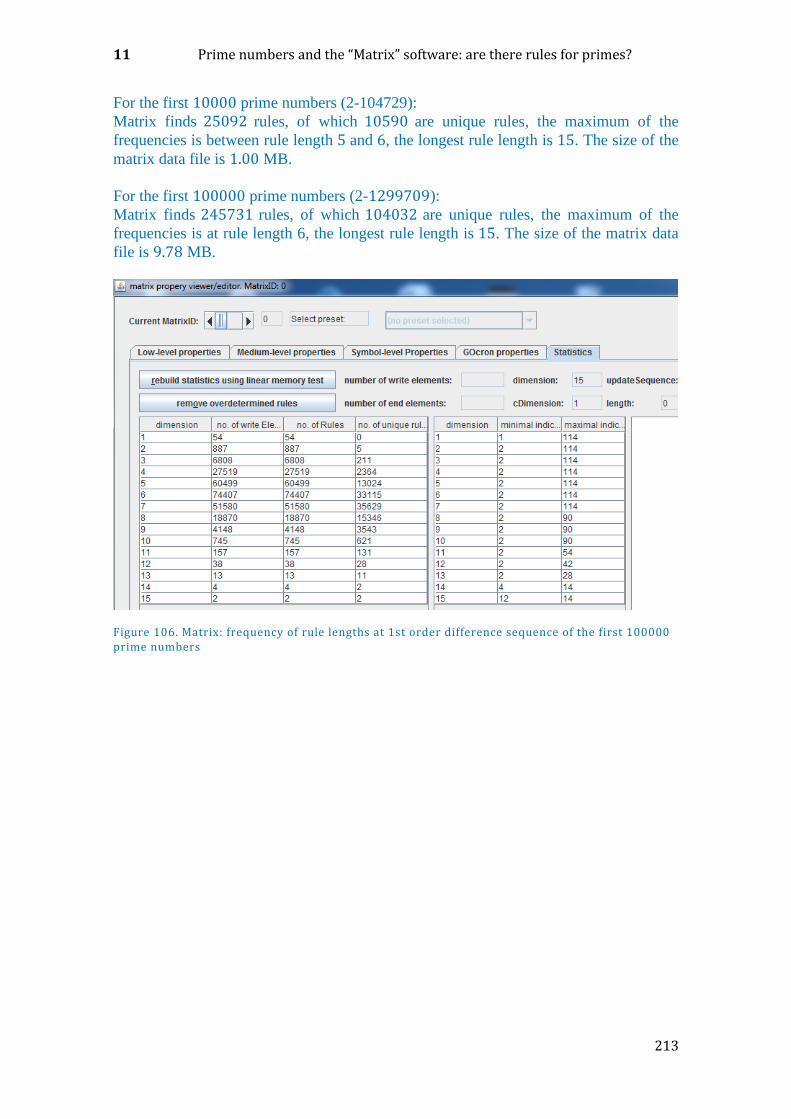
11 Prime numbers and the “Matrix” software: are there rules for primes?
213
For the first 10000 prime numbers (2-104729):
Matrix finds 25092 rules, of which 10590 are unique rules, the maximum of the
frequencies is between rule length 5 and 6, the longest rule length is 15. The size of the
matrix data file is 1.00 MB.
For the first 100000 prime numbers (2-1299709):
Matrix finds 245731 rules, of which 104032 are unique rules, the maximum of the
frequencies is at rule length 6, the longest rule length is 15. The size of the matrix data
file is 9.78 MB.
Figure 106. Matrix: frequency of rule lengths at 1st order difference sequence of the first 100000 prime numbers
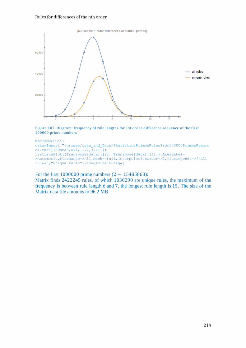
Rules for differences of the nth order
214
Figure 107. Diagram: frequency of rule lengths for 1st order difference sequence of the first 100000 prime numbers
Mathematica:
data=Import["/primes/data_and_Docs/StatisticsPrimesRulesFrom100000PrimesPrepro
c1.txt",{"Data",All,{1,2,3,4}}];
ListLinePlot[{Transpose[data][[2]],Transpose[data][[4]]},AxesLabel-
>Automatic,PlotRange->All,Mesh->Full,InterpolationOrder->2,PlotLegends->{"all
rules","unique rules"},ImageSize->Large]
For the first 1000000 prime numbers (2 − 15485863):
Matrix finds 2422245 rules, of which 1030290 are unique rules, the maximum of the
frequency is between rule length 6 and 7, the longest rule length is 15. The size of the
Matrix data file amounts to 96.2 MB.
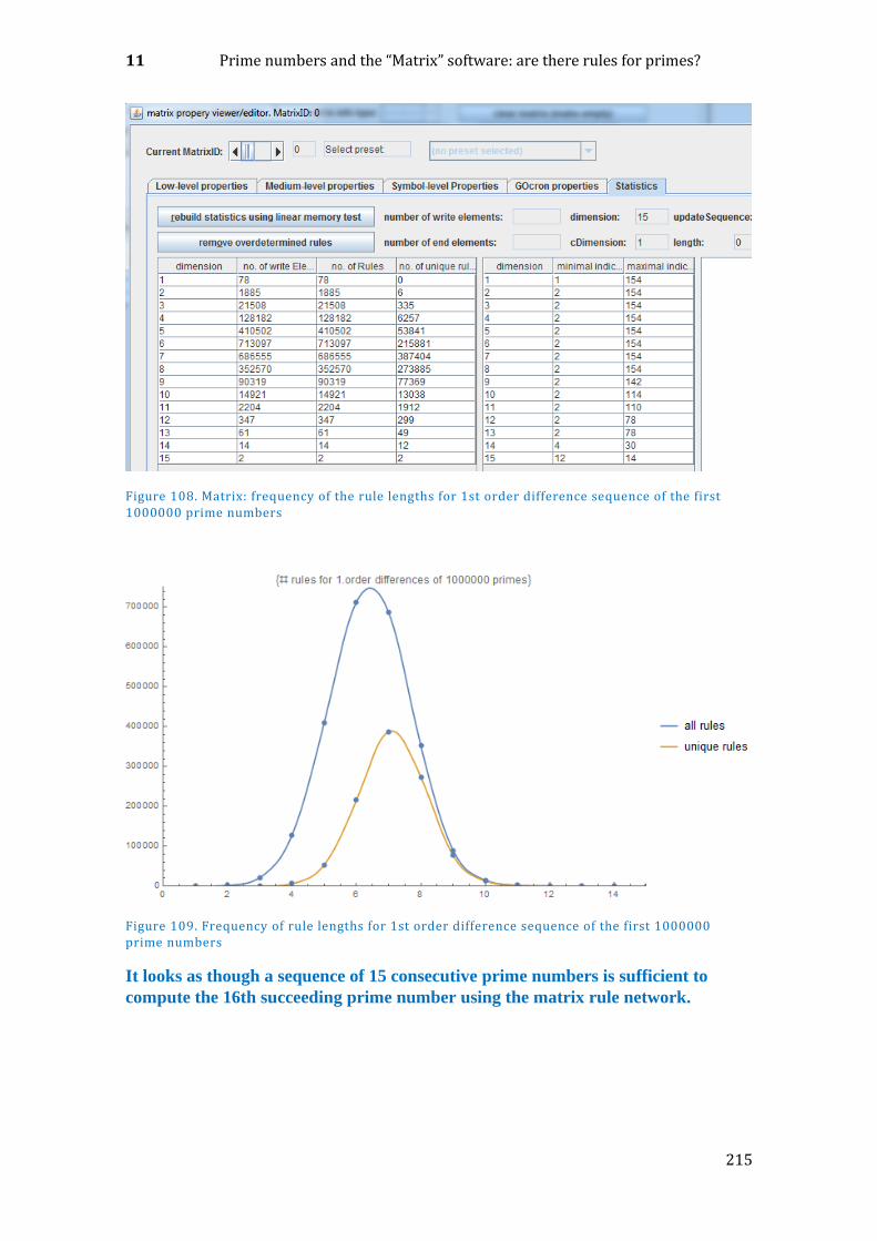
11 Prime numbers and the “Matrix” software: are there rules for primes?
215
Figure 108. Matrix: frequency of the rule lengths for 1st order difference sequence of the first 1000000 prime numbers
Figure 109. Frequency of rule lengths for 1st order difference sequence of the first 1000000 prime numbers
It looks as though a sequence of 15 consecutive prime numbers is sufficient to
compute the 16th succeeding prime number using the matrix rule network.
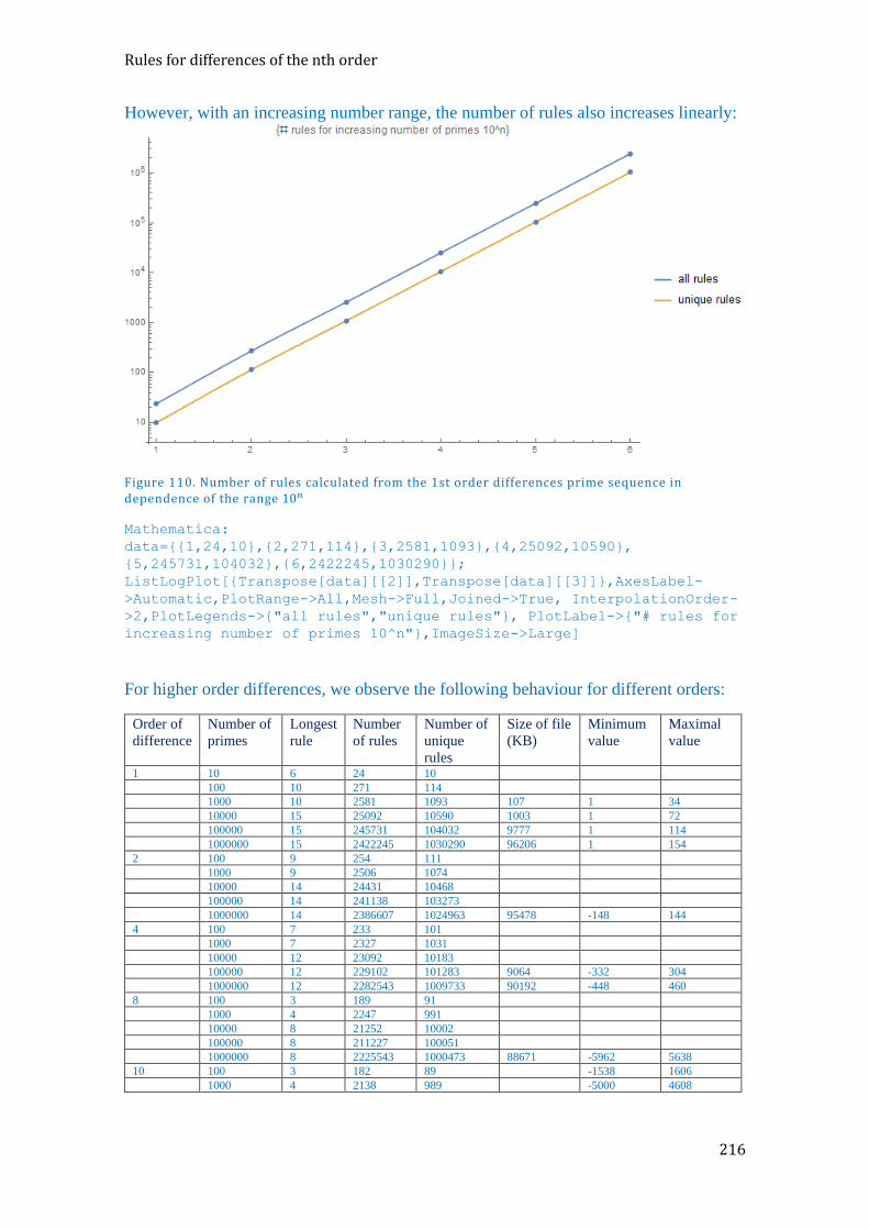
Rules for differences of the nth order
216
However, with an increasing number range, the number of rules also increases linearly:
Figure 110. Number of rules calculated from the 1st order differences prime sequence in dependence of the range 10𝑛
Mathematica:
data={{1,24,10},{2,271,114},{3,2581,1093},{4,25092,10590},
{5,245731,104032},{6,2422245,1030290}};
ListLogPlot[{Transpose[data][[2]],Transpose[data][[3]]},AxesLabel-
>Automatic,PlotRange->All,Mesh->Full,Joined->True, InterpolationOrder-
>2,PlotLegends->{"all rules","unique rules"}, PlotLabel->{"# rules for
increasing number of primes 10^n"},ImageSize->Large]
For higher order differences, we observe the following behaviour for different orders:
Order of
difference
Number of
primes
Longest
rule
Number
of rules
Number of
unique
rules
Size of file
(KB)
Minimum
value
Maximal
value
1 10 6 24 10
100 10 271 114
1000 10 2581 1093 107 1 34
10000 15 25092 10590 1003 1 72
100000 15 245731 104032 9777 1 114
1000000 15 2422245 1030290 96206 1 154
2 100 9 254 111
1000 9 2506 1074
10000 14 24431 10468
100000 14 241138 103273
1000000 14 2386607 1024963 95478 -148 144
4 100 7 233 101
1000 7 2327 1031
10000 12 23092 10183
100000 12 229102 101283 9064 -332 304
1000000 12 2282543 1009733 90192 -448 460
8 100 3 189 91
1000 4 2247 991
10000 8 21252 10002
100000 8 211227 100051
1000000 8 2225543 1000473 88671 -5962 5638
10 100 3 182 89 -1538 1606
1000 4 2138 989 -5000 4608
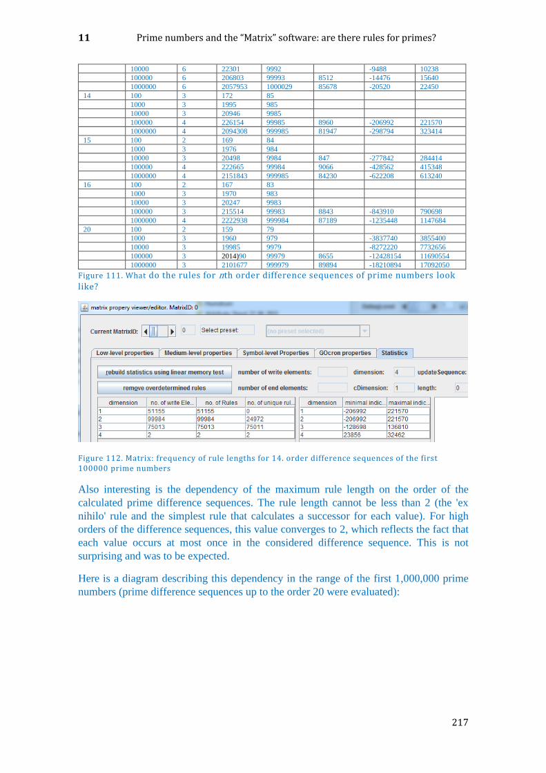
11 Prime numbers and the “Matrix” software: are there rules for primes?
217
10000 6 22301 9992 -9488 10238
100000 6 206803 99993 8512 -14476 15640
1000000 6 2057953 1000029 85678 -20520 22450
14 100 3 172 85
1000 3 1995 985
10000 3 20946 9985
100000 4 226154 99985 8960 -206992 221570
1000000 4 2094308 999985 81947 -298794 323414
15 100 2 169 84
1000 3 1976 984
10000 3 20498 9984 847 -277842 284414
100000 4 222665 99984 9066 -428562 415348
1000000 4 2151843 999985 84230 -622208 613240
16 100 2 167 83
1000 3 1970 983
10000 3 20247 9983
100000 3 215514 99983 8843 -843910 790698
1000000 4 2222938 999984 87189 -1235448 1147684
20 100 2 159 79
1000 3 1960 979 -3837740 3855400
10000 3 19985 9979 -8272220 7732656
100000 3 2014)90 99979 8655 -12428154 11690554
1000000 3 2101677 999979 89894 -18210894 17092050
Figure 111. What do the rules for nth order difference sequences of prime numbers look like?
Figure 112. Matrix: frequency of rule lengths for 14. order difference sequences of the first 100000 prime numbers
Also interesting is the dependency of the maximum rule length on the order of the
calculated prime difference sequences. The rule length cannot be less than 2 (the 'ex
nihilo' rule and the simplest rule that calculates a successor for each value). For high
orders of the difference sequences, this value converges to 2, which reflects the fact that
each value occurs at most once in the considered difference sequence. This is not
surprising and was to be expected.
Here is a diagram describing this dependency in the range of the first 1,000,000 prime
numbers (prime difference sequences up to the order 20 were evaluated):
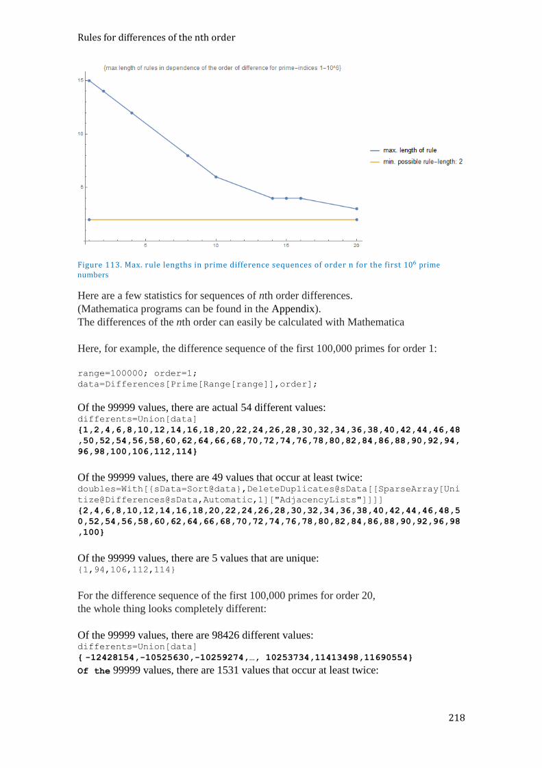
Rules for differences of the nth order
218
Figure 113. Max. rule lengths in prime difference sequences of order n for the first 106 prime
numbers
Here are a few statistics for sequences of nth order differences.
(Mathematica programs can be found in the Appendix).
The differences of the nth order can easily be calculated with Mathematica
Here, for example, the difference sequence of the first 100,000 primes for order 1:
range=100000; order=1;
data=Differences[Prime[Range[range]],order];
Of the 99999 values, there are actual 54 different values: differents=Union[data]
{1,2,4,6,8,10,12,14,16,18,20,22,24,26,28,30,32,34,36,38,40,42,44,46,48
,50,52,54,56,58,60,62,64,66,68,70,72,74,76,78,80,82,84,86,88,90,92,94,
96,98,100,106,112,114}
Of the 99999 values, there are 49 values that occur at least twice: doubles=With[{sData=Sort@data},DeleteDuplicates@sData[[SparseArray[Uni
tize@Differences@sData,Automatic,1]["AdjacencyLists"]]]]
{2,4,6,8,10,12,14,16,18,20,22,24,26,28,30,32,34,36,38,40,42,44,46,48,5
0,52,54,56,58,60,62,64,66,68,70,72,74,76,78,80,82,84,86,88,90,92,96,98
,100}
Of the 99999 values, there are 5 values that are unique: {1,94,106,112,114}
For the difference sequence of the first 100,000 primes for order 20,
the whole thing looks completely different:
Of the 99999 values, there are 98426 different values: differents=Union[data]
{ -12428154,-10525630,-10259274,…, 10253734,11413498,11690554}
Of the 99999 values, there are 1531 values that occur at least twice:

11 Prime numbers and the “Matrix” software: are there rules for primes?
219
doubles=With[{sData=Sort@data},DeleteDuplicates@sData[[SparseArray[Uni
tize@Differences@sData,Automatic,1]["AdjacencyLists"]]]]
{ -5979490,-5554652,-5075372,…, 4158040,5065004,6712100}
Of the 99999 values, there are 96895 values that are unique:
These trends are shown in the following diagrams (the ordered nth order differences).
Where there are many close-lying values, the curve is flat; where the values occurring are
far apart, the curve becomes steep. This is typically the case when the absolute values
become large.
Figure 114. Sorted prime difference values of order 10 of the first 100000 primes
Mathematica:
range=100000; data=Sort[Differences[Prime[Range[range]],10]];
ListLinePlot[data,AxesLabel->Automatic,PlotRange-
>All,InterpolationOrder->0,ImageSize->Large]
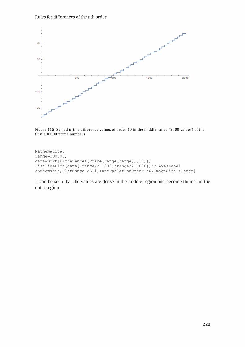
Rules for differences of the nth order
220
Figure 115. Sorted prime difference values of order 10 in the middle range (2000 values) of the first 100000 prime numbers
Mathematica:
range=100000;
data=Sort[Differences[Prime[Range[range]],10]];
ListLinePlot[data[[range/2-1000;;range/2+1000]]/2,AxesLabel-
>Automatic,PlotRange->All,InterpolationOrder->0,ImageSize->Large]
It can be seen that the values are dense in the middle region and become thinner in the
outer region.
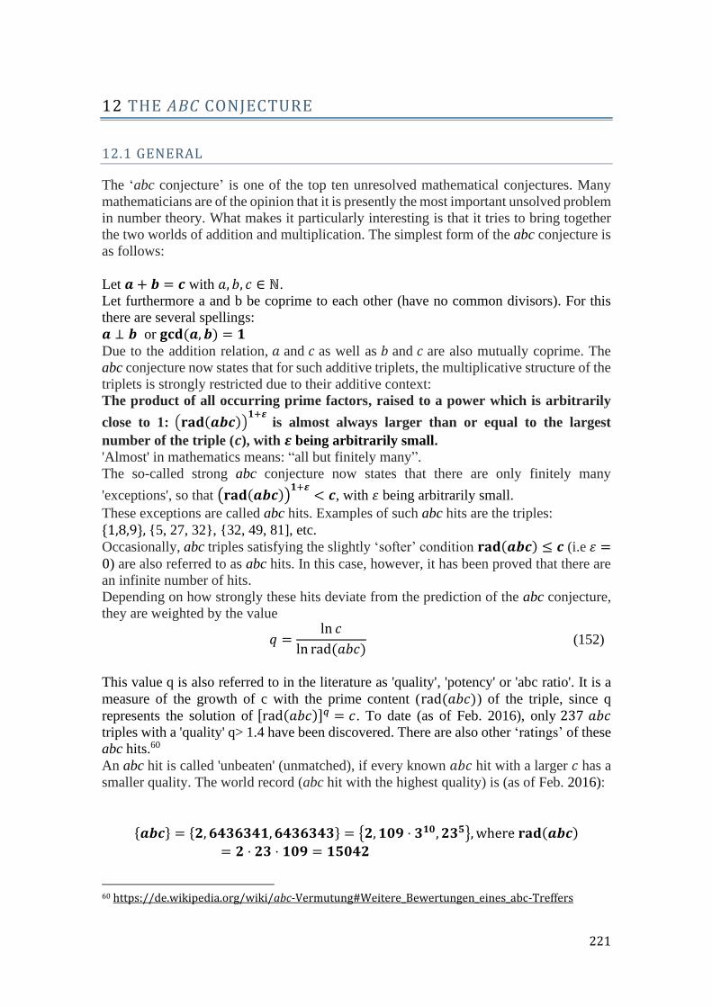
221
12 THE ABC CONJECTURE
12.1 GENERAL
The ‘abc conjecture’ is one of the top ten unresolved mathematical conjectures. Many
mathematicians are of the opinion that it is presently the most important unsolved problem
in number theory. What makes it particularly interesting is that it tries to bring together
the two worlds of addition and multiplication. The simplest form of the abc conjecture is
as follows:
Let 𝒂 + 𝒃 = 𝒄 with 𝑎, 𝑏, 𝑐 ∈ ℕ.
Let furthermore a and b be coprime to each other (have no common divisors). For this
there are several spellings:
𝒂 ⊥ 𝒃 or 𝐠𝐜𝐝(𝒂, 𝒃) = 𝟏
Due to the addition relation, 𝑎 and 𝑐 as well as 𝑏 and 𝑐 are also mutually coprime. The
abc conjecture now states that for such additive triplets, the multiplicative structure of the
triplets is strongly restricted due to their additive context:
The product of all occurring prime factors, raised to a power which is arbitrarily
close to 1: (𝐫𝐚𝐝(𝒂𝒃𝒄))𝟏+𝜺
is almost always larger than or equal to the largest
number of the triple (𝒄), with 𝜺 being arbitrarily small.
'Almost' in mathematics means: “all but finitely many”.
The so-called strong abc conjecture now states that there are only finitely many
'exceptions', so that (𝐫𝐚𝐝(𝒂𝒃𝒄))𝟏+𝜺
< 𝒄, with 휀 being arbitrarily small.
These exceptions are called abc hits. Examples of such abc hits are the triples:
{1,8,9}, {5, 27, 32}, {32, 49, 81], etc.
Occasionally, abc triples satisfying the slightly ‘softer’ condition 𝐫𝐚𝐝(𝒂𝒃𝒄) ≤ 𝒄 (i.e 휀 =0) are also referred to as abc hits. In this case, however, it has been proved that there are
an infinite number of hits.
Depending on how strongly these hits deviate from the prediction of the abc conjecture,
they are weighted by the value
𝑞 =ln 𝑐
ln rad(𝑎𝑏𝑐) (152)
This value q is also referred to in the literature as 'quality', 'potency' or 'abc ratio'. It is a
measure of the growth of c with the prime content (rad(𝑎𝑏𝑐)) of the triple, since q
represents the solution of [rad(𝑎𝑏𝑐)]𝑞 = 𝑐. To date (as of Feb. 2016), only 237 𝑎𝑏𝑐 triples with a 'quality' q> 1.4 have been discovered. There are also other ‘ratings’ of these
abc hits.60
An abc hit is called 'unbeaten' (unmatched), if every known 𝑎𝑏𝑐 hit with a larger 𝑐 has a
smaller quality. The world record (abc hit with the highest quality) is (as of Feb. 2016):
{𝒂𝒃𝒄} = {𝟐, 𝟔𝟒𝟑𝟔𝟑𝟒𝟏, 𝟔𝟒𝟑𝟔𝟑𝟒𝟑} = {𝟐, 𝟏𝟎𝟗 ⋅ 𝟑𝟏𝟎, 𝟐𝟑𝟓}, where 𝐫𝐚𝐝(𝒂𝒃𝒄)
= 𝟐 ⋅ 𝟐𝟑 ⋅ 𝟏𝟎𝟗 = 𝟏𝟓𝟎𝟒𝟐
60 https://de.wikipedia.org/wiki/abc-Vermutung#Weitere_Bewertungen_eines_abc-Treffers

General
222
If the abc hypothesis were to be correct, a whole series of important numerical theorems
would follow from its proof (for example, the proof of the famous Fermat hypothesis
would be reduced to a few lines).
The Japanese Shinichi Mochizuki published back in 2012 a proof of the abc conjecture.
The status of his proof within the mathematical community is still undecided. The proof
(which runs to 500 pages) is very difficult to understand – even for specialists in this
field61. The comments of mathematicians on his proof range from 'paper from the future'
to 'extraterrestrial'. Here is another mathematically precise formulation of the abc
conjecture:
For any arbitrarily small 휀 > 0, there exists a constant 𝐶𝜀 such that for any arbitrary triple
of natural numbers 𝑎, 𝑏, 𝑐 that are mutually coprime to each other, satisfying the equation
𝒂 + 𝒃 = 𝒄, the following inequality holds (abc conjecture):
𝐦𝐚𝐱(𝒂, 𝒃, 𝒄) ≤ 𝑪𝜺 ∏ 𝒑𝟏+𝜺
𝒑|𝒂𝒃𝒄
(153)
Note: (as of Feb. 2016) 33.18 million abc hits are known. There are only about 5
mathematicians anywhere in the world who can claim to have read the entire proof
including all the papers of Mochizuki.62
Here are a few graphic representations (created using the following Mathematica
program):
Mathematica:
rad[n_]:=Times@@First/@FactorInteger[n];
isABC[a_,b_,c_]:=(If[a+b!=c||GCD[a,b]!=1,Return[0]];r=rad[a*b*c];If[r<
c,Return[1],Return[0]]);
isC[c_]:=(For[a=1,a<=Floor[c/2],a++,If[isABC[a,c-
a,c]!=0,Return[1]]];Return[0]);
tab=Select[Range[10000],isC[#]==1&]
ListLinePlot[tab,InterpolationOrder->0,PlotStyle->Black,PlotLabel-
>"abc-conjecture: possible c-values"]
61 http://www.nature.com/news/the-biggest-mystery-in-mathematics-shinichi-mochizuki-and-the-impenetrable-proof-1.18509 62 https://en.wikipedia.org/wiki/abc_conjecture
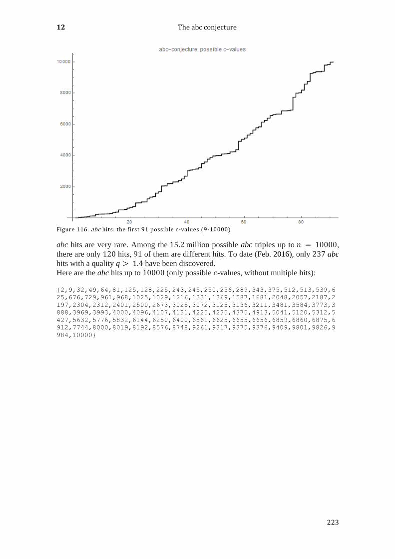
12 The abc conjecture
223
Figure 116. abc hits: the first 91 possible c-values (9-10000)
abc hits are very rare. Among the 15.2 million possible abc triples up to 𝑛 = 10000,
there are only 120 hits, 91 of them are different hits. To date (Feb. 2016), only 237 abc
hits with a quality 𝑞 > 1.4 have been discovered.
Here are the abc hits up to 10000 (only possible 𝑐-values, without multiple hits):
{2,9,32,49,64,81,125,128,225,243,245,250,256,289,343,375,512,513,539,6
25,676,729,961,968,1025,1029,1216,1331,1369,1587,1681,2048,2057,2187,2
197,2304,2312,2401,2500,2673,3025,3072,3125,3136,3211,3481,3584,3773,3
888,3969,3993,4000,4096,4107,4131,4225,4235,4375,4913,5041,5120,5312,5
427,5632,5776,5832,6144,6250,6400,6561,6625,6655,6656,6859,6860,6875,6
912,7744,8000,8019,8192,8576,8748,9261,9317,9375,9376,9409,9801,9826,9
984,10000}

General
224
Figure 117. abc hits: the first 868 possible c- values (9-1000000)
One can clearly see that the abc hits become rarer with increasing size.
Among the 380 million possible abc triples below 50000, there are 276 abc hits.
Figure 118. Max. ‘ quality’ of abc triples as a function of c (with 138 abc hits) in the range up to 20000

12 The abc conjecture
225
Clearly it can be seen that abc hits are very rare. In the 'non-critical' range with 𝑞 < 1,
clear structures can be seen. One cannot escape the feeling that further surprises are in
store…
The first abc hits in the range up to 2000 together with their qualities (in the case of
multiple abc hits for the same 𝑐, the corresponding maximum quality was taken) are:
{{2,1.},{9,1.22629},{32,1.01898},{49,1.04124},{64,1.11269},{81,1.29203},{125,1
.0272},{128,1.42657},{225,1.0129},{243,1.3111},{245,1.02883},{250,1.03261},{25
6,1.27279},{289,1.22518},{343,1.09175},{375,1.10844},{512,1.19875},{513,1.3175
7},{539,1.02512},{625,1.20397},{676,1.09219},{729,1.13667},{961,1.0048},{968,1
.03443},{1025,1.1523},{1029,1.29721},{1216,1.1194},{1331,1.24048},{1369,1.0299
1},{1587,1.00607},{1681,1.04391}}
Mathematica program: please contact the author.
12.2 THE ABC CONJECTURE AND GOCRONS: IS THERE A CONNECTION?
The abc conjecture creates a connection between the world of addition and the world of
multiplication, in that it predicts that additive operations also have a certain influence on
the multiplicative structures of the objects under consideration. What could be more
natural, then, than to investigate the abc conjecture with objects that perfectly represent
multiplicative properties: the OCRONs and GOCRONs (see 10.2.2)? We shall restrict
ourselves here to type 4 OCRONs and their extensions (EOCRONs). Since we want to
make quantitative statements, we are not using character strings (that is, OCRONs), but
their ‘Gödel numbered’ relatives: GOCRONs.
First let’s take a look at our additive structure:
We look for the set of all natural numbers 𝑎 and 𝑏, the sum of which gives a fixed value
𝒂 + 𝒃 = 𝒄, 𝒂, 𝒃 ≥ 𝟏 𝐚𝐧𝐝 𝒂, 𝒃, < 𝒄 and especially their GOCRON4 values
𝑔(𝑎), 𝑔(𝑏) 𝑎𝑛𝑑 𝑔(𝑐) , for example 𝑔(𝑎) = nToEGOCRON4(𝑎) (using the function
nToEGOCRON4() from the OCRON Mathematica library, which can be found in the
Appendix). We shall also investigate the influence of the additional boundary condition
of the abc conjecture that 𝑎 and 𝑏 are to be mutually 'coprime' (i.e. have no common
divisor).
We interpret the values {𝑔(𝑎), 𝑔(𝑏)} as points in the plane, and assign to them a function
value 𝑓[𝑔(𝑎), 𝑔(𝑏)] that forces the whole thing to take on a multiplicative structure
𝑓[𝑔(𝑎), 𝑔(𝑏)] = 𝑔(𝑎 ⋅ 𝑏).
Since GOCRON values can become very large quickly, we prefer logarithmic values
(which are better suited to the material in question). Thus, our task can be precisely
described as follows. We will search for a set of integer abc triples in which an additive
structure exists between 𝑎 and 𝑏, but a multiplicative value is assigned to the third value:
𝑴𝒂𝒃𝒄 = {𝐥𝐧𝒈(𝒂), 𝐥𝐧𝒈(𝒃), 𝐥𝐧𝒈(𝒂⋅ 𝒃)},𝐰𝐡𝐞𝐫𝐞 𝒈(𝒙): 𝐠𝐨𝐞𝐝𝐞𝐥𝐜𝐨𝐝𝐞𝐬 𝐨𝐟 𝐭𝐡𝐞 𝐎𝐂𝐑𝐎𝐍𝐬
𝐚𝐬 𝐰𝐞𝐥𝐥 𝐚𝐬 𝐭𝐡𝐞 𝐛𝐨𝐮𝐧𝐝𝐚𝐫𝐲 𝐜𝐨𝐧𝐝𝐢𝐭𝐢𝐨𝐧: 𝒂 + 𝒃 = 𝒄 𝐚𝐧𝐝 𝒂 ⊥ 𝒃
(154)
The abc conjecture and GOCRONs: is there a connection?
226
If we look at the structure of the set 𝑀𝑎𝑏𝑐, then we get a surprise, because the three-
dimensional points of 𝑀𝑎𝑏𝑐 all lie (with a deviation of about 2 to 3%) on a plane with the
incredibly simple equation 𝑧 = 𝑥 + 𝑦 + const, where the value const depends only on 𝑐!
𝑴𝒂𝒃𝒄 can be represented approximately by: z=x+y+const (155)
This seems to apply to all 𝑐 ∈ ℕ (the author has not yet found a counterexample). If the
boundary condition 𝒂 ⊥ 𝒃 is omitted, then 𝑴𝒂𝒃𝒄 does not lie on a plane for any integer 𝑐. The structures seem to be much more complicated for this general case. For the case
where 𝑐 is a prime number, 𝑴𝒂𝒃𝒄 likewise forms a plane, even if we omit the boundary
condition a⊥b, since this condition is then automatically fulfilled (the two summands of
a prime number are automatically coprime with each other).
Unfortunately, the points of 𝑴𝒂𝒃𝒄 are not exactly on a plane, but exhibit around 2 to 3
per cent ‘noise’. If the relation applied exactly, then we would have found a method of
calculating the factorization of a number (in our case 𝑐) from the values 𝑎 and 𝑏 (or
ln𝑔(𝑎), ln𝑔(𝑏) respectively). Conversely, the factorization could be calculated solely
from 𝑐, by a projection of 𝑐 onto the 𝑥 − 𝑦 axis). In general, one could also imagine a
method that searched only by evaluating the plane equation by integer values 𝑎 and 𝑏,
since the determination of 𝑔 (𝑎) and 𝑔 (𝑏) can demand a great deal of computing time
for large 𝑎 and 𝑏.
One assumes that if we were to choose a different, more suitable, GOCRON system (the
calculation and the Gödel numbering allow a degree of ‘freedom of choice’ in the
selection of parameters), the noise described could be reduced or even eliminated
altogether. There is still much work to do here!
Here are a few plots of different sets of 𝑴𝒂𝒃𝒄:

12 The abc conjecture
227
Figure 119. 𝑀𝑎𝑏𝑐: logarithmic Gödel GOCRON4 codes of abc points . C=10007 (prime number), a and b are coprime (different views).
Note: the plot in Figure 119 does not change if we omit the boundary condition 𝑎 ⊥ 𝑏,
because 1007 is a prime number.
Mathematica program: please contact the author.
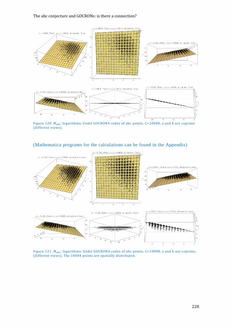
The abc conjecture and GOCRONs: is there a connection?
228
Figure 120. 𝑀𝑎𝑏𝑐: logarithmic Gödel GOCRON4 codes of abc points. C=10008, a and b are coprime (different views).
(Mathematica programs for the calculations can be found in the Appendix)
Figure 121. 𝑀𝑎𝑏𝑐: logarithmic Gödel GOCRON4 codes of abc points. C=10008, a and b not coprime, (different views). The 10004 points are spatially distributed.

12 The abc conjecture
229
Figure 122. 𝑀𝑎𝑏𝑐: logarithmic Gödel GOCRON4 codes of abc points. C=100002, a and b not coprime, (different views). The 99998 points are spatially distributed.
Figure 123. 𝑀𝑎𝑏𝑐: logarithmic Gödel GOCRON4 codes of abc points . C=100002, a and b coprime (different views). The 28558 points lie approximately on a plane.
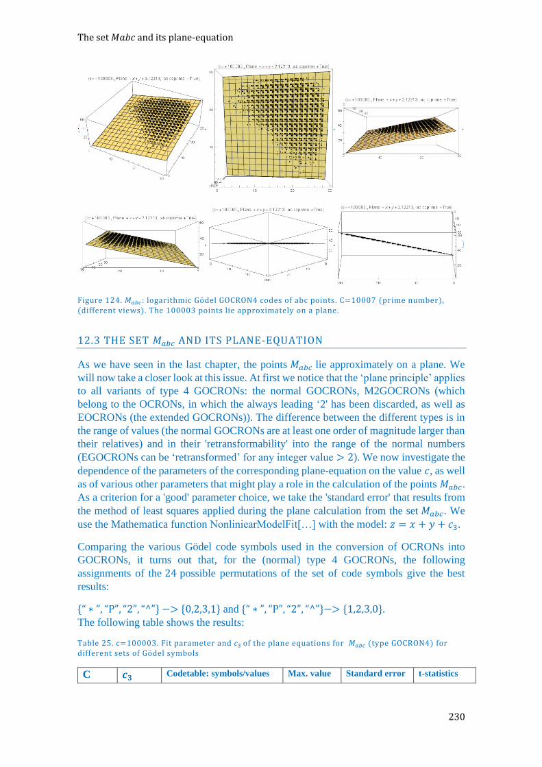
The set 𝑀𝑎𝑏𝑐 and its plane-equation
230
Figure 124. 𝑀𝑎𝑏𝑐: logarithmic Gödel GOCRON4 codes of abc points . C=10007 (prime number), (different views). The 100003 points lie approximately on a plane.
12.3 THE SET 𝑀𝑎𝑏𝑐 AND ITS PLANE-EQUATION
As we have seen in the last chapter, the points 𝑀𝑎𝑏𝑐 lie approximately on a plane. We
will now take a closer look at this issue. At first we notice that the ‘plane principle’ applies
to all variants of type 4 GOCRONs: the normal GOCRONs, M2GOCRONs (which
belong to the OCRONs, in which the always leading ‘2' has been discarded, as well as
EOCRONs (the extended GOCRONs)). The difference between the different types is in
the range of values (the normal GOCRONs are at least one order of magnitude larger than
their relatives) and in their 'retransformability' into the range of the normal numbers
(EGOCRONs can be ‘retransformed’ for any integer value > 2). We now investigate the
dependence of the parameters of the corresponding plane-equation on the value 𝑐, as well
as of various other parameters that might play a role in the calculation of the points 𝑀𝑎𝑏𝑐. As a criterion for a 'good' parameter choice, we take the 'standard error' that results from
the method of least squares applied during the plane calculation from the set 𝑀𝑎𝑏𝑐. We
use the Mathematica function NonliniearModelFit[…] with the model: 𝑧 = 𝑥 + 𝑦 + 𝑐3.
Comparing the various Gödel code symbols used in the conversion of OCRONs into
GOCRONs, it turns out that, for the (normal) type 4 GOCRONs, the following
assignments of the 24 possible permutations of the set of code symbols give the best
results:
{“ ∗ ”, “P”, “2”, “^”} −> {0,2,3,1} and {“ ∗ ”, “P”, “2”, “^”}−> {1,2,3,0}. The following table shows the results:
Table 25. c=100003. Fit parameter and 𝑐3 of the plane equations for 𝑀𝑎𝑏𝑐 (type GOCRON4) for different sets of Gödel symbols
C 𝒄𝟑 Codetable: symbols/values Max. value Standard error t-statistics

12 The abc conjecture
231
100003 1.85733 1:{*,P,2,^},{0,1,2,3} 37.0455 0.000162446 11433.5
100003 1.48688 2:{*,P,2,^},{0,1,3,2} 37.4114 0.000186537 7970.96
100003 2.34062 3:{*,P,2,^},{0,2,1,3} 36.423 0.000200917 11649.7
100003 1.44022 4:{*,P,2,^},{0,2,3,1} 37.3964 0.0000736448 19556.3
100003 2.24673 5:{*,P,2,^},{0,3,1,2} 36.3821 0.000422527 5317.36
100003 1.73226 6:{*,P,2,^},{0,3,2,1} 37.0015 0.000153876 11257.5
100003 1.93765 7:{*,P,2,^},{1,0,2,3} 37.0444 0.000332613 5825.54
100003 1.54166 8:{*,P,2,^},{1,0,3,2} 37.4107 0.000303486 5079.82
100003 4.00103 9:{*,P,2,^},{1,2,0,3} 34.4163 0.00246733 1621.61
100003 1.44418 10:{*,P,2,^},{1,2,3,0} 37.3804 0.0000698268 20682.3
100003 3.79035 11:{*,P,2,^},{1,3,0,2} 34.4462 0.00303396 1249.31
100003 1.738 12:{*,P,2,^},{1,3,2,0} 36.9777 0.000172422 10079.9
100003 2.61489 13:{*,P,2,^},{2,0,1,3} 36.4189 0.000393053 6652.77
100003 1.54569 14:{*,P,2,^},{2,0,3,1} 37.3949 0.000294348 5251.23
100003 4.50595 15:{*,P,2,^},{2,1,0,3} 34.4009 0.00207401 2172.57
100003 1.49486 16:{*,P,2,^},{2,1,3,0} 37.3796 0.000170018 8792.37
100003 3.93228 17:{*,P,2,^},{2,3,0,1} 34.4473 0.00352994 1113.98
100003 2.26812 18:{*,P,2,^},{2,3,1,0} 36.2903 0.000484516 4681.22
100003 2.62617 19:{*,P,2,^},{3,0,1,2} 36.3757 0.00036176 7259.43
100003 1.94952 20:{*,P,2,^},{3,0,2,1} 36.9981 0.000303674 6419.8
100003 4.62145 21:{*,P,2,^},{3,1,0,2} 34.018 0.00222471 2077.33
100003 1.87489 22:{*,P,2,^},{3,1,2,0} 36.9753 0.000122802 15267.6
100003 4.25883 23:{*,P,2,^},{3,2,0,1} 34.0449 0.00320799 1327.57
100003 2.37305 24:{*,P,2,^},{3,2,1,0} 36.288 0.000280365 8464.13
Further tables with different methods of Gödelization and different values of 𝑐 can be
found in the Appendix.
An evaluation of these tables shows that code table No. 10 is (albeit narrowly) the 'winner'
(with regard to the smallest standard error), if the summation of the OCRONs is
performed in the normal order (left to right). In the case of the reverse order, the selection
of a best Gödel code set is not so clear. In the following, we will use the Gödel code
assignment {'*', 'P', '2', '^' -> {1, 2, 3, 0} for all OCRON4 types and the normal order of
symbols (not 'reversed').
The program used for the evaluation can be found in the Appendix.
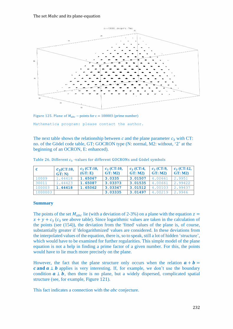
The set 𝑀𝑎𝑏𝑐 and its plane-equation
232
Figure 125. Plane of 𝑀𝑎𝑏𝑐 − points for c = 100003 (prime number)
Mathematica program: please contact the author.
The next table shows the relationship between 𝑐 and the plane parameter 𝑐3 with CT:
no. of the Gödel code table, GT: GOCRON type (N: normal, M2: without, ‘2’ at the
beginning of an OCRON, E: enhanced).
Table 26. Different 𝑐3 -values for different GOCRONs and Gödel symbols
c 𝒄𝟑(CT:10,
GT: N)
𝒄𝟑 (CT:10,
(GT: E)
𝒄𝟑 (CT:10,
GT: M2)
𝒄𝟑 (CT:4,
GT: M2) 𝒄𝟑 (CT:9,
GT: M2)
𝒄𝟑 (CT:12,
GT: M2)
10009 1.44418 1.65067 3.0335 3.01507 4.00661 2.9951
30011 1.44423 1.65087 3.03373 3.01535 4.00661 2.99422
100003 1.44418 1.65062 3.03347 3.01512 4.00103 2.99437
1000003 3.03335 3.01497 4.00219 2.9946
Summary
The points of the set 𝑀𝑎𝑏𝑐 lie (with a deviation of 2-3%) on a plane with the equation 𝑧 =𝑥 + 𝑦 + 𝑐3 (𝑐3 see above table). Since logarithmic values are taken in the calculation of
the points (see (154)), the deviation from the 'fitted' values of the plane is, of course,
substantially greater if 'delogarithmized' values are considered. In these deviations from
the interpolated values of the equation, there is, so to speak, still a lot of hidden ‘structure’,
which would have to be examined for further regularities. This simple model of the plane
equation is not a help in finding a prime factor of a given number. For this, the points
would have to lie much more precisely on the plane.
However, the fact that the plane structure only occurs when the relation 𝒂 + 𝒃 =𝒄 𝐚𝐧𝐝 𝒂 ⊥ 𝒃 applies is very interesting. If, for example, we don’t use the boundary
condition 𝒂 ⊥ 𝒃, then there is no plane, but a widely dispersed, complicated spatial
structure (see, for example, Figure 121).
This fact indicates a connection with the abc conjecture.
12 The abc conjecture
233

234
13 PRIME NUMBERS IN THE NATURAL SCIENCES
13.1 PRIME NUMBERS IN DNA CODE
Many scientists think that primes also play a role in the construction and design of DNA
sequences. Everyone knows the famous double helix of the DNA. Here are a few
arbitrarily selected examples:
Mathematica:
Import[#,"PDB"]&/@{"http://files.rcsb.org/download/1BNA.pdb","http://f
iles.rcsb.org/download/208D.pdb","http://files.rcsb.org/download/5A0W.
pdb"}
The following text is essentially the work of J.F. Yan, A.K. Yan and B.C. Yan.63
Before dealing with the underlying idea, it is useful to look at a few basic properties of
DNA and RNA.
DNA is the carrier of the genetic information that is present in the cell nuclei of all living
beings. These are huge chain molecules, which are composed of four different basic
building blocks: the nucleotides. Each nucleotide consists of a phosphate group, a sugar
(deoxyribose) and one of four possible organic bases (adenine, guanine, cytosine and
thymine).
The RNA (ribonucleic acid) is constructed by means of the information in the DNA. For
the exact mechanism, the reader is referred to the relevant literature64. The RNA (in a
similar way to the DNA) is composed of nucleotides, which in turn are composed of four
different organic bases (adenine, guanine, cytosine and uracil).
63 J. theor. Biol. (11991) 151,333-341 64 e.g. http://www.dna50.org/
13 Prime numbers in the natural sciences
235
The first three bases are present in the RNA and in the DNA; the base thymine occurs
only in the DNA and uracil only in the RNA.
The organic bases are usually abbreviated by the letters A, G, C, T and U. These are the
smallest information bits of DNA and RNA. The differences in the structure of RNA and
DNA (uracil instead of thymine) are irrelevant to the information content we are
considering. Therefore, for the sake of simplicity, we will only use the four bases A, G,
C, and U (whereas, strictly speaking, it should be ‘T’ instead of ‘U’ in the case of the
DNA).
Each successive triplet of bases (also called a ‘codon’) is specifically assigned to a
particular amino acid. The converse is not true: several different triplets may be assigned
to the same amino acid. These triplets are the smallest information units of DNA and
RNA. A few triplets (codons) contain no genetic information. However, they work as so-
called ‘stop’ triplets during replication and copying processes that take place during
protein synthesis. There are also start-up triplets, which, however, also contain
information: e.g. the triplet ‘AUG’ (methionine amino acid).
For the four different bases there are 43 = 64 different possibilities for triplet formation.
The amino acids occurring practically in nature (canonical, proteinogenic amino acids)
are coded with the aid of 61 triplets. The three remaining triplets are 'stop' triplets. A very
good representation can be found on the Internet.65 Some amino acids are encoded only
by one triplet, some by 2,3, 4 or 6 different triplets. Note: the number 5 is absent as the
number of amino acid forming triplets.
What does all this have to do with primes? How do we get from base triplets to numbers?
The answer is similar to that in Chapter 10.2.2.4: by 'Gödelization'. We assign a numerical
value to each base triplet (our smallest information unit). There are several possibilities
for this:
Klaus Lange used in his work, Primes in the construction of the DNS 66
G = 1, A = 3, C = 7, U = 9 and builds the number codes simply by using the decimal
system. An example: alanine (= GCA with the code value 173).
He then examines the resulting numerical values for their prime factor decomposition and
discovers that at least 19 of the 20 canonical amino acids contain a triplet that represents
a prime number. It is striking for him that the only amino acid to which no prime can be
assigned as a triplet is methionine (Met = AUG). According to his system, this triplet has
the value 391. Methionine is the only triplet that works as a so-called 'start signal' (see
above).
This number assignment appears to the author somewhat arbitrary. Better is the method
of Yan (see above), in which A=0, C=1, U=2 and G=3. From this assignment, a unique
set of "nucleotide numbers" (each of which can be assigned to an amino acid) is then
constructed. Special cases are the following amino acids:
65 https://de.wikipedia.org/wiki/Genetischer_Code 66 http://www.primzahlen.de/primzahlen/dns.htm
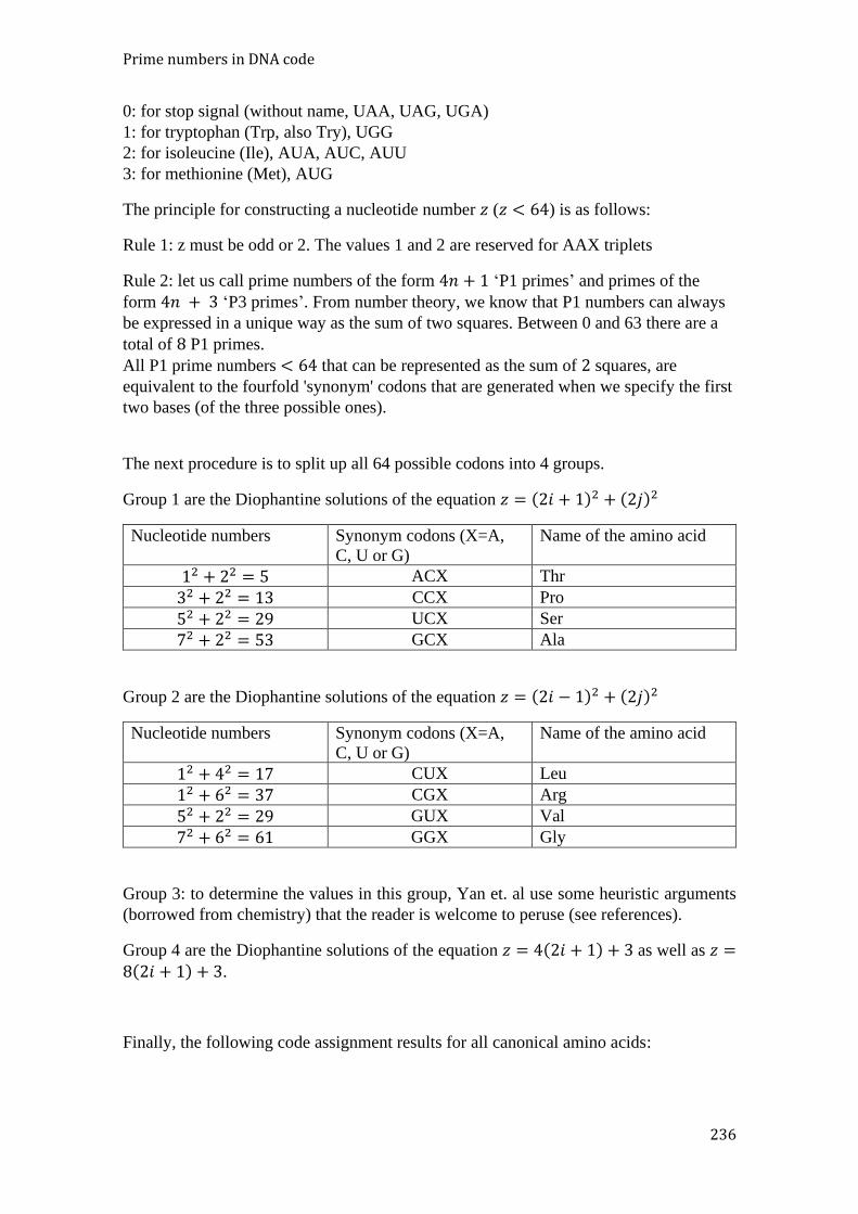
Prime numbers in DNA code
236
0: for stop signal (without name, UAA, UAG, UGA)
1: for tryptophan (Trp, also Try), UGG
2: for isoleucine (Ile), AUA, AUC, AUU
3: for methionine (Met), AUG
The principle for constructing a nucleotide number 𝑧 (𝑧 < 64) is as follows:
Rule 1: z must be odd or 2. The values 1 and 2 are reserved for AAX triplets
Rule 2: let us call prime numbers of the form 4𝑛 + 1 ‘P1 primes’ and primes of the
form 4𝑛 + 3 ‘P3 primes’. From number theory, we know that P1 numbers can always
be expressed in a unique way as the sum of two squares. Between 0 and 63 there are a
total of 8 P1 primes.
All P1 prime numbers < 64 that can be represented as the sum of 2 squares, are
equivalent to the fourfold 'synonym' codons that are generated when we specify the first
two bases (of the three possible ones).
The next procedure is to split up all 64 possible codons into 4 groups.
Group 1 are the Diophantine solutions of the equation 𝑧 = (2𝑖 + 1)2 + (2𝑗)2
Nucleotide numbers Synonym codons (X=A,
C, U or G)
Name of the amino acid
12 + 22 = 5 ACX Thr
32 + 22 = 13 CCX Pro
52 + 22 = 29 UCX Ser
72 + 22 = 53 GCX Ala
Group 2 are the Diophantine solutions of the equation 𝑧 = (2𝑖 − 1)2 + (2𝑗)2
Nucleotide numbers Synonym codons (X=A,
C, U or G)
Name of the amino acid
12 + 42 = 17 CUX Leu
12 + 62 = 37 CGX Arg
52 + 22 = 29 GUX Val
72 + 62 = 61 GGX Gly
Group 3: to determine the values in this group, Yan et. al use some heuristic arguments
(borrowed from chemistry) that the reader is welcome to peruse (see references).
Group 4 are the Diophantine solutions of the equation 𝑧 = 4(2𝑖 + 1) + 3 as well as 𝑧 =8(2𝑖 + 1) + 3.
Finally, the following code assignment results for all canonical amino acids:
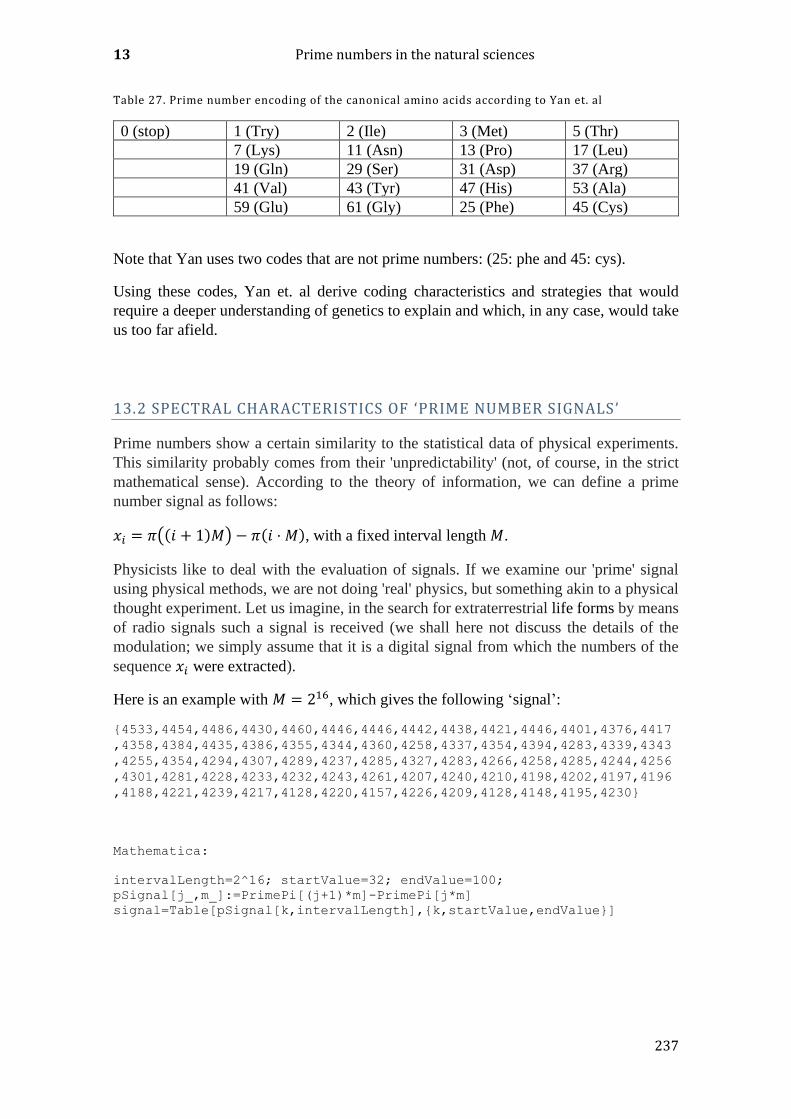
13 Prime numbers in the natural sciences
237
Table 27. Prime number encoding of the canonical amino acids according to Yan et. al
0 (stop) 1 (Try) 2 (Ile) 3 (Met) 5 (Thr)
7 (Lys) 11 (Asn) 13 (Pro) 17 (Leu)
19 (Gln) 29 (Ser) 31 (Asp) 37 (Arg)
41 (Val) 43 (Tyr) 47 (His) 53 (Ala)
59 (Glu) 61 (Gly) 25 (Phe) 45 (Cys)
Note that Yan uses two codes that are not prime numbers: (25: phe and 45: cys).
Using these codes, Yan et. al derive coding characteristics and strategies that would
require a deeper understanding of genetics to explain and which, in any case, would take
us too far afield.
13.2 SPECTRAL CHARACTERISTICS OF ‘PRIME NUMBER SIGNALS ’
Prime numbers show a certain similarity to the statistical data of physical experiments.
This similarity probably comes from their 'unpredictability' (not, of course, in the strict
mathematical sense). According to the theory of information, we can define a prime
number signal as follows:
𝑥𝑖 = 𝜋((𝑖 + 1)𝑀) − 𝜋(𝑖 ⋅ 𝑀), with a fixed interval length 𝑀.
Physicists like to deal with the evaluation of signals. If we examine our 'prime' signal
using physical methods, we are not doing 'real' physics, but something akin to a physical
thought experiment. Let us imagine, in the search for extraterrestrial life forms by means
of radio signals such a signal is received (we shall here not discuss the details of the
modulation; we simply assume that it is a digital signal from which the numbers of the
sequence 𝑥𝑖 were extracted).
Here is an example with 𝑀 = 216, which gives the following ‘signal’:
{4533,4454,4486,4430,4460,4446,4446,4442,4438,4421,4446,4401,4376,4417
,4358,4384,4435,4386,4355,4344,4360,4258,4337,4354,4394,4283,4339,4343
,4255,4354,4294,4307,4289,4237,4285,4327,4283,4266,4258,4285,4244,4256
,4301,4281,4228,4233,4232,4243,4261,4207,4240,4210,4198,4202,4197,4196
,4188,4221,4239,4217,4128,4220,4157,4226,4209,4128,4148,4195,4230}
Mathematica:
intervalLength=2^16; startValue=32; endValue=100;
pSignal[j_,m_]:=PrimePi[(j+1)*m]-PrimePi[j*m]
signal=Table[pSignal[k,intervalLength],{k,startValue,endValue}]
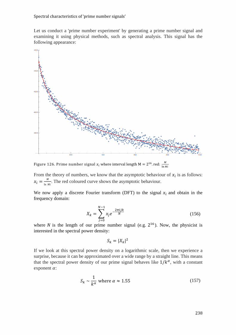
Spectral characteristics of ‘prime number signals’
238
Let us conduct a 'prime number experiment' by generating a prime number signal and
examining it using physical methods, such as spectral analysis. This signal has the
following appearance:
Figure 126. Prime number signal 𝑥𝑖 where interval length M = 216. red:
𝑀
ln𝑀𝑖
From the theory of numbers, we know that the asymptotic behaviour of 𝑥𝑖 is as follows:
𝑥𝑖 =𝑀
ln 𝑀𝑖 . The red coloured curve shows the asymptotic behaviour.
We now apply a discrete Fourier transform (DFT) to the signal 𝑥𝑖 and obtain in the
frequency domain:
𝑋𝑘 = ∑ 𝑥𝑗𝑒−2𝜋𝑖𝑗𝑘𝑁
𝑁−1
𝑗=0
(156)
where 𝑁 is the length of our prime number signal (e.g. 216 ). Now, the physicist is
interested in the spectral power density:
𝑆𝑘 = |𝑋𝑘|2
If we look at this spectral power density on a logarithmic scale, then we experience a
surprise, because it can be approximated over a wide range by a straight line. This means
that the spectral power density of our prime signal behaves like 1/𝑘𝛼, with a constant
exponent 𝛼:
𝑆𝑘 ∼1
𝑘𝛼 where 𝛼 ≈ 1.55 (157)
13 Prime numbers in the natural sciences
239
The value 𝛼 ≈ 1.64 is given in the literature.67 Computations performed by the author
lead to an approximate value of 1.55.
This behaviour is well known to physicists for a group of physical systems, namely, those
that are in a so-called ‘self-organized’ critical state. Many other physical systems also
exhibit spectral behaviour according to the 1
𝑘𝛼 law: for example voltage noise in electronic
components (flicker noise).
There are also studies of the statistical behaviour of notes (within our 12-step tonal
musical system) that show a statistical 1/f-behaviour for traditionally composed (non-
random music). Thus, we have established an (albeit remote) connection between primes
and tonal music!
Here is a plot of the spectral power density of a prime number signal:
Figure 127. Spectral power density of a prime number signal (red : 1𝑘𝛼 where 𝛼 = 1.55)
Mathematica program: please contact the author.
67 Marek Wolf: PHYSICA A: Statistical mechanics and its applications ·January 1997, pp. 493-499
240
14 PRIME NUMBERS AND ONLINE BANKING
14.1 RSA ENCRYPTION
Prime numbers entered the field of cryptography, the 'science of deciphering', some time
ago. In online banking, highly confidential data are constantly being sent back and forth.
The number of transactions is so huge that a symmetrical encryption (where both partners
have a secret key) would not be feasible, as the secret key would have to be sent on a
secure transmission path (e.g. by post) prior to the actual transaction. This is basically
impossible. There is, however, a procedure that avoids the complicated sending of keys
by post: this is known as ‘asymmetrical RSA encryption’.
We will briefly describe the RSA method first. 'RSA' stands for Rivest, Shamir and
Adleman, the trio of computer scientists who first implemented the procedure in 1978.
The original idea, however, was described by Diffie and Hellman in 1976. This
encryption method is called ‘asynchronous’ because the sender and receiver of encrypted
messages use different keys (which are public and secret). The sender uses a public key
to encrypt and send, and the recipient uses a top secret private key to receive and decrypt
the message. In order for the sender to send such encrypted messages to a receiver, the
receiver must first generate a public (non-secret) key and then send it to the sender, who
then uses it to send the message. This sending of the public key can, of course, take place
in an unencrypted manner.
Since texts are to be encrypted, we do not look at the individual characters, but their
ASCII codes.68 These assign each character a value from 32 (space) to 90 (‘Z’), where 65
= ‘A’, 66 = ‘B’ etc. Lower case letters are represented by highter numbers but this is
irrelevant to an understanding of the procedure.
The text to be encrypted is first translated into a long sequence of digits of these codes
using the ASCII code. Thereafter, blocks of a fixed length (e.g. of length 64) are formed
from this sequence of numbers. Each of these blocks is now interpreted as a (in this case,
64-digit) number in a numeral system with base 256. The formation of blocks takes place
only for reasons of manageability in order to avoid overlarge "numerical monsters". The
choice of the base is not important and this can even be smaller if we use a smaller
character set.
It is important to understand that we have converted our text into a sequence of very, very
large numbers (e.g. 50-digit numbers). It is also possible to use a single block for the
whole message. In this case, the original message text to be encrypted consists only of a
single (admittedly gigantic) number that we will call 𝑚 (= 'message'). The number
contains all our text. So far it is very easy to restore our original text from 𝑚.
Encryption is now coming into play. To recap: the sender has the public key that he has
received from the recipient. Only the recipient has the secret private key (which has been
created simultaneously with the public key at the recipient’s end).
68 ASCII: ‘American Standard Code for Information Interchange’

14 Prime numbers and online banking
241
Now we come to the details. The private and public keys are generated as follows: we are
looking for two different, very large prime numbers (typically hundreds of digits long).
Primes of this size can be generated using simple mathematical methods, such as
probabilistic prime number tests, the Fermat prime number test, the Miller-Selfridge-
Rabin test, the APRCL test or the Solovay-Strassen test (the algorithms are clearly set out
on Wikipedia).
Primes generated with a good probabilistic method are generally referred to as PRP
numbers. They are, as far as it is humanly possible to judge, 'real' primes because the error
probability of such large numbers is astronomically low (typically, for example, 10−100). Although there are also exact methods (with a polynomial run time), these are not suitable
for the generation of very large primes because of their long running time.
Note: the record for the largest currently known (as of May 2016) PRP number is a so-
called Wagstaff prime (see 4.13) and is:
(213372531 + 1)/3 number of decimal digits: 4025533
For comparison, the largest 'general' prime number found using a method valid for any
primes (not primes of a particular form) is (as of 2011):
((((((25210088873 + 80)3 + 12)3 + 450)3 + 894)3 + 3636)3 + 70756)3 + 97220
This number is the 11th Mills prime number and it has 20562 decimal digits.69
It can be seen clearly that for prime numbers of a particular form, primality tests are
available for significantly larger numbers. The Lucas-Lehmer test for Mersenne prime
numbers still provides the largest prime numbers (over 10 million digits). The largest
general prime currently known, with 20562 decimal digits, is rather modest, since it has
about 1000 times fewer decimal digits. Back to the RSA procedure:
The methods for generating large primes suitable for the RSA method are not described
here. Once again, we rely on the Mathematica software, which provides a set of
functions that are used in cryptography:
PowerMod[], PowerModList[], PolynomialMod[], RandomPrime[],
Prime[], PrimeQ[],CoprimeQ[], FactorInteger[],
GenerateAsmmetricKeyPair[], Encrypt[], Decrypt[],
PrivateKey[], PublicKey[]
69 Paulo Ribenboim: Die Welt der Primzahlen (Springer), p. 118
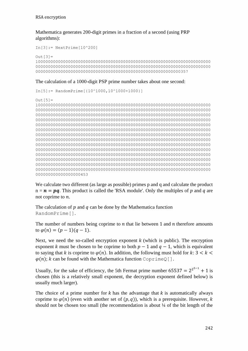
RSA encryption
242
Mathematica generates 200-digit primes in a fraction of a second (using PRP
algorithms):
In[3]:= NextPrime[10^200]
Out[3]=
1000000000000000000000000000000000000000000000000000000000000000000000
0000000000000000000000000000000000000000000000000000000000000000000000
0000000000000000000000000000000000000000000000000000000000357
The calculation of a 1000-digit PSP prime number takes about one second:
In[5]:= RandomPrime[{10^1000,10^1000+1000}]
Out[5]=
1000000000000000000000000000000000000000000000000000000000000000000000
0000000000000000000000000000000000000000000000000000000000000000000000
0000000000000000000000000000000000000000000000000000000000000000000000
0000000000000000000000000000000000000000000000000000000000000000000000
0000000000000000000000000000000000000000000000000000000000000000000000
0000000000000000000000000000000000000000000000000000000000000000000000
0000000000000000000000000000000000000000000000000000000000000000000000
0000000000000000000000000000000000000000000000000000000000000000000000
0000000000000000000000000000000000000000000000000000000000000000000000
0000000000000000000000000000000000000000000000000000000000000000000000
0000000000000000000000000000000000000000000000000000000000000000000000
0000000000000000000000000000000000000000000000000000000000000000000000
0000000000000000000000000000000000000000000000000000000000000000000000
0000000000000000000000000000000000000000000000000000000000000000000000
000000000000000000453
We calculate two different (as large as possible) primes p and q and calculate the product
n = 𝒏 = 𝒑𝒒. This product is called the 'RSA module'. Only the multiples of 𝑝 and 𝑞 are
not coprime to 𝑛.
The calculation of 𝑝 and 𝑞 can be done by the Mathematica function
RandomPrime[].
The number of numbers being coprime to 𝑛 that lie between 1 and 𝑛 therefore amounts
to 𝜑(𝑛) = (𝑝 − 1)(𝑞 − 1).
Next, we need the so-called encryption exponent 𝑘 (which is public). The encryption
exponent 𝑘 must be chosen to be coprime to both 𝑝 − 1 and 𝑞 − 1, which is equivalent
to saying that 𝑘 is coprime to 𝜑(𝑛). In addition, the following must hold for 𝑘: 3 < 𝑘 <𝜑(𝑛); 𝑘 can be found with the Mathematica function CoprimeQ[].
Usually, for the sake of efficiency, the 5th Fermat prime number 65537 = 225−1+ 1 is
chosen (this is a relatively small exponent, the decryption exponent defined below) is
usually much larger).
The choice of a prime number for 𝑘 has the advantage that 𝑘 is automatically always
coprime to 𝜑(𝑛) (even with another set of (𝑝, 𝑞)), which is a prerequisite. However, 𝑘
should not be chosen too small (the recommendation is about ¼ of the bit length of the
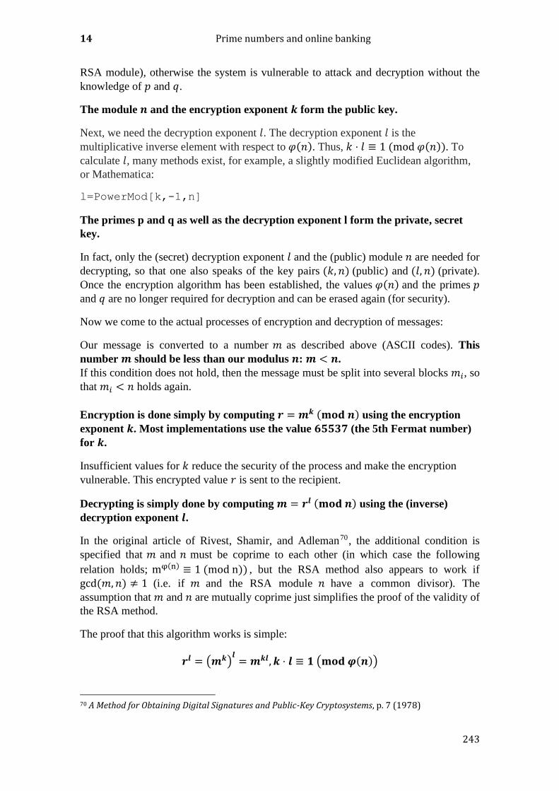
14 Prime numbers and online banking
243
RSA module), otherwise the system is vulnerable to attack and decryption without the
knowledge of 𝑝 and 𝑞.
The module 𝒏 and the encryption exponent 𝒌 form the public key.
Next, we need the decryption exponent 𝑙. The decryption exponent 𝑙 is the
multiplicative inverse element with respect to 𝜑(𝑛). Thus, 𝑘 ⋅ 𝑙 ≡ 1 (mod 𝜑(𝑛)). To
calculate 𝑙, many methods exist, for example, a slightly modified Euclidean algorithm,
or Mathematica:
l=PowerMod[k,-1,n]
The primes p and q as well as the decryption exponent l form the private, secret
key.
In fact, only the (secret) decryption exponent 𝑙 and the (public) module 𝑛 are needed for
decrypting, so that one also speaks of the key pairs (𝑘, 𝑛) (public) and (𝑙, 𝑛) (private).
Once the encryption algorithm has been established, the values 𝜑(𝑛) and the primes 𝑝
and 𝑞 are no longer required for decryption and can be erased again (for security).
Now we come to the actual processes of encryption and decryption of messages:
Our message is converted to a number 𝑚 as described above (ASCII codes). This
number 𝒎 should be less than our modulus 𝒏: 𝒎 < 𝒏.
If this condition does not hold, then the message must be split into several blocks 𝑚𝑖, so
that 𝑚𝑖 < 𝑛 holds again.
Encryption is done simply by computing 𝒓 = 𝒎𝒌 (𝐦𝐨𝐝 𝒏) using the encryption
exponent 𝒌. Most implementations use the value 𝟔𝟓𝟓𝟑𝟕 (the 5th Fermat number)
for 𝒌.
Insufficient values for 𝑘 reduce the security of the process and make the encryption
vulnerable. This encrypted value 𝑟 is sent to the recipient.
Decrypting is simply done by computing 𝒎 = 𝒓𝒍 (𝐦𝐨𝐝 𝒏) using the (inverse)
decryption exponent 𝒍.
In the original article of Rivest, Shamir, and Adleman70 , the additional condition is
specified that 𝑚 and 𝑛 must be coprime to each other (in which case the following
relation holds; mφ(n) ≡ 1 (mod n)) , but the RSA method also appears to work if
gcd(𝑚, 𝑛) ≠ 1 (i.e. if 𝑚 and the RSA module 𝑛 have a common divisor). The
assumption that 𝑚 and 𝑛 are mutually coprime just simplifies the proof of the validity of
the RSA method.
The proof that this algorithm works is simple:
𝒓𝒍 = (𝒎𝒌)𝒍= 𝒎𝒌𝒍, 𝒌 ⋅ 𝒍 ≡ 𝟏 (𝐦𝐨𝐝 𝝋(𝒏))
70 A Method for Obtaining Digital Signatures and Public-Key Cryptosystems, p. 7 (1978)

RSA encryption
244
From this, it follows that there is an integer 𝑠 such that
𝒌 ⋅ 𝒍 = 𝒔 ⋅ 𝝋(𝒏) + 𝟏
A few transformations are sufficient to show that encryption of 𝑚 and subsequent
decryption again yields 𝑚:
rl(mod n) = mkl (mod n)
= ms⋅φ(n)+1 (mod n) = m(mφ(n))s(mod n)
= m (mod n), da mφ(n) ≡ 1 (mod n) = 𝑚
Commonly used methods employ in addition various padding techniques described in the
relevant specifications. Padding means that additional information (possibly also random
elements or information about the length of the text) is attached to the text to be encrypted
in order to increase the security of the method. Common padding methods are e.g.
‘PKCS#1’', ‘OAEP’ (Optimal Asymmetric Encryption Padding), or ‘SSLV23’. PKCS1
and SSLV23 add 11 additional bytes to the data block to be encrypted, the ‘OAEP’
procedures even adds 41 bytes. Further details will not be given here. If the reader wishes
to go into the matter in greater detail, sources from the Internet are recommended.71 The
software Mathematica supports the PKCS1 padding process for encryption and
decryption. Note that for the modified message 𝑚′ it is imperative that 𝒎′ < 𝒏.
71 https://de.wikipedia.org/wiki/RSA-Kryptosystem, http://people.csail.mit.edu/rivest/Rsapaper.pdf, http://www.di-mgt.com.au/rsa_theory.html
245
14.2 THE SECURITY OF THE RSA METHOD
In the practical implementations of the RSA encryption method, some additional features
are built in that make the transfers even more secure. However, the security of the method
is based on the fact that the public key (RSA module) with the number 𝑛 representing the
product of two large prime numbers cannot be decomposed into the two prime factors by
the currently known factorization algorithms. As long as this is impossible, 𝜑(𝑛) and the
decryption exponent 𝑙 cannot be calculated either.
This is where explosives once again are hidden: no one (not even specialists in this field)
can say whether a fast factorization algorithm will be found in the future. A factorization
algorithm that worked in polynomial time would bring about a total collapse in security.
At present (as of May 2016), it is not known whether or not a sufficiently fast algorithm
might exist. This is remarkable because, in other fields, mathematicians have succeeded
in establishing whether or not fast algorithms are possible for solving entire classes of
problems.
In the case of the factorization problem, no such proof has been found, so it is perfectly
conceivable that such an algorithm is out there somewhere waiting to be discovered (see
10.3). Our entire online banking system would (literally) collapse if hackers gained access
to such an algorithm!
Note: a fast method for calculating 𝜑(𝑛) or 𝜎(𝑛) would have the same consequences
(20.9.3.2). However, the calculation methods known to date (as of May 2016) are of the
same complexity as the factorization problem.
Another danger comes from the ever-increasing speed of computer hardware. With the
computer hardware we have now, we can rule out the possibility of keys of the length in
current use being cracked, as the computing time required would equate to the entire age
of the universe. If, however, some day the highly touted quantum computers were to
become a reality (to which end an intensive research effort is underway), these would
pose a threat to the security of RSA encryption. The author is not aware whether the
possibility of increasing the depth of encryption in the RSA algorithm to reduce the risk
of ‘hacking’ by quantum computers is also being investigated …
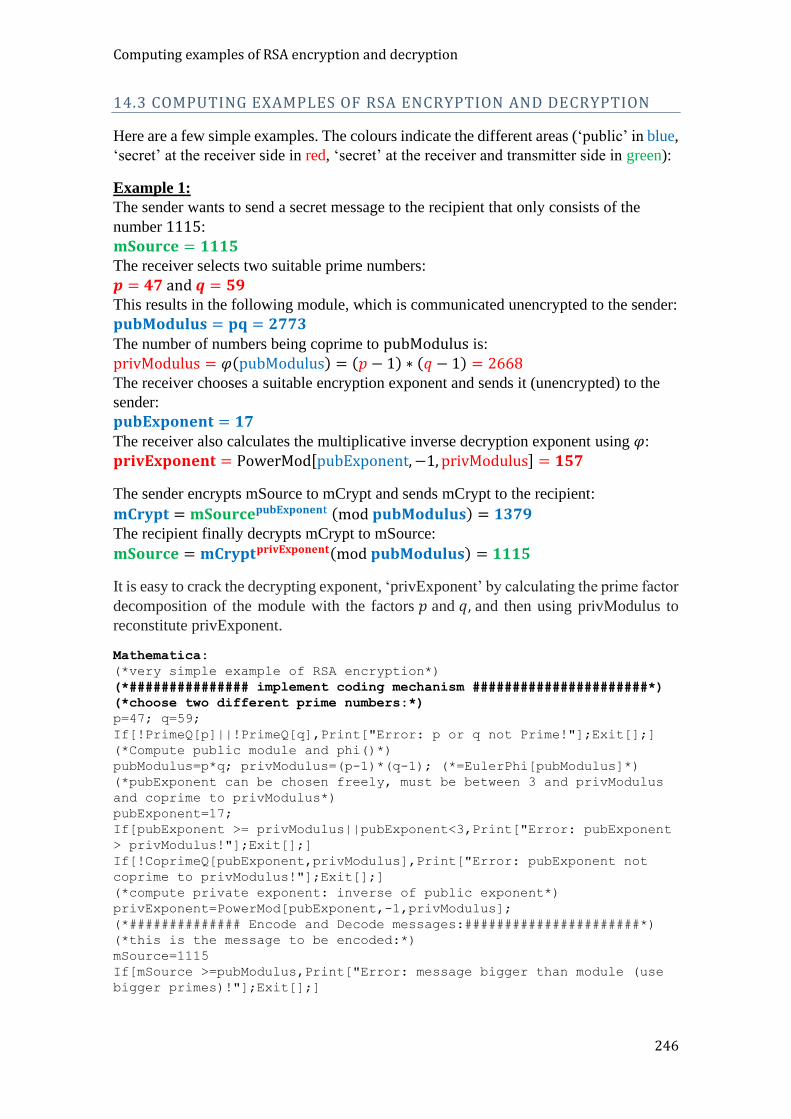
Computing examples of RSA encryption and decryption
246
14.3 COMPUTING EXAMPLES OF RSA ENCRYPTION AND DECRYPTION
Here are a few simple examples. The colours indicate the different areas (‘public’ in blue,
‘secret’ at the receiver side in red, ‘secret’ at the receiver and transmitter side in green):
Example 1:
The sender wants to send a secret message to the recipient that only consists of the
number 1115:
𝐦𝐒𝐨𝐮𝐫𝐜𝐞 = 𝟏𝟏𝟏𝟓
The receiver selects two suitable prime numbers:
𝒑 = 𝟒𝟕 and 𝒒 = 𝟓𝟗
This results in the following module, which is communicated unencrypted to the sender:
𝐩𝐮𝐛𝐌𝐨𝐝𝐮𝐥𝐮𝐬 = 𝐩𝐪 = 𝟐𝟕𝟕𝟑
The number of numbers being coprime to pubModulus is:
privModulus = 𝜑(pubModulus) = (𝑝 − 1) ∗ (𝑞 − 1) = 2668
The receiver chooses a suitable encryption exponent and sends it (unencrypted) to the
sender:
𝐩𝐮𝐛𝐄𝐱𝐩𝐨𝐧𝐞𝐧𝐭 = 𝟏𝟕
The receiver also calculates the multiplicative inverse decryption exponent using 𝜑:
𝐩𝐫𝐢𝐯𝐄𝐱𝐩𝐨𝐧𝐞𝐧𝐭 = PowerMod[pubExponent, −1, privModulus] = 𝟏𝟓𝟕
The sender encrypts mSource to mCrypt and sends mCrypt to the recipient:
𝐦𝐂𝐫𝐲𝐩𝐭 = 𝐦𝐒𝐨𝐮𝐫𝐜𝐞𝐩𝐮𝐛𝐄𝐱𝐩𝐨𝐧𝐞𝐧t (mod 𝐩𝐮𝐛𝐌𝐨𝐝𝐮𝐥𝐮𝐬) = 𝟏𝟑𝟕𝟗
The recipient finally decrypts mCrypt to mSource:
𝐦𝐒𝐨𝐮𝐫𝐜𝐞 = 𝐦𝐂𝐫𝐲𝐩𝐭𝐩𝐫𝐢𝐯𝐄𝐱𝐩𝐨𝐧𝐞𝐧𝐭(mod 𝐩𝐮𝐛𝐌𝐨𝐝𝐮𝐥𝐮𝐬) = 𝟏𝟏𝟏𝟓
It is easy to crack the decrypting exponent, ‘privExponent’ by calculating the prime factor
decomposition of the module with the factors 𝑝 and 𝑞, and then using privModulus to
reconstitute privExponent.
Mathematica:
(*very simple example of RSA encryption*)
(*############### implement coding mechanism ######################*)
(*choose two different prime numbers:*)
p=47; q=59;
If[!PrimeQ[p]||!PrimeQ[q],Print["Error: p or q not Prime!"];Exit[];]
(*Compute public module and phi()*)
pubModulus=p*q; privModulus=(p-1)*(q-1); (*=EulerPhi[pubModulus]*)
(*pubExponent can be chosen freely, must be between 3 and privModulus
and coprime to privModulus*)
pubExponent=17;
If[pubExponent >= privModulus||pubExponent<3,Print["Error: pubExponent
> privModulus!"];Exit[];]
If[!CoprimeQ[pubExponent,privModulus],Print["Error: pubExponent not
coprime to privModulus!"];Exit[];]
(*compute private exponent: inverse of public exponent*)
privExponent=PowerMod[pubExponent,-1,privModulus];
(*############## Encode and Decode messages:######################*)
(*this is the message to be encoded:*)
mSource=1115
If[mSource >=pubModulus,Print["Error: message bigger than module (use
bigger primes)!"];Exit[];]

14 Prime numbers and online banking
247
(*encode: *)
mCrypt=PowerMod[mSource,pubExponent,pubModulus]
(*decode:*)
mSource1=PowerMod[mCrypt,privExponent,pubModulus]
If[mSource!=mSource1,Print["Error: rSA Coding/Encoding failed"]];
(*########## Hacking the module:##############################*)
Print["Try to hack RSA module…"];
pqHacked=FactorInteger[pubModulus];
pH=First[pqHacked[[1]]];qH=First[pqHacked[[2]]];
privExponentH=PowerMod[pubExponent,-1,(pH-1)*(qH-1)]
If[privExponentH==privExponent,Print["Hack of RSA module
succeeded!"]];
Example 2 (similar to example 1)
The sender wants to send a secret message to the recipient that only consists of the
number 1115. In this example, however, we use the Mathematica functions
PublicKey[],PrivateKey[], Encrypt[], as well as Decrypt[]. No
padding algorithm has been used (specified by: “None”).
The program used can be found in the Appendix (20.11.11).
The private and public keys generated by Mathematica are as follows:
The original number reads: 1115
The prime numbers and module used to generate the keys are:
𝒑 = 𝟒𝟕; 𝒒 = 𝟓𝟗; public Modulus=2773 The encrypted number reads: 1379
Example 3
The sender wants to send a secret message to the recipient that only consists of the text
“OK”. In this example we use Mathematica’s built-in functions
GenerateAsymmetricKeyPair[], Encrypt[], as well as Decrypt[]
together with the “PKCS1” padding algorithm using a key length of 97 bits.
The program used can be found in the Appendix (20.11.11).
The private and public keys generated by Mathematica are as follows:
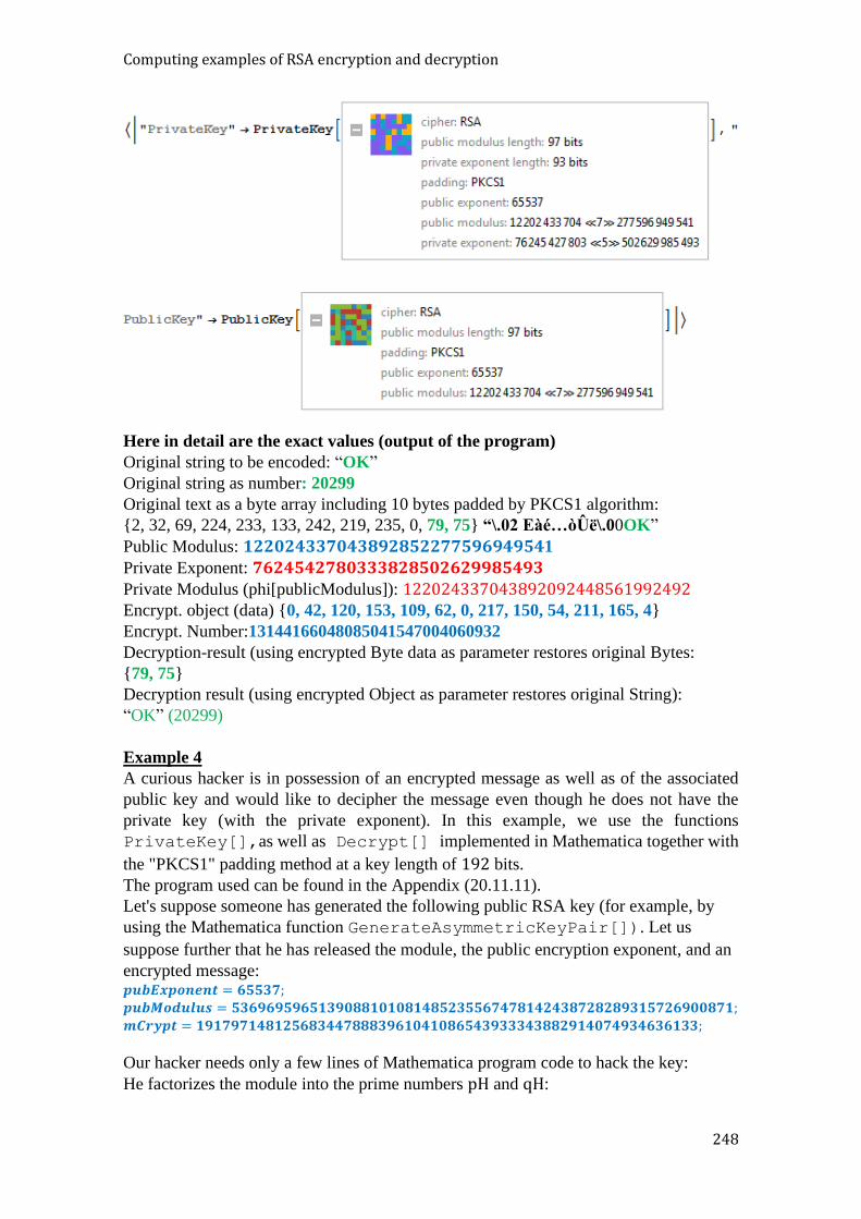
Computing examples of RSA encryption and decryption
248
Here in detail are the exact values (output of the program)
Original string to be encoded: “OK”
Original string as number: 20299
Original text as a byte array including 10 bytes padded by PKCS1 algorithm:
{2, 32, 69, 224, 233, 133, 242, 219, 235, 0, 79, 75} “\.02 Eàé…òÛë\.00OK”
Public Modulus: 𝟏𝟐𝟐𝟎𝟐𝟒𝟑𝟑𝟕𝟎𝟒𝟑𝟖𝟗𝟐𝟖𝟓𝟐𝟐𝟕𝟕𝟓𝟗𝟔𝟗𝟒𝟗𝟓𝟒1
Private Exponent: 𝟕𝟔𝟐𝟒𝟓𝟒𝟐𝟕𝟖𝟎𝟑𝟑𝟑𝟖𝟐𝟖𝟓𝟎𝟐𝟔𝟐𝟗𝟗𝟖𝟓𝟒𝟗𝟑
Private Modulus (phi[publicModulus]): 122024337043892092448561992492
Encrypt. object (data) {0, 42, 120, 153, 109, 62, 0, 217, 150, 54, 211, 165, 4}
Encrypt. Number:13144166048085041547004060932
Decryption-result (using encrypted Byte data as parameter restores original Bytes:
{79, 75}
Decryption result (using encrypted Object as parameter restores original String):
“OK” (20299)
Example 4
A curious hacker is in possession of an encrypted message as well as of the associated
public key and would like to decipher the message even though he does not have the
private key (with the private exponent). In this example, we use the functions
PrivateKey[],as well as Decrypt[] implemented in Mathematica together with
the "PKCS1" padding method at a key length of 192 bits.
The program used can be found in the Appendix (20.11.11).
Let's suppose someone has generated the following public RSA key (for example, by
using the Mathematica function GenerateAsymmetricKeyPair[]). Let us
suppose further that he has released the module, the public encryption exponent, and an
encrypted message: 𝒑𝒖𝒃𝑬𝒙𝒑𝒐𝒏𝒆𝒏𝒕 = 𝟔𝟓𝟓𝟑𝟕; 𝒑𝒖𝒃𝑴𝒐𝒅𝒖𝒍𝒖𝒔 = 𝟓𝟑𝟔𝟗𝟔𝟗𝟓𝟗𝟔𝟓𝟏𝟑𝟗𝟎𝟖𝟖𝟏𝟎𝟏𝟎𝟖𝟏𝟒𝟖𝟓𝟐𝟑𝟓𝟓𝟔𝟕𝟒𝟕𝟖𝟏𝟒𝟐𝟒𝟑𝟖𝟕𝟐𝟖𝟐𝟖𝟗𝟑𝟏𝟓𝟕𝟐𝟔𝟗𝟎𝟎𝟖𝟕𝟏; 𝒎𝑪𝒓𝒚𝒑𝒕 = 𝟏𝟗𝟏𝟕𝟗𝟕𝟏𝟒𝟖𝟏𝟐𝟓𝟔𝟖𝟑𝟒𝟒𝟕𝟖𝟖𝟖𝟑𝟗𝟔𝟏𝟎𝟒𝟏𝟎𝟖𝟔𝟓𝟒𝟑𝟗𝟑𝟑𝟑𝟒𝟑𝟖𝟖𝟐𝟗𝟏𝟒𝟎𝟕𝟒𝟗𝟑𝟒𝟔𝟑𝟔𝟏𝟑𝟑;
Our hacker needs only a few lines of Mathematica program code to hack the key:
He factorizes the module into the prime numbers pH and qH:
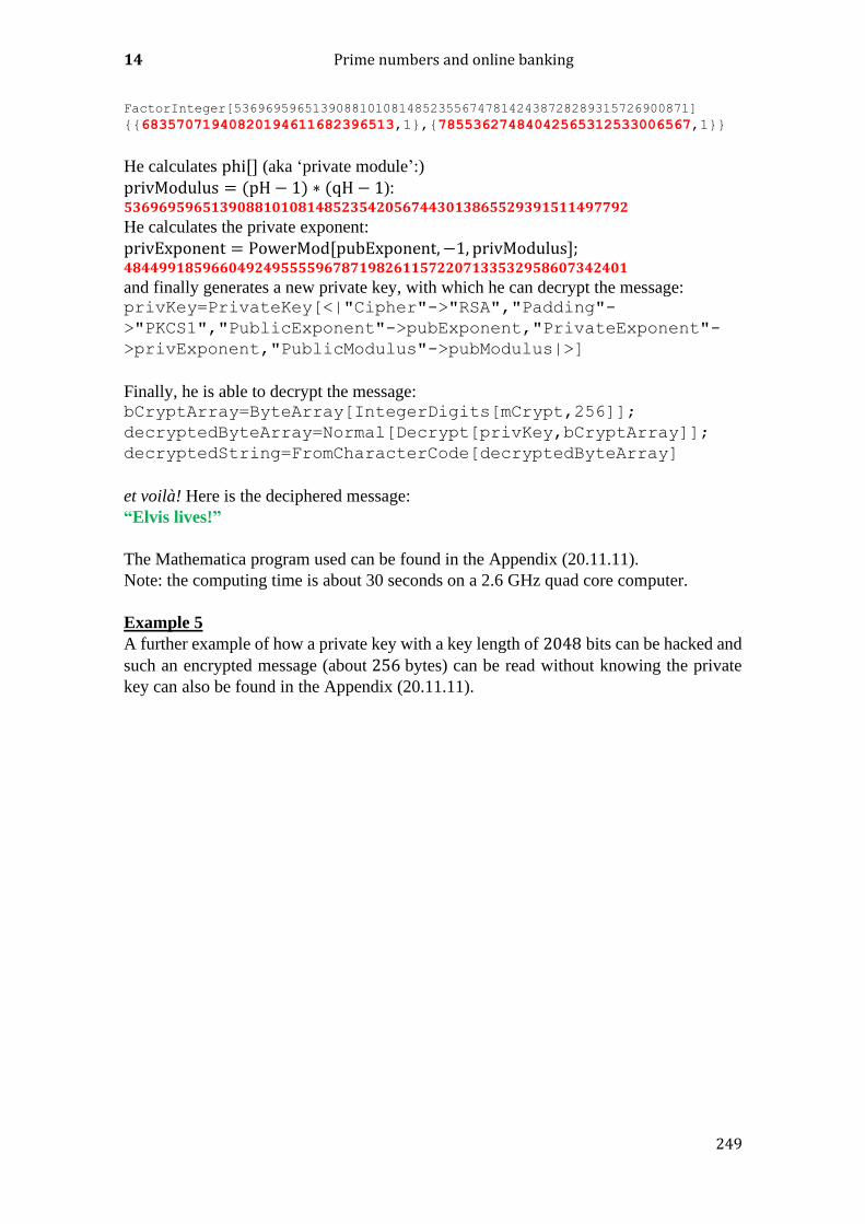
14 Prime numbers and online banking
249
FactorInteger[5369695965139088101081485235567478142438728289315726900871]
{{68357071940820194611682396513,1},{78553627484042565312533006567,1}}
He calculates phi[] (aka ‘private module’:)
privModulus = (pH − 1) ∗ (qH − 1): 𝟓𝟑𝟔𝟗𝟔𝟗𝟓𝟗𝟔𝟓𝟏𝟑𝟗𝟎𝟖𝟖𝟏𝟎𝟏𝟎𝟖𝟏𝟒𝟖𝟓𝟐𝟑𝟓𝟒𝟐𝟎𝟓𝟔𝟕𝟒𝟒𝟑𝟎𝟏𝟑𝟖𝟔𝟓𝟓𝟐𝟗𝟑𝟗𝟏𝟓𝟏𝟏𝟒𝟗𝟕𝟕𝟗𝟐
He calculates the private exponent:
privExponent = PowerMod[pubExponent,−1, privModulus]; 𝟒𝟖𝟒𝟒𝟗𝟗𝟏𝟖𝟓𝟗𝟔𝟔𝟎𝟒𝟗𝟐𝟒𝟗𝟓𝟓𝟓𝟓𝟗𝟔𝟕𝟖𝟕𝟏𝟗𝟖𝟐𝟔𝟏𝟏𝟓𝟕𝟐𝟐𝟎𝟕𝟏𝟑𝟑𝟓𝟑𝟐𝟗𝟓𝟖𝟔𝟎𝟕𝟑𝟒𝟐𝟒𝟎𝟏
and finally generates a new private key, with which he can decrypt the message: privKey=PrivateKey[<|"Cipher"->"RSA","Padding"-
>"PKCS1","PublicExponent"->pubExponent,"PrivateExponent"-
>privExponent,"PublicModulus"->pubModulus|>]
Finally, he is able to decrypt the message: bCryptArray=ByteArray[IntegerDigits[mCrypt,256]];
decryptedByteArray=Normal[Decrypt[privKey,bCryptArray]];
decryptedString=FromCharacterCode[decryptedByteArray]
et voilà! Here is the deciphered message:
“Elvis lives!”
The Mathematica program used can be found in the Appendix (20.11.11).
Note: the computing time is about 30 seconds on a 2.6 GHz quad core computer.
Example 5
A further example of how a private key with a key length of 2048 bits can be hacked and
such an encrypted message (about 256 bytes) can be read without knowing the private
key can also be found in the Appendix (20.11.11).
250
15 PRIME NUMBERS IN MUSIC
15.1 EULER’S THEORY OF CONSONANCE AND THE GRADUS SUAVITATIS
As every musician knows, musical intervals and chords can sound either consonant or
dissonant, with a flowing boundary between 'consonant' and 'dissonant' that probably also
depends on the taste of the historical epoch of the music. Nevertheless, the mathematician
Leonhard Euler (1707-1783) – and the attentive reader will have noticed that this is not
the first time we have encountered this gentleman … – was convinced it was possible to
formulate a mathematical definition of harmony, or more precisely, of the 'degree' of
harmony (aka ‘euphony’).
Euler found a formula that indicates the degree of euphony as a natural number, and called
the number derived from the formula the ‘Gradus Suavitatis’.72 In the calculation of the
Gradus Suavitatis, prime numbers (what else?) play a special role. Euler uses the concept
of consonance for arbitrary (and not only euphonious) ‘composite sounds’.
By ‘composite sounds’, we mean simultaneously sounding notes, whereby the notes
should be tuned in pure temperament and thus have mutually rational (fractions of natural
numbers) ratios. Although the Gradus Suavitatis can be computed for arbitrary numbers,
it was in former times only applied musically to intervals the ratios of which can be
described with the primes 2, 3, and 5. In his later writings, however, Euler pleads for the
introduction of the prime number 7 into 'musical arithmetic'.
72 Euler, Leonhard: Tentamen Novae Theoriae Mvsicae Ex Certissimis Harmoniae Principiis Dilvcide Expositae Petropolis 1739

15 Prime numbers in music
251
Figure 128. Opening of the 4th chapter of Leonhard Euler’s book Tentamen novae theoriae musicae
In contrast to Pythagorean tuning, in which all the scales occurring are constructed by
using fifths (which are projected into the octave space, if necessary), 'pure' tuning only
uses the number ratios 5/4 and 6/5 for the major and minor thirds. If we wish to assign
a ‘pure’ numeral ratio to all the twelve semitones of the octave, we discover a certain
ambiguity exists for the intermediate notes, because only the root, fourth, fifth, major /
minor third, and the major / minor sixth are precisely defined. If we take the root note C,
the seven precisely defined notes are:
C, Eb, E, F, G, Ab, A (having the ratios 1,6
5,5
4,4
3,3
2,8
5,5
3).
The remaining notes can be chosen in different ways, depending on the note from which
they are constructed. Here is an example: the note Bb can be constructed by starting from
F: the two consecutive fourths starting from the C then give the value 4
3⋅4
3=16
9. Bb can,
however, also be constructed starting from G. Fifth and minor third starting from C then
result in 3
2⋅6
5=9
5.
The most commonly used pure scale that is closest to the tempered tone scale, is:
Chromat. scale C Db D Eb E F F# G Ab A Bb B c
Freq. ratio 1/1 16/15 9/8 6/5 5/4 4/3 45/32 3/2 8/5 5/3 9/5 (16/9) 15/8 2/1
Euler’s theory of consonance and the Gradus Suavitatis
252
From this ambiguity, we recognize that the application of the Gradus Suavitatis to the
‘equal temperament’ tuning system we use these days (in which the frequency ratios of
the chromatic scale are simply the values of a geometric sequence with the factor 𝑞 =
√212
) is problematic.
If we define an interval in pure tuning as the frequency ratio 𝑝
𝑞, 𝑝, 𝑞 ∈ ℕ (see table), and
build the so-called Euler exponent 𝐸 = lcm(p, q) , then the Gradus Suavitatis 𝑮 is
defined as follows:
𝐺(𝐸) = 1 + ∑ 𝑒𝑖
𝝎(𝑬)
𝑖=1
(𝑝𝒏𝒊 − 1),where 𝐸 = lcm(𝑝, 𝑞) = ∏ 𝑝𝑛𝑖𝑒𝑖
𝜔(𝐸)
𝑖=1
(158)
Here lcm(𝑝, 𝑞) is the least common multiple of 𝑝 and 𝑞; 𝑝𝑛𝑖𝑒𝑖 are the occurring prime
factors with their multiplicities (as exponents), 𝑛𝑖 the indices of the occurring primes;
𝜔(𝐸) denotes the number of different primes. Sometimes the Gradus Suavitatis is also
referred to in the literature with the symbol Γ(𝑝, 𝑞). We prefer to use the symbol 𝐺 to
avoid confusion with the gamma function Γ(x). The Gradus Suavitatis can also easily be
applied to chords consisting of three notes (‘triads’) or more. In this case, 𝐸 is simply
calculated as 𝐸 = lcm(𝑞1, 𝑞2, 𝑞3, … ) where the integers 𝑞1, 𝑞2, 𝑞3, … , represent the
frequency ratios with respect to the lowest occurring note.
The Gradus Suavitatis can thus also be calculated for combinations of arbitrarily many
notes. For a single argument 𝑛, 𝐸 = 𝑛. In this case, the Gradus Suavitatis is merely an
arithmetical function depending solely upon the positive integer variable 𝑛. Furthermore,
we define: 𝐺(1) = 1. Note: we also assume that the ratios (𝑞1, 𝑞2, 𝑞3, … ) are minimal,
i.e. ’simplified’ as far as possible, since otherwise the Gradus Suavitatis would yield
higher values, thus the notation 𝐺 (3
2) is somewhat imprecise.
Since in this case we want to calculate the Gradus Suavitatis for a two-note chord (or
‘harmonic interval’) with the frequency ratios 1 (root) and 3
2 (fifth), it would be more
precise mathematically to write:
𝐺 (1,3
2)= 𝐺(2,3).
In order to avoid confusion, it is best to calculate first the Euler exponent 𝐸 for the chord
or interval to be examined, and then the Gradus Suavitatis for the integer argument 𝐸.
Here are a few examples:
𝐺(2) = 1 + 1 ⋅ (2 − 1) = 2, 𝐺(3) = 1 + 1 ⋅ (3 − 1) = 3, 𝐺(4) = 1 + 2 ⋅ (2 − 1) = 3
𝐺 (3
2) = 𝐺(3,2) = 𝐺(6) = 1 + 1 ⋅ (2 − 1) + 1 ⋅ (3 − 1) = 4 (fifth)
𝐺 (2
3) = 𝐺(2,3) = 𝐺(6) = 4 (fourth)
𝐺 (12
5) = 𝐺(12,5) = 𝐺(60) = 1 + 2 ⋅ 1 + 1 ⋅ 2 + 1 ⋅ 4 = 9 (minor tenth)
Major triad: 𝑞1 = 1, 𝑞2 =5
4, 𝑞3 =
3
2, ⇒ 𝐸 = lcm(4,5,6) = 60, 𝐺(60) = 9
1st inversion: 𝑞1 = 1, 𝑞2 =6
5, 𝑞3 =
8
5, ⇒ 𝐸 = lcm(5,6,8) = 120, 𝐺(120) = 10
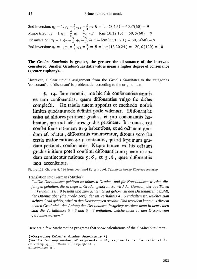
15 Prime numbers in music
253
2nd inversion: 𝑞1 = 1, 𝑞2 =4
3, 𝑞3 =
5
3, ⇒ 𝐸 = lcm(3,4,5) = 60, 𝐺(60) = 9
Minor triad: 𝑞1 = 1, 𝑞2 =6
5, 𝑞3 =
3
2, ⇒ 𝐸 = lcm(10,12,15) = 60, 𝐺(60) = 9
1st inversion: 𝑞1 = 1, 𝑞2 =5
4, 𝑞3 =
5
3, ⇒ 𝐸 = lcm(12,15,20 ) = 60, 𝐺(60) = 9
2nd inversion: 𝑞1 = 1, 𝑞2 =4
3, 𝑞3 =
8
5, ⇒ 𝐸 = lcm(15,20,24 ) = 120, 𝐺(120) = 10
The Gradus Suavitatis is greater, the greater the dissonance of the intervals
considered. Smaller Gradus-Suavitatis values mean a higher degree of consonance
(greater euphony)…
However, a clear unique assignment from the Gradus Suavitatis to the categories
'consonant' and 'dissonant' is problematic, according to the original text:
Figure 129. Chapter 4, §14 from Leonhard Euler’s book Tentamen Novae Theoriae musicae
Translation into German (Mitzler):
“…Die Dissonanzen gehören zu höheren Graden, und für Konsonanzen werden die-
jenigen gehalten, die zu tieferen Graden gehören. So wird der Ganzton, der aus Tönen
im Verhältnis 8 : 9 besteht und zum achten Grad gehört, zu den Dissonanzen gezählt,
der Ditonus aber (die große Terz), der im Verhältnis 4 : 5 enthalten ist, welcher zum
siebten Grad gehört, wird zu den Konsonanzen gezählt. Und trotzdem kann aus diesem
achten Grad nicht der Anfang der Dissonanzen festgelegt werden; denn in demselben
sind die Verhältnisse 5 : 6 und 5 : 8 enthalten, welche nicht zu den Dissonanzen
gerechnet werden.“
Here are a few Mathematica programs that show calculations of the Gradus Suavitatis:
(*Computing Euler’s Gradus Suavitatis *)
(*works for any number of arguments n >1, arguments can be rational:*)
eulerExp[q__]:=Module[{exp,qList},
qList=List[q];
Euler’s theory of consonance and the Gradus Suavitatis
254
If[Length[qList]==1&&IntegerQ[qList[[1]]],
exp=qList[[1]], exp=Apply[LCM,qList]/Apply[GCD,qList]];
Return[exp];
];
(*works for 1 argument. argument can be rational:*)
eulerExp[r_]:=eulerExp[Numerator[r],Denominator[r]];
(*works for 1 integer argument, number-theoretic version:*)
gas[n_]:=Module[{s=FactorInteger[n]},1+Sum[s[[k,2]]*(s[[k,1]]-
1),{k,Length[s]}]];
(*works for 1 or 2 arguments can be rational:*)
gs2[p_,q_]:=gs[LCM[p,q]/GCD[p,q]];
gs2[x_]:=gs2[Numerator[x],Denominator[x]];
(*works for any number of arguments n > 1, arguments can be
rational:*)
gsn[q__]:=Module[{ exp, retValue},
exp=eulerExp[q];
s=FactorInteger[exp];
retValue=1+Sum[s[[k,2]]*(s[[k,1]]-1),{k,Length[s]}];
Return[retValue];
];
15.1.1 MATHEMATICAL PROPERTIES OF THE GRADUS SUAVITATIS
1) 𝐺(1) = 1 2) 𝐺(𝑝) = 𝑝, if 𝑝 ∈ ℙ 3) 𝐺(𝑝𝑞) = 𝐺(𝑝) + 𝐺(𝑞) − 1 (‘quasi-logarithmic’) 4) 𝐺(2𝑛) = 𝑛 + 1 5) 𝐺(𝑝𝑛) = (𝑝 − 1)𝑛 + 1
6) 𝐺 (𝑝
𝑞) = 𝐺 (
𝑞
𝑝) or 𝐺(𝑝, 𝑞) = 𝐺(𝑞, 𝑝)
7) 𝐺(𝑞1, 𝑞2, 𝑞3, … 𝑞𝑛) = 𝐺(𝑞𝑖1 , 𝑞𝑖2 , 𝑞𝑖3 , … 𝑞𝑖𝑛),where i1, 𝑖2, 𝑖3, … 𝑖𝑛
represent all possible permutations of 1,2,3, … 𝑛
8) 𝐺 (1
𝑞1,1
𝑞2,1
𝑞3, …
1
𝑞𝑛 ) = 𝐺(𝑞1, 𝑞2, 𝑞3, … 𝑞𝑛)
For major and minor triads (let 𝑋 be the three frequency ratios of a major triad, 𝑋𝑚 the
three ratios of a minor triad, the indices 1 and 2 each represent the first and second
inversions, respectively):
9) 𝐺(𝑋) = 𝐺(𝑋2) = 𝐺(𝑋𝑚) = 𝐺(𝑋𝑚1) 10) 𝐺(𝑋1) = 𝐺(𝑋𝑚2)
According to Euler, a sequence of frequency ratios (which build up a chord) can be
continued in such a way that the Gradus Suavitatis value remains the same. Euler calls
this the ‘complete consonance’. For the major triad the complete consonance gives the
following frequency ratios:
1: 2: 3: 𝟒: 𝟓: 𝟔: 𝟏𝟎: 𝟏𝟐: 𝟏𝟓: 20: 30: 60…
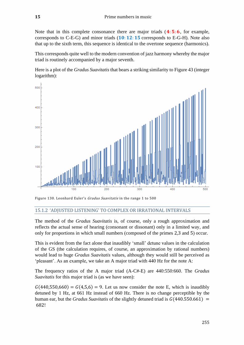
15 Prime numbers in music
255
Note that in this complete consonance there are major triads (𝟒: 𝟓: 𝟔 , for example,
corresponds to C-E-G) and minor triads (𝟏𝟎: 𝟏𝟐: 𝟏𝟓 corresponds to E-G-H). Note also
that up to the sixth term, this sequence is identical to the overtone sequence (harmonics).
This corresponds quite well to the modern convention of jazz harmony whereby the major
triad is routinely accompanied by a major seventh.
Here is a plot of the Gradus Suavitatis that bears a striking similarity to Figure 43 (integer
logarithm):
Figure 130. Leonhard Euler’s Gradus Suavitatis in the range 1 to 500
15.1.2 ‘ADJUSTED LISTENING’ TO COMPLEX OR IRRATIONAL INTERVALS
The method of the Gradus Suavitatis is, of course, only a rough approximation and
reflects the actual sense of hearing (consonant or dissonant) only in a limited way, and
only for proportions in which small numbers (composed of the primes 2,3 and 5) occur.
This is evident from the fact alone that inaudibly ‘small’ detune values in the calculation
of the GS (the calculation requires, of course, an approximation by rational numbers)
would lead to huge Gradus Suavitatis values, although they would still be perceived as
‘pleasant’. As an example, we take an A major triad with 440 Hz for the note A:
The frequency ratios of the A major triad (A-C#-E) are 440:550:660. The Gradus
Suavitatis for this major triad is (as we have seen):
𝐺(440,550,660) = 𝐺(4,5,6) = 9. Let us now consider the note E, which is inaudibly
detuned by 1 Hz, at 661 Hz instead of 660 Hz. There is no change perceptible by the
human ear, but the Gradus Suavitatis of the slightly detuned triad is 𝐺(440.550.661) = 682!
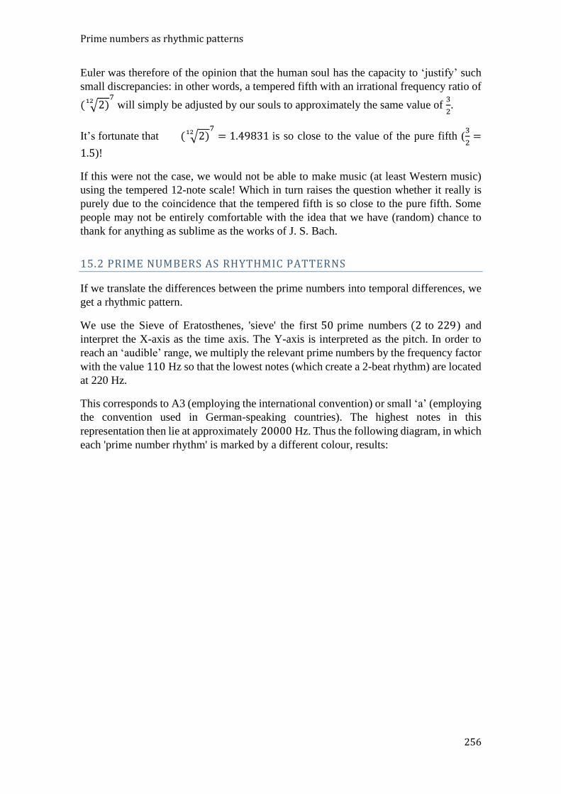
Prime numbers as rhythmic patterns
256
Euler was therefore of the opinion that the human soul has the capacity to ‘justify’ such
small discrepancies: in other words, a tempered fifth with an irrational frequency ratio of
( √2)12 7
will simply be adjusted by our souls to approximately the same value of 3
2.
It’s fortunate that ( √2)12 7
= 1.49831 is so close to the value of the pure fifth (3
2=
1.5)!
If this were not the case, we would not be able to make music (at least Western music)
using the tempered 12-note scale! Which in turn raises the question whether it really is
purely due to the coincidence that the tempered fifth is so close to the pure fifth. Some
people may not be entirely comfortable with the idea that we have (random) chance to
thank for anything as sublime as the works of J. S. Bach.
15.2 PRIME NUMBERS AS RHYTHMIC PATTERNS
If we translate the differences between the prime numbers into temporal differences, we
get a rhythmic pattern.
We use the Sieve of Eratosthenes, 'sieve' the first 50 prime numbers (2 to 229) and
interpret the X-axis as the time axis. The Y-axis is interpreted as the pitch. In order to
reach an ‘audible’ range, we multiply the relevant prime numbers by the frequency factor
with the value 110 Hz so that the lowest notes (which create a 2-beat rhythm) are located
at 220 Hz.
This corresponds to A3 (employing the international convention) or small ‘a’ (employing
the convention used in German-speaking countries). The highest notes in this
representation then lie at approximately 20000 Hz. Thus the following diagram, in which
each 'prime number rhythm' is marked by a different colour, results:

15 Prime numbers in music
257
Figure 131. Prime number rhythms, from the first 50 prime numbers with A3 as lowest note
Mathematica:
(*Generate a list with 50 different sequences of
(frequency,Primenumber)-Pairs, using A2=110Hz as the base-frequency*)
tab=Table[{j,Table[{i,110*Prime[j]},{i,Prime[j],Prime[50],Prime[j]}]},
{j,1,50}];
ListLogPlot[Table[tab[[k]][[2]],{k,1,50}],PlotLabel->"Prime-Rhythms
(First 50 prime numbers)\nLowest note: A3 (220 Hz)", ImageSize->Large]
With Mathematica, it is very easy to translate these tables into music. We use the table of
Figure 131 and generate a ‘prime number’ song 46 seconds in duration:
Mathematica:
(*needs the prime sound-library, to be found in the Appendix *)
tab=Table[{j,Table[{i,110*Prime[j]},{i,Prime[j],Prime[50],Prime[j]}]},
{j,1,50}];
sortedTab=Sort[Flatten[Drop[tab,None,1],2]];
noteList=createNoteListFromSortedTable[sortedTab];
song1=Sound[{"Percussion",Table[SoundNote[noteList[[k]][[2]]-
10,0.2],{k,1,Length[noteList]}]},{0,46}];
song2=Sound[{"Marimba",Table[SoundNote[noteList[[k]][[2]],0.2],{k,1,Le
ngth[noteList]}]},{0,46}];
primenumberSong=Sound[{song1,song2}];
Export["C:/primes/Sounds/primenumberSong46Sec.mid",primeNumberSong];
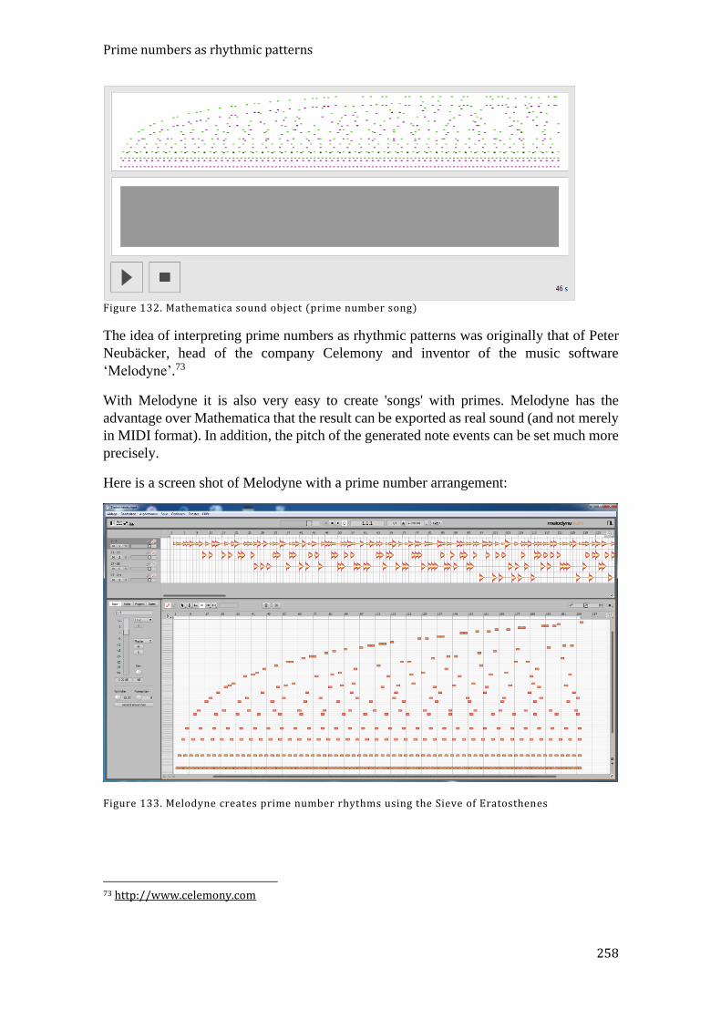
Prime numbers as rhythmic patterns
258
Figure 132. Mathematica sound object (prime number song)
The idea of interpreting prime numbers as rhythmic patterns was originally that of Peter
Neubäcker, head of the company Celemony and inventor of the music software
‘Melodyne’.73
With Melodyne it is also very easy to create 'songs' with primes. Melodyne has the
advantage over Mathematica that the result can be exported as real sound (and not merely
in MIDI format). In addition, the pitch of the generated note events can be set much more
precisely.
Here is a screen shot of Melodyne with a prime number arrangement:
Figure 133. Melodyne creates prime number rhythms using the Sieve of Eratosthenes
73 http://www.celemony.com

259
16 PRIME NUMBERS IN POETRY
16.1 HAIKUS AND TANKAS
Matsuo Bashô (松尾芭蕉), 1644-1695
道のべに清水流るる柳影
しばしとてこそ立ちどまりつれ
Michi no be ni Shimizu nagaruru
Yanagikage Shibashi tote koso Tachidomaritsure
荒海や
佐渡によこたふ
天河
ura umi ya sado ni yokotau
ama no gawa
Tosende See. nur die Milchstraße reicht
zur Insel Sado hinüber.
Turbulent the sea— across to Sado stretches
the Milky Way
古池や
蛙飛び込む
水の音
furu ike ya kawazu tobikomu
mizu no oto
Der alte Weiher: Ein Frosch springt hinein.
Oh! Das Geräusch des Wassers
Ah! The ancient pond As a frog takes the plunge
Sound of the water
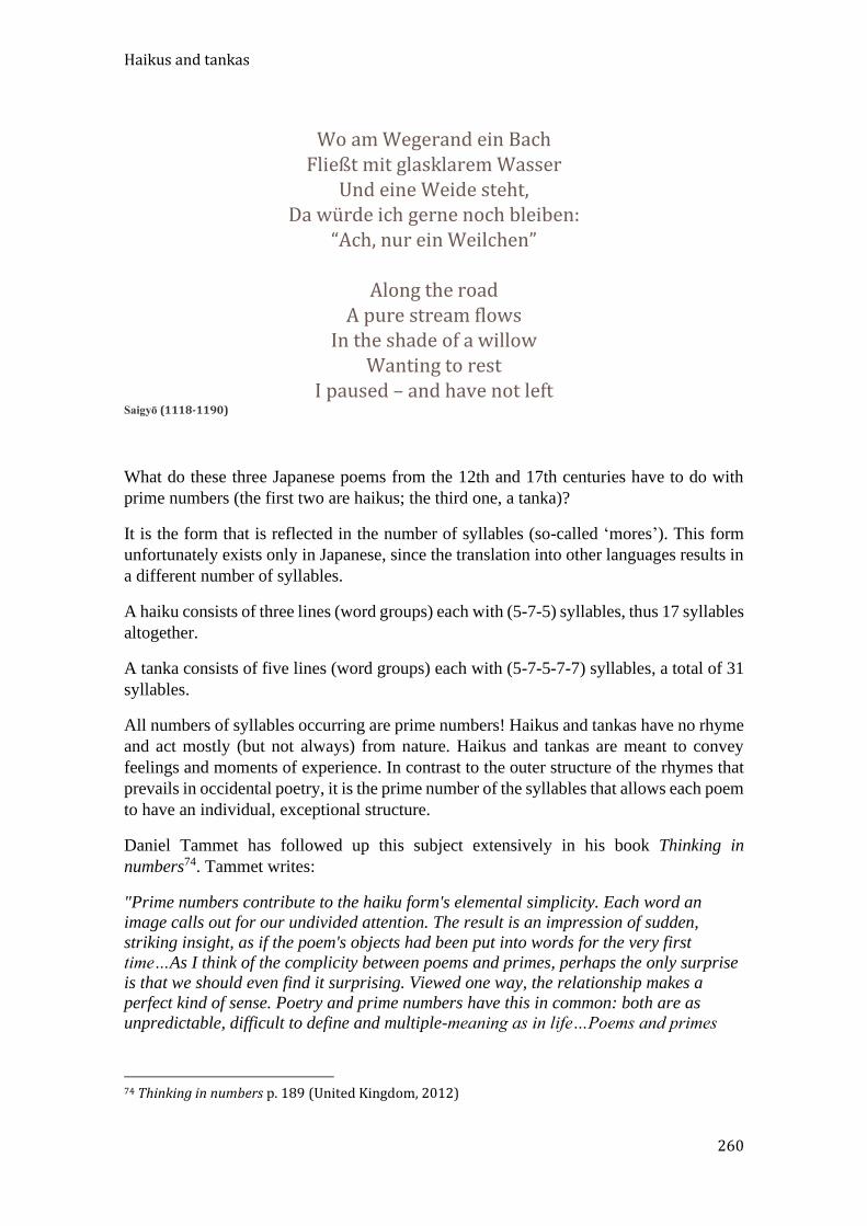
Haikus and tankas
260
Wo am Wegerand ein Bach
Fließt mit glasklarem Wasser Und eine Weide steht,
Da würde ich gerne noch bleiben: “Ach, nur ein Weilchen”
Along the road
A pure stream flows In the shade of a willow
Wanting to rest I paused – and have not left
Saigyō (1118-1190)
What do these three Japanese poems from the 12th and 17th centuries have to do with
prime numbers (the first two are haikus; the third one, a tanka)?
It is the form that is reflected in the number of syllables (so-called ‘mores’). This form
unfortunately exists only in Japanese, since the translation into other languages results in
a different number of syllables.
A haiku consists of three lines (word groups) each with (5-7-5) syllables, thus 17 syllables
altogether.
A tanka consists of five lines (word groups) each with (5-7-5-7-7) syllables, a total of 31
syllables.
All numbers of syllables occurring are prime numbers! Haikus and tankas have no rhyme
and act mostly (but not always) from nature. Haikus and tankas are meant to convey
feelings and moments of experience. In contrast to the outer structure of the rhymes that
prevails in occidental poetry, it is the prime number of the syllables that allows each poem
to have an individual, exceptional structure.
Daniel Tammet has followed up this subject extensively in his book Thinking in
numbers74. Tammet writes:
"Prime numbers contribute to the haiku form's elemental simplicity. Each word an
image calls out for our undivided attention. The result is an impression of sudden,
striking insight, as if the poem's objects had been put into words for the very first
time…As I think of the complicity between poems and primes, perhaps the only surprise
is that we should even find it surprising. Viewed one way, the relationship makes a
perfect kind of sense. Poetry and prime numbers have this in common: both are as
unpredictable, difficult to define and multiple-meaning as in life…Poems and primes
74 Thinking in numbers p. 189 (United Kingdom, 2012)
16 Prime numbers in poetry
261
are tricky things to recognize. A glance will usually not suffice to tell us if such-and-
such a number has factors, or whether a given text contains much meaning…"
Daniel Tammet is one of an estimated 100 ‘savants’ alive today.
He learns new languages within a week and calculates almost as fast as a computer. He
also holds the European record for reciting from memory the digits of the number 𝑝𝑖 (22514 decimal digits, as of June 2016).
16.2 SESTINAS
Another type of poem that long ago passed into oblivion, and in which primes also loomed
large, is the sestine. The sestine is a verse form comprising six stanzas of six lines each
with a final stanza of three lines. The name comes from the word 'sesto' (six). The inventor
of the sestine was the French troubadour Arnaut Daniel, who lived in Provence from 1150
to 1200.
Similar to the Japanese haiku, the sestine is not held together by devices like rhyme or
symbolism. Unlike the haiku, however, the number of syllables or words per line does
not play a big role. In German, however, the iambic verse meter is preferred.
The structure that holds a sestine together is the following: each sestine has a 'core' of six
words. The last word of a line must be one of these 6 core words, in fact alternating, until
all six core words have been used up, which obviously occurs after six lines. For the next
group of 6 lines, the same principle is applied, but with a different order of the core words,
each at the end of the line.
It can be seen that the ‘power’ and the almost musical appeal of the poems lie in this
repetition. In the course of the 36-line poem, each core word occurs exactly 6 times. The
order in which the core words are permuted within a group of six is complicated and
reminiscent of throwing a dice. Let us suppose that our core words are numbered from 1
to 6; then the (ending) core words in the entire poem appear in the following order:
stanza 1: 1, 2, 3, 4, 5, 6
stanza 2: 6, 1, 5, 2, 4, 3
stanza 3: 3, 6, 4, 1, 2, 5
stanza 4: 5, 3, 2, 6, 1, 4
stanza 5: 4, 5, 1, 3, 6, 2
stanza 6: 2, 4, 6, 5, 3, 1
Final stanza: (1, 2), (3, 4), (5, 6)
Note: in the three-line final stanza, there are two key words per line (one at the end and
one within the line). The order of the key words in the final stanza can, however, also be
different; in the ending lines, every core word must occur exactly once.
Here is an example of a sestine (in German) that the author found on the Internet:75
75 http://www.leselupe.de/lw/titel-Gedichtstrophen--Die-Sestine-100219.htm
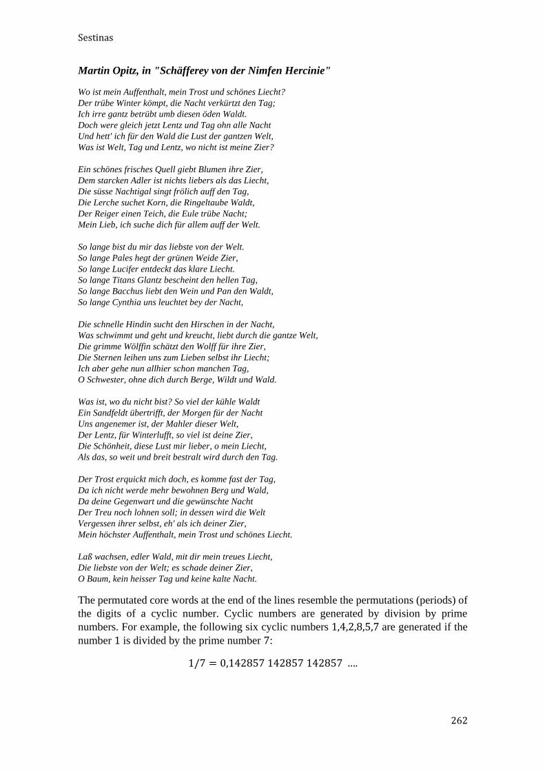
Sestinas
262
Martin Opitz, in "Schäfferey von der Nimfen Hercinie"
Wo ist mein Auffenthalt, mein Trost und schönes Liecht?
Der trübe Winter kömpt, die Nacht verkürtzt den Tag;
Ich irre gantz betrübt umb diesen öden Waldt.
Doch were gleich jetzt Lentz und Tag ohn alle Nacht
Und hett' ich für den Wald die Lust der gantzen Welt,
Was ist Welt, Tag und Lentz, wo nicht ist meine Zier?
Ein schönes frisches Quell giebt Blumen ihre Zier,
Dem starcken Adler ist nichts liebers als das Liecht,
Die süsse Nachtigal singt frölich auff den Tag,
Die Lerche suchet Korn, die Ringeltaube Waldt,
Der Reiger einen Teich, die Eule trübe Nacht;
Mein Lieb, ich suche dich für allem auff der Welt.
So lange bist du mir das liebste von der Welt.
So lange Pales hegt der grünen Weide Zier,
So lange Lucifer entdeckt das klare Liecht.
So lange Titans Glantz bescheint den hellen Tag,
So lange Bacchus liebt den Wein und Pan den Waldt,
So lange Cynthia uns leuchtet bey der Nacht,
Die schnelle Hindin sucht den Hirschen in der Nacht,
Was schwimmt und geht und kreucht, liebt durch die gantze Welt,
Die grimme Wölffin schätzt den Wolff für ihre Zier,
Die Sternen leihen uns zum Lieben selbst ihr Liecht;
Ich aber gehe nun allhier schon manchen Tag,
O Schwester, ohne dich durch Berge, Wildt und Wald.
Was ist, wo du nicht bist? So viel der kühle Waldt
Ein Sandfeldt übertrifft, der Morgen für der Nacht
Uns angenemer ist, der Mahler dieser Welt,
Der Lentz, für Winterlufft, so viel ist deine Zier,
Die Schönheit, diese Lust mir lieber, o mein Liecht,
Als das, so weit und breit bestralt wird durch den Tag.
Der Trost erquickt mich doch, es komme fast der Tag,
Da ich nicht werde mehr bewohnen Berg und Wald,
Da deine Gegenwart und die gewünschte Nacht
Der Treu noch lohnen soll; in dessen wird die Welt
Vergessen ihrer selbst, eh' als ich deiner Zier,
Mein höchster Auffenthalt, mein Trost und schönes Liecht.
Laß wachsen, edler Wald, mit dir mein treues Liecht,
Die liebste von der Welt; es schade deiner Zier,
O Baum, kein heisser Tag und keine kalte Nacht.
The permutated core words at the end of the lines resemble the permutations (periods) of
the digits of a cyclic number. Cyclic numbers are generated by division by prime
numbers. For example, the following six cyclic numbers 1,4,2,8,5,7 are generated if the
number 1 is divided by the prime number 7:
1/7 = 0,142857 142857 142857 ….
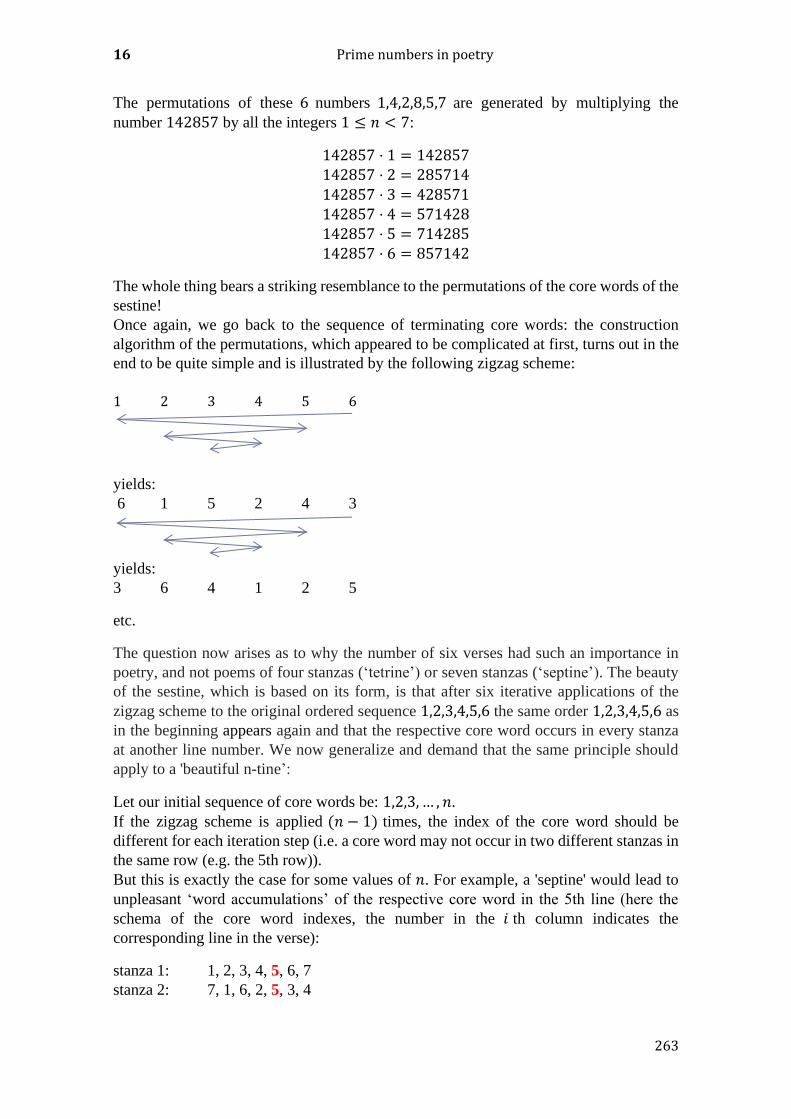
16 Prime numbers in poetry
263
The permutations of these 6 numbers 1,4,2,8,5,7 are generated by multiplying the
number 142857 by all the integers 1 ≤ 𝑛 < 7:
142857 ⋅ 1 = 142857
142857 ⋅ 2 = 285714
142857 ⋅ 3 = 428571
142857 ⋅ 4 = 571428
142857 ⋅ 5 = 714285
142857 ⋅ 6 = 857142
The whole thing bears a striking resemblance to the permutations of the core words of the
sestine!
Once again, we go back to the sequence of terminating core words: the construction
algorithm of the permutations, which appeared to be complicated at first, turns out in the
end to be quite simple and is illustrated by the following zigzag scheme:
1 2 3 4 5 6
yields:
6 1 5 2 4 3
yields:
3 6 4 1 2 5
etc.
The question now arises as to why the number of six verses had such an importance in
poetry, and not poems of four stanzas (‘tetrine’) or seven stanzas (‘septine’). The beauty
of the sestine, which is based on its form, is that after six iterative applications of the
zigzag scheme to the original ordered sequence 1,2,3,4,5,6 the same order 1,2,3,4,5,6 as
in the beginning appears again and that the respective core word occurs in every stanza
at another line number. We now generalize and demand that the same principle should
apply to a 'beautiful n-tine’:
Let our initial sequence of core words be: 1,2,3, … , 𝑛.
If the zigzag scheme is applied (𝑛 − 1) times, the index of the core word should be
different for each iteration step (i.e. a core word may not occur in two different stanzas in
the same row (e.g. the 5th row)).
But this is exactly the case for some values of 𝑛. For example, a 'septine' would lead to
unpleasant ‘word accumulations’ of the respective core word in the 5th line (here the
schema of the core word indexes, the number in the 𝑖 th column indicates the
corresponding line in the verse):
stanza 1: 1, 2, 3, 4, 5, 6, 7
stanza 2: 7, 1, 6, 2, 5, 3, 4
Sestinas
264
stanza 3: 4, 7, 3, 1, 5, 6, 2
stanza 4: 2, 4, 6, 7, 5, 3, 1
stanza 5: 1, 2, 3, 4, 5, 6, 7
In addition, the scheme repeats itself after four permutations and not as before, only after
7 permutations.
With the demands of the principle of ‘beautiful’ n-tines, a more exact investigation gives
the following results for values from 3 to 𝑛:
‘n-tines’ are ‘beautiful ‘, if 𝑛 ⋅ 2 + 1 is a prime number. That is why 'tritines', 'quintines',
sestines, or ‘11-tines’ are beautiful, but not 'quartines' or 'decines'
This condition is satisfied for 31 numbers 𝑛 < 100.
Note: a simpler version of the sestine is the ghazel verse form of the Arabic world, in
which there is only one core word (the last word of a line) that is repeated for every second
line.76
76 https://de.wikipedia.org/wiki/Ghasel
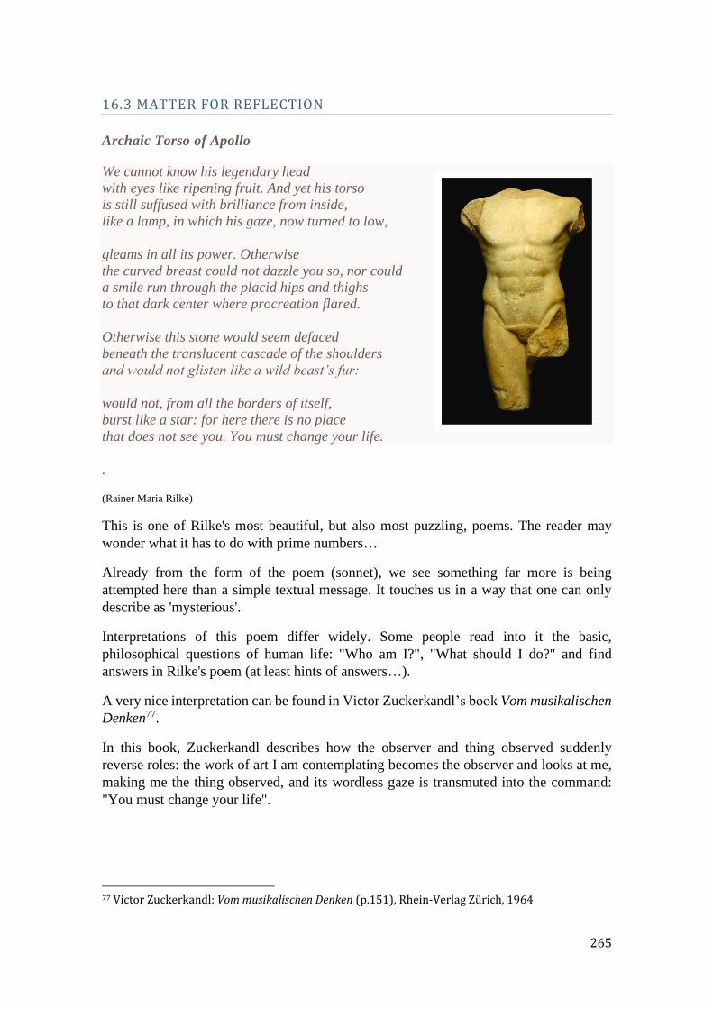
265
16.3 MATTER FOR REFLECTION
Archaic Torso of Apollo
We cannot know his legendary head
with eyes like ripening fruit. And yet his torso
is still suffused with brilliance from inside,
like a lamp, in which his gaze, now turned to low,
gleams in all its power. Otherwise
the curved breast could not dazzle you so, nor could
a smile run through the placid hips and thighs
to that dark center where procreation flared.
Otherwise this stone would seem defaced
beneath the translucent cascade of the shoulders
and would not glisten like a wild beast’s fur:
would not, from all the borders of itself,
burst like a star: for here there is no place
that does not see you. You must change your life.
.
(Rainer Maria Rilke)
This is one of Rilke's most beautiful, but also most puzzling, poems. The reader may
wonder what it has to do with prime numbers…
Already from the form of the poem (sonnet), we see something far more is being
attempted here than a simple textual message. It touches us in a way that one can only
describe as 'mysterious'.
Interpretations of this poem differ widely. Some people read into it the basic,
philosophical questions of human life: "Who am I?", "What should I do?" and find
answers in Rilke's poem (at least hints of answers…).
A very nice interpretation can be found in Victor Zuckerkandl’s book Vom musikalischen
Denken77.
In this book, Zuckerkandl describes how the observer and thing observed suddenly
reverse roles: the work of art I am contemplating becomes the observer and looks at me,
making me the thing observed, and its wordless gaze is transmuted into the command:
"You must change your life".
77 Victor Zuckerkandl: Vom musikalischen Denken (p.151), Rhein-Verlag Zürich, 1964

Matter for reflection
266
For the further interpretation, Zuckerkandl cites the story of the butterfly’s dream of
Zhuangzi78, which is so beautiful that it is also quoted here:
The dream of the butterfly
Once Zhuang Zhou dreamed he was a butterfly, a fluttering butterfly. What fun he had,
doing as he pleased! He did not know he was Zhou. Suddenly he woke up and found
himself to be Zhou. He did not know whether Zhou had dreamed he was a butterfly or a
butterfly had dreamed he was Zhou. Between Zhou and the butterfly there must be some
distinction. This is what is meant by the transformation of things.
This deeply meaningful parable (like Rilke's poem) shows that both levels have the same
quality of ‘reality’ and are coequal to each other. Every work of art has its own life;
indeed, it is alive. Therefore, it can also look at me. For the artist and the process of
creation, this means that a work of art (as soon as a certain threshold is passed during the
process of creation) begins in effect to ‘come alive’ and therefore to have a will of its
own. The work of art 'communicates' with the artist and wants to participate in its
'creation'; it demands to be realized…
The verse form, i.e. the numerical structure, in which prime numbers play a role, as well
as the ‘meter’ of the poem and, of course, the actual text comprise a complex network in
which the concept of 'aesthetics' first becomes meaningful.
That this immanent sense cannot always be rationally and logically put into words, but
nevertheless is "understood" by our aesthetic feeling, reminds us very much of the haiku
and other Japanese verse forms discussed in the last chapter.
Here, too, the two (supposedly independent) levels of meaning, "form" and "content",
seem to be inseparably merged, or, as Ludwig Wittgenstein put it:
Ethics and aesthetics are One79.
A more profound examination of Wittgenstein's argument is needed if we wish to
understand exactly what he means by this. Similarities to many koans from Zen Buddhism
are obvious. Here's an example:
"The eye with which I see God,
Is exactly the same eye with which God looks at me. "
"Show me this eye!"
In these poems the reader interested in mathematics immediately finds the element of
self-reference and recurrence or recursion. Recursion therefore appears to be not only a
very powerful instrument in mathematics, but also a means in philosophy and poetry to
'give voice' to things that cannot be expressed by words: insights into a higher level of
truth?
78 Dschuang Dsi: Das wahre Buch vom südlichen Blütenland: Eugen Diederichs Verlag München (1988) 79 From Tractatus logico-philosophicus by Ludwig Wittgenstein
267
17 PRIME NUMBERS AND EXTRATERRESTRIAL LIFE FORMS
If, in the not-too-distant future, we should happen to receive electromagnetic signals from
extraterrestrial civilizations, a discussion will be launched as to what form
communication with intelligent extraterrestrial beings should take. The search for such
signals has been going on for years and is mainly run by the project 'SETI' ('Search for
Extraterrestrial Intelligence’) in Mountain View near San Francisco.80
First of all, one must be aware that the nearest extraterrestrial planet inhabited with
intelligent living things will not be found in our immediate neighbourhood, but will most
likely be several hundreds, if not thousands, of light years away from the Earth.
Communication could only take place over a period of many centuries. In what
'interstellar language' should we send messages, or do we expect interstellar messages?
Basically, both communication partners must find something that is common to both.
This is, on the one hand, the transmission path using electromagnetic waves, which,
according to our current knowledge, is the only practicable method. One can assume that
extraterrestrial life forms, by the time they are engaged in a search for 'cosmic'
neighbours, will have mastered this technique.
The second known class of waveforms capable of dissemination over enormous distances
are the recently discovered gravitational waves. It is conceivable, theoretically, that aliens
might employ these as a medium of communication. At the moment, however, we do not
have any technology that would allow signals to be detected in modulated gravitational
waves.
The language that is probably mastered by all intelligent life forms in the universe is the
language of mathematics, which pervades every realm of our existence. All our physics
is written in the language of mathematics. Thus, we can be sure that the language of
mathematics is "understood" throughout the universe. Note: there are also theories
assuming a variety of universes that may also have a completely different physics and
perhaps even a different mathematics (Tegmark, 2015). If such universes exist, they
would not be 'physically' accessible to our universe anyway. We restrict ourselves here to
consideration of our universe, which is the only one observable by us.
Prime numbers are perfect for such interstellar messages, since a sequence of such
numbers would almost certainly be the product of intelligent design rather than pure
chance. Our universe contains very well modulated electromagnetic signals, mostly from
rotating neutron stars or other physical processes (wherever charged objects are strongly
accelerated). However, what is common to all these previously observed signals is that
they are more or less periodic, and therefore contain no information.
Since the formal language in which mathematics is carried on at different places in our
universe will also differ, it would make sense to keep the message as simple as possible.
The simplest option mathematics offers are the prime numbers. Therefore, all experts to
have considered the question of extraterrestrial communication agree that transmitting the
prime numbers – let’s say, up to 100 – on as many interesting frequencies as possible (e.g.
the absorption frequency of hydrogen) would be an excellent means of interstellar
80 http://www.seti.org

Matter for reflection
268
communication. The information could, for example, be wrapped in pulsed 'packets', the
temporal distances between the pulses being proportional to the differences of the prime
numbers.
This is exactly what happens in the movie 'Contact'81 from 1997, starring Jodie Foster.
81 https://web.archive.org/web/20071125172406/http://www.cisci.net/film.php?lang=2&display=5&topic=Astronomie%20und%20Astrophysik&seq_id=42&film=26
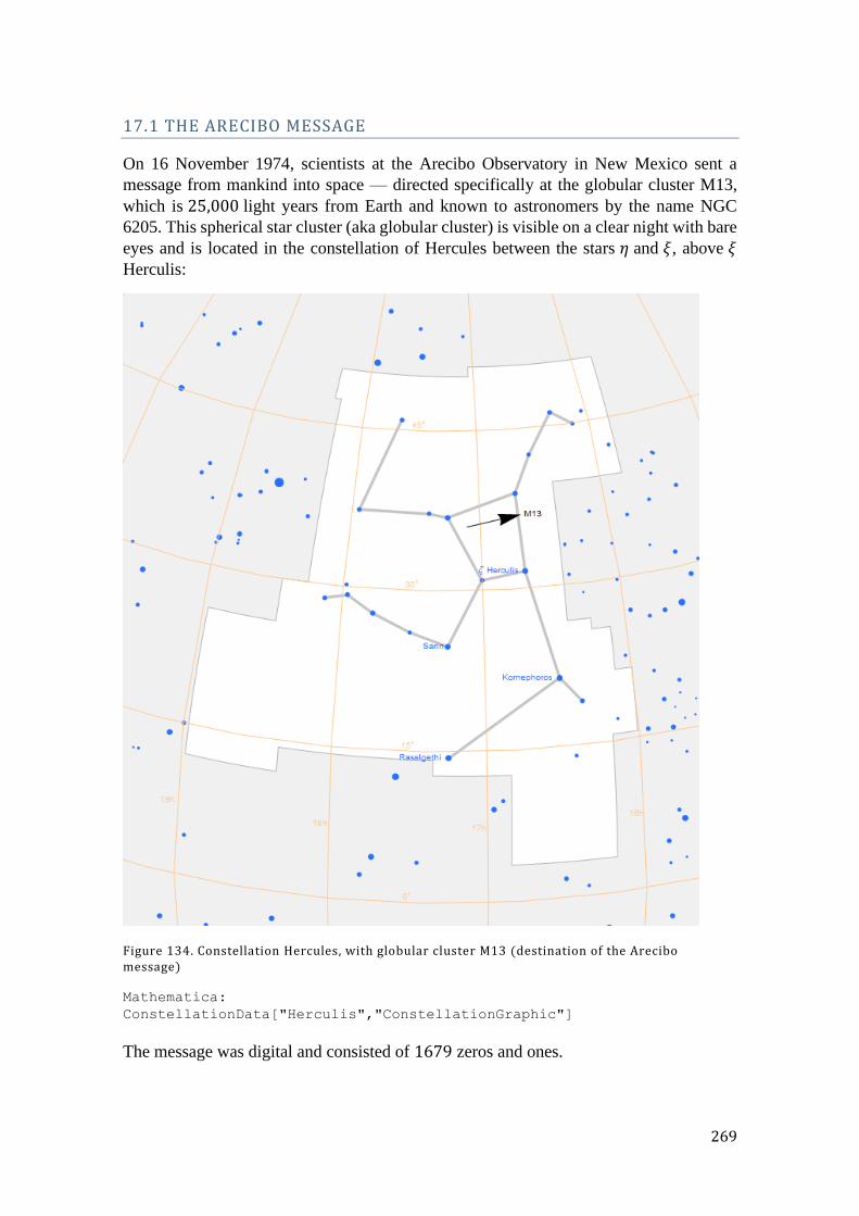
269
17.1 THE ARECIBO MESSAGE
On 16 November 1974, scientists at the Arecibo Observatory in New Mexico sent a
message from mankind into space — directed specifically at the globular cluster M13,
which is 25,000 light years from Earth and known to astronomers by the name NGC
6205. This spherical star cluster (aka globular cluster) is visible on a clear night with bare
eyes and is located in the constellation of Hercules between the stars 휂 and 𝜉, above 𝜉
Herculis:
Figure 134. Constellation Hercules, with globular cluster M13 (destination of the Arecibo message)
Mathematica:
ConstellationData["Herculis","ConstellationGraphic"]
The message was digital and consisted of 1679 zeros and ones.
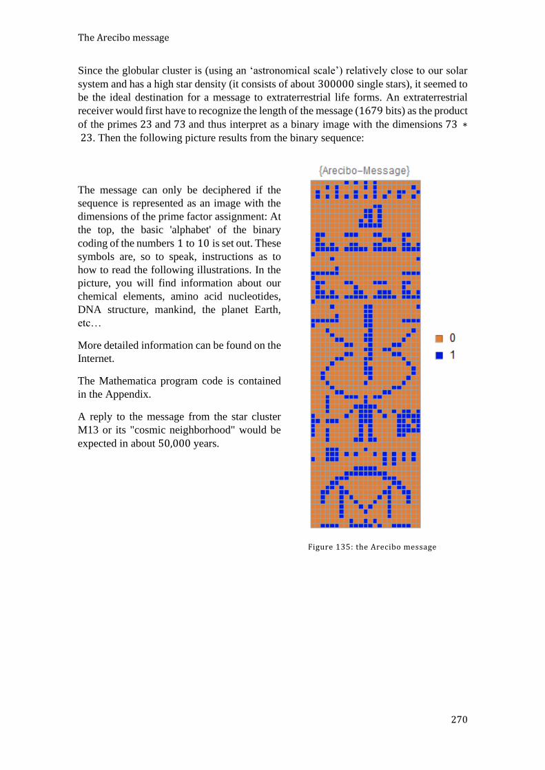
The Arecibo message
270
Since the globular cluster is (using an ‘astronomical scale’) relatively close to our solar
system and has a high star density (it consists of about 300000 single stars), it seemed to
be the ideal destination for a message to extraterrestrial life forms. An extraterrestrial
receiver would first have to recognize the length of the message (1679 bits) as the product
of the primes 23 and 73 and thus interpret as a binary image with the dimensions 73 ∗ 23. Then the following picture results from the binary sequence:
Figure 135: the Arecibo message
xxx
The message can only be deciphered if the
sequence is represented as an image with the
dimensions of the prime factor assignment: At
the top, the basic 'alphabet' of the binary
coding of the numbers 1 to 10 is set out. These
symbols are, so to speak, instructions as to
how to read the following illustrations. In the
picture, you will find information about our
chemical elements, amino acid nucleotides,
DNA structure, mankind, the planet Earth,
etc…
More detailed information can be found on the
Internet.
The Mathematica program code is contained
in the Appendix.
A reply to the message from the star cluster
M13 or its "cosmic neighborhood" would be
expected in about 50,000 years.
271
18 MISCELLANY
18.1 THE NUMBER 12
The number 12 has many special properties:
1) It was prevalent in units of measurement and counting systems until quite
recently – a case in point being the British (twelve-penny) shilling, which was
only abandoned in 1971 – and, even today, eggs are still sold by the dozen.
2) The year has 12 months; the day has 2 x 12 hours.
3) Jesus had 12 apostles; Israel had 12 tribes.
4) The octave has 12 semitone steps.
5) It is the smallest ‘abundant’ number (abundant numbers are numbers, whose ‘true’
sum of divisors is larger than the number itself …)
6) It is the 3-dimensional kissing number.82
7) There are 12 signs of the zodiac.
8) There are 12 Olympic gods.
9) The 12𝑡ℎ Fibonacci number is (among the infinitely many Fibonacci numbers)
the only square in this sequence and it has the value 122 = 144.
10) 12 is the smallest ‘sublime’ number (at least two sublime numbers are known).
Note: a sublime number is a number where the sum of its divisors and the number
of its divisors are perfect numbers. The second such number known is 6086555670238378989670371734243169622657830773351885970528324860512791691264
11) It plays a special role in music: the 12-bar blues scheme.
12) The number 12 is the only number 𝑛 for which the notable relation 𝑛 =𝑟4(𝑛)
8
applies (where 𝑟4(𝑛) is the number of four-dimensional lattice points of a squared
radius of 𝑛).
13) The world of the physicist Burkhard Heim contains exactly 12 dimensions.
14) It appears in Ramanujan's magical formula: 1 + 2 + 3 + 4 +⋯ = −1
12
15) The 12th Mersenne prime number exponent has the striking short OCRON
representation "2PPPP" which contains neither the ^ - nor the * - operator (see
chapter 10.1)
82 https://de.wikipedia.org/wiki/Kusszahl
272
18.2 THE NUMBER 313
There are also primes in comics! Who does not know Donald Duck's bright red duck
convertible ("1934 Belchfire Runabout") with the license plate number 313?
313 is a special number in several respects:
- It is a 3-digit palindromic prime number (gives the same value read forwards and
backwards)
- It is in binary representation (100111001) palindromic and 100111001 decimal
interpreted also gives a palindromic prime number!
The website https://primes.utm.edu/curios/page.php/313.html lists another 40 special
features of this number …
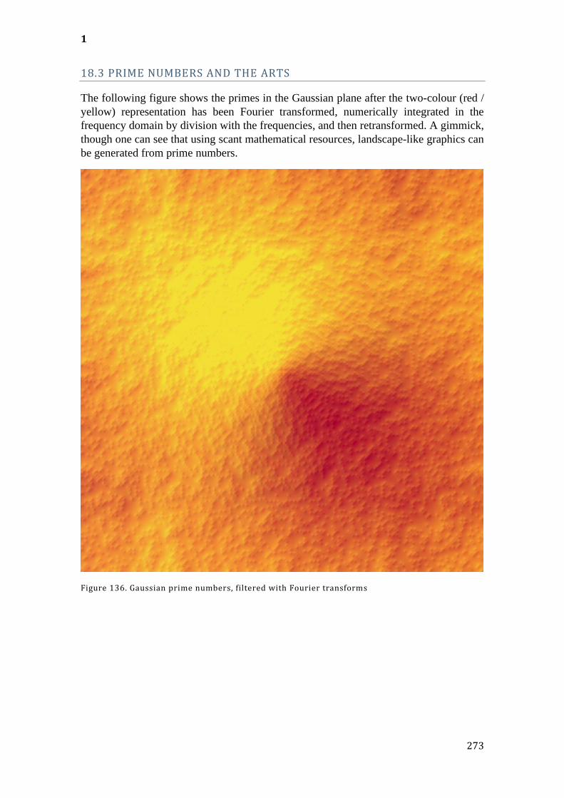
1
273
18.3 PRIME NUMBERS AND THE ARTS
The following figure shows the primes in the Gaussian plane after the two-colour (red /
yellow) representation has been Fourier transformed, numerically integrated in the
frequency domain by division with the frequencies, and then retransformed. A gimmick,
though one can see that using scant mathematical resources, landscape-like graphics can
be generated from prime numbers.
Figure 136. Gaussian prime numbers, filtered with Fourier transforms

274
19 CONCLUSION
Prime numbers have been a source of fascination to us for as long we have been studying
mathematics. Although we know a lot about them, they have lost none of their mystique.
They pervade many areas of all possible sciences and also inhabit the realms of culture,
such as poetry, as well as economic life.
We have come to understand a great deal about them, but not the true, the real "message"
that is hidden in them.
There remain many secrets still to be uncovered!
275
20 APPENDIX
20.1 CATALAN’S CONJECTURE
Catalan’s conjecture states that there are no integer powers of natural numbers that
differ exactly by the value 1, with one exception:
23 = 8 and 32 = 9
In other words: the only integer solution of the equation
𝒎𝒑 − 𝒏𝒒 = 𝟏,where 𝒎,𝒏, 𝒑, 𝒒 > 𝟏 is 𝒎 = 𝟑, 𝒏 = 𝟐, 𝒑 = 𝟐, 𝒒 = 𝟑 (159)
It was proved in the year 2002 by Preda Mihăilescu.
.
The proof was obtained with the help of ‘double Wieferich primes’ (see 4.14).
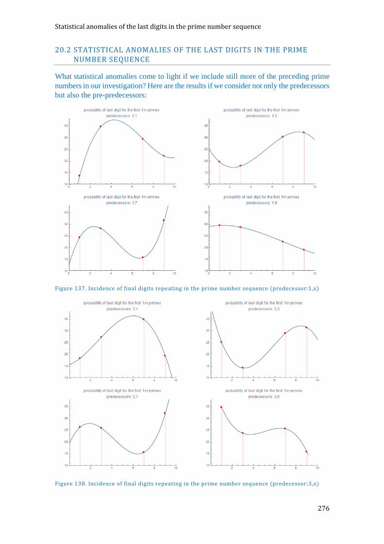
Statistical anomalies of the last digits in the prime number sequence
276
20.2 STATISTICAL ANOMALIES OF THE LAST DIGITS IN THE PRIME NUMBER SEQUENCE
What statistical anomalies come to light if we include still more of the preceding prime
numbers in our investigation? Here are the results if we consider not only the predecessors
but also the pre-predecessors:
Figure 137. Incidence of final digits repeating in the prime number sequence (predecessor:1,x)
Figure 138. Incidence of final digits repeating in the prime number sequence (predecessor:3,x)
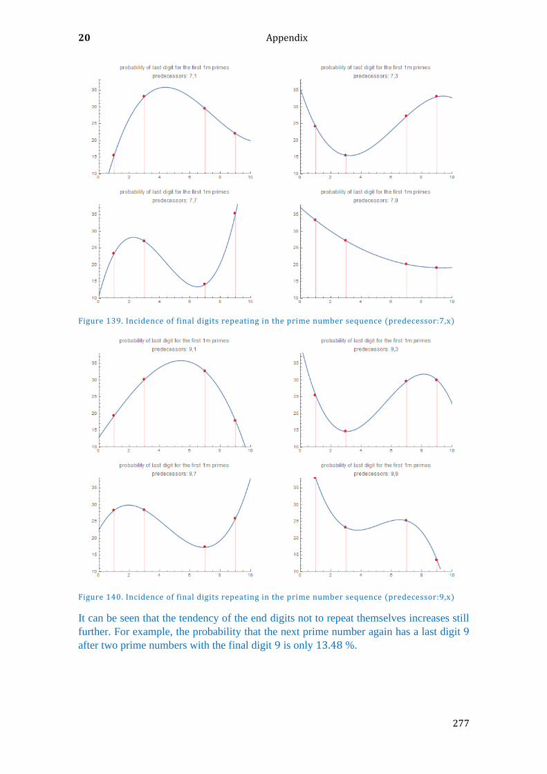
20 Appendix
277
Figure 139. Incidence of final digits repeating in the prime number sequence (predecessor:7,x)
Figure 140. Incidence of final digits repeating in the prime number sequence (predecessor:9,x)
It can be seen that the tendency of the end digits not to repeat themselves increases still
further. For example, the probability that the next prime number again has a last digit 9
after two prime numbers with the final digit 9 is only 13.48 %.
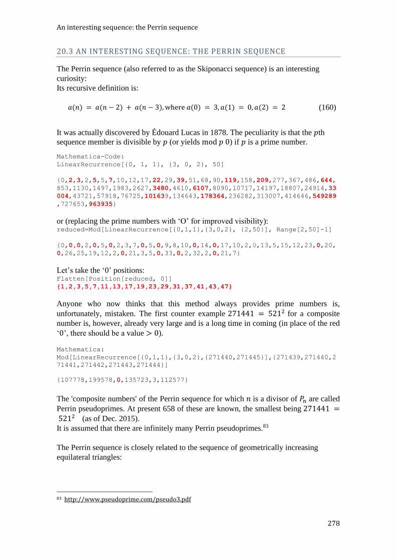
An interesting sequence: the Perrin sequence
278
20.3 AN INTERESTING SEQUENCE: THE PERRIN SEQUENCE
The Perrin sequence (also referred to as the Skiponacci sequence) is an interesting
curiosity:
Its recursive definition is:
𝑎(𝑛) = 𝑎(𝑛 − 2) + 𝑎(𝑛 − 3),where 𝑎(0) = 3, 𝑎(1) = 0, 𝑎(2) = 2 (160)
It was actually discovered by Édouard Lucas in 1878. The peculiarity is that the 𝑝th
sequence member is divisible by 𝑝 (or yields mod 𝑝 0) if 𝑝 is a prime number.
Mathematica-Code:
LinearRecurrence[{0, 1, 1}, {3, 0, 2}, 50]
{0,2,3,2,5,5,7,10,12,17,22,29,39,51,68,90,119,158,209,277,367,486,644,
853,1130,1497,1983,2627,3480,4610,6107,8090,10717,14197,18807,24914,33
004,43721,57918,76725,101639,134643,178364,236282,313007,414646,549289
,727653,963935}
or (replacing the prime numbers with ‘O’ for improved visibility): reduced=Mod[LinearRecurrence[{0,1,1},{3,0,2}, {2,50}], Range[2,50]-1]
{0,0,0,2,0,5,0,2,3,7,0,5,0,9,8,10,0,14,0,17,10,2,0,13,5,15,12,23,0,20,
0,26,25,19,12,2,0,21,3,5,0,33,0,2,32,2,0,21,7}
Let’s take the ‘0’ positions: Flatten[Position[reduced, 0]]
{1,2,3,5,7,11,13,17,19,23,29,31,37,41,43,47}
Anyone who now thinks that this method always provides prime numbers is,
unfortunately, mistaken. The first counter example 271441 = 5212 for a composite
number is, however, already very large and is a long time in coming (in place of the red
‘0’, there should be a value > 0).
Mathematica:
Mod[LinearRecurrence[{0,1,1},{3,0,2},{271440,271445}],{271439,271440,2
71441,271442,271443,271444}]
{107778,199578,0,135723,3,112577}
The 'composite numbers' of the Perrin sequence for which 𝑛 is a divisor of 𝑃𝑛 are called
Perrin pseudoprimes. At present 658 of these are known, the smallest being 271441 = 5212 (as of Dec. 2015).
It is assumed that there are infinitely many Perrin pseudoprimes.83
The Perrin sequence is closely related to the sequence of geometrically increasing
equilateral triangles:
83 http://www.pseudoprime.com/pseudo3.pdf
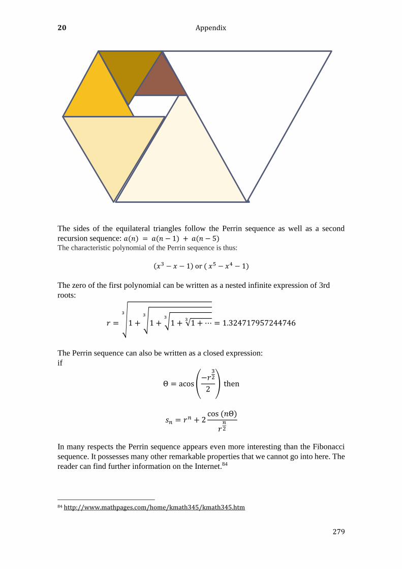
20 Appendix
279
The sides of the equilateral triangles follow the Perrin sequence as well as a second
recursion sequence: 𝑎(𝑛) = 𝑎(𝑛 − 1) + 𝑎(𝑛 − 5) The characteristic polynomial of the Perrin sequence is thus:
(𝑥3 − 𝑥 − 1) or ( 𝑥5 − 𝑥4 − 1)
The zero of the first polynomial can be written as a nested infinite expression of 3rd
roots:
𝑟 = √1 + √1 + √1 + √1 +⋯3333
= 1.324717957244746
The Perrin sequence can also be written as a closed expression:
if
Θ = acos(−𝑟
32
2) then
𝑠𝑛 = 𝑟𝑛 + 2
cos (𝑛Θ)
𝑟𝑛2
In many respects the Perrin sequence appears even more interesting than the Fibonacci
sequence. It possesses many other remarkable properties that we cannot go into here. The
reader can find further information on the Internet.84
84 http://www.mathpages.com/home/kmath345/kmath345.htm

More conjectures about prime numbers
280
20.4 MORE CONJECTURES ABOUT PRIME NUMBERS
The Goldbach conjecture
The Goldbach conjecture states that any natural even number 𝑛 > 2 can be written as the
sum of two prime numbers. The conjecture has been verified numerically for all 𝑛 < 4 ⋅1018 (as of Oct. 2015). The 'extended Goldbach conjecture' gives an estimate for the
number of representations 𝑅𝑔 of a number 𝑛 as the sum of 2 prime numbers:
𝑅𝑔(𝑛) ≈ 2Π2∏𝑝𝑘 − 1
𝑝𝑘 − 2𝑘=2𝑝𝑘|𝑛
∫𝑑𝑥
(ln 𝑥)2= 2Π2∏
𝑝𝑘 − 1
𝑝𝑘 − 2𝑘=2𝑝𝑘|𝑛
[𝑙𝑖(𝑥) −𝑥
ln (𝑥)]
𝑛
2
𝑛2
(161)
Mathematica program (from oeis.org):
a[n_] := Length @ Select[PowersRepresentations[2 n, 2, 1], (#[[1]] ==
1 || PrimeQ[#[[1]]]) && (#[[2]] == 1 || PrimeQ[#[[2]]]) &]; Array[a,
98] (* Jean-François Alcover, Apr 11 2011 *)
nn = 10^2; ps = Boole[PrimeQ[Range[2*nn]]]; ps[[1]] = 1;
Table[Sum[ps[[i]] ps[[2*n - i]], {i, n}], {n, nn}] (* T. D. Noe, Apr
11 2011 *)

20 Appendix
281
20.5 PRIME N-TUPLETS: CONSTELLATIONS OF PRIME NUMBERS
Let us assume that we have an arbitrarily large prime p at index 1. Then p+1 can certainly
be divided by 2. Hence, as in the Sieve of Eratosthenes, we delete all the following
numbers divisible by 2:
p 2 2 2 2 2 2 2 2 2 2 2 2 2 2 2 2 2 2 2 2
The next possible prime is at p+2 at index 3(twin).
p 2 p 2 2 2 2 2 2 2 2 2 2 2 2 2 2 2 2 2 2 2
The group p-2-p must contain at least one number divisible by 3. This can only be
the 2 at the 2nd position. So we delete all parts divisible by 3 (there are, of course,
multiple deletions at the positions divisible by 6):
p 2
3 p 2 3 2
2
3 2 3 2
2
3 2 3 2
2
3 2 3 2
2
3 2 3 2
2
3 2 3 2
2
3 2
The next possible prime is at p+6 at index 7: (triplet).
p 2
3 p 2 3 2 p
2
3 2 3 2
2
3 2 3 2
2
3 2 3 2
2
3 2 3 2
2
3 2 3 2
2
3 2
For the next sifting operation (divisibility by 5), one cannot find any unique requirement
(it cannot be determined which of the first 5 numbers has to be divisible by 5 since we
still have ambiguity (candidates: positions no. 4 and 5). Therefore the next possible
prime number is at position p+8 at index 9: (quadruplet).
p 2
3 p 2 3 2 p
2
3 p 2 3 2
2
3 2 3 2
2
3 2 3 2
2
3 2 3 2
2
3 2 3 2
2
3 2
The group p-2-p-2-3 must contain at least one number divisible by 5. This can only
be at the 5th position with ‘3’. Reason: the 2th position 23
can be excluded, since then
also the 7th position would have to be divisible by 5. This position, however, is already
occupied by p. The same holds true for the 4th position ‘2’, since the 9th position would
then also be divisible by 5, which is also already occupied by p. Thus the 5th position
with the '3' remains as the only possibility. We delete all positions divisible by 5:
p 2
3 p 2
3
5 2 p
2
3 p 2
5 3 2
2
3 5 2 3 2
2
3
5
2 3 2 5 2
3 2 3
2
5 2
3 2
3
5 2
2
3 2
5
The next possible prime is at p+12 at index 13: (pentuplet).
p 2
3 p 2
3
5 2 p
2
3 p 2
5 3 2 p
2
3 5 2 3 2
2
3
5
2 3 2 5 2
3 2 3
2
5 2
3 2
3
5 2
2
3 2
5
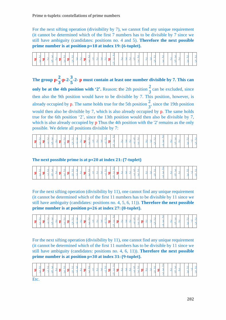
Prime n-tuplets: constellations of prime numbers
282
For the next sifting operation (divisibility by 7), we cannot find any unique requirement
(it cannot be determined which of the first 7 numbers has to be divisible by 7 since we
still have ambiguity (candidates: positions no. 4 and 5). Therefore the next possible
prime number is at position p+18 at index 19: (6-tuplet).
p 2
3 p 2
3
5 2 p
2
3 p 2
5 3 2 p
2
3 5 2 3 2 p
2
3
5
2 3 2 5 2
3 2 3
2
5 2
3 2
3
5 2
2
3 2
5
The group p-𝟐𝟑
-p-2-𝟑𝟓
-2- p must contain at least one number divisible by 7. This can
only be at the 4th position with ‘2’. Reason: the 2th position 23
can be excluded, since
then also the 9th position would have to be divisible by 7. This position, however, is
already occupied by p. The same holds true for the 5th position 23
, since the 19th position
would then also be divisible by 7, which is also already occupied by p. The same holds
true for the 6th position ‘2’, since the 13th position would then also be divisible by 7,
which is also already occupied by p Thus the 4th position with the '2' remains as the only
possible. We delete all positions divisible by 7:
p 2
3 p 2
7
3
5 2 p
2
3 p 2
5
3
7 2 p
2
3 5 2 3
2
7 p
2
3
5
2 3 2 5
7
2
3 2 3
2
5
2
3
7
2 3
5 2
2
3 7 2
5
The next possible prime is at p+20 at index 21: (7-tuplet)
p 2
3 p 2
7
3
5 2 p
2
3 p 2
5
3
7 2 p
2
3 5 2 3
2
7 p
2
3
5
p 2 3 2 5
7
2
3 2 3
2
5
2
3
7
2 3
5 2
2
3 7 2
5
For the next sifting operation (divisibility by 11), one cannot find any unique requirement
(it cannot be determined which of the first 11 numbers has to be divisible by 11 since we
still have ambiguity (candidates: positions no. 4, 5, 6, 11)). Therefore the next possible
prime number is at position p+26 at index 27: (8-tuplet).
p 2
3 p 2
7
3
5 2 p
2
3 p 2
5
3
7 2 p
2
3 5 2 3
2
7 p
2
3
5
p 2 3 2 5
7
2
3 p 2 3
2
5
2
3
7
2 3
5 2
2
3 7 2
5
For the next sifting operation (divisibility by 11), one cannot find any unique requirement
(it cannot be determined which of the first 11 numbers has to be divisible by 11 since we
still have ambiguity (candidates: positions no. 4, 6, 11)). Therefore the next possible
prime number is at position p+30 at index 31: (9-tuplet).
p 2
3 p 2
7
3
5 2 p
2
3 p 2
5
3
7 2 p
2
3 5 2 3
2
7 p
2
3
5
p 2 3 2 5
7
2
3 p 2 3
2
5 p
2
3
7
2 3
5 2
2
3 7 2
5
Etc.
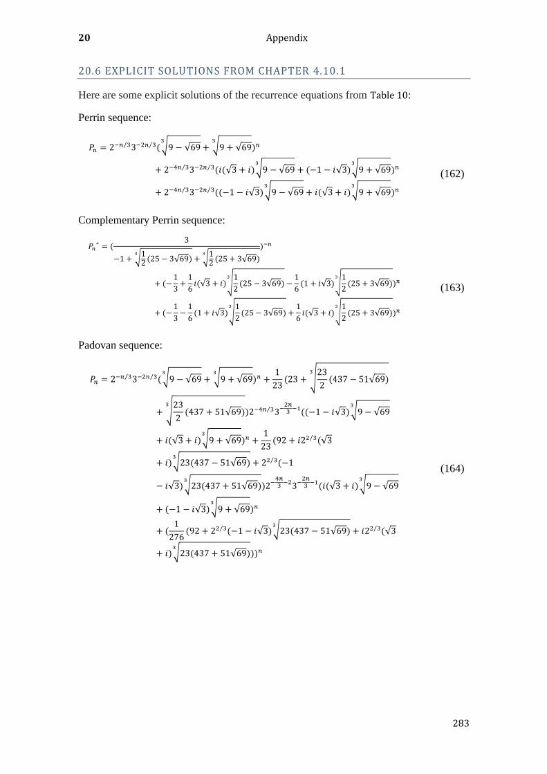
20 Appendix
283
20.6 EXPLICIT SOLUTIONS FROM CHAPTER 4.10.1
Here are some explicit solutions of the recurrence equations from Table 10:
Perrin sequence:
𝑃𝑛 = 2−𝑛 3⁄ 3−2𝑛 3⁄ (√9 − √69
3
+ √9 + √693
)𝑛
+ 2−4𝑛 3⁄ 3−2𝑛 3⁄ (𝑖(√3 + 𝑖)√9 − √693
+ (−1 − 𝑖√3)√9 + √693
)𝑛
+ 2−4𝑛 3⁄ 3−2𝑛 3⁄ ((−1 − 𝑖√3)√9 − √693
+ 𝑖(√3 + 𝑖)√9 + √693
)𝑛
(162)
Complementary Perrin sequence:
𝑃𝑛∗ = (
3
−1 + √12(25 − 3√69)
3
+ √12(25 + 3√69)
3
)−𝑛
+ (−1
3+1
6𝑖(√3 + 𝑖)√
1
2(25 − 3√69)
3
−1
6(1 + 𝑖√3)√
1
2(25 + 3√69)
3
)𝑛
+ (−1
3−1
6(1 + 𝑖√3)√
1
2(25 − 3√69)
3
+1
6𝑖(√3 + 𝑖)√
1
2(25 + 3√69)
3
)𝑛
(163)
Padovan sequence:
𝑃𝑛 = 2−𝑛 3⁄ 3−2𝑛 3⁄ (√9 − √69
3
+ √9 + √693
)𝑛 +1
23(23 + √
23
2(437 − 51√69)
3
+ √23
2(437 + 51√69)
3
)2−4𝑛 3⁄ 3−2𝑛3−1((−1 − 𝑖√3)√9 − √69
3
+ 𝑖(√3 + 𝑖)√9 + √693
)𝑛 +1
23(92 + 𝑖22 3⁄ (√3
+ 𝑖)√23(437 − 51√69)3
+ 22 3⁄ (−1
− 𝑖√3)√23(437 + 51√69)3
)2−4𝑛3−23−
2𝑛3−1(𝑖(√3 + 𝑖)√9 − √69
3
+ (−1 − 𝑖√3)√9 + √693
)𝑛
+ (1
276(92 + 22 3⁄ (−1 − 𝑖√3)√23(437 − 51√69)
3
+ 𝑖22 3⁄ (√3
+ 𝑖)√23(437 + 51√69)3
))𝑛
(164)
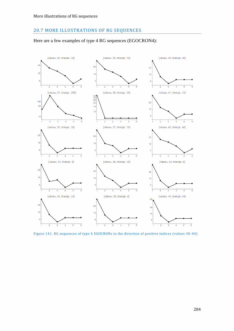
More illustrations of RG sequences
284
20.7 MORE ILLUSTRATIONS OF RG SEQUENCES
Here are a few examples of type 4 RG sequences (EGOCRON4):
Figure 141. RG sequences of type 4 EGOCRONs in the direction of positive indices (values 30 -44)
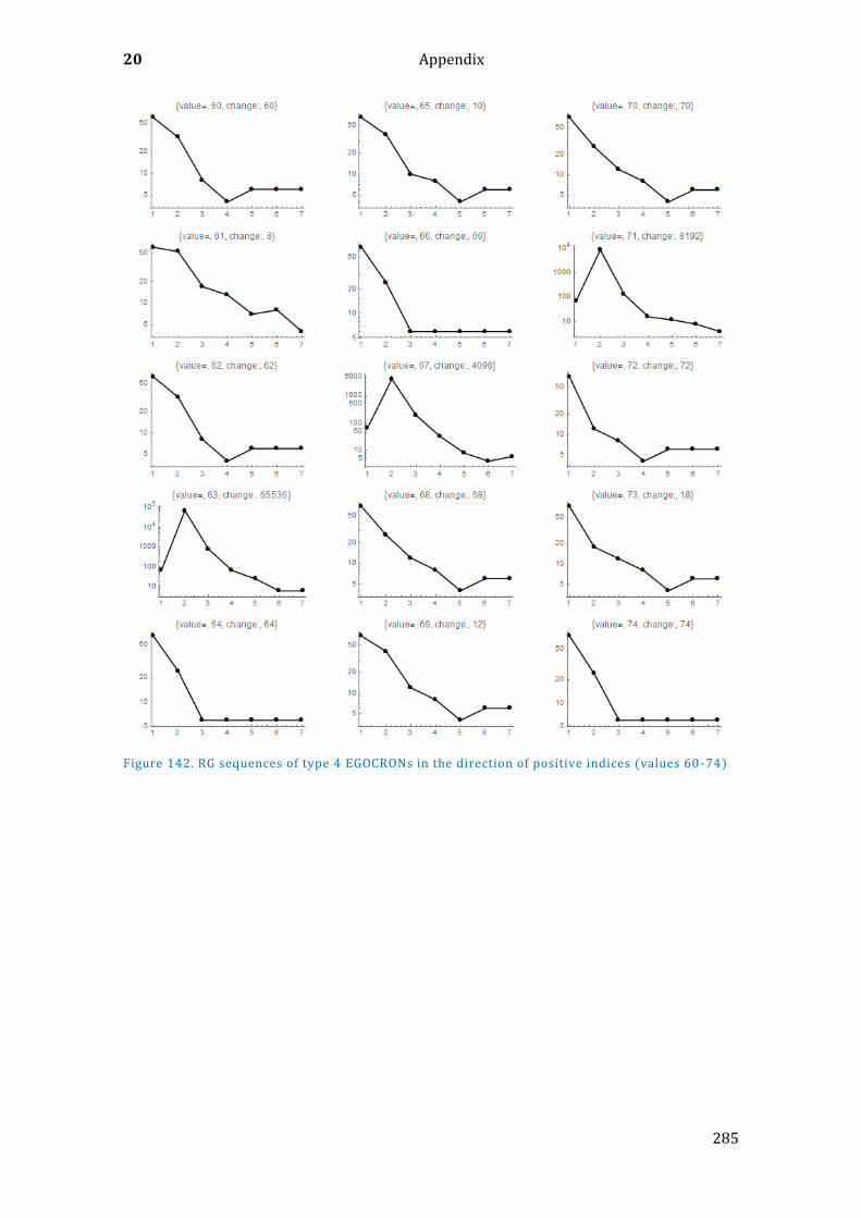
20 Appendix
285
Figure 142. RG sequences of type 4 EGOCRONs in the direction of positive indices (values 60 -74)
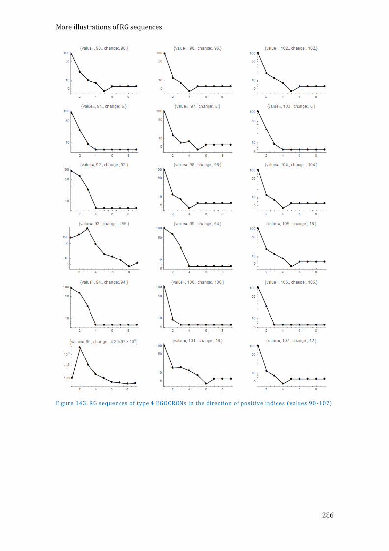
More illustrations of RG sequences
286
Figure 143. RG sequences of type 4 EGOCRONs in the direction of positive indices (values 90 -107)
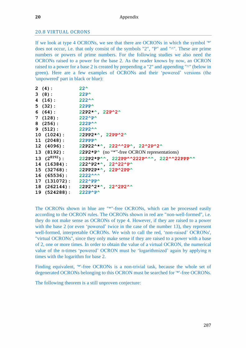
20 Appendix
287
20.8 VIRTUAL OCRONS
If we look at type 4 OCRONs, we see that there are OCRONs in which the symbol '*'
does not occur, i.e. that only consist of the symbols "2", "P" and "^". These are prime
numbers or powers of prime numbers. For the following studies we also need the
OCRONs raised to a power for the base 2. As the reader knows by now, an OCRON
raised to a power for a base 2 is created by prepending a "2" and appending "^" (below in
green). Here are a few examples of OCRONs and their ‘powered’ versions (the
'unpowered' part in black or blue):
2 (4): 22^
3 (8): 22P^
4 (16): 222^^
5 (32): 22PP^
6 (64): 22P2*^, 22P^2^
7 (128): 222^P^
8 (256): 222P^^
9 (512): 22P2^^
10 (1024): 22PP2*^, 22PP^2^
11 (2048): 22PPP^
12 (4096): 22P22^*^, 222^^2P^, 22^2P^2^
13 (8192): 22P2*P^ (no “*”-free OCRON representations)
13 (𝟐𝟖𝟏𝟗𝟐): 222P2*P^^, 222PP^^222P^^^, 222^^22PPP^^
14 (16384): 222^P2*^, 22^22^P^
15 (32768): 22PP2P*^, 22P^2PP^
16 (65536): 2222^^^
17 (131072): 222^PP^
18 (262144): 22P2^2*^, 22^2P2^^
19 (524288): 222P^P^
The OCRONs shown in blue are "*"-free OCRONs, which can be processed easily
according to the OCRON rules. The OCRONs shown in red are "non-well-formed", i.e.
they do not make sense as OCRONs of type 4. However, if they are raised to a power
with the base 2 (or even ‘powered’ twice in the case of the number 13), they represent
well-formed, interpretable OCRONs. We wish to call the red, ‘non-raised’ OCRONs',
"virtual OCRONs", since they only make sense if they are raised to a power with a base
of 2, one or more times. In order to obtain the value of a virtual OCRON, the numerical
value of the n-times ‘powered’ OCRON must be ‘logarithmized’ again by applying 𝑛
times with the logarithm for base 2.
Finding equivalent, '*'-free OCRONs is a non-trivial task, because the whole set of
degenerated OCRONs belonging to this OCRON must be searched for '*'-free OCRONs.
The following theorem is a still unproven conjecture:
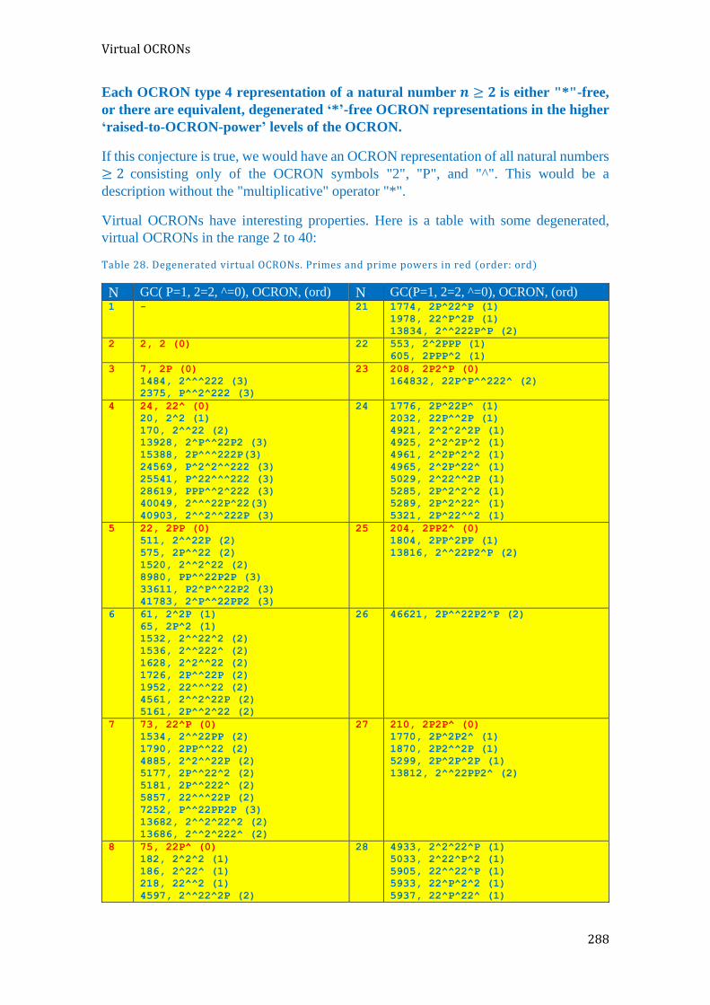
Virtual OCRONs
288
Each OCRON type 4 representation of a natural number 𝒏 ≥ 𝟐 is either "*"-free,
or there are equivalent, degenerated ‘*’-free OCRON representations in the higher
‘raised-to-OCRON-power’ levels of the OCRON.
If this conjecture is true, we would have an OCRON representation of all natural numbers
≥ 2 consisting only of the OCRON symbols "2", "P", and "^". This would be a
description without the "multiplicative" operator "*".
Virtual OCRONs have interesting properties. Here is a table with some degenerated,
virtual OCRONs in the range 2 to 40:
Table 28. Degenerated virtual OCRONs. Primes and prime powers in red (order: ord)
N GC( P=1, 2=2, ^=0), OCRON, (ord) N GC(P=1, 2=2, ^=0), OCRON, (ord) 1 - 21 1774, 2P^22^P (1)
1978, 22^P^2P (1)
13834, 2^^222P^P (2)
2 2, 2 (0) 22 553, 2^2PPP (1)
605, 2PPP^2 (1)
3 7, 2P (0)
1484, 2^^^222 (3)
2375, P^^2^222 (3)
23 208, 2P2^P (0)
164832, 22P^P^^222^ (2)
4 24, 22^ (0)
20, 2^2 (1)
170, 2^^22 (2)
13928, 2^P^^22P2 (3)
15388, 2P^^^222P(3)
24569, P^2^2^^222 (3)
25541, P^22^^^222 (3)
28619, PPP^^2^222 (3)
40049, 2^^^22P^22(3)
40903, 2^^2^^222P (3)
24 1776, 2P^22P^ (1)
2032, 22P^^2P (1)
4921, 2^2^2^2P (1)
4925, 2^2^2P^2 (1)
4961, 2^2P^2^2 (1)
4965, 2^2P^22^ (1)
5029, 2^22^^2P (1)
5285, 2P^2^2^2 (1)
5289, 2P^2^22^ (1)
5321, 2P^22^^2 (1)
5 22, 2PP (0)
511, 2^^22P (2)
575, 2P^^22 (2)
1520, 2^^2^22 (2)
8980, PP^^22P2P (3)
33611, P2^P^^22P2 (3)
41783, 2^P^^22PP2 (3)
25 204, 2PP2^ (0)
1804, 2PP^2PP (1)
13816, 2^^22P2^P (2)
6 61, 2^2P (1)
65, 2P^2 (1)
1532, 2^^22^2 (2)
1536, 2^^222^ (2)
1628, 2^2^^22 (2)
1726, 2P^^22P (2)
1952, 22^^^22 (2)
4561, 2^^2^22P (2)
5161, 2P^^2^22 (2)
26 46621, 2P^^22P2^P (2)
7 73, 22^P (0)
1534, 2^^22PP (2)
1790, 2PP^^22 (2)
4885, 2^2^^22P (2)
5177, 2P^^22^2 (2)
5181, 2P^^222^ (2)
5857, 22^^^22P (2)
7252, P^^22PP2P (3)
13682, 2^^2^22^2 (2)
13686, 2^^2^222^ (2)
27 210, 2P2P^ (0)
1770, 2P^2P2^ (1)
1870, 2P2^^2P (1)
5299, 2P^2P^2P (1)
13812, 2^^22PP2^ (2)
8 75, 22P^ (0)
182, 2^2^2 (1)
186, 2^22^ (1)
218, 22^^2 (1)
4597, 2^^22^2P (2)
28 4933, 2^2^22^P (1)
5033, 2^22^P^2 (1)
5905, 22^^22^P (1)
5933, 22^P^2^2 (1)
5937, 22^P^22^ (1)
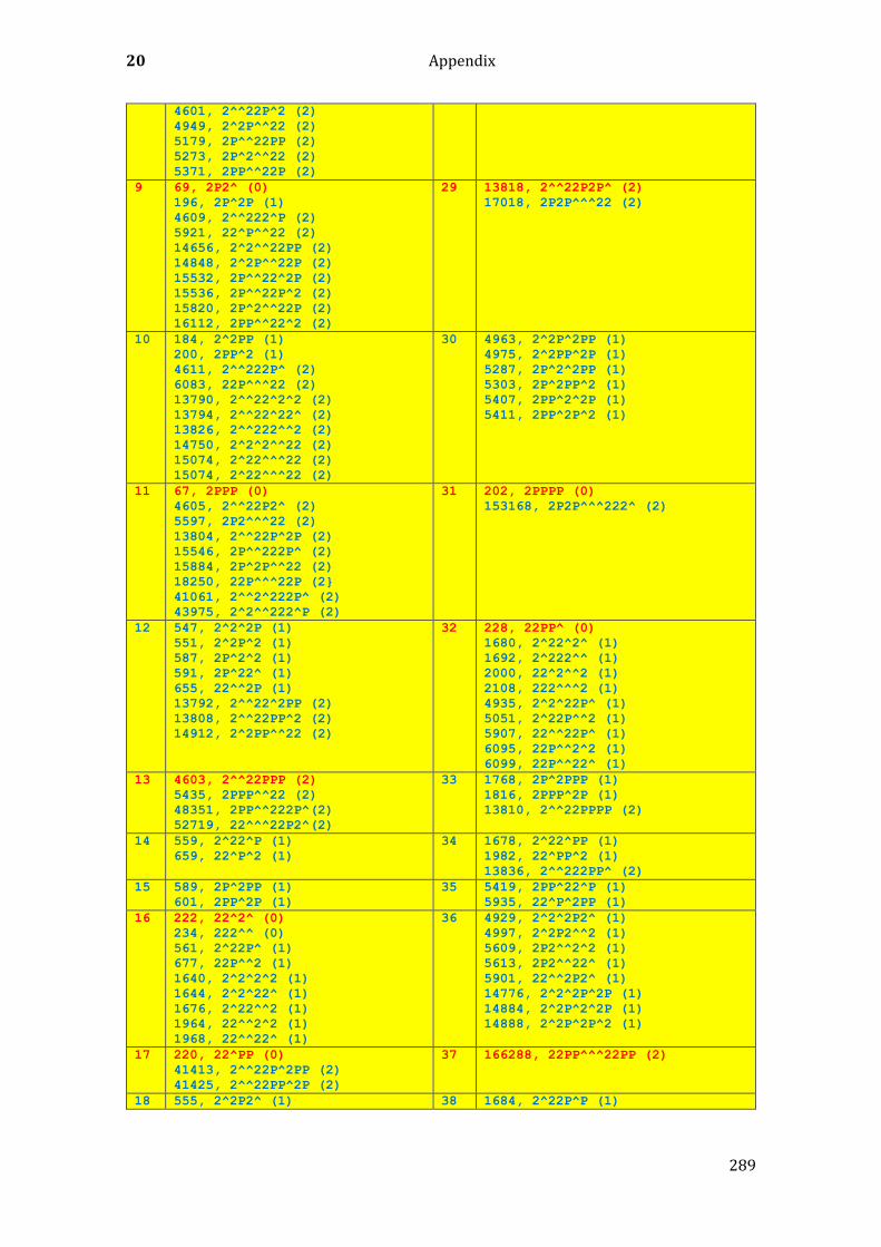
20 Appendix
289
4601, 2^^22P^2 (2)
4949, 2^2P^^22 (2)
5179, 2P^^22PP (2)
5273, 2P^2^^22 (2)
5371, 2PP^^22P (2)
9 69, 2P2^ (0)
196, 2P^2P (1)
4609, 2^^222^P (2)
5921, 22^P^^22 (2)
14656, 2^2^^22PP (2)
14848, 2^2P^^22P (2)
15532, 2P^^22^2P (2)
15536, 2P^^22P^2 (2)
15820, 2P^2^^22P (2)
16112, 2PP^^22^2 (2)
29 13818, 2^^22P2P^ (2)
17018, 2P2P^^^22 (2)
10 184, 2^2PP (1)
200, 2PP^2 (1)
4611, 2^^222P^ (2)
6083, 22P^^^22 (2)
13790, 2^^22^2^2 (2)
13794, 2^^22^22^ (2)
13826, 2^^222^^2 (2)
14750, 2^2^2^^22 (2)
15074, 2^22^^^22 (2)
15074, 2^22^^^22 (2)
30 4963, 2^2P^2PP (1)
4975, 2^2PP^2P (1)
5287, 2P^2^2PP (1)
5303, 2P^2PP^2 (1)
5407, 2PP^2^2P (1)
5411, 2PP^2P^2 (1)
11 67, 2PPP (0)
4605, 2^^22P2^ (2)
5597, 2P2^^^22 (2)
13804, 2^^22P^2P (2)
15546, 2P^^222P^ (2)
15884, 2P^2P^^22 (2)
18250, 22P^^^22P (2}
41061, 2^^2^222P^ (2)
43975, 2^2^^222^P (2)
31 202, 2PPPP (0)
153168, 2P2P^^^222^ (2)
12 547, 2^2^2P (1)
551, 2^2P^2 (1)
587, 2P^2^2 (1)
591, 2P^22^ (1)
655, 22^^2P (1)
13792, 2^^22^2PP (2)
13808, 2^^22PP^2 (2)
14912, 2^2PP^^22 (2)
32 228, 22PP^ (0)
1680, 2^22^2^ (1)
1692, 2^222^^ (1)
2000, 22^2^^2 (1)
2108, 222^^^2 (1)
4935, 2^2^22P^ (1)
5051, 2^22P^^2 (1)
5907, 22^^22P^ (1)
6095, 22P^^2^2 (1)
6099, 22P^^22^ (1)
13 4603, 2^^22PPP (2)
5435, 2PPP^^22 (2)
48351, 2PP^^222P^(2)
52719, 22^^^22P2^(2)
33 1768, 2P^2PPP (1)
1816, 2PPP^2P (1)
13810, 2^^22PPPP (2)
14 559, 2^22^P (1)
659, 22^P^2 (1)
34 1678, 2^22^PP (1)
1982, 22^PP^2 (1)
13836, 2^^222PP^ (2)
15 589, 2P^2PP (1)
601, 2PP^2P (1)
35 5419, 2PP^22^P (1)
5935, 22^P^2PP (1)
16 222, 22^2^ (0)
234, 222^^ (0)
561, 2^22P^ (1)
677, 22P^^2 (1)
1640, 2^2^2^2 (1)
1644, 2^2^22^ (1)
1676, 2^22^^2 (1)
1964, 22^^2^2 (1)
1968, 22^^22^ (1)
36 4929, 2^2^2P2^ (1)
4997, 2^2P2^^2 (1)
5609, 2P2^^2^2 (1)
5613, 2P2^^22^ (1)
5901, 22^^2P2^ (1)
14776, 2^2^2P^2P (1)
14884, 2^2P^2^2P (1)
14888, 2^2P^2P^2 (1)
17 220, 22^PP (0)
41413, 2^^22P^2PP (2)
41425, 2^^22PP^2P (2)
37 166288, 22PP^^^22PP (2)
18 555, 2^2P2^ (1) 38 1684, 2^22P^P (1)
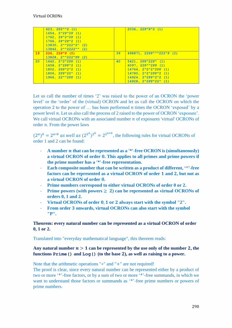
Virtual OCRONs
290
623, 2P2^^2 (1)
1654, 2^2P^2P (1)
1762, 2P^2^2P (1)
1766, 2P^2P^2 (1)
13830, 2^^222^2^ (2)
13842, 2^^2222^^ (2)
2036, 22P^P^2 (1)
19 226, 22P^P (0)
13828, 2^^222^PP (2)
39 498871, 22PP^^^222^P (2)
20 1642, 2^2^2PP (1)
1658, 2^2PP^2 (1)
1802, 2PP^2^2 (1)
1806, 2PP^22^ (1)
1966, 22^^2PP (1)
40 5421, 2PP^22P^ (1)
6097, 22P^^2PP (1)
14764, 2^2^2^2PP (1)
14780, 2^2^2PP^2 (1)
14924, 2^2PP^2^2 (1)
14928, 2^2PP^22^ (1)
Let us call the number of times ‘2’ was raised to the power of an OCRON the ‘power
level’ or the ‘order’ of the (virtual) OCRON and let us call the OCRON on which the
operation 2 to the power of … has been performed 𝑛 times the OCRON ‘exposed’ by a
power level 𝑛. Let us also call the process of 2 raised to the power of OCRON ‘exposure’.
We call virtual OCRONs with an associated number 𝑛 of exposures 'virtual' OCRONs of
order 𝑛. From the power laws
(2𝑎)𝑏 = 2𝑎∗𝑏 𝑎𝑠 𝑤𝑒𝑙𝑙 𝑎𝑠 (22𝑎)2𝑏= 22
𝑎+𝑏, the following rules for virtual OCRONs of
order 1 and 2 can be found:
- A number 𝒏 that can be represented as a '*'-free OCRON is (simultaneously)
a virtual OCRON of order 𝟎. This applies to all primes and prime powers if
the prime number has a '*'-free representation.
- Each composite number that can be written as a product of different, ‘*’-free
factors can be represented as a virtual OCRON of order 𝟏 and 𝟐, but not as
a virtual OCRON of order 𝟎.
- Prime numbers correspond to either virtual OCRONs of order 0 or 2.
- Prime powers (with powers ≥ 𝟐) can be represented as virtual OCRONs of
orders 0, 1 and 2.
- Virtual OCRONs of order 𝟎, 𝟏 𝐨𝐫 𝟐 always start with the symbol "2".
- From order 𝟑 onwards, virtual OCRONs can also start with the symbol
"P".
Theorem: every natural number can be represented as a virtual OCRON of order
0, 1 or 2.
Translated into "everyday mathematical language", this theorem reads:
Any natural number 𝒏 > 𝟏 can be represented by the use only of the number 𝟐, the
functions Prime() and Log() (to the base 𝟐), as well as raising to a power.
Note that the arithmetic operations "∗" and "+" are not required!
The proof is clear, since every natural number can be represented either by a product of
two or more ‘*’-free factors, or by a sum of two or more ‘*’-free summands, in which we
want to understand those factors or summands as ‘*’-free prime numbers or powers of
prime numbers.

291
20.9 MORE UNSOLVED MATHEMATICAL PROBLEMS
20.9.1 THE EUCLID-MULLIN SEQUENCE
This sequence is defined very simply:
Let be 𝑎1 = 2, then 𝑎𝑛 is the smallest prime factor in the decomposition:
∏𝑎𝑖
𝑛−1
𝑖=1
+ 1
The first elements of the Euclid-Mullin sequence are:
2, 3, 7, 43, 13, 53, 5, 6221671, 38709183810571, 139, 2801, 11, 17,
5471, 52662739, 23003, 30693651606209, 37, 1741, 1313797957, 887, 71,
7127, 109, 23, 97, 159227, 643679794963466223081509857, 103,
1079990819, 9539, 3143065813, 29, 3847, 89, 19, 577, 223, 139703, 457,
9649, 61, 4357,
87991098722552272708281251793312351581099392851768893748012603709343,
107, 127, 3313,
2274326891085895327549849150757748483866714395682604207544149407807612
45893,59, 31, 211
Mathematica:
f[1]=2;f[n_]:=f[n]=FactorInteger[Product[f[i],
{i,1,n-1}]+1][[1,1]];Table[f[n],{n,1,43}]
It is not known whether the Euclid-Mullin sequence runs through all prime numbers. It is
also not known whether the problem of finding out whether a given prime is contained in
the sequence belongs to the set of computable problems85. For example, it is still unclear
whether the number 41 is an element of the Euclid-Mullin sequence.
85 https://de.wikipedia.org/wiki/Berechenbarkeit

292
20.9.2 ALIQUOT SEQUENCES
20.9.2.1 GENERAL
Aliquot sequences are recursively defined sequences defined in the domain of the natural
numbers:
𝑛, 𝑠(𝑛), 𝑠(𝑠(𝑛)), 𝑠 (𝑠(𝑠(𝑛))) , … where 𝑠(𝑛) = 𝜎(𝑛) − 𝑛, 𝑛 ∈ ℕ (165)
In the process, 𝜎(𝑛) is the sum of divisors function (see Chapter 7.5). (Note: 𝜎(𝑛) is the
simplified notation of the generalized sigma function 𝜎𝑘(𝑛) for 𝑘 = 1: 𝜎(𝑛) = 𝜎1(𝑛)). 𝜎(𝑛) counts and sums all the divisors (including 1 and 𝑛 itself). 𝑠(𝑛) sums all divisors,
but without 𝑛 itself. 𝑠(𝑛) is therefore sometimes called the sum of the proper divisors of
𝑛. Occasionally, also the term 'numerical content' can be found for 𝑠(𝑛).
Here are a few examples of aliquot sequences for different starting values: {4,3,1,0,0,0,0,0,0,0,0,0,0,0,0,0,0,0,0,0,0,0,0,0,0,0}
{6,6,6,6,6,6,6,6,6,6,6,6,6,6,6,6,6,6,6,6,6,6,6,6,6,6}
{7,1,0,0,0,0,0,0,0,0,0,0,0,0,0,0,0,0,0,0,0,0,0,0,0,0}
{10,8,7,1,0,0,0,0,0,0,0,0,0,0,0,0,0,0,0,0,0,0,0,0,0,0}
{11,1,0,0,0,0,0,0,0,0,0,0,0,0,0,0,0,0,0,0,0,0,0,0,0,0}
{12,16,15,9,4,3,1,0,0,0,0,0,0,0,0,0,0,0,0,0,0,0,0,0,0,0}
{28,28,28,28,28,28,28,28,28,28,28,28,28,28,28,28,28,28,28,28}
{220,284,220,284,220,284,220,284,220,284,220,284,220,284,220,284}
{276,396,696,1104,1872,3770,3790,3050,2716,2772,5964,10164,19628,19684
,22876,26404}
{496,496,496,496,496,496,496,496,496,496,496,496,496,496,496,496}
{562,284,220,284,220,284,220,284,220,284,220,284,220,284,220,284}
{790,650,652,496,496,496,496,496,496,496,496,496,496,496,496,496}
{12496,14288,15472,14536,14264,12496,14288,15472,14536,14264,12496,142
88,15472,14536,14264,12496}
(Cycles are marked in red, OE sequences (‘open end’: blue))
Mathematica:
(*06:*)Join[NestList[DivisorSigma[1,#]-#&,6,25],PadRight[{},0,0]]
(*10:*)Join[NestList[DivisorSigma[1,#]-#&,10,4],PadRight[{},21,0]]
(*11:*)Join[NestList[DivisorSigma[1,#]-#&,11,2],PadRight[{},23,0]]
(*12:*)Join[NestList[DivisorSigma[1,#]-#&,12,7],PadRight[{},18,0]]
(*28:*)Join[NestList[DivisorSigma[1,#]-#&,28,19],PadRight[{},0,0]]
(*220:*)Join[NestList[DivisorSigma[1,#]-#&,220,15],PadRight[{},0,0]]
(*276:*)Join[NestList[DivisorSigma[1,#]-#&,276,15],PadRight[{},0,0]]
(*496:*)Join[NestList[DivisorSigma[1,#]-#&,496,15],PadRight[{},0,0]]
(*562:*)Join[NestList[DivisorSigma[1,#]-#&,562,15],PadRight[{},0,0]]
(*790:*)Join[NestList[DivisorSigma[1,#]-#&,790,15],PadRight[{},0,0]]
The Appendix contains more Mathematica programs for calculating aliquot sequences
((0). As can be seen from the examples, there are several ways in which an aliquot
sequence can end:
- prime number, followed by ‘1’ and infinitely many ‘0’ values (this is the ‘normal’
end of an aliquot sequence).
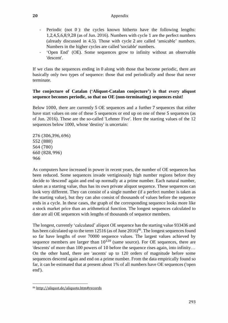
20 Appendix
293
- Periodic (not 0 ): the cycles known hitherto have the following lengths:
1,2,4,5,6,8,9,28 (as of Jun. 2016). Numbers with cycle 1 are the perfect numbers
(already discussed in 4.5). Those with cycle 2 are called ‘amicable’ numbers.
Numbers in the higher cycles are called 'sociable' numbers.
- ‘Open End’ (OE). Some sequences grow to infinity without an observable
'descent'.
If we class the sequences ending in 0 along with those that become periodic, there are
basically only two types of sequence: those that end periodically and those that never
terminate.
The conjecture of Catalan (‘Aliquot-Catalan conjecture’) is that every aliquot
sequence becomes periodic, so that no OE (non-terminating) sequences exist!
Below 1000, there are currently 5 OE sequences and a further 7 sequences that either
have start values on one of these 5 sequences or end up on one of these 5 sequences (as
of Jun. 2016). These are the so-called 'Lehmer Five'. Here the starting values of the 12
sequences below 1000, whose 'destiny' is uncertain:
276 (306,396, 696) 552 (888) 564 (780) 660 (828, 996) 966
As computers have increased in power in recent years, the number of OE sequences has
been reduced. Some sequences invade vertiginously high number regions before they
decide to 'descend' again and end up normally at a prime number. Each natural number,
taken as a starting value, thus has its own private aliquot sequence. These sequences can
look very different. They can consist of a single number (if a perfect number is taken as
the starting value), but they can also consist of thousands of values before the sequence
ends in a cycle. In these cases, the graph of the corresponding sequence looks more like
a stock market price than an arithmetical function. The longest sequences calculated to
date are all OE sequences with lengths of thousands of sequence members.
The longest, currently ‘calculated’ aliquot OE sequence has the starting value 933436 and
has been calculated up to the term 12516 (as of June 2016)86. The longest sequences found
so far have lengths of over 70000 sequence values. The largest values achieved by
sequence members are larger than 10120 (same source). For OE sequences, there are
'descents' of more than 100 powers of 10 before the sequence rises again, into infinity…
On the other hand, there are 'ascents' up to 120 orders of magnitude before some
sequences descend again and end on a prime number. From the data empirically found so
far, it can be estimated that at present about 1% of all numbers have OE sequences ('open
end').
86 http://aliquot.de/aliquote.htm#records

More unsolved mathematical problems
294
Note: most of the information in this chapter is taken from the following Internet pages
http://www.aliquot.de, http://factordb.com (Markus Tervooren),
http://christophe.clavier.free.fr/Aliquot/site/Aliquot.html
Here are a few graphs of aliquot sequences. First, the 'Lehmer Five' (open-end sequences
with starting values below 1000):
Figure 144. The first 12 values of the aliquot sequences 276,306,396,696. From the 3rd value on, the sequences are identical
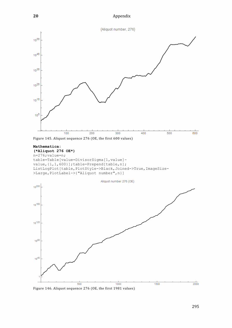
20 Appendix
295
Figure 145. Aliquot sequence 276 (OE, the first 600 values)
Mathematica:
(*Aliquot 276 OE*)
n=276;value=n;
table=Table[value=DivisorSigma[1,value]-
value,{i,1,600}];table=Prepend[table,n];
ListLogPlot[table,PlotStyle->Black,Joined->True,ImageSize-
>Large,PlotLabel->{"Aliquot number",n}]
Figure 146. Aliquot sequence 276 (OE, the first 1981 values)
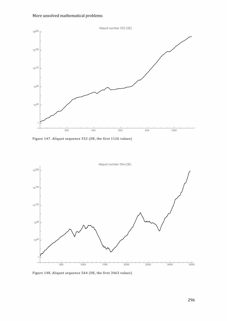
More unsolved mathematical problems
296
Figure 147. Aliquot sequence 552 (OE, the first 1126 values)
Figure 148. Aliquot sequence 564 (OE, the first 3463 values)

20 Appendix
297
Figure 149. Aliquot sequence 660 (OE, the first 971 values)
Figure 150. Aliquot sequence 966 (OE, the first 948 values)
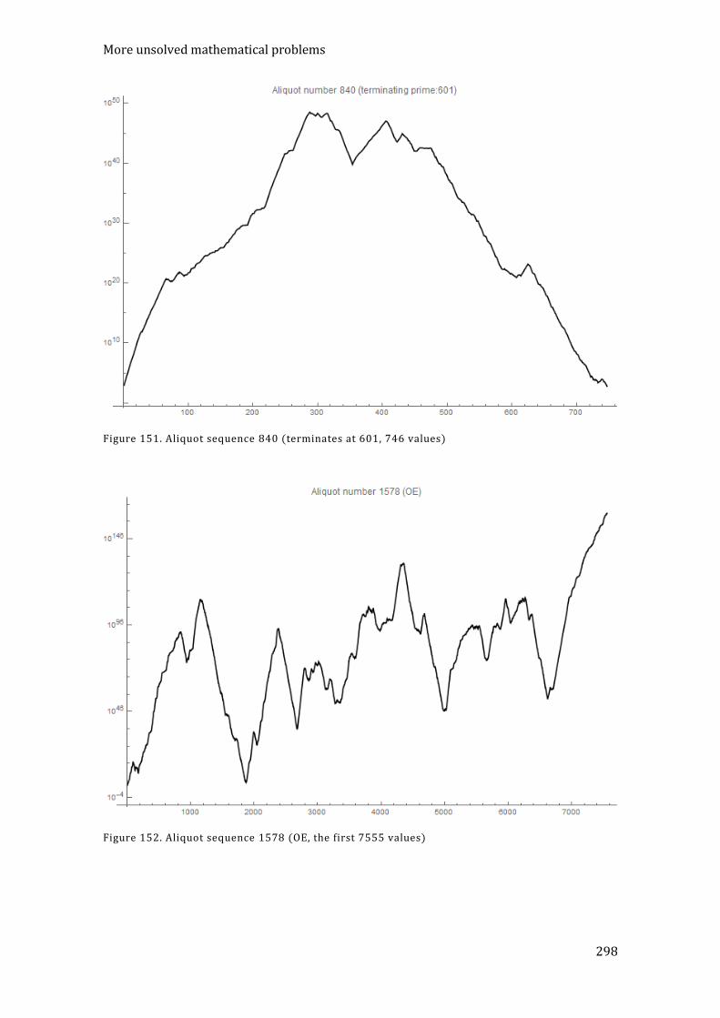
More unsolved mathematical problems
298
Figure 151. Aliquot sequence 840 (terminates at 601, 746 values)
Figure 152. Aliquot sequence 1578 (OE, the first 7555 values)
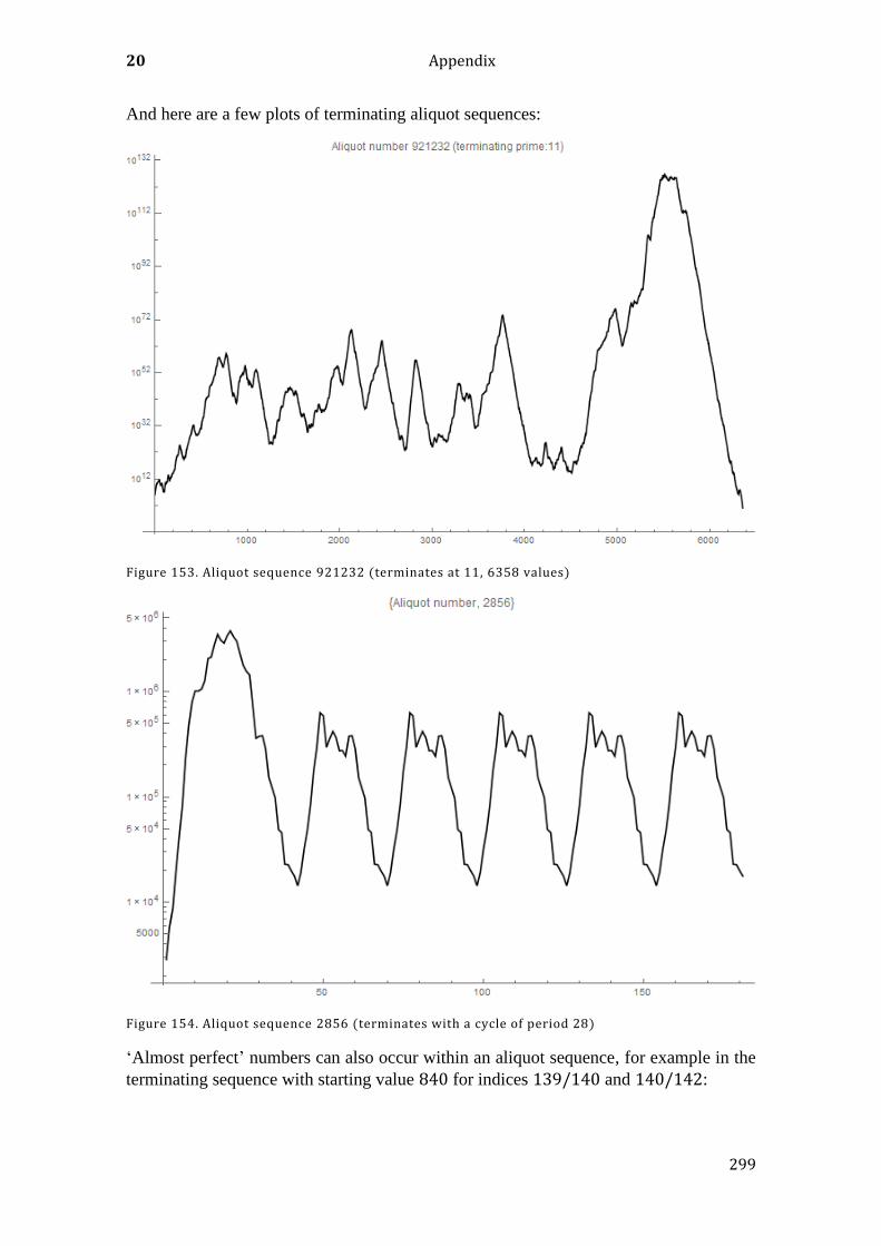
20 Appendix
299
And here are a few plots of terminating aliquot sequences:
Figure 153. Aliquot sequence 921232 (terminates at 11, 6358 values)
Figure 154. Aliquot sequence 2856 (terminates with a cycle of period 28)
‘Almost perfect’ numbers can also occur within an aliquot sequence, for example in the
terminating sequence with starting value 840 for indices 139/140 and 140/142:
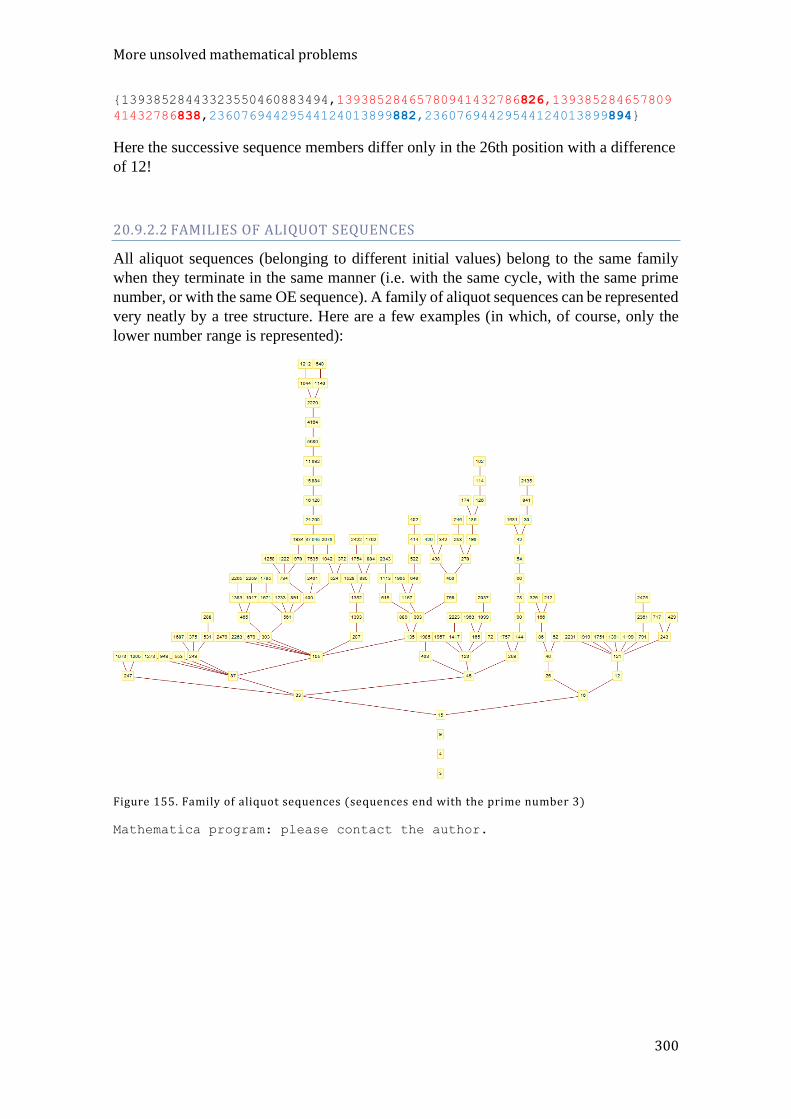
More unsolved mathematical problems
300
{13938528443323550460883494,13938528465780941432786826,139385284657809
41432786838,23607694429544124013899882,23607694429544124013899894}
Here the successive sequence members differ only in the 26th position with a difference
of 12!
20.9.2.2 FAMILIES OF ALIQUOT SEQUENCES
All aliquot sequences (belonging to different initial values) belong to the same family
when they terminate in the same manner (i.e. with the same cycle, with the same prime
number, or with the same OE sequence). A family of aliquot sequences can be represented
very neatly by a tree structure. Here are a few examples (in which, of course, only the
lower number range is represented):
Figure 155. Family of aliquot sequences (sequences end with the prime number 3)
Mathematica program: please contact the author.
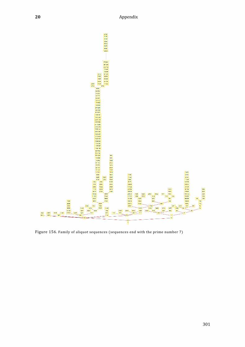
20 Appendix
301
Figure 156. Family of aliquot sequences (sequences end with the prime number 7)
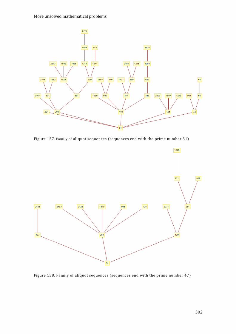
More unsolved mathematical problems
302
Figure 157. Family of aliquot sequences (sequences end with the prime number 31)
Figure 158. Family of aliquot sequences (sequences end with the prime number 47)
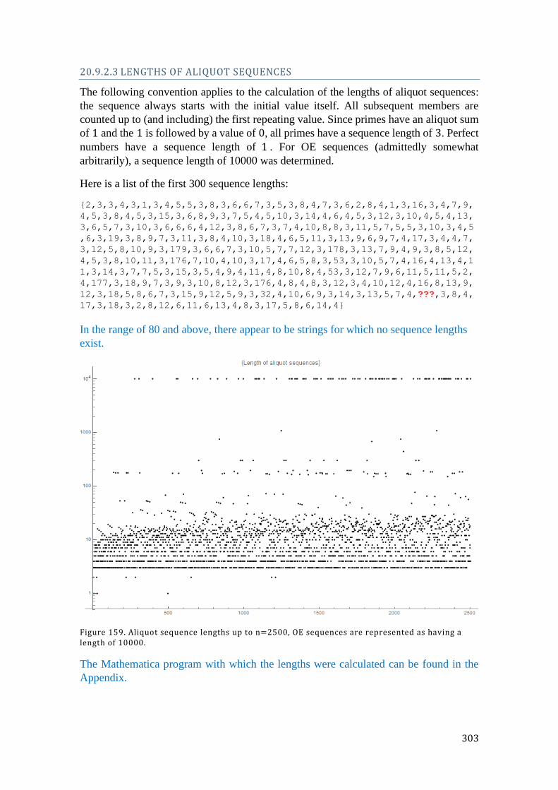
303
20.9.2.3 LENGTHS OF ALIQUOT SEQUENCES
The following convention applies to the calculation of the lengths of aliquot sequences:
the sequence always starts with the initial value itself. All subsequent members are
counted up to (and including) the first repeating value. Since primes have an aliquot sum
of 1 and the 1 is followed by a value of 0, all primes have a sequence length of 3. Perfect
numbers have a sequence length of 1 . For OE sequences (admittedly somewhat
arbitrarily), a sequence length of 10000 was determined.
Here is a list of the first 300 sequence lengths:
{2,3,3,4,3,1,3,4,5,5,3,8,3,6,6,7,3,5,3,8,4,7,3,6,2,8,4,1,3,16,3,4,7,9,
4,5,3,8,4,5,3,15,3,6,8,9,3,7,5,4,5,10,3,14,4,6,4,5,3,12,3,10,4,5,4,13,
3,6,5,7,3,10,3,6,6,6,4,12,3,8,6,7,3,7,4,10,8,8,3,11,5,7,5,5,3,10,3,4,5
,6,3,19,3,8,9,7,3,11,3,8,4,10,3,18,4,6,5,11,3,13,9,6,9,7,4,17,3,4,4,7,
3,12,5,8,10,9,3,179,3,6,6,7,3,10,5,7,7,12,3,178,3,13,7,9,4,9,3,8,5,12,
4,5,3,8,10,11,3,176,7,10,4,10,3,17,4,6,5,8,3,53,3,10,5,7,4,16,4,13,4,1
1,3,14,3,7,7,5,3,15,3,5,4,9,4,11,4,8,10,8,4,53,3,12,7,9,6,11,5,11,5,2,
4,177,3,18,9,7,3,9,3,10,8,12,3,176,4,8,4,8,3,12,3,4,10,12,4,16,8,13,9,
12,3,18,5,8,6,7,3,15,9,12,5,9,3,32,4,10,6,9,3,14,3,13,5,7,4,???,3,8,4,
17,3,18,3,2,8,12,6,11,6,13,4,8,3,17,5,8,6,14,4}
In the range of 80 and above, there appear to be strings for which no sequence lengths
exist.
Figure 159. Aliquot sequence lengths up to n=2500, OE sequences are represented as having a length of 10000.
The Mathematica program with which the lengths were calculated can be found in the
Appendix.
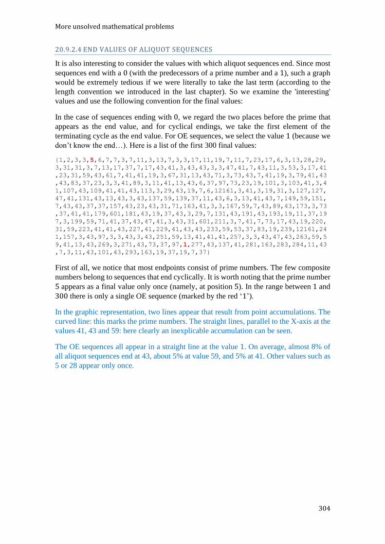
More unsolved mathematical problems
304
20.9.2.4 END VALUES OF ALIQUOT SEQUENCES
It is also interesting to consider the values with which aliquot sequences end. Since most
sequences end with a 0 (with the predecessors of a prime number and a 1), such a graph
would be extremely tedious if we were literally to take the last term (according to the
length convention we introduced in the last chapter). So we examine the 'interesting'
values and use the following convention for the final values:
In the case of sequences ending with 0, we regard the two places before the prime that
appears as the end value, and for cyclical endings, we take the first element of the
terminating cycle as the end value. For OE sequences, we select the value 1 (because we
don’t know the end…). Here is a list of the first 300 final values:
{1,2,3,3,5,6,7,7,3,7,11,3,13,7,3,3,17,11,19,7,11,7,23,17,6,3,13,28,29,
3,31,31,3,7,13,17,37,7,17,43,41,3,43,43,3,3,47,41,7,43,11,3,53,3,17,41
,23,31,59,43,61,7,41,41,19,3,67,31,13,43,71,3,73,43,7,41,19,3,79,41,43
,43,83,37,23,3,3,41,89,3,11,41,13,43,6,37,97,73,23,19,101,3,103,41,3,4
1,107,43,109,41,41,43,113,3,29,43,19,7,6,12161,3,41,3,19,31,3,127,127,
47,41,131,43,13,43,3,43,137,59,139,37,11,43,6,3,13,41,43,7,149,59,151,
7,43,43,37,37,157,43,23,43,31,71,163,41,3,3,167,59,7,43,89,43,173,3,73
,37,41,41,179,601,181,43,19,37,43,3,29,7,131,43,191,43,193,19,11,37,19
7,3,199,59,71,41,37,43,47,41,3,43,31,601,211,3,7,41,7,73,17,43,19,220,
31,59,223,41,41,43,227,41,229,41,43,43,233,59,53,37,83,19,239,12161,24
1,157,3,43,97,3,3,43,3,43,251,59,13,41,41,41,257,3,3,43,47,43,263,59,5
9,41,13,43,269,3,271,43,73,37,97,1,277,43,137,41,281,163,283,284,11,43
,7,3,11,43,101,43,293,163,19,37,19,7,37}
First of all, we notice that most endpoints consist of prime numbers. The few composite
numbers belong to sequences that end cyclically. It is worth noting that the prime number
5 appears as a final value only once (namely, at position 5). In the range between 1 and
300 there is only a single OE sequence (marked by the red ‘1’).
In the graphic representation, two lines appear that result from point accumulations. The
curved line: this marks the prime numbers. The straight lines, parallel to the X-axis at the
values 41, 43 and 59: here clearly an inexplicable accumulation can be seen.
The OE sequences all appear in a straight line at the value 1. On average, almost 8% of
all aliquot sequences end at 43, about 5% at value 59, and 5% at 41. Other values such as
5 or 28 appear only once.
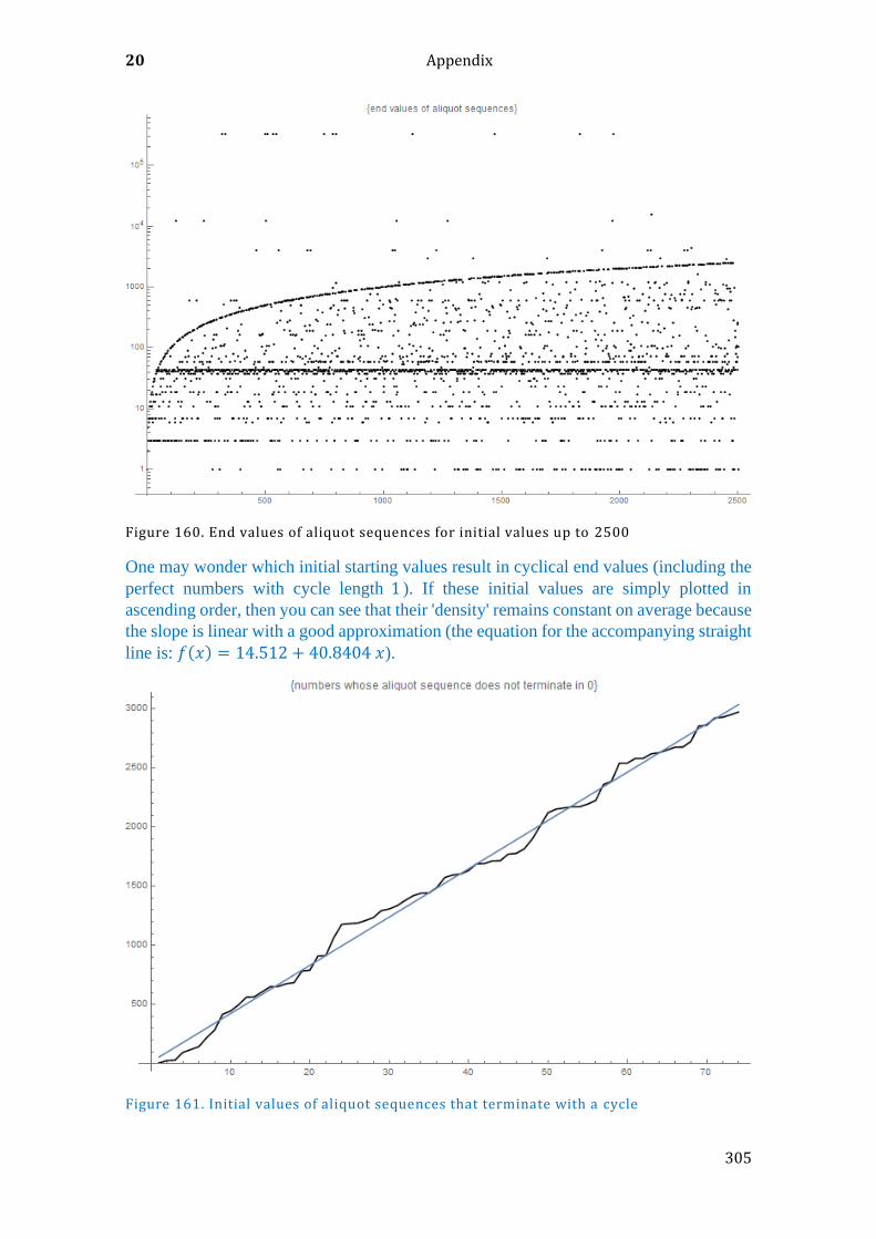
20 Appendix
305
Figure 160. End values of aliquot sequences for initial values up to 2500
One may wonder which initial starting values result in cyclical end values (including the
perfect numbers with cycle length 1 ). If these initial values are simply plotted in
ascending order, then you can see that their 'density' remains constant on average because
the slope is linear with a good approximation (the equation for the accompanying straight
line is: 𝑓(𝑥) = 14.512 + 40.8404 𝑥).
Figure 161. Initial values of aliquot sequences that terminate with a cycle
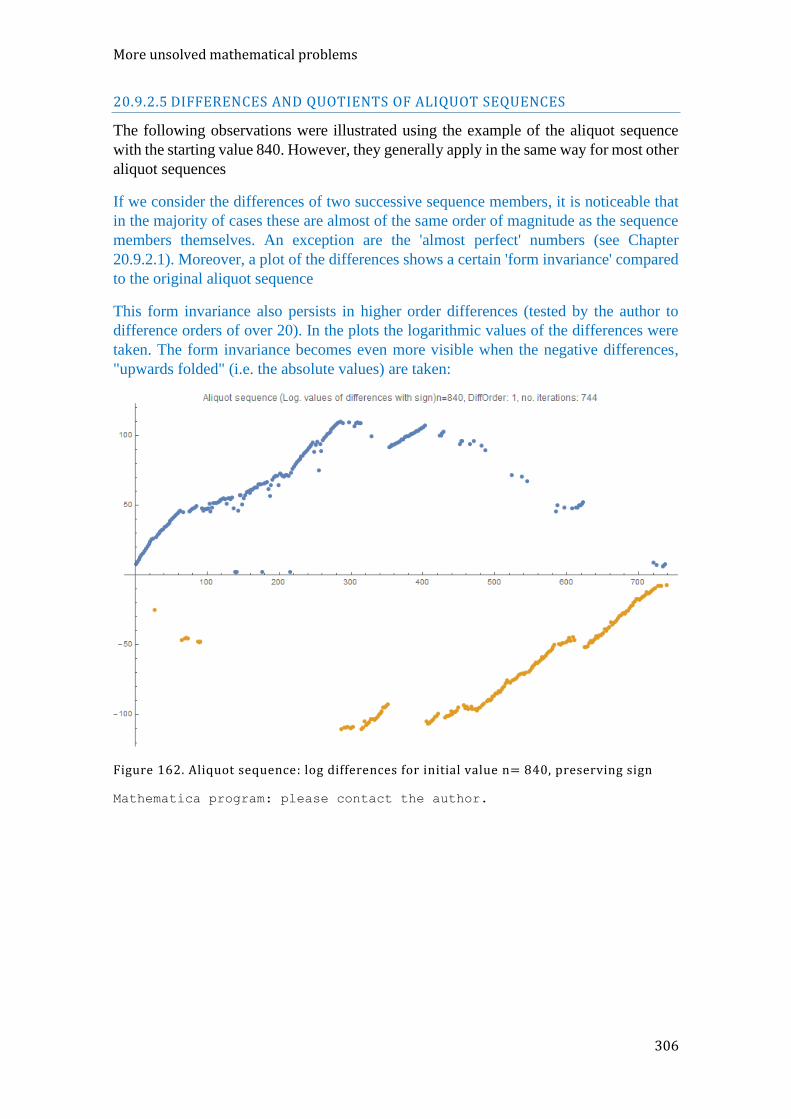
More unsolved mathematical problems
306
20.9.2.5 DIFFERENCES AND QUOTIENTS OF ALIQUOT SEQUENCES
The following observations were illustrated using the example of the aliquot sequence
with the starting value 840. However, they generally apply in the same way for most other
aliquot sequences
If we consider the differences of two successive sequence members, it is noticeable that
in the majority of cases these are almost of the same order of magnitude as the sequence
members themselves. An exception are the 'almost perfect' numbers (see Chapter
20.9.2.1). Moreover, a plot of the differences shows a certain 'form invariance' compared
to the original aliquot sequence
This form invariance also persists in higher order differences (tested by the author to
difference orders of over 20). In the plots the logarithmic values of the differences were
taken. The form invariance becomes even more visible when the negative differences,
"upwards folded" (i.e. the absolute values) are taken:
Figure 162. Aliquot sequence: log differences for initial value n= 840, preserving sign
Mathematica program: please contact the author.
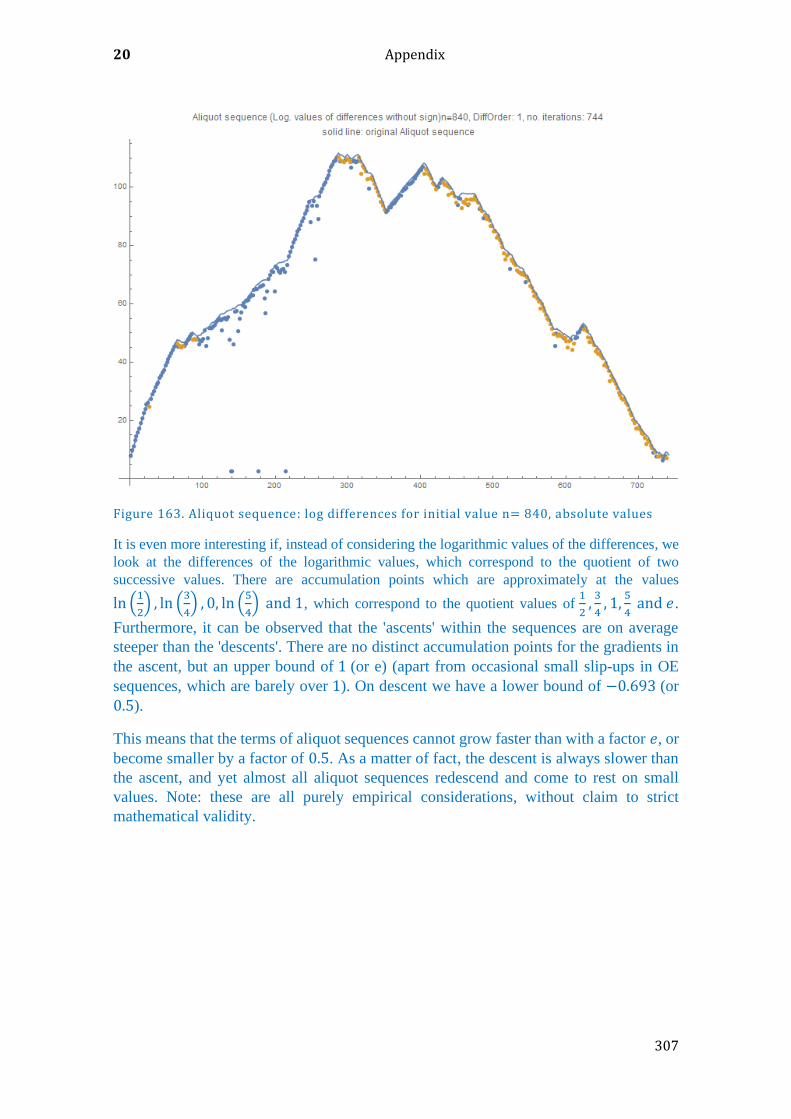
20 Appendix
307
Figure 163. Aliquot sequence: log differences for initial value n= 840, absolute values
It is even more interesting if, instead of considering the logarithmic values of the differences, we
look at the differences of the logarithmic values, which correspond to the quotient of two
successive values. There are accumulation points which are approximately at the values
ln (1
2) , ln (
3
4) , 0, ln (
5
4) and 1, which correspond to the quotient values of
1
2,3
4, 1,
5
4 and 𝑒.
Furthermore, it can be observed that the 'ascents' within the sequences are on average
steeper than the 'descents'. There are no distinct accumulation points for the gradients in
the ascent, but an upper bound of 1 (or e) (apart from occasional small slip-ups in OE
sequences, which are barely over 1). On descent we have a lower bound of −0.693 (or
0.5).
This means that the terms of aliquot sequences cannot grow faster than with a factor 𝑒, or
become smaller by a factor of 0.5. As a matter of fact, the descent is always slower than
the ascent, and yet almost all aliquot sequences redescend and come to rest on small
values. Note: these are all purely empirical considerations, without claim to strict
mathematical validity.
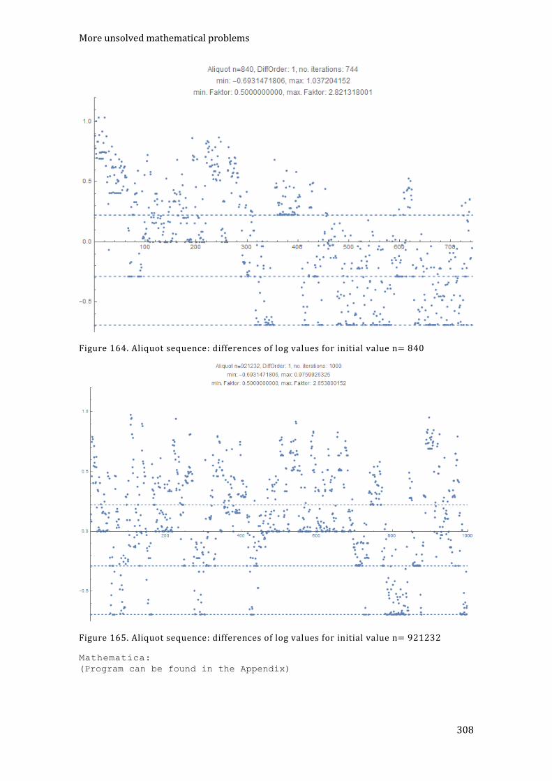
More unsolved mathematical problems
308
Figure 164. Aliquot sequence: differences of log values for initial value n= 840
Figure 165. Aliquot sequence: differences of log values for initial value n= 921232
Mathematica:
(Program can be found in the Appendix)
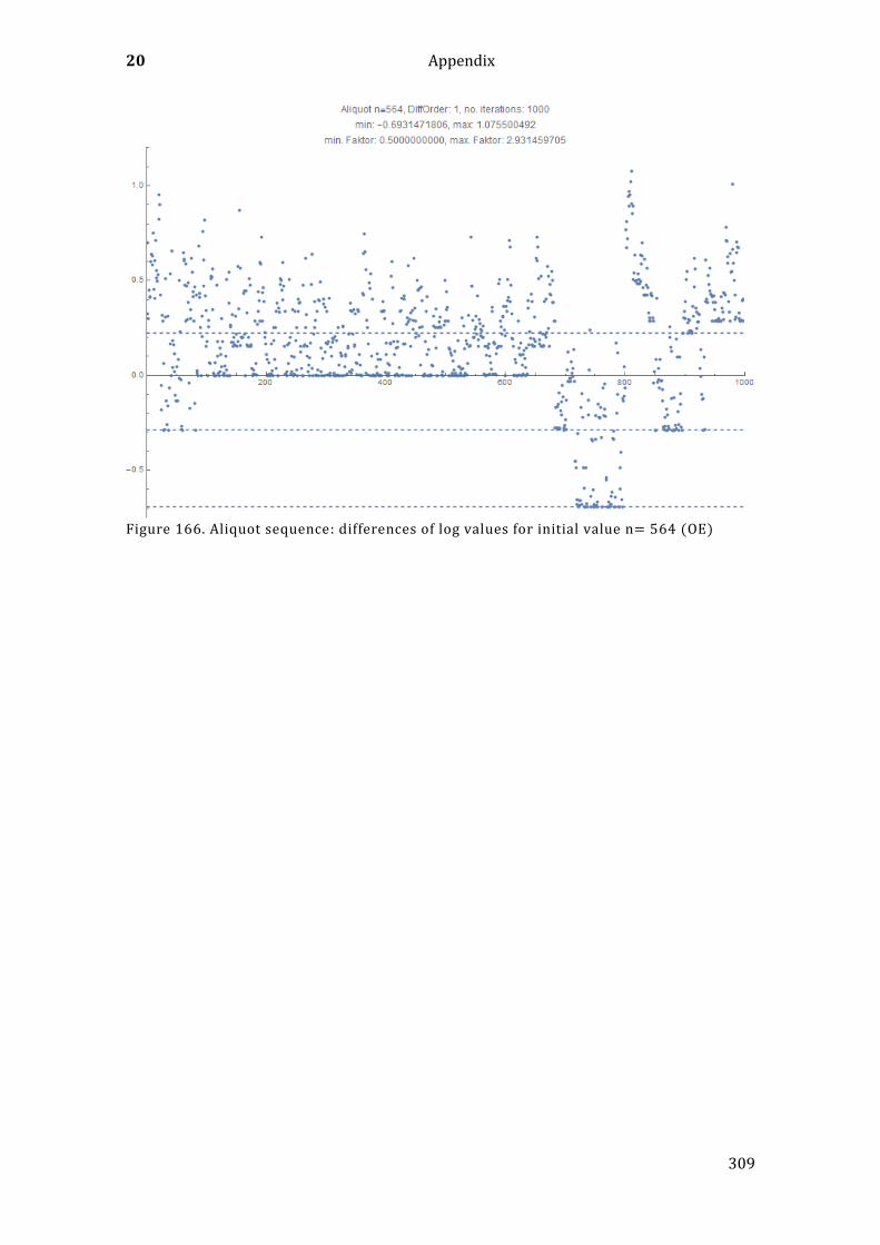
20 Appendix
309
Figure 166. Aliquot sequence: differences of log values for initial value n= 564 (OE)
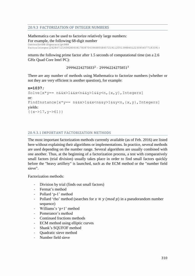
310
20.9.3 FACTORIZATION OF INTEGER NUMBERS
Mathematica can be used to factorize relatively large numbers:
For example, the following 68-digit number CenterDot@@(Superscript@@@
FactorInteger[24284712165828060817808704394685584572191120513988451223045457718339])
returns the following prime factor after 1.5 seconds of computational time (on a 2.6
GHz Quad Core Intel PC):
299962242758332 ⋅ 299962242758513
There are any number of methods using Mathematica to factorize numbers (whether or
not they are very efficient is another question), for example:
n=1037;
Solve[x*y== n&&x>1&&x<n&&y>1&&y<n,{x,y},Integers]
or: FindInstance[x*y== n&&x>1&&x<n&&y>1&&y<n,{x,y},Integers]
yields: {{x->17,y->61}}
20.9.3.1 IMPORTANT FACTORIZATION METHODS
The most important factorization methods currently available (as of Feb. 2016) are listed
here without explaining their algorithms or implementations. In practice, several methods
are used depending on the number range. Several algorithms are usually combined with
one another. Thus, at the beginning of a factorization process, a test with comparatively
small factors (trial division) usually takes place in order to find small factors quickly
before the "heavy artillery" is launched, such as the ECM method or the "number field
sieve".
Factorization methods:
- Division by trial (finds out small factors)
- Fermat’s method
- Pollard ‘p-1’ method
- Pollard ‘rho’ method (searches for 𝑥 ≡ 𝑦 (𝑚𝑜𝑑 𝑝) in a pseudorandom number
sequence)
- Williams’s ‘p+1’ method
- Pomerance’s method
- Continued fractions methods
- ECM method using elliptic curves
- Shank’s SQUFOF method
- Quadratic sieve method
- Number field sieve

20 Appendix
311
These factorization methods are documented extensively on many Internet web sites, so
we will not discuss them here.
Because of its simplicity and beauty, Fermat's method is briefly described here:
Let n be the number to be factored. The algorithm works only for odd numbers 𝑛. We test
the expression (⌈√𝑛⌉ + 𝑖)2− 𝑛 (by incrementing 𝑖, starting from 𝑖 = 0) until it gives a
squared number 𝑦2:
(⌈√𝑛⌉ + 𝑖)2− 𝑛 = 𝑦2. With 𝑥 = ⌈√𝑛⌉ + 𝑖 this yields: 𝑥2 − 𝑛 = 𝑦2, or
𝑛 = (𝑥 + 𝑦)(𝑥 − 𝑦). Thus, we have found two factors of 𝑛.
Here is an example: n=1037. Then we have ⌈√1037⌉ = 33. We then get the following
sequence:
(33 + 0)2 − 1037 = 52
(33 + 1)2 − 1037 = 119
(33 + 2)2 − 1037 = 188
(33 + 3)2 − 1037 = 259
(33 + 4)2 − 1037 = 332
(33 + 5)2 − 1037 = 407
(33 + 6)2 − 1037 = 484 (= 22 ∗ 22)
Thereby 𝒙 has a value of 𝟑𝟗 and 𝒚 the value 𝟐𝟐 and thus we have both factors 𝒑 =𝟑𝟗 + 𝟐𝟐 = 𝟔𝟏 and 𝒒 = 𝟑𝟗 − 𝟐𝟐 = 𝟏𝟕. 𝟏𝟎𝟑𝟕 = 𝟏𝟕 ∗ 𝟔𝟏.
Mathematica:
n=17*61;sqN=Ceiling[Sqrt[n]];value=2;
For[i=0,i<n&&IntegerQ[Sqrt[value]]==False,i++,
Print[i,"->",value=(sqN+i)^2-n]];i--;
y=Sqrt[value]; x=sqN+i;
p=x+y; q=x-y
Print["factors: ",p,"*",q];
The algorithm can be accelerated by avoiding the repeated squaring and computing
(𝑠 + 𝑖)2 recursively from the predecessor term: (𝑠 + 1)2 − 𝑛 = 𝑠2 + 2𝑠 + 1 − 𝑛. The
test of whether 𝑦2 is a square can also be accelerated by testing the last two digits of the
number (there are only 22 of 100 different possibilities for the last two digits for any
number of squares.
The runtime behaviour of this algorithm is good (~√𝑛)) if both factors are approximately
of equal size. However, it becomes bad when one of the factors is very small (e.g. 3). The
iteration is always finite, i.e. it will always end at a square. However, for primes, many
iterations occur so that this method is unsuitable as a prime number test.
The bad run time for factors of different sizes can be circumvented by finding a suitable
factor 𝑘 such that the algorithm is applied to 𝑘 ⋅ 𝑛, finding two factors closer together.
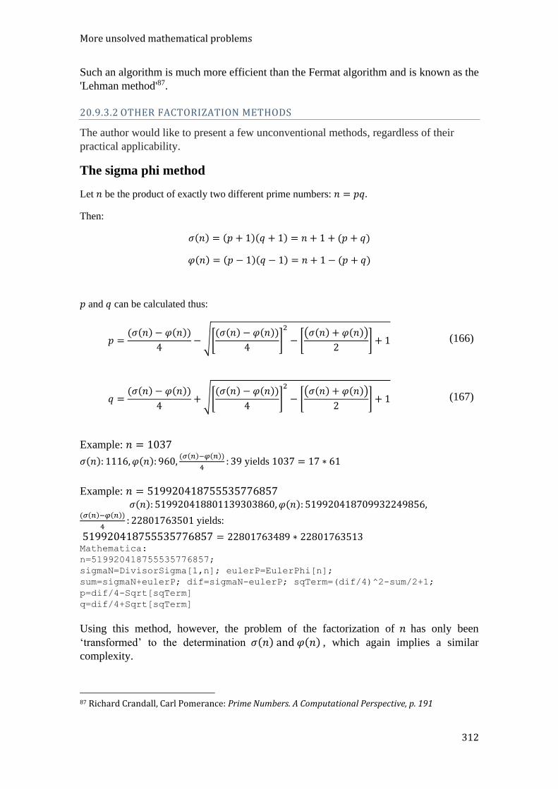
More unsolved mathematical problems
312
Such an algorithm is much more efficient than the Fermat algorithm and is known as the
'Lehman method'87.
20.9.3.2 OTHER FACTORIZATION METHODS
The author would like to present a few unconventional methods, regardless of their
practical applicability.
The sigma phi method
Let 𝑛 be the product of exactly two different prime numbers: 𝑛 = 𝑝𝑞.
Then:
𝜎(𝑛) = (𝑝 + 1)(𝑞 + 1) = 𝑛 + 1 + (𝑝 + 𝑞)
𝜑(𝑛) = (𝑝 − 1)(𝑞 − 1) = 𝑛 + 1 − (𝑝 + 𝑞)
𝑝 and 𝑞 can be calculated thus:
𝑝 =(𝜎(𝑛) − 𝜑(𝑛))
4− √[
(𝜎(𝑛) − 𝜑(𝑛))
4]
2
− [(𝜎(𝑛) + 𝜑(𝑛))
2] + 1 (166)
𝑞 =(𝜎(𝑛) − 𝜑(𝑛))
4+ √[
(𝜎(𝑛) − 𝜑(𝑛))
4]
2
− [(𝜎(𝑛) + 𝜑(𝑛))
2] + 1 (167)
Example: 𝑛 = 1037
𝜎(𝑛): 1116,𝜑(𝑛): 960,(𝜎(𝑛)−𝜑(𝑛))
4: 39 yields 1037 = 17 ∗ 61
Example: 𝑛 = 519920418755535776857
𝜎(𝑛): 519920418801139303860,𝜑(𝑛): 519920418709932249856, (𝜎(𝑛)−𝜑(𝑛))
4: 22801763501 yields:
519920418755535776857 = 22801763489 ∗ 22801763513 Mathematica:
n=519920418755535776857;
sigmaN=DivisorSigma[1,n]; eulerP=EulerPhi[n];
sum=sigmaN+eulerP; dif=sigmaN-eulerP; sqTerm=(dif/4)^2-sum/2+1;
p=dif/4-Sqrt[sqTerm]
q=dif/4+Sqrt[sqTerm]
Using this method, however, the problem of the factorization of 𝑛 has only been
‘transformed’ to the determination 𝜎(𝑛) and 𝜑(𝑛) , which again implies a similar
complexity.
87 Richard Crandall, Carl Pomerance: Prime Numbers. A Computational Perspective, p. 191
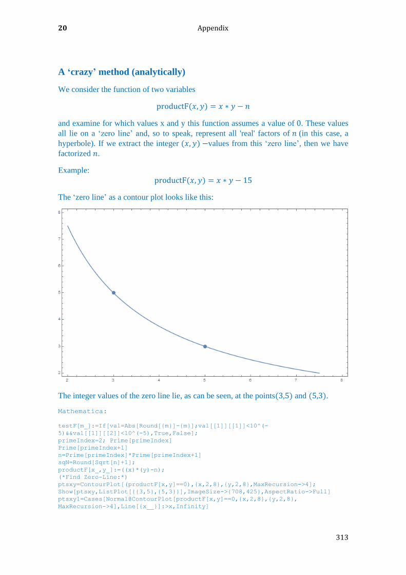
20 Appendix
313
A ‘crazy’ method (analytically)
We consider the function of two variables
productF(𝑥, 𝑦) = 𝑥 ∗ 𝑦 − 𝑛
and examine for which values x and y this function assumes a value of 0. These values
all lie on a ‘zero line’ and, so to speak, represent all 'real' factors of 𝑛 (in this case, a
hyperbole). If we extract the integer (𝑥, 𝑦) −values from this ‘zero line’, then we have
factorized 𝑛.
Example: productF(𝑥, 𝑦) = 𝑥 ∗ 𝑦 − 15
The ‘zero line’ as a contour plot looks like this:
The integer values of the zero line lie, as can be seen, at the points(3,5) and (5,3).
Mathematica:
testF[m_]:=If[val=Abs[Round[{m}]-{m}];val[[1]][[1]]<10^(-
5)&&val[[1]][[2]]<10^(-5),True,False];
primeIndex=2; Prime[primeIndex]
Prime[primeIndex+1]
n=Prime[primeIndex]*Prime[primeIndex+1]
sqN=Round[Sqrt[n]+1];
productF[x_,y_]:=((x)*(y)-n);
(*Find Zero-Line:*)
ptsxy=ContourPlot[(productF[x,y]==0),{x,2,8},{y,2,8},MaxRecursion->4];
Show[ptsxy,ListPlot[{{3,5},{5,3}}],ImageSize->{708,425},AspectRatio->Full]
ptsxy1=Cases[Normal@ContourPlot[productF[x,y]==0,{x,2,8},{y,2,8},
MaxRecursion->4],Line[{x__}]:>x,Infinity]
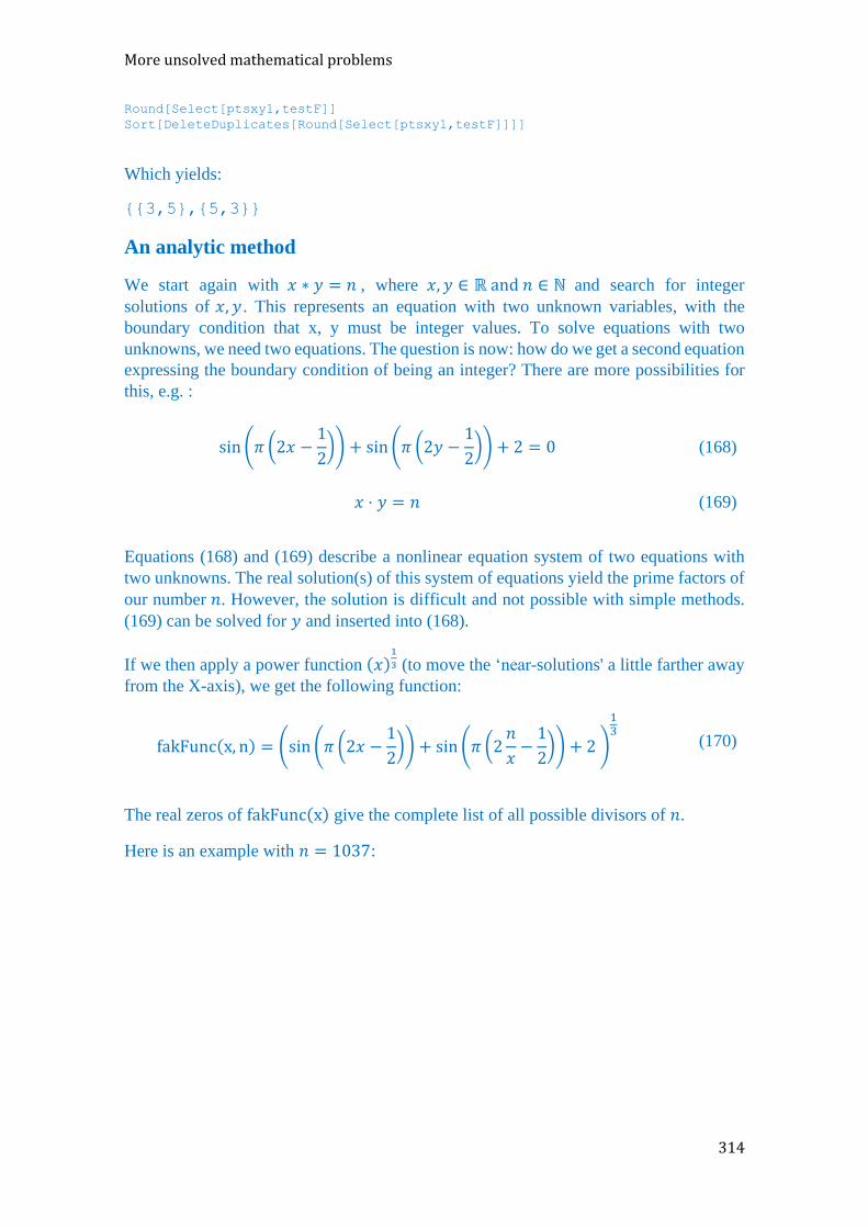
More unsolved mathematical problems
314
Round[Select[ptsxy1,testF]]
Sort[DeleteDuplicates[Round[Select[ptsxy1,testF]]]]
Which yields:
{{3,5},{5,3}}
An analytic method
We start again with 𝑥 ∗ 𝑦 = 𝑛 , where 𝑥, 𝑦 ∈ ℝ and 𝑛 ∈ ℕ and search for integer
solutions of 𝑥, 𝑦 . This represents an equation with two unknown variables, with the
boundary condition that x, y must be integer values. To solve equations with two
unknowns, we need two equations. The question is now: how do we get a second equation
expressing the boundary condition of being an integer? There are more possibilities for
this, e.g. :
sin (𝜋 (2𝑥 −1
2)) + sin (𝜋 (2𝑦 −
1
2)) + 2 = 0 (168)
𝑥 ⋅ 𝑦 = 𝑛 (169)
Equations (168) and (169) describe a nonlinear equation system of two equations with
two unknowns. The real solution(s) of this system of equations yield the prime factors of
our number 𝑛. However, the solution is difficult and not possible with simple methods.
(169) can be solved for 𝑦 and inserted into (168).
If we then apply a power function (𝑥)1
3 (to move the ‘near-solutions' a little farther away
from the X-axis), we get the following function:
fakFunc(x, n) = (sin (𝜋 (2𝑥 −1
2)) + sin (𝜋 (2
𝑛
𝑥−1
2)) + 2 )
13
(170)
The real zeros of fakFunc(x) give the complete list of all possible divisors of 𝑛.
Here is an example with 𝑛 = 1037:
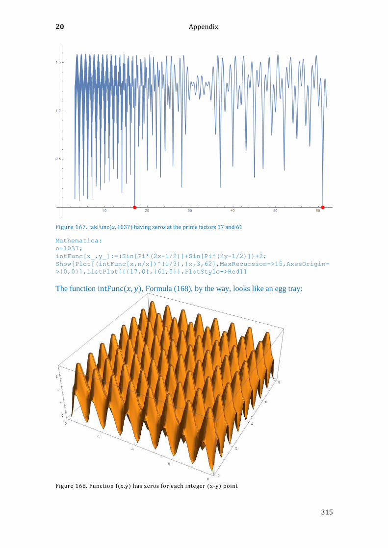
20 Appendix
315
Figure 167. fakFunc(𝑥, 1037) having zeros at the prime factors 17 and 61
Mathematica:
n=1037;
intFunc[x_,y_]:=(Sin[Pi*(2x-1/2)]+Sin[Pi*(2y-1/2)])+2;
Show[Plot[(intFunc[x,n/x])^(1/3),{x,3,62},MaxRecursion->15,AxesOrigin-
>{0,0}],ListPlot[{{17,0},{61,0}},PlotStyle->Red]]
The function intFunc(𝑥, 𝑦), Formula (168), by the way, looks like an egg tray:
Figure 168. Function f(x,y) has zeros for each integer (x-y) point
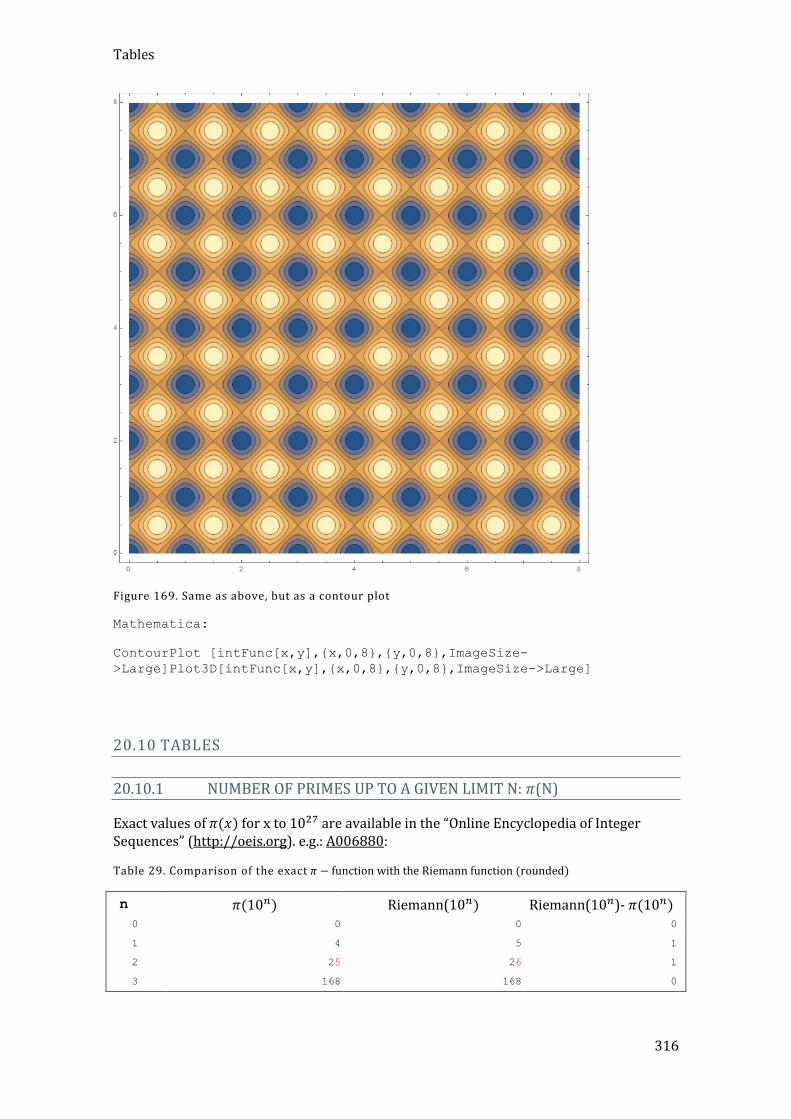
Tables
316
Figure 169. Same as above, but as a contour plot
Mathematica:
ContourPlot [intFunc[x,y],{x,0,8},{y,0,8},ImageSize-
>Large]Plot3D[intFunc[x,y],{x,0,8},{y,0,8},ImageSize->Large]
20.10 TABLES
20.10.1 NUMBER OF PRIMES UP TO A GIVEN LIMIT N: 𝜋(N)
Exact values of 𝜋(𝑥) for x to 1027 are available in the “Online Encyclopedia of Integer Sequences” (http://oeis.org). e.g.: A006880:
Table 29. Comparison of the exact 𝜋 − function with the Riemann function (rounded)
n 𝜋(10𝑛) Riemann(10𝑛) Riemann(10𝑛)- 𝜋(10𝑛) 0 0 0 0
1 4 5 1
2 25 26 1
3 168 168 0
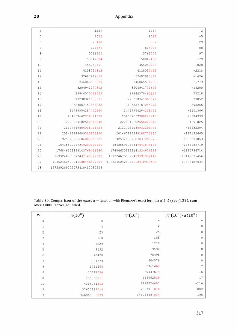
20 Appendix
317
4 1229 1227 2
5 9592 9587 -5
6 78498 78527 29
7 664579 664667 88
8 5761455 5761552 97
9 50847534 50847455 -79
10 455052511 455050683 -1828
11 4118054813 4118052495 -2318
12 37607912018 37607910542 -1476
13 346065536839 346065531066 -5773
14 3204941750802 3204941731602 -19200
15 29844570422669 29844570495887 73218
16 279238341033925 279238341360977 327052
17 2623557157654233 2623557157055978 -598255
18 24739954287740860 24739954284239494 -3501366
19 234057667276344607 234057667300228940 23884333
20 2220819602560918840 2220819602556027015 -4891825
21 21127269486018731928 21127269485932299724 -86432204
22 201467286689315906290 201467286689188773625 -127132665
23 1925320391606803968923 1925320391607837268776 1033299853
24 18435599767349200867866 18435599767347541878147 -1658989719
25 176846309399143769411680 176846309399141934626966 -1834784714
26 1699246750872437141327603 1699246750872419991992147 -17149335456
27 16352460426841680446427399 16352460426841662910939465 -17535487934
28 157589269275973410412739598
Table 30. Comparison of the exact 𝜋− function with Riema𝑛𝑛’𝑠 exact formula 𝜋∗(𝑛) (see (132), sum
over 10000 zeros, rounded
n 𝜋(10𝑛) 𝜋∗(10𝑛) 𝜋∗(10𝑛)- 𝜋(10𝑛) 0 0 - -
1 4 4 0
2 25 25 0
3 168 168 0
4 1229 1229 0
5 9592 9592 0
6 78498 78498 0
7 664579 664579 0
8 5761455 5761462 7
9 50847534 50847519 -15
10 455052511 455052528 17
11 4118054813 4118054697 -116
12 37607912018 37607911016 -1002
13 346065536839 346065537034 195
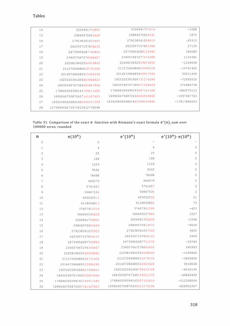
Tables
318
14 3204941750802 3204941747414 -3388
15 29844570422669 29844570424541 1872
16 279238341033925 279238341008610 -25315
17 2623557157654233 2623557157681368 27135
18 24739954287740860 24739954288134940 394080
19 234057667276344607 234057667277476288 1131681
20 2220819602560918840 2220819602559672832 -1246008
21 21127269486018731928 21127269486003990528 -14741400
22 201467286689315906290 201467286689365917696 50011406
23 1925320391606803968923 1925320391606731276288 -72692635
24 18435599767349200867866 18435599767349571354624 370486758
25 176846309399143769411680 176846309399143087341568 -682070112
26 1699246750872437141327603 1699246750872436043939840 -1097387763
27 16352460426841680446427399 16352460426841662628560896 -17817866503
28 157589269275973410412739598
Table 31. Comparison of the exact 𝜋 -function with Riemann’s exact formula 𝜋∗(𝑛), sum over
100000 zeros, rounded
n 𝜋(10𝑛) 𝜋∗(10𝑛) 𝜋∗(10𝑛)- 𝜋(10𝑛) 0 0 - -
1 4 4 0
2 25 25 0
3 168 168 0
4 1229 1229 0
5 9592 9592 0
6 78498 78498 0
7 664579 664579 0
8 5761455 5761457 2
9 50847534 50847536 2
10 455052511 455052532 21
11 4118054813 4118054886 73
12 37607912018 37607911595 -423
13 346065536839 346065537866 1027
14 3204941750802 3204941749206 -1596
15 29844570422669 29844570413033 -9636
16 279238341033925 279238341037530 3605
17 2623557157654233 2623557157660142 5909
18 24739954287740860 24739954287711076 -29784
19 234057667276344607 234057667276885600 540993
20 2220819602560918840 2220819602559328000 -1590840
21 21127269486018731928 21127269486015279104 -3452824
22 201467286689315906290 201467286689324924928 9018638
23 1925320391606803968923 1925320391606799433728 -4535195
24 18435599767349200867866 18435599767349154021376 -46846490
25 176846309399143769411680 176846309399143557103616 -212308064
26 1699246750872437141327603 1699246750872436312375296 -828952307
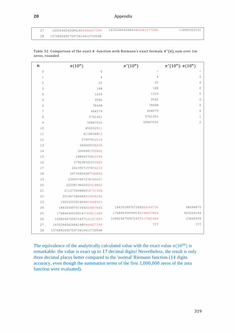
20 Appendix
319
27 16352460426841680446427399 16352460426841660481077248 -19965350151
28 157589269275973410412739598
Table 32. Comparison of the exact 𝜋 -function with Riemann’s exact formula 𝜋∗(𝑛), sum over 1m
zeros, rounded
n 𝜋(10𝑛) 𝜋∗(10𝑛) 𝜋∗(10𝑛)- 𝜋(10𝑛) 0 0 - -
1 4 4 0
2 25 25 0
3 168 168 0
4 1229 1229 0
5 9592 9592 0
6 78498 78498 0
7 664579 664579 0
8 5761455 5761456 1
9 50847534 50847536 2
10 455052511
11 4118054813
12 37607912018
13 346065536839
14 3204941750802
15 29844570422669
16 279238341033925
17 2623557157654233
18 24739954287740860
19 234057667276344607
20 2220819602560918840
21 21127269486018731928
22 201467286689315906290
23 1925320391606803968923
24 18435599767349200867866 18435599767349269364736 68496870
25 176846309399143769411680 176846309399144194637824 425226144
26 1699246750872437141327603 1699246750872437117681664 23645939
27 16352460426841680446427399 ??? ???
28 157589269275973410412739598
The equivalence of the analytically calculated value with the exact value 𝜋(1026) is
remarkable: the value is exact up to 17 decimal digits! Nevertheless, the result is only
three decimal places better compared to the 'normal' Riemann function (14 digits
accuracy, even though the summation terms of the first 1,000,000 zeros of the zeta
function were evaluated).
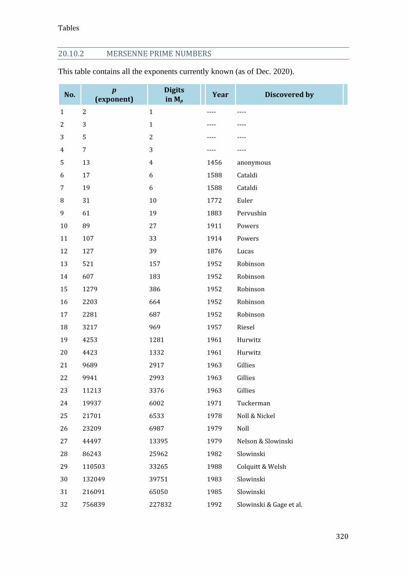
Tables
320
20.10.2 MERSENNE PRIME NUMBERS
This table contains all the exponents currently known (as of Dec. 2020).
No. p
(exponent) Digits in Mp
Year Discovered by
1 2 1 ---- ----
2 3 1 ---- ----
3 5 2 ---- ----
4 7 3 ---- ----
5 13 4 1456 anonymous
6 17 6 1588 Cataldi
7 19 6 1588 Cataldi
8 31 10 1772 Euler
9 61 19 1883 Pervushin
10 89 27 1911 Powers
11 107 33 1914 Powers
12 127 39 1876 Lucas
13 521 157 1952 Robinson
14 607 183 1952 Robinson
15 1279 386 1952 Robinson
16 2203 664 1952 Robinson
17 2281 687 1952 Robinson
18 3217 969 1957 Riesel
19 4253 1281 1961 Hurwitz
20 4423 1332 1961 Hurwitz
21 9689 2917 1963 Gillies
22 9941 2993 1963 Gillies
23 11213 3376 1963 Gillies
24 19937 6002 1971 Tuckerman
25 21701 6533 1978 Noll & Nickel
26 23209 6987 1979 Noll
27 44497 13395 1979 Nelson & Slowinski
28 86243 25962 1982 Slowinski
29 110503 33265 1988 Colquitt & Welsh
30 132049 39751 1983 Slowinski
31 216091 65050 1985 Slowinski
32 756839 227832 1992 Slowinski & Gage et al.
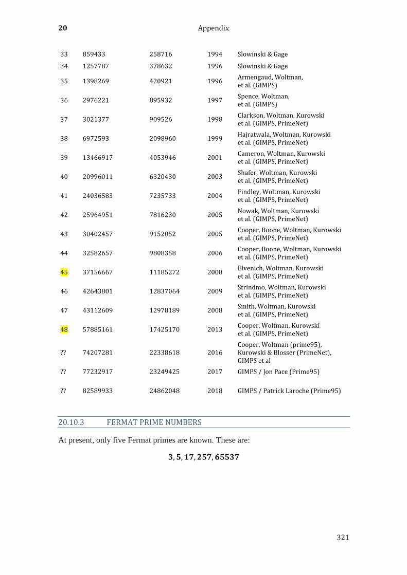
20 Appendix
321
33 859433 258716 1994 Slowinski & Gage
34 1257787 378632 1996 Slowinski & Gage
35 1398269 420921 1996 Armengaud, Woltman, et al. (GIMPS)
36 2976221 895932 1997 Spence, Woltman, et al. (GIMPS)
37 3021377 909526 1998 Clarkson, Woltman, Kurowski et al. (GIMPS, PrimeNet)
38 6972593 2098960 1999 Hajratwala, Woltman, Kurowski et al. (GIMPS, PrimeNet)
39 13466917 4053946 2001 Cameron, Woltman, Kurowski et al. (GIMPS, PrimeNet)
40 20996011 6320430 2003 Shafer, Woltman, Kurowski et al. (GIMPS, PrimeNet)
41 24036583 7235733 2004 Findley, Woltman, Kurowski et al. (GIMPS, PrimeNet)
42 25964951 7816230 2005 Nowak, Woltman, Kurowski et al. (GIMPS, PrimeNet)
43 30402457 9152052 2005 Cooper, Boone, Woltman, Kurowski et al. (GIMPS, PrimeNet)
44 32582657 9808358 2006 Cooper, Boone, Woltman, Kurowski et al. (GIMPS, PrimeNet)
45 37156667 11185272 2008 Elvenich, Woltman, Kurowski et al. (GIMPS, PrimeNet)
46 42643801 12837064 2009 Strindmo, Woltman, Kurowski et al. (GIMPS, PrimeNet)
47 43112609 12978189 2008 Smith, Woltman, Kurowski et al. (GIMPS, PrimeNet)
48 57885161 17425170 2013 Cooper, Woltman, Kurowski et al. (GIMPS, PrimeNet)
?? 74207281 22338618 2016 Cooper, Woltman (prime95), Kurowski & Blosser (PrimeNet), GIMPS et al
?? 77232917 23249425 2017 GIMPS / Jon Pace (Prime95)
??
82589933
24862048
2018
GIMPS / Patrick Laroche (Prime95)
20.10.3 FERMAT PRIME NUMBERS
At present, only five Fermat primes are known. These are:
𝟑, 𝟓, 𝟏𝟕, 𝟐𝟓𝟕, 𝟔𝟓𝟓𝟑𝟕
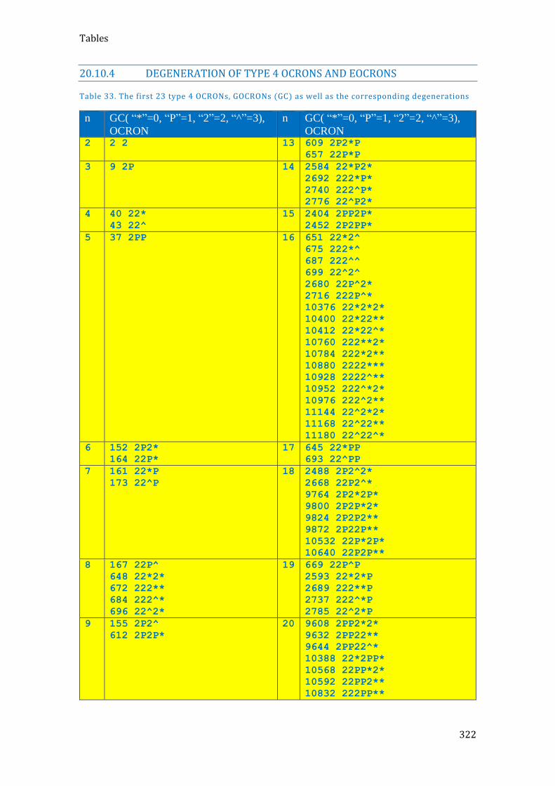
Tables
322
20.10.4 DEGENERATION OF TYPE 4 OCRONS AND EOCRONS
Table 33. The first 23 type 4 OCRONs, GOCRONs (GC) as well as the corresponding degenerations
n GC( “*”=0, “P”=1, “2”=2, “^”=3),
OCRON
n GC( “*”=0, “P”=1, “2”=2, “^”=3),
OCRON 2 2 2 13 609 2P2*P
657 22P*P
3 9 2P 14 2584 22*P2*
2692 222*P*
2740 222^P*
2776 22^P2*
4 40 22*
43 22^
15 2404 2PP2P*
2452 2P2PP*
5 37 2PP 16 651 22*2^
675 222*^
687 222^^
699 22^2^
2680 22P^2*
2716 222P^*
10376 22*2*2*
10400 22*22**
10412 22*22^*
10760 222**2*
10784 222*2**
10880 2222***
10928 2222^**
10952 222^*2*
10976 222^2**
11144 22^2*2*
11168 22^22**
11180 22^22^*
6 152 2P2*
164 22P*
17 645 22*PP
693 22^PP
7 161 22*P
173 22^P
18 2488 2P2^2*
2668 22P2^*
9764 2P2*2P*
9800 2P2P*2*
9824 2P2P2**
9872 2P22P**
10532 22P*2P*
10640 22P2P**
8 167 22P^
648 22*2*
672 222**
684 222^*
696 22^2*
19 669 22P^P
2593 22*2*P
2689 222**P
2737 222^*P
2785 22^2*P
9 155 2P2^
612 2P2P*
20 9608 2PP2*2*
9632 2PP22**
9644 2PP22^*
10388 22*2PP*
10568 22PP*2*
10592 22PP2**
10832 222PP**
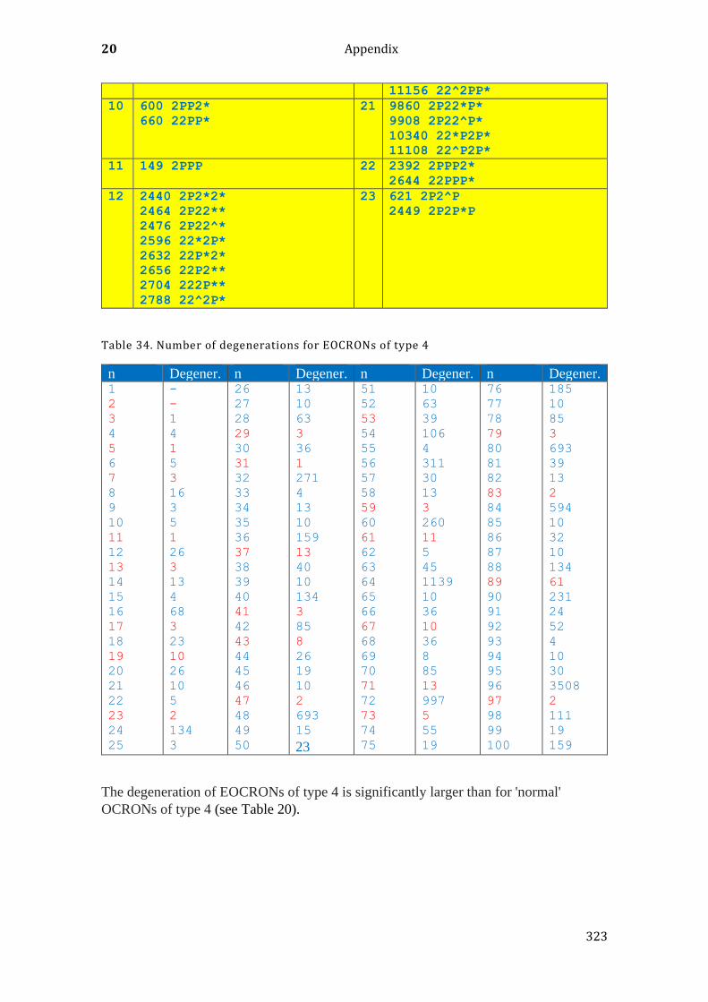
20 Appendix
323
11156 22^2PP*
10 600 2PP2*
660 22PP*
21 9860 2P22*P*
9908 2P22^P*
10340 22*P2P*
11108 22^P2P*
11 149 2PPP 22 2392 2PPP2*
2644 22PPP*
12 2440 2P2*2*
2464 2P22**
2476 2P22^*
2596 22*2P*
2632 22P*2*
2656 22P2**
2704 222P**
2788 22^2P*
23 621 2P2^P
2449 2P2P*P
Table 34. Number of degenerations for EOCRONs of type 4
n Degener. n Degener. n Degener. n Degener. 1
2
3
4
5
6
7
8
9
10
11
12
13
14
15
16
17
18
19
20
21
22
23
24
25
-
-
1
4
1
5
3
16
3
5
1
26
3
13
4
68
3
23
10
26
10
5
2
134
3
26
27
28
29
30
31
32
33
34
35
36
37
38
39
40
41
42
43
44
45
46
47
48
49
50
13
10
63
3
36
1
271
4
13
10
159
13
40
10
134
3
85
8
26
19
10
2
693
15
23
51
52
53
54
55
56
57
58
59
60
61
62
63
64
65
66
67
68
69
70
71
72
73
74
75
10
63
39
106
4
311
30
13
3
260
11
5
45
1139
10
36
10
36
8
85
13
997
5
55
19
76
77
78
79
80
81
82
83
84
85
86
87
88
89
90
91
92
93
94
95
96
97
98
99
100
185
10
85
3
693
39
13
2
594
10
32
10
134
61
231
24
52
4
10
30
3508
2
111
19
159
The degeneration of EOCRONs of type 4 is significantly larger than for 'normal'
OCRONs of type 4 (see Table 20).
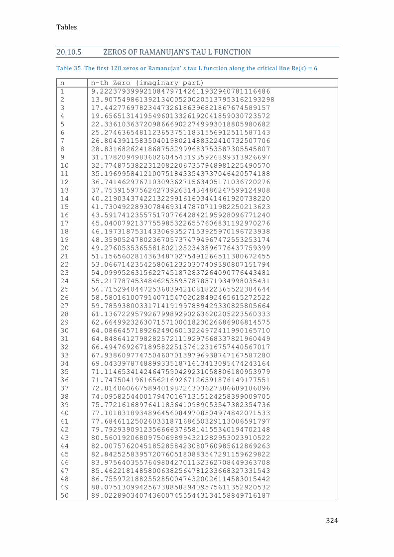
Tables
324
20.10.5 ZEROS OF RAMANUJAN’S TAU L FUNCTION
Table 35. The first 128 zeros or Ramanujan’ s tau L function along the critical line Re(𝑠) = 6
n n-th Zero (imaginary part)
1
2
3
4
5
6
7
8
9
10
11
12
13
14
15
16
17
18
19
20
21
22
23
24
25
26
27
28
29
30
31
32
33
34
35
36
37
38
39
40
41
42
43
44
45
46
47
48
49
50
9.222379399921084797142611932940781116486
13.907549861392134005200205137953162193298
17.44277697823447326186396821867674589157
19.65651314195496013326192041859030723572
22.33610363720986669022749993018805980682
25.27463654811236537511831556912511587143
26.80439115835040198021488322410732507706
28.83168262418687532999683753587305545807
31.17820949836026045431935926899313926697
32.77487538223120822067357948981225490570
35.19699584121007518433543737046420574188
36.74146297671030936271563405171036720276
37.75391597562427392631434486247599124908
40.21903437422132299161603441461920738220
41.73049228930784693147870711982250213623
43.59174123557517077642842195928096771240
45.04007921377559853226557606831192970276
46.19731875314330693527153925970196723938
48.35905247802367057374794967472553253174
49.27605353655818021252343896776437759399
51.15656028143634870275491266511380672455
53.06671423542580612320307409390807151794
54.09995263156227451872837264090776443481
55.21778745348462535957878571934998035431
56.71529404472536839421081822365522384644
58.58016100791407154702028492465615272522
59.78593800331714191997889429330825805664
61.13672295792679989290263620205223560333
62.66499232630715710001823026686906814575
64.08664571892624906013224972411990165710
64.84864127982825721119297668337821960449
66.49476926718958225137612316757440567017
67.93860977475046070139796938747167587280
69.04339787488993351871613413095474243164
71.11465341424647590429231058806180953979
71.74750419616562169267126591876149177551
72.81406066758940198724303627386689186096
74.09582544001794701671315124258399009705
75.77216168976411836410989053547382354736
77.10183189348964560849708504974842071533
77.68461125026033187168650329113006591797
79.79293909123566663765814155340194702148
80.56019206809750698994321282953023910522
82.00757620451852858423080760985612869263
82.84252583957207605180883547291159629822
83.97564035576498042701132362708449363708
85.46221814858006382564781233668327331543
86.75597218825528500474320026114583015442
88.07513099425673885889409575611352920532
89.02289034074360074555443134158849716187
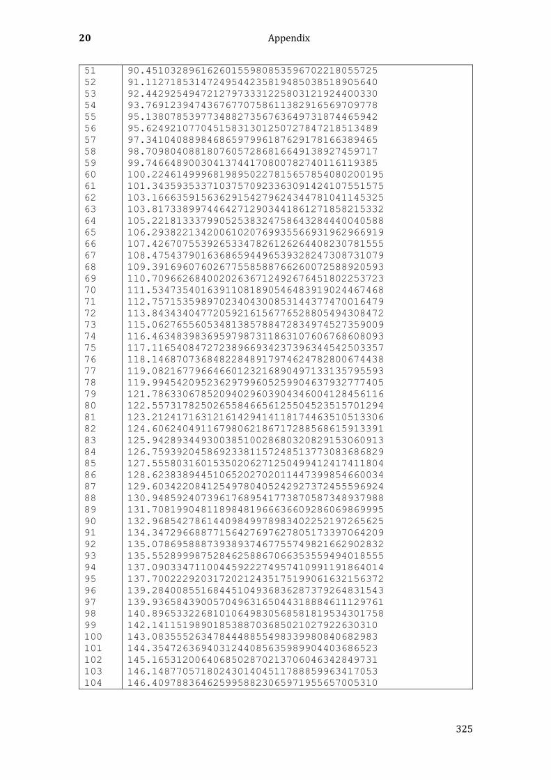
20 Appendix
325
51
52
53
54
55
56
57
58
59
60
61
62
63
64
65
66
67
68
69
70
71
72
73
74
75
76
77
78
79
80
81
82
83
84
85
86
87
88
89
90
91
92
93
94
95
96
97
98
99
100
101
102
103
104
90.45103289616260155980853596702218055725
91.11271853147249544235819485038518905640
92.44292549472127973331225803121924400330
93.76912394743676770758611382916569709778
95.13807853977348827356763649731874465942
95.62492107704515831301250727847218513489
97.34104088984686597996187629178166389465
98.70980408818076057286816649138927459717
99.74664890030413744170800782740116119385
100.22461499968198950227815657854080200195
101.34359353371037570923363091424107551575
103.16663591563629154279624344781041145325
103.81733899744642712903441861271858215332
105.22181333799052538324758643284440040588
106.29382213420061020769935566931962966919
107.42670755392653347826126264408230781555
108.47543790163686594496539328247308731079
109.39169607602677558588766260072588920593
110.70966268400202636712492676451802253723
111.53473540163911081890546483919024467468
112.75715359897023404300853144377470016479
113.84343404772059216156776528805494308472
115.06276556053481385788472834974527359009
116.46348398369597987311863107606768608093
117.11654084727238966934237396344542503357
118.14687073684822848917974624782800674438
119.08216779664660123216890497133135795593
119.99454209523629799605259904637932777405
121.78633067852094029603904346004128456116
122.55731782502655846656125504523515701294
123.21241716312161429414118174463510513306
124.60624049116798062186717288568615913391
125.94289344930038510028680320829153060913
126.75939204586923381157248513773083686829
127.55580316015350206271250499412417411804
128.62383894451065202702011447399854660034
129.60342208412549780405242927372455596924
130.94859240739617689541773870587348937988
131.70819904811898481966636609286069869995
132.96854278614409849978983402252197265625
134.34729668877156427697627805173397064209
135.07869588873938937467755749821662902832
135.55289998752846258867066353559494018555
137.09033471100445922274957410991191864014
137.70022292031720212435175199061632156372
139.28400855168445104936836287379264831543
139.93658439005704963165044318884611129761
140.89653322681010649830568581819534301758
142.1411519890185388703685021027922630310
143.0835552634784448855498339980840682983
144.3547263694031244085635989904403686523
145.1653120064068502870213706046342849731
146.1487705718024301404511788859963417053
146.4097883646259958823065971955657005310

Tables
326
105
106
107
108
109
110
111
112
113
114
115
116
117
118
119
120
121
122
123
124
125
126
127
128
148.1177541226128084872470935806632041931
149.0412678815713718449842417612671852112
150.2750742969780901603371603414416313171
150.9064237539794532949599670246243476868
152.1344343784803641028702259063720703125
153.1151471940314081621181685477495193481
154.0518290966241181649820646271109580994
154.7953122295758987547742435708642005920
155.7320793911374607887410093098878860474
157.0957831922944762936822371557354927063
157.9127528865146530279162107035517692566
158.6608139225808713490550871938467025757
159.6686139103367452207749010995030403137
161.3063702811864743580372305586934089661
161.8503586051299976134032476693391799927
162.8714549225416021727141924202442169189
163.5474941087671822970150969922542572021
164.3389052284337310538830934092402458191
165.6101228957916760009538847953081130981
166.5807970056847295836632838472723960876
167.6436347091075731441378593444824218750
168.6591247847260888192977290600538253784
169.2457741065447009987110504880547523499
170.5979320487521135873976163566112518311
Mathematica program: please contact the author.
20.10.6 THE ABC CONJECTURE: FIT PARAMETER AND C3 VALUES OF THE PLANE EQUATIONS FOR DIFFERENT GÖDELIZATION METHODS
Table 36. c=30011. Fit parameter and 𝑐3 of the plane equations for 𝑀𝑎𝑏𝑐 (type M2GOCRON4)
for different assignments of Gödel symbols
C 𝒄𝟑 Code table: symbols/values Max. value Standard error t-statistics
30011 3.50329 1:{*,P,2,^},{0,1,2,3} 31.5607 0.00147067 2382.1
30011 3.31794 2:{*,P,2,^},{0,1,3,2} 31.8085 0.00203153 1633.22
30011 3.4018 3:{*,P,2,^},{0,2,1,3} 31.1111 0.00109664 3102.03
30011 3.01535 4:{*,P,2,^},{0,2,3,1} 31.7433 0.000640746 4706.
30011 3.1857 5:{*,P,2,^},{0,3,1,2} 30.9755 0.00200754 1586.86
30011 2.97014 6:{*,P,2,^},{0,3,2,1} 31.3842 0.000996648 2980.14
30011 4.00661 9:{*,P,2,^},{1,2,0,3} 30.2574 0.00451077 886.529
30011 3.03373 10:{*,P,2,^},{1,2,3,0} 31.6698 0.000607757 4991.67
30011 3.78849 11:{*,P,2,^},{1,3,0,2} 30.2873 0.00555072 682.522
30011 2.99422 12:{*,P,2,^},{1,3,2,0} 31.2772 0.00115591 2590.36
30011 4.50418 15:{*,P,2,^},{2,1,0,3} 30.242 0.00378901 1188.75
30011 3.35767 16:{*,P,2,^},{2,1,3,0} 31.6661 0.00190649 1761.18
30011 3.93106 17:{*,P,2,^},{2,3,0,1} 30.2885 0.00646281 608.258
30011 3.2632 18:{*,P,2,^},{2,3,1,0} 30.611 0.0024814 1315.06
30011 4.61984 21:{*,P,2,^},{3,1,0,2} 29.8592 0.00406558 1136.33
30011 3.58239 22:{*,P,2,^},{3,1,2,0} 31.2661 0.0011851 3022.85
30011 4.25748 23:{*,P,2,^},{3,2,0,1} 29.886 0.00587147 725.113
30011 3.5185 24:{*,P,2,^},{3,2,1,0} 30.6002 0.0016776 2097.34
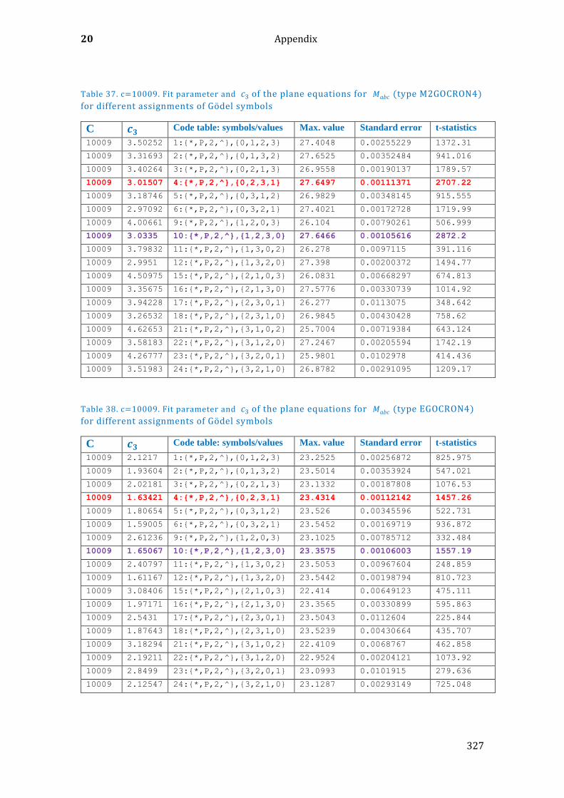
20 Appendix
327
Table 37. c=10009. Fit parameter and 𝑐3 of the plane equations for 𝑀𝑎𝑏𝑐 (type M2GOCRON4)
for different assignments of Gödel symbols
C 𝒄𝟑 Code table: symbols/values Max. value Standard error t-statistics
10009 3.50252 1:{*,P,2,^},{0,1,2,3} 27.4048 0.00255229 1372.31
10009 3.31693 2:{*,P,2,^},{0,1,3,2} 27.6525 0.00352484 941.016
10009 3.40264 3:{*,P,2,^},{0,2,1,3} 26.9558 0.00190137 1789.57
10009 3.01507 4:{*,P,2,^},{0,2,3,1} 27.6497 0.00111371 2707.22
10009 3.18746 5:{*,P,2,^},{0,3,1,2} 26.9829 0.00348145 915.555
10009 2.97092 6:{*,P,2,^},{0,3,2,1} 27.4021 0.00172728 1719.99
10009 4.00661 9:{*,P,2,^},{1,2,0,3} 26.104 0.00790261 506.999
10009 3.0335 10:{*,P,2,^},{1,2,3,0} 27.6466 0.00105616 2872.2
10009 3.79832 11:{*,P,2,^},{1,3,0,2} 26.278 0.0097115 391.116
10009 2.9951 12:{*,P,2,^},{1,3,2,0} 27.398 0.00200372 1494.77
10009 4.50975 15:{*,P,2,^},{2,1,0,3} 26.0831 0.00668297 674.813
10009 3.35675 16:{*,P,2,^},{2,1,3,0} 27.5776 0.00330739 1014.92
10009 3.94228 17:{*,P,2,^},{2,3,0,1} 26.277 0.0113075 348.642
10009 3.26532 18:{*,P,2,^},{2,3,1,0} 26.9845 0.00430428 758.62
10009 4.62653 21:{*,P,2,^},{3,1,0,2} 25.7004 0.00719384 643.124
10009 3.58183 22:{*,P,2,^},{3,1,2,0} 27.2467 0.00205594 1742.19
10009 4.26777 23:{*,P,2,^},{3,2,0,1} 25.9801 0.0102978 414.436
10009 3.51983 24:{*,P,2,^},{3,2,1,0} 26.8782 0.00291095 1209.17
Table 38. c=10009. Fit parameter and 𝑐3 of the plane equations for 𝑀𝑎𝑏𝑐 (type EGOCRON4)
for different assignments of Gödel symbols
C 𝒄𝟑 Code table: symbols/values Max. value Standard error t-statistics
10009 2.1217 1:{*,P,2,^},{0,1,2,3} 23.2525 0.00256872 825.975
10009 1.93604 2:{*,P,2,^},{0,1,3,2} 23.5014 0.00353924 547.021
10009 2.02181 3:{*,P,2,^},{0,2,1,3} 23.1332 0.00187808 1076.53
10009 1.63421 4:{*,P,2,^},{0,2,3,1} 23.4314 0.00112142 1457.26
10009 1.80654 5:{*,P,2,^},{0,3,1,2} 23.526 0.00345596 522.731
10009 1.59005 6:{*,P,2,^},{0,3,2,1} 23.5452 0.00169719 936.872
10009 2.61236 9:{*,P,2,^},{1,2,0,3} 23.1025 0.00785712 332.484
10009 1.65067 10:{*,P,2,^},{1,2,3,0} 23.3575 0.00106003 1557.19
10009 2.40797 11:{*,P,2,^},{1,3,0,2} 23.5053 0.00967604 248.859
10009 1.61167 12:{*,P,2,^},{1,3,2,0} 23.5442 0.00198794 810.723
10009 3.08406 15:{*,P,2,^},{2,1,0,3} 22.414 0.00649123 475.111
10009 1.97171 16:{*,P,2,^},{2,1,3,0} 23.3565 0.00330899 595.863
10009 2.5431 17:{*,P,2,^},{2,3,0,1} 23.5043 0.0112604 225.844
10009 1.87643 18:{*,P,2,^},{2,3,1,0} 23.5239 0.00430664 435.707
10009 3.18294 21:{*,P,2,^},{3,1,0,2} 22.4109 0.0068767 462.858
10009 2.19211 22:{*,P,2,^},{3,1,2,0} 22.9524 0.00204121 1073.92
10009 2.8499 23:{*,P,2,^},{3,2,0,1} 23.0993 0.0101915 279.636
10009 2.12547 24:{*,P,2,^},{3,2,1,0} 23.1287 0.00293149 725.048
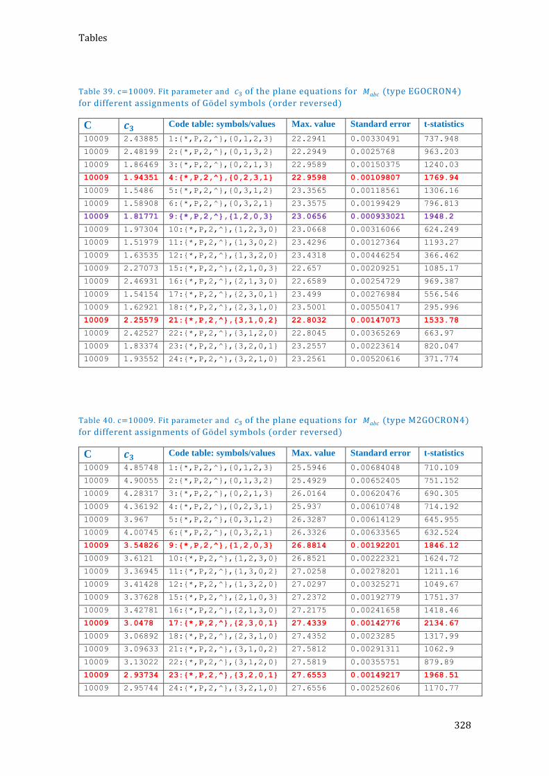
Tables
328
Table 39. c=10009. Fit parameter and 𝑐3 of the plane equations for 𝑀𝑎𝑏𝑐 (type EGOCRON4)
for different assignments of Gödel symbols (order reversed)
C 𝒄𝟑 Code table: symbols/values Max. value Standard error t-statistics
10009 2.43885 1:{*,P,2,^},{0,1,2,3} 22.2941 0.00330491 737.948
10009 2.48199 2:{*,P,2,^},{0,1,3,2} 22.2949 0.0025768 963.203
10009 1.86469 3:{*,P,2,^},{0,2,1,3} 22.9589 0.00150375 1240.03
10009 1.94351 4:{*,P,2,^},{0,2,3,1} 22.9598 0.00109807 1769.94
10009 1.5486 5:{*,P,2,^},{0,3,1,2} 23.3565 0.00118561 1306.16
10009 1.58908 6:{*,P,2,^},{0,3,2,1} 23.3575 0.00199429 796.813
10009 1.81771 9:{*,P,2,^},{1,2,0,3} 23.0656 0.000933021 1948.2
10009 1.97304 10:{*,P,2,^},{1,2,3,0} 23.0668 0.00316066 624.249
10009 1.51979 11:{*,P,2,^},{1,3,0,2} 23.4296 0.00127364 1193.27
10009 1.63535 12:{*,P,2,^},{1,3,2,0} 23.4318 0.00446254 366.462
10009 2.27073 15:{*,P,2,^},{2,1,0,3} 22.657 0.00209251 1085.17
10009 2.46931 16:{*,P,2,^},{2,1,3,0} 22.6589 0.00254729 969.387
10009 1.54154 17:{*,P,2,^},{2,3,0,1} 23.499 0.00276984 556.546
10009 1.62921 18:{*,P,2,^},{2,3,1,0} 23.5001 0.00550417 295.996
10009 2.25579 21:{*,P,2,^},{3,1,0,2} 22.8032 0.00147073 1533.78
10009 2.42527 22:{*,P,2,^},{3,1,2,0} 22.8045 0.00365269 663.97
10009 1.83374 23:{*,P,2,^},{3,2,0,1} 23.2557 0.00223614 820.047
10009 1.93552 24:{*,P,2,^},{3,2,1,0} 23.2561 0.00520616 371.774
Table 40. c=10009. Fit parameter and 𝑐3 of the plane equations for 𝑀𝑎𝑏𝑐 (type M2GOCRON4)
for different assignments of Gödel symbols (order reversed)
C 𝒄𝟑 Code table: symbols/values Max. value Standard error t-statistics
10009 4.85748 1:{*,P,2,^},{0,1,2,3} 25.5946 0.00684048 710.109
10009 4.90055 2:{*,P,2,^},{0,1,3,2} 25.4929 0.00652405 751.152
10009 4.28317 3:{*,P,2,^},{0,2,1,3} 26.0164 0.00620476 690.305
10009 4.36192 4:{*,P,2,^},{0,2,3,1} 25.937 0.00610748 714.192
10009 3.967 5:{*,P,2,^},{0,3,1,2} 26.3287 0.00614129 645.955
10009 4.00745 6:{*,P,2,^},{0,3,2,1} 26.3326 0.00633565 632.524
10009 3.54826 9:{*,P,2,^},{1,2,0,3} 26.8814 0.00192201 1846.12
10009 3.6121 10:{*,P,2,^},{1,2,3,0} 26.8521 0.00222321 1624.72
10009 3.36945 11:{*,P,2,^},{1,3,0,2} 27.0258 0.00278201 1211.16
10009 3.41428 12:{*,P,2,^},{1,3,2,0} 27.0297 0.00325271 1049.67
10009 3.37628 15:{*,P,2,^},{2,1,0,3} 27.2372 0.00192779 1751.37
10009 3.42781 16:{*,P,2,^},{2,1,3,0} 27.2175 0.00241658 1418.46
10009 3.0478 17:{*,P,2,^},{2,3,0,1} 27.4339 0.00142776 2134.67
10009 3.06892 18:{*,P,2,^},{2,3,1,0} 27.4352 0.0023285 1317.99
10009 3.09633 21:{*,P,2,^},{3,1,0,2} 27.5812 0.00291311 1062.9
10009 3.13022 22:{*,P,2,^},{3,1,2,0} 27.5819 0.00355751 879.89
10009 2.93734 23:{*,P,2,^},{3,2,0,1} 27.6553 0.00149217 1968.51
10009 2.95744 24:{*,P,2,^},{3,2,1,0} 27.6556 0.00252606 1170.77
20 Appendix
329
20.10.7 REED JAMESON PSEUDO PRIME NUMBERS
So far, the following Reed Jameson pseudoprimes are known:
4.647.272.200.763.653
13.145.972.926.201.741
37.550.172.530.083.333
91.475.036.245.333.333
138.059.041.752.628.921
1.017.051.023.982.373.381
1.198.917.598.782.691.327
2.193.915.384.965.973.241
3.451.615.699.229.107.381
3.512.610.370.112.161.753
4.595.180.567.858.094.061
6.048.451.215.682.221.781
6.338.484.791.054.344.501
7.928.915.800.561.771.753
8.145.180.508.453.751.953
8.791.425.219.802.647.241
9.298.405.698.887.024.981
9.538.676.189.678.282.653
10.465.926.737.075.038.153
10.672.259.013.245.100.833
10.832.491.549.192.774.861
10.877.405.928.733.495.009
10.956.794.257.273.312.801
11.422.820.349.626.091.841
11.555.150.568.592.132.153
13.383.002.224.373.603.221
14.127.279.039.356.766.601
17.487.206.393.334.007.501
Source: Peter Danzeglocke (calculated with an optimized C ++ program).
The range 𝑛 < 1010 contains no Reed Jameson pseudo primes (as of December 2020).
20.11 MATHEMATICA PROGRAMS
In this section you will find a collection of Mathematica programs, such as speed-
optimized versions of the example programs described above.
Chebyshev function psi(x):
The function myPsi[x] can be made somewhat faster by exploiting symmetry properties and
using the Evaluate[] and Compile[] functions:
###############################################################
myPsi[x_]:=Evaluate[-2*Sum[((x)^ZetaZero[i])/ZetaZero[i],{i,1,15}]-
0.5*Log[1-1/x^2]+x-Log[2*Pi]];
Mathematica programs
330
myPsic=Compile[{{x,_Complex}},myPsi[x],CompilationOptions-
>{"ExpressionOptimization"->True},
CompilationOptions->{"InlineCompiledFunctions"->Auto}]
Timing[Plot[Re[myPsic[x]],{x,1,100}]]
20.11.1 COMPARISON OF THE NUMBER OF TWIN, COUSIN AND SEXY PRIMES BY THE FORMULA OF HARDY-LITTLEWOOD
###############################################################
Mathematica-Program: please contact the author.
20.11.2 DIFFERENCERG SEQUENCES
RG sequences with ‘Prime GOCRONs’ (type 6): Mathematica program: please contact the author.
RG sequences with ‘EGOCRONs’ (type 4): (*The following examples need the OCRON-library (see below*)
############################################################### (*example:*)
Mathematica program: please contact the author.
20.11.3 RIEMANN’S ZETA FUNCTION
###############################################################
(*animation of the ‘noise’ of the product representation in the
complex domain:*)
Mathematica program: please contact the author.
(*(Snapshot:*)

20 Appendix
331
###############################################################
(*Iterative, approximat. method for the calculation of the product
representation, using prime numbers *)
(*along the critical line *)
Mathematica program: please contact the author.
###############################################################
(*Iterative, approximat. method for the calculation of the product
representation, using the zeros of the zeta function*)
(*along the X-axis, zeros at prime numbers*)
Mathematica program: please contact the author.
###############################################################
(*Parametric 3D-Plot of the Riemann zeta function along the crit. line
*)
Mathematica program: please contact the author.
20.11.4 REED JAMESON AND PERRIN SEQUENCES
(*##################################################################*)
Mathematica program: please contact the author.
Mathematica program: please contact the author.
20.11.5 LATTICE POINTS ON N-SPHERES (N-DIMENSIONAL SPHERES)
###############################################################
(*Interactive animation: lattice points on 1-sphere*)

Mathematica programs
332
m=Manipulate[Graphics[
dim=2;sqN=Sqrt[n];sqNInt=Round[sqN];
numberOfGridPoints=SquaresR[dim,n];
If[numberOfGridPoints>0,sol=FindInstance[a^2+b^2==n,{a,b},
Integers,numberOfGridPoints]];
Flatten[Table[{},{x,-sqNInt-2,sqNInt+2},
{y,-sqNInt-2,sqNInt+2}]],
Prolog->{If[ci,{{Black,Thickness[0.007],Circle[{0,0},sqN]},
If[numberOfGridPoints>0,{Red,PointSize[0.04],
Point[{a,b}]/.sol}]},{}]},
Frame->If[ft,Automatic,False],
PlotRange->{{-sqNInt-2,sqNInt+2},{-sqNInt-2,sqNInt+2}},
FrameTicks->If[ft,Automatic,None],
ImageSize->{480,400},ImageMargins->10,
GridLines->If[lattice,{Range[-sqNInt-2,sqNInt+2],
Range[-sqNInt-2,sqNInt+2]}]],
{{n,10,"square of radius"},2,100,1,
Appearance->"Labeled"},Delimiter,{{lattice,True,"show
lattice"},{True,False}},
{{ft,False,"show scale"},{True,False}},{{ci,True,"draw
circle"},{True,False}},
AutorunSequencing->Automatic]
(*snaphot:*)
Export["C:\\animations\\latticePointsOnN-
spheresInNDimensions\\latticePointsOn1-spheresIn2Dimensions_RQ2-
100.mov",m]
###############################################################
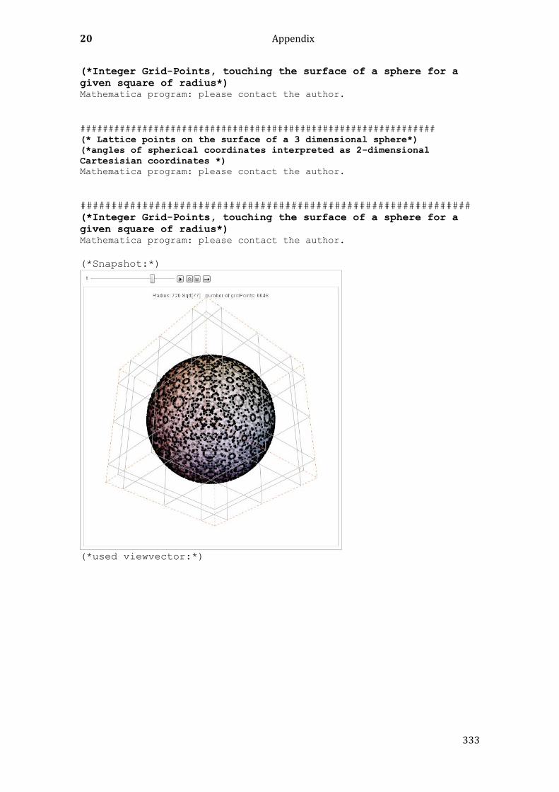
20 Appendix
333
(*Integer Grid-Points, touching the surface of a sphere for a
given square of radius*)
Mathematica program: please contact the author.
###############################################################
(* Lattice points on the surface of a 3 dimensional sphere*)
(*angles of spherical coordinates interpreted as 2-dimensional
Cartesisian coordinates *)
Mathematica program: please contact the author.
###############################################################
(*Integer Grid-Points, touching the surface of a sphere for a
given square of radius*)
Mathematica program: please contact the author.
(*Snapshot:*)
(*used viewvector:*)
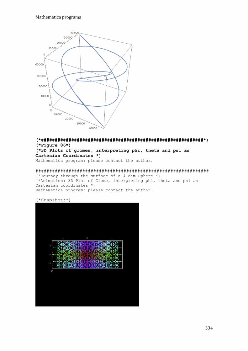
Mathematica programs
334
(*###########################################################*)
(*Figure 86*)
(*3D Plots of glomes, interpreting phi, theta and psi as
Cartesian Coordinates *)
Mathematica program: please contact the author.
###############################################################
(*Journey through the surface of a 4-dim Sphere *)
(*Animation: 3D Plot of Glome, interpreting phi, theta and psi as
Cartesian coordinates *)
Mathematica program: please contact the author.
(*Snapshot:*)

20 Appendix
335
20.11.6 EVALUATION AND STATISTICS OF DIFFERENCES OF THE PRIME SEQUENCE
(*Statistics with prime number differences of higher order*) Mathematica program: please contact the author.
336
20.11.7 THE ABC CONJECTURE
(*abc-conjecture: calculates log Gödel-GOCRON4 codes of abc-points.
Representation *)
(*as 3D-Plot together with a 'fitted' plane from different views *)
(* execution needs the OCRON Mathematica-library! *)
Mathematica program: please contact the author.
20.11.8 OTHER MATHEMATICA PROGRAMS
(*Polynomial with 26 variables of degree 25, whose positive values are
identical to the set pf primes *)
(*This program searches for positive solutions *)
c0=w z+h+j-q;
c1=(g k+2g+k+1)*(h+j)+h-z;
c2=2n+p+q+z-e;
c3=16(k+1)^3 *(k+2)*(n+1)^2+1-f^2;
c4=e^3*(e+2)*(a+1)^2+1-o^2;
c5=(a^2-1)*y^2+1-x^2;
c6=16r^2 y^4*(a^2-1)+1-u^2;
c7=((a+u^2*(u^2-a))^2-1)*(n+4d y)^2+1-(x+c u)^2;
c8=n+l+v-y;
c9=(a^2-1)*l^2+1-m^2;
c10=a i+k+1-l-i;
c11=p+l*(a-n-1)+b*(2a n+2a-n^2-2n-2)-m;
c12=q+y*(a-p-1)+s*(2a p+2a-p^2-2p-2)-x;
c13=z+p l*(a-p)+t*(2a p-p^2-1)-p m;
k=0;
FindInstance[Element[k+2,Primes]&&c0==0&&c1==0&&c2==0&&c3==0&&c4==0&&c
5==0&&c6==0&&c7==0&&c8==0&&c9==0&&c10==0&&c11==0&&c12==0&&c13==0&&a>=0
&&b>=0&&c>=0&&d>=0&&e>=0&&f>=0&&g>=0&&h>=0&&i>=0&&j>=0&&k>=0&&l>=0&&m>
=0&&n>=0&&o>=0&&p>=0&&q>=0&&r>=0&&s>=0&&t>=0&&u>=0&&v>=0&&w>=0&&x>=0&&
y>=0&&z>=0,{a,b,c,d,e,f,g,h,i,j,k,l,m,n,o,p,q,r,s,t,u,v,w,x,y,z},Integ
ers]
(*Calculation of the sigma1 function*)
myDivisorSigma[k_,n_]:=
Sum[m^(k-1)Sum[Cos[(2 pi j n)/m],{j,1,m}],{m,1,n}]
(*Example: n= 31*)
myDivisorSigma[1,31]
This expression is not seen as identical to 32
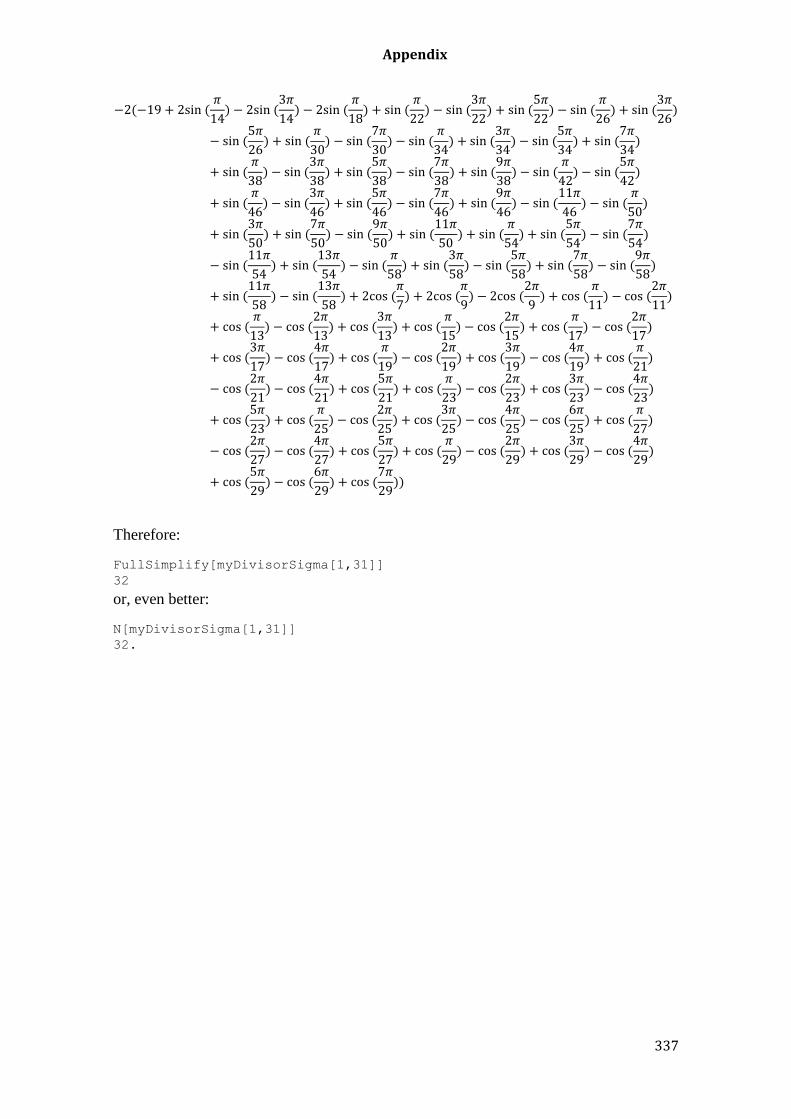
Appendix
337
−2(−19 + 2sin (𝜋
14) − 2sin (
3𝜋
14) − 2sin (
𝜋
18) + sin (
𝜋
22) − sin (
3𝜋
22) + sin (
5𝜋
22) − sin (
𝜋
26) + sin (
3𝜋
26)
− sin (5𝜋
26) + sin (
𝜋
30) − sin (
7𝜋
30) − sin (
𝜋
34) + sin (
3𝜋
34) − sin (
5𝜋
34) + sin (
7𝜋
34)
+ sin (𝜋
38) − sin (
3𝜋
38) + sin (
5𝜋
38) − sin (
7𝜋
38) + sin (
9𝜋
38) − sin (
𝜋
42) − sin (
5𝜋
42)
+ sin (𝜋
46) − sin (
3𝜋
46) + sin (
5𝜋
46) − sin (
7𝜋
46) + sin (
9𝜋
46) − sin (
11𝜋
46) − sin (
𝜋
50)
+ sin (3𝜋
50) + sin (
7𝜋
50) − sin (
9𝜋
50) + sin (
11𝜋
50) + sin (
𝜋
54) + sin (
5𝜋
54) − sin (
7𝜋
54)
− sin (11𝜋
54) + sin (
13𝜋
54) − sin (
𝜋
58) + sin (
3𝜋
58) − sin (
5𝜋
58) + sin (
7𝜋
58) − sin (
9𝜋
58)
+ sin (11𝜋
58) − sin (
13𝜋
58) + 2cos (
𝜋
7) + 2cos (
𝜋
9) − 2cos (
2𝜋
9) + cos (
𝜋
11) − cos (
2𝜋
11)
+ cos (𝜋
13) − cos (
2𝜋
13) + cos (
3𝜋
13) + cos (
𝜋
15) − cos (
2𝜋
15) + cos (
𝜋
17) − cos (
2𝜋
17)
+ cos (3𝜋
17) − cos (
4𝜋
17) + cos (
𝜋
19) − cos (
2𝜋
19) + cos (
3𝜋
19) − cos (
4𝜋
19) + cos (
𝜋
21)
− cos (2𝜋
21) − cos (
4𝜋
21) + cos (
5𝜋
21) + cos (
𝜋
23) − cos (
2𝜋
23) + cos (
3𝜋
23) − cos (
4𝜋
23)
+ cos (5𝜋
23) + cos (
𝜋
25) − cos (
2𝜋
25) + cos (
3𝜋
25) − cos (
4𝜋
25) − cos (
6𝜋
25) + cos (
𝜋
27)
− cos (2𝜋
27) − cos (
4𝜋
27) + cos (
5𝜋
27) + cos (
𝜋
29) − cos (
2𝜋
29) + cos (
3𝜋
29) − cos (
4𝜋
29)
+ cos (5𝜋
29) − cos (
6𝜋
29) + cos (
7𝜋
29))
Therefore:
FullSimplify[myDivisorSigma[1,31]]
32
or, even better:
N[myDivisorSigma[1,31]]
32.
338
20.11.9 OCRONS AND THE ABC CONJECTURE: PROGRAM LIBRARY
20.11.9.1 OCRON FUNCTIONS
(* ##################################################################################*)
(* Library: GOCRON-Routines actual version Sept.2016*)
(* ##################################################################################*)
Mathematica Program: please contact the author.
(* OCRON-Functionlist:
nToGoedelSymbolList[n_],goedelSymbolListToN[symbolList_]
nToGoedelSymbolListForPrimeOCRONS[n_],goedelSymbolListToNForPrimeOCRONS[symbolList_]
nToGoedelSymbolListForVirtualOCRONs[n_],goedelSymbolListToNForVirtualOCRONS[symbolList_]
##################### OCRON4, GOCRON4 #################
nToOCRON4[n_], oCRON4ToN[symbolList_], oCRON4ToNMaxVal[symbolList_,maxVal_]
nToGOCRON4[n_], GOCRON4ToN[n_], GOCRON4ToNMaxVal[symbolList_,maxVal_]
checkOCRON4[n_]
##################### M2OCRON4, M2GOCRON4 without leading 2 #################
nToM2OCRON4[n_], m2OCRON4ToN[symbolList_]
nToM2GOCRON4[n_], msGOCRON4ToN[n_]
##################### EOCRON4, EGOCRON4 #################
nToEOCRON4[n_],eOCRON4ToN[symbolList_], eOCRON4ToNMaxVal[symbolList_,maxVal_]
nToEGOCRON4[n_],eGOCRON4ToN[n_], eGOCRON4ToNMaxVal[symbolList_,maxVal_]
##################### PrimeOCRON, PrimeGOCRON (type 6)#################
nToPrimeOCRON[n_], primeOCRONToN[n_]
nToPrimeGOCRON[n_],primeGOCRONToN[n_]
##################### Miscellaneous #########################
createAscendingEOcron4List[n_]
createAscendingEVirtualOcron4List[n_]
createAscendingVirtualOcron4List[n_]
createAllValuesListFromAscendingVirtualOcron4s[n_]
createIntValuesListFromAscendingVirtualOcron4s[n_]
createAscendingIntList[n_]
createAscendinGOCRONListFromNaturalNumbers[n_]
createAscendingGOCRONListFromNaturalNumbers[n_]
createAscendingEOCRONListFromNaturalNumbers[n_]
createAscendingEGOCRONListFromNaturalNumbers[n_]
createAscendingM2OCRONListFromNaturalNumbers[n_]
createAscendingM2GOCRONListFromNaturalNumbers[n_]
resetGloc4Codes[]
setGLoc4CodeSymbols[symbols_]
setGLoc4CodeValues[values_]
######################### Virtual OCRONs #######################
checkVirtualOCRON4[n_], virtualOCRON4ToOCRON4[symbolList_]
virtualOCRON4ToN[symbolList_]
######################################################################################
Evaluating OCRONS by converting the Polish RPN-representation used in OCRONS to 'normal'
Mathematica expressions before numerical evaluation #######################
#######################################################################################
oCRON4ToExpression[symbolList_]
loGOCRON4ToExpression[symbolList_]
loGOCRON4ToExpressionSimplify[symbolList_]
oCRON4ToExpressionPowerExpand[symbolList_]
loGOCRON4ToExpressionPowerExpand[symbolList_]
logLoGOCRON4ToExpressionPowerExpand[symbolList_]
convertOcronToTraditionalForm[symbolList_]
convertLogOcronToTraditionalForm[symbolList_]
convertLogLogOcronNToTraditionalForm[symbolList_]
*)
20.11.9.2 THE ABC CONJECTURE
(*##########################################################################*)
(*##########################################################################*)
(*radicals, quality, isPossibleABC, radABC() computes radABC from c, but does
not always get the smallest one!!*)
Appendix
339
(*minRadABC takes always the smallest*)
20.11.9.3 THE DEGENERATION OF OCRONS
(*##########################################################################*)
(*Degeneration-values of OCRONs type 4 *)
(*Needs GOCRON4-Library *)
(*##########################################################################*)
gloc4Codes={{"*","P","2","^"},{0,1,2,3}}; (*actual code-Table,*)
(*Note: maxEGocrons should be at least 13 symbols long (e.g. 22*2*2*2*2*2* =
2^7=128) *)
(* Because of
goedelSymbolListToN[{"^","^","^","^","^","^","^","^","^","^","^","^","^"}]=671
08863 *)
(* maxEOcrons should be at least 67.108.863 to get all degeneration values up
to maxValue = 128 (=2^7 *)
(* maxEOcrons should be at least 1073741823 to get all degeneration values up
to maxValue = 256 (=2^8 *)
maxValue=128; maxEOcrons=67200000;
ocron4DegenList=Table[{},{i,1,maxValue}];
For[i=1,i<maxEOcrons,i++,
eOcron=nToGoedelSymbolList[i];
iValue=oCRON4ToNMaxVal[eOcron,maxValue];
If[iValue>0&& iValue<= maxValue,AppendTo[ocron4DegenList[[iValue]],eOcron];
];
If[Mod[i,100000]==0,Print[N[i/67200000]]];
]
For[i=1,i<maxValue,i++,
Print[i,": ",Length[ocron4DegenList[[i]]],"->",ocron4DegenList[[i]]];
]
20.11.10 SOUND ROUTINES
(*#############Prime Sound-Library#################################*)
(*Generate a sorted list of the combined (sieve number, prime number)-
pairs by: *)
Mathematica program: please contact the author.
20.11.11 RSA ENCRYPTION AND DECRYPTION
(*Example 1: encode/Decode a number (1115) *)
(*Very simple example of RSA encryption*)
(*Without Encoding/Decoding Functions from Mathematica…*)
(*############## implement coding mechanism ####################*)
(*choose two different prime numbers:*)
Mathematica program: please contact the author.
(*Example 2: same as Example 1: encode a number (1115) *)
(*using Mathematica built-in functions*)
(*publicKey[], privateKey[], Encrypt[], Decrypt[]*)
(*used padding-mode: ‚none‘ *)
(*IMPORTANT: in this Mathematica-version (10.3) Encoding with
PublicKey-Objects and padding: "None" only works for up to 16-bit
Modules *)
Mathematica program: please contact the author.
(*############## Encode and decode messages:######################*)
(*this is our message to be encoded:*)

340
Mathematica program: please contact the author.
(*Example 3: rSA-Encoding/Decoding a small String ("OK") using PKCS1
padding*)
(*let Mathematica choose p, q and the modulus using Mathematica built-
in functions*)
Mathematica program: please contact the author.
(*Example 4: hacking a
private Key from a public key using PKCS1 padding with key length
192*)
(*We use Mathematica built-in functions PrivateKey[], Decrypt[] and
FactorInteger[]*)
(*###############################################################*) Mathematica program: please contact the author.
(*###### decoding can be done different ways::#########*)
(* Decrypted data by using Decrypt[] will not contain padded data…*)
bCryptArray=ByteArray[IntegerDigits[mCrypt,256]];
decryptedByteArray=Normal[Decrypt[privKey,bCryptArray]]
decryptedString=FromCharacterCode[decryptedByteArray];
Print["Decryption-result (original String: ",decryptedString];
(**** program – output:****)
prime p from RSA:module: 68357071940820194611682396513
prime q from RSA:module: 78553627484042565312533006567
private Exponent:
4844991859660492495555967871982611572207133532958607342401
Private Modulus:
5369695965139088101081485235420567443013865529391511497792
Hacked private key:
cipher: rSA
private exponent length: 192 bits
public modulus length: 192 bits
padding: pKCS1

Appendix
341
public exponent: 65537
Original Text as Bytearray including Bytes padded by PKCS1 algorithm:
{2,11,165,77,224,174,48,231,225,235,0,69,108,118,105,115,32,108,105,11
8,101,115,33}
\.02\.0b¥Mà®0çáë\.00Elvis lives!
Decryption-result (original Byte array:
{69,108,118,105,115,32,108,105,118,101,115,33}
Decryption-result (original String):
Elvis lives!
(*Example 5: hacking a private Key from a public key using PKCS1
padding with key length 2048*)
(*We use Mathematica built-in functions PrivateKey[], Decrypt[] and
FactorInteger[]*)88
(*###############################################################*)
Mathematica program: please contact the author.
(* Decrypted data by using Decrypt[] will not contain padded data…*)
bCryptArray=ByteArray[IntegerDigits[mCrypt,256]];
decryptedByteArray=Normal[Decrypt[privKey,bCryptArray]]
decryptedString=FromCharacterCode[decryptedByteArray];
Print["Decryption-result (original String: ",decryptedString];
(**** program – output:****)
prime p from RSA-module:
5042275217484184784387456407481025964634418009557323862771843210015347
0233709220326765100448150841802101002465172565326870447505988642493935
6768330261183984688981022399271959231632244880124488202703458535772508
3261691330915873078509567583024603043325764678776810906881522663421805
761981426998378611173580023640569
prime q from RSA-module:
6230506107037277994848859713460167565407435407248343949280547643268996
2794782739027185058685887929516793028417110464017369917383411955467390
4850630650913159085619714144991810427714356257581581356417704599361604
8753993877513046170835382583128576250458442756910532302852222491700224
633245295180992749493823
private Exponent:
1030819360403968961043390501763010666063077815038257405347287921525051
2535022756352365421194768891684069779277718177933402369048702835912585
4131450497268501685537802072878657793084753037172733458691935491519525
1853460378496829887538632390637136150965931733628074554699429623111223
3269880545420815346132763817866426056363791352182879224677368503022618
4983798138489051261011671669601896311386511911972803990381100552366494
4073403141189139015889364169952790178286921216796288440782997538376575
88 The program runs with Mathematica Version 15.5 (2026) or higher

342
7085206627441700960078133155365855116355242551141828940174105853199096
690164133765434208900272472536995205015922393069952712705
Private Modulus:
3141592653589793238462643383279502884197169399375105820974944592307816
4062862089986280348253421170679821480865132823066470938446095505822317
2535940812848111745028410270193852110555964462294895493038196442881097
5665933446128475648233786783165271201909145648566923460348610454326648
2133936072602491412737302005743673942332300681176030308206877770767919
8534374004936614234231860407863629025266826226514213872656537709283991
0702130843755236406451881492103609092001021009355392277882966409625448
3914303698969808213385445154539250686410599473315757219688912541904259
662541240447603317926765114985912144304711024675664570896
Hacked private key:
cipher: rSA
private exponent length: 2047 bits
public modulus length: 2048 bits
padding: pKCS1
public exponent: 65537
Original Text as Bytearray including Bytes padded by PKCS1 algorithm:
{2,169,246,29,163,145,193,96,236,157,15,189,194,238,0,73,102,32,68,111
,110,97,108,100,32,84,114,117,109,112,32,115,104,111,117,108,100,32,11
9,105,110,32,116,104,101,32,112,114,101,115,105,100,101,110,116,105,97
,108,32,101,108,101,99,116,105,111,110,115,44,32,116,104,105,115,32,11
9,111,117,108,100,32,98,101,32,97,32,100,105,115,97,115,116,101,114,32
,102,111,114,32,116,104,101,32,85,110,105,116,101,100,32,83,116,97,116
,101,115,32,111,102,32,65,109,101,114,105,99,97,46,10,39,116,119,97,11
5,32,98,114,105,108,108,105,103,44,32,97,110,100,32,116,104,101,32,115
,108,105,116,104,121,32,116,111,118,101,115,10,100,105,100,32,103,121,
114,101,32,97,110,100,32,103,105,109,98,108,101,32,105,110,32,116,104,
101,32,119,97,98,101,58,10,65,108,108,32,109,105,109,115,121,32,119,10
1,114,101,32,116,104,101,32,98,111,114,111,103,111,118,101,115,44,10,9
7,110,100,32,116,104,101,32,109,111,109,101,32,114,97,116,104,115,32,1
11,117,116,103,114,97,98,101}
\.02©ö\.1d£‘Á`ì�\.0f½Âî\.00If Donald Trump should win the presidential elections, this would be a disaster for the United States of America.
'twas brillig, and the slithy toves
did gyre and gimble in the wabe:
All mimsy were the borogoves,
and the mome raths outgrabe
Decryption-result (original String: if Donald Trump should win the
presidential elections, this would be a disaster for the United States
of America.
'twas brillig, and the slithy toves
did gyre and gimble in the wabe:
All mimsy were the borogoves,
and the mome raths outgrabe
20.11.12 ALIQUOT SEQUENCES

Appendix
343
(* computes aliquot sequences for a few interesting initial
values*)
Mathematica program: please contact the author.
Output:
{1,Terminating,{1,0}}
{2,Terminating,{2,1,0}}
{3,Terminating,{3,1,0}}
{4,Terminating,{4,3,1,0}}
{5,Terminating,{5,1,0}}
{6,Perfect,{{6}}}
{7,Terminating,{7,1,0}}
{8,Terminating,{8,7,1,0}}
{9,Terminating,{9,4,3,1,0}}
{10,Terminating,{10,8,7,1,0}}
{11,Terminating,{11,1,0}}
{12,Terminating,{12,16,15,9,4,3,1,0}}
{28,Perfect,{{28}}}
{496,Perfect,{{496}}}
{220,Amicable,{{220,284}}}
{1184,Amicable,{{1184,1210}}}
{12496,Sociable,{{12496,14288,15472,14536,14264}}}
{1264460,Sociable,{{1264460,1547860,1727636,1305184}}}
{790,Aspiring,{790,650,652,{496}}}
{909,Aspiring,{909,417,143,25,{6}}}
{562,Cyclic,{562,{284,220}}}
{1064,Cyclic,{1064,1336,{1184,1210}}}
{1488,Non-
terminating,{1488,2480,3472,4464,8432,9424,10416,21328,22320,55056,957
28,96720,236592,459792,881392,882384,1474608}}
(*Aliquot 276 (306,396,696)OE:*)
Mathematica program: please contact the author.
(*#############################################################*)
(*Plot Differences of Log of aliquot sequences, using ListPlot*)
n=921232;noIterate=1000; diffOrder=1;
Mathematica program: please contact the author.
20.11.13 THE ARECIBO MESSAGE
(*Arecibo-Message*)
n=23;
t=Table[BitShiftRight[BitAnd[27886402056107263551714831669687744330301
5886191896083753494207226153602508928851994608485761550978983329982259
3335259720410959738432212343758921014182008038517667278025253709464080
0567916516636264434941344165234644984933485655114374616110243082450500
4833981684141550381731028954290673308020242293291528914499592811145845
8595397126461136347103419178098716188118662826517986311913829406689871
7096729057657705911386899499333419586667745206851413286366090402386362
1169622066629371322105035882727404788841080,2^i],i],{i,1679,0,-
1}];ArrayPlot[Partition[t,n],Mesh->All,
ColorRules->{1->RGBColor[.0,.1,.9],0->RGBColor[.9,.5,.2]},
ImageSize->Medium,PlotLabel->{"Arecibo-Message"},
PlotLegends->Automatic]
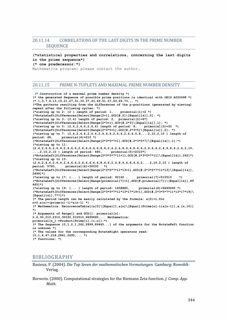
344
20.11.14 CORRELATIONS OF THE LAST DIGITS IN THE PRIME NUMBER SEQUENCE
(*statistical properties and correlations, concerning the last digits
in the prime sequence*)
(* one predecessor:*)
Mathematica program: please contact the author.
20.11.15 PRIME N-TUPLETS AND MAXIMAL PRIME NUMBER DENSITY
(* Construction of a maximal prime number density *)
(* the generated Sequence of possible prime positions is identical with OEIS A020498 *)
(* 1,3,7,9,13,19,21,27,31,33,37,43,49,51,57,63,69,73,,, *)
(*The patterns resulting from the differences of the p-positions (generated by sieving)
repeat after the following cycles: *)
(*sieving up to 2: {2 } length of period: 1, primorial(1)=2 *)
(*RotateLeft[Differences[Select[Range[2+1],GCD[#,2]\[Equal]1&]],0]; *)
(*sieving up to 3: {2,4} length of period: 2, primorial(2)=6*)
(*RotateLeft[Differences[Select[Range[2*3+1],GCD[#,2*3]\[Equal]1&]],1]; *)
(*sieving up to 5: {2,4,2,4,6,2,6,4} length of period: 8, primorial(3)=30 *)
(*RotateLeft[Differences[Select[Range[2*3*5+1],GCD[#,2*3*5]\[Equal]1&]],2]; *)
(*sieving up to 7: {2,4,2,4,6,2,6,4,2,4,6,6,2,6,4,2,6,4,6,8,...2,10,2,10 } length of
period: 48, primorial(4)=210 *)
(*RotateLeft[Differences[Select[Range[2*3*5*7+1],GCD[#,2*3*5*7]\[Equal]1&]],1];*)
(*sieving up to 11:
{2,4,2,4,6,2,6,4,2,4,6,6,2,6,6,6,4,6,8,4,2,4,2,4,8,6,4,8,4,6,2,6,6,4,2,4,6,8,4,2,4,2,10,
...,2,10,2,10 } length of period: 480, primorial(5)=2310*)
(*RotateLeft[Differences[Select[Range[2*3*5*7*11+1],GCD[#,2*3*5*7*11]\[Equal]1&]],262]*)
(*sieving up to 13:
{2,4,2,4,6,2,6,4,2,4,6,6,2,6,6,6,4,6,8,4,6,2,4,8,6,4,8,4,6,2,...2,10,2,10 } length of
period: 5760, primorial(6)=30030 *)
(*RotateLeft[Differences[Select[Range[2*3*5*7*11*13+1],GCD[#,2*3*5*7*11*13]\[Equal]1&]],
2899]*)
(*sieving up to 17: {... } length of period: 92160 , primorial(7)=510510 *)
(*RotateLeft[Differences[Select[Range[primorial[7]+1],GCD[#,primorial[7]]\[Equal]1&]],89
465]*)
(*sieving up to 19: {... } length of period: 1658880, primorial(8)=9699690 *)
(*RotateLeft[Differences[Select[Range[2*3*5*7*11*13*17*19+1],GCD[#,2*3*5*7*11*13*17*19]\
[Equal]1&]],???]*)
(* The period length can be easily calculated by the formula: a(0)=1;for
n>0,a(n)=(prime(n)-1)*a(n-1) *)
(* Mathematica: RecurrenceTable[{a[0]\[Equal]1,a[n]\[Equal](Prime[n]-1)a[n-1]},a,{n,10}]
*)
(* Arguments of Range[] and GCD[]: primorial[n]:
2,6,30,210,2310,30030,510510,9699690,... Mathematica:
primorial[n_]:=Product[Prime[i],{i,n}];*)
(* The Sequence {0,1,2,1,262,2899,89465...} of the arguments for the RotateFeft function
is unknown *)
(* The values for the corresponding RotateRight operatons read:
{0,1,6,47,218,2861,2695,... *)
(* functions: *)
BIBLIOGRAPHY
Basieux, P. (2004). Die Top Seven der mathematischen Vermutungen. Gamburg: Rowohlt-Verlag.
Borwein. (2000). Computational strategies for the Riemann Zeta function. J. Comp. App. Math.
List of illustrations
345
Edwards, H. M. (1974). Riemann's Zeta Function. San Diego, CA: Academic Press Limited.
Hardy, G. H., & Ramanujan, A. (1940 (First Edition) 1978 (Last Edition, corrected)). Ramanijan: Twelve Lectures on subjects suggested by his life and work. Cambridge, New York: American Mathematical Society.
Hofstadter, D. R. (1991 / 1985). Gödel Escher Bach. München: Ernst Klett Verlag.
Johnson F.Yan, A. K. (Jan. 1991). Prime Numbers and the Amino Acid Code: Analogy in Coding Properties. Journal of Theor. Biology, S. 333-341.
Koch, H., & Pieper, E. (1976). Zahlentheorie: Ausgewählte Methoden und Ergebnisse. Berlin: VEB Deutscher Verlag der Wissenschaften.
Ribenboim, P. (1989). The Book of Prime Number Records. New York: Springer-Verlag.
Richard Crandall, C. P. (2001). Prime Numbers: A Computational Perspective. New York: Springer-Verlag.
Sautoy, M. d. (2004). Die Musik der Primzahlen. München: Verlag C.H. Beck.
Singh, S. (1998). Fermats letzter Satz. München, Wien: Carl Hanser Verlag.
Tammet, D. (2014). Die Poesie der Primzahlen. München: Carl Hanser Verlag.
Taschner, R. (2013). Die Zahl, die aus der Kälte kam. München: Carl-Hanser Verlag.
Tegmark, M. (2015). Unser Mathematisches Universum. Berlin: Ullstein Buchverlage GmbH.
LIST OF ILLUSTRATIONS
Figure 1. Number of twin primes from 2 to 3500 ................................................................................. 22 Figure 2. Incidence of the last digits in the prime sequence (without predecessor) ............. 32 Figure 3. Incidence of the last digits in the prime sequence (predecessor: ‘1’) ....................... 33 Figure 4. Incidence of the last digits in the prime sequence (all possible predecessors) .... 33 Figure 5. nth Mersenne prime number (double logarithmic plot) ................................................ 36 Figure 6. nth Mersenne prime number (double logarithmic plot), created by KVEC ............ 36 Figure 7. nth Mersenne prime number (double logarithmic phase-space representation) 37 Figure 8. Lissajous-like graphic, created with Mersenne prime number exponents.............. 39 Figure 9. GIMPS statistics of the author .................................................................................................... 40 Figure 10. Page from Liber Abaci by Leonardo Fibonacci ................................................................. 52 Figure 11. Reed Jameson sequence: plot of the 0 positions of the sum of the modulus values ....................................................................................................................................................................... 60 Figure 12. Reed Jameson sequence: plot of the sum of the modulus values .............................. 60 Figure 13. Perrin sequence: plot of the mod values. Zeros are (almost always) at prime positions ................................................................................................................................................................. 61 Figure 14. Hofstadter’s Q sequence: a meta-Fibonacci sequence ................................................... 63 Figure 15. Carmichael numbers up to 10,000 ......................................................................................... 64 Figure 16. Wilson quotients of the first 100 prime numbers (log representation) ................ 70 Figure 17. RG sequence ‘15’ (log plot) ....................................................................................................... 73

346
Figure 18. RG sequence ‘21’ (log plot) ....................................................................................................... 74 Figure 19. RG sequence ‘25’ (log plot) ....................................................................................................... 74 Figure 20. RG sequence ‘27’ (log plot) ....................................................................................................... 75 Figure 21. RG sequence ‘33’ (log plot) ....................................................................................................... 75 Figure 22. RG sequence ‘9’ (log plot) .......................................................................................................... 76 Figure 23. RG sequences in negative direction (type EGOCRON4) ................................................ 77 Figure 24. RG sequences in positive direction (type EGOCRON4): always ending up with 6 .................................................................................................................................................................................... 78 Figure 25. Parametric 3D plot (real and imaginary parts) of the zeta function including zeros ......................................................................................................................................................................... 82 Figure 26. Parametric 3D plot (absolute and argument parts) of the zeta function including zeros ......................................................................................................................................................................... 83 Figure 27. Absolute value and phase of the zeta function along the crit. line (0-70) ............. 84 Figure 28. Comparison of the phase of the zeta function with the (negative) Riemann-Siegel function. ..................................................................................................................................................... 84 Figure 29. The zeta function (on crit. line, t=0-70, product formula with first 100 primes) .................................................................................................................................................................................... 88 Figure 30. The zeta function (abs. value,crit. line, t=0-70, product formula with first 100 primes) .................................................................................................................................................................... 89 Figure 31. The zeta function (real and imaginary parts, crit. line, t=0-70, exact formula) . 89 Figure 32. The zeta function (abs. value, crit. line, t=0-70, exact formula) ............................... 90 Figure 33. Plot using Formula (62) where 𝑥0 = 1, 𝑦0 = 0, zeros: blue circles ......................... 92 Figure 34. Zeta(s) calculated with (62) by using the first 5 prime numbers ............................ 93 Figure 35. Formula (63) (ABS(), x=10-100, product over 100 zeros of the zeta function) 94 Figure 36. Graph generated by (64) with absolute minima at primes, 𝑥0 = 1, 𝑦0 = 0......... 95 Figure 37. Number of zeros of the zeta function. Range 0-200, (exact and approximation) .................................................................................................................................................................................... 96 Figure 38. Number of zeros of the zeta function. Range: 0-200 (Formula (66) and approximation) .................................................................................................................................................... 97 Figure 39. Zero-counting function of the zeta function with prime number sum term ........ 98 Figure 40. r(x)−𝜋(x), values from x = 1 to 1000 ............................................................................... 103 Figure 41. Function 𝜔(n), number of different prime factors (red: asymptotic) ................. 105 Figure 42. Function Ω(n), total number of prime factors (red: asymptotic) .......................... 105 Figure 43. Integer logarithm: sum of all primes of the decomposition for n: sopfr(n) ...... 106 Figure 44. Liouville lambda function, from 1 to 1000 ...................................................................... 107 Figure 45. Liouville function, from 1 to 100: exact and computed analytically ..................... 108 Figure 46. Chebyshev psi function, going from 0 to 100 ................................................................. 109 Figure 47. Chebyshev psi function, computed analytically, plot from 0 to 100 ..................... 110 Figure 48. Chebyshev psi function; comparison of analytic and arithmetical methods of calculation ........................................................................................................................................................... 110 Figure 49. Euler phi function, depicted from 1 to 100 ..................................................................... 111 Figure 50. Summatory function Φ(n) of the phi function, plotted from 1 to 100 (comparison of the arithmetical and analytic method of calculation) ...................................... 112 Figure 51. Euler phi function (comparison analytical and arithmetical calculation) ......... 113 Figure 52. Number of divisors function 𝜎0(n), plotted from 0 to 50 ......................................... 116 Figure 53. Sum of divisors function 𝜎1(n), plotted from 0 to 100 .............................................. 117 Figure 54. |𝜎1𝑥|: comparison of the sigma values calculated analytically with the exact values. Ramanujan sums 𝑐𝑞(n) up to q=1000 have been evaluated, n = 0 to 12 ................ 119

List of illustrations
347
Figure 55. arg(𝜎1(𝑥)): argument of the extended sigma function. Ramanujan sums 𝑐𝑞(n) up to q=100 have been evaluated, n goes from 0 to 12. The graph in blue has been rescaled. ............................................................................................................................................................... 119 Figure 56. |𝜎1(x)|: values of sigma, calculated analytically. Ramanujan sums 𝑐𝑞(n) up to q=50 have been evaluated .......................................................................................................................... 120 Figure 57. |𝜎1(𝑥)): comparison of the sigma values calculated analytically with the exact values. Ramanujan sums 𝑐𝑞(n) up to q=1000 have been evaluated, n goes from 100 to 150 ................................................................................................................................................................................. 121 Figure 58. |𝜎1(x) |-x-1: comparison of the sigma values calculated analytically with the exact values. Zeros are at prime number positions ........................................................................... 121 Figure 59. The sigma function calculated analytically using Cos() terms ................................ 122 Figure 60. Ramanujan 𝜏(n) (gray), in red: only 𝑛 for 𝑀𝑜𝑑(𝑛, 112) = 0 ................................... 123 Figure 61. Ramanujan tau L function (Dirichlet-L-series) 0-70, having 34 zeros along the critical line .......................................................................................................................................................... 125 Figure 62. Moebius function 𝜇(n), from 1 to 100 ............................................................................... 127 Figure 63. Mertens function M(n) from 1 to 400 ............................................................................... 127 Figure 64. Radical(n) (n=1,100)............................................................................................................... 129 Figure 65. Ramanujan sums 𝑐𝑞(n) from 𝑞 = 1 to 12 and 𝑛 going from 0 to 17 ................... 133 Figure 66. Ramanujan sums 𝑐𝑞(n) from 𝑞 = 1 to 24 and 𝑛 from 0 to 24 ................................ 134 Figure 67. Ramanujan sums 𝑐𝑞(x), analytically extended (𝑞 = 1 to 6 and 𝑥 = 0 to 30) ... 136 Figure 68. Ramanujan sums 𝑐𝑞(x), analytically extended (𝑞 = 7 to 12 and 𝑥 = 0 to 30) . 137 Figure 69. Variant of ℨ(x) after (122) from 10 to 100, with zeros (minima) at prime numbers ............................................................................................................................................................... 142 Figure 70. Reed Jameson function from 0 to 100 ............................................................................... 143 Figure 71. Comparison 𝜋(n) with Gauss approximation ................................................................ 145 Figure 72. Comparison 𝜋(n) with logarithmic integral function, from 1 to 1000 ................. 146 Figure 73. Comparison 𝜋(n) with Riemann function R(x), in the range from 0 to 100 ...... 147 Figure 74. Comparison 𝜋(n) with Riemann function R(x), range from 0 to 1000 ................ 147 Figure 75. Riemann’s exact formula for 𝜋(𝑥) (x = 1 to 25, summing over the first 10 zero pairs of the zeta function) .......................................... 149 Figure 76. Riemann’s exact formula for 𝜋(𝑥) (x = 25 to 50, summing over the first 100 zero pairs of the zeta function) ..................................... 149 Figure 77. The nth composite number (‘non prime’) ....................................................................... 151 Figure 78. Lattice points on a 1-sphere, squared radius from 8 to 13 ....................................... 154 Figure 79. 𝑟2(𝑛): number/4 of possible representations of n as a sum of 2 squares. No simple relationship to prime numbers can be observed. ................................................................ 156 Figure 80. 𝑟2(𝑛): number/4 of possible representations of n as a sum of 2 squares (up to n=100000) ......................................................................................................................................................... 156 Figure 81. 𝑟2 ∗ bn: number of different representations of bn as the sum of two squares ................................................................................................................................................................................. 157 Figure 82. Integer lattice points of a sphere with squared radius 11! ....................................... 159 Figure 83. Integer lattice points of spheres (squared radius 999-102). ................................... 160 Figure 84. 𝑟3(𝑛): number/6 of possible representations of n as the sum of 3 squares. .... 162 Figure 85. Number/6 of possible representations of n as the sum of 3 squares (up to 100000) ............................................................................................................................................................... 162 Figure 86. 𝑟3 ∗ (𝑛): number of different representations of n as the sum of 3 squares, (n=1 to 500) .................................................................................................................................................................. 163 Figure 87. 𝑟3 ∗ (𝑛): number of different representations of n as the sumof 3 squares, (n=1 up to 100000).................................................................................................................................................... 163

348
Figure 88. Lattice points of the surface of a sphere where 𝑟2 = 1001, angles of the spherical coordinates interpreted as 2-dimensional Cartesian coordinates (same colour indicates identical points with respect to mirror operations) ..................................................... 164 Figure 89. Same as above, however 𝑟2 = 11! (Mathematica programs in the Appendix) 164 Figure 90. 𝑟4(𝑛): number/8 of possible representations of n as the sum of 4 squares. Values located at prime number positions are marked in red ...................................................... 167 Figure 91. 𝑟4(𝑛): number/8 of representations of n as the sum of 4 squares (up to 100000) ............................................................................................................................................................... 168 Figure 92. 𝑟4 ∗ (𝑛): number of different representations of n as the sum of four squares (n=1 up to 500) ............................................................................................................................................... 169 Figure 93. Example 1: lattice points on the 3-sphere of a 4 dim. sphere where r^2=1001 ................................................................................................................................................................................. 170 Figure 94. Six views of Figure 93: right/left, front/back, above/below ................................... 171 Figure 95. Example 2: lattice points on the 3-sphere of a 4 dim. sphere where r^2=10007 ................................................................................................................................................................................. 172 Figure 96. Two views of the illustration above ................................................................................... 173 Figure 97. Degeneration of well-formed OCRON3s up to n=768 (logarithmic plot) ........... 182 Figure 98. Lengths of type 4 OCRONs of Mersenne numbers up to 𝑀83 ................................. 185 Figure 99. Lengths of type 4 OCRONs of Wagstaff numbers up to 𝑊73 ................................... 186 Figure 100. Degeneration of well formed OCRON4s up to n=256 (logarithmic plot) ......... 192 Figure 101. Logarithmic representation of the Gödel numbers for the first 5000 natural numbers by using the Gödel codes ‘ *’=0, ‘ P’=1, ‘ 2’=2, and also ‘ ^’=3.................................. 199 Figure 102. Logarithmic representation of the Gödel numbers for the first 200 natural numbers by using the Gödel codes ‘ *’=0, ‘ P’=1, ‘ 2’=2, and also ‘ ^’=3.................................. 199 Figure 103. Degeneration of well-formed OCRONs of type 5 up to n=128 .............................. 200 Figure 104. Prime GOCRONs of type 6 (n->GOCRON[n]) from 1 to 10000 ............................ 203 Figure 105. Inverse prime GOCRONs of type 6 (GOCRON->n) from 1 to 10000 .................. 205 Figure 106. Matrix: frequency of rule lengths at 1st order difference sequence of the first 100000 prime numbers ................................................................................................................................ 213 Figure 107. Diagram: frequency of rule lengths for 1st order difference sequence of the first 100000 prime numbers ....................................................................................................................... 214 Figure 108. Matrix: frequency of the rule lengths for 1st order difference sequence of the first 1000000 prime numbers .................................................................................................................... 215 Figure 109. Frequency of rule lengths for 1st order difference sequence of the first 1000000 prime numbers .............................................................................................................................. 215 Figure 110. Number of rules calculated from the 1st order differences prime sequence in dependence of the range 10𝑛 ..................................................................................................................... 216 Figure 111. What do the rules for nth order difference sequences of prime numbers look like? ........................................................................................................................................................................ 217 Figure 112. Matrix: frequency of rule lengths for 14. order difference sequences of the first 100000 prime numbers ................................................................................................................................ 217 Figure 113. Max. rule lengths in prime difference sequences of order n for the first 106
prime numbers .................................................................................................................................................... 218 Figure 114. Sorted prime difference values of order 10 of the first 100000 primes .......... 219 Figure 115. Sorted prime difference values of order 10 in the middle range (2000 values) of the first 100000 prime numbers .......................................................................................................... 220 Figure 116. abc hits: the first 91 possible c-values (9-10000) ..................................................... 223 Figure 117. abc hits: the first 868 possible c- values (9-1000000) ............................................ 224 Figure 118. Max. ‘ quality’ of abc triples as a function of c (with 138 abc hits) in the range up to 20000 ........................................................................................................................................................ 224

List of illustrations
349
Figure 119. 𝑀𝑎𝑏𝑐: logarithmic Gödel GOCRON4 codes of abc points. C=10007 (prime number), a and b are coprime (different views). ............................................................................... 227 Figure 120. 𝑀𝑎𝑏𝑐: logarithmic Gödel GOCRON4 codes of abc points. C=10008, a and b are coprime (different views). ........................................................................................................................... 228 Figure 121. 𝑀𝑎𝑏𝑐: logarithmic Gödel GOCRON4 codes of abc points. C=10008, a and b not coprime, (different views). The 10004 points are spatially distributed. .................................. 228 Figure 122. 𝑀𝑎𝑏𝑐: logarithmic Gödel GOCRON4 codes of abc points. C=100002, a and b not coprime, (different views). The 99998 points are spatially distributed. .................................. 229 Figure 123. 𝑀𝑎𝑏𝑐: logarithmic Gödel GOCRON4 codes of abc points. C=100002, a and b coprime (different views). The 28558 points lie approximately on a plane. ......................... 229 Figure 124. 𝑀𝑎𝑏𝑐: logarithmic Gödel GOCRON4 codes of abc points. C=10007 (prime number), (different views). The 100003 points lie approximately on a plane. .................... 230 Figure 125. Plane of 𝑀𝑎𝑏𝑐 − points for c = 100003 (prime number) ..................................... 232 Figure 126. Prime number signal 𝑥𝑖 where interval length M = 216. red: 𝑀ln𝑀𝑖 .............. 238 Figure 127. Spectral power density of a prime number signal (red: 1𝑘𝛼 where 𝛼 = 1.55) ................................................................................................................................................................................. 239 Figure 128. Opening of the 4th chapter of Leonhard Euler’s book Tentamen novae theoriae musicae ................................................................................................................................................................ 251 Figure 129. Chapter 4, §14 from Leonhard Euler’s book Tentamen Novae Theoriae musicae ................................................................................................................................................................ 253 Figure 130. Leonhard Euler’s Gradus Suavitatis in the range 1 to 500 ..................................... 255 Figure 131. Prime number rhythms, from the first 50 prime numbers with A3 as lowest note ........................................................................................................................................................................ 257 Figure 132. Mathematica sound object (prime number song) ..................................................... 258 Figure 133. Melodyne creates prime number rhythms using the Sieve of Eratosthenes .. 258 Figure 134. Constellation Hercules, with globular cluster M13 (destination of the Arecibo message) .............................................................................................................................................................. 269 Figure 135: the Arecibo message .............................................................................................................. 270 Figure 136. Gaussian prime numbers, filtered with Fourier transforms ................................. 273 Figure 137. Incidence of final digits repeating in the prime number sequence (predecessor:1,x) ............................................................................................................................................. 276 Figure 138. Incidence of final digits repeating in the prime number sequence (predecessor:3,x) ............................................................................................................................................. 276 Figure 139. Incidence of final digits repeating in the prime number sequence (predecessor:7,x) ............................................................................................................................................. 277 Figure 140. Incidence of final digits repeating in the prime number sequence (predecessor:9,x) ............................................................................................................................................. 277 Figure 141. RG sequences of type 4 EGOCRONs in the direction of positive indices (values 30-44) ................................................................................................................................................................... 284 Figure 142. RG sequences of type 4 EGOCRONs in the direction of positive indices (values 60-74) ................................................................................................................................................................... 285 Figure 143. RG sequences of type 4 EGOCRONs in the direction of positive indices (values 90-107) ................................................................................................................................................................ 286 Figure 144. The first 12 values of the aliquot sequences 276,306,396,696. From the 3rd value on, the sequences are identical ...................................................................................................... 294 Figure 145. Aliquot sequence 276 (OE, the first 600 values) ........................................................ 295 Figure 146. Aliquot sequence 276 (OE, the first 1981 values) ..................................................... 295 Figure 147. Aliquot sequence 552 (OE, the first 1126 values) ..................................................... 296 Figure 148. Aliquot sequence 564 (OE, the first 3463 values) ..................................................... 296 Figure 149. Aliquot sequence 660 (OE, the first 971 values) ........................................................ 297
350
Figure 150. Aliquot sequence 966 (OE, the first 948 values) ........................................................ 297 Figure 151. Aliquot sequence 840 (terminates at 601, 746 values) .......................................... 298 Figure 152. Aliquot sequence 1578 (OE, the first 7555 values) .................................................. 298 Figure 153. Aliquot sequence 921232 (terminates at 11, 6358 values) .................................. 299 Figure 154. Aliquot sequence 2856 (terminates with a cycle of period 28) ........................... 299 Figure 155. Family of aliquot sequences (sequences end with the prime number 3) ........ 300 Figure 156. Family of aliquot sequences (sequences end with the prime number 7) ........ 301 Figure 157. Family of aliquot sequences (sequences end with the prime number 31) ..... 302 Figure 158. Family of aliquot sequences (sequences end with the prime number 47) ..... 302 Figure 159. Aliquot sequence lengths up to n=2500, OE sequences are represented as having a length of 10000. ............................................................................................................................. 303 Figure 160. End values of aliquot sequences for initial values up to 2500.............................. 305 Figure 161. Initial values of aliquot sequences that terminate with a cycle ........................... 305 Figure 162. Aliquot sequence: log differences for initial value n= 840, preserving sign .. 306 Figure 163. Aliquot sequence: log differences for initial value n= 840, absolute values .. 307 Figure 164. Aliquot sequence: differences of log values for initial value n= 840 ................. 308 Figure 165. Aliquot sequence: differences of log values for initial value n= 921232 ......... 308 Figure 166. Aliquot sequence: differences of log values for initial value n= 564 (OE) ...... 309 Figure 167. fakFunc(𝑥, 1037) having zeros at the prime factors 17 and 61 ........................... 315 Figure 168. Function f(x,y) has zeros for each integer (x-y) point ............................................. 315 Figure 169. Same as above, but as a contour plot .............................................................................. 316

List of tables
351
LIST OF TABLES
Table 1. Number of twin primes and values of the Hardy-Littlewood function ....................... 21 Table 2. Number of prime triplets and values of the Hardy-Littlewood function ................... 24 Table 3. Number of prime quadruplets and values of the Hardy-Littlewood function ......... 25 Table 4. The Hardy-Littlewood constants ................................................................................................ 30 Table 5. Number of prime quintuplets and values of the Hardy-Littlewood function .................. 30 Table 6. Number of prime n-tuplets dependent upon n ..................................................................... 31 Table 7. Lucky numbers up to 1E15............................................................................................................ 43 Table 8. The first 10 perfect numbers ........................................................................................................ 45 Table 9. Number of Sophie Germain primes up to 1E12 .................................................................... 49 Table 10. A few linear recursive defined sequences ............................................................................ 53 Table 11: Wagstaff prime numbers: exponent q ................................................................................... 66 Table 12. Generalized Wieferich primes ................................................................................................... 69 Table 13. Numbers 2 to 50 in OCRON type 3 format ........................................................................ 181 Table 14. The numbers 2 to 49 in OCRON type 4 format ................................................................ 183 Table 15. Mersenne numbers, as well as the exponents in OCRON type 4 representation ................................................................................................................................................................................. 183 Table 16. Mersenne numbers in OCRON type 4 format (prime numbers in red) ................. 184 Table 17. Wagstaff prime exponents in OCRON type 4 format (resulting primes in red) . 184 Table 18. Wagstaff numbers in OCRON type 4 format (prime numbers in red) ................... 185 Table 19. The first 100 type 4 EOCRONs (in ascending order) .................................................... 190 Table 20. Degeneration values of the first 100 type 4 OCRONs ................................................... 191 Table 21. Type 4 EOCRONs (standard representation) and Gödel numbers from 2 to 100. Gödel codes:(‘ *’=0,’P’=1,’2’=2,’^’=3) ................................................................................................... 196 Table 22. Type 4 EOCRONs (inverse Gödelization from g=0 to 99) .......................................... 197 Table 23. Prime OCRONs (P and * operator) with Gödel numbers (GCodes P=1, *=0) .... 201 Table 24. Prime GOCRONs, OCRONs and the corresponding inverse numbers from 0 to 99 ................................................................................................................................................................................. 204 Table 25. c=100003. Fit parameter and 𝑐3 of the plane equations for 𝑀𝑎𝑏𝑐 (type GOCRON4) for different sets of Gödel symbols ................................................................................... 230 Table 26. Different 𝑐3 -values for different GOCRONs and Gödel symbols .............................. 232 Table 27. Prime number encoding of the canonical amino acids according to Yan et. al .. 237 Table 28. Degenerated virtual OCRONs. Primes and prime powers in red (order: ord) ... 288 Table 29. Comparison of the exact 𝜋 − function with the Riemann function (rounded) .. 316 Table 30. Comparison of the exact 𝜋 − function with Riema𝑛𝑛’𝑠 exact formula 𝜋 ∗(𝑛) (see (132), sum over 10000 zeros, rounded ................................................................................ 317 Table 31. Comparison of the exact 𝜋 -function with Riemann’s exact formula 𝜋 ∗ (𝑛), sum over 100000 zeros, rounded ....................................................................................................................... 318 Table 32. Comparison of the exact 𝜋 -function with Riemann’s exact formula 𝜋 ∗ (𝑛), sum over 1m zeros, rounded ................................................................................................................................ 319 Table 33. The first 23 type 4 OCRONs, GOCRONs (GC) as well as the corresponding degenerations .................................................................................................................................................... 322 Table 34. Number of degenerations for EOCRONs of type 4 ......................................................... 323 Table 35. The first 34 zeros or Ramanujan’ s tau L function along the critical line Re(𝑠) = 6 ................................................................................................................................................................................. 324 Table 36. c=30011. Fit parameter and 𝑐3 of the plane equations for 𝑀𝑎𝑏𝑐 (type M2GOCRON4) for different assignments of Gödel symbols ........................................................... 326 Table 37. c=10009. Fit parameter and 𝑐3 of the plane equations for 𝑀𝑎𝑏𝑐 (type M2GOCRON4) for different assignments of Gödel symbols ........................................................... 327
352
Table 38. c=10009. Fit parameter and 𝑐3 of the plane equations for 𝑀𝑎𝑏𝑐 (type EGOCRON4) for different assignments of Gödel symbols............................................................... 327 Table 39. c=10009. Fit parameter and 𝑐3 of the plane equations for 𝑀𝑎𝑏𝑐 (type EGOCRON4) for different assignments of Gödel symbols (order reversed) ........................... 328 Table 40. c=10009. Fit parameter and 𝑐3 of the plane equations for 𝑀𝑎𝑏𝑐 (type M2GOCRON4) for different assignments of Gödel symbols (order reversed) ....................... 328
SEARCH INDEX
4-dimensional hyperspheres 19 4-dimensional spheres 170 abc conjecture 129, 221, 326 abc hits 225 abundant numbers 271 aliquot sequences
differences , patterns 19 Aliquot sequences 292 aliquot sum 44 apostle 271 Arecibo 269 arts 273 asymptotic prime counting formula 147 atomic nuclei 99 Bach, Johann Sebastian 9 Bernoulli numbers 85 Big Bang 206 blues scheme 271 Brazilian prime numbers 41 Brun’s constant 20 C. F. Gauß 145 Carmichael numbers 64 Catalan’s conjecture 275 chaos 8 chebyschev function 108 class number 165 decryption exponent 246 degeneration 26 Degeneration 181 DNA-Code 234 Donald Duck 272 Donald Trump 342 Double Wieferich primes 68 dream of the butterfly 266 dynamite 206 Dyson 99 ECM method (elliptic curves) 310 Einstein, Albert 206 elliptic curves 18 elliptic Jacobi function 158 Elvis Presley 249
energy levels 99 equal temperament 252 Euclid 14 Euclid-Mullin sequence 18, 291 Euler Phi-function 111 Euler totient-function 16 Euler, Leonhard 250 extraterrestrial civilizations 267 factorisation methods 312 Farey sequences 126 Fermat 16, 40, 41, 113
prime numbers 17 Fermat prime numbers 321 Fibonacci numbers 49
new property 19 Fibonacci prime numbers 18 Fields Medal 209 Forbes, Thomas 25, 29 four-dimensional spheres 152 Fourth dimension 166 Gandhi 138 Gaussian random matrices 99 ghazel 264 GIMPS 39 glomes see hyper spheres GOCRON 19 GOCRONs 175 Gödel number 196 Gödel, Kurt 193 Gödelization 193 Goldbach conjecture 17 golden ratio 50 Goodstein
Reuben Louis 177 gradus suavitatis 250 Gram function 103 gravitational field 206 gravitational waves 267 GUE theory 100 haikus 259 Hardy-Littlewood

Search index
353
approximation for twin primes 21 Constants 30
Heim, Burkhard 271 Hermitian operator 99 Hermitian polynomial 101 Hessenberg matrix 102 Hofstadter, Douglas R. 193 hyper spheres 166 hypersphere coordinates 170 interstellar messages 267 Jodie Foster 268 Jones, J.P. 50 kissing number 271 Knödel numbers 64 KVEC 36, 37 Leonardo Fibonacci 52 Liber Abaci 52 Liouville function 106 little Fermat theorem 114 Lucas sequence 53 Lucas-Lehmer test 34 Mangold function 108 Markov chain 212 MATHOracle 208 Matrix-Software 212 Matsuo Bashô 259 Max Tegmark 206 Melodyne 258 Mersenne 16, 34, 44
primes in phase space 37 Mersenne prime numbers 320 Mertens constant 104 Mertens function 126 Meta Fibonacci sequences 63 Mills constant 139 Mills prime numbers 139 Montgomery, H. 99 multiverse 206 Neubäcker, Peter 258 Nicomachus 44 number field sieve 18, 310 numeral systems 176, 195 OCRONians 206 OCRONs 175, 200 odd perfect numbers 47 Odlyzko, Andrew 100 olympic gods 271 Omega functions 104 online banking 240 Online Encyclopedia of Integer
Sequences 316 P1-Test 35 padding methods 244
Padovan sequence 53 Pell sequence 53 perfect number 16 perfect numbers 44 Perron’s formula 112 PFLOP 40 PKCS1 padding 244 poetry 259 Pollard ‚p-1‘ method 310 Pólya, George 99 prime counting function 143 prime numbers 8
arithmetic sequence 16 basics 14 constellations of primes 281 correlations in last digits 32 cousin- 23 EMirp prime numbers 65 gaps 16 in music 250 largest 16 last digits of 32 lucky 42 Mersenne- 34 N-tuplets 25 powerful 67 prime number Goedelization 194 quadruplets 24 quintuplets 30 recursive formula 140 rhythmical patterns 256 sexy 23 signals 237 Sophie-Germain 47 spectral power density 238 twins 17, 20 Wagstaff prime numbers 18, 65 Wieferich prime numbers 67
prime zeta function 80 Prime-OCRONs 72 probabilistic method 241 Quadranacci 56 quantum mechanics 100, 207 rabbits 52 Radical 128 Ramanujan 114, 119, 120, 121, 122, 132
sum function 117 tau function 123 tau-Dirichlet-L-function 123 tau-L-function 324 tau-theta-function 123 tau-Z-function 123
Ramanujan sums 129
354
Recursiv goedelized numbers 72 Reed Jameson
sequence 19 Reed Jameson function 142 Reed Jameson sequence 53 regular polygon, constructability 42 Representation by sums 176 RG number
sequences 19 rhythmic patterns 19 Riemann conjecture 17 Riemann's conjecture 79 Riemann-Siegel functions 80 Rilke, Rainer Maria 265 RSA encryption 240 Sacrilege 52 savant 261 Schrödinger equation 101 science-fiction 52 sestine 261 SETI-Project 267 Shinichi Mochizuki 222 sigma-function see sum-of-divisors
function Skewes 79 spheres and integer lattice points 159 star cluster 269
Stieltjes constants 104 sum-of-divisors function 115 Tammet, Daniel 260 tankas 259 tau-function 122 tempered tone scale 251 theory of consonance 250 top seven of mathematical conjectures 17 trial-factoring 35 Tribonacci sequence 53 twin prime constant 20 weeds 8 Weierstraß P-function 90 well-formed 187 Wilson prime number 70 Wilson quotient 70 Wittgenstein, Ludwig 266 Wolstenholme prime number 71 wormholes 9 zeta function 330
representations 85 zeros of 17
Zeta function 79 Z-function 93 zodiac sign 271 Zuckerkandl, Victor 265
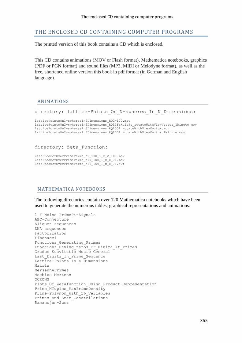
The enclosed CD containing computer programs
355
THE ENCLOSED CD CONTAINING COMPUTER PROGRAMS
The printed version of this book contains a CD which is enclosed.
This CD contains animations (MOV or Flash format), Mathematica notebooks, graphics
(PDF or PGN format) and sound files (MP3, MIDI or Melodyne format), as well as the
free, shortened online version this book in pdf format (in German and English
language).
ANIMATIONS
directory: lattice-Points_On_N-spheres_In_N_Dimensions:
latticePointsOn1-spheresIn2Dimensions_RQ2-100.mov
latticePointsOn2-spheresIn3Dimensions_RQ11Fakultät_rotateWithViewVector_1Minute.mov
latticePointsOn2-spheresIn3Dimensions_RQ1001_rotateWithViewVector.mov
latticePointsOn2-spheresIn3Dimensions_RQ1001_rotateWithViewVector_1Minute.mov
directory: Zeta_Function:
ZetaProductOverPrimeTerms_n2_200_1_x_2_100.mov
ZetaProductOverPrimeTerms_n10_100_1_x_0_71.mov
ZetaProductOverPrimeTerms_n10_100_1_x_0_71.swf
MATHEMATICA NOTEBOOKS
The following directories contain over 120 Mathematica notebooks which have been
used to generate the numerous tables, graphical representations and animations:
1_F_Noise_PrimePi-Signals
ABC-Conjecture
Aliquot sequences
DNA sequences
Factorization
Fibonacci
Functions_Generating_Primes
Functions_Having_Zeros_Or_Minima_At_Primes
Gradus_Suavitatis_Music_General
Last_Digits_In_Prime_Sequence
Lattice-Points_In_4_Dimensions
Matrix
MersennePrimes
Moebius_Mertens
OCRONS
Plots_Of_Zetafunction_Using_Product-Representation
Prime_NTuples_MaxPrimeDensity
Prime-Polynom_With_26_Variables
Primes_And_Star_Constellations
Ramanujan-Sums
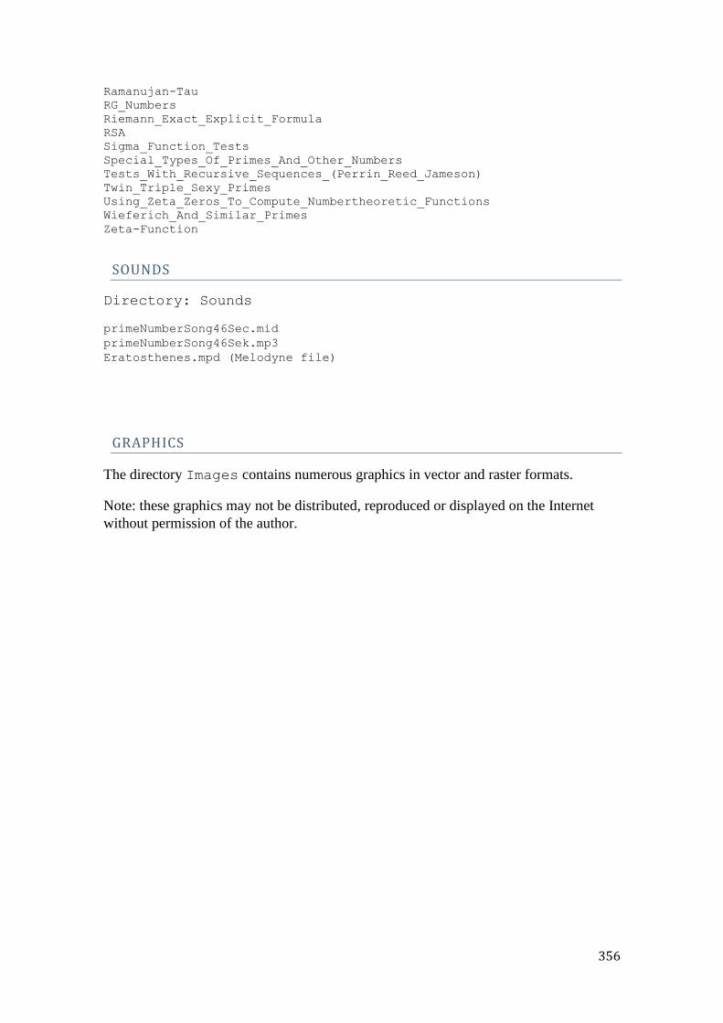
356
Ramanujan-Tau
RG_Numbers
Riemann_Exact_Explicit_Formula
RSA
Sigma_Function_Tests
Special_Types_Of_Primes_And_Other_Numbers
Tests_With_Recursive_Sequences_(Perrin_Reed_Jameson)
Twin_Triple_Sexy_Primes
Using_Zeta_Zeros_To_Compute_Numbertheoretic_Functions
Wieferich_And_Similar_Primes
Zeta-Function
SOUNDS
Directory: Sounds
primeNumberSong46Sec.mid
primeNumberSong46Sek.mp3
Eratosthenes.mpd (Melodyne file)
GRAPHICS
The directory Images contains numerous graphics in vector and raster formats.
Note: these graphics may not be distributed, reproduced or displayed on the Internet
without permission of the author.

Acknowledgements
357
ACKNOWLEDGEMENTS
I would like to thank my wife Michèle, who, in addition to professional activities and
playing piano, found time for the proofreading of this book.
My translator Ewan Whyte did a great job and struggled in addition against the
deficiencies of a common ‘Word’-processing program.
Many thanks to my friend and publisher Eckhard Bodner for the excellent and pleasant
cooperation.
My friend and founder of the company ‘Celemony’, Peter Neubäcker, kindly created the
Melodyne arrangement for the prime number song.
My old school friend Reinhard Schiller pointed out to me an error in the chapter
‘Wieferich primes’.
Many thanks to Peter Danzeglocke, who contributed important insights to the Reed
Jameson sequence.
Christof Born corrected some captions.
Thanks also to the operators of the following Internet web sites from which many
formulae and results in this book were taken:
http://www.mathworld.wolfram.com (Eric Weisstein)
https://www.primes.utm.edu (Chris Caldwell)
https://www.oeis.org (Neil J. A. Sloane)
http://www.trnicely.net (Dr. Thomas R. Nicely)
http://www.Mersenne.org (George Woltman and Scott Kurowski)
http://www.primzahlen.de (Hans-Michael Elvenich)
http://www.seti.org (Bill Diamond)
http://www.aliquot.de (Dr.rer.nat Wolfgang Creyaufmüller)
http://www.mathpages.com (Kevin Brown)
http://www.wikipedia.org
and, of course: http://www.wolfram.com/mathematica
Finally, my thanks go to the many programmers of the Mathematica software, without
which I could not have written this book.
Version: 51