Descaling Petroleum Production Tubing Using Multiple Circular High-

Pressure Nozzles.

Kabir Hassan Yaradua

School of Science, Engineering and Environment

University of Salford, Salford, UK

Submitted in Partial Fulfilment of the Requirement of the Degree of Doctor

of Philosophy, February 2020

ii

List of Contents

List of Contents ........................................................................................................... ii

List of Figures ........................................................................................................... vii

List of Tables ............................................................................................................. xii

Acknowledgements .................................................................................................. xiii

Declaration ............................................................................................................... xiv

List of Publications .................................................................................................... xv

Nomenclature ........................................................................................................... xvi

Abstract ................................................................................................................... xvii

Chapter 1 ..................................................................................................................... 1

Introduction ................................................................................................................. 1

1.1 Preamble ......................................................................................................... 1

1.2 Scales problems in oil production .................................................................. 2

1.3 Scale control ................................................................................................... 3

1.4 Research problem statement ........................................................................... 4

1.5 Research motivations ...................................................................................... 6

1.6 Research contributions ................................................................................... 7

1.7 Research aim ................................................................................................... 7

1.8 Research objectives ........................................................................................ 7

1.9 Structure of the research thesis ....................................................................... 8

1.9.1 Chapter 1: Introduction ......................................................................... 8

1.9.2 Chapter 2: Petroleum production challenges ........................................ 8

1.9.3 Chapter 3: Multiple spray characterization ........................................... 9

1.9.4 Chapter 4: Experimental set up ............................................................. 9

1.9.5 Chapter 5: Results and discussion ....................................................... 10

1.9.6 Chapter 7: Conclusions and recommendations ................................... 10

iii

................................................................................................................... 11

Petroleum Production Challenges ............................................................................. 11

2.1 Overview ....................................................................................................... 11

2.1.1 Petroleum production associated problems ........................................ 11

2.1.2 Flow assurance problems in production tubing .................................. 13

2.2 Kinetics of scale formation ........................................................................... 14

2.2.1 Factors influencing scale formation .................................................... 19

2.2.2 Scale classifications ............................................................................ 20

2.2.3 Scale compositional analysis .............................................................. 22

2.2.4 Scale chemistry ................................................................................... 23

2.3 Scale management ........................................................................................ 38

2.3.1 Scale prediction/monitoring ................................................................ 39

2.3.2 Scale prevention .................................................................................. 40

2.3.3 Economics of scale management ........................................................ 42

2.4 Scale removal techniques ............................................................................. 42

2.4.1 Effective descaling operations ............................................................ 43

2.5 Chemical descaling method .......................................................................... 45

2.5.1 Limitations of chemical descaling approach ....................................... 47

2.5.2 Successful chemical descaling operation around the world ............... 48

2.5.3 Chelating agent .................................................................................... 52

2.5.4 Factors effecting chelating agents ....................................................... 55

2.6 Mechanical descaling technique ................................................................... 56

2.6.1 Types of mechanical descaling techniques ......................................... 57

2.6.2 Successful mechanical descaling operation. ....................................... 61

2.7 Summary ....................................................................................................... 67

................................................................................................................... 68

Jet Spray Dynamics and Mechanism ........................................................................ 68

iv

3.1 Overview ....................................................................................................... 68

3.2 Nozzle performance ...................................................................................... 68

3.2.1 Spray system ....................................................................................... 68

3.2.2 Nozzle characterization ....................................................................... 69

3.2.3 Spray performance summary .............................................................. 73

3.3 Atomization .................................................................................................. 74

3.3.1 Spray jet break up ................................................................................ 74

3.3.2 Spray characterisations /atomizers ...................................................... 78

3.4 Spray analysis ............................................................................................... 85

3.4.1 Drop size ............................................................................................. 86

3.4.2 Drop size distribution (DSD) .............................................................. 86

3.4.3 Spray angle .......................................................................................... 91

3.4.4 Droplet velocity ................................................................................... 92

3.4.5 Spray impact pressure ......................................................................... 92

3.4.6 Spray pattern ....................................................................................... 93

3.5 Spray jet cleaning ......................................................................................... 96

3.5.1 Mechanism for jetting technique ......................................................... 99

3.6 Descaling Operations .................................................................................. 107

3.6.1 Spray overlap..................................................................................... 108

3.6.2 Pressure drop (multiple nozzle) ........................................................ 109

3.7 Summary ..................................................................................................... 109

................................................................................................................. 111

Experimental Set-up and Procedure ........................................................................ 111

4.1 Overview ..................................................................................................... 111

Phase One ................................................................................................................ 113

4.2 Descaling rig design and assembly ............................................................. 113

4.2.1 Descaling rig assembly ..................................................................... 113

v

4.2.2 Descaling chamber design, construction and set up ......................... 116

4.2.3 Descaling Chamber component ........................................................ 117

4.2.4 Scale holder ....................................................................................... 122

4.3 Soft scale production .................................................................................. 124

4.3.1 Wax moulder design ......................................................................... 124

4.3.2 Wax scale preparation ....................................................................... 125

4.4 Scale characterization ................................................................................. 127

4.4.1 Soft Scale compositional & chemical analysis ................................. 127

4.4.2 Hard scale compositional & chemical analysis ................................ 130

4.4.3 Hard scale compositional analysis .................................................... 130

Phase Two ............................................................................................................... 134

Descaling Experiment ............................................................................................. 134

4.5 Scale removal experimental design procedure ........................................... 134

4.5.1 Descaling experiment preparations ................................................... 135

4.5.2 Experimental procedures for scale removal ...................................... 139

4.5.3 Safety precaution measure ................................................................ 144

4.5.4 Source of errors in the scale removal test ......................................... 144

4.5.5 Scale removal error mitigation measures .......................................... 145

4.5.6 Experimental error analysis............................................................... 145

4.6 Summary ..................................................................................................... 147

................................................................................................................. 149

Results and Discussion ............................................................................................ 149

5.1 Overview ..................................................................................................... 149

PHASE 1 ................................................................................................................. 150

Pre-descaling Experiment ....................................................................................... 150

5.2 Scale characterization ................................................................................. 150

5.2.1 Chemical/compositional analysis ...................................................... 150

vi

5.2.2 Soft scale compositional & chemical analysis .................................. 150

5.2.3 Hard Scale compositional & chemical analysis ................................ 153

PHASE TWO .......................................................................................................... 157

Descaling Experiment ............................................................................................. 157

5.3 Scale removal experiment .......................................................................... 157

5.3.1 Ambient decaling experiment ........................................................... 157

5.3.2 Compressed descaling experiments .................................................. 167

5.3.3 Vacuum descaling trials .................................................................... 176

5.3.4 Chamber pressure comparison .......................................................... 186

5.3.5 Optimum descaling requirement ....................................................... 195

5.3.6 Summary ........................................................................................... 206

................................................................................................................. 207

Conclusion and Recommendations ......................................................................... 207

6.1 Conclusions ................................................................................................. 207

6.2 Recommendations....................................................................................... 209

Reference ................................................................................................................. 210

Appendices .............................................................................................................. 217

Appendix A ............................................................................................................. 217

APPENDIX B.......................................................................................................... 225

APPENDIX C.......................................................................................................... 226

APPENDIX D ......................................................................................................... 239

APPENDIX E .......................................................................................................... 242

vii

List of Figures

Figure 2.1: Scale deposit (a) in production tubing, (b) schematics of scale inflicted

production tubing by (Slumberger, 2013) ................................................................. 14

Figure 2.2: Calcium carbonate deposit (a) in production tubing, (b) SEM image

(Okocha et al 2014) ................................................................................................... 25

Figure 2.3: Effect of temperature to different types of calcium Carbonate (Guan H.

et al 2015) .................................................................................................................. 25

Figure 2.4: Calcium sulphate deposit (a) in production tubing, (b) SEM images (Esbai

et al., 2016) ................................................................................................................ 27

Figure 2.5: Effect of Temperature on solubility of CaSO4 (Johnson et al. 1999) ... 28

Figure 2.6: Barium Sulphide deposit (a) in production tubing, (b) SEM images

(Meeham, 2010) ........................................................................................................ 28

Figure 2.7: Effect of Temperature on solubility of Barium Sulphate (Meehan 2010).

................................................................................................................................... 29

Figure 2.8: Strontium sulphide deposit (a) in production tubing, (b) SEM Images (Al

Mubarak et al, 2017) ................................................................................................. 30

Figure 2.9: Iron sulphide deposit (a) in production tubing, (b)SEM Images

(Mahmoud et al., 2015) ............................................................................................. 32

Figure 2.10: Scale deposit composition in X Sour Gas (a),(b) stability of various iron

Sulphide in respect to pH (Al-Bauli et al. 2015) ....................................................... 34

Figure 2.11: Chemical structures of common aminopolycarboxylic acids

(Almubarak et al., 2017) ........................................................................................... 55

Figure 3.1 Specific gravity versus conversion factor graph (Spraying system 2015)

................................................................................................................................... 70

Figure 3.2: Spray angle Vs spray coverage (BETE 2018) ....................................... 71

Figure 3.3: Atomization (droplet size and distribution) (Spraying system 2015) ... 72

Figure 3.4: Sheet disintegration breaks up proposed by (Dombrowski et al. 1962) 74

Figure 3.5: Forces acting along spray jet (Rajendran et al. 2012). .......................... 75

Figure 3.6: Break-up length behaviour of liquid jet (Arai et al., 1995) ................... 76

Figure 3.7: Liquid atomisation mechanisms (Liu H 2000) ...................................... 76

Figure 3.8: Classification of atomisers (Yule &Dunkley 1994 ; Abuhesa M . 2010).

................................................................................................................................... 79

viii

Figure 3.9: spill returns atomiser (BETE 2018) ....................................................... 81

Figure 3.10: Hollow Cone Atomiser spray (BETE, 2014) ...................................... 82

Figure 3.11: Full cone Atomiser spray (BETE 2018) .............................................. 83

Figure 3.12: Flat Spray Pattern atomiser (BET 2014) ............................................. 84

Figure 3.13: Flat Spray Atomiser ............................................................................. 85

Figure 3.14: Typical drop size distribution (Nasr et al. 2002) ................................. 87

Figure 3.15: Drop size bars based on number and volume (Lefbvre 1989) ............ 87

Figure 3.16: Usual drop size frequency distribution curves (number and volume) 88

Figure 3.17: Usual shape of cumulative drop size ................................................... 88

Figure 3.18: Particle distribution median, mode and mean (Malvern instrument

limited 2015) ............................................................................................................. 89

Figure 3.19: Relative drop sizes by nozzle series (Spraying System 2017) ............ 91

Figure 3.20: Spray angle (Naber et al 1996) ............................................................ 91

Figure 3.21: Spray impact pressure (Naber et al 1996) ........................................... 92

Figure 3.22: Scale deposit in a production tubing ................................................... 96

Figure 3.23: Schlumberger Jetting Technique (Schlumberger 2013) ....................... 97

Figure 3.24: Classification of cavitation (Lauterborn 1980) ................................. 103

Figure 3.25: Cavitation regimes along Francis turbine (Brennen., 1995) ............. 103

Figure 3.26: Light emitted by a trapped cavitation bubble (Zhang Y 2013) ......... 104

Figure 3.27: Electro optic shock created by laser plasma (D.F Gardon 2008) ...... 104

Figure 3.28: particle cavitation (DFD 2015) .......................................................... 105

Figure 3.29: Typical flows through a nozzle (Martynov et al. 2006) .................... 106

Figure 3.30 : Arrangement of nozzles on descaling header (spray overlap) (Nasr et al

2002) ........................................................................................................................ 108

Figure 3.31: Nozzle pressure difference Vs flow rates of different numbers of nozzles

(Tian, Li, Huang, Niu, & Xia, 2009) ....................................................................... 109

Figure 4.1: Descaling rig components, (a) Compressed air system, (b) Vacuum pump

& (c) high pressure water pump .............................................................................. 113

ix

Figure 4.2: Picture of the assembled control board ............................................... 114

Figure 4.3: Descaling rig set-up ............................................................................. 115

Figure 4.4: Design of the chamber ......................................................................... 116

Figure 4.5: Interior section ..................................................................................... 116

Figure 4.6: metal plate (a) 3D image and (b) picture with O ring seal .................. 117

Figure 4.7: (a) Top plate (outside view) (b) Bottom plate (inside view) and (c)

Assembled views of metallic top cover .................................................................. 118

Figure 4.8: Scale sample assembly (without chamber tube) ................................. 118

Figure 4.9: Multiple nozzle header, (a) picture, (b) operational cross-section ...... 121

Figure 4.10: High-pressure nozzle, (a) picture, (b) operational cross-section ....... 121

Figure 4.11: Assemble nozzle header, (a) Arial & (b)side view ............................ 121

Figure 4.12: Scale holder (a) & (b) component and (c) assembly ......................... 122

Figure 4.13: Complete assembled descaling rig. ................................................... 123

Figure 4.14: 3D Pictures of wax moulder (a) component and (b) assembled ........ 124

Figure 4.15: Prepared wax scale samples preparation and after cooling ............... 126

Figure 4.16: Constructed soft scale (a) hollow shape, (b) solid shaped samples .. 127

Figure 4.17: Thermo Scientific Nicolet iS10 Fourier-transform infrared spectroscopy

(a) ATR sample drop window (b) complete FTIR system ..................................... 129

Figure 4.18: Hard Scale samples (a) CaCO3, (b) SrSO4 ........................................ 130

Figure 4.19: Experimental design process ............................................................. 134

Figure 4.20: Scale deposits .................................................................................... 136

Figure 4.21: Stand-off distance arrangement ......................................................... 137

Figure 4.22: Header and nozzles configurations .................................................... 138

Figure 5.1: NMR result of soft scale sample ......................................................... 151

Figure 5.2: Infrared analysis compared to paraffin flakes from NIST data base .. 152

Figure 5.3: Infrared analysis compared to liquid paraffin ..................................... 152

Figure 5.4: SEM Results of Sample A at (a) 1 mn, (b) 40 µm and (c) 100 µm

magnifications ......................................................................................................... 153

x

Figure 5.5: SEM Results of Sample B at (a) 1 mn, (b) 30 µm, (c) 40 µm and (d) 100

µm, magnifications .................................................................................................. 153

Figure 5.6: EDX Result Sample A at (a) 0.1, (b) 0.2 spectrums ........................... 154

Figure 5.7: EDX Result for Sample B at (a) 0.1 (b) 0.2, (c) 0.3 spectrums .......... 155

Figure 5.8: XRD result Sample A .......................................................................... 156

Figure 5.9: XRD results sample B ........................................................................ 156

Figure 5.10: Ambient descaling results for hollow soft scale at 25mm-distance .. 160

Figure 5.11: Ambient descaling results for solid soft scale at 25mm-distance .... 162

Figure 5.12: Ambient descaling results for SrSO4 scale deposit at 25mm-distance

................................................................................................................................. 164

Figure 5.13: Ambient descaling results for CaCO3 scale deposit at 25mm-distance

................................................................................................................................. 166

Figure 5.14: Compressed descaling results for hollow soft scale at 25mm-distance

................................................................................................................................. 169

Figure 5.15: Compressed descaling results for hollow soft scale at 25mm-distance

................................................................................................................................. 171

Figure 5.16: Compressed descaling results for SrSO4 scale deposit at 25mm-distance

................................................................................................................................. 173

Figure 5.17: Compressed descaling results for CaCO3 scale at deposit 25mm-distance

................................................................................................................................. 175

Figure 5.18: Vacuumed descaling results for hollow soft scale at 25mm-distance

................................................................................................................................. 178

Figure 5.19: Vacuumed descaling results for solid soft scale at 25mm-distance .. 181

Figure 5.20: Vacuumed descaling results SrSO4 scale deposit at 25mm-distance 183

Figure 5.21: Vacuumed descaling results for CaCO3 scale deposits at 25mm-distance

................................................................................................................................. 185

Figure 5.22: Chamber pressure impact comprising for descaling hollow soft scale at

25mm-distance ........................................................................................................ 188

Figure 5.23: Chamber pressure impact comprising for descaling solid soft scale at

25mm-distance ........................................................................................................ 190

Figure 5.24: Chamber pressure impact comprising for descaling SrSO4 scale deposit

at 25mm-distance .................................................................................................... 192

xi

Figure 5.25: Chamber pressure impact comprising for descaling CaCO3 scale deposit

at 25mm-distance .................................................................................................... 194

Figure 5.26: Descaling impact of non-hydro-connected parameters for respective

deposits .................................................................................................................... 198

Figure 5.27: Descaling impact of hydro-connected parameters for respective deposits

................................................................................................................................. 201

Figure 5.28: Descaling impact of chamber pressure and its efficiency for respective

deposits .................................................................................................................... 204

xii

List of Tables

Table 2.1: Summary of Scale chemistry .................................................................. 35

Table 2.2: Pre and post descaling results of the six wells (Ramones et al., 2015) .. 50

Table 2.3: Pre and Post Descaling results of Kuff well(Mirza et al., 1999) ............ 51

Table 2.4: Pre and Post Descaling Results for five Kuff Gas wells (Bolarinwa et al.,

2012) .......................................................................................................................... 63

Table 2.5: Pre-and post-descaling result of field (EW 873) Golf of Mexico (Clameto

et al. 2003) ................................................................................................................. 65

Table 2.6: Post descaling and simulation result of Ghwar field (Alabdulmohsin et al.,

2016) .......................................................................................................................... 66

Table 3.1 : Spray Performance Summary ................................................................ 73

Table 3.2: Mean diameters across and their applications (Nasr et al. 2002) ........... 89

Table 4.1: Error analysis of 3 nozzles ambient descaling results .......................... 146

Table 4.2: Error analysis of 3 nozzles compressed descaling results .................... 146

Table 4.3: Error analysis of 3 nozzles vacuumed descaling results ....................... 147

Table 5.1: Multiple High-Pressure Circular Nozzle Descaling Operations Guide 205

xiii

Acknowledgements

I would like to use this medium to express my deep gratitude to Almighty Allah for the gift of

life, faith, strength and health. To my parent (Hafsat & Kabir Yaradua) for their everlasting and

unconditional support including Mr Bello Yusuf and my subliming’s Mohammed, Bello, Umar,

Fatima, Hafsat, Aisha and Zainab Kabir. Also, to my lovely wife and child (Zainab-Abu & Bello-

Ammar) that contributed physically and spiritually tremendously toward realising this dream. It

will not be possible to finish this program without the support of my very best friend and

Supervisor Dr. Abuabakar Abbas who have been there for me for long and my Co-supervisor Dr

Amir Nuorian for his eminent support. So also, our wonderful research team of Prof G.G Nasir,

Dr Godpower Enyi, Dr Martins Bubby, Dr. Babbaie Mesiam, and Mr Mapins Alans for bringing

out the best out of me. Most importantly to Petroleum Technology Development Fund (PTDF)

and their staffs especially Mr Ahmed Galadima and Mr Bako for sponsoring this PhD program.

I wish to express my heartfelt gratitude to my friends and colleagues, most especially Engr.

Ahmadu Abdullahi, Engr Salihu Maiwalimah, Dr. Mohammed Abba, Engr Shehu Ushau, Mr

Chalasani Kiran, Dr Aminu Abba and Yusuf Bashir for their marvellous contribution toward

putting this Thesis together. To my MSC research members like Engr Joyce, Jose, John and Hamid

for their patience and contributions during the experiment hard times. In addition to, Dr Umar

Ilyas, Mr Farooq Bello, Mr Hamis Bichi, Mubarak Aliyu, Abdullatif Yusuf, Farooq Idris,

Abubakar Ibrahim and Sadiq Abdallah for their calls and prayers that made me feel at home

despite the geographical distance between us during the duration of this programme. Last but not

the list is all those that were there for me knowingly and unknowingly for their encouragement

and guidance throughout the period of this research and during the preparation of this thesis.

xiv

Declaration

I, Kabir Hassan Yaradua, declare that this dissertation report is my original work, and has not been

submitted elsewhere for any award. Any section, part or phrasing that has been used or copied from

other literature or documents copied has been clearly referenced at the point of use as well as in the

reference section of the thesis work.

…………………

……………….

Signature Date

…………………….. ……………………..

Approved by

Dr. Abubakar Abbas (Supervisor)

…………………

……………….

Signature Date

…………………….. ……………………..

Approved by

Dr. Amir Nourian

(CO-Supervisor)

xv

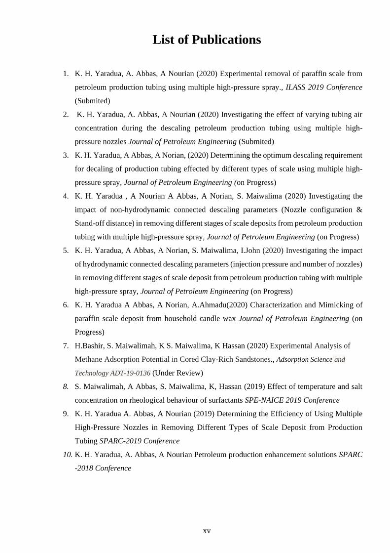
List of Publications

1. K. H. Yaradua, A. Abbas, A Nourian (2020) Experimental removal of paraffin scale from

petroleum production tubing using multiple high-pressure spray., ILASS 2019 Conference

(Submited)

2. K. H. Yaradua, A. Abbas, A Nourian (2020) Investigating the effect of varying tubing air

concentration during the descaling petroleum production tubing using multiple high-

pressure nozzles Journal of Petroleum Engineering (Submited)

3. K. H. Yaradua, A Abbas, A Norian, (2020) Determining the optimum descaling requirement

for decaling of production tubing effected by different types of scale using multiple high-

pressure spray, Journal of Petroleum Engineering (on Progress)

4. K. H. Yaradua , A Nourian A Abbas, A Norian, S. Maiwalima (2020) Investigating the

impact of non-hydrodynamic connected descaling parameters (Nozzle configuration &

Stand-off distance) in removing different stages of scale deposits from petroleum production

tubing with multiple high-pressure spray, Journal of Petroleum Engineering (on Progress)

5. K. H. Yaradua, A Abbas, A Norian, S. Maiwalima, I.John (2020) Investigating the impact

of hydrodynamic connected descaling parameters (injection pressure and number of nozzles)

in removing different stages of scale deposit from petroleum production tubing with multiple

high-pressure spray, Journal of Petroleum Engineering (on Progress)

6. K. H. Yaradua A Abbas, A Norian, A.Ahmadu(2020) Characterization and Mimicking of

paraffin scale deposit from household candle wax Journal of Petroleum Engineering (on

Progress)

7. H.Bashir, S. Maiwalimah, K S. Maiwalima, K Hassan (2020) Experimental Analysis of

Methane Adsorption Potential in Cored Clay-Rich Sandstones., Adsorption Science and

Technology ADT-19-0136 (Under Review)

8. S. Maiwalimah, A Abbas, S. Maiwalima, K, Hassan (2019) Effect of temperature and salt

concentration on rheological behaviour of surfactants SPE-NAICE 2019 Conference

9. K. H. Yaradua A. Abbas, A Nourian (2019) Determining the Efficiency of Using Multiple

High-Pressure Nozzles in Removing Different Types of Scale Deposit from Production

Tubing SPARC-2019 Conference

10. K. H. Yaradua, A. Abbas, A Nourian Petroleum production enhancement solutions SPARC

-2018 Conference

xvi

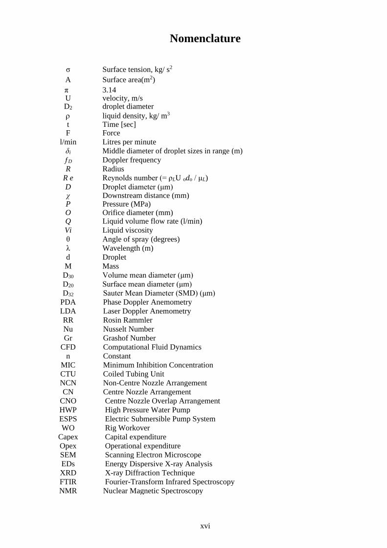
Nomenclature

σ Surface tension, kg/ s2

A Surface area(m2)

π 3.14 U velocity, m/s D2 droplet diameter

liquid density, kg/ m3

t Time [sec] F Force

l/min Litres per minute

δi Middle diameter of droplet sizes in range (m)

ƒD Doppler frequency

R Radius

R e Reynolds number (= ρLU odo / μL)

D Droplet diameter (μm) χ Downstream distance (mm) P Pressure (MPa) O Orifice diameter (mm) Q Liquid volume flow rate (l/min)

Vi Liquid viscosity

θ Angle of spray (degrees)

λ Wavelength (m)

d Droplet

M Mass

D30 Volume mean diameter (μm)

D20 Surface mean diameter (μm)

D32 Sauter Mean Diameter (SMD) (μm)

PDA Phase Doppler Anemometry

LDA Laser Doppler Anemometry

RR Rosin Rammler

Nu Nusselt Number

Gr Grashof Number

CFD Computational Fluid Dynamics

n Constant

MIC Minimum Inhibition Concentration

CTU Coiled Tubing Unit

NCN Non-Centre Nozzle Arrangement

CN Centre Nozzle Arrangement

CNO Centre Nozzle Overlap Arrangement

HWP High Pressure Water Pump

ESPS Electric Submersible Pump System

WO Rig Workover

Capex Capital expenditure

Opex Operational expenditure

SEM Scanning Electron Microscope

EDs Energy Dispersive X-ray Analysis

XRD X-ray Diffraction Technique

FTIR Fourier-Transform Infrared Spectroscopy

NMR Nuclear Magnetic Spectroscopy

xvii

Abstract

The mechanical approach of utilizing high-pressure water for scale removal has gained wider

acceptance by multinational despite facing poor downhole performance challenges (cavitation) that

need abrasion compensation (sand). Although sand particles have side effect of jeopardize the

integrity of the well completion. Replacement of sand with stealing beads was excellent with good

post descaling well completion integrity at the expense of environmental complexity. While the

recent single nozzle, solid free aerated jetting descaling technique was characterised with poor scale

coverage and high descaling time.

This novel experimental scale removal technique utilises multiple high-pressure spray of up

to10MPa and low flow rate of 12 l/m from multiple flat fan nozzles of different arrangement and

stand-off distance. Housed in a constructed simulated production tubing chamber with vacuum and

compression capacities to remove hard scale deposits of SrSO4 and CaCO3. In addition to the

constructed wax deposit (paraffin) of different shapes signifying different growth stages of paraffin

in production tubing.

Generally, the performance of each or combination of the descaling parameters during the

experiment depends on the shape and type of the scale deposit in question, most especially the

chamber air concertation and nozzles arrangements. Also, the amount removed of all the respective

scale deposit was found to increase with increase in injection pressure and reduction in number of

nozzles. Likewise, the effect of stand-off distance toward the erosion rate of all the four respective

descaling candidates was found to reduce with increase in downhole jetting position from 25mm to

50mm and 75mm, even though could be compensated with the right choice of nozzles arrangement.

Injecting at 10 MPa with 5nozzles combination at ambient air concentration removed 49g, 32g, 3.2g

& 1.8g of paraffin of hollow & solid shape, SrSO4 & CaCO3 deposits respectively, that cumulatively

increases by a factor 1.6 after altering the nozzle configuration to 4nozzles. Subsequently reducing

the numbers of nozzles to 3nozzles further increase the initial cumulative removal by a factor of 4.3

across the respective deposits at 25mm stand-off distance. Also utilising 3nozzles configuration at

ambient chamber pressure removed 43g, 5.2g, 2g, & 1.7g of the respective deposits at 4.8 MPa

injection pressure that cumulatively increased by a factor of 2 after throttling further to 6.0 MPa

injection pressure. Further increasing the injection pressure to 10 MPa cumulatively increase the

initial removal of the respective deposits by a factor of 7.2.

While nozzle configuration (header arrangement) that depends on the size and shape of the sample,

was found to remove 7% & 13% with CN arrangement more than CN and CNO configuration when

descaling hollow shape scale at the best of other parameters in ambient condition. Whereas

removing of solid, SrSO4 and CaCO3 deposit respectively, the CN arrangement removed 6%, 4%

& 0.1%, more than the CNO arrangement and 0.08% & 0.1%, 0.02% more than NCN arrangement

under the same descaling conditions.

Varying the tubing air concentration from ambient to compressed and later vacuum was found to

have direct impact on the resultant spray impact and aids erosion and hoops stress for the first

condition. In addition to cyclin stress & abrasion for the second and cavitation jetting mechanism

for the last air concentration. Likewise, 254g, 104g, 6.5g & 4.4g of the respective deposits was

removed at ambient chamber pressure at optimised descaling parameters that as a result of

introducing 0.2 MPa compressed air into the chamber increases by a factor of 1.5. Impressively, a

better cumulative removal factor of 1.7 across all the respective deposits was archived after suction

the chamber by -0.08 MPa.

Prior to the descaling experiment some descaling preparational experiment of chemical and

compositional analysis of the hard scale samples were conducted through the combination SEM,

EDX and XRD and found to be CaCO3 & SrSO4 deposit respectively. While the constructed soft

scale sample were confirmed to be paraffin through NMR & FITR analysis.

1

Chapter 1

Introduction

1.1 Preamble

Flow assurance is one of the most vital economic features of crude production. Define as the ability to

economically produce petroleum product up to the top surface production /processing facility from the

reservoir during the lifetime of an oil field (Jordan, Sjuraether, Colllns, Feasey, & Emmons, 2001), with

scale control as its integral pillar. Up to date, scale deposit in production tubing’s remain the most

troublesome flow assurance problem throughout the production life of a well. Scale deposition hinder

flow assurance not only by dramatically declining oil production rate but by limiting well accessibility

for well integrity and performance programs (Alabdulmohsin, El-zefzafy, Al-malki, Al-mulhim, & Ali,

2016). All well flow channels from reservoir, wellbore & near-well bore, downhole & downhole

equipment, production tubular, wellhead to topside production. Including processing facilities (e.g.

pump, separators, heat exchangers, etc.) are prone to scale deposit when in contact with water during

water production from the field (Guan, 2015). These posess a stargedic challenges to to acheiveing

global energy security.

Among the few to mention of noticeable oilfield around the world that have recorded scale problems

are: Kuff Gas well in Bahrain that exhibit scale deposit problem 7,000 inch from the tubing lower section

and production casing down to the perforation intervals. Limiting its flow assurance by reducing

wellbore accessibility and well deliverability (Mirza, Prasad, & Company, 1999). In addition to surface

production/processing facilities suffering erosion damages from produce scale particle encountered due

to the scale problems. Another case can be that of Fadhili wells with an average daily gross production

rate of 1500 BOPD and over 90% water cut, which was halved by production within four month (Esbai

et al., 2016). This was due to calcium carbonate scale deposited along the tubing and other flow line,

approximately a 20 to 30 BOPD drop per well. Operator data from North Sea shows almost 75% had

been plugged by scale and/or fines combination (Jordan et al. 2001) . The results of the plugging

frequency of the Statoil data is 0.02 in per well-year suggested relationship between failure due to (scale

and/or fines) plugging and the number of well-years, to be mostly caused by scale problems.

Scale cases can be instantaneous such as that of North Sea Miller field, were a 30,000 barrels of oil per

day (BOPD) production capacity well was halted to zero production capacity due to scale growth with

24 hours (Brown 1998). Likewise, scale problem has been proven to be one of the reasons Statjord Oil

field in North Sea operated by Statoil oil has fallen below the production decline curve, with 60% of its

stock tank original oil in place (STOOIP) recovered via secondary recovery techniques for the past 23

2

year (Børeng, Skinnemoen, Vigen, Vikane, Andrews, Asa, & Hauptmann 2002). Consequently, leaving

composite distributions of circumvented oil reserves, water and gas.

1.2 Scales problems in oil production

Petroleum reservoir formation are made up of different type of salt originating from different source

with different fluid constituent naturally forming together with oil and gas in same reservoir environs.

Though difficult to quarantine but can rather be identify and mitigated. Effects like nucleation in

reservoir downhole completion equipment, production tubing, casing and surface production/processing

equipment can be mitigated.

This unfortunate petroleum problem affecting large oil fields in North Sea, Canada, Saudi Arabia and

the rest. Threatened flow assurance by creating high pressure drop along the tubing due to reduction in

tubing flow cross section area that can instantaneously reduce or even halt production to zero if care is

not taken.

However, among the available oil recovery techniques (water injection) found to be effective in agitating

reservoir suffering from production decline but related to side effect of water incompatibility problems.

Usually when injection water (sea water is rich in carbonate and sulphate ions) mix with produce water

(rich in barium, magnesium, calcium etc. depending on type of formation). This leads to the precipitation

of various type of scales such as BaSO4, MgSO4, CaSO4, etc. Although many scholars such as (Ahmad,

2006) believe to some extent during water injection scale formation can simply be due to reaction of

fresh water, formation and the mineral in the rock creating mineral deposit in produce water.

Predominant scales in oil field are formed either through precipitation of natural water from reservoir

rock or oversaturated produce water (with scale component), due to mixture of incompatible water

downhole. Its more problematic in the case of sea water injection breakthrough with Barium, or

Strontium Sulphate both highly insoluble (Gholinezhad, 2006).

Among the most serious oil field problems today is scale deposition, a product of two incompatible water

usually formed during water injection operations (Merdhah & Yassin, 2009). Also Change in pressure,

partial pressure, temperature, pH, C02, H2S can be major drivers of scale formation. For instance, the

change in temperature and pressure of water flowing from one point to another can aid the production

of sulphate scale (Jordan & Mackay, 2015), which is mostly formed due to incompatible mixture of

injected water (rich in sulphate ions) and formation water (high in concentration of calcium, barium and

strontium ions). Same process can lead to formation of calcium carbonate precipitation which together

with calcium sulphate are problematic type of scale creating operational issue such as tubing, open hole

section and flow line blockage (Alabdulmohsin et al., 2016). The formation of the earlier mention type

3

of hard scale dramatically reduce porosity, permeability, production rate, case is worsen when deposited

on pay zone (Farrokhrouz & Asef, 2010). Hence, it can now be clear that scale problems are mostly

associated with the later life of a well.

1.3 Scale control

The quest for continues improvement in scale management strategies and control cannot be

overemphasis keeping in mind the threat scale formation is posing on global energy security. Since the

discovery of scale formation problems different techniques, tools and technology have been developed

to manage scale problem from prevention to removal stage, through the entire production system both

on and offshore. Though the prevention techniques (prediction ,monitoring and mitigating the risk of

scale formation) in the capital expenditure (CAPEX) phase of the field life, is always better than

confrontational measure of cure (scale removal techniques/solution) at the operating expenditure

(OPEX) phase (Jordan et al., 2001) as has since been emphisise by many scholars.

A tremendous cost savings can be achieved if the current scale control/management techniques have

been in place during the CAPEX phase. For example, the utilisation of gas lift to aid well clean-up will

reduce cost of coiled tubing operations and production decline. Scale cause by water cut rise can be

avoided through scale squeeze treatment before water breakthrough (Jordan et al., 2001). Another

technique can be the commencement of reservoir treatment prior to production to arrest any scale

formation tendency near the wellbore by deployment of solids and fluid system inhibitors. So also, the

utilizing continuous injections such as gas lift and capillary to control downhole scale and subsequently

squeeze treatment within the production circle and water cut rise of a producing well.

Despite the evolution of tools and techniques in the field of scale management, no single tool/technique

has proven to be universally applicable to all scale type, formations or oil wells, leaving the tools

selection to be determine by their pros and cons, before the development of recent technique

(Gholinezhad, 2006). Therefore, the fact as mention by (Alabdulmohsin et al., 2016) is choosing a scale

removal techniques for each well is govern by knowledge of the type, quantity, texture, composition

and location of the scale to be removed.

Even though the cost of scale removal can be high, but differing treatment might cost higher

(Gholinezhad, 2006). Hence, scale control remains centre for attraction for flow assurance. Its clear that

the rate of increase in production index and revenue generation will always outweigth the cost of scale

control (Alashhab et al., 2006). Considering some succefull after desescaling senerios discussed below.

In the case of Duri field in Indonesia an increase in revenue by $3.6MM in 90 days within 18 days

payback period was achieved after successful CaCO3 scale removal (Schlumberger, 2013). A Scale

4

inflicted oil well in Ghawar field, the world largest most prolific was return to full well accessibility

status. A 30% increase in production and more than $1 MM of cost saving after a successful descaling

operation (Alabdulmohsin et al., 2016). Similarly, Statjord Oil field in North Sea operated by Statoil oil

despite fallen below the production decline curve with history of recovering 60% of its STOOIP via

secondary recovery techniques for the past 23 year (Børeng et al., 2002). Return to stream with

approximately 700-1000 sm3/d of oil after performing a successful scale removing job.

A new descaling solution has been found promising by systematically descaling both type of scales

deposits on electric submersible pump system (ESPS) resulting in eradication of rigs work over (WO)

requirement as reported by (Ramones, Rachid, Flor, Gutierrez, & Milne, 2015). Increasing their average

run life from 40 to 140 days, 6 day per well average rig cost saving and $1.5 MM average savings in

delayed production. Likewise post-descaling and simulation nodal analysis results to asses post

descaling performance of a carbonate (sour) gas reservoir well in Saudi Arabia shows a significantly

increase from 6 MMSCFD well flow at buttonhole pressure of 3,715 psi to 10.2 MSCFD well flow at

3,825 psi bottom hole pressure (Mukhliss et al., 2014). Matching a 0.27 md permeability and (-5) skin

effect improvement corresponding to almost 80% improvement and a better AOF. Proven to have

effectively remove the damage and the reservoir is responding

1.4 Research problem statement

Proper planning by integrating scale control into asset life cycle management of a well in CAPEX phase

such as good water injection strategies or incorporating the appropriate technology during well

completion. Instead of confronting scaling problems during OPEX Phase (development/production

stage) will be more effective and economical (Jordan et al., 2001). While in the case of discovered scale

problem during OPEX phases of a well due to failed, poor preventive measures or expiration of

inhibition life, scale removal remains the only solution. Usually chemical or mechanical techniques or

even combination of the two are used for effectively removal of the scale in order to regain the flow

assurance of a well. The core principles of a successful scale removal approach depend on regaining

well accessibility and increasing production rate of the well. In an economic (cost of scale removal to

revenue generation after descaling operation), efficient (descaling time), simple (non -complex with few

steps), safe (safety of rig personnel), integrity (well completion equipment conditions) environment

friendly (environment of well and vicinity) approach. Although, seem difficult to achieved since

inception/revolution of scale removal techniques/tools.

The application of high-water jet in numerous industrial applications has been on record for a long time

for demolition, cutting different materials. Most importantly used for scale cleaning in oil and gas

5

production tubing invaded by organic or inorganic scales like paraffin, asphalting, calcium and

magnesium compound respectively. Especially the later among listed that prove to be difficult to remove

through chemical method (Aslam et al., 2000). Makes mechanical approach as the best removal option

Even though jetting technique under mechanical descaling method have recently gained wider

acceptance by multinational companies (Bajammal et al., 2013) like Saudi Aramco, Shell, Slumberger

and the rest. Despite, suffering serious setback due to its ability to only effective clean scale at ambient

condition, while backward pressure reduce it cleaning ability as it moves downhole (Crabtree & Johnson,

1996) which is attributed to cavitation effect.

Cavitation can be defined, as phenomenon where due to decrease in pressure across the jetting atomizer

cavities are form in the liquid jet (void or bubbles). Resulting from liquid change in phase to vapour or

equal to vapour pressure of water. Cavitation effect in solid free jetting led to the introduction of abrasive

(sand particles) to compensate low jetting performance downhole which end up jeopardising the integrity

of well completion. Posing a lot of threat to the integrity of the tubing itself, other well completion and

top surface facilities in addition to the environment.

Replacement of sand particles with sterling beads proves to be effective at the expense of environmental

complexity. Sterling beads side effect are not just limited to tubing damage but the complicated delivery

pump requirement for pumping the high-density suspension (liquid and solid). The slurry may end up

been deposited on the tubing or other bottom-hole completion equipment (Mahmoud, Kamal, & Geri,

2015) leading serious operation problems

Just as cavitation negative effect toward reduction in performance of high-water jet down hole prompts

multinationals to introduce sterling bead (liquid and solid). The environmental and well integrity

negative effect of using sterling bead motivated the introduction solid free jetting descaling technique

research. A pure water jetting approach that will not be affected by cavitation effect, combining both

erosion and stress cycling mechanism, by utilizing aerated chamber with incorporated single high

pressure flat fan nozzles (Abbas, 2014) .The noble research was not only able to increase solid free

jetting performance down the production tubing, but answer question related to cavitation such as

cavitation suppression distance (stand of distance), relationship between aeration and suppression of

cavitation. In addition to the relationship between air concentration in the aerated chamber and cavitation

bubble length.

Despite the tremendous achievement made by the single high pressure aerated flat fan nozzle technique

some identified research gap, and room for improvement will not be neglected (Abbas, 2014) .

Notwithstanding, the calls for improvement by many researchers and quest of developing an effective

scale removal technique by the multinational companies. The spray research group decided to extend

6

the single nozzle research by introducing a state-of-the-art technique that will include the use of multiple

high-pressure nozzles in a compressed and/or vacuum chamber this time.

The multiple high-pressure nozzle will utilize at least two of the four jetting mechanism at the same

time. Either by firstly compressing (pressuring the chamber and suppressing cavitation to archive

erosion, cyclin stress and likely abrasion mechanism). Secondly, suctioning (extending cavies by

vacuuming the chamber to achieve erosion, cavitation and abrasion jetting mechanism). Regardless of

the high achievement in scale removal recorded by the single nozzle research, the following research

problem remained un-answered.

• High rig time (descaling time) required when using single nozzles

• In adequate scale circumference coverage by using single nozzle leading to non-uniform

scale destruction that can lead to tubing blockage

• Utilizing and extending cavities flare (cavitation) instead of suppression might lead to better

well cleaning downhole since erosion, cyclin stress and abrasion effect might be archive

• Aeration effect on real oil and gas well in respect to environment, rig personnel and the

integrity of well completions

• Ambiguous cost implication of the techniques

1.5 Research motivations

Combining the above listed un-answered question from the existing aerated single high-pressure flat fan

techniques. Couple with the expected challenges from the proposed multiple high-pressure nozzles with

option of compression or cavitation. This research may likely have to answer the following question too.

• Pumping requirement needed to effectively operate multiple high-pressure atomizers

• The challenge of generating uniform descaling impact across the scale circumference due to

spray overlap region

• Rate of compression required to supress cavitation product from multiple nozzles

• Optimization of number of nozzles in order to reduce high risk of tubing overflow

• Selection of number of nozzles, type (same or combination of different type of atomizers to

couple into multiple nozzle header) for effective descaling operations

7

1.6 Research contributions

• Develop an operational guide for the selection of optimum descaling parameter/techniques

required for effective removal of different types of scales from petroleum production tubing

using multiple high-pressure nozzles.

1.7 Research aim

• Enhancing the rate of scale removal in petroleum production tubing using multiple high-pressure

nozzles header in different air conditions

1.8 Research objectives

The prime objectives of this work are the hydrodynamic characterisation of multiple high-pressure

nozzles to remove scale from production tubing with the following goals in mind.

i. To design, construct & assemble the upgraded descaling rig including the descaling chamber

(ambient, compressed and vacuumed condition), in simulation of ideal descaling conditions

ii. To design/fabricate a wax scale moulder and utilizing it in producing soft scale samples candidate

of different sizes and shape that can simulate different scale growth stages in production tubing.

iii. To characterize both scale samples, through chemical and compositionally analysing the hard

scale candidate using the combination of scanning electron microscope (SEM), energy dispersive

X-ray analysis (EDX) and X-ray diffraction (XRD) technique. In addition to nuclear magnetic

resonance (NMR) spectroscopy and Fourier-transform infrared spectroscopy (FTIR) techniques

for the constructed soft scale sample.

iv. To study the effect of descaling parameters, such as chamber air concentration, numbers of

nozzles and injection pressures, standoff distance and header arrangement towards the rate of

scale removal for different scale samples in different chamber pressure.

v. To investigate the impact of air water concentration in descaling chamber to the rate of scale

removal when using multiple HP nozzles at different chamber pressure (ambient, compressed

and vacuum) and different descaling parameters.

vi. To determine the optimal descaling requirement for the effective scale removal of different types

scale deposit in petroleum production tubing.

8

1.9 Structure of the research thesis

This thesis is structured in form of chapters, and each chapter to contain and explain relative acquired

knowledge and activities that took place during the research work.

1.9.1 Chapter 1: Introduction

This chapter introduce the concept of scale problem in flow assurance before narrowing the issue to

production tubing with example of recorded cases around the world. Followed by the brief chemistry of

scale formations coupled with life examples of scale inflicted oil well across the globe. Then scale

control and its economics with real life scenario of successful post descaling dividend across the world.

Before briefly highlighting the history/evolution of scale removal techniques, pros & cons and limitation

of application of the techniques so far. Finally narrate what conspired the introduction of single spray

aerated nozzle by Spray and Petroleum Research Group (SPRG).

In addition to what motivated the introduction of latest state of the art propose approach that involve the

utilization of multiple high-pressure nozzles in simulated chamber of different chamber pressure.

Coupled with its research motivation, contribution aims and objective of the research.

1.9.2 Chapter 2: Petroleum production challenges

The chapter elaborated in detail scale problem starting with the overview of flow assurance and

production tubing deposit problems. Followed by dynamic of scale formation, implication to flow

assurance (scale deposit) with cited examples around the world.

Further discuss the chemistry of scale formation including classification, categorization and chemical

analysis of scale sample (via SEM, EDX, XRD & XRF) as recommended in the single nozzle approach.

Scale control/management in terms of prediction and prevention (Inhibition), its economics, and brief

history on the evaluation of scale removal and control equipment’s/medium. Subsequently introduce

descaling approach in terms of its core principle, types, (chemical or mechanical), and examples of live

effective and successful combine (chemical and mechanical technique) scale operation across the globe

were later discussed. Chemical descaling technique with its limitations, followed by chelating agent with

it type, influencing factors and example of successful solo chemical descaling operation across the globe

were cited. Closing the chapter with discussion on mechanical descaling technique, type and tools. While

giving emphasis on jetting technique history, evaluation, mechanism and citing successful lone

mechanical descaling operation across the globe and wrapping all point with a summary of the whole

chapter.

9

1.9.3 Chapter 3: Multiple spray characterization

This chapter provide the fundamental and advantage of high-pressure water jet over others. Starting with

explanation on the performance of a nozzle or spraying system in terms of parameters and factors that

affect the performance of a spray system. Followed by discussion on atomization process in respect of

types and classification of atomisers, patternation and liquid break up process. Then analyses flow

behaviour, spray characterization of multiple nozzle spray focusing investigations on essential

parameters like droplet velocity, droplet size, distribution, and spray overlap region under ambient

condition. Highlight advantage and benefit of adopting multiple nozzles over single nozzle and ability

of solid free jet to effectively perform downhole without the use of starling bead. Subsequently introduce

mechanical descaling techniques by concentrating on it jetting mechanism aspect (erosion, abrasion,

cyclin stress and cavitation). Closing with their description, influencing factors, uses, operative

mechanism, relationship to fundamental parameters when utilizing multiple spray system and benefit

toward effective descaling operations.

1.9.4 Chapter 4: Experimental set up

The chapter focused on detailed experimental set up narrative, theories and strategies. Driven across, the

research, sketches, design, construction and assemblies of the experimental rig, which will be used under

ambient, pressurized and vacuum condition. The chapter is divided in to two phases of pre descaling and

descaling experiment.

The pre-descaling activities which were conducted outside the descaling chamber in preparation of the

descaling trials as further classified into two sections too. The first section covers the design,

construction and assembly of the declining rig, in addition to design/construction of wax moulder and

its further utilization to produce soft scale sample of various shapes. While the second phase includes

chemical and compositional characterization of both the available hard and constructed soft scale sample

through the combination of EDX, SEM & XRD technique and NMR & Infrared techniques respectively.

The second phase term the descaling trials (carried inside the assembled descaling chamber) covers three

sections: The first section studied the effect of descaling parameters like injection pressure, numbers of

nozzles, stand-off distance and header configurations toward the rate of scale removal. While the second

section investigated the effect chamber water/air concentration i.e. ambient, compressed and vacuum air

condition toward the rate of scale removal. Finally, the third section concentrated on determining the

optimum descaling requirement for the effective scale removal of different types scale deposit in

petroleum production tubing.

10

1.9.5 Chapter 5: Results and discussion

The chapter extensively discuss and analyse result obtained from all the set of tests conducted in chapter

(4) four. Highlighting and comparing the significant of the findings with unlimited comparison of the

result to recent industrial application by multinational and existing SPGR techniques within the effective

descaling operation threshold.

1.9.6 Chapter 7: Conclusions and recommendations

The final chapter furnish and conclude all findings and values drawn from the research. Provides

recommendation that will improve descaling operations and last but not the least identify research gaps

that could be basis for future descaling research.

11

Petroleum Production Challenges

2.1 Overview

The chapter elaborated in detail scale deposition challenges starting with the scariest of all flow

assurance problems (scale deposit). Followed by discussion on scale deposit problems in production

tubing, kinetics of scale formation, scale formation influencing factors and its implication toward flow

assurance with examples around the world. Furthermore, discusses both scale composition and

chemistry for scale formation, in the attempt of classification and categorization of scale types. Couple

with scale compositional analysis (Via SEM, EDX, XRD) as recommended in the single nozzle research

approach.

After highlight of scale problems and details of scale control management, the in depth of scale removal

technique came to board by discussing types of scale removal techniques (chemical & mechanical).

subsequently defining successful descaling programme wrapping up with few examples of combine

(chemical & mechanical) successful descaling operations around the globe. Discussion on chemical

descaling approach, limitations coupling with chelating agent, types, influence factors and examples

from some successful chemical descaling approach around the globe.

Mechanical descaling approaches were detailed and in addition are thorough on types of mechanical

approach (milling, string shoot, ultrasonic and jetting technique), Jetting technique/tools evolution and

mechanism (erosion, cycling stress, abrasion and cavitation). Together with examples from some

successful mechanical descaling operation around the globe. Finally, the whole chapter was summarised.

2.1.1 Petroleum production associated problems

Flow assurance as the ability of a well to economically produce fluid from reservoir to the surface

production facility remains threaten by production associated problem. Mostly caused by poor planning

at CAPEX phase of field development leading to avoidable remedial and work over at OPEX phase of

the field by the production technologies. This preventable and curable production technologist nightmare

does not only hinder the economy of petroleum production by production drop, limiting well

accessibility, rig integrity, personnel and environment safety, cost of preventing and curing the menace.

But also, a technical quagmire because some of the associated production problems can be trigger effect

to others. Example is the case of asphaltene precipitation aiding nuclei for paraffin precipitation (Wang

et al., 2016) or as tubular corrosion is attributed to be the primary source of iron sulphides scales

12

production. Possibility of conversion of siderite to iron sulphite scale is high been unstable in presence

of H2S (Coleman et al., 1993). Also, (Richard,1968) reported that the reactions of siderite with sodium

sulphite in aqueous solution at 25°C will produce smythite.

While some of the associated production problems treatment can be cause for others. Scale inhibitor

contains corrosion triggers just like how iron sulphate reacts to HCl to release high concentration of H2S

during chemical scale removal process forming a hazardous corrosive mixture (Wang et al., 2013).

Attributed with side effects on the metallurgies of down-hole completion particularly in high temperature

sour gas well.

The associated production problems can even occur simultaneously like combination of organic and

inorganic scale deposit at same location as recorded in Saudi Aramco well (Al-Taq et al., 2015). Also,

analysis result of collected bailer sample from wells reported by (Ali et al., 2015) indicated the

combination of organic materials like paraffin, asphaltene and in organic deposit like ankerite, anhydrite

and insignificant presence of halite and quartz. Fortunately, some of the petroleum production associated

problems may even share solution.

The history of most of the associated petroleum production problems can be rooted to dynamic nature

of hydrocarbon production process. Resulting to physiochemical changes like reduction of pressure and

temperature during the flow of fluid from reservoir to production facility causing deposition of heavy

hydrocarbon materials like Asphaltene. The petroleum production associated problems include:

Asphaltene is an associated production problem identified as the heaviest polar component of crude oil

with aggregate molecular weight of 103 to 105 moles higher than risen and aromatic with no definite

structures. Presences in colloidal particles or micelles usually stabilize by risen. For easy definition oil

fraction that are insoluble in n-heptane but soluble in benzene cause by physiochemical changes

(temperature, pressure, chemical), their combination and can be agitated by the presence of positively

charged calcite scale and that of CaCl2 & MgCl2 salt (Soheil et al., 2013; Al-Taq et al., 2015). Been a

surface-active component of crude oil with interaction/absorption properties on different rock surface.

It can easily restrict flow in production tubing, absorb on rock surface to block pore throat or even change

its wettability (Ring J.N., 1996). Sometimes asphaltene form sludge in the presence of iron during

simulations by stabilizing water-in-oil interface (Jacop et al., 1986; Figuerow Ortiz, et al., 1996; Kokal

et al., 1998) or even tight emulsions with increase asphaltene fraction in the water-oil-interface.

Another production associated problem caused by change in physiochemical properties is Paraffin. With

density around 900 kg/m3, soluble in benzene and some esters and insoluble in water with 46 and 68 °C

range of melting point usually tasteless and odourless. It can deposit at any part of the production system

13

(Armacanqui, Eyzaguirre, Flores, Zavaleta, & Camacho, 2016). Including wellbore, pumps, production

tubing, and top surface production facilities.

Hydrate is another physiochemical change related production associated problem. Found in natural gas

and oil pipeline together with other heavy carbon deposition problems like wax and asphaltenes. This

usually, agitated by hydrate forming gas molecules supply change in physiochemical parameters (high

pressure and low temperature) and water supply accessibility. (Kalland, 2006) attributed it to

consequential effects like blockage, while in deep water an ingress of gas into the umbilical may form

due to decreases in pressure and increase in temperature

Corrosion the deterioration of metal and its properties is another production associated problem. It can

attack any component of the production system at any stage during the lifetime of a well due to metallic

nature of production system component and or inheritance nature of hydrocarbon system component

term acidic corrosion. So, as hydrogen Sulphide (H2S) and other component use for in formation damage

reduction and scale inhibition. Finally, oxygen from oxygen itself, carbon dioxide (CO2), chloride ions

which are introduce through contaminated drilling fluid, injected and produce water can cause corrosion.

Denis et al. (1994) narrated that corrosion problem is estimated to cost united state industries about $170

billion a year.

Other petroleum production problems may be related to mechanical and geological causes. Like

production of fluid with sand (clumps and grain) attributed to formation breakdown or wellbore and

reservoir plugins from production of fluid with siliceous or fine clay.

Packing and raping our point with the scariest among all the production problems (Scale). This is caused

by fluid incompatibility, though not overruling the change in the physiochemical property’s fluid

(temperature, pressure, pH, and CO2/H2S) which are difficult to arrest. Due to the quest for energy drive

or production agitation from depleted reservoir throughout the lifetime of a field. Scholar like (Guan,

2015) believe the entire production system is prone to scale deposition so far its water contact

2.1.2 Flow assurance problems in production tubing

Production string does not just serve as the flow assurance gate way because it’s the main production

conduit or well access for remedial and maintenance programmes like login and the rest. But their places

were the highest percentage of the total pressure losses of the production system occurs. So, for the

production technologist to identify and treat any production ailment located from production tubing

down to the wellbore reservoir or reservoir in a cheap, effective, safe, and environmentally friendly way.

He must have a safe passage plan along the tubing that will not at any cost harm to the tubing and other

tubing string completion integrity.

14

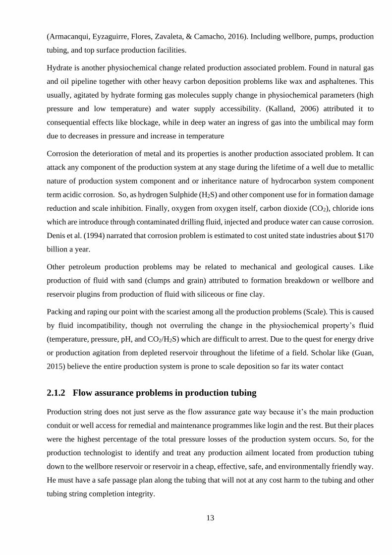
This is because the effect of scale deposition in production tubing are not limited to decline in production

rate but preventing well integrity and performance assurance programmes (Yusuf et al. 2016). Most

record on scale afflicted well around the world tip production tubing among the entire production system

to be most scale venerable because some scale grow all the way up to production tubing from other lower

production system. If not arrested in time, end up blocking it like the case reported of a well suffering

from poor deliverability, erosion damage at surface production facility and well bore restriction. This is

as a result of scale deposit in the 7000-inch lower section of the tubing and production casing all the way

to the perforation intervals (Mohamed et al 1999). Not underrating the dangers like desolation/hydration

process and other surface facilities cause by suspended mobile scale in water, although more dangerous

and difficult to treat if it’s adhered to the wall of the tubing (Salami, Monem, Development, & Zadco,

2010). Making it difficult even in presence of improves reservoir placement technology and intelligence

fluid system to archive a quick and non-damaging solution. Due to the verse chemical composition of

scale layers adhering to the inside of the production tubing (El Hajj, Pal, & Zoghbi, 2015). A typical

schematics of scale deposition in production tubing is elaborated in Figure 2.1

Figure 2.1: Scale deposit (a) in production tubing, (b) schematics of scale inflicted production tubing

by (Slumberger, 2013)

2.2 Kinetics of scale formation

Scale deposition problem is non-racial and non-boundary flow assurance and energy security threat, that

had cut and inflected almost all the oil and gas field across the entire globe.

(a) (b)

15

Starting with few cases from Gulf nations of the Asian continent like Kuff Gas well in Bahrain that

suffers from poor well deliverability, wellbore poor accessibility and erosional damages at the top

surface production/processing facility. Attributed to scale deposition from production interval up the

way to 7000 inch of the lower section of the production tubing and production casing (Mirza et al.,

1999). Fadhili field in the Eastern Saudi Arabian was half to it production capacity (150BOD and 90%

water cut) within four months. Estimated to be around 20 to 30 BOD drop per well as a result of calcium

carbonate deposited along both production tubing and other flow lines. World most prolific oil field

(Gwahar) approximately 225km length by 30km width in the same Saudi Arabia has been suffering

from Iron scale problems (Leal et al 2009). Among other golf oil field inflicted with scale deposition

problems are Zakum field in Abu-Dhabi, the world 4th largest oilfield (Al-Ashhabet al. 2006). Fateh field

Dubai, UAE (Ringen J and Read P 1982). While in the cases of deep Asia: South Sumatra oil field in

Indonesia (Mitchel. et al 1980) and Miono gas field 350km north of Karachi Pakistan (Field et al. 2013).

These are few from the many oilfields in Asia that have been experiencing production decline associated

to water influx restricting fluids flow along the production tubing due to carbonate deposit.

In the European continents, North Sea oil fields like statjoft oil field, which has fallen below production

decline curve with 60% of its STOIP recovered via secondary techniques for the past 23 years due to

scale problems (Børeng et al., 2002). Statoil oilfield were scale was proven as the major caused from

operator data showing 75% plugged by scale, fine or their combination and a plugging frequency of 0.02

int/well-year (Jordan et al., 2001). More dangerous and instantaneous is the cases of Miller field were

a 30,000bopd production capacity well was halt to zero within 24 hours (Crabtree et al., 1999). The case

of Gyda field north eastern part of Norwegian continental shelf of North Sea (Mackay, Jordan, & Torabi,

2003). Alba field in UK continental shelf (Farrelet al., 2013). In addition, some prolific wells in USSR

(Cowan et al., 1975) are among many fields suffering from severe scale plugins.

In the African continent, an African oil field like Gmasa oil field in Egypt which has suffered a

production decline approximately one tenth of its normal production capacity due to hard scale deposit

(Cowan et al., 1976). Strontium and calcium sulphate were found in surface and sub-surface production

facilities of Al Morgan field in Egypt (El-hattab, 1985). The three-water flooded field operated by

GUPCO in the gulf of Suez area (Lico et al., 1980) and also (Khelil et al., 1979) mentioned some water

flooded oilfield in Algeria

Wrapping my points with few cases from the Americans fields are: Ew 873 of the Gulf of Mexico, woe

with chronic near wellbore formation damage and tabular restriction due to barium sulphate (BaSO4)

scale build up. As a result of incompatible mixture of formation water and biocide inhibited sea water

well (Sopngwi et al., 2014). So also, (Quiroga et al., 2003) reported about Petro Bras operated oil field

16

in the Brazilian offshore that have live in the history of severe hard scale problems mostly due to the

nature of the offshore field

Scale formation is a product of many production operation factors depending on the type of scales in

question, physiochemical, kinetic and thermodynamic properties of produce fluid. Like (chemical

composition & concentration, temperature, pressure, pH, salinity, CO2/H2S liberation and outgassing,

time). Similarly, the age of the well and the oil recovery technique on ground (water incompatibility

mixture between formation water and poorly treated injected water will be inevitable when using some

secondary recovery techniques).

Mineralogy and lithology of the formation (Sandstone reservoir will contain high concentration of

strontium (Sr2+) and (Ba2+) cations). Also, while carbonate and calcite cement sandstone will be rich in

magnesium (Mg2+) and divalent calcium (Ca2+) cations. In addition, complexity of equipment and

completion design, type of well (vertical, multi mingling or even horizontal associated with low

drawdown being the ability lift carbonate scale up hole) or onshore /offshore and the type of the field

(Gas or Oil field). Lastly, level of scale preventive commitment at the CAPEX phases of the fields even

though some factors are more outweighing.

Most disturbing flow assurance problems are kinetics of crystal growth of mineral with poor solubility

(scale) which main cause can be grouped into three core-factors: Geological factors like mineral

composition, ground water circulations. Engineering related parameters like well pressure, pumping rate,

introduce fluids to the oil-bearing formation. So as physical /chemical factors like change temperature,

pressure PH and the rest (Nancollas and Reddy 1974) that are more peculiar in oilfield scale deposition

Many petroleum/flow assurance concern scholars have tried to justify or streamline the core course of

scale production to be: Reduction in solubility as a result of physiochemical changes like increase in

temperature or decrease in pressure. Precipitation as a result of mixture of incompatible waters (sea

water rich in SO4 anion and formation water containing C2+ or Ba2+cations forming mineral scale).

Increase in concentration above solubility range from the result of brine evaporation are the three

suggested mechanism for mineral scale formation by (Mackay et al., 2003) and also concurred by

(Abbas, 2014) among many scholars.

While change in temperature and pressure drop, water break through impact, like increase in sea water

mixing ratio, increase in pH level. Which can increase CaCO2 potential once the pressure fall below the

CO2 bubble point leading to liberation of carbon dioxide (Salami et al., 2010). Reductions in solubility

of salt as a result of increase in temperature or decrease in pressure of brine (contributing to the

precipitation of calcium carbonate or carbonate scales). The mixture of two in compactable fluids

(precipitation of sulphate scales BaSO4 from incompatible mixture of cation rich formation water and

17

sulphate rich sea water). The case of organic- deposit on submersible pump can be due to crude oil

cooling and the separation of volatile/light fraction near the pump intake (Ramones et al., 2015). While

in organic scale deposit can be attributed to high water cut and high pressure drop in the wellbore

Salt precipitation is as a result of increase in salt concentration above solubility limit due to brine

evaporation. (Scale precipitations like NaCl can occur as a result of dehydration from mixture of dry gas

stream with low brine stream in high pressure/high temperature well) (Bowman et al., 2010). Oil and

Gas are produced alongside produce water, which is as a result of change in pressure and temperature in

production tubing and can agitate the liberation of CO2 with the consequences of increasing the pH level

of the produce water. This leads to precipitation of calcium carbonate (Crabtree et al., 1999). Factors

behind the precipitation of scale are mixing of in compactable brines or change in PH or physical

conditions like pressure and temperature (Wang et al., 2013). While (Moghadasi et al., 2003) relate it to

the adverse effect of temperature because the higher temperature the higher the scaling tendency of

some oilfield scales (sulphate and calcium carbonate). Organic scale is usually deposited outside crude

oil and plugging the formation due to variation of temperature and pressure in oil and gas reservoir

during production is (Dale et al. 2014) thought. While the organic scale deposition and growth on surface

is agitated by both hydrodynamic of the system and the nature of the surface. Also (Heydrich, Hammami,

Choudhary, Mockel, & Ratulowski, 2019) highlighted the important of the oil and gas water volume

fraction, flow regime, shear at the surface, surface energy & roughness.

Even though water is basic reason for forming oilfield scale and so is drop in partial pressure of CO2 a

defining factor too. Temperature, variation in hydrogen ion concentration, ionic concentration,

additional striping due to gas lift operations, water flooding or reservoir communication cannot be under

emphasize. If partial pressure of CO2 drop occurs at the well head, scale is expected to form at flow line

with the potential of progressing down to the wellbore all the way to the reservoir. Also, if low enough,

at production separator scale may deposit there (Khalaf 2001). Awali field can serve as a good example

were pressure, temperature and gas striping are the primary source of scale formation (Esbai et al.,

2016). Brine production from different formation can occur due to high rate of gas production in a well

leading mixing of incompatible brines of different saturations that can easily precipitate salt and plug

well (Farrokhrouz & Asef, 2010). Still CO2 striping might be the major reason of calcium carbonate

scaling since formation water at reservoir condition is in aqueous (bicarbonate). Therefore, any

disturbance of it equilibrium by under equilibrium and CO2 stripped from it will lead to calcite scaling

due to pressure reduction (Esbai et al., 2016). As expressed in equation 2.1

CaCO3 + CO2 + H2O → Ca(HCO3)2 (2.1)

18

Despite the scholar’s consensus on primary scale agitators is to be temperature and pressure fluctuations,

water incompatibility, outgassing and shift in pressure. Quite a lot of cases of oversaturated produce

water meting all scale formation requirements refuse to form scale (Crabtree et al. 1999). It’s then

establish that another core requirement outside all the above mention is the essential growth from its

solution with creation of less stable atoms (Abbas, 2014). Through the development of unsteady bunch

of atoms (seed crystals) during homogenous nucleation process. So, lonely depending on these three

sequential requisite stages of super saturation, nucleation and precipitation

First stage is super saturation: Usually as a result of mineral concentration of brine exceeding it

equilibrium concentration, forcing salt to precipitate out of solution and form scale. Supersaturated is

aided by variation in temperature and pressure, increase in mineral concentration, thermodynamic

variation, particle sizes, hydrodynamics’ (agitation & velocity), kinetics (time). In addition to pH and

other environmental factors leading to the birth of small particle called Nuclei (El-Hattab, 1985). Since

solubility limit can be exceeded once the natural state of fluid is altered, thereby leading to scale

formation with a temperature and pressure complex tendency. Therefore, water solubility of mineral will

increase with increase in temperature and will decrease with decrease in pressure. Related to the role of

thumb that predicted by (Cabtree et al., 1999) the solubility of most minerals to decrease by a factor of

two for every pressure decreases of 48 MPa (7000 psi) with the exception calcium carbonate which

solubility in water increases with decrease in temperature.

Super saturation can occur once the solubility limit of a fluid is disturbed (Scale can form once the

thermodynamic of one or more component is exceeded). Temperature and pressure are the major

functions of the kinetic reaction that form scale. Despite, it has been well established that mixing two

in compatible water is reasons for scale formation, changing the kinetics of single water can generate

scale too (Moghadasi et al., 2003), (El Hajj et al., 2015). It can also be established that the higher the

degree of super saturations of water the higher the rate of precipitation causing more decline in

permeability (Al-Taq et al., 2015). Like the way decrease in pressure or temperature surely decrease

ionic solubility of salt (basis for carbonate scale precipitation CaCO3)

Ca(HC03)2 ↔ CaCO3(s) + CO2(g) + H2O(l) (2.2)

Second stage of scale formation begins after the birth of nuclei. As a result of the mention scale driver’s

couple with its ability to grow out of solution formation of unstable cluster of atoms from over saturated

fluids during homogenous nucleation processes. Then proceed to form seed crystal as a result of local

fluctuation in the equilibrium of the ionic concentration of the supersaturated solution (Cabtree et al.,

1999). The seed crystal increases in size as a result adsorption of ions on to the defect of the face of the

crystal. Likewise, the enlarge crystals grows in energy driven from decrease in surface free energy of

19

the crystal. Then, after the increase in radius exceed the critical radius free energy decrease rapidly.

Subsequently, leading to continues growth of the large crystal and dissolving of smaller seeds again.

Seed crystal serving as catalyst for scale formation means seed crystal formation will result to growth of

scale deposit if given large enough degree of saturation.

Thus, in heterogeneous nucleation crystal growth is expected to start on pre-existing fluid boundary

surface (Yousef et al. 2014). Defect on pipe surface like perforation, roughness in liners, joint steam in

pipelines, or production tubing are cantered to be the major site for heterogeneous nucleation process.

High degree of turbulence is another scale formation catalyst, since scale accumulation occurs at the

bobble point pressure of the flow system making it good reasons for the rapid deposition of scale on

down-hole equipment’s (Toyloret al. 2013). Similarly, (Mackey et al., 2019) added that the formation

of iron-oxyhydroxide form steel corrosion can create sites for heterogenous nucleation and aid additional

scale growth

After the formation of nuclei, a reasonable quantity of molecules must agglomerate and position in fix

crystal lattice. Pre-existing mineral or metal surface like weld, corroded surface, scratch or nicks on a

pipe, foreign crystal maters, sand & clay particles are favourable nucleation locations. Another requisite

for scale formation is adequate contact time between the supersaturated solution and the nucleation site.

There by nuclei creating a location for additional mineral deposition to form crystal that continues to

growth and adherence to form scale (El-Hattab, 1985). In conclusion is that scale forms when the kinetic

factor that inhabit the mineral growth are overwhelm by its thermodynamic driven force.

2.2.1 Factors influencing scale formation

The formation of mineral crystalline deposit (oiled filed scale) is attributed to the precipitation of solid

brine present in the production and the reservoir flow system (Abbas, 2014). Injection of incompatible

water have been single as major cause of calcium and carbonate scale formation inflicting damage in

both injection and producing well (Almubarak, Ng, Nasr-el-din, & Texas, 2017). Sulphate scales like

barium sulphate (BaSO4) and the rest are formed as a result of mixture of two in compactable brines

because formation water containing cations of barium, calcium & strontium and that of sea water are

containing sulphate compounds. Result from twenty four well brine samples from brine chemistry test

suggested acid treatment as main cause of scaling in 2009 (Farrokhrouz & Asef, 2010) linking the

precipitation of calcium sulphate to the detrimental of acidization.

Scale formation depends on water production in a well. Complex fluid rich in ions or close to saturation

limit are easily formed when water wash, dissolve and carry some of the mineral component from natural

environment by-products of marine life and water evaporation enrich sea water with ion. While water

20

associated with oil gas well are chemically different from that of ground and near ground surface. The

deeper, the more ionic concentrations due to alteration of sedimentary minerals (sandstone reservoir will

contain high concentration of strontium (Sr2+) and (Ba2+) cations. While carbonate and calcite cemented

sandstone will be rich in magnesium (Mg2+) and divalent calcium (Ca2+ cations) (Abbas, 2014). Water

quality continuously varies through the life of a well and can be counted as one of the causes of scale

formation. Particularly when injection water is used in sustaining the driver aquifer scale build up in

well (Clameto et al., 2004). This situation became even tougher with injected seawater breakthrough

resulting to deposition barium or strontium sulphate which absolutely insoluble

Gwawar onshore fields can be good case scenario with Gulf sea water as its primary sources of

floodwater (with over 4,700mg/l of sulphate and salinity 15000 mg/l near Kuwait and over 55000 mg/l

near southern parts of Saudi Arabia). Before recognising low saline aquifer water (5000 mg/l to over

70000 mg/l) as an alternative (Raju 2009). The mixture of the high sulphate concentrated Gulf sea water

and in compactable Gwawar field formation water increase scaling potential of the field

A non-universal solution has been attempted by field reservoir modelling and reservoir engineers with

the intention of lowering in-compatible water scale problem. Through the creation of a buffer bank to

serve as barrier that will separate the formation water from freshly injected water (Alabdulmohsin et al.,

2016). Though the solution depends on good knowledge of reservoir floor regime and good cooperation

between production chemistry and reservoir engineering.

The process of iron sulphide is more complex because despite factors like temperature, pH, water

composition, H2S level, variety of minerals will play a vital role in determining the final mineral phase

of the product (Benning et al. 2000). Iron can easily be introduce in to the formation during corrosion

acidization, especially if the acid is not equipped with enough corrosion inhibitors (Ramachandran, Al-

Muntasheri, Leal, & Wang, 2015). Since, in deep sour wells, iron sulphite has always been found in well

tabular after acid treatment (Nasr-El-Din and Al-Humaidan 2001, Kasnick and Engen 1989). Dissolution

of reservoir rocks that have small amount of iron, sour corrosion, drilling fluid loss and tabular corrosion

during acidization process can be considered as main source of irons (Ramachandran et al., 2015). Also

(Merdhah and Yassin 2009) believes injection systems can easily get inflicted with scale problems when

two incompatible waters are involved

2.2.2 Scale classifications

Chemical composition, solubility, cause of precipitation and physical properties like hardness and

density are the basis adopted by many scholars on their attempt to classified or categorize type of scale

in oil and gas production.

21

Organic/inorganic are the most used classification term for solid scale type. Referring to the two type of

mutual inclusive simultaneous occurring scale (mixed scale) that are classified based on their formation

factors and chemical compositions. Organic scale are hydrocarbons of high molecular weight, that are

not easily dissolve, but easily form sludge when in contact with acid. Comprising of alspahene, paraffin,

wax and soup that usually forms as a result of change in production environment i.e. significant pressure

drop expose viscous oil will surely form organic scale (Mucchi, 2007). While the crystalline deposit type

containing mineral salt like CaCO3 and BaSO4 are term inorganic (Sobie et al. 2006). These usually form

as a result of salt precipitation from brine present in production flow system. Mostly due to incompatible

mixture of brines, change in equilibrium sate of reservoir flood & ionic concentration, change in

pressure, temperature and pH. sulphate, carbonate, sulphide and chloride are most encountered (Abbas,

2014). Both the two scale types can occur simultaneously making it more difficult to dissolves and

impending the ESP system (Ramones et al., 2015). Saudi Aramco wells have recoded combination of

organic and inorganic scale deposit at same location (Al-Taq et al., 2015). Analysis of some collected

bailer sample from wells (Al-Taq et al., 2015): indicate combination of organic materials like paraffin

and asphaltene and in organic deposit like ankerite, anhydrite and insignificant presence of halite and

quartz.

Another classification basis can be tied to their solubility in acid. Like calcium carbonate called calcite

(CaCO3), Iron carbonate known as siderite (FeCO3), Iron sulphide term Pyrite (FeS, FeS2) and Iron oxide

(Fe (OH), Fe2O3, Fe3O4) are grouped under acid soluble scale type because of their solubility in acid.

While Strontium sulphide known as Celestite (SrSO4), Barium sulphide called Barite (BaSO4). In

addition to calcium sulphate which appear in two forms of anhydrite(CaSO4) at relatively high

temperature and Gypsum (CaSO4.2H2O) at relatively low temperate (Merdhah and Yassin 2009) are

grouped under acid insoluble scale type (Salami et al., 2010) due to their insolubility in acid.

To some extend scale deposit are classified in to hard medium and soft scale base on their physical

mineral hardness and density guided by Mohs scale (ability of harder minerals to scratch soft material).

Most of the organic scales are classified under the soft scale categories. While the inorganic or mineral

scale crossing through medium to hard scale range (Abbas, 2014). Were soft scale being peg with

hardness value of 1.0-3.0 on the Mohs scale, while medium has a hardness value of 0.3-0.5, and hard

scale is within the hardness value of 0.5-10 on the scale.

A crystallise organic mineral salt deposit usually cause by supersaturation of produce water that are

affected by physiochemical changes depending on the type of field are term oilfield scales and further

iron scale. Among must common oilfield scale encountered are: Sulphate compound like calcium

sulphate (anhydrite & gypsum), strontium sulphate (celestite), barium sulphate (barite), and calcium

carbonate. While iron compound like iron sulphate, iron oxide and iron carbonate related to high

22

temperature gas wells (Yassinet al. 2008) (Mahmoud et al., 2015). Sulphate scales like barium and

strontium sulphate in particular are the most troublesome scale species among the oilfield (Bedrikovetsk

et al. 2005) due to their thermodynamic stability (M. M. Jordan et al., 2001). Usually when water rich

in calcium ion comingles with another water with carbonate as its basic medium common oilfield scale

like calcium carbonate. So as (CaCO3),barium sulphate known as barite (BaSO4),gypsum (CaSO4) and

strontium sulphate(SrSO4) are expected to form (Moghadasi et al., 2003). The inorganic crystalize

deposit term as oilfield are formed as a result salt precipitation from brine that are present in both

reservoir and production system. Attributed to scale formation driving catalysts like change in ionic

concentration, temperate, pressure, pH, CO2 and the rest.

2.2.3 Scale compositional analysis

Complete understanding of chemistry and mineralogy of scale. In terms of analysing their compositional

constituent can be archive using standard analytical techniques like SEM/EDX, XRD and XRF. More

precise result can be archive by their combination. While NMR and FTIR is recommended for organic

scale analysis.

Scanning electron microscopy with energy dispersive X-ray (SEM/EDX) are chemical analysis tool and

techniques. That utilises surface analytical technique through high resolution images of surface

topography, with excellent depth of field. To determine and identify elemental and quantitative

composition of a compound.

X-ray fluorescence (XRF) is a non-destructive analysis technique carried with (XRF) spectrometer.

Utilise in determining the elemental composition of material or routine chemical analysis of rocks,

minerals, fluids and sediments. It basically operates on wavelength - dispersive spectroscopic principle

like that of electron microprobe (EPMA). Which simply measures the fluorescent (or secondary) X-ray

emitted from a sample when it is excited by a primary X-ray source.

X-ray powder diffraction (XRD) is a fast-analytical technique. Basically, used for phase identification

of crystalline material (mineralogy) like scale deposit, shale core, catalyst, cement, formation core and

the rest. Archive by differentiating numerous forms of commands with same chemical formula (Chung

1974, 1975; Klug and Alexander 1974; O’Conner et al. 1991; Sitepu et al. 2005). So, the average bulk

composition of the finely grounded, homogenized analysis material can then be determined. This sole

application is characterized with constrains in ability to provide complete information due to peak

pattern.

Therefore, to have an effective analysis and detailed scale characterization for crystalline, semi-

crystalline, and non-crystalline material. A solubility testing and extra analysis tool like XRF elemental

23

analysis are needed (El Hajj et al., 2015). An example of the publisher suggestion is a result from

combine analysis (XRD and XRF test respectively) for calcium carbonate scale. The result indicates the

presence of calcite, sodium feldspar, and calcium feldspar. The XRD still shows halite, quartz, and

magnetite while the XRF result suggests high percentage of dolomite and calcite. In addition, 82% of

the sample was readily soluble in HCl acid, while 93.11% as observed from the spot acid solubility test.

The Nuclear Magnetic Resonance (NMR) Spectroscopy is well known for revealing compounds unique

structures by identifying carbon-hydrogen framework of organic compounds.

Additionally, Infrared Spectroscopy is another tool for analysing organic substance that lies around the

interaction of infrared light and molecules either by measuring it emission, absorption or deflection for

analysing and identification of chemical substance, functional group in a compound and other

applications.

2.2.4 Scale chemistry

2.2.4.1 Calcium carbonate scale (CaCO3)

Calcium carbonate is mostly found in oil field operation due to limestone region abundance (Okochaet

al. 2014), its soluble in acid and produces white effervescence. Exist in distinct crystal geographical

forms like calcite, aroganite and vaterite with different solubility and the earliest mention exhibiting

greatest stability in respect to strength particular for oilfield situations (El Hajj et al., 2015). Equation

2.3 demonstrates calcium carbonate deposition as a result of calcium carbonate precipitation.

𝐶𝑎(𝑎𝑞)2+ + 𝐶𝑂3(𝑎𝑞)

2− → 𝐶𝑎𝐶𝑂3(𝑠) (2.3)

Calcium carbonate deposition is normally attributed to severe pressure drop between reservoirs and well

bore, along the production string (tubing, safety valves & chokes etc.) (Moghadasi et al., 2003).

Sometimes even further away from well up to the top surface facilities (M. Jordan & Mackay, 2015)

such as heat exchanger, separator etc.

Carbonate scale formation is instigated as a result of pressure drop during production leading to

supersaturating of formation water with calcium carbonate (Mackay et al., 2006). Therefore, the

pressure reduction liberating CO2 in to gas phase leaving the solution supersaturated in calcium

carbonate (Moghadasi et al., 2003). Furthermore, it can occur due to evolvement of carbon dioxide as a

result of aquifer or connate water exceeding their bobbles point. Henceforth decreasing the carbonate

solubility and forming precipice of divalent ions like iron, calcium, and the rest (Jordan et al 2015) as

outline by the equation 2.4.

𝐶𝑎(𝐻𝐶𝑂3)2→𝐶𝑎𝐶𝑂3(𝑆) + 𝐶𝑂2(𝑔) + 𝐻2𝑂(𝑔) (2.4)

24

The dissolution of CO2 and Ca2+ in brines during production is prime in calcium carbonate precipitation.

If the reservoir is static (non-flowing condition) the entire fluid system is expected to be in

thermodynamic equilibrium. Continues drop in pressure result to degassing of carbon dioxide, raising

the pH in the produce water and calcium carbonate precipitation (Yassin et al., 2006). Also, loss of CO2

produce fluid in pre-seawater breakthrough age can be another cause of CaCO3 precipitation.

It can also be proven that calcium carbonate solubility is primarily affected by the CO2 content of water.

Since bicarbonate formation increase with carbon dioxide concentration and decrease of carbon dioxide

content in an equilibrium system leading to the formation calcium carbonate (Kamari et al. 2014) as

illustrated in equation 2.5. Combination of calcium and bicarbonate ion is another likely cause of

calcium carbonate scale formation. As a result of some insignificant quantity of ions bicarbonate detach

at that pH value equivalent most of injection well to form H+ and CO3 CO32- (Kazemiet al., 2014).

Mixture of waters containing real carbonate ions will have high scaling possibilities due calcium

carbonate decomposition.

𝐶𝑎(𝑎𝑞)2+ + 2𝐻𝐶𝑂3(𝑎𝑞)

2− ↔ 𝐶𝑎(𝐻𝐶𝑂3) 2(𝑎𝑞) ↔ 𝐻𝑂2 (𝑎𝑞) + 𝐶𝑂2(𝑔) + 𝐶𝑎𝐶𝑂3(𝑠) (2.5)

The effect of carbon dioxide partial pressure toward carbonate scale formation should not be neglected

because in-depth understanding of brine and CO2 (in gas phase) chemical reactivity is vital. As most

carbonate reservoirs contain the compositions of mineral cement and carbon dioxide. At reservoir

condition (high temperature up to 200 ̊C and high pressure up to 30 MPa) the formation water is calcium

carbonate saturated. The equations bellow illustrates CO2 in contact with water dissolving to form

carbonic acid

𝐶𝑂2(𝑔) + 𝐻2𝑂(𝑙) → 𝐻2𝐶𝑂3(𝑎𝑞) (2.6)

𝐻2𝐶𝑂3(𝑎𝑞) ↔ 𝐻(𝑎𝑞)+ + 𝐻𝐶𝑂3(𝑎𝑞)

− (2.7)

𝐻𝐶𝑂3− ↔ 𝐶𝑜3

2− + 𝐻+ (2.8)

The decomposition is as a result of pressure reduction leading to liberation of carbon dioxide by

increasing the pH (shift in equilibrium of the reaction to the right).Causing precipitation of calcium

carbonate once the amount of calcium carbonate out weight that of water (El Hajj et al., 2015) as

illustrated in the equation 2.19. While Figure 2.2 illustrates a CaCO3 inflicted production tubing with

different SEM topographical magnifications.

𝐶𝑎(𝐻𝐶𝑂3)2 → 𝐶𝑎𝐶𝑜3 + 𝐶𝑂2 + 𝐻2𝑂 (2.9)

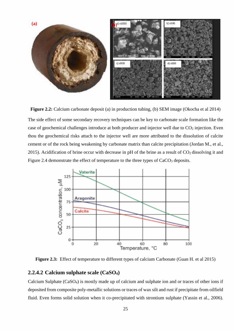
25

Figure 2.2: Calcium carbonate deposit (a) in production tubing, (b) SEM image (Okocha et al 2014)

The side effect of some secondary recovery techniques can be key to carbonate scale formation like the

case of geochemical challenges introduce at both producer and injector well due to CO2 injection. Even

thou the geochemical risks attach to the injector well are more attributed to the dissolution of calcite

cement or of the rock being weakening by carbonate matrix than calcite precipitation (Jordan M., et al.,

2015). Acidification of brine occur with decrease in pH of the brine as a result of CO2 dissolving it and

Figure 2.4 demonstrate the effect of temperature to the three types of CaCO3 deposits.

Figure 2.3: Effect of temperature to different types of calcium Carbonate (Guan H. et al 2015)

2.2.4.2 Calcium sulphate scale (CaSO4)

Calcium Sulphate (CaSO4) is mostly made up of calcium and sulphate ion and or traces of other ions if

deposited from composite poly-metallic solutions or traces of wax silt and rust if precipitate from oilfield

fluid. Even forms solid solution when it co-precipitated with strontium sulphate (Yassin et al., 2006).

(a) (b)

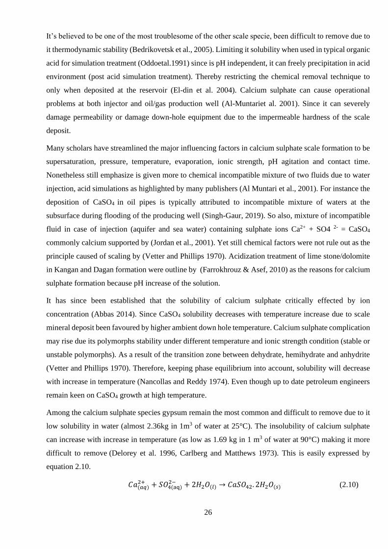
26

It’s believed to be one of the most troublesome of the other scale specie, been difficult to remove due to

it thermodynamic stability (Bedrikovetsk et al., 2005). Limiting it solubility when used in typical organic

acid for simulation treatment (Oddoetal.1991) since is pH independent, it can freely precipitation in acid

environment (post acid simulation treatment). Thereby restricting the chemical removal technique to

only when deposited at the reservoir (El-din et al. 2004). Calcium sulphate can cause operational

problems at both injector and oil/gas production well (Al-Muntariet al. 2001). Since it can severely

damage permeability or damage down-hole equipment due to the impermeable hardness of the scale

deposit.

Many scholars have streamlined the major influencing factors in calcium sulphate scale formation to be

supersaturation, pressure, temperature, evaporation, ionic strength, pH agitation and contact time.

Nonetheless still emphasize is given more to chemical incompatible mixture of two fluids due to water

injection, acid simulations as highlighted by many publishers (Al Muntari et al., 2001). For instance the

deposition of CaSO4 in oil pipes is typically attributed to incompatible mixture of waters at the

subsurface during flooding of the producing well (Singh-Gaur, 2019). So also, mixture of incompatible

fluid in case of injection (aquifer and sea water) containing sulphate ions Ca2+ + SO4 2- = CaSO4

commonly calcium supported by (Jordan et al., 2001). Yet still chemical factors were not rule out as the

principle caused of scaling by (Vetter and Phillips 1970). Acidization treatment of lime stone/dolomite

in Kangan and Dagan formation were outline by (Farrokhrouz & Asef, 2010) as the reasons for calcium

sulphate formation because pH increase of the solution.

It has since been established that the solubility of calcium sulphate critically effected by ion

concentration (Abbas 2014). Since CaSO4 solubility decreases with temperature increase due to scale

mineral deposit been favoured by higher ambient down hole temperature. Calcium sulphate complication

may rise due its polymorphs stability under different temperature and ionic strength condition (stable or

unstable polymorphs). As a result of the transition zone between dehydrate, hemihydrate and anhydrite

(Vetter and Phillips 1970). Therefore, keeping phase equilibrium into account, solubility will decrease

with increase in temperature (Nancollas and Reddy 1974). Even though up to date petroleum engineers

remain keen on CaSO4 growth at high temperature.

Among the calcium sulphate species gypsum remain the most common and difficult to remove due to it

low solubility in water (almost 2.36kg in 1m3 of water at 25°C). The insolubility of calcium sulphate

can increase with increase in temperature (as low as 1.69 kg in 1 m3 of water at 90°C) making it more

difficult to remove (Delorey et al. 1996, Carlberg and Matthews 1973). This is easily expressed by

equation 2.10.

𝐶𝑎(𝑎𝑞)2+ + 𝑆𝑂4(aq)

2− + 2𝐻2𝑂(𝑙) → 𝐶𝑎𝑆𝑂42. 2𝐻2𝑂(𝑠) (2.10)

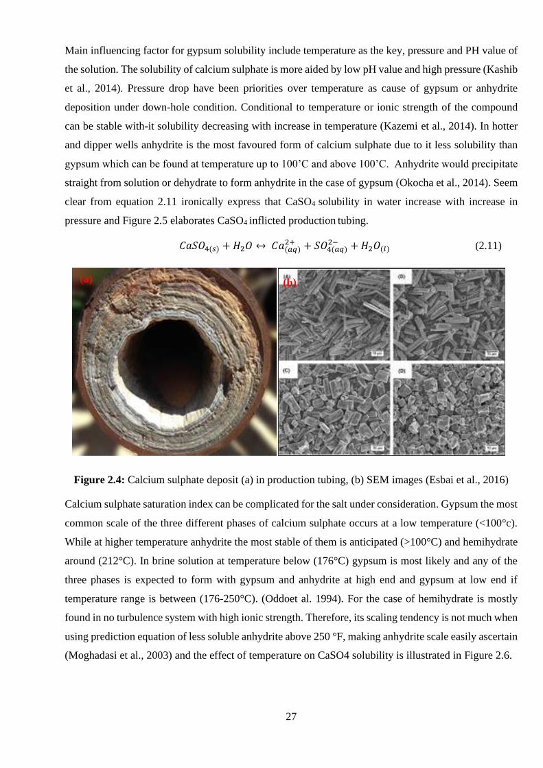
27

Main influencing factor for gypsum solubility include temperature as the key, pressure and PH value of

the solution. The solubility of calcium sulphate is more aided by low pH value and high pressure (Kashib

et al., 2014). Pressure drop have been priorities over temperature as cause of gypsum or anhydrite

deposition under down-hole condition. Conditional to temperature or ionic strength of the compound

can be stable with-it solubility decreasing with increase in temperature (Kazemi et al., 2014). In hotter

and dipper wells anhydrite is the most favoured form of calcium sulphate due to it less solubility than

gypsum which can be found at temperature up to 100’C and above 100’C. Anhydrite would precipitate

straight from solution or dehydrate to form anhydrite in the case of gypsum (Okocha et al., 2014). Seem

clear from equation 2.11 ironically express that CaSO4 solubility in water increase with increase in

pressure and Figure 2.5 elaborates CaSO4 inflicted production tubing.

𝐶𝑎𝑆𝑂4(𝑠) + 𝐻2𝑂 ↔ 𝐶𝑎(𝑎𝑞)2+ + 𝑆𝑂4(𝑎𝑞)

2− + 𝐻2𝑂(𝑙) (2.11)

Figure 2.4: Calcium sulphate deposit (a) in production tubing, (b) SEM images (Esbai et al., 2016)

Calcium sulphate saturation index can be complicated for the salt under consideration. Gypsum the most

common scale of the three different phases of calcium sulphate occurs at a low temperature (<100°c).

While at higher temperature anhydrite the most stable of them is anticipated (>100°C) and hemihydrate

around (212°C). In brine solution at temperature below (176°C) gypsum is most likely and any of the

three phases is expected to form with gypsum and anhydrite at high end and gypsum at low end if

temperature range is between (176-250°C). (Oddoet al. 1994). For the case of hemihydrate is mostly

found in no turbulence system with high ionic strength. Therefore, its scaling tendency is not much when

using prediction equation of less soluble anhydrite above 250 °F, making anhydrite scale easily ascertain

(Moghadasi et al., 2003) and the effect of temperature on CaSO4 solubility is illustrated in Figure 2.6.

(a) (b)

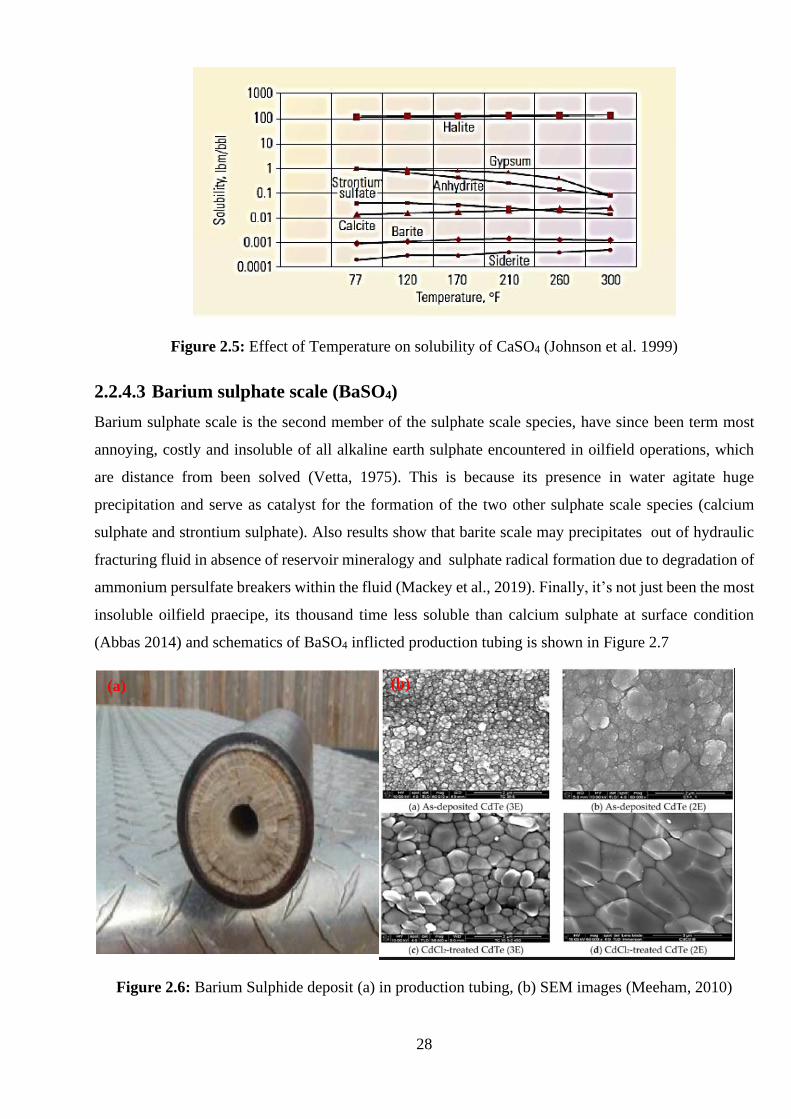
28

Figure 2.5: Effect of Temperature on solubility of CaSO4 (Johnson et al. 1999)

2.2.4.3 Barium sulphate scale (BaSO4)

Barium sulphate scale is the second member of the sulphate scale species, have since been term most

annoying, costly and insoluble of all alkaline earth sulphate encountered in oilfield operations, which

are distance from been solved (Vetta, 1975). This is because its presence in water agitate huge

precipitation and serve as catalyst for the formation of the two other sulphate scale species (calcium

sulphate and strontium sulphate). Also results show that barite scale may precipitates out of hydraulic

fracturing fluid in absence of reservoir mineralogy and sulphate radical formation due to degradation of

ammonium persulfate breakers within the fluid (Mackey et al., 2019). Finally, it’s not just been the most

insoluble oilfield praecipe, its thousand time less soluble than calcium sulphate at surface condition

(Abbas 2014) and schematics of BaSO4 inflicted production tubing is shown in Figure 2.7

Figure 2.6: Barium Sulphide deposit (a) in production tubing, (b) SEM images (Meeham, 2010)

(a) (b)

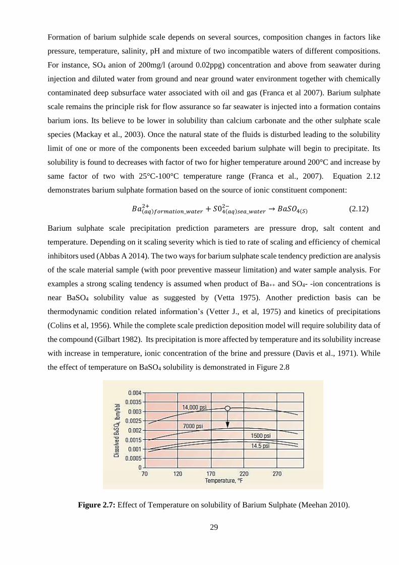
29

Formation of barium sulphide scale depends on several sources, composition changes in factors like

pressure, temperature, salinity, pH and mixture of two incompatible waters of different compositions.

For instance, SO4 anion of 200mg/l (around 0.02ppg) concentration and above from seawater during

injection and diluted water from ground and near ground water environment together with chemically

contaminated deep subsurface water associated with oil and gas (Franca et al 2007). Barium sulphate

scale remains the principle risk for flow assurance so far seawater is injected into a formation contains

barium ions. Its believe to be lower in solubility than calcium carbonate and the other sulphate scale

species (Mackay et al., 2003). Once the natural state of the fluids is disturbed leading to the solubility

limit of one or more of the components been exceeded barium sulphate will begin to precipitate. Its

solubility is found to decreases with factor of two for higher temperature around 200°C and increase by

same factor of two with 25°C-100°C temperature range (Franca et al., 2007). Equation 2.12

demonstrates barium sulphate formation based on the source of ionic constituent component:

𝐵𝑎(𝑎𝑞)𝑓𝑜𝑟𝑚𝑎𝑡𝑖𝑜𝑛_𝑤𝑎𝑡𝑒𝑟2+ + 𝑆04(𝑎𝑞)𝑠𝑒𝑎_𝑤𝑎𝑡𝑒𝑟

2− → 𝐵𝑎𝑆𝑂4(𝑆) (2.12)

Barium sulphate scale precipitation prediction parameters are pressure drop, salt content and

temperature. Depending on it scaling severity which is tied to rate of scaling and efficiency of chemical

inhibitors used (Abbas A 2014). The two ways for barium sulphate scale tendency prediction are analysis

of the scale material sample (with poor preventive masseur limitation) and water sample analysis. For

examples a strong scaling tendency is assumed when product of Ba++ and SO4- -ion concentrations is

near BaSO4 solubility value as suggested by (Vetta 1975). Another prediction basis can be

thermodynamic condition related information’s (Vetter J., et al, 1975) and kinetics of precipitations

(Colins et al, 1956). While the complete scale prediction deposition model will require solubility data of

the compound (Gilbart 1982). Its precipitation is more affected by temperature and its solubility increase

with increase in temperature, ionic concentration of the brine and pressure (Davis et al., 1971). While

the effect of temperature on BaSO4 solubility is demonstrated in Figure 2.8

Figure 2.7: Effect of Temperature on solubility of Barium Sulphate (Meehan 2010).

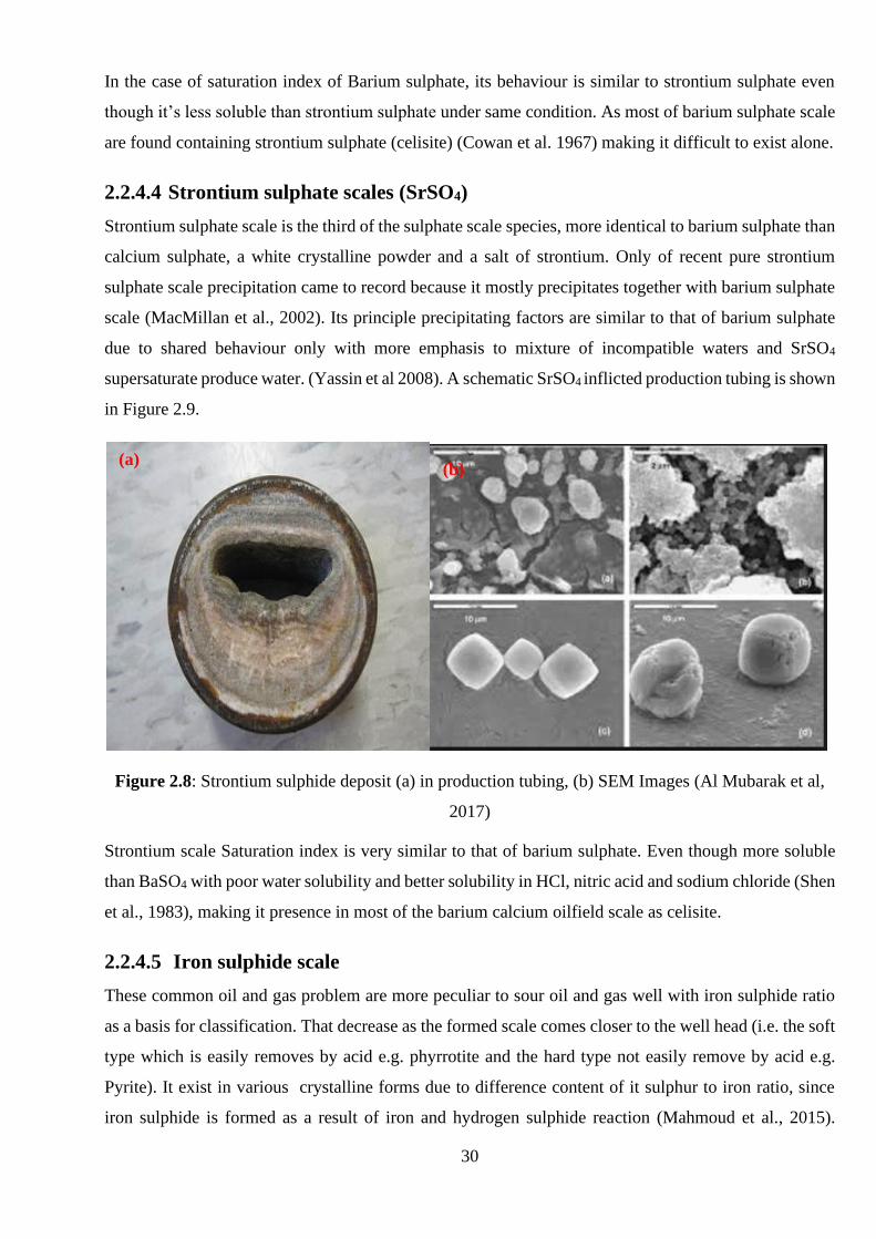
30

In the case of saturation index of Barium sulphate, its behaviour is similar to strontium sulphate even

though it’s less soluble than strontium sulphate under same condition. As most of barium sulphate scale

are found containing strontium sulphate (celisite) (Cowan et al. 1967) making it difficult to exist alone.

2.2.4.4 Strontium sulphate scales (SrSO4)

Strontium sulphate scale is the third of the sulphate scale species, more identical to barium sulphate than

calcium sulphate, a white crystalline powder and a salt of strontium. Only of recent pure strontium

sulphate scale precipitation came to record because it mostly precipitates together with barium sulphate

scale (MacMillan et al., 2002). Its principle precipitating factors are similar to that of barium sulphate

due to shared behaviour only with more emphasis to mixture of incompatible waters and SrSO4

supersaturate produce water. (Yassin et al 2008). A schematic SrSO4 inflicted production tubing is shown

in Figure 2.9.

Figure 2.8: Strontium sulphide deposit (a) in production tubing, (b) SEM Images (Al Mubarak et al,

2017)

Strontium scale Saturation index is very similar to that of barium sulphate. Even though more soluble

than BaSO4 with poor water solubility and better solubility in HCl, nitric acid and sodium chloride (Shen

et al., 1983), making it presence in most of the barium calcium oilfield scale as celisite.

2.2.4.5 Iron sulphide scale

These common oil and gas problem are more peculiar to sour oil and gas well with iron sulphide ratio

as a basis for classification. That decrease as the formed scale comes closer to the well head (i.e. the soft

type which is easily removes by acid e.g. phyrrotite and the hard type not easily remove by acid e.g.

Pyrite). It exist in various crystalline forms due to difference content of it sulphur to iron ratio, since

iron sulphide is formed as a result of iron and hydrogen sulphide reaction (Mahmoud et al., 2015).

(a) (b)

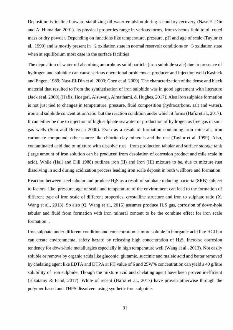
31

Deposition is inclined toward stabilizing oil water emulsion during secondary recovery (Nasr-El-Din

and Al Humaidan 2001). Its physical properties range in various forms, from viscous fluid to oil coted

mass or dry powder. Depending on functions like temperature, pressure, pH and age of scale (Taylor et

al., 1999) and is mostly present in +2 oxidation state in normal reservoir conditions or +3 oxidation state

when at equilibrium most case in the surface facilities

The deposition of water oil absorbing amorphous solid particle (iron sulphide scale) due to presence of

hydrogen and sulphide can cause serious operational problems at producer and injection well (Kasinck

and Engen, 1989; Nasr-El-Din et al. 2000; Chen et al. 2009). The characterization of the dense and black

material that resulted to from the synthetisation of iron sulphide was in good agreement with literature

(Jack et al. 2000),(Hafiz, Hoegerl, Alsuwaij, Almathami, & Hughes, 2017). Also Iron sulphide formation

is not just tied to changes in temperature, pressure, fluid composition (hydrocarbons, salt and water),

iron and sulphide concentration/ratio but the reaction condition under which it forms (Hafiz et al., 2017).

It can either be due to injection of high sulphate seawater or production of hydrogen as free gas in sour

gas wells (Seto and Beliveau 2000). Even as a result of formation containing iron minerals, iron

carbonate compound, other source like chlorite clay minerals and the rest (Taylor et al. 1999). Also,

contaminated acid due to mixture with dissolve rust from production tabular and surface storage tank

(large amount of iron solution can be produced from desolation of corrosion product and mile scale in

acid). While (Hall and Dill 1988) outlines iron (II) and Iron (III) mixture to be, due to mixture rust

dissolving in acid during acidization process leading iron scale deposit in both wellbore and formation

Reaction between steel tabular and produce H2S as a result of sulphate reducing bacteria (SRB) subject

to factors like: pressure, age of scale and temperature of the environment can lead to the formation of

different type of iron scale of different properties, crystalline structure and iron to sulphate ratio (X.

Wang et al., 2013). So also (Q. Wang et al., 2016) assumes produce H2S gas, corrosion of down-hole

tabular and fluid from formation with iron mineral content to be the combine effect for iron scale

formation .

Iron sulphate under different condition and concentration is more soluble in inorganic acid like HCl but

can create environmental safety hazard by releasing high concentration of H2S. Increase corrosion

tendency for down-hole metallurgies especially in high temperature well (Wang et al., 2013). Not easily

soluble or remove by organic acids like gluconic, glutamic, succinic and maleic acid and better removed

by chelating agent like EDTA and DTPA at PH value of 6 and 25W% concentration can yield a 40 g/litre

solubility of iron sulphide. Though the mixture acid and chelating agent have been proven inefficient

(Elkatatny & Fahd, 2017). While of recent (Hafiz et al., 2017) have proven otherwise through the

polymer-based and THPS dissolvers using synthetic iron sulphide.

32

The seven-solid phase of Fe-s system is used in presenting solubility state of iron sulphate since each of

them is characterize by different solubility behaviour. The bisulfide ion as given in equation 2.13: chosen

to be a better method of presenting the solubility product of iron sulphide due to the uncertainty of the

second ionization constant (Rickard & Luther 2007). Also Figure 2.10 illustrated sulphide inflicted

production tubing.

𝐹𝑒𝑆 + 𝐻+ = 𝐹𝑒2− + 𝐻𝑆− (2.13)

Figure 2.9: Iron sulphide deposit (a) in production tubing, (b)SEM Images (Mahmoud et al., 2015)

Pyrite (FeS2): Is the most stable of iron sulphide scale and has weak solubility in HCl acid. Possibly

generated as a result of secondary reaction of non-stoichiometric iron sulphide (Ford et al. 1992), such

as Pyrrhotite in a wet gas environ.

Pyrrhotite (𝐹𝑒1−𝑥𝑆): Mostly associated to H2S and high temperature (Shoesmith et al. 1980). Been a

non-stoichiometric group of iron sulphides makes their classification more difficult (Vaughan & Craig

1978). With number of poly types of hexagonal or mono-clinic crystal symmetry with numerous poly

types occurring with same spacemen (Buali et al., 2014) Also terms as magnetic pyrite, due to it colour

similarities to pyrite.

Troilite (Fe1-xS): Known to be the stoichiometric end-member phase of monoclinic pyrrhotite group,

without vacancies in its atomic structure (X is 0 to 0.2). It’s mainly found in meteorites, and can basically

be categorize as a subset of pyrrhotite

Marcasite (Fe𝑆2): Basically, known to be the intermediate disulphide between pyrite and

nonstoichiometric iron sulphides with iron sulphide of cubic crystal structure been the major physical

and crystal difference with pyrite. Simply polymer of pyrite with an orthorhombic crystal structure and

(a) (b)

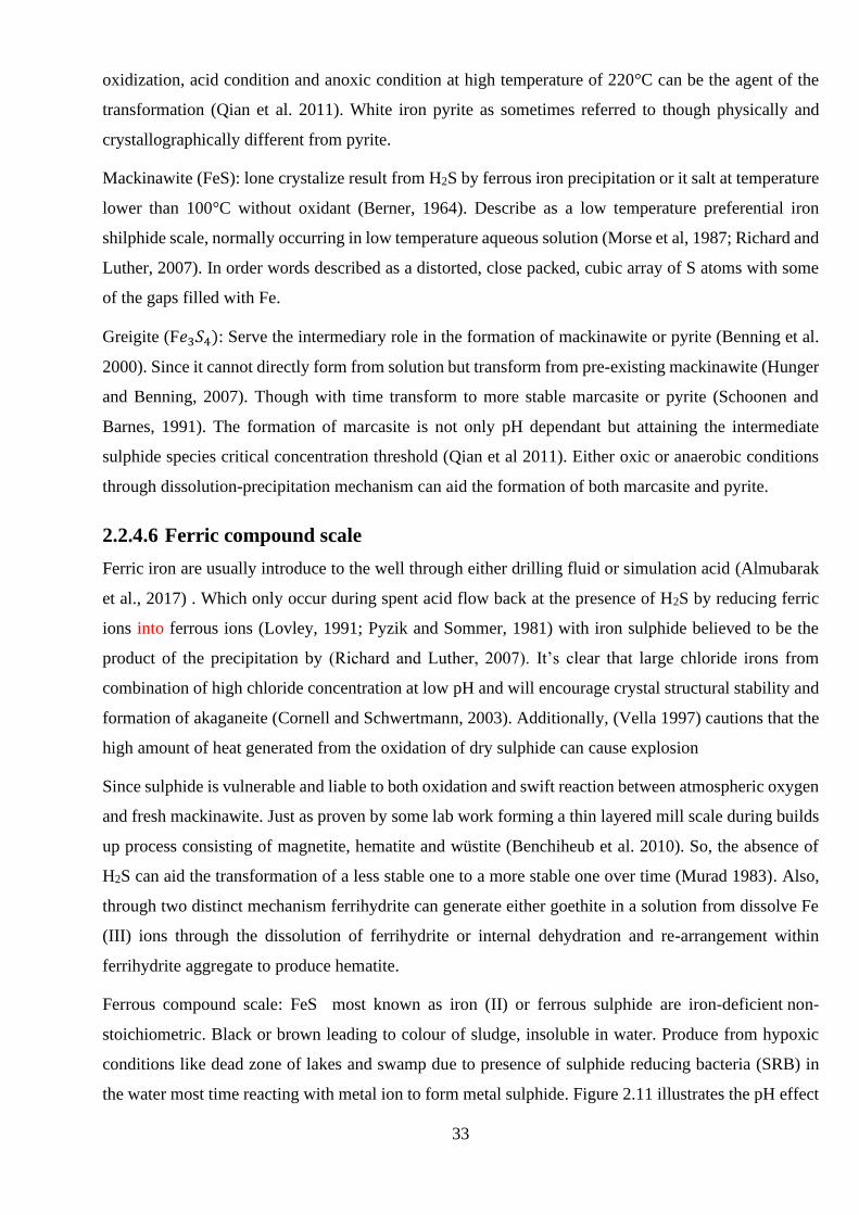
33

oxidization, acid condition and anoxic condition at high temperature of 220°C can be the agent of the

transformation (Qian et al. 2011). White iron pyrite as sometimes referred to though physically and

crystallographically different from pyrite.

Mackinawite (FeS): lone crystalize result from H2S by ferrous iron precipitation or it salt at temperature

lower than 100°C without oxidant (Berner, 1964). Describe as a low temperature preferential iron

shilphide scale, normally occurring in low temperature aqueous solution (Morse et al, 1987; Richard and

Luther, 2007). In order words described as a distorted, close packed, cubic array of S atoms with some

of the gaps filled with Fe.

Greigite (F𝑒3𝑆4): Serve the intermediary role in the formation of mackinawite or pyrite (Benning et al.

2000). Since it cannot directly form from solution but transform from pre-existing mackinawite (Hunger

and Benning, 2007). Though with time transform to more stable marcasite or pyrite (Schoonen and

Barnes, 1991). The formation of marcasite is not only pH dependant but attaining the intermediate

sulphide species critical concentration threshold (Qian et al 2011). Either oxic or anaerobic conditions

through dissolution-precipitation mechanism can aid the formation of both marcasite and pyrite.

2.2.4.6 Ferric compound scale

Ferric iron are usually introduce to the well through either drilling fluid or simulation acid (Almubarak

et al., 2017) . Which only occur during spent acid flow back at the presence of H2S by reducing ferric

ions into ferrous ions (Lovley, 1991; Pyzik and Sommer, 1981) with iron sulphide believed to be the

product of the precipitation by (Richard and Luther, 2007). It’s clear that large chloride irons from

combination of high chloride concentration at low pH and will encourage crystal structural stability and

formation of akaganeite (Cornell and Schwertmann, 2003). Additionally, (Vella 1997) cautions that the

high amount of heat generated from the oxidation of dry sulphide can cause explosion

Since sulphide is vulnerable and liable to both oxidation and swift reaction between atmospheric oxygen

and fresh mackinawite. Just as proven by some lab work forming a thin layered mill scale during builds

up process consisting of magnetite, hematite and wüstite (Benchiheub et al. 2010). So, the absence of

H2S can aid the transformation of a less stable one to a more stable one over time (Murad 1983). Also,

through two distinct mechanism ferrihydrite can generate either goethite in a solution from dissolve Fe

(III) ions through the dissolution of ferrihydrite or internal dehydration and re-arrangement within

ferrihydrite aggregate to produce hematite.

Ferrous compound scale: FeS most known as iron (II) or ferrous sulphide are iron-deficient non-

stoichiometric. Black or brown leading to colour of sludge, insoluble in water. Produce from hypoxic

conditions like dead zone of lakes and swamp due to presence of sulphide reducing bacteria (SRB) in

the water most time reacting with metal ion to form metal sulphide. Figure 2.11 illustrates the pH effect

34

on the stability of various iron sulphide and scale composition deposit in sour gas well. Also, the

summary of the entire scale compositional chemistry is presented in Table 2.1.

Figure 2.10: Scale deposit composition in X Sour Gas (a),(b) stability of various iron Sulphide in

respect to pH (Al-Bauli et al. 2015)

(a) (b)

35

2.2.4.7 Summary of scale chemistry

Table 2.1: Summary of Scale chemistry

Summary of oilfield scales type

Organic scales

Name Chemical Formula Mechanical Properties Principle variables Abundance

Alsphaten Alsphaten are

normally Polycyclic

aromatic hydrocarbons,

that may include many

substituents like alkyl

groups & heteroatoms

(e.g. N, O, or S)

Are molecular substances that are found in

crude oil, along with resins, aromatic

hydrocarbons, and saturates

Physio-chemical properties of fluid Like

increase in temperature differential,

residual time and decrease in flow rate

Deposited at borehole near formation, the

downhole pump, the tubing, surface flow

lines, separators, storage tanks and

pipelines and submerse pump

Hydrate Compound containing

water with definite mas in

H20 form and transform to

anhydrite when it loses it

water molecules

Water evolution when subjected to heating,

also solubility of its anhydrous residue in

water and when dissolved in water the

residual hydrate colour is reverse to the

colour of the hydrate

Agitated by hydrate forming gas

molecules supply, change physiochemical

parameters (high pressure and low

temperature) and water supply

accessibility

Associated problem found in natural gas

and oil pipeline together with other heavy

carbon deposition problems like wax and

asphatenes

Paraffin

CnH2n+2 Since in chemistry

it used Synonymously

with alkaline

A white tasteless colourless solid product of

petroleum product with 20-40 carbon atoms

of hydrocarbon molecules with density

around 900 kg/m3, soluble in benzene and

some esters and insoluble in water with 46

and 68 °C range of melting point

Increase in temperature differential,

residual time and decrease in flow rate

Deposited at borehole near formation, the

downhole pump, the tubing, surface flow

lines, separators, storage tanks and

pipelines and submerse pump

36

Most common oilfield scale / inorganic scale

Name Chemical Formula Properties Principle variables Abundance

Calcium

Carbonate

CaCO3 It’s an odourless, fine white powder

with2.71 g/mL density and 1,339°C melting

point at its calcite form. Aragonite, been

most common form that has a density of

2.83 g/mL and melting point of 825 °C.

Partial pressure of CO2, temperature,

total dissolved salts, pH

Found in Limestone formations and

deposited along reservoir, borehole and

production conduits

Calcium

Sulphate:

Gypsum

Hemihydrate

Anhydrite

CaSO4.2H2O

CaSO4.1/2H2O CaSO4

A white to offwhite powder with 2,525° C

melting point and 2.5 g/cm3 density that is

insoluble in water

Total dissolve salt, pressure and

temperature

Product of mixture of injected sea water

and calcium contain formation that can

deposit at reservoir, borehole and

production conducts

Barium

Sulphate

BaSO4 Decomposing white solid with 4.25 g/cm3

density and

2,235 °C melting point

Temperature, pressure & dissolved salt Product of injecting sea water containing

sulphate into sandstone formation and

most deposited from down production

system all the way the production conduct

Strontium

Sulphate

SrSO4 Coexist with barium sulphide almost all the

time

Pressure, temperature and total dissolve

salt

Share same properties with barium

sulphide

Iron sulphide scale

mackinawite FeS

Its bronze to grey-white colour tabular

crystals of mineral sulphite and anhedral

masses. With 2.5 Mohs hardness value and

4.17 a specific gravity.

precipitate from aqueous solutions with

metastable material as its main constituent

Mostly found in mineral of low

temperature aqueous environments

Cubic FeS A blue-black or pinkish chemical compound

of iron and sulphur with 4.049 g/cm3

density and 295.805 molar mass

Highly unstable not found in natural sate

Troilite Fe1-xS An Opaque material of bronze brown and

grey brown colour with 4.61 average density

Stoichiometric end member of the Fe1-xS

group. x is between 0 to 0

Normally found in meteorites

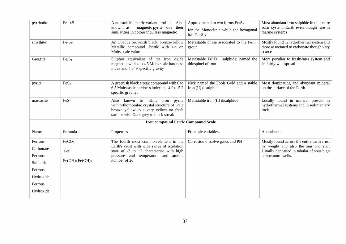
37

pyrrhotite Fe1-xS A nonstoichiometric variant troilite. Also

known as magnetic pyrite due their

similarities in colour thou less magnetic

Approximated in two forms Fe7S8

for the Monoclinic while the hexagonal

has Fe10S11

Most abundant iron sulphide in the entire

solar system, Earth even though rare in

marine systems

smythite Fe9S11 An Opaque brownish black, bronze-yellow

Metallic compound. Brittle with 4½ on

Mohs scale value

Metastable phase associated to the Fe1-xS

group

Mostly found in hydrothermal system and

more associated to carbonate though very

scarce

Greigite Fe3S4 Sulphur equivalent of the iron oxide

magnetite with 4 to 4.5 Mohs scale hardness

index and 4.049 specific gravity

Metastable FeIIFeIII sulphide; named the

thiospinel of iron

More peculiar to freshwater system and

its fairly widespread

pyrite FeS2 A greenish black streak compound with 6 to

6.5 Mohs scale hardness index and 4.9 to 5.2

specific gravity.

Nick named the Fools Gold and a stable

Iron (II) disulphide

Most dominating and abundant mineral

on the surface of the Earth

marcasite FeS2 Also known as white iron pyrite

with orthorhombic crystal structure of Pale

bronze yellow to silvery yellow on fresh

surface with Dark grey to black streak

Metastable iron (II) disulphide Locally found in mineral present in

hydrothermal systems and in sedimentary

rock

Iron compound Ferric Compound Scale

Name Formula Properties Principle variables Abundance

Ferrous

Carbonate

Ferrous

Sulphide

Ferrous

Hydroxide

Ferrous

Hydroxide

FeCO3

FeS

Fe(OH)2 Fe(OH)3

The fourth most common element in the

Earth's crust with wide range of oxidation

state of -2 to +7 characterise with high

pressure and temperature and atomic

number of 26.

Corrosion dissolve gases and PH Mostly found across the entire earth crust

by weight and also the sun and star.

Usually deposited in tabular of sour high

temperature wells.

38

2.3 Scale management

Scale management strategy have for long remained at the centre of attraction of flow assurance having

direct implications across all the production technologist basic responsibilities. Ranging from well

productivity, well completion, well simulation, associated production problems, remedial and, artificial

lift/productivity enhancement and surface processing cutting throughout workover of the life of a field.

Hence (Farrokhrouz & Asef, 2010) believe that proper adaption of scale management plan will enhance

production index and assure safe and easy production of a well for a long time.

Effective scale management strategy has been based on treatment philosophy of prevention is better than

cure. ‘’The right motto of preventing the re-occurrence of scale’’ (Ghouri, Ali, Shah, Ejaz, & Haider,

2018). Putting to consideration economic, production, time and safety of rig component, personnel and

well environment. These comprises of two vital processes of risk assessment and economic evaluations

that are applied throughout the field life cycle. Risk assessment allows the prediction of possibility of

mineral scale production, location and severity to be reviewed against current and future field

development alternative. Through allowing existing and near market scales control techniques to be

justifiably evaluated for effective scale control strategy identification. While the second process

(economic evaluation) is all about using modest economic models to compare, justify and identify the

most cost effective scale management solutions from does identified during the risk assessment process

phase at the CAPEX Phase of the field (M.Jordan et al., 2001). Lastly identify situation and stages were

scale control can be uneconomical like the case of some marginal field were cost of treatment might

exceed lifting cost (Mackay et al., 2003). Un-doubtfully over estimating threat can lead to installation of

unnecessary completion that can be economic burden to the CAPEX cost and potential maintenance

issues in the OPEX phase. Since (Graham et al. 2002) has generalized that the far away the scale

deposition is from surface facility the more difficult it’s to manage

In cooperating scale control as part of asset life cycle management is vital. For instance, developing a

scale control treatment strategy at the project development stage rather than plateau, decline or

decommission development stage. Since scale control in life cycle management is subject to various

challenges attributed to rise in water cut, as well transit from dry production to high water cut production.

This more preferred approach by (Mackay et al., 2003) because it permit the choice of suitable economic

technology and incorporation of appropriate remedial technology in both completion design and

installations.

39

Predicting, assessing the severity and location of scale problem in a new field that can be done by

calculating the mas of expected scale deposit using thermodynamic and kinetic calculation. Even thou,

the case of location of scale formation are still lagging. It can aid the selection of preventives majors like

inhibition treatment in reservoir or near wellbore infliction modelling brine mixing and stripping of

scaling ions before the production/injection fluid reaches the wellbore in more severe case (Jordan &

Mackay, 2015). Which are both are attributed to CAPEX phase (e.g. in cooperation of desulphation pant)

and OPEX (e.g. scale squeeze treatment)

2.3.1 Scale prediction/monitoring

The area of scale risk evaluation or prediction has improved over time. Evolving from simple empirical

thermodynamics calculations and limited solubility data to predicting potential of scale formation by

Stiff and Davis (1952a, 1952b), Oddo and Tomson (1981), Vaone and Skillern (1982). Recently, Oddo

and Tomson (1997) (Moghadasi et al., 2003). Then the introduction of commercial software prediction

tools like, MultiScale†4 (PetroTech†), ScaleSoftPitzer† (Rice Brine Chemistry Consortium†), and Scale

Chem† (OLI Systems†). Utilise for predicting expected type of scale to be formed, probability of scale

formation and maximum scale amount. Working on the principles of thermodynamic only instead of

kinetic equation (only few models incorporate kinetic parameters) which is not satisfactory. Since factors

like nucleation, adhesion, kinetic of crystal growth and other important factors are not considered. Lately

scale prediction tools are combining with other simulators for more accurate scale risk prediction result.

Examples include Eclipse†, Streamline/Frontsim† (Wahid et al., 2011), statistical models like principal

component analysis† (Skeck et al., 2008).Also scholars like (Guan, 2015) reported geochemical models

such as Ion Reaction† model from Heriot-Watt University and combination of models with

hydrodynamic prediction tools like PIPESIM† and computational fluid dynamics (CFD)

The latest development is not limited to considering the thermodynamic, kinetic and hydrodynamic

conditions that leads to precipitation of scale forming compound. For accurate scale prediction method,

but in addition consider all conditions that will leads to adherence of the precipitate or precipitating

compound. The area of squeeze inhibitor placement was taken care of by the introduction of Squeeze

V/VI† series software manufactured by Heriot-Watt University widely used by the industries today

(Guan 2015). While the existing gap in reactive transport modelling for calculating the impact on pH of

reservoir geo-chemicals reactions toward producer well for effective development of scale management

programme have finally been solved. Through the introduction of numerous 1D reactive transport

models like PHREEQC and Geochemist’s Workbench and for the important of brine rock and brine

mixing interaction been affected by 3D flow in complex reservoir system. 3D Simulation and reactive

transport codes like GEM, STARS, Reveal, UTChem and TOUGHReact are utilize for EOR (ASP and

40

CO2-WAG) flooding chemistry predictions (M. Jordan & Mackay, 2015). Advancement in the area of

subsea scale prediction includes laboratorial, analytical, modelling and hardware technology has been

archived through introduction of MARS system, and CIMV technologies (Gaun 2015). For the effective

scale management like identifying were exactly scaling water is coming from (formation zone), expected

location for scale deposition and most effective ways of managing it.

2.3.2 Scale prevention

Oilfield scale inhibition is a preventive measure or process of avoiding or mitigating scale deposition

from hindering flow assurance at any location of the entire production system. Using special class of

chemicals to slow or poising the scale process of growth in water system. It’s not just the key integral of

the scale management system but for both flow assurance and production economics. Likewise,

suggested by (Jordan et al., 2001) that the pre-production treatment of reservoir to avoid scale formation

near the well bore, the utilization of continues injection (capillary & gas lift) to control down-hole scale.

In additional with adhering to squeeze treatment strategy as the production well transit within their life

cycle and water cut rises will eliminate unnecessary economic burden at the OPEX phase will have a

tremendous impact toward the economy of field.

Chemical inhibitors (solid or chemical in soluble or emulsified form) are special chemical of either

organic or inorganic set of chemicals: Like organo-phosphorus compounds (phosphoric acid salts and

organic phosphate ester), phosphates (sodium tripolyphosphate and sodium hexametaphosphate) and

phosphates (sodium tripolyphosphate and sodium hexametaphosphate) (Weintri et al., 1979). That could

be applied as preventive major in a form of squeeze treatment prior to water breakthrough. Since water

break through onset will increase both mass and severity of the scale by increasing the required minimum

inhibitory concentration (MIC) and amount of inhibition to control the scale. The solid scale inhibitor is

usually applied through the rat hole or retained with in the propped fracture and utilising scale

impregnated proppant. While the liquid type scale inhibitors utilise the conventional squeeze treatment

method of enhance adsorption (Colinset al. 1997). Either precipitation (Yuan et al., 1995) or even

emulsion droplet entrapment (Williams G et al., 2001) & (Kelly R et al., 1992) deployed with fracturing

fluid during fracture operation

Also, liquid system subsequent to ‘data’ fracture or even as squeeze treatment during well clean up or

post fractures operation prior to water breakthrough (Collins et al. 2001). Gas lift, inlet of electric

submersible pump and capillary string run above the packer are main medium of deploying liquid

inhibitors (Jodan M et al., 2001). Bypass feeder cane are used to deploy the solid controlled-solubility

phosphates (Cowan J et al., 1976). Bottom hole well packs (Sloat1963), baskets and filter packs,

41

(pattonet al., 1977) and formation squeeze-fracturing. (Timsley et al.,1967) are additional inhibition

deployment mediums.

The most renowned method of pumping or applying scale inhibitor in the oil industries today are either

by pumping inhibitors into the system through squeeze and bullhead method. The first is considered as

the simplest or continues chemical injection through capillary string or gas lift method (Esbai et al.,

2016) and only effective in the absence residual scale in the system because the inhibited formation fluid

can further deposit scale on existing scale surface.

Of recent, the case of Fadili reservoir of Alwali field were utilizing only treatment pressure, quantity of

the residual acid volume and wire line dummy runs detected calcium carbonate deposition along the

tubing and flow line. With tendency of halving production of 1500BPD and over 90% water cut in four

months approximately 20 to 30 BOPD drop per well for the five fadili horizontal inflicted wells. After

the application of continues scale inhibitor injection through gas lift method and adhering to extensive

product selection process by chosen the product with the best chemistry that can endure the expected

harsh application at good economic cost. Through series of testing protocols like compatibility, gunging

tendency, temperature stability, compatibility with other treating chemicals and effective performance

at lower MIC. It successfully resulted to the optimization of volume of acid used compared to the amount

of scale measured by reducing both risk and cost. Likewise permit the conversion of the three of the

wells to annular gas lift producers and return production to 240 BOPD (Esbai et al., 2016). These can

serve as our first successful post inhibition scenario.

Most amazing is the combination of scale removal and scale inhibition treatment at once. It demonstrates

numerous opportunities of reducing the well intervention cost through single intervention operation that

will offer both economic benefit and reduction in well intervention risk. The risk of precipitation during

simulation treatment is reducing by assurance of inhibition of simulated zone. Through pumping

combine treatment which directly protect value added by the scale removal treatment (Smith et al.,

2000). Since the options of choosing inhibition or regular simulation are cost driven and attributed to

high operational cost. Although, it’s had since been established that despite planned inhibition scale can

be deposited before scale inhibition deployment or at the end of the treatment life of the scale inhibition.

Therefore, the requirement for simulation treatment in many wells to remove calcium scale is deem

necessary.

Challenges like optimizing economic benefit of the combine treatment in comparing with the cost of

sequential treatment and inhibition treatment. Also, corrosion control assurance by avoiding significant

altering of the corrosively of the simulation system by the scale inhibitors, its compatibility to the

formation fluid and the simulation system in both live and spent. So, the adverse effects of combine flow

42

back of combine scale removal and inhibition treatment (live and spent) toward the surface processing

system. Finally, the effective adsorb onto the formation within the entire potential pH ranges of the

simulation system (live and spent) are attributed to operations conditions.

Since despite the identification of HCl to be effective in calcium scale removal inhibition adsorption and

system compatibility remain difficult in combine treatment. Contrariwise chelating agent-based scale

dissolvers proves better in corrosion control and scale inhibitors when spent with consequences of higher

cost. Than the organic acid which offer a compromise that allows most of the system requirement to be

meet (Smith et al., 2000). Thereby tying the success of formulating a combing scale inhibitor and

removal system to the tailoring of scale inhibition selection to the simulation system requirement. The

availabilities of calcium carbonate scale inhibitors with effective adsorption under high acid conditions.

The inability of preventing the precipitation of calcium salt of a wide range of scales inhibitors with

calcium chelation by scale dissolvers and the threshold scale inhibitor concentration above which

corrosion control in HCl acid system was lost.

2.3.3 Economics of scale management

The economics of scale control is more subject to how well scale prevention strategies are incorporated

in CAPEX phase of a field to reduce removal and inhibition cost during the OPEX phase. While the case

of existing scales is the comparison of the cost of descaling to the expected increase in production or

cost of lifting in monetary aspect. The adaption of simple economic models to assess available scale

management options during the field life by quantifying the value of the treatment in terms of $/bbl. of

oil protected to prevent the cost of treatment from exceeding the cost of lifting. This is achieve by

considering and ranking various cost of scale related intervention against the development type (Jordan

et al., 2001). Since in highly severe scaling environment, the cost of production loss cause by scale

damage combine price of scales prevention is projected to cost more than $15/bbl produce oil making

scale control to be more than a critical issue. (Mackay et al., 2003). Similarly (Nasr & Burby, 2006)

reported that British Petroleum groups (BP) spent over £2M per annuum on mineral scale control

budget for it North sea managed wells which 20% of the losses were attributed to scale removal and

inhibition .

2.4 Scale removal techniques

Scale management have been based on the prevention is better than cure philosophy. Like mineral

concentration control in water and acidizing management for scale prevention still considered most

economical way of scale avoidance. Nevertheless in the case of already deposited scale, emergency and

43

rapid techniques response (cure) is the only option (Farrokhrouz & Asef, 2010). Since it’s clear that even

with proper plan scales management strategy in the CAPEX phase of fields scale can be deposited either

before inhibition deployment or at the end of the inhibition treatment life (Smith et al., 2000). Thereby

limiting the solution to the OPEX phase removal techniques (Mechanical or chemical descaling

techniques). Worst case in the past a full rig work over to replace the production tubing contrary to the

prevention is better than cure scale management philosophy.

The choice of the decaling techniques and tools have been govern by the knowledge of type, texture ,

quantity and composition of the scale to be remove (Alabdulmohsin et al., 2016). Both mechanical and

chemical removal approach are effective and truly depending on physical property of the scale and it

location (Salami et al., 2010). For instance chemical (dissolution) or mechanical (milling or jetting) or

rig workover when the cost of pulling and drilling out the deposit is relatively cheaper (easily assessable

and shallow land deposit location) (Alabdulmohsin et al., 2016).This leaves tools and techniques

selection on the hands of operational limitation of the tools and techniques in question. As at up till

now, no tool or technique have proven universally applicable to all scale types, formation or fields

(Gholinezhad, 2006).Sometime conflicting success and failure result from same tool or techniques run

in two similar cases can be attributed to unknown, unwanted or unpredictable problems and the diversity

of parameters and down-hole governing criteria. Therefore, the idea of imposing absolute ranking of the

tools through comparison will be difficult due to range of applicability of each tool. Even though, factors

like deploying unit, cost, and application area, available diameters and potential of removing hard scale

can be considered (Gholinezhad, 2006). For instance, chemical HCl approach will be effective for scales

like calcium carbonate and mechanical approach (mill by utilizing oscillator) the best solution for

completely plugged well since it might take jetting approach longer time

2.4.1 Effective descaling operations

A descaling approach is considered successful or effective only if it capable of regain the inflicted well

accessibility with corresponding increase in production; In an economical (total cost associated to scale

removal in comparison to the rate of revenue generation from post descaling result) efficient (descaling

time), safe (safety of the personnel). In addition to integrity of (the well and its completion/equipment

condition) simple (uncomplicated with less job) environmentally friendly way (to the well and its

environment). However, this proves difficult to achieve since the inception/revolution of scale removal

techniques/tools. Despite the suggestions of a quick and non-damaging to any of the production system

remedial approach by (Alabdulmohsin et al., 2016). Another key for a successful descaling approach is

design and execution of effective descaling operation program (Mukhliss et al., 2014) which depend on:

i. Scale in question (type, size, texture composition and location of scale)

44

ii. Well conditions (pressure limitation conditions of the well i.e. integrity and well control:

underbalance, overbalance or balance determining the need of well isolations)

iii. Well architecture, completion design and location (determine the selection of descaling down-

hole tool and conveying equipment such as CT size)

iv. Operational condition (rate limitations for effective scale debris transfer to surface i.e. solved by

the introduction of enhance transportation fluid)

v. HSE policy (content of H2S encountered during operation and surface handling of flow back

materials i.e. PFMS availability)

vi. Budget and project economic viability of the operations (the enhancement of project payback

time alongside projected production increase, logistics and associated cost of mobilizing and

deploying tools and equipment and technical risk of executing the program).

Only few among the successful combine treatment (mechanical and chemical) result including situation

and limitation. In addition to program design/execution and post descaling result of some notable scale

inflicted wells around the globe will be discuses in these junctions. Keeping the reaming successful solo

approach (mechanical or chemical) for discussion in their forth coming subheads.

Starting by singling out the case of Saudi Aramco operated sour gas production field in Saudi Arabia.

This is among many carbon steels wells whit history of producing gas with mole percentage ratio of H2S

at high temperature around the globe. Also, similar field scenarios such as Canada (Milligan 1982,

Dougherty et al 1994, Teevens 1987), United States (Place 1992, Smith and Pakalapati 2004, Kapusta

et al. 2008). Saudi Arabia (Kasnick and Engen 1989; Nasr-El-Din et al. 2007), France (Guiraudet 1974),

United Arab Emirates (Morsi 1994) and Iran (Yeganeh 1979). All Attributed with extreme conditions

such as 256-320°F buttonhole temperature, 1-23 of H2S mole percentage in gas and a scale composition

that corresponded with as function of depth (Al-Muntasheri G et al., 2015). This was due to successful

post descaling operational result that lead to the recovery of 316 kg of solid at the surface in one instance.

Subsequently (Buali et al. 2014, Mukhliss et al. 2014) reported an increase in the well gas production

and overall obtainable gas reserves

Chemical approach: Inhibition difficulties and freely occurrence of iron sulphide in sour environment

makes FeS scale prevention and removal tedious. Also, by utilising iron sulphide dispersant to keep

iron sulphide in produce water and avoid iron sulphide precipitation. Further complications like rapid

generation of H2S from the result of strong mineral acid utilization (X. Wang et al., 2013).The

interference of the dissolving power of HCl acid by both hydrogen sulphide scavengers and iron control

agent (Nasr El-din et al., 2000) prompt the introduction of mechanical techniques in to the descaling

programme flow chart.

45

Mechanical approach: Begins by the utilization of a zero-formation damage temporary reservoir

isolation technique (Buali et al. 2014, Mukhliss et al., 2014). Followed by that of fluidic oscillation

technology cleaning device (Webb et al. 2006, Leal et al. 2007, Buali et al. 2014). Together with a high

pressure-jetting tool with a down-hole motor or turbine attached to mills lead to effective iron sulphide

scale removal (Bolarinwa et al. 2012, Mukhliss et al. 2014). (Leal et al. 2007; Buali et al, 2014) had

reported the current utilization of mechanical method in southern area.

The second scenario is still a Saudi Aramco operated gas well, Kuff gas wells to be specific. Were many

of the wells are suffering from combine organic and inorganic scale deposit (iron sulphide, iron oxide

and calcium carbonate) resulting to poor well bore accessibility and weak production. The concurrent

history of failed combine descaling operations (mechanical through coiled tubing and chemical dissolves

through CT or Bull heading) between the years 2007 to middle of 2010 lead to suspension of the

approach. Leading to the introduction of newly innovated integrated mechanical descaling procedures

that lead to successful descaling result like production restoration and wellbore accessibility (Bolarinwa

et al., 2012). In addition to changing unsafe and complex interventional operation to safe and

conventional CT Intervention by eliminating rig work-over requirement

First stage includes temporary reservoir isolations to eradicate H2S return to surface followed by cleaning

with safe solid handling at low choke pressure to enable a close system and minimum surface testing

equipment’s. While the second stage focuses on eliminating the long soaking time and/or H2S generation

during chemical dissolution through a mechanical approach consisting of a design high pressure jetting

tool conveyed on CT for hard scale removal purpose. That optimizes the utilization of large outside CT

string diameter for clean out and combine with special high temperature gel for sufficient lift and

reducing the risk of stuck pipe (Bolarinwa et al., 2012). Which resulted in the control and enhancement

of scale removal treatment.

2.5 Chemical descaling method

Chemical scale removal method: Are descaling approaches that are based on the utilization of

dissolutions mechanism of inorganic (mineral) acid like HCL/HF, organic like maleic, glutamic,

succinic, and gluconic. Likewise, challenging agent like EDTA, HEDTA and the rest. In order to

effectively remove scale in any part of the production system. Most time considered the cheapest, first

and conventional solution for non-easily access scale deposit were mechanical intervention are deemed

non economical and ineffective to deployed.

The technical knowhow of how treating chemicals access the scale surface in term of surface to volume

ratio or surface to mass ratio are the governing factors for archiving successful chemical treatment.

46

Reason why the small surface area for large total deposit mass in case of production tubing scaling

considering a very small chemical reactivity made (Schlumberger. 2013) (Spe et al., 2013) tips chemical

treatment as good removal technique. Although it unsafe for both completion, personals and well

environment.

Chemical treatment depends on dissolution: a kinetic process quantified by it rate while dynamic

equilibrium state is attained when rate of dissolution is equal to rate of precipitation. Precipitation is

quantified by solubility of a chemical property refers to ability of a substance (the solute) to dissolve in

a solvent or the quantity of solute dissolvable in a given solvent under specific physical conditions. The

chemical species of interest are ions present in aqueous solution in this case which combination is

responsible for the formation of low soluble compound. Also, once the said compound solubility is

exceeded, they will precipitate from the solution in solid form a phenomenon known as precipitation

define as state of return of dissolved specie to a dissolved state. The composition of dissolve solid in a

known amount of solvent is constant with time and a solution can be in an equilibrium state when the

solution is saturated. While the solubility of any solute in a given solvent as the same concentration of a

saturated solution. A solution can be considered unsaturated if it contains solute composition that is less

than its saturation requirement. Super saturated if solute composition is higher than the saturation

solution requirement due to factors like change species concentration or temperature and the rest (Abbas

2014). Hence this can lead to increase, decrease or constant solubility depending on the type of system

involved

Solubility of selected compound in water is quite different with that in acid and so in different descaling

chemical classes (i.e. in organic acid like HCL/HF, organic acid like maleic, glutamic, succinic and

chelating agents like EDTA, HEDTA and the rest). So also, kinetic and dynamic conditions like the

case of increase in mineral solubility in water as a result of increase in temperature and pressure leading

to dissolution of greater number of ions. Even though not all mineral conforms to the temperature trend

because the solubility of barium sulphate increases by a factor of two for temperature ranging from 25°C

to 100°C and decrease by same magnitude once the temperature approaches 200°C. Which is believes

to be influence by the brine salinity background (Crabtree et al., 1999). Also increase in acidity of the

fluid from supplied acidity from CO2 and H2S at high pressure increases mineral solubility. The

difference in solubility rate of different compounds in water is as a result of combination of ions present

in aqueous solution which from onset is made up of different species. The precipitation of solid minerals

from solution can be due to change in physical conditions or water composition (Yassin et al., 2008).

Similarly (Al-Khaldi et al., 2011) reported that dissolved magnesium ions in EDTA solutions could re-

precipitate as magnesium sulphate due to dissolution of gypsum especially at low pH EDTA solutions.

47

Iron sulphide chemical treatment seems more complicated than other organic scales. Therefore,

justifying the choice of organic and chelating agent over mineral acid due to amount of risk it poses on

personnel, well environment and integrity of the well completion (Evans, 2015). While increase in

hydrocarbon demand, more emphasis on HSE policy implementation with co- existence of production

facilities getting closer to residential communities nowadays. Prompt the need for effective scavengers

of all sour gas component and environmental friendly descaling treatment (Chakraborty et al., 2017).

Contrary to conventional mineral acid approach (HCl) which is effective in removing soft scale type of

FeS with the consequence of generating high corrosion rate. In addition to high amount of H2S gas

especially at high temperature well increasing the operational risk at surface facility and well integrity

been jeopardization (Mahmoud et al., 2015). Since high dissolving power, low corrosion and safe for

usage are the optimum in achieving effective iron sulphide treatment.

Finally, a recently conducted lab experiment on iron sulphide scale removal suggests the weakness of

organic acid in the removal of iron sulphide at different pH, concentration and solubility. A solubility

of 40g/l of iron sulphide when using chelating agent like EDTA and DTPA at 25W% concentration with

pH value of 6 was archived. Even though the mixture of organic acid and chelating agent for iron

sulphide removal has been discourage. Though (Elkatatny & Fahd, 2017) reported a case were the

combination of organic and mineral acid was found promising by removing 78g/l of iron sulphide at

100°C with emphasis of keeping the temperature up to 100°C and 0.014 lb/ft3 corrosion rate

2.5.1 Limitations of chemical descaling approach

Severe corrosion, H2S generation, lack of penetration and slugging characteristic of conventional

chemical treatment (HCl) at high temperature. Couple with very low solubility of sulphate scale in

mineral acid have been the major setback for chemical treatment (Almubarak et al., 2017). Even though

the advancement of oil chemistry field has led to the introduction of innovative types of chemicals for

different oil application like advance chelating agent for scale treatment. These innovated approaches

have the opportunity of utilizing a multi-purpose chemical for removal of paraffin, asphaltenes ,

corrosion prevention and handling of scale & solid, based on properties of the chemical in use

(Armacanqui et al., 2016). Though operation and well integrity problem are still far from been solved.

In cases like that of paraffin that may contain resins, silt, gums, salt crystals, scale, sand and clay couple

with restriction of treatment test to only direct field test are not as flexible as under laboratory conditions.

Meanwhile the use of effective descaling chemicals such as Xylene have been discouraged due to

recorded eye, fertility, skin and nervous system problem. This is as a result of its exposure through

inhalation, the skin and indigestion making it difficult to handle. In addition, issues like well integrity,

personnel, HSE and low solubility in respect of some types of scales like barium sulphide. Similarly, the

48

improvement generated from adding depressants (PPDs) to the production stream to tackle wax deposit

was discouraged (Xiu et al., 2019). This was due to the utilised PPDs been organic solvent -based

polymers that require large quantities of organic hazardous solvent like xylene and toluene.

2.5.2 Successful chemical descaling operation around the world

The first scenario will be that of a five fadili wells of carbonate reservoir in active water drive in Fadili

formation located in Bahrain. Their initial oil production rate of 1500 BOPD was halved within four

month and the water cut increases to over 90% approximately 20 to 30 BOPD drop per well as a result

of calcium carbonate deposit in both production tubing and other flow lines. This subsequently lower

production, damage vales and flow line resulting to casing tubing communication leak due to frequent

descaling operations. Utilizing only treatment pressure, quantity of the residual acid volume and wire

line dummy runs detected calcium carbonate deposition along the tubing. Then continues application

of chemical scale inhibitor injection through gas lift method and adhering to extensive product selection

process by choosing the product with the best chemistry that can endure the expected harsh application

at good economic cost. Although, recommended series of testing protocols like compatibility, gunging

tendency, temperature stability, compatibility with other treating chemicals and effective performance

at lower MIC makes it more complex. It successfully resulted to the optimization of volume of acid used

compared to the amount of scale removed by reducing both risk and cost (Esbai et al., 2016). Also permit

the conversion of the three of the wells to annular gas lift producers and return production to 240 BOPD.

Second Scenario will be that of Gamsa field in Egypt that have been suffering from in-organic hard scale

problem for over four years due to incompatible mixture of injection water with Nukhul formation. The

eight well production lines were clean back to their original diameter after recovering 2500 drums of

deposit from the production through the operation. The production increase by almost 2,000 BOPD with

350 psi launcher pressure drop and a corresponding back pressure decrease at the producing well (Bakr

et al., 2012). Couple with additional producing well into the production and efficient cost/bbl.

(economic) was achieved after implementation of the following well planned descaling program.

Stage one involves the use of an organic solvent (Kerosene & Xylene with recommended mixing ratio

of 1:1). A powerful gypsum scale dissolver to remove hydrocarbon materials impregnated in the scale.

Follow by a thorough flushing with injection water.

Stage two is the main treatment that utilises 68,502-Gal line volume capacity of solution of SAG-01

(24.6%) to make the insoluble calcium sulphite soluble form that it can easily be pump by water. After

soaking the pipe for 24 hours the line was displaced to water injection.

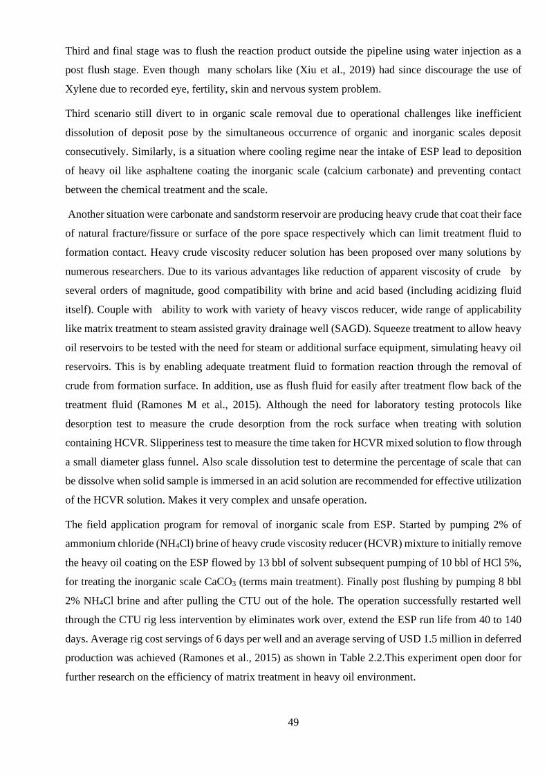
49

Third and final stage was to flush the reaction product outside the pipeline using water injection as a

post flush stage. Even though many scholars like (Xiu et al., 2019) had since discourage the use of

Xylene due to recorded eye, fertility, skin and nervous system problem.

Third scenario still divert to in organic scale removal due to operational challenges like inefficient

dissolution of deposit pose by the simultaneous occurrence of organic and inorganic scales deposit

consecutively. Similarly, is a situation where cooling regime near the intake of ESP lead to deposition

of heavy oil like asphaltene coating the inorganic scale (calcium carbonate) and preventing contact

between the chemical treatment and the scale.

Another situation were carbonate and sandstorm reservoir are producing heavy crude that coat their face

of natural fracture/fissure or surface of the pore space respectively which can limit treatment fluid to

formation contact. Heavy crude viscosity reducer solution has been proposed over many solutions by

numerous researchers. Due to its various advantages like reduction of apparent viscosity of crude by

several orders of magnitude, good compatibility with brine and acid based (including acidizing fluid

itself). Couple with ability to work with variety of heavy viscos reducer, wide range of applicability

like matrix treatment to steam assisted gravity drainage well (SAGD). Squeeze treatment to allow heavy

oil reservoirs to be tested with the need for steam or additional surface equipment, simulating heavy oil

reservoirs. This is by enabling adequate treatment fluid to formation reaction through the removal of

crude from formation surface. In addition, use as flush fluid for easily after treatment flow back of the

treatment fluid (Ramones M et al., 2015). Although the need for laboratory testing protocols like

desorption test to measure the crude desorption from the rock surface when treating with solution

containing HCVR. Slipperiness test to measure the time taken for HCVR mixed solution to flow through

a small diameter glass funnel. Also scale dissolution test to determine the percentage of scale that can

be dissolve when solid sample is immersed in an acid solution are recommended for effective utilization

of the HCVR solution. Makes it very complex and unsafe operation.

The field application program for removal of inorganic scale from ESP. Started by pumping 2% of

ammonium chloride (NH4Cl) brine of heavy crude viscosity reducer (HCVR) mixture to initially remove

the heavy oil coating on the ESP flowed by 13 bbl of solvent subsequent pumping of 10 bbl of HCl 5%,

for treating the inorganic scale CaCO3 (terms main treatment). Finally post flushing by pumping 8 bbl

2% NH4Cl brine and after pulling the CTU out of the hole. The operation successfully restarted well

through the CTU rig less intervention by eliminates work over, extend the ESP run life from 40 to 140

days. Average rig cost servings of 6 days per well and an average serving of USD 1.5 million in deferred

production was achieved (Ramones et al., 2015) as shown in Table 2.2.This experiment open door for

further research on the efficiency of matrix treatment in heavy oil environment.

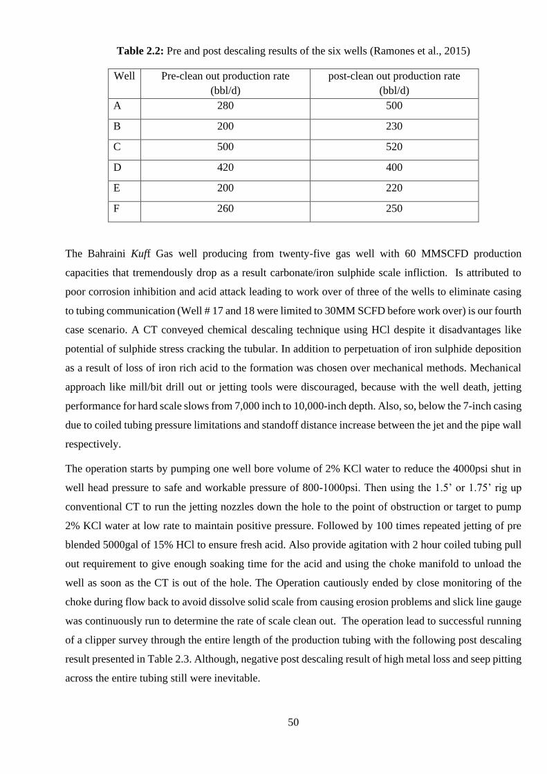
50

Table 2.2: Pre and post descaling results of the six wells (Ramones et al., 2015)

Well Pre-clean out production rate

(bbl/d)

post-clean out production rate

(bbl/d)

A 280 500

B 200 230

C 500 520

D 420 400

E 200 220

F 260 250

The Bahraini Kuff Gas well producing from twenty-five gas well with 60 MMSCFD production

capacities that tremendously drop as a result carbonate/iron sulphide scale infliction. Is attributed to

poor corrosion inhibition and acid attack leading to work over of three of the wells to eliminate casing

to tubing communication (Well # 17 and 18 were limited to 30MM SCFD before work over) is our fourth

case scenario. A CT conveyed chemical descaling technique using HCl despite it disadvantages like

potential of sulphide stress cracking the tubular. In addition to perpetuation of iron sulphide deposition

as a result of loss of iron rich acid to the formation was chosen over mechanical methods. Mechanical

approach like mill/bit drill out or jetting tools were discouraged, because with the well death, jetting

performance for hard scale slows from 7,000 inch to 10,000-inch depth. Also, so, below the 7-inch casing

due to coiled tubing pressure limitations and standoff distance increase between the jet and the pipe wall

respectively.

The operation starts by pumping one well bore volume of 2% KCl water to reduce the 4000psi shut in

well head pressure to safe and workable pressure of 800-1000psi. Then using the 1.5’ or 1.75’ rig up

conventional CT to run the jetting nozzles down the hole to the point of obstruction or target to pump

2% KCl water at low rate to maintain positive pressure. Followed by 100 times repeated jetting of pre

blended 5000gal of 15% HCl to ensure fresh acid. Also provide agitation with 2 hour coiled tubing pull

out requirement to give enough soaking time for the acid and using the choke manifold to unload the

well as soon as the CT is out of the hole. The Operation cautiously ended by close monitoring of the

choke during flow back to avoid dissolve solid scale from causing erosion problems and slick line gauge

was continuously run to determine the rate of scale clean out. The operation lead to successful running

of a clipper survey through the entire length of the production tubing with the following post descaling

result presented in Table 2.3. Although, negative post descaling result of high metal loss and seep pitting

across the entire tubing still were inevitable.

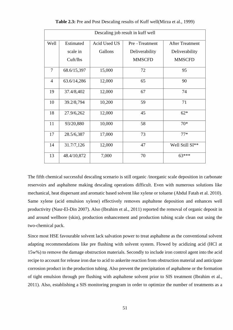
51

Table 2.3: Pre and Post Descaling results of Kuff well(Mirza et al., 1999)

Descaling job result in kuff well

Well Estimated

scale in

Cuft/lbs

Acid Used US

Gallons

Pre –Treatment

Deliverability

MMSCFD

After Treatment

Deliverability

MMSCFD

7 68.6/15,397 15,000 72 95

4 63.6/14,286 12,000 65 90

19 37.4/8,402 12,000 67 74

10 39.2/8,794 10,200 59 71

18 27.9/6,262 12,000 45 62*

11 93/20,880 10,000 58 70*

17 28.5/6,387 17,000 73 77*

14 31.7/7,126 12,000 47 Well Still SI**

13 48.4/10,872 7,000 70 63***

The fifth chemical successful descaling scenario is still organic /inorganic scale deposition in carbonate

reservoirs and asphaltene making descaling operations difficult. Even with numerous solutions like

mechanical, heat dispersant and aromatic based solvent like xylene or toluene (Abdul Fatah et al. 2010).

Same xylene (acid emulsion xylene) effectively removes asphaltene deposition and enhances well

productivity (Nasr-El-Din 2007). Also (Ibrahim et al., 2011) reported the removal of organic deposit in

and around wellbore (skin), production enhancement and production tubing scale clean out using the

two-chemical pack.

Since most HSE favourable solvent lack salvation power to treat asphaltene as the conventional solvent

adapting recommendations like pre flushing with solvent system. Flowed by acidizing acid (HCl at

15w%) to remove the damage obstruction materials. Secondly to include iron control agent into the acid

recipe to account for release iron due to acid to ankerite reaction from obstruction material and anticipate

corrosion product in the production tubing. Also prevent the precipitation of asphaltene or the formation

of tight emulsion through pre flushing with asphaltene solvent prior to SIS treatment (Ibrahim et al.,

2011). Also, establishing a SIS monitoring program in order to optimize the number of treatments as a

52

function of time could tremendously help out but makes the work more complex in addition to the risk

poses from utilisation of hazardous substance like xylene and the rest.

Our last and final scenario in the list of chemical descaling programs that recorded success around the

world. Is the case of utilizing chelating agent to remove pyrite and different type of iron sulphide scale

in oil-gas well without H2S generation which prove stubborn in the past for many approaches. Like the

used of strong acid such as HCl as 10-20WT% considered effective in the dissolution of pyrite (FeS2)

and marcasite form of iron sulphide scale but constrains by amount of large volume of H2S generated

and its corrosive tendency toward the production strings and equipment’s. Since the age of scale

determine its level of solubility with the older scale been less soluble in mineral acid. Mechanical

approach like milling and water jetting with excess pressure up to 140 MPa with or without abrasive was

used to break the scale by making slurry of hard particle that need special gelled for transportation.

Therefore, the requirement of treating each pipe or equipment with significant level of manual

intervention is expensive and time consuming (Mahmoud et al., 2015). So also ineffective for complete

descaling of sulphide scale deposit must especially unexposed area.

The solubility tendency of freshly formed iron sulphide mineral acid as in this case leads to the choice

of chemical mitigation (chelating agent) to be experimented. Executed by pouring chelating agent like

diethylenetriaminepentaacetic acid (DTPA) and converting agent such as potassium carbonate (K2CO3)

along with iron sulphide into a closed flask. Then kept at fixed string speed of 70°C temperature for

varying time period. Determining the solubility of the sample at 24 hours, 48 hours and 72 hours soaking

time respectively. In addition to calculating the solubility of formulation for a specific sample by taking

the percentage difference between initial weight and final weight of the samples. The result concluded

that a maximum of 85% was achieved using combine potassium carbonate and

diethylenetriaminepentaacetic acid. With economic impact of eradicating corrosion inhibition cost and

H2S scavengers as no H2S was generated during the removal process. Serving as multi propose solution

due to its ability to work in both oil and gas field with minimum safety consideration. It should be noted

that the conversion of pyrite to iron carbonate which is soluble in DTPA by the formulation system is

key in the pyrite removal .So also (Mahmoud et al., 2015) added that the high pH medium permit the

transformation of FeS2 to FeCO3 due to ability of potassium ions to occupy and substitute the irons

because of its small size compared to iron ions

2.5.3 Chelating agent

Chelation is the formation of two or more distinct coordinate bonds between single central atom and

polydentate (multiple bonded) lingered which are mostly organic compound. This refers to as

sequestering agent, chelators, chelants or chelating agent. Chelating agent is defined as group of

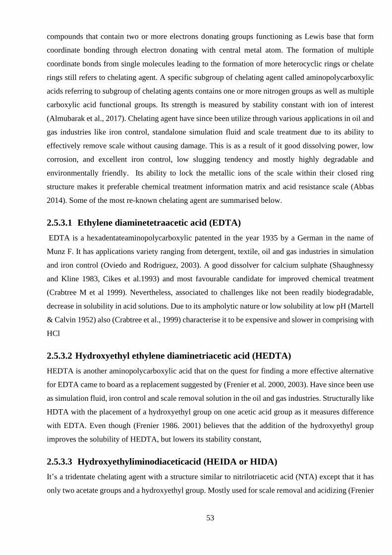
53

compounds that contain two or more electrons donating groups functioning as Lewis base that form

coordinate bonding through electron donating with central metal atom. The formation of multiple

coordinate bonds from single molecules leading to the formation of more heterocyclic rings or chelate

rings still refers to chelating agent. A specific subgroup of chelating agent called aminopolycarboxylic

acids referring to subgroup of chelating agents contains one or more nitrogen groups as well as multiple

carboxylic acid functional groups. Its strength is measured by stability constant with ion of interest

(Almubarak et al., 2017). Chelating agent have since been utilize through various applications in oil and

gas industries like iron control, standalone simulation fluid and scale treatment due to its ability to

effectively remove scale without causing damage. This is as a result of it good dissolving power, low

corrosion, and excellent iron control, low slugging tendency and mostly highly degradable and

environmentally friendly. Its ability to lock the metallic ions of the scale within their closed ring

structure makes it preferable chemical treatment information matrix and acid resistance scale (Abbas

2014). Some of the most re-known chelating agent are summarised below.

2.5.3.1 Ethylene diaminetetraacetic acid (EDTA)

EDTA is a hexadentateaminopolycarboxylic patented in the year 1935 by a German in the name of

Munz F. It has applications variety ranging from detergent, textile, oil and gas industries in simulation

and iron control (Oviedo and Rodriguez, 2003). A good dissolver for calcium sulphate (Shaughnessy

and Kline 1983, Cikes et al.1993) and most favourable candidate for improved chemical treatment

(Crabtree M et al 1999). Nevertheless, associated to challenges like not been readily biodegradable,

decrease in solubility in acid solutions. Due to its ampholytic nature or low solubility at low pH (Martell

& Calvin 1952) also (Crabtree et al., 1999) characterise it to be expensive and slower in comprising with

HCl

2.5.3.2 Hydroxyethyl ethylene diaminetriacetic acid (HEDTA)

HEDTA is another aminopolycarboxylic acid that on the quest for finding a more effective alternative

for EDTA came to board as a replacement suggested by (Frenier et al. 2000, 2003). Have since been use

as simulation fluid, iron control and scale removal solution in the oil and gas industries. Structurally like

HDTA with the placement of a hydroxyethyl group on one acetic acid group as it measures difference

with EDTA. Even though (Frenier 1986. 2001) believes that the addition of the hydroxyethyl group

improves the solubility of HEDTA, but lowers its stability constant,

2.5.3.3 Hydroxyethyliminodiaceticacid (HEIDA or HIDA)

It’s a tridentate chelating agent with a structure similar to nitrilotriacetic acid (NTA) except that it has

only two acetate groups and a hydroxyethyl group. Mostly used for scale removal and acidizing (Frenier

54

2001; Frenier et al. 2004). Numerous advantages like biodegradability, solubility and been a thermal

degradation product of EDTA makes it a good candidate to replace EDTA.

2.5.3.4 L-Glutamic acid N, N-diacetic (GLDA)

L-Glutamic acid N, N-diacetic acid is a new generation chelating agent (Heus et al. 2008) that been

utilize in the area of simulation of carbon, sandstorm reservoir and iron control. Highly soluble in both

water and high concentrated solution acid (LePage et al. 2011) due to attachment of lager group to

iminodiacetic acid that reduce crystallization tendency and increase solubility (De Wolf et al. 2014).

Additionally (Begum et al. 2012a, 2012b) believes that been made from L-glutamic acid or monosodium

glutamate made it more biodegradable and lower in terms of stability constant compared to EDTA and

HEDTA

2.5.3.5 Diethylenetriaminepentaacetic acid (DTPA)

DTPA is an octadentate chelating agent with the highest stability constant among the most commonly

used chelating agent in petroleum industry. This is used in removing hard scale like BaSO4 and SrSO4

(Putnis et al. 1995). Even though scholars like (Sykora et al. 2001) characterised it with low solubility

in water and not readily degradable challenges.

2.5.3.6 Tetraazacyclododecane (DOTA)

1, 4, 7, 10-tetraazacyclododecane: - 1, 4, 7, 10-tetraacetic acid can be best describe as a macrocyclic,

octa dentate. First discovered in the year 1976 and is synthesized using cyclen and bromoacetic acid. It

has been used in medical industry in aspect like magnetic resonance imaging (MRI) scans as an imaging

agent and a radiopharmaceutical (De León-Rodríguez et al. 2008). A chelate lanthanides due to the high

thermal stability and kinetic inertness of the complex formed.

2.5.3.7 Trans-l, 2-cyclohexylenediaminetetraacetic acid (CDTA)

Trans-l, 2-cyclohexylenediaminetetraacetic acid: - is a hexadentate chelating agent also normally used

in the medical industry alongside DOTA. Though have been tested as an alternate acidizing fluid for

carbonate formations in the petroleum industry (Fredd and Fogler 1997). Also (Misra et al. 1988)

considered lipophilic. In addition to being hydrophilic due to the cyclohexane group making it more

effective at alleviating nickel-induced alterations in the body than other chelating agents that are only

hydrophilic.

2.5.3.8 Methylglycinediacetic acid (MGDA)

Methylglycinediacetic acid: - is a quadridentate chelating agent that is prepared by reacting glycine with

formaldehyde and alkali metal cyanide in an alkaline medium (Schneider, et al. 1999). Also developed

55

based on iminodiacetic acid (IDA) with a similar chemical structure to NTA (Heldman et al. 2007). Its

main advantages over the remaining chelating agent are ability to degrade in the absence of adapted

bacteria at standard conditions and to maintain stability despite the effect of pH and temperature

(Kolodynska 2011). Mostly found in chelating agent, dishwashing liquids and detergents.

The chemical structure of the fore listed chelating agents is presented in Figure 2.11.

Figure 2.11: Chemical structures of common aminopolycarboxylic acids (Almubarak et al., 2017)

2.5.4 Factors effecting chelating agents

Many parameters have impact toward the performance of chelating agent in the dissolution of specific

scale. Like the way barite dissolution in DTPA increase from 0-212°F demonstrating a thermal activated

process (Putnis et al., 1995; Dunn and Yen 1999; Putnis et al., 2008). Similar to the thermal unstableness

demonstrated by mixture of EDTA/DTPA after been age for 24 hours at 350°F from a research toward

the impact of high temperature on sulphate scale dissolvers (M. Jordan & Mackay, 2015). While studies

56

on impact of concentration toward the chelating agent performances shows that some of the chelating

agent performance decrease with increase in concentration (Lakatos et al., 2005). Attributed to the

decrease in solubility of the scale dissolvers with increase in their concentration. As a result of firstly

fewer free acetic acid sites on the chelating agent (Lakatos et al., 2005). Secondly, increased steric

hindrance caused by a larger number of chelating agent molecules (there will be more crowding on the

path to the bulk solution and at the barite surface because of increased steric effect) (Putnis et al., 2008).

Through consequences of slowing down the surface chelating process, therefore recommending the

application of multi-cycling injection technique with dilute chelating agent solution (Putnis et al. 1995;

Lakatos et al., 2002a). Another key function effecting the performance of chelating agent is pH value,

for instance is the case of gypsum were the dissolving power was found to be increasing with increase

in pH value when trying to compare solubility of gypsum in EDTA and acidic solution (Al-muntar.s., et

al 2001). At high pH value of (>12) and highly diluted solution of pentapotassium DTPA showed the

most prominent results in barium sulphate dissolution (Putnis et al. 1995; Blanco et al. 1997; Lakatos et

al. 2005, Lakatos et al. (2002b)). While organic acid (maleic, glutamic, succinic, and gluconic) were

found to be very week in iron sulphide scale removal at different pH and concentration condition. On

the contrary (EDTA, DTPA) at a concentration of 25 wt.% and pH of 6 had a solubility of 40 g/litter of

iron sulphide from the solubility result (Elkatatny & Fahd, 2017). So, compatibility in mixing different

type of chelating agent can interfere with its performance like the combination of DTPA/GLDA or

DTPA/MGDA has lower performance than DTPA alone. Due to the barite dissolution been inhibited by

the physical presence of other chelating agent molecules (Shende 2012). Also the mixture of chelating

agent and organic acid was discourage by (Elkatatny & Fahd, 2017) because it reduces it efficiency of

removing iron sulphide.

2.6 Mechanical descaling technique

The mechanical descaling approaches are preferable over chemical approach though depending on the

nature, type, age and location of the scale. More considerable for non-acid tolerance scales and other

poor soluble scales (Coats and Tatarski 1993). Even for the soluble scale like calcium carbonate, the

advantage of solubility in HCl was accompanied by burdens like: Additional inhibition to avoid tubing

damage and post treatment well clean out making mechanical method approach a better option.

Mechanical descaling is achieved either by positive displace motor and mill, liquid jetting or impact

hammer with a mill. Varieties of mechanical descaling tool have been on ground for selection that can

effectively remove scale at any part or location of the production system, most especially for scale

inflicted production tubing through the utilization of techniques like: Abrasive slurries, sterling beads

abrasives, scale blasting technique depending on nature, type and location of the scale deposit (Eltaib et

57

al., 2012). While due to nature of tubing deposited scales mostly very thick, too strong to be remove

with explosives with low porosity (Kamari et al., 2014), making chemical treatment ineffective within a

reasonable time frame.

Despite some identify mechanical descaling approach flops like poor accessibility for scale deposited in

deep formation or proppant pack and high cost due to additional CTU or work over deployment. Its

effectiveness in removing thick scale deposit in tubing make it preferable to the chemical approach that

highly depend on type and location of scale. Couple with ineffectiveness in dissolving some scale species

like sulphate scale and deep in formation deposit (Harms et al., 1988) (far from well bore).

Among many descaling operations were mechanical descaling approach triumph chemical descaling

approach during descaling technique selections are: The case of extensive FeS scale deposit in Gwahr

field carbonate producing zone facing challenges of low pressure, high temperature, open-hole

completion and scale with high specific gravity. Case were work over was knocked out of options due

to high cost, time and production lost. So also chemical approach due to weak dissolution of FeS, safety

concern from high amount of H2S generated while using HCl and potential corrosion leaving CT

deployed mechanical approach as the only economical and safe option (Buali et al., 2014). Another case

can be that of Saudi Arabian carbonate reservoir suffering from scale deposit (mainly iron sulphide

characterized with low solubility). The initial adapted low intervention chemical approach which success

is highly attach to precise understanding of scale composition to modify the dissolver recipes and large

contact area for dissolver to react with, had since been suspended. Due to it negative impact on

productivity, the dissolution of by-product losses into the formation and replace. While Mechanical

option which despite challenges like lifting in-efficiency due to complex wellbore geometry, pipe fatigue

due to frequent CT trips. In addition to possible reservoir damage during temporary isolation was able

to successfully put the well back to production with 25 MMSCFD at 2,750 psi FWHP (Mukhliss et al.,

2014). Even though at the beginning the team had a consensus to intervene with jetting nozzle instead

of a complete descaling work scope.

2.6.1 Types of mechanical descaling techniques

Scale deposit can be effectively removed through mechanical approach by milling, ultrasonic waves,

explosives, water jetting with or without abrasion and the rest. Depending on type of scale, location of

deposit, well architecture and completions, descaling technique and scope/stage of operations (well

accessibility for operation, scale destruction or damage removal) (Bakr et al., 2012). Conditional to the

type of scale, its solubility in acid, acid tolerance of the well, completion integrity and post treatment

cleaning can be solve using conventional mechanical approach (Tatarski, 1993). Either by a positive

displacement motor and mill, an impact hammers with a mill or pure liquid jetting techniques

58

i. Milling operations are preferably chosen over others in the case of: Thick scale, tabular located,

too strong for explosive with poor permeability for effective and reasonable time chemical

treatment and case for creating well access for down-hole tool in blocked tubular (Jordan et al.,

2001). Using motors and cutters to penetrate and cut through scale deposit that are rarely evenly

distributed on tubing wall will always limit it efficiency to the type of scale and applications like

the reduction in motor stall frequency. Faster cutting can be archive by selection small-tooth, less

aggressive mill compared to other. Challenges like the integrity of the tubing string and

operational problems like high torque consumption on mud motor, frequent mill stalling, slowed

ROP (Gholinezhad, 2006). In addition to more intervention time and inefficiency in removing

long depth hard scale interval are inevitable

ii. Explosives or wire line conveyed string shot are good choice for short interval located scale and

other petroleum operations like perforation operations using guns, scale and corrosion deposit

removal in tubular. Through explosive shock generated by pre-determined quantity of detonating

cord, though reduces with increase in depth (<2000 mm) and referable for short interval not long

continues scale deposit. The explosive strength calculation must consider size and type of tabular,

depth to be initiated and wellbore fluid type. It deems time consuming due to the need for

multiple run for given zone and frequent pulling out of tool to analysis the result and the re design

of the amount of explosive for next run. In order to avoid tubing damage due to incorrect amount

of design explosives and allow simulation at will (avoid gas and water bearing reservoir

simulation). Therefore even with it high frequency wave generating ability, (Gholinezhad, 2006)

believes that the choice of explosive for effective decaling will always be disqualified by poor

hard scale removal and both completion and tool destruction.

iii. Ultra-sonic wave technology has been used in various engineering applications like

measurement, cleaning, plastic welding and also for sono-chemistry with 20 to 100kHz

ultrasound power (Mason & Lorimer, 2002). The quest for transforming from chemical to

physical cleaning process to increase cost serving and reduce environmental problems leads to

series of laboratory experiment that prove the successful removal of gypsum. With ultrasonic

wave with amplitude and vibration as key parameters couple with +sonification in a borehole.

For example, could take place in free-flowing wells during production as long as the flow rates

and the velocities at the point of sonification are not too high.

iv. Jetting: -High pressure water jetting application in household and industries had been on record

for a very long time. Petroleum application like high-pressure jet-assisted rock drilling system.

Patented in the year 1963 by the US #3112800 while some of the earliest jetting tools were

patented as back as 1940S (Gholinezhad, 2006). Also reported by (Bajammal et al., 2013) that

59

high pressure jetting has been recently gaining wider acceptance by multinational companies like

Saudi Aramco, schlumberger and the rest in scale removal applications

High pressure jetting is easily archive by focusing the kinetic energy of the high velocity of a fluid (with

or without abrasion) on the target surface to achieve the desires results. It has proven to be simple,

economical (material and equipment requirement), safe, and the only option for non-chemical soluble

scales. It can increasing performance without acidazation in case of high enough permeability formation

and multi-purpose oil and also a gas applications (Aslam et al., 2000). The inexpensive and non-

hazardous nature of water (required material) (Charles et al., 1985), couple with the ability to combing

chemical jetting to produce synergy prove to be 50% more effective than pure water or chemical

treatment solely

Despites limitations like: Ineffectiveness of pure water jetting to clean medium and hard scales in tubing

(Abbas 2014). In addition to the need of special friction reducers to allow higher fluid rates through the

jet, without increasing the fluid viscosity (Charles et al. 1985).Coupled with down-hole challenges like

high ambient pressure, confined operating space and remoteness of the tool from the pump are

formidable and in ability to remove large amount of scale have been recognise (Gholinezhad, 2006). All

these can be tackled through proper detailed engineering design and considering factors like:

Firstly, standoff distance, which have been experimentally proven that it increases lead to reduction of

the jet force impact. For instance, is a rule of thumb for removing moderate to hard scale in a submersed

liquid environment is eight-times of the orifice diameter. Secondly, the fluid velocity and pressure drop

across the orifice are another important parameter to consider. Since long and trapped orifice seems to

produce higher fluid velocity (higher velocity of more than 200ft/sec requirement for hard scales

removal). Thirdly, the jet stream profile referring to the dispersion of the jet stream after it leaves the

orifice which is found to have negative impact towards the efficiency of the jet stream. Though, can be

corrected through good nozzle shape and addition of frictional reducers. Lastly the issue of well and

target coverage as rotational nozzle type take advantage of pulsation effect to provide better coverage

than stationary jet (360o coverage). However, suffering jamming problems during length operation in

corrosive or open hole (Aslam et al., 2000) is among many challenges it faces .

Luckily multiple nozzle approach can compensate the poor coverage limitation attach to stationary

jetting technique as suggested by (Abbas, 2015). While adopting detailed and proper design of internal

fluid path, orifice geometry, jet standoff, high pump rate and using computer simulation for job design.

Together with selections of appropriate size for both coiled tubing and clean out pumping equipment are

the identified solutions to the limitations. Additional solutions include elimination of high energy lose

attributed with two-phase fluid in low hydrostatic well (Campbell et al., 2000). Since the emergence of

60

three distinct categories of tool: Non-rotating high-pressure nozzle, convention drilled nozzle and high-

pressure rotating tool have not yet completely solve the limitations.

The evolution of both jetting tools and approaches in the pursuit of archiving multipurpose and universal

applicable, effective mechanical descaling solution. That is fast, simple, economical, safe for both

equipment and personnel and environmentally friendly. Which selection is not dependable on tools

limitations have been on ongoing since the 1940S. Starting with high pressure pure water jetting with

limitation of only surface testing available (under atmospheric condition or shallow well). Were newly

build equipment will prove excellence and other wise in down-hole condition due to back pressure

impact.

An experimental jetting simulation chamber with realistic down-hole condition was built to test

different tubing scaling of various scale type including sulphide. The results demonstrated poor

performance for pure jetting without dissolvers due to considerable amount of scale left in pipe after

descaling the tube with single water jet at traverse rate of 2.4 in/rein (1 mm/s). It’s considered non-

commercial viability as the jet breaks the scale in large chunk scale size presenting transportation,

trapping and surface handling problems (Pittman 1961). Couple with tubing damage of 0.004in (0.1 mm)

steel removal after impacting jet in a spot for 3 min.

An abrasive trial by adding small sand concentration (1% by volume) improved performance with

consequence of jeopardizing the integrity of completion steel. I.e. focusing the jet for 3 min will lead to

0.19in (0.8mm) steel damage. As choosing round shape particle instead of sharp shape will reduce

damage to completion but reduce performance. While reducing particle hardness will reduce damage

and reduce performance, lead to the replacement of sand particle with special design sterling bead. The

sterling beads performance was exceptional with good well integrity after prolonged jetting on a spot

(Ashley et al 1998). Even though the tubing itself was not damage the plastic coating that line the

production tubing is damage. Surface equipment like choke and valves are at risk due to high density

suspension (liquid and solid) from the beads (Abbas 2014). While (Morkved et al., 2014) added the

requirement of complicated delivery pump to deliver the bead slurry and the slurry may end up been

deposited on the tubing or other hole completion equipment.

As cavitation negative effects toward reduction in performance of high-water jet down-hole lead the

multinationals companies to the introduction of sterling bead (liquid and solid). Environmental and well

integrity negative effect of using sterling bead motivated a solid free jetting descaling technique research

that will not be affected by cavitation effect. Combining both erosion and stress cycling mechanism by

utilizing aerated chambers with incorporated single high-pressure flat fan nozzles. This is to reduce the

amount of water getting into the well (Abbas A 2014). Contrary to multiple nozzle recommendations by

61

(El Kamki 2012) that expect the overlap of the flat fans from multiple nozzles to provides better energy

impact for effective descaling.

The single nozzle solid free jetting tubing descaling trials performance was excellence. Its answer

questions like cavitation suppression distance (stand of distance), relationship between inlet pressure

and cavitation bubble formation mechanism in spray fans, the relationship between aeration and

suppression of cavitation. However, surface testing condition limitations still exist even though aeration

by pressurizing the system could simulate down-hole condition (Abbas 2014). Configuration of multiple

nozzle by incorporating sides, back, forward, down and even angular jet will break the shackle or

stationary jet limitation toward hard scale removal, well and target coverage (Gholinezhad, 2006).

Rotational nozzle type was selected during effective descaling comparison between rotating and

stationary jetting nozzle. The choice basis been due to pulsation effect benefit that allow it to provide

360’degree (Aslam et al., 2000),which can be compensated by multiple jet approach. In case of SO2

removal in a spray tower were the efficiency archived was attributed to simultaneously use of five

nozzles. Which allow full volume coverage of the tower and smaller orifice allows small droplet size

over single nozzle. (Codolo & Bizzo, 2013). Overlap from multiple nozzle provides better energy impact

and scale coverage for effective descaling (El Kamki 2012). Considering the few among many mention

scholars’ recommendation on the adaption of multiple nozzle approach. Couple with both the single

spray limitation, identified research gaps from the single spray approach and quest for improvement.

Motivated the extension of the single nozzle research into multiple nozzle research four years later. The

detailing on the mechanism and types of jetting techniques will be done in the forthcoming chapter.

2.6.2 Successful mechanical descaling operation.

Few to mention among many successful mechanical descaling operations around the globe include

statjord field in North Sea operated by Statoil company. That have a history of drastic production decline

with 60% of its STOOIP been recovered via secondary recovery techniques for over 23 years leaving

complex distribution of by-passed oil reserve, gas and water due to hard scale deposit. Cost of differing

production and long delivery time lead to the replacement of the conventional CT with the combination

of wire line brushes (WL) together with stiff wire line brushes, wire-line tractor (WLT) milling and

string shots. Immediately after two successful runs of the combination, the scale falls out of the tubing

wall. While the multi run of multi finger clipper (MFC) carried to evaluate the level of descaling showed

a maximum of 1inc variable scale layer thickness, which was completely cleared (Sr/BaSO4 hard scale)

at the end of the 15.5 days operations (Børeng et al., 2002). After firing several shot using string shots,

scale dissolvers, WLT with torque adapter and mill, brushes and broaches a 630 bbl/d post descaling

production result was recorded.

62

The second successful mechanical descaling scenario will be carbonate producing gas zone of Ghawar

field suffering from chronic FeS scale deposition. The deposit is responsible for dropped in production

rate and making well intervention riskier. Couple with operational challenges like low reservoir pressure,

increased reservoir temperature, horizontal open-hole completion, and scale with high specific gravity.

Challenges that makes mechanical descaling approach economical and safely preferable over work over.

Also, chemical techniques were ruled out due to the poor solubility of FeS in HCl and amount of H2S

generated in additional to already existing H2S in the reservoir. The successful mechanical descaling

programme is as follows

i. Reservoir isolation includes the combination of LCM particle-based pills together with fully

cross-linked polysaccharide polymer. To act as chemical packer for proper reservoir isolation of

the two laterals open holes (approximately 3,401 ft. length and 57/8-in) instead of the two batches

of CaCO3 earlier tried.

ii. A motor and mill were successfully run together with slow rotating blasting tools to clean the

linear and tubing section which usefully recover finer scale at the surface. The fluid oscillator

and hydra jet tools with ball isolation activation sleeves in tandem was effectively and safely

used to clean and simulate the open hole section in one trip. While for the horizontal long lateral

open hole a combination of acid hydra jetting and matrix acidizing technologies in this naturally

fractured carbonate formation was used to achieve simulation.

Comparing the post scaling nodal analysis result from reservoir department, a considerable skin

decreases of -3.8, a production increase of 5 MMSCFD to 26 MMSCFD and 27 MMSCFD at a WHP of

2,100 psi at 2008 results. The 2008 pre-treatment well performance analysis result shows -0.45 well

skin with a k*h of 126 md-ft (k = 1.9 md and h = 65 ft,) and production rate of 17 MMSCF/D and 19

MMSCF/D and buttonhole shut-in pressure (BHSIP) of 1, 215 psi. (Buali et al., 2014) reported that the

comparison confirms the level of achievement of the descaling program.

Saudi Aramco’s past descaling approach in the Kuff Gas well by deploying a high-pressure jet (with or

without abrasion) through CTU in an under balance well conditions lead to many challenges. The

challenges include: Choke erosion by large-scale debris resulting to sour gas leak at surface and CT

stuck pipe lead to emergency shutdown of the well. Also embarking on integrated innovated job design

with the aim of removing the scale with the rig on side and perforating and removing formation damage

in a rig-less approach is our third successful mechanical descaling scenario.

i. Temporary reservoir isolations using calcium carbonate plugs to ensure controlled, safe and

closed system environment with a non-nitrogen gelled fluid for scale removal. Since down-hole

motor tubing with mill is expected to cut scale into smaller particles for safe and easy transport.

63

ii. The well was clean with high pressure jetting tool, and turbine through combination of 2-3/8

inches FOECT strings and special high temperature gelled (stable up to 325°F) for high pumping

rate/annular gel velocity and better suspension/transport

iii. Abrasive slot cutting tool and CT matrix stimulation monitored and optimized with FOECT real-

time down-hole measurements. Including DTS were used to for perforation and formation

damage removal.

The implementation of the above programme re-claimed the wellbore accessibility and increase it gas

production without final acid simulation for the five tested wells (Bolarinwa et al., 2012).The

achievements are described in the Table 2.4 even though scale inhibition have been recommended for

inclusion in future descaling operations for both sandstone and carbonate reservoir.

Table 2.4: Pre and Post Descaling Results for five Kuff Gas wells (Bolarinwa et al., 2012)

well Pre-treatment

Gas Rate

Flowing WHP

Post treatment Gas

Rate

Flowing WHP

A

5 MMSCFD 1,380 psi

7.5 MMSCFD 1,620 psi

B 35 MMSCFD 1,300 psi

31 MMSCFD 1,650 psi

C 20 MMSCFD 2,150 psi

35 MMSCFD 2,170 psi

D 5 MMSCFD

1,450 psi

15 MMSCFD 1,450 psi

E 30 MMSCFD 1,500 psi 37 MMSCFD 2,330 psi

The fourth scenario is field (EW 873) in an offshore, a mature field of the Gulf of Mexico that had been

producing from an unconsolidated sandstone reservoir of Middle- Upper Pliocene age. With some of the

wells like Well A-04 suffering from near wellbore impairment and BaSO4 scale build up in the tabular

throughout their production cycle due to biocide inhibition and water breakthrough related problems.

The implementation of the following five steps descaling programmes with the aim of providing enough

well access through the removal of the BaSO4 scale deposit. In order to create opportunity to conduct a

chelate-based HF acid treatment for the impaired NWB was successful. Achieved by removing 3,150 ft.

MD of BaSO4 tubular scale with no environmental or OSHA recordable incidents (Sopngwi et al,. 2014).

Through a well design coiled tubing- conveyed hydro blasting intervention and the post chelating HF

acid treatment increase the well production by almost 305%.

Step one started by selecting the best approach for BaSO4 scale removal from tubular and a coiled tubing-

conveyed hydro blasting technique was selected. Since its performance was tied to the nature and

magnitude of the BaSO4, as well as effective operational planning.

64

Step two is using INSITE a well intervention (IWI) software for selection of optimal jet-nozzle

configuration and resulting nozzle pressure drop that would optimize both cleaning coverage of BaSO4

in the tabular and jetting penetration rate.

Step three was the main intervention that include running through the hole with intervention BHA in CT

down to 9,000 ft. MD at 60 fpm, while using nitrified brine to break circulation. Then hydro blasting

from 12,150 ft. MD at 5fpm while sustaining circulation with nitrifies brine subsequently reciprocating

from 9,000 to 12,150 ft. MD at 5 fpm. Finally pulling out both CT and intervention BHA at 60 fpm still

maintaining circulation with nitrifies fluid.

Fourth and fifth steps were to conduct an integrated peer review to develop a mitigation plan that will

reduce operation, technical, HSE and financial risk associated to the design. While the fifth step

(execution) as reported by (Sopngwi et al., 2014) was proven successful after effective design

implementation with no environmental or OSHA recordable incidents.

Fifth Scenario will be a Petro Brass operated field in the Brazilian offshore diagnosed with barium or

strontium sulphate scale. Which were both not soluble in conventional acid and EDTA even though its

reaction to barium sulphate dissolver only attest the scale composition.

A careful jetting technology job design that includes a jet nozzle header with Swivel; drift ring and high-

pressure in order to keep scale cuttings in stream until circulated out. A high-pressure filter to serve as

a screen mesh that will block large particles and allow only the abrasive particles to pass through. The

Schlumberger’ special design abrasive material of rounded geometry and small in size to enhances scale

erosive performance with little or no damage to the string or jewellery completion is used. In addition

to software package for performance optimization and tool selection. Finally maintaining continues gas

lift injection, pumping cleaning gel batches (10 bbl.) after every 20 meters sections. Coupled with a

nitrogen unit back up for circulation drop during the whole treatment duration for better solid and

wellbore clean out due to the low reservoir pressure and fluids production rates.

The 7 days planned operation was successfully completely executed at the eleventh day whit a 1025%

production increase by removing depositing around 66,000 lbs of solid debris at the surface. A 19 days’

whole intervention pay out time with no records of incidence on both environment and equipment from

the QHSE performance result as presented in Table 2.5. Declaring the abrasive jetting an

environmentally friendly chemicals or green substitute for conventional environmental unfriendly

dissolvers.

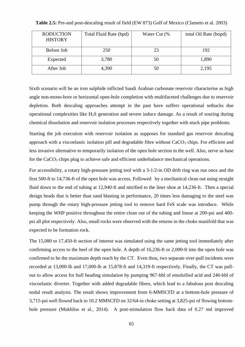
65

Table 2.5: Pre-and post-descaling result of field (EW 873) Golf of Mexico (Clameto et al. 2003)

RODUCTION

HISTORY

Total Fluid Rate (bpd) Water Cut (% total Oil Rate (bopd)

Before Job 250 23 192

Expected 3,780 50 1,890

After Job 4,390 50 2,195

Sixth scenario will be an iron sulphide inflicted Saudi Arabian carbonate reservoir characterise as high

angle non-mono-bore or horizontal open-hole completion with multifaceted challenges due to reservoir

depletion. Both descaling approaches attempt in the past have suffers operational setbacks due

operational complexities like H2S generation and severe induce damage. As a result of souring during

chemical dissolution and reservoir isolation processes respectively together with stuck pipe problems.

Starting the job execution with reservoir isolation as supposes for standard gas reservoir descaling

approach with a viscoelastic isolation pill and degradable fibre without CaCO3 chips. For efficient and

less invasive alternative to temporarily isolation of the open hole section in the well. Also, serve as base

for the CaCO3 chips plug to achieve safe and efficient underbalance mechanical operations.

For accessibility, a rotary high-pressure jetting tool with a 3-1/2-in OD drift ring was run once and the

first 500-ft to 14,736-ft of the open hole was access. Followed by a mechanical clean out using straight

fluid down to the end of tubing at 12,940-ft and nitrified to the liner shoe at 14,236-ft. Then a special

design beads that is better than sand blasting in performance, 20 times less damaging to the steel was

pump through the rotary high-pressure jetting tool to remove hard FeS scale was introduce. While

keeping the WHP positive throughout the entire clean out of the tubing and linear at 200-psi and 400-

psi all plot respectively. Also, small rocks were observed with the returns in the choke manifold that was

expected to be formation rock.

The 15,080 to 17,450-ft section of interest was simulated using the same jetting tool immediately after

confirming access to the heel of the open hole. A depth of 16,236-ft or 2,000-ft into the open hole was

confirmed to be the maximum depth reach by the CT. Even thou, two separate over-pull incidents were

recorded at 13,000-lb and 17,000-lb at 15,878-ft and 14,319-ft respectively. Finally, the CT was pull-

out to allow access for bull heading simulation by pumping 967-bbl of emulsified acid and 240-bbl of

viscoelastic diverter. Together with added degradable fibres, which lead to a fabulous post descaling

nodal result analysis. The result shows improvement from 6-MMSCFD at a bottom-hole pressure of

3,715-psi well flowed back to 10.2 MMSCFD on 32/64-in choke setting at 3,825-psi of flowing bottom-

hole pressure (Mukhliss et al., 2014). A post-stimulation flow back data of 0.27 md improved

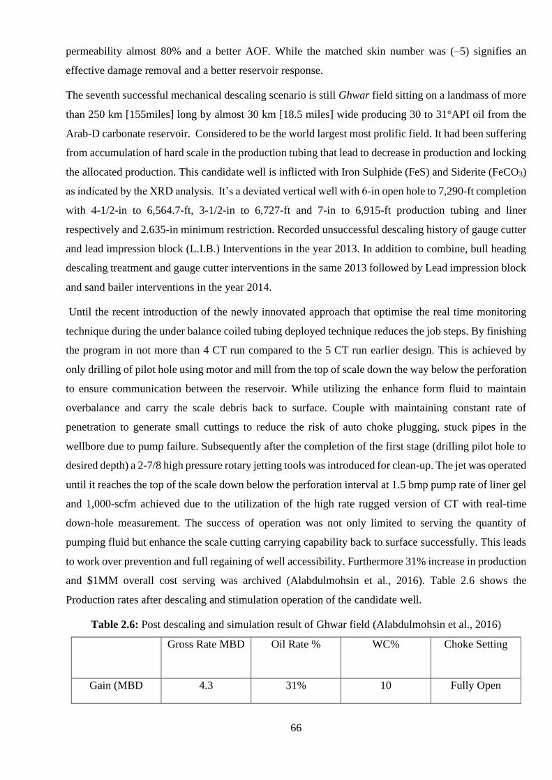
66

permeability almost 80% and a better AOF. While the matched skin number was (–5) signifies an

effective damage removal and a better reservoir response.

The seventh successful mechanical descaling scenario is still Ghwar field sitting on a landmass of more

than 250 km [155miles] long by almost 30 km [18.5 miles] wide producing 30 to 31°API oil from the

Arab-D carbonate reservoir. Considered to be the world largest most prolific field. It had been suffering

from accumulation of hard scale in the production tubing that lead to decrease in production and locking

the allocated production. This candidate well is inflicted with Iron Sulphide (FeS) and Siderite (FeCO3)

as indicated by the XRD analysis. It’s a deviated vertical well with 6-in open hole to 7,290-ft completion

with 4-1/2-in to 6,564.7-ft, 3-1/2-in to 6,727-ft and 7-in to 6,915-ft production tubing and liner

respectively and 2.635-in minimum restriction. Recorded unsuccessful descaling history of gauge cutter

and lead impression block (L.I.B.) Interventions in the year 2013. In addition to combine, bull heading

descaling treatment and gauge cutter interventions in the same 2013 followed by Lead impression block

and sand bailer interventions in the year 2014.

Until the recent introduction of the newly innovated approach that optimise the real time monitoring

technique during the under balance coiled tubing deployed technique reduces the job steps. By finishing

the program in not more than 4 CT run compared to the 5 CT run earlier design. This is achieved by

only drilling of pilot hole using motor and mill from the top of scale down the way below the perforation

to ensure communication between the reservoir. While utilizing the enhance form fluid to maintain

overbalance and carry the scale debris back to surface. Couple with maintaining constant rate of

penetration to generate small cuttings to reduce the risk of auto choke plugging, stuck pipes in the

wellbore due to pump failure. Subsequently after the completion of the first stage (drilling pilot hole to

desired depth) a 2-7/8 high pressure rotary jetting tools was introduced for clean-up. The jet was operated

until it reaches the top of the scale down below the perforation interval at 1.5 bmp pump rate of liner gel

and 1,000-scfm achieved due to the utilization of the high rate rugged version of CT with real-time

down-hole measurement. The success of operation was not only limited to serving the quantity of

pumping fluid but enhance the scale cutting carrying capability back to surface successfully. This leads

to work over prevention and full regaining of well accessibility. Furthermore 31% increase in production

and $1MM overall cost serving was archived (Alabdulmohsin et al., 2016). Table 2.6 shows the

Production rates after descaling and stimulation operation of the candidate well.

Table 2.6: Post descaling and simulation result of Ghwar field (Alabdulmohsin et al., 2016)

Gross Rate MBD Oil Rate % WC% Choke Setting

Gain (MBD 4.3 31% 10 Fully Open

67

2.7 Summary

• The chapter reflects on petroleum production and the challenges involved like concept,

mechanism and implication of scale formation problems. Couple with proffer solution including

prevention, cure and its economy with cited examples around the world:

• Minerals and heavy hydrocarbon scale deposit remain the most frightening problems among all

flow assurance problems.

• Mixture of incompatible water is key among other scale formation influencing factors like

temperature, pressure, pH and the rest.

• Scale categorization and classification are based on many factors but scale chemical and

compositional analysis by (combination of SEM, EDS, XRD & XRF) is more precise for hard

scale and NMR/FTIR for soft scale.

• Barium, strontium and iron sulphide scale are found to be the most troublesome deposit in

petroleum production.

• It’s paramount to incorporate scale management in the life cycle of a field by proper plan strategy

at CAPEX phase of a field. Through predicting and preventing scale formation since is far

economically better than remedial/removing the scale deposit at OPEX phase of the field.

• In case of failed scale prevention strategy, the removal of existing deposit remains the only option

and must be in a fast and non-damaging manner. (i.e. faster, easier, cheaper and safe for both

personnel, well completion and the well environs).

• Chemical descaling approaches are good only on acid soluble scale type with a lot of operational

and environmental challenges. Though chelating agent are better in dissolution power but still

not yet HSE certified.

• Mechanical descaling approach proved efficient in removing the non-soluble scale types and the

rest. Nevertheless, most of the approaches were found far from successful descaling compliance

(i.e. explosives jeopardizing the integrity of well completions).

• Jetting techniques are the most effective mechanical approach. Pure water high pressure spray

jetting keeps gaining wider acceptance due to its ability to safely clean production tubing in

comparison to other approaches (i.e. abrasion by sterling beads and the rest).

• Despite the tremendous achievement of single spray high pressure pure water jetting. Multiple

nozzle has been suggested to compensate single nozzle and stationary spray research gaps like

poor coverage, archiving more than one jetting mechanism (cycling stress, abrasion, cavitation

and erosion) and the rest.

68

Jet Spray Dynamics and Mechanism

3.1 Overview

This chapter provide the fundamental and advantage of solid free high-pressure water jet over others.

Starting with explanation on the performance of a nozzle or spraying system in terms of parameters and

factors that affect the performance of a spray system. Followed by discussion on atomization process in

respect of types and classification of atomisers, patternation and liquid break up process. Then analysis

of flow behaviour, spray characterization of multiple nozzle spray focusing investigations on essential

parameters like: Droplet velocity, droplet size, distribution and pressure drop. Highlighted advantage

and benefit of adopting multiple nozzles over single nozzle and ability of solid free jet to effectively

perform down-hole without the use of starling bead. Precise emphasis was provided on flat fan high

pressure nozzles, considering its suitability in descaling petroleum production tubing as selected in this

research. Subsequently introduces mechanical descaling techniques by concentrating on the aspect of

jetting mechanism (erosion, abrasion, cycling stress and cavitation). Closing with their description,

influencing factors, uses, operative mechanism, and relationship to fundamental parameters when

utilizing multiple spray system including effect of pressure drop, and spray overlap region toward

multiple nozzles spray performance. So also, benefit toward effective descaling operations, together with

examples of successful jetting descaling operation around the globe.

3.2 Nozzle performance

The basic functions of spray nozzles are to distribute liquid, break up liquid into droplet and as meter

flow. Spray nozzle performance depend on the level of operating efficiency of the entire spray system.

Therefore, it is vital to understand the relationship of spray performance to factors like: The operation

conditions i.e. temperature, pressure and variable line speed, type of the liquid been sprayed and the

position and placement of nozzle in respect to the target.

3.2.1 Spray system

As earlier mentioned, that the performances of a nozzle are tied to the operational effectiveness of the

entire spray systems consisting the atomizer/ headers manifold, system design, fittings/connections,

pump etc.

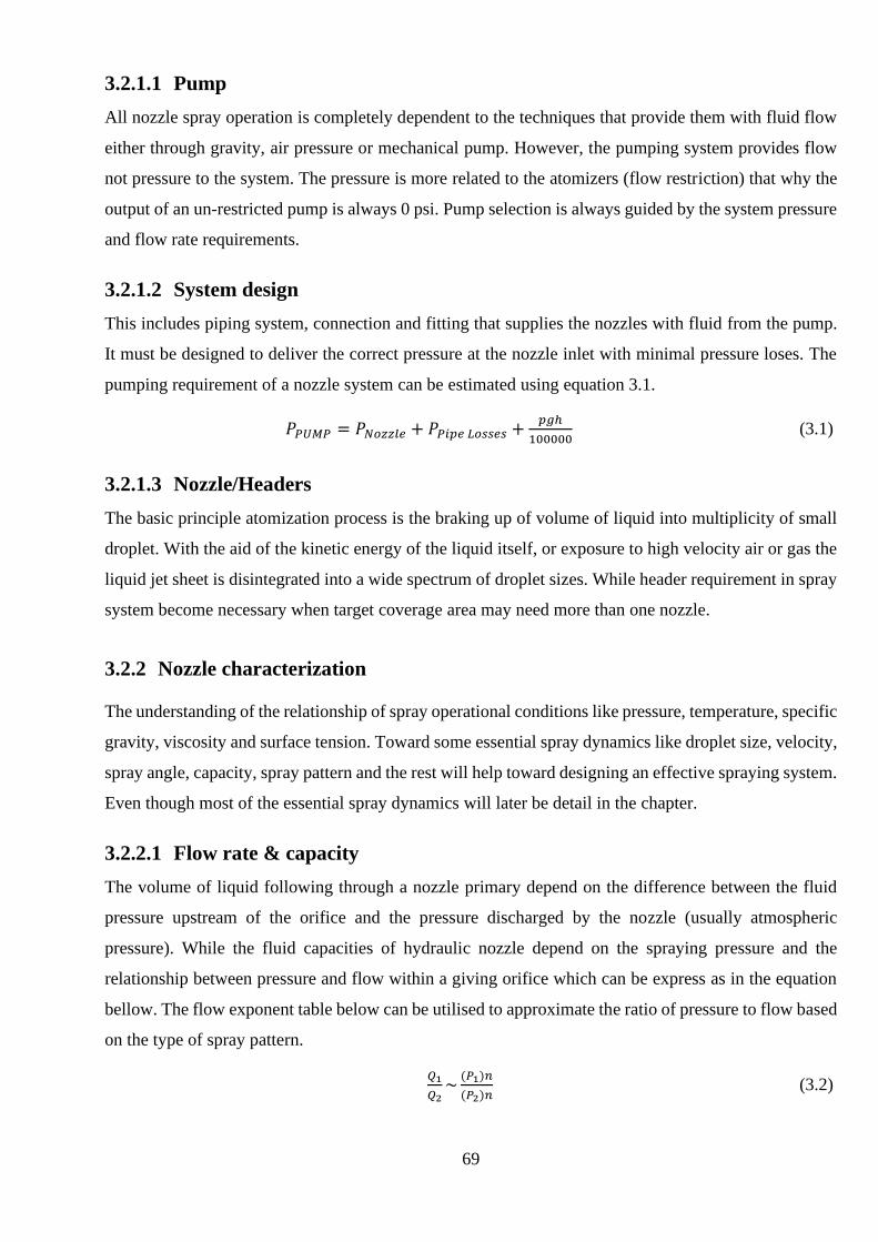
69

3.2.1.1 Pump

All nozzle spray operation is completely dependent to the techniques that provide them with fluid flow

either through gravity, air pressure or mechanical pump. However, the pumping system provides flow

not pressure to the system. The pressure is more related to the atomizers (flow restriction) that why the

output of an un-restricted pump is always 0 psi. Pump selection is always guided by the system pressure

and flow rate requirements.

3.2.1.2 System design

This includes piping system, connection and fitting that supplies the nozzles with fluid from the pump.

It must be designed to deliver the correct pressure at the nozzle inlet with minimal pressure loses. The

pumping requirement of a nozzle system can be estimated using equation 3.1.

𝑃𝑃𝑈𝑀𝑃 = 𝑃𝑁𝑜𝑧𝑧𝑙𝑒 + 𝑃𝑃𝑖𝑝𝑒 𝐿𝑜𝑠𝑠𝑒𝑠 +𝑝𝑔ℎ

100000 (3.1)

3.2.1.3 Nozzle/Headers

The basic principle atomization process is the braking up of volume of liquid into multiplicity of small

droplet. With the aid of the kinetic energy of the liquid itself, or exposure to high velocity air or gas the

liquid jet sheet is disintegrated into a wide spectrum of droplet sizes. While header requirement in spray

system become necessary when target coverage area may need more than one nozzle.

3.2.2 Nozzle characterization

The understanding of the relationship of spray operational conditions like pressure, temperature, specific

gravity, viscosity and surface tension. Toward some essential spray dynamics like droplet size, velocity,

spray angle, capacity, spray pattern and the rest will help toward designing an effective spraying system.

Even though most of the essential spray dynamics will later be detail in the chapter.

3.2.2.1 Flow rate & capacity

The volume of liquid following through a nozzle primary depend on the difference between the fluid

pressure upstream of the orifice and the pressure discharged by the nozzle (usually atmospheric

pressure). While the fluid capacities of hydraulic nozzle depend on the spraying pressure and the

relationship between pressure and flow within a giving orifice which can be express as in the equation

bellow. The flow exponent table below can be utilised to approximate the ratio of pressure to flow based

on the type of spray pattern.

𝑄1

𝑄2~

(𝑃1)𝑛

(𝑃2)𝑛 (3.2)

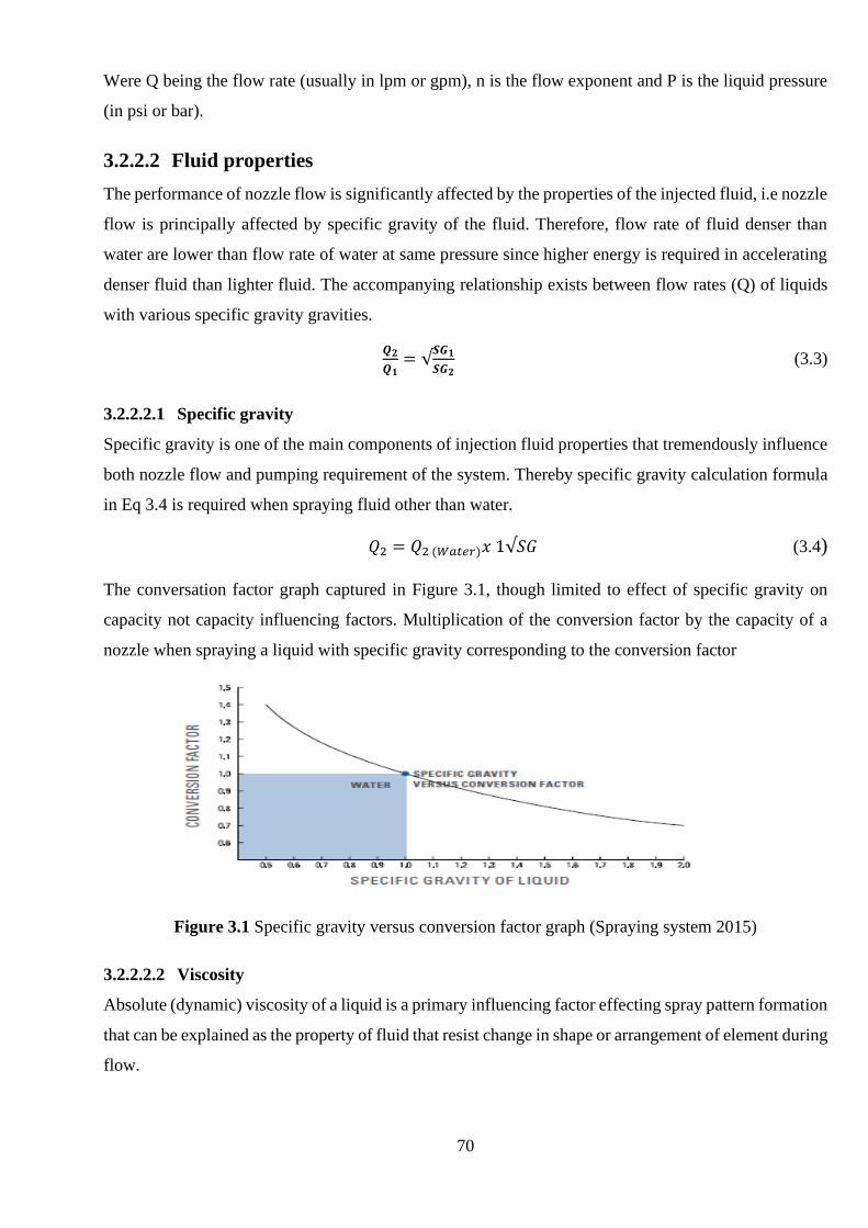
70

Were Q being the flow rate (usually in lpm or gpm), n is the flow exponent and P is the liquid pressure

(in psi or bar).

3.2.2.2 Fluid properties

The performance of nozzle flow is significantly affected by the properties of the injected fluid, i.e nozzle

flow is principally affected by specific gravity of the fluid. Therefore, flow rate of fluid denser than

water are lower than flow rate of water at same pressure since higher energy is required in accelerating

denser fluid than lighter fluid. The accompanying relationship exists between flow rates (Q) of liquids

with various specific gravity gravities.

𝑸𝟐

𝑸𝟏= √

𝑺𝑮𝟏

𝑺𝑮𝟐 (3.3)

3.2.2.2.1 Specific gravity

Specific gravity is one of the main components of injection fluid properties that tremendously influence

both nozzle flow and pumping requirement of the system. Thereby specific gravity calculation formula

in Eq 3.4 is required when spraying fluid other than water.

𝑄2 = 𝑄2 (𝑊𝑎𝑡𝑒𝑟)𝑥 1√𝑆𝐺 (3.4)

The conversation factor graph captured in Figure 3.1, though limited to effect of specific gravity on

capacity not capacity influencing factors. Multiplication of the conversion factor by the capacity of a

nozzle when spraying a liquid with specific gravity corresponding to the conversion factor

Figure 3.1 Specific gravity versus conversion factor graph (Spraying system 2015)

3.2.2.2.2 Viscosity

Absolute (dynamic) viscosity of a liquid is a primary influencing factor effecting spray pattern formation

that can be explained as the property of fluid that resist change in shape or arrangement of element during

flow.

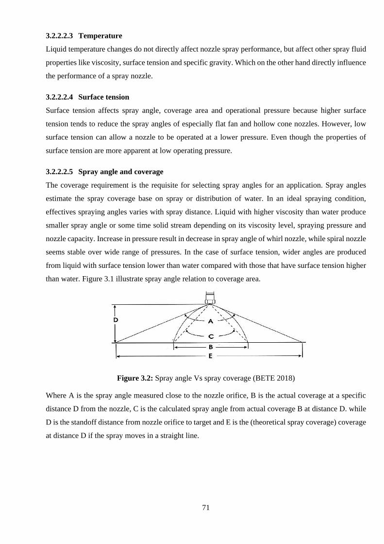
71

3.2.2.2.3 Temperature

Liquid temperature changes do not directly affect nozzle spray performance, but affect other spray fluid

properties like viscosity, surface tension and specific gravity. Which on the other hand directly influence

the performance of a spray nozzle.

3.2.2.2.4 Surface tension

Surface tension affects spray angle, coverage area and operational pressure because higher surface

tension tends to reduce the spray angles of especially flat fan and hollow cone nozzles. However, low

surface tension can allow a nozzle to be operated at a lower pressure. Even though the properties of

surface tension are more apparent at low operating pressure.

3.2.2.2.5 Spray angle and coverage

The coverage requirement is the requisite for selecting spray angles for an application. Spray angles

estimate the spray coverage base on spray or distribution of water. In an ideal spraying condition,

effectives spraying angles varies with spray distance. Liquid with higher viscosity than water produce

smaller spray angle or some time solid stream depending on its viscosity level, spraying pressure and

nozzle capacity. Increase in pressure result in decrease in spray angle of whirl nozzle, while spiral nozzle

seems stable over wide range of pressures. In the case of surface tension, wider angles are produced

from liquid with surface tension lower than water compared with those that have surface tension higher

than water. Figure 3.1 illustrate spray angle relation to coverage area.

Figure 3.2: Spray angle Vs spray coverage (BETE 2018)

Where A is the spray angle measured close to the nozzle orifice, B is the actual coverage at a specific

distance D from the nozzle, C is the calculated spray angle from actual coverage B at distance D. while

D is the standoff distance from nozzle orifice to target and E is the (theoretical spray coverage) coverage

at distance D if the spray moves in a straight line.

72

3.2.2.3 Atomization

Atomization has a direct effect to droplet sizes, droplet distribution and spray pattern. A droplet size

refers to individual spray droplet sizes that encompass a nozzle spray pattern. Spray pattern is use in

describing the location and density of the liquid released from a nozzle. While the range of spray drop

sizes provided by individual spray is term the drop size distribution, which depend on the type of spray

pattern, and varies from one type to another. Smallest drop size is obtained through air nozzle

atomization while the largest drop sizes are obtained through full cone hydraulic spray nozzle. Droplet

size requirement is relative to spray application like gas scrubbing strongly depending on exposing the

maximum possible volume of liquid surface to gas stream. Droplet size is affected by liquid property,

spraying pressure, nozzle capacity and spray angle. The higher the pressure, the lower the droplet sizes,

the higher the nozzle flow, the larger the droplet sizes and the higher the surface tension the larger the

drop size. Droplet velocity is dependent on droplet size that why small drop sizes have higher initial

velocity but quickly diminish, while larger drop sizes have the ability to maintain velocity for long and

travel further. Types of droplet sizes produce from different types of automiser is shown in Figure 3.3.

and summary of spray performance is presented in Table 3.1.

Figure 3.3: Atomization (droplet size and distribution) (Spraying system 2015)

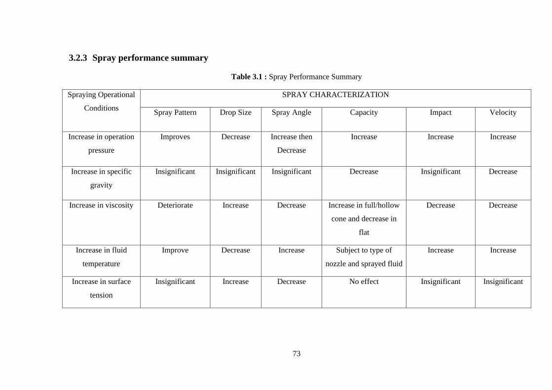
73

3.2.3 Spray performance summary

Table 3.1 : Spray Performance Summary

Spraying Operational

Conditions

SPRAY CHARACTERIZATION

Spray Pattern Drop Size Spray Angle Capacity Impact Velocity

Increase in operation

pressure

Improves Decrease Increase then

Decrease

Increase Increase Increase

Increase in specific

gravity

Insignificant Insignificant Insignificant Decrease Insignificant Decrease

Increase in viscosity Deteriorate Increase Decrease Increase in full/hollow

cone and decrease in

flat

Decrease Decrease

Increase in fluid

temperature

Improve Decrease Increase Subject to type of

nozzle and sprayed fluid

Increase Increase

Increase in surface

tension

Insignificant Increase Decrease No effect Insignificant Insignificant

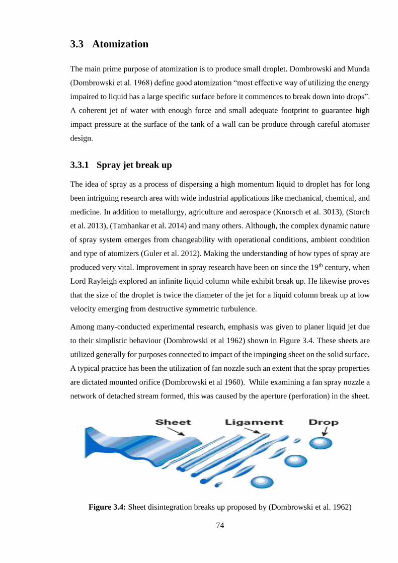
74

3.3 Atomization

The main prime purpose of atomization is to produce small droplet. Dombrowski and Munda

(Dombrowski et al. 1968) define good atomization “most effective way of utilizing the energy

impaired to liquid has a large specific surface before it commences to break down into drops”.

A coherent jet of water with enough force and small adequate footprint to guarantee high

impact pressure at the surface of the tank of a wall can be produce through careful atomiser

design.

3.3.1 Spray jet break up

The idea of spray as a process of dispersing a high momentum liquid to droplet has for long

been intriguing research area with wide industrial applications like mechanical, chemical, and

medicine. In addition to metallurgy, agriculture and aerospace (Knorsch et al. 3013), (Storch

et al. 2013), (Tamhankar et al. 2014) and many others. Although, the complex dynamic nature

of spray system emerges from changeability with operational conditions, ambient condition

and type of atomizers (Guler et al. 2012). Making the understanding of how types of spray are

produced very vital. Improvement in spray research have been on since the 19th century, when

Lord Rayleigh explored an infinite liquid column while exhibit break up. He likewise proves

that the size of the droplet is twice the diameter of the jet for a liquid column break up at low

velocity emerging from destructive symmetric turbulence.

Among many-conducted experimental research, emphasis was given to planer liquid jet due

to their simplistic behaviour (Dombrowski et al 1962) shown in Figure 3.4. These sheets are

utilized generally for purposes connected to impact of the impinging sheet on the solid surface.

A typical practice has been the utilization of fan nozzle such an extent that the spray properties

are dictated mounted orifice (Dombrowski et al 1960). While examining a fan spray nozzle a

network of detached stream formed, this was caused by the aperture (perforation) in the sheet.

Figure 3.4: Sheet disintegration breaks up proposed by (Dombrowski et al. 1962)

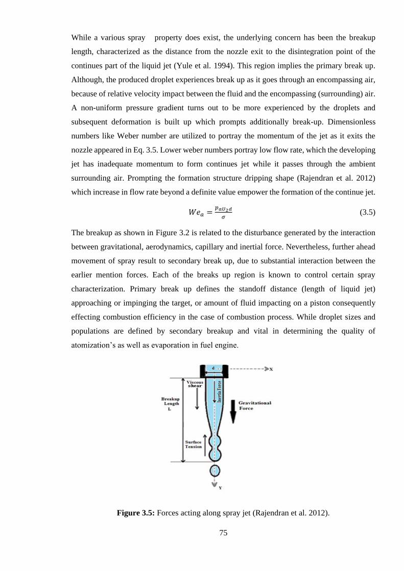
75

While a various spray property does exist, the underlying concern has been the breakup

length, characterized as the distance from the nozzle exit to the disintegration point of the

continues part of the liquid jet (Yule et al. 1994). This region implies the primary break up.

Although, the produced droplet experiences break up as it goes through an encompassing air,

because of relative velocity impact between the fluid and the encompassing (surrounding) air.

A non-uniform pressure gradient turns out to be more experienced by the droplets and

subsequent deformation is built up which prompts additionally break-up. Dimensionless

numbers like Weber number are utilized to portray the momentum of the jet as it exits the

nozzle appeared in Eq. 3.5. Lower weber numbers portray low flow rate, which the developing

jet has inadequate momentum to form continues jet while it passes through the ambient

surrounding air. Prompting the formation structure dripping shape (Rajendran et al. 2012)

which increase in flow rate beyond a definite value empower the formation of the continue jet.

𝑊𝑒𝑎 =𝑝𝑎𝑈2𝑑

𝜎 (3.5)

The breakup as shown in Figure 3.2 is related to the disturbance generated by the interaction

between gravitational, aerodynamics, capillary and inertial force. Nevertheless, further ahead

movement of spray result to secondary break up, due to substantial interaction between the

earlier mention forces. Each of the breaks up region is known to control certain spray

characterization. Primary break up defines the standoff distance (length of liquid jet)

approaching or impinging the target, or amount of fluid impacting on a piston consequently

effecting combustion efficiency in the case of combustion process. While droplet sizes and

populations are defined by secondary breakup and vital in determining the quality of

atomization’s as well as evaporation in fuel engine.

Figure 3.5: Forces acting along spray jet (Rajendran et al. 2012).

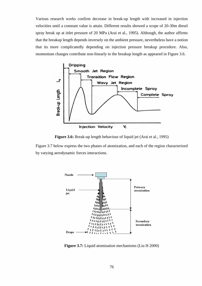
76

Various research works confirm decrease in break-up length with increased in injection

velocities until a constant value is attain. Different results showed a scope of 20-30m diesel

spray break up at inlet pressure of 20 MPa (Arai et al., 1995). Although, the author affirms

that the breakup length depends inversely on the ambient pressure, nevertheless have a notion

that its more complicatedly depending on injection pressure breakup procedure. Also,

momentum changes contribute non-linearly to the breakup length as appeared in Figure 3.6.

Figure 3.6: Break-up length behaviour of liquid jet (Arai et al., 1995)

Figure 3.7 below express the two phases of atomization, and each of the region characterized

by varying aerodynamic forces interactions.

Figure 3.7: Liquid atomisation mechanisms (Liu H 2000)

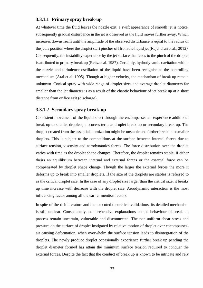
77

3.3.1.1 Primary spray break-up

At whatever time the fluid leaves the nozzle exit, a swift appearance of smooth jet is notice,

subsequently gradual disturbance in the jet is observed as the fluid moves further away. Which

increases downstream until the amplitude of the observed disturbance is equal to the radius of

the jet, a position where the droplet start pinches off from the liquid jet (Rajendran et al., 2012).

Consequently, the instability experience by the jet surface that leads to the pinch of the droplet

is attributed to primary break up (Reitz et al. 1987). Certainly, hydrodynamic cavitation within

the nozzle and turbulence oscillation of the liquid have been recognise as the controlling

mechanism (Arai et al. 1995). Though at higher velocity, the mechanism of break up remain

unknown. Conical spray with wide range of droplet sizes and average droplet diameters far

smaller than the jet diameter is as a result of the chaotic behaviour of jet break up at a short

distance from orifice exit (discharge).

3.3.1.2 Secondary spray break-up

Consistent movement of the liquid sheet through the encompasses air experience additional

break up to smaller droplets, a process term as droplet break up or secondary break up. The

droplet created from the essential atomization might be unstable and further break into smaller

droplets. This is subject to the competitions at the surface between internal forces due to

surface tension, viscosity and aerodynamics forces. The force distribution over the droplet

varies with time as the droplet shape changes. Therefore, the droplet remains stable, if either

theirs an equilibrium between internal and external forces or the external force can be

compensated by droplet shape change. Though the larger the external forces the more it

deforms up to break into smaller droplets. If the size of the droplets are stables is referred to

as the critical droplet size. In the case of any droplet size larger than the critical size, it breaks

up time increase with decrease with the droplet size. Aerodynamic interaction is the most

influencing factor among all the earlier mention factors.

In spite of the rich literature and the executed theoretical validations, its detailed mechanism

is still unclear. Consequently, comprehensive explanations on the behaviour of break up

process remain uncertain, vulnerable and disconnected. The non-uniform shear stress and

pressure on the surface of droplet instigated by relative motion of droplet over encompasses-

air causing deformation, when overwhelm the surface tension leads to disintegration of the

droplets. The newly produce droplet occasionally experience further break up pending the

droplet diameter formed has attain the minimum surface tension required to conquer the

external forces. Despite the fact that the conduct of break up is known to be intricate and rely

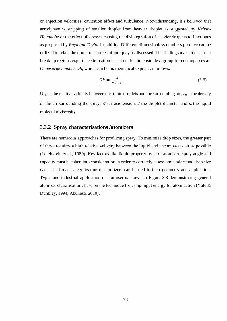
78

on injection velocities, cavitation effect and turbulence. Notwithstanding, it’s believed that

aerodynamics stripping of smaller droplet from heavier droplet as suggested by Kelvin-

Helmholtz or the effect of stresses causing the disintegration of heavier droplets to finer ones

as proposed by Rayleigh-Taylor instability. Different dimensionless numbers produce can be

utilized to relate the numerous forces of interplay as discussed. The findings make it clear that

break up regions experience transition based on the dimensionless group for encompasses air

Ohnesorge number Oh, which can be mathematical express as follows.

𝑂ℎ = µ𝑙

√𝜌𝑙𝑑𝜎 (3.6)

Urel is the relative velocity between the liquid droplets and the surrounding air, a is the density

of the air surrounding the spray, surface tension, d the droplet diameter and l the liquid

molecular viscosity.

3.3.2 Spray characterisations /atomizers

There are numerous approaches for producing spray. To minimize drop sizes, the greater part

of these requires a high relative velocity between the liquid and encompasses air as possible

(Lefebvreh. et al., 1989). Key factors like liquid property, type of atomizer, spray angle and

capacity must be taken into consideration in order to correctly assess and understand drop size

data. The broad categorization of atomizers can be tied to their geometry and application.

Types and industrial application of atomiser is shown in Figure 3.8 demonstrating general

atomizer classifications base on the technique for using input energy for atomization (Yule &

Dunkley, 1994; Abuhesa, 2010).

79

Figure 3.8: Classification of atomisers (Yule &Dunkley 1994 ; Abuhesa M . 2010).

3.3.2.1 Pressure jet atomiser

Pressure Jet atomizers are mainly utilized in fuel jet injection application, diesel engine in

peculiar by utilizing a simple orifice. A small orifice (mostly less than 0.3 mm) and high

pressure of (normally higher than 100 MPa) are the requirement for producing a fine spray

(D32<200 µm)

3.3.2.2 Pressure swirl atomiser

Pressure swirl atomizers has been for long utilized in the gas turbine engine, furnace,

agriculture related spray and petroleum direct automotive engines. The drop size might be

correlated with the wavelength that grows on the surface of the sheet as speculated by

(Dombrowski et al., 1968) and others. (Rivas et al 2014) reported that the combinations of

theoretical and empirical information are the main requirement for analysing this kind of

atomisers in terms of estimating their discharge coefficient and spray angle

3.3.2.3 Rotary atomiser

The rotary atomizer utilises centrifugal force applied to the liquid with end goal of fling a thing

film from a rotating cup, disk or bell. The essentials of the technique are well known (Nasr et

80

al., 2002) and have two distinct prospective benefits’: The likelihood of creating exceptional

narrow droplet distribution and the extra adaptability of the utilization of mechanical force to

pre film the fluid instead of depending on small orifice. The earlier listed advantage occurs for

moderately low flow rate since it requires the atomiser to work in the direct droplet or ligament

regimes of break up at the rim of the cup or disk. At higher flow rate continues sheet form at

the rim and the size distribution width is like that for the pressure jet atomiser. In any case,

this high through put method of operation can be joined with an annular air jet at right angle

to the sheet to give a pre-filming atomizer called air blast rotary cup. Mostly, a decrease in

liquid flow rate with corresponding increase in rotational speed improve the quality of the

atomization. Recent advancement has made it possible to handle flow rate up to 40 kg/s at

high wheel periphery speed that produce very fine spray (SMD below 20 microns).

3.3.2.4 Impact-type pressure atomiser

This is another category of pressure atomiser, with ability to exhibit different types of patterns.

Usually the fluid is impacted upon shaped surface as it is developed from an orifice and a flat

spray pattern is generated. Normally utilizes when spray pattern is required. Even though, the

orifice must be large enough, to reduce the possibilities of blockage. They are usually utilised

in safety system where spray must unfailingly function well (Tamhankar et al 2014), i.e. for

cooling and gases removal.

3.3.2.5 Ultrasonic atomiser

Ultrasonic atomizers are less common in comparison to the previously mentioned techniques,

yet especially suitable for generating low flow rate (<0.2l/min) spray with relatively narrow

size distribution and very low kinetic energy. Its size distribution width can be categorized in

an intermediary position between that pressure will atomizer and rotary atomisers in direct

droplet regime.

3.3.2.6 Electrostatic atomiser

This is another niche market technique. Genuine electrostatic atomiser injects charge into the

liquid sheet with end goal that the charge at the surface sheet of the fluid act again surface

tension thereby causing break up. It is hardly utilised in practical device but utilize actively in

numerous areas of application including liquid atomization. Among the advantages are

applications to what are regularly refers as electrostatic atomiser, through a release of direct

injection of charge.

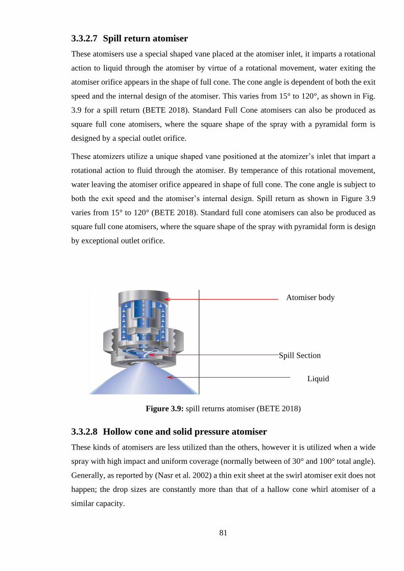
81

3.3.2.7 Spill return atomiser

These atomisers use a special shaped vane placed at the atomiser inlet, it imparts a rotational

action to liquid through the atomiser by virtue of a rotational movement, water exiting the

atomiser orifice appears in the shape of full cone. The cone angle is dependent of both the exit

speed and the internal design of the atomiser. This varies from 15° to 120°, as shown in Fig.

3.9 for a spill return (BETE 2018). Standard Full Cone atomisers can also be produced as

square full cone atomisers, where the square shape of the spray with a pyramidal form is

designed by a special outlet orifice.

These atomizers utilize a unique shaped vane positioned at the atomizer’s inlet that impart a

rotational action to fluid through the atomiser. By temperance of this rotational movement,

water leaving the atomiser orifice appeared in shape of full cone. The cone angle is subject to

both the exit speed and the atomiser’s internal design. Spill return as shown in Figure 3.9

varies from 15° to 120° (BETE 2018). Standard full cone atomisers can also be produced as

square full cone atomisers, where the square shape of the spray with pyramidal form is design

by exceptional outlet orifice.

Figure 3.9: spill returns atomiser (BETE 2018)

3.3.2.8 Hollow cone and solid pressure atomiser

These kinds of atomisers are less utilized than the others, however it is utilized when a wide

spray with high impact and uniform coverage (normally between of 30° and 100° total angle).

Generally, as reported by (Nasr et al. 2002) a thin exit sheet at the swirl atomiser exit does not

happen; the drop sizes are constantly more than that of a hallow cone whirl atomiser of a

similar capacity.

Atomiser body

Spill Section

Liquid

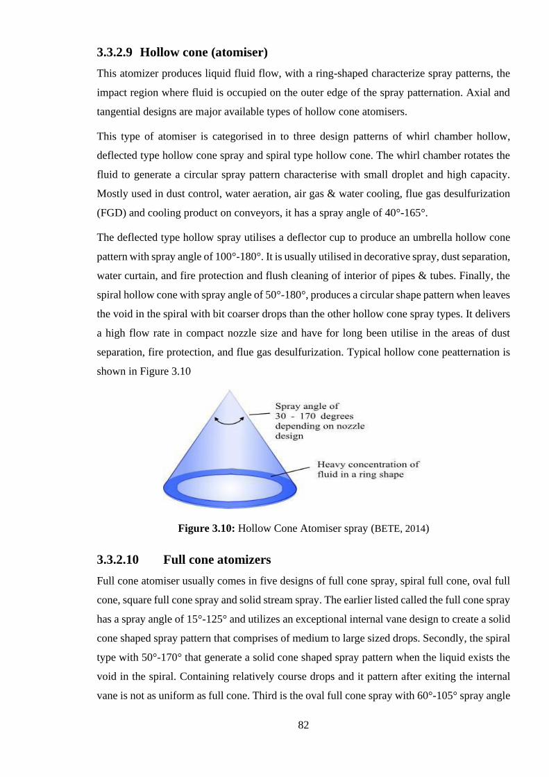
82

3.3.2.9 Hollow cone (atomiser)

This atomizer produces liquid fluid flow, with a ring-shaped characterize spray patterns, the

impact region where fluid is occupied on the outer edge of the spray patternation. Axial and

tangential designs are major available types of hollow cone atomisers.

This type of atomiser is categorised in to three design patterns of whirl chamber hollow,

deflected type hollow cone spray and spiral type hollow cone. The whirl chamber rotates the

fluid to generate a circular spray pattern characterise with small droplet and high capacity.

Mostly used in dust control, water aeration, air gas & water cooling, flue gas desulfurization

(FGD) and cooling product on conveyors, it has a spray angle of 40°-165°.

The deflected type hollow spray utilises a deflector cup to produce an umbrella hollow cone

pattern with spray angle of 100°-180°. It is usually utilised in decorative spray, dust separation,

water curtain, and fire protection and flush cleaning of interior of pipes & tubes. Finally, the

spiral hollow cone with spray angle of 50°-180°, produces a circular shape pattern when leaves

the void in the spiral with bit coarser drops than the other hollow cone spray types. It delivers

a high flow rate in compact nozzle size and have for long been utilise in the areas of dust

separation, fire protection, and flue gas desulfurization. Typical hollow cone peatternation is

shown in Figure 3.10

Figure 3.10: Hollow Cone Atomiser spray (BETE, 2014)

3.3.2.10 Full cone atomizers

Full cone atomiser usually comes in five designs of full cone spray, spiral full cone, oval full

cone, square full cone spray and solid stream spray. The earlier listed called the full cone spray

has a spray angle of 15°-125° and utilizes an exceptional internal vane design to create a solid

cone shaped spray pattern that comprises of medium to large sized drops. Secondly, the spiral

type with 50°-170° that generate a solid cone shaped spray pattern when the liquid exists the

void in the spiral. Containing relatively course drops and it pattern after exiting the internal

vane is not as uniform as full cone. Third is the oval full cone spray with 60°-105° spray angle

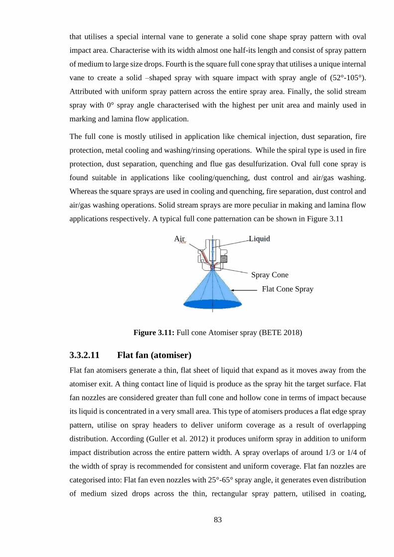
83

that utilises a special internal vane to generate a solid cone shape spray pattern with oval

impact area. Characterise with its width almost one half-its length and consist of spray pattern

of medium to large size drops. Fourth is the square full cone spray that utilises a unique internal

vane to create a solid –shaped spray with square impact with spray angle of (52°-105°).

Attributed with uniform spray pattern across the entire spray area. Finally, the solid stream

spray with 0° spray angle characterised with the highest per unit area and mainly used in

marking and lamina flow application.

The full cone is mostly utilised in application like chemical injection, dust separation, fire

protection, metal cooling and washing/rinsing operations. While the spiral type is used in fire

protection, dust separation, quenching and flue gas desulfurization. Oval full cone spray is

found suitable in applications like cooling/quenching, dust control and air/gas washing.

Whereas the square sprays are used in cooling and quenching, fire separation, dust control and

air/gas washing operations. Solid stream sprays are more peculiar in making and lamina flow

applications respectively. A typical full cone patternation can be shown in Figure 3.11

Figure 3.11: Full cone Atomiser spray (BETE 2018)

3.3.2.11 Flat fan (atomiser)

Flat fan atomisers generate a thin, flat sheet of liquid that expand as it moves away from the

atomiser exit. A thing contact line of liquid is produce as the spray hit the target surface. Flat

fan nozzles are considered greater than full cone and hollow cone in terms of impact because

its liquid is concentrated in a very small area. This type of atomisers produces a flat edge spray

pattern, utilise on spray headers to deliver uniform coverage as a result of overlapping

distribution. According (Guller et al. 2012) it produces uniform spray in addition to uniform

impact distribution across the entire pattern width. A spray overlaps of around 1/3 or 1/4 of

the width of spray is recommended for consistent and uniform coverage. Flat fan nozzles are

categorised into: Flat fan even nozzles with 25°-65° spray angle, it generates even distribution

of medium sized drops across the thin, rectangular spray pattern, utilised in coating,

Liquid Air

Spray Cone

Flat Cone Spray

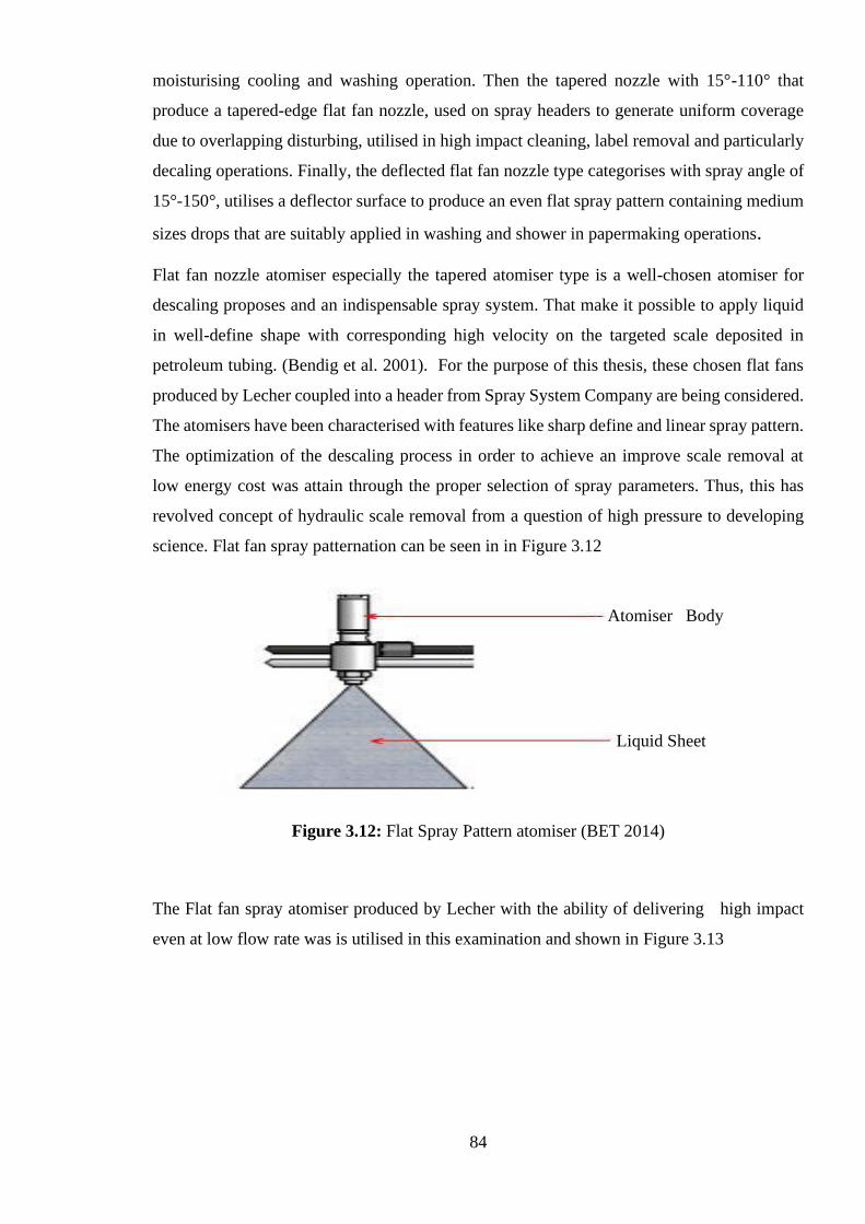
84

moisturising cooling and washing operation. Then the tapered nozzle with 15°-110° that

produce a tapered-edge flat fan nozzle, used on spray headers to generate uniform coverage

due to overlapping disturbing, utilised in high impact cleaning, label removal and particularly

decaling operations. Finally, the deflected flat fan nozzle type categorises with spray angle of

15°-150°, utilises a deflector surface to produce an even flat spray pattern containing medium

sizes drops that are suitably applied in washing and shower in papermaking operations.

Flat fan nozzle atomiser especially the tapered atomiser type is a well-chosen atomiser for

descaling proposes and an indispensable spray system. That make it possible to apply liquid

in well-define shape with corresponding high velocity on the targeted scale deposited in

petroleum tubing. (Bendig et al. 2001). For the purpose of this thesis, these chosen flat fans

produced by Lecher coupled into a header from Spray System Company are being considered.

The atomisers have been characterised with features like sharp define and linear spray pattern.

The optimization of the descaling process in order to achieve an improve scale removal at

low energy cost was attain through the proper selection of spray parameters. Thus, this has

revolved concept of hydraulic scale removal from a question of high pressure to developing

science. Flat fan spray patternation can be seen in in Figure 3.12

Figure 3.12: Flat Spray Pattern atomiser (BET 2014)

The Flat fan spray atomiser produced by Lecher with the ability of delivering high impact

even at low flow rate was is utilised in this examination and shown in Figure 3.13

Atomiser Body

Liquid Sheet

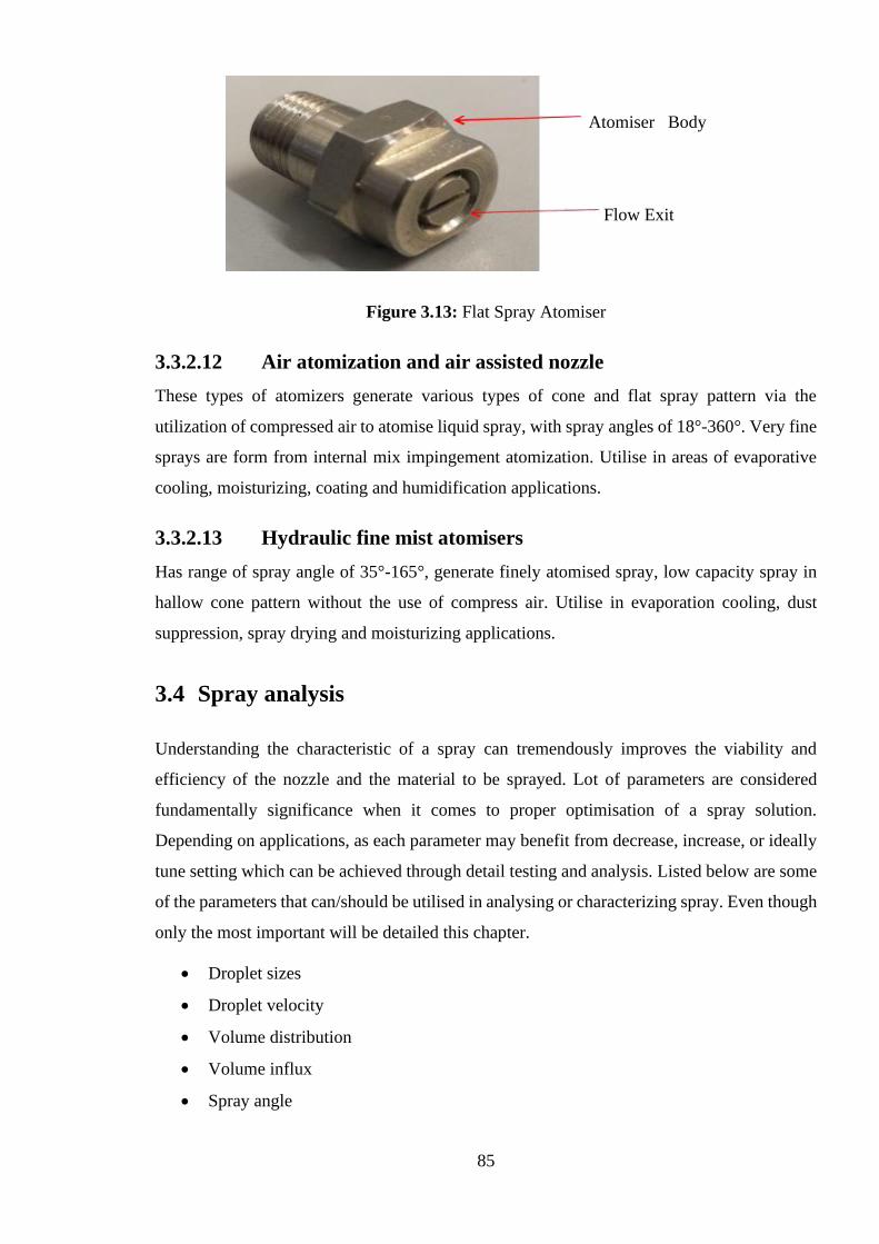
85

Figure 3.13: Flat Spray Atomiser

3.3.2.12 Air atomization and air assisted nozzle

These types of atomizers generate various types of cone and flat spray pattern via the

utilization of compressed air to atomise liquid spray, with spray angles of 18°-360°. Very fine

sprays are form from internal mix impingement atomization. Utilise in areas of evaporative

cooling, moisturizing, coating and humidification applications.

3.3.2.13 Hydraulic fine mist atomisers

Has range of spray angle of 35°-165°, generate finely atomised spray, low capacity spray in

hallow cone pattern without the use of compress air. Utilise in evaporation cooling, dust

suppression, spray drying and moisturizing applications.

3.4 Spray analysis

Understanding the characteristic of a spray can tremendously improves the viability and

efficiency of the nozzle and the material to be sprayed. Lot of parameters are considered

fundamentally significance when it comes to proper optimisation of a spray solution.

Depending on applications, as each parameter may benefit from decrease, increase, or ideally

tune setting which can be achieved through detail testing and analysis. Listed below are some

of the parameters that can/should be utilised in analysing or characterizing spray. Even though

only the most important will be detailed this chapter.

• Droplet sizes

• Droplet velocity

• Volume distribution

• Volume influx

• Spray angle

Atomiser Body

Flow Exit

86

• Solid Particle

• Droplet shape

• Spray impact

• Rheological testing

• Operation pressure

• Flow rate

• Droplet impact force

• Spray concentration

• Material solid content and the rest

3.4.1 Drop size

Drop size refers to the genuine size of the specific drop that comprises an atomiser spray

pattern. The significance of drop size and its application in spray system have considerably

increase over the years. Each spray pattern delivers a scope of drop sizes and this range is

called the droplet size distribution. The criticalities of drop size depend on the application in

question. Processes like gas scrubbing rely upon exposing the maximum amount of liquid

surface to gas stream. While other applications like a case were the spray must project into

fast moving gas stream requires the droplet size to be as large as possible. Exposing the

maximum surface area requires atomizing the liquid in smaller droplet sizes as possible. Drop

sizes are influence by factors like atomiser capacity, liquid property, spray angle and spray

pressure. Higher spraying pressure provides smaller drop sizes, while lower spraying pressure

yield larger droplet sizes.

3.4.2 Drop size distribution (DSD)

Drop size is an essential component for the choosing an atomiser for a specific application. So

as drop size distribution is a critical and significant parameter of atomization process in

addition to drop mean diameter. Simply refers to as the scope of drop sizes and ranges

delivered by a spray pattern. It might have a specific shape for instance (narrow, wide few

large drops, etc) for most ideal operations. Figure. 3.14, in which ΔD = 5μm

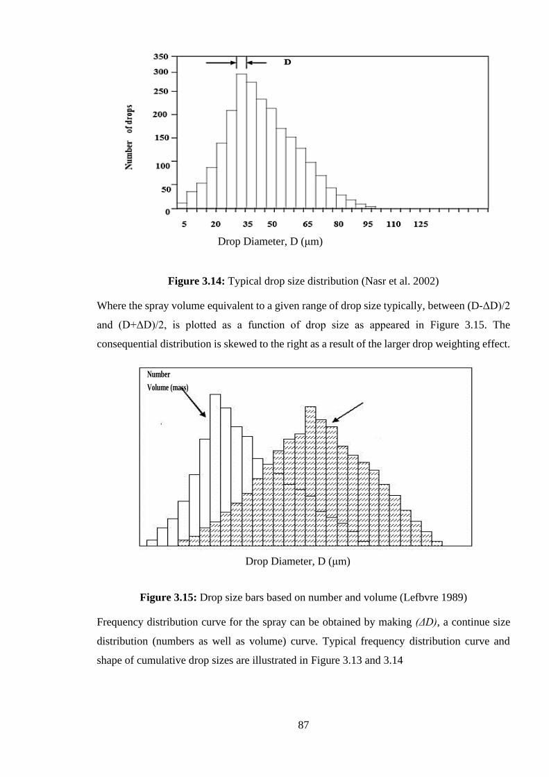
87

Figure 3.14: Typical drop size distribution (Nasr et al. 2002)

Where the spray volume equivalent to a given range of drop size typically, between (D-ΔD)/2

and (D+ΔD)/2, is plotted as a function of drop size as appeared in Figure 3.15. The

consequential distribution is skewed to the right as a result of the larger drop weighting effect.

Figure 3.15: Drop size bars based on number and volume (Lefbvre 1989)

Frequency distribution curve for the spray can be obtained by making (ΔD), a continue size

distribution (numbers as well as volume) curve. Typical frequency distribution curve and

shape of cumulative drop sizes are illustrated in Figure 3.13 and 3.14

Drop Diameter, D (μm)

Number Volume (mass)

Drop Diameter, D (μm)

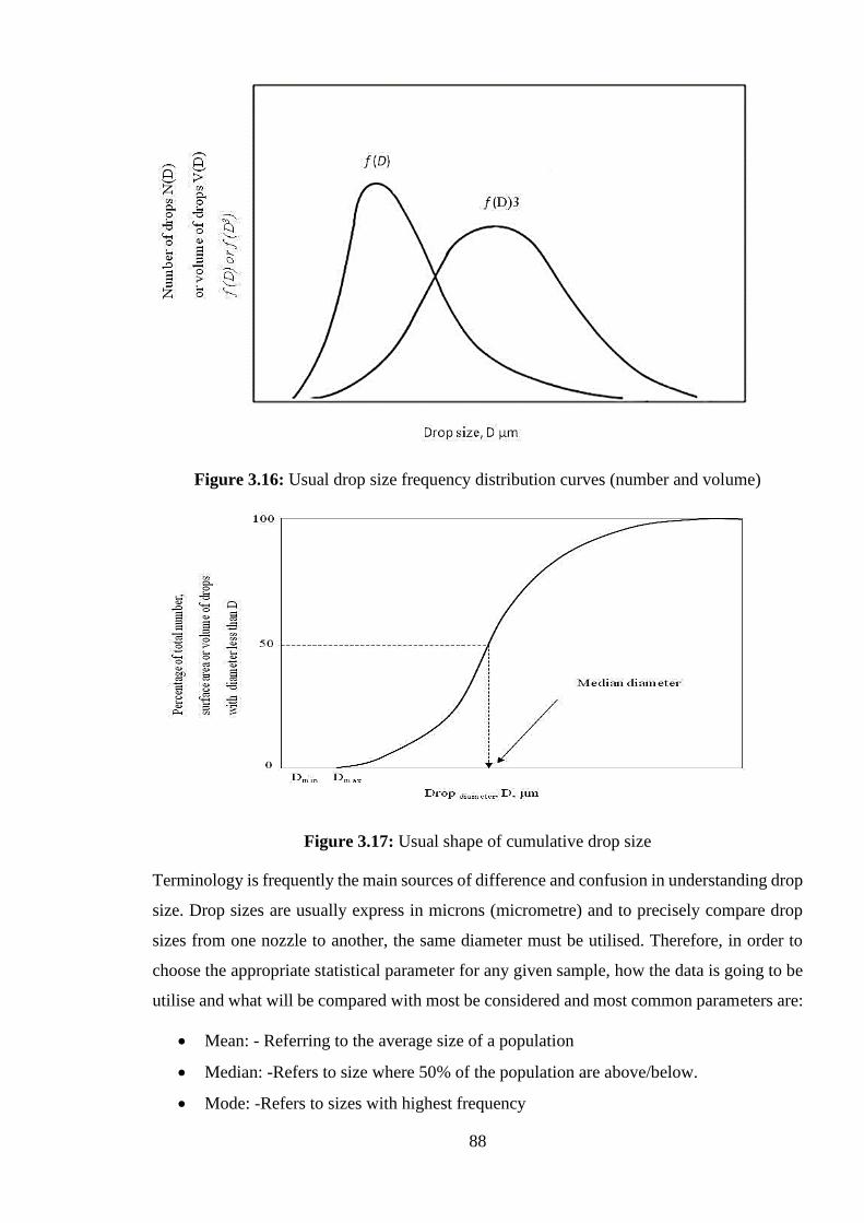
88

Figure 3.16: Usual drop size frequency distribution curves (number and volume)

Figure 3.17: Usual shape of cumulative drop size

Terminology is frequently the main sources of difference and confusion in understanding drop

size. Drop sizes are usually express in microns (micrometre) and to precisely compare drop

sizes from one nozzle to another, the same diameter must be utilised. Therefore, in order to

choose the appropriate statistical parameter for any given sample, how the data is going to be

utilise and what will be compared with most be considered and most common parameters are:

• Mean: - Referring to the average size of a population

• Median: -Refers to size where 50% of the population are above/below.

• Mode: -Refers to sizes with highest frequency

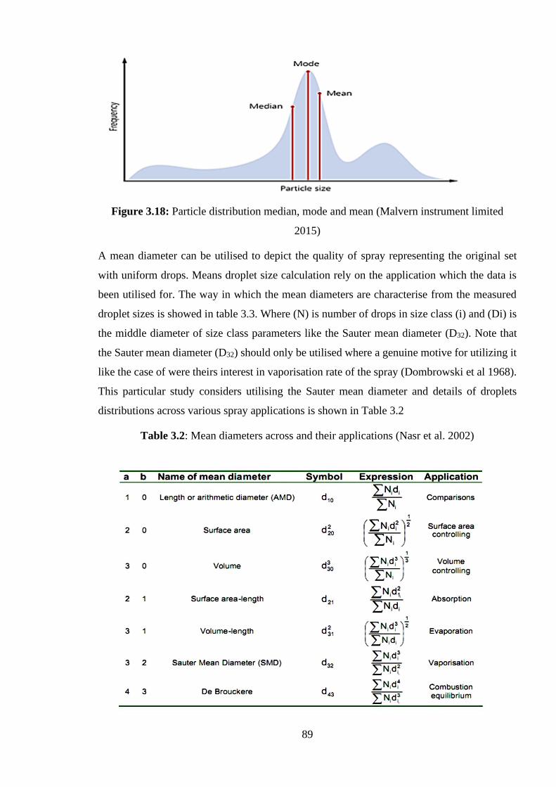
89

Figure 3.18: Particle distribution median, mode and mean (Malvern instrument limited

2015)

A mean diameter can be utilised to depict the quality of spray representing the original set

with uniform drops. Means droplet size calculation rely on the application which the data is

been utilised for. The way in which the mean diameters are characterise from the measured

droplet sizes is showed in table 3.3. Where (N) is number of drops in size class (i) and (Di) is

the middle diameter of size class parameters like the Sauter mean diameter (D32). Note that

the Sauter mean diameter (D32) should only be utilised where a genuine motive for utilizing it

like the case of were theirs interest in vaporisation rate of the spray (Dombrowski et al 1968).

This particular study considers utilising the Sauter mean diameter and details of droplets

distributions across various spray applications is shown in Table 3.2

Table 3.2: Mean diameters across and their applications (Nasr et al. 2002)

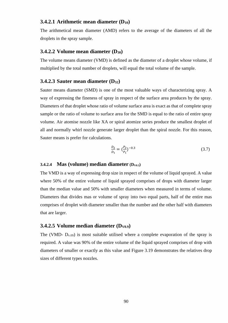
90

3.4.2.1 Arithmetic mean diameter (D10)

The arithmetical mean diameter (AMD) refers to the average of the diameters of all the

droplets in the spray sample.

3.4.2.2 Volume mean diameter (D30)

The volume means diameter (VMD) is defined as the diameter of a droplet whose volume, if

multiplied by the total number of droplets, will equal the total volume of the sample.

3.4.2.3 Sauter mean diameter (D32)

Sauter means diameter (SMD) is one of the most valuable ways of characterizing spray. A

way of expressing the fineness of spray in respect of the surface area produces by the spray.

Diameters of that droplet whose ratio of volume surface area is exact as that of complete spray

sample or the ratio of volume to surface area for the SMD is equal to the ratio of entire spray

volume. Air atomise nozzle like XA or spiral atomize series produce the smallest droplet of

all and normally whirl nozzle generate larger droplet than the spiral nozzle. For this reason,

Sauter means is prefer for calculations.

𝐷2

𝐷1= (

𝑃2

𝑃1)−0.3 (3.7)

3.4.2.4 Mas (volume) median diameter (DV0.5)

The VMD is a way of expressing drop size in respect of the volume of liquid sprayed. A value

where 50% of the entire volume of liquid sprayed comprises of drops with diameter larger

than the median value and 50% with smaller diameters when measured in terms of volume.

Diameters that divides mas or volume of spray into two equal parts, half of the entire mas

comprises of droplet with diameter smaller than the number and the other half with diameters

that are larger.

3.4.2.5 Volume median diameter (DV0.9)

The (VMD- Dv.09) is most suitable utilised where a complete evaporation of the spray is

required. A value was 90% of the entire volume of the liquid sprayed comprises of drop with

diameters of smaller or exactly as this value and Figure 3.19 demonstrates the relatives drop

sizes of different types nozzles.

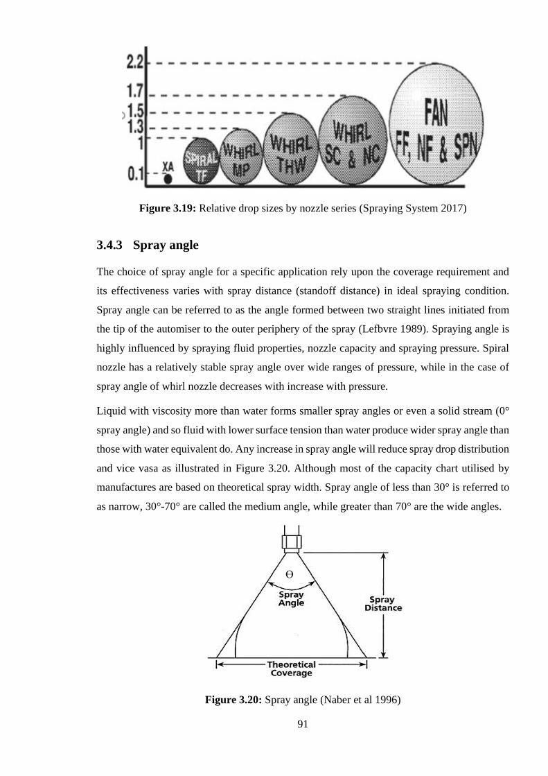
91

Figure 3.19: Relative drop sizes by nozzle series (Spraying System 2017)

3.4.3 Spray angle

The choice of spray angle for a specific application rely upon the coverage requirement and

its effectiveness varies with spray distance (standoff distance) in ideal spraying condition.

Spray angle can be referred to as the angle formed between two straight lines initiated from

the tip of the automiser to the outer periphery of the spray (Lefbvre 1989). Spraying angle is

highly influenced by spraying fluid properties, nozzle capacity and spraying pressure. Spiral

nozzle has a relatively stable spray angle over wide ranges of pressure, while in the case of

spray angle of whirl nozzle decreases with increase with pressure.

Liquid with viscosity more than water forms smaller spray angles or even a solid stream (0°

spray angle) and so fluid with lower surface tension than water produce wider spray angle than

those with water equivalent do. Any increase in spray angle will reduce spray drop distribution

and vice vasa as illustrated in Figure 3.20. Although most of the capacity chart utilised by

manufactures are based on theoretical spray width. Spray angle of less than 30° is referred to

as narrow, 30°-70° are called the medium angle, while greater than 70° are the wide angles.

Figure 3.20: Spray angle (Naber et al 1996)

Ɵ

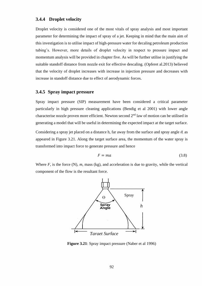
92

3.4.4 Droplet velocity

Droplet velocity is considered one of the most vitals of spray analysis and most important

parameter for determining the impact of spray of a jet. Keeping in mind that the main aim of

this investigation is to utilise impact of high-pressure water for decaling petroleum production

tubing’s. However, more details of droplet velocity in respect to pressure impact and

momentum analysis will be provided in chapter five. As will be further utilise in justifying the

suitable standoff distance from nozzle exit for effective descaling. (Opferet al.2013) believed

that the velocity of droplet increases with increase in injection pressure and decreases with

increase in standoff distance due to effect of aerodynamic forces.

3.4.5 Spray impact pressure

Spray impact pressure (SIP) measurement have been considered a critical parameter

particularly in high pressure cleaning applications (Bendig et al 2001) with lower angle

characterise nozzle proven more efficient. Newton second 2nd law of motion can be utilised in

generating a model that will be useful in determining the expected impact at the target surface.

Considering a spray jet placed on a distance h, far away from the surface and spray angle as

appeared in Figure 3.21. Along the target surface area, the momentum of the water spray is

transformed into impact force to generate pressure and hence

𝐹 = 𝑚𝑎 (3.8)

Where F, is the force (N), m, mass (kg), and acceleration is due to gravity, while the vertical

component of the flow is the resultant force.

Figure 3.21: Spray impact pressure (Naber et al 1996)

Spray

Ɵ

h

Target Surface

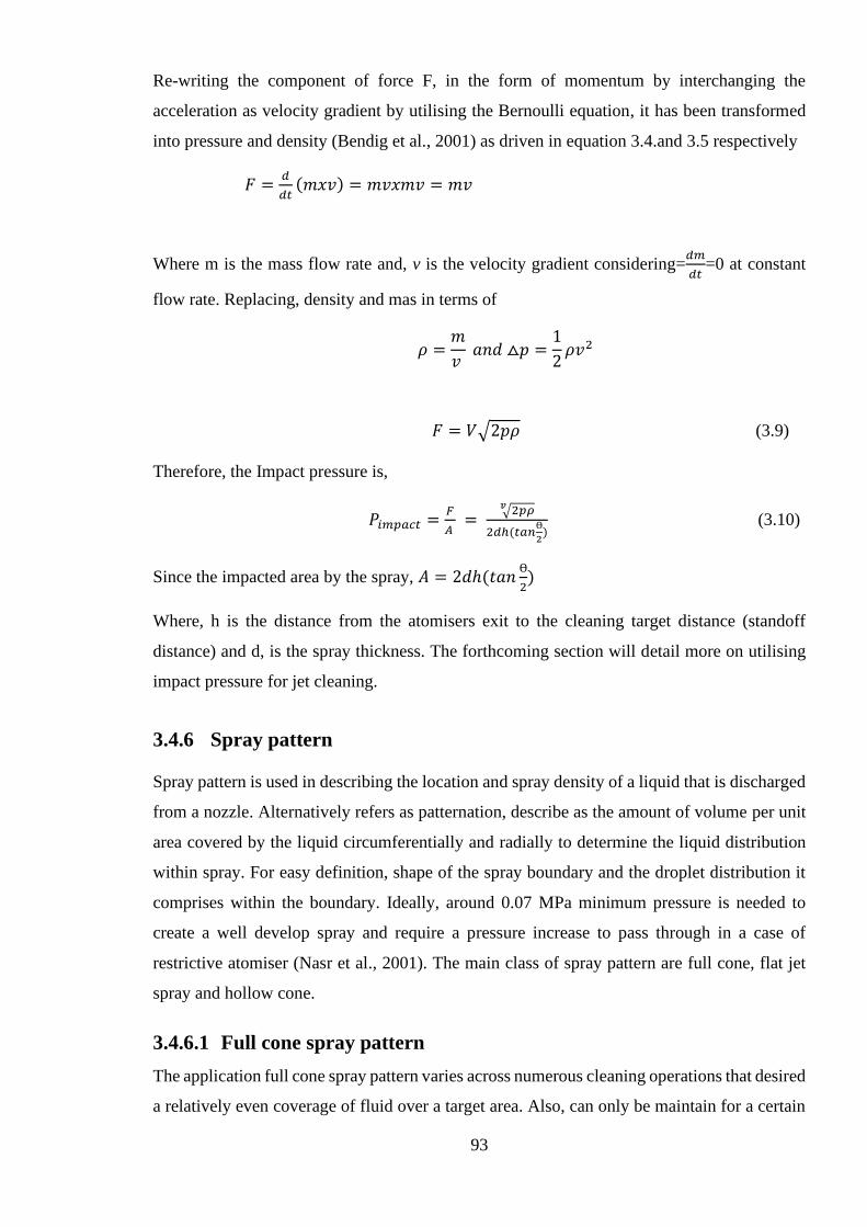
93

Re-writing the component of force F, in the form of momentum by interchanging the

acceleration as velocity gradient by utilising the Bernoulli equation, it has been transformed

into pressure and density (Bendig et al., 2001) as driven in equation 3.4.and 3.5 respectively

𝐹 =𝑑

𝑑𝑡(𝑚𝑥𝑣) = 𝑚𝑣𝑥𝑚𝑣 = 𝑚𝑣

Where m is the mass flow rate and, v is the velocity gradient considering=𝑑𝑚

𝑑𝑡=0 at constant

flow rate. Replacing, density and mas in terms of

𝜌 =𝑚

𝑣 𝑎𝑛𝑑 ⧍𝑝 =

1

2𝜌𝑣2

𝐹 = 𝑉√2𝑝𝜌 (3.9)

Therefore, the Impact pressure is,

𝑃𝑖𝑚𝑝𝑎𝑐𝑡 =𝐹

𝐴 =

√2𝑝𝜌𝑣

2𝑑ℎ(𝑡𝑎𝑛Ɵ

2) (3.10)

Since the impacted area by the spray, 𝐴 = 2𝑑ℎ(𝑡𝑎𝑛Ɵ

2)

Where, h is the distance from the atomisers exit to the cleaning target distance (standoff

distance) and d, is the spray thickness. The forthcoming section will detail more on utilising

impact pressure for jet cleaning.

3.4.6 Spray pattern

Spray pattern is used in describing the location and spray density of a liquid that is discharged

from a nozzle. Alternatively refers as patternation, describe as the amount of volume per unit

area covered by the liquid circumferentially and radially to determine the liquid distribution

within spray. For easy definition, shape of the spray boundary and the droplet distribution it

comprises within the boundary. Ideally, around 0.07 MPa minimum pressure is needed to

create a well develop spray and require a pressure increase to pass through in a case of

restrictive atomiser (Nasr et al., 2001). The main class of spray pattern are full cone, flat jet

spray and hollow cone.

3.4.6.1 Full cone spray pattern

The application full cone spray pattern varies across numerous cleaning operations that desired

a relatively even coverage of fluid over a target area. Also, can only be maintain for a certain

94

standoff distance, after which the spray forms a fog or mist. Full cone spray patterns are

classified into five major designs: Full cone spray, spiral full cone, oval full cone pattern, and

square full cone spray and solid stream spray obtain via different atomization techniques.

Full cone spray pattern is generated through the utilization of a unique internal vane design to

generate a solid cone spray pattern that is characterise with spray angles ranging from 15°-

125° and contains medium to large drop sizes. Usually utilise in chemical injection, dust

separation, fire protection, metal cooling and washing/rinsing operations.

The spiral full spray pattern is produced from spiral full cone nozzles that generate a solid

cone shaped spray pattern when the liquid exists the void in the spiral. This type of spray

pattern is not as uniform as the full cone produce from full cone nozzle that utilises an internal

vane instead. It’s characterised with spray angle ranging from 50°-170° and comprises

relatively course drops. Utilised in fire protection, dust separation, quenching and flue gas

desulfurization operations.

The oval full cone spray pattern is product of the oval type of full cone nozzle that utilises a

special internal vane to generate a solid cone shape spray pattern. That has an oval impact

area characterise with its width almost one half-its length. This spray pattern consists of

medium to large sizes drops and have a spray angle ranging from 60°-105° and it found

suitable for cooling/quenching, dust control and air/gas washing applications.

The square full cone spray pattern is produced from square full cone atomisers that utilise a

unique internal vane to create a solid –shaped spray with square impact. It’s attributed with

uniform spray with square impact, spray angle range of (52°-105°) and consist of medium to

large size drops. Cooling and quenching, fire separation, dust control and air/gas washing

operations are most peculiar application of the oval full cone spray patterns.

The solid stream spray pattern is produced from solid stream nozzles with 0° spray angle

characterise with the highest per unit area and mainly used in making and lamina flow

application

3.4.6.2 Flat fan spray pattern

Flat fan spray patterns are generated through flat fan atomisers that produce thing flat sheet of

liquid that expands as it discharges away from the nozzle exit. This flat edge spray pattern is

used on spray headers to deliver uniform coverage because of overlap distribution.

These spray patterns are considered to have more impact than hollow and full cone pattern due

to liquid concentration into a small area. Normally classified into:

95

Even spray pattern generated by flat fan even nozzle. This thin rectangular spray pattern

consists of an even distribution of medium drop size and have a spray angle ranging from 25°-

65°. An edge-edge pattern contact positioning is required when used on header and are utilised

in coating, moisturising cooling and washing applications.

The tapered edge flat spray pattern produced from flat fan (tapered) nozzle that used on spray

headers to generate uniform coverage due to overlapping distribution. It has a spray angle

ranging from 15°-110° and are utilised in high impact cleaning, label removal and particularly

decaling operations.

An even flat spray pattern containing medium size drop at spray angle of 15°-150° that is

considered suitable for washing and shower in paper making application generated with the

aid of deflected flat fan nozzle. This even flat fan spray pattern is produced through the

utilization of deflector surface technique that has a large passage design to reduce clogging

via the round orifice.

3.4.6.3 Hollow cone spray pattern

Hollow cone spray patterns are characterised as liquid flow with a ring –shaped spray pattern,

with impact region around were the fluid is occupied on the outer edge of the spray

patternation. Mainly produce from axial and tangential design hollow cone atomisers. Whirl

chamber hollow, deflected type hollow cone spray, and spiral type hollow cone spray pattern

are part of the main types of hallow spray patterns.

The circular spray pattern that contains small drop size and high capacity is produce when a

whirl chamber nozzle rotates the fluid. It has a spray angle of 40°-165° and its mostly needed

in in dust control, water aeration, air gas & water cooling, flue gas desulfurization (FGD) and

cooling product on conveyors applications.

Umbrella-shaped hollow one pattern with spray angle of 100°-180, is produce from the

deflected hollow cone spray nozzle by utilising the deflector cup to generate the spray pattern.

Usually utilise in decorative spray, dust separation, water curtain, and fire protection and flush

cleaning of interior of pipes & tubes.

Circulars shaped spray pattern with drops slightly courser than those in the other hollow cone

sprays and high flow rate in compact nozzle. This spray pattern is produced from the fluid

spiral hollow cone nozzle when the fluid leaves the void in the spiral. It has a spray angle of

50°-180° and utilised in dust separation, fire protection, and flue gas desulfurization

applications.

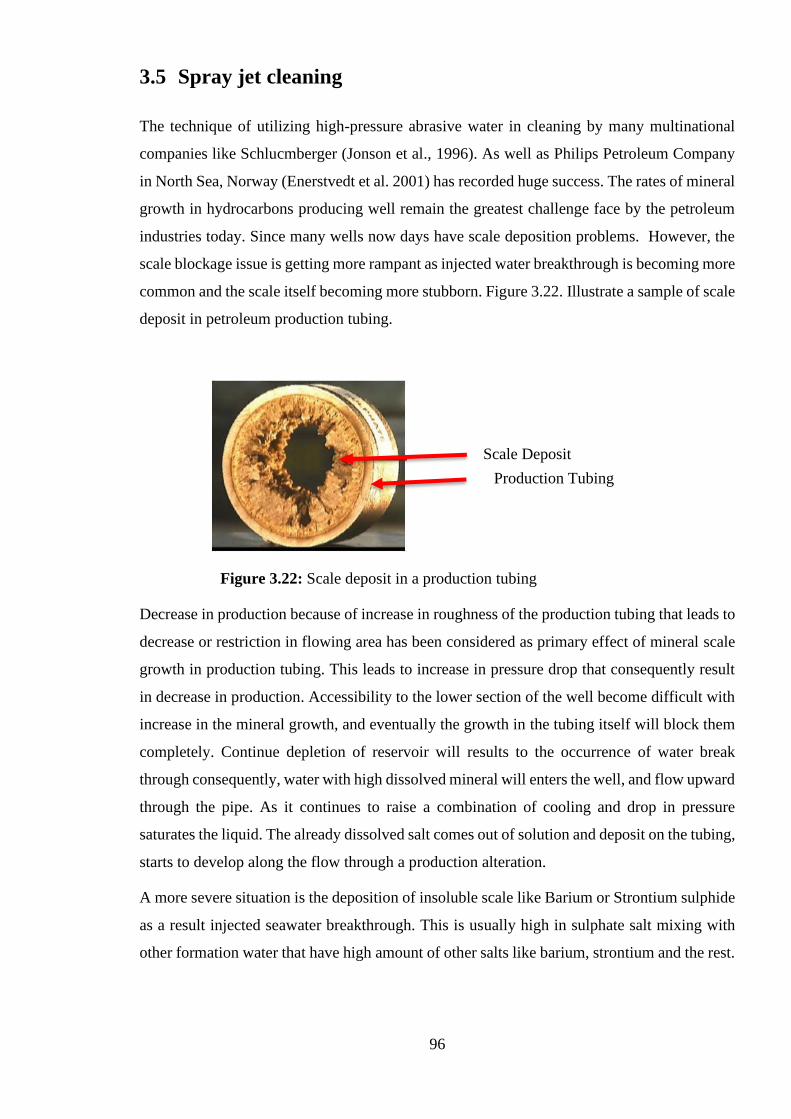
96

Figure 3.22: Scale deposit in a production tubing

3.5 Spray jet cleaning

The technique of utilizing high-pressure abrasive water in cleaning by many multinational

companies like Schlucmberger (Jonson et al., 1996). As well as Philips Petroleum Company

in North Sea, Norway (Enerstvedt et al. 2001) has recorded huge success. The rates of mineral

growth in hydrocarbons producing well remain the greatest challenge face by the petroleum

industries today. Since many wells now days have scale deposition problems. However, the

scale blockage issue is getting more rampant as injected water breakthrough is becoming more

common and the scale itself becoming more stubborn. Figure 3.22. Illustrate a sample of scale

deposit in petroleum production tubing.

Decrease in production because of increase in roughness of the production tubing that leads to

decrease or restriction in flowing area has been considered as primary effect of mineral scale

growth in production tubing. This leads to increase in pressure drop that consequently result

in decrease in production. Accessibility to the lower section of the well become difficult with

increase in the mineral growth, and eventually the growth in the tubing itself will block them

completely. Continue depletion of reservoir will results to the occurrence of water break

through consequently, water with high dissolved mineral will enters the well, and flow upward

through the pipe. As it continues to raise a combination of cooling and drop in pressure

saturates the liquid. The already dissolved salt comes out of solution and deposit on the tubing,

starts to develop along the flow through a production alteration.

A more severe situation is the deposition of insoluble scale like Barium or Strontium sulphide

as a result injected seawater breakthrough. This is usually high in sulphate salt mixing with

other formation water that have high amount of other salts like barium, strontium and the rest.

Production Tubing

Scale Deposit

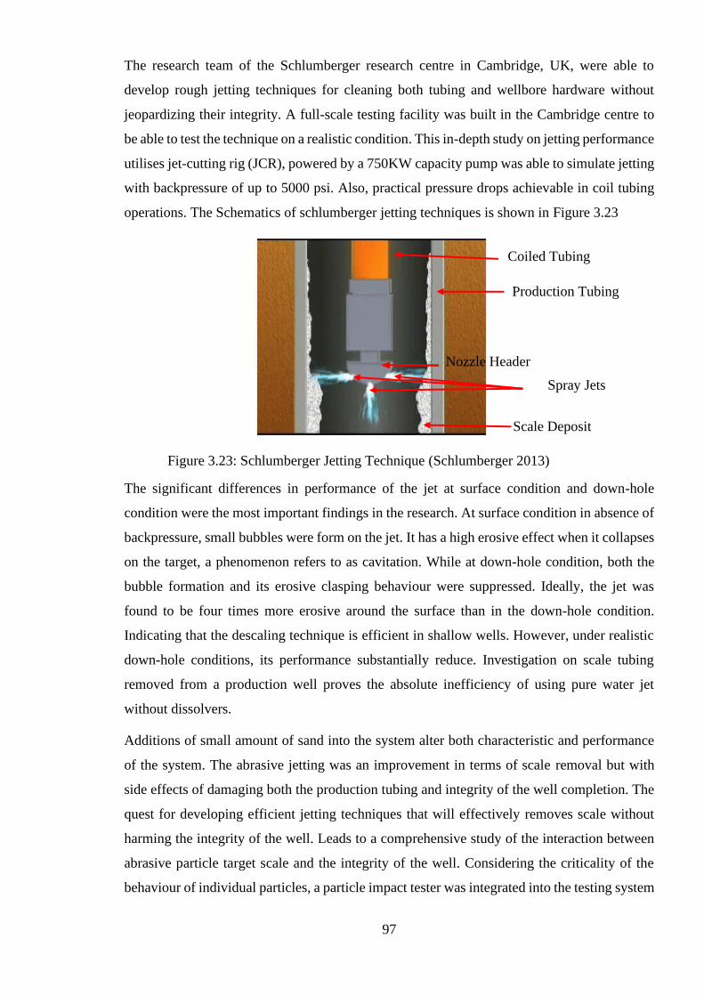
97

Figure 3.23: Schlumberger Jetting Technique (Schlumberger 2013)

The research team of the Schlumberger research centre in Cambridge, UK, were able to

develop rough jetting techniques for cleaning both tubing and wellbore hardware without

jeopardizing their integrity. A full-scale testing facility was built in the Cambridge centre to

be able to test the technique on a realistic condition. This in-depth study on jetting performance

utilises jet-cutting rig (JCR), powered by a 750KW capacity pump was able to simulate jetting

with backpressure of up to 5000 psi. Also, practical pressure drops achievable in coil tubing

operations. The Schematics of schlumberger jetting techniques is shown in Figure 3.23

The significant differences in performance of the jet at surface condition and down-hole

condition were the most important findings in the research. At surface condition in absence of

backpressure, small bubbles were form on the jet. It has a high erosive effect when it collapses

on the target, a phenomenon refers to as cavitation. While at down-hole condition, both the

bubble formation and its erosive clasping behaviour were suppressed. Ideally, the jet was

found to be four times more erosive around the surface than in the down-hole condition.

Indicating that the descaling technique is efficient in shallow wells. However, under realistic

down-hole conditions, its performance substantially reduce. Investigation on scale tubing

removed from a production well proves the absolute inefficiency of using pure water jet

without dissolvers.

Additions of small amount of sand into the system alter both characteristic and performance

of the system. The abrasive jetting was an improvement in terms of scale removal but with

side effects of damaging both the production tubing and integrity of the well completion. The

quest for developing efficient jetting techniques that will effectively removes scale without

harming the integrity of the well. Leads to a comprehensive study of the interaction between

abrasive particle target scale and the integrity of the well. Considering the criticality of the

behaviour of individual particles, a particle impact tester was integrated into the testing system

Coiled Tubing

Production Tubing

Nozzle Header

Scale Deposit

Spray Jets

98

to study the collusion and high-speed particle impact. The shape of the particle was found

critical in respect to the erosion of ductile materials like steel tubing. Examples is the way a

sharp sand particle will plunge the steel surface and cut away the steel leading to high level of

damage. Nevertheless, the impact of hard spherical particle on the surface will deform the

surface leaving a spherical hole. However, much less damaging compared to the sharp sand

particles. In the case of other brittle materials like scale, the shape of the abrasive particle is

not important, because the impact process not the powering action of the abrasives removes

the surface. The impact process causes nucleate networks of fractures through the material and

hence the choice of spherical particles could completely solve the problem. Another abrasive

property tested was the hardness of the particle considered as a key parameter in fracture

toughness. If the abrasive is very week or the target surface is very strong, the impacting

particles end up shattering into fine dust without making any damage to the scale surface.

The scientific study to design the effective abrasive material that will not harm the integrity of

the well resulted to the invention of stealing bead materials (stony beads). The performance of

sterling beads was exceptional by effectively descaling the production tubing with no damage

to the tubing. The invention of this technology has open door for the development of new

generation tubing cleaning tools. A realistic post decaling testimony can be deriving from one

of Stumberger clients. Who’s after exhausting many techniques to remove calcium carbonate

scale without success and 2000 tons of carbide mills were destroyed in a day before given the

strong beads system a trial. The strong beads trials were able to clean a 25ft of tubing at

between 30 to 90 ft/lb, but the mechanical integrity of the tubing was at risk (Mirza et al 1999),

(Leal et al 2009). Together with high environmental concern, even though the treated section

of the deposited scale has been completely cleaned.

The Research by the Schlumberger recorded some interesting result, though could not

establish nether the opportunity for enhancing cavitation as a jetting mechanism for enhancing

erosion nor developed an environmentally friendly option. Contrariwise, the proposed

abrasive jetting technique was attributed to negative consequences like environmental

concerns and the destruction of the production tubing when used for several years. The

forthcoming section discusses the main jetting mechanism techniques and detailed more on

cavitation as a jetting erosion enhancement, which was the genesis of the introduction abrasive

particles.

99

3.5.1 Mechanism for jetting technique

Water jetting techniques break down scale deposit through the utilization of any or

combination of erosion, abrasion, stress cycling and cavitation mechanism. History of series

of laboratory and field experimental programs to find the effects of varying jet velocity and

fluid viscosity, jetting head rotation. As well as jet stand-off distance toward the rate of scale

removal. In addition to the effects of abrasives, effects of using a gas shroud to increase the

jet's effective distance as a reason for effective jet cleaning. The result from this series of test

prove instead of the above mention parameters but rather more attach to the principle jetting

mechanism utilize during cleaning. Achieved either in combination or in isolation of: Stress

cycling because of continues application, removal and relaxing of pressure and abrasion

through scraping of material by the friction of two moving fluid. Erosion due to high rate jet

striking deposit, and the less utilize mechanism called cavitation when localised liquid

vaporises to create a pocket, the pocket collapses and high pressure liquid rushes in (Campbell

& Brunskill, 2013). The respective jetting mechanisms are detailed in the forthcoming sub

heads

3.5.1.1 Erosion mechanism

Erosion is an effective cleaning mechanism that significantly weathered through and across

the scale deposit or target which power relies on the jetting efficiency or the rate at which the

accelerated fluid strikes the deposit. Achieved by focusing the kinetic energy of the high

velocity of a fluid on the target surface to attain the desired results depending on the type of

scale deposit. It has for long been utilized in the petroleum industries for numerous operations

like produce sand removal, drilling solid and the rest. Tools utilizing high-powered rotating

jetting have been chosen due to effective erosion linked to complete well bore coverage

advantage but were found relatively expensive. Leaving gap between simple, inexpensive

swirl nozzles and new generation rotating tools like the non-rotating high-pressures vortex

nozzle. This nozzle harnesses the action of high-speed fluid swirl to remove deposit through

four tangential offset nozzles. Producing high-powered vortex (swirling mass) of fluid inside

the tubing, casing or open hole. The combination of the created vortex in the wellbore and the

resulted descaling debris will introduce abrasion mechanism. There by satisfying the

economic, simple and effective operation requirement even though limited to effective

removal of weaker scale (Campbell & Brunskill, 2013), i.e. calcium sulphate scales deposits.

100

3.5.1.2 Abrasion mechanism

Abrasion mechanism is an unsafe but effective jet cleaning technique that relies on the ability

of the friction between two moving particles (sand and water slurry, sterling beads etc.) to

mechanical scrap the targeted surface (scale deposit). It has for long been documented in

cutting of hard metal/rocks, blast cleaning and paint preparation. Also peculiar in oil field

operations like slots and hole cutting or tubing complete cut under down-hole condition. This

is depending on the exploited forces of either ductile or brittle erosion. The earlier mention

weathering through the material by cutting or gauging the target material surface in respect of

angle of attack which is optimum around 25° and reduces towards 90° (Caffey 1992).

Hardness to fracture strength ratio like the abrasive to target material hardness ratio should be

two for ductile cutting. For the shape of the abrasive particles angular shaped were found with

enhance cutting and gauging mechanism than the round shape which are less effective both

less damaging to steel. While for the size factor larger particles demonstrated more cutting

wear due to less momentum contract of smaller particles that made them bounce back with

little impact on target (Campbell & Brunskill, 2013).

Even with the discuss abrasive selection guide challenges like abrasive cost, scale removal

ability, safety and integrity of the tabular still exists. This is making it difficult to balance

between the economy of effective removal ability and the post descaling conditions of the

tubular. Pure water jet seems safe and only effective on soft scale, but leading large particle

cut sizes which are not good for hole cleaning and surface equipment. The addition of sand to

the jet will increase cleaning efficiency by removing hard scale with consequences of

jeopardising the integrity of both the tubing and down-hole equipment. While the sterling

bead introduction that proves to clean scale without causing damage to the tubular and

(Gholinezhad, 2006) believed it’s still not completely environmentally friendly certified

couple with CT pumping limitations

3.5.1.3 Cycling stress mechanism

Cycling Stress is another more surface-active scale destructive mechanism by continues quick

stressing and relieving a localize area. It can wear or destroy hard material like steel cutting in

the manufacturing industries using pulsating water jet technique. In addition to hard scale

removal abilities in the oil industries through the optimization and control of the stress cycling

mechanism has since been put to record. Hard scale removal can be achieved through

continues down-hole inducement of cycling stress by rotating jetting nozzles localizing stress

(Campbell & Brunskill, 2013). As result of the jet impact on the local area and pressurizing

101

the structure of the material to be remove through fissures and micro crack already exiting on

the surface and the matrix of the deposit

Another way can be the utilization of combine CT and fluid oscillator tools to develop

alternating burst of fluid. That create pulsating pressure wave within both wellbore and

formation fluid to break up near wellbore damages and enhances the permeability of both

perforation and near wellbore. The oscillator generates compressive waves that hit and cause

vibration to the target material. Seizing the advantage of differences in materials (different

vibrating resistance) of scale or formation damage causing disintegration and fall apart as

vibration continue

3.5.1.4 Cavitation mechanism

Cavitation mechanism is process of making transient vapour filled cavities in a fluid at ambient

fluid pressures exceeding the vapour pressure in the cavities. This can cause wear on material

or metal by the imploding of the collapsing void near the metal surface producing cycling

stress through repeated impulsion. It is attributed to issues like damage to both ship and pump

propeller. Instances like pump impeller wear that bends toward were the sudden change in the

direction of liquid occurs.

Cavitation can be categorized into behavioural classes like initial (transient) cavitation or

non-initial cavitation. Furthermore, when it occurs in low-pressure area during the fluid flow

through an obstruction or surface of an oscillating body is refers as passive cavitation. The

terms activate cavitation mostly employed to enhance hole making, cleaning of reservoir rock,

completion equipment from scale deposit and other down-hole task (since new cavitation tools

can reach 300m and more down-hole).

Cavitation can be achieve through the use of liquid hammer enhancement to produce vapour

bubble at very high ambient pressure (Bakker, Ivannikov, & International, 2002). Cavitation

in general has since been utilized in biomedical field for the destruction of kidney stones

through wave lithotripsy shock. As well as chemical engineering for homogenize, or mix and

break down, suspended particles in a colloidal liquid compound such as paint mixtures or milk

and vegetable oil refining. Still utilize in the petroleum industries for cleaning due to it

sufficient power to overcome the particle-to-substrate adhesion forces by cleaning tube,

plugged screen in water, oil and gas well. Further utilization including the cleaning of non-

acid soluble scale type, environmental/energy engineering for improved sludge conversion

into biogas (Bakker et al., 2002). Also (Restivo, Brune, & International, 2016) reported it

utilization in marine industries for marine removal through ROV and cavitation

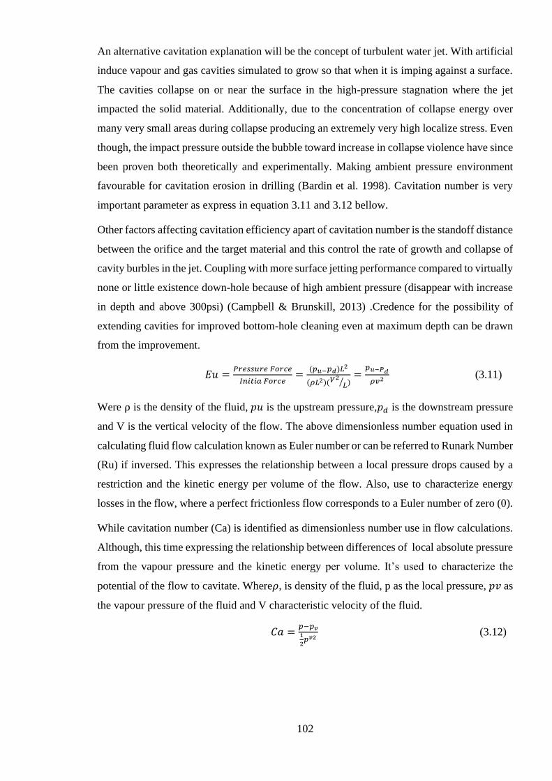
102

An alternative cavitation explanation will be the concept of turbulent water jet. With artificial

induce vapour and gas cavities simulated to grow so that when it is imping against a surface.

The cavities collapse on or near the surface in the high-pressure stagnation where the jet

impacted the solid material. Additionally, due to the concentration of collapse energy over

many very small areas during collapse producing an extremely very high localize stress. Even

though, the impact pressure outside the bubble toward increase in collapse violence have since

been proven both theoretically and experimentally. Making ambient pressure environment

favourable for cavitation erosion in drilling (Bardin et al. 1998). Cavitation number is very

important parameter as express in equation 3.11 and 3.12 bellow.

Other factors affecting cavitation efficiency apart of cavitation number is the standoff distance

between the orifice and the target material and this control the rate of growth and collapse of

cavity burbles in the jet. Coupling with more surface jetting performance compared to virtually

none or little existence down-hole because of high ambient pressure (disappear with increase

in depth and above 300psi) (Campbell & Brunskill, 2013) .Credence for the possibility of

extending cavities for improved bottom-hole cleaning even at maximum depth can be drawn

from the improvement.

𝐸𝑢 =𝑃𝑟𝑒𝑠𝑠𝑢𝑟𝑒 𝐹𝑜𝑟𝑐𝑒

𝐼𝑛𝑖𝑡𝑖𝑎 𝐹𝑜𝑟𝑐𝑒=

(𝑝𝑢−𝑝𝑑)𝐿2

(𝜌𝐿2)(𝑉2𝐿⁄ )

=𝑝𝑢−𝑃𝑑

𝜌𝑣2 (3.11)

Were ρ is the density of the fluid, 𝑝𝑢 is the upstream pressure,𝑝𝑑 is the downstream pressure

and V is the vertical velocity of the flow. The above dimensionless number equation used in

calculating fluid flow calculation known as Euler number or can be referred to Runark Number

(Ru) if inversed. This expresses the relationship between a local pressure drops caused by a

restriction and the kinetic energy per volume of the flow. Also, use to characterize energy

losses in the flow, where a perfect frictionless flow corresponds to a Euler number of zero (0).

While cavitation number (Ca) is identified as dimensionless number use in flow calculations.

Although, this time expressing the relationship between differences of local absolute pressure

from the vapour pressure and the kinetic energy per volume. It’s used to characterize the

potential of the flow to cavitate. Where𝜌, is density of the fluid, p as the local pressure, 𝑝𝑣 as

the vapour pressure of the fluid and V characteristic velocity of the fluid.

𝐶𝑎 =𝑝−𝑝𝑣1

2𝑝𝑣2

(3.12)

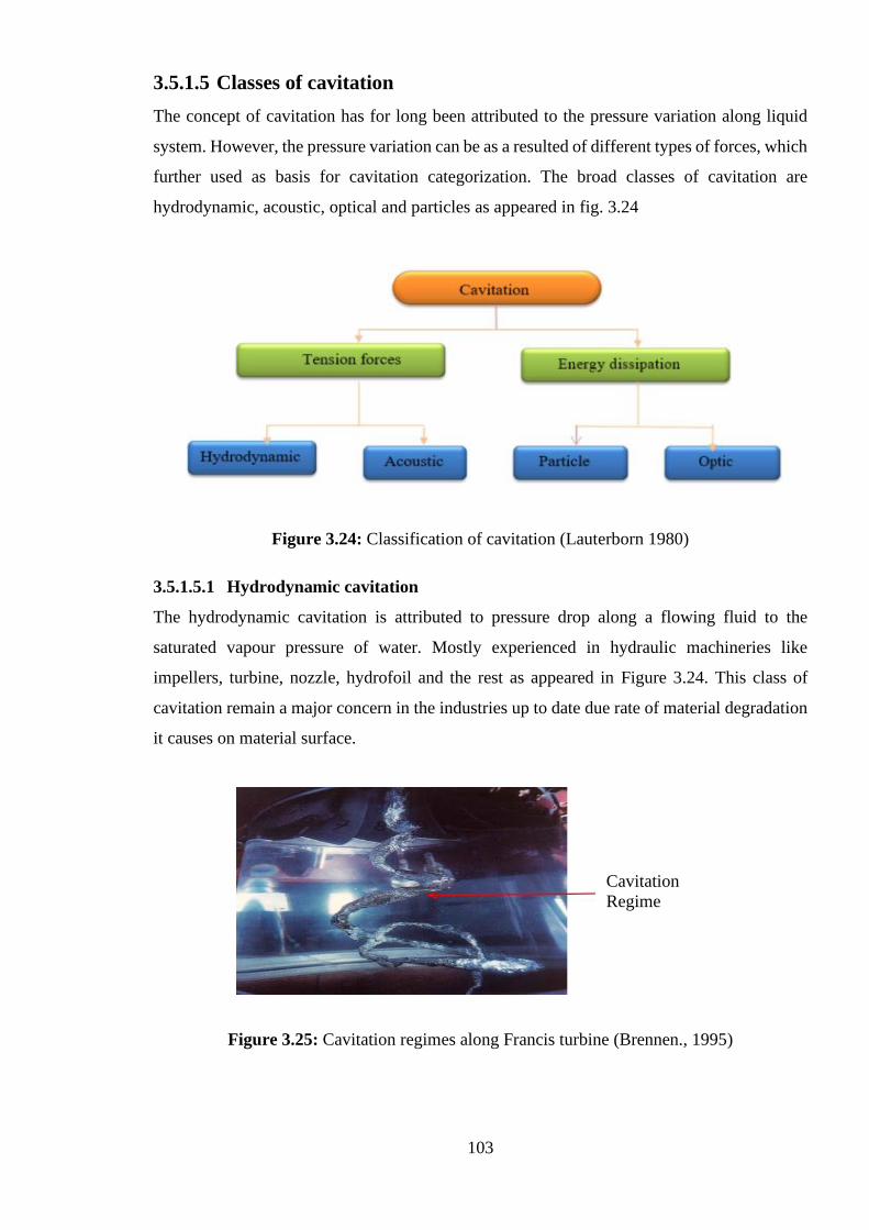
103

3.5.1.5 Classes of cavitation

The concept of cavitation has for long been attributed to the pressure variation along liquid

system. However, the pressure variation can be as a resulted of different types of forces, which

further used as basis for cavitation categorization. The broad classes of cavitation are

hydrodynamic, acoustic, optical and particles as appeared in fig. 3.24

Figure 3.24: Classification of cavitation (Lauterborn 1980)

3.5.1.5.1 Hydrodynamic cavitation

The hydrodynamic cavitation is attributed to pressure drop along a flowing fluid to the

saturated vapour pressure of water. Mostly experienced in hydraulic machineries like

impellers, turbine, nozzle, hydrofoil and the rest as appeared in Figure 3.24. This class of

cavitation remain a major concern in the industries up to date due rate of material degradation

it causes on material surface.

Figure 3.25: Cavitation regimes along Francis turbine (Brennen., 1995)

Cavitation

Regime

c

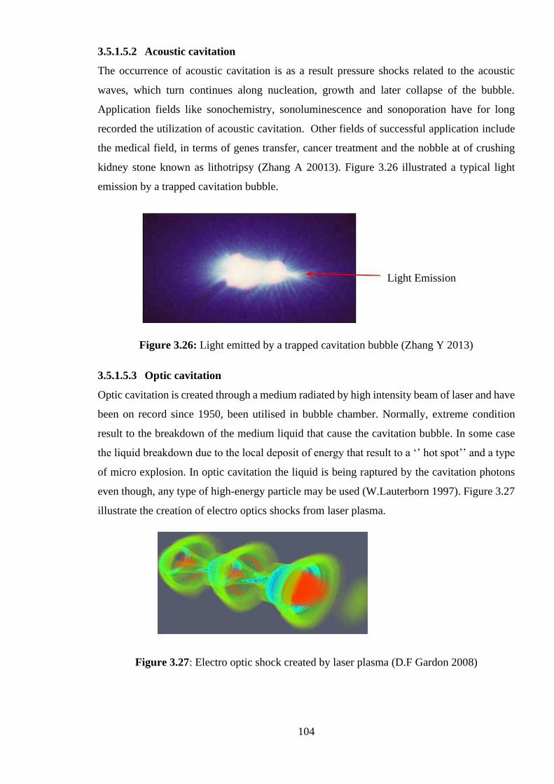
104

3.5.1.5.2 Acoustic cavitation

The occurrence of acoustic cavitation is as a result pressure shocks related to the acoustic

waves, which turn continues along nucleation, growth and later collapse of the bubble.

Application fields like sonochemistry, sonoluminescence and sonoporation have for long

recorded the utilization of acoustic cavitation. Other fields of successful application include

the medical field, in terms of genes transfer, cancer treatment and the nobble at of crushing

kidney stone known as lithotripsy (Zhang A 20013). Figure 3.26 illustrated a typical light

emission by a trapped cavitation bubble.

Figure 3.26: Light emitted by a trapped cavitation bubble (Zhang Y 2013)

3.5.1.5.3 Optic cavitation

Optic cavitation is created through a medium radiated by high intensity beam of laser and have

been on record since 1950, been utilised in bubble chamber. Normally, extreme condition

result to the breakdown of the medium liquid that cause the cavitation bubble. In some case

the liquid breakdown due to the local deposit of energy that result to a ‘’ hot spot’’ and a type

of micro explosion. In optic cavitation the liquid is being raptured by the cavitation photons

even though, any type of high-energy particle may be used (W.Lauterborn 1997). Figure 3.27

illustrate the creation of electro optics shocks from laser plasma.

Figure 3.27: Electro optic shock created by laser plasma (D.F Gardon 2008)

Light Emission

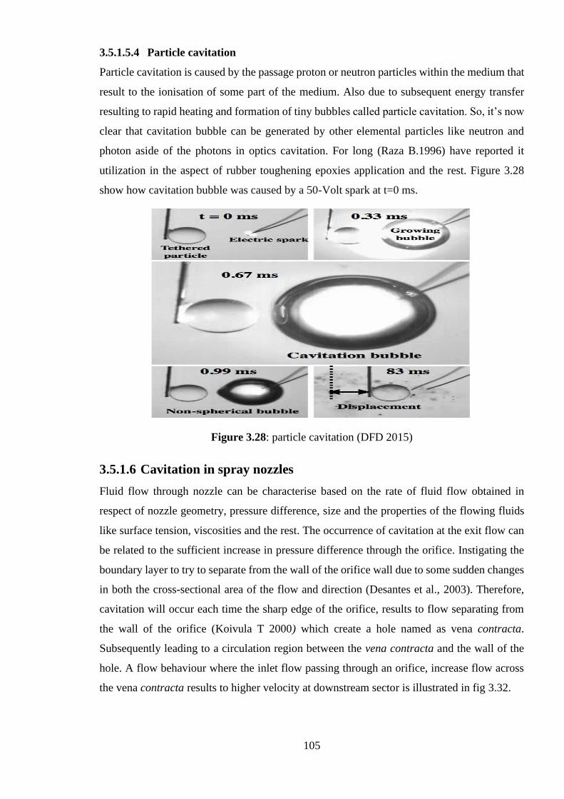
105

3.5.1.5.4 Particle cavitation

Particle cavitation is caused by the passage proton or neutron particles within the medium that

result to the ionisation of some part of the medium. Also due to subsequent energy transfer

resulting to rapid heating and formation of tiny bubbles called particle cavitation. So, it’s now

clear that cavitation bubble can be generated by other elemental particles like neutron and

photon aside of the photons in optics cavitation. For long (Raza B.1996) have reported it

utilization in the aspect of rubber toughening epoxies application and the rest. Figure 3.28

show how cavitation bubble was caused by a 50-Volt spark at t=0 ms.

Figure 3.28: particle cavitation (DFD 2015)

3.5.1.6 Cavitation in spray nozzles

Fluid flow through nozzle can be characterise based on the rate of fluid flow obtained in

respect of nozzle geometry, pressure difference, size and the properties of the flowing fluids

like surface tension, viscosities and the rest. The occurrence of cavitation at the exit flow can

be related to the sufficient increase in pressure difference through the orifice. Instigating the

boundary layer to try to separate from the wall of the orifice wall due to some sudden changes

in both the cross-sectional area of the flow and direction (Desantes et al., 2003). Therefore,

cavitation will occur each time the sharp edge of the orifice, results to flow separating from

the wall of the orifice (Koivula T 2000) which create a hole named as vena contracta.

Subsequently leading to a circulation region between the vena contracta and the wall of the

hole. A flow behaviour where the inlet flow passing through an orifice, increase flow across

the vena contracta results to higher velocity at downstream sector is illustrated in fig 3.32.

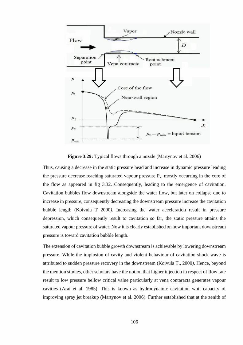
106

Figure 3.29: Typical flows through a nozzle (Martynov et al. 2006)

Thus, causing a decrease in the static pressure head and increase in dynamic pressure leading

the pressure decrease reaching saturated vapour pressure Pv, mostly occurring in the core of

the flow as appeared in fig 3.32. Consequently, leading to the emergence of cavitation.

Cavitation bubbles flow downstream alongside the water flow, but later on collapse due to

increase in pressure, consequently decreasing the downstream pressure increase the cavitation

bubble length (Koivula T 2000). Increasing the water acceleration result in pressure

depression, which consequently result to cavitation so far, the static pressure attains the

saturated vapour pressure of water. Now it is clearly established on how important downstream

pressure is toward cavitation bubble length.

The extension of cavitation bubble growth downstream is achievable by lowering downstream

pressure. While the implosion of cavity and violent behaviour of cavitation shock wave is

attributed to sudden pressure recovery in the downstream (Koivula T., 2000). Hence, beyond

the mention studies, other scholars have the notion that higher injection in respect of flow rate

result to low pressure bellow critical value particularly at vena contaracta generates vapour

cavities (Arai et al. 1985). This is known as hydrodynamic cavitation whit capacity of

improving spray jet breakup (Martynov et al. 2006). Further established that at the zenith of

107

cavitation, decrease in downstream pressure does not necessary increase flow rate due

existence of a phenomenon known as chocking.

Researchers on their pursuit for experimentally examining the cavitation flow along nozzle

came up with two dimensionless numbers (Reynold number and Cavitation number). As the

most important dimensionless group that can express cavitation, shown in Eq. 3.13

𝜎 =𝑃∞−𝑃𝑉

0.5𝜌𝑣∞2 (3.13)

Where 𝜎 is the cavitation number, 𝑃∞is the pressure of the fluid, w is density, the saturated

vapour pressure and velocity of the fluid is 𝑃𝑉 and Re is the Reynold number as express in

Eq.3.14

𝑅𝑒 =𝑝𝑤𝑢𝑑

µ𝑤 (3.14)

Where Pw is the density of water, velocity of water, U, diameter, d, and viscosity of water

as

w.

3.6 Descaling Operations

The process of applying high pressure jet water to remove scale (oxide deposit) from metal

surface in hot rolling application is the most renowned descaling process (Nasr et al., 2002).

Moreover, it’s recently more attributed to hydraulic scale removal in the petroleum industries.

Optimization of descaling process has always been tied to proper selection of spray

parameters. Archiving low energy cost and better scale removal is done through improving

nozzle designs. Thereby, turning hydraulic scale removal from simple question of high

pressure to developing science (Anon 1995) such as the development of special nozzles with

knife like (cut) impact stream for optimal descaling (Brown et al., 1993). Another important

requirement for archiving optimal descaling is the complete coverage of the target surface.

This is achieved through proper nozzle arrangement that includes some spray overlap for better

coverage and safety factors. Therefore, perquisite to optimizing descaling systems is nozzle

configurations in terms of size, type and arrangement on the header in order to achieve both

the highest impact force & target coverage at lower water requirement and energy cost.

Experience from the past emphasise on impact force apart of other parameters like droplet

sizes and injection pressure in removing hard surface scale, especially in steel making (Nasr

et al., 2002). Since it has a tremendous impact on the spray petternation, though the surface

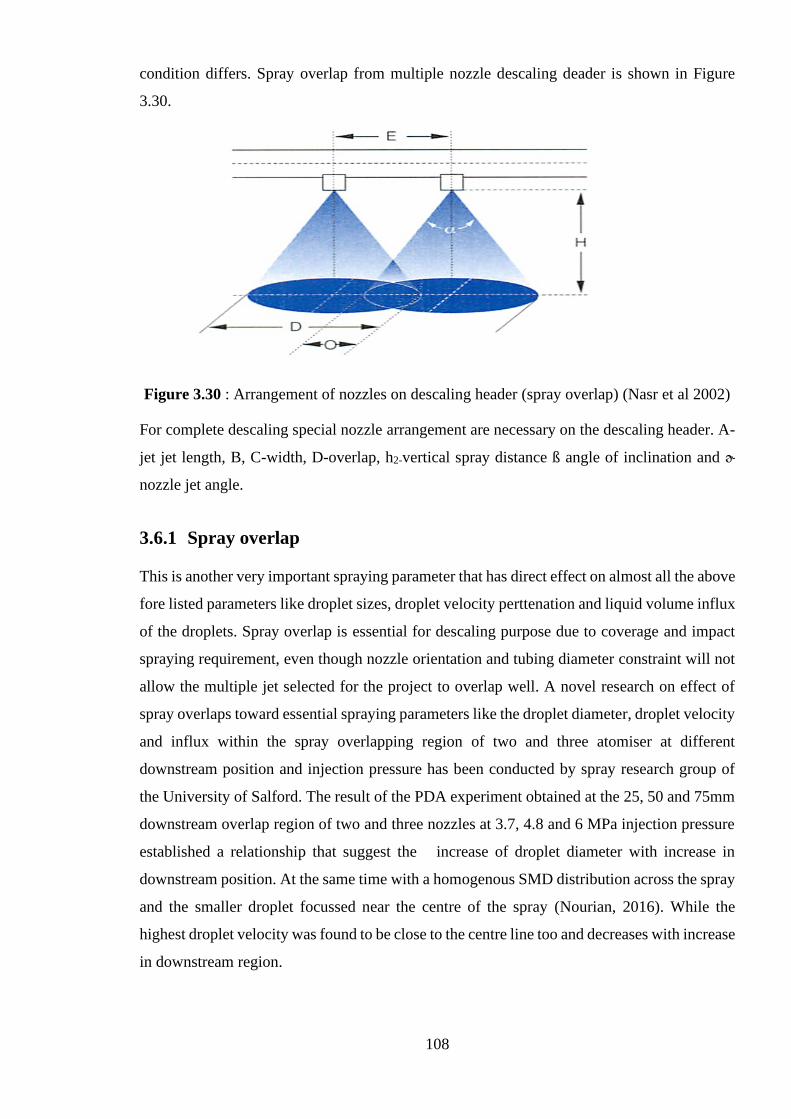
108

condition differs. Spray overlap from multiple nozzle descaling deader is shown in Figure

3.30.

Figure 3.30 : Arrangement of nozzles on descaling header (spray overlap) (Nasr et al 2002)

For complete descaling special nozzle arrangement are necessary on the descaling header. A-

jet jet length, B, C-width, D-overlap, h2-vertical spray distance ß angle of inclination and ɚ

nozzle jet angle.

3.6.1 Spray overlap

This is another very important spraying parameter that has direct effect on almost all the above

fore listed parameters like droplet sizes, droplet velocity perttenation and liquid volume influx

of the droplets. Spray overlap is essential for descaling purpose due to coverage and impact

spraying requirement, even though nozzle orientation and tubing diameter constraint will not

allow the multiple jet selected for the project to overlap well. A novel research on effect of

spray overlaps toward essential spraying parameters like the droplet diameter, droplet velocity

and influx within the spray overlapping region of two and three atomiser at different

downstream position and injection pressure has been conducted by spray research group of

the University of Salford. The result of the PDA experiment obtained at the 25, 50 and 75mm

downstream overlap region of two and three nozzles at 3.7, 4.8 and 6 MPa injection pressure

established a relationship that suggest the increase of droplet diameter with increase in

downstream position. At the same time with a homogenous SMD distribution across the spray

and the smaller droplet focussed near the centre of the spray (Nourian, 2016). While the

highest droplet velocity was found to be close to the centre line too and decreases with increase

in downstream region.

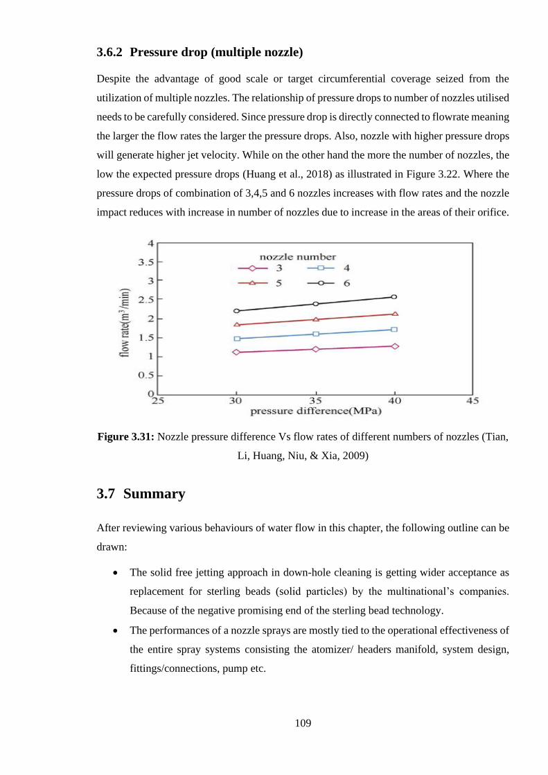
109

3.6.2 Pressure drop (multiple nozzle)

Despite the advantage of good scale or target circumferential coverage seized from the

utilization of multiple nozzles. The relationship of pressure drops to number of nozzles utilised

needs to be carefully considered. Since pressure drop is directly connected to flowrate meaning

the larger the flow rates the larger the pressure drops. Also, nozzle with higher pressure drops

will generate higher jet velocity. While on the other hand the more the number of nozzles, the

low the expected pressure drops (Huang et al., 2018) as illustrated in Figure 3.22. Where the

pressure drops of combination of 3,4,5 and 6 nozzles increases with flow rates and the nozzle

impact reduces with increase in number of nozzles due to increase in the areas of their orifice.

Figure 3.31: Nozzle pressure difference Vs flow rates of different numbers of nozzles (Tian,

Li, Huang, Niu, & Xia, 2009)

3.7 Summary

After reviewing various behaviours of water flow in this chapter, the following outline can be

drawn:

• The solid free jetting approach in down-hole cleaning is getting wider acceptance as

replacement for sterling beads (solid particles) by the multinational’s companies.

Because of the negative promising end of the sterling bead technology.

• The performances of a nozzle sprays are mostly tied to the operational effectiveness of

the entire spray systems consisting the atomizer/ headers manifold, system design,

fittings/connections, pump etc.

110

• Multiple nozzle overlaps increase the spray target coverage during descaling but

produces low pressure drop or low spray impact.

• Descaling through water jetting was found to be completely relying on any and/or

combination of erosion, abrasion, cyclin stress, cavitation mechanisms.

• Cavitation erosion has been of great concern in many industries due to it consequential

effect that are attributed to cost of repair/replacement of machinery part and the eroding

of concrete surface water dam spillway.

• Cavitation create micro bubbles which when hit a surface will collapse in a violence

behaviour that generate a pressure shocks that leads to a severe mechanical degradation

of materials called cavitation erosion.

• The substantial pressure drop experience at nozzle vena contracta when using high

velocity water flow in nozzle generate cavitation within and beyond the downstream

of the nozzle

• The material weakening effect and enhance pressure wave front due to aeration

(compression) have been sought to be applied as an abrasion compensation or

replacement of sterling beads on down-hole cleaning due to it high erosion effect.

111

Experimental Set-up and Procedure

4.1 Overview

This chapter presents the experimental design and set up including, procedures and description

of detail steps required to guarantee the achievement of the precise research objectives. The

Chapter covers the two phases including:

Phase 1: The pre-descaling experiment that are conducted outside the descaling chamber, in

preparation of descaling experiments, as further classified into three sections:

Section 1: Design, construction and assembling of the upgraded descaling rig

including the descaling chamber (ambient, compressed and vacuumed condition) in

simulation of ideal descaling conditions.

Section 2: Design/ fabrication of wax scale moulder and its further utilization to

produce soft scale samples candidate of different sizes and shape that can simulate

different stages of scale growth in production tubing.

Section 3: Chemical characterization of both the available hard samples and

constructed soft scale sample by compositionally analysing the hard scale samples via

(EDs, SEM & XRD technique) and the soft scale samples through (NMR & FTIR).

Phase 2: The main experimental descaling trials will be conducted by utilizing the special

constructed descaling chamber and is dived in to three sections:

Section 1: Studying the effect of descaling parameters like injection pressure, numbers

of nozzles, stand-off distance and header configurations toward the rate of scale

removal.

Section 2: Studying the effect chamber water/air concentration i.e. ambient,

compressed and vacuum air condition toward the rate of scale removal.

Section 3: Determining the optimum descaling requirement for the effective scale

removal of different types scale deposit in petroleum production tubing

Particulars of the experimental plan and steps are given in the flow chart shown in Fig.4.0.

Also, the experimental setups, methodology, procedure in addition precautionary measures

and source of errors are itemized in each individual section.

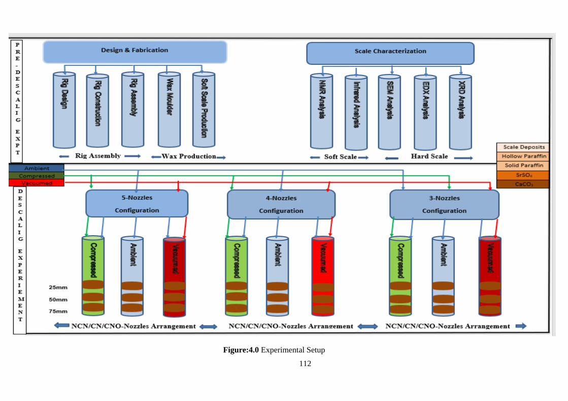
112

Figure:4.0 Experimental Setup

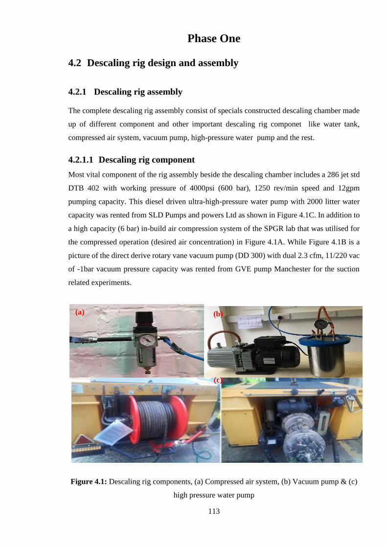
113

Phase One

4.2 Descaling rig design and assembly

4.2.1 Descaling rig assembly

The complete descaling rig assembly consist of specials constructed descaling chamber made

up of different component and other important descaling rig componet like water tank,

compressed air system, vacuum pump, high-pressure water pump and the rest.

4.2.1.1 Descaling rig component

Most vital component of the rig assembly beside the descaling chamber includes a 286 jet std

DTB 402 with working pressure of 4000psi (600 bar), 1250 rev/min speed and 12gpm

pumping capacity. This diesel driven ultra-high-pressure water pump with 2000 litter water

capacity was rented from SLD Pumps and powers Ltd as shown in Figure 4.1C. In addition to

a high capacity (6 bar) in-build air compression system of the SPGR lab that was utilised for

the compressed operation (desired air concentration) in Figure 4.1A. While Figure 4.1B is a

picture of the direct derive rotary vane vacuum pump (DD 300) with dual 2.3 cfm, 11/220 vac

of -1bar vacuum pressure capacity was rented from GVE pump Manchester for the suction

related experiments.

Figure 4.1: Descaling rig components, (a) Compressed air system, (b) Vacuum pump & (c)

high pressure water pump

(a) (b)

(c)

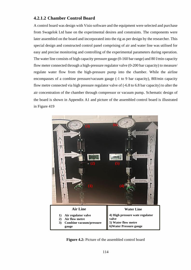
114

4.2.1.2 Chamber Control Board

A control board was design with Visio software and the equipment were selected and purchase

from Swagelok Ltd base on the experimental desires and constraints. The components were

later assembled on the board and incorporated into the rig as per design by the researcher. This

special design and constructed control panel comprising of air and water line was utilised for

easy and precise monitoring and controlling of the experimental parameters during operation.

The water line consists of high capacity pressure gauge (0-160 bar range) and 80 l/min capacity

flow meter connected through a high-pressure regulator valve (0-200 bar capacity) to measure/

regulate water flow from the high-pressure pump into the chamber. While the airline

encompasses of a combine pressure/vacuum gauge (-1 to 9 bar capacity), 80l/min capacity

flow metre connected via high pressure regulator valve of (-6.8 to 6.8 bar capacity) to alter the

air concentration of the chamber through compressor or vacuum pump. Schematic design of

the board is shown in Appendix A1 and picture of the assembled control board is illustrated

in Figure 419

Figure 4.2: Picture of the assembled control board

Air Line

1) Air regulator valve

2) Air flow metre

3) Combine vacuum/pressure

gauge

Water Line

4) High pressure wate regulator

valve

5) Water flow metre

6)Water Pressure gauge

(1)

(2) (5)

(4)

(3) (6)

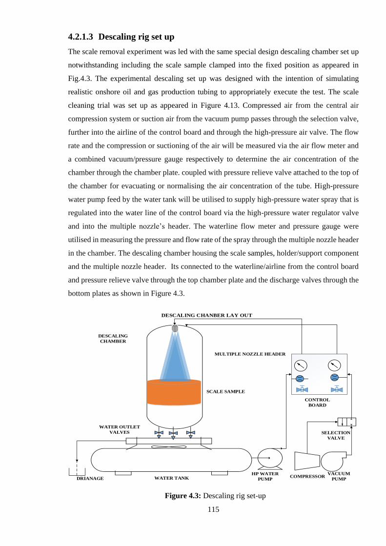
115

4.2.1.3 Descaling rig set up

The scale removal experiment was led with the same special design descaling chamber set up

notwithstanding including the scale sample clamped into the fixed position as appeared in

Fig.4.3. The experimental descaling set up was designed with the intention of simulating

realistic onshore oil and gas production tubing to appropriately execute the test. The scale

cleaning trial was set up as appeared in Figure 4.13. Compressed air from the central air

compression system or suction air from the vacuum pump passes through the selection valve,

further into the airline of the control board and through the high-pressure air valve. The flow

rate and the compression or suctioning of the air will be measured via the air flow meter and

a combined vacuum/pressure gauge respectively to determine the air concentration of the

chamber through the chamber plate. coupled with pressure relieve valve attached to the top of

the chamber for evacuating or normalising the air concentration of the tube. High-pressure

water pump feed by the water tank will be utilised to supply high-pressure water spray that is

regulated into the water line of the control board via the high-pressure water regulator valve

and into the multiple nozzle’s header. The waterline flow meter and pressure gauge were

utilised in measuring the pressure and flow rate of the spray through the multiple nozzle header

in the chamber. The descaling chamber housing the scale samples, holder/support component

and the multiple nozzle header. Its connected to the waterline/airline from the control board

and pressure relieve valve through the top chamber plate and the discharge valves through the

bottom plates as shown in Figure 4.3.

WATER TANKHP WATER

PUMP

DESCALING CHANBER LAY OUT

MULTIPLE NOZZLE HEADER

COMPRESSOR

SCALE SAMPLE

WATER OUTLET

VALVES

VACUUM

PUMP

CONTROL

BOARD

DRIANAGE

SELECTION

VALVE

DESCALING

CHAMBER

Figure 4.3: Descaling rig set-up

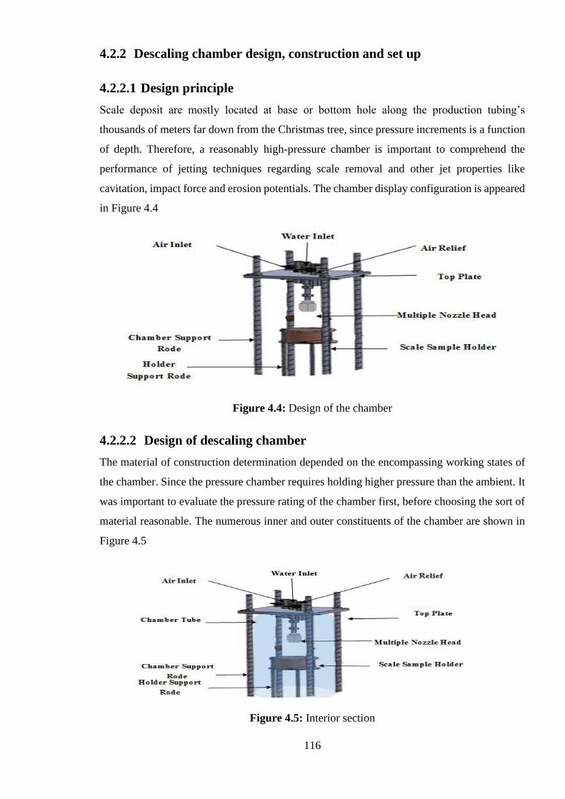
116

4.2.2 Descaling chamber design, construction and set up

4.2.2.1 Design principle

Scale deposit are mostly located at base or bottom hole along the production tubing’s

thousands of meters far down from the Christmas tree, since pressure increments is a function

of depth. Therefore, a reasonably high-pressure chamber is important to comprehend the

performance of jetting techniques regarding scale removal and other jet properties like

cavitation, impact force and erosion potentials. The chamber display configuration is appeared

in Figure 4.4

Figure 4.4: Design of the chamber

4.2.2.2 Design of descaling chamber

The material of construction determination depended on the encompassing working states of

the chamber. Since the pressure chamber requires holding higher pressure than the ambient. It

was important to evaluate the pressure rating of the chamber first, before choosing the sort of

material reasonable. The numerous inner and outer constituents of the chamber are shown in

Figure 4.5

Figure 4.5: Interior section

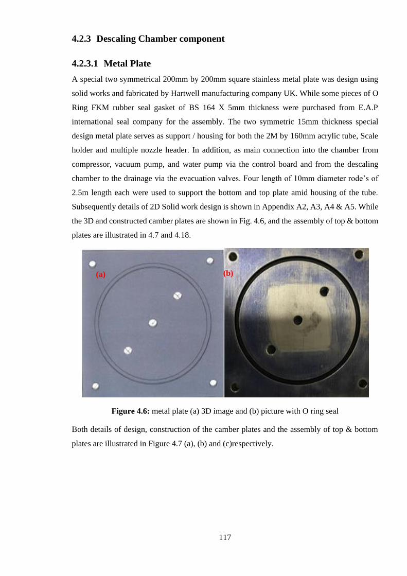
117

4.2.3 Descaling Chamber component

4.2.3.1 Metal Plate

A special two symmetrical 200mm by 200mm square stainless metal plate was design using

solid works and fabricated by Hartwell manufacturing company UK. While some pieces of O

Ring FKM rubber seal gasket of BS 164 X 5mm thickness were purchased from E.A.P

international seal company for the assembly. The two symmetric 15mm thickness special

design metal plate serves as support / housing for both the 2M by 160mm acrylic tube, Scale

holder and multiple nozzle header. In addition, as main connection into the chamber from

compressor, vacuum pump, and water pump via the control board and from the descaling

chamber to the drainage via the evacuation valves. Four length of 10mm diameter rode’s of

2.5m length each were used to support the bottom and top plate amid housing of the tube.

Subsequently details of 2D Solid work design is shown in Appendix A2, A3, A4 & A5. While

the 3D and constructed camber plates are shown in Fig. 4.6, and the assembly of top & bottom

plates are illustrated in 4.7 and 4.18.

Figure 4.6: metal plate (a) 3D image and (b) picture with O ring seal

Both details of design, construction of the camber plates and the assembly of top & bottom

plates are illustrated in Figure 4.7 (a), (b) and (c)respectively.

(a) (b)

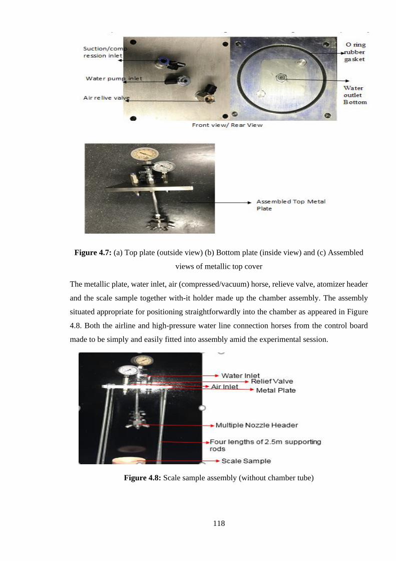
118

Figure 4.7: (a) Top plate (outside view) (b) Bottom plate (inside view) and (c) Assembled

views of metallic top cover

The metallic plate, water inlet, air (compressed/vacuum) horse, relieve valve, atomizer header

and the scale sample together with-it holder made up the chamber assembly. The assembly

situated appropriate for positioning straightforwardly into the chamber as appeared in Figure

4.8. Both the airline and high-pressure water line connection horses from the control board

made to be simply and easily fitted into assembly amid the experimental session.

Figure 4.8: Scale sample assembly (without chamber tube)

119

4.2.3.2 Clear acrylic tube

The result from volume/residence time calculation, size constraint of the multiple nozzle

header, need for expirimental visualization. Together with chamber design philosophy of

simulating real production scenario by pressurizing the chamber lead to the selection and

purchased of a 160 mm OD by 150mm ID ( 10mm thickness) of 2 M length from the Plastic

shop Company UK.

The pressure calculation was performed in light of the ambient air pressure along the

production tubing. Evaluated to primarily increment with increase in depth as the major

contributory elements, consequently utilizing the pressure equation as in Eq. 4.1:

𝑃 = 𝜌𝑔ℎ (4.1)

Where P, is the bottom pressure, the density of air along the void column of production

tubing amid maintenance, g, is the gravity, and h, the height to the scale formation. Taking the

density of air as 1.224 kg/m3, g as 9.8 m/s2 and an inexact height of 2000 m, at that point

P = 1.2249.812000 = 23,990.4 Pa = 0.24 bar _ gauge

P = 0.24+1.013 = 1.25 bar _ absolute

Having figured the anticipated pressure along the tubing, in spite of the much accessibility of

numerous materials capable of handling this pressure. A clear, transparent acrylic tube was

then picked. In view of its pressure rating of 6 bar (most extreme) and transparency to aid

imaging the investigation and recording the perceptions.

Volume and residence time calculations

The diameter of the chamber supposed to be based on the size of typical oil and gas Saudi

Aramco production tubing size. Nevertheless, due to some operational and experimental

constraints like size of the multiple nozzle headers, shape and size of the scale sample and

high spray impact from multiple high-pressure nozzles, high volume of utilize spray fluid and

the rest. A lager diameter tube was considered for the experiment, with 160 mm outside

diameter and 150mm inside diameter (10mm thickness) of 2m length. Thereby the basis of

selecting the convenient tube length, a residence time calculation was conducted which

corresponds to sufficient 2m length as available with manufacturer. While Appendix A6 show

case the clear acrylic tube (a) vendors specifications and (b) 2-meter length clear acrylic tube

with a 2.25m measuring ruler.

120

𝑉 = 𝜋𝑑2𝑙

4 (4.2)

𝑉 = 𝜋(0.15)2 𝑋 2

4= 35.4 𝑥10−3𝑚3 = 35.4 𝑙𝑖𝑡𝑟𝑒

Taking the flow rate of the flat-fan nozzle at 10 MPa as 11.3 litre/min

𝑅𝑒𝑠𝑖𝑑𝑒𝑛𝑐𝑒 𝑇𝑖𝑚𝑒 𝑜𝑓 𝑊𝑎𝑡𝑒𝑟 =𝑉𝑜𝑙𝑢𝑚𝑒

𝑉𝑜𝑙𝑢𝑚𝑒𝑡𝑟𝑖𝑐 𝐹𝑙𝑜𝑤 𝑟𝑎𝑡𝑒 (4.3)

𝑅𝑒𝑠𝑖𝑑𝑒𝑛𝑐𝑒 𝑇𝑖𝑚𝑒 𝑜𝑓 𝑊𝑎𝑡𝑒𝑟 = 35.4

11.3= 3.133 𝑚𝑖𝑛 = 188 𝑠𝑒𝑐

4.2.3.3 Multiple nozzle header assembly

A 1-inch diameter Fog Jet 7N-SS-10 fine spray female connection optional TWD hydraulic

atomiser header, housing seven set of small angle air mist nozzles was purchase from Spraying

Company System. This hydraulic atomiser was purchased to be amended for descaling

purpose by replacing the seven in-fitted air mist atomizers with high-pressure flat fan nozzles

from same vendor.

Seven numbers of ¼ MEG 2550 Wash jet high pressure flat fan nozzle of 25° standard spray

angle, 3000 psi and 5.2 gallon per minute flow rate capacity. This was earlier selected from

the wash jet standard angle performance chart to replace the fine mist atomizers inbuilt in the

7N Fog jet header. Unfortunately, the above-mentioned replacement nozzles were found un-

suitable for the test due to their high flow rate in comparison to the size of the chamber and

descaling time requirement (Residence time of 188sec). Leading to the identification and

replacement with another seven set of ¼ inch NPT male thread, 25° standard spray angle with

11.3 l/min capacity at 10 MPa (602.481.A3.07.00.0) from Lechler Ltd. Similar to the flat fan

atomiser specifications used for the single nozzle research. Additional numbers of CP2812-

SS (blank plugs) were procured from spray header manufacturers to block and vary atomizing

numbers in other to archive the desired header configuration. Figure 4.9, 4.10 ,4.11 and

Appendix A7 & A8 illustrate individual header component before and after

assembly/amendment.

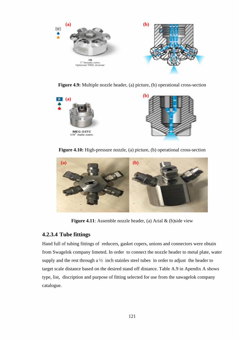
121

Figure 4.9: Multiple nozzle header, (a) picture, (b) operational cross-section

Figure 4.10: High-pressure nozzle, (a) picture, (b) operational cross-section

Figure 4.11: Assemble nozzle header, (a) Arial & (b)side view

4.2.3.4 Tube fittings

Hand full of tubing fittings of reducers, gasket copers, unions and connectors were obtain

from Swagelok company limeted. In order to connect the nozzle header to metal plate, water

supply and the rest through a ½ inch stainles steel tubes in order to adjust the header to

target scale distance based on the desired stand off distance. Table A.9 in Apendix A shows

type, list, discription and purpose of fitting selected for use from the sawagelok company

catalogue.

(a) (b)

(a) (b)

(a) (b)

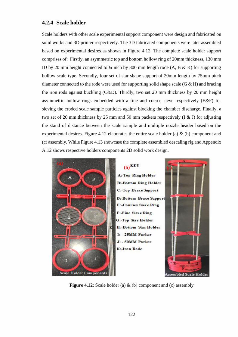
122

4.2.4 Scale holder

Scale holders with other scale experimental support component were design and fabricated on

solid works and 3D printer respectively. The 3D fabricated components were later assembled

based on experimental desires as shown in Figure 4.12. The complete scale holder support

comprises of: Firstly, an asymmetric top and bottom hollow ring of 20mm thickness, 130 mm

ID by 20 mm height connected to ¼ inch by 800 mm length rode (A, B & K) for supporting

hollow scale type. Secondly, four set of star shape support of 20mm length by 75mm pitch

diameter connected to the rode were used for supporting solid shape scale (G & H) and bracing

the iron rods against buckling (C&D). Thirdly, two set 20 mm thickness by 20 mm height

asymmetric hollow rings embedded with a fine and coerce sieve respectively (E&F) for

sieving the eroded scale sample particles against blocking the chamber discharge. Finally, a

two set of 20 mm thickness by 25 mm and 50 mm packers respectively (I & J) for adjusting

the stand of distance between the scale sample and multiple nozzle header based on the

experimental desires. Figure 4.12 elaborates the entire scale holder (a) & (b) component and

(c) assembly, While Figure 4.13 showcase the complete assembled descaling rig and Appendix

A:12 shows respective holders components 2D solid work design.

Figure 4.12: Scale holder (a) & (b) component and (c) assembly

(a) (b) (c)

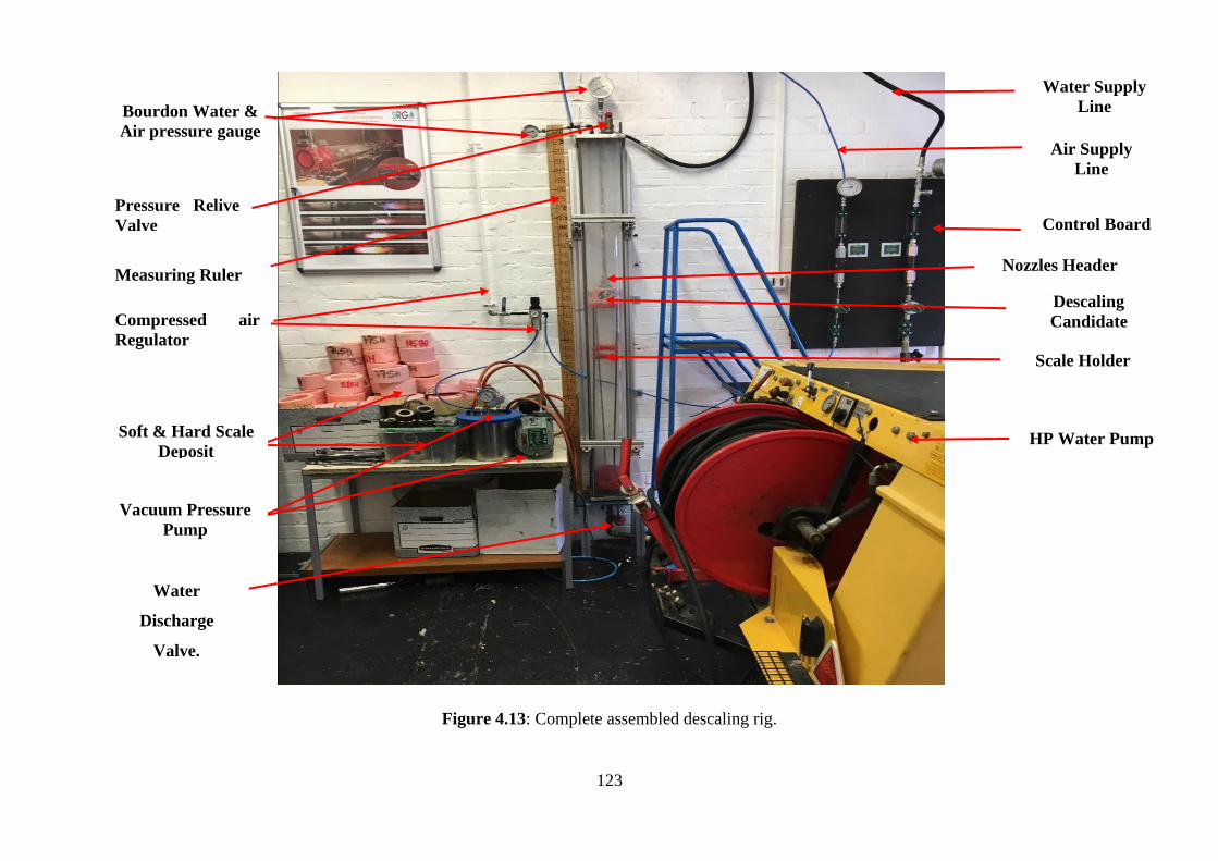
123

Figure 4.13: Complete assembled descaling rig.

Bourdon Water &

Air pressure gauge

Pressure Relive

Valve

Measuring Ruler

Compressed air

Regulator

Soft & Hard Scale

Deposit

Vacuum Pressure

Pump

Water

Discharge

Valve.

Water Supply

Line

Air Supply

Line

Control Board

Descaling

Candidate

Scale Holder

HP Water Pump

Nozzles Header

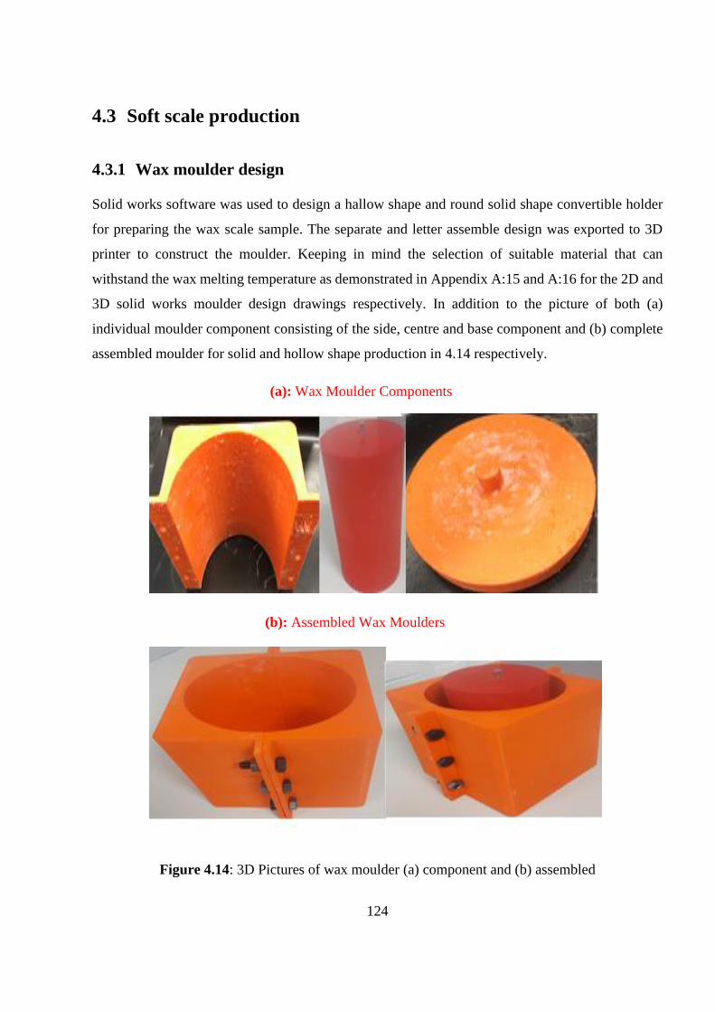
124

4.3 Soft scale production

4.3.1 Wax moulder design

Solid works software was used to design a hallow shape and round solid shape convertible holder

for preparing the wax scale sample. The separate and letter assemble design was exported to 3D

printer to construct the moulder. Keeping in mind the selection of suitable material that can

withstand the wax melting temperature as demonstrated in Appendix A:15 and A:16 for the 2D and

3D solid works moulder design drawings respectively. In addition to the picture of both (a)

individual moulder component consisting of the side, centre and base component and (b) complete

assembled moulder for solid and hollow shape production in 4.14 respectively.

Figure 4.14: 3D Pictures of wax moulder (a) component and (b) assembled

(b): Assembled Wax Moulders

(a): Wax Moulder Components

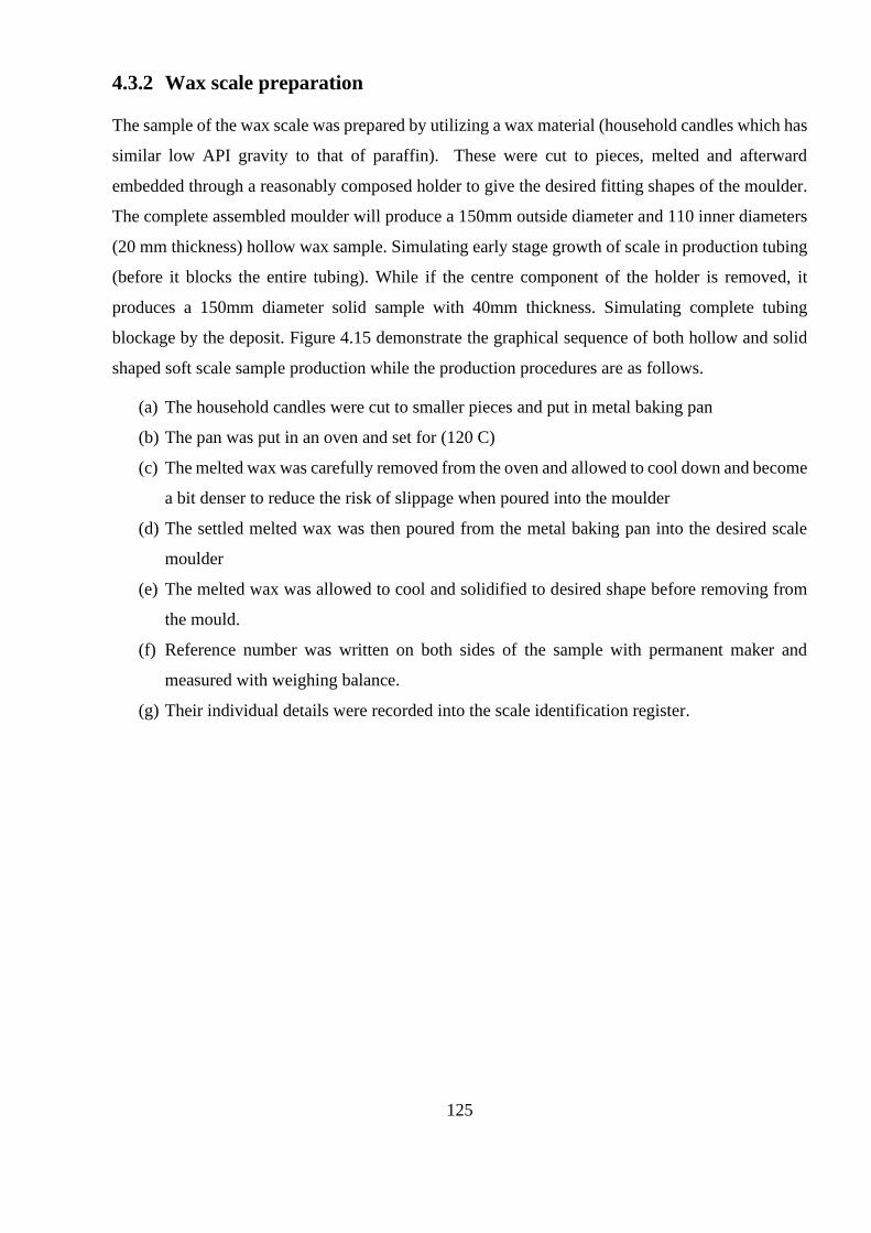
125

4.3.2 Wax scale preparation

The sample of the wax scale was prepared by utilizing a wax material (household candles which has

similar low API gravity to that of paraffin). These were cut to pieces, melted and afterward

embedded through a reasonably composed holder to give the desired fitting shapes of the moulder.

The complete assembled moulder will produce a 150mm outside diameter and 110 inner diameters

(20 mm thickness) hollow wax sample. Simulating early stage growth of scale in production tubing

(before it blocks the entire tubing). While if the centre component of the holder is removed, it

produces a 150mm diameter solid sample with 40mm thickness. Simulating complete tubing

blockage by the deposit. Figure 4.15 demonstrate the graphical sequence of both hollow and solid

shaped soft scale sample production while the production procedures are as follows.

(a) The household candles were cut to smaller pieces and put in metal baking pan

(b) The pan was put in an oven and set for (120 C)

(c) The melted wax was carefully removed from the oven and allowed to cool down and become

a bit denser to reduce the risk of slippage when poured into the moulder

(d) The settled melted wax was then poured from the metal baking pan into the desired scale

moulder

(e) The melted wax was allowed to cool and solidified to desired shape before removing from

the mould.

(f) Reference number was written on both sides of the sample with permanent maker and

measured with weighing balance.

(g) Their individual details were recorded into the scale identification register.

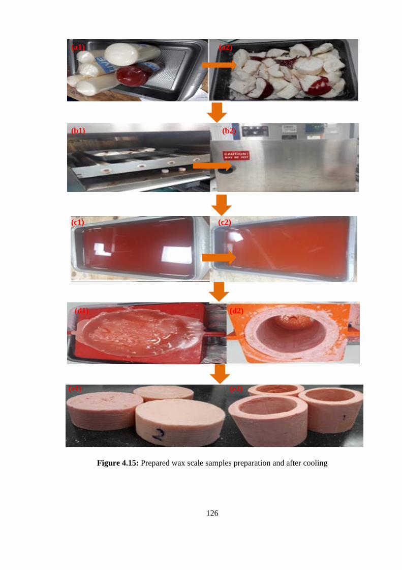
126

Figure 4.15: Prepared wax scale samples preparation and after cooling

(a1) (a2)

(b1) (b2)

(c1)

(d1)

(e1)

(c2)

(d2)

(e2)

127

4.4 Scale characterization

4.4.1 Soft Scale compositional & chemical analysis

The constructed soft scale samples of different sizes and shapes from Section 4.3.2 were subjected

to NMR and FTIR analysis. In order to determine if they truly have the same chemical properties

with the paraffin scale deposit usually found in petroleum production tubing. Figure 4.16 showcase

constructed soft scale samples of (a) hollow and (b) solid shapes respectively.

Figure 4.16: Constructed soft scale (a) hollow shape, (b) solid shaped samples

4.4.1.1 Soft scale NMR analysis procedure

Nuclear Magnetic resonance spectroscopy is a very useful technique employed in characterising

organic samples (both aliphatic and aromatic). Like other spectroscopy techniques, NMR works on

the principle that molecules interact with electromagnetic radiations thus increasing their energy

level (quantization). This energy difference will determine the molecular environment of each

nucleus present in an organic sample. However, only the atoms with spin (odd mass number) are

detected by NMR. Nuclei observed with NMR include 1H, 13C, 15N etc. The most common nuclei

used analysing organic compounds is the 1H and 13C and this makes it a versatile tool for

investigating varieties of petroleum products. In order to probe a sample by NMR method, the

sample must be completely dissolved in a deuterated solvent. The most common deuterated solvents

used include chloroform (CDCl3), water (D2O) and acetone-d6. Not necessarily, however, some

solvents are calibrated with a standard reference. Tetramethylsilane (also abbreviated TMS), is one

of the commonly used reference compounds used in solvents because it is used to indicate the

starting point of all signal peaks (in ppm) that appear on the spectra. About 10-50mg of soft scale

sample is required for NMR analysis and was solubilised in deuterated CDCl3 on a Bruker Advance

400 MHz NMR.

(a) (b)

128

1. 10mg of starting material was used to clean the tube

2. The crushed wax sample was dissolved in 0.7Ml of deuterated solvent (CDCL3 in this case)

as 4.5-5 cm is recommended as a suitable high of solvent for good spectrums

3. The NMR tube is carefully cap and the sample name is written on it.

4. The sample was gently shaken to ensure effective dissolving of the sample and precaution

were taken to avoid contaminating the sample due to solvent cap contact.

5. The spinner and the NMR tube were clean with 2 propanol and lab tissue to wipe out all dirt

and fingerprints

6. The NMR tube was gently inserted into the spinner and the spinner automatically rotate into

the magnet to ensure the whole sample experience a homogenous magnetic field. The

spinner is placed in a sample gauge to prevent the bottom of the NMR tube from sitting far

into the NMR probe to reduce the risk of damaging the spectrometer as each probe has its

own sample depth.

7. The sample was place into the NMR spectrometer and a Varian 400 MHz spectrometer

equipped with an autosampler was utilised

8. The spectrums were processed, and peak were assigned in the spectrum.

4.4.1.2 Soft Scale FTIR analysis procedure

A Thermo Scientific Nicolet iS10 Fourier-transform infrared spectroscopy (FTIR) situated in

Analytical Laboratory Service in Crowcroft building of university of Salford was utilised in

analysing the constructed wax samples as per the set up in Figure 4.17. The concept of infrared

spectroscopy lies around the interaction of infrared light and molecules either by measuring it

emission, absorption or deflection for analysing and identification of chemical substance, functional

group in a compound and other applications. In order word, molecules absorb some exact frequency

of light that are characterise by the corresponding structures of molecules. The shape of the

molecular surface, the accompanying vibrionic coupling, and the mass corresponding to the atoms

determines its energies. Normally, light atoms and stronger bonds will vibrate at a high stretching

frequency (wavenumber). The following procedures were followed to effectively analyse the

samples with the experimental set up in Figure 4.17.

i. 1-Started by logging in to the OMNIC software windows in the FTIR analyser dedicated

computer system and select the smart FITR Diamond ATR accessory

ii. 2- The system drop window was properly clean with propanol and a lab tissue paper.

iii. 3-Then the ATR was screwed against the sample holder until a click sound is heard.

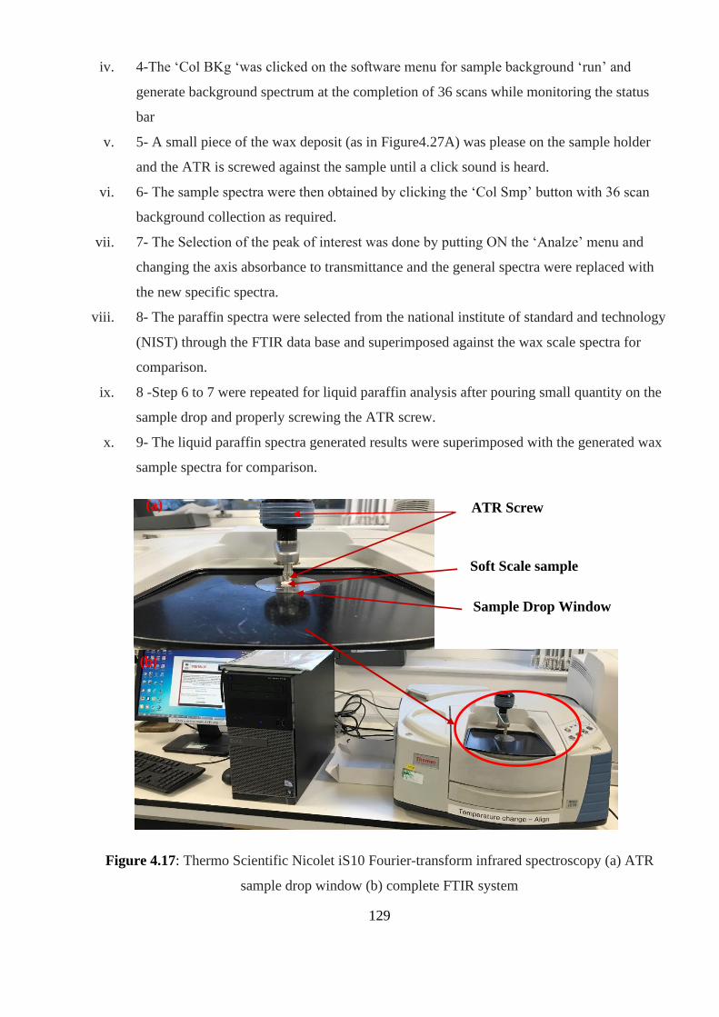
129

iv. 4-The ‘Col BKg ‘was clicked on the software menu for sample background ‘run’ and

generate background spectrum at the completion of 36 scans while monitoring the status

bar

v. 5- A small piece of the wax deposit (as in Figure4.27A) was please on the sample holder

and the ATR is screwed against the sample until a click sound is heard.

vi. 6- The sample spectra were then obtained by clicking the ‘Col Smp’ button with 36 scan

background collection as required.

vii. 7- The Selection of the peak of interest was done by putting ON the ‘Analze’ menu and

changing the axis absorbance to transmittance and the general spectra were replaced with

the new specific spectra.

viii. 8- The paraffin spectra were selected from the national institute of standard and technology

(NIST) through the FTIR data base and superimposed against the wax scale spectra for

comparison.

ix. 8 -Step 6 to 7 were repeated for liquid paraffin analysis after pouring small quantity on the

sample drop and properly screwing the ATR screw.

x. 9- The liquid paraffin spectra generated results were superimposed with the generated wax

sample spectra for comparison.

Figure 4.17: Thermo Scientific Nicolet iS10 Fourier-transform infrared spectroscopy (a) ATR

sample drop window (b) complete FTIR system

ATR Screw

Soft Scale sample

Sample Drop Window

(a)

(b)

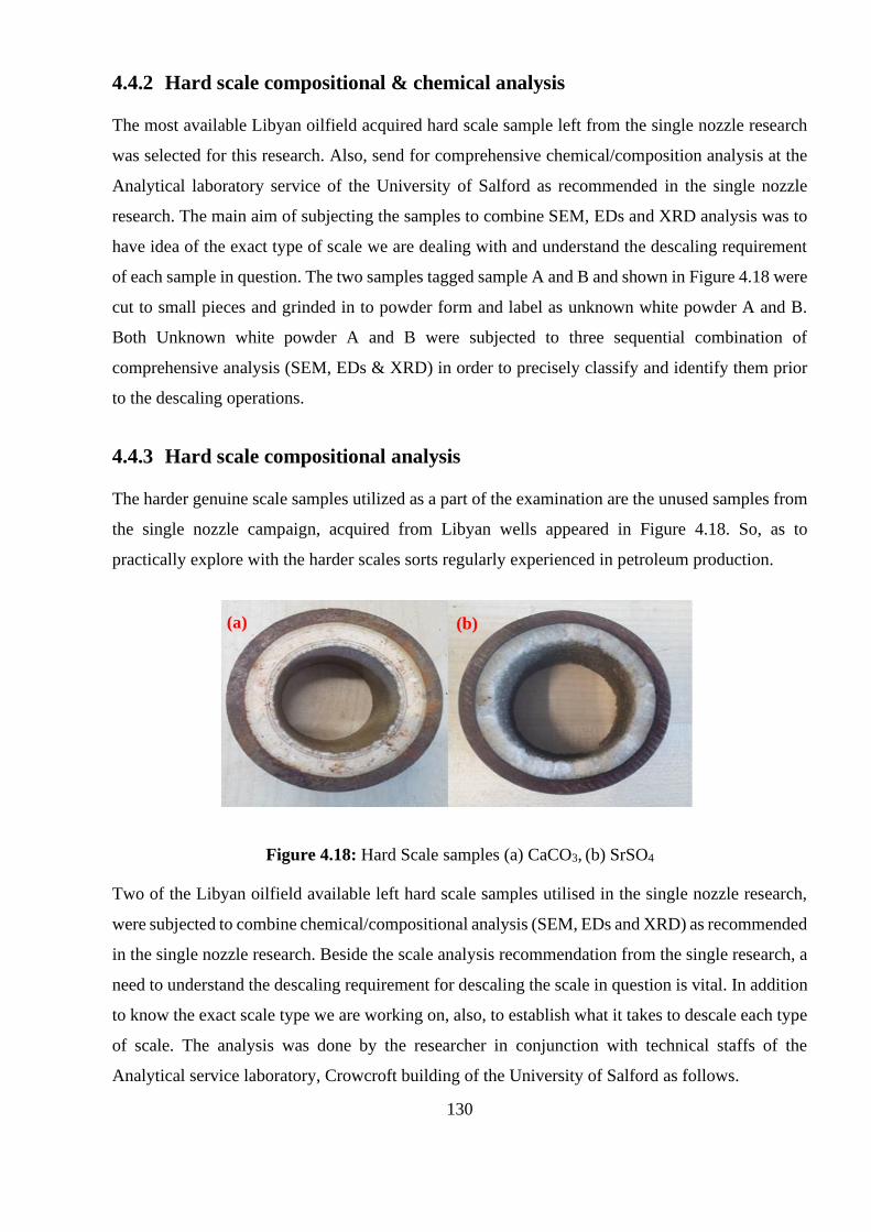
130

4.4.2 Hard scale compositional & chemical analysis

The most available Libyan oilfield acquired hard scale sample left from the single nozzle research

was selected for this research. Also, send for comprehensive chemical/composition analysis at the

Analytical laboratory service of the University of Salford as recommended in the single nozzle

research. The main aim of subjecting the samples to combine SEM, EDs and XRD analysis was to

have idea of the exact type of scale we are dealing with and understand the descaling requirement

of each sample in question. The two samples tagged sample A and B and shown in Figure 4.18 were

cut to small pieces and grinded in to powder form and label as unknown white powder A and B.

Both Unknown white powder A and B were subjected to three sequential combination of

comprehensive analysis (SEM, EDs & XRD) in order to precisely classify and identify them prior

to the descaling operations.

4.4.3 Hard scale compositional analysis

The harder genuine scale samples utilized as a part of the examination are the unused samples from

the single nozzle campaign, acquired from Libyan wells appeared in Figure 4.18. So, as to

practically explore with the harder scales sorts regularly experienced in petroleum production.

Figure 4.18: Hard Scale samples (a) CaCO3, (b) SrSO4

Two of the Libyan oilfield available left hard scale samples utilised in the single nozzle research,

were subjected to combine chemical/compositional analysis (SEM, EDs and XRD) as recommended

in the single nozzle research. Beside the scale analysis recommendation from the single research, a

need to understand the descaling requirement for descaling the scale in question is vital. In addition

to know the exact scale type we are working on, also, to establish what it takes to descale each type

of scale. The analysis was done by the researcher in conjunction with technical staffs of the

Analytical service laboratory, Crowcroft building of the University of Salford as follows.

(a) (b)

131

i. The scale samples in question were cut and grinded into small pieces powder foam (tag as

unknown powder)

ii. The unknown powders were first off, all send for SEM analysis using the scanning

electron microscope to identify the surface topography and composition of the powder

iii. The Unknown white powders results were further sent for EDs analysis using the energy

dispersive X ray spectroscopy to examine the elemental and quantitative chemical

composition of the compound in the unknown white powder.

iv. For final and confirmatory analysis to determine the crystalline material (mineralogy) of

the compound. The grinded white unknown powders were subjected to X ray powder

diffraction analysis.

v. Step 1 to 4 was followed for both samples.

4.4.3.1 Scanning electron microscope (SEM)

The two unknown white powder labelled sample A & B were first off, all, send for scanning electron

microscopy analysis in order to identify their surface topography and compound composition

through the magnifying lances of the microscope. The SEM works by detecting secondary or

backscattered electron signal from the focus electron bean that was restrain across the sample

surface by the SEM. Since both SEM and energy dispersive X-ray Spectroscopy (EDS) worked in

conjunction for the characteristic x-ray separation of different element into energy diagram, which

can be utilised in determining the presence and quantity of a particular element down to a region the

size of microns. In addition to having similar or connected procedure, only the EDs operating

protocol will be detailed in the report.

4.4.3.2 Energy dispersive X-ray analysis (EDX)

For the purpose of elemental identification and quantitative compositional information, the samples

were further subjected to EDX analysis after the SEM analysis. It depends on the interaction

between the sample and some source of X-ray excitations, resulting in the EDx detector measuring

the relative abundance of emitted X-rays against their energy. The focus electrons pass through the

sample on an atomic level that leads to the occurrence of different electron displacement, with each

displacement emitting electrons or X-rays. Subject to the return, displacement is separated and

analyse to generate elemental maps and images, just like the results of sample A and B as appeared

in Figure 5.6 and 5.7 at different spectrums. After the successful execution of the SEM analysis of

the two hard scale samples by magnifying them in different resolution, the following procedures

were performed for generating their respective elemental maps with EDx spectroscopy.

132

i. The sample was mounted, and the holder was placed into the chamber in line with the

orientation to the arrow on the bottom of the holder.

ii. The picture of the sample was taken to check how it will appear on the monitor

iii. The chamber was closed with it clip, ‘EVAC’ was pressed for 2 seconds until its light is

solid and the left side Robinson chamber view was turned on.

iv. ‘VLC’ app was selected to show the camera on the monitor and the sample was push to the

SEM

v. The ’Click Spectrum’ was pressed ‘EV/Chan’ for spectrum collections

vi. The ‘point analysis’ was clicked to transfer the to TEAM Eds system from SEM

vii. ‘Collect spectrum’ bottom was clicked, while an area of interest was choice to allow

spectrum collection and report was initiated

viii. ‘Mapping’ and ‘collect mapping’ were sequentially clicked and ‘finished’ and ‘reporting’

tabs were afterward clicked to generate summary of the data

ix. The ‘line scan’ and ‘collect line’ bottoms were clicked for better resolution configurations.

x. Finally, procedure 1 to 9 was repeated for the second sample analysis.

4.4.3.3 X-ray diffraction analysis

For final confirmatory analysis, the samples were subjected to x-ray powder diffraction analysis for

the characterization of their crystalline material. This rapid analytical technique uses Bragg’s law

to principally identify the crystalline of material and in addition provide information on unit cell

dimensions. Bragg’s law works on the concept that the observed peaks of scattering intensity when

x-ray is scattered from crystal lattice will corresponds to the following conditions: The angle of

incident will be equal to angle of scattering while the difference in path length is equal an integer

number of wavelengths. After samples are finely ground, homogenised and average bulk

composition is determined. The following procedure were adopted for XRD analysis of the two hard

scale sample.

i. A small piece of both samples was cut and separately grounded to a fine powder form.

ii. A fine mesh seize was place above the Si Crystal

iii. About 20 mg of sample A was poured on to the sieved and cautiously directed above the Si

crystal on the mount

iv. The sieve was tab from the bench to make sure the monolayer of sample covers the Si

crystal surface

v. The XRD powder pattern was collected

vi. The instrument door was opened, and the sample holder was mounted into the instrument

133

vii. The Commander software suite (An XRD powder pattern collecting program) and the

standard data collected scan was loaded by pressing the ‘Wizard’ tab.

viii. A 20-minute scan running time was selected for better powder XRD pattern resolution.

ix. A wavelength range comprising of angle range (2 θ) that was scanned at (5-70 °) that was

more suitable for inorganic materials was selected.

x. The ‘start’ bottom was pressed for data collection initiation.

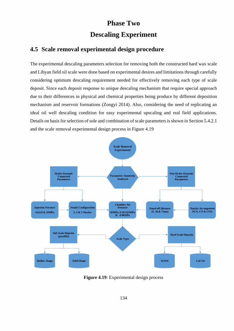
134

Phase Two

Descaling Experiment

4.5 Scale removal experimental design procedure

The experimental descaling parameters selection for removing both the constructed hard wax scale

and Libyan field oil scale were done based on experimental desires and limitations through carefully

considering optimum descaling requirement needed for effectively removing each type of scale

deposit. Since each deposit response to unique descaling mechanism that require special approach

due to their differences in physical and chemical properties being produce by different deposition

mechanism and reservoir formations (Zongyi 2014). Also, considering the need of replicating an

ideal oil well descaling condition for easy experimental upscaling and real field applications.

Details on basis for selection of sole and combination of scale parameters is shown in Section 5.4.2.1

and the scale removal experimental design process in Figure 4.19

Parametric Sensitivity

Analaysis

Hydro Dynamic Connected Parameters

Injection Pressure

4.8,6.0 & 10MPa

Stand-off Distance

25, 50,& 75mm

Nozzle Configuration

3, 4 & 5 Nozzles

Nozzles Arrangement

NCN, CN & CNO

Chamber Air Pressure

02MPa, 0.101325MPa & -0.08MPa

Scale Removal

Experiement

Non-Hydro Dynamic Connected Parameters

Soft Scale Deposits

(paraffin)Hard Scale Deposits

Hollow Shape Solid Shape SrSO4 CaCO3

Scale Type

Figure 4.19: Experimental design process

135

4.5.1 Descaling experiment preparations

The samples utilized as a part of this examination comprise of two segments that are typically like

the scale deposit experienced during oil and gas production. They incorporate the wax scale

experienced while producing highly paraffinic hydrocarbons characterize with low API gravity. In

spite of the fact that this scale sample is normally found on topside of production facility. It might

be experienced along production tubing particularly around the Christmas tree because of build-up

and condensation of heavier hydrocarbons. Other scale sample includes the genuine specimen of oil

field scale acquired from Libyan wells for the single nozzle research. These samples had been

chemically analysis using combination of XRD, EDS and SEM by the researcher.

4.5.1.1 Pump calibrations

For the purpose of familiarization of the pump and the rig system and maintaining pressure at

constant rate. The mass flow rate of the desired combination of nozzles at different injection pressure

was measured in preparation of the main descaling trials of both soft and hard scale candidates. This

was also carried out to monitor the consistency on the pressure gauges at the pump, the water line

of the control board and pressure drop on the gauges on top of the top plate. So as, individual desired

pressure, build up time and operational synergy between the pump, control board, descaling

chamber and the discharge evacuation system. The bucket weighing method was utilised and the

following procedures were followed to properly measure mass flow rate of different combinations

of nozzles at different injection pressures.

i. The desired numbers of nozzles were properly fitted in to the header and the un-desired

properly blocked with the blank plugs.

ii. The hydraulic connections from the pump to the control board to the top plate of the chamber

to the header are properly secured

iii. The header in properly inserted into 35liter measuring tank and sealed away from leakage.

With the tank properly seated on a table for easy evacuation through the tank discharge valve

to the measuring bucket.

iv. The HP pump was switched on and the timer was set to determine the pressure build-up time

for the desired pressure.

v. The HP pump was switched off once the desired pressure was reached, the time taken to

build pressure was recorded and the mass of the water build up (dead water) was measured

with the weighing balance

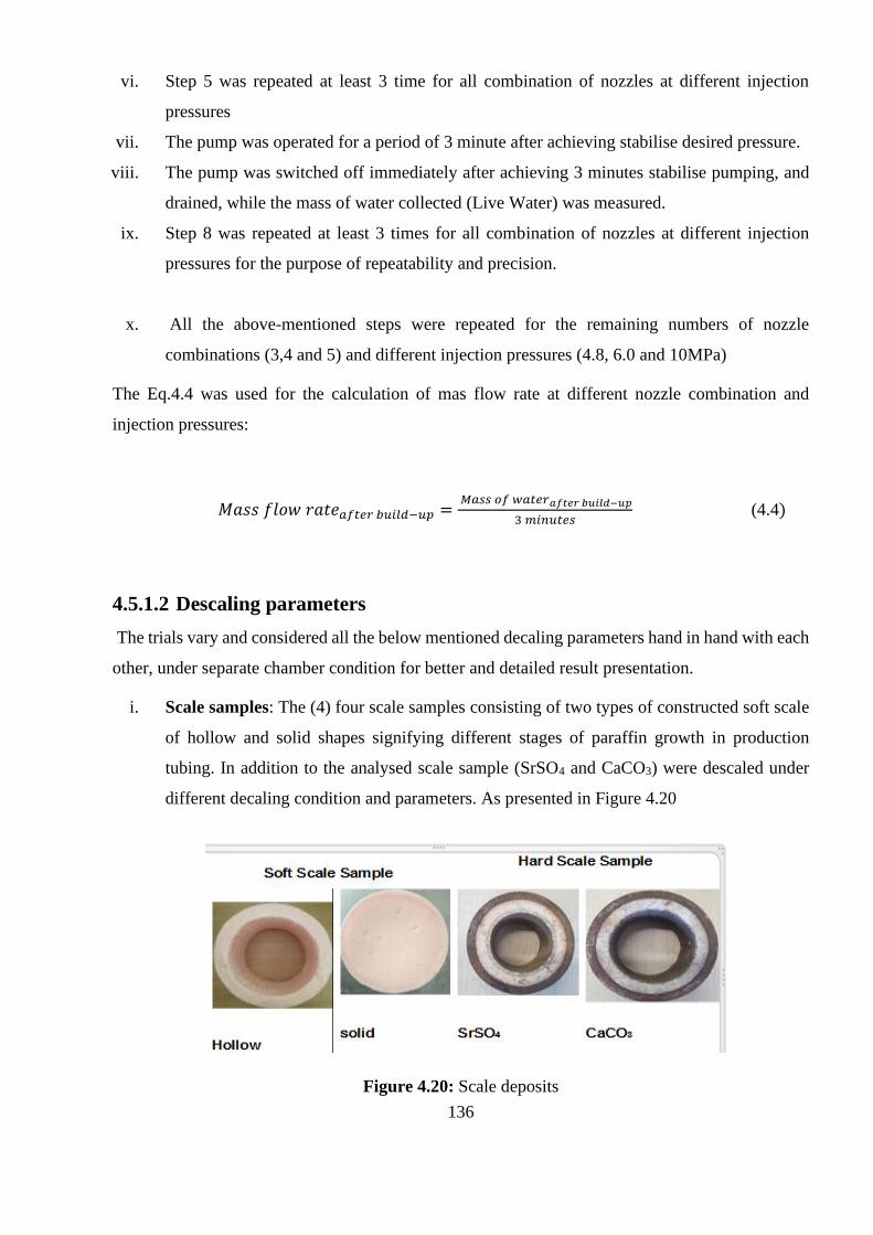
136

vi. Step 5 was repeated at least 3 time for all combination of nozzles at different injection

pressures

vii. The pump was operated for a period of 3 minute after achieving stabilise desired pressure.

viii. The pump was switched off immediately after achieving 3 minutes stabilise pumping, and

drained, while the mass of water collected (Live Water) was measured.

ix. Step 8 was repeated at least 3 times for all combination of nozzles at different injection

pressures for the purpose of repeatability and precision.

x. All the above-mentioned steps were repeated for the remaining numbers of nozzle

combinations (3,4 and 5) and different injection pressures (4.8, 6.0 and 10MPa)

The Eq.4.4 was used for the calculation of mas flow rate at different nozzle combination and

injection pressures:

𝑀𝑎𝑠𝑠 𝑓𝑙𝑜𝑤 𝑟𝑎𝑡𝑒𝑎𝑓𝑡𝑒𝑟 𝑏𝑢𝑖𝑙𝑑−𝑢𝑝 = 𝑀𝑎𝑠𝑠 𝑜𝑓 𝑤𝑎𝑡𝑒𝑟𝑎𝑓𝑡𝑒𝑟 𝑏𝑢𝑖𝑙𝑑−𝑢𝑝

3 𝑚𝑖𝑛𝑢𝑡𝑒𝑠 (4.4)

4.5.1.2 Descaling parameters

The trials vary and considered all the below mentioned decaling parameters hand in hand with each

other, under separate chamber condition for better and detailed result presentation.

i. Scale samples: The (4) four scale samples consisting of two types of constructed soft scale

of hollow and solid shapes signifying different stages of paraffin growth in production

tubing. In addition to the analysed scale sample (SrSO4 and CaCO3) were descaled under

different decaling condition and parameters. As presented in Figure 4.20

Figure 4.20: Scale deposits

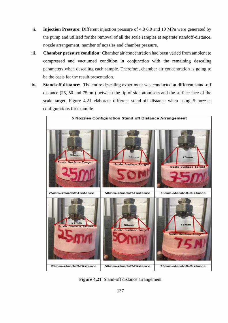
137

ii. Injection Pressure: Different injection pressure of 4.8 6.0 and 10 MPa were generated by

the pump and utilised for the removal of all the scale samples at separate standoff-distance,

nozzle arrangement, number of nozzles and chamber pressure.

iii. Chamber pressure condition: Chamber air concentration had been varied from ambient to

compressed and vacuumed condition in conjunction with the remaining descaling

parameters when descaling each sample. Therefore, chamber air concentration is going to

be the basis for the result presentation.

iv. Stand-off distance: The entire descaling experiment was conducted at different stand-off

distance (25, 50 and 75mm) between the tip of side atomisers and the surface face of the

scale target. Figure 4.21 elaborate different stand-off distance when using 5 nozzles

configurations for example.

Figure 4.21: Stand-off distance arrangement

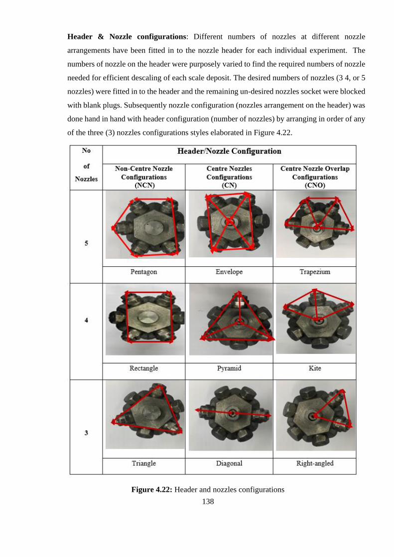
138

Header & Nozzle configurations: Different numbers of nozzles at different nozzle

arrangements have been fitted in to the nozzle header for each individual experiment. The

numbers of nozzle on the header were purposely varied to find the required numbers of nozzle

needed for efficient descaling of each scale deposit. The desired numbers of nozzles (3 4, or 5

nozzles) were fitted in to the header and the remaining un-desired nozzles socket were blocked

with blank plugs. Subsequently nozzle configuration (nozzles arrangement on the header) was

done hand in hand with header configuration (number of nozzles) by arranging in order of any

of the three (3) nozzles configurations styles elaborated in Figure 4.22.

Figure 4.22: Header and nozzles configurations

139

4.5.2 Experimental procedures for scale removal

Preceding the beginning of the analysis, there was the requirement for guaranteeing the safety,

reliability of all equipment and devices utilized, amid each trial. The same procedure and

precautions were utilised for both soft scale and hard scale sample removal trials. Even though may

differ when working at different chamber air concentrations

4.5.2.1 Ambient descaling procedure

The general trial strategies for scale removal at ambient condition for both soft and hard scale

samples at different injection pressure, standoff distance and header/nozzle configuration are as per

the following:

i. The mass of scale sample was re-measured and noted according to their reference number

as in the scale identification register.

ii. The picture of each scale sample was taken, utilizing a still standard camera, before, and

after each trial from different perspective.

iii. The required numbers of nozzles were properly fitted in to the header and the un-desired

properly blocked with the blank plugs.

iv. The desired nozzle arrangement was generated from the required numbers of nozzles (NCN,

CN or NCO)

v. The scale sample were properly placed on the scale sample holder and secured in position.

vi. The right size and combinations of packers were ensured in order to achieve the desired

stand-off distance from the sample to nozzle header.

vii. The scale sample with the base assembly were ensured to be effectively put to coincide with

the vertical axis of the atomiser, fitted to multiple nozzle head.

viii. All the chamber and rig connection were ensured to be properly and sequentially done, like

top and bottom plate to the chamber. Also, the hydraulic connections from the pump to the

control board to the top plate of the chamber to the header and chamber bottom plate were

used and pump starting procedures were followed

ix. The pump was switched on and throttle to the desired pressure to begin with, at an underlying

low pressure to 4.8 MPa pressure, and after then adjusted to acquire the desired flow rate

and pressure

x. The water line pressure gauge, flow meter on the board and the pressure gauge on the top

plate were confirmed to have corresponded to the desired pumping pressure requirement

through board regulator valve

140

xi. The timer was set to count for three (3) minute descaling time immediately after achieving

the desired pumping pressure.

xii. The pump was completely throttle off and switched off after achieving the 3-minute

descaling time from the stopwatch timer.

xiii. The descaled sample was removed and dried for 12 hours. Later, measured and it picture re-

taken with same still camera

xiv. The broken samples were collected from the two sieves below the packers, dried and later

weighed with a measuring scale (range (0.1g) for confirmation.

xv. Step 1 to 14 above were repeated for desired pressure of 4.8 and 6 and 10 MPa at the desired

flow rate flat fan spray atomisers respectively for 3 minutes each.

xvi. Step 1 to 15 above were repeated for desired standoff distance of 25mm, 50mm and 75mm

respectively and operated for 3 minutes each.

xvii. Step 1 to 16 above were repeated for desired numbers nozzles (3, 4 and 5 nozzles)

respectively

xviii. Step 1 to 17 above were repeated for desired nozzles arrangement (NCN, CN & CNO)

respectively

xix. All the above technique or sequence were applied and repeated for various scale samples

(soft hollow & solid and SrSO4 & CaCO3) deposits.

xx. All readings from each trial were recorded for further analysis.

4.5.2.2 Compressed descaling procedure (compression)

Almost similar experimental strategies with the scale removal at ambient condition, though carried

out in a compressed chamber condition. The operation incorporates a 0.2 MPa compressed air into

the chamber through the control board airline to the top plate of the chamber. Both soft and hard

scale samples were descaled at different injection pressure, standoff distance, and header/nozzle

configurations using the following steps.

i. The mass of scale sample was re-measured and noted according to their reference number

as in the scale identification register.

ii. The picture of each scale sample was taken, utilizing a still standard camera, before, and

after each trial from different perspective.

iii. The required numbers of nozzles were properly fitted in to the header and the un-desired

properly blocked with the blank plugs.

141

iv. The desired nozzle arrangement was generated from the required numbers of nozzles (NCN,

CN or NCO)

v. The scale sample were properly placed on the scale sample holder and secured in position.

vi. The right size and combinations of packers were ensured in order to achieve the desired

stand-off distance from the sample to nozzle header.

vii. The scale sample with the base assembly were ensured to be effectively put to coincide with

the vertical axis of the atomiser, fitted to multiple nozzle head.

viii. All the chamber and rig connection were ensured to be properly and sequentially done like

top and bottom plate to the chamber. Also, the hydraulic connections from the pump to the

control board to the top plate of the chamber to the header and chamber bottom plate were

used and pump starting procedures were followed

ix. The isolation/selection valve was used to select the desired chamber air condition

(compression) and vary the air concentration according to experimental desire. Also, the

proper connection of compressed air from the compressor system to the control board airline

and up to top plate air gauge inlet was ensured.

x. The HP water pump was switched on and throttle to the desired pressure to begin with, at an

underlying low pressure of to 4.8 MPa pressure, and after then adjusted to acquire the desired

flow rate and pressure

xi. The water line pressure gauge, flow meter on the board and the pressure gauge on the top

plate were confirmed to have corresponded to the desired pumping pressure requirement

through board regulator valve

xii. The compressed air system was opened to the required air compression and the regulator on

the airline system of the control board and the discharge regulator at the bottom plate were

operated to maintain the required chamber air concentration (0.2 MPa) at both combine

pressure gauge, flow meter and top plate pressure gauge throughout the 3-minute operations.

xiii. The timer was set to count for three (3) minute descaling time immediately after achieving

the desired pumping pressure and air concentration.

xiv. The compress air system was closed and the HPW pump was completely throttles-off and

switched off immediately after achieving the 3-minute descaling time from the stopwatch

timer.

xv. The descaled sample was removed and dried for 12 hours. Later, measured and it picture re-

taken with same still camera

xvi. The broken samples collected from the two sieves bellow the packers were dried and

weighed with a measuring scale (range (0.1g) for confirmation

142

xvii. Step 1 to 16 above were repeated for desired pressure of 4.8 and 6 and 10 MPa at the desired

flow rate flat fan spray atomisers respectively for 3 minutes each.

xviii. Step 1 to 17 above were repeated for desired standoff distance of 25mm, 50mm and 75mm

respectively and operated for 3 minutes each.

xix. Step 1 to 18 were repeated for desired numbers nozzles (3,4 and 5 nozzles) respectively

xx. Step 1 to 19 above were repeated for desired nozzles arrangement (NCN, CN & CNO)

respectively

xxi. All the above technique or sequence were applied and repeated for various scale samples

(soft and hard scale sample)

xxii. All readings from each trial were recorded for further analysis.

4.5.2.3 Vacuum descaling procedure (Suction)

The vacuum operations share similar decaling strategies with compressed experiment as in above,

but the compressed air system was replaced with a vacuum pump. The vacuum pump was

incorporated into to the chamber through the control board airline into the top or bottom plate of the

chamber to generate suction air concentration (-0.08 MPa). Both soft and hard scale samples were

descaled at different injection pressure, standoff distance and header/nozzle configuration using the

following steps.

i. The mass of scale sample was re-measured and noted according to their reference number

as in the scale identification register.

ii. The picture of each scale sample was taken, utilizing a still standard camera, before, and

after each trial from different perspective.

iii. The required numbers of nozzles were properly fitted in to the header and the un-desired

properly blocked with the blank plugs.

iv. The desired nozzle arrangement was generated from the required numbers of nozzles (NCN,

CN or NCO)

v. The scale sample were properly placed on the scale sample holder and secured in position.

vi. The right size and combinations of packers were ensured in order to achieve the desired

stand-off distance from the sample to nozzle header.

vii. The scale sample with the base assembly were ensured to be effectively put to coincide with

the vertical axis of the atomiser, fitted to multiple nozzle head.

viii. All the chamber and rig connection were ensured to be properly and sequentially done like

top and bottom plate to the chamber. Also, the hydraulic connections from the pump to the

143

control board to the top plate of the chamber to the header and chamber bottom plate were

used and pump starting procedures were followed

ix. The isolation/selection valve was used to select the desired chamber air condition (Suction)

and vary the air concentration according to experimental desire. Also, the proper connection

of the vacuum pumps to the control board airline and up to top or bottom plate air gauge

inlet were ensured.

x. The HP water pump was switched on and throttle to the desired pressure by beginning with,

at an underlying low flow rate 8 l/min corresponding to 4.8 MPa pressure, and after then

adjusted to acquire the desired flow rate and pressure

xi. The water line pressure gauge, flow meter on the board and the pressure gauge on the top

plate were confirmed to have corresponded to the desired pumping pressure requirement

through board regulator valve

xii. the vacuum pump was switched on, while the regulator on the airline system of the control

board and the discharge regulator at the bottom plate were operated to maintain the required

suctioned chamber air concentration (-0.08MPa) at both combine pressure gauge, flow meter

and top plate pressure gauge throughout the 3-minute operations.

xiii. The timer was set to count for three (3) minute descaling time immediately after achieving

the desired pumping pressure and air concentration.

xiv. The HP water pump was stopped once the vacuum pressure of the chamber drops to -

0.06MPa to suctioned back the chamber back to -0.08MPa

xv. The HP water pump and vacuum pump were turned off and the completely throttle off

immediately after achieving the 3-minute descaling time from the stopwatch timer.

xvi. The descaled sample was removed and dried for 12 hours. Later on, measured and it picture

re-taken with same still camera.

xvii. The broken samples collected from the two sieves bellow the packers were dried and

weighed with a measuring scale (range (0.1g) for confirmation

xviii. Step 1 to 16 above were repeated for desired pressure of 4.8 and 6 and 10 MPa at the desired

flow rate flat fan spray atomisers respectively for 3 minutes each.

xix. Step 1 to 17 above were repeated for desired standoff distance of 25mm, 50mm and 75mm

respectively and operated for 3 minutes each.

xx. Step 1 to 18 were repeated for desired numbers nozzles (3,4 and 5 nozzles) respectively

xxi. Step 1 to 19 above were repeated for desired nozzles arrangement (NCN, CN & CNO)

respectively

144

xxii. All the above technique or sequence were applied and repeated for various scale samples

(soft and hard scale sample)

xxiii. All readings from each trial were recorded for further analysis.

4.5.3 Safety precaution measure

Health safety and environment (HSE) are the fundamental worry now, they are the most significant

dangers that require serious consideration and change in our reality today. Safety measures are

activities and precaution engage to improve safety, i.e. diminish hazard related with human

wellbeing or health. The safety measures taken in during this trial are as follows.

a. All fittings and installations were appropriately confirmed and fixed well to keep away from

pressure loss due to leakages.

b. Circuit’s breakers were introduced to keep away from appliance damage, which could

emerge from surplus voltage.

c. The distinct units of the equipment’s were kept in their appropriate position keeping in mind

the end goal to work accurately to their most efficient productivity.

d. The water tank was loaded with water to the required most maximum water level.

e. The power supply was switch off to the water pump after utilization.

f. The water tank was completely drained at the end of the day to avoid Legionnaires' disease.

g. Appropriate personal protective equipment’s were worn and additionally safety gloves and

ear to protect the operator from harm and injuries.

h. The vacuum pump was switched off immediately it’s about to overheat or suction in water.

i. A Fire extinguisher was accessible if there should be an occurrence of fire incidence.

4.5.4 Source of errors in the scale removal test

a. Difference in amount of scale removed when descaling similar samples under the same

descaling conditions

b. Difference in hardness of the produce wax due to lone production and different setting time.

c. Pressure variation due to pressure drop effect when operating the high-pressure water pump

d. The chamber pressure differential effect as a result of back pressure when

compression/suctioning the chamber

e. Error in measuring the mass of descale samples in wet conditions due to difficulties of

getting it 100% dried.

145

f. Poor contact of the water jets on the hard scales sample due to reduced ID of the sample

compared to the size of header.

g. Sporadically, when operating at high pressure of 10 MPa the nozzle header would move

laterally before stabilizing, therefore changing the impact position of the water jets.

4.5.5 Scale removal error mitigation measures

a. Repeatability was maintained throughout the experiment by repeating each experiment by

three (3) runs and their average were recorded.

b. The wax scale samples were produced in batches and Colling curve test was conducted to

make sure they have the same setting or hardening time.

c. The high-pressure pump (600 bars most extreme) was operated within a tolerance of ±1bar

d. The pressure differential was kept consistent by including the chamber pressure during the

compression/cavitation test because of variation in back pressure in the pressurized or

suctioned chamber

e. The quantitative estimation for the mass of the scale recovered during each test was kept

within ±0.1g to justify the mass of water soaked by the scale amid the analysis, which could

not be gotten dry because of time constraint.

f. The high-pressure water pump was operated by gradually building up to the desired high

pressure from lower injection pressures to avoid the multiple nozzle header from vibrating

due to sudden high-pressure drop effect.

4.5.6 Experimental error analysis

To ensure precise and accurate result were obtained during the entire experiment, every set of

experiment was run three times and the average results were recorded. Also, Table 4.1, 4.2 and 4.3

shows the closeness of the merging of error (0.8 maximum standard deviation) for 3 nozzle

descaling experiment at different injection pressure, nozzle arrangements and chamber air

concentrations.

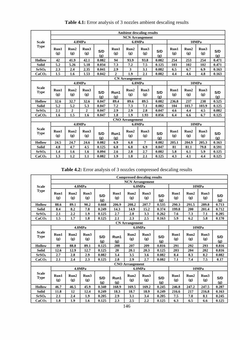
146

Table 4.1: Error analysis of 3 nozzles ambient descaling results

Scale

Type

Ambient descaling results

NCN Arrangement

4.8MPa 6.0MPa 10MPa

Run1

(g)

Run2

(g)

Run3

(g) S/D (g)

Run1

(g)

Run2

(g)

Run3

(g) S/D (g)

Run1

(g)

Run2

(g)

Run3

(g) S/D (g)

Hollow 42 41.9 42.1 0.082 94 93.9 93.8 0.082 254 253 254 0.471

Solid 5.2 5.26 5.18 0.034 7.3 7.2 7.5 0.125 103 102 102 0.471

SrSO4 2.3 2.4 2.35 0.041 2.9 3 3.1 0.082 6.5 6.7 6.9 0.163

CaCO3 1.5 1.6 1.53 0.042 2 1.9 2.1 0.082 4.4 4.6 4.8 0.163

CN Arrangement

Scale

Type

4.8MPa 6.0MPa 10MPa

Run1

(g)

Run2

(g)

Run3

(g) S/D (g)

Run1 (g)

Run2

(g)

Run3

(g) S/D (g)

Run1

(g)

Run2

(g)

Run3

(g) S/D (g)

Hollow 32.6 32.7 32.6 0.047 89.4 89.6 89.5 0.082 236.8 237 238 0.525

Solid 5.2 5.2 5.3 0.047 7.2 7.3 7.1 0.082 104 103.7 103.9 0.125

SrSO4 2.1 2 2 0.047 2.9 2.9 2.8 0.047 4.6 4.4 4.5 0.082

CaCO3 1.6 1.5 1.6 0.047 1.8 1.9 1.93 0.056 6.4 6.6 6.7 0.125

CNO Arrangement

Scale

Type

4.8MPa 6.0MPa 10MPa

Run1

(g)

Run2

(g)

Run3

(g) S/D (g)

Run1 (g)

Run2

(g)

Run3

(g) S/D (g)

Run1

(g)

Run2

(g)

Run3

(g) S/D (g)

Hollow 24.5 24.7 24.6 0.082 6.9 6.8 7 0.082 205.1 204.9 205.3 0.163

Solid 4.8 4.7 4.5 0.125 6.8 6.8 6.9 0.047 81 81.1 79.8 0.591

SrSO4 1.4 1.6 1.6 0.094 2.6 2.8 2.7 0.082 5.8 6.1 5.9 0.125

CaCO3 1.3 1.2 1.1 0.082 1.9 1.8 2.1 0.125 4.3 4.1 4.4 0.125

Table 4.2: Error analysis of 3 nozzles compressed descaling results

Scale

Type

Compressed descaling results

NCN Arrangement

4.8MPa 6.0MPa 10MPa

Run1

(g)

Run2

(g)

Run3

(g) S/D (g)

Run1

(g)

Run2

(g)

Run3

(g) S/D (g)

Run1

(g)

Run2

(g)

Run3

(g) S/D (g)

Hollow 88.6 89.1 90.2 0.668 206.9 208.2 207.7 0.535 290.3 291.5 289.8 0.713

Solid 8.4 8.2 7.8 0.249 14.3 14.9 15.2 0.374 199.8 200 201.4 0.712

SrSO4 2.1 2.2 1.9 0.125 2.7 2.8 3.3 0.262 7.6 7.3 7.1 0.205

CaCO3 1.5 1.7 1.8 0.125 2.1 2.3 2.5 0.163 5.9 6.2 5.8 0.170

CN Arrangement

Scale

Type

4.8MPa 6.0MPa 10MPa

Run1

(g)

Run2

(g)

Run3

(g) S/D (g)

Run1 (g)

Run2

(g)

Run3

(g) S/D (g)

Run1

(g)

Run2

(g)

Run3

(g) S/D (g)

Hollow 89 88.8 89.1 0.125 208 207 209 0.816 291 292 293 0.816

Solid 12.6 12.9 12.7 0.125 20 20.1 20.3 0.125 203 204 202 0.816

SrSO4 2.7 2.8 2.9 0.082 3.4 3.5 3.6 0.082 8.4 8.3 8.2 0.082

CaCO3 2.1 2.4 2.3 0.125 2.8 2.9 2.7 0.082 7.1 7.4 7.5 0.17

CNO Arrangement

Scale

Type

4.8MPa 6.0MPa 10MPa

Run1

(g)

Run2

(g)

Run3

(g) S/D (g)

Run1 (g)

Run2

(g)

Run3

(g) S/D (g)

Run1

(g)

Run2

(g)

Run3

(g) S/D (g)

Hollow 46.7 46.5 45.9 0.340 168.9 169.5 169.2 0.245 246.8 247.2 247.5 0.287

Solid 11.8 12 12.4 0.249 18.3 18.7 18.9 0.249 216.6 217 216.8 0.163

SrSO4 2.1 2.4 1.9 0.205 2.9 3.1 3.4 0.205 7.5 7.8 8.1 0.245

CaCO3 1.8 1.9 1.6 0.125 2.3 2.5 2.2 0.125 6.3 6.5 6.6 0.125

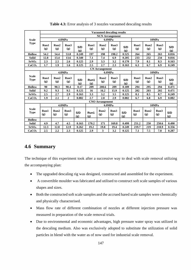
147

Table 4.3: Error analysis of 3 nozzles vacuumed descaling results

Scale

Type

Vacuumed descaling results

NCN Arrangement

4.8MPa 6.0MPa 10MPa

Run1

(g)

Run2

(g)

Run3

(g) S/D (g)

Run1

(g)

Run2

(g)

Run3

(g) S/D (g)

Run1

(g)

Run2

(g)

Run3

(g) S/D (g)

Hollow 54.2 54.4 53.8 0.249 197 198 198.2 0.525 264 265 263 0.816

Solid 12.8 13.4 13.6 0.340 7.1 7.4 6.9 0.205 233 232 234 0.816

SrSO4 2.3 2.5 2.6 0.125 2.9 3.3 3.2 0.170 7.9 8.1 8.3 0.163

CaCO3 1.7 1.9 1.6 0.125 2.5 2.7 2.3 0.163 6.3 6.7 6.9 0.249

CN Arrangement

Scale

Type

4.8MPa 6.0MPa 10MPa

Run1

(g)

Run2

(g)

Run3

(g) S/D (g)

Run1 (g)

Run2

(g)

Run3

(g) S/D (g)

Run1

(g)

Run2

(g)

Run3

(g) S/D (g)

Hollow 90 90.3 90.4 0.17 209 208.6 209 0.189 294 295 294 0.471

Solid 9.2 9.3 9.5 0.125 16 16.2 15.9 0.125 202 203 202 0.471

SrSO4 2.5 2.7 2.9 0.163 3.3 3.2 3.5 0.125 8.1 8.5 8.7 0.249

CaCO3 1.9 2.1 2 0.082 2.7 2.8 2.9 0.082 6.7 6.8 6.9 0.082

CNO Arrangement

Scale

Type

4.8MPa 6.0MPa 10MPa

Run1

(g)

Run2

(g)

Run3

(g) S/D (g)

Run1 (g)

Run2

(g)

Run3

(g) S/D (g)

Run1

(g)

Run2

(g)

Run3

(g) S/D (g)

Hollow

Solid 4.9 4.7 4.5 0.163 170.2 171 169.8 0.499 251.2 250 250.6 0.490

SrSO4 12.3 12.8 12.9 0.262 19.2 19.8 19.4 0.249 219.7 219 218.9 0.356

CaCO3 2.5 2.2 2.3 0.125 2.9 3 3.2 0.125 7.1 7.5 7.8 0.287

4.6 Summary

The technique of this experiment took after a successive way to deal with scale removal utilizing

the accompanying plan:

• The upgraded descaling rig was designed, constructed and assembled for the experiment.

• A convertible moulder was fabricated and utilised to construct soft scale samples of various

shapes and sizes.

• Both the constructed soft scale samples and the accrued hared scale samples were chemically

and physically characterised.

• Mass flow rate of different combination of nozzles at different injection pressure was

measured in preparation of the scale removal trials.

• Due to environmental and economic advantages, high pressure water spray was utilized in

the descaling medium. Also was exclusively adopted to substitute the utilization of solid

particles in blend with the water as of now used for industrial scale removal.

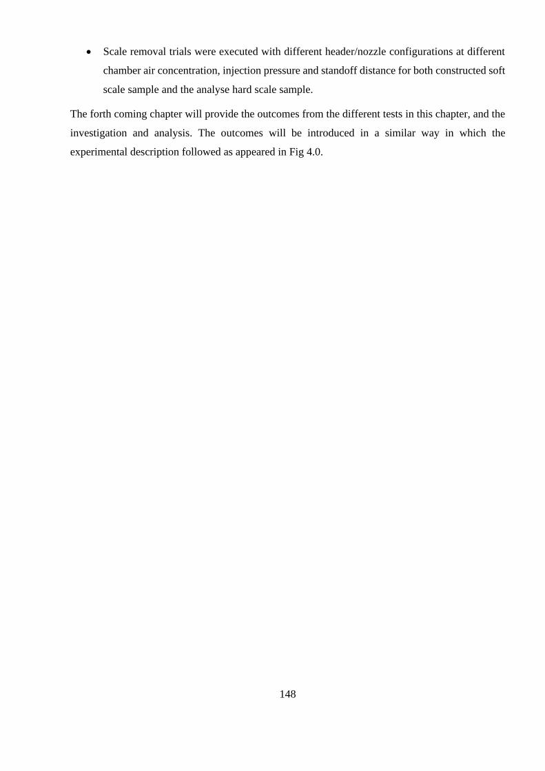
148

• Scale removal trials were executed with different header/nozzle configurations at different

chamber air concentration, injection pressure and standoff distance for both constructed soft

scale sample and the analyse hard scale sample.

The forth coming chapter will provide the outcomes from the different tests in this chapter, and the

investigation and analysis. The outcomes will be introduced in a similar way in which the

experimental description followed as appeared in Fig 4.0.

149

Results and Discussion

5.1 Overview

This chapter presents the outcomes (results) acquired from the experimental examination led by the

plan set out in Fig. 4.0. As per the original target of this examination, of utilizing multiple high-

pressure circular nozzles in a special descaling chamber (ambient, compressed and vacuum

condition) to clean mineral and organic scale deposit in petroleum production tubing. Some

descaling experimental preparation have been conducted by designing and constructing scale mould

through exporting the solid work design to a 3D printer. Subsequently used to prepare the wax scale

sample candidate of different shapes and sizes. In addition, the oil field scale obtain from Libyan

oilfield and the constructed soft scale candidate were chemically/compositionally analyse using

the combination of (SEM, EDs, XRD, Infrared and NMR).

The outcomes are categorized into sections under phases in which the experimental succession

follows:

Phase 1: The pre-descaling experiments which were conducted outside the descaling chamber

ahead of the descaling trials as further classified into two sections:

Section 1: chemical and compositional characterization of constructed soft scale sample

through NMR and FTIR techniques.

Section 2: Chemical and compositional characterization the available hard samples through

the combination of EDs, SEM & XRD technique

Phase 2: The main experimental descaling trials was conducted by utilizing the special constructed

descaling chamber and dived in to three sections:

Section 1: Studying the effect of descaling parameters like injection pressure, numbers of

nozzles, stand-off distance and nozzle arrangement toward the rate of scale removal at

different chamber pressure

Section 2: Studying the effect chamber water/air concentration i.e. ambient, compressed and

vacuum air condition toward the rate of scale removal.

Section 3: Determining the optimum descaling requirement for the effective scale removal

of different types scale deposit in petroleum production tubing

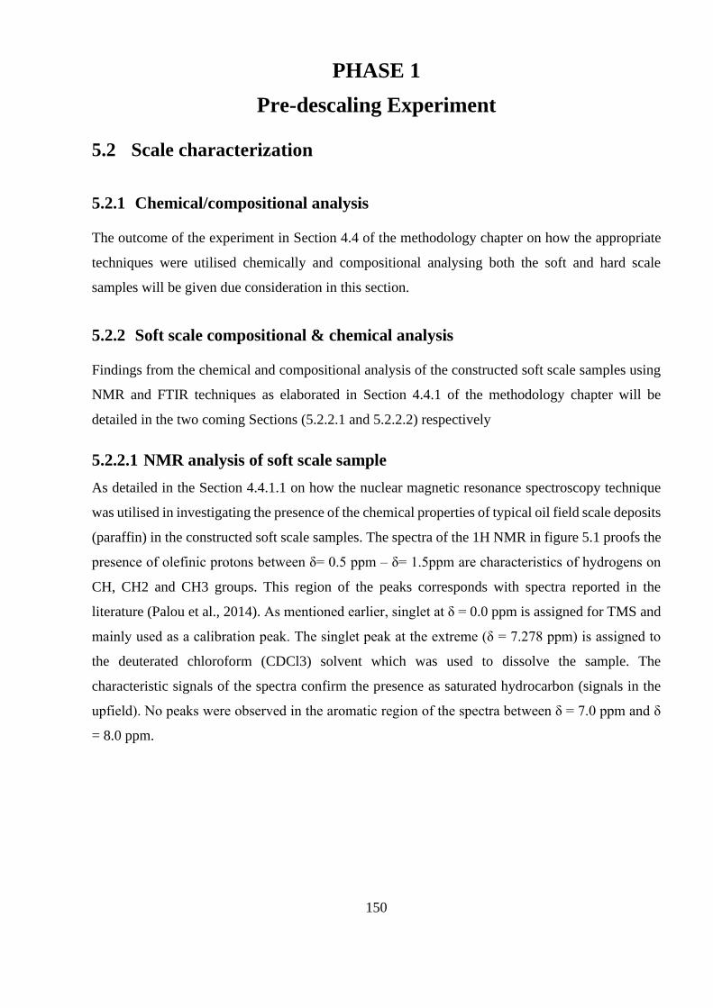
150

PHASE 1

Pre-descaling Experiment

5.2 Scale characterization

5.2.1 Chemical/compositional analysis

The outcome of the experiment in Section 4.4 of the methodology chapter on how the appropriate

techniques were utilised chemically and compositional analysing both the soft and hard scale

samples will be given due consideration in this section.

5.2.2 Soft scale compositional & chemical analysis

Findings from the chemical and compositional analysis of the constructed soft scale samples using

NMR and FTIR techniques as elaborated in Section 4.4.1 of the methodology chapter will be

detailed in the two coming Sections (5.2.2.1 and 5.2.2.2) respectively

5.2.2.1 NMR analysis of soft scale sample

As detailed in the Section 4.4.1.1 on how the nuclear magnetic resonance spectroscopy technique

was utilised in investigating the presence of the chemical properties of typical oil field scale deposits

(paraffin) in the constructed soft scale samples. The spectra of the 1H NMR in figure 5.1 proofs the

presence of olefinic protons between δ= 0.5 ppm – δ= 1.5ppm are characteristics of hydrogens on

CH, CH2 and CH3 groups. This region of the peaks corresponds with spectra reported in the

literature (Palou et al., 2014). As mentioned earlier, singlet at δ = 0.0 ppm is assigned for TMS and

mainly used as a calibration peak. The singlet peak at the extreme (δ = 7.278 ppm) is assigned to

the deuterated chloroform (CDCl3) solvent which was used to dissolve the sample. The

characteristic signals of the spectra confirm the presence as saturated hydrocarbon (signals in the

upfield). No peaks were observed in the aromatic region of the spectra between δ = 7.0 ppm and δ

= 8.0 ppm.

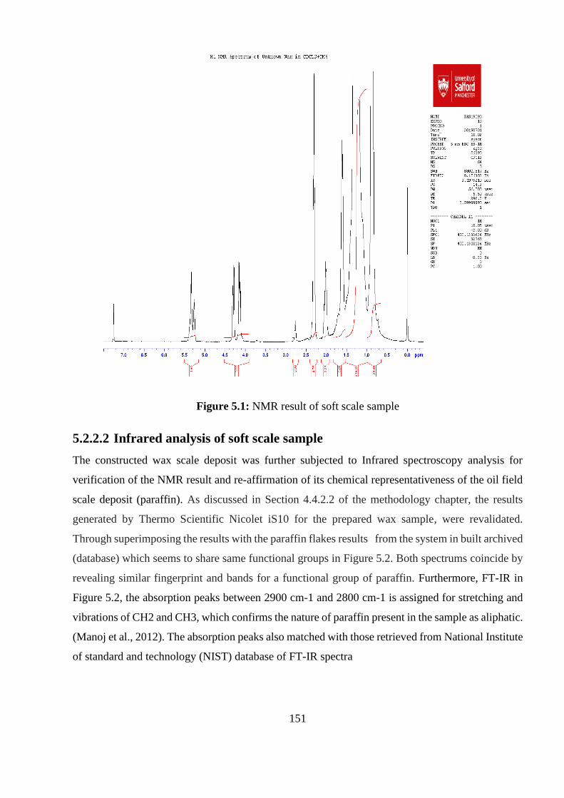
151

Figure 5.1: NMR result of soft scale sample

5.2.2.2 Infrared analysis of soft scale sample

The constructed wax scale deposit was further subjected to Infrared spectroscopy analysis for

verification of the NMR result and re-affirmation of its chemical representativeness of the oil field

scale deposit (paraffin). As discussed in Section 4.4.2.2 of the methodology chapter, the results

generated by Thermo Scientific Nicolet iS10 for the prepared wax sample, were revalidated.

Through superimposing the results with the paraffin flakes results from the system in built archived

(database) which seems to share same functional groups in Figure 5.2. Both spectrums coincide by

revealing similar fingerprint and bands for a functional group of paraffin. Furthermore, FT-IR in

Figure 5.2, the absorption peaks between 2900 cm-1 and 2800 cm-1 is assigned for stretching and

vibrations of CH2 and CH3, which confirms the nature of paraffin present in the sample as aliphatic.

(Manoj et al., 2012). The absorption peaks also matched with those retrieved from National Institute

of standard and technology (NIST) database of FT-IR spectra

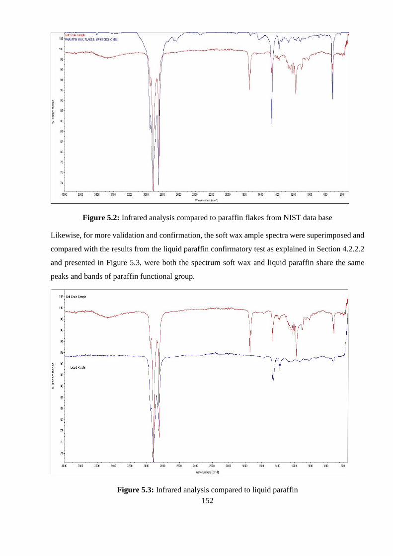
152

Figure 5.2: Infrared analysis compared to paraffin flakes from NIST data base

Likewise, for more validation and confirmation, the soft wax ample spectra were superimposed and

compared with the results from the liquid paraffin confirmatory test as explained in Section 4.2.2.2

and presented in Figure 5.3, were both the spectrum soft wax and liquid paraffin share the same

peaks and bands of paraffin functional group.

Figure 5.3: Infrared analysis compared to liquid paraffin

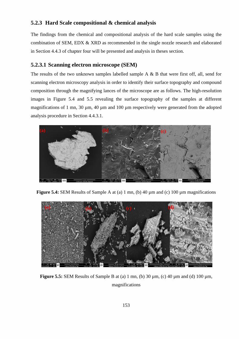
153

5.2.3 Hard Scale compositional & chemical analysis

The findings from the chemical and compositional analysis of the hard scale samples using the

combination of SEM, EDX & XRD as recommended in the single nozzle research and elaborated

in Section 4.4.3 of chapter four will be presented and analysis in theses section.

5.2.3.1 Scanning electron microscope (SEM)

The results of the two unknown samples labelled sample A & B that were first off, all, send for

scanning electron microscopy analysis in order to identify their surface topography and compound

composition through the magnifying lances of the microscope are as follows. The high-resolution

images in Figure 5.4 and 5.5 revealing the surface topography of the samples at different

magnifications of 1 mn, 30 µm, 40 µm and 100 µm respectively were generated from the adopted

analysis procedure in Section 4.4.3.1.

Figure 5.4: SEM Results of Sample A at (a) 1 mn, (b) 40 µm and (c) 100 µm magnifications

Figure 5.5: SEM Results of Sample B at (a) 1 mn, (b) 30 µm, (c) 40 µm and (d) 100 µm,

magnifications

(a) (b) (c)

(a) (b) (c) (d)

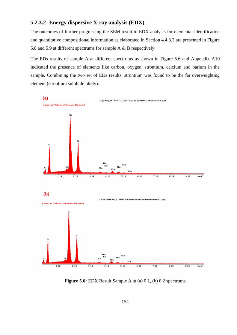
154

5.2.3.2 Energy dispersive X-ray analysis (EDX)

The outcomes of further progressing the SEM result to EDX analysis for elemental identification

and quantitative compositional information as elaborated in Section 4.4.3.2 are presented in Figure

5.8 and 5.9 at different spectrums for sample A & B respectively.

The EDs results of sample A at different spectrums as shown in Figure 5.6 and Appendix A10

indicated the presence of elements like carbon, oxygen, strontium, calcium and barium in the

sample. Combining the two set of EDs results, strontium was found to be the far overweighting

element (strontium sulphide likely).

Figure 5.6: EDX Result Sample A at (a) 0.1, (b) 0.2 spectrums

(a)

(b)

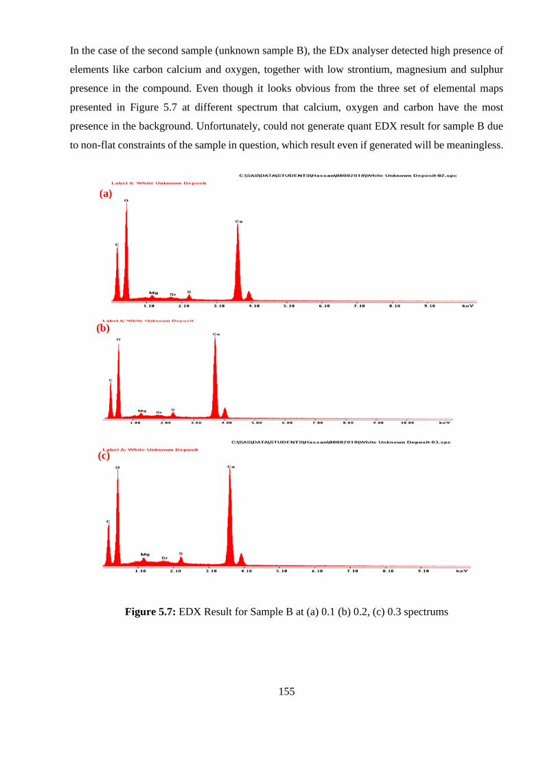
155

In the case of the second sample (unknown sample B), the EDx analyser detected high presence of

elements like carbon calcium and oxygen, together with low strontium, magnesium and sulphur

presence in the compound. Even though it looks obvious from the three set of elemental maps

presented in Figure 5.7 at different spectrum that calcium, oxygen and carbon have the most

presence in the background. Unfortunately, could not generate quant EDX result for sample B due

to non-flat constraints of the sample in question, which result even if generated will be meaningless.

Figure 5.7: EDX Result for Sample B at (a) 0.1 (b) 0.2, (c) 0.3 spectrums

(a)

(b)

(c)

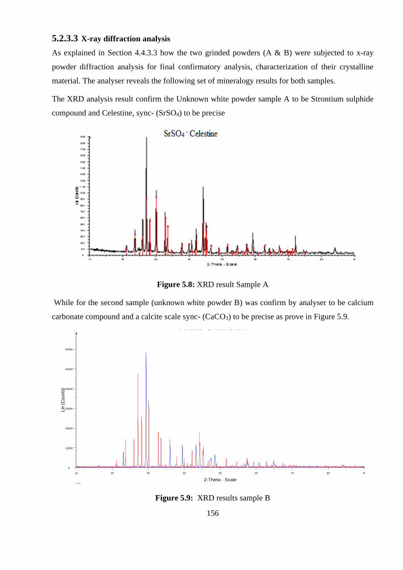
156

5.2.3.3 X-ray diffraction analysis

As explained in Section 4.4.3.3 how the two grinded powders (A & B) were subjected to x-ray

powder diffraction analysis for final confirmatory analysis, characterization of their crystalline

material. The analyser reveals the following set of mineralogy results for both samples.

The XRD analysis result confirm the Unknown white powder sample A to be Strontium sulphide

compound and Celestine, sync- (SrSO4) to be precise

Figure 5.8: XRD result Sample A

While for the second sample (unknown white powder B) was confirm by analyser to be calcium

carbonate compound and a calcite scale sync- (CaCO3) to be precise as prove in Figure 5.9.

Figure 5.9: XRD results sample B

White Unknown

Operations: Background 1.000,1.000 | Import

Unknown White Material / Pipe - File: UnknownWhiteMaterial-01.raw - Type: 2Th/Th locked - Start: 10.000 ° - End: 90.002 ° - Step: 0.039 ° - Step time: 334. s

Operations: X Offset 0.186 | X Offset 0.097 | X Offset 0.145 | X Offset 0.178 | X Offset 0.145 | Strip kAlpha2 0.500 | Background 0.550,1.0

White Unknown - File: W-Unknown-01.raw - Type: 2Th/Th locked - Start: 10.000 ° - End: 90.002 ° - Step: 0.019 ° - Step time: 334. s

Lin

(C

ounts

)

0

10000

20000

30000

40000

50000

60000

2-Theta - Scale

10 20 30 40 50 60 70 80 90

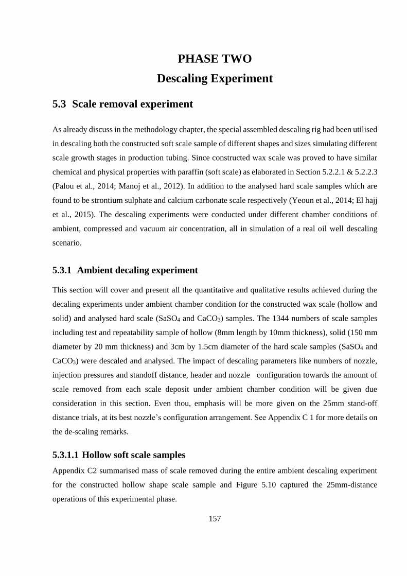
157

PHASE TWO

Descaling Experiment

5.3 Scale removal experiment

As already discuss in the methodology chapter, the special assembled descaling rig had been utilised

in descaling both the constructed soft scale sample of different shapes and sizes simulating different

scale growth stages in production tubing. Since constructed wax scale was proved to have similar

chemical and physical properties with paraffin (soft scale) as elaborated in Section 5.2.2.1 & 5.2.2.3

(Palou et al., 2014; Manoj et al., 2012). In addition to the analysed hard scale samples which are

found to be strontium sulphate and calcium carbonate scale respectively (Yeoun et al., 2014; El hajj

et al., 2015). The descaling experiments were conducted under different chamber conditions of

ambient, compressed and vacuum air concentration, all in simulation of a real oil well descaling

scenario.

5.3.1 Ambient decaling experiment

This section will cover and present all the quantitative and qualitative results achieved during the

decaling experiments under ambient chamber condition for the constructed wax scale (hollow and

solid) and analysed hard scale (SaSO4 and CaCO3) samples. The 1344 numbers of scale samples

including test and repeatability sample of hollow (8mm length by 10mm thickness), solid (150 mm

diameter by 20 mm thickness) and 3cm by 1.5cm diameter of the hard scale samples (SaSO4 and

CaCO3) were descaled and analysed. The impact of descaling parameters like numbers of nozzle,

injection pressures and standoff distance, header and nozzle configuration towards the amount of

scale removed from each scale deposit under ambient chamber condition will be given due

consideration in this section. Even thou, emphasis will be more given on the 25mm stand-off

distance trials, at its best nozzle’s configuration arrangement. See Appendix C 1 for more details on

the de-scaling remarks.

5.3.1.1 Hollow soft scale samples

Appendix C2 summarised mass of scale removed during the entire ambient descaling experiment

for the constructed hollow shape scale sample and Figure 5.10 captured the 25mm-distance

operations of this experimental phase.

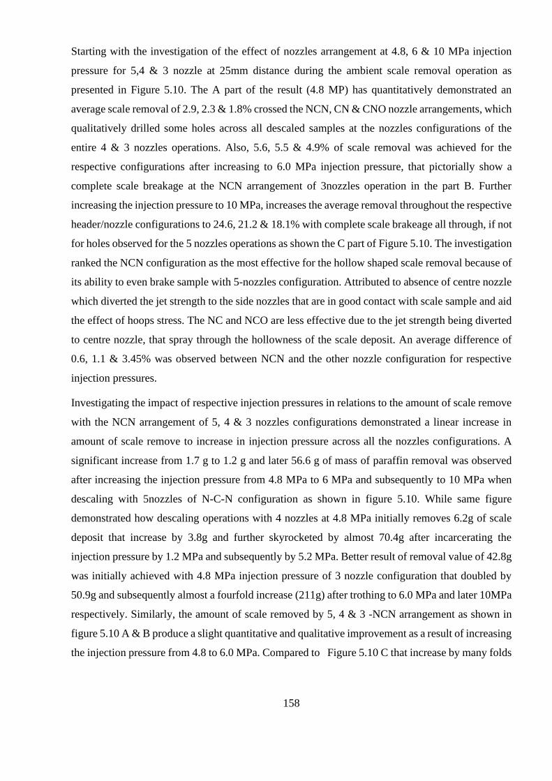
158

Starting with the investigation of the effect of nozzles arrangement at 4.8, 6 & 10 MPa injection

pressure for 5,4 & 3 nozzle at 25mm distance during the ambient scale removal operation as

presented in Figure 5.10. The A part of the result (4.8 MP) has quantitatively demonstrated an

average scale removal of 2.9, 2.3 & 1.8% crossed the NCN, CN & CNO nozzle arrangements, which

qualitatively drilled some holes across all descaled samples at the nozzles configurations of the

entire 4 & 3 nozzles operations. Also, 5.6, 5.5 & 4.9% of scale removal was achieved for the

respective configurations after increasing to 6.0 MPa injection pressure, that pictorially show a

complete scale breakage at the NCN arrangement of 3nozzles operation in the part B. Further

increasing the injection pressure to 10 MPa, increases the average removal throughout the respective

header/nozzle configurations to 24.6, 21.2 & 18.1% with complete scale brakeage all through, if not

for holes observed for the 5 nozzles operations as shown the C part of Figure 5.10. The investigation

ranked the NCN configuration as the most effective for the hollow shaped scale removal because of

its ability to even brake sample with 5-nozzles configuration. Attributed to absence of centre nozzle

which diverted the jet strength to the side nozzles that are in good contact with scale sample and aid

the effect of hoops stress. The NC and NCO are less effective due to the jet strength being diverted

to centre nozzle, that spray through the hollowness of the scale deposit. An average difference of

0.6, 1.1 & 3.45% was observed between NCN and the other nozzle configuration for respective

injection pressures.

Investigating the impact of respective injection pressures in relations to the amount of scale remove

with the NCN arrangement of 5, 4 & 3 nozzles configurations demonstrated a linear increase in

amount of scale remove to increase in injection pressure across all the nozzles configurations. A

significant increase from 1.7 g to 1.2 g and later 56.6 g of mass of paraffin removal was observed

after increasing the injection pressure from 4.8 MPa to 6 MPa and subsequently to 10 MPa when

descaling with 5nozzles of N-C-N configuration as shown in figure 5.10. While same figure

demonstrated how descaling operations with 4 nozzles at 4.8 MPa initially removes 6.2g of scale

deposit that increase by 3.8g and further skyrocketed by almost 70.4g after incarcerating the

injection pressure by 1.2 MPa and subsequently by 5.2 MPa. Better result of removal value of 42.8g

was initially achieved with 4.8 MPa injection pressure of 3 nozzle configuration that doubled by

50.9g and subsequently almost a fourfold increase (211g) after trothing to 6.0 MPa and later 10MPa

respectively. Similarly, the amount of scale removed by 5, 4 & 3 -NCN arrangement as shown in

figure 5.10 A & B produce a slight quantitative and qualitative improvement as a result of increasing

the injection pressure from 4.8 to 6.0 MPa. Compared to Figure 5.10 C that increase by many folds

159

and pictorially break all the samples across the 5,4 & 3nozzle configurations which was due to high

pressure variation of 5.2 MPa than 1.2 MPa difference of the earlier injection pressure increase.

Reducing the numbers of nozzle to 3 nozzles at ambient condition show greater impact than 4 and

5 nozzle header configurations due to multiple nozzle pressure drop effect (Tian, et al., 2009).

Although, still demonstrated increase in descaling rate with increase of injection pressure. A very

small difference of rate of scale removal of 4.5g from 1.7 g was recorded when the nozzle

configuration was reduced from five to four nozzles. Contrary to the almost 25 times increase of

41.1g to be precise, when further reducing the numbers of nozzle to three nozzles from four nozzles

at same 4.8 MPa injection pressure as shown in Figure 5.10A. The B part of Figure 5.12 shows how

reducing the number of nozzles from 5 to 4 when operating at 6.0 MPa doubled the removal form

2.9g by 7.1g and subsequently by 84g after reducing to 3 nozzles which was able to pictorially break

the sample. The analysis of the impact of number of nozzles at 10 MPa injection pressure

demonstrated a good result that qualitatively broke through all the descaled samples at the NCN

arrangement of 5, 4 & 3 nozzles configurations. The value of 58.3g of scale removed with 5 nozzles

at 10MPa was slightly increased by 18.3g and consequently by 195g after reducing the header

configuration to 4nozzles and later 3nozzles respectively.

160

A Descaling hollow shape soft scale at 4.8 MPa with different Number of Nozzles at 25mm stand-off distance

B Descaling hollow shape soft scale at 6.0 MPa with different Number of Nozzles at 25mm stand-off distance

C Descaling hollow shape soft scale at 10 MPa with different Number of Nozzles at 25mm stand-off distance

Figure 5.10: Ambient descaling results for hollow soft scale at 25mm-distance

0

50

100

150

200

250

300

2 3 4 5 6

Mas

s o

f Sc

ale

Re

mo

ved

(g)

Numbers of Nozzles

N-C-N C-N C-N-O

0

50

100

150

200

250

300

3 4 5

Mas

s o

f Sc

ale

re

mo

ved

(g)

Number of Nozzles

N-C-N C-N C-N-O

0

50

100

150

200

250

300

3 4 5

Mas

s o

f Sc

ale

Re

mo

ved

(g)

Number of Nozzles

N-C-N C-N C-N-O

161

5.3.1.2 Solid soft scale sample

Figure 5.11 demonstrates both quantitative and qualitative results generated from the ambient

descaling investigation of solid shaped scale samples at 25mm stand-off distance, while the entire

ambient descaling results for solid soft scale samples can be found in Appendix C3.

The A part of Figure 5.11 quantitatively elaborates how 5,4 and 3 nozzles were able to averagely

remove 0.2, 0.5 & 0.4% of the scale samples at low pressure of 4.8 MPa across the respective nozzle

arrangements. Even though, could only qualitative generate uniform erosion across board.

Increasing the injection pressure to 6.0 M Pa across the respective header/nozzle configurations as

shown in the B part quantitatively removes 0.2, 0.7 & 0.5% of the scale sample. While was

pictorially only able to demonstrates mild holes for entire 3nozzles configurations. Further

increasing the injection pressure to 10 MPa, increases the average scale removal to 6.6, 10.4 & 8.3%

respectively, which qualitatively broke all the 3nozzles configuration descaled samples and drilled

hole across the remaining samples as shown in Figure 5.11C. The highest removal impact observed,

was in ranking of NC, NCO and NCN in descending order and have value of 0.3, 0.5, 3.8% more

than the rest of the nozzle arrangements at respective injection pressures. NC configuration

performance is attributed to the good jet -scale surface contact with centre nozzle configurations

which aid both cyclin stress and sample particle abrasion jetting mechanism.

Analysing the results achieved from descaling soft solid samples in ambient condition at 25mm,

proves to increase with increase in injection pressure and reduction in both of numbers of nozzles

and stand-off distance. A mass of 1.2g was initially removed with 5 nozzles at 4.8 MPa injection

and increases by 0.6g & 30.5g after increasing the pressure to 6.0 & 10 MPa respectively. While the

4nozzle operation removed 2.6g of solid scale deposit at 4.8 MPa that slightly increases by 1.3g and

significantly increase by 48.1g after throttling to 10 MPa. More significant removal can be sighted

in Figure 5.11C where the 3nozzle operation originally removes 5.2g of scale at 4.8 MPa injection,

that slightly increase by 2.1g and later by many folds of 9.9g as a result of subsequent increase of

the injection pressure to 6.0 MPa and 10 MPa respectively.

Operating 5nozzles at 4.8 MPa initially remove 1.2g of scale that increases by 1.5g and 4g after

reducing the number of nozzles to 4 and later 3nozzle with no noticeable qualitative impact in Figure

5.11A. Injecting at 6.0 MPa with 5nozzles was able to remove 1.8g of scale that was rise by 2.1

with 4nozzles and better off by 5.5g after reducing to 3nozzles were some holes were drilled all

cross in Figure 5.11B. The utilization of 5nozzles at of 10 MPa was able to substantially remove

32g that increased by 19g and later almost 72g after reducing the nozzles numbers to 4 and later

3nozzles that was able to break all the samples in the C part of Figure 5.11.

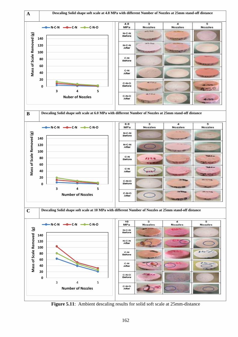
162

A Descaling Solid shape soft scale at 4.8 MPa with different Number of Nozzles at 25mm stand-off distance

B Descaling Solid shape soft scale at 6.0 MPa with different Number of Nozzles at 25mm stand-off distance

C Descaling Solid shape soft scale at 10 MPa with different Number of Nozzles at 25mm stand-off distance

Figure 5.11: Ambient descaling results for solid soft scale at 25mm-distance

0

20

40

60

80

100

120

140

3 4 5

Mas

s o

f Sc

ale

Re

mo

ved

(g)

Nuber of Nozzles

N-C-N C-N C-N-O

0

20

40

60

80

100

120

140

3 4 5

Mas

s o

f Sc

ale

Re

mo

ved

(g)

Number of Nozzles

N-C-N C-N C-N-O

0

20

40

60

80

100

120

140

3 4 5

Mas

s o

f Sc

ale

Re

mo

ved

(g)

Number of Nozzles

N-C-N C-N C-N-O

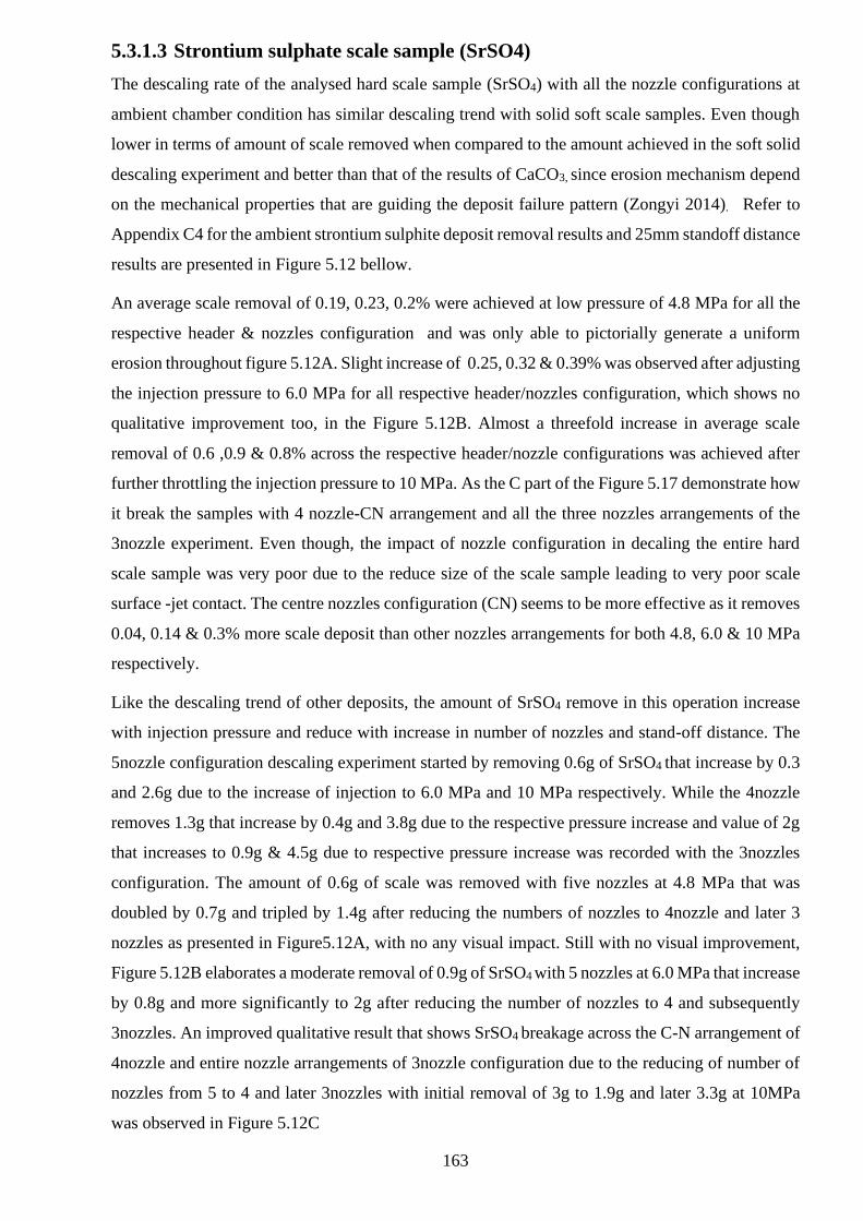
163

5.3.1.3 Strontium sulphate scale sample (SrSO4)

The descaling rate of the analysed hard scale sample (SrSO4) with all the nozzle configurations at

ambient chamber condition has similar descaling trend with solid soft scale samples. Even though

lower in terms of amount of scale removed when compared to the amount achieved in the soft solid

descaling experiment and better than that of the results of CaCO3, since erosion mechanism depend

on the mechanical properties that are guiding the deposit failure pattern (Zongyi 2014). Refer to

Appendix C4 for the ambient strontium sulphite deposit removal results and 25mm standoff distance

results are presented in Figure 5.12 bellow.

An average scale removal of 0.19, 0.23, 0.2% were achieved at low pressure of 4.8 MPa for all the

respective header & nozzles configuration and was only able to pictorially generate a uniform

erosion throughout figure 5.12A. Slight increase of 0.25, 0.32 & 0.39% was observed after adjusting

the injection pressure to 6.0 MPa for all respective header/nozzles configuration, which shows no

qualitative improvement too, in the Figure 5.12B. Almost a threefold increase in average scale

removal of 0.6 ,0.9 & 0.8% across the respective header/nozzle configurations was achieved after

further throttling the injection pressure to 10 MPa. As the C part of the Figure 5.17 demonstrate how

it break the samples with 4 nozzle-CN arrangement and all the three nozzles arrangements of the

3nozzle experiment. Even though, the impact of nozzle configuration in decaling the entire hard

scale sample was very poor due to the reduce size of the scale sample leading to very poor scale

surface -jet contact. The centre nozzles configuration (CN) seems to be more effective as it removes

0.04, 0.14 & 0.3% more scale deposit than other nozzles arrangements for both 4.8, 6.0 & 10 MPa

respectively.

Like the descaling trend of other deposits, the amount of SrSO4 remove in this operation increase

with injection pressure and reduce with increase in number of nozzles and stand-off distance. The

5nozzle configuration descaling experiment started by removing 0.6g of SrSO4 that increase by 0.3

and 2.6g due to the increase of injection to 6.0 MPa and 10 MPa respectively. While the 4nozzle

removes 1.3g that increase by 0.4g and 3.8g due to the respective pressure increase and value of 2g

that increases to 0.9g & 4.5g due to respective pressure increase was recorded with the 3nozzles

configuration. The amount of 0.6g of scale was removed with five nozzles at 4.8 MPa that was

doubled by 0.7g and tripled by 1.4g after reducing the numbers of nozzles to 4nozzle and later 3

nozzles as presented in Figure5.12A, with no any visual impact. Still with no visual improvement,

Figure 5.12B elaborates a moderate removal of 0.9g of SrSO4 with 5 nozzles at 6.0 MPa that increase

by 0.8g and more significantly to 2g after reducing the number of nozzles to 4 and subsequently

3nozzles. An improved qualitative result that shows SrSO4 breakage across the C-N arrangement of

4nozzle and entire nozzle arrangements of 3nozzle configuration due to the reducing of number of

nozzles from 5 to 4 and later 3nozzles with initial removal of 3g to 1.9g and later 3.3g at 10MPa

was observed in Figure 5.12C

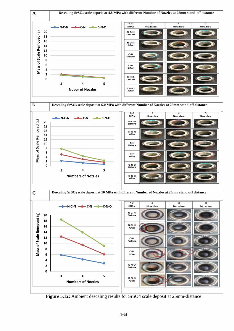
164

A Descaling SrSO4 scale deposit at 4.8 MPa with different Number of Nozzles at 25mm stand-off distance

B Descaling SrSO4 scale deposit at 6.0 MPa with different Number of Nozzles at 25mm stand-off distance

C Descaling SrSO4 scale deposit at 10 MPa with different Number of Nozzles at 25mm stand-off distance

Figure 5.12: Ambient descaling results for SrSO4 scale deposit at 25mm-distance

0

2

4

6

8

10

12

14

16

18

20

3 4 5

Mas

s o

f Sc

ale

Re

mo

ved

(g)

Nuber of Nozzles

N-C-N C-N C-N-O

02468

101214161820

3 4 5

Mas

s o

f Sc

ale

Re

mo

ved

(g)

Numbers of Nozzles

N-C-N C-N C-N-O

0

2

4

6

8

10

12

14

16

18

20

3 4 5

Mas

s o

f Sc

ale

Re

mo

ved

(g)

Numbers of Nozzles

N-C-N C-N C-N-O

165

5.3.1.4 Calcium carbonate scale sample (CaCO3)

The descaling rate of calcium carbonate hard scale sample (CaCO3) at ambient chamber condition

regardless of all descaling parameters resembled the descaling trend of strontium sulphate scales

deposit. Although, amount of CaCO3 scale removed is less than that attained when removing

strontium sulphate under the same descaling conditions. Notwithstanding this can be attached to the

difference in mineralogy and hardness of the sample as the SrSO4 is of crystalline based and the

CaCO3 is aggregate fine grains. Since the earlier expected to originates from sandstone formation

and later from limestone or carbonate reservoir. The ambient descaling details for calcium carbonate

removal at ambient condition can be found in Appendix C5 and the result of the investigation under

25mm distance is presented in Figure 5.13. An average value of 0.13, 0.17 & 0.14% of CaCO3 scale

deposit was removed with respective header and nozzles configurations when pumping at low

pressure of 4.8 MPa as shown in Figure 5.13A. This slightly increases to 0.19, 0.22, & 0.20%

respectively after increasing the injection pressure to 6 MPa as presented in Figure 5.13B. More

significant increase of 0.46, 0.56 & 0.51% of average scale deposit removal was observed after

further increase of the injection pressure to 10 MPa as captured in figure 5.13C. Qualitatively, figure

5.18 could only showcase a uniform erosion across the entire descaled samples and a difference of

0.14, 0.03 & 0.1% of more scale removal by the CN arrangement than the NCN arrangement was

recorded.

The C-N configuration of 5nozzle configuration was able remove 0.4g of CaCO3 at 4.8 MPa that

slightly improved the removal by 0.2g and subsequently 1.4g after adjusting the injection pressure

to 6.0 MPa and 10 MPa respectively. Similar removal of 0.8g that improves by 0.3g and later 2.1g

after altering the injection pressures of the 4nozzles operation from 4.8 to 6.0 and 10 MPa

respectively. More improved removal of 1.5g of CaCO3 that further improved by 0.5g and 2.9g after

the subsequent throttling of the injection pressures of the 3nozzles operation from 4.8, to 6.0 and

later 10 MPa.

Descaling CaCO3 in ambient condition with 5nozzles at low pressure of 4.8 MPa removes 0.4g,

which later improved by half (0.4g) and tripled (1.1g) due to the reduction of header configurations

to 4 and later 3nozzles as shown in Figure 5.13A. Better improve quantitative result is shown in in

figure 5.13B, were the initial scale removal of 0.6g that improvement 0.5g and later 1.4g was

recorded due to the adjustment of header configuration to 4 and 3nozzles respectively. While figure

5.13C showcase the best removal results of the CaCO3 in ambient condition, were almost 1.8g of

scale was initially remove and later improved by 1.1g and 2.6g due to adjusting the header

configuration of 5 nozzles (10 MPa operation) to 4 and later 3nozzles. The entire Figure 5.13

translates a very poor qualitative results from the CaCO3 ambient descaling campaign that could

only uniformly erode all the samples.

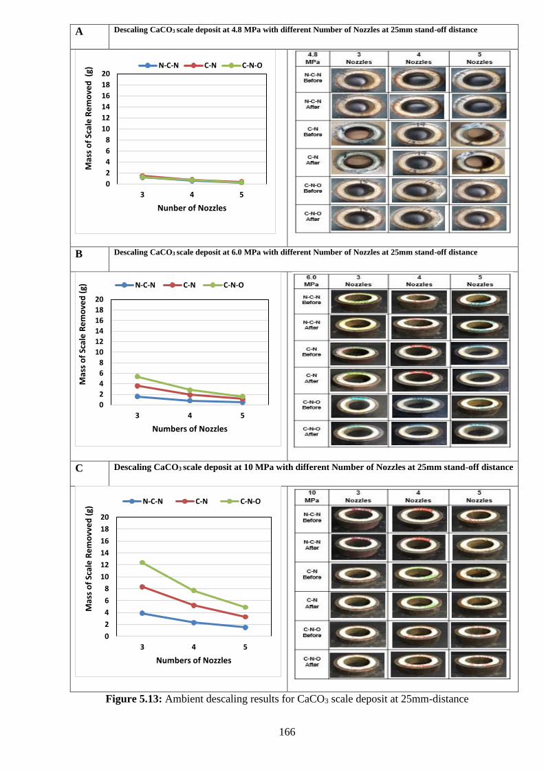
166

A Descaling CaCO3 scale deposit at 4.8 MPa with different Number of Nozzles at 25mm stand-off distance

B Descaling CaCO3 scale deposit at 6.0 MPa with different Number of Nozzles at 25mm stand-off distance

C Descaling CaCO3 scale deposit at 10 MPa with different Number of Nozzles at 25mm stand-off distance

Figure 5.13: Ambient descaling results for CaCO3 scale deposit at 25mm-distance

0

2

4

6

8

10

12

14

16

18

20

3 4 5

Mas

s o

f Sc

ale

Re

mo

ved

(g)

Nunber of Nozzles

N-C-N C-N C-N-O

0

2

4

6

8

10

12

14

16

18

20

3 4 5

Mas

s o

f Sc

ale

Re

mo

ved

(g)

Numbers of Nozzles

N-C-N C-N C-N-O

0

2

4

6

8

10

12

14

16

18

20

3 4 5

Mas

s o

f Sc

ale

Re

mo

vve

d (

g)

Numbers of Nozzles

N-C-N C-N C-N-O

167

5.3.2 Compressed descaling experiments

The compressed descaling experiments were conducted inside the special assembled chamber

but in a compressed air chamber condition for the removal of all the four scale samples. As

explained in the descaling methodology section that a compressed air of 0.2 MPa was introduced

and maintained while simultaneously pumping water at different injection pressure to remove

different scale candidate at different jetting position with different header and nozzle

configuration. This is done with the aim of utilising the additional compressive stress generated

from the compression operation to enhance rate of scale removal.

5.3.2.1 Hollow soft scale samples

The hollow shape soft scale descaled under compressed chamber air conditions as summarised

in Appendix C6 proves to have attained better scale removal than the ambient trials but with

similar descaling trend. The trend that attached the increase in amount of scale remove to increase

in injection pressure and decrease in both number of nozzle & stand-off distance and better off

with (NCN) non-centre nozzle arrangement. The additional compression on samples from the

compressed air during the compression sessions is a key reason for the additional scale removal

over the ambient experimental results. Additionally, the introduced compress stress enhances

both erosion, cyclin stress and sample particle abrasion mechanism

The investigation of effect of nozzle configuration when removing hollow shape scale deposit in

a compressed chamber air condition at 25mm stand-off distance for different injection pressures

and number of nozzles as presented in Figure 5.14. Proves NCN arrangement to be most effective

among others. As average values of 5.9, 3.8 & 3.4% deposit removal was initial achieved with

4.8 MPa cross respective header and nozzle configurations, which visually drilled holes through

the entire descaled samples with 3 & 4 nozzles configurations in Figure. 5.14A. The average

value of scale removed was tripled to 14.4, 12.8 & 11.2% across respective header and nozzle

configurations after increasing the injection pressure to 6 MPa, with scale deposit breakage

across the entire 3nozzle configurations and holes for the remaining descaled samples as shown

in Figure 5.14B. Increasing the injection pressure to 10MPa, skyrocketed the average scale

removal value to 30.1, 27.4 & 25.4%, which completely break all the scale samples across all the

header and nozzle configuration as shown in Figure 5.14C. Still obvious, that NCN configuration

is 1.6, 16 & 3.3% more effective than CN & CNO respectively in removing soft hollow shape

scale deposits. Although, the improvement is more attributed to the additional compressive stress

that aid cyclin stress, and other jetting mechanism.

The descaling of soft hollow scale samples in compressed conditions with 5nozzles using the

NC-arrangement shows a better improvement in terms of mass of scale removed than that

removed with 5 nozzles at ambient condition even at high injection pressure. Five nozzles at low

168

pressure of 4.8 MPa initially removed 2.8g of scale that was slightly improved by 2.5 g and

subsequently 65.6g with corresponding increase of injection pressure to 6.0 MPa and later 10

MPa. This was almost fifty times increased attributed to the wide pressure variation between 10

MPa injection pressure and that of 4.8 & 6.0 MPa. The 4nozzle configuration started by removing

substantial amount of scale (9.3g) at 4.8 MPa injection pressures that was a bite raised by 5.6g

after increasing to 6.0 MPa and increasing the injection pressure to 10 MPa resulted to a massive

growth of descaling rate by 141.g. Whereas, the 3nozzle configuration was able to highly

increase the initial removal at low pressure of 4.8 MPa to 89.1g that was increased by 119.1g and

doubled by 201.4g due to the increase of injection pressure to 6.0 MPa and subsequently 10 MPa

Analysis of the impact of altering header configurations for corresponding injection pressure

shows improvement in the amount of scale removed with reduction of number of nozzles in

compressed descaling trials due to multiple nozzle pressure drop effect (Huang et al., 2018).

Pumping water at low pressure of 4.8 MPa with five nozzles removed 2.8g of scale that

substantially increase by 6.5g and skyrocketed by 86.3g after reducing the numbers of nozzles to

4 and later 3 configurations. Pictorially figure 5.14A displayed some holes across all the descaled

samples at 4 & 3nozzle configurations experiments. While increasing the injection pressure to

6.0MPa with 5nozzles configuration initially removed 5.3g of scale that was improved by 9.6g

and substantially more removed by 203g after adjusting the header configuration to 4nozzles and

later 3nozzles. The pictures in Figure 5.14B demonstrated how most of the descaled samples are

either holed drilled 5-4 header configuration and broken in the 3nozzle configuration. The results

of the investigations of impact of altering the nozzles configurations at high pressure of 10 MPa

yielded the highest and best scale removal result with the highest variation observed between

three and four nozzles. Pumping at high pressure of 10 MPa with five nozzles resulted to the

substantial removal of 68.4g of scale that was increased by 82g after reducing to four nozzles.

This was further highly increased by 223.1g after subsequently reducing to three nozzles. Figure

5.14C pictorially marked all the header configuration trial with broken descaled samples.

.

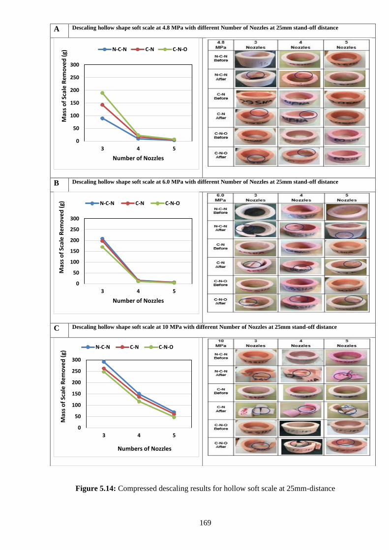
169

Figure 5.14: Compressed descaling results for hollow soft scale at 25mm-distance

A Descaling hollow shape soft scale at 4.8 MPa with different Number of Nozzles at 25mm stand-off distance

B Descaling hollow shape soft scale at 6.0 MPa with different Number of Nozzles at 25mm stand-off distance

C Descaling hollow shape soft scale at 10 MPa with different Number of Nozzles at 25mm stand-off distance

0

50

100

150

200

250

300

3 4 5

Mas

s o

f Sc

ale

Re

mo

ved

(g)

Number of Nozzles

N-C-N C-N C-N-O

0

50

100

150

200

250

300

3 4 5

Mas

s o

f Sc

ale

Re

mo

ved

(g)

Number of Nozzles

N-C-N C-N C-N-O

0

50

100

150

200

250

300

3 4 5

Mas

s o

f Sc

ale

Re

mo

ved

(g)

Numbers of Nozzles

N-C-N C-N C-N-O

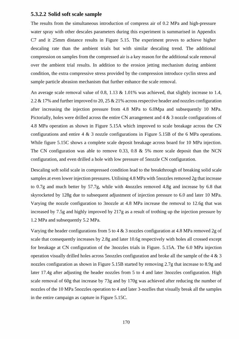
170

5.3.2.2 Solid soft scale sample

The results from the simultaneous introduction of compress air of 0.2 MPa and high-pressure

water spray with other descales parameters during this experiment is summarised in Appendix

C7 and it 25mm distance results in Figure 5.15. The experiment proves to achieve higher

descaling rate than the ambient trials but with similar descaling trend. The additional

compression on samples from the compressed air is a key reason for the additional scale removal

over the ambient trial results. In addition to the erosion jetting mechanism during ambient

condition, the extra compressive stress provided by the compression introduce cyclin stress and

sample particle abrasion mechanism that further enhance the scale removal.

An average scale removal value of 0.8, 1.13 & 1.01% was achieved, that slightly increase to 1.4,

2.2 & 17% and further improved to 20, 25 & 21% across respective header and nozzles configuration

after increasing the injection pressure from 4.8 MPa to 6.0Mpa and subsequently 10 MPa.

Pictorially, holes were drilled across the entire CN arrangement and 4 & 3 nozzle configurations of

4.8 MPa operation as shown in Figure 5.15A which improved to scale breakage across the CN

configurations and entire 4 & 3 nozzle configurations in Figure 5.15B of the 6 MPa operations.

While figure 5.15C shows a complete scale deposit breakage across board for 10 MPa injection.

The CN configuration was able to remove 0.33, 0.8 & 5% more scale deposit than the NCN

configuration, and even drilled a hole with low pressure of 5nozzle CN configuration.

Descaling soft solid scale in compressed condition lead to the breakthrough of breaking solid scale

samples at even lower injection pressures. Utilising 4.8 MPa with 5nozzles removed 2g that increase

to 0.7g and much better by 57.7g, while with 4nozzles removed 4.8g and increase by 6.8 that

skyrocketed by 128g due to subsequent adjustment of injection pressure to 6.0 and later 10 MPa.

Varying the nozzle configuration to 3nozzle at 4.8 MPa increase the removal to 12.6g that was

increased by 7.5g and highly improved by 217g as a result of trothing up the injection pressure by

1.2 MPa and subsequently 5.2 MPa.

Varying the header configurations from 5 to 4 & 3 nozzles configuration at 4.8 MPa removed 2g of

scale that consequently increases by 2.8g and later 10.6g respectively with holes all crossed except

for breakage at CN configuration of the 3nozzles trials in Figure. 5.15A. The 6.0 MPa injection

operation visually drilled holes across 5nozzles configuration and broke all the sample of the 4 & 3

nozzles configuration as shown in Figure 5.15B started by removing 2.7g that increase to 8.9g and

later 17.4g after adjusting the header nozzles from 5 to 4 and later 3nozzles configuration. High

scale removal of 60g that increase by 73g and by 170g was achieved after reducing the number of

nozzles of the 10 MPa 5nozzles operation to 4 and later 3-nozlles that visually break all the samples

in the entire campaign as capture in Figure 5.15C.

171

A Descaling Solid shape soft scale at 4.8 MPa with different Number of Nozzles at 25mm stand-off distance

B Descaling Solid shape soft scale at 6.0 MPa with different Number of Nozzles at 25mm stand-off distance

C Descaling Solid shape soft scale at 10 MPa with different Number of Nozzles at 25mm stand-off distance

Figure 5.15: Compressed descaling results for hollow soft scale at 25mm-distance

0

50

100

150

200

250

3 4 5

Mas

s o

f Sc

ale

Re

mo

ved

(g)

Nuber of Nozzles

N-C-N C-N C-N-O

0

50

100

150

200

250

3 4 5

Mas

s o

f Sc

ale

Re

mo

ved

(g)

Number of Nozzles

N-C-N C-N C-N-O

0

50

100

150

200

250

300

3 4 5

Mas

s o

f Sc

ale

Re

mo

ved

(g)

Nuber of Nozzles

N-C-N C-N C-N-O

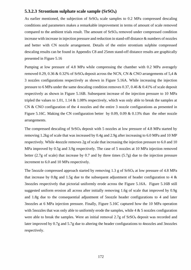
172

5.3.2.3 Strontium sulphate scale sample (SrSO4)

As earlier mentioned, the subjection of SrSO4 scale samples to 0.2 MPa compressed descaling

conditions and parameters makes a remarkable improvement in terms of amount of scale removed

compared to the ambient trials result. The amount of SrSO4 removed under compressed condition

increase with increase in injection pressure and reduction in stand-off distance & numbers of nozzles

and better with CN nozzle arrangement. Details of the entire strontium sulphite compressed

descaling results can be found in Appendix C8 and 25mm stand-off distance results are graphically

presented in Figure 5.16

Pumping at low pressure of 4.8 MPa while compressing the chamber with 0.2 MPa averagely

removed 0.29, 0.36 & 0.32% of SrSO4 deposit across the NCN, CN & CNO arrangements of 5,4 &

3 nozzles configurations respectively as shown in Figure 5.16A. While increasing the injection

pressure to 6 MPa under the same descaling condition removes 0.37, 0.46 & 0.41% of scale deposit

respectively as shown in Figure 5.16B. Subsequent increase of the injection pressure to 10 MPa

tripled the values to 1.01, 1.14 & 1.08% respectively, which was only able to break the samples at

CN & CNO configuration of the 4 nozzles and the entire 3 nozzle configurations as presented in

Figure 5.16C. Making the CN configuration better by 0.09, 0.09 & 0.13% than the other nozzle

arrangements.

The compressed descaling of SrSO4 deposit with 5 nozzles at low pressure of 4.8 MPa started by

removing 1.2kg of scale that was increased by 0.4g and 2.9g after increasing to 6.0 MPa and 10 MP

respectively. While 4nozzle removes 2g of scale that increasing the injection pressure to 6.0 and 10

MPa improved by 0.5g and 3.9g respectively. The case of 5 nozzles at 10 MPa injection removed

better (2.7g of scale) that increase by 0.7 and by three times (5.7g) due to the injection pressure

increment to 6.0 and 10 MPa respectively.

The 5nozzle compressed approach started by removing 1.3 g of SrSO4 at low pressure of 4.8 MPa

that increase by 0.8g and 1.5g due to the subsequent adjustment of header configuration to 4 &

3nozzles respectively that pictorial uniformly erode across the Figure 5.16A. Figure 5.16B still

suggested uniform erosion all across after initially removing 1.6g of scale that improved by 0.9g

and 1.8g due to the consequential adjustment of 5nozzle header configurations to 4 and later

3nozzles at 6 MPa injection pressure. Finally, Figure 5.16C captured how the 10 MPa operation

with 5nozzles that was only able to uniformly erode the samples, while 4 & 5 nozzles configuration

were able to break the samples. Were an initial removal 2.7g of SrSO4 deposit was recorded and

later improved by 0.7g and 5.7g due to altering the header configurations to 4nozzles and 3nozzles

respectively.

173

A Descaling SrSO4 scale deposit at 4.8 MPa with different Number of Nozzles at 25mm stand-off distance

B Descaling SrSO4 scale deposit at 6.0 MPa with different Number of Nozzles at 25mm stand-off distance

C Descaling SrSO4 scale deposit at 10 MPa with different Number of Nozzles at 25mm stand-off distance

Figure 5.16: Compressed descaling results for SrSO4 scale deposit at 25mm-distance

0

2

4

6

8

10

12

14

16

18

20

3 4 5

Mas

s o

f Sc

ale

Re

mo

ved

(g)

Number of Nozzles

N-C-N C-N C-N-O

0

5

10

15

20

3 4 5

Mas

s o

f Sc

ale

Re

mo

ved

(g)

Number of Nozzles

N-C-N C-N C-N-O

0

2

4

6

8

10

12

14

16

18

20

3 4 5

Mas

s o

f Sc

ale

Re

mo

ved

(g)

Number of Nozzles

N-C-N C-N C-N-O

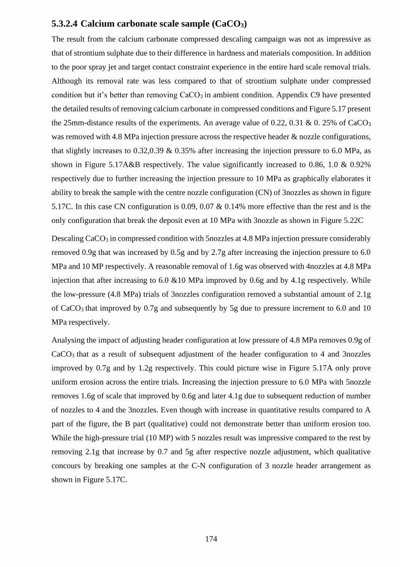
174

5.3.2.4 Calcium carbonate scale sample (CaCO3)

The result from the calcium carbonate compressed descaling campaign was not as impressive as

that of strontium sulphate due to their difference in hardness and materials composition. In addition

to the poor spray jet and target contact constraint experience in the entire hard scale removal trials.

Although its removal rate was less compared to that of strontium sulphate under compressed

condition but it’s better than removing CaCO3 in ambient condition. Appendix C9 have presented

the detailed results of removing calcium carbonate in compressed conditions and Figure 5.17 present

the 25mm-distance results of the experiments. An average value of 0.22, 0.31 & 0. 25% of CaCO3

was removed with 4.8 MPa injection pressure across the respective header & nozzle configurations,

that slightly increases to 0.32,0.39 & 0.35% after increasing the injection pressure to 6.0 MPa, as

shown in Figure 5.17A&B respectively. The value significantly increased to 0.86, 1.0 & 0.92%

respectively due to further increasing the injection pressure to 10 MPa as graphically elaborates it

ability to break the sample with the centre nozzle configuration (CN) of 3nozzles as shown in figure

5.17C. In this case CN configuration is 0.09, 0.07 & 0.14% more effective than the rest and is the

only configuration that break the deposit even at 10 MPa with 3nozzle as shown in Figure 5.22C

Descaling CaCO3 in compressed condition with 5nozzles at 4.8 MPa injection pressure considerably

removed 0.9g that was increased by 0.5g and by 2.7g after increasing the injection pressure to 6.0

MPa and 10 MP respectively. A reasonable removal of 1.6g was observed with 4nozzles at 4.8 MPa

injection that after increasing to 6.0 &10 MPa improved by 0.6g and by 4.1g respectively. While

the low-pressure (4.8 MPa) trials of 3nozzles configuration removed a substantial amount of 2.1g

of CaCO3 that improved by 0.7g and subsequently by 5g due to pressure increment to 6.0 and 10

MPa respectively.

Analysing the impact of adjusting header configuration at low pressure of 4.8 MPa removes 0.9g of

CaCO3 that as a result of subsequent adjustment of the header configuration to 4 and 3nozzles

improved by 0.7g and by 1.2g respectively. This could picture wise in Figure 5.17A only prove

uniform erosion across the entire trials. Increasing the injection pressure to 6.0 MPa with 5nozzle

removes 1.6g of scale that improved by 0.6g and later 4.1g due to subsequent reduction of number

of nozzles to 4 and the 3nozzles. Even though with increase in quantitative results compared to A

part of the figure, the B part (qualitative) could not demonstrate better than uniform erosion too.

While the high-pressure trial (10 MP) with 5 nozzles result was impressive compared to the rest by

removing 2.1g that increase by 0.7 and 5g after respective nozzle adjustment, which qualitative

concours by breaking one samples at the C-N configuration of 3 nozzle header arrangement as

shown in Figure 5.17C.

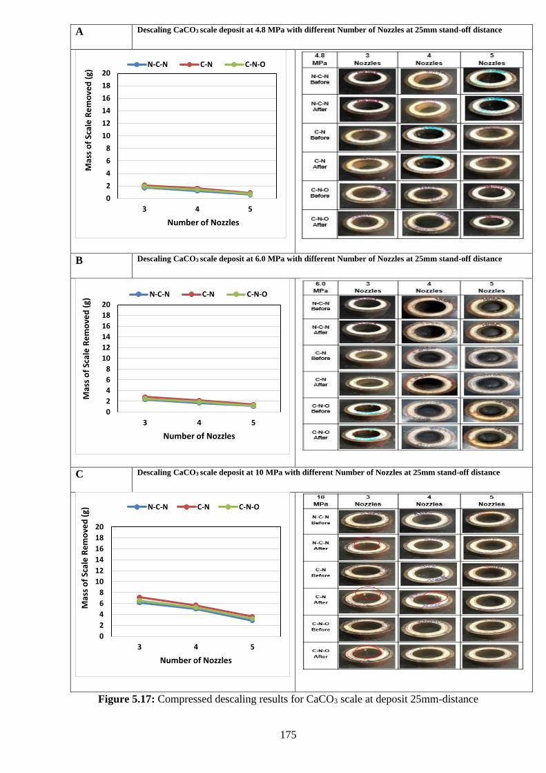
175

A Descaling CaCO3 scale deposit at 4.8 MPa with different Number of Nozzles at 25mm stand-off distance

B Descaling CaCO3 scale deposit at 6.0 MPa with different Number of Nozzles at 25mm stand-off distance

C Descaling CaCO3 scale deposit at 10 MPa with different Number of Nozzles at 25mm stand-off distance

Figure 5.17: Compressed descaling results for CaCO3 scale at deposit 25mm-distance

0

2

4

6

8

10

12

14

16

18

20

3 4 5

Mas

s o

f Sc

ale

Re

mo

ved

(g)

Number of Nozzles

N-C-N C-N C-N-O

0

2

4

6

8

10

12

14

16

18

20

3 4 5

Mas

s o

f Sc

ale

Re

mo

ved

(g)

Number of Nozzles

N-C-N C-N C-N-O

0

2

4

6

8

10

12

14

16

18

20

3 4 5

Mas

s o

f Sc

ale

Re

mo

ved

(g)

Number of Nozzles

N-C-N C-N C-N-O

176

5.3.3 Vacuum descaling trials

The vacuumed air descaling experiments are conducted inside the special assembled chamber but

in a suctioned air chamber condition (-0.08MPa) for the removal of all the four scale samples. As

explained in the descaling methodology section that suctioned air of -0.08MPa was introduced and

maintained while simultaneously pumping water at different injection pressure and other descaling

parameters to remove different scale sample. With the aim of utilising the introduce negative air

chamber pressure to enhance rate of scale removal via aiding some of the jetting mechanisms.

5.3.3.1 Hollow soft scale samples

The hollow shape soft scale descaled in a suctioned chamber air conditions as summarised in

Appendix C10 and it 25mm-distance result in Figure 5.23 proves to have attained better scale

removal than both ambient and compressed trials but with similar descaling trend. The trend that

attached the increase in amount of scale remove to increase in injection pressure and decrease in

both number of nozzle & stand-off distance and better off with non-centre nozzle (NCN)

arrangement. The introduced suction air into the chamber using the vacuum pump to remove the

samples is a key reason for the additional scale removal over both ambient and compressed trial

results. Additionally, the introduced vacuum pressure enhances both erosion, cyclin stress, sample

particle abrasion mechanism and hoop stress.

A significant amount of 6.34, 4.11 & 3.33% of the samples were averagely removed with 4.8 MPa

injection pressure at respective header and nozzles configuration that was able to drill holes across

the entire 4nozzles configuration and breaks all the 3nozzles configurations samples as captured in

Figure 5.23A. A better value of 13.9, 12.4 & 10.9% was attained after increasing the injection

pressure to 6 MPa and pictorially improved the removal by drilling throughout the entire 5nozzle

configuration and breaks the entire samples for the 4 & 3nozzle configurations as captured in Figure

5.23B. While Figure 5.23C demonstrate the highest removal value of 31.7, 28.1 & 25.11% of

paraffin deposit after increasing the injection pressure to 10 MPa that breaks all samples during the

10 MPa vacuumed descaling campaign. The NCN configuration removes 2.23, 1,5, & 3% more

scale deposit than the rest across all descaling permutation and combination coupled with the hoop

stress been aided by the introduced vacuum pressure.

The set of result obtained from the descaling experiment of soft hollow scale samples in vacuumed

conditions with all the header configurations, particularly NCN-configuration’s remove the highest

amount of scale even at lower injection pressure compared the other two chamber condition

experiments. The five-nozzle configuration vacuumed descaling experiment was able remove 3.4g

of paraffin at low injection pressure that improves by 2.6g and much more by 66.6g at medium and

high injection pressure respectively. Reducing the number of nozzles to 4 nozzles at lower pressure

(4.8 MPa) improve the removal to 10g that was later improved by 5.7g and by fifteen time (142.5g)

177

due to subsequent increase of the injection pressures to 6.0 and 10 MPa respectively. Further

reduction of the header configuration to 3 nozzles at 4.8 MPa injection produces the highest initial

paraffin removal of 90g that was later improved by 11.9g and by fivefold (204.3g) after rising the

injection pressure to 6.0 and later 10 MPa respectively.

Also, the best set of quantitative and qualitative result of hollow paraffin removal regarding the

impact of altering header configurations for corresponding injection pressure was attained in the

vacuumed descaling trials that is presented in the Figure 5.23 bellow. Starting by injecting water at

low pressure of 4.8 MPa with five nozzles initially removed 3.4g of paraffin that significantly

increase by 6.6g and shoot up by 86.3g after altering the header configuration to 4 and subsequently

3 nozzles configurations. Figure 5.23A exhibited holes being drilled across all the descaled samples

at 4nozzle and subsequent scale breakage for the entire 3nozzle configurations trials. Subsequent

increase of the injection pressure to 6.0 MPa with 5 nozzles configuration increase the initial paraffin

removal to 6g that was boosted by 9.6g and skyrocketed by 203.3g as a result of altering the header

configuration to 4 nozzles and subsequently 3 nozzles. Better qualitative descaled result that drilled

holes across 5 nozzles configurations and complete scale breakage across both 4 & 3 nozzles

configuration is exhibited in Figure 5.23B. The further increment of injection pressure to 10 MPa

with five nozzles configuration that generated a high removal of 70g of paraffin and later

substantially improved by 83g and much more by 225g was the consequences of varying the header

configuration to 4 & 3 nozzles respectively. Figure 5.23C showcase the best and breakthrough

qualitative results of removing paraffin that breaks all the samples across all header and nozzle

configurations.

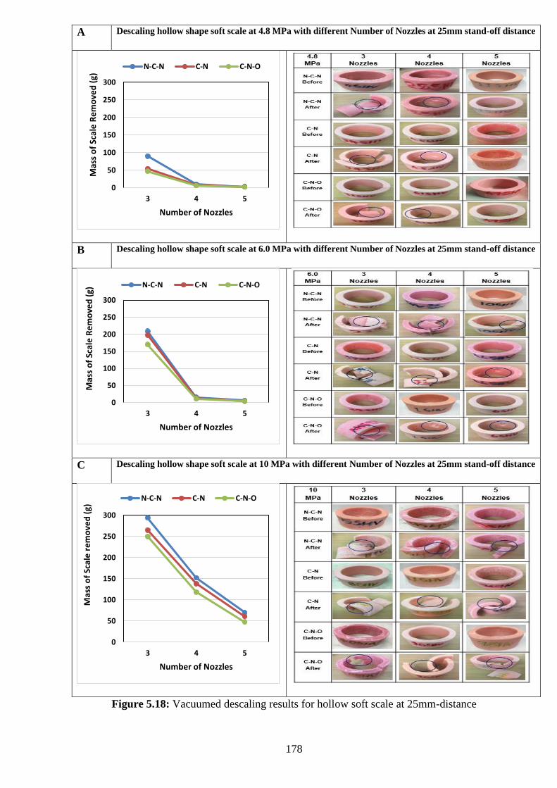
178

A Descaling hollow shape soft scale at 4.8 MPa with different Number of Nozzles at 25mm stand-off distance

B Descaling hollow shape soft scale at 6.0 MPa with different Number of Nozzles at 25mm stand-off distance

C Descaling hollow shape soft scale at 10 MPa with different Number of Nozzles at 25mm stand-off distance

Figure 5.18: Vacuumed descaling results for hollow soft scale at 25mm-distance

0

50

100

150

200

250

300

3 4 5

Mas

s o

f Sc

ale

Re

mo

ved

(g)

Number of Nozzles

N-C-N C-N C-N-O

0

50

100

150

200

250

300

3 4 5

Mas

s o

f Sc

ale

Re

mo

ved

(g)

Number of Nozzles

N-C-N C-N C-N-O

0

50

100

150

200

250

300

3 4 5

Mas

s o

f Sc

ale

re

mo

ved

(g)

Number of Nozzles

N-C-N C-N C-N-O

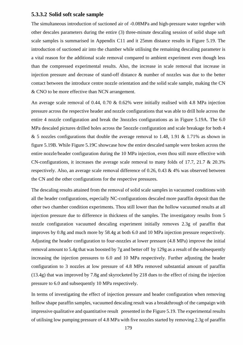
179

5.3.3.2 Solid soft scale sample

The simultaneous introduction of suctioned air of -0.08MPa and high-pressure water together with

other descales parameters during the entire (3) three-minute descaling session of solid shape soft

scale samples is summarised in Appendix C11 and it 25mm distance results in Figure 5.19. The

introduction of suctioned air into the chamber while utilising the remaining descaling parameter is

a vital reason for the additional scale removal compared to ambient experiment even though less

than the compressed experimental results. Also, the increase in scale removal that increase in

injection pressure and decrease of stand-off distance & number of nozzles was due to the better

contact between the introduce centre nozzle orientation and the solid scale sample, making the CN

& CNO to be more effective than NCN arrangement.

An average scale removal of 0.44, 0.70 & 0.62% were initially realised with 4.8 MPa injection

pressure across the respective header and nozzle configurations that was able to drill hole across the

entire 4 nozzle configuration and break the 3nozzles configurations as in Figure 5.19A. The 6.0

MPa descaled pictures drilled holes across the 5nozzle configuration and scale breakage for both 4

& 5 nozzles configurations that double the average removal to 1.48, 1.91 & 1.71% as shown in

figure 5.19B. While Figure 5.19C showcase how the entire descaled sample were broken across the

entire nozzle/header configuration during the 10 MPa injection, even thou still more effective with

CN-configurations, it increases the average scale removal to many folds of 17.7, 21.7 & 20.3%

respectively. Also, an average scale removal difference of 0.26, 0.43 & 4% was observed between

the CN and the other configurations for the respective pressures.

The descaling results attained from the removal of solid scale samples in vacuumed conditions with

all the header configurations, especially NC-configurations descaled more paraffin deposit than the

other two chamber condition experiments. Thou still lower than the hollow vacuumed results at all

injection pressure due to difference in thickness of the samples. The investigatory results from 5

nozzle configuration vacuumed descaling experiment initially removes 2.3g of paraffin that

improves by 0.8g and much more by 58.4g at both 6.0 and 10 MPa injection pressure respectively.

Adjusting the header configuration to four-nozzles at lower pressure (4.8 MPa) improve the initial

removal amount to 5.4g that was boosted by 7g and better off by 129g as a result of the subsequently

increasing the injection pressures to 6.0 and 10 MPa respectively. Further adjusting the header

configuration to 3 nozzles at low pressure of 4.8 MPa removed substantial amount of paraffin

(13.4g) that was improved by 7.8g and skyrocketed by 218 dues to the effect of rising the injection

pressure to 6.0 and subsequently 10 MPa respectively.

In terms of investigating the effect of injection pressure and header configuration when removing

hollow shape paraffin samples, vacuumed descaling result was a breakthrough of the campaign with

impressive qualitative and quantitative result presented in the Figure 5.19. The experimental results

of utilising low pumping pressure of 4.8 MPa with five nozzles started by removing 2.3g of paraffin

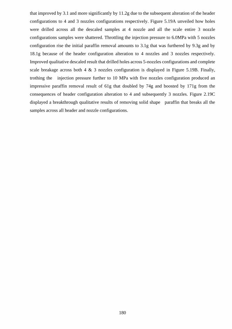
180

that improved by 3.1 and more significantly by 11.2g due to the subsequent alteration of the header

configurations to 4 and 3 nozzles configurations respectively. Figure 5.19A unveiled how holes

were drilled across all the descaled samples at 4 nozzle and all the scale entire 3 nozzle

configurations samples were shattered. Throttling the injection pressure to 6.0MPa with 5 nozzles

configuration rise the initial paraffin removal amounts to 3.1g that was furthered by 9.3g and by

18.1g because of the header configuration alteration to 4 nozzles and 3 nozzles respectively.

Improved qualitative descaled result that drilled holes across 5-nozzles configurations and complete

scale breakage across both 4 & 3 nozzles configuration is displayed in Figure 5.19B. Finally,

trothing the injection pressure further to 10 MPa with five nozzles configuration produced an

impressive paraffin removal result of 61g that doubled by 74g and boosted by 171g from the

consequences of header configuration alteration to 4 and subsequently 3 nozzles. Figure 2.19C

displayed a breakthrough qualitative results of removing solid shape paraffin that breaks all the

samples across all header and nozzle configurations.

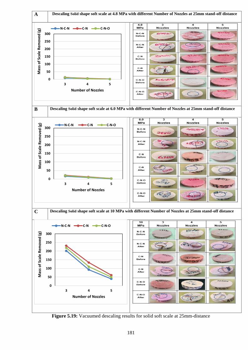
181

A Descaling Solid shape soft scale at 4.8 MPa with different Number of Nozzles at 25mm stand-off distance

B Descaling Solid shape soft scale at 6.0 MPa with different Number of Nozzles at 25mm stand-off distance

C Descaling Solid shape soft scale at 10 MPa with different Number of Nozzles at 25mm stand-off distance

Figure 5.19: Vacuumed descaling results for solid soft scale at 25mm-distance

0

50

100

150

200

250

300

3 4 5

Mas

s o

f Sc

ale

Re

mo

ved

(g)

Number of Nozzles

N-C-N C-N C-N-O

0

50

100

150

200

250

300

3 4 5

Mas

s o

f Sc

ale

Re

mo

ved

(g)

Number of Nozzles

N-C-N C-N C-N-O

0

50

100

150

200

250

300

3 4 5

Mas

s o

f Sc

ale

Re

mo

ved

(g)

Number of Nozzles

N-C-N C-N C-N-O

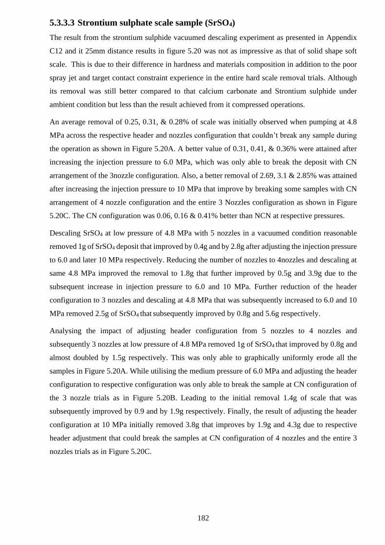
182

5.3.3.3 Strontium sulphate scale sample (SrSO4)

The result from the strontium sulphide vacuumed descaling experiment as presented in Appendix

C12 and it 25mm distance results in figure 5.20 was not as impressive as that of solid shape soft

scale. This is due to their difference in hardness and materials composition in addition to the poor

spray jet and target contact constraint experience in the entire hard scale removal trials. Although

its removal was still better compared to that calcium carbonate and Strontium sulphide under

ambient condition but less than the result achieved from it compressed operations.

An average removal of 0.25, 0.31, & 0.28% of scale was initially observed when pumping at 4.8

MPa across the respective header and nozzles configuration that couldn’t break any sample during

the operation as shown in Figure 5.20A. A better value of 0.31, 0.41, & 0.36% were attained after

increasing the injection pressure to 6.0 MPa, which was only able to break the deposit with CN

arrangement of the 3nozzle configuration. Also, a better removal of 2.69, 3.1 & 2.85% was attained

after increasing the injection pressure to 10 MPa that improve by breaking some samples with CN

arrangement of 4 nozzle configuration and the entire 3 Nozzles configuration as shown in Figure

5.20C. The CN configuration was 0.06, 0.16 & 0.41% better than NCN at respective pressures.

Descaling SrSO4 at low pressure of 4.8 MPa with 5 nozzles in a vacuumed condition reasonable

removed 1g of SrSO4 deposit that improved by 0.4g and by 2.8g after adjusting the injection pressure

to 6.0 and later 10 MPa respectively. Reducing the number of nozzles to 4nozzles and descaling at

same 4.8 MPa improved the removal to 1.8g that further improved by 0.5g and 3.9g due to the

subsequent increase in injection pressure to 6.0 and 10 MPa. Further reduction of the header

configuration to 3 nozzles and descaling at 4.8 MPa that was subsequently increased to 6.0 and 10

MPa removed 2.5g of SrSO4 that subsequently improved by 0.8g and 5.6g respectively.

Analysing the impact of adjusting header configuration from 5 nozzles to 4 nozzles and

subsequently 3 nozzles at low pressure of 4.8 MPa removed 1g of SrSO4 that improved by 0.8g and

almost doubled by 1.5g respectively. This was only able to graphically uniformly erode all the

samples in Figure 5.20A. While utilising the medium pressure of 6.0 MPa and adjusting the header

configuration to respective configuration was only able to break the sample at CN configuration of

the 3 nozzle trials as in Figure 5.20B. Leading to the initial removal 1.4g of scale that was

subsequently improved by 0.9 and by 1.9g respectively. Finally, the result of adjusting the header

configuration at 10 MPa initially removed 3.8g that improves by 1.9g and 4.3g due to respective

header adjustment that could break the samples at CN configuration of 4 nozzles and the entire 3

nozzles trials as in Figure 5.20C.

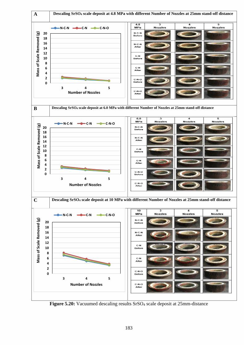
183

A Descaling SrSO4 scale deposit at 4.8 MPa with different Number of Nozzles at 25mm stand-off distance

B Descaling SrSO4 scale deposit at 6.0 MPa with different Number of Nozzles at 25mm stand-off distance

C Descaling SrSO4 scale deposit at 10 MPa with different Number of Nozzles at 25mm stand-off distance

Figure 5.20: Vacuumed descaling results SrSO4 scale deposit at 25mm-distance

0

2

4

6

8

10

12

14

16

18

20

3 4 5

Mas

s o

f Sc

ale

Re

mo

ved

(g)

Number of Nozzles

N-C-N C-N C-N-O

0

2

4

6

8

10

12

14

16

18

20

3 4 5

Mas

s o

f Sc

ale

Re

mo

ved

(g)

Number of Nozzles

N-C-N C-N C-N-O

0

2

4

6

8

10

12

14

16

18

20

3 4 5

Mas

s o

f Sc

ale

Re

mo

ved

(g)

Number of Nozzles

N-C-N C-N C-N-O

184

5.3.3.4 Calcium carbonate scale sample (CaCO3)

Subjection of CaCO3 scale samples to -0.08 MPa vacuumed descaling conditions and parameters

makes a remarkable improvement in terms of amount of scale removed compared to the ambient

result but less than the compressed results. The amount of CaCO3 removed under this condition

increase with increase in injection pressure and reduction in stand-off distance & numbers of nozzles

and better with CN nozzle arrangement. Details of the entire calcium carbonate vacuumed descaling

results can be found in Appendix C13 and the 25mm stand-off distance results are graphically

presented in Figure 5.21.

An average removal values of 0.18, 0.24 & 0.21% was initially achieved when injecting at 4.8 MPa

for the respective header and nozzle configuration that increase to 0.27, 0.34 & 0.3% after injecting

further to 6.0 MPa that was not able to break any sample as shown in Figure 5.21 A&B respectively.

The average removal value increases to 0.73, 0.89 & 0.8% after rising the injection to 10 MPa,

which was able to mildly break the samples at the CN nozzle arrangement of the 4 nozzles and the

entire 3 nozzles configuration as shown in Figure 5.21C. An average difference in removal of 0.06,

0.07 & 0.16% across the respective injection pressure was observed between CN and NCN

configurations.

Analyses of the impact of low pressure of 4.8 MPa with 5nozzle configurations during the vacuumed

descaling of CaCO3 initially removed 0.7g that improved by 0.4g and 2.5 g after adjusting the

injection to 6.0 MP and 10MPa respectively. Subsequently, the utilization of 4 nozzle configuration

at low pressure increase the initial removal to 1.4g that improved by 0.5g and by 3.4g after rising

the injection pressure to 6.0 and 10 MPa. Meanwhile, the 3nozzle configuration did better by

substantially removing 3.2g of scale that improved by 1.6g and later 3.5g as a result of increasing

the injection pressure to 6.0 and 10 MPa respectively.

The vacuumed descaling results of 5nozzles at low pressure of 4.8 MPa removed 0.7g that doubled

by 7.0g and furthered by 1.2g as result of reducing the nozzles configuration to 4 nozzles and

subsequently 3-nozzles. Figure 5.21A was only able to graphically show better erosion across all

trials. While increasing the injection pressure to 6.0 MPa with 5 nozzles boost the removal amount

to 1.1g and improved it by 0.8g and later 1.6g because of header nozzles reduction to 4 and 3 nozzles

respectively. Like the A part of the Figure 5.21, Figure 2.21B could only exhibit uniform weathering

all along. Further increment of injection pressure to 10MPa was able to further increase the scale

removal to 3.2g that improved by 1.6g and later 3.5g as a result of adjusting the header configuration

to 4 nozzle and 3 nozzles respectively. Figure 2.21C was only able to break the samples with CN

arrangement of the 4nozzle configuration and the entire configuration of the 3nozzle operation.

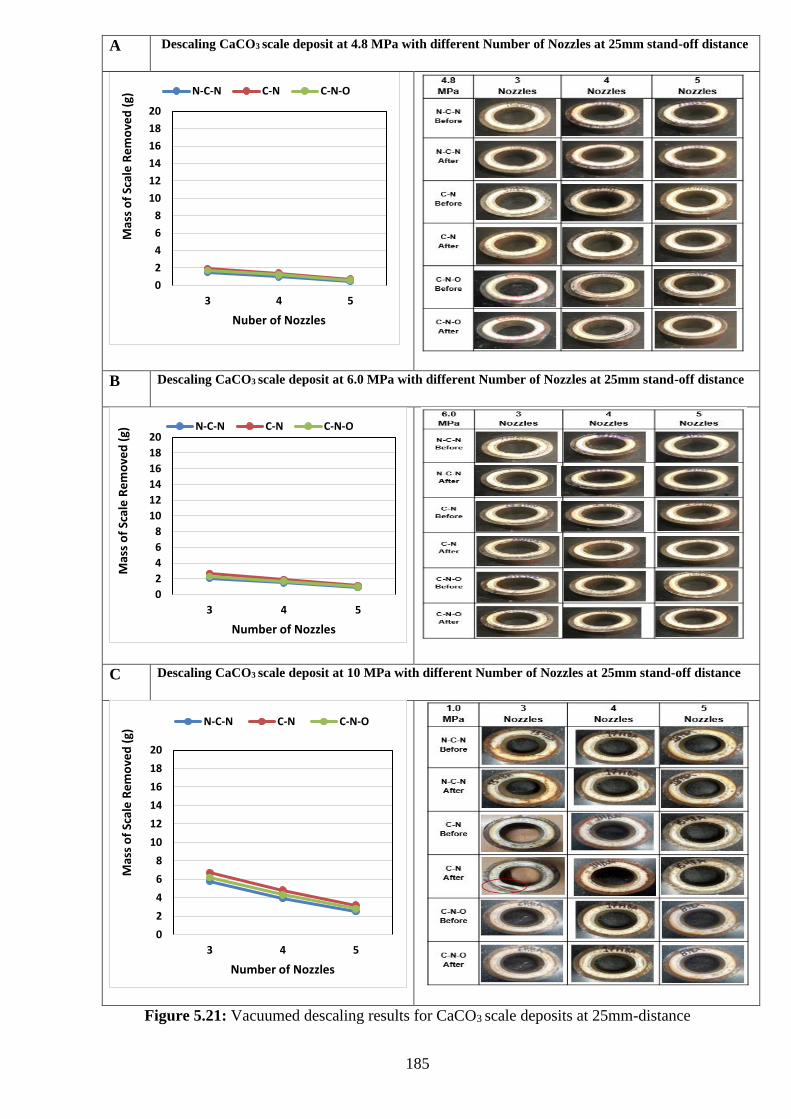
185

A Descaling CaCO3 scale deposit at 4.8 MPa with different Number of Nozzles at 25mm stand-off distance

B Descaling CaCO3 scale deposit at 6.0 MPa with different Number of Nozzles at 25mm stand-off distance

C Descaling CaCO3 scale deposit at 10 MPa with different Number of Nozzles at 25mm stand-off distance

Figure 5.21: Vacuumed descaling results for CaCO3 scale deposits at 25mm-distance

0

2

4

6

8

10

12

14

16

18

20

3 4 5

Mas

s o

f Sc

ale

Re

mo

ved

(g)

Nuber of Nozzles

N-C-N C-N C-N-O

0

2

4

6

8

10

12

14

16

18

20

3 4 5

Mas

s o

f Sc

ale

Re

mo

ved

(g)

Number of Nozzles

N-C-N C-N C-N-O

0

2

4

6

8

10

12

14

16

18

20

3 4 5

Mas

s o

f Sc

ale

Re

mo

ved

(g)

Number of Nozzles

N-C-N C-N C-N-O

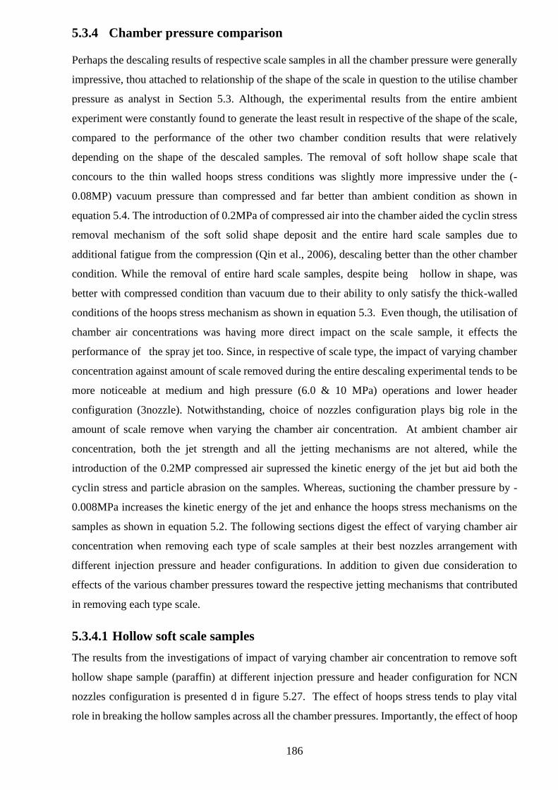
186

5.3.4 Chamber pressure comparison

Perhaps the descaling results of respective scale samples in all the chamber pressure were generally

impressive, thou attached to relationship of the shape of the scale in question to the utilise chamber

pressure as analyst in Section 5.3. Although, the experimental results from the entire ambient

experiment were constantly found to generate the least result in respective of the shape of the scale,

compared to the performance of the other two chamber condition results that were relatively

depending on the shape of the descaled samples. The removal of soft hollow shape scale that

concours to the thin walled hoops stress conditions was slightly more impressive under the (-

0.08MP) vacuum pressure than compressed and far better than ambient condition as shown in

equation 5.4. The introduction of 0.2MPa of compressed air into the chamber aided the cyclin stress

removal mechanism of the soft solid shape deposit and the entire hard scale samples due to

additional fatigue from the compression (Qin et al., 2006), descaling better than the other chamber

condition. While the removal of entire hard scale samples, despite being hollow in shape, was

better with compressed condition than vacuum due to their ability to only satisfy the thick-walled

conditions of the hoops stress mechanism as shown in equation 5.3. Even though, the utilisation of

chamber air concentrations was having more direct impact on the scale sample, it effects the

performance of the spray jet too. Since, in respective of scale type, the impact of varying chamber

concentration against amount of scale removed during the entire descaling experimental tends to be

more noticeable at medium and high pressure (6.0 & 10 MPa) operations and lower header

configuration (3nozzle). Notwithstanding, choice of nozzles configuration plays big role in the

amount of scale remove when varying the chamber air concentration. At ambient chamber air

concentration, both the jet strength and all the jetting mechanisms are not altered, while the

introduction of the 0.2MP compressed air supressed the kinetic energy of the jet but aid both the

cyclin stress and particle abrasion on the samples. Whereas, suctioning the chamber pressure by -

0.008MPa increases the kinetic energy of the jet and enhance the hoops stress mechanisms on the

samples as shown in equation 5.2. The following sections digest the effect of varying chamber air

concentration when removing each type of scale samples at their best nozzles arrangement with

different injection pressure and header configurations. In addition to given due consideration to

effects of the various chamber pressures toward the respective jetting mechanisms that contributed

in removing each type scale.

5.3.4.1 Hollow soft scale samples

The results from the investigations of impact of varying chamber air concentration to remove soft

hollow shape sample (paraffin) at different injection pressure and header configuration for NCN

nozzles configuration is presented d in figure 5.27. The effect of hoops stress tends to play vital

role in breaking the hollow samples across all the chamber pressures. Importantly, the effect of hoop

187

stress mechanism aids the ambient hollow scale removal that provide a high removal result that is

close to the values of compressed and vacuumed conditions.

𝑃𝑟

𝑡= 𝜏ℎ𝑜𝑜𝑝𝑠 (5.1)

Were P being internal resultant pressure (chamber pressure+ jet pressure), r, is the radius of the

hollow sample and t is it thickness. Considering the 10MPa injection pressure, the internal resultant

pressure for vacuum is (10+0.0101352+0.008) MPa, ambient is (10+ 0.101325) MPa, while

compressed is (10+0.0101352-0.2) MPa. Henceforth, Vacuum=10.021MPa, Ambient=10.101MPa

and Compressed=9.901MPa. Contrary to eqq.5.2., compressed descaling results slightly lagged vacuum

and better than ambient because 0.2 MPa compressed air introduction was able to impressively aid

the cyclin stress mechanism that significantly improved removal by propagating the natural fissure

and cracks of the sample.

𝜏ℎ𝑂𝑂𝑃𝑆 𝑉𝑎𝑐 > 𝜏ℎ𝑂𝑂𝑃𝑆 𝐴𝑚𝑏 > 𝜏ℎ𝑂𝑂𝑃𝑆𝐶𝑜𝑚𝑝 (5.2)

The result of analysing the effect of varying chamber pressure when descaling hollow scale sample

at 4.8 MPa with the CN header configurations is presented in Figure 5.22A. Where 5nozzles

configuration initially removes 1.7 g of paraffin at ambient pressure, which improved by 1.1 g and

by 1.7 g due to altering the chamber pressure to compressed and later suctioned respectively.

Similarly, corresponding value increase from 6.2 g and by 3.1 g & 3.8 g was recorded at respective

chamber pressure of 4nozzles operations, while the 3nozzles removes 42.8 g at ambient and

improved by 46.3 g and 4.7.2 g as a result of altering to compressed and vacuum respectively. The

6.0 MPa ambient operation presented in Figure 5.22D removes 2.9g of paraffin with 5nozzles that

improves by 2.4 and 3.1 due to respective chamber alterations, while 4nozzle ambient removes 10g

that improves by 4.9g and 5.7g respectively. Significant removal impact due chamber alteration can

be seen in the 3nozzle operation that remove 93.7g at ambient and increase by 114.5g and 1.15.6g

due to chamber alteration to compressed and later vacuum conditions. Figure 5.22G recorded an

impressive initial removal at 10 MPa, 5nozzle ambient operation of 58.3g of paraffin that improved

by 10g and 12g due to perspective chamber alterations and more impressive at 4nozzle operation

were the ambient removal of 77g of paraffin was doubled (74g and 76g respectively) as a result of

respective chamber alteration. While the respective chamber alterations with 3nozzles remove 253.g

at ambient that was improved by 38g and 41g of scale removal.

188

Figure 5.22: Chamber pressure impact comprising for descaling hollow soft scale at 25mm-distance

0

50

100

150

200

250

300

-0.08 0.101325 0.2Mas

s o

f Sc

ale

Re

mo

ved

(g)

Chamber Pressure (MPa)

Descaling rate at 4.8MPa for NCN confg

5

4

3

0

50

100

150

200

250

300

-0.08 0.101325 0.2

Mas

s o

f Sc

ale

Re

mo

ved

(g)

Chamber Pressure (MPa)

Descaling rate at 4.8MPa for CN confg.

5

4

3

0

50

100

150

200

250

300

-0.08 0.101325 0.2

Mas

s o

f Sc

ale

Re

mo

ved

(g)

Chamber Pressure (MPa)

Descaling rate at 4.8MPa for CNO confg

5

4

3

(c)

0

50

100

150

200

250

300

-0.08 0.101325 0.2Mas

s o

f Sc

ale

Re

mo

ved

(g)

Chamber Pressure (MPa)

Descaling rate at 6.0 MPa for NCN confg

5

4

3

0

50

100

150

200

250

300

-0.08 0.101325 0.2M

ass

of

Scal

e R

em

ove

d (

g)Chamber Pressure (MPa)

Descaling rate at 6.0 MPa for CN confg.

5

4

3

0

50

100

150

200

250

300

-0.08 0.101325 0.2

Mas

s o

f Sc

ale

Re

mo

ved

(g)

Chamber Pressure (MPa)

Descaling rate at 6.0 MPa for CNO confg)

5

4

3

0

50

100

150

200

250

300

-0.08 0.101325 0.2

Mas

s o

f Sc

ale

Re

mo

ved

(g)

Chamber Pressure (MPa)

Descaling rate at 10 MPa for NCN confg.

5

4

3

0

50

100

150

200

250

300

-0.08 0.101325 0.2

Mas

s o

f Sc

ale

Re

mo

ved

(g)

Chamber Pressure (MPa)

Descaling rate at 10 MPa for CN confg.

5

4

3

0

50

100

150

200

250

300

-0.08 0.101325 0.2

Mas

s o

f Sc

ale

Re

mo

ved

(g)

Chamber Pressure (MPa)

Descaling rate at 10 MPa for CNO confg)

5

4

3

(a) (b)

(d) (e) (f)

(g) (h) (i)

189

5.3.4.2 Solid soft scale sample

Results of the investigation of impact of varying chamber air concentration when descaling solid

shape paraffin scale at different injection pressure and header & nozzles configurations can be found

in Figure 5.23. Singling the CN nozzles arrangement result for analyse due to their better

performance demonstrated a trend. Contrary to hollow removal, were the compressed condition

removed better than all the chamber condition due to the direct impact of the introduced 0.2 MPa

compressed air over the entire deposit surface that propagate the natural fissure and cracks of the

sample through cyclin stress mechanism. Vacuum condition was fairly lagging the compressed

conditions and better than ambient as a result of having more resultant pressure as discussed in

Sectioned 5.3.3.2.

Figure 5.23B graphically present the analysis of the investigation of the effect of varying chamber

pressure to remove solid scale at 4.8 MPa with different number of nozzles in CN configuration.

The 5nozzle operations remove 1.2g mass of paraffin that was qualitatively improved by 1.1g and

0.8g after altering the chamber pressure from ambient to compressed and later vacuumed pressure

respectively. For the 4nozzle configuration, the ambient removal was 2.6g and improved by 2.8g

and by 2.2g as result of compressing the chamber by 0.2 MPa and later suctioning it by -0.008MPa

respectively. While in the case of 3nozzle configuration that recorded a better removal value of 5.2g

ambient pressure improved by 8.2g and 7.4g as a result of respective alteration of the chamber

conditions. The 6.0 MPa operation of CN configurations of the respective number of nozzles as

presented in figure 5.23E shows how 5nozzle was able to remove 1.8g of paraffin at ambient

condition that improved by 1.3g and 0.9g after introducing compressed air and suctioned

respectively. Likewise, the 4nozzle operation at ambient condition removes 3.9g of paraffin that

was improved by 8.5g and 7.7g due to the respective chamber air alterations. While the 3nozzles

operations at ambient condition impressively removes 7.3g of scale that almost doubled (14g and

13g respectively) due to respective chamber alterations. The consecutive alteration of chamber

pressure from ambient to compression and vacuum respectively, remarkably removes 32g of

paraffin and significantly enhanced by 29g and 28g at the 10 MPa of the 5nozzles operations. While

the 4nozzles increase the ambient removal to 51g that improved to 83g and 82g across respective

chamber conditions. A high removal value of 104g was recorded for ambient removal of 3nozzles

with significant improvement by 128g and 126g due to the respective chamber air alterations as in

Figure 5.23H.

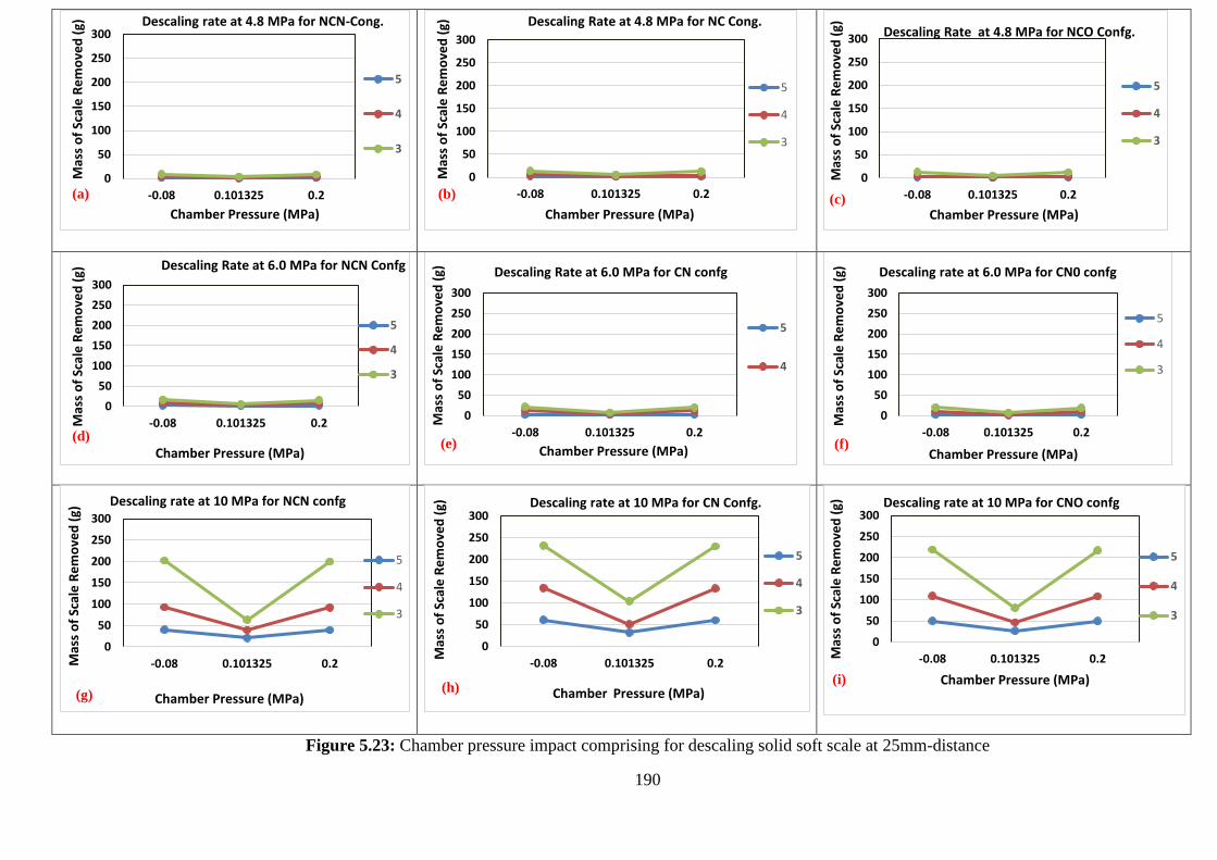
190

Figure 5.23: Chamber pressure impact comprising for descaling solid soft scale at 25mm-distance

0

50

100

150

200

250

300

-0.08 0.101325 0.2

Mas

s o

f Sc

ale

Re

mo

ved

(g)

Chamber Pressure (MPa)

Descaling rate at 4.8 MPa for NCN-Cong.

5

4

3

0

50

100

150

200

250

300

-0.08 0.101325 0.2

Mas

s o

f Sc

ale

Re

mo

ved

(g)

Chamber Pressure (MPa)

Descaling Rate at 4.8 MPa for NC Cong.

5

4

3

0

50

100

150

200

250

300

-0.08 0.101325 0.2

Mas

s o

f Sc

ale

Re

mo

ved

(g)

Chamber Pressure (MPa)

Descaling Rate at 4.8 MPa for NCO Confg.

5

4

3

0

50

100

150

200

250

300

-0.08 0.101325 0.2Mas

s o

f Sc

ale

Re

mo

ved

(g)

Chamber Pressure (MPa)

Descaling Rate at 6.0 MPa for NCN Confg

5

4

3

0

50

100

150

200

250

300

-0.08 0.101325 0.2M

ass

of

Scal

e R

em

ove

d (

g)Chamber Pressure (MPa)

Descaling Rate at 6.0 MPa for CN confg

5

4

0

50

100

150

200

250

300

-0.08 0.101325 0.2

Mas

s o

f Sc

ale

Re

mo

ved

(g)

Chamber Pressure (MPa)

Descaling rate at 6.0 MPa for CN0 confg

5

4

3

0

50

100

150

200

250

300

-0.08 0.101325 0.2Mas

s o

f Sc

ale

Re

mo

ved

(g)

Chamber Pressure (MPa)

Descaling rate at 10 MPa for NCN confg

5

4

3

0

50

100

150

200

250

300

-0.08 0.101325 0.2

Mas

s o

f Sc

ale

Re

mo

ved

(g)

Chamber Pressure (MPa)

Descaling rate at 10 MPa for CN Confg.

5

4

3

0

50

100

150

200

250

300

-0.08 0.101325 0.2Mas

s o

f Sc

ale

Re

mo

ved

(g)

Chamber Pressure (MPa)

Descaling rate at 10 MPa for CNO confg

5

4

3

(a) (c) (b)

(d)

(g)

(e) (f)

(h) (i)

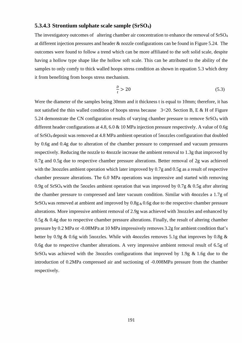
191

5.3.4.3 Strontium sulphate scale sample (SrSO4)

The investigatory outcomes of altering chamber air concentration to enhance the removal of SrSO4

at different injection pressures and header & nozzle configurations can be found in Figure 5.24. The

outcomes were found to follow a trend which can be more affiliated to the soft solid scale, despite

having a hollow type shape like the hollow soft scale. This can be attributed to the ability of the

samples to only comfy to thick walled hoops stress condition as shown in equation 5.3 which deny

it from benefiting from hoops stress mechanism.

𝐷

𝑡> 20 (5.3)

Were the diameter of the samples being 30mm and it thickness t is equal to 10mm; therefore, it has

not satisfied the thin walled condition of hoops stress because 3<20. Section B, E & H of Figure

5.24 demonstrate the CN configuration results of varying chamber pressure to remove SrSO4 with

different header configurations at 4.8, 6.0 & 10 MPa injection pressure respectively. A value of 0.6g

of SrSO4 deposit was removed at 4.8 MPa ambient operation of 5nozzles configuration that doubled

by 0.6g and 0.4g due to alteration of the chamber pressure to compressed and vacuum pressures

respectively. Reducing the nozzle to 4nozzle increase the ambient removal to 1.3g that improved by

0.7g and 0.5g due to respective chamber pressure alterations. Better removal of 2g was achieved

with the 3nozzles ambient operation which later improved by 0.7g and 0.5g as a result of respective

chamber pressure alterations. The 6.0 MPa operations was impressive and started with removing

0.9g of SrSO4 with the 5nozles ambient operation that was improved by 0.7g & 0.5g after altering

the chamber pressure to compressed and later vacuum condition. Similar with 4nozzles a 1.7g of

SrSO4 was removed at ambient and improved by 0.8g & 0.6g due to the respective chamber pressure

alterations. More impressive ambient removal of 2.9g was achieved with 3nozzles and enhanced by

0.5g & 0.4g due to respective chamber pressure alterations. Finally, the result of altering chamber

pressure by 0.2 MPa or -0.08MPa at 10 MPa impressively removes 3.2g for ambient condition that’s

better by 0.9g & 0.6g with 5nozzles. While with 4nozzles removes 5.1g that improves by 0.8g &

0.6g due to respective chamber alterations. A very impressive ambient removal result of 6.5g of

SrSO4 was achieved with the 3nozzles configurations that improved by 1.9g & 1.6g due to the

introduction of 0.2MPa compressed air and suctioning of -0.008MPa pressure from the chamber

respectively.

192

Figure 5.24: Chamber pressure impact comprising for descaling SrSO4 scale deposit at 25mm-distance

0

5

10

15

20

-0.08 0.101325 0.2

Mas

s o

f Sc

ale

Re

mo

ved

(g)

Chamber Pressure (MPa)

Descaling rate at 4.8 MPa for NCN-Cong.

5

4

3

0

5

10

15

20

-0.08 0.101325 0.2

Mas

s o

f Sc

ale

Re

mo

ved

(g)

Chamber Pressure (MPa)

Descaling Rate at 4.8 MPa for NC Cong.

5

4

3

0

5

10

15

20

-0.08 0.101325 0.2

Mas

s o

f Sc

ale

Re

mo

ved

(g)

Chamber Pressure (MPa)

Descaling Rate at 4.8 MPa for NCO Confg.

5

4

3

0

5

10

15

20

-0.08 0.101325 0.2Mas

s o

f Sc

ale

Re

mo

ved

(g)

Chamber Pressure (MPa)

Descaling Rate at 6.0 MPa for NCN Confg

5

4

3

0

5

10

15

20

-0.08 0.101325 0.2M

ass

of

Scal

e R

em

ove

d (

g)

Chamber Pressure (MPa)

Descaling Rate at 6.0 MPa for CN confg

5

4

3

0

5

10

15

20

-0.08 0.101325 0.2

Mas

s o

f Sc

ale

Re

mo

ved

(g)

Chamber Pressure (MPa)

Descaling rate at 6.0 MPa for CN0 confg

5

4

3

0

5

10

15

20

-0.08 0.101325 0.2

Mas

s o

f Sc

ale

Re

mo

ved

(g)

Chamber Pressure (MPa)

Descaling rate at 10 MPa for NCN confg.

5

4

3

0

5

10

15

20

-0.08 0.101325 0.2

Mas

s o

f Sc

ale

Re

mo

ved

(g)

Chamber Pressure (MPa)

Descaling rate at 10 MPa for CN confg.

5

4

3

0

5

10

15

20

-0.08 0.101325 0.2Mas

s o

f Sc

ale

Re

mo

ved

(g)

Chamber Pressure (MPa)

Descaling rate at 10 MPa for CNO confg.

5

4

3

(b) (a) (c)

(d)

(g)

(e)

(h)

(f)

(h)

193

5.3.4.4 Calcium carbonate scale sample (CaCO3)

The results of altering the chamber pressure when removing CaCO3 scale deposit at respective

injection pressure and header/nozzles configurations was less impressive than the results obtained

from the removal SrSO4 but shares a very similar removal trend. Although having similar shapes

with SrSO4 that couldn’t comfy with the thin walled condition of hoop stress as expressed in

equation 5.3 narrowing it removal prospects mechanisms to cyclin stress, erosion and particle

abrasion mechanism.

The effect of removing CaCO3 deposit in ambient condition, in compressed air condition and

vacuumed chamber condition at respective injection pressure and header & nozzles configuration is

demonstrated in Figure 5.25.

Figure 5.25B demonstrated how the CN configuration of the 5 nozzles removed 0.4g of CaCO3 at

4.8 MPa injection in ambient condition, that was risen by 0.5g & 0.3g after the introduction of

compressed air (0.2MPa) and suction the chamber (-0.08MPa). At 4.8 MPa injection with 4nozzle

configurations removed 0.8g at ambient condition that as a result of altering the chamber pressure

to compressed and subsequently vacuum condition improved by 08g and 0.6g respectively. While

3nozzle configuration at 4.8 MPa removed 1.5g at ambient condition and consequently improved

by 0.6g and 0.4g after altering the respective chamber pressure. The effect of altering chamber

pressure at 6.0 MP was more impressive as shown in Figure 5.25E, were the 5nozzle ambient

operation removed 0.6g that better by 0.8g & 0.5g due to respective chamber pressure alteration. It

4nozzle ambient operation was better to 1.1g that subsequently doubled by 1.1g due to chamber

compression and 0.8g due to suctioning of the chamber. More removal was noted at the ambient

operation of the 3nozzle configuration that removed 2g and improved it by 0.8g & 0.7g due to

respective chamber alterations. The investigatory results of chamber pressure alteration at high

pressure of 10 MPa for respective nozzle configurations was more noticeable than others as shown

in Figure 5.25H. A case, where the 5nozzle ambient approach removed 1.8g of CaCO3 that improved

by 1.8g and 1.4 due to respective chamber alteration, while the 2.9g ambient removal result of

4nozzles configuration was improved by 2.8g & 1.9g. Finally, 3nozzle configuration impressively

removes 4.4g at ambient condition and the respective chamber pressure alteration improved it by

2.7g & 2.3g respectively.

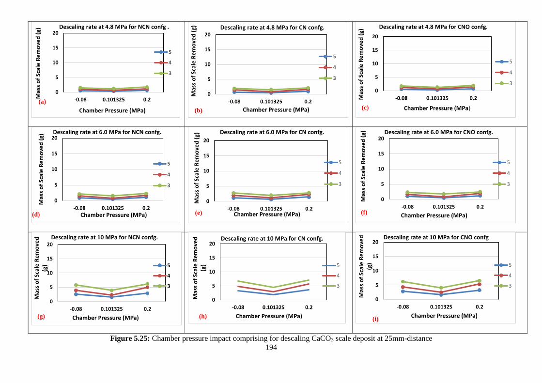
194

Figure 5.25: Chamber pressure impact comprising for descaling CaCO3 scale deposit at 25mm-distance

0

5

10

15

20

-0.08 0.101325 0.2Mas

s o

f Sc

ale

Re

mo

ved

(g)

Chamber Pressure (MPa)

Descaling rate at 4.8 MPa for NCN confg .

5

4

3

0

5

10

15

20

-0.08 0.101325 0.2

Mas

s o

f Sc

ale

Re

mo

ved

(g)

Chamber Pressure (MPa)

Descaling rate at 4.8 MPa for CN confg.

5

4

3

0

5

10

15

20

-0.08 0.101325 0.2Mas

s o

f Sc

ale

Re

mo

ved

(g)

Chamber Pressure (MPa)

Descaling rate at 4.8 MPa for CNO confg.

5

4

3

0

5

10

15

20

-0.08 0.101325 0.2

Mas

s o

f Sc

ale

Re

mo

ved

(g)

Chamber Pressure (MPa)

Descaling rate at 6.0 MPa for NCN confg.

5

4

3

0

5

10

15

20

-0.08 0.101325 0.2

Mas

s o

f Sc

ale

Re

mo

ved

(g)

Chamber Pressure (MPa)

Descaling rate at 6.0 MPa for CN confg.

5

4

3

0

5

10

15

20

-0.08 0.101325 0.2

Mas

s o

f Sc

ale

Re

mo

ved

(g)

Chamber Pressure (MPa)

Descaling rate at 6.0 MPa for CNO confg.

5

4

3

0

5

10

15

20

-0.08 0.101325 0.2

Mas

s o

f Sc

ale

Re

mo

ved

(g

)

Chamber Pressure (MPa)

Descaling rate at 10 MPa for NCN confg.

5

4

3

0

5

10

15

20

-0.08 0.101325 0.2

Mas

s o

f Sc

ale

Re

mo

ved

(g

)

Chamber Pressure (MPa)

Descaling rate at 10 MPa for CN confg.

5

4

3

0

5

10

15

20

-0.08 0.101325 0.2

Mas

s o

f Sc

ale

Re

mo

ved

(g

)

Chamber Pressure (MPa)

Descaling rate at 10 MPa for CNO confg

5

4

3

(a)

(b) (c)

(d)

(g)

(e)

(h)

(f)

(i)

195

5.3.5 Optimum descaling requirement

Despite the detailed research results obtained from section 5.3 that elaborates the erosion behaviour

of multiple high-pressure flat fan nozzles in descaling petroleum production tubing’s embedded

with different types and shapes of scale deposits. Through the adoption of both hydrodynamic

connected parameters like injection pressure & numbers of nozzles and the non-hydro connected

parameters like stand-off distance & nozzles arrangements and chamber pressure. That lead to

achieving the main research goal of enhancing the removal capacity via the permutation and

combination of the respective descaling parameter. Theirs still need of determining the best

combination of descaling parameters required for effectively and efficient descaling of each type of

scale deposit. Thereby, developing an operational guide for removing each type of scale type and

shape when utilising multiple high-pressure nozzles and other descaling parameters will be very

valuable for the petroleum production technologist handling the flow assurance of a scale inflicted

well.

5.3.5.1 Non-hydrodynamics connected parameters

The selection of the best non-hydrodynamics connected parameters like stand-off distance and

nozzles configurations which have no direct effect to the pumping requirement, mass flow rate but

interact with each other during the operations seems to play a vital role in enhancing the removal of

all the types of scale deposits

5.3.5.2 Stand-off distance

During the entire removal of all the types of scale deposits, a linear trend that increase the deposit

removal amount with decrease in stand-off distance when in combination with all the hydrodynamic

connected parameters and chamber pressure was established. Although, despite the effect of

adjusting the downstream distance towards all the scale deposit yielded the best result at 25mm,

poor result for 50mm and very poor results for the 75mm distance due to poor jet to surface target

impact (jet-profile) (Opferet al.2013). The 50mm and 75mm distance were occasionally able to

perform wonderfully to the extent of breaking the samples due to selection of a good nozzle-

configurations (nozzle arrangements on the header) and other parameters. The introduction of centre

nozzles when descaling solid soft or hard scale deposit at high pressure with few nozzles can be a

good example like the graphical elaborations of the 3nozzle scenario at various stand-off distance

in Figure 5.26A, B & C. We’re exploring the effect of adjusting the automiser to deposit distance

with 3nozzle configurations at low pressure (4.8 MPa) removes 4.8g of hollow (paraffin) at 25mm

196

distance that reduces to 9.7g and far less to 1.1g after adjusting the jetting position to 50mm and

75mm respectively. While the case of solid shape that removes 5.2g, 2.1 & 0.6g across the respective

stand-off distance. A removal value of 2g & 0.8g 0.3g and 1.5g, 0.6g & 0.2g was recorded at

respective distance for both SrSO4 and CaCO3. A removal difference of 79g & 13.8g, 4.1g & 2.3g,

2g & 0.5g, 1.2g & 0.5g was observed after respectively adjusting the atomiser from 25mm to 50mm

and from 50mm to 75mm distance when utilising 6.0 MPa injection to remove hollow & solid

paraffin, SrSO4 and CaCO3 deposit respectively. Wider removal difference of 224g & 83g, 84g &

19g, 5.2g & 07g, 3.4g & 0.6g was also recorded at high injection pressure operations (10 MPa)

when removing hollow, solid, SrSO4 and CaCO3 deposit respectively at sequential stand-off

distance increase. The high removal differences as a result sequential stand-off distance increase

when removing hollow shape scale was due to poor performance of the NCN configuration with

increase in stand-off distance. While the CN configurations was averagely performing at deeper

downhole due to good centre jet contact with the surface at wider distance when removing both

solid and the hard scale samples.

5.3.5.3 Nozzle configurations (arrangement)

Probably if not the most important descaling parameter, the nozzles configurations (header

arrangement) which selection is govern by the shape of the scale deposit in question is the first

determining factor before the selection of other descaling parameters. Section 5.31 demonstrated

how each nozzles arrangement (NCN, CN & CNO) configurations was able to suite or perform in

a distinct manner when removing each type of scale deposit. As discussed in section 5.3 and further

elaborated in Figure 5.26D, E & F by singling the removal behaviour of respective types of scale

and header configurations at 10 MPa injection pressure under different nozzle configurations

suggest: That in general NCN was better, followed by CN and CNO in decreasing order for the

removal of hollow shape samples and CN followed by CNO and NCN configuration in

descending order for both solid soft scale and the two hard scale samples. With 5nozzles, a mass

of 58g of scale was removed by NCN configurations at 10 MPa that decrease 49g and 39g after

altering the configurations to CN and CNO respectively. While the CN configurations removes 32g,

3.2g & 1.8g of Solid, SrSO4 & CaCO3 deposits respectively, that reduce to 26g, 3g & 1.6g when

altered to CNO configuration that further reduces to 21g 2.9g & 1.6g due to further alteration to the

NCN configurations. The NCN 4nozzle configurations recoded a removal of 77g, 39g, 4.3g & 2.3g

across the hollow, solid, SrSO4 and CaCO3 deposit respectively, while a value of 70g, 51g, 5.1g &

2.9g was recoded for CN removal across the respective scale deposit and mass of 66g, 46g, 4.5g &

2.5g for CNO removal across the respective scale deposits. Finally, the most impressive results

197

achieved from the 10 MPa-3nozzles descaling operations as shown in figure 5.26F demonstrate a

removal difference of 16.8g & 48.9g due consecutive alteration of NCN configurations to CN and

later CNO respectively when descaling hollow samples. A value of 23g & 41g was the removal

difference due to altering CN configuration to CNO and later NCN when removing solid shape wax

sample. While for SrSO4 and CaCO3 deposit, removal difference of 0.4g & 0.6g, 0.3 & 0.5g was

recorded after the consecutive alteration of the nozzle configurations from CN to CNO and NCN

respectively.

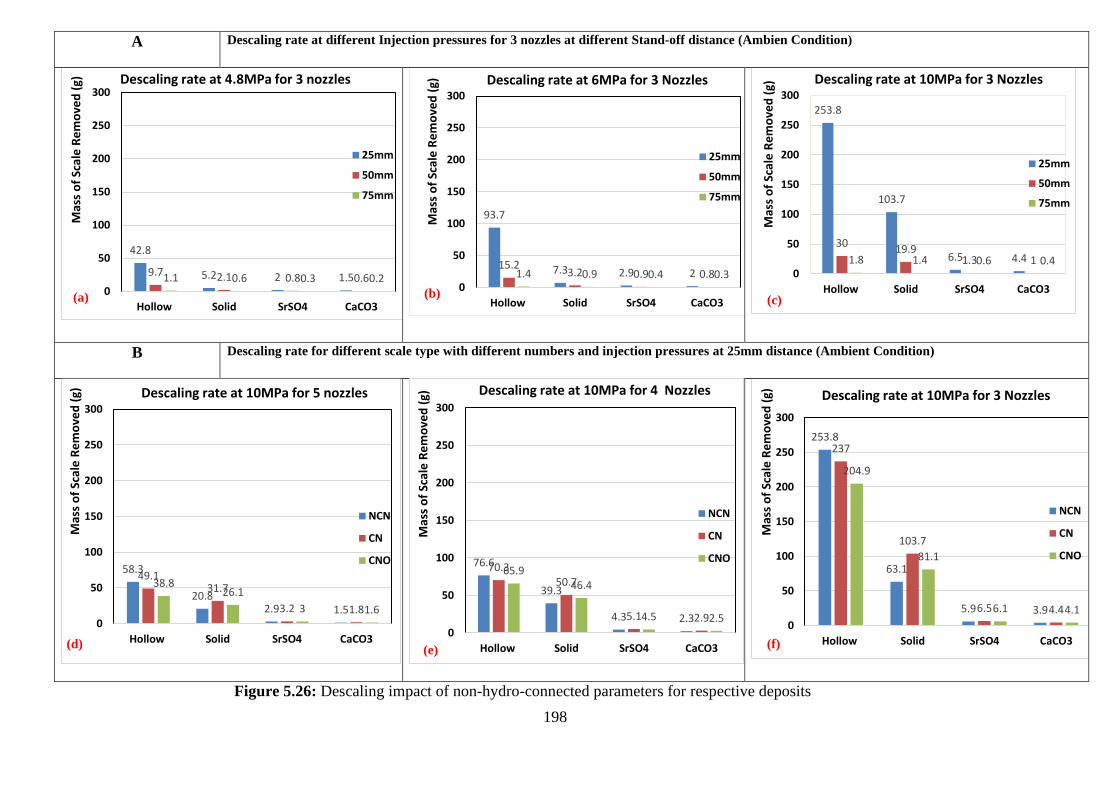
198

A Descaling rate at different Injection pressures for 3 nozzles at different Stand-off distance (Ambien Condition)

B Descaling rate for different scale type with different numbers and injection pressures at 25mm distance (Ambient Condition)

Figure 5.26: Descaling impact of non-hydro-connected parameters for respective deposits

42.8

5.2 2 1.59.7 2.1 0.8 0.61.1 0.6 0.3 0.20

50

100

150

200

250

300

Hollow Solid SrSO4 CaCO3

Mas

s o

f Sc

ale

Re

mo

ved

(g) Descaling rate at 4.8MPa for 3 nozzles

25mm

50mm

75mm

93.7

7.3 2.9 215.2

3.2 0.9 0.81.4 0.9 0.4 0.30

50

100

150

200

250

300

Hollow Solid SrSO4 CaCO3

Mas

s o

f Sc

ale

Re

mo

ved

(g) Descaling rate at 6MPa for 3 Nozzles

25mm

50mm

75mm

253.8

103.7

6.5 4.4

3019.9

1.3 11.8 1.4 0.6 0.40

50

100

150

200

250

300

Hollow Solid SrSO4 CaCO3

Mas

s o

f Sc

ale

Re

mo

ved

(g)

Descaling rate at 10MPa for 3 Nozzles

25mm

50mm

75mm

58.3

20.82.9 1.5

49.131.7

3.2 1.8

38.826.1

3 1.60

50

100

150

200

250

300

Hollow Solid SrSO4 CaCO3

Mas

s o

f Sc

ale

Re

mo

ved

(g) Descaling rate at 10MPa for 5 nozzles

NCN

CN

CNO 76.6

39.3

4.3 2.3

70.350.7

5.1 2.9

65.946.4

4.5 2.50

50

100

150

200

250

300

Hollow Solid SrSO4 CaCO3

Mas

s o

f Sc

ale

Re

mo

ved

(g) Descaling rate at 10MPa for 4 Nozzles

NCN

CN

CNO

253.8

63.1

5.9 3.9

237

103.7

6.5 4.4

204.9

81.1

6.1 4.1

0

50

100

150

200

250

300

Hollow Solid SrSO4 CaCO3

Mas

s o

f Sc

ale

Re

mo

ved

(g) Descaling rate at 10MPa for 3 Nozzles

NCN

CN

CNO

(a) (b) (c)

(d) (e) (f)

199

5.3.5.4 Hydro dynamic connected parameters

The most vital set, of all descaling components that determine the direct scale removal force of the

jet (kinetic energy and pressure drop across the nozzles) which performance depend on each other

are the injection pressure and header configurations (number of nozzles). The relationship between

header configuration and injection pressure is graphically demonstrated in figure 5.32 and

mathematically in equation 5.7, as its clear that more injection pressure will be required to produce

higher pressure drop with a greater number of nozzles than few nozzles.

5.3.5.1 Injection pressure

The relationship and high dependency of the amount of scale deposit removed in respective of its

type against the utilisation of different injected pressures has clearly been established in section 5.3

and Figure 5.27 A, B & C is singled to summarise the finding of the investigations. The effect of

injection pressure and its variations on scale removal can be mathematically expressed equation 5.4

and 5.5 also, since injection pressure is directly proportional to velocity of the jet (Jet impact). Were

Pt being the total pressure, Pd is the dynamic pressure (injection pressure), Ps is the static pressure

that is constant in ambient pressure only, another reason for the vacuum and compressed pressure

performing better. Therefore, the difference between static pressure and the stagnation pressure is

equals to the dynamic pressure (injection pressure) represented as the kinetic energy per unit volume

of a fluid particle.

𝑃𝑡 = 𝑃𝑆 + 𝑃d (5.4)

𝑃𝑑 = 𝐾𝑒 = 𝑚𝑉221 (5.5)

v = √2p/m (5.6)

The consequences of increasing injection by 1.2 MPa and by 4 MPa when descaling with 5nozzles

configuration yielded a removal difference of 1.2g & 56g, 0.6g & 30g, 0.3g & 2.3g and 0.2g & 1.2g

for hollow, solid wax, SrSO4 and CaCO3 deposit respectively. Likewise, the 4nozzle operations

increased the removal difference to 3.8g & 67g, 1.3g & 47g 0.4g & 3.4g and 0.3g & 1.8 of the

respective scale deposits. While the 3nozzle operations due to increase in pressure drop across the

nozzles improved the removal difference to 51g & 160g, 2.1g & 96g, 0.9g & 3.6g and 0.5g & 2.4g

of hollow, solid wax, SrSO4 and CaCO3 deposit respectively. Therefore, in respective of scale type

only a slim improvement is notice due to increasing the injection pressure by 1.2 MPa, compared to

significant removal achieved by the subsequent increase by 4 MPa, was due to wide pressure

variation between the two pressure ranges, hardness of the samples, size and pressure drops.

200

5.3.5.2 Number of nozzles

The most important of all the descaling parameters and the determinant of the of the jet impact that

account for most of the removal is the header configuration. The pressure drop across the nozzles is

proportional to the injection, fluid flowrate and inversely to the nozzle’s areas (number of nozzles).

Therefore, for same nozzle diameter to generate a large nozzle pressure drop a larger flow rate is

required and the fewer the number of nozzles the larger the pressure drop expected. In other words,

a higher velocity jet will be yielded from the nozzle that have greater pressure drop (Tian et al.,

2009). In our case, the scale sample target will be impacted by a high pressure drop (kinetic energy),

thereby resulting to sample breakage. Records from the analysis from Section 5.3 show how much

contribution the effect of altering header configuration have made in enhancing the amount of scale

removal of the respective scale samples and Figure 5.28D, E & F summarised it effect against

respective injection pressures.

𝑃𝑏 =513.559𝑄2 𝑝

𝐴2𝐶2 (5.7)

Were Pb is the pressure drop (MPa), Q is the flowrate (11.3lt/s), p is the density of water (0.98), C

is the nozzle discharge coefficient (0.9) and A is total areas of nozzle (0.5mm x number of nozzles)2,

therefore, inserting values into the above equations.

Pb−5NOZZLES < Pb−4Nozzles < Pb−3nozzles (5.8)

Figure 5.28D graphically demonstrates how the alteration of number of nozzles from 5nozzle to

4nozzles generate a slight removal difference 4.5g, 1.4g, 0.7g & 0.4g of paraffin hollow & solid,

SrSO4 and CaCO3 deposit respectively from the initial removal of the 5-nozzles ambient operations

at 4.8 MPa. More improve removal difference of 37g, 2.6g, 0.7g & 0.7g for respective scale deposits

was observed after altering further to 3nozzles at the same descaling conditions. Likewise in Figure

5.28E, the 6.0 MPa injection trials demonstrated a set of more improved results in term of difference

in amount of scale remove due to reducing the number of nozzles from 5 to 4nozzles by 7.1g, 2.1g,

0.8g8 0.5g of the respective scale deposit and better result of 84g,3.4g, 1.2g & 0.9g of the respective

deposit due to subsequent reduction of the number of nozzles to 3nozzles . Finally, the best set of

scale removal amount due to header alteration can be found in10 MPa operations in Figure 5.28F

were doubled amount than the previous result (4.8 & 6MPa) of altering header configuration from

5 to 4nozzles of 18g, 19g, 1.9g & 1.1g was achieved. Also, almost tenfold of the earlier descaling

amount of the low and medium pressure, of 177g, 53g, 1.4g & 1.5g was obtained for the respective

scale deposit due to pressure drops generated from the further alteration oh header configurations

from 4 to 3nozzles.

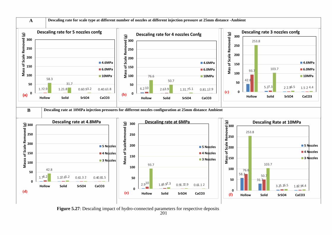
201

A Descaling rate for scale type at different number of nozzles at different injection pressure at 25mm distance -Ambient

B Descaling rate at 10MPa injection pressures for different nozzles configuration at 25mm distance Ambient

Figure 5.27: Descaling impact of hydro-connected parameters for respective deposits

1.7 1.2 0.6 0.42.9 1.8 0.9 0.6

58.3

31.7

3.2 1.80

50

100

150

200

250

300

Hollow Solid SrSO4 CaCO3

Mas

s o

f Sc

ale

Re

mo

ved

(g)

Descaling rate for 5 nozzles confg

4.6MPa

6.0MPa

10MPa

(a)

6.2 2.6 1.3 0.810 3.9 1.7 1.1

76.6

50.7

5.1 2.90

50

100

150

200

250

300

Hollow Solid SrSO4 CaCO3

Mas

s o

f Sc

ale

Re

mo

ved

(g) Descaling rate for 4 nozzles Confg

4.6MPa

6.0MPa

10MPa42.8

5.2 2 1.5

93.7

7.3 2.9 2

253.8

103.7

6.5 4.4

0

50

100

150

200

250

300

Hollow Solid SrSO4 CaCO3

Mas

of

Scal

e R

em

ove

d (

g) Descaling rate 3 nozzles confg

4.6MPa

6.0MPa

10MPa

1.7 1.2 0.6 0.46.2 2.6 1.3 0.8

42.8

5.2 2 1.50

50

100

150

200

250

300

Hollow Solid SrSO4 CaCO3

Mas

ss o

f Sc

ale

Re

mo

ved

(g)

Descaling rate at 4.8MPa

5 Nozzles

4 Nozzles

3 Nozzles

2.9 1.8 0.9 0.610 3.9 1.7 1.1

93.7

7.3 2.9 20

50

100

150

200

250

300

Hollow Solid SrSO4 CaCO3

Mas

s o

f Sc

ale

Re

mo

ved

(g) Descaling rate at 6MPa

5 Nozzles

4 Nozzles

3 Nozzles

58.3

31.7

3.2 1.8

76.6

50.7

5.1 2.9

253.8

103.7

6.5 4.4

0

50

100

150

200

250

300

Hollow Solid SrSO4 CaCO3

Mas

s o

f Sc

ale

Re

mo

ved

(g) Descaling Rate at 10MPa

5 Nozzles

4 Nozzles

3 Nozzles

(b)

(d) (e)

(c)

(f)

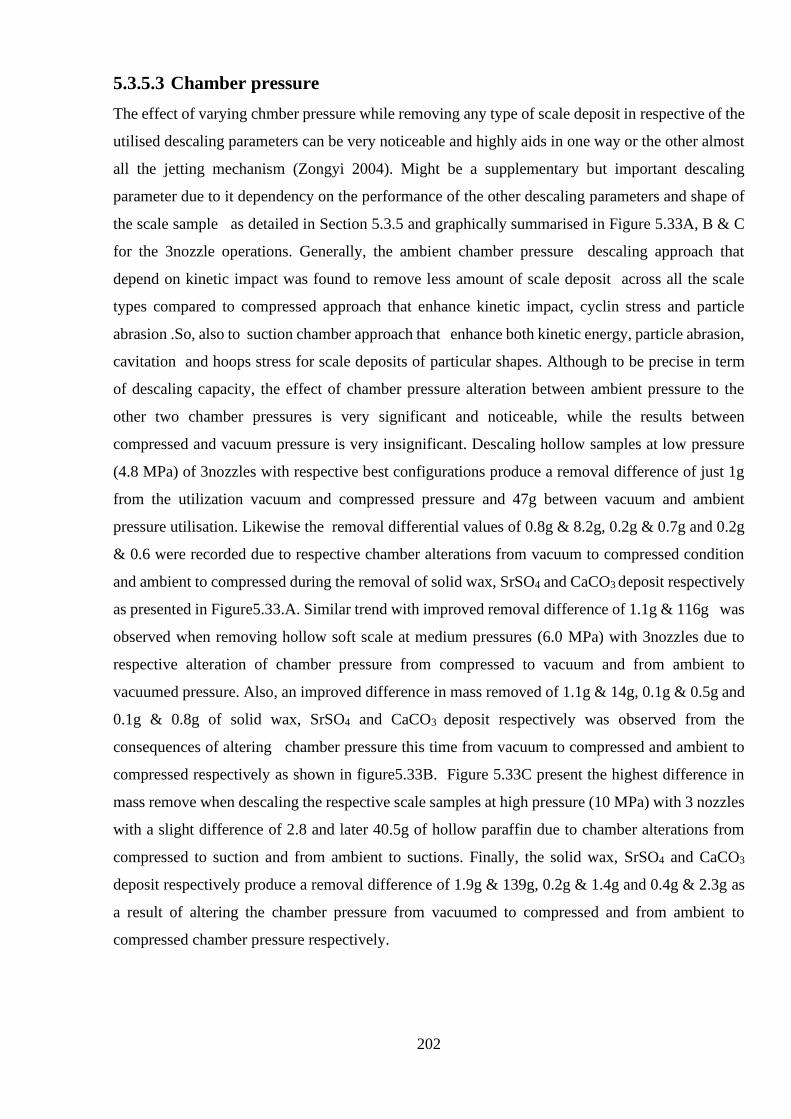
202

5.3.5.3 Chamber pressure

The effect of varying chmber pressure while removing any type of scale deposit in respective of the

utilised descaling parameters can be very noticeable and highly aids in one way or the other almost

all the jetting mechanism (Zongyi 2004). Might be a supplementary but important descaling

parameter due to it dependency on the performance of the other descaling parameters and shape of

the scale sample as detailed in Section 5.3.5 and graphically summarised in Figure 5.33A, B & C

for the 3nozzle operations. Generally, the ambient chamber pressure descaling approach that

depend on kinetic impact was found to remove less amount of scale deposit across all the scale

types compared to compressed approach that enhance kinetic impact, cyclin stress and particle

abrasion .So, also to suction chamber approach that enhance both kinetic energy, particle abrasion,

cavitation and hoops stress for scale deposits of particular shapes. Although to be precise in term

of descaling capacity, the effect of chamber pressure alteration between ambient pressure to the

other two chamber pressures is very significant and noticeable, while the results between

compressed and vacuum pressure is very insignificant. Descaling hollow samples at low pressure

(4.8 MPa) of 3nozzles with respective best configurations produce a removal difference of just 1g

from the utilization vacuum and compressed pressure and 47g between vacuum and ambient

pressure utilisation. Likewise the removal differential values of 0.8g & 8.2g, 0.2g & 0.7g and 0.2g

& 0.6 were recorded due to respective chamber alterations from vacuum to compressed condition

and ambient to compressed during the removal of solid wax, SrSO4 and CaCO3 deposit respectively

as presented in Figure5.33.A. Similar trend with improved removal difference of 1.1g & 116g was

observed when removing hollow soft scale at medium pressures (6.0 MPa) with 3nozzles due to

respective alteration of chamber pressure from compressed to vacuum and from ambient to

vacuumed pressure. Also, an improved difference in mass removed of 1.1g & 14g, 0.1g & 0.5g and

0.1g & 0.8g of solid wax, SrSO4 and CaCO3 deposit respectively was observed from the

consequences of altering chamber pressure this time from vacuum to compressed and ambient to

compressed respectively as shown in figure5.33B. Figure 5.33C present the highest difference in

mass remove when descaling the respective scale samples at high pressure (10 MPa) with 3 nozzles

with a slight difference of 2.8 and later 40.5g of hollow paraffin due to chamber alterations from

compressed to suction and from ambient to suctions. Finally, the solid wax, SrSO4 and CaCO3

deposit respectively produce a removal difference of 1.9g & 139g, 0.2g & 1.4g and 0.4g & 2.3g as

a result of altering the chamber pressure from vacuumed to compressed and from ambient to

compressed chamber pressure respectively.

203

5.3.5.4 Descaling efficiency

An effective descaling technique is defined as the ability of a scale removal approach to regain the

accessibility of a scale inflicted well in economic, fast, easy and safe ways for both the rig

equipment’s and rig personals. In order words, an operation that is cheaper, faster, easier, safer and

greener than other available techniques at the market disposal. Therefore, the reason of calculating

and ranking the efficiency of removing the respective types of scale deposit from petroleum

production tubing using the analyse descaling parameters results was to assesses and ranked hand

in hand the amount of scale removed in consideration of the volume of water utilised during each

operation. Moreover, this will cover the energy and cost requirements of the operation through the

utilization of the descaling efficiency formula expressed in equation 5.9 and the efficiency

calculation of utilising 3nozzle at respective injection pressure and other descaling parameters

against different chamber pressure is sectioned in Figure5 5.28D, E & F. The efficiency results

demonstrated a trend that is proportional to the amount of scale removed, which increases with

increase in injection pressure and reduction of numbers of nozzles, and stand-off distance that

depend on the choice of nozzle configuration. Still the results were found to be inversely

proportional to the volume of water utilise (the less the amount of water utilise the less the well

flooding tendency) which is in line with the hydro-dynamic descaling parameters.

𝐷𝑒𝑠𝑐𝑎𝑙𝑖𝑛𝑔 𝐸𝑓𝑓𝑒𝑐𝑖𝑒𝑛𝑐𝑦 𝜂 =Mass of Scale Removed

Mass of Water Utilised 𝑥 100 (5.9)

The descaling operations of 3nozzle at low pressure of 4.8 MPa that utilises 37.5kg of water

recorded an ambient efficiency of 7.8%, 0.9%, 0.4% & 0.3% for the respective scale types. The

impact of compressed air increases the efficiency by many folds (16.2%) for hollow sample, doubled

to 2.4% for solid and increase of 0.1% across the hard scale samples. Slight improvement to 16.3%

and a decrease to 2.3% and 0.3% was recorded for solid soft and CaCO3 deposit during the vacuum

operations. Likewise, the 37.8kg volume of water utilised during the 6 MPa operation of 3nozzles

was found to have an efficiency value of 17%, 1.3% 0.5% & 0.5% for the respective scale deposit

at ambient condition. The introduction of compressed air respectively tripled the hollow and solid

soft scale efficiency to 37% & 38% and no improvement was recorded for the hard scale deposits

in both including vacuum condition, while the vacuum condition increase the hollow removal

slightly efficiency by 0.2% and slightly reduces solid to 0.2%. Finally, a more reasonable removal

efficiency of 45%, 16%, 1% & 0.7% was observed due to the utilization 42.4kg of water at 10 MPa

with 3-nozzles to remove the respective deposits at ambient condition. The values significantly

increase to 51%, 37%, 1.3% & 1.1% due to compression, were as 52.3%, 36%, 1.3% for hollow &

solid soft and no improvement for hard scale due to suctioning operations.

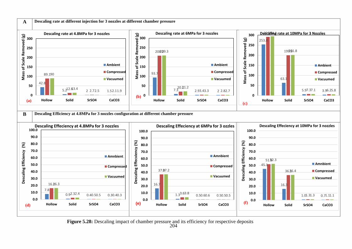
204

A Descaling rate at different injection for 3 nozzles at different chamber pressure

B Descaling Efficiency at 4.8MPa for 3 nozzles configuration at different chamber pressure

Figure 5.28: Descaling impact of chamber pressure and its efficiency for respective deposits

42.8

5.2 2 1.5

89.1

12.6 2.7 2.1

90

13.42.5 1.9

0

50

100

150

200

250

300

Hollow Solid SrSO4 CaCO3

Mas

s o

f Sc

ale

Re

mo

ved

(g)

Descaling rate at 4.8MPa for 3 nozzles

Ambient

Compressed

Vacuumed

93.7

7.3 2.9 2

208.2

20.13.4 2.8

209.3

21.23.3 2.7

0

50

100

150

200

250

300

Hollow Solid SrSO4 CaCO3

Mas

s o

f Sc

ale

Re

mo

ved

(g) Descaling rate at 6MPa for 3 nozzles

Ambient

Compressed

Vacuumed

253.8

63.1

5.9 3.9

291.5

199.9

7.3 6.2

294.3

201.8

7.1 5.8

0

50

100

150

200

250

300

Hollow Solid SrSO4 CaCO3

Mas

s o

f Sc

ale

Re

mo

ved

(g)

Descaling rate at 10MPa for 3 Nozzles

Ambient

Compressed

Vacuumed

7.8

0.9 0.4 0.3

16.2

2.3 0.5 0.4

16.3

2.4 0.5 0.30.0

10.0

20.0

30.0

40.0

50.0

60.0

70.0

80.0

90.0

100.0

Hollow Solid SrSO4 CaCO3

De

scal

ing

Effi

cie

ncy

(%

)

Descaling Effeciency at 4.8MPa for 3 nozzles

Amnbient

Compressed

Vacuumed

16.7

1.3 0.5 0.5

37.0

3.60.6 0.5

37.2

3.80.6 0.5

0.0

10.0

20.0

30.0

40.0

50.0

60.0

70.0

80.0

90.0

100.0

Hollow Solid SrSO4 CaCO3

De

scal

ing

Effe

cvie

ncy

(%

)

Descaling Effeciency at 6MPa for 3 ozzles

Amnbient

Compressed

Vacuumed

(e)

45.1

16.3

1.0 0.7

51.8

36.1

1.3 1.1

52.3

36.4

1.3 1.1

0.0

10.0

20.0

30.0

40.0

50.0

60.0

70.0

80.0

90.0

100.0

Hollow Solid SrSO4 CaCO3

De

scal

ing

Effi

cie

ncy

(%

)

Descaling Effeciency at 10MPa for 3 nozzles

Amnbient

Compressed

Vacuumed

(a) (b)

(c)

(f) (d)

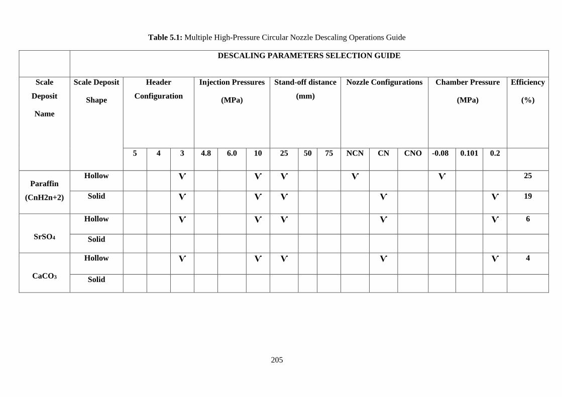
205

Table 5.1: Multiple High-Pressure Circular Nozzle Descaling Operations Guide

DESCALING PARAMETERS SELECTION GUIDE

Scale

Deposit

Name

Scale Deposit

Shape

Header

Configuration

Injection Pressures

(MPa)

Stand-off distance

(mm)

Nozzle Configurations Chamber Pressure

(MPa)

Efficiency

(%)

5 4 3 4.8 6.0 10 25 50 75 NCN CN CNO -0.08 0.101 0.2

Paraffin

(CnH2n+2)

Hollow Ѵ Ѵ Ѵ Ѵ Ѵ 25

Solid Ѵ Ѵ Ѵ Ѵ Ѵ 19

SrSO4

Hollow Ѵ Ѵ Ѵ Ѵ Ѵ 6

Solid

CaCO3

Hollow Ѵ Ѵ Ѵ Ѵ Ѵ 4

Solid

206

5.3.6 Summary

The following conclusion have been drawn from this chapter.

• The constructed soft scale sample was proven to have the same chemical properties with

paraffin wax through FTIR and NMR analysis.

• So also, the Libyan field acquired hard scale samples were found to be CaCO3 and SrSO4

respectively through the combination of SEM, EDX and XRD techniques.

• The choice of descaling technique is a function of type and shape of the scale deposit in

question

• Likewise, the choice of nozzle configuration (arrangement) relies on shape of the deposit.

i.e NCN configuration is best for hollow shapes deposit and CN & CNO for solid deposits.

• In respective of type of scale deposit, the removal increases with increase in injection

pressure and reduction in numbers of nozzles

• The descaling performance of all the types of scale rely on increase of kinetic energy or

spray velocity (injection pressure) which reduces with increase in number of nozzles.

• The jet performance reduces with increase in jetting position even though can be

compensated by the right choice of nozzle configuration & chamber pressure for each scale

deposit.

• The impact of chamber air pressure on the removal also depend on the shape & type of

deposit and optimum selection of other descaling paraments

• Introduction of 0.2MPa compressed air into the chamber at with the best parameters

approximately favoured the removal more sloid soft and SrSO4 & CaCO3 than hollow,

through enhancing cycling stress and particle abrasion jetting mechanism.

• While suctioning the chamber by -0.008MPa when utilising the best parameters increases

the average removal of hollow deposits more than the solid SrSO4 & CaCO3 through

enhancing kinetic energy, hoops stress, particle abrasion and cavitation jetting mechanism.

207

Conclusion and Recommendations

6.1 Conclusions

The results from the investigation of the descaling behaviour of oilfield scale deposits of 1, 2 & 3

Mohs scale hardness index from petroleum production tubing with multiple high-pressure circular

nozzle recorded a massive improvement. Also, yielded the following conclusions after adopting the

option of altering both the decaling parameters and the chamber air/water concentration.

• The oil field soft scale deposit (paraffin) have effectively being mimic, descaled and

characterised to have similar chemical properties with paraffin a through FTIR & NMR

analysis respectively.

• Additionally, the Libyan field acquired hard scale samples were effectively descaled and

characterised via the combination of SEM, EDX and XRD techniques and were found to be

CaCO3 and SrSO4 respectively.

• The multiple high-pressure nozzle approach at all descaling parameter combination recorded

an impressive enhancement in terms of amount of scale removed compared to the single

nozzles aerated approach. For instance, the ambient 3nozzles CN configurations technique

impressively removed 104g, 9g & 8g of solid soft, SrSO4 & CaCO3 deposits respectively,

compared to the 10g, 6g 5g of the single nozzle ambient approach. While also the

compressed approach of 3nozzles removed 200g, 14g & 10g of solid soft, SrSO4 & CaCO3

deposits respectively more than the single nozzle aerated amount of 67g, 12g & 7g.

• Considering the distinct chemical and physical properties of each scale deposit, will

consequently respond to different erosional mechanisms and require unique optimised

descaling conditions for its effective descaling.

• Therefore, the selection of the best descaling requirement for each deposit depends on the

shape, size, hardness and location of the deposit in question.

• Consequently, a high level of interaction and dependency between all the descaling

parameters and the amount of scale removed, especially within the hydro dynamic connected

and non-hydro dynamic connected parameters respectively exist.

• The amount of scale removed in respective of type of deposit in related to the hydrodynamic

parameter’s increases with increase with injection pressure (kinetic energy) and decrease

208

with increase in number of nozzles (header configuration) due to multiple nozzle pressure

drops effect.

• While the amount of scale removed for all the respective deposits in connection with the

non-hydrodynamic parameters decreases with increase in jetting position and the poor

downhole jet performance can be corrected with the right choice of nozzle configurations

• So also, the selection of nozzle configuration (header arrangement) is govern by the size and

shape of the sample, as NCN configuration was able to remove 7% & 13% than CN and

CNO configuration when descaling hollow shape scale at the best of other parameters in

ambient condition. While CN configuration removed 6%,4% & 0.1%, 0.08% &0.1%,0.02%

more deposit of solid, SrSO4 and CaCO3 than the CNO and NCN nozzles configurations

respectively.

• Fifth descaling mechanism (hoop stress) effective in removing early growth stage scale

deposit (hollow shape) was discovered and was found to be more active in suction chamber

condition together with cavitation mechanism. Even, do the compressive chamber condition

was more effective in removing complete tubing blocked deposits (solid) and hollow shape

deposit that does not fulfil the hoop stress tin wall condition through erosion, cyclin stress

and particle abrasion mechanism

• The introduction of 0.2 MPa compressed air into the chamber with the best parameters

approximately increase the removal of hollow by 23%, sloid soft by 27% and SrSO4 &

CaCO3 by 0.4% & 0.5.% through enhancing cycling stress and particle abrasion jetting

mechanism.

• While suctioning the chamber by -0.008MPa when utilising the best parameters increases

the average ambient removal of hollow by 26% solid by 18% and SrSO4 & CaCO3 by 0.3%

& 0.4% through enhancing kinetic energy, hoops stress, particle abrasion and cavitation

jetting mechanism.

• The hollow shape paraffin deposit was the only deposit that was effectively removed in

ambient chamber condition due to hope stress effect and was only lagging by 38g and 40g

behind the compressed and vacuum chamber condition removal respectively.

• The efficiency of each descaling technique from any permutation of descaling parameters is

a function of amount of the amount of scale it removes and the volume of water it utilises

during the operation

209

6.2 Recommendations

Despite the high-level of breakthrough and the enhancement in scale removal that was recorded

from this investigation, coupled with detailed designed, construction and modification procedures

of the utilised facilities, some research question remained un-answered due to time and scope

constraint. Therefore, the following recommendation will effectively be filled in the existing

research gap and contribute to the knowledge area.

• CFD model could be design for comparison with experimental result and simulations of

other non-suitable experimental measurements like cavitation measurement and the impact

spray overlap.

• A more compactable nozzle header should be design in order to reduce the size of the

descaling chamber into a typical Saudi Aramco production tubing size of 100mm diameter

that will generate good spray profile contact with the typical oilfield hard scale deposit of

100mm diameter.

• The future nozzle header should be flexible enough to allow the alteration of the nozzle’s

header orientation angles to 15̊̊, 25̊, 30̊ & 60̊ contrary the present one that have fixed 45̊ for

the side nozzles and 90̊ angle for the centre nozzles.

• Cary out the cavitation bubble length measurement of each nozzle configurations and study

of how-to extend cavities flair for scale removal instead of supressing cavitation will

improved the jet performance for effective scale removal.

• For safety and effective removal, selection of stronger, transparent and longer experimental

chamber that can withstand at least 1 MPa chamber pressure, accommodate high injection

pressure of 20 MPa and longer descaling time of at least 5 minutes is recommended. Since

the present perplex chamber has maximum design pressure of 0.6 MPa and a water resident

time of 188 sec only.

• Mechanical failure pattern and fracture mechanisms of the respective deposit should be

investigated in order to corelate the quantitative and qualitative removal of each sample,

because in this investigation some sample were highly eroded without breaking while other

break with low removal.

• Also, the combination of different type of nozzles on the spray header i.e. flat, fan and solid

stream jet might provide a better answer to the problem.

• A means of utilising Knoop or Vickers hardness technique should be devised in order to

allocate each scale deposit it real Moh’s scale of hardness index

210

Reference

Abbas, A. J. (2014). Descaling of Petroleum Production Tubing utilising Aerated High Pressure Flat

Fan Water Sprays.

Abulhamayel, N., Leal, J., Ayub, M., Driweesh, S., & Aramco, S. (2015). Recent Developments in

Mechanical Descaling Operations : A Case Study.

Al-Matar, H., Al-Ashhab, J. K., Mokhtar, M., & Ridzauddin, S. (2006). Techniques used to monitor

and remove strontium sulfate scale in UZ producing wells. Paper

Al-Khaldi, M. H., Al-Juhani, a. M., Al-Mutairi, S. H., & Gurmen, M. N. (2011). New insights into

the removal of calcium sulfate scale. Society of Petroleum Engineers - 9th European Formation

Damage Conference 2011, 2, 1052–1070. Retrieved from

http://www.scopus.com/inward/record.url?eid=2-s2.0-80052441716&partnerID=tZOtx3y1

Al-Taq, A. A., Muhaish, S. A., Nakhli, M. M., & Alrustum, A. A. (2015). Organic/Inorganic

Deposition in Oil Producing Wells from Carbonate Reservoirs: Mechanisms, Removal and

Mitigation. SPE 177447. Abu Dhabi International Petroleum Exhibition and Conference, 1–

15. https://doi.org/10.2118/177447-MS

Alabdulmohsin, Y. A., El-zefzafy, I. M., Al-malki, M. H., Al-mulhim, A. A., & Ali, A. (2016). SPE-

181286-MS Underbalanced Coiled Tubing Mechanical De-Scaling Operations : A Case

History for an Oil Well in Ghawar Field from Saudi Arabia, 1–14.

Almubarak, T., Ng, J. H., Nasr-el-din, H., & Texas, A. (2017). SPE-185636-MS Oilfield Scale

Removal by Chelating Agents : An Aminopolycarboxylic Acids Review, (Iii).

Anwar, M., & Abubakr, M. (2017). Innovation Technique and Successful Scale Removal Job With

Coiled Tubing in Belayim Oil Field, Egypt: A Case History. Paper presented at the Offshore

Mediterranean Conference and Exhibition, Ravenna, Italy. https://doi.org/

Amjad, Z., & Demadis, K. D. (2015). Mineral scales and deposits: Scientific and technological

approaches.

Ayirala, S., & Yousef, A. (2014). Injection water chemistry requirement guidelines for IOR/EOR.

Paper presented at the SPE Improved Oil Recovery Symposium.

Armacanqui, J. S., Eyzaguirre, L. D. F., Flores, M. G., Zavaleta, D. E., & Camacho, F. E. (2016).

SPE-181162-MS Testing of Environmental Friendly Paraffin Removal Products Current

Practices to Remove Paraffin Deposition.

Aslam, J., Alsalat, T., & Corporation, P. (2000). SPE 58780 High-Pressure Water Jetting : An

Effective Method To Remove Drilling Damage.

Bakker, T. W., Ivannikov, V. I., & International, W. (2002). SPE 75352 Cavitator for Effective Well

Cleaning, 1–4.

Bakr, M., Hay, A. A., & Hamdy, E. (2012). SPE 154455 A Successful Removal RI Inorganic Hard

Scale Deposits in an Offshore Pipeline in Gemsa Oil field , Egypt : Field Study, 1–7.

Bajammal, F. A., Biyanni, H. M., Riksa, A. P., Poitrenaud, H. M., & Mahardhini, A. (2013, March

26). Scale Management in Mature Gas Field: Case Study of Peciko. International Petroleum

Technology Conference. doi:10.2523/IPTC-16675-MS

211

BETE, “Full Cone Nozzles - Air Atomising Design,” 2014. [Online]. Available:

http://www.bete.co.uk/spray-nozzles/full-cone-nozzles/air-atomising-nozzles. [Accessed:

29-Jul-2018].

BET, “Air actuated flat fan nozzles,” 2014. [Online]. Available: http://www.bete.co.uk/spray-

nozzles/flat-fan-nozzles/air-actuated. [Accessed: 29-Jul-2018].

Birk, N. (2013). SPE 163904 First Field Application of 2-7 / 8 " Scale Removal Tool for Offshore

Well Abandonment, (July 2010).

Bolarinwa, S., Jauregui, J. L., Buali, M., Aramco, S., Kharrat, S. P. E. W., & Kovalenko, K. (2012).

SPE 156021 Innovative Integrated Procedure for Scale Removal in Khuff Gas Wells in Saudi

Arabia, (1), 1–16.

Børeng, R., Skinnemoen, O. K., Vigen, A., Vikane, O., Andrews, J., Asa, S., … Hauptmann, T.

(2002). SPE 86479 A Successful Scale Removal Operation by Use of New and Old

Technology, (June).

Bourne, H. M., Heath, S. M., McKay, S., Fraser, J., Stott, L., & Müller, S. (2000). Effective

Treatment of Subsea Wells with a Solid Scale Inhibitor System. Paper presented at the

International Symposium on Oilfield Scale, Aberdeen, United Kingdom.

https://doi.org/10.2118/60207-MS

Buali, M., Ginest, N., Leal, J., Sambo, O., Chacon, A., & Vielma, J. (2014). Extreme Challenges in

FeS Scale Cleanout Operation Overcome using Temporary Isolation, High Pressure Coiled

Tubing, and Tailored Fluid Systems. SPE International Oilfield Scale Conference and

Exhibition. https://doi.org/10.2118/169759-MS

Campbell, A., & Brunskill, D. (2013). Advances in Coiled Tubing Jetting Technology. SPE/ICoTA

Coiled Tubing Roundtable. https://doi.org/10.2118/60721-MS

Civan, F. (2014). Analyses of processes, mechanisms, and preventive measures of shale-gas

reservoir fluid, completion, and formation damage. Paper presented at the SPE International

Symposium and Exhibition on Formation Damage Control.

Crabtree, M., Eslinger, D., Fletcher, P., Miller, M., Johnson, A., & King, G. (1999). Fighting scale—

removal and prevention. Oilfield review, 11(3), 30-45.

Chakraborty, S., Lehrer, S., Ramachandran, S., & Incorporated, B. H. (2017). SPE-183974-MS

Effective Removal of Sour Gases Containing Mercaptans in Oilfield Applications, 1–13.

Codolo, M. C., & Bizzo, W. A. (2013). Experimental study of the SO2 removal efficiency and

volumetric mass transfer coefficients in a pilot-scale multi-nozzle spray tower. International

Journal of Heat and Mass Transfer, 66, 80–89.

https://doi.org/10.1016/j.ijheatmasstransfer.2013.07.011

Davis, J. P., & Cassel, T. E. (2001). Apparatus for removal of milling debris. In: Google Patents.

El-Hattab, M. (1985). Scale deposition in surface and subsurface production equipment in the Gulf

of Suez. Journal of Petroleum Technology, 37(9), 1640–1652. Retrieved from

http://www.onepetro.org/mslib/servlet/onepetropreview?id=00011449

El Hajj, H., Pal, O., & Zoghbi, B. (2015). Compositional Analysis and Treatment of Oilfield Scales.

212

SPE Saudi Arabia Section Annual Technical Symposium and Exhibition, (1), 21–23.

https://doi.org/10.2118/178002-MS

Elkatatny, S., & Fahd, K. (2017). SPE-183914-MS New Formulation for Iron Sulfide Scale

Removal, (March), 6–9.

Esbai, R. E., Palanisamy, G., & Petroleum, T. (2016). SPE-184204-MS Eliminating Scale Buildup

Challenges and Lessons Learnt from the Fadhili Reservoir Awali Field.

Espinosa, G., Mauricio, A., Leal, J. A., Driweesh, S. M., Buali, M. F., Khnaifir, W. K., . . . Arifin,

M. (2016). First Time Live Descaling Operation in Saudi using Coiled Tubing Fiber Optic

Real-Time Telemetry Rugged Tool, Foamed Fluid and Pressure Fluid Management System.

Paper presented at the SPE Kingdom of Saudi Arabia Annual Technical Symposium and

Exhibition.

Farrokhrouz, M., & Asef, M. R. (2010). SPE 135854 Production Enhancement via Scale Removal

in Nar Formation. Changes, (June), 8–10. https://doi.org/10.2118/135854-MS

G, M. A. E., Leal, J. A., Driweesh, S. M., Buali, M. F., Khnaifir, W. K., & Jasim, A. J. (2016). First

Time Live Descaling Operation In Saudi Using Coiled Tubing Fiber Optic Real-Time

Telemetry Rugged Tool , Foamed Fluid And Pressure Fluid.

Gholinezhad, J. (2006). Evaluation of latest techniques for remedial treatment of scale depositions

in petroleum wells. SPE Eighth International Symposium on Oilfield Scale 2006, 2006, 17–23.

https://doi.org/10.2523/99683

Guan, H. (2015). Scale Deposition Control and Management in Subsea Fields, (5480), 1–12.

Guimaraes, Z., Franca, A. B., Duque, L. H., de Souza, R. B., Porto, M., Neves, D., & Peixoto, C.

(2007). Case histories of barium sulfate scale removal in offshore wells, Brazil, using a new

engineered combination of coiled-tubing tools. Paper presented at the SPE/ICoTA Coiled

Tubing and Well Intervention Conference and Exhibition.

Ghouri, S. A., Ali, I., Shah, N. M., Ejaz, M., & Haider, S. A. (2018, January 1). Downhole Scales

Management in Mature Gas Fields. Society of Petroleum Engineers. doi:10.2118/195659-

MS

Haghtalab, A., Kamali, M. J., & Shahrabadi, A. (2014). Prediction mineral scale formation in oil

reservoirs during water injection. Fluid Phase Equilibria, 373, 43-54.

Hamid, S., De Jesus, O., Jacinto, C. M., Izetti, R., Pinto, H., Drougett, E., . . . Dagenais, P. (2013).

A practical method of predicting chemical scale formation in well completions. Paper

presented at the SPE Asia Pacific Oil and Gas Conference and Exhibition.

Hafiz, T., Hoegerl, M., Alsuwaij, A., Almathami, A., & Hughes, B. (2017). SPE-183954-MS

Synthetic Iron Sulfide Scale and Polymeric Scale Dissolvers, (March), 6–9.

Haugen, I., Døssland, L., Brankovic, M., Osaland, E., Osugo, L., Technologies, Q., & Grødem, M.

(2017). SPE-184758-MS Electric-Line Deployed Lightweight Intervention Technology for

The Effective Removal of Barium Sulphate Scale Obstructions from Small Diameter

Wellbores, 1–15.

Heydrich, M., Hammami, A., Choudhary, S., Mockel, M., & Ratulowski, J. (2019, April 26). Impact

of a Novel Coating on Inorganic Scale Deposit Growth and Adhesion. Offshore Technology

213

Conference. doi:10.4043/29218-MS

Hinrichsen, C. J. (1998). Preventing scale deposition in oil production facilities: An industry review.

Paper presented at the CORROSION 98.

J. Leal, W. Nunez, S. Al-ismail, and J Ricardo Solares, “SPE 121404 Novel Mechanical

Scale Clean-out Approach to Remove Iron Sulphide Scale from Tubulars in Vertical High

Pressure and Temperature Deep Gas Producers : A Case History,” 2009.

Jordan, M. M., Sjuraether, K., Colllns, I. R., Feasey, N. D., & Emmons, D. (2001). Life Cycle

Management of Scale Control within Subsea Fields and its Impact on Flow Assurance, Gulf of

Mexico and the North Sea Basin. Proceedings - SPE Annual Technical Conference and

Exhibition, 1971–1986. https://doi.org/10.2118/71557-MS

Jordan, M., & Mackay, E. (2015). Predicting and Managing Inorganic Scale Associated With

Produced Water from EOR Projects. SPE Latin American and Caribbean Petroleum

Engineering Conference, 1–18. https://doi.org/10.2118/177144-MS

Kamari, A., Gharagheizi, F., Bahadori, A., & Mohammadi, A. H. (2014). Rigorous modeling for

prediction of barium sulfate (barite) deposition in oilfield brines. Fluid Phase Equilibria,

366, 117-126.

Kan, A., & Tomson, M. (2012). Scale prediction for oil and gas production. Spe Journal, 17(02),

362-378.

Kazemi Nia Korrani, A., Sepehrnoori, K., & Delshad, M. (2014). A Comprehensive Geochemical-

Based Approach to Quantify the Scale Problems. Paper presented at the SPE International

Symposium and Exhibition on Formation Damage Control.

Kelland, M. A. (2014). Production chemicals for the oil and gas industry: CRC press.

Kunanz, H., Wölfel, S., & Leoben, M. (2014). Working principle of ultrasonic cleaning Preparation

of Samples, (May), 14–15.

Wang, Q., Leal, J., Syafii, I., Mukhles, A. E., Chen, T., Chang, F., & Espinosa, M. (2016). Iron

Sulfide and Removal in Scale Formation Sour Gas Wells. In SPE International Oilfield Scale

Conference and Exhibition held in Aberdeen, Scotland, UK, 11–12 May

Lewis, D. R., Aramco, S., Zainalabedin, K. A., Aramco, S., & Aramco, S. (2003). SPE 81569 Scale

Mitigation Enhances Safety and Production, 1–8.

Mackay, E. J., Jordan, M. M., & Torabi, F. (2003). Predicting Brine Mixing Deep Within the

Reservoir and Its Impact on Scale Control in Marginal and Deepwater Developments. SPE

Production & Facilities, 18(3), 210–220. https://doi.org/10.2118/85104-PA

Mahmoud, M. A., Kamal, M. S., & Geri, B. S. B. (2015). Removal of Pyrite and Different Types of

Iron Sulfide Scales in Oil and Gas Wells without H 2 S Generation. International Petroleum

Technology Conference Held in Doha, Qatar, 6–9 December.

Merdhah, A. B., & Yassin, A. (2008). Formation damage due to scale formation in porous media

resulting water injection. system, 14, 15.

Mirza, M. S., Prasad, V., & Company, O. (1999). SPE 53345 Scale Removal in Khuff Gas Wells.

214

Moghadasi, J., Jamialahmadi, M., Muller-Steinhagen, H., Sharif, a, Ghalambor, a, Izadpanah, M.

R., & Motaie, E. (2003). Scale formation in Iranian oil reservoir and production equipment

during water injection. International Oilfield Scale Symposium and Exhibition, 1–14.

https://doi.org/10.2118/80406-MS

Moradpour, M., Zamani, Z., & Moallemi, S. (2008). Controls on reservoir quality in the lower

Triassic Kangan formation, southern Persian Gulf. Journal of Petroleum Geology, 31(4),

367-385.

M. Qin, D. Y. Ju, and R. Oba, “Improvement on the process capability of water cavitation peening

by aeration,” Surf. Coatings Technol., vol. 200, no. 18–19, pp. 5364–5369, May 2006.

Zongyi, “Investigation of the cavitation mechanism and erosion of submerged high pressure water

jets,” University of Queensland, 2004.

Mukhliss, A. E., Ogundare, T. M., Dashash, A. A., Malik, A. R., Aramco, S., Rivadeneira, E. V, &

Molero, N. (2014). A Novel Non-damaging Approach to Isolate Open hole Lateral that

Allowed Performing Mechanical Descaling in the Non-Monobore Cased Completion : A Case

Study in Saudi Arabian Carbonate Reservoir, 1–9.

Nasr-El-Din, H. A., Fadhel, B. A., Al-Humaidan, A. Y., Frenier, W. W., & Hill, D. (2000). An

Experimental Study of Removing Iron Sulfide Scale from Well Tubulars. Paper presented

at the International Symposium on Oilfield Scale, Aberdeen, United Kingdom.

https://doi.org/10.2118/60205-MS

Nasr, G. G., Enyi, G. G., El-Kamki, M. E., & Burby. (2012). Characterisation of Flat fan sprays for

petroleum applications. Institution of Liquid Atomization and Sprays Systems, pp. 7–10.

Nejad, A. M. and Karimi, M. S. (2017). “Investigation of the influence of scaling on corrosion

behaviour of tubing in oil wells”, Int. J. Sci. Tech. Res. 6, 5, 109-113.

Nourian, A. (2016). High Pressure Overlapping Flat Sprays Nozzles HIGH PRESSURE

OVERLAPPING FLAT SPRAYS NOZZLES, (September 2010).

Quiroga, M. H. V, Calmeto, J. C. N., Pinto, S. L., Assis, C. A. S., & Santos, I. (2003). SPE 89627

Hard Scale Mechanical Removal : A Solution for Brazilian Offshore Operations, (May), 1–6.

Oddo, J., & Tomson, M. (1994). Why scale forms in the oil field and methods to predict it. SPE

Production & Facilities, 9(01), 47-54.

Okocha, C., & Sorbie, K. (2014). Sulphide Scale Co-Precipitation with Calcium Carbonate. Paper

presented at the SPE International Symposium and Exhibition on Formation Damage

Control.

Peng, Y. and Guo, Z. (2017). “On the sweet corrosion of oil and gas wells”, International Journal

of Science and Engineering Investigations. 6, 64, 25-27.

Pinango, J. (2003). Design Simulation of a Presurized Test Facility and Application Of CFD.

University of Salford,

Q. Zongyi, “Investigation of the cavitation mechanism and erosion of submerged high-pressure

water jets,” University of Queensland, 2004.

215

Quiroga, M., Calmeto, J., Pinto, S., Assis, C., & Santos, I. (2004). Hard Scale Mechanical Removal:

A Solution for Brazilian Offshore Operations. Paper presented at the SPE/ICoTA Coiled

Tubing Conference and Exhibition.

Onwusiri, H., Onwuzurike, C., Abiodun, A., & Uchendu, C. (2003). Rotating jetting nozzle adds

value in the cleanup of horizontally gravel packed well-case histories from sandstone

environment. Paper presented at the SPE European Formation Damage Conference.

Ramachandran, S., Al-Muntasheri, G., Leal, J., & Wang, Q. (2015). Corrosion and Scale Formation

in High Temperature Sour Gas Wells: Chemistry and Field Practice. SPE International

Symposium on Oilfield Chemistry. https://doi.org/10.2118/173713-MS

Ramones, M., Rachid, R., Flor, D., Gutierrez, L., & Milne, A. (2015). Removal of Organic and

Inorganic Scale from Electric Submersible Pumps. SPE Artificial Lift Conference — Latin

America and Caribbean, (May), 27–28. https://doi.org/10.2118/173928-MS

Restivo, A., Brune, M., & International, O. (2016). Removing Marine Growth Using an ROV with

Cavitation Technology, (May), 2–5.

Shar, A. H., Ahmad, T., & Bregar, U. B. (2010). Scale buildup, its detection and removal in high

temperature gas wells of miano field. Paper presented at the SPE Production and Operations

Conference and Exhibition.

Shepherd, A., Thomson, G., Westacott, R., Sorbie, K., Turner, M., & Smith, P. (2006). Analysis of

organic field deposits: new types of calcium naphthenate scale or the effect of chemical

treatment? Paper presented at the SPE International Oilfield Scale Symposium.

Salami, A. R. Al, Monem, A. A., Development, Z., & Zadco, C. (2010). SPE 137906 Downhole

and Topside Scale Challenge “ Removal , Prevention and Inhibition Strategy

Smith, P. S., Jr, C. C. C., Amoco, B. P., Rojas, a M., & Instituto, E. (2000). SPE 60222 Combined

Scale Removal and Scale Inhibition Treatments. Adsorption Journal Of The International

Adsorption Society. https://doi.org/10.2523/60222-MS

Schlumberger. (2018). Scale control: Remove and control scale buildup. Retrieved

fromhttp://www.slb.com/services/completions/stimulation/sandstone/scale_control.aspx

Sopngwi, J. S., Gauthreaux, A., Kiburz, D. E., Oil, M., Sonnier, B., Moghalu, D., & Smith, S. K.

(2014). SPE 168255 Successful Mechanical Removal of Barium Sulfate Tubular Scale by

Coiled Tubing : A Gulf of Mexico Case History of an Engineered Approach for Offshore

Rigless Interventions.

Spraying system, “Atomization droplet distribution,” 2018. [Online]. Available:

http://www.spraying system.co.uk/spray-nozzles/flat-fan-nozzles/air-actuated. [Accessed:

18-Jun- 2018].

Spraying system, “Specific gravity conversion graph,” 2018. [Online]. Available:

http://www.spraying system.co.uk/spray-nozzles/flat-fan-nozzles/air-actuated. [Accessed:

19-Jun-2018].

216

Spraying system, “Relative droplet sizes by nozzles series,” 2018. [Online]. Available:

http://www.spraying system.co.uk/spray-nozzles/flat-fan-nozzles/air-actuated. [Accessed:

19-Jun-2018].

Stalker, R., Collins, I. R., & Graham, G. M. (2003). The impact of chemical incompatibilities in

commingled fluids on the efficiency of a produced water reinjection system: A North Sea

example. Paper presented at the International Symposium on Oilfield Chemistry.

Sutherland, L., Johnston, C. J., & Taylor, W. (2013). The influence of turbulence (or Hydrodynamic

Effects) on barium sulphate scale formation and inhibitor performance. Paper presented at

the SPE International Symposium on Oilfield Chemistry.

Spe, T. H. P., Fajt, J. R., Danilov, A. G., Swaco, M., Company, S., Spe, B. B., & Texas, A. (2013).

SPE 163803 Aeration and Microfiltration for Solids Removal of Produced Waters from the

Barnett Shale, (Marjani 2009).

Taheri, A., Masoudi, R., Zahedzadeh, M., Ataei, A., & Fakhri, H. (2008). Simulation and

experimental studies of mineral scale formation effects on performance of an Iranian

carbonate oil reservoir under water injection. Paper presented at the SPE International

Oilfield Scale Conference.

Todd, A., & Yuan, M. (1992). Barium and strontium sulfate solid-solution scale

Wang, Q., Leal, J., Syafii, I., Mukhles, A. E., Chen, T., Chang, F., & Espinosa, M. (2016). Iron

Sulfide and Removal in Scale Formation Sour Gas Wells.

Wang, X., Qu, Q., Berry, S., Cutler, J., & Hughes, B. (2013). SPE 165199 Iron Sulfide Removal :

A Nonacidic Alternative to Hydrochloric Acid Treatment. SPE European Formation Damage

Conference & Exhibition.

Webb, P. J. C., Nistad, T. A., Knapstad, B., Ravenscroft, P. D., & Collins, I. R. (1999). Advantages

of a New Chemical Delivery System for Fractured and Gravel- Packed Wells. SPE

Production & Facilities, 14(03), 210-218. doi:10.2118/57421-PA

Yuan, M., Jamieson, E., & Hammonds, P. (1998). Investigation of scaling and inhibition

mechanisms and the influencing factors in static and dynamic inhibition tests. Paper

presented at the CORROSION 98.

Yusuf, A., Al-Hajiri, R.S., Al-Waheibi, Y.M., Jibril, B.Y., 2016b, ‘In-situ upgrading of Omani

Heavy Oil with Catalist and Hydrogen Donor’, j anal Appl Pyrol., 121.102-112

Zhang, P., Allan, K., & Hugh, B. (2015). SPE-173747-MS Selection of Calcium Carbonate Scale

Critical Values for Deepwater Production, 1–9.

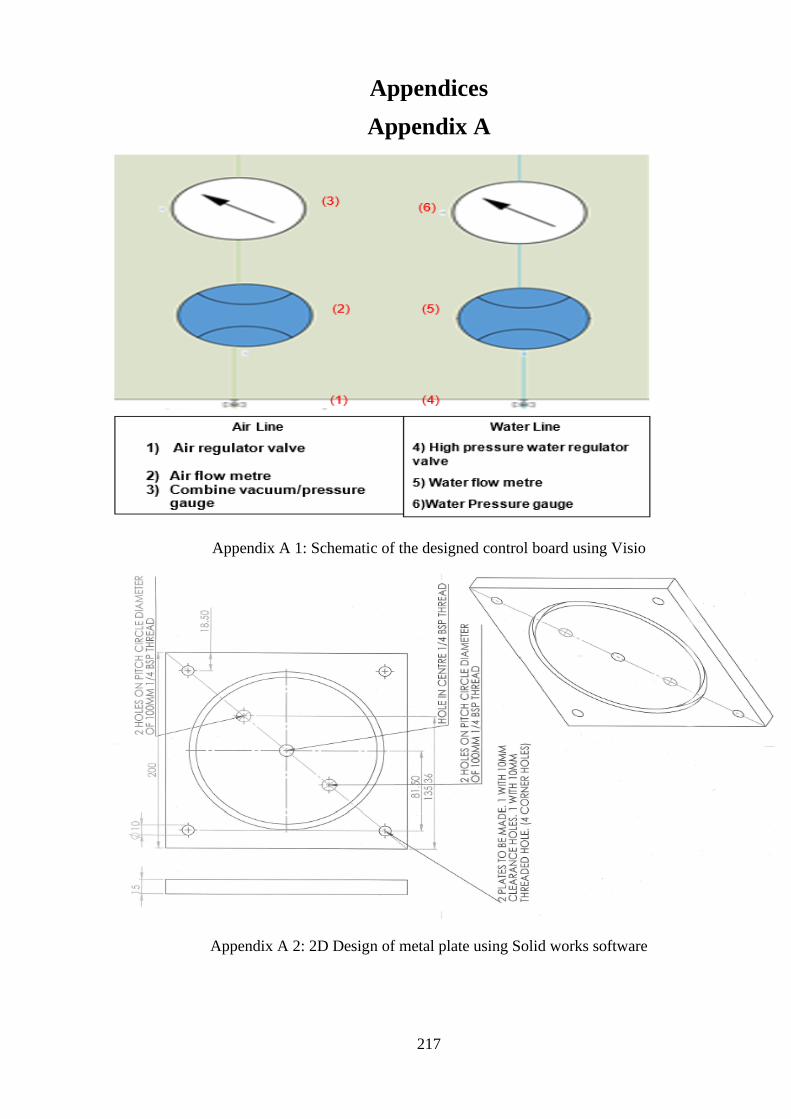
217

Appendices

Appendix A

Appendix A 1: Schematic of the designed control board using Visio

Appendix A 2: 2D Design of metal plate using Solid works software

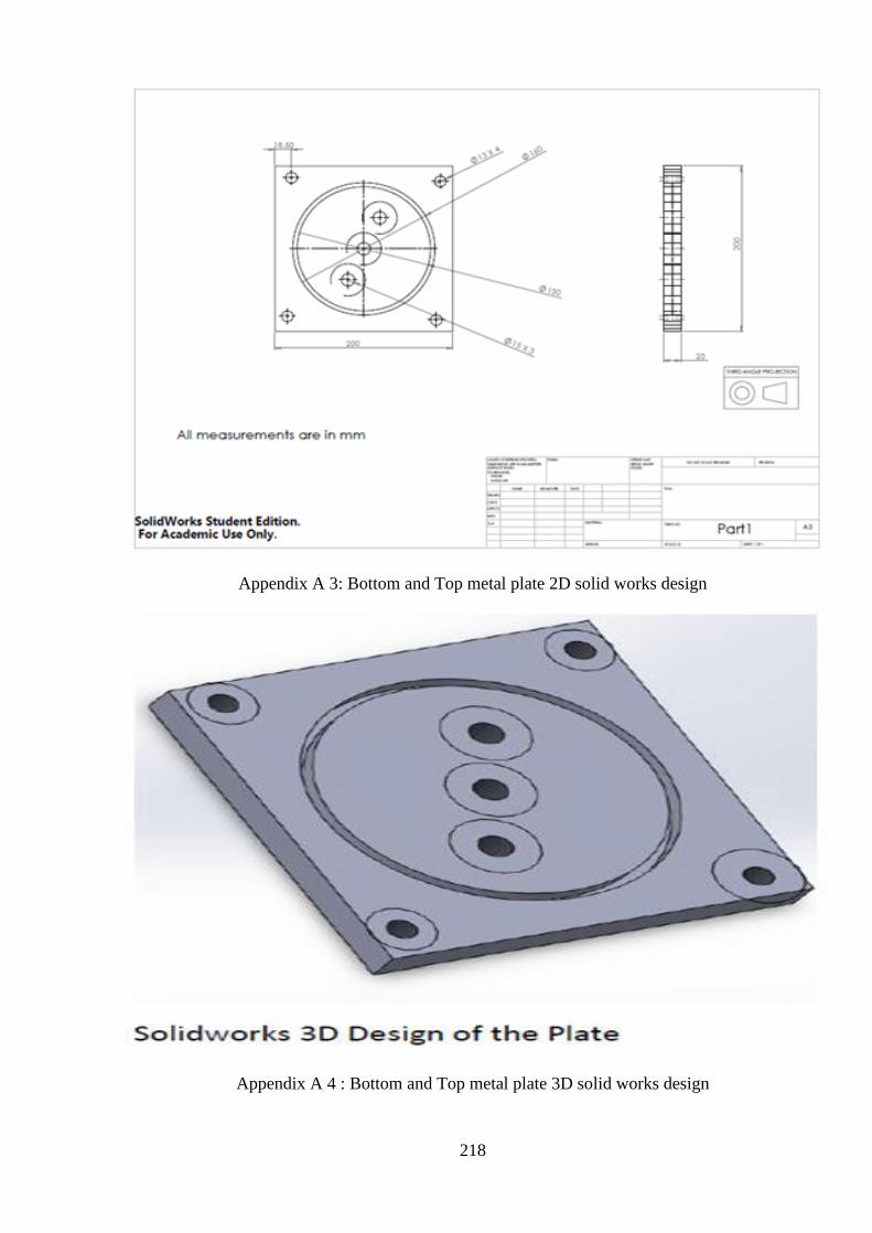
218

Appendix A 3: Bottom and Top metal plate 2D solid works design

Appendix A 4 : Bottom and Top metal plate 3D solid works design

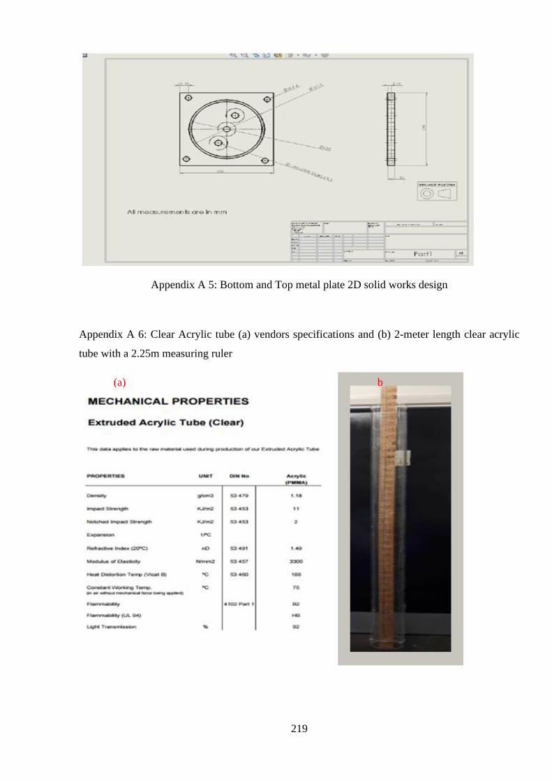
219

Appendix A 5: Bottom and Top metal plate 2D solid works design

Appendix A 6: Clear Acrylic tube (a) vendors specifications and (b) 2-meter length clear acrylic

tube with a 2.25m measuring ruler

(a) b

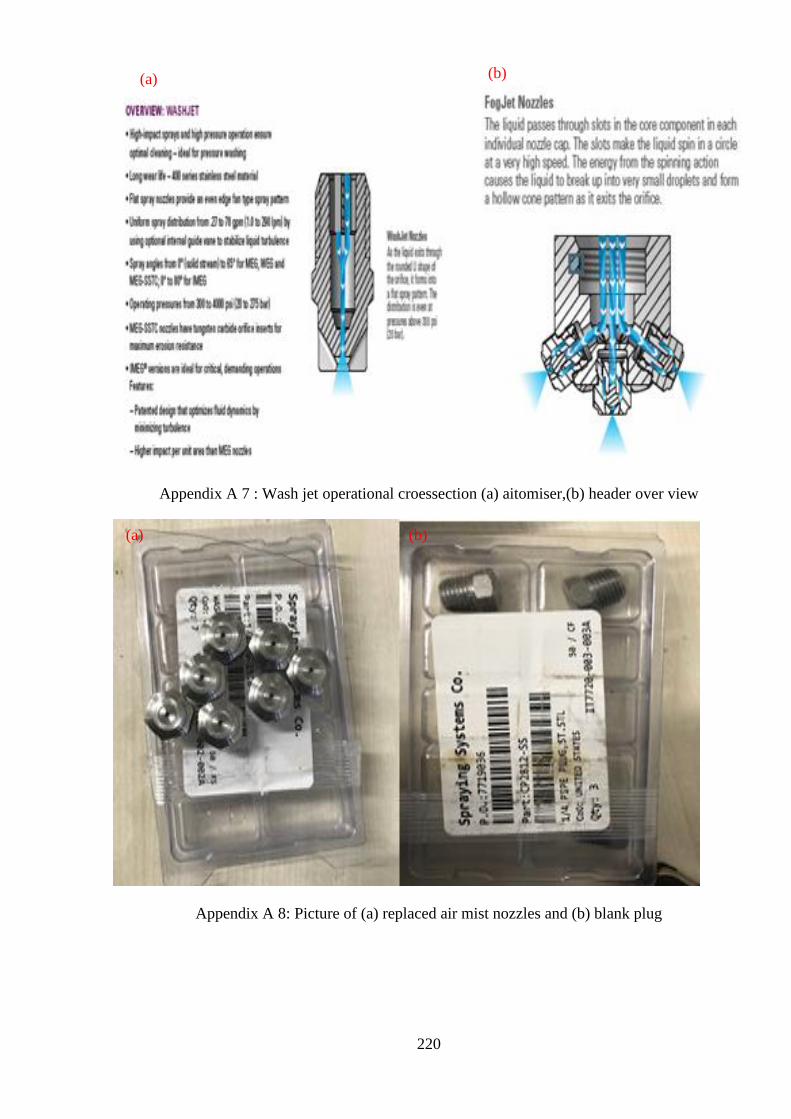
220

Appendix A 7 : Wash jet operational croessection (a) aitomiser,(b) header over view

Appendix A 8: Picture of (a) replaced air mist nozzles and (b) blank plug

(a) (b)

(a) (b)

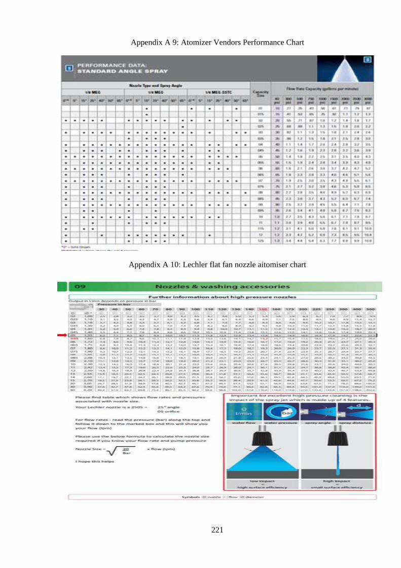
221

Appendix A 9: Atomizer Vendors Performance Chart

Appendix A 10: Lechler flat fan nozzle aitomiser chart

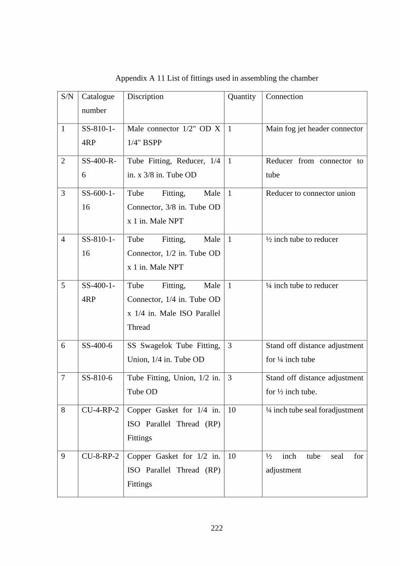
222

Appendix A 11 List of fittings used in assembling the chamber

S/N Catalogue

number

Discription Quantity Connection

1 SS-810-1-

4RP

Male connector 1/2" OD X

1/4" BSPP

1 Main fog jet header connector

2 SS-400-R-

6

Tube Fitting, Reducer, 1/4

in. x 3/8 in. Tube OD

1 Reducer from connector to

tube

3 SS-600-1-

16

Tube Fitting, Male

Connector, 3/8 in. Tube OD

x 1 in. Male NPT

1 Reducer to connector union

4 SS-810-1-

16

Tube Fitting, Male

Connector, 1/2 in. Tube OD

x 1 in. Male NPT

1 ½ inch tube to reducer

5 SS-400-1-

4RP

Tube Fitting, Male

Connector, 1/4 in. Tube OD

x 1/4 in. Male ISO Parallel

Thread

1 ¼ inch tube to reducer

6 SS-400-6 SS Swagelok Tube Fitting,

Union, 1/4 in. Tube OD

3 Stand off distance adjustment

for ¼ inch tube

7 SS-810-6 Tube Fitting, Union, 1/2 in.

Tube OD

3 Stand off distance adjustment

for ½ inch tube.

8 CU-4-RP-2 Copper Gasket for 1/4 in.

ISO Parallel Thread (RP)

Fittings

10 ¼ inch tube seal foradjustment

9 CU-8-RP-2 Copper Gasket for 1/2 in.

ISO Parallel Thread (RP)

Fittings

10 ½ inch tube seal for

adjustment

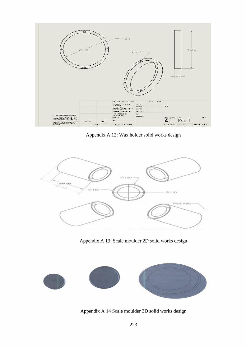
223

Appendix A 12: Wax holder solid works design

Appendix A 13: Scale moulder 2D solid works design

Appendix A 14 Scale moulder 3D solid works design

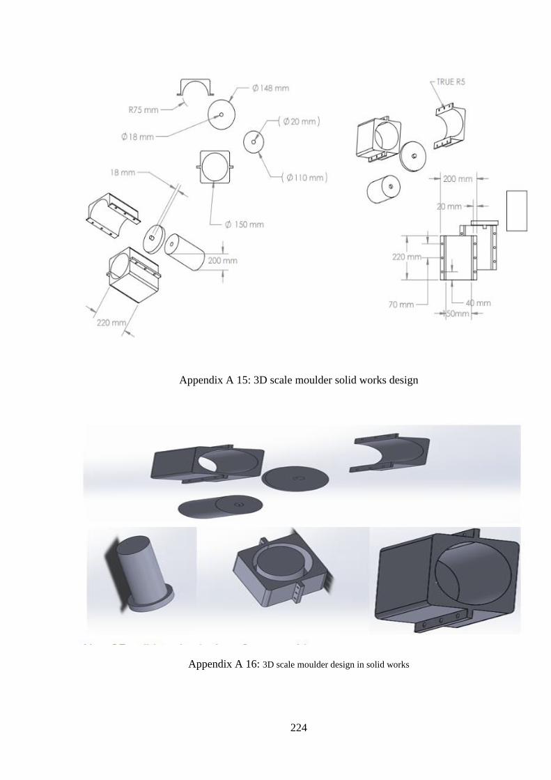
224

Appendix A 15: 3D scale moulder solid works design

Appendix A 16: 3D scale moulder design in solid works

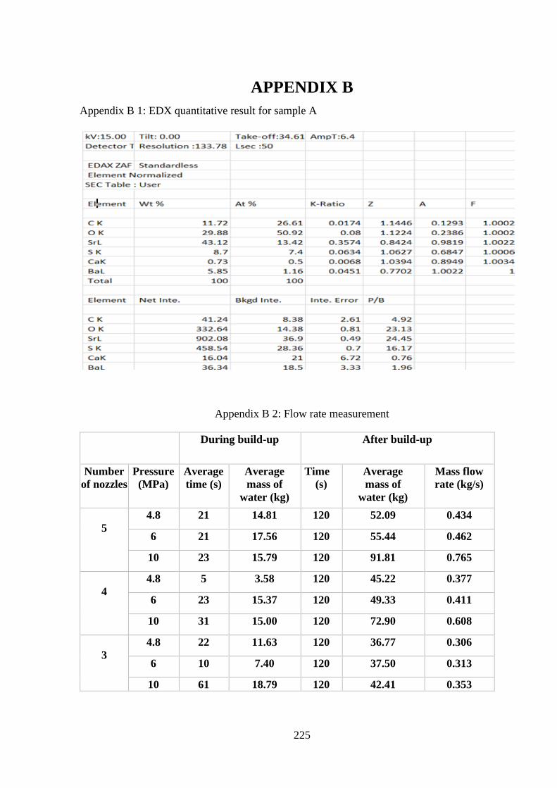
225

APPENDIX B

Appendix B 1: EDX quantitative result for sample A

Appendix B 2: Flow rate measurement

During build-up After build-up

Number

of nozzles

Pressure

(MPa)

Average

time (s)

Average

mass of

water (kg)

Time

(s)

Average

mass of

water (kg)

Mass flow

rate (kg/s)

5

4.8 21 14.81 120 52.09 0.434

6 21 17.56 120 55.44 0.462

10 23 15.79 120 91.81 0.765

4

4.8 5 3.58 120 45.22 0.377

6 23 15.37 120 49.33 0.411

10 31 15.00 120 72.90 0.608

3

4.8 22 11.63 120 36.77 0.306

6 10 7.40 120 37.50 0.313

10 61 18.79 120 42.41 0.353

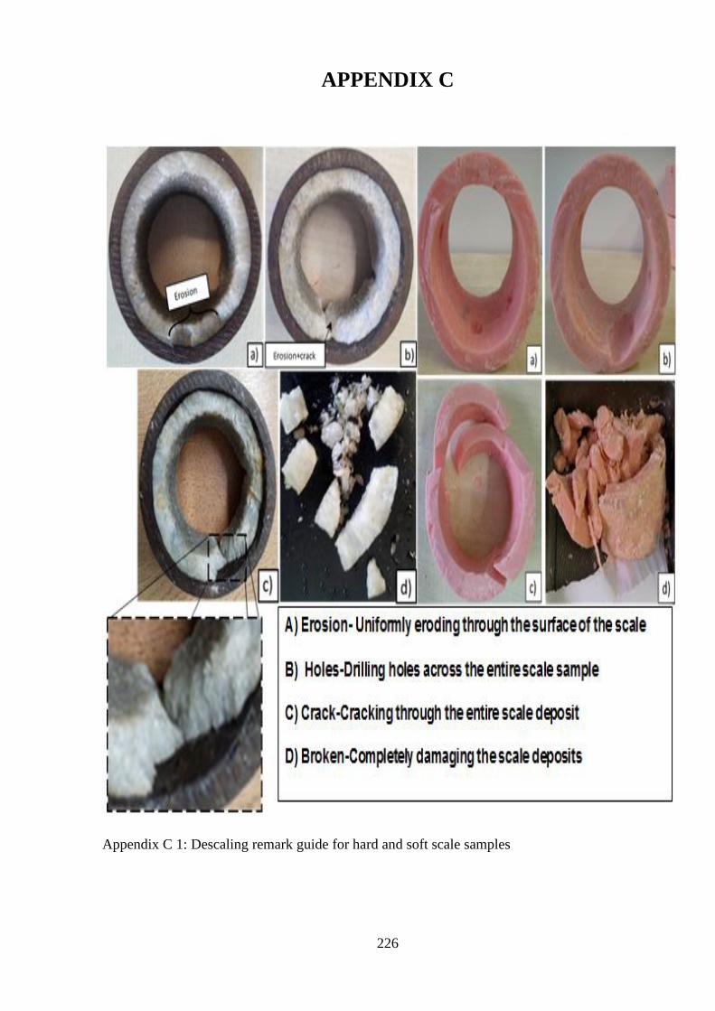
226

APPENDIX C

Appendix C 1: Descaling remark guide for hard and soft scale samples

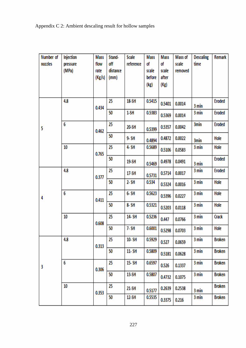
227

Appendix C 2: Ambient descaling result for hollow samples

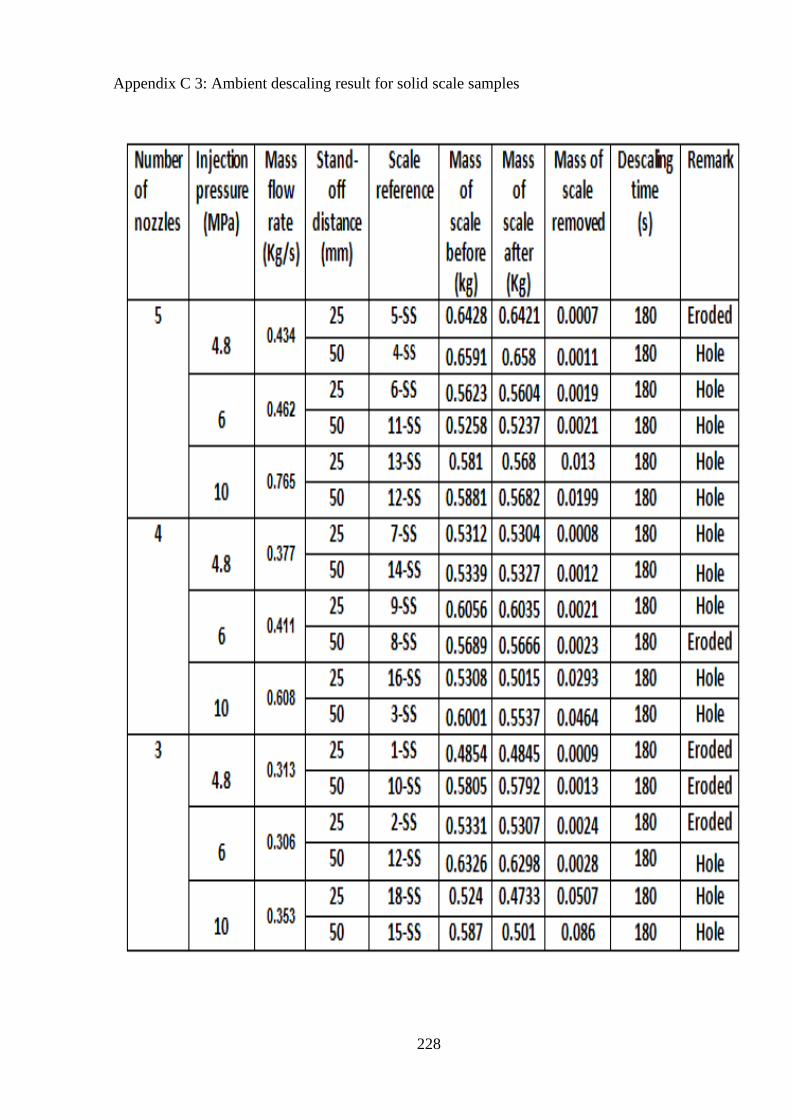
228

Appendix C 3: Ambient descaling result for solid scale samples

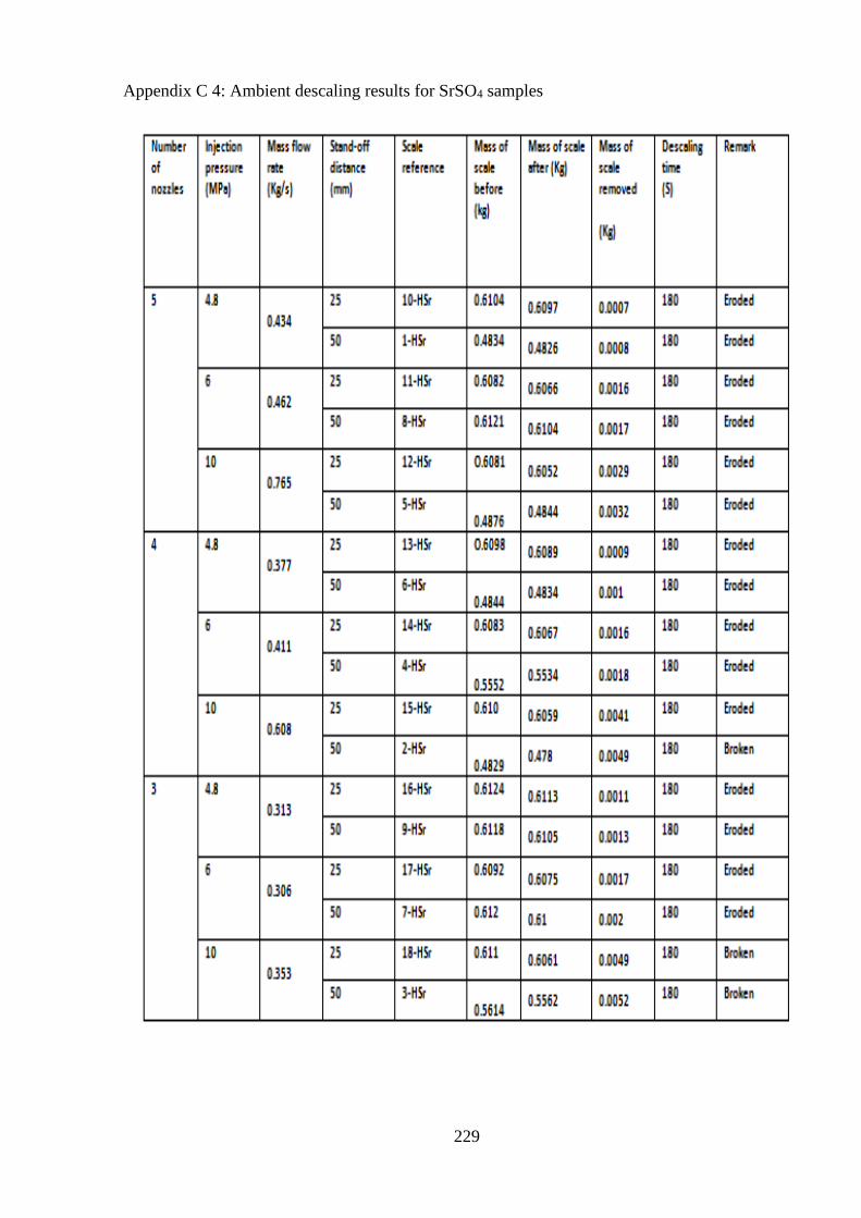
229

Appendix C 4: Ambient descaling results for SrSO4 samples

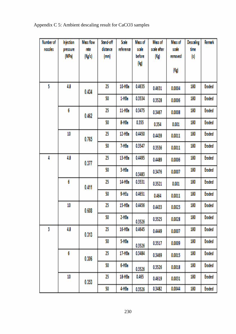
230

Appendix C 5: Ambient descaling result for CaCO3 samples

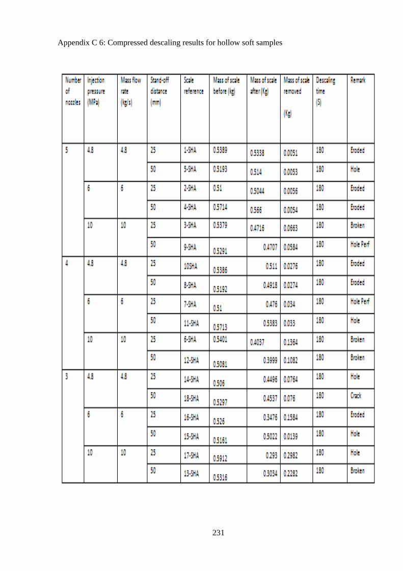
231

Appendix C 6: Compressed descaling results for hollow soft samples

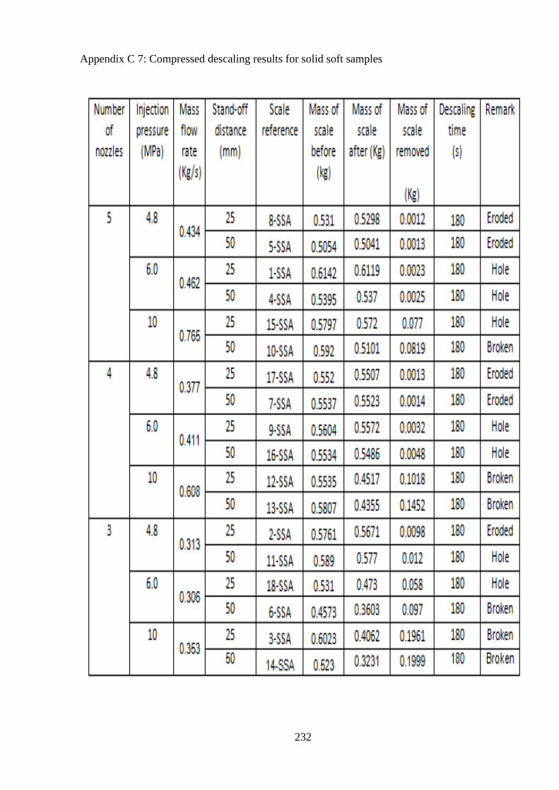
232

Appendix C 7: Compressed descaling results for solid soft samples

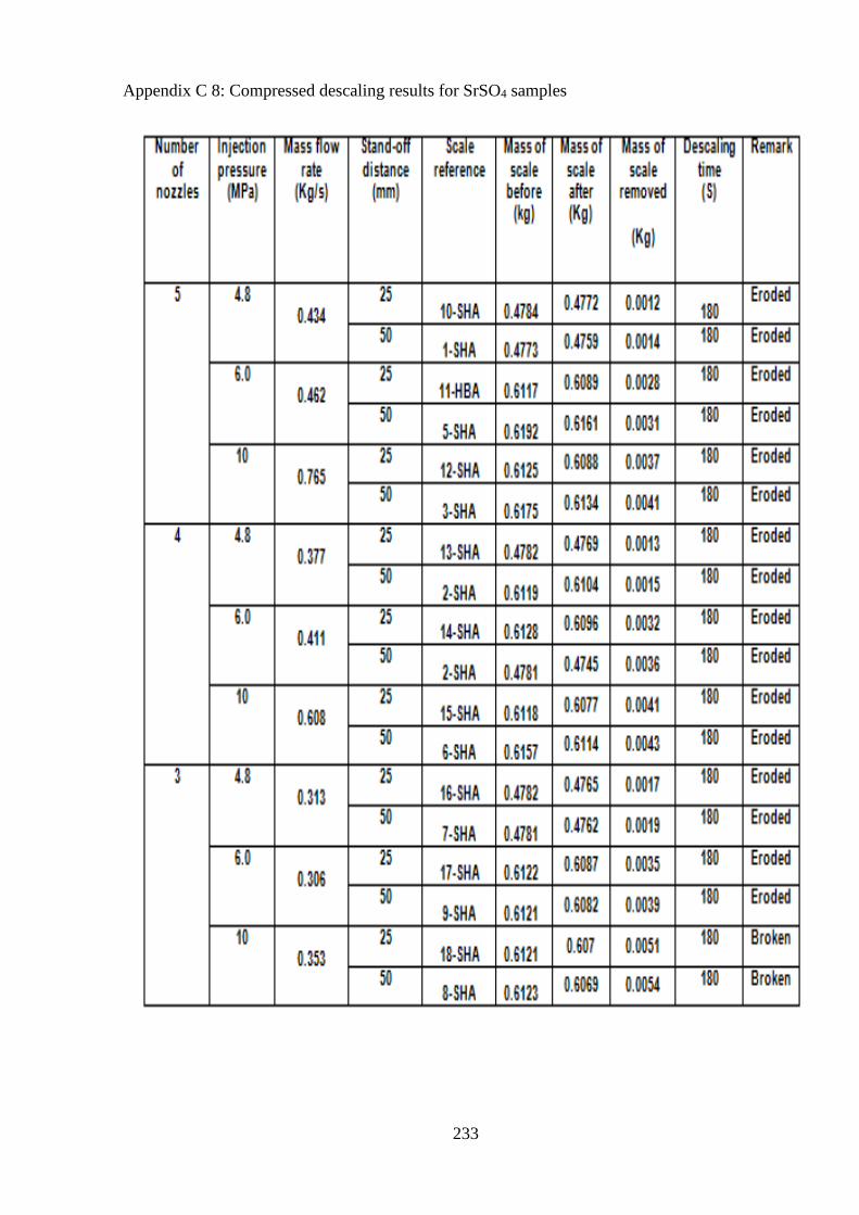
233

Appendix C 8: Compressed descaling results for SrSO4 samples

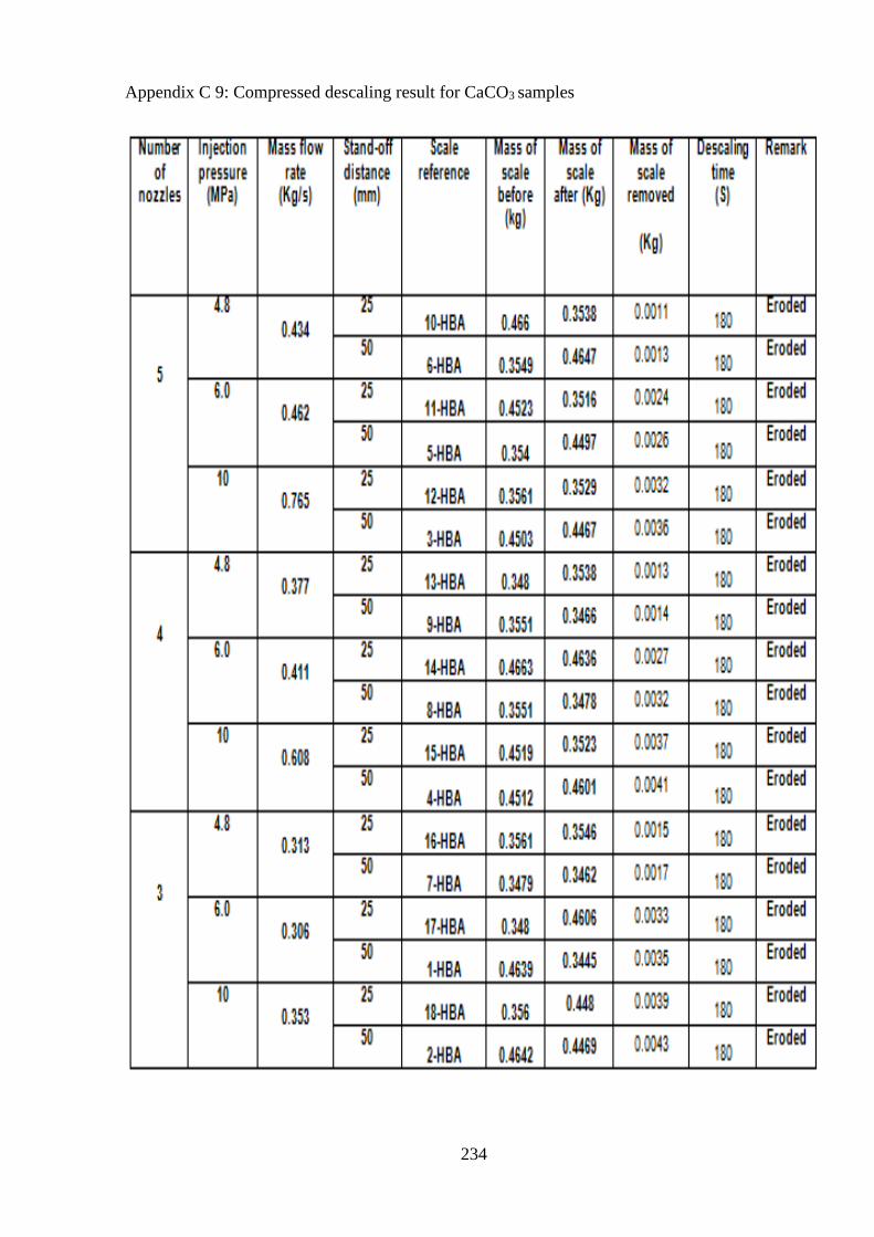
234

Appendix C 9: Compressed descaling result for CaCO3 samples

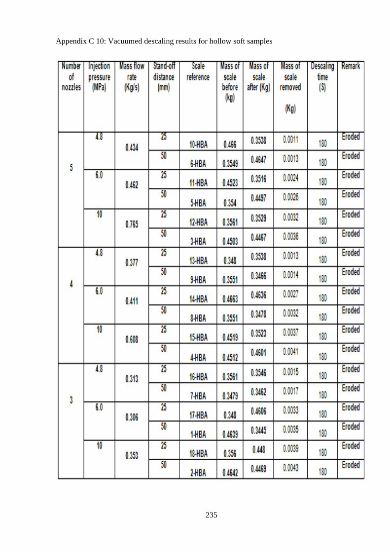
235

Appendix C 10: Vacuumed descaling results for hollow soft samples

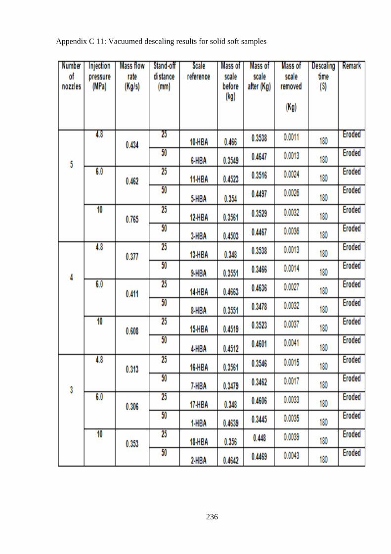
236

Appendix C 11: Vacuumed descaling results for solid soft samples

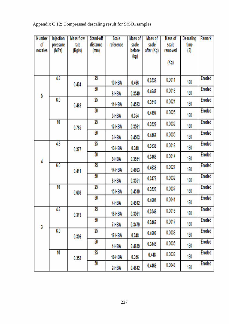
237

Appendix C 12: Compressed descaling result for SrSO4 samples

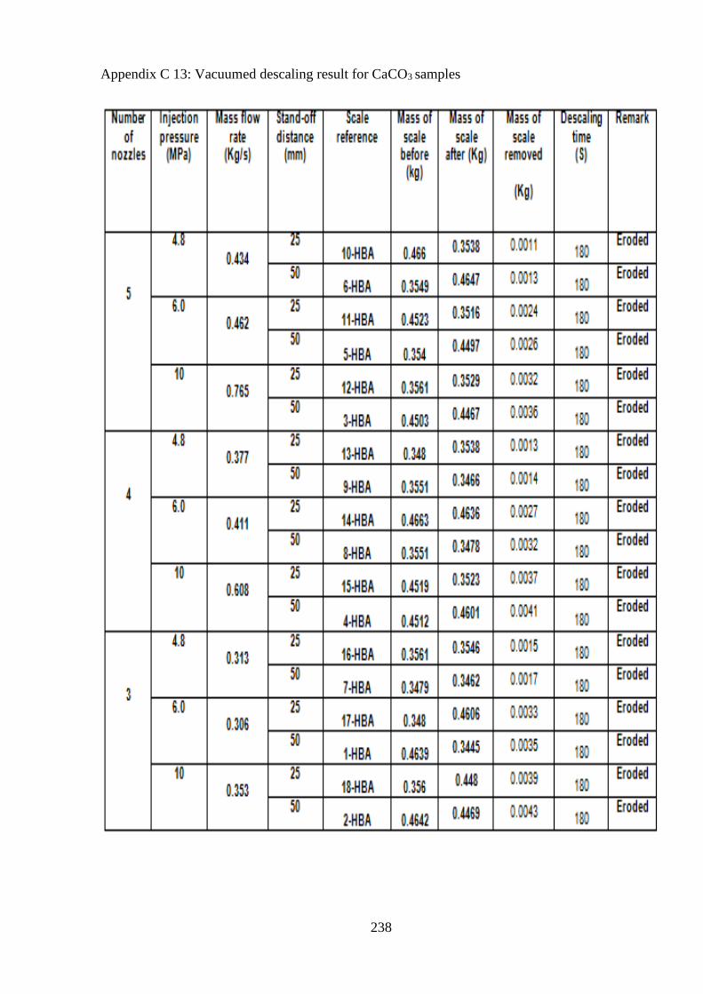
238

Appendix C 13: Vacuumed descaling result for CaCO3 samples

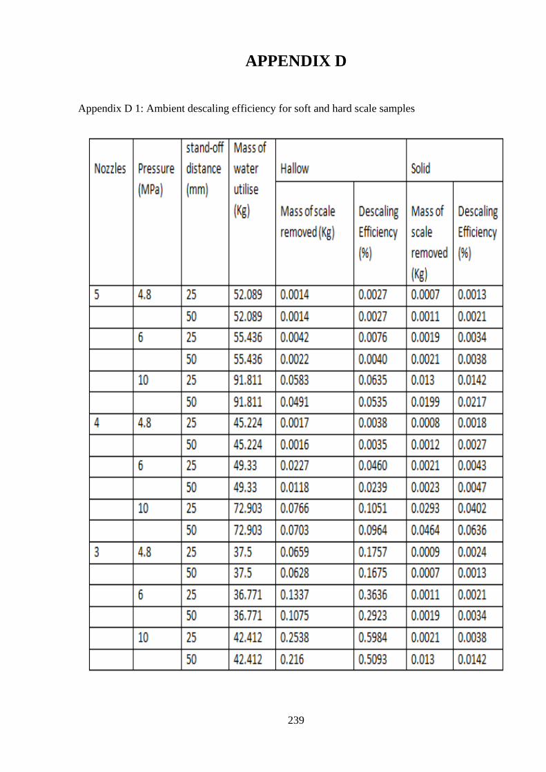
239

APPENDIX D

Appendix D 1: Ambient descaling efficiency for soft and hard scale samples

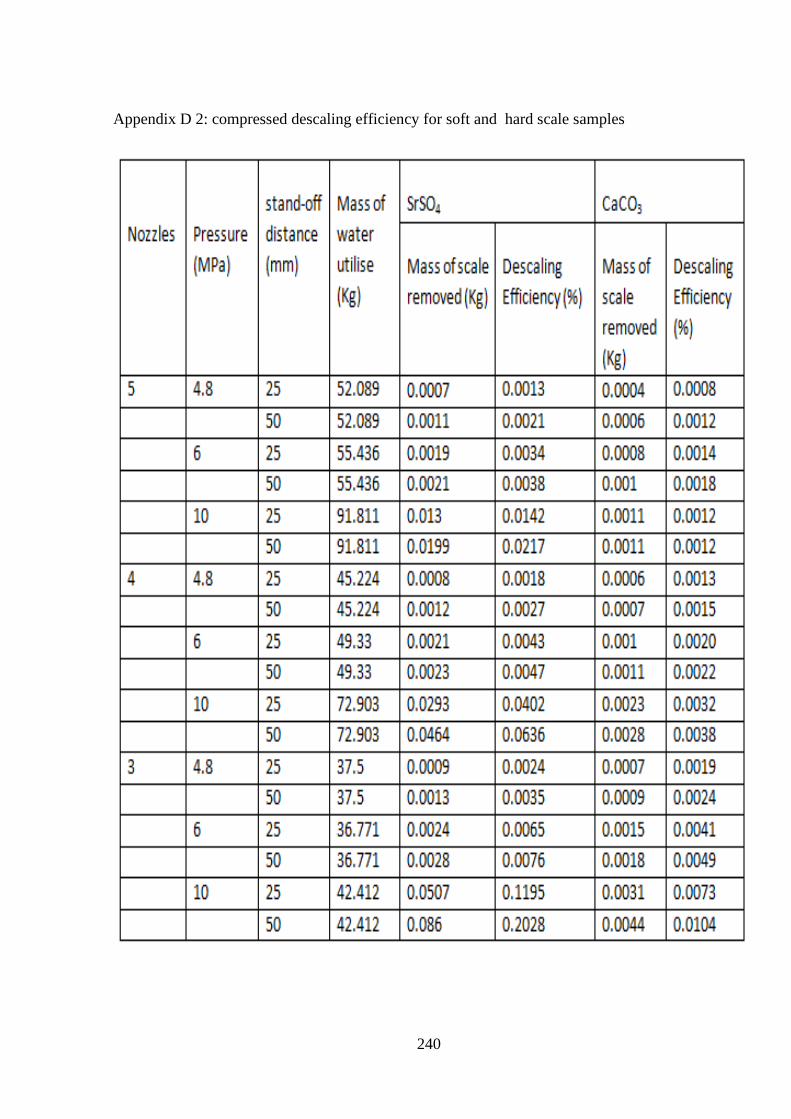
240

Appendix D 2: compressed descaling efficiency for soft and hard scale samples

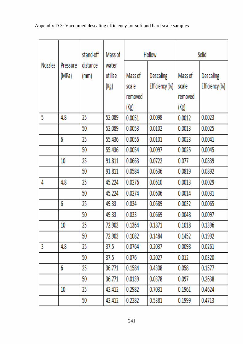
241

Appendix D 3: Vacuumed descaling efficiency for soft and hard scale samples

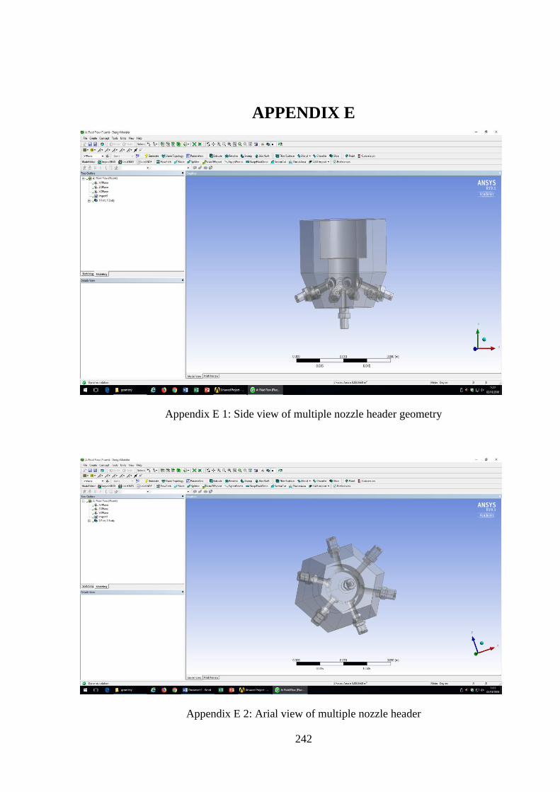
242

APPENDIX E

Appendix E 1: Side view of multiple nozzle header geometry

Appendix E 2: Arial view of multiple nozzle header

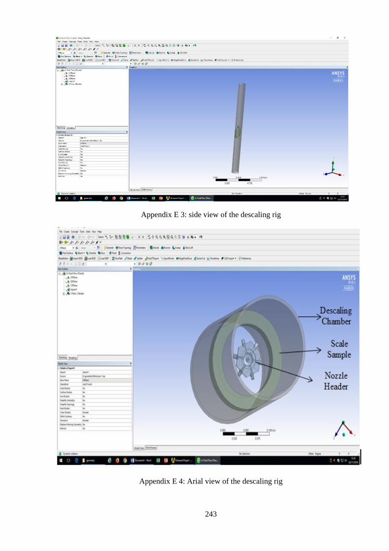
243

Appendix E 3: side view of the descaling rig

Appendix E 4: Arial view of the descaling rig

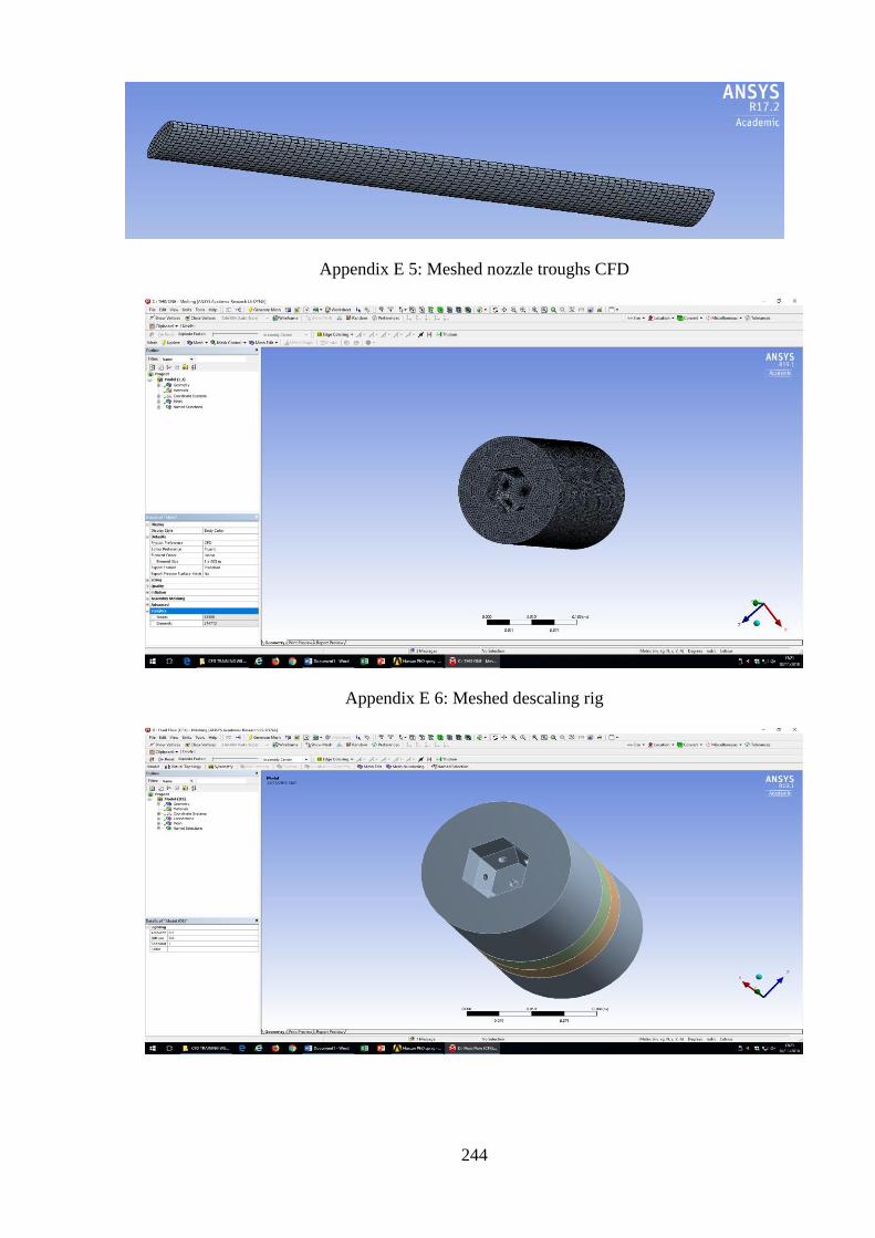
244

Appendix E 5: Meshed nozzle troughs CFD

Appendix E 6: Meshed descaling rig

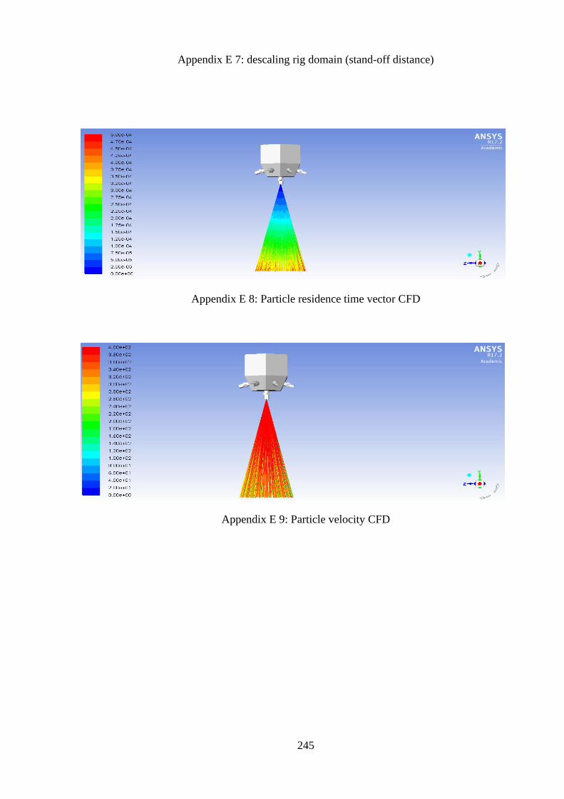
245

Appendix E 7: descaling rig domain (stand-off distance)

Appendix E 8: Particle residence time vector CFD

Appendix E 9: Particle velocity CFD