potential spawning habitat of sardine (sardina pilchardus

ICES CM 2004/Q:02 Potential spawning habitat of sardine (Sardina pilchardus) and anchovy(Engraulis encrasicolus) in the Bay of Biscay.

1

ICES CM 2004/Q:02Potential spawning habitat of sardine (Sardina pilchardus) and anchovy(Engraulis encrasicolus) in the Bay of Biscay.Benjamin Planque, Edwige Bellier and Pascal Lazure

Abstract: Large amplitude variations in the recruitment in small pelagic fishresults from interaction between a fluctuating environment and populationdynamics processes such as spawning. The spatial extent and location ofspawning, which is critical to the fate of eggs and larvae, can vary stronglyfrom year-to-year, as a result of changing population structure andenvironmental conditions. Spawning habitat can be divided in "potentialspawning habitat", defined as habitat where the hydrological conditions aresuitable for spawning, "realised spawning habitat", defined as habitat wherespawning actually occurs, and "successful spawning habitat", defined as habitatwhere fish have spawned and from where successful recruitment has resulted.Using biological data collected during the period 2000-2004, as well ashydrological data, we investigate the role of environmental parameters incontrolling the potential spawning habitat of anchovy and sardine in the Bay ofBiscay. Modelled relationships between anchovy and sardine spawning areused to predict potential spawning habitat from hydrodynamical simulations.The results show that the seasonal patterns in spawning if the two species arewell reproduced by the model, indicating that hydrological changes mayexplain a large fraction of spawning spatial dynamics. Such model may proveuseful in the context of forecasting potential impacts of future environmentalchanges on sardine and anchovy reproductive strategy in the north-eastAtlantic.

Keywords: small pelagic fish, Bay of Biscay, potential spawning habitat,climate impact

Benjamin Planque and E. Bellier: IFREMER, Laboratoire écologie halieutique,rue de l'île d'Yeu, BP21105, 44311 Nantes Cedex 3, France [tel: +33 (0)240 3741 17, fax: +33 (0)240 37 40 75, e-mail: [email protected]], PascalLazure: IFREMER, DEL/AO. BP 70. 29280 Plouzané. France.


2

Introduction

Defining the Spawning habitats

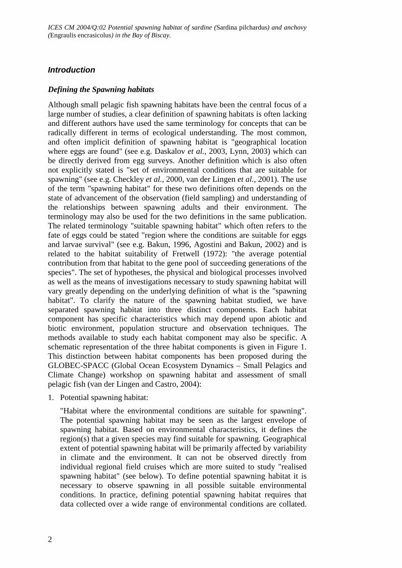
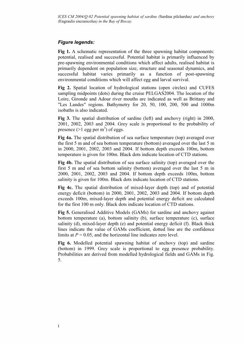
Although small pelagic fish spawning habitats have been the central focus of alarge number of studies, a clear definition of spawning habitats is often lackingand different authors have used the same terminology for concepts that can beradically different in terms of ecological understanding. The most common,and often implicit definition of spawning habitat is "geographical locationwhere eggs are found" (see e.g. Daskalov et al., 2003, Lynn, 2003) which canbe directly derived from egg surveys. Another definition which is also oftennot explicitly stated is "set of environmental conditions that are suitable forspawning" (see e.g. Checkley et al., 2000, van der Lingen et al., 2001). The useof the term "spawning habitat" for these two definitions often depends on thestate of advancement of the observation (field sampling) and understanding ofthe relationships between spawning adults and their environment. Theterminology may also be used for the two definitions in the same publication.The related terminology "suitable spawning habitat" which often refers to thefate of eggs could be stated "region where the conditions are suitable for eggsand larvae survival" (see e.g. Bakun, 1996, Agostini and Bakun, 2002) and isrelated to the habitat suitability of Fretwell (1972): "the average potentialcontribution from that habitat to the gene pool of succeeding generations of thespecies". The set of hypotheses, the physical and biological processes involvedas well as the means of investigations necessary to study spawning habitat willvary greatly depending on the underlying definition of what is the "spawninghabitat". To clarify the nature of the spawning habitat studied, we haveseparated spawning habitat into three distinct components. Each habitatcomponent has specific characteristics which may depend upon abiotic andbiotic environment, population structure and observation techniques. Themethods available to study each habitat component may also be specific. Aschematic representation of the three habitat components is given in Figure 1.This distinction between habitat components has been proposed during theGLOBEC-SPACC (Global Ocean Ecosystem Dynamics – Small Pelagics andClimate Change) workshop on spawning habitat and assessment of smallpelagic fish (van der Lingen and Castro, 2004):

1. Potential spawning habitat:

"Habitat where the environmental conditions are suitable for spawning".The potential spawning habitat may be seen as the largest envelope ofspawning habitat. Based on environmental characteristics, it defines theregion(s) that a given species may find suitable for spawning. Geographicalextent of potential spawning habitat will be primarily affected by variabilityin climate and the environment. It can not be observed directly fromindividual regional field cruises which are more suited to study "realisedspawning habitat" (see below). To define potential spawning habitat it isnecessary to observe spawning in all possible suitable environmentalconditions. In practice, defining potential spawning habitat requires thatdata collected over a wide range of environmental conditions are collated.


3

This data has to include information on areas where spawning doesnot/never occur. Experimental results on the biological and physiologicalcharacteristics of a given species can also be used to define its potentialspawning habitat. Potential spawning habitat can still be defined for areaswhere a population has collapsed and no spawning actually occurs.Potential spawning habitat has some similarities with the "basin", in thebasin model of McCall (1990). However, the potential spawning habitatdepends on spawning, but not on the contribution to population growthrate, i.e. subsequent recruitment, as is the case in McCall's basin model.Recruitment related issues will be considered in the "successful spawninghabitat" below.

2. Realised spawning habitat

"Habitat where spawning actually occurs". The realised spawning habitat isdefined by the region where fish actually spawn in a given year at a giventime. It is bounded by the potential spawning habitat. Factors that affect thelocation and extent of realised spawning habitat are primarily related toadult population size and structure as well as density dependent processes.The extent to which fish will use the potential spawning habitat will dependupon the number of mature fish, their age, migration, mating behaviour,and other population traits, as well as possible interaction with otherpopulations in the same areas (predators, competitors and preys). Densitydependent habitat selection (DDHS, McCall, 1990) will be primarilyrelated to realised spawning habitat. The realised spawning habitat is theone generally observed during "egg surveys". It is expected that realisedspawning habitat will display larger year-to-year fluctuations than willpotential spawning habitat. Note that comparing directly observed realisedhabitat with environmentally based potential habitat may in most cases notmake sense, since there is no reason a priori that a given population willfully occupy the available potential habitat in a given year.

3. Successful spawning habitat

"Habitat where fish have spawned and from where successful recruitmenthas resulted". The successful spawning habitat is defined by the fate ofeggs spawned into it. It is bounded by the realised spawning habitat (andconsequently by the potential spawning habitat). Factors that affect realisedspawning habitat are factors that will affect eggs, larvae and juveniles afterspawning has taken place. The successful spawning habitat can not beobserved at the time of spawning but only after young fish enter thepopulation as recruits. It has to be inferred from information on juvenilesand young adults. The successful spawning habitat can also be studied bynumerical modelling (and in particular IBM models) by following cohortsor individuals and their environment during their early life stages.

The present study focuses on possible ways to define and model anchovy andsardine "potential spawning habitat" in the Bay of Biscay. The issues related torealised and successful habitat will be briefly discussed.


4

Anchovy and sardine spawning habitats in the Bay of Biscay

The study of anchovy and sardine populations in the Bay of Biscay goes backat least to the early 20th century (Fage, 1911, Furnestin, 1945), but it is only inthe early 1960s that systematic sampling of sardine and anchovy eggs andlarvae over most of the Bay of Biscay continental shelf was undertaken(Arbault and Boutin, 1967). These surveys were carried out and used byArbault and Lacroix (1971, 1977) to produce the first description of sardineand anchovy spawning in the area. The geographical occupation of sardine andanchovy extends beyond the Bay of Biscay, with sardine ranging from southEuropean Atlantic coast to southern Norway (Parrish et al., 1989) and anchovyranging from western Africa (5°N) to the northern North Sea (Reid, 1966,Anonymous, 1985). However, the two populations appear in substantialquantities in the Bay of Biscay and both spawn in the area. The spatial andseasonal extent of spawning has been reviewed and re-analysed in Bellier et al.(2004). They have shown that for the two species, spawning areas can bedivided into recurrent (or refuge) sites where spawning is observed every yearand optional sites where the probability of spawning varies greatly from year-to-year. In addition, it appears that the average spawning region has movedfrom the 1960-70s to the present period 2000-2004, possibly as a result ofenvironmental changes.

Anchovy

Anchovy spawning occurs preferentially close to the coast and sometimes atthe shelf break or in oceanic slope water eddies (Motos et al., 1996). Spawningseason extends from March to August with a maximum intensity between Mayand June. Intensity of spawning appears to be constrained by thermalenvironment: Arbault and Lacroix (1977) have reported anchovy spawningwithin a thermal window of 14-20°C, Sola et al. (1990) have found a thermalwindow of 16.5-19°C whilst according to Motos et al. (1996) the thermal rangeis between 14 and 18°C. In other regions the thermal constraints may beslightly different, for example van der Lingen et al. (2001) reports thermalrange of 17.4-21.1°C in the Benguela region. In his world-wide analysis ofanchovy distribution, Reid (1966) argues that the genus Engraulis is foundfrom estuaries to high salinity waters, so that it is associated with coastal areasrather than with water of a given salinity range. Whilst river plumes (i.e. lowsalinity) appear to be recurrent preferential areas for spawning, anchovy alsospawns in other areas such as slope water eddies or shelf break which arecharacterised by high salinity throughout the water column. Although there is aconverging set of evidence that increase in river runoff is associated to increasein anchovy recruitment (see Lloret et al., 2004 and references therein), theassociation between anchovy spawning and salinity is less obvious than fortemperature and the influence of salinity on anchovy spawning distribution isstill a matter of debate. Stratification, retention and plankton production havebeen proposed as other controlling factors for anchovy spawning (or spawningsuccess ) in the Bay of Biscay (Motos et al., 1996). However, there has yetbeen no quantitative assessment of the link between these factors and anchovyspawning.


5

Finally, spawning habitat appear to depend (1) on seasonal timing, with adultsmigrating north and west as season progress (Uriarte et al., 1996) and (2) onadult population size with spawning habitat extent increasing with adultpopulation size (Motos et al., 1996). This latter effect is directly related to"realised", rather than "potential" spawning habitat.

Sardine

In the Bay of Biscay, sardine spawning occurs within a thermal window of12.5-15°C according to Sola et al. (1990) and of 10-16°C according to Arbaultand Lacroix (1977). The spatial distribution of sardine is generally morewidespread and fragmented than that of anchovy. Optimal temperature forspawning sardine can vary greatly between regions and between studies. In theNorth Pacific the thermal range for Sardinops sagax is often given as about13.5-17°C (Tibby, 1937, Ahlstrom, 1965, Parrish et al., 1989, Lluch-Belda etal., 1991), although Hammann et al. (1998) report much warmer temperaturerange of 16.9-20.8°C and conversely Lynn (2003) report spawning occurring incolder temperature of 12-13°C off southern and central California. In theBenguela upwelling system, the range of temperature for spawning sardine(Sardinops sagax) is bimodal, with a major peak at 15.5-17.5°C and asecondary peak between 18.7 and 20.5°C (van der Lingen et al., 2001). Insouth Pacific waters, Ward and Staunton-Smith (2002) report spawningtemperature range of 14-23°C. Off the Moroccan coast (north west Africa)Sardina pilchardus spawning is observed within the temperature range 16-18.5°C. The impact of salinity has been little described for sardine populations.

Objectives of the study

In the present study, we attempt to define the set of hydrological conditionsthat are suitable for spawning of sardine and anchovy populations, i.e. to definethe potential spawning habitat of sardine and anchovy in the Bay of Biscay.Sardine and anchovy populations extend outside the Bay of Biscay region, anda comprehensive study of potential spawning habitat would require the fullgeographical range of the two species to be covered. In the present work, onlydata from the Bay of Biscay is available. Our study is therefore limited to thedefinition of "potential spawning habitat" restricted to this region.

Our intention is to test whether our observations during the period 2000-2004confirm previous conclusions on the possible influence of salinity andtemperature on sardine and anchovy spawning habitat. In addition, weinvestigate the possible role of other hydrological parameters related to watercolumn stratification, on the potential spawning habitat of the two species.Finally, we show how this information can be used to represent potentialspawning habitat on the basis of simulated hydrological fields, as a first steptowards predicting spawning habitat changes under possible climate scenarios.


6

Data and method

The PELGAS cruises 2000-2004

Since 2000, large scale cruises covering most of the Bay of Biscay continentalshelf along the French coast have been carried out during spring time. Thesecruises are primarily designed for the acoustic assessment of small pelagic fishstocks in the area. However, a number of additional data are collected, whichinclude fish egg and larvae sampling, hydrology, phytoplankton andzooplankton sampling, sea mammals and sea bird observations. In the currentstudy, we have used fish egg and hydrological data.

Due to operational and logistical constraints, the cruises have taken place atdifferent dates every year: 17th April to 14th May in 2000, 28th April to 4th Junein 2001, 10th May to 5th June in 2002, 30th May to 24th June in 2003 and 27th

April to 24th May in 2004. As this is the period during which thermalstratification sets up and river runoff diminishes, slight changes in the timing ofcruise can have a large impact on the hydrological conditions encountered.

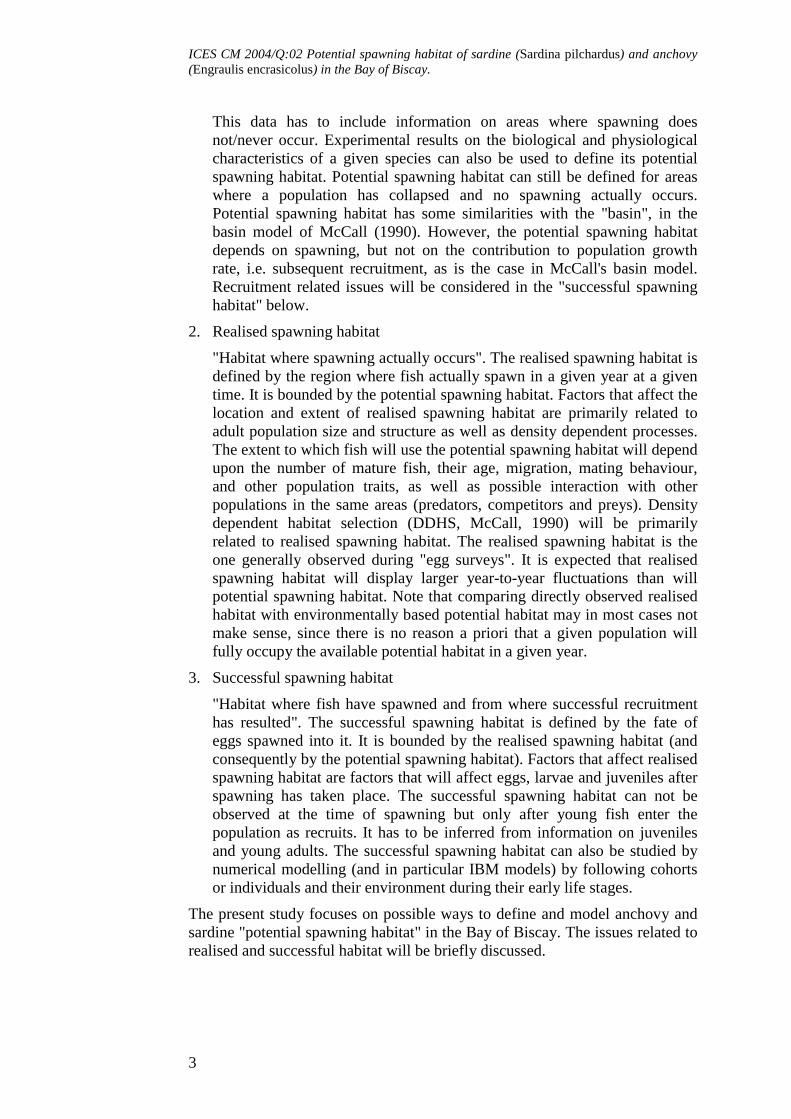
The cruise track showing the location of CUFES samples and Hydrologicalstations in 2004 is shown in Figure 2. Cruise tracks for 2000, 2001, 2002 and2003 are similar (although not strictly identical) to the one in 2004.

Collection of egg samples – data processing

Continuous fish egg sampling was performed using a CUFES (ContinuousUnderway Fish Egg Sampler, Checkley et al., 1997), mounted outboard of theR/V Thalassa. The CUFES continuously pumps sea water at 3m depth at a rateof about 500 l/min (0.0083 m3.s-1). The eggs are concentrated into a smallvolume of water and samples are collected every 20 minutes. A sampleapproximately corresponds to 10 m3 of filtered sea water whilst the ship hascovered a distance of about 3 nautical miles (5.5 km). The exact pump flowrate and duration of sampling are recorded. After collection, the eggs areidentified to species level for sardine and anchovy and are counted. The resultsare standardised to egg concentration i.e. "number of eggs per 10 m3 of filteredsea water".

Collection of hydrological data – data processing

Hydrological profiles (temperature, salinity, density) were realised at fixedstations at night using a CTD probe. The number of stations realised hasslightly varied between years. From each CTD profile, six parameters werederived: surface and bottom temperature, surface and bottom salinity, potentialenergy deficit and mixed layer depth. Potential energy deficit, which is ameasure of vertical density stratification was calculated as in Allain et al.(2001). Mixed layer depth was estimated using a two-layers model as inPlanque et al. (submitted). When vertical profiles exceeded 100 m depth, onlythe first 100 metres were retained for the analysis, as some external sensorsmounted on the probe did not always allow for deeper sampling.


7

Cartography of fish egg and hydrological data

Fish egg and hydrological data were interpolated on the same spatial grid toallow direct comparison of the two types of data. The cartography of theprobability of egg presence was performed as in Bellier et al. (2004). Eggconcentrations were transformed to presence/absence binary data, before beinginterpolated on a regular grid of 1/8th degree by kriging. The cartography of thesix hydrological parameters was also performed by kriging on the same regulargrid of 1/8th degree. Kriged data for fish eggs and hydrological parameterswere used as input to the Generalised Additive Model fitting.

Potential habitat defined from Generalised Additive Model fits

Individual predictor fits

The definition of potential spawning habitat is based on the existence of arelationship between hydrological factors and the probability of egg presence.Generalised additive models (GAMs, Hastie and Tibshirani, 1990) constitute apractical method for fitting smoothed curved to sets of data with single ormultiple predictor and single response variable. In a first step, we have usedGAM models on single predictor to identify the relationships betweenindividual hydrological predictors and the probability of egg presence. Theselection of the GAMs smoothing predictors was done following the methodproposed by Wood and Augustin (2002), using the 'mgcv' library in the Rstatistical software (R Development Core Team, 2004). The output of theGAMs are smoothed fits for each hydrological predictors. Each fit can beanalysed with regards to the level of deviance explained (0-100%, the highest,the better), the Generalised Cross Validation score (GCV, the lowest the better)and the confidence region for the smooth (which should not include zerothroughout the range of the predictor). The predictors can be ranked accordingthe above criteria.

Multiple predictor fits

GAMs allows for fitting a single response variable (here, the probability of eggpresence) to multiple predictors (here, the hydrological predictors). On thebasis of predictor ranking performed above, we have constructed series ofGAMs of increasing complexity to model the probability of egg presence forsardine and anchovy. The 'best' models for sardine and anchovy are againselected on the basis of GCV and level of deviance explained. These modelsform the basis of the potential habitat prediction (see below).

Prediction of potential spawning habitat from hydrodynamical simulations

Using the GAMs (constructed from observed egg distributions andhydrological situations) it is possible to predict egg presence probability from anew set of hydrological predictors. We have made such attempt usinghydrological results for hydrodynamical simulations. The simulations aregenerated by a MARS3D, a 3D hydrodynamical model covering the Bay ofBiscay continental shelf. The model has a 5km horizontal resolution and 10


8

vertical layers in sigma coordinates. A detailed description of the modelproperties is given in Lazure and Jégou (1998).

Results

Egg distribution

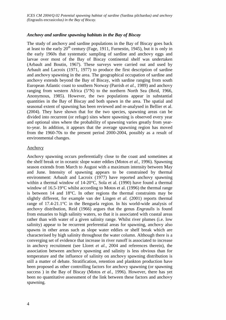
Distribution of sardine eggs can extend throughout the area covered by thesurvey, i.e. the Bay of Biscay continental shelf. Eggs can be found at thesouthern and northern bounds and in coastal as well as shelf break areas (Fig.3). There is a high degree of interannual variability of the location and extentof high probability of sardine egg presence. The distribution of anchovy eggs isgenerally confined to the southern part of the Bay of Biscay continental shelf.Again, there is a large degree of interannual variability in anchovy eggdistribution. For example, the spatial distribution in 2003 is patchy and spreadsover most of the shelf whilst in 2004 it is much narrower and concentratedalong the southern coast of Les Landes and the Adour, Gironde and Loireestuaries.

Hydrology

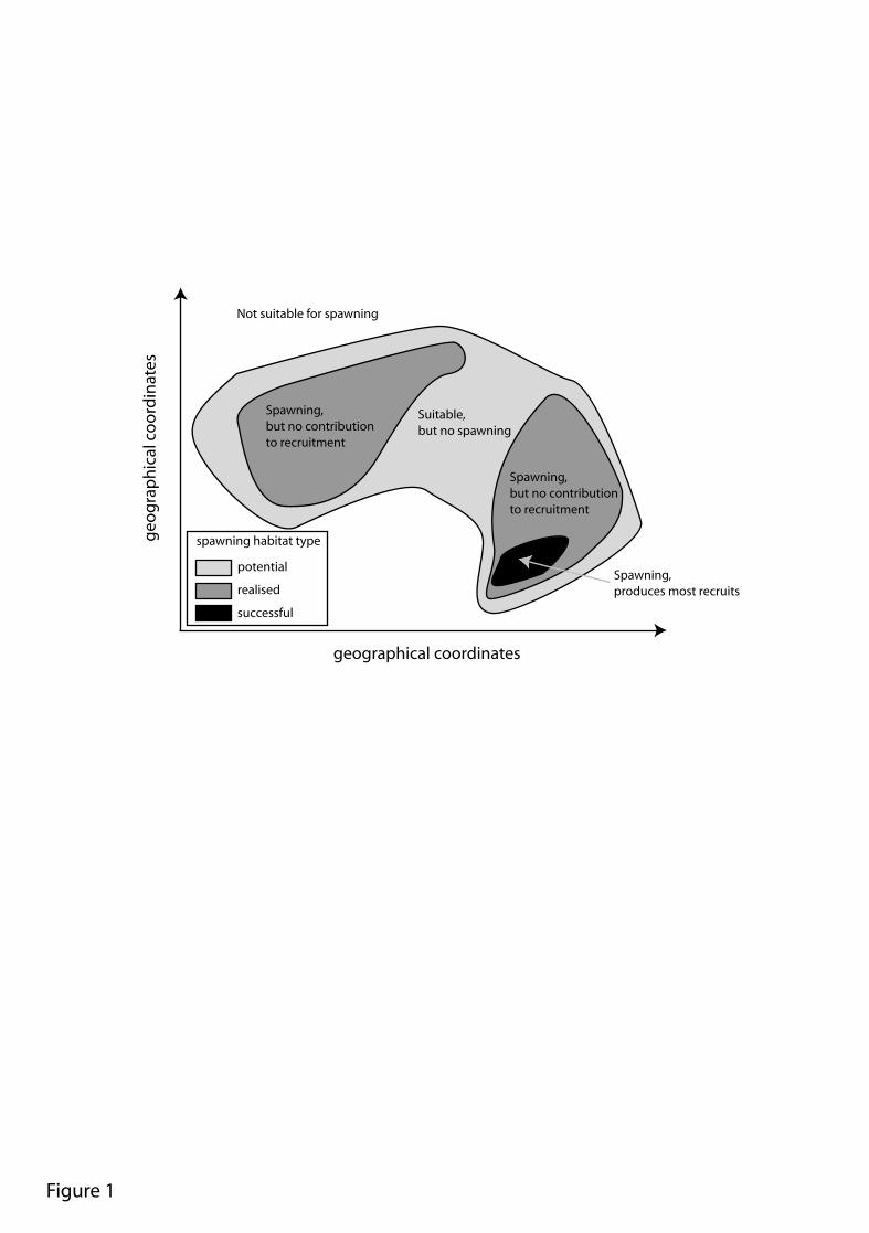
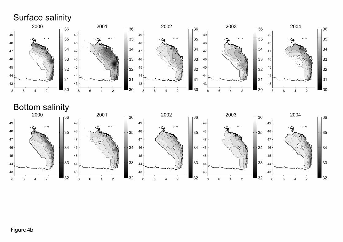
The distribution of sea surface temperature (SST, Fig. 4a) reflects the state ofthermal stratification during the cruise. In 2000 and 2004 warmer temperatureswere recorded in the northern part of the shelf as this area was visited at theend of the cruise, once stratification had taken place. In 2001, the samplingplan was reversed, with the southern part of the shelf visited during the secondpart of the cruise. This explains the apparent strong temperature gradientobserved around 47N. In 2003 the cruise took place after the onset of thermalstratification and all SST recorded display high values. Bottom temperaturesdisplay less interannual variability. The characteristic features are the presenceof the "cold pool", a cold (<12°C) bottom body of water (Vincent and Kurc,1969, Puillat et al., 2004) visible in the northern part of the shelf in 2000, 2002and 2004, and warm coastal water strips in 2001-2004. The distribution ofsurface salinity (Fig. 4b) is related to the Loire and Gironde river outflowswhich have greatly varied during the five years. A maximum runoff in 2001 isvisible with low salinity extending far out on the shelf and a low salinity waterlens located in front of the Gironde estuary. Bottom salinity is not directlyrelated to surface salinity and generally follows a the bathymetry towards theshelf break. The mixed layer depth (MLD, Fig. 4c) is also conditioned by localbathymetry with greater MLD in deeper waters. However, the geographicalextent and location of maximum MLD along the shelf break vary betweenyears, as seen for example in 2001 (maximum MLD around 47°N) and in 2000and 2004 (maximum MLD around 45°N). The potential energy deficit (PED)reflects the combined thermal and haline stratification and is greatly variablebetween cruises. In 2000, the high PED in the north reflect thermalstratification towards the end of the cruise. In 2001 the northern stratified lensreflect thermal stratification added to the presence of low salinity waterextending off the coast. The southern stratified lens is mostly the result of verylow surface salinity in front of the Gironde estuary. In 2002, the averaged PED


9

values reflect the average surface salinity and temperature distributions. In2003 the late timing of the cruise combining with abnormally warmtemperatures resulted in strong thermal stratification. Similarly, in 2004 thePED is parallel to the distribution of surface temperatures but with much lesservalues.

In summary, the five cruises have taken place in contrasted hydrologicalsituations as a result of changes in individual cruise timing and meteorologicalconditions (e.g. high precipitation in 2001, strong solar heating in 2003).

Relationships between egg presence and individual hydrological predictors

Temperature

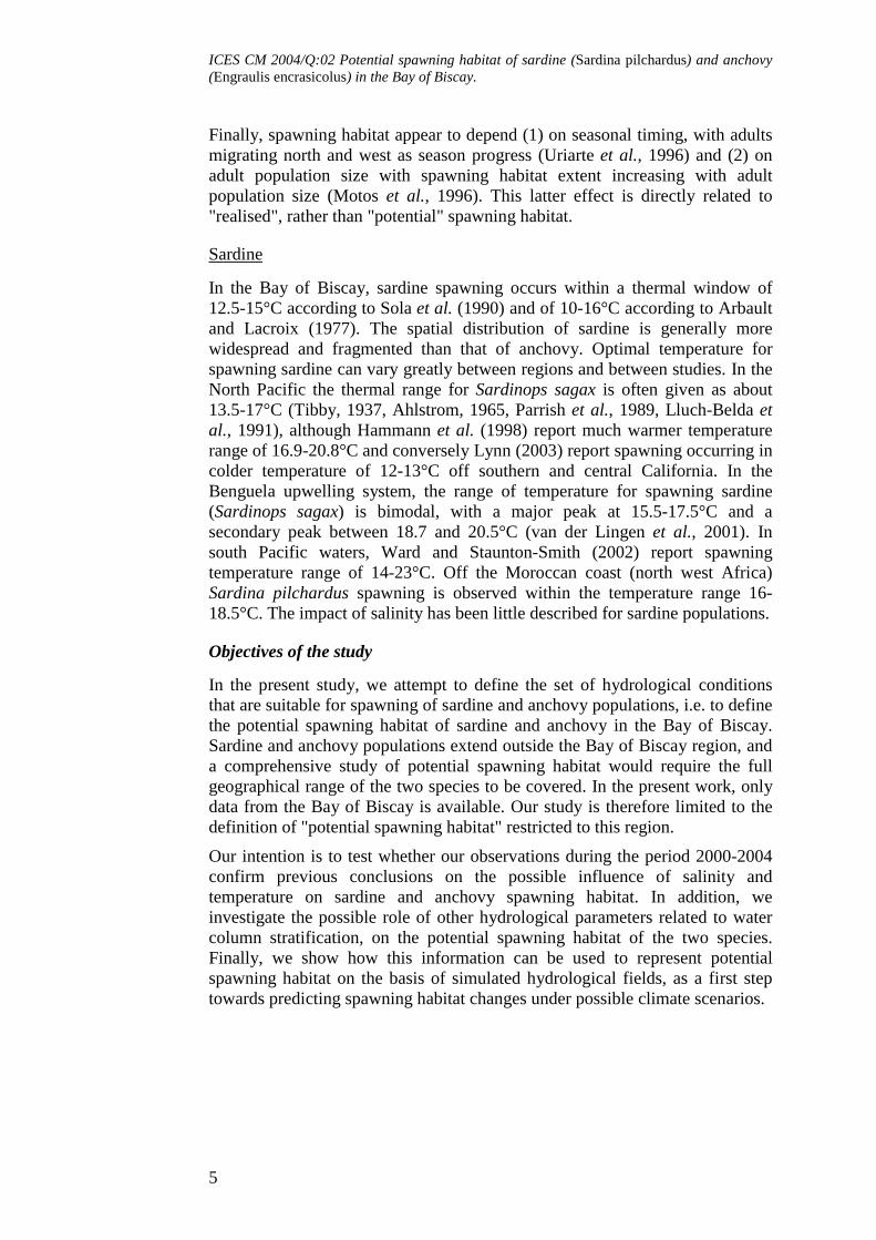
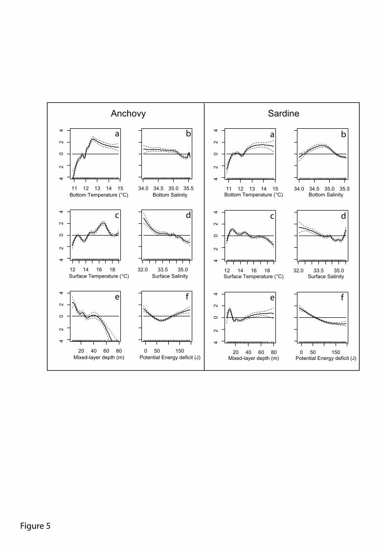
The link between temperature and the spawning of anchovy is clearly visible(Fig. 5a-b) with spawning mostly occurring in waters of 14.5-19°C at thesurface and 12-15°C at the bottom. The upper temperature limits can not beclearly defined from the GAM plot as the coefficient do not decrease towardsvalue significantly lower than zero. The lower bottom temperature limit isevident, with a sharp decline in coefficient values below 12°C. The influenceof temperature on the potential habitat of sardine is also visible. There appearto be a thermal preferendum around 12.5-15°C at the surface. For bottomtemperature the response is bimodal with a first peak around 11.75°C, andpositive coefficients values beyond 12.5°C.

Salinity

Anchovy eggs are found preferentially in waters with low surface salinity (<34Fig. 5c) with almost a monotonic decline towards high salinity values. Theinfluence of bottom salinity is less obvious although there is a decline in theGAM function with increasing salinity. A small peak is observed for highsalinity (around 35.5) probably related to spawning observed in the region ofthe shelf break. For sardine the effect of surface salinity appears bimodal withranges of <33.5 and >35.25, this latter value corresponding to open oceanconditions. The bottom salinity situation is contrasted with a single modearound 34.25-35.25 and no secondary peak for high bottom salinity values.

Stratification

Anchovy spawning is related to mixing depth, with greater egg presence inshallow mixed layer conditions (Fig. 5e). Eggs are generally found in very lownumber in waters with mixed layer depth greater than 50m. This is combinedwith a preference for either weakly stratified (PED < 30 J) or highly stratifiedwaters (PED > 110 J, Fig. 5f). The combination of shallow mixed layer depthand high stratification corresponds to river plume waters with strong andshallow haline stratification. The high values of the GAM for unstratifiedwaters corresponds to tidally mixed coastal waters. The situation for sardine isalmost reversed, with egg abundance decreasing as stratification increases andeggs found throughout the range of mixing depths with higher presenceprobabilities for either deep or very shallow mixed layers.


10

Ranking of hydrological predictors

Aside from the shape of the relationship between a given predictor and eggpresence, it is possible to rank the hydrological predictors according to thepercentage of deviance they can explain and the GCV scores of the GAMmodels (Table 1). For anchovy, the predictor that can best explain egg presenceis bottom temperature, with the highest deviance (35%) and lowest GCV score(0.508). Following predictors are surface temperature and mixed-layer depthand to a lesser extent surface salinity. Bottom salinity and potential energydeficit seem to have a more marginal link to egg presence, with percentage ofdeviance explained of less than 10%. The situation is not as clear for sardine,with all hydrological predictors having closer values in both percentage ofdeviance explained and GCV scores. The generally lower values of devianceexplained for sardine compared to anchovy suggest that hydrological influenceon sardine spawning areas is lesser that for anchovy.

Multiple predictor GAMs

GAMs with increasing number of predictors (1 to 6) have been constructed.For each level, all possible arrangements of predictors were tested and only thebest combination (i.e. with the lowest GCV score) was retained. The results ofthese models are presented in Table 2. For anchovy, the quality of the modelsincreases up to 5 predictors, although little is gained beyond the 3-predictorsmodel which includes bottom temperature, surface salinity and surfacetemperature. For sardine, there is a regular increase in model quality (both interms of GCV and deviance) as the number of predictors increases, and the bestmodel includes all hydrological predictors. The overall percentage of devianceexplained is always lower than for anchovy, a result consistent with previousobservations on single predictor models.

Model simulations

Using hydrodynamical simulations for year 1999, we have extracted the 6hydrological descriptors and used them for the prediction of egg presenceprobability. For anchovy, the model with 3 predictors was retained, whereas forsardine all 6 predictors were used, for the reasons given above. Predictionswere restricted for areas less of 1000m depth. When modelled hydrologicalpredictors were outside the range of observed values, no prediction for eggpresence probability was estimated.

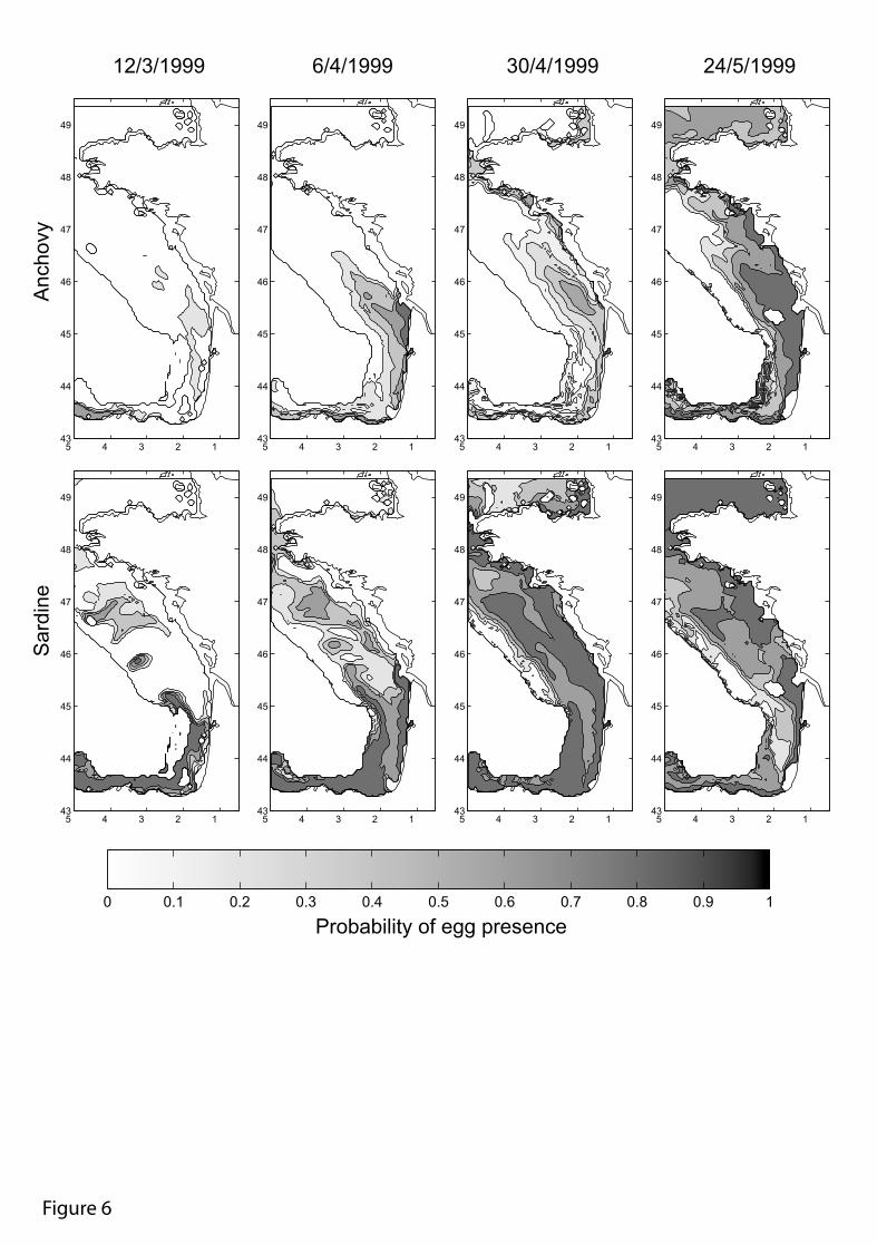
The modelled potential habitats for sardine and anchovy during spring 1999 arepresented in Figure 6 for four dates: 12 March, 6 April, 30 April and 24 May.

At the end of winter (12/03) the potential spawning habitat of anchovy isalmost absent from the Bay of Biscay continental shelf, apart from a smallcoastal region north of Spain and west of 3°W. In early spring potentialspawning habitat extends further east and along the French coast from thesouth of the Bay of Biscay up to the Gironde estuary. The potential habitatextends further offshore towards the north. Along the coast to the north of theGironde estuary, the hydrological conditions are not within the range of theGAMs, so there is no prediction of the potential spawning habitat for this


11

region. At the end of April, the southern part of the Bay seems less favourablefor spawning whilst to the north of the Gironde the potential habitat extendsfurther towards the middle of the shelf. It is also noticeable that potentiallysuitable spawning habitats are seen along the southern and western coasts ofBrittany. In late May the hydrological conditions appear favourable over awide area south of 46N and more restricted towards the coast in the north.There are small potentially favourable locations along the shelf break from 45to 46N. The coastal band along the Northern coast of Spain also seemspotentially suitable for spawning. Finally, the hydrological conditions in theChannel are such that spawning of anchovy can potentially be achieved in mostof this area.

The modelled potential spawning habitat of sardine generally covers largerareas and is more patchy than that of anchovy. In late winter, most of the coastalong northern Spain appears favourable for spawning, as well as the southernpart of the Bay of Biscay up to 45N, excluding a narrow coastal strip.Hydrological conditions also appear favourable in patchy regions over thecentral shelf. By early spring the potential spawning habitat has extended overa broader area but preserve a similar geographical structure. At the end ofApril, most of the continental shelf is suitable for sardine spawning, includingcoastal regions of north-east Brittany and west Normandy. By late May,potential spawning habitat has restricted towards shallower waters, but alsoalong the shelf break, and covers all of the western Channel region.

Discussion

The objective of the present work was to define the hydrological conditionswhich are potentially suitable for spawning of anchovy and sardine in the Bayof Biscay. As stated in the definition of "potential spawning habitat", thiswould have required data collection over a wide range of environmentalconditions, including areas where spawning does not/never occur. Since thefield cruises are primarily designed to monitor anchovy and sardinepopulations, they are centred on the spawning areas and timing of the twospecies and therefore include only a fraction of the non-spawning sites and arelimited in the range of hydrological situations encountered. Extension of thespatial and temporal coverage of the cruises would improve the generalmethodology, although this is often hardly achievable because of fieldsampling cost. Alternatively, inclusion of results from other cruises carriedaround the Iberian Peninsula (Sagarminaga et al., 2004) and in the Celtic Sea,Irish Sea (Armstrong et al., 1999) and Channel would certainly improve theresults obtained and provide a more robust description of European anchovyand sardine potential spawning habitats. Additional hydrological environmentalmay also be considered, although it seems reasonable to constrain the list ofparameters to a small number of variables that are regularly measured duringfield cruises and which provide a thorough description of the water columnstructure. The simulations of potential spawning habitat relies heavily on thecapability of the hydrodynamical model to mimic realistically hydrologicalconditions. It is expected than undergoing developments of the existing modelwill provide improved capabilities for habitat hindcasting or forecasting.


12

Despite the above limitations, the present analysis shows that potentialspawning habitat of sardine and anchovy in the Bay of Biscay can be at leastpartially modelled using hydrological predictors. Surprisingly, bottomtemperature appears to be the best predictor for anchovy potential spawninghabitat, followed by surface temperature and mixed-layer depth, whilst surfaceand bottom salinity appear to play a lesser role (Table 1 & 2). To ourknowledge the importance of bottom temperature as not been reported before,probably because it has rarely been measured in similar studies (many studiesusing satellite imagery or subsurface hydrological measurements and thereforerestricting to surface temperature). The lower limit of bottom temperature isabout 12°C, a value that corresponds to a cold bottom body of water found inthe Bay of Biscay and known as the "cold pool" (Vincent and Kurc, 1969,Puillat et al., 2004). This structure is known to be present from southernBrittany, down to the latitude of the Gironde estuary, centred over the 100-mdepth zone. Its location corresponds to the zone of weak tidal stirring, betweenareas of stronger vertical mixing along the coast and along shelf break (LeFèvre, 1986). It is difficult to specify a spawning thermal range from the resultsin Figure 5, but the optimal surface temperature for spawning appears to bearound 17°C, a value consistent with previous findings obtained withindependent data in the same region (Arbault and Lacroix, 1977, Motos et al.,1996). The moderate role of salinity in the Bay of Biscay is consistent with thefindings of Reid (1966) at the scale of the global ocean. Although it has beenreported that salinity may affect subsequent anchovy recruitment (Lloret et al.,2004) it does not appear here as a major controlling factor for potentialspawning habitat. Aside from temperature effects, high egg abundance seemsto prevail in either coastal well mixed areas (i.e. shallow mixed-layer and lowstratification energy) or highly stratified river plumes (i.e. shallow mixed-layerdepth, high stratification and low surface salinity, Fig. 5).

The possible influence of hydrological factors on the spawning habitat ofsardine seems lesser than for anchovy (Tables 1 and 2). This result is consistentwith sardine behaviour which is known to swim large distance (Parrish et al.,1981, Doston and Griffiths, 1996), to have a more fragmented spatialdistribution (Barange and Hampton, 1997, Curtis, 2004) and to be generallymore environmentally flexible than anchovy (Bakun and Broad, 2003). Allhydrological factors appear to have a similar degree of influence on thespawning distribution of sardine. Sardine appears to have a greater tolerancethan anchovy for low bottom temperature (Fig. 5) although it also appears toavoid cold pool waters. The range of optimal surface temperature is alsoshifted towards lower values (12-15°C) which is consistent with the results ofArbault and Lacroix (1977). Sardine eggs can be found in coastal waters (i.e.shallow mixing depth and low stratification energy), but contrary to anchovythey are also found in areas of deep mixing and low stratification energy whichcorrespond to thermal rather than haline stratification in early spring.

The spatial distribution patterns generated from hydrodynamical simulations(Fig. 6) provide a first attempt to predict spawning habitats from environmentalinformation only. The generated patterns are for potential spawning habitatrather than realised spawning habitat, so that it is not suggested that anchovy


13

and sardine have actually spawned in all the habitat, but rather that themodelled habitats were available for spawning.

The modelled succession of spatial patterns for anchovy potential spawninghabitat in 1999 is in agreement with field observations, as describe in Motos etal. (1996), with early spawning taking place along the coast in the southernpart of the Bay, followed by increasing spawning off the Gironde estuary and agradual displacement towards northern coastal latitudes to the South ofBrittany. The late spawning at the shelf break north of 45°N is not wellreproduced, although there are areas with high probability of egg presence butwith very restricted spatial extension. The extent of potential spawning areasthe Channel in late May may not reflect actual spawning (this would requirefield confirmation) but suggest that the area is suitable for adults during thespawning period. A suggestion that is consistent with historical populations ofanchovy present in the Channel (Cunningham, 1890), the southern North Sea(Fowler, 1890) and more recent observations in the Irish Sea (Armstrong et al.,1999). The modelled succession of spatial patterns for sardine is also consistentwith existing field observations, with potential spawning habitat showing amore fragmented distribution and covering a larger area than for anchovy andprogressively extending northward as the season progresses. As for anchovy,the shelf break spawning sites are reproduced by the model, but with veryrestricted spatial extent, at the edge of the model geographical boundaries.

Conclusion

Overall, the simulations suggest that a large fraction of previously observedseasonal patterns in spatial distribution of spawning can be explained byseasonal changes in hydrological conditions. Such condition can be seen asproviding the 'hydrological envelope' of the spawning species, a notion whichcan be related to the more general 'bioclimate envelope' or 'climate space'(Pearson and Dawson, 2003 and reference therein). This provides good hopethat realistic climate driven simulation can lead to realistic assessment of theirimpact on anchovy and to a lesser extent sardine potential spawning habitatspatial and temporal extent. However, one must not forget that predictingpotential spawning habitat is not predicting realised spawning and even lesspredicting spawning success which depend upon adult population structure,biological conditions in the ocean (e.g. predators and preys) as well asenvironmental hydrodynamical conditions after spawning has actuallyhappened. The proposed methodology provides a mean for assessing changesin potential spawning habitat in the context of predicted climate change.Whether or not these habitats will be used and will contribute to populationgrowth remains an open question.

References

Agostini, V. N. and Bakun, A. (2002) 'Ocean triads' in the Mediterranean Sea:physical mechanisms potentially structuring reproductive habitatsuitability (with example application to European anchovy, Engraulisencrasicolus). Fish. Oceanogr. 11: 129-142.


14

Ahlstrom, E. H. (1965) A review of the effects of the environment of thePacific sardine. ICNAF Special Pub. 6: 53-76.

Allain, G., Petitgas, P. and Lazure, P. (2001) The influence of meso-scaleocean processes on anchovy (Engraulis encrasicolus) recruitment in theBay of Biscay estimated with a three-dimensional hydrodynamic model.Fish. Oceanogr. 10: 151-163.

Anonymous (1985) FAO Species catalogue. Clupeoids fishes of the world.FAO Fisheries Synopsis 7: 579pp.

Arbault, S. and Boutin, N. (1967) Oeufs et larves de poissons téléostéens dansle golfe de Gascogne en 1964. Cons. int. Explor. Mer. Comité Plancton,n°L:11:

Arbault, S. and Lacroix, N. (1971) Aires de ponte de la sardine, du sprat et del'anchois dans le golfe de Gascogne et sur le plateau Celtique. Résultatsde 6 années d'études. Rev. Trav. Inst. Pêches Marit. 35: 35-56.

Arbault, S. and Lacroix, N. (1977) Oeufs et larves de clupeides et engraulidesdans le golfe de Gascogne (1969-1973). Distribution des frayères.Relations entre les facteurs du milieu et la reproduction. Rev. Trav. Inst.Pêches Marit. 41: 227-254.

Armstrong, M. J., Dickey-Collas, M., McAliskey, M., McCurdy, W. J., Burns,C. A. and Peel, J. A. D. (1999) The distribution of anchovy Eugralisencrasicolus in the northern Irish Sea from 1991 to 1999. J. Mar. Biol.Ass. UK 79: 955-956.

Bakun, A. (1996) Patterns in the Ocean. Ocean processes and marinepopulation dynamics. In: Patterns in the Ocean. Ocean processes andmarine population dynamics. La Jolla: California Sea grant collegesystem, pp. 323

Bakun, A. and Broad, K. (2003) Environmental 'loopholes' and fish populationdynamics: comparative pattern recognition with focus on El Niño effectsin the Pacific. Fish. Oceanogr. 12: 458-473.

Barange, M. and Hampton, I. (1997) Spatial structure of co-occuring anchovyand sardine populations from acoustic data: implications for surveydesign. Fish. Oceanogr. 6: 94-108.

Bellier, E., Planque, B. and Petitgas, P. (2004) Historical fluctuations ofspawning area of anchovy (Engraulis encrasicolus) and sardine (Sardinapilchardus) in the Bay of Biscay from 1967 to 2004. ICES CM2004/Q:01: **pp.

Checkley, D. M. J., Dotson, R. C. and Griffiths, D. A. (2000) Continuous,underwaysampling of eggs of Pacific sardine (Sardinops sagax) andnorthern anchovy (Engraulis mordax) in spring 1996 and 1997 offsouthern and central California. Deep Sea Res. 2 47: 1139-1155.

Checkley, D. M. J., Ortner, P. B., Cummings, S. R. and Settle, L. R. (1997) Acontinuous underway fish eggs sampler. Fish. Oceanogr. 6: 58-73.


15

Cunningham, J. T. (1890) Anchovies in the English channel. J. Mar. Biol. Ass.UK 1: 328-339.

Curtis, K. A. (2004) Fine scale spatial pattern of pacific sardine (Sardinopssagax) and northern anchovy (Engraulis mordax) eggs. Fish. Oceanogr.13: 239-254.

Daskalov, G. M., Boyer, D. C. and Roux, J. P. (2003) Relating sardineSardinops sagax abundance to environmental indices in northernBenguela. Prog. Oceanogr. 59: 257-274.

Doston, R. C. and Griffiths, D. A. (1996) A high-speed mid-water rope trawlfor collecting coastal pelagic fishes. CalCOFI Rep. 37: 134-139.

Fage, L. (1911) Recherches sur la biologie de l'anchois (Engraulisencrassicholus Linné) - races - âge - migrations. Ann. Inst. Océanogr.2(4): 45pp.

Fowler, G. H. (1890) Probable relation between temperature and the annualcatch of anchovies in the Schelde District. J. Mar. Biol. Ass. UK 1: 340.

Fretwell, S. (1972) Populations in a seasonal environment. In: Populations in aseasonal environment. New Jersey: Princeton University Press, pp.217pp

Furnestin, J. (1945) Contribution à l'étude biologique de la sardine atlantique(Sardina pilchardus WALBAUM). Rev. Trav. Off. Pêches Marit. 13:221-386.

Hammann, M. G., Nevarez-Martinez, M. O. and Green-Ruiz, Y. (1998)Sapwning habitat of the Pacific sardine (Sardinops sagax) in the Gulf ofCalifornia: egg and larval distribution 1956-1957 and 1971-1991.CalCOFI Rep. 39: 169-179.

Hastie, T. J. and Tibshirani, R. J. (1990) Generalized additive models. In:Generalized additive models. Chapman and Hall, pp. 335pp

Lazure, P. and Jégou, A.-M. (1998) 3D modelling of seasonal evolution ofLoire and Gironde plumes on Biscay bay continental shelf. Oceanol.Acta 21: 165-177.

Le Fèvre, J. (1986) Aspects of the biology of frontal systems. Adv. Mar. Biol.23: 163-299.

Lloret, J., Palomera, I., Salat, J. and Sole, I. (2004) Impact of freshwater inputand wind on landings of anchovy (Engraulis encrasicolus) and sardine(Sardina pilchardus) in shelf waters surrounding the Ebre (Ebro) Riverdelta (north-western Mediterranean). Fish. Oceanogr. 13: 102-110.

Lluch-Belda, D., Lluch-Cota, D. B., Hernandez-Vasquez, S., Salina-Zavala, C.A. and Schwartzlose, R. A. (1991) Sardine and Anchovy Spawning asrelated to temperature and upwelling in the California Current system.CalCOFI Rep. 32: 105-111.


16

Lynn, R. J. (2003) Variability in the spawning habitat of Pacific sardine(Sardinops sagax) off southern and central California. Fish. Oceanogr.12: 541-553.

McCall, A. D. (1990) Dynamic geography of marine fish populations. In:Dynamic geography of marine fish populations. Washington: Universityof Washington Press, pp. 153pp

Motos, L., Uriarte, A. and Valencia, V. (1996) The spawning environment ofthe Bay of Biscay anchovy (Engraulis encrasicolus L.). Sci. Mar. 60:117-140.

Parrish, R. H., Nelson, C. S. and Bakun, A. (1981) Transport mechanisms andreproductive success of fishes in the California Current. Biol. Oceanogr.1: 175-203.

Parrish, R. H., Serra, R. and Grant, W. S. (1989) The monotypic sardines,Sardina and Sardinops: their taxonomy, distribution, stock structure andzoogeography. Can. J. Fish. Aquat. Sci. 46: 2019-2036.

Pearson, R. G. and Dawson, T. P. (2003) Predicting the impacts of climatechange on the distribution of species: are bioclimate envelope modelsuseful? Global Ecol. Biogeogr. 12: 361-372.

Planque, B., Lazure, P. and Jegou, A. M. (submitted) Time-varyinghydrological structures over the Bay of Biscay continental shelf in spring.Mar. Ecol. Prog. Ser.

Puillat, I., Lazure, P., Jégou, A. M., Lampert, L. and Miller, P. (2004)Hydrographical variability on the French continental shelf in the Bay ofBiscay during the 1990's. Cont. Shelf Res. 24: 1143-1164.

R Development Core Team (2004) R: A language and environment forstatistical computing. R Foundation for Statistical Computing, Vienna,Austria. ISBN 3-900051-00-3, URL http://www.R-project.org. In: R: Alanguage and environment for statistical computing. R Foundation forStatistical Computing, Vienna, Austria. ISBN 3-900051-00-3, URLhttp://www.R-project.org. pp.

Reid, J. L. (1966) Oceanic environment of the genus Engraulis around theworld. CalCOFI Rep. 11: 29-33.

Sagarminaga, Y., Irigoien, X., Uriarte, A., Santos, M., Ibaibarriaga, L.,Alvarez, P. and Valencia, V. (2004) Characterization of the anchovy(Engraulis encrasicholus) and sardine (Sardinia pilchardus) spawninghabitats in the Bay of Biscay from the routine application of the annualDEPM surveys in the Southeast Bay of Biscay. ICES CM 2004/Q:06:

Sola, A., Motos, L., Franco, C. and Lago de Lanzos, A. (1990) Seasonaloccurence of pelagic fish eggs and larvae in the Cantabrian Sea (VIIIc)and Galicia (IXa) from 1987 to 1989. ICES CM 1990/H:25: 14pp.

Tibby, R. B. (1937) The relation between surface water temperature and thedistribution of spawn of the California sardine (Sardinops caerulea). Cal.Fish. Game 23: 132-137.


17

Uriarte, A., Prouzet, P. and Villamor, B. (1996) Bay of Biscay and IberoAtlantic anchovy populations and their fisheries. Sci. Mar. 60 (Suppl. 2):237-255.

van der Lingen, C. D. and Castro, L. (2004) SPACC workshop and meeting onspawning habitat and assessment of small pelagic fish, Conception,Chile, 12-16 January 2004. Globec International Newsletter 10: 28-31.

van der Lingen, C. D., Hutchings, L., Merkle, D., van der Westhuizen, J.-J. andNelson, J. (2001) Comparative spawning habitats of anchovy (Engrauliscapensis) and sardine (Sardinops sagax) in the southern Benguelaupwelling ecosystem. Journal/Spatial processes and management ofmarine populations. 185-209.

Vincent, A. and Kurc, G. (1969) Hydrologie, variations saisonnières de lasituation thermique du Golfe de Gascogne en 1967. Rev. Trav. Inst.Pêches Marit. 33: 79-96.

Ward, T. and Staunton-Smith, J. (2002) Comparison of the spawning patternsand fisheries biology of the sardine, Sardinops sagax, in temperate SouthAustralia and sub-tropical southern Queensland. Fish. Res. 56: 37-49.

Wood, S. N. and Augustin, N. H. (2002) GAMs with integrated modelselection using penalized regression splines and applications toenvironmental modelling. Ecol. Model. 157: 157-177.

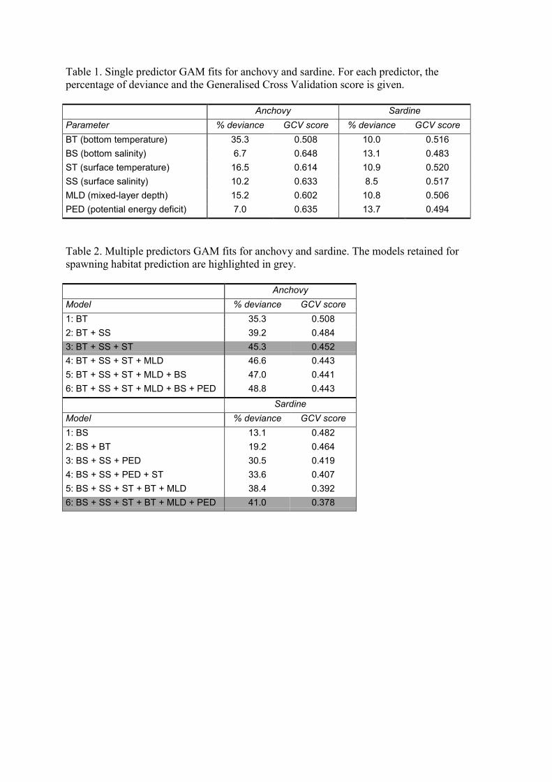
Table 1. Single predictor GAM fits for anchovy and sardine. For each predictor, thepercentage of deviance and the Generalised Cross Validation score is given.

Anchovy SardineParameter % deviance GCV score % deviance GCV scoreBT (bottom temperature) 35.3 0.508 10.0 0.516BS (bottom salinity) 6.7 0.648 13.1 0.483ST (surface temperature) 16.5 0.614 10.9 0.520SS (surface salinity) 10.2 0.633 8.5 0.517MLD (mixed-layer depth) 15.2 0.602 10.8 0.506PED (potential energy deficit) 7.0 0.635 13.7 0.494

Table 2. Multiple predictors GAM fits for anchovy and sardine. The models retained forspawning habitat prediction are highlighted in grey.

AnchovyModel % deviance GCV score1: BT 35.3 0.5082: BT + SS 39.2 0.4843: BT + SS + ST 45.3 0.4524: BT + SS + ST + MLD 46.6 0.4435: BT + SS + ST + MLD + BS 47.0 0.4416: BT + SS + ST + MLD + BS + PED 48.8 0.443

SardineModel % deviance GCV score1: BS 13.1 0.4822: BS + BT 19.2 0.4643: BS + SS + PED 30.5 0.4194: BS + SS + PED + ST 33.6 0.4075: BS + SS + ST + BT + MLD 38.4 0.3926: BS + SS + ST + BT + MLD + PED 41.0 0.378


i

Figure legends:

Fig 1. A schematic representation of the three spawning habitat components:potential, realised and successful. Potential habitat is primarily influenced bypre-spawning environmental conditions which affect adults, realised habitat isprimarily dependent on population size, structure and seasonal dynamics, andsuccessful habitat varies primarily as a function of post-spawningenvironmental conditions which will affect egg and larval survival.

Fig 2. Spatial location of hydrological stations (open circles) and CUFESsampling midpoints (dots) during the cruise PELGAS2004. The location of theLoire, Gironde and Adour river mouths are indicated as well as Brittany and"Les Landes" regions. Bathymetry for 20, 50, 100, 200, 500 and 1000misobaths is also indicated.

Fig 3. The spatial distribution of sardine (left) and anchovy (right) in 2000,2001, 2002, 2003 and 2004. Grey scale is proportional to the probability ofpresence (>1 egg per m3) of eggs.

Fig 4a. The spatial distribution of sea surface temperature (top) averaged overthe first 5 m and of sea bottom temperature (bottom) averaged over the last 5 min 2000, 2001, 2002, 2003 and 2004. If bottom depth exceeds 100m, bottomtemperature is given for 100m. Black dots indicate location of CTD stations.

Fig 4b. The spatial distribution of sea surface salinity (top) averaged over thefirst 5 m and of sea bottom salinity (bottom) averaged over the last 5 m in2000, 2001, 2002, 2003 and 2004. If bottom depth exceeds 100m, bottomsalinity is given for 100m. Black dots indicate location of CTD stations.

Fig 4c. The spatial distribution of mixed-layer depth (top) and of potentialenergy deficit (bottom) in 2000, 2001, 2002, 2003 and 2004. If bottom depthexceeds 100m, mixed-layer depth and potential energy deficit are calculatedfor the first 100 m only. Black dots indicate location of CTD stations.

Fig 5. Generalised Additive Models (GAMs) for sardine and anchovy againstbottom temperature (a), bottom salinity (b), surface temperature (c), surfacesalinity (d), mixed-layer depth (e) and potential energy deficit (f). Black thicklines indicate the value of GAMs coefficient, dotted line are the confidencelimits at P = 0.05, and the horizontal line indicates zero level.

Fig 6. Modelled potential spawning habitat of anchovy (top) and sardine(bottom) in 1999. Grey scale is proportional to egg presence probability.Probabilities are derived from modelled hydrological fields and GAMs in Fig.5.

potential

successful

realised

spawning habitat type

geographical coordinates

geo

gra

ph

ical

co

ord

inat

es

Not suitable for spawning

Suitable, but no spawning

Spawning,but no contribution to recruitment

Spawning,produces most recruits

Spawning,but no contribution to recruitment

Figure 1

Loire

Gironde

Adour

France

Spain

Figure 2

Les

lan

des

Brittany

8 6 4 2

43

44

45

46

47

48

49

�8 �6 �4 �2

43

44

45

46

47

48

49

�8 �6 �4 �2

43

44

45

46

47

48

49

�8 �6 �4 �2

43

44

45

46

47

48

49

�8 �6 �4 �2

43

44

45

46

47

48

49

Sar

dine

2000

8 6 4 2

43

44

45

46

47

48

49

2001

�8 �6 �4 �2

43

44

45

46

47

48

49

2002

�8 �6 �4 �2

43

44

45

46

47

48

49

2003

�8 �6 �4 �2

43

44

45

46

47

48

49

2004

�8 �6 �4 �2

43

44

45

46

47

48

49A

ncho

vy

0 0.1 0.2 0.3 0.4 0.5 0.6 0.7 0.8 0.9 1

Probability of egg presence

Figure 3

10

12

14

16

18

20

22

8 6 4 2

43

44

45

46

47

48

49

2000

10

12

14

16

18

20

22

�8 �6 �4 �2

43

44

45

46

47

48

49

2001

10

12

14

16

18

20

22

�8 �6 �4 �2

43

44

45

46

47

48

49

2002

10

12

14

16

18

20

22

�8 �6 �4 �2

43

44

45

46

47

48

49

2003

10

12

14

16

18

20

22

�8 �6 �4 �2

43

44

45

46

47

48

49

2004

10

11

12

13

14

15

8 6 4 2

43

44

45

46

47

48

49

2000

10

11

12

13

14

15

�8 �6 �4 �2

43

44

45

46

47

48

49

2001

10

11

12

13

14

15

�8 �6 �4 �2

43

44

45

46

47

48

49

2002

10

11

12

13

14

15

�8 �6 �4 �2

43

44

45

46

47

48

49

2003

10

11

12

13

14

15

�8 �6 �4 �2

43

44

45

46

47

48

49

2004

Surface temperature (°C)

Bottom temperature (°C)

Figure 4a

Surface salinity

Bottom salinity

30

31

32

33

34

35

36

8 6 4 2

43

44

45

46

47

48

49

2000

30

31

32

33

34

35

36

�8 �6 �4 �2

43

44

45

46

47

48

49

2001

30

31

32

33

34

35

36

�8 �6 �4 �2

43

44

45

46

47

48

49

2002

30

31

32

33

34

35

36

�8 �6 �4 �2

43

44

45

46

47

48

49

2003

30

31

32

33

34

35

36

�8 �6 �4 �2

43

44

45

46

47

48

49

2004

32

33

34

35

36

8 6 4 2

43

44

45

46

47

48

49

2000

�

32

33

34

35

36

8 �6 �4 �2

43

44

45

46

47

48

49

2001

�

32

33

34

35

36

8 �6 �4 �2

43

44

45

46

47

48

49

2002

32

33

34

35

36

�8 �6 �4 �2

43

44

45

46

47

48

49

2003

32

33

34

35

36

�8 �6 �4 �2

43

44

45

46

47

48

49

2004

Figure 4b

Mixed-layer depth (m)

Potential Energy deficit (J)

0

20

40

60

80

100

8 6 4 2

43

44

45

46

47

48

49

2000

0

20

40

60

80

100

�8 �6 �4 �2

43

44

45

46

47

48

49

2001

0

20

40

60

80

100

�8 �6 �4 �2

43

44

45

46

47

48

49

2002

0

20

40

60

80

100

�8 �6 �4 �2

43

44

45

46

47

48

49

2003

�

�

0

20

40

60

80

100

8 �6 �4 �2

43

44

45

46

47

48

49

2004

0

50

100

150

200

8 6 4 2

43

44

45

46

47

48

49

2000

0

50

100

150

200

�8 �6 �4 �2

43

44

45

46

47

48

49

2001

0

50

100

150

200

�8 �6 �4 �2

43

44

45

46

47

48

49

2002

0

50

100

150

200

�8 �6 �4 �2

43

44

45

46

47

48

49

2003

0

50

100

150

200

�8 �6 �4 �2

43

44

45

46

47

48

49

2004

Figure 4c

11 12 13 14 15

42

02

4

Bottom Temperature (°C)34.0 34.5 35.0 35.5

Bottom Salinity

12 14 16 18

42

02

4

Surface Temperature (°C)32.0 33.5 35.0

Surface Salinity

20 40 60 80

42

02

4

Mixed-layer depth (m)0 50 150


Anchovy

11 12 13 14 15

42

02

4

Bottom Temperature (°C)34.0 34.5 35.0 35.5

Bottom Salinity

12 14 16 18

42

02

4

Surface Temperature (°C)32.0 33.5 35.0

Surface Salinity

20 40 60 80

42

02

4

Mixed-layer depth (m)0 50 150


Sardine

a

fe

dc

b a

fe

dc

b

Figure 5

5 4 3 2 143

44

45

46

47

48

49

5 4 3 2 143

44

45

46

47

48

49

5 4 3 2 143

44

45

46

47

48

49

5 4 3 2 143

44

45

46

47

48

49

5 4 3 2 143

44

45

46

47

48

49

5 4 3 2 143

44

45

46

47

48

49

5 4 3 2 143

44

45

46

47

48

49

5 4 3 2 143

44

45

46

47

48

49

0 0.1 0.2 0.3 0.4 0.5 0.6 0.7 0.8 0.9 1

Probability of egg presence

24/5/199930/4/19996/4/199912/3/1999A

ncho

vyS

ardi

ne

Figure 6

potential spawning habitat of sardine (sardina pilchardus

Documents