Abstract— In this paper an algorithm is presented for the

stabilization of a non linear and multi-inputs system: a blower temperature described by a multimodel. The originality of this work lies on the fact that the applied control is quantified. In the first stage, a synthesis of a multiobserver, stabilized polyquadratically, with proper characteristic values situated in a disc inside unit circle is presented. The command law, stabilized polyquadratically, is based on the multiobserver and tracing of poles. In a second stage, the computed control can not be directly applied to the plant because of the quantification imposed by the heating resistors. To go over this problem, the variation of the ventilation’s speed can compensate for the errors of the command due to the quantification of the heated power. The choice of the optimal ventilation’s speed is based on the minimization of a criterion evaluating the distance between the measured output and the desired output.

Keywords— multimodel, multiobserver, polyquadratic D-stability, quantified commands, switching criterion

I. INTRODUCTION n article published in 1985 was written by Takagi and al [10] dealing with the possibility of describing a non

linear system by a group of aggregated linear systems opened new horizons for the command theory of this kind of systems.

The considerable progress seen during the last decades in solving linear matrix inequalities LMI, contributed to apprehend described systems by multimodel with more pertinence for the synthesis of the stabilizing command law.

Manuscript received March 3, 2007: Revised version received March 12, 2008.

E. M. is with the Electrical Engineering Department, Ecole Supérieure de Technologie et d’Informatique, 45, rue des entrepreneurs Charguia 2, Tunis Carthage, Tunisia (phone +216 22 938 887 ; fax +216 71 941 579 ; emaherzi@yahoo.fr).

M. B. is with the Electrical Engineering Department, Ecole Supérieure de Technologie et d’Informatique, 45, rue des entrepreneurs Charguia 2, Tunis Carthage, Tunisia (phone +216 98 819 453 ; fax +216 71 941 579 ; mongi.besbes@esti.rnu.tn).

M. E is with the Electrical Engineering Department, Ecole Supérieure de Technologie et d’Informatique, 45, rue des entrepreneurs Charguia 2, Tunis Carthage, Tunisia (phone +216 98 208 807 ; fax +216 71 941 579 ; mahmoud.ellouze@esti.rnu.tn).

R. M. is with the physical Department, Faculté des Sciences de Tunis, Campus Universitaire El Manar Tunis, Tunisia (phone +216 20 200 617 ; fax +216 71 941 579 ; radhi.mhiri@planet.tn).

Many works [11],[13],[22],[21]have shown the possibility of stabilizing a multimodel by quadratic approach which focuses on the use of a unique Lyapunov matrix defined positive as it guarantees the stability of each local model.

In order to reduce the conservatism of the quadratic

approach, other researchers become more interested in the construction of Parameter Dependant Lyapunov Functions [20], [4, ][19]. In this field, the polyquadratic stability concept, in the case of discrete system having variable parameters in time, is demonstrated by J. Daafouz and J. Bernussou[9].

This paper is divided into six parts. In the second part, we

start with a technical presentation of the drying system and the multimodel retained to describe the evolution of the internal temperature in relation with the heating power and the ventilation speed. Under the hypothesis of the observability of this system, the third part of this paper is interested in the polyquadratic stabilization by using a multiobserver through pole localizing. In the fourth part, the synthesis of output feedback dynamic command law is presented to guarantee the polyquadratic stability of the multimodel. The poles localization techniques are used during this synthesis. In the fifth part, an algorithm of quantified power choice and ventilation speed value is presented. In fact, the problem of the command quantification is brought about by the fact that each resistor activated or deactivated, doesn't allow the direct application of the calculated command at each discrete instant k. the choice is, then, about the nearest quantified power and an algorithm of real-time calculation which will permit to choose the adequate ventilation to compensate the mistake caused by quantification. The last part of this paper presents the obtained results through the use of an already presented algorithm in the fifth part.

II. The modeling of the drying system

A. Presentation of the blower Drying is the treatment which aims at eliminating, partly or

wholly, water from an incorporated body so as to ensure its preservation. It's an operation which is encountered in many industrial sectors (wood treatment, agro alimentary…).

The blower used in our application is like an aerothermic channel supported by 12 resistors of heating able to deliver a power of 1,5 Kw each, a central of vapor to control dampness

Polyquadratic stabilization of a multi-inputs multimodel with quantified commands

E.Maherzi, M.Besbes, M. Ellouze and R. Mhiri

A

INTERNATIONAL JOURNAL OF MATHEMATICS AND COMPUTERS IN SIMULATION

Issue 4, Volume 1, 2007 344

inside the channel and a ventilator carried by an asynchronous engine to control the emanating air during the drying operation.

The control of the heating resistors, of the central vapor and the ventilation speed is ensured by a programmable logic controller linked to a computer carrying a program of control and supervision.

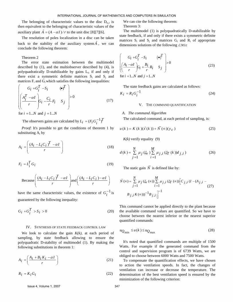
The blower is a multivariable system with the heating power, the vapor quantity and the ventilation speed like inputs and temperature, and dampness like outputs (Fig.1).

Fig 1 Inputs and outputs of the plant

We are limiting ourselves, in this paper, to control temperature by action on the heating power and ventilation speed.

B. Modeling of the blower Preliminary experiments have demonstrated that the

evolution of temperature is non linear in relation with the heating power and the ventilation speed. The idea is to apprehend the non linear behavior of this system through a group of local models either linear or affine [1]. Each local model characterizes the system's behavior in a particular functioning zone. Local models are then aggregated by specific interpolation laws [14], [11], [10], [17].

The blower, non linear discrete time system, can be represented by the following discrete multimodel

( 1) ( ) ( )( ( ), ,1 1

( ) ), ,

( ) ( ) ( ) ( ), ,1 1

N Mx k A x kj v j i T j i

j iB u k dj i j i

N My k C x kj v j i T j i

j i

μ ξ μ ξ

μ ξ μ ξ

⎧⎪ + =⎪ = =⎪⎪ + +⎨⎪⎪

=⎪⎪ = =⎩

∑ ∑

∑ ∑

(1)

Where x(k) nx1∈ℜ is the state vector, u(k) m∈ℜ is the

heating power, y(k) p∈ℜ output vector.

, ∈ℜnxnA j i , , ∈ℜnxmB j i , , ∈ℜpxnC j i and

1, ∈ℜnxd j i are respectively the state matrix, input matrix,

output matrix and a vector depending on the operating point of local model (j,i) depending on the temperature and speed ventilation. Tξ is the vector decision depending on the measurable states, temperature in this case. vξ is the vector

decision depending on the inputs of plant and the speed of ventilation.

The activating functions ( ), 1...=j Nj vμ ξ , have the

following properties:

( ) 11

0 ( ) 1 1... ,

⎧=⎪⎪

⎨ =⎪ ≤ ≤ ∀ =⎪⎩

∑N

j vi

j Nj v

μ ξ

μ ξ

(2)

These functions are known in real-time and used to

establish a command law by varying the ventilation speed. The activating functions ( ), 1... ,, =i Mj i Tμ ξ have the

following properties:

( ) 1 1... ,,1

0 ( ) 1 1... , 1... ,,

⎧= ∀ =⎪⎪

⎨ =⎪ ≤ ≤ ∀ = ∀ =⎪⎩

∑M

j Nj i Ti

i M et j Nj i T

μ ξ

μ ξ

(3)

These functions are known in real-time but can't be directly

modified by the command because they are depending on the internal non measurable states.

The number of models N and M is depending on the complexity of the non linear system, the desired precision and the structure of activating functions [2].

III. CONSTRUCTION AND STABILIZATION OF MULTIOBSERVER

A. Global control law When certain components of the state vector are non

measurable and the system is observable, it's possible to construct a multiobserver associated to a multimodel described by (4) as follows:

ˆ ˆ( 1) ( ) ( )( ( ) ( ), , ,1 1

ˆ( ( ) ( ))), , ,

ˆ ˆ( ) ( ) ( ) ( ), ,1 1

⎧⎪ + = +⎪ = =⎪⎪ + + −⎨⎪⎪

=⎪⎪ = =⎩

∑ ∑

∑ ∑

N Mx k A x k B u kj v j i T j i j i

j id L C x k x kj i j i j iN M

y k C x kj v j i T j ij i

μ ξ μ ξ

μ ξ μ ξ

(4)

Where ˆ ˆ( ) and ( )x k y k design respectively the estimation

produced by the observer of the state vector and the estimation of the output; Lj,i design the gain of the observation matrix associated to the model (j,i). We define the state error observation as follows:

ˆ( ) ( ) ( )= −k x k x kε (5)

The command u(k), in case of dynamic output feedback,

Blower

Heat power

Vapor quantity

Speed ventilation

Temperature

Humidity Blower

INTERNATIONAL JOURNAL OF MATHEMATICS AND COMPUTERS IN SIMULATION

Issue 4, Volume 1, 2007 345

based on the multiobserver (4), is :

ˆ( ) ( ) ( ) ( )( )= + ∞u k K k x k N yc (6)

Taking into account (4), (5) and (6) the augmented equation of the system is then:

( 1) ( ) ( )(( ) ( ), , , ,1 1

( ) ), , ,

( 1) ( ) ( )( ) ( ), , , ,1 1

⎧⎪ + = +⎪ = =⎪⎪ − +⎨⎪⎪

+ = −⎪⎪ = =⎩

∑ ∑

∑ ∑

N Mx k A B K x kj v j i T j i j i j i

i iB K k dj i j i j i

N Mk A L C kj v j i j i j i j i

i i

μ ξ μ ξ

ε

ε μ ξ μ ξ ε

(7)

Equality (7) can be written also as follows:

( 1)

( ) ( ),( 1) 1 1

( ), , , , , ,0 ( ) 0, , ,

+⎛ ⎞=⎜ ⎟+⎝ ⎠ = =

⎛ + −⎛ ⎞ ⎞⎛ ⎞⎛ ⎞⎜⎜ ⎟ ⎟+⎜ ⎟⎜ ⎟ ⎜ ⎟⎟⎜ ⎟⎜ − ⎝ ⎠ ⎝ ⎠⎠⎝ ⎠⎝

∑ ∑N Mx k

j v j i Tk j i

A B K B K dx kj i j i j i j i j i j iA L C kj i j i j i

μ ξ μ ξε

ε

(8)

Since the matrix of augmented system is a superior

triangular, the instantaneous characteristics values of augmented system are those of matrices

( ) ( )( ), , , ,1 1

+= =

∑ ∑N M

A B Kj v j i T j i j i j ij i

μ ξ μ ξ and

( ) ( )( ), , , ,1 1

−= =

∑ ∑N M

A L Cj v j i T j i j i j ij i

μ ξ μ ξ .

It's important to notice that the calculation of the gains K(k) and L(k) poses on the use of following relations:

( ) ( ) ( ), , , , ,1 1

== =∑ ∑M M

B K k B Kj i T j i j i T j i j ii i

μ ξ μ ξ (9)

( ) ( ) ( ), , , , ,1 1

== =∑ ∑M M

L k C L Cj i T j i j i T j i j ii i

μ ξ μ ξ (10)

B. Stabilization of the multiobserver 1) Polyquadratic Stabilization

In this part we start with citing the theorem of Daafouz and Bernussou [9] about the polyquadratic stability of the uncertain dynamic system.

An uncertain dynamic system can be described as follows:

( 1) ( ( )) ( )+ =x k A k x kξ (11)

With ∈ℜnx is the state vector, ∈ Ξ ⊂ ℜpξ is unknown parameter, time variable but bounded. The dynamic matrix A is written as follows:

( ( )) ( ) ,1

( ) 0, ( ) 1.1

==

≥ ==

∑

∑

NA k k Ai i

iN

k ki ii

ξ ξ

ξ ξ

(12)

Theorem 1 (Daafouz and Bernussou, 2001): There exists a Lyapunov function ,with a polytopic

structure, whose difference is negative definite proving asymptotic stability of the system (11) if and only if there exist N symmetric matrices S1…SN and N matrices G1...GN satisfying :

0

1,..., 1,..., .

⎛ ⎞+ −⎜ ⎟ >⎜ ⎟⎝ ⎠∀ = ∀ =

T T TG G S G Ai ii i iA G Si i j

i N et j N

(13)

The PDLF is given by :

1( ) ( )1

−==∑N

P k k Si ii

ξ (14)

2) Poles Localization In case of multimodel where state matrix is variable in each

period of sampling, the use of command by poles localization guarantees the desired performances of different controllers [21] and observers [3].

An effective way of determining the dynamic characteristics of a system is to localize poles inside a disc Dα,r contained in the unit circle, α is the center of the disc and r its ray [5], which is equivalent to the fact of placing characteristic values of auxiliary system ( ) /−A I rα in the unit circle [5].

Definition 1: (Granado, 2004) A matrix A is known as D-stable if his characteristic values

belong to the disc D(α,r) Lemma1: (Furuta et Kim 1987) :A matrix A is D-stable if

and only if ∀ Q = QT >0 the following equality:

( ) ( ² ²) 0− + + − + =T TA PA A P PA r P Qα α (15)

has a symmetric definite positive matrix solution P. This is equivalent to test if the following inequality has a

definite positive solution [5] [12]:

0− −⎛ ⎞ ⎛ ⎞ − <⎜ ⎟ ⎜ ⎟⎝ ⎠ ⎝ ⎠

TA I A IP Pr rα α (16)

INTERNATIONAL JOURNAL OF MATHEMATICS AND COMPUTERS IN SIMULATION

Issue 4, Volume 1, 2007 346

The belonging of characteristic values to the disc Dα,r is then equivalent to the belonging of characteristic values of the auxiliary plant ( ) /= −A A I rα to the unit disc [8][7][6].

The resolution of poles localization in a disc can be taken back to the stability of the auxiliary system A , we can conclude the following theorem:

Theorem 2 The error state estimation between the multimodel

described by (1), and the multiobserver described by (4), is polyquadratically D-stabilizable by gains Li, if and only if there exist a symmetric definite matrices Si and Sj and matrices Fi and Gi which satisfies the following inequalities:

( )

0

for 1... and 1...

⎛ ⎞+ − •⎜ ⎟⎜ ⎟⎛ ⎞ >−⎜ ⎟⎜ ⎟ −⎜ ⎟⎜ ⎟⎜ ⎟⎜ ⎟⎝ ⎠⎝ ⎠

= =

T TG G Si iiTA I Ci iG F Si i jr r

i N j N

α (17)

1The observers gains are calculated by ( )−= TL F Gi i i

Proof: It's possible to get the conditions of theorem 1 by substituting Ai by

( )⎛ ⎞− −⎜ ⎟=⎜ ⎟⎝ ⎠

TA L C Ii i iAi rα

(18)

= TF L Gi ii (19)

Because( )⎛ ⎞− −⎜ ⎟

⎜ ⎟⎝ ⎠

TA L C Ii i ir

αand

( )− −⎛ ⎞⎜ ⎟⎝ ⎠

A L C Ii i ir

α

have the same characteristic values, the existence of 1−Gi is

guaranteed by the following inequality:

0+ > >TG G Si ii (20)

IV. SYNTHESIS OF STATE FEEDBACK CONTROL LAW We look to calculate the gain K(k), at each period of

sampling, by state feedback allowing to ensure the polyquadratic D-stability of multimodel (1). By making the following substitutions in theorem 1:

+ −⎛ ⎞= ⎜ ⎟⎝ ⎠

A B K Ii i iAi rα

(21)

=R K Gi i i (22)

We can cite the following theorem: Theorem 3: The multimodel (1) is polyquadratically D-stabilizable by

state feedback, if and only if there exists a symmetric definite matrices Si and Sj and matrices Gi and Ri of appropriate dimensions solutions of the following LMIs:

( )0

for 1... and 1...

⎛ ⎞+ − •⎜ ⎟⎜ ⎟ >−⎛ ⎞⎜ ⎟+⎜ ⎟⎜ ⎟⎝ ⎠⎝ ⎠

= =

TTG G Si iiA I Bi iG R Si i jr ri N j N

α (23)

The state feedback gains are calculated as follows:

1−=K R Gi i i (24)

V. THE COMMAND QUANTIFICATION

A. The command Algorithm The calculated command, at each period of sampling, is:

ˆ( ) ( )( ( )) ( )( )= + ∞u k K k x k N y c (25)

K(k) verify equality (9)

( ) ( ) ( ( )) ), ,1 1

== =

∑ ∑N M

d k k dj v j i T j ij i

μ ξ μ ξ (26)

The static gain N is defined like by:

( ) ( ( )) ( ( )) ( (, , ,1 1

11( ))), ,

⎡∞ = ∞ ∞ − −⎣= =

−− ⎤∞ ⎥⎦

∑ ∑N M

N C I Aj v j i T j i j ij i

B K Bj i j i

μ ξ μ ξ(27)

This command cannot be applied directly to the plant because the available command values are quantified. So we have to choose between the nearest inferior or the nearest superior quantified commands:

min max( )≤ ≤u u k uQ Q (28)

It's noted that quantified commands are multiple of 1500

Watts. For example if the generated command from the control and supervision program is of 6739 Watts, we are obliged to choose between 6000 Watts and 7500 Watts.

To compensate the quantification effects, we have chosen to action the ventilation speeds. In fact, the changes of ventilation can increase or decrease the temperature. The determination of the best ventilation speed is ensured by the minimization of the following criterion:

INTERNATIONAL JOURNAL OF MATHEMATICS AND COMPUTERS IN SIMULATION

Issue 4, Volume 1, 2007 347

( , ) ( , )ˆ ˆ( ) ( ( 1) ) ( ( 1) )( , ) = + − + −

u uv vTJ k y k y I y k yv u e c p e cξ ξ

(29) with v: speed of ventilation obtained from the decision

vector vξ .

{ }min max,=u u uQ Q (30)

( , )ˆ ( 1)+uvy ke ξ

is the estimation of the output, at the

discrete time k+1, it depends on the inputs speed ventilation v and the command u:

( , ) ( , )ˆ ˆ( 1) ( ) ( ) ( 1), ,

1 1+ = +

= =∑ ∑u uv v

N My k C x ke j v j i T j i e

j iξ ξ

μ ξ μ ξ (31)

( , )ˆ ( 1)+

uvx ke ξ

is the estimated state , at the discrete time

k+1, it depends on the inputs speed ventilation v and the command u:

( , )ˆ ˆ( 1) ( ) ( )( ( ), ,

1 1ˆ( ) ( ( ) ( ))), , , ,

+ == =

+ + + −

∑ ∑uv

N Mx k A x ke j v j i T j i

j iB u k d L C x k x kj i j i j i j i

ξμ ξ μ ξ

(32)

The control algorithm is then: step 0 : Initialisation • calculate the gains Ki,j and Li,j using LMIs (17) and (24) • apply the maximum value of power heat • apply the maximum value of speed ventilation step 1 : Determination of the actual model and computing of u(k) • measure the internal temperature of the blower • evaluate the decision vector ( )kTξ • deduce A, B, C and d • calculate L(k ) using (10) • deduce ˆ ( )x k using (4) • calculate K(k) using (9) • deduce u(k) using (25) step 2 : quantification problem resolution • calculate

min maxu et uQ Q

• calculate ( , )

ˆ ( 1)+uv

x ke ξ using (32)

• calculate ( , )

ˆ ( 1)+uv

y ke ξ using (31)

• calculate ( )( , )J kv u using(29)

• deduce and apply ( ),

min( ( , ))⎧ ⎫⎪ ⎪= ⎨ ⎬⎪ ⎪⎩ ⎭v

u k uu

J u vξ

• deduce and apply ( ),

min( ( , ))⎧ ⎫⎪ ⎪= ⎨ ⎬⎪ ⎪⎩ ⎭v

kv vu

J u vξ ξξ

• back to step 1

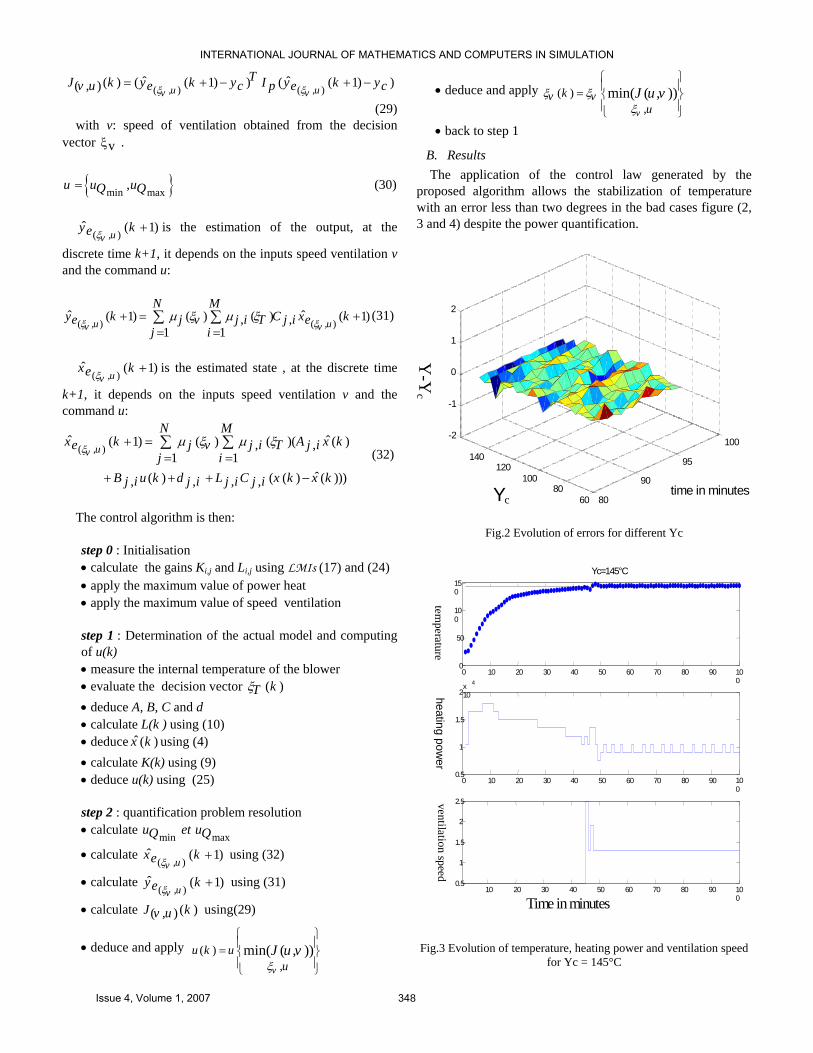
B. Results The application of the control law generated by the

proposed algorithm allows the stabilization of temperature with an error less than two degrees in the bad cases figure (2, 3 and 4) despite the power quantification.

80 90

95

100

60 80100

120140

-2

-1

0

1

2

time in minutesYc

Y-Y

c

Fig.2 Evolution of errors for different Yc

0 10 20 30 40 50 60 70 80 90 100

0

50

100

150

temperature

Yc=145°C

0 10 20 30 40 50 60 70 80 90 100

0.5

1

1.5

2x 10

4

heating power

10 20 30 40 50 60 70 80 90 100

0.5

1

1.5

2

2.5

Time in minutes

ventilation speed

Fig.3 Evolution of temperature, heating power and ventilation speed

for Yc = 145°C

INTERNATIONAL JOURNAL OF MATHEMATICS AND COMPUTERS IN SIMULATION

Issue 4, Volume 1, 2007 348

VI. CONCLUSION In this paper we have presented a modelisation of a

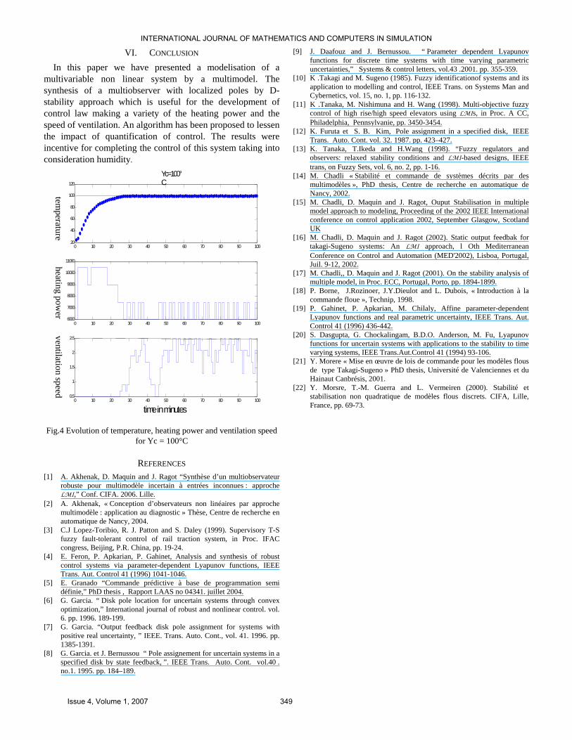
multivariable non linear system by a multimodel. The synthesis of a multiobserver with localized poles by D-stability approach which is useful for the development of control law making a variety of the heating power and the speed of ventilation. An algorithm has been proposed to lessen the impact of quantification of control. The results were incentive for completing the control of this system taking into consideration humidity.

0 10 20 30 40 50 60 70 80 90 10020 40 60 80 100 120

temperature

0 10 20 30 40 50 60 70 80 90 1006000 7000 8000 9000 10000 11000 heating pow

er

0 10 20 30 40 50 60 70 80 90 1000.5 1

1.5 2

2.5

time in minutes

ventilation speed

Yc=100°C

Fig.4 Evolution of temperature, heating power and ventilation speed for Yc = 100°C

REFERENCES [1] A. Akhenak, D. Maquin and J. Ragot “Synthèse d’un multiobservateur

robuste pour multimodèle incertain à entrées inconnues : approche LMI,” Conf. CIFA. 2006. Lille.

[2] A. Akhenak, « Conception d’observateurs non linéaires par approche multimodèle : application au diagnostic » Thèse, Centre de recherche en automatique de Nancy, 2004.

[3] C.J Lopez-Toribio, R. J. Patton and S. Daley (1999). Supervisory T-S fuzzy fault-tolerant control of rail traction system, in Proc. IFAC congress, Beijing, P.R. China, pp. 19-24.

[4] E. Feron, P. Apkarian, P. Gahinet, Analysis and synthesis of robust control systems via parameter-dependent Lyapunov functions, IEEE Trans. Aut. Control 41 (1996) 1041-1046.

[5] E. Granado “Commande prédictive à base de programmation semi définie,” PhD thesis , Rapport LAAS no 04341. juillet 2004.

[6] G. Garcia. “ Disk pole location for uncertain systems through convex optimization,” International journal of robust and nonlinear control. vol. 6. pp. 1996. 189-199.

[7] G. Garcia. “Output feedback disk pole assignment for systems with positive real uncertainty, ” IEEE. Trans. Auto. Cont., vol. 41. 1996. pp. 1385-1391.

[8] G. Garcia. et J. Bernussou “ Pole assignement for uncertain systems in a specified disk by state feedback, ”. IEEE Trans. Auto. Cont. vol.40 . no.1. 1995. pp. 184–189.

[9] J. Daafouz and J. Bernussou. “ Parameter dependent Lyapunov functions for discrete time systems with time varying parametric uncertainties,” Systems & control letters, vol.43 .2001. pp. 355-359.

[10] K .Takagi and M. Sugeno (1985). Fuzzy identificationof systems and its application to modelling and control, IEEE Trans. on Systems Man and Cybernetics, vol. 15, no. 1, pp. 116-132.

[11] K .Tanaka, M. Nishimuna and H. Wang (1998). Multi-objective fuzzy control of high rise/high speed elevators using LMIs, in Proc. A CC, Philadelphia, Pennsylvanie, pp. 3450-3454.

[12] K. Furuta et S. B. Kim, Pole assignment in a specified disk, IEEE Trans. Auto. Cont. vol. 32. 1987. pp. 423–427.

[13] K. Tanaka, T.Ikeda and H.Wang (1998). “Fuzzy regulators and observers: relaxed stability conditions and LMI-based designs, IEEE trans, on Fuzzy Sets, vol. 6, no. 2, pp. 1-16.

[14] M. Chadli « Stabilité et commande de systèmes décrits par des multimodèles », PhD thesis, Centre de recherche en automatique de Nancy, 2002.

[15] M. Chadli, D. Maquin and J. Ragot, Ouput Stabilisation in multiple model approach to modeling, Proceeding of the 2002 IEEE International conference on control application 2002, September Glasgow, Scotland UK

[16] M. Chadli, D. Maquin and J. Ragot (2002). Static output feedbak for takagi-Sugeno systems: An LMI approach, l Oth Mediterranean Conference on Control and Automation (MED'2002), Lisboa, Portugal, Juil. 9-12, 2002.

[17] M. Chadli,, D. Maquin and J. Ragot (2001). On the stability analysis of multiple model, in Proc. ECC, Portugal, Porto, pp. 1894-1899.

[18] P. Borne, J.Rozinoer, J.Y.Dieulot and L. Dubois, « Introduction à la commande floue », Technip, 1998.

[19] P. Gahinet, P. Apkarian, M. Chilaly, Affine parameter-dependent Lyapunov functions and real parametric uncertainty, IEEE Trans. Aut. Control 41 (1996) 436-442.

[20] S. Dasgupta, G. Chockalingam, B.D.O. Anderson, M. Fu, Lyapunov functions for uncertain systems with applications to the stability to time varying systems, IEEE Trans.Aut.Control 41 (1994) 93-106.

[21] Y. Morere « Mise en œuvre de lois de commande pour les modèles flous de type Takagi-Sugeno » PhD thesis, Université de Valenciennes et du Hainaut Canbrésis, 2001.

[22] Y. Morsre, T.-M. Guerra and L. Vermeiren (2000). Stabilité et stabilisation non quadratique de modèles flous discrets. CIFA, Lille, France, pp. 69-73.

INTERNATIONAL JOURNAL OF MATHEMATICS AND COMPUTERS IN SIMULATION

Issue 4, Volume 1, 2007 349