Technical note: PMR – a proxy metric to assess hydrological modelrobustness in a changing climatePaul Royer-Gaspard1, Vazken Andréassian1, and Guillaume Thirel1

1Université Paris-Saclay, INRAE, HYCAR Research Unit, 92761 Antony, France.

Correspondence: Vazken Andréassian (vazken.andreassian@inrae.fr)

Abstract. The ability of hydrological models to perform in climatic conditions different from those encountered in calibration

is crucial to ensure a reliable assessment of the impact of climate change on river regimes and water availability. However, most

evaluation studies based on the Differential Split-Sample Test (DSST) endorsed the consensus that rainfall-runoff models lack

climatic robustness. Models applied under climatologically different conditions typically exhibit substantial errors on stream-

flow volumes. In this technical note, we propose a new performance metric to evaluate model robustness without applying the5

DSST and can be performed with a single hydrological model calibration. The Proxy for Model Robustness (PMR) is based

on the systematic computation of model error on sliding sub-periods of the whole streamflow time series. We demonstrate

that the PMR metric shows patterns similar to those obtained with the DSST for a conceptual model on a set of 377 French

catchments. An analysis of sensitivity to the length of the sub-periods shows that this length influences the values of the PMR

and its equivalency with DSST biases. We recommend a range of a few years for the choice of sub-period lengths, although this10

should be context-dependent. Our work makes it possible to evaluate the temporal transferability of any hydrological model,

including uncalibrated models, at a very low computational cost.

1 Introduction

In the context of climate change, quantifying the performance of the models used for assessing the impact of a changing climate

is essential for informing model selection and estimating uncertainty. Assessing the impact of a changing climate typically in-15

volves a modeling chain ranging from general circulation models to impact models such as catchment hydrological models

(Clark et al., 2016). It is now acknowledged that the contribution of hydrological model uncertainty to the total uncertainty of

projections may be significant and should be addressed along with other sources of uncertainty (e.g. Hagemann et al., 2013;

Schewe et al., 2014; Vidal et al., 2016; Melsen et al., 2018). A key issue in the reduction of hydrological model uncertainty

is the assessment of robustness to climatic changes, i.e., their ability to perform in climatic conditions that differ from those20

encountered in calibration.

Advocating that hydrological models needed to be tested under conditions that would “represent a situation similar to which the

data are to be generated,” Klemeš (1986) suggested a series of tests to evaluate the robustness of hydrological models. Among

these testing procedures, the most popular scheme to assess model robustness to varying climatic conditions is the Differential

Split-Sample Test (DSST). The DSST consists in a calibration-evaluation exercise in two periods of the available time series25

1

chosen to be as climatically different as possible. Variants of the DSST have also been proposed for specific purposes, such

as the Generalized Split-Sample Test (Coron et al., 2012), which consists in a systematic calibration-evaluation experiment on

every pair of independent periods that one can possibly define. However, these variants all rely on the same principles as the

DSST (e.g. Dakhlaoui et al., 2019).

Many studies report poor model simulations resulting from the application of the DSST in various modeling contexts (e.g.30

Thirel et al., 2015). Among the deficiencies observed in the tested models, a common feature is their tendency to produce

biased streamflow simulations in evaluation conditions (e.g. Vaze et al., 2010; Merz et al., 2011; Broderick et al., 2016;

Dakhlaoui et al., 2017; Mathevet et al., 2020). Although changes in catchment temperature and/or precipitation are usually

associated with volume errors, these errors vary across the tested models and catchments (e.g. Vaze et al., 2010; Broderick et

al., 2016; Dakhlaoui et al., 2017). The dire need to improve hydrological models is widely recognized and is considered as one35

of the 23 unsolved problems in modern hydrology (Blöschl et al., 2019, UPH n°19). However, to improve models we first need

a good diagnostic method, and the design of alternatives to the DSST for the evaluation of model robustness could contribute

to these advancements.

The first shortcoming of the DSST is its limited application regarding a particular category of hydrological models. Indeed,

Refsgaard et al. (2014) pointed out that split-sample procedures cannot be applied to models that are not calibrated. The eval-40

uation of such models is usually performed by testing their spatial transferability with data from proxy sites. It is therefore

difficult to compare the robustness of highly complex hydrological models to simpler models such as the ones typically tested

in the aforementioned DSST studies. A further limitation is the necessity to determine a set of climatic variables to inform the

definition of different calibration and evaluation periods. This is of course highly relevant in contexts where the direction of

future changes is unambiguously predicted. In other situations, however, robustness assessment would benefit from evaluating45

the model on a wider spectrum of hydro-climatic changes. Variants of the DSST, such as the Generalized Split-Sample test,

may circumvent this problem, but at a high computational cost that not all modelers can afford (Coron et al., 2012).

This technical note presents and assesses a way to quantify model robustness as a mathematical performance criterion com-

puted without splitting time series into calibration and evaluation periods. This criterion is conceived to be a proxy for model

robustness (PMR), i.e. to reproduce the hydrological model average error as obtained by applying the DSST. It is based on50

the computation of interannual model bias derived from graphical considerations in the work of Coron et al. (2014). In order

to be reliable, the PMR must indicate typical model biases as obtained in DSST on independent evaluation periods. It should

also help to identify catchments where a model lacks robustness. We summarize the important aspects that we discuss in the

following with two research questions:

– Does the PMR faithfully relate to model robustness as assessed in DSST experiments?55

– How do computation choices (e.g. sub-period length, sub-period weight) affect the results obtained when applying the

PMR?

It is worth noting that hydrological model robustness is here considered especially through the prism of model bias. Given that

the biased simulations are one the most common outcome of the previous works about model robustness, we considered that

2

model bias was an adequate metric as a first approach. Of course, model robustness relates to the stability of model performance60

in general, and thus to every possible metrics assessing model skills. Hence, the PMR as presented here should be considered

as a satisfactory proxy for model robustness as estimated using the DSST rather that the proxy for model robustness.

The first question will be addressed by comparing the metric with model bias as determined by in the DSST for a conceptual

model across a large set of French catchments. The underpinning mathematical choices will be discussed in a sensitivity

analysis comparing the metric and the results obtained by applying the DSST. The description of the PMR is given in Section 2.65

The hydrological model and the data are presented in Section 3. The reliability of the metric is assessed in Section 4, and the

opportunities the metric offers for model evaluation as well as some inherent computation choices are discussed in Section 5

and in Appendix B.

2 Description of the Proxy for Model Robustness

2.1 Building the “moving bias curve”70

Hydrological model robustness to climate change lies in the model’s ability to perform well under different climatic condi-

tions without parameters being recalibrated to match the changes in the precipitation–streamflow relationship. Performance is

deemed “robust” if it is minimally sensitive to the characteristics of the calibration and evaluation periods. For instance, if a

model calibrated during wet years and validated during dry years exhibits similar validation bias than the same model cali-

brated during dry years and validated during wet years, then it would be deemed robust to changes in climate. A robust model75

should thus simulate streamflow volumes for any type of climatic conditions experienced by a catchment with a stable bias

(of course, the lower the bias, the better). For example, if these two model configurations both had a percent bias of 20%, the

model is robust to changes in climate, even if not particularly accurate. If one model configuration had a percent bias of 20%

in the validation period and one of -20%, then the model is not robust — it exhibits strong sensitivity to climate conditions. It

should be noted that a model may lack of robustness while providing accurate (i.e. unbiased) estimation of average streamflow80

volumes on a long period of time.

Coron et al. (2014) suggested a simple way to visualize model robustness by computing the bias of a model simulation on

sliding sub-periods of the available time series (Figure 1). The curve of model bias on the moving sub-periods, named here

the “moving bias curve,” indicates the temporal evolution of model volumetric errors. Since a robust model should perform

similarly well whatever the considered sub-period, the flatter the moving bias curve, the more robust a model. Coron et al.85

(2014) showed that hydrological models would typically not have the ability to flatten their associated moving bias curve. The

authors indeed calibrated model parameters on each sub-period of the data and plotted all the produced moving bias curves on

the same graph. One of the main conclusions of their study was that the obtained moving bias curves were all almost parallel

and that calibration conditions influenced more the vertical positioning of the curves rather than their shape. This observation

was true for models of different complexities across the small set of catchments used in that study. The phenomenon described90

by Coron et al. (2014) is illustrated in Figure 2.

The moving bias curve obtained with the model calibrated on the blue sub-period (1984–1988, coldest sub-period of the time

3

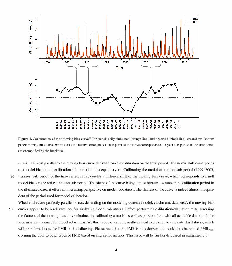
Figure 1. Construction of the “moving bias curve.” Top panel: daily simulated (orange line) and observed (black line) streamflow. Bottom

panel: moving bias curve expressed as the relative error (in %); each point of the curve corresponds to a 5-year sub-period of the time series

(as exemplified by the brackets).

series) is almost parallel to the moving bias curve derived from the calibration on the total period. The y-axis shift corresponds

to a model bias on the calibration sub-period almost equal to zero. Calibrating the model on another sub-period (1999–2003,

warmest sub-period of the time series, in red) yields a different shift of the moving bias curve, which corresponds to a null95

model bias on the red calibration sub-period. The shape of the curve being almost identical whatever the calibration period in

the illustrated case, it offers an interesting perspective on model robustness. The flatness of the curve is indeed almost indepen-

dent of the period used for model calibration.

Whether they are perfectly parallel or not, depending on the modeling context (model, catchment, data, etc.), the moving bias

curves appear to be a relevant tool for analyzing model robustness. Before performing calibration-evaluation tests, assessing100

the flatness of the moving bias curve obtained by calibrating a model as well as possible (i.e., with all available data) could be

seen as a first estimate for model robustness. We thus propose a simple mathematical expression to calculate this flatness, which

will be referred to as the PMR in the following. Please note that the PMR is bias-derived and could thus be named PMRbias,

opening the door to other types of PMR based on alternative metrics. This issue will be further discussed in paragraph 5.3.

4

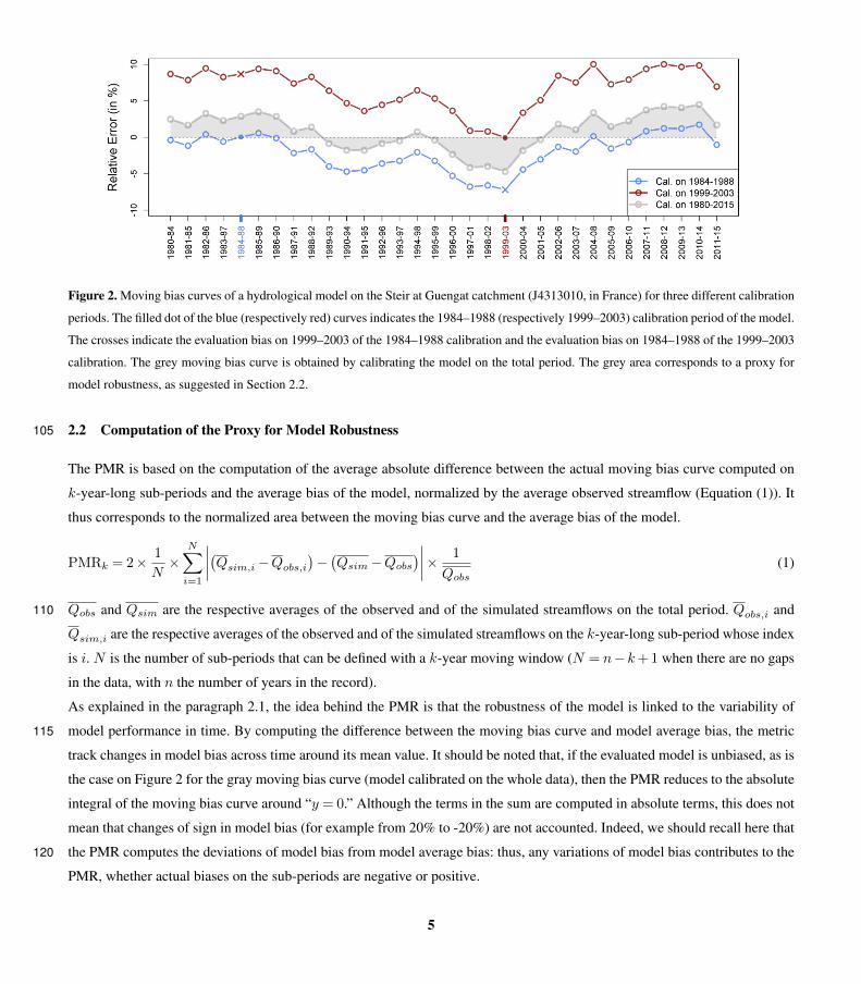
Figure 2. Moving bias curves of a hydrological model on the Steir at Guengat catchment (J4313010, in France) for three different calibration

periods. The filled dot of the blue (respectively red) curves indicates the 1984–1988 (respectively 1999–2003) calibration period of the model.

The crosses indicate the evaluation bias on 1999–2003 of the 1984–1988 calibration and the evaluation bias on 1984–1988 of the 1999–2003

calibration. The grey moving bias curve is obtained by calibrating the model on the total period. The grey area corresponds to a proxy for

model robustness, as suggested in Section 2.2.

2.2 Computation of the Proxy for Model Robustness105

The PMR is based on the computation of the average absolute difference between the actual moving bias curve computed on

k-year-long sub-periods and the average bias of the model, normalized by the average observed streamflow (Equation (1)). It

thus corresponds to the normalized area between the moving bias curve and the average bias of the model.

PMRk = 2× 1

N×

N∑i=1

∣∣∣∣(Qsim,i −Qobs,i

)−(Qsim −Qobs

)∣∣∣∣× 1

Qobs

(1)

Qobs and Qsim are the respective averages of the observed and of the simulated streamflows on the total period. Qobs,i and110

Qsim,i are the respective averages of the observed and of the simulated streamflows on the k-year-long sub-period whose index

is i. N is the number of sub-periods that can be defined with a k-year moving window (N = n−k+ 1 when there are no gaps

in the data, with n the number of years in the record).

As explained in the paragraph 2.1, the idea behind the PMR is that the robustness of the model is linked to the variability of

model performance in time. By computing the difference between the moving bias curve and model average bias, the metric115

track changes in model bias across time around its mean value. It should be noted that, if the evaluated model is unbiased, as is

the case on Figure 2 for the gray moving bias curve (model calibrated on the whole data), then the PMR reduces to the absolute

integral of the moving bias curve around “y = 0.” Although the terms in the sum are computed in absolute terms, this does not

mean that changes of sign in model bias (for example from 20% to -20%) are not accounted. Indeed, we should recall here that

the PMR computes the deviations of model bias from model average bias: thus, any variations of model bias contributes to the120

PMR, whether actual biases on the sub-periods are negative or positive.

5

In order to compare the PMR with model biases in DSST, we included multiplied by 2 in the computation of the PMR, in order

to compensate the smoothing effect of comparing model biases on sub-periods to the average model bias (see for example

the gaps between the red and blue moving bias curves on Figure 2, compared to accounted deviations from the gray moving

bias curve). A normalization by the average observed streamflow instead of the average streamflow of each sub-period was125

proposed in order to reduce the weight of very dry years. It also avoids dealing with zeros in the denominator in intermittent

catchments. This choice is further discussed in Appendix B.

In the following, sub-period length has been set to k = 5 years. The choice of the sub-period length in the computation of the

PMR is discussed in paragraph 4.3.

3 Material and methods130

3.1 Dataset

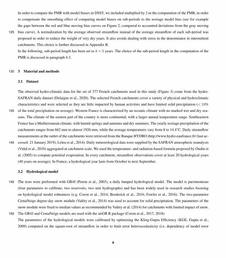
The observed hydro-climatic data for the set of 377 French catchments used in this study (Figure 3) come from the hydro-

SAFRAN daily dataset (Delaigue et al., 2020). The selected French catchments cover a variety of physical and hydroclimatic

characteristics and were selected as they are little impacted by human activities and have limited solid precipitation (< 10%

of the total precipitation on average). Western France is characterized by an oceanic climate with no marked wet and dry sea-135

sons. The climate of the eastern part of the country is more continental, with a larger annual temperature range. Southeastern

France has a Mediterranean climate, with humid springs and autumns and dry summers. The yearly average precipitation of the

catchments ranges from 662 mm to almost 1926 mm, while the average temperatures vary from 8 to 14.4°C. Daily streamflow

measurements at the outlet of the catchments were retrieved from the Banque HYDRO (http://www.hydro.eaufrance.fr/ (last ac-

cessed: 21 January 2019), Leleu et al., 2014). Daily meteorological data were supplied by the SAFRAN atmospheric reanalysis140

(Vidal et al., 2010) aggregated at catchment scale. We used the temperature- and radiation-based formula proposed by Oudin et

al. (2005) to compute potential evaporation. In every catchment, streamflow observations cover at least 20 hydrological years

(40 years on average). In France, a hydrological year lasts from October to next September.

3.2 Hydrological model

The tests were performed with GR4J (Perrin et al., 2003), a daily lumped hydrological model. The model is parsimonious145

(four parameters to calibrate, two reservoirs, two unit hydrographs) and has been widely used in research studies focusing

on hydrological model robustness (e.g. Coron et al., 2014; Broderick et al., 2016; Fowler et al., 2016). The two-parameter

CemaNeige degree-day snow module (Valéry et al., 2014) was used to account for solid precipitation. The parameters of the

snow module were fixed to median values as recommended by Valéry et al. (2014) for catchments with limited impact of snow.

The GR4J and CemaNeige models are used with the airGR R package (Coron et al., 2017, 2018).150

The parameters of the hydrological models were calibrated by optimizing the Kling-Gupta Efficiency (KGE, Gupta et al.,

2009) computed on the square-root of streamflow in order to limit error heteroscedasticity (i.e. dependency of model error

6

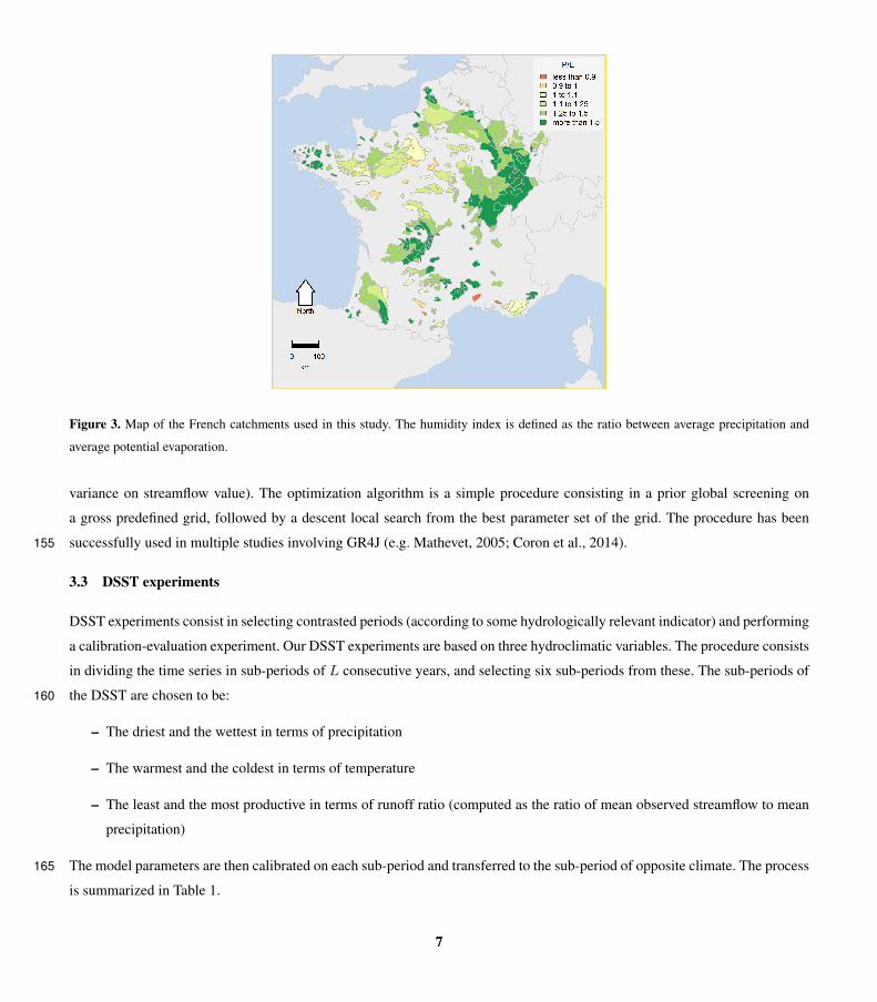
Figure 3. Map of the French catchments used in this study. The humidity index is defined as the ratio between average precipitation and

average potential evaporation.

variance on streamflow value). The optimization algorithm is a simple procedure consisting in a prior global screening on

a gross predefined grid, followed by a descent local search from the best parameter set of the grid. The procedure has been

successfully used in multiple studies involving GR4J (e.g. Mathevet, 2005; Coron et al., 2014).155

3.3 DSST experiments

DSST experiments consist in selecting contrasted periods (according to some hydrologically relevant indicator) and performing

a calibration-evaluation experiment. Our DSST experiments are based on three hydroclimatic variables. The procedure consists

in dividing the time series in sub-periods of L consecutive years, and selecting six sub-periods from these. The sub-periods of

the DSST are chosen to be:160

– The driest and the wettest in terms of precipitation

– The warmest and the coldest in terms of temperature

– The least and the most productive in terms of runoff ratio (computed as the ratio of mean observed streamflow to mean

precipitation)

The model parameters are then calibrated on each sub-period and transferred to the sub-period of opposite climate. The process165

is summarized in Table 1.

7

Table 1. Summary of the different setups of the Differential Split-Sample Test. Q̄, P̄ and T̄ respectively stand for average observed stream-

flow, precipitation and temperature computed on the sub-periods.

Name of the DSST setup

“dry” “humid” “warm” “cold” “unproductive” “productive”

Calibration min P̄ max P̄ max T̄ min T̄ min Q̄/P̄ max Q̄/P̄

Evaluation max P̄ min P̄ min T̄ max T̄ max Q̄/P̄ min Q̄/P̄

The runoff ratio was preferred to the humidity index since the latter is highly correlated to average precipitation in France

and would therefore be redundant with DSST experiments based on precipitation. Since runoff ratio is computed from average

streamflow, it cannot be used for predictive purposes of model biases in future climate conditions. However, it estimates how

catchments respond to precipitation forcings. Its use in the DSST may thus indicate how well a model is able to represent170

variations in catchment response to climatic conditions.

The sub-period length for the DSST experiments has been fixed at L = 5 years, so as to match the length of the sub-period

involved in the computation of the PMR. The length of sub-periods used in the computation of the PMR is discussed in

Section 5. The length of the sub-periods used for the DSST are discussed in paragraph 4.3. We remind the reader that the

PMR is computed from model simulations obtained by calibrating the model on the whole time series, while the DSST results175

are obtained through calibration evaluation on sub-periods of the time series. It should also be mentioned that model biases

obtained in DSST were calculated with respect to model bias in calibration so that they address the stability of bias, and thus

could be compared to PMR values, as follows:

Absolute Model Bias on subperiod b (in %) =

∣∣∣∣∣Qsim,b −Qobs,b

Qobs

−Qsim,a −Qobs,a

Qobs

∣∣∣∣∣ (2)

The index a indicates the calibration period (i.e. the dry period when validating on the humid period, etc.). Please note that in180

the case of GR4J, biases in calibration are usually very close to zero because the model is calibrated by optimizing the KGE,

which explicitly target model bias, and because GR4J has the ability to correct water balance with the free parameters govern-

ing intercatchment groundwater exchange. Therefore, the term on the right of the soustraction sign is negligible in practice. It

should also be noted that since the PMR is positive by definition, model biases were computed in absolute values. A straight-

forward drawback is that it prevents interpreting the sign of model errors. Therefore, it has been analyzed in the different DSST185

setups in Appendix A. In the following, model bias obtained in DSST will systematically be calculated in absolute terms unless

clearly stated.

The next section presents a comparison between the PMR and the model biases obtained in DSST. A prior analysis is

devoted to comparing scales of variation of the PMR and DSST absolute biases. The ability of the PMR to predict model190

biases in DSST is then investigated. Finally, the last results show the influence of the length of sub-periods on which model

errors are computed on the PMR values and on its predictive ability.

8

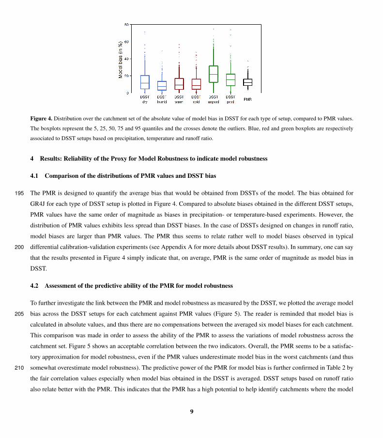
Figure 4. Distribution over the catchment set of the absolute value of model bias in DSST for each type of setup, compared to PMR values.

The boxplots represent the 5, 25, 50, 75 and 95 quantiles and the crosses denote the outliers. Blue, red and green boxplots are respectively

associated to DSST setups based on precipitation, temperature and runoff ratio.

4 Results: Reliability of the Proxy for Model Robustness to indicate model robustness

4.1 Comparison of the distributions of PMR values and DSST bias

The PMR is designed to quantify the average bias that would be obtained from DSSTs of the model. The bias obtained for195

GR4J for each type of DSST setup is plotted in Figure 4. Compared to absolute biases obtained in the different DSST setups,

PMR values have the same order of magnitude as biases in precipitation- or temperature-based experiments. However, the

distribution of PMR values exhibits less spread than DSST biases. In the case of DSSTs designed on changes in runoff ratio,

model biases are larger than PMR values. The PMR thus seems to relate rather well to model biases observed in typical

differential calibration-validation experiments (see Appendix A for more details about DSST results). In summary, one can say200

that the results presented in Figure 4 simply indicate that, on average, PMR is the same order of magnitude as model bias in

DSST.

4.2 Assessment of the predictive ability of the PMR for model robustness

To further investigate the link between the PMR and model robustness as measured by the DSST, we plotted the average model

bias across the DSST setups for each catchment against PMR values (Figure 5). The reader is reminded that model bias is205

calculated in absolute values, and thus there are no compensations between the averaged six model biases for each catchment.

This comparison was made in order to assess the ability of the PMR to assess the variations of model robustness across the

catchment set. Figure 5 shows an acceptable correlation between the two indicators. Overall, the PMR seems to be a satisfac-

tory approximation for model robustness, even if the PMR values underestimate model bias in the worst catchments (and thus

somewhat overestimate model robustness). The predictive power of the PMR for model bias is further confirmed in Table 2 by210

the fair correlation values especially when model bias obtained in the DSST is averaged. DSST setups based on runoff ratio

also relate better with the PMR. This indicates that the PMR has a high potential to help identify catchments where the model

9

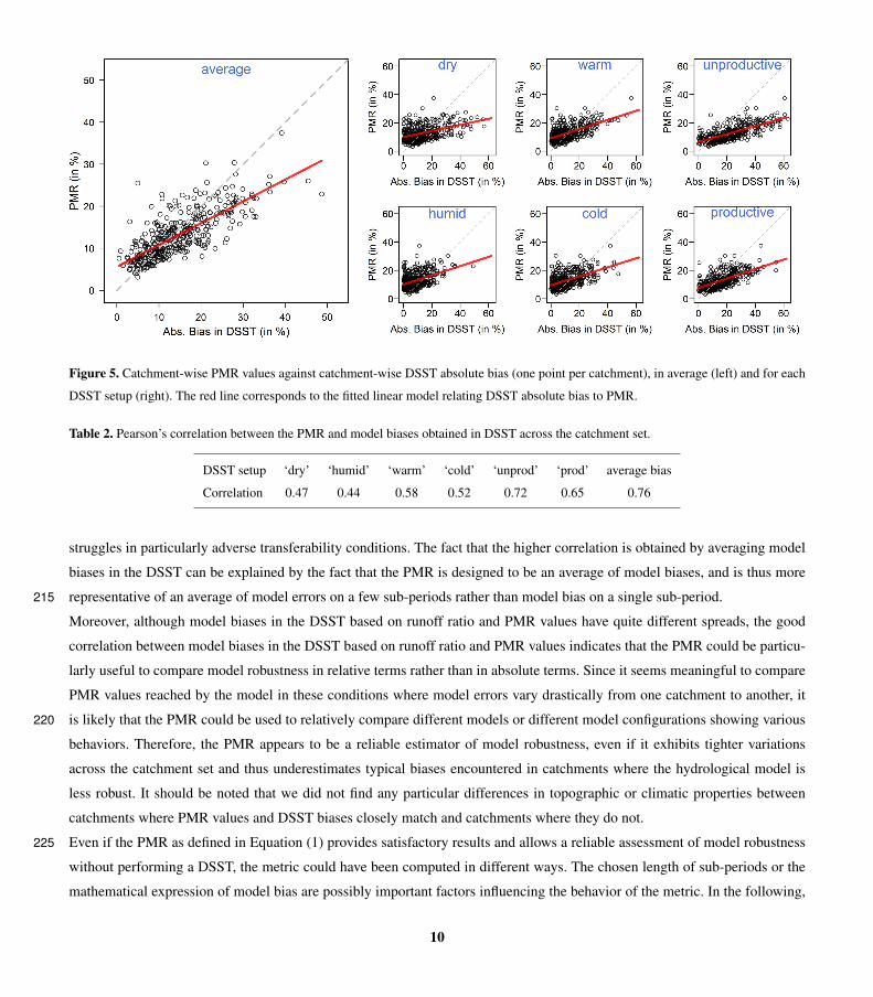
Figure 5. Catchment-wise PMR values against catchment-wise DSST absolute bias (one point per catchment), in average (left) and for each

DSST setup (right). The red line corresponds to the fitted linear model relating DSST absolute bias to PMR.

Table 2. Pearson’s correlation between the PMR and model biases obtained in DSST across the catchment set.

DSST setup ‘dry’ ‘humid’ ‘warm’ ‘cold’ ‘unprod’ ‘prod’ average bias

Correlation 0.47 0.44 0.58 0.52 0.72 0.65 0.76

struggles in particularly adverse transferability conditions. The fact that the higher correlation is obtained by averaging model

biases in the DSST can be explained by the fact that the PMR is designed to be an average of model biases, and is thus more

representative of an average of model errors on a few sub-periods rather than model bias on a single sub-period.215

Moreover, although model biases in the DSST based on runoff ratio and PMR values have quite different spreads, the good

correlation between model biases in the DSST based on runoff ratio and PMR values indicates that the PMR could be particu-

larly useful to compare model robustness in relative terms rather than in absolute terms. Since it seems meaningful to compare

PMR values reached by the model in these conditions where model errors vary drastically from one catchment to another, it

is likely that the PMR could be used to relatively compare different models or different model configurations showing various220

behaviors. Therefore, the PMR appears to be a reliable estimator of model robustness, even if it exhibits tighter variations

across the catchment set and thus underestimates typical biases encountered in catchments where the hydrological model is

less robust. It should be noted that we did not find any particular differences in topographic or climatic properties between

catchments where PMR values and DSST biases closely match and catchments where they do not.

Even if the PMR as defined in Equation (1) provides satisfactory results and allows a reliable assessment of model robustness225

without performing a DSST, the metric could have been computed in different ways. The chosen length of sub-periods or the

mathematical expression of model bias are possibly important factors influencing the behavior of the metric. In the following,

10

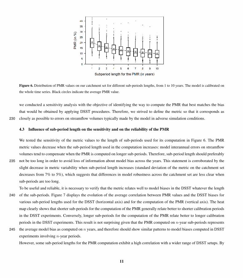
Figure 6. Distribution of PMR values on our catchment set for different sub-periods lengths, from 1 to 10 years. The model is calibrated on

the whole time series. Black circles indicate the average PMR value.

we conducted a sensitivity analysis with the objective of identifying the way to compute the PMR that best matches the bias

that would be obtained by applying DSST procedures. Therefore, we strived to define the metric so that it corresponds as

closely as possible to errors on streamflow volumes typically made by the model in adverse simulation conditions.230

4.3 Influence of sub-period length on the sensitivity and on the reliability of the PMR

We tested the sensitivity of the metric values to the length of sub-periods used for its computation in Figure 6. The PMR

metric values decrease when the sub-period length used in the computation increases: model interannual errors on streamflow

volumes tend to compensate when the PMR is computed on longer sub-periods. Therefore, sub-period length should preferably

not be too long in order to avoid loss of information about model bias across the years. This statement is corroborated by the235

slight decrease in metric variability when sub-period length increases (standard deviation of the metric on the catchment set

decreases from 7% to 5%), which suggests that differences in model robustness across the catchment set are less clear when

sub-periods are too long.

To be useful and reliable, it is necessary to verify that the metric relates well to model biases in the DSST whatever the length

of the sub-periods. Figure 7 displays the evolution of the average correlation between PMR values and the DSST biases for240

various sub-period lengths used for the DSST (horizontal axis) and for the computation of the PMR (vertical axis). The heat

map clearly shows that shorter sub-periods for the computation of the PMR generally relate better to shorter calibration periods

in the DSST experiments. Conversely, longer sub-periods for the computation of the PMR relate better to longer calibration

periods in the DSST experiments. This result is not surprising given that the PMR computed on n-year sub-periods represents

the average model bias as computed on n years, and therefore should show similar patterns to model biases computed in DSST245

experiments involving n-year periods.

However, some sub-period lengths for the PMR computation exhibit a high correlation with a wider range of DSST setups. By

11

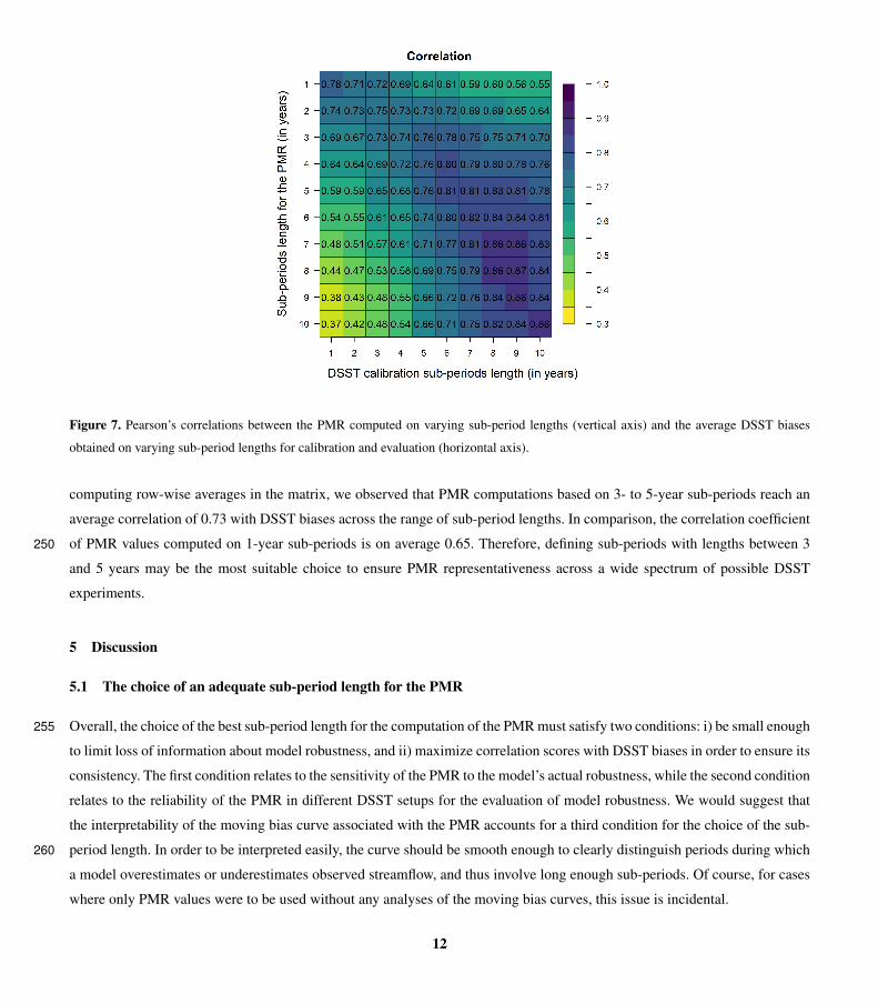
Figure 7. Pearson’s correlations between the PMR computed on varying sub-period lengths (vertical axis) and the average DSST biases

obtained on varying sub-period lengths for calibration and evaluation (horizontal axis).

computing row-wise averages in the matrix, we observed that PMR computations based on 3- to 5-year sub-periods reach an

average correlation of 0.73 with DSST biases across the range of sub-period lengths. In comparison, the correlation coefficient

of PMR values computed on 1-year sub-periods is on average 0.65. Therefore, defining sub-periods with lengths between 3250

and 5 years may be the most suitable choice to ensure PMR representativeness across a wide spectrum of possible DSST

experiments.

5 Discussion

5.1 The choice of an adequate sub-period length for the PMR

Overall, the choice of the best sub-period length for the computation of the PMR must satisfy two conditions: i) be small enough255

to limit loss of information about model robustness, and ii) maximize correlation scores with DSST biases in order to ensure its

consistency. The first condition relates to the sensitivity of the PMR to the model’s actual robustness, while the second condition

relates to the reliability of the PMR in different DSST setups for the evaluation of model robustness. We would suggest that

the interpretability of the moving bias curve associated with the PMR accounts for a third condition for the choice of the sub-

period length. In order to be interpreted easily, the curve should be smooth enough to clearly distinguish periods during which260

a model overestimates or underestimates observed streamflow, and thus involve long enough sub-periods. Of course, for cases

where only PMR values were to be used without any analyses of the moving bias curves, this issue is incidental.

12

Under the conditions of our experiment, we found that lengths between 2 and 5 years were relevant to fulfil the second

requirement. The sensitivity requirement would lead to computing the PMR on 2-year sub-periods; however, we acknowledge

from our experience with moving bias curves that such sub-periods are too short for quick visual analyses. Therefore, we265

consider 3–5 years to be adequate lengths for the computation of the PMR.

However, it should be pointed out that these results are likely to be context-dependent and may have been different for other

models. For these reasons, the aim of the study was more the demonstration that it is possible to assess hydrological model

robustness to climatic changes without performing a DSST, rather than demonstrating that the PMR is perfectly reliable and

that it should substitute Split-Sample Tests. Moreover, the length of the sub-periods involved in the computation of the PMR270

should also reflect the particular needs of each model evaluation study. One could imagine that it may be chosen according to

the temporal variability or periodicity of some climate indices (e.g. the North Atlantic Oscillation index).

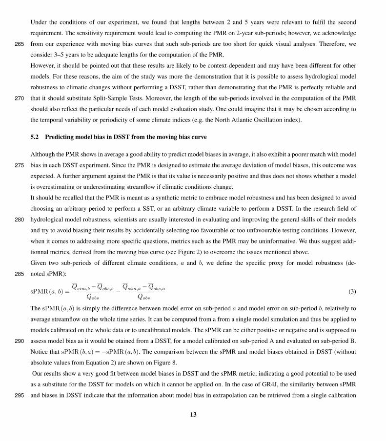
5.2 Predicting model bias in DSST from the moving bias curve

Although the PMR shows in average a good ability to predict model biases in average, it also exhibit a poorer match with model

bias in each DSST experiment. Since the PMR is designed to estimate the average deviation of model biases, this outcome was275

expected. A further argument against the PMR is that its value is necessarily positive and thus does not shows whether a model

is overestimating or underestimating streamflow if climatic conditions change.

It should be recalled that the PMR is meant as a synthetic metric to embrace model robustness and has been designed to avoid

choosing an arbitrary period to perform a SST, or an arbitrary climate variable to perform a DSST. In the research field of

hydrological model robustness, scientists are usually interested in evaluating and improving the general skills of their models280

and try to avoid biasing their results by accidentally selecting too favourable or too unfavourable testing conditions. However,

when it comes to addressing more specific questions, metrics such as the PMR may be uninformative. We thus suggest addi-

tionnal metrics, derived from the moving bias curve (see Figure 2) to overcome the issues mentioned above.

Given two sub-periods of different climate conditions, a and b, we define the specific proxy for model robustness (de-

noted sPMR):285

sPMR(a, b) =Qsim,b −Qobs,b

Qobs

−Qsim,a −Qobs,a

Qobs

(3)

The sPMR(a,b) is simply the difference between model error on sub-period a and model error on sub-period b, relatively to

average streamflow on the whole time series. It can be computed from a from a single model simulation and thus be applied to

models calibrated on the whole data or to uncalibrated models. The sPMR can be either positive or negative and is supposed to

assess model bias as it would be otained from a DSST, for a model calibrated on sub-period A and evaluated on sub-period B.290

Notice that sPMR(b,a) = −sPMR(a,b). The comparison between the sPMR and model biases obtained in DSST (without

absolute values from Equation 2) are shown on Figure 8.

Our results show a very good fit between model biases in DSST and the sPMR metric, indicating a good potential to be used

as a substitute for the DSST for models on which it cannot be applied on. In the case of GR4J, the similarity between sPMR

and biases in DSST indicate that the information about model bias in extrapolation can be retrieved from a single calibration295

13

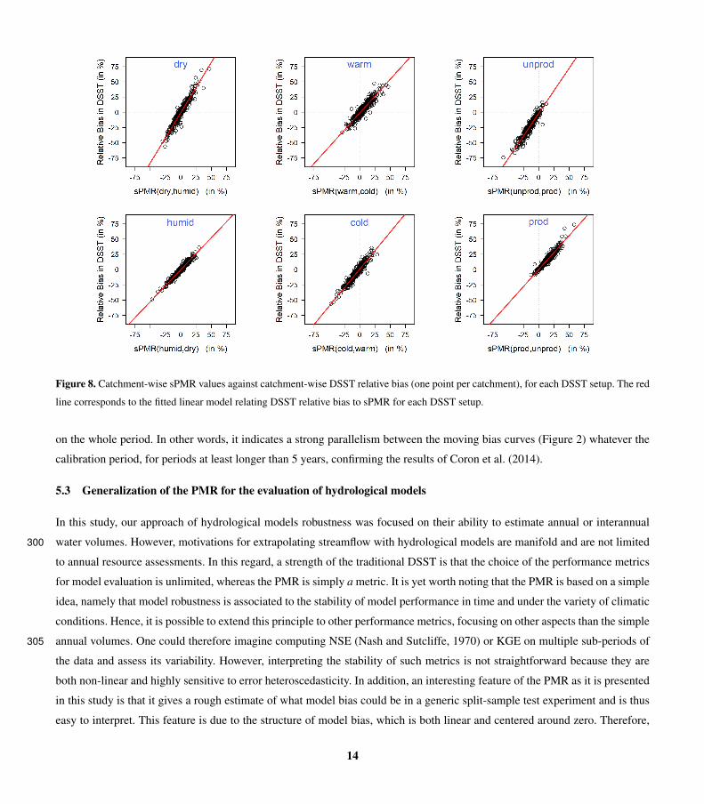
Figure 8. Catchment-wise sPMR values against catchment-wise DSST relative bias (one point per catchment), for each DSST setup. The red

line corresponds to the fitted linear model relating DSST relative bias to sPMR for each DSST setup.

on the whole period. In other words, it indicates a strong parallelism between the moving bias curves (Figure 2) whatever the

calibration period, for periods at least longer than 5 years, confirming the results of Coron et al. (2014).

5.3 Generalization of the PMR for the evaluation of hydrological models

In this study, our approach of hydrological models robustness was focused on their ability to estimate annual or interannual

water volumes. However, motivations for extrapolating streamflow with hydrological models are manifold and are not limited300

to annual resource assessments. In this regard, a strength of the traditional DSST is that the choice of the performance metrics

for model evaluation is unlimited, whereas the PMR is simply a metric. It is yet worth noting that the PMR is based on a simple

idea, namely that model robustness is associated to the stability of model performance in time and under the variety of climatic

conditions. Hence, it is possible to extend this principle to other performance metrics, focusing on other aspects than the simple

annual volumes. One could therefore imagine computing NSE (Nash and Sutcliffe, 1970) or KGE on multiple sub-periods of305

the data and assess its variability. However, interpreting the stability of such metrics is not straightforward because they are

both non-linear and highly sensitive to error heteroscedasticity. In addition, an interesting feature of the PMR as it is presented

in this study is that it gives a rough estimate of what model bias could be in a generic split-sample test experiment and is thus

easy to interpret. This feature is due to the structure of model bias, which is both linear and centered around zero. Therefore,

14

any metric respecting these requirements would have the same property as the PMR.310

Adapting the PMR framework to specific modelling issues could be done in various ways. A possibility would for example be

to compute model bias on a portion of streamflow data above (respectively below) a given threshold. This procedure has been

applied by Royer-Gaspard (2021) to assess the robustness of GR4J for the simulation of different ranges of the streamflow (low,

intermediate and high flows). Another option would be to compute model bias on streamflow components, such as baseflow

and stormflow, derived from hydrograph-separation techniques, to get insights in models ability to represent their interannual315

variations. Some authors have already applied common performance metrics on such streamflow components (e.g. Samuel

et al., 2012). Eventually, streamflow transformations may be usefully applied as well to derive alternative PMR focusing on

weighted parts of the streamflow (e.g. with exponent functions).

6 Conclusions

Traditional methods to assess the robustness of hydrological models to changes in climatic conditions rely on calibration-320

evaluation exercises, preferably performed on climatically different periods of a time series. Although the DSST or its variants

represent the most appropriate procedure one can imagine in terms of model-robustness evaluation, they cannot be used on

models that need to be calibrated on all the available data or to uncalibrated models. Furthermore, the DSST is based on the

selection of hydro-climatic variables whose change is supposed to place the model in unfavorable conditions to perform, but

whose actual link with robustness is strongly context-dependent.325

In this technical note, we propose a performance metric able to evaluate model robustness from a single model calibrated on

the entire period of record. The so-called PMR thus does not need multiple calibrations of the model on sub-periods of the

time series and can be used for any kind of hydrological model. The PMR is constructed as an indicator of the flatness of the

“moving bias curve,” which is a graphical representation of the temporal evolution of model bias across sliding sub-periods of

the data.330

The reliability of the PMR was compared with the results obtained by applying different DSST setups on GR4J, a typical

conceptual model, on a dataset of 377 French catchments. We tested the predictive ability of the metric to estimate model bias

obtained by transferring model parameters from calibration periods to climatically opposite evaluation periods, for six types of

hydro-climatic changes (changes in both directions of average precipitation, average temperature and average runoff ratio).

Our results show that PMR relates well to absolute model biases in the DSST, especially when these biases derived from the335

six DSST setups are averaged. Although the metric values do not vary much across the catchment set, this sensitivity can be

enhanced by reducing the length of the sub-periods on which PMR is computed. An analysis of the correlation between the

PMR and model biases in the DSST for different sub-period lengths pinpointed that the reliability of PMR was better when the

metric was computed on sub-periods with lengths between 2 and 5 years. Ultimately, the need to find a balance between metric

sensitivity and reliability lead us to recommend computing the PMR on 3- to 5-year sub-periods for GR4J.340

Our results should encourage hydrological modelers to include the PMR as part of their panoply of evaluation metrics to

judge their models. The metric addressing models transferability within the context of observed climate variability, it can be

15

useful in model robustness assessments. In the context of climate change impact assessments though, it should be recalled

that demonstrating model robustness in the historical period is a necessary yet not sufficient requirement to validate model

robustness in future conditions outside the range of past observations. Still, being relevant for any kind of hydrological model,345

it may be used to inform model selection for such simulations. Of course, it appears difficult to define acceptability thresholds

for the PMR a model should pass to be used in extrapolation, since it would be catchment and objective dependent. However,

one could imagine adapting a standardized PMR by comparing PMR values with a benchmark model as is done for NSE

(for example a simple yearly Budyko model). Further work should also examine the potential of PMR to be incorporated as

a hydrological signature in multi-objective calibration procedures essentially to constrain model parameters governing slow350

temporal changes in catchment response.

Code availability. The GR4J model is freely available in the airGR R package. The code for calculating the PMR can be made available

upon request.

Data availability. Streamflow data were provided by the French database "Banque HYDRO" and are available at http://www.hydro.eaufrance.

Meteorological data was provided by Météo-France and must be requested to this institute.355

Appendix A: Characterisation of model bias across DSST setups

Model biases in the DSST have been calculated in an absolute way in the Results section so that they could be compared with

PMR values. This resulted in a loss of information about the sign of model errors. In this appendix, it is shown how the sign of

these errors relates to the different DSST experiments. The biases obtained for GR4J for each of the six types of DSST setup

are plotted in Figure A1 without taking their absolute values.360

Model bias follows different patterns depending on the climatic variable used to define the calibration and evaluation periods

of the DSST. While the distribution of model errors seems comparatively even for periods characterized by different average

precipitation, transferring model parameters between periods with different runoff ratios clearly triggers opposite model bias,

whether the transfer is performed in one way or in another. For most catchments, GR4J indeed underestimates streamflow

volumes when runoff ratio increases and, conversely, overestimates streamflow volumes when runoff ratio decreases. DSSTs365

based on temperature yield situations in between, since median model bias is slightly negative (respectively positive) when

calibrated on warmer (respectively colder) periods. When calculated in absolute terms, model bias was larger in DSSTs based

on runoff ratio than for experiments based on temperature and precipitation (Figure A1). Therefore, robustness issues for the

model appear to be caused less by changes in climatic changes than by modification of the catchment response to precipitation.

This result is in line with the conclusion of Saft et al. (2016), who tested a number of hydrological models in southeastern370

Australia during prolonged droughts. The authors observed that many of these models would produce biased simulations of

16

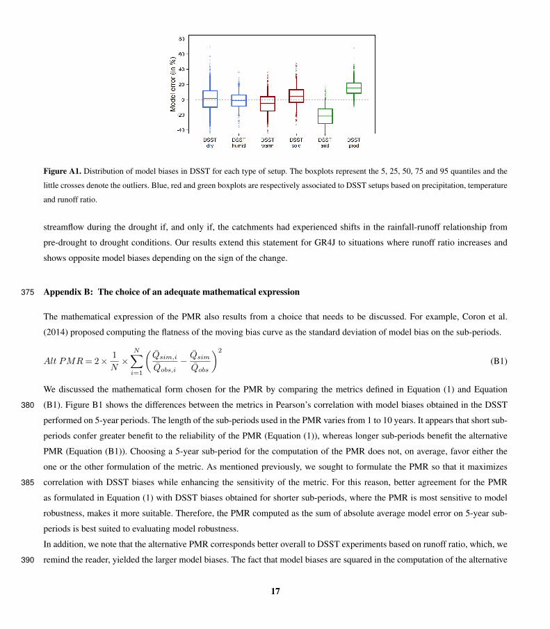
Figure A1. Distribution of model biases in DSST for each type of setup. The boxplots represent the 5, 25, 50, 75 and 95 quantiles and the

little crosses denote the outliers. Blue, red and green boxplots are respectively associated to DSST setups based on precipitation, temperature

and runoff ratio.

streamflow during the drought if, and only if, the catchments had experienced shifts in the rainfall-runoff relationship from

pre-drought to drought conditions. Our results extend this statement for GR4J to situations where runoff ratio increases and

shows opposite model biases depending on the sign of the change.

Appendix B: The choice of an adequate mathematical expression375

The mathematical expression of the PMR also results from a choice that needs to be discussed. For example, Coron et al.

(2014) proposed computing the flatness of the moving bias curve as the standard deviation of model bias on the sub-periods.

Alt PMR = 2× 1

N×

N∑i=1

(Q̄sim,i

Q̄obs,i− Q̄sim

Q̄obs

)2

(B1)

We discussed the mathematical form chosen for the PMR by comparing the metrics defined in Equation (1) and Equation

(B1). Figure B1 shows the differences between the metrics in Pearson’s correlation with model biases obtained in the DSST380

performed on 5-year periods. The length of the sub-periods used in the PMR varies from 1 to 10 years. It appears that short sub-

periods confer greater benefit to the reliability of the PMR (Equation (1)), whereas longer sub-periods benefit the alternative

PMR (Equation (B1)). Choosing a 5-year sub-period for the computation of the PMR does not, on average, favor either the

one or the other formulation of the metric. As mentioned previously, we sought to formulate the PMR so that it maximizes

correlation with DSST biases while enhancing the sensitivity of the metric. For this reason, better agreement for the PMR385

as formulated in Equation (1) with DSST biases obtained for shorter sub-periods, where the PMR is most sensitive to model

robustness, makes it more suitable. Therefore, the PMR computed as the sum of absolute average model error on 5-year sub-

periods is best suited to evaluating model robustness.

In addition, we note that the alternative PMR corresponds better overall to DSST experiments based on runoff ratio, which, we

remind the reader, yielded the larger model biases. The fact that model biases are squared in the computation of the alternative390

17

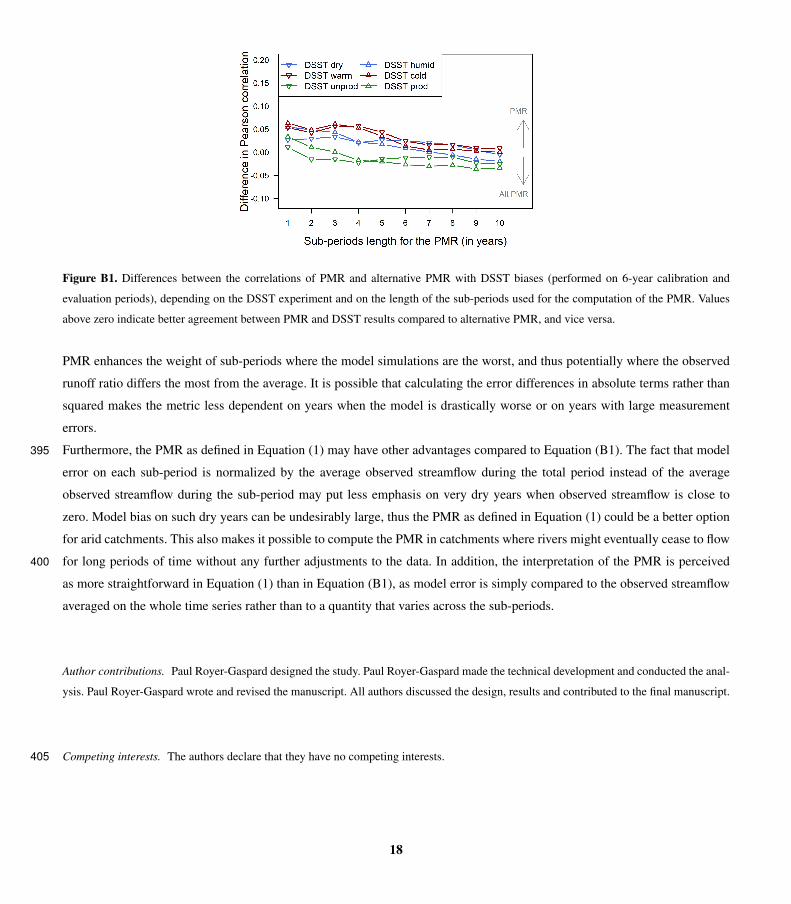
Figure B1. Differences between the correlations of PMR and alternative PMR with DSST biases (performed on 6-year calibration and

evaluation periods), depending on the DSST experiment and on the length of the sub-periods used for the computation of the PMR. Values

above zero indicate better agreement between PMR and DSST results compared to alternative PMR, and vice versa.

PMR enhances the weight of sub-periods where the model simulations are the worst, and thus potentially where the observed

runoff ratio differs the most from the average. It is possible that calculating the error differences in absolute terms rather than

squared makes the metric less dependent on years when the model is drastically worse or on years with large measurement

errors.

Furthermore, the PMR as defined in Equation (1) may have other advantages compared to Equation (B1). The fact that model395

error on each sub-period is normalized by the average observed streamflow during the total period instead of the average

observed streamflow during the sub-period may put less emphasis on very dry years when observed streamflow is close to

zero. Model bias on such dry years can be undesirably large, thus the PMR as defined in Equation (1) could be a better option

for arid catchments. This also makes it possible to compute the PMR in catchments where rivers might eventually cease to flow

for long periods of time without any further adjustments to the data. In addition, the interpretation of the PMR is perceived400

as more straightforward in Equation (1) than in Equation (B1), as model error is simply compared to the observed streamflow

averaged on the whole time series rather than to a quantity that varies across the sub-periods.

Author contributions. Paul Royer-Gaspard designed the study. Paul Royer-Gaspard made the technical development and conducted the anal-

ysis. Paul Royer-Gaspard wrote and revised the manuscript. All authors discussed the design, results and contributed to the final manuscript.

Competing interests. The authors declare that they have no competing interests.405

18

Acknowledgements. This work was funded by the project AQUACLEW, which is part of ERA4CS, an ERA-NET initiated by JPI Climate,

and funded by FORMAS (SE), DLR (DE), BMWFW (AT), IFD (DK), MINECO (ES), ANR (FR) with co-funding by the European Com-

mission [Grant 690462]. The authors from INRAE were funded by ANR. We thank Gaëlle Tallec and Charles Perrin for their careful review

prior to article submission. Ludovic Oudin, Laurent Coron, Éric Martin, and Nathalie de Noblet-Ducoudré are gratefully acknowledged for

their advice on the PhD work of the first author. Météo-France and SCHAPI are acknowledged for providing climatic and streamflow data,410

respectively. We thank Isabella Athanassiou for her cautious proofreading and help to make the English easier to read.

19

References

Blöschl, G., Bierkens, M. F. P., Chambel, A., Cudennec, C., Destouni, G., Fiori, A., Kirchner, J. W., McDonnell, J. J., Savenije, H. H. G.,

Sivapalan, M. and others: Twenty-three unsolved problems in hydrology (UPH)–a community perspective, Hydrol. Sci. J., 64, 1141–1158,

https://doi.org/10.1080/02626667.2019.1620507, 2019.415

Broderick, C., Matthews, T., Wilby, R. L., Bastola, S. and Murphy, C.: Transferability of hydrological models and ensemble averaging

methods between contrasting climatic periods, Water Resour. Res., 52, 8343–8373, https://doi.org/10.1002/2016wr018850, 2016.

Clark, M. P., Wilby, R. L., Gutmann, E. D., Vano, J. A., Gangopadhyay, S., Wood, A. W., Fowler, H. J., Prudhomme, C., Arnold, J. R.

and Brekke, L. D.: Characterizing uncertainty of the hydrologic impacts of climate change, Curr. Clim. Change Rep., 2, 55–64, https:

//doi.org/10.1007/s40641-016-0034-x, 2016.420

Coron, L., Andréassian, V., Perrin, C., Lerat, J., Vaze, J., Bourqui, M. and Hendrickx, F.: Crash testing hydrological models in contrasted

climate conditions: An experiment on 216 Australian catchments, Water Resour. Res., 48, https://doi.org/10.1029/2011wr011721, 2012.

Coron, L., Andréassian, V., Perrin, C., Bourqui, M. and Hendrickx, F.: On the lack of robustness of hydrologic models regarding water

balance simulation: a diagnostic approach applied to three models of increasing complexity on 20 mountainous catchments, Hydrol. Earth

Syst. Sci., 18, 727–746, https://doi.org/10.5194/hess-18-727-2014, 2014.425

Coron, L., Thirel, G., Delaigue, O., Perrin, C. and Andréassian, V.: The suite of lumped GR hydrological models in an R package, Environ.

Model. Softw., 94, 166–171, https://doi.org/10.1016/j.envsoft.2017.05.002, 2017.

Coron, L., Perrin, C., Delaigue, O., Thirel, G. and Michel, C.: airGR: Suite of GR Hydrological Models for Precipitation-Runoff Modelling,

R package version 1.0.12.3.2, https://webgr.inrae.fr/en/airGR/, 2018.

Dakhlaoui, H., Ruelland, D., Tramblay, Y. and Bargaoui, Z.: Evaluating the robustness of conceptual rainfall-runoff models under climate430

variability in northern Tunisia, J. Hydrol., 550, 201–217, https://doi.org/10.1016/j.jhydrol.2017.04.032, 2017.

Dakhlaoui, H., Ruelland, D. and Tramblay, Y.: A bootstrap-based differential split-sample test to assess the transferability of conceptual

rainfall-runoff models under past and future climate variability, J. Hydrol., 575, 470–486, https://doi.org/10.1016/j.jhydrol.2019.05.056,

2019.

Delaigue, O., Génot, B., Lebecherel, L., Brigode, P., and Bourgin, P. Y.: Database of watershed-scale hydroclimatic observations in France,435

Université Paris-Saclay, INRAE, HYCAR Research Unit, Hydrology group, Antony, URL = https://webgr.inrae.fr/base-de-donnees/,

2020.

Fowler, K. J. A., Peel, M. C., Western, A. W., Zhang, L. and Peterson, T. J.: Simulating runoff under changing climatic conditions: Revisiting

an apparent deficiency of conceptual rainfall–runoff models, Water Resour. Res., 52, 1820–1846, https://doi.org/10.1002/2015wr018068,

2016.440

Gupta, H. V., Kling, H., Yilmaz, K. K. and Martinez, G. F.: Decomposition of the mean squared error and NSE performance criteria:

Implications for improving hydrological modelling, J. Hydrol., 377, 80–91, https://doi.org/10.1016/j.jhydrol.2009.08.003, 2009.

Hagemann, S., Chen, C., Clark, D. B., Folwell, S., Gosling, S. N., Haddeland, I., Hanasaki, N., Heinke, J., Ludwig, F., Voss, F. and others:

Climate change impact on available water resources obtained using multiple global climate and hydrology models, Earth Syst. Dynam.,

4, 129–144, https://doi.org/10.5194/esd-4-129-2013, 2013.445

Klemeš, V.: Operational testing of hydrological simulation models, Hydrol. Sci. J., 31, 13–24, https://doi.org/10.1080/02626668609491024,

1986.

20

Leleu, I., Tonnelier, I., Puechberty, R., Gouin, P., Viquendi, I., Cobos, L., Foray, A., Baillon, M. and Ndima, P.-O.: La refonte du système

d’information national pour la gestion et la mise à disposition des données hydrométriques, La Houille Blanche, 1, 25–32, https://doi.org/

10.1051/lhb/2014004, 2014.450

Mathevet, T.: Quels modèles pluie-débit globaux au pas de temps horaire? Développements empiriques et comparaison de modèles sur un

large échantillon de bassins versants, Ph.D., ENGREF Paris, https://hal.inrae.fr/tel-02587642, 2014.

Mathevet, T., Gupta, H., Perrin, C., Andréassian, V. and Le Moine, N.: Assessing the performance and robustness of two conceptual rainfall-

runoff models on a worldwide sample of watersheds, J. Hydrol., 124698, https://doi.org/10.1016/j.jhydrol.2020.124698, 2020.

Melsen, L. A., Addor, N., Mizukami, N., Newman, A. J., Torfs, P., Clark, M. P., Uijlenhoet, R. and Teuling, A. J.: Mapping (dis) agreement455

in hydrologic projections, Hydrol. Earth Syst. Sci., 22, 1775–1791, https://doi.org/10.5194/hess-22-1775-2018, 2018.

Merz, R., Parajka, J. and Blöschl, G.: Time stability of catchment model parameters: Implications for climate impact analyses, Water Resour.

Res., 47, https://doi.org/10.1029/2010wr009505, 2011.

Nash, J. E. and Sutcliffe, J. V.: River flow forecasting through conceptual models part I—A discussion of principles, J. Hydrol., 10, 282–290,

https://doi.org/10.1016/0022-1694(70)90255-6, 1970.460

Oudin, L., Hervieu, F., Michel, C., Perrin, C., Andréassian, V., Anctil, F. and Loumagne, C.: Which potential evapotranspiration input for a

lumped rainfall–runoff model?: Part 2—Towards a simple and efficient potential evapotranspiration model for rainfall–runoff modelling,

J. Hydrol., 303, 290–306, https://doi.org/10.1016/j.jhydrol.2004.08.026, 2005.

Perrin, C., Michel, C. and Andréassian, V.: Improvement of a parsimonious model for streamflow simulation, J. Hydrol., 279, 275–289,

https://doi.org/10.1016/s0022-1694(03)00225-7, 2003.465

Refsgaard, J. C., Madsen, H., Andréassian, V., Arnbjerg-Nielsen, K., Davidson, T. A., Drews, M., Hamilton, D. P., Jeppesen, E., Kjellström,

E., Olesen, J. E. and others: A framework for testing the ability of models to project climate change and its impacts, Climatic Change,

122, 271–282, https://doi.org/10.1007/s10584-013-0990-2, 2014.

Royer-Gaspard, P.: De la robustesse des modèles hydrologiques face à des conditions climatiques variables, Ph.D., Sorbonne Université,

https://webgr.inrae.fr/wp-content/uploads/2021/04/Resume_these_Paul_Royer-Gaspard.pdf, 2021.470

Saft, M., Peel, M. C., Western, A. W., Perraud, J.-M. and Zhang, L.: Bias in streamflow projections due to climate-induced shifts in catchment

response, Geophys. Res. Lett., 43, 1574–1581, https://doi.org/10.1002/2015gl067326, 2016.

Samuel, J., Coulibaly, P. and Metcalfe, R. A.: Identification of rainfall–runoff model for improved baseflow estimation in ungauged basins,

Hydrol. Process., 26, 356–366, https://doi.org/10.1002/hyp.8133, 2012.

Schewe, J., Heinke, J., Gerten, D., Haddeland, I., Arnell, N. W., Clark, D. B., Dankers, R., Eisner, S., Fekete, B. M., Colón-González, F. J.475

and others: Multimodel assessment of water scarcity under climate change, P. Natl. Acad. Sci., 11, 3245–3250, https://doi.org/10.1073/

pnas.1222460110, 2014.

Thirel, G., Andréassian, V., Perrin, C., Audouy, J.-N., Berthet, L., Edwards, P., Folton, N. Furusho, C., Kuentz, A., Lerat, J. and others:

Hydrology under change: an evaluation protocol to investigate how hydrological models deal with changing catchments, Hydrol. Sci. J.,

60, 1184–1199, https://doi.org/10.1080/02626667.2014.967248, 2015.480

Valéry, A., Andréassian, V. and Perrin, C.: ‘As simple as possible but not simpler’: What is useful in a temperature-based snow-accounting

routine? Part 2–Sensitivity analysis of the Cemaneige snow accounting routine on 380 catchments, J. Hydrol., 517, 1176–1187, https:

//doi.org/10.1016/j.jhydrol.2014.04.058, 2014.

Vaze, J., Post, D. A., Chiew, F. H. S., Perraud, J.-M., Viney, N. R. and Teng, J.: Climate non-stationarity–validity of calibrated rainfall–runoff

models for use in climate change studies, J. Hydrol., 394, 447–457, https://doi.org/10.1016/j.jhydrol.2010.09.018, 2010.485

21

Vidal, J.-P., Martin, E., Franchistéguy, L., Baillon, M. and Soubeyroux, J.-M.: A 50-year high-resolution atmospheric reanalysis over France

with the Safran system, Int. J. Climatol., 30, 1627–1644, https://doi.org/10.1002/joc.2003, 2010.

Vidal, J.-P., Hingray, B., Magand, C., Sauquet, E. and Ducharne, A.: Hierarchy of climate and hydrological uncertainties in transient low-flow

projections, Hydrol. Earth Syst. Sci., 20, 3651–3672, https://doi.org/10.5194/hess-20-3651-2016, 2016.

22