plant engineers and managers guide to energy conservation, tenth edition
TRANSCRIPT

Plant Engineersand ManagersGuide to Energy Conservation
Tenth Edition
Albert Thumann, P.E., C.E.M. Scott Dunning, Ph.D., P.E., C.E.M.

Library of Congress Cataloging-in-Publication Data
Thumann, Albert. Plant engineers and managers guide to energy conservation / Albert Thumann, Scott Dunning. -- 10th ed p. cm.ISBN-10: 0-88173-657-0 (alk. paper)ISBN-10: 0-88173-658-9 (electronic)ISBN-13: 978-1-4398-5606-2 (taylor & francis distribution : alk. paper)1. Factories--Energy conservation--Handbooks, manuals, etc. I. Title.
TJ163.5.F3T48 2010 658.2'6--dc22 2010032142 Plant engineers and managers guide to energy conservation / Albert Thumann--10th ed. ©2011 by The Fairmont Press. All rights reserved. No part of this publication may be reproduced or transmitted in any form or by any means, electronic or mechani-cal, including photocopy, recording, or any information storage and retrieval system, without permission in writing from the publisher.
Published by The Fairmont Press, Inc.700 Indian TrailLilburn, GA 30047tel: 770-925-9388; fax: 770-381-9865http://www.fairmontpress.com
Distributed by Taylor & Francis Ltd.6000 Broken Sound Parkway NW, Suite 300Boca Raton, FL 33487, USAE-mail: [email protected]
Distributed by Taylor & Francis Ltd.23-25 Blades CourtDeodar RoadLondon SW15 2NU, UKE-mail: [email protected]
Printed in the United States of America10 9 8 7 6 5 4 3 2 1
0-88173-657-0 (The Fairmont Press, Inc.)978-1-4398-5606-2 (Taylor & Francis Ltd.)
While every effort is made to provide dependable information, the publisher, authors, and editors cannot be held responsible for any errors or omissions.
Printed on recycled paper.

xi
Introduction
The first edition of Plant Engineers and Managers Guide to Energy Conservation was published in 1977, and it was the first book to address the need for a comprehensive industrial energy management program. The book was written prior to the first energy legislation that was en-acted, The National Energy Conservation and Policy Act of 1978. In 1978 the role of the plant engineer and manager in energy conservation was just being defined. Today we are witnessing the "perfect storm" for new energy policy legislation to reduce the nation's need for oil and minimize the risk of climate change. Planet Earth is in peril. The catastrophic oil spill in the Gulf of Mexico should be a wake-up call for a comprehensive energy policy which dramatically reduces the nation's need for oil. In addition, climate change is a reality that can no longer be ignored. Applying energy management technologies dramatically reduces energy costs while benefiting the planet. A 2009 survey conducted by the Association of Energy Engineers found that 30% of respondents re-duced energy consumption by more than 10%, and 27% of respondents reduced energy costs by $1 million or more. The potential for further savings is still great. The role of the plant engineer and manager in energy conservation is ever changing. The challenge has always been great; the stakes, how-ever, are higher than ever.
vii
ContentsChapter 1 THE ROLE OF THE PLANT ENGINEER IN ENERGY MANAGEMENT Organization For Energy Utilization, What Is An Industrial Energy Assessment?, The Energy Utilization Program, Energy Accounting, The Language of the Energy Manager, Codes, Standards & Legislation,
The Energy Independence and Security Act of 2007, The Energy Policy Act of 2005, The Energy Policy Act of 1992, State Codes, Regulatory & Legislative Issues Impacting Cogeneration & Independent Power
Production.................................................................................................. 1
Chapter 2 ENERGY ECONOMIC DECISION MAKING Life Cycle Costing, Using the Payback Period Method, Using Life Cycle Costing, The Time Value of Money, Investment Decision- Making, The Job Simulation Experience, Making Decisions For Alternate Investments, Depreciation, Taxes and the Tax Credit, Impact of Fuel Inflation on Life Cycle Costing, Summary of Life Cycle Costing ........................................................................................... 29
Chapter 3 THE FACILITY SURVEY Comparing Catalogue Data With Actual Performance, Infrared Equipment, Measuring Electrical System Performance, Temperature
Measurements, Measuring Combustion Systems, Measuring Heating, Ventilation and Air Conditioning (HVAC) System Performance ............................................................................................. 61
Chapter 4 ELECTRICAL SYSTEM OPTIMIZATION Applying Proven Techniques to Reduce the Electrical Bill, Why the Plant Manager Should Understand the Electric Rate Structure, Electrical Rate Tariff, Real Time Pricing (RTP), Power Basics—The Key to Electrical Energy Reduction, Relationships Between Power, Voltage, and Current, Motor Loads, What Are the Advantages of Power Factor Correction?, How to Improve the Plant Power Factor,
Where to Locate Capacitors, Efficient Motors, Synchronous Motors and Power Factor Correction, What Is Load Management?, What Have Been Some of the Results of Load Management?, Application of Automatic Load Shedding, How Does Load Demand Control
viii
Work?, The Confusion Over Energy Management Systems, Lighting Basics—The Key to Reducing Lighting Wastes, Lighting Illumination Requirements, The Efficient Use of Lamps, Efficient Types of Incandescents For Limited Use .................................................. 77
Chapter 5 UTILITY AND PROCESS SYSTEM OPTIMIZATION Basis of Thermodynamics, The Carnot Cycle, Use of the Specific Heat
Concept, Practical Applications For Energy Conservation, Furnace Efficiency, Steam Tracing, Heat Recovery, The Mollier Diagram, Steam Generation Using Waste Heat Recovery, Pumps and Piping Systems, Distillation Columns, Incorporation of Energy Utilization In Procurement Specifications ............................................................... 109
Chapter 6 HEAT TRANSFER The Importance of Understanding the Principles of Heat Transfer, Three Ways Heat Is Transferred, How to Estimate the Heat Loss of a Vessel or Tank, How to Estimate the Heat Loss of Piping and Flat Surfaces .......................................................................................... 151
Chapter 7 REDUCING BUILDING ENERGY LOSSES Energy Losses Due to Heat Loss and Heat Gain, Conductivity Through Building Materials, The Effect of Sunlight, Window Treatments, Advanced Optical Technologies ......................................... 173
Chapter 8 HEATING, VENTILATION AND AIR-CONDITIONING SYS-TEM OPTIMIZATION
Efficient Use of Heating and Cooling Equipment Saves Dollars, Applying the Heat Pump to Save Energy, Efficient Applications of Re-
frigeration Equipment, Guide to Gas Cooling Technology, Basics of Air Conditioning System Design For Energy Conservation, Applying Variable Air Volume Systems, Applying the Economizer Cycle, Applying Heat Recovery, Cool Storage System Performance, Thermal Storage Control Systems, The Ventilation Audit, Energy Analysis Utilizing Simulation Programs, Test and Balance Considerations ....................................................................................... 225
Chapter 9 COGENERATION: THEORY AND PRACTICE Definition of "Cogeneration," Components of a Cogeneration System,
ix
An Overview of Cogeneration Theory, Application of the Cogeneration Constant, Applicable Systems, Basic Thermodynamic Cycles, Detailed Feasibility Evaluation ........................................................................... 259
Chapter 10 ESTABLISHING A MAINTENANCE PROGRAM FOR PLANT EFFICIENCY AND ENERGY SAVINGS
Good Maintenance Saves $, What Is the Effectiveness of Most Maintenance Programs?, How to Turn Around the Maintenance Program, Stop Leaks and Save, Properly Operating Steam Traps
Save Energy, Excess Air Considerations, Dirt and Lamp Lumen Depreciation Can Reduce Lighting Levels by 50% ...................... 291
Chapter 11 MANAGING AN EFFECTIVE ENERGY CONSERVATION PROGRAM Organizing For Energy Conservation, Top Management Commitment,
What to Consider When Establishing Energy Conservation Objectives, Using the Critical Path Schedule of Energy Conservation Activities,
Electrical Scheduling of Plant Activities, An Effective Maintenance Program, Continuous Conservation Monitoring, Are Outside Consul- tants and Contractors Encouraged to Save Energy by Design?, Encouraging the Creative Process, Energy Emergency and Contingency Planning ........................................................................... 305
Chapter 12 ELECTRIC MOTORS Motor Types, Motor Efficiency and Power Factor, Motor Voltage, Motor Rewinds ...................................................................................... 317
Chapter 13 RELIABLE AND ECONOMIC NATURAL GAS DISTRIBUTED GENERATION TECHNOLOGIES Elements of DG, Technologies, Market Potential .................................. 325
Chapter 14 FINANCING ENERGY EFFICIENCY PROJECTS Definitions and Clarifications, Financing Alternatives, Relative Benefits of Project Financing, Basic Structure, Proposal Review ......... 341
Chapter 15 COST CONTAINMENT DESIGN FOR COMMERCIAL GEOTHERMAL HEAT PUMPS Why GHPs? Why Now?, Design Methods to Realize Advantages, Software, Challenges in the US Market................................................. 359
x
Chapter 16 ECONOMIC EVALUATIONS FOR POWER QUALITY SOLUTIONS The Principle Investigation, Determining the Phenomenon, Choosing the Right Equipment, Economic Analysis, Graphical Analysis, A More Direct Approach ...................................................... 371
Chapter 17 PURCHASING STRATEGIES FOR ELECTRICITY AT&T vs. MCI: A Paradigm, Factors Impacting Power Prices, Three General Relationships, Who Offers These Options?, The College of Power Knowledge ........................................................... 385
Chapter 18 EVALUATING THE ECONOMICS OF SOLAR APPLICATIONS FOR COMMERCIAL & INDUSTRIAL FACILITIES
Cost of Energy, Solar Economics, Solar Water Heating System Economics, Photovoltaic System Economics ......................................... 397
Chapter 19 MEASUREMENT AND VERIFICATION OF ENERGY EFFI-CIENCY SAVINGS IN INDUSTRIAL FACILITIES: THE FLAW OF USING ENERGY INTENSITIES TO DETERMINE SAVINGS
Measurement & Verification .................................................................. 421
Chapter 20 SUPERIOR ENERGY PERFORMANCE: A ROADMAP FOR ACHIEVING CONTINUAL ENERGY PERFORMANCE IM-PROVEMENT
Need and Value to Industry, Program Elements, Qualifying for Superior Energy Performance, Superior Energy Performance Status ................. 437
Chapter 21 STEAM SYSTEM OPTIMIZATION: A CASE STUDY Overview of the Site Steam System, Savings Opportunities ................ 449
Chapter 22 ENERGY AUDIT CASE STUDY: LOG HOME MANUFACTURER General Background, Energy Accounting, Energy Reduction Recommendations, Existing Lighting, Proposed Lighting .................... 469
Chapter 23 POWER QUALITY CASE STUDIES Case Study 1, Case Study 2 .................................................................. 501
Index ............................................................................................................................. 507

1
1The Role of the Plant EngineerIn Energy Management
Energy management is now considered part of every plant engi-neer’s job. Today the plant engineer needs to keep abreast of changing energy factors which must be incorporated into the overall energy management program. The accomplishments of energy management have indeed been outstanding. Safety, maintenance, and now energy management are some of the areas in which a plant engineer is expected to be knowledgeable. The cook book and low cost/no cost energy conservation measures which were emphasized in the 1970s have been replaced with a more sophisticated approach. The plant engineer of today must have a keen understanding of both the technical and managerial aspects of energy management in order to insure its success. When oil prices dropped in 1986 it was an opportunity in many plants to switch back to oil. As electric prices escalated it was an opportunity for many plants to install cogeneration facilities. In the late 1990s deregulation took hold, opening up new op-portunities in energy purchasing. Since 2005, prices have risen again, creating new opportunities. Thus the energy management area is ever changing. Energy management or energy utilization has replaced the sim-plistic house keeping measures approach. The intent of this book is not to make you an expert in each sub-ject, but to illustrate how the overall pieces fit together. Each chapter illustrates the various pieces that comprise an industrial energy utiliza-tion program. The energy manager is analogous to a system engineer; only when the total picture is viewed will the solution become obvious. Of course, it should be noted that the energy manager must seek the
2 Plant Engineers and Managers Guide to Energy Conservation
advice of experts or specialists when required and use their expertise accordingly.
ORGANIZATION FOR ENERGY UTILIZATION
A multi-divisional corporation usually organizes energy activities on a corporate and plant basis. On the plant basis, energy activities are in many instances added on to the duties of the plant manager. An energy utilization program does not just happen. It needs a guiding force to “get the ball rolling.” Production, energy costs, and raw material supplies are of great concern to plant managers; thus, they are usually the ones to initiate the program. For a continual, ongoing program to develop, energy managers need to establish an industrial assessment program for their facilities. The term "industrial assessment" was introduced in most energy utiliza-tion programs in the late 1970s, yet it was rarely defined.
WHAT IS AN INDUSTRIAL ENERGY ASSESSMENT?
The simplest definition for an energy assessment is: An energy assessment serves the purpose of identifying where a building or plant facility uses energy and identifies energy conservation oppor-tunities. There is a direct relationship to the cost of the assessment (amount of data collected and analyzed) and the number of energy conserva-tion opportunities to be found. Thus, a first decision is made on the cost of the assessment, which determines the type of assessment to be performed. The second decision is made on the type of facility. For example, a building assessment may emphasize the building envelope, lighting, heating, and ventilation requirements. On the other hand, an assessment of an industrial plant emphasizes the process requirements. Most energy assessments fall into three categories or types, namely, walk-through, mini-assessment, or detailed assessment. Walk-through. This type of audit is the least costly and identifies preliminary energy savings. A visual inspection of the facility is made to determine maintenance and operation energy-saving opportunities,
The Role of the Plant Engineer in Energy Management 3
plus to collect information with which to determine the need for a more detailed analysis. This type of assessment often employs checklists and usually yields a 1- to 2-page summary listing potential opportunities and typical savings found at other facilities. Mini-assessment. This type of assessment requires tests and mea-surements to quantify energy uses and losses and determine the eco-nomics for changes. Data collection may consist of one-day snapshots of plant operations. Detailed assessment. This type of assessment goes one step further than the mini-assessment. It contains an evaluation of how much energy is used for each function, such as lighting or process. It also requires a model analysis, such as a computer simulation, to determine energy use patterns and predictions on a year-round basis, taking into account such variables as weather data. The chief distinction between the mini-assessment and the walk-through assessment is that the mini-assessment requires a quantification of energy uses and losses in determining the economics for change. The chief distinction between the detailed assessment and the mini-assessment is that the detailed assessment requires establishing an accounting system for energy and a computer simulation.
THE ENERGY UTILIZATION PROGRAM
The energy utilization program usually contains the following steps:
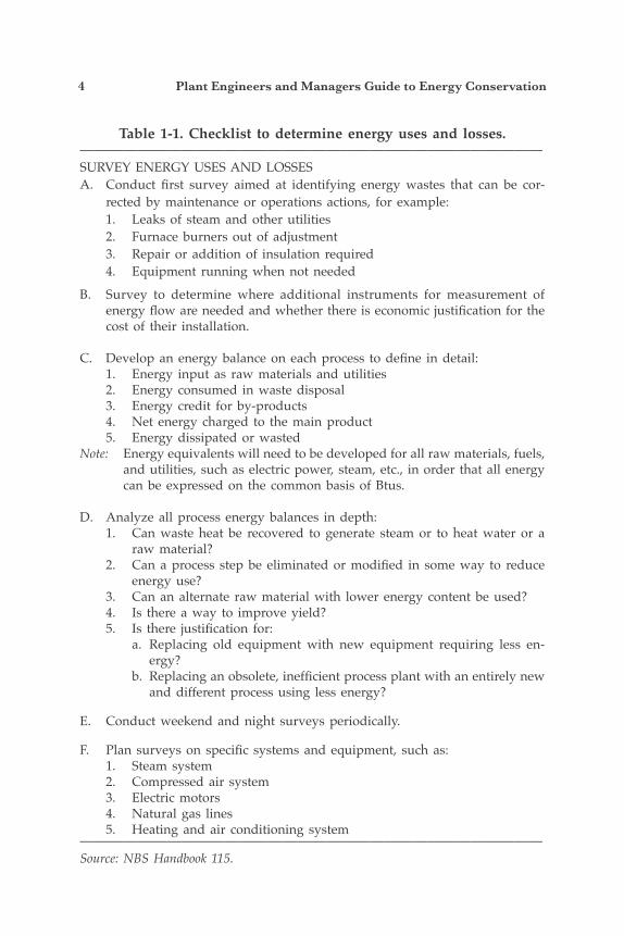
1. Determine energy uses and losses. (Refer to checklist, Table 1-1.)
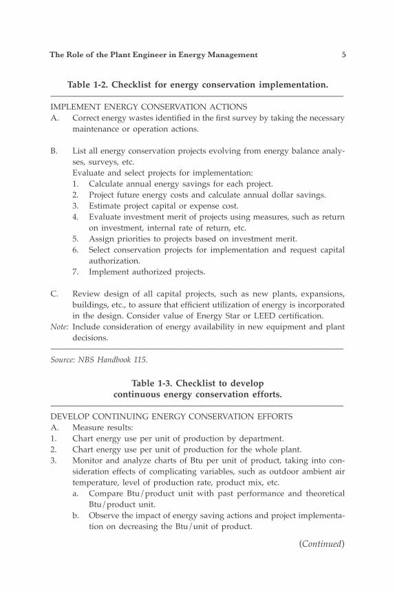
2. Implement actions for energy conservation. (Refer to checklist, Table 1-2.)
3. Continue to monitor energy conservation efforts. (Refer to checklist, Table 1-3.)
Determine Energy Uses and Losses Probably the most important aspect of an ongoing energy utili-zation program is to make individuals “accountable” for energy use. Unfortunately, many energy managers find it difficult to economically justify “submetering.” The savings as a result of increased accountability are difficult to measure.
4 Plant Engineers and Managers Guide to Energy Conservation
Table 1-1. Checklist to determine energy uses and losses.————————————————————————————————SURVEY ENERGY USES AND LOSSESA. Conduct first survey aimed at identifying energy wastes that can be cor-
rected by maintenance or operations actions, for example:1. Leaks of steam and other utilities2. Furnace burners out of adjustment3. Repair or addition of insulation required4. Equipment running when not needed
B. Survey to determine where additional instruments for measurement of energy flow are needed and whether there is economic justification for the cost of their installation.
C. Develop an energy balance on each process to define in detail:1. Energy input as raw materials and utilities2. Energy consumed in waste disposal3. Energy credit for by-products4. Net energy charged to the main product5. Energy dissipated or wasted
Note: Energy equivalents will need to be developed for all raw materials, fuels, and utilities, such as electric power, steam, etc., in order that all energy can be expressed on the common basis of Btus.
D. Analyze all process energy balances in depth:1. Can waste heat be recovered to generate steam or to heat water or a
raw material?2. Can a process step be eliminated or modified in some way to reduce
energy use?3. Can an alternate raw material with lower energy content be used?4. Is there a way to improve yield?5. Is there justification for:
a. Replacing old equipment with new equipment requiring less en-ergy?
b. Replacing an obsolete, inefficient process plant with an entirely new and different process using less energy?
E. Conduct weekend and night surveys periodically.
F. Plan surveys on specific systems and equipment, such as:1. Steam system2. Compressed air system3. Electric motors4. Natural gas lines5. Heating and air conditioning system
————————————————————————————————Source: NBS Handbook 115.
The Role of the Plant Engineer in Energy Management 5
Table 1-2. Checklist for energy conservation implementation.————————————————————————————————IMPLEMENT ENERGY CONSERVATION ACTIONSA. Correct energy wastes identified in the first survey by taking the necessary
maintenance or operation actions.
B. List all energy conservation projects evolving from energy balance analy-ses, surveys, etc.
Evaluate and select projects for implementation:1. Calculate annual energy savings for each project.2. Project future energy costs and calculate annual dollar savings.3. Estimate project capital or expense cost.4. Evaluate investment merit of projects using measures, such as return
on investment, internal rate of return, etc.5. Assign priorities to projects based on investment merit.6. Select conservation projects for implementation and request capital
authorization.7. Implement authorized projects.
C. Review design of all capital projects, such as new plants, expansions, buildings, etc., to assure that efficient utilization of energy is incorporated in the design. Consider value of Energy Star or LEED certification.
Note: Include consideration of energy availability in new equipment and plant decisions.
————————————————————————————————Source: NBS Handbook 115.
(Continued)
Table 1-3. Checklist to developcontinuous energy conservation efforts.
————————————————————————————————DEVELOP CONTINUING ENERGY CONSERVATION EFFORTSA. Measure results:1. Chart energy use per unit of production by department.2. Chart energy use per unit of production for the whole plant.3. Monitor and analyze charts of Btu per unit of product, taking into con-
sideration effects of complicating variables, such as outdoor ambient air temperature, level of production rate, product mix, etc.a. Compare Btu/product unit with past performance and theoretical
Btu/product unit.b. Observe the impact of energy saving actions and project implementa-
tion on decreasing the Btu/unit of product.
6 Plant Engineers and Managers Guide to Energy Conservation
c. Investigate, identify, and correct the cause for increases that may occur in Btu unit of product, if feasible.
B. Continue energy conservation committee activities: 1. Hold periodic meetings. 2. Each committee member is the communication link between the com-
mittee and the department supervisors represented. 3. Periodically update energy saving project lists. 4. Plan and participate in energy saving surveys. 5. Communicate energy conservation techniques. 6. Plan and conduct a continuing program of activities and communica-
tion to keep up interest in energy conservation. 7. Develop cooperation with community organizations in promoting
energy conservation.
C. Involve employees: 1. Service on energy conservation committee 2. Energy conservation training course 3. Handbook on energy conservation 4. Suggestion awards plan 5. Recognition for energy saving achievements 6. Technical talks on lighting, insulation, steam traps, and other sub-
jects 7. “Save Energy” posters, decals, stickers 8. Publicity in plant news, bulletins 9. Publicity in public news media 10. Letters on conservation to homes 11. Talks to local organizations
D. Evaluate program: 1. Review progress in energy saving. 2. Evaluate original goals. 3. Consider program modifications. 4. Revise goals as necessary.
————————————————————————————————Source: NBS Handbook 115.
Table 1-3. (Continued)————————————————————————————————
The Role of the Plant Engineer in Energy Management 7
Table 1-1 (B) indicates, as part of the initial survey, that a deter-mination should be made as to who is responsible for which area or process and where submetering would have the biggest impact.
Implement Actions for Energy Conservation Once energy usage is known, potential energy conservation projects can be identified. Each project will be recommended on the basis of the annual energy savings projected and the initial investment required.
Continue to Monitor Energy Conservation Efforts Energy usage needs to be tracked by using a common energy consumption base per unit of production. This tracking will allow quick identification of changes in energy consumption. The remaining portion of this chapter will illustrate the language of energy conservation and its applications.
ENERGY ACCOUNTING
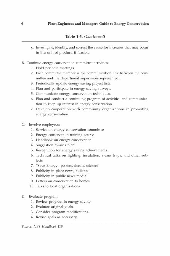
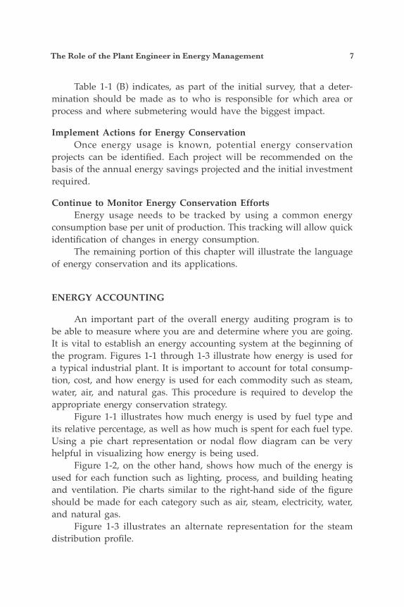
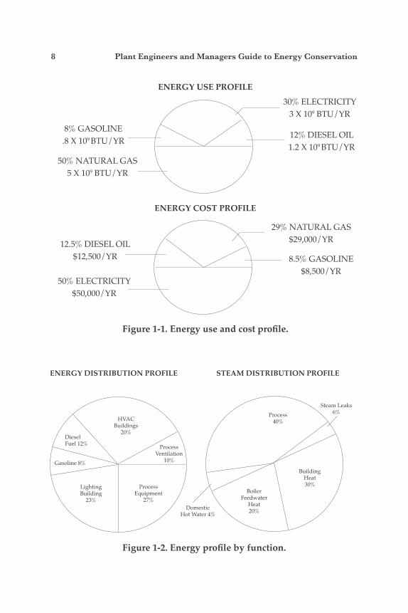
An important part of the overall energy auditing program is to be able to measure where you are and determine where you are going. It is vital to establish an energy accounting system at the beginning of the program. Figures 1-1 through 1-3 illustrate how energy is used for a typical industrial plant. It is important to account for total consump-tion, cost, and how energy is used for each commodity such as steam, water, air, and natural gas. This procedure is required to develop the appropriate energy conservation strategy. Figure 1-1 illustrates how much energy is used by fuel type and its relative percentage, as well as how much is spent for each fuel type. Using a pie chart representation or nodal flow diagram can be very helpful in visualizing how energy is being used. Figure 1-2, on the other hand, shows how much of the energy is used for each function such as lighting, process, and building heating and ventilation. Pie charts similar to the right-hand side of the figure should be made for each category such as air, steam, electricity, water, and natural gas. Figure 1-3 illustrates an alternate representation for the steam distribution profile.
8 Plant Engineers and Managers Guide to Energy Conservation
Figure 1-2. Energy profile by function.
Figure 1-1. Energy use and cost profile.
ENERGY USE PROFILE
ENERGY COST PROFILE
30% ELECTRICITY3 X 109 BTU/YR
12% DIESEL OIL1.2 X 109 BTU/YR
8% GASOLINE.8 X 109 BTU/YR
50% NATURAL GAS5 X 109 BTU/YR
29% NATURAL GAS$29,000/YR
8.5% GASOLINE$8,500/YR
12.5% DIESEL OIL$12,500/YR
50% ELECTRICITY$50,000/YR
ENERGY DISTRIBUTION PROFILE
HVACBuildings
20%DieselFuel 12%
Gasoline 8%
ProcessVentilation
10%
LightingBuilding
23%
ProcessEquipment
27%
Process40%
BuildingHeat30%
BoilerFeedwater
Heat20%
Steam Leaks 6%
DomesticHot Water 4%
STEAM DISTRIBUTION PROFILE
The Role of the Plant Engineer in Energy Management 9
One of the more important as-pects of energy management and conservation is measuring and ac-counting for energy consumption. At Carborundum an energy accounting and analysis system was developed that was unique in industry, a simple but powerful analytical, manage-ment decision-making tool. The Of-fice of Energy Programs of the U.S. Department of Commerce asked Carborundum to work with it in de-veloping this system into a national system, hopefully to be used in the voluntary industrial conservation program. A number of major U.S. corporations are using the system.
The system is offered to those who want to use it. Most energy accounting systems have been devised and are ad-ministered by engineers for engineers. The engineers’ principal interest in developing these systems has been the display of energy consumed per unit of production. That ratio has been called “energy efficiency,’’ and changes in energy efficiency are clearly energy conserved or wasted. The engineer focuses all of his attention on reducing energy consumed per unit of production. An energy efficiency ratio alone, however, cannot answer the kinds of questions asked by business managers and/or government authorities:
• If we are conserving energy, why is our total energy consumption increasing?
• If we are wasting energy, why is our total energy consumption decreasing?
• If we have made no change in energy efficiency, why is our energy consumption changing?
Thus there is a need to evaluate several impacts, such as weather, volume/mix, and pollution control that affect energy use.
Figure 1-3. Steam distributionnodal diagram.
Stea
m L
eaks
6
%
Process
40%
Building Heat 30%Steam 100%
Boiler Feedwater 20%
Hot W
ater 4%
10 Plant Engineers and Managers Guide to Energy Conservation
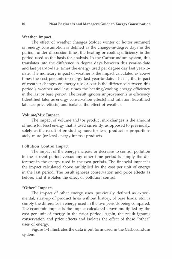
Weather Impact The effect of weather changes (colder winter or hotter summer) on energy consumption is defined as the change-in-degree days in the periods under discussion times the heating or cooling efficiency in the period used as the basis for analysis. In the Carborundum system, this translates into the difference in degree days between this year-to-date and last year-to-date, times the energy used per degree day last year-to-date. The monetary impact of weather is the impact calculated as above times the cost per unit of energy last year-to-date. That is, the impact of weather changes on energy use or cost is the difference between this period’s weather and last, times the heating/cooling energy efficiency in the last or base period. The result ignores improvements in efficiency (identified later as energy conservation effects) and inflation (identified later as price effects) and isolates the effect of weather.
Volume/Mix Impact The impact of volume and/or product mix changes is the amount of more (or less) energy that is used currently, as opposed to previously, solely as the result of producing more (or less) product or proportion-ately more (or less) energy-intense products.
Pollution Control Impact The impact of the energy increase or decrease to control pollution in the current period versus any other time period is simply the dif-ference in the energy used in the two periods. The financial impact is the impact calculated above multiplied by the cost per unit of energy in the last period. The result ignores conservation and price effects as before, and it isolates the effect of pollution control.
“Other” Impacts The impact of other energy uses, previously defined as experi-mental, start-up of product lines without history, of base loads, etc., is simply the difference in energy used in the two periods being compared. The economic impact is the impact calculated above multiplied by the cost per unit of energy in the prior period. Again, the result ignores conservation and price effects and isolates the effect of these “other” uses of energy. Figure 1-4 illustrates the data input form used in the Carborundum system.

The Role of the Plant Engineer in Energy Management 11
Figure 1-4. Carborundum energy accounting and analysis system data input form.
Carborundum Energy Accounting andAnalysis System Data Input Form
Plant _________________________________________________________ Division ________________________________________________________ Group _________________________________________________________
Today's Date ___________________________________________________ Period Covered ___________________________________________________————————————————————————————————Description Elec. kWh Gas mcf Oil gal. Coal lbs. Propane Gal. Other (000)* (000)* (000)* (000)* (000)*————————————————————————————————Total Fuel Used————————————————————————————————Quantity ————————————————————————————————Cost ($)————————————————————————————————**Conversion Factor————————————————————————————————ProductionProduct 1 NAME————————————————————————————————Production Unit————————————————————————————————Quant. Prod. (000)————————————————————————————————Fuel Used————————————————————————————————Product 2 NAME————————————————————————————————Production Unit————————————————————————————————Quant. Prod. (000)————————————————————————————————Fuel Used————————————————————————————————Product 3 NAME————————————————————————————————Production Unit————————————————————————————————Quant. Prod. (000)————————————————————————————————Fuel Used————————————————————————————————Product 4 NAME————————————————————————————————Production Unit————————————————————————————————Quant. Prod. (000)————————————————————————————————Fuel Used————————————————————————————————Product 5 NAME————————————————————————————————Production Unit————————————————————————————————Quant. Prod. (000)————————————————————————————————Fuel Used————————————————————————————————Heating————————————————————————————————Degree Days————————————————————————————————Fuel Used————————————————————————————————Cooling————————————————————————————————Degree Days————————————————————————————————Fuel Used————————————————————————————————Pollution Control————————————————————————————————Fuel Used————————————————————————————————Other————————————————————————————————Fuel Used————————————————————————————————**Alternate Fuel————————————————————————————————*All Fuel reported in thousands to two decimal places
EnergyManagement andConservationProgram
Plant Input Data
12 Plant Engineers and Managers Guide to Energy Conservation
THE LANGUAGE OF THE ENERGY MANAGER
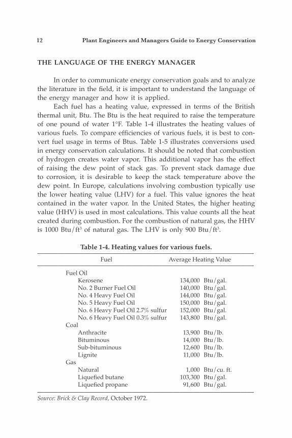
In order to communicate energy conservation goals and to analyze the literature in the field, it is important to understand the language of the energy manager and how it is applied. Each fuel has a heating value, expressed in terms of the British thermal unit, Btu. The Btu is the heat required to raise the temperature of one pound of water 1°F. Table 1-4 illustrates the heating values of various fuels. To compare efficiencies of various fuels, it is best to con-vert fuel usage in terms of Btus. Table 1-5 illustrates conversions used in energy conservation calculations. It should be noted that combustion of hydrogen creates water vapor. This additional vapor has the effect of raising the dew point of stack gas. To prevent stack damage due to corrosion, it is desirable to keep the stack temperature above the dew point. In Europe, calculations involving combustion typically use the lower heating value (LHV) for a fuel. This value ignores the heat contained in the water vapor. In the United States, the higher heating value (HHV) is used in most calculations. This value counts all the heat created during combustion. For the combustion of natural gas, the HHV is 1000 Btu/ft3 of natural gas. The LHV is only 900 Btu/ft3.
Table 1-4. Heating values for various fuels.———————————————————————————————— Fuel Average Heating Value———————————————————————————————— Fuel Oil Kerosene 134,000 Btu/gal. No. 2 Burner Fuel Oil 140,000 Btu/gal. No. 4 Heavy Fuel Oil 144,000 Btu/gal. No. 5 Heavy Fuel Oil 150,000 Btu/gal. No. 6 Heavy Fuel Oil 2.7% sulfur 152,000 Btu/gal. No. 6 Heavy Fuel Oil 0.3% sulfur 143,800 Btu/gal. Coal Anthracite 13,900 Btu/lb. Bituminous 14,000 Btu/lb. Sub-bituminous 12,600 Btu/lb. Lignite 11,000 Btu/lb. Gas Natural 1,000 Btu/cu. ft. Liquefied butane 103,300 Btu/gal. Liquefied propane 91,600 Btu/gal.————————————————————————————————Source: Brick & Clay Record, October 1972.

The Role of the Plant Engineer in Energy Management 13
Table 1-5. List of conversion factors.————————————————————————————————1 U.S. barrel = 42 U.S. gallons1 atmosphere = 14.7 pounds per square inch absolute (psia)1 atmosphere = 760 mm (29.92 in) mercury with density of 13.6 grams per cubic centimeter1 pound per square inch = 2.04 inches head of mercury = 2.31 feet head of water1 inch head of water = 5.20 pounds per square foot1 foot head of water = 0.433 pound per square inch1 British thermal unit (Btu) = heat required to raise the temperature of 1 pound of water by 1°F1 therm = 100,000 Btu1 kilowatt (kW) = 1.341 horsepower (hp)1 kilowatt-hour (kWh) = 1.34 horsepower-hour1 horsepower (hp) = 0.746 kilowatt (kW)1 horsepower-hour = 0.746 kilowatt hour (kWh)1 horsepower-hour = 2545 Btu1 kilowatt-hour (kWh) = 3412 BtuTo generate 1 kilowatt-hour (kWh) requires 10,000 Btu of fuel burned by average utility1 ton of refrigeration = 12,000 Btu per hr1 ton of refrigeration requires about 1 kW (or 1.341 hp) in commercial air condi-tioning1 standard cubic foot is at standard conditions of 60°F and 14.7 psia.1 degree day = 65°F minus mean temperature of the day, °F1 year = 8760 hours1 year = 365 days1 MBtu = 1 million Btu1 kW = 1000 watts1 trillion barrels = 1 × 10¹² barrels1 KSCF = 1000 standard cubic feet————————————————————————————————Note: In these conversions, inches and feet of water are measured at 62°F (16.7°C), and inches and millimeters of mercury at 32°F (0°C).
14 Plant Engineers and Managers Guide to Energy Conservation
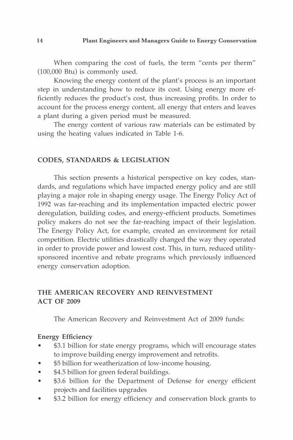
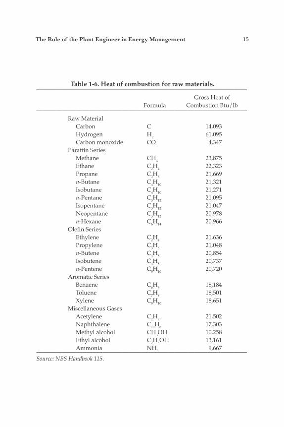
When comparing the cost of fuels, the term “cents per therm” (100,000 Btu) is commonly used. Knowing the energy content of the plant’s process is an important step in understanding how to reduce its cost. Using energy more ef-ficiently reduces the product’s cost, thus increasing profits. In order to account for the process energy content, all energy that enters and leaves a plant during a given period must be measured. The energy content of various raw materials can be estimated by using the heating values indicated in Table 1-6.
CODES, STANDARDS & LEGISLATION
This section presents a historical perspective on key codes, stan-dards, and regulations which have impacted energy policy and are still playing a major role in shaping energy usage. The Energy Policy Act of 1992 was far-reaching and its implementation impacted electric power deregulation, building codes, and energy-efficient products. Sometimes policy makers do not see the far-reaching impact of their legislation. The Energy Policy Act, for example, created an environment for retail competition. Electric utilities drastically changed the way they operated in order to provide power and lowest cost. This, in turn, reduced utility-sponsored incentive and rebate programs which previously influenced energy conservation adoption.
THE AMERICAN RECOVERY AND REINVESTMENTACT OF 2009
The American Recovery and Reinvestment Act of 2009 funds:
Energy Efficiency• $3.1 billion for state energy programs, which will encourage states
to improve building energy improvement and retrofits.• $5 billion for weatherization of low-income housing.• $4.5 billion for green federal buildings.• $3.6 billion for the Department of Defense for energy efficient
projects and facilities upgrades• $3.2 billion for energy efficiency and conservation block grants to
The Role of the Plant Engineer in Energy Management 15
Table 1-6. Heat of combustion for raw materials.———————————————————————————————— Gross Heat of Formula Combustion Btu/lb———————————————————————————————— Raw Material Carbon C 14,093 Hydrogen H2 61,095 Carbon monoxide CO 4,347 Paraffin Series Methane CH4 23,875 Ethane C2H4 22,323 Propane C3H8 21,669 n-Butane C4H10 21,321 Isobutane C4H10 21,271 n-Pentane C5H12 21,095 Isopentane C5H12 21,047 Neopentane C5H12 20,978 n-Hexane C6H14 20,966 Olefin Series Ethylene C2H4 21,636 Propylene C3H6 21,048 n-Butene C4H8 20,854 Isobutene C4H8 20,737 n-Pentene C5H10 20,720 Aromatic Series Benzene C6H6 18,184 Toluene C7H8 18,501 Xylene C8H10 18,651 Miscellaneous Gases Acetylene C2H2 21,502 Naphthalene C10H8 17,303 Methyl alcohol CH3OH 10,258 Ethyl alcohol C2H5OH 13,161 Ammonia NH3 9,667————————————————————————————————Source: NBS Handbook 115.
16 Plant Engineers and Managers Guide to Energy Conservation
help state and local governments implement energy efficiency• $500 million for job training and programs to prepare individuals
for careers in energy efficiency and renewable energy
Solar Energy—ARRA Contains Provisions for:• Renewable Energy Grant Program: Offers Department of Energy
grants equal to 30% of the cost of solar projects started in the next two years, including large-scale utility projects. This is a critical alternative to solar tax credits that are not functioning as Congress intended in the current economic climate.
• Loan Guarantee Program: Creates a new, streamlined loan guarantee program to support financing of renewable energy systems, including solar energy technology.
• Manufacturing Investment Credit: Creates a 30% investment tax credit for facilities engaged in the manufacture of renewable energy property or equipment.
Smart Grid/Advanced Battery/Energy Efficiency• $34 billion will be provided for such initiatives as a new, smart
power grid, advanced battery technology, and energy efficiency measures. According to the fact sheet, 500,000 energy jobs will be created.
THE ENERGY POLICY ACT OF 2005
The first major piece of national energy legislation since the Energy Policy Act of 1992, EPACT 2005, was signed by President George W. Bush on August 8, 2005 and became effective January 1, 2006. The major thrust of EPACT 2005 is energy production. However, there are many impor-tant sections of EPACT 2005 that do help promote energy efficiency and energy conservation. There are also some significant impacts on Federal Energy Management. Highlights are given below.
Federal Energy Management• The United States is the single largest energy user, with about a $10
billion energy budget. Forty-four percent of this budget was used for non-mobile buildings and facilities. The United States is also the
The Role of the Plant Engineer in Energy Management 17
single largest product purchaser, with $6 billion spent for energy- using products, vehicles, and equipment.
Energy Management Goals• An annual energy reduction goal of 2% is in place from fiscal year
2006 to fiscal year 2015 for a total energy reduction of 20%.
• Electric metering is required in all federal building by the year 2012.
• Energy efficient specifications are required in procurement bids and evaluations.
• Energy efficient products to be listed in federal catalogs include Energy Star and FEMP recommended products by GSA and the Defense Logistics Agency.
• Energy service performance contracts (ESPCs) are reauthorized through September 30, 2016.
• New federal buildings are required to be designed 30% below the ASHRAE standard or the International Energy Code (if life-cycle cost effective.) Agencies must identify those that meet or exceed the standard.
• Renewable electricity consumption by the federal government cannot be less than: 3% from fiscal year 2007-2009, 5% from fiscal year 2010-2012, and 7.5% from fiscal year 2013-present. Double credits are earned for renewables produced on the site or on federal lands and used at a federal facility, or renewables produced on Native American lands.
• The goal for photovoltaic energy is to have 20,000 solar energy systems installed in Federal buildings by the year 2012.
Tax Provisions• Tax credits will be issued for residential solar photovoltaic and hot
water heating systems. Tax deductions will be offered for highly efficient commercial buildings and highly efficient new homes. There will also be tax credits for improvements made to existing homes, including high efficiency HVAC systems and residential fuel cell systems. Tax credits are also available for fuel cells and microturbines used in businesses.
18 Plant Engineers and Managers Guide to Energy Conservation
THE ENERGY INDEPENDENCE AND SECURITY ACT OF 2007 (H.R.6)
The Energy Independence and Security Act of 2007 (H.R.6) was enacted into law December 19, 2007. Key provisions of the law are sum-marized below.
Title I Energy Security through Improved Vehicle Fuel Economy• Corporate average fuel economy (CAFE): The law sets a target of
35 miles per gallon for the combined fleet of cars and light trucks by 2020.
• The law establishes a loan guarantee program for advanced bat-tery development, a grant program for plug-in hybrid vehicles, incentives for purchasing heavy-duty hybrid vehicles for fleets, and credits for various electric vehicles.
Title II Energy Security through Increased Production of Biofuels• The law increases the renewable fuels standard (RFS), which sets
annual requirements for the quantity of renewable fuels pro-duced and used in motor vehicles. RFS requires 9 billion gallons of renewable fuels in 2008, increasing to 36 billion gallons in 2022.
Title III Energy Savings Through Improved Standards for Appliances and Lighting
• The law establishes new efficiency standards for motors, external power supplies, residential clothes washers, dishwashers, dehu-midifiers, refrigerators, refrigerator freezers, and residential boil-ers.
• The law contains a set of national standards for light bulbs. The first part of the standards would increase energy efficiency of light bulbs 30% and phase out most common types of incandes-cent light bulbs by 2012-2014.
• Requires the federal government to substitute energy efficient lighting for incandescent bulbs.
Title IV Energy Savings in Buildings and Industry• The law increases funding for the Department of Energy's Weath-
erization Program, providing 3.75 billion dollars over five years.• The law encourages the development of more energy efficient,
"green" commercial buildings. The law creates an Office of Com-
The Role of the Plant Engineer in Energy Management 19
mercial High Performance Green Buildings at the Department of Energy.
• A national goal is set to achieve zero-net energy use for new com-mercial buildings built after 2025. A further goal is to retrofit all pre-construction 2025 buildings to zero-net energy by 2050.
• Requires that total energy use in federal buildings relative to the 2005 level be reduced 30% by 2015.
• Requires federal facilities to conduct a comprehensive energy and water evaluation for each facility at least once every four years.
• Requires new federal buildings and major renovations to reduce fossil fuel energy use 55% relative to 2003 level by 2010 and be eliminated (100% reduction) by 2030.
• Requires that each federal agency ensure that major replacements of installed equipment (such as heating and cooling systems) or renovation or expansion of existing space employ the most en-ergy efficient designs, systems, equipment, and controls that are life cycle cost effective. For the purposes of calculating life cycle cost calculations, the time period will increase from 25 years (in the prior law) to 40 years.
• Directs the Department of Energy to conduct research to develop and demonstrate new process technologies and operating prac-tices to significantly improve the energy efficiency of equipment and processes used by energy-intensive industries.
• Directs the Environmental Protection Agency to establish a re-coverable waste energy inventory program. The program must include an ongoing survey of all major industrial and large com-mercial combustion services in the United States.
• Includes new incentives to promote new industrial energy effi-ciency through the conversion of waste heat into electricity.
• Creates a grant program for healthy, high-performance schools that aims to encourage states, local governments, and school sys-tems to build green schools.
• Creates a program of grants and loans to support energy effi-ciency and energy sustainability projects at public institutions.
Title V Energy Savings in Government and Public Institutions• Promotes energy savings performance contracting in the federal
government and provides flexible financing and training of fed-
20 Plant Engineers and Managers Guide to Energy Conservation
eral contract officers.• Promotes the purchase of energy efficient products and procure-
ment of alternative fuels with lower carbon emissions for the federal government.
• Reauthorizes state energy grants for renewable energy and en-ergy efficiency technologies through 2012.
• Establishes an energy and environmental block grant program to be used for seed money for innovative local best practices.
Title VI Alternative Research and Development• Authorizes research and development to expand the use of geo-
thermal energy.• Improves the cost and effectiveness of thermal energy storage
technologies that could improve the operation of concentrating solar power electric generation plants.
• Promotes research and development of technologies that pro-duce electricity from waves, tides, currents, and ocean thermal differences.
• Authorizes a development program on energy storage systems for electric drive vehicles, stationary applications, and electricity transmission and distribution.
Title VII Carbon Capture and Sequestration• Provides grants to demonstrate technologies to capture carbon
dioxide from industrial sources.• Authorizes a nationwide assessment of geological formations
capable of sequestering carbon dioxide underground.
Title VIII Improved Management of Energy Policy• Creates a 50% matching grants program for constructing small
renewable energy projects that will have an electrical generation capacity less than 15 megawatts.
• Prohibits crude oil and petroleum product wholesalers from using any technique to manipulate the market or provide false information.
Title IX International Energy Programs• Promotes U.S. exports in clean, efficient technologies to India,
China, and other developing countries.
The Role of the Plant Engineer in Energy Management 21
• Authorizes the U.S. Agency for International Development (USAID) to increase funding to promote clean energy technolo-gies in developing countries.
Title X Green Jobs• Creates an energy efficiency and renewable energy worker train-
ing program for "green collar" jobs.• Provides training opportunities for individuals in the energy
field who need to update their skills.
Title XI Energy Transportation and Infrastructure• Establishes an office of climate change and environment to coor-
dinate and implement strategies to reduce transportation-related energy use.
Title XII Small Business Energy Programs• Loans, grants and debentures are established to help small busi-
nesses develop, invest in, and purchase energy efficient equip-ment and technologies.
Title XIII Smart Grid• Promotes a “smart electric grid” to modernize and strengthen the
reliability and energy efficiency of the electricity supply. The term “smart grid” refers to a distribution system that allows for flow of information from a customer’s meter in two directions—both inside the house to thermostats, appliances, and other devices, and from the house back to the utility.
THE ENERGY POLICY ACT OF 1992
This comprehensive legislation impacted energy conservation, power generation, and alternative-fuel vehicles, as well as energy production. Both federal and private sectors were impacted by this comprehensive energy act. Highlights are described below.
Energy Efficiency ProvisionsBuildings• Required states to establish minimum commercial building energy
22 Plant Engineers and Managers Guide to Energy Conservation
codes and to consider minimum residential codes based on current voluntary codes.
Utilities• Required states to consider new regulatory standards that would
require utilities to undertake integrated resource planning, allow efficiency programs to be at least as profitable as new supply op-tions, and encourage improvements in supply system efficiency.
Equipment Standards• Established efficiency standards for commercial heating and air-
conditioning equipment, electric motors, and lamps.
• Gives the private sector an opportunity to establish voluntary efficiency information/labeling programs for windows, office equipment and luminaires—or the Department of Energy will establish such programs.
Renewable Energy• Established a program for providing federal support on a com-
petitive basis for renewable energy technologies. Expanded the program to promote export of these renewable energy technologies to emerging markets in developing countries.
Alternative Fuels• Gave the Department of Energy the authority to require a private
and municipal alternative fuel fleet program. Provided a federal alternative fuel fleet program with phased-in acquisition schedule; also provided a state fleet program for large fleets in large cities.
Electric Vehicles• Established a comprehensive program for the research and devel-
opment, infrastructure promotion, and vehicle demonstration for electric motor vehicles.
Electricity• Removed obstacles to wholesale power competition in the Public
Utilities Holding Company Act by allowing both utilities and non-utilities to form exempt wholesale generators without triggering the PUHCA restrictions.
The Role of the Plant Engineer in Energy Management 23
Global Climate Change• Directed the Energy Information Administration to establish a
baseline inventory of greenhouse gas emissions and established a program for the voluntary reporting of those emissions. Di-rected the Department of Energy to prepare a report analyzing the strategies for mitigating global climate change and to develop a least-cost energy strategy for reducing the generation of green-house gases.
Research and Development• Directed the Department of Energy to undertake research and
development on a wide range of energy technologies, includ-ing energy efficiency technologies, natural gas end-use products, renewable energy resources, heating and cooling products, and electric vehicles.
PUBLIC UTILITY REGULATORY POLICIES ACT (PURPA)
This legislation was part of the 1978 National Energy Act and has had perhaps the most significant effect on the development of cogeneration and other forms of alternative energy production in the past decade. Certain provisions of PURPA also apply to the exchange of electric power between utilities and cogenerators. PURPA provides a number of benefits to those cogenerators who can become "qualifying facilities" (QFs) under the act. Specifically, PURPA:
• Requires utilities to purchase the power made available by cogen-erators at reasonable buy-back rates (rates typically based on the utilities’ cost).
• Guarantees the cogenerator or small power producer interconnec-tion with the electric grid and backup service from the utility.
• Dictates that supplemental power requirements of the cogenerator must be provided at a reasonable cost.
• Exempts cogenerators and small power producers from federal and state utility regulations and their associated reporting require-ments.
24 Plant Engineers and Managers Guide to Energy Conservation
In order to assure a facility the benefits of PURPA, a cogenera-tor must become a qualifying facility. To achieve qualifying status, a cogenerator must generate electricity and useful thermal energy from a single fuel source. In addition, a cogeneration facility must be less than 50% owned by an electric utility or an electric utility holding company. Finally, the plant must meet the minimum annual operating efficiency standard established by FERC when using oil or natural gas as the prin-cipal fuel source. The standard is that the useful electric power output plus one half of the useful thermal output of the facility must be no less than 42.5% of the total oil or natural gas energy input. The minimum efficiency standard increases to 45% if the useful thermal energy is less than 15% of the total energy output of the plant.
CODES AND STANDARDS
Energy codes specify how buildings must be constructed or per-form, and are written in a mandatory, enforceable language. State and local governments adopt and enforce energy codes for their jurisdictions. Energy standards describe how buildings should be constructed to save energy cost effectively. They are published by national organizations such as the American Society of Heating, Refrigerating, and Air Conditioning Engineers (ASHRAE). They are not mandatory but serve as national rec-ommendations, with some variation for regional climate. State and local governments frequently use energy standards as the technical basis for developing their energy codes. Some energy standards are written in a mandatory, enforceable language, making it easy for jurisdictions to in-corporate the provisions of the energy standards directly into their laws or regulations. The requirement for the federal sector to use ASHRAE 90.1 and 90.2 as mandatory standards for all new federal buildings is specified in the Code of Federal Regulations—10 CFR 435. Most states use the ASHRAE 90 standard as the basis for the energy component of their building codes. ASHRAE 90.1 is used for commercial buildings and ASHRAE 90.2 is used for residential buildings. Some states have quite comprehensive building codes, i.e., California Title 24.
ASHRAE Standard 90.1• Energy efficient design for new buildings. Sets minimum requirements for the energy efficient design of new
The Role of the Plant Engineer in Energy Management 25
buildings so they may be constructed, operated, and maintained in a manner that minimizes the use of energy without constraining the building function and productivity of the occupants.
• ASHRAE 90.1 addresses building components and systems that affect energy usage.
• Sections 5-10 are the technical sections that specifically address components of the building envelope, HVAC systems and equipment, service water heating, power, lighting, and motors. Each technical section contains general requirements and mandatory provisions. Some sections also include prescriptive and performance requirements.
ASHRAE Standard 90.2• Energy efficient design of new low-rise residential buildings.
When the Department of Energy determines that a revision would improve energy efficiency, each state has two years to review the energy provisions of its residential or commercial building code. For residential buildings, a state has the option of revising its residential code to meet or exceed the residential portion of ASHRAE 90.2. For commercial build-ings, a state is required to update its commercial code to meet or exceed the provision of ASHRAE 90.1. ASHRAE standards 90.1 and 90.2 are developed and revised through voluntary consensus and public hearing processes that are critical to widespread support for their adoption. Both standards are con-tinually maintained by separate standing standards projects committees. Committee membership varies from 10 to 60 voting members and in-cludes representatives from many groups to ensure balance among all in-terest categories. After the committee proposes revisions to the standard, it undergoes public review and comment. When a majority of the parties substantially agree, the revised standard is submitted to the ASHRAE board of directors. This entire process can take anywhere from two to ten years to complete. ASHRAE Standards 90.1 and 90.2 are automatically revised and published every three years. Approved interim revisions are posted on the ASHRAE website (www.ashrae.org) and are included in the next published version. The energy cost budget method permits trade-offs between build-ing systems (lighting and fenestration, for example) if the annual energy cost estimated for the proposed design does not exceed the annual energy
26 Plant Engineers and Managers Guide to Energy Conservation
cost of a base design that fulfills the prescriptive requirements. Using the energy cost budget method approach requires simulation software that can analyze energy consumption in buildings and model the energy fea-tures in the proposed design. ASHRAE 90.1 sets minimum requirements for the simulation software; suitable programs include BLAST, eQUEST, and TRACE. The ASHRAE Standard 90-80 is essentially “prescriptive” in nature. For example, the energy engineer using this standard would compute the average conductive value for the building walls and compare it against the value in the standard. If the computed value is above the recommendation, the amount of glass or building construction materials would need to be changed to meet the standard. Most states have initiated model energy codes for efficiency stan-dards in lighting and HVAC. Probably one of the most comprehensive building efficiency standards is California Title 24. Title 24 established lighting and HVAC efficiency standards for new construction, altera-tions, and additions of commercial and noncommercial buildings.
ASHRAE Standard 90-80 has been updated into two new standards:
ASHRAE 90.1-1989 Energy Efficient Design of New Buildings Except New, Low-Rise Residential Buildings
ASHRAE 90.2 Energy Efficient Design of New, Low-Rise Residential Buildings
The purposes of ASHRAE Standard 90.1-1989 are to:(a) Set minimum requirements for the energy efficient design of new
buildings so that they may be constructed, operated, and main-tained in a manner that minimizes the use of energy without constraining the building function or the comfort or productivity of the occupants.
(b) Provide criteria for energy efficient design and methods for deter-mining compliance with these criteria.
(c) Provide sound guidance for energy efficient design.
In addition to recognizing advances in the performance of vari-ous components and equipment, the standard encourages innovative energy conserving designs. This has been accomplished by allowing the building designer to take into consideration the dynamics that exist
The Role of the Plant Engineer in Energy Management 27
between the many components of a building through use of the system performance method or the building energy cost budget method com-pliance paths. The standard, which is cosponsored by the Illuminating Engineering Society of North America, includes an extensive section on lighting efficiency, utilizing the unit power allowance method.
Natural Gas Policy Act (NGPA) The major objective of this legislation was to create a deregulated national market for natural gas. It provides for incremental pricing of higher-cost natural gas supplies to industrial customers who use gas, and it allows the cost of natural gas to fluctuate with the cost of fuel oil. Cogenerators classified as qualifying facilities under PURPA are exempt from the incremental pricing schedule established for industrial customers.
Resource Conservation and Recovery Act of 1976 (RCRA) This act requires that disposal of non-hazardous solid waste be handled in a sanitary landfill instead of an open dump. It affects only cogenerators with biomass and coal-fired plants. This legislation has had little, if any, impact on oil and natural gas cogeneration projects.
Public Utility Holding Company Act of 1935 The Public Utility Holding Company Act of 1935 (the 35 Act) authorizes the Securities and Exchange Commission (SEC) to regulate certain utility “holding companies” and their subsidiaries in a wide range of corporate transactions. The Energy Policy Act of 1992 created a new class of wholesale-on-ly electric generators—“exempt wholesale generators” (EWGs)—which are exempt from the Public Utility Holding Company Act (PUHCA). The Act dramatically enhanced competition in U.S. wholesale electric generation markets, including broader participation by subsidiaries of electric utilities and holding companies. It also opened up foreign markets by exempting companies from PUHCA with respect to retail as well as wholesale sales.
29
2Energy EconomicDecision Making
LIFE CYCLE COSTING
When a plant manager is assigned the role of energy manager, the first question to be asked is, “What is the economic basis for equipment purchases?” Some companies use a simple payback method of two years or less to justify equipment purchases. Others require a life cycle cost analysis with no fuel price inflation considered. Still other companies allow for a complete life cycle cost analysis, including the impact for the fuel price inflation and the energy tax credit. The energy manager’s success is directly related to how energy utilization methods must be justified.
USING THE PAYBACK PERIOD METHOD
The payback period is the time required to recover the capital investment out of earnings or savings. This method ignores all savings beyond the payback years, thus favoring projects that offer high sav-ings for a relatively short period over those with long life potential. The payback period criterion is used when funds are limited and it is important to know how fast dollars will come back. The payback period is simply computed as:
initial investment Payback period = ————————— (2-1) after-tax savings
30 Plant Engineers and Managers Guide to Energy Conservation
The energy manager who must justify energy equipment expendi-tures based on a payback period of one year or less has little chance for long-range success. Some companies have set higher payback periods for energy utilization methods. These longer payback periods are justi-fied on the basis that:
• Fuel pricing will increase at a higher rate than the general inflation rate.
• The “risk analysis” for not implementing energy utilization mea-sures may mean loss of production and losing a competitive edge.
USING LIFE CYCLE COSTING
Life cycle costing is an analysis of the total cost of a system, device, building, machine, etc., over its anticipated useful life. The name is new, but the subject has in the past gone by such names as “engineering economic analysis” or “total owning and operating cost summaries.” Life cycle costing has brought about a new emphasis on the comprehensive identification of all costs associated with a system. The most commonly included costs are initial in place cost, operating costs, maintenance costs, and interest on the investment. Two factors enter into appraising the life of the system—the expected physical life and the period of obsolescence. The lesser factor is the governing time period. The effect of interest can then be calculated by using one of several formulas which take into account the time value of money. When comparing alternative solutions to a particular problem, the system showing the lowest life cycle cost will usually be the first choice (with performance requirements assessed as equal in value). Life cycle costing is a tool in value engineering. Other items, such as installation time, pollution effects, aesthetic considerations, delivery time, and owner preferences will temper the rule of always choosing the system with the lowest life cycle cost. Good overall judgment is still required. The life cycle cost analysis still contains judgment factors per-taining to interest rates, useful life, and inflation rates. Even with the judgment element, life cycle costing is the most important tool in value
Energy Economic Decision Making 31
engineering because the results are quantified in terms of dollars. As the price for energy changes, and as governmental incentives are initiated, processes or alternatives not previously economically fea-sible will be considered. This chapter will concentrate on the principles of life cycle cost analysis as they apply to energy conservation decision making.
THE TIME VALUE OF MONEY
Most energy saving proposals require the investment of capital to accomplish them. By investing today in energy conservation, yearly operating dollars over the life of the investment will be saved. A dollar in hand today is more valuable than one to be received at some time in the future. For this reason, a time value must be placed on all cash flows into and out of the company. Money transactions are thought of as a cash flow to or from a com-pany. Investment decisions also take into account alternate investment opportunities and the minimum return on the investment. In order to compute the rate of return on an investment, it is necessary to find the interest rate which equates payments outgoing and incoming, present and future. The method used to find the rate of return is referred to as discounted cash flow.
INVESTMENT DECISION-MAKING
To make investment decisions, the energy manager must follow one simple principle: Relate annual cash flows and lump sum deposits to the same time base. The six factors used for investment decision mak-ing simply convert cash from one time base to another; because each company has various financial objectives, these factors can be used to solve any investment problem.
Single Payment Compound Amount—F/P The F/P factor is used to determine the future amount F that a present sum P will be, at i percent interest, in n years. If P (present worth) is known, and F (future worth) is to be determined, then Equa-tion 2-2 is used.

32 Plant Engineers and Managers Guide to Energy Conservation
F = P × (1 + i)n (2-2)
F/P = (1 + i)n (2-3)
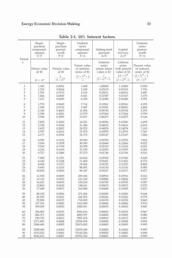
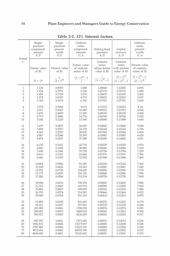
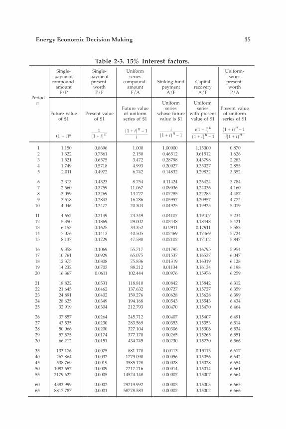
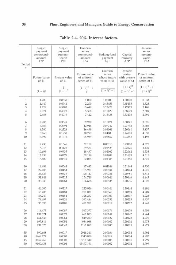
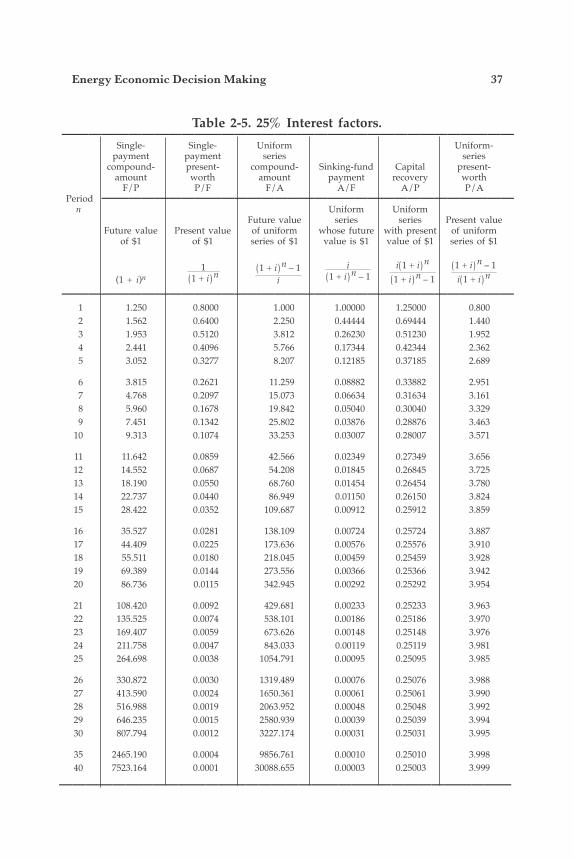
The F/P can be computed by an interest formula, but usually its value is found by using the interest tables. Interest tables for interest rates of 10%-50% are found in this chapter (Tables 2-1 through 2-8). In predict-ing future costs, there are many unknowns. For the accuracy of most calculations, interest rates are assumed to be compounded annually unless otherwise specified. Linear interpolation is commonly used to find values not listed in the interest tables. Tables 2-9 through 2-12 can be used to determine the effect of fuel escalation on the life cycle cost analysis.
Single Payment Present Worth—P/F The P/F factor is used to determine the present worth, P, that a future amount, F, will be, at interest of i percent, in n years. If F is known, and P is to be determined, then Equation 2-4 is used.
P = F × 1/(1 +i)n (2-4)
1 P/F = ——— (2-5) (1 + i)n
Figure 2-1. Single payment compound amount (F/P).
Energy Economic Decision Making 33
Table 2-1. 10% Interest factors.—————————————————————————————————— Single- Single- Uniform Uniform- payment payment series series compound- present- compound- Sinking-fund Capital present- amount worth amount payment recovery worth F/P P/F F/A A/F A/P P/A Period ——————————————————————————————— n Uniform Uniform Future value series series Present value Future value Present value of uniform whose future with present of uniform of $1 of $1 series of $1 value is $1 value of $1 series of $1
(1 + i)n —————————————————————————————————— 1 1.100 0.9091 1.000 1.00000 1.10000 0.909 2 1.210 0.8264 2.100 0.47619 0.57619 1.736 3 1.331 0.7513 3.310 0.30211 0.40211 2.487 4 1.464 0.6830 4.641 0.21547 0.31147 3.170 5 1.611 0.6209 6.105 0.16380 0.26380 3.791
6 1.772 0.5645 7.716 0.12961 0.22961 4.355 7 1.949 0.5132 9.487 0.10541 0.20541 4.868 8 2.144 0.4665 11.436 0.08744 0.18744 5.335 9 2.358 0.4241 13.579 0.07364 0.17364 5.759 10 2.594 0.3855 15.937 0.06275 0.16275 6.144
11 2.853 0.3505 18.531 0.05396 0.15396 6.495 12 3.138 0.3186 21.384 0.04676 0.14676 6.814 13 3.452 0.2897 24.523 0.04078 0.14078 7.103 14 3.797 0.2633 27.975 0.03575 0.13575 7.367 15 4.177 0.2394 31.772 0.03147 0.13147 7.606
16 4.595 0.2176 35.950 0.02782 0.12782 7.824 17 5.054 0.1978 40.545 0.02466 0.12466 8.022 18 5.560 0.1799 45.599 0.02193 0.12193 8.201 19 6.116 0.1635 51.159 0.01955 0.11955 8.365 20 6.727 0.1486 57.275 0.01746 0.11746 8.514
21 7.400 0.1351 64.002 0.01562 0.11562 8.649 22 8.140 0.1228 71.403 0.01401 0.11401 8.772 23 8.954 0.1117 79.543 0.01257 0.11257 8.883 24 9.850 0.1015 88.497 0.01130 0.11130 8.985 25 10.835 0.0923 98.347 0.01017 0.11017 9.077
26 11.918 0.0839 109.182 0.00916 0.10916 9.161 27 13.110 0.0763 121.100 0.00826 0.10826 9.237 28 14.421 0.0693 134.210 0.00745 0.10745 9.307 29 15.863 0.0630 148.631 0.00673 0.10673 9.370 30 17.449 0.0673 164.494 0.00608 0.10608 9.427
35 28.102 0.0356 271.024 0.00369 0.10369 9.644 40 45.259 0.0221 442.593 0.00226 0.10226 9.779 45 72.890 0.0137 718.905 0.00139 0.10139 9.863 50 117.391 0.0085 1163.909 0.00086 0.10086 9.915 55 189.059 0.0053 1880.591 0.00053 0.10053 9.947
60 304.482 0.0033 3034.816 0.00033 0.10033 9.967 65 490.371 0.0020 4893.707 0.00020 0.10020 9.980 70 789.747 0.0013 7887.470 0.00013 0.10013 9.987 75 1271.895 0.0008 12708.954 0.00008 0.10008 9.992 80 2048.400 0.0005 20474.002 0.00005 0.10005 9.995
85 3298.969 0.0003 32979.690 0.00003 0.10003 9.997 90 5313.023 0.0002 53120.226 0.00002 0.10002 9.998 95 8556.676 0.0001 85556.760 0.00001 0.10001 9.999——————————————————————————————————
11 + i n
1 + i n – 1i
i1 + i n – 1
i 1 + i n
1 + i n – 11 + i n – 1i 1 + i n
34 Plant Engineers and Managers Guide to Energy Conservation
Table 2-2. 12% Interest factors. —————————————————————————————————— Single- Single- Uniform Uniform- payment payment series series compound- present- compound- Sinking-fund Capital present- amount worth amount payment recovery worth F/P P/F F/A A/F A/P P/A Period ——————————————————————————————— n Uniform Uniform Future value series series Present value Future value Present value of uniform whose future with present of uniform of $1 of $1 series of $1 value is $1 value of $1 series of $1
(1 + i)n —————————————————————————————————— 1 1.120 0.8929 1.000 1.00000 1.12000 0.893 2 1.254 0.7972 2.120 0.47170 0.59170 1.690 3 1.405 0.7118 3.374 0.29635 0.41635 2.402 4 1.574 0.6355 4.779 0.20923 0.32923 3.037 5 1.762 0.5674 6.353 0.15741 0.27741 3.605
6 1.974 0.5066 8.115 0.12323 0.24323 4.111 7 2.211 0.4523 10.089 0.09912 0.21912 4.564 8 2.476 0.4039 12.300 0.08130 0.20130 4.968 9 2.773 0.3606 14.776 0.06768 0.18768 5.328 10 3.106 0.3220 17.549 0.05698 0.17698 5.650
11 3.479 0.2875 20.655 0.04842 0.16842 5.938 12 3.896 0.2567 24.133 0.04144 0.16144 6.194 13 4.363 0.2292 28.029 0.03568 0.15568 6.424 14 4.887 0.2046 32.393 0.03087 0.15087 6.628 15 5.474 0.1827 37.280 0.02682 0.14682 6.811
16 6.130 0.1631 42.753 0.02339 0.14339 6.974 17 6.866 0.1456 48.884 0.02046 0.14046 7.120 18 7.690 0.1300 55.750 0.01794 0.13794 7.250 19 8.613 0.1161 63.440 0.01576 0.13576 7.366 20 9.646 0.1037 72.052 0.01388 0.13388 7.469
21 10.804 0.0926 81.699 0.01224 0.13224 7.562 22 12.100 0.0826 92.503 0.01081 0.13081 7.645 23 13.552 0.0738 104.603 0.00956 0.12956 7.718 24 15.179 0.0659 118.155 0.00846 0.12846 7.784 25 17.000 0.0588 133.334 0.00750 0.12750 7.843
26 19.040 0.0525 150.334 0.00665 0.12665 7.896 27 21.325 0.0469 169.374 0.00590 0.12590 7.943 28 23.884 0.0419 190.699 0.00524 0.12524 7.984 29 26.750 0.0374 214.583 0.00466 0.12466 8.022 30 29.960 0.0334 241.333 0.00414 0.12414 8.055
35 52.800 0.0189 431.663 0.00232 0.12232 8.176 40 93.051 0.0107 767.091 0.00130 0.12130 8.244 45 163.988 0.0061 1358.230 0.00074 0.12074 8.283 50 289.002 0.0035 2400.018 0.00042 0.12042 8.304 55 509.321 0.0020 4236.005 0.00024 0.12024 8.317
60 897.597 0.0011 7471.641 0.00013 0.12013 8.324 65 1581.872 0.0006 13173.937 0.00008 0.12008 8.328 70 2787.800 0.0004 23223.332 0.00004 0.12004 8.330 75 4913.056 0.0002 40933.799 0.00002 0.12002 8.332 80 8658.483 0.0001 72145.692 0.00001 0.12001 8.332——————————————————————————————————
11 + i n
1 + i n – 1i
i1 + i n – 1
i 1 + i n
1 + i n – 11 + i n – 1i 1 + i n
Energy Economic Decision Making 35
Table 2-3. 15% Interest factors. —————————————————————————————————— Single- Single- Uniform Uniform- payment payment series series compound- present- compound- Sinking-fund Capital present- amount worth amount payment recovery worth F/P P/F F/A A/F A/P P/A Period ——————————————————————————————— n Uniform Uniform Future value series series Present value Future value Present value of uniform whose future with present of uniform of $1 of $1 series of $1 value is $1 value of $1 series of $1
(1 + i)n —————————————————————————————————— 1 1.150 0.8696 1.000 1.00000 1.15000 0.870 2 1.322 0.7561 2.150 0.46512 0.61512 1.626 3 1.521 0.6575 3.472 0.28798 0.43798 2.283 4 1.749 0.5718 4.993 0.20027 0.35027 2.855 5 2.011 0.4972 6.742 0.14832 0.29832 3.352
6 2.313 0.4323 8.754 0.11424 0.26424 3.784 7 2.660 0.3759 11.067 0.09036 0.24036 4.160 8 3.059 0.3269 13.727 0.07285 0.22285 4.487 9 3.518 0.2843 16.786 0.05957 0.20957 4.772 10 4.046 0.2472 20.304 0.04925 0.19925 5.019
11 4.652 0.2149 24.349 0.04107 0.19107 5.234 12 5.350 0.1869 29.002 0.03448 0.18448 5.421 13 6.153 0.1625 34.352 0.02911 0.17911 5.583 14 7.076 0.1413 40.505 0.02469 0.17469 5.724 15 8.137 0.1229 47.580 0.02102 0.17102 5.847
16 9.358 0.1069 55.717 0.01795 0.16795 5.954 17 10.761 0.0929 65.075 0.01537 0.16537 6.047 18 12.375 0.0808 75.836 0.01319 0.16319 6.128 19 14.232 0.0703 88.212 0.01134 0.16134 6.198 20 16.367 0.0611 102.444 0.00976 0.15976 6.259
21 18.822 0.0531 118.810 0.00842 0.15842 6.312 22 21.645 0.0462 137.632 0.00727 0.15727 6.359 23 24.891 0.0402 159.276 0.00628 0.15628 6.399 24 28.625 0.0349 194.168 0.00543 0.15543 6.434 25 32.919 0.0304 212.793 0.00470 0.15470 6.464
26 37.857 0.0264 245.712 0.00407 0.15407 6.491 27 43.535 0.0230 283.569 0.00353 0.15353 6.514 28 50.066 0.0200 327.104 0.00306 0.15306 6.534 29 57.575 0.0174 377.170 0.00265 0.15265 6.551 30 66.212 0.0151 434.745 0.00230 0.15230 6.566
35 133.176 0.0075 881.170 0.00113 0.15113 6.617 40 267.864 0.0037 1779.090 0.00056 0.15056 6.642 45 538.769 0.0019 3585.128 0.00028 0.15028 6.654 50 1083.657 0.0009 7217.716 0.00014 0.15014 6.661 55 2179.622 0.0005 14524.148 0.00007 0.15007 6.664
60 4383.999 0.0002 29219.992 0.00003 0.15003 6.665 65 8817.787 0.0001 58778.583 0.00002 0.15002 6.666——————————————————————————————————
11 + i n
1 + i n – 1i
i1 + i n – 1
i 1 + i n
1 + i n – 11 + i n – 1i 1 + i n
36 Plant Engineers and Managers Guide to Energy Conservation
Table 2-4. 20% Interest factors. —————————————————————————————————— Single- Single- Uniform Uniform- payment payment series series compound- present- compound- Sinking-fund Capital present- amount worth amount payment recovery worth F/P P/F F/A A/F A/P P/A Period
n ——————————————————————————————— Uniform Uniform Future value series series Present value Future value Present value of uniform whose future with present of uniform of $1 of $1 series of $1 value is $1 value of $1 series of $1
(1 + i)n
—————————————————————————————————— 1 1.200 0.8333 1.000 1.00000 1.20000 0.833 2 1.440 0.6944 2.200 0.45455 0.65455 1.528 3 1.728 0.5787 3.640 0.27473 0.47473 2.106 4 2.074 0.4823 5.368 0.18629 0.38629 2.589 5 2.488 0.4019 7.442 0.13438 0.33438 2.991
6 2.986 0.3349 9.930 0.10071 0.30071 3.326 7 3.583 0.2791 12.916 0.07742 0.27742 3.605 8 4.300 0.2326 16.499 0.06061 0.26061 3.837 9 5.160 0.1938 20.799 0.04808 0.24808 4.031 10 6.192 0.1615 25.959 0.03852 0.23852 4.192
11 7.430 0.1346 32.150 0.03110 0.23110 4.327 12 8.916 0.1122 39.581 0.02526 0.22526 4.439 13 10.699 0.0935 48.497 0.02062 0.22062 4.533 14 12.839 0.0779 59.196 0.01689 0.21689 4.611 15 15.407 0.0649 72.035 0.01388 0.21388 4.675
16 18.488 0.0541 87.442 0.01144 0.21144 4.730 17 22.186 0.0451 105.931 0.00944 0.20944 4.775 18 26.623 0.0376 128.117 0.00781 0.20781 4.812 19 31.948 0.0313 154.740 0.00646 0.20646 4.843 20 38.338 0.0261 186.688 0.00536 0.20536 4.870
21 46.005 0.0217 225.026 0.00444 0.20444 4.891 22 55.206 0.0181 271.031 0.00369 0.20369 4.909 23 66.247 0.0151 326.237 0.00307 0.20307 4.925 24 79.497 0.0126 392.484 0.00255 0.20255 4.937 25 95.396 0.0105 471.981 0.00212 0.20212 4.948
26 114.475 0.0087 567.377 0.00176 0.20176 4.956 27 137.371 0.0073 681.853 0.00147 0.20147 4.964 28 164.845 0.0061 819.223 0.00122 0.20122 4.970 29 197.814 0.0051 984.068 0.00102 0.20102 4.975 30 237.376 0.0042 1181.882 0.00085 0.20085 4.979
35 590.668 0.0017 2948.341 0.00034 0.20034 4.992 40 1469.772 0.0007 7343.858 0.00014 0.20014 4.997 45 3657.262 0.0003 18281.310 0.00005 0.20005 4.999 50 9100.438 0.0001 45497.191 0.00002 0.20002 4.999——————————————————————————————————
11 + i n
1 + i n – 1i
i1 + i n – 1
i 1 + i n
1 + i n – 11 + i n – 1i 1 + i n
Energy Economic Decision Making 37
Table 2-5. 25% Interest factors. —————————————————————————————————— Single- Single- Uniform Uniform- payment payment series series compound- present- compound- Sinking-fund Capital present- amount worth amount payment recovery worth F/P P/F F/A A/F A/P P/A Period ——————————————————————————————— n Uniform Uniform Future value series series Present value Future value Present value of uniform whose future with present of uniform of $1 of $1 series of $1 value is $1 value of $1 series of $1
(1 + i)n
—————————————————————————————————— 1 1.250 0.8000 1.000 1.00000 1.25000 0.800 2 1.562 0.6400 2.250 0.44444 0.69444 1.440 3 1.953 0.5120 3.812 0.26230 0.51230 1.952 4 2.441 0.4096 5.766 0.17344 0.42344 2.362 5 3.052 0.3277 8.207 0.12185 0.37185 2.689
6 3.815 0.2621 11.259 0.08882 0.33882 2.951 7 4.768 0.2097 15.073 0.06634 0.31634 3.161 8 5.960 0.1678 19.842 0.05040 0.30040 3.329 9 7.451 0.1342 25.802 0.03876 0.28876 3.463 10 9.313 0.1074 33.253 0.03007 0.28007 3.571
11 11.642 0.0859 42.566 0.02349 0.27349 3.656 12 14.552 0.0687 54.208 0.01845 0.26845 3.725 13 18.190 0.0550 68.760 0.01454 0.26454 3.780 14 22.737 0.0440 86.949 0.01150 0.26150 3.824 15 28.422 0.0352 109.687 0.00912 0.25912 3.859
16 35.527 0.0281 138.109 0.00724 0.25724 3.887 17 44.409 0.0225 173.636 0.00576 0.25576 3.910 18 55.511 0.0180 218.045 0.00459 0.25459 3.928 19 69.389 0.0144 273.556 0.00366 0.25366 3.942 20 86.736 0.0115 342.945 0.00292 0.25292 3.954
21 108.420 0.0092 429.681 0.00233 0.25233 3.963 22 135.525 0.0074 538.101 0.00186 0.25186 3.970 23 169.407 0.0059 673.626 0.00148 0.25148 3.976 24 211.758 0.0047 843.033 0.00119 0.25119 3.981 25 264.698 0.0038 1054.791 0.00095 0.25095 3.985
26 330.872 0.0030 1319.489 0.00076 0.25076 3.988 27 413.590 0.0024 1650.361 0.00061 0.25061 3.990 28 516.988 0.0019 2063.952 0.00048 0.25048 3.992 29 646.235 0.0015 2580.939 0.00039 0.25039 3.994 30 807.794 0.0012 3227.174 0.00031 0.25031 3.995
35 2465.190 0.0004 9856.761 0.00010 0.25010 3.998 40 7523.164 0.0001 30088.655 0.00003 0.25003 3.999
——————————————————————————————————
11 + i n
1 + i n – 1i
i1 + i n – 1
i 1 + i n
1 + i n – 11 + i n – 1i 1 + i n
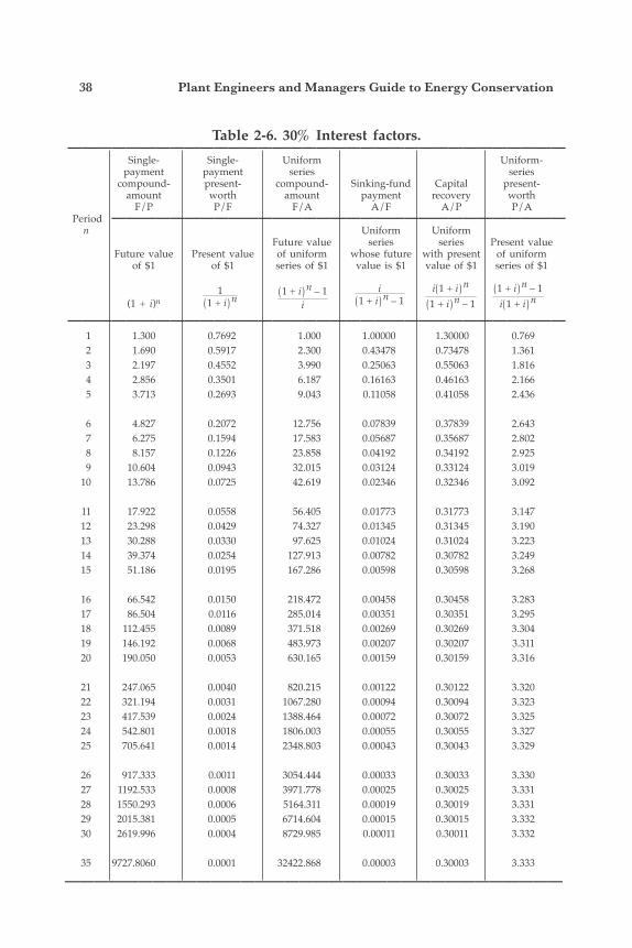
38 Plant Engineers and Managers Guide to Energy Conservation
Table 2-6. 30% Interest factors. —————————————————————————————————— Single- Single- Uniform Uniform- payment payment series series compound- present- compound- Sinking-fund Capital present- amount worth amount payment recovery worth F/P P/F F/A A/F A/P P/A Period ——————————————————————————————— n Uniform Uniform Future value series series Present value Future value Present value of uniform whose future with present of uniform of $1 of $1 series of $1 value is $1 value of $1 series of $1
(1 + i)n
—————————————————————————————————— 1 1.300 0.7692 1.000 1.00000 1.30000 0.769 2 1.690 0.5917 2.300 0.43478 0.73478 1.361 3 2.197 0.4552 3.990 0.25063 0.55063 1.816 4 2.856 0.3501 6.187 0.16163 0.46163 2.166 5 3.713 0.2693 9.043 0.11058 0.41058 2.436
6 4.827 0.2072 12.756 0.07839 0.37839 2.643 7 6.275 0.1594 17.583 0.05687 0.35687 2.802 8 8.157 0.1226 23.858 0.04192 0.34192 2.925 9 10.604 0.0943 32.015 0.03124 0.33124 3.019 10 13.786 0.0725 42.619 0.02346 0.32346 3.092
11 17.922 0.0558 56.405 0.01773 0.31773 3.147 12 23.298 0.0429 74.327 0.01345 0.31345 3.190 13 30.288 0.0330 97.625 0.01024 0.31024 3.223 14 39.374 0.0254 127.913 0.00782 0.30782 3.249 15 51.186 0.0195 167.286 0.00598 0.30598 3.268
16 66.542 0.0150 218.472 0.00458 0.30458 3.283 17 86.504 0.0116 285.014 0.00351 0.30351 3.295 18 112.455 0.0089 371.518 0.00269 0.30269 3.304 19 146.192 0.0068 483.973 0.00207 0.30207 3.311 20 190.050 0.0053 630.165 0.00159 0.30159 3.316
21 247.065 0.0040 820.215 0.00122 0.30122 3.320 22 321.194 0.0031 1067.280 0.00094 0.30094 3.323 23 417.539 0.0024 1388.464 0.00072 0.30072 3.325 24 542.801 0.0018 1806.003 0.00055 0.30055 3.327 25 705.641 0.0014 2348.803 0.00043 0.30043 3.329
26 917.333 0.0011 3054.444 0.00033 0.30033 3.330 27 1192.533 0.0008 3971.778 0.00025 0.30025 3.331 28 1550.293 0.0006 5164.311 0.00019 0.30019 3.331 29 2015.381 0.0005 6714.604 0.00015 0.30015 3.332 30 2619.996 0.0004 8729.985 0.00011 0.30011 3.332
35 9727.8060 0.0001 32422.868 0.00003 0.30003 3.333
——————————————————————————————————
11 + i n
1 + i n – 1i
i1 + i n – 1
i 1 + i n
1 + i n – 11 + i n – 1i 1 + i n
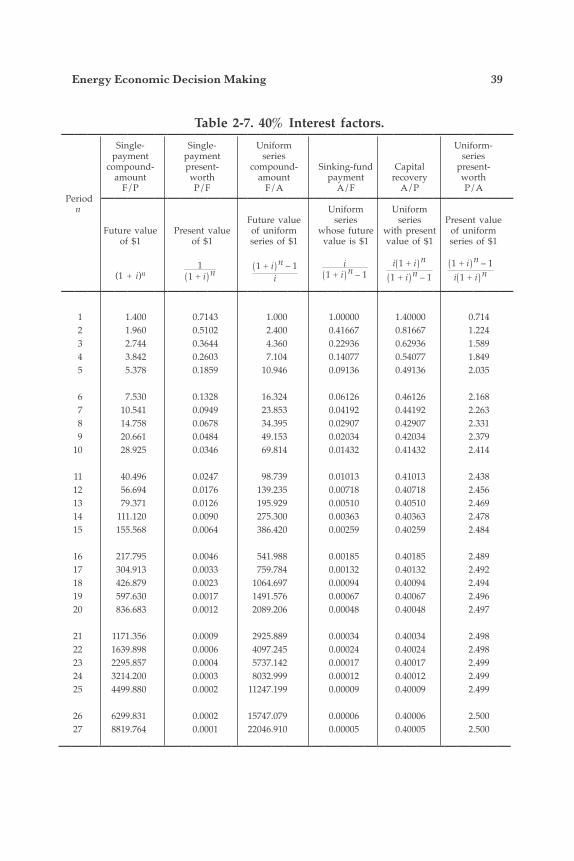
Energy Economic Decision Making 39
Table 2-7. 40% Interest factors. —————————————————————————————————— Single- Single- Uniform Uniform- payment payment series series compound- present- compound- Sinking-fund Capital present- amount worth amount payment recovery worth F/P P/F F/A A/F A/P P/A Period ——————————————————————————————— n Uniform Uniform Future value series series Present value Future value Present value of uniform whose future with present of uniform of $1 of $1 series of $1 value is $1 value of $1 series of $1
(1 + i)n
——————————————————————————————————
1 1.400 0.7143 1.000 1.00000 1.40000 0.714 2 1.960 0.5102 2.400 0.41667 0.81667 1.224 3 2.744 0.3644 4.360 0.22936 0.62936 1.589 4 3.842 0.2603 7.104 0.14077 0.54077 1.849 5 5.378 0.1859 10.946 0.09136 0.49136 2.035
6 7.530 0.1328 16.324 0.06126 0.46126 2.168 7 10.541 0.0949 23.853 0.04192 0.44192 2.263 8 14.758 0.0678 34.395 0.02907 0.42907 2.331 9 20.661 0.0484 49.153 0.02034 0.42034 2.379 10 28.925 0.0346 69.814 0.01432 0.41432 2.414
11 40.496 0.0247 98.739 0.01013 0.41013 2.438 12 56.694 0.0176 139.235 0.00718 0.40718 2.456 13 79.371 0.0126 195.929 0.00510 0.40510 2.469 14 111.120 0.0090 275.300 0.00363 0.40363 2.478 15 155.568 0.0064 386.420 0.00259 0.40259 2.484
16 217.795 0.0046 541.988 0.00185 0.40185 2.489 17 304.913 0.0033 759.784 0.00132 0.40132 2.492 18 426.879 0.0023 1064.697 0.00094 0.40094 2.494 19 597.630 0.0017 1491.576 0.00067 0.40067 2.496 20 836.683 0.0012 2089.206 0.00048 0.40048 2.497
21 1171.356 0.0009 2925.889 0.00034 0.40034 2.498 22 1639.898 0.0006 4097.245 0.00024 0.40024 2.498 23 2295.857 0.0004 5737.142 0.00017 0.40017 2.499 24 3214.200 0.0003 8032.999 0.00012 0.40012 2.499 25 4499.880 0.0002 11247.199 0.00009 0.40009 2.499
26 6299.831 0.0002 15747.079 0.00006 0.40006 2.500 27 8819.764 0.0001 22046.910 0.00005 0.40005 2.500
——————————————————————————————————
11 + i n
1 + i n – 1i
i1 + i n – 1
i 1 + i n
1 + i n – 11 + i n – 1i 1 + i n
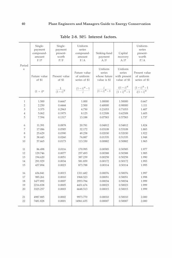
40 Plant Engineers and Managers Guide to Energy Conservation
Table 2-8. 50% Interest factors. —————————————————————————————————— Single- Single- Uniform Uniform- payment payment series series compound- present- compound- Sinking-fund Capital present- amount worth amount payment recovery worth F/P P/F F/A A/F A/P P/A
Period ——————————————————————————————— n Uniform Uniform Future value series series Present value Future value Present value of uniform whose future with present of uniform of $1 of $1 series of $1 value is $1 value of $1 series of $1
(1 + i)n
—————————————————————————————————— 1 1.500 0.6667 1.000 1.00000 1.50000 0.667 2 2.250 0.4444 2.500 0.40000 0.90000 1.111 3 3.375 0.2963 4.750 0.21053 0.71053 1.407 4 5.062 0.1975 8.125 0.12308 0.62308 1.605 5 7.594 0.1317 13.188 0.07583 0.57583 1.737
6 11.391 0.0878 20.781 0.04812 0.54812 1.824 7 17.086 0.0585 32.172 0.03108 0.53108 1.883 8 25.629 0.0390 49.258 0.02030 0.52030 1.922 9 38.443 0.0260 74.887 0.01335 0.51335 1.948 10 57.665 0.0173 113.330 0.00882 0.50882 1.965
11 86.498 0.0116 170.995 0.00585 0.50585 1.977 12 129.746 0.0077 257.493 0.00388 0.50388 1.985 13 194.620 0.0051 387.239 0.00258 0.50258 1.990 14 291.929 0.0034 581.859 0.00172 0.50172 1.993 15 437.894 0.0023 873.788 0.00114 0.50114 1.995
16 656.841 0.0015 1311.682 0.00076 0.50076 1.997 17 985.261 0.0010 1968.523 0.00051 0.50051 1.998 18 1477.892 0.0007 2953.784 0.00034 0.50034 1.999 19 2216.838 0.0005 4431.676 0.00023 0.50023 1.999 20 3325.257 0.0003 6648.513 0.00015 0.50015 1.999
21 4987.885 0.0002 9973.770 0.00010 0.50010 2.000 22 7481.828 0.0001 14961.655 0.00007 0.50007 2.000
——————————————————————————————————
11 + i n
1 + i n – 1i
i1 + i n – 1
i 1 + i n
1 + i n – 11 + i n – 1i 1 + i n
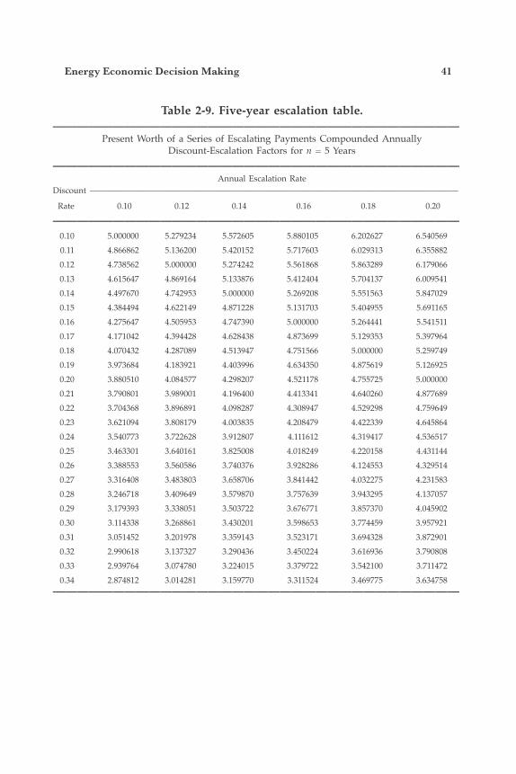
Energy Economic Decision Making 41
Table 2-9. Five-year escalation table.——————————————————————————————————
Present Worth of a Series of Escalating Payments Compounded Annually Discount-Escalation Factors for n = 5 Years——————————————————————————————————
Annual Escalation RateDiscount ————————————————————————————————————————————
Rate 0.10 0.12 0.14 0.16 0.18 0.20
—————————————————————————————————— 0.10 5.000000 5.279234 5.572605 5.880105 6.202627 6.540569 0.11 4.866862 5.136200 5.420152 5.717603 6.029313 6.355882 0.12 4.738562 5.000000 5.274242 5.561868 5.863289 6.179066 0.13 4.615647 4.869164 5.133876 5.412404 5.704137 6.009541 0.14 4.497670 4.742953 5.000000 5.269208 5.551563 5.847029 0.15 4.384494 4.622149 4.871228 5.131703 5.404955 5.691165 0.16 4.275647 4.505953 4.747390 5.000000 5.264441 5.541511 0.17 4.171042 4.394428 4.628438 4.873699 5.129353 5.397964 0.18 4.070432 4.287089 4.513947 4.751566 5.000000 5.259749 0.19 3.973684 4.183921 4.403996 4.634350 4.875619 5.126925 0.20 3.880510 4.084577 4.298207 4.521178 4.755725 5.000000 0.21 3.790801 3.989001 4.196400 4.413341 4.640260 4.877689 0.22 3.704368 3.896891 4.098287 4.308947 4.529298 4.759649 0.23 3.621094 3.808179 4.003835 4.208479 4.422339 4.645864 0.24 3.540773 3.722628 3.912807 4.111612 4.319417 4.536517 0.25 3.463301 3.640161 3.825008 4.018249 4.220158 4.431144 0.26 3.388553 3.560586 3.740376 3.928286 4.124553 4.329514 0.27 3.316408 3.483803 3.658706 3.841442 4.032275 4.231583 0.28 3.246718 3.409649 3.579870 3.757639 3.943295 4.137057 0.29 3.179393 3.338051 3.503722 3.676771 3.857370 4.045902 0.30 3.114338 3.268861 3.430201 3.598653 3.774459 3.957921 0.31 3.051452 3.201978 3.359143 3.523171 3.694328 3.872901 0.32 2.990618 3.137327 3.290436 3.450224 3.616936 3.790808 0.33 2.939764 3.074780 3.224015 3.379722 3.542100 3.711472 0.34 2.874812 3.014281 3.159770 3.311524 3.469775 3.634758——————————————————————————————————
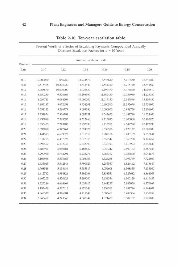
42 Plant Engineers and Managers Guide to Energy Conservation
Table 2-10. Ten-year escalation table.——————————————————————————————————
Present Worth of a Series of Escalating Payments Compounded Annually Discount-Escalation Factors for n = 10 Years——————————————————————————————————
Annual Escalation RateDiscount ————————————————————————————————————————————
Rate 0.10 0.12 0.14 0.16 0.18 0.20
—————————————————————————————————— 0.10 10.000000 11.056250 12.234870 13.548650 15.013550 16.646080 0.11 9.518405 10.508020 11.613440 12.844310 14.215140 15.741560 0.12 9.068870 10.000000 11.036530 12.190470 13.474590 14.903510 0.13 8.650280 9.526666 10.498990 11.582430 12.786980 14.125780 0.14 8.259741 9.084209 10.000000 11.017130 12.147890 13.403480 0.15 7.895187 8.672058 9.534301 10.490510 11.552670 12.731900 0.16 7.554141 8.286779 9.099380 10.000000 10.998720 12.106600 0.17 7.234974 7.926784 8.693151 9.542653 10.481740 11.524400 0.18 6.935890 7.589595 8.312960 9.113885 10.000000 10.980620 0.19 6.655455 7.273785 7.957330 8.713262 9.549790 10.472990 0.20 6.392080 6.977461 7.624072 8.338518 9.128122 10.000000 0.21 6.144593 6.699373 7.311519 7.987156 8.733109 9.557141 0.22 5.911755 6.437922 7.017915 7.657542 8.363208 9.141752 0.23 5.692557 6.192047 6.742093 7.348193 8.015993 8.752133 0.24 5.485921 5.960481 6.482632 7.057347 7.690163 8.387045 0.25 5.290990 5.742294 6.238276 6.783767 7.383800 8.044173 0.26 5.106956 5.536463 6.008083 6.526298 7.095769 7.721807 0.27 4.933045 5.342146 5.790929 6.283557 6.824442 7.418647 0.28 4.768518 5.158489 5.585917 6.054608 6.568835 7.133100 0.29 4.612762 4.984826 5.392166 5.838531 6.327682 6.864109 0.30 4.465205 4.820429 5.209000 5.634354 6.100129 6.610435 0.31 4.325286 4.664669 5.035615 5.441257 5.885058 6.370867 0.32 4.192478 4.517015 4.871346 5.258512 5.681746 6.144601 0.33 4.066339 4.376884 4.715648 5.085461 5.489304 5.930659 0.34 3.946452 4.243845 4.567942 4.921409 5.307107 5.728189
——————————————————————————————————
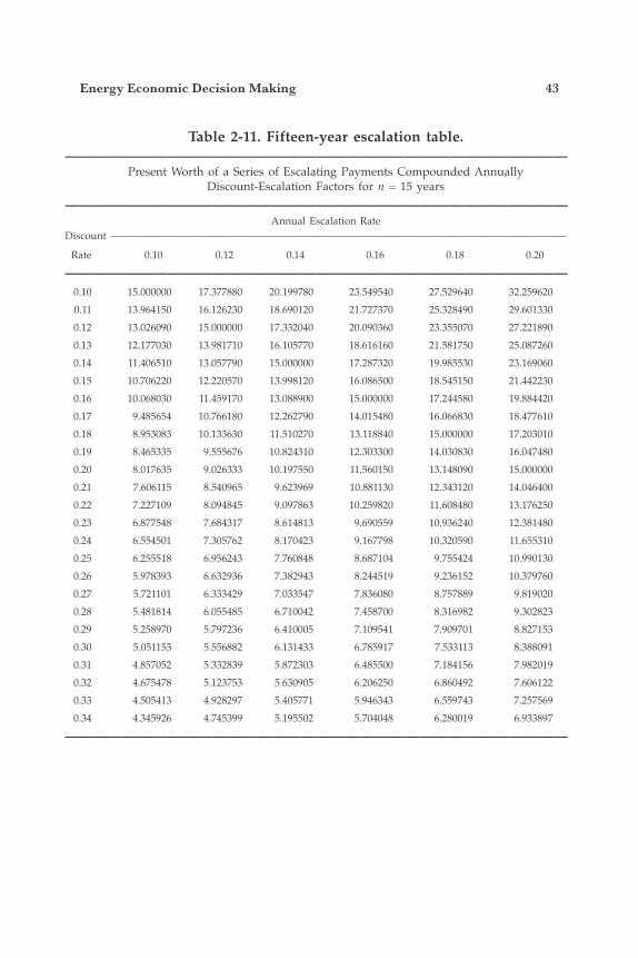
Energy Economic Decision Making 43
Table 2-11. Fifteen-year escalation table.——————————————————————————————————
Present Worth of a Series of Escalating Payments Compounded Annually Discount-Escalation Factors for n = 15 years——————————————————————————————————
Annual Escalation RateDiscount ————————————————————————————————————————————
Rate 0.10 0.12 0.14 0.16 0.18 0.20
—————————————————————————————————— 0.10 15.000000 17.377880 20.199780 23.549540 27.529640 32.259620 0.11 13.964150 16.126230 18.690120 21.727370 25.328490 29.601330 0.12 13.026090 15.000000 17.332040 20.090360 23.355070 27.221890 0.13 12.177030 13.981710 16.105770 18.616160 21.581750 25.087260 0.14 11.406510 13.057790 15.000000 17.287320 19.985530 23.169060 0.15 10.706220 12.220570 13.998120 16.086500 18.545150 21.442230 0.16 10.068030 11.459170 13.088900 15.000000 17.244580 19.884420 0.17 9.485654 10.766180 12.262790 14.015480 16.066830 18.477610 0.18 8.953083 10.133630 11.510270 13.118840 15.000000 17.203010 0.19 8.465335 9.555676 10.824310 12.303300 14.030830 16.047480 0.20 8.017635 9.026333 10.197550 11.560150 13.148090 15.000000 0.21 7.606115 8.540965 9.623969 10.881130 12.343120 14.046400 0.22 7.227109 8.094845 9.097863 10.259820 11.608480 13.176250 0.23 6.877548 7.684317 8.614813 9.690559 10.936240 12.381480 0.24 6.554501 7.305762 8.170423 9.167798 10.320590 11.655310 0.25 6.255518 6.956243 7.760848 8.687104 9.755424 10.990130 0.26 5.978393 6.632936 7.382943 8.244519 9.236152 10.379760 0.27 5.721101 6.333429 7.033547 7.836080 8.757889 9.819020 0.28 5.481814 6.055485 6.710042 7.458700 8.316982 9.302823 0.29 5.258970 5.797236 6.410005 7.109541 7.909701 8.827153 0.30 5.051153 5.556882 6.131433 6.785917 7.533113 8.388091 0.31 4.857052 5.332839 5.872303 6.485500 7.184156 7.982019 0.32 4.675478 5.123753 5.630905 6.206250 6.860492 7.606122 0.33 4.505413 4.928297 5.405771 5.946343 6.559743 7.257569 0.34 4.345926 4.745399 5.195502 5.704048 6.280019 6.933897
——————————————————————————————————
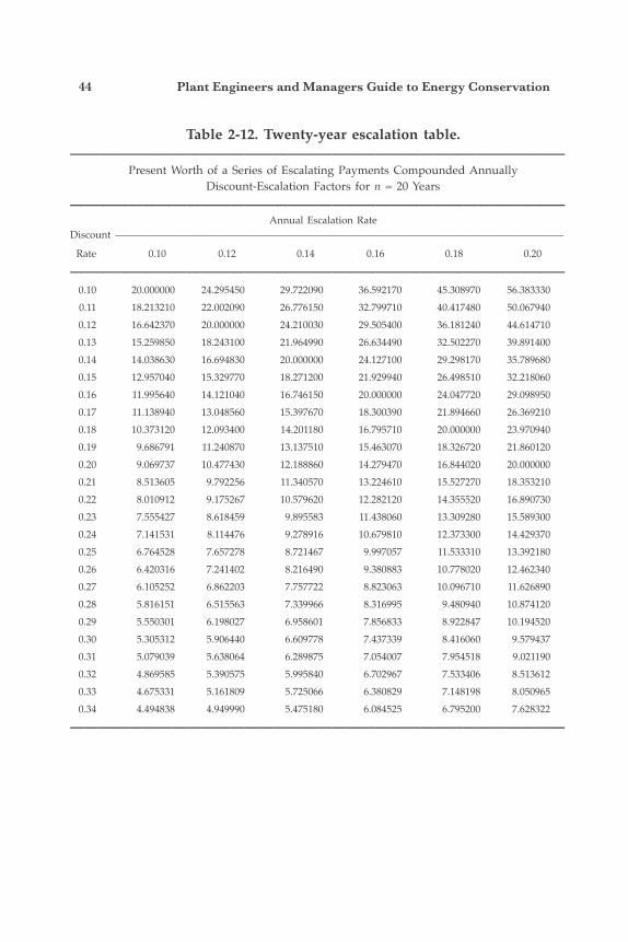
44 Plant Engineers and Managers Guide to Energy Conservation
Table 2-12. Twenty-year escalation table.——————————————————————————————————
Present Worth of a Series of Escalating Payments Compounded Annually Discount-Escalation Factors for n = 20 Years——————————————————————————————————
Annual Escalation RateDiscount ————————————————————————————————————————————
Rate 0.10 0.12 0.14 0.16 0.18 0.20
—————————————————————————————————— 0.10 20.000000 24.295450 29.722090 36.592170 45.308970 56.383330 0.11 18.213210 22.002090 26.776150 32.799710 40.417480 50.067940 0.12 16.642370 20.000000 24.210030 29.505400 36.181240 44.614710 0.13 15.259850 18.243100 21.964990 26.634490 32.502270 39.891400 0.14 14.038630 16.694830 20.000000 24.127100 29.298170 35.789680 0.15 12.957040 15.329770 18.271200 21.929940 26.498510 32.218060 0.16 11.995640 14.121040 16.746150 20.000000 24.047720 29.098950 0.17 11.138940 13.048560 15.397670 18.300390 21.894660 26.369210 0.18 10.373120 12.093400 14.201180 16.795710 20.000000 23.970940 0.19 9.686791 11.240870 13.137510 15.463070 18.326720 21.860120 0.20 9.069737 10.477430 12.188860 14.279470 16.844020 20.000000 0.21 8.513605 9.792256 11.340570 13.224610 15.527270 18.353210 0.22 8.010912 9.175267 10.579620 12.282120 14.355520 16.890730 0.23 7.555427 8.618459 9.895583 11.438060 13.309280 15.589300 0.24 7.141531 8.114476 9.278916 10.679810 12.373300 14.429370 0.25 6.764528 7.657278 8.721467 9.997057 11.533310 13.392180 0.26 6.420316 7.241402 8.216490 9.380883 10.778020 12.462340 0.27 6.105252 6.862203 7.757722 8.823063 10.096710 11.626890 0.28 5.816151 6.515563 7.339966 8.316995 9.480940 10.874120 0.29 5.550301 6.198027 6.958601 7.856833 8.922847 10.194520 0.30 5.305312 5.906440 6.609778 7.437339 8.416060 9.579437 0.31 5.079039 5.638064 6.289875 7.054007 7.954518 9.021190 0.32 4.869585 5.390575 5.995840 6.702967 7.533406 8.513612 0.33 4.675331 5.161809 5.725066 6.380829 7.148198 8.050965 0.34 4.494838 4.949990 5.475180 6.084525 6.795200 7.628322
——————————————————————————————————
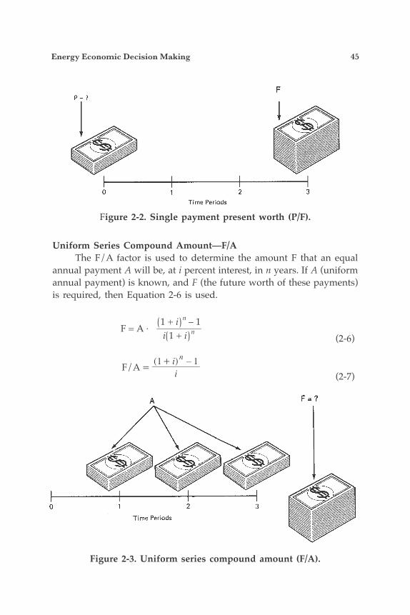
Energy Economic Decision Making 45
Uniform Series Compound Amount—F/A The F/A factor is used to determine the amount F that an equal annual payment A will be, at i percent interest, in n years. If A (uniform annual payment) is known, and F (the future worth of these payments) is required, then Equation 2-6 is used.
F = A
1 + i n – 1i 1 + i n
(2-6)
( )F/A
i
i1 1–n=
+
(2-7)
Figure 2-2. Single payment present worth (P/F).
Figure 2-3. Uniform series compound amount (F/A).
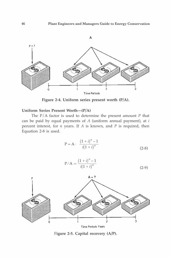
46 Plant Engineers and Managers Guide to Energy Conservation
Uniform Series Present Worth—(P/A) The P/A factor is used to determine the present amount P that can be paid by equal payments of A (uniform annual payment), at i percent interest, for n years. If A is known, and P is required, then Equation 2-8 is used.
P = A
1 + i n – 1i 1 + i n
(2-8)
P ⁄ A
1 + i n – 1i 1 + i n
(2-9)
Figure 2-4. Uniform series present worth (P/A).
Figure 2-5. Capital recovery (A/P).
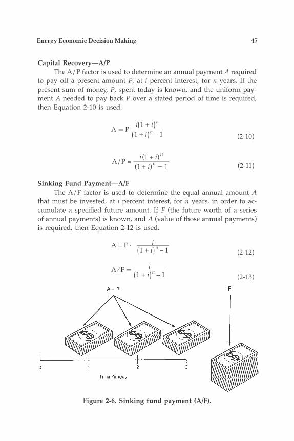
Energy Economic Decision Making 47
Capital Recovery—A/P The A/P factor is used to determine an annual payment A required to pay off a present amount P, at i percent interest, for n years. If the present sum of money, P, spent today is known, and the uniform pay-ment A needed to pay back P over a stated period of time is required, then Equation 2-10 is used.
A P
i 1 + i n
1 + i n – 1 (2-10)
A/P(1 ) 1
(1 )i
i in
n=
++- (2-11)
Sinking Fund Payment—A/F The A/F factor is used to determine the equal annual amount A that must be invested, at i percent interest, for n years, in order to ac-cumulate a specified future amount. If F (the future worth of a series of annual payments) is known, and A (value of those annual payments) is required, then Equation 2-12 is used.
A = F i
1 + i n – 1 (2-12)
A ⁄ F i
1 + i n – 1 (2-13)
Figure 2-6. Sinking fund payment (A/F).
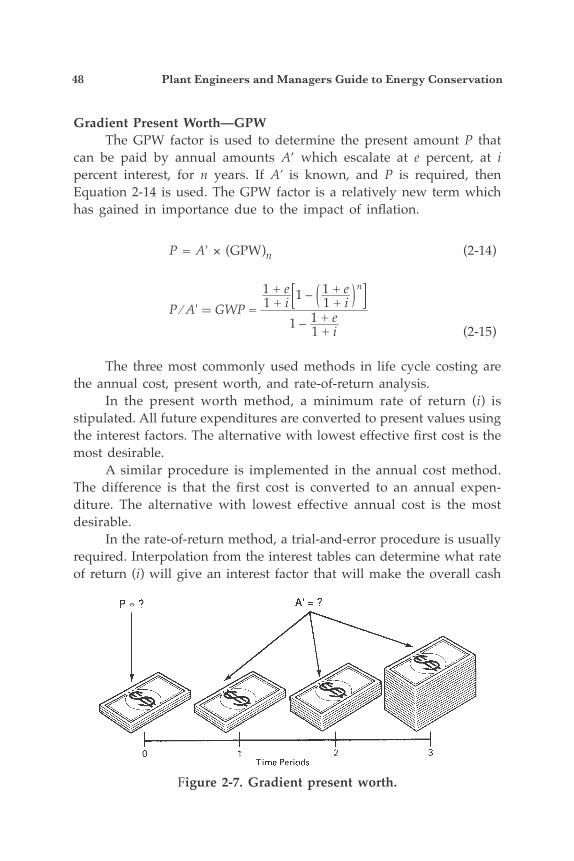
48 Plant Engineers and Managers Guide to Energy Conservation
Gradient Present Worth—GPW The GPW factor is used to determine the present amount P that can be paid by annual amounts A’ which escalate at e percent, at i percent interest, for n years. If A’ is known, and P is required, then Equation 2-14 is used. The GPW factor is a relatively new term which has gained in importance due to the impact of inflation.
P = A′ × (GPW)n (2-14)
P ⁄ A' GWP =
1 + e1 + i 1 – 1 + e
1 + in
1 – 1 + e1 + i (2-15)
The three most commonly used methods in life cycle costing are the annual cost, present worth, and rate-of-return analysis. In the present worth method, a minimum rate of return (i) is stipulated. All future expenditures are converted to present values using the interest factors. The alternative with lowest effective first cost is the most desirable. A similar procedure is implemented in the annual cost method. The difference is that the first cost is converted to an annual expen-diture. The alternative with lowest effective annual cost is the most desirable. In the rate-of-return method, a trial-and-error procedure is usually required. Interpolation from the interest tables can determine what rate of return (i) will give an interest factor that will make the overall cash
Figure 2-7. Gradient present worth.
Energy Economic Decision Making 49
flow balance. The rate-of-return analysis gives a good indication of the overall ranking of independent alternates. The effect of escalation in fuel costs can influence greatly the final decision. When an annual cost grows at a steady rate it may be treated as a gradient and the gradient present worth factor can be used. Special thanks are given to Rudolph R. Yanuck and Dr. Robert Brown for the use of their specially designed interest and escalation tables used in this text. When life cycle costing is used to compare several alternatives, the differences between costs are important. For example, if one alternate forces additional maintenance or an operating expense to occur, then these factors as well as energy costs need to be included. Remember, what was previously spent for the item to be replaced is irrelevant. The only factor to be considered is whether the new cost can be justified based on projected savings over its useful life.
THE JOB SIMULATION EXPERIENCE
Throughout the text you will experience job situations and prob-lems. Each simulation experience is denoted by SIM. The answer will be given below the problem. Cover the answers, then you can “play the game.”
SIM 2-1 An evaluation needs to be made to replace all 40-watt fluorescent lamps with a new lamp that saves 12%, or 4.8 watts, and gives the same output. The cost of each lamp is $2.80. Assuming a rate of return before taxes of 25% is required, can the immediate replacement be justified? Hours of operation are 5800 and the lamp life is 2 years. Electricity costs 7.0¢/kWh.
ANSWER A = 5800 × 4.8 × 0.070/1000 = $1.94 A/P = 1.94/2.80 = .69
From Table 2-5 a rate of return of 25 percent is obtained. When analyzing energy conservation measures, never look at what was previ-ously spent or the life remaining. Just determine if the new expenditure will pay for itself.
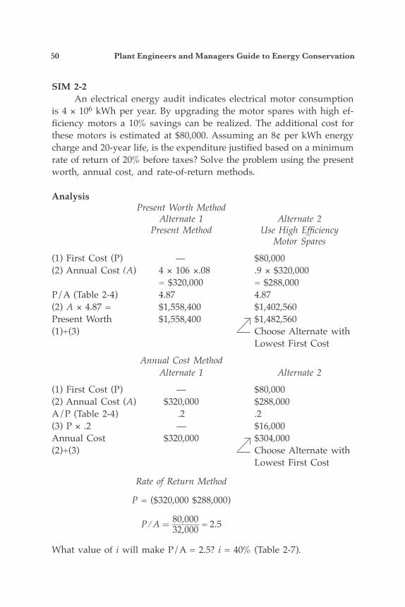
50 Plant Engineers and Managers Guide to Energy Conservation
SIM 2-2 An electrical energy audit indicates electrical motor consumption is 4 × 10⁶ kWh per year. By upgrading the motor spares with high ef-ficiency motors a 10% savings can be realized. The additional cost for these motors is estimated at $80,000. Assuming an 8¢ per kWh energy charge and 20-year life, is the expenditure justified based on a minimum rate of return of 20% before taxes? Solve the problem using the present worth, annual cost, and rate-of-return methods.
Analysis Present Worth Method Alternate 1 Alternate 2 Present Method Use High Efficiency Motor Spares
(1) First Cost (P) — $80,000(2) Annual Cost (A) 4 × 106 ×.08 .9 × $320,000 = $320,000 = $288,000P/A (Table 2-4) 4.87 4.87(2) A × 4.87 = $1,558,400 $1,402,560Present Worth $1,558,400 $1,482,560(1)+(3) Choose Alternate with Lowest First Cost
Annual Cost Method Alternate 1 Alternate 2
(1) First Cost (P) — $80,000(2) Annual Cost (A) $320,000 $288,000A/P (Table 2-4) .2 .2(3) P × .2 — $16,000Annual Cost $320,000 $304,000(2)+(3) Choose Alternate with Lowest First Cost
Rate of Return Method
P = ($320,000 $288,000)
P ⁄ A 80,000
32,000 = 2.5
What value of i will make P/A = 2.5? i = 40% (Table 2-7).
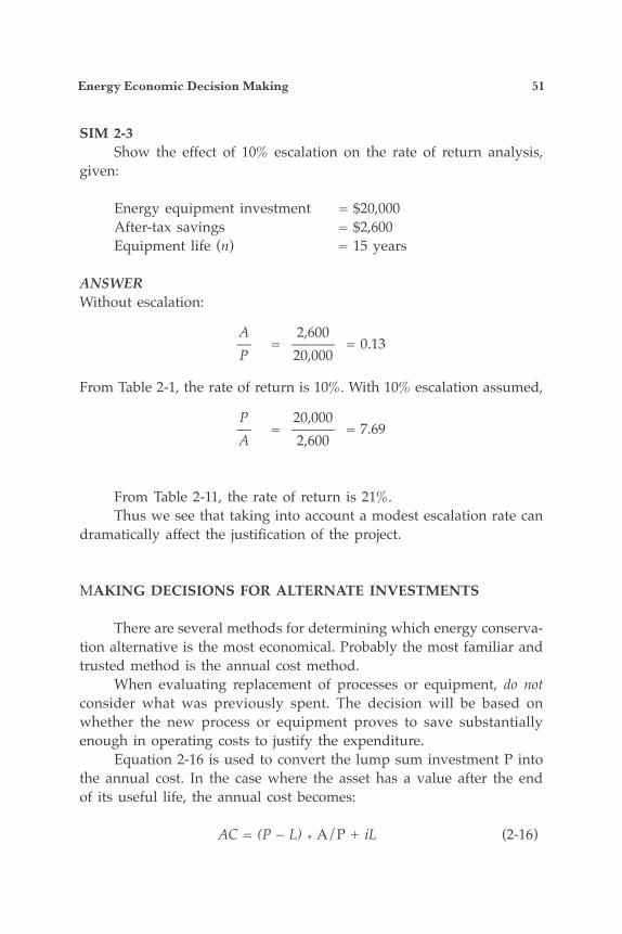
Energy Economic Decision Making 51
SIM 2-3 Show the effect of 10% escalation on the rate of return analysis, given:
Energy equipment investment = $20,000 After-tax savings = $2,600 Equipment life (n) = 15 years
ANSWERWithout escalation:
A 2,600 — = ——— = 0.13 P 20,000
From Table 2-1, the rate of return is 10%. With 10% escalation assumed,
P 20,000 — = ——— = 7.69 A 2,600
From Table 2-11, the rate of return is 21%. Thus we see that taking into account a modest escalation rate can dramatically affect the justification of the project.
MAKING DECISIONS FOR ALTERNATE INVESTMENTS
There are several methods for determining which energy conserva-tion alternative is the most economical. Probably the most familiar and trusted method is the annual cost method. When evaluating replacement of processes or equipment, do not consider what was previously spent. The decision will be based on whether the new process or equipment proves to save substantially enough in operating costs to justify the expenditure. Equation 2-16 is used to convert the lump sum investment P into the annual cost. In the case where the asset has a value after the end of its useful life, the annual cost becomes:
AC = (P – L) * A/P + iL (2-16)
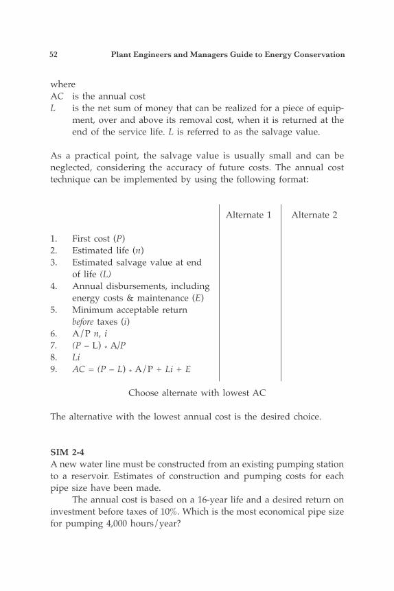
52 Plant Engineers and Managers Guide to Energy Conservation
whereAC is the annual costL is the net sum of money that can be realized for a piece of equip-
ment, over and above its removal cost, when it is returned at the end of the service life. L is referred to as the salvage value.
As a practical point, the salvage value is usually small and can be neglected, considering the accuracy of future costs. The annual cost technique can be implemented by using the following format:
Alternate 1 Alternate 2
1. First cost (P)2. Estimated life (n)3. Estimated salvage value at end of life (L)4. Annual disbursements, including energy costs & maintenance (E)5. Minimum acceptable return before taxes (i)6. A/P n, i7. (P – L) * A/P8. Li9. AC = (P – L) * A/P + Li + E
Choose alternate with lowest AC
The alternative with the lowest annual cost is the desired choice.
SIM 2-4A new water line must be constructed from an existing pumping station to a reservoir. Estimates of construction and pumping costs for each pipe size have been made. The annual cost is based on a 16-year life and a desired return on investment before taxes of 10%. Which is the most economical pipe size for pumping 4,000 hours/year?
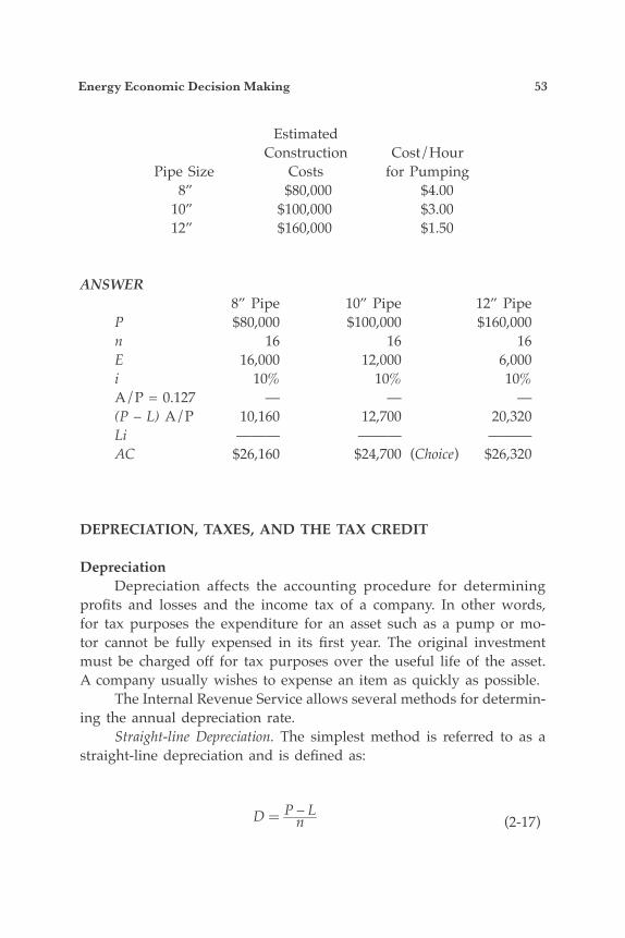
Energy Economic Decision Making 53
Estimated Construction Cost/Hour Pipe Size Costs for Pumping 8” $80,000 $4.00 10” $100,000 $3.00 12” $160,000 $1.50
ANSWER 8” Pipe 10” Pipe 12” Pipe P $80,000 $100,000 $160,000 n 16 16 16 E 16,000 12,000 6,000 i 10% 10% 10% A/P = 0.127 — — — (P – L) A/P 10,160 12,700 20,320 Li ——— ——— ——— AC $26,160 $24,700 (Choice) $26,320
DEPRECIATION, TAXES, AND THE TAX CREDIT
Depreciation Depreciation affects the accounting procedure for determining profits and losses and the income tax of a company. In other words, for tax purposes the expenditure for an asset such as a pump or mo-tor cannot be fully expensed in its first year. The original investment must be charged off for tax purposes over the useful life of the asset. A company usually wishes to expense an item as quickly as possible. The Internal Revenue Service allows several methods for determin-ing the annual depreciation rate. Straight-line Depreciation. The simplest method is referred to as a straight-line depreciation and is defined as:
D P – Ln (2-17)
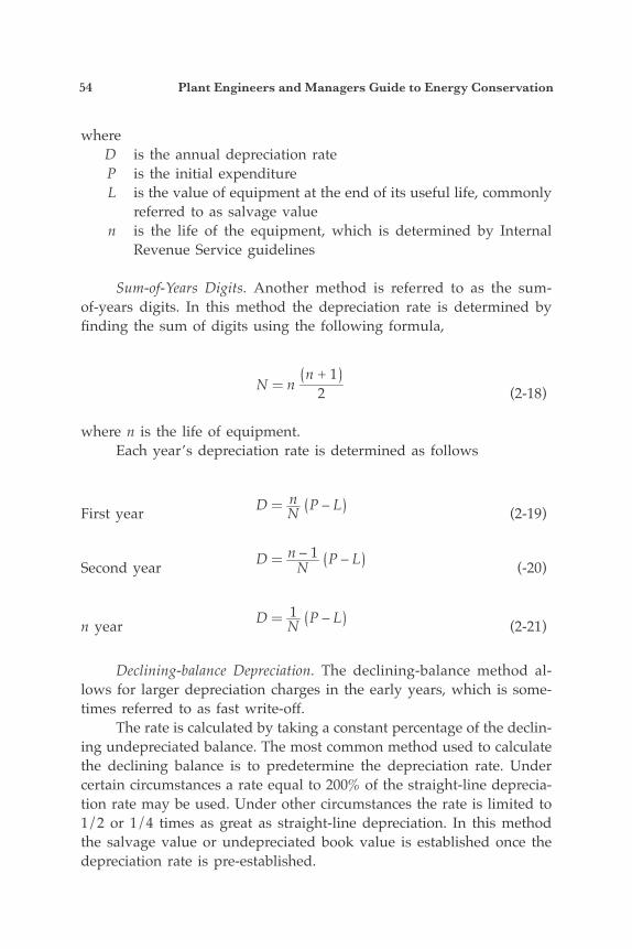
54 Plant Engineers and Managers Guide to Energy Conservation
where D is the annual depreciation rate P is the initial expenditure L is the value of equipment at the end of its useful life, commonly
referred to as salvage value n is the life of the equipment, which is determined by Internal
Revenue Service guidelines Sum-of-Years Digits. Another method is referred to as the sum-of-years digits. In this method the depreciation rate is determined by finding the sum of digits using the following formula,
N nn + 1
2 (2-18)
where n is the life of equipment. Each year’s depreciation rate is determined as follows
First year D nN P – L (2-19)
Second year D n – 1N P – L (-20)
n year D 1N P – L (2-21)
Declining-balance Depreciation. The declining-balance method al-lows for larger depreciation charges in the early years, which is some-times referred to as fast write-off. The rate is calculated by taking a constant percentage of the declin-ing undepreciated balance. The most common method used to calculate the declining balance is to predetermine the depreciation rate. Under certain circumstances a rate equal to 200% of the straight-line deprecia-tion rate may be used. Under other circumstances the rate is limited to 1/2 or 1/4 times as great as straight-line depreciation. In this method the salvage value or undepreciated book value is established once the depreciation rate is pre-established.
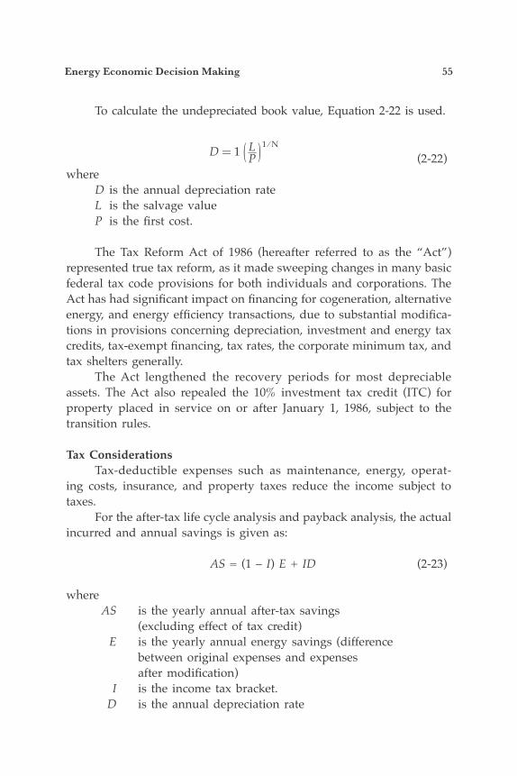
Energy Economic Decision Making 55
To calculate the undepreciated book value, Equation 2-22 is used.
D 1 LP
1 ⁄ N
(2-22)where D is the annual depreciation rate L is the salvage value P is the first cost.
The Tax Reform Act of 1986 (hereafter referred to as the “Act”) represented true tax reform, as it made sweeping changes in many basic federal tax code provisions for both individuals and corporations. The Act has had significant impact on financing for cogeneration, alternative energy, and energy efficiency transactions, due to substantial modifica-tions in provisions concerning depreciation, investment and energy tax credits, tax-exempt financing, tax rates, the corporate minimum tax, and tax shelters generally. The Act lengthened the recovery periods for most depreciable assets. The Act also repealed the 10% investment tax credit (ITC) for property placed in service on or after January 1, 1986, subject to the transition rules.
Tax Considerations Tax-deductible expenses such as maintenance, energy, operat-ing costs, insurance, and property taxes reduce the income subject to taxes. For the after-tax life cycle analysis and payback analysis, the actual incurred and annual savings is given as:
AS = (1 – I) E + ID (2-23)
where AS is the yearly annual after-tax savings (excluding effect of tax credit) E is the yearly annual energy savings (difference between original expenses and expenses after modification) I is the income tax bracket. D is the annual depreciation rate
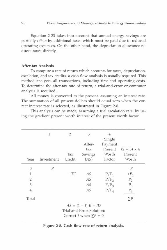
56 Plant Engineers and Managers Guide to Energy Conservation
Equation 2-23 takes into account that annual energy savings are partially offset by additional taxes which must be paid due to reduced operating expenses. On the other hand, the depreciation allowance re-duces taxes directly.
After-tax Analysis To compute a rate of return which accounts for taxes, depreciation, escalation, and tax credits, a cash-flow analysis is usually required. This method analyzes all transactions, including first and operating costs. To determine the after-tax rate of return, a trial-and-error or computer analysis is required. All money is converted to the present, assuming an interest rate. The summation of all present dollars should equal zero when the cor-rect interest rate is selected, as illustrated in Figure 2-8. This analysis can be made, assuming a fuel escalation rate, by us-ing the gradient present worth interest of the present worth factor.
———————————————————————————————— 1 2 3 4 Single After- Payment tax Present (2 + 3) × 4 Tax Savings Worth Present Year Investment Credit (AS) Factor Worth———————————————————————————————— 0 –P –P 1 +TC AS P/F1 +P1 2 AS P/F2 P2 3 AS P/F3 P3 4 AS P/F4 P4
Total ∑P
AS = (1 – I) E + IDTrial-and-Error Solution:Correct i when ∑P = 0
————————————————————————————————Figure 2-8. Cash flow rate of return analysis.
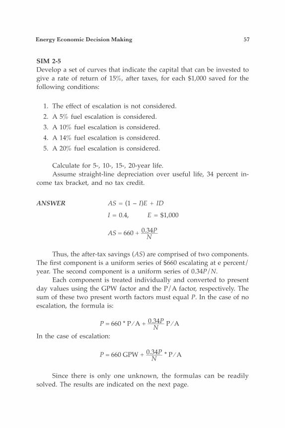
Energy Economic Decision Making 57
SIM 2-5Develop a set of curves that indicate the capital that can be invested to give a rate of return of 15%, after taxes, for each $1,000 saved for the following conditions:
1. The effect of escalation is not considered. 2. A 5% fuel escalation is considered. 3. A 10% fuel escalation is considered. 4. A 14% fuel escalation is considered. 5. A 20% fuel escalation is considered.
Calculate for 5-, 10-, 15-, 20-year life. Assume straight-line depreciation over useful life, 34 percent in-come tax bracket, and no tax credit.
ANSWER AS = (1 – I)E + ID
I = 0.4, E = $1,000
AS = 660 + 0.34PN
Thus, the after-tax savings (AS) are comprised of two components. The first component is a uniform series of $660 escalating at e percent/year. The second component is a uniform series of 0.34P/N. Each component is treated individually and converted to present day values using the GPW factor and the P/A factor, respectively. The sum of these two present worth factors must equal P. In the case of no escalation, the formula is:
P = 660 * P ⁄ A + 0.34PN P ⁄ A
In the case of escalation:
P = 660 GPW + 0.34PN * P ⁄ A
Since there is only one unknown, the formulas can be readily solved. The results are indicated on the next page.
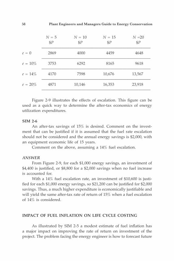
58 Plant Engineers and Managers Guide to Energy Conservation
N = 5 N = 10 N = 15 N =20 $P $P $P $P ———————————————————————————e = 0 2869 4000 4459 4648 ———————————————————————————e = 10% 3753 6292 8165 9618 ———————————————————————————e = 14% 4170 7598 10,676 13,567 ———————————————————————————e = 20% 4871 10,146 16,353 23,918 ———————————————————————————
Figure 2-9 illustrates the effects of escalation. This figure can be used as a quick way to determine the after-tax economics of energy utilization expenditures.
SIM 2-6 An after-tax savings of 15% is desired. Comment on the invest-ment that can be justified if it is assumed that the fuel rate escalation should not be considered and the annual energy savings is $2,000, with an equipment economic life of 15 years. Comment on the above, assuming a 14% fuel escalation.
ANSWER From Figure 2-9, for each $1,000 energy savings, an investment of $4,400 is justified, or $8,800 for a $2,000 savings when no fuel increase is accounted for. With a 14% fuel escalation rate, an investment of $10,600 is justi-fied for each $1,000 energy savings, so $21,200 can be justified for $2,000 savings. Thus, a much higher expenditure is economically justifiable and will yield the same after-tax rate of return of 15% when a fuel escalation of 14% is considered.
IMPACT OF FUEL INFLATION ON LIFE CYCLE COSTING
As illustrated by SIM 2-5 a modest estimate of fuel inflation has a major impact on improving the rate of return on investment of the project. The problem facing the energy engineer is how to forecast future
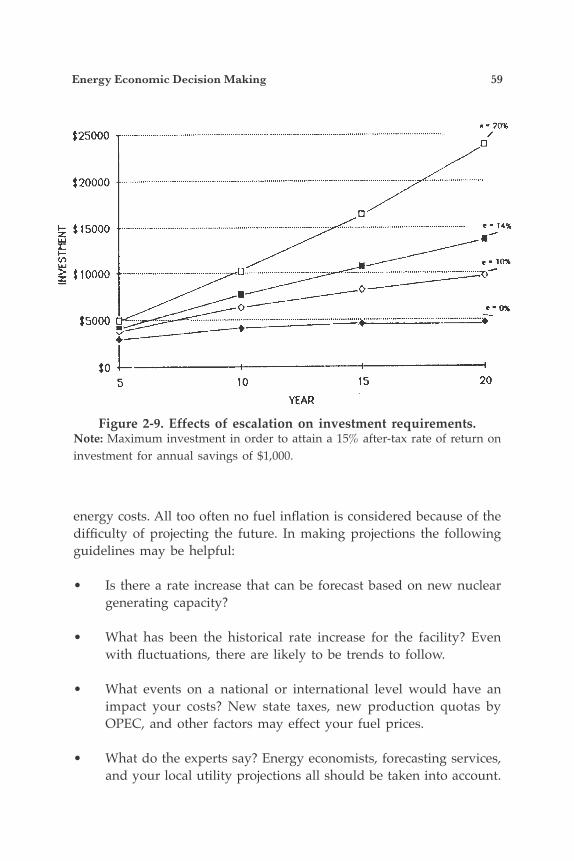
Energy Economic Decision Making 59
energy costs. All too often no fuel inflation is considered because of the difficulty of projecting the future. In making projections the following guidelines may be helpful:
• Is there a rate increase that can be forecast based on new nuclear generating capacity?
• What has been the historical rate increase for the facility? Even with fluctuations, there are likely to be trends to follow.
• What events on a national or international level would have an impact your costs? New state taxes, new production quotas by OPEC, and other factors may effect your fuel prices.
• What do the experts say? Energy economists, forecasting services, and your local utility projections all should be taken into account.
Figure 2-9. Effects of escalation on investment requirements.Note: Maximum investment in order to attain a 15% after-tax rate of return on investment for annual savings of $1,000.
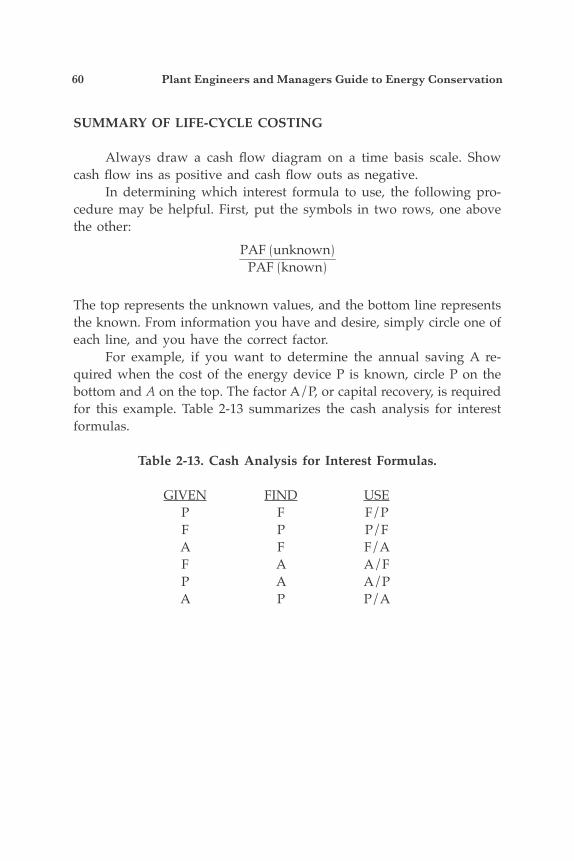
60 Plant Engineers and Managers Guide to Energy Conservation
SUMMARY OF LIFE-CYCLE COSTING
Always draw a cash flow diagram on a time basis scale. Show cash flow ins as positive and cash flow outs as negative. In determining which interest formula to use, the following pro-cedure may be helpful. First, put the symbols in two rows, one above the other:
PAF unknownPAF known
The top represents the unknown values, and the bottom line represents the known. From information you have and desire, simply circle one of each line, and you have the correct factor. For example, if you want to determine the annual saving A re-quired when the cost of the energy device P is known, circle P on the bottom and A on the top. The factor A/P, or capital recovery, is required for this example. Table 2-13 summarizes the cash analysis for interest formulas.
Table 2-13. Cash Analysis for Interest Formulas.
GIVEN FIND USE P F F/P F P P/F A F F/A F A A/F P A A/P A P P/A
61
3The Facility Survey
The survey of the facility is considered a very important part of the industrial energy audit. Chapter 1 indicated that there are many types of surveys, from a simple walk-through to a complete quantification of uses and losses. This illustrates various types of instruments that can aid in the industrial audit.
COMPARING CATALOGUE DATAWITH ACTUAL PERFORMANCE
Many energy managers are surprised when they record actual performance data of equipment and compare it with catalogue informa-tion. There is usually a great disparity between the two. Each manu-facturer has design tolerance for its equipment. For critical equipment, performance guarantees or tests should be incorporated into the initial specifications. As part of the facility survey, nameplate data of pumps, motors, chillers, fans, etc., should be taken. The nameplate data should also be compared to actual running conditions. The initial survey can detect motors that are over-sized. By replacing the motor with a smaller one, energy savings can be realized.
INFRARED EQUIPMENT
Some companies may have the wrong impression that infrared equipment can meet most of their instrumentation needs. The primary use of infrared equipment in an energy utilization program is to detect building or equipment losses. Thus, it is just one of the many options available. Several energy managers find infrared in use in their plant
62 Plant Engineers and Managers Guide to Energy Conservation
prior to the energy utilization program. Infrared equipment, in many instances, was purchased by the electrical department and used to detect electrical hot spots. Infrared energy is an invisible part of the electromagnetic spec-trum. It exists naturally and can be measured by remote heat-sensing equipment. In recent years lightweight portable infrared systems became available to help determine energy losses. Differences in the infrared emissions from the surface of objects cause color variations to appear on the scanner. The hotter the object, the more infrared radiated. With the aid of an isotherm circuit the intensity of these radiation lev-els can be accurately measured and quantified. In essence, the infrared scanning device is a diagnostic tool which can be used to determine building heat losses. Equipment costs range from $400 to $50,000. An overview energy scan of the plant can be made through an aerial survey using infrared equipment. Several companies offer aerial scan services starting at $1,500. Aerial scans can determine underground stream pipe leaks, hot gas discharges and leaks, etc. Since infrared detection and measurement equipment have gained increased importance in the energy audit process, a summary of the fundamentals is reviewed in this section. The visible portion of the spectrum runs from .4 to .75 micrometers (µm). The infrared or thermal radiation begins at this point and extends to approximately 1,000 µm. Objects such as people, plants, or buildings will emit radiation with wavelengths around 10 µm. Infrared instruments are required to detect and measure the thermal radiation. To calibrate the instrument a special “black body” radiator is used. A black body radiator absorbs all the radiation that impinges on it and has an absorbing efficiency or emissivity of 1. The accuracy of temperature measurements by infrared instru-ments depends on the three processes which are responsible for an object acting like a black body. These processes—absorbed, reflected, and transmitted radiation—are responsible for the total radiation reach-ing an infrared scanner. The real temperature of the object is dependent only upon its emitted radiation. Corrections to apparent temperatures are made by knowing the emissivity of an object at a specified temperature. The heart of the infrared instrument is the infrared detector. The detector absorbs infrared energy and converts it into electrical voltage or current. The two principal types of detectors are the thermal type and the photo type. Figure 3-2 shows a thermal camera with LCD dis-

The Facility Survey 63
play. The thermal detector generally requires a given period of time to develop an image on photographic film. The photo detectors are more sensitive and have a higher response time. Television-like displays on a cathode ray tube permit studies of dynamic thermal events on moving objects in real time. There are various ways of displaying signals produced by infrared detectors. One way is by use of an isotherm contour. The lightest areas of the picture represent the warmest areas of the subject and the dark-
———————————————————————————————— Gamma Rays X-Rays UV Visible Infrared Microwave Radio Wave—|—————|————|——|———|———|—————|———— 10–6 10–5 10–2 .4 .75 103 106
high energy low energyradiation radiationshort longwavelength wavelength————————————————————————————————
Figure 3-1. Electromagnetic spectrum.
Figure 3-2. Temperature
64 Plant Engineers and Managers Guide to Energy Conservation
est areas represent the coolest portions. These instruments can show thermal variations of less than 0.1°C and can cover a range of –30°C to over 2,000°C. The isotherm can be calibrated by means of a black body radiator so that a specific temperature is known. The scanner can then be moved and the temperatures of the various parts of the subject can be made.
MEASURING ELECTRICAL SYSTEM PERFORMANCE
An ammeter, voltmeter, wattmeter, power factor meter, and foot-candle meter are usually required to do an electrical survey. These instruments are described below.
Ammeter and Voltmeter To measure electrical currents, ammeters are used. For most audits, alternating currents are measured. Ammeters used in audits are portable and are designed to be easily attached and removed. Figure 3-3 shows a fluke 23 ammeter. There are many brands and styles of snap-on ammeters commonly available that can read up to 1000 amperes continuously. This range can be extended to 4000 amperes continuously for some models with an accessory step-down current transformer. The snap-on ammeters can be either indicating or recording with a printout. After attachment, the recording ammeter can keep recording current variations for as long as a full month on one roll of recording paper. This allows studying current variations in a conductor for extended periods without constant operator attention. The ammeter supplies a direct measurement of electrical current, which is one of the parameters needed to calculate electrical energy. The second parameter required to calculate energy is voltage, which is measured by a voltmeter. Several types of electrical meters can read the voltage or current. A voltmeter measures the difference in electrical potential between two points in an electrical circuit. In series with the probes are the galvanometer and a fixed resis-tance (which determine the voltage scale). The current through this fixed resistance circuit is then proportional to the voltage, and the galvanom-eter deflects in proportion to the voltage. The voltage drops measured in many instances are fairly constant and need only be performed once.
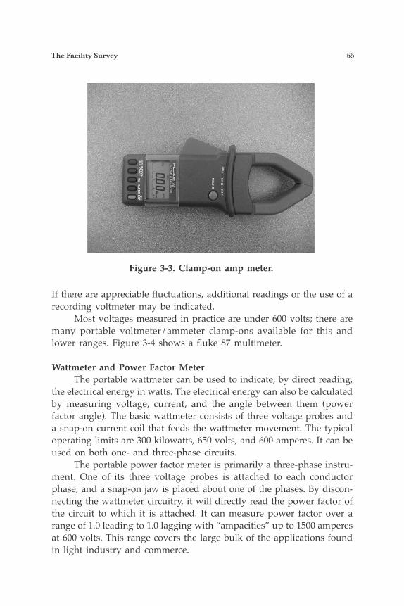
The Facility Survey 65
If there are appreciable fluctuations, additional readings or the use of a recording voltmeter may be indicated. Most voltages measured in practice are under 600 volts; there are many portable voltmeter/ammeter clamp-ons available for this and lower ranges. Figure 3-4 shows a fluke 87 multimeter.
Wattmeter and Power Factor Meter The portable wattmeter can be used to indicate, by direct reading, the electrical energy in watts. The electrical energy can also be calculated by measuring voltage, current, and the angle between them (power factor angle). The basic wattmeter consists of three voltage probes and a snap-on current coil that feeds the wattmeter movement. The typical operating limits are 300 kilowatts, 650 volts, and 600 amperes. It can be used on both one- and three-phase circuits. The portable power factor meter is primarily a three-phase instru-ment. One of its three voltage probes is attached to each conductor phase, and a snap-on jaw is placed about one of the phases. By discon-necting the wattmeter circuitry, it will directly read the power factor of the circuit to which it is attached. It can measure power factor over a range of 1.0 leading to 1.0 lagging with “ampacities” up to 1500 amperes at 600 volts. This range covers the large bulk of the applications found in light industry and commerce.
Figure 3-3. Clamp-on amp meter.

66 Plant Engineers and Managers Guide to Energy Conservation
The power factor is a basic parameter whose value must be known to calculate electric energy usage. Diagnostically it is a useful instrument to determine the sources of poor power factor in a facility. Portable digital kWh and kW demand units are now available. Figure 3-5 shows a portable load logger. Digital read-outs of energy usage in both kWh and kW demand (or in dollars and cents), including instantaneous usage, accumulated usage, projected usage for a particular billing period, alarms when over-target levels are desired for usage, and control-outputs for load shedding and cycling are possible. Continuous displays or intermittent alternating displays are avail-able at the touch of a button for any information needed, such as the cost of operating a production machine for one shift, one hour, or one week.
Foot-candle Meter Foot-candle meters measure illumination in units of foot-candles through a light-sensitive barrier layer of cells contained within them.
Figure 3-4. Fluke 87 multimeter.
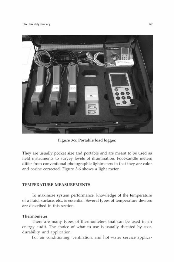
The Facility Survey 67
They are usually pocket size and portable and are meant to be used as field instruments to survey levels of illumination. Foot-candle meters differ from conventional photographic lightmeters in that they are color and cosine corrected. Figure 3-6 shows a light meter.
TEMPERATURE MEASUREMENTS
To maximize system performance, knowledge of the temperature of a fluid, surface, etc., is essential. Several types of temperature devices are described in this section.
Thermometer There are many types of thermometers that can be used in an energy audit. The choice of what to use is usually dictated by cost, durability, and application. For air conditioning, ventilation, and hot water service applica-
Figure 3-5. Portable load logger.
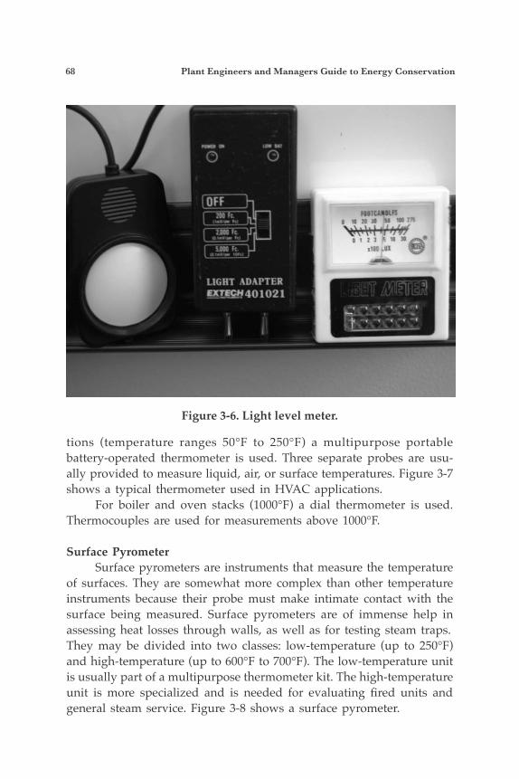
68 Plant Engineers and Managers Guide to Energy Conservation
tions (temperature ranges 50°F to 250°F) a multipurpose portable battery-operated thermometer is used. Three separate probes are usu-ally provided to measure liquid, air, or surface temperatures. Figure 3-7 shows a typical thermometer used in HVAC applications. For boiler and oven stacks (1000°F) a dial thermometer is used. Thermocouples are used for measurements above 1000°F.
Surface Pyrometer Surface pyrometers are instruments that measure the temperature of surfaces. They are somewhat more complex than other temperature instruments because their probe must make intimate contact with the surface being measured. Surface pyrometers are of immense help in assessing heat losses through walls, as well as for testing steam traps.They may be divided into two classes: low-temperature (up to 250°F) and high-temperature (up to 600°F to 700°F). The low-temperature unit is usually part of a multipurpose thermometer kit. The high-temperature unit is more specialized and is needed for evaluating fired units and general steam service. Figure 3-8 shows a surface pyrometer.
Figure 3-6. Light level meter.
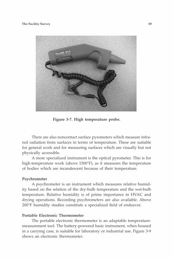
The Facility Survey 69
Figure 3-7. High temperature probe.
There are also noncontact surface pyrometers which measure infra-red radiation from surfaces in terms of temperature. These are suitable for general work and for measuring surfaces which are visually but not physically accessible. A more specialized instrument is the optical pyrometer. This is for high-temperature work (above 1500°F), as it measures the temperature of bodies which are incandescent because of their temperature.
Psychrometer A psychrometer is an instrument which measures relative humid-ity based on the relation of the dry-bulb temperature and the wet-bulb temperature. Relative humidity is of prime importance in HVAC and drying operations. Recording psychrometers are also available. Above 200°F humidity studies constitute a specialized field of endeavor.
Portable Electronic Thermometer The portable electronic thermometer is an adaptable temperature- measurement tool. The battery-powered basic instrument, when housed in a carrying case, is suitable for laboratory or industrial use. Figure 3-9 shows an electronic thermometer.
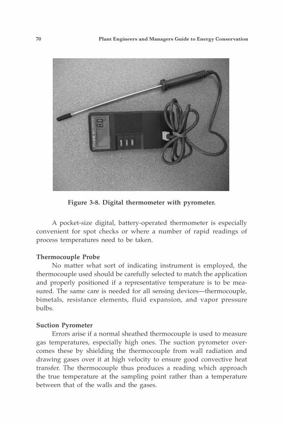
70 Plant Engineers and Managers Guide to Energy Conservation
A pocket-size digital, battery-operated thermometer is especially convenient for spot checks or where a number of rapid readings of process temperatures need to be taken.
Thermocouple Probe No matter what sort of indicating instrument is employed, the thermocouple used should be carefully selected to match the application and properly positioned if a representative temperature is to be mea-sured. The same care is needed for all sensing devices—thermocouple, bimetals, resistance elements, fluid expansion, and vapor pressure bulbs.
Suction Pyrometer Errors arise if a normal sheathed thermocouple is used to measure gas temperatures, especially high ones. The suction pyrometer over-comes these by shielding the thermocouple from wall radiation and drawing gases over it at high velocity to ensure good convective heat transfer. The thermocouple thus produces a reading which approach the true temperature at the sampling point rather than a temperature between that of the walls and the gases.
Figure 3-8. Digital thermometer with pyrometer.
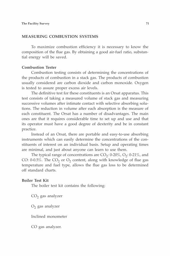
The Facility Survey 71
MEASURING COMBUSTION SYSTEMS
To maximize combustion efficiency it is necessary to know the composition of the flue gas. By obtaining a good air-fuel ratio, substan-tial energy will be saved.
Combustion Tester Combustion testing consists of determining the concentrations of the products of combustion in a stack gas. The products of combustion usually considered are carbon dioxide and carbon monoxide. Oxygen is tested to assure proper excess air levels. The definitive test for these constituents is an Orsat apparatus. This test consists of taking a measured volume of stack gas and measuring successive volumes after intimate contact with selective absorbing solu-tions. The reduction in volume after each absorption is the measure of each constituent. The Orsat has a number of disadvantages. The main ones are that it requires considerable time to set up and use and that its operator must have a good degree of dexterity and be in constant practice. Instead of an Orsat, there are portable and easy-to-use absorbing instruments which can easily determine the concentrations of the con-stituents of interest on an individual basis. Setup and operating times are minimal, and just about anyone can learn to use them. The typical range of concentrations are CO2: 0-20%, O2: 0-21%, and CO: 0-0.5%. The CO2 or O2 content, along with knowledge of flue gas temperature and fuel type, allows the flue gas loss to be determined off standard charts.
Boiler Test Kit The boiler test kit contains the following:
CO2 gas analyzer
O2 gas analyzer
Inclined monometer
CO gas analyzer.
72 Plant Engineers and Managers Guide to Energy Conservation
The purpose of the components of the kit is to help evaluate fireside boiler operation. Good combustion usually means high carbon dioxide (CO2), low oxygen (O2), and little or no trace of carbon monoxide (CO).
Gas Analyzers The gas analyzers are usually of the Fyrite type. The Fyrite type differs from the Orsat apparatus in that it is more limited in applica-tion and less accurate. The chief advantages of the Fyrite are that it is simple and easy to use and is inexpensive. This device is often used in an energy audit. Three readings using the Fyrite analyzer should be made and the results averaged.
Smoke Tester To measure combustion completeness the smoke detector is used. Smoke is unburned carbon, which wastes fuel, causes air pollution, and fouls heat-exchanger surfaces. To use the instrument, a measured volume of flue gas is drawn through filter paper with the probe. The smoke spot is compared visually with a standard scale, and a measure of smoke density is determined.
Combustion Analyzer The combustion electronic analyzer permits fast, close adjustments. The unit contains digital displays. A standard sampler assembly with probe allows for stack measurements through a single stack or breach-ing hole. Figure 3-9 shows a typical combustion analyzer.
MEASURING HEATING, VENTILATION AND AIRCONDITIONING (HVAC) SYSTEM PERFORMANCE
Air Velocity, Pressurization, and Leakage Rates Devices used include:
• Blower Door—a device containing a fan, controller and several pres-sure gauges and a frame which fits into a doorway of a building. This device is used to determine the pressurization and leakage rates of a building and its air distribution system under varying pressure conditions.
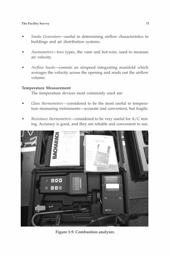
The Facility Survey 73
• Smoke Generators—useful in determining airflow characteristics in buildings and air distribution systems.
• Anemometers—two types, the vane and hot-wire, used to measure air velocity.
• Airflow hoods—contain an airspeed integrating manifold which averages the velocity across the opening and reads out the airflow volume.
Temperature Measurement The temperature devices most commonly used are:
• Glass thermometers—considered to be the most useful to tempera-ture measuring instruments—accurate and convenient, but fragile.
• Resistance thermometers—considered to be very useful for A/C test-ing. Accuracy is good, and they are reliable and convenient to use.
Figure 3-9. Combustion analyzer.
74 Plant Engineers and Managers Guide to Energy Conservation
• Thermocouples—similar to resistance thermocouples, but do not require a battery power source. Chrome-Alum or iron types are the most useful and have satisfactory accuracy and repeatability.
• Pressure bulb thermometers—more suitable for permanent installa-tion.
• Optical pyrometers—only suitable for furnace settings and therefore are limited in use.
• Radiation pyrometers—limited in use for A/C work. These are better suited for spot measurements in hard-to-reach spots. Figure 3-11 shows a radiation pyrometer.
• Thermographs—used for recording room or space temperature; gives a chart indicating variations over a 12- or 168-hour period. Reasonably accurate.
Pressure Measurement (Absolute and Differential) Common devices used for measuring pressure in HVAC applica-tions are:
• Micromanometer—not usually portable, but suitable for fixed mea-surement of pressure differentials across filter, coils, etc.
• Draft gauges—can be portable and used for either direct pressure or pressure differential.
• Manometers—can be portable. Used for direct pressure reading and with Pitot tubes for air flows. Very useful.
• Swing vane gauges—can be portable. Usually used for air flow.
• Bourdon tube gauges—very useful for measuring all forms of sys-tem fluid pressures from 5 psi up. Special types for refrigeration plants.
Humidity Measurement The data given below indicate the type of instruments available
The Facility Survey 75
for humidity measurement and the equipment suitable for HVAC ap-plications:
• Psychrometers—basically wet and dry bulb thermometers. They can be fixed on a portable stand or mounted in a frame with a handle for revolving in air.
• Dimensional change—device usually consisting of a “hair,” which changes in length proportionally with humidity changes. Not usu-ally portable; fragile and only suitable for limited temperature and humidity ranges.
• Electrical conductivity—can be compact and portable but is of a higher cost. Very convenient to use.
• Electrolytic—as above, but for very low temperature ranges; there-fore unsuitable for HVAC test work.
• Gravimeter—not suitable.

77
4Electrical SystemOptimization
APPLYING PROVEN TECHNIQUES TO REDUCE THE ELECTRIC BILL
Electric bills can be reduced by up to 30% by knowing the utility rate structure, improving the plant power factor, reducing peak loads, and us-ing efficient lighting. This chapter illustrates these measures as applied to the energy utilization program.
WHY THE PLANT MANAGER SHOULD UNDERSTAND THE ELECTRIC RATE STRUCTURE
Each plant manager should understand how the plant is billed. Utility companies usually have several rate structures offered to custom-ers. By understanding the electrical characteristics of the plant, the best rate structure for the plant can be determined. Understanding the rate structure also enables the plant manager to avoid penalties the utility company incorporates into its rates.
ELECTRICAL RATE TARIFFS
These include: Customer Charge—a fixed monthly charge that covers the utility’s ex-penses for customer metering, postage for billing, etc. Energy Charge—a charge for the number of kWh consumed that month. This covers the utility’s cost for fuel, operation of equipment, and maintenance expenses.
78 Plant Engineers and Managers Guide to Energy Conservation
Demand Charge—a charge which is a function of the peak kW con-sumed at the customer’s facility during the month. This number may represent the actual peak kW consumed, or it may be a percentage of the maximum kW measured during the last eleven months if the util-ity maintains a demand ratchet. A demand ratchet may exist, because a utility must maintain reserve capacity to meet client demands. Thus, a ratchet allows the utility to pass on part of the cost of maintaining re-serve capacity to the client. Power Factor Charge or Reactive Demand Charge—The power factor is a measurement of the ratio of resistive power (kW) consumed by a load to the apparent power (kVA) consumed. In an industrial facility, the electrical load consists of significant reactive load (kVAR) due to the magnetism necessary to operate motors and transformers. In a residen-tial load, the apparent power consumed is almost totally resistive, so the client is only billed for kW. If the utility is required to consume fuel to generate reactive energy (kVAR), then it must be allowed to recover the associated costs. The power factor measurement allows the utility to de-termine if the client load consumes too much reactive power in relation to its overall load demand. A typical threshold value is when the load power factor is below 0.85.
Time-of-use Larger facilities usually purchase electricity from utilities under
some form of time-of-use rate schedules. A time-of-use rate schedule basically divides the 24-hour day into three periods of four to twelve hours: on-peak, partial peak (mid-peak) and off-peak. Some rate sched-ules have winter on-peak periods, some have summer peak periods. This varies regionally due to HVAC loads.
Different rates are charged for each time period. Also, maximum demand charges are applied for the on-peak and partial peak periods on a monthly basis.
REAL-TIME PRICING (RTP)
The concept behind real-time pricing is that the client will be charged for the “real” cost of the energy being consumed based upon the market value for that energy at that point in time. The market value fluctuates as a function of available generation, temperature, weather,

Electrical System Optimization 79
etc. While value fluctuates on a daily basis, the value is strongly tied to both season and time of day. Pricing is provided typically on a “day ahead” basis, though some contracts use “week ahead” pricing. Typically, a client establishing real-time pricing with a utility ne-gotiates a customer base line (CBL). The CBL defines a “best guess” for the client’s consumption for the upcoming year. It is often based upon the client demand for the past year and modified to reflect predicted chang-es. The CBL is a key point in the contract negotiation and requires sig-nificant forethought to optimize cost savings. Once the CBL is defined, RTP prices are a function of marginal daily price variance. Savings can be achieved by moving energy use from periods of high marginal costs to periods of low energy costs. RTP prices may be set on a day-ahead or week-ahead schedule. RTP prices are developed from daily system cost information and vary, de-pending on such system conditions as weather and demand. For example, electricity is less expensive to produce when hydroelectric power is plenti-ful, or during times of low demand, such as late at night or on weekends. Time-of-day discounts are allowed for electrical usage during off-peak hours. A ratchet rate is where the billing demand is based on 80 to 90 per-cent of peak demand for any one month. The billing demand will remain at that ratchet for 12 months, even though the actual demand for the suc-ceeding months may be less.
POWER BASICS—THE KEY TO ELECTRICAL ENERGY REDUCTION
By understanding power basics, one can reduce the electric bill. The total power requirement is comprised of two components, as illus-trated in the power triangle, Figure 4-1. This diagram shows the resistive portion or kilowatt (kW), 90° out of phase with the reactive portion, ki-lovolt ampere reactive (kvar). The reactive current is necessary to build up the flux for the magnetic field of inductive devices, but otherwise it is non-usable. The resistive portion is also known as the active power that is directly converted to useful work. The hypotenuse of the power tri-angle is referred to as the kilovolt ampere or apparent power (kVa). The angle between kW and kVa is the power factor angle.
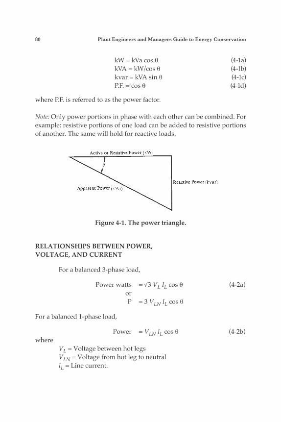
80 Plant Engineers and Managers Guide to Energy Conservation
kW = kVa cos θ (4-1a) kVA = kW/cos θ (4-1b) kvar = kVA sin θ (4-1c) P.F. = cos θ (4-1d)
where P.F. is referred to as the power factor.
Note: Only power portions in phase with each other can be combined. For example: resistive portions of one load can be added to resistive portions of another. The same will hold for reactive loads.
Figure 4-1. The power triangle.
RELATIONSHIPS BETWEEN POWER,VOLTAGE, AND CURRENT
For a balanced 3-phase load,
Power watts = √3 VL IL cos θ (4-2a) or P = 3 VLN IL cos θ
For a balanced 1-phase load,
Power = VLN IL cos θ (4-2b) where VL = Voltage between hot legs VLN = Voltage from hot leg to neutral IL = Line current.
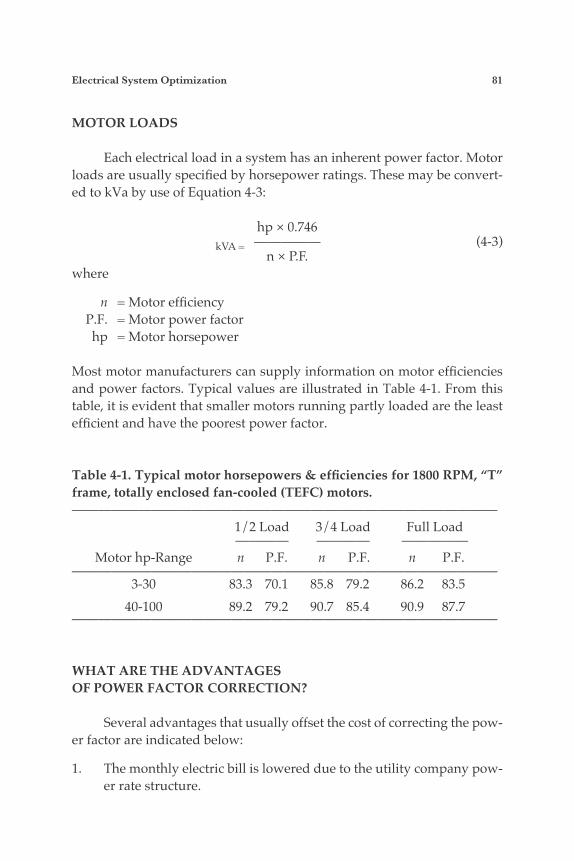
Electrical System Optimization 81
MOTOR LOADS
Each electrical load in a system has an inherent power factor. Motor loads are usually specified by horsepower ratings. These may be convert-ed to kVa by use of Equation 4-3:
hp × 0.746 kVA = ————— (4-3) n × P.F. where
n = Motor efficiency P.F. = Motor power factor hp = Motor horsepower Most motor manufacturers can supply information on motor efficiencies and power factors. Typical values are illustrated in Table 4-1. From this table, it is evident that smaller motors running partly loaded are the least efficient and have the poorest power factor.
Table 4-1. Typical motor horsepowers & efficiencies for 1800 RPM, “T” frame, totally enclosed fan-cooled (TEFC) motors.———————————————————————————————— 1/2 Load 3/4 Load Full Load ———— ———— ————— Motor hp-Range n P.F. n P.F. n P.F.———————————————————————————————— 3-30 83.3 70.1 85.8 79.2 86.2 83.5 40-100 89.2 79.2 90.7 85.4 90.9 87.7————————————————————————————————
WHAT ARE THE ADVANTAGESOF POWER FACTOR CORRECTION?
Several advantages that usually offset the cost of correcting the pow-er factor are indicated below:
1. The monthly electric bill is lowered due to the utility company pow-er rate structure.
82 Plant Engineers and Managers Guide to Energy Conservation
2. The plant system capacity is increased because the transformer load can be increased.
3. Electrical system losses are decreased and voltage regulation is im-proved.
SIM 4-1 A plant load is comprised of the following:
50 kW lighting at unity power factor Ten 30 hp motors running at full load Two 40 hp motors running at full load
What is the overall power factor resulting from these loads?
ANSWER10-30 hp motorsAssume that efficiency is 86.2% at full load and PF is .835
n = 0.862 cos θ= 0.835
hp × 0.746 10 × 30 × 0.746 PkW= ————— = ——————— = 259.6 kW n 0.862 θ = 33° tan θ = 0.65 kvar = kW tan θ= 259.6 × 0.65 = 168.7 kvar
40 hp motors – θ = 29°Assume that efficiency at full load = 90% and PF = .88
2 × 40 × 0.746 PkW= ——————— = 66.3 kW 0.90
tan θ = 0.55 kvar = 66.3 × 0.55 = 36.4———————————————————————————————— Load kW = 50 + 259.6 + 66.3 = 375.9 Total: kvar = 168.7 + 36.4 = 205.1
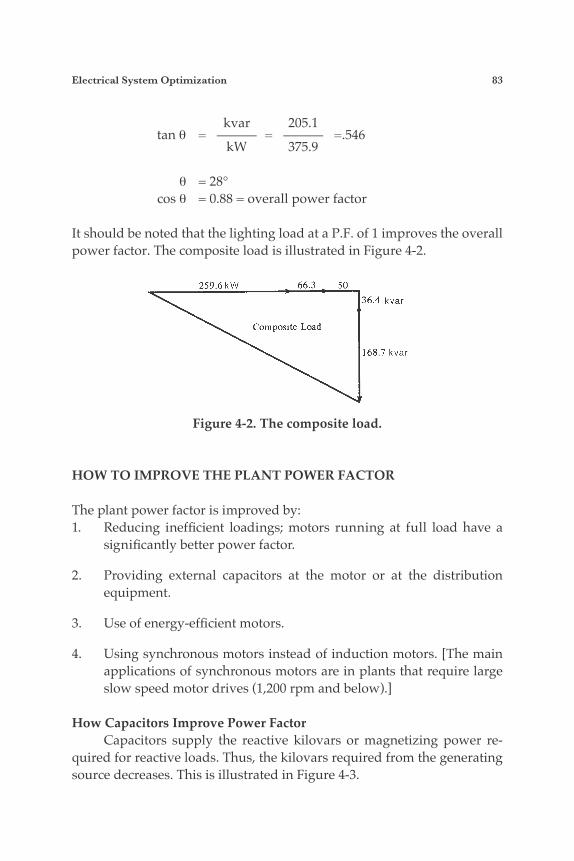
Electrical System Optimization 83
kvar 205.1 tan θ = ——— = ——— =.546 kW 375.9 θ = 28° cos θ = 0.88 = overall power factor
It should be noted that the lighting load at a P.F. of 1 improves the overall power factor. The composite load is illustrated in Figure 4-2.
Figure 4-2. The composite load.
HOW TO IMPROVE THE PLANT POWER FACTOR
The plant power factor is improved by:1. Reducing inefficient loadings; motors running at full load have a
significantly better power factor.
2. Providing external capacitors at the motor or at the distribution equipment.
3. Use of energy-efficient motors.
4. Using synchronous motors instead of induction motors. [The main applications of synchronous motors are in plants that require large slow speed motor drives (1,200 rpm and below).]
How Capacitors Improve Power FactorCapacitors supply the reactive kilovars or magnetizing power re-
quired for reactive loads. Thus, the kilovars required from the generating source decreases. This is illustrated in Figure 4-3.
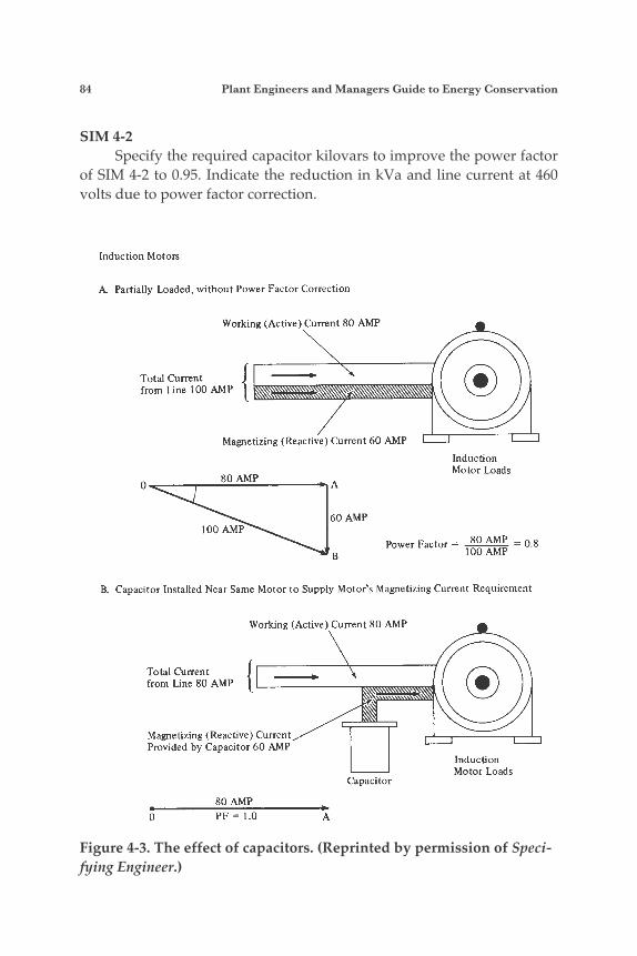
84 Plant Engineers and Managers Guide to Energy Conservation
SIM 4-2Specify the required capacitor kilovars to improve the power factor
of SIM 4-2 to 0.95. Indicate the reduction in kVa and line current at 460 volts due to power factor correction.
Figure 4-3. The effect of capacitors. (Reprinted by permission of Speci-fying Engineer.)
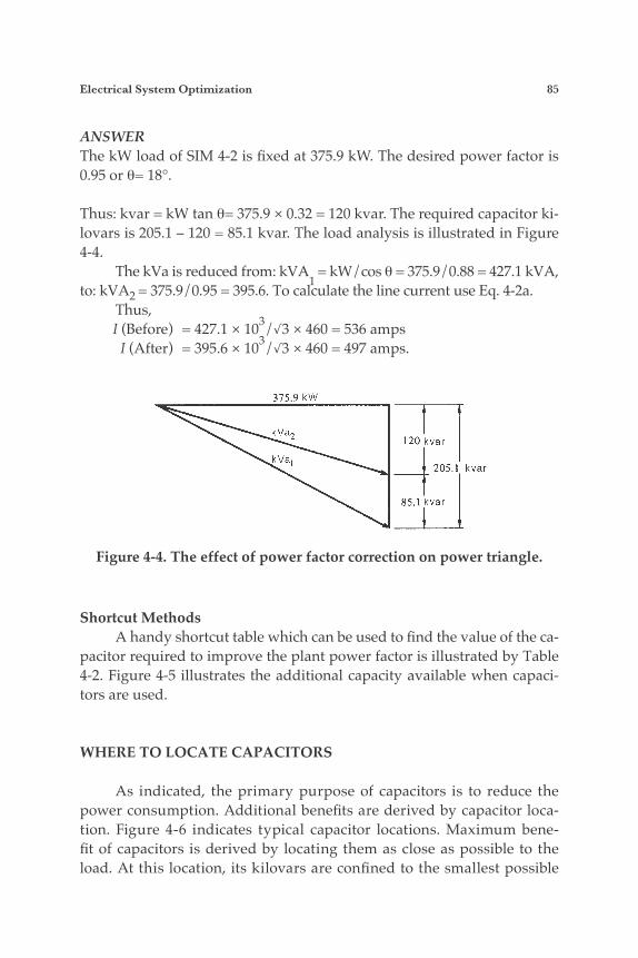
Electrical System Optimization 85
ANSWERThe kW load of SIM 4-2 is fixed at 375.9 kW. The desired power factor is 0.95 or θ= 18°.
Thus: kvar = kW tan θ= 375.9 × 0.32 = 120 kvar. The required capacitor ki-lovars is 205.1 – 120 = 85.1 kvar. The load analysis is illustrated in Figure 4-4.
The kVa is reduced from: kVA1
= kW/cos θ = 375.9/0.88 = 427.1 kVA, to: kVA2
= 375.9/0.95 = 395.6. To calculate the line current use Eq. 4-2a.Thus,
I (Before) = 427.1 × 10³/√3 × 460 = 536 amps I (After) = 395.6 × 10³/√3 × 460 = 497 amps.
Shortcut MethodsA handy shortcut table which can be used to find the value of the ca-
pacitor required to improve the plant power factor is illustrated by Table 4-2. Figure 4-5 illustrates the additional capacity available when capaci-tors are used.
WHERE TO LOCATE CAPACITORS
As indicated, the primary purpose of capacitors is to reduce the power consumption. Additional benefits are derived by capacitor loca-tion. Figure 4-6 indicates typical capacitor locations. Maximum bene-fit of capacitors is derived by locating them as close as possible to the load. At this location, its kilovars are confined to the smallest possible
Figure 4-4. The effect of power factor correction on power triangle.
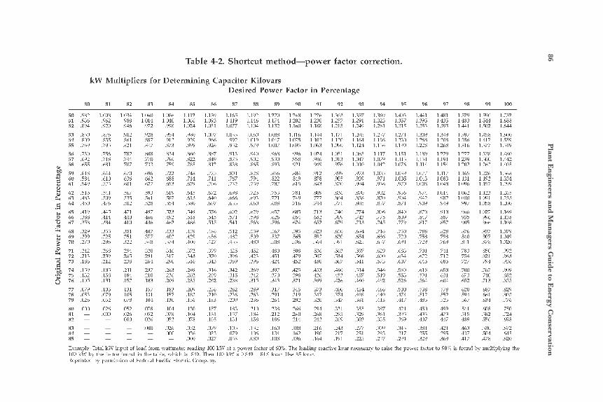
86 P
lant E
ngin
eers and
Man
agers Gu
ide to E
nergy C
onservation
Table 4-2. Shortcut method-power factor correction.
kW Multipliers for Determining Capacitor Kilovars Desired Power Factor in Percentage
80
50 ,962 51 ,936 52 ,394
53 .ss0 54 ,309 J J ,769 5G .730 57 ,692
..
~ 58 .555
2 59 ,1118 + 60 ,584 9 61 ,349
E 62 ,315 fi 6 3 AS3 c 64 ,450
65 A19 0 65 ,365 u 67 3 s
FT 60 ,329
70 ,270 ' 71 ,242
.i
il
2 69 ,299
: 72 ,213
2 73 .i ,159 ;; .I32 0 7 6 ,1175
77 ,079 78 ,053 79 ,026
80 .000 81 - 82 -
83 - 84 - 85 -
81
,006 ,902 ,920
,876 83.1 ,795
7511 718 651
b44
~
$10 J/
541 3 9 ,470
4.45 ,414 ,334 335 ,325 29b
,206 ,230 211
,185 159 131
103 079 032
0211 000 -
- - -
82
1.034 ,988 ,946
,901
X I 7S2 ,744 707
,570 ,636 ,603
,567 ,535 ,502
,471 .I40 ,410
,381 ,351 ,322
,204 ,265 ,238
,211 184
,157
,131 ,105 ,078
052 ,026 000
~
.3bl
- - -
83
1.060 1.014 ,972
,928 E97 . M i
Ell5 770 733
(1911 062 027
593 561 ,528
197 ,460 ,4311
407 ,377
s ,320 ,291 264
137 210 183
157 131 104
075 052 026
,000
~
- -
81
1,086 1.040
,998
,954 913 ,573 S31 79 6 75 9
722 688 65 3
61 9 587 ,554
523 ,492 ,402
433 ,403 374
.Y6 ,317 19 0
,203 23 6 209
183 157 130
101 078 052
,026 000
~
-
85
1.112 1.066 1.02'4
.9s0 ,939 ,899
.S60 ,822 .7s3
,749 ,714 ,079
.Mi ,013 .?SO
,549 31s ,459
,459 ,429 ,400 777
343 ,316
,259 761 '?i -
,209 .IS3 ,156
.I30 ,104 .07s
,052 ,026 .on0
~
.., -
.i -
0G
1.139 1.093 1.031
~
m; 9bb
,920 867 849 812
775 74 1 706
672 6LU
,607
576 ,54s ,515 486 .G6 427
,349 ,370 3 3
,310 ld9 ?62
230 210 333
I 3 7 131 105
,079 05 3
,027
87
1.165 1.119 1.07s
1.033 ,992 ,952 .913 ,875 33s
~
.??A
.Ibi ,732
,095 ,666 ,033
,602 ,571 ,341
,312 ,462 ,433
,4225 ,396 ,369
,342 .315 ,288
,262 ,236 ,209
.I53 ,137 .I31
,105 ,079 ,053
88
1.142 1.140 1.104
1.060 1019
,979 940 902 so5
S2 8 791 739
72 5 693
.bbU
62 9 ,548 .SbS
539 ,509 480
,452 .A23 34 b
,309 ?A2 315 289 263 236
210 184 15s ,132 106
,080
~
89
1.220 1.174 1.132
1.0ss 1.047 1.007
965 ,930 993
,956 ,522 ,737
,733 ,721 ,688
,657 ,626 .39b
,567 ,537 ,308
,430 ,451 , 2 2 4
,397 370 ,313
,317 ,291 ,264
235 ,212 136
.Ib@ ,134 ,106
~
9D
L2.E 1.202 1.100
1.116 I 073 1.035 99b 95 d 92 1
884 849 813
78 1 74 ir ,710
685 ,654 , 024 595 ,565 53 b
~
.sm ,474 452
.A25 39 d 37 1
33 3 314 292
21111 24 0 21A
,188 162
,130
91
1.276 1.230 1.133
1,144 1103 1.063
1024 936 919
912 873 a3
~
su9 ,';: ,244
713 ,632 ,632
623 ,593 564
,536 ,507 430
,453 4211 399
373 247 320
294 2b3 212 .21b 190 ,164
92
1,303 1 . 5 7 1.115
1.1;1 1.130 1.090 1 051 1.013
9:o
,934 ,905
~
.s:a ,836 ,804 .7:1
,709 , 079
,620 ,501
,503 ,534 ,507
,480 A53 ,426
,100 ,374 ,317
32 1 ,295 2b9
,243 '1"
,191
,710
,650
._ I
93
1.337 1.291 1.249
1.205 1.16'4 1.124
1.0Sj 1.047 1.010
,973 ,939 ,901
.s70 ,833 ,805
,774 ,743 ,713
,654 ,654 ,623
,597 ,369 ,541
,514 .AS7 ,460
,434 ,403 ,381
3 5 5 ,329 .303
,277 ,251 ,215
~
94 95 9G 97 98 99 100
1.403 1.M1 1.481 1.529 1.590 1 1.357 1.393 1.435 1.493 1.514 1 1.315 1.333 1.393 1.41 1.501 1.Mi
1117 1.151 1159 1 2 2 9 1277 1335 1 . S 0 1.079 1111. 1131 1.191 1239 11.00 1.162
I154 1202 1203 1. -
1.117 1165 1 2 2 6 1. 1.083 1131 1192 1. I.MS 10% 115; 1.299
,402 ,936 974 1.014 1062 1123 1.265 ,370 ,904 942 .9sz 1030 1091 1.133 ,837 ,871 ,909 ,949 ,997 1.058 1.200
0 878 ,918 966 1 02; 1.169
,019 ,663 ,7001 ,741 ,550 ,992
. 2 u ,607 t-43 ,685 794 ,936
,540 ,560 ,018 ,658 ,700 519 3 5 3 591 531 b73
,"! ,634 ,672 ,712 ,521 ,063
.&0 ,474 512 ,552 594 661 ,903
.A13 . a 7 483 ,525 567 63-1 ,776
abi .GI 450 499 541 60s .750 ,301 ,395 4-33 ,473 515 582 ,724 335 3 6 9 4 K 447 439 556 .b9J
,309 .b43 ,421 ,463 ,530 . ,283 ,317 ,395 437 504 .
*"-
,369 ,417 , 4 x . - Evample Tdtal kN' input of load from wattmrtrr reading 100 k W at a pohcr factor iif 60;. The Irading rractlve kxar necessary to raise the p d w r factor to 9W; is kound bv miiltqlving the I00 kTV by the tactor tourtd in the tablr. which 1s ,349 Then 100 kU' x 0 d49 = U.9 h.ar. Use 83 kvar Repihited by pelmission 01 Federal Pacitic Electiic COTLF~TI?
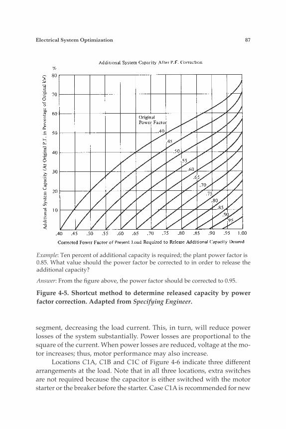
Electrical System Optimization 87
segment, decreasing the load current. This, in turn, will reduce power losses of the system substantially. Power losses are proportional to the square of the current. When power losses are reduced, voltage at the mo-tor increases; thus, motor performance may also increase. Locations C1A, C1B and C1C of Figure 4-6 indicate three different arrangements at the load. Note that in all three locations, extra switches are not required because the capacitor is either switched with the motor starter or the breaker before the starter. Case C1A is recommended for new
Example: Ten percent of additional capacity is required; the plant power factor is 0.85. What value should the power factor be corrected to in order to release the additional capacity?
Answer: From the figure above, the power factor should be corrected to 0.95.
Figure 4-5. Shortcut method to determine released capacity by power factor correction. Adapted from Specifying Engineer.
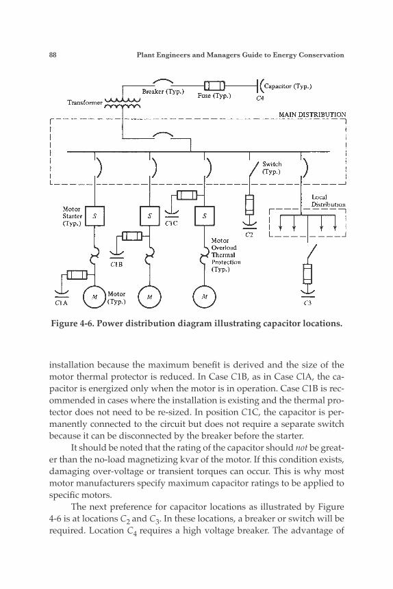
88 Plant Engineers and Managers Guide to Energy Conservation
installation because the maximum benefit is derived and the size of the motor thermal protector is reduced. In Case C1B, as in Case ClA, the ca-pacitor is energized only when the motor is in operation. Case C1B is rec-ommended in cases where the installation is existing and the thermal pro-tector does not need to be re-sized. In position C1C, the capacitor is per-manently connected to the circuit but does not require a separate switch because it can be disconnected by the breaker before the starter. It should be noted that the rating of the capacitor should not be great-er than the no-load magnetizing kvar of the motor. If this condition exists, damaging over-voltage or transient torques can occur. This is why most motor manufacturers specify maximum capacitor ratings to be applied to specific motors. The next preference for capacitor locations as illustrated by Figure 4-6 is at locations C2
and C3. In these locations, a breaker or switch will be required. Location C4
requires a high voltage breaker. The advantage of
Figure 4-6. Power distribution diagram illustrating capacitor locations.
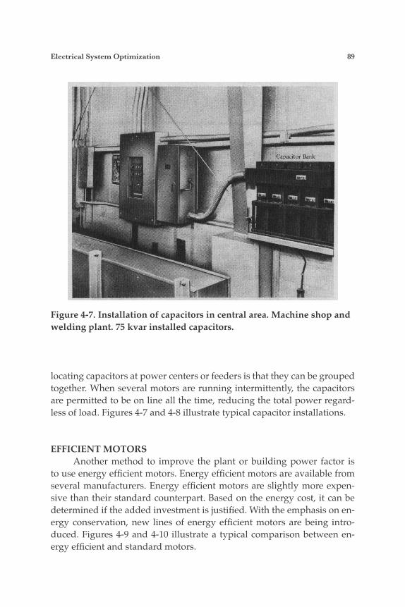
Electrical System Optimization 89
locating capacitors at power centers or feeders is that they can be grouped together. When several motors are running intermittently, the capacitors are permitted to be on line all the time, reducing the total power regard-less of load. Figures 4-7 and 4-8 illustrate typical capacitor installations.
EFFICIENT MOTORS Another method to improve the plant or building power factor is to use energy efficient motors. Energy efficient motors are available from several manufacturers. Energy efficient motors are slightly more expen-sive than their standard counterpart. Based on the energy cost, it can be determined if the added investment is justified. With the emphasis on en-ergy conservation, new lines of energy efficient motors are being intro-duced. Figures 4-9 and 4-10 illustrate a typical comparison between en-ergy efficient and standard motors.
Figure 4-7. Installation of capacitors in central area. Machine shop and welding plant. 75 kvar installed capacitors.
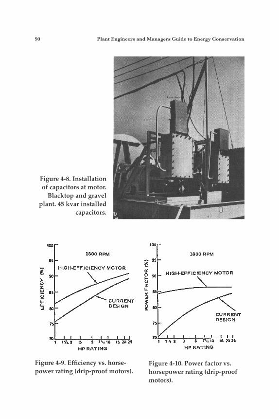
90 Plant Engineers and Managers Guide to Energy Conservation
Figure 4-8. Installation of capacitors at motor.
Blacktop and gravel plant. 45 kvar installed
capacitors.
Figure 4-10. Power factor vs. horsepower rating (drip-proof motors).
Figure 4-9. Efficiency vs. horse-power rating (drip-proof motors).
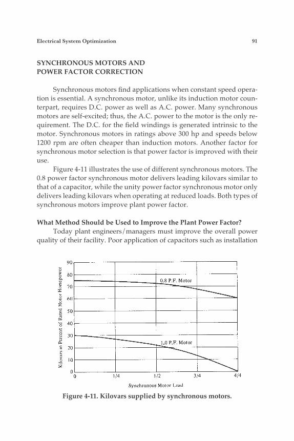
Electrical System Optimization 91
SYNCHRONOUS MOTORS ANDPOWER FACTOR CORRECTION
Synchronous motors find applications when constant speed opera-tion is essential. A synchronous motor, unlike its induction motor coun-terpart, requires D.C. power as well as A.C. power. Many synchronous motors are self-excited; thus, the A.C. power to the motor is the only re-quirement. The D.C. for the field windings is generated intrinsic to the motor. Synchronous motors in ratings above 300 hp and speeds below 1200 rpm are often cheaper than induction motors. Another factor for synchronous motor selection is that power factor is improved with their use.
Figure 4-11 illustrates the use of different synchronous motors. The 0.8 power factor synchronous motor delivers leading kilovars similar to that of a capacitor, while the unity power factor synchronous motor only delivers leading kilovars when operating at reduced loads. Both types of synchronous motors improve plant power factor.
What Method Should be Used to Improve the Plant Power Factor? Today plant engineers/managers must improve the overall power
quality of their facility. Poor application of capacitors such as installation
Figure 4-11. Kilovars supplied by synchronous motors.
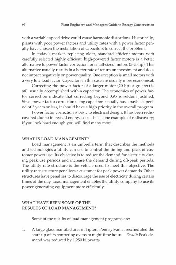
92 Plant Engineers and Managers Guide to Energy Conservation
with a variable speed drive could cause harmonic distortions. Historically, plants with poor power factors and utility rates with a power factor pen-alty have chosen the installation of capacitors to correct the problem. In today’s market, replacing older, standard efficient motors with carefully selected highly efficient, high-powered factor motors is a better alternative to power factor correction for small-sized motors (5-20 hp). This alternative usually results in a better rate of return on investment and does not impact negatively on power quality. One exception is small motors with a very low load factor. Capacitors in this case are usually more economical. Correcting the power factor of a larger motor (20 hp or greater) is still usually accomplished with a capacitor. The economics of power fac-tor correction indicate that correcting beyond 0.95 is seldom justified. Since power factor correction using capacitors usually has a payback peri-od of 3 years or less, it should have a high priority in the overall program. Power factor correction is basic to electrical design. It has been redis-covered due to increased energy cost. This is one example of rediscovery; if you look hard enough you will find many more.
WHAT IS LOAD MANAGEMENT? Load management is an umbrella term that describes the methods and technologies a utility can use to control the timing and peak of cus-tomer power use. Its objective is to reduce the demand for electricity dur-ing peak use periods and increase the demand during off-peak periods. The utility rate structure is the vehicle used to meet this objective. The utility rate structure penalizes a customer for peak power demands. Other structures have penalties to discourage the use of electricity during certain times of the day. Load management enables the utility company to use its power generating equipment more efficiently.
WHAT HAVE BEEN SOME OF THERESULTS OF LOAD MANAGEMENT?
Some of the results of load management programs are:
1. A large glass manufacturer in Tipton, Pennsylvania, rescheduled the start-up of its tempering ovens to night-time hours—Result: Peak de-mand was reduced by 1,250 kilowatts.

Electrical System Optimization 93
2. A Flemington, New Jersey, plant rescheduled the time for recharging lift truck batteries—Result: Peak daytime demand was reduced by 100 kilowatts.
3. A tool manufacturing company in Meadville, Pennsylvania, in-stalled demand-limiting equipment and started using waste heat from some of its process operations to supplement heat to its build-ing—Result: Overall power demand dropped by 1,000 kilowatts.
4. In Hamburg, Pennsylvania, a metal coating company rescheduled furnace loading from its first shift to its second shift—Result: De-mand was reduced by 1000 kilowatts during peak use periods; ex-pected savings are $35,000 to $40,000 per year.
From the above, two load management techniques can be seen. One is to reschedule energy-related activities to non-peak hour times; the other is to automatically shed loads by use of a load demand controller or com-puter. In either case, the first step is to make a load assessment. A load as-sessment indicates the electrical energy characteristics for the billing pe-riod. The electric characteristics are compared with plant operations to determine what has caused the peak power usages.
APPLICATION OF AUTOMATIC LOAD SHEDDING
Load shedding should be considered when power usage demands fluctuate substantially and load leveling is feasible because of substantial non-essential or controllable loads. Load shedding has been used wide-ly in the steel industry, but the principles of load shedding can be ap-plied to any large industrial or commercial user. The first step in apply-ing load shedding is to establish a target demand. The target demand is based on actual load readings or on a load analysis. The second step is to identify controllable loads which can be shut off to obtain the desired limit. Examples of controllable loads are electric furnaces, electric boilers, compressors, snow melters, air conditioners, heating and ventilating fans, comfort cooling, and noncritical “batch processes.” Ideally, if controllable loads matched intermittent peak uses, the plant under load demand con-trol would use a preset amount of kilowatts in a fixed amount of time. Fig-ure 4-12 shows the effect of load shedding on peak power demands.
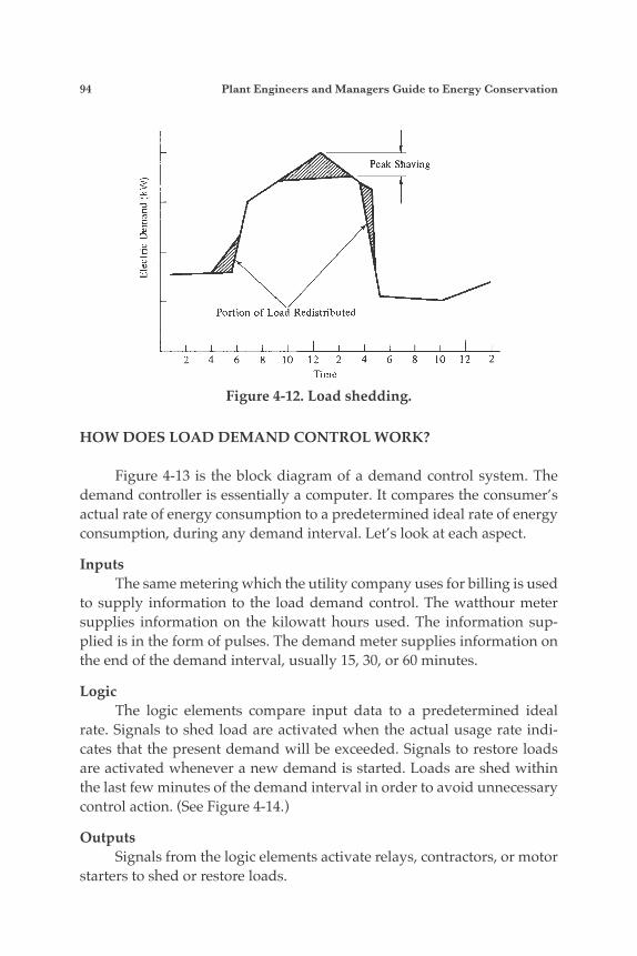
94 Plant Engineers and Managers Guide to Energy Conservation
HOW DOES LOAD DEMAND CONTROL WORK?
Figure 4-13 is the block diagram of a demand control system. The demand controller is essentially a computer. It compares the consumer’s actual rate of energy consumption to a predetermined ideal rate of energy consumption, during any demand interval. Let’s look at each aspect.
Inputs The same metering which the utility company uses for billing is used to supply information to the load demand control. The watthour meter supplies information on the kilowatt hours used. The information sup-plied is in the form of pulses. The demand meter supplies information on the end of the demand interval, usually 15, 30, or 60 minutes.
Logic The logic elements compare input data to a predetermined ideal rate. Signals to shed load are activated when the actual usage rate indi-cates that the present demand will be exceeded. Signals to restore loads are activated whenever a new demand is started. Loads are shed within the last few minutes of the demand interval in order to avoid unnecessary control action. (See Figure 4-14.)
Outputs Signals from the logic elements activate relays, contractors, or motor starters to shed or restore loads.
Figure 4-12. Load shedding.
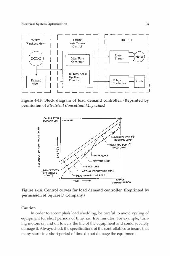
Electrical System Optimization 95
Figure 4-13. Block diagram of load demand controller. (Reprinted by permission of Electrical Consultant Magazine.)
Figure 4-14. Control curves for load demand controller. (Reprinted by permission of Square D Company.)
Caution In order to accomplish load shedding, be careful to avoid cycling of equipment for short periods of time, i.e., five minutes. For example, turn-ing motors on and off lowers the life of the equipment and could severely damage it. Always check the specifications of the controllables to insure that many starts in a short period of time do not damage the equipment.
INPUT Watthour Meter
0033
LOGIC b g i c Demand
Control
Ideal Rate Generator
Bi-Directional Up-Down Counter Oemand
Meter
OUTPUT
Motor Starter
Motor
Relays Loads Contactors
96 Plant Engineers and Managers Guide to Energy Conservation
Is a Programmable Logic Controller (PLC) Required to Shed Loads? Before buying a standard PLC to automatically shed loads, consider some of the packaged solid-state load demand controllers. These control-lers are relatively inexpensive, and several models are available to meet most needs. If a PLC is already available, then programmable control of load shedding becomes more attractive. In either case, an analysis of spe-cific electrical usage should be made by an independent consultant in or-der to determine which system is best.
THE CONFUSION OVERENERGY MANAGEMENT SYSTEMS
With the myriad electrical management systems on the market, it is no wonder why the energy manager is confused. First, there is no stan-dardization of equipment specifications. Second, the term energy manage-ment system itself is confusing.
An energy management system could be one or all of the following:
1 Simple time clock
2 Simple duty cycle device
3 Peak load shedding device
4 Heating, ventilation, and air conditioning controllers (enthalpy con-troller, temperature switch, etc.)
The main reason the controller is specified in the first place is to re-duce peak electrical demand. Once the controller is constructed for that purpose, features such as a time clock and duty cycle control are economi-cally added.
The terminology usually changes from a simple peak load shedding device to an energy management system when the heating and ventilation control features are added.
The size of the unit to be purchased depends on the number of loads that must be cycled to reduce peak demand.
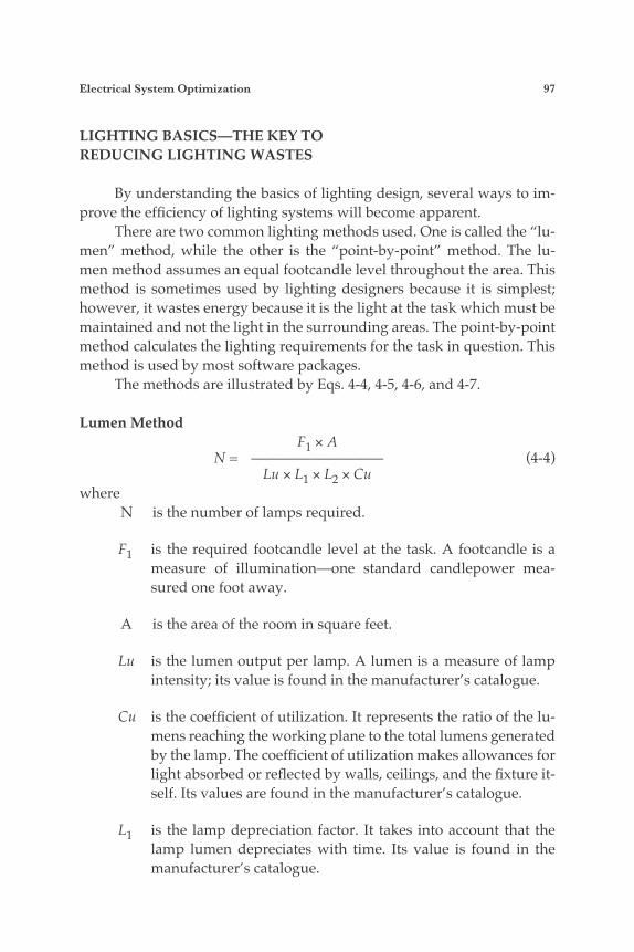
Electrical System Optimization 97
LIGHTING BASICS—THE KEY TOREDUCING LIGHTING WASTES
By understanding the basics of lighting design, several ways to im-prove the efficiency of lighting systems will become apparent.
There are two common lighting methods used. One is called the “lu-men” method, while the other is the “point-by-point” method. The lu-men method assumes an equal footcandle level throughout the area. This method is sometimes used by lighting designers because it is simplest; however, it wastes energy because it is the light at the task which must be maintained and not the light in the surrounding areas. The point-by-point method calculates the lighting requirements for the task in question. This method is used by most software packages.
The methods are illustrated by Eqs. 4-4, 4-5, 4-6, and 4-7.
Lumen Method F1 × A N = ————————— (4-4) Lu × L1 × L2 × Cuwhere
N is the number of lamps required.
F1 is the required footcandle level at the task. A footcandle is a measure of illumination—one standard candlepower mea-sured one foot away.
A is the area of the room in square feet.
Lu is the lumen output per lamp. A lumen is a measure of lamp intensity; its value is found in the manufacturer’s catalogue.
Cu is the coefficient of utilization. It represents the ratio of the lu-mens reaching the working plane to the total lumens generated by the lamp. The coefficient of utilization makes allowances for light absorbed or reflected by walls, ceilings, and the fixture it-self. Its values are found in the manufacturer’s catalogue.
L1 is the lamp depreciation factor. It takes into account that the lamp lumen depreciates with time. Its value is found in the manufacturer’s catalogue.
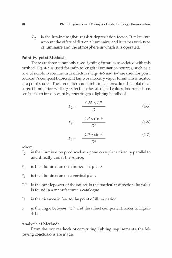
98 Plant Engineers and Managers Guide to Energy Conservation
L2 is the luminaire (fixture) dirt depreciation factor. It takes into account the effect of dirt on a luminaire, and it varies with type of luminaire and the atmosphere in which it is operated.
Point-by-point MethodsThere are three commonly used lighting formulas associated with this
method. Eq. 4-5 is used for infinite length illumination sources, such as a row of non-louvered industrial fixtures. Eqs. 4-6 and 4-7 are used for point sources. A compact fluorescent lamp or mercury vapor luminaire is treated as a point source. These equations omit interreflections; thus, the total mea-sured illumination will be greater than the calculated values. Interreflections can be taken into account by referring to a lighting handbook.
0.35 × CP
F2 = —————— (4-5) D
CP × cos θ F3 = —————— (4-6) D2
CP × sin θ (4-7) F4 = —————— D2
whereF2 is the illumination produced at a point on a plane directly parallel to
and directly under the source.
F3 is the illumination on a horizontal plane.
F4 is the illumination on a vertical plane.
CP is the candlepower of the source in the particular direction. Its value is found in a manufacturer’s catalogue.
D is the distance in feet to the point of illumination.
θ is the angle between “D” and the direct component. Refer to Figure 4-15.
Analysis of Methods From the two methods of computing lighting requirements, the fol-lowing conclusions are made:
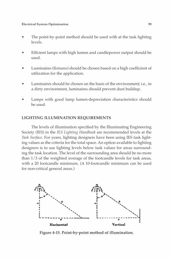
Electrical System Optimization 99
• The point-by-point method should be used with at the task lighting levels.
• Efficient lamps with high lumen and candlepower output should be used.
• Luminaires (fixtures) should be chosen based on a high coefficient of utilization for the application.
• Luminaires should be chosen on the basis of the environment; i.e., in a dirty environment, luminaires should prevent dust buildup.
• Lamps with good lamp lumen-depreciation characteristics should be used.
LIGHTING ILLUMINATION REQUIREMENTS
The levels of illumination specified by the Illuminating Engineering Society (IES) in the IES Lighting Handbook are recommended levels at the Task Surface. For years, lighting designers have been using IES task light-ing values as the criteria for the total space. An option available to lighting designers is to use lighting levels below task values for areas surround-ing the task location. The level of the surrounding area should be no more than 1/3 of the weighted average of the footcandle levels for task areas, with a 20 footcandle minimum. (A 10-footcandle minimum can be used for non-critical general areas.)
Figure 4-15. Point-by-point method of illumination.

100 Plant Engineers and Managers Guide to Energy Conservation
THE EFFICIENT USE OF LAMPS
Figure 4-16 illustrates lumen outputs of various types of lamps.
EFFICIENT TYPES OF INCANDESCENTS FOR LIMITED USE
Attempts to increase the efficiency of incandescent lighting while maintaining good color rendition have led to the manufacture of a num-ber of energy-saving incandescent lamps for limited residential use. Tungsten halogen lamps vary from the standard incandescent by the addition of halogen gases to the bulb. Halogen gases keep the glass bulb from darkening by preventing the filament from evaporating, thereby in-creasing lifetime up to four times that of a standard bulb. The lumen-per-watt rating is approximately the same for both types of incandescents, but tungsten halogen lamps average 94% efficiency throughout their extend-ed lifetime, offering significant energy and operating cost savings. How-ever, tungsten halogen lamps require special fixtures, and during opera-tion the surface of the bulb reaches very high temperatures, so they are not commonly used in the home. Reflector lamps (R-Lamps) are incandescents with an interior coating of aluminum that directs the light to the front of the bulb. Certain incan-descent light fixtures, such as recessed or directional fixtures, trap light in-side. Reflector lamps project a cone of light out of the fixture and into the room, so that more light is delivered where it is needed. In these fixtures, a 50-watt reflector bulb will provide better lighting and use less energy when substituted for a 100-watt standard incandescent bulb. Reflector lamps may be appropriate for task lighting (because they directly illuminate a work area) and for accent lighting. Reflector lamps are manufactured in sizes from 30 to 1,500 watts and in various light dis-tributions. While they have a lower initial efficiency (lumens per watt) than regular incandescents, they direct light more effectively, so that more light is actually delivered than with regular incandescents. Parabolic aluminized reflector lamps (PAR Lamps) are reflector lamps with a lens of heavy, durable glass, which makes them an appropriate choice for outdoor flood- and spot-lighting. They are available in 75, 150, and 250 watts. They have longer lifetimes with less depreciation than stan-dard incandescents. Ellipsoidal reflector lamps (ER lamps) are ideally suited for recessed fix-tures, because the beam of light produced is focused two inches ahead of
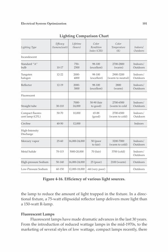
Electrical System Optimization 101
the lamp to reduce the amount of light trapped in the fixture. In a direc-tional fixture, a 75-watt ellipsoidal reflector lamp delivers more light than a 150-watt R-lamp.
Fluorescent Lamps Fluorescent lamps have made dramatic advances in the last 30 years. From the introduction of reduced wattage lamps in the mid-1970s, to the marketing of several styles of low wattage, compact lamps recently, there
Figure 4-16. Efficiency of various light sources.
Lighting Comparison Chart
Efficacy Lifetime Color ColorLighting Type (lumens/watt) (hours) Rendition Temperature Indoors/ Index (CRI) (K) Outdoors
Incandescent Standard “A” 750- 98-100 2700-2800 Indoors/bulb 10-17 2500 (excellent) (warm) Outdoors
Tungsten 12-22 2000- 98-100 2900-3200 Indoors/halogen 4000 (excellent) (warm to neutral) Outdoors Reflector 12-19 2000- 98-100 2800 Indoors/ 3000 (excellent) (warm) Outdoors
Fluorescent 7000- 50-90 (fair 2700-6500 Indoors/Straight tube 30-110 24,000 to good) (warm to cold Outdoors
Compact fluores- 50-70 10,000 65-88 2700-6500 Indoors/cent lamp (CFL) (good) (warm to cold) Outdoors
Circline 40-50 12,000 Indoors
High-Intensity Discharge Mercury vapor 25-60 16,000-24,000 50 (poor 3200-7000 Indoors/ to fair) (warm to cold) Outdoors
Metal halide 70-115 5000-20,000 70 (fair) 3700 (cold) Indoors/ Outdoors
High-pressure Sodium 50-140 16,000-24,000 25 (poor) 2100 (warm) Outdoors
Low-Pressure Sodium 60-150 12,000-18,000 -44 (very poor) Outdoors
102 Plant Engineers and Managers Guide to Energy Conservation
has been a steady parade of new products. The range of colors is more complete than mercury vapor, and lamp manufacturers have made sig-nificant progress in developing fluorescent and metal halide lamps that have much more consistent color rendering properties, allowing greater flexibility in mixing these two sources without creating disturbing color mismatches. The wide range of compact fluorescent lamps opens up the market for fluorescent sources. These lamps permit design of much small-er luminaires that can compete with incandescent and mercury vapor in the low cost, square or round fixture market so long dominated by the in-candescent and mercury sources.
Energy Efficient Fluorescents The energy efficient fluorescents represent the second generation of improved fluorescent lighting. Typical energy savings are about 6 W per lamp for the popular 4-ft 40 W replacement and 15 W per lamp for the popular 8-ft slimline 75 W replacement. Savings in energy cost normally pay back the new lamp cost in a year at typical power rates and lamp costs. While switching from T-12 standard fixtures to T-8 bulbs with elec-tronic ballasts creates savings in the office environment, T-5 fluorescent bulbs offer a competitive solution with high bay applications. For exam-ple, a 6 bulb, T-5 high output fixture can yield 25% energy savings over a 400 W metal halide fixture. Another benefit is that the T-5 fixtures do not have a long warm-up or re-strike delay time associated with them.
Light Emitting Diode (LED) Fixtures Retailers have found LED lighting offers a myriad of light color op-tions while creating significant energy savings over conventional display lights. Prior to the development of LED lighting, ambient lighting could only be provided by specialized, expensive, incandescent lights. LED lamps offer significant energy savings and much longer life than their incandes-cent counterparts. They work better in environments where vibrations are present because they are not as fragile because they have no filament. Their color rendering index is superior to compact fluorescent lamps, and their light is much more directed, improving transfer efficiency.
LED Lighting LED lighting applications are continually expanding due to several advantages. They: (1) can be designed to be quite compact; (2) handle vi-
Electrical System Optimization 103
bration better than fluorescent and HID systems; (3) offer breakage resis-tance because they contain no filaments or glass; (4) show performance improvement in cold temperatures; (5) require no “warm up” time; (6) have a lifetime unaffected by frequent switching; and (7) are compatible with a range of electronic controls to allow for change in light levels and color characteristics. Care must be taken, however, when comparing LED lighting to tra-ditional lighting. Often, LED ratings on manufacturers’ data sheets pro-vide typical luminous flux in lumens, along with test current and forward bias voltage. To calculate the efficacy of the unit, the luminous flux must be divided by the product of the forward bias voltage and the test current. The result is the efficacy for the LED only. As with fluorescent fixtures, LED fixtures require a ballast that pro-vides starting voltage and also limits current. Additionally, an electronic driver circuit is required to step down the line voltage and convert it to a regulated DC voltage and current. The driver circuit is typically 85% ef-ficient, so to estimate the overall LED fixture efficacy, the LED efficacy should be discounted by 15%. Thus, LED fixture efficacy is typically in the range of compact fluorescent fixtures. LED fixtures show significant advantages when considering appli-cation efficiency. Traditional incandescent and fluorescent fixtures must employ reflectors to direct light emissions since their bulbs emit light in all directions. This reduces the effective light delivered to a surface. For re-cessed downlights and troffers, up to 50% of the light output from the fix-tures is lost. LED fixtures are directional sources, so they can deliver light more efficiently to the selected surface. To generate different colors of light, traditional fixtures use incan-descent light sources that beam through a filter. Unfortunately, the filter may block up to 90% of the source light. LED lights emit light in a specific wavelength; for example, a red LED emits red light without the use of a red filter. This makes them considerably more efficient at generating a red light. A red LED light consumes approximately 10% of the power of an in-candescent bulb with a red filter. This is why most streetlights have been switched to LED systems. There are several residential applications where LED fixtures have proven successful. While spiral compact fluorescent fixtures offer signifi-cant improvements over incandescent units in downlighting applications, LED fixtures have proven to be even more efficient. This includes under-cabinet lighting, in-cabinet lighting, and recessed downlights. There are also

104 Plant Engineers and Managers Guide to Energy Conservation
many niche residential categories where LED fixtures have proven highly efficient. This includes accent lighting, path lighting, and cove lighting. For commercial facilities, LED fixtures offer benefits in applications such as refrigerated case lighting, elevator lighting, retail display cases, and food preparation areas. Any application that requires directed light for a task or a specific light color should be considered for LED lighting. LED lighting is even supplanting high pressure sodium and metal halide lighting in outdoor lighting applications. Quality LED fixtures can supply the necessary surface illuminance while consuming less energy and providing superior uniformity, compared to HID fixtures. Operation-al life for LED fixtures is also superior, with a typical life of 50,000 hours as compared to 15,000 to 35,000 for HID fixtures. They also offer the con-venience of instant starting and no restrike delay. Due to the rapid evolution of LED technology, caution must be em-ployed when selecting specific fixtures. IESNA has established the LM-79-08 test procedure for testing of LED fixtures. Photometric test results based upon LM-79-08 should be requested before making a purchase.
Compact Fluorescent Lamps (CFL) A compact fluorescent lamp, can replace an incandescent light source in many applications. Three configurations are possible for the installation of compact fluorescent lamps—dedicated, self-ballasted, and modular. Dedicated compact fluorescent lamp systems are similar to full-size fluorescent lighting systems in which a ballast is hard-wired to lamp holders within a luminaire. Self-ballasted and modular compact fluorescent lamp products have screwbases designed for installation in medium screw base sockets; they typically replace incandescent lamps. A self-ballasted compact fluorescent lamp contains a lamp and ballast as an inseparable unit. A modular compact fluorescent lamp product con-sists of a screwbase ballast with a replaceable lamp. The ballast and lamp connect together using a socket-and-base design that ensures compat-ibility of lamps and ballasts. While most of the modular types are oper-ated in the preheat mode, the electronic ballasted lamps are operated in the rapid-start mode and in principle could be dimmed.
High Intensity Discharge (HID) Lamps High intensity discharge lamps are electric discharge sources. The basic difference from fluorescent lamps is that HID lamps operate at a much higher arc pressure. Spectral characteristics differ from those of flu-

Electrical System Optimization 105
orescent lamps because the higher pressure arc emits a large portion of its visible light. HID lamps produce full light output only at full operating pressure, usually several minutes after starting. Most HID lamps contain both an inner and an outer bulb. The inner bulb is made of quartz or poly-crystalline aluminum; the outer bulb is generally made of thermal shock-resistant glass. HID lamps require current-limiting devices, which con-sume 10% to 20% additional watts. HID lamps include mercury, metal ha-lide, high-pressure sodium, and low-pressure sodium lamps as described below.
Mercury Lamps These are low in efficacy compared to other HID sources, and they are obsolescent for most industrial lighting applications. They are avail-able with either “clear” or phosphor-coated bulbs of 40 to 1,000 W, and in various sizes and shapes. Typical efficacy ranges from 30 to 63 lumens per watt, not including ballast loss. Clear mercury lamps produce light rich in yellow and green tones while lacking in red. Phosphor-coated lamps pro-vide improved color. Special types include semi-reflector, reflectorized, and self-ballasted lamps.
Metal Halide (MH) Lamps These are similar in construction to mercury lamps. The difference is in the arc tube, which contains various metal halides in addition to mer-cury. They are available in either clear or phosphor-coated bulbs from 32 to 1,500 W. Present efficacies range from 70 to 125 lumens per watt, not including ballast power loss. Color improvement is achieved by the metal halide additives. Metal-halide lamps generally have fairly good color rendering quali-ties. While these lamps display some very desirable qualities, they also have some distinct drawbacks, including relatively short life for an HID lamp, long restrike time to restart after having been shut off (about 15-20 minutes at 70°F), and a pronounced tendency to shift colors with age.
High-pressure Sodium (HPS) Lamps Light is produced in HPS lamps by electricity passing through so-dium vapor. They are presently available in sizes of 35 to 1,000 W. Typical initial efficacies are about twice that of mercury lamps —from 80 to 140 lumens per watt, not including ballast power loss. Normally with clear outer envelopes, they may also be obtained with coatings that improve
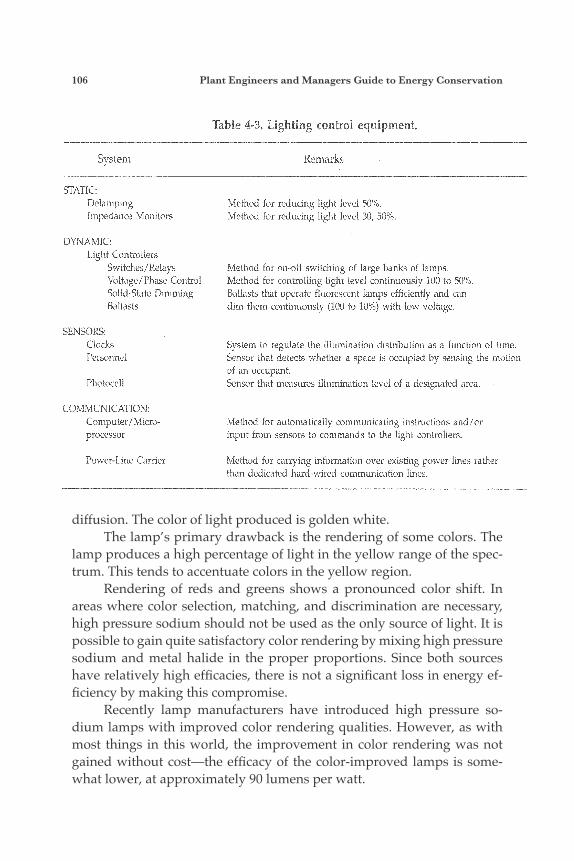
106 Plant Engineers and Managers Guide to Energy Conservation
diffusion. The color of light produced is golden white. The lamp’s primary drawback is the rendering of some colors. The lamp produces a high percentage of light in the yellow range of the spec-trum. This tends to accentuate colors in the yellow region. Rendering of reds and greens shows a pronounced color shift. In areas where color selection, matching, and discrimination are necessary, high pressure sodium should not be used as the only source of light. It is possible to gain quite satisfactory color rendering by mixing high pressure sodium and metal halide in the proper proportions. Since both sources have relatively high efficacies, there is not a significant loss in energy ef-ficiency by making this compromise. Recently lamp manufacturers have introduced high pressure so-dium lamps with improved color rendering qualities. However, as with most things in this world, the improvement in color rendering was not gained without cost—the efficacy of the color-improved lamps is some-what lower, at approximately 90 lumens per watt.
system RErrlarks
ST.4TiC; D e l o m p g Impedance Monitors
D".&biIC: Light Csntrciliers
Si+vitches/Xelays i!dtage/Pha.se Control %lid-State Dimniing Ballasts
..
SENSORS: ciocks Ferso:ii.el
P h o t m d
Mefkod for oi..-cE swiici;ing of Iiirge b a n k of iainr;s, Method ir;r cantrzlling iighi l e d :ontinuxisly 100 to jg"; Ballasts that operate fiuoresceni iamps efficiently and can dim them continuously (100 to 10%) with low voltage,
Svstem to regulate the illumination distrrbu!ion as a function of time. k s o r that detects whether of ap. occupant. Sensor that ineasures illumination lesrei of a designated area.
space is occupied by sensing the motion
Mei'red for carrying information over exkting power lines raihzr than dedicated h.a:d-rvired cainmunicaticn lines.
Electrical System Optimization 107
Low-pressure Sodium Lamps Low-pressure sodium lamps provide the highest efficacy of any of the sources for general lighting, with values ranging up to 180 lumens per watt. Low pressure sodium produces an almost pure yellow light with very high efficacy and renders all colors gray except yellow or near yel-low. The effect of this is there can be no color discrimination under low pressure sodium lighting, so it is suitable for use in a very limited number of applications. It is an acceptable source for warehouse lighting where it is only necessary to read labels, not to choose items by color. This source has application for either indoor or outdoor safety or security lighting, again as long as color rendering is not important.
Control Equipment Table 4-3 lists various types of equipment that can be components of a lighting control system, with a description of the predominant charac-teristic of each type of equipment. Static equipment can alter light levels semipermanently. Dynamic equipment can alter light levels automatically over short intervals to correspond to the activities in a space. Different sets of components can be used to form various lighting control systems in or-der to accomplish different combinations of control strategies.
Solid-state Ballasts After more than 10 years of development and 10 years of manufac-turing experience, operating fluorescent lamps at high frequency (20 to 30 kHz) with solid-state ballasts has achieved credibility. The fact that all of the major ballast manufacturers offer solid-state ballasts and the major lamp companies have designed new lamps to be operated at high frequency is evidence that the solid-state high frequency ballast is now state-of-the-art. It has been shown that fluorescent lamps operated at high frequency are 10 to 15% more efficacious than 60 Hz operation. In addition, the sol-id-state ballast is more efficient than conventional ballasts in conditioning the input power for the lamps, such that the total system efficacy increase is between 20 and 25 percent. That is, for a standard two-lamp 40 watt F40 T-12 rapid start system, overall efficacy is increased from 63 lm/w to over 80 lm/w.

108 Plant Engineers and Managers Guide to Energy Conservation
SIM 4-3 A waste treatment plant has an average 2,000-kW connected load at a PF of 0.8. Comment on the yearly savings before taxes for installing ca-pacitors to improve the PF to 0.9. The demand charge that accounts in this billing structure for poor PF is $9/kVa/month. The total installation cost of the capacitors is $25/kvar. An analysis of the electrical demand indicates that a peak of 2,500 kW can be reduced by automatically turning off decorative lighting and lighting for non-essential uses. Comment on adding a package load de-mand controller to reduce the peak demand to 2,000 kW at a PF of 0.9. The installed cost of the unit is $5,000.
ANSWER Power Factor Improvement
First cost: From Table 4-1, the multiplier is 0.266. The required correction is 2,000 kW × 0.266 = 532 kvar. The capacitor cost is $40/kvar × 532 kvar =$21,280.
Annual savings:With correction— Billing kVa = 2,000/0.8 = 2,500 kVa
Without correction— Billing kVa = 2,000/0.9 = 2,222 kVa
Savings = (2,500—2,222) × $9/kVa/month × 12 = $30,024
Since the payback period is less than one year, investment is justified.
Load Management In load shedding, the peak demand is reduced (2,500/0.9—2,000/ 0.9) without considering energy usage savings. The net savings are:
$9(2,777 – 2,222) × 12 = $54,000
With a payback period of a fraction of the year, investment is justi-fied.
109
5Utility and ProcessSystem Optimization
The energy manager should analyze total utility needs and the process for energy utilization opportunities. The overall heat and mate-rial balance and process flow diagram are very important tools. Each subprocess must also be analyzed in detail. In this chapter, waste heat recovery, boiler operation, utility, and process systems are discussed.
BASIS OF THERMODYNAMICS
Thermodynamics deals with the relationships between heat and work. It is based on two basic laws of nature: the first and second laws of thermodynamics. The principles are used in the design of equipment such as steam engines, turbines, pumps, and refrigerators, as well as in practically every process involving a flow of heat or a chemical equi-librium. First Law: The first law states that energy can neither be created nor destroyed; thus, it is referred to as the law of conservation of energy. Equation 5-4 expresses the first law for the steady-state condition.
E2 – E1 = Q – W (5-1)where
E2 – E1 is the change in stored energy at the boundary states 1 and 2 of the system
Q is the heat added to the system
W is the work done by the system
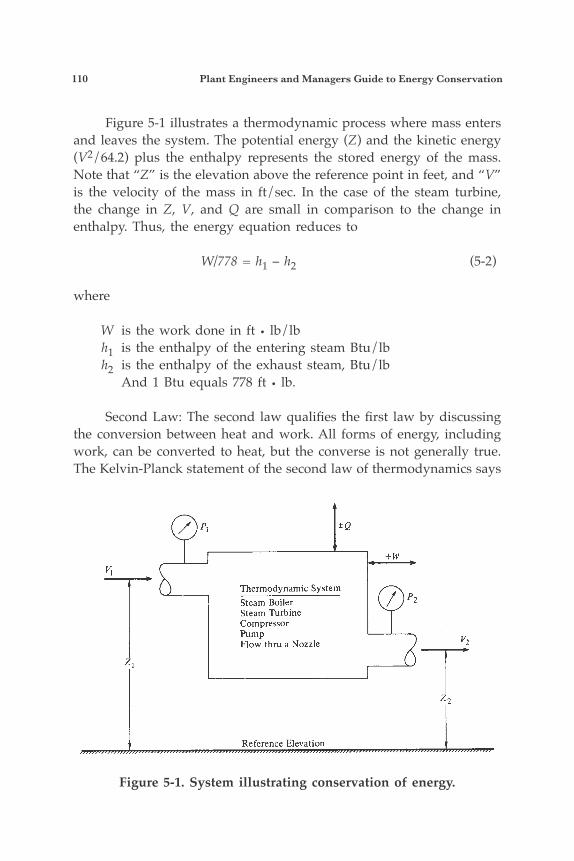
110 Plant Engineers and Managers Guide to Energy Conservation
Figure 5-1 illustrates a thermodynamic process where mass enters and leaves the system. The potential energy (Z) and the kinetic energy (V2/64.2) plus the enthalpy represents the stored energy of the mass. Note that “Z” is the elevation above the reference point in feet, and “V” is the velocity of the mass in ft/sec. In the case of the steam turbine, the change in Z, V, and Q are small in comparison to the change in enthalpy. Thus, the energy equation reduces to
W/778 = h1 – h2 (5-2)
where
W is the work done in ft • lb/lb h1 is the enthalpy of the entering steam Btu/lb h2 is the enthalpy of the exhaust steam, Btu/lb And 1 Btu equals 778 ft • lb.
Second Law: The second law qualifies the first law by discussing the conversion between heat and work. All forms of energy, including work, can be converted to heat, but the converse is not generally true. The Kelvin-Planck statement of the second law of thermodynamics says
Figure 5-1. System illustrating conservation of energy.
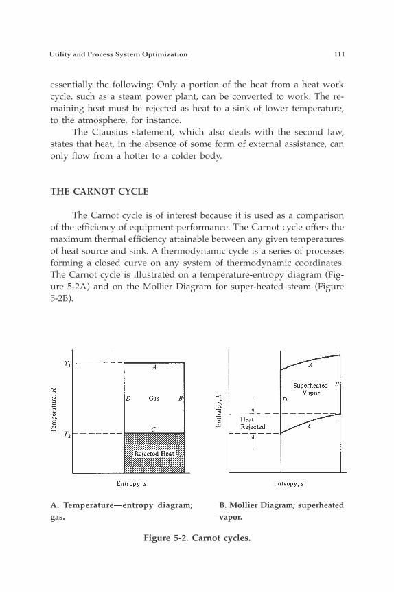
Utility and Process System Optimization 111
essentially the following: Only a portion of the heat from a heat work cycle, such as a steam power plant, can be converted to work. The re-maining heat must be rejected as heat to a sink of lower temperature, to the atmosphere, for instance. The Clausius statement, which also deals with the second law, states that heat, in the absence of some form of external assistance, can only flow from a hotter to a colder body.
THE CARNOT CYCLE
The Carnot cycle is of interest because it is used as a comparison of the efficiency of equipment performance. The Carnot cycle offers the maximum thermal efficiency attainable between any given temperatures of heat source and sink. A thermodynamic cycle is a series of processes forming a closed curve on any system of thermodynamic coordinates. The Carnot cycle is illustrated on a temperature-entropy diagram (Fig-ure 5-2A) and on the Mollier Diagram for super-heated steam (Figure 5-2B).
Figure 5-2. Carnot cycles.
A. Temperature—entropy diagram; gas.
B. Mollier Diagram; superheated vapor.
112 Plant Engineers and Managers Guide to Energy Conservation
The cycle consists of:
1. Heat addition at constant temperature, resulting in expansion work and changes in enthalpy.
2. Adiabatic isentropic expansion (change in entropy is zero) with expansion work and an equivalent decrease in enthalpy.
3. Constant temperature heat rejection to the surroundings, equal to the compression work and any changes in enthalpy.
4. Adiabatic isentropic compression returning to the starting tem-perature with compression work and an equivalent increase in enthalpy.
The Carnot cycle is an example of a reversible process and has no counterpart in practice. Nevertheless, this cycle illustrates the principles of thermodynamics. The thermal efficiency for the Carnot cycle is il-lustrated by Eq. 5-3.
Thermal efficiency = T1T2
T1 (5-3)where T1 = Absolute temperature of heat source, °R (Rankine) T2 = Absolute temperature of heat sink, °R
and absolute temperature is given by Eq. 5-4.
Absolute temperature = 460 + temperature in Fahrenheit. (5-4)
T2 is usually based on atmospheric temperature, which is taken as 500°R.
SIM 5-1 Compute the ideal thermal efficiency for a steam engine, based on the Carnot cycle and a saturated steam temperature of 540°F.
ANSWERThermal efficiency =
540 + 460 – 500540 + 460
Utility and Process System Optimization 113
Properties of Steam Pressure and Temperature Water boils at 212°F when it is in an open vessel under atmo-spheric pressure equal to 14.7 psia (pounds per square inch, absolute). Absolute pressure is the amount of pressure exerted by a system on its boundaries and is used to differentiate it from gage pressure. A pressure gage indicates the difference between the pressure of the system and atmospheric pressure.
psia = psig + atmospheric pressure in psia (5-5)
Changing the pressure of water changes the boiling temperature. Thus, water can be vaporized at 170°F, at 300°F, or any other temperature, as long as the applied pressure corresponds to that boiling point.
Solid, Liquid, and Vapor States of a Liquid Water, as well as other liquids, can exist in three states—solid, liquid, and vapor. In order to change the state from ice to water or from water to steam, heat must be added. The heat required to change a solid to a liquid is called the latent heat of fusion. The heat required to change a liquid to a vapor is called the latent heat of vaporization. In condensing steam, heat must be removed. The quantity is exactly equal to the latent heat that went into the water to change it to steam. Heat supplied to a fluid during the change of state to a vapor will not cause the temperature to rise; thus, it is referred to as the latent heat of va-porization. Heat given off by a substance when it condenses from steam to a liquid is called sensible heat. Physical properties of water, such as the latent heat of vaporization, also change with variations in pressure. Steam properties are given in the ASME steam tables.
USE OF THE SPECIFIC HEAT CONCEPT
Another physical property of a material is the specific heat. The specific heat is defined as the amount of heat in Btu required to raise one pound of a substance one degree F. For water, it can be seen from the previous examples that one Btu of heat is required to raise one lb. of water 1°F; thus, the specific heat of water Cp = 1. Specific heats for other materials are illustrated in Table 5-1. The following three equations are useful in heat recovery problems:
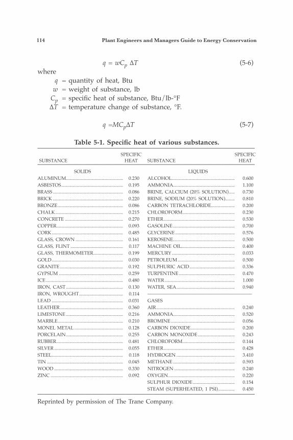
114 Plant Engineers and Managers Guide to Energy Conservation
q = wCp ∆T (5-6)where q = quantity of heat, Btu w = weight of substance, lb Cp = specific heat of substance, Btu/lb-°F ∆T = temperature change of substance, °F.
q =MCp∆T (5-7)
Table 5-1. Specific heat of various substances.———————————————————————————————— SPECIFIC SPECIFIC SUBSTANCE HEAT SUBSTANCE HEAT———————————————————————————————— SOLIDS LIQUIDSALUMINUM................................................ 0.230 ALCOHOL ..................................................... 0.600ASBESTOS .................................................... 0.195 AMMONIA .................................................... 1.100BRASS ........................................................... 0.086 BRINE, CALCIUM (20% SOLUTION) ..... 0.730BRICK ........................................................... 0.220 BRINE, SODIUM (20% SOLUTION) ........ 0.810BRONZE ....................................................... 0.086 CARBON TETRACHLORIDE.................... 0.200CHALK ......................................................... 0.215 CHLOROFORM ............................................ 0.230CONCRETE ................................................. 0.270 ETHER ............................................................ 0.530COPPER ........................................................ 0.093 GASOLINE .................................................... 0.700CORK ............................................................ 0.485 GLYCERINE .................................................. 0.576GLASS, CROWN ........................................ 0.161 KEROSENE.................................................... 0.500GLASS, FLINT ............................................ 0.117 MACHINE OIL............................................. 0.400GLASS, THERMOMETER ......................... 0.199 MERCURY ..................................................... 0.033GOLD ............................................................ 0.030 PETROLEUM ................................................ 0.500GRANITE ..................................................... 0.192 SULPHURIC ACID ...................................... 0.336GYPSUM ...................................................... 0.259 TURPENTINE ............................................... 0.470ICE ................................................................. 0.480 WATER ........................................................... 1.000IRON, CAST ................................................ 0.130 WATER, SEA ................................................. 0.940IRON, WROUGHT ..................................... 0.114 ——————————————————————LEAD ............................................................ 0.031 GASESLEATHER ..................................................... 0.360 AIR .................................................................. 0.240LIMESTONE ................................................ 0.216 AMMONIA .................................................... 0.520MARBLE ....................................................... 0.210 BROMINE ...................................................... 0.056MONEL METAL ......................................... 0.128 CARBON DIOXIDE ..................................... 0.200PORCELAIN ................................................ 0.255 CARBON MONOXIDE ............................... 0.243RUBBER ........................................................ 0.481 CHLOROFORM ............................................ 0.144SILVER .......................................................... 0.055 ETHER ............................................................ 0.428STEEL ............................................................ 0.118 HYDROGEN ................................................. 3.410TIN ................................................................ 0.045 METHANE .................................................... 0.593WOOD .......................................................... 0.330 NITROGEN ................................................... 0.240ZINC ............................................................. 0.092 OXYGEN ........................................................ 0.220 SULPHUR DIOXIDE ................................... 0.154 STEAM (SUPERHEATED, 1 PSI) .............. 0.450————————————————————————————————Reprinted by permission of The Trane Company.
Utility and Process System Optimization 115
where q = quantity of heat, Btu/hr (Btu/hr is sometimes abbreviated as
Btuh) M = Flow rate, lb/hr Cp = Specific heat, Btu/lb°F ∆T = temperature change of substance °F.
q =M∆h (5-8)where ∆h = change in enthalpy of the fluid q and M are defined above.
PRACTICAL APPLICATIONS FOR ENERGY CONSERVATION
The Steam Balance The first step in evaluating energy conservation measures is to compile a flowsheet and steam balance. The steam balance indicates ways in which steam usage can be minimized. To start a balance, the following is evaluated:
1. Requirements of users2. Steam pressure levels to satisfy process needs3. Turbine drive operating pressures4. Pressure ratings for piping valves and fittings
Figure 5-3 illustrates a simple block heat balance diagram for a steam generating process. To conserve energy, losses must be minimized and furnace efficiency must be maximized. In Chapter 6, heat losses will be treated in detail. The remaining portion of this chapter indicates ways to reduce steam consumption and apply systems efficiently.
Using the Steam Turbine Compared to other prime movers, the steam turbine remains a flexible component for most steam systems. Sizes vary from single stage units of 50-600 hp for driving pumps, fans, and compressors, to multi-stage units rated as high as 50,000 hp. The large units can drive huge process compressor trains. Turbines operate in the following way:
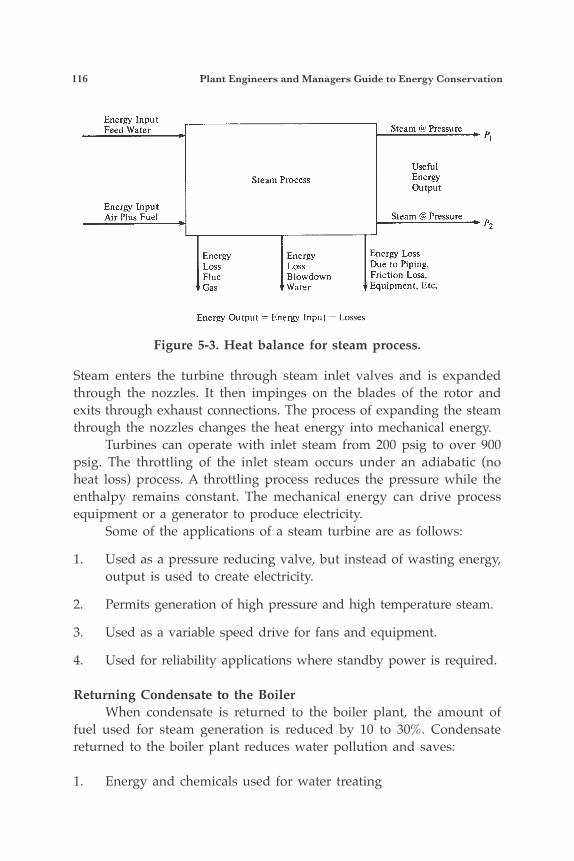
116 Plant Engineers and Managers Guide to Energy Conservation
Steam enters the turbine through steam inlet valves and is expanded through the nozzles. It then impinges on the blades of the rotor and exits through exhaust connections. The process of expanding the steam through the nozzles changes the heat energy into mechanical energy. Turbines can operate with inlet steam from 200 psig to over 900 psig. The throttling of the inlet steam occurs under an adiabatic (no heat loss) process. A throttling process reduces the pressure while the enthalpy remains constant. The mechanical energy can drive process equipment or a generator to produce electricity. Some of the applications of a steam turbine are as follows:
1. Used as a pressure reducing valve, but instead of wasting energy, output is used to create electricity.
2. Permits generation of high pressure and high temperature steam.
3. Used as a variable speed drive for fans and equipment.
4. Used for reliability applications where standby power is required.
Returning Condensate to the Boiler When condensate is returned to the boiler plant, the amount of fuel used for steam generation is reduced by 10 to 30%. Condensate returned to the boiler plant reduces water pollution and saves:
1. Energy and chemicals used for water treating
Figure 5-3. Heat balance for steam process.
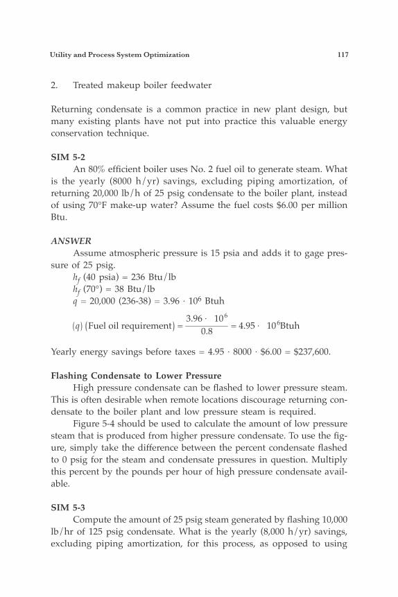
Utility and Process System Optimization 117
2. Treated makeup boiler feedwater
Returning condensate is a common practice in new plant design, but many existing plants have not put into practice this valuable energy conservation technique.
SIM 5-2 An 80% efficient boiler uses No. 2 fuel oil to generate steam. What is the yearly (8000 h/yr) savings, excluding piping amortization, of returning 20,000 lb/h of 25 psig condensate to the boiler plant, instead of using 70°F make-up water? Assume the fuel costs $6.00 per million Btu.
ANSWER Assume atmospheric pressure is 15 psia and adds it to gage pres-sure of 25 psig. hf (40 psia) = 236 Btu/lb hf (70°) = 38 Btu/lb q = 20,000 (236-38) = 3.96 × 10⁶ Btuh
q Fuel oil requirement =3.96 × 10⁶
0.8 = 4.95 × 10⁶Btuh
Yearly energy savings before taxes = 4.95 × 8000 × $6.00 = $237,600.
Flashing Condensate to Lower Pressure High pressure condensate can be flashed to lower pressure steam. This is often desirable when remote locations discourage returning con-densate to the boiler plant and low pressure steam is required. Figure 5-4 should be used to calculate the amount of low pressure steam that is produced from higher pressure condensate. To use the fig-ure, simply take the difference between the percent condensate flashed to 0 psig for the steam and condensate pressures in question. Multiply this percent by the pounds per hour of high pressure condensate avail-able.
SIM 5-3 Compute the amount of 25 psig steam generated by flashing 10,000 lb/hr of 125 psig condensate. What is the yearly (8,000 h/yr) savings, excluding piping amortization, for this process, as opposed to using
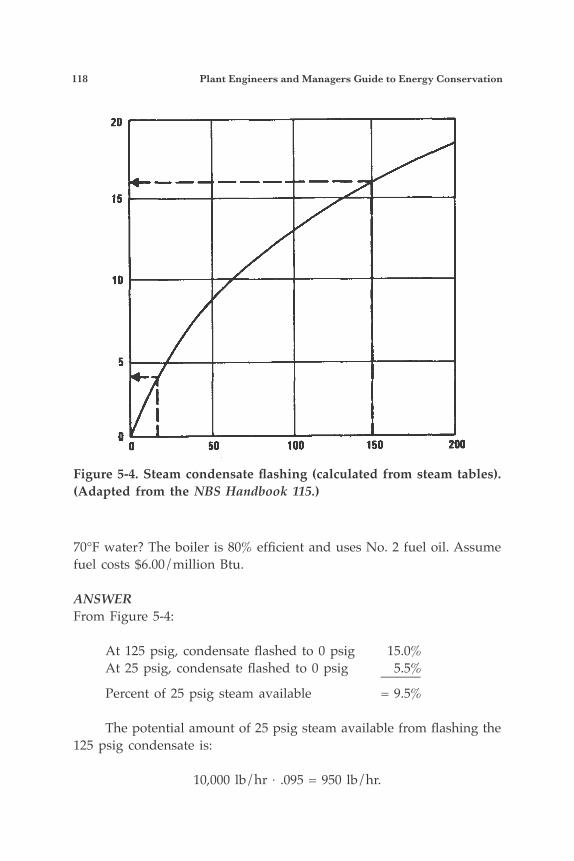
118 Plant Engineers and Managers Guide to Energy Conservation
70°F water? The boiler is 80% efficient and uses No. 2 fuel oil. Assume fuel costs $6.00/million Btu.
ANSWERFrom Figure 5-4:
At 125 psig, condensate flashed to 0 psig 15.0% At 25 psig, condensate flashed to 0 psig 5.5% ——— Percent of 25 psig steam available = 9.5%
The potential amount of 25 psig steam available from flashing the 125 psig condensate is:
10,000 lb/hr × .095 = 950 lb/hr.
Figure 5-4. Steam condensate flashing (calculated from steam tables). (Adapted from the NBS Handbook 115.)
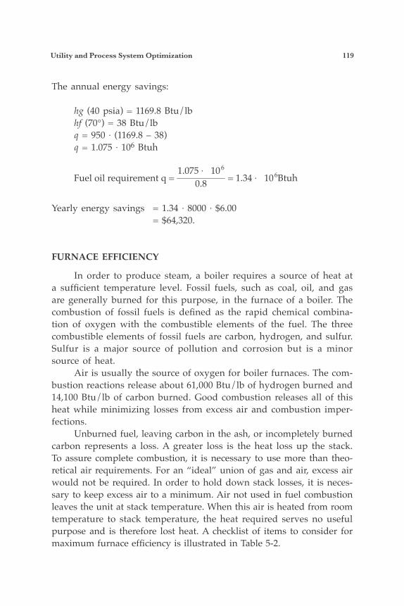
Utility and Process System Optimization 119
The annual energy savings:
hg (40 psia) = 1169.8 Btu/lb hf (70°) = 38 Btu/lb q = 950 × (1169.8 – 38) q = 1.075 × 10⁶ Btuh
Fuel oil requirement q =1.075 × 10⁶
0.8 = 1.34 × 10⁶Btuh
Yearly energy savings = 1.34 × 8000 × $6.00 = $64,320.
FURNACE EFFICIENCY
In order to produce steam, a boiler requires a source of heat at a sufficient temperature level. Fossil fuels, such as coal, oil, and gas are generally burned for this purpose, in the furnace of a boiler. The combustion of fossil fuels is defined as the rapid chemical combina-tion of oxygen with the combustible elements of the fuel. The three combustible elements of fossil fuels are carbon, hydrogen, and sulfur. Sulfur is a major source of pollution and corrosion but is a minor source of heat. Air is usually the source of oxygen for boiler furnaces. The com-bustion reactions release about 61,000 Btu/lb of hydrogen burned and 14,100 Btu/lb of carbon burned. Good combustion releases all of this heat while minimizing losses from excess air and combustion imper-fections. Unburned fuel, leaving carbon in the ash, or incompletely burned carbon represents a loss. A greater loss is the heat loss up the stack. To assure complete combustion, it is necessary to use more than theo-retical air requirements. For an “ideal” union of gas and air, excess air would not be required. In order to hold down stack losses, it is neces-sary to keep excess air to a minimum. Air not used in fuel combustion leaves the unit at stack temperature. When this air is heated from room temperature to stack temperature, the heat required serves no useful purpose and is therefore lost heat. A checklist of items to consider for maximum furnace efficiency is illustrated in Table 5-2.
120 Plant Engineers and Managers Guide to Energy Conservation
Table 5-2. Furnace efficiency checklist.———————————————————————————————— 1. Excess air should be monitored to keep it as low as is practical.
2. Portable or permanent oxygen analyzers should be used on fur-naces to help minimize oxygen in flue gas.
3. Fuel oil temperature should be monitored and checked against manufacturer’s recommendations for the fuel specification used. Proper fuel oil temperature insures good atomization.
4. Atomizing steam should be dry.
5. If fuel gas is at dew point, then a knock-out drum at the furnace with steam tracing to the burners should be used.
6. Atomizing steam rate should be at the minimum required for acceptable combustion.
7. Furnace systems should be evaluated for heat recovery, i.e., in-stalling air preheaters or waste heat boilers.
8. Furnace systems should be evaluated for using preheated com-bustion air from gas-turbine exhausts.
9. Furnace systems should be evaluated for using high pressure gas for atomization instead of steam.
10. Furnace system should incorporate automated controls and re-corders to maximize fuel usage and help the operator manage his system.
11. In particular, for existing furnace installations, the following should be checked:
(a) Reduce all air leaks. (Infrared photography can be used to check for leaks.)
(b) Burners and soot blowers should be inspected and maintained on a scheduled basis.
(c) Consider replacing burners with more efficient models.————————————————————————————————
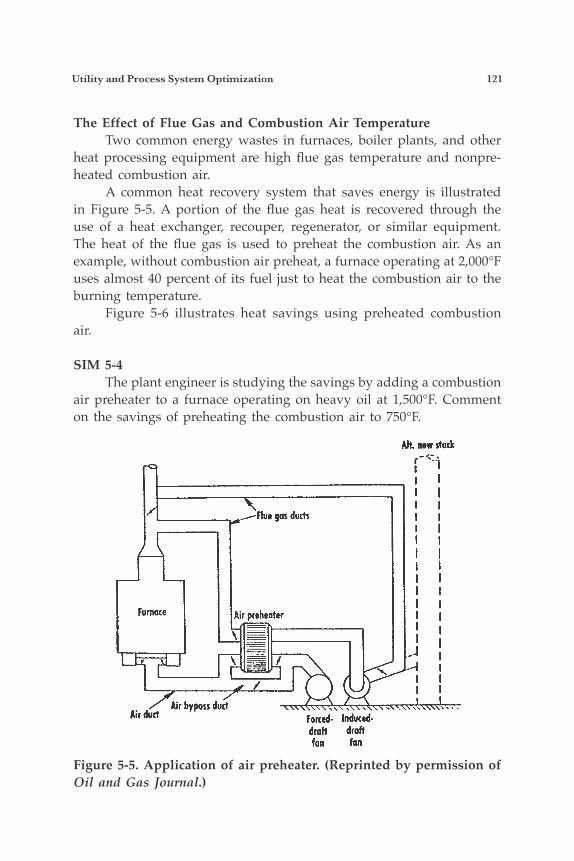
Utility and Process System Optimization 121
The Effect of Flue Gas and Combustion Air Temperature Two common energy wastes in furnaces, boiler plants, and other heat processing equipment are high flue gas temperature and nonpre-heated combustion air. A common heat recovery system that saves energy is illustrated in Figure 5-5. A portion of the flue gas heat is recovered through the use of a heat exchanger, recouper, regenerator, or similar equipment. The heat of the flue gas is used to preheat the combustion air. As an example, without combustion air preheat, a furnace operating at 2,000°F uses almost 40 percent of its fuel just to heat the combustion air to the burning temperature. Figure 5-6 illustrates heat savings using preheated combustion air.
SIM 5-4 The plant engineer is studying the savings by adding a combustion air preheater to a furnace operating on heavy oil at 1,500°F. Comment on the savings of preheating the combustion air to 750°F.
Figure 5-5. Application of air preheater. (Reprinted by permission of Oil and Gas Journal.)
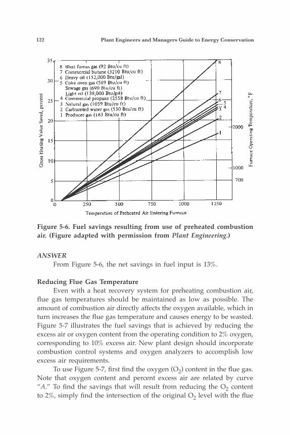
122 Plant Engineers and Managers Guide to Energy Conservation
ANSWER From Figure 5-6, the net savings in fuel input is 13%.
Reducing Flue Gas Temperature Even with a heat recovery system for preheating combustion air, flue gas temperatures should be maintained as low as possible. The amount of combustion air directly affects the oxygen available, which in turn increases the flue gas temperature and causes energy to be wasted. Figure 5-7 illustrates the fuel savings that is achieved by reducing the excess air or oxygen content from the operating condition to 2% oxygen, corresponding to 10% excess air. New plant design should incorporate combustion control systems and oxygen analyzers to accomplish low excess air requirements. To use Figure 5-7, first find the oxygen (O2) content in the flue gas. Note that oxygen content and percent excess air are related by curve “A.” To find the savings that will result from reducing the O2 content to 2%, simply find the intersection of the original O2 level with the flue
Figure 5-6. Fuel savings resulting from use of preheated combustion air. (Figure adapted with permission from Plant Engineering.)
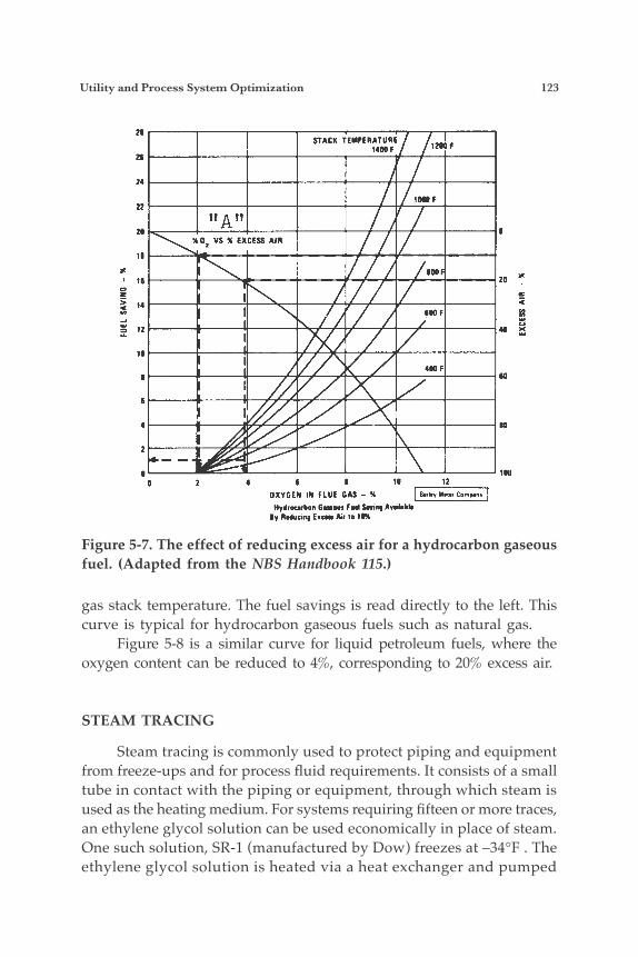
Utility and Process System Optimization 123
gas stack temperature. The fuel savings is read directly to the left. This curve is typical for hydrocarbon gaseous fuels such as natural gas. Figure 5-8 is a similar curve for liquid petroleum fuels, where the oxygen content can be reduced to 4%, corresponding to 20% excess air.
STEAM TRACING
Steam tracing is commonly used to protect piping and equipment from freeze-ups and for process fluid requirements. It consists of a small tube in contact with the piping or equipment, through which steam is used as the heating medium. For systems requiring fifteen or more traces, an ethylene glycol solution can be used economically in place of steam. One such solution, SR-1 (manufactured by Dow) freezes at –34°F . The ethylene glycol solution is heated via a heat exchanger and pumped
Figure 5-7. The effect of reducing excess air for a hydrocarbon gaseous fuel. (Adapted from the NBS Handbook 115.)
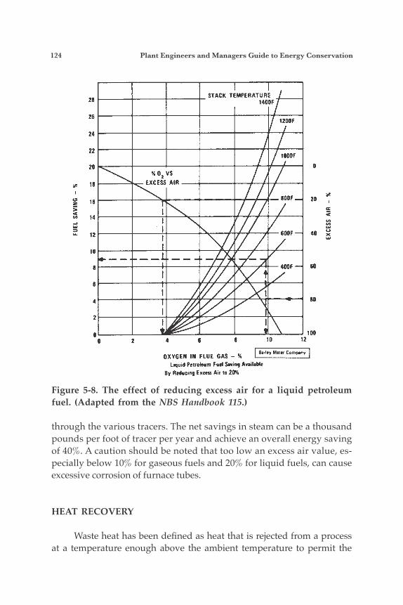
124 Plant Engineers and Managers Guide to Energy Conservation
through the various tracers. The net savings in steam can be a thousand pounds per foot of tracer per year and achieve an overall energy saving of 40%. A caution should be noted that too low an excess air value, es-pecially below 10% for gaseous fuels and 20% for liquid fuels, can cause excessive corrosion of furnace tubes.
HEAT RECOVERY
Waste heat has been defined as heat that is rejected from a process at a temperature enough above the ambient temperature to permit the
Figure 5-8. The effect of reducing excess air for a liquid petroleum fuel. (Adapted from the NBS Handbook 115.)
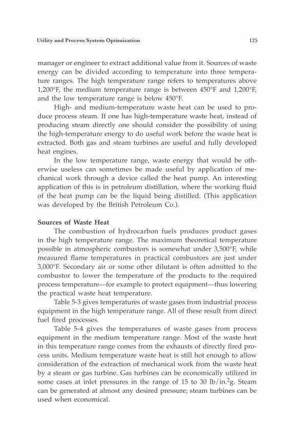
Utility and Process System Optimization 125
manager or engineer to extract additional value from it. Sources of waste energy can be divided according to temperature into three tempera-ture ranges. The high temperature range refers to temperatures above 1,200°F, the medium temperature range is between 450°F and 1,200°F, and the low temperature range is below 450°F. High- and medium-temperature waste heat can be used to pro-duce process steam. If one has high-temperature waste heat, instead of producing steam directly one should consider the possibility of using the high-temperature energy to do useful work before the waste heat is extracted. Both gas and steam turbines are useful and fully developed heat engines. In the low temperature range, waste energy that would be oth-erwise useless can sometimes be made useful by application of me-chanical work through a device called the heat pump. An interesting application of this is in petroleum distillation, where the working fluid of the heat pump can be the liquid being distilled. (This application was developed by the British Petroleum Co.).
Sources of Waste Heat The combustion of hydrocarbon fuels produces product gases in the high temperature range. The maximum theoretical temperature possible in atmospheric combustors is somewhat under 3,500°F, while measured flame temperatures in practical combustors are just under 3,000°F. Secondary air or some other dilutant is often admitted to the combustor to lower the temperature of the products to the required process temperature—for example to protect equipment—thus lowering the practical waste heat temperature. Table 5-3 gives temperatures of waste gases from industrial process equipment in the high temperature range. All of these result from direct fuel fired processes. Table 5-4 gives the temperatures of waste gases from process equipment in the medium temperature range. Most of the waste heat in this temperature range comes from the exhausts of directly fired pro-cess units. Medium temperature waste heat is still hot enough to allow consideration of the extraction of mechanical work from the waste heat by a steam or gas turbine. Gas turbines can be economically utilized in some cases at inlet pressures in the range of 15 to 30 lb/in.2g. Steam can be generated at almost any desired pressure; steam turbines can be used when economical.
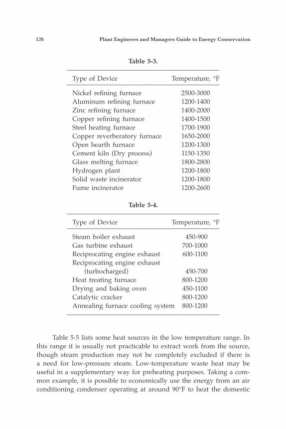
126 Plant Engineers and Managers Guide to Energy Conservation
Table 5-3.———————————————————————
Type of Device Temperature, °F———————————————————————
Nickel refining furnace 2500-3000 Aluminum refining furnace 1200-1400 Zinc refining furnace 1400-2000 Copper refining furnace 1400-1500 Steel heating furnace 1700-1900 Copper reverberatory furnace 1650-2000 Open hearth furnace 1200-1300 Cement kiln (Dry process) 1150-1350 Glass melting furnace 1800-2800 Hydrogen plant 1200-1800 Solid waste incinerator 1200-1800 Fume incinerator 1200-2600
Table 5-4.———————————————————————
Type of Device Temperature, °F———————————————————————
Steam boiler exhaust 450-900 Gas turbine exhaust 700-1000 Reciprocating engine exhaust 600-1100 Reciprocating engine exhaust (turbocharged) 450-700 Heat treating furnace 800-1200 Drying and baking oven 450-1100 Catalytic cracker 800-1200 Annealing furnace cooling system 800-1200
———————————————————————
Table 5-5 lists some heat sources in the low temperature range. In this range it is usually not practicable to extract work from the source, though steam production may not be completely excluded if there is a need for low-pressure steam. Low-temperature waste heat may be useful in a supplementary way for preheating purposes. Taking a com-mon example, it is possible to economically use the energy from an air conditioning condenser operating at around 90°F to heat the domestic
Utility and Process System Optimization 127
water supply. Since the hot water must be heated to about 160°F, ob-viously the air conditioner waste heat is not hot enough. However, because the cold water enters the domestic water system at about 50°F, energy interchange can take place raising the water to something less than 90°F. Depending upon the relative air conditioning lead and hot water requirements, any excess condenser heat can be rejected and the additional energy required by the hot water provided by the usual electrical or fired heater.
Table 5-5.—————————————————————————
Source Temperature, °F—————————————————————————
Process steam condensate 130-190 Cooling water from: Furnace doors 90-130 Bearings 90-190 Welding machines 90-190 Injection molding machines 90-190 Annealing furnaces 150-450 Forming dies 80-190 Air compressors 80-120 Pumps 80-190 Internal combustion engines 150-250 Air conditioning and refrigeration condensers 90-110 Liquid still condensers 90-190 Drying, baking and curing ovens 200-450 Hot processed liquids 90-450 Hot processed solids 200-450
—————————————————————————
How to Use Waste Heat To use waste heat from sources such as those above, one often wishes to transfer the heat in one fluid stream to another (e.g., from flue gas to feedwater or combustion air). The device that accomplishes the transfer is called a heat exchanger. In the discussion immediately below is a listing of common uses for waste heat energy and, in some cases, the name of the heat exchanger that would normally be applied in each particular case.
128 Plant Engineers and Managers Guide to Energy Conservation
The equipment used to recover waste heat can range from some-thing as simple as a pipe or duct to something as complex as a waste heat boiler. Here we categorize and describe some waste recovery sys-tems that are available commercially, suitable for retrofitting in exist-ing plants, with lists of potential applications for each of the described devices. These are developed technologies that have been employed for years in some industries.
1. Medium to high temperature exhaust gases can be used to preheat the combustion air for:
Boilers using air preheaters Furnaces using recuperators Ovens using recuperators Gas turbines using regenerators.
2. Low to medium temperature exhaust gases can be used to preheat boiler feedwater or boiler makeup water using economizers, which are simply gas-to-liquid water heating devices.
3. Exhaust gases and cooling water from condensers can be used to preheat liquid and/or solid feedstocks in industrial processes. Finned tubes and tube-in-shell heat exchangers are used.
4. Exhaust gases can be used to generate steam in waste heat boilers to produce electrical power, mechanical power, process steam, and any combination of the above.
5. Waste heat may be transferred to liquid or gaseous process units directly through pipes and ducts or indirectly through a secondary fluid such as steam or oil.
6. Waste heat may be transferred to an intermediate fluid by heat exchangers or waste heat boilers, or it may be used by circulating the hot exit gas through pipes or ducts. Waste heat can be used to operate an absorption cooling unit for air conditioning or refrigera-tion.
Waste Heat Recovery Equipment Industrial heat exchangers have many pseudonyms. They are sometimes called recuperators, regenerators, waste heat steam genera-
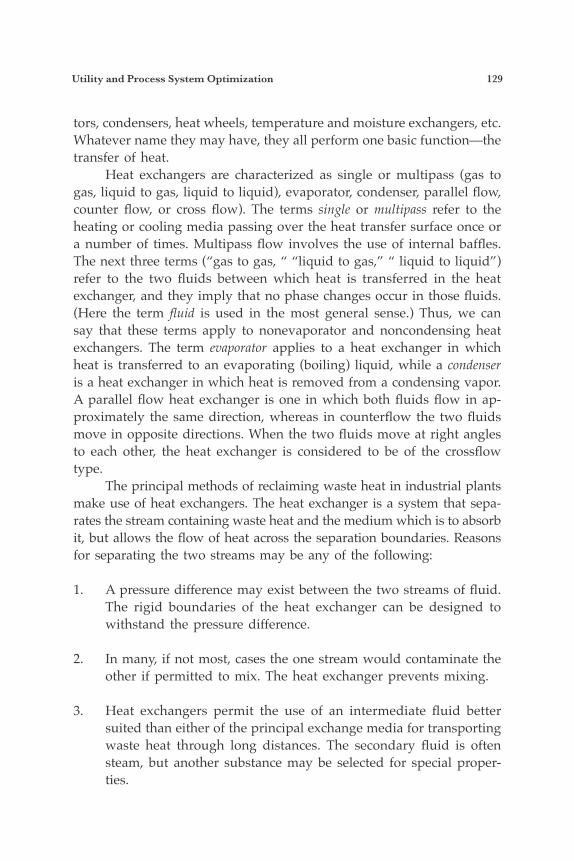
Utility and Process System Optimization 129
tors, condensers, heat wheels, temperature and moisture exchangers, etc. Whatever name they may have, they all perform one basic function—the transfer of heat. Heat exchangers are characterized as single or multipass (gas to gas, liquid to gas, liquid to liquid), evaporator, condenser, parallel flow, counter flow, or cross flow). The terms single or multipass refer to the heating or cooling media passing over the heat transfer surface once or a number of times. Multipass flow involves the use of internal baffles. The next three terms (“gas to gas, “ “liquid to gas,” “ liquid to liquid”) refer to the two fluids between which heat is transferred in the heat exchanger, and they imply that no phase changes occur in those fluids. (Here the term fluid is used in the most general sense.) Thus, we can say that these terms apply to nonevaporator and noncondensing heat exchangers. The term evaporator applies to a heat exchanger in which heat is transferred to an evaporating (boiling) liquid, while a condenser is a heat exchanger in which heat is removed from a condensing vapor. A parallel flow heat exchanger is one in which both fluids flow in ap-proximately the same direction, whereas in counterflow the two fluids move in opposite directions. When the two fluids move at right angles to each other, the heat exchanger is considered to be of the crossflow type. The principal methods of reclaiming waste heat in industrial plants make use of heat exchangers. The heat exchanger is a system that sepa-rates the stream containing waste heat and the medium which is to absorb it, but allows the flow of heat across the separation boundaries. Reasons for separating the two streams may be any of the following:
1. A pressure difference may exist between the two streams of fluid. The rigid boundaries of the heat exchanger can be designed to withstand the pressure difference.
2. In many, if not most, cases the one stream would contaminate the other if permitted to mix. The heat exchanger prevents mixing.
3. Heat exchangers permit the use of an intermediate fluid better suited than either of the principal exchange media for transporting waste heat through long distances. The secondary fluid is often steam, but another substance may be selected for special proper-ties.
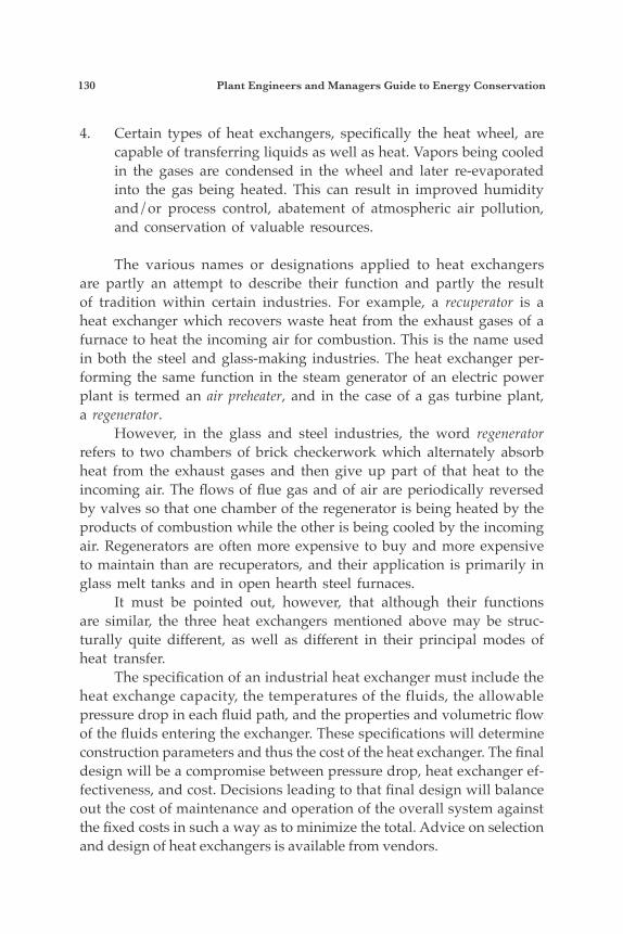
130 Plant Engineers and Managers Guide to Energy Conservation
4. Certain types of heat exchangers, specifically the heat wheel, are capable of transferring liquids as well as heat. Vapors being cooled in the gases are condensed in the wheel and later re-evaporated into the gas being heated. This can result in improved humidity and/or process control, abatement of atmospheric air pollution, and conservation of valuable resources.
The various names or designations applied to heat exchangers are partly an attempt to describe their function and partly the result of tradition within certain industries. For example, a recuperator is a heat exchanger which recovers waste heat from the exhaust gases of a furnace to heat the incoming air for combustion. This is the name used in both the steel and glass-making industries. The heat exchanger per-forming the same function in the steam generator of an electric power plant is termed an air preheater, and in the case of a gas turbine plant, a regenerator. However, in the glass and steel industries, the word regenerator refers to two chambers of brick checkerwork which alternately absorb heat from the exhaust gases and then give up part of that heat to the incoming air. The flows of flue gas and of air are periodically reversed by valves so that one chamber of the regenerator is being heated by the products of combustion while the other is being cooled by the incoming air. Regenerators are often more expensive to buy and more expensive to maintain than are recuperators, and their application is primarily in glass melt tanks and in open hearth steel furnaces. It must be pointed out, however, that although their functions are similar, the three heat exchangers mentioned above may be struc-turally quite different, as well as different in their principal modes of heat transfer. The specification of an industrial heat exchanger must include the heat exchange capacity, the temperatures of the fluids, the allowable pressure drop in each fluid path, and the properties and volumetric flow of the fluids entering the exchanger. These specifications will determine construction parameters and thus the cost of the heat exchanger. The final design will be a compromise between pressure drop, heat exchanger ef-fectiveness, and cost. Decisions leading to that final design will balance out the cost of maintenance and operation of the overall system against the fixed costs in such a way as to minimize the total. Advice on selection and design of heat exchangers is available from vendors.
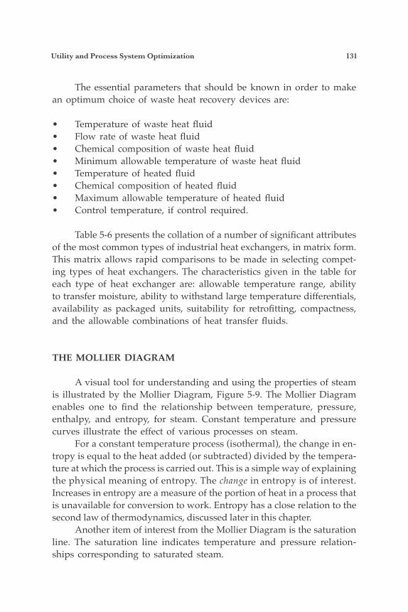
Utility and Process System Optimization 131
The essential parameters that should be known in order to make an optimum choice of waste heat recovery devices are:
• Temperature of waste heat fluid• Flow rate of waste heat fluid• Chemical composition of waste heat fluid• Minimum allowable temperature of waste heat fluid• Temperature of heated fluid• Chemical composition of heated fluid• Maximum allowable temperature of heated fluid• Control temperature, if control required.
Table 5-6 presents the collation of a number of significant attributes of the most common types of industrial heat exchangers, in matrix form. This matrix allows rapid comparisons to be made in selecting compet-ing types of heat exchangers. The characteristics given in the table for each type of heat exchanger are: allowable temperature range, ability to transfer moisture, ability to withstand large temperature differentials, availability as packaged units, suitability for retrofitting, compactness, and the allowable combinations of heat transfer fluids.
THE MOLLIER DIAGRAM
A visual tool for understanding and using the properties of steam is illustrated by the Mollier Diagram, Figure 5-9. The Mollier Diagram enables one to find the relationship between temperature, pressure, enthalpy, and entropy, for steam. Constant temperature and pressure curves illustrate the effect of various processes on steam. For a constant temperature process (isothermal), the change in en-tropy is equal to the heat added (or subtracted) divided by the tempera-ture at which the process is carried out. This is a simple way of explaining the physical meaning of entropy. The change in entropy is of interest. Increases in entropy are a measure of the portion of heat in a process that is unavailable for conversion to work. Entropy has a close relation to the second law of thermodynamics, discussed later in this chapter. Another item of interest from the Mollier Diagram is the saturation line. The saturation line indicates temperature and pressure relation-ships corresponding to saturated steam.
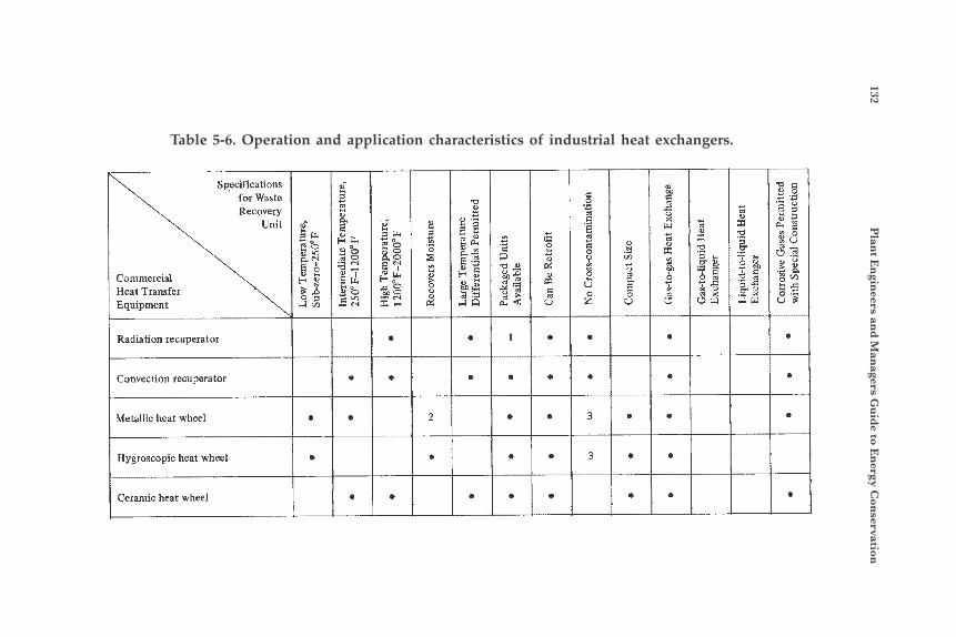
132 P
lant E
ngin
eers and
Man
agers Gu
ide to E
nergy C
onservation
Table 5-6. Operation and application characteristics of industrial heat exchangers.
Specifications for Waste Recovery
Unit \ Commercial Heat Transfer Equipment
Radiation recuperator
Convection recuperator
Metallic heat wheel
Hysroscopic heat wheel
Ceramic heat wheel
0
0
0
0
0
I ' I
0
+: 0
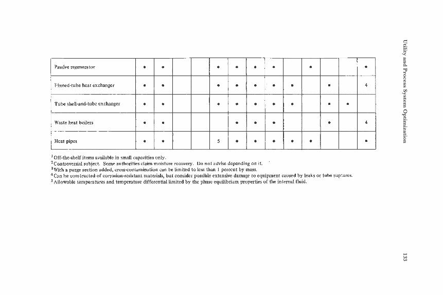
Utility an
d P
rocess System O
ptim
ization
133
Passive regenerator
Finned-tube heat exchanger _ _
Tube shell-and-tube exchanger
Waste heat boilers
Heat pipes
Off-the-shelf items available in small capacities only. 2Controversial subject. Some authorities claim moisture recovery. Do not advise depending on it. 3\\rith a purge section added. cross-contamination can be limited to less than 1 percent by mass.
Can be constructed of corrosion-resistant materials, but consider possible extensive damage to equipment caused by leaks or tube ruptures. Allowable temperatures and temperature differential limited by the phase equilibrium properties of the internal fluid.
, 0 0 0 0 0 1 .
0 0 0 0 0 0
I
0 0 0 0 0 0
I
0 0 I * 0 0
0
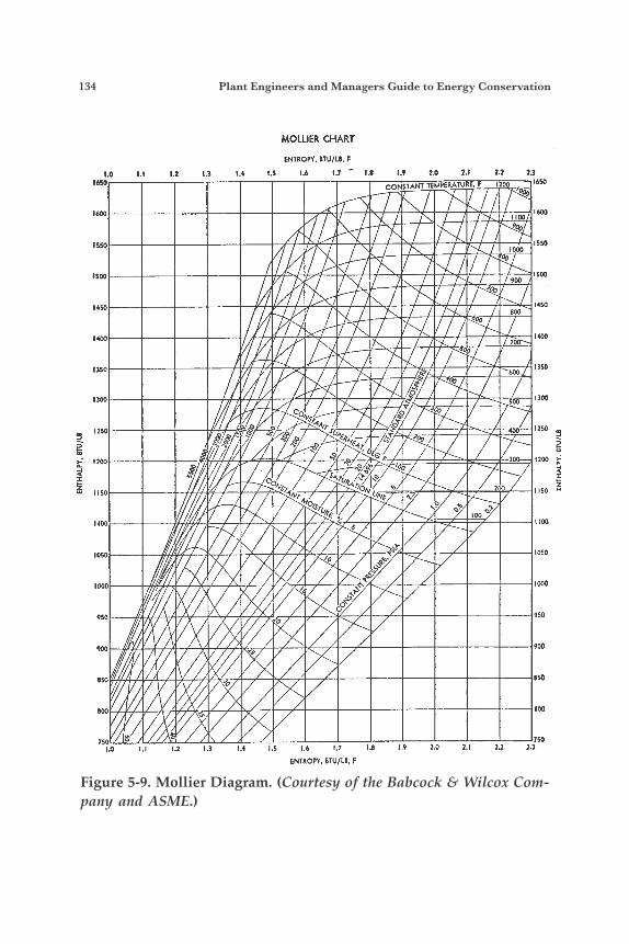
134 Plant Engineers and Managers Guide to Energy Conservation
Figure 5-9. Mollier Diagram. (Courtesy of the Babcock & Wilcox Com-pany and ASME.)
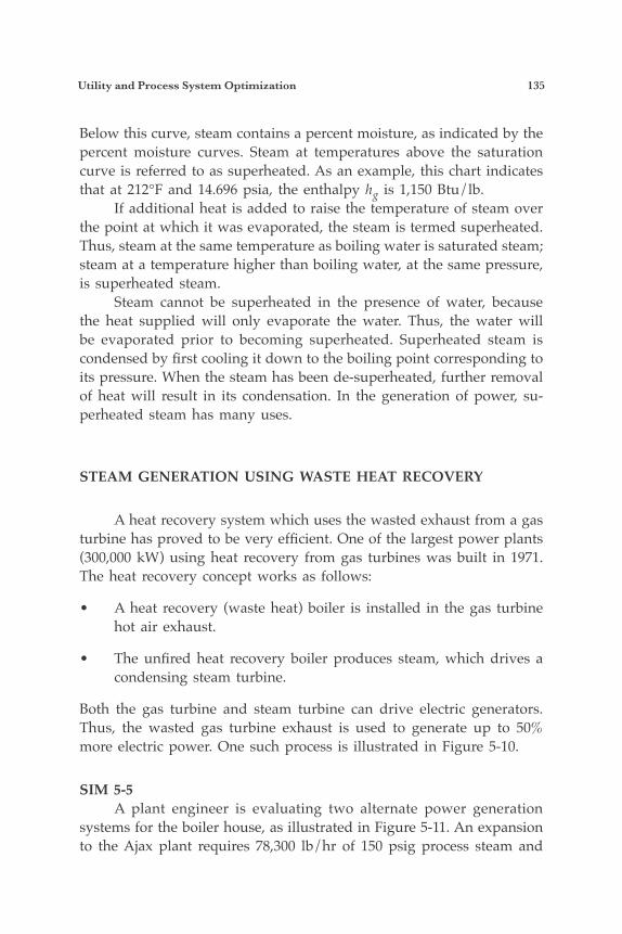
Utility and Process System Optimization 135
Below this curve, steam contains a percent moisture, as indicated by the percent moisture curves. Steam at temperatures above the saturation curve is referred to as superheated. As an example, this chart indicates that at 212°F and 14.696 psia, the enthalpy hg is 1,150 Btu/lb. If additional heat is added to raise the temperature of steam over the point at which it was evaporated, the steam is termed superheated. Thus, steam at the same temperature as boiling water is saturated steam; steam at a temperature higher than boiling water, at the same pressure, is superheated steam. Steam cannot be superheated in the presence of water, because the heat supplied will only evaporate the water. Thus, the water will be evaporated prior to becoming superheated. Superheated steam is condensed by first cooling it down to the boiling point corresponding to its pressure. When the steam has been de-superheated, further removal of heat will result in its condensation. In the generation of power, su-perheated steam has many uses.
STEAM GENERATION USING WASTE HEAT RECOVERY
A heat recovery system which uses the wasted exhaust from a gas turbine has proved to be very efficient. One of the largest power plants (300,000 kW) using heat recovery from gas turbines was built in 1971. The heat recovery concept works as follows:
• A heat recovery (waste heat) boiler is installed in the gas turbine hot air exhaust.
• The unfired heat recovery boiler produces steam, which drives a condensing steam turbine.
Both the gas turbine and steam turbine can drive electric generators. Thus, the wasted gas turbine exhaust is used to generate up to 50% more electric power. One such process is illustrated in Figure 5-10.
SIM 5-5 A plant engineer is evaluating two alternate power generation systems for the boiler house, as illustrated in Figure 5-11. An expansion to the Ajax plant requires 78,300 lb/hr of 150 psig process steam and
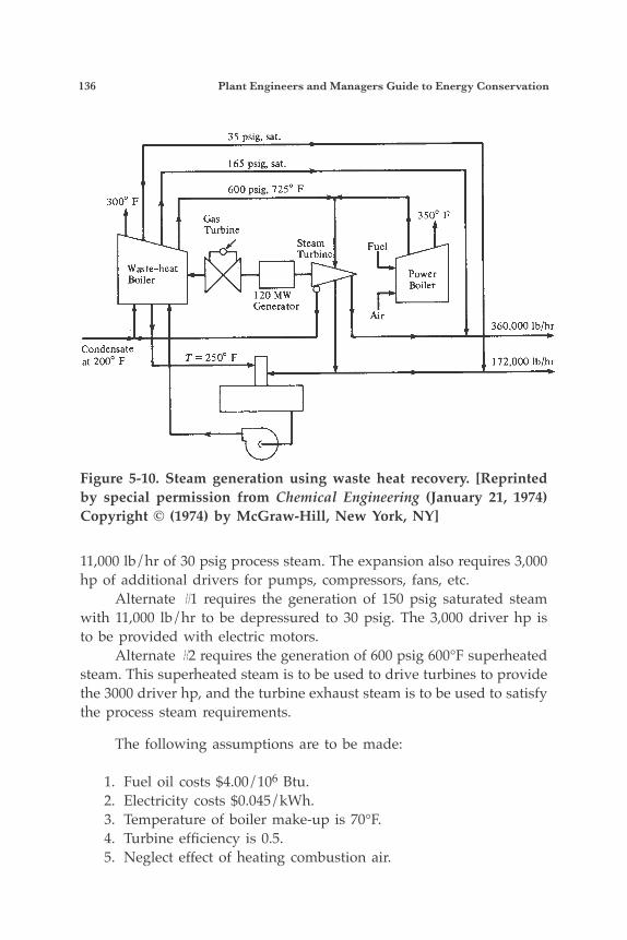
136 Plant Engineers and Managers Guide to Energy Conservation
11,000 lb/hr of 30 psig process steam. The expansion also requires 3,000 hp of additional drivers for pumps, compressors, fans, etc. Alternate #1 requires the generation of 150 psig saturated steam with 11,000 lb/hr to be depressured to 30 psig. The 3,000 driver hp is to be provided with electric motors. Alternate #2 requires the generation of 600 psig 600°F superheated steam. This superheated steam is to be used to drive turbines to provide the 3000 driver hp, and the turbine exhaust steam is to be used to satisfy the process steam requirements.
The following assumptions are to be made:
1. Fuel oil costs $4.00/106 Btu. 2. Electricity costs $0.045/kWh. 3. Temperature of boiler make-up is 70°F. 4. Turbine efficiency is 0.5. 5. Neglect effect of heating combustion air.
Figure 5-10. Steam generation using waste heat recovery. [Reprinted by special permission from Chemical Engineering (January 21, 1974) Copyright © (1974) by McGraw-Hill, New York, NY]
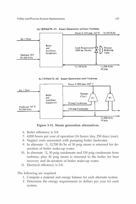
Utility and Process System Optimization 137
6. Boiler efficiency is 0.8. 7. 4,000 hours per year of operation (16 hours/day, 250 days/year). 8. Neglect costs associated with pumping boiler feedwater. 9. In alternate #1, 12,700 lb/hr of 30 psig steam is returned for de-
aeration of boiler make-up water. 10. In alternate #2, 30 psig condensate and 150 psig condensate from
turbines, plus 30 psig steam is returned to the boiler for heat recovery and de-aeration of boiler make-up water.
11. Electrical efficiency is 0.8.
The following are required. 1. Compute a material and energy balance for each alternate system. 2. Determine the energy requirements in dollars per year for each
system.
Figure 5-11. Steam generation alternatives.
ALTERNATE #1: Steam Generation without Turbines.
Steam @ 150 psig, ,365"F 78,300 Ib/hr
Air + Fuel
Feedwater 70" F 89,300 lb/hr
Boiler and Auxilliary Equipment
Load Requirement 3000 hp Electric
Pressure Reducing Valve
12,700 Ib/hr 1 1,000 lb/hr 30 psig
ALTERNATE #2: Steam Generation with Turbines.
Steam @ 600 psig, 600' F
Air + Fuel
Boiler and Auxilliary Equipment
Feedwater 70' F 89,300 lb/hr
Turbine ( ~ P J #2
30 psig Condensate
150 psig Condensate
# I
11,000 lb/hr 30 psig
138 Plant Engineers and Managers Guide to Energy Conservation
ANSWER A material balance requires that lb/hr “in” equals the lb/hr “out.” An energy balance requires the Btu/hr “in” equals the Btu/hr “out.” The steps to be taken are:
1. First find all missing material quantities.2. Second, find the corresponding enthalpies from the Mollier Dia-
gram (Figure 5-9).3. Third, compute the energy balance.
For Alternate #1Step 1: The quantity of 150 psig is 102,000 lb/hr.
Step 2: The enthalpy of 150 psig (165 psia) steam is 1,195.6 Btu/lb. The enthalpy of 30 psig (45 psia) steam is 1,172 Btu/lb. The enthalpy of water at 70°F is 38.04 Btu/lb.
Step 3: The energy balance for the system is:
(102,000 lb/hr) (1,195.6 Btu/lb) = (89,300 lb/hr (38.04 Btu/lb)+ (12,700 lb/hr) (1,172.0 Btu/lb) + input energy.
Input energy = 121,951,200 Btu/hr – 3,396,972 Btu/hr – 14,884,400 = 103,669,828 Btu/hr.The fuel required is 103,669,828 ÷ 0.8 = 129,587,285 Btu/hr.The fuel cost is 129,587,285 × $4.00 ÷ 106
= $518.33/hr or $2,073,353/yr.The electrical cost is:
The total energy cost per year for alternate system #1 is $2,073,353 + $503,550 = $2,576,903/yr.
For Alternate #2 Steps 1 and 2: To analyze turbine performance, use the Mollier Diagram of Figure 5-12. The first point “A” at 600 psig, 600°F, is located on the diagram (h = 1,290 Btu/lb). The second point “B” is drawn verti-cally from “A” until it intersects the 165 psia constant pressure line (h = 1,170 Btu/lb). The difference between inlet and exhaust enthalpy is the amount of energy available to the turbine to generate horsepower.
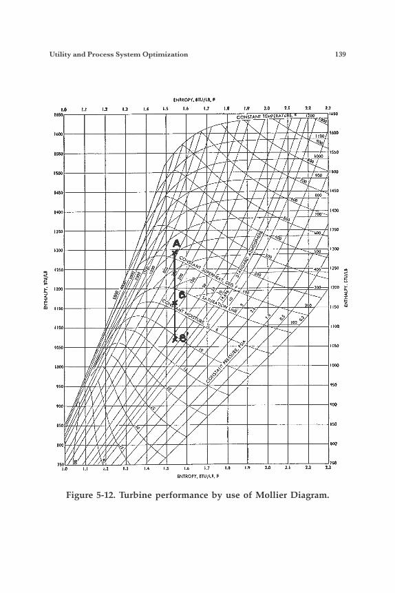
Utility and Process System Optimization 139
Figure 5-12. Turbine performance by use of Mollier Diagram.
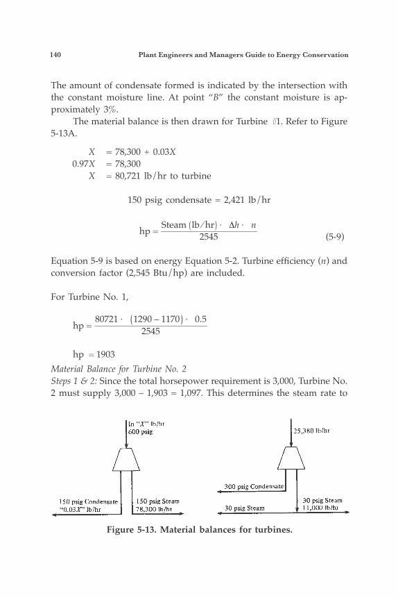
140 Plant Engineers and Managers Guide to Energy Conservation
The amount of condensate formed is indicated by the intersection with the constant moisture line. At point “B” the constant moisture is ap-proximately 3%. The material balance is then drawn for Turbine #1. Refer to Figure 5-13A.
X = 78,300 + 0.03X 0.97X = 78,300 X = 80,721 lb/hr to turbine
150 psig condensate = 2,421 lb/hr
hp = Steam lb ⁄ hr × Δh × n2545 (5-9)
Equation 5-9 is based on energy Equation 5-2. Turbine efficiency (n) and conversion factor (2,545 Btu/hp) are included.
For Turbine No. 1,
hp =80721 × 1290 – 1170 × 0.5
2545
hp = 1903Material Balance for Turbine No. 2Steps 1 & 2: Since the total horsepower requirement is 3,000, Turbine No. 2 must supply 3,000 – 1,903 = 1,097. This determines the steam rate to
Figure 5-13. Material balances for turbines.
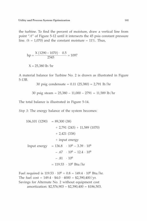
Utility and Process System Optimization 141
the turbine. To find the percent of moisture, draw a vertical line from point “A” of Figure 5-12 until it intersects the 45 psia constant pressure line. (h = 1,070) and the constant moisture = 11%. Thus,
hp =X 1290 – 1070 × 0.5
2545 = 1097
X = 25,380 lb ⁄ hr
A material balance for Turbine No. 2 is drawn as illustrated in Figure 5-13B.
30 psig condensate = 0.11 (25,380) = 2,791 lb/hr
30 psig steam = 25,380 – 11,000 – 2791 = 11,589 lb/hr
The total balance is illustrated in Figure 5-14.
Step 3: The energy balance of the system becomes:
106,101 (1290) = 89,300 (38)
+ 2,791 (243) + 11,589 (1070)
+ 2,421 (338)
+ input energy
Input energy = 136.8 × 10⁶ – 3.39 × 10⁶
– .67 × 106 – 12.4 × 10⁶
– .81 × 106
= 119.53 × 10⁶ Btu/hr
Fuel required is 119.53 × 10⁶ ÷ 0.8 = 149.4 × 10⁶ Btu/hr.The fuel cost = 149.4 × $4.0 × 4000 = $2,390,400/yr.Savings for Alternate No. 2 without equipment cost amortization: $2,576,903 – $2,390,400 = $186,503.
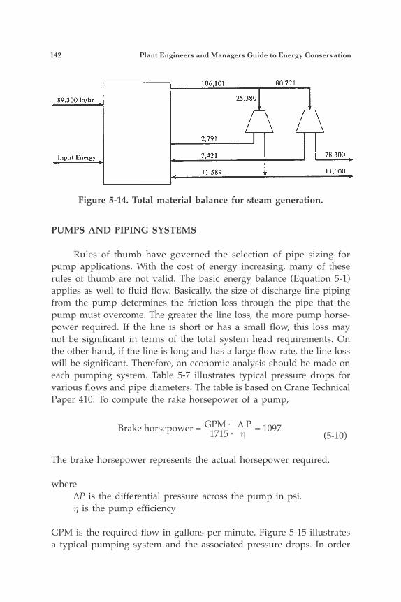
142 Plant Engineers and Managers Guide to Energy Conservation
PUMPS AND PIPING SYSTEMS
Rules of thumb have governed the selection of pipe sizing for pump applications. With the cost of energy increasing, many of these rules of thumb are not valid. The basic energy balance (Equation 5-1) applies as well to fluid flow. Basically, the size of discharge line piping from the pump determines the friction loss through the pipe that the pump must overcome. The greater the line loss, the more pump horse-power required. If the line is short or has a small flow, this loss may not be significant in terms of the total system head requirements. On the other hand, if the line is long and has a large flow rate, the line loss will be significant. Therefore, an economic analysis should be made on each pumping system. Table 5-7 illustrates typical pressure drops for various flows and pipe diameters. The table is based on Crane Technical Paper 410. To compute the rake horsepower of a pump,
Brake horsepower = GPM × Δ P
1715 × η= 1097
(5-10)
The brake horsepower represents the actual horsepower required.
where ∆P is the differential pressure across the pump in psi. is the pump efficiency
GPM is the required flow in gallons per minute. Figure 5-15 illustrates a typical pumping system and the associated pressure drops. In order
Figure 5-14. Total material balance for steam generation.
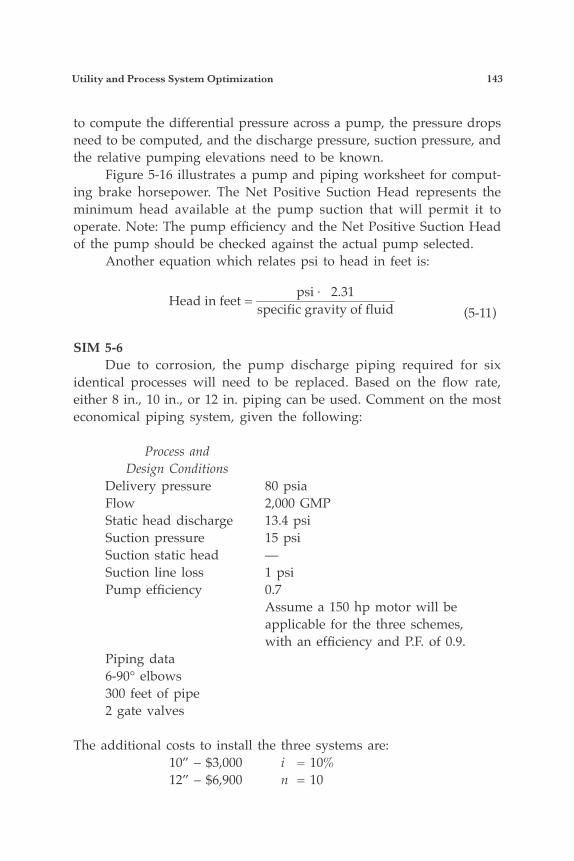
Utility and Process System Optimization 143
to compute the differential pressure across a pump, the pressure drops need to be computed, and the discharge pressure, suction pressure, and the relative pumping elevations need to be known. Figure 5-16 illustrates a pump and piping worksheet for comput-ing brake horsepower. The Net Positive Suction Head represents the minimum head available at the pump suction that will permit it to operate. Note: The pump efficiency and the Net Positive Suction Head of the pump should be checked against the actual pump selected. Another equation which relates psi to head in feet is:
Head in feet = psi × 2.31
specific gravity of fluid (5-11)
SIM 5-6 Due to corrosion, the pump discharge piping required for six identical processes will need to be replaced. Based on the flow rate, either 8 in., 10 in., or 12 in. piping can be used. Comment on the most economical piping system, given the following:
Process and Design Conditions Delivery pressure 80 psia Flow 2,000 GMP Static head discharge 13.4 psi Suction pressure 15 psi Suction static head — Suction line loss 1 psi Pump efficiency 0.7 Assume a 150 hp motor will be applicable for the three schemes, with an efficiency and P.F. of 0.9. Piping data 6-90° elbows 300 feet of pipe 2 gate valves
The additional costs to install the three systems are: 10” – $3,000 i = 10% 12” – $6,900 n = 10

144 P
lant E
ngin
eers and
Man
agers Gu
ide to E
nergy C
onservation
Table 5-7. Flow of water through schedule 40 steel pipe.
Discharge leloc- Press. Veloc- Press. ity Drop ity Drop
Feet Lbs. Feet Lbs.
kcond Sq. In. Second Sq. In. per per p e r per
1" 1 1h"
Gallons
Minute per
.2
.3
.4
.5
.6
.8
I 2 3 4 5 6 8 10 15 20
25 30 35 40 45
50 60 70 80 90
100 125 150 175 200 225 250 275 300 325
Veloc- Press. ity Drop
Feet Lbs.
Second Sq. In. per per
h b i c Ft.
Second p e r
0.000446 O.OO0668 0.000891 0.00111 0.00134 0.00178
0.00223 0.00446 0.00668 0.00891 0.01114
0.01337 0.01782 0.02228 0.03342 0.04456
0.05570 0.06684 0.07798 0.08912 0.1003
0.1114 0.1337 0.1560 0.1782 0.2005 0.2228 0.2785 0.3342 0.3899 0.4456
0.5013 0.557 0.6127 0.6684 0.7241
0.616 0.359 0.924 0.903 1.23 1.61 1.54 2.39 1.85 3.29 2.46 5.44
-
Pressure Droo w r 100 feet and Velocity in Schedule 40 Pipe for Water at 60°F.
0.504 0.159 0.672 0.345 0.840 0.539 1.01 0.751 1.34 1.25
feloc- Press. ity Drop
Feet Lbs.
kcond Sq. In per per
I/gW 1.13 1.86 1.69 4.22 2.26 6.98 2.82 10.5 3.39 14.7 4.52 25.0
5.65 37.2 1.29 134.4
2" 0.574 0.04 0.765 0.07 0.956 0.10 1.43 0.22 1.91 0.37
2.39 0.56 2.87 0.78 3.35 1.05 3.83 1.35 4.30 1.67
4.78 2.03 5.74 2.87 6.70 3.84 7.65 4.97 8.60 6.20
9.56 7.59 1.97 11.76 4.36 16.70 6.75 22.3 9.14 28.8
. . . . . . . . . . . . . . . . . . . . . . . . . . . . . .
0.317 0.061 0.422 0.086 0.528 0.167 0.633 0.240 0 844 0.408
1.06 0.600 2.11 2.10 3.17 4.33 4.22 7.42 5.28 11.2
6.33 15.8 8.45 27.7 0.56 42.4
31/1" 0.812 0.041 0.974 0.056 1.14 0.704 1.30 0.095 1.46 0.117
1.62 0.142 1.95 0.204 2.27 0.261 2.60 0.334 2.92 0.416
_ _ r'eloc- Press. Veloc- Press.
ity Drop 1 ity Drop Feet Lbs. Feet Lbs.
3/r" 0.301 0.03; 0.361 0.041 0.481 0.10;
0.602 0.15! 1.20 0.52( 1.81 1.09 2.41 1.83 3.01 2.75
3.61 3.84 4.81 6.60 6.02 9.99 9.03 21.6 12.03 37.8
4" 0.882 0.04 1.01 0.05' 1.13 0.06
1.26 0.07; 1.51 0.10 1.76 0.14 2.02 0.18' 2.27 0.22
per per per per Second Sq. In. (Second Sq. In.
3.08 8.28 6.16 30.1 9.25 64.1 2.33 111.2
2l/2" 0.670 0.046 1.01 0.094 1.34 0.158
1.68 1.85 3.36 6.58 5.04 13.9 6.72 23.9 8.40 36.7
10.08 51.9 13.44 91.1
3" 0.868
2.23 1.17 2.97 1.99 3.71 2.99 5.57 6.36 7.43 10.9
9.28 16.7 1.14 23.8 2.99 32.2 4.85 41.5
5" 1.12 0.047 1.28 0.060 1.44 0.074
1.60 0.090 2.01 0.135 2.41 0.190 2.81 0.253
3.61 0.401 4.01 0.495 4.41 0.583 4.81 0.683 5.21 0.797
3.21 0.323
1.29 0.309 0.946 0.145 1.72 0.518 1.26 0.241 2.15 0.774 1.58 0.361 3.22 1.63 2.37 0.755 4.29 2.78 3.16 1.28
5.37 4.22 3.94 1.93 6.44 5.92 4.73 2.72 7.51 7.90 5.52 3.64 8.59 10.24 6.30 4.65 9.67 12.80 7.09 5.85
10.74 15.66 7.88 7.15 12.89 22.2 9.47 10.21
11.05 13.71 12.62 17.59
6" 14.20 22.0
1 . 1 1 0.03615.78 26.9 1.39 0.055 19.72 41.4 1.67 0.077 1.94 0.102
2.50 0.162 1.44 0.043 2.78 0.195 1.60 0.051 3.05 0.234 1.76 0.061 3.33 0.275 1.92 0.072 3.61 0.320 2.08 0.083
2.22 0.130 8"
0.052
0.082 0.114 0.151 0.191 0.23C
0.28t 0.4M 0.54( 0.68; 0.861 1.05 1.61 2.24 3.00 3.87 4.83 5.93 7.14 8.36 9.89
1.68 0.234 2.01 0.327 2.35 0.436 2.68 0.556 3.02 0.668
3.35 0.839 4.02 1.18 4.69 1.59 5.36 2.03 6.03 2.53
6.70 3.09 8.38 4.71 10.05 6.69 11.73 8.97 13.42 11.68
15.09 14.63 . . . . . . . . . . . . . . . . . . . . . . . .
~~
{elof- Press. Veloc- Press. ity Drop I ity Drop
1.09 1.30 1.52 1.74 1.95
2.17 2.60 3.04 3.47 3.91
4.34 5.43 6.51 7.60 8.68
9.77 10.85 11.94 13.00 14.12
3.25 0.509 4.06 0.769 4.87 1.08 5.68 1.44 6.49 1.85
2.52 0.27 3.15 0.41 3.78 0.588 4.41 0.77 5.04 0.98
7.30 2.32 8.12 2.84 8.93 3.40 9.74 4.02 10.53 4.09
5.67 1.23 6.30 1.46 6.93 1.79 7.56 2.11 8.19 2.47
0.371 0.743 0.0461 0,164 0.429 0.044 1 11/2"
1.114 0.336 0.644 0.090 473 0.04 1.49 0.565 0.858 0.150 0.630 0.07 1.86 0.835 1.073 0.223 0.788 0.10
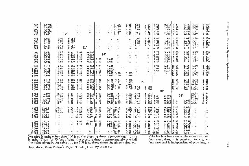
Utility an
d P
rocess System O
ptim
ization
145
350 375 400 425 450
475 500 550 600 650
700
800 850 900
950 lo00 1100 1 200 1 300
1 400 1 500 1600 1 800 2000
2 500 3000 3 500 4000 4 500
5000 6000 7000 8 0 0 0 9000
758
. . . . . . . . . . . . :r than 100 feet, the pressure
10 OOO 12 ooo 14 000 16 000 18 OOO 20 OOO
length. the value given in
8.89 25 42 4.49 !20.08 . , . h : 0 5 5.83 j22.95 . , . '32.68 7 31 25.82 . . . , , , 136.31 9103 128.69
drop is proportional to the
0.7798 0.8355 0.8912 0.9469 1.003
1.059 1.114 1 . 2 w 1.337 1.448
1.560 1.671 1.782 1 * 894 2.005
2.117 2.228 2.451 2.674 2.8%
3.119 3.342 3.565 4.010 4.456
5.570 6.684 7.798 8.912
10.03
11.14 13.37 15.60 17.82 20.05
22.28 26.74 31.19 35.65 40.10 44.56 engths of hus , for
0.112 0.127 0.143 0.160: 0.179,
0.198 0.218 0.260 0.306 0.355
I .93 2.03 2.24 2.44 2 .64
2.85 3.05 3.25 3.46 3.66
? .86 4.07 4.48 4.88 5.29
5.70 6.10 6.51 7.32 8 . I4
0.17 2.20 4.24 6.27 8 .31
0.35 4.41 8.49 . . . . . . . . . . . . . . . . . . ...
2.01 2.15 2 .29 2.44 2.58
2.72 2.87 3.15 3.44 1.73
I . . . . I . . . . . . . . . . . . .
. . ,
. . . , " ' . . .
0.808
1.24 1.76 2.38 3.08 3.87
4.71 6.74
I 0.054' 0.059 0.071 0.083 0.0971 12"
5.73
7.17 8.60
10.03 '11.47 12.90
14.33 17.20
0.321 0.451
0.04 0.05, 0.06 0.061 0.07!
0.08. 0.09 0.11( 0.121 0.15(
0.17 0.191 0.21' 0.27( 0.33l
0.51! 0.73 0.98 1.27 1.60
1.95 2.77 3.74 4.84 6.09
7.46 10.7
4 54 5 45
. . . . . , 111.36 5.41 1 8 . 8 2 . . . , . . 12.17 6.18 9.45
. . . . , , 12.98 7.03 10.08
. . . , , 13.80 7.89 10.71 . . . _ . . 114.61 8.80 i l l . 3 4
. . . 11.97
. . . . . . 111.85
I . . . . . . . . . . . : . : I ::: . . . ~ 1 2 . 6 0
. . . . . . . . . , , . / I I . I Z . . . . . .
. . . . , . ~ . . . , . . . . .
" ' 1 ' . . 14" 1 . . .
2.02 2.13
2 .25 2.37 2.61 2.85 ? .08 3.32 I . 56 3.79 4 .27 4.74
5.91 7.11 8.30 9.48 0.67
I .85 4.23 6.60 8.96 I .34
3.71 8.45 1.19 . . . . . .
. . . ~ I . .
. . . , . .
. . . ~ . . . 0.0521 . . 0.057, 16" 1 : . . 0.068 0.080 2 18 0.0931 2136
0.042~ , : 0.048: I . .
2.84 3.25 3.68 4.12 4.60
5.12 5.65 6.79 8.04
0.055
0.071 0.088 2 58 0.051 0.107 2 87 0.W
0.1631 3.59 0.09 0.2321 4 30 0.12' 0.312 5 02 0.17 0.401 5 74 0.22 0.503 6.46 0.281
0.0631 18"
~
0 617 7 17 0.341
1:l8 '10.04 0.65 1.51 11.47 0.83' 1.90 12.91 1.05
0.8771 8'61 0.48.
4 61 l18.15 2 34 14 34 1.28 6159 121.79 3:33 117:21 1.83
5 . 6 2 6.02 6.42 6 .82 7.22
7.62 8.02 8.82 9.63 0 43
1.23 2.03 2.83 3 . 6 4 4.44
5.24 6.04 7.65 . . . , . .
0.919 1.05 1.19 1.33 1.48
1.64 1.81 2.17 2.55 2.98
3.43 3.92 4.43 5.00 5.58
6.21 6.84 8.23
. . . . . .
20" 3.46 0.075 4.04 0.101 4.62 0.129 5.20 0.162
5.77 0.199
8.08 0.376 9.23 0.488 0.39 0.608
6.93 0.280
1.54 0.739 3 .85 1.06 6.16 1.43 8.47 1.85 0.77 2.32 1.08 2.86 x i t y is a fui
3.89 4.16 4.44 4.72 5 .oo 5.27 5.55 6.11 6.66 7.22
7.78 8.33 8.88 9.44 9.99
0.55 1.10 2.22 3 .33 4.43
5.55 6.66 7.77 9.99 2.21
0.365 0.416 0.471 0.525 0.59(
0.653 0.72C 0.861 1.02 1.18
1.35 1.55 1.75 1.96 2.18
2.42 2.68 3.22 3.81 4.45
5.13 5.85 6.61 8.37
10.3
24" 3.19 0.051 1.59 0.065
1.99 0.075 4.79 0.111
6.38 0.192 7.18 0.242
5.59 0.15a
2.24 2.40 2.56 2.73 2.89
3.04 3.21 3 .53 3.85 4.17
4.49 4.81 5 . 1 3 5.45 5.77
6.09 6.41 7.05 7.70 8.33
8.98 9.62 0.26 I .54 2.82
6.03 9.24 2.44 5.65 A.87
. . .
. . . I . .
, . . . . . . . . . . . . . . . . . . . .
0.095 0.108 0.121 0.136 0.151
0.166 0.182 0.219 0.258 0.301
0.343 0.392 0.443 0.497 0.554
0.613 0.675 0.807 0.948 1.11
1.28 1.46 1-65 2.08 2.55
3.94 5.59 7.56 9.80
11.1
. . . . . . . . . . . .
. . .
. . . . . . . . . . . .
. . . 2.45 3.18 4.03 4.93
V flow area: thus, it is constant for a given flow rate and is independent of pipe length.
Reproduced from Techniial Paper No. 410, Courtesy Crane Co.
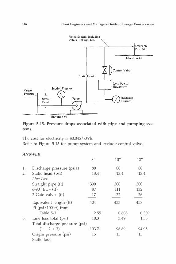
146 Plant Engineers and Managers Guide to Energy Conservation
The cost for electricity is $0.045/kWh.Refer to Figure 5-15 for pump system and exclude control valve.
ANSWER 8” 10” 12”
1. Discharge pressure (psia) 80 80 802. Static head (psi) 13.4 13.4 13.4 Line Loss Straight pipe (ft) 300 300 300 6-90° EL - (ft) 87 111 132 2-Gate valves (ft) 17 22 26 —— —— —— Equivalent length (ft) 404 433 458 Pi (psi/100 ft) from Table 5-3 2.55 0.808 0.3393. Line loss total (psi) 10.3 3.49 1.55 Total discharge pressure (psi) (1 + 2 + 3) 103.7 96.89 94.95 Origin pressure (psi) 15 15 15 Static loss
Figure 5-15. Pressure drops associated with pipe and pumping sys-tems.
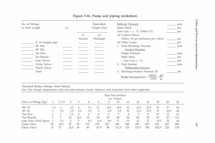
Utility an
d P
rocess System O
ptim
ization
147Figure 5-16. Pump and piping worksheet.
—————————————————————————————————————————————————No. of Fittings Equivalent Delivery Pressure _______ psiaor Total Length Le Length Total Static Head _______ psi _______________________ Line Loss = ≤ × P1 (Table 5-3) _______ psi L1 L1 ∆P Control Valves Suction Discharge (Allow 10 psi minimum per valve) _______ psi_________ ft. of straight pipe _______ _______ ∆P Other Losses _______ psi_________ 90° Ells × _______ _______ _______ 1. Total Discharge Pressure _______ psia_________ 45° Ells × _______ _______ _______ Suction Pressure_________ Tee Run × _______ _______ _______ Origin Pressure _______ psia_________ Tee Branch × _______ _______ _______ Static Head _______ psi________ Gate Valves × _______ _______ _______ – Line Loss ≤ × P1 _______ psi_________ Globe Valves × _______ _______ _______ 2. Total Suction _______ psia_________ Check Valves × _______ _______ _______ Differential Pressure Total _______ _______ 3. Discharge-Suction Pressure ∆P _______ psi
—————————————————————————————————————————————————*Standard Radius Fittings—Butt WeldedNote: For energy comparisons only exit and entrance losses, reducers and expanders have been neglected.————————————————————————————————————————————————— Pipe Size (inches) Le—ValuesValve or Fitting Type 1 1-1/2 2 3 4 6 8 10 12 14 16 18 20 24—————————————————————————————————————————————————*90° El 1.5 3 3.5 6 7.5 11 14.5 18.5 22 22.5 29.5 33 37 44*45° El 1 1.5 1.5 2.5 3.5 5 6.5 8.5 10 11.5 13.5 15 16.5 20*Tee Run 1 1 1.5 2 3 4 5 7 8 9 11 12 13 16*Tee Branch 5 7 10 14.5 19 29 39 48 58 68 78 87 97 116Gate Valve (Full Open) 1 1.5 2 3 4.5 6.5 8.5 11 13 15 17 19.5 22 26Globe Valve 28 42.5 57 85 113 170 227 283 340 397 453 510 567 686Check Valve 11 17 22.5 34 45 67.5 90 112.5 135 157.5 180 202.5 225 270
Brake horsepower = GPM × ΔP1715 × η
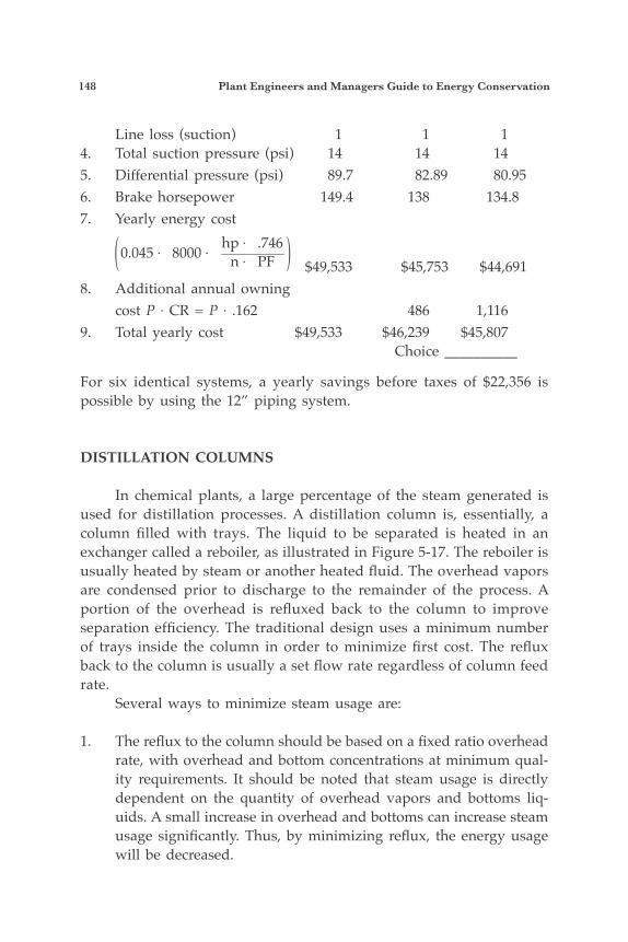
148 Plant Engineers and Managers Guide to Energy Conservation
Line loss (suction) 1 1 14. Total suction pressure (psi) 14 14 145. Differential pressure (psi) 89.7 82.89 80.956. Brake horsepower 149.4 138 134.87. Yearly energy cost
0.045 × 8000 ×
hp × .746n × PF $49,533 $45,753 $44,691
8. Additional annual owning cost P × CR = P × .162 486 1,1169. Total yearly cost $49,533 $46,239 $45,807 Choice __________
For six identical systems, a yearly savings before taxes of $22,356 is possible by using the 12” piping system.
DISTILLATION COLUMNS
In chemical plants, a large percentage of the steam generated is used for distillation processes. A distillation column is, essentially, a column filled with trays. The liquid to be separated is heated in an exchanger called a reboiler, as illustrated in Figure 5-17. The reboiler is usually heated by steam or another heated fluid. The overhead vapors are condensed prior to discharge to the remainder of the process. A portion of the overhead is refluxed back to the column to improve separation efficiency. The traditional design uses a minimum number of trays inside the column in order to minimize first cost. The reflux back to the column is usually a set flow rate regardless of column feed rate. Several ways to minimize steam usage are:
1. The reflux to the column should be based on a fixed ratio overhead rate, with overhead and bottom concentrations at minimum qual-ity requirements. It should be noted that steam usage is directly dependent on the quantity of overhead vapors and bottoms liq-uids. A small increase in overhead and bottoms can increase steam usage significantly. Thus, by minimizing reflux, the energy usage will be decreased.
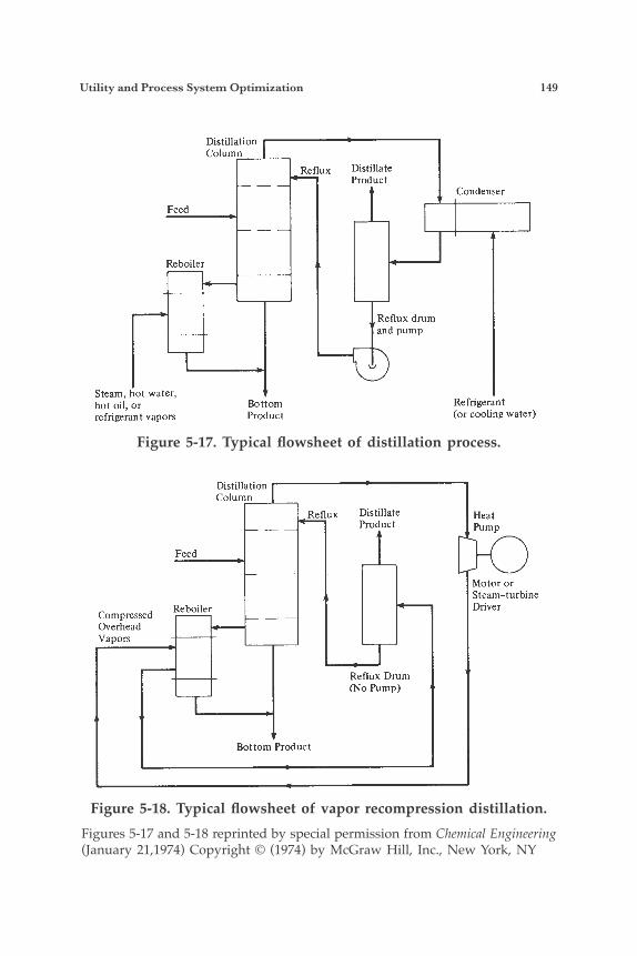
Utility and Process System Optimization 149
Figure 5-17. Typical flowsheet of distillation process.
Figure 5-18. Typical flowsheet of vapor recompression distillation.Figures 5-17 and 5-18 reprinted by special permission from Chemical Engineering (January 21,1974) Copyright © (1974) by McGraw Hill, Inc., New York, NY
Disti!lation Column
~ ~ f l ~ ~ Distillate Product
Condenser
Feed
Reboiler
Reflux drum and pump
Steam, hot water, hot oil, or refrigerant vapors
Bottom Product
Refrigerant (or cooling water)
Reboiler Compressed Overhead Vapors
Distillation Column
~ ~ f l ~ ~ Distillate Product
Feed
Heat Pump
Motor or Steam-turbine Driver
Reflux Drum (No Pump)
Bottom Product
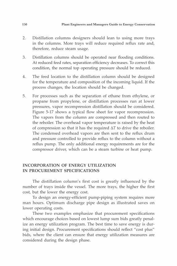
150 Plant Engineers and Managers Guide to Energy Conservation
2. Distillation columns designers should lean to using more trays in the columns. More trays will reduce required reflux rate and, therefore, reduce steam usage.
3. Distillation columns should be operated near flooding conditions. At reduced feed rates, separation efficiency decreases. To correct this condition, the normal top operating pressure should be reduced.
4. The feed location to the distillation column should be designed for the temperature and composition of the incoming liquid. If the process changes, the location should be changed.
5. For processes such as the separation of ethane from ethylene, or propane from propylene, or distillation processes run at lower pressures, vapor recompression distillation should be considered. Figure 5-17 shows a typical flow sheet for vapor recompression. The vapors from the column are compressed and then routed to the reboiler. The overhead vapor temperature is raised by the heat of compression so that it has the required ∆T to drive the reboiler. The condensed overhead vapors are then sent to the reflux drum and pressure controlled to provide reflux to the column without a reflux pump. The only additional energy requirements are for the compressor driver, which can be a steam turbine or heat pump.
INCORPORATION OF ENERGY UTILIZATIONIN PROCUREMENT SPECIFICATIONS
The distillation column’s first cost is greatly influenced by the number of trays inside the vessel. The more trays, the higher the first cost, but the lower the energy cost. To design an energy-efficient pump-piping system requires more man hours. Optimum discharge pipe design as illustrated saves on lower operating costs. These two examples emphasize that procurement specifications which encourage choices based on lowest lump sum bids greatly penal-ize an energy utilization program. The best time to save energy is dur-ing initial design. Procurement specifications should reflect “cost plus” bids, where the client can ensure that energy utilization measures are considered during the design phase.
6Heat Transfer
THE IMPORTANCE OF UNDERSTANDINGTHE PRINCIPLES OF HEAT TRANSFER
The principles of heat transfer are the fundamental building blocks needed to understand how heat losses occur and how they can be minimized. Heat transfer finds application in equipment sizing as well. For instance, a heat exchanger is used to transfer heat from one fluid to another. Thus, heat transfer applications are involved with energy transfer in equipment, piping systems, and buildings. In Chapter 7, heat transfer applications to building design will be presented. In this chapter, you will learn three modes of heat transfer, see how much energy is lost from uninsulated tanks and pipes, and discover how to use economic insulation thickness tables to reduce heat losses.
THREE WAYS HEAT IS TRANSFERRED
Heat transfer is determined by the effects of conduction, radiation, and convection. The three modes can be thought of simply as:
Conduction—Heat transfer is based on one space surrendering heat while another one gains it by the ability of the dividing surface to conduct heat.
Radiation—Heat transfer is based on the properties of light, where no surface or fluid is needed to carry heat from one object to an-other.
Convection—Heat transfer is based on the exchange of heat between a fluid, gas, or liquid as it transverses a conducting surface.
151
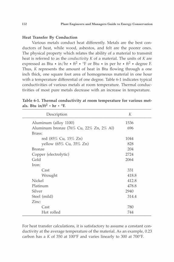
152 Plant Engineers and Managers Guide to Energy Conservation
Heat Transfer By Conduction Various metals conduct heat differently. Metals are the best con-ductors of heat, while wood, asbestos, and felt are the poorer ones. The physical property which relates the ability of a material to transmit heat is referred to as the conductivity K of a material. The units of K are expressed as Btu • in/hr • ft2 • °F or Btu • in per hr • ft2 • degree F. Thus, K represents the amount of heat in Btu flowing through a one inch thick, one square foot area of homogeneous material in one hour with a temperature differential of one degree. Table 6-1 indicates typical conductivities of various metals at room temperature. Thermal conduc-tivities of most pure metals decrease with an increase in temperature.
Table 6-1. Thermal conductivity at room temperature for various met-als. Btu in/ft2 • hr • °F.———————————————————————————————— Description K———————————————————————————————— Aluminum (alloy 1100) 1536 Aluminum bronze (76% Cu, 22% Zn, 2% Al) 696 Brass: red (85% Cu, 15% Zn) 1044 yellow (65% Cu, 35% Zn) 828 Bronze 204 Copper (electrolytic) 2724 Gold 2064 Iron: Cast 331 Wrought 418.8 Nickel 412.8 Platinum 478.8 Silver 2940 Steel (mild) 314.4 Zinc: Cast 780 Hot rolled 744————————————————————————————————
For heat transfer calculations, it is satisfactory to assume a constant con-ductivity at the average temperature of the material. As an example, 0.23 carbon has a K of 350 at 100°F and varies linearly to 300 at 700°F.
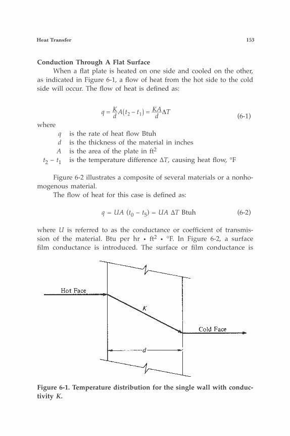
Heat Transfer 153
Conduction Through A Flat Surface When a flat plate is heated on one side and cooled on the other, as indicated in Figure 6-1, a flow of heat from the hot side to the cold side will occur. The flow of heat is defined as:
q = Kd A t2 – t1 = KA
d ΔT (6-1)where q is the rate of heat flow Btuh d is the thickness of the material in inches A is the area of the plate in ft2
t2 – t1 is the temperature difference ∆T, causing heat flow, °F
Figure 6-2 illustrates a composite of several materials or a nonho-mogenous material. The flow of heat for this case is defined as:
q = UA (t0 – t5) = UA ∆T Btuh (6-2)
where U is referred to as the conductance or coefficient of transmis-sion of the material. Btu per hr • ft2 • °F. In Figure 6-2, a surface film conductance is introduced. The surface or film conductance is
Figure 6-1. Temperature distribution for the single wall with conduc-tivity K.
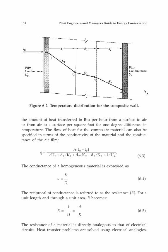
154 Plant Engineers and Managers Guide to Energy Conservation
the amount of heat transferred in Btu per hour from a surface to air or from air to a surface per square foot for one degree difference in temperature. The flow of heat for the composite material can also be specified in terms of the conductivity of the material and the conduc-tance of the air film:
q =
A t0 – t51 ⁄ U0 + d1 ⁄ K1 + d2 ⁄ K2 + d3 ⁄ K3 + 1 ⁄ U4
. (6-3)
The conductance of a homogeneous material is expressed as
K u = — (6-4) D The reciprocal of conductance is referred to as the resistance (R). For a unit length and through a unit area, R becomes:
1 d R = — = — (6-5) U K
The resistance of a material is directly analogous to that of electrical circuits. Heat transfer problems are solved using electrical analogies.
Figure 6-2. Temperature distribution for the composite wall.
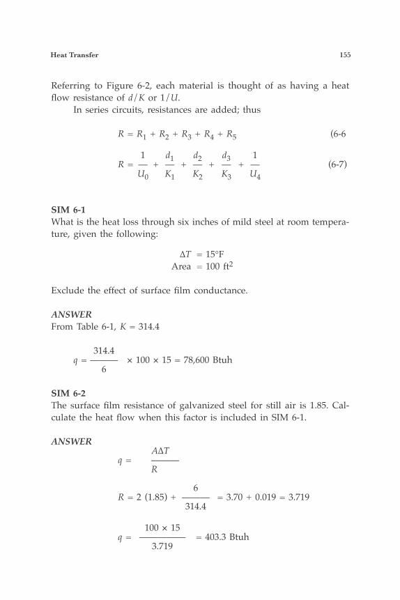
Heat Transfer 155
Referring to Figure 6-2, each material is thought of as having a heat flow resistance of d/K or 1/U. In series circuits, resistances are added; thus
R = R1 + R2 + R3 + R4 + R5 (6-6
1 d1 d2 d3 1 R = — + — + — + — + — (6-7) U0 K1 K2 K3 U4
SIM 6-1What is the heat loss through six inches of mild steel at room tempera-ture, given the following:
∆T = 15°F Area = 100 ft2
Exclude the effect of surface film conductance.
ANSWERFrom Table 6-1, K = 314.4
314.4 q = ——— × 100 × 15 = 78,600 Btuh 6
SIM 6-2The surface film resistance of galvanized steel for still air is 1.85. Cal-culate the heat flow when this factor is included in SIM 6-1.
ANSWER A∆T q = ——— R
6 R = 2 (1.85) + ——— = 3.70 + 0.019 = 3.719 314.4
100 × 15 q = ————— = 403.3 Btuh 3.719
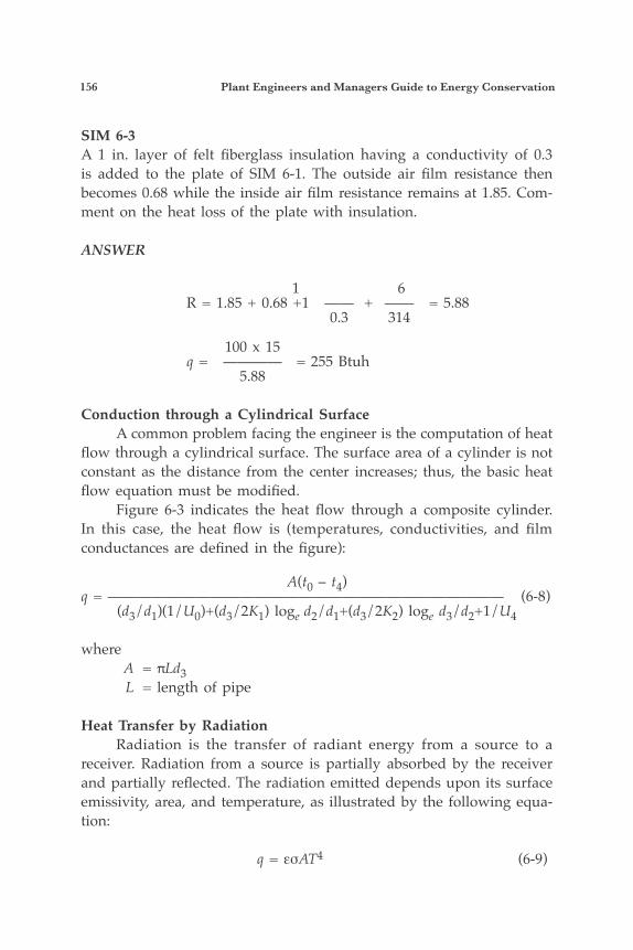
156 Plant Engineers and Managers Guide to Energy Conservation
SIM 6-3A 1 in. layer of felt fiberglass insulation having a conductivity of 0.3 is added to the plate of SIM 6-1. The outside air film resistance then becomes 0.68 while the inside air film resistance remains at 1.85. Com-ment on the heat loss of the plate with insulation.
ANSWER
1 6 R = 1.85 + 0.68 +1 —— + —— = 5.88 0.3 314
100 x 15 q = ———— = 255 Btuh 5.88
Conduction through a Cylindrical Surface A common problem facing the engineer is the computation of heat flow through a cylindrical surface. The surface area of a cylinder is not constant as the distance from the center increases; thus, the basic heat flow equation must be modified. Figure 6-3 indicates the heat flow through a composite cylinder. In this case, the heat flow is (temperatures, conductivities, and film conductances are defined in the figure):
A(t0 – t4)q = ——————————————————————————— (6-8)
(d3/d1)(1/U0)+(d3/2K1) loge d2/d1+(d3/2K2) loge d3/d2+1/U4
where A = πLd3 L = length of pipe
Heat Transfer by Radiation Radiation is the transfer of radiant energy from a source to a receiver. Radiation from a source is partially absorbed by the receiver and partially reflected. The radiation emitted depends upon its surface emissivity, area, and temperature, as illustrated by the following equa-tion:
q = εσAT4 (6-9)
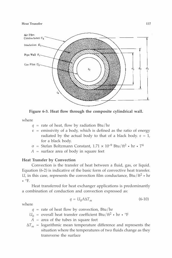
Heat Transfer 157
where q = rate of heat, flow by radiation Btu/hr ε = emissivity of a body, which is defined as the ratio of energy
radiated by the actual body to that of a black body. ε = 1, for a black body.
σ = Stefan Boltzmann Constant, 1.71 × 10⁻⁹ Btu/ft2 • hr • T4
A = surface area of body in square feet
Heat Transfer by Convection Convection is the transfer of heat between a fluid, gas, or liquid. Equation (6-2) is indicative of the basic form of convective heat transfer. U, in this case, represents the convection film conductance, Btu/ft2 • hr • °F. Heat transferred for heat exchanger applications is predominantly a combination of conduction and convection expressed as:
q = U0A∆Tm (6-10)where q = rate of heat flow by convection, Btu/hr U0 = overall heat transfer coefficient Btu/ft2 • hr • °F A = area of the tubes in square feet ∆Tm = logarithmic mean temperature difference and represents the
situation where the temperatures of two fluids change as they transverse the surface
Figure 6-3. Heat flow through the composite cylindrical wall.
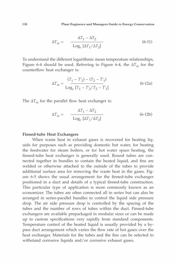
158 Plant Engineers and Managers Guide to Energy Conservation
∆T1 – ∆T2 ∆Tm = ———————— (6-11) Loge [∆T1/∆T2]
To understand the different logarithmic mean temperature relationships, Figure 6-4 should be used. Referring to Figure 6-4, the ∆Tm for the counterflow heat exchanger is:
(T1 – T'2) – (T2 – T'1) ∆Tm = ———————— (6-12a) Loge [T1 – T'2/T2 – T'1]
The ∆Tm for the parallel flow heat exchanger is:
∆T1 – ∆T2 ∆Tm = ———————— (6-12b) Loge [∆T1/∆T2]
Finned-tube Heat Exchangers When waste heat in exhaust gases is recovered for heating liq-uids for purposes such as providing domestic hot water, for heating the feedwater for steam boilers, or for hot water space heating, the finned-tube heat exchanger is generally used. Round tubes are con-nected together in bundles to contain the heated liquid, and fins are welded or otherwise attached to the outside of the tubes to provide additional surface area for removing the waste heat in the gases. Fig-ure 6-5 shows the usual arrangement for the finned-tube exchanger positioned in a duct and details of a typical finned-tube construction. This particular type of application is more commonly known as an economizer. The tubes are often connected all in series but can also be arranged in series-parallel bundles to control the liquid side pressure drop. The air side pressure drop is controlled by the spacing of the tubes and the number of rows of tubes within the duct. Finned-tube exchangers are available prepackaged in modular sizes or can be made up to custom specifications very rapidly from standard components. Temperature control of the heated liquid is usually provided by a by-pass duct arrangement which varies the flow rate of hot gases over the heat exchanger. Materials for the tubes and the fins can be selected to withstand corrosive liquids and/or corrosive exhaust gases.
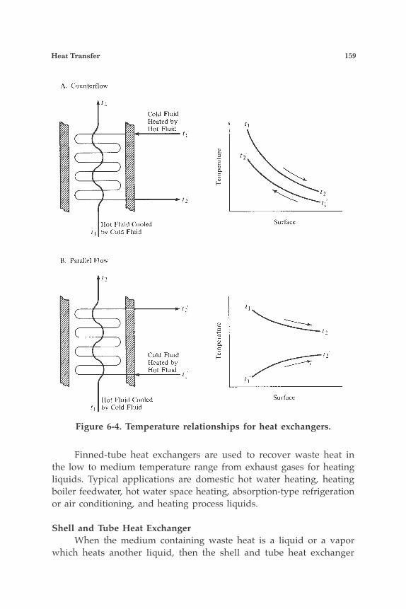
Heat Transfer 159
Finned-tube heat exchangers are used to recover waste heat in the low to medium temperature range from exhaust gases for heating liquids. Typical applications are domestic hot water heating, heating boiler feedwater, hot water space heating, absorption-type refrigeration or air conditioning, and heating process liquids.
Shell and Tube Heat Exchanger When the medium containing waste heat is a liquid or a vapor which heats another liquid, then the shell and tube heat exchanger
Figure 6-4. Temperature relationships for heat exchangers.
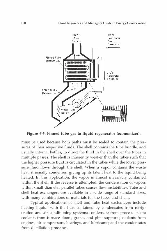
160 Plant Engineers and Managers Guide to Energy Conservation
must be used because both paths must be sealed to contain the pres-sures of their respective fluids. The shell contains the tube bundle, and usually internal baffles, to direct the fluid in the shell over the tubes in multiple passes. The shell is inherently weaker than the tubes such that the higher pressure fluid is circulated in the tubes while the lower pres-sure fluid flows through the shell. When a vapor contains the waste heat, it usually condenses, giving up its latent heat to the liquid being heated. In this application, the vapor is almost invariably contained within the shell. If the reverse is attempted, the condensation of vapors within small diameter parallel tubes causes flow instabilities. Tube and shell heat exchangers are available in a wide range of standard sizes, with many combinations of materials for the tubes and shells. Typical applications of shell and tube heat exchangers include heating liquids with the heat contained by condensates from refrig-eration and air conditioning systems; condensate from process steam; coolants from furnace doors, grates, and pipe supports; coolants from engines, air compressors, bearings, and lubricants; and the condensates from distillation processes.
Figure 6-5. Finned tube gas to liquid regenerator (economizer).
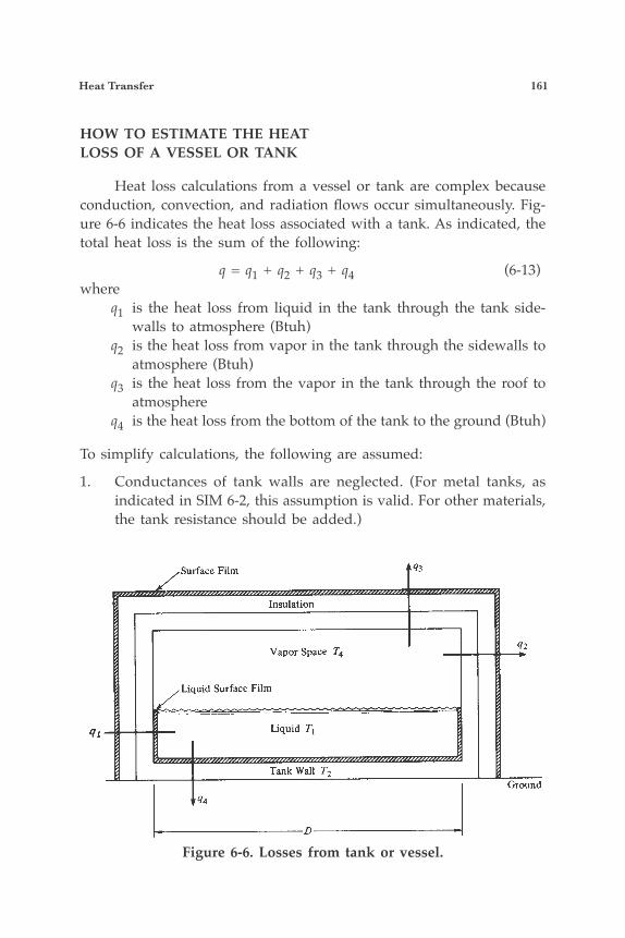
Heat Transfer 161
HOW TO ESTIMATE THE HEATLOSS OF A VESSEL OR TANK
Heat loss calculations from a vessel or tank are complex because conduction, convection, and radiation flows occur simultaneously. Fig-ure 6-6 indicates the heat loss associated with a tank. As indicated, the total heat loss is the sum of the following:
q = q1 + q2 + q3 + q4 (6-13)where q1 is the heat loss from liquid in the tank through the tank side-
walls to atmosphere (Btuh) q2 is the heat loss from vapor in the tank through the sidewalls to
atmosphere (Btuh) q3 is the heat loss from the vapor in the tank through the roof to
atmosphere q4 is the heat loss from the bottom of the tank to the ground (Btuh)
To simplify calculations, the following are assumed:
1. Conductances of tank walls are neglected. (For metal tanks, as indicated in SIM 6-2, this assumption is valid. For other materials, the tank resistance should be added.)
Figure 6-6. Losses from tank or vessel.
162 Plant Engineers and Managers Guide to Energy Conservation
2. Liquid and vapor surface conductances are neglected for uninsu-lated tanks. Heat loss is based on air surface conductance.
3. Liquid and vapor conductances are neglected for insulated tanks. Heat loss is based on insulation conductance and surface air con-ductance.
A simplified procedure to determine approximate heat losses will be illustrated. This procedure simplifies computations of the various film coefficients. As an approximation, Figure 6-6 is used to compute the heat loss for uninsulated tanks based on the surface film conductances. This figure is used to compute q1, q2, and q3 by equating qt, to the q in question. The total heat loss is computed by multiplying the heat loss from Figure 6-6 by the surface area. Another term, ∆Tw, is introduced in this figure. To compute ∆Tw:
∆ Tw = (Tw – TA) W (6-14)
where
Tw is the fluid temperature, °F, TA is the ambient temperature 70°F, and W is the correction factor which takes into account the process fluid.
W is defined as
Process Fluid W Agitated Liquid 1 Aqueous Solution 0.9 Fuel Oil 0.7 Condensing Vapor 1.0 Non-condensing Vapor 0.2 Fouling Liquids 0.4
Figure 6-7 is based on an ambient air temperature of 70°F, a surface emissivity of 0.9, and a wind velocity of zero. To use Figure 6-6 for other values, correct each term separately.
New Emissivity Value from graph qa (radiation) = ——————— × (use for other than 0.9) (6-15) 0.90
Heat Transfer 163
New Emissivity Value from graph qc (convection) = ——————— × (use for other than 0.9) (6-16) 0.90 qt = qa + qc (6-17)
Heat Loss to Ground The last portion of Equation 6-18 deals with heat losses from the bottom of the tank when it rests on the ground. It is defined as:
q4 = 2DK4 (Tw – T3) (6-18)
where D is the diameter of the tank in ft K4 is the conductance to ground Use K4 = 0.8 unless otherwise known Tw is the liquid temperature, °F T3 is the ground temperature, °F
Assume ambient temperatures unless the ground temperature is specifi-cally known.
Reducing Heat Loss of Vessels or Tanks Insulation is the common method used to reduce the heat loss from a vessel or tank. Figure 6-8 shows the effect of various insulation thicknesses. This figure can be used as a guide to determine suggested economic thickness for various temperature differentials. To use Figure 6-8, the temperature difference factor ∆T1 should be corrected for wind velocities other than zero. To correct ∆T1, multiply by the correction factors for various wind velocities given below:
Wind Velocity Correction Factors Insulation Thickness 10 mph 30 mph 1 1.09 1.14 1-1/2 1.07 1.10 2 1.06 1.09 2-1/2 1.04 1.07 3 1.04 1.06 3-1/2 1.03 1.05
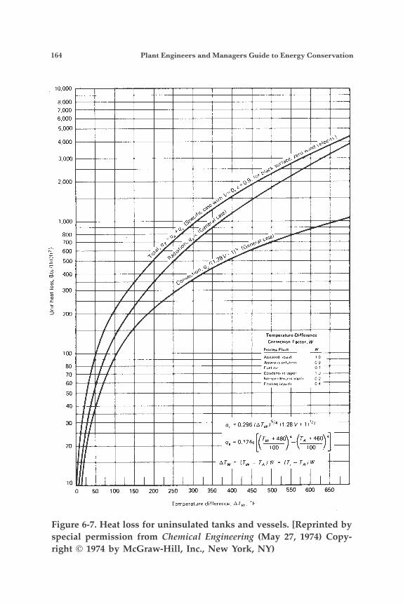
164 Plant Engineers and Managers Guide to Energy Conservation
Figure 6-7. Heat loss for uninsulated tanks and vessels. [Reprinted by special permission from Chemical Engineering (May 27, 1974) Copy-right © 1974 by McGraw-Hill, Inc., New York, NY)
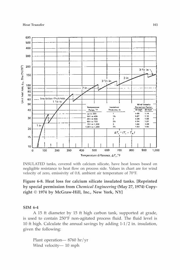
Heat Transfer 165
SIM 6-4 A 15 ft diameter by 15 ft high carbon tank, supported at grade, is used to contain 250°F non-agitated process fluid. The fluid level is 10 ft high. Calculate the annual savings by adding 1-1/2 in. insulation, given the following:
Plant operation— 8760 hr/yr Wind velocity— 10 mph
INSULATED tanks, covered with calcium silicate, have heat losses based on negligible resistance to heat flow on process side. Values in chart are for wind velocity of zero, emissivity of 0.8, ambient air temperature of 70°F.
Figure 6-8. Heat loss for calcium silicate insulated tanks. [Reprinted by special permission from Chemical Engineering (May 27, 1974) Copy-right © 1974 by McGraw-Hill, Inc., New York, NY]
166 Plant Engineers and Managers Guide to Energy Conservation
Ambient temperature—70° Emissivity of tank—0.20 Vapor space has non-condensable vapors Heat content of steam—926.1 Btu/lb Steam cost—$6/1000 lb
ANSWER Uninsulated Tank Wetted Area of Tank A1 = πDH = π × 15 × 10 = 471 ft2
∆T = (250 – 70) = 180°F ∆TW = 0.9 × 180 = 162
From Figure 6-7 q'c = qc × (1.28 × V + 1)1/2 = 180 × 3.71 = 667.8 Btu/h • ft2
0.2 q'c = qa × —— =250 × 0.222 = 55.5 Btu/h • ft2 0.9
qT = 667.8 + 55.5 = 723.3 Btu/h • ft2
q1 = 471 × 723.3 = 340,674 Btuh
Heat Loss for Vapor Space A2 = π × 15 (15 – 10) = 235.6 ft2
∆TW = ∆T × 0.20 = 36 q'c = 25 × 3.71 = 92.75 Btu/h • ft2
q'a = 35 × 0.222 = 7.77 Btu/h • ft2
qT = 100.52 Btuh q2 = 235.6 × 100.52 = 23,682 Btuh
Heat Loss for Roof pD2 A = —— = 176.7 ft2 4
q3 = 176.6 × 100.52 = 17,761 Btuh.
Heat Loss for Tank Bottom q4 = 2 × 15 × 0.8 (250 – 70) = 4,320 Btuh
Heat Transfer 167
Total Heat Loss = 386,437 Btuh
Insulated Tank ∆T = (250 – 70) = 180°F
From Figure 6-8, qT = 35 Btu/h • ft2
q’T = 35 × 1.07 = 37.45 Btu/h • ft2
Since the total tank is insulated, q = 37.45 (A1 + A2 + A3) = 37.45 (471 + 235.6 + 176.7) = 33,079 Btuh Total heat loss = 33,079 + 4,320 = 37,339 Btuh Energy savings with insulation =349,038 Btuh
Yearly energy savings by 349,038 x 8760 $6.00reducing steam usage = ——————— x —— = $19,809/year 926.1 1000
HOW TO ESTIMATE THE HEAT LOSSOF PIPING AND FLAT SURFACES
A simple method used to estimate heat losses for horizontal bare steel pipes and flat surfaces is to use Table 6-2. By knowing the tem-perature difference between the pipe surface and the ambient air, the heat loss is determined.
SIM 6-5An existing process indicated in Scheme 1 of Figure 6-9 uses a heat ex-changer to cool the discharge of the column before it enters the sewer. The traditional process supplies fluid directly to Column #1 at 104°F. The column is used as a stripper with 30 psig steam. Scheme 2 illustrates a proposed modification. The proposed scheme replaces the bottom fluid exchanger with a larger exchanger and uses the bottom fluid to heat the process liquid; the bottom fluid in turn will be cooled. What recommendations should be made, given the following data? The installed cost of heat exchanger #1 is $9000 with a 50 ft2 area. Conductance U of the heat exchanger = 100 30 psig steam is used
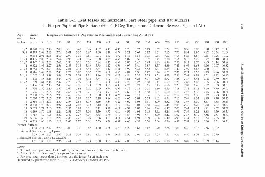
168 P
lant E
ngin
eers and
Man
agers Gu
ide to E
nergy C
onservation
Table 6-2. Heat losses for horizontal bare steel pipe and flat surfaces.In Btu per (Sq Ft of Pipe Surface) (Hour) (F Deg Temperature Difference Between Pipe and Air)
————————————————————————————————————————————————————Pipe Linear Temperature Difference F Deg Between Pipe Surface and Surrounding Air at 80 Fsize Foot ——————————————————————————————————————————————————————————————————inches Factor 50 100 150 200 250 300 350 400 450 500 550 600 650 700 750 800 850 900 950 1000———————————————————————————————————————————————————— 1/2 0.220 2.12 2.48 2.80 3.10 3.42 3.74 4.07 4.47 4.86 5.28 5.72 6.19 6.69 7.22 7.79 8.39 9.03 9.70 10.42 11.18 3/4 0.275 2.08 2.43 2.74 3.04 3.35 3.67 4.00 4.40 4.79 5.21 5.65 6.12 6.61 7.15 7.71 8.31 8.95 9.62 10.34 11.09 1 0.344 2.04 2.38 2.69 2.99 3.30 3.61 3.94 4.33 4.72 5.14 5.58 6.05 6.54 7.07 7.64 8.23 8.87 9.55 10.26 11.02 1-1/4 0.435 2.00 2.34 2.64 2.93 3.24 3.55 3.88 4.27 4.66 5.07 5.51 5.97 6.47 7.00 7.56 8.16 8.79 9.47 10.18 10.94 1-1/2 0.497 1.98 2.31 2.61 2.90 3.20 3.52 3.84 4.23 4.62 5.03 5.47 5.93 6.43 6.96 7.52 8.12 8.75 9.43 10.14 10.89 2 0.622 1.95 2.27 2.56 2.85 3.15 3.46 3.78 4.17 4.56 4.97 5.41 5.87 6.37 6.89 7.45 8.05 8.68 9.36 10.07 10.82 2-1/2 0.753 1.92 2.23 2.52 2.81 3.11 3.42 3.74 4.12 4.51 4.92 5.36 5.82 6.31 6.84 7.40 7.99 8.63 9.30 10.01 10.77 3 0.916 1.89 2.20 2.49 2.77 3.07 3.37 3.69 4.08 4.46 4.87 5.31 5.77 6.26 6.79 7.35 7.94 8.57 9.25 9.96 10.71 3-1/2 1.047 1.87 2.18 2.46 2.74 3.04 3.34 3.66 4.05 4.43 4.84 5.27 5.73 6.23 6.75 7.31 7.91 8.54 9.21 9.92 10.67 4 1.178 1.85 2.16 2.44 2.72 3.01 3.32 3.64 4.02 4.40 4.81 5.25 5.71 6.20 6.72 7.28 7.87 8.51 9.18 9.89 10.64 4-1/2 1.309 1.84 2.14 2.42 2.70 2.99 3.30 3.61 4.00 4.38 4.79 5.22 5.68 6.17 6.69 7.25 7.85 8.48 9.15 9.86 10.61 5 1.456 1.83 2.13 2.40 2.68 2.97 3.28 3.59 3.97 4.35 4.76 5.20 5.65 6.15 6.68 7.23 7.82 8.45 9.12 9.83 10.58 6 1.734 1.80 2.10 2.37 2.65 2.94 3.24 3.55 3.94 4.32 4.72 5.16 5.61 6.10 6.63 7.19 7.78 8.41 9.08 9.79 10.54 7 1.996 1.79 2.08 2.35 2.63 2.91 3.21 3.53 3.91 4.29 4.69 5.13 5.58 6.07 6.60 7.15 7.75 8.38 9.05 9.76 10.51 8 2.258 1.77 2.06 2.33 2.60 2.89 3.19 3.50 3.88 4.26 4.67 5.10 5.56 6.05 6.57 7.12 7.72 8.35 9.02 9.73 10.48 9 2.520 1.76 2.05 2.31 2.59 2.87 3.17 3.48 3.86 4.24 4.65 5.08 5.53 6.02 6.54 7.10 7.69 8.32 8.99 9.70 10.45 10 2.814 1.75 2.03 2.30 2.57 2.85 3.15 3.46 3.84 4.22 4.62 5.05 5.51 6.00 6.52 7.08 7.67 8.30 8.97 9.68 10.43 12 3.338 1.73 2.01 2.27 2.54 2.83 3.12 3.43 3.81 4.19 4.59 5.02 5.48 5.96 6.48 7.04 7.63 8.26 8.93 9.64 10.39 14 3.655 1.72 2.00 2.26 2.53 2.81 3.11 3.41 3.79 4.17 4.57 5.00 5.46 5.94 6.47 7.02 7.61 8.24 8.91 9.62 10.37 16 4.189 1.70 1.98 2.24 2.51 2.79 3.08 3.39 3.77 4.14 4.55 4.98 5.43 5.92 6.44 6.99 7.59 8.21 8.88 9.59 10.34 18 4.717 1.69 1.96 2.22 2.49 2.77 3.07 3.37 3.75 4.12 4.53 4.96 5.41 5.90 6.42 6.97 7.56 8.19 8.86 9.57 10.32 20 5.236 1.68 1.95 2.21 2.47 2.75 3.05 3.36 3.73 4.11 4.51 4.94 5.39 5.88 6.40 6.95 7.54 8.17 8.84 9.55 10.29 24 6.283 1.66 1.93 2.19 2.45 2.73 3.02 3.33 3.70 4.07 4.48 4.90 5.36 5.84 6.36 6.92 7.51 8.14 8.80 9.51 10.26Vertical Surface 1.84 2.14 2.42 2.70 3.00 3.30 3.62 4.00 4.38 4.79 5.22 5.68 6.17 6.70 7.26 7.85 8.48 9.15 9.86 10.62Horizontal Surface Facing Upward 2.03 2.37 2.67 2.97 3.28 3.59 3.92 4.31 4.70 5.12 5.56 6.02 6.52 7.05 7.61 8.21 8.85 9.52 10.24 10.99Horizontal Surface Facing Downward 1.61 1.86 2.11 2.36 2.64 2.93 3.23 3.60 3.97 4.37 4.80 5.25 5.73 6.25 6.80 7.39 8.02 8.69 9.39 10.14————————————————————————————————————————————————————Notes:1. To find losses per linear foot, multiply square foot losses by factors in column 2.2. Areas of flat surfaces are four square feet or more.3. For pipe sizes larger than 24 inches, use the losses for 24 inch pipe.Reprinted by permission from ASHRAE Handbook of Fundamentals 1972.
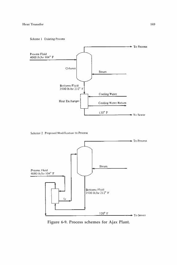
Heat Transfer 169
Figure 6-9. Process schemes for Ajax Plant.
Scheme 1 Existing Process
To Process
Process Fluid 4000 Ib/hr 104' F
Column Steam
Bottoms Fluid 3500 Ib/hr 2 12' F
Heat Exchanger
Cooling Water
Cooling Water Return
120' F To Sewer
Scheme 2 Proposed Modification t o Process
To Process
Process Fluid 4000 I b / h 104" F
tF
Steam
Bottoms Fluid 3500 Ib/hr 212' F
120' F To Sewer
170 Plant Engineers and Managers Guide to Energy Conservation
Plant operates 8760 hours/yr Steam cost $6.00/1000#
Note: To compute the cost for an exchanger of increased area, use the following approximation:
New cost = new are
original area0.6
× original price (6-19)
Analysis
The first analysis indicates that the hot bottom fluid can be used to heat the process fluid. The amount of heat supplied to the process fluid is
q = MCp ∆T = 3500 #/hr × 1(212 – 120) = 322,000 Btuh
30 psig = 30 + 14.7 = 44.7 psia steamFrom Steam Table 12-20, hfg = 928.6 Btu/#
Energy Savings of Stripper
322,000 Btuh #/hr of 30 psig steam saved = ——————— = 347 #/hr 928.6 Btu/#
$6.00 Steam savings = —— x 347 x 8760 = $18,237 1000
The temperature of the process fluid will rise to:
MCp ΔT process = 322,000 Btuh
Δt = 322,0004000 × 1 = 80°F
t f = 104 + 80 = 184°F.
The required area of heat exchanger will increase from Scheme 1
Heat Transfer 171
q = U0A ∆Tm = 100 A∆Tm = 32,00 (6-20)
ΔT m =212 – 184 – 120 – 104
log e212 – 184120 – 104
ΔT m = 82 – 16log e
2816
= 12log e 1.75 = 21.4
A = 322021.4 = 150.4 ft2
New installed cost = area newarea old
0.6× old price
= 150.450
0.6× $9000 = $17,400.
With an annual energy savings of $18,237, the investment in additional heat exchanger capacity is desirable.

173
7Reducing BuildingEnergy Losses
ENERGY LOSSES DUE TO HEAT LOSS AND HEAT GAIN
Depending on the time of year, a heat loss or a heat gain wastes energy. For example, a heat loss during the winter means wasted en-ergy in heating the building. Similarly, during the summer months, a heat gain means wasted energy in cooling the building. The building construction affects the heat loss and heat gain. Figure 7-1 illustrates the total heat gain of the building. The flow of heat is always from one temperature to a colder temperature. The heat loss of a building is il-lustrated by Figure 7-2. In this case, the building is considered the “hot body.” In the context of this book, heat loss refers to heating loads, while heat gain refers to cooling loads. By considering building materials and constructions, the associated heat loss and heat gain can be reduced. In this chapter, you will see how to apply handy building con-struction tables to solve most heat transfer problems, how substitutions of building materials saves energy, and how to apply different types of glass to save energy.
CONDUCTIVITY THROUGH BUILDING MATERIALS
The best conductors of heat are metals. Insulations such as wood, asbestos, cork, and felt are poor conductors. Conductance is widely used because many materials used in the construction of buildings are non-homogeneous. Table 7-1 should be used when the surface conductance, which is the transfer of heat from air to a surface, or from a surface to air, is
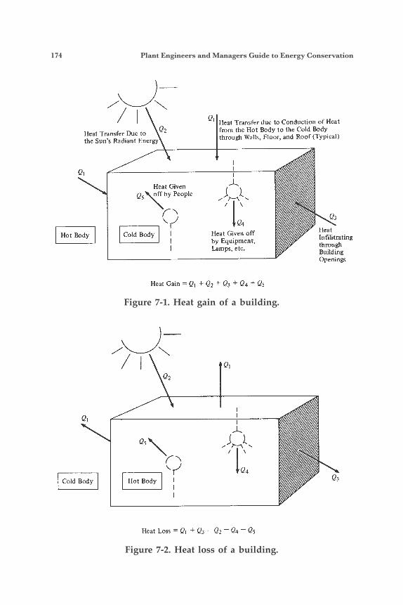
174 Plant Engineers and Managers Guide to Energy Conservation
Figure 7-1. Heat gain of a building.
Figure 7-2. Heat loss of a building.
Heat Transfer Due to Q2 the Sun’s Radiant Energy
QI
Heat Given Q~ off by People
Hot Body Cold Body
Heat Transfer due to Conduction of Heat from the Hot Body to the Cold Body through Walls, Floor, and Roof (Typical)
Q4 Heat Given off by Equipment, Lamps, etc.
Q3
Heat Infilitrating through Building Openings
Heat Gain = QI + Q, + Q3 + Q4 + Qs
Ql Qz
QI
Q5
Cold Body Hot Body Q4
Q3
Heat Loss = QI + Q3 - Qz - Q4 - Qs
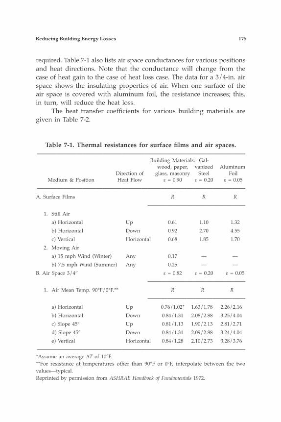
Reducing Building Energy Losses 175
required. Table 7-1 also lists air space conductances for various positions and heat directions. Note that the conductance will change from the case of heat gain to the case of heat loss case. The data for a 3/4-in. air space shows the insulating properties of air. When one surface of the air space is covered with aluminum foil, the resistance increases; this, in turn, will reduce the heat loss. The heat transfer coefficients for various building materials are given in Table 7-2.
Table 7-1. Thermal resistances for surface films and air spaces.———————————————————————————————— Building Materials: Gal- wood, paper, vanized Aluminum Direction of glass, masonry Steel Foil Medium & Position Heat Flow ε = 0.90 ε = 0.20 ε = 0.05————————————————————————————————A. Surface Films R R R ——————————————— 1. Still Air a) Horizontal Up 0.61 1.10 1.32 b) Horizontal Down 0.92 2.70 4.55 c) Vertical Horizontal 0.68 1.85 1.70 2. Moving Air a) 15 mph Wind (Winter) Any 0.17 — — b) 7.5 mph Wind (Summer) Any 0.25 — —B. Air Space 3/4” ε = 0.82 ε = 0.20 ε = 0.05 ——————————————— 1. Air Mean Temp. 90°F/0°F.** R R R ——————————————— a) Horizontal Up 0.76/1.02* 1.63/1.78 2.26/2.16 b) Horizontal Down 0.84/1.31 2.08/2.88 3.25/4.04 c) Slope 45° Up 0.81/1.13 1.90/2.13 2.81/2.71 d) Slope 45° Down 0.84/1.31 2.09/2.88 3.24/4.04 e) Vertical Horizontal 0.84/1.28 2.10/2.73 3.28/3.76————————————————————————————————*Assume an average ∆T of 10°F.**For resistance at temperatures other than 90°F or 0°F, interpolate between the two values—typical.Reprinted by permission from ASHRAE Handbook of Fundamentals 1972.
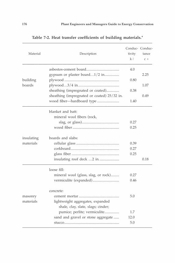
176 Plant Engineers and Managers Guide to Energy Conservation
Table 7-2. Heat transfer coefficients of building materials.*———————————————————————————————— Conduc- Conduc- Material Description tivity tance k# c +———————————————————————————————— asbestos-cement board .................................... 4.0 gypsum or plaster board…1/2 in. ............... 2.25building plywood ............................................................ 0.80boards plywood…3/4 in. ............................................ 1.07 sheathing (impregnated or coated) .............. 0.38 sheathing (impregnated or coated) 25/32 in. 0.49 wood fiber—hardboard type ........................ 1.40———————————————————————————————— blanket and batt: mineral wool fibers (rock, slag, or glass) ......................................... 0.27 wood fiber ................................................... 0.25
insulating boards and slabs:materials cellular glass ............................................... 0.39 corkboard ..................................................... 0.27 glass fiber .................................................... 0.25 insulating roof deck …2 in. ..................... 0.18———————————————————————————————— loose fill: mineral wool (glass, slag, or rock) ......... 0.27 vermiculite (expanded) ............................. 0.46
concrete:masonry cement mortar ............................................ 5.0materials lightweight aggregates, expanded shale, clay, slate, slags; cinder; pumice; perlite; vermiculite ................ 1.7 sand and gravel or stone aggregate ...... 12.0 stucco ............................................................ 5.0————————————————————————————————
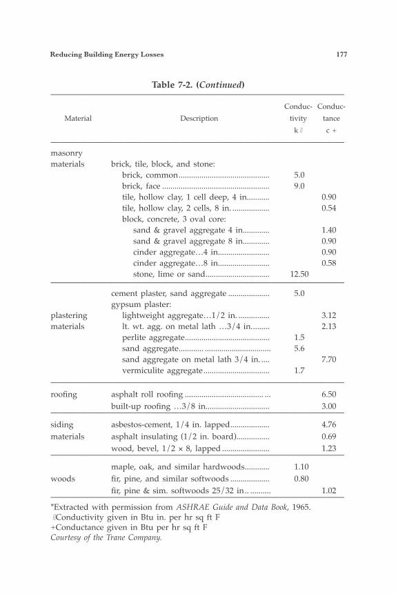
Reducing Building Energy Losses 177
Table 7-2. (Continued)———————————————————————————————— Conduc- Conduc- Material Description tivity tance k# c +————————————————————————————————masonrymaterials brick, tile, block, and stone: brick, common ............................................ 5.0 brick, face .................................................... 9.0 tile, hollow clay, 1 cell deep, 4 in. .......... 0.90 tile, hollow clay, 2 cells, 8 in. .................. 0.54 block, concrete, 3 oval core: sand & gravel aggregate 4 in............. 1.40 sand & gravel aggregate 8 in............. 0.90 cinder aggregate…4 in......................... 0.90 cinder aggregate…8 in......................... 0.58 stone, lime or sand ............................... 12.50———————————————————————————————— cement plaster, sand aggregate .................... 5.0 gypsum plaster:plastering lightweight aggregate…1/2 in. ............... 3.12materials lt. wt. agg. on metal lath …3/4 in. ........ 2.13 perlite aggregate ......................................... 1.5 sand aggregate ............ ................................ 5.6 sand aggregate on metal lath 3/4 in. .... 7.70 vermiculite aggregate ................................ 1.7————————————————————————————————roofing asphalt roll roofing ...................................... ... 6.50 built-up roofing …3/8 in............................... 3.00————————————————————————————————siding asbestos-cement, 1/4 in. lapped ................... 4.76materials asphalt insulating (1/2 in. board) ................ 0.69 wood, bevel, 1/2 × 8, lapped ....................... 1.23———————————————————————————————— maple, oak, and similar hardwoods ............ 1.10woods fir, pine, and similar softwoods ................... 0.80 fir, pine & sim. softwoods 25/32 in .. .......... 1.02————————————————————————————————*Extracted with permission from ASHRAE Guide and Data Book, 1965. #Conductivity given in Btu in. per hr sq ft F+Conductance given in Btu per hr sq ft FCourtesy of the Trane Company.
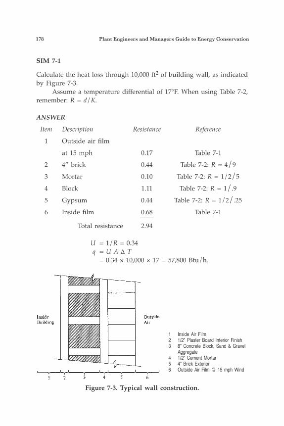
178 Plant Engineers and Managers Guide to Energy Conservation
SIM 7-1
Calculate the heat loss through 10,000 ft2 of building wall, as indicated by Figure 7-3. Assume a temperature differential of 17°F. When using Table 7-2, remember: R = d/K.
ANSWER
Item Description Resistance Reference
1 Outside air film
at 15 mph 0.17 Table 7-1
2 4” brick 0.44 Table 7-2: R = 4/9
3 Mortar 0.10 Table 7-2: R = 1/2/5
4 Block 1.11 Table 7-2: R = 1/.9
5 Gypsum 0.44 Table 7-2: R = 1/2/.25
6 Inside film 0.68 Table 7-1 —— Total resistance 2.94
U = 1/R = 0.34 q = U A ∆ T = 0.34 × 10,000 × 17 = 57,800 Btu/h.
Figure 7-3. Typical wall construction.
1 Inside Air Film2 1/2” Plaster Board Interior Finish3 8” Concrete Block, Sand & Gravel Aggregate4 1/2” Cement Mortar5 4” Brick Exterior6 Outside Air Film @ 15 mph Wind
Reducing Building Energy Losses 179
SIM 7-2In order to reduce the heat loss through the building wall, an engineer is recommending substituting cinder aggregate for the 8” concrete block wall. (Assume the structural considerations are the same.) Comment on the recommendation.
ANSWERThe conductance of the cinder aggregate concrete block wall is 0.58, as compared to 0.90; thus, the resistance will increase from 1.11 to 1.72. The effect is to increase the overall resistance of the wall to 3.54.
U = 1/R – 0.28q = 0.28 × 10,000 × 17 = 47,600 Btuh or 10,200 Btuh are saved with the change in wall construction. The total system should be evaluated from an energy conservation viewpoint.
SIM 7-3Calculate the heat gain during the summer for the construction of SIM 7-1.
ANSWERThe only item which changes is the outside air film resistance:
Item Description Resistance 1 Outside air film at 7-1/2 mps 0.25 Thus, total resistance = 3.02
1 U = —— = 0.3 3.02
q = 56,100 Btuh.
Handy Tables to Save Time Energy analysis of composite building constructions can be simpli-fied using Tables 7-3 through 7-13. These tables have been reprinted with the permission of ASHRAE and the Trane Company. To use them, simply find the column and row which describes the type of construction. The corresponding coefficient of transmission (conductance) is then found. Table 7-14 is another useful table which illustrates design tempera-tures for various cities in the United States.
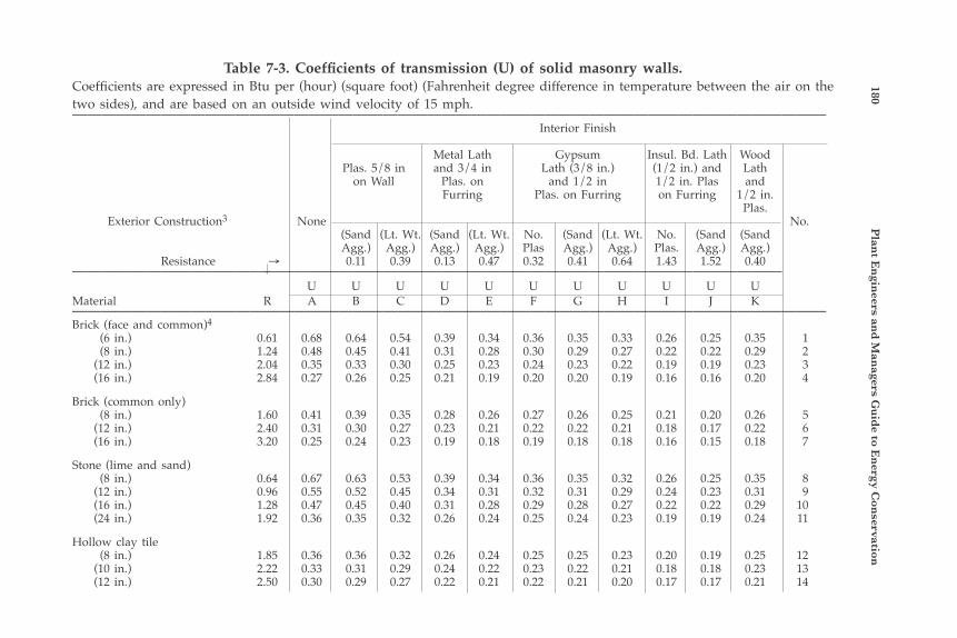
180 P
lant E
ngin
eers and
Man
agers Gu
ide to E
nergy C
onservation
Table 7-3. Coefficients of transmission (U) of solid masonry walls.Coefficients are expressed in Btu per (hour) (square foot) (Fahrenheit degree difference in temperature between the air on the two sides), and are based on an outside wind velocity of 15 mph.——————————————————————————————————————————————————— Interior Finish
Metal Lath Gypsum Insul. Bd. Lath Wood Plas. 5/8 in and 3/4 in Lath (3/8 in.) (1/2 in.) and Lath on Wall Plas. on and 1/2 in 1/2 in. Plas and Furring Plas. on Furring on Furring 1/2 in. Plas. Exterior Construction3 None No. (Sand (Lt. Wt. (Sand (Lt. Wt. No. (Sand (Lt. Wt. No. (Sand (Sand Agg.) Agg.) Agg.) Agg.) Plas Agg.) Agg.) Plas. Agg.) Agg.) Resistance → 0.11 0.39 0.13 0.47 0.32 0.41 0.64 1.43 1.52 0.40———————————————————————————————————————————————— U U U U U U U U U U UMaterial R A B C D E F G H I J K———————————————————————————————————————————————————Brick (face and common)4
(6 in.) 0.61 0.68 0.64 0.54 0.39 0.34 0.36 0.35 0.33 0.26 0.25 0.35 1 (8 in.) 1.24 0.48 0.45 0.41 0.31 0.28 0.30 0.29 0.27 0.22 0.22 0.29 2 (12 in.) 2.04 0.35 0.33 0.30 0.25 0.23 0.24 0.23 0.22 0.19 0.19 0.23 3 (16 in.) 2.84 0.27 0.26 0.25 0.21 0.19 0.20 0.20 0.19 0.16 0.16 0.20 4
Brick (common only) (8 in.) 1.60 0.41 0.39 0.35 0.28 0.26 0.27 0.26 0.25 0.21 0.20 0.26 5 (12 in.) 2.40 0.31 0.30 0.27 0.23 0.21 0.22 0.22 0.21 0.18 0.17 0.22 6 (16 in.) 3.20 0.25 0.24 0.23 0.19 0.18 0.19 0.18 0.18 0.16 0.15 0.18 7
Stone (lime and sand) (8 in.) 0.64 0.67 0.63 0.53 0.39 0.34 0.36 0.35 0.32 0.26 0.25 0.35 8 (12 in.) 0.96 0.55 0.52 0.45 0.34 0.31 0.32 0.31 0.29 0.24 0.23 0.31 9 (16 in.) 1.28 0.47 0.45 0.40 0.31 0.28 0.29 0.28 0.27 0.22 0.22 0.29 10 (24 in.) 1.92 0.36 0.35 0.32 0.26 0.24 0.25 0.24 0.23 0.19 0.19 0.24 11
Hollow clay tile (8 in.) 1.85 0.36 0.36 0.32 0.26 0.24 0.25 0.25 0.23 0.20 0.19 0.25 12 (10 in.) 2.22 0.33 0.31 0.29 0.24 0.22 0.23 0.22 0.21 0.18 0.18 0.23 13 (12 in.) 2.50 0.30 0.29 0.27 0.22 0.21 0.22 0.21 0.20 0.17 0.17 0.21 14
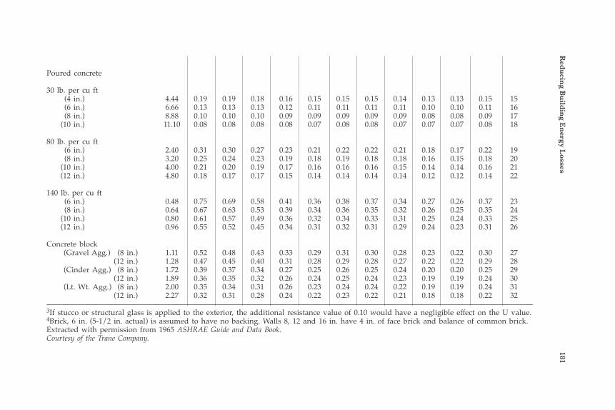
Red
ucin
g Bu
ildin
g En
ergy Losses
181
Poured concrete
30 lb. per cu ft (4 in.) 4.44 0.19 0.19 0.18 0.16 0.15 0.15 0.15 0.14 0.13 0.13 0.15 15 (6 in.) 6.66 0.13 0.13 0.13 0.12 0.11 0.11 0.11 0.11 0.10 0.10 0.11 16 (8 in.) 8.88 0.10 0.10 0.10 0.09 0.09 0.09 0.09 0.09 0.08 0.08 0.09 17 (10 in.) 11.10 0.08 0.08 0.08 0.08 0.07 0.08 0.08 0.07 0.07 0.07 0.08 18
80 lb. per cu ft (6 in.) 2.40 0.31 0.30 0.27 0.23 0.21 0.22 0.22 0.21 0.18 0.17 0.22 19 (8 in.) 3.20 0.25 0.24 0.23 0.19 0.18 0.19 0.18 0.18 0.16 0.15 0.18 20 (10 in.) 4.00 0.21 0.20 0.19 0.17 0.16 0.16 0.16 0.15 0.14 0.14 0.16 21 (12 in.) 4.80 0.18 0.17 0.17 0.15 0.14 0.14 0.14 0.14 0.12 0.12 0.14 22
140 lb. per cu ft (6 in.) 0.48 0.75 0.69 0.58 0.41 0.36 0.38 0.37 0.34 0.27 0.26 0.37 23 (8 in.) 0.64 0.67 0.63 0.53 0.39 0.34 0.36 0.35 0.32 0.26 0.25 0.35 24 (10 in.) 0.80 0.61 0.57 0.49 0.36 0.32 0.34 0.33 0.31 0.25 0.24 0.33 25 (12 in.) 0.96 0.55 0.52 0.45 0.34 0.31 0.32 0.31 0.29 0.24 0.23 0.31 26
Concrete block (Gravel Agg.) (8 in.) 1.11 0.52 0.48 0.43 0.33 0.29 0.31 0.30 0.28 0.23 0.22 0.30 27 (12 in.) 1.28 0.47 0.45 0.40 0.31 0.28 0.29 0.28 0.27 0.22 0.22 0.29 28 (Cinder Agg.) (8 in.) 1.72 0.39 0.37 0.34 0.27 0.25 0.26 0.25 0.24 0.20 0.20 0.25 29 (12 in.) 1.89 0.36 0.35 0.32 0.26 0.24 0.25 0.24 0.23 0.19 0.19 0.24 30 (Lt. Wt. Agg.) (8 in.) 2.00 0.35 0.34 0.31 0.26 0.23 0.24 0.24 0.22 0.19 0.19 0.24 31 (12 in.) 2.27 0.32 0.31 0.28 0.24 0.22 0.23 0.22 0.21 0.18 0.18 0.22 32————————————————————————————————————————————————————————————————3If stucco or structural glass is applied to the exterior, the additional resistance value of 0.10 would have a negligible effect on the U value.4Brick, 6 in. (5-1/2 in. actual) is assumed to have no backing. Walls 8, 12 and 16 in. have 4 in. of face brick and balance of common brick.Extracted with permission from 1965 ASHRAE Guide and Data Book.Courtesy of the Trane Company.
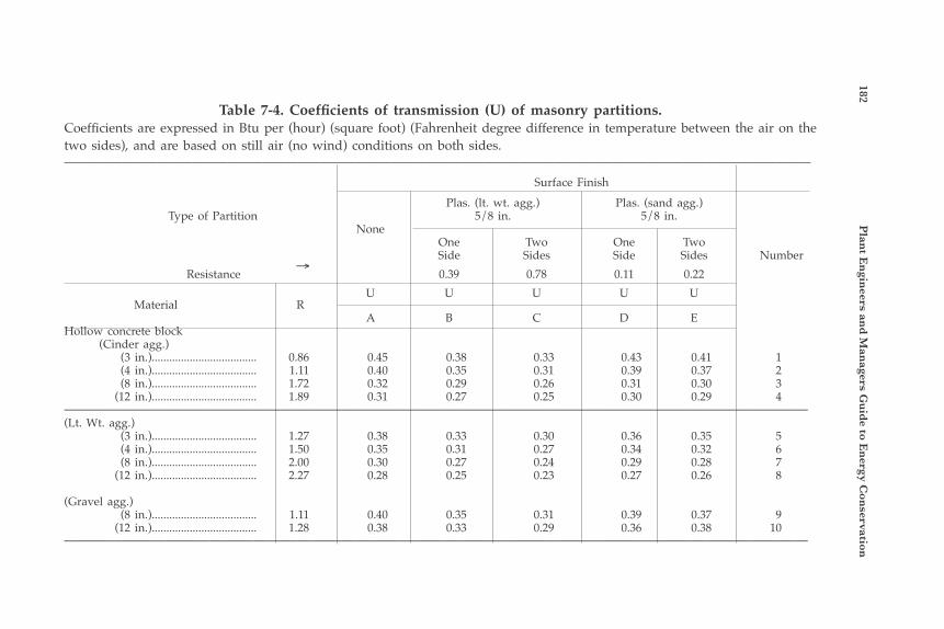
182 P
lant E
ngin
eers and
Man
agers Gu
ide to E
nergy C
onservation
Table 7-4. Coefficients of transmission (U) of masonry partitions.Coefficients are expressed in Btu per (hour) (square foot) (Fahrenheit degree difference in temperature between the air on the two sides), and are based on still air (no wind) conditions on both sides.————————————————————————————————————————————————————————————————
Surface Finish
Plas. (lt. wt. agg.) Plas. (sand agg.) Type of Partition 5/8 in. 5/8 in. None One Two One Two Side Sides Side Sides Number Resistance 0.39 0.78 0.11 0.22 U U U U U Material R A B C D EHollow concrete block (Cinder agg.) (3 in.).................................... 0.86 0.45 0.38 0.33 0.43 0.41 1 (4 in.).................................... 1.11 0.40 0.35 0.31 0.39 0.37 2 (8 in.).................................... 1.72 0.32 0.29 0.26 0.31 0.30 3 (12 in.).................................... 1.89 0.31 0.27 0.25 0.30 0.29 4———————————————————————————————————————————————————(Lt. Wt. agg.) (3 in.).................................... 1.27 0.38 0.33 0.30 0.36 0.35 5 (4 in.).................................... 1.50 0.35 0.31 0.27 0.34 0.32 6 (8 in.).................................... 2.00 0.30 0.27 0.24 0.29 0.28 7 (12 in.).................................... 2.27 0.28 0.25 0.23 0.27 0.26 8
(Gravel agg.) (8 in.).................................... 1.11 0.40 0.35 0.31 0.39 0.37 9 (12 in.).................................... 1.28 0.38 0.33 0.29 0.36 0.38 10———————————————————————————————————————————————————
↑
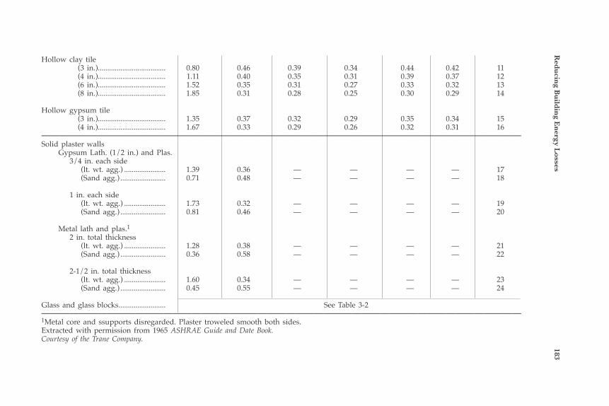
Red
ucin
g Bu
ildin
g En
ergy Losses
183Hollow clay tile (3 in.).................................... 0.80 0.46 0.39 0.34 0.44 0.42 11 (4 in.).................................... 1.11 0.40 0.35 0.31 0.39 0.37 12 (6 in.).................................... 1.52 0.35 0.31 0.27 0.33 0.32 13 (8 in.).................................... 1.85 0.31 0.28 0.25 0.30 0.29 14
Hollow gypsum tile (3 in.).................................... 1.35 0.37 0.32 0.29 0.35 0.34 15 (4 in.).................................... 1.67 0.33 0.29 0.26 0.32 0.31 16———————————————————————————————————————————————————Solid plaster walls Gypsum Lath. (1/2 in.) and Plas. 3/4 in. each side (lt. wt. agg.) ...................... 1.39 0.36 — — — — 17 (Sand agg.) ........................ 0.71 0.48 — — — — 18
1 in. each side (lt. wt. agg.) ...................... 1.73 0.32 — — — — 19 (Sand agg.) ........................ 0.81 0.46 — — — — 20
Metal lath and plas.1 2 in. total thickness (lt. wt. agg.) ...................... 1.28 0.38 — — — — 21 (Sand agg.) ........................ 0.36 0.58 — — — — 22
2-1/2 in. total thickness (lt. wt. agg.) ...................... 1.60 0.34 — — — — 23 (Sand agg.) ........................ 0.45 0.55 — — — — 24
Glass and glass blocks ......................... See Table 3-2———————————————————————————————————————————————————1Metal core and ssupports disregarded. Plaster troweled smooth both sides.Extracted with permission from 1965 ASHRAE Guide and Date Book.Courtesy of the Trane Company.
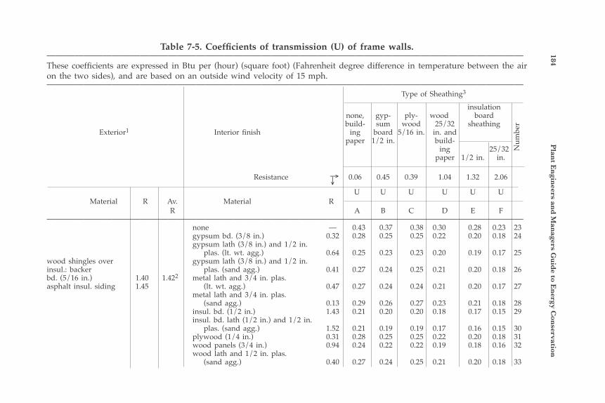
184 P
lant E
ngin
eers and
Man
agers Gu
ide to E
nergy C
onservation
Table 7-5. Coefficients of transmission (U) of frame walls.———————————————————————————————————————————————————These coefficients are expressed in Btu per (hour) (square foot) (Fahrenheit degree difference in temperature between the air on the two sides), and are based on an outside wind velocity of 15 mph.——————————————————————————————————————————————————— Type of Sheathing3
insulation none, gyp- ply- wood board build- sum wood 25/32 sheathing Exterior1 Interior finish ing board 5/16 in. in. and paper 1/2 in. build- ing 25/32 paper 1/2 in. in.
Resistance 0.06 0.45 0.39 1.04 1.32 2.06
U U U U U U Material R Av. Material R R A B C D E F——————————————————————————————————————————————————— none — 0.43 0.37 0.38 0.30 0.28 0.23 23 gypsum bd. (3/8 in.) 0.32 0.28 0.25 0.25 0.22 0.20 0.18 24 gypsum lath (3/8 in.) and 1/2 in. plas. (lt. wt. agg.) 0.64 0.25 0.23 0.23 0.20 0.19 0.17 25wood shingles over gypsum lath (3/8 in.) and 1/2 in.insul.: backer plas. (sand agg.) 0.41 0.27 0.24 0.25 0.21 0.20 0.18 26bd. (5/16 in.) 1.40 1.422 metal lath and 3/4 in. plas.asphalt insul. siding 1.45 (lt. wt. agg.) 0.47 0.27 0.24 0.24 0.21 0.20 0.17 27 metal lath and 3/4 in. plas. (sand agg.) 0.13 0.29 0.26 0.27 0.23 0.21 0.18 28 insul. bd. (1/2 in.) 1.43 0.21 0.20 0.20 0.18 0.17 0.15 29 insul. bd. lath (1/2 in.) and 1/2 in. plas. (sand agg.) 1.52 0.21 0.19 0.19 0.17 0.16 0.15 30 plywood (1/4 in.) 0.31 0.28 0.25 0.25 0.22 0.20 0.18 31 wood panels (3/4 in.) 0.94 0.24 0.22 0.22 0.19 0.18 0.16 32 wood lath and 1/2 in. plas. (sand agg.) 0.40 0.27 0.24 0.25 0.21 0.20 0.18 33
Num
ber
↑→
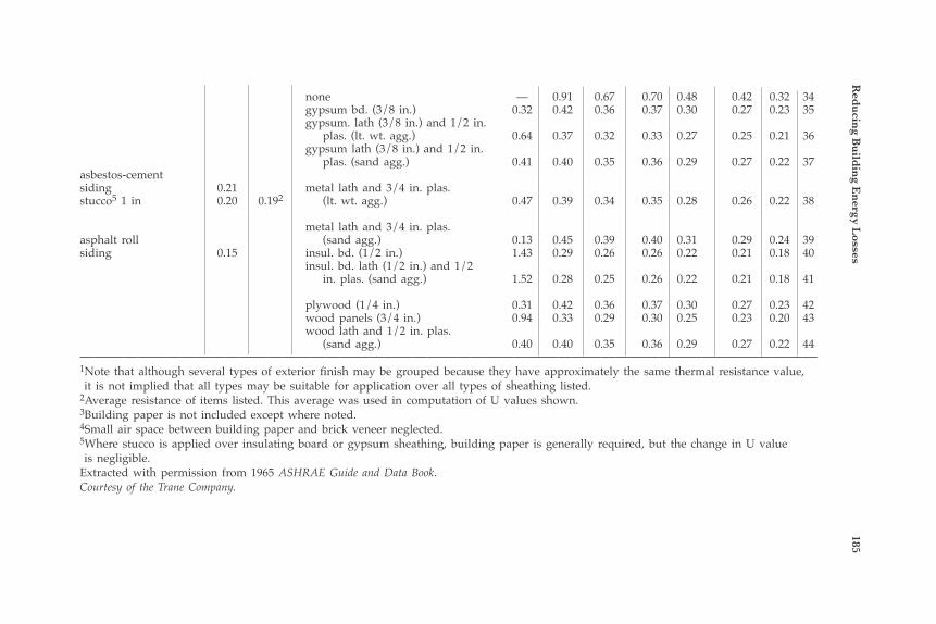
Red
ucin
g Bu
ildin
g En
ergy Losses
185 none — 0.91 0.67 0.70 0.48 0.42 0.32 34 gypsum bd. (3/8 in.) 0.32 0.42 0.36 0.37 0.30 0.27 0.23 35 gypsum. lath (3/8 in.) and 1/2 in. plas. (lt. wt. agg.) 0.64 0.37 0.32 0.33 0.27 0.25 0.21 36 gypsum lath (3/8 in.) and 1/2 in. plas. (sand agg.) 0.41 0.40 0.35 0.36 0.29 0.27 0.22 37asbestos-cementsiding 0.21 metal lath and 3/4 in. plas.stucco5 1 in 0.20 0.192 (lt. wt. agg.) 0.47 0.39 0.34 0.35 0.28 0.26 0.22 38
metal lath and 3/4 in. plas.asphalt roll (sand agg.) 0.13 0.45 0.39 0.40 0.31 0.29 0.24 39siding 0.15 insul. bd. (1/2 in.) 1.43 0.29 0.26 0.26 0.22 0.21 0.18 40 insul. bd. lath (1/2 in.) and 1/2 in. plas. (sand agg.) 1.52 0.28 0.25 0.26 0.22 0.21 0.18 41
plywood (1/4 in.) 0.31 0.42 0.36 0.37 0.30 0.27 0.23 42 wood panels (3/4 in.) 0.94 0.33 0.29 0.30 0.25 0.23 0.20 43 wood lath and 1/2 in. plas. (sand agg.) 0.40 0.40 0.35 0.36 0.29 0.27 0.22 44———————————————————————————————————————————————————1Note that although several types of exterior finish may be grouped because they have approximately the same thermal resistance value, it is not implied that all types may be suitable for application over all types of sheathing listed.2Average resistance of items listed. This average was used in computation of U values shown.3Building paper is not included except where noted.4Small air space between building paper and brick veneer neglected.5Where stucco is applied over insulating board or gypsum sheathing, building paper is generally required, but the change in U value is negligible.Extracted with permission from 1965 ASHRAE Guide and Data Book.Courtesy of the Trane Company.
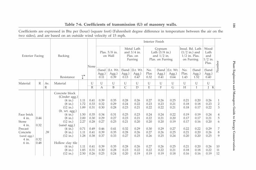
186 P
lant E
ngin
eers and
Man
agers Gu
ide to E
nergy C
onservation
Table 7-6. Coefficients of transmission (U) of masonry walls.————————————————————————————————————————————————————————————————Coefficients are expressed in Btu per (hour) (square foot) (Fahrenheit degree difference in temperature between the air on the two sides), and are based on an outside wind velocity of 15 mph.———————————————————————————————————————————————————————————————— Interior Finish
Metal Lath Gypsum Insul. Bd. Lath Wood Plas. 5/8 in. and 3/4 in. Lath (3/8 in.) (1/2 in.) and Lath Exterior Facing Backing on Wall Plas. on and 1/2 in. 1/2 in. Plas. and Furring Plas. on Furring on Furring 1/2 in. Plas. None (Sand (Lt. Wt. (Sand (Lt. Wt. No. (Sand (Lt. Wt. No. (Sand (Sand Agg.) Agg.) Agg.) Agg.) Plas Agg.) Agg.) Plas. Agg.) Agg.) Resistance 0.11 0.39 0.13 0.47 0.32 0.41 0.64 1.43 1.52 0.40——————————————————————————————————————————————————————————————Material R Av. Material U U U U U U U U U U U R R A B C D E F G H I J K———————————————————————————————————————————————————————————————— Concrete block (Cinder agg.) (4 in.) 1.11 0.41 0.39 0.35 0.28 0.26 0.27 0.26 0.25 0.21 0.20 0.26 1 (8 in.) 1.72 0.33 0.32 0.29 0.24 0.22 0.23 0.23 0.21 0.18 0.18 0.23 2 (12 in.) 1.89 0.31 0.30 0.28 0.23 0.21 0.22 0.22 0.21 0.18 0.17 0.22 3 (lt. wt. agg.)Face brick (4 in.) 1.50 0.35 0.34 0.31 0.25 0.23 0.24 0.24 0.22 0.19 0.19 0.24 4 4 in. 0.44 (8 in.) 2.00 0.30 0.29 0.27 0.23 0.21 0.22 0.21 0.20 0.17 0.17 0.21 5Stone (12 in.) 2.27 0.28 0.27 0.25 0.21 0.20 0.20 0.20 0.19 0.17 0.16 0.20 6 4 in. 0.32 (sand agg.)Precast (4 in.) 0.71 0.49 0.46 0.41 0.32 0.29 0.30 0.29 0.27 0.22 0.22 0.29 7Concrete .39 (8 in.) 1.11 0.41 0.39 0.35 0.28 0.26 0.27 0.26 0.25 0.21 0.20 0.26 8 (sand agg.) (12 in.) 1.28 0.38 0.37 0.33 0.27 0.25 0.26 0.25 0.24 0.20 0.20 0.25 9 4 in. 0.32 6 in. 0.48 Hollow clay tile (4 in.) 1.11 0.41 0.39 0.35 0.28 0.26 0.27 0.26 0.25 0.21 0.20 0.26 10 (8 in.) 1.85 0.31 0.30 0.28 0.23 0.22 0.22 0.22 0.21 0.18 0.18 0.22 11 (12 in.) 2.50 0.26 0.25 0.24 0.20 0.19 0.19 0.19 0.18 0.16 0.16 0.19 12
Num
ber
↑→
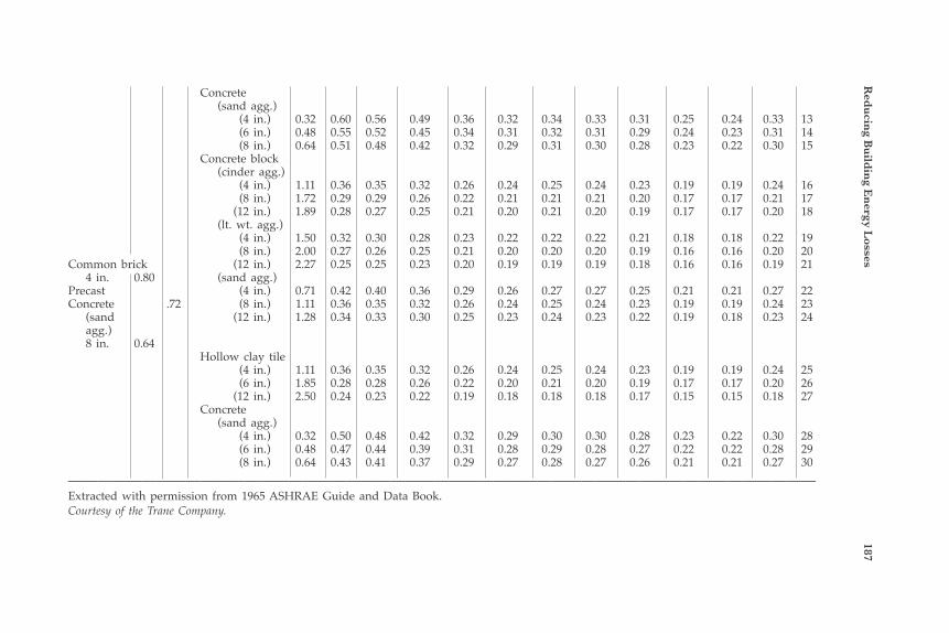
Red
ucin
g Bu
ildin
g En
ergy Losses
187 Concrete (sand agg.) (4 in.) 0.32 0.60 0.56 0.49 0.36 0.32 0.34 0.33 0.31 0.25 0.24 0.33 13 (6 in.) 0.48 0.55 0.52 0.45 0.34 0.31 0.32 0.31 0.29 0.24 0.23 0.31 14 (8 in.) 0.64 0.51 0.48 0.42 0.32 0.29 0.31 0.30 0.28 0.23 0.22 0.30 15 Concrete block (cinder agg.) (4 in.) 1.11 0.36 0.35 0.32 0.26 0.24 0.25 0.24 0.23 0.19 0.19 0.24 16 (8 in.) 1.72 0.29 0.29 0.26 0.22 0.21 0.21 0.21 0.20 0.17 0.17 0.21 17 (12 in.) 1.89 0.28 0.27 0.25 0.21 0.20 0.21 0.20 0.19 0.17 0.17 0.20 18 (lt. wt. agg.) (4 in.) 1.50 0.32 0.30 0.28 0.23 0.22 0.22 0.22 0.21 0.18 0.18 0.22 19 (8 in.) 2.00 0.27 0.26 0.25 0.21 0.20 0.20 0.20 0.19 0.16 0.16 0.20 20Common brick (12 in.) 2.27 0.25 0.25 0.23 0.20 0.19 0.19 0.19 0.18 0.16 0.16 0.19 21 4 in. 0.80 (sand agg.)Precast (4 in.) 0.71 0.42 0.40 0.36 0.29 0.26 0.27 0.27 0.25 0.21 0.21 0.27 22Concrete .72 (8 in.) 1.11 0.36 0.35 0.32 0.26 0.24 0.25 0.24 0.23 0.19 0.19 0.24 23 (sand (12 in.) 1.28 0.34 0.33 0.30 0.25 0.23 0.24 0.23 0.22 0.19 0.18 0.23 24 agg.) 8 in. 0.64 Hollow clay tile (4 in.) 1.11 0.36 0.35 0.32 0.26 0.24 0.25 0.24 0.23 0.19 0.19 0.24 25 (6 in.) 1.85 0.28 0.28 0.26 0.22 0.20 0.21 0.20 0.19 0.17 0.17 0.20 26 (12 in.) 2.50 0.24 0.23 0.22 0.19 0.18 0.18 0.18 0.17 0.15 0.15 0.18 27 Concrete (sand agg.) (4 in.) 0.32 0.50 0.48 0.42 0.32 0.29 0.30 0.30 0.28 0.23 0.22 0.30 28 (6 in.) 0.48 0.47 0.44 0.39 0.31 0.28 0.29 0.28 0.27 0.22 0.22 0.28 29 (8 in.) 0.64 0.43 0.41 0.37 0.29 0.27 0.28 0.27 0.26 0.21 0.21 0.27 30———————————————————————————————————————————————————Extracted with permission from 1965 ASHRAE Guide and Data Book.Courtesy of the Trane Company.
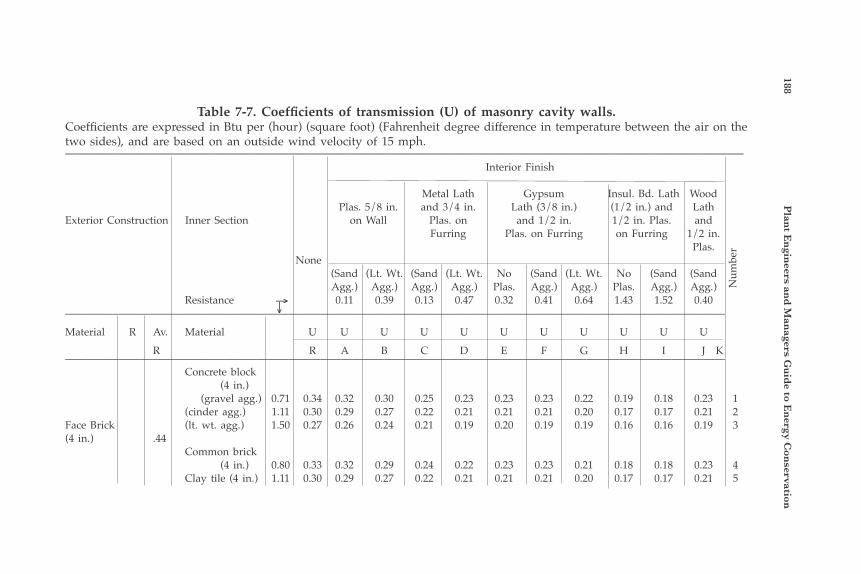
188 P
lant E
ngin
eers and
Man
agers Gu
ide to E
nergy C
onservation
Table 7-7. Coefficients of transmission (U) of masonry cavity walls.Coefficients are expressed in Btu per (hour) (square foot) (Fahrenheit degree difference in temperature between the air on the two sides), and are based on an outside wind velocity of 15 mph.——————————————————————————————————————————————————— Interior Finish
Metal Lath Gypsum Insul. Bd. Lath Wood Plas. 5/8 in. and 3/4 in. Lath (3/8 in.) (1/2 in.) and Lath Exterior Construction Inner Section on Wall Plas. on and 1/2 in. 1/2 in. Plas. and Furring Plas. on Furring on Furring 1/2 in. Plas. None (Sand (Lt. Wt. (Sand (Lt. Wt. No (Sand (Lt. Wt. No (Sand (Sand Agg.) Agg.) Agg.) Agg.) Plas. Agg.) Agg.) Plas. Agg.) Agg.) Resistance 0.11 0.39 0.13 0.47 0.32 0.41 0.64 1.43 1.52 0.40——————————————————————————————————————————————————————————————
Material R Av. Material U U U U U U U U U U U
R R A B C D E F G H I J K—————————————————————————————————————————————————————————————— Concrete block (4 in.) (gravel agg.) 0.71 0.34 0.32 0.30 0.25 0.23 0.23 0.23 0.22 0.19 0.18 0.23 1 (cinder agg.) 1.11 0.30 0.29 0.27 0.22 0.21 0.21 0.21 0.20 0.17 0.17 0.21 2Face Brick (lt. wt. agg.) 1.50 0.27 0.26 0.24 0.21 0.19 0.20 0.19 0.19 0.16 0.16 0.19 3(4 in.) .44 Common brick (4 in.) 0.80 0.33 0.32 0.29 0.24 0.22 0.23 0.23 0.21 0.18 0.18 0.23 4 Clay tile (4 in.) 1.11 0.30 0.29 0.27 0.22 0.21 0.21 0.21 0.20 0.17 0.17 0.21 5
Num
ber
↑→
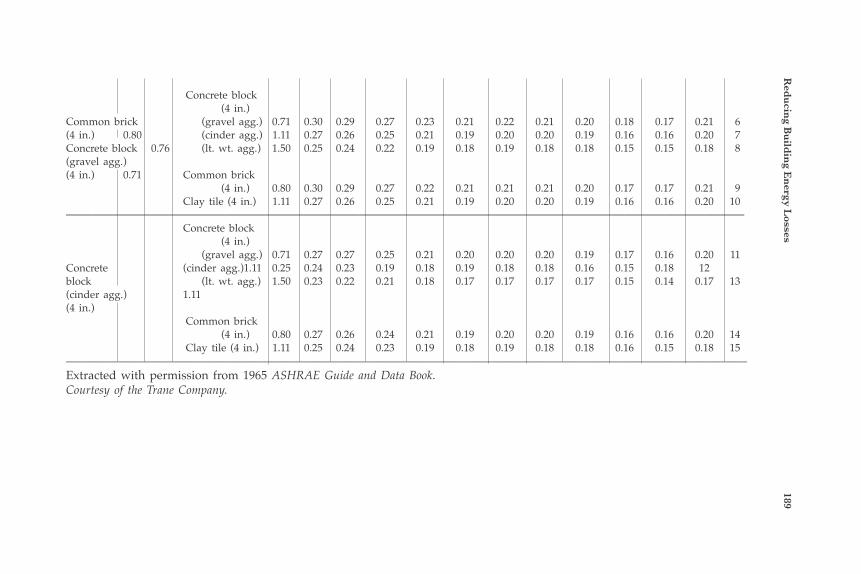
Red
ucin
g Bu
ildin
g En
ergy Losses
189
Concrete block (4 in.)Common brick (gravel agg.) 0.71 0.30 0.29 0.27 0.23 0.21 0.22 0.21 0.20 0.18 0.17 0.21 6(4 in.) 0.80 (cinder agg.) 1.11 0.27 0.26 0.25 0.21 0.19 0.20 0.20 0.19 0.16 0.16 0.20 7Concrete block 0.76 (lt. wt. agg.) 1.50 0.25 0.24 0.22 0.19 0.18 0.19 0.18 0.18 0.15 0.15 0.18 8(gravel agg.)(4 in.) 0.71 Common brick (4 in.) 0.80 0.30 0.29 0.27 0.22 0.21 0.21 0.21 0.20 0.17 0.17 0.21 9 Clay tile (4 in.) 1.11 0.27 0.26 0.25 0.21 0.19 0.20 0.20 0.19 0.16 0.16 0.20 10——————————————————————————————————————————————————— Concrete block (4 in.) (gravel agg.) 0.71 0.27 0.27 0.25 0.21 0.20 0.20 0.20 0.19 0.17 0.16 0.20 11Concrete (cinder agg.) 1.11 0.25 0.24 0.23 0.19 0.18 0.19 0.18 0.18 0.16 0.15 0.18 12block (lt. wt. agg.) 1.50 0.23 0.22 0.21 0.18 0.17 0.17 0.17 0.17 0.15 0.14 0.17 13(cinder agg.) 1.11(4 in.) Common brick (4 in.) 0.80 0.27 0.26 0.24 0.21 0.19 0.20 0.20 0.19 0.16 0.16 0.20 14 Clay tile (4 in.) 1.11 0.25 0.24 0.23 0.19 0.18 0.19 0.18 0.18 0.16 0.15 0.18 15————————————————————————————————————————————————————————————————Extracted with permission from 1965 ASHRAE Guide and Data Book.Courtesy of the Trane Company.
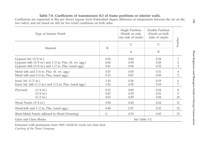
190 P
lant E
ngin
eers and
Man
agers Gu
ide to E
nergy C
onservation
Table 7-8. Coefficients of transmission (U) of frame partitions or interior walls.Coefficients are expressed in Btu per (hour) (square foot) (Fahrenheit degree difference in temperature between the air on the two sides), and are based on still air (no wind) conditions on both sides.——————————————————————————————————————————————————— Single Partition Double Partition Type of Interior Finish (Finish on only (Finish on both one side of studs) sides of studs) ———————————————————————————————————————————————— U U Material R A B ———————————————————————————————————————————————————Gypsum bd. (3/8 in.) 0.32 0.60 0.34 1Gypsum lath (3/8 in.) and 1/2 in. Plas. (lt. wt. agg.) 0.64 0.50 0.28 2Gypsum lath (3/8 in.) and 1/2 in. Plas. (sand agg.) 0.41 0.56 0.32 3———————————————————————————————————————————————————Metal lath and 3/4 in. Plas. (lt. wt. agg.) 0.47 0.55 0.31 4Metal lath and 3/4 in. Plas. (sand agg.) 0.13 0.67 0.39 5———————————————————————————————————————————————————Insul. bd. (1/2 in.) 1.43 0.36 0.19 6Insul. bd. lath (1/2 in.) and 1/2 in. Plas. (sand agg.) 1.52 0.35 0.19 7———————————————————————————————————————————————————Plywood: (1/4 in.) 0.31 0.60 0.34 8 (3/8 in.) 0.47 0.55 0.31 9 (1/2 in.) 0.63 0.50 0.28 10———————————————————————————————————————————————————Wood Panels (3/4 in.) 0.94 0.43 0.24 11———————————————————————————————————————————————————Wood-lath and 1/2 in. Plas. (sand agg.) 0.40 0.57 0.32 12———————————————————————————————————————————————————Sheet-Metal Panels adhered to Wood (Framing) 0 0.74 0.43 13———————————————————————————————————————————————————Glass and Glass Blocks See Table 3-2———————————————————————————————————————————————————Extracted with permission from 1965 ASHRAE Guide and Data Book.Courtesy of the Trane Company.
Num
ber
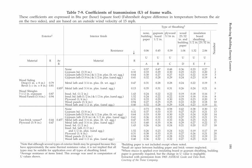
Red
ucin
g Bu
ildin
g En
ergy Losses
191
3Building paper is not included except where noted.4Small air space between building paper and brick veneer neglected.5Where stucco is applied over insulating board or gypsum sheathing, building paper is generally required, but the change in U value is negligible.Extracted with permission from 1965 ASHRAE Guide and Data Book.Courtesy of the Trane Company.
Table 7-9. Coefficients of transmission (U) of frame walls.These coefficients are expressed in Btu per (hour) (square foot) (Fahrenheit degree difference in temperature between the air on the two sides), and are based on an outside wind velocity of 15 mph.——————————————————————————————————————————————————— Type of Sheathing3
none, gupsum plywood wood insulation Exterior1 Interior finish building board 5/16 in. 25/32 board paper 1/2 in. in. and sheathing building 1/2 in. 25/32 in. paper
Resistance 0.06 0.45 0.39 1.04 1.32 2.06
U U U U U U Material R Av Material R R A B C D E F————————————————————————————————————————————————— None — 0.57 0.47 0.48 0.36 0.33 0.27 1 Gypsum bd. (3/8 in.) 0.32 0.33 0.29 0.30 0.25 0.23 0.20 2 Gypsum lath (3/8 in.) & 1/2 in. plas. (lt. wt. agg.) 0.64 0.30 0.27 0.27 0.23 0.22 0.19 3 Gypsum lath (3/8 in.) & 1/2 in. plas. (sand agg.) 0.41 0.32 0.28 0.29 0.24 0.23 0.19 4Wood Siding Drop-(1 in. × 8 in.) 0.79 Metal lath and 3/4 in. plas. (lt. wt. agg.) 0.47 0.31 0.28 0.28 0.24 0.22 0.19 5 Bevel (1/2 in. × 8 in.) 0.81 0.852 Metal lath and 3/4 in. plas. (sand. agg.) 0.13 0.35 0.31 0.31 0.26 0.24 0.21 6Wood Shingles 7-1/2 in. exposure 0.87 Insul. bd. (1/2 in.) 1.43 0.24 0.22 0.22 0.19 0.18 0.16 7Wood Panels (3/4 in.) 0.94 Insul. bd. lath (1/2 in.) & 1/2 in. plas. (sand agg.) 1.52 0.24 0.22 0.22 0.19 0.18 0.16 8 Plywood (1/4 in.) 0.31 0.33 0.29 0.30 0.25 0.23 0.20 9 Wood panels (3/4 in.) 0.94 0.27 0.25 0.25 0.22 0.20 0.18 10 Wood lath and 1/2 in. plas. (sand agg.) 0.40 0.32 0.28 0.29 0.24 0.23 0.19 11——————————————————————————————————————————————————— None — 0.73 0.56 0.58 0.42 0.38 0.30 12 Gypsum bd. (3/8 in.) 0.32 0.37 0.33 0.33 0.27 0.25 0.21 13 Gypsum lath (3/8 in.) & 1/2 in. plas. (lt. wt. agg) 0.64 0.33 0.30 0.30 0.25 0.24 0.20 14 Gypsum lath (3/8 in.) & 1/2 in. plas. (sand agg.) 0.41 0.36 0.32 0.32 0.27 0.25 0.21 15Face-brick veneer4 0.44 0.452 Metal lath and 3/4 in. plas. (lt. wt. agg.) 0.47 0.35 0.31 0.32 0.26 0.25 0.21 16Plywood (3/8 in.) 0.47 Metal lath and 3/4 in. plas. (sand agg.) 0.13 0.40 0.35 0.36 0.29 0.27 0.22 17 Insul. bd. (1/2 in.) 1.43 0.26 0.24 0.24 0.21 0.20 0.17 18 Insul. bd. lath (1/2 in.) and 1/2 in. plas. (sand agg.) 1.52 0.26 0.23 0.24 0.21 0.19 0.17 19 Plywood (1/4 in.) 0.31 0.38 0.33 0.33 0.27 0.26 0.21 20 Wood panels (3/4 in.) 0.94 0.30 0.27 0.28 0.23 0.22 0.19 21 Wood lath and 1/2 in. plas. (sand agg.) 0.40 0.36 0.32 0.32 0.27 0.25 0.21 22
Num
ber
1Note that although several types of exterior finish may be grouped because they have approximately the same thermal resistance value, it is not implied that all types may be suitable for application over all types of sheathing listed.2Average resistance of items listed. This average was used in computation of U values shown.
→
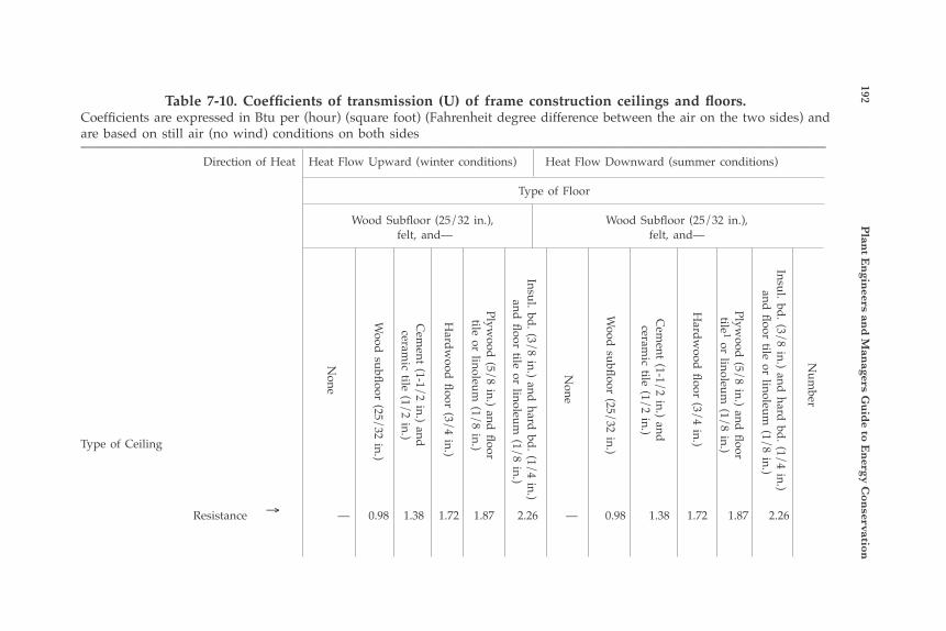
192 P
lant E
ngin
eers and
Man
agers Gu
ide to E
nergy C
onservation
Table 7-10. Coefficients of transmission (U) of frame construction ceilings and floors.Coefficients are expressed in Btu per (hour) (square foot) (Fahrenheit degree difference between the air on the two sides) and are based on still air (no wind) conditions on both sides——————————————————————————————————————————————————— Direction of Heat Heat Flow Upward (winter conditions) Heat Flow Downward (summer conditions)
Type of Floor
Wood Subfloor (25/32 in.), Wood Subfloor (25/32 in.), felt, and— felt, and—
Type of Ceiling
Resistance — 0.98 1.38 1.72 1.87 2.26 — 0.98 1.38 1.72 1.87 2.26
↑
Num
ber
Insul. bd. (3/8 in.) and hard bd. (1/4 in.) and floor tile or linoleum
(1/8 in.)
Plywood (5/8 in.) and floor
tile 1 or linoleum (1/8 in.)
Hardw
ood floor (3/4 in.)
Cem
ent (1-1/2 in.) andceram
ic tile (1/2 in.)
Wood subfloor (25/32 in.)
None
Insul. bd. (3/8 in.) and hard bd. (1/4 in.) and floor tile or linoleum
(1/8 in.)
Plywood (5/8 in.) and floor
tile or linoleum (1/8 in.)
Hardw
ood floor (3/4 in.)
Cem
ent (1-1/2 in.) andceram
ic tile (1/2 in.)
Wood subfloor (25/32 in.)
None
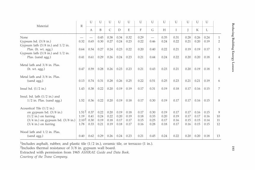
Red
ucin
g Bu
ildin
g En
ergy Losses
193 U U U U U U U U U U U U Material R A B C D E F G H I J K L———————————————————————————————————————————————————None — — 0.45 0.38 0.34 0.32 0.29 — 0.35 0.31 0.28 0.26 0.24 1Gypsum bd. (3/8 in.) 0.32 0.65 0.30 0.27 0.24 0.23 0.22 0.46 0.24 0.22 0.21 0.20 0.19 2Gypsum lath (3/8 in.) and 1/2 in. Plas. (lt. wt. agg.) 0.64 0.54 0.27 0.24 0.23 0.22 0.20 0.40 0.22 0.21 0.19 0.19 0.17 3Gypsum lath (3/8 in.) and 1/2 in. Plas. (sand agg.) 0.41 0.61 0.29 0.26 0.24 0.23 0.21 0.44 0.24 0.22 0.20 0.20 0.18 4
Metal lath and 3/8 in. Plas. (lt. wt. agg.) 0.47 0.59 0.28 0.26 0.23 0.23 0.21 0.43 0.23 0.21 0.20 0.19 0.18 5
Metal lath and 3/8 in. Plas. (sand agg.) 0.13 0.74 0.31 0.28 0.26 0.25 0.22 0.51 0.25 0.23 0.21 0.21 0.19 6
Insul bd. (1/2 in.) 1.43 0.38 0.22 0.20 0.19 0.19 0.17 0.31 0.19 0.18 0.17 0.16 0.15 7
Insul. bd. lath (1/2 in.) and 1/2 in. Plas. (sand agg.) 1.52 0.36 0.22 0.20 0.19 0.18 0.17 0.30 0.19 0.17 0.17 0.16 0.15 8
Acoustical Tile (1/2 in.) on gypsum bd. (3/8 in.) 1.51 2 0.37 0.22 0.20 0.19 0.18 0.17 0.30 0.19 0.17 0.17 0.16 0.15 9 (1/2 in.) on furring 1.19 0.41 0.24 0.22 0.20 0.19 0.18 0.33 0.20 0.19 0.17 0.17 0.16 10 (3/4 in.) on gypsum bd. (3/8 in.) 2.10 2 0.30 0.19 0.18 0.17 0.17 0.15 0.25 0.17 0.16 0.15 0.15 0.14 11 (3/4 in.) on furring 1.78 0.33 0.21 0.19 0.18 0.17 0.16 0.28 0.18 0.17 0.16 0.15 0.15 12
Wood lath and 1/2 in. Plas. (sand agg.) 0.40 0.62 0.29 0.26 0.24 0.23 0.21 0.45 0.24 0.22 0.20 0.20 0.18 13———————————————————————————————————————————————————1Includes asphalt, rubber, and plastic tile (1/2 in.), ceramic tile, or terrazzo (1 in.).2Includes thermal resistance of 3/8 in. gypsum wall board.Extracted with permission from 1965 ASHRAE Guide and Data Book.Courtesy of the Trane Company.
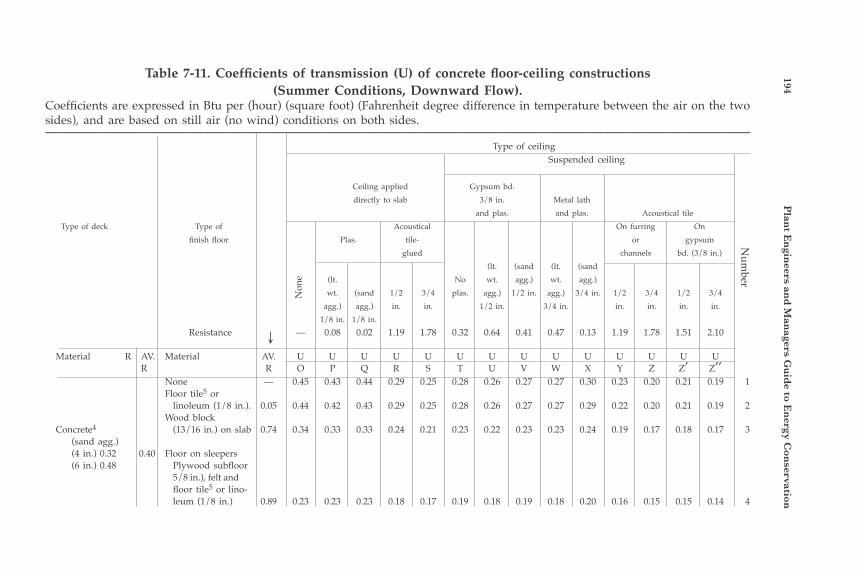
194 P
lant E
ngin
eers and
Man
agers Gu
ide to E
nergy C
onservation
Table 7-11. Coefficients of transmission (U) of concrete floor-ceiling constructions(Summer Conditions, Downward Flow).
Coefficients are expressed in Btu per (hour) (square foot) (Fahrenheit degree difference in temperature between the air on the two sides), and are based on still air (no wind) conditions on both sides.————————————————————————————————————————————————————— Type of ceiling Suspended ceiling
Ceiling applied Gypsum bd. directly to slab 3/8 in. Metal lath and plas. and plas. Acoustical tile Type of deck Type of Acoustical On furring On finish floor Plas. tile- or gypsum glued channels bd. (3/8 in.) (lt. (sand (lt. (sand (lt. No wt. agg.) wt. agg.) wt. (sand 1/2 3/4 plas. agg.) 1/2 in. agg.) 3/4 in. 1/2 3/4 1/2 3/4 agg.) agg.) in. in. 1/2 in. 3/4 in. in. in. in. in. 1/8 in. 1/8 in. Resistance — 0.08 0.02 1.19 1.78 0.32 0.64 0.41 0.47 0.13 1.19 1.78 1.51 2.10 Material R AV. Material AV. U U U U U U U U U U U U U U R R O P Q R S T U V W X Y Z Z’ Z’’ None — 0.45 0.43 0.44 0.29 0.25 0.28 0.26 0.27 0.27 0.30 0.23 0.20 0.21 0.19 1 Floor tile5 or linoleum (1/8 in.). 0.05 0.44 0.42 0.43 0.29 0.25 0.28 0.26 0.27 0.27 0.29 0.22 0.20 0.21 0.19 2 Wood block Concrete4 (13/16 in.) on slab 0.74 0.34 0.33 0.33 0.24 0.21 0.23 0.22 0.23 0.23 0.24 0.19 0.17 0.18 0.17 3 (sand agg.) (4 in.) 0.32 0.40 Floor on sleepers (6 in.) 0.48 Plywood subfloor 5/8 in.), felt and floor tile5 or lino- leum (1/8 in.) 0.89 0.23 0.23 0.23 0.18 0.17 0.19 0.18 0.19 0.18 0.20 0.16 0.15 0.15 0.14 4
Num
ber
Non
e
→
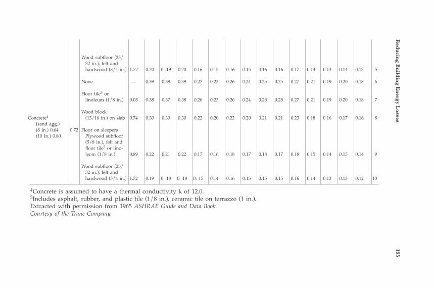
Red
ucin
g Bu
ildin
g En
ergy Losses
195
Wood subfloor (25/ 32 in.), felt and hardwood (3/4 in.) 1.72 0.20 0. 19 0.20 0.16 0.15 0.16 0.15 0.16 0.16 0.17 0.14 0.13 0.14 0.13 5
None — 0.39 0.38 0.39 0.27 0.23 0.26 0.24 0.25 0.25 0.27 0.21 0.19 0.20 0.18 6
Floor tile5 or linoleum (1/8 in.) 0.05 0.38 0.37 0.38 0.26 0.23 0.26 0.24 0.25 0.25 0.27 0.21 0.19 0.20 0.18 7
Wood block Concrete4 (13/16 in.) on slab 0.74 0.30 0.30 0.30 0.22 0.20 0.22 0.20 0.21 0.21 0.23 0.18 0.16 0.17 0.16 8 (sand agg.) (8 in.) 0.64 0.72 Floor on sleepers (10 in.) 0.80 Plywood subfloor (5/8 in.), felt and floor tile5 or lino- leom (1/8 in.) 0.89 0.22 0.21 0.22 0.17 0.16 0.18 0.17 0.18 0.17 0.18 0.15 0.14 0.15 0.14 9
Wood subfloor (25/ 32 in.), felt and hardwood (3/4 in.) 1.72 0.19 0. 18 0. 18 0. 15 0.14 0.16 0.15 0.15 0.15 0.16 0.14 0.13 0.13 0.12 10
4Concrete is assumed to have a thermal conductivity k of 12.0.5Includes asphalt, rubber, and plastic tile (1/8 in.), ceramic tile on terrazzo (1 in.).Extracted with permission from 1965 ASHRAE Guide and Data Book.Courtesy of the Trane Company.
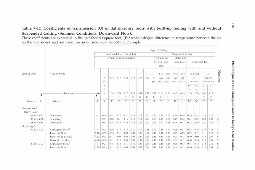
196 P
lant E
ngin
eers and
Man
agers Gu
ide to E
nergy C
onservation
Table 7-12. Coefficients of transmission (U) of flat masonry roofs with built-up roofing with and without Suspended Ceiling (Summer Conditions, Downward Flow).These coefficients are expressed in Btu per (hour) (square foot) (Fahrenheit degree difference in temperature between the air on the two sides), and are based on an outside wind velocity of 7.5 mph.—————————————————————————————————————————————————— Type of Ceiling Roof Insulation—No Ceiling Suspended Ceiling C Value of Roof Insulation Gypsum bd. Metal lath (3/8 in.) and and plas. Acoustical Tile plas.
Type of Deck Type of Form lt. wt. sand lt. wt. sand on furring on
N 0.72 0.36 0.24 0.19 0.15 0.12 No agg. agg. agg. agg. or gypsum
O plas. (1/2 “) (1/2 “) (3/4 “) (3/4 “) channels bd. (3/8 in.) N 1/2 3/4 1/2 3/4 E in. in. in. in. Resistance — 1.39 2.78 4.17 5.26 6.67 8.33 0.32 0.64 0.41 0.47 0.13 1.19 1.78 1.51 2.10 U U U U U U U U U U U U U U U U Material R Material R A’ B’ C’ D’ E’ F’ G’ H’ I’ J’ K’ L’ M’ N’ O’ P’————————————————————————————————————————————————————————————————————————————————————Concrete slab4
(gravel agg.) (4 in.)...0.32 Temporary — 0.55 0.31 0.22 0.17 0.14 0.12 0.10 0.32 0.29 0.31 0.30 0.34 0.25 0.22 0.23 0.20 1 (6 in.)...0.48 Temporary — 0.51 0.30 0.21 0.16 0.14 0.12 0.10 0.30 0.28 0.30 0.29 0.32 0.24 0.21 0.22 0.20 2 (8 in.)...0.64 Temporary — 0.47 0.28 0.20 0.16 0.14 0.11 0.10 0.29 0.27 0.28 0.28 0.31 0.23 0.20 0.22 0.19 3Lt. wt. agg.5
(2 in.)...2.22 Corrugated Metal3 0 0.27 0.20 0.15 0.13 0.11 0.10 0.08 0.20 0.19 0.20 0.19 0.21 0.17 0.15 0.16 0.15 4 Insul. bd. (1 in.) 2.78 0.15 0.13 0.11 0.09 0.09 0.08 0.07 0.13 0.12 0.13 0.13 0.13 0.12 0.11 0.11 0.10 5 Insul. bd. (1-1/2 in.) 4.17 0.13 0.11 0.09 0.08 0.08 0.07 0.06 0.11 0.11 0.11 0.11 0.11 0.10 0.09 0.10 0.09 6 Glass fib. bd. (1 in.) 4.00 0.13 0.11 0.10 0.08 0.08 0.07 0.06 0.11 0.11 0.11 0.11 0.11 0.10 0.10 0.10 0.09 7 (3 in.)...3.33 Corrugated Metal3 0 0.21 0.16 0.13 0.11 0.10 0.09 0.08 0.16 0.16 0.16 0.16 0.17 0.14 0.13 0.14 0.13 8 Insul. bd. (1 in.) 2.78 0.13 0.11 0.10 0.08 0.08 0.07 0.06 0.11 0.11 0.11 0.11 0.11 0.10 0.10 0.10 0.09 9
Num
ber
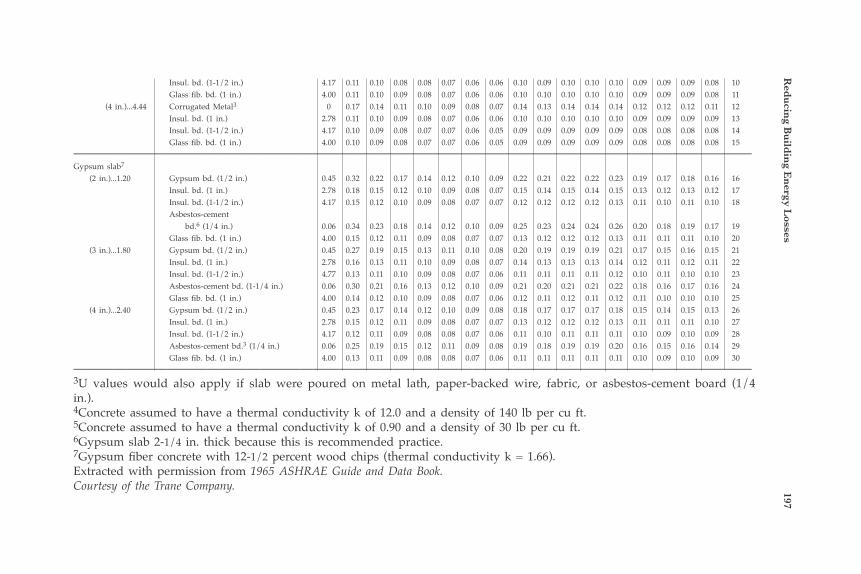
Red
ucin
g Bu
ildin
g En
ergy Losses
197 Insul. bd. (1-1/2 in.) 4.17 0.11 0.10 0.08 0.08 0.07 0.06 0.06 0.10 0.09 0.10 0.10 0.10 0.09 0.09 0.09 0.08 10 Glass fib. bd. (1 in.) 4.00 0.11 0.10 0.09 0.08 0.07 0.06 0.06 0.10 0.10 0.10 0.10 0.10 0.09 0.09 0.09 0.08 11 (4 in.)...4.44 Corrugated Metal3 0 0.17 0.14 0.11 0.10 0.09 0.08 0.07 0.14 0.13 0.14 0.14 0.14 0.12 0.12 0.12 0.11 12 Insul. bd. (1 in.) 2.78 0.11 0.10 0.09 0.08 0.07 0.06 0.06 0.10 0.10 0.10 0.10 0.10 0.09 0.09 0.09 0.09 13 Insul. bd. (1-1/2 in.) 4.17 0.10 0.09 0.08 0.07 0.07 0.06 0.05 0.09 0.09 0.09 0.09 0.09 0.08 0.08 0.08 0.08 14 Glass fib. bd. (1 in.) 4.00 0.10 0.09 0.08 0.07 0.07 0.06 0.05 0.09 0.09 0.09 0.09 0.09 0.08 0.08 0.08 0.08 15———————————————————————————————————————————————————Gypsum slab7
(2 in.)...1.20 Gypsum bd. (1/2 in.) 0.45 0.32 0.22 0.17 0.14 0.12 0.10 0.09 0.22 0.21 0.22 0.22 0.23 0.19 0.17 0.18 0.16 16 Insul. bd. (1 in.) 2.78 0.18 0.15 0.12 0.10 0.09 0.08 0.07 0.15 0.14 0.15 0.14 0.15 0.13 0.12 0.13 0.12 17 Insul. bd. (1-1/2 in.) 4.17 0.15 0.12 0.10 0.09 0.08 0.07 0.07 0.12 0.12 0.12 0.12 0.13 0.11 0.10 0.11 0.10 18 Asbestos-cement bd.6 (1/4 in.) 0.06 0.34 0.23 0.18 0.14 0.12 0.10 0.09 0.25 0.23 0.24 0.24 0.26 0.20 0.18 0.19 0.17 19 Glass fib. bd. (1 in.) 4.00 0.15 0.12 0.11 0.09 0.08 0.07 0.07 0.13 0.12 0.12 0.12 0.13 0.11 0.11 0.11 0.10 20 (3 in.)...1.80 Gypsum bd. (1/2 in.) 0.45 0.27 0.19 0.15 0.13 0.11 0.10 0.08 0.20 0.19 0.19 0.19 0.21 0.17 0.15 0.16 0.15 21 Insul. bd. (1 in.) 2.78 0.16 0.13 0.11 0.10 0.09 0.08 0.07 0.14 0.13 0.13 0.13 0.14 0.12 0.11 0.12 0.11 22 Insul. bd. (1-1/2 in.) 4.77 0.13 0.11 0.10 0.09 0.08 0.07 0.06 0.11 0.11 0.11 0.11 0.12 0.10 0.11 0.10 0.10 23 Asbestos-cement bd. (1-1/4 in.) 0.06 0.30 0.21 0.16 0.13 0.12 0.10 0.09 0.21 0.20 0.21 0.21 0.22 0.18 0.16 0.17 0.16 24 Glass fib. bd. (1 in.) 4.00 0.14 0.12 0.10 0.09 0.08 0.07 0.06 0.12 0.11 0.12 0.11 0.12 0.11 0.10 0.10 0.10 25 (4 in.)...2.40 Gypsum bd. (1/2 in.) 0.45 0.23 0.17 0.14 0.12 0.10 0.09 0.08 0.18 0.17 0.17 0.17 0.18 0.15 0.14 0.15 0.13 26 Insul. bd. (1 in.) 2.78 0.15 0.12 0.11 0.09 0.08 0.07 0.07 0.13 0.12 0.12 0.12 0.13 0.11 0.11 0.11 0.10 27 Insul. bd. (1-1/2 in.) 4.17 0.12 0.11 0.09 0.08 0.08 0.07 0.06 0.11 0.10 0.11 0.11 0.11 0.10 0.09 0.10 0.09 28 Asbestos-cement bd.3 (1/4 in.) 0.06 0.25 0.19 0.15 0.12 0.11 0.09 0.08 0.19 0.18 0.19 0.19 0.20 0.16 0.15 0.16 0.14 29 Glass fib. bd. (1 in.) 4.00 0.13 0.11 0.09 0.08 0.08 0.07 0.06 0.11 0.11 0.11 0.11 0.11 0.10 0.09 0.10 0.09 30———————————————————————————————————————————————————3U values would also apply if slab were poured on metal lath, paper-backed wire, fabric, or asbestos-cement board (1/4 in.).4Concrete assumed to have a thermal conductivity k of 12.0 and a density of 140 lb per cu ft.5Concrete assumed to have a thermal conductivity k of 0.90 and a density of 30 lb per cu ft.6Gypsum slab 2-1/4 in. thick because this is recommended practice.7Gypsum fiber concrete with 12-1/2 percent wood chips (thermal conductivity k = 1.66).Extracted with permission from 1965 ASHRAE Guide and Data Book.Courtesy of the Trane Company.
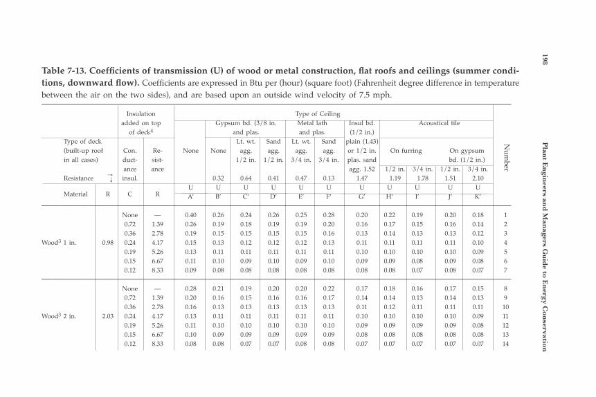
198 P
lant E
ngin
eers and
Man
agers Gu
ide to E
nergy C
onservation
Table 7-13. Coefficients of transmission (U) of wood or metal construction, flat roofs and ceilings (summer condi-tions, downward flow). Coefficients are expressed in Btu per (hour) (square foot) (Fahrenheit degree difference in temperature between the air on the two sides), and are based upon an outside wind velocity of 7.5 mph.——————————————————————————————————————————————————— Insulation Type of Ceiling added on top Gypsum bd. (3/8 in. Metal lath Insul bd. Acoustical tile of deck4 and plas. and plas. (1/2 in.) Type of deck Lt. wt. Sand Lt. wt. Sand plain (1.43) (built-up roof Con. Re- None None agg. agg. agg. agg. or 1/2 in. On furring On gypsum in all cases) duct- sist- 1/2 in. 1/2 in. 3/4 in. 3/4 in. plas. sand bd. (1/2 in.) ance ance agg. 1.52 1/2 in. 3/4 in. 1/2 in. 3/4 in. Resistance insul. 0.32 0.64 0.41 0.47 0.13 1.47 1.19 1.78 1.51 2.10 U U U U U U U U U U U A’ B’ C’ D’ E’ F’ G’ H’ I’ J’ K’——————————————————————————————————————————————————— None — 0.40 0.26 0.24 0.26 0.25 0.28 0.20 0.22 0.19 0.20 0.18 1 0.72 1.39 0.26 0.19 0.18 0.19 0.19 0.20 0.16 0.17 0.15 0.16 0.14 2 0.36 2.78 0.19 0.15 0.15 0.15 0.15 0.16 0.13 0.14 0.13 0.13 0.12 3Wood3 1 in. 0.98 0.24 4.17 0.15 0.13 0.12 0.12 0.12 0.13 0.11 0.11 0.11 0.11 0.10 4 0.19 5.26 0.13 0.11 0.11 0.11 0.11 0.11 0.10 0.10 0.10 0.10 0.09 5 0.15 6.67 0.11 0.10 0.09 0.10 0.09 0.10 0.09 0.09 0.08 0.09 0.08 6 0.12 8.33 0.09 0.08 0.08 0.08 0.08 0.08 0.08 0.08 0.07 0.08 0.07 7——————————————————————————————————————————————————— None — 0.28 0.21 0.19 0.20 0.20 0.22 0.17 0.18 0.16 0.17 0.15 8 0.72 1.39 0.20 0.16 0.15 0.16 0.16 0.17 0.14 0.14 0.13 0.14 0.13 9 0.36 2.78 0.16 0.13 0.13 0.13 0.13 0.13 0.11 0.12 0.11 0.11 0.11 10Wood3 2 in. 2.03 0.24 4.17 0.13 0.11 0.11 0.11 0.11 0.11 0.10 0.10 0.10 0.10 0.09 11 0.19 5.26 0.11 0.10 0.10 0.10 0.10 0.10 0.09 0.09 0.09 0.09 0.08 12 0.15 6.67 0.10 0.09 0.09 0.09 0.09 0.09 0.08 0.08 0.08 0.08 0.08 13 0.12 8.33 0.08 0.08 0.07 0.07 0.08 0.08 0.07 0.07 0.07 0.07 0.07 14
Num
ber
Material R C R
→→
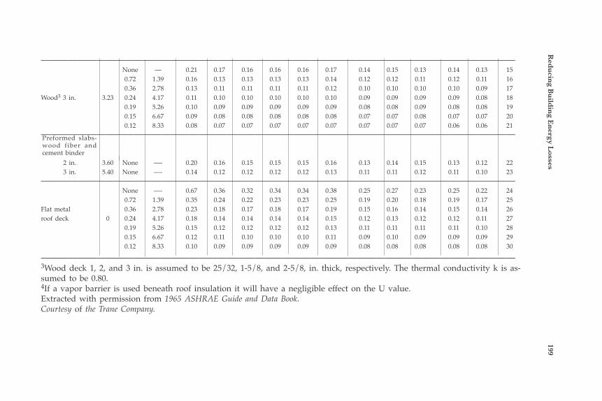
Red
ucin
g Bu
ildin
g En
ergy Losses
199——————————————————————————————————————————————————— None — 0.21 0.17 0.16 0.16 0.16 0.17 0.14 0.15 0.13 0.14 0.13 15 0.72 1.39 0.16 0.13 0.13 0.13 0.13 0.14 0.12 0.12 0.11 0.12 0.11 16 0.36 2.78 0.13 0.11 0.11 0.11 0.11 0.12 0.10 0.10 0.10 0.10 0.09 17Wood3 3 in. 3.23 0.24 4.17 0.11 0.10 0.10 0.10 0.10 0.10 0.09 0.09 0.09 0.09 0.08 18 0.19 5.26 0.10 0.09 0.09 0.09 0.09 0.09 0.08 0.08 0.09 0.08 0.08 19 0.15 6.67 0.09 0.08 0.08 0.08 0.08 0.08 0.07 0.07 0.08 0.07 0.07 20 0.12 8.33 0.08 0.07 0.07 0.07 0.07 0.07 0.07 0.07 0.07 0.06 0.06 21———————————————————————————————————————————————————
2 in. 3.60 None —- 0.20 0.16 0.15 0.15 0.15 0.16 0.13 0.14 0.15 0.13 0.12 22 3 in. 5.40 None —- 0.14 0.12 0.12 0.12 0.12 0.13 0.11 0.11 0.12 0.11 0.10 23——————————————————————————————————————————————————— None —- 0.67 0.36 0.32 0.34 0.34 0.38 0.25 0.27 0.23 0.25 0.22 24 0.72 1.39 0.35 0.24 0.22 0.23 0.23 0.25 0.19 0.20 0.18 0.19 0.17 25Flat metal 0.36 2.78 0.23 0.18 0.17 0.18 0.17 0.19 0.15 0.16 0.14 0.15 0.14 26roof deck 0 0.24 4.17 0.18 0.14 0.14 0.14 0.14 0.15 0.12 0.13 0.12 0.12 0.11 27 0.19 5.26 0.15 0.12 0.12 0.12 0.12 0.13 0.11 0.11 0.11 0.11 0.10 28 0.15 6.67 0.12 0.11 0.10 0.10 0.10 0.11 0.09 0.10 0.09 0.09 0.09 29 0.12 8.33 0.10 0.09 0.09 0.09 0.09 0.09 0.08 0.08 0.08 0.08 0.08 30
———————————————————————————————————————————————————3Wood deck 1, 2, and 3 in. is assumed to be 25/32, 1-5/8, and 2-5/8, in. thick, respectively. The thermal conductivity k is as-sumed to be 0.80.4If a vapor barrier is used beneath roof insulation it will have a negligible effect on the U value.Extracted with permission from 1965 ASHRAE Guide and Data Book.Courtesy of the Trane Company.
Preformed slabs-wood fiber and cement binder
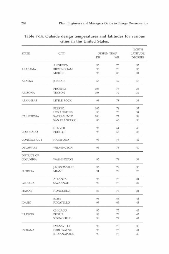
200 Plant Engineers and Managers Guide to Energy Conservation
Table 7-14. Outside design temperatures and latitudes for various cities in the United States.
———————————————————————————————— NORTHSTATE CITY DESIGN TEMP LATITUDE, DB WB DEGREES———————————————————————————————— ANNISTON 95 75 33ALABAMA BIRMINGHAM 95 78 33 MOBILE 95 80 31———————————————————————————————ALASKA JUNEAU 65 52 58——————————————————————————————— PHOENIX 105 76 33ARIZONA TUCSON 105 72 32———————————————————————————————ARKANSAS LITTLE ROCK 95 78 35——————————————————————————————— FRESNO 105 74 37 LOS ANGELES 90 70 34CALIFORNIA SACRAMENTO 100 72 38 SAN FRANCISCO 85 65 38——————————————————————————————— DENVER 95 64 40COLORADO PUEBLO 95 65 38———————————————————————————————CONNECTICUT HARTFORD 93 75 42———————————————————————————————DELAWARE WILMINGTON 95 78 40———————————————————————————————DISTRICT OFCOLUMBIA WASHINGTON 95 78 39——————————————————————————————— JACKSONVILLE 95 78 30FLORIDA MIAMI 91 79 26——————————————————————————————— ATLANTA 95 76 34GEORGIA SAVANNAH 95 78 32———————————————————————————————HAWAII HONOLULU 83 73 21——————————————————————————————— BOISE 95 65 44IDAHO POCATELLO 95 65 43——————————————————————————————— CHICAGO 95 75 43ILLINOIS PEORIA 96 76 43 SPRINGFIELD 98 77 42——————————————————————————————— EVANSVILLE 95 78 38INDIANA FORT WAYNE 95 75 41 INDIANAPOLIS 95 76 40
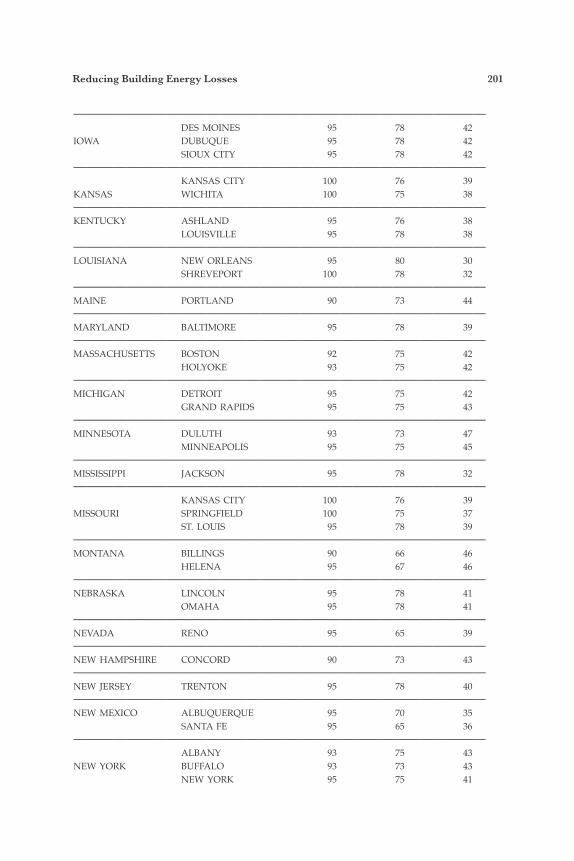
Reducing Building Energy Losses 201
——————————————————————————————— DES MOINES 95 78 42IOWA DUBUQUE 95 78 42 SIOUX CITY 95 78 42——————————————————————————————— KANSAS CITY 100 76 39KANSAS WICHITA 100 75 38———————————————————————————————KENTUCKY ASHLAND 95 76 38 LOUISVILLE 95 78 38———————————————————————————————LOUISIANA NEW ORLEANS 95 80 30 SHREVEPORT 100 78 32———————————————————————————————MAINE PORTLAND 90 73 44———————————————————————————————MARYLAND BALTIMORE 95 78 39———————————————————————————————MASSACHUSETTS BOSTON 92 75 42 HOLYOKE 93 75 42———————————————————————————————MICHIGAN DETROIT 95 75 42 GRAND RAPIDS 95 75 43———————————————————————————————MINNESOTA DULUTH 93 73 47 MINNEAPOLIS 95 75 45———————————————————————————————MISSISSIPPI JACKSON 95 78 32——————————————————————————————— KANSAS CITY 100 76 39MISSOURI SPRINGFIELD 100 75 37 ST. LOUIS 95 78 39———————————————————————————————MONTANA BILLINGS 90 66 46 HELENA 95 67 46———————————————————————————————NEBRASKA LINCOLN 95 78 41 OMAHA 95 78 41———————————————————————————————NEVADA RENO 95 65 39———————————————————————————————NEW HAMPSHIRE CONCORD 90 73 43———————————————————————————————NEW JERSEY TRENTON 95 78 40———————————————————————————————NEW MEXICO ALBUQUERQUE 95 70 35 SANTA FE 95 65 36——————————————————————————————— ALBANY 93 75 43NEW YORK BUFFALO 93 73 43 NEW YORK 95 75 41
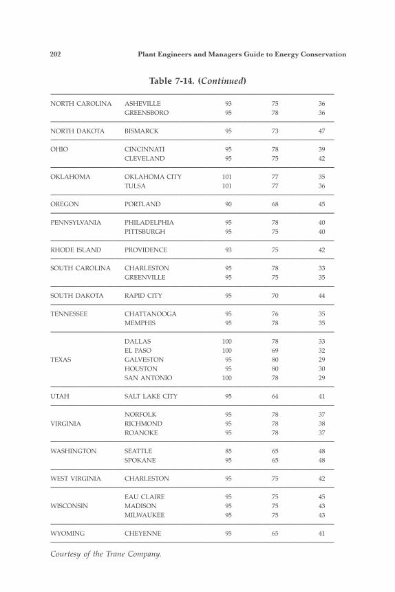
202 Plant Engineers and Managers Guide to Energy Conservation
———————————————————————————————NORTH CAROLINA ASHEVILLE 93 75 36 GREENSBORO 95 78 36———————————————————————————————NORTH DAKOTA BISMARCK 95 73 47———————————————————————————————OHIO CINCINNATI 95 78 39 CLEVELAND 95 75 42———————————————————————————————OKLAHOMA OKLAHOMA CITY 101 77 35 TULSA 101 77 36———————————————————————————————OREGON PORTLAND 90 68 45———————————————————————————————PENNSYLVANIA PHILADELPHIA 95 78 40 PITTSBURGH 95 75 40———————————————————————————————RHODE ISLAND PROVIDENCE 93 75 42———————————————————————————————SOUTH CAROLINA CHARLESTON 95 78 33 GREENVILLE 95 75 35———————————————————————————————SOUTH DAKOTA RAPID CITY 95 70 44———————————————————————————————TENNESSEE CHATTANOOGA 95 76 35 MEMPHIS 95 78 35——————————————————————————————— DALLAS 100 78 33 EL PASO 100 69 32TEXAS GALVESTON 95 80 29 HOUSTON 95 80 30 SAN ANTONIO 100 78 29———————————————————————————————UTAH SALT LAKE CITY 95 64 41——————————————————————————————— NORFOLK 95 78 37VIRGINIA RICHMOND 95 78 38 ROANOKE 95 78 37———————————————————————————————WASHINGTON SEATTLE 85 65 48 SPOKANE 95 65 48———————————————————————————————WEST VIRGINIA CHARLESTON 95 75 42——————————————————————————————— EAU CLAIRE 95 75 45WISCONSIN MADISON 95 75 43 MILWAUKEE 95 75 43———————————————————————————————WYOMING CHEYENNE 95 65 41———————————————————————————————Courtesy of the Trane Company.
Table 7-14. (Continued)
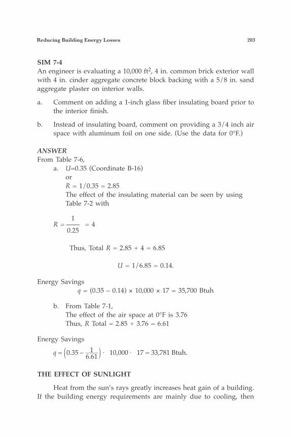
Reducing Building Energy Losses 203
SIM 7-4An engineer is evaluating a 10,000 ft2, 4 in. common brick exterior wall with 4 in. cinder aggregate concrete block backing with a 5/8 in. sand aggregate plaster on interior walls.
a. Comment on adding a 1-inch glass fiber insulating board prior to the interior finish.
b. Instead of insulating board, comment on providing a 3/4 inch air space with aluminum foil on one side. (Use the data for 0°F.)
ANSWERFrom Table 7-6, a. U=0.35 (Coordinate B-16) or R = 1/0.35 = 2.85 The effect of the insulating material can be seen by using Table 7-2 with
1 R = —— = 4 0.25
Thus, Total R = 2.85 + 4 = 6.85
U = 1/6.85 = 0.14.
Energy Savingsq = (0.35 – 0.14) × 10,000 × 17 = 35,700 Btuh
b. From Table 7-1, The effect of the air space at 0°F is 3.76 Thus, R Total = 2.85 + 3.76 = 6.61
Energy Savings
q = 0.35 – 16.61 × 10,000 × 17 = 33,781 Btuh.
THE EFFECT OF SUNLIGHT
Heat from the sun’s rays greatly increases heat gain of a building. If the building energy requirements are mainly due to cooling, then

204 Plant Engineers and Managers Guide to Energy Conservation
this gain should be minimized. Solar energy affects a building in the following ways:
1. Raises the surface temperature: Thus a greater temperature differen-tial will exist at roofs than at walls.
2. A large percentage of direct solar radiation and diffuse sky radia-tion passes through transparent materials, such as glass.
Surface Temperatures The temperature of a wall or roof depends upon:(a) the angle of the sun’s rays(b) the color and roughness of the surface(c) the reflectivity of the surface(d) the type of construction.
When an engineer is specifying building materials, he should consider the above factors. A simple example is color. The darker the surface, the more solar radiation will be absorbed. Obviously, white surfaces have a lower temperature than black surfaces after the same period of solar heating. Another factor is that smooth surfaces reflect more radiant heat than do rough ones. In order to properly take solar energy into account, the angle of the sun’s rays must be known. If the latitude of the plant is known, the angle can be determined. Tables 7-15 and 7-16 illustrate typical temperature differentials for the roof and walls, based on different locations in the United States and various material. Table 7-16 is simplified to indicate dark (D) and light (L) color materials only. A full set of tables can be found in the ASHRAE Guide and Data Book.
SIM 7-5 An engineer is evaluating three designs for a roof. In the first case the construction is a 2 in. lightweight aggregate deck with no insulation. The second case is the same as the first, except a 1 in. glass fiberboard form with roof insulation of R = 4.17 is used. The third case is the same as case two, except a 4 in. light weight aggregate is used instead of the 2 inch used in case one. The roof area is 5000 ft2. What is the maximum heat gain for August 24, if the plant were located in Indianapolis, Indiana?
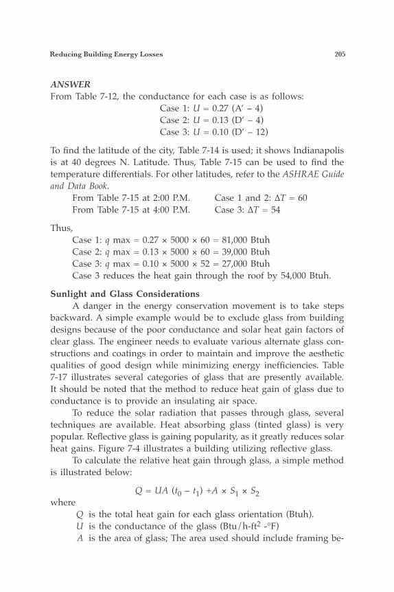
Reducing Building Energy Losses 205
ANSWERFrom Table 7-12, the conductance for each case is as follows: Case 1: U = 0.27 (A’ – 4) Case 2: U = 0.13 (D’ – 4) Case 3: U = 0.10 (D’ – 12)
To find the latitude of the city, Table 7-14 is used; it shows Indianapolis is at 40 degrees N. Latitude. Thus, Table 7-15 can be used to find the temperature differentials. For other latitudes, refer to the ASHRAE Guide and Data Book. From Table 7-15 at 2:00 P.M. Case 1 and 2: ∆T = 60 From Table 7-15 at 4:00 P.M. Case 3: ∆T = 54
Thus, Case 1: q max = 0.27 × 5000 × 60 = 81,000 Btuh Case 2: q max = 0.13 × 5000 × 60 = 39,000 Btuh Case 3: q max = 0.10 × 5000 × 52 = 27,000 Btuh Case 3 reduces the heat gain through the roof by 54,000 Btuh.
Sunlight and Glass Considerations A danger in the energy conservation movement is to take steps backward. A simple example would be to exclude glass from building designs because of the poor conductance and solar heat gain factors of clear glass. The engineer needs to evaluate various alternate glass con-structions and coatings in order to maintain and improve the aesthetic qualities of good design while minimizing energy inefficiencies. Table 7-17 illustrates several categories of glass that are presently available. It should be noted that the method to reduce heat gain of glass due to conductance is to provide an insulating air space. To reduce the solar radiation that passes through glass, several techniques are available. Heat absorbing glass (tinted glass) is very popular. Reflective glass is gaining popularity, as it greatly reduces solar heat gains. Figure 7-4 illustrates a building utilizing reflective glass. To calculate the relative heat gain through glass, a simple method is illustrated below:
Q = UA (t0 – t1) +A × S1 × S2where Q is the total heat gain for each glass orientation (Btuh). U is the conductance of the glass (Btu/h-ft2 -°F) A is the area of glass; The area used should include framing be-
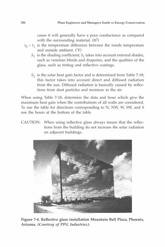
206 Plant Engineers and Managers Guide to Energy Conservation
cause it will generally have a poor conductance as compared with the surrounding material. (ft2)
t0 – t1 is the temperature difference between the inside temperature and outside ambient. (°F)
S1 is the shading coefficient; S1 takes into account external shades, such as venetian blinds and draperies, and the qualities of the glass, such as tinting and reflective coatings.
S2 is the solar heat gain factor and is determined from Table 7-18; this factor takes into account direct and diffused radiation from the sun. Diffused radiation is basically caused by reflec-tions from dust particles and moisture in the air.
When using Table 7-18, determine the data and hour which give the maximum heat gain when the contributions of all walls are considered. To use the table for directions corresponding to N, NW, W, SW, and S use the hours at the bottom of the table.
CAUTION: When using reflective glass always insure that the reflec-tions from the building do not increase the solar radiation on adjacent buildings.
Figure 7-4. Reflective glass installation Mountain Bell Plaza, Phoenix, Arizona. (Courtesy of PPG Industries.)
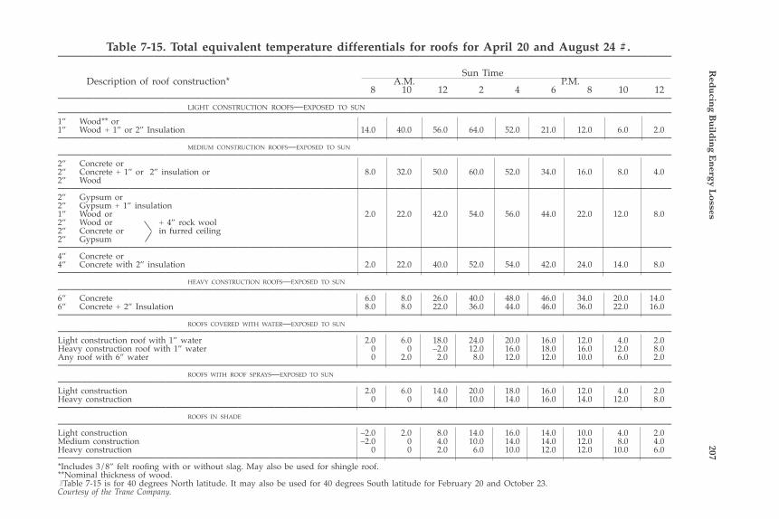
Red
ucin
g Bu
ildin
g En
ergy Losses
207
Table 7-15. Total equivalent temperature differentials for roofs for April 20 and August 24 #.——————————————————————————————————————————————————— Sun Time Description of roof construction* A.M. P.M. 8 10 12 2 4 6 8 10 12——————————————————————————————————————————————————— lighT consTrucTion roofs—exposed To sun———————————————————————————————————————————————————1” Wood** or1” Wood + 1” or 2” Insulation 14.0 40.0 56.0 64.0 52.0 21.0 12.0 6.0 2.0——————————————————————————————————————————————————— medium consTrucTion roofs—exposed To sun———————————————————————————————————————————————————2” Concrete or2” Concrete + 1” or 2” insulation or 8.0 32.0 50.0 60.0 52.0 34.0 16.0 8.0 4.02” Wood———————————————————————————————————————————————————2” Gypsum or2” Gypsum + 1” insulation1” Wood or 2.0 22.0 42.0 54.0 56.0 44.0 22.0 12.0 8.02” Wood or + 4” rock wool2” Concrete or in furred ceiling2” Gypsum ———————————————————————————————————————————————————4” Concrete or4” Concrete with 2” insulation 2.0 22.0 40.0 52.0 54.0 42.0 24.0 14.0 8.0——————————————————————————————————————————————————— heavy consTrucTion roofs—exposed To sun———————————————————————————————————————————————————6” Concrete 6.0 8.0 26.0 40.0 48.0 46.0 34.0 20.0 14.06” Concrete + 2” Insulation 8.0 8.0 22.0 36.0 44.0 46.0 36.0 22.0 16.0——————————————————————————————————————————————————— roofs covered wiTh waTer—exposed To sun———————————————————————————————————————————————————Light construction roof with 1” water 2.0 6.0 18.0 24.0 20.0 16.0 12.0 4.0 2.0Heavy construction roof with 1” water 0 0 –2.0 12.0 16.0 18.0 16.0 12.0 8.0Any roof with 6” water 0 2.0 2.0 8.0 12.0 12.0 10.0 6.0 2.0——————————————————————————————————————————————————— roofs wiTh roof sprays—exposed To sun———————————————————————————————————————————————————Light construction 2.0 6.0 14.0 20.0 18.0 16.0 12.0 4.0 2.0Heavy construction 0 0 4.0 10.0 14.0 16.0 14.0 12.0 8.0——————————————————————————————————————————————————— roofs in shade———————————————————————————————————————————————————Light construction –2.0 2.0 8.0 14.0 16.0 14.0 10.0 4.0 2.0Medium construction –2.0 0 4.0 10.0 14.0 14.0 12.0 8.0 4.0Heavy construction 0 0 2.0 6.0 10.0 12.0 12.0 10.0 6.0———————————————————————————————————————————————————*Includes 3/8” felt roofing with or without slag. May also be used for shingle roof.**Nominal thickness of wood.#Table 7-15 is for 40 degrees North latitude. It may also be used for 40 degrees South latitude for February 20 and October 23.Courtesy of the Trane Company.
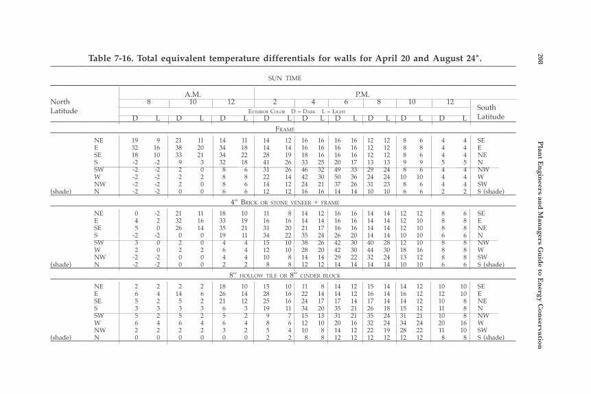
208 P
lant E
ngin
eers and
Man
agers Gu
ide to E
nergy C
onservation
Table 7-16. Total equivalent temperature differentials for walls for April 20 and August 24*.———————————————————————————————————————————————————
sun Time——————————————————————————————————————————————————— A.M. P.M.North 8 10 12 2 4 6 8 10 12 latitude exTerior color d = dark l = lighT D L D L D L D L D L D L D L D L D L———————————————————————————————————————————————————
frame——————————————————————————————————————————————————— NE 19 9 21 11 14 11 14 12 16 16 16 16 12 12 8 6 4 4 SE E 32 16 38 20 34 18 14 14 16 16 16 16 12 12 8 8 4 4 E SE 18 10 33 21 34 22 28 19 18 16 16 16 12 12 8 6 4 4 NE S -2 -2 9 3 32 18 41 26 33 25 20 17 13 13 9 9 5 5 N SW -2 -2 2 0 8 6 31 26 46 32 49 33 29 24 8 6 4 4 NW W -2 -2 2 2 8 8 22 14 42 30 50 36 24 24 10 10 4 4 W NW -2 -2 2 0 8 6 14 12 24 21 37 26 31 23 8 6 4 4 SW(shade) N -2 -2 0 0 6 6 12 12 16 16 14 14 10 10 6 6 2 2 S (shade)———————————————————————————————————————————————————
4” brick or sTone veneer + frame——————————————————————————————————————————————————— NE 0 -2 21 11 18 10 11 8 14 12 16 16 14 14 12 12 8 6 SE E 4 2 32 16 33 19 16 16 14 14 16 16 14 14 12 10 8 8 E SE 5 0 26 14 35 21 31 20 21 17 16 16 14 14 12 10 8 8 NE S -2 -2 0 0 19 11 34 22 35 24 26 20 14 14 10 10 6 6 N SW 3 0 2 0 4 4 15 10 38 26 42 30 40 28 12 10 8 8 NW W 2 0 2 2 6 4 12 10 28 20 42 30 44 30 18 16 8 8 W NW -2 -2 0 0 4 4 10 8 14 14 29 22 32 24 13 12 8 8 SW(shade) N -2 -2 0 0 2 2 8 8 12 12 14 14 14 14 10 10 6 6 S (shade)———————————————————————————————————————————————————
8’’ hollow Tile or 8’’ cinder block——————————————————————————————————————————————————— NE 2 2 2 2 18 10 15 10 11 8 14 12 15 14 14 12 10 10 SE E 6 4 14 6 26 14 28 16 22 14 14 12 16 14 16 12 12 10 E SE 5 2 5 2 21 12 25 16 24 17 17 14 17 14 14 12 10 8 NE S 3 3 3 3 6 3 19 11 34 20 35 21 26 18 15 12 11 8 N SW 5 2 5 2 5 2 9 7 15 13 31 21 35 24 31 21 10 8 NW W 6 4 6 4 6 4 8 6 12 10 20 16 32 24 34 24 20 16 W NW 2 2 2 2 3 2 5 4 10 8 14 12 22 19 28 22 11 10 SW(shade) N 0 0 0 0 0 0 2 2 8 8 12 12 12 12 12 12 8 8 S (shade)———————————————————————————————————————————————————
SouthLatitude
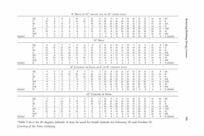
Red
ucin
g Bu
ildin
g En
ergy Losses
2098” brick or 12” hollow Tile or 12” cinder block———————————————————————————————————————————————————
NE 4 4 4 4 10 4 15 9 14 9 11 8 12 10 12 12 11 10 SE E 10 8 1 8 16 10 20 12 20 12 16 10 16 12 16 12 14 12 E SE 11 7 9 7 9 7 18 14 23 16 20 15 15 12 15 12 15 13 NE S 8 5 8 5 8 5 8 5 16 10 22 14 22 16 16 13 14 11 N SW 11 7 9 7 9 7 11 7 13 9 15 10 24 15 29 19 24 17 NW W 10 6 8 6 8 8 10 8 12 8 16 10 22 18 26 18 26 18 W NW 4 4 4 4 4 4 5 4 7 6 10 8 12 10 17 15 18 15 SW(shade) N 2 2 2 2 2 2 2 2 4 4 8 8 10 10 10 10 8 8 S (shade)———————————————————————————————————————————————————
12” brick——————————————————————————————————————————————————— NE 9 8 9 7 9 6 9 6 11 6 12 7 12 7 11 8 11 8 SE E 14 10 14 10 14 10 12 8 14 10 16 12 16 12 16 10 16 10 E SE 13 8 13 9 13 9 13 9 13 9 16 11 18 13 18 13 15 10 N S 12 9 13 10 10 7 10 7 10 7 13 7 16 10 18 12 17 11 NE SW 13 8 13 9 13 9 13 9 13 9 13 11 13 11 15 11 17 13 NW W 14 10 14 10 14 10 12 8 12 8 12 8 12 8 14 10 18 12 W NW 9 8 9 7 9 6 9 6 9 6 9 6 9 7 11 8 11 8 SW(shade) N 6 6 4 4 4 4 4 4 4 4 4 4 4 4 6 6 8 8 S (shade)———————————————————————————————————————————————————
8” concreTe or sTone or 6” or 8” concreTe block——————————————————————————————————————————————————— NE 7 5 5 4 5 4 6 4 11 8 15 11 17 13 15 11 11 9 SE E 8 6 16 10 26 14 26 14 20 12 16 12 16 12 14 12 12 10 E SE 9 4 9 7 21 14 23 16 22 15 17 15 15 12 15 13 13 11 N S 5 3 5 3 8 3 18 10 23 18 25 17 19 16 14 11 12 9 NE SW 9 4 7 4 9 4 11 6 18 13 27 20 29 19 27 20 13 11 NW W 8 6 8 6 8 6 10 8 14 10 22 16 30 20 28 20 16 12 W NW 5 4 5 2 5 4 6 6 8 8 13 11 20 15 21 16 9 8 SW(shade) N 2 2 2 2 2 2 4 4 6 6 8 8 10 10 8 8 6 6 S (shade)———————————————————————————————————————————————————
12” Concrete or Stone——————————————————————————————————————————————————— NE 7 5 7 4 7 4 13 9 14 9 11 9 11 10 13 12 11 10 SE E 12 8 10 8 12 8 20 12 20 14 18 12 14 12 16 12 16 12 E SE 11 7 11 7 9 7 18 11 20 13 20 13 17 13 15 12 15 13 N S 11 8 8 5 8 5 8 5 16 10 20 15 22 17 19 13 14 11 NE SW 11 7 11 7 9 7 9 7 11 9 13 11 22 17 24 17 22 15 NW W 12 8 10 8 10 8 12 8 12 8 14 10 18 12 26 16 24 16 W NW 7 5 7 4 7 4 7 5 7 6 9 8 11 10 18 13 20 15 SW(shade) N 2 2 2 2 2 2 2 2 4 4 6 6 9 8 10 10 8 8 S (shade)———————————————————————————————————————————————————*Table 7-16 is for 40 degrees latitude. It may be used for South latitude for February 20 and October 23.Courtesy of the Trane Company.
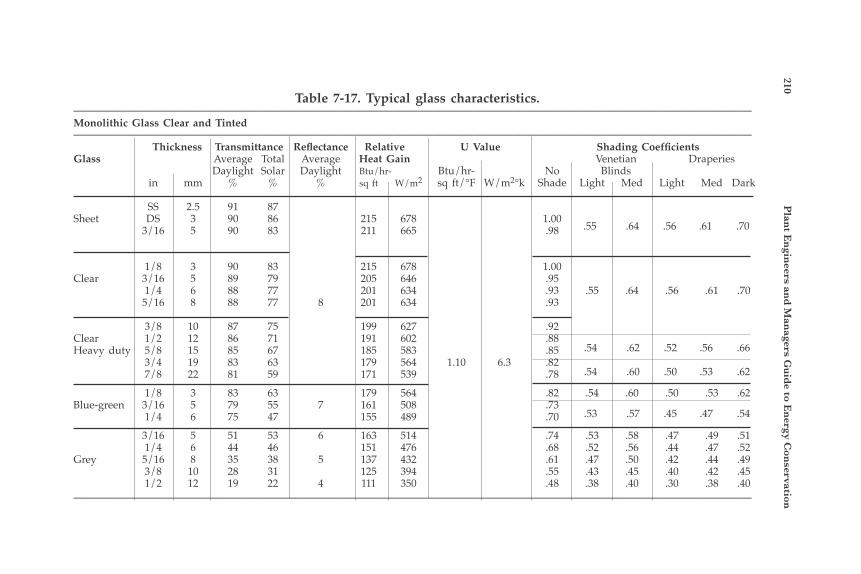
210 P
lant E
ngin
eers and
Man
agers Gu
ide to E
nergy C
onservation
.54 .62 .52 .56 .66
.54 .60 .50 .53 .62
Table 7-17. Typical glass characteristics.———————————————————————————————————————————————————Monolithic Glass Clear and Tinted——————————————————————————————————————————————————— Thickness Transmittance Reflectance Relative U Value Shading CoefficientsGlass Average Total Average Heat Gain Venetian Draperies Daylight Solar Daylight Btu/hr- Btu/hr- No Blinds in mm % % % sq ft W/m2 sq ft/°F W/m2°k Shade Light Med Light Med Dark
SS 2.5 91 87Sheet DS 3 90 86 215 678 1.00 3/16 5 90 83 211 665 .98
1/8 3 90 83 215 678 1.00Clear 3/16 5 89 79 205 646 .95 1/4 6 88 77 201 634 .93 .55 .64 .56 .61 .70 5/16 8 88 77 8 201 634 .93
3/8 10 87 75 199 627 .92Clear 1/2 12 86 71 191 602 .88Heavy duty 5/8 15 85 67 185 583 .85 3/4 19 83 63 179 564 1.10 6.3 .82 7/8 22 81 59 171 539 .78
1/8 3 83 63 179 564 .82 .54 .60 .50 .53 .62Blue-green 3/16 5 79 55 7 161 508 .73 1/4 6 75 47 155 489 .70
3/16 5 51 53 6 163 514 .74 .53 .58 .47 .49 .51 1/4 6 44 46 151 476 .68 .52 .56 .44 .47 .52Grey 5/16 8 35 38 5 137 432 .61 .47 .50 .42 .44 .49 3/8 10 28 31 125 394 .55 .43 .45 .40 .42 .45 1/2 12 19 22 4 111 350 .48 .38 .40 .30 .38 .40———————————————————————————————————————————————————
.53 .57 .45 .47 .54
.55 .64 .56 .61 .70
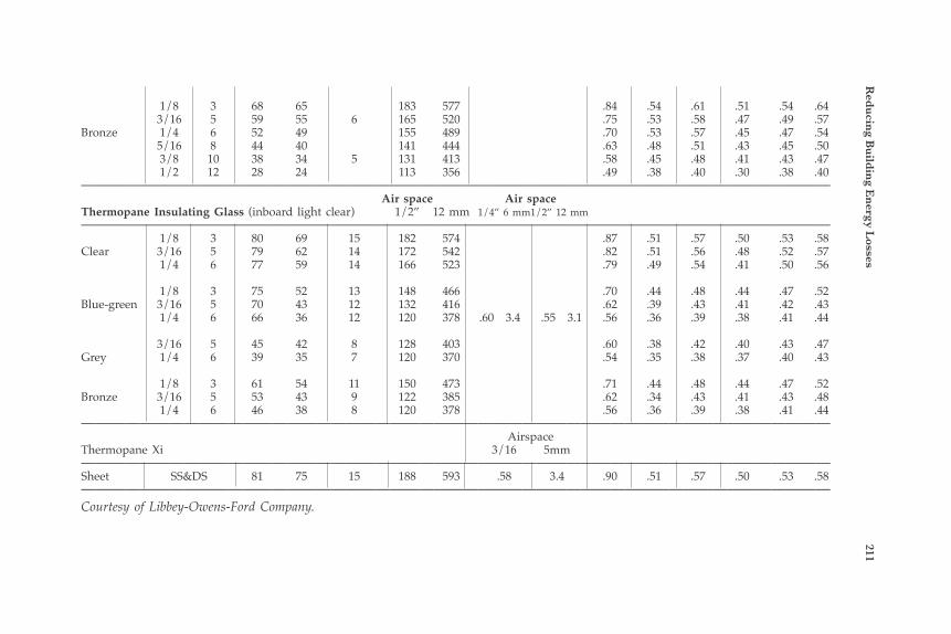
Red
ucin
g Bu
ildin
g En
ergy Losses
211
1/8 3 68 65 183 577 .84 .54 .61 .51 .54 .64 3/16 5 59 55 6 165 520 .75 .53 .58 .47 .49 .57Bronze 1/4 6 52 49 155 489 .70 .53 .57 .45 .47 .54 5/16 8 44 40 141 444 .63 .48 .51 .43 .45 .50 3/8 10 38 34 5 131 413 .58 .45 .48 .41 .43 .47 1/2 12 28 24 113 356 .49 .38 .40 .30 .38 .40——————————————————————————————————————————————————— Air space Air spaceThermopane Insulating Glass (inboard light clear) 1/2” 12 mm 1/4” 6 mm 1/2” 12 mm——————————————————————————————————————————————————— 1/8 3 80 69 15 182 574 .87 .51 .57 .50 .53 .58Clear 3/16 5 79 62 14 172 542 .82 .51 .56 .48 .52 .57 1/4 6 77 59 14 166 523 .79 .49 .54 .41 .50 .56
1/8 3 75 52 13 148 466 .70 .44 .48 .44 .47 .52Blue-green 3/16 5 70 43 12 132 416 .62 .39 .43 .41 .42 .43 1/4 6 66 36 12 120 378 .60 3.4 .55 3.1 .56 .36 .39 .38 .41 .44
3/16 5 45 42 8 128 403 .60 .38 .42 .40 .43 .47Grey 1/4 6 39 35 7 120 370 .54 .35 .38 .37 .40 .43
1/8 3 61 54 11 150 473 .71 .44 .48 .44 .47 .52Bronze 3/16 5 53 43 9 122 385 .62 .34 .43 .41 .43 .48 1/4 6 46 38 8 120 378 .56 .36 .39 .38 .41 .44——————————————————————————————————————————————————— AirspaceThermopane Xi 3/16 5mm———————————————————————————————————————————————————Sheet SS&DS 81 75 15 188 593 .58 3.4 .90 .51 .57 .50 .53 .58———————————————————————————————————————————————————Courtesy of Libbey-Owens-Ford Company.
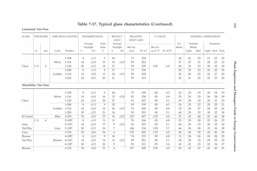
212 P
lant E
ngin
eers and
Man
agers Gu
ide to E
nergy C
onservation
Table 7-17. Typical glass characteristics (Continued).Laminated Vari-Tran———————————————————————————————————————————————————GLASS THICKNESS VARI-TRAN COATING TRANSMITTANCE REFLECT- RELATIVE1 U VALUE SHADING COEFFICIENTS ANCE HEAT GAIN Average Total Average No Venetian Draperies Daylight Solar Daylight Btu/hr- Btu/hr- Shade Blinds in mm Color Number % Tol % % Tol sq ft W/m2 sq ft/°F W/m2°k Light Med Light Med Dark——————————————————————————————————————————————————— 1-108 8 ±1.5 9 43 71 224 .28 .21 .23 .21 .22 .23 Silver 1-114 14 ±2.0 15 33 ±3.0 89 281 .37 .27 .31 .28 .29 .31Clear 1/4 6 1-120 20 ±2.5 19 27 95 299 1.05 6.0 .40 .29 .33 .30 .32 .34 1-208 8 ±1.5 8 27 73 230 .29 .22 .24 .22 .22 .24 Golden 1-214 14 ±2.0 13 24 ±3.0 85 268 .35 .26 .29 .26 .27 .29 1-220 20 ±2.5 20 21 99 312 .42 .31 .35 .32 .33 .36
Monolithic Vari-Tran——————————————————————————————————————————————————— 1-108 8 ±1.5 9 44 57 180 .80 4.5 .23 .18 .19 .18 .18 .19 Silver 1-114 14 ±2.0 16 33 ±3.0 82 258 .85 4.8 .35 .26 .29 .26 .28 .29Clear 1-120 20 ±2.5 20 27 91 287 .90 5.1 .39 .28 .32 .29 .31 .33 1-208 8 ±1.5 9 28 63 199 .80 4.5 .26 .20 .22 .20 .20 .21 Golden 1-214 14 ±2.0 14 26 ±3.0 76 240 .85 4.8 .32 .24 .27 .24 .25 .26 1-220 20 _ ±2.5 21 24 93 293 .90 5.1 .40 .29 .33 .30 .32 .34B/Green Blue 2-350 50 ±5.0 35 18 ±3.0 129 407 1.05 6.0 .57 .42 .48 .42 .44 .48 1/4 6 3-1082 8 ±1.5 11 11 78 246 .85 4.8 .33 .25 .28 .25 .26 .27Grey 3-1142 14 ±2.0 17 9 ±2.0 93 293 .90 5.1 .40 .29 .33 .30 .32 .34Tuf-Flex Grey 3-1202 20 ±2.5 24 7 106 334 1.00 5.7 .46 .34 .38 .35 .36 .39Grey 3-134 34 ±4.0 36 6 135 426 1.05 6.0 .60 .44 .50 .43 .46 .50Bronze 4-1082 8 ±1.5 9 14 74 233 .85 4.8 .31 .24 .26 .24 .24 .25Tuf-Flex Bronze 4-1142 14 ±2.0 14 11 ±2.0 89 281 .90 5.1 .38 .28 .32 .29 .30 .32 4-1202 20 ±2.5 20 9 99 312 .95 5.4 .43 .32 .35 .32 .34 .37Bronze 4-134 34 ±4.0 31 6 127 400 1.05 6.0 .56 .42 .47 .41 .43 .47
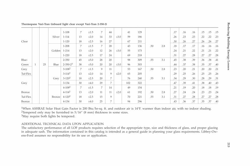
Red
ucin
g Bu
ildin
g En
ergy Losses
213Thermopane Vari-Tran (inboard light clear except Vari-Tran 2-350-2)——————————————————————————————————————————————————— 1-108 7 ±1.5 7 44 41 129 .17 .16 .16 .15 .15 .15 Silver 1-114 13 ±2.0 14 33 ±3.0 59 186 .26 .23 .23 .22 .22 .23Clear 1-120 18 ±2.5 16 27 67 211 .30 .26 .27 .26 .26 .27 1-208 7 ±1.5 7 28 43 136 .50 2.8 .18 .17 .17 .16 .16 .16 Golden 1-214 13 ±2.0 12 26 ±3.0 55 173 .24 .21 .22 .21 .21 .22 1-220 18 ±2.5 17 24 69 218 .31 .27 .28 .27 .27 .28Blue- 2-350 45 ±5.0 28 20 98 309 .55 3.1 .45 .38 .39 .36 .38 .41Green 1 25 Blue 2-350-23 38 ±5.0 20 20 ±3.0 96 303 .44 .37 .38 .35 .37 .40Grey 3-1082 7 ±1.5 9 11 53 167 .50 2.8 .23 .20 .21 .20 .20 .21Tuf-Flex 3-1142 13 ±2.0 14 9 ±2.0 65 205 .29 .25 .26 .25 .25 .26 Grey 3-1202 18 ±2.5 20 7 76 240 .55 3.1 .34 .29 .30 .28 .29 .31Grey 3-134 30 ±4.0 29 7 102 322 .47 .39 .41 .38 .40 .43 4-1082 7 ±1.5 7 14 49 154 .21 .19 .20 .18 .18 .19Bronze 4-1142 13 ±2.0 11 11 ±2.0 61 192 .50 2.8 .27 .24 .24 .23 .23 .24Tuf-Flex Bronze 4-1202 18 ±2.5 15 9 70 221 .55 3.1 .31 .27 .28 .27 .27 .28Bronze 4-134 30 ±4.0 25 7 94 296 .43 .36 .37 .35 .37 .40
1When ASHRAE Solar Heat Gain Factor is 200 Btu/hr-sq. ft. and outdoor air is 14°F. warmer than indoor air, with no indoor shading.2Tempered only may be furnished in 5/16” (8 mm) thickness in some sizes.3May require both lights be tempered.
ADDITIONAL TECHNICAL DATA UPON APPLICATIONThe satisfactory performance of all LOF products requires selection of the appropriate type, size and thickness of glass, and proper glazing in adequate sash. The information contained in this catalog is intended as a general guide in planning your glass requirements. Libbey-Ow-ens-Ford assumes no responsibility for its use or application.

214 Plant Engineers and Managers Guide to Energy Conservation
Table 7-18. Solar heat gain factors for 40° north latitude.
Solar Heat Gain Factors————————————————————————————————
June 21 AM PM 8 9 10 11 12 1 2 3 4———————————————————————————————— N 29 33 35 37 38 37 35 33 29 N NE 156 113 62 40 38 37 35 31 26 NW E 215 192 145 80 41 37 35 31 26 W SE 152 161 148 116 71 41 36 31 26 SW S 29 45 69 88 95 88 69 45 29 S 4 3 1 2 12 11 10 9 8 PM AM———————————————————————————————————————————————————————————————— September 21 AM PM 8 9 10 11 12 1 2 3 4———————————————————————————————— N 16 22 26 29 30 29 26 22 16 N NE 87 47 28 29 30 29 26 22 16 NW E 205 195 148 77 32 29 26 22 16 W SE 199 226 221 192 141 77 30 23 16 SW S 71 124 165 191 200 191 165 124 71 S 4 3 2 1 12 11 10 9 8 PM AM————————————————————————————————Courtesy of Libbey-Owens-Ford Company.
Applying Insulation As illustrated in this chapter, insulation offers one of the best methods to improve the efficiency of building designs. Table 7-19 offers a comparison of various insulation materials. In practice, the thermal con-ductivities of insulation should be based on the manufacturer’s data.
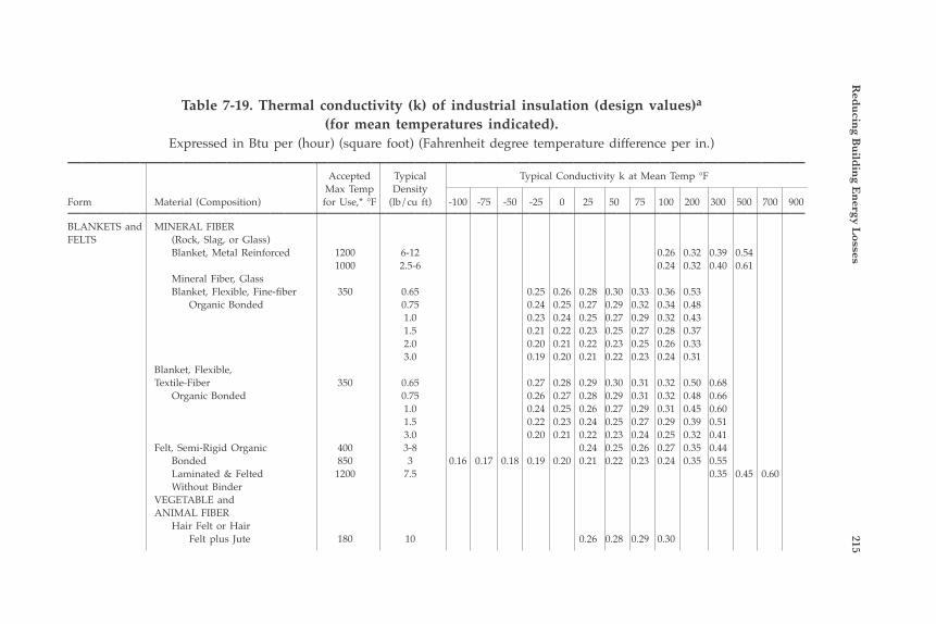
Red
ucin
g Bu
ildin
g En
ergy Losses
215
Table 7-19. Thermal conductivity (k) of industrial insulation (design values)a
(for mean temperatures indicated).Expressed in Btu per (hour) (square foot) (Fahrenheit degree temperature difference per in.)
——————————————————————————————————————————————————— Accepted Typical Typical Conductivity k at Mean Temp °F Max Temp DensityForm Material (Composition) for Use,* °F (lb/cu ft) -100 -75 -50 -25 0 25 50 75 100 200 300 500 700 900———————————————————————————————————————————————————BLANKETS and MINERAL FIBERFELTS (Rock, Slag, or Glass) Blanket, Metal Reinforced 1200 6-12 0.26 0.32 0.39 0.54 1000 2.5-6 0.24 0.32 0.40 0.61 Mineral Fiber, Glass Blanket, Flexible, Fine-fiber 350 0.65 0.25 0.26 0.28 0.30 0.33 0.36 0.53 Organic Bonded 0.75 0.24 0.25 0.27 0.29 0.32 0.34 0.48 1.0 0.23 0.24 0.25 0.27 0.29 0.32 0.43 1.5 0.21 0.22 0.23 0.25 0.27 0.28 0.37 2.0 0.20 0.21 0.22 0.23 0.25 0.26 0.33 3.0 0.19 0.20 0.21 0.22 0.23 0.24 0.31 Blanket, Flexible, Textile-Fiber 350 0.65 0.27 0.28 0.29 0.30 0.31 0.32 0.50 0.68 Organic Bonded 0.75 0.26 0.27 0.28 0.29 0.31 0.32 0.48 0.66 1.0 0.24 0.25 0.26 0.27 0.29 0.31 0.45 0.60 1.5 0.22 0.23 0.24 0.25 0.27 0.29 0.39 0.51 3.0 0.20 0.21 0.22 0.23 0.24 0.25 0.32 0.41 Felt, Semi-Rigid Organic 400 3-8 0.24 0.25 0.26 0.27 0.35 0.44 Bonded 850 3 0.16 0.17 0.18 0.19 0.20 0.21 0.22 0.23 0.24 0.35 0.55 Laminated & Felted 1200 7.5 0.35 0.45 0.60 Without Binder VEGETABLE and ANIMAL FIBER Hair Felt or Hair Felt plus Jute 180 10 0.26 0.28 0.29 0.30
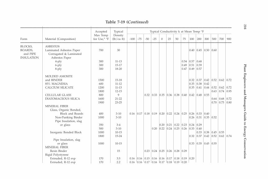
216 P
lant E
ngin
eers and
Man
agers Gu
ide to E
nergy C
onservation
Table 7-19 (Continued)——————————————————————————————————————————————————— Accepted Typical Typical Conductivity k at Mean Temp °F Max Temp DensityForm Material (Composition) for Use,* °F (lb/cu ft) -100 -75 -50 -25 0 25 50 75 100 200 300 500 700 900———————————————————————————————————————————————————BLOCKS, ASBESTOSBOARDS, Laminated Asbestos Paper 700 30 0.40 0.45 0.50 0.60 and PIPE Corrugated & LaminatedINSULATION Asbestos Paper 4-ply 300 11-13 0.54 0.57 0.68 6-ply 300 15-17 0.49 0.51 0.59 8-ply 300 18-20 0.47 0.49 0.57
MOLDED AMOSITE and BINDER 1500 15-18 0.32 0.37 0.42 0.52 0.62 0.72 85% MAGNESIA 600 11-12 0.35 0.38 0.42 CALCIUM SILICATE 1200 11-13 0.35 0.41 0.44 0.52 0.62 0.72 1800 12-15 0.63 0.74 0.95 CELLULAR GLASS 800 9 0.32 0.33 0.35 0.36 0.38 0.40 0.42 0.48 0.55 DIATOMACEOUS SILICA 1600 21-22 0.64 0.68 0.72 1900 23-25 0.70 0.75 0.80 MINERAL FIBER Glass, Organic Bonded, Block and Boards 400 3-10 0.16 0.17 0.18 0.19 0.20 0.22 0.24 0.25 0.26 0.33 0.40 Non-Punking Binder 1000 3-10 0.26 0.31 0.35 0.52 Pipe Insulation, slag or glass 350 3-4 0.20 0.21 0.22 0.23 0.24 0.29 500 3-10 0.20 0.22 0.24 0.25 0.26 0.33 0.40 Inorganic Bonded Block 1000 10-15 0.33 0.38 0.45 0.55 1800 15-24 0.32 0.37 0.42 0.52 0.62 0.74 Pipe Insulation, slag or glass 1000 10-15 0.33 0.35 0.45 0.55 MINERAL FIBER Resin Binder 15 0.23 0.24 0.25 0.26 0.28 0.29 Rigid Polystyrene Extruded, R-12 exp 170 3.5 0.16 0.16 0.15 0.16 0.16 0.17 0.18 0.19 0.20 Extruded, R-12 exp 170 2.2 0.16 0.16 0.17 0.16 0.17 0.18 0.19 0.20

Red
ucin
g Bu
ildin
g En
ergy Losses
217 Extruded 170 1.8 0.17 0.18 0.19 0.20 0.21 0.23 0.24 0.25 0.27 Molded Beads 170 1 0.18 0.20 0.21 0.23 0.24 0.25 0.26 0.28 Polyurethane** R-11 exp 210 1.5-2.5 0.16 0.17 0.18 0.18 0.18 0.17 0.16 0.16 0.17 RUBBER, Rigid Foamed 150 4.5 0.20 0.21 0.22 0.23 VEGETABLE and ANIMAL FIBER Wool Felt (Pipe Insulation) 180 20 0.28 0.30 0.31 0.33
———————————————————————————————————————————————————INSULATING MINERAL FIBERCEMENTS (Rock, Slag, or Glass) With Colloidal Clay Binder 1800 24-30 0.49 0.55 0.61 0.73 0.85 With Hydraulic Setting Binder 1200 30-40 0.75 0.80 0.85 0.95
———————————————————————————————————————————————————LOOSE FILL Cellulose insulation (Milled pulverized paper or wood pulp) 2.5-3 0.26 0.27 0.29 Mineral fiber, slag, rock or glass 2-5 0.19 0.21 0.23 0.25 0.26 0.28 0.31 Perlite (expanded) 5-8 0.25 0.27 0.29 0.30 0.32 0.34 0.35 0.37 0.39 Silica aerogel 7.6 0.13 0.14 0.15 0.15 0.16 0.17 0.18 Vermiculite (expanded) 7-8.2 0.39 0.40 0.42 0.44 0.45 0.47 0.49 4-6 0.34 0.35 0.38 0.40 0.42 0.44 0.46
———————————————————————————————————————————————————aRepresentative values for dry materials as selected by the ASHRAE Technical Committee 2.4 on Insulation. They are intended as design (not specification) values for materials of building construction for normal use. For the thermal resistance of a particular product, the user may obtain the value supplied by the manufacturer or secure the results of unbiased tests.*These temperatures are generally accepted as maximum. When operating temperature approaches these limits the manufacturer’s recom-mendations should be followed.**These are values for aged board stock.Reprinted by permission from ASHRAE Handbook of Fundamentals, 1972.

218 Plant Engineers and Managers Guide to Energy Conservation
WINDOW TREATMENTS
Several types of window treatments to reduce losses have become available. This section describes some of the products on the market, based on information supplied by manufacturers. No claims are made concerning the validity or completeness described. The summary is based on “Windows For Energy Efficient Buildings” as prepared by the Lawrence Berkeley Laboratory for U.S. DOE under contract W-7405-ENG-48.
Solar ControlSolar Control Films A range of tinted and reflective polyester films is available to ad-here to inner window surfaces to provide solar control for existing clear glazing. Films are typically two- or three-layer laminates composed of metalized, transparent and/or tinted layers. Films are available with a wide range of solar and visible light transmittance values, resulting in shading coefficients as low as 0.24. Most films are adhered with pre-coated pressure sensitive adhesives. Reflective films will reduce winter U values by about 20%. (Note that a new solar control film, which provides a U value of 0.68, is described in the Thermal Barriers section below). Films adhered to glass improve the shatter resistance of glazing and reduce transmission, thus reducing fading of furnishings.
Fiberglass Solar Control Screens Solar control screens provide sun and glare control as well as some reduction in winter heat loss. Screens are woven from vinyl-coated glass strands and are available in a variety of colors. Depending on color and weave, shading coefficients of 0.3 to 0.5 are achieved. Screens are durable, maintenance-free, and provide impact resistance. They are usually applied on the exterior of windows and may (1) be attached to mounting rails and stretched over windows, (2) mounted in rigid frames and installed over windows, or (3) made into roller shades which can be retracted and stored as desired.
Motorized Window Shading System A variety of plastic and fabric shades is available for use with a motorized window shading system. A reversible motor is located within the shade tube roller and contains a brake mechanism to stop and hold

Reducing Building Energy Losses 219
in any position. Motor controls may be gauged and operated locally or from a master station. Automatic photoelectric controls are available that (1) monitor sun intensity and angle and adjust shade position to provide solar control and (2) employ an internal light sensor and pro-vide a preset level of internal ambient light.
Exterior Sun Control Louvers Operable external horizontal and vertical louver systems are of-fered for a variety of building sun control applications. Louvers are hinged together and can be rotated in unison to provide the desired degree of shading for any sun position. Operation may be manual or electric; electrical operation may be initiated by manual switches, time clock, or sun sensors. Louvers may be closed to reduce night thermal losses. Sun control elements are available in several basic shapes and in a wide range of sizes.
External Venetian Blinds Externally mounted, all-weather venetian blinds may be manually operated from within a building or electrically operated and controlled by means of automatic sun sensors, time controls, manual switches, etc. Aluminum slats are held in position with side guides and controlled by weatherproof lifting tapes. Slats can be tilted to modulate solar gain, closed completely, or restricted to admit full light and heat. Blinds have been in use in Europe for many years and have been tested for resis-tance to storms and high winds.
Adjustable Louvered Windows Windows incorporating adjustable external louvered shading de-vices are available. Louvers are extruded aluminum or redwood, 3 to 5 inches wide, and are manually controlled. Louvers may be specified on double-hung, hinged, or louvered-glass windows. When open, the louvers provide control of solar gain and glare; when closed, they pro-vide privacy and security.
Solar Shutters The shutter is composed of an array of aluminum slats set at 45° or 22-1/2° from the vertical to block direct sunlight. Shutters are designed for external application and may be mounted vertically in front of the window or projected outward from the bottom of the window. Other

220 Plant Engineers and Managers Guide to Energy Conservation
rolling and hinged shutters are stored beside the window and roll or swing into place for sun control, privacy, or security.
Thermal BarriersMultilayer, Roll-up Insulating Window Shade A multilayer window shade stores in a compact roll and utilizes spacers to separate the aluminized plastic layers in the deployed posi-tion, thereby creating a series of dead air spaces. A five-layer shade combined with insulated glass provides R8 thermal resistance.
Thermal Barrier, Roll-up Insulating Window Shade A ThermoShade thermal barrier is a roll-up shade composed of hollow, lens-shaped, rigid, white PVC slats with virtually no air leakage through connecting joints. The side tracking system reduces window infiltration. The design is for interior installation and manual or auto-matic operation.
Using the Insulating Window Shade When added to a window, the roll-up insulating shade provides R4.5 for a single-glazed window or R5.5 for a double-glazed window. Quilt is composed of fabric outer surfaces and two polyester fiberfill layers sandwiched around a reflective vapor barrier. Quilt layers are ultrasonically welded. Shade edges are enclosed in a side track to reduce infiltration.
Reflective, Perforated Solar Control Laminate Laminate of metalized weatherable polyester film and black vinyl is then perforated with 225 holes/in.2, providing 36 percent open area. Available in a variety of metallized and nonmetallized colors, the shad-ing coefficients vary from 0.30 to 0.35 for externally mounted screens and 0.37 to 0.45 for the material adhered to the inner glass surface. The laminate is typically mounted in aluminum screen frames which are hung externally, several inches from the window; it can also be utilized in a roll-up form. Some reduction in winter U value can be expected with external applications.
Semi-transparent Window Shades Roll-up window shades are made from a variety of tinted or reflective solar control film laminates. These shades provide most of the benefits of solar control film applied directly to glass but provide

Reducing Building Energy Losses 221
additional flexibility and may be retracted on overcast days or when solar heat gain is desired. Shades are available with spring operated and gravity (cord and reel) operated rollers, as well as with motor-ized options. Shading coefficients as low as 0.13 are achieved; a tight fitting shade provides an additional air space and thus reduced U-value.
Operable External Louver Blinds Solar control louver blinds, mounted on the building exterior, can be controlled manually or automatically by sun and wind sensors. Slats can be tilted to modulate light, closed completely, or retracted to admit full light and heat. Developed and used extensively in Europe, they provide summer sun control, control of natural light, and reduction of winter heat loss.
Louvered Metal Solar Screens A solar screen consists of an array of tiny fixed horizontal lou-vers that are woven in place. Louvers are tilted at 17° to provide sun control. Screen material is set in metal frames, which may be perma-nently installed in a variety of configurations or designed for removal. Installed screens have considerable wind and impact resistance. The standard product (17 louvers/inch) has a shading coefficient of 0.23; low sun angle variant (23 louvers/inch) has a shading coefficient of 0. 15. Modest reductions in winter U value have been measured. (See Figure 7-5.)
Insulating Solar Control Film A modified solar control film designed to be adhered to the interior of windows provides conventional solar control function and has greatly improved insulating properties. Film emissivity is 0.23 to 0.25, resulting in a U value of 0.68 Btu/ft2 hr-°F under winter conditions, compared to 0.87 for conventional solar control films and 1.1 for typical single-glazed windows.
Interior Storm Windows These low-cost, do-it-yourself interior storm windows have a rigid plastic glazing panel. The glazing panel may be removed for cleaning or summer storage. It reduces infiltration losses as well as conductive/convective heat transfer.

222 Plant Engineers and Managers Guide to Energy Conservation
Retrofit Insulating Glass System Single glazing is converted to double glazing by attaching an extra pane of glass with neoprene sealant. A desiccant-filled aluminum spacer absorbs moisture between the panes. An electric resistance wire embed-ded in the neoprene is heated with a special power source. This hermeti-cally seals the window. New molding can then be applied if desired.
Infiltration
Weather-strip Tape This polypropylene film is scored along its centerline so that it can be easily formed into a “V” shape. It has a pressure-sensitive adhesive on one leg of the “V” for application to seal cracks around doors and windows. On an average fitting, double-hung window, infiltration is reduced by over 70%. It can be applied to rough or smooth surfaces.
ADVANCED OPTICAL TECHNOLOGIES
Opportunities For High-performance Window Products The product mix of the window industry of today reflects a num-ber of innovations designed to improve the energy performance, optical clarity, and aesthetics of residential and commercial windows. Low-E coatings, tints, reflective films and coatings, gas fills, and new frame
1/2”
17 per inch
17°
.05”
(Magnified View)
Figure 7-5. Louvered metal solar screen.

Reducing Building Energy Losses 223
materials and designs are features that offer substantial energy savings to consumers, as well as opportunities for window manufacturers to add value to their product line at a time of increased energy and envi-ronmental awareness. While a good window today is almost twice as energy efficient as the standard double glazed units of the early ‘80s, most of the en-ergy saving potential for advanced windows has yet to be captured. Researchers are working to further improve on current technologies, expand high performance window applications to retrofit markets, and ultimately turn windows into dynamic energy supply systems that continuously respond to the energy and daylighting needs of buildings and their occupants.
“Smart Windows” with Switchable Glazing The next technological step beyond selective glazing is the ca-pability to dynamically alter the solar-optical properties of a window. A switchable glazing can change its properties upon some external stimulus. Some types of switchable glazings respond directly to an environmental variable such as heat or light. A more controllable, and thus more desirable type, is a glazing whose properties are altered via a low voltage electrical signal. Building occupants could control heat and light transmitted through the windows by simply adjusting a switch. Some switchable glazings have been around for years. For ex-ample, photochromic glass that darkens in bright light is common in sunglasses but is not yet available in large sheets for windows. Several new switchable products are becoming available. One is a combina-tion photochromic and heat-sensitive thermochromic material intended largely for skylights. When its temperature rises, this material changes from clear to a reflective milky white to block heat gain from the sun. Another newly introduced product uses a thin layer of liquid crystals sandwiched between glass.
“Cool Windows” Using Selective Glazings Window glass and plastic films can be coated with microscopically thin metallic layers or incorporate tints that reflect or absorb some or all of the wavelengths of the solar energy spectrum. A desirable “selective glazing” would allow solar energy wavelengths in the visible spectrum (daylight) to pass through a window while reflecting near infrared

224 Plant Engineers and Managers Guide to Energy Conservation
(heat) and ultraviolet (fabric damaging) wavelengths. Reflective coatings do a better job of reflecting the sun’s energy than absorbing glazings. These “cool windows” reduce cooling loads by up to 50% but still look clear to the human eye. First generation selective coatings have already been used success-fully by several glazing manufacturers in products aimed at commercial and sunbelt residential applications. These high performance silver-based coatings require protection within a sealed glazing assembly to avoid degradation.
Superwindows A superwindow is a highly insulating window with a heat loss so low that it performs better than an insulated wall in winter because the sunlight that it admits is greater than its heat loss over a 24-hour period. Superwindow research focuses on the design, development, and testing of new windows and window components such as frames and edge seals, and on new materials and techniques to reduce thermal losses across window systems. An objective of the research is market-able window products with insulating values up to five times as high as conventional double glazed windows. Another objective is for the vast majority of window manufacturers to incorporate several of these tech-nologies into their windows. The increased availability of very high-R windows, plus incremental improvements in the mainstream windows, would effect a shift in average performance from less than R-2 to over R-5, resulting in significant energy savings.
225
8Heating, Ventilation andAir-Conditioning SystemOptimization
EFFICIENT USE OF HEATING ANDCOOLING EQUIPMENT SAVES DOLLARS
Most people have probably experienced improper air conditioning or heating controls which waste energy. Energy is saved when efficient heating, ventilation, and air conditioning (HVAC) systems are used. In this chapter, you will learn how to compare the efficiency of various systems and apply the heat pump to save energy, see how various re-frigeration systems can be used to save energy, learn the basics of air conditioning design from an energy conservation viewpoint, and begin to apply the computer approach for energy conservation.
Measuring System Efficiency by Using the Coefficient of Performance The coefficient of performance (COP) is the basic parameter used to compare the performance of refrigeration and heating systems. COP for cooling and heating applications is defined as follows:
Rate of Net Heat Removal COP (Cooling) = ———————————— (8-1) Total Energy Input
Rate of Useful Heat Delivered*CPOP (Heating, Heat Pump*) = —————————————— (8-2) Total Energy Input
*For heat pump applications, exclude supplemental heating.
226 Plant Engineers and Managers Guide to Energy Conservation
APPLYING THE HEAT PUMP TO SAVE ENERGY
The heat pump has gained wide attention due to its high potential COP. The heat pump in its simplest form can be thought of as a window air conditioner. During the summer, the air on the room side is cooled while air is heated on the outside air side. If the window air conditioner is turned around in the winter, some heat will be pumped into the room. Instead of switching the air conditioner around, a cycle reversing valve is used to switch functions. This valve switches the function of the evaporator and condenser, and refrigeration flow is reversed through the device. Thus, the heat pump is heat recovery through a refrigeration cycle. Heat is removed from one space and placed in another. In Chapter 7, it was seen that the direction of heat flow is from hot to cold. Basically, energy or pumping power is needed to make heat flow “up hill.” The mechanical refrigeration compressor “pumps” absorbed heat to a higher level for heat rejection. The refrigerant gas is compressed to a higher temperature level so that the heat absorbed by it (during the evapora-tion or cooling process) is rejected in the condensing or heating process. Thus, the heat pump provides cooling in the summer and heating in the winter. The source of heat for the heat pump can be from one of three elements: air, water or the ground.
Air-to-air Heat Pumps Heat exists in air down to 460°F below zero. Using outside air as a heat source has its limitations, because the efficiency of a heat pump drops off as the outside air level drops below 55°F. This is because the heat is more dispersed at lower temperatures, or more difficult to capture. Thus, heat pumps are generally sized on cooling load capaci-ties. Supplemental heat is added to compensate for declining capacity of the heat pump. This approach allows for a realistic first cost and an economical operating cost.
Heat Pumps Do Save Energy An average of 2 to 3 times as much heat can be moved for each kW input compared to that produced by use of straight resistance heating. Heat pumps can have a COP of greater than 3 in industrial processes, depending on temperatures. Commercially available heat pumps range in size from two to three tons for residences to up to 40 tons for com-mercial and industrial users. Figure 8-1 illustrates a simple scheme for
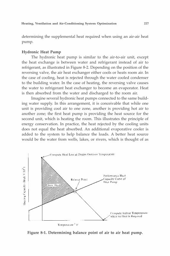
Heating, Ventilation and Air-Conditioning System Optimization 227
determining the supplemental heat required when using an air-air heat pump.
Hydronic Heat Pump The hydronic heat pump is similar to the air-to-air unit, except the heat exchange is between water and refrigerant instead of air to refrigerant, as illustrated in Figure 8-2. Depending on the position of the reversing valve, the air heat exchanger either cools or heats room air. In the case of cooling, heat is rejected through the water cooled condenser to the building water. In the case of heating, the reversing valve causes the water to refrigerant heat exchanger to become an evaporator. Heat is then absorbed from the water and discharged to the room air. Imagine several hydronic heat pumps connected to the same build-ing water supply. In this arrangement, it is conceivable that while one unit is providing cool air to one zone, another is providing hot air to another zone; the first heat pump is providing the heat source for the second unit, which is heating the room. This illustrates the principle of energy conservation. In practice, the heat rejected by the cooling units does not equal the heat absorbed. An additional evaporative cooler is added to the system to help balance the loads. A better heat source would be the water from wells, lakes, or rivers, which is thought of as
Figure 8-1. Determining balance point of air to air heat pump.
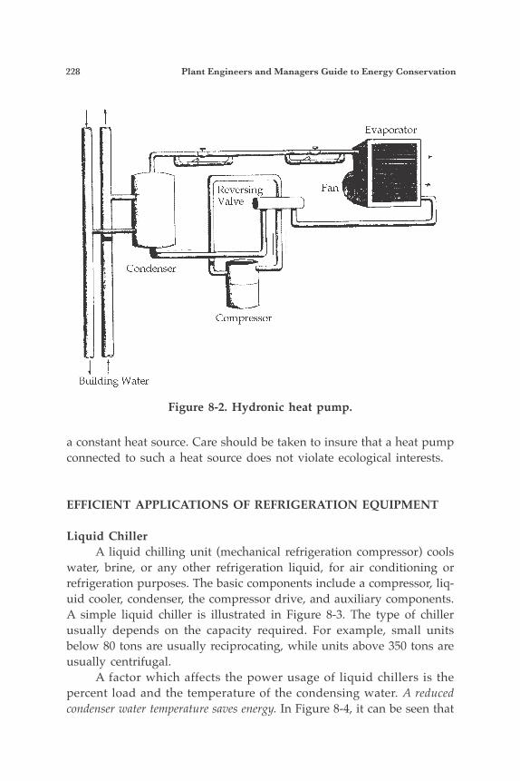
228 Plant Engineers and Managers Guide to Energy Conservation
a constant heat source. Care should be taken to insure that a heat pump connected to such a heat source does not violate ecological interests.
EFFICIENT APPLICATIONS OF REFRIGERATION EQUIPMENT
Liquid Chiller A liquid chilling unit (mechanical refrigeration compressor) cools water, brine, or any other refrigeration liquid, for air conditioning or refrigeration purposes. The basic components include a compressor, liq-uid cooler, condenser, the compressor drive, and auxiliary components. A simple liquid chiller is illustrated in Figure 8-3. The type of chiller usually depends on the capacity required. For example, small units below 80 tons are usually reciprocating, while units above 350 tons are usually centrifugal. A factor which affects the power usage of liquid chillers is the percent load and the temperature of the condensing water. A reduced condenser water temperature saves energy. In Figure 8-4, it can be seen that
Figure 8-2. Hydronic heat pump.
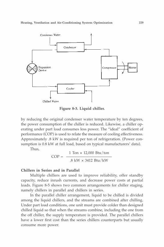
Heating, Ventilation and Air-Conditioning System Optimization 229
by reducing the original condenser water temperature by ten degrees, the power consumption of the chiller is reduced. Likewise, a chiller op-erating under part load consumes less power. The “ideal” coefficient of performance (COP) is used to relate the measure of cooling effectiveness. Approximately .8 kW is required per ton of refrigeration. (Power con-sumption is 0.8 kW at full load, based on typical manufacturers’ data). Thus, 1 Ton × 12,000 Btu/ton COP = ———————————— .8 kW × 3412 Btu/kW
Chillers in Series and in Parallel Multiple chillers are used to improve reliability, offer standby capacity, reduce inrush currents, and decrease power costs at partial loads. Figure 8-5 shows two common arrangements for chiller staging, namely chillers in parallel and chillers in series. In the parallel chiller arrangement, liquid to be chilled is divided among the liquid chillers, and the streams are combined after chilling. Under part load conditions, one unit must provide colder than designed chilled liquid so that when the streams combine, including the one from the off chiller, the supply temperature is provided. The parallel chillers have a lower first cost than the series chillers counterparts but usually consume more power.
Figure 8-3. Liquid chiller.
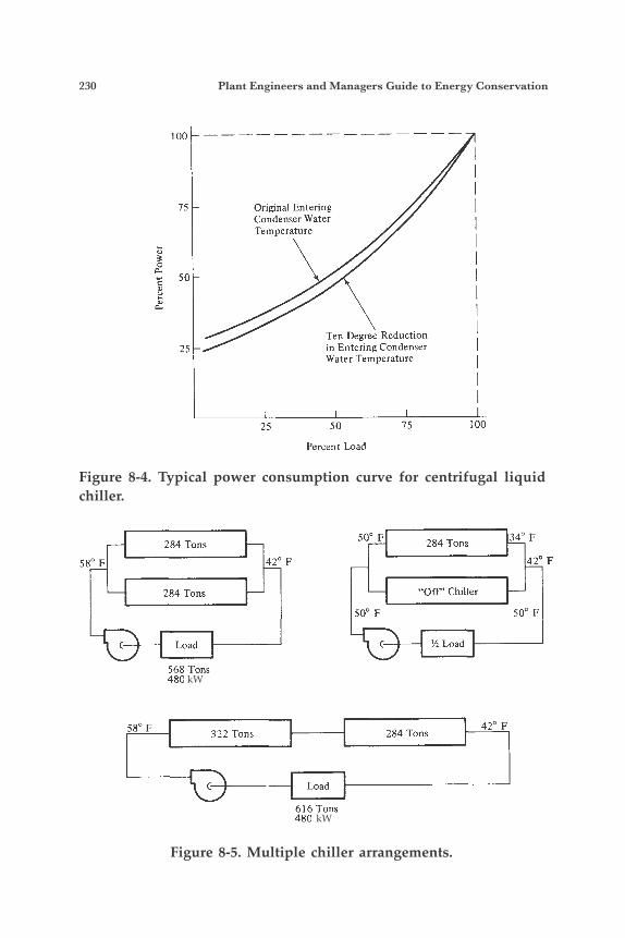
230 Plant Engineers and Managers Guide to Energy Conservation
Figure 8-4. Typical power consumption curve for centrifugal liquid chiller.
Figure 8-5. Multiple chiller arrangements.
kW
kW
100
7s
2s
Original Entering Condenser Water Temperature
Ten Degree Reduction in Entering Condenser Water Temperature
25 50
Percent Load
IS 100
284 Tons
58" F
284 Tons
Load
568 Tons 480
322 Tons 58" F
42' F
Load
616 Tons 48C
34" F 284 Tons 50" F
142' F
"Off' Chiller
50' F 50" F
Yi Load
42" F 284 Tons
Heating, Ventilation and Air-Conditioning System Optimization 231
In the series arrangement, a constant volume of flow of chilled water passes through the machines, producing better temperature con-trol and better efficiency under part load operation; thus, the upstream chiller requires less kW input per ton output. The waste of energy dur-ing the mixing aspect of the parallel chiller operation is avoided. The series chillers, in general, require higher pumping costs. The energy conservation engineer should evaluate the best arrangement, based on load required and the partial loading conditions.
Absorption System Basics The absorption cycle begins at the evaporator with heat being absorbed from the air either directly from the air through an air to re-frigerant heat exchanger or indirectly through a heat transfer loop. This heat boils the liquid refrigerant (water or R717), which migrates to the absorber where it is absorbed into solution with an absorbent (LiBr or water). This “mixed” fluid (usually called dilute solution) is then pumped to condensing pressure by a small solution pump. The high pressure dilute solution enters the generator section of the unit, where heat is added to drive the refrigerant from the solution. The now concentrated absorbent solution returns to the absorber, and refrigerant vapor migrates to the condenser, where it is liquefied by transferring heat to the outside air (either directly or through a heat transfer loop to a cooling tower). The refrigerant is then reduced in pressure by an expansion device and returned to the evaporator to begin the cycle again. A typical schematic for a single-stage absorption unit is illustrated in Figure 8-6. The basic components of the system are the evapora-tor, absorber, concentrator, and condenser. These components can be grouped in a single or double shell. Figure 8-6 represents a single-stage arrangement.
Evaporator Refrigerant is sprayed over the top of the tube bundle to provide for a high rate of transfer between water in the tubes and the refriger-ant on the outside of the tubes.
Absorber The refrigerant vapor produced in the evaporator migrates to the bottom half of the shell, where it is absorbed by a lithium bromide so-lution. Lithium bromide is basically a salt solution that exerts a strong
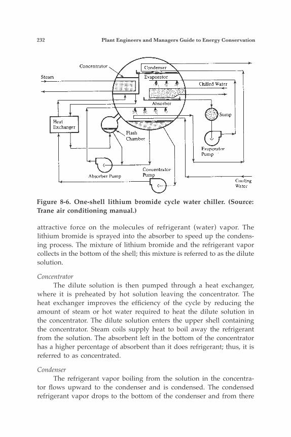
232 Plant Engineers and Managers Guide to Energy Conservation
attractive force on the molecules of refrigerant (water) vapor. The lithium bromide is sprayed into the absorber to speed up the condens-ing process. The mixture of lithium bromide and the refrigerant vapor collects in the bottom of the shell; this mixture is referred to as the dilute solution.
Concentrator The dilute solution is then pumped through a heat exchanger, where it is preheated by hot solution leaving the concentrator. The heat exchanger improves the efficiency of the cycle by reducing the amount of steam or hot water required to heat the dilute solution in the concentrator. The dilute solution enters the upper shell containing the concentrator. Steam coils supply heat to boil away the refrigerant from the solution. The absorbent left in the bottom of the concentrator has a higher percentage of absorbent than it does refrigerant; thus, it is referred to as concentrated.
Condenser The refrigerant vapor boiling from the solution in the concentra-tor flows upward to the condenser and is condensed. The condensed refrigerant vapor drops to the bottom of the condenser and from there
Figure 8-6. One-shell lithium bromide cycle water chiller. (Source: Trane air conditioning manual.)
Heating, Ventilation and Air-Conditioning System Optimization 233
flows to the evaporator through a regulating orifice. This completes the refrigerant cycle. The single-stage absorption unit consumes approximately 18.7 pounds of steam per ton of capacity. (Steam consumption at full load is based on typical manufacturers data.) For a single-stage absorption unit,
1 ton × 12,000 Btu/ton COP = ——————————— = 0.67 18.7 lb × 955 Btu/lb
The single-stage absorption unit is not as efficient as the mechani-cal chiller. It is usually justified based on availability of low pressure steam, equipment considerations, or use with solar collector systems.
SIM 8-1Compute the energy wasted when 15 psig steam is condensed prior to its return to the power plant. Comment on using the 15 psig steam directly for refrigeration.
ANSWERFrom Steam Tables 12-20 for 30 psia steam, hfg is 945 Btu per pound of steam; thus, 945 Btu per pound of steam is wasted. In this case, where excess low pressure steam cannot be used, absorption units should be con-sidered in place of their electrical mechanical refrigeration counterparts.
SIM 8-22000 lb/hr of 15 psig steam is being wasted. Calculate the yearly (8000 hr/yr) energy savings if a portion of the centrifugal refrigeration sys-tem is replaced with single-stage absorption. Assume 20 kW additional energy is required for the pumping and cooling tower cost associated with the single-stage absorption unit. Energy rate is $.045 kWh and the absorption unit consumes 18.7 lb of steam per ton of capacity. The centrifugal chiller system consumes 0.8 kWh per ton of refrig-eration.
ANSWERTons of mechanical chiller capacity replaced = 2000/18.7 = 106.95 tons.
Yearly energy savings = 2000/18.7 × 8000 × 0.8 × $.045 – 20 kW × 8000 × $.045 = $23,602
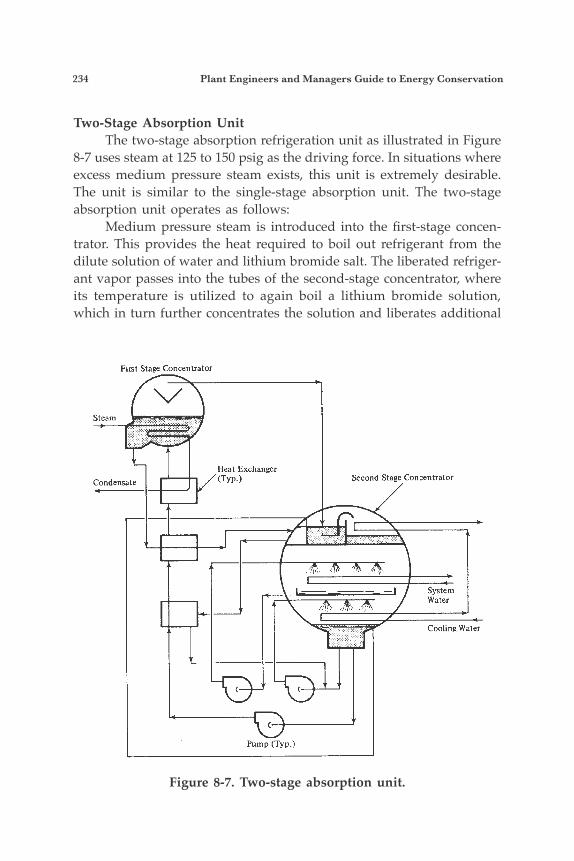
234 Plant Engineers and Managers Guide to Energy Conservation
Two-Stage Absorption Unit The two-stage absorption refrigeration unit as illustrated in Figure 8-7 uses steam at 125 to 150 psig as the driving force. In situations where excess medium pressure steam exists, this unit is extremely desirable. The unit is similar to the single-stage absorption unit. The two-stage absorption unit operates as follows: Medium pressure steam is introduced into the first-stage concen-trator. This provides the heat required to boil out refrigerant from the dilute solution of water and lithium bromide salt. The liberated refriger-ant vapor passes into the tubes of the second-stage concentrator, where its temperature is utilized to again boil a lithium bromide solution, which in turn further concentrates the solution and liberates additional
Figure 8-7. Two-stage absorption unit.
Heating, Ventilation and Air-Conditioning System Optimization 235
refrigerant. In effect, the concentrator frees an increased amount of re-frigerant from solution with each unit of input energy. The condensing refrigerant in the second-stage concentrator is piped directly into the condenser section. The effect of this is to reduce the cooling water load. A reduced cooling water load decreases the size of the cooling tower used to cool the water. The remaining portions of the system are basically the same as the single-stage unit. The two-stage absorption unit consumes approximately 18.7 pounds of steam per ton of capacity; thus, it is more efficient than a single-stage counterpart. The associated COP is
1 ton × 12,000 Btu/ton COP = ——————————— = .67 18.7 lb × 860 Btu/lb
Either type of absorption unit can be used in conjunction with centrifu-gal chillers when it is desirable to reduce the peak electrical demand of the plant, or to provide for a solar collector addition at a later date.
GUIDE TO GAS COOLING TECHNOLOGY
The era of deregulation, real time prices, and summer electric price volatility is posing significant risks for the commercial customer. Conventional cooling technologies will leave the customer exposed to the hot weather price swings seen over the last two summers. This chap-ter summarizes the available and emerging gas technologies that can meet these customers’ needs for cost containment and risk reduction, including absorption chillers, engine chillers, and desiccant systems; it also addresses how such arrangements compare or work with thermal storage and on-site power generating systems.
The Emerging Technologies Given these market needs, a number of new technologies are emerging, with implications that can significantly change the world of commercial HVAC.
A New Age of Absorption Chillers They say that if you wait long enough, everything will come around again. The use of absorption chillers in the new century is one
236 Plant Engineers and Managers Guide to Energy Conservation
of those things. Manufacturers have prepared an entire new generation of absorption chillers, with new features and user conveniences never before available to meet the challenges of electric deregulation. Absorption is attractive in that it can be driven in so many ways—by boiler steam, by waste heat, and direct-fired from either natural gas or fuel oil. When integrated with engine, steam turbine, or gas turbine generation, electricity and cooling can be supplied simultaneously. When used in conjunction with electric chillers in a “hybrid cooling plant,” absorbers offer a fuel-fired component to the cooling plant at maintenance costs equivalent to those of an electric chiller. This last element may surprise many “old hands” in the HVAC design community. Due to the addition of sophisticated electronics, automatic purge, variable speed solution pumps, and a whole host of new features, maintenance contracts on a modern absorption chiller are often quoted at or below that of an electric chiller. In addition, absorbers now feature response times similar to electric chillers, are able to handle variable chiller barrel pumping, can cope with wide and rapid swings in tower water temperature, and often have turndown capabilities that exceed those of electric chillers. Given these developments, using an absorption chiller for a por-tion of the capacity can assure the owner of flexibility in energy sourcing without a major change in overall maintenance cost profile.
Engine Chillers Another option for new chiller plants is engine-driven chillers. These chillers combine the vapor compression systems used in electric chillers with a heavy-duty, long-life engine, generally operating on natu-ral gas. These systems feature significantly higher operating efficiencies than absorption chillers and can produce low temperature chilled water if desired. Engine chillers may also be less expensive than absorption chillers, particularly in the popular 100-400RT range. However, engine chillers do have additional maintenance needs that have to be included in the decision process. However, these chillers have seen rapid market growth in the last 6 years as service structures to handle their particular needs have been established.
Thermal Storage Another element in the technology mix is thermal storage—usu-ally in the form of ice storage. This can be used to shift cooling loads
Heating, Ventilation and Air-Conditioning System Optimization 237
from day to night power usage, a distinct advantage in areas with wide time-of-use price swings. If used in all-electric plants, thermal storage requires oversizing of the electrical equipment to handle the low evaporator temperatures, as well as substantial floor space for the ice storage system. Using thermal storage to meet peak loads, however, reduces these cost issues. In a previous paper, the author has examined the comparative cost of differing systems and found the most cost ef-fective use of thermal storage to be with a peak load shaver in hybrid gas and electric cooling plants.*
Hybrid Chiller/Generator Products With the growing interest in hybrid chiller plants, some manu-facturers have developed individual “hybrid chillers.” This is a single chiller that can operate on two different energy sources alternately as desired by the owner. The first such unique product available to the market is an engine/electric-driven chiller that features a drive line consisting of an engine, a clutch, and an electric motor, all in drive line, driving the chiller com-pressor. The engine can drive the compressor or be un-clutched, free-ing the electric motor to drive the compressor. For areas with dramatic swings in time-of-day pricing, this can be highly economical. Depending on the engine for fewer hours of the year reduces maintenance, and the electric motor allows the chiller to operate even if the engine is off-line for maintenance. In time, new equipment of this type should be coming to the mar-ket with the added capability of generating electricity by reversing the motor. Using the unit as an engine driven generator allows the chiller to double as a standby generator, or as an on-site generator when cooling is not called for.
Desiccant Dehumidification Another option for thermally activated cooling systems is to re-lieve the cooling plant of some of the ventilation air cooling loads by using desiccant dehumidification to dehumidify ventilation air. Desiccant systems have unique capabilities, as they can deep dry ventilation air without overcooling and reheating. In high ventilation
*Presented at GLOBALCON 2000, April, 2000 by W.A. Ryan, “Gas Cooling in the Era of Deregulation.”

238 Plant Engineers and Managers Guide to Energy Conservation
load applications such as schools, theaters, and hospital surgical suites, this can amount to a significant load. In addition, desiccant systems can be operated either by direct-fuel firing or from waste heat, such as engine or turbine exhaust. This gives the owner an option in integrated cooling, heating, and power systems.
Trigeneration Trigeneration is a new, more specific term for combining cooling, heating, and power generation systems into one piece of equipment. Development of such comprehensive equipment is under way and should be available to the market in the next few years. In general, the generation source may be an engine, gas turbine, or fuel cell, with waste heat powering both the facility space heating and cooling system. Integration of water heating into the same system may also be used for applications where water heating is a significant load. Custom designed trigeneration systems have been applied to large installations in the past. These systems have generally been for such large applications as college campuses, major medical facilities, or major convention centers. The modern concept is to develop integrated, packaged trigeneration systems that can be applied to the huge market for individual commercial buildings. This requires smaller capacity, low maintenance, generating options such as microturbines and small fuel cell systems (both in development), and more affordable light capacity, thermally-activated cooling systems such as small absorption or desic-cant systems. One of the most attractive elements of trigeneration is the “double reduction” of the peak-demand requirements of the facility. By using waste heat to operate the cooling system, the cooling season electric peak is avoided. The power output of the system is then devoted to base loads such as lights, receptacles, and ventilating fans, further reducing the peak electric demand of these base loads. This is more practical than providing a larger, power-generation-only system to a facility with all electric chillers to produce the same annual demand limitation. This will be an important issue in the deregulated future, as the facility will need to contract for electric supply service that will handle peak power needs.
District Heating and Cooling Plants In the nearer term is the recent growth in district heating and cooling plants. After decades with little interest being shown in this
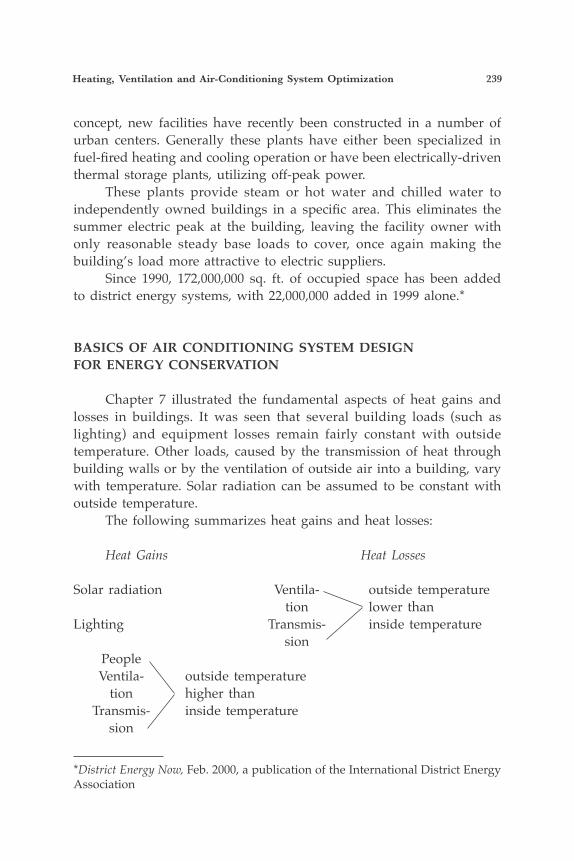
Heating, Ventilation and Air-Conditioning System Optimization 239
concept, new facilities have recently been constructed in a number of urban centers. Generally these plants have either been specialized in fuel-fired heating and cooling operation or have been electrically-driven thermal storage plants, utilizing off-peak power. These plants provide steam or hot water and chilled water to independently owned buildings in a specific area. This eliminates the summer electric peak at the building, leaving the facility owner with only reasonable steady base loads to cover, once again making the building’s load more attractive to electric suppliers. Since 1990, 172,000,000 sq. ft. of occupied space has been added to district energy systems, with 22,000,000 added in 1999 alone.*
BASICS OF AIR CONDITIONING SYSTEM DESIGNFOR ENERGY CONSERVATION
Chapter 7 illustrated the fundamental aspects of heat gains and losses in buildings. It was seen that several building loads (such as lighting) and equipment losses remain fairly constant with outside temperature. Other loads, caused by the transmission of heat through building walls or by the ventilation of outside air into a building, vary with temperature. Solar radiation can be assumed to be constant with outside temperature. The following summarizes heat gains and heat losses:
Heat Gains Heat Losses
Solar radiation Ventila- outside temperature tion lower thanLighting Transmis- inside temperature sion People Ventila- outside temperature tion higher than Transmis- inside temperature sion
*District Energy Now, Feb. 2000, a publication of the International District Energy Association
240 Plant Engineers and Managers Guide to Energy Conservation
When heat gains are traded with heat losses, energy savings are realized. The central system is the basic air conditioning system used today. It allows for cooling, dehumidification, and heating equipment to be located in one area. As the central system developed, it became apparent that heat sources varied within the space; thus, the total area had to be divided into zones or sections. The general categories of cooling systems most commonly used today are:
1. Central units serving individual zones 2. Multi-zone units 3. Double duct systems 4. Reheat systems 5. Variable volume systems 6. Individual room units
There are many variations and combinations, but the above are the basic options available. The major problem facing energy conservation engineering is to avoid generalizing. Each category has its application and economic advantage and should be evaluated based on the econom-ics of the particular systems. In this section, particular applications of air conditioning systems will be discussed.
APPLYING VARIABLE AIR VOLUME SYSTEMS
The variable air volume system has gained popularity in recent years, due to its potential of saving energy. This system is not a cure-all, but it will save energy when properly selected. Variable air volume (VAV) systems vary the quantity of air at a constant temperature, to match the system load requirements. The energy consumption closely paral-lels the load in air conditioning systems. This is in contrast to constant volume air systems that control building temperatures by varying the temperature of a constant flow of air. The most popular type of VAV system contains a terminal unit that modulates the air volume between maximum and a predetermined value. There are four main classes of VAV systems that encompass 80% of the VAV market. These classes combine the best features of several systems, to obtain maximum efficiency. Figure 8-8 illustrates the four classes.
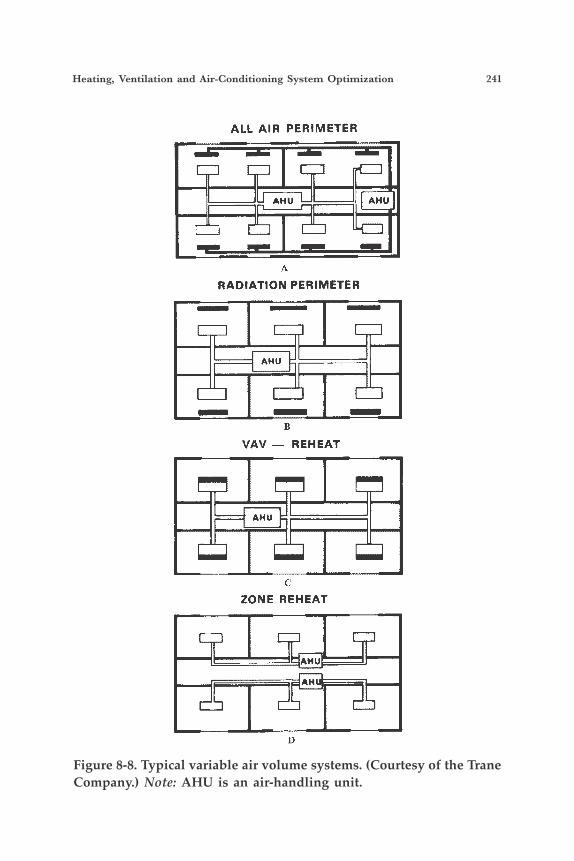
Heating, Ventilation and Air-Conditioning System Optimization 241
Figure 8-8. Typical variable air volume systems. (Courtesy of the Trane Company.) Note: AHU is an air-handling unit.
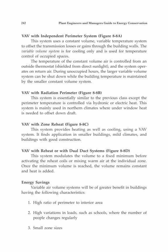
242 Plant Engineers and Managers Guide to Energy Conservation
VAV with Independent Perimeter System (Figure 8-8A) This system uses a constant volume, variable temperature system to offset the transmission losses or gains through the building walls. The variable volume system is for cooling only and is used for temperature control of occupied spaces. The temperature of the constant volume air is controlled from an outside thermostat (shielded from direct sunlight), and the system oper-ates on return air. During unoccupied hours, the larger variable volume system can be shut down while the building temperature is maintained by the smaller constant volume system.
VAV with Radiation Perimeter (Figure 8-8B) This system is essentially similar to the previous class except the perimeter temperature is controlled via hydronic or electric heat. This system is mainly used in northern climates where under window heat is needed to offset down draft.
VAV with Zone Reheat (Figure 8-8C) This system provides heating as well as cooling, using a VAV system. It finds application in smaller buildings, mild climates, and buildings with good construction.
VAV with Reheat or with Dual Duct Systems (Figure 8-8D) This system modulates the volume to a fixed minimum before activating the reheat coils or mixing warm air at the individual zone. Once the minimum volume is reached, the volume remains constant and heat is added.
Energy Savings Variable air volume systems will be of greater benefit in buildings having the following characteristics:
1. High ratio of perimeter to interior area
2. High variations in loads, such as schools, where the number of people changes regularly
3. Small zone sizes
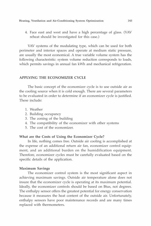
Heating, Ventilation and Air-Conditioning System Optimization 243
4. Face east and west and have a high percentage of glass. (VAV reheat should be investigated for this case.)
VAV systems of the modulating type, which can be used for both perimeter and interior spaces and operate at medium static pressure, are usually the most economical. A true variable volume system has the following characteristic: system volume reduction corresponds to loads, which permits savings in annual fan kWh and mechanical refrigeration.
APPLYING THE ECONOMIZER CYCLE
The basic concept of the economizer cycle is to use outside air as the cooling source when it is cold enough. There are several parameters to be evaluated in order to determine if an economizer cycle is justified. These include:
1. Weather 2. Building occupancy 3. The zoning of the building 4. The compatibility of the economizer with other systems 5. The cost of the economizer.
What are the Costs of Using the Economizer Cycle? In life, nothing comes free. Outside air cooling is accomplished at the expense of an additional return air fan, economizer control equip-ment, and an additional burden on the humidification equipment. Therefore, economizer cycles must be carefully evaluated based on the specific details of the application.
Maximum Savings The economizer control system is the most significant aspect in achieving maximum savings. Outside air temperature alone does not insure that the economizer cycle is operating at its maximum potential. Ideally, the economizer controls should be based on Btus, not degrees. The enthalpy sensor offers the greatest potential for energy conservation because it measures the heat content of the outside air. Unfortunately, enthalpy sensors have poor maintenance records and are many times replaced with thermometers.
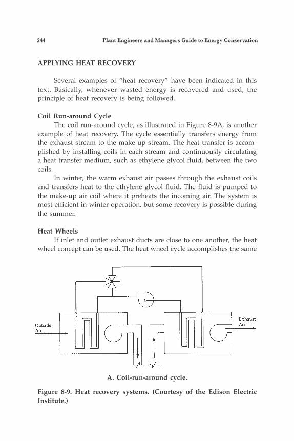
244 Plant Engineers and Managers Guide to Energy Conservation
APPLYING HEAT RECOVERY
Several examples of “heat recovery” have been indicated in this text. Basically, whenever wasted energy is recovered and used, the principle of heat recovery is being followed.
Coil Run-around Cycle The coil run-around cycle, as illustrated in Figure 8-9A, is another example of heat recovery. The cycle essentially transfers energy from the exhaust stream to the make-up stream. The heat transfer is accom-plished by installing coils in each stream and continuously circulating a heat transfer medium, such as ethylene glycol fluid, between the two coils. In winter, the warm exhaust air passes through the exhaust coils and transfers heat to the ethylene glycol fluid. The fluid is pumped to the make-up air coil where it preheats the incoming air. The system is most efficient in winter operation, but some recovery is possible during the summer.
Heat Wheels If inlet and outlet exhaust ducts are close to one another, the heat wheel concept can be used. The heat wheel cycle accomplishes the same
A. Coil-run-around cycle.
Figure 8-9. Heat recovery systems. (Courtesy of the Edison Electric Institute.)
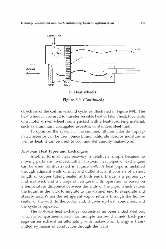
Heating, Ventilation and Air-Conditioning System Optimization 245
objectives of the coil run-around cycle, as illustrated in Figure 8-9B. The heat wheel can be used to transfer sensible heat or latent heat. It consists of a motor driven wheel frame packed with a heat-absorbing material, such as aluminum, corrugated asbestos, or stainless steel mesh. To optimize the system in the summer, lithium chloride impreg-nated asbestos can be used. Since lithium chloride absorbs moisture as well as heat, it can be used to cool and dehumidify make-up air.
Air-to-air Heat Pipes and Exchangers Another form of heat recovery is relatively simple because no moving parts are involved. Either air-to-air heat pipes or exchangers can be used, as illustrated in Figure 8-9C. A heat pipe is installed through adjacent walls of inlet and outlet ducts; it consists of a short length of copper tubing sealed at both ends. Inside is a porous cy-lindrical wick and a charge of refrigerant. Its operation is based on a temperature difference between the ends of the pipe, which causes the liquid in the wick to migrate to the warmer end to evaporate and absorb heat. When the refrigerant vapor returns through the hollow center of the wick to the cooler end, it gives up heat, condenses, and the cycle is repeated. The air-to-air heat exchanger consists of an open ended steel box which is compartmentalized into multiple narrow channels. Each pas-sage carries exhaust air alternating with make-up air. Energy is trans-mitted by means of conduction through the walls.
B. Heat wheels.
Figure 8-9. (Continued)
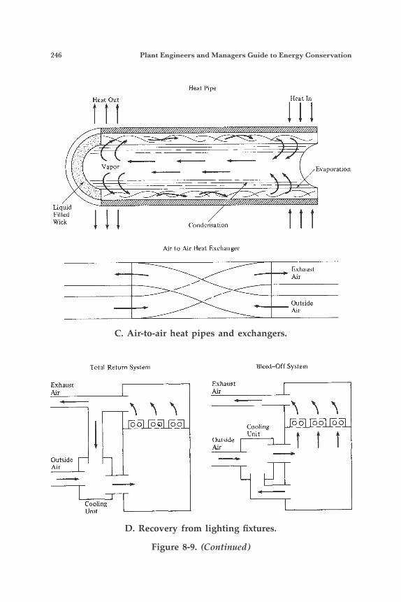
246 Plant Engineers and Managers Guide to Energy Conservation
D. Recovery from lighting fixtures.
Figure 8-9. (Continued)
C. Air-to-air heat pipes and exchangers.
Heat Pipe
Heat Out
Vapor
Liquid Filled Wick
Heat In
Evaporation
Condensation
Air to Air Heat Exchanger
Exhaust Air
Outside Air
Total Return System
Exhaust Air
Bleed-Off System
Exhaust Air
Cooling Unit
Outside Air
Outside ' Air
Cooling Unit
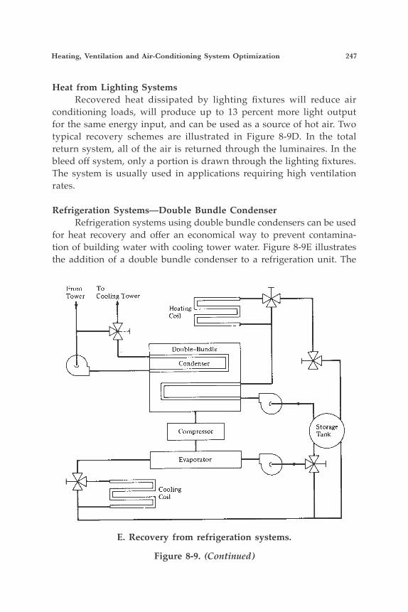
Heating, Ventilation and Air-Conditioning System Optimization 247
Heat from Lighting Systems Recovered heat dissipated by lighting fixtures will reduce air conditioning loads, will produce up to 13 percent more light output for the same energy input, and can be used as a source of hot air. Two typical recovery schemes are illustrated in Figure 8-9D. In the total return system, all of the air is returned through the luminaires. In the bleed off system, only a portion is drawn through the lighting fixtures. The system is usually used in applications requiring high ventilation rates.
Refrigeration Systems—Double Bundle Condenser Refrigeration systems using double bundle condensers can be used for heat recovery and offer an economical way to prevent contamina-tion of building water with cooling tower water. Figure 8-9E illustrates the addition of a double bundle condenser to a refrigeration unit. The
E. Recovery from refrigeration systems.
Figure 8-9. (Continued)
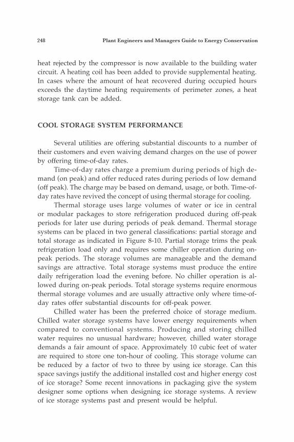
248 Plant Engineers and Managers Guide to Energy Conservation
heat rejected by the compressor is now available to the building water circuit. A heating coil has been added to provide supplemental heating. In cases where the amount of heat recovered during occupied hours exceeds the daytime heating requirements of perimeter zones, a heat storage tank can be added.
COOL STORAGE SYSTEM PERFORMANCE
Several utilities are offering substantial discounts to a number of their customers and even waiving demand charges on the use of power by offering time-of-day rates. Time-of-day rates charge a premium during periods of high de-mand (on peak) and offer reduced rates during periods of low demand (off peak). The charge may be based on demand, usage, or both. Time-of-day rates have revived the concept of using thermal storage for cooling. Thermal storage uses large volumes of water or ice in central or modular packages to store refrigeration produced during off-peak periods for later use during periods of peak demand. Thermal storage systems can be placed in two general classifications: partial storage and total storage as indicated in Figure 8-10. Partial storage trims the peak refrigeration load only and requires some chiller operation during on-peak periods. The storage volumes are manageable and the demand savings are attractive. Total storage systems must produce the entire daily refrigeration load the evening before. No chiller operation is al-lowed during on-peak periods. Total storage systems require enormous thermal storage volumes and are usually attractive only where time-of-day rates offer substantial discounts for off-peak power. Chilled water has been the preferred choice of storage medium. Chilled water storage systems have lower energy requirements when compared to conventional systems. Producing and storing chilled water requires no unusual hardware; however, chilled water storage demands a fair amount of space. Approximately 10 cubic feet of water are required to store one ton-hour of cooling. This storage volume can be reduced by a factor of two to three by using ice storage. Can this space savings justify the additional installed cost and higher energy cost of ice storage? Some recent innovations in packaging give the system designer some options when designing ice storage systems. A review of ice storage systems past and present would be helpful.
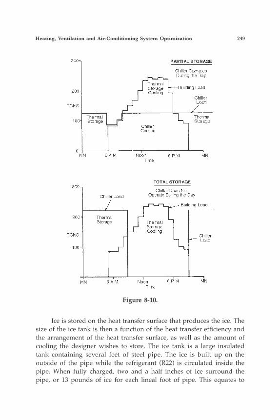
Heating, Ventilation and Air-Conditioning System Optimization 249
Ice is stored on the heat transfer surface that produces the ice. The size of the ice tank is then a function of the heat transfer efficiency and the arrangement of the heat transfer surface, as well as the amount of cooling the designer wishes to store. The ice tank is a large insulated tank containing several feet of steel pipe. The ice is built up on the outside of the pipe while the refrigerant (R22) is circulated inside the pipe. When fully charged, two and a half inches of ice surround the pipe, or 13 pounds of ice for each lineal foot of pipe. This equates to
Figure 8-10.
300 PARTIAL STORAGE
Chiller Operates During the Day
Thermal
Cooling Storage Building Load
Chiller Load
200
TONS
Thermal 100 Storage
Thermal Storage
Chiller Cooling
0 MN 6 A.M. Noon 6 P.M. MN
Time
300 TOTAL STORAGE
Chiller Does Not Operate During the Day Chiller Load
Building Load
200 Thermal Storage
TONS
Thermal Storage Cooling
Chiller Load
100
6 P.M. MN 6 A.M. Noon Time
MN
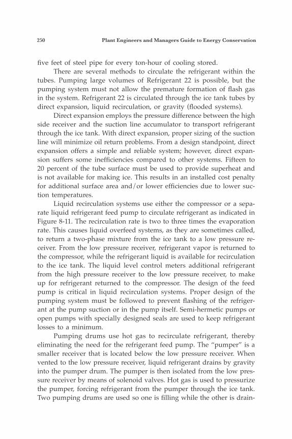
250 Plant Engineers and Managers Guide to Energy Conservation
five feet of steel pipe for every ton-hour of cooling stored. There are several methods to circulate the refrigerant within the tubes. Pumping large volumes of Refrigerant 22 is possible, but the pumping system must not allow the premature formation of flash gas in the system. Refrigerant 22 is circulated through the ice tank tubes by direct expansion, liquid recirculation, or gravity (flooded systems). Direct expansion employs the pressure difference between the high side receiver and the suction line accumulator to transport refrigerant through the ice tank. With direct expansion, proper sizing of the suction line will minimize oil return problems. From a design standpoint, direct expansion offers a simple and reliable system; however, direct expan-sion suffers some inefficiencies compared to other systems. Fifteen to 20 percent of the tube surface must be used to provide superheat and is not available for making ice. This results in an installed cost penalty for additional surface area and/or lower efficiencies due to lower suc-tion temperatures. Liquid recirculation systems use either the compressor or a sepa-rate liquid refrigerant feed pump to circulate refrigerant as indicated in Figure 8-11. The recirculation rate is two to three times the evaporation rate. This causes liquid overfeed systems, as they are sometimes called, to return a two-phase mixture from the ice tank to a low pressure re-ceiver. From the low pressure receiver, refrigerant vapor is returned to the compressor, while the refrigerant liquid is available for recirculation to the ice tank. The liquid level control meters additional refrigerant from the high pressure receiver to the low pressure receiver, to make up for refrigerant returned to the compressor. The design of the feed pump is critical in liquid recirculation systems. Proper design of the pumping system must be followed to prevent flashing of the refriger-ant at the pump suction or in the pump itself. Semi-hermetic pumps or open pumps with specially designed seals are used to keep refrigerant losses to a minimum. Pumping drums use hot gas to recirculate refrigerant, thereby eliminating the need for the refrigerant feed pump. The “pumper” is a smaller receiver that is located below the low pressure receiver. When vented to the low pressure receiver, liquid refrigerant drains by gravity into the pumper drum. The pumper is then isolated from the low pres-sure receiver by means of solenoid valves. Hot gas is used to pressurize the pumper, forcing refrigerant from the pumper through the ice tank. Two pumping drums are used so one is filling while the other is drain-
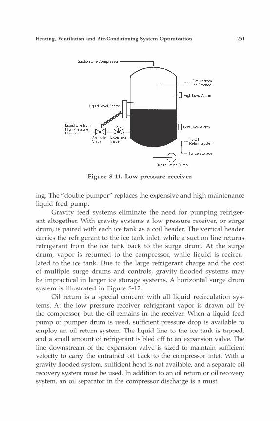
Heating, Ventilation and Air-Conditioning System Optimization 251
ing. The “double pumper” replaces the expensive and high maintenance liquid feed pump. Gravity feed systems eliminate the need for pumping refriger-ant altogether. With gravity systems a low pressure receiver, or surge drum, is paired with each ice tank as a coil header. The vertical header carries the refrigerant to the ice tank inlet, while a suction line returns refrigerant from the ice tank back to the surge drum. At the surge drum, vapor is returned to the compressor, while liquid is recircu-lated to the ice tank. Due to the large refrigerant charge and the cost of multiple surge drums and controls, gravity flooded systems may be impractical in larger ice storage systems. A horizontal surge drum system is illustrated in Figure 8-12. Oil return is a special concern with all liquid recirculation sys-tems. At the low pressure receiver, refrigerant vapor is drawn off by the compressor, but the oil remains in the receiver. When a liquid feed pump or pumper drum is used, sufficient pressure drop is available to employ an oil return system. The liquid line to the ice tank is tapped, and a small amount of refrigerant is bled off to an expansion valve. The line downstream of the expansion valve is sized to maintain sufficient velocity to carry the entrained oil back to the compressor inlet. With a gravity flooded system, sufficient head is not available, and a separate oil recovery system must be used. In addition to an oil return or oil recovery system, an oil separator in the compressor discharge is a must.
Figure 8-11. Low pressure receiver.

252 Plant Engineers and Managers Guide to Energy Conservation
Finally, there are ice tank accessories. To maintain uniform ice thickness, the water in the ice tank must be thoroughly mixed. An air pump is used to agitate the ice tank water during both the freezing and melting cycles. During the ice melting cycle, chilled water must circu-late around the ice covered pipes. An ice thickness probe is required to prevent the ice tank from over freezing or “bridging.” Bridges of ice forming between the ice-covered pipes will impede the flow of chilled water through the ice bundle during the melting cycle, resulting in uneven ice melting. Ice storage systems of this nature require very large refrigerant charges and incur substantial construction costs due to the number of field erected components. Due to these construction costs, many ice systems are difficult to justify except in larger tonnage applications. Recent innovations in the packaging of glycol-type ice tanks may make the option of ice storage a greater possibility. Glycol systems as indicated in Figure 8-13 use an ethylene glycol/water mixture as a low temperature heat transfer medium to transfer heat from the ice storage tanks to a packaged chiller and from the cooling coils to either the ice storage tanks or the chiller. The use of freeze-protected chilled water eliminates the design time, field construction, large refriger-ant charges, and leaks formerly associated with ice systems. Glycol ice storage tanks create ice by circulating the low temperature fluid through half-inch polyethylene tubing. The polyethylene tubing is coiled inside insulated polystyrene tanks. The ethylene glycol/water
Figure 8-12. Horizontal surge drum.
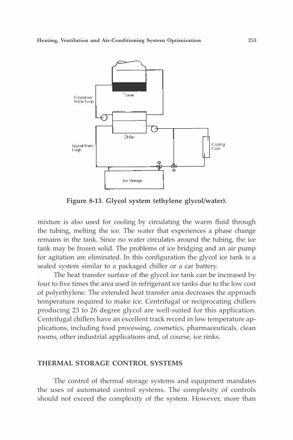
Heating, Ventilation and Air-Conditioning System Optimization 253
mixture is also used for cooling by circulating the warm fluid through the tubing, melting the ice. The water that experiences a phase change remains in the tank. Since no water circulates around the tubing, the ice tank may be frozen solid. The problems of ice bridging and an air pump for agitation are eliminated. In this configuration the glycol ice tank is a sealed system similar to a packaged chiller or a car battery. The heat transfer surface of the glycol ice tank can be increased by four to five times the area used in refrigerant ice tanks due to the low cost of polyethylene. The extended heat transfer area decreases the approach temperature required to make ice. Centrifugal or reciprocating chillers producing 23 to 26 degree glycol are well-suited for this application. Centrifugal chillers have an excellent track record in low temperature ap-plications, including food processing, cosmetics, pharmaceuticals, clean rooms, other industrial applications and, of course, ice rinks.
THERMAL STORAGE CONTROL SYSTEMS
The control of thermal storage systems and equipment mandates the uses of automated control systems. The complexity of controls should not exceed the complexity of the system. However, more than
Figure 8-13. Glycol system (ethylene glycol/water).
254 Plant Engineers and Managers Guide to Energy Conservation
a time clock and a few extra thermostats are required to insure the maximum benefit of the thermal storage system. Control concepts can range from simple to comprehensive. The simplest control is chiller priority. This control scheme allows the chiller to accept all of the cooling load until the load exceeds chiller capacity. Excess load is then met by melting ice. Control defaults to limiting chiller capacity by chiller selection or some form of demand limiting. Control is simple, but use of thermal storage is limited to cooling in excess of chiller capacity. This control may not provide the maximum financial return on the thermal storage investment. There are several variations of ice priority control schemes. The intent of ice priority control is to gain maximum benefit of time-of-day rates by maximizing ice usage each day. During intermediate seasons when the daily cooling load is less than thermal storage capacity, chiller operation can be limited to off-peak hours. When daily cooling load exceeds thermal storage capacity, chiller and ice must share the on-peak cooling load. The task of assigning cooling load to either ice or chiller is well suited for building automation systems with equation processing capabilities. If ice is used too early or too rapidly, the ice will be de-pleted before the end of the daytime cooling load, leaving several hours of building load in excess of chiller capacity. On the other hand, if the ice is not used to its maximum potential, the operating cost benefits of thermal storage are not totally realized. How does the automation system predict the daily cooling load the day before? Most of the required tools are already in place. The automation system has the ability to monitor several building or load producing trends. What the automation system does not possess is the ability to equate these trends to building cooling load. Fortunately, several HVAC system simulation programs are avail-able for this task. Simulation programs can isolate single load com-ponents and plot their dependence to an easily monitored variable. Internal loads are a function of time and calendar. Ventilation and solar loads can be equated to monitored weather variables. A daily cooling load profile can now be constructed by measurement of the monitored variables, profiling those variables for the period of prediction, and summing the results. Automation systems that can produce an expected daily load profile provide the building operator with a very powerful management tool. Only informed and prudent operation of thermal storage systems can guarantee their success.
Heating, Ventilation and Air-Conditioning System Optimization 255
THE VENTILATION AUDIT*
Indoor air quality (IAQ) is an emerging issue of concern to build-ing managers, operators, and designers. Recent research has shown that indoor air is often less clean than outdoor air, and federal legisla-tion has been proposed to establish programs to deal with this issue on a national level. This, like the asbestos issue, will have an impact on building design and operations. Americans today spend long hours inside buildings, and building operators, managers, and designers must be aware of potential IAQ problems and how they can be avoided. IAQ problems, sometimes termed “sick building syndrome,” have become an acknowledged health and comfort problem. Buildings are char-acterized as “sick” when occupants complain of acute symptoms such as headache; eye, nose and throat irritation; dizziness; nausea; sensitivity to odors; and difficulty in concentrating. The complaints may become more clinically defined such that an occupant may develop an actual building-related illness that is believed to be related to IAQ problems. The most effective means to deal with an IAQ problem is to re-move or minimize the pollutant source, when feasible. If not, dilution and filtration may be effective. Dilution (increased ventilation) admits more outside air to the building. ASHRAE’s 1981 standard recommended 5 CFM/person outside air in an office environment. The newest ASHRAE ventila-tion standard, 62-2001, now requires 20 CFM/person for offices if the prescriptive approach is used. Increased ventilation will have an impact on building energy consumption. However, this cost need not be severe. If an air-side economizer cycle is employed, and the HVAC system is controlled to respond to IAQ loads as well as thermal loads, 20 CFM/person need not be adhered to, and the economizer hours will help attain air qual-ity goals with energy savings at the same time. Incidentally, it was the energy cost of treating outside air that led to the latest standard. The superseded 1973 standard recommended 15-25 CFM/person. Energy savings can be realized by the use of improved filtration in lieu of the prescriptive 20 CFM/person approach. Improved filtration can occur at the air handler, in the supply and return ductwork, or in the
*Source: Indoor Air Quality: Problems & Cures, M. Black & W. Robertson, Pre-sented at the 13th World Energy Engineering Congress.
256 Plant Engineers and Managers Guide to Energy Conservation
spaces via self-contained units. Improved filtration can include enhance-ments such as ionization devices to neutralize airborne biological matter and to electrically charge fine particles, causing them to agglomerate and be more easily filtered. To accomplish an energy audit of the ventilation system the fol-lowing steps can be followed:
1. Measure volume of air at the outdoor air intakes of the ventilation system. Record ventilation and fan motor nameplate data.
2. Determine code requirements and compare against measure-ments.
3. If measured ventilation is more than required by code, decrease CFM by changing fan pulley, or by applying a variable speed drive.
Two savings are derived from this change, namely:• Reduced brake horsepower of fan motor.• Reduced heat loss during heating season.
To compute the savings, Equations 8-3 and 8-4 are used. Figure 8-14 can also be used to compute fan power savings as a result of air flow reduction.
HP New = HP ×
CFM NewCFM Old
3
(8-3)
1.08 Btu Q (Saved) = ——————— × CFM (Saved) × ∆T (8-4) HR – CFM – °F
kW = HP × 0.746/η (8-5)where HP = motor horsepower CFM = cubic feet per minute ∆T = average temperature gradient kW = motor kilowatts (k = 1000) η = motor efficiency
In addition to reducing air flow during occupied periods, consider-ation should be given to shutting the system down during unoccupied hours. If the space is cooled, additional savings will be achieved. The quantity of energy required to cool and dehumidify the ventilated air
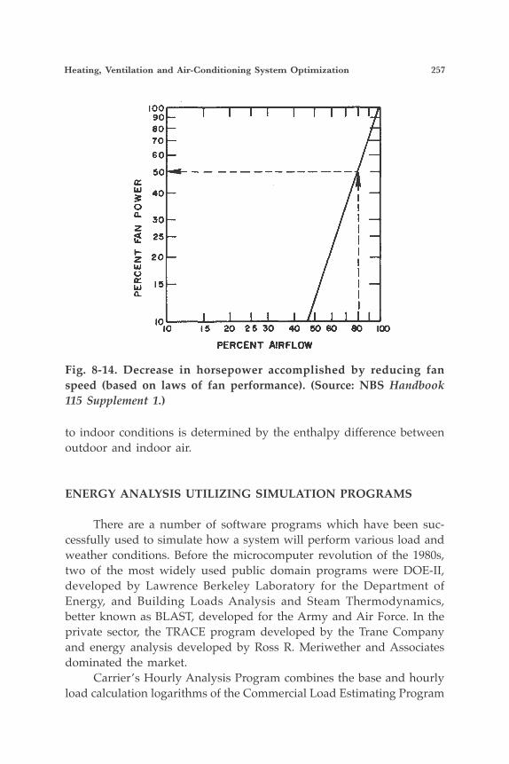
Heating, Ventilation and Air-Conditioning System Optimization 257
to indoor conditions is determined by the enthalpy difference between outdoor and indoor air.
ENERGY ANALYSIS UTILIZING SIMULATION PROGRAMS
There are a number of software programs which have been suc-cessfully used to simulate how a system will perform various load and weather conditions. Before the microcomputer revolution of the 1980s, two of the most widely used public domain programs were DOE-II, developed by Lawrence Berkeley Laboratory for the Department of Energy, and Building Loads Analysis and Steam Thermodynamics, better known as BLAST, developed for the Army and Air Force. In the private sector, the TRACE program developed by the Trane Company and energy analysis developed by Ross R. Meriwether and Associates dominated the market. Carrier’s Hourly Analysis Program combines the base and hourly load calculation logarithms of the Commercial Load Estimating Program
Fig. 8-14. Decrease in horsepower accomplished by reducing fan speed (based on laws of fan performance). (Source: NBS Handbook 115 Supplement 1.)
258 Plant Engineers and Managers Guide to Energy Conservation
with the sophisticated equipment simulation of the Operating Cost Analysis Program. The personal computer provides a cost-effective way to analyze energy consumption, make detailed building energy analysis, and implement life cycle costing in the decision-making process. There are numerous software options available that can help the plant en-gineer make the best possible choice.
TEST AND BALANCE CONSIDERATIONS
Probably the biggest overlooked low-cost energy audit require-ment is a thorough test, balance, and adjust program. In essence, the audit should include the following steps:
1. Test. Make a quantitative determination of conditions within the system boundary, including flow rates, temperature and humidity measurements, pressures, etc.
2. Balance. Balance the system for required distribution of flows by manipulation of dampers and valves.
3. Adjust. Adjust for required flow patterns the control instrument settings, regulating devices, and control sequences.
In essence, the above program checks the designer’s intent against actual performance, and balances and adjusts the system for peak per-formance. Several sources outlining test and balance procedures are:
• Construction Specifications Institute (CSI), which offers a specifica-tion series that includes a guide specification Document 15050 en-titled, “Testing and Balancing of Environmental Systems.” Reprints of this paper are available. It explains factors to be considered in using the guide specification for project specifications.
• Associated Air Balance Council (AABC), the certifying body of independent agencies.
• National Environmental Balancing Bureau (NEBB), sponsored joint-ly by the Mechanical Contractors Association of America and the Sheet Metal and Air Conditioning Contractors National Association as the certifying body of the installing contractors’ subsidiaries.

259
9Cogeneration:Theory and Practice
Because of its enormous potential, it is important to understand and apply cogeneration theory. In the overall context of energy man-agement theory, cogeneration is just another form of the conservation process. However, because of its potential for practical application to new or existing systems, it has carved a niche that may be second to no other conservation technology. This chapter is dedicated to development of a sound basis of cur-rent theory and practice of cogeneration technology. It is the blend of theory and practice, or praxis, of cogeneration that will form the basis of the most workable conservation technology in the coming years.
DEFINITION OF “COGENERATION” ORCOMBINED HEAT AND POWER (CHP)
Cogeneration is the sequential production of thermal and electric energy from a single fuel source. In the cogeneration process, heat is recovered that would normally be lost in the production of one form of energy. That heat is then used to generate the second form of energy. For example, take a situation in which an engine drives a generator that produces electricity: With cogeneration, heat would be recovered from the engine exhaust and/or coolant, and that heat would be used to produce, say, hot water. It is this combination of heat and power which leads to the name CHP. Making use of waste heat is what differentiates cogeneration fa-cilities from central station electric power generation. The overall fuel utilization efficiency of cogeneration plants is typically 70-80% versus 35-40% for utility power plants.
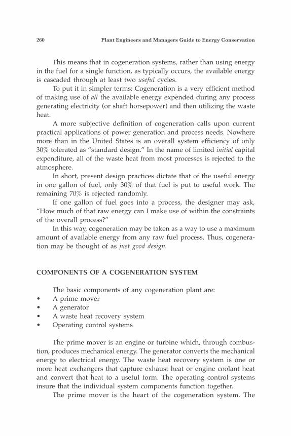
260 Plant Engineers and Managers Guide to Energy Conservation
This means that in cogeneration systems, rather than using energy in the fuel for a single function, as typically occurs, the available energy is cascaded through at least two useful cycles. To put it in simpler terms: Cogeneration is a very efficient method of making use of all the available energy expended during any process generating electricity (or shaft horsepower) and then utilizing the waste heat. A more subjective definition of cogeneration calls upon current practical applications of power generation and process needs. Nowhere more than in the United States is an overall system efficiency of only 30% tolerated as “standard design.” In the name of limited initial capital expenditure, all of the waste heat from most processes is rejected to the atmosphere. In short, present design practices dictate that of the useful energy in one gallon of fuel, only 30% of that fuel is put to useful work. The remaining 70% is rejected randomly. If one gallon of fuel goes into a process, the designer may ask, “How much of that raw energy can I make use of within the constraints of the overall process?” In this way, cogeneration may be taken as a way to use a maximum amount of available energy from any raw fuel process. Thus, cogenera-tion may be thought of as just good design.
COMPONENTS OF A COGENERATION SYSTEM
The basic components of any cogeneration plant are:• A prime mover• A generator• A waste heat recovery system• Operating control systems
The prime mover is an engine or turbine which, through combus-tion, produces mechanical energy. The generator converts the mechanical energy to electrical energy. The waste heat recovery system is one or more heat exchangers that capture exhaust heat or engine coolant heat and convert that heat to a useful form. The operating control systems insure that the individual system components function together. The prime mover is the heart of the cogeneration system. The
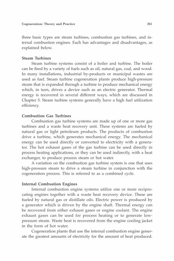
Cogeneration: Theory and Practice 261
three basic types are steam turbines, combustion gas turbines, and in-ternal combustion engines. Each has advantages and disadvantages, as explained below.
Steam Turbines Steam turbine systems consist of a boiler and turbine. The boiler can be fired by a variety of fuels such as oil, natural gas, coal, and wood. In many installations, industrial by-products or municipal wastes are used as fuel. Steam turbine cogeneration plants produce high-pressure steam that is expanded through a turbine to produce mechanical energy which, in turn, drives a device such as an electric generator. Thermal energy is recovered in several different ways, which are discussed in Chapter 5. Steam turbine systems generally have a high fuel utilization efficiency.
Combustion Gas Turbines Combustion gas turbine systems are made up of one or more gas turbines and a waste heat recovery unit. These systems are fueled by natural gas or light petroleum products. The products of combustion drive a turbine, which generates mechanical energy. The mechanical energy can be used directly or converted to electricity with a genera-tor. The hot exhaust gases of the gas turbine can be used directly in process heating applications, or they can be used indirectly, with a heat exchanger, to produce process steam or hot water. A variation on the combustion gas turbine system is one that uses high-pressure steam to drive a steam turbine in conjunction with the cogeneration process. This is referred to as a combined cycle.
Internal Combustion Engines Internal combustion engine systems utilize one or more recipro-cating engines together with a waste heat recovery device. These are fueled by natural gas or distillate oils. Electric power is produced by a generator which is driven by the engine shaft. Thermal energy can be recovered from either exhaust gases or engine coolant. The engine exhaust gases can be used for process heating or to generate low-pressure steam. Waste heat is recovered from the engine cooling jacket in the form of hot water. Cogeneration plants that use the internal combustion engine gener-ate the greatest amounts of electricity for the amount of heat produced.
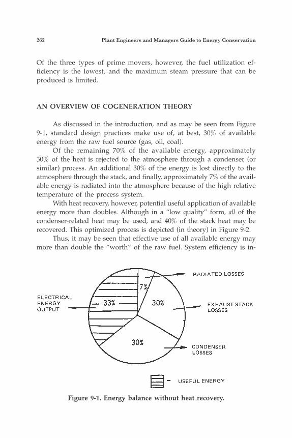
262 Plant Engineers and Managers Guide to Energy Conservation
Of the three types of prime movers, however, the fuel utilization ef-ficiency is the lowest, and the maximum steam pressure that can be produced is limited.
AN OVERVIEW OF COGENERATION THEORY
As discussed in the introduction, and as may be seen from Figure 9-1, standard design practices make use of, at best, 30% of available energy from the raw fuel source (gas, oil, coal). Of the remaining 70% of the available energy, approximately 30% of the heat is rejected to the atmosphere through a condenser (or similar) process. An additional 30% of the energy is lost directly to the atmosphere through the stack, and finally, approximately 7% of the avail-able energy is radiated into the atmosphere because of the high relative temperature of the process system. With heat recovery, however, potential useful application of available energy more than doubles. Although in a “low quality” form, all of the condenser-related heat may be used, and 40% of the stack heat may be recovered. This optimized process is depicted (in theory) in Figure 9-2. Thus, it may be seen that effective use of all available energy may more than double the “worth” of the raw fuel. System efficiency is in-
Figure 9-1. Energy balance without heat recovery.
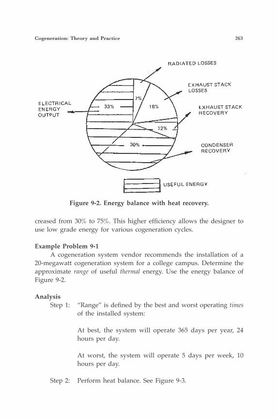
Cogeneration: Theory and Practice 263
creased from 30% to 75%. This higher efficiency allows the designer to use low grade energy for various cogeneration cycles.
Example Problem 9-1 A cogeneration system vendor recommends the installation of a 20-megawatt cogeneration system for a college campus. Determine the approximate range of useful thermal energy. Use the energy balance of Figure 9-2.
Analysis Step 1: “Range” is defined by the best and worst operating times
of the installed system:
At best, the system will operate 365 days per year, 24 hours per day.
At worst, the system will operate 5 days per week, 10 hours per day.
Step 2: Perform heat balance. See Figure 9-3.
Figure 9-2. Energy balance with heat recovery.
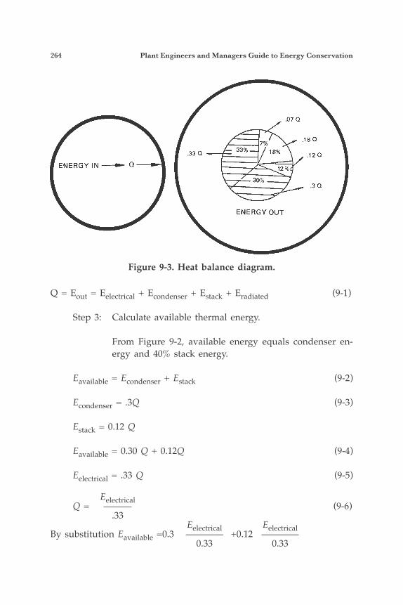
264 Plant Engineers and Managers Guide to Energy Conservation
Q = Eout = Eelectrical + Econdenser + Estack + Eradiated (9-1)
Step 3: Calculate available thermal energy.
From Figure 9-2, available energy equals condenser en-ergy and 40% stack energy.
Eavailable = Econdenser + Estack (9-2)
Econdenser = .3Q (9-3)
Estack = 0.12 Q
Eavailable = 0.30 Q + 0.12Q (9-4)
Eelectrical = .33 Q (9-5)
Eelectrical Q = ——— (9-6) .33 Eelectrical EelectricalBy substitution Eavailable =0.3 ———— +0.12 ———— 0.33 0.33
Figure 9-3. Heat balance diagram.
Cogeneration: Theory and Practice 265
Eavailable = 1.272 Electrical (9-7)
Calculate available energy
Q = Q1 × t = K1 Eavailable × K2 × t
K1 = 3413 Btu/kWh K2 = 1000 Kilowatts per megawatt t = equipment hours of operation kW Q1 = 3413 Btu/kWh × (1.272 × 20 megawatts) × 1000 kW ——— MWatt Q1 = 86.82 × 10⁶ Btu/hr
Worst Case: System operates 5 days/wk × 52 wks/yr × 10 hrs/day = 2600 hrs/yr
Best Case: System operates 365 days/yr × 24 hrs/day = 8670 hrs/yr` Thus range is
Q = 86.82 × 106 × 2600 = 225.7 × 10⁹ Btu/yr Q = 86.82 × 106 × 8760 = 760.5 × 10⁹ Btu/yr
APPLICATION OF THE COGENERATION CONSTANT
The cogeneration constant may be used as a fast check on any pro-posed cogeneration installation. Notice, from the sample problem which follows, the ease with which a thermal vs. electrical comparison of end needs may be made.
Example Problem 9-2 A cogeneration system vendor recommends a 20 megawatt instal-lation. Determine the approximate rate of useful thermal energy.
Analysis Eavailable = Eelectrical × Kc (9-8)
266 Plant Engineers and Managers Guide to Energy Conservation
E is the cogeneration system electrical rated capacity
Kc is the cogeneration constant
Eavailable = 20 MW × 1.272 = 25.4 MW of useful heat or kW 3413 Btu Therm 25.4 MW × 1000 —— × = ———— × ————— MW kWh 100,000 Btu
Eavailable = 866.9 therms/hour
APPLICABLE SYSTEMS
To ease the complication of matching power generation to load, and because of newly established laws, it is most advantageous that the generator operate in parallel with the utility grid, which thereby “absorbs” all generated electricity. The requirement for “qualifying fa-cility (QF) status,” and the consequent utility rate advantages that are available when “paralleling the grid,” is that a significant portion of the thermal energy produced in the generation process must be recovered. Specifically, formula 9-10 must be satisfied:
Power Output + 1/2 Useful Thermal Output (for any ———————————————————— ≥ 42.5% calendar (9-9) Energy Input year)
Note that careful application of the cogeneration constant will generally assure that the qualifying facility status is met.
BASIC THERMODYNAMIC CYCLES
Bottoming and Topping Cycles Cogeneration systems can be divided into “bottoming cycles” and “topping cycles.”
Cogeneration: Theory and Practice 267
Bottoming Cycles In a bottoming cycle system, thermal energy is produced directly from the combustion of fuel. This energy usually takes the form of steam that supplies process heating loads. Waste heat from the process is re-covered and used as an energy source to produce electric or mechanical power. Bottoming cycle cogeneration systems are most commonly found in industrial plants that have equipment with high-temperature heat requirements such as steel reheat furnaces, clay and glass kilns, and aluminum remelt furnaces. Some bottoming cycle plants operating in Georgia are Georgia Kraft Company, Brunswick Pulp and Paper Com-pany, and Burlington Industries.
Topping Cycles Topping cycle cogeneration systems reverse the order of bottoming cycle systems: Electricity or mechanical power is produced first, then heat is recovered to meet the thermal loads of the facility. Topping cycle systems are generally found in facilities that do not have extremely high process temperature requirements. Figure 9-3 shows schematic examples of these two cogeneration operating cycles. A sound understanding of basic cogeneration principles dictates that the energy manager should be familiar with two standard thermo-dynamic cycles—the Brayton cycle and the Rankine cycle. The Brayton cycle is the basic thermodynamic cycle for the simple gas turbine power plant. The Rankine cycle is the basic cycle for a vapor-liquid system typi-cal of steam power plants. An excellent theoretical discussion of these two cycles appears in Reference 10.
The Brayton Cycle In the open Brayton cycle plant, energy input comes from the fuel that is injected into the combustion chamber. The gas/air mixture drives the turbine, with high-temperature waste gases exiting to the atmosphere. (See Figure 9-4.) The basic Brayton cycle, as applied to cogeneration, consists of a gas turbine, a waste heat boiler, and a process or “district” heating load. This cycle is a full-load cycle. At part loads, the efficiency of the gas tur-bine goes down dramatically. A simple process diagram is illustrated in Figure 9-5.
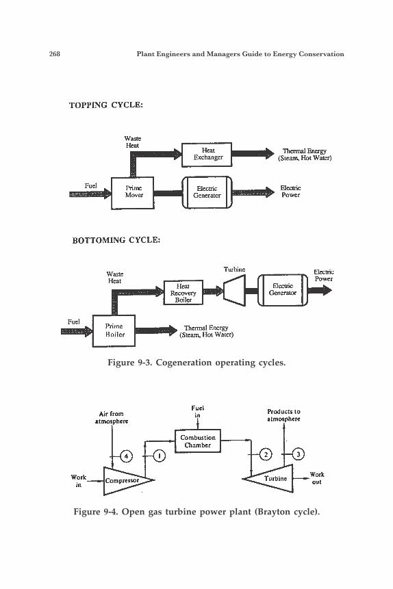
268 Plant Engineers and Managers Guide to Energy Conservation
Figure 9-3. Cogeneration operating cycles.
Figure 9-4. Open gas turbine power plant (Brayton cycle).
TOPPING CYCLE:
Waste Heat
Fuel Prime Mover
Heat Exchanger
Eleca iC Generator
Thermal Energy (Steam Hot Water)
ElecaiC Power
BOTTOMING CYCLE:
Fuel
Waste H a t
Prime Boiler
Air from atmosphere
4
W o r k Compressor in
Turbine
H a t Recovery
Boiler
'Ihermal Energy (Steam, Hot Water)
Fuel in
Combustion Chamber
E l d c Power
ElecaiC Generator
Products to atmosphere
2 3
Work out Turbine
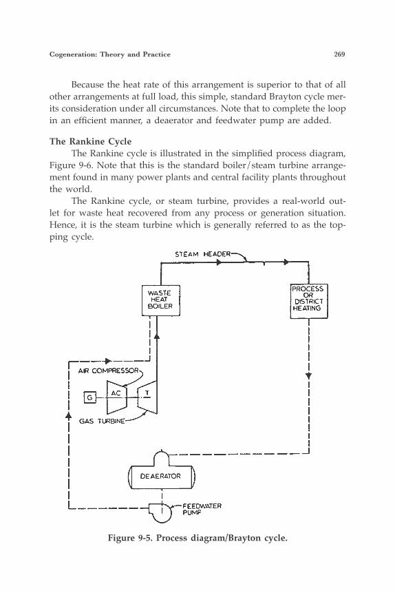
Cogeneration: Theory and Practice 269
Because the heat rate of this arrangement is superior to that of all other arrangements at full load, this simple, standard Brayton cycle mer-its consideration under all circumstances. Note that to complete the loop in an efficient manner, a deaerator and feedwater pump are added.
The Rankine Cycle The Rankine cycle is illustrated in the simplified process diagram, Figure 9-6. Note that this is the standard boiler/steam turbine arrange-ment found in many power plants and central facility plants throughout the world. The Rankine cycle, or steam turbine, provides a real-world out-let for waste heat recovered from any process or generation situation. Hence, it is the steam turbine which is generally referred to as the top-ping cycle.
Figure 9-5. Process diagram/Brayton cycle.
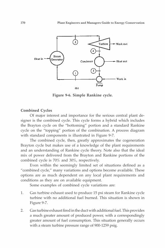
270 Plant Engineers and Managers Guide to Energy Conservation
Combined Cycles Of major interest and importance for the serious central plant de-signer is the combined cycle. This cycle forms a hybrid which includes the Brayton cycle on the “bottoming” portion and a standard Rankine cycle on the “topping” portion of the combination. A process diagram with standard components is illustrated in Figure 9-7. The combined cycle, then, greatly approximates the cogeneration Brayton cycle but makes use of a knowledge of the plant requirements and an understanding of Rankine cycle theory. Note also that the ideal mix of power delivered from the Brayton and Rankine portions of the combined cycle is 70% and 30%, respectively. Even within the seemingly limited set of situations defined as a “combined cycle,” many variations and options become available. These options are as much dependent on any local plant requirements and conditions as they are on available equipment. Some examples of combined cycle variations are:
1. Gas turbine exhaust used to produce 15 psi steam for Rankine cycle turbine with no additional fuel burned. This situation is shown in Figure 9-7.
2. Gas turbine exhaust fired in the duct with additional fuel. This provides a much greater amount of produced power, with a correspondingly greater amount of fuel consumption. This situation generally occurs with a steam turbine pressure range of 900-1259 psig.
Figure 9-6. Simple Rankine cycle.
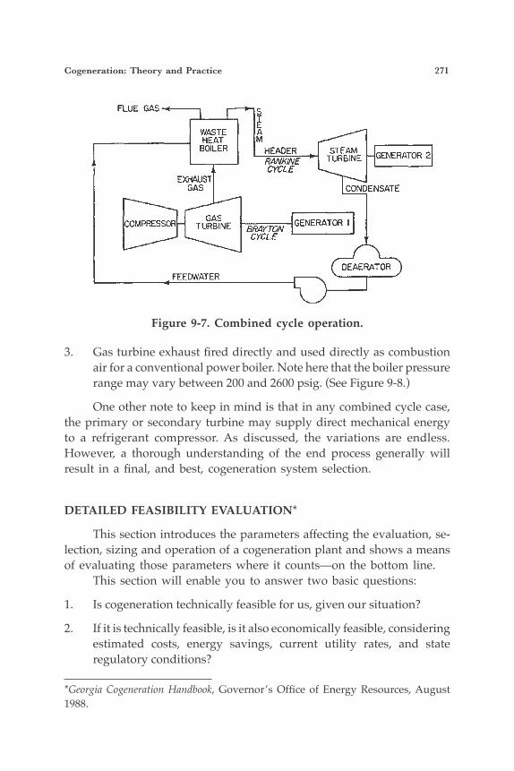
Cogeneration: Theory and Practice 271
3. Gas turbine exhaust fired directly and used directly as combustion air for a conventional power boiler. Note here that the boiler pressure range may vary between 200 and 2600 psig. (See Figure 9-8.)
One other note to keep in mind is that in any combined cycle case, the primary or secondary turbine may supply direct mechanical energy to a refrigerant compressor. As discussed, the variations are endless. However, a thorough understanding of the end process generally will result in a final, and best, cogeneration system selection.
DETAILED FEASIBILITY EVALUATION*
This section introduces the parameters affecting the evaluation, se-lection, sizing and operation of a cogeneration plant and shows a means of evaluating those parameters where it counts—on the bottom line. This section will enable you to answer two basic questions:
1. Is cogeneration technically feasible for us, given our situation?
2. If it is technically feasible, is it also economically feasible, considering estimated costs, energy savings, current utility rates, and state regulatory conditions?
Figure 9-7. Combined cycle operation.
*Georgia Cogeneration Handbook, Governor’s Office of Energy Resources, August 1988.
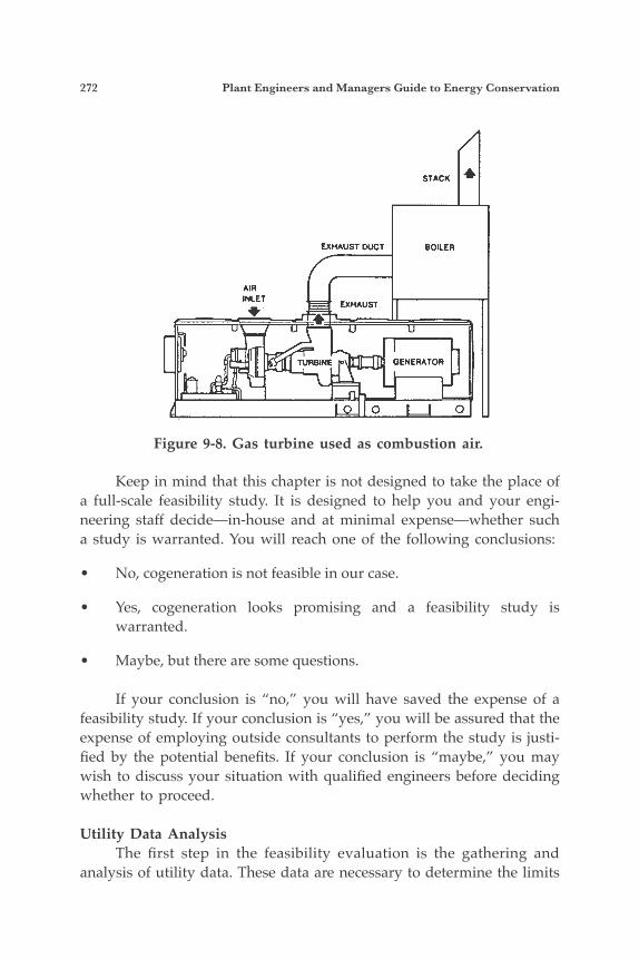
272 Plant Engineers and Managers Guide to Energy Conservation
Keep in mind that this chapter is not designed to take the place of a full-scale feasibility study. It is designed to help you and your engi-neering staff decide—in-house and at minimal expense—whether such a study is warranted. You will reach one of the following conclusions:
• No, cogeneration is not feasible in our case.
• Yes, cogeneration looks promising and a feasibility study is warranted.
• Maybe, but there are some questions.
If your conclusion is “no,” you will have saved the expense of a feasibility study. If your conclusion is “yes,” you will be assured that the expense of employing outside consultants to perform the study is justi-fied by the potential benefits. If your conclusion is “maybe,” you may wish to discuss your situation with qualified engineers before deciding whether to proceed.
Utility Data Analysis The first step in the feasibility evaluation is the gathering and analysis of utility data. These data are necessary to determine the limits
Figure 9-8. Gas turbine used as combustion air.
Cogeneration: Theory and Practice 273
of the thermal and electric energy consumed at your facility. They are also necessary for determining the timing of maximum use of each of these energy sources. From this information, you will also determine the thermal and electric load factors for your facility.
Load Factor Defined A load factor is defined as the average energy consumption rate for a facility divided by the peak energy consumption rate over a given period of time, and it is an important simplification of energy use data. These values are usually expressed as either a decimal number or a percent. To calculate a load factor you need two pieces of data: the total energy consumption for a given time period and the maximum energy demand observed during that time period. In the electric power industry, load factors serve as a measure of the utilization of generation equipment. A utility load factor of 0.90, or 90%, indicates very good utilization of power generation facilities, while a load factor of 0.30, or 30%, indicates poor utilization. The lower the load factor, the larger and more expensive your generating equipment must be merely to meet peak power demands for short time periods. The thermal and electric load factors of your facility are of great importance in sizing a cogeneration plant. In fact, they are even more important to a cogeneration plant than to an electric utility, because the cogeneration plant does not have the advantage of an electric power grid to diversify the variations in energy use. A high thermal or electrical load factor generally indicates that a cogeneration plant would be utilized a major portion of the time and therefore would provide a favorable return on your investment. An ideal situation exists when both load factors are high, indicating that a properly sized cogeneration plant would efficiently utilize most of its output. If both the thermal and electrical load factors are small, you may not be a practical candidate for cogeneration. In the analysis of your electric and thermal energy consumption data, you will calculate the load factors for your facility. In this evalua-tion, we will concentrate on annual load factors. It is important to note, however, that monthly and daily load factors may be important in your final analysis.
Electric Energy Consumption Analysis In order to obtain the necessary energy-use information, you must
274 Plant Engineers and Managers Guide to Energy Conservation
refer to your monthly electric utility bills for one complete year. From those bills, calculate the following information:
• Determine your annual kWh consumption by tabulating and adding the monthly kWh consumption.
• Tabulate the actual kW demand metered for each month. Be sure to use the actual metered demand and not the billed demand, as the billed demand may be based on time of year and a percent ratchet of the previous year’s peak demand.
• Identify the maximum monthly kW demand value as the annual peak kW.
• Determine the annual average kW demand by dividing the annual kWh consumption by 8,760 hours per year.
Annual kWh Annual Average kW = ———————— 8,760 hours/year
• Determine the annual electric load factor by dividing the annual average kW demand by the annual peak kW demand.
Annual Average kW Annual Electric Load Factor = —————————— Annual Peak kW
Thermal Energy Consumption Analysis If your boiler plant has an accurate steam or Btu metering system, the following data can be gathered directly from your metered output data. If you do not have this degree of metering, your boiler plant fuel bills for one complete year will be required to obtain the necessary data. Monthly natural gas bills can be analyzed with the same method used for analyzing electrical consumption. If you use fuel oil, propane, or coal, make sure that accurate measurements of the reserve supply were taken at the beginning and end of the year.
• Determine your annual fuel consumption. From Table 9-1, select the Btu value per unit of fuel for the type of fuel you use. To obtain the annual fuel Btu input, multiply the annual fuel consumption by this value.
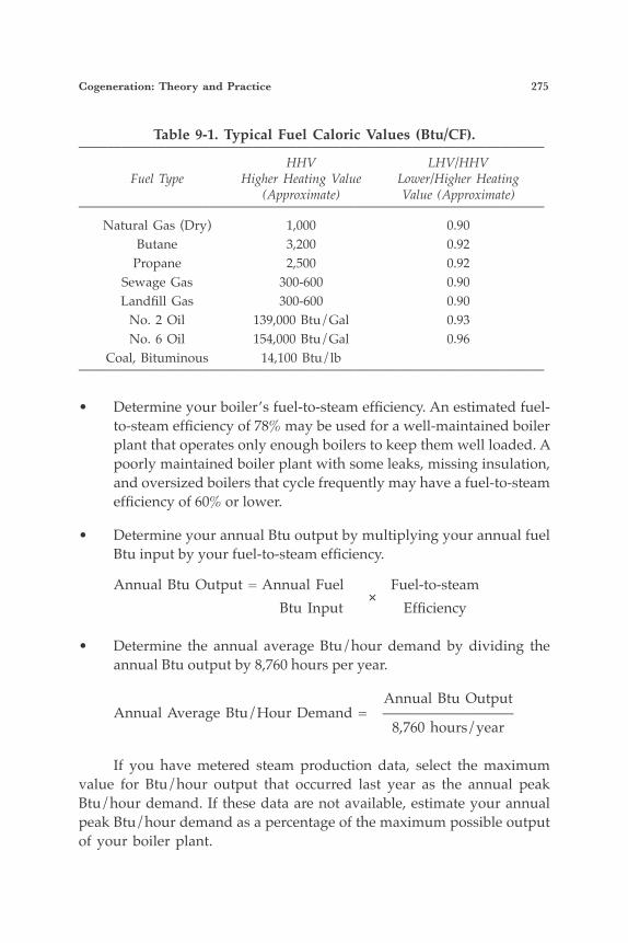
Cogeneration: Theory and Practice 275
Table 9-1. Typical Fuel Caloric Values (Btu/CF).———————————————————————————————— HHV LHV/HHV Fuel Type Higher Heating Value Lower/Higher Heating (Approximate) Value (Approximate)———————————————————————————————— Natural Gas (Dry) 1,000 0.90 Butane 3,200 0.92 Propane 2,500 0.92 Sewage Gas 300-600 0.90 Landfill Gas 300-600 0.90 No. 2 Oil 139,000 Btu/Gal 0.93 No. 6 Oil 154,000 Btu/Gal 0.96 Coal, Bituminous 14,100 Btu/lb————————————————————————————————
• Determine your boiler’s fuel-to-steam efficiency. An estimated fuel-to-steam efficiency of 78% may be used for a well-maintained boiler plant that operates only enough boilers to keep them well loaded. A poorly maintained boiler plant with some leaks, missing insulation, and oversized boilers that cycle frequently may have a fuel-to-steam efficiency of 60% or lower.
• Determine your annual Btu output by multiplying your annual fuel Btu input by your fuel-to-steam efficiency.
Annual Btu Output = Annual Fuel Fuel-to-steam × Btu Input Efficiency
• Determine the annual average Btu/hour demand by dividing the annual Btu output by 8,760 hours per year.
Annual Btu Output Annual Average Btu/Hour Demand = ————————— 8,760 hours/year
If you have metered steam production data, select the maximum value for Btu/hour output that occurred last year as the annual peak Btu/hour demand. If these data are not available, estimate your annual peak Btu/hour demand as a percentage of the maximum possible output of your boiler plant.
276 Plant Engineers and Managers Guide to Energy Conservation
NOTE: Boilers that operate at approximately 150 psig and below use the terms “lbs per hour” and “mbh output” interchangeably to represent 1,000 Btu/hour. We will use the unit “mbh” to simplify notation when referring to 1,000 Btu/hour units.
• Determine the annual thermal load factor by dividing the annual average Btu/hour demand by the annual peak Btu/hour demand.
Annual Average Btu/hour Demand
Annual Thermal = —————————————————
Load Factor Annual Peak Btu/hour Demand
If your annual minimum Btu/hour demand is extremely low or your boiler plant actually shuts down for several months during the summer, your annual thermal load factor is not an accurate indicator of your cogeneration potential. It is probably too large, and a closer examination of the number of hours at the annual minimum Btu/hour demand may be required to assess feasibility. This can be done using monthly and daily load profiles. If your annual minimum Btu/hour demand is zero for a large number of hours per year (for example, if your boiler plant shuts down during the summer months), you may not be a good candidate for co-generation.
Thermal/Electric Load Ratio For cogeneration to be feasible, the demands for thermal and elec-tric energy must overlap much of the time. Therefore, once the thermal and electric demands of your facility are known, you must determine the ratio of heat demand to electric demand that may be expected to occur together. This is done by using the thermal/electric (T/E) load ratio. The T/E load ratio is defined as the quantity of heat energy that is coincident with a quantity of electrical energy. In making these calculations, you will attempt to find an optimum match between your facility’s T/E load where
Thermal Demand Thermal/Electric = ———————— Load Ratio kW Demand
If the thermal and electric load factors calculated earlier are high, there is a good possibility that your facility’s demand for thermal energy
Cogeneration: Theory and Practice 277
occurs at about the same time as your demand for electric energy. In that case, your facility’s annual average thermal/electric load ratio is approximately equal to the annual average Btu/hour demand divided by the annual average kW demand. For convenience, we will use the term “mbh” to represent 1,000 Btu/hr.
Annual Average mbh Demand Annual Average Thermal/ = —————————————— Electric Load Ratio Annual Average kW Demand
If either the thermal or the electric load factor is small, then a worst-case assumption should be made. This assumption is called the minimum demand thermal/electric load ratio and is calculated as fol-lows:
Annual Minimum mbh Demand Minimum Demand Thermal/ = ——————————————— Electric Load Ratio Annual Minimum kW Demand
The use of either of the thermal/electric load ratios above must be tempered with the knowledge that these are only approximations of the load correlations and are useful only for a preliminary evaluation. Most facilities will require a more detailed examination of thermal and electric load profiles to obtain the number of hours per year that loads overlap and can be served with a cogeneration plant. Generally, cogeneration opportunities are good for facilities with T/E load ratios above 5 and are best for ratios above 10, with average annual Btu/hour demand above 10,000,000 Btu/hour, or 10,000 mbh. If your T/E load ratio is less than two, it is reasonable to assume that you are not a good candidate for cogeneration. This would certainly be the case if your thermal demand is extremely small during the summer months and is only significant during a few winter months. However, if your annual electric load factor is small, you may consider using electric power generation only, in a strategy known as peak shaving. This is dis-cussed in more detail under “operating strategies” in this chapter.
Equipment Sizing Considerations For efficient cogeneration, the T/E load ratio in your facility must correspond to the T/E output ratio of the cogeneration systems. T/E output ratios vary for different prime movers and cogeneration plant
278 Plant Engineers and Managers Guide to Energy Conservation
configurations. In an analysis of cogeneration options at your facility, you must decide whether to size the cogeneration plant to match your peak elec-tric load (which will produce some waste heat and lower overall plant efficiency) or to size the cogeneration plant to match your heat load and supplement your electric needs with more expensive purchased power. If your load factor is small for either thermal or electric demand, you should size toward the minimum value of that demand.
Operating StrategiesElectric Dispatch One method of operating a cogeneration plant is to supply your facility’s total electrical requirements as a first priority and generate steam as a second priority. This mode of operation is referred to as “electric dispatch.” Under the electric dispatch mode, the cogeneration plant is sized for annual peak kW demand, with some additional capacity for growth. A cogeneration plant sized in this manner can operate totally indepen-dently of the electric utility company. Standby electric service from your local utility is required for scheduled and unscheduled equipment shutdown. The cost of this standby power can be very expensive, especially if demand is high or if the utility company must provide additional generation or transmis-sion equipment to serve your facility. Total on-site backup using standby emergency power generating equipment is rarely economical. Electric dispatch requires that you operate your cogeneration plant to meet your electric load demand requirement. Operation of the major electric loads of your facility should be coordinated with the cogenera-tion plant to prevent sudden load spikes or irregular, repetitive load spikes that could exceed the capacity of your generating plant. Also, if your annual electric load factor is low, your cogeneration equipment will be oversized for your facility load most of the time. This will reduce efficiency, increase maintenance costs, and lower the return on investment.
Peak Shaving Peak shaving is the practice of selectively dropping electric loads or generating on-site electricity during periods of peak electric demand. This procedure is not cogeneration; normally, no heat recovery equip-
Cogeneration: Theory and Practice 279
ment is installed and no heat is recovered from the generating process. Peak shaving is most commonly used to reduce annual electric utility costs. Peak shaving with an electric generator has a lower initial cost than a true cogeneration system, because no heat exchangers or associ-ated recovery equipment are installed.
Thermal Dispatch Thermal dispatch operation is the complement to electric dispatch. In this mode of operation, the cogeneration plant is sized to meet your facility’s annual peak Btu/hour (or mbh) demand. You will then pur-chase a part of your electric power from the local utility and cogenerate the rest. For this mode of operation to be successful, thermal load requirements should parallel each other in the same way required for electric dispatch. For maximum savings on electric energy, electric generation should be near its maximum capacity during the summer peak electric demand period. This means that the ideal candidate for thermal dispatch opera-tion would have maximum thermal loads occurring during summertime electric peak periods. If this is not the case, you will save less on electric energy.
Hybrid Strategy A “hybrid strategy” utilizes the best features of the electrical and thermal dispatch strategies. As the name suggests, this operating strat-egy is a hybrid of the electric dispatch and thermal dispatch operating strategies, periodically adjusted to minimize operating costs and maxi-mize return on investment. With the hybrid strategy, the cogeneration plant is sized smaller than for electrical or thermal dispatch. The hybrid strategy calls for the plant to be operated to achieve maximum savings during electric peak demand periods. At other times, it would be operated in a thermal load following mode. To satisfy the total thermal load requirements, it may be necessary to maintain existing boilers or install additional ones. As in the thermal dispatch strategy, your facility still must purchase a portion of its electric energy from the utility.
Prime Mover Selection Choosing the most appropriate prime mover for a cogeneration project involves evaluation of many different criteria, including:
280 Plant Engineers and Managers Guide to Energy Conservation
• Hours of operation• Maintenance requirements• Fuel requirements• Capacity limits
Following are some general guidelines for evaluating each of the different prime movers with respect to these criteria.
Hours of Operation Most cogeneration plants are designed for continuous operation, with the exception of some small reciprocating engine packages. Large plants are not economical if they cycle on and off on an hourly or even daily basis. Because cogeneration equipment is relatively expensive as compared with boilers of similar thermal capacity, the equipment must be operated as much as possible to achieve an acceptable return on investment. If an analysis of your facility shows a low electric load factor, indicating relatively few hours of high electric demand, cogeneration is probably not a cost-effective option. Instead, you may wish to examine the potential of peak shaving with reciprocating engine generators.
Maintenance Requirements All cogeneration equipment requires some type of periodic main-tenance. The frequency and amount of maintenance varies considerably between prime movers. reciprocaTing engine generaTors have the highest maintenance requirements. Like automotive engines, diesel engines require routine maintenance such as oil and filter changes as often as once a week. However, natural gas-fired reciprocating engines require more overhauls of the head and block, and they have a shorter life expectancy. gas Turbine engines are mechanically simpler and require less fre-quent maintenance. They can operate for longer periods between major maintenance intervals, and the major maintenance is usually simpler, such as bearing inspection and replacement. sTeam Turbines require even less mechanical maintenance than gas turbines because they have no combustion equipment attached. Oc-casional bearing inspection and replacement is generally the extent of steam turbine maintenance. The cost is a function of the size and number of turbines.
Cogeneration: Theory and Practice 281
Fuel Requirements reciprocaTing engines are not flexible with respect to their fuel requirements. Generally, you buy either a diesel engine or a natural gas- fired engine. Special design adaptations can produce engines that burn other fuels, such as low Btu gas or heavier oils. Occasionally, natural gas engines can be adapted to switch between natural gas and propane as an alternate fuel. Diesel engines are more efficient in their fuel-to-energy conversion. However, air pollution regulations may impose greater con-straints on these engines than on gas turbines, usually requiring catalytic converters and carburetion limits. gas Turbines can be switched from natural gas to diesel fuel to take advantage of price fluctuations and backup fuel requirements. In addition, they can be adjusted for other fuel oils, low Btu gas, and, oc-casionally, organic by-products of industrial processes such as “black liquor” from pulp and paper mills. sTeam Turbines are limited only by the fuel for their steam source. In addition to the above fuels, coal, wood, waste, peanut shells, any suit-able biomass, and incinerated municipal waste can be used to generate steam for steam turbines.
Capacity Limits The three prime movers discussed here have separate and distinct capacity ranges. Reciprocating engine generators range in size from about 40 kW to over 3,000 kW. Generally, small electric demand plants with still smaller heat requirements can be satisfied with reciprocating engines. The quality of the heat recovered from these engines can be a limitation. Only about 35% of the recoverable heat is available as 125 psig steam; the rest of it is available only as 180°F hot water. Almost all of the gas turbine heat is recoverable as 125 psig steam. The lower limit of gas turbine equipment size is about 480 kW, and the upper limit is over 30,000 kW. Combined-cycle gas and steam turbine plants can produce over 100,000 kW. Steam turbines are the most limited with respect to power gen-eration. Their practical lower limit is about 1,000 kW. Their conversion efficiency for power generation is below 15% if practical upper limits of 200 psig of superheated inlet steam and 100 psig of saturated outlet steam are maintained. This efficiency can be improved by increasing the inlet pressure and temperature, which dramatically increases the cost of the steam production plant. Another alternative for improving electric
282 Plant Engineers and Managers Guide to Energy Conservation
generating efficiency is to use a condensing turbine, but this lowers the temperature of the outlet steam to the point that it cannot be used for much more than low-temperature hot water production. Figure 9-9 shows the thermal and electric energy output typically available from several different cogeneration system configurations.
Energy Savings Analysis To arrive at an estimate of the energy savings potential of cogen-eration at your facility, you will need to make two simplifying assump-tions. For this analysis we will assume that the proposed cogeneration system is sized such that 100% of its thermal and electric output is utilized. We will also assume that the plant will operate at or near full output capacity at all times. These assumptions represent a “best case” operating scenario for your cogeneration system. In reality, your plant probably will not operate in this manner; however, these assumptions are necessary here for the purpose of this evaluation. In addition to the above assumptions, you will need to obtain the following information on your proposed cogeneration plant:
• The thermal and electric output capacities of the cogeneration equipment
• The fuel consumption rate of the cogeneration equipment
• The number of hours per year that you plan to operate the cogeneration system
This information can be obtained from equipment data available from the manufacturer. You will need to determine the annual operating hours based on knowledge of your facility operating characteristics.
Energy Production The thermal and electric energy produced by your cogeneration plant will be used at your facility to offset thermal energy produced by your boiler plant and electricity purchased from your local utility. The next step is to determine the annual thermal and electric energy produc-tion of the proposed cogeneration equipment. The annual electric energy production is calculated as follows:
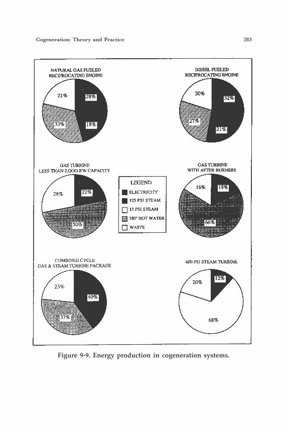
Cogeneration: Theory and Practice 283
Figure 9-9. Energy production in cogeneration systems.
NATURAL GAS FUELED RECIPROCATING ENGINE
21% 28%
33% 18%
GAS TURBINE LESS THAN 2 , 0 0 0 KW CAPACITY
LEGEND
22% FLEcTRRIcm 2 8 % 125 PSI S E A M
15 PSI S T E A M
50%
COMBINED CYCLE GAS 8: STEAM TURBINE PACKAGE
23%
40%
180" HOT W A E R
WASTE
DIESEL FUELED RECIPROCATINO ENGINE
20' 32%
27% 21%
GAS TURBINE WlTH AFIER BURNERS
16% 18%
66%
600 PSI STEAM TURBINE
12% 20%
37% 68%
284 Plant Engineers and Managers Guide to Energy Conservation
Annual Electric Electric Output Annual = × Energy Production Capacity Operating Hours
The annual thermal energy production is calculated as follows:
Annual Thermal Thermal Output Annual = × Energy Production Capacity Operating Hours
Fuel Consumption To determine the fuel use requirements of your proposed cogenera-tion plant, you will need to know the rate of fuel consumption for the equipment being evaluated here. This information can be obtained from the equipment manufacturer. Your cogeneration plant fuel consumption is calculated as follows:
Cogeneration Fuel Equipment Fuel Annual = × Consumption Consumption Rate Operating Hours
Since you have assumed that all of the output will be used by your facility, you will now calculate the value of the cogenerated energy based on your current utility costs.
Current Utility Costs To determine your annual average cost per kWh, first tabulate elec-tric energy costs from the bills that you used for gathering the electric demand and consumption data. (Generally, a more detailed analysis of your electric rate structure is needed to develop an accurate unit cost of the purchased power you will offset with cogeneration. For this evalua-tion, we will assume the unit cost of electricity is the same as the annual average unit cost of electricity.) Next, divide your annual electric cost by your annual electric consumption.
Annual Electric Cost Annual Average Cost/kWh = —————————————— Annual Electric Consumption
You can use the following method to determine your thermal en-ergy cost:
Cogeneration: Theory and Practice 285
• Tabulate monthly fuel costs from the bills used to obtain the fuel consumption data earlier.
• Determine your average fuel unit cost by dividing the annual fuel cost by your annual fuel consumption.
Annual Fuel Cost Fuel Unit Cost = ———————————— Annual Fuel Consumption
• Determine your current cost per thermal MMBtu of steam or hot water. To do this, first multiply the fuel unit cost by the Btu/unit value from Table 9-1, then divide by your boiler’s fuel-to-steam efficiency. Divide the result by 1,000,000 to convert to MMBtu units.
Current Cost Fuel Unit Cost × Btu/Fuel Unit ———————— = ———————————————— Thermal MMBtu (Fuel-to-steam Efficiency) (1,000,000)
Annual Savings The annual energy savings of your cogeneration plant are calcu-lated as the savings from electric and thermal energy production less the cost of operating the plant. The annual electric energy savings can be determined from the following equation:
Annual Electric Annual Electric Annual Average = × Energy Savings Energy Production Cost/kWh
The annual thermal energy savings is determined by the following:
Annual Thermal Annual Thermal Current Cost/ = × Energy Savings Energy Production Thermal MMBtu
Operating and Maintenance Costs Operating and maintenance costs are, to a large degree, dependent on plant operating hours and, therefore, proportional to fuel consump-tion. For the purpose of this evaluation, maintenance costs can be ap-proximated as 15% of fuel costs for reciprocating engines and 7% of fuel costs for gas or steam turbines. Use a lower figure for steam turbine
286 Plant Engineers and Managers Guide to Energy Conservation
maintenance costs if some boiler maintenance is already included in your operating expenses. The cost of the fuel to operate your cogeneration plant can be determined using the following equation:
Cogeneration Cogeneration Fuel Fuel = × Fuel Cost Consumption Unit Cost
You now have all the information necessary to determine your annual savings from the operation of a cogeneration plant. This is cal-culated as follows:
Annual Annual Electric Annual Thermal = × Savings Energy Savings Energy Savings
Cogeneration Operating and – Fuel Cost – Maintenance Cost
At this point, it is important to note that the annual savings derived from this analysis is only a preliminary estimate of the savings potential at your facility and is based on the simplifying assumptions you have made.
Economic AnalysisInitial Cost To develop the total initial cost of the cogeneration plant you are evaluating, first refer to Table 9-2 for approximate equipment cost ranges per kW of installed cogeneration electric capacity. The cost figures in Table 9-2 do not include the cost of new build-ings to house the equipment, nor do they include allowances for the electrical wiring necessary to connect your facility to your utilities. If additional space must be constructed or major work is required to con-nect the utilities, these expenses must be added to the equipment cost estimates to determine your total initial cost. Also, these costs were assembled at an earlier time and may need to be revalidated for your current analysis.
Cogeneration: Theory and Practice 287
Investment Analysis The final decision to build a cogeneration plant is usually based on investment analysis. Broadly defined, this is an evaluation of costs versus savings. The costs for cogeneration include the initial capital cost for the equipment or the cost of operating and maintaining that equipment, fuel costs, finance charges, tax liabilities, and other system costs, that may be specific to your application. Savings include offset electrical power costs, offset fuel costs, revenues from excess power sales (if any), tax benefits, and any other applicable savings that are offset by the cogeneration plant, such as planned replacement of equip-ment. A number of economic analysis techniques are available for com-paring investment alternatives. The simple payback period is the most
Table 9-2.Approximate Cost Per kW of Cogeneration Plant Capacity.
————————————————————————————————Reciprocating Engine Packages (High Speed)
———————————————————————————————— Large 900 to 3,000 kW packages .......................... $600 to $400/kW
Medium 400 to 800 kW packages ........................ $500 to $700/kW
Small 45 to 300 kW packages................................. $700 to $1,200/kW————————————————————————————————
Gas-fired Turbine Engine Packages———————————————————————————————— Large 4,000 to 10,000 kW .................................... $800 to $1,000/kW
Medium 500 to 4,000 kW ................................. $1,200 to $1,800/kW————————————————————————————————
Steam-powered Turbine Engines*———————————————————————————————— Less than 125 psig inlet turbines .......................... $100 to $130/kW
Less than 250 psig inlet turbines ............................ $90 to $120/kW————————————————————————————————*Note initial costs for steam-powered turbines are highly dependent on the en-tering and leaving pressures of the turbine. The best efficiencies are for 1,000 to 3,000 psi superheated steam. The cost of small-scale steam boilers in this range is prohibitive, and the cost of condensing steam turbines is not listed because considerable extra equipment is required. The costs as given do not include the cost of heat recovery equipment.
288 Plant Engineers and Managers Guide to Energy Conservation
commonly used and the least complex, and it is usually adequate for a go/no-go decision at this stage of project development. It is the period of time required to recover the initial investment cost through savings associated with the project. Simple payback period is calculated as fol-lows:
Initial Cost, $ Simple Payback Period = —————————— Annual Savings, $/Yr
The simple payback period will give you an indication of the at-tractiveness of cogeneration at your facility and will help you decide whether a full-scale feasibility study is warranted. Figure 9-10 is a summary of the information used in this evalu-ation of cogeneration at your facility. It is important to note that many of the variables used in this evaluation are assumed values based on your knowledge of the oper-ating characteristics of your facility and the simplifying assumptions made for this preliminary analysis. In a full-scale cogeneration feasi-bility study, it is desirable to evaluate several equipment types and sizes in conjunction with different operating strategies for each system configuration. This type of evaluation should be performed for you by an experienced consulting engineer.
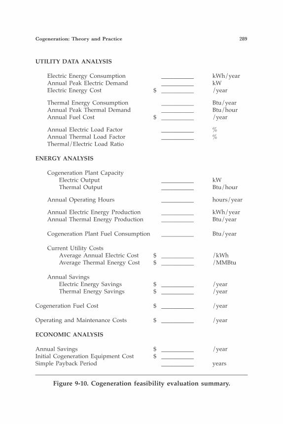
Cogeneration: Theory and Practice 289
UTILITY DATA ANALYSIS
Electric Energy Consumption ___________ kWh/year Annual Peak Electric Demand ___________ kW Electric Energy Cost $ ___________ /year
Thermal Energy Consumption ___________ Btu/year Annual Peak Thermal Demand ___________ Btu/hour Annual Fuel Cost $ ___________ /year
Annual Electric Load Factor ___________ % Annual Thermal Load Factor ___________ % Thermal/Electric Load Ratio
ENERGY ANALYSIS
Cogeneration Plant Capacity Electric Output ___________ kW Thermal Output ___________ Btu/hour
Annual Operating Hours ___________ hours/year
Annual Electric Energy Production ___________ kWh/year Annual Thermal Energy Production ___________ Btu/year
Cogeneration Plant Fuel Consumption ___________ Btu/year Current Utility Costs Average Annual Electric Cost $ ___________ /kWh Average Thermal Energy Cost $ ___________ /MMBtu
Annual Savings Electric Energy Savings $ ___________ /year Thermal Energy Savings $ ___________ /year
Cogeneration Fuel Cost $ ___________ /year
Operating and Maintenance Costs $ ___________ /year
ECONOMIC ANALYSIS
Annual Savings $ ___________ /yearInitial Cogeneration Equipment Cost $ ___________Simple Payback Period ___________ years
Figure 9-10. Cogeneration feasibility evaluation summary.

291
10Establishing aMaintenance ProgramFor Plant EfficiencyAnd Energy Savings
GOOD MAINTENANCE SAVES $
Energy losses due to leaks, uninsulated lines, dirt buildup, inoper-able furnace controls, and other poor maintenance practices is directly translated into additional energy costs. Good maintenance saves in a plant’s yearly operating costs. In this chapter, you will see the results of a survey on maintenance effectiveness, look at ways to turn around the maintenance program, and learn to apply a preventive maintenance program to energy con-servation.
WHAT IS THE EFFECTIVENESS OF MOST MAINTENANCE PROGRAMS?
Poor maintenance can be readily translated into inefficient opera-tion of systems; inefficient operation of systems spells energy waste. The problem is magnified by a survey of 1,000 plant engineers and senior maintenance supervisors that indicates the sad state of maintenance management. Findings of the survey indicate:
• Maintenance is not receiving management’s attention.
292 Plant Engineers and Managers Guide to Energy Conservation
• Planning procedures are performed by: Superintendents—35% Maintenance foremen—35% Planners, schedulers—30%
• Few maintenance departments issue regular reports to manage-ment.
• Few use a work order (maintenance request) system.
• Few maintenance departments analyze the cause of equipment backlog.
• Most companies surveyed had started preventive maintenance programs, but most were dissatisfied with their progress.
• Most companies had poor control over material and spare parts accounting.
Of specific interest to energy conservation is the fact that preven-tive maintenance is not occurring satisfactorily. Only 55 percent of the maintenance departments have a tickler file or some other filing system for automatic work order generation for filter changes and other peri-odic preventive maintenance practices. Another factor which affects the energy conservation program is that most managers have little or no control over maintenance work backlog. This means that maintenance work tends to happen rather than being planned.
HOW TO TURN AROUND THE MAINTENANCE PROGRAM
Management Attention The results of this survey indicate that the sad state of maintenance has been perpetuated because management has paid little attention to it. If management wants to conserve energy, it must give maintenance top priority. Management has historically devoted much of its efforts to improving manufacturing productivity, as well as to the reporting, measuring and analyzing of manufacturing costs. Similar efforts to improve maintenance productivity are needed. Plant engineers need to

Establishing a Maintenance Program for Plant Efficiency and Energy Savings 293
evaluate their present practices to determine the status of their mainte-nance program. Periodic reports, quantitatively stating key maintenance performance indicators, need to be issued to management.
Work Order Request Effective maintenance insures that the activity is being controlled. A work order request system needs to be established and used. Work orders serve as an historical record of repairs and alterations made to key equipment. Since the work order is used to authorize maintenance work, it is the prime requisite for any maintenance control system.
Maintenance Planning Planning of maintenance activity needs to come under the jurisdic-tion of a maintenance manager. The maintenance manager must have the same status within the organization as a manager of production. In planning maintenance work, the following needs to be identified:
Scope of the job Location of the job Priority Cause (why the work must be done) Methods to be used Material requirements Manpower requirements (number and crafts)
In addition, the following should be implemented:
• Labor time standards should be established to cover recurring or highly repetitive tasks.
• Reliable estimates should be established that cover nonrecurring (less than once a month) maintenance work.
• Procedures for issuing maintenance reports should be estab-lished.
• Reports should include productivity of the labor force.
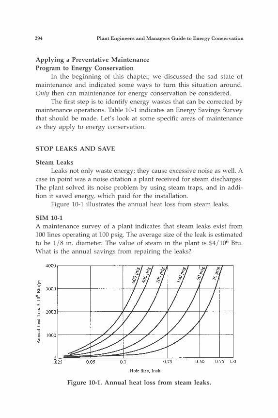
294 Plant Engineers and Managers Guide to Energy Conservation
Applying a Preventative Maintenance Program to Energy Conservation In the beginning of this chapter, we discussed the sad state of maintenance and indicated some ways to turn this situation around. Only then can maintenance for energy conservation be considered. The first step is to identify energy wastes that can be corrected by maintenance operations. Table 10-1 indicates an Energy Savings Survey that should be made. Let’s look at some specific areas of maintenance as they apply to energy conservation.
STOP LEAKS AND SAVE
Steam Leaks Leaks not only waste energy; they cause excessive noise as well. A case in point was a noise citation a plant received for steam discharges. The plant solved its noise problem by using steam traps, and in addi-tion it saved energy, which paid for the installation. Figure 10-1 illustrates the annual heat loss from steam leaks.
SIM 10-1A maintenance survey of a plant indicates that steam leaks exist from 100 lines operating at 100 psig. The average size of the leak is estimated to be 1/8 in. diameter. The value of steam in the plant is $4/106 Btu. What is the annual savings from repairing the leaks?
Figure 10-1. Annual heat loss from steam leaks.

Establishing a Maintenance Program for Plant Efficiency and Energy Savings 295
Table 10-1. Energy saving survey checklist.———————————————————————————————— Department ———————————————— Date ——————————————————— Supervised By ———————————————
Location #1 Location #2————————————————————————————————Fuel, Gas or Oil Leaks————————————————————————————————Steam Leaks————————————————————————————————Compressed Air Leaks————————————————————————————————Condensate Leaks————————————————————————————————Water Leaks————————————————————————————————Damaged or Lacking Insulation————————————————————————————————Leaks of, or Excess HVAC————————————————————————————————Burners Out of Adjustment————————————————————————————————Steam Trap OperationNote: Each trap is to betagged with date of inspection————————————————————————————————Cleanliness of Heating SurfacesSuch as Coolers, Exchangers, etc.————————————————————————————————Hot Spots on Furnaces to DetermineDeterioration of Lining————————————————————————————————Bad Bearings, Gear Drives,Pumps, Motors, etc.————————————————————————————————Dirty Motors————————————————————————————————Worn Belts————————————————————————————————Proper Viscosity of the LubricativeOils for Large Electric Drives,Hydraulic Pumps (Proper ViscosityMinimizes Pump Drive Slippage)————————————————————————————————Cleanliness of Lamps————————————————————————————————
296 Plant Engineers and Managers Guide to Energy Conservation
ANSWERFrom Figure 10-1, the steam loss per line is 540 × $6/106 Btu. The an-nual savings is thus:
540 × 100 × 6 = $324,000 per year
Steam leaks can be detected visually or by using acoustic or tem-perature probes. Leaks should also be checked at valves, heaters, and other equipment. Leaking or stuck traps, stuck bypass valves discharg-ing to the sewer, and condensate systems should also be checked. A program should be established to regularly inspect for leaks, to shut off steam to equipment taken out of service, to repair steam leaks promptly, and to route piping such that developing leaks are visible.
Leaks In Combustible Gas Lines As with steam, leaks of combustible gases such as natural gas, methane, butane, propane, hydrogen, etc., are a direct waste of valu-able energy and result in fire or explosion hazards. Tables 10-2 and 10-3 summarize losses for various combustible gas piping systems.
SIM 10-2A natural gas leak is detected in above ground piping. The natural gas pressure is 100 psig and the leak is from a 1/8 in. diameter hole. What is the annual loss, considering the value of natural gas at $6.00 per million Btu?
ANSWERFrom Table 10-3, leakage is 13,500 × 103 SCF. Since the heating value of natural gas is 1000 Btu/CF, then the heating value of the leak is:
13,500 × 106 Btu
The corresponding yearly energy waste is $81,000.
Leaks in Compressed Air Lines Leaks in compressed air lines waste energy and cost yearly operat-ing dollars. An air compressor supplies the plant air; thus, any air leak can be translated into wasting air compressor horsepower. Table 10-4 illustrates losses for various hole diameter openings.
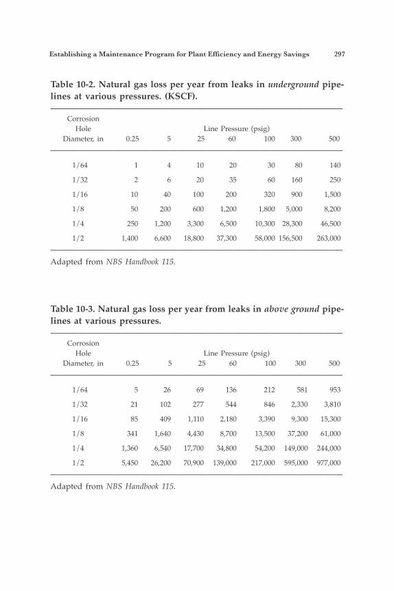
Establishing a Maintenance Program for Plant Efficiency and Energy Savings 297
Table 10-2. Natural gas loss per year from leaks in underground pipe-lines at various pressures. (KSCF).———————————————————————————————— Corrosion Hole Line Pressure (psig) Diameter, in 0.25 5 25 60 100 300 500———————————————————————————————— 1/64 1 4 10 20 30 80 140
1/32 2 6 20 35 60 160 250
1/16 10 40 100 200 320 900 1,500
1/8 50 200 600 1,200 1,800 5,000 8,200
1/4 250 1,200 3,300 6,500 10,300 28,300 46,500
1/2 1,400 6,600 18,800 37,300 58,000 156,500 263,000————————————————————————————————Adapted from NBS Handbook 115.
Table 10-3. Natural gas loss per year from leaks in above ground pipe-lines at various pressures.———————————————————————————————— Corrosion Hole Line Pressure (psig) Diameter, in 0.25 5 25 60 100 300 500———————————————————————————————— 1/64 5 26 69 136 212 581 953
1/32 21 102 277 544 846 2,330 3,810
1/16 85 409 1,110 2,180 3,390 9,300 15,300
1/8 341 1,640 4,430 8,700 13,500 37,200 61,000
1/4 1,360 6,540 17,700 34,800 54,200 149,000 244,000
1/2 5,450 26,200 70,900 139,000 217,000 595,000 977,000————————————————————————————————Adapted from NBS Handbook 115.
298 Plant Engineers and Managers Guide to Energy Conservation
SIM 10-3A maintenance inspection of the plant compressed air system revealed the following leaks in the 70 psig distribution piping system:
Number of Estimated Leaks Diameter In 5 1/4 10 1/8 10 1/16
What is the yearly energy loss, assuming an energy cost of $.060 per kWh?
ANSWERFrom Table 10-4,
Number of Estimated Cost of Power Leaks Diameter Wasted $/yr 5 1/4 17,550 10 1/8 8,882 10 1/16 2,199 ———— Total Energy Loss $ 28,631
Air leaks occur at fittings, valves, air hoses, etc. A common way of detecting leaks is by swabbing soapy water around the joints. Blowing bubbles will indicate air leaks. From SIMs 10-1, 10-2, and 10-3, the total energy waste is $433,631.00. Only when maintenance personnel understand that stop-ping leaks saves a significant amount on utility costs will the program become effective.
PROPERLY OPERATING STEAM TRAPS SAVE ENERGY
Many existing plants remove condensate from steam lines by us-ing tubing connected to the steam piping and discharged directly to the atmosphere. Figure 10-1 shows the loss of steam through a hole. Thus, all steam leaks, whether purposeful or not, should be avoided. A steam trap permits the passage of condensate, air, and noncondensible gas from the steam piping and equipment while preventing (trapping)
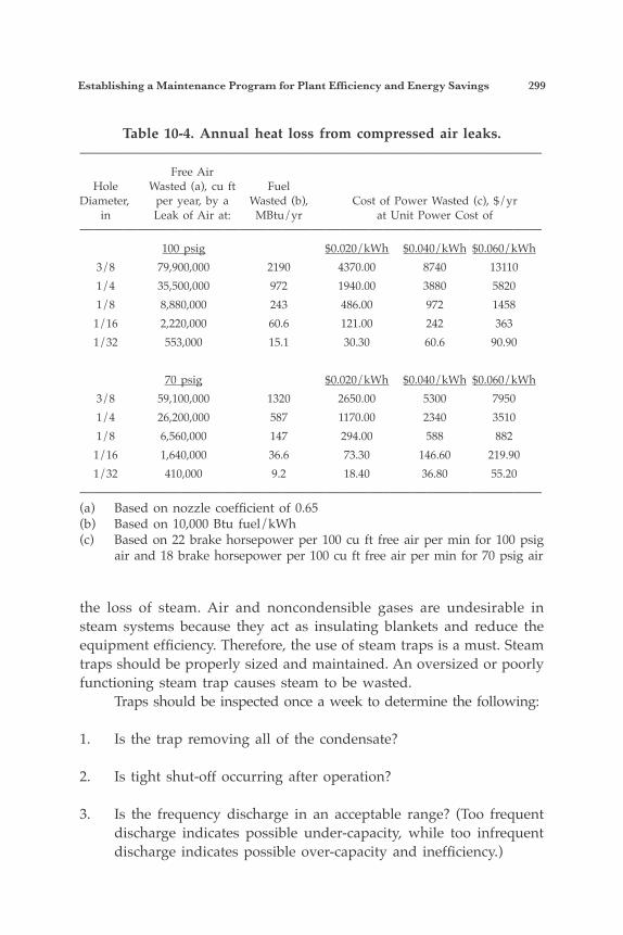
Establishing a Maintenance Program for Plant Efficiency and Energy Savings 299
the loss of steam. Air and noncondensible gases are undesirable in steam systems because they act as insulating blankets and reduce the equipment efficiency. Therefore, the use of steam traps is a must. Steam traps should be properly sized and maintained. An oversized or poorly functioning steam trap causes steam to be wasted. Traps should be inspected once a week to determine the following:
1. Is the trap removing all of the condensate?
2. Is tight shut-off occurring after operation?
3. Is the frequency discharge in an acceptable range? (Too frequent discharge indicates possible under-capacity, while too infrequent discharge indicates possible over-capacity and inefficiency.)
Table 10-4. Annual heat loss from compressed air leaks.———————————————————————————————— Free Air Hole Wasted (a), cu ft FuelDiameter, per year, by a Wasted (b), Cost of Power Wasted (c), $/yr in Leak of Air at: MBtu/yr at Unit Power Cost of———————————————————————————————— 100 psig $0.020/kWh $0.040/kWh $0.060/kWh 3/8 79,900,000 2190 4370.00 8740 13110 1/4 35,500,000 972 1940.00 3880 5820 1/8 8,880,000 243 486.00 972 1458 1/16 2,220,000 60.6 121.00 242 363 1/32 553,000 15.1 30.30 60.6 90.90
70 psig $0.020/kWh $0.040/kWh $0.060/kWh 3/8 59,100,000 1320 2650.00 5300 7950 1/4 26,200,000 587 1170.00 2340 3510 1/8 6,560,000 147 294.00 588 882 1/16 1,640,000 36.6 73.30 146.60 219.90 1/32 410,000 9.2 18.40 36.80 55.20————————————————————————————————(a) Based on nozzle coefficient of 0.65(b) Based on 10,000 Btu fuel/kWh(c) Based on 22 brake horsepower per 100 cu ft free air per min for 100 psig
air and 18 brake horsepower per 100 cu ft free air per min for 70 psig air
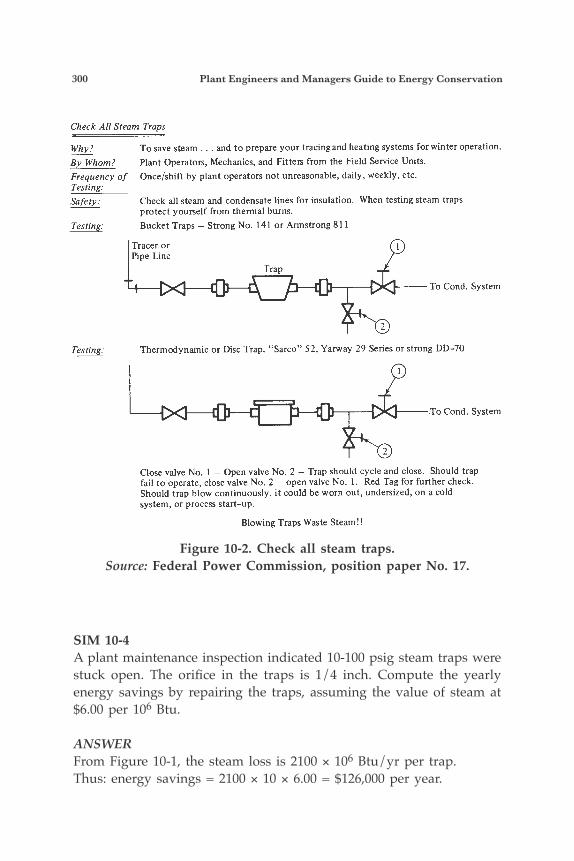
300 Plant Engineers and Managers Guide to Energy Conservation
SIM 10-4A plant maintenance inspection indicated 10-100 psig steam traps were stuck open. The orifice in the traps is 1/4 inch. Compute the yearly energy savings by repairing the traps, assuming the value of steam at $6.00 per 106 Btu.
ANSWERFrom Figure 10-1, the steam loss is 2100 × 106 Btu/yr per trap.Thus: energy savings = 2100 × 10 × 6.00 = $126,000 per year.
Figure 10-2. Check all steam traps.Source: Federal Power Commission, position paper No. 17.
Check All Steam Traps
Why? By Whom? Frequency o f Testing:
i7 4
T o save steam . . . and t o prepare your tracing and heating systems for winter operation. Plant Operators, Mechanics, and Fitters from the Field Service Units. Once/shift by plant operators not unreasonable, daily, weekly, etc.
Safety :
Testing:
-
Tesring.
Check all steam and condensate lines for insulation. When testing steam traps protect yourself from thermal burns. Bucket Traps - Strong No. 141 or Armstrong 81 1
Tracer or Pipe Line
To Cond. System
Thermodynamic or Disc Trap. “Sarco” 52, Yarway 29 Series or strong DD-70
P 1 To Cond. System
Close valve No. 1 - Open valve No. 2 - Trap should cycle and close. Should trap fail to operate, close valve No. 2 - open valve No. 1. Red Tag for further check. Should trap blow continuously, it could be worn out, undersized, on a cold system, or process start-up.
Blowing Traps Waste Steam!!
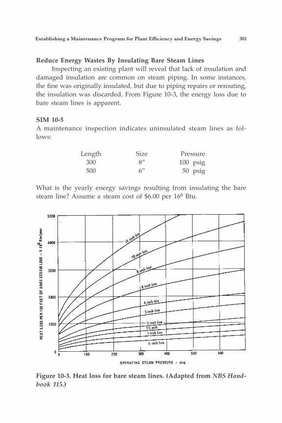
Establishing a Maintenance Program for Plant Efficiency and Energy Savings 301
Reduce Energy Wastes By Insulating Bare Steam Lines Inspecting an existing plant will reveal that lack of insulation and damaged insulation are common on steam piping. In some instances, the fine was originally insulated, but due to piping repairs or rerouting, the insulation was discarded. From Figure 10-3, the energy loss due to bare steam lines is apparent.
SIM 10-5A maintenance inspection indicates uninsulated steam lines as fol-lows:
Length Size Pressure 300 8” 100 psig 500 6” 50 psig
What is the yearly energy savings resulting from insulating the bare steam line? Assume a steam cost of $6.00 per 166 Btu.
Figure 10-3. Heat loss for bare steam lines. (Adapted from NBS Hand-book 115.)
302 Plant Engineers and Managers Guide to Energy Conservation
ANSWERFrom Figure 10-3 Energy Savings By Length Size Loss Insulating Pipes 300 8” 5700 × 106 Btu 34,200 500 6” 5500 × 106 Btu 33,000 ———— Total yearly savings $ 67,200
Don’t Overlook Steam Tracing Steam tracing must be maintained as well as turned off when not required, such as in summer periods. Either automatic controls or improved operator attention is required in order to minimize steam waste.
EXCESS AIR CONSIDERATIONS
What is common about the following?
1. Improper temperature for fuel oil atomization.
2. Worn and obsolete combustion controls.
3. The burner is operated at a setting different than the design set-ting.
4. Shortage of natural gas supplies forces a burner to be operated manually on the back-up oil system.
All of the above can lead to excess air and cause fuel to be wasted. Basi-cally, worn and obsolete combustion controls or use of manual controls prevents operating the burner at the minimum excess air levels. An improper temperature for fuel oil will cause the same result— excess air. The solution of these items involves an analysis of the pres-ent operations, changing the temperature and design settings, and a possible new combustion control system.
SIM 10-6An existing natural gas burner is operating at a stack temperature of 800°F with a 5.5% oxygen content. A maintenance check indicates that
Establishing a Maintenance Program for Plant Efficiency and Energy Savings 303
the controls are worn and that excess air is difficult to control. What an-nual (8000 hr/yr) savings can be achieved by installing a $35,000 oxygen analyzer and control system to reduce the oxygen content to 2%? The flue gas flow is 180,000 scfh (standard cubic feet per hour). Assume a 10 year life and a rate of return before taxes of 15%. The price of natural gas is $6.00 per million Btu.
ANSWERUsing Figure 5-8, the operating conditions are drawn. Figure 5-8 illus-trates a 4% fuel savings. From Table 1-4, the heating value of natural gas is 1,000 Btu/cf.
q = 8000 hr/yr × 180,000 cf/hr × 1000 Btu/cf × 0.0457,600 × 106 Btu per year
Thus, the annual savings are:57,600 × $6.00 = $345,600
Annual owning cost = $35,000 × CR = $35,000 × 0.2 = $7000.00 i = 15% n = 10
Annual savings before taxes = $338,600
DIRT AND LAMP LUMEN DEPRECIATIONCAN REDUCE LIGHTING LEVELS BY 50%
When lighting systems are designed, a light loss factor is used to compensate for lamp lumen depreciation based on lamp burning hours and dirt buildup on lamps and reflecting surfaces. This means that lighting levels will initially be higher than needed and decrease to levels below requirements based on the maintenance program. Figure 10-4 illustrates the effect of dirt on a reflector. Light must first pass through the layer of dirt to reach the reflector and then pass through again to escape from the luminaire to the working plane. The object of the lighting maintenance program is to use the available light to get the maximum output for the system. This means that lamps should be replaced prior to burning out. A group relamp program at 70-80% of lamp life and a lighting cleaning program should be initiated.
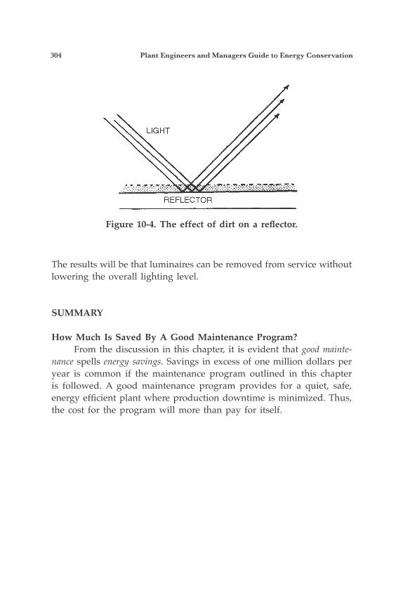
304 Plant Engineers and Managers Guide to Energy Conservation
The results will be that luminaires can be removed from service without lowering the overall lighting level.
SUMMARY
How Much Is Saved By A Good Maintenance Program? From the discussion in this chapter, it is evident that good mainte-nance spells energy savings. Savings in excess of one million dollars per year is common if the maintenance program outlined in this chapter is followed. A good maintenance program provides for a quiet, safe, energy efficient plant where production downtime is minimized. Thus, the cost for the program will more than pay for itself.
Figure 10-4. The effect of dirt on a reflector.

305
11Managing an EffectiveEnergy ConservationProgram
ORGANIZING FOR ENERGY CONSERVATION
By now it should be clear that energy management affects almost every major activity of a plant. It is involved in:
Electrical engineering Control systems engineering Utility engineering Piping design Mechanical engineering Chemical engineering Heating, ventilation, and air conditioning engineering Building design Environmental engineering Operations Maintenance Accounting and financial management
Each plant has assigned individuals who are responsible for one or more of the above functions. The problem facing management is how to organize the energy conservation activity so that all functions are mov-ing in a common direction. The situation becomes more complex when several plants or outside consultants are involved. Direction and coordi-nation for the program need to be provided. In most organizations, the function of the energy conservation coordinator/committee emerges.
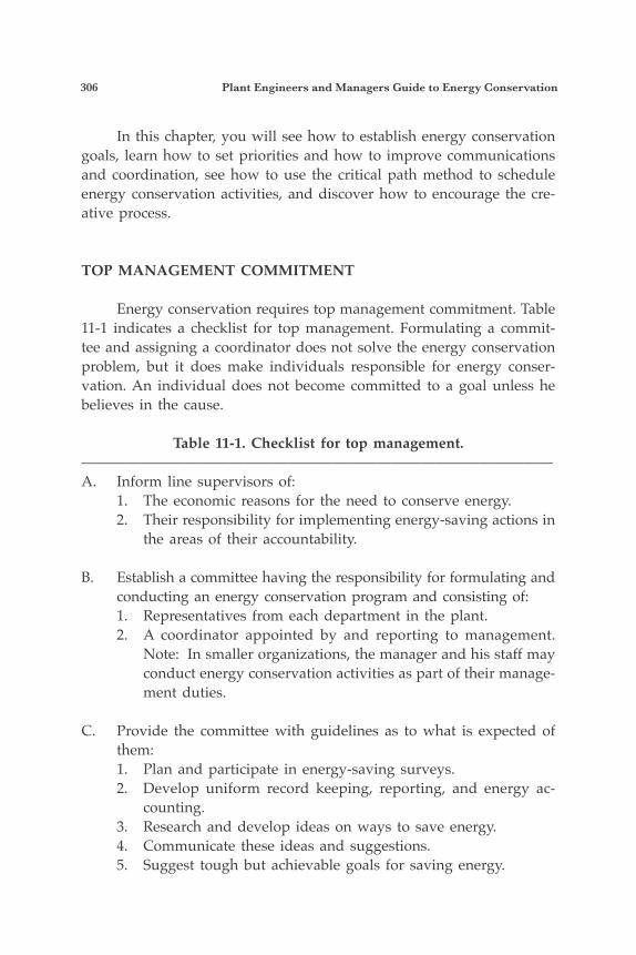
306 Plant Engineers and Managers Guide to Energy Conservation
In this chapter, you will see how to establish energy conservation goals, learn how to set priorities and how to improve communications and coordination, see how to use the critical path method to schedule energy conservation activities, and discover how to encourage the cre-ative process.
TOP MANAGEMENT COMMITMENT
Energy conservation requires top management commitment. Table 11-1 indicates a checklist for top management. Formulating a commit-tee and assigning a coordinator does not solve the energy conservation problem, but it does make individuals responsible for energy conser-vation. An individual does not become committed to a goal unless he believes in the cause.
Table 11-1. Checklist for top management.————————————————————————————————A. Inform line supervisors of:
1. The economic reasons for the need to conserve energy.2. Their responsibility for implementing energy-saving actions in
the areas of their accountability.
B. Establish a committee having the responsibility for formulating and conducting an energy conservation program and consisting of:1. Representatives from each department in the plant.2. A coordinator appointed by and reporting to management.
Note: In smaller organizations, the manager and his staff may conduct energy conservation activities as part of their manage-ment duties.
C. Provide the committee with guidelines as to what is expected of them:1. Plan and participate in energy-saving surveys.2. Develop uniform record keeping, reporting, and energy ac-
counting.3. Research and develop ideas on ways to save energy.4. Communicate these ideas and suggestions.5. Suggest tough but achievable goals for saving energy.
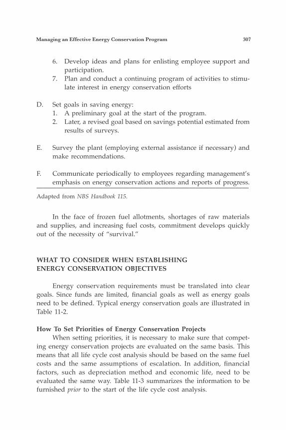
Managing an Effective Energy Conservation Program 307
6. Develop ideas and plans for enlisting employee support and participation.
7. Plan and conduct a continuing program of activities to stimu-late interest in energy conservation efforts
D. Set goals in saving energy:1. A preliminary goal at the start of the program.2. Later, a revised goal based on savings potential estimated from
results of surveys.
E. Survey the plant (employing external assistance if necessary) and make recommendations.
F. Communicate periodically to employees regarding management’s emphasis on energy conservation actions and reports of progress.
————————————————————————————————Adapted from NBS Handbook 115.
In the face of frozen fuel allotments, shortages of raw materials and supplies, and increasing fuel costs, commitment develops quickly out of the necessity of “survival.”
WHAT TO CONSIDER WHEN ESTABLISHINGENERGY CONSERVATION OBJECTIVES
Energy conservation requirements must be translated into clear goals. Since funds are limited, financial goals as well as energy goals need to be defined. Typical energy conservation goals are illustrated in Table 11-2.
How To Set Priorities of Energy Conservation Projects When setting priorities, it is necessary to make sure that compet-ing energy conservation projects are evaluated on the same basis. This means that all life cycle cost analysis should be based on the same fuel costs and the same assumptions of escalation. In addition, financial factors, such as depreciation method and economic life, need to be evaluated the same way. Table 11-3 summarizes the information to be furnished prior to the start of the life cycle cost analysis.
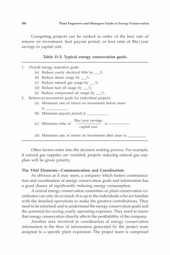
308 Plant Engineers and Managers Guide to Energy Conservation
Competing projects can be ranked in order of the best rate of returns on investment, best payout period, or best ratio of Btu/year savings to capital cost.
Table 11-2. Typical energy conservation goals.————————————————————————————————1. Overall energy reduction goals (a) Reduce yearly electrical bills by ___%. (b) Reduce steam usage by ___%. (c) Reduce natural gas usage by ___%. (d) Reduce fuel oil usage by ___%. (e) Reduce compressed air usage by ___%.2. Return-on-investment goals for individual projects. (a) Minimum rate of return on investment before taxes is ____________. (b) Minimum payout period is ____________.
Btu/year savings (c) Minimum ratio of ——————— is —————— capital cost
(d) Minimum rate of return on investment after taxes is __________.————————————————————————————————
Other factors enter into the decision making process. For example, if natural gas supplies are curtailed, projects reducing natural gas sup-plies will be given priority.
The Vital Elements—Communication and Coordination As obvious as it may seem, a company which fosters communica-tion and coordination of energy conservation goals and information has a good chance of significantly reducing energy consumption. A central energy conservation committee or plant conservation co-ordinator can only do so much. It is up to the individuals who are familiar with the detailed operations to make the greatest contributions. They need to be informed and to understand the energy conservation goals and the potential for saving yearly operating expenses. They need to know that energy conservation directly affects the profitability of the company. Another area involved in coordination of energy conservation information is the flow of information generated by the project team assigned to a specific plant expansion. The project team is comprised
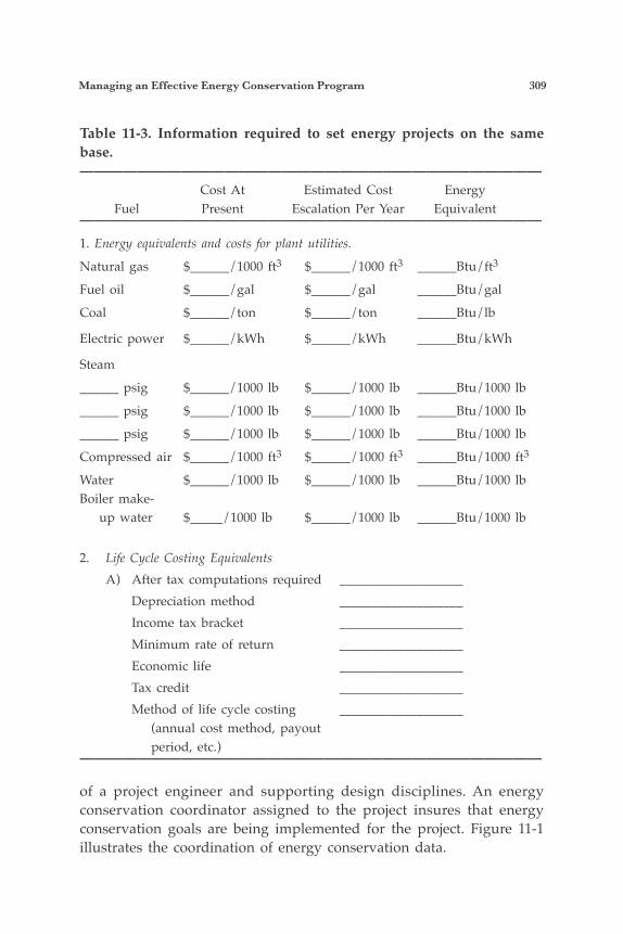
Managing an Effective Energy Conservation Program 309
of a project engineer and supporting design disciplines. An energy conservation coordinator assigned to the project insures that energy conservation goals are being implemented for the project. Figure 11-1 illustrates the coordination of energy conservation data.
Table 11-3. Information required to set energy projects on the same base.———————————————————————————————— Cost At Estimated Cost Energy Fuel Present Escalation Per Year Equivalent————————————————————————————————1. Energy equivalents and costs for plant utilities.
Natural gas $______/1000 ft3 $______/1000 ft3 ______Btu/ft3
Fuel oil $______/gal $______/gal ______Btu/gal
Coal $______/ton $______/ton ______Btu/lb
Electric power $______/kWh $______/kWh ______Btu/kWh
Steam
______ psig $______/1000 lb $______/1000 lb ______Btu/1000 lb
______ psig $______/1000 lb $______/1000 lb ______Btu/1000 lb
______ psig $______/1000 lb $______/1000 lb ______Btu/1000 lb
Compressed air $______/1000 ft3 $______/1000 ft3 ______Btu/1000 ft3
Water $______/1000 lb $______/1000 lb ______Btu/1000 lbBoiler make- up water $_____/1000 lb $______/1000 lb ______Btu/1000 lb
2. Life Cycle Costing Equivalents A) After tax computations required ___________________ Depreciation method ___________________ Income tax bracket ___________________ Minimum rate of return ___________________ Economic life ___________________ Tax credit ___________________ Method of life cycle costing ___________________ (annual cost method, payout period, etc.)————————————————————————————————
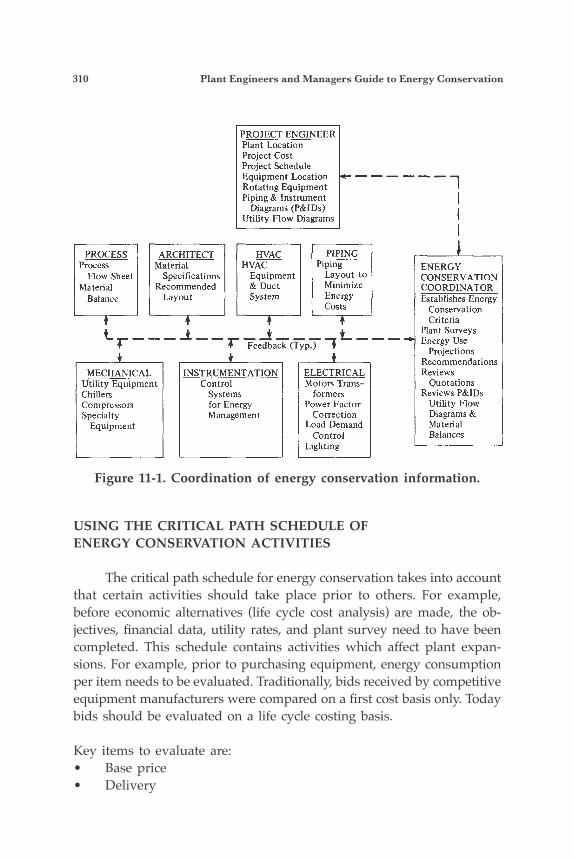
310 Plant Engineers and Managers Guide to Energy Conservation
USING THE CRITICAL PATH SCHEDULE OFENERGY CONSERVATION ACTIVITIES
The critical path schedule for energy conservation takes into account that certain activities should take place prior to others. For example, before economic alternatives (life cycle cost analysis) are made, the ob-jectives, financial data, utility rates, and plant survey need to have been completed. This schedule contains activities which affect plant expan-sions. For example, prior to purchasing equipment, energy consumption per item needs to be evaluated. Traditionally, bids received by competitive equipment manufacturers were compared on a first cost basis only. Today bids should be evaluated on a life cycle costing basis.
Key items to evaluate are:• Base price• Delivery
Figure 11-1. Coordination of energy conservation information.
Flow Sheet
Balance Material
1 Eauivment Location 1 - - - - - - PROJECT ENGINEER Plant Location Project Cost Project Schedule
Rotating Equipment Piping & Instrument
Diagrams (P&IDs)
ARCHITECT PIPING I Material I I HVAC
Recommended & Duct Layout
Layout to Minimize
MECHANICAL Utility Equipment Chillers Compressors Specialty
Equipment
INSTRUMENTATION Control
Systems for Energy Management
ELECTRICAL Motors Trans- 1
formers Power Factor
Correction Load Demand
Control Lighting
I I I L ENERGY CONSERVATIOb COORDINATOR Establishes Energ5
Conservation Criteria
Plant Surveys Energy Use
Projections Recommendation! Reviews
Quotations Reviews P&IDs
Utility Flow Diagrams & Material Balances

Managing an Effective Energy Conservation Program 311
• Technical specifications• Cost for pollution compliance• Yearly energy and maintenance cost
This means that during the quotation phase, equipment such as fans, air conditioners, pumps, compressors, etc., need to be evaluated with respect to energy consumption. This simple step will point up inefficient equipment, the penalty of operation prior to purchase.
ELECTRICAL SCHEDULING OF PLANT ACTIVITIES
As indicated in Chapter 4, the load demand controller is used to reduce peak electrical demand. Scheduling of plant operations requires more than an electrical black box. As an example, the startup of a plant expansion can involve several start-up engineers working on several systems. A peak load de-mand can occur by testing several large motors at the same time. A little coordination can save substantially on the energy demand charge. After the plant is in operation, the electrical energy curves should be analyzed. Careful analysis can indicate ways in which peak demands can be lowered by rescheduling plant operations.
AN EFFECTIVE MAINTENANCE PROGRAM
Plant maintenance cannot be overemphasized in any energy con-servation program. As indicated in Chapter 10, management needs to take an active role.
CONTINUOUS CONSERVATION MONITORING
As discussed in Chapter 1, an energy conservation program must be continuously monitored in order to be controlled. This means that each operator needs to manage his own fuel usage. Adequate instru-mentation is essential to the monitoring process. Operator accountability can exist only if all utilities are metered. In planning what point in the process will be metered, consideration

312 Plant Engineers and Managers Guide to Energy Conservation
should be given to how the process will be operated and by whom. As an example, the fuel oil tank would come under the jurisdiction of the boiler plant operator. Any fuel take-offs to the process operator should be separately metered. This will enable each operator to control his us-age, independent of other operations.
ARE OUTSIDE CONSULTANTS AND CONTRACTORS ENCOURAGED TO SAVE ENERGY BY DESIGN?
The type of contract may well influence the type of energy savings that will be realized. As an example, a competitive “lump sum” contract encourages the consultant to achieve the lowest first cost and ignore additional expenditures that will minimize future operating costs. This type of contract will not achieve the energy conservation goals unless the owner specifies the energy conservation requirements during the bid phase. Thus, the owner must be careful not to penalize creative energy conservation design during the conceptual phase.
ENCOURAGING THE CREATIVE PROCESS
Energy conservation engineering relies on creatively applying ex-isting technology in new ways. Many examples are illustrated in this text, but this in no way can be considered the entire gambit. “Why” questioning must be promoted. A team of engineers representing several disciplines should meet periodically to brainstorm energy conservation concepts. “Do it the same way as the last project,” “Use rules of thumb,” or “Experience tells us…” should be replaced with “Why” questioning. Examples are:
1. Why can’t vacuum pumps be used in this process instead of steam vacuum jets?
2. Can conventional warehouse heaters be replaced with infrared heaters?
3. Can air coolers be used instead of water coolers?
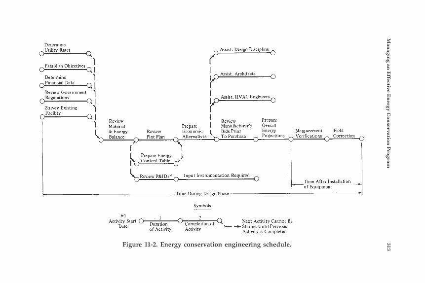
Man
aging an
Effective E
nergy C
onservation
Program
313Figure 11-2. Energy conservation engineering schedule.
Determine Utility Rates 4
91 I Establish Objectives
Determine Financial Data
Review Government Regulations
Survey Existing Facility
Sl I
Q I I ' Review I Material
' Assist. HVAC Engineers IP I I Review Prepare
Preoare I Manufacturer's Overall & Energy Review Ecinomic i BidsPrior Energy Measurement Field Balance A Plot Plan r\ Alternatives h To Purchase A Projections Verifications A Correction
r W U W
I I I Prepare Energyd J Content Table
Review p & ~ ~ s * r\ Input Instrumentation Required U Time After Installation
of Eq'uipment ~~
\\Time During Design Phase
Symbols
. 1 n 2 Duration " of Activity Activity
# I
Date Activity Start 0 Next Activity Cannot Be
Completion Of 'L -+ Started Until Previous Activity is Completed
314 Plant Engineers and Managers Guide to Energy Conservation
4. Can no-vent equipment, such as vertical motors with special packing, be used to permit process steam to be returned to the boiler without steam traps?
5. Can loads be readjusted so that equipment runs at optimal levels of efficiency?
6. Can short runs on thermal process equipment be avoided?
7. Can spot cooling for personal cooling be used instead of area cooling?
8. Can waste heat be recovered by means of systems employing organic working fluids?
9. Can smooth-coated pipe be used to reduce friction loss, thereby reducing horsepower?
10. Can pumps be eliminated by locating equipment to take advan-tage of gravity?
ENERGY EMERGENCY AND CONTINGENCY PLANNING
Energy managers need to deal with many unknowns. Experience of the last ten years indicates coal strikes and fuel allocations do occur. How to plan for emergencies such as these is an important aspect of the energy manager’s role. In November of 1979, President Carter signed Public Law 96-102, the Emergency Energy Conservation Act, giving the President the au-thority to establish energy demand targets for each state in case of a national emergency.
Risk Assessment In order to establish the contingency plan, the energy manager needs to establish the risk associated with various scenarios. There is a cost to business for doing nothing in the event an emer-gency does occur and no plan is put into effect. This cost is computed according to the following:
C = P × C1 (11-1)
Managing an Effective Energy Conservation Program 315
where C = cost as result of emergency with no contingency plans in ef-
fect P = the probability or likelihood the emergency will occur C1 = the loss in dollars as a result of an emergency with no emer-
gency plans in effect.
Thus, risk assessment can help the energy manager determine the effect, money, and resources required to meet various emergency scenarios. An example of a simple contingency plan would be the justifica-tion of a backup fuel system. The risk assessment would indicate the probable cost of losing the primary system and the expected duration of the loss. The key is to develop the plan prior to the emergency oc-curring.
CONCLUSION
The energy conservation program, when properly managed, will pay for itself. Engineering “rules of thumb” are no longer sufficient because of increases in the cost of energy and shortages of raw materi-als. The decision-making process is based on economics and local, state, and federal regulations. The guidelines and practices presented in this text will prove to save energy without decreasing the function of the system. The energy manager’s role must be understood by the public and the government. The answer to energy management is not to decrease the quality of life by living in darkness, but rather to apply the technologies avail-able to increase the efficiency of the systems. The challenge facing the energy engineer/manager is great, and the stakes are high.
12Electric Motors
Electric motors are the rotating machines that drive today’s in-dustrial manufacturing. A typical manufacturing facility may operate from hundreds to thousands of motors. The U.S. Dept. of Energy has reported that electric motors use over half of the electricity consumed in the United States in a given year. Many plant managers do not maintain a motor inventory and only examine a motor once it has failed. This reflects positively on the reliabil-ity of electric motors. Unfortunately, this approach to motor management can greatly affect the efficiency of motor operations in a facility.
MOTOR TYPES
There are three basic motor designs found in most industrial facili-ties. The first type is the AC synchronous motor. This design offers a fixed speed, rotating shaft that is useful for mechanical work. It also provides power factor correction capability.
AC Synchronous Motors The AC synchronous motor is fed from two sources. The outer stationary shell of the motor (called the stator) contains coils of wire that are fed from three-phase electric power. When energized, this creates a rotating magnetic field within the motor that can induce the inner shaft of the motor (known as the rotor) to begin spinning. Attached to the rotor are magnetic coils fed from a separate DC source, which creates a fixed magnetic field within the machine that interacts with the magnetic field created by the stator. During start-up, the stator circuit on a synchronous motor, also called the armature circuit, is first energized while the rotor circuit is not engaged. In fact, it is actually short-circuited. The circuit breaker feeding the armature circuit is often labeled as the “start” breaker. This allows
317
318 Plant Engineers and Managers Guide to Energy Conservation
the motor to begin spinning as an induction motor while it slowly gains speed. Once it reaches a steady-state speed, the field circuit is engaged, which causes the motor to lock into a fixed speed that is a function of the number of magnetic poles in the motor and the electrical frequency being applied to the stator. The breaker on this circuit is often labeled the “run” breaker. The fixed operational speed is known as synchronous speed and is calculated as:
Nsynch = (120 * fe)/# of magnetic poles fe is the electrical frequency
Both the electrical frequency and the number of poles can be found on the motor nameplate. Synchronous motors found in industrial facilities are often fairly large and typically only account for one percent of the motors found on site. They are similar in construction to induction motors, but they are far more expensive and require more maintenance. The reason for this is that to energize the field circuit, one must supply energy from an external DC source to a rotating shaft. To accomplish this, a series of slip rings are installed on the shaft, and then they form a connec-tion by resting on carbon brushes that connect back to the external DC source. The extra copper and wiring adds weight and cost, while the use of brushes in frictional connections creates maintenance issues. The primary benefit in using a synchronous motor is that the mag-netism induced in the rotor circuit allows the operator to adjust whether the motor consumes reactive power or supplies reactive power. Induction motors always operate at a lagging power factor. Elevating a synchronous motor’s excitation allows it to supply reactive power to other induction motors, thus elevating the overall power factor of the facility in the eyes of the local power utility. DC Motors A second type of motor found at some facilities is the DC motor. A DC motor is powered by direct current being applied to magnetic poles located on its inner shell, called the stator. These poles establish the primary magnetic field in the machine and are called the field poles. They could be permanent magnets, which would identify the machine as a permanent magnet DC machine. The rotating shaft on a DC motor also has its own magnetic poles.
Electric Motors 319
This circuit is energized through a frictional connection made of small copper connection points on the rotor contacting carbon brushes that are wired to an external DC source. The small copper connection points form a segmented ring around the shaft, which is called the commutator. One of the benefits of a DC motor is that the speed can be tightly controlled by varying either the voltage applied to the rotor or the volt-age applied to the field circuit on the rotor. Prior to the development of the variable frequency drive, DC motors were the only motors available which allowed for speed variation without the use of pulleys, belts, or gears. The drawbacks to DC machines are the extra costs due to the large amount of copper used in their construction, along with the increased maintenance costs due to the use of brushes and a commutator. Less than 5% of the motors in industrial facilities today are DC.
AC Induction Motors Induction motors make up the majority of motors used today. Their general construction consists of a three-phase set of armature poles being formed on the stator. They are energized by an external, three-phase source. The rotor of the motor appears like a small cage similar in shape to an exercise wheel found in a gerbil cage. In fact, a common induction motor design is called the squirrel cage induction motor. When three-phase power is applied to the stator, a rotating mag-netic field is created within the motor, which causes the rotor to begin rotating. The primary benefits of induction motors are that they are in-expensive and offer a wide range of selection for various tasks. The savings in price over DC and AC synchronous machines come from the fact that there is no electrical connection to the rotor. This results in less copper and fewer maintenance issues. It is common for a three-phase induction motor operated within limits to last thirty years. One drawback of induction motors is that they only operate on a lagging power factor.
MOTOR EFFICIENCY AND POWER FACTOR
With the wide range of motors available to the typical plant engi-neer today, one needs to closely examine the needs of the application to
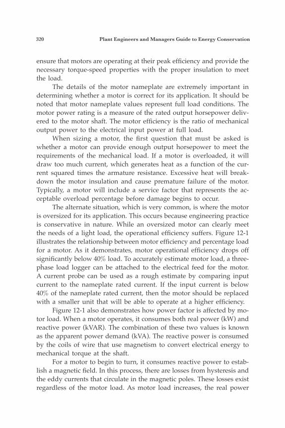
320 Plant Engineers and Managers Guide to Energy Conservation
ensure that motors are operating at their peak efficiency and provide the necessary torque-speed properties with the proper insulation to meet the load. The details of the motor nameplate are extremely important in determining whether a motor is correct for its application. It should be noted that motor nameplate values represent full load conditions. The motor power rating is a measure of the rated output horsepower deliv-ered to the motor shaft. The motor efficiency is the ratio of mechanical output power to the electrical input power at full load. When sizing a motor, the first question that must be asked is whether a motor can provide enough output horsepower to meet the requirements of the mechanical load. If a motor is overloaded, it will draw too much current, which generates heat as a function of the cur-rent squared times the armature resistance. Excessive heat will break-down the motor insulation and cause premature failure of the motor. Typically, a motor will include a service factor that represents the ac-ceptable overload percentage before damage begins to occur. The alternate situation, which is very common, is where the motor is oversized for its application. This occurs because engineering practice is conservative in nature. While an oversized motor can clearly meet the needs of a light load, the operational efficiency suffers. Figure 12-1 illustrates the relationship between motor efficiency and percentage load for a motor. As it demonstrates, motor operational efficiency drops off significantly below 40% load. To accurately estimate motor load, a three-phase load logger can be attached to the electrical feed for the motor. A current probe can be used as a rough estimate by comparing input current to the nameplate rated current. If the input current is below 40% of the nameplate rated current, then the motor should be replaced with a smaller unit that will be able to operate at a higher efficiency. Figure 12-1 also demonstrates how power factor is affected by mo-tor load. When a motor operates, it consumes both real power (kW) and reactive power (kVAR). The combination of these two values is known as the apparent power demand (kVA). The reactive power is consumed by the coils of wire that use magnetism to convert electrical energy to mechanical torque at the shaft. For a motor to begin to turn, it consumes reactive power to estab-lish a magnetic field. In this process, there are losses from hysteresis and the eddy currents that circulate in the magnetic poles. These losses exist regardless of the motor load. As motor load increases, the real power
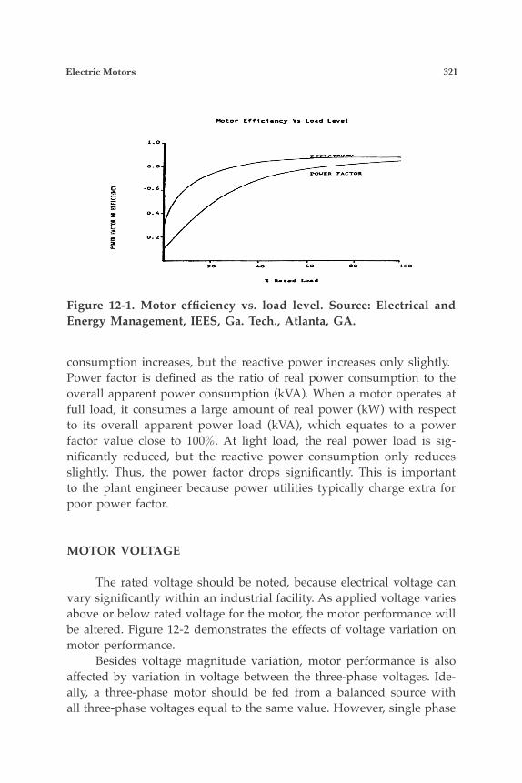
Electric Motors 321
consumption increases, but the reactive power increases only slightly.Power factor is defined as the ratio of real power consumption to the overall apparent power consumption (kVA). When a motor operates at full load, it consumes a large amount of real power (kW) with respect to its overall apparent power load (kVA), which equates to a power factor value close to 100%. At light load, the real power load is sig-nificantly reduced, but the reactive power consumption only reduces slightly. Thus, the power factor drops significantly. This is important to the plant engineer because power utilities typically charge extra for poor power factor.
MOTOR VOLTAGE
The rated voltage should be noted, because electrical voltage can vary significantly within an industrial facility. As applied voltage varies above or below rated voltage for the motor, the motor performance will be altered. Figure 12-2 demonstrates the effects of voltage variation on motor performance. Besides voltage magnitude variation, motor performance is also affected by variation in voltage between the three-phase voltages. Ide-ally, a three-phase motor should be fed from a balanced source with all three-phase voltages equal to the same value. However, single phase
Figure 12-1. Motor efficiency vs. load level. Source: Electrical and Energy Management, IEES, Ga. Tech., Atlanta, GA.

322 Plant Engineers and Managers Guide to Energy Conservation
loads within a facility can vary the load drawn from each phase, which can create a voltage imbalance between phases. Voltage imbalance will increase motor losses. Figure 12-3 illustrates the relationship between voltage imbalance and motor losses.
MOTOR REWINDS
When a motor fails, a plant manager must decide to either replace the motor with a new unit or take the damaged motor to a motor rewind shop. If a new motor is not in stock in the plant or in the inventory at the local motor supplier, the only option may be a rewind. A motor rewind involves heating the internal parts of the motor to high levels to break down the resin binding copper conductors to the motor stator or rotor. Once the parts are separated and cleaned, new windings are installed and the motor is tested before returning it back to
Figure 12-2. Motor performance vs. voltage variation. Source: http://www.reliance.com/mtr/pwrspymn.htm.
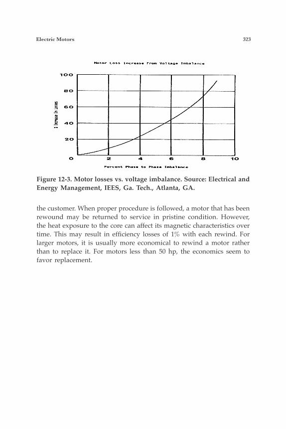
Electric Motors 323
Figure 12-3. Motor losses vs. voltage imbalance. Source: Electrical and Energy Management, IEES, Ga. Tech., Atlanta, GA.
the customer. When proper procedure is followed, a motor that has been rewound may be returned to service in pristine condition. However, the heat exposure to the core can affect its magnetic characteristics over time. This may result in efficiency losses of 1% with each rewind. For larger motors, it is usually more economical to rewind a motor rather than to replace it. For motors less than 50 hp, the economics seem to favor replacement.
325
13Reliable and EconomicNatural Gas DistributedGeneration Technologies
Distributed generation (DG) has emerged as a viable alternative to conventional central station power production. This chapter discusses natural gas-fueled distributed generation technologies, focusing on advanced industrial turbines and microturbines, reciprocating engines, and fuel cells. Each of these systems has the capability to improve power reliability and reduce environmental impacts at lower overall costs. Market barriers, such as the lack of standardized utility intercon-nection protocols, environmental permitting complexities, and public unfamiliarity with distributed generation technologies, have interfered with successful market applications. However, studies indicate that there is substantial growth potential for DG in the steel, petroleum, chemical, forest products, and other industries, as well as in commercial buildings, government facilities, hospital complexes, industrial parks, multi-family buildings, and school campuses. This chapter will show that with continued support distributed generation will play a key role in energy production in the next millennium.
INTRODUCTION
Distributed generation (DG) involves small, modular electricity generation at or near the point of use. Utilities or customers can own DG systems, but there is a growing trend towards third-party ownership. DG differs fundamentally from traditional central-station generation and
Presented at Strategic Energy Forum by William Parks, Patricia Hoffman, Debbie Haught, Richard Scheer and Brian Marchionini.
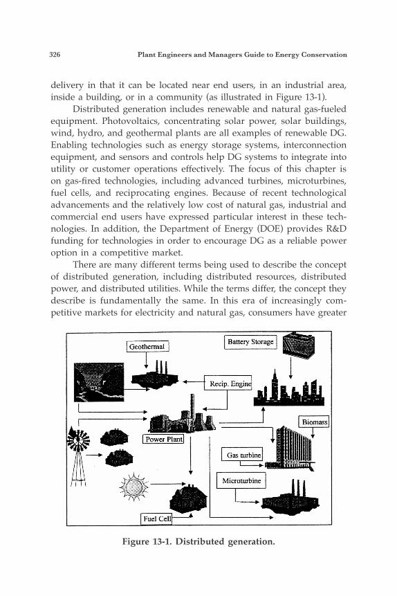
326 Plant Engineers and Managers Guide to Energy Conservation
delivery in that it can be located near end users, in an industrial area, inside a building, or in a community (as illustrated in Figure 13-1). Distributed generation includes renewable and natural gas-fueled equipment. Photovoltaics, concentrating solar power, solar buildings, wind, hydro, and geothermal plants are all examples of renewable DG. Enabling technologies such as energy storage systems, interconnection equipment, and sensors and controls help DG systems to integrate into utility or customer operations effectively. The focus of this chapter is on gas-fired technologies, including advanced turbines, microturbines, fuel cells, and reciprocating engines. Because of recent technological advancements and the relatively low cost of natural gas, industrial and commercial end users have expressed particular interest in these tech-nologies. In addition, the Department of Energy (DOE) provides R&D funding for technologies in order to encourage DG as a reliable power option in a competitive market. There are many different terms being used to describe the concept of distributed generation, including distributed resources, distributed power, and distributed utilities. While the terms differ, the concept they describe is fundamentally the same. In this era of increasingly com-petitive markets for electricity and natural gas, consumers have greater
Figure 13-1. Distributed generation.
Reliable and Economic Natural Gas Distributed Generation Technologies 327
choices than ever before for satisfying their needs for energy services. Certain industrial and commercial customers find having greater access and control over their sources of energy is advantageous. With uncer-tainty about the future utility system and concern about the reliability of energy services, distributed generation offers customers an additional energy option. Combined heat and power (CHP) is an important DG application. CHP systems capture the waste heat from power generation normally vented to the atmosphere and use it for productive purposes, such as making hot water and steam, industrial process heat, driving chillers and other mechanical devices, or regenerating desiccants for humid-ity control. CHP systems can use turbines, engines, or fuel cells and couple them with heat recovery equipment. While the most efficient electricity generation systems are able to convert 40%-50% of the fuel into useful products, CHP systems can convert as much as 80% of the fuel into useful work.1 This increase in efficiency lowers overall costs to users and reduces emissions of air pollutants and greenhouse gases.
ELEMENTS OF DG
Partnerships There are several participants involved with the development and deployment of natural gas-fired DG systems. (See Figure 13-2.) Indus-trial and commercial end users demand power that is clean, economi-cal, and reliable. Power outages and interruptions can be costly.2 These needs are recognized by federal and state government agencies, who are leading a national effort to develop cleaner, more reliable, efficient, and affordable energy systems. Equipment manufacturers are involved in the research and development efforts. Given favorable market condi-tions, equipment manufacturers can and do engage in R&D activities without the government’s encouragement. Energy service providers, such as electric and gas utilities, work with the equipment manufac-turers to market DG technologies and bring the power to the user. In addition, energy service providers are often responsible for interconnect-ing DG systems to the grid. Project developers include energy service companies, engineering companies, and design firms. Their role is sit-ing, permitting, and financing projects. The Department of Energy (DOE) is actively involved in research

328 Plant Engineers and Managers Guide to Energy Conservation
and development and supporting activities to accelerate DG system implementation into the market. DOE invests more than $250 mil-lion annually in research and development programs for advanced distributed generation technologies, including renewable and natural gas-fueled systems, as well as supporting technologies in transmission and distribution, sensors and controls, combustion, advanced materials, and energy storage systems. DOE has also proposed comprehensive electricity restructuring legislation that calls for opening markets across the country to retail competition. In addition to these research and development efforts, the Office of Energy Efficiency and Renewable Energy has launched the Combined Heat and Power Challenge, which has the goal of doubling U.S. CHP capacity by 2010 and then doubling it again by 2020. By conducting outreach activities across the nation, the department hopes to encour-age CHP use by educating legislators, policy officials, and end users of the potential benefits of utilizing distributed generation technologies in CHP applications. Additional information about these activities is available on the industrial power homepage (www.eren.doe.gov/der) and CHP Challenge website (www.eren.doe.gov/der/chp).
Benefits According to the North American Electric Reliability Council (NERC), the current economy is expected to drive long-term demand growth for electricity faster than projected; planned generating capacity
Figure 13-2. Key participants in DG.
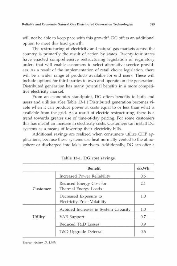
Reliable and Economic Natural Gas Distributed Generation Technologies 329
will not be able to keep pace with this growth3. DG offers an additional option to meet this load growth. The restructuring of electricity and natural gas markets across the country is primarily the result of action by states. Twenty-four states have enacted comprehensive restructuring legislation or regulatory orders that will enable customers to select alternative service provid-ers. As a result of the implementation of retail choice legislation, there will be a wider range of products available for end users. These will include options for third parties to own and operate on-site generation. Distributed generation has many potential benefits in a more competi-tive electricity market. From an economics standpoint, DG offers benefits to both end users and utilities. (See Table 13-1.) Distributed generation becomes vi-able when it can produce power at costs equal to or less than what is available from the grid. As a result of electric restructuring, there is a trend towards greater use of time-of-day pricing. For some customers this has meant an increase in electricity costs. Customers can install DG systems as a means of lowering their electricity bills. Additional savings are realized when consumers utilize CHP ap-plications, because these systems use heat normally vented to the atmo-sphere or discharged into lakes or rivers. Additionally, DG can offer a
Table 13-1. DG cost savings.———————————————————————————————— Benefit ¢/kWh———————————————————————————————— Increased Power Reliability 0.6 ———————————————————————— Reduced Energy Cost for 2.1 Customer Thermal Energy Loads ———————————————————————— Decreased Exposure to 1.0 Electricity Price Volatility———————————————————————————————— Avoided Increases in System Capacity 1.0 ———————————————————————— Utility VAR Support 0.7 ———————————————————————— Reduced T&D Losses 0.9 ———————————————————————— T&D Upgrade Deferral 0.6————————————————————————————————Source: Arthur D. Little
330 Plant Engineers and Managers Guide to Energy Conservation
new source of revenue if the customer can sell excess power or ancillary services to power markets. DG at the customer’s site can also provide many benefits to the electric utility. Utilities can defer investments in distribution system upgrades by using DG to relieve congestion at key locations in the network. For example, the addition of a new feeder line at a substation can be avoided if DG systems are used to meet the load growth. By reducing the need for transmission and distribution services, DG reduces the stress on these systems during peak periods and reduces losses. In addition, strategically located DG systems can be used by grid operators for frequency control, voltage, and reactive power support. Another attractive benefit that DG can offer the customer is in-creased power reliability. By operating a system that is on-site or near the end-user, DG can avoid or reduce the impacts of grid power outages that cause operational downtime and health and safety concerns. By contributing to a less complex transmission and distribution network, DG can reduce or eliminate grid voltage variation and harmonics that negatively affect a customer’s sensitive loads, resulting in improved power quality. The increased power efficiency of on-site CHP systems is an added benefit to DG. Currently, the electricity consumed in the United States is produced from large power plants owned by independent power producers, utilities and large industrial facilities. Over the past thirty years, there has been a slight increase in overall efficiency of the U.S. electric system. However, it has reached a plateau of around 33%. (See Figure 13-3.) Fossil and nuclear plants vent a large amount of heat into the atmosphere, lakes, and rivers each year. Although all DG technolo-gies have different efficiencies, when utilized in a combined heat and power application, they are more efficient than conventional power production methods. Environmental quality is also a major benefit of DG. Some DG sys-tems substantially reduce air pollutants. Tightened emission standards for SOx and NOx and increased concern over greenhouse gases have made low-emission DG systems more appealing for power production. Another benefit of some DG systems is size—fuel cells and microtur-bines can be the size of an air conditioning unit. The small size and modularity support a broad range of customer and grid-sited applica-tions by providing electricity and thermal power in a precise way where central power plants would be impractical.
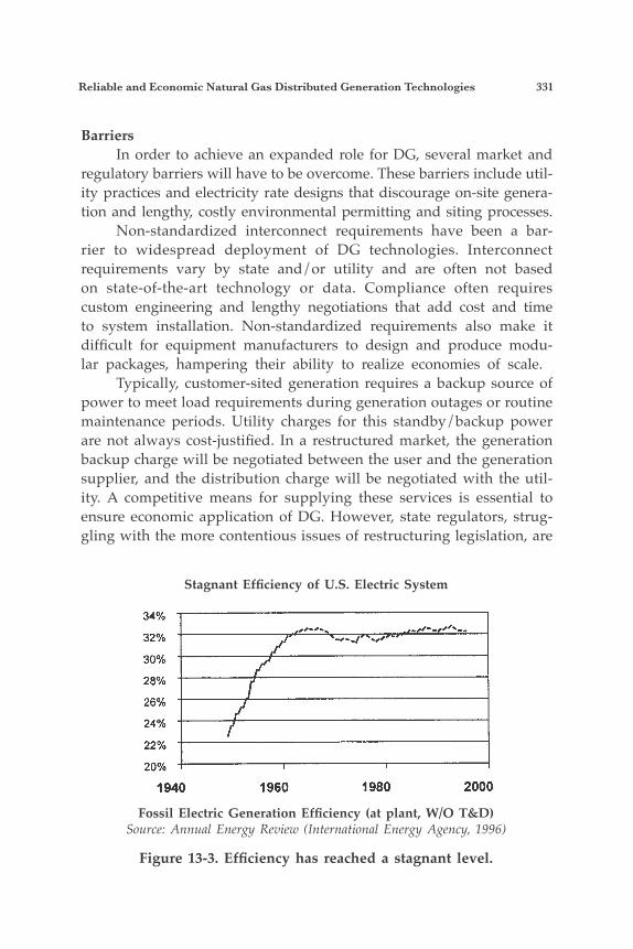
Reliable and Economic Natural Gas Distributed Generation Technologies 331
Barriers In order to achieve an expanded role for DG, several market and regulatory barriers will have to be overcome. These barriers include util-ity practices and electricity rate designs that discourage on-site genera-tion and lengthy, costly environmental permitting and siting processes. Non-standardized interconnect requirements have been a bar-rier to widespread deployment of DG technologies. Interconnect requirements vary by state and/or utility and are often not based on state-of-the-art technology or data. Compliance often requires custom engineering and lengthy negotiations that add cost and time to system installation. Non-standardized requirements also make it difficult for equipment manufacturers to design and produce modu-lar packages, hampering their ability to realize economies of scale. Typically, customer-sited generation requires a backup source of power to meet load requirements during generation outages or routine maintenance periods. Utility charges for this standby/backup power are not always cost-justified. In a restructured market, the generation backup charge will be negotiated between the user and the generation supplier, and the distribution charge will be negotiated with the util-ity. A competitive means for supplying these services is essential to ensure economic application of DG. However, state regulators, strug-gling with the more contentious issues of restructuring legislation, are
Fossil Electric Generation Efficiency (at plant, W/O T&D)Source: Annual Energy Review (International Energy Agency, 1996)
Figure 13-3. Efficiency has reached a stagnant level.
Stagnant Efficiency of U.S. Electric System
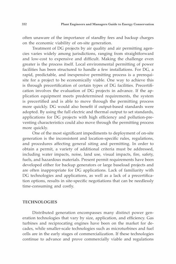
332 Plant Engineers and Managers Guide to Energy Conservation
often unaware of the importance of standby fees and backup charges on the economic viability of on-site generation. Treatment of DG projects by air quality and air permitting agen-cies varies widely among jurisdictions, ranging from straightforward and low-cost to expensive and difficult. Making the challenge even greater is the process itself. Local environmental permitting of power facilities has been structured to handle a few installations. For DG, a rapid, predictable, and inexpensive permitting process is a prerequi-site for a project to be economically viable. One way to achieve this is through precertification of certain types of DG facilities. Precertifi-cation involves the evaluation of DG projects in advance. If the ap-plication equipment meets predetermined requirements, the system is precertified and is able to move through the permitting process more quickly. DG would also benefit if output-based standards were adopted. By using the full electric and thermal output to set standards, applications for DG projects with high efficiency and pollution-pre-venting characteristics could also move through the permitting process more quickly. One of the most significant impediments to deployment of on-site generation is the inconsistent and location-specific rules, regulations, and procedures affecting general siting and permitting. In order to obtain a permit, a variety of additional criteria must be addressed, including water impacts, noise, land use, visual impacts, fire, safety, fuels, and hazardous materials. Present permit requirements have been developed either for backup generators or large baseload projects and are often inappropriate for DG applications. Lack of familiarity with DG technologies and applications, as well as a lack of a precertifica-tion options, results in site-specific negotiations that can be needlessly time-consuming and costly.
TECHNOLOGIES
Distributed generation encompasses many distinct power gen-eration technologies that vary by size, application, and efficiency. Gas turbines and reciprocating engines have been on the market for de-cades, while smaller-scale technologies such as microturbines and fuel cells are in the early stages of commercialization. If these technologies continue to advance and prove commercially viable and regulations
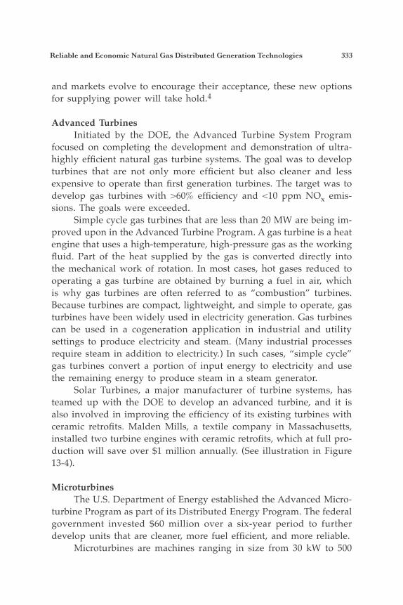
Reliable and Economic Natural Gas Distributed Generation Technologies 333
and markets evolve to encourage their acceptance, these new options for supplying power will take hold.4
Advanced Turbines Initiated by the DOE, the Advanced Turbine System Program focused on completing the development and demonstration of ultra-highly efficient natural gas turbine systems. The goal was to develop turbines that are not only more efficient but also cleaner and less expensive to operate than first generation turbines. The target was to develop gas turbines with >60% efficiency and <10 ppm NOx emis-sions. The goals were exceeded. Simple cycle gas turbines that are less than 20 MW are being im-proved upon in the Advanced Turbine Program. A gas turbine is a heat engine that uses a high-temperature, high-pressure gas as the working fluid. Part of the heat supplied by the gas is converted directly into the mechanical work of rotation. In most cases, hot gases reduced to operating a gas turbine are obtained by burning a fuel in air, which is why gas turbines are often referred to as “combustion” turbines. Because turbines are compact, lightweight, and simple to operate, gas turbines have been widely used in electricity generation. Gas turbines can be used in a cogeneration application in industrial and utility settings to produce electricity and steam. (Many industrial processes require steam in addition to electricity.) In such cases, “simple cycle” gas turbines convert a portion of input energy to electricity and use the remaining energy to produce steam in a steam generator. Solar Turbines, a major manufacturer of turbine systems, has teamed up with the DOE to develop an advanced turbine, and it is also involved in improving the efficiency of its existing turbines with ceramic retrofits. Malden Mills, a textile company in Massachusetts, installed two turbine engines with ceramic retrofits, which at full pro-duction will save over $1 million annually. (See illustration in Figure 13-4).
Microturbines The U.S. Department of Energy established the Advanced Micro-turbine Program as part of its Distributed Energy Program. The federal government invested $60 million over a six-year period to further develop units that are cleaner, more fuel efficient, and more reliable. Microturbines are machines ranging in size from 30 kW to 500
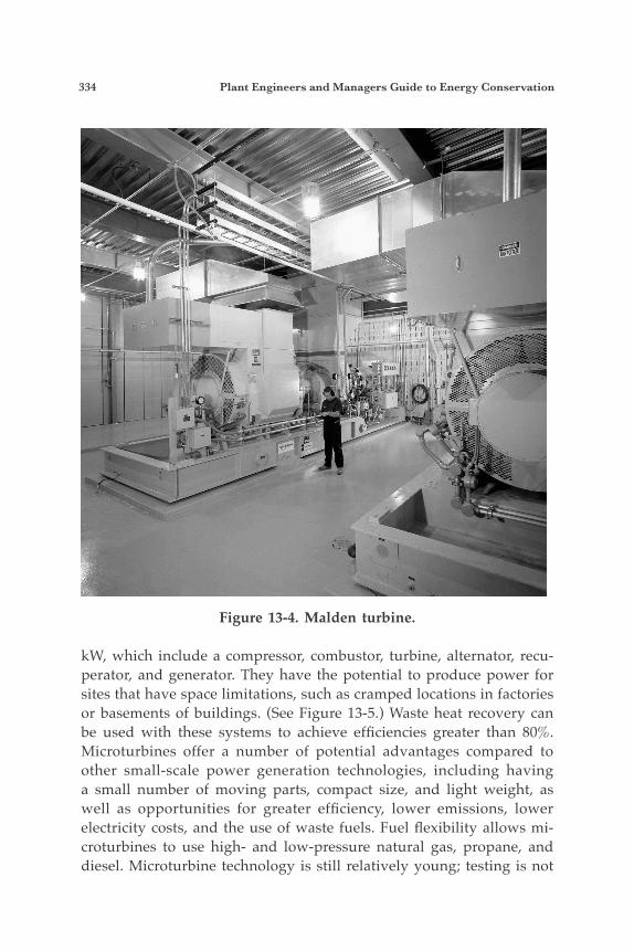
334 Plant Engineers and Managers Guide to Energy Conservation
kW, which include a compressor, combustor, turbine, alternator, recu-perator, and generator. They have the potential to produce power for sites that have space limitations, such as cramped locations in factories or basements of buildings. (See Figure 13-5.) Waste heat recovery can be used with these systems to achieve efficiencies greater than 80%. Microturbines offer a number of potential advantages compared to other small-scale power generation technologies, including having a small number of moving parts, compact size, and light weight, as well as opportunities for greater efficiency, lower emissions, lower electricity costs, and the use of waste fuels. Fuel flexibility allows mi-croturbines to use high- and low-pressure natural gas, propane, and diesel. Microturbine technology is still relatively young; testing is not
Figure 13-4. Malden turbine.
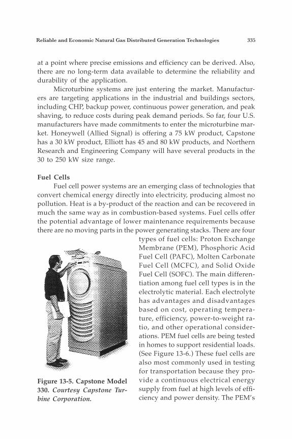
Reliable and Economic Natural Gas Distributed Generation Technologies 335
at a point where precise emissions and efficiency can be derived. Also, there are no long-term data available to determine the reliability and durability of the application. Microturbine systems are just entering the market. Manufactur-ers are targeting applications in the industrial and buildings sectors, including CHP, backup power, continuous power generation, and peak shaving, to reduce costs during peak demand periods. So far, four U.S. manufacturers have made commitments to enter the microturbine mar-ket. Honeywell (Allied Signal) is offering a 75 kW product, Capstone has a 30 kW product, Elliott has 45 and 80 kW products, and Northern Research and Engineering Company will have several products in the 30 to 250 kW size range.
Fuel Cells Fuel cell power systems are an emerging class of technologies that convert chemical energy directly into electricity, producing almost no pollution. Heat is a by-product of the reaction and can be recovered in much the same way as in combustion-based systems. Fuel cells offer the potential advantage of lower maintenance requirements because there are no moving parts in the power generating stacks. There are four
types of fuel cells: Proton Exchange Membrane (PEM), Phosphoric Acid Fuel Cell (PAFC), Molten Carbonate Fuel Cell (MCFC), and Solid Oxide Fuel Cell (SOFC). The main differen-tiation among fuel cell types is in the electrolytic material. Each electrolyte has advantages and disadvantages based on cost, operating tempera-ture, efficiency, power-to-weight ra-tio, and other operational consider-ations. PEM fuel cells are being tested in homes to support residential loads. (See Figure 13-6.) These fuel cells are also most commonly used in testing for transportation because they pro-vide a continuous electrical energy supply from fuel at high levels of effi-ciency and power density. The PEM’s
Figure 13-5. Capstone Model 330. Courtesy Capstone Tur-bine Corporation.
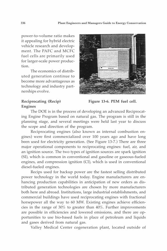
336 Plant Engineers and Managers Guide to Energy Conservation
power-to-volume ratio makes it appealing for hybrid electric vehicle research and develop-ment. The PAFC and MCFC fuel cells are primarily used for larger-scale power produc-tion. The economics of distrib-uted generation continue to become more advantageous as technology and industry part-nerships evolve.
Reciprocating (Recip)Engines The DOE is in the process of developing an advanced Reciprocat-ing Engine Program based on natural gas. The program is still in the planning stage, and several meetings were held last year to discuss the scope and direction of the program. Reciprocating engines (also known as internal combustion en-gines) were first commercialized over 100 years ago and have long been used for electricity generation. (See Figure 13-7.) There are three major operational components to reciprocating engines: fuel, air, and an ignition source. The two types of ignition sources are spark ignition (SI), which is common in conventional and gasoline or gaseous-fueled engines, and compression ignition (CI), which is used in conventional diesel-fueled engines. Recips used for backup power are the fastest selling distributed power technology in the world today. Engine manufacturers are en-hancing production capabilities in anticipation of new orders as dis-tributed generation technologies are chosen by more manufacturers both here and abroad. Institutions, large industrial establishments, and commercial buildings have used reciprocating engines with fractional horsepower all the way to 60 MW. Existing engines achieve efficien-cies in the range of 30% to greater than 40%. Further improvements are possible in efficiencies and lowered emissions, and there are op-portunities to use bio-based fuels in place of petroleum and liquids and gases derived from natural gas. Valley Medical Center cogeneration plant, located outside of
Figure 13-6. PEM fuel cell.
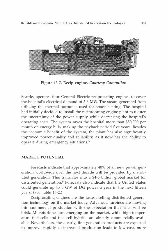
Reliable and Economic Natural Gas Distributed Generation Technologies 337
Seattle, operates four General Electric reciprocating engines to cover the hospital’s electrical demand of 3.6 MW. The steam generated from utilizing the thermal output is used for space heating. The hospital had initially decided to install the reciprocating engine plant to reduce the uncertainty of the power supply while decreasing the hospital’s operating costs. The system saves the hospital more than $50,000 per month on energy bills, making the payback period five years. Besides the economic benefit of the system, the plant has also significantly improved power quality and reliability, as it now has the ability to operate during emergency situations.5
MARKET POTENTIAL
Forecasts indicate that approximately 40% of all new power gen-eration worldwide over the next decade will be provided by distrib-uted generation. This translates into a $4-5 billion global market for distributed generation.6 Forecasts also indicate that the United States could generate up to 5 GW of DG power a year in the next fifteen years. (See Table 13-2.) Reciprocating engines are the fastest selling distributed genera-tion technology on the market today. Advanced turbines are moving into commercial production with the expectation that sales will be brisk. Microturbines are emerging on the market, while high-temper-ature fuel cells and fuel cell hybrids are already commercially avail-able. Nevertheless, these early, first generation products are expected to improve rapidly as increased production leads to low-cost, more
Figure 13-7. Recip engine. Courtesy Caterpillar.
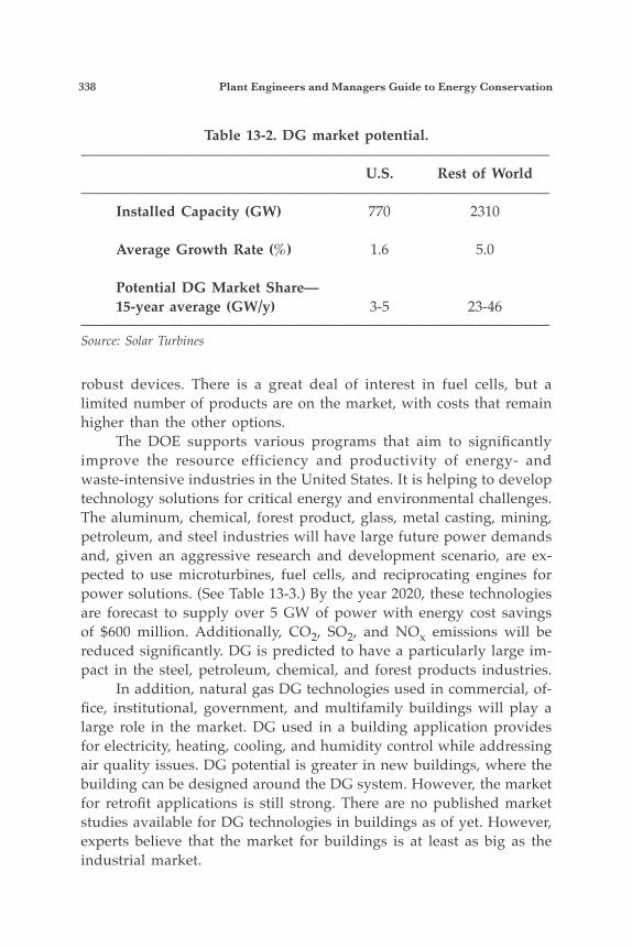
338 Plant Engineers and Managers Guide to Energy Conservation
robust devices. There is a great deal of interest in fuel cells, but a limited number of products are on the market, with costs that remain higher than the other options. The DOE supports various programs that aim to significantly improve the resource efficiency and productivity of energy- and waste-intensive industries in the United States. It is helping to develop technology solutions for critical energy and environmental challenges. The aluminum, chemical, forest product, glass, metal casting, mining, petroleum, and steel industries will have large future power demands and, given an aggressive research and development scenario, are ex-pected to use microturbines, fuel cells, and reciprocating engines for power solutions. (See Table 13-3.) By the year 2020, these technologies are forecast to supply over 5 GW of power with energy cost savings of $600 million. Additionally, CO2, SO2, and NOx emissions will be reduced significantly. DG is predicted to have a particularly large im-pact in the steel, petroleum, chemical, and forest products industries. In addition, natural gas DG technologies used in commercial, of-fice, institutional, government, and multifamily buildings will play a large role in the market. DG used in a building application provides for electricity, heating, cooling, and humidity control while addressing air quality issues. DG potential is greater in new buildings, where the building can be designed around the DG system. However, the market for retrofit applications is still strong. There are no published market studies available for DG technologies in buildings as of yet. However, experts believe that the market for buildings is at least as big as the industrial market.
Table 13-2. DG market potential.———————————————————————————————— U.S. Rest of World———————————————————————————————— Installed Capacity (GW) 770 2310 Average Growth Rate (%) 1.6 5.0 Potential DG Market Share— 15-year average (GW/y) 3-5 23-46————————————————————————————————Source: Solar Turbines
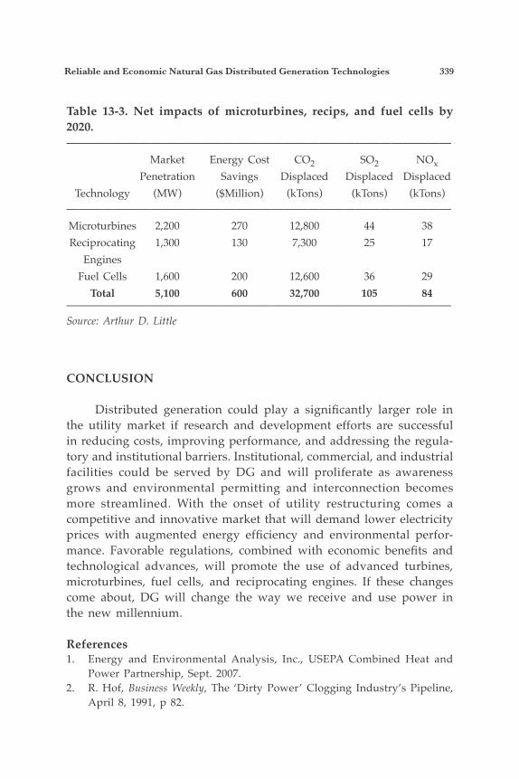
Reliable and Economic Natural Gas Distributed Generation Technologies 339
CONCLUSION
Distributed generation could play a significantly larger role in the utility market if research and development efforts are successful in reducing costs, improving performance, and addressing the regula-tory and institutional barriers. Institutional, commercial, and industrial facilities could be served by DG and will proliferate as awareness grows and environmental permitting and interconnection becomes more streamlined. With the onset of utility restructuring comes a competitive and innovative market that will demand lower electricity prices with augmented energy efficiency and environmental perfor-mance. Favorable regulations, combined with economic benefits and technological advances, will promote the use of advanced turbines, microturbines, fuel cells, and reciprocating engines. If these changes come about, DG will change the way we receive and use power in the new millennium.
References1. Energy and Environmental Analysis, Inc., USEPA Combined Heat and
Power Partnership, Sept. 2007.2. R. Hof, Business Weekly, The ‘Dirty Power’ Clogging Industry’s Pipeline,
April 8, 1991, p 82.
Table 13-3. Net impacts of microturbines, recips, and fuel cells by 2020.———————————————————————————————— Market Energy Cost CO2 SO2 NOx Penetration Savings Displaced Displaced Displaced Technology (MW) ($Million) (kTons) (kTons) (kTons)———————————————————————————————— Microturbines 2,200 270 12,800 44 38 Reciprocating 1,300 130 7,300 25 17 Engines Fuel Cells 1,600 200 12,600 36 29 Total 5,100 600 32,700 105 84————————————————————————————————Source: Arthur D. Little

340 Plant Engineers and Managers Guide to Energy Conservation
3. Arthur D. Little, White Paper, Distributed Generation: Understanding the Economics, 1999, p 4.
4. Arthur D. Little, White Paper Distributed Generation: Understanding the Economics. 1998
5. Robert Swanekamp, Power Magazine, May/June 1998, Vol. 142, No. 3, page 43.
6. Electric World, 7/97
341
14Financing EnergyEfficiency Projects
INTRODUCTION
Every day spent by an organization without having installed the appropriate energy efficiency measures means lost savings and lost opportunities. Performance contracting is a sophisticated solution to this problem. As with any sophisticated system, there are elements of complexity to be managed. Therefore, communication, knowledge, and experience are essential for successful project completion.
DEFINITIONS AND CLARIFICATIONS
For the purposes of this chapter, it is assumed that the energy services company (ESCO) is providing the energy conservation mea-sures (ECMs), such as audit, design, installation, monitoring, and maintenance for the customer, and that a separate third party, such as a bank or investment company, is providing the capital for the project. Often, energy services companies market themselves to customers as providing financing. In many cases, there is an independent financing source involved in the background. Alternatively, an ESCO can be a utility subsidiary which uses the utility’s shareholder money to finance projects. For simplicity’s sake, we will treat the ultimate source of capital for projects as a separate lender with its own guidelines.
FINANCING ALTERNATIVES
There is a variety of options for financing energy conservation projects. Some of the most common are as follows.
342 Plant Engineers and Managers Guide to Energy Conservation
General Obligation Bond Specifically applicable to municipalities, these bonds are based on the general credit of a state or local government. The process is long and complicated, but interest rates are low.
Municipal Lease Specifically applicable to municipalities, state entities and local entities, the lessor earns tax-exempt credit, and the borrowing entity pays low interest rates.
Commercial Loan This is a loan to the customer from a conventional bank based on the customer’s assets and credit quality. This form of financing is rarely offered by typical finance companies or financial institutions for energy conservation projects requiring less than $5 million of capital.
Taxable Lease There are a number of leasing vehicles with a variety of names, such as operating lease, capital lease, guideline lease, tax-oriented lease, and non-tax-oriented lease. The tax ramifications of leasing are often not well understood. Figure 14-1 will help clarify some of those distinctions. Figure 14-2 shows the dynamics of the parties involved. It is important to note that in all of the categories listed above, the customer is directly obligated to make payments relating to the installed energy-saving measures, regardless of performance of either the equipment or the ESCO. The customer may well have recourse under a separate contract to the service provider or equipment manufacturer but will still owe under the financing instrument. The interest rate and any additional loan terms are based almost exclusively on the credit-worthiness of the customer.
RELATIVE BENEFITS OF PROJECT FINANCING
Many companies and government entities are undergoing severe budget cutbacks. When these entities are approached by an ESCO of-fering virtually no up-front investment and a guaranteed amount of savings, new possibilities are created for energy projects to be developed and completed. If structured properly, performance contract financing
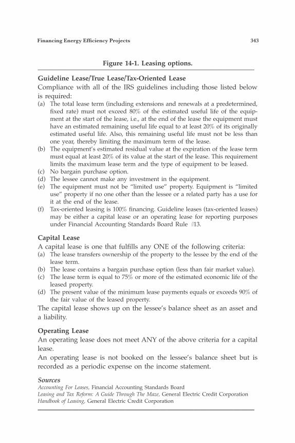
Financing Energy Efficiency Projects 343
Figure 14-1. Leasing options.————————————————————————————————Guideline Lease/True Lease/Tax-Oriented LeaseCompliance with all of the IRS guidelines including those listed below is required:(a) The total lease term (including extensions and renewals at a predetermined,
fixed rate) must not exceed 80% of the estimated useful life of the equip-ment at the start of the lease, i.e., at the end of the lease the equipment must have an estimated remaining useful life equal to at least 20% of its originally estimated useful life. Also, this remaining useful life must not be less than one year, thereby limiting the maximum term of the lease.
(b) The equipment’s estimated residual value at the expiration of the lease term must equal at least 20% of its value at the start of the lease. This requirement limits the maximum lease term and the type of equipment to be leased.
(c) No bargain purchase option.(d) The lessee cannot make any investment in the equipment.(e) The equipment must not be “limited use” property. Equipment is “limited
use” property if no one other than the lessee or a related party has a use for it at the end of the lease.
(f) Tax-oriented leasing is 100% financing. Guideline leases (tax-oriented leases) may be either a capital lease or an operating lease for reporting purposes under Financial Accounting Standards Board Rule #13.
Capital LeaseA capital lease is one that fulfills any ONE of the following criteria:(a) The lease transfers ownership of the property to the lessee by the end of the
lease term.(b) The lease contains a bargain purchase option (less than fair market value).(c) The lease term is equal to 75% or more of the estimated economic life of the
leased property.(d) The present value of the minimum lease payments equals or exceeds 90% of
the fair value of the leased property.The capital lease shows up on the lessee’s balance sheet as an asset and a liability.
Operating LeaseAn operating lease does not meet ANY of the above criteria for a capital lease.An operating lease is not booked on the lessee’s balance sheet but is recorded as a periodic expense on the income statement.
SourcesAccounting For Leases, Financial Accounting Standards BoardLeasing and Tax Reform: A Guide Through The Maze, General Electric Credit CorporationHandbook of Leasing, General Electric Credit Corporation————————————————————————————————
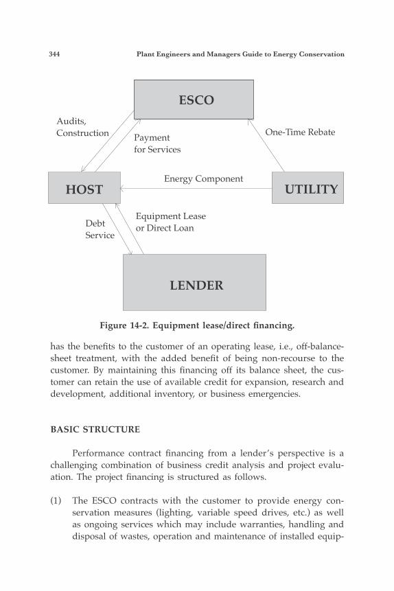
344 Plant Engineers and Managers Guide to Energy Conservation
has the benefits to the customer of an operating lease, i.e., off-balance-sheet treatment, with the added benefit of being non-recourse to the customer. By maintaining this financing off its balance sheet, the cus-tomer can retain the use of available credit for expansion, research and development, additional inventory, or business emergencies.
BASIC STRUCTURE
Performance contract financing from a lender’s perspective is a challenging combination of business credit analysis and project evalu-ation. The project financing is structured as follows.
(1) The ESCO contracts with the customer to provide energy con-servation measures (lighting, variable speed drives, etc.) as well as ongoing services which may include warranties, handling and disposal of wastes, operation and maintenance of installed equip-
DebtService
Audits,Construction Payment
for Services
One-Time Rebate
Energy Component
Equipment Leaseor Direct Loan
Figure 14-2. Equipment lease/direct financing.
ESCO
UTILITY
LENDER
HOST
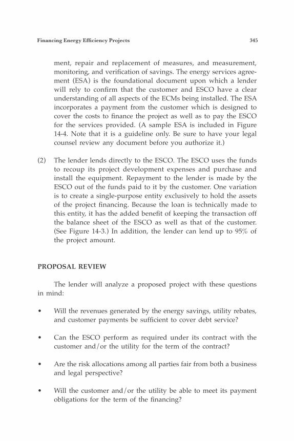
Financing Energy Efficiency Projects 345
ment, repair and replacement of measures, and measurement, monitoring, and verification of savings. The energy services agree-ment (ESA) is the foundational document upon which a lender will rely to confirm that the customer and ESCO have a clear understanding of all aspects of the ECMs being installed. The ESA incorporates a payment from the customer which is designed to cover the costs to finance the project as well as to pay the ESCO for the services provided. (A sample ESA is included in Figure 14-4. Note that it is a guideline only. Be sure to have your legal counsel review any document before you authorize it.)
(2) The lender lends directly to the ESCO. The ESCO uses the funds to recoup its project development expenses and purchase and install the equipment. Repayment to the lender is made by the ESCO out of the funds paid to it by the customer. One variation is to create a single-purpose entity exclusively to hold the assets of the project financing. Because the loan is technically made to this entity, it has the added benefit of keeping the transaction off the balance sheet of the ESCO as well as that of the customer. (See Figure 14-3.) In addition, the lender can lend up to 95% of the project amount.
PROPOSAL REVIEW
The lender will analyze a proposed project with these questions in mind:
• Will the revenues generated by the energy savings, utility rebates, and customer payments be sufficient to cover debt service?
• Can the ESCO perform as required under its contract with the customer and/or the utility for the term of the contract?
• Are the risk allocations among all parties fair from both a business and legal perspective?
• Will the customer and/or the utility be able to meet its payment obligations for the term of the financing?
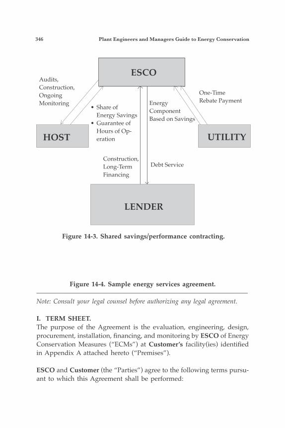
346 Plant Engineers and Managers Guide to Energy Conservation
Figure 14-4. Sample energy services agreement.————————————————————————————————Note: Consult your legal counsel before authorizing any legal agreement.
I. TERM SHEET.The purpose of the Agreement is the evaluation, engineering, design, procurement, installation, financing, and monitoring by ESCO of Energy Conservation Measures (“ECMs”) at Customer’s facility(ies) identified in Appendix A attached hereto (“Premises”).
ESCO and Customer (the “Parties”) agree to the following terms pursu-ant to which this Agreement shall be performed:
Figure 14-3. Shared savings/performance contracting.
ESCO
UTILITY
LENDER
HOST
Energy Component Based on Savings
• Share of Energy Savings• Guarantee of
Hours of Op-eration
Construction, Long-Term Financing
Debt Service
Audits,Construction, Ongoing Monitoring
One-Time Rebate Payment
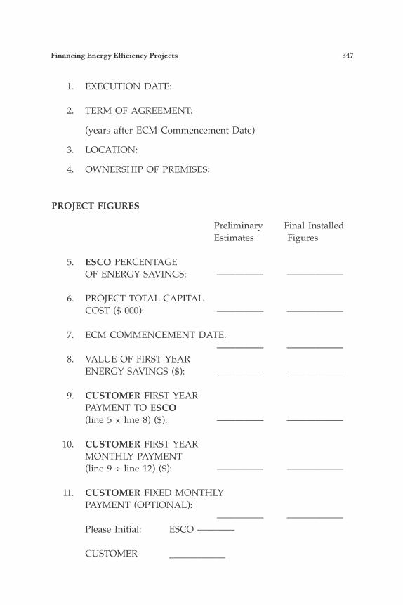
Financing Energy Efficiency Projects 347
1. EXECUTION DATE:
2. TERM OF AGREEMENT:
(years after ECM Commencement Date)
3. LOCATION:
4. OWNERSHIP OF PREMISES:
PROJECT FIGURES
Preliminary Final Installed Estimates Figures 5. ESCO PERCENTAGE OF ENERGY SAVINGS: ————— ——————
6. PROJECT TOTAL CAPITAL COST ($ 000): ————— ——————
7. ECM COMMENCEMENT DATE: ————— —————— 8. VALUE OF FIRST YEAR ENERGY SAVINGS ($): ————— ——————
9. CUSTOMER FIRST YEAR PAYMENT TO ESCO (line 5 × line 8) ($): ————— ——————
10. CUSTOMER FIRST YEAR MONTHLY PAYMENT (line 9 ÷ line 12) ($): ————— ——————
11. CUSTOMER FIXED MONTHLY PAYMENT (OPTIONAL): ————— —————— Please Initial: ESCO ————
CUSTOMER ____________
348 Plant Engineers and Managers Guide to Energy Conservation
The lender will want to see three years of audited financial state-ments (balance sheet, income statement and cash flow statement), with explanatory notes from the customer. These will be used to make trend and financial ratio analyses. The ESCO’s financial statements are also important and will receive a similar review. With utility payments and/or customer payments based on actual savings, the lender needs to make a thorough analysis of the projected savings due to the installed energy conservation measures. The project figures (simple payback; types of equipment; maintenance savings, if any; construction period) will be carefully reviewed to determine how the savings will cover the loan payments and to determine the effects of factors such as energy price fluctuations and inflation. Any information that the parties can provide early on in the pro-posal negotiation to make the lender feel more comfortable with these issues will save a tremendous amount of time, money, and effort to all parties.
CONCLUSION
The key point here is that if an event of default occurs in the ESA between the ESCO and the customer which gives the customer the right to reduce or cease its payment obligation, it is the lender which is most at risk of suffering a loss. The lender must either be comfortable that the ESCO will cure the default or be confident that it can hire another ESCO to cure the project default and force the customer to resume payments. The lender is also at risk of the energy savings not being estimated or measured properly. Despite all of this, good projects are being funded and customers are extremely satisfied with the resulting benefits. Final installed figures appearing in the right-hand column of Figure 14-4 shall be completed in accordance with Section V and the Parties shall then re-execute the Agreement below and enter their initials above.
As indicated in term #11 above, upon completion of any determi-nations required by Section V, Customer shall have the option to fix its monthly payment to ESCO, as required under Section VI, by multiply-ing One Hundred and ______ Percent (1____%) of ESCO’s Percentage of Energy Savings by the Final Installed Figure for the Value of First Year Energy Savings and paying such product to ESCO each year in
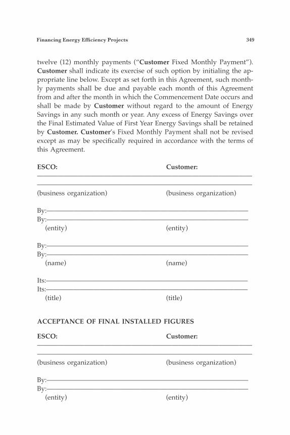
Financing Energy Efficiency Projects 349
twelve (12) monthly payments (“Customer Fixed Monthly Payment”). Customer shall indicate its exercise of such option by initialing the ap-propriate line below. Except as set forth in this Agreement, such month-ly payments shall be due and payable each month of this Agreement from and after the month in which the Commencement Date occurs and shall be made by Customer without regard to the amount of Energy Savings in any such month or year. Any excess of Energy Savings over the Final Estimated Value of First Year Energy Savings shall be retained by Customer. Customer’s Fixed Monthly Payment shall not be revised except as may be specifically required in accordance with the terms of this Agreement.
ESCO: Customer:————————————————————————————————————————————————————————————————(business organization) (business organization)
By:——————————————————————————————By:—————————————————————————————— (entity) (entity)
By:——————————————————————————————By:—————————————————————————————— (name) (name)
Its:——————————————————————————————Its:—————————————————————————————— (title) (title)
ACCEPTANCE OF FINAL INSTALLED FIGURES
ESCO: Customer:————————————————————————————————————————————————————————————————(business organization) (business organization)
By:——————————————————————————————By:—————————————————————————————— (entity) (entity)
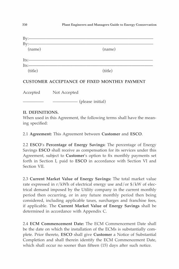
350 Plant Engineers and Managers Guide to Energy Conservation
By:——————————————————————————————By:—————————————————————————————— (name) (name)
Its:——————————————————————————————Its:—————————————————————————————— (title) (title)
CUSTOMER ACCEPTANCE OF FIXED MONTHLY PAYMENT
Accepted Not Accepted
————— —————— (please initial)
II. DEFINITIONS.When used in this Agreement, the following terms shall have the mean-ing specified:
2.1 Agreement: This Agreement between Customer and ESCO.
2.2 ESCO’s Percentage of Energy Savings: The percentage of Energy Savings ESCO shall receive as compensation for its services under this Agreement, subject to Customer’s option to fix monthly payments set forth in Section I, paid to ESCO in accordance with Section VI and Section VII.
2.3 Current Market Value of Energy Savings: The total market value rate expressed in r/kWh of electrical energy use and/or $/kW of elec-trical demand imposed by the Utility company in the current monthly period then occurring, or in any future monthly period then being considered, including applicable taxes, surcharges and franchise fees, if applicable. The Current Market Value of Energy Savings shall be determined in accordance with Appendix C.
2.4 ECM Commencement Date: The ECM Commencement Date shall be the date on which the installation of the ECMs is substantially com-plete. Prior thereto, ESCO shall give Customer a Notice of Substantial Completion and shall therein identify the ECM Commencement Date, which shall occur no sooner than fifteen (15) days after such notice.
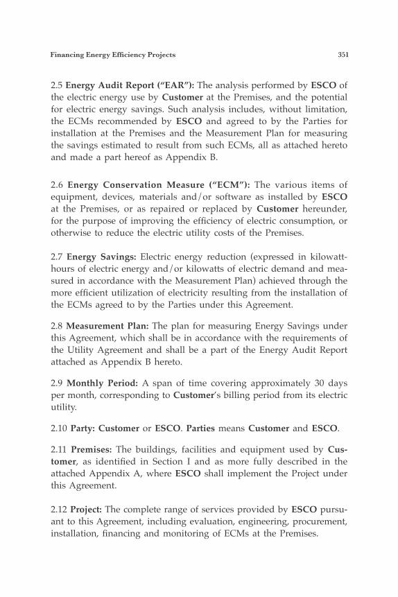
Financing Energy Efficiency Projects 351
2.5 Energy Audit Report (“EAR”): The analysis performed by ESCO of the electric energy use by Customer at the Premises, and the potential for electric energy savings. Such analysis includes, without limitation, the ECMs recommended by ESCO and agreed to by the Parties for installation at the Premises and the Measurement Plan for measuring the savings estimated to result from such ECMs, all as attached hereto and made a part hereof as Appendix B.
2.6 Energy Conservation Measure (“ECM”): The various items of equipment, devices, materials and/or software as installed by ESCO at the Premises, or as repaired or replaced by Customer hereunder, for the purpose of improving the efficiency of electric consumption, or otherwise to reduce the electric utility costs of the Premises.
2.7 Energy Savings: Electric energy reduction (expressed in kilowatt-hours of electric energy and/or kilowatts of electric demand and mea-sured in accordance with the Measurement Plan) achieved through the more efficient utilization of electricity resulting from the installation of the ECMs agreed to by the Parties under this Agreement.
2.8 Measurement Plan: The plan for measuring Energy Savings under this Agreement, which shall be in accordance with the requirements of the Utility Agreement and shall be a part of the Energy Audit Report attached as Appendix B hereto.
2.9 Monthly Period: A span of time covering approximately 30 days per month, corresponding to Customer’s billing period from its electric utility.
2.10 Party: Customer or ESCO. Parties means Customer and ESCO.
2.11 Premises: The buildings, facilities and equipment used by Cus-tomer, as identified in Section I and as more fully described in the attached Appendix A, where ESCO shall implement the Project under this Agreement.
2.12 Project: The complete range of services provided by ESCO pursu-ant to this Agreement, including evaluation, engineering, procurement, installation, financing and monitoring of ECMs at the Premises.
352 Plant Engineers and Managers Guide to Energy Conservation
2.13 Uncontrollable Circumstances: Any event or condition having a material adverse effect on the rights, duties or obligations of ESCO, or materially adversely affecting the Project, if such event or condition is beyond the reasonable control, and not the result of willful or negligent action or omission or a lack of reasonable diligence, of ESCO; provided, however, that the contesting by ESCO in good faith of any event or condition constituting a Change in Law shall not constitute or be con-strued as a willful or negligent action, or a lack of reasonable diligence. Such events or conditions may include, but shall not be limited to, circumstances of the following kind:
a. an act of God, epidemic, landslide, lightning, hurricane, earth-quake, fire, explosion, storm, flood or similar occurrence, an equipment failure or outage, an interruption in supply, an act or omission by persons or entities other than a Party, an act of war, effects of nuclear radiation, blockade, insurrection, riot, civil disturbance or similar occur-rences, or damage, interruption or interference to the Project caused by hazardous waste stored on or existing at the Project site; b. strikes, lockouts, work slowdowns or stoppages, or similar la-bor difficulties, affecting or impacting the performance of ESCO or its contractors and suppliers; c. a change in law or regulation or an act by a governmental agency or judicial authority.
2.14 Utility Agreement: The agreement entered into by ESCO with ________, a _____ public utility company (“Utility”), pursuant to which ESCO is required to install certain ECMs at facilities such as Customer’s Premises and in accordance with the terms of which ESCO has entered into this Agreement.
III. ECM COMMENCEMENT DATE AND TERM OF AGREEMENT.The term of this Agreement shall commence as of the date on which this Agreement is executed and shall continue, unless sooner terminated in accordance with the terms hereof, for the period of years after the ECM Commencement Date set forth in Section I. Upon receipt of the Notice of Substantial Completion identifying the ECM Commencement Date, Customer shall provide ESCO, within fifteen (15) days, any comments and requests for work or corrections. ESCO shall make all commercially reasonable efforts to respond to such
Financing Energy Efficiency Projects 353
comments and requests within thirty (30) days of the ECM Commence-ment Date, which shall occur on the identified date. Upon the expiration or termination of this Agreement the provi-sions of this Agreement that may reasonably be interpreted or construed as surviving the expiration or termination of this Agreement shall sur-vive the expiration or termination for such period as may be necessary to effect the intent of this Agreement.
At the end of the term of this Agreement, Customer shall purchase the ECMs and ESCO shall transfer title to Customer, free and clear of all liens and encumbrances, all as set forth in Section 6 of the General Terms and Conditions.
IV. SCOPE OF ESCO’S SERVICES.Subject to and in accordance with the terms and conditions of this Agreement, ESCO shall provide the evaluation, engineering, design, procurement, installation, financing and monitoring of the ECMs set forth in the Energy Audit Report. The ECMs in the EAR may be modi-fied pursuant to Section V. ESCO shall use reasonable commercial ef-forts to achieve the ECM Commencement Date estimated in Section I, line 7, column entitled, “Engineering Estimates.” ESCO agrees to extend its funds and install such ECMs in return for Customer’s agreement to perform hereunder and in particular, to pay ESCO’s Percentage of Energy Savings pursuant to Section VI. The Par-ties anticipate the measurement of Energy Savings, but notwithstanding this expectation or any provision of this Agreement which may suggest to the contrary, in light of the factors affecting savings which are beyond ESCO’s reasonable control, ESCO assumes no obligation that any par-ticular level of savings shall materialize due to its services hereunder. ESCO warrants that the ECMs which have a lifetime greater than one (1) year shall be, and shall remain, free of defects for one (1) year after the ECM Commencement Date. In addition, ESCO agrees to assign all manufacturers warranties for such ECMs to Customer for the period of manufacturer warranty, subject to all exclusions and limitations as may be set forth therein.
V. DETERMINATION OF FINAL TERMS.After the execution of this Agreement, if the Parties agree to revise the ECMs listed in the EAR, and to make all associated revisions to this
354 Plant Engineers and Managers Guide to Energy Conservation
Agreement, including, without limitation, to the numbers or dates, as the case may be, entered in the column entitled, “Engineering Esti-mates” appearing in lines 5 through 11 of Section I, the Parties shall, upon such agreement, make any associated revision and enter in the column entitled, “Final Installed Figures” the agreed-to numbers and/or dates. The Parties shall then re-execute Section I upon the entry of such numbers and/or dates and ESCO shall revise the Termination Values in Appendix D consistent with Appendix D and the Final Installed Project Total Capital Cost then appearing in line 6 of Section I above. All such revisions shall be voluntary and the Parties shall not be re-quired, absent mutual consent, to revise the ECMs listed in the EAR af-ter the execution hereof; provided, however, ESCO shall not be required to install ECMs affected by Uncontrollable Circumstances. Such ECMs shall be deleted from the Project unless the Parties agree to all necessary changes to the Project numbers and/or dates required to adjust to such circumstances. Changes to Project numbers and/or dates in connection with Uncontrollable Circumstances shall be entered by ESCO in the col-umn entitled “Final Installed Figures,” in lines 5 through 11 of Section I. The Parties shall then re-execute Section I and ESCO shall revise the Termination Values set forth in Appendix D consistent with Appendix D and the Final Installed Project Total Capital Cost then appearing in line 6 of Section I.
VI. COMPENSATION.From and after the ECM Commencement Date, except as provided in Sections I and VII with respect to Customer’s option to fix monthly pay-ments, Customer shall pay ESCO an amount equal to ESCO’s Percent-age of Energy Savings, as set forth in Section I above, multiplied by the applicable Current Market Value of Energy Savings, all as determined pursuant to Appendix C. ESCO shall prepare and send Customer, and Customer agrees to pay, a monthly invoice calculated pursuant to Section VII below.
VII. BILLING.ESCO will submit monthly invoices to Customer in amounts deter-mined in accordance with Section VI. In the event Customer exercises its option under Section I to fix its monthly payments to ESCO, Customer shall pay to ESCO the Customer Fixed Monthly Payment defined in Section I. If Customer does not exercise such option, monthly payments

Financing Energy Efficiency Projects 355
shall be estimated as set forth in this Section VII and paid on such es-timated basis, subject to reconciliation as provided hereinafter. Monthly invoices shall be paid within thirty (30) calendar days following receipt. Reconciliation payments, or refunds, as the case may be, shall be due within thirty (30) calendar days of receipt of a reconciliation invoice. Subject to reconciliation, invoice amounts shall be estimated for each year following the ECM Commencement Date. In the first such year, monthly payments shall be 1/12 of the product of ESCO’s Percentage of Energy Savings and the Current Market Value of Energy Savings expected in such first year as set forth in line 8 of the column entitled “Final Installed Figures” in Section I above. Such fixed amounts shall be reconciled and adjusted as necessary every six (6) months based on the difference between the Current Market Value of Energy Savings mea-sured pursuant to Appendix C and the estimated value then applicable. ESCO shall prepare and submit to Customer a reconciliation invoice within thirty (30) calendar days of the expiration of each such six-month period. The estimate of the value of Energy Savings then in effect at the end of any year shall continue until replaced with reconciled amounts in the succeeding year. In the second year and following years, the estimate of the Current Market Value of Energy Savings expected in such year shall equal the expected value (in nominal dollars for the billing year in question) of the Energy Savings actually delivered in the prior year.
VIII. NOTICES.All notices to be given by either Party to the other shall be in writing and must be delivered or mailed by registered or certified mail, return receipt requested, or sent by a courier service which renders a receipt upon delivery addressed as set forth above in Section I or such other addresses as either Party may hereinafter designate by a Notice to the other. Notices are deemed delivered or given and become effective upon mailing if mailed as aforesaid and upon actual receipt if otherwise de-livered to the addresses set forth in Section I.
IX. APPLICABLE LAW.This Agreement and the construction and enforceability thereof shall be interpreted under the laws of the state of __________________.
X. FINAL AGREEMENT.This Agreement, together with its appendices and attachments, shall
356 Plant Engineers and Managers Guide to Energy Conservation
constitute the full and final Agreement between the Parties, shall super-sede all prior agreements, communications and understandings regard-ing the subject matter hereof and shall not be amended, modified or revised except in writing. This Agreement shall bind the Parties as of the date on which it was executed. Any inconsistency in this Agree-ment shall be resolved by giving priority in the following order: (a) Amendments to the Agreement, in reverse chronological order; (b) the Agreement, Sections I through XI; (c) General Terms and Conditions of the Agreement; (d) Appendices to the Agreement; and (e) Attachments to, or other documents incorporated into, the Agreement.
XI. INCORPORATION OF GENERAL TERMS AND CONDITIONS:
THIS AGREEMENT IS SUBJECT TO THE GENERAL TERMS AND CONDITIONS ATTACHED HERETO AND MADE A PART HEREOF. IN ADDITION, THE PERFORMANCE OF THIS AGREEMENT BY ESCO IS SUBJECT TO THE PROVISIONS OF THE UTILITY AGREEMENT.
IN WITNESS WHEREOF, and intending to be legally bound, the Parties hereto subscribe their names to this instrument hereinabove in Section I as of the date of execution first written above.
SUMMARY OF GENERAL TERMS AND CONDITIONSSection 1. Operating the Premises and Maintaining the Use of the ECMs.Section 2. Equipment Location and Access.Section 3. Construction.Section 4. Ownership of ECMs.Section 5. Condition of ECMs.Section 6. Transfer of ECMs.Section 6.1. Material Shortfall in Energy Savings.Section 6.2. Customer Purchase Option.Section 6.3. Purchase Upon Customer Default.Section 6.4. Expiration of the Term.Section 6.5. Transfer Without Encumbrance.Section 7. Requirements of Utility Agreement.Section 8. Insurance.Section 8.1. Insurance on the Premises and the ECMs.
Financing Energy Efficiency Projects 357
Section 8.2. Risk of Loss of the ECMs.Section 8.3. ESCO’s Insurance Requirements.Section 9. Hazardous Materials and Activities.Section 10. Events of Default.Section 10.1. Events of Default by Customer. Section 10.2. Events of Default by ESCO. Section 11. Remedies Upon Default. Section 11.1. Remedies Upon Default by Customer. Section 11.2. Remedies Upon Default by ESCO. Section 11.3. Limitation of Remedies.Section 12. Representations and Warranties of Both Parties.Section 13. Compliance With Law and Standard Practices.Section 14. Assignment.Section 15. Taxes.Section 16. Severability.Section 17. Effect of Waiver.Section 18. Usage of Customer’s Records.Section 19. Air Emission Rights, Credits or Allowances.
APPENDICES:“A” Description and Address of Customer’s Facility(ies).“B” Energy Audit Report and List of ECMs.“C” Method of Savings Calculation.“D” Termination Values.“E” Requirements of Utility Agreement.
359
15Cost ContainmentDesign for CommercialGeothermal Heat Pumps
A geothermal heat pump (GHP) system consists of four distinct subsystems: (1) the ground heat exchanger loop, (2) the in-ground and building interior piping loop that connects the heat exchangers to the heat pumps, (3) the water source heat pumps and (4) the air distribution system. When engineers, contractors, and vendors attempt to contain installation costs, often they have concentrated on reducing the cost of item one, the ground loop. Reducing the size of the ground loop will significantly lower operating efficiency and will negatively impact system life and maintenance requirements. However, two of the other subsystems typically receive little attention—the piping loop and the air distribution system. Modifications to traditional piping and duct-ing methods can both reduce installation costs and improve operating efficiency. This chapter will discuss the design methods that will lead to these benefits. The chapter will also integrate these methods with a widely used ground loop sizing procedure. The geothermal heat pump is a heating and cooling concept that still faces barriers to realizing its full potential. There are many examples of GHP installations that have provided high levels of customer satisfaction, as noted by the rapidly increasing number of schools using this technology (GHPC Site List, 1999). There are even a few instances of systems where customers are satisfied not only with performance and dependability but also with installation costs. However, in many areas GHPs cannot shed the reputation (and reality) of having a high installation cost. There are also examples of systems
Presented at the 23rd World Energy Engineering Congress by Stephen P. Ka-vanaugh
360 Plant Engineers and Managers Guide to Energy Conservation
that have not lived up to expectations because of misguided attempts to reduce first costs. There are pathways to affordable GHPs that do not compromise their inherent efficiency, dependability, and comfort. These pathways include simplicity of design, quality of installation, access to informa-tion, and competition in the market.
Simplicity of Design GHP systems are inherently efficient and comfortable. The best de-signs are elegant in their simplicity. Systems need not contain redundant and expensive components. Complexity rarely improves performance and typically leads to customer dissatisfaction and increased service requirements.
Quality of Installation The ground loop should be installed by a well-trained and expe-rienced loop contractor. This quality must also be extended to the heat pump equipment and piping system in the building. Fortunately, this quality can be attained with simple components.
WHY GHPs? WHY NOW?
Geothermal heat pumps are becoming increasingly popular in the commercial sector, where the added premium compared to minimum efficiency equipment is much smaller than in residential applications. The most popular application is in schools, as indicated in the site list published by the Geothermal Heat Pump Consortium (GHPC, 1999). This increase in commercial application is surprising, given the modest level of support provided by the major HVAC manufacturers and the federal government. One primary reason for this increase is indicated in Figure 15-1. Although GHPs require ground loops, which are outside the scope of the traditional HVAC industry, the components in the building can be extremely simple and dependable. In fact, the primary equipment and related components are even less complicated than those used with residential HVAC systems. Furthermore, the recommended high density polyethylene (HDPE) piping material was developed for the natural gas and oil field industry, which are much more demanding applications.
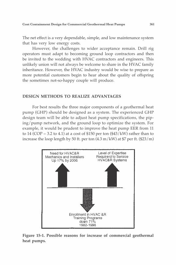
Cost Containment Design for Commercial Geothermal Heat Pumps 361
The net effect is a very dependable, simple, and low maintenance system that has very low energy costs. However, the challenges to wider acceptance remain. Drill rig operators must adapt to becoming ground loop contractors and then be invited to the wedding with HVAC contractors and engineers. This unlikely union will not always be welcome to share in the HVAC family inheritance. However, the HVAC industry would be wise to prepare as more potential customers begin to hear about the quality of offspring the sometimes not-so-happy couple will produce.
DESIGN METHODS TO REALIZE ADVANTAGES
For best results the three major components of a geothermal heat pump (GHP) should be designed as a system. The experienced GHP design team will be able to adjust heat pump specifications, the pip-ing/pump network, and the ground loop to optimize the system. For example, it would be prudent to improve the heat pump EER from 11 to 14 (COP = 3.2 to 4.1) at a cost of $150 per ton ($43/kW) rather than to increase the loop length by 50 ft. per ton (4.3 m/kW) at $7 per ft. ($23/m)
Figure 15-1. Possible reasons for increase of commercial geothermal heat pumps.
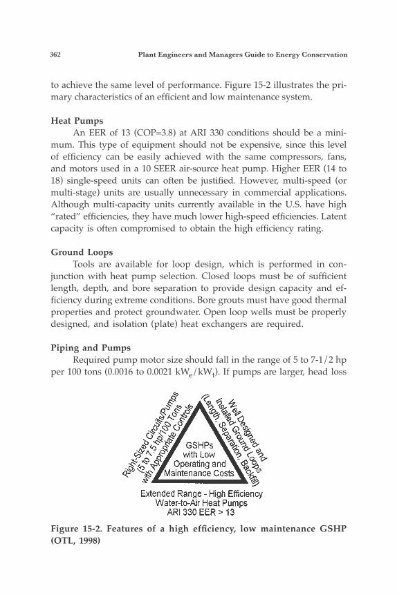
362 Plant Engineers and Managers Guide to Energy Conservation
to achieve the same level of performance. Figure 15-2 illustrates the pri-mary characteristics of an efficient and low maintenance system.
Heat Pumps An EER of 13 (COP=3.8) at ARI 330 conditions should be a mini-mum. This type of equipment should not be expensive, since this level of efficiency can be easily achieved with the same compressors, fans, and motors used in a 10 SEER air-source heat pump. Higher EER (14 to 18) single-speed units can often be justified. However, multi-speed (or multi-stage) units are usually unnecessary in commercial applications. Although multi-capacity units currently available in the U.S. have high “rated” efficiencies, they have much lower high-speed efficiencies. Latent capacity is often compromised to obtain the high efficiency rating.
Ground Loops Tools are available for loop design, which is performed in con-junction with heat pump selection. Closed loops must be of sufficient length, depth, and bore separation to provide design capacity and ef-ficiency during extreme conditions. Bore grouts must have good thermal properties and protect groundwater. Open loop wells must be properly designed, and isolation (plate) heat exchangers are required.
Piping and Pumps Required pump motor size should fall in the range of 5 to 7-1/2 hp per 100 tons (0.0016 to 0.0021 kWe/kWt). If pumps are larger, head loss
Figure 15-2. Features of a high efficiency, low maintenance GSHP (OTL, 1998)
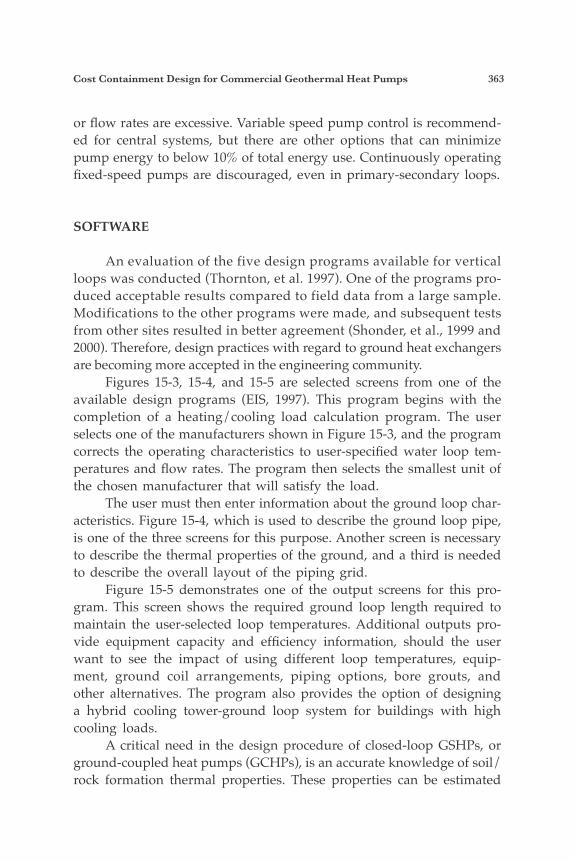
Cost Containment Design for Commercial Geothermal Heat Pumps 363
or flow rates are excessive. Variable speed pump control is recommend-ed for central systems, but there are other options that can minimize pump energy to below 10% of total energy use. Continuously operating fixed-speed pumps are discouraged, even in primary-secondary loops.
SOFTWARE
An evaluation of the five design programs available for vertical loops was conducted (Thornton, et al. 1997). One of the programs pro-duced acceptable results compared to field data from a large sample. Modifications to the other programs were made, and subsequent tests from other sites resulted in better agreement (Shonder, et al., 1999 and 2000). Therefore, design practices with regard to ground heat exchangers are becoming more accepted in the engineering community. Figures 15-3, 15-4, and 15-5 are selected screens from one of the available design programs (EIS, 1997). This program begins with the completion of a heating/cooling load calculation program. The user selects one of the manufacturers shown in Figure 15-3, and the program corrects the operating characteristics to user-specified water loop tem-peratures and flow rates. The program then selects the smallest unit of the chosen manufacturer that will satisfy the load. The user must then enter information about the ground loop char-acteristics. Figure 15-4, which is used to describe the ground loop pipe, is one of the three screens for this purpose. Another screen is necessary to describe the thermal properties of the ground, and a third is needed to describe the overall layout of the piping grid. Figure 15-5 demonstrates one of the output screens for this pro-gram. This screen shows the required ground loop length required to maintain the user-selected loop temperatures. Additional outputs pro-vide equipment capacity and efficiency information, should the user want to see the impact of using different loop temperatures, equip-ment, ground coil arrangements, piping options, bore grouts, and other alternatives. The program also provides the option of designing a hybrid cooling tower-ground loop system for buildings with high cooling loads. A critical need in the design procedure of closed-loop GSHPs, or ground-coupled heat pumps (GCHPs), is an accurate knowledge of soil/rock formation thermal properties. These properties can be estimated
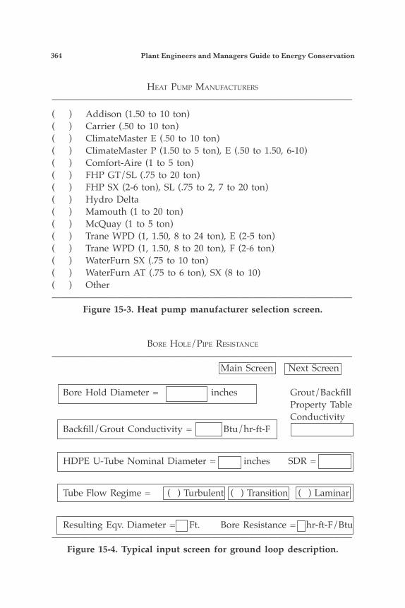
364 Plant Engineers and Managers Guide to Energy Conservation
heaT pump manufacTurers
————————————————————————————————( ) Addison (1.50 to 10 ton)( ) Carrier (.50 to 10 ton)( ) ClimateMaster E (.50 to 10 ton)( ) ClimateMaster P (1.50 to 5 ton), E (.50 to 1.50, 6-10)( ) Comfort-Aire (1 to 5 ton)( ) FHP GT/SL (.75 to 20 ton)( ) FHP SX (2-6 ton), SL (.75 to 2, 7 to 20 ton)( ) Hydro Delta( ) Mamouth (1 to 20 ton)( ) McQuay (1 to 5 ton)( ) Trane WPD (1, 1.50, 8 to 24 ton), E (2-5 ton)( ) Trane WPD (1, 1.50, 8 to 20 ton), F (2-6 ton)( ) WaterFurn SX (.75 to 10 ton)( ) WaterFurn AT (.75 to 6 ton), SX (8 to 10)( ) Other————————————————————————————————
Figure 15-3. Heat pump manufacturer selection screen.
bore hole/pipe resisTance
———————————————————————————————— Main Screen Next Screen
Bore Hold Diameter = inches Grout/Backfill Property Table Conductivity Backfill/Grout Conductivity = Btu/hr-ft-F
HDPE U-Tube Nominal Diameter = inches SDR =
Tube Flow Regime = ( ) Turbulent ( ) Transition ( ) Laminar
Resulting Eqv. Diameter = Ft. Bore Resistance = hr-ft-F/Btu————————————————————————————————
Figure 15-4. Typical input screen for ground loop description.
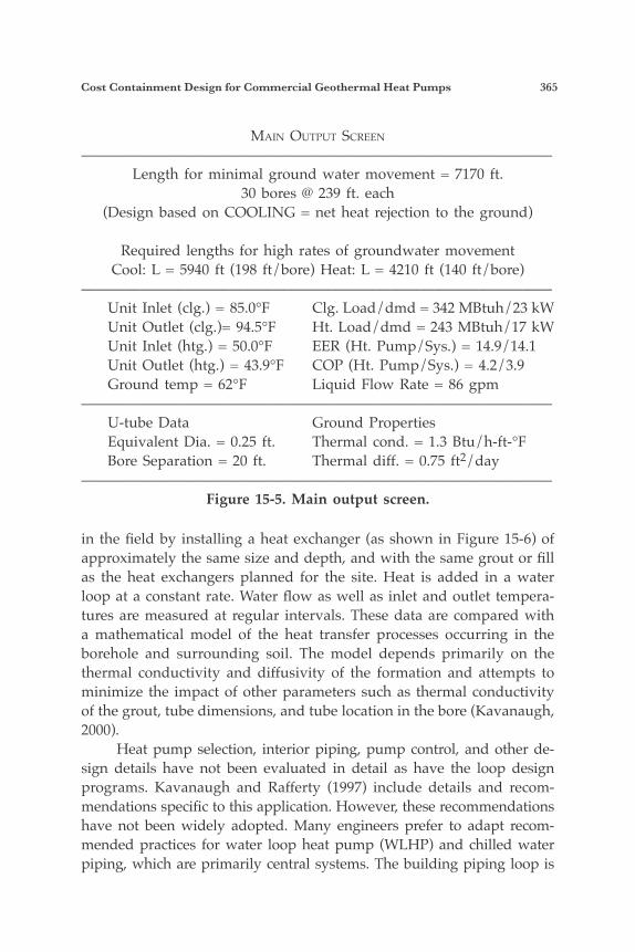
Cost Containment Design for Commercial Geothermal Heat Pumps 365
in the field by installing a heat exchanger (as shown in Figure 15-6) of approximately the same size and depth, and with the same grout or fill as the heat exchangers planned for the site. Heat is added in a water loop at a constant rate. Water flow as well as inlet and outlet tempera-tures are measured at regular intervals. These data are compared with a mathematical model of the heat transfer processes occurring in the borehole and surrounding soil. The model depends primarily on the thermal conductivity and diffusivity of the formation and attempts to minimize the impact of other parameters such as thermal conductivity of the grout, tube dimensions, and tube location in the bore (Kavanaugh, 2000). Heat pump selection, interior piping, pump control, and other de-sign details have not been evaluated in detail as have the loop design programs. Kavanaugh and Rafferty (1997) include details and recom-mendations specific to this application. However, these recommendations have not been widely adopted. Many engineers prefer to adapt recom-mended practices for water loop heat pump (WLHP) and chilled water piping, which are primarily central systems. The building piping loop is
main ouTpuT screen
————————————————————————————————Length for minimal ground water movement = 7170 ft.
30 bores @ 239 ft. each(Design based on COOLING = net heat rejection to the ground)
Required lengths for high rates of groundwater movementCool: L = 5940 ft (198 ft/bore) Heat: L = 4210 ft (140 ft/bore)
———————————————————————————————— Unit Inlet (clg.) = 85.0°F Clg. Load/dmd = 342 MBtuh/23 kW Unit Outlet (clg.)= 94.5°F Ht. Load/dmd = 243 MBtuh/17 kW Unit Inlet (htg.) = 50.0°F EER (Ht. Pump/Sys.) = 14.9/14.1 Unit Outlet (htg.) = 43.9°F COP (Ht. Pump/Sys.) = 4.2/3.9 Ground temp = 62°F Liquid Flow Rate = 86 gpm———————————————————————————————— U-tube Data Ground Properties Equivalent Dia. = 0.25 ft. Thermal cond. = 1.3 Btu/h-ft-°F Bore Separation = 20 ft. Thermal diff. = 0.75 ft2/day————————————————————————————————
Figure 15-5. Main output screen.
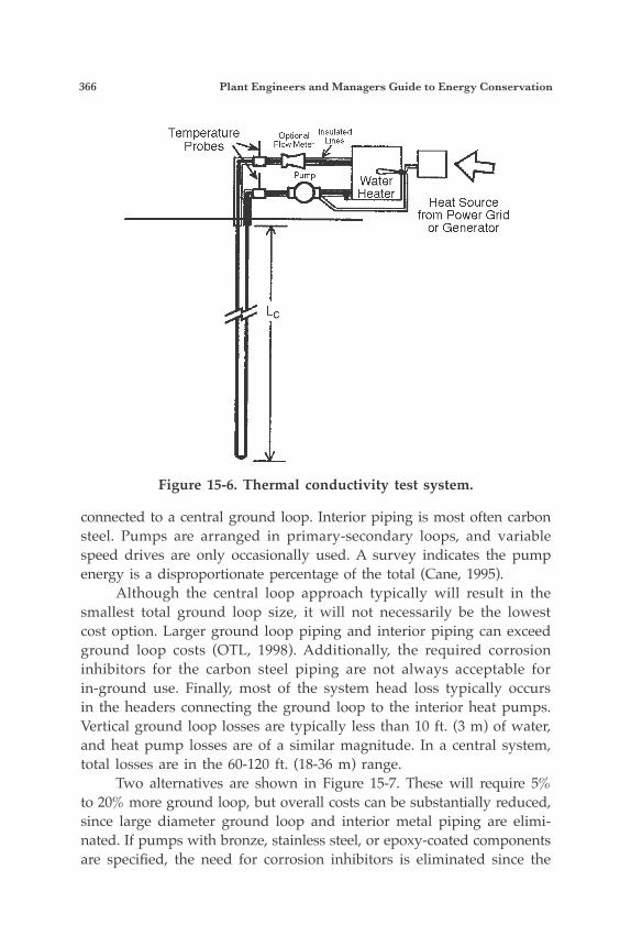
366 Plant Engineers and Managers Guide to Energy Conservation
connected to a central ground loop. Interior piping is most often carbon steel. Pumps are arranged in primary-secondary loops, and variable speed drives are only occasionally used. A survey indicates the pump energy is a disproportionate percentage of the total (Cane, 1995). Although the central loop approach typically will result in the smallest total ground loop size, it will not necessarily be the lowest cost option. Larger ground loop piping and interior piping can exceed ground loop costs (OTL, 1998). Additionally, the required corrosion inhibitors for the carbon steel piping are not always acceptable for in-ground use. Finally, most of the system head loss typically occurs in the headers connecting the ground loop to the interior heat pumps. Vertical ground loop losses are typically less than 10 ft. (3 m) of water, and heat pump losses are of a similar magnitude. In a central system, total losses are in the 60-120 ft. (18-36 m) range. Two alternatives are shown in Figure 15-7. These will require 5% to 20% more ground loop, but overall costs can be substantially reduced, since large diameter ground loop and interior metal piping are elimi-nated. If pumps with bronze, stainless steel, or epoxy-coated components are specified, the need for corrosion inhibitors is eliminated since the
Figure 15-6. Thermal conductivity test system.
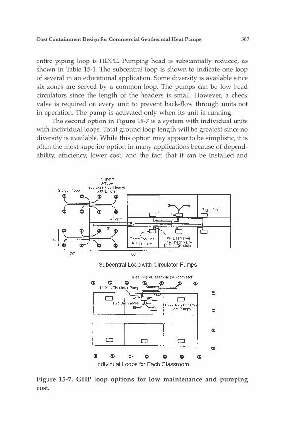
Cost Containment Design for Commercial Geothermal Heat Pumps 367
entire piping loop is HDPE. Pumping head is substantially reduced, as shown in Table 15-1. The subcentral loop is shown to indicate one loop of several in an educational application. Some diversity is available since six zones are served by a common loop. The pumps can be low head circulators since the length of the headers is small. However, a check valve is required on every unit to prevent back-flow through units not in operation. The pump is activated only when its unit is running. The second option in Figure 15-7 is a system with individual units with individual loops. Total ground loop length will be greatest since no diversity is available. While this option may appear to be simplistic, it is often the most superior option in many applications because of depend-ability, efficiency, lower cost, and the fact that it can be installed and
Figure 15-7. GHP loop options for low maintenance and pumping cost.
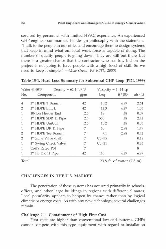
368 Plant Engineers and Managers Guide to Energy Conservation
serviced by personnel with limited HVAC experience. An experienced GHP engineer summarized his design philosophy with the statement,“I talk to the people in our office and encourage them to design systems that keep in mind what our local work force is capable of doing. The number of quality people is going down. They are still out there, but there is a greater chance that the contractor who has low bid on the project is not going to have people with a high level of skill. So we need to keep it simple.” —Mike Green, PE (OTL, 2000)
Table 15-1. Head Loss Summary for Subcentral GHP Loop (PDI, 1999)————————————————————————————————Water @ 60°F Density = 62.4 lb/ft3 Viscosity = 1. 14 cpNo. Component gpm Leq ft/100 ∆h (ft)————————————————————————————————4 2” HDPE T Branch 42 15.2 4.29 2.612 2” HDPE Butt L 42 12.3 4.29 1.061 10-Ton Header End 2.5 18 .48 0.091 1” HDPE SDR 11 Pipe 2.5 500 .48 2.421 1” HDPE UniCoil 2.5 10.2 .48 0.051 1” HDPE DR 11 Pipe 7 60 2.98 1.792 1” HDPE Tee Branch 7 7.1 2.98 0.422 1” Zone Valve (Ball) 7 Cv=35 0.181 1” Swing Check Valve 7 Cv=21 0.261 Coil’s Rated PSI 7 81 2” PE DR 11 Pipe 42 160 4.29 6.87————————————————————————————————Total 23.8 ft. of water (7.3 m)
CHALLENGES IN THE U.S. MARKET
The penetration of these systems has occurred primarily in schools, offices, and other large buildings in regions with different climates. Local popularity appears to happen by chance rather than by logical climatic or energy costs. As with any new technology, several challenges remain.
Challenge #1—Containment of High First Cost First costs are higher than conventional low-end systems. GHPs cannot compete with this type equipment with regard to installation
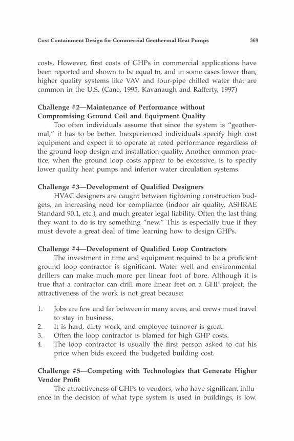
Cost Containment Design for Commercial Geothermal Heat Pumps 369
costs. However, first costs of GHPs in commercial applications have been reported and shown to be equal to, and in some cases lower than, higher quality systems like VAV and four-pipe chilled water that are common in the U.S. (Cane, 1995, Kavanaugh and Rafferty, 1997)
Challenge #2—Maintenance of Performance withoutCompromising Ground Coil and Equipment Quality Too often individuals assume that since the system is “geother-mal,” it has to be better. Inexperienced individuals specify high cost equipment and expect it to operate at rated performance regardless of the ground loop design and installation quality. Another common prac-tice, when the ground loop costs appear to be excessive, is to specify lower quality heat pumps and inferior water circulation systems.
Challenge #3—Development of Qualified Designers HVAC designers are caught between tightening construction bud-gets, an increasing need for compliance (indoor air quality, ASHRAE Standard 90.1, etc.), and much greater legal liability. Often the last thing they want to do is try something “new.” This is especially true if they must devote a great deal of time learning how to design GHPs.
Challenge #4—Development of Qualified Loop Contractors The investment in time and equipment required to be a proficient ground loop contractor is significant. Water well and environmental drillers can make much more per linear foot of bore. Although it is true that a contractor can drill more linear feet on a GHP project, the attractiveness of the work is not great because:
1. Jobs are few and far between in many areas, and crews must travel to stay in business.
2. It is hard, dirty work, and employee turnover is great.3. Often the loop contractor is blamed for high GHP costs.4. The loop contractor is usually the first person asked to cut his
price when bids exceed the budgeted building cost.
Challenge #5—Competing with Technologies that Generate Higher Vendor Profit The attractiveness of GHPs to vendors, who have significant influ-ence in the decision of what type system is used in buildings, is low.
370 Plant Engineers and Managers Guide to Energy Conservation
The increasing complexity of HVAC systems has caused engineers to rely heavily upon the resources of manufacturers to design systems. However, the simplicity of GHP systems makes the engineer more independent. Thus, the total profit per job for the equipment supplier has the potential of being much lower, and it may be viewed as being more profitable to sell conventional equipment.
ACKNOWLEDGMENTS
This chapter is part of the Strategic Outreach Program of the Geothermal Heat Pump Consortium in conjunction with the project sponsored by the Tennessee Valley Authority.
References 1. Geothermal Heat Pump Consortium, 1999, GeoExchange Site List (RP-01 1), Wash-
ington, DC. 2. Air Conditioning, Heating, & Refrigeration News, 2000, “How bad is the tech short-
age,” Business News Publishing, Troy, MI, Feb. 14. 3. Outside the Loop Newsletter, 1998. “Think system to get the most from GSHPs,”
University of Alabama. Tuscaloosa. Vol. 1, No. 2. 4. Kavanaugh, S.P. and K. Rafferty, 1997, Ground Source Heat Pumps: Design of Geo-
thermal Systems for Commercial and Institutional Buildings. ASHRAE, Atlanta. 5. Thornton, J.W., T.P. McDowell, and P.J. Hughes, 1997, “Comparison of Practical
Ground Heat Exchanger Sizing Methods to a Fort Polk Data/Model Benchmark,” ASHRAE Transactions, Atlanta, Vol. 103, Pt. 2.
6. Shonder, J.A., V. Baxter, J.W. Thornton, and P.J. Hughes, 1999, “A New Compari-son of Vertical Design Methods for Residential Applications.” ASHRAE Transac-tions, Atlanta, Vol. 105, Pt. 2.
7. Shonder, J.A., V. Baxter, P.J. Hughes, and J.W. Thornton, 2000. “A Comparison of Vertical Ground Heat Exchanger Design Software for Commercial Applications.” ASHRAE Transactions, Atlanta, Vol. 106, Pt. 1.
8. Energy Information Services, 1997, GchpCalc, V. 3.1, Tuscaloosa, AL. 9. Kavanaugh, S.P., 2000, “Field Test for Ground Thermal Properties—Methods and
Impact on GSHP Designs.” ASHRAE Transactions, Atlanta, Vol. 106, Pt. 1. 10. Cane, R.L.D, 1995, Operating Experiences with Commercial Ground-Source Heat
Pumps, 863RP (Research Project Report), ASHRAE, Atlanta, 1995. 11. Outside the Loop Newsletter, 1998, “Monticello, Iowa, High School-First Cost,”
University of Alabama, Tuscaloosa. Vol. 1, No. 2. 12. Outside the Loop Newsletter, 2000. “The KIS Philosophy of Austin’s Mike Green,
P.E.,” University of Alabama, Tuscaloosa, Vol. 2, No. 4. 13. PDI. 1999. “GHP pipe and fitting calculator,” Phillips Driscopipe Inc., Richardson,
TX.

371
16Economic Evaluations forPower Quality Solutions
SUMMARY
Power quality issues are continuing to become a greater concern, particularly to sensitive customers with critical operations. Measures can be taken to improve the power quality of a given circuit; however, the economic feasibility of the applications should be considered. As a result, the system compatibility must be examined to determine the behavior of a customer’s equipment within the electrical environment. A power quality investigation and an economic analysis can then deter-mine what mitigation tactics are most effective and whether they should be applied. With the increased interest and awareness in power quality, there is a vast increase in the number of mitigation devices now available. Many of these devices are expensive; therefore, making a decision to ap-ply mitigating devices is not an easy one. A system and process study must be done to ascertain the level of susceptibility a plant’s equipment has. Once the operation has been characterized, the most appropriate mitigation device(s) can be determined. A cost analysis must then be done to determine the cost of interruptions associated with power quality problems, as well as the number of interruptions that will be prevented. These savings are compared to the cost of the mitigation device. The intent of this chapter is to illustrate a variety of techniques used to evaluate power conditioning devices. An analysis of the cost due to power quality interruptions is presented. The effectiveness of the mitiga-tion device is examined in determining an appropriate cost. Mitigation strategies to alleviate the most problems at the lowest cost are discussed. Several techniques are presented for computing payoff time.
Presented at the 20th World Energy Engineering Congress by Stephen Mid-dlekauff
372 Plant Engineers and Managers Guide to Energy Conservation
INTRODUCTION
Power quality is a greater concern now than it has been in the past. More industrial customers are contacting their utilities about process interruptions and plant downtime. It would appear that the quality of the utility electrical service has deteriorated; however, this may not be the case. In fact, with clever protection schemes and more aggressive preventive measures, the quality of the electrical service is probably better than ever. The dawn of the power electronic era has created a higher level of sensitivity to power fluctuations. Modern industrial equipment such as motor drives, programmable logic controllers (PLCs), and other automation products are all much more susceptible to power disturbances than ever before. The result of this greater sensitivity is a greater awareness of power quality. The market is now flooded with power conditioning devices, with a very wide range of sizes, applications, and capabilities. All of them; however,, have one thing in common: they claim to prevent power disturbances from reaching your equipment. Some are very inexpensive, but may not do an adequate job in protection of sensitive equipment. Other solutions may carry a hefty price tag but may not be worth the expense. Many parameters must be considered in evaluating the cost savings of a power conditioning device.
THE PRINCIPLE INVESTIGATION
Voltage sags, surges, momentary interruptions, and other power anomalies may all look the same to an industrial customer. His process has been interrupted. A one-cycle voltage sag may have the same effect as a one-minute outage. In determining the specifications for power conditioning equipment, the nature of the disturbances must first be determined. The most accurate way for determining the behavior of the electrical environment is to monitor the power using a high speed, power quality monitor. If the disturbance is not steady-state, an extended monitoring period may be necessary to capture the culprit. If the disturbance is seasonal in nature, such as lightning from frequent summer storms, monitoring may need to be done over an entire season to best char-acterize the types of activity seen on the system. Typically, if there are
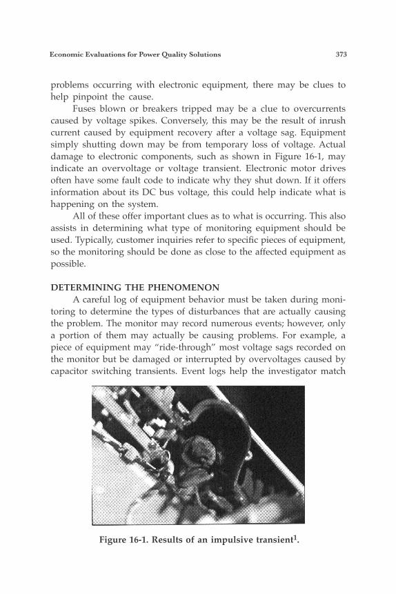
Economic Evaluations for Power Quality Solutions 373
problems occurring with electronic equipment, there may be clues to help pinpoint the cause. Fuses blown or breakers tripped may be a clue to overcurrents caused by voltage spikes. Conversely, this may be the result of inrush current caused by equipment recovery after a voltage sag. Equipment simply shutting down may be from temporary loss of voltage. Actual damage to electronic components, such as shown in Figure 16-1, may indicate an overvoltage or voltage transient. Electronic motor drives often have some fault code to indicate why they shut down. If it offers information about its DC bus voltage, this could help indicate what is happening on the system. All of these offer important clues as to what is occurring. This also assists in determining what type of monitoring equipment should be used. Typically, customer inquiries refer to specific pieces of equipment, so the monitoring should be done as close to the affected equipment as possible.
DETERMINING THE PHENOMENON A careful log of equipment behavior must be taken during moni-toring to determine the types of disturbances that are actually causing the problem. The monitor may record numerous events; however, only a portion of them may actually be causing problems. For example, a piece of equipment may “ride-through” most voltage sags recorded on the monitor but be damaged or interrupted by overvoltages caused by capacitor switching transients. Event logs help the investigator match
Figure 16-1. Results of an impulsive transient1.
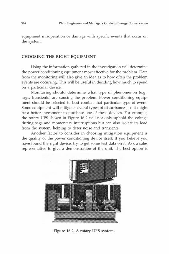
374 Plant Engineers and Managers Guide to Energy Conservation
equipment misoperation or damage with specific events that occur on the system.
CHOOSING THE RIGHT EQUIPMENT
Using the information gathered in the investigation will determine the power conditioning equipment most effective for the problem. Data from the monitoring will also give an idea as to how often the problem events are occurring. This will be useful in deciding how much to spend on a particular device. Monitoring should determine what type of phenomenon (e.g., sags, transients) are causing the problem. Power conditioning equip-ment should be selected to best combat that particular type of event. Some equipment will mitigate several types of disturbances, so it might be a better investment to purchase one of these devices. For example, the rotary UPS shown in Figure 16-2 will not only uphold the voltage during sags and momentary interruptions but can also isolate its load from the system, helping to deter noise and transients. Another factor to consider in choosing mitigation equipment is the quality of the power conditioning device itself. If you believe you have found the right device, try to get some test data on it. Ask a sales representative to give a demonstration of the unit. The best option is
Figure 16-2. A rotary UPS system.
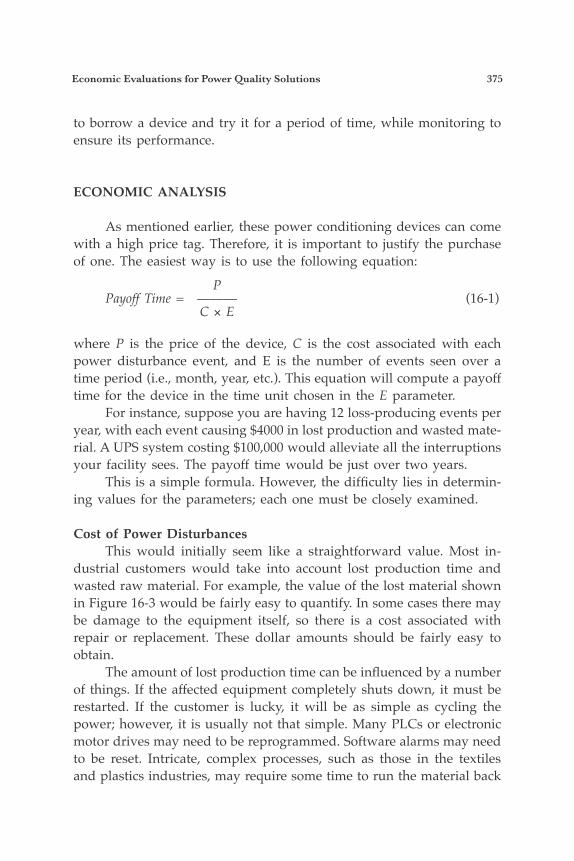
Economic Evaluations for Power Quality Solutions 375
to borrow a device and try it for a period of time, while monitoring to ensure its performance.
ECONOMIC ANALYSIS
As mentioned earlier, these power conditioning devices can come with a high price tag. Therefore, it is important to justify the purchase of one. The easiest way is to use the following equation:
P Payoff Time = ——— (16-1) C × E
where P is the price of the device, C is the cost associated with each power disturbance event, and E is the number of events seen over a time period (i.e., month, year, etc.). This equation will compute a payoff time for the device in the time unit chosen in the E parameter. For instance, suppose you are having 12 loss-producing events per year, with each event causing $4000 in lost production and wasted mate-rial. A UPS system costing $100,000 would alleviate all the interruptions your facility sees. The payoff time would be just over two years. This is a simple formula. However, the difficulty lies in determin-ing values for the parameters; each one must be closely examined.
Cost of Power Disturbances This would initially seem like a straightforward value. Most in-dustrial customers would take into account lost production time and wasted raw material. For example, the value of the lost material shown in Figure 16-3 would be fairly easy to quantify. In some cases there may be damage to the equipment itself, so there is a cost associated with repair or replacement. These dollar amounts should be fairly easy to obtain. The amount of lost production time can be influenced by a number of things. If the affected equipment completely shuts down, it must be restarted. If the customer is lucky, it will be as simple as cycling the power; however, it is usually not that simple. Many PLCs or electronic motor drives may need to be reprogrammed. Software alarms may need to be reset. Intricate, complex processes, such as those in the textiles and plastics industries, may require some time to run the material back
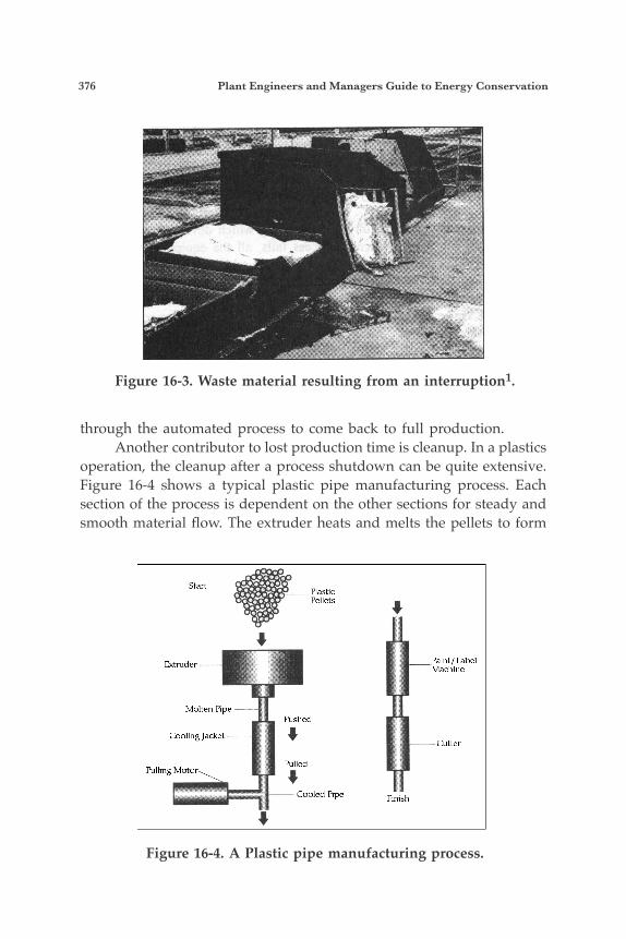
376 Plant Engineers and Managers Guide to Energy Conservation
through the automated process to come back to full production. Another contributor to lost production time is cleanup. In a plastics operation, the cleanup after a process shutdown can be quite extensive. Figure 16-4 shows a typical plastic pipe manufacturing process. Each section of the process is dependent on the other sections for steady and smooth material flow. The extruder heats and melts the pellets to form
Figure 16-3. Waste material resulting from an interruption1.
Figure 16-4. A Plastic pipe manufacturing process.
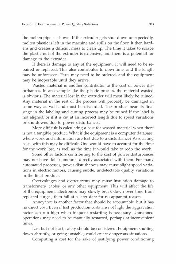
Economic Evaluations for Power Quality Solutions 377
the molten pipe as shown. If the extruder gets shut down unexpectedly, molten plastic is left in the machine and spills on the floor. It then hard-ens and creates a difficult mess to clean up. The time it takes to scrape the plastic out of the extruder is extensive, and there is a potential for damage to the extruder. If there is damage to any of the equipment, it will need to be re-paired or replaced. This also contributes to downtime, and the length may be unforeseen. Parts may need to be ordered, and the equipment may be inoperable until they arrive. Wasted material is another contributor to the cost of power dis-turbances. In an example like the plastic process, the material wasted is obvious. The material lost in the extruder will most likely be ruined. Any material in the rest of the process will probably be damaged in some way as well and must be discarded. The product near its final stage in the labeling and cutting process may be ruined if the label is not aligned, or if it is cut at an incorrect length due to speed variations or shutdowns due to power disturbances. More difficult is calculating a cost for wasted material when there is not a tangible product. What if the equipment is a computer database, where work and information are lost due to a disturbance? Associating costs with this may be difficult. One would have to account for the time for the work lost, as well as the time it would take to redo the work. Some other factors contributing to the cost of power disturbances may not have dollar amounts directly associated with them. For many automated processes, power disturbances may cause slight speed varia-tions in electric motors, causing subtle, undetectable quality variations in the final product. Overvoltages and overcurrents may cause insulation damage to transformers, cables, or any other equipment. This will affect the life of the equipment. Electronics may slowly break down over time from repeated surges, then fail at a later date for no apparent reason. Annoyance is another factor that should be accountable, but it has no direct cost. Even if lost production costs are not high, the aggravation factor can run high when frequent restarting is necessary. Unmanned operations may need to be manually restarted, perhaps at inconvenient times. Last but not least, safety should be considered. Equipment shutting down abruptly, or going unstable, could create dangerous situations. Computing a cost for the sake of justifying power conditioning

378 Plant Engineers and Managers Guide to Energy Conservation
equipment can be difficult; however, for most large processes it can be obvious. Some manufacturers have quoted losses of up to $1 million per disturbance. Even for large, complex mitigation devices, the equipment could pay for itself after just one disturbance.
Frequency of Events This number may also be difficult to ascertain. The difficulty lies in obtaining an accurate number within a short period of time, which is important because a solution is needed quickly. If the problem dis-turbance is occurring regularly, an estimate will be easier to determine. However, many disturbances are seasonal, happening more frequently during certain times of the year. For example, capacitor switching transients may occur more dur-ing the summer, as voltage support is needed more because of the added load from chillers and air conditioning systems. This can make the de-cision for power conditioning equipment difficult. A user may realize problems are occurring in August and spend a good deal of money on some mitigating equipment. There may then not be any more problems until the following May, and the user finds the device is not suitable for the application. In addition, the data may even change from year to year. Statisti-cians will tell you that the larger your data sample, the more accurate your study will be. Unfortunately, end users do not have time to moni-tor for several years; the problem needs to be fixed today.
The Price for Protection The simple equation given previously can be solved in several ways. Once the system has been characterized and costs per event have been estimated, the user can calculate how much to spend, given a desired payoff time. Alternatively, it could be calculated how long it will take for several options to pay for themselves. A mitigation strategy will help determine the expenditure for the device. There are many available “cure-all” devices designed for installation at the plant electrical service entrance. These devices claim to combat a variety of disturbances and can cost in the thousands of dollars per kVA. Thus, for a typical plant load, these solutions can cost in the millions of dollars. For many industrial processes, it is only several components that are causing a production interruption. In a long, automated process

Economic Evaluations for Power Quality Solutions 379
line, each stage of the process is dependent on the other to function properly. Often there will be one master electronic controller for the entire line. If it detects that one component has failed or shut down, it will shut the entire process down. Therefore, it could be more cost effective to identify the weak points within a process line, then apply mitigation devices to them. There is some difficulty in identifying which devices are most sensitive. When a process fails, all the equipment may shut down, and it’s impossible to tell which equipment failed first. Monitoring at different points throughout the process can help identify the sus-ceptible devices during system events. Another option is to simulate power disturbances on the systems for quicker collection of sensitive data. Some utilities have devices which can generate disturbances onto the line for controlled testing of equipment to see which devices fail first. For large facilities with many sensitive devices, such as electronic motor drives, it may not be cost effective to mitigate every single device. In this case a power conditioning device that protects the entire facility may be more cost effective. A strategy must be chosen to accurately estimate the cost of the mitigation equipment.
GRAPHICAL ANALYSIS
A method to further analyze Equation 16-1 is by graphically plot-ting several curves. After the monitoring phase has gathered some data, a characterization curve can be plotted. This curve, shown in Figure 16-5, illustrates the numbers and types of events the plant equipment is see-ing over a time period. It summarizes the expected number of events for a given magnitude and duration. An example point is shown on the graph in Figure 16-5, indicating a sag of approximately 2.5 cycles and 0.57 p.u. magnitude. From the curve, the user could predict 10-15 events per year of similar magnitude and duration. The activity log is an important step for the next curve. Correlating equipment shutdown or failure with the disturbances monitored can illustrate more clearly the susceptibility of the equipment. The example susceptibility curve shown in Figure 16-6 illustrates what combinations of magnitude and durations will cause equipment to fail. This will
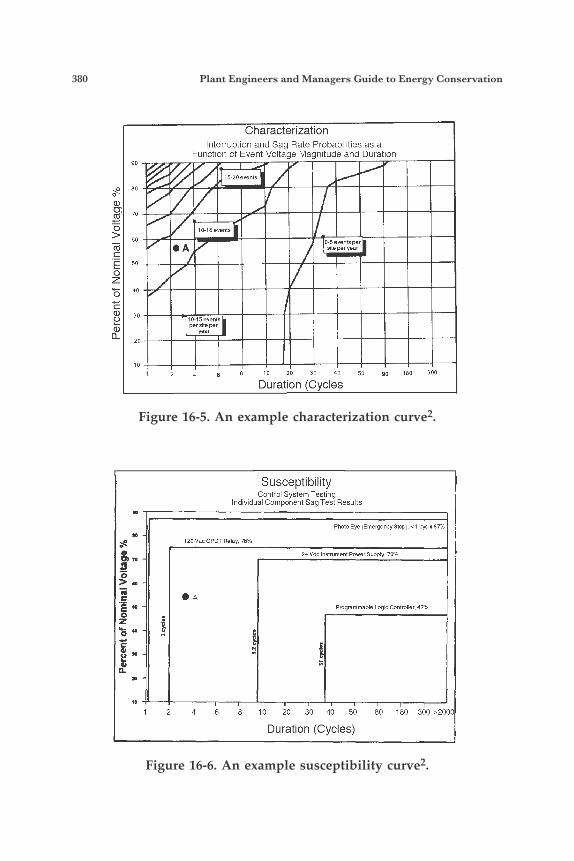
380 Plant Engineers and Managers Guide to Energy Conservation
Figure 16-5. An example characterization curve2.
Figure 16-6. An example susceptibility curve2.
Characterization Interruption and Sag Rate Probabilities as a
Function of Event Voltage Magnitude and Duration
15-20evenlr
10-15evenlr
A
10 4 6 8 10 20 30 40 50 90 180 300
Duration (Cycles
Susceptibility Control System Testing
Individual Component Sag Test Results
Photo Eye (Emergency slop) < 1 cyc x 87'Y
120 VIC OPDT Relay 75'Y
24 Vdc ln l l rumenl Power Supply 70'Y
Programmable Loglc Conlmller 47'Y
10
1 2 4 6 8 10 20 30 40 50 80 180 300 ,2000
D u ration (Cycles)
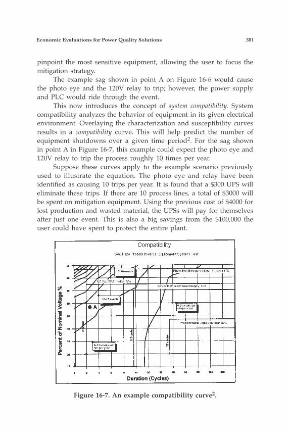
Economic Evaluations for Power Quality Solutions 381
pinpoint the most sensitive equipment, allowing the user to focus the mitigation strategy. The example sag shown in point A on Figure 16-6 would cause the photo eye and the 120V relay to trip; however, the power supply and PLC would ride through the event. This now introduces the concept of system compatibility. System compatibility analyzes the behavior of equipment in its given electrical environment. Overlaying the characterization and susceptibility curves results in a compatibility curve. This will help predict the number of equipment shutdowns over a given time period2. For the sag shown in point A in Figure 16-7, this example could expect the photo eye and 120V relay to trip the process roughly 10 times per year. Suppose these curves apply to the example scenario previously used to illustrate the equation. The photo eye and relay have been identified as causing 10 trips per year. It is found that a $300 UPS will eliminate these trips. If there are 10 process lines, a total of $3000 will be spent on mitigation equipment. Using the previous cost of $4000 for lost production and wasted material, the UPSs will pay for themselves after just one event. This is also a big savings from the $100,000 the user could have spent to protect the entire plant.
Figure 16-7. An example compatibility curve2.
382 Plant Engineers and Managers Guide to Energy Conservation
This will help in the mitigation process, giving the user a better idea for how many process interruptions he may see over a time period. Associating this with the cost information will help determine the user’s payoff time for a chosen power conditioning device.
A MORE DIRECT APPROACH
Taking the system compatibility approach one step further will paint an even more accurate picture of the effectiveness of a power conditioning device. Given the characterization and susceptibility data, the user can weight different categories of disturbances on the basis of whether or not they will cause an interruption. Table 16-1 is an example table of weighting for voltage sags.
Table 16-1. An example table for differentmagnitude voltage sags3
———————————————————————————————— Category of Event Weighting Value————————————————————————————————
Interruption 1.0
Sag below 50% 0.8
Sag between 50% and 70% 0.4
Sag between 70% and 90% 0.1————————————————————————————————
Using this weighting technique in conjunction with the charac-terization data can give a prediction of process interruptions per year. Table 16-2 is a sample table for the characterization data, taking into account the weights assigned to each category. Multiplying the events per year within each category times its weight will result in the number of probable loss-producing events. For the example shown, the prediction will be 5.4 loss-producing events per year. Given a specific power conditioning device, the user can make a quick estimate for the saved shutdowns per year. For example, suppose the user chooses a device that will mitigate all sags where the nominal voltage stays above 50%. Then he can generate new data for the ex-
Economic Evaluations for Power Quality Solutions 383
pected events per year and multiply each category by the weights. For this example, he will now expect zero events for sags 50% or above, so his total loss-producing events will now be 1.7 per year. The user will achieve much greater accuracy if the categories are broken down even further. Sags could be broken down on the basis of number of phases affected, or whether they occurred on the same or an alternate feeder. The above analysis could be done for a number of power con-ditioning devices. A comparison could then be made of the resulting number of loss-producing events versus the price of each device. From this analysis a decision could be made on which device would be most cost effective3.
CONCLUSION
As power quality becomes a greater concern for industrial custom-ers, solution providers are actively flooding the market with mitigation devices. Justifying the purchase of these devices is difficult, as many come with a high price tag. An even bigger obstacle is determining just what you are getting for your money. Careful investigation and analy-sis techniques can simplify the search for the right power conditioning device. It is important to determine exactly what type of disturbance is causing problems for the end-user’s process. Furthermore, the user should attempt to determine the effects of different severities of specific types of events. Using engineering judgment, weights or probabilities
Table 16-2. A Table of characterization data3
———————————————————————————————— Category Weighting Events Near————————————————————————————————
Interruption 1.0 0.5
Sag (<50%) 0.8 1.5
Sag (50-70%) 0.4 4.0
Sag (70-90%) 0.1 21.0————————————————————————————————

384 Plant Engineers and Managers Guide to Energy Conservation
can be given to the various categories of disturbances seen at the cus-tomer’s facility. This can be used to calculate a more accurate prediction of loss-producing events seen over a time period. Using gathered information, analyzed numerically or graphically, can help determine the best mitigation device for the application. It is usually more cost effective to mitigate individual susceptible equipment. However, in the case of large facilities with a large number of sensitive devices, it may be more beneficial to protect the entire facility.
References1. Jeff G. Dougherty and Wayne L. Stebbins, Power Quality: A Utility and Industry Per-
spective. IEEE IAS Textile Fiber and Film Technical Conference, Greenville, SC, May 1997.
2. IEEE P1346, Recommended Practice for Evaluating Electric Power System Compatibility with Electronic Process Equipment.
3. Robert J. Gilleskie, Utility Expertise in Providing Power Quality and Other Engineering Services. EPRI PQA ’97, Stockholm, Sweden, June 1997.

17PurchasingStrategies for Electricity
SUMMARY
A new age is dawning for lower-cost energy use and supply. The deregulation of the electric industry is creating new pricing structures that will change how we calculate the payback of alternatives for cutting the cost of energy in our facilities. Energy users can help themselves navigate these choices. By un-derstanding the concepts inherent in deregulation, learning to use new energy tools, influencing the deregulation process, applying new tech-nologies, and (most important of all) by being as creative as possible, smart users will grasp new options for energy cost reductions.
AT&T VS. MCI: A PARADIGM
To better understand how electric utilities will be transformed, think about how long-distance phone service has changed. When AT&T was forced by a federal judge to divest itself of many of its divisions, long-distance was separated from local service, and new providers such as MCI and Sprint became household names. While after 12 years, deregulation of that industry is not yet complete (local service is still generally a monopoly), during that time long-distance use has nearly quadrupled, while the average price of a long-distance call fell by more than 50%. To satisfy consumer demand for communication services, a vast new array of technologies was also born. How many of us antici-pated the proliferation of fax machines, cellular phones, pagers, and on-line services that would result from a single court order? While we can also expect the cost of power to fall, the future of electricity similarly holds much more than price reductions.
Presented at the 20th World Energy Engineering Congress by Lindsay Audin
385
386 Plant Engineers and Managers Guide to Energy Conservation
FACTORS IMPACTING POWER PRICES
Electricity is generated by utilities and independent power pro-ducers (IPPs), both regulated to some degree by state public utility commissions (PUCs) and then transmitted through high-tension lines criss-crossing North America in a giant network. These lines are owned by utilities and regulated by the Federal Energy Regulatory Commission (FERC). Once voltage is stepped down at substations, power is distributed through local utility-owned lines and meters regulated by PUCs. With the exception of municipal utilities (which are controlled by local governments), PUCs determine how to distribute these costs to end user classes. Most of our bills break out only charges for elec-tric consumption and demand (and perhaps a fuel adjustment), but the true cost of power includes many other components, including transmission, distribution, and a variety of ancillary services (such as voltage support, spinning reserve, and load following). Bills may also include taxes, social programs, and other charges that are not appar-ent to end users. To develop the prices we pay, the PUCs apply a standard based on the utility’s costs for providing a service, plus a guaranteed rate-of-return to ensure a ready supply of investment capital. All of these costs and profits are “bundled” together to create tariff pricing. While theory dictates that charges should be based on the true cost of service, politics and other pressures often result in cross subsidies in which one rate class (e.g., industrial) is charged more to contain prices charged to another (e.g., residential). While the electric rates we pay are controlled by PUC tariffs, utilities and IPPs buy and sell electricity among themselves, and such wholesale prices vary with time, climate, power plant outages, fuel prices, and other factors. The base cost of power seen by a utility is therefore a mix of its own generating costs and the price it pays for elec-tricity delivered to it through the transmission system from other power providers. This base cost is subject to commodity market conditions usually not visible to end users. It is increasingly being influenced by factors such as commodity trading techniques (e.g., futures and financ-ing plans), ways to adjust user load profiles (such as real-time pricing), and transmission system constraints (which can drive prices up to the highest local generating cost).
Purchasing Strategies for Electricity 387
THREE GENERAL RELATIONSHIPS
There are three general relationships that clarify how new tech-niques interact and can be applied to control energy pricing. They are:
• time,load,price• generation, transmission, natural gas options• load shaping, financing methods, user technologies.
Time, Load, and Price As deregulated retail power prices begin to vary like those at the wholesale level, they will become more time-sensitive. Because one’s de-mand for power generally changes during the day and the week (and by season) we can expect the average price to also change with time and use (unless controlled by other factors, discussed below). As a result, load profile shapes (i.e., a graph of power versus time) will influence pricing, with flat profiles generally having the lowest average cost. Utilities gen-erally typify such patterns via load factor, defined as average demand divided by peak demand. A high load factor would indicate a flattened profile, while low load factors would occur where a peak demand is relatively brief and is surrounded by much lower demand during the rest of the day. While most non-industrial building power demand varies with time, it usually does so in predictable patterns. Knowing the shape of your typical load profile can often reveal ways to cut the present and future cost (and price) of power, while also helping your power supplier offer the best and most secure pricing. Like Sprint’s “dime-a-minute” long distance rate, marketers will likely offer highly simplified rates that smooth out such time-based price variations, but subscribing to such options will not yield the low-est average power costs. Rates that vary widely over time may provide the lowest average price, and techniques that cut, level, or shift peak demand will help reduce those prices.
Transmission, Generation, and Natural Gas Options In some cities and states, peak loads exceed transmission capac-ity many hours each year. When low-cost power can’t be brought in, prices could be bid up to the highest local generating costs. A good example of such constraints appeared during the early hot spell of June 1997 in the PJM (Pennsylvania-New Jersey-Maryland) power pool.
388 Plant Engineers and Managers Guide to Energy Conservation
While daily bulk wholesale generation prices (which make up 40% to 65% of most bills) generally don’t vary from one end of the pool to another by more than $.01/kWh, June saw variations exceeding $.13/kWh when transmission constraints blocked cheap power from reaching high-cost areas.1 In some urban areas with older power systems (such as New York and San Diego), transmission constraints could yield similar results. Such areas with constraints are sometimes called “load pockets” during the period of constraint, which may exceed 1000 hours a year. In the United Kingdom, which uses a national power pool supplied by deregu-lated generators, power suppliers have also found ways to “game” the system to purposely congest transmission, thereby driving up the price of their product.2 To address such possibilities, energy marketers have begun exam-ining and/or promoting new local generation (or cogeneration) facili-ties, either at customer-owned sites or through repowering of obsolete utility plants inside the load pockets. Natural gas generators with very low emission levels have become quite cost-competitive for both peak shaving and as base load power, opening the door to competition during transmission constraints. Similarly, a variety of technologies (discussed later in this chapter) exist to reinforce existing transmission systems. A recent study3 found that a small investment toward improving transmis-sion capacity in California could have a major impact on limiting power prices. One way to shift peak demand is to substitute natural gas for electricity during peak pricing periods. As will be discussed below, a variety of technologies exists for using gas to directly provide horse-power, cooling, air compression, and other power-intensive needs. Such convertibility will create truly interruptible energy rates, allowing clever end users to contract for both interruptible gas and power, attaining the lowest possible energy prices. Under these circumstances, transmission, generation, and natural gas options will compete with each other, driv-ing all prices down over time.
Load Shaping, Financing, and User Technologies A variety of choices is emerging to configure loads in advantageous ways. While most have existed in one form or another, deregulation will allow marketers to help end users gather—and segregate—their loads more readily through metering and contractual means.
Purchasing Strategies for Electricity 389
Coincident metering has been used to cut the average cost for power at facilities with many meters on differed accounts held by one custom-er. At Columbia University in New York, for example, several dozen ac-counts existed on one property, the result of gradual expansion without attention to energy costs. Each account peaked at a different time, but (due to tariff construction) the sum of the bills was the same as though all buildings had peaked at the same time. By combining the accounts under one master demand meter, the average cost of power was cut by over 10%. Such combination will become easier under deregulation as usage (for the power commodity, as versus transmission and distribu-tion) can be contracted under one account.
Load isolation, while not favored by utilities, can allow an end user to segregate loads that would be cheaper under utility tariff-based power than under market-based power, thereby reducing the average cost for all loads.
Demand cooperatives allow end users to work together (typically through an organizing vendor) to obtain lower utility rates by pooling their interruptible loads and agreeing to curtail them when requested by the utility. Creating such a cooperative eases the difficulty of ensuring that any one load must be interrupted by allowing the demand to apply to a group of loads, only a few of which would be interrupted at any one time.
District-wide systems serve multiple customers with, for example, chilled water from a central facility that, in effect, transfers many individual electric chiller loads (which lower load factor) to a high load factor central facility that uses both electric and gas-driven units to minimize total cooling costs. Existing chillers may remain but are bypassed by a connection to a common chilled water loop serving numerous facilities.
Bill Consolidation allows many accounts held by one customer to be gathered for both coincident metering and attainment of cheaper energy block load rates, previously beyond any one account.
Aggregation involves the gathering of different customer accounts through a third party for purposes of bulk power purchasing, coin-
390 Plant Engineers and Managers Guide to Energy Conservation
cident metering, bill consolidation, transmission capacity reservation, and expert load analysis. Aggregators work along the same lines as MCI, buying co-ops, credit card handlers, and other organizations that compete for the privilege of bringing many end users together. All try to provide lower prices through bulk purchasing and han-dling. Present-day utility customers are, in effect, already “aggregat-ed” into rate classes, but only to the point of developing a rate based on an assumed typical load profile. Each of these options allows for re-shaping of loads (as portrayed to utilities and regulators) without major alterations to end user facilities.
In similar ways, financial tools exist that can cut or level costs more easily than with engineering. Both marketers and financial firms will (or already do) provide access to futures, options, and payment plans that ensure prices do not exceed a predetermined level. While a full discus-sion of financial instruments is beyond the scope of this chapter, end users need to understand the following basic concepts:
• Electric futures (which are available on the West Coast, and soon in the East) are traceable contracts for monthly blocks of firm power, purchased in advance of need, that will later be provided during normal business hours at a predetermined price. They are, in ef-fect, negotiable promises for supply of power, though there is not necessarily a guarantee of delivery unless accompanied by a secure transmission arrangement.
• Options (typically in the form of “calls” and “puts”) are contracts between suppliers and marketers (and thus end users) that allow a user of power to know that he can “call” for power and be ensured supply, or that a seller of power can be ensured a buyer when he “puts” out an offer to sell, both at predetermined prices.
• Payment plans have been offered to low-income customers by utilities for years. Now, however, marketers are ensuring level (or predetermined) monthly bills (not just pricing) through risk man-agement techniques that involve financial and load analysis tools. While some monthly bills may be higher than in prior years, other months will be lower, and the annual total will be confined to a narrow range. Such plans are often complicated, requiring careful analysis.

Purchasing Strategies for Electricity 391
• Tolling allows an end user (or his designee) to provide a genera-tor with boiler fuel (typically natural gas) in trade for electricity at negotiated, non-tariff, rates. This process is common among power marketers also trading natural gas; it is used at times that utilities have excess generating capacity that can provide power into an-other utility’s territory.
While all of these options provide end users with choices for con-trolling energy pricing, the impact of many of them can be maximized when used in cooperation with new technologies. Just as we have seen an explosion of choice in communications, it is likely that the future will see a variety of ways to create, store, and manage power. Many are already being offered or are in the prototype stages of development. Following are several which are being supplied or considered by both energy marketers and equipment vendors.
Metering. Marketers are using more sophisticated power metering (e.g., ENet, MC3) as a sales tool to ensure that their clients’ power costs are minimized through a variety of methods. The new standard in meter-ing involves wireless communications, non-invasive wiring, and hourly, quarter-hourly, or real-time monitoring. Human meter readers, obsolete for many years, will likely disappear as more cost effective systems are in-stalled. Such systems will allow better load control, more accurate power nominations, better pricing, and a reduction in theft and tampering (a major problem at the residential and small commercial levels).
Software. Computerized building simulations and load analyses have taken on new prominence as tools for predicting and flattening load profiles. Analyzing short intervals (1/4 hour) has become essential to maximize savings through tighter load control. Names and acronyms such as PEDA, RBOSS, and PowerManager will be heard quite often as marketers offer new services to cut electric bills and power pricing.
Energy Management Systems (EMS). As responding to real-time or market-based pricing signals becomes a common way to attain savings, an EMS takes on new importance for controlling variable loads, such as fans, pumps, DHW heaters, and chillers. When tied into the metering and software tools mentioned above, the load managing power of an EMS can be greatly enhanced.

392 Plant Engineers and Managers Guide to Energy Conservation
Power Storage Devices. While many power practitioners and regu-lators continue to assume that power cannot be cost effectively stored, flywheel power storage units are now in use as uninterruptible power systems (UPS) to supply “clean” power, and small (2 kWh) units act as backup power for cable TV systems. Larger units (over 12 kWh) are being prototyped as peak shifters/shavers for buildings. Chemical battery tech-nology has advanced considerably and may play a part as well. Depend-ing on how stranded costs are collected, a storage system that gets “filled” with cheap off-peak power at night (when there are no transmission con-straints) and “empties” to flatten peak loads during the day could be an instant moneymaker for a smart marketer and/or end user.
Distributed Generation. The ability to generate power in a pinch has always been useful. New small (<100 kilowatt) modular gas-fired turbine generators5 can also cut billing for peak demand by operating in parallel with utility power or (to avoid backup charges) by feeding dedicated loads, while acting as backup power when needed by the utility’s transmission and distribution system, thereby increasing overall system reliability. Using ceramics and limiting movement to a single part, the Capstone Turbine is an intriguing option, while the ONSI 200 kW fuel cell (and its soon-to-be seen competitors) has already racked up an impressive operating record. Once prices on these devices come down, watch marketers and end users grab them up as a way to mini-mize stranded cost payments.
Transmission and Distribution (T&D) Networks. Because power is cheaper only when transmission is available to move it, pressure for new or more robust transmission will increase once large price dif-ferentials occur between adjacent areas. Thyristor-based switching of high-voltage loads on T&D systems can raise the effective capacity of existing transmission lines. Such options are among a family of flexible AC transmission system (FACTS) improvements under development or deployment. Even new types of underground high-voltage cables,6 de-signed for use in transmission-constrained urban areas, are being rolled out to meet the expected demand for beefed-up transmission.
Gas-Powered Motor Drives. Natural gas-driven devices, such as gas engine-powered air compressors and chillers, have replaced electric motor-driven units in industrial and commercial facilities, cutting their peak demand.

Purchasing Strategies for Electricity 393
Advanced HVAC Systems. Chemical desiccants dehumidify outside air using natural gas, thereby cutting peak electric chiller loads. This process is already common in new buildings with large outside air loads (e.g., hospitals) and industrial processes (such as air compression). For smaller facilities configured around rooftop units, Entergy has been of-fering a super-high-efficiency replacement unit that takes advantage of several refrigeration engineering innovations.7 Many other options are either in the queue or already being sold. Try to imagine what the “fax machine” or “cell phone” of the power industry will look like. As we have seen in other industries, the com-bination of several new technologies often results in devices few of us could have imagined only a few years ago.
WHO OFFERS THESE OPTIONS?
Accompanying the profusion of technical choices will be a more bewildering expansion of vendor choices. Even as the merger and ac-quisition mania gripping the industry creates new firms out of old ones, one sees a coalescence of energy services providers (ESPs) into a few distinct groups:
• Unregulated utility subsidiaries• Independent power providers• Mega-wholesalers• Equipment vendors• Gas marketers• Existing ESCOs• Aggregators• Financial firms
Of course, local utility distribution companies (UDCs) are also try-ing to stay afloat and retain their load.
THE COLLEGE OF POWER KNOWLEDGE
How does one cope with this continuously changing panorama? Fortunately, both the advancing energy industry and other innovations are providing some of the means to do so.

394 Plant Engineers and Managers Guide to Energy Conservation
Getting Up to Speed Start by learning the “lingo” and concepts. There’s no need to en-roll in a college (and none of them teach this stuff). Most PUCs provide readable summaries of their decisions (both on paper and on their web pages), and a variety of newsletters and free magazines is available to keep abreast of the latest changes. Computer-savvy managers can “surf” informative internet sites for even quicker access. Attending a technical conference focused on power supply issues can be very helpful to get your questions answered. Such events are also a good way to make useful future contacts. Local trade associations often sponsor panel discussions on such issues or are open to holding them if interest is expressed by their members.
Speeding Up the Process You may already belong to a trade or professional organization that is (or could be) taking action toward deregulation. Several local BOMA (Building Owner’s and Manager’s Association) chapters, for example, are already actively pursuing power issues. To properly rep-resent your company’s interests, membership in a customer group—or working through an energy “partner” (i.e., a consultant or marketer) involved in rate proceedings—can also be of great value. Your PUC can provide lists of past intervenors. On the national level, ELCON (Electric-ity Consumers Resource Council, in Washington, D.C.) represents many large industrial firms and is a good resource for user-friendly informa-tion. But all the preparation in the world does no good unless your PUC or state legislature takes the right action on this issue. Experience has shown that only intervention in the process can make that happen. While the better marketers are already involved in this process (and those that aren’t don’t deserve your business), customer input is essen-tial to ensure that the results are acceptable. Waiting on the sidelines for “the other guy” or the PUC to release you from your utility’s grip will only prolong the present situation. Trusting your utility to do the right thing (by reducing its profit margins, selling off its assets, cutting its staff and perks) is naive: no industry has ever done so without the push of competition. Watching others bear the cost of interventions, while you reap the benefits, might give you a free ride on others’ success, but experience has shown that utilities take advantage of such apathy by dragging out proceedings long enough to
Purchasing Strategies for Electricity 395
exhaust opponents’ financial resources. On the other hand, like many customers around the country, you can help make the right changes happen by supporting inter-vention in the regulatory process. When a group of energy users financially sustains such actions (either directly or through an energy partner), the contribution of each is small compared to the value of hastening competition. The payback period of such efforts is typi-cally measured in weeks, not years. Become part of the changes already under way, because those who understand the opportunities will reap the benefits of that knowledge, for both their facilities and their careers!————————————————————————————————
References1. MegaWatt Daily, June 27, 1997, Pasha Publications, Houston, TX.2. “Moving to Competitive Utility Markets: Parallels with the British Experience,” by
Dr. George Backus and Susan Kleeman, in March/April 1997 PowerValue magazine, published by Intertec International Inc., Ventura, CA,
3. “The Competitive Effects of Transmission Capacity in a Deregulated Electricity In-dustry,” by Severin Borenstein, James Bushnell, and Steven Stoft, published by the University of California Energy Institute, Berkeley, CA, April 1997
4. Planergy, Inc. Web Page, http://www.planergy.com, Austin, TX, February 19975. Capstone Turbine Corporation Web page, http://www.capstonctwbine.com, April 19976. Product Announcement by Southwire Corp., Power Daily, McGraw-Hill Publishing
Co., New York, NY, April 8, 19977. Entegrity Packaged Rooftop Air Conditioner product brochure, Entergy Inc., Mem-
phis, TN, November 1996
397
18Evaluating the Economics ofSolar Applications forCommercial &Industrial Facilities*
Henry M. Healey, P.E.Paul L. McCroneFlorida Alternative Energy CorporationDba Healey & Associates Merritt Island, Floridawww.flaenergy.com
INTRODUCTION
In these times of escalating fuel costs and interruption or curtail-ment of energy supplies, building owners and managers are monitoring the costs and availability of fuels and energy sources required for build-ing operations. Most do not give serious consideration to the availability, reliability, and potential energy cost savings provided by solar and other renewable energy sources. Given the increasing fluctuations in energy costs, the concerns related to the availability of energy, and the recent explosion of economic support (e.g., tax credits, incentives, rebates) for solar and other environmentally friendly energy sources, it may well be prudent for individuals responsible for energy budgets in the commercial and industrial (C&I) sector to consider taking a second look into all en-ergy alternatives, especially solar energy. Solar energy is free, uninterruptible, and available every day. It is the most widely distributed energy resource that is delivered directly to our rooftops daily. In order to use solar energy, however, the equipment required for capturing and converting it to useful heat or power must be
*Presented at the 32nd World Energy Engineering Congress
398 Plant Engineers and Managers Guide to Energy Conservation
purchased and installed. With solar systems, one is making an investment in equipment that adds to the value of the site (building, home, facility, etc.) while providing a portion of its energy. The solar investment is de-preciable, has a resale value, and provides a return on investment (ROI) by providing and prepaying for an assured supply of future energy at a fixed or “locked-in” cost that is very likely to increase in value over the solar system’s lifetime. The recent explosion of tax credits, incentives, rebates, and renew-able energy credits has dramatically improved the economics of solar. At the present time, the price of solar on C&I facilities can be installed at a 30% discount using the increased (from 10 to 30%) Business Energy Tax Credit under the 2005 Energy Policy Act. C&I facilities can also recapture a portion of their investment in solar during the first five years using ac-celerated depreciation (MACRS), further decreasing the cost of the solar system installation. In many states there are additional tax credits, rebates, and/or incentives available which effectively cut the cost of solar installa-tions in half. Additionally, solar applications provide environmental ben-efits from the reduction in particulate emissions and CO2, earning “green tags” or renewable energy certificates (RECs) for solar projects and pro-viding income as well as the positive image of being an environmentally friendly organization. These credits and incentives are increasing interest in solar, resulting in an attractive option for C&I facility operations. Many facility managers today would consider using solar if it could be shown to be cost effective in their buildings because of price and avail-ability issues with conventional sources. Some international organiza-tions that are under pressure to reduce greenhouse gas emissions would implement solar projects to demonstrate to their stockholders and the general public that they are helping address global warming and other environmental issues, if it could be economically justified. The difficulty, however, is that comparing the cost of solar energy to conventional fu-els and energy sources appear problematic. The intent of this article is to provide readers with a simplified approach to the evaluation of the cost effectiveness of solar applications in order to compare the cost of solar energy to the cost of other available energy options. Today, building owners and managers should continually evaluate all energy alternatives, including solar energy, to maintain a cost effec-tive operation. All energy options should be economically compared and evaluated on the life cycle costs, which would be expected to include the cost of owning and operating equipment, the cost of energy, and the cost
The Economics of Solar Applications for Commercial & Industrial Facilities 399
of operation and maintenance (O&M). The difficulty is that the informa-tion required to compare and evaluate all energy options, especially solar, is not simple and readily available. In order to effectively determine and compare the cost of solar en-ergy systems to conventional sources, the life cycle costs and the value of the energy produced must be determined and compared to the cost of available energy. Solar energy is free, but the cost to capture and use it is not. The cost of using energy from electric and/or gas utilities and fuel suppliers is primarily the cost of the energy source ($/gallon, $/kWh, etc.), while the primary cost of solar energy is the cost of the equipment to collect, operate, and maintain it. These alternatives can only be truly compared with respect to life cycle cost on the basis of the “delivered” ($/Btu, $/kWh) energy from each of the alternatives, including solar energy.
COST OF ENERGY
A water or space heater, for example, provides measurable heat in British Thermal Units (Btus) as a function of its operating efficiency at the cost of the energy. The intent is to determine the cost of all energy options on the same basis, dollars per energy unit delivered, i.e., $/Btu or $/kWh. Once the cost of energy for heating water in dollars per Btu delivered is calculated, using fuel oil, natural gas, electricity, or solar as the energy source ($/kWh if electric power is generated by a utility or the solar sys-tem), will we be able to determine and compare costs of alternatives. In a conventional water, space, or process heating system, for ex-ample, the cost of energy in dollars per million Btu ($/MMBtu) can read-ily be determined. The cost of heating water in an electric water heater as compared to one using fuel oil or natural gas can be calculated by multi-plying the cost of energy (i.e., $/kWh for electric heating unit, or $/gal-lon or therm for a heater using oil or natural gas, etc.) and the conversion factor, or quantity required for 1,000,000 Btus (1MMBtu), and factoring in the equipment efficiency. The efficiencies of existing heating equipment may be available from performance tests or ratings performed on site or the manufacturer’s in-formation. Information is also available from a variety of independent organizations, including the U.S. Department of Energy (DOE), and from manufacturer’s performance (equipment ratings) data. Typical efficien-cies for water heaters, for example, run between 60% and 95%, reported
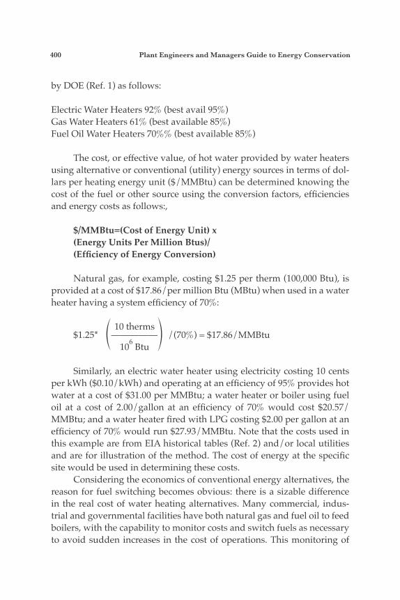
400 Plant Engineers and Managers Guide to Energy Conservation
by DOE (Ref. 1) as follows:
Electric Water Heaters 92% (best avail 95%)Gas Water Heaters 61% (best available 85%)Fuel Oil Water Heaters 70%% (best available 85%)
The cost, or effective value, of hot water provided by water heaters using alternative or conventional (utility) energy sources in terms of dol-lars per heating energy unit ($/MMBtu) can be determined knowing the cost of the fuel or other source using the conversion factors, efficiencies and energy costs as follows:,
$/MMBtu=(Cost of Energy Unit) x (Energy Units Per Million Btus)/ (Efficiency of Energy Conversion)
Natural gas, for example, costing $1.25 per therm (100,000 Btu), is provided at a cost of $17.86/per million Btu (MBtu) when used in a water heater having a system efficiency of 70%:
10 therms $1.25* e—————p /(70%) = $17.86/MMBtu 106 Btu
Similarly, an electric water heater using electricity costing 10 cents per kWh ($0.10/kWh) and operating at an efficiency of 95% provides hot water at a cost of $31.00 per MMBtu; a water heater or boiler using fuel oil at a cost of 2.00/gallon at an efficiency of 70% would cost $20.57/MMBtu; and a water heater fired with LPG costing $2.00 per gallon at an efficiency of 70% would run $27.93/MMBtu. Note that the costs used in this example are from EIA historical tables (Ref. 2) and/or local utilities and are for illustration of the method. The cost of energy at the specific site would be used in determining these costs. Considering the economics of conventional energy alternatives, the reason for fuel switching becomes obvious: there is a sizable difference in the real cost of water heating alternatives. Many commercial, indus-trial and governmental facilities have both natural gas and fuel oil to feed boilers, with the capability to monitor costs and switch fuels as necessary to avoid sudden increases in the cost of operations. This monitoring of
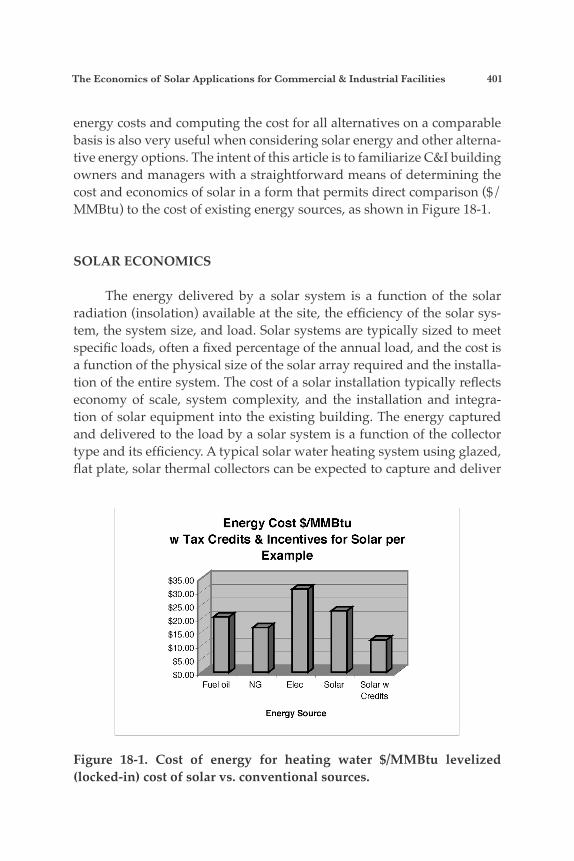
The Economics of Solar Applications for Commercial & Industrial Facilities 401
energy costs and computing the cost for all alternatives on a comparable basis is also very useful when considering solar energy and other alterna-tive energy options. The intent of this article is to familiarize C&I building owners and managers with a straightforward means of determining the cost and economics of solar in a form that permits direct comparison ($/MMBtu) to the cost of existing energy sources, as shown in Figure 18-1.
SOLAR ECONOMICS
The energy delivered by a solar system is a function of the solar radiation (insolation) available at the site, the efficiency of the solar sys-tem, the system size, and load. Solar systems are typically sized to meet specific loads, often a fixed percentage of the annual load, and the cost is a function of the physical size of the solar array required and the installa-tion of the entire system. The cost of a solar installation typically reflects economy of scale, system complexity, and the installation and integra-tion of solar equipment into the existing building. The energy captured and delivered to the load by a solar system is a function of the collector type and its efficiency. A typical solar water heating system using glazed, flat plate, solar thermal collectors can be expected to capture and deliver
Figure 18-1. Cost of energy for heating water $/MMBtu levelized (locked-in) cost of solar vs. conventional sources.
402 Plant Engineers and Managers Guide to Energy Conservation
between 40% and 70% of the solar energy (see SRCC collector ratings, Table 18-1) that falls on the collectors. A photovoltaic (PV) system, using crystalline solar cells, will deliver between 7% and 10% of the intercepted solar energy to the load as shown by the PVWATTS computation, Table 18-2. The flat plate solar collectors installed in a fixed position, with no moving parts and requiring little maintenance, would be expected to be used at most C&I facilities. These solar thermal and electric (PV) collec-tors are simple, proven, reliable, require minimal maintenance, and can be expected to provide service for 20 to 25 years without problems when properly installed and maintained. There are a wide variety of types of solar systems and technologies, including active and passive systems, solar thermal collectors and PV cells, and modules that utilize fixed-tilt, tracking, concentrators and/or a combination of technologies that have different characteristics, efficien-cies and performance. The systems discussed and evaluated herein reflect the most common type of systems and applications utilizing flat plate solar thermal collectors or PV modules and arrays that operate in a fixed position, often located on roofs of buildings. In order to determine the cost and value of solar systems, a concep-tual design of the solar system must be developed and its cost and perfor-mance (energy output) determined. While this might seem difficult, the abundance of information on the internet related to solar system costs, available solar insolation, climatic data, and equipment ratings, illustrat-ed in the examples that follow, make it a simple matter. Using the infor-mation available from equipment suppliers, it is possible to develop con-ceptual designs and to estimate system costs and performance at specific sites fairly accurately. Once the system has been sized and its cost and energy production quantified, the economics of the solar application can be determined and directly compared to the cost of conventional energy sources as discussed above. It is, however, important to realize that the installation of a solar system is a major capital improvement for an exist-ing facility or building, not an energy conservation measure that replaces existing equipment with more efficient equipment. Solar is a capital im-provement to the property that adds real value to the existing equipment and facility and is, in fact, depreciable; for C & I application it can utilize an accelerated (five-year) depreciation period. Essentially, it provides a quantifiable increase in property value as well as return on investment (the avoided cost of the energy delivered by the solar system) over its 20- to 25-year life, and it should be evaluated accordingly.
Th
e Econ
omics of Solar A
pp
lications for C
omm
ercial & In
du
strial Facilities 403
Table 18-1. Generic flat plate solar collector for SWH example
SOLAR COLLECTOR CERTIFICATION AND RATING
Megajoules Per Panel Per Day CATEGORY CLEAR MILDLY CLOIJDY
(Ti-Ta) DAY CI >OllDY DAY
SRCC OG- 100
Thousands of Btu Per Panel Per Day CATEGORY CLEAR MILDLY CLOIJDY
(Ti-Ta) DAY CLOUDY DAY
CERTIFIED SOLAR COLLECTOR
A (-5OC) I 54
SUPPLIER: A Solar Company 1234 Main St. Hometown, FL 12345
41 28 I I A (-9°F) I 51 39 27
MODEL: Be s t-40 COLLECTOR TYPE: Glazed Flat-Plate CERTIFICATION #: 100-200 1-00 I C
\ , , B (5°C) 48 35 22 c (200C) 38 25 12
E (80°C) 1 D (50°C) 17 6
I COLLECTOR THERMAL PERFORMANCE RATING
~ , , B (9°F) 45 33 21 C (36'F) 36 24 12
E (144°F) 1 D (90°F) 16 6
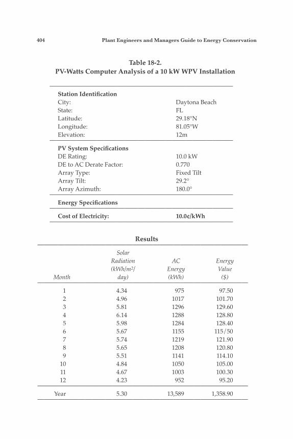
404 Plant Engineers and Managers Guide to Energy Conservation
Table 18-2.PV-Watts Computer Analysis of a 10 kW WPV Installation
——————————————————————————— Station Identification City: Daytona Beach State: FL Latitude: 29.18°N Longitude: 81.05°W Elevation: 12m ——————————————————————————— PV System Specifications DE Rating: 10.0 kW DE to AC Derate Factor: 0.770 Array Type: Fixed Tilt Array Tilt: 29.2° Array Azimuth: 180.0° ——————————————————————————— Energy Specifications ——————————————————————————— Cost of Electricity: 10.0¢/kWh ———————————————————————————
Results——————————————————————————————— Solar Radiation AC Energy (kWh/m2/ Energy Value Month day) (kWh) ($)——————————————————————————————— 1 4.34 975 97.50 2 4.96 1017 101.70 3 5.81 1296 129.60 4 6.14 1288 128.80 5 5.98 1284 128.40 6 5.67 1155 115/50 7 5.74 1219 121.90 8 5.65 1208 120.80 9 5.51 1141 114.10 10 4.84 1050 105.00 11 4.67 1003 100.30 12 4.23 952 95.20——————————————————————————————— Year 5.30 13,589 1,358.90———————————————————————————————
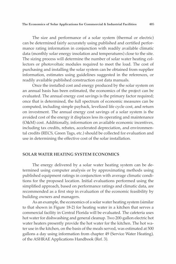
The Economics of Solar Applications for Commercial & Industrial Facilities 405
The size and performance of a solar system (thermal or electric) can be determined fairly accurately using published and certified perfor-mance rating information in conjunction with readily available climatic data (monthly solar energy insolation and temperatures) close to the site. The sizing process will determine the number of solar water heating col-lectors or photovoltaic modules required to meet the load. The cost of purchasing and installing the solar system can be obtained from supplier information, estimates using guidelines suggested in the references, or readily available published construction cost data manuals. Once the installed cost and energy produced by the solar system on an annual basis has been estimated, the economics of the project can be evaluated. The annual energy cost savings is the primary factor required; once that is determined, the full spectrum of economic measures can be computed, including simple payback, levelized life cycle cost, and return on investment. The annual energy cost savings of a solar system is the avoided cost of the energy it displaces less its operating and maintenance (O&M) cost. Additionally, information on available economic incentives, including tax credits, rebates, accelerated depreciation, and environmen-tal credits (RECS, Green Tags, etc.) should be collected for evaluation and use in determining the effective cost of the solar installation.
SOLAR WATER HEATING SYSTEM ECONOMICS
The energy delivered by a solar water heating system can be de-termined using computer analysis or by approximating methods using published equipment ratings in conjunction with average climatic condi-tions for the proposed location. Initial evaluations performed using the simplified approach, based on performance ratings and climatic data, are recommended as a first step in evaluation of the economic feasibility by building owners and managers. As an example, the economics of a solar water heating system (similar to that shown in Figure 18-2) for heating water in a kitchen that serves a commercial facility in Central Florida will be evaluated. The cafeteria uses hot water for dishwashing and general cleanup. Two 200 -gallon electric hot water heaters presently provide the hot water for the kitchen. The hot wa-ter use in the kitchen, on the basis of the meals served, was estimated at 500 gallons a day using information from chapter 49 (Service Water Heating), of the ASHRAE Applications Handbook (Ref. 3).
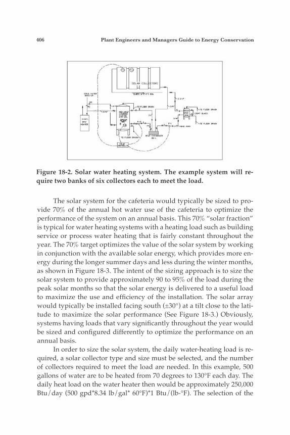
406 Plant Engineers and Managers Guide to Energy Conservation
The solar system for the cafeteria would typically be sized to pro-vide 70% of the annual hot water use of the cafeteria to optimize the performance of the system on an annual basis. This 70% “solar fraction” is typical for water heating systems with a heating load such as building service or process water heating that is fairly constant throughout the year. The 70% target optimizes the value of the solar system by working in conjunction with the available solar energy, which provides more en-ergy during the longer summer days and less during the winter months, as shown in Figure 18-3. The intent of the sizing approach is to size the solar system to provide approximately 90 to 95% of the load during the peak solar months so that the solar energy is delivered to a useful load to maximize the use and efficiency of the installation. The solar array would typically be installed facing south (±30°) at a tilt close to the lati-tude to maximize the solar performance (See Figure 18-3.) Obviously, systems having loads that vary significantly throughout the year would be sized and configured differently to optimize the performance on an annual basis. In order to size the solar system, the daily water-heating load is re-quired, a solar collector type and size must be selected, and the number of collectors required to meet the load are needed. In this example, 500 gallons of water are to be heated from 70 degrees to 130°F each day. The daily heat load on the water heater then would be approximately 250,000 Btu/day (500 gpd*8.34 lb/gal* 60°F)*1 Btu/(lb-°F). The selection of the
Figure 18-2. Solar water heating system. The example system will re-quire two banks of six collectors each to meet the load.
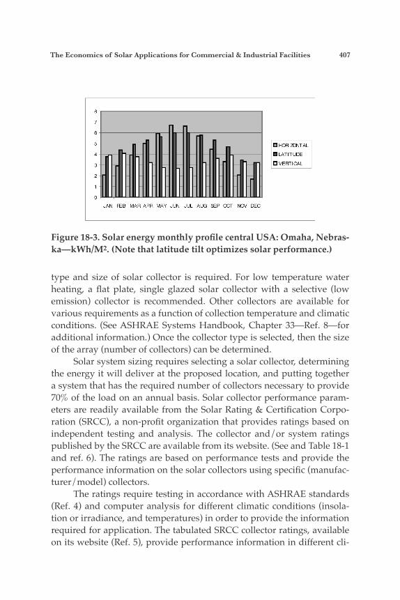
The Economics of Solar Applications for Commercial & Industrial Facilities 407
type and size of solar collector is required. For low temperature water heating, a flat plate, single glazed solar collector with a selective (low emission) collector is recommended. Other collectors are available for various requirements as a function of collection temperature and climatic conditions. (See ASHRAE Systems Handbook, Chapter 33—Ref. 8—for additional information.) Once the collector type is selected, then the size of the array (number of collectors) can be determined. Solar system sizing requires selecting a solar collector, determining the energy it will deliver at the proposed location, and putting together a system that has the required number of collectors necessary to provide 70% of the load on an annual basis. Solar collector performance param-eters are readily available from the Solar Rating & Certification Corpo-ration (SRCC), a non-profit organization that provides ratings based on independent testing and analysis. The collector and/or system ratings published by the SRCC are available from its website. (See and Table 18-1 and ref. 6). The ratings are based on performance tests and provide the performance information on the solar collectors using specific (manufac-turer/model) collectors. The ratings require testing in accordance with ASHRAE standards (Ref. 4) and computer analysis for different climatic conditions (insola-tion or irradiance, and temperatures) in order to provide the information required for application. The tabulated SRCC collector ratings, available on its website (Ref. 5), provide performance information in different cli-
Figure 18-3. Solar energy monthly profile central USA: Omaha, Nebras-ka—kWh/M2. (Note that latitude tilt optimizes solar performance.)
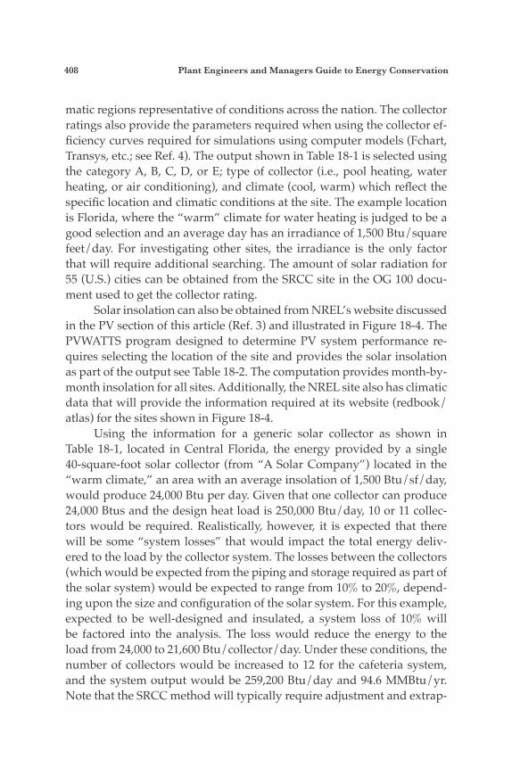
408 Plant Engineers and Managers Guide to Energy Conservation
matic regions representative of conditions across the nation. The collector ratings also provide the parameters required when using the collector ef-ficiency curves required for simulations using computer models (Fchart, Transys, etc.; see Ref. 4). The output shown in Table 18-1 is selected using the category A, B, C, D, or E; type of collector (i.e., pool heating, water heating, or air conditioning), and climate (cool, warm) which reflect the specific location and climatic conditions at the site. The example location is Florida, where the “warm” climate for water heating is judged to be a good selection and an average day has an irradiance of 1,500 Btu/square feet/day. For investigating other sites, the irradiance is the only factor that will require additional searching. The amount of solar radiation for 55 (U.S.) cities can be obtained from the SRCC site in the OG 100 docu-ment used to get the collector rating. Solar insolation can also be obtained from NREL’s website discussed in the PV section of this article (Ref. 3) and illustrated in Figure 18-4. The PVWATTS program designed to determine PV system performance re-quires selecting the location of the site and provides the solar insolation as part of the output see Table 18-2. The computation provides month-by-month insolation for all sites. Additionally, the NREL site also has climatic data that will provide the information required at its website (redbook/atlas) for the sites shown in Figure 18-4. Using the information for a generic solar collector as shown in Table 18-1, located in Central Florida, the energy provided by a single 40-square-foot solar collector (from “A Solar Company”) located in the “warm climate,” an area with an average insolation of 1,500 Btu/sf/day, would produce 24,000 Btu per day. Given that one collector can produce 24,000 Btus and the design heat load is 250,000 Btu/day, 10 or 11 collec-tors would be required. Realistically, however, it is expected that there will be some “system losses” that would impact the total energy deliv-ered to the load by the collector system. The losses between the collectors (which would be expected from the piping and storage required as part of the solar system) would be expected to range from 10% to 20%, depend-ing upon the size and configuration of the solar system. For this example, expected to be well-designed and insulated, a system loss of 10% will be factored into the analysis. The loss would reduce the energy to the load from 24,000 to 21,600 Btu/collector/day. Under these conditions, the number of collectors would be increased to 12 for the cafeteria system, and the system output would be 259,200 Btu/day and 94.6 MMBtu/yr. Note that the SRCC method will typically require adjustment and extrap-

Th
e Econ
omics of Solar A
pp
lications for C
omm
ercial & In
du
strial Facilities 409
Figure 18-4. Average daily
solar radiation. Note:
Solar radiation information
throughout the US available
specificcities 1 kWh/
m2/day = 317.1 Btu/ft2/day
http://rredc.nrel.gov/solar/
old_data/nsrdb/redbook/atlas/
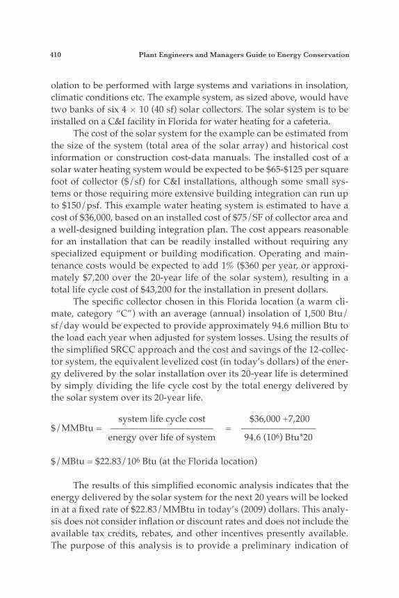
410 Plant Engineers and Managers Guide to Energy Conservation
olation to be performed with large systems and variations in insolation, climatic conditions etc. The example system, as sized above, would have two banks of six 4 ´ 10 (40 sf) solar collectors. The solar system is to be installed on a C&I facility in Florida for water heating for a cafeteria. The cost of the solar system for the example can be estimated from the size of the system (total area of the solar array) and historical cost information or construction cost-data manuals. The installed cost of a solar water heating system would be expected to be $65-$125 per square foot of collector ($/sf) for C&I installations, although some small sys-tems or those requiring more extensive building integration can run up to $150/psf. This example water heating system is estimated to have a cost of $36,000, based on an installed cost of $75/SF of collector area and a well-designed building integration plan. The cost appears reasonable for an installation that can be readily installed without requiring any specialized equipment or building modification. Operating and main-tenance costs would be expected to add 1% ($360 per year, or approxi-mately $7,200 over the 20-year life of the solar system), resulting in a total life cycle cost of $43,200 for the installation in present dollars. The specific collector chosen in this Florida location (a warm cli-mate, category “C”) with an average (annual) insolation of 1,500 Btu/sf/day would be expected to provide approximately 94.6 million Btu to the load each year when adjusted for system losses. Using the results of the simplified SRCC approach and the cost and savings of the 12-collec-tor system, the equivalent levelized cost (in today’s dollars) of the ener-gy delivered by the solar installation over its 20-year life is determined by simply dividing the life cycle cost by the total energy delivered by the solar system over its 20-year life.
system life cycle cost $36,000 +7,200$/MMBtu = ——————————— = ———————— energy over life of system 94.6 (106) Btu*20
$/MBtu = $22.83/106 Btu (at the Florida location)
The results of this simplified economic analysis indicates that the energy delivered by the solar system for the next 20 years will be locked in at a fixed rate of $22.83/MMBtu in today’s (2009) dollars. This analy-sis does not consider inflation or discount rates and does not include the available tax credits, rebates, and other incentives presently available. The purpose of this analysis is to provide a preliminary indication of
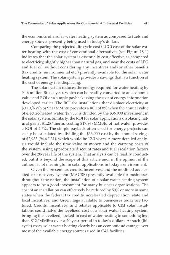
The Economics of Solar Applications for Commercial & Industrial Facilities 411
the economics of a solar water heating system as compared to fuels and energy sources presently being used in today’s dollars. Comparing the projected life cycle cost (LCC) cost of the solar wa-ter heating with the cost of conventional alternatives (see Figure 18-1) indicates that the solar system is essentially cost effective as compared to electricity, slightly higher than natural gas, and near the costs of LPG and fuel oil, without considering any incentives and/or other benefits (tax credits, environmental etc.) presently available for the solar water heating system. The solar system provides a savings that is a function of the cost of energy it is displacing. The solar system reduces the energy required for water heating by 94.6 million Btus a year, which can be readily converted to an economic value and ROI or a simple payback using the cost of energy information developed earlier. The ROI for installations that displace electricity at $0.10/kWh or $31/MMBtu provides a ROI of 8% when the annual value of electric-heated water, $2,933, is divided by the $36,000 investment in the solar system. Similarly, the ROI for solar applications displacing nat-ural gas at $1.25/therm, costing $17.86/MMBtu of hot water, provides a ROI of 4.7%. The simple payback often used for energy projects can easily be calculated by dividing the $36,000 cost by the annual savings of $2,933 (94.6 * 31), which would be 12.3 years. A more detailed analy-sis would include the time value of money and the carrying costs of the system, using appropriate discount rates and fuel escalation factors over the 20-year life of the system. That analysis can be readily conduct-ed, but it is beyond the scope of this article and, in the opinion of the author, is not meaningful in solar applications in today’s environment. Given the present tax credits, incentives, and the modified acceler-ated cost recovery system (MACRS) presently available for businesses throughout the nation, the installation of a solar water heating system appears to be a good investment for many business organizations. The cost of an installation can effectively be reduced by 50% or more in some states when the federal tax credits, accelerated depreciation, state and local incentives, and Green Tags available to businesses today are fac-tored. Credits, incentives, and rebates applicable to C&I solar instal-lations could halve the levelized cost of a solar water heating system, bringing the levelized, locked-in cost of water heating to something less than $12/MMBtu over a 20 year period in today’s dollars. At such (life cycle) costs, solar water heating clearly has an economic advantage over most of the available energy sources used in C&I facilities.
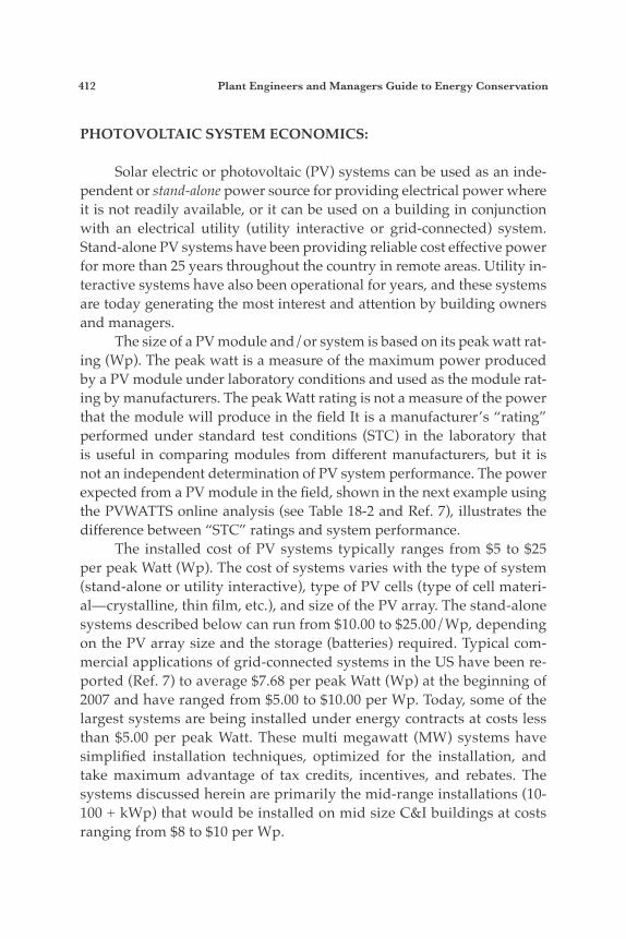
412 Plant Engineers and Managers Guide to Energy Conservation
PHOTOVOLTAIC SYSTEM ECONOMICS:
Solar electric or photovoltaic (PV) systems can be used as an inde-pendent or stand-alone power source for providing electrical power where it is not readily available, or it can be used on a building in conjunction with an electrical utility (utility interactive or grid-connected) system. Stand-alone PV systems have been providing reliable cost effective power for more than 25 years throughout the country in remote areas. Utility in-teractive systems have also been operational for years, and these systems are today generating the most interest and attention by building owners and managers. The size of a PV module and/or system is based on its peak watt rat-ing (Wp). The peak watt is a measure of the maximum power produced by a PV module under laboratory conditions and used as the module rat-ing by manufacturers. The peak Watt rating is not a measure of the power that the module will produce in the field It is a manufacturer’s “rating” performed under standard test conditions (STC) in the laboratory that is useful in comparing modules from different manufacturers, but it is not an independent determination of PV system performance. The power expected from a PV module in the field, shown in the next example using the PVWATTS online analysis (see Table 18-2 and Ref. 7), illustrates the difference between “STC” ratings and system performance. The installed cost of PV systems typically ranges from $5 to $25 per peak Watt (Wp). The cost of systems varies with the type of system (stand-alone or utility interactive), type of PV cells (type of cell materi-al—crystalline, thin film, etc.), and size of the PV array. The stand-alone systems described below can run from $10.00 to $25.00/Wp, depending on the PV array size and the storage (batteries) required. Typical com-mercial applications of grid-connected systems in the US have been re-ported (Ref. 7) to average $7.68 per peak Watt (Wp) at the beginning of 2007 and have ranged from $5.00 to $10.00 per Wp. Today, some of the largest systems are being installed under energy contracts at costs less than $5.00 per peak Watt. These multi megawatt (MW) systems have simplified installation techniques, optimized for the installation, and take maximum advantage of tax credits, incentives, and rebates. The systems discussed herein are primarily the mid-range installations (10-100 + kWp) that would be installed on mid size C&I buildings at costs ranging from $8 to $10 per Wp.
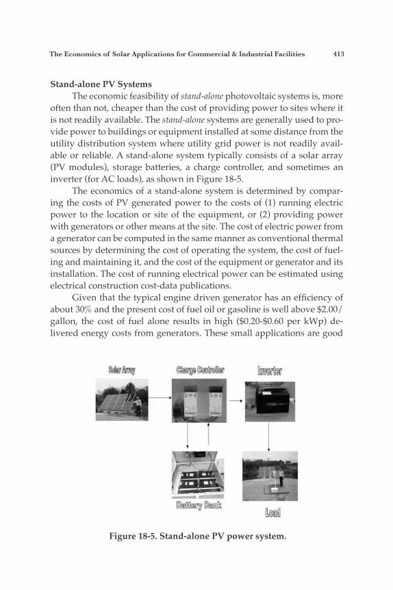
The Economics of Solar Applications for Commercial & Industrial Facilities 413
Stand-alone PV Systems The economic feasibility of stand-alone photovoltaic systems is, more often than not, cheaper than the cost of providing power to sites where it is not readily available. The stand-alone systems are generally used to pro-vide power to buildings or equipment installed at some distance from the utility distribution system where utility grid power is not readily avail-able or reliable. A stand-alone system typically consists of a solar array (PV modules), storage batteries, a charge controller, and sometimes an inverter (for AC loads), as shown in Figure 18-5. The economics of a stand-alone system is determined by compar-ing the costs of PV generated power to the costs of (1) running electric power to the location or site of the equipment, or (2) providing power with generators or other means at the site. The cost of electric power from a generator can be computed in the same manner as conventional thermal sources by determining the cost of operating the system, the cost of fuel-ing and maintaining it, and the cost of the equipment or generator and its installation. The cost of running electrical power can be estimated using electrical construction cost-data publications. Given that the typical engine driven generator has an efficiency of about 30% and the present cost of fuel oil or gasoline is well above $2.00/gallon, the cost of fuel alone results in high ($0.20-$0.60 per kWp) de-livered energy costs from generators. These small applications are good
Figure 18-5. Stand-alone PV power system.
414 Plant Engineers and Managers Guide to Energy Conservation
candidates for PV applications if the loads are relatively constant. The cost of electric power ($/kWh) from a small (2,000W to 4,000W) genera-tor using gasoline or diesel fuel at costs of $2.25/gallon ranges from 25 to 60 cents per kWh. When the cost of the equipment operation and main-tenance and the cost of transporting fuel to the generator are considered, the stand-alone PV system has advantages over the generator.
Utility Interactive PV Systems Utility interactive systems (see Figure 18-6) displace utility electric power during the daytime, which for many commercial facilities is of-ten the peak period with resulting higher charges (time-of-use rates) for electric power. PV installations can be a large tracking utility system at a power plant, a simple low maintenance fixed tilt system on a C&I facility, or a flush-mounted installation on a residence. The PV power is used on site and/or feeds solar power back to the utility when not required at the site. The economics of utility interactive PV systems can be arrived at by determining the amount of energy produced and the value of the avoided cost of the electricity in $/kWh in a similar manner as with solar water heating systems. The amount of electricity provided by the photovoltaic system is also determined in a similar manner as with the solar thermal system, us-ing the ratings of the solar equipment and climatic data. The objective is to determine the electricity delivered by the system annually so that the total energy provided over the systems life, generally assumed to be 20 to 25 years, can be determined. The power can be estimated using a variety of approaches, computation using climatic data and array performance at standard test conditions (STC), or the module peak power rating as reported by the manufacturer. A variety of methods for estimating PV system performance are available to determine the energy delivered by the solar electric system. One of the easiest to use methods is the PVWATTS program developed by Sandia National Laboratory, available on the web at the National Renew-able Energy Laboratories (NREL) site (Ref. 7). The PVWATTS program (see Table 18-2) uses the PV module rating (input), climatic data for the specific site (using long term average weather data), and the utility rates to compute the energy (kWh) delivered monthly and annually. PVWATTS computes the value of the electricity provided by the PV system at the existing utility rate. The example economic analysis that follows, using the PVWATTS program, compares the levelized cost of PV power to the

The Economics of Solar Applications for Commercial & Industrial Facilities 415
utility power to which it is interconnected. In determining the performance of the PV system, the equipment (solar array) rating of the PV modules is required, just as the ratings on solar thermal collectors for water heating are used to determine the ther-mal energy produced by the collectors. The PVWATTS program incorpo-rates the weather data from the immediate area of the project site (user selected), adjustment factors for module and/or site-specific conditions, and utility rates into an easy to use on line computational program. The PVWATTS program directly computes the annual delivered energy and value of the power produced as shown in Table 18-2.
Example Cost of Energy from a Utility Interactive PV System In this example the PVWATTS Program (Table 18-2) is used to de-termine the economics of a 10.0-kWp grid-connected PV System installed on a commercial building in Florida. The system size in the PVWATTS program is the “rating” of the PV array in DC Watts. The array rating is essentially the module rating (peak Watts or Wp) multiplied by the
Figure 18-6. Grid-connected photovoltaic systems. Source: PV in cold climates, Royce & Royer, courtesy of RETSCreen Intl.
416 Plant Engineers and Managers Guide to Energy Conservation
number of modules. The program only requires one to select the location of the system and to enter the peak power of the PV array at STC and the local utility rate (or buy-back rate) to determine the economics. The computer analysis has a built in system-derating factor (power losses) which appears to be appropriate for typical systems and can be adjusted for specific system or site parameters as required. The PVWATTS input, shown in Table 18-2 for this example, looks at a 10 kW array installed on a building in Daytona Beach, FL, where the fa-cility cost of electricity is 0.10/kWh. The annual energy production from the program, based on Daytona Beach average climatic data included in the PV Watts program, is 13,589 kWh, with an annual value or savings of $1,358.90, @ $0.10/kWh as shown in the results of Table 18-2. To de-termine the levelized cost of energy over the life of the system, simply estimate the life cycle cost (LCC) of the installation ($8-$10/Wp) and the O&M (1/2-1%/yr) over the 20 years and divide by the energy provided over the 20-year period. Note that neither cost escalation, discount rates, nor interest rates and inflation are considered in this approach. The intent is to evaluate the feasibility and get an idea of the value based on current dollars and a levelized value (without considering tax credits and other incentives) of the energy delivered by the solar installation.
System Cost @ $9.00/Wp: $ 90,000.00 Energy delivered—20 yr life: 271,780 kWh O&M Cost, 1%/yr for 20 years: $ 900.00/yr
Life Cycle Cost: $90,000 + 20 ´ $900 $ 108,000.00
PV Levelized energy cost: LCC/LC kWh: $ 108,000/271,780 kWh
PV Levelized cost w/o Incentive: $ 0.397/kWh
The levelized cost of $0.40/kWh from the grid-connected photo-voltaic system installed at a cost of $90,000 ($9/Wp) is not competitive with existing utility rates in Florida. A PV system of this type and size is not typically cost-effective without credits, incentives, or subsidies. PV systems have some economy of scale, as illustrated at the beginning of this section, especially with the larger PV systems (megawatt) that can be

The Economics of Solar Applications for Commercial & Industrial Facilities 417
installed at somewhat lower costs. This economics of utility connected PV have become quite appar-ent to the federal government, numerous states, and many utilities that have established a wide variety of credits and/or incentives to encourage the application of renewable energy applications, especially PV installa-tions. These incentives are intended to help address existing energy and environmental issues that have become major concerns throughout the world. The incentives, in the form of tax credits and rebates, are readily available and increasing daily. These incentives should help encourage the installation of all solar applications, including PV, further reducing their cost. The economic benefits that this utility interactive PV project can take advantage of include the federal tax credit and accelerated depreciation (MACRS), the state (Florida) rebate of $4.00/Wp, and possible green tags (renewable energy credits). Application of some of the incentives avail-able in Florida today for this example project reduces the cost of energy from the system from $0.40/kWh to about $0.20 per kWh as follows:
PV Cost w $4/W State rebate: Installed System Cost: $90,000 Rebate @ $4.00/Wp: $40,000 Net Cost $ 50,000
PV Cost w 30% Federal Tax Credit: Tax Credit: $15,000 Net Cost $35,000
Operation & Maintenance LCC $18,000
Life Cycle Cost: $53,000
Value of Energy @ $0.10/kWh: $27,178
PV Levelized Cost w Incentives: $53,000/271,780
$0.195/kWh (LCC/delivered Energy 20 yrs)
The levelized cost of electricity from the utility interactive system located in Daytona Beach over the 20- year life of the PV system, after
418 Plant Engineers and Managers Guide to Energy Conservation
taking advantage of the federal tax credit and state rebate, is about $0.20/kWh, double the current rate from the utility. The PV system, consider-ing the available state rebate and the federal tax credit, provides a ROI of 3.8% when the annual savings of $1,359 and the effective cost of $35,000 are considered. It should be noted that additional economic benefits available for this and similar projects installed on C&I Facilities and other businesses are also further improved, considering time-of-use rates and other site-specific factors not included in this analysis. Businesses can take advan-tage of the MACRS, or accelerated depreciation, which typically will provide of reduction of approximately 12.5%. C&I facilities are often on time-of-use rates (TOU), which are highest for C&I facilities during the daytime when usage is highest and solar energy is available. Solar in-stallations also deliver green power, eligible for renewable energy credits (RECS), or “green tags,” which are marketable. The project also provides economic benefits to businesses by virtue of the positive environmental action they have taken. Green hotels have an added marketing factor and attract those interested in ecotourism. Essentially, while the project might not be recommended on the basis of its simple economics, such projects are moving forward in today’s environment in the commercial and indus-trial sector because of the incentives and credits presently available. Additional economic benefits are available in different areas and states throughout the country. There are other incentives and benefits available that are applicable to all renewable energy. It is recommended that the latest information on state incentives be reviewed and the pos-sibility of green tags be investigated to ensure that all possible assistance is identified. The best source for information on the current incentives available in all the states for businesses or individuals considering renew-able energy systems is the Database of State Incentives for Renewables & Efficiency (DSIRE) (Ref. 10).
SUMMARY & CONCLUSION
The economics of C&I solar applications changed dramatically in 2006 with the resurgence of the tax credits. The growing awareness of the energy and environmental issues facing the world has resulted in a plethora of incentives to assist renewable energy applications, encourag-ing the installation of solar applications throughout the nation. Given the
The Economics of Solar Applications for Commercial & Industrial Facilities 419
incentives today for C&I applications, it appears that the time has come for building owners and managers to evaluate the solar option and con-sider implementing it to help better control energy costs. The approach presented herein provides a simplified method to evaluate the economics of solar and determine the economic feasibility of solar projects. The method presented will allow readers to readily deter-mine the simple payback and the levelized cost savings of a solar water heating or PV system over its 20- to 25-year life in current dollars. Both the technology and the life of both solar thermal and photovoltaics have been proven in the field, and the economics have never been better. This approach has been used successfully to identify potential solar projects for energy audits, energy savings performance contracts (ESPCs), and utility energy savings contracts (UESCs), as well as alternative energy project development. This approach can help building owners and managers determine if solar might be appropriate in their facility. The cost and availability of fuels is in a constant state of flux, costs of energy and solar equipment are constantly changing, and interruption of supplies is happening all too often. Perhaps this is a good time to spend an afternoon evaluating solar energy—an energy source that will be there when it is needed.
References1. Equipment Energy Ratings, DOE/FEMP Website Site Map with links to all Energy
Management Information including Energy Efficient Products and Renewable Energy Applications, http://www1.eere.energy.gov/femp/sitemap. html
2. Energy Information Agency, EIA, historical, current and future Energy Cost Informa-tion, http://eia.doe.gov
1 Renewable Resource Data Center of the National Renewable Energy Laboratory website, http://rredc.nrel.gov
2 ASHRAE Applications Handbook, 2003, Chapter 33, Solar Energy Use3 ASHRAE Standard 93-1986, Methods of Testing to Determine The Thermal Perfor-
mance of Solar Collectors4 Solar Thermal Collector Rating Information: Solar Rating & Certification Corp
(SRCC),www.solar-rating.org/ratings/ratings.htm5 PV-WATTS, http://rredc.nrel.gov/solar/codes-algs/PVWATTS, Web Based Software
for Grid Connected PV Systems6 “PV 2006: From Hype to Reality,” reFOCUS, January/February 2007, pp. 36-407 ASHRAE Systems Handbook, 2004, Chapter 33, Solar Energy Equipment8 Database of State Incentives for Renewables & Efficiency, www.dsireusa.org, Federal,
State and Local Incentives
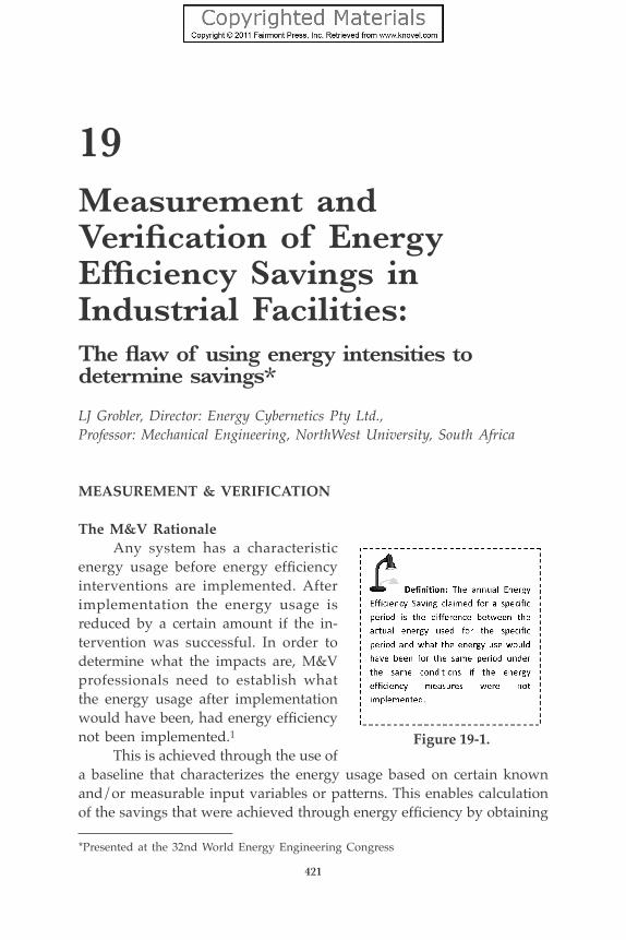
19Measurement andVerification of EnergyEfficiency Savings inIndustrial Facilities:The flaw of using energy intensities to determine savings*
LJ Grobler, Director: Energy Cybernetics Pty Ltd.,Professor: Mechanical Engineering, NorthWest University, South Africa
MEASUREMENT & VERIFICATION
The M&V Rationale Any system has a characteristic energy usage before energy efficiency interventions are implemented. After implementation the energy usage is reduced by a certain amount if the in-tervention was successful. In order to determine what the impacts are, M&V professionals need to establish what the energy usage after implementation would have been, had energy efficiency not been implemented.1 This is achieved through the use of a baseline that characterizes the energy usage based on certain known and/or measurable input variables or patterns. This enables calculation of the savings that were achieved through energy efficiency by obtaining
421
*Presented at the 32nd World Energy Engineering Congress
Figure 19-1.
422 Plant Engineers and Managers Guide to Energy Conservation
the difference between the baseline and the actual energy usage. The basic principle of M&V is to compare the measured energy use after implementation with what it was before implementation in order to determine the impacts. This is demonstrated in Equation 19-1 and shown in Figure 19-2.
energy savings = (pre-implementation energy use) – (post-implementation energy use) ± adjustments (Eq. 19-1)2
The pre-implementation energy-use conditions are described by a baseline. The baseline represents the energy use linked to a set of conditions under which the system in question was operating prior to implementation of the energy efficiency measures. This could include factors such as production, weather, or building occupancy. These fac-tors are commonly referred to as the service level. If the service level remains unchanged, the post-implementation electricity use can be di-rectly compared to that of the baseline. This is, however, seldom the case. Service level adjustments (SLA) are consequently necessary to bring the two time periods under the same set of operational conditions should any of the pre-implementation service levels change. Service level adjustments are thus made to restate baseline electricity use under post-implementation conditions. Baseline adjustments are another form of adjustment as shown in Equation 19-1. This adjustment is done in the case of equipment or scope changes to projects and is done on an ad hoc basis, not periodically as in the case of service level adjustments. Baselines are critical to the process, and care needs to be taken during the development of baselines. Baselines should accurately reflect increased energy use due to increased production for industrial sites, or due to increased occupancy in commercial buildings, for instance.
M&V Baselines and Energy Efficiency The baseline, which is a model derived and characterized from data of the financial year serving as the baseline year, should predict what the energy use would have been if the energy efficiency measures had not been implemented. The baseline model should be characterized from the energy use and energy-use drivers such as production, ambient temperatures, mining depth, occupancies, yields, etc., in a conservative manner.
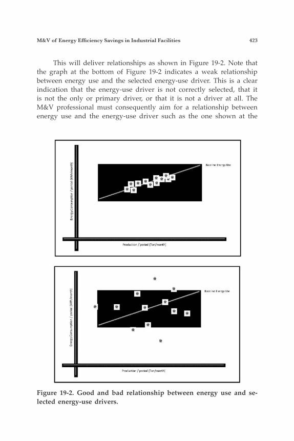
M&V of Energy Efficiency Savings in Industrial Facilities 423
This will deliver relationships as shown in Figure 19-2. Note that the graph at the bottom of Figure 19-2 indicates a weak relationship between energy use and the selected energy-use driver. This is a clear indication that the energy-use driver is not correctly selected, that it is not the only or primary driver, or that it is not a driver at all. The M&V professional must consequently aim for a relationship between energy use and the energy-use driver such as the one shown at the
Figure 19-2. Good and bad relationship between energy use and se-lected energy-use drivers.
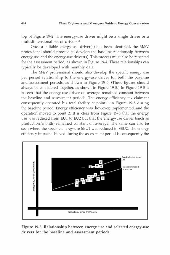
424 Plant Engineers and Managers Guide to Energy Conservation
top of Figure 19-2. The energy-use driver might be a single driver or a multidimensional set of drivers.3 Once a suitable energy-use driver(s) has been identified, the M&V professional should proceed to develop the baseline relationship between energy use and the energy-use driver(s). This process must also be repeated for the assessment period, as shown in Figure 19-4. These relationships can typically be developed with monthly data. The M&V professional should also develop the specific energy use per period relationship to the energy-use driver for both the baseline and assessment periods, as shown in Figure 19-5. (These figures should always be considered together, as shown in Figure 19-5.) In Figure 19-5 it is seen that the energy-use driver on average remained constant between the baseline and assessment periods. The energy efficiency tax claimant consequently operated his total facility at point 1 in Figure 19-5 during the baseline period. Energy efficiency was, however, implemented, and the operation moved to point 2. It is clear from Figure 19-5 that the energy use was reduced from EU1 to EU2 but that the energy-use driver (such as production/month) remained constant on average. The same can also be seen where the specific energy-use SEU1 was reduced to SEU2. The energy efficiency impact achieved during the assessment period is consequently the
Figure 19-3. Relationship between energy use and selected energy-use drivers for the baseline and assessment periods.
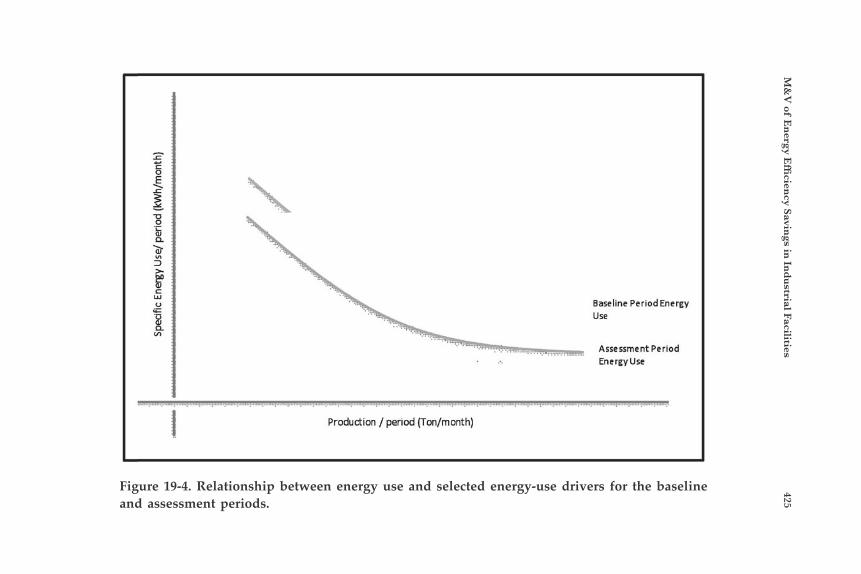
M&
V of E
nergy E
fficien
cy Savings in
Ind
ustrial Facilities
425
Figure 19-4. Relationship between energy use and selected energy-use drivers for the baseline and assessment periods.
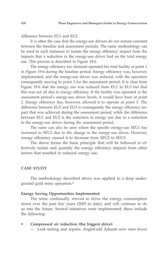
426 Plant Engineers and Managers Guide to Energy Conservation
difference between EU1 and EU2. It is often the case that the energy-use drivers do not remain constant between the baseline and assessment periods. The same methodology can be used in such instances to isolate the energy efficiency impact from the impacts that a reduction in the energy-use driver had on the total energy use. This process is described in Figure 19-6. The energy efficiency tax claimant operated his total facility at point 1 in Figure 19-6 during the baseline period. Energy efficiency was, however, implemented, and the energy-use driver was reduced, with the operation consequently moving to point 3 for the assessment period. It is clear from Figure 19-6 that the energy use was reduced from EU1 to EU3 but that this was not all due to energy efficiency. If the facility was operated at the assessment period’s energy-use driver levels, it would have been at point 2. Energy efficiency has, however, allowed it to operate at point 3. The difference between EU2 and EU3 is consequently the energy efficiency im-pact that was achieved during the assessment period, while the difference between EU1 and EU2 is the reduction in energy use due to a reduction in the energy-use driver during the assessment period. The same can also be seen where the specific energy-use SEU1 has increased to SEU2 due to the change in the energy-use driver. However, energy efficiency caused it to decrease from SEU2 to SEU3. The above forms the basic principle that will be followed to ef-fectively isolate and quantify the energy efficiency impacts from other factors that resulted in reduced energy use.
CASE STUDY
The methodology described above was applied to a deep under-ground gold mine operation.4
Energy Saving Opportunities Implemented The mine continually strived to drive the energy consumption down over the past few years (2005 to date), and will continue to do so into the future. Several initiatives were implemented; these include the following:
• Compressed air reduction (the biggest drive):— Leak testing and repairs. AngloGold Ashanti now runs fewer
M&V of Energy Efficiency Savings in Industrial Facilities 427
Figure 19-5. Relationship between energy use and specific energy use vs. selected energy-use drivers for the baseline and assessment periods with a constant energy-use driver.
machines for the same production output at both Vaal River and West Wits.
— Monthly briefing to business units regarding their consumption, best practice, and feedback regarding the progress on major leaks.
— Management of the compressed air control to enable only efficient machines to run during production period.
— Efficiency of machines tested at 6-month intervals.— Agitation via compressed air removed and replaced with
pulsating type valves or mechanical agitation.
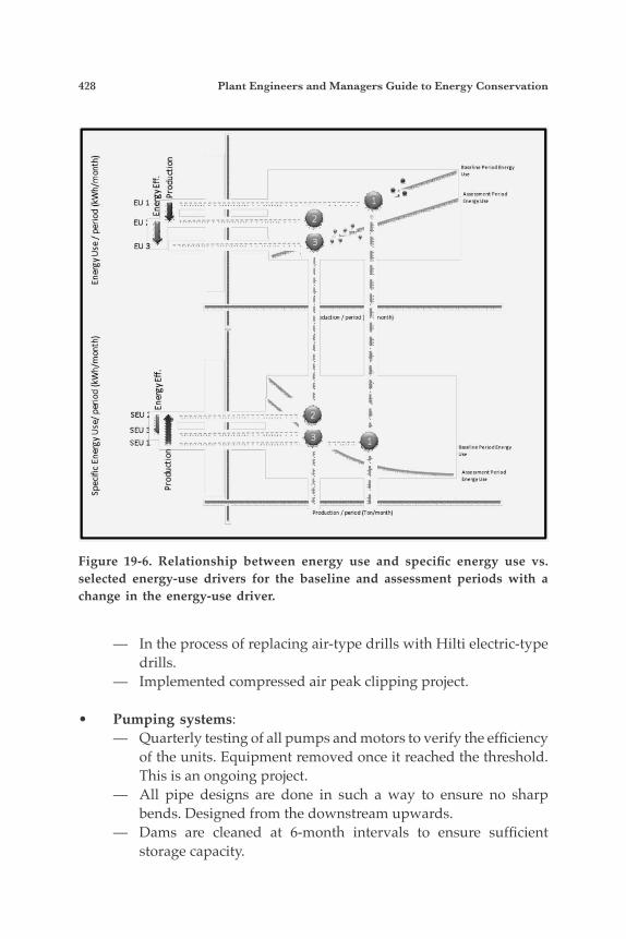
428 Plant Engineers and Managers Guide to Energy Conservation
— In the process of replacing air-type drills with Hilti electric-type drills.
— Implemented compressed air peak clipping project.
• Pumping systems:— Quarterly testing of all pumps and motors to verify the efficiency
of the units. Equipment removed once it reached the threshold. This is an ongoing project.
— All pipe designs are done in such a way to ensure no sharp bends. Designed from the downstream upwards.
— Dams are cleaned at 6-month intervals to ensure sufficient storage capacity.
Figure 19-6. Relationship between energy use and specific energy use vs. selected energy-use drivers for the baseline and assessment periods with a change in the energy-use driver.
M&V of Energy Efficiency Savings in Industrial Facilities 429
— Control management installed to ensure efficient utilization.— Turbines installed at Mponeng driving generator.— Turbines installed at Kopanang direct drive to pumps.
• Underground:— Replaced all incandescent lights with CFLs.— Replaced all fluorescent fittings with electronic controlled units.— Removed some lighting transformers after the installation of
CFLs.— Installed current control on vertical spindle pumps.— In the process of replacing all standard-type motors with
efficiency 1-type units.— Isolated power and water to the workings at end of shift.— Installed VSD drives at conveyor systems.— In process of replacing inefficient 2-pole fans with 4-pole high
efficiency units, including high efficiency motor.
• Winders:— Some business units now only hoisting 2 shifts instead of 3-shift
cycle. Better optimization of machines.— Ensured that the two divisions are not working over the same
weekend.— All man-hoisting on schedule to prevent unnecessary trips.
• Services/surface area:— Replaced incandescent with CFLs.— Removed every second high pressure sodium fitting.— Air conditioners put on one circuit to isolate daily.— Replaced calorifiers with in-line heating system.— Switched off geysers daily via radio control.— Stopped main fans over weekends.— Employee awareness through “Karabo campaign” to reduce
energy by 10%.
• Process changes:— In November 2004 the plant compressors at Vaal River were
stopped and the plants ran on ring air.— In 2005 the old west uranium plant, along with the acid plant,
was stopped, leaving only a small portion of load for residue pumping and water treatment.
430 Plant Engineers and Managers Guide to Energy Conservation
— The west monitors were stopped in 2005, and the new Sulphur pay-dam started.
— The residue pumping from the Kopanang gold plant was reduced in 2007 when pumping to the new Mispah slimes dam began.
— Fewer elutions were run at Kopanang gold plant in 2008 plant; now only running Tau Lekoa elutions every second day.
— The new mills at Noligwa run on an optimized control system called O.C.S., which maximizes the efficiency, therefore reducing the kWh per ton milled.
• Energy efficient equipment:— Metallurgy took a strategic decision to buy only high efficiency
motors.— Installation of CFL lamps and electronic type ballasts.— Kopanang rectifiers were changed to solid-state type rectifiers
from the transductor type.— Right sizing of equipment by all of the plants to ensure the drive
motors are correctly sized for the application.— The compressed air drawn from the ring since the plant Centac
compressors were stopped has been driven downwards, and the load has steadily reduced since 2005.
• Refrigeration systems:— Quarterly testing of all plants to ensure plants are operating at
design capacity.— Ice thermal storage installed and ice plants installed to improve
heat transfer capacity.— Closed loop control bulk air cooling.
Energy Use and Baseline Figure 19-7 shows the monthly energy use of the mine since 2004. Figure 19-8 shows the annual savings achieved against the 2004 baseline. Figure 19-9 shows the annual energy cost savings the mine achieved since 2004. The total of savings between 2004 and 2008 was R178 million (US$22.25 million). Figure 19-10 shows the annual percentage savings since 2004. The savings increased from 4.77% in 2005 to 12.3% in 2008.
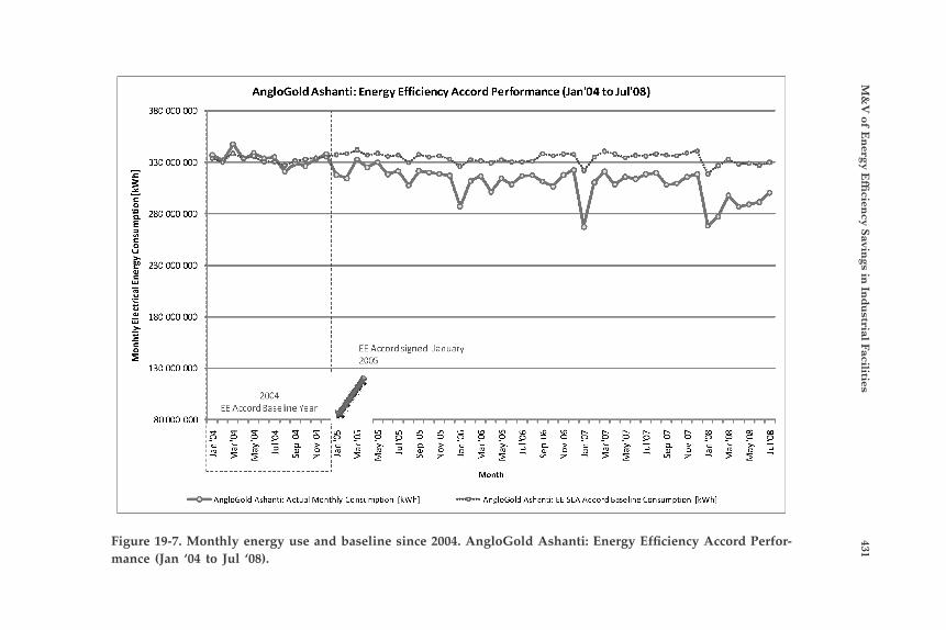
M&
V of E
nergy E
fficien
cy Savings in
Ind
ustrial Facilities
431Figure 19-7. Monthly energy use and baseline since 2004. AngloGold Ashanti: Energy Efficiency Accord Perfor-mance (Jan ‘04 to Jul ‘08).
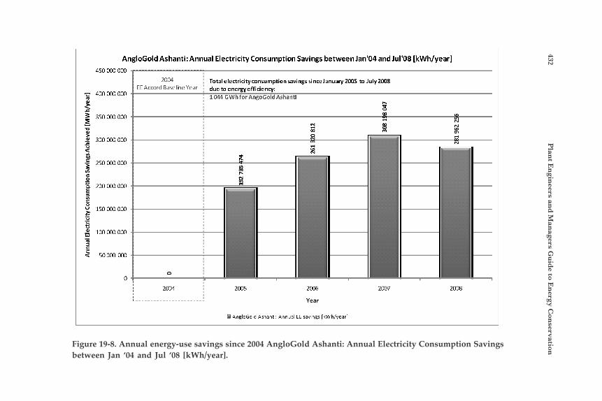
432 P
lant E
ngin
eers and
Man
agers Gu
ide to E
nergy C
onservationFigure 19-8. Annual energy-use savings since 2004 AngloGold Ashanti: Annual Electricity Consumption Savings
between Jan ‘04 and Jul ‘08 [kWh/year].
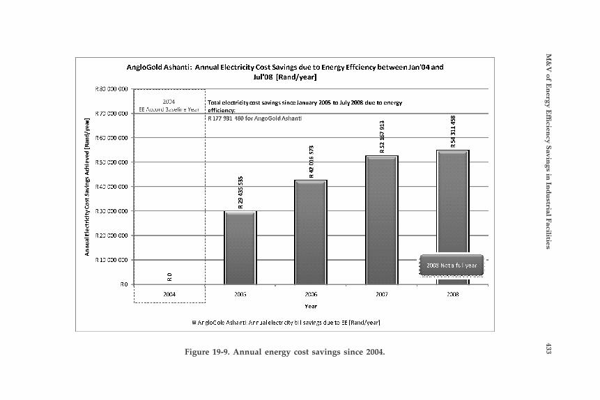
M&
V of E
nergy E
fficien
cy Savings in
Ind
ustrial Facilities
433Figure 19-9. Annual energy cost savings since 2004.
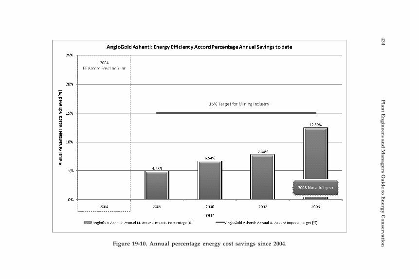
434 P
lant E
ngin
eers and
Man
agers Gu
ide to E
nergy C
onservationFigure 19-10. Annual percentage energy cost savings since 2004.
M&V of Energy Efficiency Savings in Industrial Facilities 435
CONCLUSIONS
In summary, the mine achieved the following:
• 1,044 GWh of electricity saved since 2004, due to electrical energy efficiency.
• R 178 million saving from reduce electricity account from 1 January 2005 to July 2008.
• 1,462 ML of water savings.• CO2 emissions reduced by 939,840 tons since 2005 through energy
efficiency.• SO2 emissions reduced by 9,075 tons.• NOx emissions reduced by 4,584 tons.• Particulate emissions reduced by 240 tons since 2005.• As of July 2008, the mine as a whole was already achieving a 12.3%
energy efficiency savings.
References1. Measurement and Verification Guideline for Energy Efficiency Certificates, Draft,
Council of Measurement and Verification Professionals of South Africa, June 2009.2. Efficiency Valuation Organization, 2007. International Performance Measurement
and Verification Protocol: Concepts and options for determining energy savings. April.
3. North-West University, 2006. Guideline to Measure, Verify and Track Performance under the Energy Efficiency Accord. 28 April. Available from: http://www.nbi.org.za/__documents/SF_EE/measuring_verification_protocol-20060428.pdf
4. Energy Cybernetics, 2008. AngloGold Ashanti: PCP Baseline Adjustment Analysis. 26 November. Confidential report.
437
20Superior Energy Performance:A Roadmap for AchievingContinual EnergyPerformance Improvement
Paul E. Scheihing, U.S. Department of EnergyJoe A. Almaguer, The Dow Chemical CompanySteven C. Schultz, 3M CompanyAimee T. McKane, Lawrence Berkeley National LaboratoryWilliam A. Meffert, Georgia Institute of TechnologyTracy Fisher, Energetics Incorporated
INTRODUCTION
The Superior Energy Performance initiative is designed to provide industrial facilities with a roadmap for achieving continual improvement in energy efficiency while maintaining competitiveness. Likewise, to en-courage broad participation by U.S. industry, the program offers a tiered approach to demonstrating energy intensity improvement. Superior Energy Performance strategic goals are to:
1. Foster an organizational culture of continuous improvement in en-ergy efficiency;
2. Develop a transparent system to validate energy intensity improve-ments and management practices; and thus
3. Create a verified record of energy-source fuel savings and carbon emission reductions with potential market value that could be widely recognized both nationally and internationally.
438 Plant Engineers and Managers Guide to Energy Conservation
A central element of Superior Energy Performance is the implemen-tation of the energy management standard developed by the International Organization for Standardization, ISO 50001, with additional requirements to achieve and document energy intensity improvements over each 3-year period. The program provides a framework for fostering energy efficiency at the plant level and a methodology for measuring and validating energy efficiency/intensity improvements. To ensure that Superior Energy Perfor-mance offers value and flexibility for plants of various sizes and experience in managing energy, the program is conducting field testing in four manu-facturing plants through a pilot program in Texas. The U.S. Council for Energy-Efficient Manufacturing guides the development of Superior Energy Performance. The partnership is a co-operative effort that brings together the respective strengths of industry, standards-making bodies, several federal agencies, national laboratories, universities, and technical experts to initiate the program. Superior Energy Performance will contribute toward reaching a national energy efficiency goal of reducing industrial energy intensity by 25% over the next decade. This voluntary, industry-driven certification program is being de-signed to provide a transparent, globally-accepted system for validating energy intensity performance improvement and management practices at industrial plants. A non-governmental organization will provide ANSI-accredited certification to U.S. manufacturing facilities. It is anticipated that Superior Energy Performance will launch in June 2011 and will com-plete the transition from a federally supported development period to a fee-based program administered by the non-governmental, not-for-profit entity by 2013. The U.S. Council for Energy-Efficient Manufacturing (U.S. CEEM) seeks to enable U.S. industry to achieve global leadership in energy ef-ficiency and greenhouse gas emissions reduction. It is a voluntary part-nership between industry, government, and other organizations and is led by a committee of representatives from the following organizations: 3M Company, the Alliance to Save Energy, The Dow Chemical Compa-ny, Eastman Chemical Company, Ford Motor Company, Frito-Lay, HP, Huntsman, LyondellBasell, National Institute of Science & Technology (NIST) Manufacturing Extension Partnership Program, Owens Corning, PPG Industries, Toyota Motor Corporation, Texas Industries of the Fu-ture, SSAB, U.S. Department of Energy Industrial Technologies Program (DOE/ITP), U.S. Environmental Protection Agency (EPA) ENERGY STAR program, and Weyerhaeuser.
Power Quality Case Studies 439
NEED AND VALUE TO INDUSTRY
The cost of purchasing the energy needed for production by an in-dustrial facility is viewed as managed input and typically receives signifi-cant attention, while the use of that energy once inside the factory is often viewed as simply the cost of doing business. While this is not true in all industrial facilities, experience has shown that unless facilities actively manage energy use and have a documented plan for doing so, these fa-cilities are significantly less energy efficient than they could be. Without performance indicators that relate energy consumption to production output, it is difficult to measure or document improvements in energy in-tensity. Some U.S. industrial firms have already established internal goals to improve energy intensity and their environmental footprint; participa-tion in Superior Energy Performance offers a practical and transparent approach for achieving and validating these efforts. The value proposition to U.S. industry for participation in Superior Energy Performance also includes the following benefits:• Increases a company’s ability to replicate and document energy
management successes.• Provides assurance that energy system assessment recommenda-
tions are sound and produce predicted results.• Provides a mechanism for communicating with stakeholders re-
garding energy management progress.• Provides national recognition by a third party of the site’s leader-
ship in energy management.• Puts into place a process of continuous improvement of energy use
per product output over time.• Provides a recognized mechanism for a manufacturing facility to
qualify for preferred supplier status based on energy management criteria.
• Provides improved opportunities for utility and state financial in-centives for energy efficiency as a result of using recognized assess-ment practices and measurement and verification (M&V) protocols.
PROGRAM ELEMENTS
In support of Superior Energy Performance, several program ele-ments are under development. (See Figure 20-1.) These elements will ad-
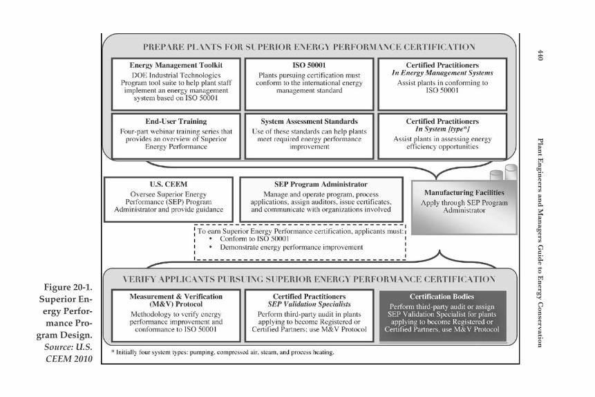
440 P
lant E
ngin
eers and
Man
agers Gu
ide to E
nergy C
onservation
Figure 20-1. Superior En-ergy Perfor-mance Pro-
gram Design. Source: U.S. CEEM 2010
Energy Management Toolkit I S 0 5oO01 Certified Practitioners DOE Industrial lcchnologics
Program tool suite to help plant staff
system bascd on IS0 50001
Plants pursuing ccrtitication niust conlimn to the international energy
In Energy .Management Sys~cms Assist plants in conlorming to
implement an energy managenient management standard I S 0 so01
End-User Training Systcm .kssament Standards Four-pan wehinar training series that
provides an overview of Supcrior Use of these standards can help plants
meet reqnired energy performance Energy Pcrformancc improvement
1J.S. CEEM SEP Program Administrator Oversee Superior Energy
Pcrfoniiancc (SEP) Program Administrator and provide guidance
Manage and operate program. prnces.. applications. assign auditors. issue ccrtiticatcs. and communicate with organizations involved
Certified Practitioners In System [type"I
Assist plants in assessing encrgy cfficiency opportunitics
Manufacturing Facilities Apply throu:h SEP Prognm
.4dininistrator
To earn Superior Energy Pertorniance certification, applicants must:
Dcmonstrate energy pcrfomiance iniprovcincnt
Measurement 8; Verification Certified Practitioners Certification Bodies
Mcthdolosq to vcrify cncrgy pcrformancc improvcmcnt and
conformance to I S 0 50001
(MBrV) Protncol .$El' Validation SpecialisLs Pertorni third-pany audit or assign SEP Validation Spccialist for plants applying to bccomc Kcgistcmd or
Certified Partners. use .MI\' Protocol
Pcrform third-party audit in plants applying to bccomc Kcgistcrrd or
Certified Pdners: use M&\' Protocol
Power Quality Case Studies 441
dress fundamental problems: lack of awareness of the energy efficiency opportunities, lack of understanding on how to implement energy effi-ciency improvements, and most importantly, the lack of a consistent orga-nizational structure within most industrial facilities to effectively manage energy use.
Energy Management Standard The ISO management system standard for energy (ISO 50001) is an international framework for industrial plants or entire companies to manage energy, including all aspects of procurement and use. ISO 50001 will provide organizations and companies with technical and manage-ment strategies to increase energy efficiency, reduce costs, and improve environmental performance. Based on broad applicability across national economic sectors, the standard could influence up to 60% of the world’s energy demand. Conformance with the energy management standard will demon-strate that the plant or company has sustainable energy management systems in place, has completed a baseline of energy use, and has a com-mitment to continuous improvement of its energy intensity. ISO 50001 is being written to be compatible with current management system stan-dards such as ISO 9001 (quality management) and ISO 14001 (environ-mental management)—standards that are used widely throughout the world. The U.S. Council for Energy-Efficient Manufacturing and DOE are supporting American National Standards Institute’s (ANSI) U.S. Techni-cal Advisory Group (TAG) and ANSI’s role as Secretariat of ISO Project Committee 242 in developing ISO 50001. The Georgia Institute of Technology developed the first comprehen-sive, ANSI-compatible energy management standard (MSE 2000) in 2000. This standard was revised in 2008 and is a core component of the Supe-rior Energy Performance pilot program in Texas. The revised ANSI/MSE standard is one of the inputs being presented to the ISO Project Commit-tee 242. The initial plants certified under Superior Energy Performance will use the ANSI/MSE energy management standard, and the program will transition to ISO 50001.
System Assessment Standards To support plants implementing a management system for energy, DOE spearheaded the development of assessment standards for four energy systems: pumping, compressed air, steam, and process heating.
442 Plant Engineers and Managers Guide to Energy Conservation
By applying these standards, the systems are analyzed through vari-ous techniques, such as measurement and analysis, which will identify, document, and prioritize energy performance improvement opportuni-ties. These standards were developed by project teams with the Ameri-can Society of Mechanical Engineers (ASME) serving as the ANSI-ac-credited standards developer. Guidance documents provide technical background and application details to support use of the standards. The system assessment standards are not required for participation in the Superior Energy Performance initiative but are very valuable for par-ticipants because they clearly define a pathway for quickly achieving energy savings.
Measurement and Verification Protocol An essential element of certifying plants for energy efficiency is validating plant performance through measurement and verification. The Superior Energy Performance Measurement and Verification Pro-tocol (M&V Protocol) offers a best practice methodology to: 1) verify the results and impact from implementation of the energy management standard; 2) quantify energy savings from specific measures or projects; and 3) track how much intensity changes over time for the overall plant. The M&V Protocol documents normalize energy performance indica-tors (such as Btu/pound of product) and validates energy savings so that reported savings can be used to determine carbon impact. Applica-tion and testing of the M&V Protocol began in the Texas pilot plants in January 2010. Separate classes of experts who can maintain independence during the verification process are required for this activity. While this area is still under development, based on other certification models, a two-part sys-tem is anticipated: individuals who are certified to validate performance for a plant seeking certification (Superior Energy Performance validation specialists), and ANSI-accredited organizations (certification bodies) le-gally qualified to issue a certification to the plant based on the reported and validated energy intensity improvement and energy management processes.
Certified Practitioners Experiences in the United States and other countries have shown that the appropriate application of the energy management standard and system assessment standards will require significant training and skill.

Power Quality Case Studies 443
For this reason, a program to certify practitioners via a professional cer-tification program is in development. These practitioners will provide assistance to applicants in assessing energy efficiency opportunities in various types of energy systems—pumping, compressed air, steam, or process heating—and will conform to the requirements of the ISO 50001 energy management system. A company or industrial plant may use the energy management or system assessment standards on its own without engaging a certified practitioner. However, using a qualified individual adds a level of assurance for the plant that the standards will be properly applied. These practitioners will be plant personnel, consulting profession-als, or service providers with the appropriate technical experience in in-dustrial systems. Candidates will be subject to a rigorous qualification exam and, once certified, periodic professional enrichment requirements. As noted above, a certification program will also be developed for appli-cation of the M&V Protocol by Superior Energy Performance validation specialists. These practitioner certification programs will be developed starting in 2010, and pilot training will begin in January 2011.
End-user Awareness Training Superior Energy Performance participants need to be made aware of the overall program requirements, ISO 50001, system assessment stan-dards, and the M&V Protocol. End-user awareness training modules will provide brief overviews of these program elements; the modules can be given stand-alone, via the internet, or integrated with more comprehen-sive training.
Texas Pilot Project Energy experts are working with staff from four manufacturing plants in Texas to field test the program elements. The goal of the Texas pilot project is to verify that the processes, standards, and performance criteria under the Superior Energy Performance are 1) practical and achievable, 2) provide benefit to participating plants, and 3) reliably iden-tify plants that meet the proposed certification criteria. Diverse facilities were recruited to provide a robust assessment of the proposed Superior Energy Performance program scheme. The sites represent three industrial sectors—insulation, semiconductors, and chemicals—and a range of size and experience in energy management. The four facilities participating in the pilot project are:
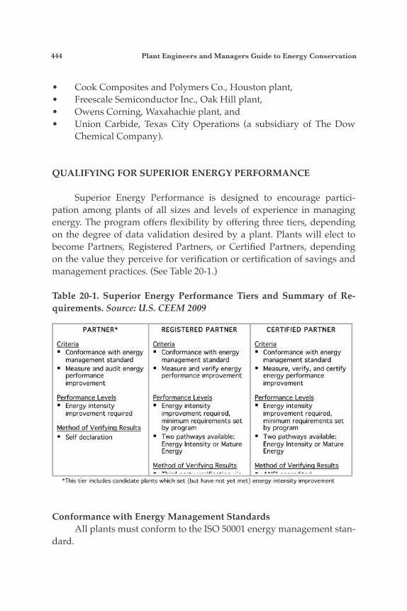
444 Plant Engineers and Managers Guide to Energy Conservation
• Cook Composites and Polymers Co., Houston plant,• Freescale Semiconductor Inc., Oak Hill plant,• Owens Corning, Waxahachie plant, and• Union Carbide, Texas City Operations (a subsidiary of The Dow
Chemical Company).
QUALIFYING FOR SUPERIOR ENERGY PERFORMANCE
Superior Energy Performance is designed to encourage partici-pation among plants of all sizes and levels of experience in managing energy. The program offers flexibility by offering three tiers, depending on the degree of data validation desired by a plant. Plants will elect to become Partners, Registered Partners, or Certified Partners, depending on the value they perceive for verification or certification of savings and management practices. (See Table 20-1.)
Table 20-1. Superior Energy Performance Tiers and Summary of Re-quirements. Source: U.S. CEEM 2009
Conformance with Energy Management Standards All plants must conform to the ISO 50001 energy management stan-dard.
PARTNER*
Criteria . Conformance with energy management standard Measwe and audit energy pelfortname impmvemnt
ktformance Levels Energy intendty improvement rquired
Method of VeriiMm Results . Self declaration
This tier includes cartdidate pl
REGISTERED PARTNER
Cnnformmsnce with energy management standard Measure and verify energy performance improvement
Performance Levels Energy intensity improvement required, minimum requirements set by program Two pathways available: Energy Intensity or Mature E n e w
Method of Verifvina Results
ts which set (but have not yet me1 - =.:-A ,s:--*,-- . . I _
CERTIFIED PARTNER
. Conformance with energy management standard Mesure. verify, and certify energy perFormance improvement
Performance Levelp Energy intensity improvement required, minimum requirements set b P m w m . Two pathways available: Energy Intensity or Mature Energy
M e t h d of Verihina Results
mergy intensity improvement - *.,r* - - - - - A - I * . - I
Power Quality Case Studies 445
Achievement of Performance Levels The variety of performance levels offered through Superior Energy Performance acknowledges the wide range of industrial plants and their varying levels of experience. All plants applying to Superior Energy Per-formance must demonstrate an energy intensity improvement over the previous three years to qualify. To encourage plants to achieve greater energy intensity reductions, Superior Energy Performance also offers sil-ver, gold, and platinum designations based on higher performance levels. These designations are available only at the Registered Partner and Certi-fied Partner tiers. The program also provides two pathways for demonstrating per-formance levels. Most plants will qualify through the first pathway by demonstrating an energy intensity improvement. Achieving high percentages of energy intensity improvements will prove to be more challenging for plants that have mature energy management programs in place and have already identified energy saving opportunities and implemented efficiency improvements for the last decade or more. Therefore, the second pathway takes into account both a plant’s energy management system and continued efforts to improve energy intensity. These two pathways apply only to plants at the Registered Partner or Certified Partner level.
Method of Verifying Results All participating plants are required to verify conformance with the energy management system and energy performance improvement us-ing the Superior Energy Performance M&V Protocol. Three methods for verifying results are offered:
• Self-declaration (Partner): Plants applying to become Superior En-ergy Performance Partners will self-declare their conformance to the program requirements. Self-declaration may include audits con-ducted by team members within the plant or by off-site corporate representatives.
• Third-party verification by remote review (Registered Partner): Plants applying to become Superior Energy Performance Regis-tered Partners are required to submit materials for a remote review. A certified Superior Energy Performance validation specialist will conduct the remote review.

446 Plant Engineers and Managers Guide to Energy Conservation
• ANSI-accredited certification with an on-site visit by a Superior En-ergy Performance validation specialist (Certified Partner): Plants applying to become Certified Partners will submit required mate-rial to an ANSI-accredited third party certification body. The veri-fication body will send a Superior Energy Performance validation specialist for a site visit and will provide certification of the results.
Renewal of Participation Every three years participating plants will resubmit performance and management system information documenting that they have met Superior Energy Performance criteria.
SUPERIOR ENERGY PERFORMANCE STATUS
The U.S. Council for Energy-Efficient Manufacturing is providing guidance and oversight throughout the development process. Industry representatives are engaged in both developing and testing the program elements, strategy, scheme, and requirements. It is anticipated that the first plants will be certified in September 2010 and that the national, vol-untary program will launch in June 2011. The current development status of Superior Energy Performance is shown in Figure 20-2. Other upcoming activities include:
• Selecting a Superior Energy Performance Program administrator to manage operations.
• Finalizing performance requirements and periods for Registered and Certified Partners seeking to qualify for silver, gold, and plati-num levels.
• Establishing the public identity for the certification program.
• Identifying qualified certification bodies.
• Identifying an ANSI-accredited personnel body to provide over-sight for each type of certified practitioner
The U.S. Council for Energy-Efficient Manufacturing will conduct outreach to a wider stakeholder base to seek input in developing and de-
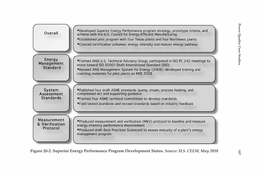
Pow
er Qu
ality Case Stu
dies
447Figure 20-2. Superior Energy Performance Program Development Status. Source: U.S. CEEM, May 2010
Ove ra I I scheme with the U.S. Council for Energy-Efficient Manufacturing .Established pilot program with four Texas plants and four Northwest plants .Created certtficatron schemes: energy intensity and mature energy pathway
System Assessment Standards i
Energy Management
Standard
.Formed ANSI U.S. Technical Advisory Group: parttlapated in IS0 PC 242 meetings t o move toward IS0 50001 Draft International Standard (DIS) .Revised ANSI Management System for Energy (2008); developed training and coaching materials for pilot plants on MSE 2008
Measurement & Verification
Protocol
.Published four draft ASME standards (pump, steam, process heating, and compressed air) and supporting guidance .Formed four ASME technical committees to develop standards "Field tested standards and revised standards based on industry feedback
I .Produced measurement and verification (M&V) protocol to baseline and measure energy intensity performance improvement .Produced draR Best Practices Scorecard t o assess maturity of a plant's energy management program

448 Plant Engineers and Managers Guide to Energy Conservation
fining the Superior Energy Performance program strategy. Stakeholders include state agencies, utilities, non-governmental organizations, trade associations, and equipment/service providers. To learn more about Superior Energy Performance and the U.S. Council for Energy-Efficient Manufacturing, visit www.superiorenergy-performance.net.
CONCLUSION
Superior Energy Performance will provide industrial plants with an opportunity to improve their energy performance and validate their energy efficiency/intensity improvements through an ANSI-accredited process. The program encourages participation by plants of all sizes and levels of experience by providing a tiered approach and mobilizing re-sources from states and utilities to assist plants. The U.S. Council for En-ergy-Efficient Manufacturing is developing Superior Energy Performance and providing leadership in the development of standards and protocols to be applied in the program to achieve energy-source fuel savings and carbon emission reductions with potential market value that could be rec-ognized both nationally and internationally.
References1. American National Standards Institute. 2008. Management System for Energy
2000:2008, developed by Georgia Institute of Technology. March 2008, Washington, DC.
2. McKane, Aimee, and Paul Sheaffer. 2008. “System Assessment Standards: Defining the Market for Assessment Services.” In Proceedings of the 30th National Industrial En-ergy Technology Conference, May 2008, New Orleans, LA.
3. McKane, Aimee, Paul Scheihing, and Robert Williams. 2007. “Certifying Industrial Energy Efficiency Performance: Aligning Management, Measurement, and Practice to Create Market Value.” In Proceedings of ACEEE Summer Study for Industry, July 24-27, 2007, White Plains, NY. LBNL- 63413.
4. Scheihing, Paul, Steve Schultz, and Joe Almaguer. 2008. “Certifying U.S. Manufactur-ing Plants for Energy Efficiency.” In Proceedings of the 30th National Industrial Energy Technology Conference, May 2008, New Orleans, LA.
449
21Steam SystemOptimization: A Case Study
The steam system optimization (generation, distribution, use, and condensate return) offers a large opportunity to comply with the new levels of energy efficiency standards. Superior design and improved maintenance practices are the two main sources of savings in steam systems. Increased competition no longer permits an industry to survive with energy waste that could be eliminated. This chapter highlights the study findings of the steam system in a plant from the food industry. The steam system operates with an annual budget of $1.9 million. Normal steam demand ranges between 80,000 and 85,000 lb/hr. The steam system analysis identified energy savings worth $270,000 per year. The optimization measures were in two categories:
• No cost/low cost optimizations that can be done through better maintenance and improved operating conditions.
• Major improvements that require a significant investment and include the modification of the process and major equipment.
INTRODUCTION
Nearly half of industrial energy is used to generate steam. Improv-ing steam system efficiency will contribute significantly to the profit-ability for every plant. There are proven energy savings techniques that
Presented at the 22nd World Energy Engineering Congress by Nevena Ior-danova, Ven V. Venkatesan, and Michael Calogero
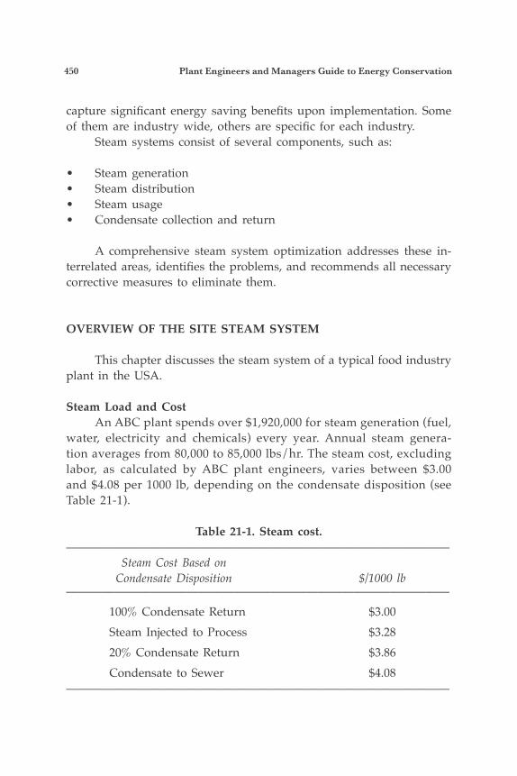
450 Plant Engineers and Managers Guide to Energy Conservation
capture significant energy saving benefits upon implementation. Some of them are industry wide, others are specific for each industry. Steam systems consist of several components, such as:
• Steam generation• Steam distribution• Steam usage• Condensate collection and return
A comprehensive steam system optimization addresses these in-terrelated areas, identifies the problems, and recommends all necessary corrective measures to eliminate them.
OVERVIEW OF THE SITE STEAM SYSTEM
This chapter discusses the steam system of a typical food industry plant in the USA.
Steam Load and Cost An ABC plant spends over $1,920,000 for steam generation (fuel, water, electricity and chemicals) every year. Annual steam genera-tion averages from 80,000 to 85,000 lbs/hr. The steam cost, excluding labor, as calculated by ABC plant engineers, varies between $3.00 and $4.08 per 1000 lb, depending on the condensate disposition (see Table 21-1).
Table 21-1. Steam cost.———————————————————————————————— Steam Cost Based on Condensate Disposition $/1000 lb———————————————————————————————— 100% Condensate Return $3.00 Steam Injected to Process $3.28 20% Condensate Return $3.86 Condensate to Sewer $4.08————————————————————————————————
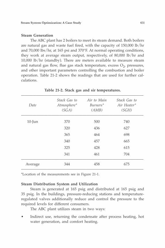
Steam System Optimization: A Case Study 451
Steam Generation The ABC plant has 2 boilers to meet its steam demand. Both boilers are natural gas and waste fuel fired, with the capacity of 150,000 lb/hr and 70,000 lbs/hr, at 165 psi and 370°F. At normal operating conditions, they work at average steam output, respectively, of 80,000 lb/hr and 10,000 lb/hr (standby). There are meters available to measure steam and natural gas flow, flue gas stack temperature, excess O2, pressures, and other important parameters controlling the combustion and boiler operation. Table 21-2 shows the readings that are used for further cal-culations.
Table 21-2. Stack gas and sir temperatures.———————————————————————————————— Stack Gas to Air to Main Stack Gas to Date Atmosphere* Burners* Air Heater* (SGA) (AMB) (SGH)———————————————————————————————— 10-Jun 370 500 740 320 436 627 365 464 698 340 457 665 325 428 615 341 461 704———————————————————————————————— Average 344 458 675————————————————————————————————*Location of the measurements see in Figure 21-1.
Steam Distribution System and Utilization Steam is generated at 165 psig and distributed at 165 psig and 35 psig. In the buildings, pressure-reducing stations and temperature-regulated valves additionally reduce and control the pressure to the required levels for different consumers. The ABC plant utilizes steam in two ways:
• Indirect use, returning the condensate after process heating, hot water generation, and comfort heating.
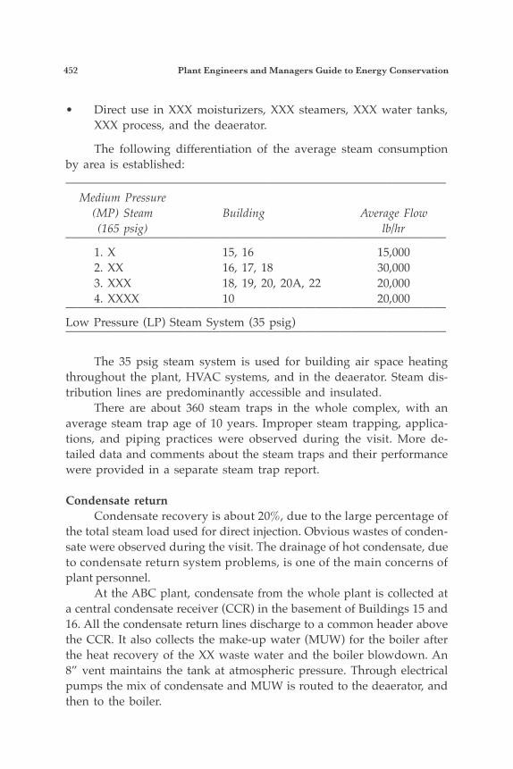
452 Plant Engineers and Managers Guide to Energy Conservation
• Direct use in XXX moisturizers, XXX steamers, XXX water tanks, XXX process, and the deaerator.
The following differentiation of the average steam consumption by area is established:———————————————————————————————— Medium Pressure (MP) Steam Building Average Flow (165 psig) lb/hr———————————————————————————————— 1. X 15, 16 15,000 2. XX 16, 17, 18 30,000 3. XXX 18, 19, 20, 20A, 22 20,000 4. XXXX 10 20,000————————————————————————————————Low Pressure (LP) Steam System (35 psig)————————————————————————————————
The 35 psig steam system is used for building air space heating throughout the plant, HVAC systems, and in the deaerator. Steam dis-tribution lines are predominantly accessible and insulated. There are about 360 steam traps in the whole complex, with an average steam trap age of 10 years. Improper steam trapping, applica-tions, and piping practices were observed during the visit. More de-tailed data and comments about the steam traps and their performance were provided in a separate steam trap report.
Condensate return Condensate recovery is about 20%, due to the large percentage of the total steam load used for direct injection. Obvious wastes of conden-sate were observed during the visit. The drainage of hot condensate, due to condensate return system problems, is one of the main concerns of plant personnel. At the ABC plant, condensate from the whole plant is collected at a central condensate receiver (CCR) in the basement of Buildings 15 and 16. All the condensate return lines discharge to a common header above the CCR. It also collects the make-up water (MUW) for the boiler after the heat recovery of the XX waste water and the boiler blowdown. An 8” vent maintains the tank at atmospheric pressure. Through electrical pumps the mix of condensate and MUW is routed to the deaerator, and then to the boiler.

Steam System Optimization: A Case Study 453
The medium pressure condensate (CM) and low pressure conden-sate (CL) is either returned by direct discharge (steam traps) to the CCR or through pumps from the farthest points of the plant (Nitrogen and Mix XX areas). The MP steam users working in a modulated pressure control were identified as the part of the system presenting the most difficulty in returning condensate to the CCR.
SAVINGS OPPORTUNITIES
A thorough review of the system confirmed there are energy sav-ing potentials in the boiler system, steam distribution system, and con-densate return system. The following paragraphs highlight eight energy savings opportunities identified at the site and describe the measures proposed to realize these savings.
1. Install Economizer in the Boiler Stack to Recover the Heat from Flue Gases. To recover the heat from the flue gases, the ABC plant has installed an air preheater in the boiler stack. During the study, the boiler was operating at an average load of 80,000 lbs/h, with 7.3% oxygen and 340°F stack temperature. A forced draft (FD) fan supplies the combus-tion air to the air preheater, and then to the boiler. The ambient air is preheated from ambient temperature to 460°F, while the flue gases are cooled by more than 360°F. Although there is heat recovery, the flue gas temperature is higher than optimum and shows a possibility for further heat recovery. One of the most effective ways to recover energy from flue gases is to use an economizer to preheat the lower temperature water (make-up water) going into the boiler. At 165 psig, the temperature of the steam and water in the boiler is about 370°F, and each pound of water needs 290 Btu/lb to reach the boiling point. Hot flue gases contain a lot of wasted energy. It is beneficial to put this energy back into the boiler with the heat recovery equipment. Preheating the incoming feedwater to the deaerator (after the CCR) in an economizer will improve the boiler efficiency. Since economizers are fairly expensive and must be justified by a high level of boiler uti-lization. Once installed, they are usually trouble-free and require little maintenance.
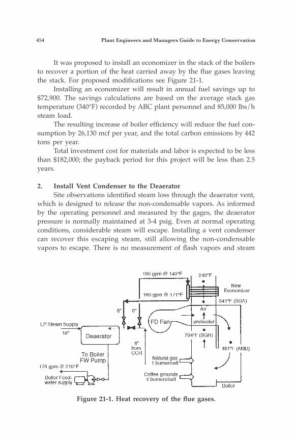
454 Plant Engineers and Managers Guide to Energy Conservation
It was proposed to install an economizer in the stack of the boilers to recover a portion of the heat carried away by the flue gases leaving the stack. For proposed modifications see Figure 21-1. Installing an economizer will result in annual fuel savings up to $72,900. The savings calculations are based on the average stack gas temperature (340°F) recorded by ABC plant personnel and 85,000 lbs/h steam load. The resulting increase of boiler efficiency will reduce the fuel con-sumption by 26,130 mcf per year, and the total carbon emissions by 442 tons per year. Total investment cost for materials and labor is expected to be less than $182,000; the payback period for this project will be less than 2.5 years.
2. Install Vent Condenser to the Deaerator Site observations identified steam loss through the deaerator vent, which is designed to release the non-condensable vapors. As informed by the operating personnel and measured by the gages, the deaerator pressure is normally maintained at 3-4 psig. Even at normal operating conditions, considerable steam will escape. Installing a vent condenser can recover this escaping steam, still allowing the non-condensable vapors to escape. There is no measurement of flash vapors and steam
Figure 21-1. Heat recovery of the flue gases.
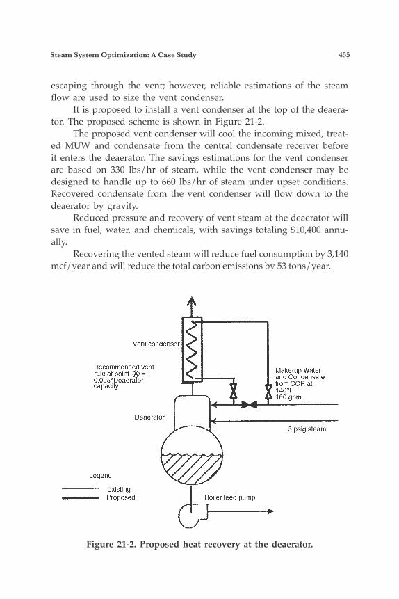
Steam System Optimization: A Case Study 455
escaping through the vent; however, reliable estimations of the steam flow are used to size the vent condenser. It is proposed to install a vent condenser at the top of the deaera-tor. The proposed scheme is shown in Figure 21-2. The proposed vent condenser will cool the incoming mixed, treat-ed MUW and condensate from the central condensate receiver before it enters the deaerator. The savings estimations for the vent condenser are based on 330 lbs/hr of steam, while the vent condenser may be designed to handle up to 660 lbs/hr of steam under upset conditions. Recovered condensate from the vent condenser will flow down to the deaerator by gravity. Reduced pressure and recovery of vent steam at the deaerator will save in fuel, water, and chemicals, with savings totaling $10,400 annu-ally. Recovering the vented steam will reduce fuel consumption by 3,140 mcf/year and will reduce the total carbon emissions by 53 tons/year.
Figure 21-2. Proposed heat recovery at the deaerator.
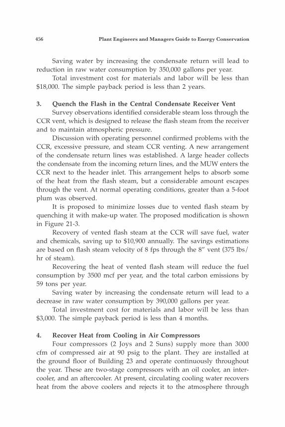
456 Plant Engineers and Managers Guide to Energy Conservation
Saving water by increasing the condensate return will lead to reduction in raw water consumption by 350,000 gallons per year. Total investment cost for materials and labor will be less than $18,000. The simple payback period is less than 2 years.
3. Quench the Flash in the Central Condensate Receiver Vent Survey observations identified considerable steam loss through the CCR vent, which is designed to release the flash steam from the receiver and to maintain atmospheric pressure. Discussion with operating personnel confirmed problems with the CCR, excessive pressure, and steam CCR venting. A new arrangement of the condensate return lines was established. A large header collects the condensate from the incoming return lines, and the MUW enters the CCR next to the header inlet. This arrangement helps to absorb some of the heat from the flash steam, but a considerable amount escapes through the vent. At normal operating conditions, greater than a 5-foot plum was observed. It is proposed to minimize losses due to vented flash steam by quenching it with make-up water. The proposed modification is shown in Figure 21-3. Recovery of vented flash steam at the CCR will save fuel, water and chemicals, saving up to $10,900 annually. The savings estimations are based on flash steam velocity of 8 fps through the 8” vent (375 lbs/hr of steam). Recovering the heat of vented flash steam will reduce the fuel consumption by 3500 mcf per year, and the total carbon emissions by 59 tons per year. Saving water by increasing the condensate return will lead to a decrease in raw water consumption by 390,000 gallons per year. Total investment cost for materials and labor will be less than $3,000. The simple payback period is less than 4 months.
4. Recover Heat from Cooling in Air Compressors Four compressors (2 Joys and 2 Suns) supply more than 3000 cfm of compressed air at 90 psig to the plant. They are installed at the ground floor of Building 23 and operate continuously throughout the year. These are two-stage compressors with an oil cooler, an inter-cooler, and an aftercooler. At present, circulating cooling water recovers heat from the above coolers and rejects it to the atmosphere through
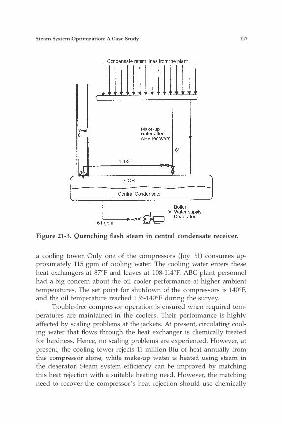
Steam System Optimization: A Case Study 457
a cooling tower. Only one of the compressors (Joy #1) consumes ap-proximately 115 gpm of cooling water. The cooling water enters these heat exchangers at 87°F and leaves at 108-114°F. ABC plant personnel had a big concern about the oil cooler performance at higher ambient temperatures. The set point for shutdown of the compressors is 140°F, and the oil temperature reached 136-140°F during the survey. Trouble-free compressor operation is ensured when required tem-peratures are maintained in the coolers. Their performance is highly affected by scaling problems at the jackets. At present, circulating cool-ing water that flows through the heat exchanger is chemically treated for hardness. Hence, no scaling problems are experienced. However, at present, the cooling tower rejects 11 million Btu of heat annually from this compressor alone, while make-up water is heated using steam in the deaerator. Steam system efficiency can be improved by matching this heat rejection with a suitable heating need. However, the matching need to recover the compressor’s heat rejection should use chemically
Figure 21-3. Quenching flash steam in central condensate receiver.
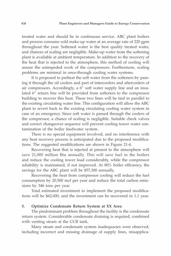
458 Plant Engineers and Managers Guide to Energy Conservation
treated water and should be in continuous service. ABC plant boilers and process consume cold make-up water at an average rate of 220 gpm throughout the year. Softened water is the best quality treated water, and chances of scaling are negligible. Make-up water from the softening plant is available at ambient temperature. In addition to the recovery of the heat that is rejected to the atmosphere, this method of cooling will assure the unimpeded work of the compressors. Furthermore, scaling problems are minimal in once-through cooling water systems. It is proposed to preheat the soft water from the softeners by pass-ing it through the oil coolers and part of intercoolers and aftercoolers of air compressors. Accordingly, a 6” soft water supply line and an insu-lated 6” return line will be provided from softeners to the compressor building to recover this heat. These two lines will be tied in parallel to the existing circulating water line. This configuration will allow the ABC plant to revert back to the existing circulating cooling water system in case of an emergency. Since soft water is passed through the coolers of the compressor, a chance of scaling is negligible. Suitable check valves and correct changeover sequence will prevent cooling tower water con-tamination of the boiler feedwater system. There is no special equipment involved, and no interference with any heat recovery process is anticipated due to the proposed modifica-tions. The suggested modifications are shown in Figure 21-4. Recovering heat that is rejected at present to the atmosphere will save 21,000 million Btu annually. This will save fuel in the boilers and reduce the cooling tower load considerably, while the compressor reliability is maintained, if not improved. At 80% boiler efficiency, the savings for the ABC plant will be $57,300 annually. Recovering the heat from compressor cooling will reduce the fuel consumption by 20,500 mcf per year and reduce the total carbon emis-sions by 346 tons per year. Total estimated investment to implement the proposed modifica-tions will be $62,000, and the investment can be recovered in 1.1 year.
5. Optimize Condensate Return System at XX Area The predominant problem throughout the facility is the condensate return system. Considerable condensate draining is required, combined with venting steam at the CCR tank. Many steam and condensate system inadequacies were observed, including incorrect and missing drainage of supply lines, misapplica-
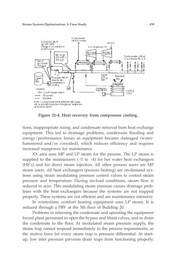
Steam System Optimization: A Case Study 459
tions, inappropriate sizing, and condensate removal from heat exchange equipment. This led to drainage problems, condensate flooding and energy/performance losses as equipment became damaged (water-hammered and/or corroded), which reduces efficiency and requires increased manpower for maintenance. XX area uses MP and LP steam for the process. The LP steam is supplied to the moisturizers (#1 to #4) for hot water heat exchangers (HE’s) and for direct steam injection. All other process users are MP steam users. All heat exchangers (process heating) are on-demand sys-tems using steam modulating pressure control valves to control steam pressure and temperature. During no-load conditions, steam flow is reduced to zero. This modulating steam pressure causes drainage prob-lems with the heat exchangers because the systems are not trapped properly. These systems are not efficient and are maintenance intensive. In wintertime, comfort heating equipment uses LP steam. It is reduced through a PRV at the 5th floor of Building 20. Problems in returning the condensate and operating the equipment forced plant personnel to open the bypass and bleed valves, and to drain the condensate to the floor. At modulated steam pressure supply, the steam trap cannot respond immediately to the process requirements, as the motive force for every steam trap is pressure differential. At start-up, low inlet pressure prevents drain traps from functioning properly.
Figure 21-4. Heat recovery from compressor cooling.
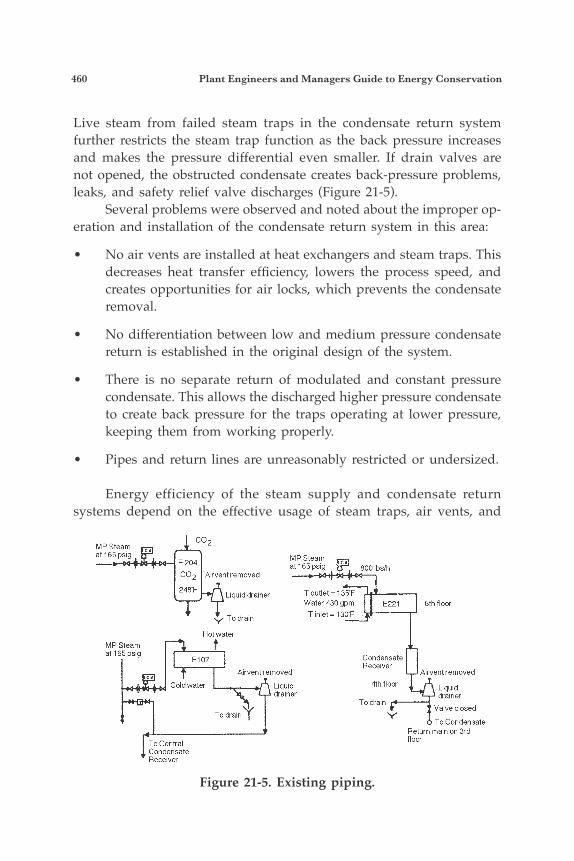
460 Plant Engineers and Managers Guide to Energy Conservation
Live steam from failed steam traps in the condensate return system further restricts the steam trap function as the back pressure increases and makes the pressure differential even smaller. If drain valves are not opened, the obstructed condensate creates back-pressure problems, leaks, and safety relief valve discharges (Figure 21-5). Several problems were observed and noted about the improper op-eration and installation of the condensate return system in this area:
• No air vents are installed at heat exchangers and steam traps. This decreases heat transfer efficiency, lowers the process speed, and creates opportunities for air locks, which prevents the condensate removal.
• No differentiation between low and medium pressure condensate return is established in the original design of the system.
• There is no separate return of modulated and constant pressure condensate. This allows the discharged higher pressure condensate to create back pressure for the traps operating at lower pressure, keeping them from working properly.
• Pipes and return lines are unreasonably restricted or undersized.
Energy efficiency of the steam supply and condensate return systems depend on the effective usage of steam traps, air vents, and
Figure 21-5. Existing piping.
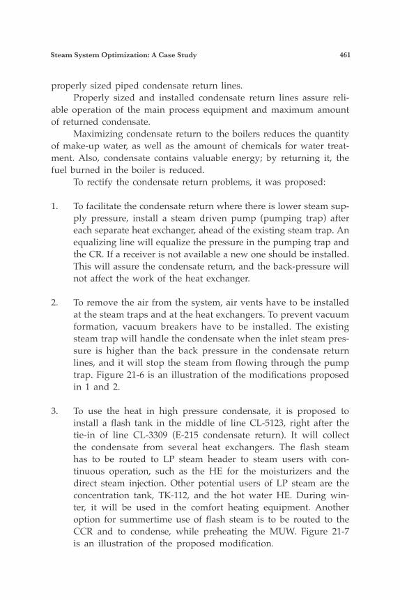
Steam System Optimization: A Case Study 461
properly sized piped condensate return lines. Properly sized and installed condensate return lines assure reli-able operation of the main process equipment and maximum amount of returned condensate. Maximizing condensate return to the boilers reduces the quantity of make-up water, as well as the amount of chemicals for water treat-ment. Also, condensate contains valuable energy; by returning it, the fuel burned in the boiler is reduced. To rectify the condensate return problems, it was proposed:
1. To facilitate the condensate return where there is lower steam sup-ply pressure, install a steam driven pump (pumping trap) after each separate heat exchanger, ahead of the existing steam trap. An equalizing line will equalize the pressure in the pumping trap and the CR. If a receiver is not available a new one should be installed. This will assure the condensate return, and the back-pressure will not affect the work of the heat exchanger.
2. To remove the air from the system, air vents have to be installed at the steam traps and at the heat exchangers. To prevent vacuum formation, vacuum breakers have to be installed. The existing steam trap will handle the condensate when the inlet steam pres-sure is higher than the back pressure in the condensate return lines, and it will stop the steam from flowing through the pump trap. Figure 21-6 is an illustration of the modifications proposed in 1 and 2.
3. To use the heat in high pressure condensate, it is proposed to install a flash tank in the middle of line CL-5123, right after the tie-in of line CL-3309 (E-215 condensate return). It will collect the condensate from several heat exchangers. The flash steam has to be routed to LP steam header to steam users with con-tinuous operation, such as the HE for the moisturizers and the direct steam injection. Other potential users of LP steam are the concentration tank, TK-112, and the hot water HE. During win-ter, it will be used in the comfort heating equipment. Another option for summertime use of flash steam is to be routed to the CCR and to condense, while preheating the MUW. Figure 21-7 is an illustration of the proposed modification.
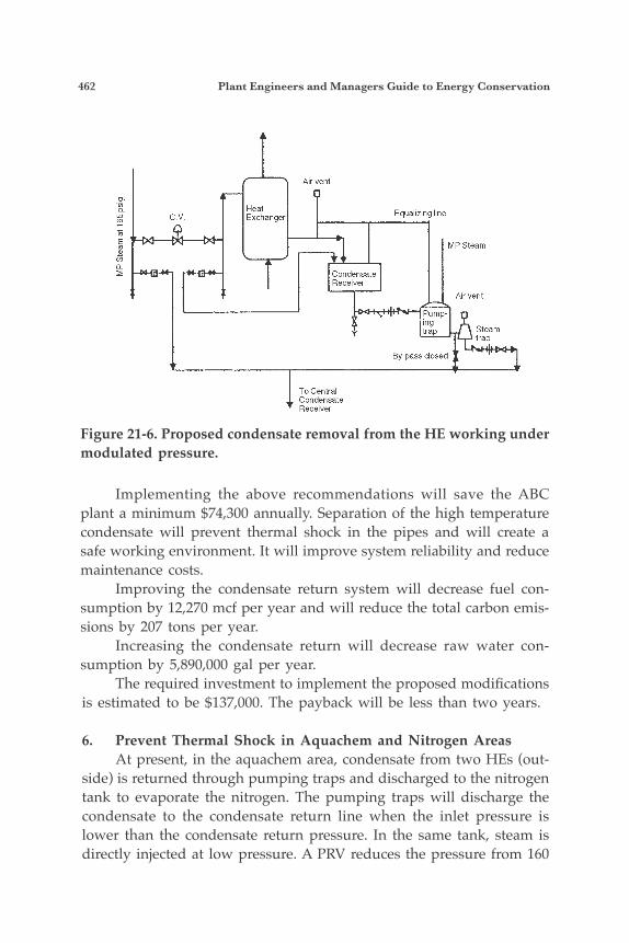
462 Plant Engineers and Managers Guide to Energy Conservation
Figure 21-6. Proposed condensate removal from the HE working under modulated pressure.
Implementing the above recommendations will save the ABC plant a minimum $74,300 annually. Separation of the high temperature condensate will prevent thermal shock in the pipes and will create a safe working environment. It will improve system reliability and reduce maintenance costs. Improving the condensate return system will decrease fuel con-sumption by 12,270 mcf per year and will reduce the total carbon emis-sions by 207 tons per year. Increasing the condensate return will decrease raw water con-sumption by 5,890,000 gal per year. The required investment to implement the proposed modifications is estimated to be $137,000. The payback will be less than two years.
6. Prevent Thermal Shock in Aquachem and Nitrogen Areas At present, in the aquachem area, condensate from two HEs (out-side) is returned through pumping traps and discharged to the nitrogen tank to evaporate the nitrogen. The pumping traps will discharge the condensate to the condensate return line when the inlet pressure is lower than the condensate return pressure. In the same tank, steam is directly injected at low pressure. A PRV reduces the pressure from 160
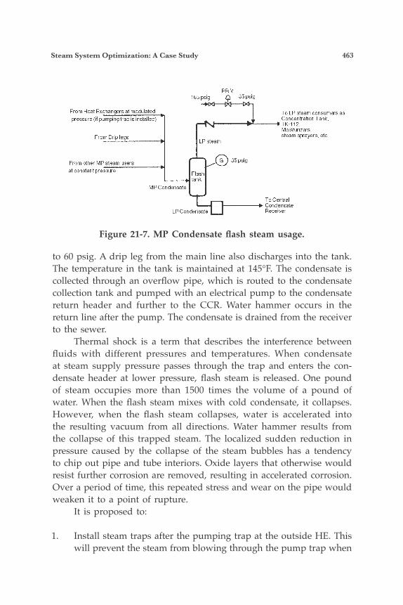
Steam System Optimization: A Case Study 463
to 60 psig. A drip leg from the main line also discharges into the tank. The temperature in the tank is maintained at 145°F. The condensate is collected through an overflow pipe, which is routed to the condensate collection tank and pumped with an electrical pump to the condensate return header and further to the CCR. Water hammer occurs in the return line after the pump. The condensate is drained from the receiver to the sewer. Thermal shock is a term that describes the interference between fluids with different pressures and temperatures. When condensate at steam supply pressure passes through the trap and enters the con-densate header at lower pressure, flash steam is released. One pound of steam occupies more than 1500 times the volume of a pound of water. When the flash steam mixes with cold condensate, it collapses. However, when the flash steam collapses, water is accelerated into the resulting vacuum from all directions. Water hammer results from the collapse of this trapped steam. The localized sudden reduction in pressure caused by the collapse of the steam bubbles has a tendency to chip out pipe and tube interiors. Oxide layers that otherwise would resist further corrosion are removed, resulting in accelerated corrosion. Over a period of time, this repeated stress and wear on the pipe would weaken it to a point of rupture. It is proposed to:
1. Install steam traps after the pumping trap at the outside HE. This will prevent the steam from blowing through the pump trap when
Figure 21-7. MP Condensate flash steam usage.
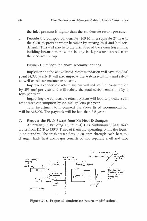
464 Plant Engineers and Managers Guide to Energy Conservation
the inlet pressure is higher than the condensate return pressure.
2. Reroute the pumped condensate (140°F) in a separate 2” line to the CCR to prevent water hammer by mixing cold and hot con-densate. This will also help the discharge of the steam traps in the building because there won’t be any back pressure created from the electrical pump.
Figure 21-8 reflects the above recommendations.
Implementing the above listed recommendation will save the ABC plant $4,300 yearly. It will also improve the system reliability and safety, as well as reduce maintenance costs. Improved condensate return system will reduce fuel consumption by 255 mcf per year and will reduce the total carbon emissions by 4 tons per year. Improving the condensate return system will lead to a decrease in raw water consumption by 520,000 gallons per year. Total investment to implement the above listed recommendation will be $15,000. The payback will be less than 3.5 years.
7. Recover the Flash Steam from X’s Heat Exchangers At present, in Building 18, four (4) HEs continuously heat fresh water from 115°F to 335°F. Three of them are operating, while the fourth is on standby. The fresh water flow is 30 gpm through each heat ex-changer. Each heat exchanger consists of two separate shell and tube
Figure 21-8. Proposed condensate return modifications.

Steam System Optimization: A Case Study 465
heat exchangers with a common steam control valve and separate steam traps. The condensate is returned directly to the CCR. The heat content of the high-pressure condensate is not used at present and the flash steam is vented through the vent of the CCR. See existing arrangement in Figure 21-9. It is proposed to rearrange the condensate return system in a way that the MP condensate can be used. The flash steam from it will preheat the incoming fresh water. This will decrease the steam flow through the PRVs and reduce the consumption of MP steam. To implement this pro-posal, the existing system will not be disturbed. A new heat exchanger will be installed on the common water supply line ahead of the four existing HEs, as well as a flash tank at the condensate discharge side downstream of the existing steam traps. The HE will use 15 psig flash steam from 165 psig condensate. A new 3” pipe originating from the flash tank will supply the LP steam to the new HE. Safety drain traps will be installed on the HE’s outlet to assure proper drainage at start-up operation. See proposed modifications in Figure 21-10. Implementing the above recommendation will benefit the ABC plant with savings of $28,700 annually.
Figure 21-9. Existing arrangement at heat exchangers.
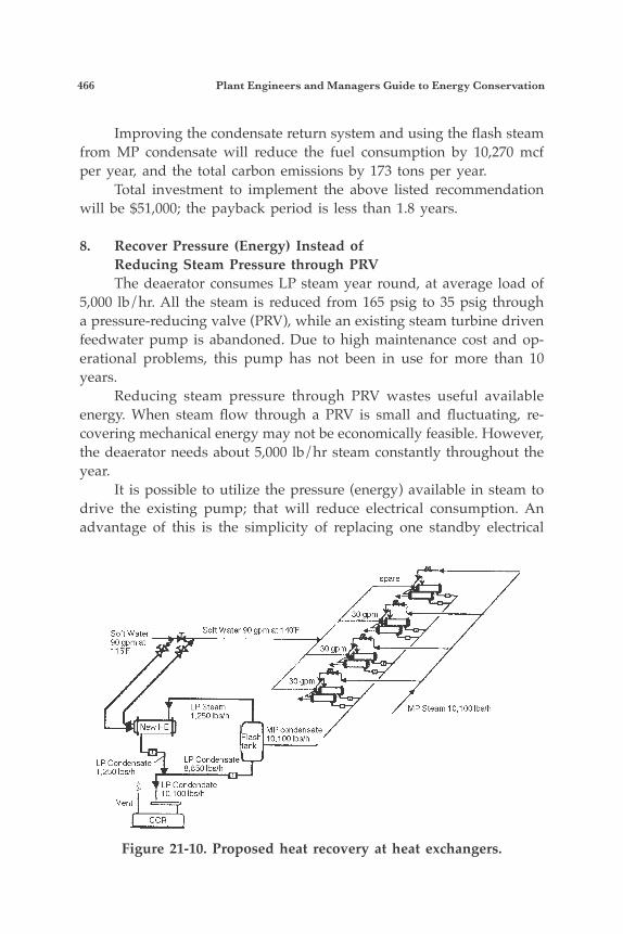
466 Plant Engineers and Managers Guide to Energy Conservation
Improving the condensate return system and using the flash steam from MP condensate will reduce the fuel consumption by 10,270 mcf per year, and the total carbon emissions by 173 tons per year. Total investment to implement the above listed recommendation will be $51,000; the payback period is less than 1.8 years.
8. Recover Pressure (Energy) Instead of Reducing Steam Pressure through PRV The deaerator consumes LP steam year round, at average load of 5,000 lb/hr. All the steam is reduced from 165 psig to 35 psig through a pressure-reducing valve (PRV), while an existing steam turbine driven feedwater pump is abandoned. Due to high maintenance cost and op-erational problems, this pump has not been in use for more than 10 years. Reducing steam pressure through PRV wastes useful available energy. When steam flow through a PRV is small and fluctuating, re-covering mechanical energy may not be economically feasible. However, the deaerator needs about 5,000 lb/hr steam constantly throughout the year. It is possible to utilize the pressure (energy) available in steam to drive the existing pump; that will reduce electrical consumption. An advantage of this is the simplicity of replacing one standby electrical
Figure 21-10. Proposed heat recovery at heat exchangers.
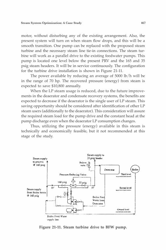
Steam System Optimization: A Case Study 467
motor, without disturbing any of the existing arrangement. Also, the present system will turn on when steam flow drops, and this will be a smooth transition. One pump can be replaced with the proposed steam turbine and the necessary steam line tie-in connections. The steam tur-bine will work as a parallel drive to the existing feedwater pumps. This pump is located one level below the present PRV and the 165 and 35 psig steam headers. It will be in service continuously. The configuration for the turbine drive installation is shown in Figure 21-11. The power available by reducing an average of 5000 lb/h will be in the range of 70 hp. The recovered pressure (energy) from steam is expected to save $10,800 annually. When the LP steam usage is reduced, due to the future improve-ments in the deaerator and condensate recovery systems, the benefits are expected to decrease if the deaerator is the single user of LP steam. This saving opportunity should be considered after identification of other LP steam users (additionally to the deaerator). This consideration will assure the required steam load for the pump drive and the constant head at the pump discharge even when the deaerator LP consumption changes. Thus, utilizing the pressure (energy) available in this steam is technically and economically feasible, but it not recommended at this stage of the study.
Figure 21-11. Steam turbine drive to BFW pump.

468 Plant Engineers and Managers Guide to Energy Conservation
CONCLUSION
The ABC plant has a potential to capture $270,000 in annual energy savings by implementing the above eight recommendations. These recommendations require no major process modification. Some of them could be implemented through a periodic maintenance program. The others, requiring new equipment, can be done during the plant turnaround. Optimization of the steam system by implementing the above recommendations will also reduce the total carbon emission to the environment by 1,284 tons annually.
References1. 1997 Operating data from client’s food processing facilities2. Turner, Wayne C., Energy Management Handbook, 1992.3. Armstrong International Inc., Steam Conservation Guidelines for Condensate Drainage,
Handbook N-101, 1994.
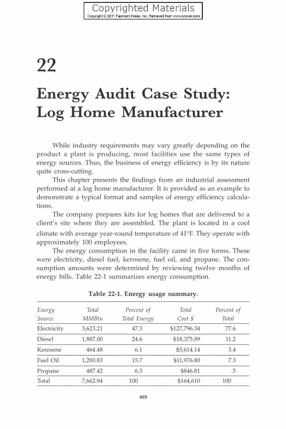
469
22Energy Audit Case Study: Log Home Manufacturer
While industry requirements may vary greatly depending on the product a plant is producing, most facilities use the same types of energy sources. Thus, the business of energy efficiency is by its nature quite cross-cutting. This chapter presents the findings from an industrial assessment performed at a log home manufacturer. It is provided as an example to demonstrate a typical format and samples of energy efficiency calcula-tions. The company prepares kits for log homes that are delivered to a client’s site where they are assembled. The plant is located in a cool climate with average year-round temperature of 41°F. They operate with approximately 100 employees. The energy consumption in the facility came in five forms. These were electricity, diesel fuel, kerosene, fuel oil, and propane. The con-sumption amounts were determined by reviewing twelve months of energy bills. Table 22-1 summarizes energy consumption.
Table 22-1. Energy usage summary.————————————————————————————————Energy Total Percent of Total Percent ofSource MMBtu Total Energy Cost $ Total————————————————————————————————Electricity 3,623.21 47.3 $127,796.34 77.6————————————————————————————————Diesel 1,887.00 24.6 $18,375.89 11.2————————————————————————————————Kerosene 464.48 6.1 $5,614.14 3.4————————————————————————————————Fuel Oil 1,200.83 15.7 $11,976.80 7.3————————————————————————————————Propane 487.42 6.3 $846.81 .5————————————————————————————————Total 7,662.94 100 $164,610 100————————————————————————————————
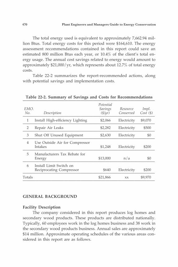
470 Plant Engineers and Managers Guide to Energy Conservation
The total energy used is equivalent to approximately 7,662.94 mil-lion Btus. Total energy costs for this period were $164,610. The energy assessment recommendations contained in this report could save an estimated 800 million Btus each year, or 10.4% of the client’s total en-ergy usage. The annual cost savings related to energy would amount to approximately $21,000/yr, which represents about 12.7% of total energy costs. Table 22-2 summarizes the report-recommended actions, along with potential savings and implementation costs.
Table 22-2. Summary of Savings and Costs for Recommendations———————————————————————————————— Potential EMO. Savings Resource Impl. No. Description ($/yr) Conserved Cost ($)———————————————————————————————— 1 Install High-efficiency Lighting $2,066 Electricity $9,070———————————————————————————————— 2 Repair Air Leaks $2,282 Electricity $500———————————————————————————————— 3 Shut Off Unused Equipment $2,630 Electricity $0———————————————————————————————— 4 Use Outside Air for Compressor Intakes $1,248 Electricity $200———————————————————————————————— 5 Manufacturers Tax Rebate for Energy $13,000 n/a $0———————————————————————————————— 6 Install Limit Switch on Reciprocating Compressor $640 Electricity $200————————————————————————————————Totals $21,866 xx $9,970————————————————————————————————
GENERAL BACKGROUND
Facility Description The company considered in this report produces log homes and secondary wood products. These products are distributed nationally. Typically, 60 employees work in the log homes business and 38 work in the secondary wood products business. Annual sales are approximately $14 million. Approximate operating schedules of the various areas con-sidered in this report are as follows.
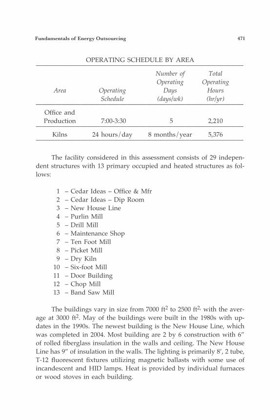
Fundamentals of Energy Outsourcing 471
OPERATING SCHEDULE BY AREA———————————————————————————————— Number of Total Operating Operating Area Operating Days Hours Schedule (days/wk) (hr/yr) ———————————————————————————————— Office and Production 7:00-3:30 5 2,210 ———————————————————————————————— Kilns 24 hours/day 8 months/year 5,376 ————————————————————————————————
The facility considered in this assessment consists of 29 indepen-dent structures with 13 primary occupied and heated structures as fol-lows:
1 – Cedar Ideas – Office & Mfr 2 – Cedar Ideas – Dip Room 3 – New House Line 4 – Purlin Mill 5 – Drill Mill 6 – Maintenance Shop 7 – Ten Foot Mill 8 – Picket Mill 9 – Dry Kiln 10 – Six-foot Mill 11 – Door Building 12 – Chop Mill 13 – Band Saw Mill
The buildings vary in size from 7000 ft2 to 2500 ft2, with the aver-age at 3000 ft2. May of the buildings were built in the 1980s with up-dates in the 1990s. The newest building is the New House Line, which was completed in 2004. Most building are 2 by 6 construction with 6” of rolled fiberglass insulation in the walls and ceiling. The New House Line has 9” of insulation in the walls. The lighting is primarily 8’, 2 tube, T-12 fluorescent fixtures utilizing magnetic ballasts with some use of incandescent and HID lamps. Heat is provided by individual furnaces or wood stoves in each building.
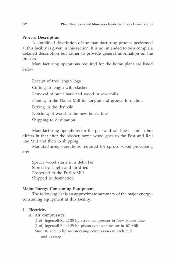
472 Plant Engineers and Managers Guide to Energy Conservation
Process Description A simplified description of the manufacturing process performed at this facility is given in this section. It is not intended to be a complete detailed description but rather to provide general information on the process. Manufacturing operations required for the home plant are listed below:
Receipt of tree length logs Cutting to length with slasher Removal of outer bark and wood in saw mills Planing in the Planar Mill for tongue and groove formation Drying in the dry kiln Notching of wood in the new house line Shipping to destination
Manufacturing operations for the post and rail line is similar but differs in that after the slasher, some wood goes to the Post and Rail line Mill and then to shipping. Manufacturing operations required for spruce wood processing are:
Spruce wood starts in a debarker Stored by length and air-dried Processed in the Purlin Mill Shipped to destination
Major Energy Consuming Equipment The following list is an approximate summary of the major energy-consuming equipment at this facility.
1. Electricity A. Air compressors: (1 of) Ingersoll-Rand 25 hp screw compressor in New House Line (1 of) Ingersoll-Rand 25 hp piston-type compressor in 10’ Mill Misc. 10 and 15 hp reciprocating compressors in each mill and in shop
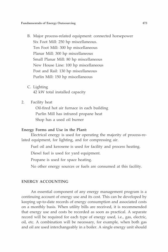
Fundamentals of Energy Outsourcing 473
B. Major process-related equipment: connected horsepower Six Foot Mill: 250 hp miscellaneous. Ten Foot Mill: 300 hp miscellaneous Planar Mill: 300 hp miscellaneous Small Planar Mill: 80 hp miscellaneous New House Line: 100 hp miscellaneous Post and Rail: 130 hp miscellaneous Purlin Mill: 150 hp miscellaneous C. Lighting 42 kW total installed capacity
2. Facility heat Oil-fired hot air furnace in each building Purlin Mill has infrared propane heat Shop has a used oil burner Energy Forms and Use in the Plant: Electrical energy is used for operating the majority of process-re-lated equipment, for lighting, and for compressing air. Fuel oil and kerosene is used for facility and process heating. Diesel fuel is used for yard equipment. Propane is used for space heating. No other energy sources or fuels are consumed at this facility.
ENERGY ACCOUNTING
An essential component of any energy management program is a continuing account of energy use and its cost. This can be developed by keeping up-to-date records of energy consumption and associated costs on a monthly basis. When utility bills are received, it is recommended that energy use and costs be recorded as soon as practical. A separate record will be required for each type of energy used, i.e., gas, electric, oil, etc. A combination will be necessary, for example, when both gas and oil are used interchangeably in a boiler. A single energy unit should
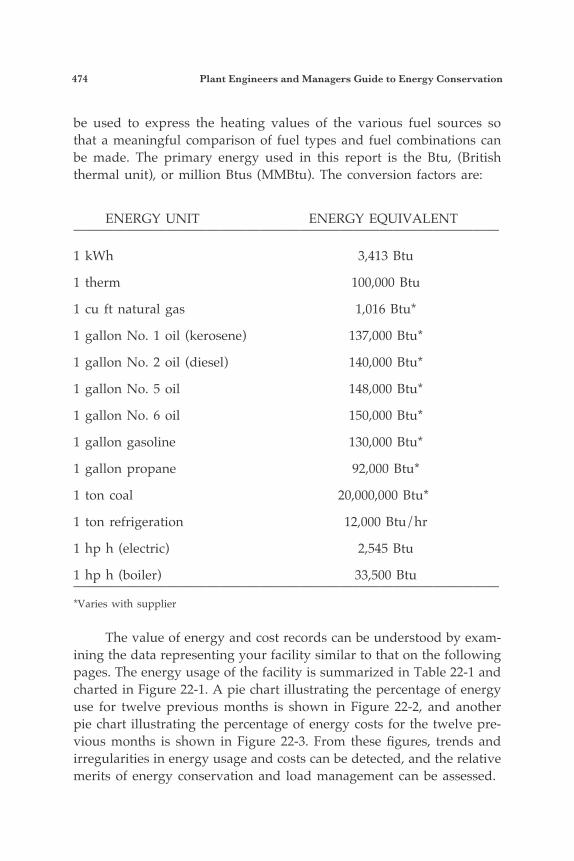
474 Plant Engineers and Managers Guide to Energy Conservation
be used to express the heating values of the various fuel sources so that a meaningful comparison of fuel types and fuel combinations can be made. The primary energy used in this report is the Btu, (British thermal unit), or million Btus (MMBtu). The conversion factors are:
ENERGY UNIT ENERGY EQUIVALENT————————————————————————————————
1 kWh 3,413 Btu
1 therm 100,000 Btu
1 cu ft natural gas 1,016 Btu*
1 gallon No. 1 oil (kerosene) 137,000 Btu*
1 gallon No. 2 oil (diesel) 140,000 Btu*
1 gallon No. 5 oil 148,000 Btu*
1 gallon No. 6 oil 150,000 Btu*
1 gallon gasoline 130,000 Btu*
1 gallon propane 92,000 Btu*
1 ton coal 20,000,000 Btu*
1 ton refrigeration 12,000 Btu/hr
1 hp h (electric) 2,545 Btu
1 hp h (boiler) 33,500 Btu————————————————————————————————*Varies with supplier
The value of energy and cost records can be understood by exam-ining the data representing your facility similar to that on the following pages. The energy usage of the facility is summarized in Table 22-1 and charted in Figure 22-1. A pie chart illustrating the percentage of energy use for twelve previous months is shown in Figure 22-2, and another pie chart illustrating the percentage of energy costs for the twelve pre-vious months is shown in Figure 22-3. From these figures, trends and irregularities in energy usage and costs can be detected, and the relative merits of energy conservation and load management can be assessed.
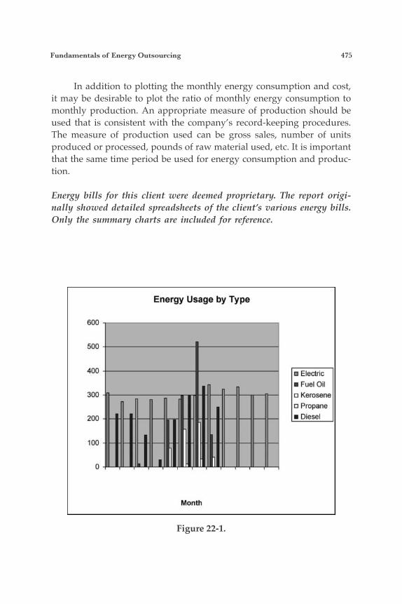
Fundamentals of Energy Outsourcing 475
In addition to plotting the monthly energy consumption and cost, it may be desirable to plot the ratio of monthly energy consumption to monthly production. An appropriate measure of production should be used that is consistent with the company’s record-keeping procedures. The measure of production used can be gross sales, number of units produced or processed, pounds of raw material used, etc. It is important that the same time period be used for energy consumption and produc-tion.
Energy bills for this client were deemed proprietary. The report origi-nally showed detailed spreadsheets of the client’s various energy bills. Only the summary charts are included for reference.
Figure 22-1.
Energy Usage by Type
600
500
400
300 -
200 - -
100 - -
0 -7
Month
H Fuel Oil 0 Kerosenc
0 Propane
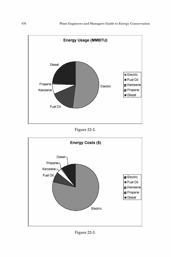
476 Plant Engineers and Managers Guide to Energy Conservation
Figure 22-2.
Figure 22-3.
Energy Usage (MMBTU)
Diesel
rn Fuel Oil
Kerosene Propane
Propane
Kerosene Electric
Fuel Oil
Energy Costs ($)
Diesel,
Propan
Kerosene
Fuel Oil Electric rn Fuel Oil
Kerosene Propane
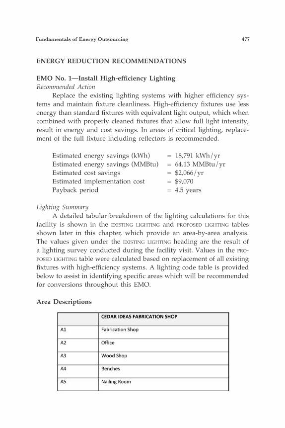
Fundamentals of Energy Outsourcing 477
ENERGY REDUCTION RECOMMENDATIONS
EMO No. 1—Install High-efficiency LightingRecommended Action Replace the existing lighting systems with higher efficiency sys-tems and maintain fixture cleanliness. High-efficiency fixtures use less energy than standard fixtures with equivalent light output, which when combined with properly cleaned fixtures that allow full light intensity, result in energy and cost savings. In areas of critical lighting, replace-ment of the full fixture including reflectors is recommended.
Estimated energy savings (kWh) = 18,791 kWh/yr Estimated energy savings (MMBtu) = 64.13 MMBtu/yr Estimated cost savings = $2,066/yr Estimated implementation cost = $9,070 Payback period = 4.5 years
Lighting Summary A detailed tabular breakdown of the lighting calculations for this facility is shown in the exisTing lighTing and proposed lighTing tables shown later in this chapter, which provide an area-by-area analysis. The values given under the exisTing lighTing heading are the result of a lighting survey conducted during the facility visit. Values in the pro-posed lighTing table were calculated based on replacement of all existing fixtures with high-efficiency systems. A lighting code table is provided below to assist in identifying specific areas which will be recommended for conversions throughout this EMO.
Area Descriptions
A 1
Wood Shop
Benches
Nailing Room
CEDAR IDEAS FAABRIUTION SHOP
fabrication Shop
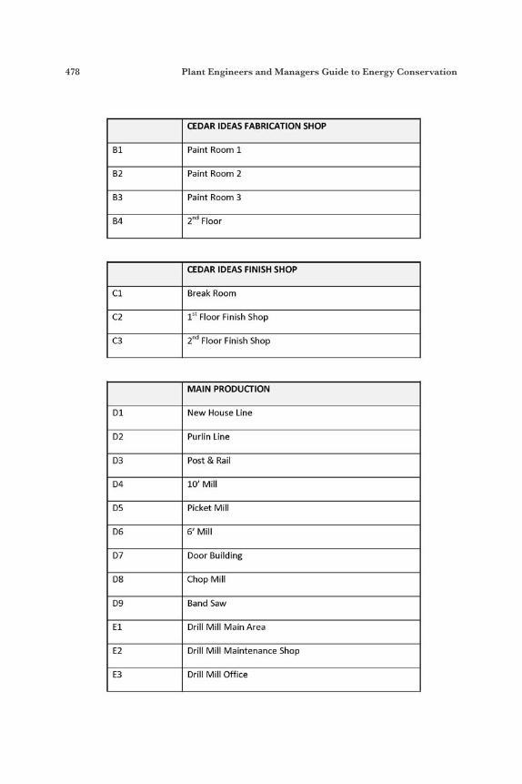
478 Plant Engineers and Managers Guide to Energy Conservation
CEDAR IDEAS FABRICATION SHOP
81 Paint Room 1
82 Paint Room 2
83 Paint Room 3
84 Znd Floor
CEDAR IDEAS FINISH SHOP
c1 Break Room
c2 1" Floor Finish Shop
c3 Znd Floor Finish Shop
MAIN PRODUCT ION
D1 New House Line
D2 Purlin Line
D3 Post & Rail
04 10' Mill
05 Picket Mill
D6 6' Mill
D7 Door Building
Q8 Chop Mill
D9 Band Saw
E l Drill Mill Main Area
E2 Drill Mill Maintenance Shop
€3 Drill Mill Office
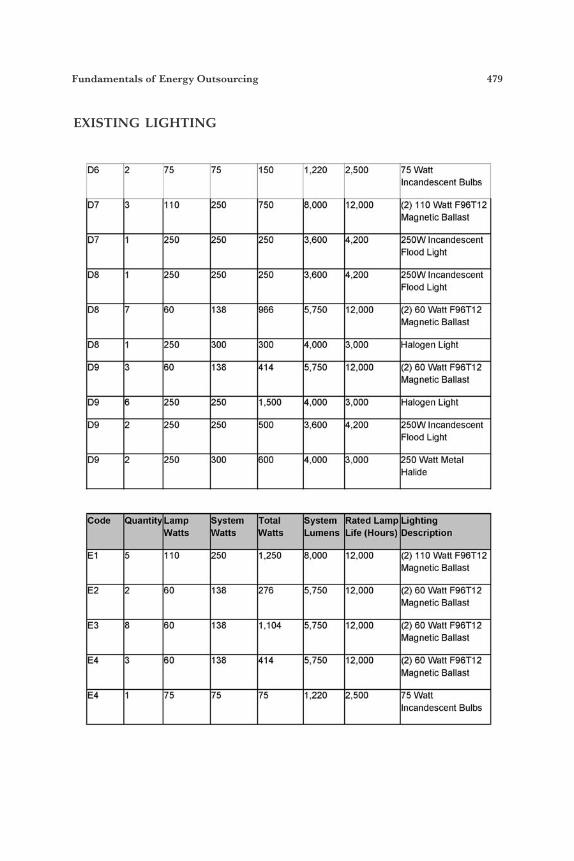
Fundamentals of Energy Outsourcing 479
EXISTING LIGHTING
D6 2 75 75 150 1,220 2.500 75 Wan Incandescent Bulbs
D7 3 110 250 750 8.000 12.000 (2) 110 Watt F96T12 Magnetic Ballast
------- D7 1 250 250 250 3,600 4200 250W Incandescent
Flood Light ------- Da 1 250 250 250 3,600 4200 250W Incandescent
Flood Light ------~ D8 7 60 138 966 5,750 12.000 (2) 60 Watt F96T12
Magnetic Ballast ------- D8 1 250 300 300 4,000 3.000 Halogen Light
D9 3 60 I 3a 414 5,750 12.000 (2) 60 Watt F96T12 ---- ---
Magnetic Ballast ------- D9 6 250 250 1.500 4.000 3.000 Halogen Light
D9 2 250 250 500 3,600 4,200 250W Incandescent ------~
Flood Light ------- D9 2 250 300 600 4.000 3.000 250 Watt Metal
Halide
Code QuantitvLamp System Total System Rated Lamp Lighting Watts Watts Watts Lumens Life (Hours) Description
- - ~ ~ - - E l 5 110 250 1.250 8.000 12.000 (2) 110 Wan F96T12
Magnetic Ballast - - ~ ~ - - E2 2 60 138 276 5,750 12.000 (2) 60 Watt F96T12
Magnetic Ballast - - ~ ~ - - ~3 a 60 138 1,104 5,750 12.000 (2) 60 Watt F96T12
Magnetic Ballast - - ~ ~ - - E4 3 60 138 414 5,750 12.000 (2) 60 Watt F96T12
Magnetic Ballast ------ E4 1 75 75 75 1.220 2.500 75 Watt
Incandescent Bulbs
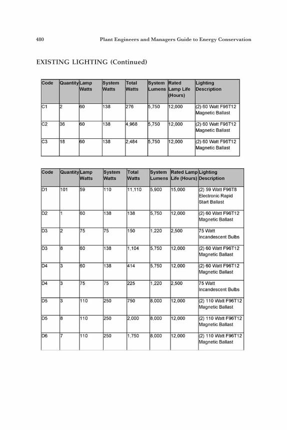
480 Plant Engineers and Managers Guide to Energy Conservation
EXISTING LIGHTING (Continued)
Code QuantityLamp System Total System Rated Lighting Watts Watts Watts lumens LampLKe Description
(Hours) ------ c 1 2 50 138 276 5.750 12,000 (2) 60 Watt F95TT12
Magnetic Ballast ------ C2 36 60 138 4.968 5.750 12,000 (2) 60 Watt F96Tl2
Magnetic Ballast ------ c3 18 50 I 3a 2.484 5.750 12,000 (2) 50 Waft F98T12
Magnetic Ballast
Coda PuantityLamp System Total System RatedLampLigMing Watts Warn Watts Lumens Life (Hours) Oescriptlon
D1 101 59 110 11 ,I 10 5.900 15.000 (2) 59 Watt F96T8 Etectronic Rapid Start Ballast
------ D2 1 60 138 138 5.750 12.000 (2) 60 Watt F96T12
Magnetic Ballast ~~~~~~
D3 2 75 75 150 1,220 2,500 75 Watt Incandescent 8ulbs
~~~~~~
D3 8 60 138 1,104 5,750 12.000 (2) 60 Watt F96T12 Magnetic Ballast
------ D4 3 60 138 414 5,750 12.000 (2) 60 Watt F96T12
Magnetic Ballast ------ D4 3 75 75 225 1,220 2.500 75 Watt
Incandescent Bulbs ------ D5 3 110 250 750 8.000 12.000 (2) 110 Watt FST12
Magnetic Ballast ------ D5 8 110 250 2,000 8.000 12.000 (2) 110 Watt FWT12
Magnetic Ballast ------ D 5 7 110 250 1,750 8.000 12.000 (2) 110 Watt FBBT12
Magnetic Ballast
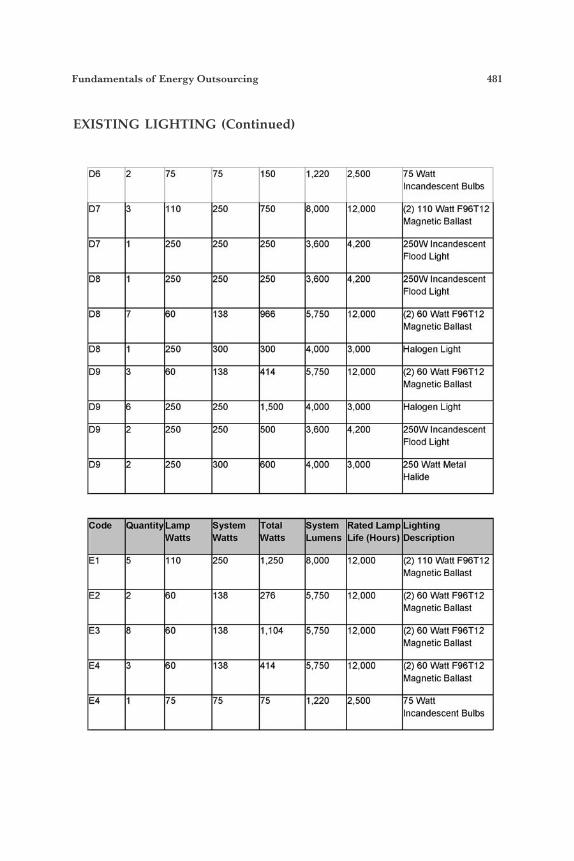
Fundamentals of Energy Outsourcing 481
EXISTING LIGHTING (Continued)
D7 3 110 250 750 8,000 12,000
----- D7 1 250 250 250 3,600 4.200
----- D8 1 250 250 250 3,600 4.200
----- 08 7 60 138 906 5,750 12.000
----- D8 1 250 300 300 4,000 3.000
D9 3 60 138 414 5,750 12,000 ppppp
----- 09 6 250 250 1,500 4,000 3,000
09 2 250 250 500 3,600 4.200 -----
p ~ p p p
I39 2 250 300 600 4,000 3.000
----- Code Quantii Lamp System Total System Rated LampLighSng
Watts Watts Watts Lumens Life (Hours) Description
5 110 250 1,250 8,000 12,000 (2) 110 Wail F90T12 -----
Magnetic Ballast ----- 2 60 138 276 5,750 12,000 (2) 60 Watt F86T12
Magnetic Ballast ----- a 60 138 1,104 5,750 12.000 (2) 60 Watt F96T12
Magnetic Ballaa ----- 3 60 138 414 5,750 12,000 (2) 60 Watt F96T12
Magnetic Ballast ----- 1 75 75 75 1,220 2.500 75 Watt
Incandescent Bulbs
(2) 110 Wan F96T12 Magnetic Ballast
250W lncandescenl Flood Light
ZSOW lncandescenl Flood Light
(2) 50 Watt Fg5T12 Magnetic Ballast
Halogen Light
(2) 60 Watt F96T1.2 Magnetic Ballast
Halogen Light
250W Iiicandescenl Flood Light
250 Wail Metal Halide
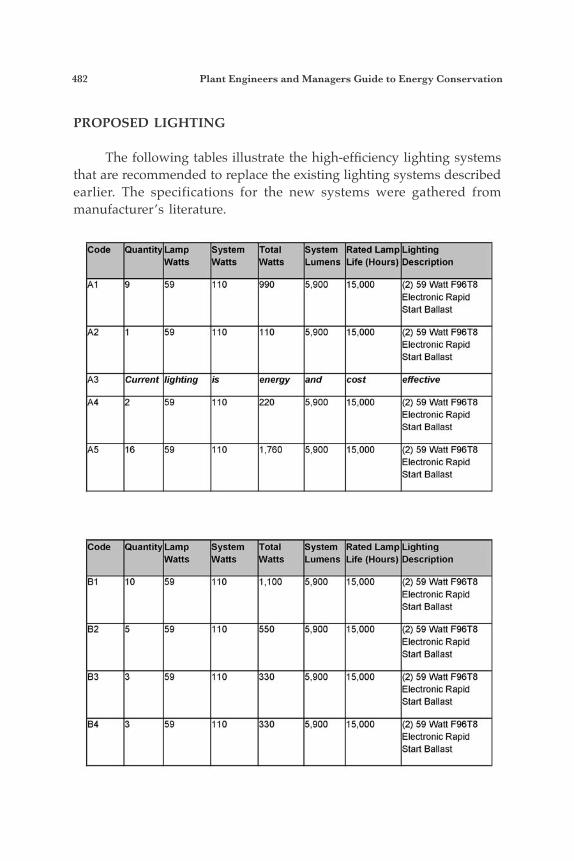
482 Plant Engineers and Managers Guide to Energy Conservation
PROPOSED LIGHTING
The following tables illustrate the high-efficiency lighting systems that are recommended to replace the existing lighting systems described earlier. The specifications for the new systems were gathered from manufacturer’s literature.
------ Code QuantiYLamp System Total System Rated Lamp Lighting
'Watts Watts Watts Lumens Life (Hours) Description
Electronic Rapid Start Ballast c Start Ballast
----~- 990 5,900 15,000 (2) 59 Watt F96T8
------ 5,900 15,000 (2) 59 Watt F96T8
Electronic Rapid
A1 9 59 110
A2 1 59 110 110
------ A3 Current lighting is energy and effective ------
220 5,900 15,000 (2) 59 Watt F96T8 Electronic Rapid Start Ballast F Start Ballast
------ I .760 5,900 15,000 (2) 59 Watt F96T8
Electronic Rapid
A4 2 59 110
A5 16 59 110
------ Code Quantity Lamp System Total System Rated Lamp Lighting
Watts Watts Watts Lumens Life (Hours) Description ------ B1 10 59 110 I ,100 5,900 15,000 (2) 59 watt F96T8
Electronic Rapid Start Ballast
- - ~ ~ ~ - 82 5 59 110 550 5,900 15,000 (2) 59 watt F96T8
Electronic Rapid Start Ballast
------ 83 3 59 110 330 5,900 15,000 (2) 59 watt F96T8
Electronic Rapid Start Ballast
- - ~ ~ ~ - 04 3 59 110 330 5,900 15,000 (2) 59 Watt F96T8
Electronic Rapid Start Ballast
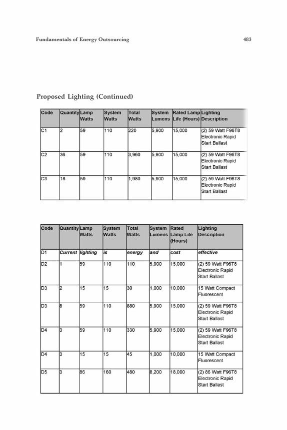
Fundamentals of Energy Outsourcing 483
Proposed Lighting (Continued)
uantity Lamp 'system Total System Rated Lamp Lighting watts Watts watts Lumens Lie ours) Description
Electronic Rapid Start Ballast
- - ~ ~ ~ - Electronic Rapid Start Ballast
~ - ~ ~ ~ - Electronic Rapid Start Ballast
c1 2 59 110 220
C2 36 59 110
c 3 18 59 110
Code Quantity Lamp bystem Total System Rated Lighting watts Watts Watts Lumens bmpLiie Description
(Hours)
0 1 Current lighting is energy a n d cost effective
0 2 1 59 110 110 5,900 15.000 (2) 59 Wan F96T8 ~-~~~~
Electronic Rapid Start Ballast
---~-- 03 2 15 15 30 1,000 10,000 15 Wan Compact
Fluorescent ---~-- 03 8 59 110 880 5,900 I 5,000 (2) 59 wan F96T8
Electronic Rapid Start Ballast
~-~~~~ 0 4 3 59 110 330 5,900 15.000 (2) 59 Watt F96T8
Electronic Rapid Start Ballast
~-~~~~ 0 4 3 15 15 45 1,000 10,000 15 Watt Compact
Fluorescent ~-~~~~ 0 5 3 86 160 480 8,200 18,000 (2) 86 Wan F96T8
Electronic Rapid Start Ballast
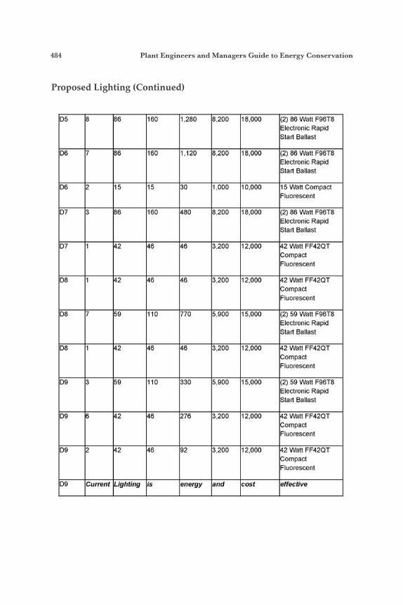
484 Plant Engineers and Managers Guide to Energy Conservation
Proposed Lighting (Continued)
------ D5 8 86 160 1,280 8,200 18,000 (2) 86 Watt F96T8
Electronic Rapid Start Ballast
--~--- 0 6 7 86 160 1,120 8,200 18,000 (2) 86 Watt F96T8
Electronic Rapid Start Ballast
- - ~ ~ ~ - D6 2 15 15 30 1.000 10,000 15 Wan Compact
Fluorescent - ~ ~ ~ ~ - 07 3 86 160 480 8.200 18.000 (2) 86 Wan F96T8
Electronic Rapid Start Ballast
- - ~ ~ ~ - 07 1 42 46 46 3,200 12,000 42 Watt FF42QT
Compact Fluorescent
- - ~ ~ ~ - D8 1 42 46 46 3,200 12,000 42 Watt FF42QT
Compact Fluorescent
------ 0 8 7 59 110 770 5,900 15,000 (2) 59 Watt F96T8
Electronic Rapid Start Ballast
- ~ ~ ~ ~ - D8 1 42 46 46 3,200 12,000 42 Watt FF42QT
Compact Fluorescent
- - ~ ~ ~ - D9 3 59 110 330 5,900 15,000 (2) 59 wan F96T8
Electronic Rapid Start Ballast
--~--- D9 6 42 46 276 3,200 12,000 42 Watt FF42QT
Compact Fluorescent
D9 2 42 46 92 3,200 12,000 42 Watt FF42QT Compact Fluorescent
D9 Current Lighting is energy and cost effective
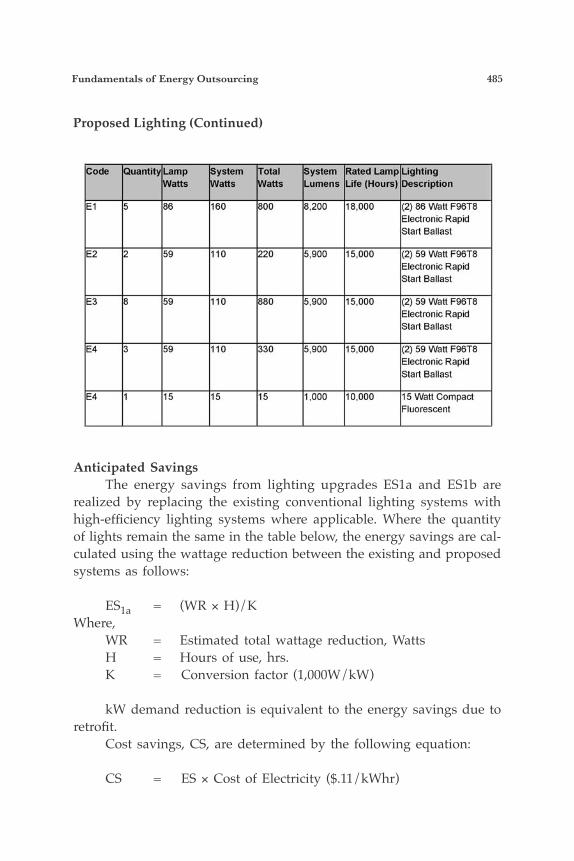
Fundamentals of Energy Outsourcing 485
Anticipated Savings The energy savings from lighting upgrades ES1a and ES1b are realized by replacing the existing conventional lighting systems with high-efficiency lighting systems where applicable. Where the quantity of lights remain the same in the table below, the energy savings are cal-culated using the wattage reduction between the existing and proposed systems as follows:
ES1a = (WR × H)/K Where, WR = Estimated total wattage reduction, Watts H = Hours of use, hrs. K = Conversion factor (1,000W/kW)
kW demand reduction is equivalent to the energy savings due to retrofit. Cost savings, CS, are determined by the following equation:
CS = ES × Cost of Electricity ($.11/kWhr)
Proposed Lighting (Continued)
------ Code Quantity Lamp System Total System Rated Lamp Lighting
Watts Watts Watts Lumens Life (Hours) Description ------ E l 5 86 160 800 8,200 18,000 (2) 86 Watt F96T8
Electronic Rapid Start Ballast
------ E2 2 59 110 220 5,900 15,000 (2) 59 Watt F96T8
Electronic Rapid Start Ballast
- - ~ ~ ~ - E3 8 59 110 880 5,900 15,000 (2) 59 Watt F96T8
Electronic Rapid Start Ballast
------ E4 3 59 110 330 5,900 15,000 (2) 59 Watt F96T8
Electronic Rapid Start Ballast
- - ~ ~ ~ - E4 1 15 15 15 1,000 10,000 15 Watt Compact
Fluorescent
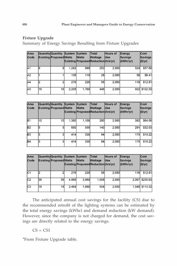
486 Plant Engineers and Managers Guide to Energy Conservation
Fixture UpgradeSummary of Energy Savings Resulting from Fixture Upgrades
The anticipated annual cost savings for the facility (CS) due to the recommended retrofit of the lighting systems can be estimated by the total energy savings (kWhr) and demand reduction (kW demand). However, since the company is not charged for demand, the cost sav-ings are directly related to the energy savings.
CS = CS1
*From Fixture Upgrade table.
------- Area QuantityQuantity System System Total Hoursof Energy cost Code Existing Proposed Watts Watts Wattage Use Savings Savings
Existing Proposed Reduction (hrslyr) (kWhr/yr) (S/yr) ------- A1 9 9 1.242 990 252 2.080 524 55766 A2 1 1 138 110 28 2.080 58 S6.41
A4 2 2 276 220 56 2.080 116$12.81
A5 16 16 2,208 1,760 448 2.080 932 $102.50
~ - ~ - ~ ~ ~
------- ~ - ~ - ~ ~ ~
-------
------ Area Quantity Quantii System System Total Hours of ,Energy cost Code Existing Proposed Watts Watts Wattage Use pavings Savings
Existing Proposed Reduction (hrs/yr) W r )
- - ~ ~ ~ - 582 S64.06 0
B1 10 10 1,380 1,100 280 2.080 -----~ 82 5 5 690 550 140 2.080 291 rn - - ~ ~ ~ ~ 83 3 3 414 330 84 2.080 175 $1922
84 3 3 414 330 84 2.080 175 $1922 ------
---- Quantity Quantity System ystem Total Hours of Energy cost
Existing Proposed Reduction(hrs/yr) (kWhr/yr) (S/yr) ode Existing Proposed Watts Wattage Use Savings Savings
--~--- L- c 1 2 2 276 220 56 2.080 116 $12.81 - ~ ~ ~ - ~ C2 36 36 4,968 3,960 1,008 2,080 2,097 $230.63 ------ c 3 18 18 2,484 1,980 504 2.080 1,048 $1 15.32
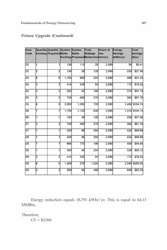
Fundamentals of Energy Outsourcing 487
Energy reduction equals 18,791 kWhr/yr. This is equal to 64.13 MMBtu.
Therefore, CS = $2,066
Fixture Upgrade (Continued)
rea QuantityQuantity System System Total Hoursof Energy cost ode Existing Proposed Watts Watts Wattage Use Savings Savings
Existing Proposed Reduction (hrslyr) (kWhr/yr) (S/yr)
------- D2 1 1 138 110 28 2.080 58 $641
D3 2 2 150 30 120 2.080 250 $2746
D3 8 8 1,104 880 224 2.080 466 $51 25
D4 3 3 414 330 84 2.080 1 7 5 5 1 9 2 2
D4 3 3 225 45 180 2.080 374 $41 18
D5 3 3 750 480 270 2.080 562
D5 8 8 2,000 1,280 720 2,080 1.498 $1 64 74
D6 7 7 1,750 1,120 630 2.080 1,310 $144 14
D6 1 1 150 30 120 2.080 250 $2746
D7 3 3 750 480 270 2.080 562
D7 1 1 250 46 204 2.080 424 $4668
D9 1 1 250 46 204 2.080 424 $4668
D8 7 7 966 770 196 2.080 408 $4484
D8 1 1 300 46 254 2.080 528 $58 12
D9 3 3 414 330 84 2,080 175 $1922
D9 6 6 1.500 276 1,224 2.080 2,546 $28005
D9 2 2 500 92 408 2,080 849 $9335
- - - - ~ ~ ~ - - - - ~ ~ ~ ------- - - - - ~ ~ ~ ------- --,-,~~
------- - - - - ~ ~ ~ ------- - - - - ~ ~ ~ - - - - ~ ~ ~ ------- ------- ~ - - - ~ ~ ~ ------- - - - - ~ ~ ~
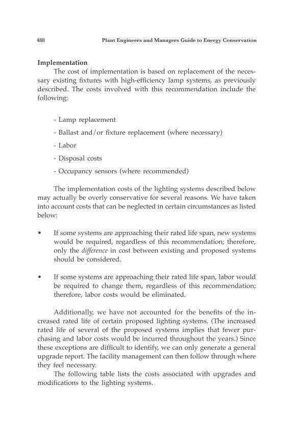
488 Plant Engineers and Managers Guide to Energy Conservation
Implementation The cost of implementation is based on replacement of the neces-sary existing fixtures with high-efficiency lamp systems, as previously described. The costs involved with this recommendation include the following:
- Lamp replacement
- Ballast and/or fixture replacement (where necessary)
- Labor
- Disposal costs
- Occupancy sensors (where recommended)
The implementation costs of the lighting systems described below may actually be overly conservative for several reasons. We have taken into account costs that can be neglected in certain circumstances as listed below:
• If some systems are approaching their rated life span, new systems would be required, regardless of this recommendation; therefore, only the difference in cost between existing and proposed systems should be considered.
• If some systems are approaching their rated life span, labor would be required to change them, regardless of this recommendation; therefore, labor costs would be eliminated.
Additionally, we have not accounted for the benefits of the in-creased rated life of certain proposed lighting systems. (The increased rated life of several of the proposed systems implies that fewer pur-chasing and labor costs would be incurred throughout the years.) Since these exceptions are difficult to identify, we can only generate a general upgrade report. The facility management can then follow through where they feel necessary. The following table lists the costs associated with upgrades and modifications to the lighting systems.
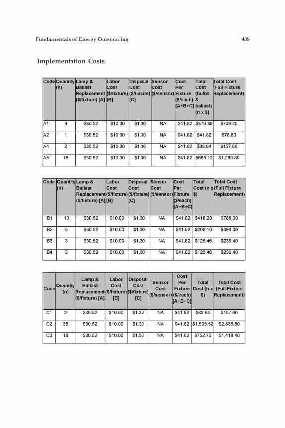
Fundamentals of Energy Outsourcing 489
Implementation Costs
-- ----- Code Quantity Lamp 8 Labor Disposal Sensor Cost Total Total Cost
(n) Ballast Cost Cost Cost Per Cost (Full Fixture Replacement ($/fixture) itfixture) ($/sensor) Fixture (bulbs Replacement) ($fixture) [A1 [el [CI ($/each) 8
[A+B+C] ballast) (n x $)
-- ----- A1 9 $30 52 $10 00 $1 30 NA $41 82 $37638 $709 20
A2 1 $30 52 $10 00 $1 30 NA $41 82 $41 82 $7880
A4 2 $30 52 $10 00 $I 30 NA $41 82 $8364 $157 60
A5 16 $3052 $1000 $1 30 NA $41 82 $66912 $1,26080
-- -~--- ~- - ~ ~ - -
-- ~ ~ ~ - -
Code Quantity Lamp 8 Labor Disposal Sensor Cost Total Total Cost (n) Ballast Cost Cost Cost Per Cost (n x(Full Fixture
Replacement($/fixtur) ($fixture) ($/sensor) Fixture $) Replacement) ($fi/fixture) [A1 [el [Cl ($/each)
[A+B+C] -- ----~ 81 10 $30.52 $10.00 $1.30 NA $41.82 $418.20 $788.00 - 82
~~~-~ 5 $30.52 $1000 $1.30 NA $41.82 $209.10 $394.00
-~ ~~~-~ 83 3 $30.52 $10.00 $1.30 NA $41.82 $125.46 $236.40
84 3 $30.52 $10.00 $1.30 NA $41.82 $125.46 $236.40 -~ ~~~-~
cost Lamp8 Labor Disposal Sensor Per
($fixture)" PI [CI [A+B+C]
Total Total Cost Cost Fixture Cost(nx (FullFixture
Code Quantity Ballast
$ ($/fixture) ($/sensor) ($/each) $) Replacement)
~- ~ - - - ~ c1 2 $30.52 $10.00 $1.30 NA $41.82 $83.64 $157.60
C2 36 $30.52 $10.00 $1.30 NA $41.82 $1,505.52 $2.836.80
C3 18 $30.52 $10.00 $1.30 NA $41.82 $752.76 $1.418.40
-- ----- -- -----
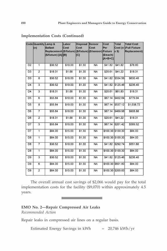
490 Plant Engineers and Managers Guide to Energy Conservation
The overall annual cost savings of $2,066 would pay for the total implementation costs for the facility ($9,070) within approximately 4.5 years.
EMO No. 2—Repair Compressed Air LeaksRecommended Action
Repair leaks in compressed air lines on a regular basis.
Estimated Energy Savings in kWh = 20,746 kWh/yr
Implementation Costs (Continued)-- ----- Code Quantii Lamp 8 Labor Disposal Sensor Cost Total Total Cost
(n) Ballast Cost Cost Cost Per Cost(n (Full Fixture Replacement ($/fixture) (Wixture) ($/sensor) Fixture x $) Replacement) (S/fiduW [A1 [el [Cl ($/each)
[A+B+C] -- -----
D2 1 $30.52 $10.00 $1.30 NA $41.82 $41.82 $78.80
D3 2 $18.31 $1.00 $1.30 NA $20.61 $41.22 $18.31
D3 8 $30.52 $10.00 $1.30 NA $41.82 $334.56 $530.40
D4 3 $30.52 $10.00 $1.30 NA $41.82 $125.46 $236.40
D4 3 $18.31 $1.00 $1.30 NA $20.61 $61.83 $18.31
D5 6 $55.84 $10.00 $1.30 NA $57.14 $402.84 $779.04
D5 8 $55.84 $10.00 $1.30 NA $67.14 $537.12 $1,038.72
-- --~-- -- --~--
-- ----- ~~ ~~~-~ -- ----- -- --~--
-- --~-- D6 7 $55.84 $10.00 $1.30 NA $67.14 $469.98 $908.88 -- -~---
D6 2 $18.31 $1.00 $1.30 NA $20.61 $41.22 $18.31
D7 3 $55.84 $10.00 $1.30 NA $57.14 $201.42 $389.52 -- --~--
-- ----- D7 1 $84.00 $15.00 $1.30 NA $100.30 $100.30 $84.00
D8 1 $84.00 $15.00 $1.30 NA $100.30 $100.30 $84.00
D8 7 $30.52 $10.00 $1.30 NA $41.82 $292.74 $551.60
D8 1 $84.00 $15.00 $1.30 NA $100.30 $100.30 $84.00
D9 3 $30.52 $10.00 $1.30 NA $41.82 $125.46 $236.40
D9 6 $84.00 $15.00 $1 30 NA $100.30 $601.80 $8400
D9 2 $84.00 $15.00 $1.30 NA $100.30 $200.60 $84.00
-- ~ ~ ~ - -
-- ----- -- --~--
-- --~--
-- ----- -- --~--
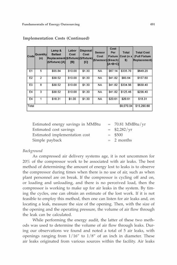
Fundamentals of Energy Outsourcing 491
Estimated energy savings in MMBtu = 70.81 MMBtu/yr Estimated cost savings = $2,282/yr Estimated implementation cost = $500 Simple payback = 2 months
Background As compressed air delivery systems age, it is not uncommon for 20% of the compressor work to be associated with air leaks. The best method of determining the amount of energy lost to leaks is to observe the compressor during times when there is no use of air, such as when plant personnel are on break. If the compressor is cycling off and on, or loading and unloading, and there is no perceived load, then the compressor is working to make up for air leaks in the system. By tim-ing the cycles, one can obtain an estimate of the lost work. If it is not feasible to employ this method, then one can listen for air leaks and, on locating a leak, measure the size of the opening. Then, with the size of the opening and the operating pressure, the volume of air flow through the leak can be calculated. While performing the energy audit, the latter of these two meth-ods was used to determine the volume of air flow through leaks. Dur-ing our observations we found and noted a total of 5 air leaks, with openings ranging from 1/16” to 1/8” of an inch in diameter. These air leaks originated from various sources within the facility. Air leaks
Implementation Costs (Continued)
cost Per Total Total Cost
Code Ballast Cost Fixture Cost(n x (Full Fixture (nl Replacement(S/fixturel ($/fi*re)($/sensor) ($/each) $) Replacement)
Lamp& Labor Disposal Sensor
(SnixtureI[Al [Bl [Cl [A+B+C] -- -----
E l 5 $55.84 $10.00 $1.30 NA $67.14 $335.70 $649.20
E2 2 $30.52 $10.00 $1.30 NA $41.82 $8364 $157.60
E3 8 $30.52 $10.00 $1.30 NA $41.82 $334.56 $630.40
E4 3 $30.52 $10.00 $1.30 NA $41.82 $125.46 $236.40
E4 1 $18.31 $1.00 $1.30 NA $20.61 $20.61 $18.31
-- ~~~-~ -- ~~~-~ -- ----- -- ~~~-~ -- ~~~-~ Total $9,070.04 $15,290.60
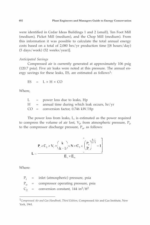
492 Plant Engineers and Managers Guide to Energy Conservation
were identified in Cedar Ideas Buildings 1 and 2 (small), Ten Foot Mill (medium), Picket Mill (medium), and the Chop Mill (medium). From this information it was possible to calculate the total annual energy costs based on a total of 2,080 hrs/yr production time [(8 hours/day) (5 days/week) (52 weeks/year)].
Anticipated Savings Compressed air is currently generated at approximately 106 psig (120.7 psia). Five air leaks were noted at this pressure. The annual en-ergy savings for these leaks, ES, are estimated as follows1:
ES = L × H × CO
Where,
L = power loss due to leaks, Hp H = annual time during which leak occurs, hr/yr CO = conversion factor, 0.746 kW/Hp
The power loss from leaks, L, is estimated as the power required to compress the volume of air lost, Vf, from atmospheric pressure, Pi, to the compressor discharge pressure, Po, as follows:
Where:
Pi = inlet (atmospheric) pressure, psia Po = compressor operating pressure, psia C2 = conversion constant, 144 in2/ft2
1Compressed Air and Gas Handbook, Third Edition, Compressed Air and Gas Institute, New York, 1961.
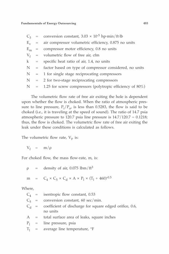
Fundamentals of Energy Outsourcing 493
C3 = conversion constant, 3.03 × 10⁻⁵ hp·min/ft·lb Ev = air compressor volumetric efficiency, 0.875 no units Em = compressor motor efficiency, 0.8 no units Vf = volumetric flow of free air, cfm k = specific heat ratio of air, 1.4, no units N = factor based on type of compressor considered, no units N = 1 for single stage reciprocating compressors N = 2 for two-stage reciprocating compressors N = 1.25 for screw compressors (polytropic efficiency of 80%) The volumetric flow rate of free air exiting the hole is dependent upon whether the flow is choked. When the ratio of atmospheric pres-sure to line pressure, Pi/Po, is less than 0.5283, the flow is said to be choked (i.e., it is traveling at the speed of sound). The ratio of 14.7 psia atmospheric pressure to 120.7 psia line pressure is 14.7/120.7 = 0.1218; thus, the flow is choked. The volumetric flow rate of free air exiting the leak under these conditions is calculated as follows.
The volumetric flow rate, Vf, is:
Vf = m/ρ
For choked flow, the mass flow-rate, m, is:
ρ = density of air, 0.075 lbm/ft3
m = C4 × C5 × Cd × A × Pl × (Tl + 460)-0.5
Where, C4 = isentropic flow constant, 0.53 C5 = conversion constant, 60 sec/min. Cd = coefficient of discharge for square edged orifice, 0.6, no units A = total surface area of leaks, square inches Pl = line pressure, psia Tl = average line temperature, °F
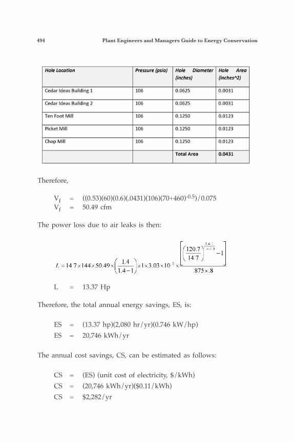
494 Plant Engineers and Managers Guide to Energy Conservation
Therefore,
Vf = ((0.53)(60)(0.6)(.0431)(106)(70+460)-0.5)/0.075 Vf = 50.49 cfm
The power loss due to air leaks is then:
L = 13.37 Hp
Therefore, the total annual energy savings, ES, is:
ES = (13.37 hp)(2,080 hr/yr)(0.746 kW/hp) ES = 20,746 kWh/yr
The annual cost savings, CS, can be estimated as follows: CS = (ES) (unit cost of electricity, $/kWh) CS = (20,746 kWh/yr)($0.11/kWh) CS = $2,282/yr
Hole Locution I Pressure (psiu) I Hole Diurneter
Cedar Ideas Building 2
Ten Foot Mill
I (inches)
106 0.0625
106 0.1250
Cedar Ideas Building 1
Chop Mill
I 106
106 0.1250
Total Area
I 0.0625
Picket Mill I 106 10.1250
(inches"2)
0.0031
0.0031
0.0123
0.0123
0.0123
0.0431
Fundamentals of Energy Outsourcing 495
Implementation Cost Implementation of this AR involves:1) Replacement of couplings and/or hoses2) Replacement of seals around filters3) Shutting off air flow during lunch or break periods4) Repairing breaks in lines, etc. Assuming that the repair work and procedural changes can be done by in-house facility maintenance and management personnel, it is estimated that these leaks can be eliminated for approximately $500. Thus, the estimated cost savings of $2,282/yr. would pay for the imple-mentation cost in approximately 2 months. Additionally, air leak inspec-tions should be incorporated into the routine preventive maintenance procedure and employees should be informed as to the importance of notifying maintenance personnel when leaks are discovered.
EMO No. 3—Turn Off Hog Motors During BreaksRecommended Action Turn off the hog motors in the Six Foot and Ten Foot Mills during the morning and afternoon breaks, as well as during lunch. Estimated energy savings (kW-hr) = 5,818.8 kW-hr Estimated energy savings (MMBtu) = 19.86 MMBtu Estimated annual savings = $640/yr Estimated implementation cost = $200 Simple payback = 4 Months
Background During the site visit it was observed that the Trask-Decrow, 20 hp compressor in the Ten Foot Mill was on during production hours but was idling approximately 75% of the time. This unit can be operated more efficiently by installing a pressure switch that will turn off the unit once it has reached a set point. Then, when the air pressure drops below a low point setting, the unit will turn back on. In discussions with the Trask-Decrow area representative, it was confirmed that if the unit is called upon for air less than six times per hour, it should be operated on a pressure switch. If it is cycled more often than that, one needs to consider the strain on components due to high cycle operation.
496 Plant Engineers and Managers Guide to Energy Conservation
Anticipated Savings The savings for the period of 6/04-5/05 are determined as fol-lows: ES = IH x .746 kW/1 hp × OH Where, ES = total energy savings, kW-hr/yr IH = idling horsepower (energy consumption while idling) OH = operating hours ( while at idle )
Therefore, ES = 5 hp x .746 × (2080 × 0.75) ES = 5,818.80 kW-hr
The cost savings are determined by multiplying the energy savings (ES) by the average electricity cost of $0.11/kW-hr.
CS = 5,818.80 kW-hr × $0.11/kW-hr = $640
Implementation Cost The costs for installation of a pressure limit switch, assuming the existing starter will still be used, were estimated to be approximately $200.
EMO No. 4—Use Outside Air Compressor IntakeRecommended Action Duct outside air directly to the intake of the 75 hp and 30 hp In-gersol Rand air compressors to improve operating efficiency (see figure No. 9 below).
Estimated energy savings (kWh) = 18,905 kWh/yr Estimated energy savings (MMBtu) = 64.52 MMBtu/yr Estimated cost savings = $1,248/yr Estimated implementation cost = $150 Simple payback = 1.5 months
Background The facility uses the 75 hp air compressor for production support and the 30 hp compressor for backup. By utilizing an outside air supply, it is possible to reduce energy requirements for compression. Outside
Fundamentals of Energy Outsourcing 497
air is (on average) cooler, therefore more dense, and requires less energy to be compressed.
Anticipated Savings The compressor work for the usual operating conditions in manu-facturing plants is proportional to the absolute temperature of the intake air. Thus, the fractional reduction in compressor work, WR, resulting from lowering the intake air temperature, is estimated as:
WR = (WI – WO)/WIOr WR = (TI – TO)/(TI + 460)
Where, WI = work of compressor with inside air, hp WO = work of compressor with outside air, hp TI = average temperature of inside air, °F TO = annual average outside air temperature, °F
The compressor intake temperature was measured as 88°F. The yearly average outdoor temperature for the client’s location was 45°F. The fractional compressor work reduction, WR, due to lowering the compressor intake air temperature, is estimated as:
WR = (88 – 45)/(88 + 460) WR = 0.0785
It is estimated that the 75 hp compressor operates for 3,500 hours annually, which was estimated by the following;
(14 hrs/day) × (5 days/wk) × (50 wks/yr) = 3,500 hrs/yr
The average mean power for the 75 hp compressor was estimated at approximately 75% rated load. The annual energy savings, ES, for the 75 hp compressor is esti-mated as:
ES = (kW) × (H) × (WR)
498 Plant Engineers and Managers Guide to Energy Conservation
Where, kW = compressor average mean power, 68.81 kW H = annual operating hours, 3,500 hrs/yr WR = compressor work reduction factor, 0.0785 (no units)Thus, ES = (68.81 kW) × (3,500 hrs/yr) × (0.0785) ES = 18,905 kWh/yr (64.52 MMBtu/yr)
An energy savings table is shown below:
kWh KW Demand Other——————————————————————— 18,905 0 None
The annual cost savings for the compressor, CS, is estimated as: CS = (ES) × (unit cost of electricity)
Therefore, CS = (18,905 kWh/yr) × ($0.066/kWh) CS = $1,248/yr*
Implementation Cost The most common material used for ducting outside air to the compressor intakes is plastic PVC pipe. One end of the pipe is at-tached to the air cleaner intake or other appropriate intake port, and the other end is routed through a wall or ceiling to the outside. Care must be taken to include a drip leg and/or hood on the intake line to prevent moisture from entering the compressor. Properly insulating and sealing the wall penetration, to prevent air infiltration, should not be overlooked. It should be a fairly simple procedure to adapt PVC pipe to the air compressor intake. The total cost for materials and labor to make these modifications to the compressor is estimated at $150. The cost savings of $1,248/yr* would pay for the implementation cost of $150 within approximately 1.5 months.
EMO No. 5—Eliminate Sales Tax on Fuel OilRecommended Action Obtain a rebate (and possible refund) for taxes paid on fuel con-
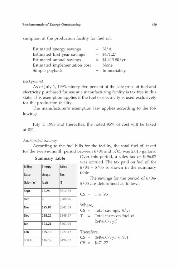
Fundamentals of Energy Outsourcing 499
sumption at the production facility for fuel oil.
Estimated energy savings = N/A Estimated first year savings = $471.27 Estimated annual savings = $1,413.80/yr Estimated implementation cost = None Simple payback = Immediately
Background As of July 1, 1993, ninety-five percent of the sale price of fuel and electricity purchased for use at a manufacturing facility is tax free in this state. This exemption applies if the fuel or electricity is used exclusively for the production facility. The manufacturer’s exemption law applies according to the fol-lowing:
July 1, 1993 and thereafter, the noted 95% of cost will be taxed at 0%.
Anticipated Savings According to the fuel bills for the facility, the total fuel oil taxed for the twelve-month period between 6/04 and 5/05 was 2,015 gallons.
Over this period, a sales tax of $496.07 was accrued. The tax paid on fuel oil for 6/04 – 5/05 is shown in the summary table. The savings for the period of 6/04-5/05 are determined as follows:
CS = T × .95
Where, CS = Total savings, $/yr T = Total taxes on fuel oil ($496.07/yr) Therefore, CS = ($496.07/yr × .95) CS = $471.27
Summary Table
Billing Energy Sales
Date Usage Tax
(Mon-Yr) (gal) (9
kpt 12.24 $612.39
OCt 0 $280.26
Nov 195.84 5541.09
Dec 298.22 5248.27
Jan 521.21 $261.99
Feb 135.19 $227.47
TOTAL 1162.7 $496.07
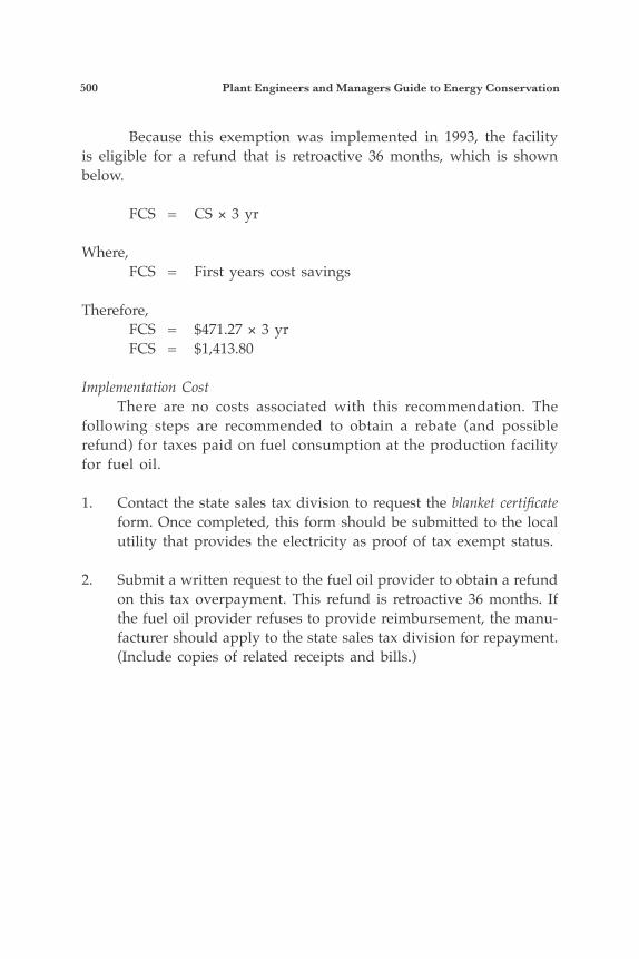
500 Plant Engineers and Managers Guide to Energy Conservation
Because this exemption was implemented in 1993, the facility is eligible for a refund that is retroactive 36 months, which is shown below.
FCS = CS × 3 yr
Where, FCS = First years cost savings
Therefore, FCS = $471.27 × 3 yr FCS = $1,413.80
Implementation Cost There are no costs associated with this recommendation. The following steps are recommended to obtain a rebate (and possible refund) for taxes paid on fuel consumption at the production facility for fuel oil.
1. Contact the state sales tax division to request the blanket certificate form. Once completed, this form should be submitted to the local utility that provides the electricity as proof of tax exempt status.
2. Submit a written request to the fuel oil provider to obtain a refund on this tax overpayment. This refund is retroactive 36 months. If the fuel oil provider refuses to provide reimbursement, the manu-facturer should apply to the state sales tax division for repayment. (Include copies of related receipts and bills.)
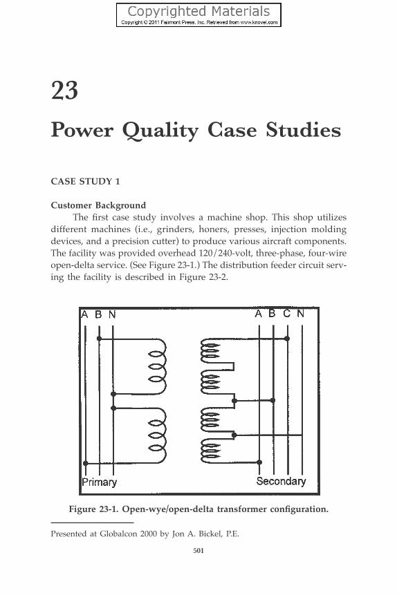
501
23Power Quality Case Studies
CASE STUDY 1
Customer Background The first case study involves a machine shop. This shop utilizes different machines (i.e., grinders, honers, presses, injection molding devices, and a precision cutter) to produce various aircraft components. The facility was provided overhead 120/240-volt, three-phase, four-wire open-delta service. (See Figure 23-1.) The distribution feeder circuit serv-ing the facility is described in Figure 23-2.
Presented at Globalcon 2000 by Jon A. Bickel, P.E.
Figure 23-1. Open-wye/open-delta transformer configuration.
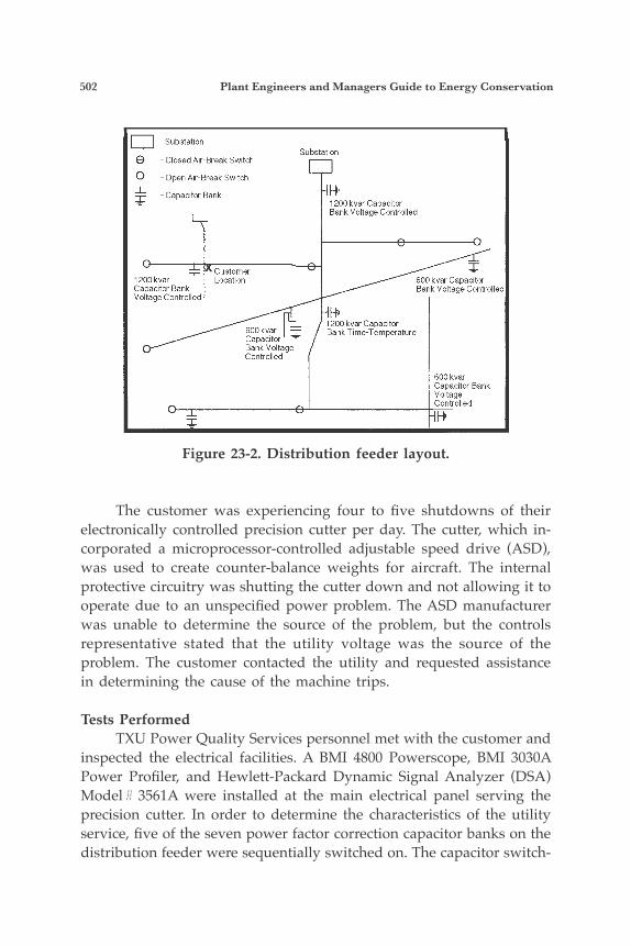
502 Plant Engineers and Managers Guide to Energy Conservation
The customer was experiencing four to five shutdowns of their electronically controlled precision cutter per day. The cutter, which in-corporated a microprocessor-controlled adjustable speed drive (ASD), was used to create counter-balance weights for aircraft. The internal protective circuitry was shutting the cutter down and not allowing it to operate due to an unspecified power problem. The ASD manufacturer was unable to determine the source of the problem, but the controls representative stated that the utility voltage was the source of the problem. The customer contacted the utility and requested assistance in determining the cause of the machine trips.
Tests Performed TXU Power Quality Services personnel met with the customer and inspected the electrical facilities. A BMI 4800 Powerscope, BMI 3030A Power Profiler, and Hewlett-Packard Dynamic Signal Analyzer (DSA) Model# 3561A were installed at the main electrical panel serving the precision cutter. In order to determine the characteristics of the utility service, five of the seven power factor correction capacitor banks on the distribution feeder were sequentially switched on. The capacitor switch-
Figure 23-2. Distribution feeder layout.
Power Quality Case Studies 503
ing transients were measured with the Powerscope; the Power Profiler and DSA were used to measure voltage distortion at the customer’s main electrical panel as each capacitor bank was energized and de-en-ergized.
Test Results and Conclusions The average voltage during the tests ranged from 238 volts to 253 volts, which is within acceptable limits. Inspection of the customer’s equipment indicated that the machine had internal circuitry which tripped the machine off if the high or low voltage, phase loss, or phase unbalance trip limits were exceeded. Because the voltage was not ex-ceeding these trip limits, it was determined that a distorted voltage waveform was causing the machine’s internal protection circuitry to erroneously sense phase unbalance or loss, resulting in the shutdown of the machine. The voltage distortion could be attributed to several factors, including the number of capacitor banks energized on the dis-tribution circuit, the load on the circuit, and the open-wye/open-delta winding configuration of the customer’s service transformers. The seven capacitor banks on the distribution circuit serving the customer total 6000 kvar. Six of the capacitor banks were operated by voltage-controlled switches, and one capacitor bank was operated by a time/temperature-controlled switch. The lowest level of total har-monic distortion (THD) was recorded when all capacitor banks were de-energized (THD of Vab = 2.9%, Vbc = 3.1%, and Vca = 5.3%), and the greatest level of THD occurred when five of the capacitor banks were energized (THD of Vab = 4.0, Vbc = 4.6%, and Vca = 7.7%). The distortion was comprised almost entirely of the 180-Hz component. All capacitor banks were not energized at the same time to prevent the excessive primary circuit voltage levels that were predicted. Disturbances due to switching transients were recorded when the two 1200-kvar capacitor banks located closest to the customer’s facility were energized. Although most of the capacitor banks have the potential to operate several times a day, none of the recorded switching transients caused the equipment to shut down. The recommended maximum voltage THD level according to IEEE Standard 519 is 5%, open-phase data/no single harmonic component exceeding 3%. Maximum distortion levels of 7.7% were observed on Vca during the tests. Higher distortion levels probably would have oc-curred if all the capacitors banks on the distribution feeder had been
504 Plant Engineers and Managers Guide to Energy Conservation
energized. Load and voltage magnitude on the distribution circuit can also affect voltage distortion levels. It is important to note that the THD on the “open” phase is approximately twice that of the other two phases (actually the sum of the distortion on the other two phases). This is a characteristic inherent to the open-wye/open delta transformation.
RECOMMENDATIONS
Prior to conducting these tests, a 1200-kvar capacitor bank one span from the customer’s facility was removed from service. The fre-quency of trips on the customer’s equipment was reduced from 4-5 occurrences per day to 1 occurrence per day. It was recommended that the size, placement, and controls of the remaining capacitor banks be reviewed to determine if modifications were necessary. As illustrated by the tests, it is often possible to reduce voltage distortion on a circuit by downsizing or removing capacitor banks. Voltage distortion may also be reduced by moving capacitor banks closer to large load centers. For this particular customer, converting the customer’s service from “open” transformation to a “closed” transformation was determined to be the most straightforward method for reducing voltage distortion to accept-able levels.
CASE STUDY 2
Customer Background This study involves a plastic foam manufacturing facility. The customer manufactures several lines of polystyrene food containers, including plates, take-out containers, etc. They are provided two 12.47 kV medium voltage points-of-delivery (POD). The customer had been in operation at this facility for approximately 10 years. The plant en-gineer reported experiencing various equipment failures over a period of approximately two months. The failed equipment included motors, electronic motor drives, and programmable logic control (PLC) cards. Two 30-hp induction motors failed simultaneously during a thun-derstorm. Both motors were rewound, but no failure report was gener-ated by the motor repair company. The motors were served from the same POD; however, the customer had experienced equipment losses
Power Quality Case Studies 505
on both PODs. TXU Power Quality Services group was requested to assist in determining the cause of the failures.
Tests Performed Power Quality Services personnel met with the plant engineer and the plant manager to discuss the equipment failures. A BMI 8800 Powerscope was installed on one of the main 480-volt electrical buses to monitor and record voltage and current. The customer provided a tour of the facility to point out specific equipment which had failed. The customer’s main electrical room and the utility facilities serving the customer were visually inspected at the time of the plant tour. The BMI 8800 was removed after a week of surveying the customer’s volt-age and current at the main.
Test Results Review of the voltage data showed that the instantaneous 6-cycle average voltage ranged from a minimum of 456 volts to a maximum of 492 volts. This voltage range is within normal equipment tolerances. Review of the current data showed that the instantaneous 6-cycle aver-age current ranged from a minimum of 1098 amperes to a maximum of 2081 amperes. The customer did not experience any equipment failures or problems during the test period. Visual inspection of the facility revealed that the failed motors (two 30-hp induction motors and an additional 10-hp drive motor) were located in close proximity to each other outside the facility on the East side. Failed remote I/O cards and control fuses were located throughout the facility. The customer had 480-volt transient voltage surge suppressors (TVSSs) installed at the main switchgear for each POD. The TVSSs did not appear to be U.L. listed and a let-through voltage of 1200 volts was written in ink on the units. Each of these units also had approximately 10 feet of lead length connecting it to the main 480-volt conductors.
CONCLUSIONS
Due to the number of failures within a brief time period, and the fact that lightning was present in the area at the time of the failures, it is likely that the failures were the result of high voltage transients from

506 Plant Engineers and Managers Guide to Energy Conservation
lightning strikes. The effects of high voltage transients (such as those caused by lightning strikes) include not only immediate equipment failures but also residual component failures due to the degradation of components caused by the high voltage stress. These failure modes were consistent with the equipment failures as experienced by the customer. A lightning strike in close proximity to the large metal tanks on the East side of the building probably caused the immediate failure of the motors and drive located in that area. It was apparent that common electrical grounding paths existed between the customer’s two PODs. With this configuration, a voltage potential rise (i.e., due to lightning) can cause damaging circulating currents to flow from one source to the other. Sensitive electronic equipment (such as the remote I/O PLC cards) that are not isolated from ground currents may be damaged or stressed under these circumstances.
This page has been reformatted by Knovel to provide easier navigation.
INDEX
Index Terms Links
A
absolute pressure 113
absorption
instruments 71
absorber 231
chillers 235
system 231
two-stage 234
after-tax life
cycle analysis 56
aggregation 389
air conditioning system design 239
airflow hoods 73
air preheaters 121 128 130
453
air velocity 72
alternative fuels 22
alternative investments 51
alternative research and development 20
American Recovery and Reinvestment Act of 2009 14
ammeter and voltmeter 64
amp meter, clamp-on 65
anemometers 73
annual cost method 48
aquachem areas 462
Index Terms Links
This page has been reformatted by Knovel to provide easier navigation.
ASHRAE 24
ASHRAE 90.2 26
ASHRAE Standard 90.1 24 26
ASHRAE Standard 90.2 25
ASHRAE Standard 90-80 26
B
ballasts, solid-state 107
baselines 422
bill consolidation 389
biofuels 18
BLAST 26
blower door 72
boiler 116
test kit 71
bottoming cycles 266 267
Bourdon tube gauges 74
brake horsepower 142
Brayton cycle 267 268 269
building design 205
C
California Title 24 26
capacitor 83 84 90
92
locations 85 88
capital recovery 47
carbon capture and sequestration 20
Carnot cycle 111
Index Terms Links
This page has been reformatted by Knovel to provide easier navigation.
cash analysis for interest formulas 60
cash flow rate of return analysis 56
cents per therm 14
characterization curve 380
chilled water 248
chillers
absorption 236
hybrid products 237
liquid
in series and in parallel 229
Clausius statement 111
coefficient of performance 225
coefficients of transmission 180 182 184
186 188 190
191 192 194
196 198
cogeneration 259 260 280
282 284 287
constant 265
energy production 283
feasibility 289
fuel cost 286
plant fuel consumption 284
systems
theory 262
coil run-around cycle 244
combined heat and power 327
combustion air temperature 121
combustion analyzer 73
combustion electronic analyzer 72
Index Terms Links
This page has been reformatted by Knovel to provide easier navigation.
combustion measuring, tester 71
compatibility curve 381
composite wall 154
compressed air leaks 299
concentrator 232
condensate
low-pressure, med. pressure 453
receiver vent 456
removal 462
return 458
modifications 464
system 452 465 466
condenser 232
condenser, vent 454 455
conduction 151 152 153
156
conductivity 75 173
controllers, programmable
logic 96 372
convection 151 157
conversion factors 13
cooling systems 240
cool storage 248
cost of energy 399
critical path schedule of energy
conservation activities 310
customer base line 79
customer charge 77
Index Terms Links
This page has been reformatted by Knovel to provide easier navigation.
D
deaerator 454 455
vent 454
dehumidification, desiccant 237
demand charge 78
demand control system 94
demand cooperatives 389
depreciation 53
declining-balance 54
desiccant systems 235 237 238
digital thermometer with pyrometer 70
dimensional change 75
discounted cash flow 31
distillation columns 148 150
distillation processes 148
distributed generation 325 326 328
329 330 331
332 338
district heating and cooling
plants 238
district-wide systems 389
draft gauge 74
E
economic analysis 286 375
economic impact 10
economizer cycle 243
electrical system performance 64
electric dispatch 278
Index Terms Links
This page has been reformatted by Knovel to provide easier navigation.
electric energy consumption
analysis 273
electric futures 390
electric vehicles 22
electrolytic 75
electromagnetic spectrum 63
ellipsoidal reflector lamps 100
energy accounting 7 11 473
energy assessment 2
energy audit 469
industrial 2
energy charge 77
energy codes 24
energy conservation 7 115 225
227 239 243
291 294
goals 308
implementation 5
energy effciency 21
ratio 9
energy efficient fluorescent lighting 102
Energy Independence and
Security Act of 2007 18
energy management 1
systems 391
energy manager 12
Energy Policy Act of 1992 14 21 27
Energy Policy Act of 2005 16
energy production in cogeneration systems 283
energy reduction recommendations 477
Index Terms Links
This page has been reformatted by Knovel to provide easier navigation.
energy saving survey checklist 295
energy services providers (ESPs) 393
energy service agreement, sample 346
energy standards 24
energy-use drivers 423 424 427
428
selected 425
energy-use profile 8
energy uses and losses 4
energy utilization 2 3 150
eQUEST 26
equipment sizing 277
equipment standards 22
escalation table 41 42 43
44
evaporator 129 231
exchangers
air-to-air 245 246
F
facility survey 61
feasibility evaluation 271
Federal Energy Regulatory Commission (FERC) 386
financing alternatives 341 342
finned-tube heat exchangers 158
fashing condensate 117
fash steam 456 464
fat plate solar collector 403
flue gas 121 122 127
fluorescent lamps 101 104
Index Terms Links
This page has been reformatted by Knovel to provide easier navigation.
food industry 449
foot-candle meters 66
fossil electric generation efficiency 330
fuel caloric values 275
fuel cell power systems 335
fuel cells 336 338 339
fuel inflation 58
furnace efficiency 119
checklist 120
Fyrite analyzer 72
G
gas analyzers 72
General Obligation Bond 342
generation 388
options 387
glazing, selective 224
glazing, switchable 223
glass characteristics 210
glass considerations 205
glass thermometers 73
global climate change 23
glycol ice storage tanks 252
glycol systems 252 253
gradient present worth 48 49 56
gravimeter 75
gravity feed systems 251
green jobs 21
Index Terms Links
This page has been reformatted by Knovel to provide easier navigation.
H
heat balance for steam process 116
heat exchangers 127 128 129
130 132 158
159 464
heat from lighting systems 247
heat gain 173 174
heating values 12
heat loss 162 166 167
174
calculations 161
for calcium silicate insulated
tanks 165
for steel pipe and fat surfaces 168
for tanks and vessels 164
of piping and fat surfaces 167
of vessels or tanks 163
to ground 163
heat of combustion for raw materials 15
heat pipes
air-to-air 245 246
heat pumps 226 362 364
air-to-air 226
hydronic 227 228
geothermal 359 360 361
heat recovery 124 244 454
455 456 459
466
system 135
Index Terms Links
This page has been reformatted by Knovel to provide easier navigation.
heat transfer 129 130 131
151
by convection 157
by radiation 156
coefficients 176
heat wheels 129 244 245
humidity measurement 74
HVAC 69 72 225
393
hybrid chiller/generator 237
hybrid strategy 279
I
ice storage systems 252
ice storage tanks
glycol 252
ice tank accessories 252
impulsive transient 373
industrial energy audit 2
infrared equipment 61 62
insulating glass system 222
insulation 214
interest factors 33 34 35
36 37 38
39 40
internal combustion engines 261
investment decision-making 31
ISO management system 441
isotherm contour 63
Index Terms Links
This page has been reformatted by Knovel to provide easier navigation.
L
lamp lumen depreciation 303
lamps
high-intensity discharge 104
low-pressure sodium 107
high-pressure sodium 105
mercury 106
metal halide lamps 105
parabolic aluminized
reflector lamps 100
tungsten halogen 100
latent heat of fusion 113
latent heat of vaporization 113
leakage rates 72
life cycle costing 29 30 58
light emitting diode fixtures 102
lighting 247
basics 97
control equipment 107
high-efficiency 477
incandescent 100
fixtures, recovery from 246
illumination requirements 99
light level meter 68
liquid chiller 228 229
liquid recirculation systems 250
load
demand controller 95
factor 273
Index Terms Links
This page has been reformatted by Knovel to provide easier navigation.
load (Cont.)
high 387
isolation 389
management 92 93
shaping 388
shedding 93 94 95
loan, commercial 342
lumen method 97
luminaires 99
M
maintenance programs 29
preventive 294
Malden turbine 334
management checklist 306
manometers 74
measurement and verification 421 422
baselines 422
measuring system efficiency 225
mercury lamps 105
metal halide lamps 105
metering 391
coincident 389
micromanometer 74
microturbines 333 339
systems 335
mitigation 374 378 379
382
Mollier diagram 131 134 139
Index Terms Links
This page has been reformatted by Knovel to provide easier navigation.
motors
induction (AC) 319
synchronous (AC) 91 317
DC 318
motor drives 372 373
gas-powered 392
motor efficiency 319 321
motor horsepowers and efficiencies 81 218
motor loads 81
motor rewinds 322
motor voltage 321
multipass flow 129
municipal lease 342
N
natural gas engine system 236
natural gas-fired DG systems 327
natural gas options 387 388
Natural Gas Policy Act (NGPA) 27
nitrogen areas 462
non-condensable vapors 454
O
oil return 251
open-wye/open-delta transformer 501
optical pyrometers 74
optical technologies 222
Orsat apparatus 71 72
Index Terms Links
This page has been reformatted by Knovel to provide easier navigation.
P
parabolic aluminized reflector
lamps 100
partnerships 327
payback analysis 55
payback period 29
method 29
payment plans 390
peak demand 387 388
peak shaving 278
photo detectors 63
photovoltaic systems 413 414 415
416
economics 412
pipe and pumping systems 146
piping systems 142
point-by-point method 97 98
pollution control impact 10
power conditioning 372 374 375
379 382
devices 371
power disturbances 375
power factor 66 83 91
92 108 319
charge 78
correction 81 85
shortcut method 86
meter 65
power fluctuations 372
Index Terms Links
This page has been reformatted by Knovel to provide easier navigation.
power prices
impacting factors 386
deregulated retail 387
ratchet rate 79
rate tariffs 77
real-time pricing (RTP) 78
time-of-day discounts 79
time-of-use rate schedules 78
power producers, independent 386
power quality 371 372 501
monitor 372
power storage devices 392
present worth method 48
pressure bulb thermometers 74
pressure drops 146
pressure measurement 74
pressure-reducing valve 466
pressurization 72
preventative maintenance program 294
prime mover selection 279
procurement specifications 150
programmable logic controllers 96 372
psychrometer 69 75
public utility commissions (PUCs) 386 394
Public Utility Holding Company
Act of 1935 27
Public Utility Regulatory Policies
Act (PURPA) 23
pump and piping worksheet 147
pumping drums 250
Index Terms Links
This page has been reformatted by Knovel to provide easier navigation.
pumps 142
purchasing strategies 385
pyrometer
suction 70
surface 68
Q
qualifying facility 24
R
radiation 151
pyrometers 74
Rankine cycle 269
ratchet rate 79
rate-of-return method 48
reactive demand charge 78
real-time pricing (RTP) 78
reciprocating engines 281 336 337
339
generators 280
recuperators 128 130
reflector lamps 100
refrigeration equipment 228
refrigeration systems-double
bundle condenser 247
regenerators 128 130
renewable energy 22
resistance thermometers 73
Index Terms Links
This page has been reformatted by Knovel to provide easier navigation.
Resource Conservation and Recovery
Act of 1976 (RCRA) 27
risk assessment 314
rotary UPS system 374
S
sensible heat 113
shell and tube heat exchanger 159 160
shortcut method 86
to determine released capacity 87
simple cycle gas turbines 333
single payment compound
amount 31
single payment present worth 32
sinking fund payment 47
small business energy programs 21
smart grid 21
smart windows 223
smoke generators 73
smoke tester 72
solar
applications 397 418
collector 403 408
control films 218 221
control screens 218
control laminate reflective,
perforated 220
economics 401
energy 16
heat gain factors 214
Index Terms Links
This page has been reformatted by Knovel to provide easier navigation.
solar (Cont.)
insolation 408
radiation 409
screen 221
louvered metal 221 222
shutters 219
system 398 401 402
406 407 410
411
turbines 333
water heating system 406
economics 405
solid-state ballasts 107
specific heat 113
concept 113
of various substances 114
standards for appliances and lighting 18
steam
balance 115
condensate flashing 118
distribution system 451
generation 135 451
alternatives 137
leaks 294
lines, bare 301
load and cost 450
loss 454
pressure 113
system optimization 449 450
tracing 123 302
Index Terms Links
This page has been reformatted by Knovel to provide easier navigation.
steam (Cont.)
traps 294 298 299
300 463
turbines 115 135 261
280 281 467
straight-line depreciation 53
suction pyrometer 70
sum-of-years digits 54
sunlight 205 219
effect of 203
Superior Energy Performance 437 438 439
440 442 443
444 445 446
447 448
super windows 224
surface pyrometers 68
surface temperatures 204
surge drum, horizontal 252
surges 372
susceptibility curve 380
swing vane gauges 74
switchable glazing 223
system compatibility 381
T
taxable lease 342
tax considerations 55
tax provisions 17
Tax Reform Act of 1986 55
Index Terms Links
This page has been reformatted by Knovel to provide easier navigation.
temperature 67 113
distribution 154
of waste gases 125
outside design temps/latitudes
for various cities 200
equivalent temp differentials
roofs 207
walls 208
surfaces 204
test and balance considerations 258
test, balance, and adjust program 258
thermal
barriers 220
conductivity 152 366
of industrial insulation 215
detector 63
dispatch 279
thermal/electric load ratio 276 277
minimum demand 277
energy consumption analysis 274
energy cost 284
load factor 276
resistances for surface films
and air spaces 175
shock 462 463
storage 236 248
control systems 253
thermocouple probe 70
thermocouples 74
thermodynamics 109
Index Terms Links
This page has been reformatted by Knovel to provide easier navigation.
thermodynamic cycles 266
thermographs 74
thermometer 67
battery operated 68
dial 68
digital 70
glass 73
portable electronic 69
pressure bulb 74
resistance 73
time-of-day discounts 79
time-of-use rate schedules 78
time value of money 31
tolling 391
topping cycles 266 267
TRACE 26
transmission 387 388
and distribution networks 392
options 387
trigeneration 238
tungsten halogen lamps 100
turbine engines, gas-powered 135 272 280
281
turbines
advanced 333
micro- 333 335 339
Malden 334
simple cycle gas 333
solar 333
Index Terms Links
This page has been reformatted by Knovel to provide easier navigation.
turbines (Cont.)
steam 115 135 261
280 281 467
U
uniform series compound amount 32 45
uniform series present worth 46
utility data analysis 272
V
vapor compression 236
vapor recompression distillation 149
variable air volume 240 242 243
systems 241
vent condenser 454 455
ventilation audit 255
voltage imbalance 323
voltage sags 372 373 382
voltage variation 322
volume/mix impact 10
W
waste heat 124 125 126
127 128
boilers 128
fluid 131
recovery 131 135 136
Index Terms Links
This page has been reformatted by Knovel to provide easier navigation.
water chiller
one-shell lithium bromide
cycle 232
wattmeter 65
weather 10
weather impact 10
weather-strip tape 222
windows
adjustable louvered 219
cool 224
interior storm 222
smart 223
super 224
window treatments 218
external blinds 219 221
high-performance window
shade 222
exterior sun control louvers 219
motorized window shading 218
multilayer, roll-up insulating 220
semi-transparent 220