planck 2013 results. vi. high frequency instrument data processing
TRANSCRIPT

Astronomy & Astrophysics manuscript no. HFIDPC c© ESO 201326th March 2013
Planck 2013 results. VI. High Frequency Instrumentdata processing
Planck Collaboration: P. A. R. Ade81, N. Aghanim56, C. Armitage-Caplan85, M. Arnaud69, M. Ashdown66,6, F. Atrio-Barandela19, J. Aumont56,C. Baccigalupi80, A. J. Banday88,10, R. B. Barreiro63, E. Battaner90, K. Benabed57,87, A. Benoît54, A. Benoit-Lévy24,57,87, J.-P. Bernard10,
M. Bersanelli33,47, P. Bielewicz88,10,80, J. Bobin69, J. J. Bock64,11, J. R. Bond9, J. Borrill14,82, F. R. Bouchet57,87∗, F. Boulanger56, J. W. Bowyer52,M. Bridges66,6,60, M. Bucher1, C. Burigana46,31, J.-F. Cardoso70,1,57, A. Catalano71,68, A. Chamballu69,16,56, R.-R. Chary53, X. Chen53,
L.-Y Chiang59, H. C. Chiang26,7, P. R. Christensen76,36, S. Church84, D. L. Clements52, S. Colombi57,87, L. P. L. Colombo23,64, C. Combet71,F. Couchot67, A. Coulais68, B. P. Crill64,77, A. Curto6,63, F. Cuttaia46, L. Danese80, R. D. Davies65, R. J. Davis65, P. de Bernardis32, A. de Rosa46,
G. de Zotti43,80, J. Delabrouille1, J.-M. Delouis57,87, F.-X. Désert50, C. Dickinson65, J. M. Diego63, H. Dole56,55, S. Donzelli47, O. Doré64,11,M. Douspis56, J. Dunkley85, X. Dupac39, G. Efstathiou60, T. A. Enßlin74, H. K. Eriksen61, F. Finelli46,48, O. Forni88,10, M. Frailis45,
A. A. Fraisse26, E. Franceschi46, S. Galeotta45, K. Ganga1, M. Giard88,10, G. Giardino40, D. Girard71, Y. Giraud-Héraud1, J. González-Nuevo63,80,K. M. Górski64,92, S. Gratton66,60, A. Gregorio34,45, A. Gruppuso46, J. E. Gudmundsson26, F. K. Hansen61, D. Hanson75,64,9, D. Harrison60,66,G. Helou11, S. Henrot-Versillé67, O. Herent57, C. Hernández-Monteagudo13,74, D. Herranz63, S. R. Hildebrandt11, E. Hivon57,87, M. Hobson6,W. A. Holmes64, A. Hornstrup17, Z. Hou27, W. Hovest74, K. M. Huffenberger91, G. Hurier56,71, T. R. Jaffe88,10, A. H. Jaffe52, W. C. Jones26,M. Juvela25, E. Keihänen25, R. Keskitalo22,14, T. S. Kisner73, R. Kneissl38,8, J. Knoche74, L. Knox27, M. Kunz18,56,3, H. Kurki-Suonio25,41,
G. Lagache56, J.-M. Lamarre68, A. Lasenby6,66, R. J. Laureijs40, C. R. Lawrence64, M. Le Jeune1, R. Leonardi39, C. Leroy56,88,10,J. Lesgourgues86,79, M. Liguori30, P. B. Lilje61, M. Linden-Vørnle17, M. López-Caniego63, P. M. Lubin28, J. F. Macías-Pérez71, C. J. MacTavish66,
B. Maffei65, N. Mandolesi46,5,31, M. Maris45, D. J. Marshall69, P. G. Martin9, E. Martínez-González63, S. Masi32, S. Matarrese30, F. Matthai74,P. Mazzotta35, P. McGehee53, P. R. Meinhold28, A. Melchiorri32,49, L. Mendes39, A. Mennella33,47, M. Migliaccio60,66, S. Mitra51,64,
M.-A. Miville-Deschênes56,9, A. Moneti57, L. Montier88,10, G. Morgante46, D. Mortlock52, S. Mottet57, D. Munshi81, P. Naselsky76,36, F. Nati32,P. Natoli31,4,46, C. B. Netterfield20, H. U. Nørgaard-Nielsen17, C. North81, F. Noviello65, D. Novikov52, I. Novikov76, F. Orieux57, S. Osborne84,C. A. Oxborrow17, F. Paci80, L. Pagano32,49, F. Pajot56, R. Paladini53, D. Paoletti46,48, F. Pasian45, G. Patanchon1, O. Perdereau67, L. Perotto71,F. Perrotta80, F. Piacentini32, M. Piat1, E. Pierpaoli23, D. Pietrobon64, S. Plaszczynski67, E. Pointecouteau88,10, G. Polenta4,44, N. Ponthieu56,50,
L. Popa58, T. Poutanen41,25,2, G. W. Pratt69, G. Prézeau11,64, S. Prunet57,87, J.-L. Puget56, J. P. Rachen21,74, B. Racine1, W. T. Reach89,R. Rebolo62,15,37, M. Reinecke74, M. Remazeilles56,1, C. Renault71, S. Ricciardi46, T. Riller74, I. Ristorcelli88,10, G. Rocha64,11, C. Rosset1,
G. Roudier1,68,64, M. Rowan-Robinson52, B. Rusholme53, L. Sanselme71, D. Santos71, A. Sauvé88,10, G. Savini78, E. P. S. Shellard12,L. D. Spencer81, J.-L. Starck69, V. Stolyarov6,66,83, R. Stompor1, R. Sudiwala81, F. Sureau69, D. Sutton60,66, A.-S. Suur-Uski25,41, J.-F. Sygnet57,
J. A. Tauber40, D. Tavagnacco45,34, S. Techene57, L. Terenzi46, M. Tomasi47, M. Tristram67, M. Tucci18,67, G. Umana42, L. Valenziano46,J. Valiviita41,25,61, B. Van Tent72, L. Vibert56, P. Vielva63, F. Villa46, N. Vittorio35, L. A. Wade64, B. D. Wandelt57,87,29, S. D. M. White74,
D. Yvon16, A. Zacchei45, and A. Zonca28
(Affiliations can be found after the references)
Preprint online version: 26th March 2013
Abstract
We describe the processing of the 531 billion raw data samples from the High Frequency Instrument (hereafter HFI), which we performed toproduce six temperature maps from the first 473 days of Planck-HFI survey data. These maps provide an accurate rendition of the sky emission at100, 143, 217, 353, 545, and 857 GHz with an angular resolution ranging from 9.′7 to 4.′6. The detector noise per (effective) beam solid angle isrespectively, 10, 6 , 12 and 39 µK in HFI four lowest frequency channel (100–353 GHz) and 13 and 14 kJy sr−1 for the 545 and 857 GHz channels.Using the 143 GHz channel as a reference, these two high frequency channels are intercalibrated within 5 % and the 353 GHz relative calibrationis at the percent level. The 100 and 217 GHz channels, which together with the 143 GHz channel determine the high-multipole part of the CMBpower spectrum (50 < ` < 2500), are intercalibrated at better than 0.2 %.
Key words. Cosmology: cosmic background radiation – Surveys – Methods: data analysis
1. Introduction
This paper, one of a set associated with the 2013 release ofdata from the Planck1 mission (Planck Collaboration I 2013),describes the processing of data from the High Frequency
∗ Corresponding author: F. R. Bouchet, [email protected] Planck (http://www.esa.int/Planck) is a project of the
European Space Agency (ESA) with instruments provided by two sci-entific consortia funded by ESA member states (in particular the leadcountries France and Italy), with contributions from NASA (USA) and
Instrument (HFI) from satellite data to calibrated and charac-terised maps. HFI (Lamarre et al. 2010; Planck HFI Core Team2011a) observes in the 100, 143, 217, 353, 545, and 857 GHzbands with bolometers cooled to 0.1 K. The HFI instrumentcomprises 50 signal bolometers, as well as two dark bolomet-ers, 16 thermometers, a resistor, and a capacitor used for mon-itoring and housekeeping. The count of 50 bolometers includes
telescope reflectors provided by a collaboration between ESA and a sci-entific consortium led and funded by Denmark.
1
arX
iv:1
303.
5067
v2 [
astr
o-ph
.CO
] 2
5 M
ar 2
013

Planck Collaboration: HFI data processing
twelve polarization sensitive bolometer (PSB) pairs, four eachat 100–353 GHz; the rest are unpolarized spider-web bolometers(SWBs). We describe the steps taken by the HFI Data ProcessingCentre (hereafter DPC) to transform the packets sent by thesatellite into sky maps at HFI frequencies, with the help of ancil-lary data, for example, from ground calibration. These are tem-perature maps alone, as obtained from the beginning of the firstlight survey on 13 August 2009, to the end of the nominal mis-sion on 27 November 2010.
Planck defines a sky survey as the time over which the spinaxis rotates by 180, a period close to six months in durationover which about 95 % of the sky is covered at each frequency.During routine operations, Planck scans the sky by spinning incircles with an angular radius roughly 85. The spin axis fol-lows a cycloidal path on the sky by periodic step-wise displace-ments of 2′, resulting in typically forty (35 to 70) circles of typ-ical duration 46 minutes, constituting a stable pointing periodbetween repointings. The scanning strategy is discussed in moredetail in Tauber et al. (2010), Planck Collaboration I (2011), andPlanck Collaboration I (2013). The 15.5 months of nominal mis-sion survey data then provide 2.5 sky surveys, and maps areprovided for the first two sky surveys separately as well as forthe complete nominal mission. As a means to estimate aspectsof the noise distribution, we also deliver “half-ring” maps madeout of the first and second half of each stable pointing period.Maps are produced for individual detectors, as well as for aver-ages over each band and for selected detector sets defined withineach band (see Table 3).
The next section provides an overview of HFI data pro-cessing. Section 3 is devoted to the processing of Time OrderedInformation (hereafter TOI) from individual detectors to producecleaned timelines. These timelines are used to estimate the tem-poral noise properties in Sect. 3.10 and to determine the detectorpointings and beams in Sects. 4 and 5. Section 6 discusses thecreation of maps and their photometric calibration, while Sect. 7presents tests applied to assess the consistency and accuracy ofthe products. For completeness, component separation and fur-ther processing is briefly described in Sect. 7.5. Section 8 con-cludes with a summary of the characteristics of the HFI datadelivered, as currently processed.
Some of the specific processing steps of HFI data aredescribed more fully elsewhere: Planck Collaboration VII(2013) discusses the transfer function and beams;Planck Collaboration VIII (2013) the calibration of HFIdetectors; Planck Collaboration IX (2013) the determination ofthe spectral bands for each detector and their combination; andPlanck Collaboration X (2013) the effect of so-called “glitches”such as cosmic-ray hits on the detectors. The processing ofdata from the Low Frequency Instrument (LFI) is discussed inPlanck Collaboration II (2013). Technical details applying tospecific data products are discussed in Planck Collaboration ES(2013). We have applied to the data products delivered manyconsistency and validation tests to assess their quality. Whilethe products meet a very high standard, as described here,we did find limitations. Their mitigation, and related dataproducts, are left to future releases. In particular, HFI analysisrevealed that nonlinear effects in the on-board analog-to-digitalconverters (ADC) modified the recovered bolometer signal. Insitu observations over 2012–2013 are measuring this effect,and algorithms have been developed to explicitly account forit in the data analysis. However, the first-order effect of theADC non-linearity mimics a gain variation in the bolometers,which the current release measures and removes as part of the
calibration procedures. This is discussed further in Sects. 6.2and 7.2.1.
The mapmaking procedure uses the full intensity and polar-ization information from the HFI bolometers. The current ana-lysis cannot guarantee that the large-scale polarization signal isfree from systematic effects. However, the preliminary analysisshows that the small-scale maps have the expected CMB con-tent at high signal to noise, as discussed in Sect. 6.7 below, andin Planck Collaboration I (2013) and Planck Collaboration XVI(2013). Although we do not use these maps for cosmologicalmeasurements, future work will use them for investigations ofthe properties of polarized emission of the Galaxy.
2. HFI data processing overview
The processing of HFI data proceeds according to a series oflevels, shown schematically in Figure 1. Level 1 (L1) creates adatabase of the raw satellite data as a function of time (TOI ob-jects). The full set of TOI comprises the signals from each HFIbolometer, ancillary information (e.g., pointing data), and asso-ciated housekeeping data (e.g., temperature monitors). Level 2(L2), the subject of this paper, uses these data to build a modelof the HFI instrument, the Instrument Model (IMO), producescleaned, calibrated timelines for each detector, and combinesthese into aggregate products such as maps at each frequency.Level 3 (L3) takes these instrument-specific products and de-rives various products: component-separation algorithms trans-form the maps at each frequency into maps of separate astro-physical components; source detection algorithms create cata-logues of Galactic and extragalactic objects; finally, a likelihoodcode assess the match between a cosmological and astrophysicalmodel and the frequency maps.
Of course, these processing steps are not done completelysequentially: HFI data is processed iteratively. In many ways,the IMO is the main internal data product from Planck, and themain task of the HFI DPC is its iterative updating. Early ver-sions of the IMO were derived from pre-launch data, then fromthe first light survey of the last two weeks of August 2009.Further revisions of the IMO, and of the pipelines themselves,were then derived after the completion of successive passesthrough the data. These new versions included expanded inform-ation about the HFI instrument: for example, the initial IMO con-tained only coarse information about shape of the detector angu-lar response (i.e., the full-wifth at half-maximum of an approx-imate Gaussian); subsequent revisions included full measuredharmonic-space window function.
In somewhat more detail, L1 software fills the databaseand updates, daily, the various TOI objects. Satellite atti-tude data, sampled at 8 Hz during science data acquisitionand at 4 Hz otherwise, are resampled by interpolation to the180.37370 Hz (hereafter 180.4 Hz) acquisition frequency of thedetectors, corresponding to the integration time for a singledata sample; further information on L1 step were given inPlanck HFI Core Team (2011b). Raw timelines and housekeep-ing data are then processed by L2 to compensate for instrumentalresponse and to remove estimates of known artefacts. The vari-ous steps in TOI processing are discussed in Sect. 3. First, theraw timeline voltages are demodulated, deglitched, corrected forthe bolometer non-linearity, and for temperature fluctuations ofthe environment using correlations with the signal TOI fromthe two dark bolometers designed as bolometer plate temperat-ure monitors. Narrow spectral lines caused by the 4He-JT (4 K)cooler are also removed before deconvolving the temporal re-
2

Planck Collaboration: HFI data processing
In-flight characterization TOI characterisation Focal plane geometry Beam shapes Noise properties Transfer functions
Mapmaking and calibration Create Healpix rings Compute destriping offsets Gather rings into maps Photometric calibration Zodiacal light & FSL correction
Create raw database Interpolate satellite attitude Create raw bolometer data TOI Create housekeeping TOI
TOI processing Demodulation Deglitching & flagging Gain nonlinearity correction Thermal drift decorrelation 4K cooler line removal Transfer functions deconvolution Jump correction Sample flagging
Clean TOIs
Trend analysisproducts
Instrument model
LE
VE
L 1
LE
VE
L 2
Frequency maps, difference maps, Healpix rings
LE
VE
L 3
Up
dat
e T
OI p
roce
ssin
g
Component Separation CMB map cleaning (non-parametric) Parametric component separation Targeted separations (CO, dust opacity)
Compact Sources Source detection, extraction Photometric measurement Monte Carlo quality assessment
Compact Source Catalogues, Masks
Component maps Likelihood Code
Figure 1. Overview of the data flow and main functional tasks of the HFI Data Processing Centre. Level 1 creates a database ofthe raw satellite data as a function of time. Level 2 builds a data model and produces maps sky maps at the six frequency of theinstrument. This flow diagram illustrates the crucial role of the Instrument Model (IMO), which is both an input and an output ofmany tasks, and is updated iteratively during successive passes of the data. Level 3 takes these instrument-specific products andderives final astrophysical products. This paper is mostly concerned with level 2 processing and its validation.
sponse of the instrument. Finally, various flags are set to markunusable samples.
Further use of the data requires knowledge of the pointingfor individual detectors as discussed in Sect. 4. During a singlestable pointing period, Planck spins around an axis pointing
towards a fixed direction on the sky (up to an accounted-forwobbling), repeatedly scanning approximately the same circle(Planck Collaboration I 2013). The Satellite is re-pointed so thatthe spin axis follows the Sun, and the observed circle sweepsthrough the sky at a rate of approximately one degree per day.
3

Planck Collaboration: HFI data processing
Assuming a focal plane geometry, i.e., a set of relations betweenthe satellite pointing and that of each of the detectors, we buildrings of data derived by analysing the data acquired by a detectorduring each stable pointing period (“ring” refers to the dataobtained during a single stable pointing period). This redund-ancy permits averaging of the data on rings to reduce instrumentnoise. The resulting estimate of the sky signal can then be sub-tracted from the timeline to estimate the temporal noise powerspectral density, a useful characterization of the detector dataafter TOI processing. This noise may be described as a whitenoise component, dominating at intermediate temporal frequen-cies, plus additional low and high-frequency noise. The effecton maps of the low frequency part of the noise can be partiallymitigated by determining an offset for each ring. These so-called“destriping” offsets are obtained by requiring that the differencebetween intersecting rings be minimised. Once the offsets areremoved from each ring, the rings are co-added to produce skymaps.
As explained in Sect. 6, a complication arises from the factthat the detector data include both the contribution from theSolar dipole induced by the motion of the Solar System throughthe CMB (sometimes referred to as the “cosmological” dipole),and the orbital dipole induced by the motion of the satellitewithin the Solar System, which is not constant on the sky andmust therefore be removed from the rings before creating thesky map. The Solar dipole is used as a calibration source at lowerHFI frequencies, and bright planet fluxes at higher frequencies.Since we need this calibration to remove the orbital dipole con-tribution to create the maps themselves, the maps and their calib-rations are obtained iteratively. The dipoles are computed in thenon-relativistic approximation. The resulting calibration coeffi-cients are also stored in the IMO, which can then be used, for in-stance, to express noise spectra in Noise Equivalent Temperature(NET). The destriping offsets, once obtained through a globalsolution, are also used to create local maps around planets. Asdescribed in Sect. 4 these are used to improve our knowledgeof the focal plane geometry stored in the previous version ofthe IMO and to improve measurements of the “scanning” beam(defined as the beam measured from the response to a pointsource of the full optical and electronic system, after the filteringdone during the TOI processing step, described in Sect. 5).
The ring and mapmaking stages allow us to generate manydifferent maps, e.g., using different sets of detectors, the first orsecond halves of the data in each ring, or from different sky sur-veys. Null tests using difference maps of the same sky area ob-served at different times, in particular, have proved extremelyuseful in characterising the map residuals, described in Sect. 7.
3. TOI processing
In the L1 stage of processing [previously described in Section 3of Planck HFI Core Team (2011b)], the raw telemetry TOI areunfolded into one time series for each bolometer. The signal isregularly sampled at 180.4 Hz. We denote as TOI processingthe transformation of the TOI coming from L1 into clean TOIobjects, which can be used for mapmaking after focal planegeometry reconstruction and photometric calibration have beendone. The general philosophy of the TOI processing is to modifythe timelines as little as possible, and therefore to flag regionscontaminated by systematic effects (e.g., cosmic-ray glitches).We deal with each bolometer signal separately. Aside from al-lowing the possible flagging of known bright sources, the onlypointing information that is used in the main TOI processing is
the phase (see Sect. 3.3) so the TOI processing assumes per-fect redundancy of the data within a given pointing period. Theoutput of TOI processing is not only a set of clean TOI butalso accompanying qualifying flags and trend parameters usedinternally for detailed statistics. Moreover, all data samples areprocessed while only clean samples will be projected on maps.For beam measurement (see Sect. 5), specific processing is per-formed on pointing periods that are close to Mars, Jupiter orSaturn (see Sect. 3.11).
A flow diagram is shown in Fig. 2 illustrating the TOI pro-cessing steps detailed in the following subsections. Section 4of Planck HFI Core Team (2011b) presents the early version ofthe TOI processing. The pipeline has changed sufficiently sinceto warrant a self-contained global description of the TOI pro-cessing. We refer the reader to Planck Collaboration ES (2013)and the various companion papers mentioned above for more de-tail. The changes mostly reflect the improvement in performanceand in understanding of the underlying effects. The TOI are notdelivered in the present data release but their processing is an es-sential, though hidden, ingredient in the delivered maps. Someof the systematic effects arising in the map analysis can only beunderstood by referring to the bolometer timeline behaviour andprocessing.
It was recently realised that some apparent gain variations,spotted comparing identical pointing circles one-year apart, ac-tually originate in non-linearities in the bolometer readout sys-tem ADCs. Note that the ADC non-linearity is not corrected forin the TOI processing, but rather as an equivalent gain variationat the mapmaking level (see Sect. 6.2 and Sect. 7.2.1).
3.1. Input flags
Strong signal gradients can adversely affect some stages of TOIprocessing. We flag the data expected to have strong gradientsusing only the pointing information, only in intermediate stagesand not for the mapmaking stage. We also flag data where thepointing is known to be unstable. Input flags come from the fol-lowing:
1. A Point-source flag. It is based on the locations of sources inthe ERCSC. A mask map is generated around each of themfrom which flag TOI objects are created using the pointinginformation.
2. A Galactic flag. It is based on IRAS maps with a thresholdthat depends on the frequency.
3. A BigPlanet flag. Any sample that falls within a given dis-tance of Mars, Jupiter or Saturn is retained for this flag.
4. An Unstable pointing flag (see Sect. 4). This accounts fordepointings between stable pointing periods and other lossesof pointing integrity.
Flagged data are either processed separately or ignored, depend-ing on the specific analysis. The flags are described in more de-tail in Planck Collaboration ES (2013).
3.2. Demodulation
The bolometers are AC square-wave modulated to put the ac-quisition electronics 1/ f noise at high temporal frequencies(Lamarre et al. 2010). A demodulation step is done as follows.First a one-hour running average of the modulated timeline iscomputed, known as the AC offset baseline. This is done by ex-cluding data that are masked due to glitches (see below) or by theGalactic flag (see above). Once the AC offset baseline is subtrac-
4

Planck Collaboration: HFI data processing
Figure 2. Main TOI processing steps. Pipeline modules are represented as filled squares. TOI: Time Ordered Information. ROI: ringordered information (i.e., one piece of information per stable pointing period). Ring: data obtained during a stable pointing period(typically 40 satellite revolutions of one minute each).
ted from the raw timeline, a simple (+,−) demodulation is ap-plied. The overall sign of the signal is set to get a positive signalon point sources and Galaxy crossings. This AC offset baselineremoval is needed in order to correct for the slow drift of thezero level of the electronics. Any possible drift of the baselineat a timescale smaller than one hour is dealt with at the filter-ing stage (see below). The baseline varies very smoothly overthe mission and fluctuates by less than ten minimum resolutionunits from the middle of 65536 values allowed by the on-boardADC, discussed in greater detail in Sect. 7.2.1.
3.3. Deglitching and gap-filling
The timelines are affected by obvious “glitches” (cosmic rayhits and other large excursions) at a rate of about one persecond. This generates a huge Poisson noise if not dealtwith. Such glitches are detected as a large positive signalfollowed by a roughly exponential tail. There are two ba-sic classes of glitches affecting bolometers. The statisticaland physical understanding of the two populations is givenby Planck HFI Core Team (2011b), revised and expanded byPlanck Collaboration X (2013). Here we present the general al-gorithm.
The type of TOI used in the deglitching is slightly differentfrom the one used in the main processing described in the fol-lowing sections. Before deglitching, the timeline is demodulatedand digitally filtered with a three-point (0.25, 0.5, 0.25) mov-ing kernel. Linear interpolation is performed on those parts ofthe timeline when the bolometer pointing nears Mars, Jupiteror Saturn, as determined by the BigPlanet flag (see Sect. 3.1).This step is done to treat the pointing periods containing a planetcrossing whose large gradients would otherwise be conflatedwith glitches.
The algorithm also requires an estimate of the sky signal inorder to assess the magnitude of excursions about the mean. Itrelies on the fact that the signal component of the timeline isperiodic within a stable pointing period (up to the slight wob-bling of the satellite spin axis). We construct a phase-binned ring(PBR), a useful estimate of the sky signal obtained by averagingthe unflagged TOI samples in bins of constant satellite rotationphase. The phase of a sample is given by the pointing reconstruc-
tion pipeline and varies continuously from 0 to 2π for each scancircle (about one minute). The bin size is about the width of asingle sample, i.e., 1.′7 and the definition of the zero of the phaseis irrelevant.
The algorithm treats each pointing period separately and onebolometer at a time. The localization of glitches is done witha sigma-clipping method applied to the sky-subtracted TOI. Atemplate fitting method is used to identify the type of each glitch.After masking and subtracting the series of fitted glitches fromthe original timeline, the PBR is then recomputed as the averageof unflagged samples. Several iterations (generally six) are per-formed until the variation of χ2 becomes negligible. The spikepart of each glitch is flagged and the exponential tail, below the3.3σ level, is subtracted using the last iteration of the glitch tem-plate fitting process.
Most of the samples flagged by this process are due to cos-mic ray hits. Figure 3 shows the mean evolution per channelof the fraction of flagged samples over the full mission. Moreglitch statistics are given by Planck Collaboration X (2013) andPlanck Collaboration ES (2013).
All gaps due to flagged samples within a ring of data arereplaced with an estimate of the signal given by the PBR. Forsamples around planets, we fill the timeline with the values readfrom a frequency map (made by excluding planets) from a previ-ous iteration of the data processing at the corresponding pointingcoordinates.
3.4. Bolometer non-linearity correction
If the environment of a bolometer changes, its response willchange accordingly. The extreme thermal stability of Planck isshown by the measured total power level, which is seen as almostconstant (see the next paragraph). Nevertheless, the timelinesmust be corrected to account for the slightly varying power ab-sorbed by the bolometer coming from the sky load and 100 mKbolometer plate temperature fluctuations. For that purpose, thevoltage-to-power conversion step is assumed to be a simplesecond order polynomial applied to the timeline:
P =v
S 0
(1 +
vv0
), (1)
5

Planck Collaboration: HFI data processing
Figure 3. Evolution of the fraction of the flagged data per bolo-meter averaged over a channel for the six HFI channels. A run-ning average over 31 pointing periods (approximately a day) isshown. The peak around day 455 comes from the sorption coolerexchange, while the peaks after day 500 are due to solar flares.
where v is the out-of-balance demodulated voltage (i.e., thevoltage difference between the square-wave compensating inputvoltage and the total bolometer voltage), S 0 is the responsivity(typically of order 109 V/W) for the fiducial v = 0 voltage. It ismeasured on ground-based I-V curves, but its exact value is un-important as it is calibrated out. The parameter v0 is determinedfor each bolometer from measurements made during the CPVphase. In general the v0 values (5 to 200 mV) are equal to orlarger than expected using a static bolometer model. The mainreason is that a TOI sample is an average of 40 on-board meas-urements (half a modulation period), which includes an elec-tronic transient (see e.g., Catalano et al. 2010). The non-linearitycorrection, as measured by v/v0 in Eq. 1, is static and accuratefor a slowly varying signal, in particular for dipole calibration.The term v/v0 is of the order of 10−3 at most, over half a dipoleperiod, the effect being largest in the 100 GHz band.
During the mission, the drift of the zero level (as meas-ured by v/S 0) is at most roughly 7 fW for bolometers up to the353 GHz channels, and 50 fW for the 545 and 857 GHz chan-nels, such that the non-linearity correction implies a drift in thegain of typically 10−3 at most, for all detectors. The correctionhas a relative precision better than 10 %, so that the gain un-certainty is at the 10−4 level. The effective gain and uncertaintyis, however, further affected by the offset in the ADC electronics,as discussed in Sect. 7.2.1 below. The dynamical bolometer non-linearity on very strong sources (Jupiter and the Galactic centre)are not corrected in the nominal TOI.
In addition, there are limits associated with the saturation ofthe analog-to-digital converters. As discussed in the explanatorysupplement, Jupiter and the Galactic centre are the only signalson the sky strong enough to trigger this effect.
3.5. Thermal drift decorrelation
The removal of the common mode due to temperature fluctu-ations of the 100 mK cooler stage is based on measured couplingcoefficients between the bolometers and the bolometer plate tem-perature. The coefficients were measured during the CPV phase(typically 50 pW/K for bolometers up to the 353 GHz chan-
nel, and 300 pW/K for the 545 and 857 GHz channels). Thetwo dark bolometers are used as a proxy for the bolometer platetemperature fluctuations, as HFI 100 mK thermometers havetoo many cosmic ray hits to be used. The two dark bolometertimelines are deglitched (in the same way as the other bolomet-ers) then smoothed with a one minute flat kernel. From each bo-lometer timeline, a linear combination of the two smoothed darktimelines is subtracted. During this stage, the timelines of all sig-nal bolometers are flagged at the samples where any of the darkbolometers is flagged for at least 30 seconds. This is done inorder to suppress the impact of large glitches happening on thebolometer plate. We found empirically that this method excludesautomatically the worse solar flares and in particular the risingcommon mode induced by massive cosmic ray events. Note thatthe total range of the temperature fluctuation of the bolometerplate is less than 80 µK, except for some strong solar flares. Asshown in Fig. 6 of Planck HFI Core Team (2011a), the temper-ature fluctuations of the 1.6 K and 4 K stages have a negligibleinfluence on the TOI noise properties.
3.6. 4 K cooler line removal
The 4He-JT cooler (hereafter, 4 K cooler) produces strong, nar-row lines in the power spectral density (PSD) of HFI data.These arise from electromagnetic interference of the 4 K coolermoving parts with the bolometer readout wires, situated in thePlanck service module. The 4 K cooler main frequency (40 Hz)and its harmonics appear as very narrow lines PSD of the sig-nal with an intensity of 10 to 100 times above the white noise.The oscillations of the moving parts of the 4 K cooler are syn-chronously driven by the same computer that records the datasamples. Hence for a given stable 4 K cooler line, only one fre-quency is affected in the PSD, i.e., a narrow line is produced,only broadened by the pointing period integration time. Onlynine individual frequencies are detectable, each of which can betraced to some 4 K cooler harmonic unfolded by the AC modu-lation. In the signal domain, they are at 10, 20, 30, 40, 50, 60,70, 80, and 17 Hz, which are these fractions of the modulationfrequency: 1/9, 2/9, 3/9, 4/9, 5/9, 6/9, 7/9, 8/9, 5/27. Somethermal instability in the service module makes the line proper-ties to change on timescales larger than ten minutes.
We now show the method used to correct the 4 K cooler linecontamination in the timelines. In order to prepare the data onwhich to compute the Fourier coefficients, we build an interme-diate set of signal-removed TOI4K objects. We “unroll” the PBRby using as a signal estimate the PBR value from the sky loca-tion observed at each time. We then subtract this unrolled signalfrom the original TOI objects. Point sources are linearly inter-polated in these intermediate TOI4K. Then, we measure the co-sine and sine Fourier coefficients on the TOI4K for each of thenine lines, once per pointing period. We thus neglect variationsof these components within the duration of a pointing period.
We can then subtract from the original TOI objects a timelinemade of the nine reconstructed components. This notch fil-ter scheme produces ripples around strong point sources(seePlanck HFI Core Team 2011b). The origin of this problem liesin the relative position of the 4 K cooler line frequencies withrespect to the harmonics of the spin frequency. Most of the time(typically 97 % of the pointing periods), a given 4 K cooler linedoes not overlap with any spin frequency harmonics and thusdoes not affect the signal at all. The spin frequency is very stablewithin a pointing period and varies from one pointing period toanother by a factor of at most 10−4 . Hence, in so-called resonant
6

Planck Collaboration: HFI data processing
pointing periods, a 4 K cooler line overlaps one harmonic of thespin frequency. The Fourier coefficients are perturbed by the sig-nal and no longer represent the systematic effect. For those point-ing periods only, we interpolate the Fourier coefficients from ad-jacent non-resonant pointing periods and subtract the systematictimeline from the original TOI objects in the same way as theother pointing periods.
While tests with simulations (described in the explanatorysupplement) demonstrate that any residual 4 K line contamina-tion is reduced a less than 3 % of other sources of noise, theselines also affect our ability to characterise and remove the ADCnon-linearity (discussed in Sect. 7.2.1), and are thus still a sub-ject of active analysis.
The efficiency of our removal may be judged by compar-ing map power spectra with this step switched on or off. Itis found that the affected multipoles are at ` ' 60 ( f /1 Hz),i.e., 600, 1020, 1200, 1800,... When the module is switchedon, the line residuals amount to no more than 2.5 % of thenoise level at those multipoles and much less elsewhere (seePlanck Collaboration ES 2013)
3.7. Fourier transform processing
The bolometer response suffer from time-constant effects, whichmust be corrected. These effects, modelled as a complex trans-fer function whose parameters are determined on planet data(see Sect. 3.11), are deconvolved at the end of TOI processing.An additional filter is applied in order to avoid a large increaseof noise (without much signal) produced by the deconvolutionin the last 20 Hz near the modulation frequency. We refer thereader to a dedicated accompanying paper for a complete de-scription (Planck Collaboration VII 2013). Filtering and decon-volution are done during the same Fourier and inverse Fouriertransform stage. Chunks of 219 samples are used at a time witha standard fast-Fourier transform (FFT) and inverse transform.The deconvolved and filtered data are then computed and savedfor the middle 218 samples. The process is continued by shift-ing the input samples by 218 until the end of the timeline. Thisensures continuity in the recovered final timelines.
For the 545 and 857 GHz channels, the filtering is digital andconsists of a simple local smoothing kernel: 0.25, 0.5, 0.25. Forthese channels, the filtering is applied first; then the deconvolu-tion is done with the FFT module.
3.8. Jump corrections
We now build another set of intermediate signal-removed TOIfrom the deconvolved data. These consist mostly of noise, ex-cept in regions of strong gradients, for example near the Galacticplane. Some pointing periods are seen to be affected by a suddenjump (either positive or negative) in the signal-removed TOI.We therefore correct for that jump by subtracting a piecewise-constant template from the timeline, while preserving the meanlevel. The exact jump location not being precisely fitted, the TOIare flagged around the recovered position with 100 samples onboth sides.
We find on average 17 jumps per day, over all bolomet-ers, with jumps affecting a single bolometer at a time. Hence,a fraction less than 10−5 of data is lost in the flagging process.The jump rate fluctuates during the mission with a peak-to-peakvalue of nine jumps per day. So far, there is no real explanationfor these events, although we can suspect cosmic ray violent hitson the warm electronics.
We have checked the jump correction process on simulatedjumps of various intensities added to pointing periods withoutjumps. All jumps above half the local standard deviation of thesignal-removed TOI are found.
3.9. Flagging samples
We now build a total flag out of several flags in order to qualifythe TOI for mapmaking. A sample with any of the followingflags is considered invalid data:
1. The unstable pointing flag described in Sect. 3.1 (see alsoPlanck Collaboration I 2013), typically accounting for threeminutes per pointing period (roughly seven percent of data).
2. The missing or compression error data flag, discard-ing a fraction of 10−9 of the whole mission (seePlanck HFI Core Team 2011a).
3. The bolometer plate temperature fluctuation flag (seeSect. 3.5). One to two percent of the data are flagged thisway depending on time.
4. The glitch flag. Typically between eight and twenty percentof data are flagged depending on the time and the bolometer(Planck Collaboration X 2013). For PSBs, both detectors areflagged even if, in a few cases, only one of them sees theglitch.
5. The jump flag. Two hundred samples per jump are flagged, afraction less than 10−5 (see Sect. 3.8).
6. The Solar System Object (SSO) flag. A zone of exclusionis defined around Mars, Jupiter, Saturn, Uranus, Neptune,and around the 24 asteroids detected at 857 GHz (seethe complete discussion of asteroids in Appendix A ofPlanck Collaboration XIV (2013)). The coordinates of theobjects are obtained from the JPL Horizons database2
(Chamberlin et al. 1997), which uses the actual position ofthe Planck Satellite in its orbit around the L2 point. As theSolar System Objects are moving in celestial coordinates,the data (although valid) must be discarded and this maskingmust be done in the time domain. One survey map has thusup to 35 holes, which are filled by information from othersurveys. Overall, the final maps have almost no holes: lessthan 10−5 of pixels are missing.
On top of flagged samples in the TOI, we show now that someflagging also has to be done at the pointing period level (i.e.,considering entire rings of data).
3.10. TOI Qualification
We will later make maps by projecting the PBR into sky co-ordinates. We therefore base our criteria for the acceptance orrejection of a given pointing period for mapmaking by using thestatistics of only the signal-removed TOI as an estimate of thenoise. Hence, the qualification is minimally biased by the signalitself.
This noise estimate timeline is first analysed in the Fourierdomain. In Planck HFI Core Team (2011b) we described howthe detector white noise level (equivalently, the NET) is de-termined from noise periodograms in the frequency region bey-ond the low frequency excess noise component and before theincrease introduced by the time-constant deconvolution. Thiswhite noise level differs from that deduced directly from themaps. We have therefore adopted a method for determining the
2 http://ssd.jpl.nasa.gov/
7

Planck Collaboration: HFI data processing
“total” noise: this is derived directly from the standard deviationof the signal-removed TOI after flagging the Galactic plane andpoint sources for each pointing period. The standard deviationis then corrected upward by a term that depends on the durationof the pointing period. This term has the form
√f d/( f d − 1),
where d is the pointing period duration in minutes and f is thefraction of valid data within a pointing period (typically 0.8).It accounts for the fact that a fraction of the noise remains inthe PBR, and that fraction is smaller on longer pointing peri-ods, where the signal is better estimated. The final value of thistotal noise level for each detector (third column of Table 1) isthen taken to be the peak of the distribution of the root-mean-square (rms) noise of the valid pointing periods. The typical bo-lometer NETs, measured on the deconvolved TOI between 0.6and 2.5 Hz, are also given in Table 1 (second column). The totalnoise can be viewed as proportional to the square root of theintegral of the noise-equivalent temperature across the total fre-quency bandpass (including filtering effects) from 0 to 91 Hz. Itis normalised to one second of integration time so that pure whitenoise would have numerically identical NET and total noise.Deconvolution and filtering effects can produce a NET larger orsmaller than the total noise.
Table 1. Noise characteristics. The quoted value is the noise thatis obtained on the map after one second of integration, i.e., about180 hits for one bolometer. This gives the noise characteristicsof bolometers, inverse quadratically averaged over the similarones within a channel (“P” is for polarization sensitive bolomet-ers and “S” for spider web unpolarized bolometers). The secondcolumn gives the white noise level measured on the power spec-trum in the range of 0.6 to 2.5 Hz. The third column gives thetotal noise, i.e., the rms noise at the map level for one secondof integration time of a single detector. The next column recallsthe goal stated before launch by Lamarre et al. (2010). Note thatthe mean integration time per detector per (1.7′)2 pixel is 0.56seconds (0.63) for the 100–353 (resp. 545–857 GHz) channels,for the nominal mission (see Fig. 21).
Band NET Total Noise Goal Units
100P 71 132 100 µKCMB s1/2
143P 58 65 82 µKCMB s1/2
143S 45 49 62 µKCMB s1/2
217P 88 101 132 µKCMB s1/2
217S 74 66 91 µKCMB s1/2
353P 353 397 404 µKCMB s1/2
353S 234 205 277 µKCMB s1/2
545S 0.087 0.052 0.116 MJy sr−1 s1/2
857S 0.085 0.056 0.204 MJy sr−1 s1/2
The noise estimate is also analysed in the time domain.Figure 4 shows one pointing period of the signal-removed TOIfor four detectors along with the histogram of the samples.
Figure 5 shows an example of the evolution of this total noise(uncalibrated at this stage) during the first four surveys (hencebeyond the nominal mission). The bias linked to the pointingperiod duration has been corrected for. Notice that the totalnoise is mostly constant with peak-to-peak variations at the per-cent level, suspected to be induced by ADC non-linearities (seeSect. 6.2).
A pointing period that deviates significantly from the othersis flagged in the qualification process and not used in furtherprocessing. Three criteria were used to quantify the deviation:
– the absolute value of the difference between the mean andthe median value of the signal-removed TOI,
– the total noise value, and– the Kolmogorov-Smirnov test deviation value. When a given
pointing period is stamped as anomalous for more than halfthe bolometers, it is discarded for all of them.
The common anomalous pointing periods are linked to somespacecraft events or strong solar flares, while the individual an-omalous pointing periods correspond to incidents in the overalllevel of the timeline (like strong drifts).
There are two detectors (one each at 143 and 545 GHz, notcounting toward the total of 50 HFI detectors) that are not used atall because they show a permanent non-Gaussian noise structure,which we denote random telegraphic signal (RTS). The RTS bo-lometer signal-removed TOI show an accumulation of values attwo to five discrete levels. The measured signal-removed TOIjump at random intervals of several seconds between the dif-ferent levels. The jumps are uncorrelated. A third detector (at857 GHz) shows the RTS phenomenon but only for some well-delimited periods. Other detectors show a significant but smallerRTS in episodes of short duration. A dedicated module searchesfor these episodes, which are then added to the list of discardedpointing periods. Ten pointing periods of exceptionally long dur-ation are discarded for all bolometers, because noise stationarityis not satisfied in those cases.
The discarded pointing periods represent less than 0.8 % ofthe total integration time for the nominal mission.
Many examples of the characterization and qualification ofthe TOI processing can be found in Planck Collaboration ES(2013), where simulations are used to limit the possible effectsof undetected RTS periods to a fraction of the overall noise level.
In addition, the explanatory supplement presents a numberof simulations and other tests which have been done to set lim-its on possible contamination from a number of other possiblesystematic effects.
3.11. Big planet TOI
As the TOI of the standard pipeline are interpolated aroundMars, Jupiter, and Saturn, they cannot be used for the beam re-construction (see Sect. 5). Therefore a dedicated pipeline is runon appropriate pointing period ranges. The difference with thestandard pipeline is mainly a special deglitching step done onthe planet samples to cope with such a strong signal and its vari-ations during a given pointing period. Also, the jump correctionis not applied to avoid its triggering by the planet transit.
4. Detector pointing
Here we summarize the pointing solution we use, determinedwith the overall goal of limiting detector pointing errors toless than 0.′5 (rms). The satellite pointing comes from the startracker camera subsystem, which gives the location of a fidu-cial boresight direction as a function of time, sampled at 8 Hz.In practice, science data analysis requrires the pointing of eachdetector, sampled at the same rate as the detector signal. This, inturn, requires a number of separate steps:
1. Resampling to the acquisition frequency (180.4 Hz);
8

Planck Collaboration: HFI data processing
1•105 2•105 3•105 4•105
Sample Number
-1500
-1000
-500
0
500
1000
1500
Sig
nal [
aW]
1 10 100 1000 10000Counts
Detector 100_1a
1•105 2•105 3•105 4•105
Sample Number
-500
0
500
Sig
nal [
aW]
1 10 100 1000 10000Counts
Detector 143_7
1•105 2•105 3•105 4•105
Sample Number
-500
0
500
Sig
nal [
aW]
1 10 100 1000 10000Counts
Detector 217_1
1•105 2•105 3•105 4•105
Sample Number
-500
0
500S
igna
l [aW
]
1 10 100 1000 10000Counts
Detector 353_7
Figure 4. The signal-removed TOI sample values are displayed for one pointing period and four detectors (left panel of the foursets). Flagged samples are not shown. Samples falling near the Galactic plane or point sources are not shown either (correspondingto one-minute periodic blanks in the plots). The right panel of the windows shows the histogram (in black) of the samples. Thecoloured curve is the symmetric version around the mean.
2. Rotation from the fiducial boresight to the detector line ofsight; and
3. Correction for detector aberration(Planck Collaboration XXVII 2013).
The second step above must be calibrated in situ: the detailedgeometry must be measured by comparison with the positionsof known objects (planets and other bright sources whose ex-tent is small compared to the width of the beam). The primarysource of this geometrical calibration is the planet Mars, whichis bright (but not so bright as to drive the detectors into a non-linear response) and nearly pointlike (with a mean disk radius of4.′′111 during the nominal mission). Figure 6 shows the pointingof each detector relative to the pre-launch optical model.
Note that the in-scan pointing is degenerate with any phaseshift induced by the combined detector time response and op-tical beam and any attempt to remove them by deconvolution.For that reason, this calibration of the pointing cannot itself beconsidered as a measurement of the focal plane geometry per se.
Because the transfer of the pointing from the star tracker tothe detectors depends on the satellite rotation axis and hence themoment of inertia tensor, we do not expect the detector pointingrelative to the star tracker to be constant in time. We thereforereconstruct the pointing solution relative to the star tracker as a
function of time, and in the following discuss the accuracy of thereconstruction in different frequency regimes.
High-frequency fluctuations in the spacecraft and focal planeorientation are inhibited by inertia but are still present in the rawstar tracker pointing. Having no useful signal content, this re-gime is treated by applying a low pass filter to the reconstruc-ted pointing. Similarly, high-frequency errors can be assessedby studying the noise-dominated high frequency pointing powerspectrum.
Intermediate-frequency pointing errors, on one minute timescales, are characterized with Jupiter transits. We make use ofthe optimal combination of high signal-to-noise ratio and rel-atively wide beam at the Planck 143 GHz channel and first doa global fit of the planet position in the transit data. We thenconsider a small pointing offset to each 60 second scanningcircle. The test succesfully recovers an expected interference sig-nal from the radiometer electronics box assembly (REBA; seePlanck Collaboration II 2011 and Planck Collaboration I 2013).Thermal control on REBA was adjusted on day 540 after launchand subsequently Jupiter transit three does not exhibit the inter-ference. We find that the intermediate-frequency pointing erroris less than 3′′ (rms) before the REBA adjustment and less than1′′ beyond day 540 (see Fig. 7).
9

Planck Collaboration: HFI data processing
Figure 5. Top: Total noise estimated for each stable pointing period for a 143 GHz PSB. A smoothed version is shown in green .Bottom: A renormalised version of the upper plot shows how outliers are picked up (above 5 σ of the moving median in green).
In scan offset [arcmin]
Cro
ss s
can
offs
et [a
rcm
in]
-2-1
01
2
-2 -1 0 1 2
100 GHz143 GHz217 GHz353 GHz545 GHz857 GHz
Figure 6. Position of the individual HFI detectors with respectto a pre-launch model as measured on the first passing of Mars.The horizontal is the direction of the scan (“in-scan”); vertical isperpendicular to this (“cross-scan”).
The pointing is easiest to monitor over long time scales, us-ing observations of bright planets. In Fig. 8 we show the dif-ference between the first two observations of Mars; differencesalong the scan direction have a mean of 0.′′85 and a standard de-viation of 0.′′59; cross-scan differences in the direction perpen-
dicular to this are 3.′′7 ± 2.′′8 and are systematic with frequency.Indeed, analysis of further planet-crossings and of aggregatehigh-frequency point-source crossings exhibits arcminute-scaleevolution over the course of the mission. Fitting for an overalloffset for each planetary transit allows us to measure long timescale (several days) pointing fluctuations. We complement thissparse sampling of the overall offset by time domain positionfits of brightest compact radio sources as well as monitoring ofmany low-flux high-frequency sources in aggregate. In the pro-cess we learned that each radio source position was biased by afew arcseconds from their catalogued position. We take the biasto result from convolving the source emission with our effect-ive beams and correct for it by assuming that the low frequencypointing correction derived from planet transits alone is alreadyaccurate enough for debiasing the positions. For each compactsource we solve for its apparent position in the Planck data byconsidering a single constant offset to its catalogued position.
The planet positions alone indicate a change in the averagelevel of the low frequency fluctuations between Jupiter transittwo and Neptune transit three (days 418 and 540). The ra-dio sources, particularly QSO J0403-3605, further narrow thetransition before day 456. It is likely that the offset is dueto thermoelastic deformation caused by the sorption coolersystem switchover on day 460 (Planck Collaboration II 2011;Planck Collaboration I 2013). If entirely untreated, the low fre-quency pointing error dominates the error budget with around15′′ (rms) error. Two independent focal plane solutions bring thelow-frequency rms error well below 10′′ and applying a time-dependent correction reduces the low frequency error to the or-der of few arcseconds.
Figure 9 shows the uncorrected planet positions with thedebiased bright point-source positions along with the resultingPlanck pointing solution, which smoothly interpolates with a
10

Planck Collaboration: HFI data processing
6 4 2 0 2 4 6Time [h]
64
20
24
6Poin
ting o
ffse
t [a
rc s
ec]
Cross-scan RMS = 2.019''
Co-scan RMS = 2.285''
5 0 5Time [h]
32
10
12
3Poin
ting o
ffse
t [a
rc s
ec]
Cross-scan RMS = 0.526''
Co-scan RMS = 0.351''
Figure 7. Measured intermediate frequency pointing errors at one minute intervals. The offsets were smoothed with a five-point me-dian filter. Vertical lines mark the pointing period boundaries. Overplotted solid line is the scaled and translated REBA temperature.REBA thermal control was adjusted between Jupiter transits two and three. Left: Pointing fluctuations during the second Jupitertransit. Right: Fluctuations during the third Jupiter transit, after the REBA thermal control was adjusted. Notice the different verticalscales.
spline fit between planet observations. Figure 8 shows the off-set of Mars for all detectors between the first and second surveysafter correction by the pointing solution and Fig. 10 the effectof the corrected pointing on the high-frequency point sources at545 and 857 GHz.
Afer these corrections, the pointing error is about 2.′′5 (rms)over the mission, varying from less than 1′′ during planet ob-servations, and increasing between planet crossings. The indi-vidual HFI detector locations (along with their respective beampatterns) are show in Fig. 11.
In scan offset [arcmin]
Cro
ss s
can
offs
et [a
rcm
in]
-0.1
0-0
.05
0.00
0.05
0.10
0.15
-0.15 -0.10 -0.05 0.00 0.05 0.10 0.15
857 GHz545 GHz353 GHz217 GHz143 GHz100 GHz
Figure 8. The difference between the pointing for the first andsecond crossings of Mars, as in Figure 6, but note the differentaxis scales.
5. Detector beams
Here we provide a brief overview of the measurement of thePlanck beams and the resulting harmonic-space window func-tions that describe the net optical and electronic response to thesky signal (for a full discussion see Planck Collaboration VII2013).
At any given time, the response to a point source is givenby the combination of the optical response of the Planck tele-scope (the optical beam) and the electronic transfer function.The latter is partially removed as discussed in Sect. 3 andPlanck Collaboration VII (2013) but any residual is taken intoaccount as part of the beam. This response pattern is referred toas the scanning beam. However, the mapmaking procedure dis-cussed in Sect. 6 below means that any map pixel is the sum ofmany different elements of the timeline, each of which has hitthe pixel in a different location and in a different direction. Thus,the effective beam (Mitra et al. 2011) takes into account the de-tails of the scan pattern (and even this is a somewhat simplifiedpicture, as long-term noise correlations mean that even samplestaken when the telescope was looking elsewhere contribute toa given pixel). Finally, the multiplicative effect on the angularpower spectrum is encoded in the effective beam window func-tion (Hivon et al. 2002), which include the appropriate weightsfor analyzing aggregate maps across detector sets or frequencies.
5.1. Scanning beams
For the single-mode HFI channels, the scanning beam iswell-described by a two-dimensional elliptical Gaussian withsmall perturbations at a level of a few percent of the peak(Huffenberger et al. 2010). We measure the beams on obser-vations of Mars, and model them with B-Spline fits to thetimeline supplemented with a smoothing criterion as discussedin Planck Collaboration VII (2013).
We measure the beam on a square patch 40′ on a side. Thismain beam pattern must be augmented by several effects that arevisible within roughly one degree of the beam centre due to vari-ations of the mirror surface. At all frequencies we see evidenceof un-modelled effectively random dimpling, well-fit by a sum
11

Planck Collaboration: HFI data processing
200 400 600 800 1000Days since launch
10
50
510
15
20
25
Off
set
[arc
sec]
PTCOR6
MARS
JUPITER
SATURN
URANUS
200 400 600 800 1000Days since launch
10
50
510
15
20
25
Off
set
[arc
sec]
cross-scan
co-scan
200 400 600 800 1000Days since launch
10
50
510
15
20
25
Off
set
[arc
sec]
PTCOR6
MARS
JUPITER
SATURN
3C 273
3C 279
3C 405
3C 84
3C 454.3
QSO B0537-441
QSO B1921-293
200 400 600 800 1000Days since launch
10
50
510
15
20
25
Off
set
[arc
sec]
cross-scan
co-scan
cross-scan
co-scan
Figure 9. Compilation of planet and bright point-source positions versus time since the start of the mission. We denote the REBAthermal control adjustment on day 540 with a dashed grey line and the end of the nominal mission (day 563) with a solid grey line.Note the two discontinuities added to the pointing correction model at days 455 and 818. The dashed green line denotes the splinefit to the planet positions used to correct the long-term pointing variations. Left: Compilation of measured planet position offsetsacross the Planck frequencies. Usable planets change by frequency: the blue spectral energy distribution of the planets renders allbut Jupiter too dim for required positioning in the LFI frequencies and Jupiter and Saturn positions above 217 GHz are compromiseddue to nonlinear bolometer response. Right: Debiased bright source position offsets in Planck 100 GHz–217 GHz data comparedto a trend line fitted to the planet position offsets. Each source was fitted for an apparent position rather than using the cataloguedposition to measure pointing offset. Two successive observations of the same source have opposite scanning directions so havingthe wrong apparent position produces opposite pointing errors that we have corrected for.
of Ruze (1966) models. At 353 GHz and higher we see evidenceof the hexagonal backing structure of the mirrors, included dir-ectly in the B-Spline fits. The scanning beam patterns for eachdetector are shown in Fig. 11.
Other steps in the data processing pipeline also affect thescanning beam pattern. We see residual effects from the decon-volution as a shoulder in the beam localised to the “trailing” sideof the scan. The residual pointing uncertainty results in a slightbroadening of the beam which is modelled in the Monte Carlosimulations we use to estimate the beam errors. Further simula-tions indicate that undetected or inaccurately removed glitches(Sect. 3.3) result in a negligible additional bias, as do the uncor-rected ADC non-linearities. Because the response of the detectordepends on the spectral shape of the source, there is a colourcorrection (see Sect. 6.6) from the approximately known planetspectrum (roughly ν2) to the nominal ν−1 shape.
All of these give a change in the beam solid angle of roughly0.5 % at 100 GHz and less than 0.2 % for 143 GHz and above.However, there is an additional contribution to the scanningbeam from near sidelobe response beyond the square patch onwhich the beam is measured (e.g., from the deconvolution of thetime response). Simulations show that the near sidelobes con-tribute less than 0.2 % of the beam power.
5.2. Effective beams
These scanning beams are used to calculate the effective beamresponse at a given pixel. A symmetric beam in a uniformly-sampled pixel (and ignoring effects induced by long-time-scalenoise correlations accounted for in the mapmaking procedure)would give an effective beam that is the convolution of thescanning beam pattern with a top-hat pixel window function.Departures from these idealities due to scanning beam asym-
12

Planck Collaboration: HFI data processing
100 200 300 400 500 600 700 800−1.
0−
0.5
0.0
0.5
1.0
cros
s-sc
anoff
set
[arc
min
]
100 200 300 400 500 600 700 800
Time (days since 14 May 2009)
−1.
0−
0.5
0.0
0.5
1.0
in-s
can
offse
t[a
rcm
in]
Figure 10. Pointing evolution from aggregate high-frequency point sources, measured by comparing point sources seen at 545 and857 GHz to known IRAS positions. Light-colored points show individual source deviations, points with error bars give ten-dayerrors. Different colors correspond to the two frequencies and four individual Planck sky surveys.
metry and the scan strategy means that the effective beam willbe asymmetric and depend upon sky location: ignoring long-term noise correlations, the effective beam is given by averagingthe scanning beam pattern at the observed locations and orienta-tions of the real scan pattern in each pixel. In practice, this mustbe approximated by using a coarse pixelization of the scanningbeam or restricting the calculation to those components with lowspherical-harmonic multipoles m. We have developed a set ofmethods in real and harmonic space to account for these effects,described more completely in Planck Collaboration VII (2013)and references therein.
We propagate the scanning beam pattern from each detector,along with the largest-variance eigenmodes of the Monte Carloerror covariance matrix, using the Planck scanning strategy. Theerror eigenmodes are scaled by a factor of 2.7 to account for theunmodelled near sidelobe bias in the scanning beam. The even-tual calculation of power spectra requires the cross-correlationof various detector pairs and more generally arbitrary weightedcombinations of detector pairs used to construct the final CMBpower spectrum. Our algorithm results in both mean beam pat-terns (Fig. 12) and sky-averaged window functions, along with
error eigenmodes on the latter (Fig. 13), for the required detectorcombinations. The far sidelobe response of the instrument (re-sponse to signal more than five degrees from the beam centroid,discussed in Sect. 6.4) negligibly biases the calibration andthe effective beam window function (Planck Collaboration VII2013; Planck Collaboration XIV 2013). The full window func-tions are available with the Planck data release, and the key nu-merical results are shown in Table 4.
6. Mapmaking and photometric calibration
This section gives an overview of the mapmaking and pho-tometric calibration procedure. More details are described inPlanck Collaboration VIII (2013).
6.1. Map projection & calibration techniques
The HFI mapmaking scheme is very similar to that describedin Planck HFI Core Team (2011b). The inputs for each detectorcome from the TOI processing (see Sect. 3) with the associ-ated invalid data flags. Mapmaking is done in three steps. We
13

Planck Collaboration: HFI data processing
−2 −1 0 1 2
cross-scan []
−2
−1
01
2
co-s
can
[]
100-1
100-2
100-3
100-4
143-1
143-2
143-3
143-4
143-5
143-6
143-7
217-5
217-6
217-7
217-8
217-1
217-2
217-3
217-4
353-3
353-4
353-5
353-6
353-1
353-2
353-7
353-8
545-1
545-2
545-4
857-1
857-2
857-3
857-4
Figure 11. The scanning beam patterns reconstructed from planet observations at their respective positions in the HFI focal plane.The beams are plotted in logarithmic contours of −3, −10, −20 and −30 dB from the peak. Polarization sensitive bolometers areindicated as a pair of contours, one black and one blue (in most cases the underlying black contour is invisible, indicating essentiallyidentical beam shapes).
first take advantage of the redundancies during a stable point-ing period (ring of data) by averaging each detector’s measure-ments in HEALPix (Górski et al. 2005) pixels, building a newdata structure, the HEALPix pixel ring (HPR). We prefer to usethis structure for mapmaking, rather than the phased binned ringspreviously described, because the latter introduce an additionalsmoothing in the reconstructed map power spectra. We set theHEALPix resolution for the HPR at the same level as for the
final maps, Nside = 2048, for the same reason. In the secondstep we use these HPR to perform the photometric calibration ofeach detector’s data. Once this is done, the mapmaking per seis performed. As for the previous release, the mapmaking pro-cedure algorithm we used is an implementation of a destripingalgorithm, which is made possible by the characteristics of theHFI detector noise.
14

Planck Collaboration: HFI data processing
104.941 108.839solid angle [arcmin2 ]
1.0165 1.2148ellipticity
Figure 12. The effective beam solid angle (upper panel) and thebest-fit Gaussian ellipticity (lower panel) of the 100 GHz effect-ive beam across the sky in Galactic coordinates.
In the destriping framework, detector noise is modelled as aset of constants, called offsets, representing the low-frequencydrift of the signal baseline over given time intervals, and a whitenoise component uncorrelated with these constants. The generalmapmaking scheme may thus be written in this approximationas
d = G × A · T + Γ · o + n, (2)
where T represents the pixelized sky [which may be a vector(I,Q,U) at each pixel if polarization is accounted for], G is thedetector gain, A is the pointing matrix indexed by sample num-ber and pixel, equal to zero when the pixel is unobserved at thatsample, one when the pixel is observed by an unpolarized de-tector, or the vector (1, cos 2α, sin 2α) for a polarized detectorat an angle α with respect to the axis defining the Stokes para-meters, and Γ is the matrix folding the ring onto the sky pixels.From the above equation, the offsets o are derived through max-imum likelihood, imposing an additional constraint, in our casethat the sum of the offsets has to be equal to zero (arbitrarily,since we do not measure the absolute temperature on the sky,only differences). The performance of this implementation hasbeen evaluated using simulations in Tristram et al. (2011).
We produce temperature (and polarization whenever pos-sible) maps for a number of data sets:
– individual detectors,– independent detectors sets at the same frequency (see
Table 3),– the combination of all detectors at each frequency.
10−3
10−2
10−1
100
100 GHz 143 GHz
10−3
10−2
10−1
100
B2 `
217 GHz 353 GHz
0 1000 2000 3000
Multipole `
10−3
10−2
10−1
100
545 GHz
0 1000 2000 3000
Multipole `
857 GHz
Figure 13. Effective beam window functions (solid lines) foreach HFI frequency. The shaded region shows the full ±1σ er-ror envelope. Dashed lines show the effective beam windowfunction for Gaussian beams with full-width at half-maximum(FWHM) parameter 9.′65,7.′25,4.′99,4.′82,4.′68, and 4.′32 for100, 143, 217, 353, 545, and 857 GHz respectively. We com-pute the 100 GHz window function to ` = 2500, 143 GHz to` = 3000, and the rest to ` = 4000.
To enable systematic checks, we build maps for the whole timeinterval spanned by the HFI data as well as more restricted in-tervals corresponding to individual surveys. We also build mapsin each of the above cases, using data from the first and secondhalf of the rings independently. In each case (a full ring or itstwo halves) we first determine the offsets on the total time rangeand apply them to produce maps on any more restricted timerange. Together with each temperature map produced, we buildother maps containing respectively the hit count (number of TOIsamples in each pixel) and the propagation of the TOI samplevariance, as measured by the total noise NET (see Sect. 3.10). Inthe end, a total of more than 6500 maps are produced.
6.2. Absolute photometric calibration
We use two techniques to perform the photometric calibrationof the HFI detectors, one for lower frequency channels (100–353 GHz, typically given in temperature units, KCMB), anotherfor higher frequency channels (545 and 857 GHz, given in fluxdensity units, MJy sr−1). In both cases, significant changes haveoccurred with respect to the early data processing. The photo-metric calibration processes and their performance are describedin detail in Planck Collaboration VIII (2013). Our philosophy isto calibrate each detector individually, without relative calibra-tion between them.
Previously (for the early results from Planck), the lower fre-quencies were calibrated using the Solar dipole, and the higherfrequencies using FIRAS dust spectra measurements assuming
15

Planck Collaboration: HFI data processing
constant gain. When more data were accumulated, comparisonsbetween measurements taken one year apart in identical detectorconfiguration unambiguously showed that the detectors’ gainsshow variations of the order of 1 to 2 %, over a wide range oftime intervals (one day to one year).
We showed that these apparent gain variations are first orderconsequences of non-linearities of the ADC used in the read-out electronic chain (see Sect. 7.2.1). Correcting for such effectsrequires a precise knowledge of the ADC transfer function. Toacquire these we characterize the read-out response using warmdata since the end of the 100 mK cooling in January 2012. Thisdata-taking was not completed in time for the 2013 HFI datarelease. At the frequencies where the Solar dipole has a highenough amplitude (100 to 217 GHz) we evaluated the apparentgain variations of the detectors by solving the non-linear equa-tion data = gain × sky + noise for both gain and sky signal.Examples of gain-variation measurements are show in Fig. 14.Note the wide range of behaviour, from slow drifts (e.g., 100-1a)to apparent jumps (e.g., 143-1a).
0 200 400 600 800Time [days since 14-May-2009]
1.00
1.05
1.10
1.15
1.20
rela
tive
gai
n
217-5a
217-5b
143-1a
143-1b
100-1a
100-1b
Figure 14. Samples of relative gain variations reconstructed forsix CMB channel bolometers. Data for each bolometer havebeen translated vertically for clarity, with a 3 % spacing. Thinlines show the averaged levels in each case. The observed vari-ations range in general over ±1.5 %.
These measurements have been used to correct the bolo-meter data in the present data release. As these gain variationsare just the first-order consequence of the ADC non-linearities,these corrections will not remove all ADC non-linearity effects.We estimate (Planck Collaboration VIII 2013) that the remain-ing apparent gain variations (or other residual time-variable sys-
tematics) after correction are lower than 0.3 %, as measured bycomparison with the Solar dipole.
The presence of residual non-linear systematic biases in ourdata precludes the use of potentially more precise techniques,such as those discussed in Tristram et al. (2011) using the orbitalCMB dipole anisotropy. In Planck Collaboration VIII (2013) weshow that using a calibration derived from the orbital dipolewould lead to larger detector-to-detector relative calibration dis-persion, which induces large-angular-scale patterns in polariza-tion through dipole leakage. In addition, for detectors for whichthe Solar and orbital dipole difference is large (typically around0.5 % but in few cases as large as 1 %), a residual dipole is appar-ent after subtracting the WMAP prediction. Thus, the calibrationfor 100 to 353 GHz is based on the Solar dipole as measured byWMAP (we use a non-relativistic calculation; the roughly 0.1 %relativistic correction is smaller than other residuals such as theuncorrected ADC non-linearities).
For the two highest frequency channels, the calibrationscheme that was used for the early data release was based onFIRAS data. As described in Planck Collaboration VIII (2013),several studies Since the first release indicated that the calibra-tion scale of these two channels was somewhat incorrect. Theseinclude measurements of the dust spectral energy distributionand of the amplitude of the CMB anisotropy itself (still detect-able at 545 GHz). An unpublished re-analysis of the FIRAS data(Liang et al. 2012) also seems to indicate that the FIRAS spectramight contain unexpected additional systematic errors. Since wealso observed systematic differences between HFI and FIRASdata, we decided to revise our calibration strategy. We thereforenow supplement our calibration using the reconstructed fluxes ofplanets, compared with models of their emission (Moreno 2010),in order to renormalize the relative FIRAS calibration at 545 and857 GHz. We used observations of Uranus, Neptune, and Mars(Jupiter and Saturn, although observed in Planck data, are toobright and hence affected by detector non-linearities). Comparedto previous data releases, this new calibration scheme amounts toa decrease in flux densities of 15 % and 7 % at 545 and 857 GHz,respectively.
Various techniques have been used to evaluate the relat-ive (intra- or inter-frequency) and absolute calibration accur-acy (Planck Collaboration VIII 2013). Results are summarizedin Table 4. The main limitations on the photometric calibrationaccuracy that we have identified result from the residual non-linearities for low frequency channels, and from the accuracy ofthe models of planetary brightness at 545 and 857 GHz.
For this data release, the zero levels of the maps, whichPlanck cannot determine internally, have not been set. Still,we estimate in (Planck Collaboration VIII 2013) a Galactic andan extragalactic zero level (Tables 4 and 5). For the Galacticcase, we compute the map brightness corresponding to zero gascolumn density as traced by the 21 cm emission from neutralhydrogen. For the monopole term of the CIB, we use an empir-ical model, which can be used to enable total emission analysis.These estimates can be used to set the appropriate zero levels ofHFI maps and are also summarised in Table 4.
6.3. Overview of HFI map properties
Figures 15 to 20 show the sky maps constructed from HFI data.These correspond to maps uncorrected for zodiacal light emis-sion and far side lobe pick-up (discussed in the next section).The top row of the figure series shows the intensity maps re-constructed from the nominal mission, while the second row
16

Planck Collaboration: HFI data processing
shows the difference between maps made of the first and thesecond half of each stable pointing period (i.e., half-ring maps),which provides intuitive evidence of the level and distribution ofthe residuals, since these maps illustrate the difference betweenmaps constructed from rings taken about 20 minutes apart; there-fore they illustrate the variation of the detector signal along asky circle on such a time-scale, which certainly dominates therms. Longer time-scale variations can be judged from the thirdrow of plots showing the difference in the sky between the firstand second surveys. This time one sees variations on a six-month time scale, which maximizes systematic effects by com-paring measurements taken with a different scan orientation ofthe satelitte. Note that for 100–217 GHz, the colour scale of thesecond row is enlarged by a factor of 75, by 200 at 353 and545 GHz, and by a factor greater than 730 at 857 GHz.
The distribution of integration time per channel is shown inFig. 21. The map noise properties may be evaluated from vari-ance maps computed from the integration time per pixel, but abetter approach uses the half-ring map differences (middle rowof Figs. 15 to 20), which gives a better rendition of the noise atmap level due to the non-white structure of the timeline noiseafter time-response deconvolution. We show the power spectraof these differences, for each frequency, in Fig. 22. With respectto the Planck early data release, these noise spectra are notablyflatter at high ` thanks to the use of a better low pass filter in theTOI processing. The figure also shows the spectra of the differ-ences between maps made from the first and second sky surveys(bottom row of Figs. 15 to 20), giving an indication of the con-tribution to the noise from longer time scales. The two sets ofspectra converge at high `.
The average of the half-ring power spectra from ` = 100 to6000 are reported in Table 4.
One should note, however, that the half-ring maps give anestimate of the noise that is biased low (by a couple of per-cent) due to small correlations induced by the way the timelineshave been degliched. This is discussed in detail with the help ofsimulations in Sect. 7.2.2. Estimates of the noise level from thetimelines and from the maps were discussed in Sect. 3.10 andgiven in Table 1. They are consistent with alternative descrip-tions of the noise which were computed in the HFI calibrationand map-making paper (Planck Collaboration VIII 2013). Thesummary Table 4 (lines c1–c2) gives sensitivity levels derivedfrom these analyses.
6.4. Far-side lobe and zodiacal light correction
Most of the signals Planck observes on the sky are fixed to thecelestial sphere. There are, however, two exceptions: zodiacallight emission (ZLE) and far side lobe (FSL) contamination.Because Planck surveys the sky twice per year with a “cycloidal”scanning strategy (Dupac & Tauber 2005), each time a givenlocation on the (distant) sky is observed, a different column ofnearby dust in our Solar System is sampled, leading to a slightlydifferent ZLE. The signature of zodiacal emission is indicatedby the “S”-shaped band along the Ecliptic plane seen in the857 GHz difference between maps made six months apart (bot-tom row of Fig. 20), when Planck is located at antipodal pointsin its orbit and therefore looking through very different columnsof zodiacal dust. Figure 23 shows the sky pattern of the ZLEmodel in each of the HFI bands.
In addition, there is some small, asymmetric, off-axis beamresponse that also leads to additional time variability. This isseen as the arcs near the north and south Galactic poles in
Fig. 20. Both of these are most pronounced in the highest-frequency channels. We remove these signals so that furtherGalactic and extragalactic studies will not suffer from interplan-etary dust emission.
The removal process is described in more depth inPlanck Collaboration XIV (2013), and summarized here. It con-sists of fitting survey maps from each horn to the COBE zodi-acal emission model (Kelsall et al. 1998) to find the emissivitiesat the HFI wavelengths, plus templates for the Galactic and di-pole signal seen through a model of the far sidelobes. With theamplitudes for each template from this fit, we again turn to theCOBE and far sidelobe models to reconstruct the implied zodi-acal emission at all times during the survey for each individualdetector. We convert the values to µKCMB, and remove these sig-nals before the data are recombined into maps.
The fit coefficients for the zodiacal emission are presentedin Planck Collaboration XIV (2013), as are representative mapsof the amount of signal removed from each map, and the powerspectra of these maps. At 143 GHz, the zodiacal emission con-sists essentially of a band of emission between Ecliptic latitudesof roughly ±15, reaching a maximum of 5 µKCMB. The powerspectrum at 143 GHz is small: it appears only at multipoles lessthan roughly 75, and expressed as (2π)−1 ` (` + 1) C` is every-where less than 2.5 µK2
CMB in all multipoles (and decreased bybinning).
Maps are made available both with and without ZLE re-moval. In addition, as there is a detection of the Galaxy seenthrough the far sidelobes in some horns at 857 and 545 GHz,these signals are removed as well, for these frequencies only,along with ZLE removal. Figure 23 shows the sky pattern correc-ted for, and Fig. 24 shows its power spectrum for 100–353 GHz,separately for odd and even multipoles, reflecting the approx-imate North/South symmetry of the pattern. The correction ismuch less uncertain at the three highest frequencies, but thelow frequency spectra allows to gauge the rough level of thecontribution to the low-` power spectra in uncorrected maps. Itshows that in the moderate-` part of the Planck likelihood, i.e.,at ` ≥ 50, the ZLE contribution in uncorrected maps is smallerthan 1 µK2
CMB and can thus be neglected. But in order to extractthe CMB, we found that one cannot use only a partial correctionof the ZLE at the frequencies where it is well determined, i.e.,at 353 GHz and higher frequencies, since lower-amplitude “S”-shaped residuals (in the CMB map) are found when the correc-ted maps are used. Nevertheless, overall, we discovered that thebest CMB cleaning was achieved by the full multi-componentCMB and foreground separation process itself on maps not oth-erwise explicitly corrected for the ZLE. This is addressed inmore detail in Planck Collaboration XII (2013), but the mainreason can be seen right away: the relative weights of the mapsthat are used to generate a CMB map are found to be the samewhen one set of HFI maps or the other is used, and are givenby (30 GHz:−0.01, 40 GHz: −0.04, 70 GHz: −0.16, 100 GHz:−0.22, 143 GHz: 1.2, 217 GHz: 0.33, 353 GHz: −0.11, 545 GHz:3×10⁻⁴, 857 GHz: 1.8×10⁻⁵ for the NILC component-separationtechnique described in Planck Collaboration XII 2013). The typ-ical peak-to-peak amplitude of the zodiacal correction is about(70 GHz: 6, 100 GHz: 6, 143 GHz: 5, 217 GHz: 15, 353 GHz:150, 545 GHz: 2400, 857 GHz: 2 × 10⁵) µK2; one sees that withthe above weights the 353–857 GHz contribution roughly can-cels the 143–217 GHz one, while lower frequency channels haveboth a lower zodiacal contribution and a lower weight in determ-ining the CMB map.
17

Planck Collaboration: HFI data processing
-250 500 µKCMB
100 GHz I
-5.0 5.0 µKCMB
100 GHz I half ring diff.
-15.0 15.0 µKCMB
100 GHz I S2 - S1
Figure 15. HFI maps at 100 GHz. The first row gives the intensity in µKCMB. The second row shows the difference between mapsmade of the first and the second half of each stable pointing period (i.e., half-ring maps). The third row shows the difference betweenthe first and second survey maps.
18

Planck Collaboration: HFI data processing
-250 500 µKCMB
143 GHz I
-5.0 5.0 µKCMB
143 GHz I half ring diff.
-15.0 15.0 µKCMB
143 GHz I S2 - S1
Figure 16. HFI maps at 143 GHz. The first row gives the intensity in µKCMB. The second row shows the difference between mapsmade of the first and the second half of each stable pointing period (i.e., half-ring maps). The third row shows the difference betweenthe first and second survey maps.
19

Planck Collaboration: HFI data processing
-250 500 µKCMB
217 GHz I
-5.0 5.0 µKCMB
217 GHz I half ring diff.
-15.0 15.0 µKCMB
217 GHz I S2 - S1
Figure 17. HFI maps at 217 GHz. The first row gives the intensity in µKCMB. The second row shows the difference between mapsmade of the first and the second half of each stable pointing period (i.e., half-ring maps). The third row shows the difference betweenthe first and second survey maps.
20

Planck Collaboration: HFI data processing
-2500 7500 µKCMB
353 GHz I
-25.0 25.0 µKCMB
353 GHz I half ring diff.
-150 150 µKCMB
353 GHz I S2 - S1
Figure 18. HFI maps at 353 GHz. The first row gives the intensity in µKCMB. The second row shows the difference between mapsmade of the first and the second half of each stable pointing period (i.e., half-ring maps). The third row shows the difference betweenthe first and second survey maps.
21

Planck Collaboration: HFI data processing
-1.0 5.0 MJy sr-1
545 GHz I
-0.015 0.015 MJy sr-1
545 GHz I half ring diff.
-0.050 0.050 MJy sr-1
545 GHz I S2 - S1
Figure 19. HFI maps at 545 GHz. The first row gives the intensity in MJy sr−1. The second row shows the difference between mapsmade of the first and the second half of each stable pointing period (i.e., half-ring maps). The third row shows the difference betweenthe first and second survey maps.
22
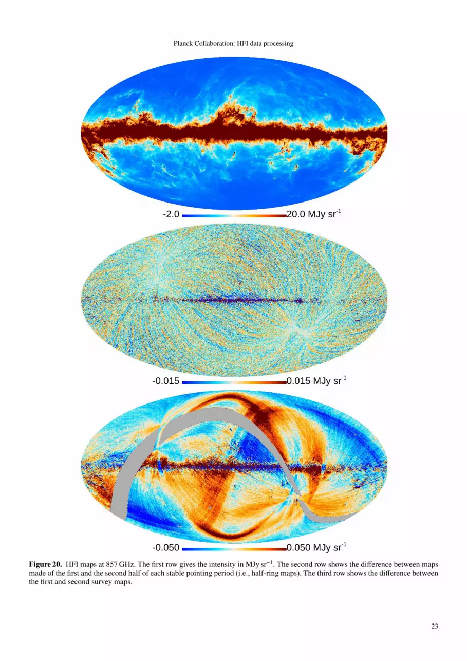
Planck Collaboration: HFI data processing
-2.0 20.0 MJy sr-1
857 GHz I
-0.015 0.015 MJy sr-1
857 GHz I half ring diff.
-0.050 0.050 MJy sr-1
857 GHz I S2 - S1
Figure 20. HFI maps at 857 GHz. The first row gives the intensity in MJy sr−1. The second row shows the difference between mapsmade of the first and the second half of each stable pointing period (i.e., half-ring maps). The third row shows the difference betweenthe first and second survey maps.
23

Planck Collaboration: HFI data processing
10-410-310-210-1
1
t df/d
t
100GHz
143GHz
10-410-310-210-1
1
t df/d
t
217GHz
353GHz
0.1 1.0 10. t [s]
10-410-310-210-1
1
t df/d
t
545GHz
0.1 1.0 10. t [s]
857GHz
Figure 21. HFI channel integration time distribution function.For each HFI channel, the histogram of the integration time tper pixel of area (1.7′)2 is shown. The black curve is for thenominal all-sky ( fsky = 1) mission. The red curve representsthe masked sky, using the CL39 ( fsky = 0.48) mask definedin Planck Collaboration XV (2013). The normalization is suchthat
∫d f = fsky. The median integration time is about 0.42 s
whereas the mean is 0.56 s. Notice that about 0.5 % of the pixelsare observed for more than 5 seconds; these mostly lie aroundthe Ecliptic poles.
6.5. CO correction
Some emission from the rotational transition lines of CO ispresent in all HFI bands. It is especially significant in the 100,217, and 353 GHz channels, due to the 115, 230, and 345 GHzCO transitions. This emission comes largely from the Galacticinterstellar medium, mainly located at low and intermediateGalactic latitudes (|b| < 20 ). Due to the wide spectral cov-erage of Planck (Planck Collaboration IX 2013), we are ableto produce velocity-integrated CO line maps for the first threetransistions J=1→0, 2→1, 3→2. A complete description of themethods used, the validation tests, and the CO products aregiven in Planck Collaboration XIII (2013). These all-sky COmap products can be used for astrophysical studies of the in-terstellar medium or in component separation methods.
Given the fraction of the sky used for the estimation of cos-mological parameters ( fsky <∼ 0.5) and that CO is only signific-ant in less than 1 % of the sky for these high Galactic latitudes,simply masking the CO-emitting regions is the course of actiontaken in cosmological studies with Planck.
6.6. Spectral bands and colour corrections
The HFI detector spectral response was determined through aseries of ground-based tests conducted with the actual HFI focalplane in a simulated space environment, i.e., evacuated and cryo-genic, prior to launch. During these tests, the HFI focal planewas coupled to a broadband radiation source observed througha continuously scanned polarizing Fourier transform spectro-meter (FTS). The individual HFI detector responses to the mod-ulated FTS signal, i.e., the observed interferograms, were recor-ded alongside that of a reference bolometer located inside anintegrating sphere within the experimental setup. Multiple scanswere averaged together to increase the signal to noise ratio ofthe resultant spectra and to allow an estimate of the spectral
1 10 100 1000
0.0001
0.0010
0.0100
0.1000
1.0000
100GHz
143GHz
217GHz
353GHz
From HR dif
From S2-S1
ℓ
Cℓ[µK
2 CM
B]
1 10 100 1000
10-10
10-9
10-8
10-7
545GHz
857GHz
From HR dif
From S2-S1
ℓ
Cℓ[M
Jy2sr
−2]
Figure 22. Power spectra of the difference between intensitymaps reconstructed from the difference between the first andsecond half of each ring (denoted “HR dif”), or from the dif-ference between survey one and survey two.
uncertainty. Standard FTS data processing techniques were em-ployed to obtain the observed spectra of each HFI detector andthat of the reference bolometer; the ratios of the detector spec-tra against the reference bolometer spectrum provide the relativeresponse of each HFI detector. This method incorporates the de-tector throughput (i.e., étendue AΩ, see Planck Collaboration IX2013) in the spectral response as the reference bolometer ac-cepts a much broader field of view, i.e., approximately 2π srover all frequencies. The HFI detector spectral transmissiondata, and their frequency band-average transmission spectra,are described more fully in Planck Collaboration IX (2013)and Planck Collaboration ES (2013), where a description of theband-averaging scheme is also provided.
As discussed in Sect. 6.2, HFI is calibrated by the CMBdipole for the four 100–353 GHz bands, expressed in units ofKCMB, and by planets for the two 545–857 GHz bands, ex-pressed in units of W m−2 sr−1 Hz−1 (equivalently, MJy sr−1).This unit conversion is defined to translate data between unitsof KCMB and MJy sr−1 , the latter for spectra with a profile con-sistent with a spectral index of −1, following the IRAS conven-tion (Beichman et al. 1988). Colour-correction coefficients areprovided for a variety of spectral indices (see Fig. 25) and othercommon spectral profiles including modified blackbody profilesand planetary spectra. It is thus important to ensure that data pro-cessing, e.g., component separation, is conducted in a consistent
24

Planck Collaboration: HFI data processing
0 15 -15 15
0 15 -15 15
0 15 -15 15
0 150 -150 150
0 0.25 -0.05 0.05
0 0.5 -0.05 0.05
Figure 23. The zodiacal light contribution in HFI channels, with 100 GHz to 857 GHz from top to bottom. Units are µKCMB for100–353 GHz and MJy sr−1 for 545 and 857 GHz. Left column: Estimate of the correction. Right column: The survey one−surveytwo difference map after correction, which can be compared with the bottom row of Figs. 15 to 20. While there is no visuallyperceptible difference in the CMB channels, note the visible cleaning of the 353–857 GHz maps.
25

Planck Collaboration: HFI data processing
20 40 60 80 100Multipole
10
-61
0-5
10
-41
0-3
10
-21
0-1
10
01
01
10
21
03
10
4
`(`+
1)Cl/
2π[ (µ
KC
MB)2]
353 GHz217 GHz143 GHz100 GHz
Figure 24. Angular power spectrum of the zodiacal light contri-bution from each channel, as labeled. Even multipoles are shownwith filled boxes, odd multiples with crosses. The systematic dif-ference reflects the approximate North/South symmetry of thezodiacal contribution. Spectra of other channels are given inPlanck Collaboration XIV (2013).
0
.80
0.9
01
.00
-6 -4 -2 0 2 4 6Powerlaw Spectral Index
Co
lou
r C
orr
ectio
n F
acto
r
100 GHz143 GHz217 GHz353 GHz545 GHz857 GHzUncertainty
Figure 25. Band-averaged colour correction for various power-law frequency spectra, normalized to spectral index −1. Thedashed lines provide estimates of the uncertainty of these cor-rections.
manner in units appropriate for the frequency band. The HFIpolicy is to operate in units of MJy sr−1 , as this is valid for all ofthe HFI frequency bands whereas KCMB is only valid for 100–353 GHz. The KCMB to MJy sr−1 unit conversion coefficients aretherefore given by the following ratios
UKCMB_to_MJy sr−1 =
∫dν τ(ν)b′ν∫
dν τ(ν)(νc/ν)× 1020
[MJy sr−1
KCMB
], (3)
where τ(ν) is the relevant spectral transmission curve, b′ν =dBν/dT |TCMB is the Planck function derivative, and νc is the nom-inal band centre frequency.
Other unit conversions are also provided, to ySZ (theSunyaev-Zeldovich Compton parameter, discussed inPlanck Collaboration XXI 2013), K km s−1 (CO transmis-
sion; see Planck Collaboration XIII 2013), and KRJ (brightnesstemperature). It is important to note that brightness temperatureis not restricted to a Rayleigh-Jeans spectral profile, but isa convention for an alternate expression of an arbitrary fluxdensity in temperature units (Rybicki & Lightman 1986).
The HFI unit conversion and colour correction philosophyexpresses equivalent flux density at a predefined nominal fre-quency depending on the spectral profile in question, rather thanmaintaining a set signal amplitude at a varying effective fre-quency, which would also depend on the spectral profile in ques-tion. This is primarily done to ease the requirements on compon-ent separation, as having all components expressed at the sameeffective frequency for all detectors within a frequency band ismuch preferred over dealing with a variety of different effectivefrequencies for each detector, and each component.
More details on the unit conversion factors are providedin Planck Collaboration IX (2013), while tables of conver-sion factors for Planck detectors (only HFI channels forsome spectral shapes, e.g., CO lines) are provided in thePlanck Collaboration ES (2013). Figure 26 illustrates the band-averaged spectra for each of the HFI bands; similar, and re-lated, plots for individual HFI detectors are provided in thePlanck Collaboration ES (2013).
A series of IDL scripts, named the UcCC routines, is avail-able to allow users of Planck data to determine unit conver-sion and colour correction coefficients, and uncertainties, foruser-specified profiles in addition to those nominally providedin the public IMO. Further details on these scripts are provided inPlanck Collaboration ES (2013).
6.7. Polarization
Together with the intensity maps, we derive polarizationmaps for each HFI frequency from 100 GHz to 353 GHz (cf.Planck Collaboration VIII 2013). The Q and U Stokes parametermaps show impressive signal dominated by Galactic dust emis-sion and CMB with noise of very low level and nearly whitespectrum. Nevertheless, at the present state of the reconstruction,polarization maps are dominated at large scales by systematic ef-fects. As a consequence, they are not included in the present re-lease. However, these data will be used in forthcoming analysesof foreground polarization, and hence we describe the major sys-tematic effects remaining in the polarization data.
The Planck scanning strategy does not allow recovery of thepolarization signal for each detector independently. We use acombination of at least four detectors oriented at 45 in orderto reconstruct the Q and U Stokes parameters. Any miscalibra-tion between the datasets will thus lead to a mix between Stokesparameters and, in particular, a leakage from intensity to polar-ization. As discussed in Planck Collaboration VIII (2013), abso-lute calibration is derived from the Solar dipole and gain vari-ations due to ADC non-linearities are corrected to a few tenthsof a percent in the time domain. Final inter-calibration uncertain-ties between HFI bolometers are of the order of 0.4 % or less forthe three lowest HFI frequencies (0.39, 0.28, and 0.21 % respect-ively at 100, 143, and 217 GHz) and rise to 1.35 % at 353 GHz.The induced leakage is dominated by the Solar dipole intens-ity, which produces large scale features in the polarization maps.We estimated the leakage due to calibration mismatch using sim-ulations. Figure 27 shows that the leakage is dominant over theCMB signal up to ` = 100 in the EE angular power spectrum aspredicted by the best-fit cosmological parameters measured fromPlanck temperature data (Planck Collaboration XVI 2013).
26

Planck Collaboration: HFI data processing
0
.00
.20
.40
.60
.81
.0
102 103
Frequency [GHz]
Sp
ectr
al T
ran
sm
issio
n
5 10 20 30
Wavenumber [cm-1]
857 GHz545 GHz353 GHz217 GHz143 GHz100 GHz
CO
J=
1→
0
CO
J=
2→
1
CO
J=
3→
2
CO
J=
4→
3
CO
J=
5→
4
CO
J=
6→
5
CO
J=
7→
6
CO
J=
8→
7
CO
J=
9→
8
Figure 26. The band-averaged transmission spectra for all HFI frequency bands. The locations of the various relevant CO transitionsare marked with vertical lines.
In addition to the calibration mismatch, the differencein the bolometer spectral transmissions will also introducea leakage from the dust emission intensity into polarization.Using the spectral transmission as measured on the ground(Planck Collaboration IX 2013), we estimated the level of leak-age introduced by bandpass mismatch as shown in Fig. 27.
Polarization angles and efficiency have been assessed duringground measurements. Values together with their uncertaintiesare reported in Rosset et al. (2010). We derive uncertainties onangular power spectra using simulations for both polarizationangle and efficiency independently.
Figure 27 shows the level of specific sources of error in EEpolarization angular power spectra compared to the CMB andthe noise level (estimated from half-ring differences) computedon 90 % of the sky excluding the Galactic plane. In the polar-ized HFI bands (100, 143, 217, and 353 GHz) systematic er-rors dominate over the CMB signal at low multipoles (` < 100)due to miscalibration leakage and bandpass mismatch leakage.Polarization angle and polarization efficiency uncertainties aresecond order effects. For Galactic emission polarization studies,the signal is more than one order of magnitude more intense. Athigher multipoles, HFI polarization maps are noise-dominated(at ` >∼ 200) but there is no evidence for correlated noise fromchannel to channel.
7. Data consistency and validation
7.1. Consistency with a severe selection of data
Another check based on real data consists of comparison withdata in which the pointing periods have been much moreseverely discarded. As mentioned in Sect. 3.10, the discardedpointing periods represent less than 1 % of the total integrationtime for the full mission and 0.2 % for the nominal mission, thedifference being due to the numerous solar flare events duringthe fifth survey. For this consistency test, we discard more than30 % of the data of the full mission, following much more severecriteria. For example, we use very conservative thresholds on thestationarity of the noise (details in Appendix B). We then create amap for each frequency with this selection. We compute pseudo-spectra of both the normal and the severely discarded selection.As can be seen in Fig. 28, the difference is compatible with theGaussian case for ` > 500.
There is a rise in the pseudo-spectrum for ` < 500. However,such a feature is far below the cosmic variance (at the percentlevel). So the level of non-stationarity of the noise in the dataof the nominal mission is negligible and does not impact thecosmological results.
27

Planck Collaboration: HFI data processing
1 10 100 1000multipole
10-8
10-6
10-4
10-2
100
102
ClE
E
[µK
2 CM
B]
1 10 100 1000multipole
10-8
10-6
10-4
10-2
100
102
ClE
E
[µK
2 CM
B]
Planck EE from TT best-fitnoise
bandpass leakagecalibration leakage
polarisation orientation errorpolarisation efficiency error
100GHz1 10 100 1000
multipole
10-8
10-6
10-4
10-2
100
102
ClE
E
[µK
2 CM
B]
1 10 100 1000multipole
10-8
10-6
10-4
10-2
100
102
ClE
E
[µK
2 CM
B]
Planck EE from TT best-fitnoise
bandpass leakagecalibration leakage
polarisation orientation errorpolarisation efficiency error
143GHz
1 10 100 1000multipole
10-8
10-6
10-4
10-2
100
102
ClE
E
[µK
2 CM
B]
1 10 100 1000multipole
10-8
10-6
10-4
10-2
100
102
ClE
E
[µK
2 CM
B]
Planck EE from TT best-fitnoise
bandpass leakagecalibration leakage
polarisation orientation errorpolarisation efficiency error
217GHz1 10 100 1000
multipole
10-8
10-6
10-4
10-2
100
102
ClE
E
[µK
2 CM
B]
1 10 100 1000multipole
10-8
10-6
10-4
10-2
100
102
ClE
E
[µK
2 CM
B]
Planck EE from TT best-fitnoise
bandpass leakagecalibration leakage
polarisation orientation errorpolarisation efficiency error
353GHz
Figure 27. Uncertainties on polarized power spectra due to residual systematics in the HFI polarization maps compared to the EEspectrum predicted for the best-fit model from Planck temperature data.
Figure 28. The difference of the pseudo-spectra for the normaland the severe selections, in units of the expected standard de-viation. If our assumptions are correct, the residual noise is sup-posed to have a Gaussian distribution centred on zero with a dis-persion of one (dashed lines). The red points correspond to astatistical check with randomly discarded rings. The points areband-averaged in bins of width ∆` ∼ 91.
7.2. Difference map consistency tests
We perform a series of difference map consistency tests to eval-uate the contribution of residual systematic effects to the angu-lar power spectrum of the temperature anisotropies. We gener-ate difference maps of halves of the nominal mission data inwhich the signal is expected to fully subtract out in the ab-
sence of systematic effects. The resulting maps are then subtrac-ted from systematics-free Yardstick realizations (Appendix A)of the same differences propagated through the same mapmak-ing pipeline as that used for data processing. The amplitude ofthe power of the remaining signal in each likelihood bin canthus be used as an estimate of the level of the residual sys-tematic contamination in this bin. This estimate is derived fromcross spectra between different detector sets to allow for a directcomparison to the spectra used as inputs by the likelihood code(Planck Collaboration XV 2013). The Yardstick simulations aredescribed in detail in Appendix A.
Many differences of halves of the data can be expected to becompatible with an absence of signal. Given Planck’s scanningstrategy, we expect the bulk of the remaining systematic con-tamination to be captured in survey difference maps. In partic-ular, transfer function errors, far-sidelobe pickup, gain instabil-ity, pointing drifts, and residual glitches will leave an imprintin these maps. Half-focal plane difference maps will be par-ticularly sensitive to relative gain errors, while also providingsome sensitivity to sidelobe pickup. Finally, difference maps ob-tained by subtracting PSB-only from SWB-only sky maps probeany unexpected behavioural difference (e.g., beam mismatch)between polarization-sensitive bolometers and unpolarized dec-tectors, and provide a check of the (I,Q,U) decomposition ap-plied to the data from the former. Bandpass difference mises-timation between the two detector technologies will also leave asignal in these maps.
Since the survey difference test is the most stringent differ-ence map consistency test at our disposal, we focus the discus-sion in this section on the corresponding results. We did not de-tect null test failures in any of our other tests from the list above.
28

Planck Collaboration: HFI data processing
0.0 0.2 0.4 0.6 0.8 1.0`
0.0
0.2
0.4
0.6
0.8
1.0
`(`
+1)C
r `/2π
[µK
2] −40
−200
2040
100 GHz
−40−20
02040
143 GHz
500 1000 1500 2000 2500
−40−20
02040
217 GHz
0.0 0.2 0.4 0.6 0.8 1.0`
0.0
0.2
0.4
0.6
0.8
1.0
`(`
+1)C
r `/2π
[µK
2]
−0.4
−0.2
0.0
0.2
0.4
100 GHz, (S2− S1)/2
−0.4
−0.2
0.0
0.2
0.4
143 GHz, (S2− S1)/2
100 101 102
−0.4
−0.2
0.0
0.2
0.4
217 GHz, (S2− S1)/2
Figure 29. (Survey 2 − Survey 1)/2 consistency test result from the ds1 × ds2 cross spectra at 100, 143, and 217 GHz with thefsky ' 0.30 mask derived from that used in the primary cosmological analysis (see the text). Left: the residual signal in eachbandpower up to the highest multipole used in the likelihood code (Planck Collaboration XV 2013). For clarity, the bins used in thelikelihood analysis are grouped four-by-four for ` > 60 and eight-by-eight for ` > 1250 in the plots above. We show in each binthe variance of the C` distribution from the simulations. Note that the amplitude of the residual signal is under the binned samplevariance envelope expected for the fsky ' 0.30 mask (shown in black) up to ` ∼ 1000 at all three frequencies. Right: zoom-in on thelow-` part of the spectrum, showing that although the difference test failures are highly significant at these scales, their amplitudesat all three CMB frequencies are less than or of the order of 0.5 µK2 for all multipoles up to ` = 200, which is a tiny fraction of thebinned sample variance at these scales.
The nominal mission survey difference test results are shown inFig. 29, while Fig. 30 shows the outcome of a suite of differencemap consistency tests at 217 GHz.
In Fig. 29, the angular power spectrum of the residual signalis obtained by taking the cross spectrum between detector setsds1 and ds2 at each frequency (see Table 3) after applicationof the fsky = 0.48 mask used in the primary cosmological ana-lysis (Planck Collaboration XV 2013) combined with a mask ofthe regions not seen by either the first or the second survey anda mask of the point sources included in the input PSM maps.The resulting sky fraction is 0.30 at 100 GHz, and 0.29 at both143 GHz and 217 GHz. Results are then binned according to thelikelihood binning. For clarity, bins at multipoles higher than` = 60 are grouped four-by-four, whereas those at ` > 1250are grouped eight-by-eight. The plot at left shows the residualsignal over the whole range of multipoles used in the likelihoodanalysis. At right, the same results are shown with a low-` zoom(` < 200). In both cases, we report the variance of the C` distri-bution in each bin as computed from the simulations.
At all three CMB frequencies, the ` < 200 residuals are strik-ingly small, never exceeding about 0.5 µK2. Excluding a singlebin in each case, residuals actually remain below or at the levelof 0.2 µK2 over this range of multipoles. Although these non-zero differences are detected with very high statistical signific-ance, they are many orders of magnitude smaller than the binnedsample variance (shown in black in Fig. 29) at these scales.In particular, they cannot affect the cosmological analysis. Thisstays true all the way up to ` ∼ 1000, at which point residualsbecome higher than binned sample variance at 100 and 217 GHz.At 143 GHz, this does not happen until ` reaches 1500.
In the multipole range from 1000 to 2500, although the amp-litude of the residuals is almost always greater than the binnedsample variance, the variance in the simulation results is signi-ficantly larger than in the ` < 1000 regime. As a result, the 100and 143 GHz residuals for that range of multipoles are fully com-
patible with zero. However, the 217 GHz residuals in the samemultipole range are not, as can be directly inferred from the plot,where a significant oscillatory feature starts at ` = 1000.
This survey-difference test has been performed at each fre-quency for all combinations of the input maps used in the like-lihood analysis (two at 100 GHz, five at 143 GHz, and six at217 GHz), and for two survey differences: Survey 1 − Survey 2and Survey 1 − Survey 3. In addition to the 217-ds1 × 217-ds2cross spectrum shown in Fig. 29, only two other cross-spectrafail this test, namely 217-1 × 217-ds2 and 217-1 × 217-3. In thelikelihood analysis (Planck Collaboration XV 2013), we havechecked that the determination of the cosmological parameters isnot affected by the inclusion, or not, of these three cross-spectra.
7.2.1. ADC non-linearity impact
We check the impact of including the effect of ADC non-linearity by the comparison of data and simulations of the twoPSB pairs at 143 GHz. Note that this effect had been suspectedto be significant, but was neither corrected for in the nominalmission products, nor included in the corresponding Yardsticksimulation, since the relevant modelling information was onlyobtained after the end of the HFI cryogenic phase through dedic-ated data gathering during the warm phase. Figure 31 shows thatthe inclusion of this effect leads to similar ` <∼ 100 deviationsfrom the Yardstick compared to those observed in the surveydifference consistency test of the 143 GHz data. The inclusionof this effect makes little difference at higher values of `.
7.2.2. Noise estimation bias from half-ring maps
A detailed comparison of the power spectra of the sum and dif-ference of half-ring maps shows a constant offset of a few per-
29

Planck Collaboration: HFI data processing
0.0 0.2 0.4 0.6 0.8 1.0`
0.0
0.2
0.4
0.6
0.8
1.0
`(`
+1)C
r `/2π
[µK
2] −10
−505
10 217 GHz, Left− Right
−10−5
05
10 217 GHz, In−Out
500 1000 1500 2000 2500
−10−5
05
10 217 GHz, PSB− SWB
Figure 30. Examples of map difference consistency tests at217 GHz with the fsky ' 0.30 mask derived from that used inthe primary cosmological analysis (see the text). The range ofmultipoles shown and the binning used are identical to those de-scribed in Fig. 29. We again show in each bin the variance ofthe C` distribution from the simulations, and in black the binnedsample variance for our mask. “Left” and “Right” refer to thetwo halves of the focal plane, whereas “In” (respectively, “Out”)refer to detectors toward the centre (respectively, the periphery)of the focal plane. Unlike in the survey difference test shown inFig. 29, no significant null test failure is detected in these tests.The detector combinations used in the example plots above are(5−8)× (1−4), (7−8)× (3−4), and (ds1−3)× (ds2−4) for, re-spectively, the (left−right), (in−out), and (PSB−SWB) tests. Asin Fig. 29, these power spectra are divided by four to allow for adirect comparison of the amplitude of the residuals to that of thecomponents in the nominal mission power spectrum.
cent at large multipole. At these scales, there is no longer anysignal remaining in the sum map, due to the beam cut-off (seeFig. 32 for an example), and we would expect that the differencemap spectrum would give a precise determination of the high-`tail of the sum map, while it is actually slightly below. This off-set shows that a noise estimate from half-ring maps difference isa slightly biased indicator of noise in the sum maps. This resultsfrom the deglitching algorithm.
In the first step, the pipeline estimates the signal by averagingthe timelines into rings. This signal estimate is removed in orderto aid detection of glitches by comparison with the noise level.Each positive sample at least 3σ above the noise level is flaggedas a glitch. One side effect of this thresholding is that the pos-itive tail of the timeline noise distribution is now clipped at 3σ.Note that the signal estimate within a ring is of course still noisy,so that its removal from the timeline before deglitching subtractsthis residual noise component periodically (coherently at all har-monics of the spin frequency), in effect periodically modulating(in both half-rings) the flagging and clipping level of the noisedistribution. In the difference of half-ring maps, this commoncontamination disappears, while it is present in the sum map,leading to this slight bias.
Figure 32 shows that the inclusion of the deglitching stepin simulations accounts quantitatively for the difference in thepower spectra of the sum and difference of half-ring maps. By fit-ting the ratio of the spectra of sum and difference maps (masked
100 101 102
multipole `
1.0
0.5
0.0
0.5
1.0
`(`+
1)/
2π C
` [µK
2] Linear model
100 101 102
multipole `
1.0
0.5
0.0
0.5
1.0
`(`+
1)/2π C
` [µK
2] Non-linear model
100 101 102
multipole `
1.0
0.5
0.0
0.5
1.0
`(`+
1)/2π C
` [µK
2] Data
Figure 31. Simulated effect of the ADC non-linearity on S1−S2survey difference at 143 GHz. Top: Difference test of a singlerealization of the full pipeline, assuming a linear response of theADC. Middle: the same, but with our current best model of thenon-linearity response of the ADC. This can be compared withthe bottom panel, which shows the result of the test applied to thedelivered data in exactly the same conditions. This demonstratesthat indeed the effect of ADC non-linearity can explain most ofcoherent deviation seen at ` <∼ 100.
to retain 37 % of the sky) at very high ` (around ` ∼ 7000) onefinds the level of the bias which are given in table 2.
30

Planck Collaboration: HFI data processing
5000 5500 6000Multipole `
1.0
01
.02
1.0
4
C` R
ati
o
data
simulation
5000 5500 6000
60
00
0
80000
10
00
00
C` `
(`+
1)/
2π[ µK
2]
143-1a
data sum
data difference
simulation sum
simulation difference
Figure 32. Comparison of the high-` part of the power spectraof the sum and difference of half-ring maps for the 143-1a de-tector, both for flight data and simulations where glitches wereintroduced and deglitched with the actual processing pipeline.The comparison shows that the simulations provide a good de-scription of this effect (which is not included in the Yardsticksimulations). Top: the sum and difference spectra. Bottom: ratiosof the sum and difference spectra for both data and simulations,which differ by about 2 %.
Table 2. Percentage increase of the power spectrum of the dif-ference of half-ring maps needed to improve the accuracy of thenoise level estimate in frequency maps.
100 143 217 353
0.53 ± 0.08 % 0.61 ± 0.08 % 0.75 ± 0.09 % 0.44 ± 0.09 %
7.3. Power spectrum consistency tests
A powerful check of the data follows from assessing thesignal consistency between detectors at the same frequencygiven the prior information on the effective beam uncertaintiesand calibration. At each frequency, an estimate of an adaptedpower spectra model is processed with the SMICA likelihood(Planck Collaboration XV 2013). At 143 and 217 GHz where theCMB is dominant, the spectrum on the measured sky is mod-elled as aa†C` + n`, a sum of the the free signal power, C`, plusa free independent noise spectrum, n`, where the known vec-tor a accounts for the fixed CMB emissivity at each frequency(bold-faced vectors have elements at each frequency). At higherfrequencies, dust emission begins to dominate the CMB, andsome foreground modelling is necessary. Thus the CMB poweris fixed to the angular spectrum determined at 143 GHz, the noiseis kept free and a free foreground is added, with colour cor-rection determined from a grey body spectral shape integratedthough the measured spectral response of each detector [40 % ofthe sky is used to estimate the binned empirical power spectrumwith spice (Szapudi et al. 2001)]. Furthermore, beam errors aremodelled as a linear combination of templates, thanks to a beamerror mode analysis (Planck Collaboration VII 2013). Then, five
beam parameters along with a calibration are estimated. The fullmodel is written as
R` = B`
(aa†c143
` + bb†g`)
+ n` (4)
where R` is the modelled spectrum, B` the free beam model,b the free dust emmisivity at each frequency, g` the free dustpower, and n` the free noise power. The beam model for detectord is written B`[d] = exp(
∑q θ
d,qT d,q`
) where θ are the beam-eigenmode amplitude parameters and T the templates. Due tothe intrinsic ambiguity between spectral power and beams, beamsimulations are used to determine the variances of a Gaussianprior on these parameters. Finally, at 100 GHz, with only twodetector sets, three parameters per ` (one signal and two noisepower) allows an estimate of the empirical spectrum, but relativecalibration and beam parameters estimation are then unfeasible.
Figure 33 shows the result of such an analysis. At 143 and217 GHz, where the CMB is dominant and used as calibrator,the only adjustments necessary are a gain recalibration by a verysmall amount (0.2 % at most) and the addition of a fraction of aσ of the first beam uncertainty eigenmode. At 545 and 857 GHz,where the CMB is subdominant and planets are used as calib-rators, the required recalibration remains just as small (about0.2 %), but larger beam adjustments are necessary. The 353 GHzcalibration is the one requiring the largest changes, of about 1 %.At 217 GHz and to a lesser extent 353 GHz, the SWB and PSBbeam window functions are at opposite sides of the “optimal”one. In conclusion, by properly modelling foregrounds at highfrequency, cross-checks on signal anisotropy with 40 % of thesky shows that map are well calibrated (relatively) within a fre-quency.
Figure 34 shows the magnitude of the beam corrections de-termined by maximising the internal consistency for the mostsensitive CMB channels of Planck. The largest correctionswould be about 2 µK2 around ` ∼ 100 and about 4 µK2 aroundthe third peak of the CMB spectrum (` ∼ 800). For the deliveredfrequency maps, which combine all detectors at the same fre-quency, the effect is even weaker, and for the likelihood analysis,this is fully accounted for (these beam eigenvalues are either ex-plored or marginalised over, including in addition their expectedcross-correlations).
7.4. Consistency of the calibration across frequencies
In the previous section, we looked at the consistency of de-tector spectra within a given frequency band. A similar ana-lysis of the spectra used in the high-` part of Planck likelihoodPlanck Collaboration XV (2013) shows that the best relative re-calibration (for the mask considered and accounting for the firstbeam eigenmode), between all 13 detectors maps in the 100, 143and 217 GHz channels, would be less than 0.2 %. This level hasno sizeable effect on the constraints on cosmological parameters.
Finally, we can further broaden our consistency checksby using the SMICA component separation method from44 to 353 GHz, in effect intercalibrating on the commonCMB anisotropies themselves, taking 143 GHz as the ref-erence (see Sect. 7.3.3 of Planck Collaboration VIII 2013and Planck Collaboration XII 2013). Figure 35 comparesthe results of such an analysis3 on an FFP6 simulation(Planck Collaboration ES 2013) and on the 2013 maps, using a
3 The analysis is actually done over 40 % of the sky, for various `ranges; the results shown here show the average in the multipole range[100, 679] for the simulations.
31

Planck Collaboration: HFI data processing
Calib EM 1 EM 2 EM 3 EM 4 EM 50.06
0.04
0.02
0.00
0.02
0.04
Beam
para
mete
rs v
alu
es θd,q
1 prior std
143-ds1
143-ds2
143-5
143-6
143-7
Calib EM 1 EM 2 EM 3 EM 4 EM 5
0.04
0.02
0.00
0.02
0.04
0.06
Beam
para
mete
rs v
alu
es θd,q
1 prior std
217-1
217-2
217-3
217-4
217-ds1
217-ds2
Calib EM 1 EM 2 EM 3 EM 4 EM 50.08
0.06
0.04
0.02
0.00
0.02
0.04
0.06
0.08
0.10
Beam
para
mete
rs v
alu
es θd,q
1 prior std
353-1
353-2
353-ds1
353-ds2
353-7
353-8
Calib EM 1 EM 2 EM 3 EM 4 EM 50.05
0.04
0.03
0.02
0.01
0.00
0.01
0.02
0.03
0.04
Beam
para
mete
rs v
alu
es θd,q
1 prior std
545-1
545-2
545-4
Calib EM 1 EM 2 EM 3 EM 4 EM 50.06
0.04
0.02
0.00
0.02
0.04
0.06
Beam
para
mete
rs v
alu
es θd,q
1 prior std
857-1
857-2
857-3
857-4
0 500 1000 1500 2000 2500`
0.0005
0.0000
0.0005
0.0010
0.0015
0.0020
0.0025
0.0030
0.0035
(C∗ `−Cbeams
`)/Cbeams
`
Ref
100
100 no calib
143
143 no calib
217
217 no calib
Figure 33. Calibration and beam uncertainty mode determination for all detectors (or detector sets) within a frequency. The greyareas show the1σ priors on each beam parameters (without assuming a prior for gain calibration, The first detector in each series isused as a fixed reference). The coloured arrows show the1σ posteriors. The bottom right shows the variations of the power spectrain the primary CMB channels when applying the recalibration and beam uncertainty correction described in the text. Altogether, thisleads to variations smaller than 0.4 % at all ` <∼ 2500. Note that the shape variations with ` are very much smaller (∆ <
∼ 5 × 10⁻⁴).
five-component foreground model. The simulations accuratelyvalidate the approach, in a realistic setting (albeit with decreas-ing accuracy at 44 and 353 GHz). For flight data, the multipolerange over which the calibration factor is averaged has been
split in two, a relatively low-` range (50–300), more appropri-ate to include the noisier 44 and 70 GHz channels, and a higher-` range, (300–700), more appropriate for HFI data. The figureconfirms that the 100–217 GHz map calibrations are consistent
32

Planck Collaboration: HFI data processing
0 500 1000 1500 2000 2500`
10
5
0
5
10
(Rbeam
`−Rcalib
`)`
(`+
1)/2π
[µK
2]
143-ds1 x 143-ds2
143-ds1 x 143-5
143-ds1 x 143-6
143-ds1 x 143-7
143-ds2 x 143-5
143-ds2 x 143-6
143-ds2 x 143-7
143-5 x 143-6
143-5 x 143-7
143-6 x 143-7
0 500 1000 1500 2000 2500`
10
5
0
5
10
(Rbeam
`−Rcalib
`)`
(`+
1)/
2π[µK
2]
217-1 x 217-2
217-1 x 217-3
217-1 x 217-4
217-1 x 217-ds1
217-1 x 217-ds2
217-2 x 217-3
217-2 x 217-4
217-2 x 217-ds1
217-2 x 217-ds2
217-3 x 217-4
217-3 x 217-ds1
217-3 x 217-ds2
217-4 x 217-ds1
217-4 x 217-ds2
217-ds1 x 217-ds2
Figure 34. This shows the derived overall beam correction ofeach detector set which minimizes their mismatch, given themodel used, at 143 and 217 GHz where there are sufficient datato simultaneously estimate beam parameters along with sig-nal and noise power spectra. These corrections peak around` ∼ 200 and 800 and are at most of the order of three µK2.
to 0.2 %, as discussed earlier. The 353 GHz results would sug-gest a slightly higher calibration than the one we finally adopted(but the SMICA analysis does not account for the Rayleigh cor-rection (see Planck Collaboration VIII 2013) and we may alsoreach the limit of a five-component foreground model). This ana-lysis also suggests a residual calibration difference between LFIat 70 GHz and HFI at 100 GHz of roughly 0.3 %.
Further checks involving comparison with the LFI andWMAP data are discussed in Planck Collaboration XI (2013).
7.5. Further validation
Other tests are described in various other papers:
– Planck Collaboration XI (2013) compares the maps from theHFI and LFI instruments on Planck and from the WMAPsatellite. We demonstrate excellent consistency amongst thethree sets of maps produced with different instruments over aa factor of thirty in wavelength, and especially over the nar-row range of 70–100 GHz covered by all three instruments,
44 70 100 143 217 3530.98
0.98
50.
990.
995
11.
005
1.01
1.01
5δg
FFP6 simulation2013 data 50-3002013 data 300-700
Figure 35. Recalibration factor maximising the CMB consist-ency in in simulations (black) and in the data considering differ-ent multipole ranges (red and blue), at each Planck frequency inGHz given on the horizontal axis.
illustrating the excellent control of systematic errors we haveachieved with Planck.
– Planck Collaboration XII (2013) discusses different meth-ods for separating the various astrophysical and cosmolo-gical data. Methods with very different assumptions aboutthe physics of the different components, and about the natureof the noise in the Planck maps, are able to converge on equi-valent maps for different components, most importantly ofthe CMB itself.
– Planck Collaboration XV (2013) discusses the angularpower spectrum, C`, computed from Planck data, as well asthe likelihood function that embodies its full probability dis-tribution. The likelihood is computed by taking into accountexplicit models foreground contamination and of systematiceffects such as beam errors and the relative calibration ofdifferent detectors. The resultant spectra explicitly illustrateconsistency across those bands with the highest signal-to-noise for the cosmological spectra at 100, 143, and 217 GHz,at the level of power spectra and of cosmological parameters.As discussed as well in 7.2, the likelihood is robust to the in-clusion or otherwise of even the 217 GHz detectors that showsome mild non-zero features in the spectra of their differencemaps.
8. Summary of product characteristics andconclusions
The data provided to the Planck collaboration by the HFI DPC,in addition to the IMO, consisted of the following (letters refersto entries in the final column of Table 3):
1. C: beam-corrected power spectra for each CMB detector setused in the Planck likelihood code, together with a descrip-tion of the relevant beam uncertainties;
2. N: frequency maps for the nominal mission duration, not cor-rected for ZLE/FSL;
3. B: effective beams and uncertainties (for N);4. F: spectral bands and uncertainties;5. H: hit count maps (for N);
33

Planck Collaboration: HFI data processing
Table 3. Detector sets used in this data release. Unpolarized SWBs are used alone, while PSBs (with individual bolometers denoted“a” and “b”) are used by pair. Here we consider only the temperature map extracted from the analysis of four bolometers (twopairs of PSBs). The weights indicate the relative weighting used in producing maps out of the TOI of several detectors. The relativeweights in a set are given in the numeric order of each detector (e.g., 1a, 1b, 2a, 2b, 3a, 3b. . . for the 100-ds0 set). The last columndetails the specific products created for each set. “N” stands for maps created from nominal mission data (with their beam and bandinformation, “B” and “F”), “H” is the corresponding hit map per pixel, “S1” and “S2” stands for the survey maps generated fromthe data collected during the first six month or during the next six months. “HR1” and “HR2” are for maps made out from the firstor second half of each ring. “C” stands for the detector-set spectra, corrected for the beam transfer function, for the detector setsused in the high-` likelihood. “Z” corresponds to the ZLE/FSL corrected frequency maps.
Set name Frequency Type Detectors in the set Weights in the set Products[GHz]
100-ds0 100 MIX All 8 detectors 0.33, 0.44, 1.50, 0.76 N, B, F, H, S1, S2, HR1, HR22.08, 1.40, 0.97, 30.52 Z-N, Z-S1, Z-S2
100-ds1 100 PSB 1a+1b + 4a+4b 0.58, 0.78, 1.71, 0.93 C100-ds2 100 PSB 2a+2b + 3a+3b 1.05, 0.53, 1.45, 0.98 C
143-ds0 143 MIX 11 detectors 1.04, 0.44, 1.06, 0.93, 0.88, 0.94 N, B, F, H, S1, S2, HR1, HR20.80, 0.66, 1.32, 1.27, 1.66 Z-N, Z-S1, Z-S2
143-ds1 143 PSB 1a+1b + 3a+3b 1.26, 0.53, 1.06, 1.15 C143-ds2 143 PSB 2a+2b + 4a+4b 1.23, 1.08, 0.92, 0.76 C143-ds3 143 SWB 143-5 C143-ds4 143 SWB 143-6 C143-ds5 143 SWB 143-7 C217-ds0 217 MIX All 12 detectors 1.54, 1.44, 1.62, 1.83, 0.60, 0.77 N, B, F, H, S1, S2, HR1, HR2
0.62, 0.67, 0.81, 0.85, 0.64, 0.59 Z-N, Z-S1, Z-S2
217-ds1 217 PSB 5a+5b + 7a+7b 0.79, 1.02, 1.07, 1.12 C217-ds2 217 PSB 6a+6b + 8a+8b 0.98, 1.06, 1.01, 0.94 C217-ds3 217 SWB 217-1 C217-ds4 217 SWB 217-2 C217-ds5 217 SWB 217-3 C217-ds6 217 SWB 217-4 C353-ds0 353 MIX All 12 detectors 2.45, 2.38, 0.44, 0.65, 0.61, 0.57 N, B, F, H, S1, S2, HR1, HR2
0.64, 0.64, 0.31, 0.34, 1.62, 1.35 Z-N, Z-S1, Z-S2
353-ds1 353 PSB 3a+3b + 5a+5b 0.75, 1.09, 1.09, 1.07353-ds2 353 PSB 4a+4b + 6a+6b 1.33, 1.25, 0.68, 0.73353-ds3 353 SWB 353-1353-ds4 353 SWB 353-2353-ds5 353 SWB 353-7353-ds6 353 SWB 353-8545-ds0 545 SWB 3 detectors (1, 2, 4) 0.94, 1.10, 0.96 N, B, F, H, S1, S2, HR1, HR2
Z-N, Z-S1, Z-S2
857-ds0 857 SWB All 4 detectors 1.14, 1.11, 1.15, 0.60 N, B, F, H, S1, S2, HR1, HR2Z-N, Z-S1, Z-S2
6. HR: half-ring maps, HR1 and HR2, two maps made fromthe first and the second half of each pointing period of thenominal mission;
7. S: survey maps, S1 and S2, made from the data of survey oneonly and survey two only; and
8. Z: zodiacal light emission and far sidelobe corrected fre-quency maps and their survey maps (Z-N, Z-S1, Z-S2).
Table 3 summarize the various detectors sets from which wemade these products while Table 4 summarizes the map char-acteristics needed to make use of the maps. Further details andcomments are given below.
Angular Response
Effective Beams provide the response of a map pixel to the sky(lines b1–b7 of Table 4). They are based on a determination ofthe scanning beam from planet scans (Sect. 5.1), which include
the effect of the optical beam, the electronic detection chain, andthe TOI processing pipeline. Scanning beams are an importantintermediate product, although they are usually not relevant forastrophysical applications. The effective beam further accountsfor the combined effect of the scanning strategy and additionaldata processing.
Different applications need different levels of accuracy anddetail, from the mean full-width at half-maximum (FWHM) ofa symmetrical Gaussian description (line b4) to an actual pointspread function at each specific map location. Beam solid anglesare given in line b1. Mean ellipticities are given in line b6. Linesb2, b3, and b7 provide information on the angular response un-certainties and variation across the sky. Our complete uncer-tainty budget, including covariances of the beam eigenvaluesbetween detectors, in a form which is usable for the power spec-tra analyses of Planck Collaboration XV (2013), is provided inPlanck Collaboration VII (2013).
34

Planck Collaboration: HFI data processing
Table 4. HFI Nominal Maps — Main Characteristics.
Quantity Units Notes
Reference frequency ν [GHz] 100 143 217 353 545 857 a1
Number of bolometers 8 11 12 12 3 4 a2
Effective beam solid angle Ω [arcmin2] 105.78 59.95 28.45 26.71 26.53 24.24 b1
Error in solid angle σΩ [arcmin2] 0.55 0.08 0.03 0.02 0.03 0.03 b2
Spatial variation (rms) ∆Ω [arcmin2] 0.31 0.25 0.27 0.25 0.34 0.19 b3
Effective beam FWHM1 [arcmin] 9.66 7.27 5.01 4.86 4.84 4.63 b4
Effective beam FWHM2 [arcmin] 9.65 7.25 4.99 4.82 4.68 4.33 b5
Effective beam ellipticity ε 1.186 1.036 1.177 1.147 1.161 1.393 b6
Variation (rms) of the ellipticity ∆ε 0.023 0.009 0.030 0.028 0.036 0.076 b7
Sensitivity per beam solid angle [µK] 10 6 12 39 c1
[kJy sr−1] 13 14 c1
Sensitivity [µK deg] 1.8 0.8 1.0 3.5 c2
[kJy sr−1 deg] 1.1 1.1 c2
Relative calibration accuracy [%] <∼ 0.2 - <
∼ 0.2 <∼ 1 <
∼ 5 <∼ 5 d1
Absolute calibration accuracy [%] <∼ 0.5 <
∼ 0.5 <∼ 0.5 <
∼ 1.2 <∼ 10 <
∼ 10 d2
Galactic zero-level offset [MJy sr−1] 0.0047 0.0136 0.0384 0.0885 0.1065 0.1470 e1
Galactic zero-level uncertainty [MJy sr−1] 0.0008 0.0010 0.0024 0.0067 0.0165 0.0147 e2
CIB monopole prediction [MJy sr−1] 0.0030 0.0079 0.033 0.13 0.35 0.64 e3
a1 Channel map reference frequency, and channel identifier.a2 Number of bolometers whose data was used in producing the channel map.b1 Mean value over detectors at the same frequency. See Sect. 5.b2 As given by simulations.b3 Variation (rms) of the solid angle across the sky.b4 FWHM of the Gaussian whose solid angle is equivalent to that of the effective beams.b4 FWHM of the mean best-fit Gaussian.b6 Ratio of the major to minor axis of the best-fit Gaussian averaged over the full sky.b7 Variability (rms) on the sky.c1 Estimate of the noise per beam solid angle given in b1. See Sect. 6.3.c2 Estimate of the noise scaled to one degree assuming the noise is white.d1 Relative calibration accuracy between frequency channels. See Sect. 6.d2 This estimate includes the estimated uncertainty of the calibrating source.e1 Offset to remove at each frequency to set the Galactic zero level. The values quoted correpond to νIν = const. At the four lowest frequencies,
the conversion factor is about 244, 371, 483, 287 MJy sr−1 K−1CMB.
e2 Overall error on the map zero point, for a νIν = const spectrum.e3 According to the Béthermin et al. (2012) model, whose uncertainty is estimated to be at the 20 % level. (Also for νIν = const).
Sensitivity
The numbers given in line c1 of the table indicate the rms contri-bution of the noise per beam solid angle, for the median integra-tion time, as scaled from maps at the full resolution (pixels of 1.7arcmin). The numbers given in line c2 of the table also convertsthis number into an rms of the noise in pixels of one degree on aside, again assuming the rms varies inversely proportional to thepixel scale, as if it were white noise. While convenient to com-pare the sensitivity of different experiments, this number may bemisleading, since it is actually an overestimate of the real noisein the map at the one-degree scale.
It is interesting to note that the sensitivity of themap delivered is quite comparable to pre-flight predictions(Planck Collaboration 2005), despite our flagging out of a signi-ficant fraction of data. This decrease of integration time per pixelis approximately compensated by the better-than-required sens-itivity of the individual bolometers. A more elaborate descrip-tion of the noise is made available as "half-ring" maps whosedifferences offers a quite accurate view of the small scale noise,differint by up to half a percent.
Photometric Accuracy
The photometric calibration (Sect. 6.2) of the 100 to 353 GHzchannels relies on the Solar dipole. Comparing the commonCMB component at these frequencies shows that the relative ac-curacy between these channels is better than 0.2 % between 100and 217 GHZ, and at the percent level for the 353 GHz chan-nel. For the two highest frequencies, this relative accuracy is atthe five percent level (lines d1–d2). We have also estimated thezero level offset of the maps which needs to be accounted for inGalactic and cosmic infrared background studies (lines e1–e3).
Spectral response and conversions
The accuracy of the HFI spectral response characterization(Sect. 6.6) is validated using a variety of HFI in-flight obser-vations. Comparisons of zodiacal light observations (Sect. 6.4)with the bandpass data reveal an out-of-band signal rejection ofbetter than 108. The bandpass-based unit conversions and colourcorrections were compared against those derived using sky-onlydata for sources including Sunyaev-Zeldovich (SZ) clusters, dust
35

Planck Collaboration: HFI data processing
emission, and CO emission. The SZ observations show agree-ment with the bandpass data within the quoted uncertainty, asdo the 100, 217 and 353 GHz dust coefficient comparisons. The143 GHz dust coefficient comparison shows differences betweenthe sky and bandpass calibration methods employed; however,the dust component is not dominant at 143 GHz so this dis-crepancy, although important to understand, is not alarming.The CO-based dust colour correction coefficients show goodagreement with their bandpass-based counterparts, while thereare some differences between the bandpass-based and sky-basedCO unit conversion coefficients. These differences compriseareas of ongoing effort which will improve the understandingof the HFI instrument and data; this will in turn lead to betterdata analysis and improved knowledge of systematic and cal-ibration uncertainties. Details are provided elsewhere, primarilyin Planck Collaboration IX (2013) and Planck Collaboration ES(2013).
Data limitations, validation, and checks for systematic errors
The most powerful top-down tests are the statistics of differencesbetween sky maps. The power spectra of these difference mapshave been computed in the same way as those used in the PlanckCMB likelihood (which are based on the nominal maps). Wehave applied a large number of such tests, differencing mapsmade from various detector groups (in/out, left/right), and skysurveys. The sky survey differences maximize the ability to de-tect effects potentially affecting a specific detector or detectorset; they have been applied to all likelihood inputs. We havefound three potentially significant departures at large multipoles,for cross-spectra involving 217 GHz detectors. A jackknife testin the CMB power spectrum and likelihood paper verified thattheir removal does not affect significantly the cosmological con-straints (Planck Collaboration XV 2013).
We also found small, microkelvin-level, residuals at lowmultipoles, which although very significant statistically, are in-significant for a cosmological analysis of the temperature. Wehave verified through simulations that most of this effect is dueto the limitations of the partial correction made for the ADCnon-linearity. This limits the accuracy of our dipole calibrationto about 0.2 % in the CMB channels, and prevents us from usingpolarization information at low multipoles. However, the datacollected at the end of the cryogenic chain will allow a moresatisfactory correction for ensuing Planck data releases.
Conclusions
The six intensity maps and ancillary information presentedabove constitute an unprecedented source of information in thisfrequency range, which is in line with our pre-flight expecta-tions. The level of understanding reached while analysing thisrelease bodes well for the expected next release of Planck datain 2014, which will take aim at polarization on all scales, anduse nearly twice as much data.
Acknowledgements. The development of Planck has been supported by:ESA; CNES and CNRS/INSU-IN2P3-INP (France); ASI, CNR, and INAF(Italy); NASA and DoE (USA); STFC and UKSA (UK); CSIC, MICINN,JA and RES (Spain); Tekes, AoF and CSC (Finland); DLR and MPG(Germany); CSA (Canada); DTU Space (Denmark); SER/SSO (Switzerland);RCN (Norway); SFI (Ireland); FCT/MCTES (Portugal); and PRACE (EU).A description of the Planck Collaboration and a list of its members,including the technical or scientific activities in which they have beeninvolved, can be found at http://www.sciops.esa.int/index.php?project=planck&page=Planck_Collaboration.
ReferencesBeichman, C. A., Neugebauer, G., Habing, H. J., Clegg, P. E., & Chester, T. J.,
eds. 1988, Infrared astronomical satellite (IRAS) catalogs and atlases. Volume1: Explanatory supplement, Vol. 1 6.6
Béthermin, M., Daddi, E., Magdis, G., et al. 2012, ApJ, 757, L23 4Catalano, A., Coulais, A., & Lamarre, J.-M. 2010, Appl. Opt., 49, 5938 3.4Chamberlin, A. B., Yeomans, D. K., Chodas, P. W., et al. 1997, in Bulletin of
the American Astronomical Society, Vol. 29, AAS/Division for PlanetarySciences Meeting Abstracts #29, 1014 6
Delabrouille, J., Betoule, M., Melin, J.-B., et al. 2012, ArXiv e-prints ADupac, X. & Tauber, J. 2005, A&A, 430, 363 6.4Górski, K. M., Hivon, E., Banday, A. J., et al. 2005, ApJ, 622, 759 6.1Hivon, E., Górski, K. M., Netterfield, C. B., et al. 2002, ApJ, 567, 2 5Huffenberger, K. M., Crill, B. P., Lange, A. E., Górski, K. M., & Lawrence, C. R.
2010, A&A, 510, A58+ 5.1Kelsall, T., Weiland, J. L., Franz, B. A., et al. 1998, ApJ, 508, 44 6.4Lamarre, J., Puget, J., Ade, P. A. R., et al. 2010, A&A, 520, A9+ 1, 3.2, 1Liang, Z., Fixsen, D. J., & Gold, B. 2012, ArXiv e-prints 6.2Mitra, S., Rocha, G., Górski, K. M., et al. 2011, ApJS, 193, 5 5Moreno, R. 2010, Neptune and Uranus planetary brightness temperature
tabulation. Tech. rep., ESA Herschel Science Center, available fromftp://ftp.sciops.esa.int/pub/hsc-calibration/PlanetaryModels/ESA2 6.2
Planck Collaboration. 2005, ESA publication ESA-SCI(2005)/01 8Planck Collaboration ES. 2013, The Explanatory Supplement to the Planck 2013
results (ESA) 1, 3, 3.1, 3.3, 3.6, 3.10, 6.6, 6.6, 7.4, 8, B.1Planck Collaboration I. 2011, A&A, 536, A1 1Planck Collaboration I. 2013, Submitted to A&A1, 2, 1, 4, 4Planck Collaboration II. 2011, A&A, 536, A2 4, 4Planck Collaboration II. 2013, Submitted to A&A1Planck Collaboration IX. 2013, Submitted to A&A1, 6.5, 6.6, 6.6, 6.7, 8Planck Collaboration VII. 2013, Submitted to A&A1, 3.7, 5, 5.1, 5.2, 5.2, 7.3, 8Planck Collaboration VIII. 2013, Submitted to A&A 1, 6, 6.2, 6.2, 6.3, 6.7, 7.4,
APlanck Collaboration X. 2013, Submitted to A&A1, 3.3, 4Planck Collaboration XI. 2013, Submitted to A&A7.4, 7.5Planck Collaboration XII. 2013, Submitted to A&A6.4, 7.4, 7.5Planck Collaboration XIII. 2013, Submitted to A&A6.5, 6.6Planck Collaboration XIV. 2013, Submitted to A&A6, 5.2, 6.4, 6.4, 24Planck Collaboration XV. 2013, Submitted to A&A21, 7.2, 29, 7.2, 7.3, 7.4, 7.5,
8, 8Planck Collaboration XVI. 2013, Submitted to A&A1, 6.7Planck Collaboration XXI. 2013, Submitted to A&A6.6Planck Collaboration XXVII. 2013, Submitted to A&A3Planck HFI Core Team. 2011a, A&A, 536, A4 1, 3.5, 2, APlanck HFI Core Team. 2011b, A&A, 536, A6 2, 3, 3.3, 3.6, 3.10, 6.1, ARosset, C., Tristram, M., Ponthieu, N., et al. 2010, A&A, 520, A13+ 6.7Ruze, J. 1966, IEEE Proceedings, 54, 633 5.1Rybicki, G. B. & Lightman, A. P. 1986, Radiative Processes in Astrophysics 6.6Szapudi, I., Prunet, S., & Colombi, S. 2001, ApJ, 561, L11 7.3Tauber, J. A., Mandolesi, N., Puget, J., et al. 2010, A&A, 520, A1+ 1Tristram, M., Filliard, C., Perdereau, O., et al. 2011, A&A, 534, A88 6.1, 6.2
Appendix A: Yardstick simulations
The Yardstick simulation pipeline has been developed for twomain purposes: to quantify the level of residual systematic ef-fects in the maps produced by the HFI DPC, and to validate ourcorrection (or lack thereof) of the data for the systematic effectsthat we are able to model. The former is achieved by comparingcombinations of the data from which the sky signal is expec-ted to vanish to an ensemble of signal and noise realizations ofthe same combinations of data subsets propagated through thesame DPC processing as the data. A mismatch between the two,e.g., in angular power spectrum space, reveals a residual system-atic effect in the data. These tests are described in Sect. 7.2. Inaddition, validating the correction of a given systematic effectrequires the implementation of both a model of the effect and itscorrection (the latter is of course unnecessary if the aim of a testis to justify an absence of correction). In Sect. 7.2.1, the valid-ation of the non correction in the data of the ADC nonlinearityis an example of such a test. The Yardstick pipeline has beendesigned in a modular way to allow for both kinds of tests.
36

Planck Collaboration: HFI data processing
For all simulations, the sky signal is taken from the PlanckSky Model (PSM), which has been described in detail inDelabrouille et al. (2012). This parametric model allows thegeneration of all-sky temperature and polarization maps of theCMB, the SZ effects, and diffuse Galactic emission (in partic-ular synchrotron, free-free, and thermal dust) with a resolutionof a few arcminutes at all Planck frequencies. The PSM alsoincludes an extensive point-source catalog, as well as spinningdust, CO line, and HII region models. From the point of viewof data validation, a particularly useful feature of the PSM is itsability to generate random realizations constrained to match ob-servational data within their uncertainties. Although these realiz-ations cannot be fully independent (with the exception of thoseof the CMB), they do allow for the propagation of some skymodelling uncertainty through the DPC pipeline. The PSM alsohandles convolution with the spectral response of the HFI bolo-meters.
The Yardstick pipeline uses the a`m spherical harmonic coef-ficients from the PSM as inputs. After generating the point-ing timelines directly from Planck’s attitude history file, itfeeds both to the LevelS-Core pipeline, software developedjointly by the HFI and LFI teams and documented in the HFIdata processing early paper (Planck HFI Core Team 2011b).LevelS-Core returns the beam-convolved signal TOI for eachbolometer, which is fed back into the Yardstick pipeline.Noise TOI are generated by a dedicated module and includeboth white noise and 1/ f components. The high-frequencycomponent is taken to be the detector noise described inPlanck Collaboration VIII (2013), while the 1/ f noise is mod-elled following Planck HFI Core Team (2011a). The overallamplitude of the noise is given on a ring-by-ring basis by half-ring map null tests. The latter is further discussed in Sect. 7.2.2.The noise model does not include correlations between detect-ors.
Instrumental effects can be added to the simulated data, eachby the addition of a dedicated module to the pipeline. We haveused this ability to improve our understanding of pointing andbeam issues, as well as to test various aspects of glitch and 4 Kline removal, among others. Section 7.2.1 shows an example ofthe use of the Yardstick simulation facility to evaluate the im-pact on null-test residuals of the non-correction of the ADC non-linearity. When evaluating the quality of the correction of a sys-tematic effect, we simply apply the relevant TOI processing priorto proceeding with mapmaking. The impact of the transfer func-tion convolution and deconvolution is in any case accounted for.
Finally, TOI are propagated through the DPC mapmakingand calibration pipelines following the procedures described inthis paper, including gain correction and application of the vari-ous flags (Planck Collaboration VIII 2013). This allows for aone-to-one comparison of the simulated and data maps. Eachsimulation leads to the generation of per-detector and per-detector-set maps for each survey, and for the nominal missionon which the results in this release are based.
Appendix B: Comparison with a very severeselection of data
This appendix describes the very severe pointing period selec-tion (called hereafter superclean) and the impact at the map andangular power spectrum levels.
B.1. Data selection
Nominal TOI processing is used; only the selection of rings (i.e.,data obtained during a stable pointing period) is changed and de-scribed here. The selected rings include only those showing suf-ficiently stationary noise, within strict bounds. To keep enoughdata, the full mission is used for this test, and not only data fromthe nominal 15.5 months. We list here the applied criteria:
– Normally discarded rings. Of course, rings that are alreadydiscarded remain so.
– 4 K cooler lines. Resonant rings are the ones for which a4 K cooler line (Sect. 3.6) coincides with a harmonic of thespin frequency. The 4 K line correction comes from an inter-polation that could introduce some problems. The 10 Hz lineis the most annoying, so we discard all the 10 Hz-4 K lineresonant rings. This criterion is common to all detectors.
– Baseline jump correction. Rings where a jump correction(Sect. 3.8) was performed are discarded.
– Bursts in the noise. Any anomaly in the noise level (asmeasured by the total noise NET ) can be discarded. FromSect. 3.10, these are due to either a baseline drift or a smalljump. The basic threshold used here is ±3 % of the mediannoise per ring.
– Two-level noise. As described by Planck Collaboration ES(2013), the following bolometers exhibit a larger than usualnoise level in a specific range of rings indicated betweenbrackets:
– 13_353_2 : [4994, end]– 23_353_3a : [5811, 9057] and [18890, end]– 50_143_3a : [9410, end]– 54_353_5b : [2572, end]
The corresponding ranges are entirely discarded.– Integration time per ring. It is possible that the deglitching
procedure might perform differently for rings with a signi-ficantly smaller integration time than average. Hence we dis-card rings with an integration time less than 35 minutes. Thiscriterion is common to all detectors.
– Planets. Rings including a big planet (i.e., flagged as inSect. 3.1) can perturb the mapmaking solution if long tailsare unseen. This criterion is common for detectors in thesame row of the focal plane.
– Medium and small RTS. All rings known to be affected byRTS (Sect. 3.10) are discarded.
– Fifth survey. Survey five is fully discarded because of solarflares, unusual integration time and end-of-life operations.This criterion is common to all detectors.
– PSB. A logical-OR of both discarded ring lists of the twobolometers of a PSB pair is performed.
B.2. Resulting ring statistics
Each criterion has a different impact on both global statistics andthose of individual bolometers.
A logical-OR of all of the criteria is shown in Fig. B.1. Blackpixels indicate that the corresponding rings of the correspond-ing bolometer are not used for the superclean subset, whereasthe red ones are those that were already discarded with the oldcriteria. Several features are notable, such as differences betweenthe highest and lowest frequency channels, and the fact that somecriteria affect all the bolometers.
The global impact of this ring selection is that about 41 % ofthe rings are discarded for the full mission: about 35 % for theCMB channels, and 45 % for the Galactic ones. With the normal
37

Planck Collaboration: HFI data processing
-30.0 30.0 µK
-30.0 30.0 µK
-30.0 30.0 µK
-30.0 30.0 µK
Figure A.1. Top row: data difference maps, for the 143-1a bolometer. Bottom row: differences from a simulation including the effectof the ADC non-linearity and 4 K lines. Left column: S1−S2 survey difference for maps made without destriping. Right column:S1−S2 differences after the destriping used to create the delivered data. The match is sufficiently good that one can use suchsimulations to estimate the combined effect of the non-linearity of the ADC on the delivered data.
criteria, only about 1 % of the rings are discarded for the fullmission (0.2 % in the nominal mission).
In order to distinguish the impact of a simple decrease ofthe observation time and the impact of the use of the supercleanselection, we check the difference between discarding 35 % ofthe rings with the criteria above, and discarding 35 % of the ringsrandomly for the 143 GHz channel.
B.3. Impact of superclean ring selection on Map making
We use the standard pipeline to create maps for each frequency.Along with the global reduction of hit number, the supercleanring selection will create stripes on the hit-maps, due to the tem-poral structure of some criteria. The sanity check with the ran-domly selected rings will have only the impact of the reduc-tion of the hit number. This can be seen on the right columnof Fig. B.2: the number of hits in the superclean maps (middle)are not as homogeneous as in the normal map (top) or the ran-dom map (bottom). On the left panel, the top map represents themasked intensity of the normal map, whereas the middle and thebottom maps correspond to the difference with the supercleanand the random map, respectively. (The differences have beenwhitened with 1/nhiteff = 1/nhitNormal + 1/nhitsevere, where nhit isthe number of hits of a map.)
B.4. Impact of superclean ring selection on spectra
We then compare the spectra for the superclean ring se-lection and the normal ring selection. We use cross-spectraof offset-corrected half-ring maps, FIRST×LAST. The off-set correction is done in order to avoid discrepancies atlow-` due to mask leakage. To avoid contamination fromthe galaxy, the masks applied to compute these offsetsdepend on the frequency: fsky= [70,70,40,40,20,20] % for[100,143,217,353,545,857] GHz. Notice that, as the same skymask is used with the normal and superclean maps, the errorsbars do not include cosmic variance.
Actually, in the Gaussian case, the expected variance of thedifference is induced by noise, and can be computed as
σ2expected
(CS` −CN
`
)= N`
2CN`
(1 − g)/g + N` (1 − g2)/g2
fsky (2` + 1),
where CS`
is the pseudo-spectrum for the superclean selection,CN`
is the pseudo-spectrum for the normal selection, N` is thenoise pseudo-spectrum of the normal map, and g = 0.65 (or 0.55for Galactic channels) is the average ratio of the hit numbers inthe superclean map with the hit numbers in the normal map. Thisformula holds if the noise of the FIRST and LAST maps havethe same pseudo-spectrum and are totally uncorrelated, and ifthe only difference between the normal and the severe selectionis the number of hits in them.
38

Planck Collaboration: HFI data processing
Figure B.1. Example of normally discarded rings (red) and severely discarded rings (black) for 201 consecutive pointing periods(the abscissa has an arbitrary offset).
Figure B.3 shows those normalized differences for all of thechannels. The difference is plotted in units of σexpected(CS
`−CN
`),
so that the expected error bars are 0 ± 1. This is the case from` = 500 to ` = 2500 for all frequencies. At 143 GHz and217 GHz, there is a rise in the pseudo-spectrum for ` < 500.Such a rise is not seen for the pseudo-spectrum computed fromthe random discarding of 35 % of the rings. However, such afeature is far below the cosmic variance (at the percent level).We conclude that the level of non-stationarity of the noise in thenominal mission data is negligible and does not impact the cos-mological results.
1 APC, AstroParticule et Cosmologie, Université Paris Diderot,CNRS/IN2P3, CEA/lrfu, Observatoire de Paris, Sorbonne ParisCité, 10, rue Alice Domon et Léonie Duquet, 75205 Paris Cedex13, France
2 Aalto University Metsähovi Radio Observatory, Metsähovintie 114,FIN-02540 Kylmälä, Finland
3 African Institute for Mathematical Sciences, 6-8 Melrose Road,Muizenberg, Cape Town, South Africa
4 Agenzia Spaziale Italiana Science Data Center, c/o ESRIN, viaGalileo Galilei, Frascati, Italy
5 Agenzia Spaziale Italiana, Viale Liegi 26, Roma, Italy6 Astrophysics Group, Cavendish Laboratory, University of
Cambridge, J J Thomson Avenue, Cambridge CB3 0HE, U.K.
7 Astrophysics & Cosmology Research Unit, School of Mathematics,Statistics & Computer Science, University of KwaZulu-Natal,Westville Campus, Private Bag X54001, Durban 4000, SouthAfrica
8 Atacama Large Millimeter/submillimeter Array, ALMA SantiagoCentral Offices, Alonso de Cordova 3107, Vitacura, Casilla 7630355, Santiago, Chile
9 CITA, University of Toronto, 60 St. George St., Toronto, ON M5S3H8, Canada
10 CNRS, IRAP, 9 Av. colonel Roche, BP 44346, F-31028 Toulousecedex 4, France
11 California Institute of Technology, Pasadena, California, U.S.A.12 Centre for Theoretical Cosmology, DAMTP, University of
Cambridge, Wilberforce Road, Cambridge CB3 0WA U.K.13 Centro de Estudios de Física del Cosmos de Aragón (CEFCA),
Plaza San Juan, 1, planta 2, E-44001, Teruel, Spain14 Computational Cosmology Center, Lawrence Berkeley National
Laboratory, Berkeley, California, U.S.A.15 Consejo Superior de Investigaciones Científicas (CSIC), Madrid,
Spain16 DSM/Irfu/SPP, CEA-Saclay, F-91191 Gif-sur-Yvette Cedex,
France17 DTU Space, National Space Institute, Technical University of
Denmark, Elektrovej 327, DK-2800 Kgs. Lyngby, Denmark18 Département de Physique Théorique, Université de Genève, 24,
Quai E. Ansermet,1211 Genève 4, Switzerland
39

Planck Collaboration: HFI data processing
Figure B.2. Top-left: 143 GHz intensity. Middle-left: difference with superclean. Bottom-left: difference with random selection.Those differences have been whitened with the corresponding hit number, shown in the right column. For the superclean selection,striping of the hit numbers is more visible..
19 Departamento de Física Fundamental, Facultad de Ciencias,Universidad de Salamanca, 37008 Salamanca, Spain
20 Department of Astronomy and Astrophysics, University ofToronto, 50 Saint George Street, Toronto, Ontario, Canada
21 Department of Astrophysics/IMAPP, Radboud UniversityNijmegen, P.O. Box 9010, 6500 GL Nijmegen, The Netherlands
22 Department of Electrical Engineering and Computer Sciences,University of California, Berkeley, California, U.S.A.
23 Department of Physics and Astronomy, Dana and David DornsifeCollege of Letter, Arts and Sciences, University of SouthernCalifornia, Los Angeles, CA 90089, U.S.A.
24 Department of Physics and Astronomy, University CollegeLondon, London WC1E 6BT, U.K.
25 Department of Physics, Gustaf Hällströmin katu 2a, University ofHelsinki, Helsinki, Finland
26 Department of Physics, Princeton University, Princeton, NewJersey, U.S.A.
27 Department of Physics, University of California, One ShieldsAvenue, Davis, California, U.S.A.
28 Department of Physics, University of California, Santa Barbara,California, U.S.A.
40

Planck Collaboration: HFI data processing
29 Department of Physics, University of Illinois atUrbana-Champaign, 1110 West Green Street, Urbana, Illinois,U.S.A.
30 Dipartimento di Fisica e Astronomia G. Galilei, Università degliStudi di Padova, via Marzolo 8, 35131 Padova, Italy
31 Dipartimento di Fisica e Scienze della Terra, Università di Ferrara,Via Saragat 1, 44122 Ferrara, Italy
32 Dipartimento di Fisica, Università La Sapienza, P. le A. Moro 2,Roma, Italy
33 Dipartimento di Fisica, Università degli Studi di Milano, ViaCeloria, 16, Milano, Italy
34 Dipartimento di Fisica, Università degli Studi di Trieste, via A.Valerio 2, Trieste, Italy
35 Dipartimento di Fisica, Università di Roma Tor Vergata, Via dellaRicerca Scientifica, 1, Roma, Italy
36 Discovery Center, Niels Bohr Institute, Blegdamsvej 17,Copenhagen, Denmark
37 Dpto. Astrofísica, Universidad de La Laguna (ULL), E-38206 LaLaguna, Tenerife, Spain
38 European Southern Observatory, ESO Vitacura, Alonso de Cordova3107, Vitacura, Casilla 19001, Santiago, Chile
39 European Space Agency, ESAC, Planck Science Office, Caminobajo del Castillo, s/n, Urbanización Villafranca del Castillo,Villanueva de la Cañada, Madrid, Spain
40 European Space Agency, ESTEC, Keplerlaan 1, 2201 AZNoordwijk, The Netherlands
41 Helsinki Institute of Physics, Gustaf Hällströmin katu 2, Universityof Helsinki, Helsinki, Finland
42 INAF - Osservatorio Astrofisico di Catania, Via S. Sofia 78,Catania, Italy
43 INAF - Osservatorio Astronomico di Padova, Vicolodell’Osservatorio 5, Padova, Italy
44 INAF - Osservatorio Astronomico di Roma, via di Frascati 33,Monte Porzio Catone, Italy
45 INAF - Osservatorio Astronomico di Trieste, Via G.B. Tiepolo 11,Trieste, Italy
46 INAF/IASF Bologna, Via Gobetti 101, Bologna, Italy47 INAF/IASF Milano, Via E. Bassini 15, Milano, Italy48 INFN, Sezione di Bologna, Via Irnerio 46, I-40126, Bologna, Italy49 INFN, Sezione di Roma 1, Università di Roma Sapienza, Piazzale
Aldo Moro 2, 00185, Roma, Italy50 IPAG: Institut de Planétologie et d’Astrophysique de Grenoble,
Université Joseph Fourier, Grenoble 1 / CNRS-INSU, UMR 5274,Grenoble, F-38041, France
51 IUCAA, Post Bag 4, Ganeshkhind, Pune University Campus, Pune411 007, India
52 Imperial College London, Astrophysics group, BlackettLaboratory, Prince Consort Road, London, SW7 2AZ, U.K.
53 Infrared Processing and Analysis Center, California Institute ofTechnology, Pasadena, CA 91125, U.S.A.
54 Institut Néel, CNRS, Université Joseph Fourier Grenoble I, 25 ruedes Martyrs, Grenoble, France
55 Institut Universitaire de France, 103, bd Saint-Michel, 75005,Paris, France
56 Institut d’Astrophysique Spatiale, CNRS (UMR8617) UniversitéParis-Sud 11, Bâtiment 121, Orsay, France
57 Institut d’Astrophysique de Paris, CNRS (UMR7095), 98 bisBoulevard Arago, F-75014, Paris, France
58 Institute for Space Sciences, Bucharest-Magurale, Romania59 Institute of Astronomy and Astrophysics, Academia Sinica, Taipei,
Taiwan60 Institute of Astronomy, University of Cambridge, Madingley Road,
Cambridge CB3 0HA, U.K.61 Institute of Theoretical Astrophysics, University of Oslo, Blindern,
Oslo, Norway62 Instituto de Astrofísica de Canarias, C/Vía Láctea s/n, La Laguna,
Tenerife, Spain63 Instituto de Física de Cantabria (CSIC-Universidad de Cantabria),
Avda. de los Castros s/n, Santander, Spain
64 Jet Propulsion Laboratory, California Institute of Technology, 4800Oak Grove Drive, Pasadena, California, U.S.A.
65 Jodrell Bank Centre for Astrophysics, Alan Turing Building,School of Physics and Astronomy, The University of Manchester,Oxford Road, Manchester, M13 9PL, U.K.
66 Kavli Institute for Cosmology Cambridge, Madingley Road,Cambridge, CB3 0HA, U.K.
67 LAL, Université Paris-Sud, CNRS/IN2P3, Orsay, France68 LERMA, CNRS, Observatoire de Paris, 61 Avenue de
l’Observatoire, Paris, France69 Laboratoire AIM, IRFU/Service d’Astrophysique - CEA/DSM -
CNRS - Université Paris Diderot, Bât. 709, CEA-Saclay, F-91191Gif-sur-Yvette Cedex, France
70 Laboratoire Traitement et Communication de l’Information, CNRS(UMR 5141) and Télécom ParisTech, 46 rue Barrault F-75634Paris Cedex 13, France
71 Laboratoire de Physique Subatomique et de Cosmologie,Université Joseph Fourier Grenoble I, CNRS/IN2P3, InstitutNational Polytechnique de Grenoble, 53 rue des Martyrs, 38026Grenoble cedex, France
72 Laboratoire de Physique Théorique, Université Paris-Sud 11 &CNRS, Bâtiment 210, 91405 Orsay, France
73 Lawrence Berkeley National Laboratory, Berkeley, California,U.S.A.
74 Max-Planck-Institut für Astrophysik, Karl-Schwarzschild-Str. 1,85741 Garching, Germany
75 McGill Physics, Ernest Rutherford Physics Building, McGillUniversity, 3600 rue University, Montréal, QC, H3A 2T8, Canada
76 Niels Bohr Institute, Blegdamsvej 17, Copenhagen, Denmark77 Observational Cosmology, Mail Stop 367-17, California Institute
of Technology, Pasadena, CA, 91125, U.S.A.78 Optical Science Laboratory, University College London, Gower
Street, London, U.K.79 SB-ITP-LPPC, EPFL, CH-1015, Lausanne, Switzerland80 SISSA, Astrophysics Sector, via Bonomea 265, 34136, Trieste,
Italy81 School of Physics and Astronomy, Cardiff University, Queens
Buildings, The Parade, Cardiff, CF24 3AA, U.K.82 Space Sciences Laboratory, University of California, Berkeley,
California, U.S.A.83 Special Astrophysical Observatory, Russian Academy of Sciences,
Nizhnij Arkhyz, Zelenchukskiy region, Karachai-CherkessianRepublic, 369167, Russia
84 Stanford University, Dept of Physics, Varian Physics Bldg, 382 ViaPueblo Mall, Stanford, California, U.S.A.
85 Sub-Department of Astrophysics, University of Oxford, KebleRoad, Oxford OX1 3RH, U.K.
86 Theory Division, PH-TH, CERN, CH-1211, Geneva 23,Switzerland
87 UPMC Univ Paris 06, UMR7095, 98 bis Boulevard Arago,F-75014, Paris, France
88 Université de Toulouse, UPS-OMP, IRAP, F-31028 Toulouse cedex4, France
89 Universities Space Research Association, StratosphericObservatory for Infrared Astronomy, MS 232-11, Moffett Field,CA 94035, U.S.A.
90 University of Granada, Departamento de Física Teórica y delCosmos, Facultad de Ciencias, Granada, Spain
91 University of Miami, Knight Physics Building, 1320 Campo SanoDr., Coral Gables, Florida, U.S.A.
92 Warsaw University Observatory, Aleje Ujazdowskie 4, 00-478Warszawa, Poland
41

Planck Collaboration: HFI data processing
Figure B.3. For each of the HFI channels, the difference of the normal spectrum and the spectrum obtained with a more severeselection of rings, is shown in units of the expected standard deviation. If our assumptions are correct, the residual noise is supposedto have a Gaussian distribution centred on zero with a dispersion of one. The red points for the 143 GHz correspond to a sanitycheck with a random discarding of rings (the points here are band-averaged in bins of width ∆` ∼ 31).
42